Geometry of tropical moduli spaces and linkage of graphs.

GEOMETRY OF TROPICAL MODULI SPACES ANDLINKAGE OF GRAPHS

LUCIA CAPORASO

Abstract. We prove the following “linkage” theorem: two p-regulargraphs of the same genus can be obtained from one another by a finitealternating sequence of one-edge-contractions; moreover this preserves3-edge-connectivity. We use the linkage theorem to prove that variousmoduli spaces of tropical curves are connected through codimension one.

Contents

1. Introduction 12. The linkage theorem 32.1. Terminology. 32.2. p-regular hamiltonian graphs 52.3. p-polygons 72.4. Proof of the linkage theorem 113. Moduli of Tropical curves 153.1. Tropical curves and tropical equivalence 153.2. The moduli space of pointed tropical curves 183.3. Connectedness properties of tropical moduli spaces. 19References 23

1. Introduction

This paper is made of two parts, with the second partially motivating thefirst. The second part studies the moduli spaces of tropical curves; in orderto establish some remarkable connectedness properties, we encounter somequestions about graphs which are of interest in their own right. The solutionof these graph theoretic problems occupies the first part of this paper.

Let us describe the two parts in some details. The first is concerned withclassification of p-regular (every vertex has valency p) connected graphs. Itis quite easy to see that there exists a unique 1-regular graph, namely twovertices joined by a unique edge. Similarly, 2-regular graphs are classified bythe number of their edges, indeed there exists a unique 2-regular graph withn-edges: the cycle on n vertices, and these are all the 2-regular graphs. Assoon as p ≥ 3 the situation gets complicated; as a matter of fact, as far as weare aware of, the number of 3-regular graphs with fixed first Betti number isnot known. And this number would be very interesting for several reasons;for instance, it counts the 0-dimensional combinatorial cycles in the modulispace of Deligne-Mumford stable curves, Mg. See [1] for more on this issue.

1

2 LUCIA CAPORASO

Our main result in the first part of the paper is Theorem 2.4.3. Thisstates, first of all, that any two p-regular connected graphs Γ and Γ′, withthe same first Betti number, are “linked”, i.e. they can be obtained onefrom the other with a finite sequence of alternating one-edge contractionsas follows. There exists a finite sequence

(1.1) Γ = Γ1

##FFFFFFFFF Γ3

~~~~~~~~~~

AAAAAAAAA. . . . . . Γ2h+1 = Γ′

yyssssssssss

Γ2 . . . Γ2h

where every arrow is the map contracting precisely one edge and leavingeverything else unchanged. Also, every odd-indexed graph in the diagramabove is p-regular. Secondly, we prove that if Γ and Γ′ are 3-edge-connectedthere exists a diagram as above where the graph Γi is 3-edge-connected, forevery i = 1, . . . , 2h + 1. This second part makes the proof seriously morecomplicated, but it does play an important role in the application of thisresult to the second part of the paper. We refer to this property as the“conservation of 3-edge-connectivity”.

In case p = 3 the result, without the conservation of 3-edge-conectivity, isdue to A.Hatcher and W.Thurston [10], by a non combinatorial argument;a combinatorial proof valid for simple graphs is given by Y.Tsukui [15].

Our proof is purely combinatorial. We first reduce it to hamiltoniangraphs (in Subsection 2.2), and then show that every hamiltonian graph islinked to a special type of graph called the p-polygon (in Subsection 2.4).

Now we turn to the part concerning moduli of tropical curves, whichoccupies Section 3. The moduli space, M trop

g , of tropical curves of genus g,and the moduli space of n-pointed tropical curves, M trop

g,n , are here treatedsimply as topological spaces. The point is, their geometry is so complex thatthey don’t look like tropical varieties (the case g = 0 is an exception); infact the problem to find a “good” category in which they should be placedis under investigation, and still awaits to be resolved. In a similar vein, itis interesting to study which topological properties of tropical varieties arealso valid for those moduli spaces.

One of the characterizing properties of tropical varieties (defined by primeideals) is that they are “connected through codimension one”; see the Struc-ture Theorem in [11, Ch. 3]. The goal of Section 3 is thus to establish thatseveral moduli spaces of tropical curves are connected through codimensionone; our motivating observation was that this property is strictly related tothe linkage properties of graphs studied in the first part of the paper.

Let us now give more details. In this paper, together with the original no-tion of tropical curve, here called “pure tropical curve”, due to G. Mikhalkin(see [13]), we use the generalization given by S. Brannetti, M. Melo and F.Viviani in [2]; the advantage of the generalized notion is that, with it, themoduli space is closed under specialization, while the moduli space of puretropical curves is not (see [2] or [3] for details).

We are interested in the spaces M tropg,n , and also in the Schottky space,

Schtropg , defined as the quotient of M trop

g via the Torelli map, studied in [2]and [5]. They are easily seen to be connected, however a stronger property

GEOMETRY OF TROPICAL MODULI SPACES AND LINKAGE OF GRAPHS 3

holds, as we are going to explain. Let us focus on M tropg for simplicity; we

have a finite decomposition M tropg = ti∈IMi where each Mi is a connected

orbifold, and M tropg is the closure of the union of those Mi having maximal

dimension (equal to 3g− 3). Every Mi has a clear geometric interpretation,for example the above mentioned dense union

M regg :=

⊔i∈I:dimMi=3g−3

Mi ⊂M tropg =

⊔i∈I

Mi

parametrizes genus-g tropical curves whose underlying graph is 3-regular.Moreover M reg

g is open in M tropg . Now, M reg

g is clearly not connected,whereas M trop

g is so, therefore one can ask: if we add to M regg all strata

Mi of codimension one (i.e. of dimension 3g − 4), do we get a connectedspace? Equivalently: is M trop

g connected through codimension one?The answer to the question is yes, and, as we said, this follows from the

linkage theorem for graphs. In fact, by Proposition 3.3.3 , connectednessthrough codimension one holds for all M trop

g,n . The proof is based on anextension of Theorem 2.4.3 for p = 3 to graphs with legs, Proposition 3.3.2.

Next, by the tropical Torelli theorem of [4], and its generalization in [2],the Schottky locus Schtrop

g is the image via the Torelli map of the locus inM tropg parametrizing 3-edge-connected tropical curves. This motivates our

interest in 3-edge-connected graphs. Indeed, the fact that graph linkagepreserves 3-edge-connectivity, enables us to prove that Schtrop

g is connectedthrough codimension one; see Theorem 3.3.6.

Acknowledgments. I am grateful to Margarida Melo and Filippo Vivianifor their precious remarks on this paper and its previous versions, and tothe referees for correcting several inaccuracies.

2. The linkage theorem

2.1. Terminology. Throughout the paper, p, g and n will be integers withp ≥ 3 and g, n ≥ 0.

Γ always denotes a graph (i.e. a one dimensional finite simplicial com-plex), V (Γ) the set of its vertices (or 0-cells) and E(Γ) the set of its edges(or 1-cells). Every e ∈ E(Γ) joins two, possibly equal, vertices, called theendpoints of e. If the two endpoints of e coincide we say that e is a loop.

We assume all graphs to be connected, unless we specify otherwise. Thecombinatorial definition of graph is in Definition 3.1.2.

The first Betti number, or the genus, of Γ is b1(Γ) = |E(Γ)| − |V (Γ)|+ cwhere c is the number of connected components of Γ.

Using the standard terminology (see [7]) a graph Γ is called(1) p-regular if every vertex has valency (or degree) equal to p;(2) a path if its first Betti number is equal to 0, and if it contains no

vertex of valency ≥ 3. A path Γ satisfies |V (Γ)| = |E(Γ)| + 1; weshall say that |E(Γ)| is the length of the path.

(3) a cycle if it is 2-regular. A cycle has b1(Γ) = 1, and hence an equalnumber of edges and vertices; this number will be called its length.

(4) p-edge-connected if |V (Γ)| ≥ 1 and if Γ r F is connected for anyF ⊂ E(Γ) with |F | < p.

4 LUCIA CAPORASO

2.1.1. Contractions and linkage. Fix Γ and e ∈ E(Γ). Let Γ/e be the graphobtained by contracting e to a point and leaving everything else unchanged([7, sect I.1.7]). Then there is a natural surjective map Γ → Γ′, called thecontraction of e. More generally, if S ⊂ E(Γ) is a set of edges, we denoteby Γ/S the contraction of every edge in S and denote by σ : Γ → Γ/S theassociated map. Let T := E(Γ) r S. Then there is a natural identificationbetween E(Γ/S) and T . Moreover σ induces a surjection

σV : V (Γ) −→ V (Γ/S); v 7→ σ(v).

Notice that every connected component of Γ−T (the graph obtained from Γby removing every edge in T ) gets contracted to a vertex of Γ/S; conversely,for every vertex v of Γ/S its preimage σ−1(v) ⊂ Γ is a connected componentof Γ− T . In particular, we obtain the following useful identity:

(2.1) b1(Γ− T ) =∑

v∈V (Γ/S)

b1(σ−1V (v)).

Remark 2.1.2. Let σ : Γ → Γ/S be the contraction of S as above. Thefollowing facts are well known and easy to prove.

(1) b1(Γ) = b1(Γ/S) + b1(Γ r T ).(2) If Γ is p-edge-connected so is Γ/S.

Definition 2.1.3. (1) Let Γ1 and Γ2 be two graphs. We say that Γ1

and Γ2 are strongly linked if for i = 1, 2 there exists a non-loop edgeei ∈ E(Γi) such that the contraction of e1 and the contraction of e2

coincide, i.e.

Γ1σ1−→ Γ1/e1 = Γ2/e2

σ2←− Γ2,

and σ1(e1) = σ2(e2) (i.e. e1 and e2 are mapped to the same vertex).(2) Let Γ and Γ′ be two graphs. We say that Γ and Γ′ are linked if there

exists a finite sequence of graphs

Γ = Γ1,Γ2, . . . ,Γn−1,Γn = Γ′

such that Γi and Γi−1 are strongly linked, for every i = 2, . . . , n.

We are particularly interested in 3-edge-connected graphs, so we need thefollowing variant.

Definition 2.1.4. Let Γ and Γ′ be two 3-edge-connected graphs. We saythat Γ and Γ′ are 3-linked if there exists a finite sequence of 3-edge-connectedgraphs

Γ = Γ1,Γ2, . . . ,Γn−1,Γn = Γ′

such that Γi and Γi−1 are strongly linked, for every i = 2, . . . , n.

Remark 2.1.5. Being linked, or 3-linked is an equivalence relation. Linkedgraphs have the same number of edges and vertices.

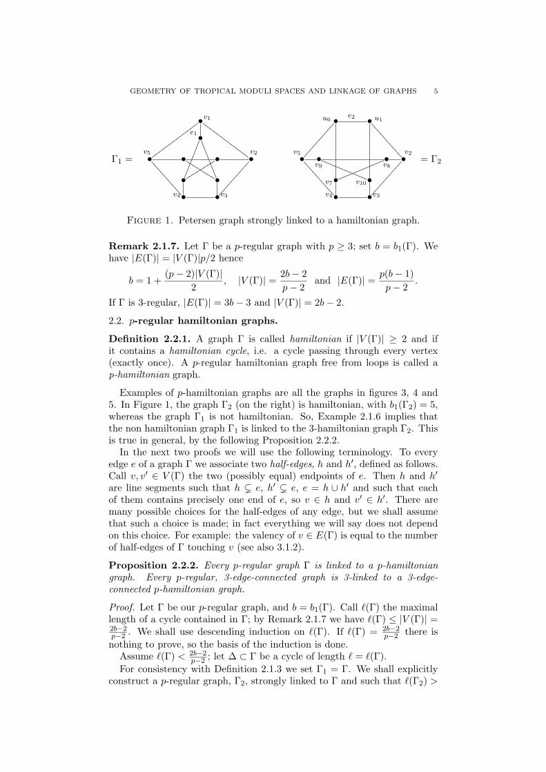
Example 2.1.6. The next picture represents two strongly linked 3-regulargraphs, with Γ1/e1 equal to Γ2/e2. Γ1 is called “Petersen” graph.


• • •e2

•e1v1

Γ1 = •v5

wwwwwwwwwwwww • • •v2

GGGGGGGGGGGGG•

u6

v5

�� • • •

u1

v2

<<<<<<<<<<= Γ2

•

��

ssssssss •

,,,,,,,,,

KKKKKKKK •v8

lllllllllll •v9

RRRRRRRRRRR

•

<<<<<<<<<<v4 •

��v3 •

<<<<<<<<<<v4

v7

•

��v3

v10

Figure 1. Petersen graph strongly linked to a hamiltonian graph.

Remark 2.1.7. Let Γ be a p-regular graph with p ≥ 3; set b = b1(Γ). Wehave |E(Γ)| = |V (Γ)|p/2 hence

b = 1 +(p− 2)|V (Γ)|

2, |V (Γ)| = 2b− 2

p− 2and |E(Γ)| = p(b− 1)

p− 2.

If Γ is 3-regular, |E(Γ)| = 3b− 3 and |V (Γ)| = 2b− 2.

2.2. p-regular hamiltonian graphs.

Definition 2.2.1. A graph Γ is called hamiltonian if |V (Γ)| ≥ 2 and ifit contains a hamiltonian cycle, i.e. a cycle passing through every vertex(exactly once). A p-regular hamiltonian graph free from loops is called ap-hamiltonian graph.

Examples of p-hamiltonian graphs are all the graphs in figures 3, 4 and5. In Figure 1, the graph Γ2 (on the right) is hamiltonian, with b1(Γ2) = 5,whereas the graph Γ1 is not hamiltonian. So, Example 2.1.6 implies thatthe non hamiltonian graph Γ1 is linked to the 3-hamiltonian graph Γ2. Thisis true in general, by the following Proposition 2.2.2.

In the next two proofs we will use the following terminology. To everyedge e of a graph Γ we associate two half-edges, h and h′, defined as follows.Call v, v′ ∈ V (Γ) the two (possibly equal) endpoints of e. Then h and h′

are line segments such that h ( e, h′ ( e, e = h ∪ h′ and such that eachof them contains precisely one end of e, so v ∈ h and v′ ∈ h′. There aremany possible choices for the half-edges of any edge, but we shall assumethat such a choice is made; in fact everything we will say does not dependon this choice. For example: the valency of v ∈ E(Γ) is equal to the numberof half-edges of Γ touching v (see also 3.1.2).

Proposition 2.2.2. Every p-regular graph Γ is linked to a p-hamiltoniangraph. Every p-regular, 3-edge-connected graph is 3-linked to a 3-edge-connected p-hamiltonian graph.

Proof. Let Γ be our p-regular graph, and b = b1(Γ). Call `(Γ) the maximallength of a cycle contained in Γ; by Remark 2.1.7 we have `(Γ) ≤ |V (Γ)| =2b−2p−2 . We shall use descending induction on `(Γ). If `(Γ) = 2b−2

p−2 there isnothing to prove, so the basis of the induction is done.

Assume `(Γ) < 2b−2p−2 ; let ∆ ⊂ Γ be a cycle of length ` = `(Γ).

For consistency with Definition 2.1.3 we set Γ1 = Γ. We shall explicitlyconstruct a p-regular graph, Γ2, strongly linked to Γ and such that `(Γ2) >

6 LUCIA CAPORASO

`(Γ). If Γ is 3-edge-connected so will be Γ2. Using the induction hypothesison Γ2 will suffice to complete the proof. Denote V (∆) = {v1, . . . , v`} (V (Γ). The forthcoming construction is pictured in Figure 2.

Pick a vertex v ∈ V (Γ) such that v 6∈ V (∆) and such that there is anedge e joining v to one of the vertices of ∆; obviously e 6∈ E(∆). We canassume, with no loss of generality, that the endpoints of e are v1 and v. Letus call e1 and e` the two edges of ∆ meeting at v1.

Since v has valency p, there are p − 1 half-edges containing v and notcontained in e; let us call them h1, . . . , hp−1. Similarly as v1 has valency pthere are p− 3 half-edges containing v1 and not contained in e, e1 or e`; wecall these hp, . . . , h2p−4. It is clear that no half-edge hi lies in ∆. Considerthe contraction of e

σ1 : Γ1 = Γ −→ Γ/e = Γ′.Clearly w := σ1(e) is a vertex of valency 2p− 2, indeed the images via σ1 ofe1, e`, h1, . . . h2p−4 all touch w, and there is no other edge touching w.

Now we perform a valency reducing extension on w (cf. [4, A.2.2]); namelywe introduce an edge contracting map σ2 : Γ2 −→ Γ′ from a new graphΓ2 such that Γ′ is obtained from Γ2 as the contraction to w of a uniqueedge, which we call e`+1; hence σ2(e`+1) = w and σ2 leaves everythingelse unchanged. The two endpoints of e`+1 are two vertices of valency p,which we call u`+1, u1 ∈ V (Γ2). In Γ2 we distribute the 2p − 2 half-edgese1, e`, h1, . . . , h2p−4 so that p− 1 of them touch u1 and the remaining p− 1touch u`+1. Moreover we have the (old) edge e1 touching u1, the old edge e`touching u`+1, and the new edge e`+1 joining u1 with u`+1. Therefore thegraph Γ2 is p-regular. Summarizing, we have

Γ2σ2−→ Γ2/e`+1 = Γ/e σ1←− Γ.

Therefore Γ and Γ2 are strongly linked. Now the given cycle ∆ ⊂ Γ ismapped to a cycle of the same length by σ1, whereas σ−1

2 (σ1(∆)) is a cycleof length at least ` + 1 (as it contains the vertices {u1, v2, . . . , v`, u`+1}).Therefore `(Γ) < `(Γ2). It is clear that by iterating this construction wearrive at a p-regular graph Γ with `(Γ) = (2b − 2)/(p − 2), so that Γ ishamiltonian graph. It is also clear that Γ and Γ are linked.

Now suppose that Γ is 3-edge-connected; then Γ′ is also 3-edge-connectedby Remark 2.1.2. To prove that Γ is 3-edge-connected we need to prove thatthe extension of w used during the proof may be constructed so as to yield a3-edge-connected graph Γ2. This follows from the proof of [4, Prop. A.2.4],with trivial modifications. Finally, by the next lemma 2.2.3, we can take Γfree from loops. �

The next picture illustrates this proof. We represent the relevant portionsof Γ, on the left, of Γ′ and of Γ2. The vertices v2 and v` belong to the cycle∆, hence they are joined by a path (not drawn) not intersecting h1 and h2.


• v1v` e` •h4

h3

e

v

v2e1 • σ1−→ • w•v` v2• σ2←− •u`+1•

h3 h4v` •u1

e`+1

v2•

•h1•h2• •

h1

�� •

h2

---------•

h1

•

h2

Figure 2. Increasing the length of ∆ in the proof of 2.2.2.

Lemma 2.2.3. Every p-regular hamiltonian graph is linked to a p-hamiltoniangraph.

Every p-regular hamiltonian 3-edge-connected graph is 3-linked to a p-hamiltonian 3-edge-connected graph.

Proof. It suffices to exhibit a procedure which decreases the number ofloops, preserving the property of being hamiltonian, p-regular and 3-edge-connected.

Let ∆ ⊂ Γ be a fixed hamiltonian cycle; denote by E(∆) = {e1, . . . , et}and V (Γ) = {v1, . . . , vt} with ei joining vi and vi+1 as usual. Suppose thatΓ contains a loop `, and assume (with no loss of generality) that this loop isbased at v1. Let `1 and `2 be the half-edges of the loop (so `1 and `2 touchv1). We know that v1 is connected to v2 by the edge e1. Since v2 has valencyp ≥ 3 there is a half-edge h touching v2, not contained in the hamiltoniancycle ∆, and not contained in an edge touching v1 (for otherwise v2 wouldhave valency less than that of v1). Let us consider Γ/e1, and call w thevertex into which e1 is contracted. The valency of w is 2p− 2.

Let Γ2 be the graph obtained from Γ by changing the loop ` into an edge,called f1, joining v1 with v2, and by changing the half-edge h into a half-edge touching v1. This operation does not create any new loop (as the edgeof Γ containing h does not touch v1), and eliminates the loop `. So thenumber of loops of Γ2 is less than that of Γ. It is clear that Γ2 is p-regular(we added and removed a half-edge from v1 and v2, and left everything elseunchanged). The hamiltonian cycle ∆ is clearly contained in Γ2, so Γ2 ishamiltonian. Finally, Γ/e1 = Γ2/e1, so Γ and Γ2 are strongly linked.

It remains to show that if Γ is 3-edge-connected so is Γ2. This follows from[4, Prop.A.2.4], in fact the extension of w given by Γ2 → Γ/e1 is the same asin Step 1 in the proof of that proposition (with obvious modifications). �

2.3. p-polygons.

2.3.1. Fixing a hamiltonian cycle in a p-hamiltonian graph. We now in-troduce some useful conventions. Let Γ be a p-hamiltonian graph, withb := b1(Γ). We fix a hamiltonian cycle, ∆, and refer to it as the distin-guished hamiltonian cycle; let γ = |V (Γ)| be the length of ∆. The choice of∆ enables us to use the following terminology. The edges of Γ which do notlie in ∆ will be called chords. The number of chords of Γ is easily computed:

(2.2) Number of chords of Γ = |E(Γ)| − γ =p(b− 1)p− 2

− 2(b− 1)p− 2

= b− 1.

8 LUCIA CAPORASO

The vertices of Γ will be labeled according to the cyclic structure of ∆, i.e.V (Γ) = V (∆) = {v1, v2, . . . , vγ} so that there exists an edge ei ∈ E(∆) ⊂E(Γ) joining vi with vi+1 for every i = 1, . . . , γ (with the cyclic conventionvγ+1 = v1); hence E(∆) = {e1, . . . , eγ}. The starting vertex v1 can be pickedarbitrarily; furthermore, for any choice of v1, there are two cyclic labelingsof the vertices (corresponding to the two cyclic orientations of ∆). Once adistinguished cycle ∆ is chosen, we shall always use such a labeling.

Let Γ be a p-hamiltonian graph where a distinguished cycle ∆ has beenfixed. Every chord has two distinct endpoints (Γ being free from loops). Weshall denote by di,j a chord joining vi with vj , and always assume i < j. Ifp ≥ 4 there may be more than one chord joining vi with vj ; if we need todistinguish between them we will use superscripts, i.e. we denote {dαi,j , α =1, . . . ,m} the chords joining vi and vj ; notice that m ≤ p− 2.

We also need a notation for a chord of which only one end is known. So,the chord having one end at the vertex vj and the other end at some othervertex will be denoted dj,∗.

Let di,j be a chord as above. Then di,j determines two paths of the cycle∆, namely the two paths Λ and Λ′ contained in ∆, having extremes vi andvj . Hence Λ ∩ Λ′ = {vi, vj} and Λ ∪ Λ′ = ∆. We call such two paths thesides of di,j . It is obvious that one of them has length j − i and the otherhas length γ−j+ i. We define the amplitude, α(di,j), of di,j as the minimumbetween these two lengths:

(2.3) α(di,j) := min{j − i, γ − j + i}.It is clear that α(di,j) does not depend on the choice of the labeling.

Lemma - Definition 2.3.2. Let Γ be a p-hamiltonian graph with a distin-guished hamiltonian cycle. Set γ := |V (Γ)| = (2b1(Γ)− 2)/(p− 2).

(1) For any chord di,j we have 1 ≤ α(di,j) ≤ γ/2. If α(di,j) ≤ γ/2 − 1we say that di,j is short.

(2) Let di,j be a short chord. The side of di,j having length α(di,j) willbe called the short side of di,j.

(3) If α(di,j) = bγ/2c for every chord, or equivalently, if Γ has no shortchords, then Γ is uniquely determined, it will be denoted by Πp

γ andwill be called the p-polygon with γ vertices (see Figures 3 and 4).

If γ is even the graph Πpγ has p − 2 chords between vi and vi+γ/2

for every i = 1, . . . , γ/2, and no other chord.If γ is odd then p is even. For every i = 1, . . . , (γ − 1)/2, the

graph Πpγ has (p − 2)/2 chords between vi and vi+(γ−1)/2, (p − 2)/2

chords between vi and vi+(γ+1)/2, and no other chord.

Proof. Since Γ has no loops we have, for any chord di,j , 1 ≤ α(di,j). If γ iseven (respectively, odd) the maximal amplitude of a chord is obviously γ/2(respectively, (γ − 1)/2 ).

Now let γ be even. If there are no short chords, every chord is of typedi,i+γ/2 for i = 1, . . . , γ/2. Moreover, every pair of vertices vi, vi+γ/2 isjoined by exactly p− 2 chords, because Γ is p-regular. This shows that Γ isuniquely determined.

Now suppose that γ is odd, and that Γ has no short chord. Then everychord is either of type di,i+(γ−1)/2 or of type di,i+(γ+1)/2. Since |E(Γ)| = pγ/2


we have that p is even; set r = (p−2)/2. For every vertex there are 2r chordstouching it.

We claim that there are exactly r chords of type di,i+(γ−1)/2 and r chordsof type di,i+(γ+1)/2 for every i = 1, . . . , (γ− 1)/2. By contradiction, suppose(with no loss of generality) that there are more than r chords joining v1

with v(γ+1)/2; hence there are less than r chords joining v1 with v(γ+3)/2.But then there are more than r chords joining v2 with v(γ+3)/2 and lessthan r chords joining v2 with v(γ+5)/2. Continuing in this way we get thatthere are less than r chords joining v(γ−1)/2 with vγ . The remaining chordstouching vγ are the ones touching also v(γ+1)/2; since there are already morethan r chords of type d1,(γ+1)/2, there can only be less than r chords of typedγ,(γ+1)/2. We conclude that there are less than 2r chords touching vγ . Acontradiction. This shows that Γ is uniquely determined. �

Example 2.3.3. If p = 3 we have γ = 2b1(Γ) − 2 and Π3γ has no multiple

edge.

•

v3

v1

v4 ��v277777 •

v6 �� •v1

v3

v2

66666

Π34 = • • Π4

6 = • •

•

��

77777•

��v5

77777• v4

��

++++++++++

Figure 3. Some p-polygons with even number of vertices.

If γ is odd, then Πpγ has no multiple edges if and only if p ≤ 4.

•

��

&&&&&&&&&&&&&&&&& •

v5

v1

��

v2::::::::::

•

v1

v9��

CCCCCCCCCCCCCC

�� •

{{{{{{{{{{{{{{

v2

????

v377777

Π49 = •

TTTTTTTTTTTTTTT •

jjjjjjjjjjjjjjj Π65 = • •

•

v8

v7

v6

???? •v4

v5

��

• •

111111111111111•v4

---------• v3

��

Figure 4. Some p-polygons with an odd number of vertices.

We need a criterion for 3-edge-connectivity.

Lemma 2.3.4. (1) Let Γ be a graph such that for every edge e thereexist two distinct cycles ∆1 and ∆2 in Γ and such that E(∆1) ∩E(∆2) = {e}. Then Γ is 3-edge-connected.

(2) Let Γ1 be a 3-edge-connected graph and let Γ2 be a graph stronglylinked to Γ1, so that Γ1/e1 = Γ2/e2 with ei ∈ E(Γi) (notation inDef. 2.1.3). Then Γ2 is 3-edge-connected if it contains two cycles∆1 6= ∆2 such that E(∆1) ∩ E(∆2) = {e2}.

(3) The p-polygon Πpγ is 3-edge-connected for every p ≥ 3.

10 LUCIA CAPORASO

Proof. For part (1), we notice that Γ has no separating edges (a separatingedge is not contained in any cycle). Suppose by contradiction that Γ is not3-edge-connected; let (e, e′) be a separating pair of edges of Γ. By [4, Lemma2.3.2 (iv) and (iii)], (e, e′) is a separating pair if and only if e and e′ belongto the same cycles of Γ. By our assumption, this is clearly impossible.

Now part (2). The graph Γ1/e1 = Γ2/e2 is 3-edge-connected as Γ1 is.Therefore any separating pair of edges of Γ2 must contain e2. The proof ofpart (1) shows that our hypothesis implies that e2 is not contained in anyseparating pair of edges, hence we are done.

To prove part (3) we use again part (1). Pick a chord di,j ; then thereobviously exist two cycles having only di,j as common edge: just take thetwo cycles obtained by adding to di,j one of its two sides (terminology insubsection 2.3.1). To prove that we can apply (1) on the remaining edgeswe need to distinguish two cases, according to the parity of γ.

Suppose γ even. By Lemma 2.3.2 in Πpγ there exists at least one chord

di,i+γ/2 joining vi with vi+γ/2, for every i = 1, . . . , γ/2. Pick an edge whichis not a chord, e = e1. Now Πp

γ contains the chords d1,γ/2+1 and d2,γ/2+2.Then ∆1 = (e1, . . . , eγ/2, d1,γ/2+1) and ∆2 = (e1, eγ , . . . , eγ/2+2, d2,γ/2+2) aretwo cycles having only e as common edge. Therefore Πp

γ is 3-edge-connected.Now suppose that γ is odd; again we use (1). By Lemma 2.3.2 in Πp

γ

there exists at least one chord joining vi with vi+(γ−1)/2, and at least onechord joining vi with vi+(γ+1)/2. Let e = e1 be an edge which is not a chord.Let ∆1 = (e1, d2,(γ+3)/2, d1,(γ+3)/2) and ∆2 = (e1, e2, . . . , e(γ−1)/2, d1,(γ+1)/2);these are two cycles whose only edge in common is e1. Hence Πp

γ is 3-edge-connected. �

We say that two chords di,j and dk,l do not cross if i < j < k < l.

Lemma 2.3.5. Let Γ be a p-hamiltonian graph with a distinguished hamil-tonian cycle(cf. 2.3.1). Let di,j be a short chord. Then there exists a shortchord dk,l with j < k (i.e. di,j and dk,l do not cross) and such that the shortside of di,j does not intersect the short side of dk,l.

Proof. We denote by ∆ the fixed hamiltonian cycle. We may assume thati = 1, so that the given chord d1,j has j ≤ γ/2 (i.e. the short side of d1,j

has vertices v1, v2, . . . , vj). We must prove that there exists a short chorddk,l such that

(a) j < k (d1,j and dk,l do not cross).(b) l− k < bγ/2c (the short side of dk,l has vertices vk, vk+1, . . . , vl−1, vl).Let us denote by D the set of chords satisfying (a); we begin by bounding

|D| from below. Consider the j vertices v1, v2, . . . , vj ; there are at most p−2chords touching each of them. Therefore the total number of distinct chordstouching these vertices is at most j(p − 2) − 1 (to explain the “−1” noticethat the chord d1,j joins v1 with vj , hence it must not be counted twice).Since Γ has b− 1 chords, we get

(2.4) |D| ≥ b− 1− j(p− 2) + 1 = b− j(p− 2).

In particular, since b = 1+(p−2)γ/2 and j ≤ γ/2, we have that |D| ≥ 1, i.e.D is not empty. To prove that there exists at least one chord in D satisfying(b) we argue by contradiction. Suppose that every chord dk,l ∈ D satisfies


l − k ≥ γ/2. This is to say that the path Λ ⊂ ∆ from vj+1 to vγ contains aside of length at least γ/2 for every non multiple chord in D. Let us restrictour attention to the subgraph Γ′ = Γ r {v1, . . . , vj}, obtained by removingthe vertices {v1, . . . , vj} and all edges adjacent to them. So, Γ′ is made ofΛ together with every chord in D. Now, two vertices of Λ are joined by achord of D only if they are separated by at least γ/2 edges. Moreover, everytwo vertices can be joined by at most p− 2 chords. Therefore the length ofthe path Λ satisfies, using (2.4),

length(Λ) ≥ γ

2+|D|p− 2

−1 ≥ b− 1p− 2

+b

p− 2−j−1 =

2b− 1p− 2

−j−1 > γ−j−1

(since γ = 2b−2p−2 ). On the other hand Λ is a path from vj+1 to vγ , whose

length is easily computed:

length (Λ) = γ − (j + 1) = γ − j − 1,

which is in contradiction with the above estimate on length(Λ). �

2.4. Proof of the linkage theorem.

2.4.1. Twisting pairs of chords in a p-hamiltonian graph. Let Γ be a p-hamiltonian graph with a distinguished hamiltonian cycle, as in 2.3.1; picktwo chords di,j and dk,l. In this subsection we momentarily suspend thegeneral convention i < j and k < l (which would be too restrictive). Weintroduce the graph Γ′ obtained from Γ by swapping two endpoints of theabove chords. So, Γ′ is obtained from Γ by replacing the chord di,j with anew chord, di,k, joining vi and vk, and by replacing dk,l with a chord dj,l.Everything else is left unchanged. We shall say that Γ′ is a twist of Γ, andthat Γ′ is obtained from Γ by twisting the pair of chords (di,j , dk,l) into thepair (di,k, dj,l). We shall also say that we swapped the end points vj and vl.

With no loss of generality we may set i = 1; the graph Γ′ is obviouslya p-regular hamiltonian graph; a distinguished hamiltonian cycle will benaturally induced by the one of Γ. So the vertices of Γ and Γ′ will have thesame names, and all the edges of Γ other than d1,j and dk,l correspond toedges of Γ′ other than d1,k and dj,l.

The picture below represents two 3-hamiltonian graphs related by twistinga pair of chords (the dotted chords are the ones that are not changed).

•v1 �� • vj

99999 •v1 �� • vj

88888

Γ = •d1,j

ssssssss • Γ′ = • •

• •dk,l

•

dj,l

�� •d1,k

RRRRRRRRRRR

•vl

????•

vk�� •

vl

????•

vk��

Figure 5. Twisting d1,j and dk,l into d1,k and dj,l.

The following technical lemma is used in the proof of Theorem 2.4.3.

Lemma 2.4.2. Let Γ be a p-hamiltonian graph with a distinguished hamil-tonian cycle.

12 LUCIA CAPORASO

(1) If Γ′ is a twist of Γ, then Γ and Γ′ are linked.(2) Let Γ be 3-edge-connected and fix a chord di,j of Γ, with i < j. Let

dj+1,∗ be a chord of Γ starting at the vertex vj+1; suppose that either(a) or (b) below hold.(a) dj+1,∗ = dj+1,h with j + 1 < h (i.e. dj+1,∗ does not cross di,j).(b) dj+1,∗ = dh,j+1 with i < h < j and there exists a third chord dx,y

such that 1 ≤ i < h < x < j < j + 1 < y.Then the graph obtained by twisting (di,j , dj+1,∗) into (di,j+1, dj,∗) is3-edge-connected and strongly linked to Γ.

Proof. We can assume i = 1 so that di,j = d1,j . The edges of the distin-guished hamiltonian cycle ∆ will be called, as usual, e1, e2, . . . , e2b−2 withei joining vi with vi+1. Let Γ′ be a twist of Γ. We prove Γ′ is linked toΓ by induction on k − j (i.e. on the distance along ∆ of the two swappedvertices). If k = j+ 1 let e be the edge of ∆ between vj and vj+1. Then thegraph obtained from Γ by contracting e is the same as the graph obtainedfrom Γ′ by contracting e; hence Γ and Γ′ are strongly linked. Now assumek − j ≥ 2. Let Γ1 be the graph obtained from Γ by twisting the chord d1,j

with a chord ending at vj+1, denoted dj+1,∗. So, in Γ1 we have the chordsd1

1,j+1 and d1j,∗, where the superscript keeps track of the graph to which the

chords belong. We already proved that Γ and Γ1 are linked. Now considerthe graph Γ2 obtained from Γ1 by twisting d1

1,j+1 and d1k,l, replacing them

with d21,k and d2

j+1,l; since k − (j + 1) < k − j, by induction Γ1 and Γ2

are linked. Finally, let Γ3 be obtained from Γ2 by twisting d2j+1,l and d2

j,∗,replacing them with d3

j,l and d3j+1,∗. Again by induction (we are swapping

vj and vj+1) Γ3 is linked to Γ2, and therefore Γ3 is linked to Γ. It is obviousthat Γ3 = Γ′.

Let us prove the second part. Consider ej , the edge between vj and vj+1

(which, abusing notation as usual, is an edge of both Γ and Γ′). It is easy tocheck that Γ and Γ′ are strongly linked, as the graphs Γ and Γ′ obtained fromΓ and Γ′ by contracting ej are obviously isomorphic. We need to prove thatif either (a) or (b) holds, then Γ′ is 3-edge-connected if Γ is. By Lemma 2.3.4(2), it is enough to show that the edge ej belongs to two distinct cycles ∆1

and ∆2 of Γ′, such that E(∆1) ∩ E(∆2) = {ej}.Suppose (a) holds, so we are twisting (d1,j , dj+1,h) into (d1,j+1, dj,h), with

h > j + 1. Then in Γ′ we have the cycles ∆1 and ∆2 whose edge sets are

E(∆1) = {ej , d1,j+1, e1, . . . , ej−1}

andE(∆2) = {ej , ej+1, . . . , eh−1, dj,h}.

It is clear that ∆1 and ∆2 are cycles and that E(∆1) ∩ E(∆2) = {ej}.Now assume (b). We are twisting (d1,j , dh,j+1) into (d1,j+1, dh,j). Let dx,y

be a chord crossing both dh,j and d1,j . We have

1 < h < x < j < j + 1 < y.

Now the edges of the two cycles containing ej and sharing no other edge are

E(∆1) = {ej , d1,j+1, e1, . . . , eh−1, dh,j}


andE(∆2) = {ej , ej+1, . . . , ey−1, dx,y, ex, ex+1, . . . , ej−1}.

Since 1 < h < x we have E(∆1) ∩ E(∆2) = {ej}. �

We are ready to prove the linkage theorem.

Theorem 2.4.3. Let Γ1 and Γ2 be p-regular graphs with b1(Γ1) = b1(Γ2).Then Γ1 and Γ2 are linked.If Γ1 and Γ2 are 3-edge-connected, then they are 3-linked.

Proof. By Proposition 2.2.2 we can assume that Γ1 and Γ2 are p-hamiltonian.We shall prove the theorem by showing that every p-hamiltonian graph

Γ is linked to the p-polygon Πpγ , where γ = 2b−2

p−2 and b = b1(Γ). Moreover,if Γ is 3-edge-connected, we will prove that it is 3-linked to Πp

γ , which is3-edge-connected by Lemma 2.3.4.

Let us fix a distinguished hamiltonian cycle ∆ of Γ and use the notationof 2.3.1. Now set

ε(Γ) :=∑(

bγ/2c − α(di,j))

where the sum is over all the chords of Γ. By Lemma 2.3.2 we have ε(Γ) ≥ 0,and ε(Γ) = 0 if and only if Γ has no short chord, if and only if Γ = Πp

γ .We will prove the theorem by induction on ε(Γ). By what we just ob-

served, if ε(Γ) = 0 there is nothing to prove, so the induction basis is settled.Assume now that ε(Γ) > 0 and let us pick a short chord; we may call it

d1,j and assume that j ≤ γ/2. By Lemma 2.3.5 we have that there existchords dk,l satisfying

(2.5) 1 < j < k < l and l − k < bγ/2c.We can assume (up to changing the labeling of the vertices) that there existsone of them such that the path (in ∆) from vj to vk is not longer than thepath from vl to v1; i.e. we can assume that

(2.6) k − j ≤ γ + 1− l.We shall pick the pair (d1,j , dk,l) such that k− j, i.e. the length of the pathin ∆ from vj to vk, is minimal with respect to all pairs satisfying (2.5) and(2.6); we shall refer to this as the “minimality property” of (d1,j , dk,l).

Now that we have fixed our two chords, we can assume, up to switchingthem and changing the labeling on the vertices, that

(2.7) j − 1 = α(d1,j) ≤ α(dk,l) = l − k.With these settings, we have

(2.8) k ≤ γ/2 + 1, more exactly k ≤ bγ/2c+ 1.

Let us prove (2.8) by contradiction. Suppose k ≥ bγ/2c + 2. Then (2.7)implies

bγ/2c+ 2 ≤ k ≤ l − j + 1.Now, by (2.6), we have l− j+ 1 ≤ γ+ 2−k. Therefore bγ/2c+ 2 ≤ γ+ 2−kand hence k ≤ bγ/2c+ 1; a contradiction.

Claim 2.4.4. Let Γ′ be the graph obtained from Γ by twisting the pair ofchords (d1,j , dk,l) into the pair (d1,k, dj,l). Then ε(Γ′) < ε(Γ).

14 LUCIA CAPORASO

To prove the claim, consider a chord d′ of Γ′. For notational clarity, wewill denote by d′∗,∗ the chords of Γ′. If d′ is not equal to d′1,k or d′j,l, then d′

corresponds to a unique chord d of Γ such that α(d) = α(d′). Therefore wehave

(2.9) ε(Γ)− ε(Γ′) = −α(d1,j)− α(dk,l) + α(d′1,k) + α(d′j,l).

We know that α(d1,j) = j − 1 and α(dk,l) = l − k, by construction and by(2.5). Furthermore, by (2.8) we have α(d′1,k) = k − 1 .

To compute the remaining term we need to distinguish two cases.Case 1: l − j ≤ γ/2. Then α(d′j,l) = l − j. Therefore

ε(Γ)− ε(Γ′) = 1− j + k − l + k − 1 + l − j = 2k − 2j ≥ 2

by (2.5). So the claim is proved in this case.Case 2: l − j ≥ γ/2 + 1. Now α(d′j,l) = γ + j − l. Therefore

ε(Γ)− ε(Γ′) = 1− j + k − l + k − 1 + γ + j − l = γ + 2(k − l) ≥ 2

as l − k < bγ/2c by (2.5). The claim is proved.

Lemma 2.4.2 says that Γ and Γ′ are linked. By the claim we may applyinduction, getting that Γ′ is linked to Πp

γ ; hence the first part of the Theoremis proved.

Before continuing, we analyze the chords having one end at a vertex vg,with j + 1 ≤ g ≤ k− 1. Let dg,∗ be one such chord. We claim that with ourchoice of the pair (d1,j , dk,l), we have

(2.10) dg,∗ = dg,m, m ≥ k.By contradiction, suppose m < k. If m < g we have (as g ≤ k − 1 andm ≥ 1)

g −m ≤ k − 1− 1 ≤ γ/2− 1by (2.8). Therefore dm,g satisfies the properties satisfied by d1,j : it is a shortchord whose short side does not intersect the short side of dk,l, and it verifies(2.6), i.e. the path from vg to vk is not shorter than the path from vl to vm.Now, the path from vg to vk is obviously shorter than the path from vj tovk, contradicting the minimality property of (d1,j , dk,l).

Suppose now that g < m < k. Again, dg,m satisfies (2.6) and vm is closerto vk than vj . Therefore, in order to respect the minimality property of(d1,j , dk,l), we must have m − g ≥ γ/2. This implies (m ≤ k − 1 ≤ γ/2 by(2.8) and g ≥ j + 1)

γ/2 ≤ m− g ≤ γ/2− j − 1

which is obviously impossible. (2.10) is proved.To finish the proof of the theorem, it is enough to show that, if Γ is 3-

edge-connected, then Γ′ is 3-edge-connected and 3-linked to Γ. To do thatwe shall factor the twist of (d1,j , dk,l) into (d1,k, dj,l) by a series of twistsswapping consecutive vertices, each of which preserves 3-edge-connectivity.We do that with two sets of twists. To define the first set, we make a choiceof a chord dh+1,∗ for every j ≤ h ≤ k − 1. This choice will be irrelevant.

(I.1) Twist (d1,j , dj+1,∗) into (d1,j+1, dj,∗).


(I.2) Twist (d1,j+1, dj+2,∗) into (d1,j+2, dj+1,∗)..........(I.h+1-j) Twist (d1,h, dh+1,∗) into (d1,h+1, dh,∗), with j ≤ h ≤ k − 1..........(I.k-j) Twist (d1,k−1, dk,l) into (d1,k, dk−1,l)

Observe that in each of the above twists, the two chords getting twisted,d1,h and dh+1,∗, do not cross, i.e. dh+1,∗ = dh+1,m with m > h + 1. This isobvious for the last step, (I.k − j), as 1 < k − 1 < k < l. For the remainingsteps, for which h ≤ k− 2, we use (2.10), according to which every dh+1,∗ isof type dh+1,m with m ≥ k. Hence 1 < h < h+ 1 ≤ k − 1 < m, as claimed.

Therefore condition (a) of Lemma 2.4.2 holds, and we conclude that thegraph Γ′′, obtained after the above set of twists, is 3-edge-connected and3-linked to Γ.

Notice that Γ′′ contains the chord d1,k and the chord dk−1,l. The secondset of twists, starting from Γ′′ is the following.

(II.1) Twist (dk−1,l, dk−2,∗) into (dk−2,l, dk−1,∗).(II.2) Twist (dk−2,l, dk−3,∗) into (dk−3,l, dk−2,∗)..........(II.k-h) Twist (dh,l, dh−1,∗) into (dh−1,l, dh,∗), where j + 1 ≤ h ≤ k − 1..........(II.k-j-1) Twist (dj+1,l, dj,∗) into (dj,l, dj+1,∗)

where the chords dh−1,∗ are those chosen for the first set of twists. Observethat the chord d1,k (which lies in every graph appearing in the above twists)crosses every chord dh,l with j + 1 ≤ h ≤ k − 1. If d1,k crosses also dh−1,∗Lemma 2.4.2 applies to the step (II.k-h) above (condition (b) of Lemma 2.4.2holds), and hence 3-edge-connectivity is preserved (to fit in precisely withthe notation of Lemma 2.4.2, one translates the starting vertex after vh, setsh−1 = j and h = j+1 so that dh−1,∗ becomes di,j and dh,l becomes dj+1,∗.).

What if d1,k does not cross dh−1,∗? Recall that by (2.10) we have dh−1,∗ =dh−1,m with m ≥ k. Therefore d1,k does not cross dh−1,m only if k = m.Let us show that twisting (dh,l, dh−1,k) into (dh−1,l, dh,k) preserves 3-edge-connectivity; let Γ be the graph obtained after this twist. By Lemma 2.3.4(2)it suffices to show that Γ contains two cycles, ∆1 and ∆2, whose only edgein common is the edge eh−1 (joining the two swapped vertices vh−1 and vh).Here are the two cycles

∆1 = (eh−1, dh,k, d1,k, e1, . . . , eh−2)

and

∆2 = (eh−1, eh, . . . , el−1, dh−1,l).

Therefore the graph Γ′′′ obtained from Γ by our two sets of twists is 3-edge-connected and 3-linked to Γ. Let us check that Γ′′′ coincides with theΓ′ of Claim 2.4.4. The chords d1,j and dk,l of Γ are twisted into d1,k and dj,lin Γ′ and Γ′′′. The remaining chords of Γ and Γ′ are the same. The chorddh+1,m ∈ E(Γ) with j ≤ h ≤ k − 2, in the first set of twists, is changed intothe chord dh,m ∈ E(Γ′′), which is changed back into dh+1,m ∈ E(Γ′′′) by the

16 LUCIA CAPORASO

second set of twists. All other chords of Γ are not touched by our twists. SoΓ′′′ = Γ′ and we are done. �

3. Moduli of Tropical curves

3.1. Tropical curves and tropical equivalence. In this subsection werecall several basic facts. The original definition of a tropical curve can begiven in terms of metric graphs, by [12] or [14]. In the following, we usea terminology slightly different from the cited references. Recall that ourgraphs are assumed connected.• A pure tropical curve is a pair (Γ, `) where Γ is a graph and ` is a length

function on the edges

` : E(Γ)→ R>0 ∪ {∞}such that `(e) = +∞ if and only if e is adjacent to a 1-valent vertex. Thegenus of (Γ, `) is g(Γ, `) = b1(Γ).• More generally, following [2], a (weighted) tropical curve is a triple (Γ, w, `)

where Γ is a graph, w : V (Γ) → Z≥0 a weight function on the vertices,and ` a length function

` : E(Γ)→ R>0 ∪ {∞}such that `(e) = +∞ if and only if e is adjacent to a 1-valent vertex ofweight 0.

The genus of (Γ, w, `) is defined as follows:

(3.1) g(Γ, w, `) = g(Γ, w) = b1(Γ) +∑

v∈V (Γ)

w(v).

By “tropical curve” without attribute we shall mean a weighted tropicalcurve. If w = 0, i.e. w(v) = 0 for every v ∈ V (Γ), the weighted tropicalcurve is pure.• Two tropical curves are (tropically) equivalent if they can be obtained

from one another by adding or removing 2-valent vertices of weight 0, or1-valent vertices of weight 0, together with their adjacent edge.

3.1.1. Pointed tropical curves. Before giving more details, we want to ex-tend our discussions to curves with points on them, so-called “pointed trop-ical curves”. First, we introduce a generalized notion of graphs, namely,graphs with legs. Here is the combinatorial definition.

Definition 3.1.2. A graph Γ with n legs is the following set of data:(1) A finite non-empty set V (Γ), the set of vertices.(2) A finite set H(Γ), the set of half-edges.(3) An involution ι : H(Γ)→ H(Γ) with n fixed points called the legs of

Γ; the set of legs is denoted by L(Γ).A pair e = {h, ι(h)} of distinct elements in H(Γ) is called an edge;

the set of edges is denoted by E(Γ).(4) A map ε : H(Γ)→ V (Γ).

If ε(h) = v we say that h is adjacent to v, or that v is its endpoint. Thevalency of v ∈ V (Γ) is the number |ε−1(v)| of half-edges adjacent to v. Wesay that Γ is p-regular if every v ∈ V (Γ) has valency p.


It is clear how to associate to the above combinatorial object a topologicalspace. Namely let Γ be a graph as defined above, with vertex set V andedge set E. The topological graph associated to it has V as the set of 0-cells;then we add a 1-cell for every e = {h, ι(h)} ∈ E, so that the boundary ofthis 1-cell is {ε(h), ε(ι(h))}. If Γ has a non empty set of legs L, we add anopen 1-cell for every h ∈ L in such a way that one extreme of the 1-cellcontains ε(h) in its closure.

Of course, if L is empty we have the same graphs treated in the previoussection of the paper. We shall henceforth view graphs with legs also astopological spaces, and we shall freely switch between the combinatorialand the topological viewpoint. As in the previous part of the paper, weshall assume that all our graphs are connected.

Now, a point of a tropical curve can be efficiently represented by a leg ofthe corresponding graph. Here is a list of basic definitions and properties,the first of which generalize those stated in Subsection 3.1; see [3] for detailsand examples.

(1) An n-pointed tropical curve is a triple (Γ, w, `) where Γ is a graph withn legs, w : V (Γ) → Z≥0 a weight function on the vertices, and ` is alength function

` : E(Γ) ∪ L(Γ)→ R>0 ∪ {∞}

such that `(x) = +∞ if and only if either x ∈ L(Γ) or x is an edgeadjacent to a 1-valent vertex of weight 0.

The legs of Γ are the marked points of the curves. The genus of(Γ, w, `) is g(Γ, w, `) = g(Γ, w) as defined in (3.1).

(2) As before, an n-pointed tropical curve is called pure if w = 0.An n-pointed tropical curve is called regular if it is pure and if its

underlying graph Γ is 3-regular.(3) The pair (Γ, w) is called a weighted graph (with n legs); we say that

(Γ, w) is the combinatorial type of the curve (Γ, w, `).(4) (Γ, w) is called stable if every vertex of weight 0 has valency at least 3,

and every vertex of weight 1 has valency at least 1 (in other words, anisolated vertex is stable only if it has weight at least 2; see [3, Ex. 2.4.7]for more on this point).

Stable graphs of genus g with n legs exist if and only if 2g−2+n > 0.(5) Two n-pointed tropical curves are (tropically) equivalent if they can be

obtained from one another by adding or removing(a) 2-valent vertices of weight 0,or(b) 1-valent vertices of weight 0, together with their adjacent edge.Tropical equivalence preserves the genus and the number of legs.

(6) Suppose 2g − 2 + n > 0. Every tropical equivalence class of n-pointedtropical curves contains a unique representative whose combinatorialtype is stable.

(7) Two n-pointed tropical curves (Γ1, w1, `1) and (Γ2, w2, `2) are isomor-phic if there exists a triple (αV , αE , αL), where αV : V (Γ1) → V (Γ2),αE : E(Γ1) → E(Γ2) and αL : L(Γ1) → L(Γ2) are bijections suchthat αV maps the endpoints of x ∈ E(Γ1) ∪ L(Γ1) to the endpoints of

18 LUCIA CAPORASO

αE(x) or αL(x) for every x ∈ E(Γ1)∪L(Γ1). Moreover ∀v ∈ V (Γ1) and∀e ∈ E(Γ1) we have w1(v) = w2(αV (v)) and `1(e) = `2(αE(e)).

(8) The automorphism group Aut(Γ, w) of a weighted graph (Γ, w) is givenby triples α = (αV , αE , αL) as in the previous item, ignoring the condi-tion on the length.

(9) A weighted graph with n legs, and hence an n-pointed tropical curve,has finitely many automorphisms.

Remark 3.1.3. In the definition of n-pointed tropical curve we did notrequire that the points be distinct, i.e. that the legs have different endpoints.This is because we shall work modulo tropical equivalence, which does notpreserve this property. On the other hand, every tropical equivalence class ofn-ponted curves contains representatives whose marked points are distinct;see [3, Prop. 2.4.10].

The addition of a weight function to a tropical curve (introduced in [2])is a way to fix the fact that the set of pure tropical curves of given genus innot closed under specialization. More precisely, families of tropical curvesare given by letting the length of the edges vary. Now if some length goesto zero, it may very well happen that some cycle gets contracted, and hencethe first Betti number drops. This problem does not arise when consideringweighted tropical curves, as we are going to explain.

First, let us formalize the process of edge length going to zero. Fix aweighted graph (Γ, w), and S ⊂ E(Γ). The weighted contraction of S is theweighted graph (Γ/S,w/S), where Γ/S is defined in subsection 2.1.1 in caseL(Γ) = ∅; if L(Γ) is not empty, the definition is trivially adjusted so thatthere is a natural identification between L(Γ) and L(Γ/S). To define w/S,recall that we have a natural map σ : Γ → Γ/S and a natural surjectionσV : V (Γ)→ V (Γ/S). We set for every v ∈ V (Γ/S)

(3.2) w/S(v) = b1(σ−1(v)) +∑

v∈σ−1V (v)

w(v).

We write

(3.3) (Γ, w) ≥ (Γ′, w′) if (Γ′, w′) is a weighted contraction of (Γ, w).

Remark 3.1.4. Suppose (Γ, w) ≥ (Γ′, w′). Then one easily checks thefollowing properties

(1) |L(Γ)| = |L(Γ′)|.(2) g(Γ, w) = g(Γ′, w′) (by identity (2.1) and remark 2.1.2).(3) If (Γ, w) is stable, so is (Γ′, w′).

Therefore, the set of stable genus-g graphs with n legs is closed underweighted contractions.

3.2. The moduli space of pointed tropical curves. From now on weshall consider tropical curves up to tropical equivalence. Therefore we willassume that our weighted graphs are stable.

Let us fix the stable graph (Γ, w) with n legs, let g = g(Γ, w), and letus consider the space M(Γ, w) of isomorphism classes of tropical curveshaving (Γ, w) as combinatorial type. More precisely, we have a natural


identification:M(Γ, w) = (R>0)E(Γ)/Aut(Γ, w)

where an automorphism (αV , αE , αL) ∈ Aut(Γ, w) acts by permuting the co-ordinates of (R>0)E(Γ) according to αE ; see item (7). In particular, M(Γ, w)is an orbifold of dimension |E(Γ)|, since Aut(Γ, w) is finite. The set M(Γ, w)is thus a topological space, with the quotient topology induced by the eu-clidean topology.

We recall the following well known and easy to prove fact:

Remark 3.2.1. Let (Γ, w) be a genus g stable graph with n legs. Then|E(Γ)| ≤ 3g − 3 + n and equality holds if and only if Γ is a 3-regular graphwith b1(Γ) = g. Moreover, in this case we necessarily have w = 0.

We now introduce the moduli space, M tropg,n , of n-pointed tropical curves

of genus g:

(3.4) M tropg,n =

⊔(Γ,w) stable

genus g, n legs

M(Γ, w).

The following statement is a summary of some of the properties of M tropg,n

(see [3] for details; in the case n = 0 some of the properties below are provedalso in [2]).

Fact 3.2.2. Assume 2g−2 +n > 0 and let (Γ, w) be a stable graph of genusg with n legs.

(1) M tropg,n is endowed with a topology such that the natural injection

M(Γ, w) ↪→M tropg,n is a homeomorphism with its image.

(2) With the notation (3.3), we have

M(Γ′, w′) ⊂M(Γ, w)⇔ (Γ, w) ≥ (Γ′, w′).

(3) Let M regg,n ⊂M trop

g,n be the subset parametrizing regular curves, i.e.

M regg,n =

⊔|L(Γ)|=n, b1(Γ)=g

Γ 3−regular

M(Γ, 0) ⊂M tropg,n .

Then M regg,n is open and dense in M trop

g,n .(4) Let Mpure

g,n be the subset parametrizing pure tropical curves. ThenMpureg,n is open and dense M trop

g,n .(5) M trop

g,n is a connected, Hausdorff topological space of pure dimension3g − 3 + n.

Remark 3.2.3. We need to explain the meaning of the last statement.Recall that a topological space X containing a dense open subset U , whereU is an orbifold (locally the quotient of a topological manifold by a finitegroup) of dimension d, is said to have pure dimension d.

Now, by part (3), M tropg,n contains the dense open subset U = M reg

g,n , whichis an orbifold has dimension 3g− 3 + n, by Remark 3.2.1. This explains theclaim on the dimension. Connectedness of M trop

g,n is trivial, since every (Γ, w)satisfies (Γ, w) ≥ (Γ∗, w∗) where (Γ∗, w∗) is the graph having no edges, onlyone vertex of weight g, and n legs attached to it. The fact that M trop

g,n isHausdorff is proved in [3, sect. 3.2].

20 LUCIA CAPORASO

3.3. Connectedness properties of tropical moduli spaces. In this lastsubsection we apply our Linkage Theorem 2.4.3 to the geometry of somemoduli spaces of tropical curves.

To begin with, we have said that M tropg,n is connected; but a stronger form

of connectedness holds, namely M tropg,n , and likewise Mpure

g,n , is connectedthrough codimension one; see Definition 3.3.1. This property is one thatis fundamental for tropical varieties defined by prime ideals (see [11]). Al-though M trop

g,n and Mpureg,n are not known to be tropical varieties in general

(the case g = 0 is a well known exception), their connectedness throughcodimension one is a sign of their being somewhat close to tropical varieties.

The next definition is adapted from [11, Definition 3.3.2].

Definition 3.3.1. Let X be a topological space of pure dimension d; see3.2.3. Assume that X is endowed with a decomposition X = ti∈IXi, whereevery Xi is a connected orbifold. We say that X is connected through codi-mension one if the subset ⊔

i∈I:dimXi≥d−1

Xi ⊂ X

is connected.

Notice that if X is pure dimensional and connected through codimensionone, then X is connected.

Now, observe that the notion of linked graphs, given in Definition 2.1.3,extends word for word to graphs with legs. We can therefore state thefollowing result, which is a consequence of Theorem 2.4.3.

Proposition 3.3.2. Let Γ1 and Γ2 be two 3-regular graphs with n legs andb1(Γ1) = b1(Γ2). Then Γ1 and Γ2 are linked.

Proof. Of course, |E(Γ1)| = |E(Γ2)|; we can assume |E(Γi)| ≥ 2 for other-wise the result is trivial. We use induction on n; the base case n = 0 is aspecial case of Theorem 2.4.3.

Suppose n ≥ 1; let us denote by G(n) the set of 3-regular graphs of genusg with n legs. Let Γ ∈ G(n), pick a leg l ∈ L(Γ) and let v ∈ V (Γ) be itsendpoint. Let Γ′ be the closure of the graph obtained by removing l and vfrom Γ. It is clear that Γ′ ∈ G(n−1). Notice that, of course, every Γ ∈ G(n)is obtained by adding a leg and its endpoint to some graph in G(n− 1).Claim. Fix a graph Γ′ ∈ G(n − 1); any two graphs in G(n) obtained byadding to Γ′ a leg and its endpoint are linked.

The claim implies our Proposition. Indeed, let Γ′1,Γ′2 ∈ G(n− 1) be such

that for, some e′i ∈ E(Γ′i) we have

(3.5) Γ′1/e′1 = Γ′2/e

′2.

Let Γ1 ∈ G(n) be obtained by adding to Γ′1 a leg whose endpoint is notin the interior of e′1. Then, by (3.5), there exists a Γ2 ∈ G(n) obtained byadding a leg and its endpoint to Γ′2 such that Γ1/e1 = Γ2/e2; so Γ1 is linkedto Γ2. Hence, by the claim, we get that all graphs in G(n) obtained fromΓ′1 are linked to those obtained from Γ′2. By the induction hypothesis everypair of elements in G(n− 1) is linked, so we are done.


It remains to prove the claim. For i = 1, 2, let Γi ∈ G(n) be the graphobtained by adding to Γ′ a vertex vi (in the interior of some edge or leg ofΓ′) and a leg li adjacent to vi. We must show that Γ1 and Γ2 are linked.Pick w ∈ V (Γ′) ⊂ V (Γi); for i = 1, 2 the vertex vi can be joined to w bysome path Πi of minimal length contained in Γi; let hi be the edge-lengthof Πi, where hi is a positive integer, since w 6= vi; we call hi the edge-pathlength from vi to w. Let h = h1 + h2; if h = 2, i.e. if h1 = h2 = 1, thereexists an edge ei ∈ E(Γi) whose endpoints are w and vi. It is clear that

Γ1/e1 = Γ2/e2

so we are done. We continue by induction on h.Suppose h ≥ 3, and let h1 ≥ 2. Let e1 be the first edge of Π1 so that v1

is an endpoint of e1; Consider the graph Γ1/e1. The coming construction isillustrated in the picture below. Now let u be the other endpoint of e1 andlet f be the next edge of Π1, starting at u; by construction, f is also an edgeof Γ′. Let Γ3 ∈ G(n) be the graph obtained from Γ′ by adding a vertex v3

in the interior of f and a leg attached to it. Now, Γ3 has a unique edge e3

whose endpoints are u and v3. The edge-path length from v3 to w is h1− 1,hence by induction Γ3 is linked to Γ2. On the other hand it is immediatelyclear that

Γ1/e1 = Γ3/e3,

hence Γ3 and Γ1 are linked, and so Γ1 is also linked to Γ2 . �

The next picture represents the construction used to prove the claim, withg = 2 and n = 3..

Γ′ = •777

�� •uf• w•

Γ1 = •666

�� •v1

e1

l1�� •u

f• w• Γ3 = •

666

�� •ue3•v3

l3666• w•

Figure 6. Γ1 and Γ3 linked, obtained from Γ′ (proof of 3.3.2).

From Proposition 3.3.2 we easily get:

Proposition 3.3.3. The spaces M tropg,n and Mpure

g,n are connected throughcodimension one.

Proof. From Fact 3.2.2 we have that M tropg,n and Mpure

g,n are of pure dimension3g − 3 + n. Also, we know that dimM(Γ, w) = |E(Γ)|. So, by 3.2.2 (2) toprove our statement it suffices to observe that any two 3-regular graphs arelinked, as stated in Proposition 3.3.2. �

Remark 3.3.4. As proved in [2, Prop. 3.2.5], the above result in case n = 0follows from [10, Prop. page 236], which is a remarkable and well knownspecial case of our Theorem 2.4.3.

22 LUCIA CAPORASO

3.3.5. The tropical Torelli map and the Schottky locus. We will now provethat connectedness through codimension one holds for other tropical modulispaces.

In analogy with the classical situation we have a tropical Torelli map

ttropg : M trop

g → Atropg

to the moduli space of tropical Abelian varieties, mapping a curve to itstropical Jacobian (see [14], [4] and [2] for details). We denote by Schtrop

g

the image of ttropg , and refer to it, as it is customary, as the tropical Schotty

locus in Atropg . A detailed analysis of Schtrop

g for small values of g is carriedout in [5].

For our purposes Schtropg can be identified with the topological quotient

Schtropg := M trop

g / ≡ttropg

where [(Γ, `, w)] ≡ttropg

[(Γ, `, w)]⇔ ttropg ([(Γ, `, w)]) = ttrop

g ([(Γ′, `′, w′)]). For

more structure on Atropg and Schtrop

g we refer to [2]. In particular, Theorem5.2.4 of loc. cit. gives a precise characterization of the tropical Schotty locusSchtrop

g in Atropg , in such a way that the Schottky problem has a satisfactory

answer in tropical geometry.As proved in [4, Thm 4.1.9], and generalized by [2, Thm 5.3.3], the Torelli

map identifies curves having the same so-called “3-edge-connected class”.More precisely, let us denote by M trop

g [3] the locus of tropical curves with3-edge-connected graph:

M tropg ⊃M trop

g [3] := {[(Γ, `, w)] : Γ is 3-edge-connected}.

Then we have

ttropg (M trop

g [3]) = ttropg (M trop

g ) = Schtropg ⊂ Atrop

g .

Furthermore, the restriction of ttropg to M trop

g [3], denoted by ttropg [3], is in-

jective on every subspace M(Γ, w) ⊂ M tropg [3], and it identifies two such

spaces, M(Γ, w) and M(Γ′, w′), only if the graphs Γ and Γ′ are cyclicallyequivalent (i.e. 2-isomorphic in the sense of Whitney, see [4, Def 2.2.3]). Inparticular, ttrop

g [3] has finite fibers.The previous results hold in the special case of pure tropical curves (in

fact, they were first proved in this case, and then generalized to weightedtropical curves). With self-explanatory notation, the Torelli map for puretropical curves is a surjection

tpureg : Mpure

g −→ Schpureg := Mpure

g / ≡tpureg⊂ Atrop

g ,

and the restriction of tpureg to the locus of pure tropical curves with 3-edge

connected graph, Mpureg [3] ⊂Mpure

g , behaves exactly as ttropg [3].

Now, the conservation of 3-edge-connectivity under linkage, proved inTheorem 2.4.3, enables us to obtain the following result.

Theorem 3.3.6. The spaces M tropg [3] and Schtrop

g have pure dimension equalto 3g − 3 and are connected through codimension one.

The same holds for the spaces Mpureg [3] and Schpure

g .


Proof. We prove the result for tropical curves; the proof for pure tropicalcurves follows precisely the same lines (and it is actually simpler). Weintroduce the locus of regular, 3-edge-connected curves

M regg [3] ⊂M reg

g ⊂M tropg .

We have that the closure in M tropg of regular, 3-edge-connected curves is the

locus of all 3-edge-connected curves, i.e.

M regg [3] = M trop

g [3].

This follows from [4, Prop A.2.4], whose proof (stated there only for pureregular curves) works also in our setting (i.e. for weighted tropical curves).It is clear that M reg

g [3] is an orbifold of pure dimension 3g− 3. We concludethat M trop

g [3] has pure dimension 3g − 3.Now, the connectedness through codimension one follows from the part

of Theorem 2.4.3 concerning 3-edge connected graphs. It suffices to addthat if (Γ′, w′) is obtained from (Γ, w) by contracting only one edge, thendimM(Γ, w) = dimM(Γ′, w′)+1 (as we also did for Proposition 3.3.6). Thisproves that M trop

g [3] is connected through codimension one.Now we turn to the Schottky locus; by what we said before there is a

surjection with finite fibers

ttropg [3] : M trop

g [3] −→ Schtropg

obtained by restricting the Torelli map. This surjection induces a homeo-morphism with its image of every subspace M(Γ, 0) ⊂M trop

g [3]. This impliesthat Schtrop

g has pure dimension 3g − 3. Furthermore, as ttropg [3] is injective

on every M(Γ, w), it preserves the dimension of these subsets; thereforeSchtrop

g is connected through codimension one, because so is M tropg [3]. �

Remark 3.3.7. What are the consequences on tropical moduli spaces ofthe linkage theorem when p ≥ 4? Consider the subset

Mp−regg :=

⊔Γ p-regular

b1(Γ)=g

M(Γ, 0) ⊂Mpureg

and assume it is not empty. By a proof similar to that of Theorem 3.3.6one obtains that the closure of Mp−reg

g is of pure dimension equal to p(g −1)/(p−2), by Remark 2.1.7 (this number is an integer by the non-emptynessassumption), and connected through codimension one.

The same holds if the above disjoint union is restricted to all 3-edge-connected and p-regular graphs with b1(Γ) = g. That is, with self-explanatorynotation, the closure of Mp−reg

g [3] is of pure dimension p(g− 1)/(p− 2) andconnected through codimension one.

A space closely related to M tropg is the outer space Og constructed in [6],

and its quotient by the group Out(Fg) (outer automorphisms of the freegroup on g generators Fg). This quotient can be interpreted as a modulispace for metric graphs, and its connection with M trop

g or Mpureg is currently

under investigation; as it has not yet been completely unraveled, we willnot be more specific about this point. We just wish to mention that Theo-rem 2.4.3 applied to Og yields analogous connectivity properties of certain

24 LUCIA CAPORASO

subcomplexes of a remarkable deformation retract of Og, called its “spine”(defined in [6, sect 1.1]).

References

[1] Artamkin I.V.: Generating functions for modular graphs and Burgers’s equa-tion. Sbornik Mathematics 196 1715–1743 (2005).

[2] Brannetti, S.; Melo, M.; Viviani, F.: On the tropical Torelli map. Adv. inMath. 226 (2011), 2546–2586. Available at arXiv:0907.3324.

[3] Caporaso, L.: Algebraic and tropical curves: comparing their moduli spaceTo appear in the volume Handbook of Moduli, edited by G. Farkas and I.Morrison. Available at arXiv: 1101.4821.

[4] Caporaso, L.; Viviani, F.: Torelli theorem for graphs and tropical curves. DukeMath. Journ.Vol. 153. No1 (2010) 129–171. Available at arXiv:0901.1389.

[5] Melody Chan, M: Combinatorics of the tropical Torelli map. To appear inANT. Available at arXiv:1012.4539.

[6] Culler, M.; Vogtmann, K.: Moduli of graphs and automorphisms of freegroups. Invent. Math. 84 (1986), no. 1, 91–119.

[7] Diestel, R.: Graph theory. Graduate Text in Math. 173, Springer-Verlag,Berlin, 1997.

[8] Gathmann, A.; Kerber, M.; Markwig, H.: Tropical fans and the moduli spacesof tropical curves. Compos. Math. 145 (2009), 173–195.

[9] Harris, J.; Morrison, I.:Moduli of curves. Graduate Texts in Mathematics, 187.Springer-Verlag, New York, 1998.

[10] Hatcher A.; Thurston W.:A presentation of the mapping class group of a closedorientable surface. Topology Vol. 19. pp. 221–237.

[11] Maclagan, D; Sturmfels, B.: Introduction to Tropical Geometry. Book in prepa-ration.

[12] Mikhalkin, G.: Tropical geometry and its applications. International Congressof Mathematicians. Vol. II, 827–852, Eur. Math. Soc., Zurich, 2006.

[13] Mikhalkin, G.: What is. . . a tropical curve? Notices Amer. Math. Soc. 54(2007), 511–513.

[14] Mikhalkin, G., Zharkov, I.: Tropical curves, their Jacobians and Theta func-tions. Contemporary Mathematics 465: Proceedings of the International Con-ference on Curves and Abelian Varieties in honor of Roy Smith’s 65th birthday.203–231.

[15] Tsukui, Y.: Transformations of cubic graphs. J. Franklin Inst. 333 (1996),565–575.

Dipartimento di Matematica, Universita Roma Tre, Largo S. Leonardo Muri-aldo 1, 00146 Roma (Italy)

E-mail address: [email protected]

Geometry of tropical moduli spaces and linkage of graphs.

Documents

Transcript of Geometry of tropical moduli spaces and linkage of graphs.