Elastic fields and moduli in defected graphene

This article has been downloaded from IOPscience. Please scroll down to see the full text article.

2012 J. Phys.: Condens. Matter 24 104020

(http://iopscience.iop.org/0953-8984/24/10/104020)

Download details:

IP Address: 192.84.153.4

The article was downloaded on 22/02/2012 at 07:15

Please note that terms and conditions apply.

View the table of contents for this issue, or go to the journal homepage for more

Home Search Collections Journals About Contact us My IOPscience

IOP PUBLISHING JOURNAL OF PHYSICS: CONDENSED MATTER

J. Phys.: Condens. Matter 24 (2012) 104020 (10pp) doi:10.1088/0953-8984/24/10/104020

Elastic fields and moduli in defectedgraphene

Riccardo Dettori1, Emiliano Cadelano2 and Luciano Colombo1,2

1 Dipartimento di Fisica dell’Universita of Cagliari, Cittadella Universitaria, I-09042 Monserrato(Cagliari), Italy2 CNR-IOM (UOS SLACS), c/o Dipartimento di Fisica, Cittadella Universitaria, I-09042 Monserrato(Cagliari), Italy

E-mail: luciano.colombo@dsf.unica.it

Received 28 July 2011, in final form 17 October 2011Published 21 February 2012Online at stacks.iop.org/JPhysCM/24/104020

AbstractBy means of tight-binding atomistic simulations we study a family of native defects ingraphene which have recently been detected experimentally. Their formation energy is foundto be as large as several electronvolts, consistent with the empirical evidence of highcrystalline quality in most graphene samples. Defects, especially if associated with bondreconstructions, induce sizable deformation and stress fields with a spatial distribution closelyrelated to their actual symmetry. The description of such fields proposed here is believed to beuseful for the unambiguous characterization of images obtained by electron microscopy. Wealso argue that they define the basin of mutual interaction between two nearby defects. Finally,we provide evidence that defects differently affect the linear elastic moduli of monolayergraphene. In general, both the Young modulus and the Poisson ratio are decreased, but theirdependence upon the defect surface density is remarkably more pronounced for vacancy-likethan for number-like defects.

(Some figures may appear in colour only in the online journal)

1. Introduction

Graphene samples with high structural quality (i.e. verylow defect concentration) are nowadays easily producedby large-scale synthesis methods, including mechanicalexfoliation [1], chemical vapor deposition [2, 3], and epitaxialgrowth [4, 5]. Most of the outstanding physical properties ofgraphene are in fact due to the almost perfect periodicity of thetwo-dimensional hexagonal scaffold where carbon atoms areplaced. Nevertheless, structural defects in graphene do exist:they are either native (as dictated by thermodynamics) ordeliberately introduced by irradiation or chemical treatments.A recent thorough classification of structural defects ingraphene is found elsewhere [6].

Structural defects largely affect both the electronic andthe mechanical properties of the honeycomb lattice, thusaffecting the performances of graphene-based nanodevices.While this is detrimental for some applications, a carefulengineering of defects could indeed be very useful, since itoffers the possibility to tailor local properties of graphene,

so achieving non-native functionalities. A better fundamentalunderstanding of the physics of defects in graphene istherefore needed for any further improvement of graphene-based nanotechnology.

In the present paper we focus on the hithertoexperimentally observed (almost) point-like defects [7, 8] andwe investigate both their energetics of formation and theirinfluence on the host lattice and its elastic properties. Thesimplest defect, as in any other material, is a missing latticeatom. Single vacancy (SV) and double vacancy (DV) defectshave been experimentally observed in graphene by high-resolution transmission electron microscopy (HR-TEM) [7]and are shown in figures 1(a) and (b), respectively. Sincedangling bonds are naturally formed upon atom(s) removal,sizable local lattice distortions are likely to occur, leading tothe formation of polygonal rings other than hexagons, becauseof the associated reconstruction. Such a reconstruction isremarkable in the case of the DV defect, generating theso-called 5–8–5 configuration shown in figure 1(c), formedby an octagon in between two side pentagons. Another

10953-8984/12/104020+10$33.00 c© 2012 IOP Publishing Ltd Printed in the UK & the USA

J. Phys.: Condens. Matter 24 (2012) 104020 R Dettori et al

Figure 1. Pictorial representation of some structural defects in graphene. (a) Single vacancy; (b) unreconstructed double vacancy;(c) reconstructed 5–8–5 double vacancy; (d) Stone–Wales defect; (e) 555–777 defect. The n-fold rings due to lattice reconstruction areshown in color.

interesting defect, namely the Stone–Wales (SW) one, has atopological nature, rather being a defect of number (like SVor DV). As shown in figure 1(d), an SW defect is obtainedby rotating a C–C bond by π/2 so forming two nearby pairsof pentagonal and heptagonal rings [9]. Interesting enough, inthis case no dangling bonds are introduced. The SW defecthas also been observed in an HR-TEM image [8]. Finally, thecoalescence of a Stone–Wales and a double 5–8–5 vacancy [6]with the formation of three pentagons and three heptagons hasbeen recently observed. This defect with a threefold symmetryis shown in figure 1(f) and it will be hereafter referred to asthe 555–777 configuration. Indeed, all the defects under studycould be described as single or multiple vacancies (perhapsreconstructed in pentagonal and octagonal rings) or as thecoalescence of vacancies and an adsorbed carbon dimer (e.g.two adjacent vacancies and a four-vacancy complex plus adimer for the 555–777 and the SW defects, respectively).

How mechanical properties of graphene are affected bydefects has not yet been studied experimentally. However,based on both experimental and theoretical data for carbonnanotubes [10, 11], point defects (in particular vacancies) areexpected to affect the Young modulus and the failure strengthof graphene. In this work we focus on the elastic fields (bothstrain and stress) generated by different structural defects inan otherwise perfect host honeycomb lattice. Moreover, weinvestigate how linear elastic moduli of graphene are affectedby an increasing number of defects.

2. Computational method and its validation

Tight-binding atomistic simulations (TB-ASs) [12] havebeen performed by making use of the TB representation byXu et al [13], which has been successfully applied in the

past to investigate low-dimensional carbon systems [14, 15].This Tb representation provides hopping integrals, scalingfunctions and the repulsive energy term up to 2.6 A,which falls beyond the second next neighbor distance in thepristine graphene. All technicalities of the TB-AS schemehere adopted are extensively discussed elsewhere [12].Recently, TB-ASs have been adopted to calculate thenonlinear elastic moduli governing the graphene stretchingelasticity [16]. In particular, they have proved the anisotropichyperelastic softening behavior of monolayer graphene, asindeed experimentally observed by atomic force microscope(AFM) nanoindentation [17, 18]. Furthermore, the failurestrength of graphene provided by TB-AS [16] (42.4 N m−1)is in almost perfect agreement with experiments [17]. Finally,the linear Young modulus E and the bending rigidity κ

have been computed by the same method [16, 19], giving,respectively, E = 312 N m−1 and κ = 1.40 eV, both in prettygood agreement with available literature [20–22].

As for defects in low-dimensional carbon systems (themain concern of the present investigation), the same TBHamiltonian has been successfully adopted as well [23].Nevertheless, in this work we extensively investigate thestructure and the energetics of several point and reconstructeddefects in graphene in order to further establish the reliabilityof our investigation. The present computational set-up will beeventually applied to characterize the elastic fields and moduliin defected graphene (see sections section 3–5).

In figure 1, the fully optimized structure of fivedefects here in study are shown. The non-reconstructed SV,figure 1(a), maintains (upon structural optimization) the samesymmetry and a planar configuration of graphene, while thedistance between dangling bonded carbons (marked by A andB labels in the pictures) is nearly unaffected (2.4 A, instead

2

J. Phys.: Condens. Matter 24 (2012) 104020 R Dettori et al

of the 2.46 A value in the pristine graphene). This comparesvery well with previous ab initio calculations [24].

In the reconstructed SV, not further discussed inthis work, two carbon atoms bond together to build apentagonal configuration (named 5–8). This reconstructedvacancy changes the symmetry to Cs and generates a localout-of-plane corrugation as small as 0.1 A. The distanceC–C between carbons involved in the pentagonal ring issizably reduced to 1.7 A, similar to the DV configuration.The literature reports a larger value of 2.02 A [25], althoughall theoretical calculations agree that out-of-plane distortionoccurs. in particular, we predict a corrugation as small as0.1 A in a 287-atom cell, which compares well with the 0.18A value reported by Ma et al [25] (by using spin-polarizedDFT calculations with a 50-atom cell). For the sake ofcompleteness, we also cite the ab initio calculation byEl-Barbary et al [26], which however we believe be affectedby a too small simulation cell size. In fact, we observe that thelattice distortion extends up to ∼10 A from the vacancy.

The di-vacancy defect exhibits both a non-reconstructedDV structure, figure 1(b), and a reconstructed 5–8–5 one,figure 1(c). In any case we have observed no deviationfrom the planar configuration upon structural relaxation. Thedistance between dangling bonds is found to be 1.66 A and2.45 A, respectively for DV and 5–8–5 defects. Both featuresare in agreement with ab initio data [27] reporting a flatreconstructed pattern with C–C bonds as large as 1.71 A (the5–8–5 configuration).

In figure 1(d) the top view of the SW defect is shown.Among the defects under study in this work, it is the onlyone that involves buckling upon relaxation, similarly to abinitio result [28]. Referring to the symmetry axis, alongthe direction of the rotated bond, there are three possiblestructures: one flat and two buckled defects, correspondingto a sine-like or a cosine-like corrugation. The sine-like SWdefect is found by TB-AS to have the minimum formationenergy (see table 1) and involves buckling with a maximumamplitude of ∼1.34 A. Once again, this is consistent withprevious ab initio results [28] reporting a stable sine-like SWdefect with corrugation as high as 0.71–1.67 A, accordingto different sizes of the simulation cell. The length of thecentral C–C bond is 1.34 A, which is in agreement with the1.33 A value reported by Ma et al [28].

The last defect considered here is the so-called 555–777defect, shown in figure 1(e). This defect relaxes in a flatconfiguration with a 1.36 A C–C bond length, in qualitativeagreement with the structure reported in [31].

Present simulations have been performed with in-planeperiodic boundary conditions. Therefore, in order to avoidpossible artifacts due to unphysical interactions among defectreplicas, we devoted special care to define the optimalchoice for the size of the simulation cell. We proceededby computing the formation energy Ef of a single defectplaced at the center of the simulation cell for increasinglylarge system size. Such a formation energy is defined as

Edf = nd[

EdT

nd−

ETn ], where n and nd are, respectively, the

number of atoms in the ideal and defected cell, while ETand Ed

T are the corresponding total energies. In order to get

Table 1. Formation energies (in units of electronvolts) for differentsimulation cell sizes and defect kinds.

No of atoms ESVf EDV

f E5−8−5f E555−777

f ESWf

200 7.27 9.70 7.98 7.05 5.26288 6.28 8.32 7.45 6.57 5.03392 7.09 9.25 7.61 7.05 5.10648 6.38 8.31 7.46 6.71 5.06800 6.93 9.05 7.54 7.05 5.10968 6.89 8.95 7.52 7.05 5.04

Expt [29] 7.00 — — — —128 [24] — — — — 4.8–5.2144 [30] 7.63 8.08 — — 5.08256 [9] — — — — 4.95260 [28] — — — — 4.63

EdT, after generating the defect, the system has been carefully

relaxed by zero temperature damped dynamics using theTB-AS machinery. The convergence criterion was set to getinteratomic forces not larger than 5 × 10−5 eV A

−1in the

final minimum-energy configuration.Results are summarized in table 1, where the data

available in the literature are reported as well. The overallagreement between TB-AS and ab initio results is good(provided that similar system sizes are compared). We remarkthat a general feature emerges, namely the formation energyis quite large for any defect kind. This is consistent with theexperimental evidence that most graphene samples contain avery low defect concentration. Furthermore, we remark thatthe TB-AS formation energy of SV with an 800-atom cell, asreported in table 1, is very close to the reported experimentalvalue 7.0 ± 0.5 eV [29]. As far as size effects are concerned,we argue that above 800 atoms they are negligibly small andaccordingly we performed all simulations described belowwith a corresponding 4.9 nm × 4.2 nm cell. We stress thatthe present dimension is remarkably larger than those used inprevious simulations (see table 1). Finally, in [31] the relativedifference in the formation energy for 5–8–5 and 555–777defects is predicted by ab initio calculations to be 0.91 eVwith a 128-atom simulation cell. This difference is close tothe 0.93 eV value here computed with a similar system size(200 atoms).

In figure 2, the calculated formation energy of twovacancies is shown as a function of their relative distance.We note that for any relative distance larger than 4 A such anenergy is just 2ESV

f (see table 1), while at shorter distances asharp decrease is observed, corresponding to the formation ofa double vacancy complex. Equivalently, we can state that thevacancy–vacancy attraction basin is only 4 A ranged. Whilethis seems to contradict the need for wide simulation cells, weanticipate that more extended displacement and stress fieldsare indeed generated by other defects.

3. Displacement field induced by defects

In order to characterize the elastic effects of defects, wecalculate first the local lattice deformations on the graphenesheet. In the absence of buckling, the induced displacement

3

J. Phys.: Condens. Matter 24 (2012) 104020 R Dettori et al

Figure 2. Formation energy of a di-vacancy complex as a functionof the vacancy–vacancy distance.

field corresponds to the in-plane displacement u = (ux, uy),where ux(x, y) and uy(x, y) are two-dimensional functions.The displacement vector u is here defined as u = (x − x0),where the x positions are referred to the relaxed configurationof the defected sample, while the reference positions x0 aredefined as the corresponding atomic positions in pristinegraphene. In computing u we consider all of the atomsexcluding those that are involved in the formation of thegiven defect. In figures 3–5(a) the displacement fields |u|are shown by using a color map representation. Accordingto the above definition and the atomistic character of thisinvestigation, the displacements are computed on a discreteset of points (corresponding to the lattice sites); we remarkthat figures 3–5(a) show a continuum field. This graphicalrepresentation has been obtained by splining the atomisticset of data by means of a Gaussian function. The correctgrid for the splining procedure has been determined in orderto superimpose on the underlying honeycomb lattice. Theatomic relaxed positions are marked by white circles, while

the gray dots highlight the structure nearby the defects. Whilethis information is somewhat redundant for the single anddi-vacancy cases, it is useful for the more complex defectsdiscussed in the following.

In general, we found that defects with bond reconstruc-tion generate wider and more intense displacement fieldsthan those generated by SV and DV (despite the presence ofdangling bonds). Furthermore, the short-range character of thedisplacement fields due to the SV and the DV is likely thereason why the vacancy–vacancy attraction basin is so smallas anticipated in table 1.

As above commented, the bond reconstruction (in orderto restore the original coordination of sp2 carbons ingraphene) generates formation of pentagonal rings (e.g. inthe 5–8–5 configuration). The more pentagons are generated,the bigger is the amplitude of the related displacement,as in the case of the double vacancy reconstructed in the555–777 configuration, which shows atomic displacementsfrom the original position up to a remarkable 0.8 A. Thenumber of reconstructed pentagons also affects the symmetryof the corresponding displacement field (as well as the stressfields discussed below). We argue that this feature shouldhelp experimental (e.g. HR-TEM) characterization of defectconfigurations.

Finally, the SW displacement field, see figure 5(a), hasa twofold symmetry and its magnitude is similar to the caseof the 5–8–5 defect (see figure 4(a)). Since the extension ofthe displacement field of 5–8–5, 555–777, and SW defects iswider than for the SV one, their attraction basin should becorrespondingly larger. We guess that it could extend up toabout 7–9 A, which is compared with the ∼7–15 A valueproposed by Ma et al [28]. The deviation from the flatconfiguration has been shown through the correspondingout-of-plane displacement field reported in figure 5(b).

4. Stress field induced by defect

As derived and discussed in detail in [32], the virial form ofthe stress tensor τi on the ith particle of a system of N bound

Figure 3. In-plane displacement field for a single vacancy (left) and for a di-vacancy (right). The positions of the carbon atoms on thedefected lattice are marked by white or gray dots. The magnitude of the field is represented according to the color code reported on the rightscale.

4

J. Phys.: Condens. Matter 24 (2012) 104020 R Dettori et al

Figure 4. In-plane displacement field for a 5–8–5 (left) and for a 555–777 vacancy (right). The positions of the carbon atoms on thedefected lattice are marked in white. Gray-colored atoms highlight the ring structure defining the actual reconstruction pattern. Themagnitude of the field is represented according to the color code reported on the right scale.

Figure 5. In-plane (a) and out-of-plane (b) displacement fields for a Stone–Wales defect. The positions of the carbon atoms on the defectedlattice are marked in white. The magnitude of the field is represented according to the color code reported on the right scale.

atoms is

τi =

N∑j6=i

xij ⊗ fij (1)

where xij = (xj − xi) is the distance vector between twoparticles at equilibrium position xj and xi, while fij is the totalforce applied on the ith atom by the jth atom. The symbol⊗ in equation (1) represents the tensor product of vectors. Itis understood that such an expression for the stress is onlyvalid at zero temperature (i.e. the kinetic contribution dictatingthermoelastic features has been set to zero).

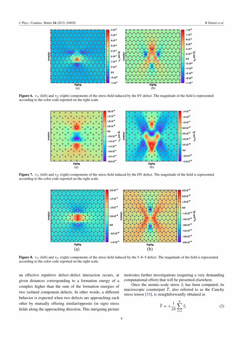
In figures 6–10 we report the calculated τ11 and τ22 stressfields generated, respectively, by an SV, DV, 5–8–5, 555–777,and SW isolated defect in the graphene sheet. We remarkthat Cartesian components labeled by 1 and 2 correspond,respectively, to the zigzag direction and to the armchairdirection (also indicated in figures) of the honeycomb lattice.Similarly to the case of the displacement field, a color map isused as obtained by splining the local value of τi computedat each ith lattice site (after relaxation). This continuumrepresentation is very effective in highlighting regions where

the stress field is compressive (blue color, negative value) ortensile (red color, positive value). This characteristic must bereferred to the carbon–carbon bonds that are correspondinglysqueezed or stretched by the relaxation following the defectformation. In general, when comparing figures 6–10 oneshould pay attention to the fact that the absolute scalecorresponding to the color code differs from plot to plot.

A first qualitative feature emerges that both τ11 and τ22are small and localized for SV and DV defects. For any defectkind, however, the τ22 component of stress field displays aremarkably more complex in-plane distribution than the τ11counterpart. This reflects, in our opinion, the non-equivalentbond sequence along the armchair and zigzag directions, aswell as the basically anisotropic nonlinear elastic behavior ofgraphene [16, 17].

By considering in detail the spatial distribution of theregions where τ11 and τ22 are compressive/tensile, it is easyto realize that high-order multipole stress fields are indeedgenerated by defects. Therefore, interaction basins for bothlike- and unlike-defect pairs are expected to be topologicallyvery complicated. At variance with the simple case of asingle vacancy (see figure 1(a)), it could be possible that

5

J. Phys.: Condens. Matter 24 (2012) 104020 R Dettori et al

Figure 6. τ11 (left) and τ22 (right) components of the stress field induced by the SV defect. The magnitude of the field is representedaccording to the color code reported on the right scale.

Figure 7. τ11 (left) and τ22 (right) components of the stress field induced by the DV defect. The magnitude of the field is representedaccording to the color code reported on the right scale.

Figure 8. τ11 (left) and τ22 (right) components of the stress field induced by the 5–8–5 defect. The magnitude of the field is representedaccording to the color code reported on the right scale.

an effective repulsive defect–defect interaction occurs, atgiven distances corresponding to a formation energy of acomplex higher than the sum of the formation energies oftwo isolated component defects. In other words, a differentbehavior is expected when two defects are approaching eachother by mutually offering similar/opposite (in sign) stressfields along the approaching direction. This intriguing picture

motivates further investigations (requiring a very demandingcomputational effort) that will be presented elsewhere.

Once the atomic-scale stress τi has been computed, itsmacroscopic counterpart T , also referred to as the Cauchystress tensor [33], is straightforwardly obtained as

T = +1

2S

N∑i=1

τi (2)

6

J. Phys.: Condens. Matter 24 (2012) 104020 R Dettori et al

Figure 9. τ11 (left) and τ22 (right) components of the stress field induced by the 555–777 defect. The magnitude of the field is representedaccording to the color code reported on the right scale.

Figure 10. τ11 (left) and τ22 (right) components of the stress field induced by the SW defect. The magnitude of the field is representedaccording to the color code reported on the right scale.

where S is the volume (actually, the surface) containing theN atoms placed on the two-dimensional hexagonal lattice.Equation (2) is useful for investigating the stress–strainconstitutive relation in defected graphene and computing itselastic moduli, as discussed in section 5.

5. Elastic moduli versus defect concentration

The linear elastic energy density U = 12 Cαβγ δεαβεγ δ is related

to the stress tensor defined in equation (2) by the relationshipTαβ = ∂U

∂εαβ= Cαβγ δεγ δ [33]. Here, the infinitesimal strain

tensor ε = 12 (∇u+∇uT) is represented by a symmetric matrix

with elements εxx =∂ux∂x , εyy =

∂uy∂y and εxy =

12 (∂ux∂y +

∂uy∂x ),

and the functions ux(x, y) and uy(x, y) correspond to the planardisplacement u = (ux, uy), where as above the x (y) labelindicates the zigzag (armchair) direction in the hexagonallattice of graphene.

By using the computed total Cauchy stress T(ε),equation (2), and the elastic energy density U(ε), the completeset of Cαβγ δ elastic constants can be computed throughstress-versus-strain curves corresponding to a set of suitablehomogeneous in-plane deformations. Alternatively, they canbe computed through energy-versus-strain curves. The straintensors, as well as the energy density, corresponding to

applied deformations depend on the unique scalar strainparameter ζ [16], so that a straightforward fit of the stress-versus-strain (or energy-versus-strain) curves, computed byTB-AS, has provided the full set of linear moduli Cαβγ δ for allstructures. This means that E and ν can be directly obtainedfrom the linear elastic constants Cαβγ δ .

In this work, the stress-versus-strain curves have beencarefully generated by varying the magnitude of ζ in stepsof 0.001 up to a maximum strain ζmax = ±0.02, andfull relaxation of the internal degrees of freedom of thesimulation cell was performed by zero temperature dampeddynamics until interatomic forces resulted not larger than0.5 × 10−4 eV A

−1. All results have been confirmed by

checking the stability of the estimated elastic moduli overseveral fitting ranges for each sample. The following in-planedeformations have been applied: (i) a uniaxial deformationζ along the zigzag direction, corresponding to a straintensor ε(zz)

ij = ζ δixδjx; (ii) a uniaxial deformation ζ alongthe armchair direction, corresponding to a strain tensorε(ac)ij = ζ δiyδjy; (iii) a hydrostatic planar deformation ζ ,

corresponding to the strain tensor ε(p)ij = ζ δij; (iv) a sheardeformation ζ , corresponding to an in-plane strain tensorε(s)ij = ζ(δixδjy + δiyδjx). Here and in the following, we use

the Voigt notation [34].

7

J. Phys.: Condens. Matter 24 (2012) 104020 R Dettori et al

Figure 11. Young modulus Ed (left) and the Poisson ratio νd (right) of graphene containing SV defects. Elastic moduli are normalized totheir value in pristine graphene, Ep and νp.

Figure 12. Young modulus Ed (left) and the Poisson ratio νd (right) of graphene containing SW defects. Elastic moduli are normalized totheir value in pristine graphene, Ep and νp.

All the investigated systems (regardless of the actualnumber of defects they host) behave as elastically isotropicmaterials (in the linear regime here explored), and theisotropicity ratio, defined as A = 2C66/(C11 − C12), is alwaysfound to be close to unity, which confirms that the assumptionof isotropicity is verified within about 10%. Accordingly, theelastic energy density (per unit of area) for a 2D isotropicsystem accumulated upon strain can be expressed as [34]

U = 12 C11(ε

2xx + ε

2yy + 2ε2

xy)+ C12(εxxεyy − ε2xy) (3)

to second order in the strain εij, corresponding to thelinear elastic regime. The constitutive in-plane stress–strainrelations, straightforwardly derived from equation (3), are

Txx = C11εxx + C12εyy Tyy = C22εyy + C12εxx

Txy = 2C66εxy(4)

and, therefore, the Young modulus E and Poisson ratio ν

are straightforwardly evaluated as E = (C 211 − C 2

12)/C11 andν = C12/C11, respectively.

We have computed the Young modulus and the Poissonratio adding one to four randomly distributed and orienteddefects of each kind under study onto a graphene cellcontaining about 800 atoms. The distance between defectsis enough to neglect interaction effects (according to thecriterion outlines in section 3). We define the defect

concentration as the number density of defects located in aunit area (in nm2) of the pristine graphene lattice.

In figures 11–13 we report the variation of E (left) andν versus an increasing number of SV, 555–777, and SWdefects, respectively. While an increasing concentration of‘missing atom’ defects (like V or 555–777) reduces the actualvalues of the elastic moduli, SW defects seem to inducethe same variation in the elastic properties of graphene,independently of their number density (at least up to themaximum concentration here considered). In other words, wefound that increasing the number of bond-switch mechanisms,driving the formation of SW defects, leaves the grapheneelasticity nearly unaffected. Interesting enough, the elasticsoftening found in the presence of SV or 555–777 defects isvery similar, especially if we focus on the Young modulus.This seems to suggest that the major role in affecting theelastic moduli is not played by dangling bonds (which indeedare missing from the 555–777 configuration) but, rather, byremoving atoms.

6. Conclusion

Structural defects in graphene can be deliberately introducedby suitable processing in order to modify local properties.This is very promising in the material-by-design perspective,where defects are engineered in order to modify the electronic

8

J. Phys.: Condens. Matter 24 (2012) 104020 R Dettori et al

Figure 13. Young modulus Ed (left) and the Poisson ratio νd (right) of graphene containing 555–777 defects. Elastic moduli are normalizedto their value in pristine graphene, Ep and νp.

and mechanical properties of graphene for achieving newfunctionalities not found in the pristine material. In this workwe have investigated the structural and elastic properties ofdefected graphene, computing as well the formation energyof a number of hitherto experimentally observed point-likedefects, namely the single or double vacancy, the Stone–Walesdefect, and the 5–8–5 and 555–777 reconstructed ones.

A full characterization of the displacement and stressfields generated by any such isolated defect is provided,by means of large-scale atomistic simulations based on asemi-empirical tight-binding quantum scheme. We provedthat such elastic fields in general die within 10 A fromthe defect position and, therefore, the mutual defect–defectinteractions are relatively short ranged. Furthermore, theirspatial distribution is quite different from case to case,reflecting the actual symmetry of the generating defect. Theinformation about the lattice displacement pattern is extractedfrom an atomistic calculation, but it is cast in the form ofa continuum field obtained by a suitable splining procedure.This is both very effective for the pictorial representation ofthe defects and could be useful for the correct interpretationof electron microscopy images.

The formation energies of the defect structures hereinvestigated vary between ∼5 and ∼9 eV, thus confirmingthe experimental evidence about the high structural quality ofgraphene samples obtained by various synthesis techniques.

Finally, we calculated the linear elastic moduli ofdefected graphene, as a function of the surface defect density.In any case we found that both the Young modulus andthe Poisson ratio are decreased with respect to their valuesin the pristine material. However, while by increasing thedensity of Stone–Wales defects the elastic moduli are notfurther affected, both the Young modulus and the Poissonratio show a monotonic decrease by increasing the numberof single or (reconstructed) double vacancies. This seemsto suggest that what actually matters in defining the linearelasticity of defected graphene is the absolute mass densityof the lattice (which is not affected by Stone–Wales defects orby any possible reconstruction of dangling bonds generatedupon atom removal).

Acknowledgments

We acknowledge financial support by the Regional Gov-ernment of Sardinia under the project ‘Ricerca di Base’titled ‘Modellizzazione Multiscala della Meccanica dei Ma-teriali Complessi’ (RAS-M4C). Moreover, we acknowledgecomputational support by CYBERSAR (Cagliari, Italy), andCASPUR (Rome, Italy).

One of us (LC) is greatly indebted to Professor GiorgioBenedek for his mentoring, for the illuminating leadershipduring the first years of his career, and for so much scientificdiscussion and advice. Grazie di cuore, Giorgio: ti sono gratoper tutto quello che mi hai insegnato.

References

[1] Novoselov K S, Geim A K, Morozov S V, Jiang D, Zhang Y,Dubonos S V, Grigorieva I V and Firsov A A 2004 Science306 666

[2] Bae S, Kim H, Lee Y, Xu X, Park J-S, Zheng Y,Balakrishnan J, Lei T, Kim H R and Song Y I 2010 NatureNanotechnol. 5 574

[3] Kim K S, Zhao Y, Jang H, Lee S Y, Kim J M, Kim K S,Ahn J-H, Kim P, Choi J-Y and Hong B H 2009 Nature457 706

[4] Berger C, Song Z, Li T, Li X, Ogbazghi A Y, Feng R, Dai Z,Marchenkov A N, Conrad E H and First P 2004 J. Phys.Chem. B 108 19912

[5] Berger C, Song Z, Li X, Wu X, Brown N, Naud C, Mayou D,Li T, Hass J and Marchenkov A N 2006 Science 312 1191

[6] Banhart F, Kotakoski J and Krasheninnikov A V 2011 ACSNano 5 26

[7] Hashimoto A, Suenaga K, Gloter A, Urita K and Iijima S 2004Nature 430 870

[8] Meyer J C, Kisielowski C, Erni R, Rossell M D,Crommie M F and Zettl A 2008 Nano Lett. 8 3582

[9] Ertekin E, Chrzan D C and Daw M S 2009 Phys. Rev. B79 155421

[10] Sammalkorpi M, Krasheninnikov A V, Kuronen A,Nordlund K and Kaski K 2004 Phys. Rev. B 70 245416

[11] Mielke S L, Troya S, Zhang S, Li J-L, Xiao S, Car R,Ruoff R S, Schatz G C and Belytschko T 2004 Chem. Phys.Lett. 390 413

[12] Colombo L 2005 Riv. Nuovo Cimento 28 1[13] Xu C H, Wang C Z, Chan C T and Ho K M 1992 J. Phys.:

Condens. Matter 4 6047

9

J. Phys.: Condens. Matter 24 (2012) 104020 R Dettori et al

[14] Canning A, Galli G and Kim J 1997 Phys. Rev. Lett. 78 4442[15] Yamaguchi Y, Colombo L, Piseri P, Ravagnan L and

Milani P 2007 Phys. Rev. B 76 134119[16] Cadelano E, Palla P L, Giordano S and Colombo L 2009 Phys.

Rev. Lett. 102 235502[17] Lee C, Wei X, Kysar J W and Hone J 2008 Science 21 385[18] Gomez-Navarro C, Burghard M and Kern K 2008 Nano Lett.

8 2045[19] Cadelano E, Giordano S and Colombo L 2010 Phys. Rev. B

81 144105[20] Zhao J, Winey J M and Gupta Y M 2007 Phys. Rev. B

75 094105[21] Arroyo M and Belytshko T 2004 Phys. Rev. B 69 115415[22] Zhang P, Huang Y, Geubelle P H, Klein P A and

Hwang K C 2002 Int. J. Solids Struct. 39 3893[23] Xu C H, Fu C L and Pedraza D F 1993 Phys. Rev.

B 48 13273[24] Li L, Reich S and Robertson J 2005 Phys. Rev. B 72 184109

[25] Ma Y, Lehtinen P O, Foster A S and Nieminen R M 2004 NewJ. Phys. 6 68

[26] El-Barbary A A, Telling R H, Ewels C P, Heggie M I andBriddon P R 2003 Phys. Rev. B 68 144107

[27] Amara H, Latil S, Meunier V, Lambin P andCharlier J-C 2007 Phys. Rev. B 76 115423

[28] Ma J, Alfe D, Michaelides A and Wang E 2009 Phys. Rev. B80 033407

[29] Thrower P A and Mayer R M 1978 Phys. Status Solidi a 47 11[30] Lusk M T and Carr L D 2009 Phys. Rev. Lett. 100 175503[31] Lee G-D, Wang C Z, Yoon E, Hwang N-M, Kim D-Y and

Ho K M 2005 Phys. Rev. Lett. 95 205501[32] Giordano S, Mattoni A and Colombo L 2010 Rev. Comp. Ch.

27 1[33] Landau L D and Lifschitz E M 1986 Theory of Elasticity

(Oxford: Butterworth Heinemann)[34] Huntington H B 1958 The Elastic Constants of Crystals

(New York: Academic)

10