three dimensional linear-elastic - Spiral – Imperial College ...

THREE DIMENSIONAL LINEAR-ELASTIC

FRACTURE MECHANICS ANALYSIS OF

THICK-WALLED PRESSURE VESSEL COMPONENTS

by

Manuel Frederico Oom de SEABRA PEREIRA, Dipl.Eng. (I.S.T.)

A thesis submitted for the degree of Doctor of Philosophy

of the University of London and for the Diploma of Imperial

College.

Mechanical Engineering Department

Imperial College of Science and Technology

University of London

February 1977

(I )

ABSTRACT

The present work deals with the evaluation of Fracture

Mechanics parameters in some pressure vessel components, viz.

corner cracks in the inside transition of a junction of thick-

walled cylinders.

This study is confined to elastic, isotropic and homog-

eneous materials. No temperature effects have been considered.

Such crack configurations, because of their particular

geometry and loading conditions, are fully three dimensional

in nature and consequently have been dealt with as such.

Moreover these configurations are gecmetrically too complicated

to be treated analytically and for this reason finite

element methods have been applied.

A three dimensional finite element computer program

using brick type elements has been brought into use and mesh

generation, plotting routines and computational procedures,

including substructuring schemes are described in detail.

Special "crack tip elements" have been introduced to

model the singularity in stress and strain fields near the

crack tips.

The effectiveness of such elements is demonstrated by

performing analyses of Compact Tension Specimens, Corner and

Part-through crack configurations and Semi-circular cracks

emanating from the inner surface of thick-walled cylinders

subjected to internal pressure.

Finally, stress intensity factors have been obtained

for some hypothetical cracks of different sizes situated in

the plane of highest nominal stresses near the intersection

regions of a T-junction of thick walled cylinders.

Consideration is given to the application of these

results to a fracture safety analysis of this particular

component.

Throughout the present work the variation of stress

intensity factor along the crack fronts of the various con-

figurations is discussed along with the general stress

behaviour of the cracked and uncracked geometries.

ERRATA

Page Line or Expr. Should read

3 13 .. hazards is particularly

relevant was ...

6 6 in the y direction

8 6 plane stress

31 17 Ni = (1 + Eo)(1 + no) (1 + co)

(Eo + n o + o - 2)/8

37 1 ... Poisson's ratio

43

45

50

3

23

2

... semi-bandwidth

and their derivatives

BACWD is described

53 25 these types of

61 22 E n=t.

63 exp.(3.10), 1:i i (3.11) 31f

66 8 ... thus equation (2.7)

74 exp. (3.43) - - + 1/2 (1 -n) (Y2 + Y6 )

76 exp.(3.46a) pl = 3/4 + 1/4n

76 exp.(3.46b) p2 = 3/4 + 1/4E

76 exp.(3.47a) x = 1/4(3 + n + LIE + C 2 - nc2 )

76 exp. (3.47b) x = 1/4(3 + -g 4n + n 2 - 2 )

77 22 to the mesh

6 in the y direction

6 plane stress

1 .. Poisson's ratio ..

3 .. semi-band width ...

23 and their derivations

2 BACWD is described

le-

Page Line or Expr.

77 25

78 9

79 17

80 10

81 9

89 15

92 18

141 foot note

145 4

146 7

148 1

148 10

148 18

157 28

144 12

159 8

175 11

175 26

180 8

250 2

Should read

.. these types of ..

.. a microfilm plotter

length a

the remaining nodes in the free

surface

Levy et al

of structure

E Eui

so has the number

this section describes

[KEL]

conditions according

largest nodal number

MATN,E(MATN)

node k as it is indicated in

Figure A1.1

., be replaced by ..

.. The four angles ..

.. to all ..

.. Poisson's Ratio ..

Ps across

ACKNOWLEDGEMENTS

I would like to express my sincere gratitude to Dr.

J.L. Head for all his help, invaluable guidance and encour-

agement throughout the course of this project.

I would like also to record my special thanks to my

former research supervisor Professor C.E. Turner whose

advice and help I have found extremely valuable.

Many thanks are also due to the Instituto de Alta

Cultura, Ministry of Education and Scientific Research,

Lisbon, Portugal for their financial support during the course

of this work. My leave of absence from the Lisbon Institute

of Technology is also gratefully acknowledged. I would

particularly like to acknowledge Professor Luciano de Faria

of the Mechanical Engineering Department for his constant

encouragement during the course of this work.

I would like to extend my gratitude to Mr. D.J.F. Slater

who helped me in coming to terms with the DIM3B code and

Mr. J.D. Silva who fully participated in the development of

the program FRONT.

Thanks are due to Madeleine Field for typing the manu-

script.

Finally, I wish to acknowledge the debt I owe to my

parents who, in every way, made this possible.

(iv)

To my wife Joao

To my son Tiago

(v)

TABLE OF CONTENTS

ABSTRACT

ACKNOWLEDGEMENTS

TABLE OF CONTENTS

NOMENCLATURE

ABBREVIATIONS

CHAPTER

1.

PAGE

INTRODUCTION TO THE PROBLEM 1

1.1 - Definition 1

1.2 - Design Criteria, The Role of Fracture Mechanics 3

1.3 - Review on the Linear Elastic Fracture Mechanics 5

1.3.1 - Introduction 5 1.3.2 - The Energy Balance Approach to Fracture 6 1.3.3 - The Stress Intensity Factor Approach to 9

Fracture 1.3.4 The Three Dimensional Crack Problem 14

2. THREE DIMENSIONAL FINITE ELEMENT ANALYSIS 23

2.1 - Introduction 23

2.1.1 - General 23 2.1.2 - The Displacement Method 24 2.1.3 - The Choice of Elements, The Computer 26

Program

2.2 - Mathematical Theory of the Three Dimensional 28 Finite Elements

2.2.1 - General 28 2.2.2 - Isoparametric Concept, Shape Functions 28 2.2.3 - Local Curvilinear Coordinates 30 2.2.4 - General Steps of Finite Element 32

Formulation 2.2.5 - Strains, Derivation of Expression (2.15) 33 2.2.6 - Stiffness Matrix [K]e 35

2.2.6.1 - Numerical Integration of Expression 36 (2.33)

2.2.6.2 - Elasticity Matrix and its Economical 36 Use

2.2.7 - Equivalent Nodal Forces 37 2.2.8 - Evaluation of Stresses 39

(vi)

2.3 - Description of the Code DIM3B 40

2.3.1 - Introduction 2.3.2 - The Solution Technique of Equation

(2.2) 2.3.3 - Frontal Method of Solution (FMS) 2.3.4 - Program Breakdown 2.3.5 - Program Environment

3. THE FINITE ELEMENT METHOD APPLIED TO LINEAR ELASTIC FRACTURE MECHANICS

3.1 - Introduction

40 41

42 43 52

53

53

3.2 - Finite Element Techniques in LEFM 55

3.2.1 - Introduction 55 3.2.2 - The Direct Method 56 3.2.2.1 - The Stress Method 56 3.2.2.2 - The Displacement Method 57

3.2.3 - Energy Methods 60

3.3 - Theory of the Singularity Element 65

3.3.1 - Introduction 65 3.3.2 - Theory 65 3.3.2.1 - One Liae Elements 65 3.3.2.2 - Extension of the Singularity in 2D 71 3.3.2.3 - Singularity in 3D Elements 73 3.3.2.4 - Conclusions 75

3.4 - Test Cases 76

3.4.1 - Introduction 76

3.4.2 - Compact Tension Specimens 79

3.4.3 - Compact Tension Specimens with Curved

84 Crack Fronts

3.4.4 - Corner Crack

88 3.4.5 - Part-Through Semi-Circular Crack

89

3.4.6 - Thick-Walled Cylinders with Radial

89 Part-Through Semi-Circular Cracks

3.4.6.1 - Mesh Generation 90

3.4.6.2 - Overall Behaviour 91

3.4.6.3 - Stress Intensity Factors 92

4. SURFACE CRACKS IN A T-JUNCTION OF THICK WALLED 97

CYLINDERS

4.1 - General

97

4.2 - Definition of the Problem 99

4.3 - Finite Element Mesh Idealizations 101

4.3.2 - General 101 4.3.2 - 32 Node Element Mesh. CASE TJUN1 101 4.3.3 - 20 Node Element Mesh. CASE TJUN2 103

4.3.3.1 - Mesh Generation 103 4.3.3.2 - Results of Finite Element Analysis 105

for CASE TJUN2. Overall Behaviour. 4.3.4 - 20 Node Element Mesh. CASE TJUN3 107

4.3.4.1 - Mesh Generation 107 4.3.4.2 - Results of Finite Element Analysis 107

for CASE TJUN3. Overall Behaviour.

4.4 - Validity of the Substructuring Technique 111

4.5 - Substructure Analysis 112

4.5.1 - The Choice of Crack Configurations 112 4.5.2 - Mesh Generation 114 4.5.3 - Analysis of the Uncracked Substructure 116

Overall Behaviour

4.6 - Analysis of the Cracked Structure 117

4.6.1 - Idealization of the Cracks 117 4.6.2 - Overall Behaviour 117 4.6.3 - Stresses Ahead of the Crack Fronts 118 4.6.4 - Evaluation of K-Factors. Discussion of 118

Results.

5. CONCLUSIONS AND RECOMMENDATIONS FOR FUTURE WORK 128

5.1 - Achievements 128

5.2 - Computing Costs 131

5.3 - Final Conclusions 133

5.3.1 - The Finite Element Method and its LEFM 133 Applications

5.3.2 - The LEFM Studies of Cracks in the Main 135 Steam Vent Pipe "T-Piece"

5.4 Recommendations for Future Work. 137

APPENDIX 1 PROGRAM FRONT. DESCRIPTION 140

A1.1 - Introduction 140

A1.2 - Displacement Boundary Conditions 141

A1.2.1 - Prescribed Displacements in Radial 142 or Axial Directions

A1.2.2 - Slope Boundary Conditions 144

A1.3 - Program Breakdown 146

A1.3.1 - Initializations 147 A1.3.2 - Total Nodal Forces, Stiffness Coef- 147

ficients, Forward Elimination A1.3.3 - Evaluation of Displacements and 151

Stresses

A1.3.4 - Flow chart of the program FRONT 152

A1.4 - User's Guide 152

A1.4.1 - Introduction 152 A1.4.2 - Preparation of the Problem 154

A1.4.2.1 - Material Properties 154 A1.4.2.2 - Mesh Generation 154 A1.4.2.3 - Loading 155 A1.4.2.4 - Displacement Boundary Conditions 155

A1.4.3 - List of Input Variables 156 A1.4.4 - Input Data Format 157 A1.4.5 - Operating FRONT Using Program EDT 158 A1.4.6 - Environmental Aspects 159

A1.5 - Listing of the FRONT Code 160

A1.6 - Listing of the program EDT 169

APPENDIX 2 DIM3B CODE USER'S GUIDE 170

A2.1 - Introduction

A2.2 - Preparation of the Problem

A2.2.1 - Material Properties A2.2.2 - Mesh Generation

A2.3 - Sets of Coordinates

A2.4 - Loading

170

170

170 170

172

177

A2.5 - Boundary Conditions and Prescribed Deflections 178

A2.6 - Computation Data 178

A2.7 - Special Modes of Operation 179

A2.8 - List of Input Variables

181

A2.9 - Data Format

182

A2.9.1 - Data Order 182 A2.9.2 - Data Deck

184

A2.10 - Error Messages 184

A2.11 - DIMDIM Code 186

A2.11.1 - Problem Size 186 A2.11.2 - General Description 187

A2.11.3 - List of Input Variables

188 A2.11.4 - Data Format for DIMDIM

189

A2.11.5 - Job File 191

A2.12 - Sample Problems 192

A2.12.1 - Cantilever Beam Loaded at the End

192 A2.12.2 - Thick-Walled Cylinder Subjected to

194 Internal Pressure

A2.13 - Listing of DIMDIM Code 196

APPENDIX 3 LISTING OF PROGRAM DIM3B 201

APPENDIX 4 LISTING OF PROGRAM DRAW 220

APPENDIX 5 REFERENCES 223

FIGURES 235

Figures relating to Chapter 1

235


238


240


263

(x )

NOMENCLATURE

a Crack length; axis of an ellipse

A Crack area

A. Coefficients of the Williams stress function

b Axis of an ellipse

B Thickness

B. Coefficients of the Williams stress function, 1 B.1 = B. (6,v) 1

[ B]

Matrix of shape function derivatives

C

Compliance of a test specimen (Reciprocal of stiffness)

C.,C.,C Weight Coefficients in the Gaussian quadrature i j m formaulae

[ D] Elasticity matrix

E Young's Modulus

E' = E for plane stress conditions

= E/(1-v2 ) for plane strain conditions

E(k) complete elliptical integral of the second kind

k ='V1-(b/a)2

f..(0,v) Functions of 0 and v in the Westergaard 13 expressions

F Externally applied generalized nodal forces

Fg Nodal equivalent point forces in a 3D element

g(x,y,z) Function representing the applied loads in the

FEM

GI

Mode I strain energy release rate

Gc

Critical strain energy release rate (at onset of fracture)

[J]

Jacobian of tranformation of coordinates

Stiffness matrix

k.. Stiffness coefficients 1J

K Stiffness matrix; stress intensity factor (assumed to be mode I)

KI'KII'KIII Mode I, Mode II, Mode III Stress intensity factors

K Stress intensity factors of cracks in infinite medium

Ko =a ,tea for a crack of length 2a in an infinite plate

Ko= 20-

Tr. for a penny shaped crack of radii a in an infinite solid

K* Stress intensity factors obtained from the displacement or stress method

[M] Matrix describing the terms of a polimonial

Mf Magnifaction factor

MUN,MKNIMU

Submatrices of the general body stiffness matrix K

[N] Shape function matrix

Ni Nodal shape functions

p Parameter defining the intermediate nodal position in the second order elements

Pi Parameter defining the intermediate nodal positions in the third or higher order elements

P Load, internal pressure

Pi Nodal point forces

Ps Parameter defining the condition of place stress or plane strain

q=u/v Parameter describing a slope boundary condition

Q Working variable in Gaussian elimination

✓ Radial coordinate in a system of polar coord-inates r,0 or in a system of cylindrical coor-dinates r,0,z

ry

R

Distance from the crack tip where the stress is equal to the yield strength

Radius of curved crack fronts in CTS specimens.

R1 Internal radius of a cylinder

R2 External radius of a cylinder

Rs External forces

Rbs Forces statically equivalent to body forces

ES Forces to suppress initial strains

S.. Stiffness coefficients 1J

T Thickness

u Displacement component in the x direction or r direction

u. Nodal displacement component

U Strain energy

✓ Displacement component in the y direction

v. Nodal displacement component

w Displacement component in the z direction

W. Nodal displacement component

x Coordinate in x,y,z system

x Cartesian unit vector in the x direction

x. Nodal coordinate in the x direction 1

x' Coordinate in a transformed x',y',z' system

y Coordinate in a x,y,z system

y Cartesian unit vector in the y direction

yi Nodal coordinate in the y direction

Y' Coordinate in a transformed x',y',z' system

Y Magnification factor or "calibration factor"

z Coordinate in x,y,z or r,0,z system

z Cartesian unit vector in the z direction

z. Nodal Coordinate in the z direction 1

z' Coordinate in a transformed x',y',z' system

0

a Angle measured from the major axis in the plane of an ellipse

{ a }

Vector of generalized nodal coordinates in a finite element

Angle defining radial planes in the T-junction

Y Specific surface energy (Griffith's theory)

Yp Plastic work (Energy balance approach)

6=6(x,y,z) Displacement field within a finite element (S=6(E,n,c)

.

KN,6UN

Nodal displacement components

Suvectors of the general displacement solution vector in the FEM

A Displacement solution vector or finite difference

Strain vector in a finite element formulation

i=1,3 corresponds to c ,c ,e x y z

i,j=1,3 corresponds to c ,c ,c xy yz zx

Coordinate in a system E,n,c of local curvil-inear coordinates

Coordinate in a system of local curvilinear coordinates

Coordinate in a r,0 or r,0,z system of co-ordinates

0 , x z Rotation of the x and z axis in program DRAW

K=3-4v for plane strain =(3-v)/(1+v) for plane stress

1.1 Shear Modulus

v Poisson's Ratio

Coordinate in a system E,n,t of local curv-ilinear coordinates

p Radius of curvature at one end of an ellipse

a Stress level or remote stress applied in a cracked body

(xiv)

(a) Stress vector in the finite element formulation

a Critical stress at the onset of fracture cr

am Membrane stress

ay,ayy Stress in the y direction

a Yield strength of the material ys

0=0(x,y,z) Field variable within a finite element

of Nodal values of the field variable.

(xv)

ABREVIATIONS

AGARD Advisory Group for Aerospace Research and

Development (NATO)

ASME American Society of Mechanical Engineers

ASKA Automatic System for Kinematic Analysis (ISD-

Institut fuer static und Dynamik der Luft -

and Raumfahrtkonstruktionen der Universitaet

Stuttgart)

ASTM American Society for Testing and Materials

BERSAFE Berkeley Stress Analysis by Finite Elements

(CEGB BNL, Berkeley, Gloucestershire)

CDC Control Data Corporation (computers available

at ICCC and ULCC)

CEGB Central Electricity Generating Board

CM Central Memory (computers)

CPU Central Processor Unit (computers)

CTS Compact tension specimen

CYL1,CYL2 Cracked cylinders test cases (Section 3.4.6)

DIMDIM Computer program for "dynamic operation" with

DIM3B

DIM3B Three dimensional finite element computer program

Version B.

DRAW Computer program for graphic mesh visualization

FEM Finite Element Method

FMS Frontal Method of Solution

FRONT Two dimensional axi-symmetric finite element

program using the FMS

ICCC Imperial College Computer Centre

LEFM Linear Elastic Fracture Mechanics

PP Peripheral Processor (computers)

SCF Stress concentration factor

TJUN1 Finite element mesh idealization of a "T-piece"

with 32 node hexahedron elements


with 20 node hexahedron elements (equivalent to

two diametrically opposed "T-pieces")


with 20 node hexahedron elements

ULCC University of London Computer Centre

2D Two-dimensional

3D Three-dimensional

- 1 -

CHAPTER1

INTRODUCTION TO THE PROBLEM

1.1 Definition

Thick walled pressure vessels occur in many enginee-

ring installations and modern technology requires these

components to work under increasingly severe conditions.

The utilization of new materials, the introduction of new

fabrication techniques, the requirements either to work

under extremely high or low temperatures such as in the

cases that occur in boilers and reactors, or to work under

adverse environmental conditions, impose new demands on

methods of design and analysis.

It is well known that a problem of stress concentration

arises in the regions of intersections or changes in

geometry, therefore knowledge of the stress distribution in

these areas is important to ensure proper and safer designs.

Furthermore, the existence of crack starting tendencies,

cracks or crack like flaws in the structure can eventually

lead to failures at loads well below the ones specified by

the conventional strength of structures.

On the other hand, the science of Fracture Mechanics

can be used, providing the designer with an approach to

safe design, even if components have crack-like defects.

Figure 1.1 a) shows a typical construction of a pressure

vessel used in Nuclear Reactor Technology. As can be seen,

these vessels normally have cylindrical and/or spherical

shapes with several discontinuities like nozzles, and the

supports of the vessel. During the last five years some

attempts have been made (1)(*) , (2) , (3) , (4), (5) to

access the severity of cracks in those nozzles.

Figure 1.1 b) shows a typical component of the piping

system associated with those vessels, they differ substant-

ially in geometry (diameter ratio and size) from the vessel

nozzles but no reports on Fracture studies of these

configurations could be found in recent literature. Such

a study was carried out by the author on amain steam vent

pipe "T" junction of a C.E.G.B. power station.

Such components seem to be too compact to be treated

analytically and for this reason recourse is to be made to

the Finite Element Method already adopted by other workers

in this field of studies.

Chapters 2 and 3 describe the Finite Element Method,

its computer implementation and relative merits for the

evaluation of Fracture Mechanics parameters. Finally,

Chapter 4 presents results for some crack configurations

in the considered "T" piece.

In the next three sections, design criteria for pressure

vessels are outlined followed by a brief review of Linear

Elastic Fracture Mechanics (LEFM) with some reference to

three dimensional crack problems.

(*) - Numerals in round brackets indicate references described in Appendix 5 of this thesis.

1.2 Design Criteria, The Role of Fracture Mechanics

The design of pressure vessel components has in the

past received considerable attention and a comprehensive

report on its developments can be found elsewhere in the

literature, (6), (7).

In the late fifties, as a result of the accumulated

experience the basic philosophy of design was mainly

governed by two general rules, first, keeping overall

stress levels at low values and second, requiring ductile

materials to safely tolerate local peak stresses and

discontinuity stresses.

The development of Nuclear Power Technology, where

concern for safety and possible serious hazards was a clear

stimulus for further research in this area.

The simultaneous development of electronic digital

computers made possible more thorough structural analysis

and improvement on the existing evaluation methods.

A better knowledge of material behaviour beyond the

elastic limit lead to a more accurate elastic plastic

analysis of pressure vessels with the use of numerical

methods and of the equivalent plastic stress-strain curve

of the material.

Pressure vessels are often subjected to cyclic loading

systems either due to flow induced vibrations or cyclic

stresses generated by major pressure changes and thermal

gradients due to start up and shut down conditions. Although

for the best part of this century fatigue has been

recognised as a potential threat to safety and reliability

cf engineering structures, it was only in the fifties

that this type of failure was explicitly recognized in

pressure vessels and specific procedures and criteria were

developed for evaluating fatigue damage.

We have seen so far, a first group of engineering

situations where the successful application of the outlined

design criteria did not take into account the service life

expected. Moreover, many structures in the past, have

experienced brittle fracture by application of a small

number of loading cycles or even failures at proof test

stages which were directly attributable to pre-existing

defects. Reports on spectacular brittle failures of pressure

vessels are well known in the literature of which some

examples are given in Refs. (8) , (9) and (10).

The necessity to assume the existence of cracks in

structures becomes evident. However, at the time it was felt

to be impossible to evaluate fast failure in terms of

stresses. This fact justified the use of the temperature

transition approach described by Pellini et al(11), based

on information obtained from notched impact tests. This

method of selection of materials provided and still provides

helpful information to the non fracture specialist, but

it cannot be applied directly to assess the resistance

of a piece in service.

The relationships between crack instability, the

surrounding stress fields and the critical flaw sizes,

forming no part of traditional design methods, remained

unsolved. It was only in the late forties, that Irwin

and Orowan laid the foundation of Fracture Mechanics, and

more recently, in the sixties that its principles were

applied providing then, the continuity between the design

method for flawed and unflawed structures.

During the last decade Fracture Mechanics and partic-

ularly the concepts of stress intensity factor and critical

stress intensity factor have advanced to the stage where

it is of direct value for the prevention of brittle frac-

ture in thick walled pressure vessels, and efforts are

being made to include these concepts in standards and codes

of practice.

An excellent compilation of papers on the developments

of the art in the 1960 - 70 period and onwards can be found

in ASME publications (12), (13) and in a recent Conference

on Reactor Technology (14).

1.3 Review on the Linear Elastic Fracture Mechanics

1.3.1 Introduction

The main objective of Fracture Mechanics is to study

in a macroscopic manner the fracture phenomenon as a function

of the applied loads. Such a study, in the absence of

large plastically yielded areas surrounding the cracks or

flaws, is referred to as Linear Elastic Fracture Mechanics

(LEFM).

Provided fracture occurs prior to large-scale yielding

of the structural member LEFM can be extended to study

fracture problems involving moderate plastic yielding by

incorporating various plasticity correction factors.

The classical stress function method of solving

elasticity problems described by Timoshenko et al. (15)

was first used by Inglis (16) to derive an equation (1.1)

for the maximum stresses at the tip of an elliptical notch

with major axis a on the x direction and minor axis b

subjected to a remote stress a on the y direction.

(ay) = ) = a (1 + 2a)

max

The ellipse degenerates to a crack when a » b and again

the methods of elasticity can be used (17), to calculate

the stresses in the vicinity of the crack. The maximum

tensile stress occurs at the end of the crack, (a ) I

Y max and is given approximately by

(a ) ..= 2 a ir for a» p Y P max

(1.2)

where p is the radius of curvature at one end of the ellipse

and is given by p = b2 /a.

1.3.2 The Energy Balance Approach to Fracture

The energy balance approach to fracture was first

proposed by Griffith (18) based on the Inglis' solutions.

The basic idea in his theory is that a crack will

begin to propagate if the elastic energy released by its

growth is greater than the energy required to create the

fractured surfaces. The main value of this thermodynamic

approach is that by considering the changes in energy as

the crack grows, it can ignore the details of the fracture

process at the crack tip.

For a problem of a crack of length 2a in a plate under

remote tension a, Griffith then found that the critical

stress, 0cr

, required for crack growth is given by the

following expressions

acr = 2Ey

in plane stress conditions (1.3.a)

a )/ - cr

2Ey r(1-v2) in plane strain conditions (1.3.b)

where E is the Young's Modulus

y is the specific surface energy

v is the Poisson's ratio

Since the terms on the right hand side of expressions

(1.3) are only material constants the factor acr la should be

an intrinsic material parameter. The experiments Griffith

performed on glass have shown encouraging results, in fact

at the instance of fracture a constant value of a ra was cr

obtained over a wide range of crack lengths.

However, Griffith's work could not be applied to materials

which did not behave in a pure elastic manner, thus vir-

tually ruling out consideration of any engineering problem.

Some twenty five years later Irwin, (19), and Orowan,

(20), in their analysis of fracture suggested that the energy

released in the fracture process was mainly dissipated by

producing plastic flow around the crack tip. A quantity yp

called plastic work was then introduced and was estimated

to be on the order 10' times greater than Griffith's

surface energy 2y which enabled Orowanto re-write equations

(1.3) in the following manner by simply neglecting the

Griffith term 2y

/EY

acr )/ in plane strain conditions (1.4.a)

Eyn acr

(1-v) in plane strain conditions (1.4.b)

Surprisingly enough this new quantity y p appeared to

be independent of the initial crack length, hence could

still he regarded as a material property. Furthermore, if

the plastic zone was small enough, all the merits in

Griffith's idea were still safeguarded and a theory corr-

elating fracture behaviour could still be substantiated.

In Irwin's view the modified theory consisted of evaluating

the strain energy release rate with respect to crack extension

at the point of fracture. If the fracture process were

essentially the same, regardless of the loading conditions

and geometry, the fracture event would occur when the strain

energy release rate reached a critical value, Gc, and this

value would be a material property.

As stated by Irwin, the Gc concept plays a similar

role in relation to fracture as the yield strength to plastic

deformation. As in the case of design methods based on the

knowledge of the stress-strain curve of the material,

experiments on cracked specimens enable the onset of fracture

to be predicted in real structures and this ability is

sufficient justification for utilizing the concept as an

engineering approach.

1.3.3 The Stress Intensity Factor Approach to Fracture

In Griffith's theory of brittle fracture a critical

stress-crack size relation was derived from an energy

postulate. An alternative interpretation of the fracture

phenomenon leads to stress-crack size relations by focussing

attention on the elastic stresses close to the tip of the

crack.

Based on the method of Westergaard (24), Irwin (19),

(22), (23), derived a general solution for the stress

system at the tip of an ideally plane sharp ended crack in

an isotropic elastic body. Referring to Figure 1.3, a

local coordinate system is chosen so that the z-axis is

parallel with the leading edge of the crack, the y-direction

is perpendicular to the plane of the crack and the x-axis

is such that the plane (xy) is normal to the crack front line.

If in the case of a straight front crack the z-dimension

of the body is large or small, plane strain or plane stress

will exist respectively. More realistically, in all but

thin plate-like geometries a mixed plane stress plane-strain

situation will exist across the z direction varying from

plane stress at the surface to plane strain at the central

area. Any plastic deformation which may occur at the crack

borders is neglected in a first approximation and will be

subsequently treated as a minor correction to the elastic

analysis.

- 10 -

Three basic modes (I, II, III) of crack surface

displacements which can lead to crack extension are shown

in Figure 1.2. During the course of this work attention

will be confined only to the opening mode of separation,

mode I.

Corresponding to opening mode conditions, the stresses

and displacements at points close to the crack front can

be shown (25) to have the form (see Figure 1.3)

KI 0 30 ax = /27r7 :2 cos - ( 1-sin -2. sin ) + . (1.5.a)

K1 0 0 30 a = cos -2- ( l+sin sin ) + . . . (1.5.b) y cos 2

0 -f 0 -2- 3 -7 + . • • - sin cos cos - xY

KI (1.5.c)

az = v(ax + ay) for plane strain

(1.5.d)

= 0 for plane stress

ux =

u = y

KI I-Tr.- 811 7

KI .07- 8p Tr

[(2K-1)cos

[(2K+1)sin

0

2

0 2

cos

sin

301

2

30] 2

▪ (1.6.a)

.

▪

(1.6.b)

uz = 0 for plane strain

where K = 3-4v for plane strain

3-v for plane stress 1+v

The omitted terms of these series expansions involve

increasing half powers of the ratio of r divided by the

crack length and consequently are important only at large

distances from the crack tip.

Results similar to expressions (1.5) and (1.6) can be

obtained for the edge sliding mode II and the tearing

Mode III.

The K term in these equations is independent of the

polar coordinates r and 0, and serves only as a positive

multiplying factor which can be shown to depend on the ap-

plied boundary load and the crack size. In Fracture

Mechanics terminology, K is referred to as the "stress

intensity factor" (SIF).

The significance of the above expressions is due to

their generality since they hold for any plane crack, thus

the elastic stresses and displacements around the crack tip

are entirely characterized by the stress intensity factor K.

Hence it must be expected that fracture will occur when K

reaches a critical K.

The Kc concept should indeed be expected to be equiva-

lent to the Gc concept already described. In fact Irwin

(19), (22), using virtual work arguments has shown that

the strain energy release rate could be identified with K

according to the following expression:

GI = KI

/E1 (1.7)

where E' = E(Young's Modulus) for plane stress conditions

or E' = E/(1-v2 ) for plane strain conditions.

- 12 -

It was mentioned early in this section that LEFM

should take into account a plasticity correction factor.

In fact the stress solutions (1.5) predict infinite

values of stress at the crack tip (r=0) which cannot occur

in practice of course. Plastic flow will therefore take

place in areas of small r values. The approximate extent

of the region of plastic flow can be estimated by substit-

uting a yield criterion into the stress field equation,

leading to

1 ,KI 2 r — y 2Tr (a ys)

for plane stress conditions (1.8)

ry is the distance ahead of the crack tip where ay reaches

the yield strength of the material.

For plane strain conditions, due to the triaxialaty

effects (see Figure 1.4) allowance must be made for the

elevation of yield stress ahead of the crack and this is

normally done (26) by substituting 1/-- ays foray, leading to

KI rIy = ( a )2 for plane strain conditions (1.9)

61T ys

Current test specimen dimensional specifications (21)

(* (56) in order to ensure proper determination of KIc

values • )

require that the crack length a, the specimen thickness B the

uncracked ligament w-a should all exceed 2.5(K_lc /a ys)2.

(*) - In KIc, I denotes opening mode I

c denotes critical for onset of fracture under plane strain conditions.

- 13 -

This limit should be proportional to the plastic zone

size rIy

(e.g. 1.9), (25)

rIy 0.02 (1.10) 2.5(KIc/oys)2

Therefore the range of applicability of LEFM is

limited in principle by the existance of a plastic zone

size at the crack tip which cannot be greater than 2%

of, for instance, the crack length a.

Finally, reference to methods of obtaining K for

different loading conditions and geometries are outlined.

In general, mode I stress intensity factors may be written

in the form

KI = Yo

The term oi/Tr. represents the SIF of a crack of length

2a in an infinite sheet subjected to a remote tensile

stress perpendicular to the plane of the crack. Y is a

nondimensional magnification factor which is a funtion of the

relevant geometric parameters and loading conditions(*)

A great variety of K1 determination methods is already

available: analytical methods using complex stress funtions,

alternating techniques or integral transforms: numerical

methods using conformal mapping techniques, boundary

collocation and finite element methods.

(*) - The evaluation of this factor Y is sometimes called "K calibration".

- 14 -

The principle of superposition (29) also enables the

calculation of solutions with different boundary conditions

to be combined to produce solutions for more complex

problems.

A comprehensive review of this subject was made by

Cartwright and Rooke (27) and Sih (28) and Cartwright and

Rooke(30) compiled a wide variety of solutions in a

"Compendium of Stress Intensity Factors".

Experimental methods have been also used to obtain

K values, amongst these the more relevant are: Compliance

Methods, also used for determination of Kic values for

different materials, Photoelasticity techniques and fatigue

tests where the K variations in the loading cycles can be

related to the crack growth rate using some fatigue crack

propagation law.

1.3.4 The Three Dimensional Crack Problem.

In real heavy-section structures, for example pressure

vessel components, cracks will often be initiated in areas

of high nominal strain. Normally these cracks will not be

through- cracks, but surface flaws or more commonly known

as part-through cracks or corner cracks. These cases,

because of their particular geometry and/or loading conditions

are fully three dimensional in nature and consequently should

be dealt with as such. Moreover, these cracks will normally

advance in a curved front and the stress intensity factor

may vary along the periphery of the crack. The analysis of

- 15 -

this type of flaw usually requires the assumption that

fracture will occur when somewhere along the crack front

the SIF exceeds the critical value Kic.

However, two major difficulties arise when dealing

with such problems. First, as pointed out by Hartranft

and Sih (31), an agreement amongst the theoreticians has

not yet been reached as regards stress and displacement

fields as well as K values in areas where the crack meets

the free surface. In their studies of a part-through

semi-circular crack, using an alternating method, they

found that a drastic drop in values of K will occur in a

small area near the surface. Benthem (33) on the other hand,

has shown that the degree of singularity in those areas is

no longer constant and equal to the well known -(for_ stresses)

suggested by Westergaard, but strongly dependant on the

Poisson's ratio. For the case where the Poisson's ratio is

equal to 0.3 he indicates a value of about .45 for the degree

of singularity, thus ruling out the usage of the stress

intensity factor concept, which has lost its meaning.

However, if this boundary layer effect is restricted

to very small areas near the free surface, as it appears to

be, it may yield only a minor contribution to the overall

distribution of K values in the more central portions of

the crack and the discrepancies introduced by neglecting it,

will be, hopefully, irrelevant for engineering purposes.

The second difficulty concerned with the surface flaw

is related to the crack front shape and the local variations

- 16 -

of K along the crack front.

Such crack configurations are normally characterized

by a length and a depth, but these two geometric parameters

are obviously insufficient to define the crack front, thus

allowing an infinity of possible shapes, (see Figure 1.5

for some examples), each one with its own K calibration and

with its own local variation of K values.

This complexity, however, may be irrelevant as stated

by Swedlow et al. (35), following R.A. Westman's reasoning

( . . . we expect, perhaps merely hope, that most of the

contours . . . will grow in a slow manner to a common shape

before rapid fracture ensues . . . The point is that

irregularities in crack shape may be expected to be smoothed

out somewhat and that the range of shapes that one might be

obliged to deal with is relatively modest

These assumptions are widely supported by post-mortem

observations of various thick walled pressure vessels, and

a typical example, which was taken from (6), is given in

Figure 1.6.

Since the famous papers by Sneddon (36) and Green et

al. (37) on the penny shaped and elliptical cracks in an

infinite solid, a good number of workers have devoted them-

selves to studies involving circular and elliptical cracks,

fully imbedd with different loading and/or geometric

conditions.

The only exact opening mode solutions are for infinite

regions. For the planar case of crack of length 2a the

SIF is given by

- 17 -

K = a iTra (1.12)

and for the circular crack of radius a the SIF is given by

K = 20111-- (1.13)

where a in both cases is the remote applied stress

perpendicular to the plane of the crack.

For the more general case of an elliptical crack Irwin

(38) derived an expression for the SIF which is given by

a b 1/4 K E (k) = (a)1/2 (a2 a + b2 cos2 a ) (1.14)

where E(k) is the complete elliptical integral of the

2 second kind with the argument k =1142) a

a,b, are the major and minor semi-axis of the ellipse

a is the angle measured from the major axis in

the plane of the crack.

Paris and Sih (25) have shown that the problem of a

crack in an infinite solid subjected to remote tension can

be replaced by a pressurized crack in an infinite solid.

Kobayashi (42) using a stress function method evaluated

the SIF for an elliptical crack in a solid subjected to an

internal varying pressure distibution which was represented

by a double-Fourrier series expansion.

He then, based on Paris' (25) ideas, extended his

studies to elliptical cracks subjected to uniaxial tension,

pure bending and transient heating, using suitable pressure

distributions on the faces of the crack. For the case of

K = 1.12M a E(K) 2 - .212(2 -)2 ys

nb (1.16)

- 18 -

uniaxial tension, he eventually arrived at the same expression

as Irwin (1.14).

The semi-elliptical surface flaw has been initially

studied by Irwin (38) based on the Green-Sneddon results.

His expression including a plasticity correction factor,

evaluates the SIF for the deepest point of a shallow crack(*)

as follows:

K - 1/ 1.2a2 b

E(K) - .212(2-)2 a ys

(1.15)

later Kobayashi et al. (39) have modified Irwin's expression

by introducing another magnification factor, Mf, as follows

This factor, being a funtion of the ratio b/a and b/B

where B is the thickness of the plate and accounts for the

proximity of the back free surface for the case when the

crack penetrates deeply inwards.

Smith et al. (32) have obtained the SIFs for semi-

circular surface flaws at its deepest points in a beam in

bending. From their results they show that the SIF does not

vanish when these points are at the neutral axis of the

beam. This means that the crack tip can penetrate further

(*) - Shallow crack means the crack depth being less than half of the plate thickness (see Ref. (41)).

- 19 -

into the compression region before it can no longer open.

The quarter elliptical corner crack bearing great

resemblance to the semi-elliptical configurations was

studied by Broek (40) by applying the expressions (1.15)

and (1.16) to particular problems such as radial corner

cracks emanating from holes in plates.

Among the several other studies on the surface flaw

problem which have been published to date, the more

accurate analytical solutions have been obtained using the

alternating method which basically combines analytical

results of two auxiliary problems with numerical techniques

(31).

The method has been used extensively by Smith et al.

(43), (44), who determined the SIF for part-circular cracks

in different loading conditions and by Shah and Kobayashi (41),

(45), for elliptical cracks, including also cracks under

uniform and non-uniform internal pressure.

Quite recently Sih (28) has introduced an entirely

new approach to LEFM based on the field strength of the local

strain energy density.

In this new theory a fundamental "strain energy density

factor", S, is derived which not only measures the amplitude

of local stresses (like K and G) but is also direction

sensitive. In his paper, Sih gives an example of the

application of these concepts in a three dimensional crack

problem yet no results have been presented at this time.

- 20 -

However, a three-dimensional analysis for predicting

the growth of an embedded elliptical crack subjected to

general loadings was carried out by Sih and Cha (58)

in which fracture is assumed to initiate in the direction

of minimum strain energy density factor.

The principles of the Compliance test(*) used in the

experimental determinations of SIFs, have also been applied

to 3D crack problems. Sih and Hartranft (57) generalized

this approach to study various elliptical surface flaw con-

figurations. They computed the compliance changes for

several possible extensions of the crack front, and indicate

how this method is applied to cracks in pressure vessels

subjected to internal pressure.

The main advantage of this method lies in the fact

that values of G derived from compliance changes ignores the

complex local stress field analyses of 3D crack problems.

However, the evaluation of local values of G using this

method, is strongly dependant on the local variation

of the crack front. The necessity to assume a particular

shape for the extended crack front may yield doubtful results.

The use of Finite Element Methods in the solution of

3D crack problems has been limited in the past due to its

inaccuracy as compared to the more rigorous analytical and

numerical methods.

(*) The strain energy release rate G can be obtained experimentally using the following expression

G = liP2N)/B Where C is the so called "compliance" or the reciprocal of the load (P) - deflection curve of a test specimen with thickness B. (see Ref.(26)).

- 21 -

However, when a real problem becomes three dimensional

most of the conventional methods can no longer be applied.

The application of the Finite Element Methods to

Fracture Mechanics will be discussed in Chapter 3.

Experimental Methods have also been studied recently

to determine the SIFs for 3D crack configurations.

Broekhoven and Ruijtenbeek (59) carried out some

experiments by monitoring crack growth rates (da/dN) under

uniaxial fatigue loading of precracked nozzle-on-plate

specimens. They then converted the resulting (da/dN)

measurements into AK values with the use of a suitable

fatigue crack propagation law for the same material of the

nozzle specimens. This method has the advantage that SIFs

are determined under conditions very similar to those in

reality.

Fatigue crack growth behaviour is strongly dependant

amongst other factors (61) on loading history, mean stress

specimen thickness and environmental conditions, therefore

the accuracy in the simple application of fatigue crack

growth laws to evaluate K values is yet to be demonstrated.

Sommer et al. (60) investigated the growth charac-

teristics of part-through cracks in thick walled plates

and tubes under fatigue loading.

They have shown that (verbatim) ( . . . Although .

the results cannot provide a refined failure analysis . .

they indicate which parameters are of importance for crack

extension and explain some general tendencies of crack

growth in thick walled plates and tubes).

- 22 -

A consise review on the various analytical methods used in

3D crack studies as well as some solutions can be found

in Refs. (31) and (41) and a reasonable collection of

practical results in this family of crack problems is given

in Refs. (25) and (42).

- 23 -

CHAPTER2

THREE-DIMENSIONAL FINITE ELEMENT ANALYSIS

2.1 Introduction

2.1.1 General

The Finite Element Method (FEM) is a very powerful

technique for numerically solving many complex field

problems.

This method which was introduced in the fifties has

been successfully applied to the solution of a great number

of problems in stress analysis.

The basic idea of the FEM is that a structure can be

represented by an idealized discrete analogue made up of

relatively small standard subregions, called elements, with

a number of nodal points related to them.

The energetic assumptions behind the Finite Element

theory allows the overall behaviour of the model to be

obtained as the sum of the contributions of all of its

elements. At the same time the characteristic behaviour of

each element can be developed based only upon its geometry

and material properties.

There exists a great number of excellent texts for

example Ref. (46) which covers the details of this method.

Refs. (47) and (48) give a good description of a wide range

of types of element which have been introduced during the

past twenty years.

- 24 -

Much has been published to date about the FEM. It

has reached such a stage where it has become a common tool

in a great number of research institutions and some

industrial organisations. Therefore a complete review of

this subject will not be given here.

One of the main features of the FEM and particularly

the displacement (stiffness) method, as compared to others,

is the ease involved in the handling of geometric shapes,

and the specification of boundary conditions of real

engineering structures.

This particular advantage was a governing aspect on

the choice of the FEM to perform the stress analysis of the

rather complex "T-junction" geometries and the subsequent

LEFM studies of some three-dimensional crack configurations

in those structures. The displacement method was adopted

in this work and will be briefly outlined and followed by

some considerations of the Finite Elements which have been

used.

2.1.2 The Displacement Method

In the displacement method, as opposed to the force or

equilibrium method, the displacement field within each

element is defined in terms of various functions 0 (usually

simple polynomials).

161 = [0(x,y,z)] fa1 (2.1)

- 25 -

where

{6} = u(x,y,z) , {a } = _a l

v(x,y,z) a 2

• w(x,y,z) an

and n is the number of generalized coordinates (a) which

is equal to the number of degrees of freedom of the element.

The x,y and z coordinates are not necessarily the global

coordinates.

Equation (2.1) can be solved for the generalized

coordinates, a , in terms of generalized nodal displacements.

By using the strain-displacements relationships and

the constitutive law, the stresses and strains within the

element can be evaluated in terms of nodal displacements.

The strain energy of the entire structure is then obtained

by adding the contributions of all its elements. Applying

the principle of minimum potential energy leads to a set

of linear equations relating the externally applied generalized

nodal forces F to the generalized nodal displacements, A ,

k A = F (2.2)

where k is the stiffness matrix of the entire system.

It can be shown through the principle of minimum

potential energy, (see (48)), that this method provides a

lower bound for the displacement solution A.

- 26 -

Criteria for convergence to the true solution by

finer mesh subdivision must be met (48), which imposes two

well-known conditions on the choice of the displacement

functions:

1. The displacement field should include "constant

strain" states and "rigid body" movements.

2. Continuity of the displacement field must be

ensured within the element and at interelement

boundaries.

A wide range of functions 0 can be found to meet these

requirements. However a proper selection of these functions

is essential to ensure good rates of convergence.

Some detailed considerations of this method, as applied

to the three dimensional elements used, will be made later

on this Chapter.

2.1.3 The Choice of Elements, the Computer Program

Finite Element Programs, in general, are bound to

require large spaces of computer memory and this problem

is obviously more relevant in the case of three-dimensional

applications, and the use of more sophisticated programming

techniques such as the "Front Method", to be described

later, becomes compulsory.

Several powerful and elaborate systems do exist in the

United Kingdom (ASKA, BERSAFE, etc.) in which libraries of

- 27 -

various finite elements are used together. However at

the time this work was started, none of these systems

were available at Imperial College. It was only quite

recently (1974) that the ASKA system was implemented at

Imperial College Computer Centre and later on at the

University of London Computer Centre.

In view of the foregoing, a computer code initially

developed by Alujevic (DIMS) Ref.(50) based on a shell

program (NAMAIN) developed by Natarajan Ref.(49) under the

supervision of Dr. J.A. Blomfield* was brought into use.

The present version of the code, now called DIM3B,

uses two different brick-based elements: 20 and 32 node

hexahedrons using second and third order displacement func-

tions respectively. However only one type of these elements

is used at a time in one computer run.

The choice of these elements was based on past exper-

ience with Finite Element applications (see Refs. (])-(5)),

Refs.(46) and (52)). Problems of idealizing second order

curved boundaries (viz. cylinders) are eased by using these

higher order curved elements. Moreover, these particular

elements have proven to be extremely useful when dealing

with cracked structures.

Bearing in mind the forseeable large costs involved

in running the DIM3B code, an attempt was made to model a

"T-junction" piece by a two-dimensional axisymetric sim-

ulation of the real problem.

* formerly Lecturer, Mechanical Engineering Department, Imperial College.

- 28 -

For this purpose a Finite Element program using

triangular axisymetric elements was developed (FRONT)

using a simplified version of the "Frontal Method".

This study was carried out in the early stages of

this work, simultaneously with the debugging nrocess of

the DIM3B code. This analysis will be omitted for no

conclusive results nave been reached. However, in order

to provide a permanent record of the program FRONT a

description and listing are given in Appendix 1 of this thesis.

2.2 Mathematical Theory of Three Dimensional Finite Elements.

2.2.1 General

This section describes the mathematical theory involved

in the calculation of the individual matrices of the two

element types available.

Although a fairly general formulation of the FEM using

these elements is known (48), a brief sketch of this theory

is presented here for the sake of completness and also to

introduce the notation which will be used later.

2.2.2 Isoparametric Concept, Shape Functions

In a typical three-dimensional isoparametric finite

element with n nodes the coordinates or any field variable

are given by, for example

$ = al + a2x +a3y +(le +a xPl7cizr

(2.3)

s a (2.6) 1

a 2

a n

= 0

$

• 2

1

On

- 29 -

where M = [1,x,y, . . . .]

or

0(x,y,z) = [M(x,y,z)

(2.4)

an

IalT = r a 1, a2, . . . ' an] L

by substituting the coordinates at each node

Oi = [1,xi,yi, . . .] {a} (2.5)

and for all nodes

1 x1 y1 . . .

1. . x2 y2 .

1 xn yn . . .

= E cla}

where [C] is a square matrix of constant terms. The

coeficients a can be calculated as follows

(2.7)

{a} . [c]-1 {0i} (2.8)

or n

$ (x,y,z) =E N.1Oi i

(2.10)

— 30 —

then from expression (2.4) and substituting {a} calculated

in (2.8)

0 (x,17,z) = [M(x,Y,z)] [ Cr' {0i} (2.9)

where i shape functions and i are the

nodal values of the field variable.

It is convenient to stress that the shape functions

Ni, so far, are funtions of the general coordinates x, y

and z.

The isoparametric concept is based on the fact that

the same interpolation functions are used for defining any

field variable, namely, in this case, coordinates and

displacements within the element.

2.2.3 Local Curvilinear Coordinates

Let us consider curvilinear coordinates n, C

varying between -1, +1 so that in the space (E,11,0 the

hexahedron (20 or 32 node 3D finite elements, see figure

2.1) becomes a cube with side length of two units.

Following expression (2.10), the relationship between

the cartesian and the curvilinear coordinates will be

n xi = E Ni E. i i=1

(2.11)

and displacements within the element will be defined as

follows

- 31 -

n {S} = 1-2 Ni {Si}

i=1 (2.12)

where

{6)T Eu,v,w] and

lyT

= [ui,vi,wi]

n = 20 or 32

Once the local coordinates have been defined, the

shape functions Ni can be expressed in terms of the local

coordinates and they become independant of the element

shape, therefore the same for all the elements. From now

on they will be considered as

Ni = 11.(t;,n i d. (2.13a)

For these elements the shape functions Ni, i=1,2, . .20/32

defined in terms of local coordinates are, using the notation

Eo = EEi ► no = nnio = cCi

Quadratic element (20 node):

Corner nodes

Ni = ( o)( o )( o +floo

-2)/8 (2.13b)

Mid-side nodes

+1 N.=(1-V) (l+no) (l+co)/4

(2.13c)

- 32 -

ni =0, ci =-+ 1, ci 1 =-1 N.(1+Eo)(I-T.1 2 )(1+Co)/4

i=0, Ei=-+

1 1, n.=-+

1 Ni(l+E0)(1+no)(1-c2 )/4

Cubic element (32 node):

Corner nodes

Ni= (1+E0) (l+n0) (1+ ,:)) 9(v+T12÷2)-19] /64 (2.13f)

Typical third side node

+13' n.=-1, c•=-1

Ni= (1-E2 ) (1+9E0) ( i+no) (1+ 0) 9/64

(2.13g)

The main advantage of this formulation is that the

numerical procedures involved with the element will always

be the same regardless of their particular distorted shape

they will assume in the idealized mesh.

2.2.4 General Steps of Finite Element Formulation

Following the basic finite element formulation descri-

bed elsewhere, Ref.(47)/ a list of wanted relationships is

described below.

i) {6}= [N]{6}e

ii) {c}= [B]{5}e

iii) {a}= [D]{E}= [ID] B{6}e

iv) [K]e= r[ B]T[ D] [ B] d vol dvole

where

(2.14)

(2.15)

(2.16)

(2.17)

[N] is called the shape function matrix

{c} are the strains {c}T={c ,E C E x y' z' xy' . .

are the nodal displacements for each element {6} are

[D] is the elasticity matrix

- 33 -

[B] is the displacement/strain transformation matrix

[K]e is the stiffness matrix for each element.

2.2.5 Strains; Derivation of Expression (2.15)

To calculate strains, derivatives of displacements with

respect to x,y,z are needed. Bearing in mind expressions

(2.13)

as

and (2.14).

= 3N1 aN2 • • 0 •

3 aE

as 3N1 aN2 • • • •

an an an

96 3N1 aN2 • • 0 •

ac _BC a?

(2.18)

d n

(2.19)

Looking at expression (2.19) [ DE] can be considered

as a derivative operator so the same principle is also

applied to the coordinates as follows

[DE] x1 y1 z1 x2 y2 z 2 -2 z2

x n Yn z n

= - ax By az - 9E aE aE

ax By az an an an

ax By az ac 9c 9c

= [ J]

(2.20)

where [J] is obviously the Jacobian of transformation of

general coordinates x,y,z to the local ones n,c.

Using now chain rule relationships of the type

- 34 -

aO 30 ax + aO 2y + a0 Bz BE 3x aE By BE 5z aE (2.21)

= [ ax By Bzi a0 BE

aE ac ax

43 By

BO Bz

(2.22)

having

ras

now

Generalizing for

the displacement

= [J]

21T . [J]

inverting

the

as

rest of the

as field variable

coordinates and

(2.23)

T

(2.24)

of expression (2.18)

. (2.25) • i)T

. (2.26) • .( r)T

aa:

as

3x

as an

as

ay

ad 9c

as

this equation

Bz

'

right

we

IJJ

Lax

into

ras

ay az '

Substituting the

expression (2.24)

T as as] =

as as] 1[Dd

r 1-1r

[DEXYZ]

aE a

hand side

obtain

iDEjks 162

[6 6 1 2

Lax By Bz

=

The matrix [DEXYZ] can be suitably changed in order

to accommodate the derivatives for the several components

of the engineering strains

- 35 -

{e } = ex ey cz e xy e yz e zx

3u/3x

3v/3y

aw/3z

3u/3y + 3v/3x

3v/3z + 3w/ay

aw/ax + 3u/3z

(2.27)

as follows : if[DEXYZ]

[DEXYZ] =

is given by

dll d12 ' ' ' dln (2.28)

d21 d22 • • . d2n

d31 d32 . . . d3n

hence

{ c } = d11 0 0 d12 0 0 . . dln 0 0 6i(2.29)

0 d21 0 0 d22 0 . . 0 d2n 0 62

0 0 d31 0 0 d32 . 0 0 d32

d21 d11 0 d22 d12 0 . . d2ndin 0 6n

T = [B] [61 62 . . . . 6n ]

(2.30)

as it was required in expression (2.15)

2.2.6 Stiffness matrix [R]e

Remembering the basic theory Ref.(48), the stiffness

matrix of an element is defined as follows

[K le =1.[ B]T( DJ [ B] dvole (2.31) vol

e

where B was defined in expression (2.29), D is the

elasticity matrix to be defined, and vole is the volume of

- 36 -

the element.

Remembering that [B] is a funtion of E,n and so

the element volume dvol must be transformed as

dxdydz = IJI dEdndc

Taking into account the definition of the local

coordinates (E,n,c) given in 2.2.3 the integral (2.31)

becomes

1+1 1 +1 1+1 I k le =

[BITE Dll B] I JI dE do szl

(2.32)

(2.33)

2.2.6.1 Numerical Integration of Expression (2.33)

The element stiffness matrix is assembled by numerical

integration of the expression (2.33). Using the Gaussian

Quadrature formula Ref.(51) as a definite integral,

+1

f f(x)dx is replaced by a summation C.3f(ai) where C. 3 -1

are the weight coefficients, ai are the Gauss abcissae and

n the number of Gauss points.

To evaluate the integral (2.33) over the volume of

the element the summation referred above will be used three

times,

n n n

[K]e = E E :E: cm C. C.f(,n.,c m) (2.34) 3 1 i3

I where f in this case is the function [Bi

T [D][B]I JI .

2.2.6.2 Elasticity Matrix and its Economical Use.

The elasticity matrix for isotropic materials (52)

will be defined as follows

m=1 j=1 i=1

- 37 -

[ D I = E 1-v v

1-v

symmetric

v v

1-v

0

0

0

1/2-v

0

0

0

0

0

1/2-v

0

0

0

0

1/2-v

(2.35) (1+v)(1-2v)

where E is the Young's modulus and v the Poisson's ration.

The multiplication of the three matrices of (2.33)

involves a very large number of arithmetic operations.

Owing to the presence of a large number of zero elements

in these matrices Irons suggested a method which improves

the matrix forms and reduces the number of operations

considerably. This feature which was inherited from the

initial version of the DIM3B code is described in detail

in Ref.(53) and, therefore, will not be included here.

2.2.7 Equivalent Nodal Forces

In general a structure is loaded by surface forces

acting on finite areas. For the FEM this loads must be

converted into consistant nodal forces by the use of the

expression

IF } liNjT {g} dA g e

(2.36)

where {g(x,y,z)} is a vector representing the applied

load and [ N] the shape function matrix.

Assume the pressurized face is = -F 1, an element

of area (5A in this face will be

(SA = dEdn (2.37)

- 38 -

or in vector notation

SA- = at x 6-;

(2.38)

where the product is a vector product, and the direction

of SA is normal to the surface c=±1.

Expression

SA =

= Det

A A

where x, y,

dAx

SA Y

SAz

and

_ A

z

(2.38) can be written also as

cicin

dEdn

unit vectors.

(2.39)

(2.40)

{3x - a

Dy

lax x an

3y DE

Dz

an

3z DE

A

3x 3y

an

A A Y z

■

az ac 3E DE

ax Dy 3z 3n 3n an _ are cartesian

The jacobian matrix

adjoint

adj [J] =

where, for instance,

term in the expression

J21 =

[ (7] (see

J11 J21

J12 J22

J13 J23

J21 is

above.

Dy 3z

expression (2.20)) has an

J31

J32

J33

]

the cofactor of the (2,1)

(2.41)

(2.42) DE 3E

3y 3z 3c 3c

- 39 -

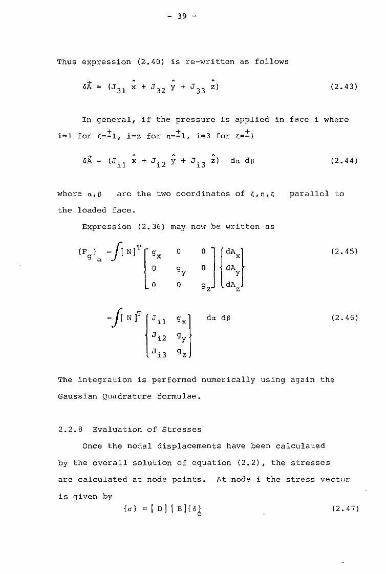
Thus expression (2..40) is re-written as follows

dA = (J31 x + J32 y + J33 z)

(2.43)

In general, if the pressure is applied in face i where

i=1 for i=z for n=-1, i=3 for c=±1

A SA = (jil x ji2 ji3 z)

da df3 (2.44)

where arf3 are the

the loaded face.

Expression (2.36)

{F "[NIT g e

=fi N ]T

may

gx 0

0

0 0

Jii gx

J.12 g y

J.13 g z

{

two coordinates

now be

00

gz

da

0

of

rd:

dAz

df3

written

n,c parallel to

as

(2.45)

(2.46)

The integration is performed numerically using again the

Gaussian Quadrature formulae.

2.2.8 Evaluation of Stresses

Once the nodal displacements have been calculated

by the overall solution of equation (2.2), the stresses

are calculated at node points. At node i the stress vector

is given by

{a} = [ D] [ E]fq (2.47)

- 40 -

where [ B] is calculated using values of the shape functions

at node i.

2.3 Description of the code DIM3B

2.3.1 Introduction

In the previous programs, NAMAIN Ref.(49) and

DIM3 Ref.(50), special subroutines were developed to perform

the initialization work and carry out the book-keeping

procedures before entering the actual solution stages.

These subroutines generate the necessary data to perform

the analysis of the particular problems being studied, with

the use of very small sets of input data.

Although it is recognised that manually assembled

programs may be advantageous for research purposes, any

potential user of these codes would have to face enormous

difficulties if a new class of problems is to be studied.

The idea to create a general purpose 3D finite element

program was the main reason for the development of the

DIM3B code.

One disadvantage, of course, is that the potential

user of such a program is faced with the tedious and

sometimes difficult task of producing large amounts of

input data.

However, he will be strictly concerned with his

particular problem without being involved in the more

difficult and complicated programming aspects of the code.

The problem of producing this type of data can be

eased with the use of automatic data generation techniques,

and this method has been adopted throughout the work

[M

KN MU 1 [ 6 = [ FUN]

T Mu

MUN

aUN

FKN

(2.48)

- 41 -

reported in this thesis.

2.3.2 The Solution Technique of Equation (2.2)

Remembering equation (2.2), the stiffness matrix

of the overall assemblage relates the nodal forces F

acting on the structure to the corresponding nodal displace-

ments S.

The stiffness matrix may be characterized in general

as symmetric, banded, positive definite and sparsely

populated.

Prescribed displacements, which are physically required

to preserve equilibrium as well as to specify initial

displacements at certain nodes, are accommodated in the

solution technique. A suitable partitioning of the

equation (2.2) is performed as

where 6KN and are known (prescribed) and unknown

nodal displacements respectively. The corresponding

unknown and known generalized forces are FUN and FKN*

The expansion of equation (2.48) yields

MKN

6KN + M

U 6UN = FUN

MT 6 = FKN U KN

+ MUN

6UN

(2.49)

(2.50)

- 42 -

or

MUN

dUN = FKN

- MTJ6KN

FUN

= MUSUN + MKNSKN

From equation (2.51) the unknown nodal variables

can be calculated by an extension of the Gaussian elimin-

ation process. In the backward substitution stages, as the

elements of SUN are explicitly known, the unknown reactions

FUN can also be found.

2.3.3 Frontal Method of Solution (FMS)

The use of these three dimensional elements with

3x20 or 3x32 degrees of freedom implies large dimensions

of the stiffness matrix k, which is equal to the number of

degrees of freedom in the structure. Normally these matrices

cannot be fully assembled and stored in fast core.

The FMS is suitable for such cases and is used in

this program with the Gaussian Elimination technique.

This method was first introduced by Irons (54) and

is based on the fact that only a small amount of the banded

matrix has to be processed before forward elimination of a

variable corresponding to a row. After the elimination

process, data pertaining to the variable is stored on a

disk file and the row is freed. Thus a variable becomes

active on its first appearance and is eliminated immediately

after its last.

- 43 -

Due to this method the total number of equations

(one per variable) is not anymore the limiting factor, rather

it is the semi-band with in the case of the matrix k.

A simplified version of this method is described

in detail in Appendix 1 as used in the FRONT code.

2.3.4 Program Breakdown

This section describes the general layout of the

program and gives a survey of each subroutine included in

the program.

An User's Guide of DIM3B code is given in Appendix 2,

which contains a definition of the relevant program

variables which will be mentioned in this section. A quick

reading of that Appendix may be useful if difficulties

are encountered in reading this section.

The DIM3B code consists of four main parts

A - Initializations

B - Determination of forces; evaluation of coefficients

for assemblage of stiffness matrices by numerical

integration.

C - Solution of the overall stiffness matrix; determin-

ation of displacements

D - Backward substitution; stress determination.

Some of the initialization procedures and parts B

and C are performed in a general DO LOOP element by element

as is shown on a primary flow chart in Fig. 2.2. A more

- 44 -

detailed flow chart of DIM3B code is shown in figure 2.3.

A - Initializations

In this initial part, the program reads the input

data concerned with the description of the two basic systems

(basic and global) as well as numerical data for the

Gaussian integration procedures, all these data correspond

to the first five input data cards.

After checking these data, the matrix TP relating

the two basic systems is evaluated. The elasticity matrix

EI is calculated and then the P matrix is formed.

The subroutine INIAL is now called and the resulting

integer values NUNKVA, NKNVA, NCELNO, NCELN1, NT, NTOTAL,

NUNVA1 and NKNVA1 are calculated and printed out.

The subroutine NODE is called by INIAL and forms the

ELNODE and PRENIC arrays which describe the topology of

the structure including the last appearances adding a

minus sign to the respective nicknames.

The ELNODE matrix is stored in a random access file

using non-standard subroutines available in the CDC system

at ICCC and ULCC.

The matrix UNKMAT, UNKNIC, UNCLE, KNOMAT, KNONIC,

KNORHS and UNRHS are reset to zero and the dimensionless

local coordinates are defined depending on the type of

element (20 or 32 node).

Finally the global coordinates are fed into the

program together with nodal point forces RHSI. If the

global system for input is cylindrical or spherical the

subroutine GTRANS is called from the main program and transforms

the coordinates into cartesian coordinates.

- 45 -

B - Determination of forces, stiffness matrices

From now on the program proceeds within a general

DO LOOP until all finite elements have been processed.

Firstly, stress data are fed into the program and

the equivalent nodal forces RHSL are calculated in sub-

routine LOAD called by the main program.

Prior to this, subroutine COORD is called and sets up

nodal matrices TR which are going to be used in subroutine

LOAD to transform the local components RHSL into new

components TRHSL, referred to the main problem system.

The subroutine COORD also stores the nodal coordinates

in a random access file no.2.

The equivalent nodal point forces TRHSL are added to

the initial prescribed nodal point forces RHSI and the sum

RHSRED of the components of these forces will be used on the

right hand side of the stiffness equations. These values

eventually can be printed out.

In the subroutine LOAD, numerical integrations are

performed (see section 2.2.7) using the shape funtions DE

and their partial derivatives with respect to the local

coordinates.

The subroutines SHAP20 and SHAP32 containing these

functions and its derivatives are called when necessary, one

or the other according to the elements in use.

The main program now calls the subroutine FEM from

which the components SK of the stiffness matrix are evaluated

(see section 2.2.6).

- 46 -

The subroutine STFTR is called next, and distributes

the SK coeficients over the UNKMAT, KNOMAT and UNCLE

matrices. According to equation (2.48) KNOMAT, UNKMAT

and UNCLE correspond to the partial matrices MKN, MUN and

Mu respectively.

In fact

UNKMAT = Submatrix corresponding to nodes with unknown

displacements

KNOMAT = Submatrix corresponding to PRENIC

UNCLE = Off diagonal submatrix of [k]

KNORHS = Known submatrix of load vector

UNRHS = Unknown submatrix of load vector

KNONIC = Addresses of known subvector of displacements

UNKNIC = Addresses of unknown subvector of displacements

The distribution of these matrices is shown again as

they are kept in the program.

... KNOMAT i ■

N, I UNCLE I

1 N,, 1 ■

UNKMAT I .,

PREDEF

- - - - U

-.,

UNRHS

KNORHS

X

NKNVA NUNKVA

Due to symmetry of this matrix only the upper triangles

and leading diagonals are kept in the computer.

In terms of computer variables expressions (2.51)

and (2.52) will become

- 47 -

UNKMAT * U = KNORHS - UNCLET * PREDEF

UNRHS = KNOMAT * PREDEF + UNCLE * U

where

PREDEF = Submatrix containing the known displacements

(boundary conditions)

U = Submatrix where the vector solution will be

stored.

C - Solution of the overall stiffness matrix

The forward elimination process for each frontal

position is performed in subroutines FORWD and BUFFER.

During the forward elimination process the system of equations

(2.51 ) and (2.52) is solved by the Gaussian Elimination

Method as follows.

Suppose the set of equations is

(e1) S1161 + S12 62 . + . .+ Sln 6 = F 1

(e2) S2161 + S2262 + . . . .+ S2n6n = F.2

(2.53) • • • • •

(en) Snl61 + Sn262 + . . .+ S = F nnn n

and when 6s is eliminated with the use of equation es one

obtains

S. .. S.1.3 - (S.l S ./S ) s s3 ss

i=1,2 . . . n,(i/ s)

(2.54)

or *

S.. = S.. - Q*S . 13 13 s3 (2.55)

where Q = Sis/Sss

- 48 -

and the modified right hand side

F* .F - Q F

(2.56)

i=1,2, . • . n

These elimination procedures are performed in subroutine

FORWD in the following manner. A completed row composed of

NUNKVA coefficients retrieved from UNKMAT and NKNVA

coefficients retrieved from UNCLE is stored in an auxiliary

array COMP and the factor Q (see exp. (2.55)) is evaluated.

The submatrices KNOMAT, UNCLE and UNKMAT are modified

according to expression (2.55).

The stored equation space is released and the data

contained in COMP is transferred to a buffer area. Also

the known and unknown righthand sides are calculated

according to expression (2.56) and then placed in a buffer

area. Finally, all the working variables used are reset

for the next forward elminiation.

Writing on a disk file takes place in blocs for all

the eliminated nodes, in order to reduce the number of

tape operations, this is done using subroutine BUFFER which

is called from subroutine FORWD where all the data already

stored in a buffer area are to be tranferrred for a random

access file.

D - Backward substitution, Evaluation of stresses

When the general DO LOOP in the main program has

processed all the elements, all the evaluated upper trian-

gular overall matrix, including the leading diagonal, is

stored on disk.

- 49 -

The main program calls subroutine BACKWD to calculate

the nodal displacements.

This subroutine firstly reads back from the random

access file the stored data in blocks in a reversed order.

Starting with the last eliminated node the unknown

displacements are now obtained directly.

8 . F* *

/s n n nn

and the rest are obtained from the formula

n * * 8

s . * (F

s _ E S . 6

i)/ S ss i=s+1

(2.56)

(2.57)

where s = n-1, n-2, 2,1

In terms of program variables the above expression,

using the same index notation, will be written as follows:

n

Us = (KNORHSs - E UNCLEsT i*PREDEFi)/UNKMATss (2.58) i=s+1

If the index s corresponds to a prescribed deflection,

the respective unknown reaction is computed using the already

calculated unknown displacements Us+1, Us+2 . . . in the

following manner.

UNRHSS = KNOMAT*PREDEF + UNCLE * U

(2.59)

The unknown reactions and the displacement solution

eventually can be printed out using subroutine DEFOUT.

- 50 -

A brief summary of the procedures involved in subroutines

FORWAD and BACKWD are described below.

Subroutine FORWAD

If in presence of an unknown displacement

(i) Storing completed row in a row matrix COMP

(ii) Modify KNOMAT, UNCLE, UNKMAT and RHS matrices

(iii) Release the stored equation space

(iv) Storing required data in buffer area (sub.BUFFER)

(v) Reset for the next element.

If in presence of a prescribed deflection

(i) Storing completed row terms of KNOMAT and column

terms of UNCLE in COMP

(ii) Modify the unknown right hand side RHS

(iii) Storing required data in buffer area (sub.Buffer)

(iv) Reset for the next element.

Subroutine BACKWD

(i) Initialization (reset KNONIC, UNKNIC, KNORS)

(ii) Read back stored data in blocks in re'iarsed

order.

If in presence of an unknown displacement

(iii) UNCLE is multiplied with known displacements

(iv) UNKMAT is multiplied with known displacements

except the diagonal term

If in presence of a prescribed deflection

(iii) Multiply KNaMAT with PREDEF

(iv) Multiply UNCLE with UNKDEF now stored in RHS

(v) Evaluate the corresponding unknown reactions.

- 51 -

If stresses are required by specifying the control

parameter IOUT=2, the subroutine STRESS is called by the

main program. The output results for the displacements

are used here to compute nodal stresses using expression

(2.16) described in section 2.2.4.

The matrix product ] B] (sometimes is referred

to as "stress" matrix) is evaluated in subroutine FEM2

using again the shape functions DE stored in subroutines

SHAP20 and SHAP32.

The stresses referred to the main problem system are

calculated using TR matrix already described.

cr I mp = TR fr ] a I L c ] TR] (2.60)

where [a]MP are the stresses referred to the main

problem system which are obtained from the stresses,

[ obtained from expression (2.16) and are referred to

the local system of coordinates (C,71,0.

If various elements meet at one node, the stresses are

averaged, i.e., the final result will be the mean of values

obtained for that particular node from each element.

The nodal stresses, if so desired, are printed out by

calling subroutine STROUT.

As it can be seen from figure 2.3, the main program

although spread in the central column from the top to the

bottom of the page, is indeed, a relatively small and simple

routine. Its basic function is to call the various

modules in an appropriate manner.

- 52 -

2.3.5 Program Environment

The DIM3B code is a program written in FORTRAN' IV

language.

One of the main features of this program as compared

to its predecessors (NAMAIN and DIM3) is related to the

transfer of data into back-up store files. In the previous

versions these operations have been made with the use of the

standard READ and WRITE Fortran statements, (see Ref.(55)).

The physical time involved in these operations has been

drastically reduced by the implementation of special

subroutines READMS and WRITMS which are presently available

in the CDC machines at ICCC and ULCC. These subroutines

transfer large amounts of data to random access files with

the use of mass storage devices.

Several other technical aspects regarding the operation

with this program are described in more detail in Appendix 2.

- 53 -

CHAPTER3

THE FINITE ELEMENT METHOD APPLIED TO

LINEAR ELASTIC FRACTURE MECHANICS

3.1 Introduction

A number of solutions for SIFs and strain energy

release rates, G, have been obtained using the more accurate

methods which have already been outlined in Chapter 1.

Unfortunately these solutions have been limited in the

past, to idealized and relatively simple-shaped configur-

ations and, in several cases, these solutions are far from

providing the engineer with good estimates of SIFs for the

more complex configurations of actual problems.

The FEM, which was originaly designed as a versatile

tool to solve general problems in structural analysis,

has become also a useful method when dealing with such

complex LEFM applications.

The next section will review the various finite element

techniques used for calculating SIFs and strain energy

release rates for cracked bodies.

It has been shown (section 2.2.3, Chapter 2) that the

displacement fields within the element (expressions 2.12

and 2.13) are described by continuous polynomials (shape

functions) of the second and third order depending on the

type of the element used.

These elements, having these type of shape functions,

are obviously unable to describe in an adequate manner the

- 54 -

square root behaviour of the displacement components and

the subsequent singularity fields in stresses and strains

near the crack tip. Moreover, the deteriorated solutions

obtained in those areas with the use of conventional

elements may eventually cause the propagation of errors

into larger regions away from the crack tip.

The need to use relatively coarse meshes in 3D finite

element analysis, due to the limitations of present genera-

tion computers, leads to the compulsory use of special

elements with embedded singularity fields modelled by the

introduction of a square root term in their displacement

functions.

Various planar elements of this type have been devel-

oped and have been reviewed by Rice and Tracey (65),

Jerram and Hellen (66) and Atluri et al. (67).

In the three dimensional family of elements Blackburn

(68) introduced an element containing an r1/2 displacement

function which was implemented in the BERSAFE system in

the CEGB Research Department. Tracey also developed a

wedge-shaped element which is described in Ref. (69). The

former is compatible with the 20-node isoparametric elements

whereas the latter can be used with 8-node linear isopara-

metric brick-type elements.

Although these elements have been used successfully by

Hellen and Dowling (2) and Schmit et al.(4), they have

specific stiffness formulations and differ from their

related conventional elements. Therefore the implementation

of these elements has the disadvantage of requiring major

- 55 -

alterations in the initial standard computer programs.

In section 3.3 of this Chapter, it is shown how a

"crack tip element" can be derived from the isoparametric

elements previously described in Chapter 2 without requiring

specific changes in the standard computer program DIM3B.

The final sections of this Chapter will describe the

results obtained in several tests which have been carried

out to assess these "crack tip elements".

3.2 Finite Element Techniques in LEFM

3.2.1 - Introduction

The various techniques for determining SIFs using

finite element methods can be divided into three groups.

Firstly, those utilizing directly the computed stresses

and displacements obtained from standard finite element

programs. Secondly, those in which the rate of reduction

of potential energy of the body with respect to increasing

crack length, G, is calculated, hence K.

A third group of techniques involves a simultaneous

use of the FEM and the analytical near tip expansions.

In this third method, which was developed by Wilson (62),

a displacement pattern associated with the leading terms

of the Williams stress function (64) is imposed in a small

circular area(*) (for 2D problems) near the crack tip. This

region is then coupled with the more conventional finite

elements in order to model the areas away from the crack tip.

(*) This circular region can be eventually regarded as another special crack tip element.

1.3

K1 13

a..(r,O) = fib (0 )

11-27--Irr

(3.1)

- 56 -

This method was well described by Hilton and Sih in

Ref.(63) in which results are given for some planar cases.

3.2.2 - The Direct Method

3.2.2.1 - The Stress Method

One of the more straightforward methods of calculating

the SIFs of cracked bodies is to correlate the stresses

at nodal points of the finite element mesh with those of

the near tip stress field which are given for the opening

mode I by

where r, 0 are the polar coordinates centred at the crack

tip, and f..(8) is a known function of 0 (see expression 13

1.5, Chapter 1).

Earlier work using this method has been done by

Chan et al.(70). They applied this approach to a compact

tension test piece, symmetric about the crack, and found

that good results could be obtained by substituting the

oy (y being normal to the crack line) stress components

ahead of the crack (8=0), and the distance, r, of the node

from the crack tip into equation (3.1).

A discrepancy of about 10% in relation to a collocation

method(*) was reached at the cost of a highly refined mesh.

(*) The collocation solution is believed to be accurate within 0.5% (see Ref(63) ).

- 57 -

In the stiffness formulation of the FEM it is

well known that the computed stresses are directly obtained

through the strains by differentiating the displacement

fields which means that the functions which model the stress

fields within the elements are of one order lower than the

displacement functions.

In fact Chan et al.(70) confirmed that a better

estimate of the SIFs could be obtained with the use of the

computed displacements rather than the stresses.

3.2.2.2 - The Displacement Method

Similarly to the stress method, the displacement

technique requires a correlation of the finite element nodal

point displacements with the known crack tip displacement

field solutions (see section 1.3.3). For plane strain

opening mode I, these solutions are:

U. . = xl rr

fi(0,v) p 27 (3.2)

where ul = u, u2 = V

f

1 ' (0 V) = cos (;) [ 1 - 2v + sin2 (2)]

12( 0 , v) = sin (—e ) [ 2 - 2v - cos' (2 ) 2

By substituting the computed displacements ut and the

respective distances rl.'i into expression (3.2) the SIF will

be obtained by extrapolating the curve

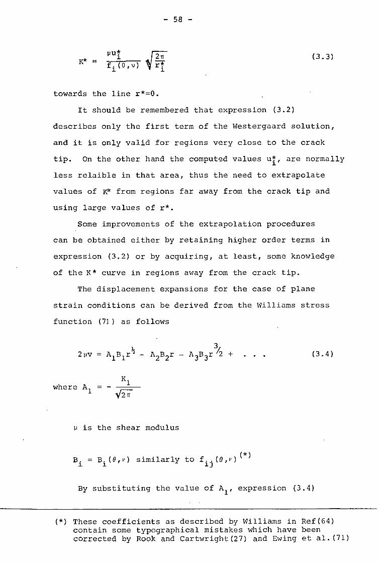
- 58 -

K* = ef ( , v ) (3.3)

towards the line r*=0.

It should be remembered that expression (3.2)

describes only the first term of the Westergaard solution,

and it is only valid for regions very close to the crack

tip. On the other hand the computed values ut, are normally

less relaible in that area, thus the need to extrapolate

values of K* from regions far away from the crack tip and

using large values of r*.

Some improvements of the extrapolation procedures

can be obtained either by retaining higher order terms in

expression (3.2) or by acquiring, at least, some knowledge

of the K* curve in regions away from the crack tip.

The displacement expansions for the case of plane

strain conditions can be derived from the Williams stress

function (71) as follows

3, 2pv = A1B1r2 A2B2r - A3B3r

+ • • • (3.4)

where Al -

p is the shear modulus

3 B.1 = B.1(0,v) similarly to f1

..(0,v)(*)

By substituting the value of A1, expression (3.4)

(*) These coefficients as described by Williams in Ref(64) contain some typographical mistakes which have been corrected by Rook and Cartwright(27) and Ewing et al.(71)

K1

- 59 -

becomes

K* = K - BTT - A2B2r 2 - A3B3r + ) (3.5) '1 1

p where K* = 2Bv r

7.T similarly to expression (3.3).

l

By inspection of the functions Bi it can be shown

that B2=0 when 6=7 thus expression (3.5) becomes

K* = K1 + (A3B 3r + . . .) (3.6) 1 B1

Therefore a plot of values of K* vs. r should be expected

to behave in a linear manner up to relatively large values

of r.

The first seven coefficients Ai have been obtained by

Leevers (72) using a variational method as it applies to

the Williams series solution to the crack problem in a

single edge notch geometry under plain strain conditions.

The various K* curves for various ratios a/w represented

in Figure 3.1 show that for this type of configurations

the variations found in the evaluated coefficients A2, A3..

..A7' have a very small effect on the overall behaviour of

those curves regarding their linearity or otherwise.

It is clear from this figure 3.1(*) that in the case of

0 = ir the influence of the square and higher order terms is

(*) The squares and circles in this figure will be referred to later on.

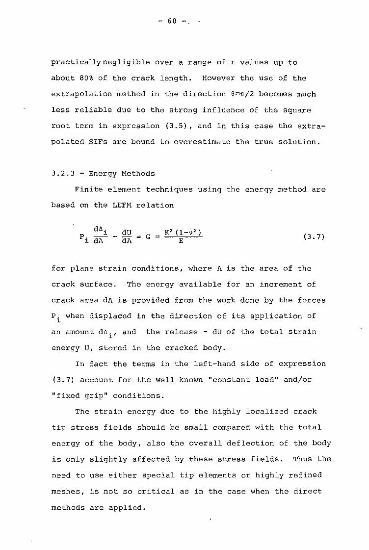
- 60 -_

practically negligible over a range of r values up to

about 80% of the crack length. However the use of the

extrapolation method in the direction 0=-1/r/2 becomes much

less reliable due to the strong influence of the square

root term in expression (3.5), and in this case the extra-

polated SIFs are bound to overestimate the true solution.

3.2.3 - Energy Methods

Finite element techniques using the energy method are

based on the LEFM relation

dei dU Pi dA dA = G

K2 (1-v2) (3.7)

for plane strain conditions, where A is the area of the

crack surface. The energy available for an increment of

crack area dA is provided from the work done by the forces

P.1 when displaced in the direction of its application of

an amount (IA.1, and the release - dU of the total strain

energy U, stored in the cracked body.

In fact the terms in the left-hand side of expression

(3.7) account for the well known "constant load" and/or

"fixed grip" conditions.

The strain energy due to the highly localized crack

tip stress fields should be small compared with the total

energy of the body, also the overall deflection of the body

is only slightly affected by these stress fields. Thus the

need to use either special tip elements or highly refined

meshes, is not so critical as in the case when the direct

methods are applied.

- 61 -

For planar cases the direct application of expression

(3.7) obliges the finite element analysis to be performed

twice, as described by Dixon and Strannigan (73), thus

increasing considerably the computing costs of such an

analysis.

In three dimensional applications the problem is com-

plicated many-fold. If localized SIFs are to be evaluated,

a set of successive runs must be carried out and small and

localized extensions of the crack front must be assumed.

A variety of techniques have been put forward to simplify

and improve the efficiency of these energy methods.

Jerram (74) suggested that the strain energy release

rates, G=dU/dA, could be obtained by evaluating the amount

of work required to close successive nodal intervals along

a crack. This procedure is illustrated in Figure 3.2 and is

particularly useful when the plane of the crack is a plane

of symmetry of the body.

For this case Broekhoven and Spaas (75) have shown that

the associated change of strain energy with successive

crack extensions (modelled by unpinning successive nodes) can

be written as

m 1 p AUi E n. 1+1 1=n

(3.8)

where AUi i+1 is the change in strain energy due to

extension from crack front i to crack

front i+1

- 62 -

n = 1,2 . . . m, is the number of node released

Pn. is the nodal force of node n for crack front i

ni+1 is the v displacement of node n due to its unpining

i=1,2, . . . indicates uncracked geometry.

This technique sometimes called "crack closure work"

has been successfully used by Broekhoven and Spaas (75) in

some three dimensional applications.

Bueckner (76) developed a similar technique to the

"crack closure work" method. He has shown that the problem

of evaluating the rate of change of strain energy with

increasing crack length in a loaded body is the same as

evaluating the rate of change of work done by tractions

acting on the surface of the crack when the body is free

from the initial loads.

The basis of Buekner's method as applied to the finite

element technique is indeed very similar to the Paris and

Sih replacement method which was briefly described in

section 1.3.4.

The "J integral" method developed by Rice (77) has

also been successfully applied to 2D cases by Chan et al.(70)

and Neal (78). Its application to 3D problems seems to be

rather complicated and no work using this technique was

yet found in the literature.

Quite recently Parks (79) has developed a "stiffness

derivative procedure" in which K values can be obtained

directly by differentiating the potential energy of the

finite element solution

- 63 -

P = 1 u [k) I u} lufr f}

(3.9)

with respect to crack length a of a 2D body under constant

load conditions

dP _ 1 u T d [k] u da

I da

F

If the crack surfaces are load free then

dPI= dUl = G - K2(1-v2) - -- da da

F F

(3.10)

(3.11)

where P is the potential energy

U is the strain energy

1 u1 is the vector of nodal displacements

[k] is the global stiffness matrix

10 is the vector of prescribed nodal forces. This method has been recently used by Hellen (80)

in 2D configurations. Broekhoven and Spaas (75) and

Schmit et al. (4) applied this method to problems of cracked

nozzles.

All computing efforts involved with the use of energy

methods can be substantially reduced if the Front Method

of solution is adopted in finite element programs.

These advanced numerical procedures for estimating G

have been described by Hellen (80), Parks (79) and

Broekhoven and Spaas (75).

Small extensions of the crack front can be modelled

by changes of the few elements adjacent to the crack front.

- 64 -

In the case of the Parks method, for example, the only

contributions to the d [k] term in expression (3.10) are

provided by the elements containing the translated nodal

points. Moreover if the nodes of the crack front and the

elements containing them are suitably numbered, the values

of d [kJ to be used in expression (3.10) can be obtained

by repeating (for an extended crack) only the very last

stages of the forward elimination procedure.

If the displacements and stresses are not required for

the entire structure, the components of the vectors

lul and luIT related to the non zero terms d [k] are then

evaluated by carrying out only a few steps of the back-

wards substitution. In conclusion, it can be said that

energy methods are bound to be more accurate as compared

to the direct techniques. However, an efficient use of the

former methods may involve a reasonably large effort in

their implementation on a standard computer program as in

the case of DIM3B.

On the other hand the inaccuracies involved with the

application of the direct method with the use of "crack

tip elements" are expected to be small enough at least for

engineering purposes.

Finally, in Figure 3.3 the more relevant methods

used to date to study 3D crack problems are summarized and

the methods used in the present work are conveniently

indicated.

r = al + a2 + a3c 2

u = bl + b2C + b3 2

- 65 -

3.3 - Theory of the Singularity Element


In this section it is intended to show how a singul-

arity in stress and strain fields can be easily accommodated

in the isoparametric (20 and 32 node) elements described

in Chapter 2. This singularity can be made to occur

within these elements at certain nodal points by carrying

out some minor mathematical changes in the theory

described in the previous Chapter.

3.3.2 - Theory

3.3.2.1 - One line elements

The modelling of near-tip fields by the second order

2D quadrilateral isoparametric elements, in which the mid-

side nodes are displaced, has been illustrated by Henshell

and Shaw (81) by reference to the corresponding line

(1-dimensional) element. The same method is used here.

The equivalent one dimensional elements to the 3D

(20,32 node) elements, in terms of the order of the shape

functions, are the (3,4 node, respectively) elements, as

they are shown in Figure 3.4.

In the second order line element (see Figure 3.4(a))

using a local natural non dimensional coordinate C, the

coordinate r and displacement u in the global system are

expressed in terms of the local coordinate by

- 66 -

where the a. and b. are constants which are obtained 1 1

from nodal values of r and u respectively and accordingly

to expressions (2.3) and (2.8). In this case [M]=[lEE2]

and tal T = [al a2 a3].

Let us assume that the mid side node (node 2) can have

a varying position identified with the value of p in the

thus

hence

general system of coordinates

equation (2.8) will be

0 = 1 -1 1-

p [ 1

0 0

2 1 1_

al = p ; a2 = 1 ; a 3

r (see

for this

1

2

{ : a3

= 1-p.

Figure 3.4(a)),

case

(3.14)

Substituting these values into equation (3.12),

r = p + ; + (1-13) Fit

(3.15)

When p=1 equation (3.15) becomes r=l+E which is obviously

the transformation of coordinates (0,1,2) to the scaled

(-1,0,1).

Developing expression (2.9) for this case and when

p=1

r= -2- (-E+E2)r1 + (1-E2 )r2 + (E+E2)r3 (3.16)

- 67 -

To obtain strains, expression (2.18) will be simplified

as follows

du _ dN1 dN2 dN

+ 3 dE dE u1 dC u2 dE u3

= 1 ( 2E-1)u1 - 2Eu2 + 1 (1+2E)u3

(3.17)

A plot of the shape functions Ni and its derivatives

fi = dNi/dE is shown in Figure 3.5.

The chain rule (2.21) to obtain the engineering strain

r is simplified as follows

du = du dr dE dr dE

(3.18)

du = —dr [J]

Hence

du dur,1-1 = = Lu1 r dr dE

(3.19)

where [J]-1 = (dr/dE)-1 is the inverse of the jacobian

of the transformation of coordinates r to E .

Combining equations (3.18) and (3.15)

r d du = {1 + 2(1-p)Er E

(3.20)

The strain will be singular where

- 68 -

1 + 2 41-p) = 0 (3.21a)

If the singularity is to occur at r=0. i.e. at c= -1, p

must satisfy the equation

1 - 2 (1-p) = 0 (3.21b)

1 i.e. p = -2-,

Thus the mid-side node must be displaced to a point

one quarter of the element length from the node at which

the singularity occurs.

W2 now investigate the order of the singularity

substituting p = 2 into equation (3.15)

1 1 f

r = -2- E + - E2 (3.22)

solving equation (3.22) in terms of r, we have

E . -1 + (2r) 1/2

(3.23)

Applying equation (3.13) to each of the nodal points

and solving for bi

1 1 bi = u2 ; b2 = -f(u3-u1) ; b3 = (u3 + ul - 2u2)

Substituting these values into equation (3.13) and

using expression (3.23) the displacements within the element

- 69 -

will be described as follows

2-3 + 2r u -

u1 + (-2r+2)u

2 + 2r-

2 u3 (3.24) 2

hence

r= {1-2 (2r) 2

1 1/2 u1+ {-2+2(2r) 2Iu2 + {1-7-(2r) }1.1 2 (3.25)

which exhibits the r 2 singularity which occurs at the

crack front.

Expressions (3.24) and (3.25) have the same form as

expressions (2.12) and (2.29) respectively.

A plot of these new shape functions i d its deriv-

atives f. = dN./dr is shown in Figure 3.6.

In the case of the third order line element (see

Figure 3.4(b)), following the same steps as in (3.12)

and (3.13), the transformation of coordinates will be

r = al + a2E + a3E2 + a4E3 (3.26)

u = bl

+ b2E + b3 2 b4E3

(3.27)

In the same manner, the intermediate nodes (2 and 3)

are assumed to have varying positions identified with the

values pl and p2. Similarly to expression (3.14) the values

of a., i=1,2,3,4 can then be evaluated.

- 70 -

1 9 a1 = .8- 4- 1-67 (p1 + p2)

1 27 , a2 = 8 + (p2 - P1) T-6

(3.28)

9 9 a3 = "g. -16 (p1 + p2)

9 27 , a4 ...

-8- - 16 (p2 - p1)

Following for this case the steps (3.18) to (3.20)

dr = aT _ a2 + 2a3C +3a4C2

(3.29)

and the singularity will be made to occur at r=0 or E= -1

when

or

dr = u ,

sd for c = -1 (3.30)

a2 -2a3 + 3a4 = 0

(3.31)

Substituting the values ai(3.28) into equation (3.31)

yields to the following equation

4 P2 = .g 4- 2P1 (3.32)

which corresponds to equation (3.22). The required positions

of the intermediate nodes (2 and 3) are not uniquely defined

for the third order line element, but related by equation (3.32).

ax au ay 3E I DX

au

au an

ax 2z 3u _ an an 317

(3.35)

- 71 -

However, if the normal position for node 3 is maintained

p2 = 1, the position of node 2 is then given by (3.3 )

as pl = 4/9. For these particular values of pl and p2 the

shape functions Ni and its derivatives are represented in

Figure 3.7.

It is impossible to solve analyticaly equation (3.26)

for in terms of r. However the function (r)

equivalent to expression (3.23) should also contain an r 2

term and subsequently the equivalent to expression (3.25)

should also exhibit the r 1/2 singularity.

3.3.2.2 - Extension of the singularity in 2D

Let us consider now the 8 node isoparametric element

as it is shown in Figure 3.8. In this case expression

(3.15) leads to

x = pl + C + (1-pl)c 2 (3.33a)

Y = P2 n (1-p2)n 2

The chain rule (2.21) will be as follows

ax au Dy 3E 3x ac ay a

(3.33b)

(3.34)

and from (2.23)

- 72 -

From equations (3.33) the inverse of the Jacobian

can be evaluated as

{ J1-1 1 1-2 (1-P1)

(3.36)

0

If the singularity would be valid for all strains then

the following conditions must be imposed

_ 1 P1 = p2 - f (3.37)

Two typical shape functions Ni = Ni(C ,n ) are repres-

ented in figure 3.10,and the derivatives of these functions

at node 1 have infinity values.

Following the same procedures as for the one line

element the strain ex, for example will be

3 ex= 3x .p_11 = [1 - -2(2x) 1/21 u1 + [ -2 + 2 (2x) 2] u2 j

+11 - 2 (2x) 2J u3 (3.38)

the strains for any direction r (see Figure 3.8)

x = r cos 0 (3.39a)

y = r sin 0 (3.39b)

thus, from expression (3.38)

du dx =

-1/2 1/2 f(r , cos 0, sin 20, u 1,u2'u3) (3.40)

- 73 -

which means that the singularity holds true for any

direction r.

3.3.2.3 - Singularity in 3D elements

Let us consider now a 3D (20 node) isoparametric

element as it is shown in Figure 3.9.

By inspection of the Jacobian in expression (2.20)

it can be seen that by shifting the nodes 8, 9, 4 and 10 as

it is indicated the same type of singularity can occur

along the line AB, in planes perpendicular to that line.

Developing new expressions similar to expressions

(3.33)

= p1

y = p2 -E. n (1—p2)n2

z = p3 + + (1-p3W (3.41c)

if pi = p2 = .5 and p3 = 1

1 x = + E + .fE2

y = 1 1 2

z = 1 +

(3.42a)

(3.42b)

(3.42c)

therefore the derivatives in the third row of the Jacobian

will only contain terms 1 or 0 which will not affect the

- 74 -

bidimensional singularity described in expression (3.40).

Conditions must be met to ensure the square root

behaviour in node 2 (see Fig. 3.9) and will be described

as follows.

Considering now a local system of coordinates x, y

and z defined by nodes 6, 2 and 14. The shape functions

of the nodes in the base of the element and for C= 0 and

c = -1 are (see exp. 2.13, Chp. 2)

N 1 = N3 = N5 = N7

= - 1(1 - 11 2 ) 4

N2 = N6 2 = 1(1 - n)

N4 = N8 2 = 1(1 - n2 )

The relationship between y and n can be derived by

using exp. 2.11, thus

1 Y = -4-(1 - fl2 )(2Y4+ 2y8 - y1- y3- y5- y7)

+ 1 -.(1 - n2 )y6 (3.43)

Differentiating y with respect to n it can be shown

that the singularity occurs when

1 1 Y6 = -2- (Y7 + Y5) - 2 (Y1 + Y3)

(3.44a)

A similar condition can be derived for node 14 as follows:

1 z15) , z14= - 2 - (z13+ z

15) - -2- kz1

+ z3) (3.44b)

- 75 -

2.3.2.4 - Conclusions

A brief summary of the present theory is laid out in

order to help to understand the manner in which singularities

can occur in isoparametric elements.

Derivatives of displacements with respect to global

coordinates x,y,z can be obtained by differentiating

expressions (2.14) with respect to local coordinates

multiplied by the Jacobian of the tranformation

a a a f.t1 - ate, an, a f Vm 1 1 „. —1 ax' ay' az' ' - aC an' W`L"iui!* u (3.45a)

If the positions of the intermediate nodes i,j,m . .

are described by varying parameters pi,pj,pm . . , the

Jacobian J will be a function of these parameters and the

local coordinates E,n,c.

J = J(PisPiflpm • • • , ,T1,C) (3.45h)

Singularities in stress and strain fields can be made

to occur at particular nodes, i.e., at particular values

of E,n,, let us call them Es, n s , c s, and the particular

positions where these intermediate nodes have to be shifted

can be found using the condition.

J(pi,pi,pm - • . , Cs'ns's) = 0 (3.45c)

- 76 -

this condition will determine a function g(p.,p3.,p m . . .)

which is the desired solution. The singularities are of

several orders and depend only on the type of the element.

These elements are incompatible with their related

conventional versions. However, if nodes i,j,k,l, (see

Figure 3.9) are kept on their original positions the

singularity still occurs at the line AB.

If pl and p2 (see figure 3.8) are assumed to vary

linearly accross the element in order to satisfy the new

positions of nodes 4 and 6 then

3 1 P1 = 4 :f t

1 P2 = 3 + 4 71

and new expressions (3.33) are derived as

1 x = 7-1- (3 + 3c + C2 -c2)

1 y = -4 (3 + 3n + n2 -n 3 )

(3.46a)

(3.46b)

(3.47a)

(3.47b)

Now, following the same procedures as from (3.34) to (3.38)

it can be shown that the new strains ex still contain the

x 2 terms.

3.4-Test Cases


Several series of test cases have been performed to

- 77 -

assess these crack tip elements. Various techniques have

been used to generate the finite element meshes for the

test case configurations.

A schematic flow chart of the strategy involved in

the generation of the finite element data is shown in

Figure 3.11.

Basically, a mesh generation program was developed

for each configuration. These programs read in the rele-

vant geometric parameters of the problem as well as data

describing the loading conditions.

These programs produce three separate sets of data

which are written on three separate output tapes. Firstly,

the relevant data for execution of program DIMDIM is

written on tape DDMDAT. A second tape, DIMDAT, will contain

all the data necessary for the execution of DIM3B code.

Finally, data describing the geometry as well as the

topology of the mesh is written on a tape called DRDAT.

This tape contains the necessary data needed for a plot

procedure (program DRAW) using some of the off-line graphic

facilities available at the Imperial College Computer Centre.

Some of the data which are needed for the DIMDIM,

DIM3B and DRAW codes but which are not relevant of the mesh

generation program, pass through it, unchanged, in the form

of card images. These data are for instance, control

parameters IIN, IOUT for DIM3B, sequential numbers for

DIMDIM code, etc.

Initially, a relatively small job consisting of the

execution of the mesh generation program and the subsequent

- 78 -

plotting procedure (execution of program DRAW) is carried

out at I.C.C.C. using an "Instanturnround" batch service.

The finite element mesh is then checked visually in a

TEKTRONIX terminal, using a "QUICK-LOOK" facility available

at I.C.C.C., (82) and the rest of the input data can be

easily examined by printing out the files DDMDAT and DIMDAT.

The plot file generated by the program DRAW is then

processed to generate the necessary magnetic tape format

to drive a microfilem plotter (see Reference (83)).

Once the necessary checks have been made a complete

run using now the DIM3B and DIMDIM codes is then executed

by resubmitting the mesh generation program at U.L.C.C.

The plot procedure, Program DRAW

A general plot program, DRAW, was developed to

produce an isometric perspective of the 3D finite element

mesh which is obtained by transforming the original coord-

inates x,y,z into new x',y',z' coordinates.

This transformation, being the result of two rotations,

as shown in figure 3.12, one around the z axis by an amount

0x and the other around the y axis by an amount 0z will be

described by a matrix TF as follows

sine cos0xcos0z sinexcos0z z

[

-sinex cost)

x 0 (3.48)

-sinexcos8z -sinezsinex

cos()z

Then the new coordinates x',y',z' are obtained by the

relation

- 79 -

x' { = [TF] x

Y i z'

{

Y z

(3.49)

By specifying the view angle defined by0x and Oz a

prespective can be obtained by plotting the y',z' values

as the logical plot coordinates for each nodal point.

The plot is then carried out one element at a time

where the order of execution of the logical functions

"pen up" and "pen down" are described in Figure 3.13.

Although this procedure involves the repetition

of edges pertaining to more than one element it provides an

easy check of systematic errors which may occur either in

the topological description of the mesh or in the specific-

ation of the nodal coordinates.

A listing of the program DRAW is described in Appendix

4.

3.4.2 - Compact Tension Specimens

A mesh was generated, representing one quadrant of a

Compact Tension Specimen (CTS) of length 2H, width W and

thickness T, having a single edge crack of length 2a in

the mid-plane. The specimen and mesh are shown in Figure 3.14.

A primary two-dimensional mesh was developed for the

plane x = T/2 and was specified in the form of input data

cards. The mesh generation program for this case, based

on this two-dimensional type of information, generates all

nodal coordinates for the rest of the mesh and subsequently

- 80 -

generates the topological description of the mesh.

Two layers of the 20-node elements were used through

the thickness of a quadrant (i.e. four elements through

the thickness of the specimen). The number of elements in

the quadrant was 88 and the number of nodes 585. A uniform

tensile stress was applied at the free end of the quadrant,

in the direction normal to the plane of the crack. Approp-

riate boundary conditions were applied at nodes of faces

representing planes of symmetry of the specimen excepting

those in the free surface of the crack which were allowed

to move freely.

Figures 3.15 and 3.16 show the variations of stresses

ahead of the crack front. In one case, Figure 3.15, the

standard 20 node elements were used throughout, in the other

case, Figure 3.16, the elements adjacent to the crack front

were distorted by displacing the mid-side nodes to the

quarter points nearest to the crack front as described in

Section 3.3 of this chapter and illustrated in Figure 3.10.

Although the results may be somewhat inaccurate, the

ability of the distorted elements to model a singularity

in stresses is well illustrated in Figure 3.16.

The stress components in the thickness direction,ax,

in the mid-plane of the specimen (x=0) are also shown in

Figure 3.16.

Figure 3.17 shows the mid-element stresses as a function

of the distance, x, from the middle surface of the specimen

for the elements adjacent to the crack tip. These nodal

points are at a distance 0.08T form the crack front.

- 81 -

Although the number of nodal points is very small to

draw any quantitative conclusions it may be suggested from

the results in Figure 3.17 that the in-plane stresses a Y

and az are nearly constant throughout the thickness except

for a rapid fall near the free surface.

The expression for the strain in the thickness direc-

tion is given by

ex E . 1-[ ax -v(ay +az) ]

(3.50)

Levey et al. (84) suggested that the condition of plane

strain and plane stress can be described by a parameter,

Ps, defined by the ratio

P

ax (3.51) s v(a y +az )

derived from expression (3.50), being unity when ex is

either zero or bounded (generalised plane strain), and zero

under plane stress conditions, ax = 0.

From the results in Figure 3.17 the variation of the

parameter Ps has been plotted on the same figure, and it

shows an immediate decrease from a maximum value of.72 even

in the more central portions of the specimen. However, from

the behaviour of the ax stresses in Figure 3.16, it is

expected that a curve of values Ps in regions very close to

the crack tip will be fairly constant reaching values of

unity and presenting a drastic drop to values near zero only

in a small region near the free surface.

- 82 -

Based on the reasoning referred to above, values of

K which are not in the free surface have been obtained

directly from the computed displacements by ploting the

following function against r/a and extrapolating to r=0.

For plane strain conditions and from expression (3.2)

with 1,1 = E/2(1+v)

K = Lim K* = E Fr

w 4 (1+v) (1-v) x

(3.51)

r+0

and values of K at free surfaces have been obtained by

using the corresponding plane stress function

27 K = Lim K* = E — w r r+0

(3.52)

where w is the displacement component normal to the crack

face.

The extrapolation procedures using expressions (3.51)

and (3.52) are shown in figures 3.19 and 3.20. In one case,

Figure 3.19, the standard 20 node elements have been used

whereas in the other case, Figure 3.20, the elements adjacent

to the crack front were distorted as was described earlier

in this Section. The results have been normalized to the

stress intensity factor in an infinite plate (Ko=a

By comparing Figures 3.19 and 3.20, the improvement in

the value of K, which is obtained by the use of the distorted

elements may be seen. The value obtained on the mid-plane

using these elements differs by only 2.6% from the value

obtained by Brown and Srawley (85) using a two dimensional

- 83 -

plane strain collocation method.

This slight increase in the extrapolated value of K

in the mid-plane as compared to the two-dimensional plain

strain analysis is in close qualitative agreement with the

results shown in Figure 3.18 which were obtained by

Yamamoto and Sumi (86) in their 3D finite element analysis

of a standard single edge notch specimen (ASTM standard

E-399-72).

A table is presented below in which the present results

(i) for CTS are compared with those obtained by Leevers (72)

(ii) using a 2D plane stress and plain strain analysis

(see Section 3.2.2.2) assuming the same configuration with

a/W = 0.25.

Values of K/a

(i) 3D Finite Element Analysis

Mid-plane of the specimen

Free surface

(ii) Williams Series Solutions

Plane strain conditions

Plane stress conditions

1.54

1.43

1.51

1.51

The discrepancies of the K* curves obtained by the two

methods of analysis for this Compact Tension Specimen (see

Figures 3.1 and 3.20) could be due to the following reason:

if variations in K values have been found with the 3D finite

element analysis it is also expected that the coefficients

of the higher order terms in expression (3.6) would also

vary across the thickness. In fact, by inspection of the

- 84 -

slopes of the K* curves obtained with the finite element

method it can be seen that the variation, across the thick-

ness, of the coefficient A3 in expression (3.6) presents a

similar trend to the variation of K values shown in

Figure 3.20 .

Figure 3.21(b) shows the results obtained by use of

the 32-node elements, distorted as shown in Figure 3.21(a).

On the mid-plane close agreement is obtained with the plane

strain results of Brown and Srawley.

3.4.3 - Compact Tension Specimens with Curved Crack Fronts

The results obtained for the compact tension specimen,

with straight crack front, show a higher value of K in the

interior planes, indicating a tendency for the crack to

advance with a curved front. There is experimental evidence

to support this conclusion (see for example Neale (87),

and Johnson and Radon (88)).

In a second series of tests, the mesh was distorted by

a simple skewing technique to model curved crack fronts,

having the form of circular arcs, in which the ratio of

crack front radius R to the specimen thickness T varied

between 0.57 and 1.13.

The curved fronts and one of these meshes are shown

in Figure 3.22. As in the first series of tests, values of

K along the curved crack fronts were obtained by the extra-

polation method from the computed displacements.

For these curved crack fronts the extrapolated values

of K are expected to be somewhat inaccurate.

- 85 -

This is due to the fact that by using the mesh shown

in Figure 3.22(b) the directions of the extrapolation

procedures being parallel to the plane yz (see Figure 3.14)

make an angle 0 with the direction perpendicular to the

crack front as it is shown in Figure 3.22(a).

This angle, 0, varies from zero in the mid-plane of

the specimen (x=0) to a maximum in the outer planes and

depending on the radius of curvature of the crack front.

If changes of displacements near the crack border

possess a certain degree of constancy relative to the

direction parallel to the crack front(*) the value of r in

expression (3.51) should be replaced, in a first approxima- (**)

tion, by the term r cos Of '. This correction is based on

the assumption that for small values of r the differences

in the opening displacements at the points A and B, as

shown in figure 3.22(a) should be negligible.

It can be seen that the application of this correction

factor for large values of r is no longer valid for two

reasons: Firstly, the new points A' and B' (see Figure 3.22(a))

would be too far from each other, thus the assumption of

displacement constancy between these two points no longer

holds true. Secondly, the displacement fields in areas away

from the crack tip, and in planes of x=constant, will be

(*)As suggested by Irwin in Reference (38)

This type of correction has been already introduced by Sih and Cha (58) by describing the crack border stresses referred to the bi-normal and osculating planes of the crack front curve of an elliptical crack. In their work, another factor,X is also introduced dep-ending also on the crack front shape. For circular cracks X = cos 0

(**)

- 86 -

mainly governed by the higher order terms of expression (3.4)

which are expected to vary across the thickness (see

previous Section) and at the same time to be less sensitive

to the particulars of the crack front than the variations

of the stress intensity factor.

Therefore the K* curve obtained from the extrapolation

method should still present its linear behaviour for large

values of r and provide a reasonable extrapolated K value.

If the finite element mesh were highly refined in the

vicinity of the crack front a drop of the K* curve would

eventually occur for small values of r which could be

corrected then by the introduction of the correction factor

suggested earlier on, however, this particular behaviour

was not noticeable with the coarse meshes used in the

. present work.

A comparison of the extrapolation procedures using the

computed displacements in the free surface of the crack

( 0=Tr ) and in planes perpendicular to the crack surface (* (0 = Tr/2) is shown in Figure 3.23(b) ) for the more critical

curved front case when the ratio R/T is 0.57.

This relatively constant increase in K values obtained

from the direction 0 = IT/2 has already been justified

earlier in this chapter and supports the assumptions referred

to above.

Also, for each radius of curvature, a single value of

K was obtained using the energy method based on equation

(3.7). In this case the energy available for an increment

of crack area dA is provided (see expression (3.7)) by the

(*) Figure 3.23(a) indicates the corresponding results for the straight crack front. The same results are also ploted in Figure 3.1.

- 87 -

work done by the nodal point forces Pi equivalent to the

remote stress applied in the top faces of the specimen

and required the computation

G = 2 (7.: Pi dwi)/dA (*) (3.53)

where d .wi are the variations of the displacements, w, in

the z direction of the nodal points where the forces Pi

are applied. Again the results of K have been normalized to

the value of K in an infinite plate. Figure 3.24 show;

the results where the single value obtained by the energy

method is indicated by a horizontal line. For each of

these crack front radii, the value of K obtained for the

mid-plane of the specimen was lower than the value obtained

for the surface. Figure 3.25 shows a graph of the normalized

K, obtained by the energy method, ploted against a parameter

which represents the crack front curvature. The figure

clearly shows the reduction of K with increasing tunnelling

supporting observations of Neale (87).

It should be pointed out that these values of K

obtained from the global energy method are associated with

the values of K which are obtained experimentally using

for example, a compliance test, provided the assumed extension

of the crack front is similar to those verified in post

mortem observations of a test specimen.

(*)The factor 2 arises from the fact that only one quarter of the specimen is considered.

- 88 -

A factor depending on a tunnelling geometric parameter

should be introduced to correct the planar K calibration

of a CTS specimen. This factor, based on results similar

to those presented in Figure 3.25 would take into account

in an adequate manner a possible non conservative inter-

pretation of test data.

3.4.4 - Corner Crack

The mesh for this case, shown in Figure 3.26 was

developed from a similar mesh of 20 node elements used in

the earlier tests, by a cylindrical skewing technique

about the z axis. The number of elements was 88 and the

number of nodes was 553. This technique has resulted in

an axial groove, see Figure 3.26, which has been made

small so that its effect on the results is negligible. This

groove could eventually be eliminated by the use of an

additional type of element.

A uniform stress was applied in the direction z and

the yz and zx faces were assumed to be free.

Values of K, obtained by the extrapolation method from

computed displacements of the crack face, are shown in

Figure 3.27. The figure also shows results obtained by

Tracey (89) for a cylindrical specimen using a different type

of singularity element. The discrepancy is verified to

increase towards the mid point of the crack front having a

maximum of 5%. at a = 45°.

In fact, for this direction, the uncracked ligament of

the present specimen, being the diagonal of the square base,

- 89 -

is greater than in Tracey's geometry, which may be the

reason of the decrease in values of K in the more central

portions of the crack front of the present specimen.

3.4.5 - Part-through Semi-Ciruclar Crack

By using the mesh shown in Figure 3.26 , changing

the boundary conditions to represent symmetry about the

zx face, a specimen with a part-through semi-circular

crack was modelled.

Values of K, obtained by the extrapolation method for

computed displacements are shown in Figure 3.28. The figure

also shows results obtained by Smith and Alavi (90).

The maximum discrepancy is 2.0%.

3.4.6 - Thick-walled Cylinders with Radial Part-Through

Semi-Circular Cracks.

Two different configurations of this type of structures

have been studied and the results are presented in this

Section.

A part-through semi-circular crack emanating from

the inner surface of the cylinders were assumed to exist

in a radial plane containing the axis of the cylinder, as

shown in Figure 3.29.

The models investigated have the following geometries:

- 90 -

GEOMETRIC PARAMETERS CASE CYL 1 CASE CYL2

R1 71.9 mm 71.9 mm

R2 135.9 mm 115.8 mm

W=R2/R1 1.88 1.61

a/(R2-R1) .2 .29

In both cases the length of the cylinders is ten

times the crack length. The cylinders were subjected to

internal pressure fully penetrating the crack, which is

the most critical case. These geometries were selected

because their geometric parameters defined above are similar

to those of the "T-Junction" structure to be described

later, in Chapter 4.

3.4.6.1 - Mesh Generation

A mesh was generated representing 1/8th of the

structure as it is shown in Figure 3.29.

This mesh was obtained from the previous corner crack

finite element idealization by a three step skewing technique

schematized in Figure 3.29.

Due to symmetry tangential boundary conditions were

applied in the y and x directions to nodes in the planes

xz and yz respectively. Of course nodes in the crack face

were allowed to move freely.

In fact this representation assumes the existance of

two equal cracks situated in the same radial plane and

- 91 -

diammetrically opposed.

Shannon (91) using the finite element method has

calculated the SIF for a single radial crack in a thick-

walled cylinder and presented also values of SIFs for two

diametrically opposed cracks in cylinders of several diameter

ratios. The results obtained by Shannon being derived from

a two dimensional analysis are not applicable to curved

crack fronts.

For the equivalent straight-front cracks having the

same geometric parameters, W and a/(R2-R1) of the cases

CYL1 and CYL2, he predicts a decrease of about 9 and 6%

respectively for the situation when two diametrically

opposed cracks are present.

It is expected that these differences should be somewhat

reduced in the part-through crack cases due to the constraint

supplied by the uncracked material beyond the diameter of

the crack in the z direction. The lack of such constraint

with two infinite length cracks is bound to cause a higher

interaction of the crack tip stress fields.

3.4.6.2 - Overall behaviour

A check on the equilibrium of forces in both x and y

directions was made. The summation of reactions at nodes

where boundary conditions were applied differs by less than

0.3% (in both cases, CYL1 and CYL2) from the total force

applied due to internal pressure.

In figure 3.30 nodal values of hoop and radial stresses

in the plane xz are compared with the Lame solution for the

- 92 -

case CYL1, and a maximum error was found to be 3%. This

discrepancy is quite acceptable in stress and is partially

due to small deviations of the mid-side nodes from their

correct positions, which is a result of the rather com-

plicated skewing techniques applied to the mesh.

In Figure 3.31 the ratio of hoop stresses ahead of

the crack tip divided by the respective Lame hoop stresses

is plotted versus the distance from the crack tip. This

plot illustrates the incapability of the finite element

analysis to model the singular stress field described by

(* expressions (1.5) ) However, it can be seen that the

raising effect caused by the presence of the crack die

away quite rapidly (approximately one crack length) and

reaches values slightly below the Lame's solution as it

was expected due to the offset of the load in that plane.

This behaviour as well as the results presented in

Figure 3.30 clearly supports the assumptions made earlier,

and representing only 1/8th of the structure.

The same behaviour and inaccuracies were verified

for the case CYL2, therefore the results are not presented

here.

3.4.6.3 - Stress Intensity Factors

Values of K along the crack front have been obtained

by the extrapolation method using the computed displacements

of the nodes in the free surface of the cracks.

(*)From expression (1.5)0 = aKr 2 thus 1 logo = Cte log r or loge = Cte -arc tg(26.5).log r

- 93 -

Plain strain conditions were assumed for all the

extrapolation procedures but for those on lines in the

inner surfaces of the cylinders where plane stress expres-

sions were used.

The variations of the SIFs along the crack fronts for

the CYL1 and CYL2 cases are shown in Figure 3.32. These

values have been non-dimensionalized by dividing them by

the quantity p ,ra- where p is the internal pressure and a

the crack length.

Qualitatively these results present a rather reasonable

behaviour as compared to those of the part-through crack

configuration studied in Section 3.4.5 (see Figure 3.28).

The ratio between the SIFs at the free surface (a = 90°)and at

the point of deepest penetration of the crack. (a =0°) is

1.12 for CYL1 and 1.16 for CYL2. These ratios are greater

than the same ratio in the part-through crack case, 1.1.

This can be explained by the fact that the opening stresses

in the uncracked cylinders are no longer constant but

decrease across the thickness according to Lamps expressions.

By inspection of the Lame solution for both cases the same

reasoning can be used to explain the higher ratio for the

CYL2 case.

On the other hand, the average increase of about 14%

of the SIFs from CYL1 to CYL2 can be associated with the

ratio 1.17 between the maximum hoop stresses in CYL1 and

CYL2 cases.

Values of SIFs for these particular configurations were

not found in the literature and a combination of existing

- 94 -

analyses, as suggested by Underwood (92), will be carried

out to obtain some estimates of K values and assess the

validity of the present results.

This analysis is based on the assumption that crack

shape effects in a pressurized cylinder can be similar,

under certain conditions, to shape effects in a plate under

tension. These analyses which will be combined are briefly

described as follows:

i) Cylinders with straight front cracks

A long tube of internal radius R1 and external

radius R2 contains a radial crack of length a from the

inner surface. A uniform internal pressure acts on the

cylinder and on the crack faces. Bowie and Freese (93)

using a collocation method obtained the opening mode stress

intensity factor K, over a wide range of radii and crack

depth to thickness ratios. A plot of these results is shown

in Figure 3.33.

ii) Cylinders with curved-front cracks

Cracks with curved fronts are more often found in

structures and their shape can be idealized by a semi-

ellipse with major axis, 2c, and minor axis, a. The present

cases CYL1 and CYL2 having semi-circular cracks are

particular cases of those ellipses.

Rice and Levy (94) obtained opening mode SIFs for a

finite thickness plate under uniform tension with a semi-

elliptical crack at the point of deepest penetration of the

crack.

The proposed combination of these analysis can be

expressed by the following relationship:

- 95 -

(K1)e = a (Ki)s (3.54)

where

(K1)e. = K1 for a pressurised cylinder with a semi-

elliptical crack

(K1)s = K1 for a pressurized cylinder with a straight

front crack

K1 for a plate with a semi-elliptical crack a -

The validity of expression (3.54) is limited either

to thin walled cylinders or to thick-walled cylinders but

with small crack depth to thickness ratio, as pointed out

by Underwood.

The values of a depend on the ratio a/(R2-R1) and on

the aspect ratio, a/2c, of the ellipses representing the

crack shape. A table of a values is presented in

Reference (92).

The K values of the equivalent straight crack fronts

to cases,CYL1 and CYL2 are indicated by two circles in

Figure 3.33, and these points are thought to lie within the

range of validity of the expression (3.54).

It should be pointed out that this method is only app-

licable to non pressurized cracks. Now, using the principle

of superposition, the effect of the pressure (P) acting on the

crack surfaces can be dealth with by modifying expression (3.54)

in the following manner.

(ye = (K1)e+ (ye = a(Ki)s+ ap(Ki)s (3.55)

where (K1)e = 2pff ; (K ) = p 1 s

K1 for a plate with a straight edge notch

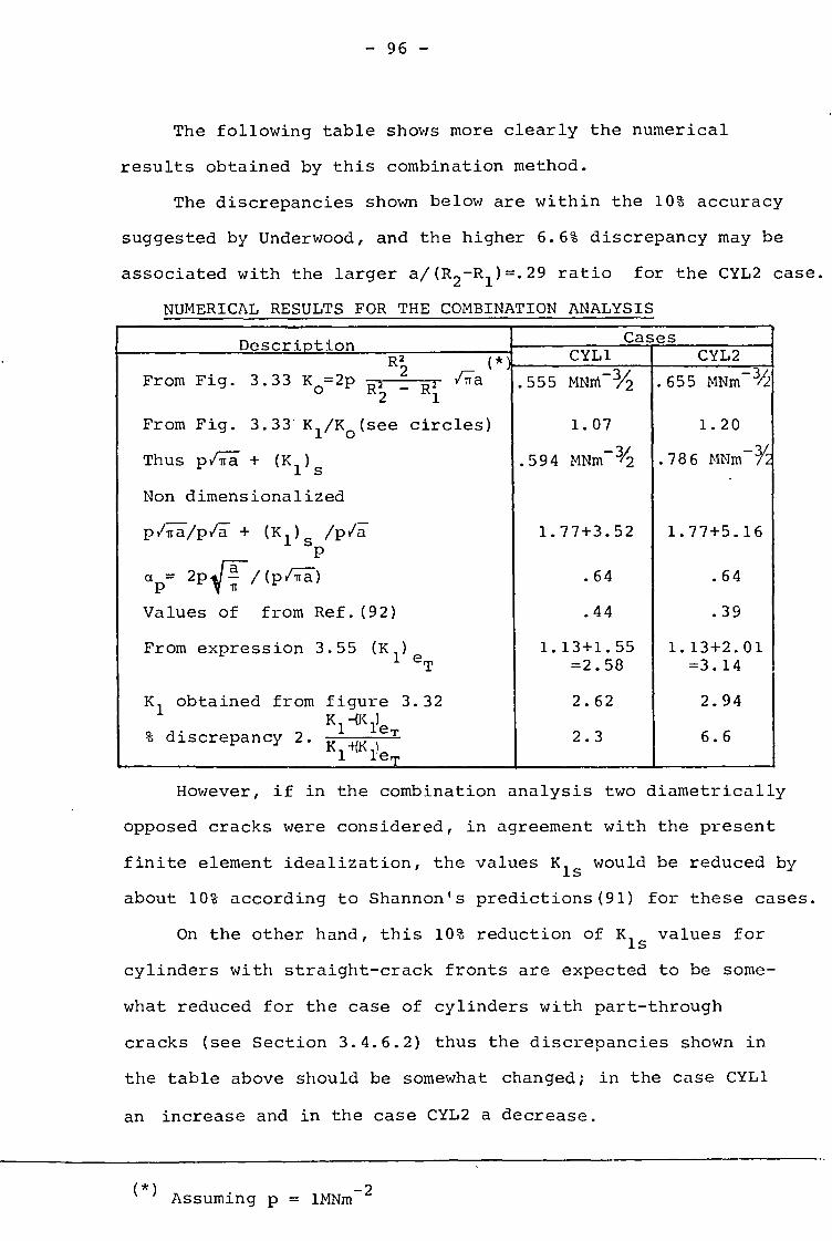
- 96 -

The following table shows more clearly the numerical

results obtained by this combination method.

The discrepancies shown below are within the 10% accuracy

suggested by Underwood, and the higher 6.6% discrepancy may be

associated with the larger a/(R2-R1)=.29 ratio for the CYL2 case.

NUMERICAL RESULTS FOR THE COMBINATION ANALYSIS

Description Cases CYL1 CYL2 R2 t (*).,

3.33 =2p '' ilra .555 MNM-3/2

1.07

.594 MNm-//2

1.77+3.52

.64

.44

1.13+1.55 =2.58

2.62

2.3

.655 MNm-3/

1.20

.786 MNmY2

1.77+5.16

.64

.39

1.13+2.01 =3.14

2.94

6.6

From Fig. K R2 R2 o R2 - Ri

From Fig. 3.33 K1/K0 (see circles)

Thus piTra + (Ki ) s

Non dimensionalized

pi7i17 /pia + (K i ) s /pia P

a P

Tr /(p 2pp/(piTTa-)

Values of from Ref.(92)

From expression 3.55 (K i) e T

K1 obtained from figure 3.32 K1--(1‹1)eT % discrepancy 2. K140‹LT

However, if in the combination analysis two diametrically

opposed cracks were considered, in agreement with the present

finite element idealization, the values Kis would be reduced by

about 10% according to Shannon's predictions(91) for these cases.

On the other hand, this 10% reduction of Kls values for

cylinders with straight-crack fronts are expected to be some-

what reduced for the case of cylinders with part-through

cracks (see Section 3.4.6.2) thus the discrepancies shown in

the table above should be somewhat changed; in the case CYL1

an increase and in the case CYL2 a decrease.

(*) Assuming p = 1MNm-2

- 97 -

CHAPTER 4

SURFACE CRACKS IN A T-JUNCTION OF THICK WALLED CYLINDERS

4.1 - General Considerations

Excessive deformation, leakage or fracture are the

most common ways by which a containment system may fail

(see Ref. (95)). It has been shown in the past that the

first two modes of failure referred to above can be effect-

ively prevented by the use of the more conventional methods

of design.

However, peak tension stresses do occur in some regions

of such containment systems and, particularly in thick-

walled components, brittle failures can initiate either from

defects in those areas, or cracks which may have grown to

critical sizes by fatigue and/or corrosion.

As a result Linear Elastic Fracture Mechanics (LEFM) can

be used to assess the structural integrity of these compon-

ents as it is suggested in Appendix G of the ASME Code,

Section III, (Ref.(96)).

The utilization of LEFM to prove the structural integrity

of a containment system requires the inter-relationship of

various aspects as follows:

i) Defect characterization

Flaws or cracks may be assumed to exist in the more

critical areas (stress concentrations) of the vessel and

with the most detrimental orientation.

- 98 -

ii) Dominant stresses during operation.

The design pressure and operating temperatures may be

considered, as well as the effect of proof loading and a

detailed estimate of the transient conditions must be made.

iii) The material fracture toughness (K1C) may be

measured by fracture tests and the variation of these values

for heat affected zones and weld metals may have to be taken

into consideration. In Nuclear Reactor Technology toughness

degradation due to radiation may also have to be considered.

As can be seen from the foregoing, any safety analysis

of a wide range of structures relating all these aspects in

a rational basis may involve a major research program which

is outside the scope of this work.

A more detailed description of the ways in which LEFM

and general yielding fracture mechanics can be used in

pressure vessels was presented by Burdekin and Dawes Ref.(97).

Mager and Riccardella Ref. (98) presented also a clear

example of Fracture Mechanics Technology in analysing the

integrity during the site life time of a heavy section

nuclear reactor pressure vessel. An excellent compilation of

papers on this subject can be found in Ref.(99).

It was already pointed out in Chapter 1 that LEFM is

mainly valid for situations where fracture occurs prior to

large scale yielding, and its use is mainly confined to the

plain strain regime, Ref. (97).

Although the application of LEFM in cases where there is

a considerable plastic region may be doubtful, it can still

be used as a lower bound (e.g. Refs.(2) and (97)).

- 99 -

Moreover the evaluation of the stress intensity factors

for assumed cracks in the containment systems under hydraulic

test conditions is a necessary part of some methods of

failure analysis(*) (e.g. Refs.(2) and (98)).

4.2 Definition of the Problem

A main steam vent pipe T-junction of a CEGB power plant

was considered as the basis for the work reported in this

Chapter. A sketch of this component is shown in Figure 4.1

and the data of the problem as supplied are:

Inside radius of the branch pipe ro = 73.1 mm

Thickness of the branch pipe (near

the junction area) to = 63.5 mm

Inside radius of the run pipe Ro = 120.6 mm

Thickness of the run pipe To = 43.9 mm

Young's Modulus E = 2.07x103 N/mm2

Poisson's ratio (assumed) v = 0.3

Internal pressure P = 17.24 N/mm2

It is expected that high local stresses will occur at

the nozzle discontinuities and these areas should be considered

as key points for a detailed stress analysis bearing in mind

the subsequent LEFM studies of possible crack configurations

situated in such regions.

(*) As a result of a hydraulic test performed on a pressure vessel it may be reasonably assumed that no flaw greater than a certain size, say a, was initially present in the vessel. Thus, subsequent studies involving transient conditions may assume an initial crack of size a.

- 100 -

Based on reports of similar studies carried out by

other workers, Refs. (1) - (5), and in view of past experience

with the various finite element analyses described in the

previous Chapter(*), it was anticipated that an adequate

mesh idealization of the crack configurations could only

be possible with the use of a substructuring technique. The

number of degrees of freedom involved in an adequate mesh

representation of the T-junction and, simultaneously, a

considerable mesh density around the cracked regions would

be incompatible with the capabilities of the computer (**)

facilities available at ULCC '.

Therefore, following a similar procedure as that

described by Hellen and Dowling, Ref.(2), the T-junction was

idealized by a finite element mesh (main structure) and an

initial stress analysis was performed using the DIM3B code.

Subsequently, a subregion of the T-junction (substructure)

was represented by a reasonably refined mesh where various

crack configurations were idealized.

Boundary conditions were prescribed in this substructure

based on the nodal displacements obtained from the previous

analysis. These boundary conditions were applied in nodes

pertaining to the interface between the main structure and

the substructure.

(*)An account of the computer requirements and costs of the various finite element analyses described in this thesis, will be made in Chapter 5.

(**) CDC 6600

- 101 -

Unfortunately, experimental results were not available

for comparison with the present finite element solutions.

Therefore, the achievement of some confidence in the present

analysis could only be obtained, with some intuition, by

a thorough check on the stress analysis results and on the

overall behaviour of the structure. Also some qualitative

comparisons of the trends shown by the present results with

others found in the literature for similar components but with

rather different geometric parameters are presented. Thus,

this stress analysis is described in Sections 4.3 - 4.5 and

the crack studies return to Section 4.6.

4.3 Finite Element Mesh Idealizations

4.3.1 - General

For the situation when the T-junction is only subjected

to internal pressure, as in the present case, the structure

has two planes of symmetry. Taking advantage of this fact

only one quarter of the structure has to be analysed as it is

shown schematically in Figure 4.2. Appropriate boundary

conditions were prescribed in nodes in these planes of

symmetry.

The top ends of the branch pipe and the run pipe were

subjected to axial loads representing the effects of end

caps.

4.3.2 - 32 Node Element Mesh. CASE TJUN1

In the early stages of this work, a simplified model

of the T-junction was idealized by a mesh of 32 node elements

- 102 -

as it is shown in Figure 4.3. Only one layer of these

elements was used across the thickness and throughout the

structure. This was justified by the fact that stresses are

modelled within these elements by second order polynomials

(see Section 2.2.3(*)), thus being able to model the Lame's

solutions in regions of the cylinders away from the junction

area.

It was also expected that this type of mesh would

represent with reasonable accuracy the stresses in the

nozzle regions. The number of elements was 49 and the number

of nodes 728,

A mesh generation program was developed to generate the

necessary data for the DIM3B code.

Due, mainly, to the lack of experience with such

problems a rather complicated and unreliable mesh generation

technique was developed. It was found that the bandwidth of

this mesh was too high (208), resulting in large computing (**)

costs ', despite the use of a simplified idealization of

the structure which did not model adequately the weld details.

As a consequence, only one run was performed and this mesh was

abandoned. Some of the results of this analysis will be

presented in the following sections of this chapter.

(*) Stresses are obtained by differentiating displacements, hence from expressions (2.13 f) and (2.13 g) it can be shown that stresses are modelled by second order poly-nomials.

(**)The computing costs involved in this analysis will be described later in Chapter 5. The bandwidth is understood to be the maximum number of unknown variables at one time (NUNKVA).

- 103 -

4.3.3 - 20 Node Element Mesh. CASE TJUN2

4.3.3.1 - Mesh Generation

Based on the previous experience, an entirely different

mesh generation technique was adopted. This technique is

similar to that described in Section 3.4.2 for the idealiz-

ation of the CTS configurations.

For the sake of the explanation let us assume the

existence of radial planes containing the axis of the branch

pipe and defined by an angle as illustrated in Figure 4.2.

These planes will be subsequently referred to by the values

of 13.

This new mesh generation technique is based on the

assumption that the entire structure can be defined by the

specification of the cross section of the structure at a= 0°

and the inner radii of the run pipe and branch pipe. Thus,

for values of a between 0° and 90° the idealized details of

the weld region may not be the same as those found in

practice. However, it is assumed that this idealization is

still acceptable for the present purposes.

A primary two dimensional mesh was developed for the

cross section of the structure at 13=0° as it is shown in

Figure 4.4.

The nodal coordinates input data were obtained from a

scaled drawing of this section using a CADMAC digitiser

This machine enables x,y coordinates of a drawing to be

picked up by an electronic probe and automatically recorded

on punched cards. The topological description of this 2D

mesh was specified manually also in the form of punched cards.

- 104 -

The mesh generation program for this case, based on

this 2D type of information generates all nodal coordinates

for the 3D structure as well as the topological description

of the 3D mesh.

Various skewing techniques have been used in order to

obtain the final mesh and they can be divided into three

stages.

Stage I: Construction of a slab with a cross section

identical to that illustrated in Figure 4.4.

Stage II: Basically a cylindrical skewing technique

around the z axis is used, generating a nozzle-on-a flat

plate configuration.

These first two stages are illustrated in Figure 4.5.

These drawings have been generated by the program DRAW using

intermediate nodal coordinate data obtained immediately

after each one of these stages.

Stage III: Another cylindrical skewing technique now

around the y-axis, is applied to the plate and to a small

portion of the branch pipe, generating then the run pipe. In

this stage some difficulties arise in the specification of

nodal coordinates in nodes near the junction area of the cyl-

inders and for values of P.near 90°. Some particular procedures

had to be used to correct in a proper manner these nodal

coordinates. The mesh as finally used is shown in Figure 4.6.

As can be seen from the foregoing, this technique

allows the generation of a 3D mesh of a T-junction based on

a rather simple set of specifications which is normally

- 105 -

available in any design drawing of such components. It is

also clear that changes in the original design details are

very easily accommodated in the input data for the mesh

generation program.

As illustrated in Figure 4.6 the structure was divided

into four sections separated by radial planes of different

value of f3. In each section 2 layers of 20 node elements

have been used throughout as it was specified intially in the

drawing shown in Figure 4.4. The total number of elements

was 104 and the total number of nodes 713. Due to the

topological regularity of this mesh and of the fact that 20

node elements have been used, the bandwidth dropped sharply

to the value NUNKVA=157, which is 25% less than the previous

case. On the other hand a better mesh density was obtained,

especially in the nozzle regions.

In this first case it was decided to assume that the

face ABCD (see Figure 4.6) would be sufficiently away from

the junction areas in order to neglect any disturbances, in

stresses and displacements, caused by the presence of the

nozzle. Therefore the nodal points in that face were only

allowed to move in a radial plane in relation of the y-axis

which is the axis of the run pipe. Due to symmetry appropriate

boundary conditions were prescribed in nodes in the planes

= 0° and 13 = 90°.

4.3.3.2 - Results of Finite Element Analysis for Case TJUN2

Overall Behaviour.

The overall behaviour of this structure has been invest-

igated in terms of stresses and displacements in various

- 106 -

sections of the structure.

A check on the equilibrium forces in the x,y and z

directions was made. For each of these directions the summ-

ation of the calculated reactions at nodes where boundary

conditions were applied differs by less than 0.1% form the

total force applied due to internal pressure.

In Figure 4.7 the thicker lines represent the original

sections of the structure for the planes a= 90°_and ii= 0°.

The thinner lines represent the displacement solution for

these sections. A perspective view of the displaced structure

is illustrated in Figure 4.8. From these results it was

found that the computed radial displacement for the point P

(see Figure 4.7) was 2.71 times greater than the value

predicted by the following Lamc expression for displacements

Illpi [ 122 1 9 U = ,._, (1-2v)r -I- (11-v) -.] r r., R2 _R2 r

2 1 (4.1)

where E = Young's Modulus

v = Poisson's ratio

pi= internal pressure

R1= internal radius

R2= external radius

r = radial coordinate from the axis of the cylinder.

This fact clearly shows that the assumed boundary cond-

itions in the face ABCD (see figure 4.6) are not valid for

this structure. Moreover, if the radial displacements for

the points situated in the face ABCD are affected by the

presence of the nozzle discontinuity, as it appears to be, the

rather large ratio, 2.71, referred to above is also associated

- 107 -

with the fact that two nozzles diametrically opposed have

been assumed in the present mesh idealization.

From these results it is clear that a proper idealization

of the structure has to include the lower part of the run

pipe, thus representing a full quarter of the structure. The

finite element analysis of this new mesh will be described

in the next Section.

4.3.4 - 20 Node Element Mesh. Case TJUN3

4.3.4.1 - Mesh generation

As illustrated in Figure 4.9 the finite element mesh

for this case was obtained from the previous mesh by simply

adding eight more elements representing the rest of the run

pipe. In the new face ABCD appropriate new boundary conditions

were prescribed and one of the nodes in the line AB was

totally fixed to avoid rigid body motion in the z direction.

The total number of elements and nodes was respectively

112 and 773. By using a suitable numbering scheme for the

extra elements (see Figure 4.10) the bandwidth was kept the

same as in the previous case.

4.3.4.2 - Results of the Finite Element Analysis for

Case TJUN3. Overall behaviour.

Again, a check on the equilibrium forces in the x,y

and z direction was made, and similarly to the previous case

the same agreement was found (less than 0.10).

Equivalent results to those shown in Figures 4.7 and

- 108 -

4.8 are illustrated for this case in Figures 4.11 and 4.12.

From these results, basically two conclusions can be drawn.

Firstly, for the same point P as in the previous case,

the ratio between the computed radial displacement and that

predicted by expression (4.1) has been now reduced to the

value 1.84. Moreover, it is clearly shown in Figure 4.11

that the line PQ loses its radial direction in the displaced

section. These two results clearly show the invalidity of

the idealization described in Section 4.3.3 for the case

TJUN2.

Secondly, it can be seen from figures 4.11 and 4.12

that the computed displacements near the ends of both

cylinders instead of converging to the predicted Lame solu-

tions were developing an oval shape.

A better illustration of this behaviour in the ends of

the branch pipe and the run pipe is shown in Figures 4.13

and 4.14 respectively. In these figures the displacements

and stresses obtained with the present analysis are compared

to the predicted Lame solutions.

By inspection of these results (see Figures 4.13(b) and

4.14(b)) it is interesting to note that the deviations

of the computed stresses from the Lame solutions do indicate

the presence of bending moments which have been superimposed

on the internal pressure.

Although no report describing this phenomenon was

found in the literature it is quite acceptable physically and

it is due to the distribution of self equilibrating forces

- 109 -

(* in the junction area of the cylinders. )

By comparison of the displacement results described in

Figures 4.7 and 4.11 it is clear that this phenomenon is less

noticeable in the present case than in the previous TJUN2 con-

figuration where two diametrically opposed nozzles were

actually assumed.

For the cases TJUN2 and TJUN3, Figs. 4.15 and 4.16 show

various contours maps of hoop stresses obtained in the nozzle

regions with the present finite element analysis. For each

case two cross sections were considered, a=o° and 0=90° in

Figures 4.15 and 4.16 respectively.

It can be seen that the stress patterns are very similar

for both cases TJUN2 and TJUN3, however, a slight decrease in

the overall stress levels was noticed for the case TJUN3.

These relative differences in the stress levels and mainly

for the plane 0=0° (see Figure 4.15) are much smaller than the

relative differences obtained for the displacements (compare

Figures 4.7 and 4.11). This fact led to the conclusion that

the prescription of radial displacements according to expres-

sion (4.1) in the ends of the cylinders, in order to avoid the

ovalization effect, would have a negligible influence on the

stress patterns indicated in Figures 4.15 and 4.16. Therefore,

possible alterations to the prescribed conditions in the mesh

TJUN3 were considered and discarded.

Figure 4.17 shows a contour map of hoop stresses in the

nozzle 'region of a PWR pressure vessel similar to that shown

in Figure 1.1. These results were obtained by Hellen and

(*)This type of behaviour can be easily visualized when sub-jecting one end of a cylinder to two types of loads: Either (i) a set of self-equilibrating axial loads or (ii) two diametrically radial loads.

- 110 -

Dowling, Ref.(2), using also a Finite Element Method.

In Figure 4.18 values of hoop stresses along the inner

surface in the crotch corner region obtained by Broekhoven,

Ref.(75), also for a PWR vessel,(*) are compared with the

results obtained by the present analysis for the case

TJUN3.

In both cases quantitiative comparisons of results are

not possible due to major differences in the geometric

parameters of this configurations and in the geometric nozzle

details (see Figure 4.19) as compared with the present

geometry. However, in the first case the similarity of the

stress patterns with those of Figure 4.15 are encouraging.

In the second case, Figure 4.18, the present results

are indicated by the full dots, the circles will be

referred to later on, and the squares indicate the results

from the case TJUN1. The results obtained by Broekhoven are

indicated by the thinner lines.

In the ascending part of these curves reasonable

agreement is verified and it is due to the fact that in both

configurations the average ratios, thickness to internal

radius, for the branch pipes, are very similar, (.94 in the

present case and 1.04 in Ref. (75)). The larger discrepancies

in the descending part of these curves are mainly due to the

fact that in Ref.(75), the vessel is modelled by a flat

plate, thus not allowing for an increase of hoop stresses in

the inner surface as predicted theoretically if a cylinder

was considered instead. The rather high peak value obtained

(*) modelled by a nozzle on a flat plate.

in the present results is associated with the sharp corner

modelled.in the TJUN3 finite element mesh. The proper

idealization of this geometric detail as specified in Figure

4.1 will be made later on.

In view of the foregoing, the subsequent studies

described in the following Sections of this Chapter will

be referred to as the stress analysis results obtained in the

TJUN3 case.

4.4 Validity of the Substructuring Technique

Part-through crack configurations in the section (3=0°

can be considered, from the stress analysis point of view,

as the most critical situation regarding the fracture safety

analysis of the present T-junction. This is due to the

rather high stress concentration factor, 3.8, which was

obtained in the crotch corner region of that section, (see

Figure 4.18).

Because the assumed crack configurations are situated in

a plane of symmetry of the T-junction, only one half of the

region surrounding the crack has to be idealized in any

substructuring technique.

Before entering the actual analysis of such crack con-

figurations, using a detailed idealization of that part of

the structure, a simple test was carried out to assess the

validity of such procedure.

Using the previous finite element mesh, the node which

represents the crotch corner in the plane fi = 0° was released

from its prescribed zero displacement in the x direction. As

- 112 -

it is illustrated in Figure 4.20 this procedure implies

the existence of a corner crack having an approximate

circular shape with an average radius of 23 mm. In addition,

a force was applied on this node in the x-direction repres-

enting the pressure acting on the crack surfaces.

Some of the nodal points which will be part of the

interface between the main structure and the substructure,

have been chosen to monitor the computed displacements

obtained in the present test. A comparison of these

results with those obtained in the main structure analysis is

shown in Figure 4.21. In this figure, the circles, which are

referred to the right hand axis, indicate for each nodal

point the ratio between the computed displacement components,

u in the x direction for the uncracked and cracked situations.

Similar results were obtained for the v and w components

and the maximum discrepancy was found to be less than 0.05%.

As long as the boundaries of the idealized subregion

are as remote from the crack regions as the nodal points

referred to above, the results shown in Figure 4.21 clearly

support the validity of the substructuring technique which

will be described in the following sections of this chapter.

4.5 Substructure Analysis

4.5.1 - The Choice of Crack Configurations

Basically, in Appendix G of the ASME code, Section III,

it is indicated that the plane strain fracture toughness

values of the material should exceed by a given safety

factor the K-values of a postulated defect. This defect has

- 113 -

a depth of one quarter of the section thickness and a length

of six times that depth. It is also suggested that for the

nozzle regions the postulated defect size may be a fraction

of that postulated for the vessel.

If these defects are small they can be treated as cracks

under constant stress fields magnified by a stress concen-

tration factor. However, the use of simplified and approx-

imate procedures for estimating K-values of larger crack

configurations in the nozzle regions may yield rather

inaccurate results. Therefore assessments of the severity of

such cracks, based on this type of approach are bound to

be too conservative.

Four circular crack configurations of successively

increasing depth were thus studied. A sketch of these crack

configurations is shown in Figure 4.22.

The particular choice of these geometries is due to

three reasons. Firstly, post mortem observation of cracked

nozzles (see Refs. (6) and (3)), indicate the existence of

initial defects of circular or nearly circular shape.

Secondly, this shape is very convenient, bearing in

mind some limitations associated with the evaluation of K-

values, using the extrapolation method. This will be expl-

ained later on.

Finally, for engineering purposes, the values of SIFs

along an elliptical crack front, may be estimated within 10%

accuracy by assuming quarter circular corner cracks instead*)

This assumption was based on the results presented by Cha(100)

(*)For ellipseswith aspect ratios down to 0.4 (see Ref.(100))

- 114 -

and is also substantiated by Kobayashi and Enetanya(101) in

their studies of elliptical corner crack configurations, even

for the situation when linear varying stress distributions

are considered.

4.5.2 Mesh Generation

A sketch of the subregion which was considered for the

present substructure analysis is shown in Figure 4.23.

It is clear from this figure that all the nodes in the

interfaces between the main structure and the substructure

are situated at similar distances, from the crack region, as

those of the nodes considered in Section 4.4 of this Chapter.

The technique used to generate the substructure was

basically derived from that used in the idealization of the

cracked cylinders described in Chapter 3 (see Section3.4.6.1).

Suitable geometric alterations to the external boundaries

were initially specified in order to account for the weld

details of the present geometry. ¶he final mesh as illus-

trated in Figure 4.24 was then obtained by subsequently

applying a cylindrical skewing technique similar to that

referred to as stage III which was described in Section 4.3.3.1.

Some relevant features associated with this mesh are

described as follows:

i) The total number of elements and nodes is 88 and

583 respectively.

ii) Using always the same topology, the various crack

configurations were idealized by the application of simple

linear skewing techniques. In these skewing procedures only

- 115 -

the interior nodes suffered changes in their geometric

positions, whereas the nodes in the interfaces were kept un-

changed. Hence, the boundary conditions based on the nodal

displacements, such as those indicated in Figure 4.21,

remained the same for the various crack configurations.

iii) At the time the TJUN3 mesh was developed it was

possible to forsee for the substructure the spatial positions

of the nodes in the interfaces. Therefore, identical spatial

nodal positions were ensured, in the main structure, by an

adequate specification of the values of f3 for the various

radial planes in which the nodal points are located. Further

complications and inaccuracies associated with the specifica-

tion of boundary conditions are avoided with this procedure.

iv) With the present mesh, a proper representation of

the crotch corner, as specified in Figure 4.1, replaced the

sharp corner idealization of the main structure (TJUN3).

v) Internal pressure was specified in the inner surfaces

and was assumed to fully penetrate the crack, thus acting on

its surfaces.

vi) As it is shown in Figure 4.24, the nodes in the free

surface of the crack are distributed in five radial directions

emanating from the crotch corner. By assuming circular-

shaped cracks, these directions remain perpendicular to the

crack fronts. Thus the evaluation of SIFs along the crack

front by using the extrapolation method in these radial

(* directions is a straight forward procedure. )

(*) The use of the extrapolation methods in directions which are not perpendicular to the crack front have been dis-cussed in Section 3.4.3.

- 116 -

4.5.3 - Analysis of the Uncracked Substructure

Overall Behaviour.

In order to obtain greater confidence in the substruct-

uring procedure a defect-free substructure was considered

before the idealization of any crack configurations. The

overall behaviour of the substructure was investigated in

terms of the stresses in the nozzle region.

A comparison of the hoop stress patterns obtained in

both the main structure and the substructure is shown in

Figure 4.26.

In Figure 4.18 the circles represent the values of the

hoop stresses which were obtained in the inner surface with

the present analysis. It is interesting to see that the

peak stress value obtained in the main structure analysis,

where a sharp corner was assumed, has been smoothed out with

the proper idealization of the crotch corner geometry.

In both cases, Figures 4.18 and 4.26, the similarity

of the stress patterns is again encouraging.

However, as illustrated in Figure 4.26, some minor

differences are noticeable in the vicinity of the crotch

corner and in the area close to the run pipe. In the former

region the results obtained in the substructure analysis are

believed to be more accurate whereas in the latter, the TJUN3

analysis should provide better results.

This is due to the fact that in the substructure ideal-

ization, a better mesh density was obtained in the crotch

corner at the cost of a coarser mesh in the areas away from

that region as illustrated in Figure 4.25.

- 117 -

4.6 Analysis of the Cracked Structure

4.6.1 - Idealization of the Cracks

The various cracks have been idealized by releasing the

nodes in the free surface of the crack from their prescribed

zero displacements in the x direction. Again, the mid-side

nodes adjacent to the crack front were displaced to the

quarter point positions nearest to the nodes in the crack

front.

4.6.2 - Overall behaviour

The influence of the presence of various cracks on

the overall behaviour of the substructure was investigated

by monitoring the changes of the boundary reactions as the

crack size increases.

The maximum changes for each crack configuration and in

various radial planes B, are shown in the table below. The

deviations are indicated in percentage values of the initial

reactions which were obtained in the uncracked substructure

analysis. CHANGES IN THE NODAL REACTIONS

CRACK SIZE mm

Max. Deviation %

13 = 0° 13= 34o fi = 90o

1 12.7 1.1 .8 .9

2 19.1 2.8 2.0 2.2

3 25.4 6.7 4.2 4.5

4 31.8 11.4 7.6 7.7

- 118 -

As can be seen from this table the deviations increase

considerably with the crack depth and the application of the

present substructuring technique may eventually underestimate

the values of the SIFs for cracks deeper than the crack 3.

The results obtained for crack 4 yet will be presented.

4.6.3 - Stresses Ahead of the Crack Fronts

The ax stress distributions for the sections a=0,

a = 45°, a = 90° ahead of the crack fronts are shown in

Figure 4.27.

It is interesting to note the values of these stresses

in areas away form the crack regions are just slightly

affected by the presence of cracks of increasing size. This

may be due to the "fixed grip" conditions to which this

substructure was subjected. Small variations of the stress

levels in these areas would be expected to occur if a full

structure were analysed instead.

Due to reasons which have already been described in

Chapter 3, the stress data in the neighbourhood of the cracks

can only support, in a qualitative manner, the distribution

of the SIFs along the various crack fronts. In fact the

stress values at the quarter point nodes are in close qualit-

ative agreement with the variation of the SIFs along the

various crack fronts (see Figure 4.28).

4.6.4 - Evaluation of K-Factors, Discussion of Results

As in the previous test cases, which were described in

Chapter 3, the extrapolation method was applied using the

- 119 -

displacement components in the x directions of the nodes in

the free surface of the cracks, thus 0=Tr . Plain strain

conditions were assumed for all the directions , with the

exception of a= 0° and a= 90° where plane stress express-

ions were used instead. This first group of results is shown

in Figure 4.28.

In order to obtain more confidence in these results the

SIFs were also obtained using the extrapolation method in

the directions perpendicular to the crack plane, thus for

0 = 7/2. This second set of results is also shown in Figure

4.28.

It is interesting to note that the K-values obtained with

this second procedure (for 0= 7/2) are consistently greater,

by about 9%, than the results obtained with the extrapolation

procedures in the free surface of the crack.

These differences, as pointed out in Chapter 3 (Section3.2.2)

are associated with the inaccuracies involved in the extra-

polation procedures and mainly in the direction e = 7/2.

Due to this, the second set of results may be regarded as

an upper bound to the true solution. Subsequently, based on

these two sets of results, areas of uncertainty of the SIFs

distributions, for each crack configuration, may be defined

as illustrated in Figure 4.28.

Another procedure was used, based on the Global Energy

Method and is described as follows.

As it is shown in Figure 4.29, when the crack is extended

by skewing the mesh, the energy balance equation for the

system can be expressed as

- 120 -

1 - A = GAA = 2 — R* Aum" "m (4.2)

provided no pressure is acting on the free surfaces of the

crack.

Now using the principle of superposition, the work done

by the nodal equivalent point forces to the internal pressure

can be added to the right hand side of equation (4.2) thus

m P1 1 + Pn.

-AU. + X ni+2

Aun

GAA = I Rm Au'

2 m n=1

where AU i i+1

R ,* mR m

Au',Au'* m

- Change of strain energy from crack i

to crack i+1

- Reaction on the node m

- Crack opening displacement in the

point A indicated in Figure 4.29.

AUn = U - U n. ni+1 1

Pni43pi - Nodal equivalent point forces to the

the internal pressure.

The work done by the internal pressure is evaluated by

assuming the displacement of forces which are an average of

the forces obtained for crack i and crack i+1 and can be

obtained from the output of DIM3B code.

The subsequent strain energy release rates obtained

with this method are best associated with an intermediate

crack by assuming the mean of the depths of cracks i and i+1.

From this method the values of strain energy release

rates have been translated into K-values and were found to be

- 121 -

about 40% lower than those predicted by the extrapolation

method. Very little importance should be attached to these

discrepancies due to the following reasons:

i) Large inaccuracies involved in the evaluation of the

u' value. n

ii) Problems associated with the evaluation of the work

done by the internal pressure on the crack surfaces.

iii) Rather coarse crack extensions have been assumed

by using the results from the analysis of cracks 1 to 4.

iv) The present procedure, as well as the crack closure

work method (see Section 3.2.3), are more accurately used

when the crack extensions are idealized by supressing the pres-

cribed conditions in nodes ahead of the crack front, instead

using skewing techniques as in the present case.

It has already been confirmed by other workers in their

LEFM studies of cracks in nozzles (see Refs. (2), (3), and

(59)) that, for these types of configurations the use of \

simplified analytical or semi-analytical procedures to eval-'

uate K-values, may result in a considerable inaccurate

estimates of the true solutions. Therefore this type of

analysis, which is bound to be inconclusive was not considered

in the present work.

Alternatively, a comparative study of the present

results with those described in Refs. (2) and (75) was carried

out and is based on the following assumptions. It has been

shown (see Figures 4.15, 4.17 and 4.18) that hoop stress

patterns in the nozzle regions, for the section fl= 0°, are

very similar for a relatively wide range of geometries.

- 122 -

In fact:

i) Maximum stress concentration factor is always found

at the crotch corner, whereas very low stress levels are

obtained in the opposite surfaces.

ii) The membrane stresses away from the nozzle regions

are normally higher in the vessel or run pipe than in the

branch pipe.

iii) However, for small distances away from the crotch

corner the stresses in the inner surfaces die away more

rapidly in the side of the vessel or run pipe.

iv) The hoop stress distributions for angles of a near

45° are lower than the same distributions for a = 0° and

a = 900.

v) The variations of SIFs along the crack fronts

show similar trends to the stress distributions with the

exception for crack depths smaller than the crotch corner

radius.

vi) The/values of the stress concentration factor in the

crotch corner regions seem to increase when the crotch

corner radius decrease.

From these conclusions, an average of SIFs for each

crack configuration in the various nozzle geometries can be

related by normalizing them to the SIF of a penny-shaped

crack, Ko, (see exp. 1.13, Chapter 1), subjected to a remote

stress equal to the membrane stress of the vessel, thus Ko

can be expressed as

Ko = 2 p R

(4.4)

- 123 -

where p is the internal pressure

R is the internal radius of the vessel

T is the thickness of the vessel

a is the crack length

Moreover, the true geometric size of each crack can

also be suitably normalized in relation to some geometric

parameter which is obtained, on an empirical basis, from

the design details of each nozzle, With this procedure

cracks which may have rather large different sizes are then

compared on the basis of the same depth to thickness ratio.

According to this procedure the results which were

obtained are shown in Figure 4.30. The circles indicate

the present results whereas the squares and the hexagonals

are referred to the results obtained by Hellen and Dowling

(2) and Broekhoven (59) respectively.

The thinner curve which is referred to the right hand

axis indicate for the present case, only, the true Ko /

variations for a range of a/T up to .5.

The following conclusions can be drawn from these

results.

i) The normalised K-values for the present crack con-

figurations are considerably higher than the values corresp-

onding to the other cracked nozzles 2 and 3.

ii) These differences can be associated with the higher

hoop stresses which where obtained in the present case (see

Figure 4.18) for the uncracked.structure.

iii) On one hand, the present results are expected to

underestimate the true solutions, due to the "fixed-grip"

- 124 -

conditions which were used in the present substructuring

technique. This is somewhat confirmed by a faster decrease

in the normalized K values as the ratio a/T increases.

iv) On the other hand, the hoop stresses in the present

case (see Figure 4.18) die away, from the crotch corner,

more rapidly as compared to the hoop stresses obtained by

Broekhoven in nozzle 2.

v) However, due to the doubly-connected nature of these

structures, regarding both the run pipe and the branch pipe,

the present technique may not yield too large an error in the

evaluation of K-values. This is more so in the present

case, where the ratio of thickness to internal radius is

much larger than in the other geometries 2 and 3.

This type of behaviour has been somewhat confirmed in

the analysis of cracked cylinders described in Chapter 3.

In these cracked cylinders it was found that the distur-

bances caused by the presence of the crack are restricted to

a small region in the plane of the crack and negligible in

radial sections perpendicular to the crack plane. (See Figs.

3.30 and 3.31).

vi) The variations of reactions with increasing crack

depth, which are described in Section 4.6.2, indicate that

the substructure idealization could have been restricted to

a smaller sector of the nozzle region between the planes

B = 0 and, say, a= 450 thus allowing for a better mesh

density in the cracked region.

vii) The cracked cylinder CYL1, described in Chapter 3,

and the present branch pipe are very similar in their geometric

- 125 -

parameters, having the same thickness and differing - by

only 2% on the internal radius.

For the same crack depth to thickness ratio, a/T=.2

the normalized SIF at the free surface of the branch pipe

is about 3.12 (see Figures 4.29 and 4.30) and the stress

concentration factor SCF, at that point (see Figure 4.18) is

3.3 in the uncracked structure. Using the same Ko value as

before (for comparison purposes) the SIF at the point where

the crack meets the inner surface of the cylinder CYL1

was found to be .97. Multiplying this value by the SCF

indicated above, yields to a correspondent SIF for the branch

pipe of 3.03 which is only 3% lower than the 3.12 value

obtained form Figures 4.29 and 4.30.

viii) In Figure 4.30, the full circle indicates the

average normalized K value obtained in the corner crack

configuration described in Chapter 3 (see Section 3.4.4).

In that spe&imen the ratio thickness to crack depth is also

.2. This averaged SIFs is2.73 times smaller than the corres-

pondent value in the present cracked nozzle, which can also

be associated with the previous SCF, 3.3, referred to above.

This larger difference is explained by the doubly-connected

nature of the present geometry where bending is restricted

thus reducing the SIFs as compared to the corner crack in

the square specimen.

ix) From the scarce results indicated in Figure 4.30,

similar trends can be observed to occur in the various

geometries and for values a/T greater than .16. However,

in these normalized SIFs strong differences, of up to about

- 126 -

50% are observed which are associated with differences in

the geometric details and the stress distributions of the

various nozzles. These differences and the complexity

of these crack configurations seem to rule out any prospect

of obtaining an exact analytical solution.

Finally, bearing in mind possible safety implications of

the present crack configurations, some conclusions can be

drawn based upon the following considerations.

i) The hoop stresses in the uncracked structure as

well as the SIFs are higher in the branch pipe than in

the run pipe, hence cracks tend to grow faster in the branch

pipe.

ii) For materials such as the A533-B steel, which is a

low alloy pressure vessel steel commonly used in the

Americal reactor technology, typical Kic values can be as _3

low as 50 MNm 2_ This value is for very low temperatures

or for higher temperatures under dynamic or impact testing

conditions.

iii) From Figure 4.29 the maximum K1 values for cracks

1,2,3 and 4 can be obtained. Based on the above K1C value,

it can be said that under extreme conditions (low temperatures

or impact conditions) the following safety factors against

instability or brittle fracture are indicated:

SAFETY FACTORS FOR CRACKS 1,2,3,4 3,

FOR K1C = 50 MN m /2

CRACK CRACK LENGTH MAX K1 SAFETY FACTOR

1 12.7 21 2.38

2 19.1 24.5 2.04

3 25.4 27 1.85

4 31.8 30 1.67

- 127 -

iv) In ultrasonic testing, the detectable defect size

for the range of thickness values specified in the present

geometry is found from Ref. (102) to be less than 2 mm.

Thus the present crack configurations can be found and measured

safely.

- 128 -

CHAPTER5

CONCLUSIONS AND RECOMMENDATIONS FOR FUTURE WORK

5.1 Achievements

i) A three dimensional general purpose linear elastic

finite element program was brought into use. In this

program (DIM3B) the input data format is quite general and

applicable to any geometric and/or loading conditions, yet its

generation may become a rather tedious and complicated job.

In order to ease some of these problems, facilities exist

in the program which allow the user, if so desired, to chose

various optional sets of coordinates to which the various

input data may be referred.

ii) The DIM3B code can be submitted in a so-called

"Dynamic mode of operation". For each analysis this procedure

attempts to optimize, in a semi-automatic manner the computing _.-

costs (in CM and CPU(*) time) involved in running the program.

iii) Various mesh generation techniques have been

developed for the three-dimensional analysis. In general,

these programs generate the necessary data for the DIM3B

code based on a rather simple 2D type of information. In all

these mesh generation programs various stages can be identified.

1 - Full description of the topology of the 3D mesh

2 - Generation of a simple 3D geometry

3 - Application of various skewing techniques separated

in distinct stages which yield to the desired geom-

etric shape.

(*) CM - Central memory CPU - Central processor unit

- 129 -

These procedures ensure

1 - Validity of the mesh generation programs for a

relatively wide range of the geometric parameters of

the type of structure under study.

2 - Topolgical regularity in the 3D meshes, thus keeping

the size of the bandwidth to a low level.

3 - Normally, changes in the geometric details of the

structure can be easily accommodated by performing

minor alterations in the 2D type of input data.

iv) Using some off-line graphics facilities available

at I.C.C.C. a plottingprogram, DRAW, was developed whereby

the various 3D meshes can be visualized and efficiently

checked in terms of the topology, nodal coordinates and

prescribed displacement boundary conditions. In this program

an isometric view of the mesh is generated from a direction

which can be suitably specified by the user.

v) An axi-symmetric general purpose linear elastic

finite element program was developed. This program, FRONT,

uses a simplified version of the FMS in which the symmetric

property of the body stiffness matrix [k] is not taken into

account. However, profiting from this fact, the introduction

of slope boundary conditions was easily accommodated in the

solution technique (see Appendix 1, Section A1.4.2.4) by

performing relatively simple alterations in the coefficients

of the matrix [k].

v) The theory outlined by Henshell and Shaw (Ref. (81))

for the "2D crack tip elements" was extended for the equivalent

3D element, i.e., for the 20 node isoparametric element

(Section 3.3).

- 130 -

vi) It was also shown that this theory could be gener-

alized so that "crack tip elements" can be derived from any

isoparametric finite elements (Section 3.3) provided they

have one or more than one intermediate nodes in the edges.

This means that any field variable within the conventional

elements must be described by quadratic or higher order

shape functions.

vii) To substantiate this theory various test cases of

CTS configurations were carried out in which the crack tip

regions were idealized by using standard 20 node elements

or their derived "singularity elements" (Section 3.4.2).

The validity of the theory was confirmed by the

improvements which were observed in the K-values when the

"crack tip elements" were used (see Figures 3.18 and 3.19).

viii) The generalization of the theory referred to in

vi) was also substantiated by the results which were obtained

when the same CTS geometries were idealized by 32 node

element meshes (see Figures 3.21 b).

ix) Some other typical 3D crack configurations were

then studied (Sections 3.4.4 to 3.4.6). The results which

were obtained from these analyses compare favourably with

suitable bounding approximate solutions and other results

already given by other authors.

x) By applying an adequate substructuring scheme it

was possible to study various crack configurations of increa-

sing size in the crotch corner region of a thick-walled

T-junction of cylinders. (Chapter 4 ).

- 131 -

5.2 Computing Costs

In Chapter 3, Section 3.4.1, the strategy which was

adopted for running a typical case with the DIM3B code was

described. This strategy, illustrated in Figure 3.11,

can be divided into two main stages.

1 - Execution of the mesh generation program followed

by the plotting procedure (execution of program DRAW)

2 - Resubmission of the mesh generation program followed

by the execution of DIMDIM and DIM3B codes.

It was found that the costs involved in the stage 1

computations are, on average, about 2% of the total computing

requirements of a complete analysis.

. A table is presented here where the computer requirements

for the execution of the DIM3B code are described in detail

for the various finite element analysis reported in this

thesis:

The usage of the CDC system at U.L.C.C. is combined via

a complex formula and translated into a measure called unit

as follows

1 Units = CP( 10+3CM) + TR x DR (1 + .3CM) +

128 30 6 1 (CR+LP)

1.44x10

where CP is the total central processor time

CM is the number of core memory words occupied

TR is the number of words transmitted to or

from magnetic tapes

DR is the number of words transmitted to or

from disk

COMPUTER REQUIREMENTS FOR THE EXECUTION OF DIM3B CODE (FTN compiler)

CASE NN ELM NELEM NODTOT NPRDEF NKNVA NUNKVA

(**) COMPUTER REQUIREMENTS NT CM (*) o CPU(*) o PP(*) UNITS

COST £

1 20 22 202 109 24 101 606 29488 147.196 35.718 4.934 9.87

2 20 44 319 123 26 162 957 39990 290.682 84.486 8.338 16.68

3 32 22 340 175 36 164 1020 45230 331.517 88.935 18.476 36.95

4 20 88 553 68 14 291 1659 74730 817.823 110.962 65.388 130.78

5 20 88 553 151 30 278 1659 75853 795.010 105.084 58.339 116.68

6 20 88 553 215 39 269 1659 76011 782.157 105.285 54.328 108.66

7 32 49 728 213 29 208 2184 59444 899.766 163.412 53.761 107.52

8 20 104 713 239 23 157 2319 48221 656.421 91.038 30.969 61.94

9 20 112 773 256 19 157 2319 48414 686.750 113.153 32.534 65.07

10 20 88 553 325 56 282 1659 85916 864.77 99.7. 64.686 129.37

(*) - CM

(**) ' - NT

- Control Memory; CPU - Central Processor Unit Time;

- Total number of degrees of freedom, NT = NODTOT x

PP - Peripheral Processor Time

o - Seconds

3

Case 1 - Compact Tension Specimen Case 6 - Cracked Cylinder, Fig.3.29 Case 2 - Compact Tension Specimen, Fig.3.14 Case 7 - TJUN1, Fig.4.3 Case 3 - Compact Tension Specimen, Fig.3.21(a) Case 8 - TJUN2, Fig.4.6 Case 4 - Corner Crack Specimen, Fig.3.26 Case 9 - TJUN3, Fig.4.9 Case 5 - Part-through Crack Specimen, Fig.3.26 Case 10- Substructure, Fig.4.24.

- 133 -

CR is the number of cards read

LP is the number of lines printed

The estimation of the costs for the various computations

is based on a rate of £2.00 per unit of the computer resour-

ces usage.

5.3 Final Conclusions

5.3.1 - The FEM and its LEFM applications.

i) The FEM is a very powerful technique to solve

general stress analysis problems. However its application

to three dimensional cases is hampered both by the present

generation computer capabilities and the rather high costs

involved in such computations. As a consequence, such

analyses are still limited to relatively coarse mesh

idealizations of the geometries in study.

ii) The utilization of "crack tip elements' in three

dimensional LEFM studies seems to be compulsory if K factors

are to be evaluated without unacceptable loss of accuracy.

For the present meshes, discrepancies of about 20% are found

if no "singulairy elements" are used.

iii) K-values obtained by the extrapolation method

and using the displacement distribution in the free surface

of the crack (0=10 show in general an agreement within 5% with

other results already given by other authors.

iv) Less accurate estimates of the K-factors are obtained

when the displacement method is applied in directions per-

pendicular to the crack plane (0=Tr/2). This is due to the

strong square root behaviour of the K* curves (see Figure

3.1) as it was described in Chapter 3, Section 3.2.2.2.

- 134 -

v) However by using these two directions of extra-

polation (0 = Tr and e = Tr/2) valuable information can be obtained

about the coefficients of the higher order terms of the

Williams series solution (exp. 3.4). These coefficients

which are derived from the K* curves can eventually be

physically interpreted by following the lines suggested by

Cotterell (106).

vi) Such coarse meshes present some limitations on

the validity of the computed stresses in the vicinity of

the crack. Therefore finer meshes would be recommended if

a detailed analysis of the near tip stress fields is

required, or if K factors are to be calculated by the "stress

method".

vii) Strain energy release rates, G, obtained from

boundary load displacements can only be used by making two

complete runs for adjacent crack configurations.

The averaged K-factors associated with the values of

G (exp. 1.7) compare favourably with those obtained by the

extrapolation method using the direction e= IT (see section

3.4.3).

viii) The variations of K-values which were obtained

along the crack fronts of all the configurations studied,

show the incapability of the FEM to detect any surface effects

in regions where the cracks meet the free surfaces. However

it is believed that in such areas the present results are

still acceptable for engineering purposes.

ix) The computation costs associated with 32 node

element meshes are considerably higher than those involved

- 135 -

in 20 node element mesh indealizations. Moreover it was

found that better mesh densities are obtained with the

use of 20 node elements.

5.3.2 - The LEFM Studies of Cracks in the Main Steam Vent

Pipe HT-Piece".

i) Confidence in the validity of the results obtained

from the finite element analysis of the defect-free "T-piece"

geometry is based on the following observations:

- Agreement of the results which were obtained with two

different mesh idealizations (see Figure 4.18). One

using 32 node elements (Figure 4.3), another using 20

node elements (Figure 4.9).

- Apart from an ovalization effect which was observed

in the ends of the cylinders, and shown to be physically

explicable, the stresses and displacements in such

areas agree well with the predicted Lame solutions.

- The hoop stress distributions in the crotch corner

regions of the present geometry and two other nozzle

configurations (see Figures 4.15 and 4.18) show rather

similar trends.

ii) By comparing these stress distributions ( in the

present case and in the other two nozzle configurations)

the following conclusions may be drawn.

- The smaller the crotch corner radius the higher the SCF

in these areas.

- This suggests that better stress distributions may

eventually be obtained if the crotch corner is smoothed

- 136 -

out by removing material and so increasing the crotch

corner radius. Comparison with other workers indicates

that this will lower the K values of possible cracks

in such regions.

iii) When two diametrically opposite branch pipes are

considered (case TJUN2) the overall stress levels in the

crotch corner regions increase by about 10% in relation to

the stress levels which were obtained for the single T-

junction geometry (case TJUN3).

iv) For the present case the maximum hoop stress in the

crotch corner regions was found to be 174 MNm2 which is

below the yield strength of a mild steel. This result

demonstrates that, for this configuration, there will be no

gross yielding and ensures the validity of the LEFM studies.

v) Whereas a relatively coarse mesh idealization was

sufficient to obtain the stress and displacement distributions

in the uncracked "T-piece" geometry, a much denser mesh was

necessary to idealize in a proper manner the various crack

configurations.

vi) Due to the limitations of the present computers, it

is necessary to use a substructuring technique in order to

achieve the desired mesh density in the regions of concern.

vii) Substructuring schemes are expected to under-

estimate somewhat the true K-values, however, due to the

doubly-connected nature of the present configuration, such

errors may not be too large.

viii) For crack depths up to about one half of the

thickness of the run pipe the present substructure idealization

could be restricted to a smaller sector of the junction area

of the cylinders.

- 137 -

5.4 Recommendations for Further Work

The results presented in this thesis clearly demonstrate

the possibility of evaluation of K-values utilizing a stand-

ard 3D finite element stress analysis computer program.

However the rather high costs involved in such comput-

ations immediately suggest the development and implementation

of new features into the DIM3B code.

i) Implementation of the 15 node wedge-shaped element.

This element is fully compatible with the presently available

20 node hexahedron elements, and the main advantages

associated with this element are:

- More versatility in the mesh idealizations

- In general, these elements yield smaller sizes of the

bandwidth,

- "Crack tip elements" are still easily derived from

this wedge-shaped element (the "quarter point distances"

rule is still applicable).

As far as the programming aspects of the DIM3B code are

concerned the implementations of these elements requires the

following major procedures.

- Addition of an extra library subroutine containing the

shape functions and its partial derivatives for these

elements.

- Suitable alterations in subroutines LOAD, FEM and

FEM2.

ii) Organization of book-keeping procedures for the

stiffness coefficients so that possible substructuring schemes

can be used in a more accurate manner and at lower costs.

- 138 -

This feature is not only suitable for general stress analysis

problems but it is also rather useful bearing in mind the

possible application of the Parks. "stiffness derivative

procedure" for evaluating strain energy release rates.

iii) The implementation of initial stresses and/or

initial strains due to temperature rises would obviously

allow the solution of a wider range of problems of pratical

interest as for instance, residual stresses and stress dis-

tributions due to thermal gradients.

Three dimensional LEFM studies are still very scarce.

A wide range of practical problems is yet to be studied and

a completely general approach to the solution of these

problems has been provided.

As an immediate extension of the present work the

following studies may be of interest.

iv) In Chapter 3, Section 3.4.3, it was suggested that

a single averaged K factor obtained by the Global Energy

Method can replace the 2D calibration factors for the

specimens used in fracture toughness testing procedures.

For the CTS with curved crack fronts the results clearly

show a reduction in K with increasing tunneling effect. A

much more accurate analysis with a finer mesh would be

required if proper correction factors are to be evaluated.

v) The present substructuring technique could eventually

yield improved results by carrying out this scheme in a step

wise manner. In other words, the imposed displacement boundary

conditions which are obtained from the analysis of the entire

structure can be updated for each crack length by grossly

- 139 -

, idealizing equivalent cracks in the main structure mesh.

The improvements of this modified scheme can be monitored by

inspection of the reactions.

vi) Some LEFM studies are suggested which may be

carried out using the FRONT code:

- Simulation of nozzle geometries by an axisymmetric

nozzle on a flat plate.

- Long and narrow banana-like cracks occur in stuctures,

as for instance, in off-shore oil rig"T-piece" components.

These cracks can eventually be studied by an approximate

axisymmetric idealization of their configurations.

vii) Finally, carefully controlled experiments are

required so that the present results, which were obtained by

a numerical method, could be properly substantiated.

- 140 -

APPENDIX1

PROGRAM FRONT . DESCRIPTION . USER'S GUIDE

A1.1 - Introduction

The program FRONT is a finite element computer program

using triangular axisymmetric finite elements. This program

has been developed from the FLAPS code for which a full

User's Guide is given in Ref. (103). The elements used are

the axisymmetric version of the well known "Constant Strain

triangular elements" which are described in Ref. (46).

The FLAPS program uses the Gaussian iteration method

to solve the system of equations

[k ] {A} = {F} (A1.1)

where [Id is the general body stiffness matrix

{A} is the unknown displacement vector

{F} is the applied nodal forces vector

The iteration method is speeded up by using an over-

relaxation factor reducing the number of cycles necessary

to reach a given tolerance.

The rate of convergence of this method is highly dep-

endant on: the over-relaxation factor, the shape of the

structure, the boundary conditions and the initial geometry

of the elements (see Refs. (48) and (104)).

Experience has shown that, in general, good results

(apart from mesh density considerations) are obtained if a

- 141 -

tolerance(*) of the order 10-5 is reached. Nevertheless it

has been found that in some cases this level of tolerance is

very difficult, if not impossible, to reach, even using

techniques for optimization of the over-relaxation factor

(see Ref. (105)).

For these cases the Gaussian iteration method is no

longer reliable and another method of solution of the equation

(A1.1) is required, such as the Gaussian elimination technique.

A description of this method has been given in Chapter 2,

therefore will not be repeated here. Only its computer imple-

mentation will be described in some detail for the present

case.

The mathematical theory involved in the prescription of

displacement boundary conditions, for the present case, is

described in the following section.

The programming aspects of the FRONT code will be out-

lined in Section A1.3 and a User's Guide as well as a listing

of the program will be included in the final sections of

this Appendix.

A1.2 - Displacement boundary conditions

In the DIM3B code full advantage is taken from the

symmetry of the overall stiffness matrix [k] whereas in the

present program the completed equations are fully stored. As

a result the partitioning of the matrices, as indicated by

expression (2.48) in Chapter 2, is no longer necessary.

(*) In the present case, tolerance is expressed as cAui

Tol = where Au. = l. uu• - Cu. 1 1+1 -il

u.1 = nodal displacements at iteration i

(A1.2) . . . + S1,211:-

. . + S2,2n

. . . +s 2n,2n

- 142 -

A description of the method whereby initial prescribed

displacements are accommodated in the present solution

technique will follow.

A1.2.1- Prescribed Displacements in the Radial or Axial

Directions.

Suppose the set of equations (A1.1) can be expressed

as

S1,1 61 + S1,2 62 + .

S2,1 61 + S2,2 62 +

S2n,1 61 + S2n,2 d2+ •

where in this two dimensional case 62k-1 = u

k and

62k = uk

for each node k.

If 6s is a prescribed displacement at node k, a suitable

alteration of equations (A1.2) can be performed as follows:

The quantities Sis 6S (for i=1, 2 .. 2n) will be transferred

to the right hand side of all equations i as known quantities.

Fs is the sum of the external applied forces Rs, the internal

forces due to initial strains and body forces for the node s.

Fs = Rs + Rbs + R

ES (A1.3)

- 343 -

where Rs = external forces

Rbs= Forces which are statically equivalent to body

forces

Rcs = Forces to suppress initial strains (thermal

strains in the present case.)

If 6s is known, Rs becomes an unknown reaction as well

as Fs. This unknown quantity is replaced in the solution

vector, A, and can be evaluated if reactions are to be cal-

culated. In view of the foregoing all equations will be

changed as follows

S. 6 + S 6 + . 1,1 1 S. 2

. + 0.6s+ . . +Si,2n62n= Fi-S.,s

(A1.4)

and the equation s which contains 6s in the leading

diagonal will be changed to

Ss,161 + Ss,262 + . . . -Fs + . . . + S

s,2n62n = -S 6

s,s s

(A1.5)

thus equation (A1.2) can now be expressed in matrix form as

51,1

S2,1

Ss,1

2n,1

s1,2

S2,2

s,2

S2n,2

.

•

.

'

.

0

. 0 .

.-1 .

. 0 .

•

.

.

.

.S1,2n

.S2,2n

.Ss,2n

S2n,2n

1

2

Fs

62n

F1-S1,s6s

F2-S2,s6s

- S 6 ss s

F2n-S2n,ss

(A1.6)

It is obvious that this procedure can only be performed in

equations which have already been completed, or, in finite

element terminology, when all the elements adjacent to the

node k=(s+1)/2 have been processed.

- 144 -

A1.2.2 - Slope Boundary Conditions

If a node k is only allowed to move on a particular

direction, as it is illustrated in Figure A1.1, the displace-

ments uk and vk for that node remain unknown and a relationship

Figura A1.1 - Slope boundary condition in node k

between these two values can be established as

uk = q. V. k (A1.7)

where q = 1/tan $

Resulting from this boundary condition, a reaction Qk

perpendicular to the prescribed direction has to be added to

the force Fk, so that the resulting total force applied in

node k will follow the prescribed direction as it is indicated

in Figure A1.1.

It is obvious that the quantities in the right hand side

of equations 2k-1 and 2k are no longer known quantities.

However, bearing in mind that the reaction Qk

must remain

perpendicular to the prescribed direction, its components Q kr

and Qk

will be related by the following expression z

- 145 -

Q k = cl•Qkr (A1.8)

The set of equations (A1.2) becomes then

S1,iu1 + S1,2v1 + . . . . S1,2nvn

= Fl

S2k-1,1u1 + s2k-1,2v1 + . . + S 2k-1,2nvn=F2k-1+ Q

kr (a)

(b) s2k,1u 1

s + F + Q 2k,2v1 2k,2nYn = 2k kz

Uk - qVk = C

Qk + k = 0 z

(A1.9) (c)

(d)

From this set of equations it can be seen that the

number of unknowns has increased by two so the number of

equations, and this fact will drastically increase some

programming aspects of the computer code. In order to over-

come this problem and bearing in mind that the evaluation of

reactions is not the aim of the problem, Qk and Qk

can be r z

eliminated by substituting equations (a) and (b) into

equation (d) in (A1.9) as follows:

- 146 -

(S2k,1+q•S2k-1,1- )ul + (S2k,2 q'S2k-1,2)v1 • •

.+( (a) S2k,2n

+ q.S2k-1,2n)vn = F2k + q.F2k-1

uk cl•vk = (b)

(A1.10)

As it is shown in the set of equations (A1.10) the

introduction of a slope boundary condition for a particular

node k is made by means of replacing - the pair of equations

2k-1 and 2k in (A1.2) by the equations (a) and (b) in

expression (A1.10).

A1.3 - Program Breakdown

This section described the layout of the program and

gives a survey of each subroutine included in the FRONT code.

Similarly to the DIM3B code the computer program FRONT

consists of four main parts

A - Initializations

B - Determination of forces. Evaluation of the stiffness

coefficients for each element and assembly of the

stiffness matrix.

C - Forward Elmination

D - Evaluation of displacements and stresses.

The primary flow chart referred to DIM3B code is also

applicable to the program FRONT (see Figure. 2.2 of Chapter

2). A detailed flow chart of the present program is described

in Section A1.3.4 of this Appendix.

- 147 -

A1.3.1 - Initializations

In this part, the program reads the initial input data

such as the title of the analysis, TITLE, and the basic

parameters, LBW(size of the bandwith). NEL (total number of

elements), NNP (total number of nodes), NBR (Number of

prescribed conditions) and NMAT (Number of materials).

Material properties, the topological description and

the geometry of the structure are fed into the program, and

finally the loads are defined.

Subroutine INIAL is then called where the last appear-

ances are calculated and identified with a minus sign.

Boundary conditions are fed in, defining the array PRENIC

and the prescribed displacements are immediately stored in

the displacement solution array UV.

Some working variables, ANP, NAP, are prepared for the

main DO LOOP and the stiffness matrix STIF is reset to zero.

A1.3.2 - Total Nodal Forces, Stiffness Coefficients.

Forward Elimination.

From now on the program proceeds within a general DO

LOOP until all finite elements have been processed.

Firstly, subroutine LOAD is called and evaluates the

total nodal point forces, REX, adding to the external applied

forces the internal body forces as well as nodal equivalent

point forces due to thermal strains.

Subroutine ELSTIF follows subroutine LOAD and evaluates

the stiffness coefficients, KEL, by performing a single point

integration over the volume of the element of the matrix product

- 148 -

KEL = [13]T [ D] [13]

where [ B] is the shape function matrix

[ D] is the elasticity matrix for each element

The subroutine STTR is called immediately after ELSTIF

and distributes KEL coefficients which were previously

calculated, into the main stiffness matrix STIF.

If a certain number of equations is complete and ready

for elimination, this subroutine, in a second stage, performs

the necessary alterations to the equations in order to deal

with the boundary conditions and according to the theory

described in Sections A1.2 of this Appendix.

Three variables, KROWI, KROWF and KROWFA are set up

to monitor the advance of the front through the structure

(one node at a time). KROWI indicates the initial node of

the front and starts with the value 1 and increases by 1 each

time a forward elimination (for the pair of equations

corresponding to node KROWI) is performed. KROWF describes

the largest node related with KROWI. Thus the front is

described each time by the nodes between KROWI and KROWF.

After each forward elimination KROWF is increased according

to new KROWI and the previous KROWF value is assigned to

the KROWFA variable.

For the sake of a better understanding of this sub-

routine, a simple example is put forward describing the

basic operations mentioned above.

Let us assume a finite element mesh composed of trian-

gular axi-symmetric finite elements as it is indicated in

Figure A1.2.

11 12 9 10

15 13

14

17

18 16

- 149 - 1 2 3 4

5

6 7 8

7 8

9 10

3 4

13 14 15 16 It Figure A1.2 - Mesh Idealization For a Thick Walled Cylinder

A table is presented below in which the evolution throughout

the structure of the process referred to above is described.

FMS. MONITORING THE FORWARD ELMINATION

ELEM NO NPI (*) (*) NPJ (*) NPM KROWI KROWF KRUWFA

SUB. FORWARD Pair of

Eq. Elim

1 1 5 2

■

-•1

t-I o-I t-i ri -4

-4

N

N M

rn

'cr I

n 1/40 1/40

N C

O C

A

5 1 - -

2 2 5 6 5 1 - -

3 -2 6 3 5 1 - -

4 3 6 7 5 2 - -

5 -3 7 4 5 2 - -

6 -4 7 8 5 3 - -

7 -5 9 6 5 4 called 1

8 6 9 10 6 5 -

9 -6 10 7 6 5 called 2

10 7 10 11 7 6 -

11 -7 11 8 7 6 called 3

12 -8 11 12 8 7 called 4

13 -9 13 10 9 8 called 5

14 10 -13 14 10 9 -

15 -10 14 11 10 9 called 6

16 11 -14 15 11 10 called 7

17 -11 15 12 12 11 called 8

18 -12 -15 -16 16 12 called 9-16

(*) NPI, NPJ, NPM describe the topology of each element in the mesh. The minus sign indicates thd last appearance.

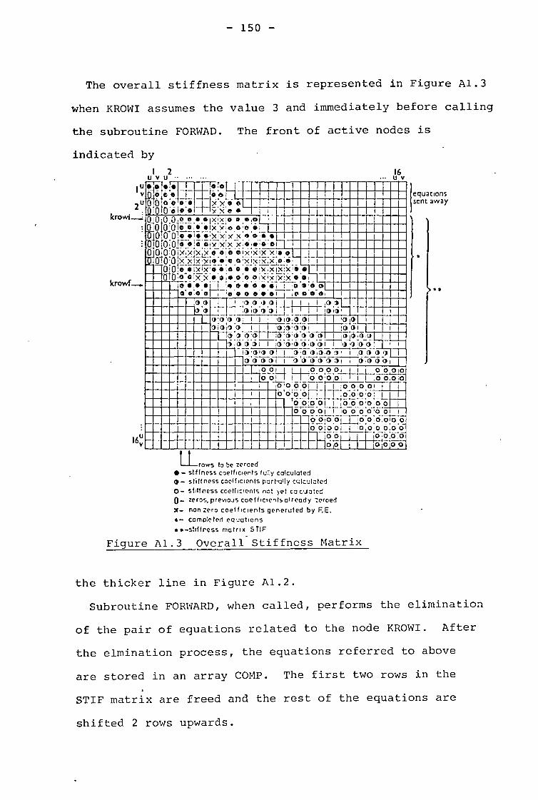
- 150 -

The overall stiffness matrix is represented in Figure Al.3

when KROWI assumes the value 3 and immediately before calling

the subroutine FORWAD. The front of active nodes is

indicatec'i by

1 2 16 u v u .. '" u v "r-" 10

,. -1 v 0 CD '. I r. & _.

u 0 (qo:~.o:OI_q2.':X:o "L : 150'01 •• )(X(!. 2

krowi_

I : I 1 .

. oJo'OO,~_!,~Oj~!~:Q • ,.:0 I : Bol0101!"~J!,,!!~?,,;o.l):., .• 1 I 1

0'0'0,00 10 .'XIXIX x • 0, •• I I : ~ QtolOl~~Ji~:~I~xi~:~ :~~~:.; 0 I I I ~ ~iOiOix.xtx .•. 0[0 o;~:~~:o.o.l I 1

krowf_

:

• .0. 010 1~_2:< ~~!I!,~:".o :)(~~ ~~!!:.: -: m- , f-I- 0tO~O_O!~!'5: •.• !. 0, • • !,-,::~~:x: •.• 1 1 f-I-Jl !L~.o!x.x.!.~i •. o.o ,~I~~~,.! 1 I

10.0!0 ,oLl_: •. o. 0 •. 01-l-:0 0:0_01 I , • • ,0 01 , '0.00.01 I .00 It o. I I I

()()~()(}()(}Lt-I I i I ,(}r) I ~)(j ---' .... ; -:() i() '() ~() I I! .... ! 1 I l() ,I)' 1

()1()()'(}1 II' '(}I(},(}()I I il 'a,(}1 (}I(};r)'()' I I I ,(};():():(j,T T I I()\) I 1 I I

1 ') j(}(} () I I !() la'a () ,a a I I !(} 'f) i() 0: , I

R~ !~: ~:~ '-lJ~ I~:()~~'~() ,,! !---l __ -1')--11) :()~() I

I()'()I(} al I ()-:-o(};(j~-ii"~""-r--~cj-a ~ H-J.... a'<lQ()-r-1 -0 'cj()oo5lT"c)~o-cjo I

H~oH H--+0000I I' I 00010 O-O! I :0'0;0;01 I ,0 o~;o I "o;o§oRi±lO_~:O,~1 I I 1

o~~~:~J ,0,0;~"':~1 ~ o ;...~~Q .0 __ ~-'.2. .... 0:()~~.0 00001 I iO 0 00'0 0 I I rl,~:~;o:oi 1 :o~o~o:~

o o:ooL~'o 0,0'0 I 1 B: 'j II] i-- ---.;c 00 0,0,0,0 I r 0:01 Ll J jo:oj~

LLrows to be zNoed • - st~fncss CoeHlclen's tully calculated ~ - stiffncss co('fllelents part'olly cc:'culatC'1 0- sliffness coetflclC'nts not Yl?t co c·.Jat('G 0- zeros,prevloJs coeiflClentsalready -::Noed

)C- non ~l'rO coefficients generuted by F.E . • - comoidNl eq'~atlons •• -shffrcss matriX 5TIF

Figure AI.3 Overall Stiffness Matrix

the thicker line in Figure AI.2.

equations sent away

••

Subroutine FOR\\1ARD, when called, performs the eliminatio:1

of the pair of equations related to the node KROWI. After

the elmination process, the equations referred to above

are stored in an array COMPo The first two rows in the

STIF matrix are freed and the rest of the equations are

shifted 2 rows upwards.

- 151 -

It should be pointed out that the coefficients in the

STIF matrix are kept in the computer in a rectangular

matrix of LBW + 1 columns and LBW rows. This book keeping

procedure is aimed to reduce to a minimum the amount of

computer memory necessary for the storage in fast core of

the non-zero coefficients.

In order to reduce the tape operations, the transfer

to a disk file of all the elminated nodes takes place in

blocks. This is done using a non standard subroutine,

WRITMS, which is called from subroutine FORWAD where all the

equations already placed in a buffer area, COMP, are to be

transferred to a random access file.

The larger the buffer area, the faster is the execution

of the program, for less transfer operations take place.

However it will be less efficient in terms of the central

memory needed.

The size of this buffer area is such that it can share

the same core spaces which will be needed later on for the

arrays describing the element stresses. This is done by

use of EQUIVALENCE statements in both the main program

and the subroutine FORWAD.

A1.3.3 - Evaluation of Displacements and Stresses

After all the elements have been processed and the

Gaussian elimination has been performed for all the equations,

the system (A1.1) is now ready for the backward substitution.

The main program calls subroutine BACKWD to perform this

operation.

- 152 -

In this subroutine, the equations are retrieved from

the random access file in reverse order and the displacement

solution for the entire structure is evaluated as it is

described in Chapter 2.

When in the presence of a previously prescribed

displacement the backward substitution operations are skipped

to preserve the initial displacement values which have been

stored in UV when the boundary conditions have been fed

into the program in subroutine INIAL. Otherwise these

particular locations UV would contain the equivalent reaction

forces as it was described in A1.2.1.

After this procedure is completed the main program

evaluates the element and/or nodal stresses if required,

in the same manner as it is done in the program FLAP5.

A1.3.4 - Flow chart of the Program FRONT

A detailed flow chart of the present code is illustrated

in Figure A1.4 on the next page.

A1.4 - User's Guide

A1.4.1. Introduction

The FRONT code is a computer program written in

FORTRAN IV.

In order to adapt its capacity to different cases ,

this code is provided with an additional program, EDT,

which makes FRONT to operate in a "dynamic version".

EDIT is a facility available in the CDC system at ICCC

which enables the contents of a particular file to be changed

by using a set of control editing commands.

C N..cK

Cho...on E 4 u oac

MC. V.1 C.

Evata.ete UV.-

Marro( rilsr.e. UV

— 153 -START

READ DATA

Tires MMPs MCL,LIW

- N • I, 1JMAT)

READ DATA EI idU(.4), t? mo to) ,A1,440.)

IEL•m

tst ot MPI,MetaIhret

L s 1, $1141,

r--{ L. 4,14ILL

A F AD DtrA

14 Pr pirt9yek, wov..) , pia-TATO.)

TRILJK ,C.1.071104. PACA14.

eta) , X Cr) kfst(luit•Of git{ (tom)

[

MS, C•.ip Dog 013 C.

IEvrtool. hrayfeecrs BODY F

E ' t rtrap.s Et

.614 15.te,

Pfepate toast.% Stilioese. *orf•ciemto Itteea ostzwt..1

t 0

L. „..L, LOAD

)

r•-•----( 0%1.3

Chr_e

ilelres5

addres... St.rc

- ST.K(tt.rc).Ktl(T.D) Te)•Kth(t. t■

-

MO Los

aoe mode

ICRI5wP4- MN/ S4.- moo, ese•

f {ICV eletrAeiapc04,0)

- ELSTIF

Ailre•leot•rerimf

FOtWAD

(2-VKA(.1eNJP.,

COMP

ROAD M. A. SICLUsLitlrr

31e 1.11••• Resat COMP

1".■.t.aft 34/alt LAN ,A7T „Pa?, CAL

eva“.•.. a u 4 414Ltk, 3 /4( 171 •f6i12 KigtkL

at. ,f{4 &At...raid. STIV a A /41

foolu. ,e Of

Stmoile.st•emeT lore Mei.31erhe. ILA-,41C•t

• Kgbv tv.t t.( Ow F

As /court , S1aJ ret e Lf44,rr ISIC

I STOP I

Figure A1.4 - Flow Chart of the FRONT Code.

- 154 -

The program EDT defines the exact amount of storage

needed and calculates each array size in the COMMON block

of the FRONT code. Moreover the EDT program writes into a

file, TEXT, the necessary control directives by which a

file containing the FRONT code will be suitably modified using

the EDIT facility. The modified version of FRONT is then

prepared to be compiled and executed.

Some environmental aspects of the programs FRONT and

EDT will be described later on.

A1.4.2 - Preparation of the Problem

A1.4.2.1 - Material properties

Values of the Young's Modulus, the Poisson's ratio,

the material density and the thermal expansion coefficients

must be provided. The program allows for the use of five

different materials. One will be specificed for each element.

A1.4.2.2 - Mesh Generation

The elements available are described by their cross-

section made by a plane containing the axis of symmetry

as illustrated in Figure A1.2.

For describing the topology of the mesh, it is necessary

to define for each element three values NPI, NPJ, NPM

containing three different nodal numbers in the mesh,

following the topological order (anticlockwise) of that part-

icular element.

Temperature rises are defined for each element and

assumed to be constant within it.

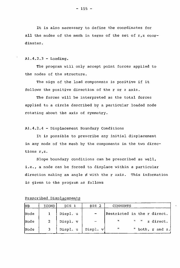
- 155 -

It is also necessary to define the coordinates for

all the nodes of the mesh in terms of the set of r,z coor-

dinates.

A1.4.2.3 - Loading.

The program will only accept point forces applied to

the nodes of the structure.

The sign of the load components is positive if it

follows the positive direction of the r or z axis.

The forces will be interpreted as the total forces

applied to a circle described by a particular loaded node

rotating about the axis of symmetry.

A1.4.2.4 - Displacement Boundary Conditions

It is possible to prescribe any initial displacement

in any node of the mesh by the components in the two direc-

tions r,z.

Slope boundary conditions can be prescribed as well,

i.e., a node can be forced to displace within a particular

direction making an angle 0 with the r axis. This information

is given to the program as follows

Prescribed Displacements

NB ICOND DIS 1 DIS 2 COMMENTS

Node 1 Displ. u - Restricted in the r direct.

Node 2 Displ. v - n II ” z direct.

Node 3 Displ. u Displ. v 11 " both, r and z. A *

- 156 -

Slope Boundary Conditions

NB ICOND DIS 1 DIS 2 COMMENTS

Node 4 Q - u = Qv


The variable data are categorized by the designations

is integer

ia integer array

rs real single

ra real array

hs hollerith single

ha hollerith array

The unit can be any consistent set with angles in

degrees.

ALPHA ia thermal expansion coefficient

DELTAT ra temperature rise in the element

DIS 1, rs prescribed displacements, or DIS 1=Q DIS 2 in slope b. conditions

E ra Young's Modulus

ICOND is Prescribed displacements code

I is member of the element

LBW is size of the bandwidth

MAT ia Material identification number in the elem.

MATN is Material identification number

NBR is Total number of diaplacement boundary conditions

NEL is Total number of elements

NMAT is Total number of different materials.

- 157 -

NNP is Total number of nodes

NPI,NPJ, is Topological description of the elements NPM

NU ra Poisson's ratio

R ra Nodal radial coordinate

REX ra Nodal point forces

RHO ra Material density

SR is Control parameter for output

SR=1 Output displacement solution and element stresses

SR=2 Output displacement solution and nodal stresses

SR=3 Output displacement solution and nodal and element stresses

WI

is Control parameter for input print out

WI=O Title, control parameters

WI=1 Title, control parameters and the rest of input data

TITLE ha Title of the analysis

A1.4.4 - Input Data Format

The following table describes the order of input of the

data defining the analysis.

CARD ORDER GROUPS OF CARDS

1

PROGRAM NAMES

TITLE

FORMAT

13A6

2 LBW, NEL, NNP, NBR, NMAT, SR, WI 515, 213

3

MAIN, E(MATN), NU(MATN), RHO(MATN),ALPHA(MATN), MATN=1,NMAT

15,4E13.5

- 158 -

4 L,NPI(L),NPJ(L) ,NPM (L) , MAT(L),DELTAT(L),L=1,NEL 15,4E13.5

. (NEL cards)

5

N,R(N),Z(N),REX(2*N-1), REX(2*N),N=1,NNP

15,4E12.5

. (NNP cards)

6

NB,ICOND,DIS1,DIS2 215,2E10.0

. (NBR cards)

A1.4.5 - Operating FRONT Using Program EDT

The listings of the programs FRONT and EDT are

described in Sections A1.5 and A1.6 repectively.

This section indicates the control cards which are

necessary for running the FRONT code at ICCC,under the KRONOS

2.1 system.

No specific data is needed for running the program EDT,

for it reads the necessary information from the basic

parameters LBW, NNP and NEL which are specified in the

second card of the FRONT code data deck.

The control cards are as follows

JOB( ) PASSWORD( ) MNF(B=BINEDT) COPYBR(INPUT,FLDAT) COPYBR(INPUT,FRONT) BINEDT(FLDAT) REWIND(FLDAT) RENAME(INPUT=TEXT) EDIT (FRONT) MNF(I=FRONT,B=BFRONT) BFRONT(FLDAT) EOR

Program EDT EOR Data for program FRONT EOR Program FRONT EOF

- 159 -

If an editing facility is not available, the necessary

alterations to the FRONT code can be obtained by printing

out the TEXT file which may be generated by a seperate run

of the program EDT.

In this file TEXT, for instance, commands such as

rs:/(NNNN)/,/(273)/;*

indicate that the string of characters (NNNN) should

be repleced by the new string (273). These changes should

be carried out for all the occurrences of (NNNN) in the FRONT

code, if the ;* sings are included in the end of the command.

A1.4.6 - Environmental aspects

Experience has shown that for a large number of cases

the number of elements in a 2D mesh of triangular elements

is related to the number of nodes by a factor of about 1.8.

NEL r--- 1.8 NNP

Based on this ratio the necessary central memory which

is needed to run the FRONT code, for different cases, can

be calculated with a reasonable accuracy taking into account

only the number of nodes and the size of the bandwidth.

A table is presented on the following page showing the

number of central memory words (*) which are needed to run

the FRONT code for a typical range of the parameters NNP

and LBW.

(*) For the CDC 6400 machine available at ICCC

- 160 -

CENTRAL MEMORY WORDS NECESSARY FOR

RUNNING THE FRONT CODE

Bandwidth LBW

Number of Nodes in the Mesh

200 500 1000 1500 2000

21

41

61

81

101

121

12971

14260

16370

19270

17810

19120

21230

24140

25910

27820

29330

34010

35370

I 37430

42110

43420

45530

48440 32240 40340

44050 22990 27855 35955 52150

56660 27500 32360 40469 48560

25 K

30K 40K 50K

K 1000 CM words

A1.5 - Listing of the FRONT code

A listing of the FRONT code is presented in the following

pages.

1 • 2

pROOPAm FRoNT(INOT=Innnl.OUTpHT=1A00B.TAnE5=INP1fT.TApc6=OuTpUT. DO 35 L = 1. NEL

1 TAPE7=T1'LEN) IF (NPI (L) -1) SO TO 35 C WRITE (6. 32) TITLE C 0 SPFCIFICAT/ON AND nATA IN/173,AILIZATION STATEMENTS.

INTEn1R TITLE. SR. 0. 35 r0;1rTINU1

1 REAO(5. ,(6) (N.R(nP).Z(NP1.REX(2tHp-1).REX(2•NP).UP=1.NNP) CASCTL. wI. AN(/' P.

2 COND. 0 36 F01tqAT(I5.4E12.5) REAL NU. KEL •

NPJ(LLLL). Npm(LLLL). (W21E:n20.123456789E35) GO TO 37 COvm(IN 1ITLE(13). NPI(LLLL).

1 R(WINN), RRENIr(NNNN). NAmE(RFC). wit/Tr (A. 32) TITLE

2 NU(5). RFX(Nnn2). LN(3).w(4.61. 37 rOrr:ITINUE R140(5). mAT(LLLL).

3 uv(NNN2). 13(4,6).

4 ALpHA(5). 01.LTAT(LLLL). ANP(On.9),

5 STIF(lP11.11RR). NAP(UnnN). • 6 SIGLRR(11.111.sIC.LTI(LLLL).SInL77(LLLL).SIGLR2(LL1L) C 40 OUTPUT THE TITLE AND THE CONTROL PARAMETERS.

WRITE (6. 41) CO"mrIN /PARAM/ fiCLORIP.WIR.N"ATILNNIL CO"'Arr /rLI. 1 111/ KNod1.viin.,r.ICODE.NEO0010.FA.K1.ICO.LR1C 41 FOkIIAT ////// DATA CASCTL / WRIFCASE / 1 45X. 411ITHE CASE TITLE ANO THE CONTROL PARAMETERS /

2 45X. 4111 /////) WRITE (A. 42) TITLE

C 10 /NDNT TIIE CASE TITLE OUT STDP IF THERE IS NO FURTHER CASE. 42 FORMAT (1H . 1386) 11 RE P (5. 1?) TITLE WRITE(6.43) NEL.NNp.NRR.NMAT.LOw .I

43 FORMAT (P6HR1HE NU-nER OF ELEmENTS IS. 15. 1H. / 12 FaN4AT (13(,) 3nHOTHE NH1 AER OF NODAL POINTS IS. 151 1P. / IF (TITLE (1) .E0 s . CASCTL fol, 1

C 2 4311JTHE Ull”tiER OF RESTRAINED DONNDARY u0nES IS. Is. 1H. / 3 37111THE NH. PrR OF nicFrurNT MATERIALS IS. I5. 1H. /

1AHRTHE OWIPWITH Is.I5.1H./ C 20 rUpHT THF CNNTRoL pARAmETERS Ann PREPARE TO INPUT THE ARRAY DATA. 5 21OSTRESSES APE FOUND FOR) READ(5.21) 1X4.NLLOINp.NnR. NmAT.SR.WI 0 H

21 FO:wrT(51,5.21S) IF (SR .10. 0) ARTIE (6. 44) 44 FOPmAT (1H.. 2IX. u2HNCITHER THE ELEMENTS NnR THE NODAL POINTS.) DO 27 N" = 1. NmAT

22 E (N ) = -1. IF (SR .10. 1) wRIIE (6. 45) " ELEmENTS OHLT.) 45 FORMAT (IN+. 23X. 16HTHE 9n 23 L = 1. NCL

?3 NPI (L) = -1 IF (SR .Ek;. 2) 4R/TE (6. 46) nO 24 = 1. NH)) 46 FORNAT 23X. 2711THE NODAL POINTS ONLY.)

24 R = -8.1234567(1 4E35 IF (SR .1;. 3) MITE (6. 47) 47 FORPAT (111.. 23X. 31)470T11 THE ELEMENTS AND THE NODAL POINTS.)

IF .10. 0) ;.MITE (6, 48) 48 FOROAT (37HRTHE INpHT ARRAY DATA ARE NOT OUTPUT.) C' 3n ItIPUT AO CHECK THE ARRAY DATA.

'.f.() (5. 31) (vATti, ),*(mATN). NU (MATH). IF (t , I .E4. 1) ,'RITE (6. 44) 49 FORMt.T (33HUTHE INPUT ARRAY DATA ARE OUTPUT.) 1 RHO (NATN). ALPHA (MATN). NM = 1. NmAT1

. 31 (15. 1113.51

110 = I. 0,'AT Iv (r ( , 4) .1E. -1.) no TO 33 C 50 OUTPOT THE ARRAY DATA. 4(ITr (4, S.!) TITLE IF (III .14. (I) 60 TO 61

dR)TE (6. 51) (04, E (Nm). NU (NM). 1(110 (NM). 32 FOchAT t1H1 ////// 5H III 11. 1384. 1H1 / 1 3;01 TIW 10- TS A MISSING INPUT DATA CA40.. 1 ALPHA (118). N4 = 1. NmAT) 2 2q14 THE jOrt IS AHANOMED.) 51 FOR -N,T (1111 ////// iT(IP 1 SAX. 191'INPHT P.ATERIAL DATA /

///// 53 CO:'TIT).)F 2 ,14g,IATERIAL ELASTIC HODULHS POIsSONOS RATIO, READ (5. 34) (LE. NPI (LE). flPJ (LC), 'PM (LE). 3

NAT IL)). DELTAT (1r). 1. 31H = 1 M11) 4 DENSITY THAL EXPN COEFF // 1 34 FOloHNT (5151 F10.3)

3 4

5 (133. X. 4E17.5)) LPEC=RCIA(OW/241) WRITE (5. 52) CALL OPENMS(7.NAME.LNAMEs0)

52 FoRmAT (1111 ////// C 1 57X. inpiptifiT ELEMENT DATA / C LAST NODAL AppEARApCES AND INPUT BOUNDARY CONDITIONS 2 57x. 1AP ///// C 3 3x1 4sPEL-T NPI rIPJ NPM MTRL DELTA T CALL INIAL

NPM MTRL DELTA T 4 4AHCLI /IP/ (IPJ C 5 321HLL'^T NPI NPJ NPM MTRL DELTA T /) C DO LOOP FOR ALL TILE ELEMENTS Ll = (NEL + 2) / 3 C Do 5= L? = I. LI 00 7? L=1.NEL L3 = mINO (L2 + 2 * Ll. NEL) C

53 4q1TE (C,. 54) (L. riPi (L). 'IPJ (L). NPM (L). C CALCULATE TOTAL EXTERNAL NODAL FORCES REX(I) 1 MAT (L). DELTAT (L). L = LP. L3. L1) C \ -54 F0111AT (111 • 515. r1(1.3. 13x. 515. F10.3. 13X. 5/59 F1O.3) CALL LOAD

A4.TTE(6.95) C I 55 FORrAAT(11I1 ////// C CALCULATE ELEMENT STIFNESS MATRIX KEL(I.J)

1 5IX.15H/NPOT NODE DATA / /////

C 1-, 2 54 u x.l CALL NJELSTIF

NJ 3 2(6)..21HHOUE RR

H 2 . C 4 R2 C CHECK IN ELEMENT STIFFNESS COEFICIENTS INTO MATRIX M AND )//) N1=( NNP+11/224" C THEN INTO RECTANGULAR MATRIX STIE(IIJ) AND IMPOSE BOUNDARY CONDITI DO 57 r1,=1 •':1 c N3=MTNo(r..?+N1.NNP) . CALL STIR

57 44/Ir(,,,,54) 01.R(N).2(0I.REX(2*N-1).REX(2*N).N=NP.N3.N1) ' 72 CONTINUE 58 F9;y14I(..!(5X.15.4E17.5)) C

d41Tr(F,07,6) C BACK SURSTITUTION CALCULATING NODAL DISPLACEMENTS 56 FORmAT (I'll /4//// C

1 44x. 35)1INPUT RESTRATNED 00UNOARY NODE DATA / ? 4AX. 3-ill /WI C

CALL BACKWO

3 331.. 2■110(EsTND (INDY NODE . C 4 37HRESTNT COWITTION OISPLA //) C 150 OUTPuT TILE 1400E DISPLACEMENTS IN THE PLANE SECTION REVOLVED.

C 151 wRITE (6. 152)

. C 152 FORMAT (1111 //////

C 1 49X. 3311THE CALCULATED NODE DISPLACEMENTS / '

C PREPARE TO SUM THE surrENEss COEFICIENTS 2 49X. 3311 /////

C 3 3X' 4711)IOOE U V . 61 00 M) 9j19=1.L.44-1 4 U V I. nn Al NC=10.1 1:. 5 u V /)

81 5T1E(NR.NC)=0.0 NI = (NNP + 2) / 3 no '7 I1q=1.U3(/2 00 153 P2 = 1. Ni 00 02 NC=1.9 ' N3 = MING (N2 + 2 * N]. NNP) A,:n( NI; , , ,r. )=0 153 wRITF(6.1541 mai(2,0J-1).1w(?*m).H=H2.113.m1)

82 A'I'(' 4.1) =r, 154 FORMAT (ill • IS. 2(16.5. In. 2E16.5. /15, 2E16.5)

,

DO Ax N4=1.H1IP C 83 NAN((•(R)=1 C

KNo*:'7=1 C 160 CAICOLATE THE ELEMENT STRESS COMPONENTS. ICr'N)=R • IF (54 .E(;. 0) GO TO 221 KWIA=Arl 00 1n4 1 = 1. hEL KRi/1=1 I=TARSOIPI(L)) UF,=P j=TAoS(HPJ(L)) LNW-T=CP.NNP-1)/RC0+1 M=1AHS(0144(L))

BI=Z(J)-7(M ) n.)=7(m)-z(/) £ BM=2(T).7(j)

CI=-0(J18R(1 £ CJ=-R(M)+R(T) CM=-R(T)+R(J) A1-,.:A=(RJ.C4-11m*CJ)/2. R1IIR = (14 (I) + H (J) + R (U)) / 3. WA=C2,01,AI:EA)/(3.*RRAR1 EEHR=InTsliV(2*I-1)+0J*OV(P/J-114To*UV(2*u-1))/(2.*APEA) EETT=IUVI20,1-11+UV(PPJ-11+UV(2*M-1))/(3.*RRAR) EL7I=ICI+UV(2oI)+CJ,UV(2•J)+CM*UV(2*M))/(2.*AREA) EER1=(CrouVI26I-11.0)I.11VI7*II+CJ*UV(2*J-1)+RJ*UV(2*,11+

1

Cv*UV(26.',-1)+Nm*uV(2*g)//(2.*AREA) MATN = mAT IL) WI = NU (''Aiii) W2 = I. - wl W3 = I. 41 W4 = 1. - 2. * hl w5 = E ("ATO) / (W3 * W4) Eiu = A1RHA (.'ATN) * DELTAT (L) ER0 = - ETH ETT = LETT - El7 = EF/4 - Fiu ER7 = EFRZ SIr.L"R (L) = w5 * (W2 * FRR + W1 * ETT * E22). SIGITT (1) = i.5 * (41 * ERR + W2 * ETT + W1 EZZ) SInL77 (L) = 45 * (1..1 * ERR + wi * ETT + W2 * EZZ) SIrLw1 (L) = .J5 * W4 * ERZ / 2.

C C C 170 cApEnLATr plE.ELE0rNT PRINCIPAL AND MEAN STRESSES IN THE PLAN*" C SEcTIoN 4EvoLVED.

IF (SW .C.1. 2) GO To ing 41 = (STr.LRq IL) + SIGL77 (0) / 2. 42 = (sT5Lk.I (L) - (L)) / 2. w3 = Sl(_'1C (L) W4 = SIJ41" ('42 4'. 2 + W3 ** 2) SIr.L1 = w1 + w4

= wI - *44

IF (PPS (42) .GT. 1.E-35 .0Q. AnS (w3) .GT. 1.E-35) GO TO 171 roPqVL = 1. Go 1*) 172

171 'Jr(Af"L. = 2?%.647e!;4756 ATAPOI )W3. w2) 172 Slr.t.3 = szlr,LTT (L)

= s.)1(1 (ISIGI1 + STSL2 + ** 2 1 - 3. * (SM.? * SIGL3 4 * sIGL1 + STGL1 * SISL21)

C C C 1A0 OUTruT TJAE EL( 4ENT sTprssEs.

Iv (I 1) GO TO 247 WKTIr (A. 1°1)

IN' FO4'AT (1111 ////// 1 4x.,4411T11r CALCULATED rLrmENT STurss CN,POOrNTS Ann. 2 43!1 ,,vAn stqESs In TIIE SINNCE AOD TI r PRInCIPAL.

3 39H STRESSES IN THE PLANE SECTION REVOLVED / 4 4X/ 5

41X

6 ///// 7

1X. 3911

•

37HSIGV1

SIGMRR

9 SIGPRZ SgP6TE1 SIGm2 SIGWM /)

182 WRITE (6. 183) L. sISLRR (L). sIsLTT (L). sIGUZ 1 SIGLR2 (L1. ARGLEL. SIGL1, sIGL2. SIGLm

183 FORMAT (IN 15, 4E16.51 r12.2. X. 3E16.5) 184 CONTINUE

IF (SR .EQ. I) GO TO 221 C

C 190 FIND THF. NODE STRESS COMPONENTS. DO 212 to = 1. NNP SIGNri/ = O. SIGN1T = n.

: g.

)-■

on = 1 DO 101 t = 1. NEL Ir(IAUS(NPI(L)).NE.N.AND.IAQS(NPJ(L)).NE.N.ANO.IABS(NPM(L)).NE.UJ

1 GO TO 3.91 SIGMA? = SIGNRR + sIGLRR (L) SIGNTT = SIGNTT SIGLIT (L) SIGN77. = SIGHL7 + SIGL22 (L) Sinnr7 = SIGTO(Z + SICLRZ (L) OA = OA + 1 IF(0A.E'),IAI)S(IJAP(IJ))) GO TO 192

. 191 CONTINUE 192 41 = FLOAT (wA - 1)

SIGmult = SIGORR / wl = sIGNTT / WI

SIt:N2Z = / SIGnR7 = "IGIJRZ /

C C C 200 CAICNLAll THE HOOF PRINCIPAL AND mEAN STRESSES IN THE PLANE C sFr.Tlo)) REVOLVED. 201 wi = (SiGNRR + s/Gp/z) / 2.

w2 = - SIC.07Z) / 2. W3 = sinoRZ W4 = SORT (v:2 ** 2 + w3 9* 2)

= WI + W4 Sir N9 = W1 - 44 IF (MIS (tr:;,) .G1. 1.r-35 .0R. AHS (W3) .GT. I.E-35) GO TO 202 ANGIrN = O. GO TP 2n3

2n2 Anr.LrH = 24.647A1197SA * PTAH? (w3. W2) 203 S1(1113 = sIGnTT

SIGN. = SORT ((SIGN' + SIGNP + SION3) ** 2 00 3 J=1.3 1 - 3. • (SIGN2 • SIGN3 + SIGN'S * SIGN1 + SIGN1 * SICN2)) J1=3-J+1

C IF(ELHOOCtI1l..11).E004) GO TO 4 C 3 CONTINUE C 210 OUTPUT TUE NODE STRESSES. 4 ELNODE(lI.U1)=-ELNODE(Il.U1)

IF (n .'1E. 11 GO TO 212 5 COnTintlE .WRITE (4. 211) C

211 FOrmAT (1111 ////// C 00UNPARY CONDITIONS 1 6X. 4111T11E CALCULATE° NODE sTRrss EOmPOPENTS ANC. C 2 '13H :411(1 STIO:SS IN THF: SPACE AHO THr PRINCIPAL. 00 ino I=1,11Np 3 3911 STI+CSsES IN nil-. PLANE SECTION REVOLVED / 100 PRENTC(1)=0

4 4 4 . 6x1r1 no 30 K=1.NUR 5 43H .

///// READ(.16 ) NO. ICOND.DIS1.DIS2

• 6 3911 16 F0PMATIJI5.2E10.11) 7 3X. 43HNUDE SIGtAR SIGMTT PRENICINR)=1COND S 4y15 Try.qz S/Ov ANGLC1 RZ . oIs=nisi

232 WRITE (61 213) '1. SIGHRR. SIGNTT. STGuZZ. STONR I.G" I) II1=1

I 9 371ISIW,*1 SIGH? IFIICON:).E0.41 GO TO 40 P-1

1 ANC.LLN. SIGN). SIC,N2. SIGNM IF(PMENTC(N6)-2) 60.70.60 Cl 233 FO4r4 AT flif • 15. 4E16.5, F12.2, X. 3[16.5) '60 INn=24NP.-1 .A.

C GO Tn 80 C . 70 Inn=2.Nn C 220 RETURN TO THE DEGInUING OE THE PROGRAM FOR THE NEXT CASE. 80 UVfInO)=OIS1

221 ST-1P III=T1I-1 EN0 IF(P1+E1ITECNB).EO.3.AND.III.E0.0) GO TO 50

GO Ti' 10 50 DIs1=DISP

GO TO 70 SUf;RnUTINC INIAL 40 uv(2,mr1)=nts

C TIlTS Sli1I.IUTLIIE FINPS THE LAST nopE APPEARANCES FOR EACH ELEMENT 10 IF(NT.E(J.0) GO TO 30 C AND 4cnnS IN UOUNOAKY CONDITIONS wRTTFI6.20) NII.PRENIC(NR).0IS.0IS2 C 20 Folv04.T(142,124,2E2c.5)

INTErr); P4EHIC.TITLE,On.wI.ArIP,P,O,ELNOOE 30 COnlINUE RE.AL nu.KLL CO,"CN TITLL(13). VPICL(.LL). NPJCLILL). NPM(LLIL). IJJ1r)U"

1 E(51.'AI, H(PinnP)). pRcotc(rwoh), NAmr(Rrc),

R110(5). Nint(Ltu.). INCHNNPI. REX(NNH2).

11(4.6). Ln(3).w(4,go, 2 NU(5). ZCNNON),

3 4 ALPHA ( 5 1 . (ILL TAI ( LLLL ) . ArIP ( ,)0 • 9 I . D(4.41. SUPR(UTINE LoAn 5 stircRiti.nro). HAPINHHH). KFL(6.(0. C THIS SUrOtOUIIHE CALCULATES TUE EXTERNAL NODAL FORCES ONE TO 6 SIGL41((ltu I.,:int_TrculL),sint.7z(LLLL).stoutz(LILL) C APPLIED FORCES.00DT roitcrs AND INITIAL STRATN COI OITTONS C0'"f1H /Pnt(A",/'iLL.,:.I1'.1:.i,(..1',AT.Lrlh.L . C Co.mrn /FLI,iI(J/ KI:).... I.vtinF.ICOnr,uEO.KNo,111).)(1,TC0,LREC 0IF.nsinri t.LilooLlulL.31 ENNIvALErCL fELHODEl1.11.NPI(I))

REAL NU.KEL CO.P;(N

INTEGER PRENICIANI

IITIE(13). NPIRALL), NRafLI1.L30 C 1

=I.I, R ( ONflit).

NPMLILL).

' C FI'D LAT APPLARAHCIS ,'AIN<ING wITH A - SIGN FOR fACH ELEMENT 2 =l1).

PRENTECNNNr). NArEIPEC).

C 3 1:110f5). Tg=9 LNI3).W(4.61.

DO 5 N=1,NNP 4 ALPHA(5). 0ELTAT(LLLL). AriP(CT.9). =1: ' 00 3 I=1.11LL 5 sTII(.11)l.r:IT). 1:Avmonio. I17.,iF.-I+1 6 SIOLRRULLL).S1t,LTIMI(L)•SIGLZ7ALLILI1S/G==

•

9 10

C

C • C C .

C

CO"m0N/mATH/M10J.0m.CT.CJ.CM.AREA CO" '') /pARAm/ NELOINp•NRR.NMAT.1.001.1..

60 DO (4- CvriRIC CALCULATIONS ON THE ELEMENTS. 1=TAr:S(NP/(1.)) J=IAr`S('i)'J(L)) M=TA''S(NPA(L)) DI=LIJI-700 E RJ=Z(r1)-Z(I) £ DM=Z(T)-Z(J) C1=-R(J)+R( 1 ) E CJ=-R(m)+R(I) £ CM=-R(I)+R(J) ARfArA(tJ•Cm-nt*CJ)/2. Ir (APIA .Gr. 1.E-35) 60 TO 71 WRITF (6. b2) L

62 Fni:11 AT (1111 ////// ELEvEHTt T5. 2511 HAS A NON-POSITIVE AREA. / 1

23H THE CASE IS A3A00OMED.1 STrIP

70 sol THE TOTAL NODAL POTUT rOPCES.

71 '1ATN = vAT (L) RBAR = (U (1) (J) (M)) / 3. wl = 3.1415926536 * ROAR * E (MAIN) * ALPHA (MAIM) * DELTAT (L)

1 / (1. - 2. * NO (MATN)) K? = (2. * /IKEA) / (3. * ROAN) BOnYr = P. • 3.1415926536 * I3AH * AREA * 14110 (MATZO) / 3. REX(n*I-1)=r,Fx(2.1-1)*'41*(nT 4 42) £ REX(2*I)=REX(2*I)+W1*CT.-nODTF REY(7*J-1)=.‘LX(2 0 J-1)+41.(RJ4, 2) f REX(2*J)=REX(2*J)4W1*CJ-00DYF REX(7•"-1)=,<LX(2 4,4 -1).U1*(Wa+w2 ) E REX(2*.:)=REx(2*m)..w1*cm-RoflYF RETuuN E.Jr,

SUrircUTTOE ELSTIF THIS SlmiJOUTIUE EVALUATES THE. STIFNESS MATRIX xi-L(1.J) FOR EACH EL

REAL nuoKEL INTEMR CO"'ON 1ITLE(13). NRI(LLLL). NPJ(L(LL). NPM(LILL).

1 E(5).4I. u(N'INrt)• PitenIC(0,1(w). onnwc), 2 1!O(5). ZINTINN). PEXID9f12), LH(3).1.(4.6). 3 vn)(5). vAT(IlLL). OvI111Rl?). R(4.6).

4 ALIMA(5). nELTATILL1L). A 10P(0';.9). 0(4.4). 5 sTir(nmum), NAP(NWIN). KrL(6.6), 6

ST(4.1It Lt t.) •cI(,LT T(LI I L) •SISLZ1 CIA 1.11•STGLIU (Ll I L ) COt,"IcriP,,NTo/ol.11J.ro.Cf.CJ.c,,./otin

C C C

B(I.1)=9I E B(1.3)=RJ £ 8(115)=EIM I=IARS(nPI(L)) J=IAPS(NPJ(L)) . M=IAI3S(OPM(L)) (MAR = (I) (1) R R (M)) / 3. W1 = (2. * AREA) / (3. * ROAR) B(211)=41 E 13(2.3)=w1 £ S(2.5)=.141 R(312)=CI £ 0(3.4)=Cd £ n(3,6)=cm n(4.1)=ci 11(492)=B1 E 0(4.3)=CJ D(4.4)=RJ f 0(4.5)=C4 f. n(4 ,6)=nm MATH = (AT (L) W1 = 110 (mATN) W2 = 1. - 41 w3 = 1. + wi W4 = 1. - 2. * WI W5 = 3.1415926536 • ROAR * E (MAIN) / (2. * AREA 0 (1. 1) = W5 * w2

f1. 3 ) : *

0 ) 1 D (2. 1) = n5 * 1 D (2. 2) = w5 * W2 0 (2. 3) = *5 * 1,11

0 3) D (4. 4) = w 5 * W4 / 2. DO 9 I' .7. 1, 4

DO 93 3 = 11 6 W (P, 0) = 0. 00 93 0 = 1. 4

93 W (P. 0) = r, (P. 0) 0 (P. 0) B (0. 0) 00 94 P = 1. 6 00 94 n= 1, 6 KEL(P.0)=0. (10 94 0 = 1. 4

94 Ki filrl=0)=14(:L (Pi()) 8(01P) * 4(0.0)

ENO

SURRODTME SITU THIS SHPRourInC CHECKS III sT/PIESS COEEFICTENTS INTO THE RECTAHGULAR MATRIX STIF(I.J)

*

KCl

W3 * W4)

Ql Lri

•I

C COvr4oVi /PA10 ,/

DO 92 p = 1. 4 no 91 -4 1, A

91 '1 (1'. :)) = 0. no 42 u = 1, 4

9?()(P.01=o.

INTErrn P.O. ANP.PPENIC.OA REAL KLL C01.-4(.4. 1TTLr(13). r ,PT(u1.1).

(Nir.r.)) . 2 .01(9). z IMMO • 3 I•110( 5 ) • MAI (ULL).

UPJ(1.1).L). 1.T",((11.1). PI(ENICINuni1). nt ,T(4f-C). REXCHHH2). LN(3)•td(41;), UV(HMH2). D(4.6).

11

4 ALPHA(51. nurnm 0(4.4). iLL), ANP(o0.9). 5 sTIrcn(Il,non). NAP(NNNN). KEL(6.6). 6 SIGLI(LLIL).SIGLTT(LIIL).SIGLUILLLL).SIGLRIALLIL)

12

KRT/=ANP(KV-KROWI+1.1) KRFF=K0TI LNAP=IAI1S(rinPcKV1)

CO' '0N /PAWHA/ MEL.NNP.WittOP.IAT.LBWIL COvmPN /ELF 1 IN/ KRiwI.K4oAr.TCOOL.NEQ.KROwrA.KI.TCOILREC

DO 1? I=2.LNAP KRPT=I4Ax0(KRFF.AMP(KV-KR0WI+1.I))

LN(11=',IPI(L) £ IN(2)=NPJ(L) £ LN(3)=NPN1(L) 12 KRII=mI”0(ANP(KV-KROWI+1.I).KRII) DO 11)6 P=I.3 DO 'in KN=K1t1I.KREF IKr+0.,F=KR0Ar Go TO 50

'ICI .:1;ENIC(1.01).E0.0.0R.PRENIDIKH).E0.4)

NP=ImIsluicr» LrJn=•,F•-KI:J,II +1 IF(PoENIC(K4)-2) 60.70,60 00 105 -;=1.3 nA=1

60 (03=2*(KH-Kfto'4I)+1 GO To 210

101 3n,-,o+1 70 WF1=2*(KI1-KItWwI)+2 • IF(QA.Lr.9) GO TO 103

wHiTr(6.102) MP 200 IT=2.KV-1

IV1=IT-(2*KtiOWI-1)+1 102 FOqt,AT Wil ////// 511 ”TIOE, 15. IVP=IV1.1

I 364 tins nolq. THAN EIGHT ADJACENT moncs. / IC1=t 1 B4 LBW/2-1V1+1 2 2311 THE CnSt. IS ABANDONED.) ICP=TC1-1 STPP Irc1cI.Eo.L11w/24.1) HEX(IT)=0.0

103 IFIA,P(LrPP.NA).E1.1.1A11 S(LMCQ))) GO TO 104 IF(IC2.00.L 1 14/2+1) REX(IT+1)=0.0 IFInrP(Lr.P,.JA).NE.01 GO TO 101 IF(I+F+EFJTC(KH).EO.2) III=0 WJP(INP..JA)=IABSW:l1)1 REX(IT)=;:FX(IT)-STIF(IV1.1C1)+IIV12*KH-III) N10c:P)=QA REXC IT+11=qLXIIT+11-STIF(IV2,IC2)*UV(2*KH-III)

104 Ik=21, ( 1W-K40,.1)+1 STIr(IV1.1C1)-0.0

IC=9.ANP(LNP.QA)-1.11.4/2-(240T-1)+1 sl)rlik .IC )=SIT1(IIt .IC ) + KELI2*P-1.24.0-1)

STIV(IV2.1C21=0.0 Ir(Icl.F).LHs1/24.11 STIF(IVIOC1)=-1.

SITFICI tIC41.)=STTF(Iii ,IC41) + KEL(2+13-1.2s0 ) ' IF(IC2.ru.1.4w/2.1) STIFIIV2.IC2)=-1. STTF(IH.'1,1C-1)=%rTICII,+1.IC-1) + KEL(201 .2+0-1) 111=111-1

105 STTF(IP.1.)C )=STIF(I1(+1.IC ) + KEL(20) .240 ) IF(PI:ENIC(KH).E0.3.AND.III.E0.0) GO TO 70. IF(L:1(P).GI.0) GO TO 111 50 CO,ITTHUF Ninp(fiw)=-ww(PiP) 11(1'REMIC(KV).NE.41 GO TO 51 Trcip.,IT.KK:)m.7 ) Go TO III If(rw.mr.1) GO TU 107 rtI,InP1(= I+1.I)-KROWI+1 Kuo...J=A•g.(1.1) IV1=2*(Kv-KHOnI)+I

00 1^1I (=?.-..

in3 ,<R,,,T=.,Axn(AriP(1.11.10flAF) Iv2=TV1.1 ICI=2,14n4L04/2-TV1

107 IF(.',OT.W.EQ.3..L.Eu.NEL)) GO TO 109 Nc.:=2.cap-..ko.4t).1

IC2=1C1-1 sur(lviocI)=surctv2.7c2)41p1(2*Kv)*Srtrmi./c11

KI1sF=WIP 55 STIF(IV1.1C1+1)=ST11(IV2.1C24.1)+UV(2*KV)*STTF(IVIIIC1+1) GO 10 1 ,ICY(')*Kv-1)=REX(240e.V)+OV(2*KV)AuCX(20(V-1)

109 00 110 I=1,0404rA+1.K1;014' ' 00 56 J=1.1.H.

IFIti 4 P(T).61.0) 1,11 TO 111 56 STIF(IV2.J)=0.0 110 Cw;TTruc STIT(IV2 1=1.1

IF(11L4.'11.2) rmo4r=IKHI)r;r STIF(Iv2.14,../2+1)=-1JV(24,KV)

IConr=1 REv(24.(v)=0.0

GO PI 1

111 1C6nr=0 51 C0f0Tilli

KROm-=1KING.IF IrtIci.,.W.r.J.0) GO TO 106 C

C mpripAicr COHOETIONS C VOI.Awil FLIOIMATION

C C IF E.WATIor'S FficTv 4q0wi TO Kun'4r AHE cnv,PLETrO H0PCrED TO 1 09 51 K4=KuO4FA41.1eNNX C

13

CALL FOnwA0 40

14

COmP(ICO./)=STIF(ICOELILOW/2+/) IcOOF=0 IF(ICO.NE.01C01 GO TO 30

106 ConT(nuc CALL wRITils(7.COmP(1.1).LREC,K1) RETURN DO 41 ICOM=1.RCO Eno DO 41 Jcnm=1.LDw/2+1

41 CONP(ICom.JCOm)=0.11 ICO=n

30 IF(RoD(IC0EL.2).NE.01 GO TO 134 SUnRnUTINE FORWAD KRowT=R11Ow1+1

C THIS SUPPOUTIHE UsES FOwARD ELIMINATION TO A SET OF NEo COLDNINS KRowFA=RnowF C STnliFS III A iiERIPHFRAL DEVICE THE COMPLETED EQUATIONS ANO SHIFTS RROwF=A1JR(KR041-KR/+111) C UP, ARDS nr.,) TIES THE mATRIx STIF(11.1) AND (NE0+1)/2 TIMES DO 71 1=2.9

C THr mATIx An),(NP.oA) 71 KR(1.,:r=mAxo(AuP(RROwI-KRI+1,I).KROWF) C IF(KROwF.LT.RRnwFA) RROWF=RROWFA INTEnER TITLE.SR.QA.O.PRENIC.WI.ANP.P 134 CONTINNE REAL nuo<ct. IF(NFO.E0.2) GO TO 60 D1mESInn cm,ocmcnolso) co...Arm TT(LE(13). np1(LLLL), NPJ(LLLL). Npm(1LLL). 43

no 43 I=1.LOo/2+1 CO4P(IC0+1.1)=STIF(NE0+1.I+LRW/2)

I

)-• 1 F(5).w N I. RUINN). PRENIc(NoNn). NAME(REC). ICO=IC0+1 a, 2 Z(Ninin). Nu(5). REX(NNN2). LN(31.w(4.6). GO Tn 5n ....] 3 RHO(5). mAl(LLLL). uv(Nnn2), B(4.6). C 4 5

ALI'IIA(',). DELTAT(LLLL). ANP(Du.9). D(4.4). sTir(roldien), NAP(NWM). KEL(6.4).

C C

SHIFTTNG MATRIX STIF(I.J1 UPWARDS 'I

,- 6 STGLRR(LLL11.stni..Tr(LLLO ,s int_zz tu.LL ) 9SIGL RZ (LLI.L 1 60 DO in IR=1.LOw-1 CO' ,N /pARAm/ NUL.Y'Jp.nRR.NIAT.LO..;.L COmAnN /ELI "In/ Ki0'...T.KR,IJF.TCor:E.HEQ.KRTAFA.Ki.TCo.LREC

DO In IC=1,LW., I1(In.GT.L114-1-ME0) GO TO 12

Eo0IvALEnCL(COmP(1.1).SIGLRR(1)) ST1F(IR.IC)=STIF(IR+NE),IC) 1 KRT=I.(RoqI GO Tn 1)

1F(KNI.FQ.1) IC0=0 12 STTF(IROC)=0.0 CO 1.;4 icoLL=tolcu 10 COHTINuE

1C0=IC0+1 DO 2n IR=1.LRw/2 LIHE=2.(1.(Ro.,F-KRI+1) DO 2'i Ic=1.9 Likc=Ltri IF(Ii(.Eo.LO0/2) GO TO 22 DO 136 IDE=1COEL+1.LIDE ANNTk.TC)=ANP(IR+10C) I=1Nr GO Tn 2n J=TUIEL+IPW/2-I+1 22 ANP(IftlIC10 IrlA:ISINTIrlI,J)/.1.7..1E-35) GO TO 136 ANp(TR.1)=KRI+IR K=TF0EL .,=LIT,./2+1

20 CONTTnuE IF(Kunt..F.EO.RRnwFA) GO TO 1

q=sTiFfl.J)/sTIF(K.m) 50 COnTlhOE DO 1A5 Il(C=ICVEL,LTRC -RETUk0

I=Wr EWO Jr-Tur+lw,, /2-I +1 SUI1RPUTINE RACKWO K=TCOFL C RACK SUmsTIWIION CALCULATING NNW.. DISPLACEmENTS -A=ihr+L.4,:/2-K+1 C STirrI,J17.,;11F(I.J)-0,STIF(K.M) INTCrrI2 TITLE.SR.on.Q.P.n.PRFNIC.64I.ANP

135 Co1.7THOL ((UAL illl.kEL

13c; '0-x((.1.,,, I.2-1-1)=Rcx(I+10(1*2-1-1)-0*RFX(ICorL+KRT*2-1-11 C/11.TIr.Ur Ki=c2*(v12 1-1)+Tcnri )/HCO

DP4I-Wirot1 CofP(HCO.(01!‘1 „,111",,), ICOm.AnN IITLE(13). NPI ( IALL), NVJUALL14

1(5 ).wI. oorfilc (romr.). PPHILLILI, twIECurx).

0) 411 1=1,1_14/2+1 2 HU(5), Z(N11,10). REX(UNN2).. LN(3).r.:(4,6).

15

3 8)10(5). MAT(ULL), UV(NNN2)0 B(4,6). 4 ALMIA(519 OELTAT(ULL). A)IP(000/o 5 STIFOOHITIBB). NANNWM). Fri(EL;46.Z). 6 STOLRR(IALL).SVATTlitil.).STOLZZ(LLLL)*STOLIIZtLUL) COv`"ON /PARAm/ nE.L.WW.110.(.w,AT.LDw.l. COmt'IN Ksv.,..41.Kno.T.ICODE.NEO.KleOwFA,K1OCCILRFC EQUIVAL 14JiCE(Cor )(1,1)1SIGLIM(1)) IVI'Mx=21, p CO 1q0 Thq=1.K14,1 NREC=K1-VIR*2

cnu REAOMS(71C0)4P(1.1)/LRECOMEO) DO 1 ,,O

• fuls=4EXIIVA ,(X) IF(Ic.F:J.FIJ.I.AND.MR.E0.1) GO TO 145 KV=AI':U(IVAx+Ln.i/2.24,nriP) DO 2 142 ThV=IvA4X*1.KV J=Tliv-IVAqX•1

142 RriS=f;IIS-COCI.J)•(JV(IKV) 1-a

145 J=1 CO U•71=(IVArx+1)/2 IF(PrErliCt1"0).Eu.31 GO TO 50 I IF(W,Erlir(110)4-2*(Tr10-1).E').TVARX) GO TO 50 . UVCIVAUX)=101S/C,V1P(I.J)

50 IVxr.IV1HX-1 oo II=1.Lo4/2+1 C0;")(ToTI1=0.0,

150 CO':TirAIC' ICO=PCO

140 ClrITTraT

ENn

- 169 -

A1.6 - Listing of the program EDT

PPOGPAM EDTcIHPUT.OUTPUT.TEXTITAPE5=INPUT.TAPE6=OUTPUT.TAPE7=TEXT) IHTEGEP PCO.TPLEH.TITLE PEAD(,5.981 TITLE

98 FOPMATeA10) REwIND 7 PEAD(5.10.LEW.HEL.NHP

10 FORMAT (3I5) C

EVALUATIOH OF HUMEEP OF PECORDS (LREC) EVALUATIOH OF HUMBER OF EOUATIONS COHTAIHED IH EACH RECORD(RCO) CALCULATE THE SIZE OF THE DUFFER AREA COMP (TPLEN)

C PC0=44,HEL .LDW 2+1 , TPLEH=PCO.,LDw 2+11 IF,TPLEH.GT.1000. TPLEN=1000 LPEC=,2*HHP-1 :'PC0+1 HHP2=2.HHP LANP=LDW 2 LDw1=LDm-1 LEw21=LAHP+1

C WRITE ALL DIRECTIVES IHTO TAPE TEXT C

WRITE(7.99)HHPITPLEH.HELOINP2.LEW1.LDW.RCOILDW21.LREC.RCO.LAMP.MEL 99 FORMAT(14HPS:si.HHHH)././(.14.4H)s;./ ❑ 12HPS:sTPLEH/../.15.1Hss 1 14HPS:/,:LLLL)s../(.14.4H)s:+s 2 14HP.:::./f.HHH2)/.s(.14.4H)s:4/ 8 17HRS:s(PD1.EDD)s.s6I311H..I3.4H)s;+s 4 17HPS:s...PCO.EDD)s../(..I3.1H.II3.4H)/;+s 5 13HRS:s(REC)s.s6I3.4H)/;../

10HPS:/RCOs.s.I3.3H/;+s A 14HRS: s (00.9) s. s I2.6H. 9) s; 7 16HRS: s (LLLL! 3) /! / (1I4.6H. 9 10HS:sCOMMOHss A ?HL;7/

3HEHD) EMD FILE 7 PEWIHD7 STOP EMD

- 170 -

APPENDIX2

DIM3B CODE USER'S GUIDE

A2.1 - Introduction

The DIM3B code is a computer program written in

FORTRAN IV. The size of the problems it can handle is very

small compared with a typical problem, so it is provided

with an additional program which makes DIM3B operate in a

so called "Dynamic version".in order to adapt its capacity

to a larger case.

This additional program (DIMDIM) is not fully

described, only the necessary details for its use are given.

A2.2 - Preparation of the problem

A2.2.1 - Material properties

Values for Poisson's Ratio and Young's Modulus must

be provided. These values will be taken to apply to all

the elements of the structure.

A2.2.2 - Mesh generation

As it is a three dimensional problem, the generation

of a mesh of 3D finite elements becomes a tedious and

complicated process for all but straightforward cases. A

particularly complex example is a T-junction of thick pipes.

The most common way to tackle this problem is to have a

mesh generation program to supply all or part of the input

data.

3 2 31 30

15

19

27 28

29 13

- 171 -

The elements available have hexahedron shape with

20 or 32 nodes as it is shown in Fig. A.2.1.

.20 node element

32 node element

Figure A2.1 - Isoparametric elements

available in DIM3B code

It is not possible to use the two types of elements

in the same mesh.

The topology of the element is also shown in figure

A2.1 which indicates the order of the nodes in the element

in relation to the local set of coordinates.

The nodes must be also numbered throughout the mesh.

Therefore, for describing the topology of the mesh, it

is necessary to define for each element an array ELNODE

containing 20 or 32 (depending on the element chosen)

different values of nodal numbers in the mesh following the

topological order of that particular element.

- 172 -

The elements are also numbered along the mesh.

It is necessary for a full description of the mesh

to define the coordinates of all nodes.

A2.3 - Sets of Coordinates

All the theory related to the program is developed

on the basis of a general system of cartesian coordinates.

It is first necessary to define the terms: Basic

Global System, Basic Problem System, Global System for Input,

Main Problem System, A Main Problem System and Local

Curvilinear System.

Basic Global System (x,y,z) is a cartesian system of

coordinates. This system will be orientated in relation

to the structure according to the geometrically preferen-

tial directions of the structure if there are any.

Basic Problem System (x',y',z') is a cartesian system

of coordinates. The orientation of this system can be

different from the Basic Global System and will be chosen

according to the loading conditions of the structure.

In order to define the position of this system in

relation to the global system it is necessary to define

the direction of the new x' and y' axis.

These new directions are specified by two angles

defining each direction and these angles are similar to

those used in spherical coordinates as it is shown in

Figure A2.2. The z' direction is defined implicitly and

the program works out internally that direction.

Both systems have the same origin.

- 173 -

Figure A2.2 - Basic Problem System and

Basic Global System

The concept and definition of the following systems

are defined from the two basic systems.

Global System for Input: This system can be a cartesian,

cylindrical or spherical system of coordinates. The choice

of this system is up to the user. It is a matter of conven-

ience depending only on the main geometrical shape of the

structure to be studied. The basic frame and orientation

of this system will be coincident with the basic global

system. The nodal coordinates are referred to this

system.

Main Problem System: Can be also cartesian, cylindrical

or spherical, but the basic frame and orientation of this

system will be coincident with the basic problem system.

The prescribed displacements (boundary conditions), the'

applied forces, the reactions, the nodal displacements

Basic Gobal System Global System for cartesian (Cartesian) Input cylindrical

spherical

Main Problem System cartesian cylindrical

Basic Problem spherical System

(Cartesian) A Main Problem System cartesian cylindrical spherical

1*

- 174 -

and stresses, all the components of these quantities are

referred to this main problem system.

A Main Problem System: Is a system that can be different

from the Main Problem System and it is used to define in a

more efficient way part or all the stresses applied to the

faces of elements which are loaded.

A table and an example are presented to help the

explanation of these concepts and relations between these

systems.

BASIC SYSTEMS

DERIVED SYSTEMS

TYPE

(*) - these two systems have the same origin and are related by 4 angles to be specified by the user.

Example

Let us think of a multinozzle-on-sphere structure as

it is shown in Figure A2.3 and subjected to internal

pressure P.

It is most suitable to define the Basic Global system

as it is represented in Figure A2.3 with its origin on

- 175 -

the geometric centre of the sphere. It is most suitable

to define the coordinates referred to a cylindrical system,

so the Global System for Input will be cylindrical.

Figure A2.3 - Multinozzle-on-sphere structure

The specification of the nodal coordinates on the

cylinder (2) is a straight forward problem. The nodal

coordinates on the cylinder (1) and on the spherical part

will be easily specified bearing in mind a clockwise rota-

tion of these parts of the structure by an angle a as it

is shown.

The four anlges specifying the relative positions of

these two basic systems are also shown in Figure A2.3 where

- 176 -

ANG1 = 0.0, ANG2 = 900.0, ANG3 = 90°.0, and ANG4 =

The main problem system can also be cylindrical,

therefore all the quantities mentioned in Section A2.3

refer to a cylindrical system of coordinates, for instance,

due to physical reasons of equilibrium, all nodes situated

on circle (1) will have zero displacements on the z'

direction.

The pressure acting on the cylindrical part (1) of

the structure is referred to the Main Problem System and

obviously the only non zero component of applied stresses

will be the radial component with a value of P throughout

this part of the structure.

The same will happen to the cylindrical part (2)

provided the applied stresses in this area are referred

to the Global System for Input.

Finally for the spherical part it is possible to define

the applied stresses in spherical coordinates (A Main

Problem System) so again with only a radial component P,

provided, it is specified the type of system to which P is

referred.

Local Curvilinear System of Coordinates: For these

hexahedron elements, dimensionless coordinates E,n,c

are chosen each varying between -1, +1 so that in the

(E,n,c) space the hexahedron become cubes with side lengths

of 2 units.

Note: With respect of all the coordinate systems, the

order of coordinates and components is understood to be

- 177 -

ORDER 1st 2nd 3rd

Cartesian X Y Z

Cylindrical R 0 Z

Spherical R 0 0

A2.4 Loading

There are two main types of loading:

i) Nodal Point Forces

ii) Constant Stresses on faces of the elements.

The components of the Nodal Point Forces are referred

to the Basic Problem System.

The stresses are defined on the same Basic Problem

System, or if it is convenient, on A Main Problem System.

The face of the element where the stresses are applied,

is identified in relation to the local curvilinear system.

Let us define the axis as direction 1, n as

direction 2 and r as direction 3. The face is referred

to as the direction to which it is perpendicular and with

a+,- sign indicating if it is on the positive or negative

side of that direction.

For example:

Figure A2.4

- 178 -

In Figure A2.4 the cross-hatched face is specified

by the code - 2.

Note: The sign of the loads is positive if it follows

the positive sense of the axis of the system to which the

loads are referred.

A2.5 - Boundary Conditions and Prescribed Deflections:

It is possible to prescribe any initial displacements

in any node of the mesh by the components in the three

directions.

This information is given to the program in two input

variables for each component: a number called nickname

(PRENIC) containing the information of the number of the

node in the mesh plus the direction on which the displacement

is prescribed. This is done by multiplying the number of

the node by 100 and then adding the identification number

of the direction (1,2,3). The other variable (PREDEF)

will specify the amount of deflection.

Let us suppose the node 72 restrained with an initial

displacement of .001 (any length unit) in the y direction,

considering the basic problem system to be a cartesian one.

The nickname will be 7202 and the corresponding deflec-

tion .001.

A2.6 - Computation Data

Into this category falls the data which govern the

variable aspects of the numerical analysis and which

addresses the program by specifying optional features.

- 179 -

In the course of execution of the program it is

necessary to perform some numerical integrations using the

Gaussian-Quadrature formula. Therefore it is required to

give the Gauss points, XG, and the respective weight

coefficients, CG. The number of Gauss points, IGAUS, can

be up to four.

A table with these values is presented below

IGAUS XO CG

2 XG1=-XGo= CG1=CGo=

.57735027 1.000000

3 XG1 =0.000000 CG1 =.8888889

XG2=-XGo= CG2=CGo=

.77459667 .5555556

4 XG2=-XG = 1 CG2=CG1=

.33998104 .65214515

XG3=-XGo= CG3=CGo

.86113631 .34785485

A2.7 - Special Modes of Operation

Facilities exist which allow the user, if so desired,

to choose a certain number of optional types of output.

The option codes are values 1,2,3 for the variable IIN

which specifies the amount of input data to be printed out.

Values 1,2,3,4 for the variable IOUT describe the amount of

data processed and stress analysis.

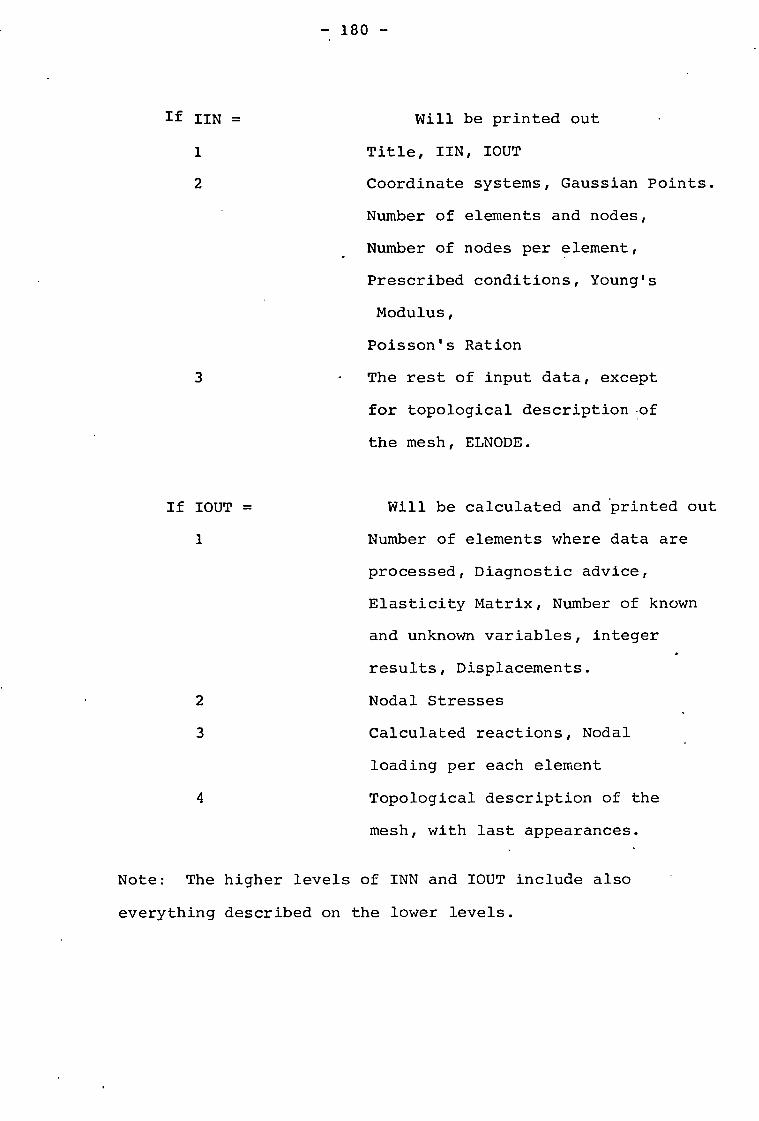
180 -

If IIN = Will be printed out

1 Title, IIN, IOUT

2 Coordinate systems, Gaussian Points.

Number of elements and nodes,

Number of nodes per element,

Prescribed conditions, Young's

Modulus,

Poisson's Ration

3

The rest of input data, except

for topological description of

the mesh, ELNODE.

If IOUT =

1

2

3

4

Will be calculated and 'printed out

Number of elements where data are

processed, Diagnostic advice,

Elasticity Matrix, Number of known

and unknown variables, integer

results, Displacements.

Nodal Stresses

Calculated reactions, Nodal

loading per each element

Topological description of the

mesh, with last appearances.

Note: The higher levels of INN and IOUT include also

everything described on the lower levels.

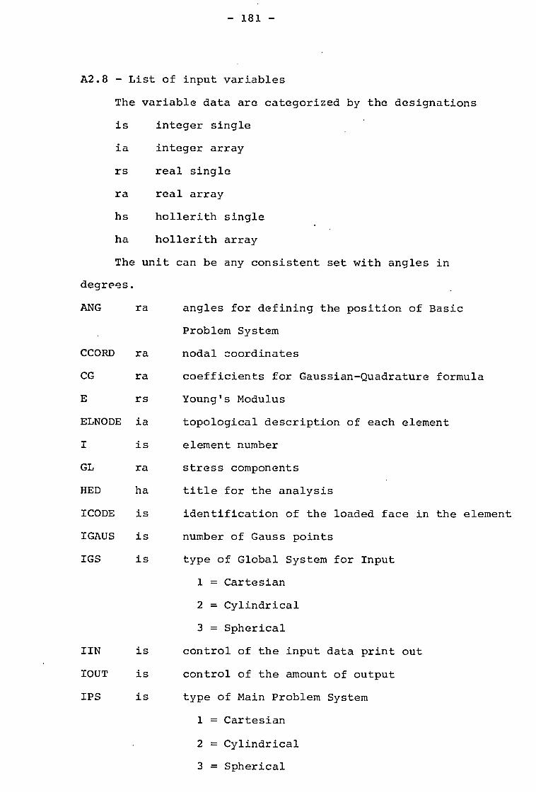
- 181 -

A2.8 - List of input variables

The variable data are categorized by the designations

is integer single

is integer array

rs real single

ra real array

hs hollerith single

ha hollerith array

The unit can be any consistent set with angles in

degrees.

ANG ra angles for defining the position of Basic

Problem System

CCORD ra nodal coordinates

CG ra coefficients for Gaussian-Quadrature formula

E rs Young's Modulus

ELNODE is topological description of each element

I is element number

GL ra stress components

HED ha title for the analysis

ICODE is identification of the loaded face in the element

IGAUS is number of Gauss points

IGS is type of Global System for Input

1 = Cartesian

2 = Cylindrical

3 = Spherical

IIN is control of the input data print out

IOUT is control of the amount of output

IPS is type of Main Problem System

1 = Cartesian

2 = Cylindrical

3 = Spherical

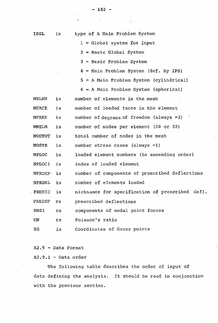
- 182 -

ISGL is type of A Main Problem System

1 = Global system for Input

2 = Basic Global System

3 = Basic Problem System

4 = Main Problem System (def. by IPS)

5 = A Main Problem System (cylindrical)

6 = A Main Problem System (spherical)

NELEM is number of elements in the mesh

NFACE is number of loader faces in the element

NFREE is number of degrees of freedom (always =3) '

NNELM is number of nodes per element (20 or 32)

NODTOT is total number of nodes in the mesh

NOSTR is number stress cases (always =1)

NPLOC is loaded element numbers (in ascending oraer)

NPLOC1 is index of loaded element

NPRDEF• is number of components of prescribed deflections

NPRSEL is number of elements loaded

.PRENIC is nicknames for specification of prescribed defl.

PREDEF ra prescribed deflections

RHSI ra components of nodal point forces

UN rs Poisson's ratio

XG is Coordinates of Gauss points

A2.9 - Data Format

A2.9.1 - Data order

The following table describes the order of input of

data defining the analysis. It should be read in conjunction

with the previous section.

- 183 -

The program variable names of various data items are

given as they are used to describe the input of the data

following them.

GROUP OF CARDS PROGRAM NAMES FORMAT

1st

CARD ORDER

1 HED 8A10

2 IIN,IOUT 215

3 IGS,IPS,(ANG(I), I=1,4)

215,4F10.0

4 IGAUS 15

5 (XG(I),CG(I),I=1, IGAUS)

8F10.0

6 NELEM,NFREE,NNELM 615 NPRDEF,NOSTR,NODTOT

2nd 1 1,19 of the nodal indices of element I

2014

2 I, the rest of nodal indices of element I

1414

.1=1,2 . . NELEM

3rd 1 (PRENIC(1,I),PREDEF (1,1), I=1,NPRDEE) 4(I10,E10.0)

(as many cards as

are needed)

4th 1 E,UN 2E15.2

5th 1 J((CCORD(I,Y),I=1,3), RHSI(I,Y),I=1,3) 110,6E10.0

J=1,2, . . .,NODTOT

- 184 -

6th 1 NPRSEL

I5 (when NPRSEL>0, then include)

2

NPLOC(I),I=1,NPRSEL

1615 (in ascending order) for each NPLOC specify

3

NPLOC1,NFACE 215

4 NPLOC1,ICODE,ISGL, (GL(I),I=1,3) 315,3E10.0

The last group of cards 3,4 is repeated NPRSEL times

A2.9.2 - Data Deck

Each data deck as defined above will consist of

[9+2*NELEM+NODT0T+NPRDEF/4+I+2xNPRSELD cards

1=0 if NPRDEF is multiple of 4

I=1 if NPRDEF is not multiple of 4

A2.10 - Error Messages

1. WRITING CONTROL PARAMETER IS INCORRECTLY SPECIFIED

This message occurs if IIN is different from 1,2,3

or/and if IOUT is different from 1,2,3,4. The program

stops.

2. THE COORDINATE SYSTEM DATA ARE INCORRECT

If IGS ans IPS are different from the values 1,2,3

This message also occurs if the second and fourth

angles defining the Basic Problem System are out of

the range 0o-1800 .

- 185 -

3. PROGRAM STOPPED DUE TO THE CASE BEING TOO BIG FOR THE

DIMENSIONS SPECIFIED

If the number of known variables (NKNVA) and the

number of unknown variables (NUNKVA) exceed resp-

ectively 24 and 60, the program stops. This happens

only on the basic version of DIM3B. However this

message will occur if the dynamic version is not

working properly.

4.

SEQUENCE ERROR IN COORDINATE DATA

J, is the number of the node where the error was

found.

5. SEQUENCE ERROR IN NPLOC DATA

If the numbers of stressed elements are not defined

in ascending order this message will appear. The

program stops.

6. PARAMETER READ BY INIAL IS INCORRECTLY SPECIFIED

The parameters are in basic version

NELEM=3

NPRDEF 24

NODTOT 44

NNELM=20

7. I,J

SEQUENCE ERROR IN ELNODE INPUT DATA

I, indicates where there is a sequential error in

the topological description of the mesh, J is the

wrong number

- 186 -

8. THE DATUM I IN THE ELEMENT OR PRESCRIBED DEFLECTION

J IS OUT OF RANGE

This occurs if the part of the nickname describing

the node number is greater than NODTOT, and if

the direction indicated is out of the range 1 to 3.

9. STRESS DATUM IS SPECIFIED INCORRECTLY

This message occurs when the number of loaded faces

in a stressed element is out of the range 1 to 6.

10. DETJ=0 PROGRAM HALTED

The value of the determinant of the Jacobian matrix

concerning the transformation of coordinates from

the problem system to the local curvilinear coor-

dinates is zero.

It is advised to check again the coordinates of the

mesh and the topological description.

A2.11 - DIMDIM code

A2.11.1 - Problem Size

The restrictions of the problem size assuming the

basic verison of DIM3B are indicated below. (The restric-

tions on the program variables are stated in parenthesis

where applicable.)

i) Total number of nodes must not be greater than

44, (NODTOT 44)

ii) Total number of elements must not be greater than

3, (NELEM 3)

iii) The number of nodes per element must be 20 (NNELM=20)

- 187 -

iv) The number of prescribed deflections must not

exceed 24 (NPRDEF -.5 24)

v) The problem must contain only one stress case

(NOSTR=1). The same will apply for the dynamic

version.

vi) The number of prestressed elements must not exceed

2 (NPRSEL-- 2)

vii) The number of known variables at one time must

not be greater than 24 (NKNVA ---5 24)

viii) The number of unknown variables at one time must

not exceed 60 (NUNKVA--5. 60) .

A2.11.2 - General Description

Any excess in computer central memory storage with

a three dimensional Finite Element Analysis usually causes

tremendous overheads unnecessarily.

The DIMDIM program attempts to minimize the demands

the DIM3B code makes on computer facilities (storage, CPU

time, etc) by using special features of the CDC systems.

UPDATE is a facility available in the CDC system at

I.C.C.C. and U.L.C.C., which enables the storage on disk

of card images of programs in a compact form.

This facility is useful for batch jobs and has various

features with which a program can be modified either tem-

porarily or permanetly by a set of control directives.

According to the particular problem to be studied,

DIMDIM defines the exact amount of storage needed by

calculating each array size.

- 188 -

Following the execution of DIMDIM the basic UPDATE

library (in this case DIM3B code) is modified by a set

of control directives and new FORTRAN statements generated

by DIMDIM.

This modified version of DIM3B, now with the suitable

declaration and executable statements is then prepared to

be compiled and executed.


Following the same categorization used in A2.8, the

list of input variables for DIMDIM is indicated below.

VARIABLE TYPE DESCRIPTION

TITLE ih Hed for the input data

NELEM is the same as for DIM3B

NNELM is the same as for DIM3B

NFREE is the same as for DIM3B

NPRDEF is the same as for DIM3B

NOSTR is the same as for DIM3B

NODTOT is the same as for DIM3B

NPRSEL is the same as for DIM3B

NKNVA is number of known variables at one

time in the overall stiffness matrix

NUNKVA is number of unknown variables at one

time in the overall stiffness matrix

CON ra constants of a function P with values

CON(1)=-.105615x10-3

CON(2)=.135723x10-3

CON(3)=.166273x10-4

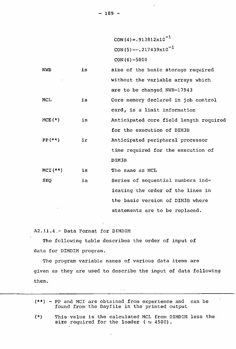
- 189 -

CON(4)=.913812x10-1

CON(5)=-.217439x10-1

CON(6)=5000

NWB is size of the basic storage required

without the variable arrays which

are to be changed NWB=17943

MCL is Core memory declared in job control

card, is a limit information

MCE(*) is Anticipated core field length required

for the execution of DIM3B

pp(**) it Anticipated peripheral processor

time required for the execution of

DIM3B

MCI(**) is The same as MCL

SEQ is Series of sequential numbers ind-

icating the order of the lines in

the basic version of DIM3B where

statements are to be replaced.

A2.11.4.- Data Format for DIMDIM

The following table describes the order of input of

data for DIMDIM program.

The program variable names of various data items are

given as they are used to describe the input of data following

them.

(**) - PP and MCI are obtained from experience and can be found from the Dayfile in the printed output

(*) This value is the calculated MCL from DIMDIM less the size required for the loader ( = 4500).

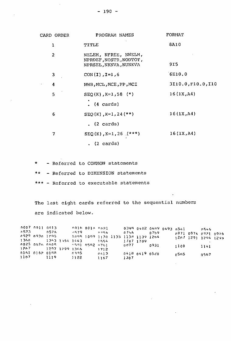
- 190 -

CARD ORDER PROGRAM NAMES FORMAT

1 TITLE 8A10

2 NELEM, NFREE, NNELM, NPRDEF,NOSTR,NODTOT, NPRSEL,NKNVA,NUNKVA 915

3 CON(I),I=1,6 6E10.0

4 NWB,MCL,MCE,PP,MCI 3110.0,F10.0,110

5 SEQ(K),K=1,58 (*) 16(1X,A4)

. (4 cards)

6

SEQ(K),K=1,24(**)

16(1X,A4)

. (2 cards)

7

SEQ(K),K=1,26 (***)

16(1X,A4)

. (2 cards)

- Referred to COMMON statements

* * - Referred to DIMENSION statements

*** - Referred to executable statements

The last eight cards referred to the sequential numbers

are indicated below.

n007 nn11 0013 0016 0018 nnP1 0.398 0402 0489 0493 n541 n546 n573 0576 ,1579 07c4 07c:,6 0759 n871 0574 09?1 0976 0929 n93n 1n05 109Q 1099 1130 1135 113t1 1139 1264 1287 1291 1294 1295 1360 1363 1164 1443 1c54 1 107 1709 - n025 002k 040c f‘co11 05R2 8761 0677 0931 1100 1141 1P67 1297 1799 13('6 1712 0161 016? OlgS n1Q5 0413 0418 0419 0520 0565 0567 1107 1119 1122 1167 1307

- 191 -

A2.11.5 - Job File

In order to submit both programs together under the

running system KRONOS 2.1 at the present in ICCC the card

deck has the following structure.

JOB ( ...)

UPDATE, N=PL3, L=1.

FUN (G).

UPDATE, P=PL3,L=1.

RETURN,PL3, CORRET.

REWIND, LGO.

FTN, I=COMPILE, OPT=1, L=0.

LGO.

EOR

*DECK DIM3B

[PROGRAM MOB]

EOR

[

PROGRAM DIMDIM . .

EOR

* IDENT NEWDIM, K=DIM3B

* READ CORRET

EOR

[

DATA FOR DIM3B

EOF

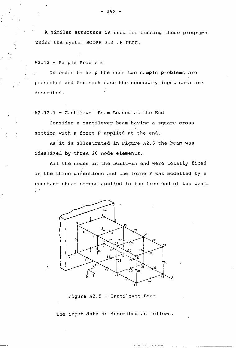
- 192 -

A similar structure is used for running these programs

under the system SCOPE 3.4 at ULCC.

A2.12 - Sample Problems

In order to help the user two sample problems are

' presented and for each case the necessary input data are

described.

A2.12.1 - Cantilever Beam Loaded at the End

Consider a cantilever beam having a square cross

section with a force F applied at the end.

As it is illustrated in Figure A2.5 the beam was

idealized by three 20 node elements.

All the nodes in the built-in end were totally fixed

in the three directions and the force F was modelled by a

constant shear stress applied in the free end of the beam.

Figure A2.5 - Cantilever Beam

The input data is described as follows.

O O

U

ro•-

• tD

J P

D

N

O 0

.) ')

0 C

)

• N

•-•

0

-4

,;1 3 0

0

I -I

•

O

n1

• L 1

W (.

.) N

N •■

•••

-4

-I

W ,J

:.) .

-r

W J

L.)

••• 1

,1

D.

n

t.1 N

•-• I

NI

•-•

.1

>

•-• ..1

7, J

1 J

V •

•• D

-4

J. - 1

P. 1

1 3

3 I`

F F

I),

Ls

1J L

.) L

.) L

.) U

IA J

I) U

r3

N N

0)

N N

N t

v N

ro

—

0 0

000 I)

0

0

1

L.) •

• F

LJ ^

.1 s

s- 0

.) !I

.... ,n

r L

J ')

.... (

) 0 (3

-4 C

s LI

F L

4 (V

s■

00

3 -4

C.

tn r

w h)

.. 0

„I 1)

„,) 3

., A

4.

L.) r

j .. .

.0 h

) .. 0

.)) ..

LJ -J

•-

• F

....,

V N

...•

N

3

3

) C

h F

0

• N

•

rn

II a‘

v 1'1

— o

:A

O

VI

4)

.1

1

...

:1 0

0F

03

13

FC

0'.C

30

)0

F ,..

..J c

z ;.

." r

1) C

.C3

:00

00

F0

13

C3

F C

)C.0

•

DO

OO

Ds

LIC

GM

F 0

0

00

00

00

U

W

• r..

) r,)

0

V•

• •

• •

• •

• •

• •

• •

• ••

•••

• •

• •

• •

• •

• •

• •

• •

• •

• •

• •

•.•

• •

• •

• •

• •

• 0

r..)

0

F ,:N

•

C.)

LJ

U

0

•

• :J

'J

)

1 N

'N v

r)

J ■

C) '0

c%

n

N •-

• U

(2

:al

.3

5 C

L)

3 7.

TO

es

0 C

1.0.

1“..)

7.3

N

CD L

.10

C"::"

,1F

5 5

.0r1

C0

C)0

00

• r

) 0

00

00

0

•

• •

• •

• •

• •

• •

• •

• •

• •

• •

• •

• •

• •

• •

• •

• •

• •

• •

• •

• •

• •

• •

N •

■ W

v

,J ;`

) J

•

N

N

o 0

-4

C)

•

0

3 •

N •

-• 3

Cl

3 3 .D

F0

00

F D

7.J

CO

3 D

DC

)0(.

.).r

clr

.1-1

)00

13

0),

F 0

00

50

(.3

31

03

13

!.2

4.0

00

F C

JC

3

0 0

0 0

0 0

U

• • •

• •

• •

• •

• •

• •

• •

• •

• . •

• •

• •

• •

• •

• •

• •

• •

• •

• •

• •

• •

•

• •

• •

• •

.3

N

0

.3

? O

• 1

.4 N

•-

u w

•-•

'3

• —

.n

oo

o )O

G r

•

• •

• •

• 0

t. •

•-•

•-•

W

•-•

CD

J a

(J

rl

N

0 C

j () 0

)O

C)

U

•-• .

A 5

, .-

LA

0 -

4

• •—•

F

C1

C.

O 0

0 C

I C

.G

U

• • •

• •

•

J

.j

131

- 194 -

A2.12.2 - Thick-Walled Cylinder Subjected to Internal Pressure.

In this case 32 node elements have been used in the

finite element mesh idealization as it is shown in Figure

A2.6

The internal pressure was specified in the inner faces

of the elements by radial components using a cylindrical

system of coordinates.

This problem exceeds the capacity of the basic DIM3B

version, thus the DIMDIM program has to be used.

Figure A2.6 - Thick-Walled Cylinder

The necessary data for this analysis is described as

follows.

0. 0. 0. 0. 0. 0. 0. n. 0. 2.

•

0. 0. n. 0. 0. 0. 0. 0. 0. 0. 0. b. • 0. 0. 0. 0. C. 0. o. 0. 0. C. 0. 0. 0. 3. J. 0. 0. 0. n. 0. 0. 0. 0. 0. 0. 0. 0. 4. 4. 4. 4. 4. 4. 4. 4. 4. 4. 4. 4. 4. 4. 4.

- 195 - • TUTRUAILY PR-;CURIZEll THICK cyLtnnE;,

8 t 3? 67 1 16n 3 140 75 -.13561E-3.133-'1 E-3.156271:7-4. 11 1117E -1-•21744 ,"-1 500)F00

17943 90000 35000 130. 90.1J0 CC37 0011 0013 nc16 coin 1'21 391 04u2 0489 0493 0541 0545 n573 0576 0579 07"i4 9756 0751 0871 0474 0)21 0926 7929 :931 109' 1,98 1C99 1133 1135 L34 1139 1264 1287 1291 1294 1295 126' 1367 !354 1442 1554 1-n7 1709 0025 0026 0415 0541 0582 07A1 0477 0931 1100 1141 1267 1297 !219 1366 1712 0161 0162 0188 0345 0411 1418 )419 3520 0565 0567 1107 1119 1122 1167 1.7C.7 data for DIMDIM

3 ...77451667 .551175555 .n .84114889

8 3 32 67 1- 4 1 97 101 1.1 115 1k6 1C7 131 114 112 1 66 1 5 7 9 10 11 12 8 2 105 1)9 111 113 114 115 11') 112 113 2 Si 9 13 15 17 18 19 20 16 3 113 117 119 121 122 123 124 12^ 118 3 70 17 21 23 75 2; 27 28 24 4 12 1 125 127 129 131 131 13? 124 126 4 72 25 21 31 31 34 35 36 32 5 129 133 17.7 137 138 139 141 136 134 5 74 33 37 39 41 42 43 44 41 6 137 141 143 145 146 147 144 144 142 6 76 41 45 47 49 5. 51 ' 12 48 7 145 149 151 153 15. 155 156 152 150 7 75 49 ql 65 57 51 59 6". 56 8 153 157 15) 97 98 9) 100 160 158 8 80 57 61 63 1 2 3 4 64

207.50E+09 0.3LE400 2 4. C.

TEST CASE 4A IHTMALLY PkESSURIZtD THICK CYLIHDER 3 4 2 2 0. 90. 90. 9C.

0. 0. o. n.

.77.59667 .55555556 1c^ 99 91 41 83 84 82 65 67 68

ri 4 .3 2 1:4 107 126 Al 85 86 84 67 69 7.) 14 12 11 10

1:6 115 114 85 87 88 86 69 71 72

11:jf. 122 18

89 9C 88 71 73 74 10 28 27 25

132 131 130 89 91 92 90 73 75 76 38 36' 35 34

141 134 138 91 93 94 92 75 77 78 46 44 33 42

148 147 146 93 95 96 94 77 79 80 54 52 51 5'

156 155 154 95 81 82 96 79 65 66 62 66 59 58

data for DIM3B

3 5. 0. 5

4 6. C 3. 15.

.

6 6. 1r.

7 3. 3C.

8 6. 30.

9 3. 41- .

1) 4. 45.

11 5. 45.

12 6. 45.

11 3. 60.

1. 6. 6; .

15 3. 75.

16 6. 75.

17 3. 91.

11 4. 90.

11 5. It.

-... 6. 91

71 3. Int.,..

22 6. 1 - 5.

23 3. 170.

2. 6. 12( .

25 3. • 35

26 4, i3''...

27 5. 175.

74 6. 135.

29 3. 15r.

30 6. 10,0.

31 3. 115.

3? 6. 165.

33 2 1gf.

. 14 4.. 1)'.

35 5. 140.

36 6. 13,".

37 3. 195.

35 6. 195.

39 3. 210.

40 6. 210.

41 3. 225.

42 4. 275.

43 5. ^^5.

4. 6. ?.75.

45 3. 24^.

46 6. 240.

47 3. 255.

48 6. 25F.

3. 231..

4. 270.

5. ._' •

6. 27".

3. 21'.

6. 235.

3. 300.

6. 1"'• 3. 315. 4. 315. 5. 315. 6. 315.

3. 331 .

6. 31( .

3. 745.

6. 345.

3. 0.

6. 0.

3. 45.

6. 45.

3. IL •

6. 9'.

3. i V- •

6. 135.

3. 180.

6. 14..

3. 22',.

6. 225.

3. 270.

6. 27( .

3. 315.

6. 315.

43 5) 51 52 53 5. 55 56 57 58 53

.6) '61

62 63 64 55 66 67 68 6') 71 71 72 73 74 75 76 77 73 79 80

31C. r. 0.

45. 1.4.,. 9C. qr..

135. 1'5. 180. 14C. 225. 225. 27(. 270. 315. 315. C. 0. 0. C.

15. 15. 3C. 30. 45. 45. L5. 45. 6:. 60. 75. 75. 90. )C. 9:. 91' 1,'5..

115. 12% 120. 1 55. 135. 135. 135. 15.'. 1cC. 165. 1(.5 140..

18r. ±50. 18G 195.

-0-. 12.

210. 12.

21'.. 12.

725. 12.

M. 12. 12.

2.5. 12.

21.. 12.

240. 12.

25I-. 12.

755. 12. 2" 12.

27C. 12.

27C, 12.

27? . 12.

285. 12.

?A5. 12. 330. 12.

3:1. 12.

315. 12.

715. 12.

315. 12.

315. 12.

331,. 12. 331. 12.

345. 12.

345. 12.

6 7 8

4. A. 8. A. 8. 8. 5. 8.• 8. 8. 8. 8. A. 8. 8. 8. 8. 12. 12. 12. 12. 12. 12. 12. 12. 12. 17. 12. 12. 12. 17. 12. 12. 12. 12. 12. 12. 12.

12. 12. 12. 12. 12. 12. 12. 12. 12. 12. 12. 12. 12. 12. 12.

- 196 -

80 6. 81 3. 82- 6. 8.11 3. 84 6. 85 3. 86 6. 87 3. 48 6. 89 3. 90 6. 91 3. qz 6. 93 3. 94 6. 95 3. 96 6. 97 3. 9i 4. 93 5.

136 1 01

6. 3.

112 6. 103 3. 1 54 6. 135 3. 1 05 4. 1 17 5. 108 6. 1 C 1 3. 110 6. 1 11 3. 11 2 6. 113 3. 114 4. 115 5. 116 6. 117 3. 119 6. 119 3. 12: 6. 121 3. 22 4.

1 2 S 5. 124 6. 25 3.

1 26 6. 127 3. 121 6. 123 3. 13; 4. 1 31 5. 132 6. 133 3. 1 34 133 . 13', 6. 137 3. 1 38 ? 23

4. 5.

140 6. 14/ 3. 142 6. 143 3. 144 6. 145 3. 2 46 4, i47 5. 148 6. 149 3. 15' 6. 151 3. 152 6. 153 3. 154 4. *55 5. 156 6. 157 3. 153 6. 151 3. 160 6.

8 1 1 I

2 1 -1

3

4

4 5 621.E+06

2 2 4 621.E+06 3 1 3 -1 4 621.E+n6 4 4 5

1 -1 1 4 621.E+16

5 -1 4 621.E406 6 1 6 -1 4 621.5+56 7 1 7 4 621.E4C6 11 . i 8 -1 4 621.E+06

A2.13 - DIMDIM code.

Finally, a listing of the DIMDIM code is presented in

the following pages.

1 2

PROG4Am DIMDIM(INPUT.OUTPUTITAPE5=INPUT.TAPF6=OUTPUT. 1C0PRFT.TApE1=CoRRETI INTFT:14 SE,J.TITLE DP,EI.SION TITLE(8),SE0(58).CON(6)

0 TIEFIPIE THE DImENSION CONSTANTS. RLN.I(0 1 READ(5.1)TITLE

1 FCP',A1(iA10) wR7Tr(A.2)TITLF

2 FOdtAT(IH1////1H0.4A101 REANc...1)NELEm.NFRFE.NNELM.NPRDEF.NOSTR.NODTOT,NPRSEL.NOVA.NUNKVA

3 FOR:AT(.15) wRITE (A.7)

7 FORmAT (11AHOTHE DI'ENSIONS or THE ARRAYS IN TNE PROGRAM DIm3D ARE I rrTrUNTNr0 MT THE FOLIJUING MAXImUN PRODLEm PARAMETER VALUES./ 4RITF(6.A)NLLE!.NEPEE.NNELN.NPRDEF.NOSTR.NODTOT.NPPSEL.NKNVA.NUNKV

IA 6 FORmAT (alio-cLcm =.13/911 NFREE =.12/AH NNELm =.I3/9H NPRDFF =.14/ 19H NRSTR =.I2/911 NnBTOT =.I4/91? NrRSEL =.I3/8H NIKNVA =.14/ 2941 UNNKvA =914) READ (5. R9) (CON II), I = 1. 6)

84 FOP.:AT (AE1u.0) WRTIr (A, 1-V1) (LON (I). 1 = 1. 6)

85 FORAT (35HRTHE P FONCTIoN CONSTANTS INPUT ARE / III 6E14.S) REAN(5.9 I iJr..,"CL .0CE .PP..ACI

4 FOV.*ATIi110.110.0.110) ,JR1Tr (f,04)

9 FO.I.-1AT (r,1110THE cxrrurron or UT '3B IS ASSUmFD TO REQUIRE TIT FOLLO IwING JO1 HARA41 TER VALUES./

4,(7/r mrc.op.,,c1 8 FOr-rT (:9110THE CDR( FIELD LENGTH =.16,7)1 wouns./3211 Tull PFRIPHFRA 1L PR(TESsoR TIpE =0-6.1.914 SECNNDS./4811 THE MAXImUM CORE FIELD LEN 2GTH r.F Ti';: (.iLTUTER =./7.7H wouns.) .4vivA1=1r..mvn.wkm9A+1))/2 NOyo/1=(,.NR.11A+('1T,KvA+1))/2 NCELN1=(FRUELL.: NCELI.n=•IT:EL 11+1 ranTAL=',i,: w+NNNKVA NI=Nr1H7r.fRiNTuT Ar.==,."Axo(NKNvA.NrNRVA) Tmr=:.,:crrmIAL.:J.rLoAT(,cc).nP.o..com). R1AU(5.01)(s-E:J(R).R=1.58)

hl FJI:tAT(IA(lx.A4)) 5 1110-C=NT/I.ROF

IF(FINIT(NTI/FLOAT(NBUF1.GT.FLOAT(NRECHNREC=NREr+1 :4RTTF (A.12)

b2 FNR- vr (tRHUTHE DERIVIN NPIENSIONAL CONSTANTS Aur AS FOLLOWS.) (Ao)31 lovivAl.numKvt,mcam:.NccLuo. NTOTAL. NT. mAn. WAIF.

1N(,EC • (13 FO1m.7 (911ONRNVA1 =.I5/9H NUNKV1 =.I5/911 NCELN1 =.13/911 NcrLNn =.

1/3/9H NTOTAL =119/5H NT =.14/6H NAB =IIS/7H NOUF =43/7H NPEC =./3 2)

C C 10 CORRECT THE COMMON STATEMENTS.

K=1 N.I=NwD CALL DELETE(SEINI.SEO(R+1).10 CALL SI(NPROU.N) Nw=Nw+N CALL S2(NPROEF.NUNRVA.NRNVA.NCELNI.NKNVAl.N(rNKV1.NOOTOT.NATI.N) Nw=Ny+N CA11 S6(NELEMOICELNO.NCELN1.NODTOTIN) NW=11',I+N CALL. DELETE(SEO(K).SEO(K+1).K) CALL SlA(NNELM.NCELN1,NTOTAL.N)

fCr"T'1%;TELETE(SEN(K),SED(1(+11,K) CALL C2(NIUF.NTOTAL+11N1(EC+1.41) hr Nw=No+N CALL. C3(NNELM.N) Nw=111,1+N CA1L OCLUTE(SEN(K).SEQ(K+I)IK) CALL CORINNELM.NUOTOT.NLLEM+1.N)

WRI(F(6.12)HwB.Nw.MCL 12 FORvAT (1171IuTHE SPECIFIED CORE rm.° LENGTH NFErED FOR LOAOING TH

1E PR0(04Am LESS THAT rou BASIC ARRAYS WITH VARIABLE DIMENSIONS =06 2.71) LOROS./5441 THE CAICULATFD CORE FIELD LENGTH munrn FOR LOADING 3 =.IA.711 WORDS./4PH THE SPECIFIED MAXIMUM GORE FIELD LENGTH =06,7 411 KIWIS.) IF(Nt,LE.mCL)GO TO 14 WRITF(6.13)

13 FORAT(A911 THE BIGGEST CORE MEMORY SPACE NECESSARY IS 'LORE THAN SP lECIEIE0.) IF (uCL.ST. MCI ) GO TO 15 NBA = NB01.(5+NTOTAL) + NREC + 2 - (NW - MCL) :F (nnti.Lc.u) GO TO 15 WINE, = NBUF NBHF = NB (qTOTAL. NT. FLOAT (MCE). PP. FLOAT (NBA). CON/ HRTTr (6.17) NBuri. NBUF

17-rOP!3 AT (7?11R11oNIVER IN ORDER THAT AN ExPurrn LARGF CASE MAY RE AC 1COmOnATFn 1)1)111 IS/ I341 urouun rRnR. 14. 3H TO, 14. 51H WHICH WILL 2 INCPEASE THE PLRIPHFRAL PROCESSOR TIME.) REWP.D 1

.;/Nr. o O :r5 15 Arr 99 14 CALL DELLTE(SE1(R).SEu(K+1).14;

CAM_ S1(NPRNEF.0) CA1L SP( 1'PR7EF.N0o1<vA,NRNVA.NCELN1INKNVA1OUNKV1.NODTOT.NAR.N) CALL sA(hru-1,mrt.:L%o.urrLnl.hoornr.(!) CALL DELETC(SEc)(1<).sEo(K+1).10

CALL 51(NPHDEF.W. CALL S2WP40EF.nUNKVA.NX ,IVA.NCF:01.I4KNVAl.NIINKVI.NODTOT.NA8.N1 CALL SAUTLIPIOICELNOOICELN1.NODTOT.N) CALL DELFTCISEQ(K),Sr1l(1441).K) CALL DELFTEtsLAK),SFu(K4.1).K) CALL 561,1CCEmoICELrmOirELN1, ,100TrIT.N) CALL COIWTILLel.NOOTOT.'1ELE ,44.1.N/ CALL CELriCISCq(KI.sE:J(K.1).K) CALL SIII(W,LL-I.FICEL"11. 1 1TOTALINI CALL DLIITL(Y:.)(K).SIK+1),K) CALL C3(r:ni.Lp,'J) CALL nELrTLISLoCK),sfu(K+1),K1 CALL Cni(WfIC.L:Olt)Tor.riELC7,14.1.11) CALL OELFTEI(K).sc:J(v..1),K) CAIL Ss(P.FLC.oCELnU.NcELNI,n0DTOT,N) CALL 11FLrTLIsFocri). ,;En(K+1).14) CAIL Slo(Irttc.•010ELNI.LanTAL.^1) CALL PELFTLIm:J(K). ,,r,J(v■I).K) CALL cn.1cro , LLmOmoToT.rflr-1+1.0) CAIL OKLFTLASI:,JCKW -u(K.1).14) CALL S20.PKOEF.NOT4VA0901VA.NCELN1.NKNVAI,NIINKV1.MOOTOT.NAS.N) CAIL Wr.FLEP , oiaLrm,nrUi.n10100TOTO) CALL DEAFTEISLAKI.Sru(“1).K) CALL SII'WUnfir,r0 CALL S2(1, PqrCro , wiwvA,TK,NA.NCELI11,IIKNVAIIN(JNKV1.NODTOT.Iltr.N) CAIL %6INFIL',1 0)CELII0./IrftN1.I190TOT.,1) CALL Slo((I'ilLo.HCEL ,IlINTIITAL.II) CALL rVirTEIsEt)01).SLu(K.1).K) CALL c2(rolur.uToTAI410mcc+1.11) CALL PEtrir(sC,J(K).sE:J(K.t).w) CALL SlOttrILLO.!ICDNI..ToTAL01) CAIL NELFTE(SCl(K).ksu(K+11.14) CALL C..CL110.01TOTAL4.1.,!RFCI.I.N1 CALL DELF- tE(',L:(K).%K(;(K+1),K) CALL SIMPW4-1-.0) CAIL S2(rvH1LF.NwiwVAO'KHVA.NCELNI.NKNVA1OUNKV1INOOTOT.NAR.N) CAIL 561t4:LCA,ncu.w.NOILN10100TOT.N) CALL Sln(trIlL'ortirLL111,11TornI,r1) CAI L riF.ur rE I sr r 1)•v.) CALL C2In.tor ,riTOTAL +1 C +1 oL) CAI L It (St •)(h1.51u(K-r1).V,) CALL SiWILLI-. 0 ..WFL:M.IicrL'Il.mOUTOT.N) CALL I IL (Sf. j(K), ,,1 of 1, 41).v.) CAL L 52(r 1,;(.JCI.NU, wvA.,R.Ivn .nCELN1.NKNVA1.NUNKVI.NODTOT.NAR.N) CALL 56C'ELLIO!CULIO.NCCLIII.'IONTOTINI CAIL S1'IMLLv.NCELNI.'ITOPIL.N1 CAIL. PELETEICOKI.cLu(K•I).K) CALL C3(':I:CL .11 ,1) CALL Cr,WimlL ,I.:1■PlinTolFLI-1+101) CAIL CEIFTL(MoIK).cFQ(K.1),K) CALL Slurr:LLr4 01CfuiloiTOTAL,U)

CALL DELF:TCISEQ(K).SEOCK+1100 CALL C3INNELmiN) CALL C0n(NNELM.NOOTOT.NELEM+1.N) CALL DELETE(SEO(K).SEOIK+1100 CALL Slq(NuCLA.NCELMI.HTOTAL.N) CALL. DELETEISEUW.SEU(K+1)00 CALL SincHIJCLII.NCELII1.CITOTAL.11) CALL DELFTE(SEOLK).SEO(K41).14) CALL S2(PPROLF.H0014VA.tIKNVA.NCELNI.NKNVAlonlINKV1.NODTOT.NAR.N)

C C 20 CONFLICT THE D1MENSTON STATEMENTS.

READ(5,31)(SEIJ(K),K=1.24) K=1 CALL 11ELFTEISE0(K).SEUI14411.1<) viRTTF(1.21)11PRSEL.rCELH1.NNCLM.NNELMINNFLm

21 ,7010,. AT(6X.3%!HOI"EWSIOH E116.61.HT(6.9).NPLOC(04.8)I).TRUSL(./4.110 1/rA.13HrliqDISLON V1(.14.5)1I.V2(.14.5H).V3(04.111))

CALL OCLETC(SF4IK).SEU(K41).10 4111T1(1.72), AB.HAB

22 FONMAT(40(.1211DMINSION A(05,41001(1I541H)) VD OD CALL DELETL(SCWKI.SFO,(4=

WRITE13.231 , 1CLLI110"nEL 23 FOIWATIAX.15HDIMLUsItIN RHSL(414.3211)0CTM(6),TRIlt3).GL(3)1JACC3$34

1o/5X.6111nEl4..14 4).TIMSL(04,171),TP(3.3),TR0LC31) CALL. OELEILISUAKI.SEOI14+1I.K) M=01(ELH14.InCELN1+11//2 WiTTF(1.241).1FJELI

24 FUlw4T(r,X.2U1IDI4ENSION A(3.31.SK(II5.26H).JAC(3.1).TJAC(3.3).DE(41 1.14.1m) CALL PELFTEISE0(K).SEO(K+1).K) 44711(1.75).A

25 FnIWAT(6X.1311OImLN,4TON SK(.75.111)) CALL DELETE(SEU(K).SE0(1(.41).14) 4141T1(1.26INTOTAL

26 FO,WATI4W50011T-USION CO"VIII4,110) CALL DELETEISEOIKI.SEG(K+11$K) WRTTF(1126)NTOTAL CAIL DELFTELSENIKI.SEO(K+1),K) M=3*rODT(IT 4HTTF(1.27Im.HrOTAL

27.F(PwATt6X,13/10P,,CUSION 02104,711).COMP(1/4.110) CAIL DELFTr(SE.7(K).SFULK+1).KI WRI7r(1.?,t):A

28 FO4r, AT(AX.13IIDVIEMSION U2(.74,111)) CAIL nELCTE(SEOCK).sEG(K+1).14) 4141TrII,24(110ELUlotOnToT.v010078T.NCELN1

29 FOP4ATC6x0? ,191,:EnsION c(.111.3511).ST4(6).ST,(3.3),STnT(3.3).SL(3,3 11/(0(.151:71i-EHSIO0 , J1-, IV(.14.5101021.140 1 1)/6X115HOII-ENSTON STSS(.14 2.1o)1.(0.DOTI4.114.1,1))

CALL 1)1LF:TIA ,,r4(w).sEr(K41),14) WRIEr(1.311)14CELMOJUL41.011EL,4

...--

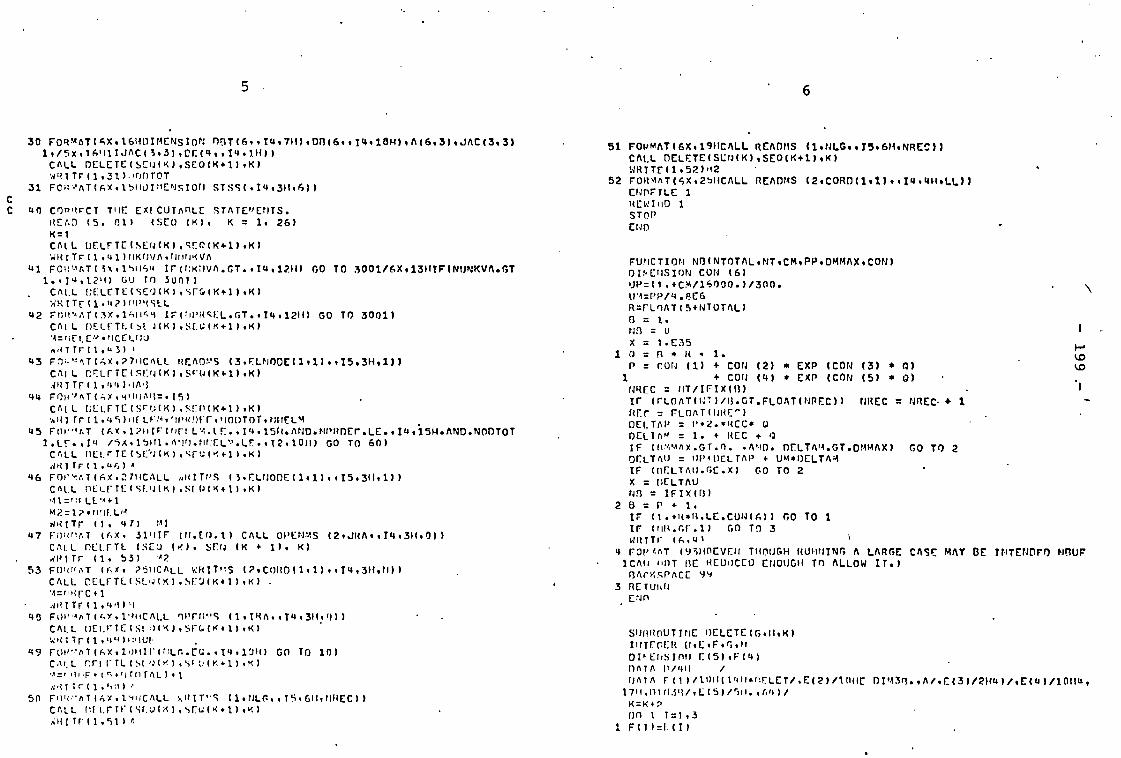
- 1

99

.-I

.

a VI

... ••■ 3 LI

3 Z.: N

..-

+4 >~

on N

C

+

f U

4"

0

"

U

I- Ll

.... C1

r

LJ N

G

LJ

C

0

C

cc

S(^

Z

.. ..; -.

..- •

L .

"

PI ..-

II W

...

* It ■-•

0 •

:7 %D.

-6 a-

U

X

Cr - O.

•

0

as .... kJ <

< 6-1 C

M

U

Ic) 0

++ •

.... C *

.., :C LJ

.

PC ... ....

0

CO

_-

▪ C

<

C

C

• -I

7.-- 0

C

X

0 C

•-• I-

0. .../ .-,

J- O

X 1.../ U

" 0 X

Z

<

N. C

. Y U

0

- ...• g_i

• C

.4 .-

.-

. .

Li

CI-

:... C IV

•4^ N

A. a. O....

C.

CJ

C)

" r- ...

V. ,4 a..

X X

C

I- LJ

11- 5

Li

+ •

-I ::` N

..... " V) 'Y

1/) £

LJ Li I-

Li + 0

0

"

.... ..-

U

* *

C

S C

O

0

I C

Y 6- ,...

CO

C

. •

o

=I-

C

O

-

t.i - <

La

<

I- c

- - _,

C. •

._ ,.., -, -

2: J

S L

i 0 L

I Z

C

NI 7

L 3

C • 0

".

ES Li

.

W<

....1 X ....1

...) .... ...j

:: 0 CV :: U

Ll L

J CP

-- :7 in

•-1 Li " N

I- C7 - I- _J CD

4: :.! 4:

>C t... in X r4 0 -I . ..P

.4

••• Li r4 sr u

M -I >

- 7 L

, v. C-

4C L, .c .- L-

. >- CV •

...

-- CD q ,

>-

I- V) •

-.1 C= ... C=

C

I-

cl F-

CCC

c)

Cn ci .4 0 27

_I S.

.., 0 • ,... < • 0 • 0

II _1 CL a D7 :7 LI 2 !,:t * * • -

*- <

Li L

J -- 0- -.1

II

2!

%. Li +

27 27 L) • %,... C7 )7 + y 1._

>- :2 . - a. c- .., .- cr c_:

Z T.

m,

vn

un Cf - >- >- C7

M,

LI * a'

..1 !:.4 !! ■:..

! :::t

! a':4

! (:::: :

3 -- . :CU: 7.:;* II 11.1

1 :: :: C

. .-.

• LI L) -- = La Cf Cf • _J x

.. ... •

LL•- - Nt

■- . C... -

..1 -. c 'if Y.

)< ,... •::: 4

C L.1 •

.4 "..1 .- * . LD

C.- •

C2

• .. ^ 22

2'

Z: 4

2 _

J II II c

II I-- >- .7

cf (2 sC .....

Li

Li -■ 1- e- .... h- ....

11 ..- -- 1:: ,-

NC C

C: L.

L I

I .: < :: < C =

C- .: 2i . < Z V. ...:

>c < < >c .4 * L.. ■ 7> C2 LJ

L'7: ^

> 5

Li LL C

1 C

u1

U

>- . U

.

:7 .2 7; 21 L. LL- v- -a

tal 0 .

..., . - .., - -.

•-• . .,

LJ ■

>- al v. 'LL -, .7 II --

..... a

.

9-.

Z.

v Vo

0 .... ... c

.

Z Z.:P. E : ... .. St. .. .. :

• v

0 0

5

LI L

i " LI

7 -

,.. ..., 7 I.:̂

.... 0 60

4

6- (\ 1l

• C. • . =

....

0

C) 42 CC

CD

27 LI >- :7 ). .J 0- C CL 2.c CD CD

:7 >. C. r II

c2

C: m

II II L. II

II u II

La L, ..J -.I

..1 II

II cr L. la La LJ L. L2 U.

C2 LL L. Cf

ES C c Li 77

C L:::: t.:„.1 : : 7.... . c•-• ....̂... :2 I- .- P

- I- • W

LI. P.! :C LA. U ff 0

/ LJ

L. C7 :7 :7 C

f cn

:: X:3

C.

27 ... Cf C

D C

D >4 0 )7 >C

:7 c

o ... .4

3 L

. UCC L

i col .-.. C

D C 22 V

- Y C U.

r4 .4

.,-. .4

N

.1

CV S

60 .4

U)

en

F-

PI

•

4)

0

•

- --

C

.

E

z

-

...

C

M

I/. •

... ✓

I-. C

... SO

=

In 0

6.6

4) . 1.4

• ...

C

.4 •

.

• a

;i .--

x ..

.4 -

• -

2

%,C .-

-

• S

co

\

r4 r4

• ..6. .4

),

2:

w4 6.4

0

•W

0

• •

• •

0

0

-. -I0

•

7

_ 7

0

0

4)

•

W., <

rl

^

...

Pr: .

L C

• C

•

•-• •

C

0

La >- in

.., a

(.1 .

CD r-

.. C

.. •

I-. ---

LLI NO

I- .

CO

N

-

0

.

-.:. 0

•

-

•

r

C

_

c:

CD

0

--

Z

-

--

..

r4 O

^

0

.4

• ..... r4

VI .4

... -...

.

r. •

0 .--: r

f.ti ..... .

;5 C

::, -.

-.

::

.4

C C 0

.4

5 Y

.4 •

I- •

7

-

N

"

J C.+

•-• Li

*-- S

7-. t"

• sO (1.11

.-1 Li

Li •

. L

i C

• CD

•-- C

•-•

.

V) CL/

44

.

0

2.2 :2 N

C

0- 5

.

0

. .. Y

::, Y

• Y

• Y 4.. Y

YO

7L

ir LiY

C ....L.,-) 7..

<

0. 3

C .;,i

i'.7-: 7:

:: D7

a ..

F.

.

Zr C

CD

.7

--2

22 Z2

. .1. ...

Li ..1 ....

0-4 /...

• .... ...., •••

.... I- •

..... ... J a.

vi 4

• ••• ...3 ....

Ln %D

• .

LJ II .

• .

I- .

. .

• I- 1.-.. ...J• ....

U DC

.- •

. .

... y -

I- -

1-

•••

C. .....

4) c.

■■•• .... •• • ■••■

Pr. ....

ow/

....

,in. ..... . .....

.4 ,.. I.. •-• ,•

C X

.4

0

,I • -A

v w4

v. C • '• ,4

..... .4

4 ....-. L.: -J +

.L 0

•-• .-.. .4,

7 ..4 ...... ve

C., or 4. I..

4. •

+

...i 4 4

4 4 4 ....

:: 4

•• 1...4 1

4 C

• X

V7 cr

3 C

IC .....: X

0 NC

Y• ...I

La 1:' V Y

•Li

h- NC Lr X

. x

V x

.1' .., .

..... < >

.....

0 ....

:t o.... •-- L

- • :2 --

L". -- 2-..

22 -■ 0

22

LJ ....- C> 22 0 5 0

C) :3

C. L., 7, .7_ 7 .- .2

s.i 3 r-1

z: 0

0 0

i- :1 C

7 L2 Li C)

_J s

LJ :" Y

". L-

2- ...C

L

-i • L.

•-• .... • •

:...?

.....1 L- L._

* Li ... ...... t_:

0-, C.I (.0 6-,

C ..., V Z. :: .-V

:7 0

Li 0

... V. :: - -'V

= V.

:7 ... ..r.

C

r.c

• L" 22 J'

N . .

IA c

= - c . - •

:.: •

in • t. L- 7'' . ,. . .

" Y

...1 • c

. e • -

..: .

5 .-

-

z

F- 0

--- 5

. L- 0

-

ti_ ...

..... s

r, ..■. : : C

C -.

.-- ...

...i .-.

.

_J

LI .1

3 F- u

) :3

LJ D

C • .. .1

)C _J -.

Y .J N

C

. NC

. ... .. r

.J Y

.,L

-N

< Y

-J Y

::: 1: ^ _I 3

CC .

--O r: U

V) -C

J- II -C u. .. -

J...

U

7q

-

14 ., -.. h- . 4

C > :I C '."., 0

r -

C - L

/ f:

2

).

L..1 :: sr •-•

LI :-

v. ..., 2

Li *....: -- <

L. .., = in

1.i

LJ .2 .

•-• 7: Ll) L.;

Li

C-j 7,-.7. ...:,

..:_ ....I.--

-.2 ,..

C-j u.C-1

73

< ^

7: "• L.. •-• 7

7.•

< '''.

--.- LJ .7

-T LI J) C :: LJ

$ Y

- :/' 2. 7 /1 .7

7 V .C.- :2 0 ..... IN .-. .rI

C

r - .1

-. .- rs. L

I, 7 L

A r :-. x. 2. - *.r

4) < -. - .1•

.. -

.-

.1

-

7 :

. .. : -

- -

..- ,

5 -

.. 7.1

Li "- •.

LI ..

Li - ..:'1

;,..1 - .4 ....: L

i - e■

LJ ■

.- 7 ..-1 -- . X L

J -- c

. LI

-7_

a ■

.2 J1

. ,..J C4 L

i - v. ...J

2' - . 7

*„. -- . .7 1- .-, .

- C

4- .4 .

1- P. . I- U

,,, . P- 7 - " Lt- X

Le' .- s

: . I- .4 _

I X I-

S. 1

- I' . .-

7 •

1.- • 7 • ..-- ••• X ••• Li tr) X

I- L-

a x

- L

i a ).: L. 7 7 14 Lu .-..- xL

- a L

C >

. L. c

>K

t- + .2

• L2

L- • L2 L-

7 P. L. 7 X

L Lr .r

xt. u

- s.: 7 .., . ..t

_.1 . .- -..7 _J . tr. ..., . . .0 ,-I . -I' _J . -

_.: . LC .J 7 Z- -- - _J ., - _

J ., . s

e ...: . s

e -

- . ,C

....: . ... ,C

LI .-, -,

P-- di

ts; .4 - rst L

.J r4 •-• U.) .-. ..■ U.' .r4 .... L.J .4

Z.. L.1 .• ...... LJ ....J .7 -

LI ..., Li ..

e4 ..... 61

...4 .../ (.... It .. ... .... 6.1

... r. C

.... /..' L

i -- 0

-- I-- r4 C. •-• 6.- 22

L.1

.- >- C

2 -- >

- 27

-- >- .. C

s.. I- :-..: ...1 • h- C

. h- C

.; Li - I- C

.. - •- C

La. -■

I-- 2: --

D .

L C

L

LC .

L.,..:

_JL...-

L.,c

Ls: .

L..<

...n

./....<

L.<

L-L

..<

L<

: L<

L.

S x _j >- 'S

t- C.: J

r n c ..J >- ., _I L, >- C JI- V ..) .- 7

. ..i 1- y ..) Z.. .... ,... L

J1- -,... ...j ..,...: 1....

7 .., ,_ -, _, ....- •-'. ..., ... 7 0 -J .- re

a <

.- _. /-. ::: V* v: I.'. ...- .' .....: I-. :

.•-• 7 _... L. L

, ..I v , ...; II II .....:.: ...,.... a, ...j :

a. ..j._ .:. ... ._, . ... ....., ....

0 ,... <

cr C) 0 Li II <

~O

~

CD v c :C 0 < II 1: C

< C

.f C' <

rr C _J <

.1.! C

C.•

N 7

:: C <

C. 0

ce 1

1 -.L: C

< .....- ::: < il -: -; < ---: LA_

. 1.) De LL

LJ Cf Df L

I 2c L

L • L

i Lc L

L I) 7

c L

. Li -c L

L L

J A L

L • tJ ": L

L L

i 7_,, X X

LL kJ ,L LL kJ :,- ...: kl. Li :

. L- ti

-c L, L

J "‹ .7

.4

.7

O

.7 C

.4

N

rn

S

in

s°

N

ml CI CD

c

M

4) a

a . a

a a

a

a

a I

n

S S

al

•

£4

C

).0

LS U

•

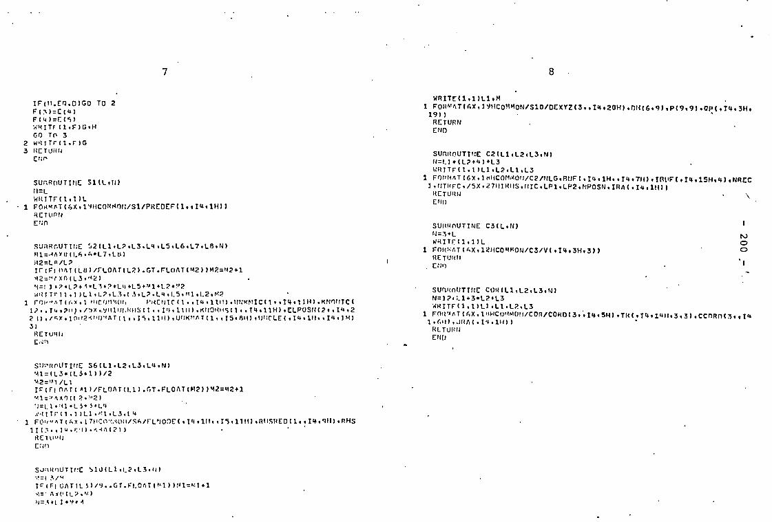
0

=

W

200 .-

M er

• z

:,- .

re: •

P. ..

.... •

7

C

.

... CC

a.'

x

c

O

to u

•

v-1 u

..

cr. a

.-

0. +4

tr)

a,

•

•

.... ft.

10

0.

1.1. •

.... 0 ...

7

tr, S.• ..-

v4 .

w w4 •

%0 .... w

3'

fro :r. d'

1.* ..

f■ 1-4

C

• .

. . ...

•7 •••

se

.. I. <

I

•• =

O

. 0.4

IS

(V

x .

S

.

v4 5 In

a

. to

... .

0-1 7 0

.... zr

• 1.4 n_

111 a-4

•

• Z:

•

. •

01 ... .

S

•

... U

. CV MI

en

N

2 3. 4.

....

/- LC -I

7

C

)4 . .

v. 2

co

0 W

0 vg

.

vs o

... -I CL

... -+

U

., 2

2

.J >

•

\

0

• %

. • S.

en C

vg tn

A, U

NI

-J 0

cr, .J V

I LI .-•

U

•

on 0

..

.

--I `,.. :: `4.

N

-I \

2

N • 2

. 2

-I

• .7_

o

...I .. 0

VI

.... 0

•

CV

0

M. •

J4 2

2

.

.4 J

E ..

3.: 4-4

• 7_Y

• 3"

-J - 5 -

0

-I N

0 .4 .J

C3 4. PO vg ...* --

ZE LI 4-4 *I _J U ::

U

'''. -J -J U -- .-I • :7

CV .J ... :: r- tr)

I

O+ . i

4447, IJ + 4-4 L N

U

N

U

N•+ r. t•

J.4

.... -J •-.. . J

.4

1 -I •-• 4-1

.... . W

7 - . X

LI

.... . W* ..■ • .

.4X

= + v1 X un Z ..X

z en .-. X ■•

. %,C NN . tO •■

1.4 .‘C

O

. + . 0 c:

4-4 4. s....j........ •

I- 4-1 •••

,... .4 r4 so ^o .. I....

2

:3 ---

4-u2

2 -.-2

:3 -J -1..72

W<

C

C * L. < L. Cf

C -J L.: c 2 C

. L. < . 4 .

F-3

2

2.41-

5 =O

2 * .-.7.7 :3 2. n■ I-

-7

I. 5 •• 4-. 0 C- .4 ". 14 I.- C:

2r2-5

C .4 .4 "'" -" 1-4 2

CC O- L.1 2

:7 II Cf C: 2 41 2: :3 it CC C L.. 2:

2 II CC G Za .1 2: 3C LL ON CC LJ

En z '......c EL - tt LJ 0 z

1.A. cc LJ VIZ3 LL . MC 141

v4 vg

vg N

vg v4

. N

4. NI .--

y)

0 • 5

5

•, 7 .-.

C

t-t . o

C • 4'

es z . I-.

x cu • cr

. .... . .

- -e. 2

1

2: V) 4-. 4-4

4-4 0

.

•

...CL 1 • .

4.

. _J r

.

,4

7 LJ •

1-g • ... 2-71

• v. la

41 .

2 -.1

4-. .4 1.1 V:

... 4-4 Z -

Li . 2

et

0.1 zr .

.

2 4-• ... ....

2' • :: ::

.4

Z . CC vg

.-. +

2 v. .

+ .4

EN . - un

cv

..

.-- .s.

es to, ..

r

IC z

IC N

7 7: • II

*4

S

• IN

3: •-• 2 • N

•

.4 CO

X • 4-4 0 .4

' •

... CV

-

. 5 .. ....

J

,4

d" •

•••• ...: d' Y i-

os ;:f

+

04 14

CV . .4 . <

CV .

.4

.

-J x

.. . - :: S

7

V

.

... .1f . .7 Y

..... 4-4

II

v4 vO

I- Cv • .4 .4 2

F. .

.4

.... -J

<

:.. Vi .4. .-. 7 <

.....

7

Li. C

• ...: 1.... • •

0

Li .....

LI is,

-J Cs: • .4 7 ...

-I C.

-

O

.J L

. J7

2

.

Z +4 7

2

U. 0

.4

41 + ...J

.4 •

.7' 7.

C

S

I- .4 4. 2 ..4

tt I-

-J ....

O. -J

0

3 N. :A. 4-4 • .J

L: 4.

•

•-

\

• 4 -I

.- tr- s.

pr. c

v4 Pe)

4+ ul •

v) .. ,n

-

sc J o

(1) .J

N: .J .,3

2 4. ..J

.-8 7 V',

• '

`... ...J

+ _. 2. •

-1 ... `....

CV ta.

-

..... N 4-.

... 7

• .: : .-. N

---

• 2 •-• -J

.4

C

J2

I-

JM 0 7'. -

..J +-

le; ■-• .... .

r- eq

:: 5

. .../

<

* _J .5,- ... ..- .

<

-J ''- . nv

.4

En .

x

.1 .

0

Cs. . 2 _

C

.-. CV 0

. :-. ...

.../ E,

.J C

Jt'- -1

+ C‘ 2 3,

J\

.J :J. ..-. C <

..... •

F. ....

L., 4. -J

L. .4 P." -1 L.:.' :..".-

.- ....

L. --. -.1 t: LJ 1' 2

7,

i

.... 2

N*

4... CV -J ■ C X Z..'

siri •-•

,... CV 4 . 7... If

.4 N.

0

• ti)

7' .1 kC

.4 T. • .4 ••• C V

V/ .4 ..-- 7 , 1 g ,

.4 Jr-.

vi - ....

0

0 0

_J ..4

•

.'1'

4

.4 . 4. 4. .4

... ;;..: ..

..... ...

w

... . LJ st

-J .1 4. •-• . . 7.. • LJ .1

, Cv ., 4 . 7 LJ

_1 . ̀ c 0 4. .4 L.

L. :;.:

.4 X

:2 .J .4 4/ C. •-• X ..s• C.

2 -1 '... ..... -.I •-• X ::

2 - A

• • 7 tr• -

•

.-. . .0

.- - C'. .4 ...- -.1 . ...: = 4.

.4 .... ... .. ..... 4 . 'C

.

.4 I- J 7.

a.... ..... ..4 in .-.

1-•

•-, •-•

I.-- :7 ..J .cr c . ,. ... c, •

1-- * -J C C- 41

ff... ••• i.

1.

< .... I.

6.1 LJ LJ .4

.... 2 :3

4. 14 2 7). N. C X 0.. ..... I- ■ X

5

7.■ 141 .... 0 X 7..- - 0- •-• .7

2 7 C :. .. 4-4

• 11 I I ... C L. S C

L. C. C

C < .:C

- 4.. • 4 < z V

S

C .J .. __ < • L. . • C •.--- '. -. '

F. I.- .. 2 CC

F- 3, 7.,

C ..:

-J L. :. .4 .- I .4 ‘..

D C

t -- 3 .. .: .. ... % . :.....

OC

...0 U. .1. .

s. r% a. .-. ..-- I--

C

C ...1 ... 2 .. C

rr II II - it __ .- z. • • >- C

r. II II 4 . II

-J .-. ..,.. r, r- C. r.f - - .

...".

LL S.

S,

CC 0 Cr 11 :7 :3 II nf 0 LJ 2

:3 .4 CV L. CU II ^' 0 . .....

CJ "" ::

..... CV LL f ...

II Ir. C., s. LJ ::

"3 II L. II II

... U. Lt. X 0 3Y

LJ V/ 2 2C LL CC LJ

CC: 2 2 .4 'F 7 i L. .N1 ''' 44 W Ci 0 7 7 1-4 7 :: ,: L. .. CC LJ

0:.- .4 7

2

.4 CV .1

r4 CV N)

4-4 v4

v4

- 201 -

APPENDIX 3

DIM3B CODE LISTING

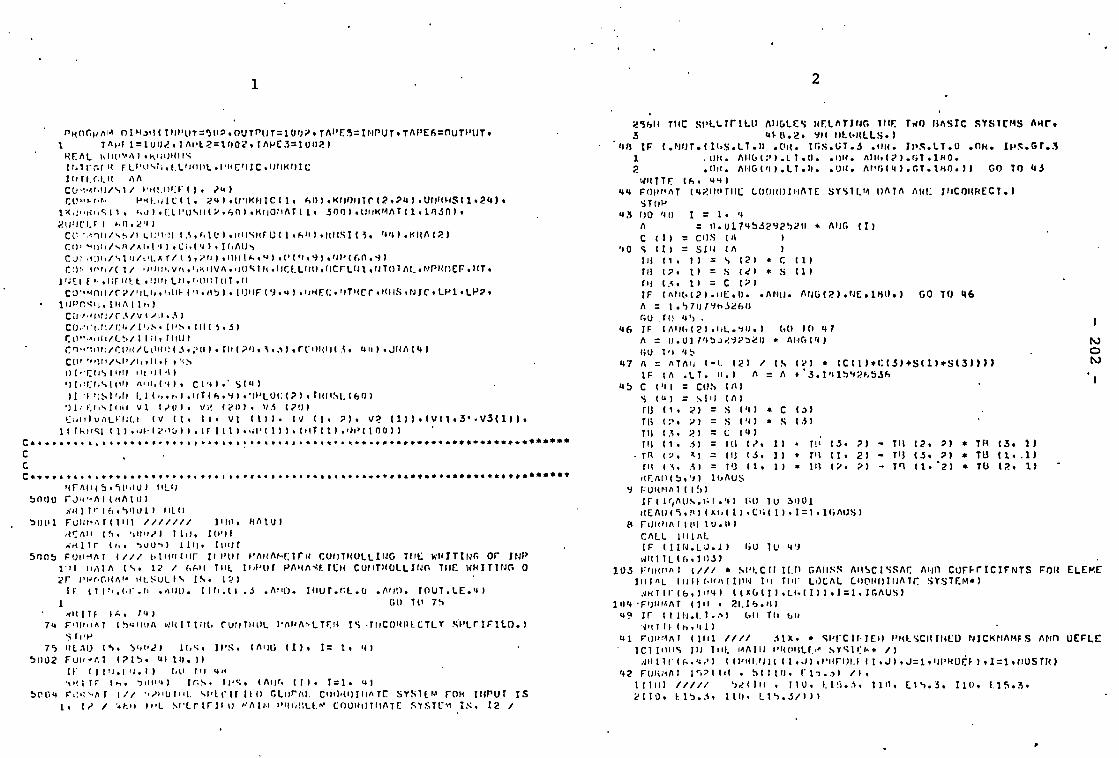
25611 TUC spiLmmo A0GLES RELATING THE TWO BASIC SYSTEMS W. pionHAm 01m.50110POT=502.0UTPOT=1002.TAPES=IMPOT.TAPE6=OUTPUT. 3 41-8.2. 911 01.(•RELS.)

1 7A01=100,!.1Apt2=1002.1APE3=1002) 48 IF 1.00T.(16S.LT.0 .0R. 1GS.UT.3 .00. Ips.LT.0 .0k. IpS.Gr.3 HEAL hoW,Al.K.JoHos 1 .ori. AH6(21.11.0. .011. A06(2).GT.1H0. IN1FrJR FLP0Nti.t.L000L.PHC01C.00KNIC 2 .00. ADG(41.LT.O. .011. APG(4).GT.Im0.1) GO TO 43 I0II,C.L1( AA CU.1.4(0)/s1/ Pt(1.01:1:1). 141 44 gir■T I 71,44V1111.: LOORDI0ATE SYS1LM DATA ARC I000RRECT.)

241.00KNIC(11 AU).KNOIJIC(2.24).UNHMS(1.24).

Lt11 1C1_c i3O•241 43 r0()% I = 1. q s.o).C1P040(2.601.1(110mATII. 5001.(JommAT(1.10511).

A = 0.017453292520 * n11G (I) cu.,1,1/0/fLwp,1(3.F.1(').uuslau(106(1),RusI(3. 441.1(10(2) C (11 = cos (A Cn,'41);1/,./1 /x(,(q).C1.14),I(.AO'l '+0 S (1) = SIN (A C'xo'Al,/,Ou/oLAY/(1.?(I).1011,....4).V('1.9).0P(60.9) III 11. II = 5 (2) • C (1) Car.wh/C1/ ,Inino,o).y,mvA0)()%Tk.IICEL11001CrLIJI.NTOIAL.NPUDEr.11I. TB (2. 1) = S (11 * S (1)

INTAEv.NT0U.uu)LN.r.uNI(.1.1) T4 (3. 1) = C (21 CO'"mnn/C?/110,.1■01- 1,).851.11.111F(9.4).1piECOITI(Ce.RHS.NIC.LPI.LP2. IF (A 1(1(2).11E.0. .AND. ANG(2).NE.180.1 GO TO 46

I01-'1,411.1HA(1.0 CO/ocin/c3/v1..,0.3)

A = 1.',70 B /9h326 GU -r(! 45

C0-*c6t:/c4/1 1,S.IPs.111(5.3) 46 IF (A06(2).01..90.1 60 10 47 CO "..,d1/15/110.1001 A = 0.01745.),A.92510 * Awr,(4) Cn,'Ion/E0R/LORP(3.;u1 ).11(120,3..1).1C040(3. 44).J0A(4) Gu In

47 A = ATAri 12) / (S (2) * tC(1)•C(5)+s(1)*51311)) 01 E10-31u0 utull) IF IA .LT. 0.1 A = A +'3.141542N536 .- 01,1 1:041(01 A.16(41. C(4).' S(4) 45 C (41 = COS (A) 1t 11 1`1'1 ,0 1.1(,.,-0.016.41,'IPLUC(2).TBNSL(60)

vl kr.! (20). vi (20) S (4 ) = SIN tA) 1)3 (1. 2) = S (4) C (a)

k:wulvALF01) (v 11. 111 VI (1)). (v (I. 2). 1J2 (1)).(V(I.3'.V3(1)). TB (p. 2) = S (4) * S 131 (1).,Jp120U».(I1(1).,w(1».(WT(1).01)(100)) TB (3. 2) = C (U)

C TB (I. 61 = III 12. 1) • TIt (3. 2) - TB (2. 2) * TB (3. 1) C - TR (2. 3) = 113 (3. 1) • TB (1. 2) - TB (3. 2) * TB (1..1)

1 11 (A. = 1') (1. 1) * TB (2. 2) - TB (1.2) * TU (2. 1)

BrAN(5.5Pd..)) NLO ==116AUS

5000 rji1-Al(mA10) Irlir,Aus.G1.4) GO lu 3001 ARItr(6.50111) 0E0 REA0(5.$)(xo(I).CGt1),I=1.11;AOS)

01 FouriAt(INI /////// 1 1 10. AA1U) 8 roHNA1(011u.u) tiCAll (5. 14 1 //) 11,1. I(0)( 4,(11r I1.. '),J0-1) lour

5005 Ful1,,4 A1 I/// bloolor pool pAHANLAra COoTHOLLING TILL wi/ITING Or INP 1'11 oAIA Is. 12 / 6AN Till 101,01 PARA,1EIER CU0TBOLLING THE WHITING 0 2r ppr,GRAt, IcisuL15 Is. 12)

Ic (11r..c.r.o .AWD. 110.11.3 .A00. T(IOI.GL.0 .A00. IOUT.LE.4 ) 1 GO TO 75

• 41(11F IA. 741 74 F-011.1x1 (541 01A wHITI06 CU0TROL PAHAr.iTE0 IS 4HCOB11ECTLY

Srop 75 uLAD (5. 5I)Pe) 164. IPS. (A'n (I). I= I. 4)

5002 FuH,P.1 1215. 4(1U.1) IF (110.1U.1) (.0 ('I 4m ARtiF 50041 Ir.S. it's. (Ant. (I). 1=1. 4 )

S004 I// Mq.Cir ILO GLOW/I. COOROTHATE SYSTEM rOH INPUT IS 1, I/ / 11 4C soLcIrtru MAIN 1'116111.1.0 COOMMIATC SYSTC+1 IS. 12 /

CALL (VIAL IF (11N.I.J.1) Gu it' 4o wRIIL(6.103)

105 FORnAI (/// * SVLCIIILD GAUSS ABSCISSAr Aq11 COFFFICIFNTS FOR ELEME 1111)(04 /%11m PI Tor LOCAL COOROINATC SYSTEM*)

ART1F(6.1 114) (0(6(11.1G(1».1=1.1GAUS) 204 -FumAAT (311 • 21.16.0) 49 IF (110.1.1.A) (A) Ti' 61)

P1(11-16.41) 41 ruRmAT (1111 //// 6IX. • SPrCII-1C0 PRISCRIBLE) NICHNAmfS ANn UEFLE

1C1101IS IN 110.. IAA1N 1'ROBLL0 SYS1F.k* /) 1(PRLNI«1.J1WRFDLIII.JI.J=1.0PHOEF).1=1.0USTB)

42 FOl(i'nl (52(111 . 5(110. 11'1.6) /1, 1(1111 ///// 52(111 • 110. 1_15.6. 11 0. 115.3. Illi. L15.3. 2110. E15.3. 11u. L15.3/1)1

sbn ,(Ln1)(S.b00.3) 1,014

5003 rOR,InT 12E1.2) '1') 3,-, 1=1.6 lo 54 J=1 .N

.39 F.1(1..1)=11.0 un/o=1/(11.+NN)•11.-2'.+0N)) 11(1.1)=pn1o11l..-0111 1:111.2)=ph('l.km F111.3)=r1(1.2) U1(2.1)=I 1(1.2) 1-.I(7.?)=L1(1.11 111?.3)=1 F1(3.1)=11(1.3) EI(3.2)=r1(s..5) C1(3.3)=1(1[.11 EI( 4 .41=1,n1 1.(1).5-14.1) 1:)('1.51=t 1(4.4) CI16.+0=11(1 .4) ANITLIG.tiout)

*4001 wydonT (11.1 ////// ill . sq1:SW:11W) 0LNCRAL CLASTICITy MATRIX* /1 .vp-(11 1.1(..4110.'1 IILIII.J).J=1.61.1=1.6)

4002 FO.,•:n1 (111 . .0.1600 II' 1 r IALTSA I 10(1

.1c)11. 1=h(TINO-1 N1=1:11411...Nu0101

ID,.1=(r•o.ii■vn.(N)ilhvr.4.1)/2) Nm.yr.1=1(.Kovn.(ro.c1vA.1)/2) 21,4Fc = lIIUIIIL, • 1 NNrC = 0'

= 0 oLl ,,W=1 IF (IIN.Lo.1.) 60 It' e,1

41'1Is (6. h/) HolLm. Hmt(HEr. nOsTN. moOTOT. IGAUS 6? FUro-nT (/// 7310sprCtrflo tHrkhric DATA. //

1x.41 ,ur•1 1rN II +11..oLol%11 (I:11 4 )= 1, 14/

ul ur tqL1141-1(IN44(.F)=.15/ 21x.6 , umil1N ElFu1q.141( 1 04LNI)=1, I9/ 41X..' (!,111111 of I'u1_NCKTIWA) lArtECTIoo (o014OrF)=*I5/ 511...1.1,,(.:11( or rn,d.(.10,0•14)=.1,-,/

nlx...1l1iIIL o.h.11(1.1-1 or :oh)I ,; roil s114uCioNT(o00101)=*15/ 914...100.1to or 1 1 i•l")lS 1.0(10 11 01.11'1^I (IGnOS) =.I5)

61 ANIIr I,. 63) 14,1I.Avn. IlKIV1I. NuTioo. NC:F.1.01. NT. NTOTAL. 00+4 (VI. 1 )JKNVA1

63 FOldo'n1 (/// 111TCh1N NnTA. // 61)(.*,N,c.:114 10 uluvvi,N v0NIA01.1: Al oIIr I(M('(oOoNVA)=*15/ 71x.+I1I.i414 linwInaL1 Al opt. riN,t(ptitivA)=*15/ 214.*rqr...;1 1 z or LoLo",.. IN f 11fwIF, r,A101XIIIC1LNo)=.15/

'0 COLO • 10 ILooOT ,../111i1X otouS OUr(01.11N1)=*T5/ 4(,(.01 1 )1■1. 01 1N!.NTLS or 10(11p)m or (III: Sf001100r(11T)=*I5/. 51x.0107 ,31. 'I f. ')I InlNlx NLN01 1 0.1, FTQI SOEIITIOU(IITOIAL)=4,15/

61.1(.4c12E OF UHROUwo NATRIX(NONKV1)=*17/ 71x.*st1Z1 OF KNowN 11AI4Ix(NtiNVA1)=.27) IF (IIN.P.1.2) GU To 64 WNTIr I... 3044) L. UN

3004 FO sPLCIFILD LLASTTC mOtIOLH4 (C) =. E13.5 / RoAl 1//// 3,!H 1 3111 s1'EC1r11.1) POISSONS RATIO (ON) L13.5)

64 IF(114017A.G1.24) NO IU 3041 IF(DUNKJA.G1.60) GO 10 6001 GU 10 3(10

3001 W0[11 (1,.300.11 3003 FoRmA1(76HopRot:Imo sloPPE(I 101E TO THE CASE' 0EINO TOO ATG FOR THE 1)

1114FOSI0115 sPLC1111:0.1

301)2 tTI C:1 1;11101: 1tI1CI¢If = U. 00 200 J=1.000T01 RErowl•211111 Tu1.(CC(IIu

2111 FooplAt(110..s(.20.0.31.13.01 Ir(N61lott...fl GO To P02 JJ 1nu I = 1. 3 NJ 1415(' r' = III SISm + ANS (RNSI (I. J)) CD

200 CUNIIHOE L.J GU ro 2 111

202 5411r(6.2041 J 204 1-01(AATIIM+SCoOLNCE LNNON IN ConROINATC OATA AT*Ib)

Stop 203 CoortooL

RIAD 101 T•lp4SrL 10 FUlo4n1(16151

IF (1111.1a.1) 0 10 bA W.(111 (.. 64) oVi(sLL

69 F04061 (/// 5904501CIrILD NUmNI...1( Or ELLmINTS TO wIlICH STRESS IS AP IOLIC;) Is. 14)

60 11-(0pSTL.G1.2) (,I) 10 5001 If (1111 .Lr.i) 6o 10 65 viN51116.70i1 (J.(CroND(I.J1.1=1.31.(NNSTIT.J1.I=1.3),J=1.NOOTOTI

,0,CCIFILD NoNAL COONDINATE Alt!) APPLIED FORCE O 205 F0414nT(1111///*U IATA IN (Or GLoonL 5r511 ,t rIb INVOT ANN Mr MAIN PNOULEM SYSTEM 'IES 21'trIivCiv* // 7x. *Hour*. 1IX. *C9oNn X*. 13X. *r00101 Y*1 13X. *CO 304(0 7*. Itx. oto(*. 10X. 1,1(Y*. 1,4X. $RL, // 50I111 • 4(1o1 ////// .10(1.1 • 14, /1/1

T9. 6E20.3 /).

65 IF (T(.5.1q.1) Gu lu 1+1 ..1 1 ) It J = Is No0101

17 CAIL NTRAHS 111.5. (COW) (1. J). CCORO (24 J). CC0N0 (J. J) ) ill 1F(ooNSLL .Lo.41 No lo 14

HL/1O 15. 101 (N0LUC(1). I=1.NPNSLL) IF (NPl(stL .C.0. 1) Gu 10 14 DU 11 1=P0Ww3LL IFININ.0C(1).LL.00LoC(1-11) GO 10 1.

11 cuotioo)_ II cooLoc(oplo,LL).1.t.010.N) (;o 11) 14

3 3 3 3

00 01 OU (10%/01111301dn'1b1•1-n .019," (1-0v010)101dn**.n*I-h) 11 10 Ill 09 (0 'ml• dl

OU 01 09 tl .141. oV0-1'11 Al 9/ w/ 'IL 0‘3

61 nl nq ill •14-3* (J(. '11(11q) 001 31 T + = List. LL

9L 01 09 lc "-i0' 1001 'mi. S ./.1' n111 31 'l 01 09 Cl *r.1* i0 JI

willn'T=11 InuI 011,94 = 11St

10.1111103 ton? 1/// Int) 1wh10.3 4L

(Vt 'ti) time 01 Ofi (w31111.01.1 •>10" O.-1M*1(1'110mo 11

111114I ' n11 /c1 .01111 iii!/103 euoz 19'0013311./..=r .(r41)3n0n1J) '1I.II1100113 few.? AiImm

willh.1=I Toue! 0(1 ftw0033/13 JO 318010 )./(ION 1S01.11 1r0,41103 3.0101 JOIe N3111 001/ 1S3310N1 FNA'-3131 1091103 110111 3010110141(91 n7 / 1.4311IS1

NIvI1 101 Ill .10001:1 WIss13mia11c4 '1031, '011I /// 11111 1V4003 0002 1000?,9111101,

99 01 09 (4-11.1111111 AI

1(11W113 WJVA 11113 SI --- I0OT 0001 110/L01Th11g onvrll'il

AnnloinD '0 = 0nen.7(41w= (.oen= (a)en

'L = 1/1W=1911(A=IGT)GA=11(1i!A=101)4A= (tilen= (bIcIA= 11cP ,‹31 (oe)en=ff,nen=isnen=tenen= fblen= IvIeh= (i)en= illeA O .11 = 107.1IP=1vI1TA= (P)1A= 1+,11A • 6i = 1611IA=16111A=1/11IA=ICI1TA=11111/1= 1/11/.= 1910= 110l0

= 1G11TA=.1111/1A=11,111A=10111A= (fOtp= (9)TA= (7)1/1.= mu. '0 = 1i.11cA=11I1VA=IIIIIVP= 1h)VP

'1- = (chit 19A ?I +I = dill

'I=(1)VA t.01=I 4 (.fi

L 01 09

'T = 1/?)0=10P1eP=0,e1eAfi

=Ihe16A=11,11eA=1w1101=(I)eA=11,11?A= (Lien= (9)en= (cdepr. (breA

= ibe)crs=(!.e)en= ivw= 191e/N 'c/"1- = (6e)en=(,:e)en= tb)(1A= (()(•A

.1- = le.c1e/1=11$1eP=thi1a9 =ITLI4A=10e1eA=ILI14P=CvlIdA=Ii11?A=Ie114A=111101=10I10%= MCA •

'i/'1 = 111/11A=14?1IA=tI111A=14/1A '4'/"1- = (es)in=cc(.)111=(?1)1n= (c)TA

-1 = (119)10=1,,;,:)(n=oiallnil .1(ce)ln=(04)in=ihnin=t41)1n=0,nin=(ontn= (h)ln= (101P=(/71P

'T- = Ifii:11A=(9?)1e=t4e)TAT =11?11/1=(UT)1A:(L1)1A=110,11A= l4:111/1= It1IA= RATA= 1e1TA= 1111/'

19(1$A- =((e)4A:(.1)0'=(u1)4A=(1114A = (41)4A=1,-.114h=(..71.71,=(111b

.1-1,t• (d 11= 'T = (psi%

el.1=I nu

4* "1 " 11'?"flf-11;1 11 13 c ( I ) r. I ) 0= ( ' [10 .

=4C■1?(,-; On

(..1(=

tr•)41111•11i, I 11 14 T1,,102=1=y4",,11(1:::

11'1:=cr'It110 A.1=n e nn 9.1=1 e 00

n'I=1b•.411n1 =(a.91.10=1L.S)10=19.511n=(0.b)111=19...1 10=(k.v1In=1c.T.IL:::(1,:= I

%Au■•::%:11=::;w11‘ 4/Z

0'0=cw,11,,n"ni we

o'0=tr.11shwhk). vArhnh.1=1. ALS UN )1j...ou.1=1 0/i ou

0=(1'11:Anon), 099 vrio.eol=p (1.-v CC

CVA, :0 .1=r 09.7 °41,

VPmih.1=r 41139 00 .

""n:11:71= (icy

1111=g11.= ueg Tomnr,st=c 00

3 11oIlv111141

3

1014111a,3 fit ciT

o.re • IV 1/11/0 30100 01 W0011 1J11109'4.400ec, 1trii0J 4'1 ( 1 ).011.1(1, ( I 1:10 1,10 (4 1'9) HP. ZT

91 1,1 1..3 I'ATIVP .10 inc. V11.0 101Hh010,i111Vh;10.1 CI

0,(.9)111hy

9

7 8

OSI.t = n

Smlo rop,r1 (10o. ■11.1,0111 no4orit 1A, tS IMO In fI•ITEtt Tlir STTF

6020 r0q,p1 tii, /A. $CALCWAILD LIAO ViCI0I( FOU THIS ELEMENT IN rot: MA

.211 po.:.00 11. 1) = RII■h).11 (1, 11 + 11m51,, (1)

• tr IhPloAL .10. ui NO to HI

• tr o..0m. 1001 .1?. 3) U0 TO 77 74 .4(11r

7n .0111 1.-..3010) 0

tH (I 11v01.11.') .0R. 1t11S1SA.LU.O. 'non. N.NE.MPLMCINLOA01) MO TU 70

1+0Iko. L.40%1100.01

,$U Ti' N

CALL Loom'

CALL LOAM .111 )1. 1 = L. 0CLLm1

IF PI 4/144 oPLot INLoA011 Go 10 14.

IF 111 .111. 11PL0L lo1oAn11 60 10 Pn

.m111 1h..50rot

Mot //I

I it' ■pti t STS ) e; rt11F (h.i0.!1)

31)21 Filo :1 1111R. 4.. &Noll, AL0o6 x+, 111. .roorE AL006 r*. 11X. .ro11[1 A1,006 /*/1 ▪ t A,',0 51) 1qw,..g1111.11.1=1.0c11,011

3(„59 rwd .ptt:t■IA.11g..v» 7U 11 1', ooL tL OlnAn) .A011. 111_OAtl 111)11%LO NOM = NL11AD*1

nj ,110 J=..t...L1Lo0 JAI=J-1 AA=1A0stiL0001.01.0)1

C C coiCK 10 U000.0,,.N NICK wior

C • 170 K=1.0onKvA tr10!.K01111.K).L0.AA) Go 10 130

520 COn(,0Ui C

To C'IEcK Ill K00so NICK 0AuL C

On 7411 1.=1.11rOwA IF1K1.0MC11.L1.11.1.AA) (0) TO

ts4q C0.11 T1101

10.coLcK 10 okr,:c1.1.1t0 01ILLCIToo

'1(1 "3/0 .4=1..40WILF IF1PPL0011.0).1.J.AA) (.11 lo 5/U

560 Cuolt0ot

If 001 t0s11c1 p. uoKotml nIcK NAAL

11.l non '11 7: IF VA

III' 1,44111 I 14■1•11.L ...t.) 1*.t1 ift

,NU COH1111Ur !Of) OutimiC1101M1=EL1100r(WiJ)

.110,01StIoNN)=1(HSRLO(1,0M11 tlY~110Jrs1)=111) ULPINO%;.100111=0 no ro 510

Nbll 11,1X=1:1:=1,1tHMUCU(IodN1) LLP0s1411,J.1)=K rLo11s1it).U411=0 GO II) -)10

511) 1011)111Ct1.1.)=kLuOUP(H.ol

FLvW011,.0011=1 GO 10 5111

5711 IU h10 mA=I.0KoVA 1+1KnotItC11.1,4011,Lio.0) MO to be,

1,111 (III'

WIHM11!..du)=0 LIhl0

5IU E-C:1 11.,=::""1):1 CALL Iro CALL StFto CAIL GrAimS I. LlhoOL(141), 1631 1) CA1L 1-oP1..Ao

1001 COHltuor CALI OACItA11 CAL1 or.root It ttoolo-,0.11 bU tU 72 CALL S1.0.SS CALL STRUM

72 slot' CNn

SUmmuTII ,C IHIAL lhatMit fulim1,1,1(L)IC

r.1 rr 11x1.11.1: Corwow/s1/ 1o1rotrti. 24; Co P.1, 00 pc.t.00Kolctl. No).Korr11r(2.241.00KoS11.94).

IKNollo,(1. ho).1Low,h(,).Got.KnoonT ( i. 3(l0).011K0A111.1o30). 2owcitt (:Ov.o11/s.,/1Loom(3.Niu)0(0Nuo(1.(..1).00si(3 , 44).KPA1?1 co., ..... //1/0o.mvA.movA.00S10.011too.0CLL61.oTUTAL.i.pHOFF.oT.

lArLI • ON IA I Will Lii.;,01,1111 A 1.1!1111 01

Cu”V"ALIliCt I 1 • 0100111 1 1 I 1 • (II( 1)•Li:ICU. (1) 1

C C C

C

C

9 10

c PAittA1oU '!').til Kt01#tl VAItIA/1Lr Alit) UHIVJOWN VARIAPLP C

11opLAPIot4 Al UNk 11HL C C

1.1AO200 oLLLotnIkLL ,NU1.OIHN0DLrtHOSTU.NOWTOT

3Aon K,1'. 4r1 1o.15) Irtw ktt oit .3.0eitostrioit..11

160 In “t IH th11.10.1.L.3 .A110 ,hONUir.1.1.24 .A00.1100T0t.lr.44.AND.MNUM.LC.201

11,11 th

61 Airtr1 ruv...AttlP10A PAHAuttilt 01/10 Hr lltIAL IS 111c,144rCTIA SPrCIPIEN.1 Stc.P

'60 t1C1'LtU=.11itLL4WILLm+1 CALL 1,0111 no tr. = 10 UM! A11)=0

711 111/=n

1:K.u/ti =0 ou 1=10"LLF,a (141 200 J.=.)tuLLLHO AA=1AusttLnou+.1141J))

C F: in (.e/ Is In A 04 It ALottre C

c

Ir It IS HOI 111 A 04 4 Oil PRLNIC sronr IT TN A C

170 on 100 11 2 1, NA4 tvio(N).10.0) 40 TO 14U

160 C01111M0+. 190 Atol=LUTOItItd)

(I TO 22J 200 COOttUUt 720 11(1 2A0 II = 11 ((Alt

111 = UAO + 1- 11 Ir(Af1111,0i.o) (10 1° 240

23(1 MOM' 240 11-(111.ol otounvAl M10012111

00 20 JJ = I. ((Alt trIAIJJI.L1.0) n(JJ1=0

2tiO Marina 00 21.0 N( n 10 MAO KIA1 = hAO + 1 - KR fri4tRx1).14L.0) 1,1) TI) '?l)

.e1,0 C0011HUF 2/0 1i(hk10001KOVAI Nv,'4VA=KK1

UO W.41 1 LL = It 11101 il(LL)=0

280 C001111OL HO COHIIMOI:

111_1000

C00

IV

171

Ou '" K 1. WAO 11- tAIK 1.1 0.,PH) GO 10 100 IF(O(K).F.w.AA) GIJ 10 11U

40 Go to 1:01

100 f\th)=ILTIo0+.II.J) • lu 210

110 GU tv 2to

C C To Cllr CK xotloro N1CKNNAL'Is viquIC IF SU STORE IN H

C 111 00 Ian

ou 140 L=1.wwn.r /FinA.L ,J„p(t.u(ctis.L)) to 140

130 Coillmur :to to Ito

140 oj = 1. unq Ir1,t(14).1 r.or 61) to I6” CoroIropt

11'')

•

'I=F'LurntL(I,,J) G0 In Plo

C

summUTI10: ' ,VOL INTIGLH rt_t4uuL.P0LuIC 1011.1;ER A

1,01.1:11-(1. 24) 24),t0IH111C(1. 60)0(0O0Trt2t24ItUNHIM(1.24)9,

IKI1F,mos11, b01,LL1'osn(p.b0).KOOmAT(1. 300).UOKI1A1(1.1)430). P110CL(1 611.2q)

COR.100/'st/LL000L1.5.+00).ROSOF011.‘,01.10151(3. 44).KKA(2) C0'...1 0/(1/00IIKVA.nhfOIA.00STH.W.XL00.0C1.-.101.0TUTAL.NOODFF.+17.

101.11P'.10-10.1.111t11.0.000101.0 0C11.0, = uttLf:0 -

• 00 1=1.01.1_1.0 drr0(t1.1) 1.1.0001.11.11.1111:00r(1.01.J=.3),IOLCV.(rLOUDECI.J)..J=

1Y4.h(LLIW.5; 1 folw,01(.?014/

fr(1.110161 11.1/.01 .1 .01t.r1.1 0101:(1.1),IIL:111LCK1 GO 10 40 00 J=:.011I00.) A=11.0o0I (I'd) 11 IA.11.1.uh.1I.GI.1.001011 GO 10 70

2 CLNUPLII.L)=Iun.ArK 10141011(1.,L1=HINIII.K) On S n=1.1 OPILII nut=1.Nt.LLA

conrtwl, o no 1 E 1. NDLLO CALL PIOAHS(CURUI1.1).1P)

no OU 7 J=1,5 1)0 7 K = 1. .5

IFIIIinnO III.J1).1Q.1Unt1141) OU IU 4

9.11 Into TK IT. J. KI = O.

3 C 90 L = 1. 3 PO 1<=1 rEln IT , = 71. (10 J. Pt (Jo * Ti' (Le K) L=010K- ) Unort. I 11 .1. I =-LLIm1.1 1 I

1 CONIInnr tr (o .ro. 1) CALL oPLHms JRA. 4, U/

5 C)' IIHOI 11- I (mil 11 (.0 TO 2 CALL ulqn:.5, (3. KRA. 2. II/ CALL hid T•k4S 129 C010 1 plio. III cALL y,R11-s (3. LLPimt(1.1). 1113o 11 2 0.10101 00 It (3

41' ..:4TIL(F..,111) 1ulovi.11-1.1). mUrf.lI.11 511 Fon,...AI(3,010SL:niChLI ERROR I') LLUOOL INPUT DATA AT 4215)

ht) "Om. 7') SUoltrtUTIME LUAU

F01,-.1T(1000101 111 ILIPLnt OR PIO.:SCR114.0 U[FLF'CTfON,I5 ULA. JAC CD 1.1711 IS 'III uF Cn17t.H/S1./x11(4).C11(4I.IhAUS

to to hn co,A,4rn/s1(1/0LArtti.2n)itm(6.9).P(9.4).Nv(611.9) q1AD15.1) (1'ifr11lL(1.11•.plu(41(1.1).1:1.11Plinrr) co,o;.nn/r1/ OnnKVA.nlinVA.110qt11 .1ICILNO.00FLNI.DTMAL.OPIIIIEF.PT. 1

I'ILLLP.OrkLLINt,LLSOIDU101.11 no In 1=1.nrtiNt1 CO'Plon/C3/Vt;?0.3)

C01.D/C4/11,5. 1PNI1DIS,3) A=Pu h lIC(1.11/100 .Q1

40 TO 70 C00,,,01./CWIlOstOUT CW.0,1111/COR/LO1OISOOI.TRI.20.3.6/0CCORDT3, 44T.JRA(4)

II-(A.11.1.01..A.Q1.i) 60 TO 7u convennp..P/4.n.F.r.5 c.n, 111.1JI i)I'-F.FS1Ul1 10011.(hn).DLIHIb1oiR 1 1(3).CL(3)*JAC(313),Dr(4i20),IRHSL(60 'IL Fiji'') C00

1).10(311S1.1t00_(3) L6)IVALrhLr MIII.QPIIII.IInnsLt1/.101SL(1).0P(200)) 90 n I = I. NCLLW1

h Tnn'CL III = o. IF tfIn.LT.5I Gn Ti) 1

soulo.UT114 Lonqn wolli If,. 401 Itiffw.1( 40 rom, At 4211osrit1ss LIM01116 111'U1 DATA role ELFPCNT/ C), n,.1/,a./FLNuNLISo..1n).nosnrntl.F.4).Png1(3. 44I.KPA(2) 1 ,l 11)1- ALL Con SYSI ComPOPCNT Y CuMPUNENT Z CO4PONENT/) CN , AoH/C1/ min4vA.'non/A.nosIK.nctLno.nCILN10110TAL.11PHDEF.ml. 1 KF41)(5.2INVLOC1.31FACI:

2 roP..A1 (P(4, IC (hOL(1(1..4..11) (.1) lo Di.loI.tvOALL.11.1.141.11FACI.I.O.AII GU TO 5n

co....nn/(0o/LLmn(s.21).1'.(1v.%.3).LCo4n(5. 44).00A(4) St, III o:1,‘“ O. IP( 51 FokonT (4)Hon DAToP IS SPIc11-1LN lIiCu'(KECTLY.) )0 I J=1 .."'1.L•• iToP

K=1 'Q N 1.1 .JOLIL ) )/Inf) SC) nO Q L11=1.111ACC nn 1 1=1.3 4CAntS.‘InPLoL1.ICoOL.TSGL.II,L(1),I=1.31

FuRvA1151s.5I11'.4)

CoknII.J)=LL.nwil. 1.) IF 111H.Li.)/ UN Iu S ow:Iwo II. 1) = Q. AQTI1(6.4111LOOL.I‘,"L.I1JL(T).1=1.3/ 11u1l-0,11 L .1).3.1.n) horn 1 4] (JO 1 I.,. I/. 4*. SLL.S.5)

13 14

IF (HPLOCI.NE.N) GO 10 56 IF (ISGL.1.1.1.0)(.ISGL.(,I.6) GO To 56 IFI.NUT.(15GL.Eo.l.ANU.IGS.NE.11) GO TO 42 CALL CTRArs (IGS. GL (1), GL(2). 603))

42 IAConL=IABS(1000L) ISc0,1 1=1cOuL/IACUUE I' (TACoUL.Li.1.01(.1ACoDE.GT.3) GO TO 56

53 00 10ou IGL=1.HHILm IFIIFIxlv(IuL.IACU(1E1).NE.ISCOUE) GU TO 1000 00 10(11 JuL = 1. 3 iv,3L=116L-1)+JUL Ou 10(01 IG = 1. IGAUS DO 1001 JG = I. IGAUS GO To 111.1,!.131.1ACO0E

11 G=1sCODE. H=xGIIG) F=xli(JG) Go To 14

12 H=IScooE G=x6(I(;) F=AG(,' ) GO To 14

13 F=ISr005: G=xI,(I(,) 11=)(G(JG)

14 Ircnr,ILm.Eu.20) GO TU 15 CALL S1IAP32 GU To 16

15 CALL SHAP20 16 DU 17 1=1.3

DO 17 K=1.3 JAc(T,K1=1). IF (IACu('l .NE.. I) GU TO 18 JAC(I.K)=1. GO TO 17

1m 00 71 J = 1. NNELP 23 JAc(r.K)=JAL(14K)+01(I.J)*CORD(K...1)

17 CON1INUE HETm(11=JAC(1.1),,JAC(2.2).JAC(3,3) 11ET.1(21:JAC(1,2)•JACC2.3)+JAC(3.11 OLTs,(3)=JAC(1.3)*JAC(2.1)*JAC(3.2) HE1:444)=JACC3.11 4,JAC(2.2)•JAc(1.31 DETm(5)=JAC(3.2).JACC2.3)*JAC(1.1) OLT,1 (6)=JAL(3.3)4JACI2.1)4JAC(1.2) IF(lAco('L-) 19.21,9.'1

21 AX .m-IF.(,(e)-01:p.14) AY =1ETm(3)-ii(T(s) AL =PCli,(1)-011'11A1 GO TO 22

20 AX =HL1,4(31-OLu4 (1.1 AY :DEIm12)-ULTm(51

AZ ITOETm(1)-0ETH(4) GO TO 22

19 AX =1)E1m(1)-DETM(51 AY :n(TMl21-UET(4161 AZ =DETm(3)-11ETM(41

22 IF (ISGL.GE.31 GU TO 25 CMpT=G.1JGL) GO TO 24

25 CMPT=0. IF (ISGL.EN.31 GU TO 2/ DU 60 1=1.3 TRGL(I)=0. 00 60 J=1.NNELM

60 TR(;LII)=IRGL(I1 40E149.11*CORD(I4J) IPS1 = IPS :Fps = s (ISG. 5) IPS = ISGL - 3 • CALL PTRAHS (TRGLITP)

00 61 K=1.3 TRGL(K1=o. DU 61 J=1.3

61 TRGL(R)=TRbL(K)+T13(UGL1J)*TP(J.K1 00 26 1=1.3

26 CMPT=CMPT 4 LiGL(Il*GL(1) GU In 24

27 DU 2A 1=1.3 28 cmpir.cmpT410(J6-11)*GL(1) • 24 RHSL (KGL) = RHSL (KGL) a. CG (1G) * CG (4G) * DE (4, IGL)

cmpT * SORT (AX * AX • AY * AY 4. AZ * AZ) 1001 CONILNUA: 1000 CONl(N0L 4 CONTINUE

UU 31 1 = 1. NNLLM 00=34(1-1) 1)0 3:1 K=1.3 TRH (K) = U.

30 TKII IK) = THI4 (K) a TR (I. 0. K) * RHSL (OK) On 31 K = 1. 3 KI=JJ4K

3; TRHSL (KI) = TRH (K) RETURN ENO

SUBROUTINE 61RANS (CGS, X. Y. L) A = 0.01745329250 * C = COS (A) S = SIN (A)

15. 16

SUBROUTINE FEm REAL JAC.IJACOVJAC COMI,ON/S6/ELNO0E(3.610).RIISRE0(1.60).RHSI(3. 44)000(2) CONm('N/S8/41,(9).CG(4),IGAUS COmNON/S1U/NEATZ(3.20).01I(6.9).14(4.9).0P(6(1.9)

• CONNInN/E1/ NUNKVA.NKNVA.NOSTRINCELNO.NCELNI.NTOTAL.NPROEF.NT. 1NELLNOWHEL.NNELm.110010T.N CONNON/C00/LORU(3.20)1TR(20.3.3).CCOR0(3. 941).J0A(4) Comm11N/51'/6 eilvr•MS DINF'ISION A13.3).s0(111301.JAC(3.1),IJAC(3.3),0E(4.20) CuolvALENCI (SK(1).LLNOUL(11).(01(1).014(1)) I = (NCELN1 (NCELN1 + 1)) / 2 DO 5 KS=1.I

5 SK(Ks)=0. C C

NUMERICAL INTEGRATION LOOP C

.U0 'not) 1G=1.IGAUS 00 1000 JG=1.IGAUS N, 00 1n00 KG=1.IGAUS C) G=X6(1G1 UD 11=x6(JG) 1=x6(KG) IF(WNLLM.10.211, GO TO 30 CALL SIIAI'32 GO To 31

30 CALL SHAP20 31 coratmuE

C C

foRMATION OF JACOBIAN MATRUX -- JAC C

DO In 1=1.3 00 111 K=1.3 JAC(I.K)=0.0 00 10 J=1.NNELM

10 JAC(I.K)=JAL(I.K)+0L(I.J).4CURU(K.J) C C VALUE OF OUTERAINANT OF JAC -- VJAC C

VJAC=JAC(1.1)*(JAC(2.2)+JAC(3.3)-JAC(2.3)*JAC(3.2))- 1JAC(1.214.(JAC(;?.1)*JAC(3.3)-JAC(2.3)*JAC(3.2))* .2JAC(1.3)*(JAC(2.1)*JAC13.2)-JAC(2.2)+JAC(3.1)) IF(VJAC) 12.11.12

11 ;MITT( (6.13) 13 FouNA1(1H0.21HOLTJ=0 PROGRAM HALTED)

STUD 12 CU/41100E

C C INVERSION OF JACOBIAN 'JAC C

IJAC (1.1)= IJAC(2.2)*JAC(3.3)-JAC(3.2 )*JAC (2.3))/VJAC

R = X X = C T = R • S IF (IGS.L0.2) GO TO 1 A = n.017953292520 * C = Cos (A) S = ,III (A) ▪ = x • S • = y • s • = 0 • C

1 RETU0N ENN

SoRRNUTME P11(A)JS (U. IF') CO"mCN/C14/IGNIIPS.TH(3.3) DIMENSION IP(313)1U0(3).11(3) DO 3 J = 1. .3 00 2 K = 1. 3

2 TP (J. K) = U. 3 TP (J. J) = 1.

(F (1PS.IN.1) GO TO 4 00 5 J = 1. .5 u0 (j) = O. UO 5 K = 1. S

5 UD(J)=u01J)+TB(K.J).4 0(K) IF (A0s100(1)).G1.1.E-35 .OR. A0S(60(2))*GT.1:E-35) GO To THEu = GO TN 9 THEO = ATANe t00 (2). OU (1))

9 C = ENS (IIILU) S = SIN (TH10) IP (1. 1) = C TP 11. 2) = -S TP (2. 1) = S TP (2. 2) = C IF (IPS.Lo.2) GO TO 6 IF (APSIoN13».61.1.E-35) GO TO 10 PHTH = 1.5707963260 GO To 11

-10 PHIO = AlAN (SUM) NO (I) " 2 + uo (2) 4.• 2) / (ID (3)) IF (01110.L1.0.) 01110 = PHIU + 3.1915926536

11 C = CUS (PH1N) S = SIN (('0(11) TP 11. 1) = TP (1. 1) • C TP (2. 1) = If' (2. 1) C VP (3. 1) = -S TI' (1. 3) = IP (2. 7) ♦ S re (2. 3) = -IP 11. 2) • S TP (3. 3) = C

6 RLTuuN EN()

3INONX NI SI 3WVN N3IN .T XIN1Vw NmON14 1113 NI

Y N;

O N)

a

n,

•-•

m,

O

.-.

%c

0

Cl

X..

:L

> Z

: c:

r-

c: L

c, . c;

n 0

c..

c)

.x G

L A

CD c;

n c

::.

.7.

, c_

C_

0 C

; ., .-.

.-.

0L

: 0

0 _

s 0

CD

-7

0 0

C- C

A - 1

CI +

, ■- C

Z C

Z +.

0 •-

• 0 C

) A )

.4 C

D A, C:

4: +

. C7

CZ C

D "L

' 'C -

a NJ .• C.) C: l. AJ h. 0

"3 C

D C7

c i

n c

rs C

C c_

c_

c_ c

_ c-

c-

C- C

- -

..

11 :7

- 1

1

II 11

II

Z7

-• -

- --

if

ii

11 0

II

--

C A

x

> >

> >

> >

> >

-4 I

I r- r- II

. a, 0-• I

I •-■

a. -

4 X

C- N

J m.

V •

-• •

-• '

V AJ

-•

.. .

.. •

-• C

_ C.

Iv

AJ C

m l.

C. N

••

.- .

...

> -

‹ NJ

-(

V NJ

r,

0 r

l In rn 01 r, n

o • c

c_...-z c

7. ...

..-.1•

-• 'V NJ V • V •

-• 7

NJ

V m.

...

m NJ

•-• *

• •

-• ■

-• •

• •

I...

41 .C

.' -I

••••

> ••

A ._

_.

C_ rn N: - - .Q. N.

, 04

0 ' •

a' Z

..7 4

- +

4-

.4 1

C

• •

• C

P L

. 0. 0, 0.

C.

11 --

--

CA

CA

Co N

NJ

N .4

•-•

•-•■•

• 'Z.

--

II

• -■

C

II L

C_

-- .-

- i

0-.

•-•

X C:

X A

X

C_ X

I I

.. .

....

C_

•-•

< C_

7

L r-

C.

O + •

A 3

. 'A

C a, -- r -.

7.; 3

Cl .4

0

X II

.-

...'

.-+

II

Cl m

- ..

m•

II I

I m. NJ II II II II C • II - II II .0 V ,.. .... A)

m+

•.,4 A

i NJ

A

C I

I ..

. •

r

4 7C

m.

-•

I. •

■ *

II m

. .

II I

I II

1-

• •-

• .... = .... ..

. >

r .

. r

•-•

•

ii i 1

t II t-

II

-

- I

- •

t. t

-. -

C

I_ a

: . .

. . . . n

- -

- . . II

II II

II II II II II

• . C-

im•

m,

7C

4.. l-

7 1

.• •

• .

7

"C "7

:. -C

L

. 4

. ,

Z.' C

: ...0

Z .

II Cm II .7 t. ■■ I .-. I ■■ I ■■ 1

:7.. C.

.,_

, I.

m . ... p

+ ...

A.

-4

.4

4- C

• ..-.:

•••••

.- --

. • . . -

•

,-.

Cl •

- r. ...

Cl

I- 0

r-

• C

l >

C_

> L

> C

- >

L

(... 1

.• 3

Z

+ A

r_

CA

N ■

-•

I-

r -

>.

c r

In

> n >

n >

c-) >

- c

..

I; . . .

x

- .-

. .t

x

- n

- r

-1 -

rt

- Cl

C

l "

T

r

DC D

C DC

•■

Cl A.

b-.

--.

A.

.- •

••-•

/.-

. ..

X

3

r -

.,

.- .. .-

.- ...

. . 1...• I■04. No I-.

•

X

•-•

N

+ +

+

•* C

- ,... -

•... . .. . N

.

Ll

• 0

0 0

rl

•

N

-.C

C

f+

r, 7

1 0

r

• -

• -

• ... •

- •

1 •-•

x

x x

.. -

C

_ •

C-

+ C

- •

C-

• C

. Y

-4

-4 -c

C

_ +

>L

>C

_>

L>

C-

...

* h

r•..

I•4

0 A

. In

> I-

1 >

-i >

n >

C

- ••

•■• ....

....

. C_

.-- n- n

- n

- n

Cl

0

CC

C

* >

N

- C

., ..

. L.

....

V .

..m

C

N

14

'. . .

Cl Cl

.. 1.- V . ;.•. Cm

-(

...

m. im.

CI ■■

N .

N .

LA

. L

.: .

-4

r

IS.

....

...

. ..

. ..0

•-•

/V .

- C,

. *-

- W

.. C

AI

oY

* • *

A •

I

•-•

I •-

• I

-- I

•-•

C.

. -C

-Z.

A

0 A

C._

I

C_

I C

. I

C_.

1 ••

•

.... .

... ..

.. --

:.-- -L

>L

>L

> C

- 0

X

C

CC

•Cl

> n

> C

l > :1 >

I-.

s.

NY

.

c

- r

) --

c-1

.-- C

-I

CI

* . 0 x

r."

.%

) - N

, .■ Cm ... V^

X

X X m.

..

. Y. V

•

L4

.

LA

<

.... .

...

A

•-• .

N.1 . •- . Al

0

C.

m• V

■■

m. •

•■ F

. • A)

>

Cl

* •-

• *

•-•

• •-

• •

•-•

Cl

...

L •

C._

• L

• C

_ •

> c_ > c_ > L > C

n>n>n>n>

rn

rn -

. •

-. L

A -

I.,

04 - ✓

•

N3 •

1..

6 N

• +

+

LA •

L.

• C

A C

m C

A

•-■

s.

<" ■■ < < < ms

C. <

C-

< C- 4: C- 4:

C >

C >

C >

Cl

•

>>

> C

l >

n

Cl C

l 0

r r

c z

C-

G •

•

n

t- I C

I 0 n

I-•

• 1

• IA

. .

,C 4

) •

1-• c

C7 0

CC

C: C

: CA

A:

••

N .4

Cr

. Cm

• .-•

ft, .+

•-• C- C_ n

.. ..

.71 ,-

. ,-,

0 a.

.,, ,.

... c

: C

I c:

:: cl rn c:

A el .. X Cd,

(1 A

CI 0

,4 :: o A .

. c:

c_

o >

X

TINY 0 :.1 C: V. TION h. C)

C *

-. r

l 0

0 2: ..

7 0 z

rr c

: z:

rn

o c

A c

A ,A -1 o

r• C

: ..

. :A

-- II il Z: II

II -

■ II II

C: 3

r-

3 3

Cl Z

.. - 3

-4 > 2:

0 -. 7 - -'_

' ...-

^..

.■

•-• II

m- 1-̂ C1 -, .4 44 C- C... ,C PI

rn

.0

c: .7.

..

I,

r"'

X X

C- X

C. r

- I- 7;

C: .4 .. 7 Y

S H

r,.. II r. ..

NJ r-

r- -.

+ 7.

: +

• 0 r-

r 2: 7 -7

<" 1' 0 -.

.., r-

0 7

.-. II

:7:

-.

.. A

0 A

• C

C:

C.

.■

• .: 1: 2 .s

.... :1 c:

77 1:

c:

7C

> C

r . :: z: -- G

l Z7

71

7c c

: Z

Z Z

7 -

cn -

- c_

r1

cg -

. cm

-- r

- C

CC c: c_ .c .. rn CC

-4

C- M-.

2:

'S\

.■

X 2: -4

C: C

: h. 42

..-•

11 .+

C

,d1 C

A rn •

z.-

* •

c_

,..4 ,A 6.

Cl-.

:r (.7. '1 n ..■

Cm

P..

0

+.

rn 71

II

A H

•

m. X C_ > +

... N3 .. m. II 72 22

II -4

Z:

:: :2' :7

h. 7, C■ .

:',

X 2:

II

+ 2: II a.

- X

C_

-Cl

Cl

71 ■•• ■•• .0

r- > rn

v) .- z --

.. C.

II .....

-- N

: +-

I I

- A;

0, .

:c

rn :A

r,

(I Aj

7 "C

72 -

. X . • b-,

• a

C..

• *

• 0

I-.

•■

C' Z

• .

= -

X •

Z r-

•

---• :

..-. .

x c

. :/:

-- cr.

::- . C

• •-•

b.. C. ....

CI C C

- --

• .- ::

rl

.. .

. el

c:

c:

- -

- c

,..-

- --

rr

CA

-4

X

27

* .

---

r-

c: -- -.

--

..

r- •

■ •

- r'

cn .. z z c

. .-.:

z

-n

CA

C:

4- C

A +

■- .

:: 2

-

•

z

-a ..

. -•

N

N

C =

C.

.--

•-

• L

A r

<I"

r^

:::

•-•

C

C

■-•

I-.

0 V

. 1

-. C

.3

> -

--

T •••

•• +

+.

+

^.

,C

2' ..

.. ... . . C

. -.

. 1...

• C

r- I-

4

-- _

.

c4 .

>

CI

I . .•-•

I...

1.0

..

c: X

Cr

2:

-

-1

•-•

A.-

. CZ

C

C

r

0 Z

•-•

•••

• N

•-■

... . N

.

-Z. C

C

-4 <

0

IV 4

L-

C ... •

• A3

r) -I

C

C >

.-•

•...

X

Ns

•■•

•

r r.

-4 •

•

a..

N *

X

Cl

. Z

7.

113

C *

0 +

CI

44.

IT.

I-,

Z C

= -

-• Z

. 0

Cl X

+

3r

Y

:12

.1

2 •

X

X

44

4 -

C

CO

>I-1

-I

- 7

Z

-4

X

-I 3

7

- rl

Z 1

-.

C

0

:02

C. rl

• 0

0

CI

...

...

r

X

Z

•-•

••••

X

••

CI -

• n

..

> 1.

.. o

C

l rn

.

-# .

C.

CA

CA

U.

r os

-•

....

-4

Z.

0

I..

7.

.• 1

-4

C.- • C

Ti

• •

..

C 1

1 Z7

CA

•

>Z

n

=

oz

•-■ r

i rl

LI

0 Z

Z ty

: ,r

I,

••••

0

Cf:

--,-

• Z

I:

•

I-• C

A C

•-•

>

3•

*

C C

I

-4 >

C

X

-

C -

I -.

C

x N

+4 A

c) 4: >.

X..

-4 --

-4 A)

..■ ,C

> . • -C

r- X a• m.

p4

• 7

• •

2

IT :a a. C:

12 .

-.

Oa z

:c 1

12

CA 7

C

2) m

• cI 3C

rn

s- Ca

11

a ...

•

I.•

Z

-4

1%

) •

.0

OTZ

-

19

KN0mATII,IJI=KNOmAT(1.1J)+SKIISI

20

Jij1=hp(1.1qA+J1

bU TO 900 130 CON.1'(mJ1)=OnKmAt(1,111) C . IP1=1+1 C Tn FILL UNCLE ANU UNKMAT WHIN NICKNAME IS AN UNKNOWN ONE 11:(11.1.1.r 1I111IKVA) i0 141 C Du 1.4o I7zIPI.nn0KvA

8111 IF(J2.EN.1) GU 10 831) 1.12=112*(12-1))/2+I Gu lo 04 0

83U UNCLE(11.J1)=uNCLE(11.J1(+811(IS) luo co.4)(hIe)=thirimA1(1,1J21 GO To 900 141 CNDI1Nm.

840 IF(J).GT.11) GO 1u 900 ' C IJ:II16(11-11)/2+J1 C IJR.D11-y Kuum81 MAIRIA UNRAAT41.1J1=UNKmATt1.I.J)+SK(IS) C

9UU CONTINUE IN) 1c0 (4=1.0Ko0A RETURN I19 = (14 • (14 - 1)) / ENI) CmP=comP(141/Comv(11)

00 1,-0) u4=1.14 • 1u4=T12....14

150 KO(o4A1(1,1J4)=KOomAT(1.1J4)-CmP•C1Imm(J4) SURRGUTINU 1-uowAU C REAL KNuPAl.KNORNS C moDIFY 111ICL1 mAlkIX WTL(.I:R ILPusD,UNKNIC.ELNOUE C INTEr.LR COPIWE 00 1‘,0 15=1,141NKVA C0Ivo1/S1/ PREDLF(1. 24) COmmoN pio.Dic(1. 24),UNKNIC(1. 60)IKNONIC(2.24) ,UNRHS(1924). MIS=1N+IIIMV4

1KDoRns(1. 601.LLvUSN(2,6o).KNOMAT(1, 300).UNKMAT(1.1830). CPIP=C0.41 ,1)/CD1w(11) 2U%CLE( 60.d.4) I))) 11.0 Jh=1.NrcovA

COr4moN/LLNUDL8.4.10).RIISRF0(1.60).RDSI(3. 44).KKA(2) 1#10 DNCLI(ItI.Dt)(=NuCLL(15.J5,-CmRsCW-P(.1.11 Cu,,(100/s10/uLxyz(3.20).u0(6,9).0(9,9).UP(60.91 C Cu•Ponn/C1/ NuNilvG,IIKNvA.NUsTR.NCELNU.NCELN1.NTOTALINPROEF.NT1 C . pu,DIVY 111,K14/11 .AA11t0( •

1;IELL'..NFREL.DIJILm.nu11181.N C Cwi-lou/c.)/(ILG.Duv(9.#15(.inuF(9.4).NRCC.NTREc.RNS.N/C,LP1ILP2. 00 I7o IA=l•11mIKVn

INvoYi.IHA(1( Cowil(R41

113 (1k * (14 - 11/ / 2 mib=lboivioim

ENDIvALLNCLICUM,(1),NP(1)) CmP=cOmPW0-1/LUmV(111 • c I))) 11U J6=1.16

C RnoT(ni MUuIF. YIdC, LLEJALDTS IN MAIN MATRIX FOR A COMPLETED AJA=J6+1IFOIVA

C unKNOwN NILKNAML 1.),,=1164aP. 170 QnKrA1(1.14t,I=o)1KMAI(1,1.1h)-Cmm•LOm14mJ6)

C C C

DU ino ((•=1.NCELN1 IF(EL100L(N.Im.1).0.0) GU TO 101 cu 10 1110

101 1=ELposn(1,1m) • IF(LLP0Sn (2.1m).10.1) GO To 210

STDRING Com(JIAILO RoW IN AN AUXILIARY ROW MATRIX -- COMP--

110 11=1444K(0,0 Ill = (1 - 1» / 2 NO 120 J=1.11K0vA

120 C(P4P(J)=UNCLE(1,4) Du 13)) J1=1.1 1J1=111+.11

C C 141 U:0SL IMIAr10).1 NV00. C

90 97u J=1..11ovA 420'ONCLI (1.,()=0.0

OU 440 J1=1.1 IJ)=1114J1

430 u0Kr1.1(1,(.11)=11 .0 IF(11,1.10.000avA) (,() In 441 00 '140 (;%=1PL.'101 1 e(VA IJi=114, (1.,-1»/e4(

440 qi4K0A1(1.1J.?/=11.0 441 Co011001'

0

2

2

CV

g

l

•47

I-.

0

2

2

AI

N

.(

0

0

e-1 .4

4.1 1 44

1.-1

LJ

U 4

4

01

.10

1J

4.3

Ll

• L

I

O

Ll

•

LI

O TERMS or

O

O

- 212

•

CV 2

3

.

•

-4

LL •

tJ

0

O

.

X .J

•••

0.

•

4-1 •-•

1J

Cr•

.7

:•

• •

4.1 (/)

Li

I-

:II •

0

0

6-• x

.

0

-

V 1-

1

J <

0

C ▪

O

2 2

X

X

U.

U

0

•-• •

C

V)

2

M

I-

V 1-

1

J <

0

C

O

2 2

X

X

U.

U

0

•-• C

V)

3. .. v.,

2.

:,- 3f

Li

O

o x

1-

44 5 4,

I x •-• •

••-•

-

3

77

:"as

3

2

_I

•-• L

:7

5

Z.

.

0

. -•

•-o

A

l

U

... U

.1-1 ..r.

L.'

.4

NI

._.

.... L

I -1

3

-1

3

3

'1

3

.... .

V

NI

D. L

i .

1-

,...1 <

.... ..-4

U.

....1 •

... 0

r_

••• 1.-

3 4

. . I.-

<

"") ..%

.-1

... <

:./1 3

2

..I

3 ....1

.-• 2

O

..1

5N

.40

4

) 3

.4

0-4

..

••• •-•• ••• .4

3 =

<

2

0

L

I -I

•-• •

0

J

X N

. •-• • .4

X

-

.2 0

•-• 7

. 7

I- •-• . .7

5

' =

=

a

<

1

_ N

4

-- a

1

7._ -

• 6

- o

7-

-

W 2

.

*4 •-•

2.

• •-• 5 o

•

m

2. x "...

< 1

1 •-••

!-.: • •-• <

I 1

5

-J

•

LI

= • • •

-0

.4 =

2:2

5

il ..-:.•

C,

- .1

I ••• 5

3

•-• . 7

: -

•

3

2

IJ 3

2

. /C

..4 •-• -N1

".

... 7. •

11

•

I1 A

II

.i. J

- •

'3 --, >

L

I 1

. 1 :..-

N U

.4'7

11

- -- .. --

--• •-•

:.r) 3

. .••• . >

X •

-•

--* ''-''

. .

5 -

):::

... "'V

.7 -7

.... -..

-

.

5 tr, 2 =

-..., :: u II

1. • 11

C P

. *4

.4

L

I 0

1 II .4

< •

-, <

e

` II

•-•

< •

•

5

II • 1

1 .4

V. :n

..L.

I-

2 ■

P.. •

-• X

X •

. 4

4

. 0

2 . Z

".. • •

-• -

. -1

II • 2

2

h

•-•

11

•

=

•os, 0

- •

... 7

-- 0 ^

, 4

. U

. c

<

a. v

v V

. ._. v

. ••

-•

•-• v

. CI:

- 7

a

-

- • - .1

.-1

•-• 3 `''' ••:

.■

2 3

a. a

. 0 3

*-1

5 1

r: •-1

• .. f

t.

Z

... .4

1- 2

*

.4 .1

.. 3

2

.1

2 2

.--

2

- .4 •

-•

O

<5

....1-/1

1 2

0

'<

==

■.=

=:A

./1

1

U

3 3

.. 3

... ." •

•••• lj

0

• = •■

■ .. 1

••• 3

r-7

: Y 7

-

p-

*- .r L

.- I... :: C

1

15

X

V7

...1

15

..7

.4

C

Cl-

-N

. -4-G

•

I-

•-•--<

Lf.

L.

.-

CO si ti II ti

.1).

....1 I.

•C 1

1 .4

= . 1

1 x

5

' 3

.=

1-

5. /1

1

1 N

11 1

V)

11 2 11 :... X

V) f., 11 a ...,

1,...: .../: •-• (N. =J

V

x

5_ 5

= 3

I

.4

... /... C-

.4

CN

. : 0

I' , U

..., - a :..•_ 3. <

55020-S

S0

2

50

.0

->

3.7

1.4

. 1

77

0

2

0

. 0

-7

=

Y -1

J

r U

.2

20

33

7:X

Y.

Z 0

1•

4 0 . 4

4 1

•••

•-• 3 •-o

U Y

0

r U

=

3. .. v.,

2.

:,- 3f

Li

O

o x

1-

44 5 4,

I x •-• •

••-•

-

3

77

:"as

3

2

_I

•-• L

:7

5

Z.

.

0

. -•

•-o

A

l

U

... U

.1-1 ..r.

L.'

.4

NI

._.

.... L

I -1

3

-1

3

3

'1

3

.... .

V

NI

D. L

i .

1-

,...1 <

.... ..-4

U.

....1 •

... 0

r_

••• 1.-

3 4

. . I.-

<

"") ..%

.-1

... <

:./1 3

2

..I

3 ....1

.-• 2

O

..1

5N

.40

4

) 3

.4

0-4

..

••• •-•• ••• .4

3 =

<

2

0

L

I -I

•-• •

0

J

X N

. •-• • .4

X

-

.2 0

•-• 7

. 7

I- •-• . .7

5

' =

=

a

<

1

_ N

4

-- a

1

7._ -

• 6

- o

7-

-

W 2

.

*4 •-•

2.

• •-• 5 o

•

m

2. x "...

< 1

1 •-••

!-.: • •-• <

I 1

5

-J

•

LI

= • • •

-0

.4 =

2:2

5

il ..-:.•

C,

- .1

I ••• 5

3

•-• . 7

: -

•

3

2

IJ 3

2

. /C

..4 •-• -N1

".

... 7. •

11

•

I1 A

II

.i. J

- •

'3 --, >

L

I 1

. 1 :..-

N U

.4'7

11

- -- .. --

--• •-•

:.r) 3

. .••• . >

X •

-•

--* ''-''

. .

5 -

):::

... "'V

.7 -7

.... -..

-

.

5 tr, 2 =

-..., :: u II

1. • 11

C P

. *4

.4

L

I 0

1 II .4

< •

-, <

e

` II

•-•

< •

•

5

II • 1

1 .4

V. :n

..L.

I-

2 ■

P.. •

-• X

X •

. 4

4

. 0

2 . Z

".. • •

-• -

. -1

II • 2

2

h

•-•

11

•

=

•os, 0

- •

... 7

-- 0 ^

, 4

. U

. c

<

a. v

v V

. ._. v

. ••

-•

•-• v

. CI:

- 7

a

-

- • - .1

.-1

•-• 3 `''' ••:

.■

2 3

a. a

. 0 3

*-1

5 1

r: •-1

• .. f

t.

Z

... .4

1- 2

*

.4 .1

.. 3

2

.1

2 2

.--

2

- .4 •

-•

0

<5

....1-/1

1 2

0

'<

==

■.=

=:A

./1

1

U

3 3

.. 3

... ." •

•••• lj

0

• = •■

■ .. 1

••• 3

r-7

: Y 7

-

p-

*- .r L

.- I... :: C

1

15

X

V7

...1

15

..7

.4

C

Cl-

-N

. -4-G

•

I-

•-•--<

Lf.

L.

.-

CO si ti II ti

.1).

....1 I.

•C 1

1 .4

= . 1

1 x

5

' 3

.=

1-

5. /1

1

1 N

11 1

V)

11 2 11 :... X

V) f., 11 a ...,

1,...: .../: •-• (N. =J

V

x

5_ 5

= 3

I

.4

... /... C-

.4

CN

. : 0

I' , U

..., - a :..•_ 3. <

55020-S

S0

2

50

.0

->

3.7

1.4

. 1

77

0

2

0

. 0

-7

=

Y -1

J

r U

.2

20

33

7:X

Y.

Z 0

1•

4 0 . 4

4 1

•••

•-• 3 •-o

U Y

0

r U

=

0 0

0

C

.2

a

r.

• .c

0

7,

.4

N

./

a

.r, 6

. .

N N

N

CV N

0 0

0

C

.2

a

r.

• .c

0

7,

.4

N

./

a

.r, 6

. .

N N

N

CV N

IN A MATER AREA

17)ftCOMPI I7PARNK

C

44

U

44

44

LI

44

U

44

44

LI

- 2

- -

'7- 0

-5

2Z

OL

DL

L_

I<

DW

Z

70

.3

L

i 0 C

. U

1

.

0 . 2

4

_, 7

C

o 7 X

2Y -4

21- 2

U

1X

3U

.40

.2

04

42

W

00

02

0

7

6-1

I-

U U

U

UU

UU

U

U U

U

U U

-• I-

)'-cc C

6-1 X

3

C

•

.4

U U

U

UU

UU

U

U U

U

U U

23.

UIftENS1011 ComP(84 ) EQUIVALENCLICDMP(1).0P(1))

C C RoOTINE iN WHICH THL ROW cORROSVONOING TO THE COMPLETED C VARIAVLL IS STUULO IN A DUFFER AREA C

If (NRIC.NL.0.0R.NLG.NL.0) GO TO 3 CALL uP).Nms(1.1)(A.1(... .0)

3 IFINL(•.4E..0) GU 10 2 OLF.=-T.LT; Go TO 10

2 NLG=NLG■1 DO 1 1=1.NTUTAL

1 OUF(NLG.I)=LoAp(1) OuF(11LG.NTRLC) = RHS I:ior(111.G.1)=L1'1 ToilF(NLG.2)=Lm2 1,3'11- 04LT...5)=01C Ioor(NLG.4)=NpusN

) GO TO 10 GO To 2o

10 NREC=NRLC+1 CALL wRITMS(1.NLGIG02.6REC) NLI;=1,

2u CONTINUE RETuRN Coo

sullwnOTINE uACW.40 RLAL KNORHS INTLGER PRENIC.uNKNIC C0•4mON/S1/ PRE0L1-(1. 24 ) (;01":40N PRINIC(1. 24).UNKNIC(1.M1).KNON/C(2.24).LINRHS(1.24). 1K1g1ROS(1. f,u).ELPusN(2.A0).KNOmAT(1. 300).UNKMAT(1.1)T30). 2UNCLEA 60.141 covAnN/N6/LLNOuL(3.A101.RHSRED(1.60).RHSI(3. 44).KRA)2) CUmmoN/s10/oLATC(3.20).0o(6.4).M(9.9).0P(60,9) cu.14on/c1/ oo1IKvA.NKNvA.NOSTR.DCILNO.UCKLN1.NTOTAL.NPROEF.NT.

1,1FLEm.rirpF.Lolw.L1o:1)n11)1.1) ( #3 ) ( 9 • .NNEc . 11 mu: •tiiiso,nc Lp2. .LP2.

INPos:i.IRA(10) co,,4owc.,,111). Tour OPAENS1 op 1)21132 1 .co(1),(84 ) EoUIVALENCL (t)( I) .RNSI ( 1 ) 1•( COmP ( 1) .UP ( 1 ) )

C C

INITIALIsAlION C

K = IF (IUUT.LT.6) GU TO 3

24

WR/TT(k.2) 2 FURmAI (1111 //// 111 • *CALCULATLO REACTIONS IN THE MAIN PROBLEM • ISTSTEM*/) 3 OU 202 I=1.111iNVA

DO 202 J=1.2. 2U2 KNONIC(J.I)=0

00 2113 1=1.o0NRVA 203 ORRNTC(1.1)=0

00 1 m=1.11011RvA 1 KNuRoS(1.14)=0.0 DO 2n m1=1.or 02(141)=0.0

20 CONTINUE C C READ RACK THE STUgED DATA IN RLOCKS IN A REVERSED ORDER ' C

NREC1=NREC U0 10 L=1.NRIC1 NREC=NREE1-L+1 CALL REA04St1.11LG.802.NREC) LG=NLG

300 00 4 1=1.NT01AL 4 EOmP(1)=RNFILG.1) RHS=001(1GINTRLC) LP1=TONE(L1-.1) LP2=111W-(Lb.21 NIC=1RUF(LG.3) NVosw=luNF(LG.4) LO=LG-1

• C C CHECK wHLTHER rN1C IS IN KNONIC C

IF(Lp2.NE.1i GO TO 14U C C rF FNIC IS IN KNONIC MULTIPLY KNOmAT WITH PREDEF C

ANS1=0.0 KNONIC(1.L!'1)=NIC KNONTC(2.LPI)=NPOsN 00 120 12=11miNvA NPosr1=1.40(lN1L(2.12) IF(opOSN.Cw.0) Go TU 120

. ANs1=Ansi+ComP(12),WREOEF(1.NPOS)J) 120 CONTINUE

C C foEN moLIIPLY ONCLL with 1.11040EF NOW STORED IN KNOWN RHS C

ANS2=0.0 DO 130 16=1.NuNKVA M13=T3+NRNVA

130 ANS2=AW+COM1'(M13)*KNURHS(1.13)

25 • 26

C C F100101, loL LOR100,0001N(. U0R1tod4 REACIInN C'

A0t:=A0s141111,!...illis

IF 1100I.LI.A) (.o 10 7110 tr l'oo(k.Se1.)u.0 ,AND. 11011.0) xRITE (6. 5) Fou-e%1 1101 ////)

h • 1 „mil! 0„10,101

1000 F11( zA7(1,10 IwALiln0 AT N01 )F .17 .?x.51) TS .1.11+.0) GO In e00

C T0 FIND !NI. uNIVRImN OLIL IF nut.: I', WIT IU )(NON%

Att.,' 1 100 IIIc low 11 nccwirs nnlanG rougAku rtAminArron 140 unlAnt('t.o41)=.,1r.

Ims=15-1 IPs=I')+1 Ius=1.)..11ovn

C. C

ILL Is "0LIIPLIEP r,i lit KNOwN 01sOLACEvINTs C

110s1=0.1,

Nu 170 1'.=1.01NvA 000s1.=m11•ilL(e.161 Ir1 1.00So.)u.01 (,u To 1/u no,.t=n0.1)(.0:*011k1WRIPLU11.0ooSNI

170 C001thOr

C 01.K.IAt Is mUr1"11)0 41 T11 UNKHowN 01sPL 1'04 KNOwN Anr STONED L 1,1 LvCr.Vi 10) 010t,00AL ILRm C

ANs/=0.0 NN IN In1

Du lqu

leo A1J,....)=An17.c0,11,trot7)4inqHm..t1.t7) 141 A ik.S=0,,u

IF (I0s.r.r. m0hvA) lo oo /”..7ws.000,4%,/.

I"u .10,..5=ANN1.(0,.10(t.)).).K0040,;(1,14) 11"1 COhlthDr.

C C

uoK ,ow0 PISPLACk ,HITS

sPr4t1.-7.whols(1.1'1) JJ=.■It It

101 J = I t(I.P • t 1J-1 411

02(J)=UNDErL 200 1F(LG.NE.0) GO TO 300 ' 10 CONTINUE

DO 430 j=1.1 11ROLF. ucrL=PREorr(1,u) NIC=PREUICII1J/ JK = NIC/lUu II = HIC-OR 100 JJ = NFREE*(JK-1)+IT

441 1)2(JJ)=1LFL 430 CONTINUE

RETURN END

SURRNUT/NE UEFOUr COMPION/S6/ELNO0E(3ob10).RHSRLO(1.60)01tHS/(3. 44).KNA12/ CO.AmNN/C1/ NUIIKVA.IIKNVA.NOSTM.NCELNO.NCELN1.NTOTALINPROEFINT.

1NELE1-',I1JF1ILL.NNILM.NUOTOT.N DIRL0S1ON 11(132) EUNIVALENCLIU2(1)14NSIIIII 41411E16,P/

2 FORmAl (1111 /// 100. 1X. 0414THE NODAL DISPLACEMENT SOLUTION OF- 1THF ST1FFHLSS LNUATION IN THE (MIN Ptinntxm sysrcki lno. 11X. *NODE 2.1 7Y. *DINPL ALONG X*. 7X. *OISPL ALONG Y*. 7X. *UISPL ALONG Z*/) MPRINI= 50) UO 1 JJ=1.NuUTOT J=OFRCE•IJJ-1/4-1 IF(mPRINI.U1.0) Gu TO 4 will IE. (6. 51

5 FOR0A1 (101 /////) mORINT = 5U

4 mpRITIT=M1'RINI-1 4RITI(6.31 JJ.112IJI.U2(J+1).U2IJs2)

3 Fol0AAT(I16,3(4X1E16.8)) RETURN END

SUNR0UTI1TE. SIRESS (;;I R ELNDOC •

PRLNICII. 24/•UNKNICt1. 60),KNONIC(2•24).UNRHS(1•24). 1KNORHS(I, 60).ELPUSN(2.60),KNOMAT(lo 300).U0KMAT(1.1830).

21==rt!LDE(3.610).HHSIWO(1.60).HUSI(3. 44).KHA(2) COMmON/S1Q/UCXYL(3,20).Ulith.4).1,(9,9),01(60,9) ComloN/Cl/ WINKVA.PRIIVA.NOSTR.NCELNOINGELNI,NTOTAL,NPROEF•NT,

11JELLm,NFOLL.NNLLM.WOU101.14 CONM('N/C3/VIPU.3)

27 28

COMmO11/COR/LoR0(3.20)1IR(20.3.3).CCORD(3. 44).JRA(4) CONwtorasP/G.H.F.NS ifALr)SIOt1 C thu ) (6) • STG( 3.3) .S TGT( 3•31 .SL ( 3.3) DIrENSIon ouIV(44).U2(132) DIOnsiOn S1SS(44.6). DUI (6.60) EonIvALENCEASTSS(1).ODKmAT(1)).(DrIT(1).0P(150)).(NDIV(1).CCORD(1)) 1.012(1).w.51(1)).(C(1).RHSRED(1)) DO 52 1=1.N0DTOT NDIv(1)=0 DO 52 J=1.b

52 STSS(L.J) = 0. 00 2n LL=1.11LLEM CALL READmS (2. LoRU(1.1). 240. LL) DO 30 K=2.oLLLI10 NIC=IABSIELNODEILL.K)) JK=NIC/100 II=D1C-JK • 1111) JJ=U1(CE*(JK-1)+11 )0../=K-1 C(KMT):02(JJ)

30 CON1INUE nO 650 MS=1.NNELM CALL FLN1 2 DU 630 I=1.6 STRI1)=0.0 Du 630 R=1.nCELN1

b30 STR())=sTu(1)+OUT(I.K),C(K) ST(;(7.1)=STR(1) ST6(1.2)=5TR(6) ST6(1.3)=Sfl(!) Sf6(2.1)=StR(6) S10(2.2)=sTR(2) SI6(2.3)=SIR(4) STG(3.1)=S1R(5) STG13,21=s1R(4) sTG(3.3)=sTRl4) DO 201 1=1.3 00 201 J=1.3 SIGT(I.0)=0.0 DJ 201 K=1.6

201 SIGT(I.J)=SIGT(1.J)+STG(1.K)*TH(MS.R...1) 00 202 J=1.3 DO 202 L=J..5 SL(O.L)=0.0 DO 202 K=1.6

202 SL(J.L)=sL(J.L)+TR(MS.K.J)*STGT(K.L) SIR(1)=SL(1.1) STR(2)=SL(2.2) STR(3)=sL(3.3) SIR(4)=SL(L6)

. STH(5)=SL(1.3) STP(6)=SL11.2) NODE=1AdS(ELDODULL13$MS-1))/1 00

NOIV(NODU)=NOIVtNUVE)+1 DO Si K=1.6

51 STSSiNONEIK) = STSS(NUUE,K) + STI( (K) IF(LLNUNECLL,3•MS.-11.E.U) GO TO 650 00 53 K=1.6

53 STsSINODE.K)=SISslouDL.K)/FLOAT(NDIV(NOOL)) 650 CunTINuE 20 CONTINuE

RETURN END

SUHHoUTInE 1-CM2 REAL JAC.IJAC cumr,:dasi oiur.AYL t 3 20 ) .1.)H(6 .9) •P( 91 9 UN )

N(1NKVA.IIKNVA.NUSTk.NCELr10.NCLLNI•NTOTAL•NPk0EF•NT. 1NCLEm.oFRLE.DDLLm.NODTUT.N COv.ION/C3/V(20.3) COmil0o/cuR/LoRD(3.20).TR(20.3.3).CCORD(3. 44),JkA(4) COM,,,(4/S1'/G.H.F.mS Ui

DImEnSIoN 01(1(6,60).00(6.60).A(A.3).JAC(A.3),IJAC(3.3).DE(4.20) EuulvALCDCL(OL(1).01)(1)).(1)1((1).0(17(1).UP(150)) • 6 = V (MS. 1) II = V IRS. 2) F = V (RS. i) IF (NNELm .L(J. 20) GO TO 30 CALL SHAP32 GO To 31

30 CALL S1IAP20 31 CONTINUE

C C FORMATION Or JACOBIAN RATRUX -- JAC C

UN 10 1=1.3 UU 10 K=1.3 JAClIsK)=0.0 DO 10 J=1.WALLm

10 JACII.K)=.JAC(I.K)+0E(I.J),PCORD(KIJ) C C

VALUE: OF DETERMINANT OF JAC -- VJAC C

VJAC=JAC(1.1)*(JAC(2.2)*JAC(3.3)-JAC(2.3)*JAC(3.2))- 1JAC(1.2)*(JAC(2.1)*JAC(3.3)-JAC(2.3)*JAC(3.1))... 2JAC(1.3)*(JAC(2.1).JAC(3.2)-JAC(2.2)•JAC(3.1)) IF(vJAC) 12.11.12

11 WRITE (6.13) 13 FORmAT(1110.:21HULTO=U PROGRAM HALTED)

VJAC=.1L-25 12 CONTINUE

•

INVERSION OF JACOMAN IJAC

IJAC (111 )=IJAC ( 2.2)*JAC(3.3)•JACI3.2)*JAC(2.3) )/VJAC IJAC(1.2)=- IJACt1.21•JAC(3.3)-JAC(3.2)*JAC(1.3))/VJAC IJAC(1.3)=1JAC(1.2)*JAEl2.3)-JAC(2.2)*JACt1.3))/VJAC IJAC12.1)=-tJAC(2.1).JAC(3.3)-JAC(3.1) ,JAC(2.3))/VJAC IJAC(2.2)=tJACt1.1)*JAC(3.3)-JAE(3.1)*JAC(1.3))/VJAC IJAC(2.i)=-(JAE(1.1).JAC(2.3)-JAC(2.1).JACt1.311/VJAC IJACt3.11=tJAC(2.1)*JAC(3.2)-JAC(2.2)•JACt3.11)/VJAC /JACt3.21=-WAC(1.1) 4JACt3.21-JAC(1.2)*JAC(3.1))/vJAE IJAC(3.3)=IJAE(1.1) , JAE(2.2)-JAE(2.1)*JAC(1.2))/vJAC 00 2n J=I.3 Uu 20 L=1.NNLL1 0ExTz(J.Lt=u.0 OU 20 K=1.3

20 NExr/(J.L)=DExYZ(J.L)+IJAC(J.K).DECK.L) OU 21 I=1.m 00 21 J=1.DLL011

21 00(1.J)=(1.0 nu 22 K.7.1.111,LLm K1=3.0.-2 K 2-3.K-1 K3=3.K 00 22 I=1.6 DO 22 J=1.3 J1=J+3 J27.J.6 • 01111.K1)=DDII.K1)en11(/.J) ,0EXY2tJ.K) 011(1.K2)=DD(1.K2)+011(1.J1)*DEXY2(J.K) 011(1.14 3)=OLIII.K3)+DD(1.J2140EXIL(J.K)

22 CUOVJUE 'JO 102 L = 1. NNELM J2 = 3 • L - 3 Ou IPI I = 1. 6 UU 1111 K = 1. A (I. K) = U. no 101 J = 1. 3 J1 = J2 • J

101 A It. K) = A (I. K) + DU (I. J1) • (II IL. J. K) DU 102 I = 1. A 00 1(12 J = 1. 3 J1 = J2 + J OBr tl. J1) = A (I. J)

102 CON-fit:DE RETuRN EN0

SunRnurinc SHAP2U EOMmON/SIU/UEXTZ(3.20).0N(A.9).P(9.9).UP(5U.9) COMPInD/SP/G.11.F.t.is OI' ENstun ULt4.2111 ENOIVALENCE101.111,01)(1)) GP1=1.+G

1041=1.-11 HP1=1.+D FPI=1.+F Fm1=1.-F G2P11=2...G+N G2m11=2.+G-11 112or=2...H+F N2m1:2.*D-F F21,0=2.4:4.6 F2mGr.7...F-U HI=HD1*FD1 112=Dp1.Fpl 113=11m10-m1 tin=Dr1.- FM1 G1=1*Fpl G2=6P1..FP1 (13=WA1.Fm1 64=GD1*Fml GS=Uml*H(41 G6=6m1.1.D1 67=G11 1.111,1 Gn=(ipl•DM1 01.(1.1)=0.1;!5*H1*(G2PH+FM1) 0E(1,2)=-0.25*111,1*111 DE(k.3)=0.125*D2*(G2M11+FM1) OL(1.4)=-o.5*G012 0E(1.5)=u.12(62141-FM1)+H2 DE(1.6)=-1.111.2) 0E11.7)=0.1254 (U2MH-FM1)*N1

DE(1.9)=-U.2514M1*111 NE(1.10)=-o.25*Fm1012 DE(1.11)=-0L(1.20) OCt1.121=-DLt101 01(1.13)=0.125.(621'11•FP1)+113 01.(1.14)=-u.2t).D6,1013 DE(1.15)=0.125stA2No..1-1)11044 DE(1.16)=-0.5 ,6 4014 01(1.171=0.1254.(G21'11-1-P1)..114 DE(1.1u)=-Dt.t1.141 DE(1.191=u.12')4tb2R41t-FP114.113 0E(1.2(l)=-u.5..G.D3 01(2.1)=0.125*t6P14D2m1) ,G1 DE(2.2)=-0.5*11.01

31 32

UE(2.3)=0.1541 (H2FT-GP1)*G1 DE(2.4 )=0.2 4,uwl*G1 DE(2.51=0.125*(1121T-Gml)*G2

UE(2.7)=0.1,e5*(o2mF+GM1)*G2 nEt2.(+)=-OE12.4 ) 0E(2.9)=-u.25*Fol*G1 OE(2.10)=-oLl2.9) DE(2,111=1).25ipm1.G2 OE12.12)=-1)tt2.11) UE(2.13)=u.125•to?PF*GP1),G3 DE12.141=-U.5.(.G3 0112.15)=u.lt5*(12oF-W-1 1)*G3 OE(2.1A)=0.2!)“,o1•63 01(2.171=0.12').(ooF-GM1)*G4 11E(2. (0)=-U.5•'1•(,4 DE(2.19)=0.12(112Pf+Gm1)*G4 oL12,2v)=-HL(2.16) Utti.1)=0.125*(12mG-O)'11 ,0 65 OL(3.2)=0.21eifi,1 4, G5 DEt.i.3)=0.1etls(12,,(,-Omlf*C6

DL1.5.5)=11.11.3.()2rG-oM1).G7

UE13.7)=0.11.021'(,-oP1)*G0 nE(3.6)=0.27.UP1s(,5 OL13.9)=-11.1,1“,!) UEt3.1U)=-u.5,F.U, DE(3.11).=-u.Voii7 UE13.12)=-0.5*F•G(s 01(3.13)=0.11.11- 2vG-toO1),G5 nE(3.141=-1)t(3.2) 01(3.15)=u.1.15.(1- 2oG+Om1)*Gb CF13.16)=-ulti.4) 0E13.17)=0.1?5.(F2mu+Hm1),, G7 Ol(i.1d)=-oL(3.6) 0E(3.19)=0.1t.".(F2r4U+o('1)+G)3 DE13.211)=-oi(30i) OL(4.1)=0.1/5*IP1*(W11+oml+FP1-5.0)*G5 nE(4.2)=4.2•3'0.1. UL(4.3)=u.125.TP1s(um1.oOl.FP1-:5.0)*G6 oi ( 4 4 I =I) •Gn •(.1 0E(4.5)=0.12t,01o1s(W1+HP1+FP1-5.0)*C7 OE I 4 ) •1 DE.14.71=U.11").V1'1 , (C,P1+HMI.IP1..5.U) 4,GA DE(4.8)=0.11465.G2 OC(4,9)=0.15.1.,3*.H1 OL1 4 .10)=0.e101.3 4, 02 nh(4,11)=0.14.11? PE(4.121=-U.e5■1 .4 *H1 UE(4,13)=1).15.FMl , lGML+IIM1+FM1-5.())*G5

UE(4,14)=0.25,1, Gb*114 0E(4.15)=0.125*FM1*(GMl+Hpl+FM1-5.0),0 66

Ot.( 4.16)=u.25*G6.G4 0E(4.17)=0.125•rm1*(GP1+OP1+FM1-5.0)*(i7

Oi( 4.18)=0.25*G7*O3 0E(4,19)=0.1254.rM1*(GP1+HM1+FM1-5.0)*G8 OE(4.20)=0.254,G5“,4 RETUPW ENO

SUOROUTINE Sl1AI'32 COMMON/S10/UEXYL(3,20)1C1(6.9),P(999)90P(60.9) COWION/SP/G.O0-.MS OINENSION OL(4.32) EUUIVALENCEME(1).UP(1)) C1=1./64. C2=9./64. A=4.*(G*G+114,11+F.PF)-19. G1,=1.4G G2=1.-G 111=1.+11 O2=1.-H F1=1.44" F2=1.-E (,3=G1.G2 G4=1.-3.*0 G5=1.+3.+G O3=111012 o4=1.-3..O O5=1.+3.*I1 F3=1-11.F2 F4=r.-3.*F F5=1.+3.*F DE(1.1)=C14012*F1*(-A+62*18.*G) DE(1.2)=-C2*O3014*F1 Di(1.3)=-C2*O3•115*r1 OLl1.4)=C1*1110:1*(-A+(:2*18.*G) 01(1.5)=C2011,F1*(-2.*G*G4-3.4.G3) OL(1.6)=C2.111+171*(-2.*G*G543.+G3) 0L(1,7)=c14.o].0-1*ln+G1*18.*G) DE(1.8)=C2*oi*1IS.F1 DE(1.91=C2*o3-10 14*1- 1 DE(1.1)))=C7,112,11 4 1A+G1+1804,1 0E(1./1)=C2$O201*(-2.sU*G54.3..G3)

DE(1.121=C2,, O20-1 4, 1-2.*GAG4-3.4,1;3) OL(1,13)=-C24134.1.H2 OC(1.141=-C10,5*(5W1 NE(1,1"))=C?t.r,5.rb+o1 OE(1,161=C20F3*F54,112

33 34

DE(3.4)=C1*u2012*IA+171+10.*F) UE(1.17)=-C20:30-4012 OC(3.5)=C2*(,3*G4sill DE(1.18)=-U44- 31,r4A1(1 DE(5.6)=C2 4,b5A.U5*H1 UE(1,191=C..*r.s.r4.10 0E(3,7)=C1*(21.111*(A4T1*18.*F) DE.(1.20)=Cw.F3*F4.11? nE(3,8)=C2*113sql*H5 DE(1.1)=C1.1120-2.(-A+G2*18.*G) DE(3.9)=C240134,G1014 nE(1,22)=-C*H3•11,1441-2 OL(3.1U)=C1+61012s(A4T1*18.*F) UE(1.23)=-e/o130PI.F2 01.13,11)=C24.63.65.412 UE(1.?4)=L1.111,01?.(-A*G2*18.*G) DE(3.121=C.G3 4(.4*1 12 DL(1.25)=Ce.111.1-e•(-2.•(,'34-3.*C,3) 0113.13)=C2*G2*112*(-2.*F*r543.*F3) DE(1,2b)=C2w1•r1s(-2.*G.G54.3.*G3) 0E(3.14)=C2.(,2.H1e1-20,r*r5+3.0.3) oE(1.27)=c1.111..(A.G1.18..G) 01.13.15)=C2*(ii*H1*(-2.*10'5+3.*F3) DE(1.2111=c,?.w3145.r? 0E(3,16)=L24G14,H2+(-2.*r.F5+3.4T3) DE(1,:e9)=5,014.r„, a(3,17)=C2*G2*1Ies(-2.4, F ,F4-3.*F3) OC(1.1u)=C1.1- ?.1A+61.1(1..,6) 0E(3.18)=C21,(,2.H14, (-?..*F.14-3..r3)

( 31) =L? .'(-2. • I -2. “,565+3,,,,G3) 01(3.19)=C2*Gl*H1*(-2.4,14-3.*I3) DE(1.32)=C2#W ,,F2*(-2.1.64,(,4-3.4,63) OEt3.2U1=C2,0 U101 2*(-2.*F.F4-3..F3) DICe.1)=Cl*we,W1•1-A+1121.1m..11) UL(3,21)=Ci•G2sH2*1-A+1-2*IBOF) DL(2.2)=c?.h2W1.(-d..11.114-3.013) OL(3,22)=-Ce.H3$62 4, 1 1 4 Utt2.3)=Cu2W10 1-;). 4 11•Hb+3.4.113) DE(3.23)=-C2 1,113H5 DE(.).4)=C14 1..1.- 16(AsH14,16.4,H) OE(3.24)=C1.62011•(-A+r2*10.ATI UL1205)=3.,(046F1 DE(3.25)=-U.G3*(,4*111 uLf20-0=12.1,34,1,54,11 01(3.26)=-C?“;3•1,5•141 ' UL(2.7)=cl.b1.W1*(A*H1418.*H) 003,27)=CI*G1011.(-A+F2*113.*F) 0E(2./1)=C2.(4 ,r1*(-2.4mati5+3.W3) DiA3.28)=-L2*H3,614H5

DL(3.29)=-CP■116*G14414 oL(?.10)=11•tAalls(-A‘H2.18.*Hl 0E(3.3U)=c1‘G1tii?*(-A0:2,0 10.*F1 UL(2.11)=-1..b3.11 UE.(3.31)=-Ces63*65+112 111(2.12)=-Cle.(A“,4.11 DE(3,32)=-C2.G3•(,44112 UL(1.13)=-C•43•154(.2 0E14.1)=C1su2,m2 4, F1+A OEt?.14)=C2.1- 310-54,G2 01(4.2)=Ce*HA.(,2 4,119•Fl UL(2.15)=C,,W54FS.b1 DE(4.3)=C2013*(2+119•F1 1)E12.1(,)=-Cesr31 DE:(40)=C1*(,2$111411.A OE(2.171=-L.e.r3o4.62 DE(4.5)=C2 4, (33+G 44011*F1 UE(2.18)=C12-13.r4.1.2 01(4,6)=C2*U34q,5 4011•Fl 01(2.19)=C44r3er 4 anl OF:(4,7)=C1sb1*Ill*Fl+A NE(2.20)=-Cd.F3,44.b1 OL(401)=C..*113*G1■115 6 1- 1 01112.;'1)=C1•12.(-18.01, OE(4,91=C2 4013,14,1 4114•F1 DE(2.711=C2 5 G2 ,F2f, t-.4011.H4-3. 0013) n1(4.11.1)=C14.61.112srl'A UE(2.:3)=C.,.n2.1- e.(-2..mo45,3.•443) DE(4,11)=C2*G3.G5.1120,1 UL(2.24)=CI.G201*(A•1114, 18.*Ill. OL(4.12)=C2*1'44('4*H2*F1 ULl.151=1,2•1;34U4,r1 DE.(4.13)=C2 40- 30- 5*G2W2 OC(2.;,b)=11*(.3.1,5*1> DL(4,14)=C2*F.5,F:5 1:GP•M OLI2.17)=C1oU104.(AWls10.W) OC(4.15)=C244,344bsulala 0E(2.>/i)=C?.c,10-r.4-..11.11.14.3.*143) UE(4.1b)=C2 44:3“- 5 4, G1•112 uE(2.2,4)=c?.(.1.1.e.t-:e.+H•114-.3.A113) OL(4.17)=C20- 3.P4.G201 2 nt.(2.30)=CI•0i.r74, 1-A+m?4,18.*H) DE(4418)=Ce0-50-4 *02*111 0E(2.31)=-Le4u3sun.i? 01_(4.19)=1-30 44 1,1 011 OL(2.32)=-C1*G5.(04.F2 OC(4.20)=C.?.1- 3 -WitGl'H2 0E(3.1)=11.1.(A.1-(.10.0F) OL(4.211=C14,b2 ,0,? 41:W oL(3,2)=C-2.113.1,,, .114 DE(4,221=12.1134,1,24,114.17 u1(3.3)=C?•1 1Se(2o,I5

- 21.9

:- Z X

0

. Y. < .-1

•-• •

LI •

•Z

i N

• I- N

.•

•

It •

1/1" ••• L1

2 0

.4

2 .4")

2

Z C

O O

. Cn

.4

Z

1.../ V

) ••••

V) •

••• <

*

N F

H

Y /

- •-•

• < 0

1-N

N X

I-

tf) * •• Y

-7 •

I.: Z .J

• .0

1-, 7

.4 < X

Z • Z

:"..1 CC 0^

.2 0

kJ

IC O

U

•

• K)

Z cn * X

:C

0 • 0

X

*2 I-1 1

- • •-•J

J••••

• 1-• •

< U

Lt. X

•

4. ••• f

C./ CI% W

0

••••

• M

Z •

• .4

Z Y

I-.

6.1 • ••• 11

•••■ . •

O

Z •

<

* C

)- 0 •

• •C • 0-f

2 X

••••

N h

N

N

N

N

N

• < 0 "2 • • • <

<

L_ L_ N

> 1

-•

ZX

•

::J

:3 -

:7 Lt

=3 •

• .4

. . .4

.4 :3 ••

rc .1. 11 .4 .4 .4 1 41

2. < 5 zr •-•

0 =

.9

='J

' t 72

-J

> J

1 I)

••• •••• • J)

N. • • 1

- ••• ••• •-• N

.1 •-•

"*") "1

•Z

00•••

2 0

0 0

0

2 0

4:

.J ••• ••• Z

•••• NI • -

• Z

• •••

- • •••1

. N

:1J

•-• ty N

N

N

•••-• U

UU

LU

U U

UU

J

L.) • • s

•Z

II II II II II II II II II II Z

•^

••• =

0

. • cs,

•-■ L- C

•

z• 11 c- •-•

N

I- •-•

2... II 7sC N

N N

fL, ZN; :L. .1

Z

221/1.•

Z •

i<

• •

• •

• •

• •

C

C I W

C .1

! r: > L

<

2<

J/

-e1

1/

.7.

0

1- 7

: I' 0 -4

--

7 •-

C

2

-J 7 2 •-•

_ N

.4

LJ W L /

J W

J:

• 7 C

44

3 Y

C 2

. 'D L

. O 2

00020:2

C.:0

C1C

.5W

LIY

2U

2 L

J c

L. :::_

• 2•-.

LL

2

•-• N

(1)

.4

- 220 -

APPENDIX 4

LISTING OF DRAW CODE

1 2

PRnGRAM DRAW (OHDAToTAPE1=0R0AT.OUTPUTITAPE?=OLITPUToTAPE62) FACX=13.0/TOTALX C FACY=13.0/TOTALY

REAL LEN FAC=FACX INTEGER TITLE. PRE"IC IF (FACY.LT.FACX) FAC=FACY CO"MON L(105.20). X(725). Y(715). Z(715). XP(715). YP(715)t X0=3.0+FAC*1IUS(EMAX)

1 TF(3.3). PPENIC(600). TITLE(8) YO=2.0+FACIABS(EMAY) C CALL START(2)

READ(.:) TITLE CALL SY.*OUL (0..0.1.71TITLE.0.,00) 6 F()l''+nTCrA10) CALL PLOT (16..2.5.3)

RFAO(1.1) OLLEmo NnOTOT. NPHOCF. NNELM • c 1 FORMAT (415) C DRAwiNG ELEMENT BY ELEMENT.

IF (NNELM.EU.32) GO TO 400 CALL INTE1JSE(15) DO 2 K=1.NLLEM X1=16.0+TF(2.1)*DISTOR*FAC

2 .EAD(113) It (L(I.J). J=1.20) Y1=2.5fTF(3.1)*DISTUR*FAC GO TO 410 CALL SY1410L (Xl. Y1. 0.35. 111 0.0. -2)

400 DO 420 K=IonELEM X1=X1+0.35*FAC 420 REAO(1.471) I. (L(I.J). J=1.32) Y1=Y1-0.35*rAC

. 421 FO1:"AT(‘II4) CALL Sr,NOL (Xl. Ti, 0.35. 51. 0.0. -1) 410 iEAn(1.4) (N. X(I). Y(I). Z(I)o 1=1.NODTOT) CALL ('LOT (16.. 2.5. 3) NJ

NJ 3 FO,ZPAT(21I4) X2=1A.WIT(212)*FAC 4 FOR1P.T(I10.3F10.4) T2=2.5+TF(3.2)*FAC

REAn(1.1) TETAX. TETAZ. DISTOR CALL Sr"f1NL 1X2. Y2. 0.35. 110 0.0. -2) 5 FOR ,AT( 4f12.4) Y2=Y2+0.35*FnC

REAI1(1,1M)) (PPINIC(I). I=1.mPROEF) CALL Sy'"noL (x2. Y2. 0.35. 52. 0.0. -1) 180 FOPiAT(4110) CALL PLOT (16.1 2.5. 3)

PI=2.01AC(N(I.0) TEIA\L- TriAx.pui8J.0 Y3=2.5+TF(3.3)*FAC TETA7=rryAl.r,r/180.0 CALL SYQB0L (xi. Y3. 0.35. 111 0.0. -2) TF(1,1).7coStTL1nx).CoS(TETAZ) X3=1A.0+0.35 TF(1.2)=CI.IITETAX)*C0S(TETAZ) CALL (X3. Y3. 0.35. 53. 0.0. 1) TF(1.3)=,,INI7ETAL) CALL PLOT (O.. 0.. 3) TF(2.1)=-si:1(ITTAx) CALL PLOT (X0. YU. -3) TFZ2,2)=CIsITLTAx) CALL'FACTOR (FAC) TFc2,3)=0.0

I TF(N,1)=-sI , I(TETAI) ,COS(TETAX) I=M.00.32) LTMK(3=13 1;. (3.2)=-SIOl7ETNZI•SIN(TETAX) DO no tJ=L!J);LFM TF(3.i)=CILS(TETAZ) INTAL=L(O91)

CALL I'LOT cXP(7NIAl), MINIAL). 3) 00 1n1 RR=1.LIt4KB-1

ct1 AY =C.1

no 1r I=1.NOnTIT 11:::(11:1NO) RIAY=0.0 - IF tKO.E0.LiMK1-1) Iti0=1

Wf1)=A(1)1, rF(2.1)PrTSTW14.T(i).TF(212). 101 CALL I'L)T (Xp(q). ?NV). 2) Tp(1)11,x(1)=Ir(s.1).01ST(m+Y(t),IF(3.2)+2(I)sT('(3.3) IIID=w4E1m-,_IMKB+2 IF(xp(I).6T.1(AAx) w-Ax=xp(I) INIA1=L(n.flu1 IF irP(T).L1.C•'Ax) EIAAY=xl(I) cAIL PLOT (x14 (INIAL). YNINIAL). 3) IF (yi, (1).(a.fi(Ay) wAnyr.rp(I) DO Ir2 KI:=1.LFIKlJ-1 [F P1 AT=Y('(I) lnor.t'OCL''i-LIvn.147

10 c')-17, 011_ 11 (wr.L0.1.10K.:-1) INC=IINEL'a-LIMKB+2 TOIAl

wAy-L:.AT < =t (P:,1141)

TorAty=. 102 CALL pLol (xv(K). yP(K). 2)

DO 103 KL=1.4 K1=(KL-1)*(1JIJELM/32+2)+1 K=L(N.K1) CALL PLOT (WM. YP(K). 3) Kr.(IN.KL+LI,'K4-1) CALL PLJT (xP(K). YP(K). 2) IF (NNCL,4.LJ.2'J) GO TO 105 K=L(L.KL+LItKII-144) CALL PLOT (xP(K). YP(K). 2)

105 INo=.,,,E1 ,A-L1e.;KO..K1+1 K=1(:..I40)

103 CALL PLOT (AP(K). YP(K). 2) 100 CUr'TII:UE . CALL INTC:•ISE (30)

DO 110 T=1.1400T0T CA1 L SY ,iP')L (XP(I). YP(I). 0.015. 1. 0.0. -1)

110 ICrinr=2

IF (1CoOF.C11.0) IcnOE=1 CALL 1%1'1NSF. (15) 0=0.,0)*TeFLOAT(3-2•ICO0E1 00 2N1 0=1,1,1 qnEF %0=PwENTC(N)/10.) Tol=pqENICIo1-100*00 CA! L PLOT (x1'010). TP(00). 3) IF (inm-2) so?. stn. 320

3n0 x,(=x:'(I:ri)evtTr(9.1)•'JISrrl( TY=TP(F.11+o•TF(3.1)4,01S1OR GO T9 211

310 X't=xP(;O)+'f•TF(2.?) YY=Yo(rio)*q*TF(392) GO To 2,;0

320 xx=>0(o))) TY.7.1N.(rio)-0.107$1F(3.3)

250 GAIL STAR0L (XX. Ty. 0.015. 1. 0.0. -2) 200 CO.,TTI:OE

CAiL ST ,, ' EN0

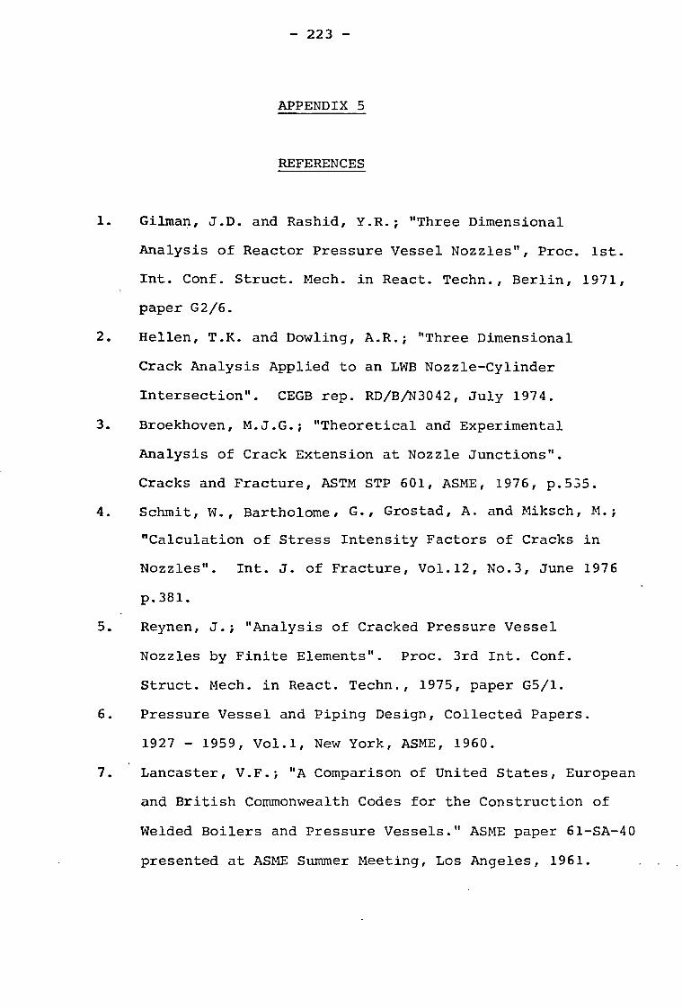
- 223 -

APPENDIX 5

REFERENCES

1. Gilman, J.D. and Rashid, Y.R.; "Three Dimensional

Analysis of Reactor Pressure Vessel Nozzles", Proc. 1st.

Int. Conf. Struct. Mech. in React. Techn., Berlin, 1971,

paper G2/6.

2. Hellen, T.K. and Dowling, A.R.; "Three Dimensional

Crack Analysis Applied to an LWB Nozzle-Cylinder

Intersection". CEGB rep. RD/B/N3042, July 1974.

3. Broekhoven, M.J.G.; "Theoretical and Experimental

Analysis of Crack Extension at Nozzle Junctions".

Cracks and Fracture, ASTM STP 601, ASME, 1976, p.535.

4. Schmit, W., Bartholome, G., Grostad, A. and Miksch, M.;

"Calculation of Stress Intensity Factors of Cracks in

Nozzles". Int. J. of Fracture, Vol.12, No.3, June 1976

p.381.

5. Reynen, J.; "Analysis of Cracked Pressure Vessel

Nozzles by Finite Elements". Proc. 3rd Int. Conf.

Struct. Mech. in React. Techn., 1975, paper G5/1.

6. Pressure Vessel and Piping Design, Collected Papers.

1927 - 1959, Vol.1, New York, ASME, 1960.

7. Lancaster, V.F.; "A Comparison of United States, European

and British Commonwealth Codes for the Construction of

Welded Boilers and Pressure Vessels." ASME paper 61-SA-40

presented at ASME Summer Meeting, Los Angeles, 1961.

- 224 -

8. Shank, M.E.; "A Critical Survey of Brittle Fracture in

Carbon Plate Steel Structures other than Ships." Pub.

Welding Research Council of the Engineering Foundations,

New York, 1954.

9. Tiffany, C.F.; "Aerospace Pressure Vessels." Fracture

Mechanics of Aircraft Structures, AGARDOgraph No. 176,

Jan 1974, Paper VC-5, p.294.

10. Boyd, G.M.; "Brittle Fracture in Steel Structures".

Pub. Butterworth, London 1970.

11. Pellini and Puzak, J. Eng. for Power ASME,Oct. 1964.

12. Pressure Vessel and Piping Design and Analysis. Vol.

1 - Analysis. ASME, New York 1972.

13. Proc. 2nd Int. Conf. on Pressure Vessel Technology,

Port 1 - Design and Analysis, ASME, 1973.

14. Proc. 3rd Int. Conf. on Struct. Mech. in React. Techn.

London 1 - 5 Sept. 1975.

15. Timoshenko, S.P. and Goodier, G.N.; "Theory of Elasticity".

pub. McGraw-Hill, Kogakusha, Tokyo, 1970.

16. Inglis, C.E.; "Stresses in a Plate Due to the Prescence

of Cracks and Sharp Corners". Trans. Inst. Naval

Architects, Vol. 60, 1913, p.219.

17. Muskhelishvilli, N.I.; "Some Basic Problems of the Mathe-

. matical Theory of Elasticity." Noordhoff, Groningen, 1953.

18. Griffith, A.A.; "The Phenomena of Rupture and Flaw in

Solids". Phil. Trans. Roy. Soc., 1921, A221, p.163.

19. Irwin, G.R.;"Relation of Stresses Near a Crack to the

Crack Extension Force". 9th Int. Congr. Appl. Mech.,

Brussels, 1957.

- 225 -

20. Orowan, E.; "Fracture and Strength of Solids". Rep.

Prog. Phys., 1949, Vol. 12, p.185.

21. Brown, W.F. Ed. "Review of Developments in Plain

Strain Fracture Toughness Testing". ASTM STP 463,

.1970.

22. Irwin, G.R.; "Analysis of Stresses and Strains near

the End of a Crack Transversing a Plate". J. App.

Mech., Vol. 24, 1957, p.361.

23. Irwin, G.R.; "Fracture". Hanbuck der Physik, Vol. VI,

Springer, Berlin, 1958.

24. Westergaard, H.M.; "Bearing Pressures and Cracks".

J. Appl. Mech., 1939, Vol. 61, p.A49.

25. Paris, P.C. and Sih, G.C.; "Stress Analysis of Cracks"

in "Fracture Toughness Testing and its Applications"

ASTM STP 381, 1965, p.31.

26. Knott, J.F.; "Fundamentals of Fracture Mechanics". Pub.

Butterworths, London, 1973.

27. Cartwright, D.J. and Rooke, D.P.; "Evaluation of Stress

Intensity Factors". J. Strain Analysis, 1975, Vol 10

(4), p.217.

28. Sih, G.C.; "Mechanics of Fracture; Methods of Analysis

and Solution of Crack Problems". Noordhoff, Leyden,

1973.

29. Rooke, D.P. and Cartwright, D.J.; "A Method of Compound-

ing Stress Intensity Factors for Complex Configurations".

Technical Rep. 75063, RAE, April 1975.

30. Rooke, D.P. and Cartwright, D.J.; "Compendium of Stress

Intensity Factors". Her Majesty's Stationery Officer,

London, 1976.

- 226 -

31. Hartranft, R.J. and Sih, G.C.; "Alternating Method

Applied to the Edge and Surface Crack Problems". paper

in Ref.(28), p.179.

32. Smith, F.W., Kobayashi, A.S. and Emery, A.F.; "Stress

Intensity Factors for Semi-Circular Cracks, Part 2 -

Semi Infinite Solid". J. Appl. Mech., Vol. 34, 1976,

p. 947.

33. Benthem, J.P.; "Three-Dimensional State of Stress at

the Vertex of a Quarter-Infinite Crack in a Half-

Space". Rep. No. 563, Laboratory of Eng. Mech.,Delft.

Sept. 1975.

34. Smith, F.W. and Alavi, M.J.; "Stress Intensity Factors

for a Part-Circular Surface Flaw". Proc. 1st Int. Conf.

on Pressure Vessel Technology, Delft, 1968.

35. Swedlow, J.L. and Ritter, M.A.; "Toward Assessing the

Effects of Crack Front Curvature (CFC)". ASTM STP

513, 1972, p.79.

36. Sneddon, I.N.; "The Distribution of Stress in the

Neighbourhood of a Crack in an Elastic Solid". Proc.

of the Royal Soc., London, Series A, 187, 1946, p.229.

37. Green, A.E. and Sneddon, I.N.; "The Stress Distribution

in the Neighbourhood of a Flat Eliptical Crack in an

Elastic Solid". Proc. of the Cambridge Phil. Soc.,

Vol. 46, 1956.

38. Irwin, G.R.; "The Crack Extension Force for a Part-

Through Crack in a Plate". J. Appl. Mech.,Dec. 1962

p.651.

- 227 -

39. Kobayashi, A.S., Zii, M. and Hall, L.R.; "Approximate

Stress Intensity Factor for an Embedded Eliptical Crack

near to Parallel Free Surfaces". Int. J. Fracture

Mech., Vol. 1, 1965, p.81.

40. Broech, D.; "Fail-Safe Design Procedures". Fracture

Mechanics of Aircraft Structures, AGARDograph No. 176,

Jan. 1974, p.121.

41. Kobayashi, A.S., Enetanya, A.N., Shah, R.C.; "Stress

Intensity Factors for Eliptical Cracks". Prospects of

Fracture Mechanics (Proceedings of an Int. Conf.)

ed. G.C. Sih, H.C. van Elst and D. Broeck. Pub. by

Noordhoff International Publishing, Leyden, 1974, p.525.

42. "Experimental Techniques in Fracture Mechanics" SESA

Monograph No. 1, 1973.

43. Smith, F.W., Emery, A.F. and Kobayashi, A.S.; "Stress

Intensity Factors for Semi-Circular Cracks". J. Appl.

Mech., Vol. 34, 1967, p.953.

44. Thresher, R.W. and Smith, F.W.; "Stress Intensity

Factors for a Surface Crack in a Finite Solid". J.Appl.

Mech., Vol. 39, 1972, p.195.

45. Shah, R.C. and Kobayashi, A.S.; "Stress Intensity

Factor for an Eliptical Crack Approaching the Surface

of a Plate in Bending". ASTM STP 513, 1972, p.3.

46. Zienkiewicz, 0.C.; "The Finite Element Method in

Engineering Science". McGraw-Hill, London,2nd Ed.

1971.

47. Desai, C.S. and Abel, J.F.; "Introduction to the Finite

Element Method". Van Nostrand Rheinhold Co., New York.

- 228 -

48. Fenner, R.T.; "Finite Element Methods for Engineers".

Macmillan, London, 1975.

49. Natarajan, R.; "Finite Element Analysis of Pipe Bends

Using Doubly Curved Shall Elements". Ph.D. thesis,

Imperial College, University of London, April, 1971.

50. Alujevic, A.; "The Analysis of Stresses in Irradiated

Nuclear Reactor Fuel Elements Using Three-Dimensional

Isoparametric Finite Elements". Ph.D. thesis, Imperial

College, University of London, March 1973.

51. Conte, S.D.; "Elementary Numerical Analysis, An

Algorithm Approach". McGraw-Hill, New York, 1965.

52. Ford, H.; "Advanced Mechanics of Materials". Longmans,

London, 1969.

53. Irons, B.M.; "Economical Computer Techniques for

Numerically Integrated Finite Elements". Int. J. Num.

Meth. in Eng., Vol.1, 1969.

54. Irons, B.M.; "A Frontal Solution Program for Finite

Element Analysis". Int. J. Num. Meth. in Eng., Vol.2,

1970.

55. McCracken, D.D.; "A Guide to FORTRAN IV Programming".

John Willey and Sons, Inc., New York, 1965.

56. Priest, A.H.; "Experimental Methods for Fracture

Toughness Measurements". J. Strain Analysis, Vol.10

(4), 1975, p.225.

57. Sih, G.C. And Hartranft, R.J.; "Growth Characteristics

of Surface Flaws in Pressure Vessels". Proc. 3rd

Int. Conf. Struct. Mech. in Nucl. React. Techn., London

Sept. 1975, paper G4/2.

- 229 -

58. Sih, G.C. and Cha, B.C.K.; "A Fracture Criterium for

Three Dimensional Crack Problems". J. Eng. Fract. Mech.,

Vol. 6, 1974, p.698.

59. Broekhoven, K.J. and Ruijtenbeek, M.G.; " Fatigue

Crack Extension in Nozzle Junctions: Comparison of

Analytical Approximations with Experimental Data".

3rd Int. Conf. in Struct. Mech. in Nucl. React. Techn.,

London Sept, 1975. paper G4/7.

60. Sommer, E., Hodulak, L. and Kordish, H; "Growth Chara-

cteristcs in Part-Through Cracks in Plates and Tubes".

Euromech-Colloquium No 77, Paris, Sept. 1976, paper

submitted to Int. Joint Pressure Vessels and Piping and

Petroleum Mech. Eng. Conf., ASME, Mexico City, Sept. 1976.

61. Moura Branco, C.A.; "A Fracture Mechanics Approach to

Environmental and Elastic-Plastic Fatigue Crack Propagation".

Ph.D. Thesis, Imperial College, University of London

June 1976.

62. Wilson, W.K.; "Some Crack Tip Finite Elements for Plane

Elasticity". ASTM STP 513, 1972, p.90.

63. Hilton, P.D. and Sih, G.C.; "Applications of the Finite

Element Method to the Calcualtions of Stress Intensity

Factors". Mechanics of Fracture 1, Methods of Analysis

and Solutions of Crack Problems. Ed. (G. Sih), Vol.1,

Noordhoff, Int. Pub., 1973.

64. Williams, M.L.; "On the Stress Distribution at the Base

of a Stationary Crack". J. Appl. Mech., Vol. 24,

1957, p.109.

- 230 -

65. Rice, J.R. and Tracey, D.M.; "Computational Fracture

Mechanics". Numerical and Computer Methods in Structural

Mechanics, Academic Press, New York, 1973.

66. Jerram, K. and Hellen, T.K.; "Finite Element Techniques

in Fracture Mechanics". Proc. Int. Conf. Welding

Research related to Power Plant, Southampton, 1972, paper

- 14, p.165.

67. Atluri, S.N.,Kobayashi, A.S. and Nakagaki, M.; "Fracture

Mechanics Application of an Assumed Displacement Hybrid

Finite Element Procedure". AIAA Journal, Vol. 13,

No. 6, 1975, p.734.

68. Blackburn, W.S.; "Calculation of Stress Intensity

Factors at Crack Tips using special Finite Elements".

Conf. Maths. of Finite Elements and Appls., Brunel

University, April 1972.

69. Tracey, D.M.; "Finite Elements for Three Dimensional

Elastic Crack Analysis". Nuclear Eng. and Design, Vol.

26, 1974, p.282.

70. Chan, S.K., Tuba, I.S. and Wilson, W.K.; "On the Finite

Element Method in Fracture Mechanics". Engng, Fracture

Mechanics, Vol. 2, 1970, p.l.

71. Ewing, P.D., Swedlow, J.L. and Williams, J.G.; "Further

Results on the Angled Crack Problem". Int. J. Fracture,

Vol. 12, No.1., 1976.

72. Leevers, P.; Unpublished results, Imperial College, 1976.

73. Dixon, J.R. and Strannigan, J.S.; "Determination of

Strain Energy Release Rates and Stress Intensity Factors

by the Finite Element Method". J. Strain Analysis,

Vol. 7, No. 2, 1972.

- 231 -

74. Discussion of paper in Ref.(34), Part III, Discussion

of Papers presented in the 1st Int. Conf. On Pressure

Vessel Technology, ASME, 1970, New York.

75. Broekhoven, M.J.G. and Spaas, H.A.C.M.; "Application

of the Finite Element Technique to a Complex 3D

Elastic Problem (nozzle junctionwith cracks)". Rep.

MMPP-101, Delf University of Technology, Delft, The

Netherlands, August 1974.

76. Buekner, H.Fd, Trans, of ASME, Vol. 80, 1958, p.1225.

77. Rice, J.R.; "A Path Independent Integral and the

Approximate Analysis of Strain Concentrations by

Notches and Cracks". J. Appl. Mech., Vol. 35, 1968,

p.379.

78. Neale, B.K.; "Finite Element Crack Analysis Using the

J-Integral Method". CEGB report RD/B/N2785, Sept. 1973.

79. Parks, D.M.; "A Stiffness Derivative Finite Element

Technique for Determination of Crack Tip Stress

Intensity Factors". Int. J. of Fracture, Vol.10, 1974

p.487

80. Hellen, T.K.; "On the Method of Virtual Crack Extensions".

Int. J. Num. Meth. in Engng., Vol.9, 1975, p.187.

81. Henshell R.D. and Shaw, K.G.;"Crack Tip Finite Elements

Are Unnecessary". Int. J. Num. Meth. in Engng., Vol.9,

1975, p.495

82. ICCC Bulletin, ICST 6.3/7 November 1974, Imperial

College.

83. ICCC Bulletin, ICST 4.6/1.6, June 1971, Imperial College.

- 232 -

84. Levy, N., Marcal, P.V. and Rice, J.R.; "Progress in

Three Dimensional Elastic Plastic Stress Analysis for

Fracture Mechanics". Nuclear Eng. and Design, Vol.17,

1971, p.64.

85. Brown, W.F. and Srawley, J.E.; "Plane Strain Crack

Toughness Testing of High Strength Metallic Materials".

AST STP 410, 1966.

86. Yamamoto, Y. and Sumi, Y.; "Stress Intensity Factors

for Three Dimensional Cracks". To be presented at

the 14th Int. Congress in Theoretical and Applied

Mechanics, Delft, 1976.

87. Neal, B.K. "The Influence of Crack Shape on Fracture

Toughness Testing". Int. J. of Fracture, Vol. 12,

1976, p.499.

88. Johnson, R.A. and Radon, J.C.; "Fracture Energy and

Crack Tunnelling". J. of Testing and Evaluation,

Vol. 4, No. 3, May 1976, p.209.

89. Tracey, D.M.; "3-D Elastic Singularity Element for

Evaluation of K Along an Arbitrary Crack Front". Int.

J. of Fracture, Vol.9, 1973, p.340.

90. Smith, F.W. and Alavi, M.J.; "Stress Intensity Factors

for a Part Circular Surface Flaw". Proc. 1st Int. Conf.

on Pressure Vessel Technology, Delft, 1968.

91. Shannon, R.W.E.; "Stress Intensity Factors for Thick

Walled Cylinders". Int. J. Pressure Vessels and Piping

Vol. 2, 1974.

92. Underwood, J.H., "Stress Intensity Factors for Internally

Pressurized Thick Walled Cylinders". Proc. of the 1971

National Symposium on Fracture Mechanics, Part I, ASTM

STP 513, 1972, p.59.

- 233 -

93. Bowie, O.L. and Freese, C.E.; "Elastic Analysis for a

Radial Crack in a Circular Ring". Engng. Fracture

Mechanics, Vol. 4, 1972, p.315.

94. Rice, U.R. and Levi, N.; "The Part-Through Surface

Crack in an Elastic Plate". Tec. Rep. NASA NGL

40-002-080/3, 1970.

95. Nichols, R.W.; "Steel's Contribution to Nuclear Power:

It's Problems and Promise". Metals and Materials, The

J. of the Metals Society, April 1976, p.24.

96. "Protection Against Noductile Failure". Section III,

Appendix G, ASME Code, 1974.

97. Burdekin, F.M. and Dawes, M.G.; "Practical Use of

Linear Elastic and Yielding Fracture Mechanics with

Particular Reference to Pressure Vessels". Paper

C5/71 in Ref. (99), p.56.

98. Mager, T.R. and Riccardella, P.C.; "Use of LEFM in

Safety Analysis of Heavy Section Nuclear Reactor

Pressure Vessels". Paper C8/71 in Ref.(99), p.56.

99. "Practical Application of Fracture Mechanics to Pressure

Vessel Technology". Pub. by I. Mech. Eng., 1971.

100. Cha, R.C.; "Stress Intensity Factors for Through and

Part-Through Cracks Originating at Fastener Holes".

Mechanics of Crack Growth, ASTM STP 590, 1976, p.429.

101. Kobayashi, A.S. and Enetanya, A.N.; Mechanics of Crack

Growth, ASTM STP 590, 1976, p.477.

102. Bartholome, G. and Dorner, H.; "Safety Evaluation of

Nuclear Reactor Pressure Vessels for Pressurized Water

Reactors". Paper C51/71 in Ref.(99), p.175.

- 234 -

103. Slater, D.J.F.; "A User's Manual for FLAPS a Finite

Elements Computer Program for an Elastic Body of

Revolution". Internal publication, Imperial College,

November 1971.

104. Pereira, M.S.; "Remarks on Iterative or Elimination

Methods of Solution: The Frontal Method". Computation

Methods in Fracture Mechanics. Welding Institute/

Imperial College Post Experience Course June 1976.

105. Carre, B.A.; "The Determination of the Optimum Accel-

erating Factor for Successive Over-Relaxation".

Computer Journal, Vol.4, 1961, p.73.

106. Cotterell, B.; "Notes on the Paths and Stability of

Cracks". Int. J. Fracture Mechanics, Vol.?, No. 3,

1966, p.526.

Spherical shell_

Too lid flange

Bolts

Vessel flange

Cylindrical shell

4 Steam nozzles

2 Core spray / nozzles

4 Feedwater nozzles

145 Control rods

penetrations

9 Pump nozzles

- 235 -

(a) Prespective view of Pressure Vessel

(b) Tee Junction of thick walled cylinders

Figure 1.1

mid-section (plahe strain) crack tip

surface +✓(plane stress)

— 236 —

Mode I Mode II Mode III

Fig. 1.2 Basic modes of crack surface displacements

rxy

Tyz

rxz

X trz

leading edge of the crack

z

Fig. 1.3 Coordinates measured from the leading edge of a crack and the stress components in the crack tip stress field

Fig. 1.4 Plastic zone ahead of a crack in a plate of thickness B

10•IA ID FORCED NOME (AII2•CI)

MIA ID SIM

(A302

irElD

- 237 -

Fig. 1.5 Various crack configurations having the same length and depth

Fig. 1.6 Section of a nozzle showing two fatigue cracks

- 238 -

(a) second order (quadratic) (b) third order(cubic) 20 nodes 32 nodes

Fig.2.1 3D hexahedron finite elements

I—IWITIALIZATIONS

PART B

PART C

PART D

Fig. 2.2 Primary Flow-Chart of DIM3B code

RM1RSD. SACK • tea

WRITE M.S. J RETURN

Vr R. , rte. T4-3

g r1 car r ar MAA,, sta

ALL 3ANNELM •

KM UN

COM• • UNCLZ COMP•umirmAr

ITNONAT•injamkr_x,com

tfreCIL •UNCzt Otorcomil

T•(lMEM4r-ScreDMP

laaASE PO SPACE

COMP. ANOmAt COMR.OPActl

moo,er rat VV. g NO. MI Arcsr

UNRNS

N09 ,171 THE stNoorr• AtChr DC

)(HORNS

INLIFfEri rroaws QEO ,JAGR

DATA .2ro4r:s Af LoAkD

OA TA

r

L - I EW AN I

• MESE r FDA INEr I FLEhtimr I

• LIII3•Etat311

1READ DArA

NODE tm3D,

L•sr A 001.A • AMC IS

NA NVA NUN VA

RHSRED•RW.51

- 239 I sTARTl

'RCA° DATAI 1

MATRIX RELATING OASIC S rd 74/43

(TB]

NJ

rANA,NuNVA

NODAL DATA CCOAD RUSE

1 rEeuu MATER;AE DATA

EL/ST.47T 44,4*. r(17

IINTEGER RESULT'S I

IOUTPUT 1. R.

ALL NODES ) I

RETURN

Witt E.NNECM,NrR0Er. NorrA,NOOTOT,JEA.15, NwikvA,NKNVA, NT, N TOTAL NvAorur dirrdIV

RESIT 70 ZERO ETarhirgo SU PM A ,I ,CIS

LII,KMAT UN" Ane

ommaL LR14-[NfottLi•CiTqlvTe (ccaticay Moira

I WOE 0E3

--- ALL Ni.amsavrs

CoOft D

11 RI

HED ICN. !CUT Ic1,tR7,Amc(t)♦r,44 [CAWS X; (2) ,C2(23,2”,11CAQ,

a ALK•ArD 4ACAN•..7, 3J11471

STADVT .7.1r ..sra

LirATE,mtAAm

NEO74,NOETor

Imvoo0 READ 7OPOLOficA1 DATA

r

L

CHECK Err UNKNOWN AND *NO.,* or■Cle WANE 3 UNKSI*C KNONIC

CAISCA. Zna :AEsCA BIT L. PTOENtc

FEM co./.

Sh

OuraUTOTAL NODAL ror,5_5

troirSSIM [-Lam tsar

LOAD E.-W.1,4LE"/ T NOTAL

ragc-ES TRN3L

3L

Ea -II D eCOMPEALA4A31.1C-111

< STrTR oweft•At,

UNNM Ar

ar"'""A's'

GOA ,

T • - NC

3.8*-1,Da4ta3trtl*CDE.walm 1Pla,cAtz)..4C3).cc0.)

IELNOD

PRIAPIC AUDIT

I EJ1.57 AJWARANEES

WRITE M.S.

coNO. DATA READ ammo. I

Arrumv

STRESS com,c3/vgovr YES COMP

N DE.o,

p*cl <WROU .VTaaT Sera..cncINS

...21an,. r p,sol."(...w”

SrA£5595 RfoUgail

'71 CD

luNStr.les -3454 -April -41P.MA rINEAt

at .- of," CP 41 t • •4 EDS"

lit* To •L CJAC 2 S•65•3111

inCTOAM

.552.-Epaiainsl END

Fig. 2.3 Flow-Chart of DIM3B code

A,

(a) Variation of the coefficients A; of the Williams series solution

2.4

2.2

2.0

1.8

1.6

1.4

1.2

1.0

•

if

-,-

/ /

/

er.

1(0_ K, - (F.

a. orFa Az B1 r - 133r ... 1

. CI

0 ---- ---

_Al

/- - e• ✓

....... • 0

...D._•------

• —

0

---

a/W

.

/ ..----- ...." 0

--- ---

0

I

__••---- 0 _—rs---6—

L

------.1

1 --

e-- 1

1 2 3 4 5

.10 .20 .25 .30 .40 „..ko , rr/2

--.7r io -- • —

r

IOK0

2.6

.4 .6 .8 10 1.2 rAl • (b) K*curves for various ratios a/W of a CTS

Fig. 3.1 Results from a 2D analysis as it applies to the Williams series solution to crack problems

- 241 -

n n+1 n+

Fig, 3.2 Application of the Energy Method to the derivation of K factors from the crack plane nodal forces and displacements

Numerical Methods 'Analytical Methods Exnerimental Methods

Crack Closure Work

Strain Energy Release Rates

Parks' Method Bueckner's

Method - Integral

Evaluation of SIFs

Fig. 3.3 Chart of possible methods for obtaining K factors. The thicker frames indicate the methods used in the present work

Westergaard Stress function

Alternating Methods

Williams Stress functions

Conformal Mapping

Finite Elements

Boundary Collocation

Fatigue Crack Growth

Photoelasticity

Compliance

Complex Stress Functions

Fine Meshes element j Cracked tip

1

Direct Method Energy Method

Stress Method Displ. Method

243 —

1 2 3 g=-1 g=0 g.:•1 r=0 r=p r=•2

u=u, u=4,

(a) SecOnd Order (quadratic)

1 2 3 4 0 o o o g=-1 .g=-1/3 . g=•1/3 g=.1 r= 0 r=p, r=pi r=2 u=u, u=u, u=u3 u=ua

(b) Third Order (cubic) %.= local coordinate r = global coordinate p= coordinate of mid-side node in global system

Fig. 3.4 One dimensional line elements

g,r,u

.43 77 yV fi .'"-.. f

-1 7 ■

Fig. 3.5 Shape functions Ni and its derivatives fi for the second order line element

1

N

0

/ /

I / ft Fig. 3.6 New shape functions Ni and its derivatives

fi for the singularity element

f2

- 244 -

Fig. 3.7 Shape functions Ni and its derivatives fi for the 4 node singularity element

yl

(02) (1 2) (2.2)

(2.1)

(0.0) (0,p1 ) (0.21

Fig. 3.8 2D 8 node isoparametric element

11

Fig. 3.9 3D 20 node singularity element

- 245 -

5 (a) Shape function N1

5 (b) Shape function N8

Fig. 3.10 Two tipical shape functions for the 2D 8 node singularity element

TAPE62

DDMDAT

O

. CONTROL OUTPUT. 4',.„....

CORRET (UPDATE

/ I iDIM3B f I

Program] DIM3B

MESH GENERATION PROGRAM

DIMDAT DDMDATI DRDAT

DIMDAT

/ Program DIMDIM

1 /Program DRAW

"QUICK-LOOK" '.

. . RESULTS . . O

ULCC ICCC

Fig. 3.11 Procedure for data generation and execution of DIM3B code

- 247 -

Fig. 3.12 Transformation of coordinates to obtain a prespective view of a finite element mesh

PEN UP PEN DOWN

Fig. 3.13 Order of execution of logical functions 'Pen up','Pen down' in a hexahedron element

— 248 —

2H

y

V. - (a) Compact Tension Specimen

boundary

Fig. 3.14 Finite element mesh idealization for the CTS shown in figure 3.14 (a)

- 249 -

6.----------------~--------------------------------------~ y

<> x = o. .... r----t-7"'""7'-;~-D x=TII.-

o x = Tl2 - l .... ~-a""-----t------'--

o.~----------~------------~----------~------------.0 .25 .50 .75 r/(W-a) 1. Fig. 3.15 UndistortQd QlQmQnts. Variation of CTZ strQssQs

ahQad of thQ crack f ron t.

6~----------~-------------------------------------~

<> x = 0

c X = TIt. 4 ~-------+-----o x = T/2

y •

r

2~~~-----+--------~--------~---------,

O.~------~~~--+---~--~~~-r---~~~==~~ .0 .25 .50 .75 r/(W-a) 1.

Fig. 3.16 DistortQd QlQmQnts. Variation of ax and CTZ

strQssQs ahead of thQ crack front

-three dimensional solution

"Pl

wo dimensional solution

- 250 -

ai cr

5.-

4.-

3.

-.5

0. I • J I I

. .1 ,

..., .4 x/T .5 Fig. 3.17

0 Variation of the mide e mide ement stresses and the parameter

P accross the thickness in the vicinity of the crack front

PS

1.

2.0

M f

.0 .5,

2x/T .0 1.0 Fig. 3.18 Variation of the K factor obtained along the

crack of a CTS by Yamamoto & Sumi,Ref.(86)

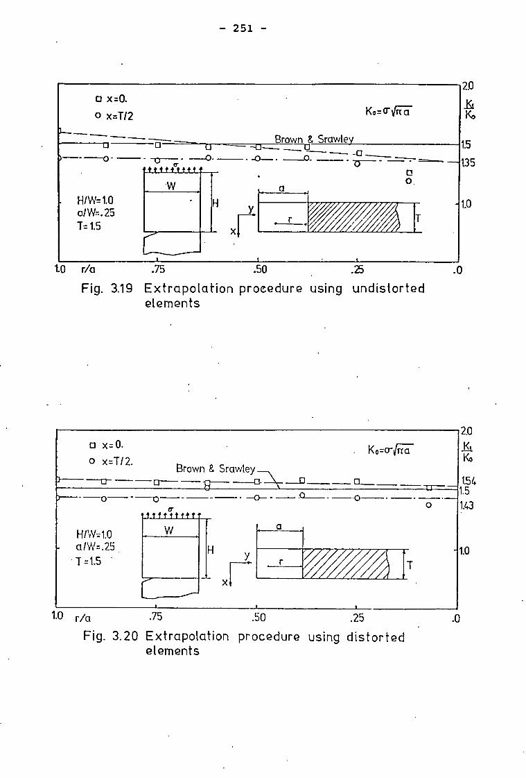
K0=cr FFt

Brown & Srawley -❑ 73—

o.

H/W=1.0 a/W= . 25 T=1.5

❑ x=0. o x =T/2

20

Ko

1.5 —135

-1.0

0

2.0

Ko ❑ x= O. o x=T/ 2.

. Ko=a-FiTa Brown & Srawley

9 -07 \ 1.54 1.5

0 1.43 _0_ —0_

H/W=1.0 - a /W= .25

T =1.5 • -1.0

– 251 –

tO r/a .75 .50 .25 .0 Fig. 3.19 Extrapolation procedure using undistorted

elements

1.0 r/a .75 .50 .25 .0 Fig. 3.20 Extrapolation procedure using distorted

elements

Ko=crTFT:t

—

. - 252 -

(a) Finite element mesh idealization of a CTS using 3D 32 node elements

0

und. dist. 0

--a E-- X-70

x=T/2 Brown & Srawley

1.0 r/a .75 .50 .25 (b) Comparison of extrapolation procedures

2.0 iq Ko

1.5 1.35 1.28 1.19

1.0

Fig. 3.21 Singularity elements derived from 32 node isoparametric elements

1 R =17 R=1.4 R=1.2 R=1.0 R=.85

a Act.

A - 253 -

(a)

Fig. 3.22 CTS with curved crack front and its mesh idealization

- 254

~------~------~~----------~-----------r-----------2P Q-----_ K~ K/Ke K-

0 ...................... . ' .......... .

··0··· ..... ················0

-. --~ ..... ............

·····0

-- 1<0= a" .,Ina

- -__ - .i.:-. :':';".--..

r-____ -+ ______ ~B~R~O~W~N~&~S~R~AW~LE~Y~----------~~~--~W15 9 = 900 9= 1800

x=O 0-- +-x = TIL. 0 -- .--x = T/2 0 ......... • ..•.......

.....•....•. ........... • o

________ ----i ___________ ---L._~~~_--L.. ______ --'-_______ _'1.0

rIa 2.0 1.5 1.0 0.5 .0 (a) straight crack front

~------~----------~------------~----------~-----------,2D K= KIKo K-

0··· ..... ·········0·· .. ............. ",-

. ·o····················o················~·········· '-....

8 = 900

x = 0 0-x= TIl. 0-

e =180° '-+--11--

x = T/2 0 ......... • •....... ...........

....... • ·v ......

K= crv'rta

o ···············0················

1.5

o ~

--_---L.. _____ ~ ____ ---l. _____ -L ____ --..J1.0

rIa 2.0 1.5 to 0.5 .0 (b) curved crack front

Fig. 3.23 Comparison of extrapolation procedures using two directions of extrapolation. 8=TC and 9=7l/2

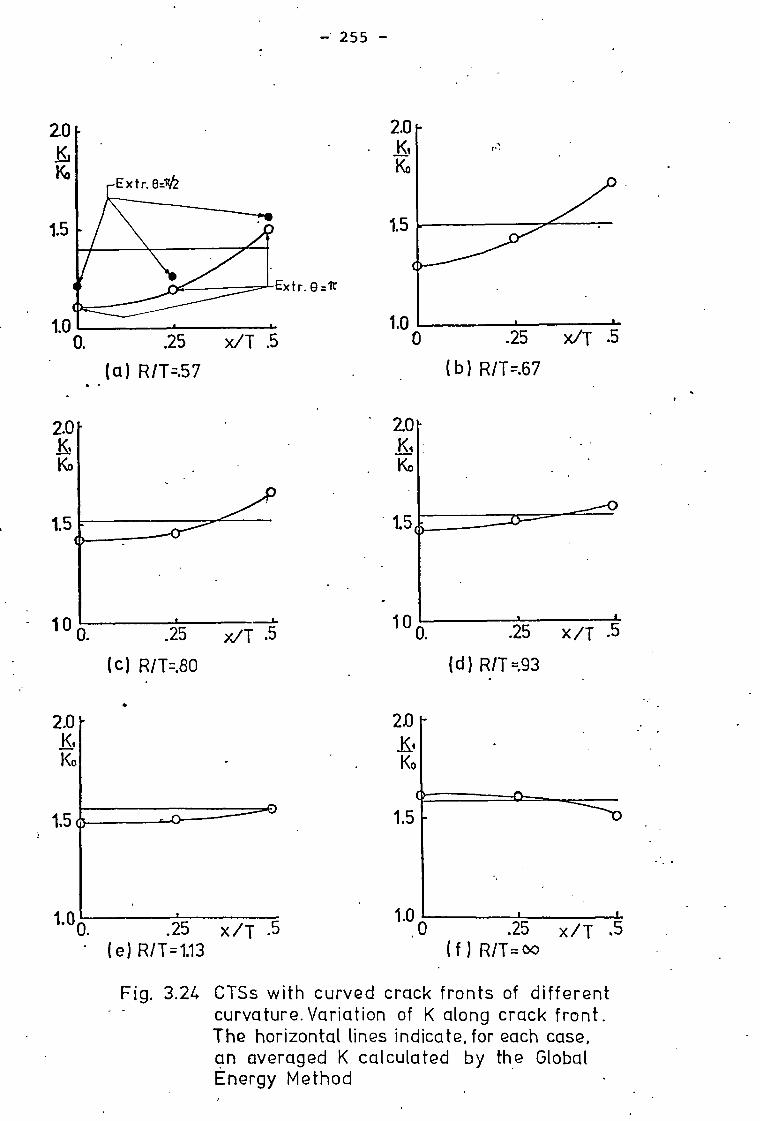
.25 x/T (c) R/T=.80

1.5

10

2.0

Ko

.25 x/T (d) R/T=.93

.25 x/T .5 (e) R/T=1.13

1.0

2.0 K,

.25 x/T (f) R/T=00

255 —

2.0

Ko

1.5

Extr.

1.0 0. .25 x/T .5 • . (a) R/Tr..57

.25 x/T

(b) R/T=.67

2.0

Ko

1.5

1.0

Fig. 3.24 CTSs with curved crack fronts of different curvature. Variation of K along crack front. The horizontal lines indicate, for each case, an averaged K calculated by the Global Energy Method

1.6

1.55

1 5

o

1.45~----------------------~----------------------~---O. .14

6afT .28

Fig. 3.25 CTS. Variation of thQ aVQragQd K valuQs (SQQ fig.3.24) with a normalizQd paramQtrar dQfining thQ crack front curva turQ

Fig. 3.26 Mesh idealization o x

corner crack specimen

Ki

— TRACEY o FEM (1.2%) c ( ) percent. of discrepancy

Ko

1.1

- 257 -

22.50 45.0° 67.5° ot° 90,0° Fig. 3.27 Corner crack specimen. Variation of K along

the crack front

10.0 67.5 DEGREES

90. 22.5 45.0

— Smith &Alavi . OFEM

( ) percent. error

Ko

1.2

1.1

- 258 -

Flg. 3.28 Part-through semi-circular crack. Variation of K along the crack front

- 259 -

III

v

(I)) Three step skewing technique and final mesh idealization

Fig. 3.29 Part-through semi-circular crack emanating from the inner surface of a thick-walled cylinder

- 260 -

1.0

.5

.0

.5

0

•

Hoop stresses

° FE

• •

solution

C

— Lame solution

Radial

..

stresses

1.0

cr. p

1.5

p -1.0

.25 .50 .75 (r-Ri) (R2- R1)

Fig. 3.30 Radial and hoop stresses obtained with the FEM in the radial section y=0 for the case CYL1

3.

5[ o IR. 1 0 ax

u 2 0

I I I I I I 3 <)

2.1 o 0 4 •

5 •

• 1 1- 1 1 ,//"'/~ - ./ A

Y -.

o o

.~I~ ---+---+-1 -+--1 -+-+-1 1-+-+-11 It--i-I" 0_0 <)0-+-1$---+° 0 t--T-~ ~-+--¢i r°-t-t-t 9 "t-t-t-I"t i -1" I 8' ! I! I I r ! ! !'!! I ! ! ! ! ,

. .1 .2 .4.6.8 1. 2. 4. 6. 8. 10. ria

Fig. 3.31 CYL1 case. Hoop s tresses, ax ,ahead of the crack front in the plane x=O

• l\.)

0\ .....

1·6

100

262

K, Ko CASE

0 CYL1 3.4 • CYL2

Ko= pro

3.2

3.0'---------+:=-4~------t--------t

2.81---------f--------+-i"\:7~------t

o

30 60 cx.0 90

Fig. 3.32 CYL1 and CYL2 caSQs. Variation of K along thQ crack fronts

" .. -.. ,-, . . ...... :- .... : .- ..

~~'f:: r:;J:LJ~~-' i; ·:·;::~~~tLriI'1;;---:~· ;.-·t_lJ_~t;'i;~~iii_;f~!f0r~; .. ;::;' :~ :.:.: : :-; .... :': -: 1 : : ~ :. : ~ . ..- :.::.:- :.1.~·:;··: ':.t .:.: ',:":- t :

.. ; .. : .... ! <t- -: .... : ~ ;. ........ ..

: ~:: :.:.:-: .. :.J..:..:'.::.::r :.::.: . . -: ... :.,. : .-. : : :.: " ~ : ::. i : :-, 7': ~ .

. . ... : ..... i ..... ! ...... .•. :-.. ;

it;:d .. --..... -~ .;. ...... ':".j,.; ~·:r:~ : t ; .. ",. i

tffl11Ifd ~;:EillT_E~::;=!C:: ~{EL_Ij:n Li :~tEl'~_~~~ :: :-; .... .. ', ~ ..... .... _.i •

_ ._: ~. :,,:,:. ~ ::~:~~.~:L·.~:,:::~'l ~ .............. ; •••••• I ..... : ..

. ; ... ; ! ... ,_ .... __ . ..l ••••••• : .:. •• ~ .... ;. •

. .: ~ ~ ',. ~ ~. ~ : : -:. ; ~ ~ ~ : ~: -: : :. ~ -, _ ......... - ... -_ ....•. _._-_ ..... -.-... -.... ~ ... -.--.--... - -... . ; .. -•.. - : .. . .. :.. .. ...: i : . . ... . :, : ':'; :",- ... :.: . : '~ I ~ ~'-'~': ! :-: -:.-: i ..

0'0 0'1 0'2 0'3 0'4 0·5 0'7

F"ig. 3.33 K valuQs for a prQssurizQd intQrnal radial QdgQ crack in a tube subjQcted to a uni form intQrnal prQssurQ (from RQf. (30))

'.

• -s: C'\

• <"'I c-~I

___ -JO~·. ____ i8vi ___ ---l

~S1!a"

'

r' ;¥.. 'L;;};

I ! II

I I

10"'20· • :;.! ("'l

• -;;: '.

z Vz"~.:J,:\//,·~·;-;1"/I ~//",~a----'/ / ./.,0 . < _ . '1cJ·2d' /

---·-·-1·-----_. _. --.-I

"./' " , .' / / ,"

,. .//~ / /

/ / ~ , , ~,~ • -;,o ,/,' / j .,', , ,', // '/«// , . . . .', /,/,~,,/.

E='i g. 4.1 Specifica ti on of geometric details of a main steam vent pipe"T-piece"

~1

radial plane defined by the angle

Fig. 4.2 Prespective view'of the"r -piece·.~

N 0'\ W

- 264

Number of Nodes per Element 32 Total Number of Elements 49 Total Number of Nodes 728

Fig. 4.3 TJUN1 case. 32 node element mesh idealization of a T-junction of thick walled cylinders

- 265 - 1.41...•■•.,

Fig. 4.4 Primary 2D mesh idealization for the section J3=0°

Fig. 4.5 Intermediate stages in the generation technique for the node element meshes

- 266 -

C Fig. 4.6 TJUN2 case. 20 node element mesh idealization

of a T-junction of thick walled cylinders

- 267 -

I

1

1

1

1

Stile for dIsplccements

9 ? .107mm Scale for the structure

0 LO 80 mm

1

1

1

Fig. 4.7 Case TJUN2. Displacement solution for the cross sections p =0° and p=9o0

Fig. 4.8 Case TJUN2. Prospective view of the mid-surface of the structure and the correspondent displa-cement solution.

- 268 -

Fig. 4.9 Case TJUN3. Finite element mesh idealization of a T-junction of thick walled cylinders

tat Immo 10.01 •Ipot

1 103 102

ft14107

108

Fig. 4.10 Numbering scheme for elements and nodes of the mesh illustrated in figure 4.9

22

St9

7S7 755

- 269 -

Scale for dIsplocements

9 ? • • 10 2mrn Scale for the structure

0 40 op mm _ Fig. 4.11 CaSe TJUN3. Displace:nent solution for the

cross sections 13=00 and 13=90°

Fig. 4.12 Case TJUN3. Prespective view of the mid-surface of the structure and the correspondent displa-cement solution

y

(10 107)

(101) Lame solution

( )-V,3 Discrepancy

— 270 —

105) \

(103)

(84) (a) Displacements of nodes in the inner surface

• p =o° . o p =90°

— theor.

0 ......... . ........ .. .... • ........... ---

-....0.............

.... ..... . is .. .

--(

0 .25 .50 .75 (r-Ri)/t

.

(b) Hoop stress distributions

Fig, 4.13 Ovalization effect in the end of the branch pipe

3

2

- 272 -

TJUN 3 TJUN 2

Fig. 415 Distribution of hoop stresses,crx /pi,in the nozzle region for the cross sections )9=0° of cases TJUN2 and TJUN3 . The membrane stress in the run pipe is 2.75 times the internal pressure pi

TJUN 3 TJUN 2

Fig. 4.16 Cases TJUN2 and TJUN3.Hoop stress distributions, ax/pain the nozzle region for the cross sections p =gob

M embrane Stress 120 tvlt,1.m-2

Mellen and Dowling

- 273 -

Fig. 4.17 Stress contour 'map of hoop stresses in the nozzle region of a BWR pressure vesselaRef.(2)

- 274 -

TJUN3 Analysis 0 Subst. Analysis O TJUN1 Analysis ASKA Results, Ref.(75)

Fig. 4.18 Variation of hoop stresses along the inner surface in the crotch corner region

- 275 -

1- prosent case 2- Ref.(21.(scaled down 4 times)

3- Ref.(59)

Fig. 4.19 Comparison of geometric _details of three different nozzle configurations

Fig. 4.20 Idealization of a corner crack using the TJUN3 finite element mesh

- 276 -

549 550 551 552 553 554 555 556 557 node

Fig. 4.21 Monitoring changes in nodal displacements when a crack is assumed to exist in the crotch region

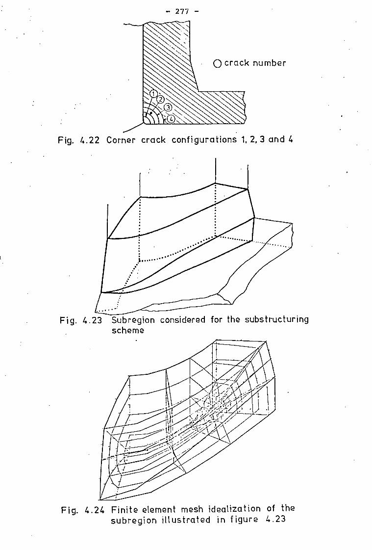
- 277 -

0 crack number

Fig. 4.22 Corner crack configurations 1, 2,3 and 4

Fig. 4.23 Subregion considered for the substructuring scheme

Fig. 4.24 Finite element mesh idealization of the subregion illustrated in figure 4.23

TJUN3 SUBSTRUCTURE

- 278 -

Fig. 4.25 Comparison of distribution of nodes in the nozzle region (cross section p=00)

TJUN3 SUBSTRUCTURE

Fig. 4.26 TJUN3 and uncracked substructure analyses. Comparison of stress contour maps of hoop stresses, crx /pi in the nozzle region (cross section p=o°)

o-x <Trnl

N ANGLE ex

8 CRACK 0 0 1.5 0 I 900

..... 1 0 () c a 0 []I

1 L. 2 ..... u

\ \ .::t. 3 0 <) u a

\ \ . .

I. 0 () L. U L Cl"m-'membra ne stress in

6 I . \: \ : . I the ,'u n pipe =2 .75 P

T

4 I ". , • 't" '1 I. (' , • v

I '""". ", '., ',' ---"'lOi!' ......... '. -r. -=~~".,,,,,~ .• o,, 9. ' dL. I 2 -- ' . _ """'-....... '- .. ' - " """ . " ....

~--~ t __ --O~l ________________ ~ ______________ ~ ______________ ~~ ______________ ~ ______ _

j7 .4 .5 .8 1.0 r/T

Fig. 4.27 O'x st rQ ss d istributions ahQad of crack fronts 1, 2, 3 and 4

N ....,J \0

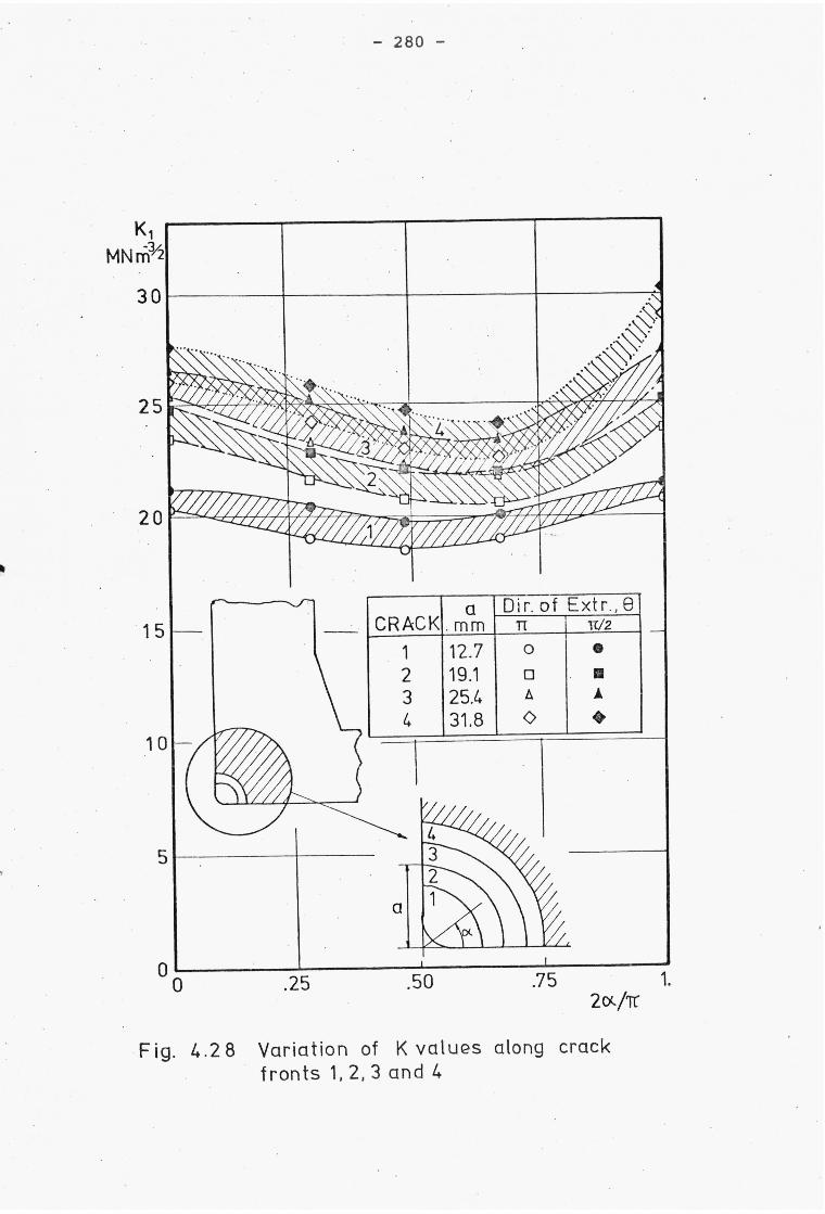
Ko = 2 cr ITir,I-. a membrane stress

(") scaled down 4 times

•0

Present results with substr. anal.-

Hellen and Dowling , Ref.12)

Brokhoven , Ref.(59)

Corner crack in a square spe-cimen, see Chapter 3 I I 1

1 0 10... 0

3 0

— 281 —

-■______----------"---■_,

AlJd, I Qum., N 'pin-l"'

\ mi .1 m.I I

liin,

Fig. 4.29 Evaluation of K values by the Global Energy Method based on crack plane nodal point for-ces and displacements

•••

Ka .„ MNre2

12

10

8

6

4

2

.4 .5 .6 aiTi

Fig. 4.30 Comparison of averaged K values of corner cracks emanating from the crotch corner of three different no-zzle geometries

three dimensional linear-elastic - Spiral – Imperial College ...

Documents

Transcript of three dimensional linear-elastic - Spiral – Imperial College ...