
The High Speed Double Torsion Test - Spiral
154
Thesis submitted for the degree of Doctor of Philosophy of the University of London and the Diploma of Imperial College The High Speed Double Torsion Test by Stephen Ritchie Department of Mechanical Engineering Imperial College of Science, Technology and Medicine London SW7 2BX England November 1995
-
Upload
khangminh22 -
Category
Documents
-
view
3 -
download
0
Transcript of The High Speed Double Torsion Test - Spiral

Thesis submitted for the degree of Doctor of Philosophy of the University of London
and the Diploma of Imperial College
The High Speed Double Torsion Test
by Stephen Ritchie
Department of Mechanical Engineering Imperial College of Science, Technology and Medicine
London SW7 2BX England
November 1995

Abstract
Abstract
The high speed double torsion test is a high rate version of the standard double torsion
fracture test. The test has been used by previous researchers to induce rapid crack
propagation in tough engineering polymers in order to measure a material's dynamic
fracture resistance as a function of crack velocity. Experimental results show that at
medium to high impact speeds the crack propagates at a fairly constant velocity but at low
impact speeds the crack propagates in a stick-slip manner.
In order to calculate the dynamic fracture resistance, a post-mortem analysis of the test is
required. The analysis previous to this work consisted of modelling the test using a
numerical finite difference scheme. The discretised equations of motion used in the scheme
included the effects of axial stresses in the test specimen but ignored axial inertia. The
equations of motion used have been modified to include axial inertia and the boundary
conditions corrected.
This work examines and models the more transient characteristics of the test, exemplified
by the stick-slip crack propagation mentioned above. In order to achieve this goal, the
finite difference model has been re-formulated in propagation mode where the dynamic
fracture resistance is prescribed and the crack history calculated, as opposed to the
previously used generation mode where the crack history is prescribed and the dynamic
fracture resistance calculated.
Previous work has examined the effects of the characteristic curved crack front in the
double torsion test and the possible non-linear material behaviour of the test specimen.
These aspects have been re-examined and previous assumptions found to be invalid.
Correcting the errors had a significant influence on the calculated value of dynamic fracture
resistance.
Contact stiffness and overhang effects have been analysed and their incorporation into the
model has resulted in an accurate prediction of the experimental load history oscillations.
The resulting model was extensively validated and allowed the characteristics of the high
speed double torsion test to be examined. A variety of polymers have been tested and
analysed. The results show that the stick-slip behaviour is, at least in part, due to the
dynamics of the HSDT test rather than the material's dynamic fracture resistance falling
with crack velocity.

Acknowledgements
Acknowledgements
My sincerest thanks goes to Dr P.S. Leevers for his supervision of this work. His advice
and willingness to discuss this work were invaluable.
I am grateful to my friends and colleagues Dr Ndiba Dioh, Mr Chris Greenshields, Dr
Alojz Ivankovic, Ms Rachel Ruffle and Mr Gregory Venizelos for their fruitful discussions
and encouragement. Mr Tom Nolan provided excellent technical assistance throughout this
work.
This work was funded by the Science and Engineering Research Council.

Contents
Contents
Title page 1
Abstract 2
Acknowledgements 3
Contents 4
Nomenclature 9
Abbreviat ions 12
Chapter 1: Introduction 13 1.1 What is rapid crack propagation ? 13
1.2 Experimental methods and analytical techniques for RCP 15
1.2.1 Dynamic Fracture Mechanics 15
1.2.2 Dynamic fracture test methods in tough polymers 19
1.3 The HSDT test 21
1.3.1 The test rig 21
1.3.2 Analysis for the HSDT test 24
1.3.2.1 Review 24
1.3.2.2 Adopted analysis 26
1.4 R e f e r e n c e s 27
Chapter 2: An Optical Crack Gauge for the HSDT test 28 2 .1 In troduct ion 28
2 . 2 The Optical Crack Gauge 28
2.2.1 Theory 28
2.2.2 Design 29
2.2.2.1 Gauge 29
2.2.2.2 Signal Processing 32
2.2.3 Comparison of timing line and OCG results 34
2.2.4 Section rotation measurements 36
2 .3 Striker velocity measurement system 36
2.3.1 Design 36
2.3.2 Results 37
2.3.2.1 Response time 37
2.3.2.2 Striker acceleration 38

Contents
2 .4 Specimen geometry 39
2.4.1 Initial notch 39
2.4.2 Razor blade slit 40
2 .5 Specimen supports and alignment 40
2 .6 R e f e r e n c e s 41
Chapter 3: Analysis of the high speed double torsion test 42 3 . 1 In troduct ion 42
3 . 2 Differential equations of motion 43
3.2.1 General equations 43
3.2.2 Boundary conditions 47
3.2.3 Total energy 49
3 . 3 R e s o n a n c e 49
3 .4 Timoshenko Case 54
3 .5 R e f e r e n c e s 58
Chapter 4: The double torsion test and the curved crack front 59
4 . 1 I n t r o d u c t i o n 59
4 . 2 The straight crack front DT test model 60
4.2.1 Foundation stiffness 60
4.2.2 Analytical model ; 62
4.2.2.1 General solution 63
4.2.2.2 Boundary conditions 64
4.2.3 Finite element model 66
4.2.3.1 Mesh 66
4.2.3.2 Boundary conditions 66
4.2.3.3 Finite element results 67
4.2.4 Experimental Method 72
4.2.5 Results 73
4 . 3 The curved crack front DT model 75
4.3.1 Experimental method 75
4.3.2 Analytical Model 76
4 .4 Crack driving force model 79
4.4.1 Static case 79
4.4.2 Dynamic Case 81
4 .5 D i s c u s s i o n 83
4 .6 R e f e r e n c e s 83

Contents
Chapter 5: Material properties 84 5 .1 In troduct ion 84
5 . 2 The torsional impedance test 86
5 .3 Problems with the analysis 88
5 .4 A revised analysis of the torsional impedance test 88
5.4.1 Definition of effective strain 88
5.4.1.1 Circular Bar 88
5.4.1.2 Prismatic Bar 91
5.4.2 Calculation of effective strain in the torsional impedance test 92
5.5 Implementation of the analysis 93
5 .6 Va l ida t ion 98
5.6.1 Finite difference model 98
5.6.2 Section Rotation 99
5.6.3 Geometry Dependence 103
5.7 Resu l t s 103
5 . 8 S u m m a r y 105
5 .9 R e f e r e n c e s 105
Chapter 6: The finite difference model 106 6 .1 In troduct ion 106
6 .2 The finite difference model of the HSDT test 107
6.2.1 General features 107
6.2.3 Initial test case 108
6.2.2 Specific features 108
6.2.2.1 Load plane boundary conditions 108
6.2.2.2 Free end boundary conditions 109
6.2.2.3 Non-linear elastic material 109
6.2.2.4 Crack propagation and the curved crack front 110
6.2.2.5 Dynamic fracture resistance as a function
of crack velocity I l l
6.2.2.6 Energy Balance 114
6 .3 S o f t w a r e 114
6 .4 Validation and Testing 116
6.4.1 Contact Stiffness 116
6.4.2 Non-linear material properties 118
6.4.3 Curved crack front 119
6.4.3.1 Sensitivity to foundation stiffness coefficient 119

Contents
6.4.3.2 Dynamic fracture resistance as a function
of crack velocity 120
6.4.4 Oscillations in the crack history 123
6.4.4.1 Oscillations due to the overhang 123
6.4.4.2 Stress wave reflections from free end 124
6.4.4.3 Unloading waves from crack front 124
6.4.5 Energy balance 124
6.4.6 Sensitivity of crack velocity to striker velocity and Go 126
6 .5 S u m m a r y 127
6 .6 R e f e r e n c e s 128
Chapter 7: Results 129 7 . 1 In troduc t ion 129
7 . 2 Oscillation in the load trace 129
7.2.1 Effects of overhang 129
7.2.2 Dependence of load history on measurement point 130
7.2.3 High speed photographic results 131
7.2.4 Conclusions 132
7 . 3 HSDT results for PEIOO 133
7.3.1 Effective modulus 133
7.3.2 Dynamic fracture resistance of PEIOO 133
7.3.3 Accuracy of the HSDT analysis 135
7.3.3.1 Rotation histories 135
7.3.3.2 Load histories 137
7.3.3.3 Crack histories 139
7.3.3.4 Fracture surfaces 141
7.3.4 Summary 143
7 .4 P o l y p r o p y l e n e 144
7 .5 P o l y o x y m e t h y l e n e 147
7 . 6 R e f e r e n c e s 148
Chapter 8: Conclusions and recommendations 149 8 .1 Summary of conclusions 149
8.1.1 Experimental test improvements 149
8.1.2 Derivation of analytical equations to model the HSDT test 149
8.1.3 Non-linear material properties.. 150
8.1.4 Propagation mode 151
8.1.5 Finite difference model 151

Contents
8.1.6 Experimental results 152
8 . 2 Future directions 153
8.2.1 Dynamic fracture resistance as a falling
function of crack velocity 153
8.2.2 Reduced striker velocities 153
8.2.3 Rate sensitivity of modulus 153
8.2.4 Steady state analysis 153
8.2.5 Improvements to the HSDT experimental procedure 154
8 . 3 R e f e r e n c e s 154
Appendix 1: Drawing of optical crack gauge design 155
Appendix 2: Circuit for optical crack gauge 156
Appendix 3: Location of sensors to measure striker velocity 157
Appendix 4; Circuit for measuring striker velocity 158
8

Nomenclature
Nomenclature
a Axial crack length
a Axial crack velocity
Distance of the crack front from the bottom surface of specimen
A Region between load plane and crack front
A Fracture surface area
B Specimen thickness
c, c' New and old foundation stiffness coefficients
C Phase velocity
Cs Shear wave speed
Ct Saint-Venant's torsional wave speed
C° Ct calculated using
F Reaction force at support
G Crack driving force
Gj) Dynamic fracture resistance
Gp Peak load toughness
h Variable proportional to order of resonance
H Specimen width
J Section constant defined in equation (3.7c)
K Stress intensity factor.
Section constant defined in equation (3.9b)
Kj) Dynamic fracture toughness
r, m',n' Direction cosines
L Specimen length
L Section constant defined in equation (3.7c)
M Applied moment
AL Effective shortening of torsion beam
m-e Calibration factor for calculating striker velocity
Slope of linear regions modelling torsional impedance results
N Normalised frequency
p Circular frequency
Psv Resonant frequency predicted by the Saint-Venant
P Overhang region
P Section constant defined in equation (3.9b)
Pc Critical pressure
r, 6 Polar co-ordinates

Nomenclature
s
St
F
R
R
S
T
U, V, w
Uk
Us
^impact
w X, y, z
X, Y,Z
X, Y,Z
Remaining ligament thickness
Difference between B and 'V groove depth
Reaction force at support point
Radius of circular bar
Region ahead of crack front
Striker force
Calibration factor for calculating striker velocity
Applied torque
Displacements in the x, y, z directions respectively
Internal kinetic energy
Internal strain energy
Impact velocity of striker
External work
Cartesian co-ordinates
Body forces in the x, y, z directions respectively
External force in the x, y, z directions respectively
1 5
<t>
7
Ye
7max r .
Side ratio of rectangular section (<1)
Contact stiffness adjustment factor
Beam separation at the crack front
Direct strains in the x, y, z directions
Warping function
Section constant
Effective strain
Maximum strain in section
First polar moment of area of section
Strain moment
Non-dimensional section constant defined in equation (3.10)
Yxy^ Yyz^ Tzx Shear strains
A
Ai
lio
fit
CO
m
e LP
Crack velocity normal to the crack front
Non-dimensional section constant defined in equation (3.10)
Shear modulus
High strain rate, low strain shear modulus
Effective section secant shear modulus
Effective section tangent shear modulus
Frequency
Angle subtended by the normal to the crack front to the z axis
Rotation rate imposed by the striker
10

Nomenclature
p Density
Ox, Oy, Direct stresses in the x, y, z directions
Tg Effective shear stress
To Effective stress if /x =)Uo
Txy, tyz, Tzx Shear stresses
V Poison's ratio
^ Steady state variable.
Section constant defined in equation (3.27)
I y co-ordinate of bottom of the ' V groove
y/ Axial displacement function
A Wavelength
Foundation stiffness/unit length
77

Abbreviations
Abbreviations
ASIM American society for testing materials
COD Crack opening displacement
DCB Double Cantilever beam
EPDM Ethylene-propylene non-conjugated diene
SEN Single edge notched
DT Double torsion
FD Finite difference
FE Finite element
FV Finite volume
HDPE High density polyethylene
HSDT High speed double torsion
LEFM Linear elastic fracture mechanics
OCG Optical crack gauge
MDPE Medium density polyethylene
PE Polyethylene
PESO Grade of medium density polyethylene
PEIOO Grade of high density polyethylene
PMMA Polymethylmethacrylate
POM Polyoxymethylene
RCP Rapid crack propagation
SI, S2 Support points in the DT test
S4 Steady state, small scale
TIL Transistor-transistor logic
12

Chapter 1: Introduction
Chapter 1
Introduction
1.1 What is rapid crack propagation ?
This work has been motivated by the need to understand and quantify rapid crack
propagation in pressurised plastic pipes. Rapid crack propagation (RCP) is a dynamic
fracture event where a crack propagates rapidly through a structure. The propagation is
characterised by a steady crack velocity and a smooth, uniform fracture surface. Full scale
field tests, performed by British Gas [1.1], have demonstrated that propagation of a fast
crack, initiated in a gas pressurised plastic pipe, can be sustained indefinitely. Steady
crack velocities of up to 350 m/s were observed. Figure 1.1 depicts one of these tests, the
picture being dominated by the clouds of backfill blown upwards by the escaping gas.
" i
Fig. 1.1 Rapid crack propagation in a full scale test on a gas pressurised pipe
Underlying this event is an apparently steady crack propagation displaying a constant
frequency, sinusoidal crack path (figure 1.2). The fracture surface is typically of a
smooth, brittle appearance with some ductility (shear lips) at the free surfaces, particularly
at the bore of the pipe. Arrest marks indicate a curved crack front, generally having a well
defined leading edge close to the bore of the pipe and a long trailing edge asymptotic to the
outer surface.
13

Chapter 1: Introduction
Fig. 1.2 Crack path in the full scale pipe test
The energy required for the fracture is predominantly supplied by the de-pressurising gas,
forcing open the pipe wall behind the crack front, which in turn produces tensile,
circumferential stresses at the crack front. A relatively small amount of additional energy
is provided by the strain energy stored in the pipe wall prior to initiation. In order for the
crack to continue propagating the crack front must therefore keep pace with the de-
pressurisation wave front. For any particular pipe there is a critical pressure ( f j , above
which RCP is sustainable and below which an initiated crack will quickly arrest.
The pipe industry needs to ensure that catastrophic RCP failure never occurs in service.
The only certain guarantee is to design a pipe such that an RCP event, once initiated, will
quickly arrest. An alternative approach is to design against initiation, but this is
impossible for a pipe which is to remain in service for up to fifty years and is susceptible
to accidental damage.
In order to investigate RCP failure in pressurised pipes a small scale, steady state (S4)
pipe test which is fast and economical, relative to the full scale test, has been developed by
Leevers and Yayla [1.2]. From their work, and subsequent work by Venizelos [1.3], a
much greater understanding has been gained of the RCP failure mode. This
14

Chapter 1: Introduction
understanding has led to the development, by Ivankovic [1.6], of a predictive finite
volume model which is aimed at estimating a prospective material's performance, with
regard to RCP in pressurised pipes, for any given temperature, geometry or pressure.
The model involves simulation of the complicated dynamic interaction between the
pressurised fluid and pipe wall. A main parameter required by the model is the pipe
material's dynamic fracture resistance (Gd). The value of Gd is, in theory, obtainable
from the model and the S4 test itself, but this requires production of pipe specimens and
the use of elaborate testing techniques.
One of the major concerns of this thesis is to establish a reliable technique to determine the
lower bound Gd of pipe grade materials, which is relevant to RCP in pressurised pipes.
The technique should also provide a rapid, efficient means of testing so that it can be used
in quality control by both material and pipe manufacturers.
By exact definition RCP is concerned only with continuous crack propagation, but in all
practical situations there is also a start (initiation) and end point to the event. The end
point can either be due to arrest or to the crack reaching a free surface. Under certain
conditions a series of RCP events may occur in rapid succession denoted as 'stick-slip'.
Since, as was stated above, the only means to guarantee against RCP is to ensure arrest
occurs quickly, this work also examines arrest criteria.
1.2 Experimental methods and analytical techniques for RCP
1.2.1 Dynamic Fracture Mechanics
In order to design against RCP one first needs to investigate and define the criteria under
which it occurs. To be of a predictive value these criteria must be independent of the test
geometry and loading conditions used to evaluate them. This is the role of dynamic
fracture mechanics.
Dynamic fracture mechanics must be used for situations in which the inertia of the
structure becomes a dominant feature of the fracture, as opposed to static fracture where
the crack growth can be described by a series of static equilibrium states. As with static
fracture mechanics, the foundation of dynamic fracture mechanics lies in Griffiths' theory.
His theory is an energy balance approach which states that crack extension only occurs
when the available energy for the crack propagation released by a body during crack
extension (crack driving force), is equal to or greater than that energy required to separate
15

Chapter 1: Introduction
the material to form the new crack surfaces. For a propagating crack, the equality of
equation (1.1) must hold if the global energy balance is to be satisfied.
G = Gg (1.1)
where G is the crack driving force. For the dynamic case the crack driving force is
normally expressed as;
G = dW dU, dUA KdA
dt dt dt J \dt (1.20
where t is time, W is the external work done on the body, Us and Uk are respectively the
internal strain and kinetic energies of the body and A is the fracture surface area. This is
generally described as the global energy approach. Continuum mechanics is used in the
evaluation of G.
When using the global energy approach it is not necessary to evaluate the total energy of
the body but rather just the energy balance of a volume enclosed by some contour around
the crack tip.
The other major approach of fracture mechanics is to consider the stress field local to the
crack tip. The stresses local to the crack tip are dominated by a singular term such that
these stresses are of the same form, whatever the loading conditions. The magnitudes of
the stresses are determined by the loading conditions and are characterised in terms of K,
the stress intensity factor. For example, the stress intensity factor for mode I (opening
mode) is defined as:
K, = lim r - > 0
{2Kr)2C7,
where r is the distance from the crack tip, 6 is the angle from the crack path and Oxx is the
direct stress normal to the crack path. For crack propagation the equality:
holds, where Kb is the dynamic fracture toughness. The problem then becomes one of
evaluating the appropriate value of K for the particular case in question. Although some
analytical solutions do exist this is, in general, performed numerically, extrapolating the
value of AT at r = 0 (where, for a Unear elastic solution, a stress singularity exists).
16

Chapter 1: Introduction
demanding, prone to programming errors which are difficult to detect and their results are
difficult to analyse in terms of cause and effect. With today's availability of cheap and fast
computing power, it is this last point which is the biggest draw-back of numerical
methods and the greatest advantage of the first three methods.
A compromise is to use a combination of numerical and analytical solutions to understand
any particular dynamic fracture problem. The analytical solution being used both as a
precursor to the numerical solution in order to gain an insight into the characteristics of the
problem and then, if feasible, as a final analysis once the assumptions made have been
verified by a numerical solution. In general it is better to keep a numerical solution as
transparent and as uncomplicated as possible in order to allow a better understanding of
the problem.
The discussion of analysis techniques so far, has only been concerned with the dynamics
of RCP. An equally important factor is the modulus used in the analysis for the test
material. The modulus of most polymers is very strain and strain rate dependent. The fact
that RCP occurs at high strain rates invalidates the use of a modulus value determined
from static test methods. Ivankovic [1.10] matched his FE results to experimentally
measured strains close to the crack path by adjusting the value of the modulus in a thin
strip of elements containing the crack path. Using this procedure he calculated that the
effective modulus in this strip was much lower than either that measured using static tests,
or the dynamic modulus measured using low strain, high strain rate ultrasonic methods.
With this adjustment he showed that the upswing in Gd at high crack velocities (>200
m/s), calculated using a single dynamic modulus, was eliminated giving a flat Gq- a
characteristic.
1.2.2 Dynamic fracture test methods in tough polymers
In order to observe and investigate RCP, a reasonable amount of crack growth is required
in an easy to perform and analyse test. When investigating tough polymers there is the
additional problem of initiating a fast crack. Research [1.11] shows that RCP can only be
initiated in tough polymers if the local loading rate and therefore local strain rate at the
initiation point is comparable to that occurring during RCP itself. An ideal test would be
one which is quick and cheap to perform, initiation and propagation effects are completely
divorced, there are no transient effects such as reflection of stress waves from free
boundaries, there is a reasonable length of crack propagation and the crack velocity can be
accurately controlled and measured. In order to put the High Speed Double Torsion
19

Chapter 1: Introduction
(HSDT) test, which is used in this work, into the perspective of existing testing
techniques the main characteristics of two alternative tests are described below. The tests
are very different in both their form and associated analysis. They typify present day test
methods.
D Three point bend test
The test is one of the oldest and most simple tests, and includes the well known
instrumented Charpy test. Recent advances have been made by Glutton [1.12] in the
analysis and interpretation of this test. He used an instrumented tup to measure load
and calculate and measure the energy absorbed up to the peak load in tough polymers.
He showed that the point of peak load corresponded closely to the onset of fast fracture
relative to the total time of the test. By integrating under the load-displacement curve up
to peak load, he calculated the associated crack driving force {Gp). He showed that Gp
was independent of thickness and decreased with increasing impact speed. He proved
that increasing impact speed was accompanied by a reduction in size of the initial craze
zone and postulated that the lower bound value of Gp (high strain rates) was equivalent
to Gd- The test and its analysis are fast and easy to perform but a large number of tests
are required to define the lower bound value of Gp. The combination of small crack
propagation length and the presence of shear lips in tough polymers prevent any
accurate measurement of crack velocity, and transient effects dominate the test at high
loading rates.
2) Duplex single edge notch CSENl (e.g. Genussov fl . l 11 and Ivankovic 11.1011
This test involves bonding a notched brittle material to the tough polymer to be tested.
The sample is then put under slowly increasing tension until a fast crack initiates in the
brittle material which, under the correct conditions, propagates across the interface and
through the test material. The test shows a constant crack velocity, which can be
controlled by the depth of pre-notch, and a fairly straight crack front. The
disadvantages of the test are that the specimen preparation is time consuming requiring
a good bond between the two materials to allow the transmission of stress waves
emanating from the crack front. The analysis of the test is performed using a fully
dynamic, two spatial dimension FE code, briefly described in section 1.2.1 in the
context of appropriate modulus values in dynamic analysis.
The High Speed Double Torsion (HSDT) test, developed by Leevers [1.13] and
subsequently Wheel [1.14], is the test method used in this work. The HSDT test is a high
20

Chapter 1: Introduction
speed form of the standard double torsion (DT) test. The test is an ideal candidate for
analysing RCP, particularly with reference to pressurised plastic pipes, because:
1) The test is quickly and easily performed apart from the specimen preparation
required for the measurement of crack velocity.
2) The crack path is long (approximately 160 mm) over which there is a reasonably
steady crack velocity.
3) The crack front shape is curved, intersecting the lower surface at an acute angle
equal to and asymptotic to the upper surface. The fracture surface has a brittle,
smooth appearance over much of its area but shows signs of ductility at the trailing
edge of the crack front. The general features are therefore similar to that seen in the
pipe test.
4) The test analysis is amenable to a one spatial dimension FD solution.
5) At low loading rates the crack history shows accelerations and decelerations which
in the extreme become stick-slip propagation. Although this might be considered a
disadvantage the arrest marks are clear and occur under well defined conditions.
The HSDT test can therefore be used to examine the process of arrest, provided that
the analysis is capable of dealing with this transient behaviour.
1.3 The HSDT test
1.3.1 The test rig
The test specimen is a plate 100 mm by 200 mm and 9 mm thick. A 2 mm deep axial 'V
groove is machined along the axial centre line on the under side of the specimen to control
the crack propagation direction. The specimen rests horizontally on four support points as
shown in figure 1.3. A conductive grid is painted onto the underside of the specimen,
consisting of twelve equally spaced conductive grid lines across the crack path connected
by resistive grid lines to form a wheatstone bridge arrangement. As the propagating crack
breaks the grid lines a staircase voltage output is produced from which the crack history,
and thus d, can be calculated. In order to obtain maximum, constant step changes in the
output voltage the resistance of each grid line should be a factor of 1.2 larger than the
permanent bridge arm resistors.
The specimen has an initial notch of 40 mm machined into it at one end. The crack driving
force is provided by impacting a 1.336 kg striker vertically at this end. This sends equal
and opposite torsional waves along the two opposing halves of the specimen. As they
pass the crack tip the crack driving force begins to increase. At some point in time, a
critical value is reached and the crack begins to propagate, 'surfing' on the torsional wave
21

Chapter 1: Introduction
towards the free end of the specimen. The two halves of the specimen behave as
rectangular sectioned torsion beams. Beyond the crack front, each beam is subjected to a
restoring force by the other. Since the displacement rate is constant, the crack is driven at
a fairly uniform velocity along the specimen.
Infra-red emitters Projectile Transient recorder traces
Infra-red receivers to timer
Load
J / V / w ^ Crack Gauge
Time
Crack Gauge Crack Gauge
Time
i U I
Piezoelectric load cells in supports
Resistive lines Conductive Lines Specimen
DC power connections
Fig. 1.3 Schematic of the High Speed Double Torsion test
Deformation of HSDT specimen
crack length (a)
Beam rotation profile
Fig. 1.4 Definition of the beam rotation profile
22

Chapter 1: Introduction
The deformation is symmetric about the future crack plane and can be described at any
point in time by a beam rotation profile: this is a plot of section rotation (0) against axial
distance (z) as shown in figure 1.4. Section rotation is defined here as the rotation of a
half-specimen section about the z axis, remote from the crack plane; i.e. the distortion of a
section due to the restraint of the opposing half-specimen is ignored.
The striker is accelerated towards the specimen using a gas gun. The pressure can be
adjusted (6 bar maximum) to control the impact velocity (5 m/s to 35 m/s). Just prior to
impact the striker passes two infra-red sensors, 40 mm apart. The time that the striker
takes to pass between the two sensors is recorded using an electronic timer, allowing the
calculation of striker velocity. Crack velocity is dependent on the imposed displacement
rate and therefore a range of crack velocities can be obtained by varying the gas gun
pressure. A picture of the HSDT rig used in this work is shown in figure 1.5.
•Accumulator
Gas gun barrel
Specimen holder
Sand bucket to
arrest striker
Fig. 1.5 The HSDT test rig
In addition to the crack history and striker velocity the reaction force at the support points,
on which the impacted end of the specimen rests, is recorded by means of piezoelectric
load cells.
23

Chapter 1: Introduction
The main advantage of the HSDT test are the long crack propagation distances under
reasonably constant loading rate. The HSDT crack front shape is curved (see figure
7.18). Although this complicates the analysis, the curved shape has the advantage of
promoting a plane strain mode of failure.
Most of the tests in this work were performed at 0°C, since this is the minimum expected
operating temperature of buried pressurised plastic pipes and is deemed to be the worst
case conditions. Each material was tested at a range of striker velocities to obtain Gd as a
function of crack velocity.
During this work a number of improvements were made to the rig. The most notable of
these was a new method of measuring crack velocity, the optical crack gauge (OCG),
which reduces specimen preparation time to approximately ten minutes as opposed to over
fifty minutes for the timing line technique described above. The improvements are
discussed in detail in Chapter 2.
1.3.2 Analysis for the HSDT test
1.3.2.1 Review
To evaluate Gb a post-mortem analysis of the test is required, taking the experimental data
as its input. Wheel [1.14] has written a review on the possible analysis techniques, which
is briefly summarised here. In all the analyses only one half of the sample is modelled
since the deformation is symmetric about the crack path.
One of the first analyses that attempted to take into account dynamic effects was a quasi
static formulation using the torsional wave equation of Saint-Venant [1.15]. Saint-Venant
was the first to account for the fact that the section of a rectangular beam subjected to
torsion undergoes warping. That is, the section is subjected to displacements out of its
plane. The quasi static solution for the DT test gave:
Go = A
where A is a constant dependent on the geometry, modulus, loading rate and
instantaneous crack length of the specimen and C j is the torsional wave speed predicted
by Saint-Venant. Although this quasi static solution gave very scattered results, it did
show that the limiting crack speed corresponds to Ct and that the results for Go are very
f 1 -
a 1 -
V /
24

Chapter 1: Introduction
sensitive to crack velocity as the velocity approaches Cj- These predictions were borne
out by experiment.
Popelar [1.16] produced one of the earliest dynamic analyses of the DT test, solving
Saint-Venant's wave equation by the method of characteristics. The model indicated the
important influence that stress waves in the specimen have on the crack driving force.
Leevers [1.13] introduced the concept of foundation stiffness into the analysis of the
HSDT test. The previous models had always assumed the half-specimen torsional beams
where buUt in at the crack tip, such that beyond it the section rotation was zero (see figure
1.6).
Leevers [1.17] proposed the use of a foundation stiffness per unit length, which was
constant at sections beyond the crack tip. This allowed the development of a far more
realistic model of the test, such that the section rotation decays towards zero in front of the
crack. His solution therefore predicted that the beams in the region of the crack tip were
subjected to non-uniform twist. Non-uniform twist of rectangular beams is accompanied
by axial stresses which are not included in Saint-Venant's solution. Leevers incorporated
a modified form of Timoshenko's solution for non-uniform twist into his analysis to
account for the axial stresses.
a Fig. 1.6 Rotation profile for torsion beams modelled as being built in at the crack tip
The steady state analysis, with the inclusion of foundation stiffness and axial stresses,
was used by both Leevers and Wheel [1.18], to analyse the HSDT test. The results were
comparable to the quasi static model but showed less scatter.
Wheel modelled the HSDT test using a numerical FD scheme. He also incorporated the
effects of material non-linearity, foundation stiffness, and axial stresses (via the solution
of Gere[1.19]) into his model. He modelled the crack velocity as being constant and
calculated the crack driving force using a local holding back force approach. His model
2 5

Chapter 1: Introduction
was effective in reducing the scatter of previous analyses. In addition, he modelled the
crack front as curved, as opposed to straight, to examine the effect on predicted Gb- He
came to the conclusion that any difference between the curved and straight crack fronts
was negligible and therefore continued to use the simpler straight crack front model.
1.3.2.2 Adopted analysis
The present work was initially aimed at investigating the nature of the stick-slip crack
propagation seen in the HSDT test at low loading rates. In order to achieve this the
dynamic analysis of the test must be accurate.
The more basic approach of FE and FV methods, although of a more standard
mathematical formulation, has not been pursued in the HSDT analysis since a large
number of degrees of freedom would be required for an accurate model. With the
inclusion of non-linear material properties a FE or FV model would take a considerable
time to solve. By applying reasonably accurate assumptions the equation of motion can be
reduced to one spatial dimension. The FD method can be used to integrate these equations
and attain a solution within a few minutes on a modem personal computer. This allows a
rapid assessment of any alterations made to the model. The fact that the equations of
motion can be reduced to one spatial dimension allows their characteristics to be
examined, which leads to a deeper understanding of the results from the FD model.
The FD model used in this work has been completely changed from that developed by
Wheel. The major alterations are listed below:
1) Axial inertia was not included in Wheel's model. Localised axial disturbances were
therefore modelled as having an infinite speed. Chapter 3 describes the equations
of motion used to account for axial inertia.
2) The foundation stiffness was modified and the effects of the curved crack front re-
examined (Chapter 4).
3) The non-linear material analysis of Wheel was examined and found to contain an
invalid assumption which was corrected (Chapter 5).
4) The FD model was rewritten to run in propagation mode, such that the model
predicted the crack history given the value of Go. This removed the constraint of
assuming the crack velocity to be constant.
5) Wheel's model predicted a fairly constant load imposed by the striker during the test
and did not account for the oscillations seen in the load trace. The effect was
examined using the new FD model with the incorporation of contact stiffness
between the load point and the specimen.
The FD model and its characteristics are discussed in Chapter 6.
26

Chapter 1: Introduction
Three materials were examined during the course of this work: a high density pipe grade
polyethylene (PEIOO), a pure and rubber toughened polyoxymethylene (Delrin) and a pure
and rubber toughened polypropylene homopolymer. The results for these materials are
discussed in Chapter 7.
1.4 References (1.1) Greig, J.M. and Ewing, L., 'Fracture propagation in polyethylene gas pipes',
Proc., Plastic Pipes V, York, UK, (1982). (1.2) Greig, J.M., Leevers, P.S. and Yayla, P., 'Rapid crack propagation in
pressurised plastic pipe I: Full scale and small scale RCP testing'. Eng. Fracture Mech., 42, p. 663, (1992).
(1.3) Leevers, P.S., Venizelos, G. and Ivankovic, A., 'The driving force for rapid crack propagation along pressurised pipelines', Proc., 9th European Conference on Fracture, Varna, Bulgaria, Sept. 21-25, (1992).
(1.4) Ames, W.F., Numerical methods for partial differential equations. Nelson, (1969).
(1.5) Zienkiewicz, O.C. and Taylor, R.L., The finite element method, McGraw-Hill, (1989).
(1.6) Ivankovic, A., Demirdzic, I., Williams, J.G. and Leevers, P.S., 'Application of the finite volume method to the analysis of dynamic fracture problems'. Int. J. of Fracture, 66, p. 357, (1994).
(1.7) Mott, N.F., 'Fracture of Metals: Theoretical considerations'. Engineering, 165, p. 16, (1948).
(1.8) Broberg, K.B., "The Propagation of a Brittle Crack", Arkiv for Fysik, 18, p. 159, (1960).
(1.9) Williams, J.G., 'the analysis of dynamic fracture using lumped mass-spring models'. Int. J. of Fracture, 33, p.47, (1987).
(1.10) Ivankovic, A., Rapid crack propagation in polymer multi-layer system, PhD Thesis, Univ. of London, (1991).
(1.11) Genussov, R.M.S., Rapid crack propagation in pipe grades of polyethylene, PhD Thesis, Univ. of London, (1989).
(1.12) Hemingway, A.J., Channell, A.D. and Clutton, E.Q., 'Instrumented Charpy impact testing of polyethylene'. Plastics Rubber and Composites Processing Applications, 17, p. 147, (1992).
(1.13) Leevers, P.S. 'Resistance of pipe grade polyethylenes to high speed crack propagation', J. De Physique, 49, p. C3-231, (1988).
(1.14) Wheel, M.A., High Speed Double Torsion Testing of Pipe Grade Polyethylenes, PhD Thesis, Univ. of London , (1991).
(1.15) Saint-Venant, B. de, 'Memoir sur les vibrations tournemantes des verges elastiques', Comptes Rendus, 28, pp. 69, (1849).
(1.16) Popelar, C.H., 'A model for dynamic fracture in a double torsion fracture specimen'. Crack Areest Methodology and Applications, ASTM, STP 711 (Eds. G.T. Hahn and M.F. Kanninen), p. 24, (1980).
(1.17) Leevers, P.S., 'Crack front shape effects in the double torsion test', 17, p. 2469, (1982).
(1.18) Wheel, M.A. and Leevers, P.S., 'High speed double torsion tests on tough polymers. 11: Non-linear elastic dynamic analysis'. Int. J. of Fracture, 61, p. 349, (1993).
(1.19) Gere, J.M., 'Torsional Vibrations of Beams of Thin Walled Open Sections', J. App. Mech., 21, p. 381, (1954).
27

Chapter 2: An Optical Crack Gauge for the HSDT test
Chapter 2
An Optical Crack Gauge for the HSDT test
2.1 Introduction
One of the main disadvantages of the HSDT test was the long (fifty minutes) specimen
preparation time needed. This was dominated by the application of a timing line crack
gauge to allow measurement of crack velocity. A new optical technique of measuring
crack velocity that reduces specimen preparation time to ten minutes, has been developed.
Further modifications have been made to the HSDT test rig during the course of this
work. These include the redesign and testing of the infra red detector system to measure
striker velocity, changes to the structures used to support and align the specimen in the rig
and alterations to the specimen geometry.
All of the above modifications are discussed in the following sections.
2.2 The Optical Crack Gauge
In the HSDT test it is essential to record the crack length history throughout the test in order
to calculate Gd- The existing timing line crack gauge technique required extensive
specimen preparation. The Optical Crack Gauge (OCG) design avoids this completely by
using an 'off-specimen' method, the optical sensors being resident on the rig, not the
specimen.
2.2.1 Theory
The concept behind the OCG reUes on the large out-of-plane displacements associated with
torsion about an in-plane axis. Static finite volume [2.1] analysis indicates that local
rotation adjacent to the crack path rapidly increases within a few millimetres of the crack
front (see figure 2.1a). In the dynamic case it is reasonable to assume that any section
would display a local angular acceleration in this region as the crack front passed. The
specimen's surface displacement is therefore sensed optically at a series of points adjacent
to the crack path.
The results in figure 2.1a relate to a straight crack front, whereas in reality the crack front is
curved (see figure 2. lb). This fact does not invahdate the theory behind the OCG since;
1) The distance to which the local change in curvature extends into the section is
proportional to the remaining ligament thickness to a power greater than unity.
28

Chapter 2: An Optical Crack Gauge for the HSDT test
2) At the leading edge of the crack front the remaining ligament thickness reduces
much more rapidly than at the trailing edge.
Axia l distance ahead
o f front
3 m m
1 m m
•1 m m
•3 m m
Distance from crack plane (mm) Fig. 2.1a Finite volume results showing top surface beam section rotations in one half
of a static double torsion specimen at different axial distances (thickness=9 mm, V Groove depth=2 mm, crack length = 100 mm, straight crack front)
Trailing Ligament Leading edge
Crack length (a) 'V groove Fig. 2.1b Glossary of terms used to describe the curved crack front
Therefore, provided that the average section rotation over the region of the local change in
curvature is considered an acceleration will be seen in the rotation rate as the leading edge
of the crack front passes.
2.2.2 Design
The following discussion is divided into two areas. The first section relates to the design
of the physical gauge and the correct positioning of the optical sensors that measure the
local rotation. The second section describes the signal processing circuit.
2.2.2.1 Gauge
The deformation of the specimen is symmetrical about the major axis and therefore only
one half of the specimen need be considered. To calculate the average section rotation in
29

Chapter 2: An Optical Crack Gauge for the HSDT test
the region close to the crack plane, vertical displacement must be measured at two points
across the section and the results subtracted. Each sensor consists of two phototransistors
(receivers) and a of photoemitter to illuminate the surface of the specimen. A schematic of
one sensor is shown in figure 2.2.
R R = 0
Receiver
Emitter
Fig. 2.2 Schematic of one sensor of the Optical Crack Gauge
White PVC insulating tape is applied to the top surface of the specimen on the sensor side
of the crack path to scatter incident light. Since the light is scattered the intensity of
radiation measured by each receiver is related to the vertical displacement of the region of
specimen directly beneath it, not to the angle of incidence. The scattering also smoothes
irregularities in the radiation distribution of the emitters over their illuminated area. Black
PVC insulating tape is applied to the other side of the top surface to prevent interference
and to normalise the optical characteristics.
Ten sensors are used in total, spaced at 10 mm axial intervals, starting at 60 mm from the
loaded end of the specimen. Infra-red, spectrally matched silicon phototransistors and
wide angle emitters were chosen since:
1) The use of an infra red, narrow spectral range (80 nm) minimised interference firom
ambient light.
2) Their low cost far outweighed the increased accuracy of, for example, fibre-
optic/laser techniques used by Beguelin [2.2].
3) The intensity (20 mW at IF=100 mA) met the requirements of linearity and noise
levels.
Several geometric factors are taken into account in the gauge design (see figure 2.3):
30

Chapter 2: An Optical Crack Gauge for the HSDT test
1) The lateral distance between receivers (10 mm), and their field of view (2 mm
diameter) are minimised, since only the rotation over only a small proportion of the
section width is required.
2) The vertical separation between the specimen and the gauge must be minimised to
maximise luminous intensity, but must allow for clearance of the specimen whilst it
is rotating. This separation also determines the region of response linearity of the
sensors.
B o t t o m V i e w
32 nun
- 1 2 0 m m
Photo-
Transistor
S e c t i o n X X '
Photo-
Emitter
S e c t i o n Y Y '
Fig. 2.3 Drawing of the OCG
The sensors are mounted in an aluminium block. This is secured to the test rig above the
specimen by a tripod arrangement of spacers to allow adjustment of trim and height. The
aluminium block is earthed to provide electromagnetic shielding of the sensors.
The sensors are individually connected to the signal processing circuit via shielded cables.
A picture of the OCG in-situ is shown in figure 2.4. A detailed drawing of the gauge
design is given in Appendix 1.
Fig 2.4 Picture of the OCG in situ on the HSDT rig, viewed from below
31

Chapter 2: An Optical Crack Gauge for the HSDT test
2.2.2.2 Signal Processing
The signal processing provides a composite output to one channel of a high speed transient
recorder, showing the time at which the crack tip passes each sensor along its path. The
front end stage for each sensor consists of a difference amplifier whose output represents
local surface rotation. An example of the rotation outputs from sensors 3 and 7, at 70 mm
and 110 mm respectively from the load point, is shown in figure 2.5, which also shows the
composite output from the conventional timing line crack gauge.
The rotation signal is then passed through two differentiator stages to obtain the angular
acceleration. Analogue differentiation, being frequency dependent, means that high
frequency interference can completely obscure the signal. To avoid this, low value
feedback capacitors were used to form low pass, first order filters to limit the frequency
response of both differentiation stages. The output from this stage for sensors 3 and 7 is
also shown in figure 2.5.
Both sensors indicate some rotation before the crack front reaches them, this is indicative of
the rotation corresponding to the average over the region close to the crack plane, not the
rotation actually at the crack plane itself. Comparing the two sensors, there is a more
pronounced angular acceleration in the rotation history of sensor 7 as the crack front
passes. This is because the dominant (Saint-Venant's) torsional wave and the crack front
diverge as they propagate through the specimen.
12
Timing Lines
Rotation
Second Denvative
12" ' ' I > > I 1 - 0 . 6 -0.4 - 0 . 2 0 .0 0 .2
Time (ms)
• I ' ' 0.4 0.6
Sensor 3 Crack passes: # Sensor 3,
Sensor 7 Sensor 7
Fig. 2.5 Rotation and acceleration outputs from sensors 3 and 7.
32

Chapter 2: An Optical Crack Gauge for the HSDT test
In the frequency domain the majority of the information relevant to the angular acceleration
is carried by frequencies up to 10 kHz. The value of 10 kHz might be expected to depend
on crack speed, crack shape and loading rate but was found to be appropriate for all the
cases observed in this work. In order to stop higher frequencies dominating the second
differential output an ideal filter would have a brick wall response (rectangular filter) with a
cut off frequency at 10 kHz. For a first order filter, as used in this work, the roll off is
only 20 dB/decade and produces a 45° phase shift at the cut off frequency; it is therefore far
from the brick wall response. A higher order filter would increase the roll off rate and
could reduce the phase shift in the frequency region of interest, but was not used in this
development work in order to keep the circuit as simple as possible. A compromise was
therefore made between filtering unwanted high frequency interference and retaining the
frequencies of interest. The best compromise was found by altering the feedback filter
capacitors, in an iterative experimental approach, to obtain the best output. As can be seen
from figure 2.5 the second differential output is not perfect, there being no well defined
peak as the crack tip passes. However, very soon after the crack tip has passed each
sensor (30 |i.s), the second derivative outputs have the same gradient and are separated by
the time it took the leading edge of the crack front to pass between them.
After the differentiation stage a Schmidt trigger is used to produce a step change in voltage
output when the second differential signal crosses a pre-set level. Noting the above
discussion it should not matter where the trigger level is taken provided that it is the same in
each sensor circuit. Due to this method a small time shift (40 |j,s) is apparent which is not
important in terms of calculating d. For the results shown here the level was set at -5V.
The output from the Schmidt trigger is then passed to a monostable multivibrator and
amplitude control stage. The final output from each sensor circuit appears as a pulse of 10
[IS duration with an amplitude proportional to its position number, i.e. 0.1 V from sensor
1, 0.2V from sensor 2, etc. The outputs from all sensors are summed to provide a single
composite signal (see figure 2.8). The circuit developed is shown as a block diagram in
figure 2.6 and in detail in Appendix 2. The OCG with its associated circuitry is shown in
figure 2.7.
Rr
R: R R = 8 a'e
Trigger Pulse R R = 8
at' Trigger
Generat ion
Set Trigger
Level
Fig. 2.6 Block diagram of the OCG circuit.
33

Chapter 2: An Optical Crack Gauge for the HSDTtest
St
Fig. 2.7 Picture of the OCG and its associated circuitry
2.2.3 Comparison of timing line and OCG results
An example of the OCG output compared against the timing lines is shown in figure 2.8 for
a toughened polyoxymethylene (Delrin ST). The crack histories from both outputs are
plotted in figure 2.9. Only OCG gauges at crack lengths 100 and 110 mm show any
noticeable deviation from the timing lines. On closer examination, however, it can be seen
that both methods display a locahsed increase in d in this region.
r . 1.0 Timing Lines
6 0 . 5
I I I I I I 1 I I I I I I I I I I I ( 1 1 1 - 0 . 5 - 0 . 4 - 0 . 3 - 0 . 2 - 0 . 1 - 0 . 0 0 . 1 0 . 2
Time (ms) Fig. 2.8 Output from crack timing lines and OCG
34

Chapter 2: An Optical Crack Gauge for the HSDT test
180
1
160 -
140 -
tWD 120
3
I 100 -
80
60
40
O Timing Lines • OCG a /
Qy/ a
242 m/s — \
y / #
— 221 m/s
-0.4 0.1 0 .2 -0.3 -0.2 -0.1 0.0
Time (ms) Fig. 2.9 Crack histories from crack timing lines and OCG outputs shown in figure 2.8
Tests were also performed on high (PEIOO) and medium (PESO) density poly ethylenes
which are summarised in Table 2.1.
As can be seen the results are reasonable with a 11% maximum error in crack velocity.
There are still some improvements that could be made to the OCG circuit. The rotation
traces all show a clearly defined acceleration as the crack tip passes but this could be
further improved by reducing the spacing between the receivers of a sensor. A higher
order, critically damped filter is also needed to produce a sharper roll off in its frequency
response since the frequency of the interference is close to the frequencies of interest.
Material Temperature CO
OCG crack velocity (m/s)
Timing lines crack velocity (m/s)
PEIOO 0 236 250
PEIOO 0 221 234
PEIOO 0 247 253
PEIOO 20 143 161
PEIOO 20 110 121
PESO 0 229 237
PESO 0 204 229
PESO 0 217 227
PESO 20 138 150
Table 2.1 Summary of OCG results on PEIOO and PESO.
35

Chapter 2: An Optical Crack Gauge for the HSDT test
2.2.4 Section rotation measurements
A modified form of the OCG was designed to approximately measure the section rotation
remote from the crack path (i.e. to measure the development of the beam rotation history).
The physical arrangement of this gauge is exactly the same as described above except that
the receivers and emitters are laterally shifted to lie over the centre line of the half-
specimen. This gauge is incorporated into the OCG design which is shown in figures 2.4
and 2.7.
2.3 Striker velocity measurement system
The striker velocity measurement system, used by both Leevers and Wheel [2.3], was
described in section 1.3.1. The accuracy of the system relied on the assumption that the
striker had achieved its maximum velocity by the time it passed the infra red sensors and is
no longer accelerating. This assumption has never been checked. Simple ideal gas
expansion calculations indicate that at high accumulator pressures, there is still a significant
driving force energy remaining in the gas by the time the striker passes the sensors.
The system was prone to giving sporadic, erroneous results. The main cause was
attributed to part of the associated circuitry of the sensors being mounted on the gas gun,
which is subjected to vibrations each time a test is performed. At high firing pressures
these vibrations disturbed both the circuit and the alignment of the sensors.
Taking these points into account the striker velocity measurement system was redesigned,
both to improve the system performance, and to check the assumption of constant striker
velocity. The basic concept of using infra red sensors to time the passing of the leading
edge of the striker was retained.
2.3.1 Design
In order to measure acceleration, four rather than two sensor stages are used. Each sensor
consists of an infra-red emitter and receiver, the emitter being on one side of the gas gun
barrel and the receiver on the opposite side. Each emitter and receiver was attached
independently to the gas gun via their own holders. The full assembly drawing for the
holder design and location on the rig is shown in Appendix 3. In the following discussion
the sensors are numbered 1 (the upper most sensor) to 4 (the lowest, nearest the impact
point). The impact point is 77 mm below sensor 4.
The measurement of acceleration on a regular basis for each test was not considered to be
necessary. The circuit was therefore designed such that all four sensors had associated
36

Chapter 2: An Optical Crack Gauge for the HSDT test
circuitry to allow the recording of their signals by a four channel transient recorder.
Additional circuitry for the lower two sensors (i.e. those nearest the specimen) was
developed to produce a pulse, the length of which corresponded to the time it took for the
leading edge of the striker to pass between the two sensors. The response from all four
sensors could then be used to calibrate the pulse response from the lower two in terms of
striker velocity at the time of impact. For normal testing an independent electronic timer
could then be used to time the pulse length and, using the pre-determined calibration, the
striker velocity could be accurately calculated.
The circuitry for the lower two sensors is similar to the original design but with the
following modifications:
1) All the circuit components, apart from the infra red emitters and receivers are located
off the rig. The cables connecting the emitters and sensors to the circuit are fully
shielded.
2) The emitters and sensors have been selected and implemented so as to be extremely
sensitive, producing a sharp transition from 'on' to 'off states. The most important
features are a narrow field of view for the receivers and maximum intensity from the
emitters.
3) After converting the analogue outputs to TTL logic compatible signals a latch is used
to guard against any noise in the analogue signal. The latch is reset after the leading
edge has passed both sensors by utilising the trailing edge signal.
The circuits for the first two sensors are identical to that described above but with the
omission of the logic circuit required for pulse generation. The full circuit diagram for the
lower two sensors is shown in Appendix 4.
2.3.2 Results
A detailed study to determine the calibration was performed by Traebert [2.4] under the
author's supervision. The main results from her study are given below:
2.3.2.1 Response t ime
The response from the infra-red sensors consists of an initial high or 'on' steady voltage
output. As the leading edge of the striker passes a sensor the infra-red beam from the
opposing emitter is interrupted, producing a rapid decay to zero in sensor output voltage
(the 'off state). The timing pulse is generated by triggering of this decaying output when it
reaches its mid-point between 'on' and 'off states. The point at which the sensor output
starts to decay, as supposed to the mid point of the decay, was found to give a more
37

Chapter 2: An Optical Crack Gauge for the HSDT test
accurate measurement of when the striker passes a sensor (see figure 2.10). However, the
error introduced by using the mid point trigger method in calculating the time for the striker
to pass any two sensors was found to be constant. The average striker velocity between
sensors 3 and 4 is therefore;
V34 -As. 34
^ 34 + 4I34
where (48.4 |is) is the error of the mid point trigger method for sensors 3 and 4, As'34
is the distance between sensors 3 and 4, and is the pulse length measured using the
mid point trigger method.
t I
Sensor 3
Sensor 4
Start of decay
Mid-point trigger level
Time
Fig. 2.10 Schematic of voltage output from sensors 3 and 4
2.3.2.2 Striker acceleration
At high gas gun pressures there is still a definite acceleration of the striker as it passes the
sensors. In order to extrapolate the striker velocity to that at the impact point a one
dimensional model of the gas gun was developed. The model assumed a perfect seal
between the gas gun bore and the striker, isothermal expansion, no turbulence and constant
cross sectional area of the gas gun tube. The results from this model were not expected to
quantitatively agree with experiment but, by adjusting the assumed initial pressure before
firing, a good fit could be obtained. Using this method the impact velocity could be
extrapolated (see figure 2.11).
38

Chapter 2: An Optical Crack Gauge for the HSDT test
I
'D •I >
'B % tapact
/ point
0.00 0.25 0.50 0.75 1.00
Distance from Hring point (m) 1.25
Initial accumulator pressure
Predicted
Obar 0.4 bar 2.2 bar
Experimental
o 0.0 bar • 1.5 bar A 5.2 bar
Fig. 2.11 Comparison of experimental and predicted striker velocity results
In the range of interest the extrapolated impact velocity (vimpact) was found to be directly
proportional to the measured velocity between sensors 3 and 4 such that:
dV/^pac, ^ ^ dv-34
where is the calibrated constant slope equal to 1.035. From the output pulse the impact
striker velocity can therefore be calculated as:
impact ^ 34 + el34
The new striker velocity measurement system has proved to be very reliable in service.
2.4 Specimen geometry
The basic specimen geometry adopted by Wheel [2.5] has been changed in two ways:
2.4.1 Initial notch
A tapered initial notch was used to provide a smooth initiation. This has not been retained
since it is difficult both to machine and to analyse. In its place, a straight initial notch is
39

Chapter 2: An Optical Crack Gauge for the HSDTtest
used which is 40 mm long (see figure 2.12). This length was decided on as a compromise
between allowing the torsional deformation to develop properly before initiation and
retaining a reasonable length of crack propagation.
X
2 0 0 m m
X'
1 0 m m
1' \////////77A Section XX'
4 0 m m
Fig 2.12 HSDT Specimen geometry
2.4.2 Razor blade slit
Wheel cut a l t o 2 mm razor blade slit along the crack path on the top of the specimen in
order to eliminate the effects of ductility seen in this region. This again is difficult both to
machine and to analyse. The razor bade slit was not used in this work.
2.5 Specimen supports and alignment
The method of specimen alignment used by Wheel took the form of two 45° chamfers on
the rig at the impact end of the specimen (see figure 2.13a). This system relied on the
lateral sides of the specimen being oriented by eye parallel to the sides of the rig's specimen
cage. A new, easier to use, system was developed where four hemi-spherical studs in the
rig's specimen cage are used which together form a right angled contact surface (see figure
2.13b). The specimen is inserted into the rig so as to be in contact with all four studs.
Impact End Impact End
Specimen Specimen
/ } [Z
Fig. 2.13a Old specimen alignment Fig. 2.13b New specimen alignment
40

Chapter 2: An Optical Crack Gauge for the HSDT test
Prior to impact the specimen rests on four contact points, one at each corner of the
specimen positioned 10 mm in from the sides. In order to measure the imposed load on the
specimen, the support points at the impacted end of the specimen consist of ball bearings
which rest freely on piezoelectric load cells. The cage assembly used by Wheel to retain the
ball bearings did not prevent them from moving vertically upwards (see figure 2.14a). At
high impact speeds these ball bearings were completely dislodged, requiring time to be
replaced. A conical cage was designed to retain the ball bearings shown in figure 2.14b.
Bail-Bearing
Cage
Piezo electric load cell
pecimen. x \ \ \
Fig. 2.14a Old support Fig 2.14b New support
2.6 References (2.1) Demirdzic, L, Ivankovic, A., Martinovic, D. and Muzaferija, S., 'Numerical
methods for solving linear and non-linear solid body problems', Proc., 1st Congress of Croatian Society of Mechanics, Pula, (1994).
(2.2) Beguelin, P., 'Mechanical characterisation of polymers and composites with a servohydraulic high-speed tensile tester', J. De Physique, 1, p. 1867, (1991).
(2.3) Wheel, M.A. and Leevers, P.S., 'High speed double torsion tests on tough polymers I: Linear Elastic Steady State and Dynamic Analysis', Int. J. of Fracture, 61, p. 331, (1993).
(2.4) Traebert, A., 'Investigation of dynamic fracture toughness of rubber modified polymer blends', Imp. Coll. Mech. Eng. Dept., ERASMUS exchange student project report, (1995).
(2.5) Wheel, M.A., High Speed Double Torsion Testing of Pipe Grade Polyethylenes, PhD Thesis, Univ. of London , (1991).
41

Chapter 3: Analysis of the high speed double torsion test
Chapter 3
Analysis of the high speed double torsion test
3.1 Introduction
The crack speeds in the high speed double torsion (HSDT) test are of the same order as the
torsional wave speeds. The energy to propagate the crack is transmitted to the crack front
by these waves. This means that the calculated value of Gd is strongly dependent on the
accuracy with which the speed and ampUtude of the torsional disturbances are modelled.
This chapter describes the derivation and validation of equations used to model this
transient behaviour.
Experiments have shown that torsional waves in prismatic bars undergo dispersion, which
is a result of phase velocity increasing as the wavelength decreases. The classical solution
for torsional waves was given by Saint-Venant, but his theory does not predict any
dispersion. In regions of non-uniform twist, axial stresses must exist due to the restraint
on the warping of the section. Barr [3.1] has proposed an approximate theory to model the
dispersion, which accounts for axial stresses and also axial inertia associated with the
warping. This theory differs from former theories which only take into account either axial
stresses (Gere [3.2]) or axial inertia (Love [3.3]), or neither (Saint-Venant [3.4]). Barr's
results lie in between those of the stress corrected and inertia corrected theories.
To check his theory Barr performed torsional vibration experiments. These appeared to
show the requirement for an adjustment factor in his derived equations, to match theoretical
prediction with experimental results. This correction had the overall effect of reducing the
predicted asymptotic phase velocity at short wavelengths from the shear to the Rayleigh
wave velocity.
The initial analysis presented in the following section closely follows that of Barr, but for
the incorporation of a term modelling the foundation stiffness. Wheel [3.5] showed that
the shear moduli of the materials he tested were not constant. Based on this observation,
effective section secant and tangent shear moduli are defined. Their purpose is developed
further in the discussion of non-linear material properties in chapter 5. In Section 3.3 a
detailed discussion of the above mentioned correction factor is presented. The derived
equations are then used to analyse static, non-uniform torsion of prismatic beams as in the
classical case of Timoshenko [3.6]. These results are compared with those of a finite
volume (FV) solution.
42

Chapter 3: Analysis of the high speed double torsion test
3.2 Differential equations of motion
3.2.1 General equations
Only one half of the double torsion (DT) specimen is modelled since the deformation is
symmetric about the crack path. This can be clearly seen from high speed photographic
results of Wheel [3.7].
The approximate theory is derived by using the variational equation of motion given by
Love [3.3]:
^\L{u)5u +L{y)5v +L{\v)5w\ixdydz = 0 (3.1)
where u, v and w are respectively the displacements in the x, y and z directions and
& Sy Sz ^ St^
interchange of the co-ordinates).
L(m) = — + X (Lfvj a n d L f w j being obtained by cyclic
The semi-inverse method of Saint-Venant is used to solve these equations. The
displacements are assumed to be of Saint-Venant's form with the addition of an axial
displacement function (i/^:
W = -),e(zX) V = x6(z,f) = (3.2)
This form assumes that torsional and flexural motions are not coupled.
The z axis corresponds to the neutral axis of the beam, y/models the axial stresses existing
in areas of non-uniform twist by scaling the warping function {(p). The axial stresses
produce a greater torsional stiffness than would be predicted by Saint-Venant's solution for
the same twist. The function (pis assumed to be the same as Saint-Venant's warping
function for static uniform torsion:
^•^^(2n + l);rx (j) _ xy f j i j 2 (-)" . {2n + \)7ty n - I E t ^ — ( " ) . W S ( 2 « + l)%ggl,(2n + l)^ HP
2/3
where <1 is the side ratio B/H. B and H are respectively the thickness and width of the
specimen so that -H/2 <x <H/2, and -B/2 <y <B/2 (see figure 3.1)
43

Chapter 3: Analysis of the high speed double torsion test
B
; L
ii
V Cj J
^ •
H
Fig. 3.1 Section definition of torsion beam
The variations of the displacements from equations (3.2) are:
du = —ySd Sv = xSd Sw = (l)d\j/
Equation (3.1) will be satisfied for any variations if
+ L{v){x)}iydx = 0
and j j Z, {w)(^dydx = 0
The strains evaluated from equation (3.2) are:
= , g. = ey = 0, r„ = 0.
dip
dz
d(j) dd
(3.4)
(3.5a)
(3.5b)
(3.6)
Consider equation (3.5a). The terms containing (Jx and are found to be zero on
integrating by parts and using the boundary conditions. Evaluating the shear stresses by
Hooke's law gives the integral of the stress components as:
JI ^ ^ ( / I (3.7a)
where [i is the shear modulus.
Substituting for the strain components from equation (3.6), this becomes:
2 dz
dd) dd) ¥ dydx (3.7b)
44

Chapter 3: Analysis of the high speed double torsion test
In the case of a non-linear elastic material an effective section secant shear modulus is
defined which is a function of the strain field of the section such that equation (3.7b) can be
written as:
(3.7c)
where L=\ \ ^ x - ^ y dydx and / = f f \x^ -^y^^ydx JzJ)' dy ox JxJy^ J
In the case of a linear elastic material jis is simply equal to the shear modulus.
In the beam root region, the foundation stiffness due to the opposing half is modelled as
exerting a restoring moment {Q) per unit length per radian rotation [3.8]. This is equated to
a body force having components Y and X\
Q.d = \^\\Yx-XyYydx (3.8)
The derivation of Q is discussed further in section 4.2.1.
Equation (3.5a) thus reduces to:
(3.9a)
where /x, denotes an effective section tangent shear modulus with respect to the z axis.
Turning now to equation (3.5b), the integration of the shear stresses is carried out as
follows:
j = j j{V • T)(j)dxdy = j jiyT-'V<l)yixdy
where T= T^/+ By Green's theorem, the right hand integral of the above equation
is equivalent to:
j{<l>T)-nds-j j{r-'V(l))dxdy
X y
45

Chapter 3: Analysis of the high speed double torsion test
Where s is the arc length of C, the boundary of the section. The first integral is zero since T
must be tangential to C at all points to satisfy free surface boundary conditions. Expanding
the second integral gives:
111 <?T„ dT. yt dx By
X y
<9
Using Hooke's law to evaluate the shear stresses in the integral on the right hand side, and
substituting for the strain components from equations (3.6) gives :
-JJ dcj)
\dx J + yz+H
d<b dd)
dy dx _
de
dz dydx
As in the derivation of equation (3.9a) an effective section shear modulus (/^^) is defined
such that the above integral can be written as;
* -rr * T B o
where /sT = J | dip
dx
V
dy dydx.
For the case of a linear elastic material is equal to jis- In the case of a non-linear
material this will, in general, only be a first approximation. In the HSDT test the
deformation of regions subjected to high shear strains, and therefore sensitive to material
non-linearity, is governed largely by equation (3.9a). The approximation is therefore made
that fil is equal to
In calculating the axial stress in equation (3.5b), the lateral stresses are neglected, rather
than their corresponding strains [3.9], so that the axial stress is simply equal to where
E is the Young's modulus. Assuming that the Young's modulus is constant (Chapter 5),
equation (3.5b) therefore reduces to:
(3.9b)
where f = j j (p^dydx.
46

Chapter 3: Analysis of the high speed double torsion test
In order to reduce the number of section constants (/, K, L and P) the following non-
dimensional section constants are defined: and /l = ( / + L)/7 . Their
evaluation is given by Davies [3.10] as:
A — ^
(1+m 1 -
K n = 0 (2n + l)--tanh
(2n + l);r and
4(1+/3^) 1 768j8^ ^
{2n + iy {2n + l)n: • + tanh^ (2n +1) ;r/3/2 - 3
Since K=-L (Love [3.3]) the following relationships can then be derived:
P/K = -P/L= - A)
With these substitutions equation (3.9a) becomes:
(3.10a)
and equation (3.9b) becomes:
dz (3.10b)
3.2.2 Boundary conditions
The surface condition arising from the variational equations of motion is given by Love
[3.3] as:
+T^wi' +T„n' -Z]5M + [cTj.m' +tJ! -y]5v s
+[<T «' +Tyjm' -Z^5w^dS = 0 (3.11)
where l',m',n' axe the direction cosines of the external normal to the surface S on the jc, y,
and z, directions and X, Y, Z are the components of external force per unit area.
47

Chapter 3: Analysis of the high speed double torsion test
For plane, normal ends to the rod where l'=m'=0, n'=l, equation (3.11) becomes:
\X{[^z<l> - Z(l)]5\i/ + [(r^x - r^y) + Xy- Yx\5eyydx = 0
For equation (3.12) to be satisfied, either
6\i/ = 0 (3.13a)
or 1 1 j ((T - Z ) ^ = 0 (3.13b)
and either
Sd = 0 (3.14a)
or - z^y^ydx = - Yx)dydx = T (3.14b)
Two sets of boundary equations which are important to this work can now be derived:
Clamped end
At a clamped end both rotation and axial displacement must be zero:
6=\(fi=0 (3.15)
Free end
At a free end both the transmitted torque and the axial stresses must be zero. Equations
(3.13b) and (3.14b) give respectively:
dz (3.16a)
and {X-i)y/ + ^ j = 0 (3.16b) V
Equation (3.14b) also defines the transmitted torque at any section:
^ = (3.17)
48

Chapter 3: Analysis of the high speed double torsion test
3.2.3 Total energy
The analysis of total energy (strain energy plus kinetic energy) is important in than it can be
used to provide a check on the numerical accuracy of the HSDT finite difference model in
terms of conservation of energy.
From Love [3.3], the rate of change of kinetic energy is:
dt
d^u du d^v dv d^w dw dxdydz
and rate of change of strain energy is:
dt =UJi A dt
•+CT,,-de
It
de,
' dt
dy.
dt dt
dt dt dt dxdydz
Substituting for displacements from equations (3.2) and strains from equations (3.6), and
evaluating the integrals with respect to the jc and y axes, gives respectively:
dt pd^y/ dy/ jd^d dd
dt^ dt ^ dt'^ dt dz
and
dt "I dt dtdz dz dt dz dtdz dt dz
3.3 Resonance
Resonance analysis is useful in examining dispersion characteristics in the frequency
domain. The analysis below relates to unrestrained prismatic beams and so the foundation
stiffness term (X2) is set to zero. The material is assumed to be linear elastic. The first part
of this section considers the resonance of an infinite beam since it is simple to obtain the
phase velocity as a function of frequency for this case. Consider an infinite train of
torsional waves of unit amplitude. The displacement will be of the form:
# = cos pt-iKZ
49

Chapter 3: Analysis of the high speed double torsion test
Where A is the wavelength and p is the circular frequency. The phase velocity C is
therefore:
C = 2k
Eliminating y between equations (3.10a) and (3.10b) and evaluating the derivatives of 6
from its resonant form gives the following relationship between phase velocity and
wavelength:
3 + 2t> + 1 - A A
{ijtyHIA) 2(1+1;) +
A(l-A)
{iTcyHIAf = 0 (3.18)
where C = J — is the shear wave speed.
The dispersion curve for a rectangular section (j3=0.25) predicted from this equation is
shown in figure 3.2. Also shown in the same figure are the dispersion curves predicted
from the stress corrected theory used by Wheel, and the Saint-Venant theory. The stress
corrected theory predicts an infinite phase velocity at very short wavelengths, where as the
present theory shows the phase velocity to become asymptotic to the shear wave speed.
% U
1.0
0.9
0.8
0.7-
0.6
0.5
0.4
0.3
0.2
Stress Corrected Theory / ' Stress and Inertia
Stress Corrected Theory / corrected theory equation (3.18)_____—--—
Saint-Venant theory (No stress or inertia correction)
Love theory (Inertia corrected)
0 . 0 0.1 0 .2 0.5 0.6 0.3 0.4
B/?t Fig 3.2 Dispersion curves for a rectangular section ^=0.25 for various theories
0.7
50

Chapter 3: Analysis of the high speed double torsion test
In order to test his theory, Barr performed resonance experiments on prismatic, steel bars
of finite length for a range of /3 values. He then compared these results with those
predicted from the theory for infinite bars and found a notable discrepancy between the
two. To correct for this he incorporated a correction factor into the differential equation for
6 derived from equations (3.10a) and (3.10b). This effectively reduced the asymptotic
phase velocity from the shear wave speed to the Raleigh wave speed.
The analysis for the resonance of finite bars presented below reduces the above mentioned
error without the need for a correction factor. To allow for end effects, no initial
assumption is made of the mode shape. The harmonic motion of circular frequency p of a
free rod is then taken to be:
^ = f{z)Cos{pt) (3. IS))
where/(zj, the mode shape, is to be found. Let the length of the beam be L such that it lies
in the region -L/2 <z <L/2.
Eliminating i/a between equations (3.10a) and (3.10b) gives the general torsional wave
equation in rectangular bars:
d^d ( p d^O A(l — A)// (9^0 ^ (l — A)p (9^0 ^ (9* 0 _ Q
dz'
Substituting for 8 from equation (3.19) shows that the above equation is always satisfied
provided that: ft
(3.20) dz' de
A(l —A) X{3 + 2v) f jji \2/
\Psv J
and = • A' p
2(1+u) I I J \Ps\ J
A(l-A) 2{\+v)y^WyL \Psv j
The term is the resonant frequency of mode j predicted by the Saint-Venant frequency
equation:
57

Chapter 3: Analysis of the high speed double torsion test
The general solution of equation (3.20) is:
e = Cig""" 4- Q g - " " " + Q g " " ' + ( 3 . 2 1 )
where 0).
1 / . . r-i — \
V
A — V ~ 4/^ 2
2
and C1..4 are constants.
One root will be real and the other complex provided that:
A < 1 and < • .2 . G ( l - A )
pfH^
The first inequality is always met and the second denotes a border between a higher and
lower branch of torsional motion. The higher branch is predominantly axial motion and is
not dealt with in this work.
Assuming that the above inequalities are satisfied, equation (3.21) can be transformed to:
6 = C,Sinh((UiZ) + C2Cosh(6);z) + QSin(m2Z) + QCos(m2z) (3.22)
where CO2 is redefined as: 0)2 =
1 / r r ^ — r r . ^2 -4 A2 - A,
2 J
The coefficients C3 and C4 correspond to the resonance amplitude which is taken as unity
here. Due to asymmetry about the mid-point of the beam for uneven modes and symmetry
for even modes equation (3.22) can be expressed as two simpler equations:
0 = C, Sinh(C(),z) + Sin(C02z) (3.23a)
(uneven Modes)
and 9 = C2Cosh(a)iZ) + Cos(a)2z) (3.23b)
(even modes)
At z-LI2, free end conditions from equations (3.16) give:
J ' 9
dt + 5,0 = 0 (3.24a)
5 2

Chapter 3: Analysis of the high speed double torsion test
where 5) = A \ L j \Psv J
96 d'e and 4 - ^ = 0
oz oz (3.24b)
where fi, = A - (3 + 2 f — 1 f — - • • W
Consider uneven modes: Substituting 6 and its second derivative from equation (3.23a)
into equation (3.24a) gives:
Cj -(f02 - fij)Sin((»2 A/2)
(fof+ ^)Sinh(£t),L/2) (3.25)
Substituting the first and third derivatives of 6 from equation (3.23a) into equation (3.24b)
gives:
co2[B COI + B2)Cos(£02 Z,/2)
(0 [B (01 - 52)Cosh(<Wi 1/2) (3.26)
Elimination of C; between equations (3.25) and (3.26) gives:
A numerical technique was used to solve this equation, and the results for various values of
P are shown in figure 3.3. This figure also depicts experimental results of Barr and the
theoretical solution obtained when the bar is assumed to be infinite. The finite bar theory
shows a considerably improved correlation with experiment, although the discrepancy with
experiment does increase for squarer cross sections (jS-»l).
The finite beam effect can be seen when the mode shapes are plotted as in figure 3.4. End
effects can clearly be seen to increase with decreasing wavelength.
53

Chapter 3: Analysis of the high speed double torsion test
J y V" 1 1—1—1 1 1 1—1 1 1 1
0 . 0 0 0 . 0 1 0 . 0 2 '
0 . 0 3 0 . 0 4 0 . 0 5 O.C , 2 p
(i n/L) 2
h = r (i n/L)
o Exper imenta l po ints p = 0 . 2 5 F in i te b e a m theory
o Exper imenta l points p = 0 . 1 6 7 Inf ini te b e a m theory ^ Exper imenta l points 3 = 0 . 1 2 5
Inf ini te b e a m theory
Fig. 3.3 Experimental values of (p/psvP compared with theory
1 . 2 5
o TS 9
a B <
M o d e 1 M o d e 5 M o d e 9
1.00-
0 . 5 0 -
0 . 2 5 -
0.00-
0 . 2 5
0 . 5 0
1.00 -
Normalised Length (z/L)
Fig. 3.4 Mode Shapes For Torsional Resonance with 15=0.12.
3.4 Timoshenko Case
Timoshenko presented [3.6] a classical problem of static non-uniform torsion of
rectangular beams, which he attempted to solve for thin sections. In this case the section at
54

Chapter 3: Analysis of the high speed double torsion test
one end is forced to remain plane (clamped end boundary condition). The other end is
loaded by a pure torque. Timoshenko used a strain energy minimisation approach and the
assumption that the axial stresses were proportional to the associated axial displacement (w)
for the unrestrained case, decreasing exponentially from the clamped end.
This section derives the solution for this case using the static form of equations (3.10a) and
(3.10b). The results are then compared with numerical results from a FV model written by
Ivankovic [3.11]. The material is taken as being linear elastic.
Eliminating i/Afrom equations (3.10a) and (3.10b), and setting all derivatives with respect
to t to zero gives the general differential equation describing the deformation of a static
continuous prismatic beam:
d'e ^ Y d'd = 0 (3.27)
where ^ = A(l-A)
2(1 + v)y^
The general solution of equation (3.27) is:
+CiH' = e (3.28)
where C1..4 are constants.
The clamped end is taken to be at z=0 and the boundary conditions of equations (3.15)
give:
d'e (A-l)f cY ^0 2 = 0
Hj dz = 0 (for V = 0)
z=0
(3.29a)
and 0 = 0 . (3.29b)
Load plane boundary conditions (z=L)
n • n <7 = 0 gives = 0
and d = dz L.
(3.30a)
(3.30b)
5 5

Chapter 3: Analysis of the high speed double torsion test
Substituting for Band its derivatives from equation (3.28) into equations (3.29) and (3.30)
gives:
(A - 1 ) — Q - Q + Q = 0
Cj + C3 + C4 = 0
2^L C4 + C e " = 0
-il C, + CjL +C^e" + C,e " = 9^^
Eliminating Cj, C3 and C4 from the above equations gives:
Q =
where AL = ( l -A)
e z=L L- -AL
- 1
X) I X) f 2^L
+ 1
C131)
H
The transmitted toque is the same at all values of z. The torque is most easily calculated at
z=0 yielding:
T =
Substituting for C2'. T = fjJX e.-L L-AL'
This result was compared with FV results (a numerical method) for different section ratios.
This problem is numerically difficult due to the high stress gradients across the section and
the non uniform twist being concentrated within a small axial distance. In order to deal
with these problems plates of 200 by 50mm and a range of thicknesses were modelled
using very small elements (1mm sided cubes). The length AL corresponds to the effective
shortening of the beam such that a beam of length (L-AL) subject to the same angle of
rotation at the loaded end, but with a constant twist along its length, would display the
same transmitted torque. The effective shortening was calculated from the FV results by
using a straight line fit to the rotation profile in its linear region (see figure 3.5).
56

Chapter 3: Analysis of the high speed double Torsion test
a B 0
2
1 -w U V CA
2.0e-3
1.5e-3 -
1 .Oe-3 -
5.0e-4 -
Points used for linear fit
0.0©"t"0 "" I I 1 I I I I I "1"*" " I I I I I
0 2 0 4 0 6 0 8 0 1 0 0 1 2 0 1 4 0 1 6 0 1 8 0 2 0 0
z (mm)
Fig. 3.5 Calculation of AL from the FV rotation profile (13=0.04)
The final results are shown in figure 3.6 and show excellent agreement between FV and
analytical solutions. Timoshenko's solution is reasonable for very thin sections but rapidly
diverges from the analytical solution with increasing values of /?.
5 6
<
- X.
A L (Analytical)
: A L (Timoshenko)
: • AL (Finite volume)
- 1 1 1 1 1 1 1 1 1 1 1 1 1 1 1 1 i 1 1 [ 1 1 1 1 1 1 1 1 t 1 1 1 1 1 1 1 1 1 1 i 1 1 1 1 1 1 1 i 1 1 0 . 0 0 . 1 0 . 2 0 . 3 0 . 4 0 . 5 0 . 6 0 . 7 0 . 8 0 . 9 1 .0
Aspect Ratio i p )
Fig 3.6 AL as a function of P calculated using both FV and analytical approaches
57

Chapter 3: Analysis of the high speed double torsion test
3.5 References (3.1) Barr, A.D.S., 'Torsional waves in uniform rods of non-circular cross section', J.
Mech. Eng. Sci., 4, p. 127, (1962). (3.2) Gere, J.M., 'Torsional vibrations of beams of thin walled open sections',
J. App. Mech., 21, p. 381, (1954). (3.3) Love, A.E.H., Mathematical theory of elasticity, Fourth Edition, Cambridge
University Press, (1927). (3.4) Saint-Venant, B. de, 'Memoir sur les vibrations tournemantes des verges
elastiques', Comptes Rendus, 28, pp. 69, (1849). (3.5) Wheel, M.A. and Lee vers, P.S., 'High speed double torsion tests on tough
polymers. 11: Non-linear elastic dynamic analysis'. Int. J. of Fracture, 61, p. 349, (1993).
(3.6) Timoshenko, S.P. and Goodier, J.N., Theory of elasticity. Third Edition, McGraw-Hill, (1970).
(3.7) Wheel, M.A. and Leevers, P.S., 'High speed double torsion tests on tough polymers I: Linear Elastic Steady State and Dynamic Analysis', Int. J. of Fracture, 61, p. 331, (1993).
(3.8) Leevers, P.S., 'Crack Front Shape Effects in the Double Torsion Test', J. of Mat. Science, 17, p. 2469, (1982).
(3.9) Reissner, E., 'On non-uniform torsion of cylindrical rods', J. Math. Phys., 31, ]). 214,(1952).
(3.10) Davies, R.M., 'Frequency of longitudinal and torsional vibration of unloaded and loaded bars', Phil. Mag., 25, p. 364, (1938).
(3.11) Demirdzic, L, Ivankovic, A., Martinovic, D. and Muzaferija, S., 'Numerical methods for solving linear and non-linear solid body problems', Proc., 1st Congress of Croatian Society of Mechanics, Pula, (1994).
58

Chapter 4: The double torsion test and the curved crack front
Chapter 4
The double torsion test and the curved crack front
4.1 Introduction
The Double Torsion (DT) test displays a pronounced curved crack front (see figure 7.18).
This chapter demonstrates the different characteristics of the crack driving force (G) when
analysing the DT test with a curved as compared to a straight crack front. Leevers [4.1]
has examined the shape of the curved crack front; he used a crack opening displacement
(COD) approach to successfully predict this shape in low rate tests on thermosetting
polyester resins. Wheel [4.2] used this approach in his dynamic analysis, examining the
effect of the curved crack front on G. His results showed little difference in predicted
dynamic fracture resistance {Go) between straight and curved crack front models.
The initial aim of this part of the work was to quantify crack speed along the whole crack
front, rather than just the axial crack velocity of the leading edge generated by the straight
crack front model. To enable this calculation the shape of the evolving crack front had to
be determined. At this stage a discrepancy was found with Wheel's statement that the
calculated Gd was not affected by whether the crack front was modelled as straight or
curved.
Dynamic effects have been avoided in most of the work of this chapter since they are
difficult both to measure experimentally and to analyse. The displacement rates were
therefore kept low (less than 1 mm/min) or at zero. The exclusion of dynamic behaviour
does not preclude the use of the derived equations (for foundation stiffness) in the dynamic
model as justified in section 4.5. Further simplifications are made by assuming the material
to be linear elastic with a crack speed independent fracture resistance (Gg).
Section 4.2 derives the equations used to model the deformation of the DT specimen with a
straight crack front. These include a description of Leevers' analysis of the foundation of
the DT specimen, which incorporated a calibration factor which was originally attributed a
constant, geometry independent value. Here the calibration factor is determined by
experiment and finite element (FE) analysis as a function of thickness and 'V groove
depth.
Section 4.3 examines the curved crack front case of the static DT test. This section is based
on experimental measurements of the compliance of PMMA DT specimens with natural
59

Chapter 4: The double torsion test and the curved crack front
(fracture induced) curved crack fronts. These results are compared with those measured
for a machined straight crack front. The analytical model for the case of the curved crack
front is then developed.
Section 4.4 derives equations to calculate the local crack driving force along the crack front
and develops a new method of predicting the crack front shape. Finally, a method of
implementing this work in the dynamic model is discussed.
4.2 The straight crack front DT test model
The full analytical solution of the straight crack front DT model is derived from the
equations presented in chapter 3. This model forms the basis for all of the following work.
4.2.1 Foundation stiffness
The derivation of the equations of motion in chapter 3 assumes that foundation stiffness can
be modelled as a restoring moment per unit length acting across the torsion beam section,
such that the section does not change in shape. In reality, the moment is due to material
continuity between the two half-specimen torsion beams, so that by symmetry dvldx must
be zero along the future crack plane (see figure 4.1).
M
undeformed shape —
Real Modelled
Fig. 4.1 Half-specimen section showing the real and modelled restoring moments due to
the foundation.
To evaluate the restoring moment the real case of figure 4.1 is considered below.
Consider a section through the foundation in the plane as shown in figure (4.2). The
foundation is assumed to deform as a simple elastic beam subjected to a pure bending
moment about its built-in ends. The thickness of the beam is taken to be (B/2+^), ^ being
the y co-ordinate of the bottom of the 'V. The effects of the material in the region
and associated stress concentrations are therefore neglected in this initial
analysis. The length of beam is defined here as 2c'//where c'is a non-dimensional factor
60

Chapter 4: The double torsion test and the curved crack front
to be determined. The definition differs slightly from that of Leevers and Wheel [4.2] in
that the width of the beam {H) is used, rather than the remaining ligament thickness {s), as
a normalising parameter.
(Full width of torsion beams not shown)
2c'H
Fig. 4.2 Section of Specimen Showing the Elastic Foundation
The normal stresses and strains in the x direction can then be calculated by simple beam
bending theory:
<^x = {y-y)^ (4.1)
(4 2)
In this equation £" is the flexural modulus and y is the position of the neutral axis. R is the
local radius of curvature:
1 e R dH
Where 9 is the asymptotic foundation rotation at x=H.
^L3)
The restoring moment (M) about y, per unit length of foundation, is calculated by
integrating across the thickness of the foundation in the normal manner:
M = aXy-y)dy
61

Chapter 4: The double torsion test and the curved crack front
Evaluating this integral gives:
M = Ee(B' (4.4) c'H 24 4 2 3
For a constant ligament thickness in the root region equal to s, it is assumed that y =(B-
s)/2 (the centre of the remaining ligament). Since ^B-2s)/2 equation (4.4) then reduces
to;
By definition from equation (3.8) the foundation stiffness is:
The inclusion of this equation in the full analytical solution is described in section 4.2.2.
The ligament thickness, s, in the case of the straight crack front, is equal to the difference
between B and the depth of the 'V groove. The validity of equation (4.6) is questionable
when a 'V groove is present because of the asymmetry between stresses at the groove root
and the flat free surface. In this case equation (4.6) will be treated as a normalising
function which allows the dependence of c' on 5 and B to be determined by iteratively
matching the analytical compliance to FE and experimental results. The dual approach of
FE and experiment was taken in order to provide a check on each method's reliability. The
effect of two parameters was tested:
1) Specimen thickness dependency
In these tests there was no 'V groove and B was varied between 7 mm and 9.525 mm.
2) 'V groove dependency
In these tests B was kept constant at 9.525 mm and the depth of 'V groove was varied
between 0 mm and 7 mm.
In all tests the standard geometry of the DT test was used (see section 1.3.1) with a 100
mm long straight fronted crack. The tests are discussed in the sections 4.2.3 and 4.2.4.
4.2.2 Analytical model
The material is assumed to be linearly elastic. To model the double torsion test with a
straight crack front the beam must be split into three discontinuous regions, as shown in
figure 4.3.
62

Chapter 4: The double torsion test and the curved crack fi'ont
Free End
• P
a
R.
T,
Load Plane Elastic Foundation
Fig. 4.3 Modelling of the static Double Torsion test
Free ^ End
Region P : The region of overhang beyond the load point.
Region A : The region between the load point and the crack front.
Region R : The beam root region ahead of the crack front.
The general solution is derived first, followed by the boundary conditions.
4.2.2.1 General solution
The first step is to eliminate y/"between equations (3.10a) and (3.10b). Noting the partial
derivatives with respect to time are zero for the static case, the equation used to model
region P and A is identical to equation (3.27):
dz' i
dz' = 0
and to model region R is:
dz' \H) Be \H 0 = 0
* C where (O = -Ql , (p and Q* is the non dimensional form of Q. such that:
iij
The general solution for region P is therefore:
4 : 6 = P^+ P2Z + P^e" +P^e " , (4.7a)
63

Chapter 4: The double torsion test and the curved crack front
and region A is:
Iz - iz 6 = A^+ A2Z + A^e" +A^e " , (4.7b)
and finally region R is:
e = + R^e'"' + R^e-"'' (4.7c)
where ^ ~ P„, A„, /?„ (n=1..4) are constants derived from the
boundary conditions.
4.2.2.2 Boundary conditions
The boundary conditions are as follows:
z=-p (free end)
Eliminating y/ from equations (3.16) and substituting for 6 and its derivatives from
equation (4.7a) gives:
Pj = 0 (4.8a)
2^P & P, + P^e" = 0 (4.8b)
z=0 (load plane)
Substituting the load plane rotation (6£) in equations (4.7a) and (4.7b) gives:
P,+P^ + P,=e,^ (4.8c)
Aj + A3 + A4 = 0^ (4.8d)
Axial displacements must be continuous across the regions P and A, so that:
¥b = ¥a
Equations (4.7a) and (4.7b) therefore give:
(4.8e)
64

Chapter 4: The double torsion test and the curved crack front
Similarly, axial stresses must be continuous across the regions P and A, so that:
i f " ! ,dz J h I dz J a
Equations (4.7a) and (4.7b) therefore give:
^3+^4 = ^ + A (4.8f)
z=a (crack tip plane)
Continuity in all displacements and stresses across regions A and R is assumed. This is
satisfied by matching 6 and its first 3 derivatives with respect to z in equations (4.7b)
and (4.7c):
+ R2e~^^'' + = Aj + Ajfl + Age ^ 0L8g)
c 1 ' X -ar:. r c " ' + [^^J Aifi " (4.8i)
1 La f r\^ ~a
A^e H I yHj
AaC H (4.8j)
z=r (free end)
As for z=-p, y/ is eliminated from equations (3.16) and substituting for 6 and its
derivatives from equation (4.7c) gives:
(m^i -(m^i -nqfy~^^'R2 + [mq2 -nql)e''^'R^ - {mq2 -nql)e~^ 'R^^ = 0
(4.8k)
where m = A
and
^ 2
V
+
Q
f +
V
and n = A
Q
lU
\ / R^e""' + 2 + 2
92 -V lU
R ^ e " " = 0 (4.81)
65

Chapter 4: The double torsion test and the curved crack front
These twelve equations (4.8a-l) can then be solved using Gaussian elimination and the
beam profile and compliance calculated for a given value of c'.
4.2.3 Finite element model
ABAQUS, a standard FE software package, was used to model the static case of the DT
test. The package IDEAS was used as a post processor to obtain stress contour plots. The
element type used was a twenty noded, quadratic, 3D brick (C3D20). As in the analytical
case only one half of the DT specimen needed to be modelled due to symmetry. The mesh
and boundary conditions were designed to match the experimental configuration as
accurately as possible and are described below. Small displacement theory was used in all
the solutions.
4.2.3.1 Mesh
The half-specimens modelled had the dimensions 200 by 50 mm and between 7 and 9.525
nrai thickness. Each mesh consisted of 500 elements (five elements through the thickness
and width and twenty elements along the length of the specimen). The minimum aspect
ratio of any element was 100:100:14 (14 corresponding to the thickness direction). The
notation used to define the support and load points is shown in figure 4.4.
Fig. 4.4 Notation used in the FE model.
4.2.3.2 Boundary conditions
The boundary conditions can be divided into four areas:
a) The loading (F) was simulated by imposing a 20 kN nodal force in the negative y
direction at the appropriate node.
b) The support at the load plane (SI) was modelled by restraining the appropriate node
in the z and y directions. The restraint in the z direction was made to avoid a singularity
due to rigid body motion. The solution predicted reaction forces in the order of 10" N
66

Chapter 4: The double torsion test and the curved crack front
at this node in the z direction, which is negligible relative to the applied force. The
magnitude of the j component of the reaction force was always within 0.1 % of the
applied force.
c) The rear support (S2) was modelled by restraining the appropriate node in the v
direction.
d) The plane of symmetry was modelled by restraining all the element nodes in this
plane in the % direction (rotational degrees of freedom are not applicable to this element
type). Ligament thickness and crack length were simulated by releasing this restraint
on the appropriate element nodes.
4.2.3.3 Finite element results
The results from the FE modelling that relate to the calibration of c' are presented in section
4.2.5 with the experimental results. Additional results specific to the FE modelling are
presented in this section.
Initial FE calculations were performed to check the convergence of the solution in terms of
the number of elements used in the z and y directions. The final spacing was set such that
any further mesh refinement produced only a 0.05% change in the predicted compliance of
the DT specimen.
I g
i &
- 2 5
Fig.
Linear Curved
V = - 5.8966e-3 - 0.13747% R^2 = 1.0
- 1 5 - 1 0 -5 0 5 10 15
Lateral distance from centre x (mm) 4.5 Calculation of section rotation from nodal displacements
The outputs from selected FE solutions were converted into rotation profiles. This was
calculated using the y component of the nodal displacements on the upper surface of the
mesh to produce section rotation plots (see figure 4.5) at each cross-section. A linear least
67

Chapter 4: The double torsion test and the curved crack front
squares fit was used to calculate the equation of the line through the nodes in the linear
region. By small displacement theory the slope of this line gives the section rotation in
radians.
a) Loading conditions
The axis of rotation in the analytical solution is assumed to be coincident with the
centroidal axis of the half beam and the torque applied as shown in figure 4.6b. In
reality the torque and displacement of the load plane are as shown in figure 4.6a, the
axis of rotation passing approximately through the support points (S1 and S2 in figure
4.4).
(a) Actual (b) Analytical model
Fig. 4.6 Actual and assumed loading conditions on the DT half-specimen
Both cases (actual and modelled) were tested with the FE model. The results are
shown in the form of rotation profiles in figure 4.7. There is only a slight disparity
between the two cases (0.7% maximum difference in section rotation at 70 mm from
the loaded end).
I CE>
I I
# Analytical model loading condition "S— Actual loading condition
Fig. 4.
60 80 100 120 140 160 180 200 Axial distance z (mm)
7 Rotation profiles for the two loading cases shown in figure 4.6
(crack length = 100 mm)
68

Chapter 4: The double torsion test and the curved crack front
b) The direct and shear stresses in the free beam
The shear stress distributions of Txz and closely match those predicted analytically
(see figures 4.8 and 4.9), txy is negligible as assumed in the analytical solution. The
distribution of the direct stresses along the axis of the plate (a^) closely follows that of
the analytical solution as shown in figure 4.10. The direct stresses in the through
thickness direction are negligible, as assumed, but in figure 4.11 the influence of the
foundation can be seen on
-1 . 6Be-*BS
J
- 4 : M
i ' S . i M
Fig. 4.8 txz the free beam (z = 80 mm)
HBBfp, HB9f
A y
X
Fig. 4.9 Tyz in the free beam (z = 80 mm)
69

Chapter 4: The double torsion test and the curved crack front
eae- BS
A y
Fig. 4.10 a2. in the free beam (z = 80 mm)
A y
X
Fig. 4.11 (Jx in the free beam {z~ 80 mm)
c) The direct and shear stresses in the beam root
In the beam root region Gx acts as a pure moment on the plane of symmetry (see figure
4.12) as modelled in the analysis of the foundation. The foundation distorts the
assumed distributions of T^^and close to the plane of symmetry (see figures 4.13
and 4.14).
70

Chapter 4: The double torsion test and the curved crack front
3 . eit-*09
A y
X
-3, C|1E->>1S
Fig. 4.12 Ox in the beam root (z = 150 mm)
-0. SaE-»Q7
A y
X
-B.
I Fig. 4.13'Txz in the beam root (z = 150 mm)
71

Chapter 4: The double torsion test and the curved crack front
5
A y
X
Fig. 4.14 in the beam root (z~ 150 mm)
4.2.4 Experimental Method
A static DT rig was designed by Sevsek [4.3] and later modified by Blumei [4.4] to the
authors specification. The geometry of the rig conformed to that of the HSDT test
described in section 1.3.1. An INSTRON 1168 low rate tensile testing machine was used
to apply and measure the load. The test specimens were machined from aluminium alloy
type 2014A-TF. This was chosen for its high yield strength to rigidity ratio and linear
material properties. The experimental loads were chosen so that the elastic limit of the
material was not exceeded (as calculated from the FE results). The material properties are
quoted in table 4.1.
Aluminium type; 2014A-TF
Density (kg/m^3) 2800
Poison's ratio (133
Young's Modulus (GPa) 74
Yield Stress (MPa) 420
Table 4.1 Material properties of aluminium alloy used in the experiment [4.5]
When examining the effects of 'V groove depth and beam thickness the specimen
compliance was measured. This was performed for a range of 'V groove depths from 0 to
72

Chapter 4: The double torsion test and the curved crack front
1 mm on a 9.525 mm thick specimen and for a range of thicknesses from 7 to 9.525 mm
with no 'V groove. The 'V groove angle was 60° with a root radius of 0.15 mm.
For one case (5 = 7 mm, no 'V groove) the full rotation profile was determined. This
required measurement of the section rotation, at a series of sections, as a function of load.
The technique used consisted of measuring the upper surface vertical displacement at two
points on each section with a linear displacement dial gauge. The two points were
separated laterally by 25 mm and located within the outer half of the beam so as to be
within the linear region (see figure 4.5). Since maximum rotation values never exceeded
two degrees, the rotation could be calculated by dividing the difference of the two
displacements by the point separation distance. This was repeated for a series of three
loads. From these results a linear least squares fit was used to calculate the rate of section
rotation with load. The specimen was always pre-loaded to the maximum load to be used,
in order to minimise the effects of plastic deformation at the contact between the load points
and the specimen.
4.2.5 Results
All the FE and experimental calibration results for c' are shown in figure 4.15. Good
agreement is seen between the two methods. Although equation (4.6) is valid for the case
of no 'V groove, c'being approximately constant for the range of thicknesses used in the
HSDT test, this is clearly not the case when a 'V groove is present.
0.35
s '3
0 u CA £ 1 %
§ i -a e §
0.25
0.20
0.15
0.10
0.05
0.00
• B Experimental (B=9.525 mm) ^
Finite Element (B=9.525 mm)
iFul l T h i c k n e s s
^ g O O B g
A #
O
Finite Element (Double sided 'V groove, B=9.525 mm) Experimental (no 'V groove) Finite Element (no 'V groove)
B
. • : 2 4 6
Ligament thickness s (mm)
Fig. 4.15 Calibration tests for c'
10
73

Chapter 4: The double torsion test and the curved crack front
Figure 4.16 shows a log-log plot of c'versus s/B, the function showing reasonable
linearity. A good approximation of all the results is obtained if c' is replaced by the 1.75
function cy/^] where this new c is equal to 0.29.
-0.5 -
-1.0
w o
log (c") = - 0.53654 + 1.7537*log(s/B) = 0.978
-1.5 -
0.2
log (s/B)
Fig. 4.16 All the calibration tests shown in figure 4.15 for c' on a log-log plot
Equation 4.6 now becomes:
Q = Es'
(4.9)
The effect of the stress concentration due to the 'V groove can be seen when equations
(4.9) and (4.6) are compared: the rotational stiffness is directly proportional to 25, not to
In other words, the rate at which foundation stiffness decays with 'V groove depth is
much less than that predicted by the simple analysis which resulted in equation (4.6).
Full rotation profiles were obtained from the analytical, FE and experimental methods for
the case of a 7 mm thick specimen with no 'V groove. They are shown in figure 4.17.
74

Chapter 4: The double torsion test and the curved crack front
u u %
30
5 -
Normalised crack length (a/L)=0.5
Experiment Finite Element Analytical (c=0.29)
- 0 . 1 0 0.05 -0 .05 0.00
Axial distance (m)
Fig. 4.17 Rotation profiles from FE, experimental and analytic approaches
(B=7mm, Load= 20 kN)
0.10
The agreement in compliance between the FE and experimental results was excellent
(0.02% difference). Using the above calibrated value of c in the analytical solution
generates a rotation profile which agrees well with experiment and FE results, especially at
the section corresponding to the crack front. The agreement between analytical and
experimental comphance was again very good (1.15% difference).
4.3 The curved crack front DT model
The preceding section described an accurate static model of the DT specimen with a straight
crack front. The dependence of foundation stiffness on 'V groove depth and thickness
being accurately modelled. The work described below studied the dependence of the DT
specimen compliance on the shape of the crack front. A method of calculating the crack
front shape and the associated foundation stiffness is presented, along with experimental
verification.
4.3.1 Experimental method
The experimental verification of the DT curved crack front analysis was performed on
PMMA specimens. PMMA was considered ideal for this case since:
1) The material can be considered to deform Unearly in low rate tests.
75

Chapter 4: The double torsion test and the curved crack front
2) Slow rate DT tests on PMMA show reasonably steady crack propagation.
3) Due to its transparency and weU defined crack front the propagation of the crack can
be easily monitored.
The experiments compared the compliance, as a function of crack length, of a straight crack
front specimen to that of a curved crack front. The experimental set-up was the same as
that described in section 4.2.4. The procedure used for the straight crack front case was to
machine a progressively longer crack in the specimen, measuring the compliance for each
crack length by producing a load-displacement plot.
For the curved crack front case, the crack was grown at a constant displacement rate of 1
mm/min. At a series of crack lengths the specimen was unloaded and the crack length
measured. During unloading it was noted that the crack shape altered, the leading edge of
the crack front extending by up to 5 mm such as to reduce the angle of interception with the
lower boundary (bottom of the 'V groove). The specimen was then reloaded (during
which there was no observable change in crack shape) to produce a load-displacement plot
from which the compliance could be determined.
The compliance test results and crack front shape are shown in figures 4.18 and 4.19
respectively, together with the analytical results.
4.3.2 Analytical Model
The full solution of the static form of the DT test with the inclusion of the curved crack
front is now considered. The shape was first modelled according to Leevers assumption
[4.1] such that:
s = sj-— (4.10) t q
Where Oj is the section rotation at z =a (the leading edge of the crack front) and st is the
uncracked ligament thickness at z=a.
Leevers [4.1] showed equation (4.10) provided a good approximation to the shape of the
crack when used in conjunction with his prediction of the rotation profile. Equation (4.10)
can be considered to be based on a constant crack opening displacement (COD) criteria: Let
the displacements of the free beam surfaces in the crack plane be described by a simple
rotation about the centre of the remaining ligament, the beam separation at the crack front (S
in figure 4.2) is then equal to sO. Leevers showed that S is several times larger than the
76

Chapter 4: The double torsion test and the curved crack front
estimated critical COD, but that variations in critical COD between materials are reflected by
variations in 8. He therefore demonstrated that 5 could be taken as a criterion for fracture,
which is appUcable along the complete length of the crack front.
The general equations and boundary conditions used to model the deformation in this work
are similar to those described in section 4.2.1. The only difference is in the model of the
foundation stiffness in region P which was previously zero. The general equation
modelling region R is now also used to model region P, the ligament thickness (f) in the
foundation stiffness term {O) being a function of 6 as described by equation (4.10),
whereas in R it remains constant.
The simplest method of solving the system of equations to evaluate compliance was to use
the dynamic finite difference model (described in chapter 6) with striker displacement held
at a constant level and a small degree of damping added to stabilise the solution. The
analysis was allowed to iterate until the change in predicted striker force was less than
0.1%.
The value of 5 is required for the solution. This can be found by iterating on d so that the
analytically predicted crack length is equal to that in the experiment, for a given load
displacement. This iterative procedure is not dependent on the value of the modulus used
since the solution is fully displacement controlled. For a crack length of 100.14 mm 6 was
found to be 60 |im. From the results of Leevers, this value can be taken to be constant for
every crack length case analysed.
In order to compare these results with experiment the following procedure was used: All
the experimental tests were modelled using the appropriate model (straight or curved crack
front) with the approximate modulus for PMMA (E=3.3 GPa). The ratio of the
experimental and predicted compliances for the 99 mm crack length of the straight crack
front was then calculated. This gave the correction factor for the modulus and load cell
calibration, which was then applied to all the remaining straight and curved crack front
results. The results are shown in figure 4.18.
The experimental accuracy of absolute load point displacement versus crack length on
which the determination of d is based is questionable due to non-linearity in the load
displacement curve at small displacements (less than 0.2 mm). The sensitivity of
compliance to 5 was therefore estimated by repeating the analysis with a value of S half
that stated above. These results are also shown in figure 4.18 and it can be seen that the
sensitivity is low.
77

Chapter 4: The double torsion test and the curved crack front
The predicted compliances for the curved crack front case are much less than those
measured experimentally. The predicted crack shape for a crack length of 100.14 mm is
shown in figure 4.19 with reference to that actually measured. As can be seen the crack
shapes are markedly different; the predicted shape producing a much larger remaining
ligament thickness behind the leading edge. The reduction of the predicted compliance with
reference to that measured is therefore unsurprising, the larger remaining ligament
thickness providing a higher restoring moment.
A second curved crack front model was developed in which the experimentally measured
curved crack front shape was used to define the shape, as supposed to employing equation
(4.10). The compliance results are shown in figure 4.18 and good agreement is seen with
experiment. Equation (4.10) is therefore inaccurate in modelling crack front shape and an
alternative method is required, which is presented in the following section.
1.6e-5
1.4e-5 -
S 1 . 2 6 - 5 -
s C 1.0e-5-
S 8.0e-6 -
6.0e-6 -
4.0e-6 90 100 110 120
Crack length (mm) 140
• Experimental (Straight crack front) O Experimental (Curved crack front)
Analytical (Straight crack front) • Analytical (Curved crack front, equation 4.9, S=30|im)
Analytical (Curved crack front, equation 4.9,5=60|im) Analytical (Crack front shape defined from experiment)
° Analytical (Curved crack front with constant G=0.57 kJ/m^ ) ^ Analytical (Curved crack front with constant G=0.29 kJ/m^ )
Fig. 4.18 Compliance versus crack length results for straight and curved crack fronts
(The definition of crack length for the curved crack front cases is as shown in figure 2.1b)
78

Chapter 4: The double torsion test and the curved crack front
1 . 0 q
? 0 . 8 :
e 0 . 6 - i
w
0 . 4 :
% 0 . 2 :
0 . 0 -
O Experiment Analytical (G constant) Analyitical (S constant)
I I I I I I—r-4 0 5 0 60 7 0 8 0 9 0 1 0 0
Axial distance (mm)
Fig. 4.19 Experimental and predicted crack shapes
110 120
4.4 Crack driving force model
This section works from the hypothesis that the crack shape during propagation can be
predicted by assuming that the crack driving force (G) is constant along its length. In order
to utilise this hypothesis a method of locally calculating the crack driving force along the
front must be determined.
4.4.1 Static case
The dependence of G on the shape of the curved crack front has not yet been considered.
This can be looked at in either a global or a local manner. In the global approach the total
work done by the external load, the total strain energy of the specimen and the total crack
surface area are calculated as functions of crack length to give the well known LEFM
equation [4.6]:
G = P""Vda 2 (4.11)
The local approach considers the local release of strain energy at a section. The two
approaches are equivalent, but only the local approach is suitable for analysing the HSDT
test in terms of predicting the crack shape.
Consider the generalised section shown in figure 4.2. At a section where the crack has
started to propagate through the thickness, let ^ now denote the front of the advancing
crack as opposed to the 'V groove depth. Let the crack front advance through the section
by 5^. During this extension let the change in section rotation be 56. The work done by
the two opposing moments on the foundation per unit length at this section is then:
dW^lMSd
79

Chapter 4: The double torsion test and the curved crack front
Substituting for M=I20from equation (4.9) and dividing through by 5^ gives:
dW de (4.12)
The strain energy per unit length of the foundation is:
e U = 2jMd9
0
Substituting again for M from equation (4.9) and evaluating the integral gives:
u =
Differentiating with respect to ^ gives:
\1.75 /I / \1,75 (4.13) H 6c(j/g)
The increase in fracture surface area (M) per unit length is:
HA 5A^5^ . - . ^ = 1 (4.14)
The crack driving force is defined by equation (1.2). In considering the crack driving force
at the section the crack length variable (a^) is defined here as the distance of the crack front
from the bottom edge of the specimen:
D / ^ da c — / 2 ^
The derivatives with respect to ^ in equations (4.12) to (4.14) are therefore equivalent to
the derivatives with respect to a^. Substituting for the derivatives of work done (equation
(4.12)), strain energy (equation (4.13)) and fracture surface area per unit length (equation
(4.14)) with respect to a^in equation (1.2) gives, assuming changes in kinetic energy are
negligible:
G = (4.17) 12c 141 H
80

Chapter 4: The double torsion test and the curved crack front
Now, assuming G is constant along the crack front, equation (4.17) can be used to predict
the compliance and crack shape of the static test for the experiments described in section
4.3.1. The appropriate value of G was found by iterating on its value until the predicted
crack length matched that of the experiment for a given load displacement. The calculated
value of G (0.57 kJ/m^) was then used to predict compliance versus crack length. The
compliance results are shown in figure 4.18 and show poor correspondence with the
experimental curved crack front results but good correspondence to the straight crack front.
The correspondence can be easily understood when the predicted crack shape from the
constant G case is considered (see figure 4.19). The leading edge of the crack front is
much blunter than seen in the experiment, so tending towards the straight crack front.
The accuracy of the assumption of constant G along the crack front together with the
calculation of crack driving force (equation (4.17)) therefore appears inaccurate at first
sight. If, however, the observation that the crack front shape sharpened as it was unloaded
is taken into account, it is probable that the dynamic, propagating shape of the front is close
to that predicted using the constant G assumption but the compliance results relate only to
the unloaded, arrested shape.
4.4.2 Dynamic Case
The inertia term in equation (3.9a) includes the material constituting the foundation and the
whole section is modelled as rotating without change in shape. In reality the foundation
region adjacent to the future crack plane is prevented from rotating, this restraint decreasing
with distance from the crack plane (see figure 4.1). In the dynamic case the contribution of
the foundation ahead of the crack front to the section inertia is assumed to be negligible for
two reasons: firstly, due to its relatively small size and, secondly, because it is subjected to
low section rotation rates relative to the region behind the leading edge of the crack front.
The neglect of dynamic effects in the previous sections does not therefore preclude the use
of the derived equations for foundation stiffness being implemented in the dynamic model.
For completeness, the difference between the plane and curved crack front when
considering the dynamic case is considered. For the case of a straight crack front, the
foundation stiffness was modelled as:
and the crack driving force by the local approach as:
81

Chapter 4: The double torsion test and the curved crack front
/ /\i.75 (4-18)
1 2 { % j
where d j is the rotation at the crack front.
In Wheel's analysis [4.2] his c' can be considered as being {sjjB^'^^ grouped together
with the constant c and H replaced by sj. Calculating an equivalent c' for Wheel's analysis
gives, for his specimen dimensions (7 mm thick specimen with a 1.5 mm deep 'V
groove), a value of 1.7. This is a 24% increase in the value he actually used of 1.3.
In order to compare the straight and curved crack front shapes the dynamic model described
in chapter 6 with a straight crack front case was used to solve a case of specified geometry
and boundary conditions for a non-linear material (HDPE at 0°C), with a Gu of 3.56
kJ/m^. The dynamic model for the curved crack front case was then used to compute the
value of Gd which gave the same crack velocity as that predicted by the straight crack front
model, for the same geometry and boundary conditions. Two cases were analysed, one for
a striker velocity of 7 m/s and another for 25 m/s.
For the 7 m/s case, the crack velocity predicted by the straight crack front model was 107
m/s and the associated value of Gd computed from the curved crack front model was 3.563
kJ/m^. For the 25 m/s case, the crack velocity predicted by the straight crack front model
was 187 m/s and the associated value of Gq computed from the curved crack front model
was 4.188 kJ/m^. The Saint-Venant's torsional wave speed for both cases was 371 m/s.
It can be concluded that the difference between the straight and curved crack front analyses
is negligible at low crack speeds but of the order of 20% at crack speeds approaching the
torsional wave speed.
To explain this effect equations (4.17) and (4.18) must be compared. If rotation profiles
for the straight and curved crack front cases were to be the same, then the value of the crack
driving force would be a factor of 1.25 greater for the curved crack front case. This
situation is indeed approached at high striker velocities, since the kinetic and strain energies
of the torsion beams are far higher than the strain energy of the foundation and dominate
the test. In this case the foundation behaves passively, conforming to, but not affecting,
the imposed deformation of the torsion beams. As the crack velocity decreases, quasi static
stresses from the relatively light foundation exert a greater relative effect on the overall
deformation. The rotation at the crack front of the straight crack front model (and thus the
predicted Go) increases with respect to that at the leading edge of the curved crack front
model for a given crack history.
82

Chapter 4: The double torsion test and the curved crack front
4.5 Discussion
The analysis of the DT test presented in this chapter can be used to accurately model the
deformation in the low rate test if the shape of the crack front is known. The use of
Leevers' [4.1] constant COD approach to predict crack front shape does not agree with
experiment. An alternative approach has been proposed to predict the crack shape by
assuming G is constant along its length. This approach gives a much better agreement
with experiment, but there is still some doubt about the shape of the propagating crack
front.
Wheel's analysis of the curved crack front assumed Leevers constant COD approach
throughout. This would have produced a marked variation of G along the curved crack
front which was not observable since he only used a global energy balance approach in his
analysis of the curved crack front. His results with regards to the curved crack front are
therefore questionable, particularly so when it is noted that his assumed decay of restoring
moment with ligament thickness was incorrect.
At crack velocities much lower than the characteristic wave speed of the material there is
little difference in predicted Gd between the straight and curved crack front models, but at
higher crack velocities the Gj) predicted by the curved crack front model is significantly
higher.
4.6 References (4.1) Leevers, P.S., 'Crack front shape effects in the double torsion test', J. of Mat.
Science, 17, p. 2469, (1982). (4.2) Wheel, M.A. and Leevers, P.S., 'High speed double torsion tests on tough
polymers I: Linear elastic steady state and dynamic analysis'. Int. J. of Fracture, 61, p. 331, (1993).
(4.3) Sevsek, B., Experimental and finite element verification of analytical equations used to model torsion of rectangular beam, Msc Thesis, Univ. of London, (1992).
(4.4) Blumel, C., Development of the HSDT fracture test for brittle polymers. Imp. Coll. Mech. Eng. Dept., Third year project report, (1994).
(4.5) Aluminium Federation, "The properties of aluminium and its alloys", ALFED, (1985).
(4.6) Williams, G.J., Fracture mechanics of polymers, Ellis Horwood Ltd., (1987).
83

Chapter 5: Material properties
Chapter 5
Material properties
5.1 Introduction
As was stated in chapter 3, the accuracy of the calculated dynamic fracture resistance (Gd)
from the HSDT analysis is strongly dependant on the accuracy to which the torsional
waves are modelled. The velocity and amplitude of these waves are dependant on both the
inertia and the stiffness of the specimen. The inertia and stiffness are functions of the
specimen material's density and moduli respectively, as described by equations (3.10).
The prime objective of this chapter is to establish a method to evaluate the moduli of a
material appropriate to the HSDT test conditions.
Wheel [5.1] initially modelled the HSDT test specimen using a linear elastic material. He
used a direct contact ultrasonic technique developed by Dioh [5.2] to determine both the
tensile and shear moduli. These moduli correspond to a very low strain (0.15 %) and high
strain rate (20,000 s'l). The values measured for the tensile and shear moduli using this
technique are denoted in this work as E and jIq respectively. He measured the density, as
in this work, using the ASTM standard D 792 water displacement test for plastics. His
model over-predicted the experimentally measured load by approximately 50%, this
disparity varying little with strain. The over prediction led him to the conclusion that the
shear modulus was non-Unear, decreasing with increasing strain.
Wheel [5.3] made the assumption, which is maintained throughout this work, that the
tensile modulus was constant with strain and equal to the value determined by the ultrasonic
method. This assumption was based on the fact that the appearance of the tensile modulus
in the equations of motion is due only to the presence of axial stresses. Since the axial
strains in the HSDT test are small it is reasonable to treat this material property as linear
within these bounds.
The importance of shear modulus non-linearity can be clearly seen if an idealised case is
considered, where the following assumptions are made;
1) Dispersion is negligible and the deformation is governed by Saint-Venant's wave
equation.
2) The rotation profile, at any point in time, consists of a region of constant twist
behind the wave front, such that the role the foundation stiffness plays in the
deformation is negUgible with respect to the torsional impedance (see figure 5.1).
84

Chapter 5: Material properties
3) The twist remains constant with time.
4) The crack velocity (a) is constant.
/+2AF
1.0 = Crack tip position
Propagation velocity ^ of profile = C,
a>Q
Fig. 5.1 Idealised Rotation Profiles
As will be seen in the following sections the propagation velocity of this rotation profile,
along the specimen, is equal to the Saint-Venant torsional wave speed (Q) which is directly
proportional to the square root of the effective section tangent shear modulus (/x,):
(5 .1)
Since Gj) is directly proportional to the square of the section rotation at the leading edge of
the crack front (see section 4.4) it is possible to identify three regions in the relationship
between d and C,:
a) d <Ct would show Go decreasing with crack length.
b) d =Ct would show Go constant with crack length.
c) d >Ct would show Go increasing with crack length.
Figure 5.1 demonstrates the case for constant Q and a varying crack velocity. In the
HSDT analysis the converse is true, the crack velocity being determined by experiment and
C, calculated, but the above equalities still hold. It is clear that in this highly simplified case
an increase in C, would produce an increase in predicted Go for any given crack length or
velocity.
In practice the foundation stiffness plays an important role and as d decreases the profile
becomes governed by d rather than C,, but the above case indicates how the calculated
value of Gd depends strongly on the accuracy of the shear modulus used in the analysis.
85
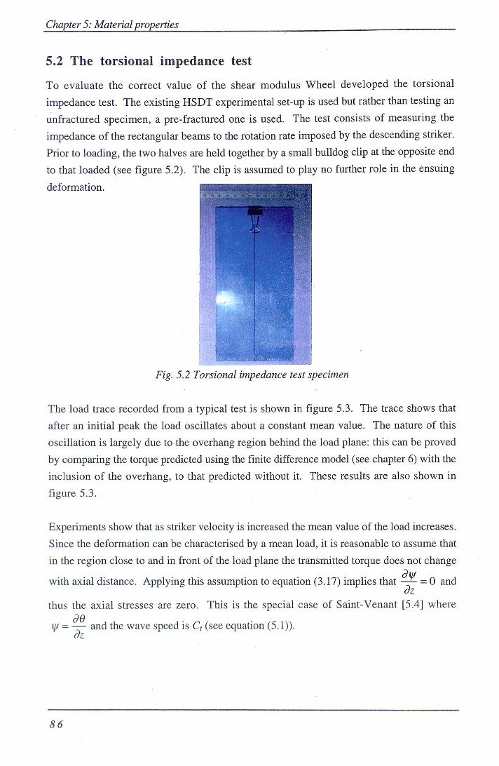
Chapter 5: Material properties
5.2 The torsional impedance test
To evaluate the correct value of the shear modulus Wheel developed the torsional
impedance test. The existing HSDT experimental set-up is used but rather than testing an
unfractured specimen, a pre-fractured one is used. The test consists of measuring the
impedance of the rectangular beams to the rotation rate imposed by the descending striker.
Prior to loading, the two halves are held together by a small bulldog clip at the opposite end
to that loaded (see figure 5.2). The clip is assumed to play no further role in the ensuing
deformation.
Fig. 5.2 Torsional impedance test specimen
The load trace recorded from a typical test is shown in figure 5.3. The trace shows that
after an initial peak the load oscillates about a constant mean value. The nature of this
oscillation is largely due to the overhang region behind the load plane: this can be proved
by comparing the torque predicted using the finite difference model (see chapter 6) with the
inclusion of the overhang, to that predicted without it. These results are also shown in
figure 5.3.
Experiments show that as striker velocity is increased the mean value of the load increases.
Since the deformation can be characterised by a mean load, it is reasonable to assume that
in the region close to and in front of the load plane the transmitted torque does not change dy/
with axial distance. Applying this assumption to equation (3.17) implies that 0 and
thus the axial stresses are zero. This is the special case of Saint-Venant [5.4] where
y/ = — and the wave speed is Q (see equation (5.1)).
86

Chapter 5: Material properties
1800
1600
1400
g 1200
V u 1000 k
b 800
u V 600
'B 400 in
200
0
-200
Experiment Finite Difference (no overhang) Finite Difference (with overhang)
1111111111111 11111111111 1111111111 111 1111 11 I I 11111 I 111 0.0 0.1 0.2 0.3 0.4 0.5 0.6 0.7 0.8 0.9 1.0 1.1
Time (ms)
Fig 5.3 Experimental and Predicted Load Traces
(HDPE, 0°C, striker velocity = 22.2 m/s)
Wheel's [5.3] analysis consisted of calculating the low strain, high strain rate Saint-Venant torsional wave speed (C°) using fig. Given the rotation rate imposed by the striker (0^p),
the twist in the deformed region can then be calculated from:
dd ^djj, dz C.
C5.2)
In Wheel's analysis C, = C% which is the torsional wave speed calculated from equation
(5.1) using jn, = / J . F r o m the value of the twist he then defined the effective strain as the
maximum shear strain in the section, which occurs at the centre of the longer edge of the
section. The calculation of maximum shear strain assumed axial stresses to be negligible.
The appropriate value of /Xjfor the effective strain was found by substituting the
experimentally measured torque into equation (3.17). The torque was calculated by
integrating the load trace over time, excluding the initial peak, and dividing by the time
period of the integration. At low striker velocities, the load trace becomes very oscillatory
and the evaluation of mean torque is inaccurate. By repeating the test at different striker
velocities, Wheel was able to define the secant shear modulus as a function of effective
strain. From this function the tangent shear modulus could then be calculated as a function
of effective strain.
As in this work, Wheel incorporated his results into the analysis of the HSDT test as a non-
linear elastic model.
87

Chapter 5: Material properties
5.3 Problems with the analysis
The analysis described in the previous section is flawed by the fact that the wave speed in
the specimen depends on the local tangent shear modulus which, assuming the material
behaves non-linearly (which is the whole point of this analysis), will not be equal to jig.
Wheel's [5.3] analysis therefore predicted lower strains for a given striker speed than
actually existed, and thus too fast a decay of fig with strain. Including this correction in the
analysis means the twist can no longer be determined explicitly, since it depends on the
value of which is to be calculated.
There is one other discrepancy in the analysis: the evaluation of the effective strain in
regions of non-linear twist. Wheel's approach (see above) is adequate in regions of
uniform twist (where ^ = — is a constant) since, for this case, equation (3.6) shows that dz
the strain at any point is directly proportional to twist. However, regions of non-uniform
twist do exist in the fracture test, where the twist does not equal y/. Wheel's definition of
effective strain therefore does not correctly characterise the strain across the section. These
problems are corrected by a new analysis detailed in the next section.
5.4 A revised analysis of the torsional impedance test
5.4.1 Definition of effective strain
In a M l three dimensional solution the shear modulus at a point is defined as a function of
the state of strain at that point. In a prismatic torsion beam all non-zero components of
strain vary across the section. In order that the equations of motion involve only one
spatial dimension, an effective modulus representative of the whole section was defined in
deriving equations (3.9). This effective section modulus must be defined as a unique
function of some effective strain, 7 , which characterises the entire strain field at any
section.
5.4.1.1 Circular Bar
To clarify the definition of 7 the case of a circular bar subjected to a constant twist is
considered before that of a prismatic bar. Let the material of the circular bar behave in a
non-linear elastic manner. Assuming that sections rotate without change in shape the
torque T is calculated as:
R T = j{27Cr^yii{Y))dr. (5.3)
88

Chapter 5: Material properties
where r is the distance from the centroidal axis of the bar, R is the radius of the bar and
/if y) is the secant shear modulus, a function of the shear strain % which itself varies with r.
An effective secant shear modulus is defined in a similar fashion to the derivation of
equation (3.7) such that
T = Pt.{y.)T„ (5.4)
where the strain moment
T„,=jr'r{r)drde (5.5)
is, in this case
r„,^j27tr'r{r)dr.
The effective secant shear modulus has been assumed to be a function of je which, as
stated above, should completely define the strain field. This is achieved by using the
following definition:
(5.6) C
where is the first polar moment of area of the section and therefore a section constant
= I rdrdd which is, in this case
T^ = ](2Kr^)dr = -7rR\
Equations (5.4) and (5.5) identify % as that strain which, if considered constant across the
section and substituted for / in equation (5.3), would yield the same value of Fas the actual
strain distribution y{r). For a circular bar the strain distribution is
Y = rd' (5.7)
where d' is the twist, so that from equation (5.5)
and from equations (5.6)
y . = | R S ' (5.8)
89

Chapter 5: Material properties
Thus once IJ-XVe) has been measured, the torque can be calculated for any value of i? and
6', since, from equation (5.4)
(5.9)
Where is a function of geometry and /g is a function of geometry and twist. The
preceding analysis therefore allows the true modulus and strain which vary across a
section, once redefined as effective ones, to be brought outside of the integration term of
equation (5.3). The most important characteristic of equation (5.7) is that it can be applied
to any radius of bar, the function being independent of the radius of the bar. Once
l^e[7e) is found for one particular radius it can therefore be used to any to predict the
torque/twist relationship for any radius of bar of the same material. The geometry
independence is proved below.
Consider the case where fig as a function of % is determined for a circular bar of radius R\
and the torque/twist relationship is to be predicted for a circular bar of the same material but
of radius Ri-
The true torque-twist relationship, for the bar of radius i?2 can be determined from the
substitution of shear strain from equation (5.7) into equation (5.3):
T^=2K\r^ll{re'^Yr 0
where the subscripts 1 and 2 denote the bars with radii R\ and /?2 respectively.
Changing the integration variable such that r^=—r gives: 7?2
7*2 = 2;r #2
V y 0 dr^. (5.10)
To produce the same effective strain in the bar of radius R\ the twist must be (from equation (5.8)):
From equations (5.4) and (5.3) the effective modulus, calculated from the bar of radius R],
for the same effective strain is therefore:
27t\r'n\^r^e A dr.
F„ "1
90

Chapter 5: Material pwpeities
Using equation (5.4) to now calculate the torque in the bar of radius Ri for this effective
strain and corresponding effective modulus gives:
T,=^27t\r'n dr^ = Ik R.
R
V -"-i y 0 V y R dr„
The value for T2 is identical to that given in equation (5.10), thus proving the geometry
independence.
5.4.1.2 Prismatic Bar
In defining % for a prismatic bar, it is first noted that from equations (3.6) the following is
true:
The effective strain is defined as that strain which, when assigned such that for
y>0 and y = y, for x<0, and the previous definition is taken into account, the resulting
value of the integral in equation (3.7a) is identical to that evaluated using the actual strain
field. As for the circular bar
7e =
where the strain moment is now
= j j (r z - Yxzy ydx = -1) + dz
and the first polar moment of area of the section is
% 0 . r , = 4 j \{x-y)dxdy = -BH{B + H).
0 4
The definition of % does not define a unique strain field since the field also depends on the
ratio i/Ato twist for a particular value of effective strain. It does, however, characterise the
strain across the section for all possible ratios; the magnitudes of jxi increasing with the
magnitude of y and increasing with the magnitude of x in all cases. Given that there is
some inaccuracy in the prediction of the strain field when t/^does not equal the twist (see
derivation of equation (3.9b)), this approximation is reasonable.
91

Chapter 5: Material properties
The definition of Ye also has another major advantage when the calculation of is
considered, since the differentiation with respect to the longitudinal axis (z) in equation
(3.7c) to derive equation (3.9a) yields the term:
By the chain rule this is equivalent to:
r C
=
dYg dz dz
dz
where ^ [ = - ^ { ^ s 7 e ) - (5.11)
The effective stress is defined by the normal rules of Hooke's law as:
t , ==/j,y, (5 12)
Substituting into equation (5.11) gives:
(5J^)
This definition of fit is the same as that in the standard calculation of the tangent modulus
with the tangent shear modulus, shear stress and shear strain replaced by their
corresponding effective section variables.
5.4.2 Calculation of effective strain in the torsional impedance test
Using equation (3.17) and putting y/ = the imposed torque can be written as:
]r== AtJTm (5.14)
and for this case r„, = X J ^ . (5.15) az
Applying the identity of equation (5.12) to calculate the geometry independent effective
shear stress from the torque gives:
T ^ = — (5.16) ^ C
92

Chapter 5: Material properties
If the above assumptions are valid this relationship is independent of the section
dimensions.
Substituting for /x, from equation (5.13) in (5.1) and the resulting equation for Saint-
Venant's torsional wave speed in equation (5.2) gives a function defining the twist.
Substitution of this into equation (5.15) gives:
(5.17)
where = = (5.18) r. c;
The variable % is the effective stress that would be produced for a particular geometry and
rotation rate if the material was linear elastic and the shear modulus equal to the low strain
high strain rate modulus The experimental results are used to define (equation
(5.16)) as a function of tg (equation (5.18)) which should be independent of section
dimensions:
T, ==JF(T.) (5.19)
By the chain rule, dVe dz„ dy^
Substituting from equation (5.17) for the derivative of effective stress with effective strain
and integrating by separation of variables gives:
d r j ^ dr. (5.20)
Equation (5.20) thus allows the effective strain to be calculated as a function of effective
stress.
5.5 Implementation of the analysis
In order to proceed with the evaluation of the shear moduli a mathematical form of the
function in equation (5.19) must be stated. A characteristic set of normalised results from
the torsional impedance test for an HDPE material is shown in figure 5.4.
93

Chapter 5: Material properties
I 0) «-
6
5
4
3
I I I I I 0 1
' ' I ' 2
-r-T 3
I I I I 4
To (MPa)
Fig 5.4 Torsional impedance results for an HDPE
At first sight the data appear linear and could thus be approximated by a simple straight
line. This would imply that both jUj and jit are constant and equal to the product of the
square of this slope and //G (see equation (5.24)). Results from section rotation
measurements (see section 5.6.2) will show this cannot be true at low values of strain and
that in this region fig and fit are close to fig. The shear moduli must therefore decay from fig
at low strains to a value which is determined from the slope of the results. A problem
arises from this decay in that Tg is not a single-valued function of This is best
demonstrated by performing the analysis of section 5.3 in reverse: in other words, assume
a stress-strain relationship and calculate the dependency of Tg on Tq. Consider a stress-
strain relationship which consists of two linear regions connected by a cubic spline as
shown in figure 5.5.
Substituting for the slope of the effective stress-strain curve from equation (5.17) into
equation (5.13) gives the equation:
= 7e4^t (5 .21)
From this equation and the stress-strain curve depicted in figure 5.5, as a function of %
can be calculated. The function is shown in figure 5.6. The figure clearly shows that Tg is
not single valued since, in the region corresponding to the spline, the rate of decay of fit
with % rapidly increases, producing a dip in To as a function of % (see equation (5.21)).
94

Chapter 5: Material properties
Delimits of spline
0 [ I 11 111 11 111 11 111 11 111 11 111 11 111 11 111 11 111 11 111 11 111 ' ' 111 11 I 0.0 0.1 0.2 0.3 0.4 0.5 0.6 0.7 0.8 0.9 1.0 1.1 1.2
Effective strain (%)
Fig 5.5 Stress-strain curve composed of linear and spline regions
1.2-
1.1 -j
1.0 •;
CQ 0 .9: k
0.8 •: w
V 0.74
0.6 •;
0.5 •:
0.4 i
0 .3 :
0.2-
Dehmits of spline region
I I I I I I I I I I I I I I I I I I I I i I I I I I I I i I I I I I I I I I I I I I I I I i I I I I I I I I I I I 0.2 0.3 0.4 0.5 0.6 0.7 0.8 0.9 1.0 1.1 1.2 1.3 1.4
To (MPa)
Fig 5.6 Te as a function of Tg predicted from the effective stress-strain curve of
figure 5.5
A function of the form depicted in figure 5.6 would therefore have to be fitted to the
experimental results. This is not a viable approach, firstly because the experiment cannot
be restrained to operate at a particular value of Tg, and secondly the results are unreliable at
low values of (low striker velocities).
95

Chapter 5: Material properties
The approach taken in this work is to consider the experimental data as a number of linear
regions. The corresponding linear regions of the stress-strain curve can then be evaluated
and connected by cubic splines, the start and end points of these splines and the slope at
these points being defined by the adjacent linear regions. Spline fits between the linear
regions are used to prevent instabilities that arise with a piecewise linear fit due to the
singularity in fXt that occurs at the strain demarking the cross-over from one region to
another. The details are described below:
Let the experimental data be approximated to a series of linear regions, as shown in figure
(5.7). The regions are numbered from 1 to N. Each region is defined by two points, such
that region n is defined by the two points: n-1 and n, and is described by the following
equation:
(5.22)
T — T where the slope, and 0 < n < N.
n—1
Region= 1 n N
Fig. 5.7 Schematic of the piecewise linear approximation used to model the torsional
impedance test results.
Substituting into equation (5.20) and evaluating the integral gives the reciprocal of the
effective strain as:
» e o
(5.23)
96

Chapter 5: Material properties
Substituting for the effective strain from above in equation (5.17) gives the effective section
tangent shear modulus from equation (5.13) as:
r^o
Since this equation refers to individual, linear regions the effective section tangent shear
modulus must be constant and therefore:
4 = 0
The identity for thus reduces to:
Substituting for Tg from equation (5.22) and To from (5.23) into equation (5.16) gives,
after rearranging, the effective section secant shear modulus as:
T — ffl T \ (5.25)
7e
The strain which demarks the change between region n-1 and n can take one of two values
depending on which region is considered. The difference in these two possible values of
strain reduces as the difference in slope between the two regions reduces. Rather than using
either of these two values the intercept is taken (point I in figure 5.8):
T y = ^ ' ^\n-l
It now remains to define the spline connecting region n-1 and n. The mid strain of the
spline is taken to correspond to the strain at the intercept (I). The interval of strain (A%,)
corresponding to the spline is equal to twice the difference in strain between the intercept
and strain defined by point n-1 of region n-1:
97

Chapter 5: Material properties
Region n
Region (n-1)
Fig. 5.8 Schematic of effective stress-strain regions: n-1 and n.
5.6 Validation
5.6.1 Finite difference model
One of the main validations of the analysis discussed in this chapter was to include the
derived material stress-strain characteristic in the finite difference model (see chapter 6).
The model was then used to predict the experimental results from which the characteristic
was derived. The striker velocity and specimen dimensions were input in to the model and
the mean striker force evaluated. These results were then transformed in exactly the same
manner as the original experimental ones to produce a plot of Tg versus To- The two sets of
results (finite difference and experimental) are shown in figure 5.9. As can be seen the two
results show good agreement.
The validity of the low strain region of the stress-strain curve cannot be confirmed by this
method since it is impossible to obtain reliable data at the low striker speeds, as explained
earlier. To examine this further a second finite difference analysis of the experiments
shown in figure 5.9 was performed, but the material model was changed to being linear,
and /I; being constant and equal to the product of the square of the experimentally
determined slope {dtg/dT^) and jUo(see equation (5.24)). This linear material model thus
excludes the low strain, high gradient of the stress-strain curve corresponding to /ig. The
results from this model are also shown in figure 5.9.
There is a slight reduction in the calculated Tg from the analysis as compared to experiment.
This reduction is greater for the linear material model results than for the non-linear. For
the non-linear case the error is probably due to the assumption made in deriving equation
(5.2) that the rotation rate is constant. The rotation rate does in fact vary slightly through
98

Clmpter 5: Material properties
the test and the value used in calculating To was the rotation rate at the time when a wave
travelling at C° would pass the mid-length section of the torsion beam. This assumption
could therefore be modified but on noting the scatter of the experimental results the
apparent reduction in Tg is relatively insignificant.
Piecewise linear approximation to experimental results
Linear analysis
(2
Non-lmear analysis
3
To (MPa) Fig 5.9 Normalised torsional impedance test results and the equivalent values predicted
from the finite difference analysis
There is therefore little significant difference between the linear and non-linear cases. This
can be explained once it is noted that the strains close to the load plane of the test specimen,
throughout the time of the test, lie largely in the domain of the low gradient linear region of
the non-linear stress-strain curve. The first point on figure 5.9 (lowest Tg) is the most
interesting in that it clearly shows the difference in the low strain modulus between the
linear and non-linear models. Since experimental results are difficult to obtain in this
region an experimental method, which is detailed in the next section, was developed to
check the validity of using fig.
5.6.2 Section Rotation
The modified optical crack gauge (described in chapter 2) can be used to measure rotation at
a series of sections along the specimen as a function of time. The technique provides a
method of checking the above theory by comparing the modified OCG section rotation
measurements during a torsional impedance test to those predicted using the finite
difference method.
The maximum slew rate of the OCG sensor stage used in processing the signals was 13
V/|is (at least two orders of magnitude higher than the rates actually measured) and thus did
99

Chapter 5: Material properties
not affect the results. The output from seven sensors during a test were captured on a
Nicolet 500 transient recorder with a sampling rate of 100 kHz. Sample results from two
tests are shown in figure 5.12. The OCG was primarily designed to define times at which
angular acceleration occurs at a section rather than to measure absolute rotation values. As
such, the results for angular rotation show considerable scatter.
Software post-processing was used to determine the time at which each of the seven section
rotations, recorded using the OCG, reached a set value. A 'propagation rate' (V) of that
rotation along the specimen was then evaluated. An example of one test result is shown in
figure 5.10 together with the prediction from the non-linear finite difference model without
the modelling of the overhang.
B B
"o. 140 -"a
o
1 v u e 2 %
% §
C/3
160
80
° Finite difference • OCG
•
« •
•
0 . 4 0 . 5 0.6 0 . 7 0.8
Time (ms)
Fig. 5.10 Experimental and predicted propagation rates for a rotation amplitude of 8^
As can be seen the propagation rate is reasonably constant with an acceleration and
deceleration at 120 mm due to a combination of overhang effects and reflected, unloading
torsional waves reflected from the free end. Due to this reflection a linear least squares fit
through only the first three points was used to determine the propagation rate from each set
of experimental results. The corresponding propagation rate was then predicted using the
finite difference model. The material was modelled as both linear and non-linear as
described in section 5.6.1. The modelling of the overhang was omitted to reduce
oscillations which would produce a scattering of the results (see section 5.2). The tests
analysed correspond to those shown in figure 5.9, the propagation rate for an angular
rotation of eight degrees and the minimum rotation (see figure 5.12) was calculated from
both the finite difference model and experimental results.
100

Chapter 5: Material properties
The results from these experiments are shown in figures 5.11. There is good agreement
between the non-linear finite difference model and experimental results for the propagation
rate of the minimum rotation. This speed is, on average, just less than C,". The linear
finite difference model results for this propagation rate do not show good agreement, the
rate corresponding to the Saint Venant wave speed calculated using the high strain shear
modulus input into this model. All results show reasonable agreement for the propagation
rate of the 8° rotation amplitude.
O % 1.2
1.0
1 0.8-
§
& CQ
s
Ph
1 1 o Z 0.0
0.4-
o
• •
• o
• u
Q %
O Experimental minimum rotation O Finite Difference minimum (non-linear) A Finite Difference minimum (linear)
-1—1—I—r 10
T 15
I I I I I I
20 25 T 30
Striker velocity (m/s) Fig. 5.11a Experimental and predicted propagation rates of the minimum rotation amplitude
It is conceivable that the propagation rate of the minimum amplitude is dependent on the
dispersive nature of torsional waves in rectangular beams. If this amplitude is carried by
high frequency components then the propagation rate could be higher than that predicted by
Saint Venant's equation. The dispersion is due to the existence of axial stresses in the
beam which are in turn dependant on the tensile modulus. The tensile modulus in the linear
material finite difference model was set to the same value as that in the non-linear model
and therefore the difference in propagation rate of the minimum amplitude cannot be due to
dispersion. From these results it is clear that the non-linear material model is more
appropriate for modelling the HSDT test.
101

Chapter 5: Material properties
0 -
1 ! %
e
1 2 P4 ns a
•I
1 Z
0.8
0 . 7 -
0 . 6 -
0 . 5 -
0 . 4 -
0 . 3 H
0.2
0.1 •
•
0 1
A
•
• • • 2 ° 2 ^ 1
O Experimental 8° O Finite Difference 8° (non-linear) A Finite Difference 8° (linear)
10 1 5 20 2 5 3 0
striker velocity (m/s) Fig. 5.11b Experimental and predicted propagation rates of the 8° rotation amplitude
A final observation can be made from the measured section rotation histories. This
concerns the pronounced negative section rotation at the firont of the torsional wave due to
the dispersive nature of the deformation. Two sets of results are shown in figure 5.12.
Both the predicted and the experimental results show an increase in magnitude of this
negative rotation with striker velocity and with distance from the load plane.
Striker velocity = 28.9 m/s
Striker velocity = 11.8 m/s
10
S 8
I TJ
Finite Difference Experiment
6 -
§ • • 3 4
2 a o u V t/3
z = 9 0 m m z = 1 4 0 m m
z = 9 0 m m z = 1 4 0 m m
Minimum Finite Difference rotation -2 - I I I ' I I I I I I I I I I I I I I I I I I I I I I I I I
0 . 0 0 . 2 0 . 4 0 . 6 0 . 8 1 . 0 1 . 2
Time (ms) Fig. 5.12 Experimental and predicted rotation histories
102

CJvxpter 5: Material properties
5.6.3 Geometry Dependence
4 -
C3
% 2 4
<u 1 -
• Nominal Thickness 7mm O Nominal Thickness 10mm n n • •
• • •
• •
I I I I I I I
0 1 2 3 4 5 6 7
(MPa)
Fig. 5.13 Normalised torsional impedance results for specimens of both 7 and 10 mm
nominal thickness.
Figure 5.13 shows torsional impedance test results for two thicknesses (7 and 10 mm) of
the same grade of HDPE. The figure shows the results to be similar and confirms that the
effective section modulus is geometry independent.
• ' I ' ' ' ' I 4 5
I I I I I I
6
5.7 Results
Torsional impedance and ultrasonic modulus tests were performed on a range of materials.
All the results could be modelled adequately by a bilinear fit. They are summarised in
tables 5.1 and 5.2.
Material HDPE MDPE
Temperature (°C) -5 0 10 20 0 10 20
Mo (GPa) 1.25 1.127 0.94 (186 0.94 0.82 (X64
Poison's ratio (D) 0.38 &38 &39 0.40 &39 0.40 0.41
Density (kg/m^) 960 960 960 960 940 940 940
Slope (mj) 0J32 0.544 0.477 &394 0.435 0.363 (1418
Point 1
( s e e figure 5 . 7 )
To (MPa) 1.734 1.047 0.672 0.794 0.648 0.519 0.164 Point 1
( s e e figure 5 . 7 ) Te (MPa) " " " " "
Point 2
( s e e figure 5 . 7 )
To (MPa) 7.00 7.00 6.00 6.00 5.00 6.00 5.00 Point 2
( s e e figure 5 . 7 ) Tg (MPa) 5.59 4.29 3.22 2.85 2.5 2.51 2.18
(mi)^IJ.o (GPa) 0.67 (133 0.21 0.13 0.18 0.11 0.11
Table 5.1 Summary of torsional impedance test results for polyethylene at a range of
temperatures
103

Chapter 5: Material properties
Polyoxymethylene Polypropylene
Material Delrin NC Delrin ST Homo- 30% weight
(unmodified) (modified) polymer EPDM
Temperature (°C) 0 0 0 0
Ho (GPa) L783 1.209 L79 (X856
Poison's ratio (v) 0.37 038 &33 0.40
Density (kg/m^) 1420 1330 9123 894.9
Slope (m;) 0.545 &394 0.951 0.844
Point 1 To (MPa) 0.706 0.172 0.0 (1593
Te (MPa) " "
Point 2 To (MPa) 10.00 8.00 6.0 5.00
Tg (MPa) 5.77 3.26 5.706 4.31
(GPa) 0.53 0.19 1.61 0.61 Table 5.2 Summary of torsional impedance test results for polyoxymethylene and
polypropylene
For all the results the high strain shear modulus is considerably less than {ig. It is not easy
to determine the physical relevance of the change from high to low modulus. The
maximum strain in a section, where the axial stresses are zero {v/ = can be derived
from equation (3.6):
/max - f -
For the HDPE results shown in figure 5.14 the maximum strain corresponding to the
effective stress demarking the transition point between the two regions is approximately 0.8
%. Dioh [5.2] has investigated the stress-strain characteristics of HDPE at 0°C under
compression at a range of strain rates; they are shown in figure 5.14.
1.6% strain
I % I "W
High strain rate
Intermediate strain rate
Low strain rate
4 5 6
Strain (%) Fig. 5.14 Uni-axial stress-strain curves for HDPE at 0°C (Dioh [5.2])
104

Chapters.- Material properties
A 0.8 % shear strain corresponds approximately to a 1.6 % normal strain (assuming pure
shear stress conditions) which, from Dioh's data, is close to the yield point of the material.
The transition may therefore be due to the onset of the section yielding. As the effective
section shear strain increases beyond the transition a larger and larger proportion of the
section undergoes yielding. This effect manifests itself as a reduction in the effective
section shear modulus which remains constant after the initial transition period.
5.8 Summary
Once effective section shear stress, strain and moduli are defined the torsional impedance
test provides an ideal method for measuring the effective stress-strain characteristic at the
strain rates appropriate to the analysis of the HSDT test. The ultrasonically measured shear
modulus is relevant at low shear strains, but at high strains it can over-estimate the shear
modulus by a factor of two to three. The majority of the deformation is controlled by the
Saint-Venant wave equation. The dispersive nature of torsional waves in rectangular
beams is a secondary effect, which is most apparent in its production of a negative section
rotation close to the wave front.
The modified OCG provides a convenient alternative to measuring jig which does not
require the apparatus of the ultrasonic method and produces a result more appropriate to the
HSDT test.
5.9 References (5.1) Wheel, M.A. and Leevers, P.S., 'High speed double torsion tests on tough
polymers I: Linear elastic steady state and dynamic analysis'. Int. J. of Fracture, 61, p. 331, (1993).
(5.2) Dioh, N.N., High strain rate behaviour of polymers at various temperatures, PhD Thesis, Univ. of London, (1993).
(5.3) Wheel, M.A. and Leevers, P.S., 'High speed double torsion tests on tough polymers. 11: Non-linear elastic dynamic analysis'. Int. J. of Fracture, 61, p. 349, (1993).
(5.4) Saint-Venant, B. de, 'M6moir sur les vibrations tournemantes des verges elastiques', Comptes Rendus, 28, pp. 69, (1849).
205

Chapter 6: The finite difference model
Chapter 6
The finite difference model
6.1 Introduction
In order to calculate the dynamic crack driving force from the HSDT test results the
equations of motion and appropriate boundary conditions derived in chapter 3 must be
solved. These are non-linear differential equations due to non-linear material properties.
To obtain a solution to these equations a two dimensional (one spatial, one time), finite
difference model is used throughout this work.
The finite difference (FD) method has been used in many areas of engineering in the
solution of differential equations of motion. The most notable researchers in this area with
regard to RCP are Kanninen [6.1] who simulated the Double Cantilever Beam (DCB)
fracture test and Wheel [6.2] who simulated the HSDT test. Both researchers employed a
two dimensional (one spatial, one time) FD solution and due to symmetry about the crack
plane, only modelled a half-specimen. They modelled the restraint imposed by the
opposing half using an elastic foundation.
Kanninen used his FD scheme in propagation mode. That is, he assumed that for crack
advance the crack driving force at the node corresponding to the crack front, must satisfy
the equality of equation (1.1) and at this point the crack front was advanced by one node.
The fracture resistance was adjusted until the predicted crack history matched that measured
experimentally.
Wheel's approach was to use a FD model in generation mode, where the experimental
crack history is input in to the model and the crack driving force predicted. Wheel stated
that it was not possible to accurately measure initiation time from the experimental results
and so iterated on this parameter to find the initiation time which produced minimum
variation in crack driving force during the test.
The FD model that is used in this work is discussed in the next sections. Its important
features are described and its numerical accuracy and sensitivity to important parameters are
discussed. The results from the model are used to examine the characteristics of the HSDT
test and so determine the most suitable operating points to achieve accurate results for
fracture resistance.
106

Chapter 6: The finite difference model
6.2 The finite difference model of the HSDT test
6.2.1 General features
An explicit, second order accurate, central difference finite difference scheme is used. This
was shown to be both efficient and stable by Wheel [6.2], provided both the time step and
node spacing are below the size required for convergence. Before discretising the
equations of motion derived in Chapter 3, they were non dimensionalised using the
following definitions;
* Z * TT * C? z = — ¥ = WH t = t—^
H ^ ^ H
Where t* and z* correspond to non-dimensional time and distance respectively and is the
non-dimensional axial displacement function.
Equations (3.10a) and (3.10b) were discretised in their second order forms and both y/and
6 solved at each time step. An alternative approach would have been to combine the two
equations to eliminate y/ and discretise the resulting fourth-order partial differential
equation. This approach was not taken since there is limited literature on using the FD
method to solve fourth-order equations and because it would have increased the complexity
of the coding. The resulting discretised equations are as follows:
In order to ensure stability the time step (At) must be less than the time taken for a
disturbance, travelling at the maximum possible velocity, to traverse the distance between
two adjacent nodes. The time step chosen was one fifth of the time it takes a shear wave
(asymptotic phase velocity of dispersive torsional waves at high frequencies) to travel
between two adjacent nodes;
where Cf = V/WP (As shear wave speed) and Az is the spatial distance between nodes.
120, equally spaced nodes were used to define the test specimen. The dependence of the
numerical accuracy of the model on At and Az is discussed further in section 6.4.5.
107

Chapter 6: The finite dijference model
6.2.3 Initial test case
A test case used for the above FD scheme was that of resonance, for which the analytical
solution is known (see section 3.3). This was implemented by setting the initial nodal
values of ^and 6 to that of a particular mode, predicted from equation (3.23), and then
using the FD model to predict the resulting deformation. The model geometry
corresponded to the standard HSDT half-specimen and the material properties to HDPE,
with a constant shear modulus equal to that measured using the direct contact ultrasonic
method (see section 5.1). The predicted frequency of oscillation was within 0.01 % of that
calculated analytically and the mode shape showed no change over twenty oscillations.
This procedure was repeated for all mode numbers up to and including the sixteenth, with
no increase in the error between analytical and FD results.
6.2.2 Specific features
This section describes the specific features of the FD model of the HSDT test not already
covered in section 6.2.1. Each feature that will be described influences the dependence of
crack velocity on Gd- Where appropriate, default values for parameters are given. In
section 6.4 the sensitivity of the model to each of these parameters is discussed in turn.
6.2.2.1 Load plane boundary conditions
The load trace from the HSDT test shows a characteristic oscillation about a mean load.
Work by Williams [6.3] and Crouch [6.4] show that two possible causes for the oscillation
are contact stiffness and overhang effects. These effects were therefore included in the FD
model.
The load plane boundary conditions are exactly the same as those in the static case (see
section 4.2.2.2) with the additional modelling of contact stiffness between the planar
specimen surface and both the spherical contact points of the striker and support. The
contact stiffness was modelled, according to Hertz [6.5], assuming no friction or relative
slip between the contacting surfaces and linear material properties;
a = 9 p% 16 R
where R is the radius of the contact point, a is the distance that the two contacting bodies 1_ v2
approach one another, outside of the region locally deformed by the contact. c„ = is 7rF„
a compliance term, the subscript n having a value of 1 or 2, denoting the different material
properties of the two bodies; E being the tensile modulus and u the Poison's ratio. In the
lOS

Chapter 6: The finite difference model
FD model E for the specimen material is equal to the product of the direct contact
ultrasonically measured modulus (see section 5.1) and an adjustment factor (%). The
adjustment factor was introduced since the value of E appropriate to the strain and strain
rate at the contact point is unknown prior to performing the analysis. The value of % is
adjusted to match experimental with predicted load histories.
The deceleration of the striker due to the contact force was included in the model.
6.2.2.2 Free end boundary conditions
The free end boundary conditions are exactly the same as those in the static case (see
section 4.2.2.2)
6.2.2.3 Non-linear elastic material
Non-linear material behaviour is discussed in detail in Chapter 5. At each time step the
effective strain at each node is calculated from the discretised form derived in section
5.4.1.2 and the associated stress-strain region identified and recorded. The corresponding
nodal shear moduli are then calculated and used in calculating the future values of 6 and y/.
The effective strain region is recorded at each time step so that at the proceeding time step a
reasonable first guess can be made at the region in which the effective strain lies. This
procedure considerably shortens the execution time if there are a large number of stress-
strain regions.
An instability problem due to non-linear material effects occurs with some materials when
there is a large difference between the low and high strain tangent shear moduli. To explain
this effect it is convenient to consider the development in time of an oscillating rotation
profile, as shown in figure 6.1a. The effective strain is largely governed by the twist and is
therefore of the form shown in figure 6. lb. If the variation in effective strain is of the right
value and amplitude to span the region between the low and high strain tangent shear
moduli, there will be a dramatic difference in local torsional wave speeds between the
regions L and H. This effect shows a form of positive feedback, in that the twist then
tends to increase further in high strain regions, promoting a kind of 'shock wave', as
shown in figure 6.1c. The rotation profile can become unrealistically 'noisy', since in
reality the natural damping of the material will tend to smooth these fluctuations.
To overcome this problem a smoothing function is applied to the effective strain before the
nodal shear moduli are calculated. 'The concept of smoothing lies in a murky area' [6.6].
The approach used here was to calculate the smoothed strain at a node as the 'windowed
median' of 5 nodal strains; the node itself and the two nodes in front and the two nodes
109

Chapter 6: The finite difference model
behind it. This method prevents any instability and produces little change in results from
the unsmoothed method when no instabUity occurs (see table 6.1). A more elegant method
is to use Fast Fourier Transforms to perform filtering in the frequency domain, but this is
very costly in terms of run time, compared to the method used.
Direction of propagation
II L H . ^
- L ^
H L
^
(.a) Axial distance (z)
(b) Axial distance (z)
(c) Axial distance (z)
Fig. 6.1 Development of instabilities due to the non-linear material model
(a): propagating rotation profile
(b): effective strain associated with the rotation profile of (a)
(c): development of rotation profile shown in (a)
6.2.2.4 Crack propagation and the curved crack front
Propagation mode is used in the model for the following reasons;
1) Propagation mode requires iteration on Gj) to find that value which predicts the same
crack history as recorded from the experiment. The iteration time involved is
comparable to that in generation mode when finding the correct initiation time.
2) Propagation mode produces fewer constraints in the model, since the crack velocity
is allowed to fluctuate. In the test itself the crack histories all show some oscillation
and in the extreme case of stick-sUp crack propagation, the crack velocity acmally drops
to zero for a short period of time.
110

Chapter 6: The finite dijference model
3) In order to determine Go from an experimental test using propagation mode the value
of Gd must be assumed to be constant during the analysis. This limitation is discussed
further in section 6.2.2.5.
The crack front shape in the Double Torsion test is noticeably curved as discussed in
chapter 4. The curved crack front was included in the model by employing equation (4.18)
to calculate the shape of the crack front at each time step, assuming Go to be constant along
the crack front throughout analysis. Knowing the remaining ligament thickness at each
node, the restoring moment due to the foundation can then be calculated, and thus the nodal
values of 6 and i/ at the proceeding time step.
The iterative method used by the model, to find the value of Go that produces a predicted
crack history the same as that measured experimentally, is as follows:
1) A straight line is fitted through the experimental crack history points using a least
squares approach. The slope of this line gives the steady state crack velocity.
2) The model then steps through values of Go, calculating the corresponding predicted
steady state crack velocity at each step. The same number and spatial positions of crack
history points as obtained experimentally are used in the calculation of predicted steady
state crack velocity.
3) After identifying the step interval that encompasses the correct value of Go, the
method of bisection is used to converge to a value of Go within the required accuracy.
This rather simplistic iterative scheme was used since d is not a smooth function of
(see figure 6.17). A more refined scheme such as the Newton-Raphson method would not
be reliable since it is dependant on the smooth increase (or decrease) of the first derivative
of the function to be solved.
6.2.2.5 Dynamic fracture resistance as a function of crack velocity
The existence of a curved crack front complicates the definition of crack velocity. Consider
the propagation of a curved crack front and assume its shape does not change as it
translates along the specimen length, as shown in figure 6.2.
a
Fig. 6.2 Schematic of the HSDTfracture surface showing the idealised
propagation of the curved crack front
111

Chapter 6: The finite difference model
Let the translation velocity be constant and equal to d. The normal velocity to the crack
front (77) at any point is then described by:
77 = dCos{(n)
where C7 is the angle subtended by the normal to the crack front to the z axis of the
specimen. For this simplified case the true local crack velocity along the crack front
reduces from a maximum at the leading edge to a minimum at the trailing edge. It is
commonly accepted that as crack velocity reduces to low values there must be an increase in
Gj).
Leevers [6.7] has developed a thermal decohesion model of the fracture process in
thermoplastic polymers where the crack propagates by a micron scale melting process. The
model assumes that Gu is the energy required to melt a material thickness equal to a weight
averaged, half chain length of material either side of the future crack plane. On achieving
this criterion the material then poses no resistance to separation. Leevers has developed
this theory in order to calculate Gd as a function of crack velocity. The results for PEIOO at
0°C are shown in figure 6.3. At 215 m/s there is a minimum which corresponds to a value
for Gd of 3.56 kJ/m^. If the crack velocity reduces from this minimum point there is more
time for heat to be conducted away from the crack front and if the crack velocity is
increased there is less time for the heat to be conducted to the required depth.
In the HSDT test it would therefore appear that a higher crack driving force is required to
propagate a crack at the trailing edge of the crack front (where the 77 is low) as compared to
the leading edge (where 77 is high). In order to evaluate the influence of this effect in the
HSDT analysis, a second version of the code was written that predicted crack propagation,
given Gd as a function of crack velocity. The routine used to predict crack propagation is
outlined below.
Consider a rotation and crack front profile at time t and the calculation of the profiles at the
next (future) time step. The future rotation profile is easily calculated since both the present
and past rotations and the foundation stiffness are known at every node. The local
propagation direction of the crack front (trajectory) at any node is assumed to be normal to
the slope of the front. The angle of this trajectory to the z axis is calculated in the FD model
by central difference in space as:
CJj = tan ^ 2Az
v C i - C i y
112

Chapter 6: The finite difference model
3
s §
I
I I
I I I I I I I I I I i I I I I I I I I I I I I
1 0 0 2 0 0 3 0 0 4 0 0 5 0 0
Crack velocity (m/s)
600
Fig 6.3 Prediction of fracture toughness as a function of crack velocity
from the thermal decohesion model for PEIOO at 0°C
The crack driving force (G) versus true crack velocity function is then calculated along this
trajectory. The method used in this function is as follows: consider that the crack
propagates from its present point (P) to a future point (F) along the trajectory. The crack
driving force (during the propagation firom P to F) is calculated by taking the average of G
at the present time step at P and future time step at F. The value of G at F is found by
interpolating the rotation at F from the two adjacent nodes and then applying equation
(4.18). Equation (4.18) can be applied directly to calculate G at P since P lies at a node.
The crack velocity during the propagation from point P to F is assumed to be constant.
This procedure is then repeated for a series of points along the trajectory to define the G- f]
function. The intercept between the G- f] and the Go- "H functions can then be found. In
this work, if two intercepts occur the one corresponding to the higher crack velocity is
taken unless otherwise stated. From the calculated trajectory and crack velocity at each
node the new crack front position can then be mapped back onto the nodes and the next
iteration started.
This method requires Go as a function of 77 to be known in advance, and so rules out its
use as a method of calculating Go from the experimental results. This routine does,
however, provide a means of examining the inaccuracies in the model as described in
section 6.2.3.3 due to Go actually being a function of 77.
113

Chapter 6: The finite difference model
6.2.2.6 Energy balance
In addition to solving the equations of motion at each time step, an additional routine
calculates the incremental internal energy and work done on the specimen during each time
step, from the discretised form of the equations given in section 3.2.3. The integration is
performed using Simpson's method. These results provide a check that both the model is
coded correctly and that the solution has converged such that the results from the model are
independent of the size of Az and At.
6.3 Software
Before coding the model certain objectives were set for the final program. These were as
follows;
1) The model should be user friendly.
2) The model could be modified by anyone with a basic knowledge of the Pascal
programming language.
3) The large amount of numerical data produced by the analysis could be displayed in
a graphical form in order to ease their interpretation.
In order to meet these objectives the program was written in a modular form using
Borland's object oriented Turbo Pascal for Windows. This compiler facilitates writing
mouse driven software that is compatible with Microsoft Windows, and is of a standard
'look and feel' form which anyone familiar with Windows could easily use.
The input files for the model are dialogue boxes which are activated from a simple menu
(see figure 6.4). Once the data has been entered it can be easily saved, loaded and edited.
The data files created can then be selected and run in batches. Output files are of two types;
1) A display file which the application uses to produce an animated image of both the
rotation profile and crack front shape as they develop in time (see figure 6.5).
2) An ASCII results file detailing the components of the internal energy, work done,
striker force and crack length as a function of time. This file is compatible with
standard graphing packages such as Cricket Graph and Excel.
Although the input and output routines are written using object oriented techniques, they
are designed to be easily updated with little programming expertise. The core analysis
routine is written in standard Pascal apart from dynamic memory allocation of the nodal
arrays. Two versions of the executable program, plus source code, are contained on the
attached disk. To run, 'double click' on hsdt.exe seen from File Manager of Microsoft
Windows whilst viewing the directories of the floppy disk drive. The programs are;
1) const_gd\hsdt.exe {Go is assumed to be constant with d)
2) vary_gd\hsdt.exe (Go as a function of d is prescribed in the input)
114

Chapter 6: The finite dijference model
HSDT k -
#B: 3Fwc&)n, ;8 un i Qfsqi '. \ a...
(est Data Flic Nhiiu' c Ui!i(!r5Wt(<vc\{jc mo\tub(nr?0 tst
I ;.nlfrl I Material filcN.irrip
I Seipct I Parameter FBe Name:
« Uisi>re\£.t(!vo o moMub0ttub124mat
r-VJSi»retetweVP mo\curved par 1 Seloct i Display RIe Name:
Sek'ct I Datrt F lie Ndiiip
BO Single Run
r ' ImpCitlKfK p tpsi L 1 ncr(jy Check
C ilLul.'Ction Step (kJ/tnV)
Accuracy (kJ/m*s):
Notch Length (mm);
Thickness (mm);
Groove Depth (mm):
QockTime (ms);
cAiJsrr>:\stc>vp\(j(; moMubOttZO.dsp
c1usor k pvc\{)(. moltub(M20.Res
Output F rpqupncy:
0.1 1 i
40
9.389
1.50
161111
, 1 <ao! I
Oack Data
Fig. 6.4 Input dialogue box for test data
HSDT
Display
File Name cAusers\steve\p«i nioMubOtUO.dsp ResuK Display Rotation (Deg)
21.8817 g
3.4392
Time 0.456 ms
CrackLength 112.774 mm
Striker Force 521.05 N
ADol 247.689 m/s
rward I
I
Backward! I I I I I I I I I 1"I"I"
Length (mm]
I Crack Shape Djsplav
Fig. 6.5 Display screen show crack and rotation profiles
(The forward and backward buttons cause the display to step through time)
115

Chapter 6: The finite difference model
6.4 Validation and Testing
Section 6.2 described the various components of the finite difference model used to analyse
the HSDT test. The following section examines each of these components in turn. Unless
otherwise stated the results refer to the following conditions:
Contact stiffness adjustment factor (%) = 0.2 Non-linear material properties of PEIOO 0°C (see section 5.7) Smoothed effective strain formulation Constant Go-d formulation, Gd= 3.56 kJ/m^ Foundation stiffness coefficient (c) = 0.29 Number of crack points =10 Striker velocity = 17 m/s Thickness (B) = 9.27 mm Side groove depth =1.80 mm Initial notch = 46 mm
The definition of crack points is as follows: The first crack point is always at 60 mm from
the loaded end of the specimen (50 mm from load plane). The subsequent points are then
spaced at 10 mm intervals i.e. if 4 points are used then they lie at 60, 70, 90 and 100 mm
from the loaded end of the specimen. These points are plotted against the time that the
crack passes them. The crack velocity for this case refers to the slope of the line fitted to
these points using the least squares method.
6.4.1 Contact stiffness
The dependence of predicted load on contact stiffness is shown in figure 6.5.
1750
1500 •
Z 1250 -
V V u a
k
1000 •
750
500
250
C = 0.1 c = 0.3 c = 0.7
0.00
i I I I I I I I I I I I I I I I I I I I I I I I I I I I I I i I I I I I I I
0 . 1 7 0 . 3 4 0 . 5 1 0 . 6 8 0 . 8 5
Time (ms)
Fig. 6.6 Dependence of predicted load on contact stiffness
116

Chapter 6: The finite difference model
The main cause of the oscillations is not the contact stiffness but the overhang region
behind the contact point as is shown in figure 5.3. Decreasing the contact stiffness reduces
both the amplitude and frequency of the striker force oscillations whilst the mean force
remains constant. This result would be expected from a mass-spring model [6.3]. The
effect of contact stiffness on crack velocity for low, medium and high velocity cases for a
variety of crack point numbers is shown in figure 6.7. The predicted crack histories for the
minimum and maximum values of contact stiffness are shown in figure 6.8. 260 :
240 4 V J
1 220 4
200 4 u
O
180 -a 180 ->
160 -w a k
U 140 :
120 :
100 -
0.0
I I I I I I I I I I I I I I I I I I I I
0 . 2 0 . 4 0 . 6 0 . 8 1 .0
Contact Stiffness factor ( X ) 1 .2
Striker velocity=25 m/s (10 point) Striker velocity=25 m/s (8 point) Striker velocity=17 m/s (10 point) Striker velocity=17 m/s (8 point) Striker velocity=7 m/s (10 point) Striker velocity=7 m/s (8 point)
Fig. 6.7 Dependence of crack velocity on contact stiffness
In general, decreasing the contact stiffness increases the crack velocity, an effect which is
mediated by increasing the delay in initiation and subsequent crack acceleration (see figure
6.8). Figure 6.7 also shows the dependence of crack velocity on contact stiffness
calculated using 10 and 8 crack points, demonstrating that the calculated steady state
velocity is dependant on the number of points used. The dependence on the number of
points is due to the combination of stress waves produced by the load plane oscillations and
reflections from the free end. In other words, the contact stiffness can have a strong
influence on the points at which the crack accelerates and decelerates in the latter region of
propagation. As a general rule it is better to take sample points over as wide a range as
possible since low sampling numbers give a poor distinction between tests at high striker
velocities (see results in figure 6.10).
117

Chapter 6: The finite difference model
160
<u 100
X = OJ
0 . 1 0 . 2 0 . 3 0 . 4 0 . 5 0 . 6 0 . 7 0 . 8
Time (ms)
Fig. 6.8 Crack histories for two different values of contact stiffness
0 . 9
6.4.2 Non-linear material properties
In chapter 4 it was stated that all torsional impedance test results could be represented by a
bi-linear function. Due to the limitation of the test at low striker velocities the transition
point is not well defined from the experimental results. In order to examine the sensitivity
of the predicted crack velocity to the transition point, a series of different non-linear
material properties were examined. Each case is shown in table 6.1, together with the
predicted crack velocity from the model at low and high striker velocities. In order to
assess the smoothing function, each of these cases was tested using smoothed and
unsmoothed versions of the model.
The definition in case 1 is that measured and described in chapter 5. Cases 2 and 3 are
similar but with, respectively, a lower and a higher transition point (point 1). Cases 4 and
5 are effectively linear material properties; case 4 being the high strain modulus and case 5
the low strain modulus. Case 6 is similar to case 1 but with a more refined transition from
the low strain to the high strain modulus.
None of the cases using the unsmoothed calculation of the effective shear strain showed
signs of instability and as such comparison between unsmoothed and smoothed results
therefore gives an indication of the error introduced by smoothing. As can be seen from
the results the error is low apart from the medium striker velocity results of case 2 (9%
increase from the smoothed to the unsmoothed result).
118

Chapter 6: The finite difference model
The crack velocity shows a low sensitivity to the modulus transition strain particularly at
the low and high striker speeds. At the medium striker velocity, for the smoothed results,
there is a 15% reduction from case 1 to case 3. Providing the transition effective stress is
accurate to within 50% the error produced in predicted crack velocity should be less than
10%.
Case Number 1 2 3 4 5 6
|io (GPa) 1.13 1.13 1.13 0.334 1.13 1.13
Point 0 To(MPa) 0.0 0.0 0.0 0.0 0.0 0.0
Tg(MPa) 0.0 0.0 0.0 0.0 0.0 0.0
Point 1 To(MPa) 1.05 0.5 2.0 1.0 1.0 0.52
Xe (MPa) 1.05 0.5 2.0 1.0 1.0 (X52
Point 2 To(MPa) 7.0 7.0 7.0 7.0 7.0 3.0
Te (MPa) 4.29 4.29 4.29 7.0 7.0 2.11
Point 3 To (MPa) - - - - - 7.0
Te (MPa) - - - - - 4.29
Smoothed (s) /
Unsmoothed (u)
Striker velocity
(m/s) Predicted crack velocity (m/s)
s 7 110 119 105 183 99 120
u 7 110 120 109 183 99 120
s 17 148 158 126 272 148 157
u 17 147 172 127 272 148 158
s 25 208 216 194 368 199 214
u 25 208 217 194 368 199 220
Table 6.1 Sensitivity of crack velocity to different non-linear shear modulus definitions
6.4.3 Curved crack front
6.4.3.1 Sensitivity to foundation stiffness coefficient
The sensitivity of predicted crack velocity to the foundation stiffness coefficient for low and
high striker velocity cases is shown in figure 6.9.
As can be seen the crack velocity shows a complex sensitivity to c with a maximum error
of 16% in predicted crack velocity over the range considered. The data in figure 6.9 also
shows the sensitivity of the model to the value of E used in the foundation, since a change
in the value of c can alternatively be considered as an inversely proportional change in E, in
both the foundation stiffness and crack driving force terms (equations (4.9) and (4.18)
119

Chapter 6: The finite difference model
respectively). The actual value of c should be reasonably accurate but the value used for E
in the foundation is questionable. An estimate of the possible errors can be made from the
work of Morgan [6.8] who examined the plane strain value of the flexural modulus in the
Charpy test. His results show that the flexural modulus could fall by up to 50% for the PE
80 and PE 100 materials at the maximum strains in the HSDT foundation. If it is noted that
the strain rates in the HSDT test are 50-100 times greater than the rates at which Morgan
performed his tests, and noting Dioh's prediction of strain rate sensitivity of these materials
(see figure 5.14), it is unlikely that E would be less than 75% of the direct contact
ultrasonic measured value (an increase in c from 0.29 to 0.39). This error in E would only
produce a maximum error in crack velocity of 4%.
c = 0.29
260
I
240 -
220
200
Striker velocity = 25 m/s Striker velocity = 17 m/s Striker velocity = 7 m/s
.-S 180 u o "3 >
u 2 u
160 -
140
120
100
- 0
80 0 . 0 0 0 . 2 5 0 . 5 0 0 . 7 5 1 . 0 0 1 . 2 5
Foundation stiffness coefficient (c)
1 . 5 0
Fig. 6.9 Sensitivity of crack velocity to foundation stiffness coefficient
6.4.3.2 Dynamic fracture resistance as a function of crack velocity
The alternative crack propagation model described in section 6.2.2.5 was used to examine
the effect of Gd as a function of true crack velocity. The crack histories for both low,
medium and high striker velocities, calculated using Leevers [6.7] predicted relationship of
Gd to 77, are shown in figure 6.10. For comparison, the same cases, but with a constant
Gd- 77 relationship (Gd = 3.56 kJ/m^) for the low and high striker velocities are also
shown in figure 6.10. The results remain unaltered if At and Az are reduced.
120

Chapter 6: The finite dijference model
As can be seen the results are very similar due to the crack front propagating, at all points
along it, near the minimum value of the Gq (3.56 kJ/m^).
Striker veloci ty = 1 7 m/s Str iker veloci ty = 25 m/s
130 i
S 110 J - 100 - Str iker veloci ty = 7 m/s
G g c o n s t a n t
° U n a s a func t ion of crack veloci ty
Time (ms)
Fig. 6.10 Comparison of crack histories from different propagation models
Consider any point on the crack front where the crack driving force (G) is below the
minimum value of Gg. Clearly the crack cannot be propagating at this point. By the nature
of the deformation of the HSDT test, G must eventually increase, provided that the striker
is not brought to a standstill. After G reaches the minimum value of Gg the crack will
propagate when one of two conditions is met:
1) The crack propagates immediately at a velocity corresponding to the minimum
position of Go-
2) The crack remains stationary whilst the average G increases over the propagation
distance to a value large enough to sustain propagation at a lower crack velocity.
Case 1 is always satisfied first since the rate of increase in G never keeps pace with the
increase in crack velocity necessary to satisfy criteria 2. The fact that the crack does not
propagate in regions where dGjdd < 0 is a recognised instability problem [6.9].
HSDT results for rubber toughened polypropylene (section 7.4) indicate that in reality a
material can operate in regions where dG/dd < 0. Therefore there must be some additional
relationship for the Gq- f] function that is not included in the model. The missing link
121

Chapter 6: The finite difference model
could be the fact that the rate of change of G is not included in the model. In other words,
the model does not distinguish between a slow foundation rotation rate and a fast one. At
slow rotation rates there is more time for heat to be conducted away from the crack front
into the underlying material. It should be this time dependency of Go that is included in the
model rather than the more simplistic Gq- 77 function that was actually used.
However, in regions where the model predicts a fairly low rate of change of crack velocity,
the approximation of the thermal decohesion analysis by using a Go- i function is
reasonable. This situation is true in the most important area close to the bottom of the 'V
groove where the foundation plays an important role in the ensuing deformation. As the
remaining ligament thickness decreases, the remaining foundation plays a decreasing role in
the overall deformation. Furthermore, the Gq- 77 formulation of the model mimics the
experimental fracture surface quite well, in that arrest lines are predicted towards the upper
region of the fracture surface at high striker velocities while the lower surface has no such
lines. As the striker velocity is reduced, the arrest lines extend down towards the bottom of
the 'V groove. Figures 6.11a and 6.1 lb show the local normal velocity of the crack front
(77) at 71.7 mm from the loaded end of the specimen. The results refer to two striker
velocities (7 and 25 m/s), the G^- V material definition being that predicted by Leevers
from his thermal decohesion model where the minimum value of Gd occurs at 215 m/s.
100
0 . 8 5 0 . 8 7 0 . 8 9 0 . 9 1
Time (ms)
(a) Striker velocity = 7 tn/s
0 . 9 3
S
u o
2 W 15 s o B "5 u
350
300 •
250 -
200 -
150
100
0 . 2 5 0 . 3 0 0 . 3 5
Time (ms)
(b) Striker velocity = 25 m/s
0 . 4 0
Fig. 6.11 Local normal velocity of the crack front at 71.7 mm from the
loaded end of the specimen
122

Chapter 6: The finite difference model
1.0
e u B & M)
II l l
1 O %
0.8
0.6 •
0.4 '
0 . 2 -
0.0
Striker velocity = 7 m/s Striker velocity = 25 m/s
• Onset of crack arrest
I
0 . 2 0 . 4 0 . 6 0 . 8 1 .0
Time (ms)
6.12 Reduction in ligament thickness at 71.7 mm from the
loaded end of the specimen
Fig.
Figure 6.12 shows the change in ligament thickness with time. As can be seen, arrests
begin at a lower ligament thickness for the higher striker velocity as is seen in experiments.
For the high striker velocity case the crack initially propagates at a value of Gq above the
minimum but as the ligament thickness reduces Gd decays to the minimum value, at which
point crack arrest is predicted. In the low striker velocity case, where the rate of supply of
energy to the crack front is much lower, the crack front is predicted as propagating at the
minimum value of Go in a stick-slip manner throughout the time of the test.
6.4.4 Oscillations in the crack history
The oscillations in the crack history (accelerations and decelerations of the crack) are due to
a complex combination of a number of properties of the HSDT test. In the extreme these
oscillations can cause the crack front to arrest either partially or along its whole length. The
most important of these properties are discussed, in turn, below:
6.4.4.1 Oscillations due to the overhang
The overhang, in effect, superimposes an oscillation on the linear increase in rotation at the
load plane. The oscillations are transmitted to the crack front through the torsion beams
behind it producing localised (in time) accelerations. The comparison of the predicted crack
histories with and without the overhang are shown in figure 6.13.
123

Chapter 6: The finite difference model
Since the contact stiffness modulates the load plane oscillations, it also plays a role in the
oscillations seen in the crack history.
6.4.4.2 Stress wave reflections from the free end.
The torsional wave emanating from the load plane, which provides the crack driving force,
does not stop at the crack front, but continues past it and is reflected back as an unloading
wave. The reflected unloading wave then interferes with the loading wave at the crack
front producing localised decelerations. This can be demonstrated by modelling a specimen
of twice the standard length (L=400 mm) and comparing the predicted crack history with
that for the standard length under otherwise identical conditions (see figure 6.13).
150
140
130 E E 120
•B 110
bC 100 B
100
90
u 80 CQ k 70
u 70
60
50
40
No Overhang, L=200 mm Overhang, L=400 mm Overhang, L=2(X) mm
-|—I—I—1—1—(—1—I I I I I—r-0 . 4 0 . 6 0 . 8 1 .0
—I—'III—I—r 1 .2 1 .4
1—I—r—I—I—r 1.6 1.8
Time (ms)
Fig 6.13 Dependence of oscillations in the crack history on overhang and specimen length
6.4.4.3 Unloading waves from the crack front
The crack front propagating along the specimen produces unloading waves which travel
away from it in both directions. These waves are reflected from the ends of the specimen
and return to the crack front, affecting its propagation.
6.4.5 Energy balance
The crack driving force calculated using the energy balance approach for the default case
is shown in figure 6.14. Also shown are results using 1000 nodes with the default
calculation of At plus the case for 120 nodes with a value of At reduced by a factor of 50
from the default case.
124

Chapter 6: The finite difference model
3 s s *
1 s B u 2
1000 nodes, default time step 120 nodes, reduced time step
O 120 nodes, default time step
- 3.56
I I I I I I I I I I I I I I I I I I I I I I I I I I I I I I I I I I I I I I
0.1 0.2 0.3 0.4 0.5 0.6 0.7 0.8 0.9 1.0
Time (ms)
Fig. 6.14 Dynamic fracture resistance calculated from the global energy balance
The results all show an initial error but soon settle close to the expected value of input G/j
value of 3.56 kJ/m^. The finer mesh results are significantly more accurate. The initial
error is due to only a small number of nodes being used to model the curved crack front
just after initiation. As the crack propagates along the specimen more and more nodes are
used and resulting in a more accurate model of then crack shape. The crack histories from
these two results are shown in figure 6.15, showing only a 0.01 % difference in the steady
state crack velocity. The coarser mesh is therefore suitable for analysing the HSDT test
when a local crack driving force approach is taken.
180
160 160
E 140
-f= 120 Ml B 100 Ol
100
80 w 2 60 u
40
20
120 nodes O 1000 nodes
20 11 111 I • I ' 11 11 ' I 11 • ' • I I I I 'I ' ' ' ' I ' ' ' ' I ' ' ' ' I ' ' ' ' I ' ' ' ' 0.0 0.1 0.2 0.3 0.4 0.5 0.6 0.7 0.8 0.9 1.0
Time (ms)
Fig. 6.15 Crack histories from a coarse and fine mesh
125

Chapter 6: The finite difference model
A greater understanding of the energy balance results can be gained if the work done and
internal energy (kinetic, strain, foundation and contact energies) are examined (see figure
6.16). The crack driving force is calculated as the difference between the work done and
internal energy divided by the fracture surface area (see equation (1.2)).
Since the crack driving force is calculated from the difference of two large numbers any
small numerical errors are compounded by the energy balance approach. This observation
demonstrates the usefulness of the local crack driving force approach in minimising errors.
12
e
10 -
8 -
6 -
Work done • Strain energy ® Kinetic energy
Strain energy in foundation y Total internal energy
0 . 0 0.2 0.4 0.6 0.8 1 .0 1.2
Time (ms)
Fig. 6.16 Energy components in the HSDT test
6.4.6 Sensitivity of crack velocity to striker velocity and Gd
The previous sections (6.4.1 to 6.4.5) have looked at the sensitivity of the model's
predicted crack history to various parameters. The final aim of the model is to enable the
calculation of Gq from the experimental results of striker velocity and crack history. To
examine the characteristics of the HSDT test, the default test case was used to predict crack
velocity over a wide range of values for Gq and striker velocity. The results are shown in
figure 6.17.
All of the results initially show a maximum crack velocity corresponding to the Saint-
Venant torsional wave speed in the half beams, calculated using Hq. There is a much
slower decay of crack velocity from with increasing Go for the higher striker velocities. At
low striker velocities and high values of Gd the crack velocity bottoms out and even
126

Chapter 6: The finite difference model
becomes multi-valued due to the effects of stick-slip propagation. The sensitivity of the
model's calculated value of Gd to inaccuracies in the experimental and predicted results for
crack velocity is therefore at a minimum in the mid-range striker velocities.
u 0 1
2 u
300
250
200
Increasing striker velocity (steps of 2m/s)
Striker velocity = 29 m/s
Striker velocity= 7 m/s
150 -
100
0 . 5 1 . 0 1 .5 2 . 0 2 . 5 3 . 0 3 . 5 4 . 0 4 . 5 5 . 0 5 . 5 6 . 0
Fracture toughness (kj/m ^ )
Fig. 6.17 Typical characteristics of the HSDT test
With regards to the low striker velocities, where stick-slip occurs, the points of acceleration
and deceleration of the curved crack front provide a much improved convergence criterion
to determine the correct value of Gd- This approach is discussed further in section 7.3.
6.5 Summary
From the results presented here, the maximum possible error in predicted crack velocity
due to inaccuracies in the various model parameters is unlikely to exceed 10%. If the low
crack velocities are ignored, a 10% error in crack velocity can produce an error in Go of
approximately 1 kJ/m^.
The predicted crack velocity is dependant on the correct modelling of the oscillations in the
crack history. The main cause of these oscillations is dynamic nature of the HSDT test
itself rather than the Gd- a characteristic of the material. The only parameter on which
these oscillations depend but cannot be directly calculated is the contact stiffness.
However, the contact stiffness can be easily adjusted to match predicted and measured load
127

Chapter 6: The finite difference model
histories. Since the model can therefore be adjusted to impose the same load on the
specimen as occurs experimentally the fluctuations in crack velocity due to the load plane
oscillations should be realistic.
The steady state crack velocity is a slightly misleading conception since the crack velocity
tends to reduce as the crack approaches the end of the specimen. In addition there are
superimposed oscillations at the lower striker velocities. Although this result was only
shown here from the FD model predictions it is also seen in the experimental results [6.10].
The calculated steady state crack velocity is therefore dependant on the number of crack
points used. This dependency should not be important in terms of predicted Gd provided
the same crack points are used in the FD model as in experiment and the FD model
accurately simulates the fluctuations in crack velocity seen in the experiment.
The possibility that Gd is a function of crack velocity should not invalidate the use of a
constant value of Go if the crack is operating at the lower shelf region of the Go-a
characteristic of the material under test whilst it is propagating through the lower part of the
foundation. This is because of the rapid decay in foundation stiffness as the crack front
moves upwards through a section.
6.6 References (6.1) Kanninen, M.F., 'A dynamic analysis of unstable crack propagation and arrest
in the DCB test specimen', Int. J. of Fracture Mechanics, 10, p. 415, (1974). (6.2) Wheel, M.A. and Leevers, P.S., 'High speed double torsion tests on tough
polymers I: Linear elastic steady state and dynamic analysis'. Int. J. of Fracture, 61, p. 331, (1993).
(6.3) Williams, J.G., The analysis of dynamic fracture using lumped mass-spring models. Int. J. of Fracture, 33, p. 47, (1987).
(6.4) Crouch, B., 'Finite element modelling of the three-point bend impact test'. Computers and Structures, 48, p. 167, (1993).
(6.5) Timoshenko, S.P. and Goodier, J.N., Theory of elasticity. Third Edition, McGraw-Hill, (1970).
(6.6) Press, W.H., Flannery, B.P., Teukolsky, S.A., Vetterling, W.P., Numerical recipes in Pascal, Cambridge Univ. Press, (1990).
(6.7) Leevers, P.S. and Greenshields, C.J., A model for predicting the dynamic fracture and impact fracture resistance of tough thermoplastics, Proc., 53rd Annual Tecnical Conference of the Soc. of Plastic Engineers, Boston, MA, (1995).
(6.8) Morgan, R.E., Ductile-brittle transitions in pipe grade polyethylenes, PhD Thesis, Univ. of London , (1994).
(6.9) Leevers, P.S., 'Crack front shape effects in the double torsion test', J. of Mat. Science, 17, p. 2469, (1982).
(6.10) Wheel, M.A., High speed double torsion testing of pipe grade polyethylenes, PhD Thesis, Univ. of London , (1991).
128

Chapter 7: Results
Chapter 7
Results
7.1 Introduction
During this work the HSDT test has been used to determine the dynamic fracture
resistance, as a function of axial crack velocity, of a number of polymers: high density
polyethylene and pure and rubber toughened blends of both polypropylene homopolymer
and polyoxymethylene. All the HSDT results relating to these materials are presented in
this chapter.
During the tests on the high density polyethylene (PEIOO) at -5°C additional measurements
of the section rotation at a series of points were made using the modified form of the OCG
(section 2.2.4). The OCG was therefore unavailable to measure the crack velocity and so
the timing line technique was used. The tests on PEIOO are presented in more detail than
the other results, to validate the theory presented in the preceding chapters.
Before discussing the HSDT results, experimental results and conclusions relating to the
characteristic oscillations seen in the HSDT test load history are presented.
7.2 Oscillation in the load trace
7.2.1 Effects of overhang
600
500
400
300
J 200 -
100
Time (ms)
Experiment (5 mm overhang) Experiment (15 mm overhang)
Predicted (5 mm overhang) Predicted (15 mm overhang)
Fig. 7.1 Dependence of load oscillations on overhang length
129
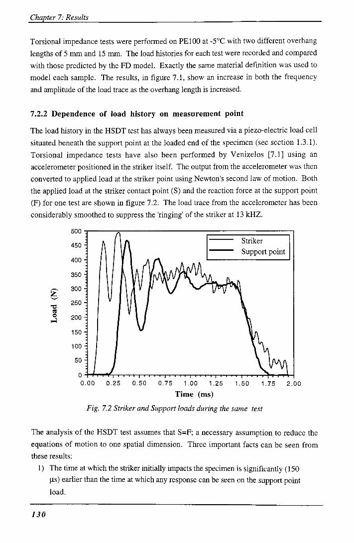
Chapter 7: Results
Torsional impedance tests were performed on PEIOO at -5°C with two different overhang
lengths of 5 mm and 15 mm. The load histories for each test were recorded and compared
with those predicted by the FD model. Exactly the same material definition was used to
model each sample. The results, in figure 7.1, show an increase in both the frequency
and amplitude of the load trace as the overhang length is increased.
7.2.2 Dependence of load history on measurement point
The load history in the HSDT test has always been measured via a piezo-electric load cell
situated beneath the support point at the loaded end of the specimen (see section 1.3.1).
Torsional impedance tests have also been performed by Venizelos [7.1] using an
accelerometer positioned in the striker itself. The output from the accelerometer was then
converted to applied load at the striker point using Newton's second law of motion. Both
the applied load at the striker contact point (S) and the reaction force at the support point
(F) for one test are shown in figure 7.2. The load trace from the accelerometer has been
considerably smoothed to suppress the 'ringing' of the striker at 13 kHZ.
500
450
400
350
300
250 250 a o 200
150
100
50
0
Striker Support point
0.00 0.25 0.50 0.75 1.00 1.25 1.50 1.75 2.00
Time (ms)
Fig. 7.2 Striker and Support loads during the same test
The analysis of the HSDT test assumes that S=F; a necessary assumption to reduce the
equations of motion to one spatial dimension. Three important facts can be seen from
these results:
1) The time at which the striker initially impacts the specimen is significantly (150
|is) earlier than the time at which any response can be seen on the support point
load.
130

Chapter 7: Results
2) The duration of the event is apparently longer if the striker , as opposed to the
support point, load is considered. Both results indicate that the response ends at a
well defined time.
3) The average load, after the initial peak, calculated firom the two measurements is
the same (within the calibration error of the accelerometer).
Before discussing the reasons for the differences between the two load traces the results
from high speed photographic results are presented.
7.2.3 High speed photographic results
Wheel [7.2] examined the HSDT test using high speed photography. He used the results
to measure beam section rotation directly. The photographs were used in this work to
measure the vertical translation of a section in addition to its rotation. The results are not
very accurate, due to the low resolution of the photographic film, but do indicate the
general nature of the deformation. The results are shown in figure 7.3 for the beam
section rotation at 25 mm from the loaded end of the specimen (15 mm from the load
plane).
S 5
4 -
3 -
1 . 2 1 0 -
Time= -0.0891 ms Time= 0.1698 ms Time= 0.6877 ms Time= 1.2055 ms Time= 1.7234 ms
1 I I I 1 1 I I I I I 1 1 I I I I I 1 1 1 | I I I 1 1 I I 1 1 | 1 1 I I I I I 1 1 | 1 1 I I I I I 1 1 | i I I I 1 1 I I I | i n I I I I I 1 1 I I I I I 1 1 I I
10 15 20 25 30 35 40 45
Lateral distance from crack plane (mm)
Fig. 7.3 Vertical displacement of a section 25 mm from the loaded end of the specimen
As can be seen there is a definite initial rotation of the section about an axis close to the
centroid which quickly changes to a rotation about the support point.
131

Chapter 7: Results
7.2.4 Conclusions
The above results allow the following conclusions to be drawn about the nature of the
deformation close to the load plane. As the striker impacts the specimen, the load plane
section begins to rotate about a point close to the centroidal axis and the specimen actually
lifts off the support point (Figure 7.4b). Torsional loading waves emanate from the load
plane, in both directions, along the axis of the specimen. The wave travelling towards the
impacted free end of the specimen is reflected back towards the load plane as an unloading
wave (figure 7.4c). During this time the rotating sections also gain a net downward
velocity component due to the continuing downwards motion of the striker.
As the reflected unloading wave reaches the load plane, contact between the specimen and
the support point occurs and the reaction force at this point begins to increase (figure
7.4d), whilst the contact force between the striker and the specimen reduces. This process
is then repeated, producing the characteristic oscillations in the load trace. The support
and striker force oscillations are therefore in anti-phase and the initial increase in support
load does not correspond to the time of impact but is delayed by approximately one time
period of the load oscillations.
Striker
(a)
Support
(b)
(c)
(d)
Fig. 7.4 Schematic of the deformation of the overhang region proceeding striker contact
132

Chapter 7: Results
The single spatial dimension FD analysis is unable to fully model this deformation, but
does qualitatively account for the contact stiffness and overhang effects in the nature of the
oscillations in the load trace. The predicted load trace resembles the striker contact force
as opposed to the support point load. As was shown in section 6.4.4, the oscillations are
only one factor in the accelerations and decelerations of the crack during an HSDT test.
The question remains of what errors are introduced by modelling the striker and support
forces as being equal. This question can only be answered by examining the correlation
between the measured and predicted crack length histories (see section 7.3.3.3).
7.3 HSDT results for PEIOO
7.3.1 Effective modulus
The effective modulus for PEIOO at -5°C was given in section 5.7, using three points to
fully characterise the stress-strain curve. Since the HSDT results for this material are
examined in depth a more complete, ten point definition of the characteristic was used, as
shown in figure 7.5.
Ten point, piecewise linear fit Experimental points
I
(MPa)
Fig. 7.5 Ten point definition of % as a function of to for PEIOO at -5 °C
7.3.2 Dynamic Fracture resistance of PEIOO
Nineteen HSDT tests were performed on PEIOO at -5°C ±1°C. The material was supplied
in granule form by BP Chemicals pic and was then compression moulded into 9.5 mm
133

Chapter 7; Results
thick sheets. The overhang for these tests was 5 mm, with a 30 mm long, straight fronted
initial notch. The overhang was reduced to 5 mm from the standard 10 mm in order to
minimise any errors due to the associated oscillations in the load trace. The average
thickness of the specimens was 9.2 mm with a side groove depth of 1.6 mm.
The section rotation at distances 85, 95, 105, 115, 125 and 135 mm along the length of
the specimen were measured using the modified OCG. Using the section rotation results
in conjunction with the timing lines allowed the approximate average section rotation at the
leading edge of the crack front to be calculated for each test. Equation (4.17) was then
used to calculate Gd directly without the need for the FD analysis. The results for Gq
from this section rotation method and from the FD analysis are compared in figure 7.6.
3
1 g
2
I
E A S
O
7
6 •
5 -
4
3
2
1
A OCG
A , • Finite difference
• # ••
\ A
3.56
Fig.
I I I I I I I I I I I I I I I I I I I [ I I I i I I I I I I I I I I
1 4 0 1 6 0 1 8 0 2 0 0 2 2 0 2 4 0 2 6 0 2 8 0
Crack velocity (m/s)
7.6 Gofor PEIOO calculated from both the FD method and directly from the crack
front section rotation
The modified OCG results show a greater amount of scatter (as expected due to the
inaccuracies of using the OCG to measure absolute section rotation), but the mean value
(3.86 kJ/m2) correlates well with that from the FD results (3.20 kJ/m^). The correlation is
very significant since it verifies all the main assumptions used in the HSDT analysis and
FD model presented in the preceding chapters. The results correlate well with the
minimum Go prediction from Levers' model [7.3] (3.56 kJ/m^).
The FD results show pronounced scatter at the low crack velocities and this is discussed in
detail in the following sections.
134

Chapter 7: Results
7.3.3 Accuracy of the HSDT test analysis
The accuracy of HSDT test analysis is discussed below by comparing predicted results to
experimental results for three typical cases covering the range of striker velocities used:
High (25.7 m/s), medium (19.1 m/s) and low (11.9 m/s) rates. The results are presented
below by comparing the measured and predicted crack histories, load traces and section
rotations for each case.
7.3.3.1 Rotation histories
The rotation histories for the medium and high striker velocity cases are shown in figures
7.7 and 7.8 respectively. For the medium and high striker velocity cases, the FD results
correspond to the value of Gd which produced the same steady state crack velocity as that
measured experimentally (an automated method described in section 6.2.2.4). As
explained in section 7.2.4, the time that the striker made contact with the specimen could
not be determined from the experimental load history. The correct time offset for the
results from an experiment was calculated as the time difference between the occurrence of
the predicted minimum in section rotation of the 85 mm section and that measured
experimentally. This time offset was then apphed to all the experimental results for that
case. The calculated time offset is independent of the value of Gjj since the minimum
rotation is due to the low strain, dispersive nature of the high frequency components in the
torsional wave, which travel much faster than the crack.
0 . 1 6 -
0 . 1 4 •;
0 . 1 2 - i
0 . 1 0 -n s et La 0 . 0 8 :
c o 0 . 0 6 :
a - w O 0 . 0 4 :
0 . 0 2 :
0 . 0 0 4
- 0 . 0 2 -
Experiment
Finite Difference
z=85 mm
z=135 mm
I I I 1 I i I I I I I I I I I I I I I I 1 I I I I I I I » I I I I I I I I I I I I I
0 . 0 0 . 1 0 . 2 0 . 3 0 . 4 0 . 5 0 . 6 0 . 7 0 . 8 0 . 9
Time (ms)
Fig. 7.7 Experimental and predicted section rotation histories at two positions
(Striker velocity = 19.1m/s), Crack tip rotation = 0.042 rad)
135

Chapter 7: Results
T3 2
I I S •2 u C/2
Experiment
Finite Difference 0 . 1 4 -
0 . 1 2 -
0.10
z=85 mm
z=135 mm 0 . 0 6 -
Fig.
Time (ms)
7.8 Experimental and predicted section rotation histories at two positions
(Striker velocity = 25.7 m/s, Crack tip rotation = 0.046 rad)
u
C 0 CQ
1
0 . 0 9
0.081
0 . 0 7 -
z=85 mm 0 . 0 5 -
z=135 mm
Time (ms)
iiiiiiiniMiiiiii
Experiment
Finite Difference (G^=2.29 kJ/m^, %=0.2)
Finite Difference (G^ =3.56 kJ/m^, %=0.2)
Finite Difference (C^ =3.56 kJ/m^, %=0.08
Fig. 7.9 Experimental and predicted section rotation histories at two positions
(striker velocity = 11.9 m/s)
(Crack tip rotation = 0.035 rad for Go=2.29 kJ/m^)
(Crack tip rotation = 0.043 rad for G[)=3.56 kJ/m^)
136

Chapter 7; Results
For the medium and high striker velocity cases there is a good correlation between
experimental and predicted results. It can be seen that section rotation begins to increase
significantly before the leading edge of the crack tip passes the section. There is little, if
any, discontinuity in the rotation history as the leading edge actually passes.
The low striker velocity case corresponds to the solid triangular point (A) shown in figure
7.6. For the crack velocities typified by this test, there is a considerable increase in the
scatter of the calculated Go values. The measured rotation histories, together with the
predicted results from the automated FD method are shown in figure 7.9. The calculated
value of Gjt) for the predicted results is 2.29 kJ/m^. As can be seen there is a considerable
disparity between the FD and experimental rotation histories.
The FD model was then used to predict the rotation histories for the case of Gd = 3.56
kJ/m2 . The results, also shown in figure 7.9, have a much improved correlation with the
experimental results. There seems, therefore, to be considerable doubt as to the validity of
the predicted result for Gb of 2.29 kJ/m2 for this test. This is examined further in section
7.3.3.3. For completeness, the effect of contact stiffness was also examined and, as can
be seen from the results shown in figure 7.9, a reduction in contact stiffness by a factor of
more than two has little effect on the rotation histories.
7.3.3.2 Load histories
The measured and predicted load histories for low, medium and high striker velocity cases
are shown in figures 7.10 to 7.12. There is a good correlation between the FD predicted
and measured loads, for all tests. The experimental load trace measured at the support
points is delayed by one period of oscillation as explained in section 7.2.4.
For the high striker velocity case (figure 7.12) the predicted load is less than that
measured. The most probable reason is that the effective stress-strain data for the material
is limited for the high striker velocity and corresponding high strain tests (due to the
limitation in maximum striker velocity). The initially increasing load in the low striker
velocity case is due to the relatively long time required to achieve initiation.
137

Chapter 7: Results
9 0 0
800
7 0 0 / V i/' \ s \
.."•>.1
« 5 0 0 -3
#3
1111111111111111111111111''' I ' ' ' ' I ' ' ' ' I ' ' ' 0 . 0 0 . 1 0 . 2 0 . 3 0 . 4 0 . 5 0 . 6 0 . 7 0 . 8 0 . 9 1 . 0
Time (ms)
Experiment
Finite Difference (G^=2.29 kJ/m^, %=0.2)
Finite Difference (G])=3.56 kJ/m \ %=0.08)
"""" Finite Difference (Gd=3.56 kJ/m^, %=0.2)
Fig. 7.10 Experimental and predicted load histories (striker velocity = 11.9 m/s)
'Q a
•J
1200
1000 -
800 -
600 -
4 0 0 -
200 - Experiment
Finite Difference
' t 111 ' 11 •• I ' I •• 11 111 111 11 111 111 111 111 [ 11 111 111 I 0 . 0 0 . 1 0 . 2 0 . 3 0 . 4 0 . 5 0 . 6 0 . 7 0 . 8 0 . 9 1 . 0
Time (ms)
Fig. 7.11 Experimental and predicted load histories (striker velocity = 19.1m/s)
138

Chapter 7: Results
o
1 5 0 0
1 2 5 0
1000
7 5 0
5 0 0
2 5 0 Experiment Finite Difference
I I f i I I I I I I I I I I I I I I I I I I I I I I I 11 I I I I 1 I I I I I I I I I I I I I I 0 . 0 0 . 1 0 . 2 0 . 3 0 . 4 0 . 5 0 . 6 0 . 7 0 . 8 0 . 9 1 . 0
Time (ms)
Fig. 7.12 Experimental and predicted load histories {striker velocity = 25.7 m/s)
7.3.3.3 Crack histories
The measured and predicted crack histories for the medium and high striker velocity cases
are shown in figures 7.13 and 7.14. The time origin of the experimental histories has
been offset as discussed in section 7.2.4, in order to facilitate comparison. As can be seen
there is a good correlation between the FD predictions and the measured data.
Examining the low striker velocity case, the automated FD solution calculated Go to be
2.29 kJ/m^. The corresponding predicted crack history is shown in figure 7.15 together
with the time offset measured crack history. The predicted crack history when Gq is
changed to 3.56 kJ/m^ is also shown in figure 7.15. The predicted steady state crack
velocity for G^ = 2.29 kJ/m^ is within 0.5% of that measured, but for Go = 3.56 m/s the
difference is increased to 12 % (194 to 171 m/s). The difference in crack velocity would
at first seem to be very significant until the form of the crack histories is examined. As
can be seen, both the predicted and experimental crack histories show pronounced
oscillations about the steady state velocity. Since the steady state velocity is calculated
from twelve discrete points, its value is strongly dependant on the position of the points
along the crack path and the correct prediction of the oscillations. The results show that
the oscillations are reasonably accurate apart from the initial few points which produce an
apparently slower calculated steady state velocity.
139

Chapter 7: Results
OX)
s
I u
180
160 -
1 4 0 -
120
100 -
80
60
• Experiment O Finite Difference
O
O o
o
o o
Time (ms)
Fig. 7.13 Experimental and predicted crack histories (striker velocity = 19.1m/s)
(crack velocity = 230 m/s)
1 U)
I u CQ u U
1 8 0
1 6 0
1 4 0
1 2 0 -
1 0 0
8 0 :
6 0 - O
• Experiment O Finite Difference
O CM
o
o
4 0 t i l l 1 —
0 . 2 0 . 3 —I—1—I—I—I—I—
0 . 4 0 . 5
-1 1 1 1 1 r 0 . 6 0 . 7
Time (ms)
Fig. 7.14 Experimental and predicted crack histories (striker velocity = 25.7 ?n/s)
(crack velocity = 259 m/s)
140

Chapter 1: Results
1 W) 1 u 2 u
1 8 0
160 -1
1 4 0 '
1 2 0
1 0 0
8 0
60
4 0
o W '
20 I I I I I I I ' I I I I I I I I I I I I I I I I I I • I I I I I ' I I I I I I ' I I I I I I I I I I I 0 . 1 0 . 2 0 . 3 0 . 4 0 . 5 0 . 6 0 . 7 0 . 8 0 . 9 1 . 0 1 . 1
Time (ms)
— — Experiment
Finite Difference (G^ =2.29 kJ/m^, %=0.2)
Finite Difference (G^=3.56 kJ/m^, %=0.2)
Finite Difference ((^ =3.56 kJ/m^, %=0.08
Fig. 7.15 Experimental and predicted crack histories (striker velocity = 11.9 m/s)
7.3.3,4 Fracture surfaces
A typical fracture surface is shown in figure 7.16. A fairly featureless surface is seen in
the lower 80% of the surface with some frosting (micro ductility).
*
Ir-s ^ ^
Direction of propagation
'V Groove
Axial distance: 130 mm 120 mm
Fig 7.16 Picture of characteristic fracture surface (striker velocity = 9.0 m/s)
141

Chapter 7: Results
Partial arrest lines approach, but do not reach, the lower surface boundary. At the upper
boundary an increase in surface roughening can be seen, shown magnified in figure 7.17.
The roughening corresponds to very low, or highly oscillatory, crack speeds along the
trailing edge of the crack front, (see figure 6.11).
Fig 7.17 Magnification of picture shown in figure 7.16 detailing the increased ductility
close to the upper surface at 130 mm from the loaded end of the specimen
(Scale increments = 0.5 mm)
A full arrest line is shown in figure 7.18 and the corresponding predicted crack shape is
shown in figure 7.19.
Direction of propagation
'V Groove
Axial distance: 110mm 100 mm
Fig 7.18 Picture of arrest line seen on specimen tested at a striker velocity of 7.5 m/s
142

Chapter 1: Results
P3
U
1.0
0.8-
0.6 -
0.2-
0.0
Predicted crack shape Experimental arrest line
0.0 I I I I I I I I I I I I I I I I I I I I I I I I I I I I I I I I I I I I I I I I I I I I I I I I 1*1 95 97 99 101 103 105 107 109 111 113 115
Fig 7.19 Predicted crack shape from the FD model compared to
arrest line depicted in figure 7.18
The predicted shape does not match the arrest line observed, the leading edge of the
predicted shape being much blunter. To investigate this further the arrest line depicted in
figure 7.18 was used to define the dynamic crack front shape in the FD model. The
steady state velocity used was the same as in the experiment. The section rotation
histories predicted from the model for this crack front shape showed a very poor
correlation with those measured, the foundation being far too stiff. The good agreement
between the predicted and experimental low striker velocity crack history results suggests
that the predicted shape is correct. There is no reason why the shapes of the arrest lines
and the propagating crack front should match however. An arrest line does not represent
an instantaneous position, but rather the locus of arrest points along a front which
continues to propagate. Arrest can be viewed as the final stage of crack deceleration (with
little change in Gd) and is caused by an interaction of stress waves which reduces the rate
of energy supply to the crack tip. A loading stress wave travelling towards the load plane,
or an unloading wave travelling away from the load plane, can produce a localised
deceleration (and arrest) of the crack front which, as it propagates along the crack front,
leaves an arrest line which has a sharper (more acute) leading edge than the dynamic crack
front shape.
7.3.4 Summary
From the above results for PEIOO it can be concluded that the HSDT analysis can be used
to determine a material's Go as a function of crack velocity using the FD model described
143

Chapter 7: Results
in chapter 6, provided that the striker velocity is high enough to overcome the dominance
of the oscillations in the crack length history. At low crack velocities the test must be
instrumented so as to provide a method for determining the time of contact between the
striker and the specimen.
At low striker velocities the crack velocity oscillations are predominantly due to
fluctuations in the rate of supply of energy to the crack front caused by local interactions
of loading and unloading torsional waves.
The high striker velocity results presented above demonstrate a non-linear material
characteristic seen in the HSDT test. The crack velocity for one test was 259 m/s with a
striker velocity of 25.9 m/s. A lower striker velocity test (21.4 m/s) showed a crack
velocity of 274 m/s. That is, a higher striker velocity produced a lower crack velocity.
This can be understood by considering the rate of energy supply to the crack front. At
higher striker velocities, as the crack velocity approaches its limit, the effective strain in
the torsional beams behind the crack tip is approximately proportional to striker velocity.
Therefore, as the striker velocity is increased the effective strain increases and the torsional
wave speed decreases, decreasing the rate of supply of energy to the crack front. Thus the
crack speed is reduced.
7.4 Polypropylene
The HSDT test was used to determine Go as a function of crack velocity of a pure
polypropylene homopolymer (PP) material and a rubber toughened form (PP/EPDM,
30% by weight EPDM). The material was supplied in granule form by the University of
Twente, Netherlands and was then compression moulded into 9.5 mm thick sheets.
Both the pure and blended forms have been tested by Gaymans [7.4] using a notched
tensile impact test to calculate Gj). His analysis of the test did not account for dynamic
effects and as such his results, which showed the blended material to be superior, are
dubious. The blended materials showed a rapid fall in Gd from over 100 kJ/m^ to 12
kJ/m^ as the loading rate was increased from to lO-i m/s. At lO-i m/s a transition
occurred and Go increased with further increases in piston speed. The Go of the pure
material appeared to be virtually zero throughout the range of loading rates.
Further Scanning Electron Microscopy work by Gaymans revealed a melt layer 3-5 |a,m
thick close to the fracture surface in the blended material subjected to high rate tests, but
this was not evident in the low rate tests. Gaymans then proposed that the transition in the
144

Chapter 7: Results
frequency oscillations in the crack velocity and is unable to account for the experimental
results presented above. The stability of crack propagation at low rates therefore requires
further investigation.
7.5 Polyoxymethylene
In this section, HSDT results for Polyoxymethylene (POM, DuPont 'Delrin') in both a
toughened (ST) and a pure (NC) form are presented.
Injection moulded, 12 mm thick Delrin plates were provided for testing. To decrease the
thickness and remove surface residual stresses 1.5 mm was machined off each face. All
tests were performed at 0°C and at impact velocities between 7 m/s and 22 m/s. At impact
velocities of less than 10 m/s, Delrin ST showed stick-slip propagation with characteristic
arrest lines. All other tests showed a smooth crack surface.
^ 1.2
I ^ 1.0
I 0.8
I 0.6-
I rt 0.4 6
S 0.2 I a
O Dekin NC # Delrin ST
O
oo CDDO
100 500 600 200 300 400
Crack velocity (m/s)
Fig. 7.22 Gd as a function of crack velocity for Delrin (ST and NC)
The results of tests are shown in figure 7.22. The toughened Delrin specimens show no
improved resistance to RCP but in fact a lower resistance than the pure form at crack
velocities less than 300 m/s. Both materials show a fall in their Gd versus a characteristic
until they reach a lower limit. The figure indicates very little scatter in this lower plateau
region but this is only an artefact of the FD model as Gd was only calculated to an accuracy
of ±0.05 kJ/m^.
The fact that the toughened Delrin exhibited a lower Gd than the pure material could be
qualitatively explained in terms of Leevers thermal decohesion model [7.3]: The rubber is
147

Chapter 7: Results
present in small particles which are regarded as having no intrinsic structural effect. The
presence of the rubber therefore merely reduces the energy to melt a one-chain-length thick
layer, since the overall enthalpy to melt is reduced.
Both Delrin materials have significantly lower Gd values than PEIOO. These results
suggest that POM would exhibit a low critical pressure in pipe tests. Tests on 50 mm
diameter, 6 mm thick pipe have indeed shown this to be true [7.5]. In the presence of an
axial internal notch, introduced to induce plane strain conditions, RCP occurred
spontaneously driven by residual stress only, i.e. at zero internal pressure. Without the
axial notch initiation of the crack was unstable, being very sensitive to impact speed.
Similar tests on PEIOO pipe gave a finite critical pressure with no such sensitivity to impact
speed.
7.6 References (7.1) Venizelos, G.P., Investigation of the S4 test for RCP in thermoplastics pipe, PhD
Thesis, Univ. of London , (1995). (7.2) Wheel, M.A. and Leevers, P.S., 'High speed double torsion tests on tough
polymers I: Linear Elastic Steady State and Dynamic Analysis', Int. J. of Fracture, 61, p. 331, (1993).
(7.3) Leevers, P.S. and Greenshields, C.J., A model for predicting the dynamic fracture and impact fracture resistance of tough thermoplastics, Proc., 53rd Annual Tecnical Conference of the Soc. of Plastic Engineers, Boston, MA, (1995).
(7.4) Gay mans, R.J. Dijkstra, K., Janik, H., 'Polyamide-rubber blends: Influence of deformation speed on crack propagation process', Proc., 9th International conference on deformation yield and fracture of polymers, Cambridge (1994).
(7.5) Leevers, P.S., Freeman, P.N., Arthur, M.M., 'Rapid crack propagation in small diameter thermoplastic pipe', Plastics ,Rubber and Composites Processing and Applications, 24, p. 113, (1995).
148

Chapter 8: Conclusions and recommendations
Chapter 8
Conclusions and recommendations
The HSDT test, although initially conceived as a simple, straightforward rapid fracture test,
possesses many complicating dynamic characteristics. It is essential to accurately model
the local deformations in order to correctly partition the work done into strain, kinetic and
fracture energies. A previous FD model by Wheel [8.1] was found to be flawed and did
not account for many of the important dynamic characteristics of the test. The majority of
this work has been devoted to understanding the dynamic characteristics of the HSDT test
and developing a new model to account for them. The new model has been validated
extensively. No other existing analysis of an experimental test used to investigate rapid
crack propagation can match this validation. The HSDT test now provides an efficient and
accurate tool to investigate a polymer's G^-a characteristic.
The HSDT test is unrivalled in terms of continuous crack propagation length and its plane
strain nature of fracture. The fact that the crack velocity oscillates during a test at low
striker velocities can be viewed as an advantage, since it provides a method of investigating
propagation stabUity in a test of known dynamic characteristics.
The most important achievements and conclusions of this work are summarised in the next
section followed by recommendations for future work.
8.1 Summary of conclusions
8.1.1 Experimental test improvements
The HSDT experimental rig was modified in a number of ways. The most notable were the
redesign of the striker velocity measurement system and the design and construction of an
optical crack gauge (OCG) to measure crack velocity. The basic OCG design is now
proven. It reduces specimen preparation to a few minutes, but would benefit from some
minor alterations to improve its accuracy. A modified form of the OCG allows
approximate section rotations to be measured as a function of time.
8.1.2 Derivation of analytical equations to model the HSDT test
To calculate the dynamic fracture resistance {Gd) of a material from the test results, a post
mortem analysis that models the deformation during the test given the striker and crack
velocities is required. A previous two dimensional (one spatial, one time) analysis, made
149

Chapter 8: Conclusions and recommendations
by Wheel [8.1], included the effects of axial stress but not axial inertia. Since the duration
of the test is of the same order as the time taken for the axial stress waves to travel the
length of the specimen, axial inertia is important and has now been included. The
derivation of the fourth-order differential equations followed that of previous researchers
but, by examining end effects, it was shown that an adjustment factor, resorted to
previously, was not necessary. The restoring moment, due to the elastic foundation
between the two torsion beams beyond the crack front, was included in a more rigorous
and accurate manner than in previous analyses. The end boundary conditions used by
Wheel were also corrected, allowing the model's load plane region to deform more
realistically. The predictions from the resulting analytical solution correlated well with
experimental and numerical results for both non-uniform twist of simple torsion beams and
static deformation of the DT specimen.
'I'he resulting equations were used to accurately determine the restoring moment of the
elastic foundation as a function of 'V groove depth. With the accuracy for the relatively
simple static, straight crack front case proven, it was then possible to move on to the
analysis of the curved crack front. It was shown that a simple model could be used to
model the foundation where, along a curved crack front it is only partly separated. This
model was then used to test the hypothesis that the crack shape could be predicted by
assuming the crack driving force along a propagating curved crack front to be constant.
The hypothesis was in part proved, but is still in doubt due to lack of data on the shape of
the propagating crack.
Comparing results from the dynamic analysis of the straight and curved crack fronts,
showed that the straight crack front model under predicted Gd. This effect became more
pronounced as the crack velocity approached the torsional wave speed in the half-
specimens.
8.1.3 Non-linear material properties
To examine the non-linear behaviour of polymers in the HSDT test. Wheel [8.1] developed
the torsional impedance test to measure the shear modulus data required by the FD model.
His analysis of the test was deeply flawed because he did not account for the reduction in
torsional wave speed at the high strains due to the corresponding reduction in tangent
modulus. A new, corrected analysis of the torsional impedance test has been derived, the
assumptions of which have been fully tested and verified. The results from the analysis are
thickness independent.
150

Chapter 8: Conclusions and recommendations
The results show that a material, whose modulus shows a low sensitivity to temperature at
high strain rates and low strains, may possess a modulus at intermediate strain rates and
high strains which is very sensitive to temperature. This may prove to be very important
when considering RCP in pipes since the critical pressure appears to be strongly dependant
on the relationship between decompression rate and crack speed. The crack speed is
closely Unked to modulus via the dominant wave speed in the pipe.
8.1.4 Propagation mode
Crack propagation can be modelled in one of two modes: generation or propagation. The
previous analysis of Wheel [8.1] used generation mode, in which the crack history is
prescribed and Go calculated throughout the test. The disadvantage of generation mode is
that the discrete experimental crack length data indicate that the crack velocity is not
constant, but the resolution is not high enough to define the oscillations accurately. A
prescribed history will therefore put unrealistic constraints on the model. The main
advantage of generation mode is that Go need not be assumed to be constant during a test.
Wheel was unable to capitalise on this advantage since the initiation time of the crack cannot
be measured accurately. He calculated the initiation time for a test by finding the value
which produced minimum variation in predicted Gp from the model during the test; a
method which assumes, a priori, that Go is constant during the test.
This work used propagation mode, which, from the outset, assumes a constant Gd during
a test, and proceeds to calculate Go by finding that value which produces the best
correlation between predicted and experimental crack histories.
8.1.5 Finite difference model
The computational finite difference model used to analyse the HSDT test is fast (less than 5
minutes), efficient and easy to use, generating an animated display of the deformation to
ease interpretation of the results. Due to the speed of the model (as compared to a full 3D
solution) the characteristics of a test can be easily examined, and the sensitivity to any
parameter quickly investigated. The model has been used to demonstrate that the
characteristics of the test are dominated by its dynamic nature and has led to an
understanding of features such as the oscillating load and crack velocities and the curved
crack front.
The term 'steady state crack velocity' (calculated as the slope of the best fit straight line
through the crack history points) originated from the assumption that the crack velocity
could be considered constant during an HSDT test. The constant crack velocity assumption
151

Chapter 8: Conclusions and recommendations
is not valid but the steady state crack velocity is still used to characterise the crack velocity
during the test. The steady state crack velocity is therefore dependant on the number and
position of discrete points used to determine the crack velocity, if the spacing between the
points is of the same order as the wavelength of oscillations in the crack history.
8.1.6 Experimental results
Detailed tests were performed on an HDPE. A large amount of additional data was
gathered on the deformation of the test, which was then used to validate the dynamic FD
model. The detailed checking of the model has no precedent in other fracture tests where
only the minimum amount of data is gathered to model the deformation. The characteristic
stick-slip nature of HSDT test seen at low striker velocities has been shown to be due
largely to the dynamc characteristics of the geomecy and loading conditions, as opposed to
tlie Gij d characteiisiic of the material.
Comparisons between predicted crack front shapes and observed arrest lines indicate that
arrest lines seen on the HSDT fracture surface do not reflect the shape of the propagating
crack front. In other words, arrest is a dynamic process which does not necessarily occur
simultaneously along the whole length of the front.
At low crack speeds the steady state crack velocity is insensitive to Gd. TO calculate GG for
these cases the relationship between the crack history and the time of striker impact must be
measured. A single section rotation history, measured using the optical crack gauge,
allows this to be performed, with the added benefit of providing an extra check on the
analysis.
Results for polyoxymethylene and polypropylene materials showed Gj) to decrease with
crack velocity. Although this result is intuitively sensible it was not expected that the crack
could propagate with any stability whilst operating on a falling Gd-o. characteristic. There
are two known inaccuracies in the results:
1) The variation in crack velocity along the crack front is not accounted for.
2) The region where Gd is falling most rapidly with crack velocity corresponds to low
rate tests for which the analysis has been shown to give unacceptable scatter.
However, the above inaccuracies are insufficient to explain the dramatic fall in the
measured G^-a characteristic of these materials. The results therefore show the
importance of considering the loading rate in a fracture problem dealing with these
materials.
152

Chapter 8: Conclusions and recommendations
At the loading rates considered in this work, the 'toughening' of a material by blending it
with rubber appears to have the opposite effect to that intended. The rubber toughened
POM actually has a lower Gq for a given crack velocity than the pure form. This result
agrees with the prediction from Leevers' thermal decohesion model [8.2].
8.2 Future directions
8.2.1 Dynamic fracture resistance as a falling function of crack velocity
The next stage in the development of the HSDT test is to investigate why a material, with a
falling G/)-d characteristic, can fracture at a controlled rate without large oscillations in
crack velocity. The approach should be to simulate a material with a known, or assumed,
falling gd- d characteristic and find which parameters can generate, or affect, crack
propagation stability. The model described in section 6.1.1 should be used with the
inclusion of rate effects in the G^-a characteristic. The sensitivity to rate effects can, as a
first approximation, be deduced from Leevers' thermal decohesion model.
8.2.2 Reduced striker velocities
In order to cover a more complete range of crack velocities for any material, the present
minimum striker velocity is inadequate. Currently the minimum striker velocity is limited
by the rig since the free fall distance (zero accumulator pressure) is set at 1.5m. This can
simply be overcome, but problems of striker retardation will become a problem due to its
low momentum and the long crack propagation time. The best solution for these cases is to
use the static rig described in section 4.2.4, in conjunction with a high rate tensile testing
machine.
8.2.3 Rate sensitivity of modulus
The effective modulus for the HSDT test has been defined without accounting for rate
effects. This was justified by the torsional impedance test operating at approximately the
same rate as the HSDT test. To check this approximation, a form of torsional pendulum
test could be used, with the standard cylindrical bar specimen replaced by a rectangular bar,
similar in geometry to the HSDT test half-specimen.
8.2.4 Steady state analysis
In the past, the steady state analysis has not proved to be an effective tool in analysing the
HSDT test. Now that the important parameters of the test have been evaluated it may well
be possible to use a steady state analysis to calculate at least an approximate Go from the
HSDT test results. The two most important improvements that could be made are the use
153

Chapter 8: Conclusions and recommendations
of the correct time offset for the crack history results, and of the correct non-linear material
properties.
The steady state analysis is unable to account for wave reflections from boundaries, or the
oscillating load and crack histories, but it does offer a far simpler and faster analysis of the
HSDT test than that presented in this work. The steady state solution will be most accurate
at intermediate crack speeds since:
1) At high crack speeds, and therefore high strains, the section rotation rates will be
characterised by the high strain torsional wave speed as well as the crack velocity.
2) The steady state analysis will be unable to account for stick-slip behaviour which
is common at low crack speeds.
8.2.5 Improvements to the HSDT experimental procedure
The HSDT test procedure requires some adaptations to be able to measure a material's Gd
at low crack velocities. The main i'lipiovement required is to measure initiation time.
There are a number of methods available, such as incorporating a load cell in the striker
itself, but the most practical would be to use the modified OCG, as described in section
7.3.3.1, to measure a single rotation history at a known distance from the load plane. If a
single crack timing line was also used, positioned at the same distance from the load plane,
the rotation history would provide an additional check on the analysis, by measuring the
section rotation at the leading edge of the crack front.
8.3 References (8.1) Wheel, M.A., High Speed Double Torsion Testing of Pipe Grade Polyethylenes,
PhD Thesis, Univ. of London , (1991). (8.2) Leevers, P.S. and Greenshields, C.J., A model for predicting the dynamic
fracture and impact fracture resistance of tough thermoplastics, Proc., 53rd Annual Tecnical Conference of the Soc. of Plastic Engineers, Boston, MA, (1995).
154

MATERIAL •ALUMINIUM REMOVE ALL SHARP EDGES. 3 H O L E S
D R I L L 042 & T A P M 5 T H R O '
SECTION X X
HOLE SPACING REGULAR AS INDICATED
1 H O L E D R I L L 0 4 . 2 * 1 5 D E E P — ^ & T A P M 5 * 1 2 M I N
MACHINE A L L O V E R
TOLERANCES ON MACHINED SURFACES
UPTD SCO * 0 S 500 TO 1000 ' 0 . 4
D A T E : 7 / 3 / 9 3 DRAVN BY S.RITCHIE CRACK GAUOL n o NOT SCALE ( POM P P A U I N G C G 0 7 DRAWING NO
o
3 g. & o o sr. n &9
o
fo
9r CTQ
C CTQ
a fD !/5
3
%
ft)
a w* %

Appendix 1: Drawing of optical crack gauge design
Appendix 2
Circuit for optical crack gauge
±L5v Difference Am£li£ication
Vo I ]—j R500K— R240K LF 34 7N RIQK I— RIQK I— RIOK
44-H RIOK L F 347N
p-| R240K "|—I R500K ] —
RIOK Phoio Transistor
12 10) Differentiation Stage Cl.SnF
Sc h mjdt gipj_ ^ £
ClOnFl OPA 606KP RIOOK I—
UA 741Cj
^innixtaklt-ld}ijti£ihrj>lqr—sfjf££—^ j^omijlu.lj^tfig£-aiijus.l^ag€..
R200K Output
CloF .JL,
OPA 6061
156

Appendix 3: Location of sensors to measure striker velocity
Appendix 3
Location of sensory to measure striker velocity
40 mm
50 mm
32 mm
44 mm
157

Appendix 1: Drawing of optical crack gauge design
Appendix 4
Circuit for measuring striker velocity
+15 V
+1%
Photo Tnmastw
I
+4V Comparator
Output from detector
I X
Signal from detector 3 ,
H - o -
Signal from detector 4
H - o
OR
D Q 74HCn5
G
I
Output to
D Q 74HCT75 G
— r _ electronic timer
. J
4 > -
_LMch res^t stage _
158