TORSION FATIGUE SYSTEM

FOR

MECHANICAL CHARACTERIZATION OF MATERIALS

A Thesis Presented to the Faculty of the

Fritz J. and Dolores H. Russ College of Engineering and Technology

Ohio University

In Partial Fulfillment

of the Requirement for the Degree

Master of Science

BY

Hyder Hussain

Department of Mechanical Engineering

November. 2000

THIS THESIS ENTITLED

" TORSION FATIGUE SYSTEM FOR

MECHANICAL CHARACTERIZATION OF MATERIALS"

Hyder Hussain

has been approved for the

Ilepartment of Mechanical Engineering

And

The Russ College of Engineering and Technology

Dr. Hajrudin Pasic, Professor Department of Mechanical Engineering

Jerrel Mitchell, Interim Dean Fritz J. and Dolores H. Russ

College of Engineering and Technology

ACKNOWLEDGEMENTS

I would like to express deep gratitude and sincere appreciation to my advisor, Dr.

Hajrudin Pasic, for his exceptional guidance, valuable support, and encouragement

throughout this project. I would also like to thank my defense committee members--Dr.

Larry Snyder and Dr. Gregory G. Kremer--for their valuable time and suggestions. I

would especially like to thank Dr. M. K. Alam, Moss Professor, for helping me through

my graduate program and for his helpful suggestions throughout my degree program. I

also like to thank Dr. Madhu Annapragada for helping me in various aspects of my

project and for all the invaluable help that he provided in the design and development of

the Torsion Fatigue System.

I also like to thank the Engineering Research Facility staff at Ohio University's Russ

College of Engineering and Technology, especially Len Huffman, for all the help and

support that he extended all along. Finally, I would like to thank my parents and friends

for their love, understanding, and constant encouragement throughout this endeavor.

TABLE OF CONTENTS

LIST OF TABLES ...................................................................................................... ix

LIST OF FIGURES .......................................................................................................... x

CHAPTER: 1 INTRODUCTION ................................................................................... 1

.................................................................................................... 1.1 FATIGUE LOADING 1

1.2 CHALLENGES OF MATERIAL DEVELOPMENT ............................................................. 2

.................................................................................... 1.3 NEED FOR FATIGUE: TESTING 3

............................................................................ 1.4 SCOPE AND OBJECTIVE OF THESIS 4

................................................................. CHAPTER: 2 FATIGUE OF MATERIALS 7

2.1 INTRODUCTION ......................................................................................................... 7

.............................................................................................. 2.2 FATIGUE MECHANISM 8

......................................................................... 2.2.1 Structural Features of Fatigue 8

2.2.2 Fatigue Norrlenclature ................................................................................... 11

.................... . 2.2.3 Cyclic Stress-Controlled vs Cyclic Strain-Controlled Fatigue 14

.......................................................................... 2.3 PRESENTATION OF :FATIGUE DATA 18

....................................................................................... 2.3.1 S/N (Wohler:) Curve 18

.......................................................................... 2.3.2 Statistical Nature of Fatigue 21

........................................................................ 2.4 DESIGN FOR FATIGUE PREVENTION 22

2.4.1 Strain Life Equation .................................................................. 23

2.5 FACTORS INFLUENC:ING FATIGUE ............................................................................. 25

2.5.1 Stress Concentrators ...................................................................................... 26

2.5.2 Metallurgical Factors .................................................................................... 26

2.5.3 Machining and Processing ............................................................................ 27

.................................................. 2.6 CLASSIFICATION OF FATIGUE TESTING MACHINES 27

............................................ 2.6.1 Axial (Direct-Stress) Fatigue Testing Machine 29

2.6.2 Bending Fatigue Machines .......................................................................... -30

............................................................. 2.6.3 Torsional Fatigue Testing Machines 33

........................................................... 2.6.4 Multiaxial Fatigue Testing Machines 34

2.6.5 Specialized :Fatigue Testing Equipment ........................................................ 35

.......................................................... CHAPTER: 3 FATIGUE TESTING SYSTEM 38

................................................................................ 3.1 INTRODUCTION 38

.......................................................................... 3.2 TEST SPECIFICATION 40

3.3 SURVEY OF EXISTING SYSTEMS ............................................................. 41

....................................................... 3.4 TORSION FATIGUE TESTING SYSTEM 43

........................................................................................................ 3.4.1 Overview 43

................................................................ 3.4.2 System Configuration 44

3.4.3 Machine Characteristics ............................................................. 47

...................................................................... 3.4.4 Production Cost -50

............................................................................ 3.4.5 Advantages 50

......................................................... CHAPTER: 4 MOTION CONTROL SYSTEM 53

........................................................................................... 4.1 THE CONTROL SYS'TEM 53

....................................................................................... 4.2 HOST COMPUTER OR PLC 55

........................................................... 4.2.1 Cornrnunical.ion Standards 55

............................................................................... 4.3 MOTOR OR ACTUATOR DESIGN 58

........................................................................ 4.3.1 Stepper Motors 58

4.3.2 DC Brush Motors ....................................................................... 60

4.3.3 Brushless Mlotors .................................................................... 60

4.4 MOTOR DRIVES ....................................................................................................... 64

4.4.1 Stepper Motor Drive .................................................................. 65

4.4.2 DC Brush Motor Drives ............................................................. 66

4.4.3 Brushless Motor Drives ............................................................. 69

4.4.4 APEX Brushless Servo Drive ...................................................... 70

4.5 FEEDBACK TRANSDUCERS ................................................................... 72

.......................................... 4.5.1 Classification of Feedback Transducers 73

4.5.2 Resolver ................................................................................. 75

4.6 CONTROLLER ................................................................................. 78

4.6.1 2-Axis Servo Controller ............................................................. 79

CHAPTER: 5 SYSTEM SOFTWARE ........................................................................ 83

5.2 GRAPHIC USER INTERFACE DESIGN PROCESS ......................................................... 84

5.2.1 Analysis ................................................................................ 85

................................................................................... 5.2.2 Design 85

........................................................................... 5.2.3 Construction 86

............................................................ 5.2.4 Who's Driving the Design 87

................................................................................. 5.3 FATIGUE TESTING SOFTWARE 88

................................................................. 5.3.1 Test Selection Mode 89

...................................................................... 5.3.2 Data Input Mode 91

5.3.3 Test Execution Mode ................................................................ 95

......................... CHAPTER: 6 FATIGUE TESTING ANALYSIS AND RESULTS 99

.............................................................................................................. 6.1 OVERVIEW 99

.................................................................................... 6.2 TORSION FATIGUE 'TESTING 99

.......................................................................................... 6.3 DISPLACEMENT MODE 100

................................................ 6.3.1 Test 1 - Specifications and Results 101

............................................... 6.3.2 Test 2 - Specifications and Results 103

............................................... . 6.3.3 Test 3 Specifications and Results 105

............................................... 6.3.4 Test 4 . Specifications and Results 107

..................................................................................................... 6.4 TORQUE MODE 109

................................................ 6.4.1 Test 1 . Specifications and Results 110

............................................... 6.4.2 Test 2 - Specifications and Results 112

............................................... . 6.4.3 Test 3 Specifications and Results 114

6.4.4 Test 4 . Specifications and Results ............................................... 116

6.5 TESTING RESULTS .................................................................................................. 119

CHAPTER: 7 CONCLUSION AND FUTURE WORK ................................ 120

BIBLIOGRAPHY ......................................................................................................... 122

APPENDICES ............................................................................................................... 124

. APPENDIX A: APEX SERIES DRIVES PARAMETERS .................................................. 124

-- .............................. APPENDIX B: 6250 SERVO CONTROLLER SPECIFICATIONS 125

. APPENDIX C: APEX MOTOR SPECIFICATIONS ........................................... 126

-- ............................ APPENDIX D: FATIGUE TESTING SOFTWARE SOURCE CODE 127

List of Tables

Table 3.1

Table 6.1

Table 6.2

Table 6.3

Table 6.4

Table 6.5

Table 6.6

Table 6.7

Table 6.8

Test Specifications ............................................................... 40

..................... Displacement Mode Test Parameters (+ 5" at 10Hz.). 101

...................... Displacement Mode Test Parameters ( f 5" at 20Hz.). 103

....................... Displacement Mode Test Parameters ( f 8" at 10Hz.). 105

...................... Displacement Mode Test Parameters (+ 3" at 20Hz.). 107

........................... Torque Mode Test Parameters (+ 2Nm at 20Hz.). 110

................ Torque Mode Test Parameters (+4Nm & -2Nm at 20Hz.). 112

......................... Torque Mode Test Parameters (f 2.5Nm at 20Hz.). 114

............................ Torque Mode Test Parameters (f 3Nm at 20Hz.). 116

List of Figures

Figure 2.1

Figure 2.2

Figure 2.3

Figure 2.4

Figure 2.5

Figure 2.6

Figure 2.7

Figure 2.8

Figure 2.9

Figure 3.1

Figure 3.2

Figure 3.3

Figure 3.4

Figure 3.5

Figure 4.1

Figure 4.2

Figure 4.3

Figure 4.4

Figure 4.5

Figure 4.6

............... Plastic blunting process for growth of stage I1 fatigue crack 10

.................................................... Types of stress or load cycles 12

.............................................. Hysteresis loops for cyclic loading 15

................................................................ S/N (Wohler) curve 19

. . . . ............................................................. Statistical fatigue data 21

.......................................... Principles of fatigue testing machines 29

................................................ Hydraulic torsion fatigue system 30

............................................................... S/N (Wohler) curve 33

............................................................ Statistical fatigue data 34

........................... A sampling of material testing systems from MTS 41

Fatigue testing system ............................................................ 44

................................. Controller and diver of fatigue testing system 45

................................................................... Tabletop system 46

........................................ Rear view (of the fatigue testing system 47

............................................. Elements of motion control system 54

............................................................ Serial port connections 56

................................................... Conventional DC brush motor 60

................................................................... Brushless rnotor 62

......................................................... 3-Phase brushless motor 63

................................................... Position-torque characteristics 64

Figure 4.7

Figure 4.8

Figure 4.9

Figure 4.10

Figure 4.1 1

Figure 4.12

Figure 4.13

Figure 4.14

Figure 4.1 5

Figure 5.1

Figure 5.2

Figure 5.3

Figure 5.4

Figure 5.5

Figure 5.6

Figure 5.7

Figure 5.8

Figure 5.9

Figure 5.10

Figure 5.1 1

Figure 6.1

............................................................ Stepper drive elements 65

Analog servo system ............................................................. 68

............................................ Two-phase sinewave brushless drive 69

..................................................... Torque mode block diagram 71

................................................... Velocity mode block diagram 72

................................................................. Resolver principle 75

................................................................... Resolver output 76

.................................................... Resolver-to-digital converter 77

................................................................ Brushless resolver 77

........................................................ Phases of interface design 84

Design from user in vs . from the system out .................................. 87

...................................................................... Login window 90

....................................................................... Splash screen 90

............................................................. Test selection module 91

................................................................ File selection menu 92

........................................................... Control selection menu 93

............................................................... Help selection menu 93

........................................................... Test infonnation editor 94

.............................................................. Torque control mode 95

...................................................... Displacement control mode 97

......................... Displacement mode characteristics (k5" at I0 Hz) 102

...................... Figure 6.2 Displacement mode characteristics (f 5" at 20 Hz) .. .. 104

........................... Figure 6.3 Displacement mode characteristics (+So at 10 Hz) 106

........................... Figure 6.4 Displacement mode characteristics (k3" at 20 Hz) 108

............................... Figure 6.5 Torque mode characteristics (+_2 Nm at 20 Hz) 111

............................... Figure 6.6 Torque mode characteristics (+4 Nm at 20 Hz) 113

............................ Figure 6.7 Torque mode characteristics (k2.5 Nm at 20 Hz) 115

............................... Figure 6.8 Torque mode characteristics (k3 Nm at 20 Hz) 117

Chapter: 1 Introduction

1.1 Fatigue Loading

Engineering applications of various structural materials involve a wide variety of

operating conditions. Only rarely, however, are mechanical components and structural

elements subjected to constant loads throughout their entire service history. The majority

of components in motor vehicles, forging equipment, hoisting gear, and numerous other

forms of machinery and structures experience variable loading conditions. This loading

can result from vibration, fluctuating power or load requirements, non-uniform road

surfaces, and repeated temperature changes, to mention only a few.

A repeated (cyclic) application of a 'safe' load from static design considerations may

ultimately cause sudden and catastrophic failure. Such failures are referred to as fatigue

failures. Unlike corrosion, wear, distortion, or creep, fatigue failures often give no prior

indication of a deterioration in the performance or strength of the component or structure

or warning of impending failure. The incidence of fatigue failures in engineering

structures and equipment is widespread, and fatigue failures constitute the most common

source of service failures in machinery and structures.

1.2 Challenges of Material Development

The quest for better materials has been going on since the dawn of time. Our earliest

successes with materials depended largely on fortuitous experience and are seen more as

an art, rather than a science. Recent years have seen a momentous change-the birth of a

new materials age. In every area of science and technology, we find work being done to

push back the boundaries of existing materials constraints to seek new freedom from the

past. Everyday we find new materials applications that are challenging mankind to

expand the existing horizons. Totally new approaches are required to solve such

fundamental questions.

The demand for better materials has created a new revolution in materials development-

the field of materials science. Some of our best scientific minds are banding together in

an interdisciplinary effort to probe the basic nature of materials and the forces, which

control their behavior. industry research laboratories are seeking ways to improve

processing, efficiency, and quality. Academic laboratories are seeking to discover and

evolve new theories of materials and the impact of interrelationships with structural

design.

The application of scientific principles, techniques, and instrumentation can resolve many

questions across a wide spectrum of materials applications. Against this backdrop, a

fatigue testing system was proposed to be developed for material characterization.

Fatigue properties are often most important because virtually all fabrication processes

and most service conditions involve some type of mechanical loading.

1.3 Need for Fatigue Testin g

Much of the present general awareness of the problem of fatigue failure in engineering

components has resulted from several well-publicized and, unfortunately, catastrophic

accidents involving ships, bridges, aircraft, etc. The task of the designer is usually one of

compromise between conflicting requirements in terms of structural or mechanical

efficiency, structural or mechanical integrity, and economy. The development of fatigue

research, from the relatively simple experiments of Wohler in the 1 9 t h century [2] to the

present complex test facilities, has been associated with a number of basic problems and

expanding design requirements. These include:

The inability of the more common mechanical tests--e.g., static tensile, impact

and hardness--to provide adequate information or even any indication of fatigue

behavior of materials under repeated loads.

The importance of detail design under fatigue loading conditions. Stress analysis,

either theoretical or experimental, can not only be complicated and expensive but

may result in only a qualitative indication of fatigue behavior. Fatigue testing of

components enables the influence of changes in detail design to be readily

assessed.

A need for information on the most fatigue prone regions and sequence of failures

in a built-up structure so that realistic inspection and repair schedules can be

established before the introduction of the item into service. In general, such

information is best obtained from full-scale fatigue tests.

. The need to obtain an indication of fatigue performance at an accelerated rate

compared with service experience, so that preventive modifications can be

incorporated, if necessary, before failures occur in service.

The need for more accurate or confident predictions of service life, safe life, or

probability of fatigue failures under loading conditions similar to those likely in

service.

1.4 Scope and Objective of Thesis

The control of fracture and fatigue has become a high priority of designers and materials

researchers. Results from various fatigue testing methods have been used as a guide in

the selection of materials for use under cyclic stress conditions. The key factors in

performing such fatigue tests are specimen alignment, specimen surface conditions, and

precision in setting and maintaining cyclic loading parameters and test frequency as high

as possible. Against this backdrop, in 1995 a mini-fatigue testing system was developed

at Ohio University's Russ College of Engineering and Technology under the guidance of

Dr. H. Pasic to study the high and low cycle fatigue behavior of materials and small

components in torsion. This fatigue system (with electro-servomotor and controller)

enables test conditions to be accurately established. There was some contribution for the

initial development of the 'Fatigue Testing System' by graduate students working under

Dr. Pasic and the engineers and craftsmen at Ohio University, as well as the technician,

Len Huffman. The current thesis extends that contribution by configuring the fatigue

testing system to suit the fatigue testing requirements and by developing robust and

flexible Windows-based fatigue testing software, which enables the fatigue testing

system to perform high-and-low cycle fatigue testing in various modes (torque mode,

displacement mode, etc). The goal was to provide a friendly GUI for controlling all

aspects of the fatigue test for both high-and-low cycle fatigue testing and give the

flexibility of automatic data collection, monitoring, analysis, and storage. The GUI

(Graphic User Interface) has been developed using Visual Basic 5.0 software with RS232

standard as the serial port communication protocol between the terminal and the testing

system. Various tests have been carried out on some specimens using the fatigue testing

software, and the results have been analyzed and documented.

The following chapters elaborate more on the description, specifications, design and

development of the torsion fatigue testing system developed by Dr. H. Pasic along with

the author's contributions to the system configuration. They also discuss extensively the

fatigue testing software package developed as part of this thesis and future extension to

current research for developing bi-axial fatigue testing system. The content of this report

is organized as follows. Chapter 1 is an introduction to fatigue testing and the current

industry requirements for studying the fatigue behavior of materials. Chapter 2 presents

literature review regarding fatigue mechanisms and factors affecting fatigue behavior of

materials. Also discussed are the various fatigue testing machines available to carry out

the tests and present the fatigue data. Chapter 3 is concerned with the summary of

research and analysis done in terms of our testing requirements for fatigue testing and

comparison of available systems for this purpose. Also given are the reasons why we

opted to design our Torsion Fatigue Testing System with appropriate system

configurations, machine characteristics, and production costs suited for our testing needs.

Chapter 4 explains the architecture, configuration, and design of motion control system

for the fatigue testing system, which includes the actuator, motor, feedback transducer,

and controller. Chapter 5 discusses the testing software design issues and the procedure

for conducting the tests in various modes using the testing software. Chapter 6 documents

and analyzes the results obtained after conducting the high- and low-cycle fatigue tests

using the fatigue testing software. Finally, Chapter 7 presents the conclusion of the thesis

and the scope of future enhancements to the fatigue testing system and the associated

software. Appendices A, B, and C provide detailed specifications for the motor, drive,

and controller used for the motion control system of the testing system. Finally,

Appendix D contains the source code for the software developed in Visual Basic 5.0 on

Windows platform.

Chapter: 2 Fatigue of Materials

2.1 Introduction

This chapter reviews the fatigue mechanism and the factors affecting fatigue behavior of

materials with special emphasis on design considerations for fatigue prevention. The

subsequent topics also analyze various fatigue testing machines available to carry out the

tests and present the fatigue data.

Fatigue is the progressive, localized, permanent structural change that occurs in materials

subjected to fluctuating stresses and strains that may result in cracks or fracture after a

sufficient number of fluctuations. Fatigue fractures are caused by the simultaneous action

of cyclic tensile stress and plastic strain. In the absence of these conditions, fatigue

cracking will not initiate and propagate. The cyclic stress starts the crack; the tensile

stress produces crack growth (propagation). Although comprehensive stress will not

cause fatigue, compression load may sometimes do so.

Fatigue cracking normally results from cyclic stresses that are well below the static yield

strength of the material. Fatigue cracks initiate and propagate in regions where the strain

is most severe. Because most engineering materials contain defects and thus regions of

stress concentration that intensify strain, most fatigue cracks initiate and grow from

structural defects. Under the action of cyclic loading, a plastic zone (or region of

deformation) develops at the defect tip. This zone of high deformation becomes an

initiation site for fatigue crack. The crack propagates under the applied stress through the

material until complete fracture results [2]. On the microscopic scale, the most important

feature of the fatigue process is nucleation of one or more cracks under the influence of

reversed stresses that exceed the flow stress at the crack tip due to stress-concentration,

followed by the development of cracks at persistent slip bands or at grain boundaries [4].

2.2 Fatigue Mechanism

2.2.1 Structural Features of F atigue

Studies of the basic structural changes that occur when a metal is subjected to cyclic

stress have found it convenient to divide the fatigue process [2] into the following stages:

. Crack initiation - initial fatigue damage consisting of crack nucleation and crack

initiation. This includes the early development of fatigue damage, which can be

removed by a suitable thermal anneal.

Slip-band crack growth - involves the deepening of the initial crack on planes of

high shear stress. This frequently is called Stage I crack growth.

Crack growth on planes of high tensile stress - involves growth of well defined

but still short (about 0.5mm) crack in direction normal to maximum tensile stress,

usually called Stage I1 crack growth.

. Ultimate failure occurs when the crack reaches sufficient length so that the

remaining cross section cannot support the applied load.

Fatigue crack can be formed before 10% of the total life of the component has elapsed,

but this depends on a material and test condition. In general, larger proportions of the

total cycles to failure are spent with the propagation in Stage I1 in low-cycle fatigue than

in high-cycle fatigue, while Stage I crack growth comprises the largest segment for low-

stress, high-cycle fatigue. If the tensile stress is high as in the fatigue of sharply notched

specimens, Stage I crack growth may not be observed at all. The rate of crack

propagation in Stage I is generally very low--on the order of angstroms per cycle,

compared with crack propagation rates of microns per cycle for Stage 11, which is 1000

times faster.

Fatigue cracks in smooth components are initiated on a free surface. Metal deforms under

cyclic strain by slip on the same atomic planes and in the same crystallographic directions

as in unidirectional strain. In the case of unidirectional deformation, slip is usually

widespread throughout all the grains, but in the case of fatigue only some grains will

show slip lines. Slip lines are generally formed during the first few thousand cycles of

stress. Successive cycles produce additional slip bands, but the number of slip bands is

not directly proportional to the number of cycles of stress.

Extensive structural studies [2] of dislocation arrangements in persistent slip bands have

brought much basic understanding to the fatigue fracture process. The Stage I crack

propagates initially along the persistent slip bands. In a polycrystalline metal, the crack

may extend for only a few grain diameters before the crack propagation changes to Stage

11. By marked contrast, the fracture surface of Stage I1 crack propagation frequency

shows a pattern of ripples or fatigue fracture striations. Each striation represents the

successive position of an advancing crack front that is normal to the greatest tensile

stress. Each striation is produced by a single cycle of stress. The presence of these

striations unambiguously defines that failure was produced by fatigue, but their absence

does not preclude the possibility of fatigue fracture. Since Stage I1 cracking does not

occur for the entire fatigue life, it does not follow that counting striations will give the

complete history of cycles to failure.

Stage I1 crack propagation occurs by a plastic blunting process that is illustrated in Figure

2.1. At the start of the loading cycle, the crack tip is sharp (Figure. 2.la). As the tensile

load is applied, the small double notch at the crack tip concentrates the slip along planes

Figure 2.1 Plastic blunting process for growth of Stage I1 fatigue crack [6]

at 450 to the plane of the crack (Figure 2.lb). As the crack widens to its maximum

extension (Figure 2. lc), it grows longer by plastic shearing and, at the same time, its tip

becomes blunter. When the load is changed to compression, the slip direction in the end

zones is reversed (Figure 2.ld). The crack faces are crushed together and the new crack

surface created in tension is forced into the plane of the crack (Figure 2.le), where it

partly folds by buckling to form a resharpened crack tip. The resharpened crack is then

ready to advance and be blunted in the next stress cycle.

2.2.2 Fatigue Nomenclature

The 'fatigue' sequence shown in Figure 2.2 is typical of many service loading sequences

experienced by components and structures. In a number of cases, the variation of stress

(or load) with time may be approximated by a sinusoidal type of loading sequence

(Figure 2.2) which, in fact, is the type of sequence produced by many commercial fatigue

testing machines. However, some service conditions--particularly those involving low

cyclic frequencies and repeated impact--involve distinctly non-sinusoidal types of

sequence. Some modern fatigue testing machines can closely simulate or even reproduce

exactly the complex service load history of components or structures.

Irrespective of the nature of the applied forces and the shape of the loading cycle, there

are a number of common parameters which can be used to define the stress cycle [ I ] . In

Figure 2.2, nomenclature relating to the common features of the stress cycle--i.e.,

alternating stress amplitude (S,), stress range (2Sa = SJ, maximum stress (Smax),

minimum stress (Smin), and mean stress (S,) - are self-evident. To define the stress cycle

completely, it is necessary to specify at least two of the four parameters--Smax. Smi,, Sa.

and Sm. The usual convention is that tensile loading is denoted as positive and

compressive loading is denoted as negative.

TENSILE (+) ALTERNATING

STRESS AMPLITUDE

0 , \ 4 /MEAN STRESS (sQ) HlNIMUM t STRESS (smi,) -

Figure 2.2 Types of stress or load cycles [I]

The meaning of these stresses is as follows:

. S = nominal stress - the stress calculated on the net section by simple elastic

theory, disregarding the influence of notches and other geometric discontinuities.

. Su = ultimate tensile stress (U.T.S) - the ratio of the maximum load sustained in a

static test divided by the original net cross-section area.

. R = stress ratio - the algebraic ratio of the minimum stress to the maximum stress

in one fatigue cycle; i.e., R = Smi,/Smax For completely reversed stress (i.e., zero

mean stress) conditions, R = -1, while if the minimum stress of the cycle is zero,

then R= 0. A value of R between 0 and + I indicates a non-reversed or fluctuating

tensile stress.

. A = stress ratio - the ratio of the alternating stress amplitude and the mean stress

of the fatigue cycle; i.e. A = Sa/Sm = 1 - RIl+R.

. N = fatigue life - the number of stress cycles causing failure under given loading

conditions. The endurance is usually expressed as decimal fractions or multiples

of 106 cycles.

. n = stress cycles endured - the total number of cycles applied up to any stage

during the fatigue test.

. C = cycle ratio - the ratio of the stress cycles (n) applied at a given stress level to

the average fatigue life (N) at that stress level, based on the fatigue curve; i.e., C =

n/N.

. SN = fatigue strength - the value of the stress level at which the fatigue life (which

may be statistically determined) is N cycles. The fatigue life should always be

stated and, as well as, the mean stress or another parameter to define the type of

stress cycle.

. S, = fatigue limit - the value, which may be statistically determined, of the stress

condition below which a material may endure an infinite number of stress cycles.

. Fatigue Ratio - the ratio of the fatigue limit (S,) or fatigue strength (SN) to the

ultimate tensile stress (S"); i.e., SD/Su or SN/SU.

2.2.3 Cyclic Stress-Controlled vs. Cyclic Strain-Controlled Fatigue

Many engineering components must withstand numerous load or stress reversals during

their service lives. Depending on a number of factors, these load excursions may be

introduced either between fixed strain or fixed stress limits; hence, the fatigue process in

a given situation may be governed by a strain- or stress-controlled condition.

One of the earliest investigations of stress-controlled cyclic loading effects on fatigue life

was conducted by Wohler, who studied railroad wheel axles that were plagued by an

annoying series of failures. Several important facts emerged from this investigation, as

may be seen in the plot of stress versus the number of cycles to failure (a so-called S-N

diagram) given in Figure 2.4.

First, the cyclic life of an axle increased with decreasing stress level, and below a certain

stress level it seemed to possess infinite life; hence, fatigue failure did not occur.

Secondly, the fatigue life was reduced drastically by the presence of a notch. These

Figure 2.3 Hysteresis loops for cyclic loading in (a) Ideally elastic material and (b)

Material undergoing elastic and plastic deformation [2].

observations have led many current investigators to view fatigue as a three-stage process

involving initiation, propagation, and final failure stages. When design defects of

metallurgical flaws are pre-existent, the initiation stage is shortened drastically or

completely eliminated, resulting in a reduction in potential cyclic life.

Localized plastic strains can be generated by loading a component that contains a notch.

Regardless of the external mode of loading (cyclic stress or strain controlled), the

plasticity near the notch root experiences a strain-controlled condition dictated by the

much larger surrounding mass of essentially elastic material. Scientists and engineers at

SAE and ASTM have recognized this phenomenon and have developed a strain-

controlled test to evaluate cumulative damage in engineering materials.

Cyclic strain-controlled fatigue (rather than stress-controlled) is found in thermal cycling,

where a component expands and contracts in response to fluctuations in the operating

temperature or in a reversed bending between fixed displacements. By monitoring strain

and stress during a cyclic loading experiment, the response of the material can be clearly

identified. For example, for a material exhibiting stress-strain behavior involving only

elastic deformation under the applied loads, a hysteresis curve like that shown in Figure

2.3 is produced. The material's stress-strain response is retraced completely; that is, the

elastic strains are completely reversible. For the behavior involving elastic-homogeneous

plastic flow, the complete load excursion (positive and negative) produces a curve similar

to Figure 2.3 that reflects both elastic and plastic deformation. The area contained within

the hysteresis loop represents a measure of plastic deformation work done on the

material. Some of this work is stored in the material as cold work and /or associated with

configurational changes (entropic changes), such as in polymer chain realignment; the

remainder is emitted as heat. From Figure 2.3, the elastic strain range in the hysteresis

loop is given by [2]

The plastic strain range is equal to TQ or equal to the total strain range minus the elastic

strain range. Hence,

It is important to recognize that fatigue damage will occur only when cyclic plastic

strains are generated. Since plastic deformation is not completely reversible,

modifications to the structure occur during cyclic straining, which results in the stress-

strain response. Depending on the initial state, a metal may undergo cyclic hardening,

softening, or remain cyclically stable. All three behaviors may occur in the same

material, depending on the initial state of the material and the test conditions. Generally,

hysteresis loop stabilizes after about 100 cycles and the material arrives at an equilibrium

condition. The cyclically stabilized stress-strain curve may be quite different from the

stress-strain curve obtained by monotonic static loading.

The cyclic stress strain curve may be described by a power curve [2]

A o = K' (AE,) "' A

where n' - cyclic strain hardening component, K' - cyclic strength coefficient.

2.3 Presentation of Fatigue Data

In carrying out routine fatigue investigations using small specimens, the U.T.S of the

material is usually first determined and then, making use of this information, a specimen

is fatigue tested at an alternating stress level (S,,) estimated to cause failure after a

relatively small number of stress cycles (Ns,), e.g., between 10,000 and 50,000.

Identically prepared specimens may then be tested to failure at lower stress amplitudes

until they endure, without breaking up to 106 cycles and beyond. To monitor and analyze

the fatigue data of the test, various methods are adopted [4], [8]. Some methods for the

presentation of fatigue data are given below.

2.3.1 S/N (Wohler) Curve

The relationship between stress (S) and the number of load applications (N) is commonly

represented graphically by plotting the stress as ordinate and the cycles to failure on the

abscissa. This procedure results in what is known as the SIN curve, the plot of which is

shown in Figure 2.4. In order to represent both long and short endurance on one diagram,

a logarithmic scale is commonly used for (N). A linear stress scale is most frequently

used, although logarithmic scales are usually the alternating stress amplitude (S,) or range

(S,), but under non-zero mean stress conditions the maximum stress (S,,) is sometimes

adopted. A common convention is to represent specimens unbroken at the completion of

a test by an arrow extending beyond the test point.

Figure 2.4 S/N (Wohler) curve

At very high loads, yielding or plastic deformation of the material may markedly affect

the stress distribution in the specimen and the total deformation will, therefore, be the

summation of both elastic and plastic strain components. Under these circumstances,

where endurances are relatively short in terms of cycles to failure--i.e., less than about

30,000--it is often more appropriate to consider strain amplitude rather than stress

amplitude as the parameter on the ordinate of the S/N diagram. Most determinations of

the fatigue properties of materials have been made in completed reverse bending with the

zero mean stress (S, = 0) and R = -1.

Most non-ferrous materials (aluminum, magnesium, and copper alloys) have an S-N

curve without fatigue limit; i.e., the S-N curve slopes gradually downward with

increasing number of cycles. In such a case, fatigue properties of the material are given

by Fatigue Strength (SN) at an arbitrary number of cycles--for example, at N = 108. The

S-N curve is sometimes described by the Basquin Equation in the high-cycle region:

Where Sa - stress amplitude and n, C - empirical constants

The usual procedure for obtaining S-N curve is to test the first specimen at a high stress,

where failure is expected in a short number of cycles; e.g., S = 213 SU (S, - ultimate

static stress). Next, the stress is decreased for each succeeding specimen until one or two

specimens do not fail in about 107 cycles (for ferrous materials). The highest stress at

which the failure does not occur is taken as fatigue limit.

2.3.2 Statistical Nature of Fatigue

Fatigue life and fatigue limit are statistical quantities, and considerable deviation from

the S-N curve obtained with only a few specimen is to be expected. Therefore, more

specimens and statistical interpretations of experimental data are needed. The data should

then lie on a three-dimensional surface [6] representing the relationship between stress,

number of cycles to failure, and probability of failure. The two-dimensional

representation is given in Figure 2.5 below. At S, > 1% of the specimens would be

expected to fail at N, cycles, 50% at N, cycles. The figure also represents decreasing

i \ 'P=o.io ' - f += I P=L?O? I I

P=o.OI

I I Mean fatigue limit

I i I 1 I

NI N2 No Number of cycles (log scale)

Figure 2. 5 Statistical fatigue data

scatter in fatigue life with increasing stress. For the statistical interpretation of the fatigue

limit, we are concerned with the stress distribution at a constant fatigue life.

2.4 Design for Fatigue Prevention

In design for fatigue and damage tolerance, one of two initial assumptions is often made

about the state of the material. Both of these are related to the need to invoke continuum

mechanics to make the stress/strain/fracture mechanics analysis tractable [6]:

The material is an ideal homogeneous, continuous, isotropic continuum that is

free of defects or flaws.

The material is an ideal homogeneous, isotropic continuum but contains an ideal

crack-like discontinuity that may or may not be considered a defect or flaw,

depending on the entire design approach.

The former assumption leads to either the stress-life or strain-life fatigue design

approach. These approaches are typically used to design for finite life or "infinite life".

Under both assumptions, the material is considered to be free of defects, except insofar as

the sampling procedure used to select material test specimens may "capture" the probable

"defects" when the specimen locations are selected for fatigue tests. This often has

proved to be an unreliable approach and has led--at least in part--to the damage-tolerant

approach.

Another possible difficulty with these assumptions is that inspectability and detectability

are not inherent parts of the original design approach. Rather, past and current experience

guides field maintenance and inspection procedures, if and when they are considered.

The damage-tolerant approach [5] is used to deal with the possibility that a crack-like

discontinuity (or multiple ones) will escape detection in either the initial product release

or field inspection practices. Therefore, it couples directly to nondestructive inspection

(NDI) and evaluation (NDE). In addition, the potential for initiation of crack propagation

must be considered an integral part of the design process and the subcritical crack growth

characteristics under monotonic, sustained, and cyclic loads must be incorporated in the

design. The final instability parameter, such as plane strain fracture toughness also

must be incorporated in design. The damage-tolerant approach is based on the ability to

track the damage throughout the entire life cycle of the components/system. Material

characterization procedures are needed to ensure that valid evaluation of the required

material "property" or response characteristic is made.

2.4.1 Strain Life Equation

Cyclically stabilized material properties affect the life of a specimen or engineering

component subjected to strain-controlled loading. To accomplish this, it is convenient to

begin our analysis by considering the elastic and plastic strain components separately.

The elastic term is often described in terms of a relation between the true stress amplitude

and number of load reversals [2]:

where = elastic strain amplitude

E = modulus of elasticity

Ga = stress amplitude

' = fatigue strength coefficient, defined by the stress intercept at one load Of

reversal (2Nf= 1)

N, = cycles to failure

2Nf = number of load reversals to failure

b = fatigue strength exponent

The above equation is called Basquin's equation and is used for the high-cycle (low

strain) regime, where the nominal strains are elastic.

There are a large number of cases when fatigue occurs at high stresses and, therefore, at

a low number of cycles, (say at N< 104 cycles). Low-cycle fatigue failures are created

whenever repeated stresses are of thermal origin. Since thermal stresses arise from

thermal expansions of materials, fatigue results from fatigue cyclic strain rather than from

cyclic stress. For describing the relationship between plastic strain and fatigue life in the

low-cycle (high strain) regime, the Coffin-Manson equation is used. The usual way of

presenting low-cycle fatigue test results is to plot the plastic strain-range versus N. A

straight line is obtained when a log-log scale is used. This relation is called the Coffin-

Manson equation, which is given below:

where AE 12 = plastic strain amplitude P

Ef' = strain intercept (or fatigue ductility coefficient) obtained at 2N = 1.

For most metals, it is equal to the true fraction strain Ef,

2N = number of strain reversals

c = fatigue ductility exponent ( for many metals -0.5 < c < -0.7)

2.5 Factors Influencing Fatigue

Many factors which exert little, if any, influence on the static properties of materials and

components can cause marked changes in their fatigue characteristics. Irrespective of the

type of fatigue loading, their fatigue behavior is particularly sensitive to factors which

influence the surface or sub-surface conditions. Some basic factors necessary to cause

fatigue failures are

. Large enough fluctuation in the applied stress,

Maximum tensile stress must be sufficiently high,

Sufficiently large number of cycles,

. Stress concentration,

. Corrosion,

. Temperature,

. Overload,

. Residual Stress, and

. Metallurgical Factors.

2.5.1 Stress Concentrators

Discontinuities of some form are always present in every machine component and

structural assembly. When a component is loaded, discontinuities can result in the

development of non-uniform and complex stress fields adjacent to the discontinuity with

local peak stresses in such regions much greater than the average or nominal stress across

the section. For this reason, such discontinuities are referred to as stress concentrators or

stress raisers, and it is usually at such locations that fatigue cracks originate.

2.5.2 Metallurgical Factors

Different manufacturing processes, such as casting, forging, rolling or extrusion, all result

in a characteristic metallurgical composition; distribution of inclusions, and porosity are

possible within a single piece of material or component. These variations have been

shown to affect not only fatigue properties but also other mechanical properties. They

should be closely controlled if optimum fatigue properties are to be attained.

2.5.3 Machining and Processing

Only a small percentage of mechanical components are placed in service without the

removal of metal in one way or another. Most machining processes impart a

characteristic surface finish to the part, but this term refers to the contour or surface

profile produced. Profile is, however, only one of the three variables, the other two being

residual stresses (which may be favorable or unfavorable) and work hardening.

2.6 Classification of Fatigue Testing Machines

In order to represent the types of fatigue loading to which parts are subjected in service,

five main groups of fatigue testing machines [3] have been developed. The principles in

each case are shown in Figure 2.6; their classification is related to the basic type of

straining action or loading system which is applied to the specimen; i.e.,

Rotating bending

. Plane bending

. Axial loading (direct tension)

Torsion

Combined stress

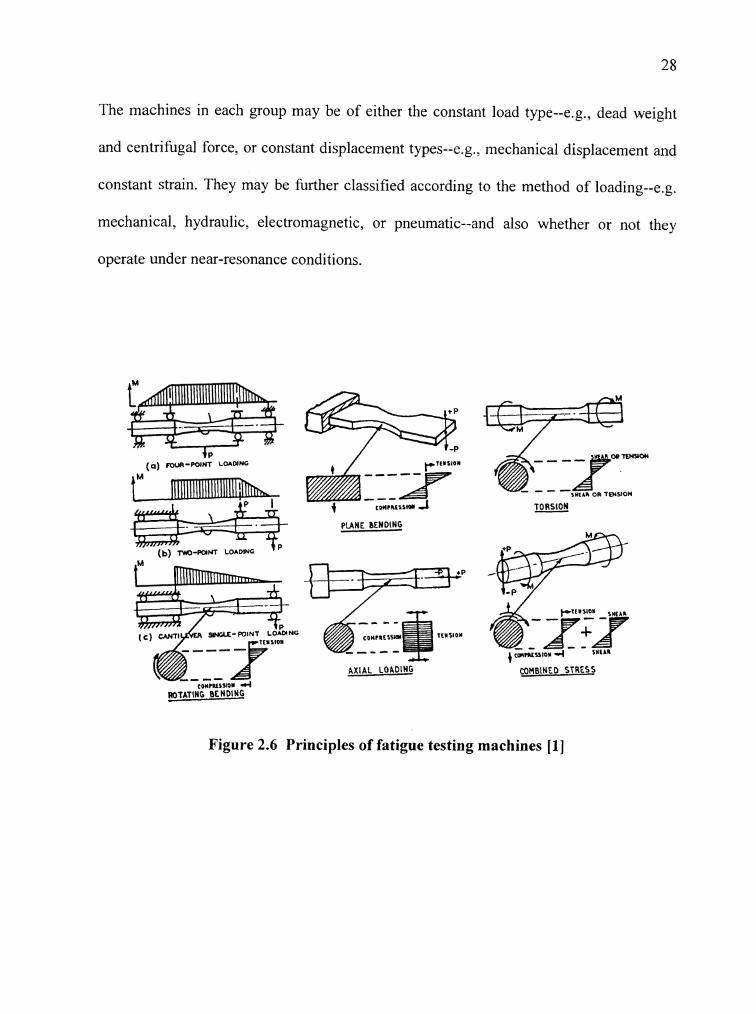
The machines in each group may be of either the constant load type--e.g., dead weight

and centrifugal force, or constant displacement types--e.g., mechanical displacement and

constant strain. They may be further classified according to the method of loading--e.g.

mechanical, hydraulic. electromagnetic, or pneumatic--and also whether or not they

operate under near-resonance conditions.

~~+ (b) TWO-POINT LOADING

PlANE BENDING

& AXIAL LOADING

ROTA TI^ BENDING

Figure 2.6 Principles of fatigue testing

TORSION

COMBINED STRESS

machines [I]

2.6.1 Axial (Direct-Stress) Fatigue Testing Machine

The direct-stress fatigue testing machine subjects a test specimen to a uniform stress or

strain throughout its cross section. For the same cross-section, an axial fatigue testing

machine must be able to apply a greater force than a static bending machine to achieve

the same stress. Axial machines are used to obtain fatigue data for most applications and

offer the best method of establishing--by closed-loop control--a controlled strain range in

the plastic strain regime (low-cycle fatigue).

Electromechanical Systems

These systems have been developed for axial fatigue studies. Generally they are open-

loop systems, but often have partial closed-loop features to continuously correct the mean

load. The rotating eccentric mass machine with a direct-stress fixture and the crank and

lever machine (Fig 2.7) are typical testing systems using this drive mechanism.

Load nlalnta?wr piston

Variable thmw eacmtric

parallel rnction

Figure 2.7 Crank and lever testing machine [3]

Servohydraulic closed-loop systems

These systems offer optimum control, monitoring, and versatility in fatigue testing

systems. These can be obtained as component systems and can be upgraded as required.

A hydraulic actuator typically is used to apply the load in axial fatigue testing. Because of

the versatility the servohydraulic system provides in control modes (load, strain, or

actuator displacement), the same machine can be used for both high-cycle fatigue and

low-cycle (strain-controlled) fatigue testing. A wide variety of grips--particularly self-

aligning types--are available for these machines.

Electromagnetic or magnetostrictive excitation is used for axial fatigue testing machine

drive systems, particularly when low-load amplitudes and high-cycle fatigue lives are

desired in short test duration. The high cyclic frequency of operation of these types of

machines enables testing to long fatigue lives (>I08 cycles) within weeks.

2.6.2 Bending Fatigue Machines

The most common types of fatigue machines are small bending fatigue machines. In

general, these simple, inexpensive systems allow laboratories to conduct extensive test

programs with a low equipment investment. The common general-purpose fatigue

machines are cantilever beam plane bending (repeated flexure) and rotating beam.

Cantilever beam machines

In this the test specimen has a tapered width, thickness, or diameter and results in a

portion of the test area having uniform stress with smaller load requirements than

required for uniform bending or axial fatigue of the same section size. In bending, the

surface stress is highest (maximum outer fibre stress), and this test mode is preferred to

study the effect of surface treatments or coatings. The cam or eccentric principles used in

the plane-bending machine typically have limited cyclic frequency compared to rotating

beam types. Both deflection-controlled and load-controlled types are in common use.

Rotating Beam Machines

The earliest type of fatigue testing machine and the most commonly used is the rotating

beam machine, in which a specimen with a round cross section is subjected to a dead-

weight load while bearings permit rotation. A given point on the circular test section

surface is subjected to a sinusoidal stress amplitude from tension on the top to

compression on the bottom with each rotation. Typical rotating beam machine types are

shown in the Figure 2.8. The R.R. Moore-type machines can operate up to 10,000 rpm.

In all bending-type tests, only the material near the surface is subjected to the maximum

stress; therefore, in a small-diameter specimen, only a very small volume of material is

under test. Thus, the fatigue properties obtained from small rotating beam fatigue tests

typically are higher than those obtained from axial fatigue tests on the same cross-section.

Load --'

I b)

Figure 2 .8 Rotating beam fatigue testing machine [3]

The nominal longitudinal stress amplitude Sa is usually calculated on the basis of elastic

bending, but if the elastic range is exceeded, the stress calculated in this way is

inaccurate. Under elastic conditions

where M = bending at the net test section

I = moment of inertia at the net test section

y = distance from neutral axis to extreme fibre at test section

For a circular section specimen this becomes

Sa = 32MIn d 3 ~

where d = net diameter of test section.

2.6.3 Torsional Fatigue Testing Machines

Some engineering applications--e.g., tailshafts of motor vehicles, torque tubes, splined

driving shafts, torsion bars, and coil springs--involve repeated torsional loading. Several

types of machines have been developed to apply this type of loading in laboratory tests,

and most of these have standard fixtures enabling them to be also used for plane bending

tests. Zero and non-zero mean stress conditions can be reproduced.

Servo- ----------- Toroue feedback -- - -- - - - - - - -- - - - -. Controller + I

I

Servo-valve I I

/ I I I

Angular I I

displacement '------: I

feedback I I I I L - - -

Displacement Rotarv actuator Hydraulic service transducer

manifold

Figure 2.9 Hydraulic torsion fatigue system [3]

Torsional fatigue tests can be performed on axial-type machines using the proper fixtures

if the maximum twist required is small. Specially designed torsional fatigue testing

machines consist of electromechanical machines, in which linear motion is changed to

rotational motion by the use of cranks, and servohydraulic machines, in which rotary

actuators are incorporated in closed-loop testing systems (Figure 2.9).

Nominal shear stress at the test section is again calculated on the basis of elastic stress

conditions existing throughout the whole section; i.e.,

where T = applied torque

y = distance from neutral axis to extreme fibre at test section

J = polar moment of inertia at the net test section.

For a circular section specimen of net test section diameter, d, the stress becomes T =

1 6 ~ l n d ~ . As in the case of flexural loading, the maximum stresses occur at the surface

and a stress gradient, decreasing from the surface to the center of the specimen, exists

under torsional loading.

2.6.4 Multi-axial Fatigue Testing Machines

Many special fatigue testing machines have been designed to apply two or more modes of

loading--in or out of phase--to specimens to determine the properties of metals under

biaxial or triaxial stresses. Such tests are of particular significance because most actual

service conditions involve complex stress systems, and fatigue failure criteria based on

simpler modes must be verified in controlled tests in which multiaxial stress states are

imposed.

Bi-axial tension is a common service stress state often requiring evaluation in pressurized

systems. A common biaxial fatigue test specimen is a tubular specimen subjected to

simultaneous internal pressure and axial loading. In tension-torsion systems, push-pull

axial loading and torsional loading are applied simultaneously. Bending-torsion machines

are similar. By offsetting the applied load with respect to the specimen centerline, simple

machines have been designed to apply simultaneous bending and torsion.

2.6.5 Specialized Fatigue Testing Equipment

To perform fatigue testing of components that are prone to fatigue failure, specialized

fatigue testing equipment has been developed for proving tests, research on manufactured

components or structural elements, or testing crankshafts, motor vehicles axles, coil and

leaf springs, gears, pistons, wheel and tyre assemblies, wire ropes, turbine blades, and

aircraft propellers. Frequently these items are too large to be accommodated in

conventional fatigue testing machines or involve highly specialized requirements, such as

the testing under repeated thermal cycling or testing under acoustic vibration conditions.

Equipment for fundamental research is also frequently of a highly specialized nature.

Equipment for the testing of Large Components and Structures - In recent years

there has been an increasing tendency to test full-scale structures, components, and

assemblies under fatigue loads. Among these are included aircraft structures (wings,

pressure cabins, or the complete structure, simultaneously), propeller shafts of ships,

welded or riveted steel, and axle assemblies. Thorough inspection of the structures or

components at frequent intervals during the test is, thus, usually essential so that failures

may be documented and rates of crack propagation determined. For realistic results, the

loading spectrum must be representative of service conditions.

Frequently, the loading system is built around the item to be tested. The two most

common systems for generating the applied loads in large-scale testing are:

Resonance or more strictly sub-resonance systems, usually mechanically excited.

Direct loading systems utilizing hydraulic or mechanical loading.

Resonance System - In the resonance system, the frequency of operation is close to a

natural frequency of vibration of the assembly being tested. This forms part of a spring-

mass system, and amplitude control may be achieved by a combination of either constant

exciting force and variable frequency or constant frequency and variable exciting force.

The exciting force can be produced by a rotating out-of-balance mass or oscillator,

variable stroke mechanically-driven crank or connecting rod, hydraulic vibrator, or an

electromagnetic exciter.

These type of system has two distinct advantages:

Relatively high cyclic frequencies are usually possible, although because of the

mass and flexibility of the specimen these are much less than in the case of small

laboratory resonant-type machines.

Power requirements are considerably less than in direct loading systems as only

frictional and damping forces must be overcome.

Direct Loading Systems - These systems consist essentially of a hydraulic jack or jacks

connected to a pulsating pressure source with a mechanical system of levers, beams, or

cables to transmit the jack force to the loading points of the assembly. This system of

loading--although restricted to lower cyclic frequencies--is much more versatile than the

resonance system and is also suitable for the simultaneous application of loads in several

directions.

To conclude, this chapter has given a brief literature review regarding fatigue

mechanisms, factors affecting fatigue behavior of materials, and the various fatigue

testing machines available to carry out the tests and present the fatigue data. The next

chapter deals with the summary of research and analysis done in terms of testing

requirements for fatigue testing, and the comparison of available systems for this

purpose, and why we opted to design the Torsion Fatigue Testing System with

appropriate system configurations, machine characteristics, and production costs suited

for our testing needs.

Chapter: 3 Fatigue Testing System

3.1 Introduction

This chapter presents a summary of research and analysis done in terms of our testing

requirements for fatigue testing and a comparison of available systems for this purpose. It

explains why the Torsion Fatigue Testing System with appropriate system configurations,

machine characteristics, and production costs was designed to meet high and low cycle

fatigue testing needs.

Fatigue properties of materials are of utmost importance in the design of mechanical

equipment. Many failures in machine parts can be traced to a disregard for this important

consideration. In a typical design cycle, however, one does not have the luxury of

contemplating the stability of the materials under extended fatigue. There are a very few

companies--MTS and INSTRON for instance--which offer machines capable of

performing fatigue tests. The typical cost of one of these machines is in the order of a

hundred thousand dollars. All of these factors encourage the designer to skip the extended

fatigue test and design the system based on static considerations.

Fatigue testing would be a very valuable addition to the designer's toolbox, if a machine

capable of performing the test with a sufficient degree of accuracy and a minimum level

of investment could be produced. The initial goal of this project was to design a machine

and the author's role was to configure the system and design and develop the associated

software for conducting various fatigue tests. The system developed has the following

specifications:

Low cost,

Capable of testing small specimens for material characterization by applying:

(a) torsion (b) tension (c) any combination of torsion and tension in

displacement, torque or velocity modes,

Capable of regulating the amount of angularllinear displacement or velocity very

accurately,

Capable of maintaining the specified parameters for extended periods of time

(days or even weeks) with very little drift in the operating characteristics or

perform a single static test, and

A user-friendly fatigue testing software that can be used to design various tests in

a step-by-step manner--defining the function generation and data acquisition

requirements for each part of the test--and to control all aspects of the test.

The torsion fatigue testing system has already been developed and the associated

software that can carry out high-cycle and low-cycle torsion fatigue testing in torque and

displacement modes was developed as part of this research. The long-term goal is to

develop this system further, which will be capable of conducting multi-axial fatigue tests,

simultaneously, under torsion and tension. The associated software can be further

developed to support this feature. The rest of the chapter deals with the configuration of

the machine and its characteristics, the associated software, and recommendations

regarding future enhancements.

3.2 Test Specifications

The first step in the design was the determination of the maximum forces and torque that

would be needed in a test. These specifications were arrived at by considering a steel

specimen with a diameter of 5mm under static conditions. The maximum torque that the

machine would be expected to produce is 50Nm. Maximum torsional displacement would

typically be in the order of a few degrees. The maximum axial force that the machine

would need to produce would typically be about 300N. The maximum axial displacement

under tension or compression would be in the order of a few millimeters. The table below

(Table 3.1) summarizes these figures.

Table 3. 1 Test Specifications

Maximum Force and Torque Specifications

Torsion

Tension

Displacement

Frequency

5 8Nm

3 00N

10 degrees in torsion, 10mm in tension or compression

50Hz

3.3 Survey of Existing Systems

The next step in the design process was a survey of existing machines. The type of

machines looked at were systems capable of performing bi-axial testing under a variety

of load conditions. During the course of the survey, it was noticed that there were very

few companies that offered a good range of test beds. The following is a sampling of the

survey. All of these systems are available from MTS corporation.

In Figure 3.1, System 1 is a standard tension hydraulic test bed with a max loading value

of 1,000,000 lbf (5MN). System 2 is the hydraulic tabletop version of System 1 with a

maximum loading of 5500 Ibf (5kN).

Figure 3.1 A Sampling of the material testing systems from MTS

In 1997 MTS released System 3, a "micro-force" test bed called TITRON for performing

tensile tests with a maximum loading 250N linear force and a minimum of 0.002 lbf

(0.01N). This system is run using an electro-servomotor. This system was released two

years after our current Torsion Fatigue Testing System, also based on electro-servomotor,

was designed and built. In addition to these systems, MTS offers a similar range of

hydraulic machines for torsion tests. MTS has recently released a bi-axial hydraulic test

bed that is capable of performing both torsion and tension at the same time.

All of these test beds have been designed for extended fatigue testing. There is, however,

one obvious drawback. The accuracy of hydraulic systems is not as good as a system

driven by an electro-servo motor. Also, cost is in the order of a hundred thousand dollars

for each of these machines. The tests that can be done on any of them is limited in scope

in the sense that the user of the machine is usually presented with a number of choices

about the nature of the test, and any deviations from the norm are not possible. The initial

goal of the project was to design around these drawbacks. The machine to be designed

must be both low cost and capable of performing a wide variety of tests with very good

accuracy for extended periods of time.

3.4 Torsion Fatigue Testing System

3.4.1 Overview

This small-size, low torque, and low-cost computer-controlled torsion fatigue testing

system run by electro-servomotor was developed by Dr. H. Pasic and his research team at

Ohio Universtiy. It has both static and dynamic loading capabilities and may be run in

torque-controlled, angular-velocity controlled, and angular-displacement controlled

modes. The fatigue testing software was developed and tested on this machine for high

and low-cycle fatigue, and its performance has been tested, analyzed and documented. It

also provides a good basis for further development to incorporate bi-axial fatigue testing

in the future.

This system may be used in a wide variety of torsion tests for testing various material

properties and fatigue studies for advanced material characterization, composite testing,

plastics testing, quality of coating testing, biomedical and biomechanical testing, soil and

elastomer testing, educational and research purposes, as well as for general purpose

fatigue testing of components (electrical switches, connectors, fasteners, springs,

automotive parts, appliance parts, tools, sporting equipment, etc.). The system may also

be used for the measurement of different material properties, such as shear modulus,

creep and viscoelastic properties, fatigue characterization, wear characteristics, quality of

coating, response characteristics, etc.

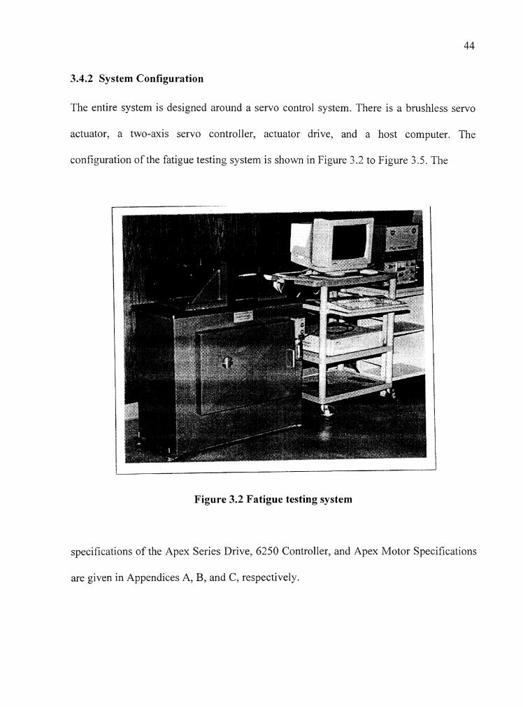
3.4.2 System Configuration

The entire system is designed around a servo control system. There is a brushless servo

actuator, a two-axis servo controller, actuator drive, and a host computer. The

configuration of the fatigue testing system is shown in Figure 3.2 to Figure 3.5. The

Figure 3.2 Fatigue testing system

specifications of the Apex Series Drive, 6250 Controller, and Apex Motor Specifications

are given in Appendices A, B, and C, respectively.

Figure 3.3 Controller and driver of fatigue testing system

Tabletop system - The servomotor is attached to a rigid "L" shaped adjustable mount, as

shown in Figure 3.4. A similar mount is used as the fixed-grip holder. Both mounts rest

on a rigid, smooth horizontal plate. This solution provides very high stiffness of the

system as well as simple specimen's alignment. The controller and the driver are installed

in the case below the plate (see Figure 3.3). With the 4.7kW servomotor, the dimensions

of the system are 45"x35"~18".

Figure 3. 4 Tabletop system

The system needs no extra cooling under fairly heavy-duty conditions. However, if

necessary, both configurations--the driver and servocontroller--may have built-in cooling

fans, while cooling the system (up to !A inch pipe wound around the motor).

Figure 3 .5 Rear view of the fatigue testing system

Safety screen and environmental chamber (for conducting experiments at elevated or low

temperatures, or in vacuum) may also be installed in the working section.

3.4.3 Machine Characteristics

Depending on the power of the servomotor used (ranging from several tens of watts to

SkW), the system can run either monotonic or fatigue tests. The more powerful motors

may be used for testing metallic, ASTM standard small-size rounded specimens (typical

diameter about 2-6 rnm for metals) with permanent torque ranging up to 50Nm and peak

intermittent torque of up to 120Nm, depending on the size of the servomotor used. The

motor belongs to the class of so-called "bmshless motors" in which the rotor (not stator)

is the magnet (made from rare-earth materials). This technology makes it possible to

overcome the heating problem while retaining large torque and large velocities (more

than 20 revolutions per second and also, due to small rotor-inertia, very high

accelerations of up to 10,000 rev/sec2. Therefore, a high enough testing frequency may be

achieved; it amounts to about 5Hz (at largest torque and twist angles of up to 120') and

even up to 50Hz at small loads. The twist angle and, therefore, the shear and the stress (as

they are mutually proportional) are measured with high resolution of about of a

degree (or even higher) by an encoder (also known as a resolver), which is an integral

part of the servocontroller (which controls the motor), such that additional devices for

measuring the twist angle are unnecessary.

Since the specimen's alignment in torsion testing is not as important as in uniaxial testing

(to avoid buckling), the alignment is simple and inexpensive. Also, in metal testing in

torsion the grips may be extremely simple, such as the socket-type with non-circular hole.

(The hole is somewhat deeper than the specimen's head, allowing for free axial creep of

the specimen).

The servomotor, its controller, the driver, and the PC make a closed-loop system such

that the system operation is fully computer-controlled. A digital signal processor is used

for high speed control, while a 32-bit microprocessor is used for executing high-level

motion programs in all the three modes (load-, velocity- and displacement controlled

tests).

The encoder (or resolver) is the integral part of the servomotor's controlling system and

is used for twist-angle measurements. Since strains and, therefore, stresses are

proportional to the twist-angle; no other instruments apart from the encoder (or resolver)

are needed for measuring strains or stresses.

A comprehensive software, which also is an integral part of the system (i.e., of the

controller), creates and executes motion-control programs under Microsoft

WindowsNT/98 platform. The basis for this software was the Motion Architect command

language for running the controller of the machine. Visual Basic 5.0 was used to develop

a GUI and incorporate the motion architect commands to run the system without having

to run it through the command prompt. The Visual Basic software development tool

allows the user to display a graphic user interface. The command language incorporates

subroutine definition, conditional programming, unit scaling, programmable 110,

contouring, and mathematical functions. The detailed description of the control system

and the associated software is discussed in subsequent chapters.

3.4.4 Production Cost

The total production cost depends on the servomotor used. For the electro-servo motor

(4.7kW, continuous torque 28Nm, and intermittent 56Nm), the total retail price of the

motor, driver, controller, software twist-angle measuring system, and the PC is $1 0,000.

Therefore, the total production price, including the case and even simple grips (for testing

metals) for this--the most expensive--version should not exceed $12,000 to $1 3,000. The

smaller-power systems may certainly be produced for less than $10,000 and the smallest

ones with the torque below 1Nm for less than $5,000.

3.4.5 Advantages

Fatigue testing machines of this kind (with electro-servomotor) is not available on the

market. A vast majority of these machines are large hydraulic testers, primarily made for

axial testing of larger size specimens with only a few exceptions, such as when hydraulic

systems are also used for torsion testing (For example, INSTRON and MTS, the world

leading producers, have recently started the production of medium-size hydraulic torsion

testing machines.).

The MTS system corporation's hydraulic machine (with torque up to 100Nm) costs

$100,000. Since the largest specimen's diameter is proportional to the cubic root of the

largest torque applied, this means that these machines may run experiments on tough-

steel specimens having only about a 30% larger diameter than those tested on the 50Nm

machine proposed here (cubic root of 100150 times 100%). Practically speaking, if the

50Nm machine may run experiments on the tough-steel 6mm specimens, the lOONm

hydraulic machine may test 8mm specimens. This small difference cannot be justified by

a price almost ten times higher.

Hydraulic systems must be expensive because their production cost must be high. MTS's

cheapest hydraulic power-supply unit alone costs $1 5,000 and the same cost is hydraulic

actuator. For measuring deformations (stresses), expensive transducers and extensometers

are used (MTS's typically cost several thousand dollars each), not to mention other

disadvantages (space needed for the power-supply unit, numerous moving parts and

hydraulic fixtures, alignment devices, large energy consumption devices, etc.). Many of

these problems simply do not exist when an electro-servomotor is used.

The system being proposed here is not to be compared with large and expensive systems.

It has its own characteristics, and it has been designed for meeting other requirements. Its

main properties are:

Low-torque and small size,

Low-production price, up to ten times less than the price of a comparable

hydraulic machine,

Additional strain (stress) measuring devices are unnecessary,

The system has one moving part only ( the motor shaft),

Easy to produce and maintain,

High precision,

The system operation is computer controlled and easy to configure and conduct

experiments, and

It meets the current market demands (torsion testing, small size, low cost).

Based on the research conducted, after reviewing the existing systems the torsion fatigue

testing system's configuration has been designed to offer a maximum peak torque of

58Nm (continuous torque of 28Nm) with frequency of up to 50Hz. The twist angle

measurement resolution is of the order of degrees (or even higher). The motor is

capable of delivering a maximum power of 4.7kW and a rated speed of up to 1,600

rev/sec.

The next chapter deals with the motion control system of the fatigue testing system,

which includes the actuator, motor, feedback transducer, and controller. It discusses and

accesses the various motion control system configurations available today and analyzes

the current system architecture of the Torsion Fatigue System.

Chapter: 4 Motion Control System

4.1 Configuration of Testing System

This chapter explains the architecture, configuration, and design of motion control

systems for the fatigue testing system, which includes the actuator, motor, feedback

transducer, and controller. It discusses and accesses the various motion control system

configurations available today and analyzes each component selected for the current

system architecture of the "Torsion Fatigue System".

Many industrial designers are concerned with controlling an entire process. Motion

control is one important and influential aspect of complete machine control. Motion

control in its widest sense could relate to anything from a welding robot to the hydraulic

system in a mobile crane. In the field of electronic motion control, one is primarily

concerned with the systems falling within a limited power range typically up to about

lOHP (7kW) and requiring precision in one or more aspects. This may involve accurate

control of distance or speed--very often both--and sometimes other parameters, such as

torque or acceleration rate. In the case of material testing, it may require a precise control

of applied torquelforce, speed, and distance.

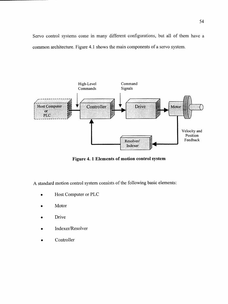
Servo control systems come in many different configurations, but all of them have a

common architecture. Figure 4.1 shows the main components of a servo system.

High-Level Command Commands Signals

Figure 4. 1 Elements of motion control system

A standard motion control system consists of the following basic elements:

Host Computer or PLC

Motor

Drive

Indexer/Resolver

Controller

There are many different machine control architectures that integrate these elements.

Each results in varying levels of complexity and integration of both motion and non-

motion elements. PLC-based, [15] bus-based, and integrated solutions are all

commercially available. The selection of a machine control strategy is based on

requirements, performance, total application cost, and technology experience.

4.2 Host Computer or PLC

The host computer, typically a PC, is used to send high-level commands to the controller

and to acquire and record data when needed. The PC has the testing software through

which the user interacts with the control system. The host computer and the controller are

in constant communication via the RS232 link, which is a serial port communication.

4.2.1 Communication Standards

Various standards have been drawn up to define the protocol for the transmission of

binary data from within the microcomputer bus structure to external devices, such as

display monitors, controllers, and other peripheral equipment. The most commonly

accepted standards are those defined by the Institute of Electrical Engineers (IEEE) [12],

[ I 61. The standards fall into the two categories of serial and parallel data communication.

The difference between the two relates to the number of bits of information transmitted

simultaneously between the devices.

Serial Communication - It is the most common method used for the interconnection of a

microcomputer to the relatively slow peripheral hardware or between two computers

when transferring a low volume of information. The bits denote the characters of

information travelling sequentially along a single path. The (EIA) RS232C or its

successors, the RS422 and RS423 [16], is the most widely adopted standard employed,

and connection between devices is made via a standard 25-pin connector. This allows

communication with one peripheral device only. Twenty-one of the signal lines is defined

in the standard, although only five (or even three) are usually required.

Figure 4 .2 Serial port connections [16]

The three main connections are 'transmitted data' (pin 2), 'received data' (pin 3), and

'signal ground or common return' (pin 7). These would normally be connected, as shown

in Figure 4.2. For communication in both directions - i.e., full duplex - the two

handshaking control lines--'request to send' (pin4) and 'clear to send' (pin 5)--are also

required.

The standard applies to data transmission interchange usually at rates between 110 and

9600 baud. A Logic ' 1' is represented by a voltage in the range of -3 to -1 5V and a logic

'0' by range of +3 to +15V. This large differentiation between '1' and '0' ensures good

immunity against electrical noise. The RS232C is limited to short communication links of

about 30m. The voltages and signal connections for the plug are defined in the standard,

but the data protocol is not defined. This must be known for the devices, which are to be

connected and can be set accordingly by software. The requirements are:

Baud rate,

Number of bits in ASCII group defining the character being transmitted,

Odd, even or no parity,

Number of stop bits.

Parallel Communication - This communication standard emerged from the need to

establish a means of interfacing a variety of instruments for data-logging applications.

The most common standard for the integration of automated test systems, developed by

Hewlett-Packard, is referred to as the IEEE-488 interface bus, which consists of 24 lines

accommodated within standard stacked-type connections. The eight bi-directional data

lines carry information as 7-bit ASCII codes between the microcomputer (controller) and

an instrument (listener) on the bus. The roles may be reversed when the data are being

logged. To process the information on the data bus, up to eight control and status signals

are available. The bus is designed to interface with up to 15 instruments within a

localized area, involving a total cable length of not more than 20m.

4.3 Motor or Actuator Design

There are essentially three types of electric motors normally used in machine tools--a

stepper motor (either rotary or linear or a combination of both), a DC brush motor, or a

brushless "servomotor". Servo systems have more or less the same architecture. The term

"servomotor" is used to signify that the motor includes an integral feedback device,

usually an optical shaft encoder. The motor must be fitted with some kind of feedback

device, unless it is a stepper motor.

4.3.1 Stepper Motors

Stepper motors have the benefits of low cost, ruggedness, simplicity in construction, high

reliability, no maintenance, wide acceptance, no tweaking to stabilize, no feedback

components are needed, and they work in just about any environment and are inherently

more fail-safe than some other servo motor types. This is because there is virtually no

conceivable failure within the stepper drive module, which could cause the motor to run

away. Stepper motors are simple to drive and control in an open-loop configuration. They

only require four leads. They provide excellent torque at low speeds--up to 5 times the

continuous torque of a brush motor of the same frame size or double the torque of the

equivalent brushless motor. This often eliminates the need of a gearbox. A stepper-driven

system is inherently stiff with known limits to the dynamic position error. There are three

main types of stepper motor:

Permanent magnet (P.M.) motors - This is widely used for non-industrial

applications in fields such as computer peripherals. The motor construction results

in relatively large step angles, but its overall simplicity lends itself to economic

high-volume production at very low cost. The axial-air gap or disc motor is a

variant of the permanent magnet design which achieves higher performance,

largely because of its very low rotor inertia. However, this does restrict the

applications of the motor to those involving little inertia.

Variable reluctance motors (V.R.) - There is no permanent magnet in a V.R.

motor, so the rotor spins freely without "detent" torque. Torque output for a given

frame size is restricted, although the torque-to-inertia ratio is good. This type of

motor is frequently used in small sizes for applications such as micro-positioning

tables. Variable reluctance motors are seldom used.

Hybrid motors - The hybrid motor is by far the most widely used stepper motor in

industrial applications. The name derives from the fact that it combines the

operating principles of other two motor types (P.M and V.R). Most hybrid motors

are 2-phase, although 5-phase versions are available. A recent development is the

"enhanced hybrid" motor which uses flux-focusing magnets to give a significant

improvement in performance, albeit at extra cost.

4.3.2 DC Brush Motors

A basic DC brush motor consists of a permanent magnet servomotor, as shown in Figure

4. 3. These magnets are used to provide a permanently energized magnetic field. They are

made of the rare-earth type materials which reduces size and weight in relation to torque

produced. The magnet segments are fixed to the steel outer housing by adhesive or bolts.

This type of construction provides efficiency and reduces heating. Several different types

of DC motor [12] are currently in use, such as

Iron-cored motor

Moving coil motor

Brushless motor

+ - Commutator

Figure 4 . 3 Conventional DC brush motor

4.3.3 Brushless Motors

The term "brushless" has become accepted as referring to a particular variety of servo

motor. Clearly a step motor is a brushless device, as is an AC induction motor. (In fact

the step motor can form the basis of a brushless servo motor, often called a hybrid servo,

which is discussed later.) However, the so-called "brushless" motor has been designed to

have a similar performance to the DC brush servo without the limitations imposed by a

mechanical commutator.

Within the brushless category are two basic types, referred to as trapezoidal and sinewave

motors. In simple terms, the trapezoidal motor is really a brushless DC servo, whereas the

sinewave motor bears a close resemblance to the AC synchronous motor. A simple

conventional DC brush motor (Figure 4.3) consists of a wound rotor, which can turn

within a magnetic field provided by the stator. If the coil connections were to be made

through slip rings, this motor would behave like a step motor; reversing the current in the

rotor would cause it to flip through 180". By including the commutator and brushes, the

reversal of current is made automatically and the rotor continues to turn in the same

direction. By including the commutator and brushes, the reversal of the current is made

automatically and the rotor continues to turn in the same direction.

Brushless motor operation - To turn this motor into a brushless design, one must start

by eliminating the windings on the rotor. This can be achieved by turning the motor

inside out; in other words, make the permanent magnet the rotating part and put the

windings on the stator poles. In servo-application, some form of electronic amplifier or

drive will be used, so the commutation is done in response to low-level signals from an

optical or Hall-effect sensor, (Figure 4.4). This component is referred to as the

commutation encoder. So unlike the DC brush motor, the brushless version cannot be

driven by simply connecting it to a source of direct current. The current in the external

circuit must be reversed at defined rotor positions; as such, the motor is in fact being

driven by an alternating current.

Figure 4.4 Brushless motor [17]

In a conventional brush motor, a rotor consisting of only one coil will exhibit a large

torque variation as it rotates. In fact, the characteristic will be sinusoidal, with maximum

torque produced when the rotor field is at right angles to the stator field and zero torque

at the commutation point (Figure4.5). A practical DC motor has a large number of coils

on the rotor with each one connected not only to its own pairs of commutator segments

but to the other coils, as well. In this way, the chief contribution to torque is made by a

coil operating close to its peak-torque position. There is also an averaging effect

produced by current flowing in all the other coils, so the resulting torque ripple is very

small.

Figure 4.5 3-Phase brushless motor [17]

A similar situation in the brushless motor, however, requires a large number of coils

distributed around the stator. This in itself may be feasible, but each coil would then

require its own individual drive current. This is clearly prohibitive, so in practice a

compromise is made and a typical motor has either two or three sets of coils or "phases",

(Figure 4.5). The motor shown in the diagram is a two-pole, three-phase design. The

torque characteristic (Figure 4.6) indicates that maximum torque is produced when the

rotor and stator fields are at 90' to each other.

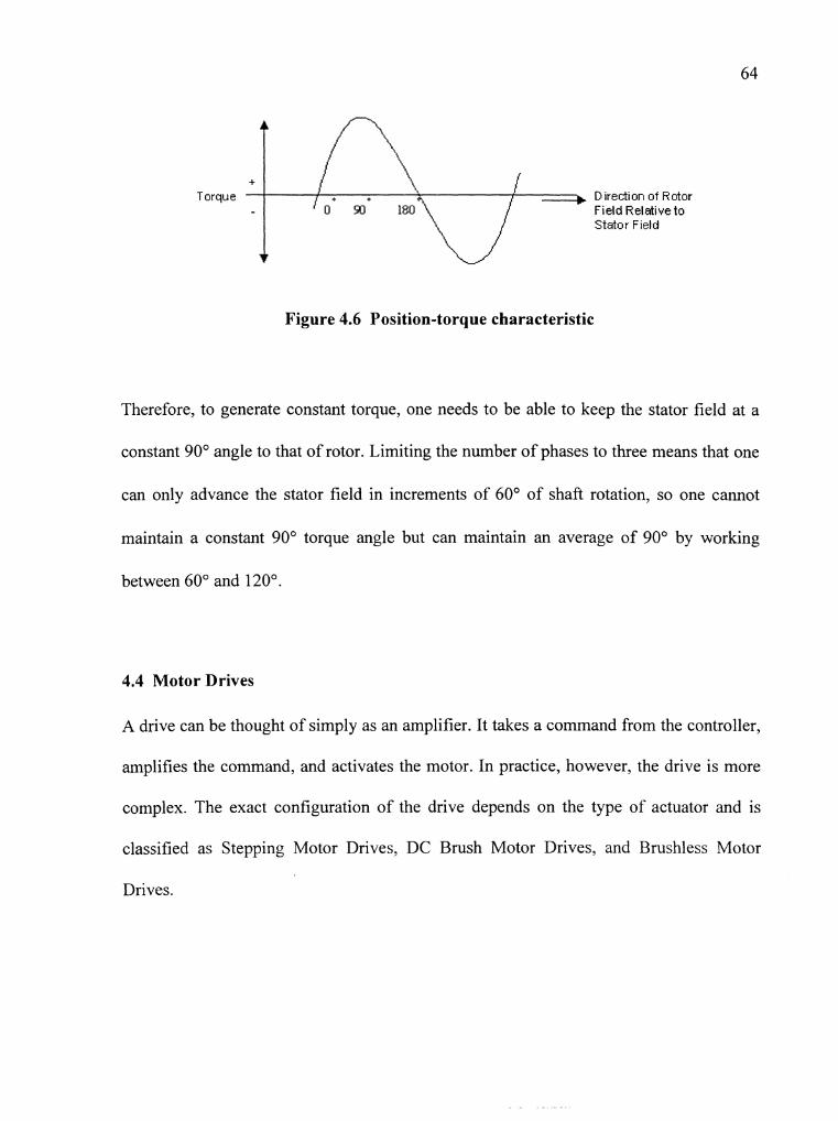
Torque D irection of Rotor Field Relative to Stator Field

Figure 4.6 Position-torque characteristic

Therefore, to generate constant torque, one needs to be able to keep the stator field at a

constant 90" angle to that of rotor. Limiting the number of phases to three means that one

can only advance the stator field in increments of 60" of shaft rotation, so one cannot

maintain a constant 90" torque angle but can maintain an average of 90" by working

between 60" and 120".

4.4 Motor Drives

A drive can be thought of simply as an amplifier. It takes a command from the controller,

amplifies the command, and activates the motor. In practice, however, the drive is more

complex. The exact configuration of the drive depends on the type of actuator and is

classified as Stepping Motor Drives, DC Brush Motor Drives, and Brushless Motor

Drives.

4.4.1 Stepper Motor Drive

The stepper drive delivers electrical power to the motor in response to low-level signals

from the control system. The motor is a torque producing device and this torque is

oenerated by the interaction of magnetic fields. The driving force behind the stator field a

is the magneto-motive force (MMF), which is proportional to the current and to the amp-

turns product. Essentially, the drive must act as a source of current. The applied voltage is

only significant as a means of controlling the current.

Stepper Drive

Direction

Figure 4.7 Stepper drive elements [17]

Input signals to the stepper drive consist of step pulses and a direction signal. One step

pulse is required for every step the motor takes. This is true regardless of the stepping

mode. So the drive may require 200 to 101,600 pulses to produce one revolution of the

shaft. The most commonly used stepping mode in industrial applications is the half-step

pulse frequency of 20kHz.

4.4.2 DC Brush Motor Drives

The amplifiers for both brush and brushless servo motors are either analog or digital. The

analog drive has been around for many years, whereas the digital drive is a recent

innovation. Both types have their merits.

The Analog Drive - In the traditional analog drive, the desired motor velocity is

represented by an analog input voltage usually in the range *10 volts. Full forward

velocity is represented by +10V, and full reverse by -10V. Zero volts represent the

stationary condition, and intermediate voltages represent speeds in proportion to the

voltage. The various adjustments needed to tune an analog drive are usually made with

potentiometers.

The Digital Drive - An alternative to the analog system is the digitally-controlled drive

in which tuning is performed by sending data from a terminal or computer. This leads to

easy repetition between units and, since such drives are invariably processor-based,

facilitates fully-automatic self tuning. The input signal to such a drive may also be an

analog voltage but can equally take the form of step and direction signals, like a stepper

drive. Digital drives are used more in conjunction with brushless servo motors than with

DC brush motors.

A Comparison of Analog and Digital Drives - The analog drive offers the benefit of

lower cost and, in the case of a drive using tach feedback, very high performance. The

wide bandwidth of the brush tach allows high gains to be used without inducing jitter at

standstill, resulting in a very "stiff' system.

The digital drive, while more costly, is comparatively easy to set up and adjustments can

quickly be repeated across several units. Automatic self-tuning can be a distinct

advantage where the load parameters are unknown or difficult to measure. The digital

drive also offers the possibility of dynamic tuning-sometimes vital where the load inertia

changes dramatically during machine operation.

Analog DC Drive operation - The elements of an analog velocity amplifier are shown in

Figure 4.8. The function of the system is to control motor velocity in response to an

analog input voltage.

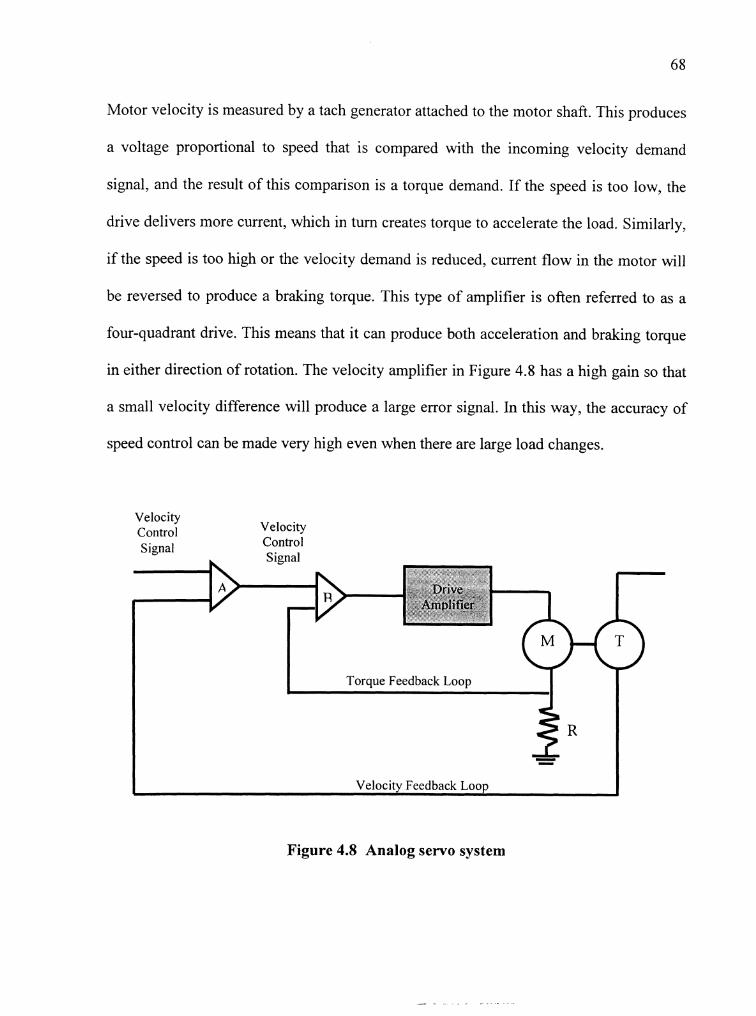
Motor velocity is measured by a tach generator attached to the motor shaft. This produces

a voltage proportional to speed that is compared with the incoming velocity demand

signal, and the result of this comparison is a torque demand. If the speed is too low, the

drive delivers more current, which in turn creates torque to accelerate the load. Similarly,

if the speed is too high or the velocity demand is reduced, current flow in the motor will

be reversed to produce a braking torque. This type of amplifier is often referred to as a

four-quadrant drive. This means that it can produce both acceleration and braking torque

in either direction of rotation. The velocity amplifier in Figure 4.8 has a high gain so that

a small velocity difference will produce a large error signal. In this way, the accuracy of

speed control can be made very high even when there are large load changes.

Velocity Control Velocity

Control

Figure 4.8 Analog servo system

4.4.3 Brushless Motor Drives

This provides a drive technology, which assures specified speed, acceleration, and torque

performance. It also provides high torque per motor size and weight, rapid acceleration,

and smooth machine operation. A brushless motor drive comes in various configurations

and a typical setup for a brushless sinewave drive is shown in Figure 4.9. A sinewave

brushless motor can be two or three phase, and the one illustrated in Figure 4.9 is a two-

phase version. This uses two H-bridges to control current in the two motor windings, and

the power section of this drive closely resembles a pair of DC brush drives. This drive

uses a digital processor-based control section, which takes its input in the form of step

and direction signals. One needs to generate currents in the two motor windings which

follow a sine and cosine pattern as the shaft rotates.

-1_1__1 I " - - - r'----- - - - i

I - -%-? 3 0 - . ., .."

! U c r

7 ---

1 "- "2, -)L Csnvertsr Control

Q - Ii

--- 1 "- "2,

Csnvertsr Control Q -

Figure 4.9 Two-phase sinewave brushless drive [17]

The drive shown in the diagram uses a brushless resolver and a resolver-to-digital

converter (RDC) to detect the shaft position 1141. From this, one gets a number which can

be fed to a look-up table to determine the instantaneous current values for the particular

shaft position. The look-up table gives only relative currents in the two windings-the

absolute values will depend on the torque demand at the time. So the processor must

multiply the sine and cosine values by the torque demand to get the final value of current

in each phase. The resulting numbers are fed to D-to-A converts, which produce an

analog voltage proportional to demanded current. This is fed to the two PWM chopper

amplifiers.

Commutation information for a sinewave drive may also be derived from an absolute or

incremental optical encoder. An incremental encoder will be less expensive for the same

resolution but requires some form of initialization at power-up in order to establish the

required 90" torque angle.

4.4.4 APEX Brushless Sewo Drive

The APEX series of brushless servo systems from Compumotor has been selected as a

drive for the fatigue testing system as it delivers high performance and reliability. The

series can operate a variety of servo motors, in addition to the standard resolver-based

motors. Each unit can accept either hall effect or resolver commutation feedback and can

be configured for different pole pair motors. The series incorporates sophisticated

electronics, which includes a smart power block that interfaces directly to the control

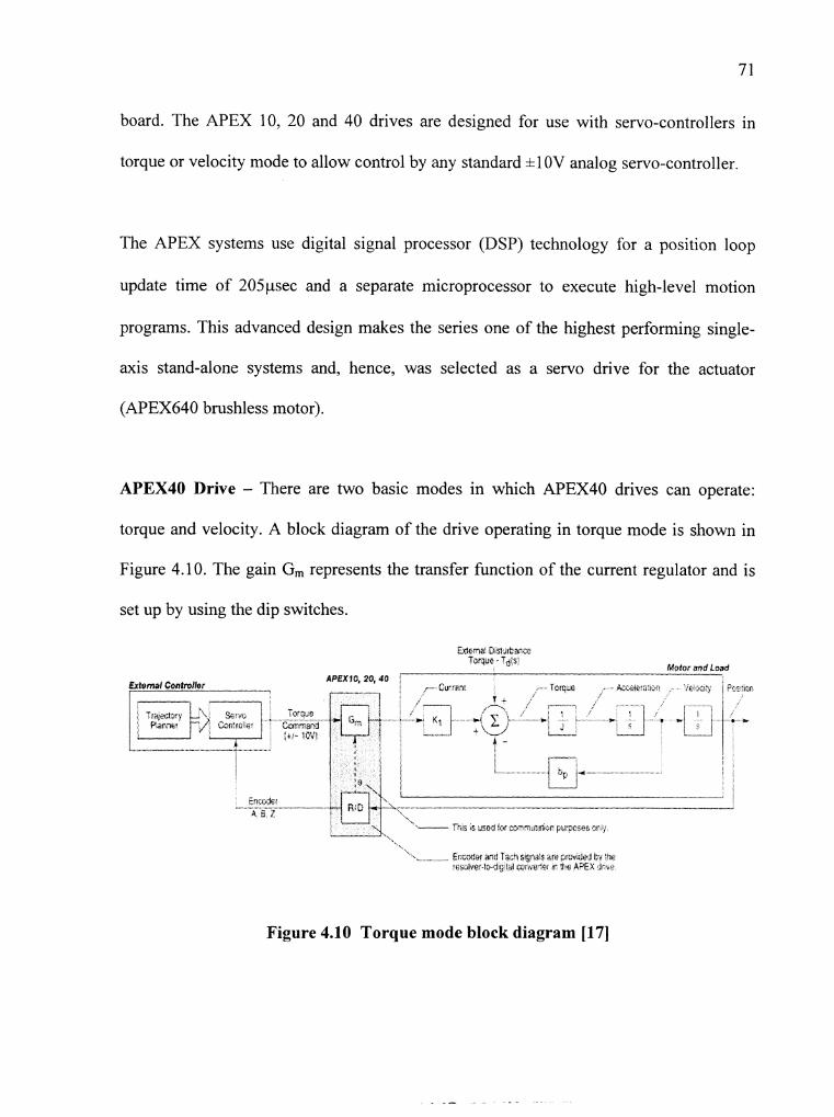
7 1

board. The APEX 10, 20 and 40 drives are designed for use with servo-controllers in

torque or velocity mode to allow control by any standard i l OV analog servo-controller.

The APEX systems use digital signal processor (DSP) technology for a position loop

update time of 205psec and a separate microprocessor to execute high-level motion

programs. This advanced design makes the series one of the highest performing single-

axis stand-alone systems and, hence, was selected as a servo drive for the actuator

(APEX640 brushless motor).

APEX40 Drive - There are two basic modes in which APEX40 drives can operate:

torque and velocity. A block diagram of the drive operating in torque mode is shown in

Figure 4.10. The gain G, represents the transfer f~inction of the current regulator and is

set up by using the dip switches.

Cfio7a- :I~k!t:trm Torque. -c( j'

Motor and Load APEX lo, 20, 40

External ContmNor . !a:e*e . ,&:;.L.:~~Q.B'~U.: , ';e.:.cj; I r?cr:wc.

y- -- ..- -'I)

.-" " -.*. .. . . , , , .- " , 1 / I i ; I.. . .. . < * . . . . . .

j i , :

, ,

\ ._____ 7- ,, is . s usud ior : y " ~ : g : , ~ r pij3i.5e~ 51. ;

'. _ . Et:i\7t2~: =!I Ta:.'i eve'$ are @rw:laJ l:y !7c .hiui.ie*.tcrdii; id cc?,;elt c ?.b A3EX Y i r

Figure 4.10 Torque mode block diagram [17]

The drive can also be set up in displacement and velocity modes. In case of velocity

mode; the * 10 volt signal represents commanded motor speed. This block diagram is

shown in Figure 4.11 below. The gains Kc and Ki are set by the pots labeled "Collective"

and "Vel integral" gain, respectively. The gain Kp, is factory set to 1. The gain G, again

represents the transfer function of the current regulator and is set up by dip switches.

Figure 4.1 1 Velocity mode block diagram [17]

4.5 Feedback Transducers

The previous sections in this chapter have covered the principles of operation of a

machine control system, the actuators necessary to effect movement, and the methods of

control of these actuators. This section examines the elements necessary to provide

feedback to the system controller on position, proximity, displacement, velocity and

force. There is a wide range of these feedback sensors available like inductive sensors,

capacitive sensors, photosensors, pneumatic sensors, resolvers and optical encoders. In

order to keep track of the position of the actuator while running the test on a fatigue

testing system, one needs a displacement transducer that provides accurate feedback of

the displacement, velocity, and torque levels at all times during the test. The displacement

transducers may be linear or rotary, analogue or digital, and incremental or absolute.

They can also be used to provide direct or indirect feedback. Direct feedback occurs

when the transducer is mounted integrally with the elements being monitored. For

example, if the movement of a machine-tool table is being measured relative to a fixed

bed, then a feedback transducer mounted on the table and/or the bed will provide a direct

measurement of displacement. However, if the movement of a torsion fatigue specimen is

being measured, then a feedback transducer mounted on the actuator shaft will provide an

indirect measurement of displacement of the motor and, hence, the position of the

specimen at every instance, because the movement being measured must still be

transmitted to the machine-tool table.

4.5.1 Classification of Feedback Transducers

Linear/Rotary Transducers - They are commonly used on machine-tool tables and

slideways. They provide reliable and precise direct displacement feedback using optical

gratings and encoders. Rotary transducers in the form of optical shaft encoders,

potentiometers, and resolvers are popular for mounting integral with servomotor

assemblies for indirect displacement feedback.

AnalogueDigital Transducers - They produce a continuously changing signal

analogous to the value being measured; potentiometers and resolvers are analogue

transducers. Digital transducers produce digital signals; e.g., an optical grating will

produce--after signal conditioning--a train of square-wave pulses for input to an

electronic counter.

IncrementaYAbsolute Transducers - They provide signals that must be added as they

arrive at the counter to determine the displacement from a known starting, or 'zero',

point. However, with an absolute transducer each signal pattern specifies uniquely where

the device is located.

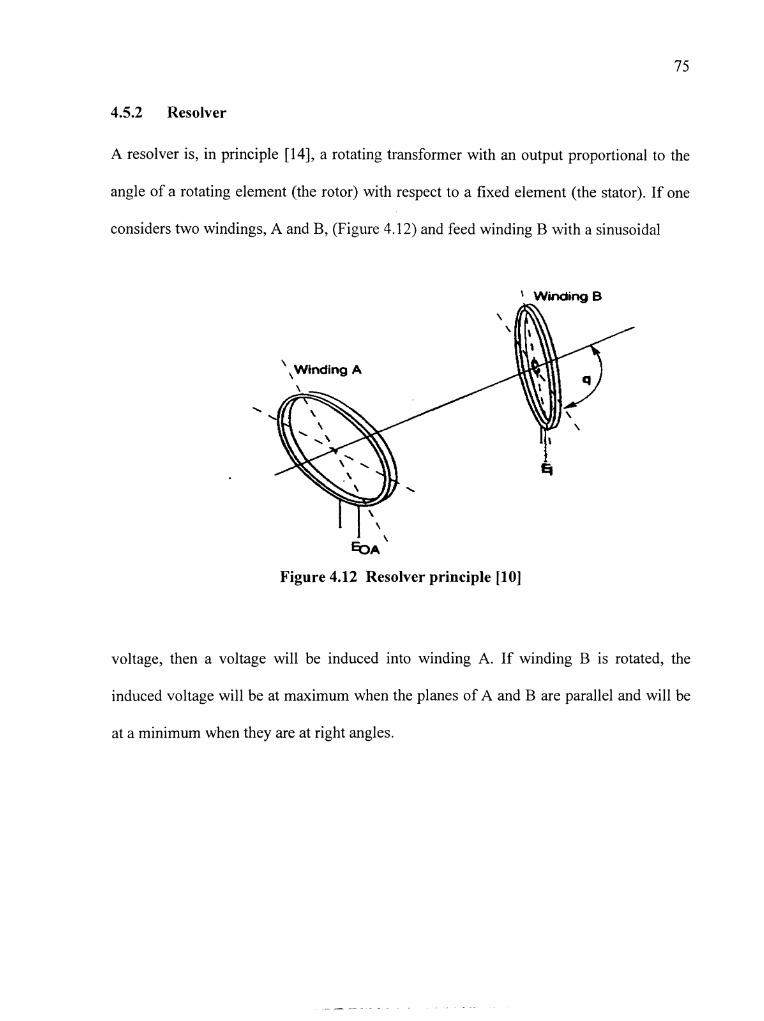
4.5.2 Resolver

A resolver is, in principle [14], a rotating transformer with an output proportional to the

angle of a rotating element (the rotor) with respect to a fixed element (the stator). If one

considers two windings, A and B, (Figure 4.12) and feed winding B with a sinusoidal

\ Winding B

Figure 4.12 Resolver principle 1101

voltage, then a voltage will be induced into winding A. If winding B is rotated, the

induced voltage will be at maximum when the planes of A and B are parallel and will be

at a minimum when they are at right angles.

Also, the voltage induced into A will vary sinusoidally at frequency of rotation of B so

that EOA = El sin$. If one introduces a third winding (C) positioned at right angles to

winding A, then as B is rotated, a voltage will be induced into this winding and this

voltage will vary as the cosine of the angle $ so that Eoc = EI Cos$. Referring to Figure

4.13, one can see that if we are able to measure the relative amplitudes of the two

windings (A and C) outputs at a particular point in the cycle, these two outputs will be

unique to that position.

E I Cos

Figure 4.13 Resolver output (101

The information output from the two phases will usually be converted from analog to

digital form for use in a digital positioning system by means of a resolver-to-digital

converter. Resolutions up to 65,536 counts per revolution are typical of this type of

system. In addition to position information, speed and direction information may also be

derived. The resolver is an absolute position feedback device. Within each electrical

cycle, Phase A and Phase B maintain a constant (fixed) relationship.

Dieits1 output (Shafi Angle)

Figure 4.14 Resolver-to-digital converter [16]

The excitation voltage E may be coupled to the rotating windings by slip rings and

brushes, though this arrangement is a disadvantage when used with a brushless motor. In

such applications, a brushless resolver may be used so that the excitation voltage is

inductively coupled to the rotor windings (Figure 4.1 5).

Stator Phase 1

Figure 4.15 Brushless resolver [12]

4.6 Controller

The controller is an essential part of any motion control system. It determines speed,

direction, distance, and acceleration rate-in fact, all the parameters associated with the

operation that the motor performs. The output from the controller is connected to the

drive's input, either in the form of an analog voltage or as step and direction signals. In

addition to controlling one or more motors, many controllers have additional inputs and

outputs that allow them to monitor other functions on a machine.

Controllers can take a wide variety of forms. Some of the common architectures [15] are

Standalone, Bus-based, PLC-based, and X Code-based controllers.

Standalone - This type of controller operates without data or other control

signals from external sources. A standalone unit usually incorporates a keypad for

data entry as well as display, and frequency includes a main power supply. It will

also include some form of nonvolatile memory to allow it to store a sequence of

operations. Many controllers that need to be programmed from a terminal or

computer can, once programmed, also operate in standalone mode.

Bus-based - A bus-based controller is designed to accept data from a host

computer using a standard communications bus. Typical bus systems include

STD, VME, and IBM-PC bus. The controller will usually be a plug-in card that

conforms to the standards for the corresponding bus system. For example, a

controller operating on the IBM-PC bus resides within the PC, plugging into an

expansion slot and functioning as an intelligent peripheral.

4.6.1 2-Axix Servo Controller

Compumotor's 6250 is a stand-alone two-axis servo controller. The 6250 provides

sophisticated control for any standard +10V analog input servo drive system and is

perfect for the synchronization of two axes of motion. A Digital Signal Processor (DSP)

is used for high-speed servo control. A separate microprocessor is used for executing

high-level motion programs. The 6250 controller uses the dual processor approach for

precise servo control and motion command execution.

The 6250 controller uses the 6000 command language. This language is powerful enough

to implement complex motion control applications. Many useful features are incorporated

into the command language, including subroutine definition, conditional programming,

unit scaling, programmable 110, contouring, and mathematical functions. The controller

also comes with Motion Architect software, a software package for creating and

executing motion control programs under Microsoft Windows.

The 6250 controller is ideal for generating motion control programs for carrying out

torsion fatigue testing (both low and high cycle) because of its enormous features and

functionality. Some of these are enumerated below:

Motion

- 2 axis of optically isolated servo control (+_ 10V-12bit analog interface) with

incremental encoder feedback

- Control servo drives in velocity or torque mode

- Update rtes for servo loop as fast as 205 micro-sec for one axis

- Digital Signal Processor (DSP) for servo-control (PIV with velocity and

acceleration feed-forward)

- 1.2MHz post - quadrature position feedback frequency.

110

- Home limit, positive and negative end-of-travel limits

- 48 programmable inputs (24) and outputs (24)

- Auxiliary high-speed programmable inputs and outputs providing position capture

or output on position to t- 1 count at maximum encoder frequency

- Drive Enable outputs, Drive Fault inputs

- 3 8-bit analog inputs that can be used for joystick or variable input (temperature,

tension, etc.)

- 6250 AN1 option offers two +_ 10V, 14-bit analog inputs (one per axis) with anti-

aliasing filter; it can also be used for position feedback.

Language

- Capability to interrupt program execution on error conditions

- Position-based following

- Linear interpolation

- Variable storage, conditional branching, and math capability

- Program debug tools--trace mode, break points and simulation of 110

- Scaling of distance, velocity and acceleration

- S curve or trapezoidal motion profiling

- 150,000 bytes of non-volatile memory for storage of programs and paths

Software Provided

- Motion Architect - Microsoft Windows-based application development software

- DOS support software program editor and terminal emulator software

- Dynamic Link Library (DLL) provided for use with Microsofe Windows software

development kit

Interface Capability

- Operates stand-alone or interfaces to computers, programmable logic controllers

- Compatible with RP-240 operator interface panel

- Two RS-232C Communications Ports

Physical

- Standalone Package

- 120-240VAC

A partial list of the command language along with the specifications and dimensions of

6250 controller are provided in Appendix B.

The existing motor/drive technologies have been researched, and it was decided that the

following configuration will be used for the system which offer a maximum peak torque

of 58Nm (continuous torque of 28Nm) with frequency of up to 50Hz and an angular

resolution of 10" degrees (or even higher). Appendices A, B, and C give the

specifications for the various parts of the system.

Drive - Compumotor's APEX 605 Brushless Servo Drive, which is capable of

delivering a maximum power of 8kW and accelerations of up to 10,000 rev/sec2 and

frequency of more than 50Hz.

Controller - Compumotor's 6250 Servo-Controller (32-bit CPUI 24-bit DSP

processor).

Resolver - Two-phase quadrature incremental encoder with differential or single

ended outputs (+5V DC). Max frequency = 1.2 MHz.

The next chapter looks at the material testing software developed for torsion fatigue

testing and the testing procedure for the fatigue testing system. It discusses and assesses

the various features of the software and establishes a testing procedure to be adopted for

carrying out a fatigue test.

Chapter: 5 System Software

5.1 Introduction

This chapter describes the design and development of fatigue testing software and various

issues involved. It also discusses the procedure for conducting the high and low cycle

fatigue tests in torque and displacement modes using the testing software.

Testing needs may change from week-to-week, month-to-month, or even day-to-day. To

meet these changing requirements or to do tests that are not based upon an existing

standard, one needs a very flexible program that can carry out the specific tests. Driven

by these needs, a flexible software program for high- and low-cycle fatigue testing has

been developed along with a Graphic User Interface to execute motion control programs

in torque, displacement, and velocity modes for torsional (uniaxial testing). It can also be

used to create and run a wide variety of other test programs. Through a series of

windows, one can design a test in a step-by-step manner, defining the function generation

and data acquisition requirements for the test. The software can be modified easily to

incorporate multi-channel control applications, like Bi-Axial Fatigue Testing.

5.2 Graphic User Interface Design Process

A user interface is the part of an application that the user sees and with which he or she

interacts. Narrowly defined, this interface comprises the input and output devices and the

software that services them. Broadly defined, the interface includes everything that

shapes the user's experiences with computers--including documentation, training, and

human support.

The user interface is so important to users, designers, and developers of software

products because that is what users view and work with. From the user's point of view,

the interface is the software. There is a body of knowledge about how people think, learn

and work. Intelligent interface design [l 11 taps into that body of knowledge and applies it

to the design of a software interface.

A typical intelligent interface design process consists of analysis, design, and

construction, as shown in Figure 5.1.

Figure 5.1 Phases of interface design

5.2.1 Analysis

The analysis phase includes both learning about and documenting current testing systems

and software and verifying the future tasks. One has to identify all the system hardware,

software and project features and requirements that might constrain the interface design.

Identify the interface technology that will be employed - for example, GUI. Identify the

platform (for example UNIX, DOS, WINDOWS, OSl2; see Ross, Paul [13]) and

machines (for example, UNIX workstations, X terminals, PC's). Identify what user

interface techniques will be available. Once these issues have been identified, one defines

the product usability goals and objectives and develop a user scenarios and tasks.

5.2.2 Design

During this phase, one takes everything that helshe has learned during analysis and

creates a solution based on all that helshe knows. The design phase progresses through a

number of well-defined steps that should be followed in sequence before one codes the

final design.

Once the user's scenarios and tasks have been identified, the next step is the design

process of defining interface objects and actions. Next one identifies key object

attributes; that is, the information about the objects that the user needs to see when

performing tasks, such as the current time and the time when the test run was started. One

might also want to display the test parameters that the user has selected for performing

the test. Next, one identifies user actions on task objects using information from the task

analysis and case scenarios. Once objects have been defined, one determines how to best

represent them on the screen and how users will view these objects and the information

they contain. When determining object views, one considers the way users u7ill interact

with each object and its information. After designing objects and their icons, one

determines how users will interact with objects and windows using various types of

menus.

5.2.3 Construction

Once the high-level design mockup is tested and revised, one goes about creating a more

realistic version of the interface. Prototypes are the tools for constructing the interface.

Construction has several purposes:

Create a hi-fi computer prototype

Further iterate the design and test the program

Document the complete, final design for development.

The purpose of a prototyping [ l l ] is to quickly and easily visualize design alternatives

and ideas, not to build code that must be used as part of the product. There are many

ways to prototype interfaces, starting with pencil-and-paper methods using chalkboards,

whiteboards, flipcharts, and storyboards. Prototypes may show visualizations of the

interface. There are two ways to approach prototyping-using prototyping tools

specifically designed for the task, or using development tools like Visual Basic or Visual

C++, that are normally used to write product code.

After the computer prototype is developed, one must implement it in the code. Also the

communication and documentation of the entire interface design is done so that while

developing the interface one knows how the interface looks and behaves. At this point

one will have developed a full interface design--series of screens that match the way the

user is going to work with the new system. The interface must be tested and revised

several times. This is an interface that will be usable and will not need a lot of changes

once it is coded.

5.2.4 Who's Driving the Design - The System or the Interface?

Designing and developing a software product may require integrating many subsystems,

programs, and so on. In many cases, the operating system, programming languages, and

the svstem out

Figure 5 .2 Design from User-In vs. from the System-Out

development tools are already in place or have previously been determined before the

user interface is designed. Figure 5 . 2 shows two different approaches to interface design.

Designing from the system out can predetermine and constrain what type of user

interface can be designed and built. The technology itself (the language selected, CASE

tool chosen, etc.) often overshadows the paradigm (the frame of reference, way of seeing,

process of understanding, and method of mapping).

If you design "from the user in" perspective, you follow the design process outlined here

and work with users to build product goals, objectives, and user requirements. You are

more likely to design interface metaphors, visual elements, and inputJoutput techniques

that match user requirements. Then see if it is possible to build the appropriate user

interface using the current development environment. If it cannot be supported, then try

implementing it using new widgets and using a different approach.

5.3 Fatigue Testing Software

The Fatigue Testing Software has been developed in Visual Basic 5.0 and runs on a

Windows platform (95198NT). The beta version of the software has been tested during

the senior project rotation. The software, in essence, presents the user with a number of

choices regarding the test and parameters of the test and then programs the controller to

run the appropriate test. The host computer and the controller are in constant

communication [I61 during the test via the RS232 link. Data from the controller, such as

torque, angular displacement etc., is sent back to the host computer, which then records

the data in a file and generates a real-time plot for the process. The source code for this

software is included in Appendix D.

This material testing software is primarily composed of three modules:

Test Selection Module

Data Input Module

Test Execution Module

5.3.1 Test Selection Module

To run a test using the fatigue testing software, one begins by first switching on the

control system of the fatigue testing system and mounting the specimen correctly. After

running the executable file of the testing software, the application starts and prompts the

user for a login and password, as shown in Figure 5.3. After proper validation, a splash

screen comes up displaying information about the software, as shown in Figure 5.4. The

welcome screen automatically unloads after a few seconds to display the test selection

form where one defines the basic types of test to be run.

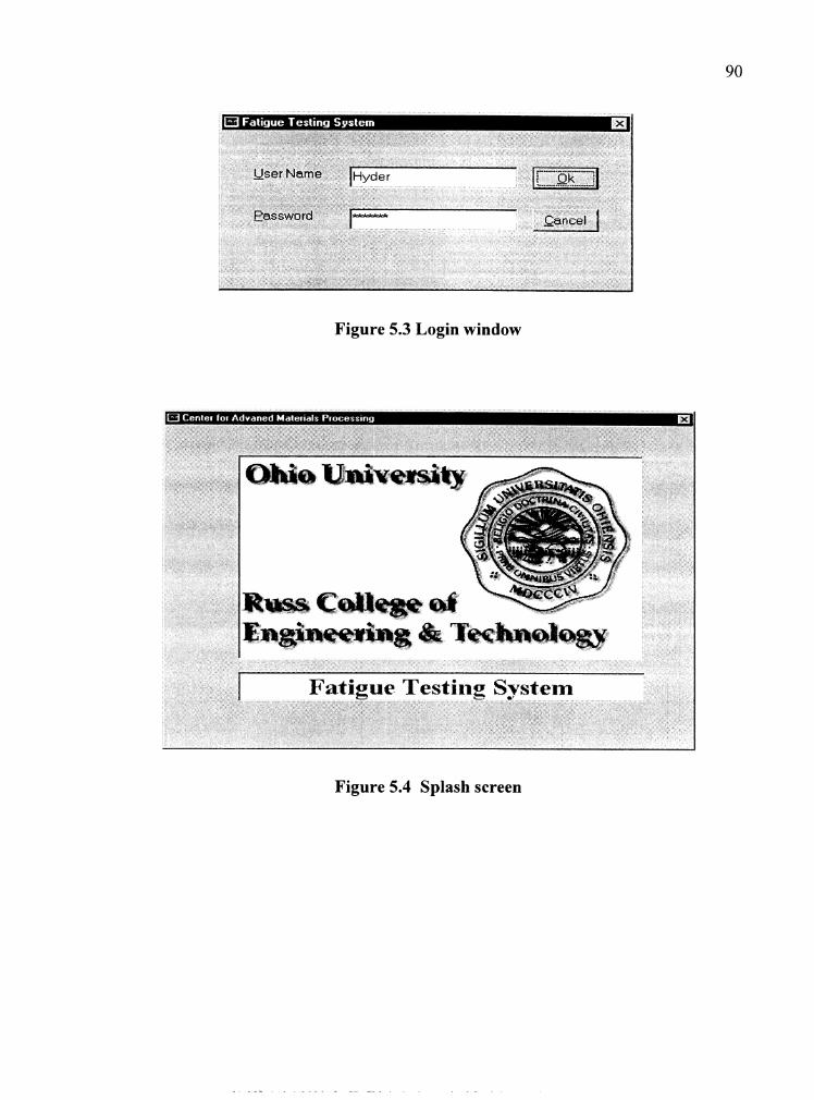
Figure 5.3 Login window

Figure 5.4 Splash screen

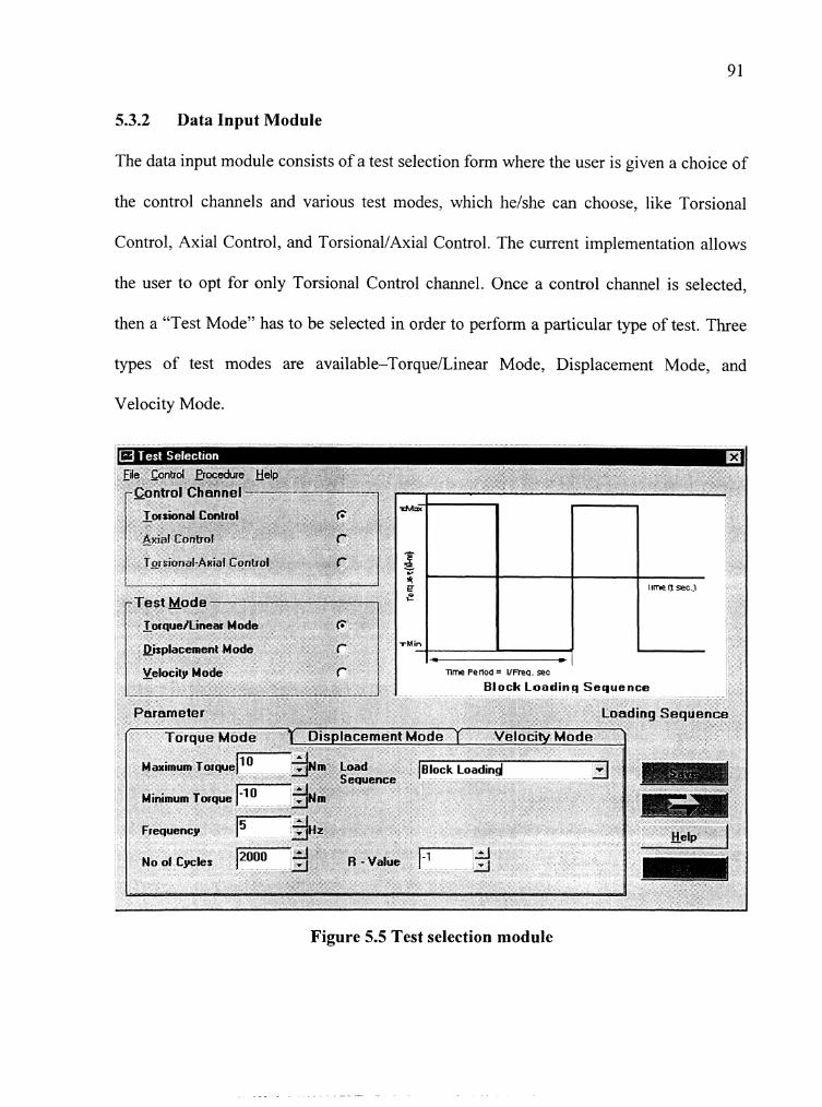
5.3.2 Data Input Module

The data input module consists of a test selection form where the user is given a choice of

the control channels and various test modes, which helshe can choose, like Torsional

Control, Axial Control, and Torsional/Axial Control. The current implementation allows

the user to opt for only Torsional Control channel. Once a control channel is selected,

then a "Test Mode" has to be selected in order to perform a particular type of test. Three

types of test modes are available-Torqueilinear Mode, Displacement Mode, and

Velocity Mode.

Figure 5.5 Test selection module

Once a particular test mode is selected, the user is allowed to input certain process

parameters. As shown in Figure 5.5, if one selects the "Torque" test mode, then the

appropriate tab is displayed in the parameter tab list where helshe can input hislher test

conditions. Here, for this particular case, it will allow the user to enter

maximum/minimum torque, frequency, number of cycles, type of loading sequence, and

the R-value.

Figure 5.6 File selection menu

In the Test Selection form, the menu bar at the top gives a set of options for opening the

test files and printing and saving them, as shown in Figure 5.6. It also gives the option of

Figure 5.7 Control selection menu

selecting the control channel (Figure 5.7), and an online help about the Motion Architect

Software, Compumotor etc., (Figure 5.8).

In the test selection form, an image is displayed on the top right-hand comer, which

indicates the type of test selection mode and the loading sequence. This image changes,

depending upon the type of loading sequence.

Figure 5.8 Help selection menu

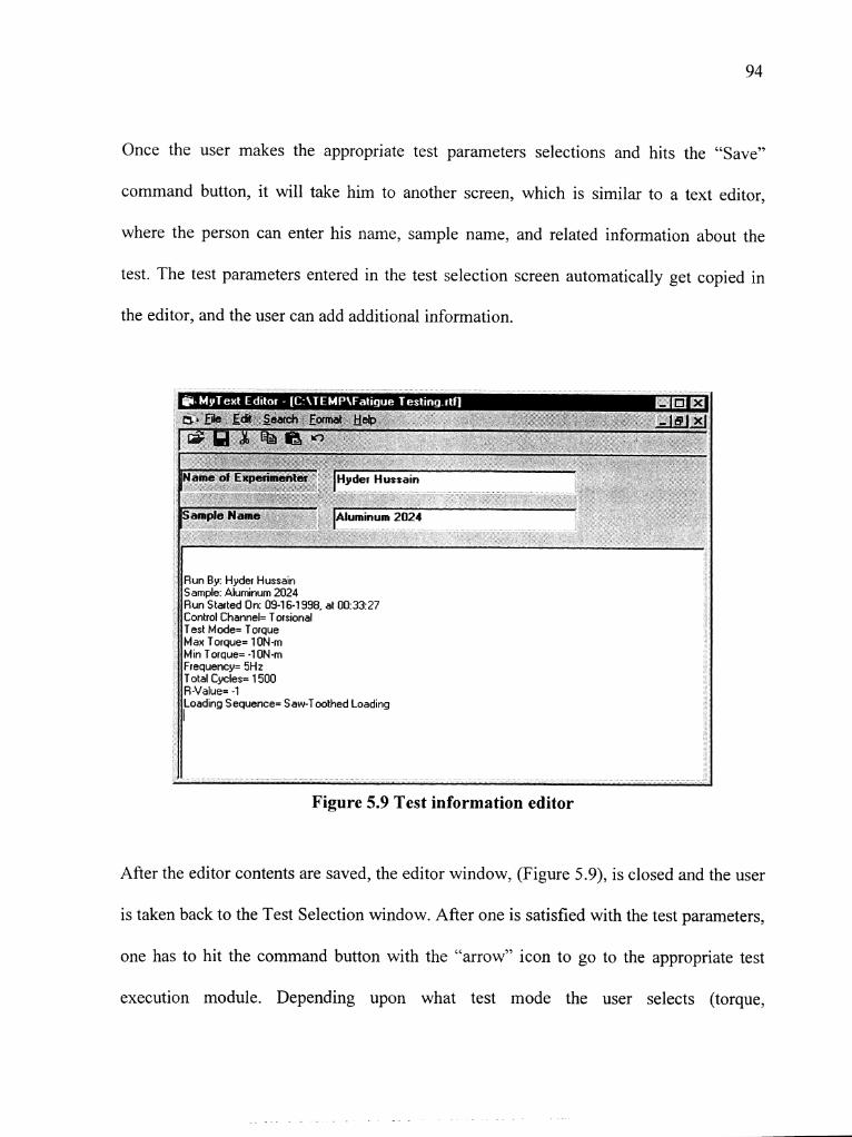
Once the user makes the appropriate test parameters selections and hits the "Save"

command button, it will take him to another screen, which is similar to a text editor,

where the person can enter his name, sample name, and related information about the

test. The test parameters entered in the test selection screen automatically get copied in

the editor, and the user can add additional information.

Run By: Hyder Hussain Sample: Aluminum 2024 Run Started On: 09-16-1 998, at 00:33:27 Control Channel= Torsional Test Mode= Torque Max Torque= ION-m Min Torque= .I ON-m

Total Cycles= 1 500

Loading Sequence= Saw-1 oothed Loading

Figure 5.9 Test information editor

After the editor contents are saved, the editor window, (Figure 5.9), is closed and the user

is taken back to the Test Selection window. After one is satisfied with the test parameters,

one has to hit the command button with the "arrow" icon to go to the appropriate test

execution module. Depending upon what test mode the user selects (torque,

displacement, or velocity), the corresponding test execution module loads up and the

form for executing the test is displayed, as shown in Figure 5.10.

5.3.3 Test Execution Module

Once the user has made all the appropriate test selections and provided the input

parameters, the test can be started by hitting the "Start" button in the control panel of the

test execution window, as shown in Figure 5.10. The program for running the motor with

the given parameters is downloaded to the controllers memory through the RS232 serial

port when the test execution window is loaded into the memory and displayed on the

screen.

Figure 5.10 Torque control mode

Once the command button is clicked, the software sends a signal to the controller to start

the test with the appropriate process parameters. The test execution window has four

major parts associated with it-Data Display, Data Plot, Test Parameters, and Control

Panel. The Data Display frame consists of text boxes and labels which display various

parameters, such as number of cycles, current time, run started at, current theta max,

current theta min, starting theta max, starting theta min, etc. The test parameter label

displays all the values of the process parameters that have been selected for this particular

test. The "Control Panel" consists of "Start" button for starting the test, "Stop" button for

stopping the system, "Graph" button for displaying the real time plot of the test data,

"Back" button for going back to the test selection screen to change the test parameters,

"Quit" button to quit the application. A status bar shows the current status of the test.

The test is monitored in real-time by plotting the process parameters in the Data Plot

frame through OLE (Object Linking and Embedding) automation. In case of the torque

mode, the current maximum/minimum torque is plotted against the number of cycles. The

feedback from the encoder is sent back to the controller of the machine from where the

data is read through a serial port using a MSComm control. After reading, the data is

automatically imported into an Excel spreadsheet in real-time as the test is in progress

and a display of the plot is shown in the Data Plot frame, as shown in Figure 5.14. The

data in the Excel spreadsheet can be saved for further analysis.

A similar procedure is adopted for carrying out the test in Displacement Mode. Once the

appropriate parameters are selected for the fatigue test in displacement mode, a control

panel, as shown in Figure 5.1 1, is loaded to run the test.

Figure 5.11 Displacement control mode

In this test, the user can monitor the fluctuations in torque (maximum and minimum

values) over a period of time. The test execution window is similar to that in "Torque

Mode" and has four major parts associated with it-Data Display, Data Plot, Test

Parameters, and Control Panel. The Data Display frame consists of text boxes and labels

which display various parameters like number of cycles, current time, run started at,

current torque max, current torque min, starting torque max, starting torque min, etc. The

test parameter label displays all the values of the process parameters that have been

selected for this particular test.

The fatigue system software package is flexible enough to carry out high-low cycle

fatigue testing. It can be used to create and run a wide variety of test programs, as

described in the previous section, through a series of software windows in a step-by-step

manner, defining the function generation and data acquisition requirements for the test.

(The source code for the software developed is described in Appendix D).

The next chapter deals with the high- and low-cycle torsion fatigue testing carried out to

test the machine performance and analyze the material testing software developed for

torsion fatigue testing system. It discusses and accesses the various features of the

software and establishes a testing procedure to be adopted to carry out a fatigue test.

Chapter: 6 Fatigue Testing Analysis and Results

6.1 Overview

This chapter reviews the fatigue testing experiments carried out to test the performance of

the fatigue testing machine and the software developed. It also discusses and accesses the

various features of the software and establishes a testing procedure to be adopted to carry

out a fatigue test.

A metal may fail under sufficient cycles of repeated stress, even though the maximum

stress applied is considerably less than the strength of the material determined by a static

test. Therefore, the control of fracture and fatigue has become a high priority for

designers and materials researchers. The following sections describe some of the high-

and low-cycle torsion fatigue tests carried out in various modes and under different test

parameters to test the specimens and analyze and review the performance of the Fatigue

Testing System and its associated software.

6.2 Torsion Fatigue Testing

A broad method for constant amplitude (torque or displacement mode), low-cycle torsion

fatigue testing--typically of homogeneous metallic materials--is applied in this case. A

requirement of uniform--though not necessarily ambient--temperature, pressure,

humidity, etc., is applied to the specimen. Tests have been conducted in constant

amplitude stress or strain cycling (without hold times). Such tests are useful in

developing data from mechanical design, materials R and D, process and quality control,

product performance, and failure analysis. Much valuable information can be obtained

regarding the stability of materials under cyclic loading or whether changes occur due to

cyclic plastic straining and when cracks begin to form.

The "Torsion Fatigue System" has been used to test the low-cycle fatigue behavior of

materials under constant amplitude (stress and displacement) with varying test

parameters, such as torque, displacement, frequency, stress ratio, loading cycles, etc.

6.3 Displacement Mode

In this mode, the specimen is subjected to a constant cyclic angular displacement over a

period of time and the behavior of the material is studied at different frequencies and

different stress ratios (R-value). A low-cycle torsion fatigue test in displacement mode

for aluminum 2024 samples were carried out on the "Torsion Fatigue System" and the

observations have been analyzed and are presented below.

6.3.1 Test 1 - Specifications and Results

A torsion fatigue test in displacement mode was carried out on an aluminum specimen.

The specimen was subjected to a saw-toothed loading sequence with an overall

displacement of 10" (2 5") at a frequency of 10 Hz.

Table 6.1 Displacement Mode Test Parameters (+ 5" at 10Hz.)

Test Parameters

SAMPLE

CONTROL CHANNEL

TEST MODE

Aluminum 2024

Torsional

Displacement

MAX ANGLE

MIN ANGLE

FREQUENCY

TOTALCYCLES

R-VALUE

The behavior of the specimen was monitored over time and the characteristic of torque

versus number of cycles is plotted in Figure 6.1. As seen in the figure, the amount of

torque applied on the specimen is approximately f 3 N-m that remains constant for 800

5Deg

-5Deg

1 OHz

1000

- 1

LOADING SEQUENCE Saw-Toothed Loading

cycles. This behavior corresponds to the initial fatigue damage leading to crack

nucleation and crack initiation, which includes the early development of fatigue damage

(crack initiation) and leads to slip-band crack growth involving the deepening of the

initial crack on the planes of high torsional shear stress.

Plot of Torque vs Cycles

No. of Cycles N

Figure 6.1 Displacement mode characteristics (It 5" at 10Hz.)

As the specimen starts becoming weaker due to the application of constant displacement

load on the specimen making it weaker as the number of applied cycles increase, the

applied load starts to decrease drastically (due to the crack growth on planes of high

tensile stress-Stage I1 of low-cycle fatigue) as seen in the figure and drops to zero at

around 1000 cycles, when the specimen finally breaks due to ultimate ductile failure

(Stage I11 of low-cycle fatigue). This occurs when the crack reaches sufficient length so

that the remaining cross-section cannot support the applied load. It can be seen that a

larger proportion of the total cycles to failure is spent with the propagation in Stage I1 in

low-cycle fatigue test.

6.3.2 Test 2 - Specifications and Results

This low-cycle torsion fatigue test in displacement was carried out on the same aluminum

specimen as in Test 1, with the same set of parameters except for frequency-- which in

this case has been increased from lOHz to 20Hz--and the low cycle behavior of the

specimen with change in the frequency of applied displacement has been studied.

Table 6.2 Displacement Mode Test Parameters (+ 5' at 20Hz.)

Test Parameters

SAMPLE

I

TEST MODE 1 Displacement

Aluminum 2024

i

CONTROL CHANNEL Torsional

MAX ANGLE 5Deg

MIN ANGLE -5Deg

FREQUENCY

I

R-VALUE I -1

20Hz

TOTAL CYCLES 1100

LOADING SEQUENCE Saw-Toothed Loading

The characteristics of torque versus number of cycles have been plotted as in Figure 6.2.

P I a t d T ~ v s q r d e s

Figure 6.2 Displacement mode characteristics (+ 5" at 20Hz.)

As seen from Figure 6.2, there is no drastic change in the behavior of the material when

the frequency is increased to 20Hz. The applied load on the specimen is initially + 3N-m.

The torque remains relatively constant for 900 cycles. This behavior corresponds to the

initial fatigue damage leading to crack nucleation and crack initiation. The specimen

starts becoming weaker due to the application of constant displacement load on the

specimen making it weaker as the number of applied cycles increase. The applied load

starts to decrease (Stage I1 of low cycle fatigue), as seen in Figure 6.2, and drops to zero

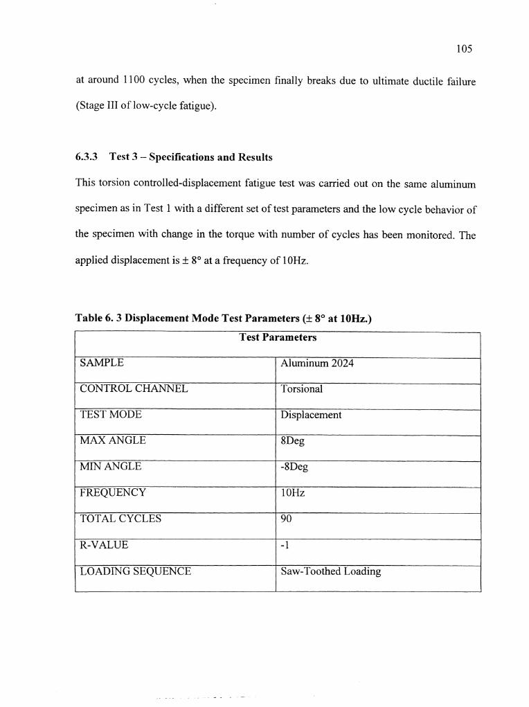
at around 1 1 00 cycles, when the specimen finally breaks due to ultimate ductile failure

(Stage 111 of low-cycle fatigue).

6.3.3 Test 3 - Specifications and Results

This torsion controlled-displacement fatigue test was carried out on the same aluminum

specimen as in Test 1 with a different set of test parameters and the low cycle behavior of

the specimen with change in the torque with number of cycles has been monitored. The

applied displacement is + 8" at a frequency of 10Hz.

Table 6 . 3 Displacement Mode Test Parameters (+ 8" at 10Hz.)

Test Parameters

SAMPLE

CONTROL CHANNEL

TEST MODE

MAX ANGLE

MIN ANGLE

FREQUENCY

TOTAL CYCLES

Aluminum 2024

Torsional

Displacement

8Deg

-8Deg

1 OHz

90

R-VALUE -11 LOADING SEQUENCE Saw-Toothed Loading

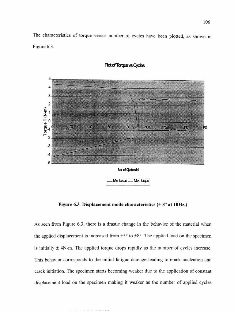
The characteristics of torque versus number of cycles have been plotted, as shown in

Figure 6.3.

Figure 6.3 Displacement mode characteristics (rt 8' at 10Hz.)

As seen from Figure 6.3, there is a drastic change in the behavior of the material when

the applied displacement is increased from +5" to t-8". The applied load on the specimen

is initially ? 4N-m. The applied torque drops rapidly as the number of cycles increase.

This behavior corresponds to the initial fatigue damage leading to crack nucleation and

crack initiation. The specimen starts becoming weaker due to the application of constant

displacement load on the specimen making it weaker as the number of applied cycles

increase. The applied load starts to decrease drastically (Stage I1 of low cycle fatigue) and

drops to zero at around 90 cycles, when the specimen finally breaks due to ultimate

ductile failure (Stage 111 of low cycle fatigue).

6.3.4 Test 4 - Specifications and Results

This high-cycle torsion fatigue test in displacement mode was carried out on the same

aluminum specimen (Aluminum 2024) with a different set of test parameters and the

high-cycle behavior of the specimen with change in the torque with number of cycles has

been monitored. The applied displacement in this case is + 3" at a frequency of 20Hz.

Table 6. 4 Displacement Mode Test Parameters (+ 3" at 20Hz.)

Test Parameters

SAMPLE

CONTROL CHANNEL

Aluminum 2024

Torsional

TEST MODE Displacement

MAX ANGLE 3Deg

MIN ANGLE

FREQUENCY

-3Deg

2 0Hz

I

TOTAL CYCLES

R-VALUE

LOADING SEQUENCE

14500

- 1

Saw-Toothed Loading

The characteristics of torque versus number of cycles have been plotted, as shown in

Figure 6.4.

Plot of Torque vs Cycles

No. of Cycles N

Figure 6 . 4 Displacement mode characteristics (+ 3" at 20Hz.)

As seen from Figure 6.4, there is a drastic change in the behavior of the material when

the applied displacement is decreased to +3O. The applied load on the specimen is

initially + 1.2N-m. The applied torque remains steady as the number of cycles increases.

This behavior corresponds to the initial fatigue damage leading to crack nucleation and

crack initiation. This sort of behavior is observed for approximately 8000 cycles before

there is any significant change in the applied torque as the number of cycles increases.

The specimen starts becoming weaker due to the application of constant displacement

load on the specimen making it weaker as the number of applied cycles increase. The

applied load starts to decrease drastically (Stage I1 of low cycle fatigue) and drops to zero

at around 14,000 cycles, when the specimeil finally breaks due to ultimate ductile failure

(Stage 111 of low cycle fatigue).

It is also observed that any tests carried out on the aluminum 2024 specimen in

displacement mode with < f 3 O results in a significant increase in the number of cycles to

failure (>30,000 cycles), at which point the test enters the high-cycle fatigue region and

approaches the limit of infinite number of cycles before failure occurs (also known as the

fatigue limit).

6.4 Torque Mode

In this mode, the specimen is subjected to a constant cyclic torque over a period of time

and the behavior of the material is studied at different frequencies and different stress

ratios (R-value). A low-cycle torsion fatigue test in torque mode for aluminum 2024

samples were carried out on the "Torsion Fatigue System", and the observations have

been analyzed and are presented below.

6.4.1 Test 1 - Specifications and Results

A torsion fatigue test in torque mode was carried out on an aluminum specimen. The

specimen was subjected to a saw-toothed loading sequence with an overall torque of

4Nm (+ 2Nm) at a frequency of 20 Hz.

Table 6 .5 Torque Mode Test Parameters (+_ 2Nm at 20Hz.)

( Test Parameters

SAMPLE Aluminum 2024

CONTROL CHANNEL Torsional

I

TEST MODE

MAX TORQUE

Torque

2N-m

MIN TORQUE -2N-m

FREQUENCY 20Hz

TOTAL CYCLES 9800

R-VALUE

The behavior of the specimen was monitored over time, and the characteristics of angular

displacement versus number of cycles is plotted in Figure 6.5.

- 1

LOADING SEQUENCE Saw-Toothed Loading

Mot of Displacement vs Cycles

No. of Cycles N

Figure 6.5 Torque mode test parameters (+ 2Nm at 20Hz)

As seen in the figure, the amount of initial angular displacement shown by the specimen

is approximately f O.SO, which remains constant for 8500 cycles. This behavior

corresponds to the initial fatigue damage leading to crack nucleation and crack initiation,

which includes the early development of fatigue damage (crack initiation) and leads to

slip-band crack growth involving the deepening of the initial crack on the planes of high

torsional shear stress. The specimen starts becoming weaker due to the application of

constant torque load and increase in the number of applied cycles. For the same applied

torque, the applied displacement starts to increase drastically (due to the crack growth on

planes of high tensile stress-Stage I1 of low cycle fatigue), as seen in the figure, and

grows to infinity at around 98000 cycles, when the specimen finally breaks due to

ultimate ductile failure (Stage 111 of low cycle fatigue). This occurs when the crack

reaches sufficient length so that. the remaining cross section cannot support the applied

load. It can be seen that a larger proportion of the total cycles to failure is spent with the

propagation in Stage I1 in low-cycle fatigue test.

6.4.2 Test 2 - Specifications and Results

A torsion fatigue test in torque mode was carried out on an aluminum specimen. The

specimen was subjected to a saw-toothed loading sequence with an overall torque of

6Nm (+ 4Nm & -2Nm) at a frequency of 20 Hz.

Table 6 .6 Torque Mode Test Parameters (+4Nm & -2Nm at 20Hz.) 0 Test Parameters

SAMPLE Aluminum 2024

CONTROL CHANNEL

MAX TORQUE

MIN TORQUE

Torsional

TEST MODE Torque

FREQUENCY 20Hz

TOTAL CYCLES 4800

The behavior of the specimen was monitored over time and the characteristics of angular

displacement versus number of cycles is plotted in Figure 6.6.

Figure 6.6 Torque mode test parameters (+4Nm & -2Nm at 20Hz)

As seen from Figure 6.6, there is a significant change in the behavior of the material

when the applied torque is changed to a maximum torque of +4Nm and a minimum

torque of -2Nm at a frequency of 20Hz. The initial angular displacement of the specimen

is initially +1.6" and -0.8". The overall displacement remains relatively constant for 4800

cycles. This behavior corresponds to the initial fatigue damage leading to crack

nucleation and crack initiation. The specimen starts becoming weaker due to the

application of constant torque load and increase in the number of applied cycles. The

angular displacement of the specimen increases drastically, as seen in Figure 6.6, and

drops to zero at around 4900 cycles, when the specimen finally breaks due to ultimate

ductile failure (Stage I11 of low cycle fatigue).

6.4.3 Test 3 - Specifications and Results

This torsion fatigue test in displacement was carried out on the same aluminum specimen

as in Test 1 with a different set of test parameters and the low-cycle behavior of the

specimen with change in the torque with number of cycles has been monitored. The

applied displacement is f 8" at a frequency of 10Hz.

Table 6.7 Torque Mode Test Parameters (& 2.5Nm at 20Hz.)

Test Parameters

SAMPLE

CONTROL CHANNEL

TEST MODE

MAX TORQUE

MIN TORQUE

FREQUENCY

TOTAL CYCLES

R-VALUE

LOADING SEQUENCE

Aluminum 2024

Torsional

Torque

2.5N-m

-2.5N-m

20Hz

670

- 1

Saw-Toothed Loading

The behavior of the specimen was monitored over time and the characteristics of angular

displacement versus number of cycles is plotted in Figure 6.7.

Figure 6.7 Torque mode test parameters (-t 2.5Nm at 20Hz)

As seen from Figure 6.7, there is a drastic change in the behavior of the material when

the applied torque is increased to f2.5Nm. The displacement on the specimen is initially

f lo. The angular displacement of the specimen increases rapidly as the number of

cycles increases. This behavior corresponds to the initial fatigue damage leading to crack

nucleation and crack initiation. The specimen starts becoming weaker due to the

application of constant torque load and increase in the number of applied cycles. The

angular displacement starts to increase drastically (Stage I1 of low cycle fatigue) and

shoots to infinity at around 680 cycles, when the specimen finally breaks due to ultimate

ductile failure (Stage I11 of low cycle fatigue).

6.4.4 Test 4 - Specifications and Results

This low-cycle torsion fatigue test in torque mode was carried out on the same aluminum

specimen (Aluminum 2024) with a different set of test parameters. The fatigue behavior

of the specimen was monitored with change in the angular displacement with number of

cycles. The applied torque in this case is + 3Nm at a frequency of 20Hz.

Table 6. 8 Torque Mode Test Parameters (+ 3Nm at 20Hz.)

Test Parameters

SAMPLE Aluminum 2024

CONTROL CHANNEL Torsional

TEST MODE

MAX TORQUE

MIN TORQUE

FREQUENCY

Torque

3N-m

-3N-m

20Hz

TOTAL CYCLES

R-VALUE

LOADING SEQUENCE

475

- 1

Saw-Toothed Loading

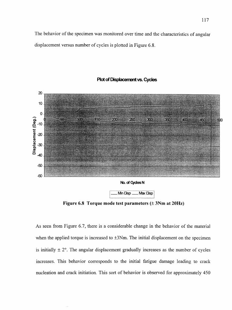
The behavior of the specimen was monitored over time and the characteristics of angular

displacement versus number of cycles is plotted in Figure 6.8.

Plot of Dlsplacementvs. Cydes

Figure 6.8 Torque mode test parameters (+ 3Nm at 20Hz)

As seen from Figure 6.7, there is a considerable change in the behavior of the material

when the applied torque is increased to k3Nm. The initial displacement on the specimen

is initially + 2". The angular displacement gradually increases as the number of cycles

increases. This behavior corresponds to the initial fatigue damage leading to crack

nucleation and crack initiation. This sort of behavior is observed for approximately 450

cycles before there is any significant change in the angular displacement as the number

of cycles increase. The specimen starts becoming weaker due to the application of

constant torque load and increase in the number of applied cycles. The angular

displacement increases drastically at around 480 cycles, and shoots to infinity when the

specimen finally breaks due to ultimate ductile failure (Stage I11 of low-cycle fatigue).

It is also observed that any tests carried out on the aluminum 2024 specimen in torque

mode with > +_ 3Nm results in a significant decrease in the number of cycles to failure

(GO cycles). When the applied torque is reduced to less than 1.5Nm, the number of

cycles to failure increases significantly (>15,000 cycles), at which point the test enters the

high-cycle fatigue region and approaches the limit of infinite number of cycles before

failure occurs (also known as the fatigue limit).

6.5 Testing Results

Torsion fatigue tests carried out in torque mode and displacement mode on the aluminum

specimens using the fatigue testing machine and the associated software have shown

remarkably impressive results, as shown above. Tests have been conducted in various

modes and under varying test parameters. The data obtained from these tests is on a real-

time basis and is automatically recorded and plotted using the testing software developed

for the user to see and analyze the behavior of the test specimen.

In many applications, materials are subjected to vibrating or oscillating forces. The

behavior of materials in such applications requires the application of cyclic loading in a

laboratory test to determine how a material will behave under repeated cycles of loading

and unloading. Because the material is subjected to repeated load cycles in actual use,

designers are faced with predicting material life, which is defined as total number of

cycles to failure under specified loading conditions. This is plotted on a stress versus

number of cycles (or S-N) curve. The frequency of loading, type of loading sequence,

applied torque and applied displacement, and R-value and are some of the parameters that

effect the material behavior, as shown in the above conducted experiments in

displacement mode and torque mode. The dynamic behavior of the materials can be

accurately determined using the Torsion Fatigue System with a great deal of accuracy.

This fatigue testing gives much data to predict in-service life of materials.

Chapter: 7 Conclusion and Future Work

7.1 Conclusion

Considering the fact that many structures and vital machine components are subjected to

fluctuating loads, the need to develop new fatigue testing machines has gained a high

importance. The torsion fatigue testing system has been developed at Ohio University

against this backdrop to resolve many questions across a wide spectrum of materials

applications. The main objective of this thesis was to configure the existing fatigue

testing system and to design a graphic user interface (GUI) based testing software to

carryout high and low cycle fatigue tests.

There is a wide combination of tests possible on this system using the testing software

developed. The Fatigue Testing Software is developed for this machine on a Windows

platform using Visual Basic 5.0. It is robust enough to perform high- and low-cycle

torsion fatigue tests in both torque-controlled mode and displacement-controlled mode by

providing a user the convenience of choosing test parameters, such as frequency, angular

displacement, torque, R-value, loading sequence, and number of cycles. The flexibility is

virtually unlimited, and almost any combination of tests with complex stress functions

can be programmed into the system. The operator interface is kept to a bare minimum,

and this can be further enhanced in the future. To the best of the author's knowledge,

there is no other similar system currently available on the market.

Future Work

Knowledge of fatigue and fracture resistance of materials requires extensive analysis and

testing. Because of the increasing demands for material testing requirements and the need

for a more precise and accurate study of fatigue behavior of materials in various loading

modes, there is a need for further development of the existing system in the future. The

machine can be developed to incorporate additional functionality for carrying out a bi-

axial fatigue testing (simultaneous torsion and tension).

There is also a growing need to study the fatigue behavior of materials at high

temperatures. An environmental chamber can be built to encase the specimen that could

be subjected to elevated temperatures during fatigue testing. The system software can

also be enhanced to incorporate subroutine definitions, contouring, mathematical

functions, etc.

Finally, additional functionality, such as simulating service loading sequences, user

defined tests, and multi-channel control, can be developed in the future to enhance the

performance of the existing fatigue testing system.

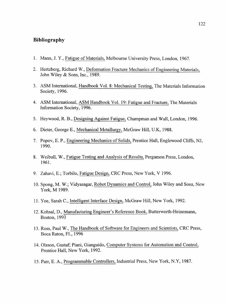
Bibliography

1. Mann, J. Y., Fatigue of Materials, Melbourne University Press, London, 1967.

2. Hertzberg, Richard W., Deformation Fracture Mechanics of Engineering Materials, John Wiley & Sons, Inc., 1989.

3. ASM International, Handbook Vol. 8: Mechanical Testing, The Materials Information Society, 1996.

4. ASM International, ASM Handbook Vol. 19: Fatigue and Fracture, The Materials Information Society, 1996.

5. Heywood, R. B., Designing Against Fatigue, Champman and Wall, London, 1996.

6. Dieter, George E., Mechanical Metallurgy, McGraw Hill, U.K, 1988.

7. Popov, E. P., Engineering Mechanics of Solids, Prentice Hall, Englewood Cliffs, NJ, 1990.

8. Weibull, W., Fatigue Testing and Analysis of Results, Pergamon Press, London, 1961.

9. Zahavi, E.; Torbilo, Fatigue Design, CRC Press, New York, V 1996.

10. Spong, M. W.; Vidyasagar, Robot Dynamics and Control, John Wiley and Sons, New York, M 1989.

1 I . Yoe, Sarah C., Intelligent Interface Design, McGraw Hill, New York, 1992.

12. Kohsal, D., Manufacturing Engineer's Reference Book, Butterworth-Heinemann, Boston, 1993

13. Ross, Paul W., The Handbook of Software for Engineers and Scientists, CRC Press, Boca Raton, FL, 1996

14. Olsson, Gustaf; Piani, Gianguido, Computer Systems for Automation and Control, Prentice Hall, New York, 1992.

15. Parr, E. A., Programmable Controllers, Industrial Press, New York, N.Y, 1987.

16. Putmann, Byron W., RS-232 Simplified, Englewood Cliffs, NJ: Prentice-Hall, 1987

17. Compumotor, Step Motor and Servo Motor Systems and Controls, Parker Automation, Rohnert Park, CA, 1999.

Appendix A: APEX Series Drives - Specifications for the APEX drives used in the fatigue testing system (171.

Catalog 8000-2fUSA APEX Serie: Drives and

parameter Description Drive/Con troller Performance

Repeatability i 5 arcmin R d e r Accuracy f 22 arcmin Resolution 4096 post quadrature counts

Output Power APEX1 0 APEX20 APEX40 Voltage 170 or 340VDC (nominal); 340VDC (nominal); 340VDC (minai);

42oVDC (max) 4 2 0 m (max) 420VDC (max) Frequency C-400 Hz fundamental 04CO Hz fundamental 0-400 Hz fundamental

(1 5 kHz FWM) (8 kHz FWM) (8 H z PWM) Current (ma% continuous) 8A continuous/phase 12A continwusJphase 20A continuous/phase

sinusoidal (5.65A rms); sinusoidal (8.5A rms); sinusoidal (1 4.14A rms): 16A peak per phase 24A peak per phase 40A peak per phase sinusoidal(11.3A rms) sinusoidal(17.OA rms) sinusoidal (28.3A rms)

Input Power - APEX1 0 APEX20 APW40 Motor Supply Voltage 120-240VAC (1 -phase) 205-252VAC (1 - or 3-phase) 205-252VAC (1 - or 3-phase)

Frequency Range 47-66 Hz 47-66 Hz 47-66 Hz Current (max continuous) 14A (rms) 8 1 2OVAC single phase; 8A (rms) 3-phase 15A (rrns) 3-phase

10A (rms) 8 240VAC single phase Power (max continuous) 2.4 KVA 3.3 KVA 6.2 KVA Fuses No internal fuses. Recommend external fuse. Isolation Transformer Not required Not required Not required

Logic Supply Voltage 85-252 (1 -phase) 85-252 (1 -phase) 85-252 (1-phase) Frequency Range 47-66 Hz 47-66 Hz 47-66 H i Cunent (max continuous) 1 .OA 1 .OA 1 .OA Power (max continuous) 0.08 KVA 0.08 KVA 0.08 KVA Fuses 3.OA 250VAC internal fuse. Not user replaceable. Isolation Transformer Not required Not required Not required

Protection Short Circuit Brownout Overvoltage Overtemperature IT

Phase-to-phase, phase-to-earth Below 1 OOVAC 385VDC (provls~on for power dump) Motor 170°C (330"FJ: drtve 65°C (149"R Current foldback (motor dependent)

Inputs Command i 10V differential (velocity or torque) Enable Logic high -amplifier disabled;

Logic low - amplifier enabled Reset. Vel. Int. Enabie TTL compatible

Outputs i15V Reference Encoder Fault Tach out

15 mA available CHA. CHB, CHZ. Differential, opttcally ~solated. Max~murn frequency - 300 kHz Open collector 5-24V Nominal 1 Vl l kRPM

- ~

Physical Connectjons

Drive-to-Servo Controller 13-pin removable for control; 7 pin removable for encoder Drive-to-Motor &pin high power removable connector Resolver-to-Drive 13-pin removable Power ?-pin high power removable connector

Environment Drive Temp 32"-1 2Z°F (0"-50°C) Maximum Heat Sink Temp 182°F (75'C) Motor Temp 32"-104OF (OP40"C) Maximum Motor Case Temp 257°F (1 25%) Humidity 0-95% non-condensing Storage 4 0 - 1 85'F

Tuning Torque Mode Oftset balance Vekxity Mode Offset balance, collective gain, velocity integral gain

Diagnostics Test Points Torque Cmd, velocity enor LEDs Enable, Bridge Fault. Drive Faun, Motor Faun, Overvoltage, IT Limit. Regen Faun, ~egen Active

Appendix B: 6250 Servo Controller - Specifications [17]

Specifications Parameter Value

Power Input 100-120/200-240VAC, 50-60 Hz, or 110-340VDC

Servo Performance Processor Servo update Encoder

Position Velocity Acceleration

32-bit CPU/24 bit DSP As fast as 205 p e c per axis, user selectable Two phase quadrature incremental encoders with differential (recommended) or'single ended outputs (+5VDC 'm compatible). Max frequency = 1.2 MHz, post-quadrature. Minimum time between transitions = 833 ns. Optically isolated *2,147,483,648 encoder counts 1 to 1,200,000 encoder countdsec. 1 to 50,000,000 encoder counts/sec2

-- - - - -- -

Inputs 24 Programmable Plug compatible with OPTO-221M signal conditioning equipment (50 pin DIN header). TTL

compatible, voltage range 0-24VDC. 2 interrupt TTL compatible, voltage range 0-24VDC. 3 Analog Voltage range 0-2.5VDC, 8-bit N D converter. Enable Hardware analog command output enable. TTL compatible, voltage range 0-24VDC. Home; Pos and Neg lTL compatible, voltage range 0-24VDC. Limits: Drive Fault; Trigger; Release: Axis Select, & Velocity Select

Outputs 24 Programmable Plug compatible with OPTO-221M signal conditioning equipment (50 pin DIN header). Open

collector output will sink up to 30 mA, and allow up to 24VDC. 2 Auxiliary Open collector output will sink up to 30 mA, and allow up to 24VDC. Command signal i10V Analog output. 12 bi resolution DAC. Enable drive Relay output will sink up to 30 mA and allow up to 24VDC. (Normally open and normally closed

available)

Dimensions (-) denotes millimeters

Appendix C: APEX Motor - Specifications [17]

Detail

APEX Motor Only Technical Data

Continuous Stall Torque Ib-in @ 40" ambient oz-in

Nm

Peak Torque Ib-in oz-in Nm

APEX602 APEX603

13.9 21.6 222 346 1.57 2.44

39.4 65.4 630 1,046

k Watts

Rated Speed rPm

APEX604 APEX605 APEX606 - 20 22 40

31 5 346 634 2.22 2.44 4.48

56 68 122 899 1,085 1.957

4.45 7.38

rPs

6.35 7.66 13.82

Rated Power hp 1.12 1 .O

7,500 3,800

- - -. . 1.5 1.5 1.6

7,500 6,200 3.600 125 63

18.0 16.6 17.2

4.18 5.43 9.44 0.01 0.01 0.02 76.5 99.6 172.9

8.5 10.0 13.4

. . ,

kg

Recommended APEX Drive

1.5 1.3

125 103 60

Rated Current A ( n s )

Peak Current A (ns)

Rotor Inertia oz-in2 (mass) oz-in-sec2 kg m2x 10"

Motor Weight Ibs

2.0 2.0 7 1

12.6 9.6

2.52 4.02 0.006 0.01 46.1 99.6

7.0 9.0 3.2 4.1

APEX1 0 or APEX61 51

4.2 3.0

3.9 4.5 6.1

APEX20 or APEX61 52

6 .O 5 5-73

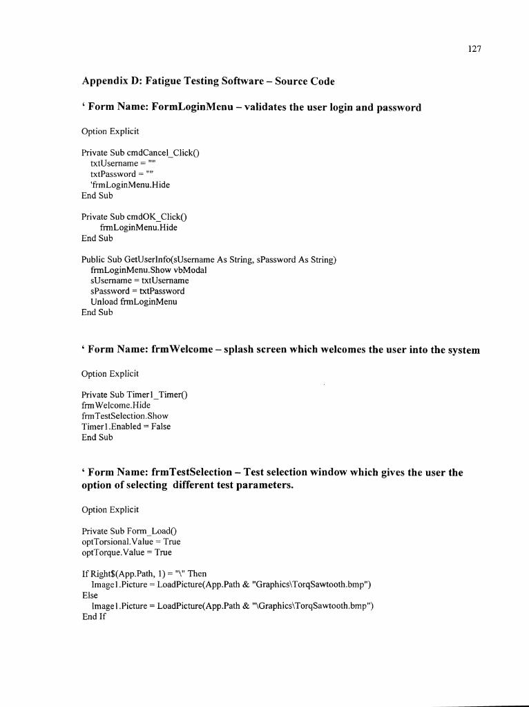
Appendix D: Fatigue Testing Software - Source Code

' Form Name: PormLoginMenu -validates the user login and password

Option Explicit

Private Sub cmdcancel-Click() atusername = "" txtPassword = "" 'frmLoginMenu.Hide

End Sub

Private Sub cmdOK-Click() frrnLoginMenu.Hide

End Sub

Public Sub GetUserInfo(sUsername As String, spassword As String) fimLoginMenu.Show vbModal susername = txtusername spassword = txtpassword Unload h L o g i n M e n u

End Sub

' Form Name: frmwelcome - splash screen which welcomes the user into the system

Option Explicit

Private Sub Timer 1-Timer() frm Welcome.Hide frmTestSelection.Show Timer1 .Enabled = False End Sub

' Form Name: frmTestSelection - Test selection window which gives the user the option of selecting different test parameters.

Option Explicit

Private Sub Form-Load() optTorsional.Value = True optTorque.Value = True

If Right$(App.Path, 1) = "\" Then Image1 .Picture = LoadPicture(App.Path & "Graphics\TorqSawtooth.bmp")

Else Image 1 .Picture = LoadPicture(App.Path & "\Graphics\TorqSawtooth.bmp")

End If

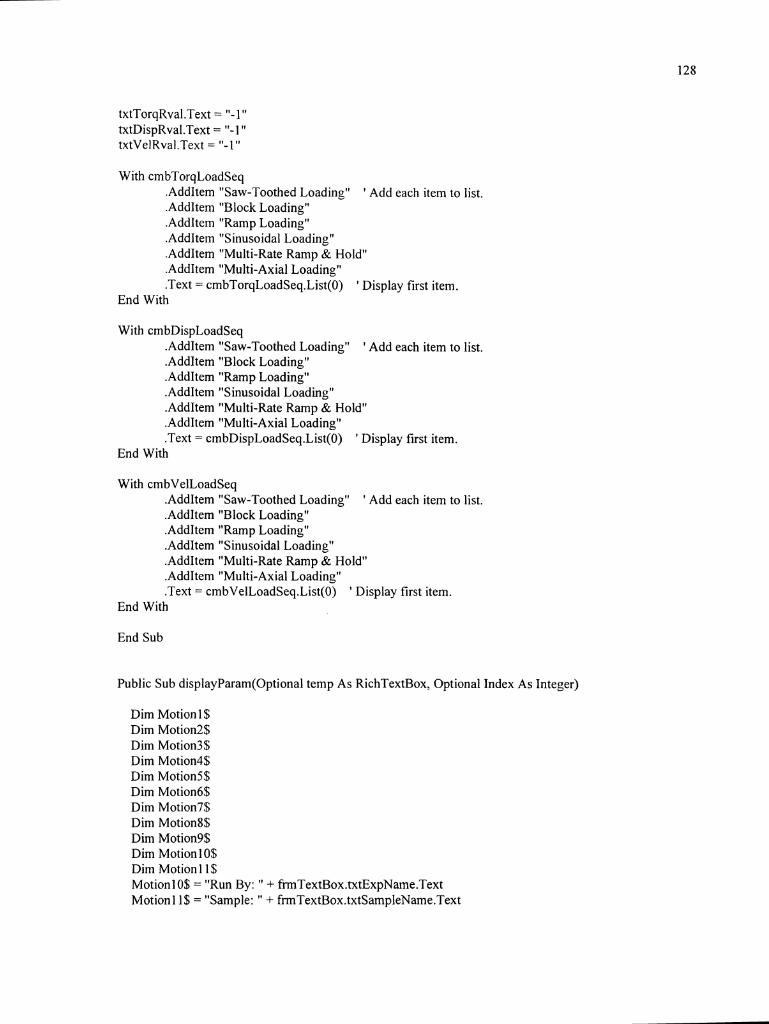
With cmbTorqLoadSeq .AddItem "Saw-Toothed Loading" ' Add each item to list, .Addhem "Block Loading" .AddItem "Ramp Loading" .Addltem "Sinusoidal Loading" .Addltem "Multi-Rate Ramp & Hold" .AddItem "Multi-Axial Loading" .Text = cmbTorqLoadSeq.List(0) ' Display first item.

End With

With cmbDispLoadSeq .AddItem "Saw-Toothed Loading" ' Add each item to list. .AddItem "Block Loading" .AddItem "Ramp Loading" .AddItem "Sinusoidal Loading" .AddItem "Multi-Rate Ramp & Hold" .AddItem "Multi-Axial Loading" .Text = cmbDispLoadSeq.List(0) ' Display first item.

End With

With cmbVelLoadSeq .AddItem "Saw-Toothed Loading" ' Add each item to list. .AddItem "Block Loading" .AddItem "Ramp Loading" .AddItem "Sinusoidal Loading" .AddItem "Multi-Rate Ramp & Hold" .AddItem "Multi-Axial Loading" .Text = cmbVelLoadSeq.List(0) ' Display first item.

End With

End Sub

Public Sub displayParam(Optiona1 temp As RichTextBox, Optional Index As Integer)

Dim Motionl $ Dim Motion2$ Dim Motion3$ Dim Motion4$ Dim Motions$ Dim Motion6$ Dim Motion7$ Dim Motions$ Dim Motion9$ Dim Motion 1 O$ Dim Motion 11 $ Motionlo$ = "Run By: " + f?mTextBox.txtExpName.Text Motionl I$ = "Sample: " + fm'~extBox.txtSamp1eName.Text

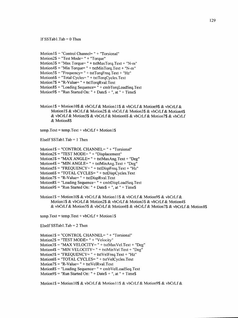
If SSTab1 .Tab = 0 Then

Motionl$ = "Control Channel= " + "Torsional" Motion2$ = "Test Mode= " + "Torque" Motion3$ = "Max Torque= " + txtMaxTorq.Text + "N-m" Motion4$ = "Min Torque= " + txtMinTorq.Text + "N-m" MotionS$ = "Frequency= " + txtTorqFreq.Text + "Hz" Motion6$ = "Total Cycles= " + txtTorqCycles.Text Motion7$ = "R-Value= " + txtTorqRval.Text Motions$ = "Loading Sequence= " + cmbTorqLoadSeq.Text Motion9$ = "Run Started On: " + Date$ + ", at " + Time$

Motion1 $ = Motionl O$ & vbCrLf & Motionl 1 $ & vbCrLf & Motion9$ & vbCrLf & Motionl$ & vbCrLf & Motion2$ & vbCrLf & Motion3$ & vbCrLf & Motion4$ & vbCrLf & Motion5$ & vbCrLf & Motion6$ & vbCrLf & Motion7$ & vbCrLf & Motions$

temp.Text = temp.Text + vbCrLf + Motion 1 $

ElseIf SSTabl .Tab = 1 Then

Motionl$ = "CONTROL CHANNEL= " + "Torsional" Motion2$ = "TEST MODE= " + "Displacement" Motion3$ = "MAX ANGLE= " + txtMaxAng.Text + "Deg" Motion4$ = "MIN ANGLE= " + txtMinAng.Text + "Deg" MotionS$ = "FREQUENCY= " + txtDispFreq.Text + "Hz" Motion6$ = "TOTAL CYCLES= " + txtDispCycles.Text Motion7$ = "R-Value= " + txtDispRval.Text Motion8$ = "Loading Sequence= " + cmbDispLoadSeq.Text Motion9$ = "Run Started On: " + Date$ + ", at " + Time$

Motionl $ = Motion 10$ & vbCrLf & Motion 1 1 $ & vbCrLf & Motion9$ & vbCrLf & Motionl$ & vbCrLf & Motion2$ & vbCrLf & Motion3$ & vbCrLf & Motion4$ & vbCrLf & MotionS$ & vbCrLf & Motion6$ & vbCrLf & Motion7$ & vbCrLf & Motion8$

temp.Text = temp.Text + vbCrLf + Motion1 $

ElseIf SSTab1 .Tab = 2 Then

Motionl$ = "CONTROL CHANNEL= " + "Torsional" Motion2$ = "TEST MODE= " + "Velocity" Motion3$ = "MAX VELOCITY= " + txtMaxVel.Text + "Deg" Motion4$ = "MIN VELOCITY= " + txtMinVel.Text + "Deg" MotionS$ = "FREQUENCY= " + txtVelFreq.Text + "Hz" Motion6$ = "TOTAL CYCLES= " + txtVelCycles.Text Motion7$ = "R-Value= " + txtVelRval.Text Motion8$ = "Loading Sequence= " + cmbVelLoadSeq.Text Motion9$ = "Run Started On: " + Date$ + ", at " + Time$

Motion1 $ = Motion 10$ & vbCrLf & Motion 1 1 $ & vbCrLf & Motion9$ & vbCrLf &

Motionl$ & & vbCrLf & & Motions$

vbCrLf & Motion2$ & vbCrLf & Motion3$ & vbCrLf & Motion4$ Motion5$ & vbCrLf & Motion6$ & vbCrLf & Motion7$ & vbCrLf

temp.Text = temp.Text + vbCrLf + Motion1 $

End If

' parameter to be passed to the rich text box for display in the test running forms par = temp.Text

End Sub

Sub cmdcontinue-Click0

If SSTab 1 .Tab = 0 Then TabIndex = Val(SSTab1 .Tab) Load frmMainTorque

' Call displayParam(fimMainTorque.rtffext, 1) frmMainTorque.Show frmTestSelection.Hide

Elself SSTab 1 .Tab = 1 Then TabIndex = Val(SSTab 1 .Tab) Load fimMainDisplacement

' Call displayParam(f?mMainDisplacement.rtffext, 1) frmMainDisplacement Show frmTestSelection.Hide

Elself SSTab 1 .Tab = 2 Then TabIndex = Val(SSTab1 .Tab) Load fimMainVelocity

' Call displayParam(frmMainVelocity.rtffext, I ) fhMainVelocity.Show frmTestSelection.Hide

End If

End Sub

Private Sub cmdExit-Click() End End Sub

Private Sub cmdHelp-Click() Load fimHelp frmHelp.Show End Sub

Private Sub cmdSave-Click() Call textpad End Sub

Private Sub mnuAbout-Click(1ndex As Integer) Load frmAbout frrnAbout.Show End Sub

Private Sub mnuMotionArc-Click(1ndex As Integer) Dim RetVal RetVal = Shell("C:\Ma6000\Ma6000.EXE", 1) ' Run Motion Architect End Sub

Private Sub mnuMTS-Click(1ndex As Integer) Dim RetVal RetVal = Shell("C:\Program Files\Netscape\Navigator\Program\NETSCAPE.EXE -h http:l/www.mts.com", 1) ' Run Netscape. End Sub

Private Sub mnuParker-Click(1ndex As Integer) Dim RetVal RetVal = Shell("C:\Program Files\Netscape\Communicator\Program\NETSCAPE.EXE -h http://www.parker.com", 1) ' Run Netscape. End Sub

Private Sub mnuSave-Click(1ndex As Integer) Load fimInfo frm1nfo.Show End Sub

Private Sub mnuTorsion-Click(1ndex As Integer) optTorsional.Value = True End Sub

Private Sub optTorque-Click() SSTab1 .Tab = 0 Image1 .Picture = LoadPicture(App.Path & "\Graphics\TorqSawtooth.bmp") txtTorqRval.Text = "-1 " End Sub

Private Sub optDisplacement-Click() SSTab 1 .Tab = 1 Image1 .Picture = LoadPicture(App.Path & "\Graphics\DispSawtooth.bmp") txtDispRval.Text = "-1 " End Sub

Private Sub optvelocity-Click() SSTab 1 .Tab = 2 Image1 .Picture = LoadPicture(App.Path & "\Graphics\VelSawtooth.bmp")

txtVelRval.Text = "-1" End Sub

Private Sub udDispCycles-Downclick() txtDispCycles.Text = str$(Val(txtDispCycles.Text) - 100)

If Val(txtDispCycles.Text) < 0 Then txtDispCycles.Text = 0 MsgBox "No Of Cycles Cannot Be Less Than OM, vbInformation

End If txtDispCycles.Refresh End Sub

Private Sub udDispCycles-Upclick() txtDispCycles.Text = str$(Val(txtDispCycles.Text) + 100)

'If Val(txtTorqCyc1es.Text) > 50 Then 'txtTorqCycles.Text = 50

'End If If Val(txtDispCycles.Text) < 0 Then

txtDispCycles.Text = 0 MsgBox "No Of Cycles Cannot Be Less Than ON, vblnformation

End If txtDispCycles.Refresh End Sub

Private Sub udDispFreqDownClick() txtDispFreq.Text = str$(Val(txtDispFreq.Text) - 0.5)

If Val(txtDispFreq.Text) < 0 Then txtDispFreq.Text = 0 MsgBox "Frequency Cant Be Less Than OH, vblnformation

End If txtDispFreq.Refresh End Sub

Private Sub udDispFreq_UpClick() txtDispFreq.Text = str$(Val(txtDispFreq.Text) + 0.5)

If Val(txtDispFreq.Text) >= 50 Then txtDispFreq.Text = 50

End If If Val(txtDispFreq.Text) < 0 Then

txtDispFreq.Text = 0 MsgBox "Frequency Cant Be Less Than ON, vblnformation

End If txtDispFreq.Refresh End Sub

Private Sub udDispRval-Downclick() txtDispRval.Text = str$(Val(txtDispRval.Text) - 0.1)

txtDispRval.Refresh End Sub

Private Sub udDispRva1-Upclick()

txtDispRva1,Refresh End Sub

Private Sub udMaxAng-Downclick() txtMaxAng.Text = str$(Val(txtMaxAng.Text) - 0.5)

If Val(txtMaxAng.Text) <= -360 Then txtMaxAng.Text = 0

End If txtMaxAng.Refresh End Sub

Private Sub udMaxAng-Upclick() txtMaxAng.Text = str$(Val(txtMaxAng.Text) + 0.5)

If Val(txtMaxTorq.Text) >= 360 Then txtMaxTorq.Text = 0

End If txtMaxAng.Refresh End Sub

Private Sub udMaxTorq_DownClick() txtMaxTorq.Text = str$(Val(txtMaxTorq.Text) - 0.5)

If Val(txtMaxTorq.Text) < -40 Then txtMaxTorq.Text = -40

End If txtMaxTorq.Reffesh End Sub

Private Sub udMaxTorpUpClick() txtMaxTorq.Text = str$(Val(txtMaxTorq.Text) + 0.5)

If Val(txtMaxTorq.Text) > 40 Then txtMaxTorq.Text = 40

End If txtMaxTorq.Refresh End Sub

Private Sub udMaxVel-Downclick() txtMaxVel.Text = str$(Val(txtMaxVel.Text) - 0.1)

If Val(txtMaxVel.Text) < -40 Then txtMaxVel.Text = -40

End If txtMaxVel.Refresh End Sub

Private Sub udMaxVe1-Upclick() txtMaxVe1.Text = str$(Val(txtMaxVel.Text) + 0.1)

If Val(txtMaxVel.Text) >= 40 'Then txtMaxVel.Text = 40

End If txtMaxVel.Refresh End Sub

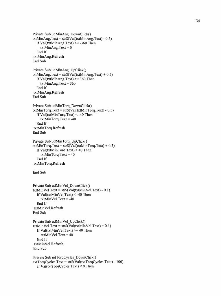
Private Sub udMinAngDownClick() txtMinAng.Text = str$(Val(txtMinAng.Text) - 0.5)

If Val(txtMinAng.Text) <= -360 Then txtMinAng.Text = 0

End If txtMinAng.Refresh End Sub

Private Sub udMinAng-Upclick() txtMinAng.Text = str$(Val(txtMinAng.Text) + 0.5)

If Val(txtMinAng.Text) >= 360 Then txtMinAng.Text = 360

End If txtMinAng.Refresh End Sub

Private Sub udMinTorqDownClick() txtMinTorq.Text = str$(Val(txtMinTorq.Text) - 0.5)

If Val(txtMinTorq.Text) < -40 Then txtMinTorq.Text = -40

End If txtMinTorq.Refresh End Sub

Private Sub udMinTorq_UpClick() txtMinTorq.Text = str$(Val(txtMinTorq.Text) + 0.5)

If Val(txtMinTorq.Text) > 40 'Then txtMinTorq.Text = 40

End If txtMinTorq.Refresh

End Sub

Private Sub udMinVel-Downclick() txtMinVel.Text = str$(Val(txtMinVel.Text) - 0.1)

If Val(txtMinVel.Text) < -40 Then txtMinVel.Text = -40

End If txtMinVel.Refresh End Sub

Private Sub udMinVel-Upclick() txtMinVel.Text = str$(Val(txtMinVel.Text) + 0.1)

If Val(txtMinVel.Text) >= 40 Then txtMinVel.Text = 40

End If txtMinVel.Refresh End Sub

Private Sub udTorqCycles-Downclick() txtTorqCycles.Text = str$(Val(txtTorqCycles.Text) - 100)

If Val(txtTorqCycles.Text) < 0 Then

txtTorqCycles.Text = 0 MsgBox "No Of Cycles Cannot Be Less Than 0", vblnfonnation

End If txtTorqCycles.Refresh End Sub

Private Sub udTorqCycles-UpC:lick() txtTorqCycles.Text = str$(Val(txtTorqCycles.Text) + 100)

'If Val(txtTorqCyc1es.Text) :> 50 Then 'txtTorqCycles.Text = 50

'End If If Val(txtTorqCycles.Text) < 0 Then

txtTorqCycles.Text = 0 MsgBox "No Of Cycles Cannot Be Less Than OM, vbInformation

End If txtTorqCycles.Refresh End Sub

Private Sub udTorqFreq_DownClick() txtTorqFreq.Text = str$(Val(txtTorqFreq.Text) - 0.5)

If Val(txtTorqFreq.Text) < 0 Then txtTorqFreq.Text = 0 MsgBox "Frequency Should be greater Than Ow, vbInformation

End If txtTorqFreq.Refresh End Sub

Private Sub udTorqFreq_UpClick() txtTorqFreq.Text = str$(Val(txtTorqFreq.Text) + 0.5)

If Val(txtMinTorq.Text) > 50 Then txtMinTorq.Text = 50

End If If Val(txtTorqFreq.Text) < 0 Then

txtTorqFreq.Text = 0 MsgBox "Frequency Should be greater Than 0", vbInformation

End If txtTorqFreq.Refresh End Sub

Private Sub udVelCycles-DownClick() txtVelCycles.Text = str$(Val(txtVelCycles.Text) - 100)

If Val(txtVelFreq.Text) < 0 Then txtVelFreq.Text = 0 MsgBox "No Of Cycles Should Be Greater Than 0", vblnformation

End If txtVelCycles.Refresh End Sub

Private Sub udVelCycles-Upclick() txtVelCycles.Text = str$(Val(txtVelCycles.Text) + 100)

If Val(txtVelFreq.Text) < 0 Then

txtVelFreq.Text = 0 MsgBox "No Of Cycles Should Be Greater Than 0", vbInformation

End If

txtVelCycles.Refresh End Sub

Private Sub udVelFreq_DownClick() txtVelFreq.Text = str$(Val(txtVelFreq.Text) - 0.5)

If Val(txtVelFreq.Text) < 0 Then txtVelFreq.Text = 0 MsgBox "Frequency Cannot Be Less Than OM, vbInformation

End If txtVelFreq.Refresh

End Sub

Private Sub udVelFreq_UpClick() txtVelFreq.Text = str$(Val(txtVelFreq.Text) + 0.5)

If Val(txtVe1Freq.Text) >= 50 Then txtVelFreq.Text = 50

End If If Val(txtVelFreq.Text) < 0 Then

txtVelFreq.Text = 0 MsgBox "Frequency Cannot Be Less Than Ow, vbInformation

End If txtVelFreq.Refresh End Sub

Private Sub udVelRva1-Downclick() txtVelRval.Text = str$(Val(txtVelRval.Text) - 0.1)

txtVelRval.Refiesh End Sub

Private Sub udVelRval-Upclick() txtVelRval.Text = str$(Val(txtVelRval.Text) + 0.1)

txtVelRva1.Refresh End Sub

Private Sub cmbTorqLoadSeqClick() If txtMaxTorq = "" Or txtMinTorq = "" Or WtTorqFreq = "" Or txtTorqCycles = "" Then Call LoadSeqChange Exit Sub Else Call Loadse lchange txtTorqRval.Text = str$(Val(txtMaxTorq) 1 Val(txtMinT0rq)) txtTorqRval.Refresh End If End Sub

Private Sub cmbDispLoadSeqClick() If txtMaxAng = "" Or txtMinAng = "" Or txtDispFreq = "" Or txtDispCycles = "" Then Call LoadSeGhange Exit Sub Else Call LoadSeq-Change txtDispRval.Text = str$(Val(txtMaxAng) 1 Val(txtMinAng)) txtDispRval.Refiesh End If End Sub

Private Sub cmbVelLoadSe~Click() If txtMaxVel = "" Or txtMinVeI = "" Or txtVelFreq = "" Or txtVelCycles = "" Then Call LoadSeqChange Exit Sub Else Call LoadSeGhange txtVelRval.Text = str$(Val(txtMaxVel) 1 Val(txtMinVe1)) txtVelRval.Refresh End If End Sub

Private Sub Loadselchange()

Dim stab stab = SSTab 1 .Tab

On Error GoTo ErrHandler Select Case stab

Case 0 If cmbTorqLoadSeq.ListIndex = 0 Then Image1 .Picture = LoadPicture(App.Path & "\Graphics\TorqSawtooth.bmp") ElseIf cmbTorqLoadSeq.ListIndex = 1 Then Image1 .Picture = LoadPicture(App.Path & "\Graphics\TorqBlock.bmp") ElseIf cmbTorqLoadSeq.Listlndex = 2 Then Image1 .Picture = LoadPicture(App.Path & "\Graphics\TorqRamp.bmp") ElseIf cmbTorqLoadSeq.List1ndex = 3 Then Image1 .Picture = LoadPicture(App.Path & "\Graphics\TorqSine.bmp") ElseIf cmbTorqLoadSeq.List1ndex = 4 Then Image1 .Picture = LoadPicture(App.Path & "\Graphics\Multi-RateRampHold.bmpM) ElseIf cmbTorqLoadSeq.ListIndex = 5 Then Imagel .Picture = LoadPicture(:App.Path & "\Graphics\Multi-Axial.bmpM) End If

Case 1 If cmbDispLoadSeq.List1ndex = 0 Then Imagel .Picture = LoadPicture(App.Path & "\Graphics\DispSawtooth.bmp") ElseIf cmbDispLoadSeq.ListIndex = 1 Then 1magel.Picture = LoadPicture(App.Path & "\Graphics\DispBlock.bmp") ElseIf cmbDispLoadSeq.ListIndex = 2 Then Image1 .Picture = LoadPicture(App.Path & "\Graphics\DispRamp.bmp")

ElseIf cmbDispLoadSeq.ListIndex = 3 Then Imagel .Picture = LoadPicture(App.Path & "\Graphics\DispSine.bmp") Elself cmbDispLoadSeq.ListIndex = 4 Then Image 1 .Picture = LoadPicture(App.Path & "\Graphics\Multi-RateRampHold.bmpW) ElseIf cmbDispLoadSeq.ListIndex = 5 Then Image1 .Picture = LoadPicture(App.Path & "\Graphics\Multi-Axial.bmpM) End If

Case 2 If cmbVelLoadSeq.ListIndex = 0 Then Image1 .Picture = LoadPicture(App.Path & "\Graphics\VelSawtooth.bmp") ElseIf cmbVelLoadSeq.List1ndex = 1 Then Imagel .Picture = LoadPicture(App.Path & "\Graphics\VelBlock.bmp") ElseIf cmbVelLoadSeq.List1ndex = 2 Then Image 1 .Picture = LoadPicture(App.Path & "\Graphics\VelRamp.bmpV) ElseIf cmbVelLoadSeq.ListIndex = 3 Then Image 1 .Picture = LoadPicture(App.Path & "\Graphics\VelSine.bmpfl) ElseIf cmbVelLoadSeq.ListIndex = 4 Then Image 1 .Picture = LoadPicture(App.Path & "\Graphics\Multi-RateRampHoId.bmp") ElseIf cmbVelLoadSeq.List111dex = 5 Then Image1 .Picture = LoadPicture(App.Path & "\Graphics\Multi-Axial.bmpW) End If

End Select Exit Sub

ErrHandler: Select Case Err.Number 'Analyze error code and load messge

Case 53 MsgBox "This Loading Sequence is not available." & Chr$(lO) & Chr$(l3) &

"Please Make Another Selection": vbExclamation + vbOKOnly, "Loading Sequence"

Case Else MsgBox "This Loading Sequence is not available." & Chr$(lO) & Chr$(l3) &

"Please Make Another Selection", vbExclamation + vbOKOnly, "Loading Sequence"

End Select

End Sub

' Form Name: frmMainTorque - Test execution window for running the test in torque mode.

Option Explicit Dim RowNo As Integer 'Dim Index As Integer Dim bLog As Boolean

Private Sub Forrr-Load()

'startdonemax = False 'startdonemin = False fileopen = True startbutton = True

Set Excel1 = New Excel.Application Excel 1 .Workbooks.Add Call LogTorqData 01eChart.Visible = True

' Calling the Main Torsion Program from Torsion Module Call Torsion-Program

rtfText.Text = par

1blStatus.Caption = "Ready ..."

Call TimerTorque-Timer

End Sub

Private Sub cmdTorqBack-Click() If MSComml .Portopen = True Then

MSComml .Output = "k" + Chr$(l3) MSComml .Output = "!resetu + Chr$(l3) Do Loop Until MSComml .OutBufferCount = 0

End If fileopen = False sdmax = 0 sdmin = 0 startbutton = False Close

frmMainTorque.Hide 'Load frmTestSelection frmTestSelection.Show

End Sub

Private Sub cmdTorqGraph-Click() Dim msg If frmTestSelection.cmdSave.Va1ue = False Then

msg = "Sorry! you have not opted to record the experiment" + Chr$(l3) msg = msg & "A display of the graph is not possible" + Chr$(l3) msg = msg & "Please save the data." MsgBox msg, vbOKCancel + vbInfonnation, "Save Data" Exit Sub

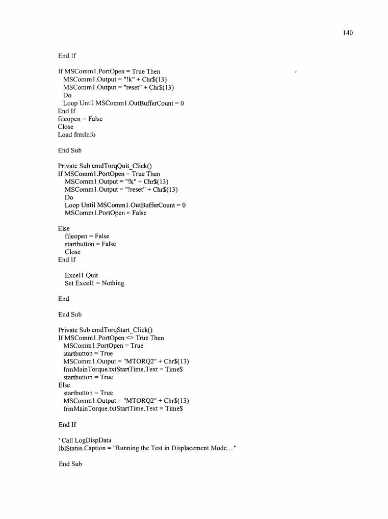
End If

If MSComml .Portopen = True Then MSComm I .Output = "!k" + C:hr$(l3) MSComm 1 .Output = "reset" -t Chr$( 13) Do Loop Until MSComml .OutBufferCount = 0

End If fileopen = False Close Load frmInfo

End Sub

Private Sub cmdTorqQuit-Click() If MSComm 1 .Portopen = True Then

MSComrnl .Output = " ! k + Chr$(l3) MSComm 1 .Output = "!reset" + Chr$(l3) Do Loop Until MSComml.OutBufferCount = 0 MSComm1 .Portopen = False

Else fileopen = False startbutton = False Close

End If

Excell .Quit Set Excel l = Nothing

End

End Sub

Private Sub cmdTorqStart-Click() If MSComm1 .Portopen 0 True Then

MSComm 1 .Portopen = True startbutton = True MSComm 1 .Output = "MTORQ2" + Chr$(l3) frmMainTorque.txtStartTime.Text = Time$ startbutton = True

Else startbutton = True MSComm 1 .Output = "MTORQ2" + Chr$( 13) frmMainTorque.txtStartTime.7'ext = Time$

End If

' Call LogDispData 1blStatus.Caption = "Running the Test in Displacement Mode ...."

End Sub

Private Sub cmdTorqStop-Click() MSComm I .Output = "!kM t Chr$(l3) MSComm 1 .Output = "reset" + Chr$(l3) Do Loop Until MSComm 1 .OutBufferCount = 0 Close fileopen = False startbutton = False 1blStatus.Caption = "The Test has been Stopped!" End Sub

Private Sub mnuAboutHelp-Click(1ndex As Integer) Load h A b o u t fi-mAbout.Show End Sub

Private Sub mnuexit-Click(1ndex As Integer) If MSComm 1 .Portopen = True Then

MSComml.Output = "!k" + Chr$(l3) MSCommI .Output = "!resetw + Chr$(l3) Do Loop Until MSComml .OutBufferCount = 0 MSComm1 .Portopen = False

Else fileopen = False startbutton = False Close

End If

Excel 1 .Quit Set Excel 1 = Nothing

End End Sub

Private Sub mnuMotionArc-Click(1ndex As Integer) Dim RetVal RetVal = Shell("C:\Ma6000\Ma6000.EXE", 1) ' Run Motion Architect End Sub

Private Sub mnuMTS-Click(1ndex As Integer) Dim RetVal RetVal = Shell("C:\Program Files\Netscape\Communicator\Program\NETSCAPE.EXE -h http://www.mts.com", 1) ' Run 'Netscape. End Sub

Private Sub mnuParker-Click(1ndex As Integer) Dim RetVal RetVal = Shell("C:\Program Files\Netscape\Communicator\Program\NETSCAPE.EXE -h http://www.parker.com", 1) ' Run Netscape. End Sub

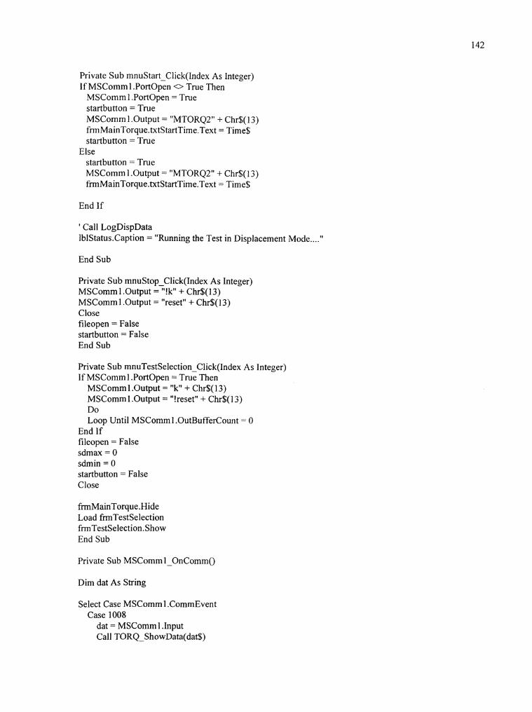
Private Sub mnuStart-Click(1ndex As Integer) If MSComm 1 .Portopen 0 True Then

MSComm 1 .Portopen = True startbutton = True MSComm 1 .Output = "MTORQ2" + Chr$(l3) frmMainTorque.txtStartTime.Text = Time$ startbutton = True

Else startbutton = True MSComm 1 .Output = "MTOR.Q2" + Chr$(l3) frmMainTorque.txtStartTime.Text = Time$

End If

' Call LogDispData 1blStatus.Caption = "Running the Test in Displacement Mode ...."

End Sub

Private Sub mnuStop-Click(1ndex As Integer) MSComm 1 .Output = "!k" + Chr$(l3) MSComm 1 .Output = "reset" + Chr$(l3) Close fileopen = False startbutton = False End Sub

Private Sub mnuTestSelection~Click(Index As Integer) If MSComm 1 .Portopen = True 'Then

MSComm 1 .Output = "k" + Chr$(l3) MSComml .Output = "!resetH + Chr$(l3) Do Loop Until MSComm 1 .OutBufferCount = 0

End If fileopen = False sdmax = 0 sdmin = 0 startbutton = False Close

frmMainTorque.Hide Load fmTestSelection frmTestSelection.Show End Sub

Private Sub MSComm I-OnComm()

Dim dat As String

Select Case MSComm 1 .CommEvent Case 1008

dat = MSComml .Input Call TORQ-ShowData(dat$)

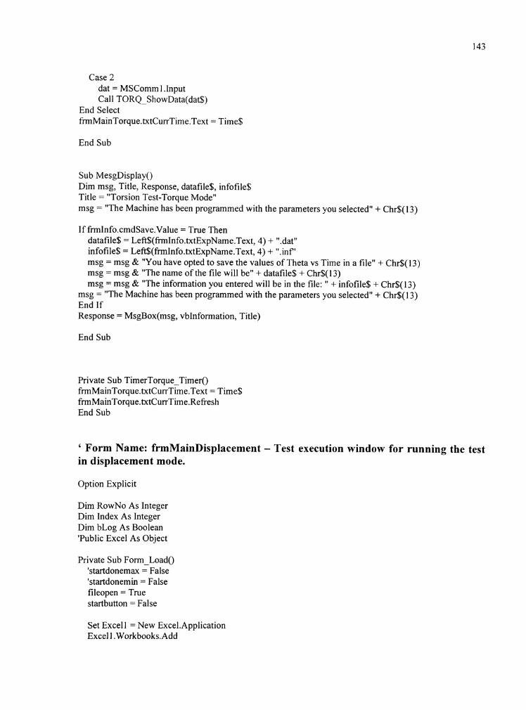
Case 2 dat = MSComm l .Input Call TORQ-ShowData(dat$)

End Select frmMainTorque.txtCurrTime.Text = Time$

End Sub

Sub MesgDisplay() Dim msg, Title, Response, datafile$, infofile$ Title = "Torsion Test-Torque Mode" rnsg = "The Machine has been programmed with the parameters you selected" + Chr$(l3)

If frm1nfo.cmdSave.Value = True Then datafile$ = Left$(frmInfo.txtExpName.Text, 4) + ".datU infofile$ = Left$(frmInfo.txtI3xpName.Text, 4) + ".inf" msg = msg & "You have opted to save the values of Theta vs Time in a file" + Chr$(l3) msg = rnsg & "The name of the file will be" + datafile$ + Chr$(l3) msg = msg & "The information you entered will be in the file: " + infofile$ + Chr$(l3)

msg = "The Machine has been programmed with the parameters you selected" + Chr$(l3) End If Response = MsgBox(msg, vbInformation, Title)

End Sub

Private Sub TimerTorque-Timer() frmMainTorque.txtCurrTime.Text = Time$ frmMainTorque.txtCurrTime.Refresh End Sub

' Form Name: frmMainDisplacement - Test execution window for running the test in displacement mode.

Option Explicit

Dim RowNo As Integer Dim Index As Integer Dim bLog As Boolean 'Public Excel As Object

Private Sub Form-Load() 'startdonemax = False 'startdonemin = False fileopen = True startbutton = False

Set Excel l = New Excel.Application Excel 1 .Workbooks.Add

Call LogDispData 01eChart.Visible = True

' Calling the Main Torsion Program from Torsion Module Call Torsion-Program

rtfText.Text = par

1blStatus.Caption = "Ready ..."

Call TimerDisp-Timer

End Sub

Private Sub mnuAboutHelp-Click(1ndex As Integer) Load frmAbout frrnAbout.Show End Sub

Private Sub mnuexit-Click(1ndex As Integer) If MSComml .Portopen = True 'Then

MSComml .Output = "!kU + Chr$(l3) MSComm l .Output = "!RESETw + Chr$(l3) Do Loop Until MSComml .OutBufferCount = 0 MSComm 1 .Portopen = False

Else fileopen = False startbutton = False Close

End If

Excel1 .Quit Set Excell = Nothing

End End Sub

Private Sub mnuMotionArchitect~Click(Index As Integer) Dim RetVal RetVal = Shell("C:\Ma6000\Ma6000.EXE", 1) ' Run Motion Architect End Sub

Private Sub mnuMTS-Click(Inc1ex As Integer) Dim RetVal RetVal = Shell("C:\Program Files\Netscape\Communicator\Program\NETSCAPE.EXE -h http:l/www.mts.com", 1) ' Run Netscape. End Sub

Private Sub mnuParker-Click(1ndex As Integer) Dim RetVal

RetVal http://www End Sub

= Shell("C:\Program Files\Netscape\Communicator\Program\NETSCAPE.EXE -h .parker.comU, 1) ' Kun Netscape.

Private Sub mnustart-Click(1ndex As Integer) If MSComm 1 .Portopen 0 True Then

MSComm 1 .Portopen = True startbutton = True MSComm I .Output = "MDISPI " + Chr$(l3) fmMainDisplacement.txtStartTime.Text = Time$

Else startbutton = True MSComml .Output = "MDISPI" + Chr$(l3) frmMainDisp1acement.txtStartTime.Text = Time$

End If

' Call LogDispData 1blStatus.Caption = "Running the Test in Displacement Mode ...."

End Sub

Private Sub mnuStop-Click(1ndex As Integer) MSComm1.Output = "!k" + Chr$(l3) MSComm 1 .Output = "RESET" + Chr$(l3) Do Loop Until MSComml .OutBufferCount = 0

Close fileopen = False startbutton = False End Sub

Private Sub mnuTestSelection~Click(Index As Integer) If MSComm 1 .Portopen = True Then

MSCommI.Output = "!k" + Chr$(l3) MSCommI .Output = "RESET" + Chr$(l3) Do Loop Until MSComml .OutBufferCount = 0

End If

fileopen = False

sdmax = 0 sdmin = 0

startbutton = False Close frmMainDisplacement.Hide Load fmTestSelection fmTestSelection.Show End Sub

Private Sub MSComml -OnComm() Dim dat As String

Select Case MSComm 1 .CommEvent Case 1008

dat = MSComm 1 .Input Call DISP-ShowData(dat1;)

Case 2 dat = MSComm 1 .Input If startbutton = True Then

Call DISP-ShowData(dat$) End If

End Select

End Sub

Private Sub cmdDispStart-Click() If MSComml .Portopen 0 True Then

MSComm1 .Portopen = True startbutton = True MSComm 1 .Output = "MDISP 1 " + Chr$(l3) frmMainDisplacement.txtStartTime.Text = Time$

Else startbutton = True MSComml .Output = "MDISPI " + Chr$(l3) frmMainDisp1acement.txtStartTime.Text = Time$

End If

' Call LogDispData 1blStatus.Caption = "Running the Test in Displacement Mode ...."

End Sub

Private Sub cmdDispStop-Click() MSComml .Output = "!k" + Chr$(l3) MSComml .Output = "RESET" -t Chr$(l3) Do Loop Until MSComm l .OutBufferCount = 0

Close fileopen = False startbutton = False 1blStatus.Caption = "The Test has been Stopped!" End Sub

Private Sub cmdDispBack-Click.()

If MSComml .Portopen = True Then MSComm I .Output = "!kV + Chr$(l3)

MSComm 1 .Output = "RESET" + Chr$(l3) Do Loop Until MSComml .OutBufferCount = 0

End If

fileopen = False

sdmax = 0 sdmin = 0

startbutton = False Close

fimMainDisplacement.Hide 'Load hTestSelection fimTestSelection.Show End Sub

Private Sub cmdDispQuit-Click() If MSComm 1 .Portopen = True Then

MSComm I .Output = "!k" + C'hr$(l3) MSComml.Output = "!RESE'TV + Chr$(l3) Do Loop Until MSComm l .OutBufferCount = 0 MSComm 1 .Portopen = False

Else fileopen = False startbutton = False Close

End If

Excel 1 .Quit Set Excel1 = Nothing

End

End Sub

Private Sub TimerDisp-Timer() frmMainDisp1acement.txtCurrTime.Text = Time$ frmMainDisplacement.rxtCurrTime.Refresh End Sub

' Porm Name: frmAbout - Window that displays information about the testing software and its copy rights.

Option Explicit

' Reg Key Security Options ... Const READ-CONTROL = &H20000 Const KEY-QUERY-VALUE = &H 1 Const KEY-SET-VALUE = &.H2 Const KEY-CREATE-SUB-KEY = &H4 Const KEY-ENUMERATE-SIJB-KEYS = &H8 Const KEY-NOTIFY = &H 10 Const KEY-CREATE-LINK =: &H20 Const KEY-ALLACCESS = KEY-QUERY-VALUE + KEY SET VALUE +

KEY-CREATE-SUB-KEY + KEY-ENUMER'TE-SUB-KEYS; - KEY-NOTIFY +- KEY-CREATE-LINK + READ-CONTROL

' Reg Key ROOT Types ... Const HKEY-LOCAL-MACHINE = &H80000002 Const ERROR-SUCCESS = 0 Const REG-SZ = 1 ' Unicode nu1 terminated string Const REG-DWORD = 4 ' 32-bit number

Const gREGKEYSYSINFOLOC = "SOFTWARE\Microsoft\Shared Tools Location" Const gREGVALSYSINFOLOC = "MSINFO" Const gREGKEYSYSINF0 = "SOFTWARE\Microsoft\Shared Tools\MSINFO" Const gREGVALSYSINF0 = "PATH"

Private Declare Function RegOpenKeyEx Lib "advapi32" Alias "RegOpenKeyExA1' (ByVal hKey As Long, ByVal lpSubKey As String, ByVal uloptions As Long, ByVal samDesired As Long, ByRef phkResult As Long) As Long Private Declare Function RegQueryValueEx Lib "advapi32" Alias "RegQueryValueExAU (ByVal hKey As Long, ByVal 1pValueName As String, ByVal IpReserved As Long, ByRef lpType As Long, ByVal lpData As String, ByRef IpcbData As L,ong) As Long Private Declare Function RegCloseKey Lib "advapi32" (ByVal hKey As Long) As Long

Private Sub cmdSysInfo-Click() Call StartSysInfo

End Sub

Private Sub cmdOK-Click() Unload Me

End Sub

Private Sub Form-Load() Me.Caption = "About " & App.Title 1blVersion.Caption = "Version " & App.Major & "." & App.Minor & "." & App.Revision 1blTitle.Caption = App.Title

End Sub

Public Sub StartSysInfo() On Error GoTo SysInfoErr

Dim rc As Long Dim SysInfoPath As String

' Try To Get System Info Program Path\Name From Registry..

tmpVal = Left(tmpVa1, KeyValsize - 1) ' Null Found, Extract From String Else ' WinNT Does NOT Null Terminate String ...

tmpVal = Left(tmpVa1, KeyValsize) ' Null Not Found, Extract String Only End If

' Determine Key Value Type For Conversion..

Select Case KeyValType ' Search Data Types ... Case REG-SZ ' String Registry Key Data Type

KeyVal = tmpVal ' Copy String Value Case REG-DWORD ' Double Word Registry Key Data Type

For i = Len(tmpVa1) To 1 Step -1 ' Convert Each Bit KeyVal = KeyVal + Hex(Asc(Mid(trnpVa1, i, 1))) ' Build Value Char. By Char.

Next KeyVal = Format$("&h" + KeyVal) ' Convert Double Word To String

End Select

GetKeyValue = True ' Return Success rc = RegCloseKey(hKey) ' Close Registry Key Exit Function ' Exit

GetKeyError: ' Cleanup After An Error Has Occured ... KeyVal = "" ' Set Return Val To Empty String GetKeyValue = False I Return Failure rc = RegCloseKey(hKey) ' Close Registry Key

End Function

' Form Name: frmHelp - Window that displays help information regarding the testing software.

Option Explicit

Private Sub cmdClose-Click() Unload fmHelp End Sub

Private Sub Fom-Load() Dim helptext

helptext = vbCrLf & " TYPES OF FATIGUE TESTS " & vbCrLf helptext = helptext & (1 ,, helptext = helptext & vbCrLf & vbCrLf helptext = heiptext & "Torque Mode" & vbCrLf helptext = helptext & " " & vbCrLf & vbCrLf helptext = helptext & "The specimen will be placed in torsion. When this test is performed," & vbCrLf helptext = helptext & "the motor will supply a constant torque (specified) in a cyclic fashion" & vbCrLf helptext = helptext & "i.e in the positive and negative sense. The maximum torque(= -min torque)" & vbCrLf helptext = helptext & "will be applied to the speciment at a specified frequency." & vbCrLf & vbCrLf

helptext helptext helptext helptext helptext

= helptext & "Disp1act:ment Mode" & vbCrLf = helptext & " " & vbCrLf & vbCrLf = helptext & "The specimen will be subjected to a positive and negative displacement" & vbCrLf = helptext & "in a cyclic fashion with a specified frequency. In this mode the motor" & vbCrLf = helptext & "is essentially executing a sinusoidal path in terms of its shaft angle" & vbCrLf

rtfHelp.Text = helptext

End Sub

' Form Name: frmTextEdit - Window that gives the user the option of including the experimenter name and the test specifications which are saved to a file.

Option Explicit

Private Sub imgproc-Click(1ndex As Integer) Select Case Index

Case 0 Call mFileProc(frmTextBox.dlgText, firnTextBox.rtfText, 1) 'open

Case 1 Call mFileProc(hTextBox.dlgText, firnTextBox.rtffext, 2) 'save

Case 2 Call mEditProc(frmTextBox.dlgText, fmTextBox.rtfText, 2) 'cut

Case 3 Call mEditProc(hTextBox.dlgText, frmTextBox.rtffext, 3) 'copy

Case 4 Call mEditProc(frmTextBox.dlgText, frmTextBox.rtffext, 4) 'paste

Case 5 Call mEditProc(frmTextBox.dlgText, frmTextBox.rtffext, 0) 'undo

End Select End Sub

Private Sub mnuexit-Click() End End Sub

' Form Name: frmTextBox

Option Explicit

Private Sub Form-Load() frmtexted.imgproc(j).Enabled = False 'undo image mnuedit(O).Enabled = False 'undo menu

End Sub

Private Sub Fonn-Resize() Call mRsizeTextBox End Sub

Private Sub mnualign-Click(1ndex As Integer) Call mAlignProc(dlgText, rtflext, Index) End Sub

Private Sub mnuedit-Click(1ndex As Integer) Call mEditProc(dlgText, rtiText, Index) Select Case Index

Case 0 htexted.imgproc(5).Enabled = False mnuedit(O).Enabled = False

Case 5 htexted.imgproc(5).Enabled = True mnuedit(O).Enabled = True

End Select End Sub

Private Sub mnueditmain-Click() If Clipboard.GetText 0 "" Then

frmtexted.imgproc(4).Enabled = True mnuedit(4).Enabled = True

Else fimtexted.imgproc(4).Enabled = False mnuedit(4).Enabled = False

End If

If rtffext.SelText = "" Then frmtexted.imgproc(2).Enabled= False 'cut image is disabled fhntexted.imgproc(3).Enabletl= False 'copy image is disabled

mnuedit(2).Enabled = False 'cut menu item is disabled mnuedit(3)Enabled = False 'copy menu item is disabled mnuedit(5).Enabled = False 'del menu item is disabled

Else fimtexted.imgproc(2).EnabIecl= True 'cut image is disabled fmtexted.imgproc(3).Enableci = True 'copy image is disabled mnuedit(2).Enabled = True mnuedit(3).Enabled = True mnuedit(5).Enabled = True

End If End Sub

Private Sub mnufile-Click(1ndex As Integer) Call mFileProc(dlgText, rtfText, Index) End Sub

Private Sub mnuhelp-Click(1ndex As Integer) Call mHelpProc(dlgText, rtffext, Index) End Sub

Private Sub mnusearch-Click(1ndex As Integer) Call mSearchProc(dlgText, rtflext, Index) End Sub

Private Sub rtff ext-Change() rtffext.Tag = "1" End Sub

Private Sub rtffext-KeyPress(KeyAscii As Integer) If txtExpName.Text = "" Or txtSampleName.Text = "" Then

KeyAscii = 0 End If End Sub

Private Sub txtExpName-KeyPress(KeyAscii As Integer) Select Case KeyAscii Case 9

If txtExpName.Text 0 "" And txtSampleName.Text 0 "" Then rtffext.Text = rtflext.Text + vbCrLf Call fi-mTestSelection.displayParam(rtfText)

End If

Case 13 If txtExpName.Text 0 "" And txtSampleName.Text o "" Then

rtffext.Text = rtffext.Text + vbCrLf Call f?mTestSelection.displayParam(rtffext, 1)

End If End Select End Sub

Private Sub txtSampleName-KeyPress(KeyAscii As Integer) Select Case KeyAscii

Case 9 If txtExpName.Text 0 "" And txtSampleName.Text 0 "" Then rtffext.Text = rtfText.Text .+ vbCrLf Call frmTestSelection.displayParam(rtffext) End If

Case 13 1ftxtExpName.Text 0 "" Anti txtSampleName.Text 0 "" Then

rtffext.Text = rtfText.Text + vbCrLf Call frmTestSelection.displayParam(rtffext)

End If

End Select End Sub

' Module Name: Module1

------ ' Variable Declarations

DefInt A-Z Global Tablndex As Integer Global port Global sdmax Global sdmin Global fileopen Global oldmax$ Global oldmin$ Global startbutton Global Echo ' Echo onloff flag Global Cancelsend ' Flag to stop sending a text file Global par As String 'parameters to be passed to the richtext box in the main forms

( _ _ _ _ _ _ MSComm Event Constants

Global Const mscomm-ev-send = 1 Global Const mscomm~ev~recieve = 2 Global Const mscomm-ev-cts := 3 Global Const m s c o m m ~ e v ~ d s r = 4 Global Const mscomm-ev-cd == 5 Global Const mscomm-ev-ring = 6 Global Const msscomm-ev-eof = 7

------ ' MSComm Error Code Constants

Global Const mscomm-er-break = 1001 Global Const mscomm-er-ctsto = 1002 Global Const mscomm-er-dsrto = 1003 Global Const mscomm-er-frame = 1004 Global Const mscomm-er-overrun = 1006 Global Const mscomm-er-cdto = 1007 Global Const mscomm-er-txover = 1008 Global Const mscomm-er-rxparity = 1009 Global Const mscomm-er-txfull = 1010

------ ' Common Dialog Constants

Global Const C D E R W A N C E L = 32755 Global Const CF-SCREENFONTS = &H 1&

Sub Main()

Dim susername As String Dim spassword As String

If susername = "fatigue" And spassword = "fatigue" Then Unload IimLoginMenu Load frmWelcome fimWelcome.Show

Else MsgBox "The user cancelled or failed to log in", vblnformation, "Login Aborted"

End If

End Sub

' Module Name: Torsion Module

Option Explicit

Dim RowNo As Integer Dim Index As Integer Dim bLog As Boolean Dim datafile As String Global Excel1 As Object

' Main program for Torsion Testing

Public Sub Torsion-Program()

On Error GoTo CommunicationError

' Dim sTestSelection ' Dim sLoadingSeq

Select Case TabIndex

t _ _ _ _ _ _ _ _ _ _ Torque Mode Case 0

' Open the MSComml Call OpenPort

' Download Torque Program to the Controller Call TORQ-ProgramDown

' Display the graph of Displacement vs time Call TORQ-Graphparam

' Open the file to save Displacement vs time data 'Call OpenFile

J _ r _ _ _ _ _ _ _ _ Displacement Mode Case 1

' Open the MSComm 1

Call OpenPort

' Download Displacement Program to the Controller Call DISP-ProgramDown

' Display the graph of Torque vs time Call DISP-Graphparam

' Open the file to save Torclue vs time data 'Call OpenFile

---------- Velocity Mode Case 2

' Open the MSComml Call OpenPort

' Download Velocity Program to the Controller Call VEL-ProgramDown

' Display the graph of Velocity vs time Call VEL-Graphparam

' Open the file to save Velocity vs time data 'Call OpenFile

End Select

Exit Sub

End Sub

Public Sub Openport()

Select Case TabIndex

f _ _ _ _ _ _ _ _ _ _ Torque Mode Case 0 With hMainTorque.MSComm1

.CommPort = 1

.Settings = "9600,N,8,lW

.InputLen = 0

.InBufferCount = 0

.OutBufferCount = 0

.OutBufferSize = 1024

.InBufferSize = 4096

.Handshaking = XonXoff

.RThreshold =. 20

.NullDiscard := True

.Portopen =- True End With

---------- Displacement Mode Case 1 fmMainDisplacement.MSComm 1 .CommPort = 1 frmMainDisp1acement.MSComm 1 .Settings = "9600,N,8,1n frmMainDisplacement.MSComm1 .InputLen = 0 frmMainDisplacement.MSCc)mm 1 .InBufferCount = 0 fnnMainDisplacement.MSCc~mm I .OutBufferCount = 0 fmMainDisplacement.MSComm I .OutBufferSize = 1024 frmMainDisplacement.MSCc~mm 1 .InBufferSize = 4096 frmMainDisplacement.MSComm 1 .Handshaking = XonXoff fnnMainDisplacement.MSComm 1 .RThreshold = 20 frmMainDisplacement.MSComm 1 .NullDiscard = True frmMainDisplacement.MSComm 1 .Portopen = True

f _ _ _ _ _ _ _ _ _ _ Velocity Mode Case 2 With frmMainVelocity.MSComm 1

.CommPort == 1

.Settings = "!)600,N,8,lW

.InputLen = 0

.InBufferCount = 0

.OutBufferCount = 0

.OutBufferSize = 1024

.InBufferSize = 4096

.Handshaking = XonXoff

.RThreshold = 20

.NullDiscard = True

.Portopen = True End With

End Select

End Sub

' New Torque Program ---- MTORQ2

Public Sub TORQ-ProgramDown() Dim TORQFREQ As Double Dim TMAX As Double

Dim TMIN As Double Dim CYCLES As Integer Dim loadlndex As Integer ' List Index for the items in the combo boxes for loading seq

TORQFREQ = Val(frmTestSelection.txtTorqFreq) TMAX = Val(fnnTestSelection.1xtMaxTorq) TMIN = Val(fi~nTestSelection.tr;tMinTorq) CYCLES = Val(frmTestSelection.txtTorqCycles)

Ioadlndex = fimTestSelection.cmbTorqLoadSeq.Listlndex

' Main Torque Program for MTORQ2

frmMainTorque.MSComm1 .Output = "" + Chr$(l3) + Chr$(l3) + Chr$(l3) 'frmMainTorque.MSComm 1 .Output = "ECHOO" + Chr$(l3) fi-mMainTorque.MSComm1 .Output = "DEL MTORQ2" + Chr$(l3) frmMainTorque.MSComm 1 .Output = "DEF MTORQ2" + Chr$(l3) frmMainTorque.MSComm I .Output = "GOSUB STORQ2" + Chr$(l3) fhMainTorque.MSComm I .Output = "GOSUB MOTTOR2" + Chr$(l3) frmMainTorque.MSComm 1 .Output = "END" + Chr$(l3)

' Setup Program for MTORQ2 for torque mode fimMainTorque.MSComm 1 .Output = "DEL STORQ2" + Chr$(l3) ?hMainTorque.MSComm 1 .Output = "DEF STORQ2" + Chr$(l3) fimMainTorque.MSComm 1 .Output = "INDAXI " + Chr$(l3) frmMainTorque.MSComm1 .Output = "SGPO" + Chr$(l3) fhMainTorque.MSComm 1 .Output = "SGIO" + Chr$(l3) frmMainTorque.MSComm 1 .Output = "SGVO" + Chr$(l3) frmMainTorque.MSComm I .Output = "ERES4000" + Chr$(l3) frmMainTorque.MSComm 1 .Output = "DRIVE I " + Chr$(l3) frmMainTorque.MSComm 1 .Output = "PSETO" + Chr$(l3) fi-mMainTorque.MSComm 1 .Output = "SMPERSOO" + Chr$(l3) frmMainTorque.MSComm I .Output = "END" + Chr$(l3)

' MOTTOR2 program for motion in torque mode

frmMainTorque.MSComm1 .Output = "DEL MOTTOR2" + Chr$(l3) frmMainTorque.MSComm 1.Output = "DEF MOTTOR2" + Chr$(l3) frmMainTorque.MSComm 1 .Output = "VARI =" + CStr(TMAX) + Chr$(l3) fnnMainTorque.MSComm I .Output = "VAR2=" + CStr(TM1N) + Chr$(l3) frmMainTorque.MSComm 1 .Output = "VAR3=" + CStr(T0RQFREQ) + Chr$(l3) frmMainTorque.MSComm 1 .Output = "VARI O=VARl*(118.24)" + Chr$(l3) fi-mMainTorque.MSComm1.Output = "VAR20=VAR2*(118.24)" + Chr$(l3) frmMainTorque.MSComm 1 .Output = "VAR3O= I I(VAR3 *2)" + Chr$(13) fmMainTorque.MSComm 1 .Output = "VAR6=" + CStr(CYCLES) + Chr$(l3) frmMainTorque.MSComm1 .Output = "VARSI=" + Chr$(34) + "THMAX" + Chr$(34) + Chr$(l3) frmMainTorque.MSComm1 .Output = "VARS2=" + Chr$(34) + "THMIN" + Chr$(34) + Chr$(l3) frmMainTorque.MSComm I .Output = "VARS3=" + Chr$(34) + "C" + Chr$(34) + Chr$(l3) frmMainTorque.MSComm 1 .Output = "VARS4=" + Chr$(34) + "EN + Chr$(34) + Chr$(l3) frmMainTorque.MSComm 1 .Output = "VAR9=O" + Chr$(l3)

Select Case IoadIndex

' Motion Architect Program for Saw-Toothed Loading Sequence in Torque Mode Case 0

frmMainTorque.MSComm 1 .Output = "L" + Chr$(l3) fimMainTorque.MSComm1 .Output = "WRVARS3" + Chr$(l3) frmMainTorque.MSComm I .Output = "SOFFS(VARl0)" + Chr$(l3) frmMainTorque.MSComm I .Output = "VAR4=PEM + Chr$(l3) frmMainTorque.MSComm I .Output = "WRVARSI " + Chr$(l3)

frmMainTorque.MSComm 1 .Output = "WRVAR4" + Chr$(l3) 'fmMainTorque.MSComm I .Output = "TDAC" + Chr$(l3) frmMainTorque.MSComm I .Output = "T(VAR30)" + Chr$(l3) frmMainTorque.MSComm I .Output = "SOFFSO" + Chr$(l3) frmMainTorque.MSComm I .Output = "T0.02" + Chr$(l3) frmMainTorque.MSComm 1 .Output = "SOFFS(VAR20)" + Chr$(l3) frmMainTorque.MSComm I .Output = "T(VAR30)" + Chr$(l3) frmMainTorque.MSCommI .Output = "VAR5=PEU + Chr$(l3) frmMainTorque.MSCornrn 1 .Output = "WRVARS2" + Chr$(l3) frmMainTorque.MSComm 1 .Output = "WRVARS" + Chr$(l3) 'frmMainTorque.MSComm1 .Output = "TDAC" + Chr$(l3) 'frmMainTorque.MSComm I .Output = "WRVAR9" + Chr$(l3) 'frmMainTorque.MSComm1 .Output = "TPE" + Chr$(l3) frmMainTorque.MSComm I ..Output = "SOFFSO" + Chr$(l3) frmMainTorque.MSComm 1 .Output = "T0.02" + Chr$(l3)

frmMainTorque.MSComm 1 .Output = "IF(PE>SOO OR PE<-500)" + Chr$(l3) frmMainTorque.MSComm1 .Output = "WRVARS4" + Chr$(l3) frmMainTorque.MSComm 1 .Output = "TI 0" + Chr$(l3) frmMainTorque.MSComm1 .Output = "DRIVEO" + Chr$(l3) frmMainTorque.MSComm I .Output = "NIF" + Chr$(l3)

frmMainTorque.MSComm I .Output = "L10" + Chr$(l3) frmMainTorque.MSComm 1 .Output = "WRVARS3" + Chr$(l3) frmMainTorque.MSComm I .Output = "SOFFS(VARI0)" + Chr$(l3) frmMainTorque.MSComm I .Output = "T(VAR30)" + Chr$(l3) frmMainTorque.MSComm1 .Output = "SOFFSO" + Chr$(l3) frmMainTorque.MSComm1 .Output = "T0.02" + Chr$(l3) frmMainTorque.MSComm1 .Output = "SOFFS(VAR20)" + Chr$(l3) frmMainTorque.MSComm I .Output = "T(VAR30)" + Chr$(l3) frmMainTorque.MSComm I .Output = "SOFFSO" + Chr$(l3) fmMainTorque.MSComm1 .Output = "T0.02" + Chr$(l3)

frmMainTorque.MSComm 1 .Output = "IF(PE>SOO OR PE<-500)" + Chr$(l3) frmMainTorque.MSComrn I .Output = "WRVARS4" + Chr$(l3) frmMainTorque.MSComm1 .Output = "TI 0" + Chr$(l3) frmMainTorque.MSComm I .Output = "DRIVEO" + Chr$(l3) frmMainTorque.MSComm1 .Output = "NIF" + Chr$(l3)

frmMainTorque.MSComm I .Output = "VAR9=VAR9+lV + Chr$(l3) fimMainTorque.MSComm I .Output = "IF(VAR9>VAR6)" + Chr$(l3) frmMainTorque.MSComm1 .Output = "GOT0 FINISH" + Chr$(l3) frmMainTorque.MSComm I .Output = "NIF" + Chr$(l3) frmMainTorque.MSComm1 .Output = "LN" + Chr$(l3)

frmMainTorque.MSComm 1 .Output = "VAR9=VAR9+ I " + Chr$(l3) frmMainTorque.MSComm1 .Output = "IF(VAR9>VAR6)" + Chr$(l3) frmMainTorque.MSComm 1 .Output = "GOT0 FINISH" + Chr$(l3) frmMainTorque.MSComm 1 .Output = "NIF" + Chr$(l3) frmMainTorque.MSCommI .Output = "LN" + Chr$(l3) frmMainTorque.MSComm 1 .Output = "END" + Chr$(l3)

'Motion Architect Program in Torque Mode for Block Loading Sequence

Case I

' Motion Architect Program in Torque Mode for Ramp Loading Sequence Case 2

' Motion Architect Program in Torque Mode for Sinusoidal Loading Sequence Case 3

' Motion Architect Program in Torque Mode for Multi-Rate Ramp & Hold Loading Sequence Case 4

' Motion Architect Program in Torque Mode for Multi-Axial Loading Loading Sequence Case 5

End Select

End Sub

' New Torque Program ---- MTORQ2

Public Sub DISP-ProgramDown() Dim DISPFREQ As Double Dim TMAX As Double Dim TMIN As Double Dim CYCLES As Integer Dim IoadIndex As Integer ' List Index for the items in the combo boxes for loading seq

DISPFREQ = Val(frmTestSe1ection.txtDispFreq) TMAX = Val(frmTestSe1ection.txtMaxAng) TMIN = Val(frmTestSelection.txtMinAng) CYCLES = Val(fnnTestSelection.txtDispCyc1es)

loadlndex = frmTestSelection.cmbDispLoadSeq.Listlndex

' Main Displaement Program for MDISPl

frmMainDisplacement.MSComm1 .Output = "" + Chr$(l3) + Chr$(l3) + Chr$(l3) frmMainDisplacement.MSComm 1 .Output = "ECHOO" + Chr$(l3) fimMainDisplacement.MSComm1 .Output = "DEL MDISPI " + Chr$(l3) frmMainDisplacement.MSComm 1 .Output = "DEF MDISP I " + Chr$(l3) frmMainDisplacement.MSComm1 .Output = "GOSUB SDISPl " + Chr$(l3) frmMainDisplacement.MSComm1 .Output = "GOSUB MOTDIS 1 " + Chr$(l3) frmMainDisplacement.MSComm1 .Output = "END" + Chr$(l3)

' Setup Program for MDISPI in displacement mode

frmMainDisp1acement.MSComrn 1 .Output = "DEL SDISPl " + Chr$(l3) frmMainDisplacement.MSComrn1 .Output = "DEF SDISPI " + Chr$(l3) fnnMainDisplacement.MSComrn I .Output = "INDAXI " + Chr$(l3) frmMainDisplacement.MSComm 1 .Output = "SGP 18" + Chr$(l3) fmMainDisplacement.MSComrn1 .Output = "SGIO" + Chr$(l3) frmMainDisp1acement.MSComm 1 .Output = "SGVS" + Chr$( 13)

frmMainDisplacement.MSComm 1 .Output = "ERES4000" + Chr$(l3) frmMainDisplacement.MSComm 1 .Output = "SMPERO" + Chr$(13) frmMainDisplacement.MSComm 1 .Output = "SCALE1 " + Chr$(l3) frmMainDisplacement.MSComm 1 .Output = "SCLDI " + ChrS(13) frmMainDisplacement.MSComm 1 .Output = "SCLV4000" + Chr$(l3) frmMainDisplacement.MSComm 1 .Output = "SCLA4000" + Chr$(l3) fmMainDisplacement.MSComm1 .Output = "MA 1 " + Chr$(l3) frmMainDisplacement.MSComm I .Output = "LHO" + Chr$(l3) frmMainDisplacement.MSComm 1 .Output = "LSO" + Chr$(13) frmMainDisplacement.MSComm 1 .Output = "DRFLVL I " + ChrS(l3) frmMainDisplacement.MSComm 1 .Output = "DRIVE I " + Chr$(l3) frmMainDisplacement.MSCornm I .Output = "PSETO" + Chr$(l3) fmMainDisplacement.MSComm1 .Output = "END" + Chr$(l3)

' MOTDIS 1 program for motion in displacement mode

fi-mMainDisplacement.MSComm 1 .Output = "DEL MOTDIS 1 " + Chr$( 13) frmMainDisplacement.MSComm 1 .Output = "DEF MOTDIS 1 " + Chr$(l3) frmMainDisplacement.MSComm 1 .Output = "VARI =" + CStr(TMAX) + Chr$(l3) fi-mMainDisplacement,MSComm 1 .Output = "VAR2=" + CStr(TM1N) + Chr$(l3) frmMainDisplacement.MSCornm1 .Output = "VAR3=" + CStr(D1SPFREQ) + Chr$(l3) fmMainDisplacement.MSComm 1 .Output = "VARIO=VARl*(4000/360)" + Chr$(l3) frmMainDisplacement.MSComm 1 .Output = "VAR20=VAR2*(4000/360)" + Chr$(l3) frmMainDisplacement.MSCon~ml .Output = "VAR30=1/(VAR3 *2)" + Chr$(13) frmMainDisplacement.MSCon~m1 .Output = "VAR5=" + CStr(CYCLES) + Chr$(l3) frmMainDisplacement.MSConim I .Output = "VARS I=" + Chr$(34) + "THMIN" + Chr$(34) + Chr$(l3) frmMainDisplacement.MSConim1.Output = "VARS2=" + Chr$(34) + "THMAX" + Chr$(34) + Chr$(l3) frmMainDisplacement.MSConlm1.Output = "VARS3=" + Chr$(34) + "L" + Chr$(34) + Chr$(l3) frmMainDisplacement.MSConim1 .Output = "VARS4=" + Chr$(34) + "VAR6" + Chr$(34) + Chr$(l3) frmMainDisplacement.MSComm1 .Output = "VAR9=OU + Chr$(l3)

Select Case IoadIndex

' Motion Architect Program for Saw-Toothed Loading Sequence Case 0

'frmMainDisp1acement.MSCommI .Output = "DEL SAWT" + Chr$(l3) 'fmMainDisplacement.MSCommI .Output = "DEF SAWT" + Chr$(l3) frmMainDisplacement.MSComm1 .Output = "IF (VAR20<0)" + Chr$(l3) frmMainDisplacement.MSComm1 .Output = "VAR8=(2*VARlO-2*VAR20)*VAR3" + Chr$(l3) frmMainDisplacement.MSComm I .Output = "ELSE" + Chr$(l3) frmMainDisplacement.MSComml.Output = "VAR8=(2*VAR10+2*VAR20)*VAR3" + Chr$(l3) frmMainDisp1acement.MSGomm 1 .Output = "NIF" + Chr$(l3) frmMainDisplacement.MSComm 1 .Output = "V, (VAR8)" + Chr$(l3) 'frmMainDisp1acement.MSComm 1 .Output = "V50" + Chr$(l3) frmMainDisplacement.MSComm1 .Output = "VAR7=(1/1 O)*VAR 10*(1/40)*VAR3" + Chr$(l3) frmMainDisp1acement.MSComm 1 .Output = "A, (VAR7)" + Chr$( 13) frmMainDisplacement.MS(hmI .Output = "L" + Chr$(l3) frmMainDisplacement.MSComm 1 .Output = "WRVARS3" + Chr$(l3) frmMainDisplacement.MSComm I .Output = "D(VAR10)" + Chr$(l3) frmMainDisplacement.MSComm 1 .Output = "GO" + Chr$(l3) frrnMainDisplacement.MSCommI .Output = "WAIT(MOV=BO)" + Chr$(l3) frmMainDisplacement.MSComm l .Output = "WRVARSI " + Chr$(l3)

frrnMainDisp1acement.MSComm 1 .Output = "TDAC" + Chr$(l3) frmMainDisplacement.MSComm1 .Output = "t(VAR30)" + Chr$(l3)

frmMainDisplacement.MSComm 1 .Output = "D(VAR20)" + Chr$(l3) frmMainDisplacement.MSComml .Output = "GO" + Chr$(l3) frmMainDisplacement.MSComm 1 .Output = "WAIT(MOV=BO)" + Chr$( 13) frrnMainDisplacement.MSComrn I .Output = "WRVARS2" + Chr$(l3) frmMainDisplacement.MSComm 1 .Output = "TDAC" + Chr$(l3) frmMainDisplacement.MSCornm I .Output = "t(VAR30)" + Chr$(l3) frmMainDisplacement.MSComm 1 .Output = "L5" + Chr$(l3) frmMainDisplacement.MSComm I .Output = "WRVARS3" + Chr$(l3) frmMainDisplacement.MSComm 1 .Output = "D(VARI0)" + Chr$(l3) frmMainDisplacement.MSComm1 .Output = "GO" + Chr$(l3) frmMainDisp1acement.MSComm 1 .Output = "WAIT(MOV=BO)" + Chr$(l3) frmMainDisplacement.MSComm 1 .Output = "t(VAR30)" + Chr$(l3) frmMainDisplacement.MSComm I .Output = "D(VAR20)" + Chr$(l3) frmMainDisplacement.MSComm 1 .Output = "GO" + Chr$(l3) frmMainDisp1acement.MSComm I .Output = " WAIT(MOV=BO)" + Chr$( 13) fimMainDisplacement.MSComm1 .Output = "t(VAR30)" + Chr$(l3) frmMainDisp1acement.MSComm 1 .Output = ItVAR9=VAR9+ 1 " + Chr$(l3) fimMainDisplacement.MSComm1 .Output = "IF (VAR9>=VARS)" + Chr$(l3) frmMainDisplacement.MSComm I .Output = "GOT0 FINISH" + Chr$(l3) fimMainDisplacement.MSComm1 .Output = "NIF" + Chr$(l3) frmMainDisplacement.MSComm 1 .Output = "LN" + Chr$(l3) frmMainDisplacement.MSComm 1 .Output = "VAR9=VAR9+lU + Chr$(l3) frmMainDisp1acement.MSComm 1 .Output = "IF (VAR9>=VARS)" + Chr$( 13) frmMainDisplacement.MSComm1 .Output = "GOT0 FINISH" + Chr$(l3) frmMainDisp1acement.MSCommI .Output = "NIF" + Chr$(l3) frmMainDisplacement.MSComm 1 .Output = "LN" + Chr$(l3) frmMainDisplacement.MSCornm1 .Output = "END" + Chr$(l3)

frmMainDisplacement.MSCommI .Output = "DEL FINISH" + Chr$(l3) fmMainDisplacement.MSComml .Output = "DEF FINISH" + Chr$(l3) frmMainDisplacement.MSCommI .Output = "S" + Chr$(l3) frmMainDisplacement.MSCornm 1 .Output = "TDAC" + Chr$(l3) frmMainDisplacement.MSComm1 .Output = "END" + Chr$(l3)

'Motion Architect Program for Block Loading Sequence

Case 1 frmMainDisplacernent.MSComm1 .Output = "VAR7=2* 1 OO*(VARlO-VAR20)*VAR3" + Chr$(l3) frmMainDisplacement.MSComml .Output = "V, (VAR7)" + Chr$(l3) fmMainDisplacement.MSComm1.Output = "A, (VAR7)" + Chr$(l3) frmMainDisplacement.MSComm 1 .Output = "AD, (VAR7)" + Chr$(l3) frmMainDisp1acement.MSCommI .Output = "PSETO" + Chr$(l3) fmMainDisp1acement.MSComm 1 .Output = "L" + Chr$(l3) frmMainDisplacement.MSComm1 .Output = "WRVARS3" + Chr$(l3) frmMainDisplacement.MSComm1 .Output = "D(VAR10)" + Chr$(l3) frmMainDisplacement.MSComm 1 .Output = "GO" + Chr$(l3) fmMainDisplacement.MSComm 1 .Output = "WAIT(MOV=BO)" + Chr$(l3)

frmMainDisplacement.MSComm 1 .Output = "WRVARS 1 " + Chr$(l3) fimMainDisp1acement.MSComm 1 .Output = "TDAC" + Chr$(l3) frrnMainDisplacement.MSComm1 .Output = "D(VAR20)" + Chr$(l3) frmMainDisplacement.MSComm1 .Output = "GO" + Chr$(l3) frmMainDisplacement.MSComm 1 .Output = "WAIT(MOV=BO)" + Chr$(l3) frrnMainDisplacement.MSComm 1 .Output = "WRVARS2" + Chr$(l3) frmMainDisplacement.MSComm1 .Output = "TDAC" + Chr$(l3) frmMainDisp1acement.MSComm 1 .Output = "T(VAR30)" + Chr$(l3) fmMainDisplacement.MSComm 1 .Output = "L5" + Chr$(l3) frmMainDisplacement.MSComm 1 .Output = "WRVARS3" + Chr$(l3) frmMainDisplacement.MSComm 1 .Output = "D(VAR1O)" + Chr$(l3) frmMainDisplacement.MSComm1 .Output = "GO" + Chr$(l3) fimMainDisplacement.MSComm 1 .Output = " WAIT(MOV=BO)" + Chr$(l3) frmMainDisplacement.MSComm I .Output = "TDAC" + Chr$(l3) frmMainDisplacement.MSComm 1 .Output = "T(VAR30)" + Chr$(l3) frmMainDisplacement.MSComm1 .Output = "VAR9=VAR9+lU + Chr$(l3) frmMainDisplacement.klSComm1 .Output = "IF (VAR9>=VAR5)" + Chr$(l3) frmMainDisplacement.MSComm1 .Output = "GOT0 FINISH" + Chr$(l3) frmMainDisplacement.MSComm 1 .Output = "NIF" + Chr$(l3) frmMainDisplacement.MSComm1 .Output = "LN" + Chr$(l3) frmMainDisp1acement.MSComm 1 .Output = "END" + Chr$(l3)

frrnMainDisp1acement.MSComm 1 .Output = "DEL FINISH" + Chr$(l3) frmMainDisplacement.MSComm1 .Output = "DEF FINISH" + Chr$(l3) frmMainDisplacement.MSComm 1 .Output = "S" + Chr$(l3) frmMainDisp1acement.MSComm 1 .Output = "TDAC" + Chr$(l3) frmMainDisplacement.MSComm 1 .Output = "END" + Chr$(l3)

' Motion Architect Program for Ramp Loading Sequence Case 2

' Motion Architect Program for Sinusoidal Loading Sequence Case 3

' Motion Architect Program fix Multi-Rate Ramp & Hold Loading Sequence Case 4

' Motion Architect Program for Multi-Axial Loading Loading Sequence Case 5

End Select

End Sub

Sub VEL-ProgramDown()

End Sub

Sub TORQ-Graphparam()

End Sub

Sub DISP-Graphparam()

End Sub

Sub VEL-Graphparam()

End Sub Sub TORQ-ShowData(dat$) Dim cycle, angle$, sign$ Dim i As Integer Dim j As Integer Dim k As Integer Dim n As Integer sdmax = 0 sdmin = 0

If startbutton = False Then Exit Sub

i = InStr(UCase$(dat$), "E")

'If i Then ' Call salute I Exit Sub

' End If

Do i = InStr(i + 1, dat$, "T") j = InStr(i + 1, dat$, Chr$(l3:)) k = InStru + 1, dat$, Chr$(l3))

If i And j Then sign$ = Mid$(dat$, i, 5) angle$ = Mid$(dat$, Cj + 1 ), 3)

End If

If sign$ = "THMAX" Then frmMainTorque.txtCurrTheta.Max.Text = Val(Format(Val(angle$) * 360 / 400, "0.00"))

End If

If sign$ = "THMIN" Then frmMainTorque.txtCurrThetaMin.Text = Val(Format(Val(angle$) * 360 / 400, "0.00"))

End If

Loop While i

If sdmax <= 5 And Val(frrnMainTorque.txtCurrThetaMax.Text) 0 0 Then frmMainTorque.txtStrThetaMax.Text = fmMainTorque.txtCurrThetaMax.Text fmMainTorque.txtStrThetaMax.Refresh sdmax = sdmax + 1

End If

If sdmin <= 5 And Val(frmMainTorque.txtStrThetaMin.Text) 0 0 Then fimMainTorque.txtStrThetaMin.Text = fmMainTorque.txtCurrThetaMin.Text frmMainTorque.txtStrThetaMin.Refresh sdmin = sdmin + 1

End If

Do i = InStr(i + 1 , dat$, "C") If i Then

!imMainTorque.txtCycles.Text = Val(frmMainTorque.txtCycles.Text) + 1 frrnMainTorque.txtCyc1es.Refresh

End If Loop While i

RowNo = RowNo + 1 Excel l .Visible = True Excel l .Windowstate = xlMiriimized

If RowNo > 1 And RowNo <= 400 Then

Excel 1 .ActiveWorkbook.ActiveSheet.Range("A" & RowNo).Value =

Val(fnnMainTorque.txtCyc1es.Text) Excel1 .ActiveWorkbook.ActiveSheet.Range("B" & RowNo).Value =

Val(fmMainTorque.txtCurrThetaMax.Text) Excel l .ActiveWorkbook.ActiveSheet.Range("C" & RowNo).Value =

Val(frrnMainTorque.txtCurrThetaMin.Text)

n = RowNo Mod 20 If n = 0 And RowNo > 20 Then

Call TorqDataPlotMacro frmMainTorque.oleChart.Paste

End If

Else ' call Macro for clearing the Cells in the excel Call Clear-Cell

RowNo = 1 End If

'If fileopen = True Then ' If Val(frmMainTorque.txtCycles.Text) 0 0 And Val(fimMainTorque.txtCurrThetaMax.Text) o 0 And Val(fmMainTorque.txtCurrThetaMin.Text) 0 0 Then ' If (frmMainTorque.txtCurrThetaMax.Text) <> oldmax$ Or (frmMainTorque.txtCurrThetaMin.Text) 0 oldmin$ Then

' Print # I , Val(fmMainTorque.txtCycles.Text); " "; fnnMainTorque.txtCurrThetaMax.Text; " "; fmMainTorque.txtCurrThetaMin.Text

' oldmax$ = frmMainTorque.txtCurrThetaMax.Text ' oldmin$ = fmMainTorque.txtCurrThetaMin.Text ' End If

'End If 'End If

End Sub Sub salute()

Dim dgdef, msg, Response, 'Title 'declare variables

msg = "A signal has been recieved from the machine indicating " msg = msg & "the conclusion of the test. If you perceive that there is no " msg = msg & "crack visible please hit the 'CANCEL' button to go back and " msg = msg & "start the test. 1\11 the values collected so far will be preserved " msg = msg & "and the test will continue as before. " rnsg = msg & "Hit the OK button to conlude the test" Title = "Torsion Fatigue Testing" dgdef = 49 Response = MsgBox(msg, dgdef, Title) If Response = 1 Then Exit Sub If Response = 2 Then Exit Sub

End Sub

Sub DISP-ShowData(dat$) Dim cycle, torque$, sign$ Dim i As Integer Dim j As Integer Dim k As Integer Dim n As Integer

i = 0 Do

i = InStr(i + 1 , dat$, "TH") j = InStr(i + 1, dat$, Chr$(l3)) k = InStrCj + 1 , dat$, "*TDACV) If i Then

sign$ = Mid$(dat$, i, 5) torque$ = Mid$(dat$, Cj + 6), 6)

End If

If sign$ = "THMAX" Then frrnMainDisp1acement.txtCurrTorqMax.Text = Val(Fonnat(Val(torque$) * 8.24!, "0.0000"))

End If

If sign$ = "THMIN" Then ' frrnMainDisplacement.txtCurrTorqMin.Text = (Val(torque$)) * 8.24! frmMainDisplacement.txtCurrTorqMin.Text = Val(Fonnat(Val(torque$) * 8.24!, "0.0000"))

End If

If sdmax <= 5 And Val(hnMainDisplacement.txtCurrTorqMax.Text) 0 0 Then fmMainDisp1acement.txtStrTorqMax.Text = fmMainDisplacement.txtCurrTorqMax.Text frrnMainDisplacement.txtStrTorqMax.Refresh sdmax = sdmax + 1

End If

If sdmin <= 5 And Val(fi~nMainDisplacement.txtCurrTorqMin.Text) 0 0 Then fmMainDisplacement.txtStrTorqMin.Text = fmMainDisplacement.txtCurrTorqMin.Text f?mMainDisplacement.txtStrTorqMin.Refresh sdmin = sdmin + 1

End If

Loop While i

Do i = InStr(i + 1 . dat$, "L")

If i Then frmMainDisplacement.txtCycles.Text = Val(f?mMainDisplacement.txtCycles.Text) + 1 fimMainDisplacement.txtCycles.Refresh

End If Loop While i

RowNo = RowNo + 1 Excell .Visible = True Excel1 .Windowstate = xlMinimized

If RowNo > 1 And RowNo <== 400 Then

Excel 1 .ActiveWorkbook.ActiveSheet.Range("A" & RowNo).Value = Val(frmMainDisplacement.txtCyc1es.Text)

Excel 1 .ActiveWorkbook.ActiveSheet.Range("B" & RowNo).Value =

Val(fmMainDisp1acement.txtCurrTorqMax.Text)

n = RowNo Mod 20 If n = 0 Or RowNo > 20 Then

Call DataPlotMacro hMainDisplacement.oleChart.Paste

End If

Else ' call Macro for clearing the Cells in the excel Call Clear-Cell RowNo = 1

End If

End Sub

Sub VEL-ShowData(dat$)

End Sub

Sub OpenFile()

Dim str As String, i As Integer, j As Integer

F o r i = j - 4 T o 1 Step-1 If Mid$(strFileName, i, 1) = "\" Then Exit For End If str = Mid$(strFileName, i, 1) + str Next i

datafile$ = str + It-data.txtU

Open datafile$ For Output As # 1

End Sub

Public Sub DataPlotMacro()

' DataPlotMacro Macro I Macro recorded 9/28/98 by Hyder Hussain

On Error GoTo ErrHandler

With Excell .ActiveWorkbook.~4ctiveSheet .Range("A2:C400"). Select

End With

With Excel l .Activeworkbook .Charts.Add .ActiveChart.chartType = xlXYScatterSmoothNoMarkers .ActiveChart.SetSourceData Source:=Sheets("Sheet 1 ").Range("A2:C 1 OM), PlotBy -

:=xlColumns .ActiveChart.Location Where:=xlLocationAsObject, Name:="Sheet 1 "

End With

With Excel 1 .ActiveWorkbook.ActiveChart .HasTitle = True .ChartTitle.Characters.Text = "Plot of Torque vs Cycles" .Axes(xlCategory, xlPrimary).HasTitle = True .Axes(xlCategory, xlPrimary).AxisTitle.Characters.Text = "No. of Cycles N" .Axes(xlValue, xlPrimary).HasTitle = True .Axes(xlValue, xlPrimary)l.AxisTitle.Characters.Text = "Torque T (N-m)"

End With

With Excel 1 .ActiveWorkbook.,4ctiveChart.Axes(xlCategory) .HasMajorGridlines = True .HasMinorGridlines = True

End With

With Excel 1 .ActiveWorkbook.ActiveChart.Axes(xlValue) .HasMajorGridlines = True .HasMinorGridlines = True

End With With Excel 1 .Activeworkbook

.ActiveChart.HasLegend = True

.ActiveChart.ChartArea.Cc)py End With

Exit Sub

ErrHandler: Select Case Err.Number

Case 1004 ' Don't want to save the file On Error Resume Next

Case Else MsgBox "An error has occured in Plotting the Data!"

End End Select

End Sub

Public Sub LogDispDataO RowNo = l 'Excel 1 .Workbooks.Add 'Excel.Visible = false

'Excel. Windowstate = xlMinimized With Excel l .ActiveWorkbook.ActiveSheet

.Columns("A:A").ColurnnWidth = 13.1 1

.Columns("B:B").ColumnWidth = 22.0 1

.Columns("C:C").ColunlnWidth = 22.0 1

.Columns("D:D").ColurnnWidth = 22.01 End With

Excel l .ActiveWorkbook.ActiveSheet.Range("A" & ]).Value = "CYCLES" Excel 1 .ActiveWorkbook.ActiveSheet.Range("B" & l).Value = "Max Torque@-m)" Excel 1 .ActiveWorkbook.ActiveSheet.Range("C" & I).Value = "Min Torque (N-m)" Excel 1 .ActiveWorkbook.ActiveSheet.Range("D" & 1).Value = "Mean Torque (N-m)"

'Call DataPlotMacro 'fimMainDisplacement.oleC11art.Paste

End Sub Sub Clear-Cell()

' Macro Clear-Cell ' Macro recorded 1011198 by Hyder Hussain

With Excel.ActiveWorkbook.ActiveSheet .Range("A2:C400").Select .Selection.ClearContents .Range("A2").Select

End With

End Sub

Public Sub TorqDataPlotMacro()

' TorqDataPlotMacro Macro ' Macro recorded 1017198 by Hyder Hussain

Range("D2").Select ActiveCell.FormulaR1 C 1 = "=AVERAGE(RC[-2]:RC[- I])" Range("D2").Select Selection.AutoFil1 Destination:=Range("D2:D 1 1 "), Type:=xlFillDefault Range("D2:D400").Select Range("A2:D400").Select Charts.Add ActiveChart.chartType = xlXYScatterSmoothNoMarkers ActiveChart.SetSourceData Source:=Sheets("Sheet2").Range("A2:D400"), PlotBy -

:=xlColumns ActiveChart.Location Where:=xlLocationAsObject, Name:="Sheet2" With Activechart

.HasTitle = True

.ChartTitle.Characters.Text = "Plot of Displacement vs Cycles"

.Axes(xlCategory, xlPrimary).HasTitle = True

.Axes(xlCategory, xlPrimary).AxisTitle.Characters.Text = "No. of Cycles Nu

.Axes(xlValue, xlPrimary).HasTitle = True

.Axes(xlValue, xlPrimary).AxisTitle.Characters.Text = "Displacement (deg)"

End With ActiveChart.HasLegend = True ActiveChart.Legend.Select Selection.Position = xlBottorn ActiveChart.App1yDataLabeIs Type:=xlDataLabelsShowNone, LegendKey:=False ActiveChart.ChartArea.Copy

End Sub

Public Sub LogTorqDatao RowNo = 1 'Excel 1 .Workbooks.Add

With Excel 1 .ActiveWorkbook.ActiveSheet .Columns("A:A").ColumnWidth = 13.1 1 .Columns("B:B").Colun~nWidth = 22.01 .Columns("C:C").Colun~nWidth = 22.01 .Columns("D:D").Colun~nWidth = 22.01

End With Excel 1 .ActiveWorkbook.ActiveSheet.Range("A" & l).Value = "CYCLES" Excel1 .ActiveWorkbook.ActiveSheet.Range("B" & l).Value = "Max Disp (deg)" Excel1 .ActiveWorkbook.ActiveSheet.Range("C" & l).Value = "Min Disp (deg)" Excel1 .ActiveWorkbook.ActiveSheet.Range("D" & l).Value = "Mean Disp (deg)"

End Sub

' Module Name: mTextPad

Option Explicit Global strundo As String Global intstart As Integer Global strFileName As String

Public Sub textpad() Dim PauseTime, Start, Finish, TotalTime Call mRsizeTextBox Load fi-mtexted frmtexted.Show Load fmTextBox fmTextBox.Caption = "Untitled - Textpad" fi-mTextBox.rtfText.Tag = 0 fmTextBox.dlgText.Filter = "A.11 Files (*.* )/*.* /rtf files (*.rtf,/*.rtfl fmTextBox.dlgText.Filter1ndex = 2

End Sub

Public Sub mRsizeTextBox()

End Sub

Public Sub mFileProc(d1g As CommonDialog, rtf As RichTextBox, Index As Integer) Dim frmNew As New frmTextBox Dim choice As Integer Dim askedtoclose As Boolean Select Case Index

Case 0 'new If rtf.Tag = " 1 " Then

If dlg.filename 0 "" Then Call mFileProc(dlg, rtf, 2)

Else Call mFileProc(dlg, rtf, 3)

End If End If rtf.Text = "" rtf.Tag = "0" fmTextBox.Caption = "Untitled - TextPad"

Case 1 'open If rtf.Tag = " 1 " Then

If dlg.filename 0 "" Then Call mFileProc(dlg, rtf, 2)

Else Call mFileProc(dlg, rtf, 3)

End If End If

dlg.ShowOpen If dlg.filename 0 "" Then

rtf.Text = "" rtf.LoadFile dlg.filename, rtfRTF frmTextBox.Caption = dlg.filename rtf.Tag = "0"

End If Case 2 'save

If dlgfilename 0 "" Then choice = MsgBox("Do you wanted to save the changes made", vbYesNo, "Save File..") If choice = vbYes Then

rtf.SaveFile dlgfilename, rtfRTF End If rtf.Tag = "0"

Else Call mFileProc(dlg, rtf, 3)

End If Case 3 'save as

dlg.ShowSave If dlg.filename 0 "" Then

rtf.Tag = "0" rtf.SaveFile dlg.filename frmTextBox.Caption = dlg.filename

End If Case 4 'ignore Case 5 'pagesetup

dlg.Flags = cdlPDPrintSetup dlg.ShowPrinter

Case 6 'print dlg.Flags = cdlPDRetumDefault dlg.Flags = cdlPDAllPages dlg.ShowPrinter Printer.Print rtf.Text Printer.EndDoc

Case 7 'ignore Case 8 'Close

If rtf.Tag = "1 " Then If dlg.filename 0 "" Then

rtf.SaveFile dlglilename

'strFileName = dlg.filename rtf.Tag = "0"

Else dlg.ShowSave

End If End If askedtoclose = True 'Unload frmTextBox 'Unload frmtexted

End Select If askedtoclose = True Then strFileName = dlg.filename Unload fmTextBox Unload frmtexted End If End Sub

Public Sub mEditProc(d1g As CommonDialog, rtf As RichTextBox, Index As Integer) Static counter As Integer Static counterwrap As Integer Select Case Index

Case 0 'undo If counter = 1 Then

rtf.SelStart = intstart rtf.SelText = strundo counter = 0 fimTextBox.mnuedit(O).Enabled = False

End If

Case 1 'ignore

Case 2 'Cut

Clipboard.Clear Clipboard.SetText rtf.SelText rtf.SelText = ""

Case 3 'copy Clipboard.Clear Clipboard.SetText rtf.SelText

Case 4 'paste rtf.SelText = Clipboard.GetText

Case 5 'del strundo = rtf.SelText intstart = rtf.SelStart counter = 1 rtf.SelText = "" frmTextBox.mnuedit(O).Enabled = True

Case 6 'ignore Case 7 'select all

rtf.SelStart = 0 rtf.SelLength = Len(rtf.Text)

Case 8 'time date rtf.SelText = Now

Case 9 'ignore Case 10 'word wrap

If counterwrap = 0 Then rtf.ScrollBars = rtNertical countenvrap = 1

Else rtf.ScrollBars = rtfBoth countenvrap = 0

End If End Select End Sub

Public Sub mSearchProc(d1g As CommonDialog, rtf As RichTextBox, Index As Integer) Static strFind As String Static strReplace As String Static intPos As Integer Select Case Index

Case 0 'find strFind = InputBox("Find ...", "Find String", strFind) intPos = rtf.Find(strFind, 0, Len(rtf), 2) rtf.SelStart = intPos

Case 1 'fmd next intPos = rtf.Find(strFind, rtf.SelStai-t + 1, Len(rtf), 2 ) If intPos > - 1 Then

rtf.SelSta~-t = intPos End If

Case 2 Call mSearchProc(dlg, rtf, 0) strReplace = InputBox("Rep1ace with ..", "Find and Replace", "") rtf.SelStart = intPos

rtf.SelLength = Len(strRep1ace) rtf.SelText = "" rtf.SelText = strReplace

End Select End Sub

Public Sub mHelpProc(d1g As CommonDialog, rtf As RichTextBox, Index As Integer) Select Case Index

Case 0 dlg.HelpFile = "notepad.HLPM dlg.HelpCommand = cdlHelpContents dlg.ShowHelp ' Display Visual Basic Help contents topic.

Case 1 'ignore

Case 2 Load h A b o u t fimAbout.Show

End Select End Sub

Public Sub mAlignProc(d1g As CommonDialog, rtf As RichTextBox, Index As Integer) Select Case Index

Case 0 ' left alignment rtf.SelAlignment = 0

Case 1 ' alignment rtf.SelAlignment = 1

Case 2 'center alignment rtf.SelAlignment = 2

End Select End Sub