Fatigue Testing and Analysis - WordPress.com

Fatigue Testing

and Analysis

(Theory and Practice)

Fatigue Testing

and Analysis(Theory and Practice)

Yung-Li Lee

DaimlerChrysler

Jwo Pan

University of Michigan

Richard B. Hathaway

Western Michigan University

Mark E. Barkey

University of Alabama

AMSTERDAM . BOSTON . HEIDELBERG . LONDON . NEW YORK

OXFORD . PARIS . SAN DIEGO . SAN FRANCISCO . SINGAPORE

SYDNEY . TOKYO

Elsevier Butterworth–Heinemann

200 Wheeler Road, Burlington, MA 01803, USA

Linacre House, Jordan Hill, Oxford OX2 8DP, UK

Copyright � 2005, Elsevier Inc. All rights reserved.

No part of this publication may be reproduced, stored in a retrieval system, or transmitted in

any form or by any means, electronic, mechanical, photocopying, recording, or otherwise,

without the prior written permission of the publisher.

Permissions may be sought directly from Elsevier’s Science & Technology Rights

Department in Oxford, UK: phone: (þ44) 1865 843830, fax: (þ44) 1865 853333,

e-mail: [email protected]. You may also complete your request on-

line via the Elsevier homepage (http://www.elsevier.com), by selecting ‘‘Customer

Support’’ and then ‘‘Obtaining Permissions.’’

Recognizing the importance of preserving what has been written, Elsevier prints its books on

acid-free paper whenever possible.

Library of Congress Cataloging-in-Publication Data

ISBN 0-7506-7719-8

British Library Cataloguing-in-Publication Data

A catalogue record for this book is available from the British Library.

(Application submitted)

For information on all Butterworth–Heinemann publications

visit our Web site at www.bh.com

04 05 06 07 08 09 10 10 9 8 7 6 5 4 3 2 1

Printed in the United States of America

Thank our families for their support and patience.

To my parents and my wife Pai-Jen.

- Yung-Li Lee

To my Mom and my wife Michelle.

- Jwo Pan

To my wife Barbara.

- Richard B. Hathaway

To my wife, Tammy, and our daughters Lauren and Anna.

- Mark E. Barkey

Preface

Over the past 20 years there has been a heightened interest in improving

quality, productivity, and reliability of manufactured products in the ground

vehicle industry due to global competition and higher customer demands for

safety, durability and reliability of the products. As a result, these products

must be designed and tested for sufficient fatigue resistance over a large range

of product populations so that the scatters of the product strength and

loading have to be quantified for any reliability analysis.

There have been continuing efforts in developing the analysis techniques for

those who are responsible for product reliability and product design. The

purpose of this book is to present the latest, proven techniques for fatigue

data acquisition, data analysis, test planning and practice. More specifically,

it covers the most comprehensive methods to capture the component load, to

characterize the scatter of product fatigue resistance and loading, to perform

the fatigue damage assessment of a product, and to develop an accelerated

life test plan for reliability target demonstration.

The authors have designed this book to be a useful guideline and reference to

the practicing professional engineers as well as to students in universities who

are working in fatigue testing and design projects. We have placed a primary

focus on an extensive coverage of statistical data analyses, concepts,

methods, practices, and interpretation.

The material in this book is based on our interaction with engineers and

statisticians in the industry as well as based on the courses on fatigue testing

vii

and analysis that were taught at Oakland University, University of Michigan,

Western Michigan University and University of Alabama. Five major con-

tributors from several companies and universities were also invited to help us

enhance the completeness of this book. The name and affiliation of the

authors are identified at the beginning of each chapter.

There are ten chapters in this book. A brief description of these chapters is

given in the following.

Chapter 1 (Transducers and Data Acquisition) is first presented to address

the importance of sufficient knowledge of service loads/stresses and how to

measure these loads/stresses. The service loads have significant effects on the

results of fatigue analyses and therefore accurate measurements of the actual

service loads are necessary. A large portion of the chapter is focused on the

strain gage as a transducer of the accurate measurement of the strain/stress,

which is the most significant predictor of fatigue life analyses. A variety of

methods to identify the high stress areas and hence the strain gage placement

in the test part are also presented. Measurement for temperature, number of

temperature cycles per unit time, and rate of temperature rise is included. The

inclusion is to draw the attention to the fact that fatigue life prediction is

based on both the number of cycles at a given stress level during the service

life and the service environments. The basic data acquisition and analysis

techniques are also presented.

In Chapter 2 (Fatigue Damage Theories), we describe physical fatigue mech-

anisms of products under cyclic mechanical loading conditions, models to

describe the mechanical fatigue damages, and postulations and practical

implementations of these commonly used damage rules. The relations of

crack initiation and crack propagation to final fracture are discussed in this

chapter.

In Chapter 3 (Cycle Counting Techniques), we cover various cycle counting

methods used to reduce a complicated loading time history into a series of

simple constant amplitude loads that can be associated with fatigue

damage. Moreover the technique to reconstruct a load time history with

the equivalent damage from a given cycle counting matrix is introduced in

this chapter.

In Chapter 4 (Stress-Based Fatigue Analysis and Design), we review methods

of determining statistical fatigue properties and methods of estimating the

fatigue resistance curve based on the definition of nominal stress amplitude.

These methods have been widely used in the high cycle fatigue regime for

decades and have shown their applicability in predicting fatigue life of

notched shafts and tubular components. The emphasis of this chapter is on

viii Preface

the applications of these methods to the fatigue design processes in the

ground vehicle industry.

In Chapter 5 (Strain-Based Fatigue Analysis and Design), we introduce the

deterministic and statistical methods for determining the fatigue resistance

parameters based on a definition of local strain amplitude. Other accompan-

ied techniques such as the local stress-strain simulation and notch analysis are

also covered. This method has been recommended by the SAE Fatigue

Design & Evaluation Committee for the last two decades for its applicability

in the low and high cycle fatigue regimes. It appears of great value in the

application of notched plate components.

In Chapter 6 (Fracture Mechanics and Fatigue Crack Propagation), the

text is written in a manner to emphasize the basic concepts of stress concen-

tration factor, stress intensity factor and asymptotic crack-tip field for linear

elastic materials. Stress intensity factor solutions for practical cracked

geometries under simple loading conditions are given. Plastic zones and

requirements of linear elastic fracture mechanics are then discussed. Finally,

fatigue crack propagation laws based on linear elastic fracture mechanics are

presented.

In Chapter 7 (Fatigue of Spot Welds), we address sources of variability in the

fatigue life of spot welded structures and to describe techniques for calculat-

ing the fatigue life of spot-welded structures. The load-life approach, struc-

tural stress approach, and fracture mechanics approach are discussed in

details.

In Chapter 8 (Development of Accelerated Life Test Criteria), we provide

methods to account for the scatter of loading spectra for fatigue design

and testing. Obtaining the actual long term loading histories via real time

measurements appears difficult due to technical and economical reasons.

As a consequence, it is important that the field data contain all possible

loading events and the results of measurement be properly extrapolated.

Rainflow cycle counting matrices have been recently, predominately used

for assessing loading variability and cycle extrapolation. The following

three main features are covered: (1) cycle extrapolation from short term

measurement to longer time spans, (2) quantile cycle extrapolation from

median loading spectra to extreme loading, and (3) applications of the

extrapolation techniques to accelerated life test criteria.

In Chapter 9 (Reliability Demonstration Testing), we present various statis-

tical-based test plans for meeting reliability target requirements in the accel-

erated life test laboratories. A few fatigue tests under the test load spectra

should be carried out to ensure that the product would pass life test criteria.

Preface ix

The statistical procedures for the choice of a test plan including sample size

and life test target are the subject of our discussion.

In Chapter 10 (Fatigue Analysis in the Frequency Domain), we introduce the

fundamentals of random vibrations and existing methods for predicting

fatigue damage from a power spectral density (PSD) plot of stress response.

This type of fatigue analysis in the frequency domain is particularly useful for

the use of the PSD technique in structural dynamics analyses.

The authors greatly thank to our colleagues who cheerfully undertook the

task of checking portions or all of the manuscripts. They are Thomas Cordes

(John Deere), Benda Yan (ISPAT Inland), Steve Tipton (University of

Tulsa), Justin Wu (Applied Research Associates), Gary Halford (NASA-

Glenn Research Center), Zissimos Mourelatos (Oakland University), Keyu

Li (Oakland University), Daqing Zhang (Breed Tech.), Cliff Chen (Boeing),

Philip Kittredge (ArvinMeritor), Yue Chen (Defiance), Hongtae Kang (Uni-

versity of Michigan-Dearborn), Yen-Kai Wang (ArvinMeritor), Paul

Lubinski (ArvinMeritor), and Tana Tjhung (DaimlerChrysler).

Finally, we would like to thank our wives and children for their love,

patience, and understanding during the past years when we worked most of

evenings and weekends to complete this project.

Yung-Li Lee, DaimlerChrysler

Jwo Pan, University of Michigan

Richard B. Hathaway, Western Michigan University

Mark E. Barkey, University of Alabama

x Preface

Table of Contents

1 Transducers and Data Acquisition 1

Richard B. Hathaway, Western Michigan University

Kah Wah Long, DaimlerChrysler

2 Fatigue Damage Theories 57


3 Cycle Counting Techniques 77


Darryl Taylor, DaimlerChyrysler

4 Stress-Based Fatigue Analysis

and Design 103



5 Strain-Based Fatigue Analysis

and Design 181



xi

6 Fracture Mechanics and Fatigue Crack

Propagation 237

Jwo Pan, University of Michigan

Shih-Huang Lin, University of Michigan

7 Fatigue of Spot Welds 285


Shicheng Zhang, DaimlerChrysler AG

8 Development of Accelerated Life

Test Criteria 313



9 Reliability Demonstration Testing 337

Ming-Wei Lu, DaimlerChrysler

10 Fatigue Analysis in the Frequency

Domain 369


xii Table of Contents

About the Authors

Dr. Yung-Li Lee is a senior member of the technical staff of the Stress Lab &

Durability Development at DaimlerChrysler, where he has conducted re-

search in multiaxial fatigue, plasticity theories, durability testing for automo-

tive components, fatigue of spot welds, and probabilistic fatigue and fracture

design. He is also an adjunct faculty in Department of Mechanical Engineer-

ing at Oakland University, Rochester, Michigan.

Dr. Jwo Pan is a Professor in Department of Mechanical Engineering of

University of Michigan, Ann Arbor, Michigan. He has worked in the area of

yielding and fracture of plastics and rubber, sheet metal forming, weld

residual stress and failure, fracture, fatigue, plasticity theories and material

modeling for crash simulations. He has served as Director of Center for

Automotive Structural Durability Simulation funded by Ford Motor Com-

pany and Director for Center for Advanced Polymer Engineering Research

at University of Michigan. He is a Fellow of American Society of Mechanical

Engineers (ASME). He is on the editorial boards of International Journal of

Fatigue and International Journal of Damage Mechanics.

Dr. Richard B. Hathaway is a professor of Mechanical and Aeronautical

engineering and Director of the Applied Optics Laboratory at Western

Michigan University. His research involves applications of optical measure-

ment techniques to engineering problems including automotive structures

and powertrains. His teaching involves Automotive structures, vehicle sus-

pension, and instrumentation. He is a 30-year member of the Society of

xiii

Automotive Engineers (SAE) and a member of the Society of Photo-Instru-

mentation Engineers (SPIE).

Dr. Mark E. Barkey is an Associate Professor in the Aerospace Engineering

and Mechanics Department at the University of Alabama. He has conducted

research in the areas of spot weld fatigue testing and analysis, multiaxial

fatigue and cyclic plasticity of metals, and multiaxial notch analysis. Prior to

his current position, he was a Senior Engineering in the Fatigue Synthesis and

Analysis group at General Motors Mid-Size Car Division.

xiv About the Authors

1

Transducers and Data

Acquisition

Richard Hathaway

Western Michigan University

Kah Wah Long

DaimlerChrysler

1.1 introduction

This chapter addresses the sensors, sensing methods, measurement

systems, data acquisition, and data interpretation used in the experimental

work that leads to fatigue life prediction. A large portion of the chapter is

focused on the strain gage as a transducer. Accurate measurement of strain,

from which the stress can be determined, is one of the most significant

predictors of fatigue life. Prediction of fatigue life often requires the experi-

mental measurement of localized loads, the frequency of the load occurrence,

the statistical variability of the load, and the number of cycles a part will

experience at any given load. A variety of methods may be used to predict the

fatigue life by applying either a linear or weighted response to the measured

parameters.

Experimental measurements are made to determine the minimum and

maximum values of the load over a time period adequate to establish the

repetition rate. If the part is of complex shape, such that the strain levels

cannot be easily or accurately predicted from the loads, strain gages will need

to be applied to the component in critical areas. Measurements for tempera-

ture, number of temperature cycles per unit time, and rate of temperature rise

may be included. Fatigue life prediction is based on knowledge of both the

number of cycles the part will experience at any given stress level during that

1

life cycle and other influential environmental and use factors. Section 1.2

begins with a review of surface strain measurement, which can be used to

predict stresses and ultimately lead to accurate fatigue life prediction. One of

the most commonly accepted methods of measuring strain is the resistive

strain gage.

1.2 strain gage fundamentals

Modern strain gages are resistive devices that experimentally evaluate the

load or the strain an object experiences. In any resistance transducer,

the resistance (R) measured in ohms is material and geometry dependent.

Resistivity of the material (r) is expressed as resistance per unit length� area,

with cross-sectional area (A) along the length of the material (L) making up

the geometry. Resistance increases with length and decreases with cross-

sectional area for a material of constant resistivity. Some sample resistivities

(mohms-cm2=cm) at 208C are as follows:

Aluminum: 2.828

Copper: 1.724

Constantan: 4.9

In Figure 1.1, a simple wire of a given length (L), resistivity (r), and cross-

sectional area (A) has a resistance (R) as shown in Equation 1.2.1:

R ¼ rL

p

4D2

0

B

@

1

C

A¼ r

L

A

� �

If the wire experiences a mechanical load (P) along its length, as shown

in Figure 1.2, all three parameters (L, r, A) change, and, as a result, the end-

to-end resistance of the wire changes:

L

D

R = Resistance (ohms) L = Length r = Resistivity [(ohms � area) / length)]

A = Cross-sectional Area:

Area is sometimes presented in circular mils, which is the area of a 0.001-inch diameter.

r

figure 1.1 A simple resistance wire.

2 Transducers and Data Acquisition

DR ¼ rL �LL

p

4D2

L

0

B

@

1

C

A� r�

Lp

4D2

0

B

@

1

C

A(1:2:2)

The resistance change that occurs in a wire under mechanical load makes it

possible to use a wire to measure small dimensional changes that occur

because of a change in component loading. The concept of strain (e), as it

relates to the mechanical behavior of loaded components, is the change in

length (DL) the component experiences divided by the original component

length (L), as shown in Figure 1.3:

e ¼ strain ¼DL

L(1:2:3)

It is possible, with proper bonding of a wire to a structure, to accurately

measure the change in length that occurs in the bonded length of the wire.

This is the underlying principle of the strain gage. In a strain gage, as shown

in Figure 1.4, the gage grid physically changes length when the material to

which it is bonded changes length. In a strain gage, the change in resistance

occurs when the conductor is stretched or compressed. The change in resist-

ance (DR) is due to the change in length of the conductor, the change in cross-

sectional area of the conductor, and the change in resistivity (Dr) due to

mechanical strain. If the unstrained resistivity of the material is defined as rusand the resistivity of the strained material is rs, then rus � rs ¼ Dr.

LL

DL

rL

P P

figure 1.2 A resistance wire under mechanical load.

P P

DL/2DL/2L

e DL/L

Wheree = strain; L = original length;DL = increment due to force P

figure 1.3 A simple wire as a strain sensor.

Strain Gage Fundamentals 3

R ¼rL

A

DR

R�

DL

LþDr

r�DA

A(1:2:4)

The resistance strain gage is convenient because the change in resistance

that occurs is directly proportional to the change in length per unit length

that the transducer undergoes. Two fundamental types of strain gages are

available, the wire gage and the etched foil gage, as shown in Figure 1.5. Both

gages have similar basic designs; however, the etched foil gage introduces

some additional flexibility in the gage design process, providing additional

control, such as temperature compensation. The etched foil gage can typically

be produced at lower cost.

The product of gage width and length defines the active gage area, as shown

in Figure 1.6. The active gage area characterizes the measurement surface and

the power dissipation of the gage. The backing length and width define the

requiredmounting space. The gage backingmaterial is designed such that high

Backing Material

Strain Wire

Lead Wires

figure 1.4 A typical uniaxial strain gage.

Foil Gage

gage base

Resistancewire

gage leads

Wire Gage

Etchedresistance

foil

figure 1.5 Resistance wire and etched resistance foil gages.


transfer efficiency is obtained between the test material and the gage, allowing

the gage to accurately indicate the component loading conditions.

1.2.1 GAGE RESISTANCE AND EXCITATION VOLTAGE

Nominal gage resistance is most commonly either 120 or 350 ohms.

Higher-resistance gages are available if the application requires either a

higher excitation voltage or the material to which it is attached has low

heat conductivity. Increasing the gage resistance (R) allows increased excita-

tion levels (V) with an equivalent power dissipation (P) requirement as shown

in Equation 1.2.5.

Testing in high electrical noise environments necessitates the need for

higher excitation voltages (V). With analog-to-digital (A–D) conversion for

processing in computers, a commonly used excitation voltage is 10 volts. At

10 volts of excitation, each gage of the bridge would have a voltage drop

of approximately 5V. The power to be dissipated in a 350-ohm gage is thereby

approximately 71mW and that in a 120-ohm gage is approximately 208mW:

P350 ¼V 2

R¼

52

350¼ 0:071W P120 ¼

V 2

R¼

52

120¼ 0:208W (1:2:5)

At a 15-volt excitation with the 350-ohm gage, the power to be dissipated

in each arm goes up to 161mW. High excitation voltage leads to higher

signal-to-noise ratios and increases the power dissipation requirement. Ex-

cessively high excitation voltages, especially on smaller grid sizes, can lead to

drift due to grid heating.

1.2.2 GAGE LENGTH

The gage averages the strain field over the length (L) of the grid. If the gage

is mounted on a nonuniform stress field the average strain to which the active

gage length

backing

length

gagewidth

backingwidth

gage leadgird

length

gridarea

figure 1.6 Gage dimensional nomenclature.


gage area is exposed is proportional to the resistance change. If a strain field

is known to be nonuniform, proper location of the smallest gage is frequently

the best option as shown in Figure 1.7.

1.2.3 GAGE MATERIAL

Gage material from which the grid is made is usually constantan. The

material used depends on the application, the material to which it is bonded,

and the control required. If the gage material is perfectly matched to the

mechanical characteristics of the material to which it is bonded, the gage can

have pseudo temperature compensation with the gage dimensional changes

offsetting the temperature-related component changes. The gage itself will be

temperature compensated if the gage material selected has a thermal coeffi-

cient of resistivity of zero over the temperature range anticipated. If the gage

has both mechanical and thermal compensation, the system will not produce

apparent strain as a result of ambient temperature variations in the testing

environment. Selection of the proper gage material that has minimal tem-

perature-dependant resistivity and some temperature-dependent mechanical

characteristics can result in a gage system with minimum sensitivity to

temperature changes in the test environment. Strain gage manufacturers

broadly group their foil gages based on their application to either aluminum

or steel, which then provides acceptable temperature compensation for

ambient temperature variations.

The major function of the strain gage is to produce a resistance change

proportional to the mechanical strain (e) the object to which it is mounted

experiences. The gage proportionality factor, commonly called the gage

factor (GF), which makes the two equations of 1.2.6 equivalent, is defined

A gage length that is one-tenth of the corresponding dimension of anystress raiser where the measurement is made is usually acceptable.

Peak Strain

Indicated Strain

Str

ain

Position X

figure 1.7 Peak and indicated strain comparisons.


in Equation 1.2.7. Most common strain gages have a nominal gage factor of

2, although special gages are available with higher gage factors.

e ¼ Strain ¼DL

Le /

DR

R(1:2:6)

GF ¼

DR

R

� �

e¼

DR

R

� �

DL

L

� � therefore DR ¼ GF� e� R (1:2:7)

The gage factor results from the mechanical deformation of the gage grid

and the change in resistivity of the material (r) due to the mechanical strain.

Deformation is the change in length of the gage material and the change in

cross-sectional area due to Poisson’s ratio. The change in the resistivity, called

piezoresistance, occurs at a molecular level and is dependent on gage material.

In fatigue life prediction, cyclic loads may only be a fraction of the loads

required to cause yielding. The measured output from the instrumentation

will depend on the gage resistance change, which is proportional to the strain.

If the loads are relatively low, Equation 1.2.7 indicates the highest output and

the highest signal-to-noise ratio is obtained with high-resistance gages and a

high gage factor.

Example 1.1. A 350-ohm gage is to be used in measuring the strain magni-

tude of an automotive component under load. The strain gage has a gage

factor of 2. If the component is subjected to a strain field of 200 microstrain,

what is the change in resistance in the gage? If a high gage factor 120-ohm

strain gage is used instead of the 350-ohm gage, what is the gage factor if the

change in resistance is 0.096 ohms?

Solution. By using Equation 1.2.7, the change in resistance that occurs with

the 350-ohm gage is calculated as

DR ¼ GF� e� R ¼ 2� 200� 10�6 � 350 ¼ 0:14 ohms

By using Equation 1.2.7, the gage factor of the 120-ohms gage is

GF ¼

DR

Re

¼

0:096

120200� 10�6

¼ 4

1.2.4 STRAIN GAGE ARRANGEMENTS

Strain gages may be purchased in a variety of arrangements to make

application easier, measurement more precise, and the information gained

more comprehensive. A common arrangement is the 908 rosette, as shown


in Figure 1.8. This arrangement is popular if the direction of loading is

unknown or varies. This gage arrangement provides all the information

required for a Mohr’s circle strain analysis for identification of principle

strains. Determination of the principle strains is straightforward when a

three-element 908 rosette is used, as shown in Figure 1.9.

Mohr’s circle for strain would indicate that with two gages at 908 to each

other and the third bisecting the angle at 458, the principle strains can

be identified as given in Equation 1.2.8. The orientation angle (f) of principle

strain (e1), with respect to the X-axis is as shown in Equation 1.2.9, with the

shear strain (gxy) as given in Equation 1.2.10:

e1, 2 ¼ex þ ey� �

2þ =�

ffiffiffiffiffiffiffiffiffiffiffiffiffiffiffiffiffiffiffiffiffiffiffiffiffiffiffiffiffiffi

ex � ey� �2

þg2xy

q

2(1:2:8)

tan 2f ¼gxy

ex � ey(1:2:9)

gxy ¼ 2e45 � ex � ey (1:2:10)

The principle strains are then given by Equations 1.2.11 and 1.2.12:

figure 1.8 Three-element rectangular and stacked rectangular strain rosettes.

X�0

Y�9045

figure 1.9 Rectangular three-element strain rosette.


e1 ¼ex þ ey� �

2þ

ffiffiffiffiffiffiffiffiffiffiffiffiffiffiffiffiffiffiffiffiffiffiffiffiffiffiffiffiffiffiffiffiffiffiffiffiffiffiffiffiffiffiffiffiffiffiffiffiffiffiffiffiffiffiffiffiffi

ex � ey� �2

þ 2e45 � ex � ey� �2

q

2(1:2:11)

e2 ¼ex þ ey� �

2�


ex � ey� �2

þ 2e45 � ex � ey� �2

q

2(1:2:12)

Correspondingly, the principle angle (f) is as shown in Equation 1.2.13:

tan 2f ¼2e45 � ex � ey

ex � ey(1:2:13)

With principle strains and principle angles known, principle stresses can be

obtained from stress–strain relationships. Linear stress–strain relationships

are given in Equations 1.2.14–1.2.25. In high-strain environments, these

linear equations may not hold true.

The linear stress–strain relationships in a three-dimensional state of stress

are shown in Equations 1.2.14–1.2.16 for the normal stresses. The stresses and

strains are related through the elastic modulus (E) and Poisson’s ratio (m):

ex ¼1

Esx � m sy þ sz

� ��

(1:2:14)

ey ¼1

Esy � m sx þ szð Þ� �

(1:2:15)

ez ¼1

Esz � m sx þ sy

� ��

(1:2:16)

The relationship between shear strains and shear stresses are given in

Equation 1.2.17. Shear strains and shear stresses are related through the

shear modulus (G):

gxy� �

¼1

Gsxy gxz½ � ¼

1

Gsxz gyz

� �

¼1

Gsyz (1:2:17)

Equations 1.2.18–1.2.20 can be used to obtain the normal stresses given

the normal strains, with a three-dimensional linear strain field:

sx ¼E

1þ mð Þ 1� 2mð Þ¼ 1� mð Þex þ m ey þ ez

� ��

(1:2:18)

sy ¼E

1þ mð Þ 1� 2mð Þ¼ 1� mð Þey þ m ex þ ezð Þ

� �

(1:2:19)

sz ¼E

1þ mð Þ 1� 2mð Þ¼ 1� mð Þez þ m ex þ ey

� ��

(1:2:20)

Shear stresses are directly obtained from shear strains as shown in Equa-

tion 1.2.21:

sxy ¼ Gbgxyc sxz ¼ Gbgxzc syz ¼ Gbgyzc (1:2:21)


Equations 1.2.22 and 1.2.23 can be used to obtain principle stresses from

principle strains:

s1 ¼E

1þ m2ð Þ(e1 þ me2) (1:2:22)

s2 ¼E

1þ m2ð Þ(e2 þ me1) (1:2:23)

Principle stresses for the three-element rectangular rosette can also be

obtained directly from the measured strains, as shown in Equations 1.2.24

and 1.2.25:

s1 ¼E

2

ex þ ey� �

1� mð Þþ

1

1þ mð Þ


ex � ey� �2

þ 2e45 � ex � ey� �2

q�

(1:2:24)

s2 ¼E

2

ex þ ey� �

1� mð Þ�

1

1þ mð Þ


ex � ey� �2

þ 2e45 � ex � ey� �2

q�

(1:2:25)

1.3 understanding wheatstone bridges

The change in resistance that occurs in a typical strain gage is quite small,

as indicated in Example 1.1. Because resistance change is not easily measured,

voltage change as a result of resistance change is always preferred. A Wheat-

stone bridge is used to provide the voltage output due to a resistance change

at the gage. The strain gage bridge is simply a Wheatstone bridge with the

added requirement that either gages of equal resistance or precision resistors

be in each arm of the bridge, as shown in Figure 1.10.

1.3.1 THE BALANCED BRIDGE

The bridge circuit can be viewed as a voltage divider circuit, as shown in

Figure 1.11. As a voltage divider, each leg of the circuit is exposed to the same

e0

R2

D

R1

R4

B

R3

A CEex

figure 1.10 A Wheatstone bridge circuit.


excitation voltage (Eex). The current that flows through each leg of the circuit

is the excitation voltage divided by the sum of the resistances in the leg, as

shown in Equation 1.3.1. If the resistance value of all resistors is equal

(R1 ¼ R2 ¼ R3 ¼ R4 ¼ R), the current flow from the source is the excitation

voltage (Eex) divided by R, as shown in Equation 1.3.2:

IA ¼Eex

R1 þ R4

IC ¼Eex

R2 þ R3

(1:3:1)

IA ¼Eex

2RIC ¼

Eex

2RIex ¼ IA þ IC ¼

Eex

R(1:3:2)

As a voltage divider circuit, the voltages measured between points

A and D and between C and D, at the midpoint, are as shown in Equation

1.3.3:

eA ¼R4

R1 þ R4

� �

Eex eC ¼R3

R2 þ R3

� �

Eex (1:3:3)

The strain gage bridge uses the differential voltage measured between

points A and C in Figure 1.11 to determine the output of the bridge resulting

from any imbalance, as indicated in Equation 1.3.4:

eo ¼ eA � eC ¼ Eex

R4

R1 þ R4

�R3

R2 þ R3

�

(1:3:4)

If the bridge is initially balanced, points A and C are of equal potential,

which implies that the differential e0 equals zero, as shown in Equation 1.3.5:

eo ¼ 0 ¼ Eex

R4

R1 þ R4

�R3

R2 þ R3

�

(1:3:5)

Eexe0 eCeA

R2

R3

R1

R4

A C

B

D

figure 1.11 The Wheatstone bridge as a voltage divider circuit.

Understanding Wheatstone Bridges 11

With the bridge output zero, eA � eC ¼ 0, Equation 1.3.6 results for a

balanced bridge. Note that the bridge can be balanced without all resistances

being equal (Figure 1.12). If R2 ¼ R3, then R1 � R4, or if R3 ¼ R4, then

R1 � R2 for a balanced bridge resulting in zero differential output:

R4

R1 þ R4

� �

¼R3

R2 þ R3

� �

therefore R1 ¼R2R4

R3

(1:3:6)

1.3.2 CONSTANT-CURRENT WHEATSTONE BRIDGE

The constant-current Wheatstone bridge (Figure 1.13) employs a current

source for excitation of the bridge. The nonlinearity of this circuit is less than

that of the constant-voltage Wheatstone bridge (Dally and Riley, 1991). The

constant-current bridge circuit is mainly used with semiconductor strain

gages. The voltage drop across each arm of the bridge and the output voltage

are as shown in Equations 1.3.7 and 1.3.8:

VAD ¼ I1R1 VDC ¼ I2R2 (1:3:7)

eo ¼ VAD � VDC ¼ I1R1 � I2R2 (1:3:8)

If the constant-current bridge is balanced, then the voltage drop VAD is

equal to the voltage drop VDC . The voltage drop across the total bridge (VBD)

is then as shown in Equation 1.3.9:

Bridge Excitation 5 V

Example#

Bridge Type ResistanceValues

BridgeOut/Excitation

(V/V)

BridgeOut/Excitation

(mV/V)

BridgeOutput at 5(mV)

R1

R2

R3

R4

R1

R2

R3

R4

R1

R2

R3

R4

R1

R2

R3

R4

R1

R2

R3

R4

120

120

120

1balanced

bridge

120

0 0.0 0.0

120

120

120

2one leg

unbalanced

121

0.002075 2.075 10.37

119

120

1203

two legsunbalancedand opposite

121

0.004167 4.167 20.83

119

121

1194

three legsunbalanced

121

0.008333 8.333 41.67

119

119

121

5

four legsunbalanced,improperly

wired 121

0 0.0 0.0

figure 1.12 Classical bridge output comparisons.


eo ¼ VAD � VDC ¼ I1R1 � I2R2 ¼ 0 (1:3:9)

Because the bridge is representative of a parallel circuit, the voltage drop

on each leg is equivalent and equal to the circuit voltage drop, as shown in

Equation 1.3.10:

VBD ¼ I1(R1 þ R4) ¼ I2(R2 þ R3) (1:3:10)

By transposing Equation 1.3.10 and adding the current in each leg to

obtain the source current (I), Equation 1.3.11 is obtained:

I ¼ I2R1 þ R2 þ R3 þ R4

R1 þ R4

� �

(1:3:11)

The individual currents in each leg (I1, I2) in terms of total circuit current

(I) can then be obtained by applying Equations 1.3.12 and 1.3.13:

I1 ¼ IR2 þ R3

R1 þ R2 þ R3 þ R4

� �

(1:3:12)

I2 ¼ IR1 þ R4


� �

(1:3:13)

Substitution of Equations 1.3.12 and 1.3.13 into Equation 1.3.9 results in

Equation 1.3.14 for the constant-current bridge:

eoCI ¼ IR2 þ R3


� �

R1 �R1 þ R4


� �

R2

�

eoCI ¼I


�

(R1R3 � R2R4)

(1:3:14)

Equation 1.3.14 clearly indicates that for bridge balance, R1 � R3

¼ R2 � R4.

If the circuit is designed as a quarter bridge with R1 being the transducer

(R1 ¼ Rþ DR1), R2 is equal in resistance to R1(R2 ¼ R), and R3 and

e0

R2

D

R1

R4

B

R3

A C I

figure 1.13 A constant-current Wheatstone bridge circuit.

Understanding Wheatstone Bridges 13

R4 are multiples of R(R3 ¼ R4 ¼ kR, where k is any constant multiplier),

a balanced, more flexible output circuit can be designed as shown in Figure

1.14.

By substituting the resistance values in the circuit of Figure 1.14, Equation

1.3.15 is obtained:

eoCI ¼I

(Rþ DR1)þ Rþ kRþ kR

�

[(Rþ DR)(kR)� R(kR)]

eoCI ¼I

(DR1)þ R(2þ 2k)

�

[(DR1)(kR)]

(1:3:15)

By further reducing Equation 1.3.15, Equation 1.3.16 results for a

constant-current bridge. Equation 1.3.16 provides insight into the sensitivity

and linearity of the constant-current bridge:

eoCI ¼IDR1

(DR1)

2R(1þ k)þ 1

2

6

6

4

3

7

7

5

k

1þ k

� �

(1:3:16)

1.3.3 CONSTANT-VOLTAGE WHEATSTONE BRIDGE

The constant-voltage Wheatstone bridge employs a voltage source for

excitation of the bridge. The output voltage is as shown in Equation 1.3.17:

eoCV ¼ Eex

R4

R1 þ R4

�R3

R2 þ R3

�

(1:3:17)

If the circuit is designed as a quarter bridge with R1 being the transducer

(R1 ¼ Rþ DR1), R2 is equal in resistance to R1, (R2 ¼ R), and R3 and R4 are

B

kRkR

C

R

D

R+ ∆R1

Ae0

figure 1.14 A constant-current quarter-bridge circuit.


multiples of R(R3 ¼ R4 ¼ kR), a balanced, more flexible output circuit can be

designed, as shown in Figure 1.15.

By substituting the resistance values of Figure 1.15 into Equation 1.3.18,

the sensitivity and linearity of the constant voltage Wheatstone bridge can be

calculated:

eoCV ¼ Eex

kR

(Rþ DR1)þ kR�

kR

Rþ kR

�

eoCV ¼Eex

R

DR1

DR1

R(1þ k)þ 1

� �

2

6

6

4

3

7

7

5

k

(1þ k)2

� � (1:3:18)

1.4 constant–voltage strain gage

bridge output

Depending on the configuration, either one gage, called a quarter bridge;

two gages, called a half bridge; or four gages, called a full bridge, are used. In

a quarter bridge, one of the resistors is replaced with a strain gage, whereas

the other three arms employ high-precision resistors with a nominal value the

same as that of the gage. If a half bridge is used, the gages are usually

positioned in the bridge such that the greatest unbalance of the bridge is

achieved when the gages are exposed to the strain of the part; the remaining

two arms receive precision resistors. If a full bridge is used, all four resistors

in the bridge are replaced with active strain gages.

With strain gages installed in the bridge arms, the bridge output is easily

determined. Figure 1.16 shows the previously examined bridge with a strain

gage replacing one of the bridge resistors (R4). This bridge is referred to as a

quarter bridge as only one arm has been equipped with a strain-sensing

device. The anticipated bridge output is important, because most output is

B

kRkR

C

R

D

R + ∆R1

A e0 Eex

figure 1.15 A constant-voltage Wheatstone bridge circuit.

Constant–Voltage Strain Gage Bridge Output 15

digitized through an A–D conversion process and then analyzed by

a computer. Combining Equations 1.2.7 and 1.3.18 and letting

R1 ¼ R2 ¼ R3 ¼ Rgage ¼ R results in Equation 1.4.1:

eoCVEex

¼(R4 þ DR)

R1 þ (R4 þ DR)�

R3

R2 þ R3

�

¼(R4 þ GF� e� R)

R1 þ (R4 þ GF� e� R)�

R3

R2 þ R3

�

¼(1þ GF� e)

2þ (GF� e)�1

2

�

¼GF� e

4þ (2� GF� e)

�

�GF� e

4

(1:4:1)

Example 1.2. A component is manufactured from material that has an elastic

modulus (E) of 210GPa and a tensile yield strength (syp) of 290Mpa. Predict

the strain and the bridge output if the component is expected to be loaded to

approximately 70% of its yield strength and the single gage has a gage factor

of 2.

Solution. The tensile strain at yield would be approximately 1380� 10�6

mm/mm or 1380 microstrain.

The strain to be expected is 70%� 1380� 10�6 � 1000� 10�6 or 1000

microstrain.

If the gage factor is 2 and the material is at 1000 microstrain, the bridge

output would be approximately 0.50mV/V:

eoCVEex

¼GF� e

4þ (2� GF� e)

�

¼2� 0:0010

4þ 4� 0:0010

¼ 0:0005V=V or 0:50mV=V

If the bridge excitation is 10V, the bridge output with thematerial loaded to

70% of yield is only 5.0mV, or approximately 0.50mV per 100 microstrain.

If the bridge is configured with additional strain gages, the output of the

bridge can be enhanced, provided the gages are properly positioned in the

Eexe0

R2

R3

ecC

B

D

R1

eA

A

figure 1.16 A constant-voltage quarter-bridge circuit.


bridge. If a component under test experiences a bending load, it may be

advantageous to mount the gages such that one gage experiences a tensile

strain while the second gage experiences a compressive strain. The two gages

when wired into the bridge result in a half-bridge configuration, as shown in

Figure 1.17. For the half bridge, the bridge output is predicted by using

Equation 1.4.2:

eoCVEex

¼(R4 þ DR)

(R1 � DR)þ (R4 þ DR)�

R3

R2 þ R3

�

¼(R4 þ GF� e� R)

(R1 � GF� e� R)þ (R4 þ GF� e� R)�

R3

R2 þ R3

�

¼(R4 � R1 þ 2GF� e)

2R1 þ 2R4

�

eoCVEex

¼2� GF� e

4

�

(1:4:2)

The component of Example 1.2 is instrumented with two strain gages and

wired into the bridge to provide maximum output. The bridge output can be

predicted by using Equation 1.4.2.

In the analysis, let the initial values of the bridge be as follows, with

Rgage1 ¼ R2 ¼ R3 ¼ Rgage2 ¼ R.

For the half bridge shown in Figure 1.17, the output, with two active gages

is approximately 1.0mV/V at 1000 microstrain. If the bridge excitation is

10V, the bridge output with the material loaded to about 70% of the yield is

10.0mV, or approximately 1.0mV per 100 microstrain.

If the bridge is configured with additional strain gages, the output of the

bridge can be enhanced, provided the gages are properly positioned in the

bridge. If a component under test experiences a bending or torsional load,

it may be advantageous to mount the gages such that two gages experience

a tensile strain while the other two gages experience a compressive strain. The

Eexe0

R2

R3

ecC

B

D

eA

A

G4

G1

figure 1.17 A constant-voltage half-bridge circuit.

Constant–Voltage Strain Gage Bridge Output 17

four gages, when wired into the bridge, complete what is referred to as a full

bridge, as shown in Figure 1.18.

eoCVEex

¼2� GF� e

4

�

¼4� 0:0010

4¼ 0:001V=V or 1:0mV=V

Assume that the gages G4 and G2 are in tension and G1 and G3 in

compression. This arrangement will provide maximum bridge output:

eoCVEex

¼(R4 þ DR)

(R1 � DR)þ (R4 þ DR)�

R3 � DR

(R2 þ DR)þ (R3 � DR)

�

¼(R4 þ (GF� e� R) )

R1 þ R4

�(R3 � (GF� e� R) )

R1 þ R4

�

eoCVEex

¼(2R� GF� eþ 2� R� GF� e)

4R2

�

¼ [GF� e]

(1:4:3)

For the constant, voltage strain gage bridge, the ratio of the output to

excitation voltages is given by Equation 1.4.4, where N is the number of

active gages, GF the gage factor, e the strain, eoCV the bridge output, and Eex

the bridge excitation:

eoCVEex

¼N� GF� e

4

�

(1:4:4)

1.5 gage and lead-wire compensation

Lead wires and lead-wire temperature changes affect the balance and the

sensitivity of the bridge. If temperature changes occur during measurement,

drift will occur. Dummy gages are used to compensate for component

temperature variations that occur during the test.

Eexe0 ecC

B

D

eA

A

G4

G1

G3

G2

figure 1.18 A constant-voltage full-bridge circuit.


1.5.1 TWO-LEAD-WIRE CONFIGURATION

A gage that has two lead wires between the gage and the bridge may

introduce an error if the lead wires are subjected to any temperature change

or temperature variation (Figure 1.19). If long lead wires are used in a

two-wire system, the measurement system may demonstrate a loss of balance

control, a loss of temperature compensation, or a change in signal attenuation.

For balance, without temperature change, Equation 1.5.1 applies:

R2

R3

¼Rg þ RL1

þ RL2

R4

(1:5:1)

For balance with temperature change occurring along the lead length,

Equation 1.5.2 prevails. If a temperature change occurs on the leads, the

resistance of the leads changes and error is introduced during the test.

R2

R3

¼

Rg þ RL1þ RL2

þDRL1

DT

� �

DTþDRL2

DT

� �

DT

R4

(1:5:2)

1.5.2 THREE-LEAD-WIRE CONFIGURATION

A three-lead configuration can be used to eliminate lead temperature

errors (Figure 1.20). This can be important when long lead wires are used

between the gage and the instrument system.

R2

R3

¼

Rg þ RL1þ RL2

þDRL1

DT

� �

DTþDRL2

DT

� �

DT

R4 þ RL2þ RL3

þDRL2

DT

� �

DTþDRL3

DT

� �

DT

(1:5:3)

Eexe0

R3R4

L2

L1

R2

C

B

D

A

GridArea

GridLength

figure 1.19 A two-lead-wire gage system.

Gage and Lead-Wire Compensation 19

If all lead wires are of equal length, subject to the same temperature, and

of the same material, then Equation 1.5.4 is the governing equation. A three-

lead system compensates for lead-wire resistance and resistance change due to

D T along the leads.

RL1¼ RL2

¼ RL3

DRL1

DT¼

DRL2

DT¼

DRL3

DT(1:5:4)

Rg

R4

¼R2

R3

(1:5:5)

1.5.3 LEAD-WIRE SIGNAL ATTENUATION

If long leads are used, the resistance in the leads will tend to reduce

the gage factor of the system, reducing sensitivity, and, potentially, introdu-

cing error. The gage factor is based on gage resistance and gage resist-

ance change, k ¼ (DR=R)=", as defined previously. If long leads are

introduced and the resistance for each lead is RL then Equation 1.5.6 can

be applied:

k ¼

DRg

Rg þ 2RL

e¼

DRg=Rg

e[1þ (2RL=Rg)](1:5:6)

Equation 1.5.6 is used to quantify the reduced gage factor and the

resulting signal loss associated with lead-wire resistance.

Eexe0

R3R4

L2

L1

L3

R2

C

B

D

A

figure 1.20 A three-lead-wire gage system.


1.5.4 DUMMY GAGES

Dummy gages can be used as temperature compensation devices, as shown

in Figure 1.21. The dummy gage and its lead wires provide compensation for

temperature changes of the test specimen, lead wires, and lead-wire resistance

changes if properly designed. The dummy gage is ideally mounted on the

same type of material with the same mass as the test component or mounted

on the test component itself in an unstressed area. The dummy gage must be

exposed to identical conditions, excluding the load, as the test component.

1.6 strain gage bridge calibration

System calibration is a very important part of any measuring system

(Figure 1.22). Calibration is performed by shunting a high-calibration resis-

tor across one arm of the bridge circuit. When possible, the shunt is placed

across one of the active arms. With the calibration resistor in position, the

bridge is unbalanced and a known output is produced. The output voltage as

a function of the excitation voltage for this bridge is given quite accurately by

Equation 1.6.1 and exactly by Equations 1.3.17 and 1.4.4:

DE

VIN

¼Rg

4� (Rg þ RC)(1:6:1)

Example 1.3. A 60-kohm shunt resistor is placed across the active arm of a

120-ohm bridge.

Eexe0

R3

L4

L2

L1

L3

R2

C

B

D

AActive Gage

Dummy orCompensating Gage

figure 1.21 A gage system incorporating a dummy or compensating gage.

Strain Gage Bridge Calibration 21

Determine the equivalent resistance of the shunted arm and determine the

bridge output.

If 120-ohm gages with a gage factor (GF) of 2 are used, determine the

indicated strain.

Solution. The equivalent resistance in the shunted arm (R1) is predicted from

equations for a parallel resistance circuit as follows:

Rl ¼Rs � Rg

Rs þ Rg

¼120� 60000

60120¼ 119:76 ohms

The bridge output in terms of the excitation voltage, as derived in Equa-

tion 1.3.17, is as follows:

eo

Eex

¼120

119:76þ 120�

120

120þ 120

�

� 1000 ¼ 0:50mV=V

For a previously balanced bridge, with a 60-kohm shunt resistor in one arm,

a GF of 2, using a 120-ohm gage, the indicated strain is then given as

previously shown in Equation 1.4.4.

eind ¼eo

Eex

� �

�4

GF¼ 0:00050�

4

2¼ 1000 microstrains

Excitation

RgRg

Rg Rg Amplifier

Recordinginstrument

RCal

Switch

figure 1.22 Bridge calibration arrangement.


1.7 strain gage transducer configuration

Strain gages are commonly used to construct transducers for measuring

loads. This section reviews some of the more common types of load-sensing

configurations. In most cases, the load cell is configured to maximize the

intended quantity and minimize the influence of the other indirect quantities.

Isolation of the intended and secondary quantities is best performed with the

transducer or system configuration; however, it may have to be performed at

the data analysis stage. The interdependency of the desired quantity and

any unintended load-related quantities produces a cross-talk between the

measured data.

1.7.1 CANTILEVER BEAM IN BENDING

One of the simplest types of strain gage sensors is a cantilever beam in

bending, as shown in Figure 1.23. For a cantilever beam, with the load

applied between the end of the beam and the gage, the flexural outer fiber

stresses and the strain on the top surface of the beam at the gage location are

as given in Equation 1.7.1:

s ¼Mc

I¼ Ee (1:7:1)

where s is the stress, E the elastic modulus, M the applied moment, I the

moment of inertia, e the strain, and c the distance from the neutral axis. This

load system is sensitive to axial loading and is sensitive to temperature

variations of the beam.

L

F

D

R2

R3

R4

B

CA

1/4 Bridge Configuration

Eexo

figure 1.23 A single-gage cantilever beam in bending.

Strain Gage Transducer Configuration 23

1.7.2 CANTILEVER BEAM IN BENDING WITH AXIAL

LOAD COMPENSATION

The cantilever beam shown in Figure 1.24 has gages on both surfaces.

Because of the configuration of the bridge, the gages compensate for any

applied axial load and compensate for uniform temperature changes while

having increased sensitivity over the system shown in Figure 1.24. For the

cantilever beam, Equation 1.7.2 is used, which is derived from Equation 1.4.4:

eoCVEex

¼(2� R� GF� eþ 2� R� GF� e)

4R

�

¼ [GF� e] (1:7:2)

1.7.3 TENSION LOAD CELL WITH BENDING COMPENSATION

The bridge shown in Figure 1.25 has two gages in the axial loaded direc-

tion and two gages in the Poisson orientation. This cell has both bending and

torsion compensation and is therefore sensitive to tensile and compressive

loads only. The resulting bridge output is as given in Equation 1.7.3:

DE

Eex

¼GF

2� (1þ v)e (1:7:3)

1.7.4 SHEAR FORCE LOAD CELL

The shear force load cell is designed with high sensitivity to shear force

while canceling the bending and torsion load output. The bridge output of

Figure 1.26, as a function of the excitation voltage (Eex), is as shown in

Equation 1.7.4:

DE

Eex

¼ GF� e (1:7:4)

R2

R4

R1

R3

BENDING CELL

R1

R4

R2

R3

WHITE

BLACK

RED

GREEN

(E+)

(S+)

(E−)

(S−)

A

B

D

C

P

figure 1.24 A multigage cantilever beam system.


1.7.5 TORSION LOAD CELL

The torsion cell shown in Figure 1.27 is highly sensitive to torsional

loading and insensitive to bending loads. It is common to build this cell

with a pair of 908 gages located exactly 1808 around the shaft from each

other.

1.7.6 COMMERCIAL S-TYPE LOAD CELL

A typical commercial-type load cell is shown in Figure 1.28. The commer-

cially available S-type load cell is a high-output load-measuring device that

offers temperature compensation and inherent damage protection for the

strain gages. These units are available in a range of load capacities.

BLACK

WHITE

GREEN

REDA

B

D

C

TENSION CELL

R1

R4 R3

R2

(E+)

(S+)

(E−)

(S−)

R3

R2

R1

R4

P

P

figure 1.25 A tension load cell.

R4R1

R2 R3

R1

R4

R2

R3

SHEAR GAGES

SHEAR BRIDGET C

TC

WHITE

BLACK

RED

GREEN

(E+)

(S+)

(E−)

(S−)

A

B

D

C

figure 1.26 Shear force load cell and bridge.

Strain Gage Transducer Configuration 25

1.8 matrix-based load transducer design

When analyzing complex shapes, there is often a difficulty in separating

the load–strain directional relationships. The interdependency of the load

and strain fields produces a cross-talk between the measured data. Separation

of the loads into orthogonal loading directions and the strain related to those

orthogonal load components enable the experimenter to examine the direct

and indirect relationships that exist between the applied loads and the strain.

The number of gages, gage locations, and orientations are optimized by

maximizing the determinant of jATAj in order to minimize the estimated load

variance. This so-called D-optimal technique can be used to separate the

loading directions and strains (Lee et al., 1997). The matrix [A] is called

EexCA

SG

- 3

SG -2

SG -

1

SG - 4

e0

Full Bridge Configuration

Bottom GagesSG 3

SG 2SG 4

SG 1 Top Surface Gages

figure 1.27 A torsion load cell.

B

T

C

C

D

T

C

A e0Eex

C

C

T

T

F

F

figure 1.28 A commercial S-type load cell.


the sensitivity coefficient matrix. A linear elastic relationship between the nth

strain vector ({S}n�1) and the pth applied load vector ({L}p�1) is assumed for

the analysis.

{S}n�1 ¼ [A]n�p{L}p�1 (1:8:1)

The n elements of the strain matrix can be replaced with the n bridge

output elements (in mV/V) with similar results. With the given {S}n�1 and

{L}p�1, the best estimated {L}p�1 is as given in Equation 1.8.2:

{LL} ¼ ([A]T [A])�1[A]T{S} (1:8:2)

The estimated load variance–covariance matrix is as given in Equation

1.8.3:

s2(LL) ¼ (ATA)�1s2 (1:8:3)

where s is the strain measurement error, A the sensitivity coefficient matrix

(LL), and s the standard deviation.

1.8.1 SENSITIVITY COEFFICIENT MATRIX

The sensitivity coefficient matrix tabulates the measured strain from each

gage when a specific load case is applied (Figure 1.29). If each load case is

orthogonal to the other, the dependency of each strain output to the load case

is established.

Example 1.4. The vertical and lateral loads on an automotive differential

cover are to be determined. Because of the complex shape of the structure, a

matrix-based transducer method is used. The transducer consists of two axial

bridges mounted to the torque arm, as shown in Figure 1.30. The sensitivity

of the transducer is given by the following matrix:

[A] ¼2:1676� 10�4 �5:1492� 10�4

8:6979� 10�5 4:0802� 10�4

�

mV=V=lb

Find the relationship between the orthogonal load and the bridge

output.

Measured strain per unit load (µe/lb) Load case 1 Load case 2 Load case 3

Gage #1 a11 a12 a13

Gage #2 a21 a22 a23

Gage #3 a31 a33 a33

Gage #4 a41 a42 a43

Gage #5 a51 a52 a53

figure 1.29 A matrix technique array.

Matrix-Based Load Transducer Design 27

Solution.

[A]T [A] ¼5:4552� 10�8 �7:6127� 10�8

�7:6127� 10�8 4:3162� 10�7

�

upper bridge, Su

lower bridge, S1

LY LZ

mv=v=lb mv=v=lb

[A]T ¼2:1676� 10�4 8:6979� 10�5

�5:1492� 10�4 4:0802� 10�4

�

([A]T [A])�1 ¼24316060 4288682

4288682 3073234

�

([A]T [A])�1[A]T ¼3062:5 3864:9�652:8 1627:0

�

{LL} ¼3062:5 3864:9�652:8 1627:0

�

{S}

LLY ¼ 3062:5� Su þ 3864:9� Sl

LLZ ¼ �652:8� Su þ 1627:0� Sl

where Su and Sl are the upper and lower bridge outputs (mV/V) and LY and

LZ the applied loads (lb).

1.8.2 POTENTIAL SOURCES OF ERROR IN MATRIX TECHNIQUES

Many experimental and analytical techniques have inherent errors; the

matrix techniques are no exception. Knowing the potential source of errors is

paramount to understanding the quality of the obtained data. The sources of

error in the matrix methods include the following: (1) assumption of a linear

elastic relationship between strains and loads, (2) statistically based formula

dependent on the calibrated sample size, (3) a calibration loading frequency

that is different from that of the measured system, and (4) a calibrated

Upper Axial Bridge

Upper Axial Bridge

Load Case 2: Y Load

Load Case 1: Z Load

DifferentialCover

CalibrationFixture

figure 1.30 Loading example of an automotive differential torque arm.


boundary condition different from the actual boundary conditions that exist

in the real application.

1.9 transducer (gage) placement and

identification of regions of interest

Proper placement of strain gages in the strain field is critical. The fatigue

life prediction is directly a function of the magnitude of strain to which the

material is exposed. If the fatigue life prediction of a component that has a

complex shape is necessary, it is imperative that the maximum strain be

accurately measured. It is beneficial to have an understanding of where the

high-stressed areas of a part are located or to be able to provide an initial full-

field view of the strains or deformations before gages are applied. In this

section, a limited number of full-field techniques are introduced to inform the

reader of some of the techniques available.

A number of methods have been traditionally used to locate the area of

maximum strain, including brittle lacquer treatments as well as a variety of

optical methods including stress coatings. In most cases, techniques that

require minimum surface preparation are preferred.

1.9.1 BRITTLE COATING TECHNIQUE

Brittle coating is a full-field method by which a component is sprayed with

a special lacquer coating that cracks when exposed to certain strain levels.

This technique is a relatively simple and direct method of obtaining strain

levels and regions of high strain where high accuracy is not required.

In fatigue life prediction, this technique can be used to identify critical

high-stress areas, which can allow the test engineer to locate strain gages in

the most critical areas of the part.

Brittle coating can be used to identify the principle strain orientation as the

cracks propagate in a direction normal to the principle strain direction, which

can be used to orient the strain gage on the part. This technique is very

sensitive to application methods as the sensitivity is a function of the coating

thickness and the environmental conditions during the curing process.

1.9.2 PHOTO-STRESS COATING

Photostress coating is a full-field method by which a special coating is

applied to a prototype or the actual component. The applied coating is double

refractive, or more often called birefringent. The coating has a reflective base

material with the birefringent coating on the surface. The area of interest is

then illuminated with a monochromatic light source and viewed through

a polariscope. A steady-state load can then be applied to the object under

Transducer Placement and Identification of Regions of Interest 29

study and stress-related fringes can be viewed through the polariscope.

The photostress coating method is an extension of the more classical photo-

elasticity, which requires a part model be made of special material that has

a high stress-optic coefficient. The fringes form as a result of the change

in material’s refractive index when loaded because the refractive index is

stress related.

Photostress coating requires very careful application of the coating mater-

ial, which may be difficult on complex shapes. This technique can be very

informative in identifying the magnitude and direction of the stress field if

steady-state loads representative of the actual loads can be applied. This

technique is appropriate if very high accuracy in the load strain relationship

is not required. In fatigue life prediction, it can be used to identify strain

directions and magnitudes, allowing the test engineer to locate strain gages

in the critical areas of the part for further dynamic analysis.

The special coating material, when applied, relies on a perfect bond

between the object and the base material, and the base material’s elastic

modulus must be low in comparison to the elastic modulus of the project.

Photostress coatings can be used to identify the principle strain orientation

and the difference in the principle stresses.

1.9.3 OPTICAL STRAIN MEASURING TECHNIQUES

An interferometer is a device used to determine differences in optical path

lengths to which light from the same source might be exposed. These path

length differences can be used to evaluate strain and strain fields. These

methods allow full-field evaluation of strain-related displacement to be

performed.

1.9.3.1 Holographic Interferometry

Holographic interferometry (Kobayashi, 1993) makes use of a change in

path length distance, which creates interference fringes in a double-exposure

hologram, a real-time hologram, or a sandwich hologram (Figure 1.31). The

double exposure is a commonly used technique in holographic interferom-

etry. The technique employed is to expose the hologram to the object and

reference beams from a single, coherent monochromatic light source of

wavelength l while the object is in an unloaded state. The object is then

loaded, as would normally occur, and a second exposure on the same holo-

graphic plate is made. The doubly exposed hologram, when reconstructed,

shows the basic object with fringes superimposed on it. These fringes reflect

phase differences due to changes in path length from the undeformed to the

deformed state.

I ¼ I1 þ I2 þ 2ffiffiffiffiffiffiffiffi

I1I2p

Cos Df ¼ 2I0[1þ Cos Df] (1:9:1)


(2n� 1)l

2¼ [(Sin y)uþ (Sin f)vþ (1þ Cos y)w] (1:9:2)

The angles y and f represent the sensitivity vectors to the three linear

displacements u, v, and w. As an example, if v is the vertical displacement at

a point and the illumination and sensing angles are at zero angle to the surface

normal (horizontal plane), the interferometric pattern is insensitive to the

displacement that occurs in the v direction. Three equations, resulting from

using three different angles, can be used to separate the three unknowns in

Equation 1.9.2.

1.9.3.2 Speckle-Shearing Interferometry

Speckle-shearing interferometry includes a variety of optical methods,

allowing the measurement of in-plane and out-of-plane displacement deriva-

tives (slope) of object surfaces. This discussion focuses on one method:

shearography.

Shearography (Hung, 1982) has much in common with holographic inter-

ferometry and the more common speckle interferometric methods; however,

there are many important differences. Shearography, speckle interferometry,

and holographic interferometry require the use of a coherent light source. All

these methods rely on interference phenomena in the recording.

Shearography is an optical method that results in the recording of fringe

patterns in a transparent film or imaging system. The resulting speckle

recording is a two-dimensional recording that contains information related

to the displacement of the object surface. Shearography and speckle interfer-

ometry utilize the random variations on the object surface to provide

constructive and destructive interference of the coherent light impinging

on it. The random interference results in dark (destructive) and light

(constructive) spots on the object surface called speckles.

Both shearography and speckle interferometry require an imaging lens

because the speckle itself is being recorded. As a result, speckle interferometry

LASERBEAM SPLITTER

OBJECT PATH

BEAMEXPANDER

FIL

M P

LA

NE

BEAMEXPANDER

RE

FE

RE

NC

E P

AT

H

M3

M2

M1

M4

OB

JE

CT

figure 1.31 A holographic interferometry test system and a pattern formed from a

displaced diaphragm.

Transducer Placement and Identification of Regions of Interest 31

results in a two-dimensional recording. The imaging lens must be of sufficient

quality to focus the speckle onto the film plane. Shearography makes use of a

special image-shearing camera to record the image. The camera consists of an

imaging lens with a small-angle prism positioned either in front of the lens or

in the iris plane of one half of the lens. The small angle prism deviates (bends)

the light waves impinging on the portion of the lens covered by the prism. In

both shearography and speckle interferometry, the speckle pattern, which is

photographed during the first exposure, moves when the object is deformed

and the surface displaces. The second exposure captures the speckles in the

deformed position.

The image-shearing lens of shearography causes two images, one slightly

displaced by a distance dx, to be displayed in the film plane. The second

exposure results in a similar display of the deformed object. The interfero-

metric pattern is then a fringe pattern resulting from the change between the

two exposures. Each exposure has two sheared images, and, as a result,

the fringes are a record of a change with respect to the double image spacing

or the displacement derivative. The measurement of displacement derivatives

also makes the method especially appealing for nondestructive testing where

structural anomalies result in high strains detectable on the object surface.

The recording of the speckle in the photographic transparency is the

recording of a complex waveform similar to that of holographic interfer-

ometry. The fringes viewed in a double-exposure hologram are the result of a

total optical path length change in multiples of l=2.

I ¼ 2 Io[1þ cos d] Io ¼ A2 (1:9:3)

The hologram records a change in path length, whereas in speckle the

transparency records relative phase changes between speckles (Figure 1.32).

POSITIONABLEMIRRORS

M

M

M

M

M

M

VIDEOSENSOR

B.S.

B.S.

LENS

FRAME GRABBER

COMPUTER

OBJECT

OBJECT

BEAM

LASER

figure 1.32 Electronic speckle interferometry and a shearography pattern from a

deformed diaphragm.


The waveform recorded in the photographic transparency in shearography

is due to a complex waveform that is completely random. This randomness

occurs because of the scattering of the light rays when they impinge on the

surface.

I ¼ 4 Io 1þ cos fþD

2

� �

� cosD

2

� ��

(1:9:4)

D ¼2p

l� sin y

@u

@x

� �

� (1þ cos y)@w

@x

� ��

dx (1:9:5)

1.10 introduction to temperature measurement

Temperature measurement may be an important part of a fatigue meas-

urement system, as it may influence the material performance as well as the

strain measurement system. Thermal cycling at elevated temperatures can

also lead to fatigue-related failures. Although there are many different

methods to measure temperature, this section focuses on the thermoelectric

devices that could serve as sensors in the fatigue measurement system.

1.10.1 THERMOCOUPLE CHARACTERISTICS

A thermocouple is a measuring device that produces a voltage change

because of relative temperature differences between the junction of two

dissimilar metals and the output junction. Two dissimilar metals when joined

form a junction that produces an electromotive force (EMF), which varies

with the temperature to which the junction is exposed (Figure 1.33).

The junction of the two dissimilar materials forms the thermocouple

junction. Materials for thermocouples are chosen for their temperature

range and their sensitivity. The K-type thermocouple shown in Figure 1.34

is one of the most commonly used in an engineering environment. Thermo-

couples have a variety of different junction ends allowing the junction to be

bolted, inserted into a cavity, or attached by using a heat-conducting material

(Figure 1.35).

Material 1

Material 2

BimetalJunction

figure 1.33 A typical thermocouple with the bimetal junction.

Introduction to Temperature Measurement 33

1.10.2 THERMISTORS

Thermistors can be used as a temperature measurement device or very

effectively as a monitoring and control device. Thermistors are made from

semiconductor materials, typically metallic oxides, using cobalt, manganese,

or nickel. The temperature–resistance relationship in a thermistor is non-

linear and negative, as shown in Equation 1.10.1. The resistance change of

the thermistor is used to produce a voltage change, which is easily read

through the data acquisition system.

R ¼ R0 � e b 1T� 1

Toð Þ½ � (1:10:1)

Base Material Composition

Alumel 90% Nickel, 2% Aluminum + Silicon, ManganeseChromel 10% Chromium, 90% Nickel

Constantan 60% Copper, 40% NickelCopper ElementIridium Element

Iron ElementPlatinum ElementRhodium Element

figure 1.34 Common alloys used in thermocouples.

T-C Type ThermocoupleMaterials

Temperature Range(Recom Range){Maximum Range}

Features

More Common Types

J Iron−Constantan 0 to +500�C{0 to 750�C}

Low CostHi Output

K Chromel−Alumel 0 to +1000�C{−200 to 1250�C}

Hi OutputDurable,Ox. Resist.

T Copper−Constantan −200 to +3 00�C Low CostHi Output

Less Common Types

E Chromel−Constantan −20 to +550�C{−200 to 900�C}

Hi OutputStable

R Platinum−

13% Rhodium700 to 1700�C{0 to 1450�C}

Hi Cost,Low Output

B Platinum−

30% Rhodium700 to 1700�C{0 to 1700�C}

Hi Cost,Low Output

N Nickel−14.2% Chromium −270 to 1300�C Alternative to K-type

figure 1.35 Thermocouple types.


In Equation 1.10.1, R is the resistance at temperature T(�K), R0 the

resistance at reference temperature T0, (8K), e the base of natural log, and

b a constant that varies from about 3400 to 4600, depending on thermistor

composition. Thermistor resistance change is large and negative (usually 100

to 450,000 ohm-cm) and the practical operating range of thermistors is

relatively low (�100 to þ3008C).

1.10.3 ELECTRICAL RESISTANCE THERMOMETERS AND

RESISTANCE-TEMPERATURE DETECTORS

The electrical resistance thermometer and resistance-temperature detectors

(RTDs) are accurate methods of temperature measurement. The RTD relies

on the change in resistance in the temperature-sensing material as an indicator

of the thermal activity. Unlike thermistors, which are made of semiconductor

materials and have a negative temperature–resistance relationship, the RTD

has a positive temperature–resistance relationship, although the sensitivity is

lower than that of a thermistor. RTD temperature–resistance characteristics

may also be somewhat nonlinear. The RTD typically can be used over a

higher temperature range than a thermistor, having temperature ranges of

�250 to 10008C. A constant-voltage bridge circuit, similar to that used with

strain gages, is usually used for sensing the resistance change that occurs.

1.10.4 RADIATION MEASUREMENT

The temperature of a body can be determined by measuring the amount of

thermal radiation emitted by the body. Thermal radiation is electromagnetic

radiation emitted owing to the temperature of the body. Thermal radiation

has a wavelength of approximately 100 to 100,000 nm. Ideal radiation is

called blackbody radiation and is expressed in Equation 1.10.2:

Eb ¼ sT4 ð1:10:2Þ

where Eb is the emissive power (W=m2) and T the absolute temperature (8K),

s the Steffan–Boltzmann constant ¼ 5:669� 10�8W=(m28K4). The emissive

power of a blackbody varies as a function of wavelength as governed by

Planck’s distribution.

Ebl ¼(3:743� 108W�mm4=m2)� l�5

e(1:4387� 104mm�K)

lT

�

� 1

(1:10:3)

1.10.5 OPTICAL PYROMETERS

Optical pyrometers allow easy measurement of the temperature of objects

that would normally be difficult to measure with contact devices. Examples

Introduction to Temperature Measurement 35

are rotating components, hazardous materials, or high-electrical-field/high-

voltage environments. The primary error sources in infrared pyrometry are in

the field of view and the emissivity correction.

Optical pyrometers are designed with a field of view, basically defined by

the instrument sensor and optics. The field of view is determined by the ratio

of the object distance to spot diameter ratio, which is related to the diver-

gence of the beam to the viewing area. It is important that if thermal

gradients exist, proper distances be used so as to fill the viewing spot with

the interest area. Optical pyrometers are designed for short or long viewing.

With long viewing, a relatively small area can be examined at large distances

(up to 20m). For example, an instrument with a ratio of 120:1 would have a

spot size of 5 cm at a 6-m distance. Infrared pyrometry is accomplished by

measuring the thermal radiation emitted from the object. The emissivity (e) of

a body can range from 0 to 1.0, with 1.0 being an ideal emitter or blackbody.

Generally, the higher the emissivity, the easier and more accurate is the

infrared measurement. If reflectivity is high, correspondingly emissivity

must be low. Emissivity is defined as the ratio of the emissive power of the

object to that of a blackbody:

e ¼E

Eb

(1:10:4)

where

E ¼ esT4 or T ¼

ffiffiffiffiffi

E

es

4

r

(1:10:5)

1.10.6 TEMPERATURE MEASUREMENT BY CHANGE OF STATE

If the only concern is the maximum temperature reached during the test,

temperature devices that physically change state can be used. These are

typically of the telltale variety and include temperature-sensing crayons, in

which the substance melts, changes to a liquid, and flows if the temperature is

reached. These typically have an operating range of 40 to 10008C. Tempera-

ture tapes having discrete locations with thermally different characteristics in

each location are available. These tapes behave similarly to a thermometer,

with the temperature reached designated by the last location at which change

in color occurred. Thermal paints are spray-on substances that liquefy at a

specific temperature and change color. Similar to the crayons, stick-on pellets

liquefy at a specified temperature.

1.11 the generalized measurement system

The simplest form of measurement system might be considered a three-

phase system (Figure 1.36 and 1.37). The system consists of the detector,


which senses the signal; a modifying stage, which typically amplifies the

relatively small signal from the sensor; and a final stage, which interprets

the signal, visually displays the interpreted signal, and provides some form of

data storage.

1.11.1 ELEMENT PURPOSE

The detector senses desired input to the exclusion of all other inputs and

provides an analogous output. The transducer is any device that accepts one

form of energy from a system and transmits that energy (typically in another

form) to another system. The modifying stage is present to modify the signal

received from the transducer into a form usable by the final stage.

The modifying stage commonly increases amplitude and/or power. The

termination stage provides indication and/or recording in a form for easy

interpretation and evaluation.

The detector types presented in this text are those that are commonly

associated with fatigue life testing. The detector’s function is to sense input

and change it to a more convenient form. Electrical transducers discussed in

the previous sections included strain gages and thermocouples. Of major

interest is the transducer’s transfer efficiency. The ideal transducer has a

transfer efficiency of 1, which means that the measured value is transferred

Detector-TransducerStage

ModifyingStage

Indicating-RecordingStage

figure 1.36 A three-phase measurement system.

Detector-Transducer

Stage

Intermediate

Stage

Indicating

Stage

Calibration signal

representing a known

value of the physical

variable

External

Power

Physical variable

to be measuredController

Recording

Data Processing

Data Storage

INPUT STAGE OUTPUT STAGE

figure 1.37 Generalized measurement and control.

The Generalized Measurement System 37

to the modifying stage without loss. Transfer efficiency should be close to 1,

but can never be higher than 1.

ZT ¼Info delivered

Info received¼

Iout

Iin(1:11:1)

The modifying stages of interest include amplifying, filtering, attenuating,

digitizing, and other signal modification techniques. The terminating stage is

any component aiding the engineer in experimental data analysis, including

digitized indication, recorders, digitized signals for computer data analysis,

graphical displays, and possibly any controlling devices.

Output from transducers used in fatigue measurement is generally small.

To facilitate proper signal handling in the A–D conversion process and post–

A–D stages, the signal often needs to be amplified. The amplified signal then

becomes of such magnitude that the A–D conversion can function in a

useable range. Figure 1.38 presents a common arrangement for high-input

impedance signal amplification.

1.11.2 SOURCE LOADING

Every attempt at measuring any variable tends, in some way, to alter the

quantity being measured. An engineer or experimentalist must design instru-

mentation systems that minimize this system loading. Typically, minimizing

the inertial effects of the transducer with respect to the quantity of interest is

always the best path. Source loading is always critical when time-varying data

are anticipated. This implies that if the quantity to be measured is tempera-

ture, then the mass of the thermocouple tip or the mass of the equivalent

transducer should not affect the response of the measured temperature.

1.11.3 FILTERING UNWANTED SIGNALS IN THE MODIFYING STAGE

Filters discriminate between the components of an electrical signal

according to their frequencies. Filters therefore alter the amount of those

e1

e01

e0

e02

e2I

I R2R3

R3

R4

R4

R1

R2

+vs −vs

+

+

+

−

−

−

+

−

figure 1.38 A typical instrumentation amplifier.


frequencies present at the output. The range of input frequencies over which

the filter produces substantial output are the passbands, whereas the ranges

that the filter suppresses are called the stopbands. The simplest types of filters

are low-pass filters, whose passbands are at lower frequencies than the stop-

bands, and high-pass filters, whose passbands are at higher frequencies than

the stopbands.

Low signal strengths from the transducers invite the potential for

unwanted signals to alter the data. Ideally, high signal-to-noise ratios are

imperative. When the transducer is in a noisy environment, where a large

ambient electrical field is present near the transducer, it may be necessary to

filter the unwanted noise before the signal is amplified. Filtering requires

knowledge of the frequencies associated with the desired analog signal. Low-

pass filters are used when the desired analog signal is below the frequency of

the unwanted signal. High-pass filters are used when the anticipated analog

signal frequency is above the background noise frequency. Notch or band

pass filters allow only signals within a certain frequency range to pass or

frequencies within a certain frequency range to be filtered out. Filter charac-

teristics are shown in Figure 1.39.

Filters can be designed as passive filters, as shown in Figures 1.40 and 1.41.

These filters consist of a resistance–capacitance (R–C) circuit or a resistance–

inductance–capacitance (R–I–C) circuit. The passive implementation is less

expensive; however, the input and output resistance is high, which may

require the use of a buffer. Filters may also be designed as active filters, as

shown in Figures 1.42 and 1.43, using operational amplifiers that allow better

roll-off characteristics (sharpness) to the filter and better input and output

impedance characteristics. The active implementations have low output

resistance. The ideal filter cuts off unwanted frequencies, does not load the

circuit, and passes the desired frequencies along undisturbed.

Low-Pass Filter

Frequency

Ou

tpu

t/In

pu

tO

utp

ut/

Inp

ut

Ou

tpu

t/In

pu

tO

utp

ut/

Inp

ut

High-Pass Filter

Frequency

Frequency

Frequency

Band-Pass Filter

Band-Rejection Filter

figure 1.39 Simple filter characteristics.

The Generalized Measurement System 39

For active low-pass (Figure 1.42) and active high-pass filters (Figure 1.43),

the filter is designed with a certain cutoff frequency, as defined in

Equation 1.11.2:

cut off ¼1

2pRC(1:11:2)

In data acquisition, the most important use for filters concerns aliasing.

Aliasing occurs when specific values cannot be uniquely tracked with their

corresponding frequencies. Anti-aliasing filters are applied to limit the input

frequency components present in the data. Otherwise, there are many

possible input frequencies (the aliases), all of which can produce the same

Frequency

Low-Pass Filter

Outp

ut/In

put

eI eI

eIeI

eo

eo eo

eo

R-C Circuit

R-I-C Circuit R-I-C Circuit

R-C Circuit

XL = 2 p F L XC = 1/(2 p F C)

figure 1.40 Passive low-pass filters.

High-Pass Filter

Outp

ut/In

put

Frequency

eo eoeI eI

R-C Circuit R-C Circuit

Xc = 1/(2p FC)

figure 1.41 Passive high-pass filters.


data points. Anti-aliasing filters remove all the unwanted input frequencies.

Anti-aliasing filters are commonly, but not always, low-pass filters. Aliasing

is covered in greater detail in Section 1.12.4.

1.12 data acquisition

A data acquisition system allows data to be taken from an experiment and

fed to a display or a system for manipulation or storage. The signal generated

by the strain transducer and the load transducer must be measured to

determine the strain or the load. The system takes the signals from the strain

gages, load cells, and temperature sensors and converts them to a form that

the instrumentation system can process. Many commercial data acquisition

systems are available on the market. The price ranges and the capabilities of

Frequency Out

+

e0

R1 = R2 = R

C1 = C2 = C+Vs −Vs

C2

R2R1

C1

eB

eA

−

+

figure 1.42 Active low-pass filters.

Frequency Out

+

e0

R1 = R2 = R

C1 = C2 = C−ve+veR2

C2

eA

eB

R1

C1

−

+

figure 1.43 Active high-pass filters.

Data Acquisition 41

the systems can vary, but the basic components are almost identical. A basic

data acquisition system consists of a signal conditioner, analog filters, A–D

converter, digital filters, storage media, and the software to interface all the

modules together. After the data are in digital form, they can be processed

using common digital signal process techniques. This section gives an

overview of the basic operating principle of the data acquisition system.

Analog signals are signals that vary continuously and can take on an

infinite number of values in a given range. Most measuring devices

(transducers) are analog devices. Digital signals vary in discrete steps and

as a result can only take on a finite number of values in a given range.

Common computers are digital devices that imply that both input and output

are in digital form. This brings about the need for analog-to-digital (A–D)

and digital-to-analog (D–A) converters.

1.12.1 SIGNAL CONDITIONING MODULE

The main function of the signal-conditioning module is to provide a means

to accept various types of input signals, amplify the signals, and provide a

means for filtering unwanted signals. The input signal can be the analog

voltage from a strain gage Wheatstone bridge or the signal from a frequency

counter. After receiving the signal, the signal conditioner amplifies the signal

to the appropriate level. The module also provides an excitation voltage,

balance and zero, and means for shunt calibration of the Wheatstone bridge.

In the case of strain gage input, the device provides bridge excitation to

the strain gage circuit. There are two ways to provide bridge excitation:

constant-voltage and constant-current excitation. These have been described

in Sections 1.3.2 and 1.3.3. The constant-voltage method is the most

commonly used.

1.12.2 ANALOG-TO-DIGITAL CONVERSION

Digital computers and digital signal processors are used extensively for

measurement and control. Their use leads to the need for A–D converters,

which allow analog sensors to communicate with the digital computer

(Figure 1.44). The A–D converter is responsible for converting the continu-

ous analog signal to the digital form, allowing the digital computer to interact

with the digitized representation of the original signal. There are two steps in

the A–D process.

Sample andHold

Anaogto

Digital

DigitalOutput

AnalogInput

figure 1.44 The analog-to-digital process.


The output of the sample-and-hold is allowed to change only at periodic

intervals and maintain the instantaneous value at which the input signal was

sampled. Changes in the input signal that occur between these sampling times

are ignored. The sampling process is illustrated in Figure 1.45. The analog

signal is multiplied by a unity magnitude sampling function, which produces

the digital output signal (Figure 1.46).

Selection of the proper A–D converter aids in data resolution. An 8-bit

converter has 28 bits of resolution, or 255 amplitude levels. A 12-bit converter

has 212 bits of resolution, or 4095 amplitude levels. A 16-bit converter has 216

bits of resolution, or 65,535 amplitude levels. The bits of resolution are

commonly used over a � signal range resulting in the amplitude level reso-

lution being half of the bits of resolution.

Another important selection criterion for the A–D card is the data

throughput. Data throughput addresses how frequently the system reads

channel data. Data throughput is a card function, not an individual channel

function. This implies the sampling rate is determined by how many channels

of data are being read.

Example 1.5. If a 0- to 4.095-V signal were to be digitized with a 12-bit

digitizer, the corresponding digital output would vary between 0 and 4095 if

the full range of the card could be used for this signal. This might lead one

to believe that the original signal, when digitized, has a resolution of 4.095/

4095 or 0.001 volts or 1mV. This assumption is not quite accurate, as the

A–D card is most likely to be configured for a �5V signal. If the input is

−1.5

−1

−0.5

0

0.5

1

1.5

0 2 4 6 8 10 12

Time

Analo

g V

oltage

figure 1.45 An analog transducer input signal.

Data Acquisition 43

configured in this manner, the resolution is approximately 10/4095 or

0.0024V or 2.4mV. If a 16-bit A–D card is used, the output range will be 0

to 65,535. For the 16-bit card with a �5-V configuration, the resolution is 10/

65,535 or 0.00015V or 0.15mV.

1.12.3 SAMPLING FREQUENCY

The sampling frequency (Fs), the sampling points per measurement period

(N), and the frequency resolution are defined in Equations 1.12.1 and 1.12.2:

Sampling frequency Fs ¼1

Dt(1:12:1)

Number of sample points N ¼T

Dt(1:12:2)

The time interval, Dt, is the uniform sample spacing between two adjacent

sampling points; N is the sampling points per measurement period; and T is

the total time for the measurement.

1.12.4 ALIASING ERROR

Anti-aliasing filters are applied so that when a set of sample points is

inspected, the input frequency components that are present are uniquely

0

1

2

0 0.5 1 1.5 2.5 3 3.5

Time

Sa

mp

lin

g F

un

cti

on

2

figure 1.46 A sampling function.


related to the input data. Otherwise, there are many possible input frequen-

cies (the aliases), all of which can produce the same data points. The

anti-aliasing filters theoretically should remove all but the wanted input

frequencies.

Aliasing error results when the digitizing sampling rate is too low. As the

input signal frequency nears the digitizing frequency, some components of the

signal can be lost. The higher-frequency signal, after being digitized, can then

show up as a lower-frequency signal (Figure 1.47). Because the data is no

longer uniquely related to the analog signal, a unique reconstruction is impos-

sible. Figure 1.48 shows an example of an aliasing error in the time domain. In

the frequency domain, the spectrum will be shown as in Figure 1.49.

According to Shannon’s sampling theorem, the sampling frequency

should be a minimum of twice the signal frequency, as shown in Equation

1.12.3:

Fsignal <Fsampling

2(1:12:3)

The term on the right side of Equation 1.12.3 is exactly half of the

sampling rate, which is commonly referred to as the Nyquist frequency.

A continuous signal can only be properly sampled if it does not contain

frequency components above the Nyquist frequency. For example, a sample

rate of 1000 samples/s will be enough for an analog signal to be composed of

frequencies below 500 cycles/s. If the analog signal contains frequencies

−1.5

−1

−0.5

0

0.5

1

1.5

0 2 4 6 8 10 12

Time

Dig

ital V

olt

ag

e

figure 1.47 A resulting digitized signal.

Data Acquisition 45

above this limit, they will be aliased to frequencies between 0 and 500 cycles/s

and combined, in an untraceable way, with those that were properly meas-

ured. When the signal is digitized for fatigue analysis, a sample rate of at least

10 times the maximum frequency of interest is recommended. A lower

sampling rate may not capture the signal peaks.

An analog filter is required to remove the portion of the signal that can

cause an aliasing error. To prevent aliasing in a complex signal, a more

complex filter needs to be used. Real-world analog filters, as with digital

filters, do not produce a theoretical, clean cut-off characteristic in the fre-

quency domain. An on–off type of filter (clean cut-off) theoretically requires

an infinite number of poles (implying an infinite number of amplifiers,

figure 1.48 Aliasing of the signal due to low sampling rate.

ActualObserved

Nyquist Frequency

Fmax

figure 1.49 Frequency spectrum of an aliased signal.


resistors, and capacitors) and is inherently unstable in the time domain. The

number of poles needed in the filter response increases with the complexity of

the signal in the application. Approaching the filter circuit from the perspec-

tive of frequency will force issues such as the filter bandwidth, design, and

order (number of poles) to be considered.

The first concern is with the relationship between the unwanted and

desired frequencies. The challenge is the separation of wanted frequency

components from nearby unwanted ones. The difficulty is related to the

frequency ratio between wanted and unwanted components. As this number

gets closer to unity, separation becomes more difficult and a filter is needed

with more discrimination. The corner, or knee, of the cut-off frequency and

the roll-off frequencies determines how cleanly this can be accomplished.

The second task is to separate desired frequency components from

unwanted frequency components, which are at a much higher level. The

difficulty is in determining how much the unwanted signals need to be

reduced. As the need to reduce the unwanted frequency components

increases, the rejection capabilities of the filter must increase.

The third challenge is to preserve the waveform accuracy of the signal,

made up of only the wanted frequency components. The problem is that all

filters change the signal passing through them in some way. If more accurate

waveform reproduction is required, less filter vector error can be tolerated.

The fourth difficulty is in controlling the disturbance caused to the output

signal by a sudden step change in the input signal. All filters take some time to

recover after being shocked by a sudden change in the input signal. The faster

the system can settle down, the lower the overshoot in the filter response.

A few of the more common filter designs used in data acquisition are the

Butterworth, Bessel, and Chebyshev filters. These filter designs are well

understood and can be realized with an operational amplifier, resistors, and

capacitors.

A typical characteristic of the low-pass anti-alias filter is shown in Figure

1.50. General filter characteristics are covered in Section 1.11.3. The two

main factors to be considered when selecting a filter are the cut-off frequency

and the roll-off rate. The cut-off frequency, sometimes called the corner

frequency, is the frequency at which the filter begins to attenuate a signal.

The roll-off rate, typically defined in units of signal attenuation per frequency

change (dB/octave), defines how sharply the filter attenuates the higher

(low-pass filter) or lower (high-pass filter) frequencies.

Data acquisition systems also have a limited dynamic range (Section

1.12.2). This is the ratio of the largest and the smallest signals that can be

recorded. Before these limits are reached, the ability of the system to discrim-

inate between different components of a mixed input is compromised. Small

important signals can be mixed in with large but irrelevant signals, resulting

in erroneous data capture. A filtering process can be applied to the data once

the data are in digital form, but the signal that remains will be corrupted with

Data Acquisition 47

residues of the unwanted signal. This process, known as swamping, is caused

by the failure of the acquisition process.

1.12.5 SAMPLING RATE CONSIDERATION

High sampling rates allow more accurate capture of the peak values of the

analog signal. This leads to a more precise analog-to-digital conversion. This

provides not only a better time base resolution but also good resolution in the

frequency domain. The negative effect of the high sampling rate is that

the number of the data points is larger for a given data acquisition interval.

More data occupies more storage space and takes longer for the subsequent

processing. An optimal sampling rate should be chosen based on themaximum

frequency of the expected input signal. When the data is to be used for fatigue

analysis, it is good practice to start with a high sampling rate. The common

practice is to use a sampling rate at least 10 times the frequency of interest.

1.12.6 FREQUENCY DOMAIN ANALYSIS

The frequency composition of a time series can be described in terms of the

power spectrum or the PSD. Analyzing the PSD of the digital data is also

useful in confirming the sampling rate used. If a lower frequency is desired

after the data is digitized, a digital filter can be used to remove frequencies out

of the range of interest. However, the digital filter cannot remove the alias

error components because it cannot identify which frequency is the true

frequency and which is the alias frequency. This lack of discrimination is

because the aliased components are dropped into the lower frequency data.

The frequency content of a time series provides information about its

characteristics. It is always possible to compare two time histories and

determine the correlation based on the PSD.

1.13 data verification

Data verification is the process used to determine whether the data are

valid. To perform data verification, a statistical examination of the data is

80−100 DB/octaveroll-off

Fcutoff Fmax

figure 1.50 Typical characteristics of an anti-alias (low-pass) filter.


frequently required. This section overviews discrete data statistics and then

examines continuous data techniques.

1.13.1 STATISTICAL DECISION MAKING

The measure of central tendency of data is accomplished through the mean

and the median. The mean for a population is the sum of the values in a data

set divided by the number of elements in the set, as shown in Equation 1.13.1.

The median is the central value in a set of data arranged in order of

magnitude:

m ¼

P

n

i¼1

(Xi)

n(1:13:1)

The mode can be defined as the observation that occurs most frequently in

a sample of data. If the data are symmetrically distributed, the mean, the

median, and the mode are the same. The measure of variability of the data is

the range or dispersion. Range (R) is the absolute difference between the

lowest and highest values in a data set.

R ¼ jXhigh � Xlowj (1:13:2)

The mean deviation and the standard deviation of the data are presented

in Equations 1.13.3 and 1.13.4 respectively:

Mean Dev ¼

Pni¼1 jXi �X j

n(1:13:3)

Standard Dev ¼ s ¼

ffiffiffiffiffiffiffiffiffiffiffiffiffiffiffiffiffiffiffiffiffiffiffiffiffiffiffiffiffiffi

Pni¼1 (Xi �X )2

n� 1

s

¼

ffiffiffiffiffiffiffiffiffiffiffiffiffiffiffiffiffiffiffiffiffiffiffiffiffiffiffiffiffiffiffiffiffiffiffiffi

Pni¼1 (Xi)

2 � nX2

n� 1

s

(1:13:4)

where n is the number of observations and Xi the values of the random

sample variables. Variance (S2) indicates the spread of the distribution and

is defined by the square of the standard deviation:

S2 ¼

Pni¼1 (Xi �X )2

n� 1(1:13:5)

The distribution of the data about the mean is its measure of skewness, as

shown in Equation 1.13.6:

Skew ¼3(m�median)

s(1:13:6)

Data Verification 49

1.13.2 EXPERIMENTAL DATA VERIFICATION

Most transducers and data acquisition systems are susceptible to external

interference such as electrical noise or even bad contacts on a transducer.

Removing unwanted signals that are larger than the wanted ones allows the

desired signal to be amplified and captured with greater security, independent

of the type of data acquisition or recording being used. The data shows up as

a dropout, spike, or drift. A typical data set with a data spike is shown in

Figure 1.51. The spike in the data generated can cause numerous problems

in the subsequent analysis in both the time domain and the frequency

domain. For example, the fatigue life prediction will be invalid with the

presence of the bogus data.

After a set of data is collected, it is necessary to verify the integrity of the

data by calculating the statistics of the data and examining any questionable

data. The following parameters are commonly used to determine the statistics.

The maximum and minimum values are the maximum and minimum of

the entire data set. The difference between the maximum and minimum was

previously defined as the range or dispersion.

Themean of the sample is defined as the area under the data curve divided by

the total time interval, as shown in Equation 1.13.7. Functionally, it is the

summation of each discrete data value at each time interval divided by the

numberof time intervals in the total sampleperiod,as showninEquation1.13.1.

x ¼1

T

ðT

0

x(t)dt

x2 ¼1

T

ðT

0

x2(t)dt

(1:13:7)

figure 1.51 Typical data with an unwanted spike.


The square of the standard deviation is referred to as the variance. The

value of the variance of a set of data is given in Equation 1.13.8:

S2(x) ¼1

T

ðT

0

[x(t)�x]dt (1:13:8)

The root mean square (RMS) is defined as the absolute value of the square

root of the mean squares. If the mean is equal to zero, the RMS value is equal

to the standard deviation (S). The crest or crest factor is the ratio of the

maximum or minimum value to the standard deviation of the data set, as

defined in Equation 1.13.9:

Crest ¼max jmaximumj, jminimumjð Þ

S(1:13:9)

A spike or dropout is when there are data with significant amplitude above

(spike) or below (dropout) the mean of the data sample. A spike or dropout

can be detected by observing the data maximums and minimums, by statis-

tically analyzing the data, and by examining the amplitude change rate by

differentiation. The maximum and minimum method is simply that when a

spike or dropout occurs in the data, its magnitude will always tend toward

full scale. The maximum and minimum magnitude of the data set is usually a

good way to check for spikes and dropouts.

The statistical method of identifying erroneous data uses the standard

deviation (S) of the data. The crest factor is used to detect the spike or

dropout. If the crest calculated from the data is higher than a predetermined

level, it may be indicative of a spike or dropout in the data.

The differentiation method examines the data from the perspective of the

rate of change between adjacent data or data blocks in a stream of data. If the

amplitude of the data changes too rapidly over a small time interval, it may

be indicative of a spike or dropout.

The methods described here demonstrate the basic concepts used in

detecting a spike in the data. In actual applications, computer programs are

written to implement spike detection. It is a very tedious job to detect a spike

manually.

Another useful way to verify the data is in the frequency domain. The

frequency composition of a time series can be described in terms of the PSD,

which describes how the signal’s power is distributed among the different

frequencies (Figure 1.52).

The Fourier transform is the background for modern time series analysis.

In most modern instrumentation and software analysis for spectral analysis,

the calculation involves determining the amplitude and phase of a given

data set. There exist two important definitions of the Fourier transform,

the integral Fourier transform and the discrete Fourier transform. The

integral transform, with its limits of integration (�1, þ1), forms the

Data Verification 51

basis for all Fourier analysis. The integral Fourier transform is shown in

Equation 1.13.10:

X ( f ) ¼

ð1

�1

x(t)e�j2pftdt (1:13:10)

As shown in this expression, to evaluate a function, the function has to be

continuous and exist from �1 to þ1. In reality, data are available in a

discrete form and over a limited time period.

The discrete Fourier transform is based on the assumption that the signal

is transient with respect to the period observed, or, if it is not, the signal must

then be composed of the harmonics of the time period. The discrete Fourier

transform is shown in Equation 1.13.11:

X (mDf ) ¼2

TDt

X

N�1

n¼0

x(nDt)e�j2pm nN (1:13:11)

The PSD provides information for comparing the time series. If the

frequency measured by the transducer is near the natural frequency of the

figure 1.52 A typical PSD plot of time data.


structure or if the structure is excited by a dominant frequency, the PSD will

show a large amplitude at the frequency line corresponding to the excitation

frequency. If the time series are similar, the PSD will be almost similar. It is

therefore possible to compare two time histories and determine the correl-

ation based on the PSD.

1.14 data transmission from rotating shafts

Data from rotating assemblies must have an interface between the rotating

and stationary components of the data acquisition system. The most

common forms of interfacing are slip rings and telemetry systems (Dally

and Riley, 1991).

1.14.1 SLIP RING ASSEMBLIES

Strain gage transducers are often used on rotating components in which it

is impossible to use ordinary wire to connect them to the recording system.

To enable the data from the rotating assembly to be transmitted to the

stationary data acquisition system, a coupling system called a slip ring

assembly is used (Figure 1.53). Slip ring assemblies are used to connect the

transducers on the rotating structure to the power supply and recording

system. The slip rings of the assembly are mounted on the rotating part.

The shell of the slip ring assembly is stationary and consists of a series of

isolated brushes. Bearings are used to keep the brushes and the rings aligned

and concentric.

ecC

B

D

eAA

G4

G1

G3

G2

Eo

Ei

Shaft mounted sensors Slip ring coupling

figure 1.53 Schematic diagram of a slip ring coupling.

Data Transmission from Rotating Shafts 53

Slip ring couplings must be mounted at the end of the rotating shaft or

assembly from which the data is being collected. Slip ring assemblies also

tend to introduce noise into the measurement system. The inherent tendency

toward bouncing between the ring and the brush can be minimized if all parts

are aligned. Dirt and excessive wear on the slip ring and brush tend to

generate electrical noise. The use of multiple rings and corresponding brushes

for each connection helps minimize the noise.

1.14.2 TELEMETRY SYSTEMS

Telemetry systems are an alternative method of transmitting data from the

rotating assembly to the stationary data acquisition system. Basic telemetry

systems consist of a modulator, a voltage-controlled oscillator (VCO), and a

power supply for the strain gage bridge. The signal from the strain gage

bridge is used to pulse modulate a constant-amplitude square wave. The

output pulse width is proportional to the voltage from the bridge. This square

wave serves to vary the frequency of the voltage-controlled oscillator, which

has a center frequency (fc). The VCO signal is transmitted by an antenna

mounted on the rotating shaft and is received by a stationary loop antenna,

which encircles the shaft. After the signal is received, it is demodulated,

filtered, and amplified before recording. Most of the transmitting unit of

a telemetry system is completely self-contained. The power supply to the

components on the rotating shaft is obtained by inductively coupling

the power supply through the stationary loop antenna. Figure 1.54 is a

schematic diagram of the operating principle of a typical single channel

telemetry system.

When more than one channel is to be transmitted, two different methods

can be used: frequency-division multiplexing and time-division multiplexing.

In addition to more VCOs, the frequency-division multiplexing uses multi-

plexing equipment to attach specific channel data to specific frequencies

before transmitting. The VCO is designed so that the VCO output frequency

range of each channel is not overlapped. At the receiving end, demultiplexing

equipment is required to separate the frequencies so that the data in each

channel are restored.

In time-division multiplexing, all the channels use the same frequency

spectrum, but at different times. Each channel is sampled in a repeated

VCOModulator DemodulatorBridgeOutput

figure 1.54 Schematic diagram of a simplified telemetry system.


sequence by a commuter building a composite signal containing the time-

spaced signals from each channel. A decommuter, operating at the same

frequency as that of the commuter, separates the channels at the receiving

end. Because the channels are not monitored continuously, the sample rate

must be sufficient to ensure that the signal amplitude does not change

appreciably during the time between samples. Most telemetry systems use

sample rates at least five times higher than the highest expected frequency.

1.15 virtual instrument systems and their

hierarchical structure

Virtual instrumentation systems are software systems that are assembled

on the computer to perform all the functions of a stand-alone system, with

the additional advantage of taking all the different measured data through

the same system. Virtual systems can usually perform both measurement and

control functions. The instruments are called virtual because they are created

as software only. The virtual instruments have an appearance and operation

that can imitate conventional instruments. The software then controls cards

that take transducer signals into the computer, making the virtual instru-

ments perform as functional instruments. Many virtual instrumentation

packages use a graphical interface and a graphical programming language

and adhere to the concept of modular programming to simplify set-up.

The virtual instrument (VI) has a front panel that is an interactive user

interface that allows the operator to control the instrument. The operator can

view the measurements as an analog, digital, or graphical representation on

the computer monitor.

The VI receives its instructions from a block diagram, which the user creates

in graphical format. The block diagram presents a pictorial representation to

the problem solution and supplies the source code for the interpretation.

Sub VIs are virtual instruments within other VIs. This allows

modular system setup and provides a hierarchical structure to the program.

Debugging is also simplified, as each VI can be verified individually. Data can

be passed from one VI to the next in the system. Icon or connector planes are

used to turn the VI into an object to be used in the block diagrams of other

VIs as subroutines or functions.

references

Brophy, J. J., Basic Electronics for Scientists, 3rd ed., McGraw-Hill, New York, 1997.

Dally, J. W., and Riley, W. F., Experimental Stress Analysis, 3rd ed., McGraw-Hill, New York,

1991.

Dally, J. W., Riley, W. F., andMcConnell, K. G., Instrumentation for Engineering Measurements,

2nd ed., Wiley, New York, 1993.

Virtual Instrument Systems and Their Hierarchical Structure 55

Hung, Y. Y., Shearography: A new optical method for strain measurement and nondestructive

testing, Optical Engineering, May/June, 1982, pp. 391–395.

Lee, Y. L., Lu, M. W., and Breiner, R. W., Load acquisition and damage assessment of a vehicle

bracket component, International Journal of Materials and Product Technology, Vol.12, Nos.

4–6, 1997, pp. 447–460.

Kobayashi, A. S., Handbook on Experimental Mechanics, 2nd rev. ed., VCH Publishers, New

York, 1993.

Perry, C. C., and Lissner, H. R., The Strain Gage Primer, 2nd ed., McGraw-Hill, New York,

1962.


2

Fatigue Damage Theories

Yung-Li Lee

DaimlerChrysler

2.1 introduction

Predicting fatigue damage for structural components subjected to variable

loading conditions is a complex issue. The first, simplest, and most widely

used damage model is the linear damage. This rule is often referred to as

Miner’s rule (1945). However, in many cases the linear rule often leads to

nonconservative life predictions. The results from this approach do not take

into account the effect of load sequence on the accumulation of damage due

to cyclic fatigue loading. Since the introduction of the linear damage

rule many different fatigue damage theories have been proposed to improve

the accuracy of fatigue life prediction. A comprehensive review of many

fatigue damage approaches can be found elsewhere (Fatemi and Yang,

1998). This chapter addresses (1) underlying fatigue damage mechanisms,

(2) fatigue damage models commonly used in the automotive industry, and

(3) postulations and practical implementations of these damage rules.

2.2 fatigue damage mechanism

Fatigue is a localized damage process of a component produced by cyclic

loading. It is the result of the cumulative process consisting of crack initi-

ation, propagation, and final fracture of a component. During cyclic loading,

localized plastic deformation may occur at the highest stress site. This plastic

deformation induces permanent damage to the component and a crack

develops. As the component experiences an increasing number of loading

cycles, the length of the crack (damage) increases. After a certain number of

cycles, the crack will cause the component to fail (separate).

57

In general, it has been observed that the fatigue process involves the

following stages: (1) crack nucleation, (2) short crack growth, (3) long

crack growth, and (4) final fracture. Cracks start on the localized shear

plane at or near high stress concentrations, such as persistent slip bands,

inclusions, porosity, or discontinuities. The localized shear plane usually

occurs at the surface or within grain boundaries. This step, crack nucleation,

is the first step in the fatigue process. Once nucleation occurs and cyclic

loading continues, the crack tends to grow along the plane of maximum

shear stress and through the grain boundary.

A graphical representation of the fatigue damage process shows where

crack nucleation starts at the highest stress concentration site(s) in the per-

sistent slip bands (Figure 2.1). The next step in the fatigue process is the crack

growth stage. This stage is divided between the growth of Stage I and Stage II

cracks. Stage I crack nucleation and growth are usually considered to be the

initial short crack propagation across a finite length of the order of a couple

of grains on the local maximum shear stress plane. In this stage, the crack tip

plasticity is greatly affected by the slip characteristics, grain size, orientation,

and stress level, because the crack size is comparable to the material micro-

structure. Stage II crack growth refers to long crack propagation normal to

the principal tensile stress plane globally and in the maximum shear stress

direction locally. In this stage, the characteristics of the long crack are less

affected by the properties of the microstructure than the Stage I crack. This is

because the crack tip plastic zone for Stage II crack is much larger than the

material microstructure.

extrusion intrusion

ori

gin

al su

rface

Stage I fatigue crack

Stage II fatigue crack

(Persistent slip band)

figure 2.1 The fatigue process: a thin plate under cyclic tensile loading.

58 Fatigue Damage Theories

In engineering applications, the amount of component life spent on crack

nucleation and short crack growth is usually called the crack initiation period,

whereas the component life spent during long crack growth is called the crack

propagation period. An exact definition of the transition period from initi-

ation to propagation is usually not possible. However, for steels the size of a

crack at the end of the initiation stage, a0, is of the order of a couple of grains

of the material. This crack size typically ranges from about 0.1 to 1.0mm.

The crack initiation size can be estimated using the linear elastic fracture

mechanics approach for smooth specimens by Dowling (1998):

a0 ¼1

p

DKth

DSe

� �2

(2:2:1)

or by 0.1 to 0.2 times the notch-tip radius for notched specimens (Dowling,

1998), or by twice the Peterson empirical material constant for steels

(Peterson, 1959):

a0(mm) ¼ 2� 0:0254�2079

Su(MPa)

� �1:8

(2:2:2)

where Su is the ultimate tensile strength of a material, DSe is the stress range

at the fatigue limit, and DKth is the range of the threshold intensity factor for

R ¼ �1.

Typically, the crack initiation period accounts for most of the fatigue life

of a component made of steels, particularly in the high-cycle fatigue regime

(approximately >10,000 cycles). In the low-cycle fatigue regime (approxi-

mately <10,000 cycles), most of the fatigue life is spent on crack propagation.

Once a crack has formed or complete failure has occurred, the surface of a

fatigue failure can be inspected. A bending or axial fatigue failure generally

leaves behind clamshell or beach markings. The name for these markings

comes from the appearance of the surface. An illustration of these markings is

shown in Figure 2.2. The crack nucleation site is the center of the shell, and

the crack appears to propagate away from the nucleation site, usually in

a radial manner. A semielliptical pattern is left behind. In some cases,

inspection of the size and location of the beach marks left behind may

indicate where a different period of crack growth began or ended.

Within the beach lines are striations. The striations shown in Figure 2.2

appear similar to the rings on the cross-section of a tree. These striations

represent the extension of the crack during one loading cycle. Instead of

a ring for each year of growth, there is a ring for each loading cycle. In the

event of a failure, there is a final shear lip, which is the last bit of material

supporting the load before failure. The size of this lip depends on the type of

loading, material, and other conditions.

Fatigue Damage Mechanism 59

2.3 cumulative damage models—the damage

curve approach

The component’s damage can be expressed in terms of an accumulation of

the crack length toward a maximum acceptable crack length. For example, a

smooth specimen with a crack length at fracture of af is subjected to cyclic

loading that results in a crack length of a. The amount of damage, D, at a

given stress level S1, would be the ratio of a to af . To illustrate the cumulative

damage concept, a crack growth equation developed by Manson and Halford

(1981) is adopted:

a ¼ a0 þ (af � a0)n

Nf

� �af

(2:3:1)

Equation 2.3.1 was derived based on early crack growth fracture mechan-

ics and fitted with a large amount of test data for loading with two-step life/

stress levels, where n is the number of loading cycles applied to achieve a

crack length of a, and a0 is the initial crack length. The value Nf represents

the number of cycles applied to achieve the crack length af at final fracture.

The exponent af is empirically determined and has the following form:

af ¼2

3N0:4

f (2:3:2)

Initial crack site

896,574 cycles

45,740 cycles

1205 cycles

780 cycles

figure 2.2 Fracture surface markings and striations.


Cumulative damage (D) is the ratio of instantaneous to final crack length

and can be expressed as follows:

D ¼a

af¼

1

afa0 þ (af � a0)

n

Nf

� �af� �

(2:3:3)

This damage equation implies that fatigue failure occurs when D is equal

to unity (i.e., a ¼ af ).

Consider a two-step high–low sequence loading in Figure 2.3, where n1denotes the initial applied load cycles with a higher stress or load level and

n2, f the remaining cycles to eventual fatigue failure with a lower stress or load

level. Note that the subscripts 1 and 2 refer to sequence of the applied

loading: 1 is the first and 2 is the second load level. The S–N curve is used

to obtain the fatigue lives N1, f and N2, f for each load level. Nonlinear

damage curves for two different loads are shown schematically in Figure

2.4. Each of these curves represents a different loading condition that leads to

a different time to failure (or life level). At each load level or life level, the

relation between the damage value and the applied cycles or the cycle ratio

follows the power law equation in Equation 2.3.3. If a cycle ratio n1=N1, f is

first applied along the curves representing the life level N1, f to point OA, the

damage accumulation process will be represented by the life level curve N1, ffrom zero to point A. If at this point a new loading level with a life of N2, f is

introduced and this loading is applied, the damage process will proceed from

point A to point A0 from the same damage value.

If the load corresponding to the cycle ratio n2, f =N2, f is applied from A0 to

B0 at the life level N2f , failure takes place if D ¼ 1:0 is reached at point B0.

From this figure, it is clear that if a higher load level with a lower life along

OA is first applied and followed by the lower load magnitude with a higher

Nf

high-low sequence

−500−400−300−200−100

0100200300400500

N1,f N2,f

Sa

n1 n2,f to failure

S

n1/N1,f n2,f / N2,f

figure 2.3 A block of two-step high–low sequence loading.

Cumulative Damage Models—The Damage Curve Approach 61

life along A0B0, the sum of cycle ratios will be smaller than unity. Thus, the

estimated fatigue life depends on the sequence of loading. However, if a lower

load level is applied first along OA0 and is followed by the higher load level

along AB, the summation of the cycle ratios is greater than unity because the

cycle ratio AA0 is accounted for twice.

Based on the equal damage at A and A0 in Figure 2.4 for the two load

levels, the following equations hold true for the relation between the cycle

ratio n1=N1, f and the equivalent damage cycle ratio n2=N2, f :

n2, f

N2, f

� �

¼ 1�n1

N1, f

� � N1; f =N2; fð Þ0:4

(2:3:4)

and

n1

N1, f¼

n2

N2, f

� � N2; f =N1; fð Þ0:4

(2:3:5)

where n2 is the number of cycles at the life level N2, f , equivalent damage to

the initial cycle ratio n1=N1, f .

It is clear that Equation 2.3.5 is independent of material and geometric

parameters (e.g., a0, af , and af ) that were introduced in the damage accumu-

lation equation (Equation 2.3.3). Thereby, a nonlinear damage curve for a

reference life level (N1, f ) can be linearized by replacing a0 by zero and 2/3 by

1=N1, f� �0:4

. Thus, the damage function for the reference life level can be

simplified as a linear line connecting (0,0) with (1,1), i.e.,

D1 ¼n1

N1, f(2:3:6)

N2,fN1,f n2n10

1.0

A A�

B�B

Nf, Cycles

A

B, B�

0

1.0

1.0n1/N1,f

n/Nf, Cycle Fraction

D. D

am

age

D. D

am

age

n2/N2,f

A�

n2,fn2,f / N2,f

figure 2.4 Nonlinear damage accumulation.


Therefore, the damage curve for another life level (N2, f ) is then given by

the power law damage equation defined as:

D2 ¼n2

N2, f

� � N2; f =N1; fð Þ0:4

(2:3:7)

For multiple life levels (e.g., N1, f < N2, f < � � � < Nn, f ), the damage curves

can be constructed expeditiously by letting the damage curve for the lowest

life level be the reference life.

Two other methods have been developed to determine the power law

damage equation. Based on the experimental observations that the equivalent

damage S–N lines converge to the fatigue limit, Subramanyan (1976) calcu-

lated damage by referring to the reference stress amplitude Sref and the

fatigue limit Se as follows:

DN ¼ nn

Nn, f

� �(Sn�Se)=(Sref�Se)

(2:3:8)

On the other hand, Hashin (1980) expressed this differently by using the

fatigue life Ne at the fatigue limit Se:

DN ¼ nn

Nn, f

� �log (Nn; f =Ne)= log (Nref =Ne)

(2:3:9)

The power law accumulation theories using the three different methods

are compared with the experimental data by Manson et al. (1967). The high-

to-low (H-L) step-stress series was applied to smooth components made of

SAE 4130 steel with a soft heat treatment. The two stress levels are 881 and

594 MPa, which correspond to fatigue lives of 1700 and 81,250 cycles,

respectively. A fatigue limit of 469 MPa was also determined at 800,000

cycles. By applying Equations 2.3.7–2.3.9, the three power law exponent

values are obtained (i.e., 0.213 on Manson and Halford, 0.303 on Subraman-

yan, and 0.372 on Hashin). Figure 2.5 compares the predicted fatigue behav-

ior of the three power law damage rules with experimental data for SAE

4130. The curve derived from the Mason rule is close to the experimental data

and the Subramanyan and the Hashin curves are slightly nonconservative.

Example 2.1. An unnotched component is subjected to a four-level step-

stress fatigue test, which starts with the highest load level, �800 MPa, to

the lowest level, �200 MPa. At each load level, a cycle fraction of 0.01 is

added before proceeding to the next level. The sequence 1, 2, 3, 4 is repeated

until failure occurs when D ¼ 1:0. The specific four-level step stresses (Si), the

applied cycles (ni), and the associated fatigue lives (Ni, f ) are listed in Table

2.1. Estimate the fatigue life of the specimen based on the damage curve

approach by Manson and Halford.


Solution. Choose Nref ¼ 103 cycles for the reference life because it has the

shortest life of the four life levels and so the linear damage rule applies for this

life level. For the first block of loading, proceed along the straight line curve

until D1 ¼ 10=103 ¼ 0:01. Then stop and traverse horizontally until on the

damage curve for N2, f ¼ 104 cycles at D1 ¼ 0:01. The equivalent damage

cycles for N2, f ¼ 104 cycles are n2, eq ¼ N2, f � [D1](Nref =N2, f )0:4 ¼ 104�

(0:01)(103=104)0:4 ¼ 1599 cycles.

With the additional n2 ¼ 102 cycles applied in the second block of loading,

the accumulated damage value becomes

D1þ2 ¼n2, eq þ n2

N2, f

� � N2; f =Nref½ �0:4¼ 1599þ 100

104

� � 104=103½ �0:4¼ 0:01165

0

0.2

0.4

0.6

0.8

1

0 0.2 0.4 0.6 0.8 1

n1/N1,f

n2,f / N

2,f

Subramanyan

Hashin

Manson

experiment

figure 2.5 Comparison of predicted fatigue behavior with experimental data for SAE

4130 steel for two-step loading.

table 2.1 Four-Level Step-Stress Fatigue Test Data

Four-Level Step-Stress Si (Mpa) ni (cycles) Ni; f (cycles)

�800 10 1000

�600 100 10,000

�400 1000 100,000

�200 10,000 1,000,000


Proceed horizontally to the next damage curve for N3, f ¼ 105 cycles at

D1þ2 ¼ 0:01165. The corresponding number of cycles are

n3, eq ¼ N3, f � D1þ2½ �(Nref =N3, f )0:4¼ 105 � (0:01165)(103=105)0:4 ¼ 49378 cycles

By adding n3 ¼ 103 cycles in the third block of loading, the damage

accumulation so far is

D1þ2þ3 ¼n3, eq þ n3

N3, f

� � N3, f =Nref½ �0:4¼ 49378þ 1000

105

� � 105=103½ �0:4¼ 0:01322

Finally, move horizontally to the last damage curve for N4, f ¼ 106 cycles

at D1þ2þ3 ¼ 0:01322. The equivalent damage cycles are

n4, eq ¼ N4, f � D1þ2þ3½ �(Nref =N4, f )0:4¼ 106 � (0:01322)(103=106)0:4 ¼ 761,128

The accumulated damage for additional n4 ¼ 104 cycles is calculated:

D1þ2þ3þ4 ¼n4, eq þ n4

N4, f

� � N4, f =Nref½ �0:4¼ 761128þ 10000

106

� � 106=103½ �0:4¼ 0:01626

This completes the calculation of the total damage accumulation for the

four-level step loading. Then traverse horizontally back to the first curve

where you move up along the linear line from the damage value of 0.01626 to

0.02626 before going back horizontally to the second curve, etc. Advance

alternately up these curves until a total damage value of D ¼ 1 is eventually

reached. The complete list of iterations is illustrated in Figure 2.6 and Table

2.2. In this example, it takes 11 blocks to reach the failure point.

n/Nf , Cycle Fraction

N1,f =1,000 (Ref)

N2,f =10,000

N3,f =100,000

N4,f =1,000,000

n1/N1,f

n2/N2,f

n4/N4,f

n3/N3,f

1.0

1.0

0.0

D, D

am

ag

e

figure 2.6 An example of DCA for four-step loading.


2.4 linear damage models

If the damage curves in the cycle Ni, f coordinate are linearized, the linear

damage rule is developed by reducing the damage curves to a single line in the

cycle ratio ni=Ni, f domain, as shown in Figure 2.7. In this case, the fatigue

damage has a unique, linear relation with the cycle ratio regardless of the

stress levels. Hence, at a given level of damage, the cycle ratio for two

different damage curves will be the same. This is illustrated by Figure 2.7,

in which two linear damage curves plotted on a graph of damage versus

cycles to failure are equal to each other when plotted on a graph of damage

versus cycle ratio. Failure will occur when the sum of the ratios at each stress

table 2.2 Procedures for Fatigue Life Estimations Based on the Manson and Halford

Damage Curve Approach

No. of

Blocks neq þ n1 D1 neq þ n2 D1þ2 neq þ n3 D1þ2þ3 neq þ n4 D1þ2þ3þ4

1 10 0.01000 1699 0.01165 50378 0.01322 771128 0.01625

2 26 0.02625 2448 0.02915 58105 0.03253 815621 0.03955

3 50 0.04955 3123 0.05377 63923 0.05940 846818 0.07170

4 82 0.08170 3789 0.08738 68956 0.09582 872450 0.11503

5 125 0.12503 4470 0.13234 73577 0.14427 895010 0.17239

6 182 0.18239 5179 0.19155 77957 0.20780 915622 0.24731

7 257 0.25731 5925 0.26855 82191 0.29012 934891 0.34403

8 354 0.35403 6714 0.36763 86334 0.39567 953177 0.46765

9 478 0.47765 7552 0.49392 90423 0.52982 970713 0.62432

10 634 0.63432 8443 0.65354 94482 0.69898 987656 0.82131

11 831 0.83131 9391 0.85397 98529 0.91074 1004118 1.06730

N2,fN1,f n2n1

0

1.0

A A�

B�B

Nf, Cycles

A, A�

B, B�

0

1.0

1.0n1/N1,f = n2/N2,f


D, D

am

age

D, D

am

age

n2,f

figure 2.7 Linear damage accumulation.


level reaches a value of 1.0. In terms of mathematics, the linear damage rule

can be expressed as follows:

Di ¼ni

Ni, f(2:4:1)

Failure is predicted when

SDi ¼X ni

Ni, f$1:0 (2:4:2)

The universally used linear damage assessment model was first proposed

by Palmgren (1924) for application to the Swedish ball bearing industry.

Langer (1937), working for Westinghouse in the electric power generation

area, independently proposed a similar linear rule for pressure vessel and

piping components made of steel. Miner (1945) of Douglas Aircraft built on

Langer’s work and applied the linear damage rule to tension–tension axial

fatigue data for aircraft skin material (aluminum alloy 24S-T ALCLAD).

Miner demonstrated excellent agreement between the predictions from the

linear damage rule and his experimental results. This success led to the strong

association between Miner and the linear damage rule, and the linear damage

rule is commonly referred to as Miner’s linear damage rule.

Since Miner’s work was conducted, the linear damage rule has been

demonstrated to be unreliable. Studies by Wirshing et al. (1995) and Lee et

al. (1999) are listed in Table 2.3 and show that the median damage values to

test specimens under certain loading conditions range from 0.15 to 1.06. This

is attributable to the fact that the relationship between physical damage (i.e.,

crack size or crack density) and cycle ratio is not unique and varies from one

stress level to another.

table 2.3 Statistics on Damage Values

Median

Coefficient

of Variation

Statistical

Distribution

Miner: Original work 0.95 0.26 Lognormal

Schutz: Crack initiation

29 Random sequence test series 1.05 0.55 Lognormal

Test with large mean load change 0.60 0.60 Lognormal

Significant notch plastic strain 0.37 0.78 Lognormal

Automotive axle spindle 0.15 0.60 Lognormal

Shin and Lukens: Extensive random test data 0.90 0.67 Lognormal

Gurney: Test data on welded joints 0.85 0.28 Lognormal

Lee: Mean stress effect—SAE cumulative

fatigue test data

1.06 0.47 Normal

Linear Damage Models 67

Example 2.2. Repeat Example 2.1 to determine the damage value for the

four-level step loading, using the linear damage rule.

Solution. The damage value due to the four-level step stresses is

X

Di ¼n1

N1, fþ n2

N2, fþ n3

N3, fþ n4

N4, f¼ 10

103þ 102

104þ 103

105þ 104

106¼ 0:04

The total number of repetitions required for the four-step loading to reach

the fatigue failure point can be determined as follows:

Repetitions ¼ 1:0P

Di

¼ 1:0

0:04¼ 25

The estimated 25 repetitions based on the linear damage rule are noncon-

servative compared with the estimated 11 repetitions from the nonlinear

damage theory.

2.5 double linear damage rule by manson

and halford

The tedious iteration process using the nonlinear damage theory and the

deficiency in damage assessment using the simple linear damage rule have

motivated researchers to look for a better way to overcome the disadvantages

of each method. Based on the observation that fatigue is at least a two-phase

process—crack initiation and crack propagation—the models for the damage

curves can be assumed to be bilinear.

Examples of such curves are shown in Figure 2.8. The bilinear model

represents an equivalent damage model to the damage curve accumulation

rule.

Manson and Halford (1981) derived the required criteria to determine the

coordinates of the knee point, i.e., the intersection between the two straight

lines of the bilinear curves. It is suggested that the straight line connecting

(0, 0) and (1, 1) be the reference damage line for the lowest life level. Because

of the nonlinear nature of damage and the accumulation of damage being

modeled as a bilinear process, the two regions of damage are identified. The

region of damage from the origin to the level of AA0 is designated as Phase

I (DI ), and the region of damage from AA0 to BB0 is defined as Phase II (DII ).

Using an approach similar to the method presented to normalize the cycle

ratio for linear damage accumulation, the cycle ratios for Phase I and Phase

II damage accumulations are constructed in a linear fashion, as shown in

Figure 2.9.

Figure 2.9 illustrates that the total damage can be decomposed into Phase

I damage (DI ) and Phase II damage (DII ). The Phase I linear damage


accumulation rule states that prior to reaching the damage DI , the cycle

ratios can be summed linearly and are independent of the loading sequence

(i.e., from OA to OA0 or from OA0 to OA). When the sum of the cycle ratios

reaches unity, Phase I damage is completed. After the total damage beyond

DI , the Phase II linear damage accumulation rule applies. Regardless of the

loading sequence, the damage accumulation depends only on the total sum of

cycle fractions at each level. Based on the considerable amount of test data

developed for two-step loading on many materials, Manson and Halford

discovered that the knee point between Phase I and Phase II damage depends

on the ratio of N1, f =N2, f instead of the physical significance of crack initi-

ation and crack propagation. Figure 2.10 shows the linear damage rule for

the H-L step stress loading with the initial applied cycle fraction n1=N1, f and

B, B�

N2,fN1,f n2n1

0

1.0

A A�

B’B

Nf, Cycles

0

1.0


D, D

am

age

D, D

am

age

1.0n1/N1,f n2/N2,f

A A’

Phase I

DI

Phase II

DII

Nref

figure 2.8 Double linear damage accumulation.

0

1.0

A, A� B, B�

0

1.0

Phase II Cycle Fraction

DII, D

am

age

1.0Phase I Cycle Fraction

DI,

Dam

age

1.0

A, A�

figure 2.9 Phase I and Phase II linear damage rules.

Double Linear Damage Rule by Manson and Halford 69

the remaining cycle fraction n2, f =N2, f . Figure 2.10 illustrates the double

linear damage rule and damage curve accumulations for the two-step loading

and the relationship between n1=N1, f and n2, f =N2, f . Equation 2.3.4 is the

mathematical model for the description of the relationship between n1=N1, fand n2, f =N2, f . To meet the condition that the bilinear model is equivalent to

the damage curve accumulation rule, the knee point coordinates were derived

and are found to depend on the ratio of N1, f =N2, f . Figure 2.11 shows that

the test data on the knee point coordinates correlates well with N1, f =N2, f .

The coordinates of the knee point are empirically determined as follows:

n1

N1, f

� �

knee

¼ 0:35� N1, f

N2, f

� �0:25

(2:5:1)

1.0

1.0n1/N1,f

Initial Cycle Fraction

n2,f / N2,f

B

D

0

1.0

n1/N1,f


D, D

am

age

n2,f /N2,f

C

A

Rem

ain

ing C

ycle

Fra

ction

N1,f

N2,f

N1,f

N2,f

figure 2.10 Double linear damage and damage curve accumulations for two-step

loading.

−3.0 −1.0−2.0 0

log (N1,f /N2,f)

−0.5

−1.0

log

(n

1/N

1,f

+n

2,f /N

2,f)

KN

EE

MARAGING 300 CVM STEEL

SAE 4130 STEEL

Ti−6AL−4AV

MARAGING 300 CVM STEEL

SAE 4130 STEEL

Ti−6AL−4AV

SLOPE=0.25

−3.0 −1.0−2.0 0

−1.0

−2.0

log (N1,f /N2,f)

log

(n

2,f

/N2,f)

KN

EE

figure 2.11 The knee point coordinates for the double linear damage rule.


n2, f

N2, f

� �

knee

¼ 0:65� N1, f

N2, f

� �0:25

(2:5:2)

It is important to note that the knee coordinates are independent of the

specific material. Hence, the knee points would be the same for all materials.

Their location is dependent only on maximum and minimum lives.

Example 2.3. Block loads are successively applied to a component until

failure occurs. Each block has a two-step loading in which 10 cycles of the

first loading are applied and followed by 103 cycles of the second loading. The

first and second loading alone will fail the component to 103 cycles and 105

cycles, respectively. Determine how many blocks the component can sustain.

Solution. The first step is to construct the double linear damage rule. As

shown in the double linear damage accumulation plot (Figure 2.12), a

straight line connecting (0,0) with (1,1) is chosen as the reference damage

curve for the lower life level (N1, f ¼ 103 cycles). Along this line, the damage

and the coordinate at the breakpoint are defined by Equation 2.5.1, i.e.,

Dknee ¼n1

N1, f

� �

knee

¼ 0:35� N1, f

N2, f

� �0:25

¼ 0:35� 103

105

� �0:25

¼ 0:111

Therefore, the number of cycles to Phase I damage for the 103-cycle-life

loading is 111 cycles (i.e., NI1, f ¼ 0:111� 103), and the number of cycles to

Phase II damage is 889 cycles (i.e., NII1, f ¼ 1000 --- 111). The remaining cycle

D, D

am

age

1.0

0.0

0.111

N1,f = 103

N2,f = 105

1.00.2060.111

Phase I, DI

Phase II, DII


figure 2.12 Double linear damage rule for two-step load levels.


fraction of the break point at the equivalent damage of 0.111 for 103-cycle-

life loading can be defined by Equation 2.5.2:

n2, f

N2, f

� �

knee

¼ 0:65� N1, f

N2, f

� �0:25

¼ 0:65� 103

105

� �0:25

¼ 0:206

The number of cycles to Phase II damage for the 105-cycle-life loading is

20,600 cycles (i.e., NII2, f ¼ 0:206� 105), and the number of cycles to Phase I

damage is 79,400 cycles (i.e., NI2, f ¼ 100,000 --- 20,600).

The next step is to track the damage accumulation as successive loading

blocks are applied. To reach Phase I damage the number of cycles for the 103-

cycle-life loading alone is 111 cycles and for the 105-cycle-life loading alone is

79,400 cycles. Therefore, the number of blocks (BI ) to complete Phase I

damage can be calculated as follows:

BI �10

111þ 1000

79400

� �

¼ 1:0; BI ¼ 9:7 blocks

In the similar fashion, the number of blocks (BII ) to complete Phase II

damage is estimated in the following:

BII �10

899þ 1000

20600

� �

¼ 1:0; BII ¼ 17:0 blocks

Thus, based on the double linear damage rule the total blocks to failure

(BI þ BII ) are 26.7 blocks (¼ 9:7þ 17:0). For reference purpose, the Miner

linear damage rule would have unconservatively predicted 50 blocks for this

sequence of loading.

For block loading involving more than two load levels, the following

procedures (Manson and Halford, 1981) for the double linear damage rule

were developed. It is conservative to assume that if the individual loading

within the block has lives from Nlow ¼ N1, f to Nhigh ¼ N2, f , the bilinear

damage curve for other loading can be interpolated from the double linear

damage rule established by Equations 2.5.1 and 2.5.2. It is stated that the

total fatigue life (Nf ) can be decomposed into Phase I fatigue life (NI ) and

Phase II fatigue life (NII ), i.e.,

Nf ¼ NI þNII (2:5:3)

One chooses the following form for the relationship between Phase I

fatigue life and the total fatigue life:

NI ¼ Nf exp (ZNff ) (2:5:4)

where Z and f are constants. The two parameters can be determined from

the two knee points on the NI curve for the double linear damage rule.

Applying Equations 2.5.1 and 2.5.2 for the knee points leads to the following


equations for the number of cycles to Phase I damage for the two loads with

the N1f and N2f life levels:

NI,N1, f ¼ N1, fn1

N1, f

� �

knee

¼ 0:35N1, fN1, f

N2, f

� �0:25

(2:5:5)

NI,N2, f ¼ N2, f 1� n2, f

N2, f

� �

knee

� �

¼ N2, f 1� 0:65N1, f

N2, f

� �0:25 !

(2:5:6)

Substituting into Equation 2.5.4 allows the solution for Z and f as

follows:

f ¼ 1

Ln N1, f =N2, f� �Ln

Ln(0:35(N1, f =N2, f )0:25)

Ln(1� 0:65(N1, f =N2, f )0:25)

" #

(2:5:7)

Z ¼ Ln(0:35(N1, f =N2, f )0:25)

Nf1, f

(2:5:8)

The equation for NII becomes

NII ¼ Nf �NI ¼ Nf (1� exp (ZNff ) ) (2:5:9)

Example 2.4. An additional loading with 100 cycles is inserted into the

previous two-step loading in Example 2.3. This loading will produce

the intermediate fatigue life of 104 cycles. Determine how many blocks the

component can sustain.

Solution. Because the double linear damage rule based on Nlow ¼ N1, f ¼ 103

cycles and Nhigh ¼ N2, f ¼ 105 cycles was constructed in Example 2.3, the

interpolation formulas will be used to generate the bilinear damage model for

the 104-cycle-life loading (as shown in Figure 2.13). From Equations 2.5.7

and 2.5.8, the two parameters Z and f are determined as follows:

f ¼ 1

Ln 103=105ð ÞLnLn 0:35 103=105

� �0:25� �

Ln 1� 0:65 103=105ð Þ0:25� �

2

4

3

5 ¼ �0:4909

Z ¼Ln 0:35 103=105

� �0:25� �

(103)�2:077¼ �65:1214

Based on Equation 2.5.4, the number of cycles to Phase I damage for the

104-cycle-life loading is


NI,3, f ¼ Nf exp (ZNff ) ¼ 104 exp (� 65:1214� (10000)�0:4904) ¼ 4910 cycles

The number of cycles to Phase II damage is then calculated:

NII,3, f ¼ Nf �NI ¼ 10,000� 4909 ¼ 5090 cycles

Therefore, the number of blocks (BI ) to complete Phase I damage can be

calculated as follows:

BI �10

111þ 100

4910þ 1000

79400

� �

¼ 1:0; BI ¼ 8:1 blocks

The number of blocks (BII ) to complete Phase II damage is estimated in

the following:

BII �10

899þ 100

5910þ 1000

20600

� �

¼ 1:0; BII ¼ 13:1 blocks

The total number of blocks to failure is estimated to be 21.2 blocks

(¼ 8:1þ 13:1). The Miner linear damage rule would have unconservatively

predicted 33 blocks.

Example 2.5. Repeat Example 2.1 by using the double linear damage rule for

fatigue life estimation.

Solution. To construct the double linear damage rule, Nlow ¼ N1, f ¼ 103

cycles and Nhigh ¼ N2, f ¼ 106 cycles were chosen. The bilinear damage

models for the 104-cycle-life and the 105-cycle-life loads are interpolated

D, D

am

age

1.0

0.0

0.111

N1,f = 103

N3,f = 104

N2,f = 105

1.00.7940.111

Phase I, DI

Phase II, DII


0.491

figure 2.13 Double linear damage rule for three-step load levels.


later with the two calculated parameters (f ¼ �0:4514 and Z ¼ �62:7717).The coordinates of the knee points and the corresponding Phase I and Phase

II damage values for four-step step-stress loads are presented in Table 2.4.

The blocks required to complete Phase I and Phase II are calculated as 4.7

blocks and 6.8 blocks, respectively, leading to a total of 11.5 blocks to

produce failure. When compared with the estimated 11 blocks to failure

using the damage curve approach as illustrated in Example 1.1, this shows

a very good correlation. The predicted 11.5 blocks to failure by using the

double linear damage rule is very close to the prediction (11 blocks) by the

damage curve accumulation rule.

2.6 conclusions

The double linear damage rule by Manson and Halford is recommended

for use in engineering design for durability because of the tedious iteration

process by the nonlinear damage theory and the deficiency in linear damage

assessment. Note that the knee coordinates in the double linear damage rule

are independent of the specific material. Hence, the knee points would be the

same for all materials. Their location depends only on the maximum and

minimum lives.

references

Dowling, N. E., Mechanical Behavior of Materials: Engineering Methods for Deformation,

Fracture, and Fatigue, 2nd ed., Prentice Hall, New York, 1998.

Fatemi, A., and Yang, L., Cumulative fatigue damage and life prediction theories: a survey of the

state of the art for homogeneous materials, International Journal of Fatigue, Vol. 20, No. 1,

1998, pp. 9–34.

Hashin, Z. A., A reinterpretation of the Palmgren-Miner rule for fatigue life prediction, Journal

of Applied Mechanics, Vol. 47, 1980, pp. 324–328.

Langer, B. F., Fatigue failure from stress cycles of varying amplitude, Journal of Applied

Mechanics, Vol. 59, 1937, pp. A160–A162.

table 2.4 Four-Level Step-Stress Fatigue Test Data

Si (MPa) ni (cycles) Ni,f (cycles) NI,i,f (cycles) NII,i,f (cycles) DI,i DII,i

�800 10 1000 62 938 0.1613 0.0107

�600 100 10000 3750 6250 0.0267 0.0160

�400 1000 100000 70700 29300 0.0141 0.0341

�200 10000 1000000 883000 117000 0.0113 0.0855

Total 0.2134 0.1463

Note: Blocks to complete Phase I damage¼ 1/0.2134 ¼ 4.7 blocks; blocks to complete Phase II damage

¼ 1/0.1463 ¼ 6.8 blocks; total blocks to failure ¼ 4.7 þ 6.8 ¼ 11.5 blocks.

References 75

Lee, Y., Lu, M., Segar, R. C., Welch, C. D., and Rudy, R. J., Reliability-based cumulative

fatigue damage assessment in crack initiation, International Journal of Materials and Product

Technology, Vol. 14, No. 1, 1999, pp. 1–16.

Manson, S. S., Freche, J. C., and Ensign, C. R., Application of a double linear damage rule to

cumulative fatigue, Fatigue Crack Propagation, ASTM STP 415, 1967, pp. 384–412.

Manson, S. S., and Halford, G. R., Practical implementation of the double linear damage rule

and damage curve approach for testing cumulative fatigue damage, International Journal of

Fracture, Vol. 17, No. 2, 1981, pp. 169–192.

Miner, M. A., Cumulative damage in fatigue, Journal of Applied Mechanics, Vol. 67, 1945,

pp. A159–A164.

Palmgren, A., Die Lebensdauer von Kugellagern, Zeitschrift des Vereinesdeutscher Ingenierure,

Vol. 68, No. 14, 1924, pp. 339–341.

Peterson, R. E., Analytical approach to stress concentration effects in aircraft materials,

Technical Report 59-507, U. S. Air Force—WADC Symposium on Fatigue Metals, Dayton,

Ohio, 1959.

Subramanyan, S., A cumulative damage rule based on the knee point of the S-N curve, Journal of

Engineering Materials and Technology, Vol. 98, 1976, pp. 316–321.

Wirshing, P. H., Paez, T. L., and Ortiz, H., Random Vibration: Theory and Practice, Wiley, New

York, 1995.


3

Cycle Counting

Techniques

Yung-Li Lee

DaimlerChrysler

Darryl Taylor

DaimlerChrysler

3.1 introduction

The fatigue damage theories discussed in Chapter 2 indicate that fatigue

damage is strongly associated with the cycle ratio, ni=Ni, f , where ni and Ni, fare, respectively, the number of applied stress and/or strain cycles and the

fatigue life at a combination of stress and/or strain amplitude and mean stress

levels. The fatigue life, Ni, f , can be obtained from baseline fatigue data

generated from constant-amplitude loading tests. There are three commonly

used methods—the stress-life (S-N) method, the strain-life (e-N) method, and

the linear elastic fracture mechanics (LEFM)—to characterize the baseline

fatigue data. These methods are addressed in Chapters 4–6. Each of these

methods relates fatigue life to cycles of loading. The engineering methods of

determining ni are presented in this chapter.

In the service lives of typical structural components, the components are

subjected to cyclic loads. These loads may have a constant amplitude or an

amplitude that varies with time. For cases that exhibit constant amplitude

loading with or without mean offset loading, the determination of the ampli-

tude of a cycle and the number of cycles experienced by a component is a

straightforward exercise. However, if the amplitude of the loading changes

with time, it is more difficult to determine what constitutes a cycle and the

corresponding amplitude of that cycle.

77

Cycles can be counted using time histories of the loading parameter of

interest, such as force, torque, stress, strain, acceleration, or deflection. In

Figure 3.1, one complete stress cycle in a time domain is related to a closed

hysteresis loop in the local stress–strain coordinate and consists of two

reversals. The reversal can be described as the event of unloading or loading.

The objective of this chapter is to introduce several cycle counting tech-

niques that can be used to reduce a complicated variable amplitude loading

history into a number of discrete simple constant amplitude loading events,

which are associated with fatigue damage. The one-parameter cycle counting

and the two-parameter cycle counting techniques are discussed in detail. A

technique to reconstruct load-time histories based on cycle counting results is

then introduced.

3.2 one-parameter cycle counting methods

Over the years, one-parameter cycle counting methods such as level cross-

ing, peak-valley, and range counting have been commonly used for extracting

the number of cycles in a complex loading history. These methods are

unsatisfactory for the purpose of describing a loading cycle and fail to link

the loading cycles to the local stress–strain hysteresis behavior that is known

to have a strong influence on fatigue failure. Thus, these methods are con-

sidered inadequate for fatigue damage analysis. However, the following

sections present descriptions of the one-parameter cycle counting methods

as an illustration of the techniques used in cycle counting and for comparison

to the more effective two-parameter cycle counting methods.

3.2.1 LEVEL CROSSING CYCLE COUNTING

In this counting method, the magnitude of the loads in the load-time

history has to be divided into a number of levels. This process is shown in

−500

−250

0

250

500

−10,000 −5000 0 5000 10,000

−500

−250

0

250

500

0 3 4 7

one reversal one reversal

one cycle

one cycle

1 2 5 6 8

σ σ

ε

figure 3.1 Definition of cycles and reversals.

78 Cycle Counting Techniques

Figure 3.2(a). One count at a specific level is defined when a portion of the

load-time history with a positive slope crosses through this level above a

reference load or when a portion of the load-time history with a negative

slope passes through this level below a reference load. The reference load

level is usually determined by the mean of the complete load-time history.

A variation of this method is to count all of the levels crossing with the

positive-sloped portion of the load-time history. Table 3.1 and Figure 3.2(b)

show the tabulated and plotted results using the level-crossing count from the

load-time history in Figure 3.2(a).

Once all the counts are determined, they are used to form cycles. Based on

the SAE Fatigue Design Handbook (Rice et al., 1997), the cycle extraction rule

follows that the most damaging fatigue cycles can be derived by first

constructing the largest possible cycle, followed by the second largest possible

cycle, and so on. This process is repeated until all available counts are used

up. Figure 3.2(c) illustrates this process in which the cycles are formed. Table

3.2 summarizes the cycle counting results.

3.2.2 PEAK-VALLEY CYCLE COUNTING

This counting technique first identifies the counts of peaks and valleys in a

load-time history and subsequently constructs the possible cycles from the

most to the least damaging events according to the extracted peak-valley

counts. The peak is the transition point where a positive-sloped segment

turns into a negative-sloped segment, and the valley is the point where a

negative-sloped segment changes to a positive-sloped one. Peaks above and

−12

−10

−8

−6

−4

−2

0

2

4

6

8

10

12

a

figure 3.2 (a) Level crossing counting of a service load-time history.

Continued

One-Parameter Cycle Counting Methods 79

valleys below a reference load level are counted. Table 3.3 shows the tabulated

results from the peak-valley counting in the load-time history in Figure 3.3(a).

The process to generate the cycles from the peak-valley counts is illustrated in

Figure 3.3(b). Table 3.4 summarizes the final cycle counting results.

3.2.3 RANGE COUNTING

This counting technique defines one count as a range, the height between a

successive peak and valley. According to the SAE Fatigue Design Handbook

(Rice et al., 1997), a sign convention is assigned to a range. Positive ranges

−15

−10

−5

0

5

10

15

0 1 2 3 4 5 6 7

b

−12

−10

−8

−6

−4

−2

0

2

4

6

8

10

12

c

figure 3.2 Cont’d (b) Level crossing counting plot; (c) a process to generate cycles from

level crossing counts.


and negative ranges are defined on positively sloped reversals and negatively

sloped reversals, respectively. Each range represents on one-half cycle

(reversal). Figure 3.4 illustrates the counts of positive and negative ranges.

Table 3.5 lists the summary of the range counts and Table 3.6 shows the final

cycles extracted from the range counts.

table 3.1 Tabulated Results from the

Level Crossing Counting Method

Level Counts

12 1

10 2

8 2

6 4

4 4

2 6

0 6

�2 5

�4 4

�6 4

�8 2

�10 2

table 3.2 Tabulated Cycles Extracted

from the Level Crossing Counts

Range Cycles

22 1

20 1

12 2

4 1

table 3.3 Tabulated Results from the

Peak-Valley Counting Method

Peaks/Valleys Counts

12 1

10 1

6 2

2 2

�2 1

�4 1

�6 2

�10 2

One-Parameter Cycle Counting Methods 81

3.3 two-parameter cycle counting methods

Two-parameter cycle counting methods, such as the rainflow cycle

counting method, can faithfully represent variable-amplitude cyclic loading.

Dowling (1979) states that the rainflow counting method is generally

regarded as the method leading to better predictions of fatigue life. It can

identify events in a complex loading sequence that are compatible with

constant-amplitude fatigue data.

−12

−10

−8

−6

−4

−2

0

2

4

6

8

10

12

a

−12

−10

−8

−6

−4

−2

0

2

4

6

8

10

12

b

figure 3.3 (a) Peak-valley counting of a service load-time history; (b) a process to

derive cycles from peak-valley counting.


table 3.4 Tabulated Cycles Extracted

from Peak-Valley Counts

Range Cycles

22 1

20 1

12 2

6 1

4 1

−12

−10

−8

−6

−4

−2

0

2

4

6

8

10

12

figure 3.4 Range counting of a service load-time history.

table 3.5 Tabulated Range Counts

Results from the Range Counting Method

Range Counts

þ20 1

þ18 1

þ12 2

þ8 1

þ6 1

�8 1

�12 1

�14 1

�16 2

Two-Parameter Cycle Counting Methods 83

Matsuishi and Endo (1968) originally developed the rainflow cycle

counting method based on the analogy of raindrops falling on a pagoda

roof and running down the edges of the roof. A number of variations of

this original scheme have been published for various applications. Among

these variants are the three-point cycle counting techniques (including the

SAE standard [Rice et al., 1997], the ASTM standard [ASTM E1049, 1985],

and the range-pair method [Rice et al., 1997]) and the four-point cycle and

counting rule (Amzallag et al., 1994). The following sections describe the

two-parameter cycle counting methods.

3.3.1 THREE-POINT CYCLE COUNTING METHOD

As per the SAE and the ASTM standards, the three-point cycle counting

rule uses three consecutive points in a load-time history to determine whether

a cycle is formed. Figure 3.5 shows the rules that identify the two possible

closed cycles in a time history where stress is the load parameter. The three

consecutive stress points (S1, S2, S3) define the two consecutive ranges as

DS1 ¼ jS1 � S2j and DS2 ¼ jS2 � S3j. If DS1#DS2, one cycle from S1 to S2 is

table 3.6 Tabulated Cycle Extracted

from the Range Counts

Range Cycles

20 0.5

18 0.5

16 1

14 0.5

12 1.5

8 1

6 0.5

1

2

31

2

3

1

2

3

S2S1

Cycle: 1 − 2 Cycle: 1 − 2No cycle

S

>∆ ∆ S2S1�∆ ∆ S2S1�∆ ∆

figure 3.5 Rules of three-point rainflow cycle counting.


extracted, and if DS1 > DS2, no cycle is counted. The three-point cycle

counting method requires that the stress time history be rearranged so that it

contains only the peaks and valleys and it starts with either the highest peak or

the lowest valley, whichever is greater in absolute magnitude. Then, the cycle

identification rule is applied to check every three consecutive points from the

beginning until a closed loop is defined. The two points forming the cycle are

discarded and the remaining points are connected to each other. This proced-

ure is repeated from the beginning until the remaining data are exhausted.

A variation of the three-point counting is the range-pair counting method,

which applies the same rule for a cycle extraction to a load-time history and

does not require the load sequence to start with either the maximum peak or

the minimum valley.

Example 3.1. Use the three-point rainflow cycle counting method to deter-

mine the number of cycles in the load-time history shown in Figure 3.6.

Solution. First, the load-time history needs to be rearranged so that the cycle

starts with the maximum peak or the minimum valley, whichever is greater in

absolute magnitude. In this example, the highest peak with a magnitude of 12

occurs first as opposite to the lowest valley and is therefore chosen as the

beginning point for the rearranged load-time history. The new time history

shown in Figure 3.7(a) is generated by cutting all the points prior to and

including the highest peak and by appending these data to the end of the

original history. An additional highest peak is included in the new time

history to close the largest loop for conservatism.

−12

−10

−8

−6

−4

−2

0

2

4

6

8

10

12

figure 3.6 Example of a service load-time history.


The three-point rainflow cycle counting rule is then applied to every three

consecutive load points in the rearranged load-time history. The first cycle

formed by two data points from �2 to 6 is extracted. A new load-time history

is generated by connecting the point before �2 and the point after 6 to each

other. This is illustrated in Figure 3.7(b). The same process is repeated until

all the cycles are identified. This repetition is illustrated in Figures 3.7(c)–(g).

−12

−10

−8

−6

−4

−2

0

2

4

6

8

10

12

a

−12

−10

−8

−6

−4

−2

0

2

4

6

8

10

12

b

figure 3.7 (Cont’d) Rearrangement of the service load-time history; (b) extracted cycle:

from �2 to 6.


The rainflow cycle counting results are tabulated in Table 3.7. They can be

alternatively described by the from–to rainflow matrix in Table 3.8 or the

range–mean matrix in Table 3.9. In the form of a rainflow matrix, the number

of cycles is stored in the cell (i, j) that defines each constant-amplitude loading

starting from i to j in the from–to matrix or the combination of range i and

mean j in the range–mean matrix. The from–to format is useful for recon-

structing a loading sequence because of the directional characteristic, whereas

−12

−10

−8

−6

−4

−2

0

2

4

6

8

10

12

c

−12

−10

−8

−6

−4

−2

0

2

4

6

8

10

12

d

figure 3.7 Cont’d (c) Extracted cycle: from �10 to 2; (d) extracted cycle: from �4 to 2

Continued


the range–mean one is often used in the U.S. automotive industry to generate

a load-history profile.

Example 3.2. Use the range-pair cycle counting method to determine the

number of cycles in the load-time history given in Figure 3.6.

Solution. There is no need to rearrange the loading-time history for the

range-pair cycle counting method. The cycle extraction technique used in

the three-point rainflow cycle counting method is applied to every three

consecutive load points in the original load-time history. The first loading

−12

−10

−8

−6

−4

−2

0

2

4

6

8

10

12

e

−12

−10

−8

−6

−4

−2

0

2

4

6

8

10

12

f

figure 3.7 Cont’d (e) Extracted cycle: from �6 to 6; (f) extracted cycle: from 10 to �6.


points from 2 to �6 are counted as one cycle and the two data points are

discarded. A new load-time history is generated by connecting the point

before 2 and the point after �6 to each other. This process is illustrated in

Figure 3.8(a). The same process is carried out until all the cycles are identi-

fied, as shown in Figures 3.8(b)–(d). The remaining data points that are not

qualified to form the cycles shown in Figure 3.8(e) can be recounted by

starting at the end of the load-time history and counting backward. In this

example, one cycle from 6 to �6 and one half-cycle from 10 to �10 are

extracted. The rainflow cycle counting results are tabulated in Table 3.10.

3.3.2 FOUR-POINT CYCLE COUNTING METHOD

Similar to the three-point cycle counting method, the four-point cycle

counting rule uses four consecutive points to extract a cycle. Figure 3.9

illustrates the principles for two possible cycles counted in a nominal

−12

−10

−8

−6

−4

−2

0

2

4

6

8

10

12

g

figure 3.7 Cont’d (g) Extracted cycle: from 12 to �10.

table 3.7 Summary of the Three-Point Rainflow Cycle

Counting Results

No. of Cycles From To Range Mean

1 �2 6 8 2

1 �10 2 12 �4

1 �4 2 6 �1

1 �6 6 12 0

1 10 �6 16 2

1 12 �10 22 1


stress-time history and the corresponding local stress–strain response. Two

possible cycles are defined: one with a hanging cycle in (a) and another with a

standing cycle in (b). The four consecutive stress points (S1, S2, S3, S4) define

the inner (DS1 ¼ jS2 � S3j) and the outer stress range (DS0 ¼ jS1 � S4j). If theinner stress range is less than or equal to the outer stress range (DSI#DS0) and

the points comprising the inner stress range are bounded by (between) the

points of the outer stress range, the inner cycle from S2 to S3 is extracted,

table 3.8 The From–To Rainflow Cycle CountingMatrix: Three-Point Cycle Counting

To

�10 �8 �6 �4 �2 0 2 4 6 8 10 12

�10 1

�8

�6 1

�4 1

�2 1

0

From 2

4

6

8

10 1

12 1

table 3.9 The Range-Mean Rainflow Cycle Counting

Matrix

Mean

�4 �3 �2 �1 0 1 2

6 1

7

8 1

9

10

11

12 1 1

13

Range 14

15

16 1

17

18

19

20

21

22 1


the two inner points discarded, and the two outer points (S1 and S4) connected

to each other. Otherwise, no cycle is counted, and the same check is done

for the next four consecutive stress points (S2, S3, S4, S5) until no

data remain.

Unlike the three-point rainflow cycle counting method, this technique does

not guarantee that all the data points will form closed cycles. The remaining

data points that cannot constitute a cycle are called the residue. With

−12

−10

−8

−6

−4

−2

0

2

4

6

8

10

12

a

−12

−10

−8

−6

−4

−2

0

2

4

6

8

10

12

b

figure 3.8 (a) Extracted cycle: from 2 to �6. (b) extracted cycle: from �2 to 6.

Continued


this difference, the three-point rainflow counts can still be derived from the

four-point counting as follows:

1. Extract the cycles and the residue, based on the four-point counting

method.

2. Duplicate the residue to form a sequence of [residue þ residue].

3. Apply the same rainflow technique to the sequence of [residue þ residue].

−12

−10

−8

−6

−4

−2

0

2

4

6

8

10

12

c

−12

−10

−8

−6

−4

−2

0

2

4

6

8

10

12

d

figure 3.8 Cont’d (c) Extracted cycle: from�10 to 2; (d) extracted cycle: from�4 to 12.


4. Add the newly extracted cycles to the original cycles.

Both rainflow cycle counting methods lead to the identical range–mean

rainflow matrix.

There are some unique features of the four-point cycle counting

method. First, this tecnique is very easy to use in conjunction with

as-recorded data acquisition and data reduction, because it does not require

rearrangement of the load-time history. Second, this method can be easily

implemented for cycle extrapolation and load-time history reconstruction.

Finally, this cycle counting method is very generic, because the three-point

rainflow matrix can be deduced from the four-point rainflow matrix and

its residue.

−12

−10

−8

−6

−4

−2

0

2

4

6

8

10

12

e

figure 3.8 (e) Extracted remaining cycle: from 6 to �6.

table 3.10 Summary of the Range-Pair Cycle Counting

Results

No. of Cycles From To Range Mean

1 �2 �6 4 �4

1 �2 6 8 2

1 �10 2 12 �4

1 �4 12 16 4

1 6 �6 12 0

0.5 10 �10 20 0


Example 3.3. Use the four-point rainflow cycle counting method to deter-

mine the number of cycles in the load-time history given in Figure 3.6.

Solution. Double-check the load-time history to ensure that it contains only

the peaks and valleys. Apply the four-point rainflow cycle counting rule to

every four consecutive load points in the history. The first cycle from �2 to 6

and the two data points are extracted. A new load-time history is generated

by connecting the point before �2 and the point after 6 to each other. This is

illustrated in Figure 3.10(a). The same process is carried out until the second

cycle from �10 to 2 is identified as shown in Figure 3.10(b). Finally, the four-

point rainflow technique results in two cycles extracted and the residue with

eight remaining points shown in Figure 3.10(c).

To arrive at a three-point rainflow count, Figure 3.11(a) shows the

new sequence because of duplication of the residues, and Figure 3.11(b)–(f)

illustrates the extraction of the cycles from this new time history and its

residue. It is interesting to note that the residue remains the same with and

without the process of counting the residue into cycles. The exactly identical

range–mean rainflow matrix as in Table 3.3 is formed by adding the

six counted cycles into the cells. However, the resulting from–to rainflow

matrix in Table 3.10 appears slightly different than the one by the three-point

rainflow method in Table 3.8, in which the last largest cycle (a hanging

cycle from 12 to �10) extracted by the three-point counting method is

s

s

t

t

(a)

(b)

1

1

2

2

3

3

4

4

1

2

3

4

1

2

3

4

∆SO

∆SI

∆SI

∆SO

σ

σ

ε

ε

figure 3.9 Principle of the four-point rainflow cycle counting.


opposite to the one (a standing cycle from �10 to 12) by the four-point

counting method.

3.4 reconstruction of a load-time history

Often, it is necessary to take the results from cycle counting and recon-

struct a load-time history as an input to fatigue testing or simulation

−12

−10

−8

−6

−4

−2

0

2

4

6

8

10

12

a

−12

−10

−8

−6

−4

−2

0

2

4

6

8

10

12

b

figure 3.10 (a) Extracted cycle from �2 to 6; (b) Extracted cycle from �10 to 2.

Continued

Reconstruction of a Load-Time History 95

(Khosrovaneh and Dowling, 1990; Amzallag et al., 1994). A method to

reconstruct a new load-time history based on the four-point counting matrix

and its residue is given in this section. The procedure for reconstruction is the

reverse process of the four-point cycle extraction. The old and the recon-

structed loading sequences are considered equivalent in terms of the same

rainflow counting results and different in the exact loading sequence that is

lost during the reconstruction process. The load-time reconstruction process

follows the technique developed (Amzallag et al., 1994).

−12

−10

−8

−6

−4

−2

0

2

4

6

8

10

12

c

figure 3.10 Cont’d (c) Residues: (�4)-(2)-(�6)-(12)-(�10)-(10)-(�6)-(6).

−12

−10

−8

−6

−4

−2

0

2

4

6

8

10

12

a

figure 3.11 (a) Duplication of residues: [residue]þ [residue].

Continued


The procedure for reconstruction is illustrated in Figure 3.12. A hanging

cycle can be inserted in a positive-sloped reversal, and a standing cycle can be

inserted in a negative-sloped reversal. According to this rule, a cycle may

be inserted in many different reversals where the two principles of inserting

a cycle are satisfied. Therefore, the reconstructed load-time history is not

unique. This can be demonstrated in Figure 3.13, in which a cycle to be

inserted is denoted by a-b-a and a residue is formed by A-B-C-D-E-F. In this

case, cycle a-b-a may be inserted into the three possible reversals: A-B, C-D,

−12

−10

−8

−6

−4

−2

0

2

4

6

8

10

12

b

−12

−10

−8

−6

−4

−2

0

2

4

6

8

10

12

c

figure 3.11 Cont’d (b) extracted cycle:�4 to 2; (c) Extracted cycle:�4 to 2.

Continued


and E-F. The possible reconstructed load-time histories including this cycle

are shown in Figure 3.14(a)–(c). The choice of one of the three possible

reversals is a random process. Moreover, the biggest cycle must be treated

first in order to insert all the cycles to the residue.

Example 3.4. Reconstruct a new load-time history based on the cycle ex-

tracted and the residue obtained in Example 3.3 (Figure 3.15).

−12

−10

−8

−6

−4

−2

0

2

4

6

8

10

12

d

−12

−10

−8

−6

−4

−2

0

2

4

6

8

10

12

e

figure 3.11 Cont’d (d) Extracted cycle: 10 to �6; (e) extracted cycle: �10 to 12.


Solution. Figure 3.15 shows the two cycles extracted (a-b-a and c-d-c) and

the residue (A-H) from Example 3.3 by the four-point rainflow cycle counting

method. First, the larger cycle c-d-c is identified and is inserted into the only

reversal (D-E) that includes cycle c-d-c, as shown in Figure 3.16(a). It is

found next that the remaining cycle a-b-a can be inserted into the two

possible reversals (D-C and F-G). From the random selection process, the

cycle a-b-a is inserted into the reversal F-G as shown in Figure 3.16(b). This

completes the new load-time reconstruction procedure.

table 3.11 The From–To Rainflow Cycle Counting Matrix: Four-Point Cycle

Counting

To

�10 �8 �6 �4 �2 0 2 4 6 8 10 12

�10 1 1

�8

�6 1

�4 1

�2 1

0

From 2

4

6

8

10 1

12

−12

−10

−8

−6

−4

−2

0

2

4

6

8

10

12

f

figure 3.11 (f) residues: (�4)-(2)-(�6)-(12)-(�10)-(10)-(�6)-(6).


s

s

t

t

(a)

(b)

A

A

a

a

b

b

B

B

=

=

+

+

B

Ab

a

b

a

B

A

figure 3.12 Principle of inserting a cycle.

−12

−10

−8

−6

−4

−2

0

2

4

6

8

10

12

a

b

a

A

B

C

DF

E

ResidueCycles to be inserted

figure 3.13 Example of reconstructed load-time history.


−12

−10

−8

−6

−4

−2

0

2

4

6

8

10

12

a

b

a

A

B

C

D

F

E

AA

BB

C C

D D

E E

F F

b b

a

oror

(a) (c)(b)

figure 3.14 (a)–(c) Possible reconstructed load-time histories.

−12

−10

−8

−6

−4

−2

0

2

4

6

8

10

12

b

a

C

H

G

A

B

D

E

F

a

cc

d

figure 3.15 Cycles to be inserted and a residue.


references

Amzallag, C., Gerey, J. P., Robert J. L., and Bahuaud, J., Standardization of the rainflow

counting method for fatigue analysis, International Journal of Fatigue, Vol. 16, 1994,

pp. 287–293.

ASTM Standard E1049, Standard Practices for Cycle Counting in Fatigue Analysis, Phila-

delphia, PA, 1985.

Dowling, N. E., Fatigue at notches and the local strain and fracture mechanics approaches,

Fracture Mechanics, ASTM STP 677, American Society of Testing and Materials, 1979.

Khosrovaneh, A. K., and Dowling, N. E., Fatigue loading history reconstruction based on the

rainflow technique, International Journal of Fatigue, Vol. 12, No. 2, 1990, pp. 99–106.

Matsuishi, M. and Endo, T., Fatigue of metals subjected to varying stress. Presented to the Japan

Society of Mechanical Engineers, Fukuoka, Japan, 1968.

Rice, R. C., et al. (Eds.), Fatigue Design Handbook, 3rd ed., Society of Automotive Engineers,

Warrendale, PA, 1997.

−12

−10

−8

−6

−4

−2

0

2

4

6

8

10

12

b

a

C

H

GA

B

D

c,E

F

a

c

d

a

figure 3.16 (a) Load-time reconstruction process 1.

Continued

−12

−10

−8

−6

−4

−2

0

2

4

6

8

10

12

b

a

C

H

G

A

B

D

c,E

F

a

c

d

b

figure 3.16 Cont’d (b) Load-time reconstruction process 2.


4

Stress-Based Fatigue

Analysis and Design

Yung-Li Lee

DaimlerChrysler

Darryl Taylor

DaimlerChrysler

4.1 introduction

The fatigue damage theories in Chapter 2 indicate that fatigue damage is

strongly associated with the cycle ratio (ni=Ni, f ), where ni and Ni, f are,

respectively, the number of applied stress cycles and the fatigue life at a

combination of stress amplitude and mean stress levels. The cycle counting

techniques for the determination of ni have been addressed in Chapter 3. This

chapter focuses on how to establish baseline fatigue data, determine the

fatigue life based on a stress-based damage parameter, and demonstrate

engineering applications of this methodology.

Since the mid-1800s, a standard method of fatigue analysis and design has

been the stress-based approach. This method is also referred to as the stress–

life or the S–N approach and is distinguished from other fatigue analysis and

design techniques by several features:

. Cyclic stresses are the governing parameter for fatigue failure

. High-cycle fatigue conditions are present

– High number of cycles to failure

– Little plastic deformation due to cyclic loading

103

During fatigue testing, the test specimen is subjected to alternating loads until

failure. The loads applied to the specimen are defined by either a constant

stress range (Sr) or a constant stress amplitude (Sa). The stress range is

defined as the algebraic difference between the maximum stress (Smax) and

minimum stress (Smin) in a cycle:

Sr ¼ Smax � Smin (4:1:1)

The stress amplitude is equal to one-half of the stress range:

Sa ¼Sr

2¼ (Smax � Smin)

2(4:1:2)

Typically, for fatigue analysts, it is a convention to consider tensile stresses

positive and compressive stresses negative. The magnitude of the stress range

or amplitude is the controlled (independent) variable and the number of

cycles to failure is the response (dependent) variable. The number of cycles

to failure is the fatigue life (Nf ), and each cycle is equal to two reversals (2Nf ).

The symbols of stresses and cycles mentioned previously are illustrated in

Figure 4.1.

Most of the time, S–N fatigue testing is conducted using fully reversed

loading. Fully reversed indicates that loading is alternating about a zero mean

stress. The mean stress (Sm) is defined as

Sm ¼ (Smax þ Smin)

2(4:1:3)

Exceptions exist when stress-life testing is performed for specimens for

which this type of loading is physically not possible or is unlikely. One example

is the fatigue testing of spot welded specimens. Cyclic loading varying from

-500

-250

0

250

500

4

2 reversals

1 cycle

Smax

Smin

Sa

SrSm

1 2 3 5 6 7 8

figure 4.1 Symbols used with cyclic stresses and cycles.

104 Stress-Based Fatigue Analysis and Design

zero to tension is used in fatigue testing on specimens with a single spot weld,

because compression may cause local buckling of the thin sheet metal.

Actual structural components are usually subjected to alternating loads

with a mean stress. Two parameters, the stress ratio (R) and the amplitude

ratio (A), are often used as representations of the mean stress applied to an

object. The stress ratio is defined as the ratio of minimum stress to maximum

stress:

R ¼ Smin

Smax

(4:1:4)

The amplitude ratio is the ratio of the stress amplitude to mean stress:

A ¼ Sa

Sm

¼ 1� R

1þ R(4:1:5)

To generate data useful for fatigue designs using the stress-life approach,

stress-life fatigue tests are usually carried out on several specimens at differ-

ent fully reversed stress amplitudes over a range of fatigue lives for identically

prepared specimens. The fatigue test data are often plotted on either semilog

or log–log coordinates. Figure 4.2 shows the bending fatigue data of steel

plotted on semilog coordinates. In this figure, the single curve that represents

the data is called the S–N curve or the Wohler curve. When plotted on log–

log scales, the curve becomes linear. The portion of the curve or the line with

a negative slope is called the finite life region, and the horizontal line is the

infinite life region. The point of this S–N curve at which the curve changes

from a negative slope to a horizontal line is called the knee of the S–N curve

and represents the fatigue limit or the endurance limit. The fatigue limit is

associated with the phenomenon that crack nucleation is arrested by the first

10

15

20

25

30

35

40

45

50

55

1.E+03 1.E+04 1.E+05 1.E+06 1.E+07 1.E+08 1.E+09

Life N, cycles (log)

Str

ess a

mp

litu

de S

a, ksi

normalized steel with 120 BHN

figure 4.2 Bending fatigue data plotted on semilog coordinates.

Introduction 105

grain boundary or a dominant microstructural barrier. Also, it can be over-

come by the application of a few overloads, in a corrosive environment, etc.

When generating log–log graphs of applied stress versus fatigue life from

S–N fatigue tests, the y-coordinate is expressed in terms of the stress ampli-

tude or the stress range, and the x-coordinate is expressed in terms of the

number of reversals to failure or the number of cycles to failure. Here, the

fatigue life (cycles or reversals) refers to the life required to nucleate and grow

a small crack to visible crack length.

Equation 4.1.6 represents the typical S–N curve:

Sa ¼ S0f (2Nf )

b (4:1:6)

where b is the fatigue strength exponent, and S0f is the fatigue strength

coefficient. This expression developed from log–log S–N graphs is the most

widely used equation (known as the Basquin relation) in the stress-based

approach to fatigue analysis and design. There are also other S–N expres-

sions, such as the following:

Sa ¼ A(Nf )B ¼ (S0

f � 2b)(Nf )b (4:1:7)

or

Sr ¼ C(2Nf )D ¼ (S0

f � 2)(2Nf )b (4:1:8)

or

Sr ¼ E(Nf )F ¼ (S0

f � 2bþ1)(Nf )b (4:1:9)

In this chapter, the stress-life approach refers to the use of the cyclic

nominal stresses (S) versus fatigue life. Determination of the nominal stress

depends on the loading and configuration of the specimen. The most

common loading modes are bending (M ), axial force (P), or torque (T ).

These loads can be related to nominal stresses by using traditional elastic

stress formulas. For example, these familiar equations are

S ¼ Mc

Ifor bending M (4:1:10)

S ¼ P

Afor axial load P (4:1:11)

S ¼ Tr

Jfor torsion T (4:1:12)

where S can be the nominal normal or shear stress, depending on the equation

used, A is the cross-sectional area, I is the moment of inertia, J is the polar

moment of inertia, c is the distance from the neutral axis to the point of

interest, and r is the distance from the center of a cross section to the point

of interest.


An S–N curve can be generated for standard smooth material specimens,

for individual manufactured structural components, for subassemblies, or for

complete structures. Standard smooth specimens can be flat or cylindrical

unnotched precision-machined coupons with polished surfaces so as to min-

imize surface roughness effects. The material S–N curve provides the baseline

fatigue data on a given geometry, loading condition, and material processing

for use in subsequent fatigue life and strength analyses. This baseline data can

be adjusted to account for realistic component conditions such as notches,

size, surface finish, surface treatments, temperature, and various types of

loading. Other than from testing, there is no rational basis for determining

these correction factors. The S–N curve for real components, subassemblies,

or structures represents the true fatigue behavior of production parts/struc-

tures including all the aforementioned variables. However, if a design has

changed, it is necessary to regenerate the S–N curve to incorporate the

change effect. This adds cost and time to the fatigue design process. In

general, a limitation of the S–N method is that it cannot predict local

plasticity and mean stress effect.

4.2 the stress-life (s–n) and fatigue

limit testing

Between 1852 and 1870, August Wohler, a German railway engineer,

conducted the first systematic fatigue investigations. In honor of his contri-

butions to the study of fatigue, S–N fatigue tests in which constant-amplitude

stress cycles with a specific mean stress level are applied to test specimens are

sometimes called classical Wohler tests. These tests are the most common

type of fatigue testing. From these tests, it is possible to develop S–N curves

that represent the fatigue life behavior of a component or of a material test

specimen. Regardless of the type of test sample used, these S–N fatigue tests

provide valuable information to an engineer during the design process. When

conducting S–N fatigue tests, engineers do not have an unlimited amount of

time or an unlimited number of test samples. Thus, it is necessary that the

requirements, limitations, and approaches to the construction of an S–N

curve be understood in order to effectively plan fatigue life tests. These are

the major topics discussed in this section.

Fatigue life data exhibit widely scattered results because of inherent

microstructural inhomogeneity in the materials properties, differences in the

surface and the test conditions of each specimen, and other factors. In

general, the variance of log life increases as the stress level decreases. It has

been observed that once grains nucleate cracks in a material at high-stress

levels, these cracks have a better chance of overcoming the surrounding

microstructure. Most of the grains can successfully nucleate cracks at low

stress levels, but only very few of them can overcome the surrounding

The Stress Life (S–N) and Fatigue Limit Testing 107

obstacles (such as orientation, size, and microstructure) to grow a crack. As a

result of the unavoidable variation in fatigue data, median S–N fatigue life

curves are not sufficient for fatigue analysis and design. The statistical nature

of fatigue must be considered.

There is a need for statistical S–N testing to predict fatigue life at various

stress amplitude and mean stress combinations. The S–N test methods

presented by the Japan Society of Mechanical Engineers (1981), Nakazawa

and Kodama (1987), ASTM (1998), Shen (1994), Wirshing (1983), and

Kececioglu (2003) are widely used by researchers for S–N testing and fatigue

life predictions.

The median S–N test method with a small sample size as described

elsewhere (Japan Society of Mechanical Engineers, 1981; Nakazawa and

Kodama, 1987) can be used as a guideline to determine an S–N curve with

a reliability of 50% and a minimum sample size. This method requires 14

specimens. Eight specimens are used to determine the finite fatigue life region,

and six specimens are used to find the fatigue limit. The curve for the finite life

region is determined by testing two samples at each of four different levels of

stress amplitude and the fatigue limit is tested by the staircase method

(introduced in Section 4.2.3) with six specimens. The recommended test

sequence is shown in Figure 4.3, in which the number next to the data

point represents the order in which the specimen is to be tested. The finite

life region data is assumed linear in the log–log coordinates, and the data are

analyzed by the least-squares method. The fatigue limit is determined by

taking the average of the stress levels in a staircase test.

1

6

5

4

3

2

10

9 8

711

12

13

14300

400

200

105104 106 107 Nf (cycles)

Sa (MPa)

8 specimens

6 specimens

(staircase method)

failure

suspension

figure 4.3 S–N testing with a small sample size.


The guidelines for the generation of statistical S–N curves are documented

elsewhere (Wirshing, 1983; Shen, 1994; ASTM, 1998). It is recommended that

more than one specimen be tested at each stress level. Tests with more than

one test sample at a given stress amplitude level are called tests with replicate

data. Replicate tests are required to estimate the variability and the statistical

distribution of fatigue life. Depending on the intended purpose of the S–N

curve, the recommended number of samples and number of replicated tests

vary. The recommended sample size for the number of test samples used to

generated the S–N curve is

. 6–12 for preliminary and research and development tests

. 12–24 for design allowable and reliability tests

The percent replication (PR), based on the number of stress levels (L) and

a sample size (ns), is defined as follows:

PR ¼ 100(1� L=ns) (4:2:1)

The percent replication value indicates the portion of the total number of

specimens tested that may be used for determining an estimate of the vari-

ability of replicate tests. These guidelines recommend that the percent repli-

cation for various tests be

. 17–33 for preliminary and exploratory tests

. 33–50 for research and development tests

. 50–75 for design allowable data tests

. 75–88 for reliability data tests

Example 4.1. As a test engineer, you are requested to present a test plan

(number of samples and number of stress levels required) to generate an S–N

curve for reliability design. Provide justification for your proposal.

Solution. The guideline states that for reliability test, the sample size should

be between 12 and 24. It also states that for reliability test, the percent

replication should be between 75 and 88. To demonstrate the application of

Equation 4.2.1, the numbers of stress levels corresponding to the two extreme

sample sizes are tabulated in Table 4.1. Because any of the rows fits the

aforementioned criteria, the engineering decision is made on how many

samples are available and cost.

4.2.1 ANALYSIS OF FATIGUE DATA IN THE FINITE LIFE REGION

Once fatigue life data in the finite life region has been collected from S–N

tests, the least-squares method for generating a line of best fit from the data is

recommended. For the statistical analysis of the fatigue data, this method of


generating a line of best fit is feasible because the data can be represented as

a straight line on a log–log plot of stress amplitude versus reversals to failure.

It is assumed that the fatigue life resulting at a given stress amplitude level

follows the lognormal distribution and that the variance of log life is constant

over the tested range. The assumption of constant variance for all stress

levels is referred to in statistics as the assumption of homoscedasticity. The

least-squares regression model is

Y ¼ Aþ BXþ e (4:2:2)

where e is a random variable of error. The regression line is

YY ¼ AAþ BBX (4:2:3)

where the estimated values of AA and BB are obtained by minimizing the sum of

the square of the deviations of the observed values of Y from those predicted,

i.e.,

D2 ¼X

ns

i¼1

(Yi �YYi)2 ¼

X

ns

i¼1

(Yi � AA� BBXi)2 (4:2:4)

where the number of test samples is represented by the variable ns. This leads

to the following:

@D2

@AA¼X

ns

i¼1

2(Yi � AA� BBXi)(� 1) ¼ 0 (4:2:5)

@D2

@BB¼X

ns

i¼1

2(Yi � AA� BBXi)(� Xi) ¼ 0 (4:2:6)

From this, the least-squares method estimates BB and AA as follows:

BB ¼

X

ns

i¼1

(Xi �X )(Yi �Y )

P

n

i¼1

(Xi �X )2(4:2:7)

table 4.1 Summary of Sample Size, Stress Levels,

and PR for Sample Sizes 12 and 24

Sample Size (ns) Stress Levels (L) PR

12 2 83.3

12 3 75.0

24 3 87.5

24 4 83.3

24 5 79.2

24 6 75.0


AA ¼Y � BBX (4:2:8)

where X andY are the average values of X and Y (for example, X ¼P

Xi=nsandY ¼

P

Yi=ns).The measure of deviation about Yi on Xi (i.e., the residual mean square) is

assumed to be constant within the range of Xi of interest and is described as

follows:

s2 ¼ 1

ns � 2

X

ns

i¼1

Yi � AAþ BBXi

� �h i2

(4:2:9)

where s is the sample standard error of Yi estimates on Xi.

Taking logarithms (either the log base10 or the natural log) of both sides

of the S–N equation (Equation 4.1.6) and rearranging yield the following

equation:

log (2Nf ) ¼ � 1

blog (S0

f )þ1

blog (Sa) (4:2:10)

In this equation, the log10 is used. By comparing Equation 4.2.10 to the

least-squares equation, Y ¼ AAþ BBX , it can be determined that X( ¼ log(Sa) )

is the independent variable; and Y ( ¼ log (2Nf ) ) is the dependent variable.

Similarly, the coefficients from the least squares equation take the forms

AA ¼ (� 1=b) log (S0f ) and BB ¼ 1=b.

In summary, the fatigue strength exponent b can be related to the linear

regression constant BB by the following expression:

b ¼ 1=BB (4:2:11)

The fatigue strength coefficient can be calculated as follows:

For the case using the base-10 logarithm,

S0f ¼ 10 �AA�bð Þ (4:2:12)

For the case using the natural logarithm,

S0f ¼ exp (� AA� b) (4:2:13)

For probabilistic design and analysis, the following statistical fatigue

properties were derived (Wirshing, 1983; Lee et al., 1999). It is assumed

that the slope of the S–N curve b and the variance of Y estimate on X are

constant. Based on the given s (the sample standard error of Yi estimates on

Xi), the coefficient of variation of S0f (CS0

f) is defined as the ratio of the

standard deviation to the mean and is estimated as follows:

For the case of base-e logarithm,

CS0f¼

ffiffiffiffiffiffiffiffiffiffiffiffiffiffiffiffiffiffiffiffiffiffiffiffiffiffiffiffi

exp (b2s2)� 1p

(4:2:14)

For the case of base-10 logarithm:


CS0f

¼ffiffiffiffiffiffiffiffiffiffiffiffiffiffiffiffiffiffiffiffi

10b2s2 � 1

p

(4:2:15)

Example 4.2. Based on the engineering decision in Example 4.1, rotating

bending fatigue testing under R ¼ �1 loading was conducted on 12 structural

components for reliability development. Table 4.2 shows the fatigue test data

in the finite life region.

. Determine the S–N curve using the least-squares method and plot the

fatigue data on the log–log coordinates.

. Compare the test data to the predicted S–N curve. Also determine the

statistical fatigue properties.

. State the limitations of the S–N equation.

Solution. The independent and dependent variables (X and Y) are defined in

the third and fourth columns in Table 4.2 by taking the base-10 logarithm of

the stress amplitude and reversals in the first and second columns. Using the

least-squares analysis method, the regression coefficients are

AA ¼ 65:564

BB ¼ �26:536

s ¼ 0:48850

According to Equations 4.2.11, 4.2.12, and 4.2.15,

b ¼ 1=BB ¼ �0:0377

S0

f ¼ 10(�AA�b) ¼ 296MPa

table 4.2 Summary of the Component S–N Fatigue Test Data

Stress Amplitude

Sa (MPa)

Fatigue Life

2Nf (Reversals)

X

Log(Sa)

Y

Log(2Nf )

200 9.8E þ 03 2.30103 3.99123

200 1.2E þ 04 2.30103 4.07918

200 4.1E þ 04 2.30103 4.61278

200 2.4E þ 04 2.30103 4.38021

175 7.7E þ 06 2.24304 6.88649

175 5.6E þ 05 2.24304 5.74819

175 4.0E þ 06 2.24304 6.60206

175 5.2E þ 06 2.24304 6.71600

150 2.5E þ 07 2.17609 7.39794

150 9.0E þ 07 2.17609 7.95424

150 4.2E þ 07 2.17609 7.62325

150 3.0E þ 07 2.17609 7.47712


CS0f


10b2s2 � 1

p

¼ffiffiffiffiffiffiffiffiffiffiffiffiffiffiffiffiffiffiffiffiffiffiffiffiffiffiffiffiffiffiffiffiffiffiffiffiffiffiffiffiffiffi

10(�0:0377)2(0:4885)2 � 1p

¼ 0:0280

Thus, the equation for the S–N curve is

Sa ¼ S0

f 2Nf

� �b¼ 296� 2Nf

� ��0:0377

Figure 4.4 shows the comparison between the predicted median S–N curve

and the experimental fatigue data in a semilog scale. The limitations of the

predicted S–N equation are as follows:

1) Only valid for the test data presented (i.e., effective life range from

9:8� 103 to 9:0� 107 reversals).

2) Only valid for the same failure mode due to rotating bending testing.

3) Representative of the median fatigue data.

4) Lognormal distribution of Nf is assumed.

5) Variance of Nf is considered constant for all Nf .

4.2.2 DESIGN S–N CURVES IN THE FINITE LIFE REGION

This section presents a practical method for constructing a design S–N

curve that characterizes the minimum fatigue life at a given fatigue strength

level so that majority of the fatigue data fall above the minimum or the lower-

bound value. A schematic representation of the design S–N curve is given in

Figure 4.5. The choice of the lower-bound S–N curve (a so-called design S–N

curve) is fairly arbitrary and dependent on materials cost, safety policy, and

industry standards. For example, if a value of R95C90 is used for component

designs, this particular value ensures that there is a 95% possibility of survival

(reliability) with a 90% of confidence level for a fatigue life at a specified stress

140

150

160

170

180

190

200

210

1.E+03 1.E+04 1.E+05 1.E+06 1.E+07 1.E+08 1.E+09

Reversals to failure, 2Nf

Str

ess a

mplit

ude, S

a (

MP

a) 95% confidence interval on ASTM E739

R95C90 lower bound curve

Sa = 296 x (2Nf)-0.0377

Median S-N curve:

figure 4.4 Predicted and experimental S–N data.


level. Because a sample size is usually limited, the 90% confidence level is

introduced to ensure that there is a 90% of possibility that the actual 95% of

reliability value may be expected to fall above this lower bound.

Traditionally the engineering community prefers to use the lower 2-sigma

or 3-sigma design curve in which the design curve can be derived by shifting

the median S–N curve in logarithm coordinates to the left by two or three

times the sample standard deviation. That means the design S–N curve can be

expressed as follows:

YL(Xi) ¼YY (Xi)� K� s (4:2:16)

where s is the sample standard error of Y on Xi, K is a multiplier equal to

2 or 3, YL is defined as the lower limit of Y ( ¼ ln 2Nf or lnNf ) at a

given Xi( ¼ lnSa,i). An example of this application can be found in

Kececioglu (2003). However, these methods fail to account for the statistical

distribution of fatigue life due to the sample size and the reliability level of

interest.

Another design curve methodology, the one-side lower-bound tolerance

limit method (Lieberman, 1958), has been proposed to overcome the previ-

ously mentioned shortcomings. The design S–N curve is obtained by moving

the median to the left by a factor of K dependent on the sample size of

Yi at Xi. This method is valid when samples are tested at a fixed stress

amplitude and the only variable (e.g., the log life) follows a normal distribu-

tion. When performing regression analyses in which both X and Y are

variables, this method appears incorrect because it accounts for only the

variable Y.

The double-sided confidence intervals approach (ASTM, 1998) and the

approximate Owen one-side tolerance limit (Shen et al., 1996) have been

proposed to account for uncertainty in regression analyses. Though more

widely used and accepted at this time than the latter method, the ASTM

Y=log N

X=log S

median curve

pdf of N given S

design curve

figure 4.5 Concept of a design S–N curve.


standard only provides an exact confidence band for the entire median S–N

curve, i.e., the two-sided confidence level for an R50 value. On the other

hand, the one-sided tolerance limit, derived based on the approximate Owen

tolerance limit method, has the flexibility of obtaining the lower-bound

confidence level with any reliability value.

The double-sided confidence intervals approach the ASTM method,

includes the effect of the additional variable X in the K value and is defined as

KASTM ¼ �ffiffiffiffiffiffiffiffiffiffiffiffiffiffiffiffiffiffiffiffiffiffi

2Fp,(2, ns�2)

p

�

ffiffiffiffiffiffiffiffiffiffiffiffiffiffiffiffiffiffiffiffiffiffiffiffiffiffiffiffiffiffiffiffiffiffiffiffiffi

1

nsþ Xi � X

� �2

P

ns

k¼1

Xi � X� �2

v

u

u

u

u

t

(4:2:17)

where Fp,(2, ns�2) is the F-distribution value with the desired confidence interval

p for (2, ns�2) degrees of freedom in Appendix 9.3. Because the ASTM

standard is used to generate a double-sided confidence band, there must

be two values of KASTM. KASTM takes the negative value for the upper

confidence band whereas the lower confidence band takes the positive value

when KASTM is used in Equation 4.2.16. Note that ns is the test sample size.

For the approximate Owen one-sided tolerance limit, the K value was

derived in the following expression:

Kowen ¼ KD � Rowen (4:2:18)

where

KD ¼ c1KR þ KC

ffiffiffiffiffiffiffiffiffiffiffiffiffiffiffiffiffiffiffiffiffiffiffi

c3K2R þ c2a

q

(4:2:19)

Rowen ¼ b1 þb2

f b3þ b4 exp (� f ) (4:2:20)

in which

KR ¼ j�1(R) (4:2:21)

KC ¼ j�1(C) (4:2:22)

f ¼ ns � 2 (4:2:23)

a ¼ 1:85

ns(4:2:24)

where the subscripts R and C denote the reliability and confidence levels, and

f(:) is the standard normal cumulative distribution function. Coefficients for

empirical forms of Kowen are shown in Tables 4.3 and 4.4. A schematic

illustration of this method is depicted in Figure 4.6.

Example 4.3. Determine the Kowen with the sample size of 10, a 90% prob-

ability of survival (R90), and a 95% confidence level (C95).

AU: correct?


Solution.f ¼ ns � 2 ¼ 10� 2 ¼ 8

a ¼ 1:85

ns¼ 0:185

KR ¼ f�1(0:90) ¼ 1:282

KC ¼ f�1(0:95) ¼ 1:645

c1 ¼ 1þ 3

4( f� 1:042)¼ 1:1078

table 4.3 Empirical Coefficients bi(i ¼ 1, 2, 3, 4) for Kowen

Confidence Level (C) b1 b2 b3 b4

0.95 0.9968 0.1596 0.60 �2:6360.90 1.0030 �6:0160 3.00 1.099

0.85 1.0010 �0:7212 1.50 �1:486

0.80 1.0010 �0:6370 1.25 �1:554

Source: From Shen et al., 1996.

table 4.4 Empirical Coefficients ci(i ¼ 1, 2, 3) for Kowen

c1 c2 c3

f < 2 1 11

2f

f � 2 1þ 3

4( f� 1:042)

f

f� 2c2 � c21

Source: From Shen et al., 1996.

Y=log N

X=log S

50%

Y = + BXˆA

X

Y(X)ˆYD(X)ˆ

w/s

design curve

Kowen � s

figure 4.6 Design S–N curve based on the approximate Owen tolerance limit method.


c2 ¼f

f� 2¼ 1:3333

c3 ¼ c2 � c21 ¼ 0:1061

KD ¼ c1KR þ KC

ffiffiffiffiffiffiffiffiffiffiffiffiffiffiffiffiffiffiffiffiffiffiffi

c3K2R þ c2a

q

¼ 2:488

Therefore, based on the empirical coefficient b1, b2, b3, b4 corresponding to

the 95% confidence level in Table 4.3, R and K are calculated as follows:

Rowen ¼ b1 þb2

f b3þ b4 exp (� f ) ¼ 1:0417

K ¼ KDRowen ¼ 2:488� 1:0417 ¼ 2:592

The Kowen factors for various sample sizes, reliability levels, and confidence

levels generated by Williams et al. (2003) are tabulated in Table 4.5.

table 4.5 Kowen Factors for the Approximate Owen Tolerance Limits

nS

C ¼ 0:90 C ¼ 0:95

R ¼ 0:90 R ¼ 0:95 R ¼ 0:99 R ¼ 0:90 R ¼ 0:95 R ¼ 0:99

6 2.862 3.504 4.750 3.560 4.331 5.837

7 2.608 3.190 4.319 3.167 3.846 5.173

8 2.441 2.987 4.043 2.910 3.534 4.751

9 2.323 2.843 3.851 2.728 3.314 4.455

10 2.253 2.736 3.707 2.592 3.151 4.237

11 2.162 2.651 3.595 2.485 3.024 4.069

12 2.105 2.583 3.505 2.400 2.923 3.936

13 2.057 2.526 3.430 2.331 2.840 3.827

14 2.016 2.478 3.367 2.272 2.771 3.737

15 1.980 2.436 3.313 2.222 2.712 3.660

16 1.949 2.400 3.266 2.178 2.661 3.594

17 1.922 2.369 3.225 2.140 2.617 3.536

18 1.898 2.340 3.189 2.106 2.577 3.485

19 1.876 2.315 3.156 2.076 2.542 3.440

20 1.857 2.292 3.127 2.048 2.510 3.399

21 1.839 2.272 3.100 2.024 2.482 3.363

22 1.822 2.252 3.076 2.001 2.456 3.329

23 1.807 2.235 3.054 1.981 2.432 3.300

24 1.793 2.219 3.034 1.961 2.410 3.271

25 1.781 2.204 3.015 1.947 2.389 3.247

26 1.769 2.191 2.997 1.927 2.370 3.221

27 1.757 2.178 2.981 1.912 2.353 3.199

28 1.747 2.166 2.966 1.898 2.337 3.178

29 1.737 2.155 2.952 1.885 2.321 3.158

30 1.728 2.144 2.939 1.872 2.307 3.140

Source: From Williams et al., 2003.


Example 4.4. According to Example 4.2, an S–N curve with 50% reliability

(S0f ¼ 296MPa and b ¼ �0:0377) is determined to be

Sa ¼ 296� (2Nf )�0:0377

where Sa is the nominal stress amplitude. (1) Given that the sample size is 12

and the sample standard error is 0.4885, determine the lower-bound S–N

curve with 95% probability of survival (R95) and 90% confidence level (C90)

based on the approximate Owen tolerance limit method. (2) Establish the

95% confidence intervals for the median S–N curve, based on the ASTM

Standard E739.

Solution. (1) A stress amplitude of Sa ¼ 171MPa is determined by the input

of 2Nf ¼ 2� 106 reversals to the previous equation. Note that this point

(Sa ¼ 171, 2Nf ¼ 2� 106) on the median S–N curve is arbitrarily chosen.

The new design curve with R95C90 in the log–log scales can be constructed

by a line with the same fatigue strength exponent b of �0:0377 that is

horizontally shifted to the left from the median baseline with a distance of

Kowen � s. In Table 4.5, the Kowen factor with the sample size (ns ¼ 12), the

95% possibility of survival, and the 90% confidence level is 2.583. Therefore,

the logarithm of the R95C90 fatigue life in reversals can be determined by

subtracting from the logarithm of the median fatigue life by a value of

Kowen � s, i.e., log (2Nf ,R95C90) ¼ log (2� 106)� 2:583� 0:4885 ¼ 5:039or

2Nf ,R95,C90 ¼ 10(5:039) ¼ 109,400 reversals

The S–N equation with R95C90 can be determined by the identical slope, b,

and the pair of Sa ¼ 171 and 2Nf ,R95C90 ¼ 109,400. The fatigue strength

coefficient S0f ,R90C95 is then obtained as follows:

S0

f ,R95C90 ¼Sa

(2Nf ,R95C90)b¼ 171

(109, 400)�0:0377¼ 265MPa

Thus, the new S–N equation with R95C90 shown in Figure 4.4 has the

following form:

Sa ¼ S0

f ,R95C90(2Nf )b ¼ 265� (2Nf )

�0:0377

(2) Based on the desired confidence level p ¼ 0:95 and the test sample size

ns ¼ 12, look up F0:95 value for (2, ns � 2) degrees of freedom in Appendix 9.3.

It is found that F0:95,(2, 10) ¼ 4:10. Also, X ¼ 2:24005 andP12

k¼1 (X� X )2 ¼0:031274 can be obtained from Table 4.2. Choose a number ofX values within

the range of the data at which to compute points for drawing the confidence

level. For example, let X be 2.30103, 2.24304, and 2.17609 at the three given

stress amplitudes. At each selected X value, compute YY based on the least-

squares regression line:


YY ¼ AAþ BBX ¼ 65:5638þ (� 26:536)� X

and KASTM on Equation 4.2.17. A 95% confidence band for the whole line can

then be obtained by

YY � KASTM � s ¼YY � KASTM � 0:4885

Finally, as illustrated in Figure 4.4, the 95% confidence band can be

constructed by connecting the upper series of three points and the lower

series of three points via smooth curves. The upper bound and the lower

bound represent the curves with R50C2.5 and R50C97.5, respectively.

4.2.3 FATIGUE STRENGTH TESTING

The objective of the fatigue strength test (also called the fatigue limit test,

the strength test, or the response test) is to estimate a statistical distribution

of the fatigue strength at a specific high-cycle fatigue life. Among many

fatigue strength test methods, the staircase method (often referred to as the

up-and-down method) is the most popular one that has been adopted by

many standards (e.g., the British Standard Institution, 1966; Japanese Society

of Mechanical Engineers, 1981, L’association Francaise de Normalisation,

1991; MPIF, 2000) to assess statistical properties of a fatigue limit.

In this test, the mean fatigue limit has to be first estimated, and a fatigue

life test is then conducted at a stress level a little higher than the estimated

mean. If the specimen fails prior to the life of interest, the next specimen has

to be tested at a lower stress level. If the specimen does not fail within this life

of interest, a new test has to be conducted at a higher stress level. Therefore,

each test is dependent on the previous test results, and the test continues with

a stress level increased or decreased. This process is illustrated in Figure 4.7.

Collins (1993) recommends that the test be run with at least 15 specimens.

The stress increments are usually taken to be less than about 5% of the initial

estimate of the mean fatigue limit.

Two typical data reduction techniques, the Dixon-Mood (1948) and

the Zhang-Kececioglu (1998) methods, are used to determine the statistical

parameters of the test results. Discussion of the two methods can be found

elsewhere (Lin et al., 2001). The Zhang-Kececioglu method proposed to use

either the maximum likelihood estimation method or the suspended-items

analysis method for statistical analysis. The Dixon-Mood method is derived

on the maximum likelihood estimation method and assumes a normal distri-

bution best fit for the fatigue limit. The former method has the flexibility of

fitting the test data to a statistical distribution other than the normal distribu-

tion and can be used for variable stress steps. The latter method is easy to use

and often provides conservative results. Thus, it is the focus of this chapter.

The Dixon-Mood method provides approximate formulas to calculate the

mean ( mS) and the standard deviation (sS) of a fatigue limit (Se). The method


assumes that the fatigue limit follows a normal distribution. It requires that

the two statistical properties be determined by using the data of the less

frequent event (i.e., either only the failures or only the survivals). The stress

levels Si spaced equally with a chosen increment d are numbered i, where

i ¼ 0 for the lowest stress level So. The stress increment should be in the range

of half to twice the standard deviation of the fatigue limit.

Denoting by nDM, i the number of the less frequent event at the numbered

stress level i, two quantities ADM and BDM can be calculated:

ADM ¼X

i� nDM, i (4:2:25)

BDM ¼X

i2 � nDM, i (4:2:26)

The estimate of the mean is then

mS ¼ So þ d� ADMP

nDM, i� 1

2

� �

(4:2:27)

where the plus sign (þ) is used if the less frequent event is survival and the

minus sign (�) is used if the less frequent event is failure.

The standard deviation is estimated by

sS ¼ 1:62� d� BBM

P

nDM, i � ADM2

P

nDM, i� �2

þ 0:029

" #

ifBDM

P

nDM, i � ADM2

(P

nDM, i)2

$0:3

(4:2:28)

or

sS ¼ 0:53� d ifBDM

P

nDM, i � ADM2

P

nDM, i� �2

< 0:3 (4:2:29)

With the mean mS and standard deviation sS determined for a normal

distribution, the lower-bound value associated with reliability and confidence

levels can be determined by the one-side lower-bound tolerance limit K factor

(Lieberman, 1958) as follows:

Se,R,C ¼ mS � K� ss (4:2:30)

where the K factors for one-side tolerance limit for a normal distribution are

given in Tables 4.6 and 4.7. The lower-bound fatigue limit Se,R,C means that

with a confidence level of C%, R% of the tested fatigue limit might be

expected to exceed the Se,R,C level.

Example 4.5. Determine the statistical properties of the fatigue limit and its

R95C90 value based on the staircase test results shown in Figure 4.7, where


the black dots and the open circles represent test data failed prior to 107

cycles and suspended at 107 cycles, respectively.

Solution. The survivals are used in this analysis because they are the less

frequent event for these results. Thus, for

i ¼ 0 So ¼ 360MPa nDM, 0 ¼ 1

i ¼ 1 S1 ¼ 380MPa nDM, 1 ¼ 4

i ¼ 2 S2 ¼ 400MPa nDM, 2 ¼ 6

i ¼ 3 S3 ¼ 420MPa nDM, 3 ¼ 1

i ¼ 4 S4 ¼ 440MPa nDM, 4 ¼ 0

table 4.6 K-Factor for One-Side Lower-Bound Tolerance Limit for a Normal

Distribution

C 0.75 0.90

R 0.75 0.90 0.95 0.99 0.999 0.75 0.90 0.95 0.99 0.999

n

3 1.464 2.501 3.152 4.396 5.805 2.602 4.258 5.310 7.340 9.651

4 1.256 2.134 2.680 3.726 4.910 1.972 3.187 3.967 5.437 7.128

5 1.152 1.961 2.463 3.421 4.507 1.698 2.742 3.400 4.666 6.112

6 1.087 1.860 2.336 3.243 4.273 1.540 2.494 3.091 4.242 5.556

7 1.043 1.791 2.250 3.126 4.118 1.435 2.333 2.894 3.972 5.201

8 1.010 1.740 2.190 3.042 4.008 1.360 2.219 2.755 3.783 4.955

9 0.984 1.702 2.141 2.977 3.924 1.302 2.133 2.649 3.641 4.772

10 0.964 1.671 2.103 2.927 3.858 1.257 2.065 2.586 3.532 4.629

11 0.947 1.646 2.073 2.885 3.804 1.219 2.012 2.503 3.444 4.515

12 0.933 1.624 2.048 2.851 3.760 1.188 1.966 2.448 3.371 4.420

13 0.919 1.606 2.026 2.822 3.722 1.162 1.928 2.403 3.310 4.341

14 0.909 1.591 2.007 2.796 3.690 1.139 1.895 2.363 3.257 4.274

15 0.899 1.577 1.991 2.776 3.661 1.119 1.866 2.329 3.212 4.215

16 0.891 1.566 1.977 2.756 3.637 1.101 1.842 2.299 3.172 4.164

17 0.883 1.554 1.964 2.739 3.615 1.085 1.820 2.272 3.136 4.118

18 0.876 1.544 1.951 2.723 3.595 1.071 1.800 2.249 3.106 4.078

19 0.870 1.536 1.942 2.710 3.577 1.058 1.781 2.228 3.078 4.041

20 0.865 1.528 1.933 2.697 3.561 1.046 1.765 2.208 3.052 4.009

21 0.859 1.520 1.923 2.686 3.545 1.035 1.750 2.190 3.028 3.979

22 0.854 1.514 1.916 2.675 3.532 1.025 1.736 2.174 3.007 3.952

23 0.849 1.508 1.907 2.665 3.520 1.016 1.724 2.159 2.987 3.927

24 0.845 1.502 1.901 2.656 3.509 1.007 1.712 2.145 2.969 3.904

25 0.842 1.496 1.895 2.647 3.497 0.999 1.702 2.132 2.952 3.882

30 0.825 1.475 1.869 2.613 3.545 0.966 1.657 2.080 2.884 3.794

35 0.812 1.458 1.849 2.588 3.421 0.942 1.623 2.041 2.833 3.730

40 0.803 1.445 1.834 2.568 3.395 0.923 1.598 2.010 2.793 3.679

45 0.795 1.435 1.821 2.552 3.375 0.908 1.577 1.986 2.762 3.638

50 0.788 1.426 1.811 2.538 3.358 0.894 1.560 1.965 2.735 3.604

Source: From Lieberman, 1958.


P

nDM ¼ 12, d ¼ equal stress increment ¼ 20MPa.

From Equations 4.2.25 and 4.2.26, one obtains

ADM ¼X4

i¼0i� nDM, i ¼ 0þ (1� 4)þ (2� 6)þ (3� 1)þ 0 ¼ 19

BDM ¼X4

i¼0i2 � nDM, i ¼ 0þ (12 � 4)þ (22 � 6)þ (32 � 1)þ 0 ¼ 37

From Equation 4.2.27,

mS ¼ So þ d� ADMP

nDM

þ 1

2

� �

¼ 360þ 2019

12þ 1

2

� �

¼ 401:7MPa

Since

table 4.7 K Factors for One-Side Lower-Bound Tolerance Limit for a Normal

Distribution

C 0.95 0.99

R 0.75 0.90 0.95 0.99 0.999 0.75 0.90 0.95 0.99 0.999

n

3 3.804 6.158 7.655 10.55 13.86 — — — — —

4 2.619 4.163 5.145 7.042 9.215 — — — — —

5 2.149 3.407 4.202 5.741 7.501 — — — — —

6 1.895 3.006 3.707 5.062 6.612 2.849 4.408 5.409 7.334 9.550

7 1.732 2.755 3.399 4.641 6.061 2.490 3.856 4.730 6.411 8.348

8 1.617 2.582 3.188 4.353 5.686 2.252 3.496 4.287 5.811 7.566

9 1.532 2.454 3.031 4.143 5.414 2.085 3.242 3.971 5.389 7.014

10 1.465 2.355 2.911 3.981 5.203 1.954 3.048 3.739 5.075 6.603

11 1.411 2.275 2.815 3.852 5.036 1.854 2.897 3.557 4.828 6.284

12 1.366 2.210 2.736 3.747 4.900 1.771 2.773 3.410 4.633 6.032

13 1.329 2.155 2.670 3.659 4.787 1.702 2.677 3.290 4.472 5.826

14 1.296 2.108 2.614 3.585 4.690 1.645 2.592 3.189 4.336 5.561

15 1.268 2.068 2.566 3.520 4.607 1.596 2.521 3.102 4.224 5.507

16 1.242 2.032 2.523 3.463 4.534 1.553 2.458 3.028 4.124 5.374

17 1.220 2.001 2.486 3.415 4.471 1.514 2.405 2.962 4.038 5.268

18 1.200 1.974 2.453 3.370 4.415 1.481 2.357 2.906 3.961 5.167

19 1.183 1.949 2.423 3.331 4.364 1.450 2.315 2.855 3.893 5.078

20 1.167 1.926 2.396 3.295 4.319 1.424 2.275 2.807 3.832 5.003

21 1.152 1.905 2.371 3.262 4.276 1.397 2.241 2.768 3.776 4.932

22 1.138 1.887 2.350 3.233 4.238 1.376 2.208 2.729 3.727 4.866

23 1.126 1.869 2.329 3.206 4.204 1.355 2.179 2.693 3.680 4.806

24 1.114 1.853 2.309 3.181 4.171 1.336 2.154 2.663 3.638 4.755

25 1.103 1.838 2.292 3.158 4.143 1.319 2.129 2.632 3.601 4.706

30 1.059 1.778 2.220 3.064 4.022 1.249 2.029 2.516 3.446 4.508

35 1.025 1.732 2.166 2.994 3.934 1.195 1.957 2.431 3.334 4.364

40 0.999 1.697 2.126 2.941 3.866 1.154 1.902 2.365 3.250 4.255

45 0.978 1.669 2.092 2.897 3.811 1.122 1.857 2.313 3.181 4.168

50 0.961 1.646 2.065 2.863 3.766 1.096 1.821 2.269 3.124 4.096

Source: From Lieberman, 1958.


BDM

P

nDM � A2DM

(P

nDM)2¼ 0:58 > 0:3,

the standard deviation can be estimated from Equation 4.2.28 as follows:

sS¼1:62dBDM

P

nDM�A2DM

(P

nDM)2þ0:029

!

¼1:62(20)(0:58þ0:029)¼19:7MPa

Hence, the estimated mean and standard deviation of the fatigue endur-

ance strength are 401.7 MPa and 19.7 MPa, respectively.

Assuming that the fatigue limit follows a normal distribution, the R95C90

fatigue limit value can be found from the one-side lower-bound tolerance

limit method:

Se, 0:95, 0:9 ¼ mSe� K� sSe

where K is obtained as 2.448 from Table 4.6 with nS ¼ 12. Thus,

Se, 0:95, 0:9 ¼ mSe� K� sSe

¼ 401:7� 2:448� 19:7 ¼ 353:5MPa

Example 4.6 (Application). An automotive intake-valve cam with translat-

ing follower, long push rod, rocker arm, valve, and valve spring is shown in

Figure 4.8. The automotive intake-valve rocker arms are made of SAE 1008

hot rolled steels with a surface finish of 1.1mm. The Rockwell hardness (RB)

of the material varies from 50 to 70. Check the rocker arm for the durability

criterion. This means that the R90C90 fatigue strength at 107 cycles should

exceed the maximum operating load by a safety factor. It is assumed that the

safety factor of 1.3 is used in this example.

340

360

380

400

420

440

460

0 5 10 15 20 25 30

specimen ID

str

ess a

mp

litu

de, M

Pa suspension failure

figure 4.7 Example of the staircase fatigue data.


The staircase (or up-and-down) fatigue tests for fatigue strength of the

rocker arm at 107 cycles were performed by cycling loading with R ¼ 0. The

test fixture was designed to sustain the cyclic load from the valve tip and to

constrain the pivot shaft and push rod in three translations. The cyclic valve

tip load varies from zero to a specified maximum load. Figure 4.9 shows the

staircase results and Figure 4.10 illustrates the calculated valve tip load in

Newtons versus engine speed (rpm).

(1) Use the Dixon-Mood method to analyze the staircase fatigue tests for

statistical fatigue strength at 107 cycles.

(2) Use the one-side lower-bound tolerance limit method to determine the

R90C90 fatigue strength at 107 cycles.

(3) Calculate the factor of safety to examine if the rocker arm design meets

the durability target.

Solution. Counting the survival specimens since the number survivals are less

than the number failures:

i ¼ 0 P0 ¼ 14, 500N nDM, 0 ¼ 3

i ¼ 1 P1 ¼ 14, 900N nDM, 1 ¼ 4

Valuespring

Value

Cam

Tappet

Pushrod

Rocker

A B

a b

figure 4.8 Automobile intake-valve system.


i ¼ 2 P2 ¼ 15, 300N nDM, 2 ¼ 4

i ¼ 3 P3 ¼ 15, 700N nDM, 3 ¼ 3

i ¼ 4 P4 ¼ 16, 100N nDM, 4 ¼ 1

i ¼ 5 P5 ¼ 16, 500N nDM, 5 ¼ 0X

nDM,i ¼ 15

(1) Solving for mean of the fatigue limit,

14100

14500

14900

15300

15700

16100

16500

16900

0 5 10 15 20 25 30 35

sample ID

max.

valv

e t

ip l

oad

, N

suspension failure

figure 4.9 Staircase fatigue data for the rocker arm.

4000

5000

6000

7000

8000

9000

1000 2000 3000 4000 5000 6000

engine RPM

max.

valv

e t

ip l

oad

, N

figure 4.10 Operating valve tip load versus engine speed.


ms ¼ Po þ Pd

ADMP

nDM, i� 1

2

� �

where ADM ¼P

(i)(ni), ms ¼ mean fatigue strength at a prescribed life;

Po ¼ lowest load level at which the less frequent event occurred; Pd ¼ load

increment; and nDM,i ¼ number of the less frequent event at the numbered

stress level, i.

Note that the plus sign is used if the less frequent event is survival, and the

minus sign is used if the less frequent event is failure.

ADM ¼X

(i)(nDM,i) ¼ (0)(3)þ (1)(4)þ (2)(4)þ (3)(3)þ (4)(1)þ (5)(0) ¼ 25

ms ¼ Po þ Pd

AP

nDM,iþ 1

2

� �

¼ 14, 500þ 40025

15þ 1

2

� �

¼ 15, 400

(2) Solving for standard deviation of the fatigue limit,

BDM ¼X

(i2)(nDM,i)

BDM ¼ (02)(3)þ (12)(4)þ (22)(4)þ (32)(3)þ (42)(1)þ (52)(0) ¼ 63

BDM

P

nDM, i � ADM2

(P

nDM,i)2

¼ (63)(15)� 252

152¼ 1:42

As 1:42 > 0:3, ss ¼ 1:62(Pd)BDM

P

nDM, i � ADM2

P

nDM,i� �2

þ 0:029

!

ss ¼ 1:62(400)(63)(15)� 252

(15)2þ 0:029

� �

¼ 940

(3) Use the one-sided lower-bound tolerance limit method and n ¼ 15 in

Table 4.6 to determine the R90C90 fatigue strength at 107 cycles:

PR90C90 ¼ ms � KR90C90ss ¼ 15, 400� (1:866)(940) ¼ 13, 646

(4) Calculate the factor of safety to examine whether the rocker arm design

meets the target:

With Pmax ¼ 8000N

Design factor ¼ PR90C90

Pmax

¼ 13, 646

8, 000¼ 1:71 > S:F: ¼ 1:3

4.3 estimated s–n curve of a component based

on ultimate tensile strength

In the event that experimental S–N data are not available, methods for

estimating the S–N behavior of a component becomes useful and crucial for


the design process. This section focuses on the technique for estimating an

S–N curve based on limited information. Materials presented here have

drawn heavily from numerous references (Juvinall, 1967; Bannantine et al.,

1990; Dowling, 1998; Stephens et al., 2001). Large amounts of S–N data have

been historically generated based on fully reversed rotating bending testing

on standard specimens. The standard test specimen is a round hourglass-

shaped bar with a diameter of 7.6mm (0.3 in.) and a mirror-polished surface.

Two types of rotating bending test set-up are illustrated in Figure 4.11.

The S–N curve derived on the standard specimens under fully reversed bend-

ing loads can be constructed as a piecewise-continuous curve consisting of three

distinct linear regionswhenplottedon log–log coordinates.As shownschematic-

ally in Figure 4.12, there are two inclined linear segments and one horizontal

segment in a typical log–log S–N curve. The two inclined linear segments repre-

sent the low-cycle fatigue (LCF) and high-cycle fatigue (HCF) regions, and the

horizontal asymptote represents the bending fatigue limit. The boundary be-

tween low- and high-cycle fatigue cannot be defined by a specific number of

cycles. A rational approach to the difference is discussed in detail in Chapter 5.

For specimens made of steels, the fatigue strength values at 1, 103, 106

cycles define an S–N curve. These fatigue strength values will be referred to as

S0f , S1000, and Sbe, respectively. The slope of the S–N curve in the high-cycle

fatigue region is denoted as b and expressed as follows:

b ¼ logS1000 � logSbe

log 103 � log 106¼ � 1

3log

S1000

Sbe

� �

(4:3:1)

The inverse slope of the curve (slope factor) is denoted as k:

(Richards, 1961)

(Waisman and Sines, 1959)

figure 4.11 Rotating beam and rotating cantilever fatigue testing machines. Repro-

duced from Richards (1961) and Sines and Waisman (1959) with permission of the author.

A Component Based on Ultimate Tensile Strength 127

k ¼ � 1

b(4:3:2)

With a given S–N data point (S1, N1), the slope b or the inverse slope k can

be used to determine the number of equivalent damage cycles (N2) for a stress

amplitude (S2) as follows:

N2 ¼ N1

S1

S2

� ��1=b

or N2 ¼ N1

S1

S2

� �k

(4:3:3)

In general, if fatigue behavior is dominated by the crack propagation

mechanism (e.g., welded joints or sharp notched components, etc.), the S–N

curve often has a steep slope (b � �0:3; k � 3). If fatigue behavior is

controlled by the crack initiation mode (e.g., smooth and blunt notched

components), the S–N curve has a flatter slope (b � �0:15; k � 7). Equation

4.3.3 indicates that in the case of b ¼ �0:15, an increase of the stress ampli-

tude by 10% decreases the fatigue life by 53%.

Through many years of experience and testing, empirical relationships that

relate fatigue strength data and the ultimate tensile strength, Su, have been

developed. These relationships are not scientifically based but are simple and

useful engineering tools to estimate the fatigue lives of components in the high-

cycle fatigue region. Thus, the estimated fatigue strength corresponding to the

two fatigue lives (e.g., 103 cycles and 106 cycles) for the baseline test specimens

are discussed. If a component or loading condition deviates from the standard

test setup used to generate the aforementioned S–N data, it is necessary

to modify the baseline S–N curve to account for the differences. Such

adjustments are accomplished through the use of modifying factors. Figure

4.13 illustrates the effects of modifying factors on a baseline S–N curve.

Sa in

a lo

gari

thm

scale

Nf, cycles to failure in a logarithm scale

Fatigue limit

high-cycle fatigue

low-cycle fatigue

LCF HCF

1 103 106

b

1

1k

Sbe

S1000

figure 4.12 Schematic of an S–N curve for steels.


4.3.1 METHODOLOGY

To generate a baseline S–N curve for a component, the ultimate strength

of that given material must first be known or determined by some means.

Once determined, the fatigue strengths at 103 cycles and at the fatigue limit

life can be approximated using the ultimate strength. These strength values

can be later modified to include the effects of other factors such as loading,

surface finish, size, and reliability on the S–N curve.

4.3.2 ESTIMATED ULTIMATE TENSILE STRENGTH OF A STEEL

For low and medium strength of steels with low Brinell hardness (<500

BHN), the ultimate tensile strength of a material can be linearly approxi-

mated as

Su(MPa) ¼ 3:45BHN (4:3:4)

or

Su(ksi) ¼ 0:5BHN (4:3:5)

The ultimate tensile strength for cast iron can be estimated (Krause, 1969) as

Su(MPa) ¼ 1:58BHN� 86 (4:3:6)

or

Su(ksi) ¼ 0:23BHN� 12:5 (4:3:7)

Life, N, cycles (log)

mirror-polished, notch free

Str

ess a

mp

litu

de, S

a (

log

)

CL Load

103

CD Size

CS Surface

Sbe

S1000

Se

CR Reliability

Haibach, slope factor 2k-1

106

slope factor k

Miner, slope factor k

figure 4.13 Modified S–N curves for smooth components made of steels.


4.3.3 ESTIMATED FATIGUE STRENGTH AT 103 CYCLES

The fatigue strength at 103 cycles (S1000) depends on the reliability level

and the type of loading. For example,

S1000,R ¼ S1000 � CR (4:3:8)

where S1000 is the fatigue strength at 103 cycles based on the standard test

specimens under different loading conditions and CR is the modifying factor

at a specified reliability level.

4.3.3.1 Baseline Fatigue Strength at 103 Cycles for Various Types

of Loading

Empirically, the S1000 value is observed to be approximately 90% of

ultimate tensile strength, Su, for bending and 75% of the ultimate tensile

strength for axial loading. For torsional loading, the S1000 value is estimated

as 90% of the ultimate shear strength, Sus. Note that the ultimate shear

strength is material dependent and is roughly approximated as 80%, 70%,

and 130% of the ultimate tensile strength for steel, nonferrous metals, and

cast irons, respectively. Estimates of S1000 are summarized in Table 4.8.

4.3.3.2 Modifying Factor for Reliability, CR, at the Fatigue

Strength at 103 Cycles

If the statistical scatter of fatigue data is considered, the fatigue strength of

a component would be modified from the median baseline S–N data for a

specified reliability level. If fatigue test data are not available, a rigorous

statistical analysis cannot be performed to account for the random nature of

fatigue life. In the absence of a rigorous statistical analysis, suggested values

of modifying factors CR for various reliability levels are given in Table 4.9.

The tabulated values for CR are derived in Appendix 4-A. Although pre-

sented as a modifying factor for fatigue strengths at 103 cycles, the reliability

factors listed in Table 4.9 can be used for estimating the fatigue strength at

the fatigue limit as well.

table 4.8 Estimates of S1000

Type of Material Type of Loading S1000

All Bending 0:9� Su

All Axial 0:75� Su

Steel Torsion 0:9� Sus ¼ 0:72� Su

Nonferrous Torsion 0:9� Sus ¼ 0:63� Su

Cast iron Torsion 0:9� Sus ¼ 1:17� Su


4.3.4 ESTIMATED FATIGUE LIMIT

In view of the asymptotic character of the S–N curve, the fatigue limit can

be defined as the constant stress amplitude at which the fatigue life becomes

infinite or fatigue failures do not occur. However, in some cases where fatigue

testing must be terminated at a specific large number of cycles (e.g., 107

cycles), this nonfailure stress amplitude is often referred to as the endurance

limit. Even the endurance limit needs not be a fatigue limit, but from the

engineering point of view, the term of a fatigue limit is commonly used to

refer to either case.

A fatigue limit can be interpreted from the physical perspective of the

fatigue damage phenomenon under constant amplitude loading. Because of

operating cyclic stresses, a microcrack will nucleate within a grain of material

and grow to the size of about the order of a grain until a grain boundary

barrier impedes its growth. If the grain barrier is not strong enough, the

microcrack will eventually propagate to a macrocrack and may lead to final

failure. If the grain barrier is very strong, the microcrack will be arrested and

become a nonpropagating crack. The minimum stress amplitude to overcome

the crack growth barrier for further crack propagation is referred to as the

fatigue limit (McGreevy and Socie, 1999; Murakami and Nagata, 2002).

The fatigue limit might be negatively influenced by other factors such as

periodic overloads, elevated temperatures, or corrosion. When the Miner rule

is applied in variable-amplitude loading, the stress cycles with amplitudes

below the fatigue limit could become damaging if some of the subsequent

stress amplitudes exceed the original fatigue limit. It is believed that the

increase in crack driving force due to the periodic overloads will overcome

the original grain barrier and help the crack propagate until failure. As

shown in Figure 4.13, two methods, the Miner rule and the Miner–Haibach

model (Haibach, 1970), were proposed to include the effect of periodic

overloads on the stress cycle behavior below the original fatigue limit. The

Miner rule extends the S–N curve with the same slope factor k to approach

zero-stress amplitude, whereas the Miner–Haibach rule extends the original

table 4.9 Reliability Factors, CR

Reliability CR

0.50 1.000

0.90 0.897

0.95 0.868

0.99 0.814

0.999 0.753

0.9999 0.702

0.99999 0.659

0.999999 0.620


S–N curve below the fatigue limit to the zero-stress amplitude with a flatter

slope factor 2k� 1. Stanzl et al. (1986) found good agreement between

measured and calculated results when using the Miner–Haibach model.

Historically, engineers have relied on macroscopic properties such as

hardness and tensile strength to estimate fatigue limits. A general relationship

between the fatigue limit and the ultimate strength of a material has been

observed. As shown in Figure 4.14, the bending fatigue limit Sbe at 106 cycles

for wrought steels can be estimated as 0.5 times the ultimate tensile strength

Su for ultimate tensile strengths less than 1400MPa and as 700MPa for

ultimate tensile strengths greater than 1400MPa. The value for the ratio of

the bending fatigue limit and the ultimate tensile strength in the linear range

varies from 0.25 to 0.6, depending on the microstructure of the steel (e.g.,

grain size, inclusions, porosity, and graphite nodules). Based on Juvinall

(1967), Table 4.10 shows the effect of microstructure of steels on the baseline

bending fatigue limit.

The relationship between the fatigue limit and ultimate strength of steels

can be examined from the microscopic perspective. For mild- and high-

strength steels in which the flaws and the inhomogeneity (e.g., inclusions,

carbides, graphite nodules, and porosity) are approximately smaller than the

size of a grain, cracks nucleate within a grain and are arrested by the grain

barrier that is approximately proportional to the hardness of a material.

Thus, the fatigue limit initially increases in a nearly linear fashion with

ultimate strength. Once a critical ultimate strength value is reached, the

fatigue limit either remains constant or decreases with ultimate strength.

This phenomenon is attributed to flaws in the material due to processing,

e.g., grinding cracks, surface finish, and severe quench cracks. For example,

0

200

400

600

800

1000

0 200 400 600 800 1000 1200 1400 1600 1800 2000

Ultimate strength Su (MPa)

Fatigue lim

it S

be (

MP

a)

Sbe /Su = 0.5

Sbe = 700 MPa

figure 4.14 Schematic of the fatigue strength data at 106 cycles for wrought steels.


quenching of high-strength steel to produce superior wear performance can

introduce microcracking and promote intergranular crack nucleation that are

detrimental to fatigue resistance.

Expanding this concept to materials other than steel, the bending fatigue

limit of cast iron occurs at 5� 107 cycles and is estimated to be 0.4 times the

ultimate tensile strength. Even though aluminum alloys do not have a true

fatigue limit, a common practice is to take the fatigue strength at 5� 108

cycles as the endurance limit, the pseudo fatigue limit value. As shown in

Figure 4.15, the bending fatigue limit of wrought aluminum is 0.4 times the

ultimate tensile strength with the ultimate tensile strength less than 336MPa

and is 130MPa otherwise. Also, bending fatigue limits for permanent mold

(PM) cast aluminum and sand cast aluminum are 80MPa and 55MPa,

respectively. Table 4.10 summarizes the estimates of baseline bending fatigue

limit for various materials.

The fatigue limit Se can be estimated by modifying the bending fatigue

limit (Sbe) with the four factors for the type of loading (CL), surface finish

(CS), size (CD), and reliability level (CR):

Se,R ¼ Sbe � CL � CS � CD � CR (4:3:9)

Note that these modifying factors are empirically based and usually range

from 0.0 to 1.0. The modifying factors are introduced in the following

sections.

table 4.10 Estimates of Baseline Bending Fatigue Limits for Various Materials (From

Juvinall, 1967)

Sbe @ Cycles Comments

Type of Material

Microstructure of Steels

Steel - Ferrite 0:58� Su 106

Steel – Ferrite þ Pearlite 0:38� Su 106

Steel - Pearlite 0:38� Su 106

Steel – Untempered martensite 0:26� Su 106

Steel – Highly tempered Martensite 0:55� Su 106

Steel – Highly Tempered Martensite þTempered Bainite

0:5� Su 106

Steel – Tempered Bainite 0:5� Su 106

Steel - Austenite 0:37� Su 106

Type of Material

Wrought Steels 0:5� Su 106 Su < 1400MPa

Wrought Steels 700MPa 106 Su$1400MPa

Cast iron 0:4� Su 5� 107 -

Aluminum alloys 0:4� Su 5� 108 Su < 336MPa

Aluminum alloys 130MPa 5� 108 Su$336MPa

PM cast aluminum 80MPa 5� 108 -

Sand cast aluminum 55MPa 5� 108 -


4.3.4.1 Modifying Factor for the Type of Loading (CL)

at the Fatigue Limit

Historically, baseline S–N data have been generated from fully reversed

bending stresses. However, real components (e.g., powertrain and driveline

shafts in automobiles) are often subjected to other loading conditions. This

requires that the fatigue limit for bending be modified for loading conditions

other than bending. In general, the loading factor is determined by consider-

ing the effects of the stress gradient and the type of stresses (normal or shear

stresses).

Test results show that CL varies from 0.7 to 0.9 for unnotched components

under axial loading. The difference between axial loading and bending is the

result of the different stress gradients for each loading condition. Under

the circumstance of identical maximum nominal stresses, the fatigue strength

of a component in axial loading is smaller than that in bending. In axial

loading, a large percentage of the cross-sectional material is loaded with a

uniform high stress level and it is more likely to initiate a crack in a corres-

pondingly larger volume of the material. The CL value is recommended as 0.9

for pure axial loading without bending and 0.7 for loads with slight bending

induced by misalignment.

Experimental results for ductile steels indicateCL ranges from 0.5 to 0.6 for

an unnotched component under torsional loading. Based on the von Mises

theory, a CL of 0.58 is recommended for ductile materials. However, a CL of

0.8 is suggested for use in cast iron. The effects of CL are summarized in Table

4.11. Generalized S–N curves that incorporate these modifying factors for

steels under different loading conditions are illustrated in Figure 4.16.

0

50

100

150

0 100 200 300 400 500 600

Ultimate strength Su (MPa)

En

du

ran

ce

lim

it S

be (

MP

a)

Sbe = 130 MPa

Sbe /Su = 0.4

figure 4.15 Schematic of fatigue strength data at 5� 108 cycles for wrought alumi-

num alloys.


4.3.4.2 Modifying Factor for the Surface Finishing Factor (CS) at the

Fatigue Limit

Because fatigue cracks initiate predominantly at the free surface of a

material, the surface condition of a test sample becomes critical. The surface

condition can be characterized by considering two factors: (1) notch-like

surface irregularities or roughness and (2) residual stress in the surface

layer. Irregularities along the surface act as stress concentrations and result

in crack initiation at the surface. Figure 4.17 is an empirical chart used to

determine the surface finishing modifying factor for steels when measurement

of the surface roughness is known.

Surface treatments are usually used to induce residual surface stresses.

Some operations such as chemical process (decarburization, carburization,

and nitriding), electroplating, and thermal processing can alter the physical

properties of the surface layer of the materials. Decarburization processes

(e.g., forging and hot rolling) deplete carbon from the surface layer and

induce tensile residual stresses. These tensile stresses result in fatigue strength

reduction. Carburization and nitriding processes force carbon and nitrogen

table 4.11 Load Factors, CL

Type of Loading CL Comments

Pure axial loading 0.9

Axial loading (with slight bending) 0.7

Bending 1.0

Torsional 0.58 For steels

Torsional 0.8 For cast iron

0.1

1

1.E+03 1.E+04 1.E+05 1.E+06 1.E+07

Life N, cycles (log)

Sa/S

u (

log

)

Se = Sbe = 0.5Su

Se = 0.58Sbe = 0.29Su

Se = 0.9Sbe = 0.45Su

S1000 = 0.9Su

S1000 = 0.75Su

S1000 = 0.9Sus =0.72Su

Bending

Axial (no eccentricity)

Torsion

figure 4.16 Generalized S–N curves for different loading—steels.


into the surface layer and strengthen the surface layer and produce compres-

sive residual stress. These compressive residual stresses increase the fatigue

strength of materials.

Mechanical processes can introduce residual stresses into a material. For

example, tensile residual stresses can be generated from machining and

compressive residual stresses may be introduced in a material by peening

and cold working processing. Figure 4.18 is used to estimate the surface-

modifying factors based on manufacturing process for steels. In general,

surface finish is more critical for high-strength steel and at high-cycle fatigue

lives where crack initiation dominates the fatigue life. At short lives where

crack propagation dominates the fatigue life, the effect of surface finish on

fatigue strength is minimal.

4.3.4.3 Modifying Factor for the Specimen Size (CD) at the Fatigue Limit

The size effect on fatigue strength can be explained by the critical volume

theory of Kuguel (1961), according to which fatigue damage can be related to

the volume of the material subjected to the critical stress range taken as 95 to

100% of the maximum applied stress. In the same maximum bending stress,

as the diameter of a round specimen increases, a larger volume of the material

is subjected to the critical stress range. This results in higher damage and

smaller fatigue strength than those of a round specimen with a smaller

diameter. The quantitative description of the size factor for a round compon-

ent under bending and torsion is illustrated in Figure 4.19 and expressed in

the following forms:

0.4

0.5

0.6

0.7

0.8

0.9

1.0

300 400 500 600 700 800 900 1000 1100 1200 1300 1400 1500 1600 1700

Tensile ultimate strength Su (MPa)

Su

rfa

ce

fa

cto

r C

s

5

0.40.8

1.63.2

6.412.5

25

0.050.10.2

Surface Roughness (mm)

figure 4.17 Qualitative description of CS surface finish factor. Adapted from Johnson

(1973) with permission of Penton Media, Inc.


CD ¼ 1:0 for d < 8mm ( ¼ 0:3 in:) (4:3:10)

CD ¼ 1:189� d�0:097 for 8mm < d < 250mm (4:3:11)or

CD ¼ 0:869� d�0:097 for 0:3 in: < d < 10 in: (4:3:12)

where d is the diameter of the component.

0.0

0.1

0.2

0.3

0.4

0.5

0.6

0.7

0.8

0.9

1.0

400 600 800 1000 1200 1400 1600 1800

Tensile ultimate strength Su, MPa

Su

rface f

cto

r, C

sMirror-polished

Fine-ground orcommercially polished

Machined

Hot-rolled

As-forged

figure 4.18 Qualitative description of Cs surface finish factor. Adapted from Juvinall

and Marshek (2000) Copyright � 2000 John Wiley & Sons, Inc., and used with permission of

John Wiley & Sons, Inc.

0 5 10 15 20 25 30 35 40 45 50

0.7

0.8

0.9

1.0

1.1

1.2

diameter of specimen, mm

siz

e f

ac

tor,

CD

CD = 1.0

for d<8 mm

CD = 1.189 d -0.097

for d>8 mm

figure 4.19 Quantitative description of the size factor (CD). Based on data from

Heywood (1962) and Horger (1965).


For a component subjected to axial loading, themacroscopic stress gradient

does not exist, and the critical axial stress is the same throughout the cross-

section of the material, regardless the size of the diameters. It may be supposed

that the fatigue strength for a larger component is lower than that of a smaller

one because larger components have more volume of material loaded with the

same critical axial stress. However, fatigue tests have indicated that there is

little size effect for axially loaded components. Thus, a modifying factor

(CD ¼ 1:0) is recommended.

For situations where specimens do not have a round cross-section, an

effective diameter de can be estimated by equating the area of material

stressed at and above 95% of the maximum stress to the same area in the

rotating beam specimen. The effective stressed area for a round cross section

under rotating bending is

A0:95S ¼ p

4d2e � (0:95de)

2�

¼ 0:0766d2e (4:3:13)

A rectangular section of dimensions w� t under fully reversed bending has

the effective stressed area

A0:95S ¼ 0:05w� t (4:3:14)

Setting Equations 4.3.13 and 4.3.14 equal to each other leads to the

solution for the effective diameter:

de ¼ffiffiffiffiffiffiffiffiffiffiffiffiffiffiffiffiffiffiffiffi

0:65w� tp

(4:3:15)

Example 4.7. Given a fine-ground unnotched steel bar with a diameter of

14mm and an ultimate strength of 800MPa, estimate the allowable axial

stress amplitude for lives of 103, 104, 105, and 106 cycles.

Solution. For axial loading, fatigue strength at 1000 cycles is estimated to

be

S1000 ¼ 0:75Su ¼ 0:75(800) ¼ 600MPa

For axial loading, the fatigue limit of the bar is estimated to be

Se ¼ SbeCLCDCSCR

where the bending fatigue limit for wrought steels with Su ¼ 800MPa

< 1400MPa is

Sbe ¼ 0:5Su ¼ 0:5(800) ¼ 400MPa

The load factor for pure axial loading without bending is CL ¼ 0:9.Because tests indicate little size effect for axially loaded parts, the size factor

is CD ¼ 1:0. Using the graph of surface finish factor versus ultimate strength,

the curve representing fine ground materials gives for a surface finish factor


of CS ¼ 0:9 for steels with Su ¼ 800MPa. Because no reliability requirement

is stated, it is assumed that the median S–N curve is adequate. Therefore, the

reliability factor is taken as CR ¼ 1:000.The resulting fatigue limit at 106 cycles is

Se ¼ (400MPa)(0:9)(1:0)(0:9)(1:000) ¼ 324MPa

After both S1000 and Se have been determined, they can be graphed to

estimate the S–N curve as shown in Figure 4.20. Also, the fatigue strength at

a specific fatigue life can be determined by the following equation:

log (103)� log (106)

log (S1000)� log (Se)¼ log (103)� log (Nf )

log (S1000)� log (SN )

This leads to fatigue strengths at 104 and 105 cycles of 489 and 403MPa,

respectively.

Example 4.8. Generate the S–N curve with 90% of reliability for a forged

steel shaft under torsional loading. The shaft has a diameter of 20mm and an

ultimate strength Su of 1000MPa.

Solution. For torsional loading, the fatigue strength at 1000 cycles is esti-

mated to be

S1000 ¼ 0:9SusCR

where Sus ¼ 0:8Su for steel and CR ¼ 0:897 for 90% reliability.

S1000 ¼ 0:9(0:8)(0:897)(1000) ¼ 646MPa

For torsional stress the fatigue limit is estimated to be

100

1000

1000 10000 100000 1000000 10000000

Fatigue life, cycles

str

es

s a

mp

litu

de

, M

Pa

figure 4.20 Estimated S–N curve for fine-ground unnotched steel bar under axial

loading.


Se ¼ SbeCLCDCSCR

where the bending fatigue limit for wrought steels with Su ¼ 1000MPa

< 1400MPa is

Sbe ¼ 0:5Su ¼ 0:5(1000) ¼ 500MPa

The load factor is CL ¼ 0:58 for ductile steels in torsion.

The size factor for d ¼ 20mm > 8:0mm is

CD ¼ 1:189� (d)�0:097 ¼ 1:189� (20)�0:097 ¼ 0:89

Using the curve on the surface finish factor graph for forged steel with

Su ¼ 1000MPa, the surface factor is CS ¼ 0:33. The reliability factor with

90% reliability is CR ¼ 0:897.Therefore, the fatigue limit of the shaft under torsional loading is

Se ¼ (500MPa)(0:58)(0:89)(0:33)(0:897) ¼ 76:4MPa

After both S1000 and Se have been determined, they can be graphed to

estimate the S–N curve as shown in Figure 4.21.

4.4 notch effect

Fatigue failure of a component typically occurs at a notch on a surface

where the stress level increases due to the stress concentration effect. The

term notch is defined as a geometric discontinuity that may be introduced

either by design, such as a hole, or by the manufacturing process in the form

of material and fabrication defects such as inclusions, weld defects, casting

defects, or machining marks. For a component with a surface notch, the

maximum elastic notch stress (s e) can be determined by the product of a

nominal stress (S) and the elastic stress concentration factor (Kt):

10

100

1000

1000 10000 100000 1000000 10000000

Fatigue life, cycles

sh

ear

str

ess a

mp

litu

de, M

Pa

figure 4.21 Estimated S–N curve with 90% reliability for forged unnotched steel

shafts under torsional loading.


se ¼ S� Kt (4:4:1)

The maximum elastic notch stress can be calculated from an elastic finite

element analysis and is sometimes referred to as the pseudo-stress if the

material at a notch is actually inelastic. Because notch stresses and strains

are controlled by net section material behavior, the nominal stress for deter-

mination of Kt is defined by an engineering stress formula based on basic

elasticity theory and the net section properties that do not consider the

presence of the notch.

The elastic stress concentration factor is a function of the notch geometry

and the type of loading. For the cases in which the component geometry and

loading conditions are relatively simple and the nominal stress can be easily

defined, elastic stress concentration factors are often available in the refer-

ences (Peterson, 1974; Pilkey, 1997). However, because of complexities of the

geometry and loads in most real components, the value of se can be directly

obtained from the elastic finite element analysis.

4.4.1 NOTCH EFFECT AT THE FATIGUE LIMIT

Theoretically speaking, based on the same high-cycle fatigue life (i.e., the

same maximum stress creating a microcrack in the notched and the

unnotched members), the nominal strength of a smooth component should

be higher than that of a notched component by a factor of Kt. However, tests

indicate that at the fatigue limit, the presence of a notch on a component

under cycling nominal stresses reduces the fatigue strength of the smooth

component by a factor Kf and not the factor Kt. Tryon and Dey

(2003) presented a study revealing the effect of fatigue strength reduction

for Ti-6Al-4V in the high-cycle fatigue region in Figure 4.22. The Kf factor is

called the fatigue strength reduction factor or the fatigue notch factor, and is

usually defined as the ratio of the nominal fatigue limits for smooth and

notched test samples or components, i.e.,

Kf ¼unnotched fatigue limit

notched fatigue limit(4:4:2)

In general, Kf is equal to or less than Kt. The difference between Kt and Kf

increases with a decrease in both the notch root radius and ultimate tensile

strength. This difference can be explained by either the local cyclic yielding

behavior or the theory of the stress field intensity (Yao, 1993; Qylafku et al.,

1999; Adib and Pluvinage, 2003).

It is believed that cyclic yielding at a notch root in materials reduces the

peak stress from the value predicted by Kt. Also, based on the concept of

the stress field intensity, it indicates that the fatigue strength of a notched

component depends on the average stress in a local damage zone, rather

than the peak notch stress. The average stress is associated with the stress

Notch Effect 141

distribution and the local damage volume at the notch. Figure 4.23 schemat-

ically shows two notched components with the same peak stress and material

for which the damage zones are identical. As the notch radius decreases,

the stress gradient becomes steeper, resulting in a lower average stress

level and Kf . Figure 4.24 illustrates another example of the same notched

components made of steel with different ultimate strength values. Because

the damage zone for high-strength steel is usually smaller than that for

mild-strength steel, a larger damage zone decreases the average stress

value. Thus, the value of Kf is lower for the material with lower ultimate

strength.

0

0.2

0.4

0.6

10,000 100,000 1,000,000 10,000,000

Nf, cycles to failure

Sa /

Sy

Kt = 2.5

Kf = 2.2r = 0.53 mm

w = 5 mm

w

Ti-6Al-4V, R = -1

figure 4.22 Effect of a notch on S–N behavior. Adapted from Tryon and Dey (2003).

Kt X S1 Kt X S2

Kf X S1Kf X S2

(a) large notch radius& mild gradient

(b) small notch radius& steep gradient

figure 4.23 Effect of notch size and stress gradient on Kf .


For engineering applications, the fatigue strength reduction factor can be

empirically related to the elastic stress concentration factor by a notch

sensitivity factor q:

q ¼ Kf � 1

Kt � 10# q# 1 (4:4:3)

Equation 4.4.3 can be written in the following practical formula for Kf :

Kf ¼ 1þ (Kt � 1)� q (4:4:4)

If q ¼ 1, Kf ¼ Kt and the material is considered to be fully notch sensitiv-

ity; on the other hand, if q ¼ 0, Kf ¼ 1:0 and the material is not considered to

be notch sensitivity (the so-called notch blunting effect).

Peterson (1959) assumed that fatigue damage occurs when a point stress at

a critical distance (ap) away from the notch root is equal to the fatigue

strength of a smooth component. Assuming the stress near the notch drops

linearly, Peterson obtained the following empirical equation for q:

q ¼ 1

1þ ap

r

(4:4:5)

where r is the notch root radius and aP is a material constant related to grain

size and loading. A plot by Peterson (1959) is provided in Figure 4.25 to

determine the notch sensitivity for high- and low-strength steels. For rela-

tively high-strength steels (Su > 560MPa), aP can be approximately related

to the ultimate tensile strength Su by the following expressions:

ap(mm) ¼ 0:0254� 2079

Su(MPa)

� �1:8

for axial and bending (4:4:6)

ap(mm) ¼ 0:01524� 2079

Su(MPa)

� �1:8

for torsion (4:4:7)

Kf � S1

Kt � S1

Kf � S1

Kt � S1

(a) low-strength steel (b) high-strength steel

figure 4.24 Effect of ultimate strength of materials on Kf .

Notch Effect 143

or

ap(inches) ¼ 0:001� 300

Su(ksi)

� �1:8

for axial and bending (4:4:8)

ap(inches) ¼ 0:0006� 300

Su(ksi)

� �1:8

for torsion (4:4:9)

Assuming that the fatigue failure occurs if the average stress over a length

(aN ) from the notch root is equal to the fatigue limit of a smooth component,

Neuber (1946) proposed the following empirical equation for q:

q ¼ 1

1þffiffiffiffiffi

aN

r

r (4:4:10)

where aN is the Neuber’s material constant related to the grain size. Figure

4.26 shows the plots of aluminum alloys for determining Neuber’s material

constantffiffiffiffiffi

aN

pin

ffiffiffiffiffiffiffiffi

mmp

versus the ultimate tensile strength.

A uniform fine-grained material is very sensitive to the presence of a notch,

whereas gray cast iron has a low sensitivity factor because the graphite flakes

act as internal notches and significantly reduce the effect of external notches.

Based on intrinsic defects, Heywood (1962) obtained the following empirical

equation of estimating Kf for cast irons:

0.0

0.1

0.2

0.3

0.4

0.5

0.6

0.7

0.8

0.9

1.0

0.0 0.5 1.0 1.5 2.0 2.5 3.0 3.5 4.0

notch radius r, mm

q

1380 (400 BHN)1240 (360 BHN)

970(280BHN)

690 (200BHN)

550 (160BHN)

410(120BHN)

350 (100 BHN)

830(240 BHN)

550 (160BHN)

410(120BHN)

350 (100BHN)

Su (MPa) for bending and axial loading

Su (MPa) for torsional loading

figure 4.25 Peterson’s notch sensitivity curves for steels. Adapted from Sines and

Waisman (1959) with permission of the author.


Kf ¼Kt

1þ 2

ffiffiffiffi

a0pffiffi

rp Kt � 1

Kt

� �(4:4:11)

where a0 corresponds to the length of equivalent material flaws. Note that for

cast iron with flake graphite,ffiffiffiffi

a0p

¼ 0:605, for cast iron with spheroid graph-

ite,ffiffiffiffi

a0p

¼ 173:6=Su, and for magnesium alloys,ffiffiffiffi

a0p

¼ 0:0756, where a0 and r

are in mm and Su in MPa.

Instead of using the notch root radius to account for the stress gradient

effects on the fatigue strength reduction, Siebel and Stieler (1955) introduced

a new parameter, the relative stress gradient (RSG), defined by

RSG ¼ 1

se(x)

dse(x)

dx

� �

x¼0

(4:4:12)

where x is the normal distance from the notch root and se(x) is the theoreti-

cally calculated elastic stress distribution shown in Figure 4.27. By testing the

fatigue strength of smooth and notched components at 2� 107 cycles, they

generated a series of empirical curves relating the values of Kt=Kf to RSG

for various materials. These curves are shown in Figure 4.28 and can be

expressed by the following formula:

0.0

0.4

0.8

1.2

1.6

2.0

2.4

2.8

0 100 200 300 400 500 600 700

Ultimate tensile strength Su, MPa

Ne

ub

er

co

ns

tan

t, a

N1/2

, m

m1/2

Heat-treated (T)

Annealed & strain-hardened (O and H)

figure 4.26 Neuber’s notch sensitivity curves for aluminum alloys. Adapted from

Kuhn and Figge (1962).

Notch Effect 145

Kt

Kf

¼ 1þffiffiffiffiffiffiffiffiffiffiffiffiffiffiffiffiffiffiffiffiffiffiffiffi

CSS �RSGp

(4:4:13)

whereCSS is amaterial constant dependent on the yield stress of amaterial (Sy).

RSG values was calculated by the theory of elasticity and presented by

Siebel and Stieler for various notched members:

1. A notch plate with a notch radius (r) and a net cross-sectional width (w):

a) Axial loading:

Stress gradient

s e

se (x)

x

max

figure 4.27 Elastic stress distribution and the stress gradient at a notch root.

1

1.2

1.4

1.6

1.8

2

2.2

2.4

0 2 64 8 10

Relative Stress Gradient (RSG), 1/mm

Kt /

Kf

Grey Cast Iron Cast Steel

Austenitic Steel

Mild Steel

QuenchedandTemperedSteel

S y =

150 M

Pa

S y = 300 M

Pa S y = 600 M

Pa

S y = 300 M

Pa

S y = 200 MPa

Sy = 400 MPa

Sy = 150 MPa

Sy = 200 MPa

Sy = 400 MPa

Sy = 900 MPa

Sy = 500 MPaSy = 400 MPa

figure 4.28 Relative stress gradient effect on Kt=Kf . Adapted from Siebel and Stieler

(1995).


RSG ¼ 2

r(4:4:14)

b) Bending:

RSG ¼ 2

rþ 2

w(4:4:15)

2. A grooved shaft with a notch radius (r) and a minimum diameter (d)

a) Axial loading:

RSG ¼ 2

r(4:4:16)

b) Bending:

RSG ¼ 2

rþ 2

d(4:4:17)

c) Torsion:

RSG ¼ 1

rþ 2

Dþ d(4:4:18)

3. A shoulder shaft with a notch radius (r) and two different diameters

(D and d):

a) Axial loading:

RSG ¼ 2

r(4:4:19)

b) Bending:

RSG ¼ 2

rþ 4

Dþ d(4:4:20)

c) Torsion:

RSG ¼ 1

rþ 4

Dþ d(4:4:21)

Despite being basically empirical, these formulas for Kf have found wide

application and are still recommended in many textbooks and handbooks of

fatigue design.

4.4.2 NOTCH EFFECT AT INTERMEDIATE AND SHORT LIVES

In the low and intermediate fatigue life regions at which larger local

yielding occurs at a notch, the notch may be less sensitive to that predicted

by Kf at the fatigue limit. Figure 4.29 shows the general trends of the fatigue

strength reduction factor versus the cycles to failure. The fatigue notch

sensitivity factor at 1000 cycles is empirically defined as follows:

Notch Effect 147

q0

1000 ¼K

0f � 1

Kf � 1(4:4:22)

where K0f is the fatigue strength reduction factor at 1000 cycles, and Kf is the

fatigue strength reduction factor at the fatigue limit. Figure 4.30 shows the

0

200

400

600

102 103 104 105 106 1070

20

40

60

80

100

Nf, Cycles to Failure

σa o

r S

a,

Str

ess A

mplit

ude, M

Pa

Sa, ksi

AISI 4340 Steel, R = −1σu = 786 MPa, σo = 646 MPa

σ

6.35 mm

6.35 mm

p = 2.54mm

25.4mm

kt = 2.43

S

figure 4.29 Notch effects at intermediate and short lives. Reprinted by permission of

Pearson Education, Inc., Upper Saddle River, NJ, from Mechanical Behavior of Materials,

2nd edition by Dowling (1998).

0

0.1

0.2

0.3

0.4

0.5

0.6

0.7

0.8

0.9

0 400 800 1200 1600 2000 2400

Su, Ultimate tensil strength, MPa

q' 1

00

0

steel

aluminum

magnesium

figure 4.30 Fatigue notch factor K0f at Nf ¼ 1000 cycles. Based on data from

Heywood, 1962.


empirical curves between q01000 and Su for materials such as steel, aluminum,

and magnesium.

4.4.3 ESTIMATE OF FATIGUE LIFE FOR A NOTCHED COMPONENT

There are two ways of predicting fatigue life for a notched component.

One is to calculate the notch stress by multiplying the nominal stress with an

assumed fatigue strength reduction factor and to enter the calculated notch

stress to the S–N curve of a smooth component for life estimates. Based on

the relationship between K0f at 103 cycles and Kf at 106 cycles, this process

requires numerous iterations for adjustment of the fatigue strength reduction

factor to the life solution. For example, if one is provided with the fatigue

strength reduction factors K0f and Kf for a component at 1000 cycles and the

fatigue limit, the fatigue strength reduction factor Kf , N at a life N, where

103 � N � 106, can be determined as follows:

log (103)� log (106)

log (K0f )� log (Kf )

¼ log (103)� log (N)

log (K0f )� log (Kf , N)

(4:4:23)

This approach has been widely adopted in multiaxial states of stresses and

is discussed in Section 4.6.

Another approach is to modify the S–N curve of a smooth member for

notch effects so that the fatigue life can be determined for any given nominal

stress. This approach appears simpler and widely used for uniaxial states of

stress. Two versions of the modified S–N curves for the notch effect, one by

Heywood (1962) and the other by Collins (1993), are illustrated in Figures

4.31 (a) and (b), respectively. Based on Heywood’s model, the S–N curve for

a notched component takes into account the specific effects of a notch in

the high-cycle and low-cycle fatigue regions. Based on the Collins model, the

S–N curve for the notched component is established by a straight line

connecting the corrected fatigue limit for a notch and the fatigue strength

at one cycle. In general, the Collins model has the benefit of being easier to

employ and can be used if the fatigue properties (S–N curve) are given,

whereas the Heywood model would be a better choice when the fatigue

properties are estimated based on the ultimate strength of a material.

Example 4.9. A grooved shaft made of high-grade alloy steel is heat-treated

to 400 BHN and finished with a careful grinding operation. The geometry of

the shaft is shown in Figure 4.32, with the dimensions of D ¼ 28:0mm,

d ¼ 25:5mm, and the notch radius r ¼ 1:28mm. The elastic stress concen-

tration factors due to bending, axial loading, and torsional loading are

calculated as Kt, bending ¼ 2:26, Kt, tension ¼ 2:50, and Kt, torsion ¼ 1:64. Basedon the Heywood approach, estimate the fatigue limit and the fatigue strength

at 1000 cycles of the notched shaft with a reliability of 0.999 for the following

loading conditions:

Notch Effect 149

(1) Reversed bending loading

(2) Reversed axial loading assuming negligible intermediate bending

(3) Reversed torsional loading

Solution. The general formulas to determine Se and S1000 for the notched

shaft made of a steel are

Se ¼SbeCLCSCDCR

Kf

and S0

1000 ¼S1000CR

K0f

where S1000 depends on the loading condition, i.e., 0:90Su for bending, 0:75Su

for axial loading, or 0:72Su for torsion. For a steel with the Brinell hardness

of 400 BHN, Su ¼ 3:5BHN ¼ 3:5(400) ¼ 1400MPa.

Sbe ¼ 700MPa for a steel where Su � 1400MPa.

The following correction factors apply to all three loading conditions:

S1000

S1000/K�f

Se

Se

Se /Kf

Se /Kf

S�f

S�f

106

106

103100

100

Sa

Sa

Cycles to failure, Nf

Cycles to failure, Nf

(a) The Heywood model

(b) The Collins model

figures 4.31 (a) and (b) Models for the effect of notches.

r

dD

figure 4.32 Geometry of the grooved shaft.


CR ¼ 0:753 for the reliability of 99.9%.

CS ¼ 0:85 is obtained by entering the surface finish curve for the grinding

operation for steels with Su ¼ 1400MPa

For bending and torsion,

CD ¼ 1:189(d)�0:097 ¼ 1:189(25:5)�0:097 ¼ 0:868, since d ¼ 25:5mm > 8:0mm

For tension, CD ¼ 1:0.CL depends on the loading condition. For example, CL ¼ 1:0 for bending,

CL ¼ 0:58 for torsion, and because of the presence of similar steep stress

gradient as seen in bending stress load cases, CL ¼ 1:0 for a notched shaft

under tension.

For a steel for which Su ¼ 1400MPa > 560MPa, Peterson’s formula for

fatigue strength reduction factor at the fatigue limit life can be estimated as

follows:

Kf ¼ 1þ (Kt � 1)q

where for bending and tension:

a ¼ 0:0254� 2079

Su

� �1:8

¼ 0:0254� 2079

1400

� �1:8

¼ 0:0518mm

q ¼ 1

1þ a

r

¼ 1

1þ 0:0518

1:28

¼ 0:961

Thus,

Kf , bending ¼ 1þ (Kt, bending � 1)q ¼ 1þ (2:26� 1)� 0:961 ¼ 2:21

Kf , tension ¼ 1þ (Kt, tension � 1)q ¼ 1þ (2:50� 1)� 0:961 ¼ 2:45

For torsion,

a ¼ 0:01524 � 2079

Su

� �1:8

¼ 0:01524� 2079

1400

� �1:8

¼ 0:0311

q ¼ 1

1þ a

r

¼ 1

1þ 0:0311

1:28

¼ 0:976

Kf , torsion ¼ 1þ (Kt, torsion � 1)q ¼ 1þ (1:64� 1)� 0:961 ¼ 1:62

Next, it is necessary to determine the fatigue strength reduction factor at

1000 cycles by the empirical relation between Kf and K0f as follows:

K0f � 1

Kf � 1¼ q

0

1000

where q01000 ¼ 0:5 is obtained from the empirical curve for steels with

Su ¼ 1400MPa. Therefore,

Notch Effect 151

K0

f , bending ¼ 1þ (Kf , bending � 1)q0

1000 ¼ 1þ (2:21� 1)� 0:5 ¼ 1:61

K0

f , tension ¼ 1þ (Kf , tension � 1)q0

1000 ¼ 1þ (2:45� 1)� 0:5 ¼ 1:73

K0

f , torsion ¼ 1þ (Kf , torsion � 1)q0

1000 ¼ 1þ (1:62� 1)� 0:5 ¼ 1:31

In summary, the fatigue limits of the notched shaft for bending, tension,

and torsion are

Se, bending ¼SbeCLCSCDCR

Kf , bending¼ 700(1)(0:85)(0:868)(0:753)

2:21¼ 176MPa

Se, tension ¼ SbeCLCSCDCR

Kf , tension¼ 700(1)(0:85)(1)(0:753)

2:45¼ 183MPa

Se, torsion ¼ SbeCLCSCDCR

Kf , torsion¼ 700(0:58)(0:85)(0:868)(0:753)

1:62¼ 139MPa

And the fatigue strengths of the notched shaft at N ¼ 1000 cycles for

bending, tension, and torsion are

S0

1000, bending ¼S1000, bendingCR

K0f , bending

¼ (0:9� 1400)(0:753)

1:61¼ 589MPa

S0

1000, tension ¼ S1000, tensionCR

K0f , tension

¼ (0:75� 1400)(0:753)

1:73¼ 457MPa

S0

1000, torsion ¼S1000, torsionCR

K0f , torsion

¼ (0:72� 1400)(0:753)

1:31¼ 579MPa

4.5 mean stress effect

From the perspective of applied cyclic stresses, fatigue damage of a com-

ponent correlates strongly with the applied stress amplitude or applied stress

range and is also influenced by the mean stress (a secondary factor). In the

high-cycle fatigue region, normal mean stresses have a significant effect on

fatigue behavior of components. Normal mean stresses are responsible

for the opening and closing state of microcracks. Because the opening of

microcracks accelerates the rate of crack propagation and the closing

of microcracks retards the growth of cracks, tensile normal mean stresses

are detrimental and compressive normal mean stresses are beneficial in terms

of fatigue strength. The shear mean stress does not influence the opening and

closing state of microcracks, and, not surprisingly, has little effect on crack

propagation. There is very little or no effect of mean stress on fatigue

strength in the low-cycle fatigue region in which the large amounts of plastic

deformation erase any beneficial or detrimental effect of a mean stress.


Early empirical models by Gerber (1874), Goodman (1899), Haigh (1917),

and Soderberg (1930) were proposed to compensate for the tensile normal

mean stress effects on high-cycle fatigue strength. These empirical models can

be plotted as constant life diagrams. The most useful graphical representa-

tions of experimental fatigue data are constant life plots of Smax versus Smin

or Sa versus Sm. As illustrated in Figure 4.33, these constant-life models can

be determined experimentally from a family of S–N curves generated with

specific values of Sa and Sm.

In 1874, Gerber proposed a parabolic representation of Wohler’s fatigue

limit data on a plot of Smax=Su versus Smin=Su as shown in Figure 4.34.

In 1899, Goodman introduced a theoretical line representing the available

fatigue data (i.e., the two straight lines in Figure 4.34), based on an impact

criterion for bridge designs. Goodman justified the use of the impact criterion

on the basis that it was easy, simple to use, and provided a good fit to the

data. In 1917, Haigh first plotted fatigue data for brasses on a Sa versus Smplot. Figure 4.35 illustrates the Haigh plot of the Gerber and the Goodman

mean stress corrections. The ordinate of the Haigh plot is the normalized

fatigue limit, and the maximum mean stress is limited to the ultimate strength

Su. The curve connecting these two points on the two axes represents

combinations of stress amplitudes and means stresses given at the fatigue

limit life.

Mathematically, the Gerber parabola and the Goodman line in Haigh’s

coordinates can be expressed as the following expressions:

. Gerber’s mean stress correction

Se ¼Sa

1� Sm

Su

� �2(4:5:1)

SmN1 N2 N3 N4

Sa

0

+Sm2

+Sm1

+Sm3 N4

N1

Sa

Sy or Su

0 < + Sm1 < + Sm2 < + Sm3

0

figure 4.33 Construction of constant life diagrams in Sa and Sm coordinates.

Mean Stress Effect 153

. Goodman’s mean stress correction

Se ¼Sa

1� Sm

Su

(4:5:2)

where Se is the fatigue limit for fully reversed loading that is equivalent to the

load case with a stress amplitude Sa and a mean stress Sm. In 1930, Soderberg

-0.5

0

0.5

1

-1-1

-0.5 0 0.5 1

Smin/Su

Sm

ax/S

u

Sm /SuSa /Su

figure 4.34 Gerber’s and Goodman’s diagrams for Wohler’s data.

0

0.1

0.2

0.3

0.4

0.5

0 0.2 0.4 0.6 0.8 1

Sm /Su

Sa

/Su

Goodman (1899)

Gerber (1874)

Se /Su

figure 4.35 Haigh’s plot for Gerber’s and Goodman’s diagrams.


suggested that the maximum normal mean stress should be limited to the

yield strength Sy and this mean stress correction is represented by

Se ¼Sa

1� Sm

Sy

(4:5:3)

These equations are later extended to account for the normal mean stress

effect by simply replacing the fatigue limit Se with a fully reversed stress

amplitude Sar, corresponding to a specific life in the high-cycle fatigue region.

Among these early empirical equations, the Goodman formula is simple,

attractive, and works reasonably well for tensile normal mean stress situ-

ations at the fatigue limit. For ductile materials, the ultimate strength of a

notched member is approximately the same as that for a smooth member.

Therefore, the Goodman equation can be summarized as follows for notched

and smooth members of ductile materials:

Sar ¼Sa

1� Sm

Su

(4:5:4)

It is conservative to assume that for most ductile materials, the compres-

sive normal mean stress does not benefit fatigue strength. This means that the

fully reversed stress amplitude is the same as the stress amplitude if the

normal mean stress is negative. A modified Goodman diagram for both

tensile and compressive normal mean stresses is schematically illustrated in

the Haigh plot at the fatigue limit as shown in Figure 4.36. Wilson and Haigh

(1923) introduced the line of constant yield strength as an additional con-

straint for ductile materials on the safe design stress region, named the safe

design region for fatigue limit and yield strength, shown in Figure 4.36.

Since 1960, some models for the mean stress effect have been proposed as

improvements on past models. Fatigue test data indicate that a tensile normal

Sy

-Sy Sy Su

Se

0+Sm-Sm

Sa

Fatigue limit envelope

Yield envelope

safe for yield and fatigue

figure 4.36 Models for combined fatigue limit and yield—ductile materials.


mean stress would reduce the fatigue strength coefficient and a compressive

normal mean stress would increase it. Also, considering that the monotonic

yield and ultimate strength are not appropriate for describing the fatigue

behavior of a material, Morrow (1968) suggested that the stress amplitude

plus the mean stress could never exceed the fatigue strength coefficient S0f , the

fatigue strength at one reversal. Morrow’s statement is expressed in the

following form of constant life diagram:

Sar ¼Sa

1� Sm

S0f

(4:5:5)

or

Sa ¼ (S0

f � Sm)� (2Nf )b (4:5:6)

The difference between the Goodman and the Morrow equations can be

observed from the Haigh plot shown in Figure 4.37, in which the negative

value of the slope of the line is termed as themean stress sensitivity factor,M. If

the M factor is given, the mean stress correction line in the Haigh diagram is

Sar ¼ Sa þM� Sm (4:5:7)

Another popular method is the Smith, Watson, and Topper (SWT)

equation (Smith et al., 1970), in which the equivalent fully reversed stress

amplitude is expressed as follows:

Sar ¼ffiffiffiffiffiffiffiffiffiffiffiffiffiffiffiffiffiffiffiffi

Smax � Sa

p

¼ S0

f � (2Nf )b Smax > 0 (4:5:8)

Mathematically, this equation predicts infinite life if Smax � 0 and the

fatigue crack can be considered not to initiate under these conditions. This

SWT formula is commonly used in assessing the mean stress effects for

component life data (Dowling, 1998).

Sm

Sa

Su

Se

Goodman line

S�f

Morrow line

-M

1

figure 4.37 Comparison of Goodman’s and Morrow’s mean stress models.


For relatively small mean stress loading, the Morrow and the SWT

approaches are considered better than the Goodman method. The Goodman

mean stress correction formula should only be used if none of the fatigue

properties are available. In general, the SWT model correlates to the experi-

mental fatigue data for most of structural metals and appears to work

particularly well for aluminum alloys.

For relatively large mean stress conditions, an empirical model based on

the concept of the mean stress sensitivity factor was introduced. As illustrated

in Figure 4.38, M factors were found to vary in different mean stress levels

(Radaj and Sonsino, 1998). For example, the mean stress sensitivity factor for

low mean stress loading (�1 � R < 0) denotes M defined as follows:

M ¼ Se, R¼�1 � Se, R¼0

Se, R¼0

(4:5:9)

The mean stress sensitivity factor for loading with low, compressive mean

stress levels (�1 � R < �1) denotes M2 and varies from 0 to M. The mean

stress sensitivity factor for higher mean stress levels (0 � R � 1 or Sm > Sa)

denoting M3 is usually lower than M by a factor of 3 (M3 � M=3). This isbased on the empirical observation that loading with high mean and small

amplitude shows higher damaging effects than that predicted by M. It is also

found by Schutz (1968) that the M factor for a material increases with a

higher ultimate strength, as illustrated in Figure 4.39.

In the case of weldments, local notch plasticity may take place at very low

nominal stresses due to the presence of high-tensile residual stress levels that

are about two thirds of yield stress after welding. Thus, it is the common

practice in the welding industry to predict fatigue life of weldments based on

the nominal stress amplitude without mean stress corrections. According to

Radaj and Sonsino (1998), this corresponds to the value of M3 ¼ 0 in the

Haigh plot.

Se,R=-1

-M

1Se,R=0

Se,R=0

R = −�

Sa

Sm

R = −1

R = 0

R = 1

1

1-M2

-M3

figure 4.38 Mean stress sensitivity factors.


If the baseline S–N curve was generated by specimens under R ¼ 0

loading, it is required to convert any positive mean offset loading to an

equivalent R ¼ 0 loading. For a given mean stress sensitivity factor, the

following conversion formula is used:

Sar,R¼0 ¼Sa þM� Sm

Mþ 1(4:5:10)

This equation is popular in spot welded fatigue life prediction because

single spot weld laboratory specimens cannot resist any compression that

leads to local buckling of the metal sheet. Thus, these specimens are often

subjected to R ¼ 0 loading for the generation of a baseline S–N curve.

Any shear mean stress can be considered positive because signs of shear

are arbitrarily chosen. Experimental fatigue data indicate that shear mean

stress has little effect on fatigue strength of unnotched members under

torsion. Where significant stress raisers are present in a component subjected

to torsional loading, the state of stress at high-stress-concentration areas

deviates from pure shear. Thus, experimental results under these conditions

show a shear mean stress detrimental to the fatigue strength approximately as

significant as that observed for bending stresses in other load cases. It is

recommended to use the Goodman equation in ta � tm for notched torsion

members for which the ultimate shear strength Sus is given.

Example 4.10. A hot-rolled notched component made of SAE 1005

(Su ¼ 321MPa) consists of a plate with a center hole of 4.0mm. As shown

in Figure 4.40, the plate has a width of 16mm and a thickness of 5mm. The

elastic stress concentration factor Kt of 2.4 due to tension was calculated

based on the geometric ratio. Fatigue tests with cyclic axial loading on the

hot-rolled unnotched plates of the same material were conducted to generate

a baseline S–N curve that has the following fatigue properties: S0f ¼ 886MPa

and b ¼ �0:14.

0.0

0.2

0.4

0.6

0.8

1.0

0 1000 2000

Su, MPa

M f

acto

r

Steel & Ti-alloys

Cast steelAl-alloys

figure 4.39 Effect of the ultimate strength of a material on the M factor. Adapted

from Schutz (1968) and used with permission of FAT-Schriftenreihe.


(a) Based on Morrow’s mean stress correction, determine the fatigue life of

this notched plate subjected to a cyclic axial loading varying from

þ8000N to �6000N.

(b) Based on Morrow’s mean stress correction, determine the fatigue life of

this notched plate subjected to a variable-amplitude loading history as

shown in Figure 4.41.

Solution. (a) From the given fatigue properties, the S–N equation for the

unnotched component can be expressed:

Sa ¼ S0

f 2Nf

� �b¼ 886 2Nf

� ��0:14

Calculating the fatigue limit at 106 cycles (smooth plate),

Sa ¼ 886 2� 106� ��0:14¼ 116MPa

The plate to be analyzed has a hole, which acts as a stress raiser. The

previous S–N equation must be adjusted. The component is made of steel.

16 mmP P

5 mm4 mm

figure 4.40 Geometry of a hot-rolled notched plate.

-10

-8

-6

-4

-2

0

2

4

6

8

10

1 2 3 4 5

Forc

e, K

N

figure 4.41 Variable amplitude loading-time history.


Therefore, Peterson’s equation should be used to determine the fatigue

strength reduction factor Kf .

Kf ¼ 1þ Kt � 1ð ÞqBecause the ultimate strength of the material is less than 560MPa, the

emperical notch sensitivity curve for steel should be used to determine q. For

a notch radius of 2mm and the ultimate strength of 321MPa, q is determined

to be 0.68 from the graph for axial loading. Thus,

Kf ¼ 1þ (2:4� 1)0:68 ¼ 1:952

Collin’s approach is used to adjust the S–N curve for a notch effect. The

fatigue limit of the notched plate is calculated as follows:

Se;notched ¼ Se

Kf

¼ 116

1:952¼ 59:5MPa

The adjusted S–N equation is obtained by determining the new slope

between the fatigue strength values at 1 and 2� 106 reversals:

b0 ¼ log (59:5)� log (886)

log (2� 106)� log (1)¼ �1:17

6:30¼ �0:186

Sa;notched ¼ 886 2Nf

� ��0:186

After determining the S–N curve for the notched plate, the loading of the

plate is considered. First, the following loading must be converted into

nominal stress.

Pmax ¼ 8000N Pmin ¼ �6000N

Because the plate is axially loaded, the nominal stress in the plate can be

determined by the following elastic equation based on the net cross-sectional

area:

S ¼ P

Anet

For Pmax and Pmin,

Smax ¼Pmax

Anet

¼ 8000

(16� 4)(5)¼ 8000

60¼ 133MPa

Smin ¼ Pmin

Anet

¼ �6000

(16� 4)(5)¼ �6000

60¼ �100MPa

From the maximum and minumum stress, the nominal stress amplitude

and mean stress is determined:

Sa ¼ 117MPa Sm ¼ 16:7MPa


Because this loading results in a mean stress, the Morrow equation is used

to determine the fatigue life of the notched plate:

117 ¼ (886� 16:7) 2Nf

� ��0:186and Nf ¼ 24, 100 cycles

(b) Since the approach for determining the notched S–N equation is the same

as Part (a), the previous results are used. Performing a rainflow count on

the loading history and using the same S–N formula for the notched plate

from Part (a), the life can be estimated in the following:

ni(cycles)

Pmax

(N)

Pmin

(N)

Smax

(MPa)

Smin

(MPa)

Sa

(MPa)

Sm

(MPa)

Nf

(cycles)

d

1 6000 �4000 100 �66:7 83.3 16.7 1.50Eþ5 6.67E�6

1 10000 �8000 167 �133 150 16.7 6.33Eþ3 1.58E�4P

d ¼ 1.65E�4

Because the total damage due to one block of the load time history isP

d ¼ 1:65� 10�4, the notched plate subjected to this variable loading will

live for 6060 blocks of loading (¼ 1:0=1:65� 10�4).

Example 4.11 (Application). A hollow shaft made of nodular cast iron is

used to transmit torque within an automatic transmission. The shaft has a

machined surface finish and an ultimate tensile strength of 552MPa. The

geometric dimensions of the notched shaft are shown in Figure 4.42. The

elastic stress concentration factor Kt of 4.04 due to torsion was calculated

based on the notch radius of 0.13mm. By using the Goodman mean stress

correction formula, determine the number of cycles to failure for the shaft

subjected to 0 to 678 N�m torque loading.

Solution. Based on the net sectional properties, the maximum nominal shear

stress due to the maximum applied torque on the shaft is calculated:

35.73 mm40.79 mm

2.3 mm

r = 0.13 mm

Kt = 4.04

Torque, T

figure 4.42 Geometry of an automatic transmission hollow shaft.


Smax ¼16Tmaxdo

p(d4o � d4

i )¼ 16� 678� 40:79

p(40:794 � 35:734)¼ 123:7MPa

The nominal shear stress amplitude and mean stress are then determined:

Sa ¼ Sm ¼ 61:85MPa

The ultimate shear strength Sus for the nodular cast iron is estimated:

Sus ¼ 1:3� Su ¼ 1:3� 552 ¼ 717:6MPa

Because of the stress raiser, Goodman’s mean stress correction formula is

used to produce the fully reversed nominal shear stress:

Sar ¼Sa

1� Sm

Sus

¼ 61:85

1� 61:85

717:6

¼ 67:7MPa

To determine the number of cycles to failure, one needs to generate the

S–N curve for the notched shaft under torsion. The fatigue limit for cast iron

at 5� 107 cycles is estimated to be

Se ¼SbeCLCSCDCR

Kf

where

Sbe ¼ 0:4Su for cast iron ¼ 0:4(552) ¼ 221MPa

The load factor for torsion CL is 0.8. Based on the graph of surface

finish factors and using the curve for machined surfaces, the surface finish

factor Cs is 0.76. The size factor CD is obtained on the net outer diameter of

the shaft

CD ¼ 1:189� d�0:097 ¼ 1:189� (40:79)�0:097 ¼ 0:82

The reliability factor CR is 1.0 for the assumed reliability of 0.5.

An estimate of Kf for cast iron with spheroid graphite relies on Heywood’s

empirical equation:

Kf ¼Kt

1þ 2ffiffiffiffi

a0pffiffi

rp Kt � 1

Kt

� �

where

ffiffiffiffi

a0p

¼ 173:6

Su

¼ 173:6

552¼ 0:314 mm1=2

Thus, Kf ¼4:04

1þ 20:314ffiffiffiffiffiffiffiffiffi

0:13p 4:04� 1

4:04

� � ¼ 1:75


The fatigue limit of the notched hollow shaft at 5� 107 cycles is deter-

mined to be

Se ¼SbeCLCSCDCR

Kf

¼ 221� 0:8� 0:76� 0:82� 1

1:75¼ 63:0MPa

The next step is to find out the fatigue strength at 1000 cycles, which is

S1000 ¼0:9� Sus � CR

K0f

From the empirical graph of steels for Kf and K0f , one has the following

relation:

K0f � 1

Kf � 1¼ 0:1

The value of K0f is then determined to be 1.05.

Thus, the fatigue strength at 1000 cycles is

S1000 ¼0:9� Sus � CR

K0f

¼ 0:9� 717:6� 1

1:05¼ 615MPa

The fatigue life at 67.7MPa is then determined as

log (103)� log (5� 107)

log (615)� log (63:0)¼ log (103)� log (Nf )

log (615)� log (67:7)

which leads to Nf ¼ 3:55� 107 cycles.

Example 4.12 (Application). A semielliptic leaf spring in Figure 4.43 is

subjected to a cyclic center load, 2F, varying from 1500 to 6000N. It is

given that the central bolt used to hold the five leaves together causes a

fatigue strength reduction factor Kf of 1.3. Each leaf spring has a length L

of 1200mm, a width w of 80mm, and a thickness t of 7mm.

2F

F F

bolt, Kf = 1.3

t = 7 mm

L = 1200 mm

figure 4.43 A semielliptic leaf spring with loads.


The leaf spring made of a steel alloy was heat-treated and then

shot-peened prior to installation. The steel alloy has an ultimate strength of

700MPa. The shot peening process on the leaf spring introduces a compres-

sive residual stress of �350MPa on the surface, increases the hardness to

250BHN, and increases the surface roughness (AA) to 1:3mm. Does this leaf

spring subject to the cyclic loads have an infinite life?

Solution. Owing to the symmetry of the semielliptical leaf spring, it can be

sectioned through the center of the bolt-hole and only one half of the overall

system is considered. Each half of the leaf spring acts as a cantilever carrying

half of the total load. The induced bending stress is the most dominant cause

of failure. The shear stress due to the force, F, acting in the vertical direction

can be neglected. The clamp load of the bolt is neglected in this example.

Also, it is assumed that there is no friction between the leaves, so each leaf

acts individually to resist exactly one fifth of the bending load at the bolt

hole region. Therefore, one leaf can be analyzed, and the result applies to all

five leaves.

The bending load applied to the leaf spring center varies from a maximum

of 6000N to a minimum of 1500N. Because the problem has been simplified

as stated previously, these loads are reduced by half at each end.

Fmax ¼ 3000N Fmin ¼ 750N

From the maximum and minumum loads, the mean load and load ampli-

tude at both ends can be determined.

Fm ¼ 1875N Fa ¼ 1125N

To determine the stress per leaf spring caused by the bending loads, an

equation for elastic bending stress must be derived from the geometrical infor-

mation provided. For bending loads, the nominal stress is S ¼ McI. From the

geometry, it is known that M ¼ F (L=2)5

, c ¼ t2, and I ¼ 1

12wt3. Simplifying

the equation provides the bending nominal stress equation for a leaf spring:

S ¼ 3FL

5wt2

Using the derived nominal stress equation, the stress amplitude and mean

stress can be calculated.

Sa ¼3FaL

5wt2¼ 3(1125)(1200)

5(80)(7)2¼ 207MPa

Sm, bending ¼3FmL

5wt2¼ 3(1875)(1200)

5(80)(7)2¼ 344MPa

Because the leaf spring is shot peened, the residual stress of �350MPa

must be considered in the mean stress calculation.


Sm ¼ Sm, bending þ Sm, shotpeen ¼ 344þ (� 350) ¼ �5:61MPa

Because the loading results in a compressive mean stress, it is conservative

to ignore this stress and the equivelent fully reversed stress amplitude Sar

becomes 207MPa.

Now, to determine whether the life is infinite or not, the value of the

applied stress must be compared with the fatigue limit that can be estimated

in the following:

Se ¼SbeCLCDCSCR

Kf

where for steel Su ¼ 3:45BHN ¼ 3:45(250) ¼ 863 < 1400MPa,

Sbe ¼ 0:5Su ¼ 0:5(863) ¼ 431MPa

The load factor for bending is CL ¼ 1:000.Because the spring leaf is not circular, the equivalent diameter must be

determined using

de ¼ffiffiffiffiffiffiffiffiffiffiffiffiffiffi

0:65wtp

¼ffiffiffiffiffiffiffiffiffiffiffiffiffiffiffiffiffiffiffiffiffiffiffi

0:65(80)(7)p

¼ 19:1mm

The size factor is then determined:

For de > 8mm, CD ¼ 1:189(d)�0:097 ¼ 1:189(19:1)�0:097 ¼ 0:89

The surface factor is found using the surface finish factor graph with

Su ¼ 863MPa and a surface finish of 1:3mm:

Cs ¼ 0:92

Because no reliability requirement is given, it is assumed that a reliability

of 50% is adequate for this analysis. Thus,

CR ¼ 1:000

The fatigue strength reduction factor is Kf ¼ 1:3 and is the information

provided within the problem statement. Thus, the corrected fatigue limit of

the leaf spring is

Se ¼(431)(1:000)(0:826)(0:92)(1:000)

1:3¼ 272MPa

Because the applied bending stress (Sar ¼ 207MPa) is below the fatigue

limit (Se ¼ 272MPa), it is concluded that the leaf spring under the applied

cyclic loads will have infinite life.

Example 4.13 (Application). According to a Proving Grounds (PG) endur-

ance schedule, the manufactured rear axle shafts installed in a rear wheel

drive (RWD) vehicle experienced two types of fatigue failure: cracking at the

rotor pilot radius and at the spline end, as shown in Figures 4.44 and 4.45,


respectively. Field investigation suggested that the cornering force at the tire

patch is the primary loading that causes cracks at the rotor pilot radius and

that the alternating torque levels on the axle shafts are responsible for the

shear failure mechanism found at the spline end.

A new design with the detailed drawing dimensions shown in Figures 4.44

and 4.45 was proposed for improvement. The newly designed axle shaft made

800.0

END OF SHAFT

BEARING CENTER

58.0 16.0

R3.0

41.1

R7.0

R1.0 atcriticallocation

Φ99.0

Φ78.5 Φ167.0

figure 4.44 Axle shaft hub end rotor pilot.

Φ29.7

R6.3

Φ33.0

figure 4.45 Geometry of axle shaft spline end.


of SAE 1050 steel has the ultimate strength of 690 MPa. The entire shaft was

heat treated to the Brinell hardness of 300 BHN except for the shaft hub end.

The pilot radius and the spline end were machined to meet the dimensional

specification. The Kt values at the rotor pilot radius in bending and at the

spline end in torsion are 4.01 and 1.16, respectively.

According to an axle manufacturer’s design manual, the axle shaft should

have the capability of resisting the centrifugal force of 0.9 G due to vehicle

cornering for 1,000,000 stress cycles, and the shafts should be designed for

alternating the maximum slip torque levels for 8000 cycles.

The loads acting on the rear axle shaft can be calculated as follows:

(a) Effect of vehicle cornering: The cornering force at the tire patch induces

bending moment and axial force on the flange end of the axle shaft. The

bending moment and axial force are calculated as follows:

M ¼ 0:9� (GAWR=2)� SLR

P ¼ 0:9� (GAWR=2)

where GAWR is the gross axle weight rating (15 KN) and SLR is the static

loaded radius of the tire (358mm).

(b) Effect of maximum slip torque: The maximum slip torque for each axle

shaft is given as follows:

Tr, max ¼m�GAWR

1� mH

L

� SLR � 0:5

where L is the wheel base (3330mm), H is the vehicle C.G. height (625mm),

and m is the coefficient of friction for a dry pavement (0.9).

Determine whether the newly designed axle shaft meets the two design

guidelines by estimating the fatigue life of the axle shafts due to the vehicle

cornering force and maximum alternating slip torque.

Solution. (a) To validate the design of the axle shaft, fatigue analyses for

both durability criteria—cornering and torsion—should be performed. First,

consider cornering loading on the rotor pilot. For the bending moment

caused by the vehicle cornering,

M ¼ 0:9(SLR)GAWR

2

� �

¼ 0:9(0:358)15000

2

� �

¼ 2417 N�m

As the shaft rotates one revolution, the stresses due to bending on the

rotor pilot will alternate between tension and compression. Therefore, in one

revolution of the shaft, there is one cycle of fully reversed applied moments

(Ma ¼ 2417N�m) acting on the rotor pilot area.


The axial load caused by vehicle cornering induces constant compression

to the rotor pilot and zero load amplitude. Thus,

Pm ¼ �0:9GAWR

2

� �

¼ �0:915000

2

� �

¼ �6750 N

For bending loading, the nominal bending stress amplitude in the shaft

hub can be determined:

Sa ¼32Ma

pd3¼ 32� 2417� 1000

p� 78:53¼ 50:9MPa

For the axial loading, the nominal mean stress in the shaft is determined:

Sm ¼ 4Pm

p d2ð Þ ¼4(� 6750)

p(78:52)¼ �1:39MPa

Because of the compressive mean stress on the pilot radius, it is conserva-

tive to consider the fully reversed nominal bending stress (�50:9MPa) acting

alone in this fatigue analysis.

To determine whether the shaft subjected to applied bending stresses of

�50:9MPa can survive 1,000,000 cycles, the fatigue limit must be estimated.

This value can be obtained as follows:

Se ¼SbeCLCDCSCR

Kf

where

Sbe ¼ 0:5Su ¼ 0:5(690) ¼ 345MPa, for steel where Su ¼ 690 < 1400 MPa

The load factor for bending CL ¼ 1:0.The size factor is

CD ¼ 1:189(d)�0:097 ¼ 1:189(78:5)�0:097 ¼ 0:779, for d ¼ 78:5mm > 8mm

Because Su ¼ 690MPa, comparing this value to the machined curve on the

graph of surface finish factor leads to Cs ¼ 0:75. Because no reliability

requirement is given, it is assumed that a median value (a reliability of

50%) is adequate, i.e., CR ¼ 1:000.Because the stress concentration factor at the rotor pilot radius due to

bending is known as Kt ¼ 4:01, Peterson’s equation is used to determine Kf

for the steel shaft. As Su ¼ 690 > 560 MPa, the equation for the emperical

notch sensitivity can be used to determine q. For bending,

a ¼ 0:0254� 2079

Su

� �1:8

¼ 0:0254� 2079

690

� �1:8

¼ 0:185mm

q ¼ 1

1þ a

r

¼ 1

1þ 0:185

1:00

¼ 0:844


Estimates of Kf can be found by

Kf ¼ 1þ (Kt � 1)q

Thus,

Kf ¼ 1þ (4:01� 1)0:844 ¼ 3:54

As a result, the fatigue limit is

Se ¼SbeCLCDCSCR

Kf

¼ 345(1:0)(0:779)(0:75)(1:0)

3:54¼ 56:9MPa

Because the applied bending nominal stress amplitude (50.9 MPa) is less

than the fatigue limit (56.9 MPa), the newly designed axle shaft under vehicle

cornering should survive for infinite life and will have no problem meeting the

design guideline (>1,000,000 cycles).

(b) The torsional loaded spline end is checked here. First, the maximum

slip torque must be determined and then converted into nominal shear stress.

The maximum slip torque is determined as follows:

T ¼ 0:5(SLR)m(GAWR)

1� m(H)

L

0

B

@

1

C

A¼ 0:5(0:358)

0:9(15000)

1� 0:9(0:625)

3:33

0

B

@

1

C

A¼ 2908 N�m

The design criterion for the shaft in torsion requires that this load is

applied cyclically, i.e., Ta ¼ 2908N�m. The nominal shear stress amplitude

is obtained:

Sa ¼16Ta

p(d)3¼ 16(2908)(1000)

p(29:7)3¼ 565 MPa

To determine the fatigue life of the shaft subjected to fully reversed

nominal shear stress amplitude Sa ¼ 565MPa, first estimate the S–N curve

for this notched shaft. The fatigue limit is estimated to be

Se ¼SbeCLCDCSCR

Kf

Because the shaft is heat treated in this area, the ultimate strength of the

material with the heat treatment must be used.

Su ¼ 3:45(BHN) ¼ 3:45(300) ¼ 1035 MPa for BHN < 500 BHN

Sbe ¼ 0:5Su ¼ 0:5(1035) ¼ 518 MPa for steel where Su < 1400 MPa

The load factor for torsion is CL ¼ 0:58. The size factor for d ¼ 29:7 >8

mm is

CD ¼ 1:189(d)�0:097 ¼ 1:189(29:7)�0:097 ¼ 0:856


Comparing Su ¼ 1034 MPa to the machined curve on the graph of the

surface finish leads to the surface factor Cs ¼ 0:69. Because no reliability

requirement is given, it is assumed that the median is adequate and the

reliability factor for a reliability of 50% is CR ¼ 1:000.Because the stress concentration factor at the spline end under torsion is

given as Kt ¼ 1:16, Peterson’s equation can be used to determine Kf . The

ultimate strength of the material is greater than 560 MPa, and therefore, the

emperical notch sensitivity formula should be used to determine q.

For torsional loading,

a ¼ 0:01524� 2079

Su

� �1:8

¼ 0:01524� 2079

1034

� �1:8

¼ 0:0536mm

q ¼ 1

1þ a

r

¼ 1

1þ 0:0536

6:3

¼ 0:992

Estimating Kf using Peterson’s equation,

Kf ¼ 1þ Kt � 1ð Þq¼ 1þ (1:16� 1)0:992 ¼ 1:16

Thus, the fatigue limit of the notched shaft is

Se ¼SbeCLCDCSCR

Kf

¼ (518)(0:58)(0:856)(0:69)(1:000)

1:16¼ 153:0 MPa

The fatigue strength at 1000 cycles is estimated to be

S1000 ¼0:9SusCR

K0f

where the ultimate shear strength Sus for steels is approximated to be 0:8Su ¼827 MPa, and CR ¼ 1:0 K

0f can be found from the emperical relationship

between Kf and K0f . For steel with Su ¼ 1034 MPa,

S0

1000 ¼K

0f � 1

Kf � 1¼ 0:384

K0

f ¼ 1þ (1:16� 1)0:384 ¼ 1:06

Therefore, the fatigue strength at 1000 cycles of the notched component is

S1000 ¼0:9SusCR

K0f

¼ 0:9(827)(1:0)

1:06¼ 702 MPa

After both S1000 and Se have been determined, they can be used to

determine the number of cycles for the shaft under Sa ¼ 565 MPa. Determin-

ing the life at the applied stress,


log 103� �

� log 106� �

log (702)� log (153)¼ log 103

� �

� log Nf

� �

log (702)� log (565), solving for Nf ¼ 2680 cycles:

Because the cycles to failure (2680 cycles) are less than 8000 cycles at the

alternatingmaximum slip torque levels, the spline areawill require redesigning.

4.6 combined proportional loads

The previous sections deal with the cases where a structural component is

subject to cyclic uniaxial loading. However, actual components are often

subjected simultaneously to multiple loads in several directions, and the

components may be under a multiaxial state of stresses. In many cases,

these loads are applied in such a way that the principal stress orientation in

the member does not vary with time (proportional loading). Under multiaxial

proportional loads, a slightly different stress-life approach should be taken.

This approach is described as follows:

1. The baseline S–N curve is established for bending (CL ¼ 1:0) and without

correcting the fatigue strength reduction factors (K0f and Kf ).

2. For ductile materials, the multiaxial stresses can be combined into an

equivalent uniaxial bending stress amplitude. This effective stress can be

found by using the von Mises criterion with the stresses calculated from

the loads and the corresponding fatigue strength reduction factors. For

brittle materials, the maximum principal stress theory is recommended.

For a ductile material in a biaxial stress state (i.e., plane stress state), the

local stress amplitudes are

sx, a ¼ Sx, a � Kf ,N, axial=bending (4:6:1)

sy, a ¼ Sy, a � Kf ,N, axial=bending (4:6:2)

txy, a ¼ Sxy, a � Kf ,N, torsion (4:6:3)

and the local mean stresses are

sx,m ¼ Sx,m � Kf ,N, axial=bending (4:6:4)

sy,m ¼ Sy,m � Kf ,N, axial=bending (4:6:5)

txy,m ¼ Sxy,m � Kf ,N, torsion (4:6:6)

The equivalent bending stress amplitude, according to the von Mises

theory, is expressed as follows:

seq, a ¼ffiffiffiffiffiffiffiffiffiffiffiffiffiffiffiffiffiffiffiffiffiffiffiffiffiffiffiffiffiffiffiffiffiffiffiffiffiffiffiffiffiffiffiffiffiffiffiffiffiffiffiffiffiffiffiffiffiffiffiffiffiffiffiffiffiffiffiffi

s2x, a þ s2y, a � sx, a � sy, a þ 3t2xy, a

q

(4:6:7)

Combined Proportional Loads 171

Note that the sign conventions are important in the equivalent stress

calculation. When two normal stresses peak at the same time, both ampli-

tudes (sx, a and sy, a) should have the same algebraic sign.When one is at the

valley while the other is at a peak, the two should have the opposite

algebraic sign.

3. The multiaxial mean stresses can be converted into an equivalent uniaxial

mean stress. There are two approaches for the equivalent mean stress

calculation. One derived from the von Mises theory is as follows:

seq,m ¼ffiffiffiffiffiffiffiffiffiffiffiffiffiffiffiffiffiffiffiffiffiffiffiffiffiffiffiffiffiffiffiffiffiffiffiffiffiffiffiffiffiffiffiffiffiffiffiffiffiffiffiffiffiffiffiffiffiffiffiffiffiffiffiffi

s2x,m þ s2y,m � sx,msy,m þ 3t2xy,m

q

(4:6:8)

The other is derived from the Sines experimental observations (Sines,

1955). Sines found that a torsional mean stress did not affect the fatigue

life of a component subjected to alternating torsion or bending stresses.

Thus, ignoring the effect of torsional mean stress on a fatigue life, the

equivalent mean stress is calculated as follows:

seq,m ¼ sx,m þ sy,m (4:6:9)

The latter approach is preferable and has been used by Socie et al. (1997)

for estimating fatigue life under proportional multiaxial loading.

4. Finally, the Goodman mean stress correction equation is used to deter-

mine the equivalent stress amplitude with zero mean stress. By using the

Goodman mean stress correction formula, the equivalent fully reversed

bending stress is

Sar ¼seq,a

1� seq,m

su

(4:6:10)

5. An iterative process to determine the fatigue life of a ductile component is

required because the fatigue strength reduction factor is dependent on

fatigue life. It is important to make an initial guess of a fatigue life for the

appropriate fatigue strength reduction factors. After the fatigue strength

reduction factors are determined, the equivalent mean and bending stress

amplitude can be calculated by Equations 4.6.7 and 4.6.9, and the equiva-

lent fully reversed bending stress can be computed by Equation 4.6.10.

The stress Sar is then used in the S–N curve for the fatigue life of the

ductile component. The iterative procedure will continue until the guessed

fatigue life for the fatigue strength reduction factor is identical to the life

found from the S–N curve.

Example 4.14. An automatic transmission shaft shown in Figure 4.46 is

subjected to the following proportional loads:


(1) A torsional load (T) alternating from 860 to 340 N�m(2) An axial load (P) varying from 21000 to 5900 N

The tubular shaft made of ductile steel with an ultimate tensile strength of

1000 MPa is machined. The elastic stress concentration factors due to tor-

sional and axial loading are Kt,torsion ¼ 3:75 and Kt,axial ¼ 3:23, respectively.Based on Heywood’s S–N approach, determine the number of cycles to

failure with R99.9 for the shaft subjected to combined loading.

Solution. To determine the fatigue life of the tubular shaft under combined

loading, first estimate the S–N curve for this component due to bending

without the notch. The fatigue limit is estimated to be

Se ¼ SbeCLCDCSCR

where the bending fatigue limit for steels where Su ¼ 1000MPa <1400MPa is

Sbe ¼ 0:5Su ¼ 0:5(1000) ¼ 500MPa

The load factor for bending is CL ¼ 1:0. The size factor for d ¼ 32:8mm >8:0mm is

CD ¼ 1:189(d)�0:097 ¼ 0:869(1:29)�0:097 ¼ 0:85

Entering the machined curve on the surface finish factor graph with

Su ¼ 1000 MPa, the surface factor is Cs ¼ 0:68.The reliability factor for a reliability of 99.9% is CR ¼ 0:753. Thus, the

bending fatigue limit is

Se ¼ (500)(1:0)(0:85)(0:68)(0:753) ¼ 218MPa

The fatigue strength at 1000 cycles is estimated to be

S1000 ¼ 0:9SuCR ¼ 0:9(1000)0:753 ¼ 678MPa

After both S1000 and Se have been determined, they are used to graph the S–N

curve for the component with no notch effect.

The loading is now considered. First, the applied loads must be converted

into local stresses and then adjusted for any mean stress.

T or P

Time

P T

4.4 mm

32.8 mm27.5 mm

T

P

figure 4.46 A notched tube subjected to combined loading.


Torsional loading: Tmax ¼ 860N�m; Tmin ¼ 340N�mAxial loading: Pmax ¼ 21000 N; Pmin ¼ 5900 N

From the maximum and minumum loads, the mean load and load ampli-

tude are determined:

Pm ¼ 13450N; Tm ¼ 600N�mPa ¼ 7550N; Ta ¼ 260N�m

For axial loading, the nominal mean stress and stress amplitude in the

shaft are determined:

Sx,m ¼ 4Pm

p d2o � d2

i

� � ¼ 4 13450ð Þp 0:03282 � 0:02752ð Þ ¼ 53:6 MPa

Sx,a ¼ Sx,mPa

Pm

� �

¼ 53:87550

13500

� �

¼ 30:1 MPa

For torsional loading, the nominal stress mean and amplitude in the shaft

can be determined:

Sxy,m ¼ 16Tmd

p d4o � d4

i

� � ¼ 16(600� 1000)32:8

p 32:84 � 27:54ð Þ ¼ 171 MPa

Sxy,a ¼ Sxy,mTa

Tm

� �

¼ 171260

600

� �

¼ 74:1 MPa

The steel shaft to be analyzed has a hole that acts as a stress riser.

Therefore, the fatigue strength reduction factor, which is dependent on the

fatigue life, must be adjusted by interpreting Kf and K0f at 10

6 and 103 cycles.

Because the component is made of steel, Peterson’s equation should be used

to determine Kf . Also, because of Su ¼ 1000 MPa > 560MPa, the emperical

notch sensitivity formula could be used to determine q.

For axial loading,

a ¼ 0:0254� 2079

Su

� �1:8

¼ 0:02542079

1000

� �1:8

¼ 0:0948mm

qaxial ¼1

1þ a

r

¼ 1

1þ 0:0948

4:4=2

¼ 0:96


a ¼ 0:01524� 2079

Su

� �1:8

¼ 0:01524� 2079

1000

� �1:8

¼ 0:0569mm

q ¼ 1

1þ a

r

¼ 1

1þ 0:0569

4:4=2

¼ 0:97


Kf is estimated by using Peterson’s equation,

Kf ¼ 1þ (Kt � 1)q

For axial loading at 106 cycles,

Kf , axial ¼ 1þ Kt, axial � 1� �

qaxial ¼ 1þ (3:23� 1)0:96 ¼ 3:14

For torsional loading at 106 cycles:

Kf , torsion ¼ 1þ (Kt, torsion � 1)qtorsion ¼ 1þ (3:75� 1)0:98 ¼ 3:67

K0f can be obtained from the emperical relationship between Kf and K

0f :

K0f � 1

Kf � 1¼ f 0 0:36

K0

f ¼ 1þ Kf � 1� �

0:36

For axial loading at 103 cycles,

K0

f , axial ¼ 1þ (Kf , axial � 1)q0

1000 ¼ 1þ (3:14� 1)0:36 ¼ 1:77

For torsional loading at 103 cycles,

K0

f , torsion ¼ 1þ (Kf , torsion � 1)q0

1000 ¼ 1þ (3:67� 1)0:36 ¼ 1:96

Making an initial guess of the number of cycles to failure and estimating

the corresponding fatigue strength factor by the following linear relationship

give

log 103� �

� log 106� �

log K0f

� �

� log Kf

� �

¼ log 103� �

� log Nf , guess� �

log K0f

� �

� log Kf ,N, guess� �

The initial guess of the fatigue life is Nf , guess ¼ 10,000 cycles.

For axial loading,

log 103� �

� log 106� �

log (1:77)� log (3:14)¼ log 103

� �

� log 104� �

log (1:77)� log Kf , axial, 104� � ,

solving for Kf , axial, 104 ¼ 2:14


log 103� �

� log 106� �

log (1:96)� log (3:67)¼ log 103

� �

� log 104� �

log (1:96)� log Kf , torsion, 104� � ,

solving for Kf , torsion, 104 ¼ 2:42

After the Kf factors for tension and torsion have been determined based

on the initial guess, the local stresses are determined.


For axial loading,

sx, a ¼ Sx, aKf ,N, axial ¼ (30:1)(2:14) ¼ 64:4MPa

sx,m ¼ Sx,mKf ,N, axial ¼ (53:6)(2:14) ¼ 115MPa


txy, a ¼ Sxy, aKf ,N,Torsion ¼ (74:2)(2:42) ¼ 180MPa

txy,m ¼ Sxy,mKf ,N,Torsion ¼ (171)(2:42) ¼ 414MPa

Calculating the equivalent bending stress amplitude and mean,

seq, a ¼ffiffiffiffiffiffiffiffiffiffiffiffiffiffiffiffiffiffiffiffiffiffiffiffiffiffiffiffiffiffiffiffiffiffiffiffiffiffiffiffiffiffiffiffiffiffiffiffiffiffiffiffiffiffiffiffiffiffiffiffiffiffiffi

s2x, a þ s2y, a � sx, asy, a þ 3t2xy, a

q

seq, a ¼ffiffiffiffiffiffiffiffiffiffiffiffiffiffiffiffiffiffiffiffiffiffiffiffiffiffiffiffiffiffiffiffiffiffiffiffiffiffiffiffiffiffiffiffiffiffiffiffiffiffiffiffiffiffiffiffiffiffiffiffiffiffi

64:42 þ 02 � 64:4(0)þ 3(180)2q

¼ 318MPa

seq,m ¼ sx,m þ sy,m ¼ 115þ 0 ¼ 115MPa

Because the local equivalent stresses do not result in a nonzero mean

stress, the Goodman equation is used to determine the equivelent stress

amplitude with zero mean stress:

Sar ¼seq, a

1� seq,m

Su

� � ¼ 318

1� 115

1000

� � ¼ 359MPa

Determining the life at this stress value:

log 103� �

� log 106� �

log (678)� log (218)¼ log 103

� �

� log Nf

� �

log (678)� log (359), solving for Nf

Nf ¼ 48, 000 cycles

Because the cycles to failure do not match the initial guess, this process of

iterations continues by using the average of the calculated and the guessed

lives from the previous iteration as the next guessed value. Table 4.12

illustrates the important calculated parameters for the iteration process.

From the data shown in the table, Nf ¼ 26,000 cycles.

table 4.12 Iteration Process for Estimating the Fatigue Life of a Component with

Combined Stresses, Using the Modified Sines Method

Nguess Kf, axial Kf, torsional sx, a sx,m sxy,m sxy,m seq, a seq,m Sar Nf

10,000 2.14 2.42 64.9 115 180 414 318 115 359 48,000

29,000 2.34 2.66 70.9 126 197 455 349 126 399 25,200

27,100 2.32 2.65 70.3 125 197 453 348 125 398 25,600

26,400 2.32 2.64 70.3 125 196 451 347 125 397 26,000

26,200 2.32 2.64 70.3 125 196 451 347 125 397 26,000


references

Adib, H. and Pluvinage, G., Theoretical and numerical aspects of the volumetric approach for

fatigue life prediction in notched components, International Journal of Fatigue, Vol. 25, 2003,

pp. 67–76.

American Society for Testing and Materials (ASTM), Standard practice for statistical analysis

of linear or linearized stress-life (S–N) and strain-life (e-N) fatigue data, ASTM Standard,

E739-91, West Conshohocken, PA, 1998, pp. 631–637.

Bannantine, J. A., Comer, J. J., and Handrock, J. L., Fundamentals of Metal Fatigue Analysis,

Prentice Hall, New York, 1990.

British Standard Institution, Methods of fatigue testing. Part 5: Guide to the application of

statistics, British Standard 3518, 1996.

Collins, J. A. Failure of Materials in Mechanical Design—Analysis, Prediction, and Prevention,

2nd ed., Wiley, New York, 1993.

Dixon, W. J. andMood, A. M., A method for obtaining and analyzing sensitivity data, Journal of

the American Statistical Association, Vol. 43, 1948, pp. 109–126.

Dowling, N. E., Mechanical Behavior of Materials: Engineering Methods for Deformation,

Fracture, and Fatigue, 2nd ed., Prentice Hall, New York, 1998.

Gerber, W. Z., Calculation of the allowable stresses in iron structures, Z. Bayer Archit Ing Ver,

Vol. 6, No. 6, 1874, pp. 101–110.

Goodman, J., Journal ofMechanics Applied to Engineering, 1st ed., Longmans, Green, NewYork,

1899.

Haibach, E., Modifizierte Lineare Schadensakkumulations-hypothese zur Berucksichtigung des

Dauerfestigkeitsabfalls mit Fortschreitender Schadigung, LBF TM No 50/70 (Lab fur

Betriebsfestigkeit Darmstadt, FRG, 1970).

Haigh, B. P., Experiments on the fatigue of brasses, Journal of the Institute of Metals, Vol. 18,

1917, pp. 55–86.

Heywood, R. B., Designing Against Failure, Chapman & Hall, London, 1962.

Horger, O. J.,ASMEHandbook:Metals Engineering – Design, 2nd ed., McGraw-Hill, New York,

1965.

Japan Society of Mechanical Engineers, Standard method of statistical fatigue testing, JSME S

002-1981, 1981.

Johnson, R. C., Specifying a surface finish that won’t fail in fatigue,Machine Design, Vol. 45, No.

11, 1973, p.108.

Juvinall, R. C., Engineering Considerations of Stress, Strain, and Strength, McGraw-Hill,

New York, 1967.

Juvinall, R. C. and Marshek, K.M., Fundamentals of Machine Component Design, 3rd ed., John

Wiley & Sons, New York, 2000, 314 pp.

Kececioglu, D. B., Robust Engineering Design-by-Reliability with Emphasis on Mechanical Com-

ponents & Structural Reliability, Vol. 1, DEStech Publications, 2003, pp. 185–218.

Krause, D. E., Cast iron—a unique engineering material, ASTM Special Publication 455,

American Society for Testing and Materials, West Conshohocken, PA , 1969, pp. 3–29.

Kuguel, R. A., Relation between theoretical stress concentration factor and fatigue notch factor

deduced from the concept of highly stressed volume, American Society for Testing and

Materials Proceedings, Vol. 61, 1961, pp. 732–748.

Kuhn, P., and Figge, I. E., ‘‘Unified Notch-Strength Analysis for Wrought Aluminum Alloys,’’

NASA TN D-125 9, 1962.

Lassociation Francaise de Normalisation, ‘‘Essais de Fatigue’’ Tour Europe, Paris, la Dedense,

Normalisation Francaise A 03-405, 1991.

Lee, Y., Lu, M., Segar, R., Welch, C., and Rudy, R., A reliability-based cumulative fatigue

damage assessment in crack initiation, International Journal of Materials and Product


References 177

Lieberman, G. J., Tables for one-sided statistical tolerance limits, Industrial Quality Control, Vol.

XIV, No.10, 1958, pp. 7–9.

Lin, S., Lee, Y., and Lu, M., Evaluation of the staircase and the accelerated test methods for

fatigue limit distribution, International Journal of Fatigue, Vol. 23, 2001, pp. 75–83.

McGreevy, T. E. and Socie, D. F., Competing roles of microstructure and flaw size, Journal of

Fatigue & Fracture of Engineering Materials & Structures, Vol. 22, 1999, pp. 495–508.

Metal Power Industries Federation,Material Standards for PM Structural Parts, 2000 ed., MPIF

Standard 35, 2000.

Morrow, J., Fatigue Design Handbook, Advances in Engineering, Vol. 4, SAE, Warrendale, PA,

1968, pp. 21–29.

Murakami Y. and Nagata, J., Effects of small defects on fatigue properties of materials,

mechanism of ultralong life fatigue and applications to fatigue design of car components,

SAE Paper 2002-01-0575, 2002.

Nakazawa H. and Kodama, S. Statistical S–N Testing Method with 14 Specimens: JSME

standard method for determination of S–N curve, Statistical Research on Fatigue and

Fracture (Tanaka, T., Nishijima,S., and Ichikawa, M., Eds.), Current Japanese Materials

Research, Vol. 2, 1987, pp. 59–69.

Neuber, H., Theory of Notch Stress, J.W. Edwards, Ann Arbor, MI, 1946.

Peterson, R. E., Analytical approach to stress concentration effects in aircraft materials, Tech-

nical Report 59-507, U. S. Air Force – WADC Symposium on Fatigue Metals, Dayton, Ohio,

1959.

Peterson, R. E., Stress Concentration Factors, Wiley, New York, 1974.

Pilkey, W. D., Peterson’s Stress Concentration Factors, 2nd ed., Wiley, New York, 1997.

Qylafku, G., Azari, Z., Kadi, N., Gjonaj, M., and Pluvinage, G., Application of a new model

proposal for fatigue life prediction on notches and key-seats, International Journal of Fatigue,

Vol. 21, 1999, pp. 753–760.

Radaj, D. and Sonsino, C. M., Fatigue Assessment of Welded Joints by Local Approaches,

Abington Publishing, Cambridge, 1998.

Richards, C. W., Engineering Materials Science, Wadsworth, San Francisco, 1961.

Schutz, W., View points of material selection for fatigue loaded structures (in German), Labor-

atorium fur Betriebsfestigkeit LBF, Darmstadt, Bericht Nr. TB-80, 1968.

Shen, C. The statistical analysis of fatigue data, Ph.D. Thesis, Department of Aerospace and

Mechanical Engineering, University of Arizona, 1994.

Shen, C. L., Wirshing, P. H., and Cashman, G. T., Design curve to characterize fatigue strength,

Journal of Engineering Materials and Technology, Vol. 118, 1996, pp. 535–541.

Siebel, E. and Stieler, M., Significance of dissimilar stress distributions for cycling loading,

VDI-Z., Bd 97, No. 5, 1955, pp. 121-126 (in German).

Sines, G., Failure of materials under combined repeated stress superimposed with static stresses,

Tech. Note 3495, National Advisory Council for Aeronautics, Washington, D.C., 1955.

Smith, K. N., Watson, P., and Topper, T. H., A stress-strain function for the fatigue of metals,

Journals of Materials, Vol. 5, No. 4, 1970, pp. 767–778.

Socie, D., Reemsnyder, H., Downing, S., Tipton, S., Leis, B., and Nelson, D., Fatigue life

prediction. In SAE Fatigue Design Handbook, 3rd ed., Society of Automotive Engineers,

Warrendale, PA, 1997, pp. 320–323.

Soderberg, C. R., Fatigue of safety and working stress, Transactions of the American Society of

Mechanical Engineers Vol. 52 (Part APM-52-2), 1930, pp.13–28.

Stanzl, S. E., Tschegg, E. K., and Mayer, H., Lifetime measurements for random loading in

the very high cycle fatigue range, International Journal of Fatigue, Vol. 8, No. 4, 1986, pp.

195–200.

Stephens, R. I., Fatemi, A., Stephens, R. R., and Fuchs, H. O.,Metal Fatigue in Engineering, 2nd

ed., Wiley, New York, 2001.


Tryon, R. G. and Dey, A., Reliability-based model for fatigue notch effect, SAE Paper

2003-01-0462, 2003.

Waisman, J.L. and Sines, G., Metal Fatigue, McGraw-Hill, New York,1959.

Williams, C. R., Lee, Y., and Rilly, J. T., A practical method for statistical analysis of strain-life

fatigue data, International Journal of Fatigue, Vol. 25/5, 2003, pp. 427–436.

Wilson, J. S. and Haigh, B. P., Stresses in bridges, Engineering (London), 1923, pp. 446–448.

Wirshing, P. H., Statistical summaries of fatigue data for design purposes, NASA Contract

Report 3697, N83-29731, 1983.

Yao, W., Stress field intensity approach for predicting fatigue life, International Journal of

Fatigue, Vol. 15, No. 3, 1993, pp. 243–245.

Zhang, J. and Kececioglu, D. B., New approaches to determine the endurance strength distribu-

tion. In Proceedings of the 4th ISSAT International Conference on Reliability & Quality in

Design, Seattle, WA, 1998, pp. 297–301.

appendix 4-a

DERIVATION OF RELIABILITY FACTORS, CSe

The effects of scatter on the required reliability of a structural component

under fatigue loading should be incorporated into the design procedure by

introducing a reliability correction factor CR that shifts the median fatigue

limit mSedownward to a fatigue limit to a specific reliability level Se,R. The

reliability correction factor is defined as

Se,R ¼ CR � mSe

Assuming that the fatigue limits are normally distributed and

have the coefficient of variations CSe¼ 0:08, the reliability correction

factors to the reliability levels of 0.90, 0.95, and 0.99 are determined as

follows:

A random variable for a fatigue limit is denoted by Se and the standard

deviation of the fatigue limit (sSe) is calculated as

sSe¼ CSe

� mSe

Denote a reliability level as R, and the probability of failure follows:

P[Se,R < Se] ¼ 1� R

Introducing a new variable,

Z ¼ Se;r � mSe

sSe

then,

P[Se,R < Se] ¼ �j(Z) ¼ 1� R

where j(z) is the standard normal density function and

Appendix A 179

Z ¼ �j�1(1� R)

The fatigue limit with a reliability R can be written as follows:

Se, R ¼ mSe� f�1(1� R)� sSe

¼ mSe� f�1(1� R)� CSe

� mSe

and

CR ¼ Se, R

mSe

¼ 1� f�1(1� R)� CSe

Based on the coefficient of variations (CSe¼ 0:08), the reliability factors

for R ¼ 0:9, 0:95, and 0.99 are summarized as follows:

R 1� R f�1(1� R) CR

0.90 0.1 �1:282 0.897

0.95 0.05 �1:645 0.868

0.99 0.001 �2:326 0.814

Author Query

AQ1: Check year: 1946 in list.

AQ2: Spell out journal name.

AQ3: Place of publication.

AQ4: Page no?

AQ5: Spell out journal name.

AQ6: Cite ref. in text.

AQ7: Two sets of page no’s. given check.


5

Strain-Based Fatigue

Analysis and Design

Yung-Li Lee

DaimlerChrysler

Darryl Taylor

DaimlerChrysler

5.1 introduction

In the previous chapters, the analysis and design of components using

stress-based fatigue life prediction techniques were presented. This approach

to the fatigue analysis of components works well for situations in which only

elastic stresses and strains are present. However, most components may

appear to have nominally cyclic elastic stresses, but notches, welds, or other

stress concentrations present in the component may result in local cyclic

plastic deformation. Under these conditions, another approach that uses

the local strains as the governing fatigue parameter (the local strain–life

method) was developed in the late 1950s and has been shown to be more

effective in predicting the fatigue life of a component.

The local strain–life method is based on the assumption that the life spent

on crack nucleation and small crack growth of a notched component can be

approximated by a smooth laboratory specimen under the same cyclic de-

formation at the crack initiation site. This is illustrated in Figure 5.1. By using

this concept it is possible to determine the fatigue life at a point in a cyclically

loaded component if the relationship between the localized strain in the

specimen and fatigue life is known. This strain–life relationship is typically

represented as a curve of strain versus fatigue life and is generated

by conducting strain-controlled axial fatigue tests on smooth, polished

181

specimens of the material. Strain-controlled axial fatigue testing is recom-

mended because the material at stress concentrations and notches in a

component may be under cyclic plastic deformation even when the bulk of

the component behaves elastically during cyclic loading.

The local strain–life method can be used proactively for a component

during early design stages. Fatigue life estimates may be made for various

potential design geometries and manufacturing processes prior to the

existence of any actual components provided the material properties are

available. This will result in a reduction in the number of design iter-

ations by identifying and rejecting unsatisfactory designs early in the

design process. This reduces the design cycle and gets product to market

quickly. The local strain–life approach is preferred if the load history is

irregular or random and where the mean stress and the load sequence effects

are thought to be of importance. This method also provides a rational

approach to differentiate the high-cycle fatigue and the low-cycle fatigue

regimes and to include the local notch plasticity and mean stress effect on

fatigue life.

Because the material data used are only related to the laboratory

specimen, the fabrication effects in the actual component, such as surface

roughness/finish, residual stress, and material properties alteration due to

cold forming, and welding, may not appropriately be taken into account in

the local strain–life approach. The effect of surface finish may be included by

testing laboratory specimens with the same surface condition, but the extra

cost and time involved may decrease the benefit of using the local strain–life

approach.

This chapter presents the strain–life fatigue methodology in the following

sequence: experimental test programs, determination and estimates of cyclic

stress–strain and fatigue properties, mean stress correction models, and notch

analysis.

Strain-controlledfatigue specimen

Critical zone

Crack nucleationand small crackgrowth

figure 5.1 Concept of the local strain life approach.

182 Strain-Based Fatigue Analysis and Design

5.2 experimental test program

5.2.1 SPECIMEN FABRICATION

According to the relevant standards, cylindrical specimens of approxi-

mately 12mm and 6mm diameter are normally tested for monotonic tensile

and strain–life fatigue testing, respectively, though flat coupons may also be

used. The recommended specimens have uniform or hourglass test sections.

The specimen surface has to be longitudinally polished and checked carefully

under magnification to ensure complete removal of machine marks within the

test section. ASTM Standards E8M (ASTM, 2001) and E606 (ASTM, 1998a)

list various types of sample configurations and dimensions for use in mono-

tonic and constant-amplitude axial fatigue tests. Figure 5.2 shows configur-

ations and dimensions of two typical fatigue test samples.

5.2.2 TEST EQUIPMENT

To perform strain–life fatigue analyses, several monotonic and cyclic

material properties are needed. In this section, the test procedures, test

equipment, and test samples used to determine these properties are described.

12.7 mm

108 +/- 0.2 mm

19.05 mm

uniform section

6.0 mmdiameter

25.4 mmradius

round bar

76.2 mm

7.83 mm

12.7mm

2.0 mm

8.0 mm

flat specimen

figure 5.2 Configurations and dimensions of exemplary fatigue samples.

Experimental Test Program 183

5.2.2.1 Apparatus

A commercial closed-loop servohydraulic axial load frame is used to

conduct the tests. An extensometer or a high-quality clip gauge is used

to measure the strain. The test machine uses the strain output to provide

feedback to the servocontrollers. Figure 5.3 illustrates the schematic diagram

of a strain-controlled fatigue testing system layout. To protect the specimen

surface from the knife edge of the extensometer, ASTM E606 recommends

the use of a transparent tape or epoxy to cushion the attachment. Most of the

tests are conducted at room temperature. To minimize temperature effects

on the extensometer and load cell calibration, ASTM E606 requires that

temperature fluctuations be maintained within �28C (�3.68F).

5.2.2.2 Alignment

Alignment of the load path components is essential for the accurate

measurement of strain–life material constants. Misalignment of the load

path components (such as load cell, grips, specimens, and actuator) can result

from both tilt and offset between the center line of the load path system.

According to ASTM E606, the maximum bending strain should not exceed

5% of the minimum axial strain range imposed during any test program.

For example, if the minimum axial strain range is 6000 microstrains, the

maximum allowable bending strain should be equal to or less than 300

loadcell

MTS

grip

specimen

grip

load frame

extensometers

servo valve

hydraulic

actuator

LVDT

SV

load feedback

strain feedback

command signal

stroke feedback

digitalcontroller

PC

D/A – A/D

σ / εσ / ε

recorder

figure 5.3 Schematic diagram of the strain-controlled fatigue testing system layout.

Reproduced from Yang (1994).


microstrains. ASTM Standard E1012 (ASTM, 1999) documents methods to

verify specimen alignment.

5.2.3 TEST METHODS AND PROCEDURES

5.2.3.1 Monotonic Tension Tests

ASTM Standard E8M (ASTM, 2001) defines the test method and require-

ments for the determination of the stress–strain relationship for a material

from monotonic tension tests. Two specimens are used to obtain the mono-

tonic properties. The specimens are tested to fracture under strain or

displacement control. For the elastic and initial region (0 to 0.5%mm/mm),

a strain rate about three quarters of the maximum allowable rate is chosen.

After yielding (0.5 to 15%mm/mm), the strain rate is increased by a factor of

3. After the tension tests are concluded, the broken specimens are carefully

reassembled. The final gage lengths of the fractured specimens, the final

diameter, and the necking radius are then measured to determine the

final strain state of the specimens.

5.2.3.2 Constant-Amplitude Axial Fatigue Tests

Constant-amplitude axial fatigue tests provide information about the

cyclic and fatigue behavior of materials. All constant-amplitude axial fatigue

tests are performed according to ASTM E606 to develop a strain–life curve

over a range of approximately 100 to 5,000,000 cycles. In general, for each

material of interest, at least 18 specimens are tested at various strain ampli-

tudes (either with three duplicate tests per strain level or with one test for each

strain amplitude). Failure of the specimens is defined when the maximum

load decreases by 50% because of a crack or cracks being present. Each

specimen is cycled by using fully reversed triangular waveform loads at an

applied frequency between 0.20 and 3.0Hz.

At long lives, the total strain becomes quite small, and the control of these

quantities requires accurate instrumentation and extreme precision in the test

procedure. A temporary solution of this problem is to use stress control at

long lives. Tests with anticipated lives exceeding 1 million cycles are changed

to stress control mode if the shape of the hysteresis loop and the stress

amplitude are stabilized. Higher load frequencies in the range of 20 to

35Hz can be used to shorten the overall test time and cost. As per ASTM

E606, the frequency or strain rate should not increase the test sample tem-

perature by more than the room temperature plus 28C (3.68F).

Incremental step-stress testing is an alternative approach that can be used

to determine the cyclic stress–strain behavior. As illustrated in Figure 5.4,

these tests are performed under fully reversed strain control using a constant

ramp time. The specimen is cycled at �0.1% increments from �0.1% to

Experimental Test Program 185

a maximum strain amplitude. The specimen is then unloaded starting with

the maximum strain and continues in a similar progression to �0.1%. The

entire process is repeated until the cyclic stress–strain curve is stabilized,

which means that there is no change in the stress–strain values between the

last two loading blocks.

5.3 analysis of monotonic and cyclic

stress–strain behavior of materials

Once monotonic and cyclic stress–strain data are generated by using the

tests described in Section 5.2, these data are analyzed to determine the

material constants needed for strain–life analyses.

5.3.1 MONOTONIC MECHANICAL PROPERTIES

The following parameters are determined from monotonic tensile tests:

Sys ¼ 0:2% Offset yield strength

Su ¼ Ultimate tensile strength

%RA ¼ Percent reduction area

%EI ¼ Percent elongation

E ¼ Modulus of elasticity

Str

ain

Time

0.01

0.02

0.03

-0.01

-0.02

-0.03

0

figure 5.4 Strain–time and stress–time plots obtained by using the incremental step

stress test for a material.


K ¼ Monotonic strength coefficient

n ¼ Monotonic strain hardening exponent

sf ¼ True fracture strength

ef ¼ True fracture ductility

The engineering stress (S) and strain (e) relationship is determined by

monotonic tensile tests performed on smooth, cylindrical specimens. Engin-

eering stresses and strains are defined by using the original cross-sectional

area (Ao) and original length (lo) of the test specimen. For example, the

engineering stress is

S ¼ P

Ao

(5:3:1)

where P is the applied load. The engineering strain is

e ¼ l� lo

lo¼ Dl

lo(5:3:2)

where l is the instantaneous length.

Four parameters can be measured directly from the engineering stress–

strain relationship: yield strength (Sy), ultimate tensile strength (Su), percent-

age elongation (%EI), and reduction in area (%RA). A typical engineering

stress and strain curve is plotted in Figure 5.5. The yield strength represents

the limit of elastic behavior and is commonly defined as the stress associated

with 0.2% plastic strain. The ultimate tensile strength is the maximum load

carrying capability of a specimen and is defined as

Su ¼Pmax

Ao

(5:3:3)

Strain, e

Str

ess,

S Sys

Su

fracture

onset of necking

yield

ultimate load

0.2% offset

figure 5.5 Engineering stress–strain curve.

Analysis of Monotonic and Cyclic Stress–Strain Behavior of Materials 187

Both percent elongation and reduction in area are measured by assembling

a fractured tensile specimen together and measuring the final length (lf ) and

final cross-sectional area (Af ). These two parameters are the measure of metal

ductility prior to fracture and are defined as follows:

%EI ¼ 100� lf � lo

lo(5:3:4)

%RA ¼ 100� Af � Ao

Ao

(5:3:5)

Instead of the original dimensions of the specimen, the true stress (s) and

the true strain (e) are defined by using the instantaneous cross-sectional area

(A) and length (l). They are expressed as follows:

s ¼ P

A(5:3:6)

e ¼ðl

lo

dl

l¼ ln

l

lo(5:3:7)

Based on the assumption of constant volume during tensile testing, true

stress and true strain are calculated from engineering stress and engineering

strain, according to the following relationships:

s ¼ S(1þ e) (5:3:8)

e ¼ ln (1þ e) (5:3:9)

These relationships are only valid up to the onset of necking in the

specimen.Assuming that the total strain can be decomposed into elastic (ee) and

plastic strain (ep) components, the true stress versus true strain plot shown in

Figure 5.6 is often described by the following equation (Ramberg and

Osgood, 1943):

e ¼ ee þ e

p ¼ s

Eþ s

K

� �1=n(5:3:10)

where E is the modulus of elasticity. The material constants K and n describe

the monotonic stress-plastic strain relationship and can be evaluated by

the least-squares fit to the data plotted on a log–log graph as illustrated in

Figure 5.7:

s ¼ K epð Þn (5:3:11)

In accordance with ASTM Standard E739 (ASTM, 1998b), when perform-

ing the least-squares fit, the logarithms of the stresses are assumed to be

statistically dependent and the logarithms of the plastic strain statistically

independent. It is suggested that any plastic strain less than a threshold value

of 0.0005mm/mm (Williams et al., 2003) be ignored to exclude the measure-

ment errors.


The true fracture strength is the true stress at the point of fracture during a

monotonic tensile test and is corrected for necking by applying the Bridgman

correction factor (Bridgman, 1944):

sf ¼

Pf

Af

1þ 4R

Df

� �

ln 1þ Df

4R

� � (5:3:12)

0.2%

(ef, sf)true s-e curve

engineering S-e curve

εe εp

ε

ε

E

1

s

figure 5.6 True stress–strain curve.

100

1000

0.01 0.1 1

true plastic strain

tru

e s

tre

ss

, M

Pa

1

n

K

figure 5.7 Monotonic true stress versus true plastic strain curve.


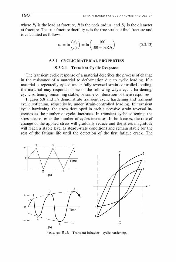
where Pf is the load at fracture, R is the neck radius, and Df is the diameter

at fracture. The true fracture ductility ef is the true strain at final fracture and

is calculated as follows:

ef ¼ lnAo

Af

� �

¼ ln100

100�%RA

� �

(5:3:13)

5.3.2 CYCLIC MATERIAL PROPERTIES

5.3.2.1 Transient Cyclic Response

The transient cyclic response of a material describes the process of change

in the resistance of a material to deformation due to cyclic loading. If a

material is repeatedly cycled under fully reversed strain-controlled loading,

the material may respond in one of the following ways: cyclic hardening,

cyclic softening, remaining stable, or some combination of these responses.

Figures 5.8 and 5.9 demonstrate transient cyclic hardening and transient

cyclic softening, respectively, under strain-controlled loading. In transient

cyclic hardening, the stress developed in each successive strain reversal in-

creases as the number of cycles increases. In transient cyclic softening, the

stress decreases as the number of cycles increases. In both cases, the rate of

change of the applied stress will gradually reduce and the stress magnitude

will reach a stable level (a steady-state condition) and remain stable for the

rest of the fatigue life until the detection of the first fatigue crack. The

s5

3

1

2

4

+

−

+

−

s

1

1

3

3

5

5

2

2 4

4

Time

Time

e

e

(a)

(b)

(c)

figure 5.8 Transient behavior—cyclic hardening.


transient cyclic behavior is handled by using the cyclically stable behavior in

the local strain–life approach since the percentage of the number of cycles

spent on this transient response is relatively small compared to the total

fatigue life.

The transient phenomenon is believed to be associated with stability of the

dislocation substructure within the metal crystal lattice of a material. In

general, soft materials such as aluminum alloys with low dislocation densities

tend to harden and hard materials such as steels tend to soften.

5.3.2.2 Steady-State Cyclic Stress–Strain Behavior

The properties determined from the steady-state cyclic stress–strain

response are the following:

s0y ¼ 0:2% Offset cyclic yield strength

K 0 ¼ Cyclic strength coefficient

n0 ¼ Cyclic strain hardening exponent

Fatigue life can be characterized by the steady-state behavior because for

constant strain–amplitude controlled testing, the stress–strain relationship

becomes stable after rapid hardening or softening in the initial cycles corres-

ponding to the first several percent of the total fatigue life. The cyclic stable

stress–strain response is the hysteresis loop and is identified in Figure 5.10.

The hysteresis loop defined by the total strain range (De) and the total stress

range (Ds) represents the elastic plus plastic work on a material undergoing

loading and unloading. Usually, the stabilized hysteresis loop is taken at half

of the fatigue life.

σ

σ

5

3

1

4

2

e

+

−

1

1

3

3

5

5

2

2

4

4

Time

Time

ε

(a)

(c)(b)

figure 5.9 Transient behavior—cyclic softening.


When a family of stabilized hysteresis loops with various strain amplitude

levels is plotted on the same axes as shown in Figure 5.11, a cyclic stress–

strain curve is defined by the locus of the loop tips and has the following form

similar to the monotonic stress–strain response:

e ¼ ee þ e

p ¼ s

Eþ s

K 0

� �1=n0

(5:3:14)

where 0 represents the parameters associated with cyclic behavior to differen-

tiate them from those associated with monotonic behavior.

The cyclic yield stress (s0y) is the stress at 0.2% plastic strain on a cyclic

stress–strain curve. This value is determined by constructing a line parallel to

the modulus of elasticity through the 0.2% strain offset at the zero stress

point. The stress at which the line intersects the cyclic stress–strain curve is

taken as the cyclic yield stress.

Masing’s assumption (Masing, 1926) states that the stress amplitude

versus strain amplitude curve can be described by the cyclic stress–strain

curve, meaning

ea ¼ eea þ e

pa ¼

sa

Eþ sa

K 0

� �1=n0

(5:3:15)

E

1

e

∆εe

∆s

∆εp

∆ε

s

figure 5.10 Hysteresis loop.


It also states that the material should have symmetric behavior in tension

and compression. This is true for many homogeneous metals. Equation

5.3.15 can be rewritten in terms of strain range and stress range:

De

2¼ Dee

2þ Dep

2¼ Ds

2Eþ Ds

2K 0

� �1=n 0

(5:3:16)

which can be reduced to the following stabilized hysteresis loop equation:

De ¼ Ds

Eþ 2

Ds

2K 0

� �1=n 0

(5:3:17)

Equation 5.3.17 has been widely used for describing and tracking the

stress–strain behavior under variable amplitude loading conditions.

The cyclic strength coefficient K 0 and the cyclic strain hardening exponent

n0 are the intercept and slope of the best fit line, respectively, to the true stress

amplitudeDs

2versus true plastic strain amplitude

DeP

2data plotted on a

log–log scale:

Ds

2¼ K 0 Dep

2

� �n0

(5:3:18)

where the true plastic strain amplitude is calculated by the following

equation:

Dep

2¼ De

2� Ds

2E(5:3:19)

hysteresis loops

cyclicmonotonic

e

s

figure 5.11 Cyclic stress-strain curve.


When performing the least-squares fit to determine K 0 and n0, the loga-

rithms of the true plastic strain amplitude are the statistically independent

variable, and the logarithms of the stress amplitude are the statistically

dependent variable. It is recommended (Williams et al., 2003) that plastic

strain amplitudes less than 0.0005mm/mm be neglected in the regression

analysis

The cyclic stress–strain curve reflects the resistance of a material to cyclic

deformation and can be different from the monotonic stress–strain curve.

Superimposed monotonic and cyclic curves are shown in Figure 5.12. Typic-

ally, metals with a high monotonic strain–hardening exponent (n > 0:2) willharden whereas those with a low monotonic strain hardening exponent

(n < 0:1) will cyclically soften. A rule of thumb (Bannantine et al., 1990) is

that the material will harden if Su=Sy > 1:4 and the material will soften if

Su=Sy < 1:2. For ratios of Su=Sy between 1.2 and 1.4, the material can exhibit

hardening, softening, or both. These figures indicate that use of monotonic

material properties for fatigue life predictions can sometimes lead to inaccur-

ate results.

Example 5.1. A notched component made of SAE 1137 carbon steel has the

following material properties: E ¼ 209000 MPa, K 0 ¼ 1230 MPa, n0 ¼ 0:161.When the component is subjected to cyclic loading, a strain gage placed at the

notch root records a fully reversed constant strain amplitude of 10,000 micro-

strains (me). Model the hysteresis stress–strain response at the notch root.

Solution. To determine the stress–strain response and hysteresis loop, we

must first determine the initial loading case and then the initial reversal and

all of the following. We first consider the initial loading.

Cyclic softening Cyclic hardening

Cyclically stable Mixed behavior

cyclic

monotonic

monotonic

monotonic

monotonic

cyclic

cyclic

cyclic

ss

e

e

e

e

figure 5.12 Cyclic and monotonic stress–strain behavior.


The initial loading starts from 0:0me and extends to the first 10; 000me( ¼ 0:010). To define the curve generated by the stress–strain relationship

during initial loading, it is important to analyze multiple points along the

strain path. For the initial loading, steps from 0.002 to 0.01 strains are used.

To determine the stress at each intermediate step of the strain, the cyclic

stress–strain equation is used:

e1 ¼s1

Eþ s1

K 0

� � 1n0

For example, in the case of strain changing from 0 to 0.01, the stress s1 at

the strain of 0.01 is determined:

0:01 ¼ s1

209000þ s1

1230

� � 10:161

Solving for s1,

s1 ¼ 557:46MPa

Table 5.1 shows the values for s and e at each increment in the initial

loading condition. Having defined the initial loading condition, we can now

move on to the first loading reversal. Again, it is important to define the curve

so that multiple points along the strain are considered. To determine the

change in stress, the following Masing model is used:

De ¼ Ds

Eþ 2

Ds

2K 0

� � 1n0

For example, in the case of the strain changing from 0.01 to �0:01, thestress increment Ds corresponding to the strain increment De ¼ 0:02 is

obtained by

0:02 ¼ Ds

209000þ 2

Ds

2� 1230

� � 10:161

Solving for Ds results

table 5.1 Initial Loading: True

Stress and Strain Data Points

e s (MPa)

0.002 342.98

0.004 447.03

0.006 497.56

0.008 531.56

0.010 557.46


Ds ¼ 1114:92MPa

Because Masing’s model calculates the change in stress, to determine the

stress at this point (e ¼ �0:01), the change must be compared to any stress

value in this reversal with respect to the reference stress s ¼ 557:46MPa, the

ending point of this reversal.

s2 ¼ s1 � Ds ¼ 557:46� 1114:92 ¼ �557:46MPa

Table 5.2 shows the values for s and e at each increment in the first loading

reversal. All the stress and the strain increments in each step are calculated

with respect to the reference point.

For the second loading reversal, the same procedure is used as that for the

first. For example, in the case of strain changing from �0:010 to 0.010, Dscorresponding to De ¼ 0:020 is determined by

0:02 ¼ Ds

209000þ 2

Ds

2� 1230

� � 10:161

Solving for Ds,

Ds ¼ 1114:92MPa

Again, when comparing to the reference stress (s2 ¼ �557:46MPa), the

stress at this point is calculated as

s3 ¼ s2 þ Ds ¼ �557:46þ 1114:92 ¼ 557:46MPa

Table 5.3 shows the tabulated values for s and e at each increment in the

second reversal. From the points calculated for the initial, first, and second

reversals, the hysteresis loop can be graphed in Figure 5.13, in which the local

s� e coordinate is located at each reference point.

table 5.2 First Loading Reversal: True Stress

and Strain Data Points

e De Ds (MPa) s (MPa)

0.010 Reference 0.0 557.46

0.008 0.002 411.70 145.76

0.006 0.004 685.96 �128.5

0.004 0.006 815.30 �257.84

0.002 0.008 894.06 �336.6

0.000 0.010 950.70 �393.24

�0.002 0.012 995.12 �437.66

�0.004 0.014 1031.79 �474.33

�0.006 0.016 1063.12 �505.66

�0.008 0.018 1090.52 �533.06

�0.010 0.020 1114.92 �557.46


5.3.2.3 Constant-Amplitude Fatigue Behavior

The properties that are determined from stabilized hysteresis loops and

strain–life data are the following:

s0f ¼ Fatigue strength coefficient

b ¼ Fatigue strength exponent, usually varying between �0:04 and

�0:15 for metals

e0f ¼ Fatigue ductility coefficient

table 5.3 Second Loading Reversal: True

Stress and Strain Data Points


�0.010 Reference 0.0 �557.46

�0.008 0.002 411.70 �145.76

�0.006 0.004 685.96 128.5

�0.004 0.006 815.30 257.84

�0.002 0.008 894.06 336.6

0.000 0.010 950.70 393.24

0.002 0.012 995.12 437.66

0.004 0.014 1031.79 474.33

0.006 0.016 1063.12 505.66

0.008 0.018 1090.52 533.06

0.010 0.020 1114.92 557.46

-600

-400

-200

0

200

400

600

-15000 -10000 -5000 0 5000 10000 15000

strain, microstrains

str

ess,

MP

a

e

e

e

s

s

s

figure 5.13 Hysteresis stress-strain curve at the notch root.


c ¼ Fatigue ductility exponent, usually varying between �0:3 and

�1:0 for metals

2NT ¼ Transition fatigue life in reversals

Based on the proposal by Morrow (1965), the relation of the total strain

amplitude (ea) and the fatigue life in reversals to failure (2Nf ) can be

expressed in the following form:

ea ¼ eea þ e

pa ¼

s0f

E(2Nf )

b þ e0

f (2Nf )c (5:3:20)

Equation 5.3.20, called the strain–life equation, is the foundation for the

strain-based approach for fatigue. This equation is the summation of two

separate curves for elastic strain amplitude–life (eea � 2Nf ) and for plastic strain

amplitude-life (epa � 2Nf ). Dividing the Basquin (1910) equation by the modu-

lus of elasticity gives the equation for the elastic strain amplitude-life curve:

eea ¼Dee

2¼ sa

E¼

s0f

E2Nf

� �b(5:3:21)

Both Manson (1953) and Coffin (1954) simultaneously proposed the equa-

tion for the plastic strain amplitude-life curve:

epa ¼Dep

2¼ e

0

f (2Nf )c (5:3:22)

When plotted on log–log scales, both curves become straight lines as

shown in Figure 5.14. Besides the modulus of elasticity E, the baseline strain

0.001

0.01

1.E+03 1.E+04 1.E+05 1.E+06 1.E+07

fatigue life (reversals)

str

ain

am

plit

ude

Elastic

Plastic

Total

b

c

1

1

2NT =25,000

reversals

figure 5.14 Schematic of a total strain–life curve.


life expression is defined by four regression parameters: fatigue strength

coefficient (s0f ), fatigue strength exponent (b), fatigue ductility coefficient

(e0f ), and fatigue ductility exponent (c).

When determined by using a least-squares analysis, these parameters are

valid in the range of the experimental data. This emphasizes the necessity for

a broad range in experimental data and a sufficient number of data points

required in each of the elastic strain dominant and the plastic strain dominant

regions. Instead of using the nonlinear least-squares method for the strain–

life model (Langlais and Vogel, 1995), the approach preferred here is to use

the linear model for fitting each linear range of the data because it gives less

weight to misleading low-cycle and high-cycle data and provides better

results (Yan et al., 1992; Williams et al., 2003). The choice of the linear

range of data depends on the transition fatigue life.

The transition fatigue life point is defined as the fatigue life when

the magnitude of plastic strain amplitude is equal to that of elastic strain

amplitude. As shown in Figure 5.14, the transition fatigue life (2NT ) is the

intersection of the elastic and plastic strain-life curves. In this case, a fatigue

life of 25,000 reversals is just an example of where the transition life may occur.

The region to the left of this point where fatigue life is less than the transition

fatigue life is considered the plastic strain dominant region and is referred to as

the low-cycle fatigue (LCF) region. The region to the right where fatigue life is

higher than the transition fatigue life is the elastic strain dominant region and

is referred to as the high-cycle fatigue (HCF) region. Figure 5.15 shows the

100 300 500 700

hardness, BHN

105

104

103

102

101

1

trans. fa

tigue life, 2N

T

figure 5.15 Relationship between transition life and hardness for steels. Adapted with

permission from Landgraf (1970), ASTM STP467, Copyright ASTM International.


order-of-magnitude variation in transition life for steels with various hard-

ness values where steels with high hardness and ultimate strength have lower

transition fatigue life.

The following two examples demonstrate how strain–life fatigue param-

eters are determined by the least-squares analysis. Different from the ASTM

standard E739 (ASTM 1998b), an approach for the statistical analysis of

strain–life fatigue data (Williams et al., 2003) is introduced here and has the

following unique features:

(1) A linear regression model is restricted to the linear range of the data, e.g.,

either the low-cycle fatigue data or the high-cycle fatigue data.

(2) A threshold of plastic strain amplitude of 0.0005 is suggested. Below this

value, the data points can be neglected to avoid measurement errors.

(3) A method based on a modification of the Owen tolerance interval (Shen

et al., 1996) is used to quantify the statistical variation of fatigue data.

In these examples, the introduction of the transition fatigue life is import-

ant to accurately determine the fatigue strength parameters (b and s0f ) and the

fatigue ductility parameters (c and e0f ). The elastic strain dominant and

the plastic strain dominant regions need to be emphasized, respectively. By

using the transition fatigue life as the boundary between these two regions,

the data points in each region can be accurately represented and appropri-

ately weighted in this analysis.

Example 5.2. A test company conducted strain-controlled constant-ampli-

tude axial fatigue tests on 16 samples with one sample for each strain

amplitude. A summary of the test results is shown in Table 5.4. The samples

were made of SAE 1137 mild carbon steel. Throughout the tests, failures

were defined when load drop was 50% of the initial value. BKE denotes

failure detected between knife edges and NOKE denotes failure detected

outside the knife edges, with no other cracks in between. Based on the

available experimental data, determine the median and the R90C90 cyclic

and fatigue properties.

Solution. First, the fracture location must be considered for each sample. If

the sample did not fail, the data point should be excluded from this analysis,

because this analysis technique is valid only for failure occurrences. In this

case, the data point with Sample 13 is not considered in this analysis.

If the sample displayed a failure that occurs outside of the knife edges (test

section) with no other cracks evident within the test section, a NOKE failure,

that point is circumspect. To determine the validity of this point, the duration

before failure must be checked. If the failure was obviously premature,

occurring after a small fraction of the anticipated number of cycles with

respect to the life trend, the point should be excluded and a note with an


explanation made. The data point for Sample 11 is valid from the aspect of

the life trend. Other measurements can be checked to verify the decision to

exclude a point. For example, one can check the minimum and maximum

stresses observed during an individual test. The absolute value of the min-

imum and maximum should be approximately equal. If not, a mean or

residual stress has likely developed because of improper testing procedure.

Such effects should not occur in testing of this nature.

Next, the elastic and plastic strain amplitudes are calculated. The

measured data allow one to determine the location of the transition fatigue

life. The plastic strain and elastic strain amplitudes are required to be calcu-

lated for each sample in the test. A new data set for fatigue data analysis is

generated in Table 5.5. Based on the same magnitude of the calculated elastic

and plastic strain amplitudes in Table 5.5, the transition life is roughly

estimated as 22,000 reversals.

Once the transition life is estimated, the data to be analyzed are chosen

such that an intersection of the plastic and elastic strain curve is ensured. The

choice of the data points in each region is very subjective. Extra data points

beyond the elastic-strain or the plastic-strain dominant region are selected

because the transition fatigue life has a stochastic nature. In this example, all

the data points with viable lives less than and the two data points immedi-

ately greater than the transition life are selected for obtaining fatigue ductility

parameters. Fatigue strength parameters are developed by using all the data

points with viable lives greater than and the two points immediately less than

the transition life.

table 5.4 Constant-Amplitude Axial Fatigue Test Data for SAE 1137 Carbon Steel

Sample

Number

Modulus

(MPa)

Total Strain

Amplitude

(mm/mm)

Max. Stress

at Half-Life

(MPa)

Min. Stress

at Half-Life

(MPa)

Total

Fatigue Life

(cycles)

Failure

Location

16 208229 0.00900 545 �561 2117 BKE

15 207815 0.00800 532 �550 2351 BKE

12 206850 0.00700 515 �529 3699 BKE

10 211676 0.00600 500 �513 5502 BKE

4 208919 0.00500 461 �467 7384 BKE

9 215124 0.00450 456 �466 10035 BKE

1 206850 0.00400 437 �444 15264 BKE

3 207540 0.00350 420 �427 20884 BKE

2 210297 0.00300 401 �409 38552 BKE

5 208229 0.00250 374 �379 66838 BKE

8 209608 0.00225 354 �366 92467 BKE

6 210298 0.00200 342 �358 218749 BKE

11 209963 0.00188 330 �336 336546 NOKE

7 206161 0.00175 316 �322 1663979 BKE

13 207367 0.00150 288 �295 5000000 NONE


Low-Cycle Fatigue Data Analysis

To begin the fatigue ductility parameter analysis, the following data are

required: total life and calculated plastic strain amplitude for the plastic

region data points. Because the plastic strain amplitude is the control param-

eter, the statistical independent variable X for the analysis will be the loga-

rithms of the plastic strain amplitude, log (epa), and the statistical dependent

variable Y will be the logarithms of the fatigue life, log (2Nf ). A linear

regression analysis by using the least-squares method on the data selected is

performed. The R2 regression statistic should be more than 0.90. A lower R2

value suggests that substantial variations due to factors other than the linear

relationship between the two variables exist. Given the intercept (A), slope

(B), and variables X and Y, the equation for the regression line takes the

linear form:

Y ¼ AAþ BBX

where

AA ¼ (� 1=c) log (e0

f )

BB ¼ 1=c

and

table 5.5 Summary of Useful Fatigue Test Data for SAE 1137 Mild Carbon Steel

Sample

Number

Total

Strain

Amplitude

(mm/mm)

Average

Stress

Amplitude

at Half-Life

(MPa)

Modulus

(MPa)

Total

Fatigue

Life

(reversals)

Calculated

Elastic

Strain

Amplitude

(mm/mm)

Calculated

Plastic Strain

Amplitude

(mm/mm)

16 0.00900 553 208229 4234 0.002656 0.006344

15 0.00800 540 207815 4702 0.002603 0.005397

12 0.00700 522 206850 7398 0.002523 0.004477

10 0.00600 507 211676 11004 0.002394 0.003606

4 0.00500 464 208919 14768 0.002221 0.002779

9 0.00450 461 215124 20070 0.002144 0.002356

1 0.00400 441 206850 30528 0.00213 0.001870

3 0.00350 424 207540 41774 0.002041 0.001459

2 0.00300 405 210297 77104 0.001925 0.001075

5 0.00250 376 208229 133676 0.001806 0.000695

8 0.00225 360 209608 184934 0.001718 0.000532

6 0.00200 350 210298 437498 0.00163 0.000337

11 0.00188 333 209963 673092 0.001587 0.000293

7 0.00175 319 206161 3327958 0.001548 0.000202

Note: Underlined values indicate which data points were used for the low-cycle and high-cycle fatigue

data analysis.


c ¼ 1=BB (5:3:23)

e0

f ¼ 10(�c�AA) (5:3:24)

The linear regression analysis results in AA ¼ 0:06933, BB ¼ �1:611,R2 ¼ 0:9942, and s ¼ 0:03011. By using Equations 5.3.23 and 5.3.24, the

fatigue ductility parameters are found to be c ¼ �0:6207 and e0f ¼ 1:104.

Because the number of data points in the analysis exceeds five, a reliability

and confidence analysis can be performed. For this example, an R90C90

analysis is illustrated. Following the statistical analysis method described

in Section 4.2.2, the R90C90 regression line YR90C90 can be determined

by shifting the median regression line toward the left with the following

equation:

YR90C90 ¼ Y� KOWEN � s (5:3:25)

where s is the standard error of Y on X. In this case for the sample size n ¼ 8,

the Owen tolerance factor, KOWEN, is 2.441, and the standard error (s) from

the linear regression analysis is 0.03011. Following the procedure in Section

4.2.2 and the assumption of a constant fatigue ductility exponent

(c ¼ �0:6207), the R90C90 fatigue ductility coefficient (e0f ,R90C90) is deter-

mined to be 0.9938.

High-Cycle Fatigue Data Analysis

The analysis for the cyclic properties relevant to the elastic-strain domin-

ant region (b and s0f ) is performed using the same method and criteria

previously detailed, but the half-life stress amplitude is used instead of the

plastic strain amplitude. The elastic strain amplitude could be used, but

the coefficient produced would have to be multiplied by the average value

of the modulus of elasticity to produce the desired strength coefficient. To

generate the values of s0f and b when performing the least squares on the

high-cycle fatigue data, the logarithms of the stress amplitude, log (sa), are

the statistical independent variable, and the logarithms of the reversals to

failure, log (2Nf ), are the statistical dependent variable. Again, the regression

equation assumes the following linear form:

Y ¼ AAþ BBX

where

AA ¼ (� 1=b) log (s0

f )

BB ¼ 1=b

and

b ¼ 1=BB (5:3:26)

s0

f ¼ 10(�b�AA) (5:3:27)


The linear regression analysis results in AA ¼ 37:11, BB ¼ �12:36, R2 ¼0:9517, and s ¼ 0:1742. By using Equations 5.3.26 and 5.3.27, the fatigue

strength parameters are determined to be b ¼ �0:0809 and s0f ¼ 1006MPa.

Because the number of data points in the analysis exceeds five, a reliability

and confidence analysis can be performed. In this case, for a sample size

n ¼ 10, the Owen tolerance factor, KOWEN, is 2.253, and the standard error, s,

from the linear regression analysis is 0.1742. Following the procedure

in Section 4.2.2 and using the assumption of constant fatigue strength expo-

nent (b ¼ �0:0809), the R90C90 fatigue strength coefficient (s0f ,R90C90) is

determined to be 936MPa.

Once the four fatigue parameters have been derived, the total strain–life

curve can be assembled. The graph in Figure 5.16 consists of the total strain–

life curve, plastic strain–life curve, and elastic strain–life curve. These three

curves are plotted on a log–log scale graph with the experimental data

superimposed on the graph. This aids in demonstrating the quality of

the curve fit. If the R90C90 curves were generated, these curves can be

superimposed with the median curves for design, as shown in Figure 5.16.

Analyses of the Cyclic Stress–Strain Behavior

The cyclic strength coefficient K 0 and the cyclic strain hardening exponent

n0 are related by Equation 5.3.18. Instead of using the nonlinear least-squares

0.001

0.01

1.E+03 1.E+04 1.E+05 1.E+06 1.E+07


str

ain

am

plit

ud

e (

mm

/mm

)

R50 Total Strain

R90C90 Total Strain

Experimental Data

R50 Elastic

R90C90 Elastic

R50 Plastic

R90C90 Plastic

figure 5.16 Total strain–life curves, R50 and R90C90, for SAE 1137 steel.


method (Langlais and Vogel, 1995) for the Masing equation, Equation

5.3.15, the fitting procedure illustrated here is to use the linear least-squares

analysis to fit the entire range of the logarithms of stress and plastic

strain data. When performing the least-squares fit, the logarithms of the

true plastic strain amplitude, log (epa), are the statistical independent variable

X and the logarithms of the stress amplitude, log (sa), are the statistical

dependent variable Y. Plastic strain amplitudes of less than 0.0005

are neglected to avoid measurement errors. Given the intercept A, slope

B, and variables X and Y, the equation for the regression line takes the linear

form:

Y ¼ AAþ BBX

where

AA ¼ log (K 0)

BB ¼ n0

and

n0 ¼ BB (5:3:28)

K 0 ¼ 10 AA (5:3:29)

In an analysis of the data presented in Table 5.5, all the sample data inwhich

plastic strain amplitude exceeds 0.0005 are included. The linear regression

analysis results in AA ¼ 3:090, BB ¼ 0:1608, R2 ¼ 0:9905, and s ¼ 0:008126.Thus, n0 ¼ 0:1608 and K 0 ¼ 1230MPa.

Reliability and confidence analysis for the cyclic stress–strain parameters

can be performed. In this case, for the sample size n ¼ 11, the Owen tolerance

factor, KOWEN, is 2.162, and the standard error, s, from the linear regression

analysis is 0.008126. With the assumption of constant cyclic strain hardening

exponent (n0 ¼ 0:1608), the R90C90 cyclic strength coefficient (K0R90C90) is

determined to be 1181MPa. The R50 and R90C90 cyclic stress–strain curves

for SAE 1137 carbon steel are illustrated in Figure 5.17.

If these simple power laws (Masing equation, Basquin equation, and

Coffin and Manson equation) are perfect fits to the test data, only four of

the six constants are independent. Solving Equations 5.3.21 and 5.3.22 to

eliminate fatigue life (2Nf ) and then comparing the results with Equation

5.3.18 gives the following relation between these six fatigue properties:

K 0 ¼s

0f

e0f

� �n0 (5:3:30)

n0 ¼ b

c(5:3:31)


However, because of the different choice of the fitting data range, these

equations are no longer valid. A discrepancy arises because the Basquin

equation and the Coffin and Manson equation apply only locally and the

equations are incorrect for data outside the range as a result of the local

fitting procedure. Similarly, plastic strain components are in error outside the

range in which the Massing equation (Equation 5.3.18) was fit. Consequently,

elastic and plastic strains calculated from the strain life curve disagree with

the elastic and plastic strains computed from the cyclic stress–strain curve, or

s0f

E2Nf

� �b 6¼ sa

E(5:3:32)

and

e0

f 2Nf

� �c 6¼ sa

K 0

� �1=n0

(5:3:33)

Determination of the Transition Fatigue Life

The transition fatigue life in reversals (2NT ) can be calculated by equating

the elastic and plastic strain components from the strain–life equation:

s0f

E2NTð Þb¼ e

0

f 2NTð Þc (5:3:34)

and

2NT ¼e0fE

s0f

!1=b�c

(5:3:35)

0

100

200

300

400

500

600

0 0.002 0.004

ε

0.006 0.008 0.01

sM

Pa

)

R50

R90C90

figure 5.17 Cyclic stress–strain curves, R50 and R90C90, for SAE 1137 steel.


Therefore, the transition fatigue lives for R50 and R90C90 are obtained as

23,700 reversals and 22,300 reversals, respectively. A typical summary of this

analysis is presented in Table 5.6.

Example 5.3. Repeat the same fatigue data analysis demonstrated in

Example 5.2 for the SAE D4512, a low-ductility, high-strength alloy used

in the industrial case components. The strain-controlled axial fatigue test

results are summarized in Table 5.7. Determine the median and the R90C90

strain–life curves.

Solution. A brief material analysis is provided for SAE D4512, which is a

steel used in industrial cast components. This is a low-ductility, high-strength

alloy that does not exhibit the transition fatigue life point within a commonly

tested total strain range. The transition life point for this material occurs

beyond the experimental data range at approximately 800 reversals. In such a

case, the criterion for data selection is plastic strain being greater than

0.0005mm/mm rather than the data’s relationship to the position of the

transition life point.

The data presented in Table 5.7 are analyzed by the same method dis-

cussed in the example for SAE 1137 carbon steel. The only difference is how

the data are selected. The data are reviewed using the same failure location

criteria and the same minimum plastic strain requirements. The selection of

data to use for the plastic strain analysis is the primary difference. In the

situation in which the transition life point is not present in the data, all data

with a calculated plastic strain greater than 0.0005mm/mm are used to

develop the fatigue ductility coefficient and exponent. To determine the

fatigue strength coefficient and exponent, all data points that were not

excluded because of an improper failure are used. Figure 5.18 shows the

median and R90C90 total strain–life curves, the median and R90C90 plastic

and elastic regression curves, and the experimental data. Figure 5.19 depicts

the R50 and R90C90 cyclic stress–strain curves. A typical summary of this

analysis is presented in Table 5.8.

table 5.6 Data Analysis Summary for SAE 1137 Carbon Steel

R50 R90C90

Average Young’s modulus (MPa) E 209000 209000

Fatigue strength coefficient (MPa) s0f 1006 936

Fatigue strength exponent b �0.0809 �0.0809

Fatigue ductility coefficient e0f 1.104 0.9938

Fatigue ductility exponent c �0.6207 �0.6207

Cyclic strength coefficient (MPa) K 0 1230 1181

Cyclic strain hardening exponent n0 0.1608 0.1608

Transition fatigue life (reversals) 2NT 23600 22200


5.4 mean stress correction methods

In designing for durability, the presence of a nonzero mean normal stress

can influence fatigue behavior of materials because a tensile or a compressive

normal mean stress has been shown to be responsible for accelerating or

decelerating crack initiation and growth. Experimental data support that

compressive mean normal stresses are beneficial and tensile mean normal

stresses are detrimental to fatigue life. This has been observed under condi-

tions when the mean stress levels are relatively low compared to the cyclic

yield stress and the fatigue behavior falls in the long-life regime where elastic

strain is dominant.

In conjunction with the local strain life approach, many models have been

proposed to quantify the effect of mean stresses on fatigue behavior. The

commonly used models in the ground vehicle industry are those by Morrow

(1968) and by Smith, Watson, and Topper (Smith et al., 1970). These equa-

tions are empirically based and should be compared with test data to deter-

mine which model is the most appropriate for the material and test conditions

of interest. The two models are described in the following sections.

table 5.7 Summary of Useful Fatigue Test Data for SAE 4512

Sample

Number

Total Strain

Amplitude

(mm/mm)

Average

Stress

Amplitude

at Half-Life

(MPa)

Modulus

(MPa)

Total

Fatigue

Life

(reversals)

Calculated

Elastic

Strain

Amplitude

(mm/mm)

Calculated

Plastic

Strain

Amplitude

(mm/mm)

Failure

Location

14 0.00500 477 175695 1066 0.002715 0.002285 BKE

6 0.00450 469 177762 3780 0.002638 0.001862 BKE

9 0.00400 451 173628 5914 0.002598 0.001402 BKE

11 0.00350 433 172250 14842 0.002514 0.000986 BKE

16 0.00315 422 172939 21126 0.002440 0.000710 BKE

4 0.00300 411 171561 33064 0.002396 0.000604 BKE

15 0.00275 403 172939 22138 0.002330 0.000420 BKE

19 0.00265 395 173284 31888 0.002280 0.000370 BKE

1 0.00250 376 172939 72100 0.002174 0.000326 BKE

8 0.00235 373 175695 114936 0.002123 0.000227 BKE

10 0.00215 354 175695 125840 0.002015 0.000135 BKE

2 0.00200 329 174317 314982 0.001887 0.000113 OKE

13 0.00183 303 172250 1337430 0.001759 0.000071 BKE

3 0.00175 289 174317 438390 0.001658 0.000092 BKE

12 0.00165 278 172939 930654 0.001608 0.000043 BKE

5 0.00150 257 174317 11025548 0.001474 0.000026 NONE

7 0.00100 171 174317 305602 0.000981 0.000019 NONE

Note: Underlined values indicate which data points were used for the elastic analysis and the plastic

analysis. The last two rows of data points were excluded from the analysis for no cracks.


0.001

0.01

1.E+02 1.E+03 1.E+04 1.E+05 1.E+06 1.E+07


str

ain

am

plit

ud

e (m

m/m

m)

R50 Total Strain

R90C90 Total Strain

Experimental Data

R50 Elastic

R90C90 Elastic

R50 Plastic

R90C90 Plastic

figure 5.18 Total strain–life curves, R50 and R90C90, for SAE D4512 steel.

0

100

200

300

400

500

0 0.001 0.002 0.003 0.004 0.005 0.006

sM

Pa

)

R50

R90C90

e

figure 5.19 Cyclic stress–strain curves, R50 and R90C90, for SAE D4512 steel.

Mean Stress Correction Methods 209

5.4.1 MORROW’S MEAN STRESS CORRECTION METHOD

Morrow has proposed the following relationship when a mean stress is

present:

ea ¼s

0f � sm

E2Nf

� �bþe0

f 2Nf

� �c(5:4:1)

This equation implies that mean normal stress can be taken into account

by modifying the elastic part of the strain–life curve by the mean stress (sm).

As illustrated in Figure 5.20, the model indicates that a tensile mean stress

would reduce the fatigue strength coefficient s0f whereas a compressive mean

stress would increase the fatigue strength coefficient. This equation has been

extensively cited for steels and used with considerable success in the long-life

regime when plastic strain amplitude is of little significance.

Walcher, Gray, and Manson (Walcher et al., 1979) noted that for other

materials such as Ti-6Al-4V, s0f is too high a value for mean stress correction

table 5.8 Data Analysis Summary for SAE D4512 Steel

R50 R90C90

Average Young’s modulus (MPa) E 174000 174000

Fatigue strength coefficient (MPa) s0f 978 884

Fatigue strength exponent b �0.0876 �0.0876

Fatigue ductility coefficient e0f 0.0556 0.0371

Fatigue ductility exponent c �0.4305 �0.4305

Cyclic strength coefficient (MPa) K 0 939 926

Cyclic strain hardening exponent n0 0.111 0.111

Transition fatigue life (reversals) 2NT 799 329

Plastic

Elastic

Total

b1

c1

(s�f − sm) / E

s�f / E

1 2Nf (log)2NT

e�f

ea(log)

figure 5.20 Morrow’s mean stress correction model.


and an intermediate value of kms0f can be determined by experiment. Thus, a

generic formula was proposed:

ea ¼kms

0f � sm

E2Nf

� �bþe0

f 2Nf

� �c(5:4:2)

This equation requires additional test data to determine kms0f .

5.4.2 SMITH–WATSON–TOPPER (SWT) MODEL

Smith, Watson, and Topper (Smith et al., 1970) proposed a method that

assumes that the amount of fatigue damage in a cycle is determined by

smaxea, where smax is the maximum tensile stress and ea the strain amplitude.

Also, the SWT parameter is simply a statement that ‘‘saea for a fully reversed

test is equal to smaxea for a mean stress test.’’ Thus, this concept can be

generalized and expressed in the following mathematical form (Langlais and

Vogel, 1995):

smaxea ¼ sa, rev ea, rev smax > 0 (5:4:3)

where sa, rev and ea, rev are the fully reversed stress and strain amplitudes,

respectively, that produce an equivalent fatigue damage due to the SWT

parameter. The value of ea, rev should be obtained from the strain–life curve

(Equation 5.3.20) and the value of sa, rev from the cyclic stress–strain curve

(Equation 5.3.15). The SWT parameter predicts no fatigue damage if the

maximum tensile stress becomes zero and negative. The solutions to Equa-

tion 5.4.3 can be obtained by using the Newton–Raphson iterative procedure.

For a special case of Equation 5.4.3, in which materials behave ideally and

satisfy the compatibility condition (i.e., n0 ¼ b=c and K

0 ¼ s0f = e

0f

� �n0

), the

maximum tensile stress for fully reversed loading is given by

smax ¼ sa ¼ s0

f 2Nf

� �b(5:4:4)

and by multiplying the strain–life equation, the SWT mean stress correction

formula is expressed as follows:

smaxea ¼s

0f

� �2

E2Nf

� �2b þ s0

f e0

f 2Nf

� �bþcsmax > 0 (5:4:5)

The SWT formula has been successfully applied to grey cast iron (Fash

and Socie, 1982), hardened carbon steels (Koh and Stephens, 1991; Wehner

and Fatemi, 1991), and microalloyed steels (Forsetti and Blasarin, 1988). The

SWT formula is regarded as more promising for use. As illustrated in Figure

5.21, a set of fatigue data with several levels of mean stress values coalesces

into a single curve. This indicates that the data points can be represented by

the SWT parameter.


Example 5.4. A component is made of steel with the following cyclic proper-

ties: E ¼ 210000MPa, s0f ¼ 1, 100MPa, b ¼ �0:1, e

0f ¼ 0:6, and c ¼ �0:5.

If the component were cycled under bending loads that induce a fully

reversed strain amplitude of 0.004, would you expect to shot peen the

component for fatigue life increase?

Solution. An appropriate shot-peening process will produce compressive

residual stress on the surface. The beneficial residual stress will enhance the

fatigue strength of the part in the high-cycle fatigue region, but the residual

stress will gradually dissipate in the low-cycle fatigue region because of the

phenomenon of mean stress relaxation. The transition fatigue life will serve as

a criterion for our decision making. From Equation 5.3.35, the transition

fatigue life can be calculated as follows:

2NT ¼e0fE

s0f

!1=b�c

¼ 140425 reversals

AISI 4340 Steelsu = 1172 MPa

102 103 105 106 107104

0.5

1

2

5

10

20

Nf, cycles to failure

sm

axe a

, (M

Pa)

sm, MPa

0

207

414

621

-207

figure 5.21 The SWT mean stress correction model. Reprinted by permission of

Pearson Education, Inc., Upper Saddle River, NJ, from ‘‘Mechanical Behavior of Materials,’’

2nd edition by Dowling (1998).


The total strain amplitude at the fatigue life transition can be determined

by calculating either the elastic strain amplitude or the plastic strain ampli-

tude at that life and multiplying the result by a factor of 2:

epa ¼

Dep

2¼ e

0

f 2Nf

� �c¼ 0:6� 140425�0:5 ¼ 0:0016

The total strain amplitude is 0:0032 ¼ 2� 0:0016ð Þ. The applied strain

amplitude of 0.0040 is higher than the strain amplitude at the transition

life. This indicates that the loading can be considered to fall within the low-

cycle fatigue region. Under this circumstance, shot peening should not be

considered to improve the fatigue strength of the component. This can also

be done by comparing the calculated fatigue life of the component to the

transition life.

Example 5.5. A single active strain gage was placed at the notch root of a

notched plate as shown in Figure 5.22. A notched component made of SAE

1137 carbon steel has the following material properties: E ¼ 209000MPa,

K0 ¼ 1230MPa, n0 ¼ 0:161, s

0f ¼ 1006MPa, b ¼ �0:0809, e

0f ¼ 1:104, and

c ¼ �0:6207. The recorded strain time history because of the applied load

is repetitive and is shown in Figure 5.23.

1. Plot the cyclic stress–strain response (hysteresis loop).

2. Estimate the fatigue life of the notched plate with the SWT formula.

3. Estimate the fatigue life of the notched plate with the Morrow equation.

Solution. To determine the hysteresis loop, we must first establish the initial

loading case and then the first loading reversal and all the subsequent cycles.

First, the initial loading is considered. The initial loading starts from zero

strain and extends to 5000me. To define the curve generated by the stress–

strain relationship during the loading, it is important to analyze multiple

points along the strain path. For the initial loading, steps of 0.0005 to a value

d = 3.2 mm

15.9 mm

thickness = 6.4 mm

P P

strain gage

figure 5.22 Configuration and dimension of a plate with a center hole.


of 0.005 are used. To determine the stress at each intermediate step of the

strain, the cyclic stress–strain equation is used.

e1 ¼s1

Eþ s1

K 0

� � 1n0

For example, s1 at e1 ¼ 0:005 is obtained by

0:005 ¼ s1

209000þ s1

1230

� � 10:161

Solving for s1

s1 ¼ 475:35MPa


initial loading.

−4000

−3000

−2000

−1000

0

1000

2000

3000

4000

5000

6000

time

str

ain

re

ad

ing

(m

icro

str

ain

) 5

4

3

2

1

figure 5.23 Recorded strain reading in microstrains at the notch root.

table 5.9 Initial Loading to Point 1:

True Stress and Strain Data Points

e1 s1 (MPa)

0.0005 104.45

0.0010 205.85

0.0015 288.10

0.0020 342.98

0.0025 380.21

0.0030 407.65

0.0035 429.24

0.0040 447.03

0.0045 462.17

0.0050 475.35


Having defined the initial loading condition, the first loading reversal can

now be examined (e1 ¼ 0:0050 ! e2 ¼ �0:0010). Again, it is important to

define the curve so that multiple points along the strain path are considered

with respect to the reference point (Point 1). To determine the change in stress

and strain, Masing’s model is used:

De ¼ Ds

Eþ 2

Ds

2K 0

� � 1n0

For example, in the case of strain change from 0.0050 to �0:0010(De ¼ 0:0060), the stress change, Ds, is obtained:

0:0060 ¼ Ds

209000 MPaþ 2

Ds

2� 1230

� � 10:161

Solving for Ds

Ds ¼ 815:30MPa

Because Masing’s model calculates the change in stress, the change must

be compared with the reference stress (s1 ¼ 475:35MPa) to determine the

stress at Point 2.

s2 ¼ s1 � Ds ¼ 475:35� 815:30 ¼ �339:95MPa


first loading reversal. For the second loading reversal (e2 ¼ �0:0010 ! e3 ¼0:0040), the same procedure is used as for the first, except that Point 2 serves

as the new reference point. For example, in the case of De ¼ 0:0050, Ds, isdetermined:

0:0050 ¼ Ds

209000þ 2

Ds

2� 1230

� � 10:161

Solving for Ds,

Ds ¼ 760:42MPa

Again, because Masing’s model calculates the change in stress, the change

must be compared with the reference stress (s2 ¼ �339:95MPa) to determine

the stress at Point 3.

s3 ¼ s2 þ Ds ¼ �339:95þ 760:42 ¼ 420:47MPa

For the third and fourth loading reversals, the same procedure is used.

When a material response returns to its previously experienced deformation,

it will remember the past path to reach such a state and will follow the path

with additional increase in deformation. This is the so-called memory effect

observed in materials undergoing complex loading histories. In the third


reversal, after the smaller reversal from Points 3 to 2 returns to the previously

experienced maximum deformation, Point 2, the rest of the loading reversal

will follow the path from Points 1 to 4. Tables 5.11–5.13 show the tabulated

values for s and e at each increment in the second, third, and fourth loading

reversals. From the points calculated for the initial and reversals, the hyster-

esis loops are graphed in Figure 5.24.

After determining the hysteresis loops, an estimate of the fatigue life using

the SWT method is needed. Ignoring the initial loading, a rainflow cycle

counting analysis is performed on the strain results. By using SWT Equation

5.4.3, the damage calculation results are determined in Table 5.14. The total

damage and fatigue life prediction are obtained as follows:

Sdi ¼ 1:78� 10�5 þ 8:09� 105 ¼ 9:87� 10�5

table 5.10 First Loading Reversal (Points 1 to 2): True Stress and Strain Data Points


0.0050 Reference 1 0.00 475.35

0.0045 0.0005 104.50 370.85

0.0040 0.0010 208.91 266.44

0.0035 0.0015 312.37 162.98

0.0030 0.0020 411.70 63.65

0.0025 0.0025 501.15 �25:8

0.0020 0.0030 576.20 �100:850.0015 0.0035 636.88 �161:53

0.0010 0.0040 685.96 �210:61

0.0005 0.0045 726.38 �251:03

0.0000 0.0050 760.42 �285:07�0:0005 0.0055 789.69 �314:34

�0:0010 0.0060 815.30 �339:95

table 5.11 Second Loading Reversal (Points 2 to 3): True Stress and Strain Data Points


�0:0010 Reference 2 0.00 �339:95

�0:0005 0.0005 104.50 �235:450.0000 0.0010 208.91 �131:04

0.0005 0.0015 312.37 �27:58

0.0010 0.0020 411.70 71.70

0.0015 0.0025 501.15 161.20

0.0020 0.0030 576.20 236.25

0.0025 0.0035 636.88 296.93

0.0030 0.0040 685.96 346.01

0.0035 0.0045 726.38 386.43

0.0040 0.0050 760.42 420.47


Life ¼ 1

Sdi¼ 1

9:87� 10�5¼ 10, 100 blocks

For comparison with the SWT method, an estimate of the fatigue life by

using Morrow’s method is generated. By using the rainflow counting analysis

given previously and the Morrow equation (Equation 5.4.1), the damage

calculation is presented in Table 5.15. The total damage and fatigue life

prediction are given as follows:

table 5.12 Third Loading Reversal (Points 3 to 4): True Stress and Strain Data Points


0.0040 Reference 3 0.00 420.47

0.0035 0.0005 104.50 315.97

0.0030 0.0010 208.91 211.56

0.0025 0.0015 312.37 108.10

0.0020 0.0020 411.70 8.77

0.0015 0.0025 501.15 �80:68

0.0010 0.0030 576.20 �155:730.0005 0.0035 636.88 �216:41

0.0000 0.0040 685.96 �265:49

�0:0005 0.0045 726.38 �305:91

�0:0010 0.0050 760.42 �339:950.0050 Reference 1 0.00 475.35

�0:0015 0.0065 838.04 �362:69

�0:0020 0.0070 858.48 �383:13

�0:0025 0.0075 877.05 �401:70�0:0030 0.0080 894.06 �418:71

table 5.13 Fourth Loading Reversal (Points 4 to 5): True Stress and Strain Data Points


�0:0030 Reference 4 0.00 �418:71

�0:0025 0.0005 104.50 �314:21�0:0020 0.0010 208.91 �209:80

�0:0015 0.0015 312.37 �106:34

�0:0010 0.0020 411.70 �7:01

�0:0005 0.0025 501.15 82.44

0.0000 0.0030 576.20 157.49

0.0005 0.0035 636.88 218.17

0.0010 0.0040 685.96 267.25

0.0015 0.0045 726.38 307.67

0.0020 0.0050 760.42 341.71

0.0025 0.0055 789.69 370.98

0.0030 0.0060 815.30 396.59

0.0035 0.0065 838.04 419.33

0.0040 0.0070 858.48 439.77

0.0045 0.0075 877.05 458.34

0.0050 0.0080 894.06 475.35


-400

-300

-200

-100

-500

0

100

200

300

400

500

600

-2000 0 2000 4000-4000 6000

strain, microstrains

str

ess, (M

Pa)

1

2

3

4ε

ε

ε

ε

ε

σ

σ

σ σ

σ

figure 5.24 Hysteresis stress strain curves at the notch root.

table 5.14 Summary of Rainflow Cycle Counting and Damage Calculation Results

Based on the SWT Formula

ni

From–

To (me)

emax

(me)

emin

(me)

smax

(MPa)

smin

(MPa)

ea

(me)

smax

(MPa)

Nf

(cycles) di

1 �1000

to 4000

4000 �1000 420.47 �339:95 2500 420.47 56316 1.78E-05

1 5000 to

�3000

5000 �3000 475.35 �418:71 4000 475.35 12354 8.09E-5

table 5.15 Summary of Rainflow Cycle Counting and Damage Calculation Results

Based on the Morrow Formula

ni

From–

To (me)

emax

(me)

emin

(me)

smax

(MPa)

smin

(MPa)

ea

(me)

sm(MPa)

Nf

(cycles) di

1 �1000

to 4000

4000 �1000 420.47 �339:95 2500 40.26 67384 1.48E-05

1 5000 to

�3000

5000 �3000 475.35 �418:71 4000 28.32 13596 7.35E-05


Sdi ¼ 1:48� 10�5 þ 7:35� 10�5 ¼ 8:83� 10�5

Life ¼ 1

Sdi¼ 1

8:83� 10�5¼ 11300 blocks

5.5 estimation of cyclic and fatigue properties

If no experimental data are available, an estimate of the cyclic and fatigue

behavior of a material can be helpful in the design stage. However, the

parameter estimation does not eliminate the need for real data. In Boardman

(1982), the following parameters for most steels that harden below 500 BHN

have been empirically developed:

a. Ultimate tensile strength, Su: A commonly used approximation for the

ultimate tensile strength based on Brinell hardness, BHN < 500, for low-

and medium-strength carbon and alloy steels is

Su(MPa) � 3:45� BHN (5:5:1)

b. Fatigue strength coefficient, s0f : An approximation relates the fatigue

strength coefficient s0f to the true fracture strength sf with a range from

0:9sf to 1:2sf . However, tests indicate the fatigue strength coefficient

shows a linear relation with the ultimate strength, Su, in the form

s0

f (MPa) � sf � Su þ 345MPa (5:5:2)

c. Fatigue strength exponent b:

b � � 1

6log

s0f

0:5� Su

!

(5:5:3)

d. Fatigue ductility coefficient e0f : The fatigue ductility coefficient e

0f is

thought to be of the same order as the true fracture ductility, ef .

e0

f � ef � ln100

100�%RA

� �

(5:5:4)

e. Fatigue ductility exponent c:

1. Strong steels, for which ef � 0:5, c ¼ �0:52. Ductile steels, for which ef � 1:0, c ¼ �0:6

f. Transition fatigue life 2NT (reversals): For steels, it is found that the

transition fatigue life has a dependence on Brinell hardness. Because

hardness varies inversely with ductility, the transition life decreases as

the hardness increases. The transition life is estimated as follows:

2NT � ln�1 (13:6� 0:0185� BHN) (5:5:5)

Estimation of Cyclic and Fatigue Properties 219

g. Cyclic strain hardening exponent n0:

n0 � b

c(5:5:6)

h. Cyclic stress coefficient K 0:

K 0 �s

0f

e0f

� �n0 (5:5:7)

For materials including steels, aluminum, and titanium alloys, Baumel and

Seeger (1990) proposed a method of approximating the cyclic properties from

monotonic stress strain relationships. The results of the so-called uniform

material law are documented in Table 5.16, where c ¼ 1 if Su

E#3� 10�3 or

c ¼ 1:375� 125 Su

E

� �

# 0 if Su

E> 3� 10�3. Other estimating procedures and

their uses are included elsewhere (Muralidharan and Manson, 1988; Roessle

and Fatemi, 2000; Park and Song, 2003).

Example 5.6. A notched component is made of SAE 4340 steel and has a

reported hardness of 242 BHN and modulus of elasticity of 205,000MPa.

Estimate the fatigue and cyclic material properties based on Boardman’s

approach.

Solution. The first step in this analysis is to determine the fatigue properties

for the material of the component.

Su ¼ 3:45(BHN) ¼ 3:45(242) ¼ 835MPa

s0

f ¼ Su þ 345MPa ¼ 835þ 345 ¼ 1180MPa

table 5.16 Estimated Cyclic Material Properties on Uniform

Material Law

Cyclic Material

Parameters

Steels, Unalloyed and

Low-Alloy

Aluminum and

Titanium Alloys

s0f 1:67Su 1.67 Su

b �0:087 �0:095e0f 0:59c 0.35

C �0:58 �0:69

K 0 1:65Su 1:61Su

n0 0.15 0.11

Se 0:45Su 0:42Su

Source: From Baumel and Seeger (1990).


b ¼ � 1

6log

2s0f

Su

!

¼ � 1

6log

2(1180)

835

� �

¼ �0:075

2Nt ¼ ln�1 (13:6� 0:0185BHN) ¼ ln�1 (13:6� 0:0185(242) ) ¼ 9164 reversals

Because the material is ductile steel, the fatigue ductility exponent c is

estimated to be �0:6.By using the following equation to determine the elastic strain amplitude

at the transition point,

Dee

2¼

s0f

E2NTð Þb¼ 1180

205000(9164)�0:075 ¼ 0:0029 at 2NT reversals

Because the elastic and plastic strain amplitudes are equal at the transition

life point,

Dep2

¼ e0

f 2NTð Þc¼ 0:0029, solving for e0

f

e0

f ¼0:0029

2NTð Þc ¼0:0029

(9164)�0:6¼ 0:691

Also, Equations (5.5.6) and (5.5.7) give

n0 ¼ b

c¼ �0:076

�0:6¼ 0:125

K 0 ¼s

0f

e0f

� �n0 ¼1180

(0:691)0:125¼ 1236MPa

5.6 notch analysis

Notch analysis is used to relate the nominal stress or strain changes in a

component to the local stress and strain response at a notch. This can be used

to predict the crack initiation life of notched components by using fatigue life

data from smooth laboratory specimens.

Neuber (1961) first analyzed a grooved shaft subjected to monotonic

torsional loading and derived a rule for nonlinear material behavior at the

notch root. Neuber observed, as illustrated in Figure 5.25, that after local

yielding occurs, the local true notch stress (s) is less than the stress predicted

by the theory of elasticity (se) whereas the local true notch strain (e) is greater

than that estimated by the theory of elasticity. Normalizing the local true

notch stress with respect to the nominal stress (S) and the true notch strain to

the nominal strain (e) leads to the true stress concentration (Ks) and the true

strain concentration (Ke) factors, respectively.

Figure 5.26 schematically illustrates the relation of three concentration

factors (Kt, Ks, Ke) versus the true stress with regard to the yield stress

Notch Analysis 221

(sy). Neuber hypothesized that the elastic stress concentration factor (Kt) is

the geometric mean of the true stress and strain concentration factors, i.e.,

Kt ¼ffiffiffiffiffiffiffiffiffiffiffi

KsKe

p

(5:6:1)

Squaring both sides of Equation 5.6.1 leads to the following expression

se ¼ (SKt)(eKt) (5:6:2)

When below the proportional limit, the product of S Kt is the local notch

stress calculated on an elastic material. The physical interpretation of the

Neuber rule is shown in Figure 5.27.

1sy

2sy

Stress

Distance from center

2r 3r 4r 5r 6r

Actual

Elastic theory

2ey

1ey

Strain

Distance from center

2r 3r 4r 5r 6r

Actual

Elastic theory

3ey

s

se

e

figure 5.25 Stresses and strains at a notch.

strain concentration, Ke

stress concentration, Ks

Kt = Ks = Ke

eKe =

SKs =

sy0.0 1.0

1.0

K

s

s

e

figure 5.26 Schematic of concentration factors.


For cyclic stress and strain behavior at a notch root under a plane stress

condition, the Neuber rule can be revised by replacing Kt with the fatigue

strength reduction factor (Kf ) (Wetzel, 1968; Topper et al., 1969) as follows:

Kf ¼ffiffiffiffiffiffiffiffiffiffiffi

KsKe

p

(5:6:3)

and

Ks ¼ sa

Sa

(5:6:4)

Ke ¼ea

ea(5:6:5)

where Sa and ea are the nominal stress and strain amplitudes, respectively,

and sa and ea are the local true stress and strain amplitudes, respectively. The

Kf factor was introduced in the Neuber rule to improve fatigue life predic-

tions and to include the stress gradient effect. However, this has been criti-

cized for both accounting twice the notch root plasticity effects and

incorporating the S–N empiricism into the more fundamentally satisfying

theory. By knowing these conflicting results, we recommend that the modified

Neuber rule (Equation 5.6.3) be used for local notch stress/strain estimates

and fatigue life predictions. The fatigue strength reduction factor was covered

in detail in Section 4.4.

During cyclic loading, it is assumed that the material follows the cyclic

stress–strain curve for the initial loading and the hysteresis stress–strain be-

havior for the subsequent loading reversals. Therefore, in terms of the initial

cyclic stress–strain curve the modified Neuber equation can be reduced to

s1e1 ¼ K2f S1e1 (5:6:6)

and, in terms of the hysteresis stress–strain curve, to

strain

stress

Kt S

Kt e

True stress-straincurve

Stress-strain curve basedon elastic behavior

s

e

figure 5.27 Interpretation of the Neuber model.

Notch Analysis 223

DsDe ¼ K2f DSDe (5:6:7)

Equations 5.6.6 and 5.6.7 represent the equations of a hyperbola (i.e., XY ¼constant) for given Kf and nominal stress/strain data. This constant which is

the right-handed side of Equation 5.6.7 is often referred to Neuber’s con-

stant. To solve for the two unknowns X and Y (i.e., s1 and e1 or Ds and De),an additional equation for cyclic material behavior is required.

Figure 5.28 shows the application of the modified Neuber model to a

notched plate subjected to an initial loading where the nominal strain

e1 and Kf are known based on the applied nominal stress S1 and the notch

geometry. The Neuber constant C1 can be calculated and a hyperbola of

the local stress and strain (s1e1 ¼ C1) is created. Then, a cyclic stress–strain

curve for the material is needed to intersect the hyperbola for the solution

of (s1,e1).

Figure 5.29 shows the application of the modified Neuber model to a

notched plate subjected to a first loading reversal, where the nominal strain

De and Kf are known based on the applied nominal stress DS and the notch

geometry. The Neuber constant C2 can be calculated and a hyperbola of the

local stress and strain changes (DsDe ¼ C2) is generated. A hysteresis stress-

strain curve for the material is needed to intersect the hyperbola for the

solution of (Ds,De).Depending on the nominal stress-strain behavior, the equations for

the local notch stress and strain solutions are discussed in the following

sections.

5.6.1 NOMINALLY ELASTIC BEHAVIOR

When the bulk of a notched component behaves elastically and plasticity

takes place locally at the notch root (i.e., a nominally elastic condition), the

following equations hold:

S1

S (

no

min

al str

ess)

time

strain, e

stress, s

cyclic s−e curve

(b) LOCAL(a) NOMINAL

S1

s1

e1

s1 e1 = C1

figure 5.28 Initial nominal stress loading with the modified Neuber rule.


- For the initial cyclic stress-strain curve

e1 ¼S1

E(5:6:8)

e1 ¼s1

Eþ s1

K 0

� �1=n00

(5:6:9)

- For the hysteresis stress-strain curve,

De ¼ DS

E(5:6:10)

De ¼ Ds

Eþ 2

Ds

2K 0

� �1=n0

(5:6:11)

The assumption of nominally elastic material behavior works well when

nominal stress is below 30% of the cyclic yield stress.

Substituting the elastic nominal stress–strain and the local cyclic stress–

strain relations (Equations 5.6.8–5.6.11) into the modified Neuber equations

(Equations 5.6.6 and 5.6.7) results in the following equations:

s21E

þ s1s1

K 0

� �1=n0

¼ KfS1

� �2

E(5:6:12)

and

(Ds)2

Eþ 2Ds

Ds

2K 0

� �1=n0

¼ KfDS� �2

E(5:6:13)

∆SS (

nom

inal str

ess)

time

strain, e

stress, s

∆s ∆e = C2

hysteresis s−e

curve

(B) LOCAL(A) NOMINAL

S1

S2

∆s

∆e

figure 5.29 Nominal stress reversal loading with the modified Neuber rule.

Notch Analysis 225

Given Kf and the nominal stress data, these equations for the local stress

can be solved by using the Newton–Raphson iteration technique. Once

the local stress is determined, Equation 5.6.9 or 5.6.11 is used to obtain the

corresponding local strain value.

If the residual stress (sr) and the residual strain (er) at a notch root due to a

welding process exist prior to any operating load reversals, Equation 5.6.12

for initial loading needs to be modified. The following modifications have

been proposed:

. Lawrence et al. (1982):

s21E

þ s1s1

K 0

� �1=n0

¼ KfS1 þ sr� �2

E(5:6:14)

. Reemsnyder (1981):

1� sr

s1

� �2s21E

þ s1s1

K 0

� �1=n0�

¼ KfS1

� �2

E(5:6:15)

. Baumel and Seeger (1989):

s1 e1 � erð Þ ¼ KfS1

� �2

E(5:6:16)

Molsky and Glinka (1981) proposed another notch analysis method that

assumes that the strain energy density at the notch root We is related to the

energy density due to the nominal stress Ws by a factor of K2t . That means

We ¼ K2t Ws (5:6:17)

The Kt factor, not Kf , should be used in the strain energy density method.

Figure 5.30 illustrates the physical interpretation of the strain energy density

strain

stress

Kt S

Kt e

True stress-straincurve

Stress-strain curve basedon elastic behavior

s

ε

figure 5.30 Interpretation of the strain energy density method.


method. If nominally elastic behavior of the notched specimen is assumed,

the following strain energy equations can be obtained:

Ws ¼1

2

S2a

E(5:6:18)

and

We ¼s2a2E

þ sa

1þ n0sa

K 0

� �1=n0

(5:6:19)

Substituting Equations 5.6.18 and 5.6.19 into Equation 5.6.17 leads to the

well-known energy density formula:

s2aE

þ 2sa

1þ n0sa

K 0

� �1=n0

¼ KtSað Þ2E

(5:6:20)

For initial loading case, Equation 5.6.20 can be reduced to

s21E

þ 2s1

1þ n0s1

K 0

� �1=n0

¼ KtS1ð Þ2E

¼ se1� �2

E(5:6:21)

For stabilized hysteresis behavior, Equation 5.6.20 can be reduced to

(Ds)2

Eþ 4Ds

1þ n0Ds

2K 0

� �1=n0

¼ KtDSð Þ2E

¼ Dseð Þ2E

(5:6:22)

where se1 and Dse are the local stress and the stress change at a notch root

based on an elastic finite element analysis, respectively.

Again it should be emphasized that the formulas presented in this section

are only valid to local yielding, plane stress, and a uniaxial state of stress.

Although these fail to account for gross yielding of a net section, the assump-

tion of nominally elastic behavior of a component has been considered very

useful in the majority of the automotive design applications. Notch analyses

for the multiaxial stress and strain state is beyond the scope of our discussion

and can be found elsewhere (Hoffman and Seeger, 1985; Barkey et al., 1994;

Lee et al., 1995, Moftakhar et al., 1995; Koettgen et al., Gu and Lee, 1997).

5.6.2 NOMINALLY GROSS YIELDING OF A NET SECTION

When nonlinear net section behavior is considered, the nominal stress (S)

and nominal strain (e) need to follow a nonlinear material relationship and

Neuber’s rule has to be modified. Seeger and Heuler (1980) proposed a

modified version of nominal stress SM to account for general yielding and

is defined as follows:

SM ¼ Ssy

Sp

� �

(5:6:23)

Notch Analysis 227

where Sp is the nominal stress at the onset of general yielding of a net section

area. This equation indicates that SM ¼ sy when S is equal to Sp. The ratio of

sy=Sp is a function of the notch geometry and the type of loading. For

instance, a value of 0.667 is found for a beam with a rectangular section

under bending.

Because the elastic notch stress (se) calculated by the elastic finite element

analysis is independent of the definition of nominal stress, a modified elastic

stress concentration (KM) associated with SM is introduced in the following

form:

se ¼ SMKMt ¼ SKt (5:6:24)

The Neuber rule can be rewritten:

se ¼ KMt

� �2SMeM (5:6:25)

The new form of Neuber’s rule can be rearranged and extended to

se ¼ SMKMt eMKM

t

SME

SME

� �

(5:6:26)

or

se ¼ SKtð Þ2E

eME

SM

� �

(5:6:27)

Equation 5.6.27 is the generalized Neuber’s rule for nonlinear net section

behavior where SM and eM lie on the cyclic stress–strain curve and have the

following expression:

eM ¼ SM

Eþ SM

K 0

� �1=n0

(5:6:28)

If the SM---eM curve remains in the elastic range, the factor eME=SMð Þbecomes unity and the equation reduces to the known Neuber equation.

There are two other expressions for the modified nominal stress. For

example, SM can be rewritten as follows:

SM ¼ Lsy

Lp

� �

(5:6:29)

where L is the applied load and Lp is the plastic limit load for elastic-

perfectly plastic material. Another alternative is expressed in the following

equation:

SM ¼ SKt

Kp

� �

(5:6:30)

where Kp, called the limited load factor, is defined as


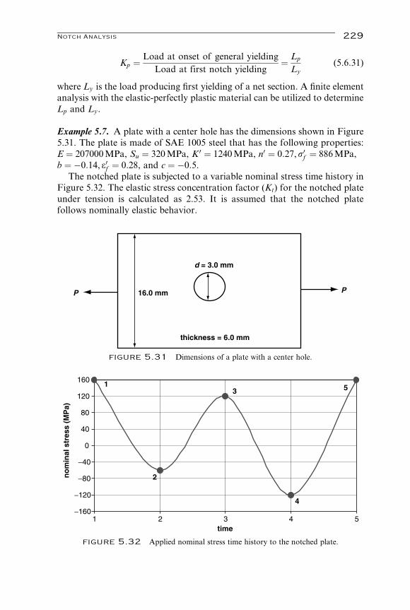
Kp ¼Load at onset of general yielding

Load at first notch yielding¼ Lp

Ly

(5:6:31)

where Ly is the load producing first yielding of a net section. A finite element

analysis with the elastic-perfectly plastic material can be utilized to determine

Lp and Ly.

Example 5.7. A plate with a center hole has the dimensions shown in Figure

5.31. The plate is made of SAE 1005 steel that has the following properties:

E ¼ 207000MPa, Su ¼ 320MPa, K 0 ¼ 1240MPa, n0 ¼ 0:27,s0f ¼ 886MPa,

b ¼ �0:14, e0f ¼ 0:28, and c ¼ �0:5.The notched plate is subjected to a variable nominal stress time history in

Figure 5.32. The elastic stress concentration factor (Kt) for the notched plate

under tension is calculated as 2.53. It is assumed that the notched plate

follows nominally elastic behavior.

d = 3.0 mm

16.0 mm

thickness = 6.0 mm

P P

figure 5.31 Dimensions of a plate with a center hole.

−160

−120

−80

−40

0

40

80

120

160

1 3 5

time

no

min

al str

ess (

MP

a)

5

4

3

2

1

2 4

figure 5.32 Applied nominal stress time history to the notched plate.

Notch Analysis 229

(1) Determine the fatigue life of the notched plate, using the modified Neuber

rule for the notch analysis and the SWT mean stress correction formula.

(2) Repeat Part (1), using the strain energy density method by Molsky and

Glinka for the notch analysis.

Solution. (1) To determine the fatigue life of the component by using the

modified Neuber rule, the notch sensitivity factor must first be determined.

Because Su ¼ 320 MPa < 560 MPa, the empirical Peterson formula for a

notch sensitivity factor (q) is no longer valid and has to be estimated from

Peterson’s empirical notch sensitivity curves for steels. Based on Su ¼ 320

MPa, q is estimated as 0.65.

Kf ¼ 1þ (Kt � 1)q ¼ 1þ (2:53� 1)0:65 ¼ 1:99

With all the known material constants and the notch effects to the plate,

the local notch stress–strain responses can be simulated by using the modified

Neuber rule and the Massing hypothesis.

State of Stress and Strain at Point 1 Based on the Initial Loading Path

from Time 0 to 1

First, it is given that the initial nominal stress starts from S0 ¼ 0MPa

to S1 ¼ 160MPa. Neuber’s constant can be calculated by using the nominal

stress and the fatigue strength reduction factor:

KfS1

� �2

E¼ (1:99� 160)2

207000¼ 0:48975

The true stress, s1, can be determined by a nonlinear equation solver in

MS Excel or by other means for the following Neuber equation:

(s1)2

207000þ s1

s1

1240

� � 10:27¼ 0:48975

s1 ¼ 208:2MPa

Substituting the true stress back into the cyclic stress–strain equation gives

e1 ¼s1

Eþ s1

K 0

� � 1n0¼ 208:2

207000þ 208:2

1240

� � 10:27

¼ 0:002353 ¼ 2353me

State of Stress and Strain at Point 2 Based on the First Loading Reversal

from 1 to 2

For the first reversal, S1 ¼ 160MPa to S2 ¼ �60MPa, the nominal

stress range is calculated as DS ¼ 220MPa. The Neuber constant can

be calculated by using the nominal stress delta and the fatigue strength

reduction factor:


K2f DSDe ¼

KfDS� �2

E¼ (1:99� 220)2

207000¼ 0:92594

The local stress delta, Ds, can be determined by a nonlinear equation

solver in MS Excel for the following Neuber formula:

(Ds)2

207000þ 2Ds

Ds

2� 1240

� � 10:27

¼ 0:92594

Ds ¼ 332:7MPa

Substituting the true stress delta back into the hysteresis stress–strain

equation, the true strain delta, De, is determined:

De ¼ Ds

Eþ 2

Ds

2K 0

� � 1n0

¼ 332:7

207000þ 2

332:7

2� 1240

� � 10:27

¼ 0:002783 ¼ 2783me

From the true stress and strain deltas, the true stress and strain at Time 2

can be determined by comparing the deltas with the reference true stress and

true strain, which means

s2 ¼ s1 � Ds ¼ 208:2� 332:7 ¼ �124:5MPa

e2 ¼ e1 � De ¼ 2353� 2783 ¼ �430me

Following the methodology and calculation for the first loading reversal,

the true stress and strain for each remaining reversals can be calculated. Table

5.17 shows the summary of the results for each reversal. Because of the

material memory effect, the state of stress and strain at Point 4 follows the

path 1–4. Figure 5.33 shows the complete hysteresis loops at the notch root

based on the modified Neuber rule.

Next, it is necessary to estimate the fatigue life of the notched plate by

using the rainflow cycle counting technique and the SWT method. The

damage calculation for each extracted cycle is presented in Table 5.18.

Then, the total damage and fatigue life prediction are obtained as follows:

Sdi ¼ 5:28� 10�6 þ 3:30� 10�5 ¼ 3:83� 10�5

table 5.17 True Stress and Strain Results for Each Reversal Based on the Modified

Neuber Rule

Point

No. Path

SRef

(MPa)

DS

(MPa)

Neuber

Constant

Ds

(MPa)

De

(me)

sRef

(MPa)

eRef

(me)

s

(MPa)

e

(me)

1 0–1 0 160 0.48975 208.2 2353 0 0 208.2 2353

2 1–2 160 220 0.92594 332.7 2783 208.2 2353 �124:5 �430

3 2–3 �60 180 0.61984 291.4 2127 �124:5 �430 166.9 1697

4 1–4 160 280 1.49986 385.5 3890 208.2 2353 �177:3 �1537

5 4–5 �120 280 1.49986 385.5 3890 �177:3 �1537 208.2 2353

Notch Analysis 231

Predicted life ¼ 1

Sdi¼ 1

3:83� 10�5¼ 26100 blocks

(2) A very similar process is used to determine the fatigue life, using the

strain energy density method. The following steps explain the analysis.

State of Stress and Strain at Point 1 Based on the Initial Loading Path

from Time 0 to 1

First it is given that the initial nominal stress starts from S0 ¼ 0MPa

to S1 ¼ 160MPa. Neuber’s constant can be calculated by using the nominal

stress and the Kt factor:

KtS1ð Þ2E

¼ (2:53� 160)2

207000¼ 0:79161

The true stress s1 can be determined by a nonlinear equation solver in MS

Excel for the Molsky and Glinka equation:

-200

-150

-100

-50

0

50

100

150

200

250

-0.002-0.0015 -0.001 -0.0005 0 0.0005 0.001 0.0015 0.002 0.0025 0.003

Strain

Str

es

s (

MP

a)

Modified Neuber rule

Strain energy density method

figure 5.33 Hysteresis loops at the notch root based on the modified Neuber rule and

the strain energy density method.

table 5.18 SWT Mean Stress Correction Results Based on the Modified Neuber’s Rule

ni(cycles)

From–

To

emax

(me)

emin

(me)

smax

(MPa)

smin

(MPa)

ea

(me)

smax

(MPa)

Nf

(cycles) di

1 2 to 3 1697 �430 166.9 �124:5 1064 166.9 189346 5.28E-6

1 1 to 4 2353 �1537 208.2 �177:3 1945 208.2 30273 3.30E-5


s1ð Þ2207000

þ 2s1

1þ 0:27

s1

1240

� � 10:27¼ 0:79161

s1 ¼ 218:9MPa

Substituting the true stress back into the cyclic stress–strain equation gives

e1 ¼s1

Eþ s1

K 0

� � 1n0¼ 218:9

207000þ 218:9

1240

� � 10:27

¼ 0:002682 ¼ 2682me

State of Stress and Strain at Point 2 Based on the First Loading Reversal

from 1 to 2

For the first reversal, S1 ¼ 160MPa toS2 ¼ �60MPa, the nominal stress

range is calculated as DS ¼ 220MPa.

The Neuber constant can be calculated by using the nominal stress delta

and the Kt factor:

KtDSð Þ2E

¼ (2:53� 220)2

207000¼ 1:49664

The local stress delta, Ds, can be determined by a nonlinear equation

solver in MS Excel for the Molsky and Glinka equation:

(Ds)2

207000þ 4Ds

1þ 0:27

Ds

2� 1240

� � 10:27

¼ 1:49664

Ds ¼ 358:6MPa

Substituting the true stress delta back into the hysteresis stress–strain

equation, the true strain delta, De, is determined:

De ¼ Ds

Eþ 2

Ds

2K 0

� � 1n0

¼ 358:6

207000þ 2

358:6

2� 1240

� � 10:27

¼ 0:003283 ¼ 3283me

From the true stress and strain deltas, the true stress and strain at Time 2

can be determined by comparing the deltas with the reference true stress and

true strain, which means

s2 ¼ s1 � Ds ¼ 218:9� 358:6 ¼ �139:7MPa

e2 ¼ e1 � De ¼ 2682� 3283 ¼ �601me

Following the methodology and calculation for the first loading reversal,

the true stress and strain for each remaining reversals can be calculated. Table

5.19 shows the summary of the results for each reversal. Because of the

material memory effect, the state of stress and strain at Point 4 follows

the path 1–4. Figure 5.33 shows the complete hysteresis loops at the notch

root based on the strain energy density method.

Notch Analysis 233

Next, it is necessary to estimate the fatigue life of the notched plate by

using the rainflow cycle counting technique and the SWT method. The

damage calculation for each extracted cycle is presented in Table 5.20.

The total damage accumulation and life prediction are given below.

Sdi ¼ 9:61� 10�6 þ 4:92� 10�5 ¼ 5:88� 10�5

Predicted life ¼ 1

Sdi¼ 1

5:88� 10�5¼ 17000 blocks

references

ASTM, Standard practice for statistical analysis of linear or linearized stress-life (S-N) and strain-

life (e-N) fatigue data, ASTM Standard E739, ASTM Designation E 739–91 (reapproved

1998), 1998b, pp. 1–7.

ASTM, Standard practice for strain-controlled fatigue testing, ASTM Standard E 606, ASTM

Designation: E 606–92 (reapproved 1998), 1998a, pp. 1–7.

ASTM, Standard practice for verification of specimen alignment under tensile loading, ASTM

Standard E1012, ASTM Designation E 1012–99, 1999, pp. 1–8.American Society for Testing

and Materials (ASTM), Standard test methods for tension testing of metallic materials

[metric], ASTM Standard E 8M, ASTM Designation E 8M-01, 2001, pp. 1–7.

Bannantine, J. A., Comer, J. J., and Handrock, J. L., Fundamentals of Metal Fatigue Analysis,

Prentice Hall, New York, 1990.

Barkey, M. E., Socie, D. F., and Hsia, K. J. A yield surface approach to the estimation of notch

strains for proportional and nonproportional cyclic loading. Journal of Engineering Materials

and Technology, Vol. 116, 1994, pp. 173–180.

table 5.19 True Stress and Strain Results for Each Reversal Based on the Strain Energy

Density Method

Point

No. Path

SRef

(MPa)

DS

(MPa)

Neuber

Constant

Ds

(MPa)

De

(me)

sRef

(MPa)

eRef

(me)

s

(MPa)

e

(me)

1 0–1 0 160 0.79161 218.9 2682 0 0 218.9 2682

2 1–2 160 220 1.49664 358.6 3283 218.9 2682 �139:7 �601

3 2–3 �60 180 1.00188 319.5 2555 �139:7 �601 179.8 1954

4 1–4 160 280 2.42430 408.6 4488 218.9 2682 �189:7 �1806

5 4–5 �120 280 2.42430 408.6 4488 �189:7 �1806 218.9 2682

table 5.20 SWT Mean Stress Correction Results Based on the Strain Energy Density

Method

ni(cycles)

From–

To

emax

(me)

emin

(me)

smax

(MPa)

smin

(MPa)

ea

(me)

smax

(MPa)

Nf

(cycles) di

1 2 to 3 1954 �601 179.8 �139:7 1278 179.8 104084 9.61E-6

1 1 to 4 2682 �1806 218.9 �189:7 2244 218.9 20314 4.92E-5


Basquin, O. H., The exponential law of endurance tests, American Society for Testing and

Materials Proceedings, Vol. 10, 1910, pp. 625–630.

Baumel, A., Jr. and Seeger, T., Material Data for Cyclic Loading, Supplemental Volume,

Erscheint Anfang Bei, Elsevier, Amsterdam, 1990.

Baumel, A., Jr. and Seeger, T., Thick surface layer model: life calculations for specimens with

residual stress distribution and different material zones. In Proceedings of International

Conference on Residual Stress (ICRS2), London, 1989, pp. 809–914.

Boardman, B. E. Crack initiation fatigue: data, analysis, trends and estimations, SAE 820682,

1982.

Bridgman, P. W. Stress distribution at the neck of tension specimen Transactions of the American

Society for Metals, Vol. 32, 1944, pp. 553–572.

Coffin, L. F., Jr., A study of the effect of cyclic thermal stresses on a ductile metal, Transactions

of ASME, Vol. 76, 1954, pp. 931–950.

Dowling, N. E., Mechanical Behavior of Materials: Engineering Methods for Deformation, Frac-

ture, and Fatigue, 2nd ed., Prentice Hall, New York, 1998.

Fash, J. and Socie, D. F., Fatigue behavior and mean effects in grey cast iron, International

Journal of Fatigue, Vol. 4, No. 3, 1982, pp. 137–142.

Forsetti, P. and Blasarin, A., Fatigue behavior of microalloyed steels for hot forged mechanical

components, International Journal of Fatigue, Vol. 10, No. 3, 1988, pp. 153–161.

Gu, R. and Lee, Y., A new method for estimating nonproportional notch-root stresses and

strains, Journal of Engineering Materials and Technology, Vol. 119, 1997, pp. 40–45.

Hoffmann, M. and Seeger, T., A generalized method doe estimating multiaxial elastic-plastic

notch stresses and strains. Part 1: Theory, Journal of Engineering Materials and Technology,

Vol. 107, 1985, pp. 250–254.

Koettgen, V. B., Barkey, M. E., and Socie, D. F., Pseudo stress and pseudo strain based

approaches to multiaxial notch analysis, Fatigue and Fracture of Engineering Materials and

Structures, Vol. 18, No. 9, 1995, pp. 981–1006.

Koh, S. K. and Stephens, R. I., Mean stress effects on low cycle fatigue for a high strength steel,

Fatigue and Fracture Engineering Materials and Structures, Vol. 14, No. 4, 1991, pp. 413–428.

Langlais, T. E. and Vogel, J. H., Overcoming limitations of the conventional strain-life fatigue

damage model, Journal of Engineering Materials and Technology, Vol. 117, 1995, pp. 103–108.

Landgraf, R. W., High Fatigue Resistance in Metals and Alloys, ASTM STP467, American

Society for Testing and Materials, 1970, pp. 3–36.

Lawrence, F. V., Burk, J. V., and Yung, J. Y., Influence of residual stress on the predicted fatigue

life of weldments. In Residual Stress in Fatigue, ASTM STP 776, ASTM, West Consho-

hocken, PA, pp. 33–43, 1982.

Lee, Y., Chiang, Y., and Wong, H., A constitutive model for estimating multiaxial notch strains,


Manson, S. S. Behavior of materials under conditions of thermal stress. In Heat Transfer

Symposium, University of Michigan Engineering Research Institute, MI, 1953, pp. 9–75.

Masing, G. Eigerspannungen and Verfestigung bein Messing, Proceeding of the 2nd Inter-

national Congress of Applied Mechanics, Zurich, 1976, pp. 332–335.

Moftakhar, A., Buczynski, A., and Glinka, G., Elastic-plastic stress–strain calculation in notched

bodies subjected to nonproportional loading, International Journal of Fracture, Vol. 70, 1995,

pp. 357–373.

Molsky, K. and Glinka, G., A method of elastic-plastic stress and strain calculation at a notch

root, Materials Science and Engineering, Vol. 50, 1981, pp. 93–100.

Morrow, J. D., Cyclic plastic strain energy and fatigue of metals. In Internal Friction, Damping,

and Cyclic Plasticity, ASTM, West Conshohocken, PA, 1965, pp. 45–86.

Morrow, J. D. Fatigue Design Handbook, Section 3.2, SAE Advances in Engineering, Vol. 4,

Society for Automotive Engineers, Warrendale, PA, 1968, pp. 21–29.

References 235

Muralidharan, U. and Manson, S. S. A modified universal slopes equation for estimating of

fatigue characteristics of metals, Journal of Engineering Materials and Technology, Vol. 110,

1988, pp. 55–58.

Neuber, H. Theory of stress concentration for shear-strained prismatical bodies with arbitrary

nonlinear stress–strain law, Journal of Applied Mechanics (Transactions of ASSM, Section E),

Vol. 28, 1961, pp. 544–550.

Park, J. -H. and Song, J. -H., New estimation method of fatigue properties of aluminum alloys,


Ramberg, W. and Osgood, W. R., Description of stress–strain curves by three parameters,

NACA Technical Note No. 902, 1943.

Reemsnyder, H. S., Evaluating the effect of residual stresses on notched fatigue resistance. In

Materials, Experimentation and Design in Fatigue, Society of Environmental Engineers,

Buntingford, U.K.,1981.

Roessle, M. L., and Fatemi, A., Strain-controlled fatigue properties of steels and some simple

approximations, International Journal of Fatigue, Vol. 22, 2000, pp. 495–511.

Seeger T. and Heuler P., Generalized application of Neuber’s rule, Journal of Testing and

Evaluation, Vol. 8, No. 4, 1980, pp. 199–204.

Shen, C. L. and Wirsching, P. H., Design curve to characterize fatigue strength, Journal of

Engineering Materials and Technology, Vol. 118, 1996, pp. 535–541.

Sines, G. and Waisman, J. L., Metal Fatigue, McGraw-Hill, New York, 1959.

Smith, K. N., Watson, P., and Topper, T. H., A stress–strain function for the fatigue of metals,

Journal of Materials, Vol. 5, No. 4, 1970, pp. 767–778.

Topper, T. H., Wetzel, R. M., and Morrow, J., Neuber’s rule applied to fatigue of notched

specimens, Journal of Materials, Vol. 4, No. 1, 1969, pp. 200–209.

Yang, L., Mechanical Behavior and cumulative fatigue damage of vanadium-based micro-

alloyed forging steel, Ph.D. Thesis, University of Toledo, Toledo, OH, 1994.

Yan, X., Cordes, T. S., Vogel, J. H., and Dindinger, P. M., A property fitting approach for

improved estimates of small cycle fatigue damage, SAE Paper No. 920665, 1992.

Walcher, J., Gary, D., and Manson, S. S. Aspects of cumulative fatigue damage analysis of cold

end rotating structures, AIAA Paper 79–1190, 1979.

Wehner T., and Fateni, A. Effect of mean stress on fatigue behavior of a hardened carbon steel,

International Journal of Fatigue, Vol. 13, No. 3, 1991, pp. 241–248.

Wetzel, R. M., Smooth specimen simulation of the fatigue behavior of notches, Journal of

Materials, Vol. 3, No. 3, 1968, pp. 646–657.

Williams, C. R., Lee, Y., and Rilly, J. T., A practical method for statistical analysis of strain-life

fatigue data, International Journal of Fatigue, Vol. 25, No. 5, 2003, pp. 427–436.


6

Fracture Mechanics

and Fatigue Crack

Propagation

Jwo Pan and Shih-Huang LinUniversity of Michigan

6.1 introduction

Use of crack propagation laws based on stress intensity factor ranges is the

most successful engineering application of fracture mechanics. This chapter

gives a review of the basic concepts of fracture mechanics. In contrast to the

traditional stress–life and strain–life approaches to fatigue, cracks are as-

sumed to exist in materials and structures within the context of fracture

mechanics. Fracture parameters such as K and J can be used to characterize

the stresses and strains near the crack tips. A fundamental understanding of

fracture mechanics and the limit of using the fracture parameters is needed

for appropriate applications of fracture mechanics to model fatigue crack

propagation.

In this chapter, the concept of stress concentration of linear elasticity is first

introduced. Griffith’s fracture theory and energy release rate are discussed.

Different fracture modes and asymptotic crack-tip fields are then presented.

Linear elastic stress intensity factors are introduced. Stress intensity factor

solutions for simple cracked geometries and loading conditions are given.

Also, stress intensity factor solutions for circular and elliptical cracks are

given. Plastic zones and requirements of linear elastic fracture mechanics are

discussed. Finally, fatigue crack propagation laws based on linear elastic

fracture mechanics are presented.

237

6.2 stress concentration based on

linear elasticity

6.2.1 ELLIPTICAL HOLE

Consider an elliptical hole in a two-dimensional infinite solid under remote

uniaxial tension. The major and minor axes for the elliptical hole are denoted

as c and b, as shown in Figure 6.1. The elliptical hole surface can be described

by the equation

x2

c2þ y2

b2¼ 1 (6:2:1)

The radius of curvature at x ¼ �c and y ¼ 0 is denoted as r, as shown in the

figure. The radius of curvature r can be related to c and b as

r ¼ b2

c(6:2:2)

The two-dimensional infinite solid is subjected to a uniformly normal stress

s1 in the y direction at y ¼ �1. The linear elasticity solution gives the stress

solution at x ¼ �c and y ¼ 0 as

x

y

rb

c

b

c

s�

s�

figure 6.1 An elliptical hole in a two-dimensional infinite solid under a remote

tension s1.

238 Fracture Mechanics and Fatigue Crack Propagation

syy(x ¼ �c, y ¼ 0) ¼ s1 1þ 2c

b

� �

(6:2:3)

Based on Equation 6.2.2, Equation 6.2.3 can be rewritten as

syy(x ¼ �c, y ¼ 0) ¼ s1 1þ 2

ffiffiffi

c

r

r� �

(6:2:4)

We can define the stress concentration factor Kt for the elliptical hole under

the remote uniaxial tension as

Kt ¼syy(x ¼ �c, y ¼ 0)

s1¼ 1þ 2

ffiffiffi

c

r

r

(6:2:5)

6.2.2 CIRCULAR HOLE

For the special case of a circular hole with a radius of a as shown in Figure

6.2(a), the equations for the elliptical hole will be valid with r ¼ b ¼ c ¼ a.

A polar coordinate system for the circular hole problem is shown in Figure

6.2(a). The solutions for the normalized stresses ~ssrr, ~ssyy, and ~ssry for this case

are

~ssrr ¼srr

s1¼ 1

21� a2

r2

� �

� cos 2y

2

3a4

r4� 4a2

r2þ 1

� �

(6:2:6)

~ssry ¼sry

s1¼ � sin 2y

2

3a4

r4� 2a2

r2� 1

� �

(6:2:7)

~ssyy ¼syy

s1¼ 1

21þ a2

r2

� �

þ cos 2y

2

3a4

r4þ 1

� �

(6:2:8)

Figure 6.2(b) shows the normalized hoop stress ~ssyy distribution as a function

of the normalized radius r/a along the x axis (y ¼ 0). As shown in the figure,

the normalized hoop stress quickly reduces from 3 to approach to 1 as r/a

increases. The hoop stress along the circumference of the circular hole surface

is a function of the angular location y. Figure 6.2(c) shows the normalized

hoop stress ~ssyy as a function of y along the circumferential surface of the hole

(r ¼ a). As shown in the figure, the normalized stress ~ssyy reduces from 3 to�1

and increases to 3 as y increases from 08 to 908 and then to 1808. The hoop

stresses at the locations of y ¼ 08, 908, 1808, and 2708 are schematically

shown in Figure 6.2(a). The stress concentration factor Kt for the circular

hole in a two-dimensional infinite solid under remote uniaixal tension equals

3. Now consider the case of the circular hole under equal biaxial tension as

shown in Figure 6.3. By using the superposition of the elasticity, the stress

concentration factor Kt can be obtained as 2. From the example of the

circular hole as discussed previously, the stress concentration factor depends

not only on geometry but also on loading.

Stress Concentration Based on Linear Elasticity 239

3s�

3s�

−s�

−s�

qry

x

(a)

y

x 1 2 3 4 5 6 70

0.5

1

1.5

2

2.5

3

3.5

4

q = 0o

(b)

(c)

r/a

s�

s�

sqq~

90 180 270 360

-1

0

1

2

3

∼

q

r = a

σqq

figure 6.2 A circular hole in a two-dimensional infinite solid under a remote tension

s1. (a) Cartesian and polar coordinate systems (b) the normalized hoop stress ~ssyy distribution

as a function of the normalized radius r/a along the x axis (y ¼ 08), (c) the normalized stress

~ssyy as a function of y along the circumferential surface of the hole (r ¼ a).


6.2.3 LIMIT CASE FOR ELLIPTICAL HOLE

As the elliptical hole becomes increasingly flatter or b/c approaches 0, the

geometry of the hole approaches that of a crack. In this case, b � c and

r ! 0. syy at x ¼ �c and y ¼ 0 based on the elastic solution for an elliptical

hole becomes unbounded.

6.3 griffith’s fracture theory for

brittle materials

As shown in Figure 6.4, we consider a large two-dimensional plate

of thickness t under a remote uniform tensile stress s. A center through-

thickness crack with a crack length of 2c is shown. This cracked plate is

considered under plane-stress loading conditions. According to Griffith

(1921), fracture occurs when the decrease of the potential energy due to an

increment of crack area equals the surface energy of newly created crack

surfaces. For the large plate, the potential energy F can be written in terms of

s as

F ¼ �s2

2EV� p

s2c2

Et (6:3:1)

2s�

2s�

Kt = 2

2s�

2s�

s�

s�

s�

s�

figure 6.3 A circular hole in a two-dimensional infinite solid under an equal biaxial

remote tension s1.

Griffith’s Fracture Theory for Brittle Materials 241

where V represents the total volume of the plate.

The energy release rate per unit crack area can be expressed as

� @F

@Ac

¼ � 1

2t

dF

dc¼ p

s2c

E(6:3:2)

where Ac represents the crack area. In this case, Ac ¼ 2ct. Now, the stress at

fracture can be denoted as sf . At fracture the energy release per unit crack

area growth should equal the surface energy g of the newly created crack

surface. Therefore,

� @F

@Ac

¼ ps2f c

E¼ 2g (6:3:3)

In this case, the fracture stress sf can be obtained as

sf ¼ffiffiffiffiffiffiffiffi

2gE

pc

r

(6:3:4)

2c

Ac

A

t

s

s

figure 6.4 A large two-dimensional plate of thickness t under a remote uniform tensile

stress s.


6.4 fracture parameters based on linear

elastic fracture mechanics (lefm)

6.4.1 THREE PRIMARY LOADING MODES

Consider a segment of crack front as shown in Figures 6.5–6.7. Because of

different loading conditions, the crack front can be subjected to three primary

loading modes and their combinations. A Cartesian coordinate system is

assigned such that the crack front is in the z direction. We consider idealized

planar crack problems, in which the stresses and strains near the crack tip can

be expressed in terms of the in-plane coordinates x and y only. As shown in

Figure 6.5, the crack is subject to Mode I, the opening or tensile mode, where

the in-plane stresses and strains are symmetric with respect to the x axis. As

shown in Figure 6.6, the crack is subject to Mode II, the sliding or in-plane

yx

z

figure 6.5 Mode I or opening mode.

yx

z

figure 6.6 Mode II or in-plane shearing mode.

yx

z

figure 6.7 Mode III or out-of-plane shearing mode.

Fracture Parameters Based on Linear Elastic Fracture Mechanics 243

shearing mode, where the stresses and strains are anti-symmetrical with

respect to the x axis. As shown in Figure 6.7, the crack is subject to Mode

III, the tearing or anti-plane shearing mode, where the out-of-plane stresses

and strains are anti-symmetrical with respect to the x axis.

6.4.2 ASYMPTOTIC CRACK-TIP FIELD FOR LINEAR

ELASTIC MATERIALS

Here, the asymptotic crack-tip stresses and strains for different modes of

loading are explored for linear elastic isotropic materials. As shown in Figure

6.8, we concentrate on a very small area near a crack tip, where the stresses

and strains should be naturally expressed in terms of the polar coordinates

r and y. The three stresses srr, syy, and sry are shown for a material element.

The two in-plane equilibrium equations for the plane problem are

@srr@r

þ 1

r

@sry@y

þ srr � syy

r¼ 0 (6:4:1)

@sry@r

þ 1

r

@syy@y

þ 2srr

r¼ 0 (6:4:2)

As schematically shown in Figure 6.8, the traction on the crack surfaces

should vanish. This leads to the traction boundary conditions on the two

crack faces as

syy ¼ sry ¼ 0 at y ¼ �p (6:4:3)

Combining the compatibility equation, the two in-plane equilibrium

equations and the elastic Hooke’s law under both plane stress and plane

strain conditions leads to

x

y

srr

sqq

sqq= = 0

r

srq

srq

q

figure 6.8 A crack with the Cartesian and polar coordinate systems centered at the tip.


@2

@rþ 1

r

@

@rþ 1

r2@2

@y2

� �

(srr þ syy) ¼ 0 (6:4:4)

Solutions are sought for the three governing equations: Equations 6.4.1,

6.4.2, and 6.4.4, with the homogeneous boundary conditions in Equation

6.4.3. The stresses can be assumed to be separable functions of r and y as

srr ¼ Crl~ssrr(y) (6:4:5)

syy ¼ Crl~ssyy(y) (6:4:6)

sry ¼ Crl~ssry(y) (6:4:7)

where l represents an eigenvalue. C is an undetermined constant, which

represents the singularity amplitude when l is negative. ~ssrr(y), ~ssry(y), and

~ssyy(y) represent the normalized stress functions of y.

When the boundary-valued problem is solved based on the separable

functions in Equations 6.4.5–6.4.7, the allowable singular solution is with

l ¼ �1=2 by consideration of finite strain energy for a small circular region

of size r centered at the crack tip. Under plane strain or plane stress condi-

tions, two primary modes, Modes I and II, are considered. For Mode I, the

stresses are symmetrical with respect to the crack line direction (y ¼ 0).

Therefore, the stress intensity factor KI for Mode I is defined as the singular-

ity amplitude of the opening stress syy directly ahead of the tip (y ¼ 0) as

KI ¼ limr!0

ffiffiffiffiffiffiffi

2prp

syy(r, y ¼ 0) (6:4:8)

For Mode II, the stresses are anti-symmetrical with respect to the crack

line direction (y ¼ 0). Therefore, the stress intensity factor KII is defined as

the singularity amplitude of the shear stress sry directly ahead of the tip

(y ¼ 0) as

KII ¼ limr!0


2prp

sry(r, y ¼ 0) (6:4:9)

Substituting Equations 6.4.5–6.4.7 into the governing equations in Equa-

tions 6.4.1, 6.4.2, and 6.4.4 with use of the boundary conditions in Equation

6.4.3 and the definitions in Equation 6.4.8 for KI, the asymptotic stresses

under Mode I loading conditions can be obtained as

syy ¼KIffiffiffiffiffiffiffi

2prp cos3

y

2(6:4:10)

srr ¼KIffiffiffiffiffiffiffi

2prp cos

y

21þ sin2

y

2

� �

(6:4:11)

sry ¼KIffiffiffiffiffiffiffi

2prp sin

y

2cos2

y

2(6:4:12)


Similarly, the asymptotic stresses under Mode II loading conditions are

syy ¼KIIffiffiffiffiffiffiffi

2prp �3 sin

y

2cos2

y

2

� �

(6:4:13)

srr ¼KIIffiffiffiffiffiffiffi

2prp sin

y

21� 3 sin2

y

2

� �

(6:4:14)

sry ¼KIIffiffiffiffiffiffiffi

2prp cos

y

21� 3 sin2

y

2

� �

(6:4:15)

The Mode III stress intensity factor KIII can be defined as the singularity

amplitude of the shear stress syz directly ahead of the tip (y ¼ 0) as

KIII ¼ limr!0


2prp

syz(r, y ¼ 0) (6:4:16)

Following the similar procedure as summarized above to solve the anti-plane

boundary-valued problem with the homogeneous stress boundary condi-

tions, the asymptotic stresses can be obtained as

syz ¼KIIIffiffiffiffiffiffiffi

2prp cos

y

2(6:4:18)

srz ¼KIIIffiffiffiffiffiffiffi

2prp sin

y

2(6:4:17)

For the asymptotic analyses, because the boundary conditions are homo-

genous (syy ¼ sry ¼ syz ¼ 0 at y ¼ �p), only the angular dependence of the

stresses can be determined. The singularity amplitudes KI, KII, and KIII

cannot be determined by the asymptotic analyses. KI, KII, and KIII depend

on the crack geometry and loading conditions. In general, the solutions of

KI, KII, and KIII for relatively simple geometric configurations and loading

conditions can be found in stress intensity factor handbooks such as in Tada

et al. (2000).

6.4.3 STRESS INTENSITY FACTOR SOLUTIONS FOR SIMPLE

GEOMETRIES AND LOADING CONDITIONS

For small cracks in infinite or semi-infinite solids, dimensional analyses

can guide the selection of the form of the stress intensity factor solutions. For

example, KI has a dimension of

[KI] ¼[F ]

[L]2[L]1=2 (6:4:19)

where [KI] represents the dimension of the stress intensity factor KI, [F ] the

force dimension, and [L] the length dimension. The unit of stress intensity

factor KI can be MPa �m1=2 or ksi�in1=2. We now consider three geometric

and loading conditions as shown in Figures 6.9–6.11.


2a

K =

s

s

s πa

figure 6.9 A center crack in a two-dimensional infinite solid under a remote uniform

tensile stress s.

a

K = 1.12

s

s

πa

figure 6.10 An edge crack in a two-dimensional semi-infinite solid under a remote

uniform tensile stress s.


6.4.3.1 Center Crack in a Two-Dimensional Infinite Solid

Figure 6.9 shows a center crack with the crack length 2a in a two-dimen-

sional infinite solid under a remote uniform tensile stress s. For the center

crack, the stress intensity factor solution is

KI ¼ sffiffiffiffiffiffi

pap

(6:4:20)

6.4.3.2 Edge Crack in a Two-Dimensional Semi-infinite Solid

Figure 6.10 shows an edge crack with the crack length a in a two-

dimensional semi-infinite solid under a remote uniform tensile stress s. For

the edge crack, the stress intensity factor solution is

KI ¼ 1:12sffiffiffiffiffiffi

pap

(6:4:21)

6.4.3.3 Penny-Shaped Crack in a Three-Dimensional Infinite Solid

Figure 6.11 shows a penny-shaped crack with the diameter 2a in a three-

dimensional infinite solid under a remote uniform tensile stress s. For the

penny-shaped crack, the stress intensity factor solution is

KI ¼2

psffiffiffiffiffiffi

pap

(6:4:22)

K = πa2

2a

2a

s

s

πs

figure 6.11 A penny-shaped crack in a three-dimensional infinite solid under a remote

uniform tensile stress s.


The stress intensity factor solutions for these three crack problems have

the same forms except the proportionality constants for different geometries

and loading conditions. The stress intensity factor solutions must be propor-

tional to the magnitude of the remote uniform tensile stress s due to the

linearity of linear elasticity. The stress intensity factor solutions must be

proportional to the square root of the only significant length dimension,

which is the crack length a. For relatively simple geometries and loading

conditions, finite element or other numerical methods can be used to find the

relevant proportionality constants in the stress intensity factor solutions

determined by dimensional analyses.

In general, for a center-cracked panel or an edge-cracked panel of finite

size, the stress intensity factor can be written in the following form:

KI ¼ F (a)Sg

ffiffiffiffiffiffi

pap

(6:4:23)

where a represents the crack length; Sg the gross nominal stress, either the

nominal stress or the maximum nominal bending stress; and F (a) a geometric

function of the normalized crack length a. Here, a ¼ a=b, where b represents

the width of the panel.

6.4.3.4 Center-Cracked Plate Under Tension

Figure 6.12(a) shows a center-cracked panel subject to a tensile load P.

For the center-cracked panel in tension, Sg and F (a) are

Sg ¼P

2bt(6:4:24)

F (a) ¼ 1� 0:5aþ 0:326a2ffiffiffiffiffiffiffiffiffiffiffi

1� ap for h=b$1:5 (6:4:25)

where a represents the normalized crack length, h the height of the panel, and

b the width of the panel.

6.4.3.5 Edge-Cracked Plate Under Tension

Figure 6.12(b) shows an edge-cracked panel subject to a tensile load P. For

the edge-cracked panel in tension, Sg and F (a) are

Sg ¼P

bt(6:4:26)

F (a) ¼ 0:265(1� a)4 þ 0:857þ 0:265a

(1� a)3=2for h=b$1:0 (6:4:27)




a

P

P

t

b

h

a

P

P

t

b

h

(a)

(b)

figure 6.12 (a) A center cracked panel subject to a remote tensile load P. (b) An edge

cracked panel subject to a tensile load P.

Continued


6.4.3.6 Edge-Cracked Plate Under Bending

Figure 6.12(c) shows an edge-cracked panel subject to a bending moment

M. For the edge-cracked panel in bending, Sg and F (a) are

Sg ¼6M

b2t(6:4:28)

F (a) ¼ffiffiffiffiffiffiffiffiffiffiffiffiffiffiffiffiffiffiffi

2

patan

pa

2

r

0:923þ 0:199 1� sinpa

2

� �4

cospa

2

2

6

4

3

7

5for large h=b’s (6:4:29)



Figure 6.13 show the geometric function F (a) for the three cases. As shown

in the figure, as a becomes smaller, F (a) approaches 1 for the center-cracked

panel case and 1.12 for the edge-cracked panel cases in order to be consistent

with the solutions for a center crack in an infinite solid and an edge crack in a

semi-infinite solid under remote tensile stress. As shown in the figure, when a

increases, F (a) increases.

6.4.3.7 Cracks Emanating from a Hole Under Remote Tension

As shown in Figure 6.14, small cracks with the crack length l are emanat-

ing from a hole with a radius of c under a remote tensile stress S. When l � c,

the stress intensity factor KA can be expressed as

a

M

M

t

b

h

(c)

figure 6.12 Cont’d (c) An edge cracked panel subject to a bending moment M


KA ¼ 1:12KtSffiffiffiffiffi

plp

(6:4:30)

where the stress concentration factor Kt equals 3 in this case. When l is in the

same order of c, the stress intensity factor KB can be expressed as

F

0.2 0.4 0.6 0.80 10

1

2

3

4

5

6

(c)

a = a/b

K = FSg πa

Sg = 6Mbt2

Sg = P2bt

Sg = Pbt

(a)

(b)

figure 6.13 Plots of F(a) for the three cracked panels.

t

b b

c

h

a

S

S

a << b

a << h

l

figure 6.14 Small cracks with the crack length l emanating from a hole with a radius

of c under a remote tensile stress S.


KB ¼ FSffiffiffiffiffiffi

pap

(6:4:31)

where a ¼ cþ l. In general, the stress concentration factor K can be expressed

as (Tada et al., 2000)

K ¼ F (d)Sffiffiffiffiffi

plp

(6:4:32)

Here, the geometric function F(d) is in terms of the normalized crack length d

as

F (d) ¼ 0:5(3� d)(1þ 1:243(1� d)3) (6:4:33)

where

d ¼ l

a¼ l

cþ l(6:4:34)

6.4.4 NON-SINGULAR ASYMPTOTIC CRACK-TIP FIELD FOR LINEAR

ELASTIC MATERIALS

As discussed earlier, l ¼ �1=2 is adopted for the most singular asymptotic

crack-tip stress and strain solutions. The next available solution is based on

l ¼ 0 to satisfy the governing equations and boundary conditions for the

asymptotic crack-tip fields. The non-singular stress satisfied the boundary

conditions for the in-plane modes is the normal stress sxx or s11 in the crack

line (x or x1) direction. The non-singular stress that satisfied the boundary

conditions for the anti-plane mode is the shear stress szx or s31. Under

generalized plane strain conditions, we can write the asymptotic crack-tip

fields with the non-singular stresses T for the in-plane modes and S for the

anti-plane mode (Rice, 1974) as

sij ¼KIffiffiffiffiffiffiffi

2prp ~ssIij(y)þ

KIIffiffiffiffiffiffiffi

2prp ~ssIIij (y)þ

KIIIffiffiffiffiffiffiffi

2prp ~ssij

III(y)

þ di1dj1Tþ di3dj3nTþ di1dj3Sþ � � �

(6:4:35)

where ~ssIij(y), ~ssIIij (y), and ~ssIIIij (y) are the normalized angular functions for

Mode I, II, and III asymptotic stress solutions, respectively, as specified

earlier. The range of the subscripts i and j is from 1 to 3. Here, dij represents

the components of the Kronecker delta function. For example, di1 equals

1 when i equals 1 and di1 equals 0 when i does not equal 1. The T and

S stresses, just as the stress intensity factors KI, KII, and KIII are functions of

the geometries and loading conditions [e.g., see Sham (1991)].

Figure 6.15 shows a center crack in a two-dimensional infinite solid subject

to remote biaxial stressing conditions. Here, s represents the normal stress

perpendicular to the crack and Rs represents the normal stress in the crack

line direction. The stress intensity factor solution for this case is



pap

(6:4:36)

The T stress solution can be expressed as

T

KI

¼ R� 1ffiffiffiffiffiffi

pap (6:4:37)

Substituting the stress intensity solution into the T stress solution gives a

simple solution for the T stress as

T ¼ s(R� 1) (6:4:38)

Therefore, under uniaxial tension, R ¼ 0 and T ¼ �s. Under equal biaxial

tension, R ¼ 1 and T ¼ 0. When R > 1, T > 0 and when R < 1, T < 0.

When T < 0, there should be stable Mode I crack growth. When T > 0,

there should be unstable Mode I crack growth (Cotterell and Rice, 1980). The

effects of the T stress on the stability of Mode I crack growth is schematically


6.4.5 CIRCULAR AND ELLIPTICAL CRACKS

6.4.5.1 Circular Cracks

In practical situations, circular and semi-circular cracks are usually

found in engineering structures. The stress intensity factor solution for a

RsRs

2a

s

s

figure 6.15 A center crack in a two-dimensional infinite solid subject to remote

biaxial stressing conditions.


penny-shaped crack in a three-dimensional infinite solid under a remote

tensile stress S is available as discussed earlier:

KI ¼2

pSffiffiffiffiffiffi

pap

(6:4:39)

where a represents the crack length. When the penny-shaped crack is in a

finite body, the size of the body can affect the stress intensity factor solution.

When the crack length a is small compared with the width or the thickness of

the cracked structures, Equation 6.4.39 is a good approximation. Now, we

will concentrate on surface cracks. For a semi-circular surface crack in a

rectangular bar under a tensile force P and a bending moment M as shown in

Figure 6.17(a), the stress intensity factor solution varies along the crack front

(Newman and Raju, 1986). The maximum values occur at the crack front on

the free surface. The gross nominal stresses for the bar due to tension and

bending, St and Sb, can be expressed as

St ¼P

2bt(6:4:40)

Sb ¼3M

bt2(6:4:41)

where b represents the width and t the thickness.

For small surface cracks, the maximum values of the stress intensity factor

solutions due to tension and bending can be expressed, respectively, as

KI ¼ 0:728St

ffiffiffiffiffiffi

pap

(6:4:42)

KI ¼ 0:728Sb

ffiffiffiffiffiffi

pap

(6:4:43)

The stress intensity factor solution decreases by about 10% at the crack

deepest front.

T < 0

T > 0

Stable Mode I Growth

Unstable Mode I Growth

figure 6.16 A schematic plot of the effects of the T stress on the stability of mode I

crack growth.


For a semi-circular surface crack in a circular bar under a tensile force

P and a bending moment M as shown in Figure 6.17(b), the gross nominal

stresses for the bar due to tension and bending, St and Sb, can be expressed,

respectively, as (Newman and Raju, 1986)

a

P

t

b

P

M

M

a

(a)

a

P

M

P

M

d

(b)

figure 6.17 (a) A semi-circular surface crack (b) in a rectangular bar under tension

and bending. (b) A semi-circular surface crack in a circular bar under tension and bending.


St ¼4P

pd2(6:4:44)

Sb ¼32M

pd3(6:4:45)

where d represents the diameter.

For small surface cracks, the maximum values of the stress intensity factor

solutions due to tension and bending can be expressed, respectively, as

KI ¼ 0:728St

ffiffiffiffiffiffi

pap

(6:4:46)

KI ¼ 0:728Sb

ffiffiffiffiffiffi

pap

(6:4:47)

6.4.5.2 Elliptical Cracks

The stress intensity factor solution for an elliptical crack in an infinite solid

under a remote tensile stress S is also available. Figure 6.18 shows an

elliptical crack in an infinite solid under a remote tensile stress S. The

major axis for the elliptical crack front is c and the minor axis is a. Figure

6.19 shows a top view of the crack and the coordinate system. The stress

intensity factor varies along the crack front. The maximum value of KI occurs

at Point D and the minimum value of KI occurs at Point E. The stress

intensity factor solution KI is expressed in terms of the orientation angle f

as shown in Figure 6.19.

The solution KI is expressed as a function of the orientation angle f as

S

S

a x

y

c c

a

figure 6.18 An elliptical crack in an infinite solid under a remote tensile stress S.


K ¼ S

ffiffiffiffiffiffi

pa

Q

r

ff (6:4:48)

where

ff ¼ a

c

� �2

cos2 fþ sin2 f

� �14

fora

c#1 (6:4:49)

and

ffiffiffiffi

Qp

¼ E(k) ¼ðp=2

0

ffiffiffiffiffiffiffiffiffiffiffiffiffiffiffiffiffiffiffiffiffiffiffiffiffi

1� k2 sin2 b

q

db (6:4:50)

where Q represents the flaw shape factor and

k2 ¼ 1� a

c

� �2

(6:4:51)

Here, E(k) is the elliptical integral of the second kind. E(k) can be approxi-

mated as

ffiffiffiffi

Qp

¼ E(k) � 1þ 1:464a

c

� �1:65� �1=2

(6:4:52)

The maximum value of KI occurs at Point D where f ¼ 90� and ff ¼ 1. The

minimum value of KI occurs at Point E where f ¼ 0� and ff ¼ffiffiffiffiffiffiffi

a=cp

.

Therefore, the maximum value of KI at Point D is

KD ¼ S

ffiffiffiffiffiffi

pap

E(k)(6:4:53)

The minimum value of KI at Point E is

KE ¼ S

ffiffiffiffiffiffi

pap

E(k)

ffiffiffi

a

c

r

(6:4:54)

a

c

x

y

a

c

f

D

E

P

a

figure 6.19 Top view of the elliptical crack and the coordinate system.


For semi-elliptical cracks, the maximum value of KI still occurs at Point

D when the ratio a=c is small. When the ratio a=c is close to unity, the

maximum value of KI occurs at Point E for the semi-circular surface cracks.

For semi-elliptical surface cracks, the stress intensity factor solutions should

be based on the embedded elliptical crack solutions multiplied by the free

surface factor of 1.12.

6.5 plastic zone size and requirement of linear

elastic fracture mechanics (lefm)

6.5.1 ESTIMATION OF PLASTIC ZONE SIZE AHEAD OF

A MODE I CRACK

We consider a crack with the Cartesian and the polar coordinate systems

centered at the tip as shown in Figure 6.20. Here, z represents the out-

of-plane coordinate. For in-plane modes (Modes I and II), the out-of-plane

shear stresses are

szr ¼ szy ¼ 0 (6:5:1)

6.5.1.1 Plane Stress Conditions

Under plane stress conditions, the out-of-plane normal stress is

szz ¼ 0 (6:5:2)

We can estimate the plastic zone size at y ¼ 0 directly ahead of a crack tip.

Based on the asymptotic stress solutions in Equations 6.4.10–6.4.12, the

stresses ahead of the crack tip at y ¼ 0 are

srr ¼ syy ¼KIffiffiffiffiffiffiffi

2prp (6:5:3)

sry ¼ 0 (6:5:4)

r

y

xz

q

figure 6.20 A crack with the Cartesian and the polar coordinate systems centered at

the tip.

Plastic Zone Size, Requirement of Linear Elastic Fracture Mechanics 259

Figure 6.21 shows schematically the distribution of syy as a function of the

radial distance r or x ahead of the crack tip. As shown in the figure, syyincreases as x decreases. As the stress increases, plastic flow generally occurs

for metallic materials. The Mises yield criterion can be expressed in terms of

the three principal stresses srr, syy, and szz as

s20 ¼1

2(srr � syy)

2 þ (srr � szz)2 þ (syy � szz)

2�

(6:5:5)

where s0 is the tensile yield stress.

Under the plane stress conditions with Equation 6.5.2, the yield criterion

for the material element at y ¼ 0 becomes

s20 ¼ s2yy (6:5:6)

For Mode I cracks, this leads to

syy ¼ s0 (6:5:7)

As shown in Figure 6.21, when the yield criterion is satisfied, s0 ¼ syy at

r ¼ r0s. Therefore, from Equation 6.5.3,

s0 ¼ syy ¼KIffiffiffiffiffiffiffiffiffiffiffi

2pr0sp (6:5:8)

Rearranging Equation 6.5.8 gives the plastic zone size ahead of the crack tip

as

r0s ¼ 1

2p

KI

s0

� �2

(6:5:9)

Now we consider the elastic perfectly plastic material behavior. The tensile

stress–strain curve for an elastic perfectly plastic material is shown in

Figure 6.22. For the elastic perfectly plastic material, the plastic zone should

be larger than the size of r0s estimated from the linear elastic asymptotic

stress solution. An estimated plastic zone size for the elastic perfectly plastic

material as schematically shown in Figure 6.21 can be expressed as

x

s0

r0s 2r0s

sqq

figure 6.21 The distribution of syy as a function of the radial distance r or x ahead of

the crack tip.


2r0s ¼1

p

KI

s0

� �2

(6:5:10)

6.5.1.2 Plane Strain Conditions

Under plane strain conditions, ezz ¼ 0. This leads to

szz ¼ n(sxx þ syy) ¼ n(srr þ syy) (6:5:11)

Directly ahead of the crack tip at y ¼ 0, sry ¼ 0 and

srr ¼ syy ¼KIffiffiffiffiffiffiffi

2prp (6:5:12)

Based on Equations 6.5.11 and 6.5.12, szz is

szz ¼ 2nsyy (6:5:13)

The yield criterion for the material element at y ¼ 0 now becomes

s20 ¼ [(1� 2n)syy]2 (6:5:14)

For Mode I cracks, when the yield criterion is satisfied,

s0 ¼ (1� 2n)syy (6:5:15)

or

syy ¼1

1� 2ns0 (6:5:16)

For example, when n ¼ 0:3, syy has to be equal to 2.5 s0 to satisfy the

yield criterion under plane strain conditions. Therefore, the plastic zone

size ahead of the crack tip should be smaller under plane strain conditions

when compared to that under plane stress conditions. From Equation

6.5.12,

s0

s

e

figure 6.22 The tensile stress–strain curve of an elastic perfectly plastic material.


s0

1� 2n¼ syy ¼

KIffiffiffiffiffiffiffiffiffiffiffi

2pr0ep (6:5:17)

at r ¼ r0e. This leads to

r0e ¼(1� 2n)2

2p

KI

s0

� �2

(6:5:18)

Similar to the plane stress case, the plastic zone size estimated for elastic

plastic materials is

2r0e ¼(1� 2n)2

p

KI

s0

� �2

(6:5:19)

For example, when n ¼ 0:3, (1� 2n)2 ¼ 0:16. Therefore, the plastic zone

ahead of the crack tip under plane strain conditions is much smaller than

that under plane stress conditions. Estimation of the plastic zone from Irwin

can be written as

r0e ¼1

6p

KI

s0

� �2

(6:5:20)

2r0e ¼1

3p

KI

s0

� �2

(6:5:21)

6.5.2 ESTIMATION OF PLASTIC ZONE SIZE AND SHAPE UNDER

MODE I LOADING CONDITIONS

Plastic zone size and shape for Mises materials can be estimated based on

the asymptotic linear elastic crack-tip stress fields. The Mises yield criterion in

the cylindrical coordinate system for the in-plane modes can be expressed as

s20 ¼1

2(srr � syy)

2 þ (syy � szz)2 þ (szz � srr)

2�

þ 3s2ry (6:5:22)

The asymptotic stress fields in Equations 6.4.10–6.4.12 can be substituted

into the Mises yield criterion in Equation 6.5.22.

Under plane stress conditions, the plastic zone size rp(y) as a function of y

can be obtained as

rp(y) ¼1

2p

KI

s0

� �21

2(1þ cos y)þ 3

4sin2 y

� �

(6:5:23)

Under plane strain conditions, the plastic zone size rp(y) as a function of y

can be obtained as

rp(y) ¼1

2p

KI

s0

� �21

2(1� 2n)2(1þ cos y)þ 3

4sin2 y

� �

(6:5:24)


The size and shape of the plastic zones based on Equations 6.5.23 and

6.5.24 in the normalized coordinate system under plane stress and plane

strain conditions for n ¼ 0:3 are shown in Figure 6.23. As shown in the

figure, the size of the plastic zone under plane strain conditions is much

smaller than that under plane stress conditions.

The non-singular stress T can also affect the plastic zone size and shape.

However, the size and shape based on the linear elastic asymptotic crack-tip

fields do not in general agree well with the computational results for elastic

plastic materials [e.g., see Ben-Aoun and Pan (1996)]. Figures 6.24 and 6.25

show the general trends of plastic zone size and shape for different T stresses

for elastic perfectly plastic materials under small-scale yielding plane strain

and plane stress conditions.

6.5.3 REQUIREMENT OF LINEAR ELASTIC FRACTURE MECHANICS

The most important requirement of linear elastic fracture mechanics

(LEFM) is that the size of the plastic zone near the crack tip should be

much smaller than any relevant length dimensions for the crack problem of

interest. In this way, the stress intensity factor K controls the plastic deform-

ation near the crack tip, and, in turn, the fracture process near the crack tip.

Figure 6.26 shows a schematic representation of the K field and the plastic

zone near the tip of a crack with the length a in a specimen. The requirement

of LEFM is

−0.5 0 0.5 1 1.5 2 2.5 3 3.5−2

−1.5

−1

−0.5

0

0.5

1

1.5

2

Plane Strain

Plane Stress

2ps

02y

KI2

2ps02x

KI2

figure 6.23 Estimations of the size and shape of the plastic zones in the normalized

coordinate system under plane stress and plane strain conditions for v ¼ 0:3.


a, b, h$4

p

KI

s0

� �2

(6:5:25)

where b and h are the remaining ligament and height of the specimen,

respectively.

T > 0

T < 0

T = 0

figure 6.24 The general trends of plastic zone size and shape for different T stresses

under small-scale yielding plane strain conditions.

T < 0 T = 0

T > 0

figure 6.25 The general trends of plastic zone size and shape for different T stresses

under small-scale yielding plane stress conditions.

a b

h Plastic Zone

K Field

figure 6.26 A schematic representation of the K field and the plastic zone near the tip

of a crack in a specimen.


The definition of plane stress and plane strain conditions depends on the

thickness of the specimens or structures and the load amplitude. For

example, consider a cracked specimen with the thickness t and the plastic

zone 2r0 on the lateral surface as shown in Figure 6.27. A Cartesian coordin-

ate system is shown in the figure. The crack front is in the z direction. The

plastic zone size is larger on the specimen lateral surface, because the surface

material element has no constraint and is under plane stress conditions.

However, for the crack front in the middle of the specimen, the plastic

zone becomes smaller because the material element has the constraint in the

z direction. This concept is illustrated in Figure 6.28. Figure 6.28 shows

the side views of the specimen with the plastic zones shown as the shaded

regions. When the load P is small, most of the plastic zone along the crack

front is small compared to the thickness of the specimen. The specimen is

subjected to mostly plane strain conditions. When the load P is large, the

plastic zone along the crack front becomes large compared to the thickness of

the specimen and the specimen is subjected to plane stress conditions. The

requirement of plane strain conditions is

t, a, h, b$2:5KI

s0

� �2

(6:5:26)

6.5.4 FRACTURE TOUGHNESS TESTING

Figure 6.29 shows a three-point bend specimen and Figure 6.30 a compact

tension specimen. These two types of specimens are used for fracture

toughness testing according to the ASTM standard E399 (ASTM, 1997).

The stress intensity factor KQ can be related to the load PQ by

t

a b

2r0

h

z

y

x

P

figure 6.27 A cracked specimen with the thickness t and the plastic zone 2r0.


KQ ¼ PQ

1

tffiffiffiffiffiffi

Wp F

a

W

� �

(6:5:27)

where F(a/W) represents the geometric function for the three-point bend

specimen and the compact tension specimen.

There are several ways to determine the load PQ from different types of

the load–displacement curves. Figure 6.31 shows a simple rule for a Type I

load–displacement curve. In the figure, P represents the load and v the

displacement. The initial slope of the load–displacement curve is denoted as

y

z

t

y

z

Plane Stress

Plane Strain

figure 6.28 Side views of the plastic zone size distribution along the crack front.

Shaded regions represent the plastic zones.

t

w

a

figure 6.29 A three-point bend specimen.


K. The intersection of the load–displacement curve and a line with the slope

0.95K from the origin defines the load P5. PQ is the smaller value of P5 or

the maximum load Pmax.

Figure 6.32 shows a schematic plot of KQ as a function of the thickness

t. In general, as the thickness t increases, the value of KQ decreases. The

fracture toughness KIc is the asymptotic value of KQ. Under the plane

strain conditions, the thickness and other dimensions of the specimens must

satisfy Equation 6.5.26. The values of KIc are in the range of 20–200MPaffiffiffiffi

mp

for metals, 1–5MPaffiffiffiffi

mp

for polymers, and 1–5MPaffiffiffiffi

mp

for ceramics.

Typical values of the fracture toughness KIc for several metals are listed in

Table 6.1 (Dieter, 1988). In general, as the yield stress increases, the value of

KIc usually decreases.

t

w

h

a

P

P

figure 6.30 A compact tension specimen.

P

v

PQ

K

0.95K

P5

Pmax

figure 6.31 A simple rule to determine the load PQ for a typical Type I load-

displacement response.


6.5.5 PLASTIC ZONE UNDER MONOTONIC AND CYCLIC

LOADING CONDITIONS

As discussed earlier, the plastic zone sizes ahead of the crack tip under

Mode I plane stress and plane strain loading conditions can be expressed as

2(r0s)monotonic ¼1

p

KI

s0

� �2

(6:5:28)

2(r0e)monotonic ¼1

3p

KI

s0

� �2

(6:5:29)

where s0 represents the uniaxial tensile yield stress under monotonic loading

conditions.

However, under cyclic loading conditions, if we adopt the elastic perfectly

plastic material behavior with an anisotropic kinematic hardening law, the

effective Mises yield stress for the fully reversed plastic reloading is 2s0.

Therefore, the estimations of the plastic zone sizes under cyclic loading

conditions are one quarter of those under monotonic loading conditions.

2(r0s)cyclic ¼1

p

KI

2s0

� �2

¼ 1

42(r0s)monotonic (6:5:30)

KIc

t

KQ

figure 6.32 A schematic plot of KQ as a function of the thickness t. The asymptotic

value represents the fracture toughness KIc.

table 6.1 Typical Values of KIc

Material Yield Strength (MPa)

Fracture Toughness

KIc (MPaffiffiffiffi

mp

)

Maraging steel 1730 90

4340 steel 1470 46

Ti-6Al-4V 900 57

7075-T6 Al alloy 500 24

2024-T3 Al alloy 385 26


2(r0e)cyclic ¼1

3p

KI

2s0

� �2

¼ 1

42(r0e)monotonic (6:5:31)

Figure 6.33 illustrates the concept of elastic unloading and plastic reloading

near the crack tip. Curve 1 represents the distribution of syy due to the initial

tensile loading. The plastic zone size is denoted as 2r0. Once the load is

released, the unloading process introduces a compressive crack-tip stress

field. This will cause the plastic reloading close to the crack tip and elastic

unloading outside the plastic reloading zone. The distribution of syy due to

the unloading can be represented byCurve 2. The combination of Curves 1 and

2 gives Curve 3, which represents the resulting distribution of syy ahead of the

crack tip.

6.5.6 ENERGY RELEASE RATE UNDER DISPLACEMENT-

CONTROLLED CONDITIONS

Consider a nonlinear elastic cracked solid as shown of thickness t in Figure

6.34 under displacement-controlled conditions. Figure 6.35 shows the load–

displacement curve of a cracked solid. In the figure,P represents the load and v

represents the displacement. The area under the loading–displacement curve

represents the strain energyU stored in the cracked solid. The potential energy

F of the cracked solid is

F ¼ U (6:5:32)

x

s0

r0 2r0

2

3

1

2

2s0

s0

figure 6.33 Estimation of the plastic zone size under cyclic loading conditions based

on the concept of elastic unloading and plastic reloading near the crack tip.


The energy release rate G is defined as

G ¼ � 1

t

@F

@a¼ � 1

t

@U

@a

v

(6:5:33)

Estimation of the energy release rate G based on the load–displacement curve

is illustrated in Figure 6.36. For a small amount of crack growth Da, the

change of strain energy, DU , can be used to estimate the energy release rate G

as

G � � 1

t

DU

Da(6:5:34)

For linear elastic materials, the load–displacement curve is linear, as

shown in Figure 6.37. The slope of the curve represents the stiffness of the

a

v (displacement)

t

figure 6.34 A nonlinear elastic cracked solid under displacement-controlled

conditions.

P

v

U = Strain Energy

figure 6.35 The load–displacement curve of a nonlinear elastic cracked solid. The

area under the loading–displacement curve represents the strain energy U.


cracked solid as shown. The stiffness of the cracked solid, K(a), depends on

the crack length a. Under displacement-controlled conditions, the potential

energy F of the cracked solid can be expressed as

F ¼ U ¼ 1

2Pv ¼ 1

2K(a)v2 (6:5:35)

The energy release rate G is defined as

G ¼ � 1

t

@U

@a

n

¼ � 1

tK 0(a)n2 (6:5:36)

Estimation of G based on the change of the strain energy, DU , is illustrated in

Figure 6.38.

G can be related to stress intensity factors for linear elastic materials. For a

crack front under combined Modes I, II, and III loading conditions, the local

energy release rate G (Irwin, 1957) is

G ¼ 1� n2

E(K2

I þ K2II)þ

1þ n

EK2

III (6:5:37)

P

vv

area = − DU

a

a + Da

figure 6.36 Estimation of the energy release rate G based on the change of the strain

energy, DU , for a small amount of crack growth Da.

P

v

K = Stiffness

figure 6.37 The linear load–displacement curve of a linear elastic-cracked solid.


Under plane stress conditions,

G ¼ 1

E(K2

I þ K2II) (6:5:38)

For nonlinear elastic power-law hardening material, G can be related to

the path-independent J integral (Rice, 1968), which represents the singularity

amplitude of the HRR crack-tip singular stress and strain fields (Hutchinson,

1968; Rice and Rosengren, 1968)

6.6 fatigue crack propagation based on linear

elastic fracture mechanics

6.6.1 EXTENDED SERVICE LIFE

Different inspection methods that use visual, X-ray, ultrasonic waves, and

electric potential drop methods can be employed to detect cracks. Once

cracks are detected, fracture mechanics methods can be used to determine

the extended life of the structures or components.

Figure 6.39 shows the concept by plotting the crack length a as a function

of the number of cycles, N. In the figure, ai represents the initial crack length

within a structure or component, ad a detectable crack length, and ac the

critical crack length when the stress intensity factor of the crack reaches

the critical value or the structure or component reaches fully plastic condi-

tions. The number of cycles when a crack is detected is denoted as Nd . The

number of cycles when the crack length reaches the critical length ac is

denoted as Nc. The extended life Ncd equals Nc �Nd . The damage-tolerant

approach used in the aerospace industry is based on the worst-case analysis

with the assumption that the largest cracks missed by each inspection exist in

the structures or components.

P

v

a

a + Da

area = −DU

figure 6.38 Estimation of the energy release rate G based on the change of the strain

energy, DU , for a linear elastic-cracked solid.


6.6.2 CRACK GROWTH BEHAVIOR

Linear elastic fracture mechanics has been successfully used to model the

fatigue crack growth behavior. Consider a cracked structure with a crack

length a under cyclic stressing conditions, as shown in Figure 6.40(a).

The applied stress S as a function of time t is shown in Figure 6.40(b). The

maximum and minimum stress intensity factors Kmax and Kmin are linearly

related to the maximum and minimum applied stresses Smax and Smin,

respectively, according to the linear elastic fracture mechanics.

Kmax ¼ FSmax

ffiffiffiffiffiffi

pap

(6:6:1)

Kmin ¼ FSmin

ffiffiffiffiffiffi

pap

(6:6:2)

where F represents the function depending on the geometries and loading

conditions.

The stress intensity factor range DK is defined as

DK ¼ Kmax � Kmin (6:6:3)

The load ratio R in the stress–life approach is defined as

R ¼ Smin

Smax

(6:6:4)

Due to the linearity, R also represents the stress intensity factor ratio

R ¼ Kmin

Kmax

(6:6:5)

ad

N

ac

Extended ServiceLife (Nc - Nd)

ai

a(Crack

Length)

NcNd

figure 6.39 The concept of extended life based on the plot of the crack length a as a

function of the number of cycles, N.

Fatigue Crack Propagation Based on Linear Elastic Fracture Mechanics 273

Based on experimental results, Figure 6.41 shows schematically the crack

growth rate da/dN as a function of the stress intensity factor range DK in a

log–log scale. Note that 10�7 mm represents the spacing between atoms. In

Region I, when DK decreases, the crack growth rate drops significantly. The

asymptote DKth is the threshold of the stress intensity factor range below

which no fatigue crack growth should occur. The values of DKth are 5–16

MPaffiffiffiffi

mp

for steels and 3–6 MPaffiffiffiffi

mp

for aluminum alloys, depending on the

value of R. In Region III, when DK is large, the crack growth rate accelerates

significantly. This can happen when Kmax approaches Kc, which represents

the critical K for crack initiation for a given thickness.

a

S

S

Smin

t

Smax

Sm

S

(a)

(b)

figure 6.40 (a) A cracked structure with a crack length a under cyclic stressing

conditions. (b) The applied stress S varies as a function of time t.


In Region II, the crack growth rate da/dN can be approximately linear

related to the stress intensity factor range DK in the log–log scale plot. The

Paris law for crack growth (Paris et al., 1961; Paris and Erdogan, 1963) is

da

dN¼ C(DK)m (6:6:6a)

where C and m represent the material constants. To obtain the values of C

and m, a least-square method can usually be adopted to fit the fatigue data in

the log–log scale plot of da/dN as a function of DK as

Y ¼ Aþ BX (6:6:6b)

where

Y ¼ logda

dN

� �

, X ¼ log (DK), A ¼ logC, and B ¼ m (6:6:6c)

The typical value of m is 3.0 for ferrite-pearlite steel, 2.25 for matensitic steel,

and 3.25 for austenitic steel. The load ratio R can affect the fatigue crack

growth rate. Typical values of material constants C and m for steels are listed

in Table 6.2 (Barsom and Rolfe, 1987). Two approaches with consideration

of the load ratio effects are discussed in the following section.

6.6.3 WALKER EQUATION

Load ratio effects can be accounted for by an equivalent zero-to-

maximum stress intensity factor range DK introduced by Walker (1970):

log(DK)

10−3

da

dadN

= C(DK)m

I IIIII

10−5

10−7

DKth

dN(mm/cycle)

log

figure 6.41 Crack growth rate da/dN schematically plotted as a function of the stress

intensity factor range DK in a log–log scale.


DK ¼ Kmax(1� R)g (6:6:7)

where g is a constant in the range of 0.4 to 0.9. The Walker equation can be

rewritten as

DK ¼ DK(1� R)g�1 (6:6:8)

or

DK ¼ DK

(1� R)1�g(6:6:9)

The Paris law can be rewritten as

da

dN¼ C1(DK)m1 (6:6:10)

where C1 and m1 are material constants. For R ¼ 0, Equation 6.6.9 becomes

DK ¼ DK (6:6:11)

Therefore,

da

dN¼ C1(DK)m1 (6:6:12)

For R > 0, substituting Equation 6.6.9 into 6.6.10 gives

da

dN¼ C1

DK

(1� R)1�g

� �m1

(6:6:13)

Rearranging Equation 6.6.13 gives

da

dN¼ C1

(1� R)m1(1�g)(DK)m1 (6:6:14)

Comparing Equation 6.6.13 with 6.6.6(a) gives

C ¼ C1

(1� R)m1(1�g)(6:6:15)

table 6.2 Typical Values of Material Constants C

and m in the Paris Law for R � 0

Material Ca m

Martensitic steel 1:36� 10�7 2.25

Ferritic-pearlitic steel 6:89� 10�9 3

Austentic steel 5:61� 10�9 3.25

a The values of C are obtained with the units of MPaffiffiffiffi

mp

for DK

and mm/cycle for da/dN.


and

m ¼ m1 (6:6:16)

For R < 0, g ¼ 0. Therefore,

DK ¼ DK

(1� R)1�g¼ DK

(1� R)¼ Kmax (6:6:17)

Therefore,

da

dN¼ C1K

m1

max (6:6:18)

If g ¼ 1,

DK ¼ DK

(1� R)1�g¼ DK (6:6:19)

Therefore, there is no effect of R on the crack growth rate.

6.6.4 FORMAN EQUATION

The crack growth depends on Kc, which is the critical stress intensity

factor for a material and a given thickness. The crack growth rate is written

as (Forman et al., 1967)

da

dN¼ C2(DK)m2

(1� R)Kc � DK(6:6:20)

or

da

dN¼ C2(DK)m2

(1� R)(Kc � Kmax)(6:6:21)

Typical values of material constants for the Walker and Forman equations

are listed in Table 6.3 (Dowling, 1999). When the crack-tip plastic zone

becomes large compared with the relevant physical length of the cracked

solid, linear elastic fracture mechanics should not be used. Use of the crack-

tip opening displacement (CTOD) or the J integral to model the fatigue crack

growth is possible.

6.6.5 LIFE ESTIMATION

Life estimation under constant load amplitude loading conditions usually

needs numerical integration. In general, DK increases as a increases with DS

being kept as constant. The crack growth rate da/dN can be expressed as

da

dN¼ f (DK , R) (6:6:22)


Integration of Equation 6.6.22 gives

ðNf

Ni

dN ¼ðaf

ai

da

f (DK , R)(6:6:23)

where ai represents the initial crack length, af the final crack length, Ni the

number of cycles at the initial crack length, and Nf the number of cycles at

the final crack length. The left hand side of the equation can be integrated as

Nif ¼ Nf �Ni ¼ðNf

Ni

dN (6:6:24)

where Nif represents the number of cycles for crack propagation from the

initial crack length ai to the final crack length af .

The Paris law gives a specific form for the crack growth rate da/dN as

da

dN¼ C(DK)m (6:6:25)

Consider the solution for DK in the form as

DK ¼ FDSffiffiffiffiffiffi

pap

(6:6:26)

where F is a function of geometry and loading.

The crack growth rate da=dN now can be written as

da

dN¼ C(FDS

ffiffiffi

pp

)mam=2 (6:6:27)

Then, the number of cycles Nif for crack propagation from the initial crack

length ai to the final crack length af can be integrated as

Nif ¼ðNf

Ni

dN ¼ðaf

ai

dN

da

� �

da ¼ðaf

ai

1

C(FDSffiffiffi

pp

)ma

�m2da (6:6:28)

If we assume that F is a constant, Equation 6.6.27 can be integrated

explicitly as

table 6.3 Typical Values of Material Constants in the Walker and Forman Equations

Walker Equation Forman Equation

Material Ca1 m1 g(R$0) g(R<0) Ca

2 m2 Kbc

4340 Steel 5:11� 10�10 3.24 0.42 0 n/a n/a n/a

2024-T3 Al alloy 1:42� 10�8 3.59 0.68 n/a 2:31� 10�6 3.38 110

7075-T6 Al alloy 2:71� 10�8 3.70 0.64 0 5:29� 10�6 3.21 78.7

a The values of C1 and C2 are obtained with the units of MPaffiffiffiffi

mp

for DK and mm/cycle for da/ dN.b The thickness of the material is 2.3mm.


Nif ¼1� ai

af

� �m2�1

!

C(FDSffiffiffi

pp

)mm

2� 1

� �

1

am2�1

i

(6:6:29)

Equation 6.6.29 indicates that Nif is very sensitive to the selection of ai.

Because F is a function of geometry, loading, and crack length, a numerical

integration is usually needed. The numerical integration is usually carried out

by taking F as a constant for a small range of a.

From the fracture mechanics viewpoint, a structure of interest contains

initial defects or cracks. Therefore, a dominant crack with an initial crack

length can be found to correlate the fatigue life of the structure under

cyclic loading conditions. From the strain–life or stress–life viewpoint, the

fatigue initiation life for the material near the notches or stress concentrators

in the structure can be estimated. Then, the fatigue life due to crack propa-

gation can be estimated by the fracture mechanics methodology based on the

Paris law. The total fatigue life of the structure is the combination of

the initiation life and propagation life [e.g., see Dowling (1979) and Socie

et al. (1984)].

Example 6.6.1. Consider a very large plate with a small center crack. The

initial total crack length 2a is 20mm. The plate is subjected to repeated

remote stress cycles from smin ¼ 0MPa to smax ¼ 75MPa. The initial crack

grows as the stress cycles are applied. The critical stress intensity factor Kc for

fracture initiation for the plate is 25MPaffiffiffiffi

mp

. The material is assumed to

have a very high yield stress such that the plastic zone size is small compared

to the crack size under the applied stresses. Assume that the Paris law will be

applicable to the plate material to characterize the fatigue crack growth

da

dN¼ C(DK)m (6:6:25)

where C ¼ 1� 10�9 and m ¼ 3. The value of C is obtained with the units of

MPaffiffiffiffi

mp

for DK and mm/cycle for da/dN.

1. Determine the final half crack length af at fracture initiation.

2. Determine the number of cycles before the fracture initiation of the plate.

Solution. For a center crack in a large plate,


pap

(6:4:20)

The critical Kc for fracture initiation is 25MPaffiffiffiffi

mp

. Fracture initiation takes

place when KI ¼ Kc at the final half crack length af under the maximum

applied stress smax. Equation 6.4.20 becomes

Kc ¼ smaxffiffiffiffiffiffiffiffi

pafp

(6:6:30)


The final half crack length af can be obtained by substituting Kc ¼ 25MPaffiffiffiffi

mp

and smax ¼ 75MPa into Equation 6.6.30 as

af ¼ 35:37mm

The initial half crack length ai is

ai ¼ 10mm

The stress range Ds is determined as

Ds ¼ smax � smin ¼ 75MPa

For a center crack in a large plate, the geometric parameter F in Equation

6.6.29 is 1. Equation 6.6.29 becomes

Nif ¼1� ai

af

� �m2�1

!

C(Dsffiffiffi

pp

)mm

2� 1

� �

1

aim2�1

(6:6:29a)

Based on Equation 6.6.29 and the given values of C and m, the number of

cycles Nif for crack propagation from the initial half crack length ai to the

final half crack length af under the stress range Ds is obtained as 3:99� 106.

Example 6.6.2. Consider a spot-weld cup specimen of dual-phase steel as

shown in Figure 6.42(a) under cyclic loads of Pmax ¼ 200N and Pmin ¼ 0.

Figure 6.42(a) only shows a half specimen to represent the weld nugget

clearly. As shown in the figure, the sheet thickness is represented by t, the

nugget diameter by d, and the specimen diameter by D. Here, t is 1mm, d is

5mm, and D is 40mm. Figure 6.42(b) shows a symmetric cross section of the

cup specimen containing the weld nugget before testing. The notch near

the weld nugget can be considered as an original crack. When the cup speci-

men is under pure opening loading conditions, the stress intensity factorKI for

the original crack can be obtained as (Pook, 1975; Wang et al., 2004)

KI ¼P

2p

3

t3

� �1=2 2D

d

� �2

lnD

d

� �

D

d

� �2

�1

� 1

2

6

6

6

4

3

7

7

7

5

(6:6:31)

The stress intensity factor KII is 0 for the specimen under pure opening

loading conditions. During the testing, a kinked crack is initiated near the

weld nugget and then propagates through the thickness with a kink angle a as

shown in Figure 6.42(c).

Figure 6.43 shows a schematic plot of a main crack and a kinked crack

with the kink length a and the kink angle a. Here, KI and KII represent the

global stress intensity factors for the main crack, and kI and kII represent


(c)

(a)

(b)

Original Crack

Weld Nugget

D

t

d

Typical Crack Path

a

figure 6.42 (a) A schematic plot of a half specimen with the sheet thickness t, nugget

diameter d, and the specimen diameter D under the applied force (shown as the bold arrows).

(b) A schematic plot of the symmetry cross section near the spot weld with the notch

considered as an original crack. (c) The typical fatigue crack propagation path shown with

a kink angle a.

Main Crack

Kinked Crack

KI

KIKII

KII

a

a

figure 6.43 A schematic plot of a main crack and a kinked crack with the kink length

a and the kink angle a.


the local stress intensity factors for the kinked crack. The arrows in the figure

represent the positive values of the global and local stress intensity factors

KI, KII, kI, and kII. In general, the local stress intensity factors of the kinked

crack, kI and kII, are different from the global stress intensity factors of the

original crack, KI and KII. When the kink length a approaches 0, the local

stress intensity factors kI and kII can be obtained from the global stress

intensity factors KI and KII as (Bibly et al., 1978; Cotterell and Rice, 1980)

kI ¼1

43 cos

a

2þ cos

3a

2

� �

KI þ3

4sin

a

2þ sin

3a

2

� �

KII (6:6:32)

kII ¼ � 1

4sin

a

2þ sin

3a

2

� �

KI þ1

4cos

a

2þ 3 cos

3a

2

� �

KII (6:6:33)

For the cup specimen subjected to pure opening loading conditions, the

stress intensity factor KII is 0. Therefore, the local stress intensity factors kIand kII are

kI ¼1

43 cos

a

2þ cos

3a

2

� �

KI (6:6:34)

kII ¼ � 1

4sin

a

2þ sin

3a

2

� �

KI (6:6:35)

The effective local stress intensity factor is assumed to be

keq ¼ffiffiffiffiffiffiffiffiffiffiffiffiffiffiffiffi

k2I þ k2II

q

(6:6:36)

Assume that the local stress intensity factors remain constants during the

crack propagation and the Paris law is applicable to characterize the fatigue

crack growth. In this case, the material constants C and m are chosen for

martensitic steels as C ¼ 1:36� 10�7 and m ¼ 2:25. The value of C is

obtained with the units of MPaffiffiffiffi

mp

for DK and mm/cycle for da/dN.

1. Determine the range of local stress intensity factors for the kinked

crack.

2. Determine the number of cycles when the kinked crack grows through the

thickness and the cup specimen is separated.

Solution. Based on Equation 6.6.31,

DKI ¼ DKI, max � DKI, min ¼ Pmax � Pmin

2p

3

t3

� �1=2

2D

d

� �2

lnD

d

� �

D

d

� �2

�1

� 1

2

6

6

6

4

3

7

7

7

5

¼ 5:62MPaffiffiffiffi

mp (6:6:37)


For the cup specimen under pure opening loading conditions, the Mode II

stress intensity factor of the original crack is 0. The range of local stress

intensity factors of the kinked crack can be calculated by Equations 6.6.34

and 6.6.35 with the kink angle a ¼ 90� as

DkI ¼ 1:99MPaffiffiffiffi

mp

DkII ¼ �1:99MPaffiffiffiffi

mp

The range of effective local stress intensity factors for the kinked crack can be

calculated by using Equation 6.6.36 as

Dkeq ¼ffiffiffiffiffiffiffiffiffiffiffiffiffiffiffiffiffiffiffiffiffiffiffi

Dk2I þ Dk2II

q

¼ 2:81MPaffiffiffiffi

mp

Based on the Paris law in Equation 6.6.25, the number of cycles Nf for

the cup specimen as the kinked crack propagates through the thickness can

be obtained as

ðNf

0

N ¼ðt= sin a

0

da

C(Dkeq)m (6:6:38)

Because the local stress intensity factors are assumed to be constant during

crack propagation, Equation 6.6.35 can be integrated as

Nf ¼t

C(Dkeq)m sin a

(6:6:39)

Therefore, the number of cycles Nf to failure is calculated as 719,236.

references

American Society for Testing and Materials (ASTM), Annual Book of ASTM Standards, ASTM

E399, ASTM, West Conshohocken, PA, 1997.

Barsom, J. M., and Rolfe, S. T., Fracture and Fatigue Control in Structures: Applications of

Fracture Mechanics, 2nd ed., Prentice Hall, Upper Saddle River, NJ, 1987.

Ben-Aoun, Z. E. A., and Pan, J., Effects of nonsingular stresses on plane-stress near-tip fields for

pressure-sensitive materials and applications to transformation toughened ceramics, Inter-

national Journal of Fracture, Vol. 77, 1996, pp. 223–241.

Bibly, B. A., Cardew, G. E., and Howard, I. C., Stress intensity factors at the tips of kinked and

forked cracks. In Fourth International Conference on Fracture, Pergamon Press, New York,

Vol. 3A, 1978, pp. 197–200. University of Waterloo, Ontario, June 19–24, 1977.

Cotterell, B., and Rice, J. R., Slightly curved or kinked cracks, International Journal of Fracture,

Vol. 16, 1980, pp. 155–169.

Dieter, G. E., Mechanical Metallurgy, SI Metric ed., McGraw-Hill, New York, 1988.

Dowling, N. E., Fatigue at notches and the local strain and fracture mechanics approaches, In

Fracture Mechanics, C. W. Smith (Ed.), ASTM STP 677, American Society for Testing and

Materials, Philadelphia, PA, 1979, pp. 247–273.

Dowling, N. E., Mechanical Behavior of Materials, Prentice Hall, Upper Saddle River, NJ, 1999.

References 283

Forman, R. G., Keary, V. E., and Engle, R. M., Numerical analysis of crack propagation in

cyclic-loaded structures, Journal of Basic Engineering, Vol. 89, 1967, pp. 459–464.

Griffith, A. A., The phenomena of rupture and flow in solids, Philosophical Transaction of the

Royal Society of London, Vol. A221, 1921, pp. 163–197.

Hutchinson, J. W., Singular behavior at the end of a tensile crack in a hardening material,

Journal of Mechanics and Physics of Solids, Vol. 16, 1968, pp. 13–31.

Irwin, G. R., Analysis of stresses and strains near the end of a crack transversing a plate, Journal

of Applied Mechanics, Vol. 24, 1957, pp. 361–364.

Newman, J. C., Jr., and Raju, I. S., Stress intensity factor equations for cracks in three-

dimensional finite bodies subjected to tension and bending loads. In Computational Methods

in the Mechanics of Fracture, S. N. Atluri (Ed.), Elsevier, New York, 1986.

Paris, P. C., and Erdogan F., A critical analysis of crack propagation laws, Journal of Basic

Engineering, Vol. 85, 1963, pp. 528–534.

Paris, P. C., Gomez M. P., and Anderson W. P., A rational analytic theory of fatigue, The Trend

in Engineering, Vol. 13, 1961, pp. 9–14.

Pook, L. P., Fracture mechanics analysis of the fatigue behaviour of spot welds, International

Journal of Fracture, Vol. 11, 1975, pp. 173–176.

Raju, I. S., and Newman, J. C., Jr., Stress intensity factors for circumferential surface cracks

in pipes and rods under tension and bending loads, In Fracture Mechanics: Seventeenth

Symposium, J. H. Underwood et al. (Eds.), ASTM STP 905, American Society for Testing

and Materials, West Conshohocken, PA, 1986.

Rice, J. R., Limitations to the small scale yielding approximation for crack tip plasticity, Journal

of the Mechanics and Physics of Solids, Vol. 22, 1974, pp. 17–26.

Rice, J. R., A path independent integral and the approximate analysis of strain concentration by

notches and cracks, Journal of Applied Mechanics, Vol. 35, 1968, pp. 379–386.

Rice, J. R., and Rosengren, G. F., Plane strain deformation near a crack in a power-law

hardening materials, Journal of Mechanics and Physics of Solids, Vol. 16, 1968, pp. 1–12.

Sham, T. -L, The determination of the elastic T-Term using higher order weight functions,

International Journal of Fracture, Vol. 48, 1991, pp. 81–102.

Socie, D. F., Dowling, N. E., and Kurath, P., Fatigue life estimation of notched members.

In Fracture Mechanics: Fifteenth Symposium, R. J. Sanford (Ed.), ASTM STP 833, American

Society for Testing and Materials, Philadelphia, PA, 1984, pp. 284–299.

Tada, H., Paris, P., and Irwin, G., The Stress Analysis of Cracks Handbook, ASME, New York,

2000.

Walker, K., The effects of stress ratio during crack propagation and fatigue for 2024-T3 and

7075-T6 aluminum. In Effects of Environment and Complex Load History for Fatigue Life,

STP 462, American Society for Testing and Materials, Philadelphia, PA, 1970, pp. 1–14

Wang, D. -A., Lin, S. -H., and Pan, J, Stress intensity factors for spot welds and associated

kinked cracks in cup specimens, submitted for publication in International Journal of Fatigue,

2004.


7

Fatigue of Spot Welds

Mark E. BarkeyThe University of Alabama

Shicheng ZhangDaimlerChrylser AG

7.1 introduction

The fatigue-resistant design of spot-welded connections epitomizes the

confluence of a number of diverse issues that durability engineers must deal

with during the automotive design and analysis process. Some of these issues

and their relation to spot-weld fatigue are as follows:

Manufacturing: Properly formed spot welds are the result of a combin-

ation of the appropriate current, pressure, and hold time for a particular

sheet thickness and material property combination. Residual stresses are

normally inevitable.

Metallurgy: Base sheet metal properties will change in the weld nugget and

heat affected zone (HAZ) of the spot weld.

Probability and Statistics: Electrode wear through the manufacturing

cycle, the nonuniform nature of the joining surface, and missed or incom-

plete welds create variability at both the local spot-weld level and the

structural level.

Stress Analysis: Large-scale automotive structural modeling of spot welds

typically relies on finite element analysis techniques based on crudely

simplified spot-weld models, and single-weld analysis typically relies

on mechanics of materials, elasticity, and fracture mechanics approaches

in which detailed models are often employed.

Fatigue Analysis: Fatigue critical weld locations must be determined

and then appropriate damage parameters and damage accumulation

techniques must be chosen to model spot-weld fatigue behavior.

285

Automotive Design: The number and placement of spot-weld lines within

the load path must be determined, and the weld sequence must be specified

to reduce assembly stresses.

This chapter focuses on particular spot-weld analysis techniques and the

relation of basic specimen test results to automotive design. However, it

should be understood that many issues, including those listed previously,

directly affect the fatigue performance of spot-welded structures. Therefore,

where appropriate, advice should be sought from welding engineers, design-

ers, statisticians, and others. In addition, the durability engineer will often

work with vehicle crash analysis engineers to also consider the ultimate

strength and dynamic behavior of spot welds.

7.2 electrical resistance spot welding

Electrical resistance spot welds are formed by bringing electrodes in

contact with sheet metal. Electrical current flows though the electrodes and

encounters high resistance at the interface, or faying surface, between

the sheets. This resistance creates a large amount of heat, which locally

melts the sheet material. The current flowing through the electrodes is then

stopped, but the electrodes remain in place as the weld nugget forms from the

molten material (Figure 7.1). This molten material is sometimes ejected from

figure 7.1 Schematic of the spot-welding process.

286 Fatigue of Spot Welds

between the sheets and is referred to as expulsion, sometimes resulting in

a visible display of sparks. The formation of an acceptable weld depends

on the proper combination of current, electrode tip force, and the timing

of these quantities, called the weld schedule. The weld schedule can be

programmed with modern spot-welder controllers, which allows for nomin-

ally repeated welding schedules. A pedestal-type spot welder is shown

in Figure 7.2.

Although the welding parameters of a certain weld schedule may be

nominally the same, slight changes in the response of the welder and the

sheet material can produce slightly different spot weld nugget diameters

and fusion zone characteristics. Additionally, although spot welds are

often schematically represented as perfect circles, weld expulsion and joint

characteristics can produce spot welds that are nonuniform around the

circumference. A consequence of this variability in manufacturing is that

fatigue test results of spot welds will usually have more variability than

fatigue test results of polished laboratory fatigue specimens typically used

to determine fatigue properties of materials. An example of the variability of

the button size with welding parameters is listed in Table 7.1 and shown

schematically in Figure 7.3.

figure 7.2 Pedestal-type spot welder.

Electrical Resistance Spot Welding 287

The button diameter is roughly the same as the diameter of the weld

nugget and is usually determined by peeling one of the sheets back over the

spot weld, leaving a hole in one sheet and a button of attached material to the

other sheet, as in Figure 7.4. If the button is elliptical in diameter, the average

of the major and minor button diameters is usually reported.

table 7.1 Spot-Weld Button Size Variability

Sample % Current Current (kA) Button Size (mm)

A-1 82 11.60 8.57

A-2 82 11.60 8.10

A-3 82 11.60 8.17

A-4 80 11.00 6.83

A-5 80 11.10 6.93

A-6 80 11.10 6.67

A-7 78 10.60 5.45

A-8 78 10.60 5.43

A-9 78 10.60 6.13

A-10 76 10.10 4.77

A-11 76 10.10 4.87

A-12 76 10.10 4.57

A-13 74 9.75 3.43

A-14 74 9.72 3.53

A-15 74 9.74 3.20

Note: Material—galvanized steel.

5.00

5.50

6.00

6.50

7.00

7.50

8.00

8.50

9.00

9.00 9.50 10.00 10.50 11.00

Current (kA)

Bu

tto

n S

ize (

mm

)

figure 7.3 Weld button diameter variability.


7.3 specimen testing

Fatigue analysis of spot-welded joints is often based on experimental results

from test specimens, or coupons, that contain a single spot weld (Figure 7.5).

Various standard and nonstandard specimens have been used, but the most

common specimen type is the tensile-shear specimen (Figure 7.6).

The tensile-shear specimen consists of two overlapping strips of sheet

metal joined by a single electrical resistance spot weld. Tensile load is applied

to the ends of the sheet, nominally placing the weld surface between the sheets

in shear. Tensile-shear specimens are used for both strength testing and

fatigue testing of spot welds.

Fatigue testing is often conducted in the load-controlled, constant-ampli-

tude loading mode, and, because of the possibility of buckling of the sheet,

with R-ratios greater than zero. Data from fatigue tests of these specimens

are often presented in the form of load–life data, in which the abscissa is

either load amplitude or maximum load. Experimental data from tensile-

shear specimens of a high-strength galvannealed sheet steel with two different

nominal nugget diameters are shown in Figure 7.7.

figure 7.4 Spot-weld button.

Specimen Testing 289

Interpretation of tensile-shear data and application of the data to

automotive structural analysis must be done carefully, as the deformation

characteristics of the tensile-shear specimens do not reflect those of spot

welds in typical automotive configurations; that is, the deformation of an

automotive spot weld is constrained by that of the surrounding welds and

structure. In addition, the definition of failure for the laboratory test may not

reflect an appropriate definition of failure for a weld in an automotive

structure. Common specimen failure definitions are separation of the

specimen into two pieces, percentage of load drop from desired constant-

amplitude levels, or a specified elongation limit on the specimen.

P

P

P

P

P

P

P

P

(a) (b) (c)

P

P

P

P

figure 7.5 Examples of single spot-welded specimens: (a) tensile shear, (b) double

shear, (c) cross-tension.

P

P

d

P

P

d

figure 7.6 Tensile-shear specimen.


For multiaxial spot-weld testing, two basic types of multiaxial spot-welded

specimens have been recently proposed by Hahn (Gieske and Hahn, 1994;

Hahn et al., 2000) and Lee (Lee et al., 1998; Barkey and Kang, 1999; Barkey

and Han, 2001; Barkey et al., 2001), by which the loading condition at a spot

weld can be investigated with the same specimen by changing the loading

direction.

Whereas fatigue properties of spot welds are most commonly evaluated by

using single-weld specimens, other specimens with multiple welds, such as

box-beams, have been proposed for more direct application to automotive

structures. However, at present, no particular standard multiply welded

specimen has been developed.

7.4 fatigue life calculation techniques

If enough experimental data are available, a multivariable load–life type of

approach can be employed, as in Kang and Barkey (1999). However, it can

advantageous to employ a fatigue damage parameter for spot welds. In

damage parameter approaches, an analytical model of the joint is developed

to determine how the stress, deformation, or stress intensity depends on the

applied load. These quantities are then related to a fatigue damage parameter

and calibrated by specimen tests.

103 104 105 106 107 108101

102

103

104

dL= 8.0 mm

dS= 5.4 mm

Load A

mplit

ude (

N )

Fatigue Life (cycles)

figure 7.7 Applied load amplitude versus fatigue life for two nugget diameters.

Fatigue Life Calculation Techniques 291

To apply these damage parameters to automotive structures, the loads on

the spot welds are typically calculated by unit elastic finite element analysis

(Figure 7.8), and time histories of the damage parameters are determined by

the linear application of structural loading histories.

The result of the unit load analysis is a set of influence factors, ckij , where i

refers to the spot-weld number from 1 to m, j refers to the unit load number

from 1 to n, and k refers to the force or moment component (1, 2, 3 for forces;

4, 5, 6 for moments). Local spot-weld force histories are determined from a

superposition of loading histories, Lj(t), that correspond to the unit load

applications. The local spot-weld force histories for spot-weld number i are

computed from

Fki (t) ¼

X

n

j¼1

ckijLj(t), (7:4:1)

where

Fki ¼

Fx

Fy

Fz

Mx

My

Mz

8

>

>

>

>

>

>

<

>

>

>

>

>

>

:

9

>

>

>

>

>

>

=

>

>

>

>

>

>

;

i

(7:4:2)

Typically, a spot-weld damage parameter time history such as an

equivalent force, structural stress, or stress intensity is determined from the

local force components, because direct computation of local spot-weld

stresses is not practical for large-scale structural finite element analysis. For

variable-amplitude loading, accumulated fatigue damage is then determined

from a rainflow cycle count of the damage parameter history, a damage

23

4

Ui

U1

U2

U3

Un

1

j

m

5

figure 7.8 Unit load analysis for spot-welded structure.


parameter–life curve, and summation of the calculated damage for each

identified cycle.

Several common finite element techniques for determining loads are

applied to spot welds. Often, rigid elements or stiff beams are used to

represent the spot weld between sheets of material that are modeled with

shell elements. More sophisticated techniques for representing spot welds

are being proposed by some researchers. Examples of common damage

parameters are discussed later, and a more detailed explanation of using

finite element analysis to determine spot-weld loads and stresses is presented

in Sections 7.5.2 and 7.5.3.

7.4.1 BASIC LOAD–LIFE ANALYSIS

The most direct and least sophisticated approach for determining fatigue

life is a basic load–life analysis approach. In this approach, load is the basic

damage parameter; for example, the shear force in the plane of the nugget is

determined from

V ¼ (F2x þ F 2

y )1=2 (7:4:3)

The shear force load history of a spot weld is rainflow counted, and the

resulting fatigue damage based on each load level is summed. The drawback

of this approach is that basic test data must exist for each geometric and

material parameter of the structural spot welds. Geometrical parameters

include sheet thickness and spot-weld nugget diameter. Material parameters

include not only the base metal properties but also the HAZ properties,

which could depend on the welding process parameters. However, if data

are available, this approach can lead to useful results without detailed stress

analysis assumptions.

7.4.2 STRUCTURAL STRESS APPROACHES

The objective of structural stress approaches is to characterize some

critical aspect of the stress state at the crack initiation location of the spot-

welded joint and incorporate this stress state into a damage parameter that

depends on the nugget forces, moments, and geometry of the connection,

such as the nugget diameter d and sheet thickness t.

sij ¼ f (Fx, Fy, Fz, Mx, My, Mz, d, t, . . . ) (7:4:4)

These parameters are usually expressed in terms of structural (or nominal)

stresses that are linearly related to nugget loads. These approaches sometimes

also include factors to account for loading mode or geometry. The feature

that distinguishes these approaches from each other is the specific details of

how the stress is determined from the loads and geometry of the joint.


Because the general nature of each structural stress approach is similar, only

one representative approach is discussed in detail.

7.4.2.1 Rupp’s Structural Stress Approach1

Rupp et al. (1995) noted that very detailed stress analyses from finite

element calculations are generally not practical or even useful for most auto-

motive applications, because of the large expense of extremely detailed ana-

lyses and general lack of appropriateness of commonly available

plastic deformation models. Hence, they reasoned that because exact stress

calculations at spot welds are not effective, a nominal local structural

stress directly related to the loads carried by the spot-welded joint and correl-

ated with the fatigue life would be of more use in the engineering and design of

structures. These local structural stresses were calculated based on the nugget

cross-sectional forces andmoments by using the beam, sheet, and plate theory,

using the loads determined from a finite element model of the structure in

which the spot-welded connections are represented with stiff beam elements.

For cases of nonproportional loading, in which the critical location for fatigue

crack initiation was not known in advance, stresses were computed at several

stations around the circumference of the nugget, and the station with the most

calculated damage was determined to be the critical location. The fatigue life

calculated at this location is life of the welded joint.

For this approach, two types of failure modes of the spot-welded joints

were considered: cracking in the sheet metal or cracking through the weld

nugget. They determined the cracking mode with a generally accepted rule of

thumb: when the diameter of the weld is more than 3:5ffiffi

tp

, where t is the sheet

thickness (mm), the crack will be in the sheet. Otherwise, the crack will be

through the weld nugget.

In either case, a central idea of Rupp’s approach was to calibrate

the structural stress parameter with the fatigue life results of spot-welded

structures and not just with single spot-welded coupons. For St1403

(300HV), St1403 (200HV), StW24, and St1203, they have shown that the

mean-stress-corrected fatigue life results of spot welds in various structures

reduced scatter quite well in a log–log plot of the structural stress parameter

versus fatigue life.

7.4.2.2 Cracking in the Sheet Metal

For the case of cracking in the sheet metal, the formulae of circular plate

with central loading are applied to calculate local structural stresses. For

1 Portions of this section, including Figures 7.10–7.17, reprinted from Kang et al. (2000), with

permission.


deriving these formulae, the spot-welded connection was treated as a circular

plate with a central, rigid circular kernel, and the outer edges of the plate were

treated as fixed, as shown schematically in Figure 7.9.

The solution of the radial stresses for this plate problem is presented in

Roark’s formulas for stress and strain (Cook, 1989). The maximum radial

stress (sr, max) resulting from lateral forces was determined as follows:

sr, max ¼Fx, y

pdt(7:4:5)

where t is sheet thickness, d is nugget diameter, and Fx, y is a lateral force in

the X or Y direction, as shown in Figure 7.10. The radial stress sr due to

normal force Fz on the weld nugget is given by

sr ¼k1Fz

t2(7:4:6)

where k1 is 1.744, a parameter that depends on the ratio of the nugget radius

and specimen span, and the maximum radial stress (sr, max) due to applied

moment occurs at the edge of the nugget and is

sr, max ¼k2Mx, y

dt2(7:4:7)

where k2 is 1.872, another parameter that depends on the ratio of the nugget

radius and specimen span.

The parameters k1 and k2 are determined for an assumed ratio ofradius

span¼ 0:1.

The equivalent stresses for the damage parameter are calculated by the

appropriate combination and superposition of the local radial structural

stress. For nonproportional loading, the equivalent stresses can be calculated

as a function of the angle y around the circumference of the spot weld as

follows:

seq1(y) ¼� smax Fxð Þ cos y� smax Fy

� �

sin yþ s Fzð Þþ smax Mxð Þ sin y� smax My

� �

cos y(7:4:8)

where

smax Fxð Þ ¼ Fx

pdt


Fx

Fy

Fz

Mx

My

Fy

Fz

Mx

My

Fx

(a) Circular plate model for sheet metals.

(b) Beam model for nugget subjected to tension, bending, and shear.

figure 7.9 Models of spot-welded connection for stress calculations. From Kang et al.

(2000), with permission.


smax Fy

� �

¼ Fy

pdt

s Fzð Þ ¼ k1:744Fz

t2

� �

for Fz > 0 (7:4:9a---g)

s Fzð Þ ¼ 0 for Fz#0

smax Mxð Þ ¼ k1:872Mx

dt2

� �

smax My

� �

¼ k1:872My

dt2

� �

k ¼ 0:6ffiffi

tp

y is the angle measured from a reference axis in the plane of the spot-weld

nugget.

7.4.2.3 Cracking Through Weld Nugget

For the nugget failure mode, structural stresses for cracking through the

nugget were calculated based on the formulae of a beam subjected to tension,

bending, and shear loading, as shown in Figure 7.9(b). This failure mode can

occur when a spot weld is used to connect relatively thick sheets. In this case,

the spot-weld nugget is modeled as a circular cross-section of a

beam subjected to tension, bending, and shear loading. The normal stress

(sn), bending stress (sb), and the maximum shear stress (tmax) are given by

mechanics of materials formulae for these stresses:

sn ¼4Fz

pd2

sb ¼32Mx, y

pd3

tmax ¼16Fx, y

3pd2

(7:4:10a---c)

where Fz is normal force, Fx, y is a shear force in the X or Y direction, and d is

the nugget diameter.

The nominal nugget stresses in this case can be calculated by superposi-

tioning these formulae, and a failure orientation can be determined by using a

stress-based critical plane approach. The resolved tensile stress on the critical

plane is taken as the damage parameter. As a function of angle y along the

circumference of the spot-weld, these stresses are

t(y) ¼ tmax Fxð Þ cos yþ tmax Fy

� �

cos y

s(y) ¼ s Fzð Þ þ smax Mxð Þ sin y� smax My

� �

cos y(7:4:11)

where


tmax Fxð Þ ¼ 16Fx

3pd2

tmax Fy

� �

¼ 16Fy

3pd2

s Fzð Þ ¼ 4Fz

pd2for Fz > 0 (7:4:12a---f)

s Fzð Þ ¼ 0 for Fz#0

smax Mxð Þ ¼ 32Mx

pd3

smax My

� �

¼ 32My

pd3

7.4.2.4 Mean Stress Corrections for Fatigue Calculations

Stress histories of plate or nugget stresses detailed previously are used to

calculate the fatigue life of spot-welded components. Rainflow cycle counting

of these histories can be used to determine the equivalent stress amplitude

and mean stress associated with each cycle. If the structure is subjected to

proportional loading, a single crack initiation site near each nugget can

be readily determined. If the structure is subjected to nonproportional

loading, then the many potential sites for crack initiation around the circum-

ference of each weld nugget must be examined.

In either proportional or nonproportional loading, corrections may

be made for mean stress sensitivity. Rupp et al. (1995) proposed modifying

the equivalent stress based on a Goodman-type mean stress correction

procedure, determined from the equivalent stress amplitude at R ¼ 0:

S0 ¼SþMSm

Mþ 1(7:4:13)

where S is the stress amplitude at each cycle, M the mean stress sensitivity,

and Sm the mean stress at each cycle. Then, the total fatigue life is correlated

with the calculated maximum equivalent mean-stress-corrected stress ampli-

tude, S0.

Example. The approach by Rupp and coworkers was developed to use for

typical spot-welded structures that contain multiple welds. However, the

approach will be demonstrated for fatigue life data collected from combined

tension and shear specimens (Kang et al., 2000).

The data include 140 fatigue test results of high-strength steel specimens.

The thickness of the specimens was 1.6mm and the nominal spot-weld

diameters of the specimens were 5.4 and 8.0mm. The typical shape and

dimensions of the specimen are shown in Figure 7.10. Combined loads


were applied by using a special test fixture developed by the DaimlerChrysler

spot-weld design and evaluation committee. This fixture allowed the applica-

tion of several combinations of tension and shear loading by varying

the plane of the spot-welded nugget with respect to the applied loading

axis. The three loading directions, 308, 508, and 908, were employed

Flange

Resistance Spot Weld

Metal Strip 2

Metal Strip 1

78 mm

1.6 mm

31 mm

d

Y

23 mm

x

figure 7.10 A typical specimen subjected to the combined tension and shear loads

(d ¼ 8:0 or 5.4mm). From Kang et al. (2000), with permission.


to apply the multiaxial loads on the weld nugget, as shown in Figure 7.11.

Three mean loads of 1110, 2220, and 3340 N (250, 500, and 750 lb) were

applied for each testing angle, and load ratios were varied from 0 to 0.76.

The results of these fatigue tests are presented in the load–life plots in Figures

7.12–7.14.

First, the failure mode was determined by using the rule of thumb (3:5ffiffi

tp

).

All specimens were anticipated to fail in the sheet metal because all the nugget

diameters are greater than 3:5ffiffi

tp

. Therefore, the plate theory equations were

applied to calculate local structural stresses at the center plane of the sheet

metal. The next step would typically be to account for the mean stress

sensitivity of the material and structure. In this particular case, the test data

exhibited very little mean stress sensitivity, and therefore the mean stress

sensitivity factor was set at zero. This results in the total fatigue life (Nt)

versus maximum equivalent stress amplitude plot shown in Figure 7.15.

Lock Plate

Actuator Bolt

Clamping Frame

Spacer Inserts

Test Coupon

q=90

�

figure 7.11 The test fixture to apply the combined tension and shear loads on the spot

welded specimens. From Kang et al. (2000), with permission.


The equation of the power law relation from Figure 7.15 becomes the

governing equation to calculate fatigue life. The correlation coefficient (cc)

between maximum equivalent stress amplitude and experimental fatigue

life was �0:91. Because this comparison is for constant-amplitude data, a

comparison can be readily made, and the calculated versus measured fatigue

life for multiaxial fatigue test data is presented in Figure 7.16. The dotted line

in the figure represents a perfect correlation between themeasurements and the

calculations, and the solid lines represent a variation by a factor of three from a

perfect correlation. As shown in figure, the approach by Rupp and coworkers

102 103 104 105 106 107

Fatigue life, Nf (cycles)

102

103

104

105

Applie

d a

xia

l lo

ad a

mplit

ude(N

) 5.4 mm nugget diameter

8.0 mm nugget diameter

figure 7.12 Experimental results of applied axial load amplitude versus fatigue life for

308 loading direction. From Kang et al. (2000), with permission.

102 103 104 105 106 107


102

103

104

105

Applie

d a

xia

l lo

ad a

mplit

ude(N

) 5.4 mm nugget diameter





resulted in a reasonable correlation with measured fatigue life for the multi-

axial results.

7.4.2.5 Summary

Rupp and coworkers calculated local structural stresses by using the plate,

sheet, and beam theory based on the cross-sectional forces and moments.

102 103 104 105 106 107


102

103

104

105

Applie

d a

xia

l lo

ad a

mplit

ude(N

)5.4 mm nugget diameter




102 103 104 105 106 107

Experimental fatigue life, Nf (cycles)

101

102

103

104

Maxim

um

equiv

ale

nt str

ess a

mplit

ude,σ

eq1(M

Pa)

-------- seq1 = 14109(Nf)−0.34, cc = −0.91

figure 7.15 Experimental life versus Rupp and coworkers’ maximum equivalent

stress amplitude for the specimens subjected to multiaxial loads. From Kang et al. (2000),

with permission.


This method is suitable for application to large finite element models, because

mesh refinement is not necessary for spot welds.

This approach relies on a rule of thumb to determine failure mode that

determines the applying theory to calculate local structural stresses. This

method requires the following information:

1. The estimated failure mode

2. The forces and moments around nugget

3. Local structural stresses as given by the equations presented

4. Mean stress sensitivity

5. A relation between maximum equivalent stress amplitude and total fatigue

life, such as a power law relation, obtained from a fit of experimental data.

7.4.3 STRESS INTENSITY APPROACH

7.4.3.1 Survey of the Approach

The fatigue failure of spot welds is normally considered from two aspects:

failure driving force and failure resistance. The former is a load to be

calculated and the latter a material property to be experimentally determined.

102 103 104 105 106 107

Experimental fatigue life, Nf (cycles)

102

103

104

105

106

107

Calc

ula

ted fatigue life(c

ycle

s)

figure 7.16 Experimental life versus calculated life using Rupp and coworkers’

method for multiaxial load test data. From Kang et al. (2000), with permission.


The driving force of failure is mainly given by external loads and structural

geometry, whereas the failure resistance is mainly dictated by the internal

composition and microstructure of the material. By comparing the two, one

makes safety assessments or establishes failure criteria. The comparison

needs a common parameter, which can also be considered as a damage

parameter. Structural stress, notch stress, stress intensity factors or other

fracture mechanics parameters are common damage parameters. The

approaches based on structural stresses have been discussed in Section

7.4.2, and the approach based on stress intensity factors is discussed here.

The stress intensity approach for spot welds was first proposed by Pook

(1975a, b), in which the fatigue strength of tensile-shear spot welds is assessed

in terms of the stress intensity factor at the spot weld. The work by Yuuki et

al. (1986) first showed the feasibility of the stress intensity factor in correlat-

ing the fatigue strength of spot welds across different specimens. The essential

point of the approach was the determination of stress intensity factors at spot

welds. The finite element method is widely used to determine stress intensity

factors at spot welds. A three-dimensional finite solid element model

was given by Cooper and Smith (1986) and Smith and Cooper (1988), and

a similar but substantially refined model was developed by Swellam et al.

(1992). A three-dimensional coupled finite/boundary element analysis of spot

welds was given by Yuuki and Ohira (1989). Radaj (1989) developed another

three-dimensional finite element model in which the spot weld was modeled

by solid elements and the sheets by shell elements, with an appropriate

coupling of the two kinds of elements. This method was substantially

improved by Zhang (1997, 1999a–c, 2001, 2003). All these models relied on

refined finite element meshes of and near spot welds.

Theoretically, stress intensity factors at a spot weld subjected to general

loads can be directly calculated by the finite element method, but it often

demands three-dimensional solid elements and a high degree of mesh refine-

ment near the spot weld. Special expertise is also needed for extracting stress

intensity factors from the stresses and displacements in the vicinity of the

nugget edge. Two kinds of solutions to stress intensity factors at spot welds

are introduced here, without using solid elements: (1) the structural-stress-

based solution, in which the stress intensity factors are determined by stresses

in the shell elements around the spot weld, and (2) the force-based solution, in

which the stress intensity factors are estimated by the interface forces and

moments in the beam element that simulates the spot weld.

7.4.3.2 Structural-Stress-Based Method

Some classical work in fracture mechanics as compiled in Tada et al.

(1985, pp. 16.2, 16.5, and 29.9) showed that stress intensity factors at a

crack between two sheets under edge loads can be expressed alternatively

by structural stresses (plate theory stresses) at the crack tip times square root


of sheet thickness. The work of Pook (1979, Equations 11, 48, and 94)

resulted in the same finding and actually states stress intensity factors in the

following form:

KI ¼ kIsbffiffi

tp

(7:4:14)

KII ¼ kIIsffiffi

tp

(7:4:15)

KIII ¼ kIIItffiffi

tp

(7:4:16)

where sb, s, and t are structural stresses and t the sheet thickness. Symmet-

rical and nonsymmetrical loads are differentiated from each other and ana-

lytic values of kI ¼ 1=ffiffiffi

3p

, kII ¼ 1=2, and kIII ¼ffiffiffi

2p

are given for three special

cases. Pook concluded in his work that local crack tip stresses obtained from

simple beam/plate theory can be used directly to calculate stress intensity

factors. This was the pioneering work to determine stress intensity factors

based on structural stresses. Note that sheet thickness plays the same role as

crack length in conventional fracture mechanics.

The structural-stress-based method proposed by Pook (1979) was further

developed by Radaj (1989) and Zhang (1997, 1999a–c, 2001) for spot welds.

Spot-welded lap joints are considered in three groups in terms of sheet

thickness and material combinations: equal thickness and identical material,

unequal thickness and identical material, and unequal thickness and dissimi-

lar materials. The recent results based on J-integral analysis and elementary

plate theory in the later references (Zhang [1997, 1999a–c, 2001]) provide a

number of formulae for stress intensity factors expressed by structural

stresses. For example, the formulae for the first group of spot welds are as

follows (Zhang, 1999b):

KI ¼1

6

ffiffiffi

3p

2(sui � suo þ sli � slo)þ 5

ffiffiffi

2p

(tqu � tql)

" #

ffiffi

tp

(7:4:17)

KII ¼1

4(sui � sli)þ

2

3ffiffiffi

5p (tqu þ tql)

� �

ffiffi

tp

(7:4:18)

KIII ¼ffiffiffi

2p

2(tui � tli)

ffiffi

tp

(7:4:19)

The structural stresses (Figure 7.17) in these equations include normal

stresses sui, suo, sli, slo; circumferential shear stresses tui and tli; and trans-

verse shear stresses tqu and tql on the verge of the spot weld. Note that these

structural stresses are plate theory stresses without stress singularity. They

represent external loads generally. The stress singularity lost is recovered by

Equations 7.4.17–7.4.19. The transverse shear stresses tqu and tql are in

average values through the sheet thickness and the other stresses are linearly

distributed through the sheet thickness.

Anappropriate finite elementmodel is needed to extract plate theory stresses

at spot welds. A special spoke pattern as shown in principle in Figure 7.18


is considered as a simplified model without using solid elements. The central

beam in the spoke pattern is actually a cylindrical elastic beam element with

a diameter as that of the nugget. The elasticity parameters such as Young’s

modulus and Poisson’s ratio of the beam element may be set equal to those of

the base material. The stress results are actually insensitive to these elasticity

parameters. The pattern itself consists of rigid bar elements transferring

or connecting all six translational and rotational degrees of freedom between

the nodes of beam element (master nodes) and those (slave nodes) of the shell

elements. The diameter of the pattern is also equal to the nugget diameter.

To avoid overconstraints, the rigid bars may be set to transfer only three

translational and one rotational (in the radial direction) degrees of freedom

(1235 according to the MSC/NASTRAN convention), with the other two

rotational degrees of freedom being set free. The effect of overconstraint

is negligible for most engineering applications. Adequate mesh refinements

should be introduced around the spoke pattern in order to obtain the

structural stresses accurately.

Attention should be paid to the coordinate system (Figure 7.17) that must

be employed consistently. The origin of the coordinate system is moving

along the periphery of the nugget with the positive direction of the abscissa

always pointing at the nugget center, as shown in Figure 7.17. The positive

direction of the ordinate runs downward through the lower sheet. The

Slit

d

x

y

t

t

Nuggetσuo

sui

sli

σlo

tql

tli

tui

tqu

figure 7.17 Structural stresses (plate theory stresses) around a spot weld according to

Zhang (2001).

figure 7.18 Simplified finite element model for spot welds. From Zhang (1999b), with

permission.


positive direction of the shear stresses is also shown in the figure. The sign

convention for the normal stresses is as usual, i.e., tensile stress is positive and

compressive stress negative. The sign of stress intensity factors is referred to

the same coordinate system. The approach given previously, i.e., Equations

7.4.17–7.4.19, plus the simplified finite element model may be applied

straightforwardly in finite element simulations for determining stress inten-

sity factors at spot welds. Stresses at the first ring of nodes on the spot-weld

verge in the spoke pattern should be used. Alternatively, the stresses from the

first ring of elements in the vicinity of the spoke pattern may also be used if

heavy mesh refinements are introduced. The output stresses from finite

element simulations are normally based on other coordinate systems and

must be carefully converted to the current system.

7.4.3.3 Interface-Force-Based Method

Mesh refinements around spot welds are required in finite element analysis

for obtaining reliable structural stresses around the spot welds. For automo-

tive structures with a large number of spot welds, one cannot afford to spend

too many elements for a single spot weld. A common practice is then to

model spot welds with beam elements, which connect two sheets of shell

elements without mesh refinements. The crude structural stresses around the

spot weld are then not applicable for the structural-stress-based method. In

this case, the interface forces (Fx, Fy, and Fz) and moments (Mx, My, and

Mz) in the beam element are applicable, i.e., the forces and moments trans-

ferred by the spot weld. A methodology for estimating the structural stress

based on the interface forces and moments was developed by Rupp et al.

(1994), Sheppard (1993), and Maddox (1992). A similar estimation was given

by Zhang (1997) additionally for the notch stress and stress intensity factors

at spot welds. The stress intensity factors at a spot weld were estimated by

Zhang (1997, 1999a) as follows:

KI ¼ffiffiffi

3p

F

2pdffiffi

tp þ 2

ffiffiffi

3p

M

pdtffiffi

tp þ 5

ffiffiffi

2p

Fz

3pdffiffi

tp (7:4:20)

KII ¼2F

pdffiffi

tp (7:4:21)

KIII ¼ffiffiffi

2p

F

pdffiffi

tp þ 2

ffiffiffi

2p

Mz

pd2ffiffi

tp (7:4:22)

with F ¼ffiffiffiffiffiffiffiffiffiffiffiffiffiffiffiffiffi

F2x þ F 2

y

q

, M ¼ffiffiffiffiffiffiffiffiffiffiffiffiffiffiffiffiffiffiffiffi

M2x þM2

y

q

in the interface of the joint and

Fz, Mz along or about the z-axis, which is perpendicular to the interface.

The interface forces and moments are also termed as joint face forces and

moments or cross-sectional forces and moments. The interface forces

and moments are obtained from the output of the beam elements, but they


should be referred to the interface of the joint. The stress intensity factors

given by the previous equations are maximum values on the spot-weld verge,

with KI and KII at the leading vertex of the spot weld in line with the principal

loading direction and KIII at the side vertex which is at 908 from the leading

direction. Equations 7.4.20–7.4.22 are primarily valid for spot welds between

sheets of identical material of equal thickness and otherwise t is to be replaced

by the smaller sheet thickness as a crude approximation.

7.4.3.4 Examples of Application

The tensile-shear specimen with a single spot weld (Figure 7.19) is well

analyzed and widely used in spot-weld testing. The stress intensity factors

for the specimen are available from different sources, inclusive of the detailed

three-dimensional finite element results. The approach given previously,

i.e., the structural-stress-based solutions plus the simplified finite element

model, is applied to the specimen. The stress intensity factors at the spot

weld with d ¼ 5mm and t ¼ 1mm under tensile-shear force of F ¼ 1 kN

are predicted by the approach and compared in Table 7.2 with results from

other sources. The width of specimen differs to some extent among the

t

F dF

figure 7.19 Tensile-shear specimen.

F1

t

F2

Nugget II

Nugget I

Interface II

Interface I

figure 7.20 Multisheet spot welds with diameter d ¼ 5mm of both nuggets, sheet

thickness t ¼ 1mm, notch root radius r ¼ 0:2mm, and peel (F1) eccentricity e ¼ 13:5mm

under loads of F1 ¼ F2 ¼ 100N. From Zhang (2001), reprinted with kind permission of

Kluwer Academic Publishers.


different sources, but this does not matter because it is significantly larger

than the nugget diameter. In the current finite element analysis, a local

refinement of the mesh with smallest shell elements of about 0.25mm

(the nugget periphery is divided by 64 elements and it is much finer than

the mesh shown in Figure 7.18) is introduced around the spot weld and the

structural stresses are evaluated from the first ring of the shell elements

adjacent to the nugget edge. The table shows that the stress intensity factors

predicted by the current approach are quite close to predictions from

other sources, especially for the leading stress intensity factor of KII and the

circumferential KIII. The KI value predicted by the current model seems

too high. This is attributed to the rigid support in the radial direction.

The effect of the deviation in KI is limited in this case in terms of

the equivalent stress intensity factor that should be really considered in the

strength assessment.

As another example of application, the stress-based solutions are applied

to a three-sheet spot-welded joint (Figure 7.20). The joint with d ¼ 5mm of

both nuggets, t ¼ 1mm of all the sheets, and e ¼ 13:5mm of load eccentricity

is subjected to shear and peel forces of F1 ¼ F2 ¼ 100N. The notch root

radius at the nugget edge is assumed as r ¼ 0:2mm. The distributions of the

stress intensity factors around the two spot welds are shown in Figure 7.21.

As expected, the opening effect is dominant at interface I whereas there is

a closure effect at interface II as a result of the reaction to the peel force F1.

7.4.3.5 Summary

Stress intensity factors at a spot weld are expressed by the structural

stresses around the spot weld or estimated by the interface forces and

moments in the spot weld. The determination of the stress intensity factors

at spot welds is as simplified as determining the structural stresses or the

interface forces and moments. Force-based solutions are less accurate than

stress-based ones.

table 7.2 Stress Intensity Factors KI and KII at the Leading Vertex and

KIII at the Side Vertex of the Weld Spot, all in N=mm3=2

, Under Tensile-Shear

Force F ¼ 1 kN with Nugget Diameter d ¼ 5mm and Sheet Thickness t ¼ 1mm

Authors KI KII KIII

Pook (1975b), analytic approximation 163.3 199.8 —

Radaj (1989) FEM 60.0 147.8 65.4

Smith and Cooper (1986), FEM 63.2 132.4 99.0

Swellam et al. (1992), FEM 64.2 134.6 —

Yuuki and Ohira (1989), FEMþ BEM 55.5 123.2 90.3

Zhang (1997), analytic approximation 55.1 127.3 90.0

Zhang (1999b), FEM 77.9 130.0 86.9


The limitations of these results are stressed here. First, they are linear

solutions and therefore bounded to elastic and small-deformation behavior

of the material. The results should be applicable to brittle fracture, high-cycle

fatigue, and high-speed impact failure of spot welds in which plasticity is

contained by a large elastic stress field. For low-cycle fatigue and ultimate

failure of spot welds in which plasticity or large deformation may prevail, the

results are hardly applicable, although they will not necessarily always fail.

Second, material heterogeneity, residual stress, welding imperfection, and

other welding-related factors have not been considered here.

references

Barkey, M. E., Kang, H., and Lee, Y., Failure modes of single resistance spot welded

joints subjected to combined fatigue loading, International Journal of Materials and Product

Technology, Vol. 16, No. 6/7, 2001, pp. 510–526.

Barkey, M. E. and Han, J., Fatigue analysis of spot welds subjected to a variable amplitude

loading history, SAE Technical Paper 2001-01-0435, 2001.

Barkey, M. E. and Kang, H., Testing of spot welded coupons in combined tension and shear,

Experimental Techniques, Vol. 23, No. 5, 1999, pp. 20–22.

Cook, R. D., Roark’s Formulas for Stress & Strain, 6th ed., McGraw-Hill, New York, 1989.

Cooper, J. F. and Smith, R. A., Initial fatigue crack growth at spot welds. In Fatigue

of Engineering Materials and Structures, Institution of Mechanical Engineers, London,

1986.

Gieske, D. and Hahn, O., Neue Einelement-probe zum Prufen von Punktschweiß verbindungen

unter kombinierten Belastungen, Schweißen und Schneiden, Vol. 46, 1994, pp. 9–12.

Hahn, O., Dolle, N., Jendrny, J., Koyro, M., Meschut, G., and Thesing, T., Prufung und

Berechnung geklebter Blech-Profil-Verbindungen aus Aluminium, Schweißen und Schneiden,

Vol. 52, 2000, pp. 266–271.

0 30 60 90 120 150 180−300

−200

−100

0

100

200

300

400

500

Peripheral angle q (degree)

Str

ess inte

nsity facto

rs [N

/mm

3/2

]

Interface I

Interface IIKI

KIII

KII

KI

figure 7.21 Stress intensity factors around the spot welds at the two interfaces I and

II. From Zhang (2001), reprinted with kind permission of Kluwer Academic Publishers.


Kang, H. and Barkey, M. E., Fatigue life estimation of resistance spot-welded joints using

an interpolation/extrapolation technique, International Journal of Fatigue, Vol. 21, 1999,

pp. 769–777.

Kang, H., Barkey, M. E., and Lee, Y., Evaluation of multiaxial spot weld fatigue parameters for

proportional loading, International Journal of Fatigue, Vol. 22, 2000, pp. 691–702.

Lee, Y., Wehner, T., Lu, M., Morrissett, T., and Pakalnins, E., Ultimate strength of resistance

spot welds subjected to combined tension and shear, Journal of Testing and Evaluation, Vol.

26, 1998, pp. 213–219.

Maddox, S. J., Fatigue design of welded structures. In Engineering Design in Welded Construc-

tions, Pergamon Press, Oxford, 1992, pp. 31–56.

Pook, L. P., Approximate stress intensity factors for spot and similar welds, NEL Report No.

588, 1975a.

Pook, L. P., Fracture mechanics analysis of the fatigue behavior of spot welds, International

Journal of Fracture, Vol. 11, 1975b, pp. 173–176.

Pook, L. P., Approximate stress intensity factors obtained from simple plate bending theory.

Engineering Fracture Mechanics 12, 1979, pp. 505–522.

Radaj, D., Stress singularity, notch stress and structural stress at spot welded joints, Engineering

Fracture Mechanics, Vol. 34, 1989, pp. 495–506.

Rupp, A., Grubisic, V., and Buxbaum, O., Ermittlung ertragbarer Beanspruchungen am

Schweißpunkt auf Basis der ubertragenen Schnittgroßen, FAT Schriftenreihe, Vol. 111, 1994.

Rupp, A., Storzel, K., and Grubisic, V., Computer aided dimensioning of spot welded automo-

tive structures, SAE Technical Report No. 950711, 1995.

Sheppard, S. D., Estimation of fatigue propagation life in resistance spot welds, ASTM STP

1211, 1993, pp. 169–185.

Smith, R. A. and Cooper, J. F., Theoretical predictions of the fatigue life of shear spot welds. In

Fatigue of Welded Constructions, The Welding Institute, Abington, Cambridge, 1988.

Swellam, M. H., Ahmad, M. F., Dodds, R. H., and Lawrence, F. V., The stress intensity factors

of tensile-shear spot welds, Computing Systems in Engineering, Vol. 3, 1992, pp. 487–500.

Tada H., Paris P., and Irwin, G., The Stress Analysis of Cracks Handbook, Paris Productions Inc

and Del Research Corp, 1985, pp. 16.2, 16.5, 29.9.

Yuuki, R. and Ohira, T., Development of the method to evaluate the fatigue life of spot-welded

structures by fracture mechanics, IIW Doc. III-928-89, 1989.

Yuuki, R., Ohira, T., Nakatsukasa, H., and Yi, W., Fracture mechanics analysis of the fatigue

strength of various spot welded joints. In Symposium on Resistance Welding and Related

Processes, Osaka, 1986.

Zhang, S., Stress intensities at spot welds, International Journal of Fracture, Vol. 88, 1997,

pp. 167–185.

Zhang, S., Approximate stress intensity factors and notch stresses for common spot-welded

specimens, Welding Journal, Vol. 78, 1999a, pp.173-s–179-s.

Zhang, S., Recovery of notch stress and stress intensity factors in finite element modeling of spot

welds. In NAFEMS World Congress on Effective Engineering Analysis, Newport, Rhode

Island, 1999b, pp. 1103–1114.

Zhang, S., Stress intensities derived from stresses around a spot weld, International Journal of

Fracture, Vol. 99, 1999c, pp. 239–257.

Zhang, S., Fracture mechanics solutions to spot welds, International Journal of Fracture, Vol.

112, 2001, pp.247–274.

Zhang, S., Stress intensity factors for spot welds joining sheets of unequal thickness, International

Journal of Fracture, Vol. 122, 2003, pp. L119–L124.

References 311

8

Development of

Accelerated Life Test

Criteria

Yung-Li LeeDaimlerChrysler

Mark E. BarkeyUniversity of Alabama

8.1 introduction

Product validation tests are essential at later design stages of product

development. In the automotive industry, fatigue testing in a laboratory

is an accelerated test that is specifically designed to replicate fatigue damage

and failure modes from proving grounds (PG) testing. Detailed damage

analysis is needed to correlate the accelerated test to PG testing. Therefore,

accurate representation of PG loading is essential for laboratory durability

test development.

PG loading can be measured by driving an instrumented vehicle over the

PG with various test drivers. The vehicle is equipped with transducers for

component loading histories and sensors for other important vehicle param-

eters, such as temperature, speed, and displacement. A typical test schedule

that was derived on a target customer (usually the 95th percentile customer

usage) comprises numerous repeated cycles, usually varying from 800 to

1000. Each cycle then combines several mixed events (e.g., rough road,

high-speed laps, city route, and country route). Data acquisition is usually

performed on one test cycle. As illustrated in Figure 8.1, the one-cycle

loading measurement for various drivers should be extrapolated to

the expected complete loading history. The statistical techniques for cycle

313

extrapolation (Drebler et al., 1996; Roth, 1998; Socie, 2001; Nagode et al.,

2001; Socie and Pompetzki, 2003) are briefly described here.

It is believed that vehicle usage, operational conditions (such as weather

and road roughness), and driver variability can affect the loading profile.

Weather can influence traction force of the tires. For example, wet weather

induces a smaller coefficient of friction between a tire and the ground than

dry weather does. Roughness of a dirt road varies from time to time

and can be washed out abruptly after rains. A study (Socie and Park, 1997)

has shown that even for professional drivers, the driving patterns are not

repeatable and can significantly alter the measured loading profile. In

general, the weather and road roughness conditions have less significant

impact to powertrain components than to the chassis and body components.

To design components with a very low probability of fatigue failure, it

is essential to quantify the severe damage-loading spectrum with a very

low probability of occurrence (usually less than or equal to 5%) and

the component fatigue resistance with a very high probability of survival.

In this chapter, the quantile extrapolation techniques (Drebler et al., 1996;Roth, 1998; Socie and Pompetzki, 2003) in the rainflow cycle domain

are reviewed.

This chapter demonstrates how to develop an accelerated fatigue test

criterion to account for test driver variability. An equivalent damage concept

is used to correlate the accelerated test to PG loading, meaning that the

damage value due to a laboratory test is equivalent to that from a PG

loading. Based on the specific percentile damaging loading profile, product

validation tests for durability are developed accordingly. This chapter specif-

ically describes the development procedures of two types of product

validation tests: one for powertrain system durability testing (dynamometer

testing) and the other for general mechanical component fatigue testing

(component life testing).

Load measurement

* Driver A - 40 km

* Driver B - 50 km

* Driver C - 60 km

Extrapolated mileage

* Driver A - 35,000 km

* Driver B - 35,000 km

* Driver C - 35,000 km

Goal

* 95% Driver - 35,000 km

quantile extrapolation

cycle extrapolation

figure 8.1 Schematic illustration of cycle extrapolation and quantile extrapolation.

314 Development of Accelerated Life Test Criteria

8.2 development of dynamometer testing

A dynamometer, referred to as a differential or a transmission dynamom-

eter, has been widely used in the automotive industry to validate durability

and mechanical integrity of a gear set. For example, a typical differential

dynamometer shown in Figure 8.2 consists of a driving shaft, a differen-

tial gear set, and two driven shafts. With a control module, a driving shaft

will develop horsepower to turn the differential gears and the driven shafts

from which the dynamometer motors absorb power and generate electricity.

The electricity is then used to provide power back to the driving shaft.

The control module defines the torque level and speed of the driving shaft

with a specific running time. For example, according to a particular vehicle

figure 8.2 A rear differential dynamometer test setup.

Development of Dynamometer Testing 315

application, the bogey (a term borrowed from golf, whose meaning here is

the minimum life requirement or target life) for a differential dynamometer

requires x-hour driving shaft running time at y rpm with a z% of wheel

slip torque.

Dynamometer testing is usually conducted to correlate PG testing in terms

of fatigue damage to the associated gear set. Gear-tooth analysis indicates

that the local gear-tooth bending moment and the number of cycles are

linearly related to the driving shaft torque and revolutions. Thus, it is fair

to assess the gear-set fatigue damage based on information of the driving

shaft torque and revolutions (the so-called rotating moment histograms)

experienced from PG and dynamometer testing. Figure 8.3 schematically

demonstrates the use of rotating moment histograms for a driving shaft to

develop either the transmission or the differential dynamometer schedule.

Fatigue testing is conducted to establish the fatigue resistance (T–N) curve

(shown in Figure 8.4) for fatigue life estimates of a dynamometer system with

a driving shaft under various torque levels. The linear damage rule as

described in Chapter 2 is then used to calculate the amount of damage

accumulated in the driving shaft using the T–N curve and the PG rotating

moment histograms. It should be noted that other failure mechanisms, such

as clutch slippage, thermal variation, and wear, are not a part of the analysis

because of the lack of appropriate mathematical models and material data.

Therefore, PG testing is always required for final validation.

At the PG, durability data on driveline components of a vehicle were first

recorded on a powertrain endurance (PTE) test schedule at PG and then

reduced to rotating moment histograms for driveline shafts. The PTE test is

TORQUE

SPEED

GEAR

0

5000

10000

15000

20000

25000

30000

35000

−600−500 −400 −300−200−100 0 100 200 300 400 500 600 700 800 900 1000

PROPSHAFT TORQUE (FT-LB)

PR

OP

SH

AF

T R

EV

OL

UT

ION

S

1PT2-4x2

2PT2-4x2

MEAN CUSTOMER

95TH PERCENTILE

CUSTOMER

GEAR 4

0

2000

4000

6000

8000

10000

12000

14000

16000

-600 -500 -400 -300 -200 -100 0 100 200 300 400 500 600 700 800 900 1000


PR

OP

SH

AF

T R

EV

OL

UT

ION

S

in 1PT2-4x2

in 2PT2-4x2

MEAN CUSTOMER

95TH PERCENTILECUSTOMER

GEAR 3

0

100

200

300

400

500

600

700

800

900

1000

1100

1200

1300

1400

1500

1600

1700

1800

−600 −500 −400 −300 −200 −100 0 100 200 300 400 500 600 700 800 900 1000


PR

OP

SH

AF

T R

EV

OL

UT

ION

S 1PT2-4x2

2PT2-4x2

MEAN CUSTOMER

95TH PERCENTILE

CUSTOMER

GEAR 2

0

50

100

150

200

250

300

350

400

450

-600 -500 -400 -300 -200 -100 0 100 200 300 400 500 600 700 800 900 1000


PR

OP

SH

AF

T R

EV

OL

UT

ION

S

1PT2-4x2

2PT2-4x2

MEAN CUSTOMER

95TH PERCENTILECUSTOMER

GEAR 1

24,000 WOT events

TRANSMISSION

3 hrs @ 1500 rpm

Historical bogey

DIFFERENTIAL

0

5000000

10000000

15000000

20000000

25000000

−5

92

−5

28

−4

64

−4

00

−3

36

−2

72

−2

08

−1

44

−8

0

−1

6

48

11

2

17

6

24

0

30

4

36

8

43

2

49

6

56

0

62

4

68

8

75

2

81

6

88

0

94

4


PR

OP

SH

AF

T R

EV

OL

UT

ION

S

NO GEARDECOMPOSITION

PG raw data Rotating moment histogram Dyno. schedule

figure 8.3 Transmission and differential dynamometer schedule development process.


specially designed to test the durability of the engine, transmission, torque

converter, axle shafts, bearings, and seals. Depending on a vehicle applica-

tion, a PTE test can comprise 700 test cycles in 35,000 PG miles, equivalent to

100,000 customer miles with a 95th percentile customer severity that has a

low probability of occurrence of 5%.

The following sections detail the analysis procedures for driver variability

in the PG load profile required for the dynamometer schedule development.

A differential dynamometer test schedule for a rear wheel drive vehicle is

illustrated for demonstration.

8.2.1 ROTATING MOMENT HISTOGRAMS

The torque versus revolution histogram (also named the rotating moment

histogram, RMH) is an application of range-based counting methods to

rotating components such as shafts. It has been widely used in gear-train

designs and analyses. To construct the RMH, simultaneous measurements

of both torque and rotational speed of a driving shaft are needed. As shown in

Figure 8.5, the number of revolutions (ni) is counted at a fixed torque level (Ti),

given the discrete time intervals (Dti, i ¼ 1, m) in rotational speed time history

(rpm (t)). The number of revolutions at Ti can be expressed as follows:

ni ¼X

m

i¼1

ð

Dti

rpm(t)dt (8:2:1)

(100)

(1000)

(10000)

(10000) (100000) (1000000)

Nf, revolutions to failure

To

rqu

e, N

-m

test data

median

R90C90

figure 8.4 Fatigue test data of a differential gear set with gear ratio of 3.92.


To make statistical analysis possible, the RMH from each driver must have

the same bin limits, therefore resulting in identical bin size and torque values

at each bin. One can specify the bin limits by taking the absolute maximum

torque as the upper limit and the absolute minimum torque as the lower

bin limit.

8.2.2 RMH CYCLE EXTRAPOLATION

The purpose of the RMH cycle extrapolation is to estimate the RMH for a

much longer time period based on one short-term load measurement. The

method for including loading variability in longer times is to shift the RMH

upward with an extrapolated factor for higher numbers of cycles and then to

extrapolate the loading spectrum to the two extremes for higher torque

estimates. For example, Figure 8.6 demonstrates the RMHs for one lap

and 700 laps of the PTE schedule for the 95th percentile driver profiles.

Given one lap of the RMH, the loading histogram for 700 laps is extrapo-

lated by a factor of 700. Then, the extrapolation technique for higher torques

can be approximately done by graphically extending the data backward and

intercepting with the torque axis at one revolution. A check needs to

be performed to determine whether the estimated maximum torque value

meets or exceeds the physical limit of the driveline system, which can be

governed either by the wheel slip torque or by the maximum engine output

torque. In Figure 8.6, the y-axis is a log scale of the number of propshaft

revolutions calculated and the x-axis is for torque values. Any point on the

histograms represents a certain number of revolutions found at the corres-

ponding torque level. In this example, the positive torque and the negative

torque represent the driving shaft torque due to the test vehicle under

acceleration and coasting, respectively. This is the type of information used

for a dynamometer test schedule development.

time

time

torq

ue

sp

ee

d (

rpm

)

Ti

∆t4∆t3∆t2∆t1

rpm (t)

figure 8.5 Generation of torque versus number of revolutions of a rotating component.


8.2.3 RMH QUANTILE EXTRAPOLATION

The purpose of the RMH quantile extrapolation is to predict the RMH of

the single most damaging driver that would exist in a much larger set of data,

based on a set of several time history measurements due to driver variability.

It is assumed that the damage generated by a loading history correlates with

the total number of revolutions in that history. This implies that the most

damaging RMH contains the most revolutions.

When the sample size is six or more, the median and the 95th percentile

histograms can be generated with an assumption that the revolutions in each

torque bin follow a certain statistical distribution. However, in the case where

the sample size is limited to less than five, a special statistical method is

required to calculate the median and the 95th percentile driver profile with

reasonable accuracy. Therefore, a process is developed to make statistical

analysis possible. First, the total number of revolutions for all drivers is

calculated by adding the number of revolutions in each bin. Second, the

average number of revolutions is calculated. Next, the number of revolutions

for each driver in each bin is normalized (i.e., average revolutions divided by

total revolutions). The average customer revolution profile is determined

by the following equation:

1.E+00

1.E+01

1.E+02

1.E+03

1.E+04

1.E+05

1.E+06

1.E+07

−400 −200 0 200 400 600 800 1000

TORQUE (N-m)

RE

VO

LU

TIO

NS

700 times

extrapolation

extrapolation

figure 8.6 Cycle extrapolation of rotating moment histograms.


x ¼ 1

n

X

n

1

xi (8:2:2)

Next is the task of determining a 95th percentile customer revolution profile.

To do so, per the study by Lipson and Sheh (1973), the standard deviation (s)

from a given data range (range) and sample size (ns) can be estimated as

follows:

s ¼ range� CF (8:2:3)

where CF is the conversion factor, given for various values of sample size

(Table 8.1). The range is the difference between the largest and smallest

revolutions in each torque bin. The 95th percentile customer revolution

profile (x95%) is then derived by Equation 8.2.4:

x95% ¼ �xxþ 1:645� s (8:2:4)

in which the constant of 1.645 is the 95% value of the standard normal

distribution.

Figure 8.7 shows the RMHs for a driving shaft of a vehicle under eight

different PG drivers over one cycle of the PTE schedule. The various dots

represent the effect of PG drivers to the response of the driving shaft and the

two solid lines are the median and the 95th percentile driver PG loading

profiles. For each torque level, significant scatter in the eight measured

revolutions is observed. This driver variability study indicates that each

driver has different driving patterns.

8.2.4 DAMAGE ANALYSIS

Among the many mathematical models to describe progressive and

accumulated damage, a linear damage rule has been widely accepted by

practicing engineers because of its simplicity, despite its shortcomings of

unpredictability and the exclusion of the load-sequence effect. The linear

damage rule assumes damage (life-used up) is additive and defines failure to

occur when

table 8.1 Factors

for the Standard

Deviation for a Range

ns CF

2 0.886

3 0.591

4 0.486

5 0.430


D ¼X

di ¼X ni

Ni

$1:0 (8:2:5)

The summation notion represents the accumulation of each individual

damage (di), which is defined by the ratio of ni to Ni, where ni is the counted

number of revolutions at a driving shaft torque level Ti from PG testing and

Ni is the fatigue life in revolutions to failure at the same torque level deter-

mined from a torque versus life (T–N) curve.

For a gear-train system with a rotating driving shaft subjected to a

variable torque history with various speeds in revolutions per minute (rpm),

the range-pair counting algorithm is used to identify the number of revolu-

tions (ni) at each torque level with reference to the RMH. Fatigue testing with

a differential dynamometer as shown in Figure 8.2 is required to generate the

baseline fatigue resistance curve of the system. The T–N curve for the rear

differential dynamometer in Figure 8.4 can be expressed as follows:

Ti ¼ T0

f (Ni)b (8:2:6)

where Ti is a torque level, T0f ( ¼ 2500N�m) is the fatigue strength coefficient,

and b (¼ �0:1) is the fatigue strength exponent. With number of revolutions

(ni) counted at a torque level (Ti), the fatigue life (Ni) and damage (di) for

each bin can be easily calculated from Equations 8.2.5 and 8.2.6.

1.E

1.E+01

1.E+02

1.E+03

1.E+04

1.E+05

−400 −200 0 200 400 600 800 1000

TORQUE (N-m)

RE

VO

LU

TIO

NS

PTE_1

PTE_2

PTE_3

PTE_4

PTE_5

PTE_6

PTE_7

PTE_8

DRIVER_50%

DRIVER_95%

figure 8.7 Quantile extrapolation of rotating moment histogram for one PTE

test cycle.


8.2.5 DEVELOPMENT OF A DYNAMOMETER TEST SCHEDULE

To reproduce the same damage value from PG, a differential dynamom-

eter test requires the driving shaft running at a critical torque level for a

certain amount of revolutions. The critical torque level is chosen as the

torque associated with the highest damage value calculated from the PG

loading profile. The total revolutions required can be reached by running

the driving shaft at a specific speed for a certain time duration. Either the

most frequent speed occurrence or the speed corresponding to the critical

torque level is assigned as the test speed.

Damage distributions for the median and the 95th percentile PG drivers

are illustrated in Figure 8.8, in which negative torque is assumed to be

positive torque for a conservative reason, and the damage values shown in

the positive torque range include the contribution from the negative torque

range. The highest damage value to both driver profiles occurs at the torque

level of 650 N�m and the accumulated damage values of the two drivers at

that level are 0.52 and 0.95, respectively.

If the driving shaft to the rear differential dynamometer were subjected to

a critical torque level of 650 N�m, the expected life to failure would be 710,000

revolutions estimated from Equation 8.2.6, the T–N curve with a damage of

1.0. Therefore, to replicate the same damage values from the median and the

95th percentile PG drivers (i.e., 0.52 and 0.95), the corresponding lives to

failure are 370,000 and 670,000 revolutions, respectively. Given that

1500 rpm of the driving shaft speed is of interest, the running time required

is 4.1 h for 370,000 revolutions to the median PG driver and 7.4 h for 670,000

revolutions to the 95th percentile PG driver.

0

0.02

0.04

0.06

0.08

0.1

0.12

(0) (100) (200) (300) (400) (500) (600) (700) (800) (900) (1000)

Torque, N-m

Dam

ag

e

driver_50%

driver_95%

figure 8.8 Damage density profile of a driving shaft in a complete PTE test.


Example 8.2.1. A transmission dynamometer has been widely used in the

automotive industry to validate durability and mechanical integrity of a gear

set. A transmission dynamometer consists of a transmission input shaft,

a transmission gear set, and a transmission output shaft. With a control

module, the input shaft will develop horsepower to turn the transmission

gears and the output shaft, from which the dynamometer motors absorb

power and generate electricity. The control module defines the torque level

and speed of the input shaft, with a specific turning time, which will produce

an equivalent damage level from a PG schedule. Figure 8.9 shows the

schematic of a transmission dynamometer test step-up.

Development of a transmission dynamometer schedule often requires

information of the transmission input shaft torque and revolutions, which

are often determined by propshaft torque and speed from a PG data acquisi-

tion. The number of revolutions experienced by the propshaft is counted at a

fixed torque level given the discrete time intervals in the speed time history.

Finally, the input shaft torque and revolutions can approximately be related

as follows:

TI ¼TP

GR(8:2:7)

REVI ¼ REVP �GR (8:2:8)

where TI and TP are the torque levels for input shaft and propshaft; REVI

and REVP are the revolutions of the input shaft and propshafts, and GR

is the transmission gear ratio. It should be noted that transmission gear

efficiency (nearly 0.95) is ignored in this calculation.

TransmissionGear Box

Input ShaftTorque (Nm)Speed (rpm)

Output ShaftTorque (Nm)Speed (rpm)

DynamometerMotor

DynamometerMotor

ControlModule

TransmissionControl Module

figure 8.9 Schematic of a transmission dynamometer test stand.


Determine a transmission dynamometer schedule for an input shaft torque

level of 165 N�m running at 3000 rpm in a first-gear position. The dynamom-

eter schedule should produce the same damage level from a target PG

schedule. It is given that the slope (b) of the torque versus revolution

(T---N) curve is �0:1 from previous transmission dynamometer testing. The

transmission equipped in a rear wheel drive vehicle has a transmission gear

ratio of 4.0 in the first gear. The propshaft torque and speed data for this

vehicle were acquired based on a PG PTE schedule. The driveline data in first-

gear position were further reduced and are presented in Table 8.2 in which the

positive (þ) torque and the negative (�) torque represent the transmission

input shaft torque due to the test vehicle under acceleration and coasting,

respectively.

Solution. The dynamometer lab test should be preformed at an input

shaft torque level of 165 N�m and an input shaft speed of 3000 rpm. Because

table 8.2 Propshaft Torque and

Revolutions at First Gear in the PG Schedule

Bin No. Tp(N�m) REVP

1 �500 2788

2 �450 3448

3 �400 6589

4 �350 7949

5 �300 8934

6 �250 11189

7 �150 14250

8 �100 43115

9 �50 456087

10 50 415545

11 100 640668

12 150 484805

13 200 243964

14 250 180651

15 300 163882

16 350 133320

17 400 101181

18 450 85591

19 500 73170

20 550 51583

21 600 50111

22 650 36108

23 700 15537

24 750 7060

25 800 2148

26 850 1306

27 900 206


the PG torque and revolution information is measure from the propshaft,

the transmission output, the data must be converted to determine the

PG transmission input torque and revolutions. To perform this conversion,

the transmission first-gear ratio and the previous equations are used.

For conservative reasons, the coast (negative) torques will be converted

to positive torques for this analysis. The converted torque level and

revolutions for each bin of the transmission input shaft are tabulated in

Table 8.3.

To determine the number of revolutions (REVeq) at a specific torque level

(Ttarget) inducing the same amount of damage as to a number of revolutions

(REVI) at a different torque level (TI), the equation of equivalent damage

revolution is introduced as follows:

REVeq ¼ REVI

TI

Ttarget

� ��1=b

(8:2:9)

table 8.3 Propshaft Torque and Revolutions at First Gear in the PG Schedule

Bin No. TP(N�m) REVP TI(N�m) REVI REVeq at Ttarget

1 �500 2788 125 11152 694

2 �450 3448 113 13792 313

3 �400 6589 100 26356 176

4 �350 7949 88 31796 59

5 �300 8934 75 35739 13

6 �250 11189 63 44756 3

7 �150 14250 38 57000 0

8 �100 43115 25 172460 0

9 �50 456087 13 1824348 0

10 50 415545 13 1662180 0

11 100 640668 25 2562672 0

12 150 484805 38 1939220 0

13 200 243964 50 975856 6

14 250 180651 63 722604 48

15 300 163882 75 655528 247

16 350 133320 88 533280 993

17 400 101181 100 404724 2706

18 450 85591 113 342364 7770

19 500 73170 125 292680 18224

20 550 51583 138 206332 34556

21 600 50111 150 200444 77280

22 650 36108 163 144432 127850

23 700 15537 175 62148 111936

24 750 7060 188 28240 104137

25 800 2148 200 8592 58824

26 850 1306 213 5224 67137

27 900 206 225 824 18319

631291 TOTAL


where b ¼ �0:1 is the slope of the fatigue resistance curve and Ttarget ¼ 165

N�m is the input shaft controlled torque in the transmission dynamometer

testing.

Application of Equation 8.2.9 leads to the equivalent damage revolutions

for each pair of (TI and REVI ), as shown in Table 8.3. It is also found that

the torque level at 163 N�m causes more damage to the system than others.

Therefore, the critical torque value (165 N�m) to the dynamometer system is a

reasonable choice. Knowing the total equivalent damage revolutions for the

input shaft (631,291 revolutions) and the input shaft rotational speed

(3000 rpm), the time to produce the equivalent damage to the PG data set

is 3.5 h (¼631,291/3000/60).

8.3 development of mechanical component

life testing

Component life testing is commonly designed to validate fatigue strength

of a component based on a target customer usage or a PG schedule.

The knowledge of the loads acting on a component is crucial for such a

loading spectrum generation. Normally, strain gages are employed to correl-

ate the relationship between strains and loads. The placement of strain gages

in a smooth section in which the gross material behaves elastically is by

far preferred. If possible, real-time load measurement should be conducted

for an actual load time history, but because of the costs of long-term

measurement and safety measures, the measurement period is usually not

long enough to be used directly in a test. The acquired short-term load

time data have to be extrapolated in rainflow cycle matrices instead of in

the time domain. This is called the cycle extrapolation process. The scatter of

loading depends on operating conditions and customer usage. It is often

not feasible to quantify the scatter of loading (quantile extrapolation) in

the time domain, and therefore this often has been done in the rainflow

cycle domain.

After the rainflow cycle counting procedure, the measured loading

spectrum can be available for development of component life test criteria.

There are two widely accepted methods for component life tests: constant

amplitude and block load cycle. The constant-amplitude fatigue test is the

fastest, simplest, most straightforward, least expensive, and most frequently

used laboratory fatigue test. Over the years, much vital information has been

created via this type of testing. However, the constant-amplitude test has the

limitation that it does not take into account the effect of loading sequence on

the fatigue life of a component. Occasional overloads may cause plasticity at

the high area of stress concentration, resulting in stress redistribution

and a residual stress that will affect overall fatigue performance of the

part. The block load cycle test (or so-called programmed fatigue test) is


preferable over the constant-amplitude fatigue test, because it resembles

the actual service or PG loading spectrum, which is broken into a series of

short constant-amplitude loading tests. The test set-up requires six to

eight load blocks (steps) in a program and at least 10 repetitions of the

program to test the part. Both tests are valid only when the following

conditions are met:

(1) The failure location and mode in the service/PG loading and on the test

must be same.

(2) The damage value associated with the test criterion should be identical to

that calculated on the service life or the PG schedule.

The following section discusses the cycle extrapolation technique from

a short-term measurement to a longer time span, the quantile extrapolation

technique from an average loading spectrum to an extreme loading, and their

applications to the component life test development.

8.3.1 RAINFLOW CYCLE EXTRAPOLATION

The purpose of the rainflow cycle extrapolation is to predict the rainflow

histogram for a much longer time period based on a short-term load

measurement. In general, fatigue analysis is performed on a recorded

load history, assuming that the possibility of overload occurrence in a longer

time period is ignored. This is an incorrect postulate because the load meas-

urement may be different because a driver can maneuver a vehicle over a

repeatable event each time in a different manner. That means, for example,

that a driver will not hit the pothole every time with the same speed and the

same steering angle.

One traditional technique (Grubisic, 1994) is to construct a cumulative

frequency distribution (cumulative exceedance histogram) from the rainflow

cycle counting matrix based on a short-term measurement and then to

extrapolate the cycles and load levels to the target life. In this approach, the

rainflow cycle counting matrix must be reduced to a simple frequency histo-

gram that contains the number of cycles at each specific load range or

amplitude. This can be accomplished by first converting the number of cycles

counted for each offset load at any given load range to an equivalent number

of damage cycles with a zero mean load range. Second, the cumulative

exceedance cycles are generated at each load amplitude level in such a manner

that all the cycles for the load levels are accumulated, which exceed and equal

the specific load amplitude. The load amplitude versus the cumulative cycle

curve is termed the cumulative exceedance diagram, which is a simple way to

represent an envelope of the service/PG loading spectrum. In Figure 8.10,

the long-term loading spectrum can be generated by shifting this loading

spectrum rightward to higher cycles by an extrapolation factor and by fitting

Development of Mechanical Component Life Testing 327

and projecting the data curve to the upper left corner for higher load

estimates. This technique fails to take into account the effect of mean

load variability.

A life test criterion can be developed after the extrapolated PG loading

spectrum is developed. There are two ways to accelerate the test very easily.

One is that the small stress cycles that are below the fatigue limit of the

material can be left out. As a rule of thumb (Heuler and Seeger, 1986), about

half of the fatigue limit for smooth coupons can be the allowable filter level of

omission of small cycles for notched specimens. Or, if the fatigue limit is

unknown, 15% of the maximum load is chosen as the cut-off load level for

omission of nondamaging cycles, because this load is generally below half of

the fatigue limit. The other is that the test frequency may be increased as long

as there is no resonance within the system or otherwise does not change the

damage mechanism of the component, such as what may occur with non-

metallic components. Based on the historical cycle extrapolation technique,

the following example illustrates the procedures to develop a block load cycle

test from a PG loading spectrum.

Example 8.3.1. One axial load cell was designed to measure PG loads

(in newtons) on one vehicle suspension component (a tie rod). The calibrated

tie rod was instrumented to a vehicle running at the PG with one cycle of a

PG endurance schedule. It is known that one complete PG schedule consists

of 100 PG cycles. The acquired axial loads on the tie rod per PG cycle were

then rainflow-counted, and the rainflow matrix with a range-mean format is

listed in Table 8.4. Four component fatigue tests at two different load levels

were carried out to determine the approximate fatigue properties of the tie

rod. The load-life equation is

0

1000

2000

3000

4000

5000

6000

7000

8000

9000

10, 000

1.E+00 1.E+01 1.E+02 1.E+03 1.E+04 1.E+05 1.E+06 1.E+07 1.E+08

cumulative exceedance cycles

load

am

plitd

e (

N)

Omission ofthe low loads

Physical limit

Load life curve

Extrapolation factorof 100

Omission of the high loads

figure 8.10 Cycle extrapolation of a cumulative exceedance histogram for a chassis

component under PG loading.


Pa ¼ P0

f (2Nf )b

where P0f , the fatigue strength coefficient ¼ 20,000 N and b ¼ �0:14. Develop

a block load cycle test bogey. Note that the test setup requires six to eight

load blocks (steps) in a program and at least 10 repetitions of the program to

test the part.

Solution. One needs to perform the damage calculation per bin, using

Morrow’s mean stress correction formula in which negative mean loads are

treated as positive mean loads to be conservative because the polarity of the

load is not associated with sign of the stress on the critical location. Results of

the damage value for every bin are tabulated in Table 8.5. The next step is to

sum all the damage values per row (di, row) and calculate the equivalent

damage cycles (ni, R¼�1) for each load amplitude Pa with R ¼ �1. Then

the cumulative exceedance cycles (ni,R¼�1, cumulative) and load amplitude are

calculated in Table 8.6 and plotted on a semilog scale in Figure 8.10.

The tie rod loads in one PG cycle were reduced to a cumulative exceedance

histogram form as shown in Figure 8.10, in which the ordinate represents

load amplitude and the abscissa the number of cycles accumulated at or

greater than a specific magnitude of load amplitude. This histogram needs

to extend to a complete PG schedule by translating the histogram toward the

right for higher cycles with a multiplying factor of 100 and extrapolating

the PG load toward lower cycles for larger field loads. This procedure is


One is required to examine that the physical limit of the tie rod governs the

maximum extrapolated field load. The physical limit can be derived from

the large but infrequent load amplitudes from accidental or exceptional

situations, which may occur at most a dozen times in the life time for the

vehicle. In this example, the maximum extrapolated load for the tie rod is

assumed to be limited to 8000 N, above which all the load amplitudes should

be truncated. It is also needed to reduce the test time by eliminating

the number of low-amplitude loads that are considered not damaging. The

table 8.4 Rainflow Cycle Counting Matrix: One Cycle of Tie Rod PG Loads

Mean (N)

Range (N)

�5000 �3000 �1000 1000 3000 5000 7000 9000

2000 10 158 250 500 410 300 30 9

4000 7 28 60 50 36 2

6000 17 35 23 7

8000 1 10 5

10000 9 4

12000 5 1

14000 1


magnitude of load amplitude (1200 N), 15% of the maximum load amplitude

(8000 N) is the cut-off value for omission of nondamaging cycles. This

reduces the test time from 107 cycles to 400,000 cycles (a factor of 25).

To simulate the complete PG loads in the laboratory, the cumulative

exceedance histogram is reduced to a step load histogram (Figure 8.11).

The step load histogram is developed based on the fact that the total damage

done to the part under testing conditions would be the same as the damage

in the PG schedule. In this example, the histogram is divided into six load

steps and ten repetitions, as this appears to be sufficient to duplicate the

PG loads.

Recently, state-of-the-art cycle extrapolation techniques (Drebler et al.,

1996; Roth, 1998; Socie, 2001; Nagode et al., 2001; Socie and Pompetzki,

2003) have been developed to account for mean load variability. An illustra-

tion of this approach is shown in Figure 8.12, which shows two rainflow

matrices represented by a from–to format, instead of the one matrix in

the range–mean form. The number of cycles in each bin is depicted by a

different color or a larger size. The left and right figures are the cycle counting

results from a short-term measurement and a long-term extrapolation,

respectively. The left rainflow matrix is also equivalent to a two-dimensional

probability density function that can be obtained by dividing the number of

table 8.5 Associated Damage Values: One Cycle of Tie Rod PG Loads

Mean (N)

Range (N)

�5000 �3000 �1000 1000 3000 5000 7000 9000

2000 0.000000 0.000001 0.000000 0.000001 0.000001 0.00002 0.000001 0.000001

4000 0.000003 0.000006 0.000012 0.000023 0.000040 0.000006

6000 0.000064 0.000132 0.000191 0.000142

8000 0.000029 0.000293 0.000325

10,000 0.001300 0.001297

12,000 0.002656 0.001176

14,000 0.001598

table 8.6 Tabulated Cumulative Exceedance Cycles: One Cycle of Tie

Rod PG Loads

Pa(N) di, row

Nf ,R¼�1

(cycles)

ni,R¼�1

(cycles)

ni,R¼�1, cumulative

(cycles)

1000 0.000007 981841539 6610 7515

2000 0.000091 6947477 633 905

3000 0.000529 3837477 203 272

4000 0.000647 49160 32 69

5000 0.002579 9986 26 37

6000 0.003832 2715 10 11

7000 0.001598 903 1 1


cycles in each bin of the matrix by the total number of cycles. To any number

of total cycles, a new rainflow matrix can be constructed by randomly

inserting the cycles in each bin based on their probability of occurrence

at each bin and around its neighborhood bins, described as the elliptic

bandwidth in Figure 8.12.

An adaptive variable bandwidth in Figure 8.12 is selected to account for

variability of the centered cycles in the boundary. The cycles at extreme

loading vary much more than low load cycles. That means that considerable

0

1000

2000

3000

4000

5000

6000

7000

8000

9000

10000

1.E+00 1.E+01 1.E+02 1.E+03 1.E+04 1.E+05 1.E+06 1.E+07 1.E+08

cumulative exceedance cycles

load

am

plitd

e (

N)

Omission of the low loads

Omission of the high loads

figure 8.11 Development of a step load histogram.

figure 8.12 Method of cycle rainflow extrapolation.


variability, indicted as a bigger bandwidth, is expected at extreme load cycles

and little variability, as indicated by a smaller bandwidth, is used at a lower

load region.

For extrapolation purposes, a nonparametric density estimator converts

the discrete probability density distribution into a continuous probability

density function. Kernel estimators (Drebler et al., 1996; Roth, 1998) provide

a convenient way to estimate the probability density. This method is

considered as fitting an assumed probability distribution to a local area of

the rainflow matrix. The size of the local area is determined by the bandwidth

of the estimator. Consider the rainflow matrix to be the representative of

x� y data points. The probability density at any point (f (x, y)) can be

obtained by summing the contribution from all of the kernels that lie over

that point.

f (x, y) ¼1

n

X

n

i¼1

1

(hli)2K

x� Xi

hli,y� Yi

hli

� ��

(8:3:1)

where n is the total number of cycles in the rainflow matrix, K is the kernel

estimator corresponding to points Xi and Yi, h and li are the kernel and

adaptive bandwidths.

Once the adaptive bandwidths have been determined, the overall density

histogram can easily be obtained from Equation 8.3.1. Finally, the extrapo-

lated rainflow matrix to any desired total number of cycles is constructed

by randomly placing cycles in the matrix with the appropriate probability

density function.

8.3.2 RAINFLOW CYCLE QUANTILE EXTRAPOLATION

The purpose of the rainflow quantile extrapolation is to predict the

rainflow histogram of the single most damaging driver that would exist in a

much larger set of data, based on a set of several time histories due to driver

variability. In the past, it was assumed that the damage generated by a

loading history correlated with the total number of cycles in that history,

which implies that the most damaging rainflow matrix contains the most

cycles. For example, several load-time histories (say, quantity m) have been

converted into m rainflow histograms with the same number of bins and sizes.

Then, based on the m measured cycles in each bin and the appropriate

statistical distribution, one may construct the x-percentile damaging rainflow

histogram by determining the x-percentile of the number of cycles in each

bin. This approach totally excludes the dependency of the number of cycles in

different bins of a rainflow matrix.

To include the dependency of the cycle entries in the bins, the quantile

extrapolation techniques have been published elsewhere (Drebler et al., 1996;

Roth, 1998; Socie and Pompetzki, 2003). A brief discussion is given here


for illustration. To optimize the concept of the multidimensional statistical

analysis, numbers of bins in a rainflow matrix have to be divided into a series

of clusters (regions) with similar damage characteristics. In general, three

regions are chosen for simplicity. The damage in each bin was calculated by

an assigned S–N curve and was later clustered into the three defined regions.

Figure 8.13 shows two figures: the left one with a from–to rainflow matrix

and the right one corresponding to three similar damage clusters. Each

cluster is represented by the total damage values of all the bins within. As a

result, for each rainflow matrix, three total damage values for the three

similar clusters are presented.

In the case of eight rainflow histograms corresponding to eight different

drivers, there will be an 8� 3 damage matrix formed e.g., (D1(1), D1(2),

D1(3) ), (D2(1), D2(2), D2(3) ), . . . , (D8(1), D8(2), D8(3) ). One can calculate

the average vector and a covariance matrix and finally determine the x per-

centile damage vector (Dxp(1), Dxp(2), Dxp(3) ) based on the assumption that

the measured damage matrix follows a multidimensional normal distribution.

A new rainflow matrix will be calculated by superimposing all the measured

rainflow histograms and by extrapolating the resulting histogram to a desired

total number of cycles. The new damage vector (Dnew(1), Dnew(2), Dnew(3) )

for the newly generated matrix is determined as before. Finally, one will

generate the x-percentile damaging rainflow histogram by scaling the new

matrix by a factor of the x-percentile damage vector to the new damage vector

in each cluster, i.e, Dxp(i)=Dnew(i), where i ¼ 1, 2, and 3.

figure 8.13 Rainflow matrix and clusters of similar damage variability.


8.3.3 DEVELOPMENT OF A BLOCK LOAD CYCLE TEST

A block load cycle test schedule for a driveshaft based on the 95th

percentile PG driver in the PTE testing is illustrated in this section. A test

vehicle was instrumented with the strain-gauged driveshaft for torque

measurement. For driver variability, eight PG drivers were assigned to

maneuver the test vehicle over the same test track for only one PTE cycle.

It is given that a complete PTE schedule consisted of 700 test cycles.

After data acquisition, the raw data in the time domain were cleaned up by

eliminating anomaly signals. To predict a complete PTE schedule with 700

cycles based on one cycle of a short-term measurement, the torque time data

for the eight different drivers should first be converted to rainflow cycle

counting histograms and then be extrapolated to the long-term histograms

by a factor of 700. It is noted that the physical torque limit for the driveshaft

( ¼ 800 ft�lb) governed by wheel slip was assigned in the cycle extrapolation

analysis. The quantile extrapolation technique was used to identify the

target histogram for the 95th percentile driver profile, based on the eight

extrapolated rainflow-counting histograms.

The three-dimensional target histogram was finally condensed to a

two-dimensional histogram. This was accomplished by firstly converting the

number of cycles counted for each offset load at any given load range to an

equivalent damage cycles with a zero mean load range. Second, cumulative

exceedance cycles were generated for each load amplitude level in such a

manner that all the cycles for the load levels that exceed and equal to

the specific load amplitude are accumulated. Figure 8.14 demonstrates the

cumulative exceedance diagrams for the driveshaft response due to eight

different PG drivers and the 95th percentile driver profile.

0

100

200

300

400

500

600

700

800

1.E+00 1.E+02 1.E+04 1.E+06

Cumulative cycles

To

rqu

e, N

-m

driver_1 driver_2 driver_3 driver_4 driver_5

driver_6 driver_7 driver_8 driver_95%

figure 8.14 Cumulative exceedance diagrams for various drivers.


Development of a block cycle test bogey for the driveshaft needs the PTE

cumulative exceedance histogram with the 95th percentile driver severity. As

shown in Figure 8.15, six block loads were chosen to resemble the PG loading

history. Given ten repetitions of the block load program, the block load

levels, the corresponding cycles, and the cycles per repetition are summarized

in Table 8.7. Figure 8.16 schematically shows the block cycle test program.

(0)

(100)

(200)

(300)

(400)

(500)

(600)

(700)

(800)

1.E+00 1.E+02 1.E+04 1.E+06

Cumulative cycles

To

rqu

e,

N-m

figure 8.15 Development of block cycle load testing.

table 8.7 Summary of Block Load Cycle Testing

Block Load Amplitude (N�m) Cycles Cycles Per Repetition

740 10 1

660 190 19

580 4800 480

380 15000 1500

200 40000 4000

60 3000000 300000


references

Drebler, K., Grunder, B., Hack, M., and Kottgen, V. B., Extrapolation of rainflow matrices,

SAE No. 960569, 1996.

Grubisic, V., Determination of load spectra for design and testing, International Journal of

Vehicle Design, Vol. 15, Nos. 1/2, 1994, pp. 8–26.

Heuler, P., and Seeger, T., A criterion for omission of variable amplitude loading histories,

International Journal of Fatigue, Vol. 8, No. 4, 1986, pp. 225–230.

Lipson, C., and Sheh, N. J., Statistical Design and Analysis of Engineering Experiments,

McGraw-Hill, New York, 1973.

Nagode, M., Klemenc, J., and Fajdiga, M., Parametric modeling and scatter prediction of

rainflow matrices, International Journal of Fatigue, Vol. 23, 2001, pp. 525–532.

Roth, J. S., Statistical modeling of rainflow histograms, Report No. 182 / UILU ENG-98-4017,

M.S. Thesis, University of Illinois at Urbana-Champaign, IL, 1998.

Socie, D. F., and Park, K., Analytical descriptions of service loading suitable for fatigue analysis.

In Proceedings of the Tenth International Conference on Vehicle Structural Mechanics and

CAE, SAE P308, 1997, pp. 203–206.

Socie, D. F., Modeling expected service usage from short-term loading measurements,

International Journal of Materials and Product Technology, Vol. 16, Nos. 4/5, 2001,

pp. 295–303.

Socie, D. F., and Pompetzki, M. A., Modeling variability in service loading spectra. In Probabil-

istic Aspects of Life Predictions, ASTM STP 1450, ASTM International, West

Conshohocken, PA, 2003.

one repetition one repetition

# of cycles

torq

ue, ft-lb

total of 10 repetitions

figure 8.16 Block cycle load test schedule.


9

Reliability

Demonstration Testing

Ming-Wei Lu

DaimlerChrysler

9.1 introduction

Prevention is the strategy of employing appropriate precautionary actions

during the product development cycle to eliminate nonconformance in

products delivered to customers. The ultimate goal is to design and manufac-

ture products that will meet the needs and expectations of customers. When

adequate preventive actions are not taken, there may not be sufficient time to

fix nonconformance found late in the testing program, and the goal of

delivering a defect-free product may not be met. The primary role of reliabil-

ity testing is to measure the reliability of a component or system released

to the conformance to customer requirements. To ensure that customer

expectations are fully addressed, product development specifications must

require that products provide reliable performance over the entire customer

ownership period. Verification of design conformance to customer-driven

specifications is a key step within a prevention methodology development

program. Reliability testing is the only practical means to verify that

products meet life and functional specifications.

Assessing the reliability of products during the product development cycle

is an important task in satisfying customers. Severity of usage is the prime

factor affecting field reliability. The engineer must be knowledgeable of usage

severity and incorporate this factor into the product design. Laboratory

testing is a critical step in the development of a product. It allows the design

engineer to evaluate design reliability early in the development phase. The lab

test is performed under controlled conditions, often in an accelerated

337

manner. Several methods can be used to establish a correlation between the

laboratory and field. These methods are, for example, life data comparison

(lab test life data to field test life data), analytical models (mathematical

model based on the part’s physical conditions), and duty cycle simulation

(duplication of the duty cycle imposed by the field test schedule such as

proving ground test for vehicle). Once the required correlation is established

between the laboratory and field, the engineer can perform lab reliability

demonstration testing. Establishing a meaningful lab test criterion at which

reliability quantification is made is an important task for the engineer in

order to provide a reliable product. This test criterion (i.e., required test time

under a specific loading condition) is called a test bogey. The reliability is

defined as the probability that a component/system will function at customer

expectation levels at a test bogey under specified environmental and duty

cycle conditions. One of the situations encountered frequently in testing

involves a tradeoff between the number of samples for a test and testing time.

There are two unique test phases within a reliability development process:

reliability development testing and reliability demonstration testing. Reliabil-

ity development testing is performed to identify problems and evaluate

the effectiveness of corrective redesign actions. The primary purpose is to

improve reliability performance rather than measure the reliability. The most

important actions are to log all failures generated during testing and to

ensure that corrective actions are taken. This verifies through testing that

failure-prone areas of the design are fixed. Reliability quantification during

this development phase is intent on measuring improvement. The purpose of

a reliability demonstration test is to determine whether a product meets or

exceeds the established minimum reliability requirement.

No two parts produced are exactly the same. Given a small sample out of a

population, how may the information derived from the sample be used to

obtain valid conclusions about the population? This kind of problem can be

treated with the aid of statistical tools. In engineering tests, it is generally

assumed that the test sample was chosen at random. The objective of statis-

tics is to make inferences about a population based on information contained

in a sample. Two types of estimations are in common use: (1) point estima-

tion and (2) interval estimation. The first type of estimate is called a point

estimate because a single number represents the estimate. The second type is

called an interval estimate by using the data in the sample to calculate two

points that are intended to enclose the true value of the parameter estimated.

It should be recognized that when population parameters are estimated on

the basis of finite samples, errors of estimation are unavoidable. The signifi-

cance of such errors is not reflected in the point estimation.Apoint estimate of a

parameter is not verymeaningful without somemeasure of the possible error in

the estimate. The point estimation is a single value. This estimated value rarely

coincides with the true value of the parameter being estimated. An interval is

needed that is expected to cover the true value of the parameter with some

338 Reliability Demonstration Testing

specified odds with a prescribed confidence level. This interval is called the

confidence interval. Thus, a 90% confidence interval for a given parameter

implies that in the long sequence of replications of an experiment, the computed

limits of the interval will include the true value of the parameter about 90 times

in 100. This fraction 90% is called the confidence level. The confidence interval

can be one sided or two sided. It is true that higher the degree of confidence,

longer the resulting interval. In reliability life testing with a demonstration

target, for example, R95C90 requirement, it means that the 90% confidence

lower limit of a product’s reliability estimate at ameasurement point should be

greater than 95%. The reliability and confidence are related when one attempts

to project reliability determined from a sample to the population.

Appropriate statistical tools can assist engineers in dealing with variability

in product characteristics, such as life and performance, and thus obtain

a valid conclusion about populations. Insufficient testing increases the risk

of introducing an unsatisfactory product whereas excessive testing is costly,

time consuming, and a misuse of engineering resources. This chapter presents

approaches for (1) determining the quantity of test samples required and the

test length that must be tested to meet the reliability program objectives (or

reliability demonstration target requirement), and (2) reliability predictions.

9.2 binomial test method

The binomial test method is a ‘‘success/failure,’’ ‘‘go/no go,’’ or ‘‘accept-

able/not acceptable’’ type of analysis. A system or component is submitted to

a minimum test or performance bogey. If a test sample makes it to the bogey,

it is a success; if it does not, it is a failure. Such tests are typical in verifying

minimum reliability levels for new products prior to production release. The

following are some limitations of using the binomial method: (1) requires

multiple test samples, (2) no test failures are allowed, and (3) failure modes

and variability are not disclosed.

For ‘‘success/failure’’ type situations, the binomial distribution applies.

The relationship between reliability, confidence level, sample size, and

number of failures is given by the following equation:

X

r

x¼0

n

x

� �

Rn�x(1� R)x#1� C (9:2:1)

where n is the sample size, r the number of failures in the sample size, R the

reliability (probability of success), and C the confidence level.

For special cases inwhich no failures occur (r ¼ 0), Equation 9.2.1 becomes:

Rn#1� C (9:2:2)

The lower limit of R with C confidence level can also be given by (Kapur

and Lamberson, 1977):

Binomial Test Method 339

y

[yþ (n� yþ 1) F1�C, 2(n�yþ1), 2y](9:2:3)

where y is the number of successes in the sample of size n and F1�C, 2(n�yþ1), 2yis a value with the upper tail area equal to (1� C) from the F distribution

with 2(n� yþ 1) and 2y degrees of freedom.

Example 9.1. What is the minimum number of samples required with no

failures in order to verify a reliability of 90% at a 90% confidence level?

Solution. The use of Equation 9.2.2 with R ¼ 0:9 and C ¼ 0:9 gives n ¼ 22.

Thus, 22 samples tested without failures will demonstrate 90% reliability at a

90% confidence level.

Example 9.2. A company purchased 14 new machines and found that 2 of the

14 failed to operate satisfactorily. What is the reliability of the new machine

at 90% confidence?

Solution. We can use either Equation 9.2.1 or Equation 9.2.3 to calculate the

reliability. Here, by Equation 9.2.3 with n ¼ 14, r ¼ 2, y ¼ 12, C ¼ 0:9, andF1�C, 2(n�yþ1), 2y ¼ F0:1, 6:24 ¼ 2:04 (Appendix 9.3), the lower limit of R is

66.2%. Hence, the reliability is 66.2% at 90% confidence.

9.3 binomial test method for a finite population

In many situations, we want to accept or reject a population with a small

or finite population size. In this section, we describe the binomial test method

(Section 9.2) for the reliability demonstration test based on the samples from

a finite population.

A method for determining the sample size from a given finite population

size is described next. The following notations are used in this method.

N ¼ Population size

X ¼ Number of defectives in a population

n ¼ Sample size selected from a population of size N

k ¼ Number of defectives from a sample of size n

E ¼ Event with {k defectives out of n samples}

q ¼ X/N percent of defective items in a population

The ‘‘90% reliability with 90% confidence’’ type requirement will be used to

accept or reject a population. Testing is performed until 90% confidence and

90% reliability is achieved. For use of this type of requirement, it is conveni-

ent to replace X (the number of defectives) by the variable q ¼ X=N, the

fraction of defective items in the population.


For products that are highly critical, it may be useful to describe a criter-

ion of at least, say, 90% confidence that there are zero defectives in the

population. Such criteria can only possibly be met if the sample found zero

defectives (k ¼ 0). A stringent criterion of this ‘‘zero defective’’ type would

require almost a 100% sample.

Let K be the number of defectives in a sample of size n. Hence (by

hypergeometric distribution), the probability of K ¼ k is

P(K ¼ k) ¼

X

k

� �

N� X

n� k

� �

N

n

� � k ¼ a, aþ 1, . . . , b� 1, b (9:3:1)

where a ¼ max {0, n�Nþ X} and b ¼ min {X , n}

The relationship between population size (N), sample size (n), number of

defectives (k) in the sample of size n, confidence level (C), and percent

defective (Xo=N) is given by (Lu and Rudy, 2001)

P

k

i¼0

X0

i

� �

N� X0

n� i

� �

N

n

� � #1� C (9:3:2)

where Xo is the highest X value satisfying Equation 9.3.2.

For the special case in which no defectives occurred (k ¼ 0), Equation

9.3.2 becomes

N� X0

n

� �

N

n

� � #1� C (9:3:3)

As N is high, let q ¼ X=N be the percent of defective items in the popula-

tion. Then, from Equation 9.3.1,

P(K ¼ k) ¼n

k

� �

qk(1� q)n�k (9:3:4)

That is, when the sampling fraction n/N is small enough, binomial prob-

abilities can be used as an approximation to the hypergeometric probabilities

in Equation 9.3.1. Hence, one is back to the usual binomial distribution. The

relationship between sample size (n), number of defectives (k) in the sample of

size n, confidence level (C), and percent defective (q) is given by

X

k

i¼0

n

i

� �

qi(1� q)n�i#1� C (9:3:5)

Binomial Test Method for a Finite Population 341

For the special case in which k ¼ 0,

(1� q)n #1� C (9:3:6)

From Equation 9.3.3, the minimum sample size (n) required with no

failures by different lot size (N) and quality targets (reliability 90%, 95%

with confidence 90%, 95%) are given in Table 9.1.

Example 9.3. (1) For a population size N ¼ 40 with a 95% reliability with

90% confidence target requirement, what is the minimum sample size that

without failures will demonstrate 95% reliability with 90% confidence target?

(2) For a lot size of 284, with the number of defectives k ¼ 1 in a sample

of size of n ¼ 30, what is the percent defective of the lot with C ¼ 90%

confidence?

Solution. (1) By Equation 9.3.3, n ¼ 27; that is, n ¼ 27 samples tested with-

out failures will demonstrate 95% reliability with 90% confidence target for a

population size of 40.

(2) By Equation 9.3.2, the lot percent defective is 12%.

9.4 weibull analysis method (test to failure)

The Weibull distribution is a useful theoretical model of life data that has

been successfully applied in engineering practices. It is a general distribution

that can be made (by adjustment of the distribution parameters) to model

a wide range of different life distributions. For component testing, it is

table 9.1 Minimum Sample Size Requirements with No Failures by Lot Sizes and

Quality Targets

90% Reliability 95% Reliability 90% Reliability 95% Reliability

90% Confidence 90% Confidence 95% Confidence 95% Confidence

N n N n N n N n

20 14 20 18 20 16 20 19

40 17 40 27 40 21 40 31

60 19 60 32 60 23 60 38

80 20 80 35 80 24 80 42

100 21 100 37 100 25 100 45

230 22 120 38 150 26 150 48

140 39 270 27 200 51

160 40 290 28 250 52

200 41 300 29 300 54

260 42 400 55

340 43 500 56

460 45 600 59


recommended to run the test to failure. This is advantageous because the

component’s life distribution and failure modes can be obtained.

The cumulative distribution function for the three-parameter Weibull of

the random variable T is given by (Kapur and Lamberson, 1977)

F (t) ¼ 1� exp {� [(t� d)=(y� d)]b}, t > d (9:4:1)

where y is the characteristic life (scale parameter), b the Weibull slope (shape

parameter), and d the minimum life (location parameter). The reliability at

t is defined as

R(t) ¼ 1� F (t) ¼ exp {� [(t� d)=(y� d)]b} (9:4:2)

The mean life of the Weibull distribution is

m ¼ dþ (y� d)G(1þ 1=b) (9:4:3)

where G(x) is the gamma function. Bq life is the life by which q% of the items

or less is expected to fail. For example, for a B10 life of 1000 cycles, the

percent failure must be 10% or less at 1000 cycles. This means that at 1000

cycles, the reliability is at least 90%. The Bq life is given by

Bq ¼ dþ (y� d) {ln [(100=(100� q)]}1=b (9:4:4)

The two-parameter Weibull has a minimum life of zero (d ¼ 0). The

density function f(t) and the distribution function F(t) are given by

f (t) ¼ b=y(t=y)b�1 exp [� (t=y)b], t > 0 (9:4:5)

F (t) ¼ 1� exp [� (t=y)b], t > 0 (9:4:6)

Bq ¼ y{ ln [100=(100� q)]}1=b (9:4:7)

The rate at which failures occur in a certain time interval is called the

failure rate during that interval. The hazard rate function h(t) is defined as

the limit of the failure rate as the interval approaches zero. Thus the hazard

rate function is the instantaneous failure rate. It is defined as h(t) ¼ f (t)=R(t).

h(t) ¼ f (t)=R(t) ¼ btb�1=yb (9:4:8)

When b ¼ 1, h(i) is a constant. When b > 1 h(t) is strictly increasing.

When b < 1 h(t) is strictly decreasing. The mean life is

m ¼ yG(1þ 1=b) (9:4:9)

and the variance is

s2 ¼ y2[G(1þ 2=b)� G2(1þ 1=b)] (9:4:10)

Two basic parameter estimation methods (rank regression method

and maximum likelihood estimator, MLE, method) are used in most

commercially available software packages. The rank regression method is a

Weibull Analysis Method (Test to Failure) 343

graphical plotting technique by using linear regression along with median

rank plotting (Kapur and Lamberson, 1977). The MLE method is a statistical

procedure for parameter estimation by maximizing the likelihood function

(Mann et al., 1974). The MLE method is recommended because the

maximum likelihood estimates often have desirable statistical properties.

A graphical plot provides a representation of the data that is easily

understood by the engineer. It is extremely useful in detecting outliers, in

estimating the minimum life (location parameter), and in helping with the

decision as to whether observed failure times are from a Weibull distribution.

Example 9.4. Nine lower control arms were tested to failure on a jounce to

rebound test fixture. The cycles to failure were 35,000; 38,000; 46,500; 48,000;

50,000; 57,000; 58,000; 68,000; and 71,000.

1. Determine the Weibull slope, the characteristic life, and the B10 life of the

lower control arm.

2. Does the lower control arm meet the 90% reliability at 30,000 cycles with

90% confidence reliability requirement?

Solution. 1. The Weibull plot is shown in Figure 9.1 by using the MLE

method and the likelihood ratio method for 90% confidence lower bound

(WINSmith, 2002). From Figure 9.1, we have

30,000

14.97 %

Datum (Units)

10,0001

2

5

20

10

30

50

70

90

99

40

60

80

95occurrence CDF

%

100,000

YR2003M02D21

RESULTS

1

FF

Eta Beta n/s56688 4.689 8/0

W/mle/c%=lr−90

figure 9.1 Weibull plot of lower control arm failures.


Weibull slope ¼ 4.689

Characteristic life ¼ 56,688 cycles

B10 life ¼ 26,328 cycles

2. Using the 90% lower bound line, the percent failure is 14.97% (or reliabil-

ity ¼ 85.03%) at 30,000 cycles. Therefore, the lower control arm does not

meet the 90% reliability at 30,000 cycles with 90% confidence reliability

requirement.

9.5 extended test method

One of the situations encountered frequently in testing involves a tradeoff

between sample size and testing time. If the test item is expensive, the number

of test items can be reduced by extending the time of testing on fewer items.

Extended testing is a method to reduce sample size by testing the samples to a

time that is higher than the test bogey requirement. Two limitations of

using the extended test method are: (1) requires knowledge of Weibull slope

and (2) extended test time and no failures are allowed. In this section,

a relationship among sample size, test time, confidence level, and reliability

is developed.

The approach is based on the Weibull distribution with parameters b and y

and Equation 9.2.2. It is assumed that there are no failures in the samples

while running the test for a time and the Weibull slope is also given. The

assumed Weibull slope is based on prior knowledge from similar component

testing data or engineering experience. The following notations are used in

this method:

t1 ¼ Extended testing time

n1 ¼ Number of items running without failure to t1t2 ¼ Test bogey

n2 ¼ Number of items running without failure to t2R ¼ Reliability

C ¼ Confidence level

b ¼ Weibull slope

The reliability at t2 with a confidence C is

R2 ¼ (1� C)1=n2 ¼ exp [� (t2=y)b] (9:5:1)

Similarly, the reliability at t1 with a confidence C is

R1 ¼ (1� C)1=n1 ¼ exp [� (t1=y)b] (9:5:2)

From Equations 9.5.1 and 9.5.2,

Extended Test Method 345

n2

n1¼ t1

t2

� �b

(9:5:3)

Also, from Equation 9.2.2,

Rn2 ¼ 1� C (9:5:4)

where t1=t2 is the ratio of test length to test bogey.

Combining Equations 9.5.3 and 9.5.4, the relationship between sample

size (n1), extended testing time (t1), confidence level (C), and reliability (R)

can be found in Equation 9.5.5, assuming a Weibull slope (b) and a given test

bogey (t2).

R(n1)(t1=t2)b ¼ 1� C (9:5:5)

Example 9.5. A bearing engineer has developed a new bearing. The new

bearing must have a B10 life of 1000 h. The company has set a requirement

of a 90% confidence level for all decisions. Only 10 bearings are available for

testing. How long must 10 bearings run without failure to meet the R90C90

reliability requirement (90% reliability at 1000 hours with 90% confidence)?

The Weibull slope is assumed to be 1.5.

Solution. By using Equation 9.5.5 with n1 ¼ 10, t2 ¼ 1000, b ¼ 1:5, R ¼ 0:9,and C ¼ 0:9,

t1 ¼ {ln (1� C)

(n1) ln (R)}1=b ¼ 1000{

ln (1� 0:9)

(10) ln (0:9)}1=1:5 ¼ 1684 h

Hence, 10 bearings must run 1684 h to meet the R90C90 at a 1000-h

requirement.

9.6 weibull analysis of reliability data with

few or no failures

In fitting a Weibull distribution to reliability data, one might have few or

no failures. However, there must be at least two failures to calculate estimates

for Weibull parameters. This section presents more accurate estimates of

reliability and confidence limits that apply to few or no failures with an

assumed shape parameter value of b. The reliability function at time t from

a two-parameter Weibull distribution is given by

R(t) ¼ exp [� (t=y)b], t > 0 (9:6:1)

For a given sample of size n, suppose that the r$0 failure times and the

(n� r) times of nonfailures are t1, t2, . . . , tn. Assuming that b is given,

the corresponding lower C% confidence limit for the true y is given by

(Nelson, 1985):


yC ¼ {2T=w2(C; 2rþ2)}1=b (9:6:2)

where T ¼ tb1 þ t

b2 þ . . .þ tbn , and w2(C; 2rþ2) is the Cth percentile of the chi-

square distribution with (2rþ 2) degrees of freedom. Hence, the reliability at

t cycles with C90 is given by

R(t) ¼ 1� exp [� (t=yC)b] (9:6:3)

Example 9.6. For vehicle liftgate life testing, a total of 12 tests were con-

ducted with no failures (six suspended at 15,000 cycles and six suspended at

30,000 cycles). The test bogey is 15,000 cycles. What is the reliability value at

15,000 cycles with C90?

Solution. Assuming that b ¼ 1:5, from Equation 9.6.2, the corresponding

lower 90% confidence limit for the true y is given by

yC ¼ 69, 514 cycles

where n¼ 12, r¼ 0,C¼ 90,T¼ tb1 þ t

b2 þ�� þ t

b12 ¼ 42,199,618, and w2(C;2rþ2) ¼

w2(90; 2) ¼ 4:605 (Appendix 9.2).

Hence, the reliability at 15,000 cycles with C90 is given by

R(15, 000) ¼ exp [� (15, 000=69, 514)1:5] ¼ 90:5%

9.7 bias sampling approach

The bias sampling approach offers a means to achieve design verification

from a reduced number of samples. The reduction is achieved by appropriate

selection of test specimens prior to the actual test. The samples selected

for testing must be from that portion of the population that can confidently

be expected to yield results in the lower 50th percentile. In effect, it is worse-

case testing, by using a subpopulation of samples bias to the worst case

rather than a single worst-case sample. For related information, see Allmen

and Lu (1994).

Analysis of the test results assumes data will be distributed as if a random

sample were tested, except that all data points will fall below the midpoint.

With this assumption, equally confident predictions can be achieved by using

around half the sample size of a random sample. The approach is most

applicable when applied to components containing a single predominant

variable effecting test results, e.g., BHN versus fatigue life. When two

predominate variables exist, the sample savings are somewhat reduced by a

need to add some conservatism to the analysis and prediction. The following

process illustrates the methodology employed for application of the bias

sampling approach:

Bias Sampling Approach 347

1. Identify design factors affecting test results. Application of the bias

sampling approach necessitates the knowledge of the various design

factors and how variability in these factors affect test results. Such

knowledge is gained through prior observations, experiments, and the

engineer’s intuition.

2. Determine relationship between design factors and results. Although vari-

ability exists in all design factors, certain factors have a dominant effect on

test results whereas others have a negligible effect. Application of the bias

sampling approach requires identification of the predominant factors and

the establishment of their effect on test results.

3. Devise the appropriate means for selection of the test samples. Many

components will contain only a single predominant factor (Factor A)

affecting test results. When this is the situation, test specimens from a

random sample lot should be selected such that all Factor A characteris-

tics lie within the minimal to nominal range. When possible, this scheme

should be employed by isolating a random sample and then sorting out the

desired samples from the total samples. Often, it is not possible to sort

from a large sample when sample availability is restricted. In this case,

samples should be procured with the critical Factor A specified within the

desired range, i.e., minimal to nominal. The objective then is to obtain

a sample with variability in the lower specified range. When two predom-

inant factors exist, additional attention must be given to sample selection

or specification. In addition, there should be an understanding of the

interaction between the two factors and treated appropriately in the

sampling process.

4. Conduct tests and analyze test results by the Weibull analysis method. The

Weibull distribution is one of the most versatile and widely used distribu-

tions within the fields of strength testing and life testing. The Weibull

distribution is represented by a family of curves rather than one curve.

Here, test to failure is employed, and the Weibull analysis method is used

to analyze the data and predict population performance. For any given n

test to failure results, the Weibull analysis is run on a total of 2n samples.

The additional n samples are handled as suspended items with test results

greater than any of the actual tested parts. The reliability- and confidence-

bound calculation are also based on 2n observations.

Example 9.7. The reliability verification test plan for a new stamped

suspension arm requires demonstration of R90C90 at 50,000 cycles on a

vertical jounce to rebound loading text fixture (for testing in the up and

down directions). Four suspension arms were selected and tested to failure

on a jounce to rebound test fixture. The four selected samples were confidently

worse than average samples from a population, e.g., minimum material prop-

erties. The cycles to failure data were 75,000, 95,000, 110,000 and 125,000.

Does the part conform to the reliability demonstration target requirement?


Solution. Because of the biased samples, one can run the Weibull analysis,

assuming eight samples were tested. Thus, the test data are treated as

follows—four failures and four suspended items:

Cycles to Failure Status

75,000 Failure

95,000 Failure

110,000 Failure

125,000 Failure

125,000 Suspension

125,000 Suspension

125,000 Suspension

125,000 Suspension

Figure 9.2 shows the graphical plot of the results of the Weibull paper

with 90% confidence lower bound (WINSmith, 2002). For the typical data

illustrated, the reliability demonstrated at 50,000 cycles with 90% confidence

is 93.8%, indicating conformance to the objective.

Attribute analysis can be used if all the lower region samples pass the test

criteria. When this is the case, it can be assumed that almost twice the actual

number of samples tested met the criteria. The test sample size with no failure

at a selected reliability level (R) with 90% confidence is shown in Table 9.2.

50,000

6.2 %

RESULTS

Datum (Units)

10,000 100,000 1,000,000

YR2003M02D24

Eta Beta n/s134801 5.04 8/4

W/mle/c%=lr−90

1

2

5

10

30

50

70

90

40

60

80

20

occurrence CDF

%

1

FF

figure 9.2 Weibull plot of suspension arm failures.

Bias Sampling Approach 349

The appropriate quantification of the results is presented in Section 9.2 with a

modified reliability level R0, where R0 ¼ 1� (2)(1� R) for a given R.

Example 9.8. Periodic production samples of engine connecting rods are

tested to confirm conformance to reliability specifications. The specification

requires a minimum reliability demonstration of R90C90 at the established

bogey life. The experience has proved that material hardness is the predomi-

nant variable affecting life. A total of 22 parts are selected, and all are then

checked for hardness in a noncritical area. The 11 parts with the lowest

hardness are selected to provide the bias sample. If all samples successfully

reach the bogey (no failures), do the parts meet the R90C90 specification?

Solution. From Table 9.2, which shows 11 parts with no failures, the parts

are deemed to be in conformance to the R90C90 specification.

9.8 bayesian approach

In product development and testing of automotive systems or compo-

nents, the designer, drawing on a wealth of past experience, strives to meet

or exceed given reliability goals. However, the traditional approach to statis-

tical inference does not account for past experience. Thus, a large amount of

hard data obtained by testing is necessary to demonstrate a reliability level

with a high degree of confidence. In practice, the number of systems or

components actually life tested is always very small. One answer to this

dilemma is provided by Bayesian statistics, which combines subjective judg-

ment or experience with hard data to provide estimates similar to those

obtained from the traditional statistical inference approach. To use the

Bayesian approach, the degree of belief in the performance of a new system

or component must be quantified before the reliability demonstration test.

Assume that the reliability at t0 is at least Ro before the reliability demon-

stration test. If there is no strong information on our prior distribution on

system unreliability q, it can be assumed that the prior distribution on system

unreliability is uniformly distributed between 0 and B ¼ (1� Ro).

table 9.2 Test Sample Size Determination (90%

Confidence)

Reliability (%)

80 90 95 99

Bias sampling 5 11 22 114

Binomial (Section 9.2) 11 22 45 230


The density function of q is

f (q) ¼ 1=B, 0#q#B (9:8:1)

Let X be the number of successes in n tests. The probability function is

f (xjq) ¼ P[X ¼ xjq] ¼ n

x

� �

(1� q)xqn�x, x ¼ 0, 1, . . . , n (9:8:2)

The posterior distribution of q given x is

h(qjx) ¼ f (q)f (xjq)=f (x)

¼ (1=B)[n

x

� �

(1� q)xqn�x]=(

ð

B

0

(1=B)n

x

� �

(1� q)xqn�xdq)(9:8:3)

When x ¼ n (no failures), then

h(qjx) ¼ (1� q)n=(

ð

B

0

(1� q)ndq)

¼ (nþ 1)(1� q)n=(1� Rnþ1o )

(9:8:4)

Given n tests without failure. Let R0 be such that

ð

1�R0

0

h(qjx)dq ¼ C (9:8:5)

From Equation 9.8.4,

ð

1�R0

0

(nþ 1)(1� q)n=(1� Rnþ1o )dq ¼ C (9:8:6)

That is,

(1� R0nþ1)=(1� Rnþ1

o ) ¼ C (9:8:7)

Hence,

R0 ¼ [1� C(1� Rnþ1o )]1=(nþ1) (9:8:8)

R0 is the reliability at t0 with C confidence.

Example 9.9. Given 10 tests without failure, what is the reliability value R0 at

t0 ¼ 10, 000 cycles with 90% confidence assuming the reliability at t0 is at least

70% before the reliability demonstration test?

Solution. From Equation 9.8.8 with n ¼ 10, Ro ¼ 70%, and C ¼ 90%, the

reliability is 82.3% with 90% confidence.

Bayesian Approach 351

Example 9.10. What is the minimum number of tests required without

failures for a reliability of 90% at 10,000 cycles with a 90% confidence

reliability demonstration requirement assuming the reliability at t0 is at

least 70% before the reliability demonstration test?

Solution. From Equation 9.8.8 with Ro ¼ 70%, R0 ¼ 90%, and C ¼ 90%, the

minimum number of tests required without failures is 21.

Table 9.3 shows the R0 values with 90% confidence by different n and R

values.

9.9 step-stress accelerated test method

Most products are designed to operate for a long period of time, and in

such cases life testing can be a relatively lengthy procedure. Lengthy tests

tend to be expensive, and the results become available too late to be of much

use. An accelerated test can be used if the physical law leading to failure is

known. For example, in fatigue testing, the life over a range of stresses

is known to follow the relationship (Equation 4.1.7)

Sa ¼ S0

fNb (9:9:1)

where N is life (number of fatigue cycles), Sa is the stress amplitude, and S0f

and b are material constants.

For a newly developed product, there usually are not many test units

available for life testing. It may not be practical to use constant stress

accelerated testing. This roadblock must be overcome; the step-stress test is

discussed here. An example of a rear suspension aft lateral link is used to

validate the SSAT method.

The step-stress test is a test where a product is subjected to successively

higher levels of stress. A product is tested initially at the normal stress level

for a specified length of time. If it does not fail, it is subjected to a higher

table 9.3 R0 Values with 90% Confidence by

n ¼ 5, 10, 15, 20, 22 and R ¼ 70%, 80%, 85%, 90%

Ro (%)

n 70 80 85 90

5 76.8 83.4 87.2 91.3

10 82.3 85.4 88.2 91.6

15 86.8 87.8 89.4 92.1

20 89.6 90.0 90.7 92.6

22 90.5 90.7 91.2 92.8


stress level for a specified time. The stress on a product is thus increased step

by step until it fails. The stress level cannot be raised too high and change the

material response from linear to nonlinear or change the failure mode.

Usually, all products go through the same specified pattern of stress levels

and test times. The parameters can be temperature, voltage, amplitude of

vibration, etc. Some related topics are discussed in Lu and Rudy (2003)

and Nelson (1990). The cumulative exposure model (Nelson, 1990) is also

discussed. This model can predict a product’s life quickly. Thus, the cost of

conducting a life test can be reduced significantly.

9.9.1 STEP-STRESS ACCELERATED TEST (SSAT) MODEL

In the SSAT model, instead of a time axis, there is a stress–time axis for the

probability plot of failure data. As in Section 9.4, the density function f(t) and

the cumulative distribution function F(t) of the random variable T with a

two-parameter Weibull distribution are given by

f (t) ¼ b=y(t=y)b�1 exp [� (t=y)b], t > 0 (9:9:2)

F (t) ¼ 1� exp [� (t=y)b], t > 0 (9:9:3)

where y is the characteristic life (scale parameter) and b the Weibull slope

(shape parameter).

The mathematical formulation is described as follows.

Assumptions:

(1) For any constant stress S, the life distribution is Weibull.

(2) The Weibull shape parameter b is constant.

(3) The Weibull scale parameter y ¼ (a=Si)g, where a and g are positive

parameters.

Let S1 be a normal test stress level for the product. Let S1 < S2 < � � � < Sm

denote m levels of stress.

The testing stress S of a SSAT experiment can be defined as

S ¼ S1, 0#t < t1

¼ S2, t1#t < t2

..

.

¼ Sm, tm�1#t < tm

The cumulative distribution at a constant stress Si is defined as

Fi(t) ¼ 1� exp {� (t=yi)b}, i ¼ 1, 2, . . . ,m (9:9:4)

where

Step-Stress Accelerated Test Method 353

yi ¼ (a=Si)g

Here, a, b, and g are three positive parameters. Let

t0 ¼ 0 and Di ¼ ti � ti�1 for i ¼ 1, 2, . . . ,m

The cumulative distribution F0(t) of an SSAT can be shown as (Nelson,

1990)

F0(t) ¼ 1� exp {� [D(t)]b}, ti�1# t < ti, i ¼ 1, 2, . . . ,m (9:9:5)

where D(t) ¼ D1=y1 þ D2=y2 þ � � � þ (t� ti�1)=yi

9.9.2 ESTIMATIONS OF a,b, AND g

Given a sample of testing times (n failure and n0 suspended) from a

population having F0(t), let Mi(i ¼ 1, . . . , n) be the corresponding median

ranks of n failure times. The least squares estimators (a0, b0, g0) can be

obtained by minimizing O,

O ¼X

(F0(t)�Mi)2 (9:9:6)

where the summationP

is over t at n failure times.

Based on the observed failure data, a, b, and g can be estimated. Hence,

the life distribution at a normal test stress can be determined by using

b ¼ b0 and y ¼ (a0=S1)g0

For 90% confidence band, similar to that seen previously, we can use 90%

ranks (instead of median rank) in Equation 9.9.6 to estimate a, b, and g.

Median rank is the method most frequently used in probability plotting,

particularly if the data are known not to be normally distributed. When

there are suspended data in the test data, median ranks can also be obtained.

More information on these ranks can be found in Kapur and Lamberson

(1977).

Example 9.11. A rear suspension aft lateral link was selected for SSAT model

validation (Lu et al. 2003).

Let S1 < S2 < � � � < S8 denote eight levels of stress. S1 ¼ 2000 lb is the

normal test stress level for rear suspension aft lateral link and the test bogey is

9184 cycles.

Because one would like to cover at least half of one bogey (9184 cycles) at

stress S1 and have at least a full bogey cycle by the end of stress S2, the block

cycle at each stress Si is defined as follows: the block cycle at stress S1 is two

thirds of one bogey, and the subsequent block cycles are one half of the

previous block cycles. The 400-lb test load step increase is selected for our

SSAT experiment.

The testing stress (S) of a SSAT experiment is defined as follows:


Block Cycles

S ¼ 2000 0#t < 6123 6123

¼ 2400 6123#t < 9184 3061

¼ 2800 9184#t < 10715 1531

¼ 3200 0715#t < 11480 765

¼ 3600 11480#t < 11863 383

¼ 4000 11863#t < 12054 191

¼ 4400 12054#t < 12150 96

¼ 4800 12150#t < 12198 48

The 12 cumulative failure stress cycles along with median ranks (Appendix

9.4) are shown in Table 9.4. What are the estimations of a, b, and g and the

Weibull life distribution at a test load S1 ¼ 2000?

Solution As y ¼ (a=S)g and the median life ¼ y[ ln (2)]1=b, from Sa ¼ S0fN

b,

we have g ¼ �1=b. The calculated b value from the S–N curve is �0:149. Thetrue b value lies most likely within b + 30% of b; that is, b ranges from

�0:194 to �0:104. Hence, the g value ranges from 5.15 to 9.62.

By using the Excel Solver program with constraints b > 1 and 5# g# 10

from Equation 9.9.6 and median rank and stress cycles in Table 9.4,

a0 ¼ 6490:98, b0 ¼ 1:584, and g0 ¼ 10

The corresponding minimum value of O is 0.011662. Hence, the life

distribution at a test load S1 ¼ 2000 is a Weibull distribution with

b ¼ 1:584

y ¼ (a0=S1)g ¼ 129, 659 cycles

table 9.4 Cumulative Failure

Stress Cycles and Median Rank

Stress Cycles Median Rank

9,063 0.056

9,319 0.137

10,015 0.218

10,685 0.298

10,905 0.379

10,929 0.460

11,173 0.540

11,247 0.621

11,308 0.702

11,527 0.783

11,576 0.863

11,820 0.944

Step-Stress Accelerated Test Method 355

B10 life ¼ 31, 319 cycles

B50 ¼ 102, 876 cycles

Reliability at bogey (9184 cycles) ¼ 98:50%

9.10 comparison testing analysis method

An extremely effective method to verify the adequacy of a proposed new

product (Design B) is to evaluate it against a proven existing or baseline

product (Design A). This approach is attractive because it eliminates the need

for test correlation, usage severity knowledge, and fixed reliability/confidence

level criteria. This section covers the method to compare the Bq life of two

designs, using the two-parameter Weibull distribution. The Bq life is given by

(Equation 9.4.7)

Bq ¼ y[ ln (100=(100� q) )1=b (9:10:1)

This method assumes that there are three Bq lives (Bq life, 90% lower

bound, and 90% upper bound) for Design A and Design B. It also assumes

that the B10 life distribution is approximately normally distributed. The

confidence and the percent improvement with a given confidence level can

be determined. This method is best illustrated by Example 9.12 for statistical

comparison of B10 lives.

Example 9.12. For a given test data (all parts were run to failure).

Design A Design B

46,927 198,067

76,708 248,359

111,950 290,935

116,764 294,634

168,464 593,354

292,111 794,436

Step 1. Determine Weibull parameters and B10 lives.

Based on the maximum likelihood ratio approach, we can have the

following results.

B10 Life B10 Life

Char. Life Slope (90% lower

bound)

B10 Life (90% upper

bound)

Design A 153,559 1.836 19,053 45,090 76,633

Design B 458,934 2.028 69,300 151,286 245,410


Step 2. Compute approximate standard deviations.

For Design A:

sA ¼ (B10 upper� B10 lower)=(2� 1:28) ¼ (76, 633� 19, 053)=(2� 1:28)

¼ 22, 492

For Design B:

sB ¼ (B10 upper� B10 lower)=(2� 1:28) ¼ (245, 410� 69, 300)=(2� 1:28)

¼ 68, 793

Step 3. Compute confidence (C).

The confidence (C) is defined as

C ¼ P{(B10 life)B > (B10 life)A}

Hence,

C ¼ F{(151, 286� 45, 090)}=[(22, 492)2 þ (68, 793)2]1=2} ¼ F(1:47) ¼ 92:9%

where F is the cumulative distribution function for the standard normal

random variable (Appendix 9.1). We can be 92.9% confident that the life of

Design B is longer than that of Design A.

Step 4. Compute improvement.

Let

z ¼ [(B10 life)2 � (B10 life)1 � (Improvement)]=[(sA)2 þ (sB)

2]1=2

Here the 90% confidence level is chosen for the improvement factor. There-

fore, from the standard normal table, z ¼ 1:28 (Appendix 9.1). Let

1:28 ¼ (151, 286� 45, 090� (Improvement) )=[(sA)2 þ (sB)

2]1=2

Then

Improvement ¼ 13, 554, or 13, 554=45, 090 ¼ 31%

In other words, we can be 90% confident that Design B has a 31% longer

B10 life than Design A.

There is no precise statistical test for a significant difference between two

samples if the population is assumed to be Weibull. When comparing sample

sets with different slopes, one design might be superior in median life (B50 life)

and the other design superior for B10 life. This occurs when Weibull lives

cross each other when the two data sets are plotted on Weibull probability

paper. Caution must be exercised to ascertain which life (median or B10) is of

greater concern. An improved median life will not necessarily improve field

reliability or warranty if the B10 life is not also improved. Similarly, the

caution for a situation where one design might be superior in B10 life and

Comparison Testing Analysis Method 357

the other superior for B5 life or less (less than 5% failure) and B5 or less is

more concern for safety-related components.

9.11 repairable system reliability prediction

This section describes a major system reliability assessment process that

utilizes the repairable system reliability method. This technique is used to

predict reliability and warranty of the field product. Many systems can be

categorized into two basic types: one-time or nonrepairable systems, and

reusable or repairable systems. For example, if the system is a vehicle

and the water pump fails, then the water pump is replaced and hence the

vehicle is repaired. The vehicle is considered a repairable system and the water

pump a nonrepairable component. However, if the water pump is serviceable,

its failed component replaced (say, the impeller), and the pump placed back

in service, then the water pump can be considered a repairable system.

For a repairable system, failures are not necessarily independent or

identically distributed. Repairable systems can use stochastic models to assess

reliability. The non-homogeneous Poisson process (NHPP) model to assess

the repairable system reliability is discussed. For related information, see

Ascher and Feingold (1984), Crow (1974), and Lu and Rudy (1994).

Repairable systems require the use of stochastic models to assess reliabil-

ity. A stochastic model is used to describe random events in a continuum. In

our case, the random events are incidents and the continuum is time (or

mileage). Given next are the definitions for the NHPP model (Ascher

and Feingold, 1984; Crow, 1974). The random variables can be considered

incident times.

The NHPP is defined as a nonterminating sequence of nonnegative

random variables X1, X2, . . . , such that the number of incidents in any

interval of length (t2 � t1) has a Poisson distribution with mean

ðt2

t1

u(t)dt (9:11:1)

That is, for all t2 > t1 > 0, and j ¼ 0, 1, 2, . . . ,

P[N(t2)�N(t1) ¼ j] ¼e�Ð t2

t1u(t)dt

(Ð t2

t1u(t)dt)j

j!(9:11:2)

where N(t) is the number of incidents by the end of time t.

It follows that

E[N(t2)�N(t1)] ¼

ðt2

t1

u(t)dt (9:11:3)


u(t) is called the rate of occurrence of failures (ROCOF) and varies with time

rather than being a constant. The u(t) is also called the intensity function

(Crow, 1974). The NHPP model is considered for reliability estimation when

the process has the following ROCOF (or intensity function):

u(t) ¼ lbtb�1 (9:11:4)

where l and b are parameters estimated from actual test data.

When b ¼ 1, u(t) is a constant. When b > 1, u(t) is strictly increasing and

the successive interarrival times are stochastically decreasing (characteristic

of a wear-out situation). When b < 1, u(t) is strictly decreasing and

the successive interarrival times are stochastically increasing (characteristic

of a debugging situation).

The parameters l and b, of the intensity function, can be determined as

follows. Let k be the total number of systems in the study. For the ith system,

i ¼ 1, 2, . . . , k, let

Si ¼ Starting time of the ith system

Ti ¼ Ending (or current) time of the ith system

Ni ¼ Total number of failures experienced by the ith system

xij ¼ System time of the ith system at the jth occurrence of a failure,

j ¼ 1, 2, 3, . . . , Ni

The maximum likelihood estimates of l and b are values ll and bb satisfying

the equations (Crow, 1974)

ll ¼

P

k

i¼1

Ni

P

k

i¼1

(Tbi � S

bi )

(9:11:5)

^b ¼

P

k

i¼1

Ni

llP

k

i¼1

(Tbi lnTi � S

bi lnSi)�

P

k

i¼1

P

Ni

j¼1

ln xij

(9:11:6)

where 0* ln 0 is taken to be 0.

If the xijs represent all incidents that would be considered warranty

conditions, the expected number of incidents’ estimation at system age t is

then given by

llt^b (9:11:7)

If xijs represent all incidents that meet the definition of reliability, then the

reliability at system age t is given by

Repairable System Reliability Prediction 359

R(t) ¼ exp (� llt^b) (9:11:8)

The reliability of going another d interval without failure at system age t is

given by

R(t) ¼ exp [� ll(tþ d)^b � llt

^b] (9:11:9)

Example 9.13 (Lu and Rudy, 1994). A new heating, ventilation, and air

conditioning (HEVAC) system was developed and is considering extending

its warranty coverage to 50,000 miles or 100,000 miles. The new HEVAC

system was put into each of two vehicles for a duration of 100,000 miles of

road testing with the following observed incidents:

System No. Incidents No. System Miles Description

1 1 2,300 Fan switch inoperative

2 15,100 Duct loose, right side I/P

3 35,500 No air, left side

4 51,200 Defroster inoperative

5 60,000 Fan switch inoperative

6 78,000 Selector switch efforts too high

7 98,500 Heater core failed

2 1 6,500 Recirculate switch inoperative

2 13,100 Vent loose

3 31,100 Drier bottle inoperative

4 42,000 Fan switch inoperative

5 49,500 A/C inoperative

6 61,000 Refrigerant leak

7 85,000 Condenser failed

8 94,500 Vent loose

The design life of the HEVAC system is 70,000 miles and the mission length

(arbitrary trip length for which a reliability estimate is desired) is 1000 miles.

Answer the following questions:

(1) What are the estimations for the two parameters l and b of the intensity

function?

Solution. From Equations 9.11.5 and 9.11.6 with k ¼ 2, S1 ¼ S2 ¼ 0,

T1 ¼ T2 ¼ 100, 000, N1 ¼ 7, and N2 ¼ 8, bb ¼ 0:9169, and ll ¼ 1:9532 E-4:

(2) What is the reliability and number of expected incidents at the design life

of 70,000 miles?


Solution. From Equation 9.11.8, the reliability at 70,000 cycles is 4.48 E-3.

From Equation 9.11.7, the expected number of incidents is 5.408.

(3) What is the probability of experiencing no incidents during a 1000-mile

trip if the vehicle has 20,000 miles on it at the start of the trip?

Solution. From Equation 9.11.9 with d ¼ 1000 miles and t ¼ 20, 000 miles,

the probability of experiencing no incidents during a 1000-mile trip is 92%.

references

Allmen, C. R. and Lu, M. W., A reduced sampling approach for reliability verification, Quality

and Reliability Engineering International, Vol. 10, 1994, pp. 71–77.

Ascher, H. and Feingold, H., Repairable System Reliability, Modeling, Inference, Misconceptions

and Their Causes, Marcel Dekker, New York, 1984.

Crow, L. H., Reliability analysis for complex, repairable systems, Reliability and Biometry,

Statistical Analysis of Lifelength, SIAM, Philadelphia, 1974.

Kapur, K. C. and Lamberson L. R., Reliability in Engineering Design, Wiley, New York,

1977.

Lipson, C. and Sheh, N. J., Statistical Design and Analysis of Engineering Experiments, McGraw-

Hill, New York, 1973.

Lu, M. W., Leiman, J. E., Rudy, R. J., and Lee, Y. L., Step-stress accelerated test method: a

validation study. In SAE World Congress, Detroit, MI, SAE Paper 2003-01-0470, 2003.

Lu, M. W. and Rudy, R. J., Reliability demonstration test for a finite population, Quality and

Reliability Engineering International, Vol. 17, 2001, pp. 33–38.

Lu, M. W. and Rudy, R. J., Vehicle or system reliability assessment procedure. In Proceedings

of the IASTED International Conference on the Reliability Engineering and its Applications,

Honolulu, August 1994, pp. 37–42.

Mann, N. R., Schafer, R. E., and Singpurwalla, N. D., Method for Statistical Analysis of

Reliability and Life Data, Wiley, New York, 1974.

Nelson, W., Weibull analysis of reliability data with few or no failures, Journal of Quality


Nelson, W., Accelerated Testing: Statistical Models, Test Plans, and Data Analysis, Wiley, New

York, 1990.

WINSmithTM Weibull Software, Fulton FindingsTM, 2002.

References 361

appendix 9.1 Standard Normal Distribution

z 0.00 0.01 0.02 0.03 0.04 0.05 0.06 0.07 0.08 0.09

0.0 0.5000 0.5040 0.5080 0.5120 0.5160 0.5199 0.5239 0.5279 0.5319 0.5359

0.1 0.5398 0.5438 0.5478 0.5517 0.5557 0.5596 0.5636 0.5675 0.5714 0.5753

0.2 0.5793 0.5832 0.5871 0.5910 0.5948 0.5987 0.6026 0.6064 0.6103 0.6141

0.3 0.6179 0.6217 0.6255 0.6293 0.6331 0.6368 0.6406 0.6443 0.6480 0.6517

0.4 0.6554 0.6591 0.6628 0.6664 0.6700 0.6736 0.6772 0.6808 0.6844 0.6879

0.5 0.6915 0.6950 0.6985 0.7019 0.7054 0.7088 0.7123 0.7157 0.7190 0.7224

0.6 0.7257 0.7291 0.7324 0.7357 0.7389 0.7422 0.7454 0.7486 0.7517 0.7549

0.7 0.7580 0.7611 0.7642 0.7673 0.7704 0.7734 0.7764 0.7794 0.7823 0.7852

0.8 0.7881 0.7910 0.7939 0.7967 0.7995 0.8023 0.8051 0.8078 0.8106 0.8133

0.9 0.8159 0.8186 0.8212 0.8238 0.8264 0.8289 0.8315 0.8340 0.8365 0.8389

1.0 0.8413 0.8438 0.8461 0.8485 0.8508 0.8531 0.8554 0.8577 0.8599 0.8621

1.1 0.8643 0.8665 0.8686 0.8708 0.8729 0.8749 0.8770 0.8790 0.8810 0.8830

1.2 0.8849 0.8869 0.8888 0.8907 0.8925 0.8944 0.8962 0.8980 0.8997 0.9015

1.3 0.9032 0.9049 0.9066 0.9082 0.9099 0.9115 0.9131 0.9147 0.9162 0.9177

1.4 0.9192 0.9207 0.9222 0.9236 0.9251 0.9265 0.9279 0.9292 0.9306 0.9319

1.5 0.9332 0.9345 0.9357 0.9370 0.9382 0.9394 0.9406 0.9418 0.9429 0.9441

1.6 0.9452 0.9463 0.9474 0.9484 0.9495 0.9505 0.9515 0.9525 0.9535 0.9545

1.7 0.9554 0.9564 0.9573 0.9582 0.9591 0.9599 0.9608 0.9616 0.9625 0.9633

1.8 0.9641 0.9649 0.9656 0.9664 0.9671 0.9678 0.9686 0.9693 0.9699 0.9706

1.9 0.9713 0.9719 0.9726 0.9732 0.9738 0.9744 0.9750 0.9756 0.9761 0.9767

2.0 0.9772 0.9778 0.9783 0.9788 0.9793 0.9798 0.9803 0.9808 0.9812 0.9817

2.1 0.9821 0.9826 0.9830 0.9834 0.9838 0.9842 0.9846 0.9850 0.9854 0.9857

2.2 0.9861 0.9864 0.9868 0.9871 0.9875 0.9878 0.9881 0.9884 0.9887 0.9890

2.3 0.9893 0.9896 0.9898 0.9901 0.9904 0.9906 0.9909 0.9911 0.9913 0.9916

2.4 0.9918 0.9920 0.9922 0.9925 0.9927 0.9929 0.9931 0.9932 0.9934 0.9936

2.5 0.9938 0.9940 0.9941 0.9943 0.9945 0.9946 0.9948 0.9949 0.9951 0.9952

2.6 0.9953 0.9955 0.9956 0.9957 0.9959 0.9960 0.9961 0.9962 0.9963 0.9964

2.7 0.9965 0.9966 0.9967 0.9968 0.9969 0.9970 0.9971 0.9972 0.9973 0.9974

2.8 0.9974 0.9975 0.9976 0.9977 0.9977 0.9978 0.9979 0.9979 0.9980 0.9981

2.9 0.9981 0.9982 0.9982 0.9983 0.9984 0.9984 0.9985 0.9985 0.9986 0.9986

3.0 0.9987 0.9987 0.9987 0.9988 0.9988 0.9989 0.9989 0.9989 0.9990 0.9990

3.1 0.9990 0.9991 0.9991 0.9991 0.9992 0.9992 0.9992 0.9992 0.9993 0.9993

3.2 0.9993 0.9993 0.9994 0.9994 0.9994 0.9994 0.9994 0.9995 0.9995 0.9995

3.3 0.9995 0.9995 0.9995 0.9996 0.9996 0.9996 0.9996 0.9996 0.9996 0.9997

3.4 0.9997 0.9997 0.9997 0.9997 0.9997 0.9997 0.9997 0.9997 0.9997 0.9998

Note: Entries in the table are values of F (z), where F (z) ¼ P{Z#z}, Z is a standard normal random

variable.


appendix 9.2 Chi-square Distribution

p

0.995 0.99 0.98 0.975 0.95 0.9 0.8 0.75 0.7 0.5

n

1 0.000 0.000 0.001 0.001 0.004 0.016 0.064 0.102 0.148 0.455

2 0.010 0.020 0.040 0.051 0.103 0.211 0.446 0.575 0.713 1.386

3 0.072 0.115 0.185 0.216 0.352 0.584 1.005 1.213 1.424 2.366

4 0.207 0.297 0.429 0.484 0.711 1.064 1.649 1.923 2.195 3.357

5 0.412 0.554 0.752 0.831 1.145 1.610 2.343 2.675 3.000 4.351

6 0.676 0.872 1.134 1.237 1.635 2.204 3.070 3.455 3.828 5.348

7 0.989 1.239 1.564 1.690 2.167 2.833 3.822 4.255 4.671 6.346

8 1.344 1.647 2.032 2.180 2.733 3.490 4.594 5.071 5.527 7.344

9 1.735 2.088 2.532 2.700 3.325 4.168 5.380 5.899 6.393 8.343

10 2.156 2.558 3.059 3.247 3.940 4.865 6.179 6.737 7.267 9.342

11 2.603 3.053 3.609 3.816 4.575 5.578 6.989 7.584 8.148 10.341

12 3.074 3.571 4.178 4.404 5.226 6.304 7.807 8.438 9.034 11.340

13 3.565 4.107 4.765 5.009 5.892 7.041 8.634 9.299 9.926 12.340

14 4.075 4.660 5.368 5.629 6.571 7.790 9.467 10.165 10.821 13.339

15 4.601 5.229 5.985 6.262 7.261 8.547 10.307 11.037 11.721 14.339

16 5.142 5.812 6.614 6.908 7.962 9.312 11.152 11.912 12.624 15.338

17 5.697 6.408 7.255 7.564 8.672 10.085 12.002 12.792 13.531 16.338

18 6.265 7.015 7.906 8.231 9.390 10.865 12.857 13.675 14.440 17.338

19 6.844 7.633 8.567 8.907 10.117 11.651 13.716 14.562 15.352 18.338

20 7.434 8.260 9.237 9.591 10.851 12.443 14.578 15.452 16.266 19.337

21 8.034 8.897 9.915 10.283 11.591 13.240 15.445 16.344 17.182 20.337

22 8.643 9.542 10.600 10.982 12.338 14.041 16.314 17.240 18.101 21.337

23 9.260 10.196 11.293 11.689 13.091 14.848 17.187 18.137 19.021 22.337

24 9.886 10.856 11.992 12.401 13.848 15.659 18.062 19.037 19.943 23.337

25 10.524 11.524 12.697 13.120 14.611 16.473 18.940 19.939 20.867 24.337

26 11.160 12.198 13.409 13.844 15.379 17.292 19.820 20.843 21.792 25.336

27 11.808 12.878 14.125 14.573 16.151 18.114 20.703 21.749 22.719 26.336

28 12.461 13.565 14.847 15.308 16.928 18.939 21.588 22.657 23.647 27.336

29 13.121 14.256 15.574 16.047 17.708 19.768 22.475 23.567 24.577 28.336

30 13.787 14.953 16.306 16.791 18.493 20.599 23.364 24.478 25.508 29.336

Note: Entries in the table are values of x2p, where p ¼ P{x2$x2p}, x2 has a x2 distribution with n degree

of freedom.

(Continued )

Appendix 9.2 363

appendix 9.2 Chi-square Distribution (Continues)

p

0.3 0.25 0.2 0.1 0.05 0.025 0.02 0.01 0.005 0.001

n

1 1.074 1.323 1.642 2.706 3.841 5.024 5.412 6.635 7.879 10.827

2 2.408 2.773 3.219 4.605 5.991 7.378 7.824 9.210 10.597 13.815

3 3.665 4.108 4.642 6.251 7.815 9.348 9.837 11.345 12.838 16.266

4 4.878 5.385 5.989 7.779 9.488 11.143 11.668 13.277 14.860 18.466

5 6.064 6.626 7.289 9.236 11.070 12.832 13.388 15.086 16.750 20.515

6 7.231 7.841 8.558 10.645 12.592 14.449 15.033 16.812 18.548 22.457

7 8.383 9.037 9.803 12.017 14.067 16.013 16.622 18.475 20.278 24.321

8 9.524 10.219 11.030 13.362 15.507 17.535 18.168 20.090 21.955 26.124

9 10.656 11.389 12.242 14.684 16.919 19.023 19.679 21.666 23.589 27.877

10 11.781 12.549 13.442 15.987 18.307 20.483 21.161 23.209 25.188 29.588

11 12.899 13.701 14.631 17.275 19.675 21.920 22.618 24.725 26.757 31.264

12 14.011 14.845 15.812 18.549 21.026 23.337 24.054 26.217 28.300 32.909

13 15.119 15.984 16.985 19.812 22.362 24.736 25.471 27.688 29.819 34.527

14 16.222 17.117 18.151 21.064 23.685 26.119 26.873 29.141 31.319 36.124

15 17.322 18.245 19.311 22.307 24.996 27.488 28.259 30.578 32.801 37.698

16 18.418 19.369 20.465 23.542 26.296 28.845 29.633 32.000 34.267 39.252

17 19.511 20.489 21.615 24.769 27.587 30.191 30.995 33.409 35.718 40.791

18 20.601 21.605 22.760 25.989 28.869 31.526 32.346 34.805 37.156 42.312

19 21.689 22.718 23.900 27.204 30.144 32.852 33.687 36.191 38.582 43.819

20 22.775 23.828 25.038 28.412 31.410 34.170 35.020 37.566 39.997 45.314

21 23.858 24.935 26.171 29.615 32.671 35.479 36.343 38.932 41.401 46.796

22 24.939 26.039 27.301 30.813 33.924 36.781 37.659 40.289 42.796 48.268

23 26.018 27.141 28.429 32.007 35.172 38.076 38.968 41.638 44.181 49.728

24 27.096 28.241 29.553 33.196 36.415 39.364 40.270 42.980 45.558 51.179

25 28.172 29.339 30.675 34.382 37.652 40.646 41.566 44.314 46.928 52.619

26 29.246 30.435 31.795 35.563 38.885 41.923 42.856 45.642 48.290 54.051

27 30.319 31.528 32.912 36.741 40.113 43.195 44.140 46.963 49.645 55.475

28 31.391 32.620 34.027 37.916 41.337 44.461 45.419 48.278 50.994 56.892

29 32.461 33.711 35.139 39.087 42.557 45.722 46.693 49.588 52.335 58.301

30 33.530 34.800 36.250 40.256 43.773 46.979 47.962 50.892 53.672 59.702

Note: Entries in the table are values of x2p, where p ¼ P{x2$x2p}, x2 has a x2 distribution with n degree

of freedom.


appendix 9.3 F-Distribution

n1

1 2 3 4 5 6 7 8 9 10 11 12

n2 p

1 0.90 39.86 49.50 53.59 55.83 57.24 58.20 58.91 59.44 59.86 60.19 60.47 60.71

0.95 161.4 199.5 215.7 224.6 230.2 234.0 236.8 238.9 240.5 241.9 243.0 243.9

0.99 4052 4999 5404 5624 5764 5859 5928 5981 6022 6056 6083 6107

2 0.90 8.53 9.00 9.16 9.24 9.29 9.33 9.35 9.37 9.38 9.39 9.40 9.41

0.95 18.51 19.00 19.16 19.25 19.30 19.33 19.35 19.37 19.38 19.40 19.40 19.41

0.99 98.50 99.00 99.16 99.25 99.30 99.33 99.36 99.38 99.39 99.40 99.41 99.42

3 0.90 5.54 5.46 5.39 5.34 5.31 5.28 5.27 5.25 5.24 5.23 5.22 5.22

0.95 10.13 9.55 9.28 9.12 9.01 8.94 8.89 8.85 8.81 8.79 8.76 8.74

0.99 34.12 30.82 29.46 28.71 28.24 27.91 27.67 27.49 27.34 27.23 27.13 27.05

4 0.90 4.54 4.32 4.19 4.11 4.05 4.01 3.98 3.95 3.94 3.92 3.91 3.90

0.95 7.71 6.94 6.59 6.39 6.26 6.16 6.09 6.04 6.00 5.96 5.94 5.91

0.99 21.20 18.00 16.69 15.98 15.52 15.21 14.98 14.80 14.66 14.55 14.45 14.37

5 0.90 4.06 3.78 3.62 3.52 3.45 3.40 3.37 3.34 3.32 3.30 3.28 3.27

0.95 6.61 5.79 5.41 5.19 5.05 4.95 4.88 4.82 4.77 4.74 4.70 4.68

0.99 16.26 13.27 12.06 11.39 10.97 10.67 10.46 10.29 10.16 10.05 9.96 9.89

6 0.90 3.78 3.46 3.29 3.18 3.11 3.05 3.01 2.98 2.96 2.94 2.92 2.90

0.95 5.99 5.14 4.76 4.53 4.39 4.28 4.21 4.15 4.10 4.06 4.03 4.00

0.99 13.75 10.92 9.78 9.15 8.75 8.47 8.26 8.10 7.98 7.87 7.79 7.72

7 0.90 3.59 3.26 3.07 2.96 2.88 2.83 2.78 2.75 2.72 2.70 2.68 2.67

0.95 5.59 4.74 4.35 4.12 3.97 3.87 3.79 3.73 3.68 3.64 3.60 3.57

0.99 12.25 9.55 8.45 7.85 7.46 7.19 6.99 6.84 6.72 6.62 6.54 6.47

8 0.90 3.46 3.11 2.92 2.81 2.73 2.67 2.62 2.59 2.56 2.54 2.52 2.50

0.95 5.32 4.46 4.07 3.84 3.69 3.58 3.50 3.44 3.39 3.35 3.31 3.28

0.99 11.26 8.65 7.59 7.01 6.63 6.37 6.18 6.03 5.91 5.81 5.73 5.67

9 0.90 3.36 3.01 2.81 2.69 2.61 2.55 2.51 2.47 2.44 2.42 2.40 2.38

0.95 5.12 4.26 3.86 3.63 3.48 3.37 3.29 3.23 3.18 3.14 3.10 3.07

0.99 10.56 8.02 6.99 6.42 6.06 5.80 5.61 5.47 5.35 5.26 5.18 5.11

10 0.90 3.29 2.92 2.73 2.61 2.52 2.46 2.41 2.38 2.35 2.32 2.30 2.28

0.95 4.96 4.10 3.71 3.48 3.33 3.22 3.14 3.07 3.02 2.98 2.94 2.91

0.99 10.04 7.56 6.55 5.99 5.64 5.39 5.20 5.06 4.94 4.85 4.77 4.71

11 0.90 3.23 2.86 2.66 2.54 2.45 2.39 2.34 2.30 2.27 2.25 2.23 2.21

0.95 4.84 3.98 3.59 3.36 3.20 3.09 3.01 2.95 2.90 2.85 2.82 2.79

0.99 9.65 7.21 6.22 5.67 5.32 5.07 4.89 4.74 4.63 4.54 4.46 4.40

12 0.90 3.18 2.81 2.61 2.48 2.39 2.33 2.28 2.24 2.21 2.19 2.17 2.15

0.95 4.75 3.89 3.49 3.26 3.11 3.00 2.91 2.85 2.80 2.75 2.72 2.69

0.99 9.33 6.93 5.95 5.41 5.06 4.82 4.64 4.50 4.39 4.30 4.22 4.16

13 0.90 3.14 2.76 2.56 2.43 2.35 2.28 2.23 2.20 2.16 2.14 2.12 2.10

0.95 4.67 3.81 3.41 3.18 3.03 2.92 2.83 2.77 2.71 2.67 2.63 2.60

0.99 9.07 6.70 5.74 5.21 4.86 4.62 4.44 4.30 4.19 4.10 4.02 3.96

14 0.90 3.10 2.73 2.52 2.39 2.31 2.24 2.19 2.15 2.12 2.10 2.07 2.05

0.95 4.60 3.74 3.34 3.11 2.96 2.85 2.76 2.70 2.65 2.60 2.57 2.53

0.99 8.86 6.51 5.56 5.04 4.69 4.46 4.28 4.14 4.03 3.94 3.86 3.80

(Continued )

Appendix 9.3 365

appendix 9.3 (Continues)

n1

1 2 3 4 5 6 7 8 9 10 11 12

15 0.90 3.07 2.70 2.49 2.36 2.27 2.21 2.16 2.12 2.09 2.06 2.04 2.02

0.95 4.54 3.68 3.29 3.06 2.90 2.79 2.71 2.64 2.59 2.54 2.51 2.48

0.99 8.68 6.36 5.42 4.89 4.56 4.32 4.14 4.00 3.89 3.80 3.73 3.67

16 0.90 3.05 2.67 2.46 2.33 2.24 2.18 2.13 2.09 2.06 2.03 2.01 1.99

0.95 4.49 3.63 3.24 3.01 2.85 2.74 2.66 2.59 2.54 2.49 2.46 2.42

0.99 8.53 6.23 5.29 4.77 4.44 4.20 4.03 3.89 3.78 3.69 3.62 3.55

17 0.90 3.03 2.64 2.44 2.31 2.22 2.15 2.10 2.06 2.03 2.00 1.98 1.96

0.95 4.45 3.59 3.20 2.96 2.81 2.70 2.61 2.55 2.49 2.45 2.41 2.38

0.99 8.40 6.11 5.19 4.67 4.34 4.10 3.93 3.79 3.68 3.59 3.52 3.46

18 0.90 3.01 2.62 2.42 2.29 2.20 2.13 2.08 2.04 2.00 1.98 1.95 1.93

0.95 4.41 3.55 3.16 2.93 2.77 2.66 2.58 2.51 2.46 2.41 2.37 2.34

0.99 8.29 6.01 5.09 4.58 4.25 4.01 3.84 3.71 3.60 3.51 3.43 3.37

19 0.90 2.99 2.61 2.40 2.27 2.18 2.11 2.06 2.02 1.98 1.96 1.93 1.91

0.95 4.38 3.52 3.13 2.90 2.74 2.63 2.54 2.48 2.42 2.38 2.34 2.31

0.99 8.18 5.93 5.01 4.50 4.17 3.94 3.77 3.63 3.52 3.43 3.36 3.30

20 0.90 2.97 2.59 2.38 2.25 2.16 2.09 2.04 2.00 1.96 1.94 1.91 1.89

0.95 4.35 3.49 3.10 2.87 2.71 2.60 2.51 2.45 2.39 2.35 2.31 2.28

0.99 8.10 5.85 4.94 4.43 4.10 3.87 3.70 3.56 3.46 3.37 3.29 3.23

22 0.90 2.95 2.56 2.35 2.22 2.13 2.06 2.01 1.97 1.93 1.90 1.88 1.86

0.95 4.30 3.44 3.05 2.82 2.66 2.55 2.46 2.40 2.34 2.30 2.26 2.23

0.99 7.95 5.72 4.82 4.31 3.99 3.76 3.59 3.45 3.35 3.26 3.18 3.12

24 0.90 2.93 2.54 2.33 2.19 2.10 2.04 1.98 1.94 1.91 1.88 1.85 1.83

0.95 4.26 3.40 3.01 2.78 2.62 2.51 2.42 2.36 2.30 2.25 2.22 2.18

0.99 7.82 5.61 4.72 4.22 3.90 3.67 3.50 3.36 3.26 3.17 3.09 3.03

26 0.90 2.91 2.52 2.31 2.17 2.08 2.01 1.96 1.92 1.88 1.86 1.83 1.81

0.95 4.23 3.37 2.98 2.74 2.59 2.47 2.39 2.32 2.27 2.22 2.18 2.15

0.99 7.72 5.53 4.64 4.14 3.82 3.59 3.42 3.29 3.18 3.09 3.02 2.96

28 0.90 2.89 2.50 2.29 2.16 2.06 2.00 1.94 1.90 1.87 1.84 1.81 1.79

0.95 4.20 3.34 2.95 2.71 2.56 2.45 2.36 2.29 2.24 2.19 2.15 2.12

0.99 7.64 5.45 4.57 4.07 3.75 3.53 3.36 3.23 3.12 3.03 2.96 2.90

30 0.90 2.88 2.49 2.28 2.14 2.05 1.98 1.93 1.88 1.85 1.82 1.79 1.77

0.95 4.17 3.32 2.92 2.69 2.53 2.42 2.33 2.27 2.21 2.16 2.13 2.09

0.99 7.56 5.39 4.51 4.02 3.70 3.47 3.30 3.17 3.07 2.98 2.91 2.84

40 0.90 2.84 2.44 2.23 2.09 2.00 1.93 1.87 1.83 1.79 1.76 1.74 1.71

0.95 4.08 3.23 2.84 2.61 2.45 2.34 2.25 2.18 2.12 2.08 2.04 2.00

0.99 7.31 5.18 4.31 3.83 3.51 3.29 3.12 2.99 2.89 2.80 2.73 2.66

60 0.90 2.79 2.39 2.18 2.04 1.95 1.87 1.82 1.77 1.74 1.71 1.68 1.66

0.95 4.00 3.15 2.76 2.53 2.37 2.25 2.17 2.10 2.04 1.99 1.95 1.92

0.99 7.08 4.98 4.13 3.65 3.34 3.12 2.95 2.82 2.72 2.63 2.56 2.50

Note: Entries in the table are values of Fp, where p ¼ P{F#Fp}, F has the F distribution with n1 and n2

degrees of freedom.


appendix 9.4 Median, 90%, 95% Ranks

Median Ranks

Sample size

Rank order 1 2 3 4 5 6 7 8 9 10 11 12 13 14 15

1 0.5000 0.2929 0.2063 0.1591 0.1294 0.1091 0.0943 0.0830 0.0741 0.0670 0.0611 0.0561 0.0519 0.0483 0.0452

2 0.7071 0.5000 0.3864 0.3147 0.2655 0.2295 0.2021 0.1806 0.1632 0.1489 0.1368 0.1266 0.1178 0.1101

3 0.7937 0.6136 0.5000 0.4218 0.3648 0.3213 0.2871 0.2594 0.2366 0.2175 0.2013 0.1873 0.1751

4 0.8409 0.6853 0.5782 0.5000 0.4404 0.3935 0.3557 0.3244 0.2982 0.2760 0.2568 0.2401

5 0.8706 0.7345 0.6352 0.5596 0.5000 0.4519 0.4122 0.3789 0.3506 0.3263 0.3051

6 0.8909 0.7705 0.6787 0.6065 0.5481 0.5000 0.4596 0.4253 0.3958 0.3700

7 0.9057 0.7979 0.7129 0.6443 0.5878 0.5404 0.5000 0.4653 0.4350

8 0.9170 0.8194 0.7406 0.6756 0.6211 0.5747 0.5347 0.5000

9 0.9259 0.8368 0.7634 0.7018 0.6494 0.6042 0.5650

10 0.9330 0.8511 0.7825 0.7240 0.6737 0.6300

11 0.9389 0.8632 0.7987 0.7432 0.6949

12 0.9436 0.8734 0.8127 0.7599

13 0.9481 0.8822 0.8249

14 0.9517 0.8899

15 0.9548

90% Ranks

Sample size

Rank Order 1 2 3 4 5 6 7 8 9 10 11 12 13 14 15

1 0.9001 0.6838 0.5359 0.4377 0.3691 0.3188 0.2803 0.2501 0.2259 0.2057 0.1889 0.1746 0.1624 0.1517 0.1424

2 0.9487 0.8042 0.6796 0.5839 0.5104 0.4526 0.4062 0.3684 0.3369 0.3103 0.2875 0.2679 0.2507 0.2357

3 0.9655 0.8575 0.7516 0.6669 0.5962 0.5382 0.4901 0.4497 0.4152 0.3855 0.3599 0.3373 0.3174

4 0.9741 0.8878 0.7992 0.7214 0.6554 0.5995 0.5518 0.5108 0.4758 0.4443 0.4170 0.3929

Appendix

9.4

367

5 0.9792 0.9075 0.8304 0.7603 0.6991 0.6458 0.5995 0.5590 0.5235 0.4920 0.4641

6 0.9827 0.9212 0.8581 0.7869 0.7327 0.6823 0.6377 0.5983 0.5631 0.5318

7 0.9851 0.9314 0.9705 0.8125 0.7595 0.7118 0.6692 0.6309 0.5966

8 0.9869 0.9393 0.8842 0.8308 0.7818 0.7364 0.6995 0.6586

9 0.9884 0.9455 0.8953 0.8458 0.7896 0.7569 0.7179

10 0.9896 0.9506 0.9044 0.8585 0.8149 0.7745

11 0.9905 0.9548 0.9121 0.8691 0.8291

12 0.9913 0.9584 0.9186 0.8783

13 0.9920 0.9614 0.9242

14 0.9925 0.9641

15 0.9931

95% Ranks

Sample size

Rank Order 1 2 3 4 5 6 7 8 9 10 11 12 13 14 15

1 0.9500 0.7764 0.6316 0.5271 0.4507 0.3930 0.3482 0.3123 0.2831 0.2589 0.2384 0.2209 0.2058 0.1926 0.1810

2 0.9747 0.8646 0.7514 0.6574 0.5818 0.5207 0.4707 0.4291 0.3942 0.3644 0.3387 0.3163 0.2967 0.2794

3 0.9830 0.9024 0.8107 0.7287 0.6587 0.5997 0.5496 0.5069 0.4701 0.4381 0.4101 0.3854 0.3634

4 0.9873 0.9326 0.8468 0.7747 0.7108 0.6551 0.6076 0.5644 0.5273 0.4946 0.4657 0.4398

5 0.9898 0.9371 0.8713 0.8071 0.7436 0.6965 0.6502 0.6091 0.5726 0.5400 0.5107

6 0.9915 0.9466 0.8889 0.8312 0.7776 0.7287 0.6848 0.6452 0.6096 0.5774

7 0.9926 0.9532 0.9032 0.8500 0.7993 0.7535 0.7117 0.6737 0.6392

8 0.9935 0.9590 0.9127 0.8637 0.8176 0.7745 0.7348 0.6984

9 0.9943 0.9632 0.9200 0.8755 0.8329 0.7918 0.7541

10 0.9949 0.9667 0.9281 0.8873 0.8473 0.8091

11 0.9953 0.9693 0.9335 0.8953 0.8576

12 0.9957 0.9719 0.9389 0.9033

13 0.9960 0.9737 0.9426

14 0.9963 0.9755

15 0.9966

368

ReliabilityDemonstrationTesting

10

Fatigue Analysis in the

Frequency Domain

Yung-Li LeeDaimlerChrysler

10.1 introduction

Fatigue analysis is often performed in the time domain, in which all input

loading and output stress or strain response are time-based signals. In this

case, the response time history can be calculated either by the static stress

analysis (or inertia relief method) (Lee et al., 1995) or by the modal transient

analysis (Crescimanno and Cavallo, 1999; Vellaichamy, 2002). In the static

stress analysis, stress can be obtained by superimposing all stress influences

from the applied loads at every time step. In the modal transient analysis,

stress can be calculated by using the modal stress and the modal coordinates.

The modal transient analysis is recommended if resonant fatigue is of

primary concern; that is, the loading frequencies appear closer to the system

natural frequencies.

In some situations, however, response stress and input loading are prefer-

ably expressed as frequency-based signals, usually in the form of a power

spectral density (PSD) plot. In this case, a system function (a characteristic of

the structural system) is required to relate an input PSD of loading to the

output PSD of response. The PSD techniques for dynamic analysis have been

widely used in the offshore engineering field. PSD represents the energy of

the time signal at different frequencies and is another way of denoting the

loading signal in time domain. The Fast Fourier Transform (FFT) of a time

signal can be used to obtain the PSD of the loading, whereas the Inverse

Fourier Transform (IFT) can be used to transform the frequency-based

signal to the time-based loading. The transform of loading history between

369

the time domain and frequency domain is subject to certain requirements, as

per which the signal must be stationary, random, and Gaussian (normal).

This chapter has two objectives. First, the fundamental theories of random

vibration, which can be found elsewhere (Newland, 1984; Bendat and Piersol,

1986; Wirsching et al., 1995), are summarized in Sections 10.1–10.5 for the

benefit of readers. Second, in Sections 10.6 and 10.7, the methods of predict-

ing fatigue damage from an output PSD of stress response are introduced.

10.2 a random sample time history

A system produces a certain response under excitation. If the excitation or

the response motion, X(t), is unpredictable, the system is in random vibra-

tion because the exact value of X(t) cannot be precisely predicted in advance.

It can only be described probabilistically.

The probability density function (PDF) of a time history X(t) can be

obtained by calculating its statistical properties. Figure 10.1 shows a sample

time history for a random process, x(t), during the time interval T, where

X(t) exits between the values of x and xþ dx for a total time of

(dt1 þ dt2 þ dt3 þ dt4). The probability that x#X (t)#xþ dx is therefore

given by

P[x#X (t)#xþ dx] ¼ dt1 þ dt2 þ dt3 þ dt4

T(10:2:1)

If the duration T is long enough, the PDF fX (x) is given by

T

dt1 dt2 dt3 dt4

xx+dx

X(t)

t

figure 10.1 Probability density function (PDF) for a random process X(t).

370 Fatigue Analysis in the Frequency Domain

fX (x) ¼ P[x#X (t)# xþ dx] ¼

P

k

i¼1

dti

T(10:2:2)

Equation 10.2.2 is correct if the time duration T goes to infinity, and

implies that the sample time history continues forever. Measurement of the

time segments,P

dti, for the PDF fX (x) in Equation 10.2.2 is very cumber-

some.

Alternatively, the PDF can be determined by the fraction of the total

number of samples in the band between x and xþ dx. This can be done by

digitizing the time history at a certain sampling rate in the time interval T. As

shown in Figure 10.2, fX (x) is then given by

fX (x) ¼ P[x#X (t)# xþ dx] ¼ # sampleband

# sampleT¼ 6

69(10:2:3)

With a given PDF fX (x), some statistical properties of the random process

X(t) can be obtained. The mean, mX , and the variance, s2X , of the process can

be calculated as

mX ¼ð

þ1

�1

xfX (x)dx ffi 1

T

ð

T

0

X (t)dt (10:2:4)

s2X ¼ð

þ1

�1

[x� mX ]2 fX (x)dx ffi 1

T

ð

T

0

[X (t)� mX ]2dt (10:2:5)

T

xx+dx

t

figure 10.2 PDF for a digitized random process X(t).

A Random Sample Time History 371

where T is the record length. When mX ¼ 0,sX is the root mean square

(RMS) of the random process X(t). The RMS is a measure of the amplitude

of the process. The process X(t) is called Gaussian if its PDF fX (x) follows

the bell-shape distribution of Figure 10.3. The PDF is given by

fX (x) ¼1ffiffiffiffiffiffi

2pp

sXexp � 1

2

x� mXsX

� �2" #

�1 < x < þ1 (10:2:6)

where mX and sX are the mean and standard deviation of the process,

respectively.

10.3 a random process

A collection of an infinite number of sample time histories, such as

X1(t), X2(t), and X3(t) makes up the random process X(t) as shown in Figure

10.4. Each time history can be generated from a separate experiment. For

example, the front axle shaft torque of a vehicle is of interest. It is necessary

to learn how the torque varies during long-distance driving. A large number

of time histories for various road and weather conditions must be recorded.

In engineering, the ensemble of a sufficiently large number of sample time

histories approximates the infinite collection representing a random process.

Instead of being measured along a single sample, the ensemble statistical

properties are determined across the ensemble, as shown in Figure 10.5. For a

Gaussian random process, the ensemble probability density at each time

instant and at any two time units must be Gaussian. A random process is

said to be stationary if the probability distributions for the ensemble remain

0

0.01

0.02

0.03

0.04

0.05

−20 0 20 40 60

fX(x)

x

mx

figure 10.3 PDF for a Gaussian process.


the same (stationary) for each time instant. This implies that the ensemble

mean, standard deviation, variance, and mean square are time invariant.

A stationary process is called ergodic if the statistical properties along any

single sample are the same as the properties taken across the ensemble. That

means each sample time history completely represents the ensemble. Note

that if a random process is ergodic, it must be stationary. However, the

converse is not true: a stationary process is not necessary ergodic.

figure 10.4 Random process—ensemble of random sample time histories.

X1(t)

X2(t)

X3(t)

X4(t)

X5(t)

t1 t2

t

t

t

t

t

figure 10.5 Illustration of ensemble statistical data.

A Random Process 373

The autocorrelation function of a random process is the mean value of the

product X (t1)X (t2), and is denoted by E[X (t1)X (t2)]. It can be approximated

by the average value of the product X (t1)X (t2), which can be obtained by

sampling the random variable x at times t1 and t2.

For a stationary random process, the value of E[X (t1)X (t2)] is time invari-

ant. However, it depends only on the time difference t ¼ jt2 � t1j. Therefore,the autocorrelation function of X(t), denoted by R(t), is actually a function

of t. It is expressed as

R(t) ¼ E[X (t1)X (t2)] (10:3:1)

Also, because X(t) is stationary, its mean and standard deviation are

independent of t. Thus,

E[X (t1)] ¼ E[X (t2)] ¼ mX (10:3:2)

sX (t1) ¼ sX (t2) ¼ sX (10:3:3)

The correlation coefficient, r, for X (t1) and X (t2) is given by

r ¼ RX (t)� m2Xs2X

(10:3:4)

If r ¼ �1, there is perfect correlation between X (t1) and X (t2), and if r ¼ 0,

there is no correlation. Because the value of r lies between �1 and 1, it

has

m2X � s2X #RX (t)# m2X þ s2X (10:3:5)

Figure 10.6 shows the properties of the autocorrelation function R(t) of a

stationary random process X(t). When the time interval approaches infinity,

the random variables at times t1 and t2 are not correlated. That means

RX (t ! 1) ffi mX and r ! 0 (10:3:6)

0

RX(t)

+m2

X

m2

X

s2

X

−m2

X s2

X

t

figure 10.6 Autocorrelation function Rx(t) of a stationary random process.


When the time interval is zero,

RX (t ¼ 0) ¼ m2X þ s2X ¼ E[X2] (10:3:7)

and R(0) becomes the mean square value of the process. Also, for a stationary

random process, R(t) is an even function, i.e.,

RX (t) ¼ RX (� t) (10:3:8)

10.4 fourier analysis

Any periodic time history can be represented by the summation of a series

of sinusoidal waves of various amplitude, frequency, and phase. If X(t) is a

periodic function of time with a period T, X(t) can be expressed by an infinite

trigonometric series of the following form:

X (t) ¼ A0 þX

1

k¼1

Ak cos2pkt

Tþ Bk sin

2pkt

T

� �

(10:4:1)

where

A0 ¼1

T

ð

T=2

�T=2

X (t)dt

Ak ¼2

T

ð

T=2

�T=2

X (t) cos2pkt

Tdt

Bk ¼2

T

ð

T=2

�T=2

X (t) sin2pkt

Tdt

The Fourier series can be also expressed by using complex coefficients as

X (t) ¼X

1

k¼1

Ckei2pkt=T (10:4:2)

where the complex coefficients Ck are given by

Ck ¼1

T

ð

T=2

�T=2

X (t)e�i2pkt=Tdt (10:4:3)

The Fourier transform can be considered as the limit of the Fourier series

of X(t) as T approaches infinity. This can be illustrated as follows by

rewriting Equation 10.4.2 with infinite T:

Fourier Analysis 375

X (t) ¼ limT!1

X

1

k¼�1

1

T

ð

T=2

�T=2

X (t)e�i2pkt=Tdt

0

B

@

1

C

Aei2pkt=T (10:4:4)

If the frequency of the kth harmonic, !k, in radians per second, is

!k ¼2pk

T(10:4:5)

and the spacing between adjacent periodic functions, D!, is

D! ¼ 2p

T(10:4:6)

Equation 10.4.4 becomes

X (t) ¼ limT!1

X

1

k¼�1

D!

2p

ð

T=2

�T=2

X (t)e�ikD!tdt

0

B

@

1

C

AeikD! (10:4:7)

As T goes to infinity, the frequency spacing, D!, becomes infinitesimally

small, denoted by d!, and the sum becomes an integral. As a result, Equation

10.4.7 can be expressed by the well-known Fourier transform pair X(t)

and X (!):

X (!) ¼ 1

2p

ð

1

�1

X (t)e�i!tdt (10:4:8)

X (t) ¼ð

1

�1

X (!)ei!td! (10:4:9)

The function X (!) is the forward Fourier transform of X(t), and X(t) is

the inverse Fourier transform of X (!). The Fourier transform exists if the

following conditions are met:

1. The integral of the absolute function exists, i.e.,Ð1�1 jX (t)jdt < 1.

2. Any discontinuities are finite.

10.5 spectral density

The Fourier transform of a stationary random process X(t) usually does

not exist because the condition

ð

1

�1

jX (t)jdt < 1 (10:5:1)


is not met. However, the Fourier transform of the autocorrelation function

RX (t) always exists. If the stationary random process X(t) is adjusted

(or normalized) to a zero-mean value, i.e.,

RX (t ! 1) ¼ 0 (10:5:2)

the condition

ð

1

�1

jRX (t)jdt < 1 (10:5:3)

is met. In this case, the forward and inverse Fourier transforms of RX (t) are

given by

SX (!) ¼1

2p

ð

1

�1

RX (t)e�i!tdt (10:5:4)

RX (t) ¼ð

1

�1

SX (!)ei!td! (10:5:5)

where SX (!) is the spectral density of the normalized stationary random

process X(t). If t ¼ 0, Equation 10.5.5 reduces to

E[X 2] ¼ RX (0) ¼ð

1

�1

SX (!)d! ¼ s2X (10:5:6)

This means that the square root of the area under a spectral density plot

SX (!) is the RMS of a normalized stationary random process. SX (!) is alsocalled mean square spectral density and is illustrated in Figure 10.7.

0 ω

SX (w)dw = �2

x∫�

−�

SX(ω)

figure 10.7 Relationship between the spectral density and root mean square of a

normalized stationary random process.

Spectral Density 377

The idea of a negative frequency has been introduced for mathematical

completeness. However, it has no physical meaning. It is common practice to

consider the frequency from zero to infinity and to have the frequency

expressed in hertz (cycle/second) rather than radians/second. Therefore,

the two-sided spectral density, SX (!), can be transformed into an equivalent

one-sided spectral density WX ( f ) as follows:

E[X2] ¼ s2X ¼ð

1

0

WX ( f )df (10:5:7)

where

WX ( f ) ¼ 4pSX (!) (10:5:8)

is the PSD and

f ¼ !

2p(10:5:9)

The following spectral density relationships exist for first and second

derivatives of a stationary random process X(t):

SX�(!) ¼ !2SX (!) (10:5:10)

WX� ( f ) ¼ (2p)2f 2WX ( f ) (10:5:11)

s2X� ¼ð

1

�1

SX� (!)d! ¼

ð

1

�1

!2SX (!)d! ¼ (2p)2ð

1

0

f 2WX ( f )df (10:5:12)

SX��(!) ¼ !4SX (!) (10:5:13)

WX��( f ) ¼ (2p)4f 4WX ( f ) (10:5:14)

s2X�� ¼ð

1

�1

SX��(!)d! ¼

ð

1

�1

!4SX (!)d! ¼ (2p)4ð

1

0

f 4WX ( f )df (10:5:15)

A random process is called a narrow-band process if its spectral density

has only a narrow band of frequencies. In contrast, a broad-band process is a

process whose spectral density covers a broad band of frequencies. White

noise is a broad-band process. Figure 10.8 shows examples of a narrow-band

process, a wide-band process, and white noise.

The PSD function is usually presented on a log–log scale. An octave (oct)

is a doubling of frequency. The increase in octaves from f1 to f2 is

oct ¼ 1

log10 2log

f2

f1(10:5:16)


A bel is the common logarithm of the ratio of two measurements of power.

A decibel (db) is one-tenth of a bel and is defined by

db ¼ 10 log10WX (f2)

WX (f1)(10:5:17)

A doubling of PSD corresponds to an increase of approximately 3 db.

If the PSD doubles for each doubling of frequency, the spectrum increases

figure 10.8 (a) Narrow-band, wide-band, and white noise random processes,

(b) power spectral densities (PSDs) of narrow-band, wide-band, and white noise random

processes.


at 3 db/octave or the spectrum has a positive roll-off rate of 3 db/octave.

Figure 10.9 shows a random vibration test profile with a constant positive

and negative roll-off rate of 6 db/octave. It is noted that on a log–log scale the

constant decibel per octave lines are straight. The negative roll-off rate of 6

db/octave indicates a power decrease of 4:1 in one octave from 1000 to

2000Hz.

Example 10.1 Calculate the RMS acceleration for the WX ( f ) profile shown

in Figure 10.9.

Solution. The calculation of the RMS acceleration may appear relatively

simple, at first, as being the RMS sum of the three areas under the PSD

curve in Figure 10.9. But because the profile is drawn on a log scale, the

slopes that appear to be straight lines are actually exponential curves. Thus,

we need to replot using linear graph paper as in Figure 10.10 and subse-

quently calculate the area under the exponential curves. Mathematically, the

exponential curve can be expressed in the following form:

WX ( f ) ¼ A� ( f )B (10:5:18)

where A and B are the exponential parameters. B is the slope of the roll-off

line on log–log scales and is defined as

B ¼log

WX (f2)

WX (f1)

logf2

f1

¼

1

10� 10 log

WX (f2)

WX (f1)

� �

log 2� 1

log 2log

f2

f1

� �

¼ 1

3(the roll-off rate in db=octave)

(10:5:19)

0.1

1

100 100010 10000

Frequency (Hz)

Po

we

r s

pe

ctr

um

de

ns

ity

(g

2/H

z)

+ 6 db/octave - 6 db/octave

1 4

32

figure 10.9 Example of a random vibration test profile on log–log scales.


A is the exponential coefficient and is obtained as

A ¼ WX (f1)

(f1)B

¼ WX (f2)

(f2)B

(10:5:20)

The area under the roll-off curve is therefore

Area ¼ð

f2

f1

WX ( f )df ¼ð

f2

f1

A� ( f )Bdf ¼ A

Bþ 1( f2)

Bþ1 � ( f1)Bþ1

� �

(10:5:21)

For the first segment 1–2, that the following is known:

f1 ¼ 50Hz, WX ( f1) ¼ 0:25 g2=Hz

and

f2 ¼ 100Hz, WX ( f2) ¼ 1:00 g2=Hz:

B and A are therefore equal to

B ¼log

1:0

0:25

log100

50

¼ 2

and

A ¼ WX ( f1)

( f1)B

¼ 0:25

502¼ 10�4

0.2

0.4

0.6

0.8

0

1

500 1000 15000 2000

Frequency (Hz)

Po

wer

sp

ectr

um

den

sit

y g

2/H

z

4

32

1

figure 10.10 Example of a random vibration test profile on linear scales.


The area under the segment 1–2 is then equal to

Area1�2 ¼A

Bþ 1( f2)

Bþ1 � ( f1)Bþ1

� �

¼ 10�4

2þ 1[1002þ1 � 502þ1] ¼ 29:2 g2

For the second segment 2–3, the calculation of the rectangular area is

Area2�3 ¼ 1:0� (1000� 100) ¼ 900 g2

For the third segment 3–4, the following is known:

f1 ¼ 1000Hz, WX ( f1) ¼ 1:00g2=Hz

and

f2 ¼ 2000Hz, WX ( f2) ¼ 0:25g2=Hz:

By using Equations 10.5.19 and 10.5.20, B and A are equal to �2 and 106,

respectively. The area under the segment 3–4 is

Area3�4 ¼A

Bþ 1f2ð ÞBþ1� f1ð ÞBþ1

h i

¼ 106

�2þ 12000�2þ1 � 1000�2þ1� �

¼ 500 g2

Thus, the total area is equal to

Area1�2 þArea2�3 þArea3�4 ¼ 29:2þ 900þ 500 ¼ 1429:2g2

and the RMS acceleration is equal toffiffiffiffiffiffiffiffiffiffiffiffiffiffi

1429:2p

¼ 37:8 g.

10.6 level crossing rate of narrow-band

random processes

For a continuous and differentiable stationary process, X(t), the expected

number of positively sloped crossing (upcrossing) in an infinitesimal interval

is only dependent on dt. We have

E[Naþ (dt)] ¼ uaþdt (10:6:1)

where uaþ is the expected rate of upcrossing per time unit. If A denotes the

event that any random sample from X(t) has an upcrossing x ¼ a in an

infinitesimal time interval dt, the probability of Event A, PðAÞ, is givenP(A) ¼ uaþdt (10:6:2)

Equation 10.6.2 allows us to express uaþ in terms of P(A). For Event A to

exist, we must have

a� X (t) < X (t) < a and X�(t) > 0


Combining these two conditions, P(A) can be written as

P(A) ¼ P(a� X (t) < X (t) < a \ X�(t) > 0) (10:6:3)

These conditons define a triangle area in the X (t)� X�(t) plane, as shown in

Figure 10.11.

The probability of Event A is calculated by integrating the joint PDF of

X(t) and X�(t) over this region, i.e.,

P(A) ¼ð

1

0

ð

a

a�vdt

fXX� (u, v)dudv (10:6:4)

Substituting Equation 10.6.4 into Equation 10.6.2 leads to the following

expression of the level upcrossing rate for a stationary random process:

uaþ ¼ð

1

0

ufXX� (a, u)du (10:6:5)

If X(t) is Gaussian, the expected upcrossing rate of x ¼ a is

uaþ ¼ 1

2p

sX�sX

exp�a2

2s2

� �

(10:6:6)

The expected rate of zero upcrossings E[0þ] is found by letting a ¼ 0 in

Equation 10.6.6:

E[0þ] ¼ 1

2p

sX�sX

(10:6:7)

By using Equations 10.5.7 and 10.5.12, the expected rate of zero upcross-

ing is

dtxa−

x

x

a

·

·

figure 10.11 The region where Event A occurs.

Level Crossing Rate of Narrow-Band Random Processes 383

E[0þ] ¼

ffiffiffiffiffiffiffiffiffiffiffiffiffiffiffiffiffiffiffiffiffiffiffiffiffiffiffiffiffi

Ð

1

0

f 2WX ( f )df

Ð

1

0

WX ( f )df

v

u

u

u

u

u

u

t

(10:6:8)

The expected rate of peak crossing, E [P], is found from a similar analysis

of the velocity process _XX (t). The rate of zero downcrossing of the velocity

process corresponds to the occurrence of a peak in _XX (t). The result for a

Gaussian process is

E[P] ¼ 1

2p

sX��sX

(10:6:9)

By using Equations 10.5.12 and 10.5.15, we have

E[P] ¼

ffiffiffiffiffiffiffiffiffiffiffiffiffiffiffiffiffiffiffiffiffiffiffiffiffiffiffiffiffi

Ð

1

0

f 4WX ( f )df

Ð

1

0

f 2WX ( f )df

v

u

u

u

u

u

u

t

(10:6:10)

A narrow-band process is smooth and harmonic. For every peak there is a

corresponding zero upcrossing, meaning E[0þ] is equal to E[P]. However, the

wide-band process is more irregular. A measure of this irregularity is the ratio

of the zero upcrossing rate to the peak crossing rate. The ratio is known as

the irregularity factor, g, i.e.,

g ¼ E[0þ]

E[P](10:6:11)

Figure 10.12 shows a simple example of how to calculate the irregularity

factor. Note that when g ! 0, there is an infinite number of peaks for every

zero upcrossing. This is considered a wide band random process. The vaue

of g ¼ 1 corresponds to one peak per one zero upcrossing and it represents

a narrow-band random process.

Alternatively, a narrow- or wide-band process can be judged by the width of

its spectrum. For this reason, the spectral width parameter, l, is introduced as

l ¼ffiffiffiffiffiffiffiffiffiffiffiffiffi

1� g2p

(10:6:12)

Note that l ! 0 represents a narrow-band random process.

If Mj is the jth moment of a one-sided PSD function (Figure 10.13)

defined as

Mj ¼ð

1

0

f jWSa( f )df (10:6:13)


the rate of zero crossings E 0þ½ � and rate of peaks E P½ � are given by

E 0þ½ � ¼ffiffiffiffiffiffiffi

M2

M0

r

(10:6:14)

E[P] ¼ffiffiffiffiffiffiffi

M4

M2

r

(10:6:15)

g ¼

ffiffiffiffiffiffiffiffiffiffiffiffiffiffi

M22

M0M4

s

(10:6:16)

T

t

7

4==

E [P ]

E [0+]γX(t)

figure 10.12 Calculation of the irregularity factor g.

f,(Hz)

WSa(Sa)

fa

df

(Hz)

S2

a

figure 10.13 Moments from a one-side PSD.

Level Crossing Rate of Narrow-Band Random Processes 385

l ¼

ffiffiffiffiffiffiffiffiffiffiffiffiffiffiffiffiffiffiffiffiffiffi

1� M22

M0M4

s

(10:6:17)

10.7 models of fatigue damage under narrow-

band random processes

In this section, a linear S–N curve in log–log coordinates and the linear

damage accumulation rule are employed. It is assumed that all stress cycles

have the same mean value. If a mean stress exists, it can be accounted for by

various mean stress correction models (see Chapter 4).

Variable amplitude loading is simulated by a sequence of blocks of

constant amplitudes. Damage D is defined as

D ¼X

k

i¼1

ni

Nf , i(10:7:1)

where ni is the total number of cycles in the ith block of constant-stress

amplitude Sa, i, Nf , i is the number of cycles to failure under Sa, i, and k

is the total number of blocks. Failure occurs when D � 1. Recall that

the relationship between constant stress amplitude Sa, i (or constant

stress range Sr, i) and the fatigue life Nf , i (see Chapter 4) has the following

expression:

Sa, i ¼ S0

f 2Nf , i� �b

(10:7:2)

or

Nf , i ¼1

2

Sa, i

S0f

!1=b

(10:7:3)

where S0f is the fatigue strength coefficient and b is the fatigue strength

exponent. If m ¼ �1=b and A ¼ 0:5� S0f

� m

, an alternative form of the

S–N curve is given by

Nf , i ¼ A� S�ma, i (10:7:4)

This is a very convenient formula to predict Nf , i for a given Sa, i.

The cycle counting histogram (also called discrete stress spectrum) for a

narrow-band stress process S(t) can be established by either performing the

rainflow cycle counting technique (see Chapter 3) or by the counting

the number of peaks ni in the window DS around a stress level. Suppose

that the total number of peaks counted in the S(t) process is denoted byP

k

i¼1

ni.

The probability fi that a stress amplitude Sa ¼ Sa, i will occur is


fi ¼ni

P

k

i¼1

ni

(10:7:5)

Thus, fi is the PDF of the random variable Sa. In this case, the total fatigue

damage can be written as

D ¼X

k

i¼1

ni

Nf , i¼X

k

i¼1

fiP

k

i¼1

ni

Nf , i(10:7:6)

By using the linear S–N model, the expression for fatigue damage is

D ¼

P

k

i¼1

ni

A

X

k

i¼1

fiSma, i (10:7:7)

Also, the expected value of Sma is

E(Sma ) ¼

X

k

i¼1

fiSmi (10:7:8)

Therefore,

D ¼

P

k

i¼1

ni

AE(Sm

a ) (10:7:9)

where the total count of cyclesP

k

i¼1

ni is equal to the rate of upcrossing

multiplying the total time period T ( ¼ E[0þ]� T).

Assume that the PDF of stress amplitude Sa can be treated as a

continuous random variable as shown in Figure 10.14. The expected value

of Sma is

E(Sma ) ¼

ð

1

0

sma fSa(sa)dsa (10:7:10)

Even though any statistical model of Sa can be employed, it is common to

use the Weibull distribution with the following CDF:

FSa(sa) ¼ 1� exp � sa

a

� b �

(10:7:11)

where a and b are the scale parameter (characteristic life) and shape

parameter (Weibull slope), respectively. For the Weibull distribution,

Models of Fatigue Damage Under Narrow-Band Random Processes 387

E(Sma ) ¼ amG

m

bþ 1

� �

(10:7:12)

where G(:) is the gamma function.

In the special case in which b ¼ 2, the Weibull distribution reduces to the

Rayleigh distribution. This is an important case, because Rayleigh is the

distribution of peaks or ranges or amplitude in a stationary narrow-band

Gaussian process that has an RMS value of sS. Also, it can be shown that

a ¼ffiffiffiffiffiffiffiffi

2sSp

(10:7:13)

Therefore, if S(t) is stationary narrow-band Gaussian and the stress

amplitudes follow the Rayleigh distribution,

E(Sma ) ¼

ffiffiffi

2p

sS

� m

Gm

2þ 1

�

(10:7:14)

where sS ¼ffiffiffiffiffiffiffi

M0

p.

In such a case, therefore, the expected total fatigue damage DNB of a zero-

mean stationary narrow-band Gaussian stress process over a time interval t

can be written as

DNB ¼

P

k

i:1

ni

AE(Sm

a ) ¼E[0þ]� T

A

ffiffiffiffiffiffiffiffiffiffi

2M0

p

� m

Gm

2þ 1

�

(10:7:15)

10.8 models of fatigue damage under wide-band

random processes

Based on the rainflow counting method, a model for predicting fatigue

damage under stationary wide band Gaussian stress process has been

Sa

fSa(Sa)

sa

dsa

pro

babili

ty d

ensity

stress amplitude

figure 10.14 Continuous PDF of stress amplitude.


proposed by Wirsching and Light (1980). By using the narrow-band ap-

proach as a starting point, the general expression for the damage

DWB,Wirsching over a time interval t is

DWB,Wirsching ¼ zWDNB (10:8:1)

where DNB is the fatigue damage under a narrow-band random process and

zW is the rainflow correction factor. zW is an empirical factor derived from

extensive Monte Carlo simulations that include a variety of spectral density

functions. It is expressed as follows:

zS ¼ aS þ [1� aS](1� l)bW (10:8:2)

where

aS ¼ 0:926� 0:033m bS ¼ 1:587m� 2:323

Note that m is the slope of the S–N curve defined in Equation 10.7.4, and l

is the spectral width parameter defined in Equations 10.6.12 or 10.6.17.

Oritz and Chen (1987) also derived another similar expression for fatigue

damage, DWB,Ortiz, under wide-band stresses as

DWB,Oritz ¼ zODNB (10:8:3)

where

zO ¼ 1

g

ffiffiffiffiffiffiffiffiffiffiffiffiffiffiffiffiffiffi

M2Mk

M0Mkþ2

s

and k ¼ 2:0

m(10:8:4)

The irregularity factor g is defined in Equation 10.6.11 or 10.6.16.

Instead of using the damage correction factor from the narrow-band

stresses to the wide-band stresses, Dirlik (1985) developed an empirical

closed-form expression for the PDF of rainflow amplitude, fSa(sa), based on

extensive Monte Carlo simulations of the stress amplitudes. Dirlik’s solutions

were sucessfully verified by Bishop (1988) in theory. Dirlik’s damage model

for a time period of t is as follows:

DWB,Dirlik ¼ E[P]t

A

ð

1

0

sma fSa(Sa)dSa (10:8:5)

fSa(sa) ¼

D1

2ffiffiffiffiffiffiffi

M0

pQe�ZQ�sa þ D2 � Z


M0

pR2

e�Z2

2R2�s2a þD3 � Z


M0

p � e�Z2

2�s2a (10:8:6)

where

Z ¼ 1


M0

p g ¼ M2ffiffiffiffiffiffiffiffiffiffiffiffiffiffi

M0M4

p Xm ¼ M1

M0


M2

M4

r

Models of Fatigue Damage under Wide-Band Random Processes 389

D1 ¼2(Xm � g2)

1þ g2R ¼ g� Xm �D2

1

1� g�D1 þD21

D2 ¼1� g�D1 þD2

1

1� R

D3 ¼ 1�D1 �D2 Q ¼ 1:25(g�D3 �D2 � R)

D1

Bishop and Sherratt (1989) and Bishop (1994) concluded that the Dirlik

solution gives the better results as compared with the corresponding time

domain results.

Example 10.7.1. A hot-rolled component made of SAE 1008 steel is

subjected to random loading process. The fatigue strength coefficient (S0f )

and the fatigue strength exponent, (b) are 1297MPa and �0:18, respectivelyThe stress response at a critical location is calculated in terms of the PSD in

Figure 10.15. The PSD has two frequencies of 1 and 10Hz, corresponding to

10,000 and 2500MPa2=Hz, respectively. Determine the fatigue damage of

this component, using the equations for wide-band stresses. Note that a crest

factor is defined as the ratio of peak (maximum) to RMS values. A sine wave

has a crest factor offfiffiffi

2p

¼ 1:414.

Solution. We will calculate the fatigue damage of the component in time

domain first and use it as baseline information to compare with the predicted

damage based on the PSD. The original stress time history can be obtained

by adding two sine waves, one for each block in the PSD. For a sine wave, the

amplitude of each is calculated from 1.414 times the RMS value, i.e., the area

of each PSD block. The stress amplitude Sa, 1 of the sine wave at 1Hz is

Sa, 1 ¼ffiffiffiffiffiffiffiffiffiffiffiffiffiffiffiffiffiffiffiffiffi

10000 � 1p

� 1:414 ¼ 141:4MPa

2000

4000

6000

8000

10000

0

12000

7 8 10 110 12

Frequency (Hz)

PS

D (

MP

a2/H

z)

1 2 3 4 5 6 9

∆f =1 Hz

∆f =1 Hz

figure 10.15 PSD of the stress response of a component made of SAE 1008 steel.


The stress amplitude Sa, 2 of the second sine wave at 10Hz is

Sa, 2 ¼ffiffiffiffiffiffiffiffiffiffiffiffiffiffiffiffiffiffi

2500� 1p

� 1:414 ¼ 70:7MPa

The material S–N curve for vibration fatigue usually follows the following

expression:

Nf , i ¼ A� S�ma, i

where

m ¼ �1=b ¼ �1=(� 0:18) ¼ 5:56

A ¼ 0:5� S0

f

� m

¼ 0:5� 12975:56 ¼ 1:02� 1017 MPa

With this S–N curve, we determine the fatigue life for each sine wave as

follows:

Nf , 1 ¼ 1:02� 1017 � 141:4�5:56 ¼ 1:13� 105 cycles

Nf , 2 ¼ 1:02� 1017 � 70:7�5:56 ¼ 5:32� 106 cycles

In a 1-sec time interval, the sine waves at 1 and 10Hz represent 1 cycle (i.e.,

n1 ¼ 1) and 10 cycles (i.e., n2 ¼ 10) of reversed loading, respectively. The

linear damage calculation for this time interval gives

Dtime ¼n1

Nf , 1þ n2

Nf , 2¼ 1

1:13� 105þ 10

5:32� 106¼ 1:08� 10�5

This corresponds to a fatigue life of 93,000 seconds (¼ 1=1:08� 10�5).

We then calculate the fatigue damage to the component based on the given

PSD. The aforementioned frequency domain methods will be used for the

damage estimation. The jth moment of the PSD can be easily calculated as

Mj ¼ð

1

0

f jWSa( f )df ¼ 1j � 10000� 1þ 10j � 2500� 1

M0 ¼ 10 � 10000� 1þ 100 � 2500� 1 ¼ 12500

M2 ¼ 12 � 10000� 1þ 102 � 2500� 1 ¼ 260000

M4 ¼ 14 � 10000� 1þ 104 � 2500� 1 ¼ 25010000

From this we can compute

E[0þ] ¼ffiffiffiffiffiffiffi

M2

M0

r

¼ffiffiffiffiffiffiffiffiffiffiffiffiffiffiffi

260000

12500

r

¼ 4:56

E[P] ¼ffiffiffiffiffiffiffi

M4

M2

r


25010000

260000

r

¼ 9:81


g ¼ E[0þ]

E[P]¼ 4:56

9:81¼ 0:465

l ¼ffiffiffiffiffiffiffiffiffiffiffiffiffi

1� g2p

¼ffiffiffiffiffiffiffiffiffiffiffiffiffiffiffiffiffiffiffiffiffiffi

1� 0:4652p

¼ 0:885

1. Wirsching and Light Method

Fatigue damage DNB of a zero-mean stationary narrow-band Gaussian

stress process over a time interval t ¼ 1 sec can be written as

DNB ¼ E[0þ]� t

A

ffiffiffiffiffiffiffiffiffiffi

2M0

p

� m

Gm

2þ 1

�

DNB ¼ 4:56� 1

1:02� 1017

ffiffiffiffiffiffiffiffiffiffiffiffiffiffiffiffiffiffiffiffiffi

2� 12500p� 5:56

G5:56

2þ 1

� �

DNB ¼ 0:000345

The rainflow correction factor is calculated as

aw ¼ 0:926� 0:033m ¼ 0:926� 0:033� 5:56 ¼ 0:743

bw ¼ 1:587m� 2:323 ¼ 1:587� 5:56� 2:323 ¼ 6:501

zW ¼ aW þ [1� aW ](1� l)bW ¼ 0:743þ (1� 0:743)� (1� 0:885)6:501 ¼ 0:743

Finally, the fatigue damage DWB,Wirsching is computed as

DWB,Wirsching ¼ zWDNB ¼ 0:743� 0:000345 ¼ 0:000256=second

This corresponds to a fatigue life of 3900 seconds (¼ 1=0:000256), which is

very conservative as compared with the baseline fatigue life (93,000 seconds).

2. Oritz and Chen Method

DNB ¼ 0:000345 is the same as that calculated previously. Calculation of

the rainflow correction factor zO is required. Given the slope of the S–N

curve, m ¼ 5:56,

k ¼ 2:0

m¼ 2:0

5:56¼ 0:3597

Mk ¼ 10:3597 � 10000� 1þ 100:3597 � 2500� 1 ¼ 15723

Mkþ2 ¼ 10:3597þ2 � 10000� 1þ 100:3597þ2 � 2500� 1 ¼ 582338

zO ¼ 1

g

ffiffiffiffiffiffiffiffiffiffiffiffiffiffiffiffiffiffi

M2Mk

M0Mkþ2

s

¼ 1

0:465

ffiffiffiffiffiffiffiffiffiffiffiffiffiffiffiffiffiffiffiffiffiffiffiffiffiffiffiffiffiffiffiffiffi

260000� 15723

12500� 582338

r

¼ 0:432

The fatigue damage DWB,Lutes is computed as


DWB,Oritz ¼ zODNB ¼ 0:432� 0:000345 ¼ 0:00015=second

This corresponds to a fatigue life of 6700 seconds (¼ 1=0:00015), which is

very conservative as compared with the baseline fatigue life (93,000 seconds).

3. Dirlik Method

It is required to determine the following parameters for the PDF of stress

amplitudes that have been rainflow cycle counted.

Z ¼ 1


M0

p ¼ 1

2ffiffiffiffiffiffiffiffiffiffiffiffiffi

12500p ¼ 0:004472

Xm ¼ M1

M0


M2

M4

r

¼ 35000

12500

ffiffiffiffiffiffiffiffiffiffiffiffiffiffiffiffiffiffiffiffi

260000

25010000

r

¼ 0:2855

D1 ¼2(Xm � g2)

1þ g2¼ 2(0:2855� 0:4652)

1þ 0:4652¼ 0:1074

R ¼ g� Xm �D21

1� g�D1 þD21

¼ 0:465� 0:2855� 0:10742

1� 0:465� 0:1074þ 0:10742¼ 0:3825

D2 ¼1� g�D1 þD2

1

1� R¼ 1� 0:465� 0:1074þ 0:10742

1� 0:3825¼ 0:7111

D3 ¼ 1�D1 �D2 ¼ 1� 0:1074� 0:7111 ¼ 0:1815

Q¼ 1:25(g�D3�D2�R)

D1

¼ 1:25(0:465� 0:1815� 0:7111� 0:3825)

0:1074¼ 0:1339

Substituting these values into Equation 10.8.6 gives the Dirlik’s PSD of

stress amplitudes as follows:

fSa(sa) ¼ 0:003587e�0:0334sa þ 9:72� 10�5e�6:84�10�5s2a þ 3:63� 10�6e�1:0�10�5s2a

The fatigue damage in a given time period of 1 second is

DWB,Dirlik ¼ E[P]t

A

ð

1

0

Sma fSa

(sa)dsa ¼9:82� 1

1:02� 1017

ð

1

0

s5:56a fSa(sa)dsa

¼ 9:627� 10�17

ð

1

0

s5:56a fSa(sa)dsa

The previous equation can be approximated by the discrete intergration

scheme listed next:


DWB,Dirlik ffi 9:627� 10�17X

1

i¼1

(0:003587s5:56a, i e�0:0334sa, iþ

9:72� 10�5s5:56a, i e�6:84�10�5s2

a, i )Dsaþ

9:627� 10�17(X

1

i¼1

3:63� 10�6s5:56a, i e�1:0�10�5s2

a, i )Dsa

where

sa, i ¼Dsa2

þ ( j� 1)Dsa

The numerical integration technique leads to DWB,Dirlik ¼1:268� 10�5=second. This corresponds to a fatigue life of 79,000 seconds,

which correlates better to the baseline fatigue life (93,000 seconds). Therefore,

the Dirlik method is the preferred method for fatigue damage calculation

based on the PSD and has been widely adopted by many commercial fatigue

software packages.

references

Bendat, J. S., and Piersol, A. G., Random Data, Analysis and Measurement Procedures, 2nd ed.,

Wiley Interscience, New York, 1986.

Bishop, N. W. M., Spectral methods for estimating the integrity of structural components

subjected to random loading. In Handbook of Fatigue Crack Propagation in Metallic

Structures, Vol. 2, Carpinteri, A. (Eds.), Elsevier, Dordrecht, 1994, pp. 1685–1720.

Bishop, N. W. M., The Use of Frequency Domain Parameters to Predict Structural Fatigue, Ph.D.

Thesis, Warwick University, 1988.

Bishop, N. W.M., and Sherratt, F., Fatigue life prediction from power spectral density data. Part

2: Recent Development, Environmental Engineering, Vol. 2, Nos. 1 and 2, 1989, pp. 5–10.

Crescimanno, M. R., and Cavallo, P., On duty simulation of a trimmed body under dynamics

loads: modal superposition approach to evaluate fatigue life, SAE Paper 1999-01-3150, 1999.

Dirlik, T., Application of Computers in Fatigue Analysis, Ph.D. Thesis, Warwick University, 1985.

Lee, Y., Raymond, M. N., and Villaire, M. A., Durability design process of a vehicle suspension

component, Journal of Testing and Evaluation, Vol. 23, No. 5, 1995, pp. 354–363.

Newland, D. E., An Introduction to Random Vibrations and Spectral Analysis, 2nd ed., Longman,

New York, 1984.

Oritz, K., and Chen, N. K., Fatigue damage prediction for stationary wide-band stresses.

Presented at the 5th International Conference on the Applications of Statistics and Probability

in Civil Engineering, Vancouver, Canada, 1987.

Vellaichamy, S., Transient dynamic fatigue analysis using inertia relief approach with modal

resonance augmentation, SAE Paper 2002-01-3119, 2002.

Wirsching, P. H., and Light, M. C., Fatigue under wide band random stresses, ASCE Journal of

Structural Division, Vol. 106, 1980, pp. 1593–1607.

Wirsching, P. H., Paez, T. L., and Oritiz, K., Random Vibrations: Theory and Practice, Wiley,

New York, 1995.


Index

AAccelerated life test, 313, 314A-D conversion, 55Aliasing, 58Aliasing error, 63Amplifying, 54Amplitude ratio, 104Analog filters, 58Analog-digital converter, 59Anti-aliasing filters, 62ASTM standard

ASTM E1012, 183ASTM E606, 182–184ASTM E739, 186ASTM E8M, 182, 183

Asymptotic crack tip stress, 240HRR crack tip stress, 259mode I, 242mode II, 242mode III, 243non-singular stress, 247T stress, 247

Attenuating, 54Attribute analysis method, 349Autocorrelation function, 374

BBasquin relation, 105Basquin equation, 192, 198Bayesian approach, 350, 351

Beldecibel, 379, 380

Bias sampling approach, 347–350Binomial test methodfor a finite population, 340–342

Block load cycle test, 326–329, 334–336Bogey, 316, 329, 335Bq lifeB10 life, 343–346,356,357B50 life, 357

Bridgman correction factor, 186Brittle coating, 41Button, 286

CCalibration resistor, 31Cantilever beam, 34Characteristic life, 343–345, 353Coefficient of variation, 109Coffin-Manson equation, 192, 198Cold forming, 182Comparison testing analysis method,

356, 357Component life test, 314, 326–336Confidence, 111, 196–198, 338, 339Confidence intervaldouble-sided, 112

Constant-amplitude fatigue test, 326–327Constant Current Wheatstone Bridge, 17Constant Voltage Wheatstone Bridge, 21

395

Correlation coefficient, 374Corrosion, 127Covariance matrix, 333Crack, 104, 105, 187growth, 191, 201initiation, 124, 181, 201, 210macrocrack, 127microcrack, 127, 134, 141nucleation, 128, 181propagation, 124, 141

Crack geometrycenter crack, 243center cracked panel, 245circular crack, 248crack emanating from hole, 247edge crack, 244edge cracked plate, 246elliptical crack, 250kinked crack, 267penny shaped crack, 245, 248semi-circular crack, 249semi-elliptical crack, 251surface crack, 249

Critical plane approach, 295Cross-talk, 33Cumulative damage concept, 60Cumulative damage model, 60–66damage curve approach, 60–67, 75double-linear (bilinear) damage rule,

72–74linear damage model (rule), 66–68

Cumulative exceedance histogram,327–329, 335

Cumulative frequency distribution, 327Cutoff frequency, 66Cycle counting techniquesone-parameter, 78–82level crossing, 78–79peak-valley, 79–80range counting, 80–82

two-parameter, 82–96four-point cycle counting, 89–96rainflow cycle, 82–84range-pair method, 84, 85, 88three-point cycle counting, 84–89

Cycle extraction, 79, 85, 97Cycle extrapolation, 314, 318, 319, 326,

327–332, 334Cycle ratio, 61–62, 66–69, 77Cyclic hardening, 187Cyclic softening, 187

Cyclic strain hardening exponent, 209Cyclic stress coefficient, 209

DDamage accumulationMiner-Haibach model, 127Miner’s rule, 127

Damage parameter, 289, 294, 301Damage rule, 316, 320Data acquisition, 1, 58Data reduction techniquesDixon and Mood method, 117Zhang and Kececioglu method, 117

Deformationcyclic, 181cyclic plastic, 181

Digital filters, 59Digitizing, 54Discrete Fourier transform, 73Discrete stress spectrum, 376Dislocation, 187Distortion energy theory, 155Distributionchi-square, 363, 364F, 340, 365, 366hypergeometric, 341lognormal, 108mean, 118normal, 118, 354, 356, 362standard deviation, 118Weibull, 342–346

Drift, 70Driver variability, 314, 317, 319–320,

334Dropout, 70, 72Dummy gages, 27, 30Dynamometerdifferential, 315–317, 321–322transmission, 315, 323–324, 326

EEffective stress, 154Elastic modulus, 12Electrical noise, 70Endurance limit. See fatigue limit.Energy release rate, 239, 258, 259J-integral, 259, 302

Equivalent damage cycles, 65Equivalent force, 290Excitation voltage, 5, 16Expulsion, 286

396 Index

Extended test method, 345, 346Extensometer, 182

FFatigue

high cycle, 124, 141, 182, 193, 196life, 103low cycle, 124, 141, 182, 193, 195

Fatigue crack growth, 260crack growth rate, 261Forman equation. See load ratiolife estimation. See load ratioload ratio, 261Paris law, 261stress intensity factor range, 260stress intensity factor range threshold,

261Walker equation. See load ratio

Fatigue damage, 77, 78, 386–394Fatigue damage mechanism, 57–59

beach markings, 59clamshell, 59discontinuities, 58inclusions, 58persistent slip bands, 58porosity, 58shear lip, 59striations, 59–60

Fatigue ductility coefficient, 192, 209Fatigue ductility exponent, 192, 209Fatigue limit, 59, 63, 104, 117, 127

bending, 124, 127, 127estimated, 126

Fatigue notch factor. See fatigue strengthreduction factor

Fatigue process, 58–59crack nucleation, 58–59final fracture, 57–58, 60long crack growth, 58–59short crack growth, 58–59stage I crack, 58stage II crack, 58

Fatigue strengthestimated at 1000 cycles, 125estimated at 1000 cycles for various

loading coefficient, 192, 202,208

conditions, 125exponent, 192, 208reduction factor, 211testing, 117test methods, 117

Fatigue strength coefficient, 105, 109,321, 329, 386, 390

Fatigue strength exponent, 105, 109, 321,390

Fatigue strength reduction factor, 124Fatigue testingalignment, 183design allowable testing, 107preliminary testing, 107reliability testing, 107replicate data, 107research and development testing, 107strain-controlled, 181strain-controlled testing system, 183strain-life, 182stress control, 184

F-distribution, 112Filtering, 54Filtersactive filters, 57band pass filters, 56high pass filters, 56low pass filters, 56notch pass filters, 56passive filters, 56

Finite element analysis, 289Finite element method, 301Fourier analysisfast Fourier transformation (FFT),

369forward Fourier transform, 376Fourier series, 375inverse Fourier transformation (IFT),

369trigonometric series, 375

Fourier transform, 73Fracture ductility, 184, 186, 209Fracture mechanics, 302Fracture modemode I, 240mode II, 240mode III, 240

Fracture strength, 184, 208

GGamma function, 388Grain, 128, 135barrier, 127, 128

HHardnessBrinell, 125, 208

Index 397

Holecircular hole, 238elliptical hole, 237

Holographic interferometry, 43Hysteresis loopcycle(s), 78, 81, 97–100hanging cycle, 90, 95, 97reversal(s), 78, 81, 97–100stabilized, 192standing cycle, 90, 95, 97

IInertia relief method, 369Intensity function, 359, 360Interface forces, 305Irregularity factor, 384, 385

JJ-integral, 259, 302

KKernel estimator, 332Knee. See fatigue limitK-type thermocouple, 48

LLead wire signal attenuation, 20Least squares analysis, 186, 192, 196LEFM approach; see linear elastic

fracture mechanicsLevel crossing rate, 382–385Limited load factor, 216Linear elastic fracture mechanics

(LEFM), 77fracture toughness, 257fracture toughness testing, 256plane strain requirement. See plastic

zonerequirement. See plastic zone

Loadingaxial, 105, 125bending, 105, 125constant amplitude, 77, 78, 82, 87fully-reversed, 104proportional, 154torque, 105torsional, 125variable amplitude, 78, 82

Load historyirregular, 181

Load-life, 290Load parameters, 78

acceleration, 78deflection, 78force, 78strain, 78

stress, 78torque, 78Load sequence effects, 181

MMassing equation, 188, 197, 198Matrix based load transducer, 26–27Mean deviation, 69Mean stress, 141, 181multiaxial, 155shear, 144

Mean stress correction, 201Gerber model, 141, 142Goodman model, 141, 142, 155Haigh model, 141mean stress sensitivity factor, 143Morrow model, 143Morrow’s method, 201Smith, Watson, and Topper (SWT)

model, 143, 202Soderberg model, 142

Mean stress effect, 141, 182Mean stress sensitivity, 296Mechanical propertiesmonotonic, 184

Memory effect, 206Modal transient analysismodal stress, 369modal coordinates, 369

Modifying factors, 124, 129Collin’ notch effect method, 138Heywood’s notch effect method,

138loading, 129reliability, 125, 126specimen size, 131surface finish, 130

Modulus of elasticity, 184Mohr’s circle, 10Monte Carlo simulations, 389Morrow proposal, 192Multiaxial, 288

Ne-N approachstrain-life, 77

Natural frequency, 74Necking, 185, 186

398 Index

Neuber rule, 211, 215modified, 212

Non-homogeneous Poisson process(NHPP), 358, 359

Nonlinear damage curve, 61–62Nonparametric density estimator, 332Nonproportional, 292, 296Notch, 181

analysis, 210blunting, 135effect, 133maximum elastic stress, 133nominal stress, 133nominally elastic behavior, 212nominally gross yielding of a net

section, 214plasticity, 182strain, 211stress, 211

Notch effectat intermediate and short lives, 137

Notch root, 213plasticity, 211

Notch sensitivity, 135Heywood model, 136Neuber model, 136Peterson model, 135relative stress gradient, 136

Nyquist frequency, 64

OOctave, 378–380One-side power spectral density

function, 384Optical pyrometers, 51Optical Strain Measuring, 43Over-constraint, 303Overload, 104, 127

PPeak

highest, 85, 86maximum, 85

Peak crossing, 384Percent elongation, 184, 185Percent reduction area, 184, 185Percent replication, 107Photo-stress coating, 42Piezoresistance, 8Plastic deformation, 141Plastic limit load, 215Plastic zone

cyclic loading, 248monotonic loading, 257non-singular stress, 255plane strain, 254, 255plane stress, 252, 255

Plasticity, 144Poisson’s ratio, 8, 12Posterior distribution, 351Power law damage equation, 61, 63Power spectral density (PSD), 73, 369,

370, 378–380, 390, 391Power spectrum, 67Power spectrum density, 67Powertrain endurance (PTE), 316Principle strains, 10Principle stresses, 12Prior distribution, 350Probabilitymean, 371–374, 386of occurrence, 314, 317, 331probability density function, 330–332,

370–372standard deviation, 372–374variance, 371, 373

Proving grounds (PG), 313

QQuantile extrapolation, 314, 319–320,

321, 326–327, 332–333Quenching, 128

RR2 regression statistic, 196Rainflow correction factor, 389, 392Rainflow matrixfrom-to, 87, 90, 95range-mean, 93, 94

Ramberg-Osgood equation, 186Random processensemble, 372, 373ergodic, 373Gaussian, 370, 372narrow band, 378, 379, 382–388stationary, 372, 373white noise, 378, 379wide band, 378, 379, 384, 388–394

Rankmedian, 344, 354, 355, 36790%, 354, 367tables, 355, 362–368

Rate of occurrence of failures (ROCOF),359

Index 399

Rayleigh distribution, 388Reconstruction, 96–101Reference life level, 62Reference load level, 79, 80Reference stress amplitude, 63Regression, 112, 189, 196–198least squares, 108

Regression analysisleast squares method, 108

Reliability, 111, 125, 196–198, 337–339Repairable system reliability prediction,

358, 359Residual strain, 213Residual stress, 130, 181, 182, 213Resistance, 2Resistivity, 2Reversal, 103Root mean square (RMS), 71, 372, 377,

380Rosette, 10Rotating bending testing, 123Rotating moment histogram (RMH),

316–319, 321

SSAE Fatigue Design Handbook, 79, 80Safe design stress region, 142Sampling frequency, 62Sampling rates, 67Semiconductor strain gages, 17Sensitivity coefficient matrix, 37, 38Shannon’s sampling theorem, 63Shear force load cell, 35Shear modulus, 12Shear strain, 10Shearography, 45Signal conditioner, 58Signal-to-noise ratio, 8Skewness, 69Slip ring, 75S-N approachstress-life, 77

S-N curve, 106, 155. See Wohler curvebaseline, 124, 125, 154component, 123for design, 111notch effects, 138test methods, 106

Specimen fabrication, 182Speckle-shearing interferometry, 44

Spectral densitymean square spectral density, 377spectral width, 384, 389

Spike, 70, 72Spot weldcup specimen, 267

Spot-weld fatigue, 285Stacked rectangular strain rosettes, 10Staircase testing method, 117Standard deviation, 69Static stress analysisstress influences, 369

Step-stress accelerated test (SSAT)method, 352–355

Step-stress testing, 184Strainelastic, 186engineering, 184nominal, 211plastic, 186true, 185

Strain amplitudeplastic, 188, 189

Strain concentration, 211Strain energy density, 214Strain gages, 1, 2, 9, 59Strain gagebridge calibration, 30gage factor, 8, 31gage length, 6gage material, 7

Strain hardening exponent, 189cyclic, 187, 188, 197monotonic, 184

Strain-liferelationship, 181

Strain-life approach, 181, 201Strain-life curveelastic, 197plastic, 197total, 197

Strain-life equation, 192Strain-life method, 181Strain range, 187Strength coefficientcyclic, 187, 188, 197monotonic, 184

Stressamplitude, 103, 184, 188engineering, 184

400 Index

equivalent fully-reversed bending, 155maximum, 103maximum principal, 154mean, 104minimum, 103multiaxial, 154nominal, 211range, 103ratio, 104true, 185

Stress amplitudeequivalent bending, 155

Stress concentration, 133, 181elastic, 211

Stress concentration factor, 238elastic, 133, 211

Stress field intensity, 134Stress gradient, 211Stress intensity, 290, 301Stress intensity factor

mode I, 241mode II, 242mode III, 242

Stress-life approach. See S-NStress range, 187Stress-strain curve, 185

cyclic, 188, 189, 212monotonic, 189

Stress-strain relationship, 183Stress-strain response

steady state cyclic, 187Structural stress, 290–292, 302, 306Surface finish, 181, 182

TTelemetry systems, 75Temperature effects, 183Tensile-shear, 288

specimen, 287, 288, 306Tension load cell, 34Tension test

monotonic, 183Test bogey, 338, 346Test equipment, 182Test equpment, 182Testing

monotonic tensile, 182Thermistors, 49Three lead wire configuration, 28Tolerance limit

approximate Owen, 114

double-sided confidence interval,112

lower Owen single-sided, 112, 193one-side lower bound, 111single-sided, 118, 119, 120

Torsion load cell, 35Transient cyclic response, 186Transition fatigue life, 192, 193, 199,

209Transmission gear ratio, 323, 324Transmission gear efficiency, 323Two lead wire configuration, 27Two-phase process, 68Phase I damage, 68–69, 71–74Phase I fatigue life, 72Phase II damage, 68, 69, 71, 72, 74, 75Phase II fatigue life, 72

Two-step high–low sequence loading,61

UUltimate strength, 124, 125estimated, 125shear, 125tensile, 184, 185, 208

Uniform Material Law, 209Up-and-down testing method. See

staircase testing method

VValleyMinimum, 85

Variable amplitude loading, 386Variance, 69, 128homoscedasticity, 108

Voltage divider circuit, 15von Mises stress, 154

WWeibull analysis method, 342–345Weibull analysis of reliability data with

few or no failures, 346, 347Weibull distributioncharacteristic life, 387scale parameter, 387shape parameter, 387

Weibull slope, 343–345, 387Weldspot, 104, 144

Welding, 182, 213Weld schedule, 286

Index 401

Welds, 144, 181Wheatstone bridges, 14, 59full bridge, 22half bridge, 22quarter bridge, 22, 23

Wohler curve. See S-N curveWohler, August, 106Work, 187

YYield strength, 184, 185Yield stress, 211cyclic, 187,188

ZZero upcrossings 383, 384

402 Index

Fatigue Testing and Analysis - WordPress.com

Documents

Transcript of Fatigue Testing and Analysis - WordPress.com