
finance - WordPress.com
1065
-
Upload
khangminh22 -
Category
Documents
-
view
0 -
download
0
Transcript of finance - WordPress.com

STUDENTS GET:
• Easy online access to homework, tests, and
quizzes assigned by your instructor.
• Immediate feedback on how you’re doing.
(No more wishing you could call your
instructor at 1 a.m.)
• Quick access to lectures, practice materials,
eBook, and more. (All the material you need
to be successful is right at your fi ngertips.)
• A Self-Quiz and Study tool that assesses
your knowledge and recommends specifi c
readings, supplemental study materials,
and additional practice work.*
*Available with select McGraw-Hill titles.
With McGraw-Hill's Connect™ Plus Finance,
Want to get better grades? (Who doesn’t?)
Prefer to do your homework online? (After all, you are online anyway…)
Need a better way to study before the big test?
(A little peace of mind is a good thing…)
STUDENTS...
finance

Less managing. More teaching. Greater learning.
INSTRUCTORS GET:
• Simple assignment management, allowing you to
spend more time teaching.
• Auto-graded assignments, quizzes, and tests.
• Detailed Visual Reporting where student and
section results can be viewed and analyzed.
• Sophisticated online testing capability.
• A fi ltering and reporting function that
allows you to easily assign and report
on materials that are correlated to
accreditation standards, learning
outcomes, and Bloom’s taxonomy.
• An easy-to-use lecture capture tool.
• The option to upload course
documents for student access.
With McGraw-Hill's Connect™ Plus Finance,
Would you like your students to show up for class more prepared? (Let’s face it, class is much more fun if everyone is engaged and prepared…)
Want an easy way to assign homework online and track student progress? (Less time grading means more time teaching…)
Want an instant view of student or class performance? (No more wondering if
students understand…)
Need to collect data and generate reports required for administration or accreditation? (Say goodbye to manually tracking student learning outcomes…)
Want to record and post your lectures for students to view online?
INSTRUCTORS...

Want an online, searchable version of your textbook?
Wish your textbook could be available online while you’re doing
your assignments?
Want to get more value from your textbook purchase?
Think learning fi nance should be a bit more interesting?
Connect™ Plus Finance eBook
If you choose to use Connect™ Plus Finance, you have an
affordable and searchable online version of your book
integrated with your other online tools.
Connect™ Plus Finance eBook offers
features like:
• Topic search
• Direct links from assignments
• Adjustable text size
• Jump to page number
• Print by section
Check out the STUDENT RESOURCES
section under the Connect™ Library tab.
Here you’ll fi nd a wealth of resources designed to help you
achieve your goals in the course. Every student has different
needs, so explore the STUDENT RESOURCES to fi nd the
materials best suited to you.


Investments

Saunders and Cornett Financial Institutions Management: A Risk
Management Approach
Seventh Edition
Saunders and Cornett Financial Markets and Institutions
Fourth Edition
International Finance
Eun and Resnick International Financial Management
Fifth Edition
Kuemmerle Case Studies in International
Entrepreneurship: Managing and Financing
Ventures in the Global Economy
First Edition
Robin International Corporate Finance
First Edition
Real Estate
Brueggeman and Fisher Real Estate Finance and Investments
Fourteenth Edition
Ling and Archer Real Estate Principles: A Value Approach
Third Edition
Financial Planning and Insurance
Allen, Melone, Rosenbloom, and Mahoney
Retirement Plans: 401(k)s, IRAs, and Other
Deferred Compensation Approaches
Tenth Edition
Altfest Personal Financial Planning
First Edition
Harrington and Niehaus Risk Management and Insurance
Second Edition
Kapoor, Dlabay, and Hughes Focus on Personal Finance: An Active
Approach to Help You Develop Successful
Financial Skills
Third Edition
Kapoor, Dlabay, and Hughes Personal Finance
Ninth Edition
Ross, Westerfield, Jaffe, and Jordan Corporate Finance: Core Principles
and Applications
Third Edition
Ross, Westerfield, and Jordan Essentials of Corporate Finance
Seventh Edition
Ross, Westerfield, and Jordan Fundamentals of Corporate Finance
Ninth Edition
Shefrin Behavioral Corporate Finance: Decisions
that Create Value
First Edition
White Financial Analysis with an Electronic
Calculator
Sixth Edition
Investments
Bodie, Kane, and Marcus Essentials of Investments
Eighth Edition
Bodie, Kane, and Marcus Investments
Ninth Edition
Hirschey and Nofsinger Investments: Analysis and Behavior
Second Edition
Hirt and Block Fundamentals of Investment Management
Ninth Edition
Jordan and Miller
Fundamentals of Investments: Valuation and
Management
Fifth Edition
Stewart, Piros, and Hiesler Running Money: Professional Portfolio
Management
First Edition
Sundaram and Das Derivatives: Principles and Practice
First Edition
Financial Institutions and Markets
Rose and Hudgins Bank Management and Financial Services
Eighth Edition
Rose and Marquis Money and Capital Markets: Financial
Institutions and Instruments in a Global
Marketplace
Eleventh Edition
Financial Management
Adair Excel Applications for Corporate Finance
First Edition
Block, Hirt, and Danielsen Foundations of Financial Management
Fourteenth Edition
Brealey, Myers, and Allen Principles of Corporate Finance
Tenth Edition
Brealey, Myers, and Allen Principles of Corporate Finance,
Concise Edition
Second Edition
Brealey, Myers, and Marcus Fundamentals of Corporate Finance
Sixth Edition
Brooks FinGame Online 5.0
Bruner Case Studies in Finance: Managing for
Corporate Value Creation
Sixth Edition
Chew The New Corporate Finance: Where Theory
Meets Practice
Third Edition
Cornett, Adair, and Nofsinger Finance: Applications and Theory
First Edition
DeMello Cases in Finance
Second Edition
Grinblatt (editor) Stephen A. Ross, Mentor: Influence through
Generations
Grinblatt and Titman Financial Markets and Corporate Strategy
Second Edition
Higgins Analysis for Financial Management
Ninth Edition
Kellison Theory of Interest
Third Edition
Kester, Ruback, and Tufano Case Problems in Finance
Twelfth Edition
Ross, Westerfield, and Jaffe Corporate Finance
Ninth Edition
Stephen A. Ross, Franco Modigliani Professor of Finance and Economics, Sloan School of Management, Massachusetts Institute of Technology, Consulting Editor
The McGraw-Hill/Irwin Series in Finance, Insurance and Real Estate
ZVI BODIE Boston University
ALEX KANE University of California, San Diego
ALAN J. MARCUS Boston College
N I N T H E D I T I O N
Investments

INVESTMENTS
Published by McGraw-Hill/Irwin, a business unit of The McGraw-Hill Companies, Inc., 1221 Avenue of the Americas, New York, NY, 10020. Copyright © 2011, 2009, 2008, 2005, 2002, 1999, 1996, 1993, 1989 by The McGraw-Hill Companies, Inc. All rights reserved. No part of this publication may be reproduced or distributed in any form or by any means, or stored in a database or retrieval system, without the prior written consent of The McGraw-Hill Companies, Inc., including, but not limited to, in any network or other electronic storage or transmission, or broadcast for distance learning.
Some ancillaries, including electronic and print components, may not be available to customers outside the United States.
This book is printed on acid-free paper. 1 2 3 4 5 6 7 8 9 0 WVR/WVR 1 0 9 8 7 6 5 4 3 2 1 0
ISBN 978-0-07-353070-3 MHID 0-07-353070-0
Vice president and editor-in-chief: Brent Gordon Publisher: Douglas Reiner Executive editor: Michele Janicek Director of development: Ann Torbert Development editor II: Karen L. Fisher Vice president and director of marketing: Robin J. Zwettler Senior marketing manager: Melissa S. Caughlin Vice president of editing, design, and production: Sesha Bolisetty Project manager: Dana M. Pauley Senior buyer: Michael R. McCormick Interior designer: Laurie J. Entringer Lead media project manager: Brian Nacik Media project manager: Joyce J. Chappetto Typeface: 10/12 Times Roman Compositor: Laserwords Private Limited Printer: Worldcolor
Library of Congress Cataloging-in-Publication Data
Bodie, Zvi. Investments / Zvi Bodie, Alex Kane, Alan J. Marcus.—9th ed. p. cm.—(The McGraw-Hill/Irwin series in finance, insurance and real estate) Includes index. ISBN-13: 978-0-07-353070-3 (alk. paper) ISBN-10: 0-07-353070-0 (alk. paper) 1. Investments. 2. Portfolio management. I. Kane, Alex. II. Marcus, Alan J. III. Title. HG4521.B564 2011332.6—dc22 2010018924
www.mhhe.com

v
ZVI BODIE Boston University
Zvi Bodie is the Norman and Adele Barron Professor of Management at Boston University. He holds a PhD from the Massachusetts Institute of Technology and has served on the finance fac-ulty at the Harvard Business School and MIT’s Sloan School of Management. Professor Bodie has published widely on pension finance and investment strategy in leading professional jour-nals. In cooperation with the Research Foundation of the CFA Institute, he has recently produced a series of Webcasts and a monograph entitled The
Future of Life Cycle Saving
and Investing.
ALEX KANE University of California, San Diego
Alex Kane is professor of finance and economics at the Graduate School of International Relations and Pacific Studies at the University of California, San Diego. He has been visit-ing professor at the Faculty of Economics, University of Tokyo; Graduate School of Business, Harvard; Kennedy School of Government, Harvard; and research asso-ciate, National Bureau of Economic Research. An author of many articles in finance and management journals, Professor Kane’s research is mainly in corpo-rate finance, portfolio man-agement, and capital markets, most recently in the measure-ment of market volatility and pricing of options.
ALAN J. MARCUS Boston College
Alan Marcus is the Mario J. Gabelli Professor of Finance in the Carroll School of Management at Boston College. He received his PhD in economics from MIT. Professor Marcus has been a visiting professor at the Athens Laboratory of Business Administration and at MIT’s Sloan School of Management and has served as a research associate at the National Bureau of Economic Research. Professor Marcus has published widely in the fields of capital markets and portfolio management. His consulting work has ranged from new-product develop-ment to provision of expert testimony in utility rate proceedings. He also spent 2 years at the Federal Home Loan Mortgage Corporation (Freddie Mac), where he developed models of mortgage pricing and credit risk. He cur-rently serves on the Research Foundation Advisory Board of the CFA Institute.
About the Authors

vi
PART III
Equilibrium in Capital Markets 280
9 The Capital Asset Pricing Model 280
10 Arbitrage Pricing Theory and Multifactor
Models of Risk and Return 318
11 The Efficient Market Hypothesis 343
12 Behavioral Finance and Technical
Analysis 381
13 Empirical Evidence on Security Returns 407
PART IV
Fixed-Income Securities 439
14 Bond Prices and Yields 439
15 The Term Structure of Interest Rates 480
16 Managing Bond Portfolios 508
Preface xvi
PART I
Introduction 1 1
The Investment Environment 1
2 Asset Classes and Financial Instruments 28
3 How Securities Are Traded 59
4 Mutual Funds and Other Investment
Companies 92
PART II
Portfolio Theory and Practice 117
5 Introduction to Risk, Return,
and the Historical Record 117
6 Risk Aversion and Capital Allocation
to Risky Assets 160
7 Optimal Risky Portfolios 196
8 Index Models 246
Brief Contents

vii
Brief Contents
PART VII
Applied Portfolio Management 819
24 Portfolio Performance Evaluation 819
25 International Diversification 863
26 Hedge Funds 903
27 The Theory of Active Portfolio
Management 926
28 Investment Policy and the Framework
of the CFA Institute 952
REFERENCES TO CFA PROBLEMS 993
GLOSSARY G-1
NAME INDEX I-1
SUBJECT INDEX I-4
PART V
Security Analysis 548 17
Macroeconomic and Industry Analysis 548
18 Equity Valuation Models 583
19 Financial Statement Analysis 627
PART VI
Options, Futures, and Other Derivatives 667
20 Options Markets: Introduction 667
21 Option Valuation 711
22 Futures Markets 755
23 Futures, Swaps, and Risk Management 784

viii
Preface xvi
PART I
Introduction 1 Chapter 1
The Investment Environment 1
1.1 Real Assets versus Financial Assets 2
1.2 Financial Assets 4
1.3 Financial Markets and the Economy 5
The Informational Role of Financial Markets /
Consumption Timing / Allocation of Risk / Separation
of Ownership and Management / Corporate Governance
and Corporate Ethics
1.4 The Investment Process 8
1.5 Markets Are Competitive 9
The Risk–Return Trade-Off / Efficient Markets
1.6 The Players 11
Financial Intermediaries / Investment Bankers
1.7 The Financial Crisis of 2008 14
Antecedents of the Crisis / Changes in Housing Finance /
Mortgage Derivatives / Credit Default Swaps / The Rise
of Systemic Risk / The Shoe Drops / Systemic Risk and the
Real Economy
1.8 Outline of the Text 23
End of Chapter Material 24–27
Chapter 2
Asset Classes and Financial Instruments 28
2.1 The Money Market 29
Treasury Bills / Certificates of Deposit / Commercial
Paper / Bankers’ Acceptances / Eurodollars / Repos and
Reverses / Federal Funds / Brokers’ Calls / The LIBOR
Market / Yields on Money Market Instruments
2.2 The Bond Market 34
Treasury Notes and Bonds / Inflation-Protected Treasury
Bonds / Federal Agency Debt / International Bonds /
Municipal Bonds / Corporate Bonds / Mortgages and
Mortgage-Backed Securities
2.3 Equity Securities 41
Common Stock as Ownership Shares / Characteristics of
Common Stock / Stock Market Listings / Preferred Stock /
Depository Receipts
2.4 Stock and Bond Market Indexes 44
Stock Market Indexes / Dow Jones Averages / Standard
& Poor’s Indexes / Other U.S. Market-Value Indexes /
Equally Weighted Indexes / Foreign and International
Stock Market Indexes / Bond Market Indicators
2.5 Derivative Markets 51
Options / Futures Contracts
End of Chapter Material 54–58
Chapter 3
How Securities Are Traded 59
3.1 How Firms Issue Securities 59
Investment Banking / Shelf Registration / Private
Placements / Initial Public Offerings
3.2 How Securities Are Traded 63
Types of Markets
Direct Search Markets / Brokered Markets / Dealer
Markets / Auction Markets
Types of Orders
Market Orders / Price-Contingent Orders
Trading Mechanisms
Dealer Markets / Electronic Communication
Networks (ECNs) / Specialist Markets
3.3 U.S. Securities Markets 68
NASDAQ / The New York Stock Exchange
Block Sales / Electronic Trading on the NYSE / Settlement
Electronic Communication Networks / The National
Market System / Bond Trading
Contents

ix
Contents
5.2 Comparing Rates of Return for Different Holding
Periods 122
Annual Percentage Rates / Continuous Compounding
5.3 Bills and Inflation, 1926–2009 125
5.4 Risk and Risk Premiums 127
Holding-Period Returns / Expected Return and Standard
Deviation / Excess Returns and Risk Premiums
5.5 Time Series Analysis of Past Rates of Return 130
Time Series versus Scenario Analysis / Expected Returns
and the Arithmetic Average / The Geometric (Time-
Weighted) Average Return / Variance and Standard
Deviation / The Reward-to-Volatility (Sharpe) Ratio
5.6 The Normal Distribution 134
5.7 Deviations from Normality and Risk Measures 136
Value at Risk / Expected Shortfall / Lower Partial
Standard Deviation and the Sortino Ratio
5.8 Historical Returns on Risky Portfolios: Equities
and Long-Term Government Bonds 139
Total Returns / Excess Returns / Performance / A Global
View of the Historical Record
5.9 Long-Term Investments 147
Risk in the Long Run and the Lognormal Distribution /
The Sharpe Ratio Revisited / Simulation of Long-Term
Future Rates of Return / Forecasts for the Long Haul
End of Chapter Material 154–159
Chapter 6
Risk Aversion and Capital Allocation to Risky Assets 160
6.1 Risk and Risk Aversion 161
Risk, Speculation, and Gambling / Risk Aversion
and Utility Values / Estimating Risk Aversion
6.2 Capital Allocation across Risky and Risk-Free
Portfolios 167
6.3 The Risk-Free Asset 169
6.4 Portfolios of One Risky Asset and a Risk-Free
Asset 170
6.5 Risk Tolerance and Asset Allocation 174
Nonnormal Returns
6.6 Passive Strategies: The Capital Market Line 179
End of Chapter Material 182–190
Appendix A: Risk Aversion, Expected Utility, and the
St. Petersburg Paradox 191
Appendix B: Utility Functions and Equilibrium Prices
of Insurance Contracts 194
Chapter 7
Optimal Risky Portfolios 196
7.1 Diversification and Portfolio Risk 197
7.2 Portfolios of Two Risky Assets 199
3.4 Market Structure in Other Countries 74
London / Euronext / Tokyo / Globalization
and Consolidation of Stock Markets
3.5 Trading Costs 76
3.6 Buying on Margin 76
3.7 Short Sales 79
3.8 Regulation of Securities Markets 82
Self-Regulation / The Sarbanes-Oxley Act / Insider Trading
End of Chapter Material 86–91
Chapter 4
Mutual Funds and Other Investment Companies 92
4.1 Investment Companies 92
4.2 Types of Investment Companies 93
Unit Investment Trusts / Managed Investment
Companies / Other Investment Organizations
Commingled Funds / Real Estate Investment
Trusts (REITS) / Hedge Funds
4.3 Mutual Funds 96
Investment Policies
Money Market Funds / Equity Funds / Sector Funds /
Bond Funds / International Funds / Balanced Funds /
Asset Allocation and Flexible Funds / Index Funds
How Funds Are Sold
4.4 Costs of Investing in Mutual Funds 99
Fee Structure
Operating Expenses / Front-End Load / Back-End
Load / 12b-1 Charges
Fees and Mutual Fund Returns / Late Trading
and Market Timing
4.5 Taxation of Mutual Fund Income 103
4.6 Exchange-Traded Funds 104
4.7 Mutual Fund Investment Performance:
A First Look 106
4.8 Information on Mutual Funds 109
End of Chapter Material 112–116
PART II
Portfolio Theory and Practice 117
Chapter 5
Introduction to Risk, Return, and the Historical Record 117
5.1 Determinants of the Level of Interest Rates 118
Real and Nominal Rates of Interest / The Equilibrium
Real Rate of Interest / The Equilibrium Nominal Rate
of Interest / Taxes and the Real Rate of Interest

x
Contents
PART III
Equilibrium in Capital Markets 280
Chapter 9
The Capital Asset Pricing Model 280
9.1 The Capital Asset Pricing Model 280
Why Do All Investors Hold the Market Portfolio? / The
Passive Strategy Is Efficient / The Risk Premium of
the Market Portfolio / Expected Returns on Individual
Securities / The Security Market Line
9.2 The CAPM and the Index Model 293
Actual Returns versus Expected Returns / The Index
Model and Realized Returns / The Index Model and the
Expected Return–Beta Relationship
9.3 Is the CAPM Practical? 296
Is the CAPM Testable? / The CAPM Fails Empirical
Tests / The Economy and the Validity of the CAPM / The
Investments Industry and the Validity of the CAPM
9.4 Econometrics and the Expected Return–Beta
Relationship 300
9.5 Extensions of the CAPM 301
The Zero-Beta Model / Labor Income and Nontraded
Assets / A Multiperiod Model and Hedge Portfolios /
A Consumption-Based CAPM
9.6 Liquidity and the CAPM 306
End of Chapter Material 310–317
Chapter 10
Arbitrage Pricing Theory and Multifactor Models of Risk and Return 318
10.1 Multifactor Models: An Overview 319
Factor Models of Security Returns / A Multifactor
Security Market Line
10.2 Arbitrage Pricing Theory 323
Arbitrage, Risk Arbitrage, and Equilibrium / Well-
Diversified Portfolios / Betas and Expected Returns /
The One-Factor Security Market Line
10.3 Individual Assets and the APT 330
The APT and the CAPM
10.4 A Multifactor APT 331
10.5 Where Should We Look for Factors? 333
The Fama-French (FF) Three-Factor Model
10.6 A Multifactor CAPM and the APT 336
End of Chapter Material 336–342
7.3 Asset Allocation with Stocks, Bonds, and Bills 206
The Optimal Risky Portfolio with Two Risky Assets
and a Risk-Free Asset
7.4 The Markowitz Portfolio Selection Model 211
Security Selection / Capital Allocation and the Separation
Property / The Power of Diversification / Asset Allocation
and Security Selection / Optimal Portfolios and
Nonnormal Returns
7.5 Risk Pooling, Risk Sharing, and the Risk
of Long-Term Investments 220
Risk Pooling and the Insurance Principle / Risk Pooling /
Risk Sharing / Investments for the Long Run
End of Chapter Material 224–234
Appendix A: A Spreadsheet Model for Efficient
Diversification 234
Appendix B: Review of Portfolio Statistics 239
Chapter 8
Index Models 246
8.1 A Single-Factor Security Market 247
The Input List of the Markowitz Model / Normality
of Returns and Systematic Risk
8.2 The Single-Index Model 249
The Regression Equation of the Single-Index Model /
The Expected Return–Beta Relationship / Risk and
Covariance in the Single-Index Model / The Set of
Estimates Needed for the Single-Index Model / The
Index Model and Diversification
8.3 Estimating the Single-Index Model 254
The Security Characteristic Line for Hewlett-Packard /
The Explanatory Power of the SCL for HP / Analysis
of Variance / The Estimate of Alpha / The Estimate of
Beta / Firm-Specific Risk / Correlation and Covariance
Matrix
8.4 Portfolio Construction and the Single-Index
Model 261
Alpha and Security Analysis / The Index Portfolio as an
Investment Asset / The Single-Index-Model Input List /
The Optimal Risky Portfolio of the Single-Index Model /
The Information Ratio / Summary of Optimization
Procedure / An Example
Risk Premium Forecasts / The Optimal Risky
Portfolio
8.5 Practical Aspects of Portfolio Management
with the Index Model 268
Is the Index Model Inferior to the Full-Covariance
Model? / The Industry Version of the Index Model /
Predicting Betas / Index Models and Tracking Portfolios
End of Chapter Material 274–279
xi
Contents
Bubbles and Behavioral Economics / Evaluating the
Behavioral Critique
12.2 Technical Analysis and Behavioral Finance 392
Trends and Corrections
Dow Theory / Moving Averages / Breadth
Sentiment Indicators
Trin Statistic / Confidence Index / Put/Call Ratio
A Warning
End of Chapter Material 400–406
Chapter 13
Empirical Evidence on Security Returns 407
13.1 The Index Model and the Single-Factor APT 408
The Expected Return–Beta Relationship
Setting Up the Sample Data / Estimating the SCL /
Estimating the SML
Tests of the CAPM / The Market Index / Measurement
Error in Beta / The EMH and the CAPM / Accounting for
Human Capital and Cyclical Variations in Asset Betas /
Accounting for Nontraded Business
13.2 Tests of Multifactor CAPM and APT 417
A Macro Factor Model
13.3 The Fama-French Three-Factor Model 419
Risk-Based Interpretations / Behavioral Explanations /
Momentum: A Fourth Factor
13.4 Liquidity and Asset Pricing 426
Liquidity and Efficient Market Anomalies
13.5 Consumption-Based Asset Pricing and the Equity
Premium Puzzle 428
Consumption Growth and Market Rates of Return /
Expected versus Realized Returns / Survivorship Bias /
Extensions to the CAPM May Resolve the Equity
Premium Puzzle / Liquidity and the Equity Premium
Puzzle / Behavioral Explanations of the Equity Premium
Puzzle
End of Chapter Material 435–438
PART IV
Fixed-Income Securities 439
Chapter 14
Bond Prices and Yields 439
14.1 Bond Characteristics 440
Treasury Bonds and Notes
Accrued Interest and Quoted Bond Prices
Chapter 11
The Efficient Market Hypothesis 343
11.1 Random Walks and the Efficient Market
Hypothesis 344
Competition as the Source of Efficiency / Versions of the
Efficient Market Hypothesis
11.2 Implications of the EMH 348
Technical Analysis / Fundamental Analysis / Active versus
Passive Portfolio Management / The Role of Portfolio
Management in an Efficient Market / Resource Allocation
11.3 Event Studies 353
11.4 Are Markets Efficient? 356
The Issues
The Magnitude Issue / The Selection Bias Issue /
The Lucky Event Issue
Weak-Form Tests: Patterns in Stock Returns
Returns over Short Horizons / Returns over Long
Horizons
Predictors of Broad Market Returns / Semistrong Tests:
Market Anomalies
The Small-Firm-in-January Effect / The Neglected-
Firm Effect and Liquidity Effects / Book-to-Market
Ratios / Post–Earnings-Announcement Price Drift
Strong-Form Tests: Inside Information / Interpreting
the Anomalies
Risk Premiums or Inefficiencies? / Anomalies
or Data Mining?
Bubbles and Market Efficiency
11.5 Mutual Fund and Analyst Performance 368
Stock Market Analysts / Mutual Fund Managers /
So, Are Markets Efficient?
End of Chapter Material 373–380
Chapter 12
Behavioral Finance and Technical Analysis 381
12.1 The Behavioral Critique 382
Information Processing
Forecasting Errors / Overconfidence / Conservatism /
Sample Size Neglect and Representativeness
Behavioral Biases
Framing / Mental Accounting / Regret Avoidance /
Prospect Theory
Limits to Arbitrage
Fundamental Risk / Implementation Costs / Model Risk
Limits to Arbitrage and the Law of One Price
“Siamese Twin” Companies / Equity Carve-Outs /
Closed-End Funds

xii
Contents
16.2 Convexity 518
Why Do Investors Like Convexity? / Duration and
Convexity of Callable Bonds / Duration and Convexity
of Mortgage-Backed Securities
16.3 Passive Bond Management 526
Bond-Index Funds / Immunization / Cash Flow Matching
and Dedication / Other Problems with Conventional
Immunization
16.4 Active Bond Management 535
Sources of Potential Profit / Horizon Analysis
End of Chapter Material 538–547
PART V
Security Analysis 548 Chapter 17
Macroeconomic and Industry Analysis 548
17.1 The Global Economy 549
17.2 The Domestic Macroeconomy 551
17.3 Demand and Supply Shocks 553
17.4 Federal Government Policy 554
Fiscal Policy / Monetary Policy / Supply-Side Policies
17.5 Business Cycles 557
The Business Cycle / Economic Indicators / Other
Indicators
17.6 Industry Analysis 562
Defining an Industry / Sensitivity to the Business Cycle /
Sector Rotation / Industry Life Cycles
Start-Up Stage / Consolidation Stage / Maturity Stage /
Relative Decline
Industry Structure and Performance
Threat of Entry / Rivalry between Existing Competitors /
Pressure from Substitute Products / Bargaining Power of
Buyers / Bargaining Power of Suppliers
End of Chapter Material 574–582
Chapter 18
Equity Valuation Models 583
18.1 Valuation by Comparables 583
Limitations of Book Value
18.2 Intrinsic Value versus Market Price 586
18.3 Dividend Discount Models 587
The Constant-Growth DDM / Convergence of Price
to Intrinsic Value / Stock Prices and Investment
Opportunities / Life Cycles and Multistage Growth
Models / Multistage Growth Models
Corporate Bonds
Call Provisions on Corporate Bonds / Convertible
Bonds / Puttable Bonds / Floating-Rate Bonds
Preferred Stock / Other Issuers / International Bonds /
Innovation in the Bond Market
Inverse Floaters / Asset-Backed Bonds / Catastrophe
Bonds / Indexed Bonds
14.2 Bond Pricing 446
Bond Pricing between Coupon Dates
14.3 Bond Yields 451
Yield to Maturity / Yield to Call / Realized Compound
Return versus Yield to Maturity
14.4 Bond Prices over Time 456
Yield to Maturity versus Holding-Period Return / Zero-
Coupon Bonds and Treasury Strips / After-Tax Returns
14.5 Default Risk and Bond Pricing 461
Junk Bonds / Determinants of Bond Safety / Bond
Indentures
Sinking Funds / Subordination of Further Debt /
Dividend Restrictions / Collateral
Yield to Maturity and Default Risk / Credit Default Swaps /
Credit Risk and Collateralized Debt Obligations
End of Chapter Material 472–479
Chapter 15
The Term Structure of Interest Rates 480
15.1 The Yield Curve 480
Bond Pricing
15.2 The Yield Curve and Future Interest Rates 483
The Yield Curve under Certainty / Holding-Period
Returns / Forward Rates
15.3 Interest Rate Uncertainty and Forward Rates 488
15.4 Theories of the Term Structure 490
The Expectations Hypothesis / Liquidity Preference
15.5 Interpreting the Term Structure 494
15.6 Forward Rates as Forward Contracts 497
End of Chapter Material 499–507
Chapter 16
Managing Bond Portfolios 508
16.1 Interest Rate Risk 509
Interest Rate Sensitivity / Duration / What Determines
Duration?
Rule 1 for Duration / Rule 2 for Duration / Rule 3
for Duration / Rule 4 for Duration / Rule 5 for
Duration

xiii
Contents
20.2 Values of Options at Expiration 674
Call Options / Put Options / Option versus Stock
Investments
20.3 Option Strategies 678
Protective Put / Covered Calls / Straddle / Spreads /
Collars
20.4 The Put-Call Parity Relationship 687
20.5 Option-like Securities 690
Callable Bonds / Convertible Securities / Warrants /
Collateralized Loans / Levered Equity and Risky Debt
20.6 Financial Engineering 696
20.7 Exotic Options 698
Asian Options / Barrier Options / Lookback Options /
Currency-Translated Options / Digital Options
End of Chapter Material 699–710
Chapter 21
Option Valuation 711
21.1 Option Valuation: Introduction 711
Intrinsic and Time Values / Determinants of Option
Values
21.2 Restrictions on Option Values 714
Restrictions on the Value of a Call Option / Early Exercise
and Dividends / Early Exercise of American Puts
21.3 Binomial Option Pricing 718
Two-State Option Pricing / Generalizing the Two-State
Approach
21.4 Black-Scholes Option Valuation 724
The Black-Scholes Formula / Dividends and Call Option
Valuation / Put Option Valuation / Dividends and Put
Option Valuation
21.5 Using the Black-Scholes Formula 733
Hedge Ratios and the Black-Scholes Formula / Portfolio
Insurance / Hedging Bets on Mispriced Options
21.6 Empirical Evidence on Option Pricing 743
End of Chapter Material 744–754
Chapter 22
Futures Markets 755
22.1 The Futures Contract 756
The Basics of Futures Contracts / Existing Contracts
22.2 Trading Mechanics 760
The Clearinghouse and Open Interest / The Margin
Account and Marking to Market / Cash versus Actual
Delivery / Regulations / Taxation
22.3 Futures Markets Strategies 766
Hedging and Speculation / Basis Risk and Hedging
18.4 Price–Earnings Ratio 601
The Price–Earnings Ratio and Growth Opportunities /
P/E Ratios and Stock Risk / Pitfalls in P/E Analysis /
Combining P/E Analysis and the DDM / Other
Comparative Valuation Ratios
Price-to-Book Ratio / Price-to-Cash-Flow Ratio /
Price-to-Sales Ratio
18.5 Free Cash Flow Valuation Approaches 609
Comparing the Valuation Models
18.6 The Aggregate Stock Market 613
Explaining Past Behavior / Forecasting the Stock Market
End of Chapter Material 615–626
Chapter 19
Financial Statement Analysis 627
19.1 The Major Financial Statements 627
The Income Statement / The Balance Sheet /
The Statement of Cash Flows
19.2 Accounting versus Economic Earnings 632
19.3 Profitability Measures 632
Past versus Future ROE / Financial Leverage and ROE
19.4 Ratio Analysis 635
Decomposition of ROE / Turnover and Other Asset
Utilization Ratios / Liquidity Ratios / Market Price
Ratios: Growth versus Value / Choosing a Benchmark
19.5 Economic Value Added 644
19.6 An Illustration of Financial Statement Analysis 646
19.7 Comparability Problems 648
Inventory Valuation / Depreciation / Inflation and Interest
Expense / Fair Value Accounting / Quality of Earnings /
International Accounting Conventions
19.8 Value Investing: The Graham Technique 654
End of Chapter Material 655–666
PART VI
Options, Futures, and Other Derivatives 667
Chapter 20
Options Markets: Introduction 667
20.1 The Option Contract 668
Options Trading / American and European Options /
Adjustments in Option Contract Terms / The Options
Clearing Corporation / Other Listed Options
Index Options / Futures Options / Foreign Currency
Options / Interest Rate Options

xiv
Contents
24.2 Performance Measurement for Hedge Funds 830
24.3 Performance Measurement with Changing Portfolio
Composition 833
24.4 Market Timing 834
The Potential Value of Market Timing / Valuing Market
Timing as a Call Option / The Value of Imperfect
Forecasting
24.5 Style Analysis 840
Style Analysis and Multifactor Benchmarks/Style
Analysis in Excel
24.6 Morningstar’s Risk-Adjusted Rating 844
24.7 Evaluating Performance Evaluation 845
24.8 Performance Attribution Procedures 846
Asset Allocation Decisions / Sector and Security Selection
Decisions / Summing Up Component Contributions
End of Chapter Material 852–862
Chapter 25
International Diversification 863
25.1 Global Markets for Equities 864
Developed Countries / Emerging Markets / Market
Capitalization and GDP / Home-Country Bias
25.2 Risk Factors in International Investing 868
Exchange Rate Risk / Political Risk
25.3 International Investing: Risk, Return, and Benefits
from Diversification 875
Risk and Return: Summary Statistics / Are Investments
in Emerging Markets Riskier? / Average Country-Index
Returns and Capital Asset Pricing Theory / Benefits
from International Diversification / Misleading
Representation of Diversification Benefits / Realistic
Benefits from International Diversification / Are Benefits
from International Diversification Preserved in Bear
Markets?
25.4 Assessing the Potential of International
Diversification 888
25.5 International Investing and Performance
Attribution 893
Constructing a Benchmark Portfolio of Foreign Assets /
Performance Attribution
End of Chapter Material 897–902
Chapter 26
Hedge Funds 903
26.1 Hedge Funds versus Mutual Funds 904
26.2 Hedge Fund Strategies 905
Directional and Nondirectional Strategies / Statistical
Arbitrage
22.4 Futures Prices 770
The Spot-Futures Parity Theorem / Spreads / Forward
versus Futures Pricing
22.5 Futures Prices versus Expected Spot Prices 776
Expectation Hypothesis / Normal Backwardation /
Contango / Modern Portfolio Theory
End of Chapter Material 778–783
Chapter 23
Futures, Swaps, and Risk Management 784
23.1 Foreign Exchange Futures 784
The Markets / Interest Rate Parity / Direct versus Indirect
Quotes / Using Futures to Manage Exchange Rate Risk
23.2 Stock-Index Futures 791
The Contracts / Creating Synthetic Stock Positions: An
Asset Allocation Tool / Index Arbitrage / Using Index
Futures to Hedge Market Risk
23.3 Interest Rate Futures 798
Hedging Interest Rate Risk
23.4 Swaps 800
Swaps and Balance Sheet Restructuring / The Swap
Dealer / Other Interest Rate Contracts / Swap Pricing /
Credit Risk in the Swap Market / Credit Default Swaps
23.5 Commodity Futures Pricing 806
Pricing with Storage Costs / Discounted Cash Flow
Analysis for Commodity Futures
End of Chapter Material 810–818
PART VII
Applied Portfolio Management 819
Chapter 24
Portfolio Performance Evaluation 819
24.1 The Conventional Theory of Performance
Evaluation 819
Average Rates of Return / Time-Weighted Returns versus
Dollar-Weighted Returns / Adjusting Returns for Risk /
The M 2 Measure of Performance / Sharpe’s Measure
as the Criterion for Overall Portfolios / Appropriate
Performance Measures in Two Scenarios
Jane’s Portfolio Represents Her Entire Risky Investment
Fund / Jane’s Choice Portfolio Is One of Many
Portfolios Combined into a Large Investment Fund
The Role of Alpha in Performance Measures / Actual
Performance Measurement: An Example / Realized
Returns versus Expected Returns

xv
Contents
Chapter 28
Investment Policy and the Framework of the CFA Institute 952
28.1 The Investment Management Process 953
Objectives / Individual Investors / Personal Trusts /
Mutual Funds / Pension Funds / Endowment Funds / Life
Insurance Companies / Non–Life Insurance Companies /
Banks
28.2 Constraints 957
Liquidity / Investment Horizon / Regulations / Tax
Considerations / Unique Needs
28.3 Policy Statements 959
Sample Policy Statements for Individual Investors
28.4 Asset Allocation 967
Policy Statements / Taxes and Asset Allocation
28.5 Managing Portfolios of Individual Investors 969
Human Capital and Insurance / Investment in Residence /
Saving for Retirement and the Assumption of Risk /
Retirement Planning Models / Manage Your Own
Portfolio or Rely on Others? / Tax Sheltering
The Tax-Deferral Option / Tax-Deferred Retirement
Plans / Deferred Annuities / Variable and Universal
Life Insurance
28.6 Pension Funds 975
Defined Contribution Plans / Defined Benefit Plans /
Alternative Perspectives on Defined Benefit Pension
Obligations / Pension Investment Strategies
Investing in Equities / Wrong Reasons to Invest
in Equities
28.7 Investments for the Long Run 979
Advice from the Mutual Fund Industry / Target Investing
and the Term Structure of Bonds / Making Simple
Investment Choices / Inflation Risk and Long-Term Investors
End of Chapter Material 982–992
REFERENCES TO CFA PROBLEMS 993
GLOSSARY G-1
NAME INDEX I-1
SUBJECT INDEX I-4
26.3 Portable Alpha 908
An Example of a Pure Play
26.4 Style Analysis for Hedge Funds 910
26.5 Performance Measurement for Hedge Funds 912
Liquidity and Hedge Fund Performance / Hedge Fund
Performance and Survivorship Bias / Hedge Fund
Performance and Changing Factor Loadings / Tail Events
and Hedge Fund Performance
26.6 Fee Structure in Hedge Funds 919
End of Chapter Material 921–925
Chapter 27
The Theory of Active Portfolio Management 926
27.1 Optimal Portfolios and Alpha Values 926
Forecasts of Alpha Values and Extreme Portfolio Weights /
Restriction of Benchmark Risk
27.2 The Treynor-Black Model and Forecast
Precision 933
Adjusting Forecasts for the Precision of Alpha /
Distribution of Alpha Values / Organizational Structure
and Performance
27.3 The Black-Litterman Model 937
A Simple Asset Allocation Decision / Step 1: The
Covariance Matrix from Historical Data / Step 2:
Determination of a Baseline Forecast / Step 3: Integrating
the Manager’s Private Views / Step 4: Revised (Posterior)
Expectations / Step 5: Portfolio Optimization
27.4 Treynor-Black versus Black-Litterman: Complements,
Not Substitutes 943
The BL Model as Icing on the TB Cake / Why Not Replace
the Entire TB Cake with the BL Icing?
27.5 The Value of Active Management 945
A Model for the Estimation of Potential Fees / Results
from the Distribution of Actual Information Ratios /
Results from Distribution of Actual Forecasts / Results
with Reasonable Forecasting Records
27.6 Concluding Remarks on Active Management 948
End of Chapter Material 949–951
Appendix A: Forecasts and Realizations of Alpha 950
Appendix B: The General Black-Litterman Model 950

xvi
Preface
We wrote the first edition of this textbook more
than two decades ago. The intervening years
have been a period of rapid, profound, and
ongoing change in the investments industry. This is due
in part to an abundance of newly designed securities, in
part to the creation of new trading strategies that would
have been impossible without concurrent advances in
computer technology, in part to rapid advances in the
theory of investments that have come out of the academic
community, and in part to unprecedented events in the
global securities markets. In no other field, perhaps, is the
transmission of theory to real-world practice as rapid as is
now commonplace in the financial industry. These devel-
opments place new burdens on practitioners and teachers
of investments far beyond what was required only a short
while ago. Of necessity, our text has evolved along with
financial markets and their influence on world events.
Investments, Ninth Edition, is intended primarily as a
textbook for courses in investment analysis. Our guiding
principle has been to present the material in a framework
that is organized by a central core of consistent funda-
mental principles. We make every attempt to strip away
unnecessary mathematical and technical detail, and we
have concentrated on providing the intuition that may
guide students and practitioners as they confront new
ideas and challenges in their professional lives.
This text will introduce you to major issues currently
of concern to all investors. It can give you the skills to
conduct a sophisticated assessment of watershed current
issues and debates covered by the popular media as well
as more-specialized finance journals. Whether you plan to
become an investment professional, or simply a sophisti-
cated individual investor, you will find these skills essen-
tial, especially in today’s ever-changing environment.
Our primary goal is to present material of practical
value, but all three of us are active researchers in the sci-
ence of financial economics and find virtually all of the
material in this book to be of great intellectual interest.
Fortunately, we think, there is no contradiction in the field
of investments between the pursuit of truth and the pursuit
of money. Quite the opposite. The capital asset pricing
model, the arbitrage pricing model, the efficient markets
hypothesis, the option-pricing model, and the other cen-
terpieces of modern financial research are as much intel-
lectually satisfying subjects of scientific inquiry as they
are of immense practical importance for the sophisticated
investor.
In our effort to link theory to practice, we also have
attempted to make our approach consistent with that of
the CFA Institute. In addition to fostering research in
finance, the CFA Institute administers an education and
certification program to candidates seeking the desig-
nation of Chartered Financial Analyst (CFA). The CFA
curriculum represents the consensus of a committee of
distinguished scholars and practitioners regarding the
core of knowledge required by the investment profes-
sional. This text also is used in many certification pro-
grams for the Financial Planning Association and by the
Society of Actuaries.
Many features of this text make it consistent with and
relevant to the CFA curriculum. Questions from past CFA
exams appear at the end of nearly every chapter, and, for
students who will be taking the exam, those same ques-
tions and the exam from which they’ve been taken are
listed at the end of the book. Chapter 3 includes excerpts
from the “Code of Ethics and Standards of Professional
Conduct” of the CFA Institute. Chapter 28, which dis-
cusses investors and the investment process, presents the

xvii
Preface
CFA Institute’s framework for systematically relating
investor objectives and constraints to ultimate investment
policy. End-of-chapter problems also include questions
from test-prep leader Kaplan Schweser.
In the Ninth Edition, we have continued our systematic
collection of Excel spreadsheets that give tools to explore
concepts more deeply than was previously possible.
These spreadsheets, available on the Web site for this text
( www.mhhe.com/bkm ), provide a taste of the sophisti-
cated analytic tools available to professional investors.
UNDERLYING PHILOSOPHY
In the Ninth Edition, we address many of the changes in
the investment environment, including the unprecedented
events surrounding the financial crisis.
At the same time, many basic principles remain impor-
tant. We believe that attention to these few important
principles can simplify the study of otherwise difficult
material and that fundamental principles should orga-
nize and motivate all study. These principles are crucial
to understanding the securities traded in financial markets
and in understanding new securities that will be intro-
duced in the future, as well as their effects on global mar-
kets. For this reason, we have made this book thematic,
meaning we never offer rules of thumb without reference
to the central tenets of the modern approach to finance.
The common theme unifying this book is that security
markets are nearly efficient, meaning most securities are
usually priced appropriately given their risk and return
attributes. Free lunches are rarely found in markets as
competitive as the financial market. This simple observa-
tion is, nevertheless, remarkably powerful in its implica-
tions for the design of investment strategies; as a result,
our discussions of strategy are always guided by the
implications of the efficient markets hypothesis. While
the degree of market efficiency is, and always will be, a
matter of debate (in fact we devote a full chapter to the
behavioral challenge to the efficient market hypothesis),
we hope our discussions throughout the book convey a
good dose of healthy criticism concerning much conven-
tional wisdom.
Distinctive Themes Investments is organized around several important themes:
1. The central theme is the near-informational-efficiency
of well-developed security markets, such as those
in the United States, and the general awareness that
competitive markets do not offer “free lunches” to
participants.
A second theme is the risk–return trade-off. This too
is a no-free-lunch notion, holding that in competitive
security markets, higher expected returns come only
at a price: the need to bear greater investment risk.
However, this notion leaves several questions unan-
swered. How should one measure the risk of an asset?
What should be the quantitative trade-off between
risk (properly measured) and expected return? The
approach we present to these issues is known as
modern portfolio theory, which is another organiz-
ing principle of this book. Modern portfolio theory
focuses on the techniques and implications of efficient
diversification, and we devote considerable attention
to the effect of diversification on portfolio risk as
well as the implications of efficient diversification for
the proper measurement of risk and the risk–return
relationship.
2. This text places greater emphasis on asset allocation
than most of its competitors. We prefer this emphasis
for two important reasons. First, it corresponds to
the procedure that most individuals actually follow.
Typically, you start with all of your money in a bank
account, only then considering how much to invest in
something riskier that might offer a higher expected
return. The logical step at this point is to consider
risky asset classes, such as stocks, bonds, or real
estate. This is an asset allocation decision. Second,
in most cases, the asset allocation choice is far more
important in determining overall investment perfor-
mance than is the set of security selection decisions.
Asset allocation is the primary determinant of the
risk–return profile of the investment portfolio, and so
it deserves primary attention in a study of investment
policy.
3. This text offers a much broader and deeper treatment
of futures, options, and other derivative security mar-
kets than most investments texts. These markets have
become both crucial and integral to the financial uni-
verse and are the major drivers in that universe and in
some cases, the world at large. Your only choice is to
become conversant in these markets—whether you are
to be a finance professional or simply a sophisticated
individual investor.
NEW IN THE NINTH EDITION
The following is a guide to changes in the ninth Edition.
This is not an exhaustive road map, but instead is meant to
provide an overview of substantial additions and changes
to coverage from the last edition of the text.

xviii
Preface
Chapter 19 Financial Statement Analysis We look closely at the mark-to-market accounting and
the new FASB guideline controversy in the context of the
crisis.
Chapter 20 Options Markets While much about this chapter remains constant, we
included a much-needed new box on the role of deriva-
tives in risk management.
Chapter 25 International Diversification This chapter underwent a significant revision with fully
updated results on the efficacy of international diver-
sification. It also includes an extensive discussion of an
international CAPM. Only six pages in the entire chapter
escaped any significant changes.
Chapter 26 Hedge Funds We have incorporated new treatments of style analysis
and liquidity involving hedge fund returns. We also intro-
duced the Madoff scandal and the role that hedge funds
played in the situation.
Chapter 28 Investment Policy and the Framework of the CFA Institute In this chapter, we update our discussion of investment
policy statements, with many examples derived from the
suggestions of the CFA Institute.
ORGANIZATION AND CONTENT
The text is composed of seven sections that are fairly
independent and may be studied in a variety of sequences.
Because there is enough material in the book for a two-
semester course, clearly a one-semester course will
require the instructor to decide which parts to include.
Part One is introductory and contains important insti-
tutional material focusing on the financial environment.
We discuss the major players in the financial markets,
provide an overview of the types of securities traded in
those markets, and explain how and where securities are
traded. We also discuss in depth mutual funds and other
investment companies, which have become an increas-
ingly important means of investing for individual inves-
tors. Perhaps most important, we address how financial
markets can influence all aspects of the global economy,
as in 2008.
The material presented in Part One should make it
possible for instructors to assign term projects early in
the course. These projects might require the student to
analyze in detail a particular group of securities. Many
Chapter 1 The Investment Environment This chapter has been revised extensively to include a
comprehensive section on the financial crisis of 2008 and
its causes. Background includes a timeline, and the chap-
ter addresses the now-prevalent idea of systemic risk.
Chapter 2 Asset Classes and Financial Instruments Following the financial crisis, the need to shed a bit more
light on certain classes of financial instruments became
apparent. This chapter does so by including new boxes
and other material on the strategies and failures of Fannie
Mae and Freddie Mac.
Chapter 3 How Securities Are Traded We cover the new restrictions on short selling in the wake
of the 2008 crash, and their implications for the markets.
Chapter 5 Introduction to Risk, Return, and the Historical Record Discussion of the historical record on risk and return has
been thoroughly revised, with considerable new material
on tail risk and extreme events.
Chapter 7 Optimal Risky Portfolios We added a section on stock risk in the long run and the
fallacy of “time diversification.”
Chapter 9 The Capital Asset Pricing Model We incorporated an expanded treatment of liquidity risk
and risk premia.
Chapter 11 The Efficient Market Hypothesis This chapter has been expanded to include more complete
coverage of possible security price bubbles in the wake of
the 2008 crisis.
Chapter 13 Empirical Evidence on Security Returns We revised and updated the discussion of the role of
liquidity risk in asset pricing, consistent with recent
empirical evidence.
Chapter 14 Bond Prices and Yields We added a section that discusses credit risk, focusing on
credit default swaps and their role in the 2008 crisis.
Chapter 17 Macroeconomic and Industry Analysis This chapter incorporates a new look at macro policy fol-
lowing the 2008 crisis, including global stock market dis-
persion and monetary versus fiscal policy.

xix
Preface
rationale as well as evidence that supports the hypothesis
and challenges it. Chapter 12 is devoted to the behavioral
critique of market rationality. Finally, we conclude Part
Three with Chapter 13 on empirical evidence on secu-
rity pricing. This chapter contains evidence concerning
the risk–return relationship, as well as liquidity effects on
asset pricing.
Part Four is the first of three parts on security valua-
tion. This part treats fixed-income securities—bond pric-
ing (Chapter 14), term structure relationships (Chapter 15),
and interest-rate risk management (Chapter 16). Parts
Five and Six deal with equity securities and derivative
securities. For a course emphasizing security analysis and
excluding portfolio theory, one may proceed directly from
Part One to Part Four with no loss in continuity.
Finally, Part Seven considers several topics important
for portfolio managers, including performance evalua-
tion, international diversification, active management, and
practical issues in the process of portfolio management.
This part also contains a chapter on hedge funds.
instructors like to involve their students in some sort of
investment game, and the material in these chapters will
facilitate this process.
Parts Two and Three contain the core of modern
portfolio theory. Chapter 5 is a general discussion of risk
and return, making the general point that historical returns
on broad asset classes are consistent with a risk–return
trade-off, and examining the distribution of stock returns.
We focus more closely in Chapter 6 on how to describe
investors’ risk preferences and how they bear on asset
allocation. In the next two chapters, we turn to portfolio
optimization (Chapter 7) and its implementation using
index models (Chapter 8).
After our treatment of modern portfolio theory in Part
Two, we investigate in Part Three the implications of that
theory for the equilibrium structure of expected rates of
return on risky assets. Chapter 9 treats the capital asset
pricing model and Chapter 10 covers multifactor descrip-
tions of risk and the arbitrage pricing theory. Chapter 11
covers the efficient market hypothesis, including its

A Guided Tour . . .
This book contains several features designed to make it easy for the student to understand, absorb, and apply the concepts and techniques presented.
2 2 YOU LEARNED IN Chapter 1 that the pro-
cess of building an investment portfolio usu-
ally begins by deciding how much money to
allocate to broad classes of assets, such as safe
money market securities or bank accounts,
longer term bonds, stocks, or even asset
classes like real estate or precious metals. This
process is called asset allocation. Within each
class the investor then selects specific assets
from a more detailed menu. This is called
security selection.
Each broad asset class contains many spe-
cific security types, and the many variations
on a theme can be overwhelming. Our goal
in this chapter is to introduce you to the
important features of broad classes of securi-
ties. Toward this end, we organize our tour of
financial instruments according to asset class.
Financial markets are traditionally seg-
mented into money markets and capital
markets. Money market instruments include
short-term, marketable, liquid, low-risk debt
securities. Money market instruments some-
times are called cash equivalents, or just cash
for short. Capital markets, in contrast, include
longer term and riskier securities. Securities
in the capital market are much more diverse
than those found within the money market.
For this reason, we will subdivide the capital
market into four segments: longer term bond
markets, equity markets, and the derivative
markets for options and futures.
We first describe money market instru-
ments. We then move on to debt and equity
securities. We explain the structure of various
stock market indexes in this chapter because
market benchmark portfolios play an impor-
tant role in portfolio construction and evalua-
tion. Finally, we survey the derivative security
markets for options and futures contracts.
Asset Classes and Financial Instruments
CHAPTER TWO
Notice that the prices of call options decrease as the exercise price increases. For example, the November expiration call with exercise price $21 costs only $.64. This makes sense, because the right to purchase a share at a higher exercise price is less valuable. Conversely, put prices increase with the exercise price. The right to sell a share of Intel at a price of $20 in November costs $.52 while the right to sell at $21 costs $.94.
Option prices also increase with time until expiration. Clearly, one would rather have the right to buy Intel for $20 at any time until November rather than at any time until October. Not surprisingly, this shows up in a higher price for the November expiration options. For example, the call with exercise price $20 expiring in November sells for $1.21, compared to only $.84 for the October call.
CONCEPT CHECK
6
What would be the profit or loss per share of stock to an investor who bought the January 2010 expiration Intel call option with exercise price $20 if the stock price at the expiration date is $22? What about a purchaser of the put option with the same exercise price and expiration?
NUMBERED EXAMPLES NUMBERED AND TITLED examples are integrated throughout chapters. Using the worked-out solutions to these examples as models, students can learn how to solve specific problems step-by-step as well as gain insight into general principles by seeing how they are applied to answer concrete questions.
Example 1.1 Carl Icahn’s Proxy Fight with Yahoo!
In February 2008, Microsoft offered to buy Yahoo! by paying its current shareholders $31 for each of their shares, a considerable premium to its closing price of $19.18 on the day before the offer. Yahoo’s management rejected that offer and a better one at $33 a share; Yahoo’s CEO Jerry Yang held out for $37 per share, a price that Yahoo! had not reached in more than 2 years. Billionaire investor Carl Icahn was outraged, arguing that management was protecting its own position at the expense of shareholder value. Icahn notified Yahoo! that he had been asked to “lead a proxy fight to attempt to remove the current board and to establish a new board which would attempt to negotiate a successful merger with Micro-soft.” To that end, he had purchased approximately 59 million shares of Yahoo! and formed a 10-person slate to stand for election against the current board. Despite this challenge, Yahoo’s management held firm in its refusal of Microsoft’s offer, and with the support of the board, Yang managed to fend off both Microsoft and Icahn. In July, Icahn agreed to end the proxy fight in return for three seats on the board to be held by his allies. But the 11-person board was still dominated by current Yahoo management. Yahoo’s share price, which had risen to $29 a share during the Microsoft negotiations, fell back to around $21 a share. Given the difficulty that a well-known billionaire faced in defeating a determined and entrenched management, it is no wonder that proxy contests are rare. Historically, about three of four proxy fights go down to defeat.
CHAPTER OPENING VIGNETTES SERVE TO OUTLINE the upcoming material in the chapter and provide students with a road map of what they will learn.
CONCEPT CHECKS A UNIQUE FEATURE of this book! These self-test questions and problems found in the body of the text enable the students to determine whether they’ve understood the preceding material. Detailed solutions are provided at the end of each chapter.

xxi
Investment bankers advise the issuing corporation on the prices it can charge for the securities issued, appropriate interest rates, and so forth. Ultimately, the investment bank-ing firm handles the marketing of the security in the primary market, where new issues of securities are offered to the public. Later, investors can trade previously issued securities among themselves in the so-called secondary market.
The End of the Stand-Alone Investment Banking Industry
Until 1999, the Glass-Steagall Act had prohibited banks in the United States from both accepting deposits and underwriting securities. In other words, it forced a separation of the investment and commercial banking industries. But when Glass-Steagall was repealed, many large commercial banks began to transform themselves into “universal banks” that could offer a full range of commercial and investment banking services. In some cases, commercial banks started their own investment banking divisions from scratch, but more frequently they expanded through merger. For example, Chase Manhattan acquired J.P. Morgan to form JPMorgan Chase. Similarly, Citigroup acquired Salomon Smith Barney to offer wealth management, brokerage, invest-ment banking, and asset management services to its cli-ents. Most of Europe had never forced the separation of commercial and investment banking, so their giant banks such as Credit Suisse, Deutsche Bank, HSBC, and UBS had long been universal banks. Until 2008, however, the stand-alone investment banking sector in the U.S. remained large and apparently vibrant, including such storied names as Goldman Sachs, Morgan-Stanley, Merrill Lynch, and Lehman Brothers.
But the industry was shaken to its core in 2008, when several investment banks were beset by enormous losses on their holdings of mortgage-backed securities. In March, on the verge of insolvency, Bear Stearns was merged into
JPMorgan Chase. On September 14, Merrill Lynch, also suffering steep mortgage-related losses, negotiated an agreement to be acquired by Bank of America. The next day, Lehman Brothers entered into the largest bankruptcy in U.S. history, having failed to find an acquirer able and willing to rescue it from its steep losses. The next week, the only two remaining major independent investment banks, Goldman Sachs and Morgan Stanley, decided to convert from investment banks to traditional bank holding companies. In doing so, they became subject to the supervision of national bank regulators such as the Federal Reserve and the far tighter rules for capital ade-quacy that govern commercial banks. 1 The firms decided that the greater stability they would enjoy as commercial banks, particularly the ability to fund their operations through bank deposits and access to emergency borrow-ing from the Fed, justified the conversion. These mergers and conversions marked the effective end of the indepen-dent investment banking industry—but not of investment banking. Those services now will be supplied by the large universal banks.
1 For example, a typical leverage ratio (total assets divided by bank capital) at commercial banks in 2008 was about 10 to 1. In contrast, leverage at investment banks reached 30 to 1. Such leverage increased profits when times were good but provided an inadequate buffer against losses and left the banks exposed to failure when their investment portfolios were shaken by large losses
WO
RD
S FR
OM
TH
E ST
REE
T
eXcel APPLICATIONS: Buying On Margin
T he Online Learning Center ( www.mhhe.com/bkm ) contains the Excel spreadsheet model below, which
makes it easy to analyze the impacts of different margin
levels and the volatility of stock prices. It also allows you to compare return on investment for a margin trade with a trade using no borrowed funds.
A B C D E F G H
Initial Equity InvestmentAmount BorrowedInitial Stock PriceShares PurchasedEnding Stock PriceCash Dividends During Hold Per.Initial Margin PercentageMaintenance Margin Percentage
Rate on Margin LoanHolding Period in Months
Return on Investment
Capital Gain on StockDividendsInterest on Margin LoanNet IncomeInitial Investment
Return on Investment
Ending
St Price
$20.0025.0030.0035.0040.0045.0050.0055.0060.0065.0070.0075.0080.00
−41.60%−121.60%−101.60%
−81.60%−61.60%−41.60%−21.60%
−1.60%18.40%38.40%58.40%78.40%98.40%
118.40%
Ending
St Price
$20.0025.0030.0035.0040.0045.0050.0055.0060.0065.0070.0075.0080.00
LEGEND:
Enter data
Value calculated
1
2
3
4
5
6
7
8
9
10
11
12
13
14
15
16
17
18
19
20
21
22
−18.80%−58.80%−48.80%−38.80%−28.80%−18.80%
−8.80%1.20%
11.20%21.20%31.20%41.20%51.20%
61.20%
A B C D E F HG I
Purchase Price = $100
State of theMarket ProbabilityExcellentGoodPoor
0.05
0.250.450.25
Expected Value (mean)
Standard Deviation of HPRVariance of HPR
Crash
Year-endPrice
46.00
126.50110.0089.75
2.00
4.504.003.50
−0.5600
0.27000.1000
−0.10750.3815
0.04510.00180.0273
−0.5200
0.31000.1400
−0.0675
CashDividends
T-bill Rate = 0.04
HPR
−0.6176
0.21240.0424
−0.1651
SquaredDeviationsfrom Mean
Deviationsfrom Mean
0.3815
0.04510.00180.0273
0.03800.1949
0.0976
ExcessReturns
SquaredDeviationsfrom Mean
1
2
3
4
5
6
7
8
9
10
11
12
13
14
15
16
SUMPRODUCT(B8:B11, E8:E11) =SUMPRODUCT(B8:B11, G8:G11) =
SQRT(G13) =
0.0576Risk PremiumStandard Deviation of Excess Return 0.1949SQRT(SUMPRODUCT(B8:B11, I8:I11)) =
SUMPRODUCT(B8:B11, H8:H11) =
Spreadsheet 5.1
Scenario analysis of holding period return of the stock-index fund
eXce lPlease visit us at www.mhhe.com/bkm
EXCEL APPLICATIONS THE NINTH EDITION features Excel Spreadsheet Applications. A sample spreadsheet is presented in the Investments text with an interactive version available on the book’s Web site at www.mhhe.com/bkm .
EXCEL EXHIBITS SELECTED EXHIBITS ARE set as Excel spreadsheets and are denoted by an icon. They are also available on the book’s Web site at www.mhhe.com/bkm .
WORDS FROM THE STREET BOXES SHORT ARTICLES FROM business periodicals, such as The Wall Street
Journal, are included in boxes throughout the text. The articles are chosen for real-world relevance and clarity of presentation.

End Of Chapter Features . . .
PROBLEM SETS WE STRONGLY BELIEVE that practice in solving problems is critical to understanding investments, so a good variety of problems is provided. For ease of assignment we separated the questions by level of difficulty Basic, Intermediate, and Challenge.
EXAM PREP QUESTIONS NEW Practice questions for the CFA ® exams provided by Kaplan Schweser, A Global Leader in CFA ® Education, are now available in selected chapters for additional test practice. Look for the Kaplan Schweser logo. Learn more at www.schweser.com .
CFA PROBLEMS WE PROVIDE SEVERAL questions from recent CFA examinations in applicable chapters. These questions represent the kinds of questions that professionals in the field believe are relevant to the “real world.” Located at the back of the book is a listing of each CFA question and the level and year of the CFA exam it was included in for easy reference when studying for the exam.
us
at w
ww
.mh
he.
com
/bkm
C H A P T E R 2 Asset Classes and Financial Instruments 55
1. In what ways is preferred stock like long-term debt? In what ways is it like equity?
2. Why are money market securities sometimes referred to as “cash equivalents”?
3. Which of the following correctly describes a repurchase agreement?
a. The sale of a security with a commitment to repurchase the same security at a specified future date and a designated price.
b. The sale of a security with a commitment to repurchase the same security at a future date left unspecified, at a designated price.
c. The purchase of a security with a commitment to purchase more of the same security at a specified future date.
4. What would you expect to happen to the spread between yields on commercial paper and Treas-ury bills if the economy were to enter a steep recession?
5. What are the key differences between common stock, preferred stock, and corporate bonds?
6. Why are high-tax-bracket investors more inclined to invest in municipal bonds than low-bracket investors?
7. Turn back to Figure 2.3 and look at the Treasury bond maturing in February 2039.
a. How much would you have to pay to purchase one of these notes? b. What is its coupon rate? c. What is the current yield of the note?
8. Suppose investors can earn a return of 2% per 6 months on a Treasury note with 6 months remaining until maturity. What price would you expect a 6-month maturity Treasury bill to sell for?
9. Find the after-tax return to a corporation that buys a share of preferred stock at $40, sells it at year-end at $40, and receives a $4 year-end dividend. The firm is in the 30% tax bracket.
10. Turn to Figure 2.8 and look at the listing for General Dynamics.
a. How many shares could you buy for $5,000? b. What would be your annual dividend income from those shares? c. What must be General Dynamics earnings per share? d. What was the firm’s closing price on the day before the listing?
PROBLEM SETS
i. Basic
ii. Intermediate
4. A market order has:
a. Price uncertainty but not execution uncertainty. b. Both price uncertainty and execution uncertainty. c. Execution uncertainty but not price uncertainty.
5. Where would an illiquid security in a developing country most likely trade?
a. Broker markets. b. Electronic crossing networks. c. Electronic limit-order markets.
6. Dée Trader opens a brokerage account and purchases 300 shares of Internet Dreams at $40 per share. She borrows $4,000 from her broker to help pay for the purchase. The interest rate on the loan is 8%.
a. What is the margin in Dée’s account when she first purchases the stock? b. If the share price falls to $30 per share by the end of the year, what is the remaining margin in
her account? If the maintenance margin requirement is 30%, will she receive a margin call? c. What is the rate of return on her investment?
Problems
Vis
it u
s at
ww
w.m
hh
e.co
m/b
km
1. Given $100,000 to invest, what is the expected risk premium in dollars of investing in equities versus risk-free T-bills (U.S. Treasury bills) based on the following table?
Action Probability Expected Return
Invest in equities .6 $50,000
.4 �$30,000
Invest in risk-free T-bill 1.0 $ 5,000
2. Based on the scenarios below, what is the expected return for a portfolio with the following return profile?
Market Condition
Bear Normal Bull
Probability .2 .3 .5
Rate of return �25% 10% 24%
Use the following scenario analysis for Stocks X and Y to answer CFA Problems 3 through 6 (round to the nearest percent).
Bear Market Normal Market Bull Market
Probability 0.2 0.5 0.3
Stock X �20% 18% 50%
Stock Y �15% 20% 10%
3. What are the expected rates of return for Stocks X and Y?
4. What are the standard deviations of returns on Stocks X and Y?
5. Assume that of your $10,000 portfolio, you invest $9,000 in Stock X and $1,000 in Stock Y. What is the expected return on your portfolio?

xxiii
SUMMARY AT THE END of each chapter, a detailed summary outlines the most important concepts presented. A listing of related Web sites for each chapter can also be found on the book’s Web site at www.mhhe.com/bkm . These sites make it easy for students to research topics further and retrieve financial data and information.
E-INVESTMENTS BOXES THESE EXERCISES PROVIDE students with simple activities to enhance their experi-ence using the Internet. Easy-to-follow instructions and questions are presented so students can utilize what they have learned in class and apply it to today’s Web-driven world.
EXCEL PROBLEMS SELECTED CHAPTERS CONTAIN prob-lems, denoted by an icon, specifically linked to Excel templates that are available on the book’s Web site at www.mhhe.com/bkm .
Vis
it u
s at
ww
w.m
hh
e 9. You are bullish on Telecom stock. The current market price is $50 per share, and you have
$5,000 of your own to invest. You borrow an additional $5,000 from your broker at an interest rate of 8% per year and invest $10,000 in the stock.
a. What will be your rate of return if the price of Telecom stock goes up by 10% during the next year? The stock currently pays no dividends.
b. How far does the price of Telecom stock have to fall for you to get a margin call if the main-tenance margin is 30%? Assume the price fall happens immediately.
10. You are bearish on Telecom and decide to sell short 100 shares at the current market price of $50 per share.
a. How much in cash or securities must you put into your brokerage account if the broker’s initial margin requirement is 50% of the value of the short position?
b. How high can the price of the stock go before you get a margin call if the maintenance mar-gin is 30% of the value of the short position?
11. Suppose that Intel currently is selling at $40 per share. You buy 500 shares using $15,000 of your own money, borrowing the remainder of the purchase price from your broker. The rate on the margin loan is 8%.
a. What is the percentage increase in the net worth of your brokerage account if the price of Intel immediately changes to: (i) $44; (ii) $40; (iii) $36? What is the relationship between your percentage return and the percentage change in the price of Intel?
b. If the maintenance margin is 25%, how low can Intel’s price fall before you get a margin call?
c. How would your answer to ( b ) change if you had financed the initial purchase with only $10,000 of your own money?
d. What is the rate of return on your margined position (assuming again that you invest $15,000 of your own money) if Intel is selling after 1 year at: (i) $44; (ii) $40; (iii) $36? What is the relationship between your percentage return and the percentage change in the price of Intel? Assume that Intel pays no dividends.
e. Continue to assume that a year has passed. How low can Intel’s price fall before you get a margin call?
eXce lPlease visit us at www.mhhe.com/bkm
eXce lPlease visit us at www.mhhe.com/bkm
eXce lPlease visit us at www.mhhe.com/bkm
.mh
he.
com
/bkm
Stock Market Listing Standards
Each exchange sets different criteria that must be satisfied for a stock to be listed there. The NYSE refers to their requirements as “Listing Standards.” NASDAQ refers to the requirements as “Listing Qualifications.” Listing requirements for these markets can be found at www.nyse.com and www.nasdaq.com . Find the listing requirements for firms with securities traded on each exchange. The NYSE also provides “continued listing stan-dards.” What are those requirements? Using the security search engine on either the NYSE or NASDAQ, search for stocks that do not meet the continued listing standards of the NYSE. Which variables would lead to the stock being delisted from the NYSE? What do you think is the likelihood that this stock will continue to be listed on the NYSE?
E-INVEST-MENTS EXERCISES
sit
us
at w
ww
.mh
he.
com
/bkm
sit
us
at w
ww
.mh
he.
com
/bkm
1. Real assets create wealth. Financial assets represent claims to parts or all of that wealth. Finan-cial assets determine how the ownership of real assets is distributed among investors.
2. Financial assets can be categorized as fixed income, equity, or derivative instruments. Top-down portfolio construction techniques start with the asset allocation decision—the alloca-tion of funds across broad asset classes—and then progress to more specific security-selection decisions.
3. Competition in financial markets leads to a risk–return trade-off, in which securities that offer higher expected rates of return also impose greater risks on investors. The presence of risk, how-ever, implies that actual returns can differ considerably from expected returns at the beginning of the investment period. Competition among security analysts also promotes financial markets that are nearly informationally efficient, meaning that prices reflect all available information concern-ing the value of the security. Passive investment strategies may make sense in nearly efficient markets.
4. Financial intermediaries pool investor funds and invest them. Their services are in demand because small investors cannot efficiently gather information, diversify, and monitor portfo-lios. The financial intermediary sells its own securities to the small investors. The intermediary invests the funds thus raised, uses the proceeds to pay back the small investors, and profits from the difference (the spread).
5. Investment banking brings efficiency to corporate fund-raising. Investment bankers develop expertise in pricing new issues and in marketing them to investors. By the end of 2008, all the major stand-alone U.S. investment banks had been absorbed into commercial banks or had reorganized themselves into bank holding companies. In Europe, where universal banking had never been prohibited, large banks had long maintained both commercial and investment bank-ing divisions.
6. The financial crisis of 2008 showed the importance of systemic risk. Policies that limit this risk include transparency to allow traders and investors to assess the risk of their counterparties, capital adequacy to prevent trading participants from being brought down by potential losses, frequent settlement of gains or losses to prevent losses from accumulating beyond an institu-tion’s ability to bear them, incentives to discourage excessive risk taking, and accurate and unbiased risk assessment by those charged with evaluating security risk.
SUMMARY
Related Web sites for this chapter are available at www.mhhe.com/bkm

xxiv
Supplements
FOR THE INSTRUCTOR
Online Learning Center www.mhhe.com/bkm Find a wealth of information online! At this book’s Web
site instructors have access to teaching supports such as
electronic files of the ancillary materials. Students have
access to study materials created specifically for this text
and much more. All Excel spreadsheets, denoted by an
icon in the text are located at this site. Links to the addi-
tional support material are also included.
• Instructor’s Manual Prepared by Nicholas Racculia,
Saint Vincent College, has been revised and improved
for this edition. Each chapter includes a Chapter
Overview, Learning Objectives, and Presentation of
Material.
• Test Bank Prepared by Larry Prather, Southeastern
Oklahoma State University, has been revised to
improve the quality of questions. Each question is
ranked by level of difficulty, which allows greater flex-
ibility in creating a test and also provides a rationale
for the solution.
• Computerized Test Bank A comprehensive bank
of test questions is provided within a computer-
ized test bank powered by McGraw-Hill’s flex-
ible electronic testing program EZ Test Online
( www.eztestonline.com ). You can select questions
from multiple McGraw-Hill test banks or author
your own, and then print the test for paper distri-
bution or give it online. This user-friendly program
allows you to sort questions by format, edit exist-
ing questions or add new ones, and scramble ques-
tions for multiple versions of the same test. You can
export your tests for use in WebCT, Blackboard,
PageOut, and Apple’s iQuiz. Sharing tests with col-
leagues, adjuncts, and TAs is easy! Instant scoring
and feedback is provided and EZ Test’s grade book
is designed to export to your grade book.
• PowerPoint Presentation These presentation
slides, created by Amanda Adkisson, Texas A&M
University, contain figures and tables from the text,
key points, and summaries in a visually stimulating
collection of slides that you can customize to fit your
lecture.
• Solutions Manual Also prepared by Nicholas Racculia,
provides detailed solutions to the end-of-chapter prob-
lem sets. This supplement is also available for pur-
chase by your students or can be packaged with your
text at a discount.
FOR THE STUDENT
Solutions Manual Prepared by Nicholas Racculia, Saint Vincent College, this
manual provides detailed solutions to the end-of-chapter
problems.
Student Problem Manual Prepared by Larry Prather, Southeastern Oklahoma State
University, this useful supplement contains problems cre-
ated to specifically relate to the concepts discussed in
each chapter. Solutions are provided at the end of each
chapter in the manual. Perfect for additional practice in
working through problems!
• Standard & Poor’s Educational Version of Market
Insight McGraw-Hill/Irwin has partnered exclusively
with Standard & Poor’s to bring you the Educational
Version of Market Insight. This rich online resource
provides 6 years of financial data for 1,000 companies
in the renowned COMPUSTAT ® database. S&P prob-
lems can be found on the book’s Web site.

xxv
Supplements
up-to-date, the suggested sites as well as their links are
provided online. Each chapter summary contains a ref-
erence to its related sites.
• Online Quizzes These multiple-choice questions
are provided as an additional testing and reinforce-
ment tool for students. Each quiz is organized by
chapter to test the specific concepts presented in that
particular chapter. Immediate scoring of the quiz
occurs upon submission and the correct answers are
provided.
• Excel Templates are available for selected spread-
sheets featured within the text, as well as those fea-
tured among the Excel Applications boxes. Selected
end-of-chapter problems have also been designated
as Excel problems, for which the available template
allows students to solve the problem and gain expe-
rience using spreadsheets. Each template can also be
found on the book’s Web site www.mhhe.com/bkm.
• Related Web Sites A list of suggested Web sites is
provided for each chapter. To keep Web addresses

xxvi
Robert G. Hansen Dartmouth College
Joel Hasbrouck New York University
Andrea Heuson University of Miami
Eric Higgins Drexel University
Shalom J. Hochman University of Houston
Eric Hughson University of Colorado
Delroy Hunter University of South Florida
A. James Ifflander A. James Ifflander and Associates
Robert Jennings Indiana University
George Jiang University of Arizona
Richard D. Johnson Colorado State University
Susan D. Jordan University of Kentucky
G. Andrew Karolyi Ohio State University
Ajay Khorana Georgia Institute of Technology
Josef Lakonishok University of Illinois at Champaign/Urbana
Malek Lashgari University of Hartford
Dennis Lasser Binghamton SUNY
Hongbok Lee Western Illinois University
Bruce Lehmann University of California at San Diego
Acknowledgments
Throughout the development of this text,
experienced instructors have provided criti-
cal feedback and suggestions for improve-
ment. These individuals deserve a special
thanks for their valuable insights and con-
tributions. The following instructors played
a vital role in the development of this and
previous editions of Investments:
J. Amanda Adkisson Texas A&M University
Tor-Erik Bakke University of Wisconsin
Richard J. Bauer Jr. St. Mary’s University
Scott Besley University of Florida
John Binder University of Illinois at Chicago
Paul Bolster Northwestern University
Phillip Braun University of Chicago
Leo Chan Delaware State University
Charles Chang Cornell University
Kee Chaung SUNY Buffalo
Ludwig Chincarini Pomona College
Stephen Ciccone University of New Hampshire
James Cotter Wake Forest University
L. Michael Couvillion Plymouth State University
Anna Craig Emory University
Elton Daal University of New Orleans
David C. Distad University of California at Berkeley
Craig Dunbar University of Western Ontario
David Durr Murray State University
Bjorn Eaker Duke University
John Earl University of Richmond
Michael C. Ehrhardt University of Tennessee at Knoxville
Venkat Eleswarapu Southern Methodist University
David Ellis Babson College
Andrew Ellul Indiana University
John Fay Santa Clara University
Greg Filbeck University of Toledo
David Gallagher University of Technology, Sydney
Jeremy Goh Washington University
Richard Grayson Loyola College
John M. Griffin Arizona State University
Weiyu Guo University of Nebraska at Omaha
Mahmoud Haddad Wayne State University
Greg Hallman University of Texas at Austin

xxvii
Acknowledgments
Gopala Vasuderan Suffolk University
Joseph Vu DePaul University
Qinghai Wang Georgia Institute of Technology
Richard Warr North Carolina State University
Simon Wheatley University of Chicago
Marilyn K. Wiley Florida Atlantic University
James Williams California State University at Northridge
Tony R. Wingler University of North Carolina at
Greensboro
Guojun Wu University of Michigan
Hsiu-Kwang Wu University of Alabama
Geungu Yu Jackson State University
Thomas J. Zwirlein University of Colorado at Colorado
Springs
Edward Zychowicz Hofstra University
For granting us permission to include many of their examination questions in the text, we are grateful to the CFA Institute.
Much credit is due to the development and production team at McGraw-Hill/Irwin: our special thanks go to Michele Janicek, Executive Editor; Karen Fisher, Developmental Editor II; Dana Pauley, Project Manager; Melissa Caughlin, Marketing Manager; Jennifer Jelinski, Marketing Specialist; Michael McCormick, Senior Production Supervisor; Laurie Entringer, Designer; and Brian Nacik, Media Project Manager.
Finally, we thank Judy, Hava, and Sheryl, who contribute to the book with their support and understanding.
Zvi Bodie
Alex Kane
Alan J. Marcus
William Reese Tulane University
Craig Rennie University of Arkansas
Maurico Rodriquez Texas Christian University
Leonard Rosenthal Bentley College
Anthony Sanders Ohio State University
Gary Sanger Louisiana State University
Don Seeley University of Arizona
John Settle Portland State University
Edward C. Sims Western Illinois University
Robert Skena Carnegie Mellon University
Steve L. Slezak University of North Carolina
at Chapel Hill
Keith V. Smith Purdue University
Patricia B. Smith University of New Hampshire
Ahmad Sohrabian California State Polytechnic
University–Pomova
Laura T. Starks University of Texas
Mick Swartz University of Southern California
Manuel Tarrazo University of San Francisco
Steve Thorley Brigham Young University
Ashish Tiwari University of Iowa
Jack Treynor Treynor Capital Management
Charles A. Trzincka SUNY Buffalo
Yiuman Tse Binghamton SUNY
Joe Ueng University of St. Thomas
Jack Li Northeastern University
Larry Lockwood Texas Christian University
Christopher K. Ma Texas Tech University
Anil K. Makhija University of Pittsburgh
Davinder Malhotra Philadelphia University
Steven Mann University of South Carolina
Deryl W. Martin Tennessee Technical University
Jean Masson University of Ottawa
Ronald May St. John’s University
Rick Meyer University of South Florida
Mbodja Mougoue Wayne State University
Kyung-Chun (Andrew) Mun Truman State University
Carol Osler Brandeis University
Gurupdesh Pandner DePaul University
Don B. Panton University of Texas at Arlington
Dilip Patro Rutgers University
Robert Pavlik Southwest Texas State
Eileen St. Pierre University of Northern Colorado
Marianne Plunkert University of Colorado at Denver
Andrew Prevost Ohio University
Herbert Quigley University of the District of Columbia
Murli Rajan University of Scranton
Speima Rao University of Southwestern Louisiana
Rathin Rathinasamy Ball State University


AN INVESTMENT IS the current commitment
of money or other resources in the expecta-
tion of reaping future benefits. For example,
an individual might purchase shares of stock
anticipating that the future proceeds from
the shares will justify both the time that her
money is tied up as well as the risk of the
investment. The time you will spend studying
this text (not to mention its cost) also is an
investment. You are forgoing either current
leisure or the income you could be earning
at a job in the expectation that your future
career will be sufficiently enhanced to justify
this commitment of time and effort. While
these two investments differ in many ways,
they share one key attribute that is central
to all investments: You sacrifice something
of value now, expecting to benefit from that
sacrifice later.
This text can help you become an informed
practitioner of investments. We will focus on
investments in securities such as stocks, bonds,
or options and futures contracts, but much of
what we discuss will be useful in the analysis
of any type of investment. The text will pro-
vide you with background in the organization
of various securities markets; will survey the
valuation and risk-management principles
useful in particular markets, such as those for
bonds or stocks; and will introduce you to the
principles of portfolio construction.
Broadly speaking, this chapter addresses
three topics that will provide a useful per-
spective for the material that is to come later.
First, before delving into the topic of “invest-
ments,” we consider the role of financial
assets in the economy. We discuss the rela-
tionship between securities and the “real”
assets that actually produce goods and ser-
vices for consumers, and we consider why
financial assets are important to the function-
ing of a developed economy. Given this back-
ground, we then take a first look at the types
of decisions that confront investors as they
assemble a portfolio of assets. These invest-
ment decisions are made in an environment
where higher returns usually can be obtained
only at the price of greater risk and in which
it is rare to find assets that are so mispriced
as to be obvious bargains. These themes—the
risk–return trade-off and the efficient pricing
of financial assets—are central to the invest-
ment process, so it is worth pausing for a brief
discussion of their implications as we begin
the text. These implications will be fleshed
out in much greater detail in later chapters.
We provide an overview of the organiza-
tion of security markets as well as the various
11 The Investment Environment
PAR
T I CHAPTER ONE
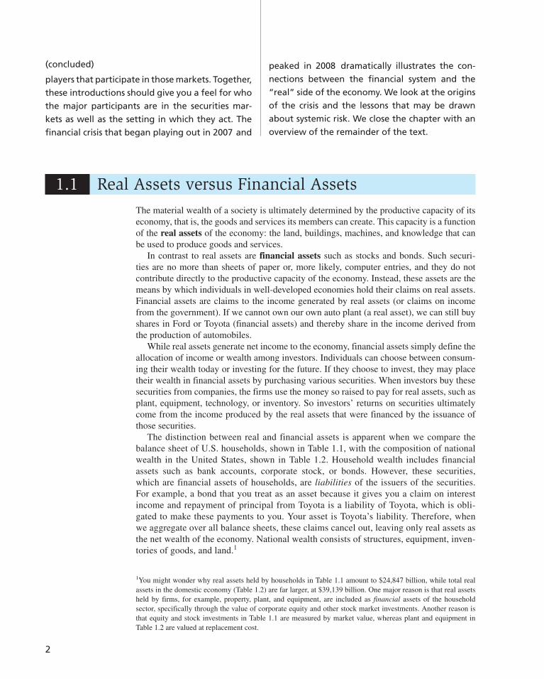
2
(concluded)
players that participate in those markets. Together,
these introductions should give you a feel for who
the major participants are in the securities mar-
kets as well as the setting in which they act. The
financial crisis that began playing out in 2007 and
peaked in 2008 dramatically illustrates the con-
nections between the financial system and the
“real” side of the economy. We look at the origins
of the crisis and the lessons that may be drawn
about systemic risk. We close the chapter with an
overview of the remainder of the text.
1.1 Real Assets versus Financial Assets
The material wealth of a society is ultimately determined by the productive capacity of its economy, that is, the goods and services its members can create. This capacity is a function of the real assets of the economy: the land, buildings, machines, and knowledge that can be used to produce goods and services.
In contrast to real assets are financial assets such as stocks and bonds. Such securi-ties are no more than sheets of paper or, more likely, computer entries, and they do not contribute directly to the productive capacity of the economy. Instead, these assets are the means by which individuals in well-developed economies hold their claims on real assets. Financial assets are claims to the income generated by real assets (or claims on income from the government). If we cannot own our own auto plant (a real asset), we can still buy shares in Ford or Toyota (financial assets) and thereby share in the income derived from the production of automobiles.
While real assets generate net income to the economy, financial assets simply define the allocation of income or wealth among investors. Individuals can choose between consum-ing their wealth today or investing for the future. If they choose to invest, they may place their wealth in financial assets by purchasing various securities. When investors buy these securities from companies, the firms use the money so raised to pay for real assets, such as plant, equipment, technology, or inventory. So investors’ returns on securities ultimately come from the income produced by the real assets that were financed by the issuance of those securities.
The distinction between real and financial assets is apparent when we compare the balance sheet of U.S. households, shown in Table 1.1 , with the composition of national wealth in the United States, shown in Table 1.2 . Household wealth includes financial assets such as bank accounts, corporate stock, or bonds. However, these securities, which are financial assets of households, are liabilities of the issuers of the securities. For example, a bond that you treat as an asset because it gives you a claim on interest income and repayment of principal from Toyota is a liability of Toyota, which is obli-gated to make these payments to you. Your asset is Toyota’s liability. Therefore, when we aggregate over all balance sheets, these claims cancel out, leaving only real assets as the net wealth of the economy. National wealth consists of structures, equipment, inven-tories of goods, and land. 1
1 You might wonder why real assets held by households in Table 1.1 amount to $24,847 billion, while total real assets in the domestic economy ( Table 1.2 ) are far larger, at $39,139 billion. One major reason is that real assets held by firms, for example, property, plant, and equipment, are included as financial assets of the household sector, specifically through the value of corporate equity and other stock market investments. Another reason is that equity and stock investments in Table 1.1 are measured by market value, whereas plant and equipment in Table 1.2 are valued at replacement cost.

C H A P T E R 1 The Investment Environment 3
Table 1.1
Balance sheet of U.S. households Note: Column sums may differ from total because of rounding error. Source: Flow of Funds Accounts of the United States, Board of Governors of the Federal Reserve System, September 2009.
Assets $ Billion % Total Liabilities and Net Worth $ Billion % Total
Real assets
Real estate $ 20,026 29.8% Mortgages $10,652 15.8%
Consumer durables 4,601 6.8 Consumer credit 2,476 3.7
Other 221 0.3 Bank and other loans 253 0.4
Total real assets $ 24,847 37.0% Security credit 148 0.2
Other 541 0.8
Total liabilities $14,068 20.9%
Financial assets
Deposits $ 7,760 11.5%
Life insurance reserves 1,198 1.8
Pension reserves 10,656 15.9
Corporate equity 6,266 9.3
Equity in noncorp. business 6,996 10.4
Mutual fund shares 3,741 5.6
Debt securities 4,327 6.4
Other 1,418 2.1
Total financial assets 42,361 63.0 Net worth 53,140 79.1
Total $67,208 100.0% $67,208 100.0%
Note: Column sums may differ from total because of rounding error.Source: Flow of Funds Accounts of the United States, Board of Governors of the Federal Reserve System, September 2009.
Assets $ Billion
Nonresidential real estate $ 8,316
Residential real estate 20,026
Equipment and software 4,542
Inventories 1,654
Consumer durables 4,601
Total $39,139
Table 1.2
Domestic net worth
CONCEPT CHECK
1
Are the following assets real or financial?
a. Patents
b. Lease obligations
c. Customer goodwill
d. A college education
e. A $5 bill
We will focus almost exclusively on financial assets. But you shouldn’t lose sight of the fact that the successes or failures of the financial assets we choose to purchase ultimately depend on the performance of the underlying real assets.

4 P A R T I Introduction
1.2 Financial Assets
It is common to distinguish among three broad types of financial assets: fixed income, equity, and derivatives. Fixed-income or debt securities promise either a fixed stream of income or a stream of income determined by a specified formula. For example, a corporate bond typically would promise that the bondholder will receive a fixed amount of interest each year. Other so-called floating-rate bonds promise payments that depend on current interest rates. For example, a bond may pay an interest rate that is fixed at 2 percentage points above the rate paid on U.S. Treasury bills. Unless the borrower is declared bankrupt, the payments on these securities are either fixed or determined by formula. For this reason, the investment performance of debt securities typically is least closely tied to the financial condition of the issuer.
Nevertheless, fixed-income securities come in a tremendous variety of maturities and payment provisions. At one extreme, the money market refers to debt securities that are short term, highly marketable, and generally of very low risk. Examples of money market securities are U.S. Treasury bills or bank certificates of deposit (CDs). In contrast, the fixed-income capital market includes long-term securities such as Treasury bonds, as well as bonds issued by federal agencies, state and local municipalities, and corporations. These bonds range from very safe in terms of default risk (for example, Treasury securities) to relatively risky (for example, high-yield or “junk” bonds). They also are designed with extremely diverse provisions regarding payments provided to the investor and protection against the bankruptcy of the issuer. We will take a first look at these securities in Chapter 2 and undertake a more detailed analysis of the debt market in Part Four.
Unlike debt securities, common stock, or equity, in a firm represents an ownership share in the corporation. Equityholders are not promised any particular payment. They receive any dividends the firm may pay and have prorated ownership in the real assets of the firm. If the firm is successful, the value of equity will increase; if not, it will decrease. The performance of equity investments, therefore, is tied directly to the success of the firm and its real assets. For this reason, equity investments tend to be riskier than investments in debt securities. Equity markets and equity valuation are the topics of Part Five.
Finally, derivative securities such as options and futures contracts provide payoffs that are determined by the prices of other assets such as bond or stock prices. For example, a call option on a share of Intel stock might turn out to be worthless if Intel’s share price remains below a threshold or “exercise” price such as $20 a share, but it can be quite valu-able if the stock price rises above that level. 2 Derivative securities are so named because their values derive from the prices of other assets. For example, the value of the call option will depend on the price of Intel stock. Other important derivative securities are futures and swap contracts. We will treat these in Part Six.
Derivatives have become an integral part of the investment environment. One use of derivatives, perhaps the primary use, is to hedge risks or transfer them to other parties. This is done successfully every day, and the use of these securities for risk management is so commonplace that the multitrillion-dollar market in derivative assets is routinely taken for granted. Derivatives also can be used to take highly speculative positions, however. Every so often, one of these positions blows up, resulting in well-publicized losses of hundreds of millions of dollars. While these losses attract considerable attention, they are
2 A call option is the right to buy a share of stock at a given exercise price on or before the option’s expiration date. If the market price of Intel remains below $20 a share, the right to buy for $20 will turn out to be valueless. If the share price rises above $20 before the option expires, however, the option can be exercised to obtain the share for only $20.

C H A P T E R 1 The Investment Environment 5
in fact the exception to the more common use of such securities as risk management tools. Derivatives will continue to play an important role in portfolio construction and the finan-cial system. We will return to this topic later in the text.
In addition to these financial assets, individuals might invest directly in some real assets. For example, real estate or commodities such as precious metals or agricultural products are real assets that might form part of an investment portfolio.
1.3 Financial Markets and the Economy
We stated earlier that real assets determine the wealth of an economy, while financial assets merely represent claims on real assets. Nevertheless, financial assets and the markets in which they trade play several crucial roles in developed economies. Financial assets allow us to make the most of the economy’s real assets.
The Informational Role of Financial Markets
In a capitalist system, financial markets play a central role in the allocation of capital resources. Investors in the stock market ultimately decide which companies will live and which will die. If a corporation seems to have good prospects for future profitability, investors will bid up its stock price. The company’s management will find it easy to issue new shares or borrow funds to finance research and development, build new production facilities, and expand its operations. If, on the other hand, a company’s prospects seem poor, investors will bid down its stock price. The company will have to downsize and may eventually disappear.
The process by which capital is allocated through the stock market sometimes seems wasteful. Some companies can be “hot” for a short period of time, attract a large flow of investor capital, and then fail after only a few years. But that is an unavoidable implication of uncertainty. No one knows with certainty which ventures will succeed and which will fail. But the stock market encourages allocation of capital to those firms that appear at
the time to have the best prospects. Many smart, well-trained, and well-paid professionals analyze the prospects of firms whose shares trade on the stock market. Stock prices reflect their collective judgment.
Consumption Timing
Some individuals in an economy are earning more than they currently wish to spend. Others, for example, retirees, spend more than they currently earn. How can you shift your purchasing power from high-earnings periods to low-earnings periods of life? One way is to “store” your wealth in financial assets. In high-earnings periods, you can invest your savings in financial assets such as stocks and bonds. In low-earnings periods, you can sell these assets to provide funds for your consumption needs. By so doing, you can “shift” your consumption over the course of your lifetime, thereby allocating your consumption to periods that provide the greatest satisfaction. Thus, financial markets allow individuals to separate decisions concerning current consumption from constraints that otherwise would be imposed by current earnings.
Allocation of Risk
Virtually all real assets involve some risk. When Ford builds its auto plants, for example, it cannot know for sure what cash flows those plants will generate. Financial markets and the diverse financial instruments traded in those markets allow investors with the greatest taste

6 P A R T I Introduction
for risk to bear that risk, while other, less risk-tolerant individuals can, to a greater extent, stay on the sidelines. For example, if Ford raises the funds to build its auto plant by selling both stocks and bonds to the public, the more optimistic or risk-tolerant investors can buy shares of its stock, while the more conservative ones can buy its bonds. Because the bonds promise to provide a fixed payment, the stockholders bear most of the business risk but reap potentially higher rewards. Thus, capital markets allow the risk that is inherent to all investments to be borne by the investors most willing to bear that risk.
This allocation of risk also benefits the firms that need to raise capital to finance their investments. When investors are able to select security types with the risk-return character-istics that best suit their preferences, each security can be sold for the best possible price. This facilitates the process of building the economy’s stock of real assets.
Separation of Ownership and Management
Many businesses are owned and managed by the same individual. This simple organiza-tion is well suited to small businesses and, in fact, was the most common form of business organization before the Industrial Revolution. Today, however, with global markets and large-scale production, the size and capital requirements of firms have skyrocketed. For example, in 2009 General Electric listed on its balance sheet about $73 billion of property, plant, and equipment, and total assets of nearly $780 billion. Corporations of such size simply cannot exist as owner-operated firms. GE actually has more than 600,000 stock-holders with an ownership stake in the firm proportional to their holdings of shares.
Such a large group of individuals obviously cannot actively participate in the day-to-day management of the firm. Instead, they elect a board of directors that in turn hires and supervises the management of the firm. This structure means that the owners and managers of the firm are different parties. This gives the firm a stability that the owner-managed firm cannot achieve. For example, if some stockholders decide they no longer wish to hold shares in the firm, they can sell their shares to other investors, with no impact on the man-agement of the firm. Thus, financial assets and the ability to buy and sell those assets in the financial markets allow for easy separation of ownership and management.
How can all of the disparate owners of the firm, ranging from large pension funds hold-ing hundreds of thousands of shares to small investors who may hold only a single share, agree on the objectives of the firm? Again, the financial markets provide some guidance. All may agree that the firm’s management should pursue strategies that enhance the value of their shares. Such policies will make all shareholders wealthier and allow them all to better pursue their personal goals, whatever those goals might be.
Do managers really attempt to maximize firm value? It is easy to see how they might be tempted to engage in activities not in the best interest of shareholders. For example, they might engage in empire building or avoid risky projects to protect their own jobs or overconsume luxuries such as corporate jets, reasoning that the cost of such perquisites is largely borne by the shareholders. These potential conflicts of interest are called agency
problems because managers, who are hired as agents of the shareholders, may pursue their own interests instead.
Several mechanisms have evolved to mitigate potential agency problems. First, com-pensation plans tie the income of managers to the success of the firm. A major part of the total compensation of top executives is often in the form of stock options, which means that the managers will not do well unless the stock price increases, benefiting shareholders. (Of course, we’ve learned more recently that overuse of options can create its own agency problem. Options can create an incentive for managers to manipulate information to prop up a stock price temporarily, giving them a chance to cash out before the price returns to a

C H A P T E R 1 The Investment Environment 7
level reflective of the firm’s true prospects. More on this shortly.) Second, while boards of directors are sometimes portrayed as defenders of top management, they can, and increas-ingly do, force out management teams that are underperforming. Third, outsiders such as security analysts and large institutional investors such as pension funds monitor the firm closely and make the life of poor performers at the least uncomfortable.
Finally, bad performers are subject to the threat of takeover. If the board of directors is lax in monitoring management, unhappy shareholders in principle can elect a differ-ent board. They can do this by launching a proxy contest in which they seek to obtain enough proxies (i.e., rights to vote the shares of other shareholders) to take control of the firm and vote in another board. However, this threat is usually minimal. Shareholders who attempt such a fight have to use their own funds, while management can defend itself using corporate coffers. Most proxy fights fail. The real takeover threat is from other firms. If one firm observes another underperforming, it can acquire the underperforming busi-ness and replace management with its own team. The stock price should rise to reflect the prospects of improved performance, which provides incentive for firms to engage in such takeover activity.
Corporate Governance and Corporate Ethics
We’ve argued that securities markets can play an important role in facilitating the deploy-ment of capital resources to their most productive uses. But for markets to effectively serve this purpose, there must be an acceptable level of transparency that allows investors to make well-informed decisions. If firms can mislead the public about their prospects, then much can go wrong.
Despite the many mechanisms to align incentives of shareholders and managers, the 3 years between 2000 and 2002 were filled with a seemingly unending series of scandals that collectively signaled a crisis in corporate governance and ethics. For example, the tele-com firm WorldCom overstated its profits by at least $3.8 billion by improperly c lassifying
Example 1.1 Carl Icahn’s Proxy Fight with Yahoo!
In February 2008, Microsoft offered to buy Yahoo! by paying its current shareholders $31 for each of their shares, a considerable premium to its closing price of $19.18 on the day before the offer. Yahoo’s management rejected that offer and a better one at $33 a share; Yahoo’s CEO Jerry Yang held out for $37 per share, a price that Yahoo! had not reached in more than 2 years. Billionaire investor Carl Icahn was outraged, arguing that management was protecting its own position at the expense of shareholder value. Icahn notified Yahoo! that he had been asked to “lead a proxy fight to attempt to remove the current board and to establish a new board which would attempt to negotiate a successful merger with Micro-soft.” To that end, he had purchased approximately 59 million shares of Yahoo! and formed a 10-person slate to stand for election against the current board. Despite this challenge, Yahoo’s management held firm in its refusal of Microsoft’s offer, and with the support of the board, Yang managed to fend off both Microsoft and Icahn. In July, Icahn agreed to end the proxy fight in return for three seats on the board to be held by his allies. But the 11-person board was still dominated by current Yahoo management. Yahoo’s share price, which had risen to $29 a share during the Microsoft negotiations, fell back to around $21 a share. Given the difficulty that a well-known billionaire faced in defeating a determined and entrenched management, it is no wonder that proxy contests are rare. Historically, about three of four proxy fights go down to defeat.
8 P A R T I Introduction
expenses as investments. When the true picture emerged, it resulted in the largest bank-ruptcy in U.S. history. The second-largest U.S. bankruptcy was Enron, which used its now-notorious “special-purpose entities” to move debt off its own books and similarly present a misleading picture of its financial status. Unfortunately, these firms had plenty of company. Other firms such as Rite Aid, HealthSouth, Global Crossing, and Qwest Communications also manipulated and misstated their accounts to the tune of billions of dollars. And the scandals were hardly limited to the United States. Parmalat, the Italian dairy firm, claimed to have a $4.8 billion bank account that turned out not to exist. These episodes suggest that agency and incentive problems are far from solved.
Other scandals of that period included systematically misleading and overly optimistic research reports put out by stock market analysts. (Their favorable analysis was traded for the promise of future investment banking business, and analysts were commonly compen-sated not for their accuracy or insight, but for their role in garnering investment banking business for their firms.) Additionally, initial public offerings were allocated to corporate executives as a quid pro quo for personal favors or the promise to direct future business back to the manager of the IPO.
What about the auditors who were supposed to be the watchdogs of the firms? Here too, incentives were skewed. Recent changes in business practice had made the consulting businesses of these firms more lucrative than the auditing function. For example, Enron’s (now-defunct) auditor Arthur Andersen earned more money consulting for Enron than by auditing it; given Arthur Andersen’s incentive to protect its consulting profits, we should not be surprised that it, and other auditors, were overly lenient in their auditing work.
In 2002, in response to the spate of ethics scandals, Congress passed the Sarbanes-Oxley Act to tighten the rules of corporate governance. For example, the act requires corporations to have more independent directors, that is, more directors who are not themselves manag-ers (or affiliated with managers). The act also requires each CFO to personally vouch for the corporation’s accounting statements, created an oversight board to oversee the auditing of public companies, and prohibits auditors from providing various other services to clients.
1.4 The Investment Process
An investor’s portfolio is simply his collection of investment assets. Once the portfolio is established, it is updated or “rebalanced” by selling existing securities and using the pro-ceeds to buy new securities, by investing additional funds to increase the overall size of the portfolio, or by selling securities to decrease the size of the portfolio.
Investment assets can be categorized into broad asset classes, such as stocks, bonds, real estate, commodities, and so on. Investors make two types of decisions in constructing their portfolios. The asset allocation decision is the choice among these broad asset classes, while the security selection decision is the choice of which particular securities to hold within each asset class.
Asset allocation also includes the decision of how much of one’s portfolio to place in safe assets such as bank accounts or money market securities versus in risky assets. Unfortunately, many observers, even those providing financial advice, appear to incor-rectly equate saving with safe investing. 3 “Saving” means that you do not spend all of your
3 For example, here is a brief excerpt from the Web site of the Securities and Exchange Commission. “Your ‘savings’ are usually put into the safest places or products . . . When you ‘invest,’ you have a greater chance of losing your money than when you ‘save’.” This statement is incorrect: Your investment portfolio can be invested
in either safe or risky assets, and your savings in any period is simply the difference between your income and consumption.

C H A P T E R 1 The Investment Environment 9
current income, and therefore can add to your portfolio. You may choose to invest your savings in safe assets, risky assets, or a combination of both.
“Top-down” portfolio construction starts with asset allocation. For example, an individ-ual who currently holds all of his money in a bank account would first decide what propor-tion of the overall portfolio ought to be moved into stocks, bonds, and so on. In this way, the broad features of the portfolio are established. For example, while the average annual return on the common stock of large firms since 1926 has been better than 11% per year, the average return on U.S. Treasury bills has been less than 4%. On the other hand, stocks are far riskier, with annual returns (as measured by the Standard & Poor’s 500 index) that have ranged as low as –46% and as high as 55%. In contrast, T-bills are effectively risk-free: you know what interest rate you will earn when you buy them. Therefore, the decision to allocate your investments to the stock market or to the money market where Treasury bills are traded will have great ramifications for both the risk and the return of your portfo-lio. A top-down investor first makes this and other crucial asset allocation decisions before turning to the decision of the particular securities to be held in each asset class.
Security analysis involves the valuation of particular securities that might be included in the portfolio. For example, an investor might ask whether Merck or Pfizer is more attrac-tively priced. Both bonds and stocks must be evaluated for investment attractiveness, but valuation is far more difficult for stocks because a stock’s performance usually is far more sensitive to the condition of the issuing firm.
In contrast to top-down portfolio management is the “bottom-up” strategy. In this process, the portfolio is constructed from the securities that seem attractively priced without as much concern for the resultant asset allocation. Such a technique can result in unintended bets on one or another sector of the economy. For example, it might turn out that the portfolio ends up with a very heavy representation of firms in one industry, from one part of the country, or with exposure to one source of uncertainty. However, a bottom-up strategy does focus the portfolio on the assets that seem to offer the most attractive investment opportunities.
1.5 Markets Are Competitive
Financial markets are highly competitive. Thousands of intelligent and well-backed ana-lysts constantly scour securities markets searching for the best buys. This competition means that we should expect to find few, if any, “free lunches,” securities that are so under-priced that they represent obvious bargains. This no-free-lunch proposition has several implications. Let’s examine two.
The Risk–Return Trade-Off
Investors invest for anticipated future returns, but those returns rarely can be predicted pre-cisely. There will almost always be risk associated with investments. Actual or realized returns will almost always deviate from the expected return anticipated at the start of the investment period. For example, in 1931 (the worst calendar year for the market since 1926), the S&P 500 index fell by 46%. In 1933 (the best year), the index gained 55%. You can be sure that investors did not anticipate such extreme performance at the start of either of these years.
Naturally, if all else could be held equal, investors would prefer investments with the highest expected return. 4 However, the no-free-lunch rule tells us that all else cannot be
4 The “expected” return is not the return investors believe they necessarily will earn, or even their most likely return. It is instead the result of averaging across all possible outcomes, recognizing that some outcomes are more likely than others. It is the average rate of return across possible economic scenarios.

10 P A R T I Introduction
held equal. If you want higher expected returns, you will have to pay a price in terms of accepting higher investment risk. If higher expected return can be achieved without bear-ing extra risk, there will be a rush to buy the high-return assets, with the result that their prices will be driven up. Individuals considering investing in the asset at the now-higher price will find the investment less attractive: If you buy at a higher price, your expected rate of return (that is, profit per dollar invested) is lower. The asset will be considered attractive and its price will continue to rise until its expected return is no more than com-mensurate with risk. At this point, investors can anticipate a “fair” return relative to the asset’s risk, but no more. Similarly, if returns were independent of risk, there would be a rush to sell high-risk assets. Their prices would fall (and their expected future rates of return rise) until they eventually were attractive enough to be included again in investor portfolios. We conclude that there should be a risk–return trade-off in the securities mar-kets, with higher-risk assets priced to offer higher expected returns than lower-risk assets.
Of course, this discussion leaves several important questions unanswered. How should one measure the risk of an asset? What should be the quantitative trade-off between risk (properly measured) and expected return? One would think that risk would have some-thing to do with the volatility of an asset’s returns, but this guess turns out to be only partly correct. When we mix assets into diversified portfolios, we need to consider the interplay among assets and the effect of diversification on the risk of the entire portfolio. Diversification means that many assets are held in the portfolio so that the exposure to any particular asset is limited. The effect of diversification on portfolio risk, the implica-tions for the proper measurement of risk, and the risk–return relationship are the topics of Part Two. These topics are the subject of what has come to be known as modern portfolio
theory. The development of this theory brought two of its pioneers, Harry Markowitz and William Sharpe, Nobel Prizes.
Efficient Markets
Another implication of the no-free-lunch proposition is that we should rarely expect to find bargains in the security markets. We will spend all of Chapter 11 examining the theory and evidence concerning the hypothesis that financial markets process all relevant information about securities quickly and efficiently, that is, that the security price usually reflects all the information available to investors concerning its value. According to this hypothesis, as new information about a security becomes available, its price quickly adjusts so that at any time, the security price equals the market consensus estimate of the value of the security. If this were so, there would be neither underpriced nor overpriced securities.
One interesting implication of this “efficient market hypothesis” concerns the choice between active and passive investment-management strategies. Passive management calls for holding highly diversified portfolios without spending effort or other resources attempting to improve investment performance through security analysis. Active manage-
ment is the attempt to improve performance either by identifying mispriced securities or by timing the performance of broad asset classes—for example, increasing one’s commit-ment to stocks when one is bullish on the stock market. If markets are efficient and prices reflect all relevant information, perhaps it is better to follow passive strategies instead of spending resources in a futile attempt to outguess your competitors in the financial markets.
If the efficient market hypothesis were taken to the extreme, there would be no point in active security analysis; only fools would commit resources to actively analyze securities. Without ongoing security analysis, however, prices eventually would depart from “correct” values, creating new incentives for experts to move in. Therefore, even in environments

C H A P T E R 1 The Investment Environment 11
as competitive as the financial markets, we may observe only near -efficiency, and profit opportunities may exist for especially diligent and creative investors. In Chapter 12, we examine such challenges to the efficient market hypothesis, and this motivates our discus-sion of active portfolio management in Part Seven. More important, our discussions of security analysis and portfolio construction generally must account for the likelihood of nearly efficient markets.
1.6 The Players
From a bird’s-eye view, there would appear to be three major players in the financial markets:
1. Firms are net borrowers. They raise capital now to pay for investments in plant and equipment. The income generated by those real assets provides the returns to inves-tors who purchase the securities issued by the firm.
2. Households typically are net savers. They purchase the securities issued by firms that need to raise funds.
3. Governments can be borrowers or lenders, depending on the relationship between tax revenue and government expenditures. Since World War II, the U.S. government typically has run budget deficits, meaning that its tax receipts have been less than its expenditures. The government, therefore, has had to borrow funds to cover its budget deficit. Issuance of Treasury bills, notes, and bonds is the major way that the govern-ment borrows funds from the public. In contrast, in the latter part of the 1990s, the government enjoyed a budget surplus and was able to retire some outstanding debt.
Corporations and governments do not sell all or even most of their securities directly to individuals. For example, about half of all stock is held by large financial institutions such as pension funds, mutual funds, insurance companies, and banks. These financial institutions stand between the security issuer (the firm) and the ultimate owner of the security (the individual investor). For this reason, they are called financial intermediaries. Similarly, corporations do not market their own securities to the public. Instead, they hire agents, called investment bankers, to represent them to the investing public. Let’s examine the roles of these intermediaries.
Financial Intermediaries
Households want desirable investments for their savings, yet the small (financial) size of most households makes direct investment difficult. A small investor seeking to lend money to businesses that need to finance investments doesn’t advertise in the local news-paper to find a willing and desirable borrower. Moreover, an individual lender would not be able to diversify across borrowers to reduce risk. Finally, an individual lender is not equipped to assess and monitor the credit risk of borrowers.
For these reasons, financial intermediaries have evolved to bring lenders and borrow-ers together. These financial intermediaries include banks, investment companies, insur-ance companies, and credit unions. Financial intermediaries issue their own securities to raise funds to purchase the securities of other corporations.
For example, a bank raises funds by borrowing (taking deposits) and lending that money to other borrowers. The spread between the interest rates paid to depositors and the rates charged to borrowers is the source of the bank’s profit. In this way, lenders and borrowers
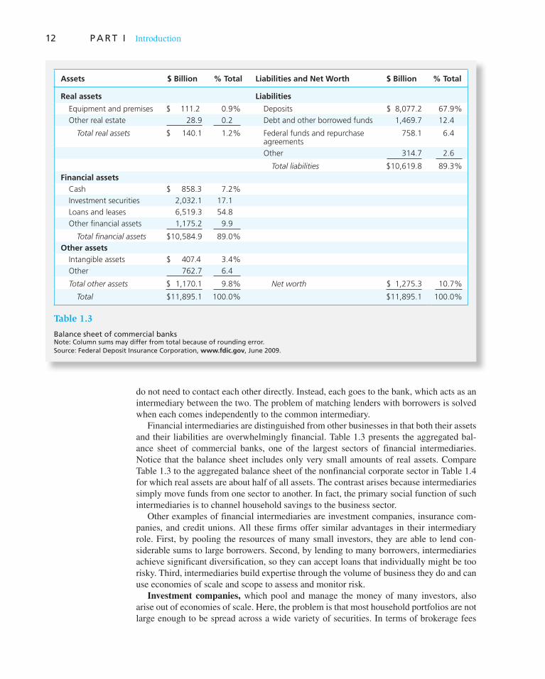
12 P A R T I Introduction
do not need to contact each other directly. Instead, each goes to the bank, which acts as an intermediary between the two. The problem of matching lenders with borrowers is solved when each comes independently to the common intermediary.
Financial intermediaries are distinguished from other businesses in that both their assets and their liabilities are overwhelmingly financial. Table 1.3 presents the aggregated bal-ance sheet of commercial banks, one of the largest sectors of financial intermediaries. Notice that the balance sheet includes only very small amounts of real assets. Compare Table 1.3 to the aggregated balance sheet of the nonfinancial corporate sector in Table 1.4 for which real assets are about half of all assets. The contrast arises because intermediaries simply move funds from one sector to another. In fact, the primary social function of such intermediaries is to channel household savings to the business sector.
Other examples of financial intermediaries are investment companies, insurance com-panies, and credit unions. All these firms offer similar advantages in their intermediary role. First, by pooling the resources of many small investors, they are able to lend con-siderable sums to large borrowers. Second, by lending to many borrowers, intermediaries achieve significant diversification, so they can accept loans that individually might be too risky. Third, intermediaries build expertise through the volume of business they do and can use economies of scale and scope to assess and monitor risk.
Investment companies, which pool and manage the money of many investors, also arise out of economies of scale. Here, the problem is that most household portfolios are not large enough to be spread across a wide variety of securities. In terms of brokerage fees
Table 1.3
Balance sheet of commercial banks Note: Column sums may differ from total because of rounding error.Source: Federal Deposit Insurance Corporation, www.fdic.gov, June 2009.
Assets $ Billion % Total Liabilities and Net Worth $ Billion % Total
Real assets Liabilities
Equipment and premises $ 111.2 0.9% Deposits $ 8,077.2 67.9%
Other real estate 28.9 0.2 Debt and other borrowed funds 1,469.7 12.4
Total real assets $ 140.1 1.2% Federal funds and repurchase agreements
758.1 6.4
Other 314.7 2.6
Total liabilities $10,619.8 89.3%
Financial assets
Cash $ 858.3 7.2%
Investment securities 2,032.1 17.1
Loans and leases 6,519.3 54.8
Other financial assets 1,175.2 9.9
Total financial assets $10,584.9 89.0%
Other assets
Intangible assets $ 407.4 3.4%
Other 762.7 6.4
Total other assets $ 1,170.1 9.8% Net worth $ 1,275.3 10.7%
Total $11,895.1 100.0% $11,895.1 100.0%

C H A P T E R 1 The Investment Environment 13
and research costs, purchasing one or two shares of many different firms is very expensive. Mutual funds have the advantage of large-scale trading and portfolio management, while participating investors are assigned a prorated share of the total funds according to the size of their investment. This system gives small investors advantages they are willing to pay for via a management fee to the mutual fund operator.
Investment companies also can design portfolios specifically for large investors with particular goals. In contrast, mutual funds are sold in the retail market, and their investment philosophies are differentiated mainly by strategies that are likely to attract a large number of clients.
Economies of scale also explain the proliferation of analytic services available to inves-tors. Newsletters, databases, and brokerage house research services all engage in research to be sold to a large client base. This setup arises naturally. Investors clearly want infor-mation, but with small portfolios to manage, they do not find it economical to personally gather all of it. Hence, a profit opportunity emerges: A firm can perform this service for many clients and charge for it.
Investment Bankers
Just as economies of scale and specialization create profit opportunities for financial inter-mediaries, so do these economies create niches for firms that perform specialized services for businesses. Firms raise much of their capital by selling securities such as stocks and bonds to the public. Because these firms do not do so frequently, however, investment
bankers that specialize in such activities can offer their services at a cost below that of maintaining an in-house security issuance division. In this role, they are called underwriters.
Assets $ Billion % Total Liabilities and Net Worth $ Billion % Total
Real assets Liabilities
Equipment and software $ 4,322 16.3% Bonds and mortgages $ 5,284 19.9%
Real estate 6,562 24.7 Bank loans 638 2.4
Inventories 1,654 6.2 Other loans 1,347 5.1
Total real assets $12,538 47.2% Trade debt 1,642 6.2
Other 4,448 16.7
Total liabilities $13,359 50.3%
Financial assets
Deposits and cash $ 637 2.4%
Marketable securities 936 3.5
Trade and consumer credit 2,202 8.3
Other 10,259 38.6
Total financial assets $14,034 52.8%
Total $26,572 100.0% Net worth $13,214 49.7%
$26,572 100.0%
Table 1.4
Balance sheet of nonfinancial U.S. businessNote: Column sums may differ from total because of rounding error.Source: Flow of Funds Accounts of the United States, Board of Governors of the Federal Reserve System, September 2009.
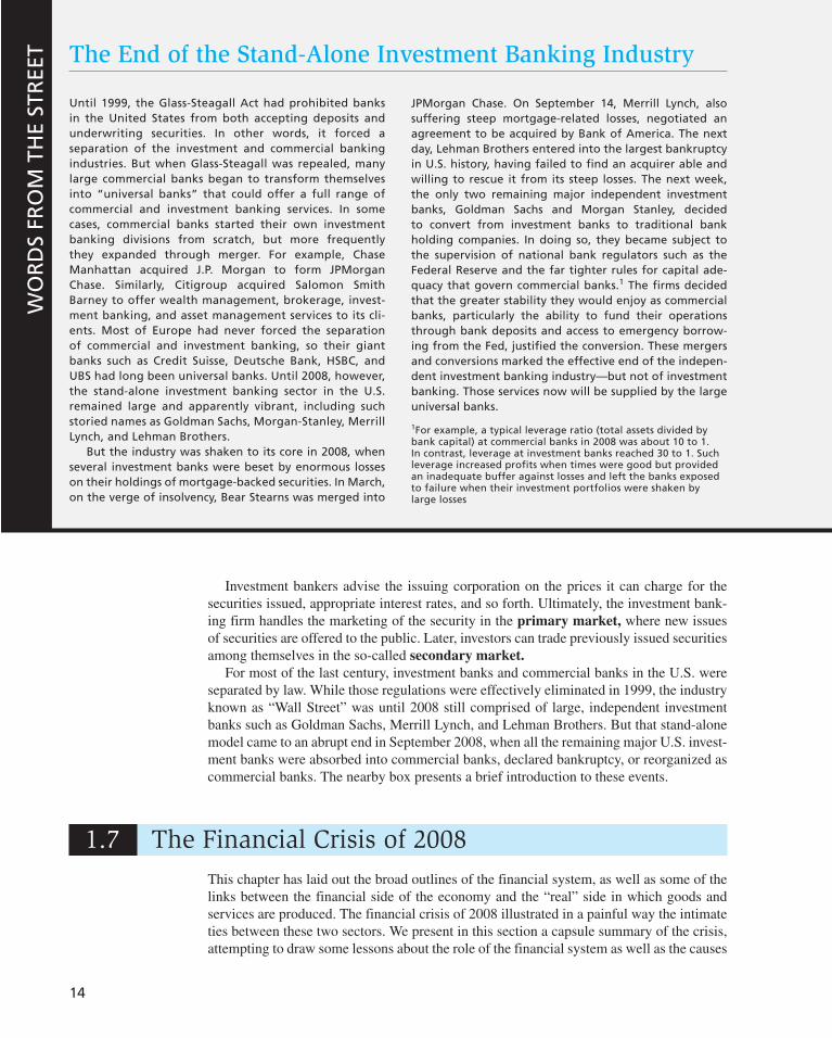
14
Investment bankers advise the issuing corporation on the prices it can charge for the securities issued, appropriate interest rates, and so forth. Ultimately, the investment bank-ing firm handles the marketing of the security in the primary market, where new issues of securities are offered to the public. Later, investors can trade previously issued securities among themselves in the so-called secondary market.
For most of the last century, investment banks and commercial banks in the U.S. were separated by law. While those regulations were effectively eliminated in 1999, the industry known as “Wall Street” was until 2008 still comprised of large, independent investment banks such as Goldman Sachs, Merrill Lynch, and Lehman Brothers. But that stand-alone model came to an abrupt end in September 2008, when all the remaining major U.S. invest-ment banks were absorbed into commercial banks, declared bankruptcy, or reorganized as commercial banks. The nearby box presents a brief introduction to these events.
The End of the Stand-Alone Investment Banking Industry
Until 1999, the Glass-Steagall Act had prohibited banks in the United States from both accepting deposits and underwriting securities. In other words, it forced a separation of the investment and commercial banking industries. But when Glass-Steagall was repealed, many large commercial banks began to transform themselves into “universal banks” that could offer a full range of commercial and investment banking services. In some cases, commercial banks started their own investment banking divisions from scratch, but more frequently they expanded through merger. For example, Chase Manhattan acquired J.P. Morgan to form JPMorgan Chase. Similarly, Citigroup acquired Salomon Smith Barney to offer wealth management, brokerage, invest-ment banking, and asset management services to its cli-ents. Most of Europe had never forced the separation of commercial and investment banking, so their giant banks such as Credit Suisse, Deutsche Bank, HSBC, and UBS had long been universal banks. Until 2008, however, the stand-alone investment banking sector in the U.S. remained large and apparently vibrant, including such storied names as Goldman Sachs, Morgan-Stanley, Merrill Lynch, and Lehman Brothers.
But the industry was shaken to its core in 2008, when several investment banks were beset by enormous losses on their holdings of mortgage-backed securities. In March, on the verge of insolvency, Bear Stearns was merged into
JPMorgan Chase. On September 14, Merrill Lynch, also suffering steep mortgage-related losses, negotiated an agreement to be acquired by Bank of America. The next day, Lehman Brothers entered into the largest bankruptcy in U.S. history, having failed to find an acquirer able and willing to rescue it from its steep losses. The next week, the only two remaining major independent investment banks, Goldman Sachs and Morgan Stanley, decided to convert from investment banks to traditional bank holding companies. In doing so, they became subject to the supervision of national bank regulators such as the Federal Reserve and the far tighter rules for capital ade-quacy that govern commercial banks. 1 The firms decided that the greater stability they would enjoy as commercial banks, particularly the ability to fund their operations through bank deposits and access to emergency borrow-ing from the Fed, justified the conversion. These mergers and conversions marked the effective end of the indepen-dent investment banking industry—but not of investment banking. Those services now will be supplied by the large universal banks.
1 For example, a typical leverage ratio (total assets divided by bank capital) at commercial banks in 2008 was about 10 to 1. In contrast, leverage at investment banks reached 30 to 1. Such leverage increased profits when times were good but provided an inadequate buffer against losses and left the banks exposed to failure when their investment portfolios were shaken by large losses
WO
RD
S FR
OM
TH
E ST
REE
T
1.7 The Financial Crisis of 2008
This chapter has laid out the broad outlines of the financial system, as well as some of the links between the financial side of the economy and the “real” side in which goods and services are produced. The financial crisis of 2008 illustrated in a painful way the intimate ties between these two sectors. We present in this section a capsule summary of the crisis, attempting to draw some lessons about the role of the financial system as well as the causes
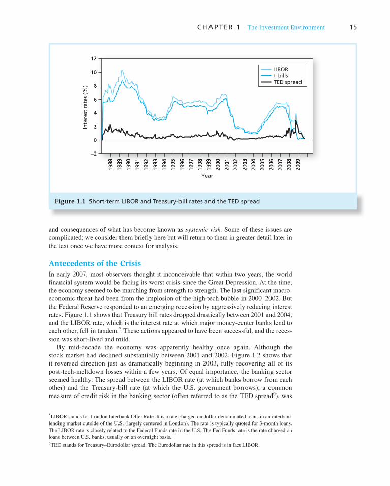
C H A P T E R 1 The Investment Environment 15
and consequences of what has become known as systemic risk. Some of these issues are complicated; we consider them briefly here but will return to them in greater detail later in the text once we have more context for analysis.
Antecedents of the Crisis
In early 2007, most observers thought it inconceivable that within two years, the world financial system would be facing its worst crisis since the Great Depression. At the time, the economy seemed to be marching from strength to strength. The last significant macro-economic threat had been from the implosion of the high-tech bubble in 2000–2002. But the Federal Reserve responded to an emerging recession by aggressively reducing interest rates. Figure 1.1 shows that Treasury bill rates dropped drastically between 2001 and 2004, and the LIBOR rate, which is the interest rate at which major money-center banks lend to each other, fell in tandem. 5 These actions appeared to have been successful, and the reces-sion was short-lived and mild.
By mid-decade the economy was apparently healthy once again. Although the stock market had declined substantially between 2001 and 2002, Figure 1.2 shows that it reversed direction just as dramatically beginning in 2003, fully recovering all of its post-tech-meltdown losses within a few years. Of equal importance, the banking sector seemed healthy. The spread between the LIBOR rate (at which banks borrow from each other) and the Treasury-bill rate (at which the U.S. government borrows), a common measure of credit risk in the banking sector (often referred to as the TED spread 6 ), was
5 LIBOR stands for London Interbank Offer Rate. It is a rate charged on dollar-denominated loans in an interbank lending market outside of the U.S. (largely centered in London). The rate is typically quoted for 3-month loans. The LIBOR rate is closely related to the Federal Funds rate in the U.S. The Fed Funds rate is the rate charged on loans between U.S. banks, usually on an overnight basis. 6 TED stands for Treasury–Eurodollar spread. The Eurodollar rate in this spread is in fact LIBOR.
1988
Inte
rest
rat
es (
%)
12
10
8
6
4
2
0
Year
1989
1990
1991
1992
1993
1994
1995
1996
1997
1998
1999
2000
2001
2002
2003
2004
2005
2006
2007
2008
2009
LIBORT-billsTED spread
−2
Figure 1.1 Short-term LIBOR and Treasury-bill rates and the TED spread
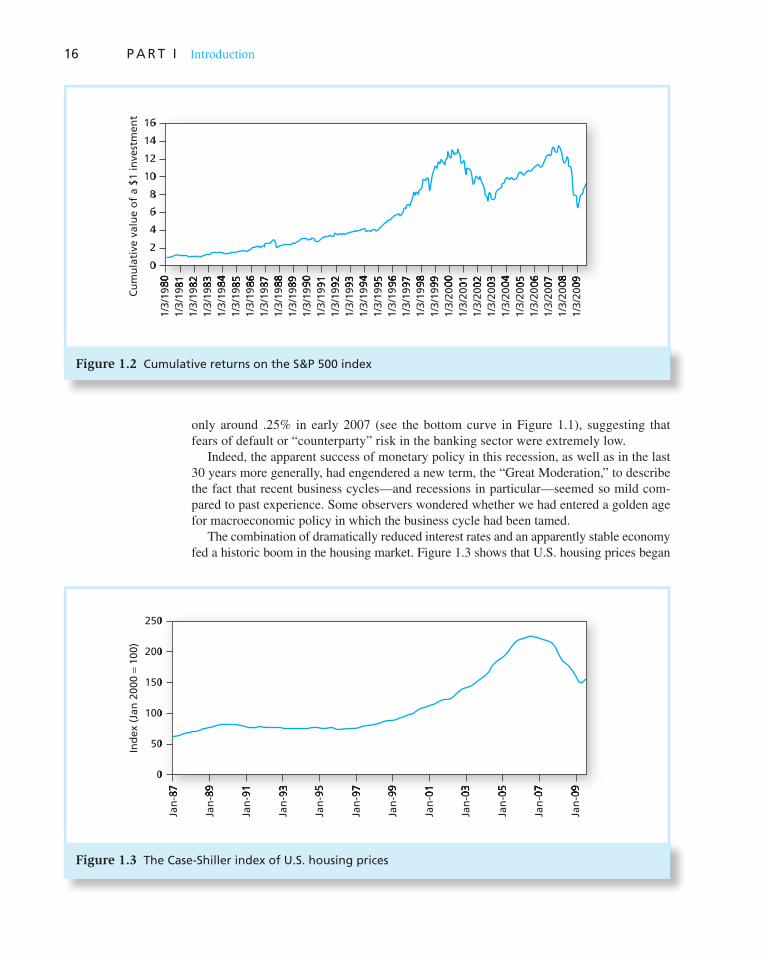
16 P A R T I Introduction
only around .25% in early 2007 (see the bottom curve in Figure 1.1 ), suggesting that fears of default or “counterparty” risk in the banking sector were extremely low.
Indeed, the apparent success of monetary policy in this recession, as well as in the last 30 years more generally, had engendered a new term, the “Great Moderation,” to describe the fact that recent business cycles—and recessions in particular—seemed so mild com-pared to past experience. Some observers wondered whether we had entered a golden age for macroeconomic policy in which the business cycle had been tamed.
The combination of dramatically reduced interest rates and an apparently stable economy fed a historic boom in the housing market. Figure 1.3 shows that U.S. housing prices began
1/3/
1980
1/3/
1981
1/3/
1982
1/3/
1983
1/3/
1984
1/3/
1985
1/3/
1986
1/3/
1987
1/3/
1988
1/3/
1989
1/3/
1990
1/3/
1991
1/3/
1992
1/3/
1993
1/3/
1994
1/3/
1995
1/3/
1996
1/3/
1997
1/3/
1998
1/3/
1999
1/3/
2000
1/3/
2001
1/3/
2002
1/3/
2003
1/3/
2004
1/3/
2005
1/3/
2006
1/3/
2007
1/3/
2008
1/3/
2009
0
2
4
6
8
10
12
14
16C
um
ula
tive
val
ue
of
a $1
inve
stm
ent
Figure 1.2 Cumulative returns on the S&P 500 index
0
50
100
150
200
250
Ind
ex (
Jan
200
0 =
100
)
Jan
-87
Jan
-89
Jan
-91
Jan
-93
Jan
-95
Jan
-97
Jan
-99
Jan
-01
Jan
-03
Jan
-05
Jan
-07
Jan
-09
Figure 1.3 The Case-Shiller index of U.S. housing prices

C H A P T E R 1 The Investment Environment 17
rising noticeably in the late 1990s and accelerated dramatically after 2001 as interest rates plummeted. In the 10 years beginning 1997, average prices in the U.S. approximately tripled.
But the newfound confidence in the power of macroeconomic policy to reduce risk, the impressive recovery of the economy from the high-tech implosion, and particularly the housing price boom following the aggressive reduction in interest rates may have sown the seeds for the debacle that played out in 2008. On the one hand, the Fed’s policy of reducing interest rates had resulted in low yields on a wide variety of investments, and investors were hungry for higher yielding alternatives. On the other hand, low volatility and growing complacency about risk encouraged greater tolerance for risk in the search for these higher yielding investments. Nowhere was this more evident than in the explod-ing market for securitized mortgages. The U.S. housing and mortgage finance markets were at the center of a gathering storm.
Changes in Housing Finance
Prior to 1970, most mortgage loans would come from a local lender such as a neigh-borhood savings bank or credit union. A homeowner would borrow funds for a home purchase and repay the loan over a long period, commonly 30 years. A typical thrift insti-tution would have as its major asset a portfolio of these long-term home loans while its major liability would be the accounts of its depositors. This landscape began to change when Fannie Mae (FNMA, or Federal National Mortgage Association) and Freddie Mac (FHLMC, or Federal Home Loan Mortgage Corporation) began buying mortgage loans from originators and bundling them into large pools that could be traded like any other financial asset. These pools, which were essentially claims on the underlying mortgages, were soon dubbed mortgage-backed securities, and the process was called securitization.
Fannie and Freddie quickly became the behemoths of the mortgage market, between them buying around half of all mortgages originated by the private sector.
Figure 1.4 illustrates how cash flows passed from the original borrower to the ulti-mate investor in a mortgage-backed security. The loan originator, for example, the savings and loan, might make a $100,000 home loan to a homeowner. The homeowner would repay principal and interest (P&I) on the loan over 30 years. But then the originator would sell the mortgage to Freddie Mac or Fannie Mae and recover the cost of the loan. The originator could continue to service the loan (collect monthly payments from the home-owner) for a small servicing fee, but the loan payments net of that fee would be passed along to the agency. In turn, Freddie or Fannie would pool the loans into mortgage-backed securities and sell the securities to investors such as pension funds or mutual funds. The agency (Fannie or Freddie) typically would guarantee the credit or default risk of the loans
$100 K
P&I P&I –servicing fee
P&I – servicing-guarantee fee
$100 K $100 K
Originator Agency InvestorHomeowner
Figure 1.4 Cash flows in a mortgage pass-through security
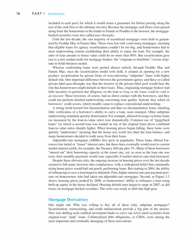
18 P A R T I Introduction
included in each pool, for which it would retain a guarantee fee before passing along the rest of the cash flow to the ultimate investor. Because the mortgage cash flows were passed along from the homeowner to the lender to Fannie or Freddie to the investor, the mortgage-backed securities were also called pass-throughs.
Until the last decade, the vast majority of securitized mortgages were held or guaran-teed by Freddie Mac or Fannie Mae. These were low-risk conforming mortgages, meaning that eligible loans for agency securitization couldn’t be too big, and homeowners had to meet underwriting criteria establishing their ability to repay the loan. For example, the ratio of loan amount to house value could be no more than 80%. But securitization gave rise to a new market niche for mortgage lenders: the “originate to distribute” (versus origi-nate to hold) business model.
Whereas conforming loans were pooled almost entirely through Freddie Mac and Fannie Mae, once the securitization model took hold, it created an opening for a new product: securitization by private firms of nonconforming “subprime” loans with higher default risk. One important difference between the government agency and these so-called private-label pass-throughs was that the investor in the private-label pool would bear the risk that homeowners might default on their loans. Thus, originating mortgage brokers had little incentive to perform due diligence on the loan as long as the loans could be sold to
an investor. These investors, of course, had no direct contact with the borrowers, and they could not perform detailed underwriting concerning loan quality. Instead, they relied on borrowers’ credit scores, which steadily came to replace conventional underwriting.
A strong trend toward low-documentation and then no-documentation loans, entailing little verification of a borrower’s ability to carry a loan, soon emerged. Other subprime underwriting standards quickly deteriorated. For example, allowed leverage on home loans (as measured by the loan-to-value ratio) rose dramatically. Common use of “piggyback loans” (in which a second loan was loaded on top of the original loan) drove combined loan-to-value ratios sharply higher. When housing prices began falling, these loans were quickly “underwater,” meaning that the house was worth less than the loan balance, and many homeowners decided to walk away from their loans.
Adjustable-rate mortgages (ARMs) also grew in popularity. These loans offered bor-rowers low initial or “teaser” interest rates, but these rates eventually would reset to current market interest yields, for example, the Treasury bill rate plus 3%. Many of these borrowers “maxed out” their borrowing capacity at the teaser rate, yet, as soon as the loan rate was reset, their monthly payments would soar, especially if market interest rates had increased.
Despite these obvious risks, the ongoing increase in housing prices over the last decade seemed to lull many investors into complacency, with a widespread belief that continually rising home prices would bail out poorly performing loans. But starting in 2004, the ability of refinancing to save a loan began to diminish. First, higher interest rates put payment pres-sure on homeowners who had taken out adjustable-rate mortgages. Second, as Figure 1.3 shows, housing prices peaked by 2006, so homeowners’ ability to refinance a loan using built-up equity in the house declined. Housing default rates began to surge in 2007, as did losses on mortgage-backed securities. The crisis was ready to shift into high gear.
Mortgage Derivatives
One might ask: Who was willing to buy all of these risky subprime mortgages? Securitization, restructuring, and credit enhancement provide a big part of the answer. New risk-shifting tools enabled investment banks to carve out AAA-rated securities from original-issue “junk” loans. Collateralized debt obligations, or CDOs, were among the most important and eventually damaging of these innovations.

C H A P T E R 1 The Investment Environment 19
CDOs were designed to concentrate the credit (i.e., default) risk of a bundle of loans on one class of investors, leaving the other investors in the pool relatively protected from that risk. The idea was to prioritize claims on loan repayments by dividing the pool into senior versus junior slices, called tranches. The senior tranches had first claim on repayments from the entire pool. Junior tranches would be paid only after the senior ones had received their cut. 7 For example, if a pool were divided into two tranches, with 70% of the pool allocated to the senior tranche and 30% allocated to the junior one, the senior investors would be repaid in full as long as 70% or more of the loans in the pool performed, that is, as long as the default rate on the pool remained below 30%. Even with pools comprised of risky subprime loans, default rates above 30% seemed extremely unlikely, and thus senior tranches were fre-quently granted the highest (i.e., AAA) rating by the major credit rating agencies, Moody’s, Standard & Poor’s, and Fitch. Large amounts of AAA-rated securities were thus carved out of pools of low-rated mortgages. (We will describe CDOs in more detail in Chapter 14.)
Of course, we know now that these ratings were wrong. The senior-subordinated struc-ture of CDOs provided far less protection to senior tranches than investors anticipated. A common argument in defense of high ratings had been that if the mortgages used to form pools were taken from across several geographic regions, then aggregate default rates for entire pools would be unlikely to ever rise to levels at which senior investors would suffer losses. But when housing prices across the entire country began to fall in unison, defaults in all regions increased, and the hoped-for benefits from spreading the risks geographically never materialized.
Why had the rating agencies so dramatically underestimated credit risk in these sub-prime securities? First, default probabilities had been estimated using historical data from an unrepresentative period characterized by a housing boom and an uncommonly prosper-ous and recession-free macroeconomy. Moreover, the ratings analysts had extrapolated historical default experience to a new sort of borrower pool—one without down payments, with exploding-payment loans, and with low- or no-documentation loans (often called liar loans). Past default experience was largely irrelevant given these profound changes in the market. Moreover, the power of cross-regional diversification to minimize risk engendered excessive optimism.
Finally, agency problems became apparent. The ratings agencies were paid to provide ratings by the issuers of the securities—not the purchasers. They faced pressure from the issuers, who could shop around for the most favorable treatment, to provide generous ratings.
Credit Default Swaps
In parallel to the CDO market, the market in credit default swaps also exploded in this period. A credit default swap, or CDS, is in essence an insurance contract against the default of one or more borrowers. (We will describe these in more detail in Chapter 14.) The purchaser of the swap pays an annual premium (like an insurance premium) for
7 CDOs and related securities are sometimes called structured products. “Structured” means that original cash flows are sliced up and reapportioned across tranches according to some stipulated rule.
CONCEPT CHECK
2
When Freddie Mac and Fannie Mae pooled mortgages into securities, they guaranteed the underlying mortgage loans against homeowner defaults. In contrast, there were no guaran-tees on the mortgages pooled into subprime mortgage-backed securities, so investors would bear credit risk. Was either of these arrangements necessarily a better way to manage and allocate default risk?
20 P A R T I Introduction
p rotection from credit risk. Credit default swaps became an alternative method of credit enhancement, seemingly allowing investors to buy subprime loans and insure their safety. But in practice, some swap issuers ramped up their exposure to credit risk to unsupport-able levels, without sufficient capital to back those obligations. For example, the large insurance company AIG alone sold more than $400 billion of CDS contracts on subprime mortgages.
The Rise of Systemic Risk
By 2007, the financial system displayed several troubling features. Many large banks and related financial institutions had adopted an apparently profitable financing scheme: bor-rowing short term at low interest rates to finance holdings in higher yielding long-term illiquid assets, 8 and treating the interest rate differential between their assets and liabilities as economic profit. But this business model was precarious: By relying primarily on short-term loans for their funding, these firms needed to constantly refinance their positions (i.e., borrow additional funds as the loans matured), or else face the necessity of quickly selling off their less-liquid asset portfolios, which would be difficult in times of financial stress. Moreover, these institutions were highly leveraged and had little capital as a buffer against losses. Large investment banks on Wall Street in particular had sharply increased leverage, which added to an underappreciated vulnerability to refunding requirements—especially if the value of their asset portfolios came into question. For example, both Lehman Brothers and Merrill Lynch were reported to have leverage ratios in 2008 of around 30:1, meaning that around 97% of their funds were borrowed. Even small portfolio losses could drive their net worth negative, at which point no one would be willing to renew outstanding loans or extend new ones.
Their high leverage and the mismatch between the liquidity of their assets and liabilities made financial institutions particularly vulnerable to crises of confidence. If assessments of their portfolio value declined, there could be a “run” on assets, as investors rushed to be first to pull out funds. But the low liquidity of those assets could make it difficult to sell them to meet such redemption requests in a timely manner.
Another source of fragility was widespread investor reliance on “credit enhancement” through structured products. For example, CDO tranching created lots of AAA-rated paper, but with largely unrecognized reliance on diversification benefits that were likely overstated and on default projections that were likely understated. Many of the assets underlying these pools were illiquid, hard to value, and highly dependent on forecasts of future performance of other loans. In a widespread downturn, with rating downgrades, these assets would prove difficult to sell.
The steady displacement of formal exchange trading by informal “over-the-counter” markets created other problems. In formal exchanges such as futures or options markets, participants must put up collateral called margin to guarantee their ability to make good on their obligations. Prices are computed each day, and gains or losses are continually added to or subtracted from each trader’s margin account. If a margin account runs low after a series of losses, the investor can be required either to contribute more collateral or to close out the position before actual insolvency ensues. Positions, and thus exposures to losses, are transparent to other traders. In contrast, the over-the-counter markets where CDS contracts traded are effectively private contracts between two parties with less pub-lic disclosure of positions, less standardization of products (which makes the fair value
8 Liquidity refers to the speed and the ease with which investors can realize the cash value of an investment. Illiquid assets, for example, real estate, can be hard to sell quickly, and a quick sale may require a substantial discount from the price at which it could be sold in an unrushed situation.

C H A P T E R 1 The Investment Environment 21
of a contract hard to discover), and consequently less opportunity to recognize either cumulative gains or losses over time or the resultant credit exposure of each trading part-ner. Although over-the-counter markets also may require collateral, collateral levels are updated less frequently and are harder to negotiate when fair market prices are difficult to ascertain.
This new financial model was brimming with systemic risk, a potential breakdown of the financial system when problems in one market spill over and disrupt others. Many of these market innovations had unwittingly created new feedback loops for systemic risk to feed on itself. When firms are fully leveraged (i.e., have borrowed to their maximum capacity), losses on their portfolios can force them to sell some of their assets to bring their leverage back into line. But waves of selling from institutions that simultaneously need to “de-leverage” can drive down asset prices and exacerbate portfolio losses—forcing addi-tional sales and further price declines in a downward spiral.
When lenders such as banks have limited capital and are afraid of further losses, they may rationally choose to hoard their capital instead of lending it to customers such as small firms, thereby exacerbating funding problems for their customary borrowers. The possibil-ity of one default setting off a chain of further defaults means that lenders may be exposed to the default of an institution with which they do not even directly trade. For example, AIG’s insolvency would have triggered the insolvency of other firms, particularly banks, which had relied on its promise of protection (via CDS contracts) against defaults on hun-dreds of billions of dollars of mortgage loans. Those potential bank insolvencies would in turn have fed into insolvencies of the banks’ trading partners, and so on. The potential for contagion seemed great: by August 2008, $63 trillion of credit default swaps were report-edly outstanding. (Compare this figure to U.S. gross domestic product, which was approxi-mately $14 trillion at the time.)
The Shoe Drops
The first hints of serious difficulties in the financial system began to emerge in the sum-mer of 2007. Delinquency rates in subprime mortgages had been accelerating starting as early as 2006, but in June, the large investment bank Bear Stearns surprised investors by announcing huge losses on two of its subprime mortgage–related hedge funds. Banks and hedge funds around the world were “discovered” to have considerable exposure to sub-prime loans, leading to a general decline in market liquidity and higher borrowing rates for banks. By Fall 2007, housing price declines were widespread ( Figure 1.3 ), mortgage delin-quencies increased, and the stock market entered its own free fall ( Figure 1.2 ). In March 2008, with Bear Stearns on the verge of bankruptcy, the Federal Reserve arranged for it to be acquired by JPMorgan Chase (and provided guarantees to protect JPMorgan against further losses on Bear Stearns’s positions).
The crisis peaked in September 2008. On September 7, the giant federal mortgage agen-cies Fannie Mae and Freddie Mac, both of which had taken large positions in subprime mortgage–backed securities, were put into conservatorship. (We will have more to say on their travails in Chapter 2.) The failure of these two mainstays of the U.S. housing and mortgage finance industries threw financial markets into a panic. By the second week of September, it was clear that both Lehman Brothers and Merrill Lynch were on the verge of bankruptcy. On September 14, Merrill Lynch was sold to Bank of America, again with the benefit of government brokering and protection against losses. The next day, Lehman Brothers, which was denied equivalent treatment, filed for bankruptcy protection. Two days later, on September 17, the government reluctantly lent $85 billion to AIG, reasoning that its failure would have been highly destabilizing to the banking industry, which was

22 P A R T I Introduction
holding massive amounts of its credit guarantees (i.e., CDS contacts). The next day, the Treasury unveiled its first proposal to spend $700 billion to purchase “toxic” mortgage-backed securities.
A particularly devastating fallout of the Lehman bankruptcy was on the “money market” for short-term lending. Lehman had borrowed considerable funds by issuing very short-term debt, called commercial paper. Among the major customers in commer-cial paper were money market mutual funds, which invest in short-term, high-quality debt of commercial borrowers. When Lehman faltered, the Reserve Primary Money Market Fund, which was holding large amounts of (AAA-rated!) Lehman commercial paper, suffered investment losses that drove the value of its assets below $1 per share. 9 Fears spread that other funds were similarly exposed, and money market fund customers across the country rushed to withdraw their funds. The funds in turn rushed out of com-mercial paper into safer and more liquid Treasury bills, essentially shutting down short-term financing markets.
The freezing up of credit markets was the end of any dwindling possibility that the finan-cial crisis could be contained to Wall Street. Larger companies that had relied on the com-mercial paper market were now unable to raise short-term funds. Banks similarly found it difficult to raise funds. (Look back to Figure 1.1 , where you will see that the TED spread, a measure of bank insolvency fears, skyrocketed in 2008.) With banks unwilling or unable to extend credit to their customers, thousands of small businesses that relied on bank lines of credit also became unable to finance their normal businesses operations. Capital-starved companies were forced to scale back their own operations precipitously. The unemploy-ment rate rose rapidly, and the economy was in its worst recession in decades. The turmoil in the financial markets had spilled over into the real economy, and Main Street had joined Wall Street in a bout of protracted misery.
Systemic Risk and the Real Economy
We pointed out earlier in the chapter that the real economy needs a well-oiled financial sector for it to function well. Small firms rely on banks for short-term credit, and banks rely on investors to purchase their short-term debt securities such as certificates of deposit or commercial paper. All investors need to be able to assess the credit risk of their coun-terparties to determine which securities are worthy of purchase. Larger firms can access capital markets on their own, but they too depend on a well-functioning financial market, and when markets such as the one for commercial paper froze, the spillover to real opera-tions was immediate and painful.
Government responses to the crisis were largely attempts to break a vicious circle of valuation risk/counterparty risk/liquidity risk. One approach was for the government to reduce risk of the financial sector by pouring capital into precarious banks. The reason-ing was that with the new capital, insolvency risk would be reduced, and newly stabilized banks would once again be able to raise funds and resume lending among themselves and to their customers. With more capital supporting banks, the potential for one insolvency to trigger another could be contained. In addition, when banks have more capital, they have less incentive to ramp up risk, as potential losses will come at their own expense and not the FDIC’s.
9 Money market funds typically bear very little investment risk and can maintain their asset values at $1 per share. Investors view them as near substitutes for checking accounts. Until this episode, no other retail fund had “broken the buck.”

C H A P T E R 1 The Investment Environment 23
Proposals also have been targeted at increasing transparency. For example, one sug-gestion is to standardize CDS contracts and allow or force them to trade in centralized exchanges where prices can be determined in a deep market and gains or losses can be set-tled on a daily basis. Margin requirements, enforced daily, would prevent CDS participants from taking on greater positions than they can handle, and exchange trading would facili-tate analysis of the exposure of firms to losses in these markets.
Finally, incentive issues have been raised. Among these are proposals to force employee compensation to reflect longer term performance. For example, a portion of compensa-tion might be put aside and made available only after a period of several years, when the “true” profitability of employees’ actions can be more fully assessed. The motivation is to discourage excessive risk-taking in which big bets can be wagered with the attitude that a successful outcome will result in a big bonus while a bad outcome will be borne by the company or, worse, the taxpayer. The incentives of the bond rating agencies are also a sore point. Few are happy with a system that has the ratings agencies paid by the firms they rate.
It is still too early to know which, if any, of these reforms will stick. But the crisis surely has made clear the essential role of the financial system to the functioning of the real economy.
1.8 Outline of the Text
The text has seven parts, which are fairly independent and may be studied in a variety of sequences. Part One is an introduction to financial markets, instruments, and trading of securities. This part also describes the mutual fund industry.
Parts Two and Three contain the core of what has come to be known as “modern port-folio theory.” We start in Part Two with a general discussion of risk and return and the les-sons of capital market history. We then focus more closely on how to describe investors’ risk preferences and progress to asset allocation, efficient diversification, and portfolio optimization.
In Part Three, we investigate the implications of portfolio theory for the equilibrium relationship between risk and return. We introduce the capital asset pricing model, its implementation using index models, and more advanced models of risk and return. This part also treats the efficient market hypothesis as well as behavioral critiques of theories based on investor rationality and closes with a chapter on empirical evidence concerning security returns.
Parts Four through Six cover security analysis and valuation. Part Four is devoted to debt markets and Part Five to equity markets. Part Six covers derivative assets, such as options and futures contracts.
Part Seven is an introduction to active investment management. It shows how different investors’ objectives and constraints can lead to a variety of investment policies. This part discusses the role of active management in nearly efficient markets and considers how one should evaluate the performance of managers who pursue active strategies. It also shows how the principles of portfolio construction can be extended to the international setting and examines the hedge fund industry.

Vis
it u
s at
ww
w.m
hh
e.co
m/b
kmV
isit
us
at w
ww
.mh
he.
com
/bkm
24 P A R T I Introduction
1. Real assets create wealth. Financial assets represent claims to parts or all of that wealth. Finan-cial assets determine how the ownership of real assets is distributed among investors.
2. Financial assets can be categorized as fixed income, equity, or derivative instruments. Top-down portfolio construction techniques start with the asset allocation decision—the alloca-tion of funds across broad asset classes—and then progress to more specific security-selection decisions.
3. Competition in financial markets leads to a risk–return trade-off, in which securities that offer higher expected rates of return also impose greater risks on investors. The presence of risk, how-ever, implies that actual returns can differ considerably from expected returns at the beginning of the investment period. Competition among security analysts also promotes financial markets that are nearly informationally efficient, meaning that prices reflect all available information concern-ing the value of the security. Passive investment strategies may make sense in nearly efficient markets.
4. Financial intermediaries pool investor funds and invest them. Their services are in demand because small investors cannot efficiently gather information, diversify, and monitor portfo-lios. The financial intermediary sells its own securities to the small investors. The intermediary invests the funds thus raised, uses the proceeds to pay back the small investors, and profits from the difference (the spread).
5. Investment banking brings efficiency to corporate fund-raising. Investment bankers develop expertise in pricing new issues and in marketing them to investors. By the end of 2008, all the major stand-alone U.S. investment banks had been absorbed into commercial banks or had reorganized themselves into bank holding companies. In Europe, where universal banking had never been prohibited, large banks had long maintained both commercial and investment bank-ing divisions.
6. The financial crisis of 2008 showed the importance of systemic risk. Policies that limit this risk include transparency to allow traders and investors to assess the risk of their counterparties, capital adequacy to prevent trading participants from being brought down by potential losses, frequent settlement of gains or losses to prevent losses from accumulating beyond an institu-tion’s ability to bear them, incentives to discourage excessive risk taking, and accurate and unbiased risk assessment by those charged with evaluating security risk.
SUMMARY
Related Web sites for this chapter are available at www.mhhe.com/bkm
investment real assets financial assets fixed-income (debt) securities equity derivative securities agency problem
asset allocation security selection security analysis risk–return trade-off passive management active management financial intermediaries
investment companies investment bankers primary market secondary market securitization systemic risk
KEY TERMS
1. Financial engineering has been disparaged as nothing more than paper shuffling. Critics argue that resources used for rearranging wealth (that is, bundling and unbundling financial assets) might be better spent on creating wealth (that is, creating real assets). Evaluate this criticism. Are any benefits realized by creating an array of derivative securities from various primary securities?
2. Why would you expect securitization to take place only in highly developed capital markets?
3. What is the relationship between securitization and the role of financial intermediaries in the economy? What happens to financial intermediaries as securitization progresses?
PROBLEM SETS
i. Basic

Vis
it u
s at
ww
w.m
hh
e.co
m/b
km
C H A P T E R 1 The Investment Environment 25
4. Although we stated that real assets comprise the true productive capacity of an economy, it is hard to conceive of a modern economy without well-developed financial markets and security types. How would the productive capacity of the U.S. economy be affected if there were no markets in which one could trade financial assets?
5. Firms raise capital from investors by issuing shares in the primary markets. Does this imply that corporate financial managers can ignore trading of previously issued shares in the secondary market?
6. Suppose housing prices across the world double.
a. Is society any richer for the change? b. Are homeowners wealthier? c. Can you reconcile your answers to ( a ) and ( b )? Is anyone worse off as a result of the
change?
7. Lanni Products is a start-up computer software development firm. It currently owns computer equipment worth $30,000 and has cash on hand of $20,000 contributed by Lanni’s owners. For each of the following transactions, identify the real and/or financial assets that trade hands. Are any financial assets created or destroyed in the transaction?
a. Lanni takes out a bank loan. It receives $50,000 in cash and signs a note promising to pay back the loan over 3 years.
b. Lanni uses the cash from the bank plus $20,000 of its own funds to finance the development of new financial planning software.
c. Lanni sells the software product to Microsoft, which will market it to the public under the Microsoft name. Lanni accepts payment in the form of 1,500 shares of Microsoft stock.
d. Lanni sells the shares of stock for $80 per share and uses part of the proceeds to pay off the bank loan.
8. Reconsider Lanni Products from the previous problem.
a. Prepare its balance sheet just after it gets the bank loan. What is the ratio of real assets to total assets?
b. Prepare the balance sheet after Lanni spends the $70,000 to develop its software product. What is the ratio of real assets to total assets?
c. Prepare the balance sheet after Lanni accepts the payment of shares from Microsoft. What is the ratio of real assets to total assets?
9. Examine the balance sheet of commercial banks in Table 1.3 . What is the ratio of real assets to total assets? What is that ratio for nonfinancial firms ( Table 1.4 )? Why should this difference be expected?
10. Consider Figure 1.5 , which describes an issue of American gold certificates.
a. Is this issue a primary or secondary market transaction?
b. Are the certificates primitive or derivative assets? c. What market niche is filled by this offering?
11. Discuss the advantages and disadvantages of the fol-lowing forms of managerial compensation in terms of mitigating agency problems, that is, potential con-flicts of interest between managers and shareholders.
a. A fixed salary. b. Stock in the firm that must be held for five years. c. A salary linked to the firm’s profits.
ii. Intermediate
Figure 1.5 A gold-backed security

Vis
it u
s at
ww
w.m
hh
e.co
m/b
km26 P A R T I Introduction
12. We noted that oversight by large institutional investors or creditors is one mechanism to reduce agency problems. Why don’t individual investors in the firm have the same incentive to keep an eye on management?
13. Give an example of three financial intermediaries and explain how they act as a bridge between small investors and large capital markets or corporations.
14. The average rate of return on investments in large stocks has outpaced that on investments in Treasury bills by about 7% since 1926. Why, then, does anyone invest in Treasury bills?
15. What are some advantages and disadvantages of top-down versus bottom-up investing styles?
16. You see an advertisement for a book that claims to show how you can make $1 million with no risk and with no money down. Will you buy the book?
17. Why do financial assets show up as a component of household wealth, but not of national wealth? Why do financial assets still matter for the material well-being of an economy?
18. Wall Street firms have traditionally compensated their traders with a share of the trading profits that they generated. How might this practice have affected traders’ willingness to assume risk? What is the agency problem this practice engendered?
19. What reforms to the financial system might reduce its exposure to systemic risk?
Market Regulators
1. Go to the Securities and Exchange Commission Web site, www.sec.gov. What is the mission of the SEC? What information and advice does the SEC offer to beginning investors?
2. Go to the NASD Web site, www.finra.org What is its mission? What information and advice does it offer to beginners?
3. Go to the IOSCO Web site, www.iosco.org. What is its mission? What information and advice does it offer to beginners?
E-INVEST-MENTS EXERCISES
SOLUTIONS TO CONCEPT CHECKS
1. a. Real
b. Financial
c. Real
d. Real
e. Financial
2. The central issue is the incentive to monitor the quality of loans when originated as well as over time. Freddie and Fannie clearly had incentive to monitor the quality of conforming loans that they had guaranteed, and their ongoing relationships with mortgage originators gave them opportunities to evaluate track records over extended periods of time. In the subprime mortgage market, the ultimate investors in the securities (or the CDOs backed by those securities), who were bearing the credit risk, should not have been willing to invest in loans with a disproportionate likelihood of default. If they properly understood their exposure to default risk, then the (correspondingly low) prices they would have been willing to pay for these securities would have imposed discipline on the mortgage originators and servicers. The fact that they were willing to hold such large positions in these risky securities suggests that they did not appreciate the extent

Vis
it u
s at
ww
w.m
hh
e.co
m/b
km
C H A P T E R 1 The Investment Environment 27
of their exposure. Maybe they were led astray by overly optimistic projections for housing prices or by biased assessments from the credit reporting agencies. In principle, either arrangement for default risk could have provided the appropriate discipline on the mortgage originators; in practice, however, the informational advantages of Freddie and Fannie probably made them the better “recipients” of default risk. The lesson is that information and transparency are some of the preconditions for well-functioning markets.

2 2 YOU LEARNED IN Chapter 1 that the pro-
cess of building an investment portfolio usu-
ally begins by deciding how much money to
allocate to broad classes of assets, such as safe
money market securities or bank accounts,
longer term bonds, stocks, or even asset
classes like real estate or precious metals. This
process is called asset allocation. Within each
class the investor then selects specific assets
from a more detailed menu. This is called
security selection.
Each broad asset class contains many spe-
cific security types, and the many variations
on a theme can be overwhelming. Our goal
in this chapter is to introduce you to the
important features of broad classes of securi-
ties. Toward this end, we organize our tour of
financial instruments according to asset class.
Financial markets are traditionally seg-
mented into money markets and capital
markets. Money market instruments include
short-term, marketable, liquid, low-risk debt
securities. Money market instruments some-
times are called cash equivalents, or just cash
for short. Capital markets, in contrast, include
longer term and riskier securities. Securities
in the capital market are much more diverse
than those found within the money market.
For this reason, we will subdivide the capital
market into four segments: longer term bond
markets, equity markets, and the derivative
markets for options and futures.
We first describe money market instru-
ments. We then move on to debt and equity
securities. We explain the structure of various
stock market indexes in this chapter because
market benchmark portfolios play an impor-
tant role in portfolio construction and evalua-
tion. Finally, we survey the derivative security
markets for options and futures contracts.
Asset Classes and Financial Instruments
CHAPTER TWO PA
RT
I

C H A P T E R 2 Asset Classes and Financial Instruments 29
2.1 The Money Market
The money market is a subsector of the fixed-income market. It consists of very short-term debt securities that usually are highly marketable. Many of these securities trade in large denominations, and so are out of the reach of individual investors. Money market funds, however, are easily accessible to small investors. These mutual funds pool the resources of many investors and purchase a wide variety of money market securities on their behalf.
Treasury Bills
U.S. Treasury bills (T-bills, or just bills, for short) are the most marketable of all money market instruments. T-bills represent the simplest form of borrowing: The government raises money by selling bills to the public. Investors buy the bills at a discount from the stated maturity value. At the bill’s maturity, the holder receives from the government a payment equal to the face value of the bill. The difference between the purchase price and ultimate maturity value constitutes the investor’s earnings.
T-bills are issued with initial maturities of 4, 13, 26, or 52 weeks. Individuals can pur-chase T-bills directly, at auction, or on the secondary market from a government securi-ties dealer. T-bills are highly liquid; that is, they are easily converted to cash and sold at low transaction cost and with not much price risk. Unlike most other money market instruments, which sell in minimum denominations of $100,000, T-bills sell in minimum denominations of only $100, although $10,000 denominations are far more common. The income earned on T-bills is exempt from all state and local taxes, another characteristic distinguishing them from other money market instruments.
Figure 2.1 is a partial listing of T-bill rates. Rather than providing prices of each bill, the financial press reports yields based on those prices. You will see yields cor-responding to both bid and asked prices. The asked price is the price you would have to pay to buy a T-bill from a securities dealer. The bid price is the slightly lower price you would receive if you wanted to sell a bill to a dealer. The bid–asked spread is the difference in these prices, which is the dealer’s source of profit. (Notice in Figure 2.1 that the bid yield is higher than the ask yield. This is because prices and yields are inversely related.)
The first two yields in Figure 2.1 are reported using the bank-discount method. This means that the bill’s discount from its maturity or face value is “annualized” based on a 360-day year, and then reported as a percentage of face value. For example, for the highlighted bill maturing on November 19, days to maturity are 36 and the yield under the column labeled “Asked” is given as 0.043%. This means that a dealer was willing to sell the bill at a discount from par value of 0.043% � (36/360) � .0043%. So a bill with $10,000 par value could be purchased for $10,000 � (1 � .000043) � $9,999.57. Similarly, on the basis of the bid yield of 0.05%, a dealer would be willing to purchase the bill for $10,000 � [1 � .0005 � (36/360)] � $9,999.50.
The bank discount method for computing yields has a long tradition, but it is flawed for at least two reasons. First, it assumes that the year has only 360 days. Second, it com-putes the yield as a fraction of par value rather than of the
Oct 22 09 8 0.055 0.050 unch. 0.051Oct 29 09 15 0.058 0.053 −0.002 0.053Nov 12 09 29 0.055 0.048 +0.005 0.048Nov 19 09 36 0.050 0.043 unch. 0.044Nov 27 09 44 0.043 0.035 −0.010 0.036
BIDMATURITYDAYS TO
MAT ASKEDASKYLDCHG
Treasury Bills
Figure 2.1 Treasury bill yields
Source: Compiled from data obtained from The Wall Street Journal Online, October 15, 2009.

30 P A R T I Introduction
price the investor paid to acquire the bill. 1 An investor who buys the bill for the asked price and holds it until maturity will see her investment grow over 90 days by a multiple of $10,000/$9,999.57 � 1.000043, or .0043%. Annualizing this return using a 365-day year results in a yield of .0043% � 365/36 � .044%, which is the value reported in the last column under “Asked Yield.” This last value is called the Treasury-bill’s bond-equivalent
yield.
Certificates of Deposit
A certificate of deposit, or CD, is a time deposit with a bank. Time deposits may not be withdrawn on demand. The bank pays interest and principal to the depositor only at the end of the fixed term of the CD. CDs issued in denominations greater than $100,000 are usually negotiable, however; that is, they can be sold to another investor if the owner needs to cash in the certificate before its maturity date. Short-term CDs are highly marketable, although the market significantly thins out for maturities of 3 months or more. CDs are treated as bank deposits by the Federal Deposit Insurance Corporation, so they are cur-rently insured for up to $250,000 in the event of a bank insolvency. 2
Commercial Paper
Large, well-known companies often issue their own short-term unsecured debt notes rather than borrow directly from banks. These notes are called commercial paper. Very often, commercial paper is backed by a bank line of credit, which gives the borrower access to cash that can be used (if needed) to pay off the paper at maturity.
Commercial paper maturities range up to 270 days; longer maturities would require registration with the Securities and Exchange Commission and so are almost never issued. Most often, commercial paper is issued with maturities of less than 1 or 2 months. Usually, it is issued in multiples of $100,000. Therefore, small investors can invest in commercial paper only indirectly, via money market mutual funds.
1 Both of these “errors” were dictated by computational simplicity in precomputer days. It is easier to compute percentage discounts from a round number such as par value rather than purchase price. It is also easier to annual-ize using a 360-day year, because 360 is an even multiple of so many numbers. 2 In October 2008, FDIC deposit insurance temporarily increased from $100,000 to $250,000 per depositor through December 31, 2013.
*Small denominations are less than $100,000.Sources: Economic Report of the President, U.S. Government Printing Office, 2009; Flow of Funds Accounts of the United States, Board of Governors of the Federal Reserve System, September 2009.
$ Billion
Repurchase agreements $1,245
Small-denomination time deposits* 1,175
Large-denomination time deposits* 2,152
Treasury bills 2,004
Commercial paper 1,280
Savings deposits 4,612
Money market mutual funds 3,584
Table 2.1
Major components of the money market

C H A P T E R 2 Asset Classes and Financial Instruments 31
Commercial paper is considered to be a fairly safe asset, because a firm’s condition presumably can be monitored and predicted over a term as short as 1 month.
While most commercial paper is issued by nonfinancial firms, in recent years there was a sharp increase in asset-backed commercial paper issued by financial firms such as banks. This was short-term commercial paper typically used to raise funds for the institu-tion to invest in other assets. These assets were in turn used as collateral for the commer-cial paper—hence the label “asset backed.” This practice led to many difficulties starting in the summer of 2007 when the subprime mortgages in which the banks invested performed poorly as default rates spiked. The banks found themselves unable to issue new commer-cial paper to refinance their positions as the old paper matured.
Bankers’ Acceptances
A banker’s acceptance starts as an order to a bank by a bank’s customer to pay a sum of money at a future date, typically within 6 months. At this stage, it is similar to a postdated check. When the bank endorses the order for payment as “accepted,” it assumes respon-sibility for ultimate payment to the holder of the acceptance. At this point, the acceptance may be traded in secondary markets like any other claim on the bank. Bankers’ acceptances are considered very safe assets because traders can substitute the bank’s credit standing for their own. They are used widely in foreign trade where the creditworthiness of one trader is unknown to the trading partner. Acceptances sell at a discount from the face value of the payment order, just as T-bills sell at a discount from par value.
Eurodollars
Eurodollars are dollar-denominated deposits at foreign banks or foreign branches of American banks. By locating outside the United States, these banks escape regulation by the Federal Reserve. Despite the tag “Euro,” these accounts need not be in European banks, although that is where the practice of accepting dollar-denominated deposits outside the United States began.
Most Eurodollar deposits are for large sums, and most are time deposits of less than 6 months’ maturity. A variation on the Eurodollar time deposit is the Eurodollar certificate of deposit. A Eurodollar CD resembles a domestic bank CD except that it is the liability of a non-U.S. branch of a bank, typically a London branch. The advantage of Eurodollar CDs over Eurodollar time deposits is that the holder can sell the asset to realize its cash value before maturity. Eurodollar CDs are considered less liquid and riskier than domestic CDs, however, and thus offer higher yields. Firms also issue Eurodollar bonds, which are dollar-denominated bonds outside the U.S., although bonds are not a money market investment because of their long maturities.
Repos and Reverses
Dealers in government securities use repurchase agreements, also called “repos” or “RPs,” as a form of short-term, usually overnight, borrowing. The dealer sells government securi-ties to an investor on an overnight basis, with an agreement to buy back those securities the next day at a slightly higher price. The increase in the price is the overnight interest. The dealer thus takes out a 1-day loan from the investor, and the securities serve as collateral.
A term repo is essentially an identical transaction, except that the term of the implicit loan can be 30 days or more. Repos are considered very safe in terms of credit risk because the loans are backed by the government securities. A reverse repo is the mirror image of a repo. Here, the dealer finds an investor holding government securities and buys them, agreeing to sell them back at a specified higher price on a future date.

32 P A R T I Introduction
Federal Funds
Just as most of us maintain deposits at banks, banks maintain deposits of their own at a Federal Reserve bank. Each member bank of the Federal Reserve System, or “the Fed,” is required to maintain a minimum balance in a reserve account with the Fed. The required balance depends on the total deposits of the bank’s customers. Funds in the bank’s reserve account are called federal funds, or fed funds. At any time, some banks have more funds than required at the Fed. Other banks, primarily big banks in New York and other financial centers, tend to have a shortage of federal funds. In the federal funds market, banks with excess funds lend to those with a shortage. These loans, which are usually overnight transactions, are arranged at a rate of interest called the federal funds rate.
Although the fed funds market arose primarily as a way for banks to transfer bal-ances to meet reserve requirements, today the market has evolved to the point that many large banks use federal funds in a straightforward way as one component of their total sources of funding. Therefore, the fed funds rate is simply the rate of interest on very short-term loans among financial institutions. While most investors cannot participate in this market, the fed funds rate commands great interest as a key barometer of mon-etary policy.
Brokers’ Calls
Individuals who buy stocks on margin borrow part of the funds to pay for the stocks from their broker. The broker in turn may borrow the funds from a bank, agreeing to repay the bank immediately (on call) if the bank requests it. The rate paid on such loans is usually about 1% higher than the rate on short-term T-bills.
The LIBOR Market
The London Interbank Offered Rate (LIBOR) is the rate at which large banks in London are willing to lend money among themselves. This rate, which is quoted on dollar- denomi-nated loans, has become the premier short-term interest rate quoted in the European money market, and it serves as a reference rate for a wide range of transactions. For example, a corporation might borrow at a floating rate equal to LIBOR plus 2%.
LIBOR interest rates may be tied to currencies other than the U.S. dollar. For example, LIBOR rates are widely quoted for transactions denominated in British pounds, yen, euros, and so on. There is also a similar rate called EURIBOR (European Interbank Offered Rate) at which banks in the euro zone are willing to lend euros among themselves.
Yields on Money Market Instruments
Although most money market securities are of low risk, they are not risk-free. The secu-rities of the money market promise yields greater than those on default-free T-bills, at least in part because of greater relative riskiness. In addition, many investors require more liquidity; thus they will accept lower yields on securities such as T-bills that can be quickly and cheaply sold for cash. Figure 2.2 shows that bank CDs, for example, consistently have paid a premium over T-bills. Moreover, that premium increased with economic crises such as the energy price shocks associated with the two OPEC disturbances, the failure of Penn Square bank, the stock market crash in 1987, the collapse of Long Term Capital Management in 1998, and the credit crisis beginning with the breakdown of the market in subprime mortgages beginning in 2007. If you look back to Figure 1.1 in Chapter 1, you’ll
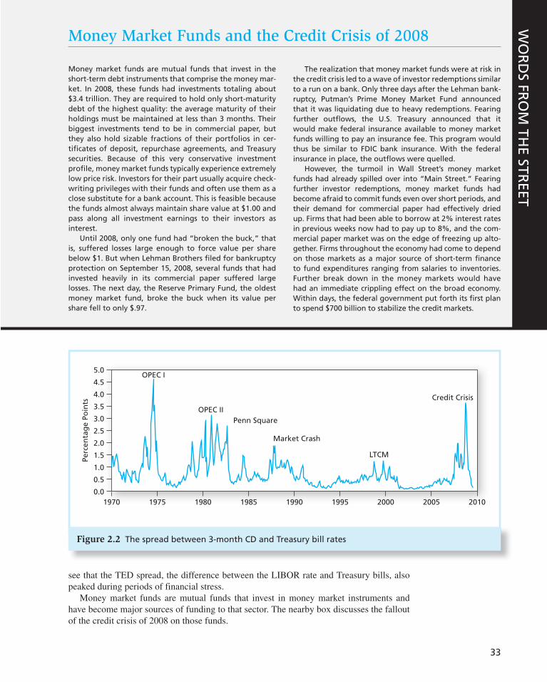
33
19700.0
0.5
1.0
1.5
2.0
2.5
3.0
3.5
4.0
4.5
5.0
1975 1980 1985 1990
Market Crash
Penn SquareOPEC II
OPEC I
Perc
enta
ge
Poin
ts
LTCM
Credit Crisis
1995 2000 20102005
Figure 2.2 The spread between 3-month CD and Treasury bill rates
Money Market Funds and the Credit Crisis of 2008
Money market funds are mutual funds that invest in the short-term debt instruments that comprise the money mar-ket. In 2008, these funds had investments totaling about $3.4 trillion. They are required to hold only short-maturity debt of the highest quality: the average maturity of their holdings must be maintained at less than 3 months. Their biggest investments tend to be in commercial paper, but they also hold sizable fractions of their portfolios in cer-tificates of deposit, repurchase agreements, and Treasury securities. Because of this very conservative investment profile, money market funds typically experience extremely low price risk. Investors for their part usually acquire check-writing privileges with their funds and often use them as a close substitute for a bank account. This is feasible because the funds almost always maintain share value at $1.00 and pass along all investment earnings to their investors as interest.
Until 2008, only one fund had “broken the buck,” that is, suffered losses large enough to force value per share below $1. But when Lehman Brothers filed for bankruptcy protection on September 15, 2008, several funds that had invested heavily in its commercial paper suffered large losses. The next day, the Reserve Primary Fund, the oldest money market fund, broke the buck when its value per share fell to only $.97.
The realization that money market funds were at risk in the credit crisis led to a wave of investor redemptions similar to a run on a bank. Only three days after the Lehman bank-ruptcy, Putman’s Prime Money Market Fund announced that it was liquidating due to heavy redemptions. Fearing further outflows, the U.S. Treasury announced that it would make federal insurance available to money market funds willing to pay an insurance fee. This program would thus be similar to FDIC bank insurance. With the federal insurance in place, the outflows were quelled.
However, the turmoil in Wall Street’s money market funds had already spilled over into “Main Street.” Fearing further investor redemptions, money market funds had become afraid to commit funds even over short periods, and their demand for commercial paper had effectively dried up. Firms that had been able to borrow at 2% interest rates in previous weeks now had to pay up to 8%, and the com-mercial paper market was on the edge of freezing up alto-gether. Firms throughout the economy had come to depend on those markets as a major source of short-term finance to fund expenditures ranging from salaries to inventories. Further break down in the money markets would have had an immediate crippling effect on the broad economy. Within days, the federal government put forth its first plan to spend $700 billion to stabilize the credit markets.
WO
RD
S FRO
M TH
E STREET
see that the TED spread, the difference between the LIBOR rate and Treasury bills, also peaked during periods of financial stress.
Money market funds are mutual funds that invest in money market instruments and have become major sources of funding to that sector. The nearby box discusses the fallout of the credit crisis of 2008 on those funds.
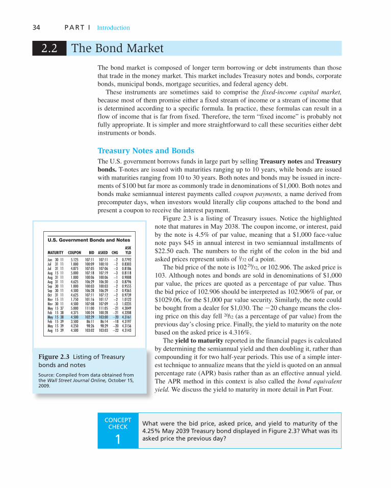
34 P A R T I Introduction
2.2 The Bond Market
The bond market is composed of longer term borrowing or debt instruments than those that trade in the money market. This market includes Treasury notes and bonds, corporate bonds, municipal bonds, mortgage securities, and federal agency debt.
These instruments are sometimes said to comprise the fixed-income capital market,
because most of them promise either a fixed stream of income or a stream of income that is determined according to a specific formula. In practice, these formulas can result in a flow of income that is far from fixed. Therefore, the term “fixed income” is probably not fully appropriate. It is simpler and more straightforward to call these securities either debt instruments or bonds.
Treasury Notes and Bonds
The U.S. government borrows funds in large part by selling Treasury notes and Treasury
bonds. T-notes are issued with maturities ranging up to 10 years, while bonds are issued with maturities ranging from 10 to 30 years. Both notes and bonds may be issued in incre-ments of $100 but far more as commonly trade in denominations of $1,000. Both notes and bonds make semiannual interest payments called coupon payments, a name derived from precomputer days, when investors would literally clip coupons attached to the bond and present a coupon to receive the interest payment.
Figure 2.3 is a listing of Treasury issues. Notice the highlighted note that matures in May 2038. The coupon income, or interest, paid by the note is 4.5% of par value, meaning that a $1,000 face-value note pays $45 in annual interest in two semiannual installments of $22.50 each. The numbers to the right of the colon in the bid and asked prices represent units of 1/32 of a point.
The bid price of the note is 102 29/32, or 102.906. The asked price is 103. Although notes and bonds are sold in denominations of $1,000 par value, the prices are quoted as a percentage of par value. Thus the bid price of 102.906 should be interpreted as 102.906% of par, or $1029.06, for the $1,000 par value security. Similarly, the note could be bought from a dealer for $1,030. The � 20 change means the clos-ing price on this day fell 20/32 (as a percentage of par value) from the previous day’s closing price. Finally, the yield to maturity on the note based on the asked price is 4.316%.
The yield to maturity reported in the financial pages is calculated by determining the semiannual yield and then doubling it, rather than compounding it for two half-year periods. This use of a simple inter-est technique to annualize means that the yield is quoted on an annual percentage rate (APR) basis rather than as an effective annual yield. The APR method in this context is also called the bond equivalent
yield. We discuss the yield to maturity in more detail in Part Four.
Jun 30 11 5.125 107:11 107:11 −2 0.7792Jul 31 11 1.000 100:09 100:10 −2 0.8303Jul 31 11 4.875 107:05 107:06 −3 0.8186Aug 15 11 5.000 107:18 107:19 −3 0.8118Aug 31 11 1.000 100:06 100:06 −1 0.9008Aug 31 11 4.625 106:29 106:30 −3 0.8796Sep 30 11 1.000 100:03 100:03 −2 0.9555Sep 30 11 4.500 106:28 106:29 −2 0.9365Oct 31 11 4.625 107:11 107:12 −2 0.9739Nov 15 11 1.750 101:16 101:17 −2 1.0122Nov 30 11 4.500 107:08 107:09 −3 1.0235May 15 37 5.000 111:00 111:05 −21 4.3049Feb 15 38 4.375 100:24 100:28 −21 4.3208May 15 38 4.500 102:29 103:00 −20 4.3161Feb 15 39 3.500 86:11 86:14 −18 4.3197May 15 39 4.250 98:26 98:29 −20 4.3156Aug 15 39 4.500 103:02 103:03 −22 4.3143
U.S. Government Bonds and Notes
MATURITY COUPON BID ASKED CHGASKYLD
Figure 2.3 Listing of Treasury bonds and notes
Source: Compiled from data obtained from the Wall Street Journal Online, October 15, 2009.
CONCEPT CHECK
1 What were the bid price, asked price, and yield to maturity of the 4.25% May 2039 Treasury bond displayed in Figure 2.3 ? What was its asked price the previous day?

C H A P T E R 2 Asset Classes and Financial Instruments 35
Inflation-Protected Treasury Bonds
The best place to start building an investment portfolio is at the least risky end of the spec-trum. Around the world, governments of many countries, including the United States, have issued bonds that are linked to an index of the cost of living in order to provide their citi-zens with an effective way to hedge inflation risk. See the E-Investments box on inflation-protected bonds around the world at the end of this chapter.
In the United States inflation-protected Treasury bonds are called TIPS (Treasury Inflation-Protected Securities). The principal amount on these bonds is adjusted in propor-tion to increases in the Consumer Price Index. Therefore, they provide a constant stream of income in real (inflation-adjusted) dollars. Yields on TIPS bonds should be interpreted as real or inflation-adjusted interest rates. We return to TIPS bonds in more detail in Chapter 14.
Federal Agency Debt
Some government agencies issue their own securities to finance their activities. These agencies usually are formed to channel credit to a particular sector of the economy that Congress believes might not receive adequate credit through normal private sources.
The major mortgage-related agencies are the Federal Home Loan Bank (FHLB), the Federal National Mortgage Association (FNMA, or Fannie Mae), the Government National Mortgage Association (GNMA, or Ginnie Mae), and the Federal Home Loan Mortgage Corporation (FHLMC, or Freddie Mac). The FHLB borrows money by issuing securities and lends this money to savings and loan institutions to be lent in turn to individuals bor-rowing for home mortgages.
Although the debt of federal agencies is not explicitly insured by the federal govern-ment, it has long been assumed that the government would assist an agency nearing default. Those beliefs were validated when Fannie Mae and Freddie Mac encountered severe finan-cial distress in September 2008. With both firms on the brink of insolvency, the govern-ment stepped in and put them both into conservatorship, assigned the Federal Housing Finance Agency to run the firms, but did in fact agree to make good on the firm’s bonds. A box later in the chapter (page 40) discusses the events leading up to their takeover.
International Bonds
Many firms borrow abroad and many investors buy bonds from foreign issuers. In addition to national capital markets, there is a thriving international capital market, largely centered in London.
A Eurobond is a bond denominated in a currency other than that of the country in which it is issued. For example, a dollar-denominated bond sold in Britain would be called a Eurodollar bond. Similarly, investors might speak of Euroyen bonds, yen-denominated bonds sold outside Japan. Because the European currency is called the euro, the term Eurobond may be confusing. It is best to think of them simply as international bonds.
In contrast to bonds that are issued in foreign currencies, many firms issue bonds in foreign countries but in the currency of the investor. For example, a Yankee bond is a dollar-denominated bond sold in the United States by a non-U.S. issuer. Similarly, Samurai bonds are yen-denominated bonds sold in Japan by non-Japanese issuers.
Municipal Bonds
Municipal bonds are issued by state and local governments. They are similar to Treasury and corporate bonds except that their interest income is exempt from federal income
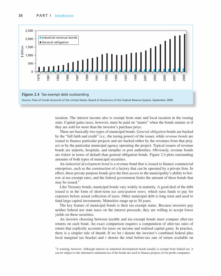
36 P A R T I Introduction
t axation. The interest income also is exempt from state and local taxation in the issuing state. Capital gains taxes, however, must be paid on “munis” when the bonds mature or if they are sold for more than the investor’s purchase price.
There are basically two types of municipal bonds. General obligation bonds are backed by the “full faith and credit” (i.e., the taxing power) of the issuer, while revenue bonds are issued to finance particular projects and are backed either by the revenues from that proj-ect or by the particular municipal agency operating the project. Typical issuers of revenue bonds are airports, hospitals, and turnpike or port authorities. Obviously, revenue bonds are riskier in terms of default than general obligation bonds. Figure 2.4 plots outstanding amounts of both types of municipal securities.
An industrial development bond is a revenue bond that is issued to finance commercial enterprises, such as the construction of a factory that can be operated by a private firm. In effect, these private-purpose bonds give the firm access to the municipality’s ability to bor-row at tax-exempt rates, and the federal government limits the amount of these bonds that may be issued. 3
Like Treasury bonds, municipal bonds vary widely in maturity. A good deal of the debt issued is in the form of short-term tax anticipation notes, which raise funds to pay for expenses before actual collection of taxes. Other municipal debt is long term and used to fund large capital investments. Maturities range up to 30 years.
The key feature of municipal bonds is their tax-exempt status. Because investors pay neither federal nor state taxes on the interest proceeds, they are willing to accept lower yields on these securities.
An investor choosing between taxable and tax-exempt bonds must compare after-tax returns on each bond. An exact comparison requires a computation of after-tax rates of return that explicitly accounts for taxes on income and realized capital gains. In practice, there is a simpler rule of thumb. If we let t denote the investor’s combined federal plus local marginal tax bracket and r denote the total before-tax rate of return available on
3 A warning, however. Although interest on industrial development bonds usually is exempt from federal tax, it can be subject to the alternative minimum tax if the bonds are used to finance projects of for-profit companies.
0
500
1,000
1,500
2,000
2,500
1979
1981
1983
1985
1987
1989
1991
1993
1995
1997
1999
2001
2003
2005
2007
2009
Industrial revenue bonds
General obligation
$ B
illio
n
Figure 2.4 Tax-exempt debt outstanding
Source: Flow of Funds Accounts of the United States, Board of Governors of the Federal Reserve System, September 2009.

C H A P T E R 2 Asset Classes and Financial Instruments 37
taxable bonds, then r (1 � t ) is the after-tax rate available on those securities. 4 If this value exceeds the rate on municipal bonds, r m , the investor does better holding the taxable bonds. Otherwise, the tax-exempt municipals provide higher after-tax returns.
One way to compare bonds is to determine the interest rate on taxable bonds that would be necessary to provide an after-tax return equal to that of municipals. To derive this value, we set after-tax yields equal, and solve for the equivalent taxable yield of the tax-exempt bond. This is the rate a taxable bond must offer to match the after-tax yield on the tax-free municipal.
r(1 2 t) 5 rm (2.1)
or
r 5 rm /(1 2 t) (2.2)
Thus the equivalent taxable yield is simply the tax-free rate divided by 1 � t. Table 2.2 presents equivalent taxable yields for several municipal yields and tax rates.
This table frequently appears in the marketing literature for tax-exempt mutual bond funds because it demonstrates to high-tax-bracket investors that municipal bonds offer highly attractive equivalent taxable yields. Each entry is calculated from Equation 2.2. If the equivalent taxable yield exceeds the actual yields offered on taxable bonds, the inves-tor is better off after taxes holding municipal bonds. Notice that the equivalent taxable interest rate increases with the investor’s tax bracket; the higher the bracket, the more valuable the tax-exempt feature of municipals. Thus high-tax-bracket investors tend to hold municipals.
We also can use Equation 2.1 or 2.2 to find the tax bracket at which investors are indif-ferent between taxable and tax-exempt bonds. The cutoff tax bracket is given by solving Equation 2.2 for the tax bracket at which after-tax yields are equal. Doing so, we find that
t 5 1 2rm
r (2.3)
Thus the yield ratio r m / r is a key determinant of the attractiveness of municipal bonds. The higher the yield ratio, the lower the cutoff tax bracket, and the more individuals will prefer to hold municipal debt. Figure 2.5 graphs the yield ratio since 1953.
4 An approximation to the combined federal plus local tax rate is just the sum of the two rates. For example, if your federal tax rate is 28% and your state rate is 5%, your combined tax rate would be approximately 33%. A more precise approach would recognize that state taxes are deductible at the federal level. You owe federal taxes only on income net of state taxes. Therefore, for every dollar of income, your after-tax proceeds would be (1 � tfederal ) � (1 � tstate ). In our example, your after-tax proceeds on each dollar earned would be (1 � .28) � (1 � .05) � .684, which implies a combined tax rate of 1 � .684 � .316, or 31.6%.
Table 2.2
Equivalent taxable yields corresponding to various tax-exempt yields
Tax-Exempt Yield
Marginal Tax Rate 1% 2% 3% 4% 5%
20% 1.25% 2.50% 3.75% 5.00% 6.25%
30 1.43 2.86 4.29 5.71 7.14
40 1.67 3.33 5.00 6.67 8.33
50 2.00 4.00 6.00 8.00 10.00

38 P A R T I Introduction
Corporate Bonds
Corporate bonds are the means by which private firms borrow money directly from the public. These bonds are similar in structure to Treasury issues—they typically pay semian-nual coupons over their lives and return the face value to the bondholder at maturity. They differ most importantly from Treasury bonds in degree of risk. Default risk is a real con-sideration in the purchase of corporate bonds, and Chapter 14 discusses this issue in con-siderable detail. For now, we distinguish only among secured bonds, which have specific collateral backing them in the event of firm bankruptcy; unsecured bonds, called deben-
tures, which have no collateral; and subordinated debentures, which have a lower priority claim to the firm’s assets in the event of bankruptcy.
Figure 2.5 Ratio of yields on municipal debt to corporate debt
Source: Authors’ calculations, using data from www.federalreserve.gov/releases/h15/data.htm .
0.40
0.45
0.55
0.50
0.60
0.65
0.70
0.75
0.80
0.85
0.90
Rat
io
Jan
-53
Jan
-57
Jan
-61
Jan
-65
Jan
-69
Jan
-73
Jan
-77
Jan
-81
Jan
-85
Jan
-89
Jan
-93
Jan
-97
Jan
-01
Jan
-05
Jan
-09
Example 2.1 Taxable versus Tax-Exempt Yields
Figure 2.5 shows that in recent years, the ratio of tax-exempt to taxable yields has fluctu-ated around .75. What does this imply about the cutoff tax bracket above which tax-exempt bonds provide higher after-tax yields? Equation 2.3 shows that an investor whose tax bracket (federal plus local) exceeds 1 � .75 � .25, or 25%, will derive a greater after-tax yield from municipals. Note, however, that it is difficult to control precisely for differences in the risks of these bonds, so the cutoff tax bracket must be taken as approximate.
CONCEPT CHECK
2 Suppose your tax bracket is 30%. Would you prefer to earn a 6% tax-able return or a 4% tax-free return? What is the equivalent taxable yield of the 4% tax-free yield?
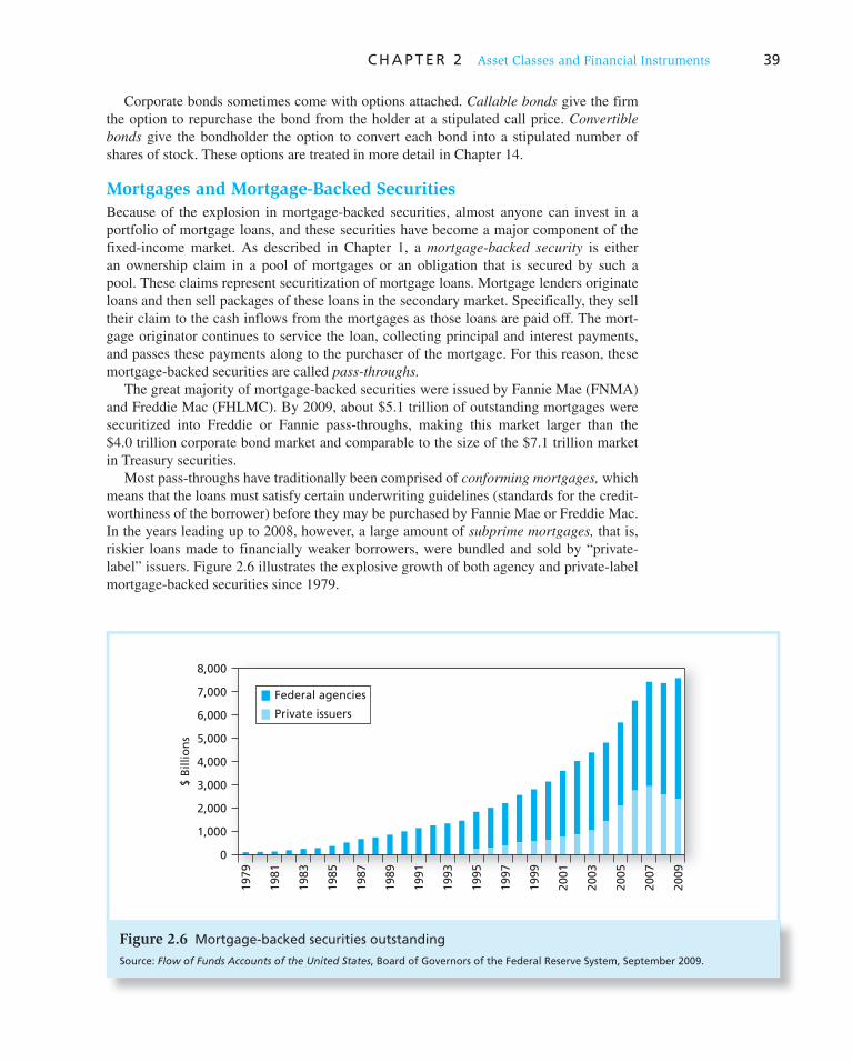
C H A P T E R 2 Asset Classes and Financial Instruments 39
Corporate bonds sometimes come with options attached. Callable bonds give the firm the option to repurchase the bond from the holder at a stipulated call price. Convertible
bonds give the bondholder the option to convert each bond into a stipulated number of shares of stock. These options are treated in more detail in Chapter 14.
Mortgages and Mortgage-Backed Securities
Because of the explosion in mortgage-backed securities, almost anyone can invest in a portfolio of mortgage loans, and these securities have become a major component of the fixed-income market. As described in Chapter 1, a mortgage-backed security is either an ownership claim in a pool of mortgages or an obligation that is secured by such a pool. These claims represent securitization of mortgage loans. Mortgage lenders originate loans and then sell packages of these loans in the secondary market. Specifically, they sell their claim to the cash inflows from the mortgages as those loans are paid off. The mort-gage originator continues to service the loan, collecting principal and interest payments, and passes these payments along to the purchaser of the mortgage. For this reason, these m ortgage-backed securities are called pass-throughs.
The great majority of mortgage-backed securities were issued by Fannie Mae (FNMA) and Freddie Mac (FHLMC). By 2009, about $5.1 trillion of outstanding mortgages were securitized into Freddie or Fannie pass-throughs, making this market larger than the $4.0 trillion corporate bond market and comparable to the size of the $7.1 trillion market in Treasury securities.
Most pass-throughs have traditionally been comprised of conforming mortgages, which means that the loans must satisfy certain underwriting guidelines (standards for the credit-worthiness of the borrower) before they may be purchased by Fannie Mae or Freddie Mac. In the years leading up to 2008, however, a large amount of subprime mortgages, that is, riskier loans made to financially weaker borrowers, were bundled and sold by “private-label” issuers. Figure 2.6 illustrates the explosive growth of both agency and private-label mortgage-backed securities since 1979.
$ B
illio
ns
0
1979
1981
1983
1985
1987
1989
1991
1993
1995
1997
1999
2001
2003
2005
2007
2009
1,000
2,000
3,000
4,000
5,000
6,000
7,000
8,000
Federal agencies
Private issuers
Figure 2.6 Mortgage-backed securities outstanding
Source: Flow of Funds Accounts of the United States, Board of Governors of the Federal Reserve System, September 2009.

40
The Failures of Freddie Mac and Fannie Mae
Fannie Mae was created in 1938 to provide funds to and enhance the liquidity of the mortgage market. It initially operated by issuing large amounts of its own debt to raise funds, using those funds to buy mortgages from their orig-inators, and holding them in its own portfolio. The origi-nator would typically continue to service the mortgage (keep track of monthly payments, taxes, and insurance) for a “servicing fee.” Often, the originator did not have an independent source of funds. These mortgage bankers, as they are called, do not take deposits. They simply originate loans and quickly sell them to Fannie, Freddie, and other buyers.
Freddie Mac was established in 1970 to create a sec-ondary market where conventional mortgages could be traded. At the time, most mortgages were issued and held by local savings and loan associations, which were largely restricted to taking deposits and making mortgage loans. However, interest rate ceilings on deposits and laws against interstate banking made it difficult for the savings and loan industry to provide sufficient funds for the hous-ing market. Freddie pioneered the mortgage pass-through security. This created a national mortgage market, allevi-ating regional imbalances in the supply and demand for mortgage credit. Mortgage-backed securities traded like other securities, and the funds used to purchase them became another large source of financing for home buy-ers. Ultimately, Fannie and Freddie mimicked each other’s policies; both issued many mortgage-backed securities and both held many mortgages on their own balance sheets, financed by issuing their own debt.
Freddie and Fannie bore the credit risk of the mortgages they purchased as well as the mortgages they bundled and sold as pass-throughs. This is because mortgage pass-through securities were sold with guarantees that if the homeowner defaulted on the loans, the agencies would in effect buy the loans back from the investor. Fannie and Freddie charged a guarantee fee for this credit insurance,
priced at what appeared at the time to provide a generous profit margin. Since the agencies were presumably in bet-ter position to evaluate the risk of the loans than outside investors, it made sense for them to monitor credit risk and charge an appropriate fee for bearing it.
Until the last decade, the vast majority of mortgages held or guaranteed by the agencies were low-risk con-forming mortgages, meaning that the loans couldn’t be too big and homeowners had to meet criteria establishing their ability to repay the loan. But several developments in recent years all worked to put the companies at risk. First, both agencies began purchasing or guaranteeing large amounts of so-called subprime mortgages. These loans did not conform to usual underwriting standards for bor-rower creditworthiness, and the down payments were far lower than the standard 20% that the agencies tradition-ally required. The agencies were encouraged by Congress and the Department of Housing and Urban Development (HUD) to enter these markets as a way of supporting affordable housing goals, and they also chose to purchase these loans as a way of maintaining growth and market share. Second, a severe downturn in home prices start-ing in 2006 meant that default rates on even apparently safe conforming loans spiked. With heavy default rates, particularly on subprime loans, the agencies experienced large credit losses. Finally, despite the clearly increasing risks these companies were assuming, they failed to raise more capital as a buffer against potential losses. For exam-ple, at the end of 2007, they were reported to have only $83.2 billion of capital to support $5.2 trillion of debt and guarantees. This was not a sufficient cushion when trouble hit. Fearing the fallout from their imminent collapse, the U.S. Treasury decided in September 2008 to place the firms into conservatorship. The government promised to make good on the bonds previously issued by the agencies, but the investors in both common and preferred stock of the co mpanies were largely wiped out.
WO
RD
S FR
OM
TH
E ST
REE
T
In an effort to make housing more affordable to low-income households, Fannie and Freddie were allowed and in fact encouraged to buy subprime mortgage pools. As we saw in Chapter 1, these loans turned out to be disastrous, with trillion-dollar losses spread among banks, hedge funds and other investors, and Freddie and Fannie, which lost billions of dollars on the subprime mortgage pools they had purchased. In September 2008, both agencies faced insolvency and were taken over by the federal government. 5 The nearby box discusses that episode.
Despite these troubles, few believe that securitization itself will cease, although prac-tices in this market are highly likely to become far more conservative than in previous
5 The companies did not go through a normal bankruptcy. Fearing the damage that their insolvency would wreak on capital and housing markets, the federal government instead put the agencies into conservatorship, mean-ing that they could continue to operate but would be run by the Federal Housing Finance Agency until they could be restructured. However, at this time, no one knows precisely how Freddie and Fannie ultimately will be reorganized.

C H A P T E R 2 Asset Classes and Financial Instruments 41
years, particularly with respect to the credit standards that must be met by the ultimate borrower. Indeed, securitization has become an increasingly common staple of many credit markets. For example, car loans, student loans, home equity loans, credit card loans, and even debt of private firms now are commonly bundled into pass-through securities that can be traded in the capital market. Figure 2.7 documents the rapid growth of nonmortgage asset-backed securities since 1995.
Figure 2.7 Asset-backed securities outstanding
Source: The Securities & Industry and Financial Markets Åssociation, www.sifma.org
Other
Student loan
Home equity
Credit card
Automobile
0
500
1,000
1,500
2,000
$ B
illio
n
3,000
2,500
1996
1997
1998
1999
2000
2001
2002
2003
2004
2005
2006
2007
2008
2009
2.3 Equity Securities
Common Stock as Ownership Shares
Common stocks, also known as equity securities or equities, represent ownership shares in a corporation. Each share of common stock entitles its owner to one vote on any matters of corporate governance that are put to a vote at the corporation’s annual meeting and to a share in the financial benefits of ownership. 6
The corporation is controlled by a board of directors elected by the shareholders. The board, which meets only a few times each year, selects managers who actually run the corporation on a day-to-day basis. Managers have the authority to make most business decisions without the board’s specific approval. The board’s mandate is to oversee the management to ensure that it acts in the best interests of shareholders.
6 A corporation sometimes issues two classes of common stock, one bearing the right to vote, the other not. Because of its restricted rights, the nonvoting stock might sell for a lower price.
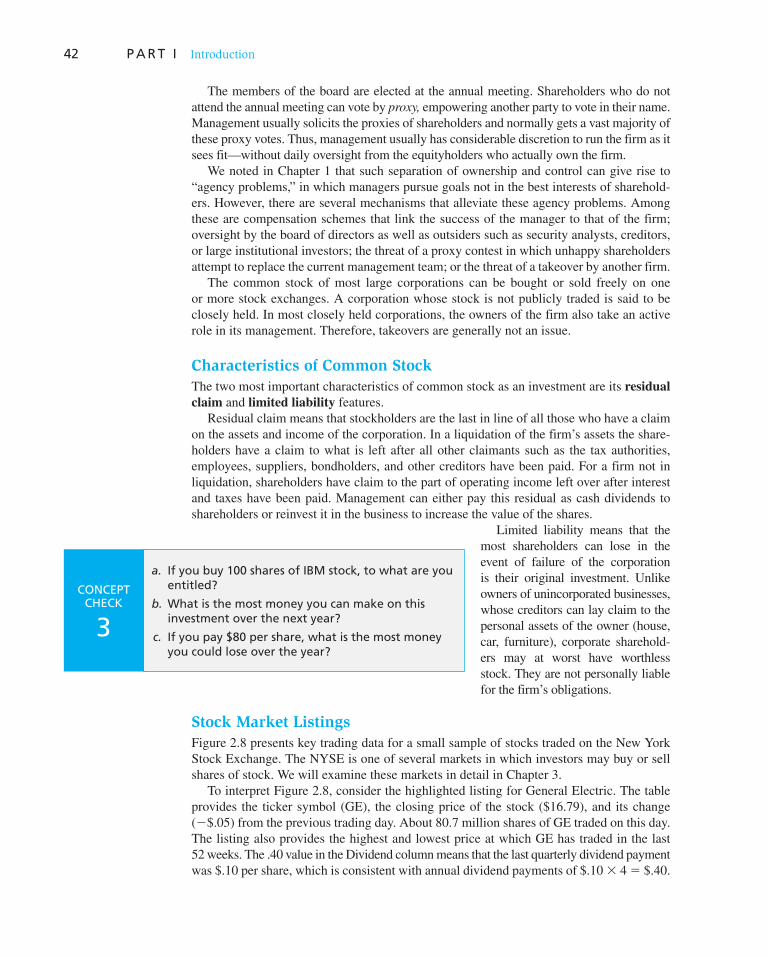
42 P A R T I Introduction
The members of the board are elected at the annual meeting. Shareholders who do not attend the annual meeting can vote by proxy, empowering another party to vote in their name. Management usually solicits the proxies of shareholders and normally gets a vast majority of these proxy votes. Thus, management usually has considerable discretion to run the firm as it sees fit—without daily oversight from the equityholders who actually own the firm.
We noted in Chapter 1 that such separation of ownership and control can give rise to “agency problems,” in which managers pursue goals not in the best interests of sharehold-ers. However, there are several mechanisms that alleviate these agency problems. Among these are compensation schemes that link the success of the manager to that of the firm; oversight by the board of directors as well as outsiders such as security analysts, creditors, or large institutional investors; the threat of a proxy contest in which unhappy shareholders attempt to replace the current management team; or the threat of a takeover by another firm.
The common stock of most large corporations can be bought or sold freely on one or more stock exchanges. A corporation whose stock is not publicly traded is said to be closely held. In most closely held corporations, the owners of the firm also take an active role in its management. Therefore, takeovers are generally not an issue.
Characteristics of Common Stock
The two most important characteristics of common stock as an investment are its residual
claim and limited liability features. Residual claim means that stockholders are the last in line of all those who have a claim
on the assets and income of the corporation. In a liquidation of the firm’s assets the share-holders have a claim to what is left after all other claimants such as the tax authorities, employees, suppliers, bondholders, and other creditors have been paid. For a firm not in liquidation, shareholders have claim to the part of operating income left over after interest and taxes have been paid. Management can either pay this residual as cash dividends to shareholders or reinvest it in the business to increase the value of the shares.
Limited liability means that the most shareholders can lose in the event of failure of the corporation is their original investment. Unlike owners of unincorporated businesses, whose creditors can lay claim to the personal assets of the owner (house, car, furniture), corporate sharehold-ers may at worst have worthless stock. They are not personally liable for the firm’s obligations.
Stock Market Listings
Figure 2.8 presents key trading data for a small sample of stocks traded on the New York Stock Exchange. The NYSE is one of several markets in which investors may buy or sell shares of stock. We will examine these markets in detail in Chapter 3.
To interpret Figure 2.8 , consider the highlighted listing for General Electric. The table provides the ticker symbol (GE), the closing price of the stock ($16.79), and its change (�$.05) from the previous trading day. About 80.7 million shares of GE traded on this day. The listing also provides the highest and lowest price at which GE has traded in the last 52 weeks. The .40 value in the Dividend column means that the last quarterly dividend payment was $.10 per share, which is consistent with annual dividend payments of $.10 � 4 � $.40.
CONCEPT CHECK
3
a. If you buy 100 shares of IBM stock, to what are you entitled?
b. What is the most money you can make on this investment over the next year?
c. If you pay $80 per share, what is the most money you could lose over the year?

C H A P T E R 2 Asset Classes and Financial Instruments 43
This corresponds to an annual dividend yield (i.e., annual dividend per dol-lar paid for the stock) of .40/16.79 � .024, or 2.4%.
The dividend yield is only part of the return on a stock investment. It ignores prospective capital gains (i.e., price increases) or losses. Low-dividend firms presumably offer greater prospects for capital gains, or investors would not be willing to hold these stocks in their portfolios. If you scan Figure 2.8 , you will see that dividend yields vary widely across companies.
The P/E ratio, or price–earnings ratio, is the ratio of the current stock price to last year’s earnings per share. The P/E ratio tells us how much stock purchasers must pay per dollar of earnings that the firm generates. For GE, the ratio of price to earnings is 13. The P/E ratio also varies widely across firms. Where the dividend yield and P/E ratio are not reported in Figure 2.8 , the firms have zero dividends, or zero or negative earnings. We shall have much to say about P/E ratios in Chapter 18. Finally, we see that GE’s stock price has increased by 3.6% since the beginning of the year.
Preferred Stock
Preferred stock has features similar to both equity and debt. Like a bond, it promises to pay to its holder a fixed amount of income each year. In this sense preferred stock is similar to an infinite-maturity bond, that is, a perpetuity. It also resembles a bond in that it does not convey voting power regarding the management of the firm. Preferred stock is an equity investment, however. The firm retains discretion to make the dividend payments to the preferred stockholders; it has no contractual obligation to pay those dividends. Instead, preferred dividends are usually cumulative; that is, unpaid dividends cumulate and must be paid in full before any dividends may be paid to holders of common stock. In contrast, the firm does have a contractual obligation to make the interest payments on the debt. Failure to make these payments sets off corporate bankruptcy proceedings.
Preferred stock also differs from bonds in terms of its tax treatment for the firm. Because preferred stock payments are treated as dividends rather than interest, they are not tax-deductible expenses for the firm. This disadvantage is somewhat offset by the fact that corporations may exclude 70% of dividends received from domestic corporations in the computation of their taxable income. Preferred stocks therefore make desirable fixed- income investments for some corporations.
Even though preferred stock ranks after bonds in terms of the priority of its claims to the assets of the firm in the event of corporate bankruptcy, preferred stock often sells at lower yields than do corporate bonds. Presumably, this reflects the value of the divi-dend exclusion, because the higher risk of preferred would tend to result in higher yields than those offered by bonds. Individual investors, who cannot use the 70% tax exclusion, generally will find preferred stock yields unattractive relative to those on other available assets.
Figure 2.8 Listing of stocks traded on the New York Stock Exchange
Source: Compiled from data from The Wall Street Journal Online, October 15, 2009.
Gannett Co. GCI 13.19 −0.29 6,606,846 13.77 1.85 .16 1.2 dd 64.9Gap Inc. GPS 22.79 −0.18 5,785,671 23.11 9.41 .34 1.5 17 70.2General Cable Corp. BGC 40.29 555,237 42.73 6.73 .... .... 11 127.8General Dynamics Corp. GD 67.32 0.47 1,688,963 67.04 35.28 1.52 2.3 11 16.9General Electric Co. GE 16.79 −0.05 80,686,921 22.39 5.73 .40 2.4 13 3.6General Maritime Corp. GMR 8.45 0.11 643,380 14.53 6.40 23.7 14 −21.8General Mills Inc. GIS 65.29 0.47 2,156,259 69.00 46.37 1.88 2.9 16 7.5General Steel Holdings Inc. GSI 4.37 0.29 1,443,272 7.61 1.84 .... .... .... 19.9Genesco Inc. GCO 26.66 0.99 467,448 32.34 10.37 .... .... 19 57.6Genesee & Wyoming Inc. Cl A GWR 33.12 0.02 127,785 37.58 16.42 .... .... 18 8.6Genesis Lease Ltd. ADS GLS 8.40 −0.26 300,526 9.32 2.01 .40 .... 8 196.8Genpact Ltd. G 11.72 −0.01 65,278 14.45 6.30 .... .... 18 42.5
NAME YTD% CHGP/EYIELDDIV52 WK LOW52 WK HIGHVOLUMENET CHGCLOSESYMBOL
2.00e

44 P A R T I Introduction
Preferred stock is issued in variations similar to those of corporate bonds. It may be callable by the issuing firm, in which case it is said to be redeemable. It also may be convertible into common stock at some specified conversion ratio. Adjustable-rate pre-ferred stock is another variation that, like adjustable-rate bonds, ties the dividend to current m arket interest rates.
Depository Receipts
American Depository Receipts, or ADRs, are certificates traded in U.S. markets that rep-resent ownership in shares of a foreign company. Each ADR may correspond to ownership of a fraction of a foreign share, one share, or several shares of the foreign corporation. ADRs were created to make it easier for foreign firms to satisfy U.S. security registration requirements. They are the most common way for U.S. investors to invest in and trade the shares of foreign corporations. In Figure 2.8 , the letters ADS denote American Depository Shares, an alternative terminology for ADRs. See, for example, the listing for Genesis Lease.
2.4 Stock and Bond Market Indexes
Stock Market Indexes
The daily performance of the Dow Jones Industrial Average is a staple portion of the evening news report. Although the Dow is the best-known measure of the performance of the stock market, it is only one of several indicators. Other more broadly based indexes are computed and published daily. In addition, several indexes of bond market performance are widely available.
The ever-increasing role of international trade and investments has made indexes of foreign financial markets part of the general news as well. Thus foreign stock exchange indexes such as the Nikkei Average of Tokyo and the Financial Times index of London are fast becoming household names.
Dow Jones Averages
The Dow Jones Industrial Average (DJIA) of 30 large, “blue-chip” corporations has been computed since 1896. Its long history probably accounts for its preeminence in the public mind. (The average covered only 20 stocks until 1928.)
Originally, the DJIA was calculated as the simple average price of the stocks included in the index. Thus, one would add up the prices of the 30 stocks in the index and divide by 30. The percentage change in the DJIA would then be the percentage change in the average price of the 30 shares.
This procedure means that the percentage change in the DJIA measures the return (excluding dividends) on a portfolio that invests one share in each of the 30 stocks in the index. The value of such a portfolio (holding one share of each stock in the index) is the sum of the 30 prices. Because the percentage change in the average of the 30 prices is the same as the percentage change in the sum of the 30 prices, the index and the portfolio have the same percentage change each day.
Because the Dow corresponds to a portfolio that holds one share of each component stock, the investment in each company in that portfolio is proportional to the company’s share price. Therefore, the Dow is called a price-weighted average.
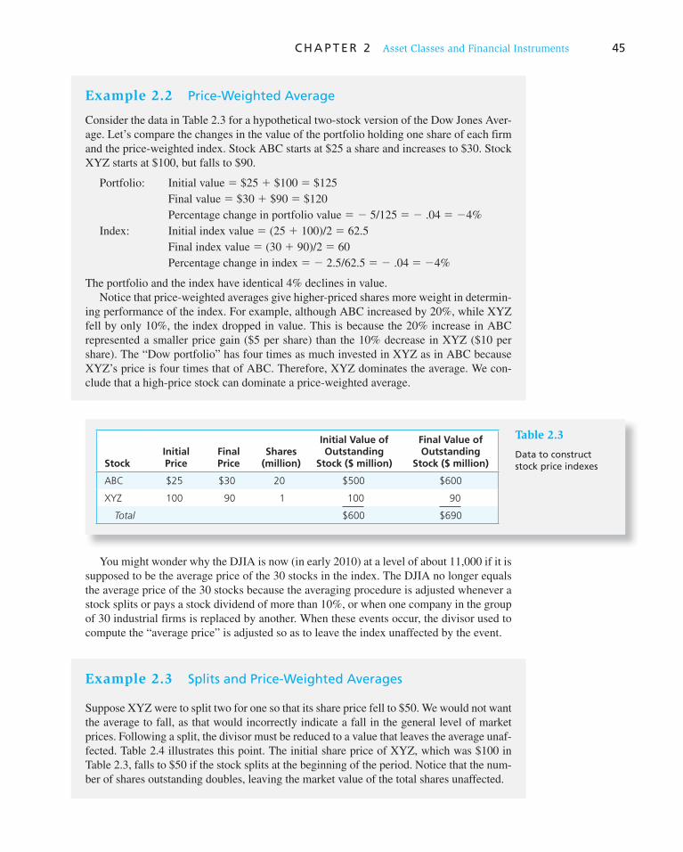
C H A P T E R 2 Asset Classes and Financial Instruments 45
Table 2.3
Data to construct stock price indexesStock
Initial Price
Final Price
Shares (million)
Initial Value of Outstanding
Stock ($ million)
Final Value of Outstanding
Stock ($ million)
ABC $25 $30 20 $500 $600
XYZ 100 90 1 100 90
Total $600 $690
You might wonder why the DJIA is now (in early 2010) at a level of about 11,000 if it is supposed to be the average price of the 30 stocks in the index. The DJIA no longer equals the average price of the 30 stocks because the averaging procedure is adjusted whenever a stock splits or pays a stock dividend of more than 10%, or when one company in the group of 30 industrial firms is replaced by another. When these events occur, the divisor used to compute the “average price” is adjusted so as to leave the index unaffected by the event.
Example 2.3 Splits and Price-Weighted Averages
Suppose XYZ were to split two for one so that its share price fell to $50. We would not want the average to fall, as that would incorrectly indicate a fall in the general level of market prices. Following a split, the divisor must be reduced to a value that leaves the average unaf-fected. Table 2.4 illustrates this point. The initial share price of XYZ, which was $100 in Table 2.3, falls to $50 if the stock splits at the beginning of the period. Notice that the num-ber of shares outstanding doubles, leaving the market value of the total shares unaffected.
Example 2.2 Price-Weighted Average
Consider the data in Table 2.3 for a hypothetical two-stock version of the Dow Jones Aver-age. Let’s compare the changes in the value of the portfolio holding one share of each firm and the price-weighted index. Stock ABC starts at $25 a share and increases to $30. Stock XYZ starts at $100, but falls to $90.
Portfolio: Initial value � $25 � $100 � $125
Final value � $30 � $90 � $120
Percentage change in portfolio value � � 5/125 � � .04 � �4%
Index: Initial index value � (25 � 100)/2 � 62.5
Final index value � (30 � 90)/2 � 60
Percentage change in index � � 2.5/62.5 � � .04 � �4%
The portfolio and the index have identical 4% declines in value.Notice that price-weighted averages give higher-priced shares more weight in determin-
ing performance of the index. For example, although ABC increased by 20%, while XYZ fell by only 10%, the index dropped in value. This is because the 20% increase in ABC represented a smaller price gain ($5 per share) than the 10% decrease in XYZ ($10 per share). The “Dow portfolio” has four times as much invested in XYZ as in ABC because XYZ’s price is four times that of ABC. Therefore, XYZ dominates the average. We con-clude that a high-price stock can dominate a price-weighted average.

46 P A R T I Introduction
Table 2.4
Data to construct stock price indexes after a stock split
StockInitial Price
Final Price
Shares (million)
Initial Value of Outstanding
Stock ($ million)
Final Value of Outstanding
Stock ($ million)
ABC $25 $30 20 $500 $600
XYZ 50 45 2 100 90
Total $600 $690
We find the new divisor as follows. The index value before the stock split � 125/2 � 62.5. We must find a new divisor, d, that leaves the index unchanged after XYZ splits and its price falls to $50. Therefore, we solve for d in the following equation:
Price of ABC 1 Price of XYZ
d5
25 1 50
d5 62.5
which implies that the divisor must fall from its original value of 2.0 to a new value of 1.20.Because the split changes the price of stock XYZ, it also changes the relative weights of
the two stocks in the price-weighted average. Therefore, the return of the index is affected by the split.
At period-end, ABC will sell for $30, while XYZ will sell for $45, representing the same negative 10% return it was assumed to earn in Table 2.3. The new value of the price-weighted average is (30 � 45)/1.20 � 62.5, the same as its value at the start of the year; therefore, the rate of return is zero, rather than the �4% return that we calculated in the absence of a split.
The split reduces the relative weight of XYZ because its initial price is lower; because XYZ is the poorer performing stock, the performance of the average is higher. This exam-ple illustrates that the implicit weighting scheme of a price-weighted average is some-what arbitrary, being determined by the prices rather than by the outstanding market values (price per share times number of shares) of the shares in the average.
Because the Dow Jones averages are based on small numbers of firms, care must be taken to ensure that they are representative of the broad market. As a result, the composi-tion of the average is changed every so often to reflect changes in the economy. Table 2.5 presents the composition of the Dow industrials in 1928 as well as its composition as of 2010. The table presents striking evidence of the changes in the U.S. economy in the last 80 years. Many of the “bluest of the blue chip” companies in 1928 no longer exist, and the industries that were the backbone of the economy in 1928 have given way to some that could not have been imagined at the time.
In the same way that the divisor is updated for stock splits, if one firm is dropped from the average and another firm with a different price is added, the divisor has to be updated to leave the average unchanged by the substitution. By 2010, the divisor for the Dow Jones Industrial Average had fallen to a value of about .132.
Dow Jones & Company also computes a Transportation Average of 20 airline, trucking, and railroad stocks; a Public Utility Average of 15 electric and natural gas utilities; and a Composite Average combining the 65 firms of the three separate averages. Each is a price- weighted average, and thus overweights the performance of high-priced stocks.

C H A P T E R 2 Asset Classes and Financial Instruments 47
CONCEPT CHECK
4 Suppose XYZ in Table 2.3 increases in price to $110, while ABC falls to $20. Find the per-centage change in the price-weighted average of these two stocks. Compare that to the percentage return of a portfolio that holds one share in each company.
Table 2.5
Companies included in the Dow Jones Industrial Average: 1928 and 2010
Dow Industrials in 1928Current Dow Companies Ticker Symbol Industry
Year Added
to Index
Wright Aeronautical 3M MMM Diversified industrials 1976
Allied Chemical Alcoa AA Aluminum 1959
North American American Express AXP Consumer finance 1982
Victor Talking Machine AT&T T Telecommunications 1999
International Nickel Bank of America BAC Banking 2008
International Harvester Boeing BA Aerospace and defense 1987
Westinghouse Caterpillar CAT Construction 1991
Texas Gulf Sulphur Chevron CVX Oil and gas 2008
American Sugar Citigroup C Banking 1997
American Tobacco Coca-Cola KO Beverages 1987
Texas Corp DuPont DD Chemicals 1935
Standard Oil (N.J.) ExxonMobil XOM Oil and gas 1928
General Electric General Electric GE Diversified industrials 1907
General Motors General Motors GM Automobiles 1925
Sears Roebuck Hewlett-Packard HPQ Computers 1997
Chrysler Home Depot HD Home improvement retailers 1999
Atlantic Refining Intel INTC Semiconductors 1999
Paramount Publix IBM IBM Computer services 1979
Bethlehem Steel Johnson & Johnson JNJ Pharmaceuticals 1997
General Railway Signal JPMorgan Chase JPM Banking 1991
Mack Trucks Kraft Foods KFT Food processing 2008
Union Carbide McDonald’s MCD Restaurants 1985
American Smelting Merck MRK Pharmaceuticals 1979
American Can Microsoft MSFT Software 1999
Postum Inc Pfizer PFE Pharmaceuticals 2004
Nash Motors Procter & Gamble PG Household products 1932
Goodrich United
Technologies
UTX Aerospace 1939
Radio Corp Verizon VZ Telecommunications 2004
Woolworth Walmart WMT Retailers 1997
U.S. Steel Walt Disney DIS Broadcasting and entertainment 1991
48 P A R T I Introduction
Standard & Poor’s Indexes
The Standard & Poor’s Composite 500 (S&P 500) stock index represents an improvement over the Dow Jones Averages in two ways. First, it is a more broadly based index of 500 firms. Second, it is a market-value-weighted index. In the case of the firms XYZ and ABC in Example 2.2, the S&P 500 would give ABC five times the weight given to XYZ because the market value of its outstanding equity is five times larger, $500 million versus $100 million.
The S&P 500 is computed by calculating the total market value of the 500 firms in the index and the total market value of those firms on the previous day of trading. The percent-age increase in the total market value from one day to the next represents the increase in the index. The rate of return of the index equals the rate of return that would be earned by an investor holding a portfolio of all 500 firms in the index in proportion to their market values, except that the index does not reflect cash dividends paid by those firms.
Actually, most indexes today use a modified version of market-value weights. Rather than weighting by total market value, they weight by the market value of free float, that is, by the value of shares that are freely tradable among investors. For example, this procedure does not count shares held by founding families or governments. These shares are effec-tively not available for investors to purchase. The distinction is more important in Japan and Europe, where a higher fraction of shares are held in such nontraded portfolios.
A nice feature of both market-value-weighted and price-weighted indexes is that they reflect the returns to straightforward portfolio strategies. If one were to buy shares in each component firm in the index in proportion to its outstanding market value, the
Example 2.4 Value-Weighted Indexes
To illustrate how value-weighted indexes are computed, look again at Table 2.3 . The final value of all outstanding stock in our two-stock universe is $690 million. The initial value was $600 million. Therefore, if the initial level of a market-value-weighted index of stocks ABC and XYZ were set equal to an arbitrarily chosen starting value such as 100, the index value at year-end would be 100 � (690/600) � 115. The increase in the index reflects the 15% return earned on a portfolio consisting of those two stocks held in proportion to out-standing market values.
Unlike the price-weighted index, the value-weighted index gives more weight to ABC. Whereas the price-weighted index fell because it was dominated by higher-price XYZ, the value-weighted index rises because it gives more weight to ABC, the stock with the higher total market value.
Note also from Tables 2.3 and 2.4 that market-value-weighted indexes are unaffected by stock splits. The total market value of the outstanding XYZ stock decreases from $100 million to $90 million regardless of the stock split, thereby rendering the split irrel-evant to the performance of the index.
CONCEPT CHECK
5 Reconsider companies XYZ and ABC from Concept Check 4. Calculate the percentage change in the market-value-weighted index. Compare that to the rate of return of a portfolio that holds $500 of ABC stock for every $100 of XYZ stock (i.e., an index portfolio).
C H A P T E R 2 Asset Classes and Financial Instruments 49
value-weighted index would perfectly track capital gains on the underlying portfolio. Similarly, a price-weighted index tracks the returns on a portfolio comprised of an equal number of shares of each firm.
Investors today can easily buy market indexes for their portfolios. One way is to pur-chase shares in mutual funds that hold shares in proportion to their representation in the S&P 500 or another index. These index funds yield a return equal to that of the index and so provide a low-cost passive investment strategy for equity investors. Another approach is to purchase an exchange-traded fund, or ETF, which is a portfolio of shares that can be bought or sold as a unit, just as one can buy or sell a single share of stock. Available ETFs range from portfolios that track extremely broad global market indexes all the way to nar-row industry indexes. We discuss both mutual funds and ETFs in detail in Chapter 4.
Standard & Poor’s also publishes a 400-stock Industrial Index, a 20-stock Transportation Index, a 40-stock Utility Index, and a 40-stock Financial Index.
Other U.S. Market-Value Indexes
The New York Stock Exchange publishes a market-value-weighted composite index of all NYSE-listed stocks, in addition to subindexes for industrial, utility, transportation, and financial stocks. These indexes are even more broadly based than the S&P 500. The National Association of Securities Dealers publishes an index of more than 3,000 firms traded on the NASDAQ market.
The ultimate U.S. equity index so far computed is the Wilshire 5000 index of the market value of essentially all actively traded stocks in the U.S. Despite its name, the index actu-ally includes about 6,000 stocks. The performance of many of these indexes appears daily in The Wall Street Journal.
Equally Weighted Indexes
Market performance is sometimes measured by an equally weighted average of the returns of each stock in an index. Such an averaging technique, by placing equal weight on each return, corresponds to an implicit portfolio strategy that places equal dollar values on each stock. This is in contrast to both price weighting (which requires equal numbers of shares of each stock) and market-value weighting (which requires investments in proportion to outstanding value).
Unlike price- or market-value-weighted indexes, equally weighted indexes do not corre-spond to buy-and-hold portfolio strategies. Suppose that you start with equal dollar invest-ments in the two stocks of Table 2.3 , ABC and XYZ. Because ABC increases in value by 20% over the year while XYZ decreases by 10%, your portfolio no longer is equally weighted. It is now more heavily invested in ABC. To reset the portfolio to equal weights, you would need to rebalance: sell off some ABC stock and/or purchase more XYZ stock. Such rebalancing would be necessary to align the return on your portfolio with that on the equally weighted index.
Foreign and International Stock Market Indexes
Development in financial markets worldwide includes the construction of indexes for these markets. Among these are the Nikkei (Japan), FTSE (U.K.; pronounced “footsie”), DAX (Germany), Hang Seng (Hong Kong), and TSX (Canada).
A leader in the construction of international indexes has been MSCI (Morgan Stanley Capital International), which computes over 50 country indexes and several regional indexes. Table 2.6 presents many of the indexes computed by MSCI.
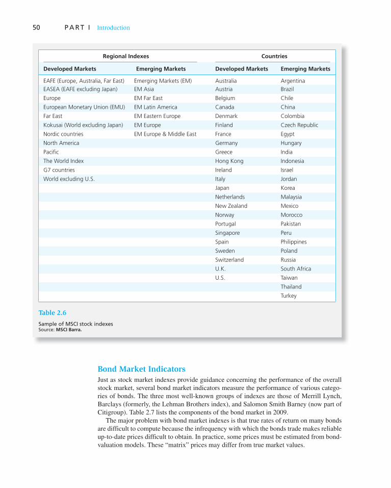
50 P A R T I Introduction
Bond Market Indicators
Just as stock market indexes provide guidance concerning the performance of the overall stock market, several bond market indicators measure the performance of various catego-ries of bonds. The three most well-known groups of indexes are those of Merrill Lynch, Barclays (formerly, the Lehman Brothers index), and Salomon Smith Barney (now part of Citigroup). Table 2.7 lists the components of the bond market in 2009.
The major problem with bond market indexes is that true rates of return on many bonds are difficult to compute because the infrequency with which the bonds trade makes reliable up-to-date prices difficult to obtain. In practice, some prices must be estimated from bond-valuation models. These “matrix” prices may differ from true market values.
Table 2.6
Sample of MSCI stock indexes Source: MSCI Barra.
Regional Indexes Countries
Developed Markets Emerging Markets Developed Markets Emerging Markets
EAFE (Europe, Australia, Far East) Emerging Markets (EM) Australia Argentina
EASEA (EAFE excluding Japan) EM Asia Austria Brazil
Europe EM Far East Belgium Chile
European Monetary Union (EMU) EM Latin America Canada China
Far East EM Eastern Europe Denmark Colombia
Kokusai (World excluding Japan) EM Europe Finland Czech Republic
Nordic countries EM Europe & Middle East France Egypt
North America Germany Hungary
Pacific Greece India
The World Index Hong Kong Indonesia
G7 countries Ireland Israel
World excluding U.S. Italy Jordan
Japan Korea
Netherlands Malaysia
New Zealand Mexico
Norway Morocco
Portugal Pakistan
Singapore Peru
Spain Philippines
Sweden Poland
Switzerland Russia
U.K. South Africa
U.S. Taiwan
Thailand
Turkey
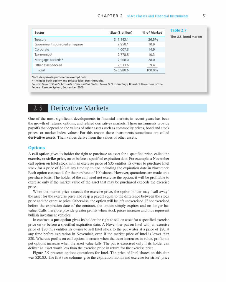
C H A P T E R 2 Asset Classes and Financial Instruments 51
2.5 Derivative Markets
*Includes private-purpose tax-exempt debt.**Includes both agency and private-label pass-throughs.Source: Flow of Funds Accounts of the United States: Flows & Outstandings, Board of Governors of the Federal Reserve System, September 2009.
Table 2.7
The U.S. bond marketSector Size ($ billion) % of Market
Treasury $ 7,143.1 26.5%
Government sponsored enterprise 2,950.1 10.9
Corporate 4,007.3 14.9
Tax-exempt* 2,778.5 10.3
Mortgage-backed** 7,568.0 28.0
Other asset-backed 2,533.6 9.4
Total $26,980.6 100.0%
One of the most significant developments in financial markets in recent years has been the growth of futures, options, and related derivatives markets. These instruments provide payoffs that depend on the values of other assets such as commodity prices, bond and stock prices, or market index values. For this reason these instruments sometimes are called derivative assets. Their values derive from the values of other assets.
Options
A call option gives its holder the right to purchase an asset for a specified price, called the exercise or strike price, on or before a specified expiration date. For example, a November call option on Intel stock with an exercise price of $35 entitles its owner to purchase Intel stock for a price of $20 at any time up to and including the expiration date in November. Each option contract is for the purchase of 100 shares. However, quotations are made on a per-share basis. The holder of the call need not exercise the option; it will be profitable to exercise only if the market value of the asset that may be purchased exceeds the exercise price.
When the market price exceeds the exercise price, the option holder may “call away” the asset for the exercise price and reap a payoff equal to the difference between the stock price and the exercise price. Otherwise, the option will be left unexercised. If not exercised before the expiration date of the contract, the option simply expires and no longer has value. Calls therefore provide greater profits when stock prices increase and thus represent bullish investment vehicles.
In contrast, a put option gives its holder the right to sell an asset for a specified exercise price on or before a specified expiration date. A November put on Intel with an exercise price of $20 thus entitles its owner to sell Intel stock to the put writer at a price of $20 at any time before expiration in November, even if the market price of Intel is lower than $20. Whereas profits on call options increase when the asset increases in value, profits on put options increase when the asset value falls. The put is exercised only if its holder can deliver an asset worth less than the exercise price in return for the exercise price.
Figure 2.9 presents options quotations for Intel. The price of Intel shares on this date was $20.83. The first two columns give the expiration month and exercise (or strike) price
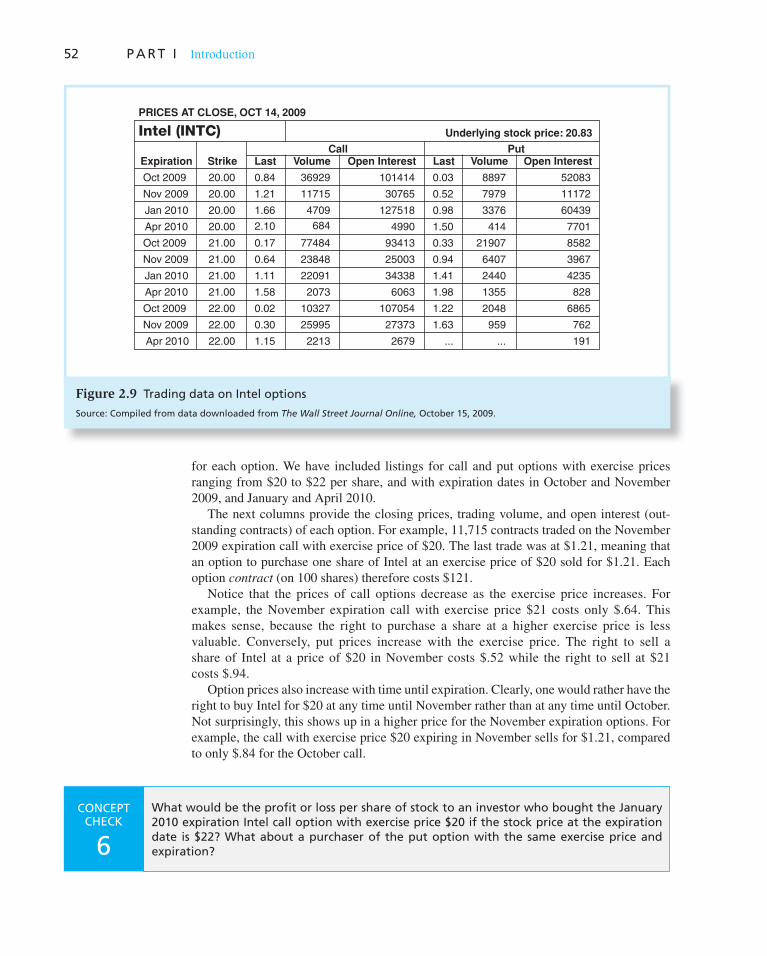
52 P A R T I Introduction
for each option. We have included listings for call and put options with exercise prices ranging from $20 to $22 per share, and with expiration dates in October and November 2009, and January and April 2010.
The next columns provide the closing prices, trading volume, and open interest (out-standing contracts) of each option. For example, 11,715 contracts traded on the November 2009 expiration call with exercise price of $20. The last trade was at $1.21, meaning that an option to purchase one share of Intel at an exercise price of $20 sold for $1.21. Each option contract (on 100 shares) therefore costs $121.
Notice that the prices of call options decrease as the exercise price increases. For example, the November expiration call with exercise price $21 costs only $.64. This makes sense, because the right to purchase a share at a higher exercise price is less valuable. Conversely, put prices increase with the exercise price. The right to sell a share of Intel at a price of $20 in November costs $.52 while the right to sell at $21 costs $.94.
Option prices also increase with time until expiration. Clearly, one would rather have the right to buy Intel for $20 at any time until November rather than at any time until October. Not surprisingly, this shows up in a higher price for the November expiration options. For example, the call with exercise price $20 expiring in November sells for $1.21, compared to only $.84 for the October call.
Figure 2.9 Trading data on Intel options
Source: Compiled from data downloaded from The Wall Street Journal Online, October 15, 2009.
Open Interest
52083
11172
60439
7701
8582
3967
4235
828
6865
762
191
Volume
7979
3376
414
21907
6407
2440
1355
2048
959
Last
0.03 8897
0.52
0.98
1.50
0.33
0.94
1.41
1.98
1.22
1.63
Open Interest
101414
30765
127518
4990
93413
25003
34338
6063
107054
27373
2679
Volume
36929
11715
4709
77484
23848
22091
2073
10327
25995
2213
Last
0.84
1.21
1.66
0.17
0.64
1.11
1.58
0.02
0.30
1.15
Strike
20.00
20.00
20.00
20.00
21.00
21.00
21.00
21.00
22.00
22.00
22.00
Expiration
Apr 2010
Oct 2009
Nov 2009
Jan 2010
Apr 2010
Oct 2009
Nov 2009
Jan 2010
Apr 2010
Oct 2009
Nov 2009
Underlying stock price: 20.83
PRICES AT CLOSE, OCT 14, 2009
PutCall
2.10 684
... ...
Intel (INTC)
CONCEPT CHECK
6
What would be the profit or loss per share of stock to an investor who bought the January 2010 expiration Intel call option with exercise price $20 if the stock price at the expiration date is $22? What about a purchaser of the put option with the same exercise price and expiration?
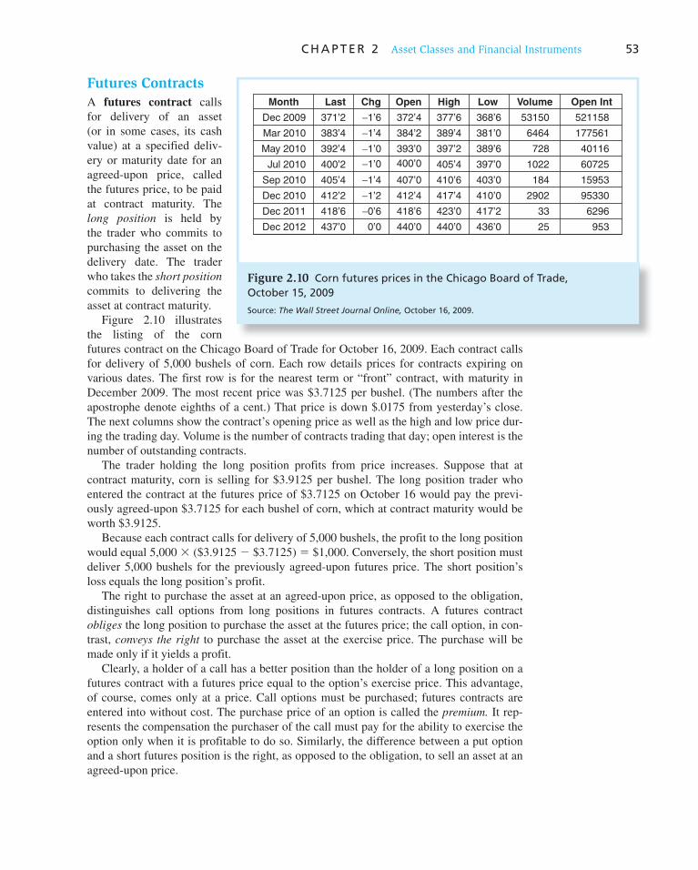
C H A P T E R 2 Asset Classes and Financial Instruments 53
Futures Contracts
A futures contract calls for delivery of an asset (or in some cases, its cash value) at a specified deliv-ery or maturity date for an agreed-upon price, called the futures price, to be paid at contract maturity. The long position is held by the trader who commits to purchasing the asset on the delivery date. The trader who takes the short position commits to delivering the asset at contract maturity.
Figure 2.10 illustrates the listing of the corn futures contract on the Chicago Board of Trade for October 16, 2009. Each contract calls for delivery of 5,000 bushels of corn. Each row details prices for contracts expiring on various dates. The first row is for the nearest term or “front” contract, with maturity in December 2009. The most recent price was $3.7125 per bushel. (The numbers after the apostrophe denote eighths of a cent.) That price is down $.0175 from yesterday’s close. The next columns show the contract’s opening price as well as the high and low price dur-ing the trading day. Volume is the number of contracts trading that day; open interest is the number of outstanding contracts.
The trader holding the long position profits from price increases. Suppose that at contract maturity, corn is selling for $3.9125 per bushel. The long position trader who entered the contract at the futures price of $3.7125 on October 16 would pay the previ-ously agreed-upon $3.7125 for each bushel of corn, which at contract maturity would be worth $3.9125.
Because each contract calls for delivery of 5,000 bushels, the profit to the long position would equal 5,000 � ($3.9125 � $3.7125) � $1,000. Conversely, the short position must deliver 5,000 bushels for the previously agreed-upon futures price. The short position’s loss equals the long position’s profit.
The right to purchase the asset at an agreed-upon price, as opposed to the obligation, distinguishes call options from long positions in futures contracts. A futures contract obliges the long position to purchase the asset at the futures price; the call option, in con-trast, conveys the right to purchase the asset at the exercise price. The purchase will be made only if it yields a profit.
Clearly, a holder of a call has a better position than the holder of a long position on a futures contract with a futures price equal to the option’s exercise price. This advantage, of course, comes only at a price. Call options must be purchased; futures contracts are entered into without cost. The purchase price of an option is called the premium. It rep-resents the compensation the purchaser of the call must pay for the ability to exercise the option only when it is profitable to do so. Similarly, the difference between a put option and a short futures position is the right, as opposed to the obligation, to sell an asset at an agreed-upon price.
Figure 2.10 Corn futures prices in the Chicago Board of Trade, October 15, 2009
Source: The Wall Street Journal Online, October 16, 2009.
Open Int
521158
177561
40116
60725
15953
95330
6296
953
Volume
6464
728
1022
184
2902
33
25
Low
368’6 53150
381’0
389’6
397’0
403’0
410’0
417’2
436’0
High
377’6
389’4
397’2
405’4
410’6
417’4
423’0
440’0
Open
372’4
384’2
393’0
407’0
412’4
418’6
440’0
Chg
−1’6
−1’4
−1’0
−1’4
−1’2
−0’6
0’0
Last
371’2
383’4
392’4
400’2
405’4
412’2
418’6
437’0
Month
Dec 2009
Mar 2010
May 2010
Jul 2010
Sep 2010
Dec 2010
Dec 2011
Dec 2012
−1’0 400’0

Vis
it u
s at
ww
w.m
hh
e.co
m/b
kmV
isit
us
at w
ww
.mh
he.
com
/bkm
54 P A R T I Introduction
1. Money market securities are very short-term debt obligations. They are usually highly market-able and have relatively low credit risk. Their low maturities and low credit risk ensure minimal capital gains or losses. These securities trade in large denominations, but they may be purchased indirectly through money market funds.
2. Much of U.S. government borrowing is in the form of Treasury bonds and notes. These are c oupon-paying bonds usually issued at or near par value. Treasury notes and bonds are similar in design to coupon-paying corporate bonds.
3. Municipal bonds are distinguished largely by their tax-exempt status. Interest payments (but not capital gains) on these securities are exempt from federal income taxes. The equivalent taxable yield offered by a municipal bond equals r m /(1 � t ), where r m is the municipal yield and t is the investor’s tax bracket.
4. Mortgage pass-through securities are pools of mortgages sold in one package. Owners of pass-throughs receive the principal and interest payments made by the borrowers. The originator that issued the mortgage merely services it, simply “passing through” the payments to the purchas-ers of the mortgage. A federal agency may guarantee the payment of interest and principal on mortgages pooled into its pass-through securities, but these guarantees are absent in private-label pass-throughs.
5. Common stock is an ownership share in a corporation. Each share entitles its owner to one vote on matters of corporate governance and to a prorated share of the dividends paid to shareholders. Stock, or equity, owners are the residual claimants on the income earned by the firm.
6. Preferred stock usually pays fixed dividends for the life of the firm; it is a perpetuity. A firm’s failure to pay the dividend due on preferred stock, however, does not precipitate corporate bank-ruptcy. Instead, unpaid dividends simply cumulate. Newer varieties of preferred stock include convertible and adjustable-rate issues.
7. Many stock market indexes measure the performance of the overall market. The Dow Jones averages, the oldest and best-known indicators, are price-weighted indexes. Today, many broad-based, market-value-weighted indexes are computed daily. These include the Standard & Poor’s 500 stock index, the NYSE index, the NASDAQ index, the Wilshire 5000 index, and indexes of many non-U.S. stock markets.
8. A call option is a right to purchase an asset at a stipulated exercise price on or before an expiration date. A put option is the right to sell an asset at some exercise price. Calls increase in value while puts decrease in value as the price of the underlying asset increases.
9. A futures contract is an obligation to buy or sell an asset at a stipulated futures price on a maturity date. The long position, which commits to purchasing, gains if the asset value increases while the short position, which commits to delivering, loses.
SUMMARY
Related Web sites for this chapter are available at www.mhhe.com/bkm
money market capital markets asked price bid price bid–asked spread certificate of deposit commercial paper banker’s acceptance Eurodollars repurchase agreements federal funds
London Interbank Offered Rate (LIBOR)
Treasury notes Treasury bonds yield to maturity municipal bonds equivalent taxable yield equities residual claim limited liability capital gains
price–earnings ratio preferred stock price-weighted average market-value-weighted index index funds derivative assets call option exercise (strike) price put option futures contract
KEY TERMS

Vis
it u
s at
ww
w.m
hh
e.co
m/b
km
C H A P T E R 2 Asset Classes and Financial Instruments 55
1. In what ways is preferred stock like long-term debt? In what ways is it like equity?
2. Why are money market securities sometimes referred to as “cash equivalents”?
3. Which of the following correctly describes a repurchase agreement?
a. The sale of a security with a commitment to repurchase the same security at a specified future date and a designated price.
b. The sale of a security with a commitment to repurchase the same security at a future date left unspecified, at a designated price.
c. The purchase of a security with a commitment to purchase more of the same security at a specified future date.
4. What would you expect to happen to the spread between yields on commercial paper and Treas-ury bills if the economy were to enter a steep recession?
5. What are the key differences between common stock, preferred stock, and corporate bonds?
6. Why are high-tax-bracket investors more inclined to invest in municipal bonds than low-bracket investors?
7. Turn back to Figure 2.3 and look at the Treasury bond maturing in February 2039.
a. How much would you have to pay to purchase one of these notes? b. What is its coupon rate? c. What is the current yield of the note?
8. Suppose investors can earn a return of 2% per 6 months on a Treasury note with 6 months remaining until maturity. What price would you expect a 6-month maturity Treasury bill to sell for?
9. Find the after-tax return to a corporation that buys a share of preferred stock at $40, sells it at year-end at $40, and receives a $4 year-end dividend. The firm is in the 30% tax bracket.
10. Turn to Figure 2.8 and look at the listing for General Dynamics.
a. How many shares could you buy for $5,000? b. What would be your annual dividend income from those shares? c. What must be General Dynamics earnings per share? d. What was the firm’s closing price on the day before the listing?
11. Consider the three stocks in the following table. P t represents price at time t, and Q t represents shares outstanding at time t. Stock C splits two for one in the last period.
P0 Q0 P1 Q1 P2 Q2
A 90 100 95 100 95 100
B 50 200 45 200 45 200
C 100 200 110 200 55 400
a. Calculate the rate of return on a price-weighted index of the three stocks for the first period ( t � 0 to t � 1).
b. What must happen to the divisor for the price-weighted index in year 2? c. Calculate the rate of return for the second period ( t � 1 to t � 2).
12. Using the data in the previous problem, calculate the first-period rates of return on the following indexes of the three stocks:
a. A market-value-weighted index. b. An equally weighted index.
13. An investor is in a 30% tax bracket. If corporate bonds offer 9% yields, what must municipals offer for the investor to prefer them to corporate bonds?
PROBLEM SETS
i. Basic
ii. Intermediate

Vis
it u
s at
ww
w.m
hh
e.co
m/b
km56 P A R T I Introduction
14. Find the equivalent taxable yield of a short-term municipal bond currently offering yields of 4% for tax brackets of zero, 10%, 20%, and 30%.
15. What problems would confront a mutual fund trying to create an index fund tied to an equally weighted index of a broad stock market?
16. Which security should sell at a greater price?
a. A 10-year Treasury bond with a 9% coupon rate versus a 10-year T-bond with a 10% coupon. b. A 3-month expiration call option with an exercise price of $40 versus a 3-month call on the
same stock with an exercise price of $35. c. A put option on a stock selling at $50, or a put option on another stock selling at $60 (all
other relevant features of the stocks and options may be assumed to be identical).
17. Look at the futures listings for the corn contract in Figure 2.10 .
a. Suppose you buy one contract for March delivery. If the contract closes in March at a level of 3.875, what will your profit be?
b. How many March maturity contracts are outstanding?
18. Turn back to Figure 2.9 and look at the Intel options. Suppose you buy a November expiration call option with exercise price $21.
a. Suppose the stock price in November is $21.75 Will you exercise your call? What is the profit on your position?
b. What if you had bought the November call with exercise price $22? c. What if you had bought a November put with exercise price $22?
19. Why do call options with exercise prices greater than the price of the underlying stock sell for positive prices?
20. Both a call and a put currently are traded on stock XYZ; both have strike prices of $50 and expirations of 6 months. What will be the profit to an investor who buys the call for $4 in the following scenarios for stock prices in 6 months? What will be the profit in each scenario to an investor who buys the put for $6?
a. $40 b. $45 c. $50 d. $55 e. $60
21. Explain the difference between a put option and a short position in a futures contract.
22. Explain the difference between a call option and a long position in a futures contract.
iii. Challenge
1. A firm’s preferred stock often sells at yields below its bonds because
a. Preferred stock generally carries a higher agency rating. b. Owners of preferred stock have a prior claim on the firm’s earnings. c. Owners of preferred stock have a prior claim on a firm’s assets in the event of liquidation. d. Corporations owning stock may exclude from income taxes most of the dividend income
they receive.
2. A municipal bond carries a coupon of 6¾% and is trading at par. What is the equivalent taxable yield to a taxpayer in a combined federal plus state 34% tax bracket?
3. Which is the most risky transaction to undertake in the stock index option markets if the stock market is expected to increase substantially after the transaction is completed?
a. Write a call option. b. Write a put option. c. Buy a call option. d. Buy a put option.

Vis
it u
s at
ww
w.m
hh
e.co
m/b
km
C H A P T E R 2 Asset Classes and Financial Instruments 57
4. Short-term municipal bonds currently offer yields of 4%, while comparable taxable bonds pay 5%. Which gives you the higher after-tax yield if your tax bracket is:
a. Zero b. 10% c. 20% d. 30%
5. The coupon rate on a tax-exempt bond is 5.6%, and the rate on a taxable bond is 8%. Both bonds sell at par. At what tax bracket (marginal tax rate) would an investor be indifferent between the two bonds?
Inflation-Protected Bonds around the World
Barclays maintains a Web site at www.barcap.com/inflation/index.shtml with infor-mation about inflation around the world and tools to help issuers and investors under-stand the inflation-linked asset class. Inflation-linked bonds were issued by a number of c ountries after 1945, including Israel, Argentina, Brazil, and Iceland. However, the modern market is generally deemed to have been born in 1981, when the first index-linked gilts were issued in the U.K. The other large markets adopted somewhat different calculations to those used by the U.K., mostly copying the more straightforward model first employed by Canada in 1991. In chronological order, the markets are the U.K. (1981), Australia (1985), Canada (1991), Sweden (1994), the United States (1997), France (1998), Italy (2003), and Japan (2004).
E-INVEST-MENTS EXERCISES
SOLUTIONS TO CONCEPT CHECKS
1. The bond sells for 98:26 bid which is a price of 98.813% of par, or $988.13, and 98:29 ask, or
$989.06. This ask price corresponds to a yield of 4.3156%. The ask price fell 20/32 from its level yesterday, so the ask price then must have been 99:17, or $995.31.
2. A 6% taxable return is equivalent to an after-tax return of 6(1 � .30) � 4.2%. Therefore, you would be better off in the taxable bond. The equivalent taxable yield of the tax-free bond is 4/(1 � .30) � 5.71%. So a taxable bond would have to pay a 5.71% yield to provide the same after-tax return as a tax-free bond offering a 4% yield.
3. a. You are entitled to a prorated share of IBM’s dividend payments and to vote in any of IBM’s stockholder meetings.
b. Your potential gain is unlimited because IBM’s stock price has no upper bound.
c. Your outlay was $80 � 100 � $8,000. Because of limited liability, this is the most you can lose.
4. The price-weighted index increases from 62.5 [i.e., (100 � 25)/2] to 65 [i.e., (110 � 20)/2], a gain of 4%. An investment of one share in each company requires an outlay of $125 that would increase in value to $130, for a return of 4% (i.e., 5/125), which equals the return to the price-weighted index.
5. The market-value-weighted index return is calculated by computing the increase in the value of the stock portfolio. The portfolio of the two stocks starts with an initial value of $100 million � $500 million � $600 million and falls in value to $110 million � $400 million � $510 million, a loss of 90/600 � .15, or 15%. The index portfolio

Vis
it u
s at
ww
w.m
hh
e.co
m/b
km58 P A R T I Introduction
return is a weighted average of the returns on each stock with weights of 1⁄6 on XYZ and 5⁄6 on ABC (weights proportional to relative investments). Because the return on XYZ is 10%, while
that on ABC is � 20%, the index portfolio return is 1⁄6 � 10% � 5⁄6 � (�20%) � � 15%, equal to the return on the market-value-weighted index.
6. The payoff to the call option is $2 per share at expiration. The option cost is $1.66 per share. The dollar profit is therefore $.34. The put option expires worthless. Therefore, the investor’s loss is the cost of the put, or $.98.

THIS CHAPTER WILL provide you with a
broad introduction to the many venues and
procedures available for trading securities in
the United States and international markets.
We will see that trading mechanisms range
from direct negotiation among market partic-
ipants to fully automated computer crossing
of trade orders.
The first time a security trades is when it is
issued to the public. Therefore, we begin with
a look at how securities are first marketed to
the public by investment bankers, the mid-
wives of securities. We turn next to a broad
survey of how already-issued securities may be
traded among investors, focusing on the dif-
ferences between dealer markets, electronic
markets, and specialist markets. With this
background, we then turn to specific trading
arenas such as the New York Stock Exchange,
NASDAQ, and several foreign security mar-
kets, examining the competition among these
markets for the patronage of security traders.
We consider the costs of trading in these mar-
kets, the quality of trade execution, and the
ongoing quest for cross-market integration of
trading.
We then turn to the essentials of some
specific types of transactions, such as buying
on margin and short-selling stocks. We close
the chapter with a look at some important
aspects of the regulations governing security
trading, including insider trading laws and
the role of security markets as self-regulating
organizations.
3 How Securities Are Traded 3
PAR
T I CHAPTER THREE
3.1 How Firms Issue Securities
When firms need to raise capital they may choose to sell or float securities. These new issues of stocks, bonds, or other securities typically are marketed to the public by invest-ment bankers in what is called the primary market. Trading of already-issued securi-ties among investors occurs in the secondary market. Trading in secondary markets does not affect the outstanding amount of securities; ownership is simply transferred from one investor to another.
There are two types of primary market issues of common stock. Initial public offer-
ings, or IPOs, are stocks issued by a formerly privately owned company that is going public, that is, selling stock to the public for the first time. Seasoned equity offerings are
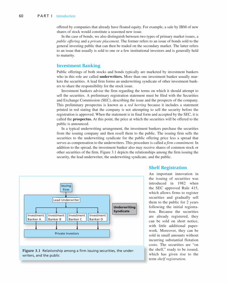
Figure 3.1 Relationship among a firm issuing securities, the under-writers, and the public
IssuingFirm
Lead Underwriter
InvestmentBanker A
Private Investors
InvestmentBanker D
InvestmentBanker B
InvestmentBanker C
Underwriting
Syndicate
60 P A R T I Introduction
offered by companies that already have floated equity. For example, a sale by IBM of new shares of stock would constitute a seasoned new issue.
In the case of bonds, we also distinguish between two types of primary market issues, a public offering and a private placement. The former refers to an issue of bonds sold to the general investing public that can then be traded on the secondary market. The latter refers to an issue that usually is sold to one or a few institutional investors and is generally held to maturity.
Investment Banking
Public offerings of both stocks and bonds typically are marketed by investment bankers who in this role are called underwriters. More than one investment banker usually mar-kets the securities. A lead firm forms an underwriting syndicate of other investment bank-ers to share the responsibility for the stock issue.
Investment bankers advise the firm regarding the terms on which it should attempt to sell the securities. A preliminary registration statement must be filed with the Securities and Exchange Commission (SEC), describing the issue and the prospects of the company. This preliminary prospectus is known as a red herring because it includes a statement printed in red stating that the company is not attempting to sell the security before the registration is approved. When the statement is in final form and accepted by the SEC, it is called the prospectus. At this point, the price at which the securities will be offered to the public is announced.
In a typical underwriting arrangement, the investment bankers purchase the securities from the issuing company and then resell them to the public. The issuing firm sells the securities to the underwriting syndicate for the public offering price less a spread that serves as compensation to the underwriters. This procedure is called a firm commitment. In addition to the spread, the investment banker also may receive shares of common stock or other securities of the firm. Figure 3.1 depicts the relationships among the firm issuing the security, the lead underwriter, the underwriting syndicate, and the public.
Shelf Registration
An important innovation in the issuing of securities was introduced in 1982 when the SEC approved Rule 415, which allows firms to register securities and gradually sell them to the public for 2 years following the initial registra-tion. Because the securities are already registered, they can be sold on short notice, with little additional paper-work. Moreover, they can be sold in small amounts without incurring substantial flotation costs. The securities are “on the shelf,” ready to be issued, which has given rise to the term shelf registration.

C H A P T E R 3 How Securities Are Traded 61
Private Placements
Primary offerings also can be sold in a private
placement rather than a public offering. In this case, the firm (using an investment banker) sells shares directly to a small group of insti-tutional or wealthy investors. Private placements can be far cheaper than public offerings. This is because Rule 144A of the SEC allows corporations to make these placements with-out preparing the extensive and costly registration statements required of a public offering. On the other hand, because private placements are not made available to the general public, they generally will be less suited for very large offerings. Moreover, private placements do not trade in secondary markets like stock exchanges. This greatly reduces their liquidity and presumably reduces the prices that investors will pay for the issue.
Initial Public Offerings
Investment bankers manage the issuance of new securities to the public. Once the SEC has commented on the registration statement and a preliminary prospectus has been dis-tributed to interested investors, the investment bankers organize road shows in which they travel around the country to publicize the imminent offering. These road shows serve two purposes. First, they generate interest among potential investors and provide information about the offering. Second, they provide information to the issuing firm and its under-writers about the price at which they will be able to market the securities. Large inves-tors communicate their interest in purchasing shares of the IPO to the underwriters; these indications of interest are called a book and the process of polling potential investors is called bookbuilding. These indications of interest provide valuable information to the issu-ing firm because institutional investors often will have useful insights about the market demand for the security as well as the prospects of the firm and its competitors. Investment bankers frequently revise both their initial estimates of the offering price of a security and the number of shares offered based on feedback from the investing community.
Why do investors truthfully reveal their interest in an offering to the investment banker? Might they be better off expressing little interest, in the hope that this will drive down the offering price? Truth is the better policy in this case because truth telling is rewarded. Shares of IPOs are allocated across investors in part based on the strength of each inves-tor’s expressed interest in the offering. If a firm wishes to get a large allocation when it is optimistic about the security, it needs to reveal its optimism. In turn, the underwriter needs to offer the security at a bargain price to these investors to induce them to participate in book-building and share their information. Thus, IPOs commonly are underpriced com-pared to the price at which they could be marketed. Such underpricing is reflected in price jumps that occur on the date when the shares are first traded in public security markets. The most dramatic case of underpricing occurred in December 1999 when shares in VA Linux were sold in an IPO at $30 a share and closed on the first day of trading at $239.25, a 698% 1-day return. 1
While the explicit costs of an IPO tend to be around 7% of the funds raised, such under-pricing should be viewed as another cost of the issue. For example, if VA Linux had sold its shares for the $239 that investors obviously were willing to pay for them, its IPO would have raised 8 times as much as it actually did. The money “left on the table” in this case
1 It is worth noting, however, that by December 2000, shares in VA Linux (now renamed VA Software) were selling for less than $9 a share, and by 2002, for less than $1. This example is extreme, but consistent with the generally disappointing long-term investment performance of IPOs.
CONCEPT CHECK
1 Why does it make sense for shelf registra-tion to be limited in time?

62 P A R T I Introduction
far exceeded the explicit cost of the stock issue. This degree of underpricing is far more dramatic than is common, but underpricing seems to be a universal phenomenon.
Figure 3.2 presents average first-day returns on IPOs of stocks across the world. The results consistently indicate that IPOs are marketed to investors at attractive prices. Underpricing of IPOs makes them appealing to all investors, yet institutional investors are allocated the bulk of a typical new issue. Some view this as unfair discrimination against small investors. However, our analysis suggests that the apparent discounts on IPOs may be in part payments for a valuable service, specifically, the information contributed by the institutional investors. The right to allocate shares in this way may contribute to efficiency by promoting the collection and dissemination of such information. 2
Both views of IPO allocations probably contain some truth. IPO allocations to institu-tions do serve a valid economic purpose as an information-gathering tool. Nevertheless, the system can be—and has been—abused. Part of the Wall Street scandals of 2000–2002 centered on the allocation of shares in IPOs. In a practice known as “spinning,” some investment bankers used IPO allocations to corporate insiders to curry favors, in effect as implicit kickback schemes. These underwriters would award generous IPO allocations to executives of particular firms in return for the firm’s future investment banking business.
Pricing of IPOs is not trivial and not all IPOs turn out to be underpriced. Some do poorly after issue. Other IPOs cannot even be fully sold to the market. Underwriters left with unmarketable securities are forced to sell them at a loss on the secondary market. Therefore, the investment banker bears price risk for an underwritten issue.
2 An elaboration of this point and a more complete discussion of the bookbuilding process is provided in Lawrence Benveniste and William Wilhelm, “Going by the Book,” Journal of Applied Corporate Finance 9 (Spring 1997).
Figure 3.2 Average initial returns for (A) European and (B) Non-European IPOs
Source: Provided by Professor J. Ritter of the University of Florida, 2008. This is an updated version of the information contained in T. Loughran, J. Ritter, and K. Rydqvist, “Initial Public Offerings,” Pacific-Basin Finance Journal 2 (1994), pp. 165–199. Copyright 1994 with permission from Elsevier Science.
50%
40%
30%
20%
10%
0%
Ave
rag
e f
irst
-da
y re
turn
s
Gre
ece
Ire
lan
dC
ypru
s
Swe
de
nG
erm
an
y
Po
lan
dIt
aly
Un
ited
Sta
tes
Un
ited
Kin
gd
om
Be
lgiu
mIs
rae
l
Tu
rke
yFr
an
ce
Po
rtu
ga
lSp
ain
Neth
erl
an
ds
No
rwa
y
Au
stri
aR
uss
ia
De
nm
ark
Fin
lan
d
50%60%70%80%90%
100%110%120%130%140%150%160%170%
40%30%20%10%0%
Ave
rag
e f
irst
-da
y re
turn
s
Ma
lays
iaK
ore
aB
razi
l
Ch
ina (
A s
ha
res)
Ind
ia
Jap
an
Ta
iwa
nT
ha
ila
nd
Sin
ga
po
re
Ph
ilip
pin
es
Ira
n
Au
stra
lia
Un
ited
Sta
tes
New
Ze
ala
nd
Ind
on
esi
a
Ho
ng
Ko
ng
Me
xico
Nig
eri
aT
urk
ey
Ch
ile
Ca
na
da
Arg
en
tin
a
Isra
el
Sou
th A
fric
a
A B
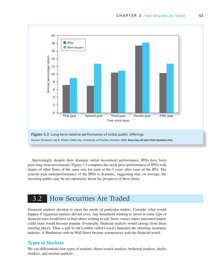
C H A P T E R 3 How Securities Are Traded 63
Interestingly, despite their dramatic initial investment performance, IPOs have been poor long-term investments. Figure 3.3 compares the stock price performance of IPOs with shares of other firms of the same size for each of the 5 years after issue of the IPO. The year-by-year underperformance of the IPOs is dramatic, suggesting that, on average, the investing public may be too optimistic about the prospects of these firms.
Figure 3.3 Long-term relative performance of initial public offerings
Source: Professor Jay R. Ritter’s Web site, University of Florida, October 2009, bear.cba.ufl.edu/ritter/ipodata.htm .
20
18
16
14
12
10
8
6
4
2
0
An
nu
al p
erce
nta
ge
retu
rn
First year Second year Third year Fourth year Fifth year
IPOs
Non-issuers
Year since issue
3.2 How Securities Are Traded
Financial markets develop to meet the needs of particular traders. Consider what would h appen if organized markets did not exist. Any household wishing to invest in some type of financial asset would have to find others wishing to sell. Soon, venues where interested traders could meet would become popular. Eventually, financial markets would emerge from these meeting places. Thus, a pub in old London called Lloyd’s launched the maritime insurance industry. A Manhattan curb on Wall Street became synonymous with the financial world.
Types of Markets
We can differentiate four types of markets: direct search markets, brokered markets, dealer markets, and auction markets.

64 P A R T I Introduction
Direct Search Markets A direct search market is the least organized market. Buyers and sellers must seek each other out directly. An example of a transaction in such a market is the sale of a used refrigerator where the seller advertises for buyers in a local newspaper or on Craigslist. Such markets are characterized by sporadic participation and low-priced and nonstandard goods. Firms would find it difficult to profit by specializing in such an environment.
Brokered Markets The next level of organization is a brokered market. In markets where trading in a good is active, brokers find it profitable to offer search services to buyers and sellers. A good example is the real estate market, where economies of scale in searches for available homes and for prospective buyers make it worthwhile for participants to pay brokers to conduct the searches. Brokers in particular markets develop specialized knowl-edge on valuing assets traded in that market.
An important brokered investment market is the primary market, where new issues of securities are offered to the public. In the primary market, investment bankers who market a firm’s securities to the public act as brokers; they seek investors to purchase securities directly from the issuing corporation.
Another brokered market is that for large block transactions, in which very large blocks of stock are bought or sold. These blocks are so large (technically more than 10,000 shares but usually much larger) that brokers or “block houses” may be engaged to search directly for other large traders, rather than bring the trade directly to the markets where relatively smaller investors trade.
Dealer Markets When trading activity in a particular type of asset increases, dealer
markets arise. Dealers specialize in various assets, purchase these assets for their own accounts, and later sell them for a profit from their inventory. The spreads between dealers’ buy (or “bid”) prices and sell (or “ask”) prices are a source of profit. Dealer markets save traders on search costs because market participants can easily look up the prices at which they can buy from or sell to dealers. A fair amount of market activity is required before dealing in a market is an attractive source of income. Most bonds trade in over-the-counter dealer markets.
Auction Markets The most integrated market is an auction market, in which all traders converge at one place (either physically or “electronically”) to buy or sell an asset. The New York Stock Exchange (NYSE) is an example of an auction market. An advantage of auction markets over dealer markets is that one need not search across dealers to find the best price for a good. If all participants converge, they can arrive at mutually agreeable prices and save the bid–ask spread.
Continuous auction markets (as opposed to periodic auctions, such as in the art world) require very heavy and frequent trading to cover the expense of maintaining the market. For this reason, the NYSE and other exchanges set up listing requirements, which limit the stocks traded on the exchange to those of firms in which sufficient trading interest is likely to exist.
The organized stock exchanges are also secondary markets. They are orga-nized for investors to trade existing securities among themselves.
Types of Orders
Before comparing alternative t rading practices and competing security m arkets,
CONCEPT CHECK
2
Many assets trade in more than one type of market. What types of markets do the following trade in?
a. Used cars
b. Paintings
c. Rare coins
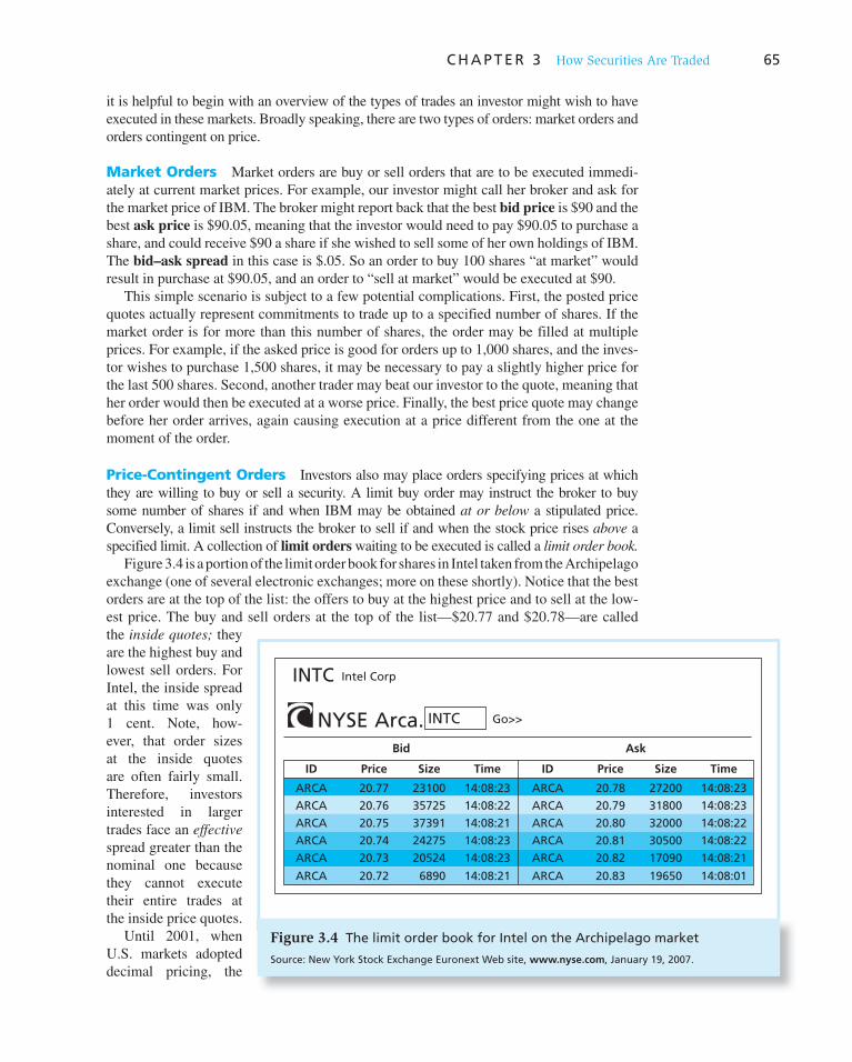
C H A P T E R 3 How Securities Are Traded 65
it is helpful to begin with an overview of the types of trades an investor might wish to have executed in these markets. Broadly speaking, there are two types of orders: market orders and orders contingent on price.
Market Orders Market orders are buy or sell orders that are to be executed immedi-ately at current market prices. For example, our investor might call her broker and ask for the market price of IBM. The broker might report back that the best bid price is $90 and the best ask price is $90.05, meaning that the investor would need to pay $90.05 to purchase a share, and could receive $90 a share if she wished to sell some of her own holdings of IBM. The bid–ask spread in this case is $.05. So an order to buy 100 shares “at market” would result in purchase at $90.05, and an order to “sell at market” would be executed at $90.
This simple scenario is subject to a few potential complications. First, the posted price quotes actually represent commitments to trade up to a specified number of shares. If the market order is for more than this number of shares, the order may be filled at multiple prices. For example, if the asked price is good for orders up to 1,000 shares, and the inves-tor wishes to purchase 1,500 shares, it may be necessary to pay a slightly higher price for the last 500 shares. Second, another trader may beat our investor to the quote, meaning that her order would then be executed at a worse price. Finally, the best price quote may change before her order arrives, again causing execution at a price different from the one at the moment of the order.
Price-Contingent Orders Investors also may place orders specifying prices at which they are willing to buy or sell a security. A limit buy order may instruct the broker to buy some number of shares if and when IBM may be obtained at or below a stipulated price. Conversely, a limit sell instructs the broker to sell if and when the stock price rises above a specified limit. A collection of limit orders waiting to be executed is called a limit order book.
Figure 3.4 is a portion of the limit order book for shares in Intel taken from the Archipelago exchange (one of several electronic exchanges; more on these shortly). Notice that the best orders are at the top of the list: the offers to buy at the highest price and to sell at the low-est price. The buy and sell orders at the top of the list—$20.77 and $20.78—are called the inside quotes; they are the highest buy and lowest sell orders. For Intel, the inside spread at this time was only 1 cent. Note, how-ever, that order sizes at the inside quotes are often fairly small. Therefore, investors interested in larger trades face an effective spread greater than the nominal one because they cannot execute their entire trades at the inside price quotes.
Until 2001, when U.S. markets adopted decimal pricing, the
Figure 3.4 The limit order book for Intel on the Archipelago market
Source: New York Stock Exchange Euronext Web site, www.nyse.com , January 19, 2007.
Bid
INTC Intel Corp
INTC Go>>
ARCA
ARCA
ARCA
ARCA
ARCA
20.77
20.76
20.75
20.74
20.73
23100
35725
37391
24275
20524
14:08:23
14:08:22
14:08:21
14:08:23
14:08:23
.
NYSE Arca.
ID Price Size Time
Ask
ARCA
ARCA
ARCA
ARCA
ARCA
20.78
20.79
20.80
20.81
20.82
27200
31800
32000
30500
17090
14:08:23
14:08:23
14:08:22
14:08:22
ARCA 20.72 6890 14:08:21 ARCA 20.83 19650 14:08:01
14:08:21
ID Price Size Time

66 P A R T I Introduction
minimum possible spread was “one tick,” which on the New York Stock Exchange was $1/8 until 1997 and $1/16 thereafter. With deci-mal pricing, the spread can be far lower. The average quoted bid–ask spread on the NYSE is less than 5 cents.
Stop orders are similar to limit orders in that the trade is not to be executed unless the stock hits a price limit. For stop-loss orders, the stock is to be sold if its price falls below a stipulated level. As the name suggests, the order lets the stock be sold to stop further losses from accumulating. Similarly, stop-buy orders specify that a stock should be bought when its price rises above a limit. These trades often accompany short sales (sales of securities you don’t own but have borrowed from your broker) and are used to limit potential losses from the short position. Short sales are discussed in greater detail later in this chapter. Figure 3.5 organizes these types of trades in a convenient matrix.
Figure 3.5 Price-contingent orders
Buy
Sell
Price abovethe Limit
Price belowthe Limit
Limit-BuyOrder
Limit-SellOrder
Stop-BuyOrder
Stop-LossOrder
Act
ion
Condition
CONCEPT CHECK
3
What type of trading order might you give to your broker in each of the following circumstances?
a. You want to buy shares of Intel to diversify your portfolio. You believe the share price is approximately at the “fair” value, and you want the trade done quickly and cheaply.
b. You want to buy shares of Intel, but believe that the current stock price is too high given the firm’s prospects. If the shares could be obtained at a price 5% lower than the current value, you would like to purchase shares for your portfolio.
c. You plan to purchase a condominium sometime in the next month or so and will sell your shares of Intel to provide the funds for your down payment. While you believe that the Intel share price is going to rise over the next few weeks, if you are wrong and the share price drops suddenly, you will not be able to afford the purchase. Therefore, you want to hold on to the shares for as long as possible, but still protect yourself against the risk of a big loss.
Trading Mechanisms
Broadly speaking, there are three trading systems employed in the United States: over-the-counter dealer markets, electronic communication networks, and formal exchanges. The best-known markets such as NASDAQ or the New York Stock Exchange actually use a variety of trading procedures, so before you delve into specific markets, it is useful to understand the basic operation of each type of trading system.
Dealer Markets Roughly 35,000 securities trade on the over-the-counter or OTC
market. Thousands of brokers register with the SEC as security dealers. Dealers quote prices at which they are willing to buy or sell securities. A broker then executes a trade by contacting a dealer listing an attractive quote.
Before 1971, all OTC quotations were recorded manually and published daily on so-called pink sheets. In 1971, the National Association of Securities Dealers Automatic Quotations System, or NASDAQ, was developed to link brokers and dealers in a com-puter network where price quotes could be displayed and revised. Dealers could use the network to display the bid price at which they were willing to purchase a security and the ask price at which they were willing to sell. The difference in these prices, the

C H A P T E R 3 How Securities Are Traded 67
bid–ask spread, was the source of the dealer’s profit. Brokers representing clients could examine quotes over the computer network, contact the dealer with the best quote, and execute a trade.
As originally organized, NASDAQ was more of a price-quotation system than a trading system. While brokers could survey bid and ask prices across the network of dealers in the search for the best trading opportunity, actual trades required direct negotiation (often over the phone) between the investor’s broker and the dealer in the security. However, as we will see shortly, NASDAQ has effectively evolved into an electronic market. While deal-ers still post bid and ask prices over the network, the vast majority of trades are executed electronically, without need of direct negotiation.
Electronic Communication Networks (ECNs) Electronic communication
networks allow participants to post market and limit orders over computer networks. The limit-order book is available to all participants. An example of such an order book from Archipelago, one of the leading ECNs, appeared in Figure 3.4 . Orders that can be “crossed,” that is, matched against another order, are done automatically without requiring the intervention of a broker. For example, an order to buy a share at a price of $50 or lower will be immediately executed if there is an outstanding asked price of $50. Therefore, ECNs are true trading systems, not merely price-quotation systems.
ECNs offer several attractions. Direct crossing of trades without using a broker-dealer system eliminates the bid–ask spread that otherwise would be incurred. Instead, trades are automatically crossed at a modest cost, typically less than a penny per share. ECNs are attractive as well because of the speed with which a trade can be executed. Finally, these systems offer investors considerable anonymity in their trades.
Specialist Markets In formal exchanges such as the New York Stock Exchange, trading in each security is managed by a specialist assigned responsibility for that security. Brokers who wish to buy or sell shares on behalf of their clients must direct the trade to the specialist’s post on the floor of the exchange.
Each security is assigned to one specialist, but each specialist firm—currently there are fewer than 10 on the NYSE—makes a market in many securities. This task may require the specialist to act as either a broker or a dealer. The specialist’s role as a broker is simply to execute the orders of other brokers. Specialists also may buy or sell shares of stock for their own portfolios. When no other trader can be found to take the other side of a trade, specialists will do so even if it means they must buy for or sell from their own accounts. Specialist firms earn income both from commissions for managing orders (as implicit brokers) and from the spreads at which they buy and sell securities (as implicit dealers).
Part of the specialist’s job as a broker is simply clerical. The specialist maintains a limit-order book of all outstanding unexecuted limit orders entered by brokers on behalf of clients. When limit orders can be executed at market prices, the specialist executes, or “crosses,” the trade.
The specialist is required to use the highest outstanding offered purchase price and the lowest outstanding offered selling price when matching trades. Therefore, the specialist system results in an auction market, meaning all buy and all sell orders come to one location, and the best orders “win” the trades. In this role, the specialist acts merely as a facilitator.
The more interesting function of the specialist is to maintain a “fair and orderly market” by acting as a dealer in the stock. In return for the exclusive right to make the market in a specific stock on the exchange, the specialist is required by the exchange to maintain an

68 P A R T I Introduction
orderly market by buying and selling shares from inventory. Specialists maintain their own portfolios of stock and quoted bid and ask prices at which they are obligated to meet at least a limited amount of market orders.
Ordinarily, in an active market, orders can be matched without specialist intervention. Sometimes, however, the specialist’s bid and ask prices are better than those offered by any other market participant. Therefore, at any point, the effective ask price in the mar-ket is the lower of either the specialist’s ask price or the lowest of the unfilled limit-sell orders. Similarly, the effective bid price is the highest of the unfilled limit-buy orders or the specialist’s bid. These procedures ensure that the specialist provides liquidity to the market.
Specialists strive to maintain a narrow bid–ask spread for at least two reasons. First, one source of the specialist’s income is frequent trading at the bid and ask prices, with the spread as a trading profit. A too-large spread would make the specialist’s quotes uncom-petitive with the limit orders placed by other traders. If the specialist’s bid and asked quotes are consistently worse than those of public traders, the specialist will not participate in any trades and will lose the ability to profit from the bid–ask spread.
An equally important reason for narrow specialist spreads is that specialists are obli-gated to provide price continuity to the market. To illustrate price continuity, suppose the highest limit-buy order for a stock is $30, while the lowest limit-sell order is $32. When a market buy order comes in, it is matched to the best limit sell at $32. A market sell order would be matched to the best limit buy at $30. As market buys and sells come to the floor randomly, the stock price would fluctuate between $30 and $32. The exchange authorities would consider this excessive volatility, and the specialist would be expected to step in with bid and/or ask prices between these values to reduce the bid–ask spread to an accept-able level, typically below $.05 for large firms.
3.3 U.S. Securities Markets
We have briefly sketched the three major trading mechanisms used in the United States: over-the-counter dealer markets, exchange trading managed by specialists, and direct trad-ing among brokers or investors over electronic networks. Originally, NASDAQ was pri-marily a dealer market and the NYSE was primarily a specialist market. As we will see, however, these markets have evolved in response to new information technology and both have moved dramatically to automated electronic trading.
NASDAQ
While any security can be traded in the over-the-counter network of security brokers and dealers, not all securities were included in the original National Association of Security Dealers Automated Quotations System. That system, now called the NASDAQ Stock
Market, lists about 3,200 firms and offers three listing options. The NASDAQ Global Select Market lists over 1,000 of the largest, most actively traded firms, the NASDAQ Global Market is for the next tier of firms, and the NASDAQ Capital Market is the third tier of listed firms. Some of the requirements for initial listing are presented in Table 3.1 . For even smaller firms that may not be eligible for listing or that wish to avoid disclosure requirements associated with listing on regulated markets, Pink Sheets LLC offers real-time stock quotes on www.pinksheets.com , as well as Pink Link, an electronic messaging and trade negotiation service.
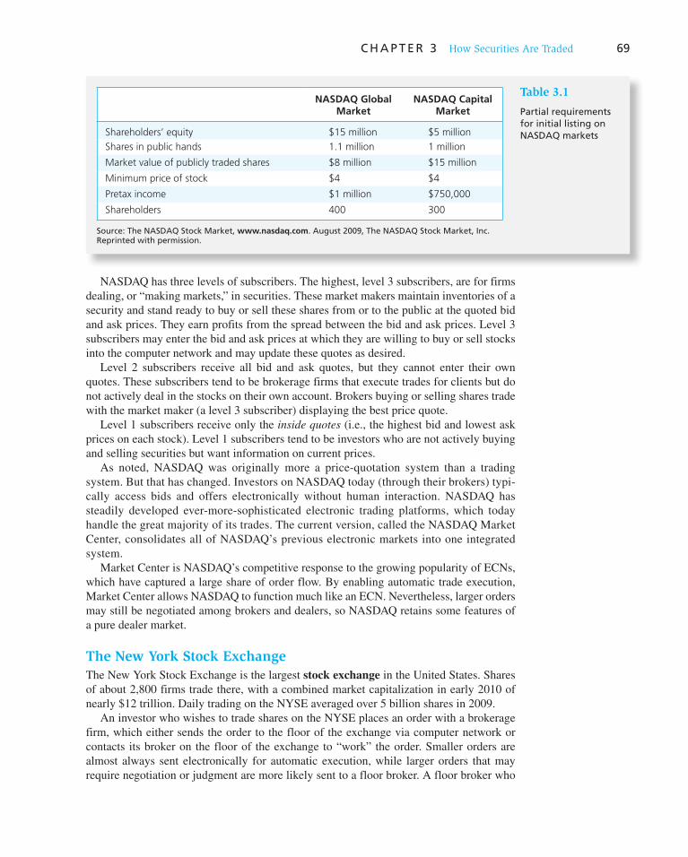
C H A P T E R 3 How Securities Are Traded 69
NASDAQ has three levels of subscribers. The highest, level 3 subscribers, are for firms dealing, or “making markets,” in securities. These market makers maintain inventories of a security and stand ready to buy or sell these shares from or to the public at the quoted bid and ask prices. They earn profits from the spread between the bid and ask prices. Level 3 subscribers may enter the bid and ask prices at which they are willing to buy or sell stocks into the computer network and may update these quotes as desired.
Level 2 subscribers receive all bid and ask quotes, but they cannot enter their own quotes. These subscribers tend to be brokerage firms that execute trades for clients but do not actively deal in the stocks on their own account. Brokers buying or selling shares trade with the market maker (a level 3 subscriber) displaying the best price quote.
Level 1 subscribers receive only the inside quotes (i.e., the highest bid and lowest ask prices on each stock). Level 1 subscribers tend to be investors who are not actively buying and selling securities but want information on current prices.
As noted, NASDAQ was originally more a price-quotation system than a trading system. But that has changed. Investors on NASDAQ today (through their brokers) typi-cally access bids and offers electronically without human interaction. NASDAQ has steadily developed ever-more-sophisticated electronic trading platforms, which today handle the great majority of its trades. The current version, called the NASDAQ Market Center, consolidates all of NASDAQ’s previous electronic markets into one integrated system.
Market Center is NASDAQ’s competitive response to the growing popularity of ECNs, which have captured a large share of order flow. By enabling automatic trade execution, Market Center allows NASDAQ to function much like an ECN. Nevertheless, larger orders may still be negotiated among brokers and dealers, so NASDAQ retains some features of a pure dealer market.
The New York Stock Exchange
The New York Stock Exchange is the largest stock exchange in the United States. Shares of about 2,800 firms trade there, with a combined market capitalization in early 2010 of nearly $12 trillion. Daily trading on the NYSE averaged over 5 billion shares in 2009.
An investor who wishes to trade shares on the NYSE places an order with a brokerage firm, which either sends the order to the floor of the exchange via computer network or contacts its broker on the floor of the exchange to “work” the order. Smaller orders are almost always sent electronically for automatic execution, while larger orders that may require negotiation or judgment are more likely sent to a floor broker. A floor broker who
Table 3.1
Partial requirements for initial listing on NASDAQ markets
NASDAQ Global Market
NASDAQ Capital Market
Shareholders’ equity $15 million $5 million
Shares in public hands 1.1 million 1 million
Market value of publicly traded shares $8 million $15 million
Minimum price of stock $4 $4
Pretax income $1 million $750,000
Shareholders 400 300
Source: The NASDAQ Stock Market, www.nasdaq.com. August 2009, The NASDAQ Stock Market, Inc. Reprinted with permission.
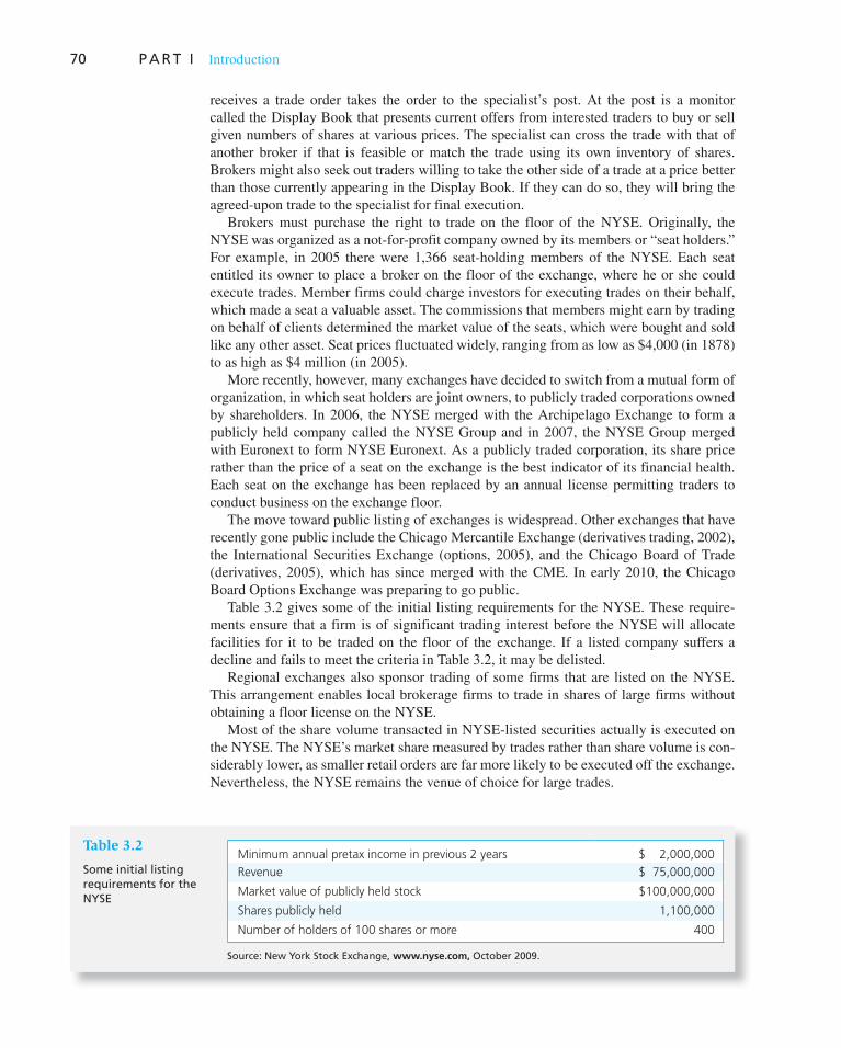
70 P A R T I Introduction
receives a trade order takes the order to the specialist’s post. At the post is a monitor called the Display Book that presents current offers from interested traders to buy or sell given n umbers of shares at various prices. The specialist can cross the trade with that of another broker if that is feasible or match the trade using its own inventory of shares. Brokers might also seek out traders willing to take the other side of a trade at a price better than those currently appearing in the Display Book. If they can do so, they will bring the agreed-upon trade to the specialist for final execution.
Brokers must purchase the right to trade on the floor of the NYSE. Originally, the NYSE was organized as a not-for-profit company owned by its members or “seat holders.” For example, in 2005 there were 1,366 seat-holding members of the NYSE. Each seat entitled its owner to place a broker on the floor of the exchange, where he or she could execute trades. Member firms could charge investors for executing trades on their behalf, which made a seat a valuable asset. The commissions that members might earn by trading on behalf of clients determined the market value of the seats, which were bought and sold like any other asset. Seat prices fluctuated widely, ranging from as low as $4,000 (in 1878) to as high as $4 million (in 2005).
More recently, however, many exchanges have decided to switch from a mutual form of organization, in which seat holders are joint owners, to publicly traded corporations owned by shareholders. In 2006, the NYSE merged with the Archipelago Exchange to form a publicly held company called the NYSE Group and in 2007, the NYSE Group merged with Euronext to form NYSE Euronext. As a publicly traded corporation, its share price rather than the price of a seat on the exchange is the best indicator of its financial health. Each seat on the exchange has been replaced by an annual license permitting traders to conduct business on the exchange floor.
The move toward public listing of exchanges is widespread. Other exchanges that have recently gone public include the Chicago Mercantile Exchange (derivatives trading, 2002), the International Securities Exchange (options, 2005), and the Chicago Board of Trade (derivatives, 2005), which has since merged with the CME. In early 2010, the Chicago Board Options Exchange was preparing to go public.
Table 3.2 gives some of the initial listing requirements for the NYSE. These require-ments ensure that a firm is of significant trading interest before the NYSE will allocate facilities for it to be traded on the floor of the exchange. If a listed company suffers a decline and fails to meet the criteria in Table 3.2 , it may be delisted.
Regional exchanges also sponsor trading of some firms that are listed on the NYSE. This arrangement enables local brokerage firms to trade in shares of large firms without obtaining a floor license on the NYSE.
Most of the share volume transacted in NYSE-listed securities actually is executed on the NYSE. The NYSE’s market share measured by trades rather than share volume is con-siderably lower, as smaller retail orders are far more likely to be executed off the exchange. Nevertheless, the NYSE remains the venue of choice for large trades.
Table 3.2
Some initial listing requirements for the NYSE
Minimum annual pretax income in previous 2 years $ 2,000,000
Revenue $ 75,000,000
Market value of publicly held stock $100,000,000
Shares publicly held 1,100,000
Number of holders of 100 shares or more 400
Source: New York Stock Exchange, www.nyse.com, October 2009.
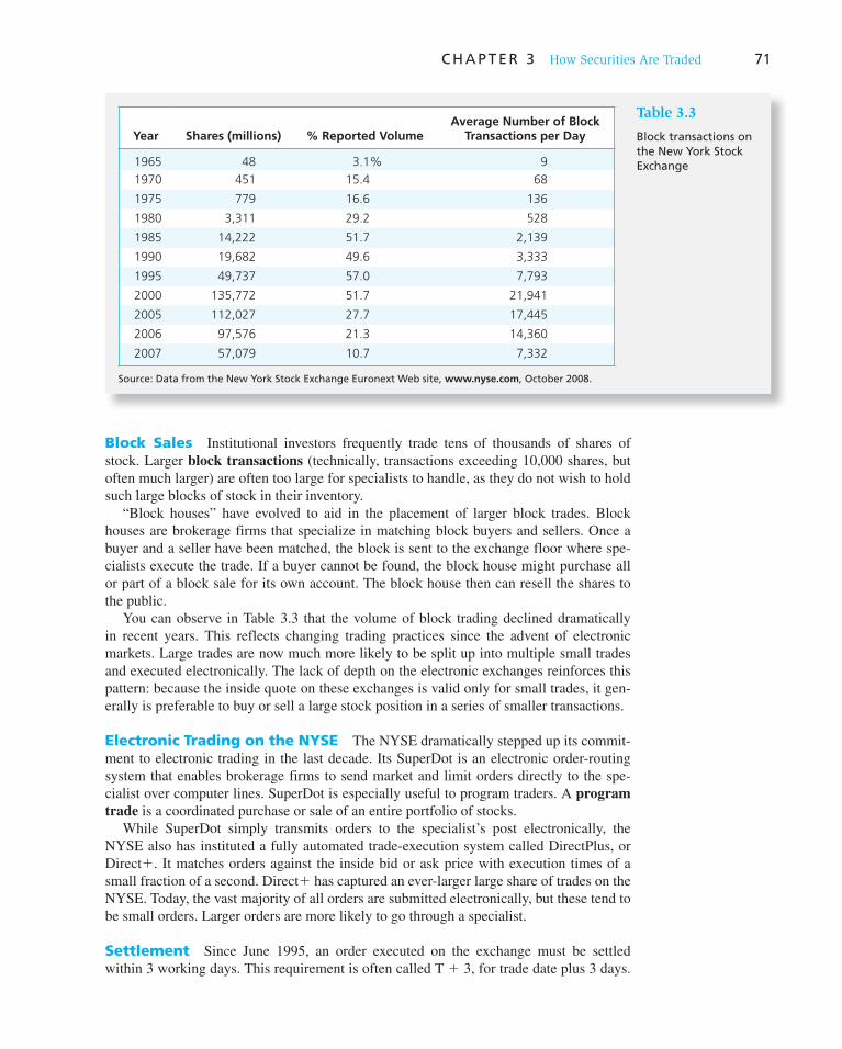
C H A P T E R 3 How Securities Are Traded 71
Block Sales Institutional investors frequently trade tens of thousands of shares of stock. Larger block transactions (technically, transactions exceeding 10,000 shares, but often much larger) are often too large for specialists to handle, as they do not wish to hold such large blocks of stock in their inventory.
“Block houses” have evolved to aid in the placement of larger block trades. Block houses are brokerage firms that specialize in matching block buyers and sellers. Once a buyer and a seller have been matched, the block is sent to the exchange floor where spe-cialists execute the trade. If a buyer cannot be found, the block house might purchase all or part of a block sale for its own account. The block house then can resell the shares to the public.
You can observe in Table 3.3 that the volume of block trading declined dramatically in recent years. This reflects changing trading practices since the advent of electronic markets. Large trades are now much more likely to be split up into multiple small trades and executed electronically. The lack of depth on the electronic exchanges reinforces this p attern: because the inside quote on these exchanges is valid only for small trades, it gen-erally is preferable to buy or sell a large stock position in a series of smaller transactions.
Electronic Trading on the NYSE The NYSE dramatically stepped up its commit-ment to electronic trading in the last decade. Its SuperDot is an electronic order-routing system that enables brokerage firms to send market and limit orders directly to the spe-cialist over computer lines. SuperDot is especially useful to program traders. A program
trade is a coordinated purchase or sale of an entire portfolio of stocks. While SuperDot simply transmits orders to the specialist’s post electronically, the
NYSE also has instituted a fully automated trade-execution system called DirectPlus, or Direct � . It matches orders against the inside bid or ask price with execution times of a small fraction of a second. Direct � has captured an ever-larger large share of trades on the NYSE. Today, the vast majority of all orders are submitted electronically, but these tend to be small orders. Larger orders are more likely to go through a specialist.
Settlement Since June 1995, an order executed on the exchange must be settled within 3 working days. This requirement is often called T � 3, for trade date plus 3 days.
Table 3.3
Block transactions on the New York Stock Exchange
Year Shares (millions) % Reported VolumeAverage Number of Block
Transactions per Day
1965 48 3.1% 9
1970 451 15.4 68
1975 779 16.6 136
1980 3,311 29.2 528
1985 14,222 51.7 2,139
1990 19,682 49.6 3,333
1995 49,737 57.0 7,793
2000 135,772 51.7 21,941
2005 112,027 27.7 17,445
2006 97,576 21.3 14,360
2007 57,079 10.7 7,332
Source: Data from the New York Stock Exchange Euronext Web site, www.nyse.com , October 2008.

72 P A R T I Introduction
The purchaser must deliver the cash, and the seller must deliver the stock to the broker, who in turn delivers it to the buyer’s broker. Frequently, a firm’s clients keep their securi-ties in street name, which means the broker holds the shares registered in the firm’s own name on behalf of the client. This convention can speed security transfer. T � 3 settlement has made such arrangements more important: It can be quite difficult for a seller of a secu-rity to complete delivery to the purchaser within the 3-day period if the stock is kept in a safe deposit box.
Settlement is simplified further by the existence of a clearinghouse. The trades of all exchange members are recorded each day, with members’ transactions netted out, so that each member need transfer or receive only the net number of shares sold or bought that day. A brokerage firm then settles with the clearinghouse instead of individually with every firm with which it made trades.
Electronic Communication Networks
ECNs are private computer networks that directly link buyers with sellers. As an order is received, the system determines whether there is a matching order, and if so, the trade is executed immediately. Brokers that have an affiliation with an ECN have computer access and can enter orders in the limit-order book. Moreover, these brokers may make their ter-minals (or Internet access) available directly to individual traders who then can enter their own orders into the system. The major ECNs are NASDAQ’s Market Center, ArcaEx, Direct Edge, BATS, and LavaFlow. Together, these electronic markets account for a large majority of all trades executed.
Electronic markets have captured ever-larger shares of overall trading volume in the last few years as technology has improved. A new development in this market is superfast flash
trading. Computer programs designed to follow specified trading rules scour the markets looking for even the tiniest bits of mispricing, and execute trades in small fractions of a second. Some high-speed traders are given direct access to their broker’s computer-trading codes and can execute trades in a little as 250 microseconds, that is, .00025 second! The nearby box notes that such naked access has become a subject of concern among market regulators.
The National Market System
The Securities Act Amendments of 1975 directed the Securities and Exchange Commission to implement a national competitive securities market. Such a market would entail central-ized reporting of transactions as well as a centralized quotation system, with the aim of enhanced competition among market makers.
In 1975, Consolidated Tape began reporting trades on the NYSE, Amex, and major regional exchanges, as well as trades of NASDAQ-listed stocks. In 1977, the Consolidated Quotations Service began providing online bid and ask quotes for NYSE securities also traded on various other exchanges. In 1978, the Intermarket Trading System (ITS) was implemented. ITS links exchanges and allows brokers and market makers to display and view quotes for all markets and to execute cross-market trades when the Consolidated Quotation System shows better prices in other markets. However, the ITS has been only a limited success. Orders need to be directed to markets with the best prices by participants who might find it inconvenient or unprofitable to do so.
However, the growth of automated electronic trading has made market integration more feasible. The SEC reaffirmed its so-called trade-through rule in 2005. Its Regulation NMS requires that investors’ orders be filled at the best price that can be executed immediately, even if that price is available in a different market.
73
The trade-through rule is meant to improve speed of execution and enhance integration of competing stock markets. Linking markets electronically through a unified book dis-playing all limit orders would be a logical extension of the ITS, enabling trade execution across markets. But this degree of integration has not yet been realized. Regulation NMS requires only that the inside quotes of each market be publicly shared. Because the inside or best quote is typically available only for a specified number of shares, there is still no guarantee that an investor will receive the best available prices for an entire trade, espe-cially for larger trades.
Bond Trading
In 2006, the NYSE obtained regulatory approval to expand its bond-trading system to include the debt issues of any NYSE-listed firm. Until then, each bond needed to be regis-tered before listing, and such a requirement was too onerous to justify listing most bonds. In conjunction with these new listings, the NYSE has expanded its electronic bond-trading platform, which is now called NYSE Bonds and is the largest centralized bond market of any U.S. exchange.
Nevertheless, the vast majority of bond trading occurs in the OTC market among bond dealers, even for bonds that are actually listed on the NYSE. This market is a network of bond dealers such as Merrill Lynch (now part of Bank of America), Salomon Smith Barney (a division of Citigroup), or Goldman, Sachs that is linked by a computer quotation system. However, because these dealers do not carry extensive inventories of the wide range of bonds that have been issued to the public, they cannot necessarily offer to sell bonds from their inventory to clients or even buy bonds for their own inventory. They may instead work to locate an investor who wishes to take the opposite side of a trade. In practice, however, the corporate bond market often is quite “thin,” in that there may be few investors interested in trading a specific bond at any particular time. As a result, the bond market is subject to a type of liquidity risk, for it can be difficult to sell one’s holdings quickly if the need arises.
Big Slice of Market Is Going “Naked”
“Naked” access, a controversial trading practice largely employed by high-speed traders, accounts for nearly 40% of U.S. stock-trading volume, a study by Aite Group, a Boston research outfit, has found.
The finding comes amid increasing regulatory concern about the practice, which leaves exchanges in the dark about the identity of the firms doing the trading. That reduces accountability in case of a destabilizing or problematic trade.
Broadly, there are two ways that a firm can trade on an exchange. It can become a registered broker with the SEC and become a member of an exchange, both of which are costly. Alternatively, a firm can pay a registered broker to use the broker’s computer code to trade, or sponsored access.
Some sponsored firms trade through the broker’s com-puter system, and give the broker the ability to employ pretrade checks that could catch risky trades before they reach the market. Traders using naked access, however, trade directly on the exchange and aren’t subject to a third party’s pretrade checks.
Behind regulators’ concerns are the increasingly fast speeds employed by high-frequency traders. According to
the Aite report, a firm that uses naked access can execute a trade in 250 to 350 microseconds, compared with 550 to 750 microseconds for trades that travel through a broker’s computer system by sponsored access.
The small sliver of time can mean the difference between success and failure in the computer-driven uni-verse of high-frequency trading. It highlights the mind-bending speeds these firms compete at as electronic markets race to provide superfast access.
Critics say naked access heightens the risk of reck-less trades that could destabilize the broader market. Exchanges often don’t know the identity of firms using sponsored access, since the only way to identify the firms is through the computer code.
That means it could be difficult to quickly track down a firm whose trades have run amok. But exchanges have rushed to offer the service because it brings in huge trad-ing volumes and fees.
Source: Scott Patterson, “Big Slice of Market Is Going ‘Naked,’” The Wall Street Journal, December 14, 2009. Reprinted by permis-sion of The Wall Street Journal, © 2009.
WO
RD
S FRO
M TH
E STREET
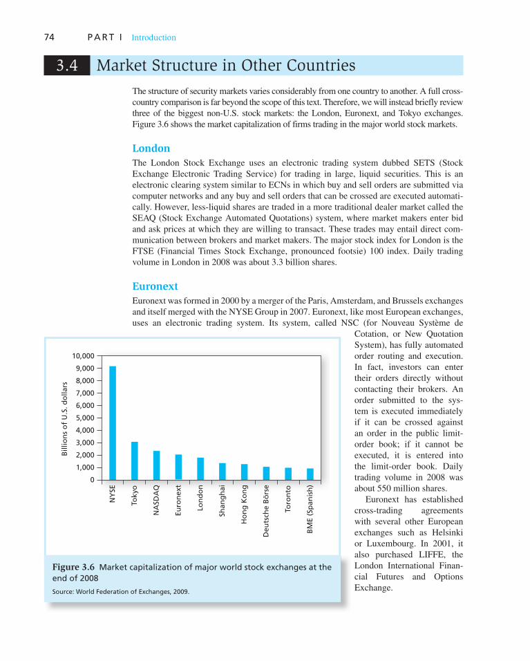
74 P A R T I Introduction
3.4 Market Structure in Other Countries
The structure of security markets varies considerably from one country to another. A full cross-country comparison is far beyond the scope of this text. Therefore, we will instead briefly review three of the biggest non-U.S. stock markets: the London, Euronext, and Tokyo exchanges. Figure 3.6 shows the market capitalization of firms trading in the major world stock markets.
London
The London Stock Exchange uses an electronic trading system dubbed SETS (Stock Exchange Electronic Trading Service) for trading in large, liquid securities. This is an electronic clearing system similar to ECNs in which buy and sell orders are submitted via computer networks and any buy and sell orders that can be crossed are executed automati-cally. However, less-liquid shares are traded in a more traditional dealer market called the SEAQ (Stock Exchange Automated Quotations) system, where market makers enter bid and ask prices at which they are willing to transact. These trades may entail direct com-munication between brokers and market makers. The major stock index for London is the FTSE (Financial Times Stock Exchange, pronounced footsie) 100 index. Daily trading volume in London in 2008 was about 3.3 billion shares.
Euronext
Euronext was formed in 2000 by a merger of the Paris, Amsterdam, and Brussels exchanges and itself merged with the NYSE Group in 2007. Euronext, like most European exchanges, uses an electronic trading system. Its system, called NSC (for Nouveau Système de
Cotation, or New Quotation System), has fully automated order routing and execution. In fact, investors can enter their orders directly without contacting their brokers. An order submitted to the sys-tem is executed immediately if it can be crossed against an order in the public limit-order book; if it cannot be executed, it is entered into the limit-order book. Daily trading volume in 2008 was about 550 million shares.
Euronext has established cross-trading agreements with sev eral other European exchanges such as Helsinki or Luxembourg. In 2001, it also purchased LIFFE, the London International Finan-cial Futures and Options Exchange.
Figure 3.6 Market capitalization of major world stock exchanges at the end of 2008
Source: World Federation of Exchanges, 2009.
7,000
8,000
10,000
9,000
Billio
ns
of
U.S
. d
ollars
6,000
5,000
4,000
3,000
2,000
1,000
NY
SE
Tokyo
Eu
ron
ext
NA
SDA
Q
Lon
do
n
Shan
gh
ai
Ho
ng
Ko
ng
Toro
nto
Deu
tsch
e B
örs
e
BM
E (
Span
ish
)
0

C H A P T E R 3 How Securities Are Traded 75
Tokyo
The Tokyo Stock Exchange (TSE) is among the largest in the world, measured by the market capitalization of its roughly 2,400 listed firms. It exemplifies many of the general trends that we have seen affecting stock markets throughout the world. In 1999, it closed its trading floor and switched to all-electronic trading. It switched from a membership form of organization to a corporate form in 2001.
The TSE maintains three “sections.” The First section is for large companies, the Second is for midsized firms, and the “Mothers” section is for emerging and high-growth stocks. About three-quarters of all listed firms trade on the First section, and about 200 trade in the Mothers section.
The two major stock market indexes for the TSE are the Nikkei 225 index, which is a price-weighted average of 225 top-tier Japanese firms, and the TOPIX index, which is a value-weighted index of the First section companies.
Globalization and Consolidation of Stock Markets
All stock markets have come under increasing pressure in recent years to make inter-national alliances or mergers. Much of this pressure is due to the impact of elec-tronic trading. To a growing extent, traders view stock markets as computer networks that link them to other traders, and there are increasingly fewer limits on the securi-ties around the world that they can trade. Against this background, it becomes more important for exchanges to provide the cheapest and most efficient mechanism by which trades can be executed and cleared. This argues for global alliances that can facilitate the nuts and bolts of cross-border trading and can benefit from economies of scale. Moreover, in the face of competition from electronic networks, established exchanges feel that they eventually need to offer 24-hour global markets and platforms that allow trading of different security types, for example, both stocks and derivatives. Finally, companies want to be able to go beyond national borders when they wish to raise capital.
These pressures have resulted in a broad trend toward market consolidation. In the last decade, most of the mergers were “local,” that is, involving exchanges operating on the same continent. In the U.S., the NYSE merged with the Archipelago ECN in 2006, and in 2008 acquired the American Stock Exchange. NASDAQ acquired Instinet (which operated another major ECN, INET) in 2005 and the Boston Stock Exchange in 2007. In the deriva-tives market, the Chicago Mercantile Exchange acquired the Chicago Board of Trade in 2007 and the New York Mercantile Exchange in 2008, thus moving almost all futures trad-ing in the U.S. onto one exchange. In Europe, Euronext was formed by the merger of the Paris, Brussels, Lisbon, and Amsterdam exchanges and shortly thereafter purchased Liffe, the derivatives exchange based in London. The LSE merged in 2007 with Borsa Italiana, which operates the Milan exchange.
There has also been a wave of intercontinental consolidation. The NYSE Group and Euronext merged in 2007. The NYSE has purchased 5% of India’s National Stock Exchange, and has entered a cooperation agreement with the Tokyo Stock Exchange. NASDAQ acquired a foothold in Europe in 2007, when it joined forces with Börse Dubai to acquire the Swedish exchange OMX. The parent company of the exchange is now called NASDAQ OMX Group. In 2007, Eurex acquired International Securities Exchange Holdings, and ISE announced that it would launch a new derivatives market in partnership with the Toronto Stock Exchange.
76 P A R T I Introduction
3.5 Trading Costs
Part of the cost of trading a security is obvious and explicit. Your broker must be paid a commission. Individuals may choose from two kinds of brokers: full-service or discount brokers. Full-service brokers who provide a variety of services often are referred to as account executives or financial consultants.
Besides carrying out the basic services of executing orders, holding securities for safe-keeping, extending margin loans, and facilitating short sales, brokers routinely provide information and advice relating to investment alternatives.
Full-service brokers usually depend on a research staff that prepares analyses and fore-casts of general economic as well as industry and company conditions and often makes specific buy or sell recommendations. Some customers take the ultimate leap of faith and allow a full-service broker to make buy and sell decisions for them by establishing a discretionary account. In this account, the broker can buy and sell prespecified securi-ties whenever deemed fit. (The broker cannot withdraw any funds, though.) This action requires an unusual degree of trust on the part of the customer, for an unscrupulous bro-ker can “churn” an account, that is, trade securities excessively with the sole purpose of generating commissions.
Discount brokers, on the other hand, provide “no-frills” services. They buy and sell securities, hold them for safekeeping, offer margin loans, facilitate short sales, and that is all. The only information they provide about the securities they handle is price quota-tions. Discount brokerage services have become increasingly available in recent years. Many banks, thrift institutions, and mutual fund management companies now offer such services to the investing public as part of a general trend toward the creation of one-stop “financial supermarkets.” Stock trading fees have fallen steadily over the last decade, and discount brokerage firms such as Schwab, E * Trade, or TD Ameritrade now offer commis-sions below $10.
In addition to the explicit part of trading costs—the broker’s commission—there is an implicit part—the dealer’s bid–ask spread. Sometimes the broker is also a dealer in the security being traded and charges no commission but instead collects the fee entirely in the form of the bid–ask spread. Another implicit cost of trading that some observers would distinguish is the price concession an investor may be forced to make for trading in quanti-ties greater than those associated with the posted bid or asked price.
An ongoing controversy between the NYSE and its competitors is the extent to which better execution on the NYSE offsets the generally lower explicit costs of trading in other markets. The NYSE believes that many investors focus too intently on the costs they can see, despite the fact that “quality of execution” may be far more important to their total trading costs. Part of the quality of execution refers to the ability of a large exchange like the NYSE to accommodate big trades without encountering a large impact on security price. Another part is the size of the effective bid–ask spread, which will be smaller when limit-order books are deeper.
3.6 Buying on Margin
When purchasing securities, investors have easy access to a source of debt financing called broker’s call loans. The act of taking advantage of broker’s call loans is called buying on
margin.
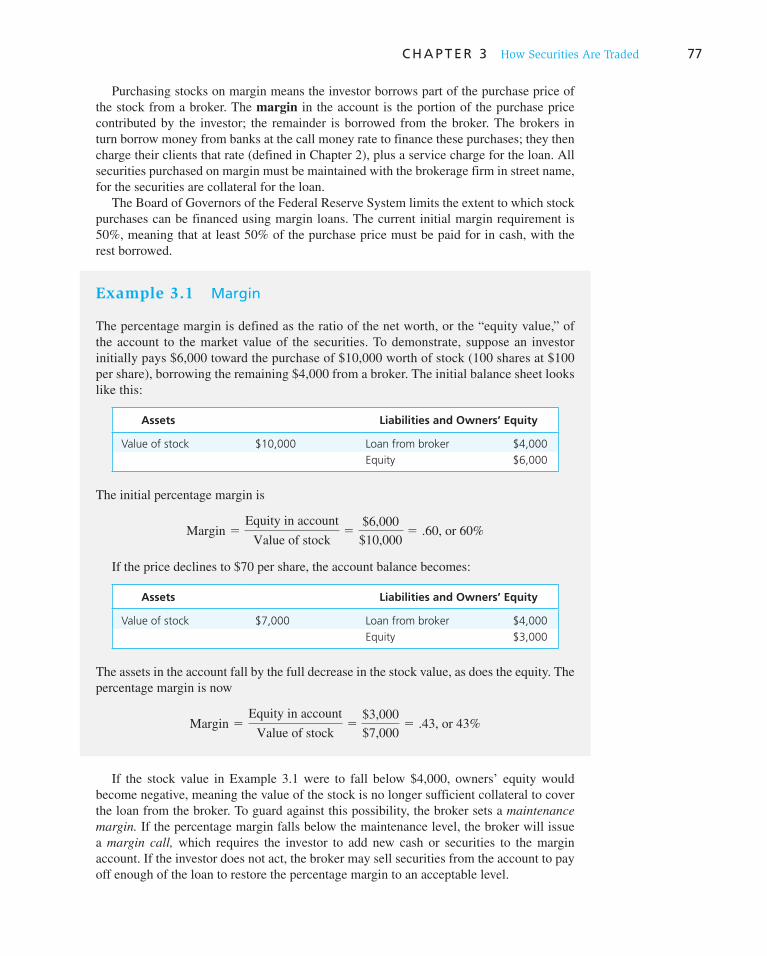
C H A P T E R 3 How Securities Are Traded 77
Purchasing stocks on margin means the investor borrows part of the purchase price of the stock from a broker. The margin in the account is the portion of the purchase price contributed by the investor; the remainder is borrowed from the broker. The brokers in turn borrow money from banks at the call money rate to finance these purchases; they then charge their clients that rate (defined in Chapter 2), plus a service charge for the loan. All securities purchased on margin must be maintained with the brokerage firm in street name, for the securities are collateral for the loan.
The Board of Governors of the Federal Reserve System limits the extent to which stock purchases can be financed using margin loans. The current initial margin requirement is 50%, meaning that at least 50% of the purchase price must be paid for in cash, with the rest borrowed.
If the stock value in Example 3.1 were to fall below $4,000, owners’ equity would become negative, meaning the value of the stock is no longer sufficient collateral to cover the loan from the broker. To guard against this possibility, the broker sets a maintenance
margin. If the percentage margin falls below the maintenance level, the broker will issue a margin call, which requires the investor to add new cash or securities to the margin account. If the investor does not act, the broker may sell securities from the account to pay off enough of the loan to restore the percentage margin to an acceptable level.
Example 3.1 Margin
The percentage margin is defined as the ratio of the net worth, or the “equity value,” of the account to the market value of the securities. To demonstrate, suppose an investor initially pays $6,000 toward the purchase of $10,000 worth of stock (100 shares at $100 per share), borrowing the remaining $4,000 from a broker. The initial balance sheet looks like this:
Assets Liabilities and Owners’ Equity
Value of stock $10,000 Loan from broker $4,000
Equity $6,000
The initial percentage margin is
Margin 5Equity in account
Value of stock5
$6,000
$10,0005 .60, or 60%
If the price declines to $70 per share, the account balance becomes:
Assets Liabilities and Owners’ Equity
Value of stock $7,000 Loan from broker $4,000
Equity $3,000
The assets in the account fall by the full decrease in the stock value, as does the equity. The percentage margin is now
Margin 5Equity in account
Value of stock5
$3,000
$7,0005 .43, or 43%
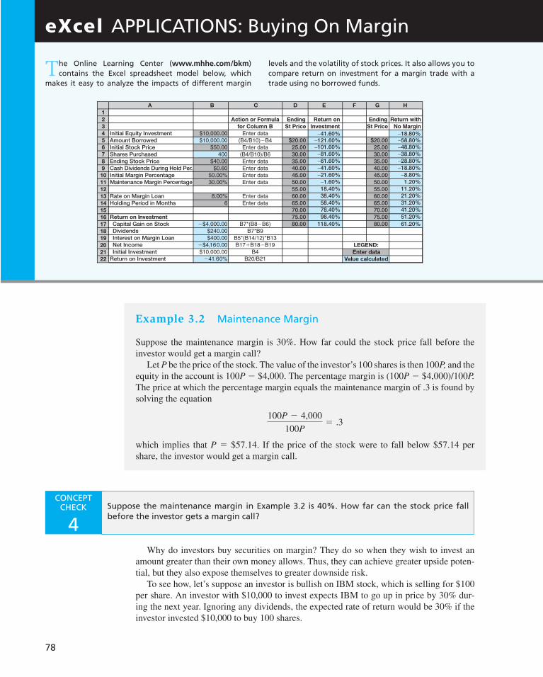
78
Why do investors buy securities on margin? They do so when they wish to invest an amount greater than their own money allows. Thus, they can achieve greater upside poten-tial, but they also expose themselves to greater downside risk.
To see how, let’s suppose an investor is bullish on IBM stock, which is selling for $100 per share. An investor with $10,000 to invest expects IBM to go up in price by 30% dur-ing the next year. Ignoring any dividends, the expected rate of return would be 30% if the investor invested $10,000 to buy 100 shares.
Example 3.2 Maintenance Margin
Suppose the maintenance margin is 30%. How far could the stock price fall before the investor would get a margin call?
Let P be the price of the stock. The value of the investor’s 100 shares is then 100 P, and the equity in the account is 100 P � $4,000. The percentage margin is (100 P � $4,000)/100 P. The price at which the percentage margin equals the maintenance margin of .3 is found by solving the equation
100P 2 4,000
100P5 .3
which implies that P � $57.14. If the price of the stock were to fall below $57.14 per share, the investor would get a margin call.
eXcel APPLICATIONS: Buying On Margin
T he Online Learning Center ( www.mhhe.com/bkm ) contains the Excel spreadsheet model below, which
makes it easy to analyze the impacts of different margin
levels and the volatility of stock prices. It also allows you to compare return on investment for a margin trade with a trade using no borrowed funds.
A B C D E F G H
Initial Equity InvestmentAmount BorrowedInitial Stock PriceShares PurchasedEnding Stock PriceCash Dividends During Hold Per.Initial Margin PercentageMaintenance Margin Percentage
Rate on Margin LoanHolding Period in Months
Return on Investment
Capital Gain on StockDividendsInterest on Margin LoanNet IncomeInitial Investment
Return on Investment
Ending
St Price
$20.0025.0030.0035.0040.0045.0050.0055.0060.0065.0070.0075.0080.00
−41.60%−121.60%−101.60%
−81.60%−61.60%−41.60%−21.60%
−1.60%18.40%38.40%58.40%78.40%98.40%
118.40%
Ending
St Price
$20.0025.0030.0035.0040.0045.0050.0055.0060.0065.0070.0075.0080.00
LEGEND:
Enter data
Value calculated
1
2
3
4
5
6
7
8
9
10
11
12
13
14
15
16
17
18
19
20
21
22
−18.80%−58.80%−48.80%−38.80%−28.80%−18.80%
−8.80%1.20%
11.20%21.20%31.20%41.20%51.20%
61.20%
CONCEPT CHECK
4 Suppose the maintenance margin in Example 3.2 is 40%. How far can the stock price fall before the investor gets a margin call?

C H A P T E R 3 How Securities Are Traded 79
But now assume the investor borrows another $10,000 from the broker and invests it in IBM, too. The total investment in IBM would be $20,000 (for 200 shares). Assuming an interest rate on the margin loan of 9% per year, what will the investor’s rate of return be now (again ignoring dividends) if IBM stock goes up 30% by year’s end?
The 200 shares will be worth $26,000. Paying off $10,900 of principal and interest on the margin loan leaves $15,100 (i.e., $26,000 – $10,900). The rate of return in this case will be
$15,100 2 $10,000
$10,0005 51%
The investor has parlayed a 30% rise in the stock’s price into a 51% rate of return on the $10,000 investment.
Doing so, however, magnifies the downside risk. Suppose that, instead of going up by 30%, the price of IBM stock goes down by 30% to $70 per share. In that case, the 200 shares will be worth $14,000, and the investor is left with $3,100 after paying off the $10,900 of principal and interest on the loan. The result is a disastrous return of
$3,100 2 $10,000
$10,0005 269%
Table 3.4 summarizes the possible results of these hypothetical transactions. If there is no change in IBM’s stock price, the investor loses 9%, the cost of the loan.
Table 3.4
Illustration of buying stock on margin
Change in Stock Price
End-of-Year Value of Shares
Repayment of Principal and Interest*
Investor’s Rate of Return
30% increase $26,000 $10,900 51%
No change 20,000 10,900 �9
30% decrease 14,000 10,900 �69
CONCEPT CHECK
5 Suppose that in this margin example, the investor borrows only $5,000 at the same interest rate of 9% per year. What will the rate of return be if the price of IBM goes up by 30%? If it goes down by 30%? If it remains unchanged?
3.7 Short Sales
Normally, an investor would first buy a stock and later sell it. With a short sale, the order is reversed. First, you sell and then you buy the shares. In both cases, you begin and end with no shares.
A short sale allows investors to profit from a decline in a security’s price. An investor borrows a share of stock from a broker and sells it. Later, the short-seller must purchase
* Assuming the investor buys $20,000 worth of stock, borrowing $10,000 of the purchase price at an interest rate of 9% per year.

A B C D E
Initial InvestmentInitial Stock PriceNumber of Shares Sold ShortEnding Stock PriceCash Dividends Per ShareInitial Margin PercentageMaintenance Margin Percentage
Return on Short Sale
Capital Gain on StockDividends PaidNet IncomeInitial InvestmentReturn on Investment
Margin Positions
Margin Based on Ending Price
Price for Margin Call
$50,000.00$100.00
1,000$70.00$0.00
50.00%30.00%
$30,000.00$0.00
$30,000.00$50,000.00
60.00%
114.29%
$115.38
Ending
St Price
$170.00160.00150.00140.00130.00120.00110.00100.0090.0080.0070.0060.0050.0040.0030.0020.0010.00
60.00%−140.00%−120.00%−100.00%
−80.00%−60.00%−40.00%−20.00%
0.00%20.00%40.00%60.00%80.00%
100.00%120.00%140.00%160.00%180.00%
12345678910111213141516171819202122232425
LEGEND:
Enter data
Value calculated
80
a share of the same stock in order to replace the share that was borrowed. This is called covering the short position. Table 3.5 compares stock purchases to short sales. 3
The short-seller anticipates the stock price will fall, so that the share can be purchased later at a lower price than it initially sold for; if so, the short-seller will reap a profit.
3Naked short-selling is a variant on conventional short-selling. In a naked short, a trader sells shares that have not yet been borrowed, assuming that the shares can be acquired in time to meet any delivery deadline. While naked short-selling is prohibited, enforcement has been spotty, as many firms have engaged in it based on their “reason-able belief” that they will be able to acquire the stock by the time delivery is required. Now the SEC is requiring that short-sellers have made firm arrangements for delivery before engaging in the sale.
eXcel APPLICATIONS: Short Sale
T he Online Learning Center ( www.mhhe.com/bkm ) con-tains this Excel spreadsheet model, built using the text
example for Dot Bomb. The model allows you to analyze the
effects of returns, margin calls, and different levels of initial and maintenance margins. The model also includes a sensitiv-ity analysis for ending stock price and returnt on investment.
Table 3.5
Cash flows from purchasing versus short-selling shares of stock
Purchase of Stock
Time Action Cash Flow*
0 Buy share � Initial price
1 Receive dividend, sell share Ending price � Dividend
Profit � (Ending price � Dividend) � Initial price
Short Sale of Stock
Time Action Cash Flow*
0 Borrow share; sell it � Initial price
1 Repay dividend and buy share to
replace the share originally borrowed
� (Ending price � Dividend)
Profit � Initial price � (Ending price � Dividend)
* A negative cash flow implies a cash outflow.

C H A P T E R 3 How Securities Are Traded 81
Short-sellers must not only replace the shares but also pay the lender of the security any dividends paid during the short sale.
In practice, the shares loaned out for a short sale are typically provided by the short-seller’s brokerage firm, which holds a wide variety of securities of its other investors in street name (i.e., the broker holds the shares registered in its own name on behalf of the client). The owner of the shares need not know that the shares have been lent to the short-seller. If the owner wishes to sell the shares, the brokerage firm will simply borrow shares from another investor. Therefore, the short sale may have an indefinite term. However, if the brokerage firm cannot locate new shares to replace the ones sold, the short-seller will need to repay the loan immediately by purchasing shares in the market and turning them over to the brokerage house to close out the loan.
Finally, exchange rules require that proceeds from a short sale must be kept on account with the broker. The short-seller cannot invest these funds to generate income, although large or institutional investors typically will receive some income from the proceeds of a short sale being held with the broker. Short-sellers also are required to post margin (cash or collateral) with the broker to cover losses should the stock price rise during the short sale.
4 Notice that when buying on margin, you borrow a given amount of dollars from your broker, so the amount of the loan is independent of the share price. In contrast, when short-selling you borrow a given number of shares, which must be returned. Therefore, when the price of the shares changes, the value of the loan also changes.
Example 3.3 Short Sales
To illustrate the mechanics of short-selling, suppose you are bearish (pessimistic) on Dot Bomb stock, and its market price is $100 per share. You tell your broker to sell short 1,000 shares. The broker borrows 1,000 shares either from another customer’s account or from another broker.
The $100,000 cash proceeds from the short sale are credited to your account. Suppose the broker has a 50% margin requirement on short sales. This means you must have other cash or securities in your account worth at least $50,000 that can serve as margin on the short sale. Let’s say that you have $50,000 in Treasury bills. Your account with the broker after the short sale will then be:
Assets Liabilities and Owners’ Equity
Cash $100,000 Short position in Dot Bomb
stock (1,000 shares owed)
$100,000
T-bills 50,000 Equity 50,000
Your initial percentage margin is the ratio of the equity in the account, $50,000, to the current value of the shares you have borrowed and eventually must return, $100,000:
Percentage margin 5Equity
Value of stock owed5
$50,000
$100,0005 .50
Suppose you are right and Dot Bomb falls to $70 per share. You can now close out your position at a profit. To cover the short sale, you buy 1,000 shares to replace the ones you bor-rowed. Because the shares now sell for $70, the purchase costs only $70,000. 4 Because your account was credited for $100,000 when the shares were borrowed and sold, your profit is $30,000: The profit equals the decline in the share price times the number of shares sold short.

82 P A R T I Introduction
Like investors who purchase stock on margin, a short-seller must be concerned about margin calls. If the stock price rises, the margin in the account will fall; if margin falls to the maintenance level, the short-seller will receive a margin call.
You can see now why stop-buy orders often accompany short sales. Imagine that you short-sell Dot Bomb when it is selling at $100 per share. If the share price falls, you will profit from the short sale. On the other hand, if the share price rises, let’s say to $130, you will lose $30 per share. But suppose that when you initiate the short sale, you also enter a stop-buy order at $120. The stop-buy will be executed if the share price surpasses $120, thereby limiting your losses to $20 per share. (If the stock price drops, the stop-buy will never be executed.) The stop-buy order thus provides protection to the short-seller if the share price moves up.
Short-selling periodically comes under attack, particularly during times of financial stress when share prices fall. The last few years have been no exception to this rule. For example, following the 2008 financial crisis, the SEC voted to restrict short sales in stocks that decline by at least 10% on a given day. Those stocks may now be shorted on that day and the next only at a price greater than the highest bid price across national stock markets. The nearby box examines the controversy surrounding short sales in greater detail.
Example 3.4 Margin Calls on Short Positions
Suppose the broker has a maintenance margin of 30% on short sales. This means the equity in your account must be at least 30% of the value of your short position at all times. How much can the price of Dot Bomb stock rise before you get a margin call?
Let P be the price of Dot Bomb stock. Then the value of the shares you must pay back is 1,000 P and the equity in your account is $150,000 � 1,000 P. Your short position margin ratio is equity/value of stock � (150,000 � 1,000 P )/1,000 P. The critical value of P is thus
Equity
Value of shares owed5
150,000 2 1,000P
1,000P5 .3
which implies that P � $115.38 per share. If Dot Bomb stock should rise above $115.38 per share, you will get a margin call, and you will either have to put up additional cash or cover your short position by buying shares to replace the ones borrowed.
CONCEPT CHECK
6 a. Construct the balance sheet if Dot Bomb in Example 3.4 goes up to $110.
b. If the short position maintenance margin in the Dot Bomb example is 40%, how far can the stock price rise before the investor gets a margin call?
3.8 Regulation of Securities Markets
Trading in securities markets in the United States is regulated by a myriad of laws. The major governing legislation includes the Securities Act of 1933 and the Securities Exchange Act of 1934. The 1933 Act requires full disclosure of relevant information relat-ing to the issue of new securities. This is the act that requires registration of new securities
83
and issuance of a prospectus that details the financial prospects of the firm. SEC approval of a prospectus or financial report is not an endorsement of the security as a good invest-ment. The SEC cares only that the relevant facts are disclosed; investors must make their own evaluation of the security’s value.
The 1934 Act established the Securities and Exchange Commission to administer the provisions of the 1933 Act. It also extended the disclosure principle of the 1933 Act by requiring periodic disclosure of relevant financial information by firms with already-issued securities on secondary exchanges.
The 1934 Act also empowers the SEC to register and regulate securities exchanges, OTC trading, brokers, and dealers. While the SEC is the administrative agency responsible for broad oversight of the securities markets, it shares responsibility with other regula-tory agencies. The Commodity Futures Trading Commission (CFTC) regulates trading in futures markets, while the Federal Reserve has broad responsibility for the health of the U.S. financial system. In this role, the Fed sets margin requirements on stocks and stock options and regulates bank lending to security market participants.
The Securities Investor Protection Act of 1970 established the Securities Investor Protection Corporation (SIPC) to protect investors from losses if their brokerage firms fail. Just as the Federal Deposit Insurance Corporation provides depositors with federal protection against bank failure, the SIPC ensures that investors will receive securities held for their account in street name by a failed brokerage firm up to a limit of $500,000 per customer. The SIPC is financed by levying an “insurance premium” on its participating, or member, brokerage firms.
Short-Selling Comes Under Fire—Again
Short-selling has long been viewed with suspicion, if not outright hostility. England banned short sales for a good part of the 18th century. Napoleon called short-sellers enemies of the state. In the U.S., short-selling was widely viewed as contributing to the market crash of 1929, and in 2008, short-sellers were blamed for the collapse of the investment banks Bear Stearns and Lehman Brothers. With share prices of other financial firms tumbling in September 2008, the SEC instituted a temporary ban on short-selling of nearly 1,000 of those firms. Similarly, the Financial Services Authority, the financial regulator in the U.K., pro-hibited short sales on about 30 financial companies, and Australia banned shorting altogether.
The rationale for these bans is that short sales put downward pressure on share prices that in some cases may be unwarranted: rumors abound of investors who first put on a short sale and then spread negative rumors about the firm to drive down its price. More often, however, short-ing is a legitimate bet that a share price is too high and is due to fall. Nevertheless, during the market stresses of late 2008, the widespread feeling was that even if short positions were legitimate, regulators should do what they could to prop up the affected institutions.
Hostility to short-selling may well stem from confusion between bad news and the bearer of that news. Short-selling allows investors whose analysis indicates a firm is overpriced to take action on that belief—and to profit if they are correct. Rather than causing the stock price
to fall, shorts may be anticipating a decline in the stock price. Their sales simply force the market to reflect the deteriorating prospects of troubled firms sooner than it might have otherwise. In other words, short-selling is part of the process by which the full range of information and opinion—pessimistic as well as optimistic—is brought to bear on stock prices.
For example, short-sellers took large (negative) posi-tions in firms such as WorldCom, Enron, and Tyco even before these firms were exposed by regulators. In fact, one might argue that these emerging short positions helped regulators identify the previously undetected scandals. And in the end, Lehman and Bear Stearns were brought down by their very real losses on their mortgage-related investments—not by unfounded rumors.
Academic research supports the conjecture that short sales contribute to efficient “price discovery.” For example, the greater the demand for shorting a stock, the lower its future returns tend to be; moreover, firms that attack short-sellers with threats of legal action or bad publicity tend to have especially poor future returns. 1 Short-sale bans may in the end be nothing more than an understand-able, but nevertheless misguided, impulse to “shoot the messenger.”
1 See, for example, C. Jones and O. A. Lamont, “Short Sale Constraints and Stock Returns,” Journal of Financial Economics, November 2002, pp. 207–39, or O. A. Lamont, “Go Down Fighting: Short Sellers vs. Firms,” Yale ICF Working Paper No. 04–20, July 2004.
WO
RD
S FRO
M TH
E STREET

84 P A R T I Introduction
In addition to federal regulations, security trading is subject to state laws, known gener-ally as blue sky laws because they are intended to give investors a clearer view of invest-ment prospects. State laws to outlaw fraud in security sales existed before the Securities Act of 1933. Varying state laws were somewhat unified when many states adopted portions of the Uniform Securities Act, which was enacted in 1956.
In the wake of the 2008 financial crisis, the regulatory framework is under scrutiny. Expanded powers for the Fed are likely, as is a new agency that would screen consumer financial products for excessive risk and fairness. But at the moment, specific proposals for reform are still being hotly debated in Congress, and the final compromises between House and Senate versions of reform legislation are uncertain.
Self-Regulation
In addition to government regulation, the securities market exercises considerable self-regulation. The most important overseer in this regard is the Financial Industry Regulatory Authority (FINRA), which is the largest nongovernmental regulator of all securities firms in the United States. FINRA was formed in 2007 through the consolidation of the National Association of Securities Dealers (NASD) with the self-regulatory arm of the New York Stock Exchange. It describes its broad mission as the fostering of investor protection and market integrity. It examines securities firms, writes and enforces rules concerning trading practices, and administers a dispute-resolution forum for investors and registered firms.
In addition to exchange regulation, there is also self-regulation among the community of investment professionals. For example, the CFA Institute has developed standards of professional conduct that govern the behavior of members with the Chartered Financial Analysts designation, commonly referred to as CFAs. The nearby box presents a brief outline of those principles.
The Sarbanes-Oxley Act
The scandals of 2000–2002 centered largely on three broad practices: allocations of shares in initial public offerings, tainted securities research and recommendations put out to the public, and, probably most important, misleading financial statements and accounting practices. The Sarbanes-Oxley Act was passed by Congress in 2002 in response to these problems. Among the key reforms are:
• Creation of a Public Company Accounting Oversight Board to oversee the auditing of public companies.
• Rules requiring independent financial experts to serve on audit committees of a firm’s board of directors.
• CEOs and CFOs must now personally certify that their firms’ financial reports “fairly represent, in all material respects, the operations and financial condition of the company,” and are subject to personal penalties if those reports turn out to be misleading. Following the letter of the rules may still be necessary, but it is no longer sufficient accounting practice.
• Auditors may no longer provide several other services to their clients. This is intended to prevent potential profits on consulting work from influencing the quality of their audit.
• The Board of Directors must be composed of independent directors and hold regular meetings of directors in which company management is not present (and therefore cannot impede or influence the discussion).
More recently, there has been a fair amount of pushback on Sarbanes-Oxley. Many observers believe that the compliance costs associated with the law are too onerous,

85
especially for smaller firms, and that heavy-handed regulatory oversight is giving foreign locales an undue advantage over the United States when firms decide where to list their securities. Moreover, the efficacy of single-country regulation is being tested in the face of increasing globalization and the ease with which funds can move across national borders.
Insider Trading
Regulations also prohibit insider trading. It is illegal for anyone to transact in securities to profit from inside information, that is, private information held by officers, directors, or major stockholders that has not yet been divulged to the public. But the definition of insiders can be ambiguous. While it is obvious that the chief financial officer of a firm is an insider, it is less clear whether the firm’s biggest supplier can be considered an insider. Yet a supplier may deduce the firm’s near-term prospects from significant changes in orders. This gives the supplier a unique form of private information, yet the supplier is not techni-cally an insider. These ambiguities plague security analysts, whose job is to uncover as
Excerpts from CFA Institute Standards of Professional Conduct
I. Professionalism
• Knowledge of law. Members must understand, have knowledge of, and comply with all applicable laws, rules, and regulations including the Code of Ethics and Standards of Professional Conduct.
• Independence and objectivity. Members shall main-tain independence and objectivity in their profes-sional activities.
• Misrepresentation. Members must not knowingly misrepresent investment analysis, recommenda-tions, or other professional activities.
II. Integrity of Capital Markets
• Non-public information. Members must not exploit material non-public information.
• Market manipulation. Members shall not attempt to distort prices or trading volume with the intent to mislead market participants.
III. Duties to Clients
• Loyalty, prudence, and care. Members must place their clients’ interests before their own and act with reasonable care on their behalf.
• Fair dealing. Members shall deal fairly and objec-tively with clients when making investment recom-mendations or taking actions.
• Suitability. Members shall make a reasonable inquiry into a client’s financial situation, investment experience, and investment objectives prior to mak-ing appropriate investment recommendations.
• Performance presentation. Members shall attempt to ensure that investment performance is presented fairly, accurately, and completely.
• Confidentiality. Members must keep information about clients confidential unless the client permits disclosure.
IV. Duties to Employers
• Loyalty. Members must act for the benefit of their employer.
• Compensation. Members must not accept compen-sation from sources that would create a conflict of interest with their employer’s interests without written consent from all involved parties.
• Supervisors. Members must make reasonable efforts to detect and prevent violation of applica-ble laws and regulations by anyone subject to their supervision.
V. Investment Analysis and Recommendations
• Diligence. Members must exercise diligence and have reasonable basis for investment analysis, rec-ommendations, or actions.
• Communication. Members must distinguish fact from opinion in their presentation of analysis and disclose general principles of investment processes used in analysis.
VI. Conflicts of Interest
• Disclosure of conflicts. Members must disclose all matters that reasonably could be expected to impair their objectivity or interfere with their other duties.
• Priority of transactions. Transactions for clients and employers must have priority over transactions for the benefit of a member.
VII. Responsibilities as Member of CFA Institute
• Conduct. Members must not engage in conduct that compromises the reputation or integrity of the CFA Institute or CFA designation.
Source: Summary of the Code of Ethics and Standards of Professional Conduct of the CFA Institute. Copyright 2005, CFA Institute. Reproduced with permission from the CFA Institute. All rights reserved. www.cfainstitute.org/centre/codes/ethics
WO
RD
S FRO
M TH
E STREET

Vis
it u
s at
ww
w.m
hh
e.co
m/b
km86 P A R T I Introduction
much information as possible concerning the firm’s expected prospects. The dividing line between legal private information and illegal inside information can be fuzzy.
The SEC requires officers, directors, and major stockholders to report all transactions in their firm’s stock. A compendium of insider trades is published monthly in the SEC’s Official Summary of Securities Transactions and Holdings. The idea is to inform the public of any implicit vote of confidence or no confidence made by insiders.
Insiders do exploit their knowledge. Three forms of evidence support this conclusion. First, there have been well-publicized convictions of principals in insider trading schemes.
Second, there is considerable evidence of “leakage” of useful information to some trad-ers before any public announcement of that information. For example, share prices of firms announcing dividend increases (which the market interprets as good news concerning the firm’s prospects) commonly increase in value a few days before the public announcement of the increase. Clearly, some investors are acting on the good news before it is released to the public. Share prices still rise substantially on the day of the public release of good news, however, indicating that insiders, or their associates, have not fully bid up the price of the stock to the level commensurate with the news.
A third form of evidence on insider trading has to do with returns earned on trades by insiders. Researchers have examined the SEC’s summary of insider trading to measure the performance of insiders. In one of the best known of these studies, Jaffee 5 examined the abnormal return of stocks over the months following purchases or sales by insiders. For months in which insider purchasers of a stock exceeded insider sellers of the stock by three or more, the stock had an abnormal return in the following 8 months of about 5%. Moreover, when insider sellers exceeded insider buyers, the stock tended to perform poorly.
5 Jeffrey E. Jaffee, “Special Information and Insider Trading,” Journal of Business 47 (July 1974).
1. Firms issue securities to raise the capital necessary to finance their investments. Investment bank-ers market these securities to the public on the primary market. Investment bankers generally act as underwriters who purchase the securities from the firm and resell them to the public at a markup. Before the securities may be sold to the public, the firm must publish an SEC-accepted prospectus that provides information on the firm’s prospects.
2. Already-issued securities are traded on the secondary market, that is, on organized stock exchanges; the over-the-counter market; and for very large trades, through direct negotiation. Only license holders of exchanges may trade on the exchange. Brokerage firms holding licenses to trade on the exchange sell their services to individuals, charging commissions for executing trades on their behalf.
3. Trading may take place in dealer markets, via electronic communication networks, or in special-ist markets. In dealer markets, security dealers post bid and ask prices at which they are willing to trade. Brokers for individuals execute trades at the best available prices. In electronic markets, the existing book of limit orders provides the terms at which trades can be executed. Mutually agreeable offers to buy or sell securities are automatically crossed by the computer system operat-ing the market. In specialist markets, the specialist acts to maintain an orderly market with price continuity. Specialists maintain a limit-order book, but also sell from or buy for their own inven-tories of stock. Thus, liquidity in specialist markets comes from both the limit-order book and the specialist’s inventory.
4. NASDAQ was traditionally a dealer market in which a network of dealers negotiated directly over sales of securities. The NYSE was traditionally a specialist market. In recent years, however, both exchanges have dramatically increased their commitment to electronic and automated trading. Most trades today are electronic.
SUMMARY

Vis
it u
s at
ww
w.m
hh
e.co
m/b
kmV
isit
us
at w
ww
.mh
he.
com
/bkm
C H A P T E R 3 How Securities Are Traded 87
5. Trading costs include explicit commissions as well as the bid–ask spread. An ongoing contro-versy among markets concerns overall trading costs including the effect of spreads and price impact. The NYSE argues that it is often the cheapest trading venue when quality of execution is recognized.
6. Buying on margin means borrowing money from a broker to buy more securities than can be purchased with one’s own money alone. By buying securities on a margin, an investor magnifies both the upside potential and the downside risk. If the equity in a margin account falls below the required maintenance level, the investor will get a margin call from the broker.
7. Short-selling is the practice of selling securities that the seller does not own. The short-seller bor-rows the securities sold through a broker and may be required to cover the short position at any time on demand. The cash proceeds of a short sale are kept in escrow by the broker, and the broker usu-ally requires that the short-seller deposit additional cash or securities to serve as margin (collateral).
8. Securities trading is regulated by the Securities and Exchange Commission, by other government agencies, and through self-regulation of the exchanges. Many of the important regulations have to do with full disclosure of relevant information concerning the securities in question. Insider trading rules also prohibit traders from attempting to profit from inside information.
Related Web sites for this chapter are available at www.mhhe.com/bkm
primary market secondary market initial public offerings (IPOs) underwriters prospectus private placement dealer markets auction market
bid price ask price bid–ask spread limit order stop orders over-the-counter (OTC) market electronic communication
networks (ECNs)
specialist NASDAQ stock exchanges block transactions program trade margin short sale inside information
KEY TERMS
1. Call one full-service broker and one discount broker and find out the transaction costs of imple-menting the following strategies:
a. Buying 100 shares of IBM now and selling them 6 months from now. b. Investing an equivalent amount in 6-month at-the-money call options on IBM stock now and
selling them 6 months from now.
2. Who sets the bid and asked price for a stock traded over the counter? Would you expect the spread to be higher on actively or inactively traded stocks?
3. Suppose you short sell 100 shares of IBM, now selling at $120 per share.
a. What is your maximum possible loss? b. What happens to the maximum loss if you simultaneously place a stop-buy order at $128?
4. A market order has:
a. Price uncertainty but not execution uncertainty. b. Both price uncertainty and execution uncertainty. c. Execution uncertainty but not price uncertainty.
5. Where would an illiquid security in a developing country most likely trade?
a. Broker markets. b. Electronic crossing networks. c. Electronic limit-order markets.
6. Dée Trader opens a brokerage account and purchases 300 shares of Internet Dreams at $40 per share. She borrows $4,000 from her broker to help pay for the purchase. The interest rate on the loan is 8%.
a. What is the margin in Dée’s account when she first purchases the stock? b. If the share price falls to $30 per share by the end of the year, what is the remaining margin in
her account? If the maintenance margin requirement is 30%, will she receive a margin call? c. What is the rate of return on her investment?
PROBLEM SETS
i. Basic
ii. Intermediate

Vis
it u
s at
ww
w.m
hh
e.co
m/b
km88 P A R T I Introduction
7. Old Economy Traders opened an account to short sell 1,000 shares of Internet Dreams from the previous problem. The initial margin requirement was 50%. (The margin account pays no inter-est.) A year later, the price of Internet Dreams has risen from $40 to $50, and the stock has paid a dividend of $2 per share.
a. What is the remaining margin in the account? b. If the maintenance margin requirement is 30%, will Old Economy receive a margin call? c. What is the rate of return on the investment?
8. Consider the following limit-order book of a specialist. The last trade in the stock occurred at a price of $50.
Limit Buy Orders Limit Sell Orders
Price Shares Price Shares
$49.75 500 $50.25 100
49.50 800 51.50 100
49.25 500 54.75 300
49.00 200 58.25 100
48.50 600
a. If a market buy order for 100 shares comes in, at what price will it be filled? b. At what price would the next market buy order be filled? c. If you were the specialist, would you want to increase or decrease your inventory of this
stock?
9. You are bullish on Telecom stock. The current market price is $50 per share, and you have $5,000 of your own to invest. You borrow an additional $5,000 from your broker at an interest rate of 8% per year and invest $10,000 in the stock.
a. What will be your rate of return if the price of Telecom stock goes up by 10% during the next year? The stock currently pays no dividends.
b. How far does the price of Telecom stock have to fall for you to get a margin call if the main-tenance margin is 30%? Assume the price fall happens immediately.
10. You are bearish on Telecom and decide to sell short 100 shares at the current market price of $50 per share.
a. How much in cash or securities must you put into your brokerage account if the broker’s initial margin requirement is 50% of the value of the short position?
b. How high can the price of the stock go before you get a margin call if the maintenance mar-gin is 30% of the value of the short position?
11. Suppose that Intel currently is selling at $40 per share. You buy 500 shares using $15,000 of your own money, borrowing the remainder of the purchase price from your broker. The rate on the margin loan is 8%.
a. What is the percentage increase in the net worth of your brokerage account if the price of Intel immediately changes to: (i) $44; (ii) $40; (iii) $36? What is the relationship between your percentage return and the percentage change in the price of Intel?
b. If the maintenance margin is 25%, how low can Intel’s price fall before you get a margin call?
c. How would your answer to ( b ) change if you had financed the initial purchase with only $10,000 of your own money?
d. What is the rate of return on your margined position (assuming again that you invest $15,000 of your own money) if Intel is selling after 1 year at: (i) $44; (ii) $40; (iii) $36? What is the relationship between your percentage return and the percentage change in the price of Intel? Assume that Intel pays no dividends.
e. Continue to assume that a year has passed. How low can Intel’s price fall before you get a margin call?
eXce lPlease visit us at www.mhhe.com/bkm
eXce lPlease visit us at www.mhhe.com/bkm
eXce lPlease visit us at www.mhhe.com/bkm

Vis
it u
s at
ww
w.m
hh
e.co
m/b
km
C H A P T E R 3 How Securities Are Traded 89
12. Suppose that you sell short 500 shares of Intel, currently selling for $40 per share, and give your broker $15,000 to establish your margin account.
a. If you earn no interest on the funds in your margin account, what will be your rate of return after 1 year if Intel stock is selling at: (i) $44; (ii) $40; (iii) $36? Assume that Intel pays no dividends.
b. If the maintenance margin is 25%, how high can Intel’s price rise before you get a margin call?
c. Redo parts ( a ) and ( b ), but now assume that Intel also has paid a year-end dividend of $1 per share. The prices in part ( a ) should be interpreted as ex-dividend, that is, prices after the dividend has been paid.
13. Here is some price information on Marriott:
Bid Asked
Marriott 19.95 20.05
You have placed a stop-loss order to sell at $20. What are you telling your broker? Given market prices, will your order be executed?
14. Here is some price information on Fincorp stock. Suppose that Fincorp trades in a dealer market.
Bid Asked
55.25 55.50
a. Suppose you have submitted an order to your broker to buy at market. At what price will your trade be executed?
b. Suppose you have submitted an order to sell at market. At what price will your trade be executed?
c. Suppose you have submitted a limit order to sell at $55.62. What will happen? d. Suppose you have submitted a limit order to buy at $55.37. What will happen?
15. Now reconsider the previous problem assuming that Fincorp sells in an exchange market like the NYSE.
a. Is there any chance for the market buy order considered in part ( a ) to be executed at a price below $55.50, and the sell order in part ( b ) at a price above $55.25?
b. Is there any chance of an immediate trade at $55.37 for the limit-buy order in part ( d )?
16. You’ve borrowed $20,000 on margin to buy shares in Disney, which is now selling at $40 per share. Your account starts at the initial margin requirement of 50%. The maintenance margin is 35%. Two days later, the stock price falls to $35 per share.
a. Will you receive a margin call? b. How low can the price of Disney shares fall before you receive a margin call?
17. On January 1, you sold short one round lot (that is, 100 shares) of Lowes stock at $21 per share. On March 1, a dividend of $2 per share was paid. On April 1, you covered the short sale by buy-ing the stock at a price of $15 per share. You paid 50 cents per share in commissions for each transaction. What is the value of your account on April 1?
eXce lPlease visit us at www.mhhe.com/bkm
1. FBN, Inc., has just sold 100,000 shares in an initial public offering. The underwriter’s explicit fees were $70,000. The offering price for the shares was $50, but immediately upon issue, the share price jumped to $53.
a. What is your best guess as to the total cost to FBN of the equity issue? b. Is the entire cost of the underwriting a source of profit to the underwriters?

Vis
it u
s at
ww
w.m
hh
e.co
m/b
km90 P A R T I Introduction
2. If you place a stop-loss order to sell 100 shares of stock at $55 when the current price is $62, how much will you receive for each share if the price drops to $50?
a. $50. b. $55. c. $54.87. d. Cannot tell from the information given.
3. Specialists on the New York Stock Exchange do all of the following except:
a. Act as dealers for their own accounts. b. Execute limit orders. c. Help provide liquidity to the marketplace. d. Act as odd-lot dealers.
Stock Market Listing Standards
Each exchange sets different criteria that must be satisfied for a stock to be listed there. The NYSE refers to their requirements as “Listing Standards.” NASDAQ refers to the requirements as “Listing Qualifications.” Listing requirements for these markets can be found at www.nyse.com and www.nasdaq.com . Find the listing requirements for firms with securities traded on each exchange. The NYSE also provides “continued listing stan-dards.” What are those requirements? Using the security search engine on either the NYSE or NASDAQ, search for stocks that do not meet the continued listing standards of the NYSE. Which variables would lead to the stock being delisted from the NYSE? What do you think is the likelihood that this stock will continue to be listed on the NYSE?
E-INVEST-MENTS EXERCISES
SOLUTIONS TO CONCEPT CHECKS
1. Limited-time shelf registration was introduced because its cost savings outweighed the disad-vantage of slightly less up-to-date disclosures. Allowing unlimited shelf registration would circumvent “blue sky” laws that ensure proper disclosure as the financial circumstances of the firm change over time.
2. a. Used cars trade in dealer markets (used-car lots or auto dealerships) and in direct search markets when individuals advertise in local newspapers or on the Web.
b. Paintings trade in broker markets when clients commission brokers to buy or sell art for them, in dealer markets at art galleries, and in auction markets.
c. Rare coins trade mostly in dealer markets in coin shops, but they also trade in auctions and in direct search markets when individuals advertise they want to buy or sell coins.
3. a. You should give your broker a market order. It will be executed immediately and is the cheapest type of order in terms of brokerage fees.
b. You should give your broker a limit-buy order, which will be executed only if the shares can be obtained at a price about 5% below the current price.
c. You should give your broker a stop-loss order, which will be executed if the share price starts falling. The limit or stop price should be close to the current price to avoid the possibility of large losses.
4. Solving
100P 2 $4,000
100P5 .4
yields P � $66.67 per share.

Vis
it u
s at
ww
w.m
hh
e.co
m/b
km
C H A P T E R 3 How Securities Are Traded 91
5. The investor will purchase 150 shares, with a rate of return as follows:
Year-End Change in Price
Year-End Value of Shares
Repayment of Principal and Interest
Investor’s Rate of Return
30% $19,500 $5,450 40.5%
No change 15,000 5,450 �4.5
�30% 10,500 5,450 �49.5
6. a. Once Dot Bomb stock goes up to $110, your balance sheet will be:
Assets Liabilities and Owner’s Equity
Cash $100,000 Short position in Dot Bomb $110,000
T-bills 50,000 Equity 40,000
b. Solving
$150,000 2 1,000P
1,000P5 .4
yields P � $107.14 per share.

4 4 THE PREVIOUS CHAPTER introduced you to
the mechanics of trading securities and the
structure of the markets in which securities
trade. Commonly, however, individual inves-
tors do not trade securities directly for their
own accounts. Instead, they direct their funds
to investment companies that purchase secu-
rities on their behalf. The most important
of these financial intermediaries are open-
end investment companies, more commonly
known as mutual funds, to which we devote
most of this chapter. We also touch briefly
on other types of investment companies
such as unit investment trusts, hedge funds,
and closed-end funds. We begin the chap-
ter by describing and comparing the various
types of investment companies available to
investors. We then examine the functions of
mutual funds, their investment styles and pol-
icies, and the costs of investing in these funds.
Next we take a first look at the investment
performance of these funds. We consider the
impact of expenses and turnover on net per-
formance and examine the extent to which
performance is consistent from one period
to the next. In other words, will the mutual
funds that were the best past performers be
the best future performers? Finally, we dis-
cuss sources of information on mutual funds,
and we consider in detail the information
provided in the most comprehensive guide,
Morningstar’s Mutual Fund Sourcebook.
Mutual Funds and Other Investment Companies
CHAPTER FOUR PA
RT
I
4.1 Investment Companies
Investment companies are financial intermediaries that collect funds from individual investors and invest those funds in a potentially wide range of securities or other assets. Pooling of assets is the key idea behind investment companies. Each investor has a claim to the portfolio established by the investment company in proportion to the amount invested. These companies thus provide a mechanism for small investors to “team up” to obtain the benefits of large-scale investing.
Investment companies perform several important functions for their investors:
1. Record keeping and administration. Investment companies issue periodic status reports, keeping track of capital gains distributions, dividends, investments, and redemptions, and they may reinvest dividend and interest income for shareholders.
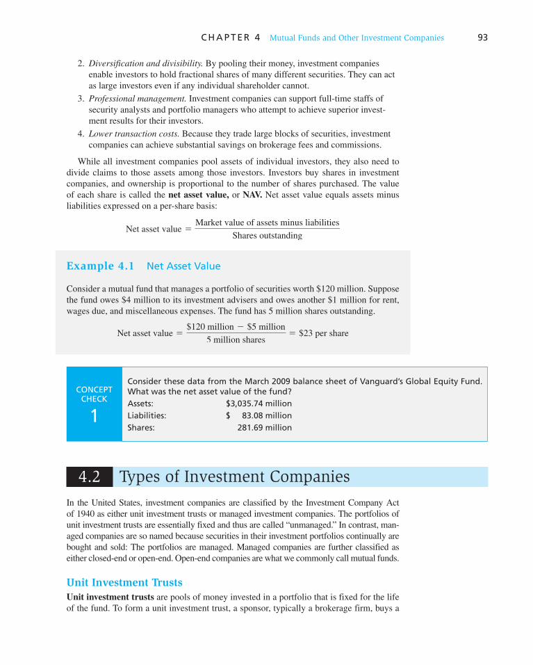
C H A P T E R 4 Mutual Funds and Other Investment Companies 93
2. Diversification and divisibility. By pooling their money, investment companies enable investors to hold fractional shares of many different securities. They can act as large investors even if any individual shareholder cannot.
3. Professional management. Investment companies can support full-time staffs of security analysts and portfolio managers who attempt to achieve superior invest-ment results for their investors.
4. Lower transaction costs. Because they trade large blocks of securities, investment companies can achieve substantial savings on brokerage fees and commissions.
While all investment companies pool assets of individual investors, they also need to divide claims to those assets among those investors. Investors buy shares in investment companies, and ownership is proportional to the number of shares purchased. The value of each share is called the net asset value, or NAV. Net asset value equals assets minus liabilities expressed on a per-share basis:
Net asset value 5Market value of assets minus liabilities
Shares outstanding
Example 4.1 Net Asset Value
Consider a mutual fund that manages a portfolio of securities worth $120 million. Suppose the fund owes $4 million to its investment advisers and owes another $1 million for rent, wages due, and miscellaneous expenses. The fund has 5 million shares outstanding.
Net asset value 5$120 million 2 $5 million
5 million shares5 $23 per share
CONCEPT CHECK
1
Consider these data from the March 2009 balance sheet of Vanguard’s Global Equity Fund. What was the net asset value of the fund? Assets: $3,035.74 million Liabilities: $ 83.08 million Shares: 281.69 million
4.2 Types of Investment Companies
In the United States, investment companies are classified by the Investment Company Act of 1940 as either unit investment trusts or managed investment companies. The portfolios of unit investment trusts are essentially fixed and thus are called “unmanaged.” In contrast, man-aged companies are so named because securities in their investment portfolios continually are bought and sold: The portfolios are managed. Managed companies are further classified as either closed-end or open-end. Open-end companies are what we commonly call mutual funds.
Unit Investment Trusts
Unit investment trusts are pools of money invested in a portfolio that is fixed for the life of the fund. To form a unit investment trust, a sponsor, typically a brokerage firm, buys a
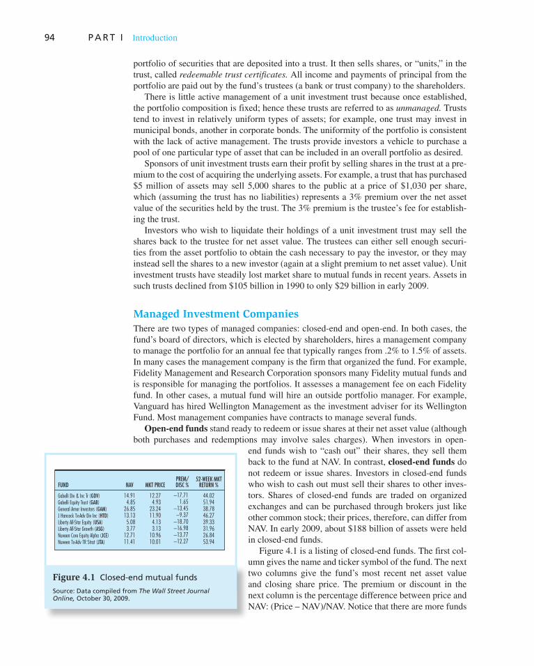
94 P A R T I Introduction
portfolio of securities that are deposited into a trust. It then sells shares, or “units,” in the trust, called redeemable trust certificates. All income and payments of principal from the portfolio are paid out by the fund’s trustees (a bank or trust company) to the shareholders.
There is little active management of a unit investment trust because once established, the portfolio composition is fixed; hence these trusts are referred to as unmanaged. Trusts tend to invest in relatively uniform types of assets; for example, one trust may invest in municipal bonds, another in corporate bonds. The uniformity of the portfolio is consistent with the lack of active management. The trusts provide investors a vehicle to purchase a pool of one particular type of asset that can be included in an overall portfolio as desired.
Sponsors of unit investment trusts earn their profit by selling shares in the trust at a pre-mium to the cost of acquiring the underlying assets. For example, a trust that has purchased $5 million of assets may sell 5,000 shares to the public at a price of $1,030 per share, which (assuming the trust has no liabilities) represents a 3% premium over the net asset value of the securities held by the trust. The 3% premium is the trustee’s fee for establish-ing the trust.
Investors who wish to liquidate their holdings of a unit investment trust may sell the shares back to the trustee for net asset value. The trustees can either sell enough securi-ties from the asset portfolio to obtain the cash necessary to pay the investor, or they may instead sell the shares to a new investor (again at a slight premium to net asset value). Unit investment trusts have steadily lost market share to mutual funds in recent years. Assets in such trusts declined from $105 billion in 1990 to only $29 billion in early 2009.
Managed Investment Companies
There are two types of managed companies: closed-end and open-end. In both cases, the fund’s board of directors, which is elected by shareholders, hires a management company to manage the portfolio for an annual fee that typically ranges from .2% to 1.5% of assets. In many cases the management company is the firm that organized the fund. For example, Fidelity Management and Research Corporation sponsors many Fidelity mutual funds and is responsible for managing the portfolios. It assesses a management fee on each Fidelity fund. In other cases, a mutual fund will hire an outside portfolio manager. For example, Vanguard has hired Wellington Management as the investment adviser for its Wellington Fund. Most management companies have contracts to manage several funds.
Open-end funds stand ready to redeem or issue shares at their net asset value (although both purchases and redemptions may involve sales charges). When investors in open-
end funds wish to “cash out” their shares, they sell them back to the fund at NAV. In contrast, closed-end funds do not redeem or issue shares. Investors in closed-end funds who wish to cash out must sell their shares to other inves-tors. Shares of closed-end funds are traded on organized exchanges and can be purchased through brokers just like other common stock; their prices, therefore, can differ from NAV. In early 2009, about $188 billion of assets were held in closed-end funds.
Figure 4.1 is a listing of closed-end funds. The first col-umn gives the name and ticker symbol of the fund. The next two columns give the fund’s most recent net asset value and closing share price. The premium or discount in the next column is the percentage difference between price and NAV: (Price – NAV)/NAV. Notice that there are more funds
Figure 4.1 Closed-end mutual funds
Source: Data compiled from The Wall Street Journal Online, October 30, 2009.
FUND NAV MKT PRICEPREM/DISC %
52-WEEK MKTRETURN %
Gabelli Equity Trust (GAB)General Amer Investors (GAM)J Hancock Tx-Adv Div Inc (HTD)Liberty All-Star Equity (USA)Liberty All-Star Growth (ASG)Nuveen Core Equity Alpha (JCE)Nuveen Tx-Adv TR Strat (JTA)
Gabelli Div & Inc Tr (GDV)4.85
26.8513.13
5.083.77
12.7111.41
14.91
23.2411.904.133.13
10.9610.01
12.274.93 1.65
−13.45−9.37
−18.70−16.98−13.77−12.27
−17.7151.9438.7846.2739.3331.9626.8453.94
44.02

C H A P T E R 4 Mutual Funds and Other Investment Companies 95
selling at discounts to NAV (indicated by negative differences) than premiums. Finally, the 52-week return based on the percentage change in share price plus dividend income is presented in the last column.
The common divergence of price from net asset value, often by wide margins, is a puzzle that has yet to be fully explained. To see why this is a puzzle, consider a closed-end fund that is selling at a discount from net asset value. If the fund were to sell all the assets in the portfolio, it would realize proceeds equal to net asset value. The difference between the market price of the fund and the fund’s NAV would represent the per-share increase in the wealth of the fund’s investors. Moreover, fund premiums or discounts tend to dissipate over time, so funds selling at a discount receive a boost to their rate of return as the discount shrinks. Pontiff estimates that a fund selling at a 20% discount would have an expected 12-month return more than 6% greater than funds selling at net asset value. 1
Interestingly, while many closed-end funds sell at a discount from net asset value, the prices of these funds when originally issued are often above NAV. This is a further puzzle, as it is hard to explain why investors would purchase these newly issued funds at a pre-mium to NAV when the shares tend to fall to a discount shortly after issue.
In contrast to closed-end funds, the price of open-end funds cannot fall below NAV, because these funds stand ready to redeem shares at NAV. The offering price will exceed NAV, however, if the fund carries a load. A load is, in effect, a sales charge. Load funds are sold by securities brokers and directly by mutual fund groups.
Unlike closed-end funds, open-end mutual funds do not trade on organized exchanges. Instead, investors simply buy shares from and liquidate through the investment company at net asset value. Thus the number of outstanding shares of these funds changes daily.
Other Investment Organizations
Same intermediaries are not formally organized or regulated as investment companies, but nevertheless serve similar functions. Three of the more important are commingled funds, real estate investment trusts, and hedge funds.
Commingled Funds Commingled funds are partnerships of investors that pool funds. The management firm that organizes the partnership, for example, a bank or insur-ance company, manages the funds for a fee. Typical partners in a commingled fund might be trust or retirement accounts with portfolios much larger than those of most individual investors, but still too small to warrant managing on a separate basis.
Commingled funds are similar in form to open-end mutual funds. Instead of shares, though, the fund offers units, which are bought and sold at net asset value. A bank or insur-ance company may offer an array of different commingled funds, for example, a money market fund, a bond fund, and a common stock fund.
Real Estate Investment Trusts ( REIT s) A REIT is similar to a closed-end fund. REITs invest in real estate or loans secured by real estate. Besides issuing shares, they raise capital by borrowing from banks and issuing bonds or mortgages. Most of them are highly leveraged, with a typical debt ratio of 70%.
There are two principal kinds of REITs. Equity trusts invest in real estate directly, whereas mortgage trusts invest primarily in mortgage and construction loans. REITs gen-erally are established by banks, insurance companies, or mortgage companies, which then serve as investment managers to earn a fee.
1 Jeffrey Pontiff, “Costly Arbitrage: Evidence from Closed-End Funds,” Quarterly Journal of Economics 111 (November 1996), pp. 1135–51.

96 P A R T I Introduction
Hedge Funds Like mutual funds, hedge funds are vehicles that allow private inves-tors to pool assets to be invested by a fund manager. Unlike mutual funds, however, hedge funds are commonly structured as private partnerships and thus subject to only minimal SEC regulation. They typically are open only to wealthy or institutional investors. Many require investors to agree to initial “lock-ups,” that is, periods as long as several years in which investments cannot be withdrawn. Lock-ups allow hedge funds to invest in illiquid assets without worrying about meeting demands for redemption of funds. Moreover, because hedge funds are only lightly regulated, their managers can pursue investment strategies involving, for example, heavy use of derivatives, short sales, and leverage; such s trategies typically are not open to mutual fund managers.
Hedge funds by design are empowered to invest in a wide range of investments, with various funds focusing on derivatives, distressed firms, currency speculation, convertible bonds, emerging markets, merger arbitrage, and so on. Other funds may jump from one asset class to another as perceived investment opportunities shift.
Hedge funds enjoyed great growth in the last several years, with assets under manage-ment ballooning from about $50 billion in 1990 to just under $2 trillion in mid-2008, before contracting to around $1.4 trillion in the face of the credit crisis that began in mid-2008. Because of their recent prominence, we devote all of Chapter 26 to these funds.
4.3 Mutual Funds
Mutual funds are the common name for open-end investment companies. This is the domi-nant investment company today, accounting for more than 90% of investment company assets. Assets under management in the U.S. mutual fund industry were approximately $10 trillion in early 2009, and approximately another $9 trillion was held in non-U.S. funds.
Investment Policies
Each mutual fund has a specified investment policy, which is described in the fund’s pro-spectus. For example, money market mutual funds hold the short-term, low-risk instru-ments of the money market (see Chapter 2 for a review of these securities), while bond funds hold fixed-income securities. Some funds have even more narrowly defined man-dates. For example, some bond funds will hold primarily Treasury bonds, others primarily mortgage-backed securities.
Management companies manage a family, or “complex,” of mutual funds. They orga-nize an entire collection of funds and then collect a management fee for operating them. By managing a collection of funds under one umbrella, these companies make it easy for investors to allocate assets across market sectors and to switch assets across funds while still benefiting from centralized record keeping. Some of the most well-known management companies are Fidelity, Vanguard, Putnam, and Dreyfus. Each offers an array of open-end mutual funds with different investment policies. In early 2009, there were nearly 9,000 mutual funds in the U.S., which were offered by fewer than 700 fund complexes.
Funds are commonly classified by investment policy into one of the following groups.
Money Market Funds These funds invest in money market securities such as com-mercial paper, repurchase agreements, or certificates of deposit. The average maturity of these assets tends to be a bit more than 1 month. Money market funds usually offer

C H A P T E R 4 Mutual Funds and Other Investment Companies 97
check-writing features, and net asset value is fixed at $1 per share, 2 so that there are no tax implications such as capital gains or losses associated with redemption of shares.
Equity Funds Equity funds invest primarily in stock, although they may, at the portfo-lio manager’s discretion, also hold fixed-income or other types of securities. Equity funds commonly will hold between 4% and 5% of total assets in money market securities to provide liquidity necessary to meet potential redemption of shares.
Stock funds are traditionally classified by their emphasis on capital appreciation versus current income. Thus, income funds tend to hold shares of firms with consistently high dividend yields. Growth funds are willing to forgo current income, focusing instead on prospects for capital gains. While the classification of these funds is couched in terms of income versus capital gains, in practice, the more relevant distinction concerns the level of risk these funds assume. Growth stocks, and therefore growth funds, are typically riskier and respond far more dramatically to changes in economic conditions than do income funds.
Sector Funds Some equity funds, called sector funds, concentrate on a particular industry. For example, Fidelity markets dozens of “select funds,” each of which invests in a specific industry such as biotechnology, utilities, precious metals, or telecommunications. Other funds specialize in securities of particular countries.
Bond Funds As the name suggests, these funds specialize in the fixed-income sec-tor. Within that sector, however, there is considerable room for further specialization. For example, various funds will concentrate on corporate bonds, Treasury bonds, mortgage-backed securities, or municipal (tax-free) bonds. Indeed, some municipal bond funds invest only in bonds of a particular state (or even city!) to satisfy the investment desires of residents of that state who wish to avoid local as well as federal taxes on interest income. Many funds also specialize by maturity, ranging from short-term to intermediate to long-term, or by the credit risk of the issuer, ranging from very safe to high-yield, or “junk,” bonds.
International Funds Many funds have international focus. Global funds invest in securities worldwide, including the United States. In contrast, international funds invest in securities of firms located outside the United States. Regional funds concentrate on a particular part of the world, and emerging market funds invest in companies of developing nations.
Balanced Funds Some funds are designed to be candidates for an individual’s entire investment portfolio. These balanced funds hold both equities and fixed-income securi-ties in relatively stable proportions. Life-cycle funds are balanced funds in which the asset mix can range from aggressive (primarily marketed to younger investors) to conservative (directed at older investors). Static allocation life-cycle funds maintain a stable mix across stocks and bonds, while targeted-maturity funds gradually become more conservative as the investor ages.
2 The box in Chapter 2 noted that money market funds are able to maintain NAV at $1.00 because they invest in short-maturity debt of the highest quality with minimal price risk. In only the rarest circumstances have any funds incurred losses large enough to drive NAV below $1.00. In September 2008, however, Reserve Primary Fund, the nation’s oldest money market fund, “broke the buck” when it suffered losses on its holding of Lehman Brothers commercial paper, and its NAV fell to $.97.

98 P A R T I Introduction
Asset Allocation and Flexible Funds These funds are similar to balanced funds in that they hold both stocks and bonds. However, asset allocation funds may dramatically vary the proportions allocated to each market in accord with the portfolio manager’s fore-cast of the relative performance of each sector. Hence these funds are engaged in market timing and are not designed to be low-risk investment vehicles.
Index Funds An index fund tries to match the performance of a broad market index. The fund buys shares in securities included in a particular index in proportion to each secu-rity’s representation in that index. For example, the Vanguard 500 Index Fund is a mutual fund that replicates the composition of the Standard & Poor’s 500 stock price index. Because the S&P 500 is a value-weighted index, the fund buys shares in each S&P 500 company in proportion to the market value of that company’s outstanding equity. Investment in an index fund is a low-cost way for small investors to pursue a passive investment strategy—that is, to invest without engaging in security analysis. Of course, index funds can be tied to nonequity indexes as well. For example, Vanguard offers a bond index fund and a real estate index fund.
Table 4.1 breaks down the number of mutual funds by investment orientation. Sometimes a fund name describes its investment policy. For example, Vanguard’s GNMA fund invests in mortgage-backed securities, the Municipal Intermediate fund invests in intermediate-term municipal bonds, and the High-Yield Corporate bond fund invests in large part in speculative grade, or “junk,” bonds with high yields. However, names of common stock funds often reflect little or nothing about their investment policies. Examples are Vanguard’s Windsor and Wellington funds.
Table 4.1
U.S. mutual funds by investment classification
Assets ($ billion)
% of Total Assets
Number of Funds
Equity funds Capital appreciation focus $1,650.1 17.2% 3,019
World/international 866.6 9.0 1,062
Total return 1,187.8 12.4 749
Total equity funds $3,704.5 38.6% 4,830
Bond funds Corporate $ 246.1 2.6% 281
High yield 111.4 1.2 195
World 86.2 0.9 131
Government 235.2 2.4 294
Strategic income 549.1 5.7 378
Single-state municipal 134.9 1.4 417
National municipal 202.9 2.1 220
Total bond funds $1,565.8 16.3% 1,916
Hybrid (bond/stock) funds $ 498.7 5.2% 492
Money market funds Taxable $3,340.8 34.8% 536
Tax-exempt 491.5 5.1 248
Total money market funds $3,832.3 39.9% 784
Total $9,601.3 100.0% 8,022
Note: Column sums subject to rounding error.Source: Investment Company Institute, 2009 Mutual Fund Fact Book.

C H A P T E R 4 Mutual Funds and Other Investment Companies 99
How Funds Are Sold
Mutual funds are generally marketed to the public either directly by the fund underwriter or indirectly through brokers acting on behalf of the underwriter. Direct-marketed funds are sold through the mail, various offices of the fund, over the phone, or, more so, over the Internet. Investors contact the fund directly to purchase shares.
About half of fund sales today are distributed through a sales force. Brokers or financial advisers receive a commission for selling shares to investors. (Ultimately, the commission is paid by the investor. More on this shortly.) In some cases, funds use a “captive” sales force that sells only shares in funds of the mutual fund group they represent.
Investors who rely on their broker’s advice to select their mutual funds should be aware that brokers may have a conflict of interest with regard to fund selection. This arises from a practice called revenue sharing, in which fund companies pay the brokerage firm for preferential treatment when making investment recommendations.
Revenue sharing poses potential conflicts of interest if it induces brokers to recommend mutual funds on the basis of criteria other than the best interests of their clients. In addi-tion, the mutual fund may be violating its obligation to its existing investors if it uses fund assets to pay brokers for favored status in new sales. SEC rules require brokerage firms to explicitly reveal any compensation or other incentives they receive to sell a particular fund, both at the time of sale and in the trade confirmation.
Many funds also are sold through “financial supermarkets” that sell shares in funds of many complexes. Instead of charging customers a sales commission, the broker splits management fees with the mutual fund company. Another advantage is unified record keeping for all funds purchased from the supermarket, even if the funds are offered by different complexes. On the other hand, many contend that these supermarkets result in higher expense ratios because mutual funds pass along the costs of participating in these programs in the form of higher management fees.
4.4 Costs of Investing in Mutual Funds
Fee Structure
An individual investor choosing a mutual fund should consider not only the fund’s stated investment policy and past performance but also its management fees and other expenses. Comparative data on virtually all important aspects of mutual funds are available in the annual reports prepared by CDA Wiesenberger Investment Companies Services or in Morningstar’s Mutual Fund Sourcebook, which can be found in many academic and public libraries. You should be aware of four general classes of fees.
Operating Expenses Operating expenses are the costs incurred by the mutual fund in operating the portfolio, including administrative expenses and advisory fees paid to the investment manager. These expenses, usually expressed as a percentage of total assets under management, may range from 0.2% to 2%. Shareholders do not receive an explicit bill for these operating expenses; however, the expenses periodically are deducted from the assets of the fund. Shareholders pay for these expenses through the reduced value of the portfolio.
In addition to operating expenses, many funds assess fees to pay for marketing and distribution costs. These charges are used primarily to pay the brokers or financial advis-ers who sell the funds to the public. Investors can avoid these expenses by buying shares directly from the fund sponsor, but many investors are willing to incur these distribution fees in return for the advice they may receive from their broker.
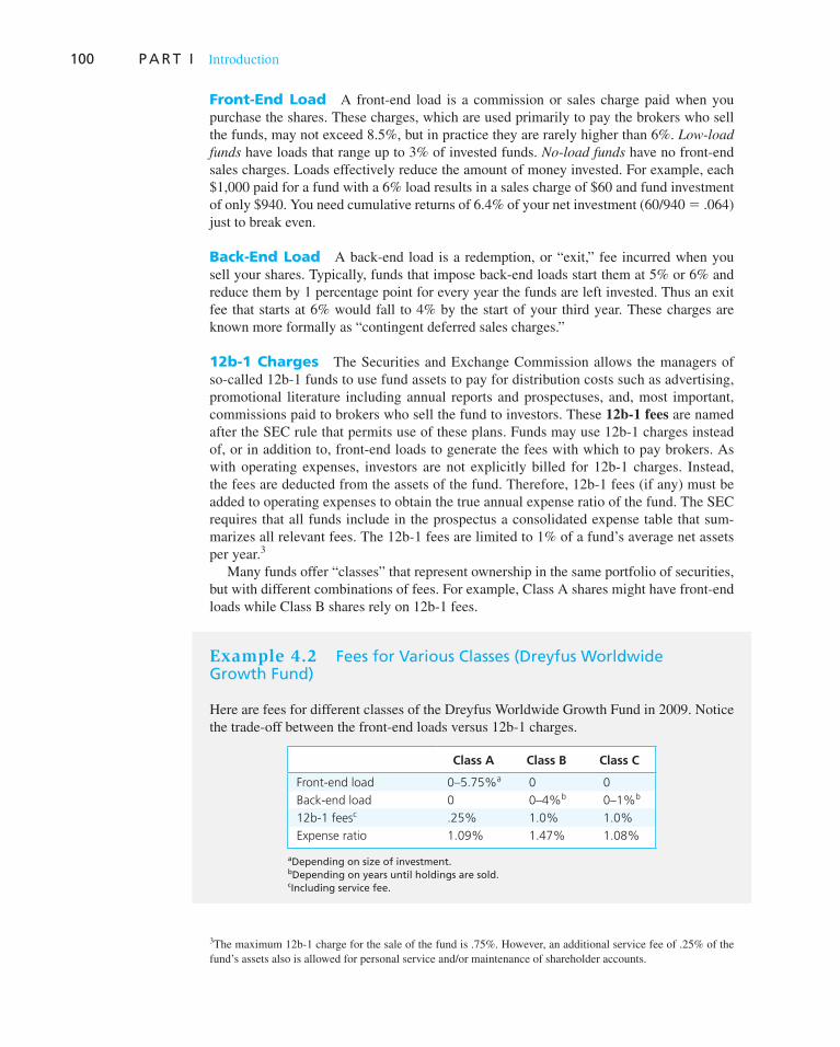
100 P A R T I Introduction
Front-End Load A front-end load is a commission or sales charge paid when you purchase the shares. These charges, which are used primarily to pay the brokers who sell the funds, may not exceed 8.5%, but in practice they are rarely higher than 6%. Low-load
funds have loads that range up to 3% of invested funds. No-load funds have no front-end sales charges. Loads effectively reduce the amount of money invested. For example, each $1,000 paid for a fund with a 6% load results in a sales charge of $60 and fund investment of only $940. You need cumulative returns of 6.4% of your net investment (60/940 � .064) just to break even.
Back-End Load A back-end load is a redemption, or “exit,” fee incurred when you sell your shares. Typically, funds that impose back-end loads start them at 5% or 6% and reduce them by 1 percentage point for every year the funds are left invested. Thus an exit fee that starts at 6% would fall to 4% by the start of your third year. These charges are known more formally as “contingent deferred sales charges.”
12b-1 Charges The Securities and Exchange Commission allows the managers of so-called 12b-1 funds to use fund assets to pay for distribution costs such as advertising, promotional literature including annual reports and prospectuses, and, most important, commissions paid to brokers who sell the fund to investors. These 12b-1 fees are named after the SEC rule that permits use of these plans. Funds may use 12b-1 charges instead of, or in addition to, front-end loads to generate the fees with which to pay brokers. As with operating expenses, investors are not explicitly billed for 12b-1 charges. Instead, the fees are deducted from the assets of the fund. Therefore, 12b-1 fees (if any) must be added to operating expenses to obtain the true annual expense ratio of the fund. The SEC requires that all funds include in the prospectus a consolidated expense table that sum-marizes all relevant fees. The 12b-1 fees are limited to 1% of a fund’s average net assets per year. 3
Many funds offer “classes” that represent ownership in the same portfolio of securities, but with different combinations of fees. For example, Class A shares might have front-end loads while Class B shares rely on 12b-1 fees.
3 The maximum 12b-1 charge for the sale of the fund is .75%. However, an additional service fee of .25% of the fund’s assets also is allowed for personal service and/or maintenance of shareholder accounts.
Example 4.2 Fees for Various Classes (Dreyfus Worldwide Growth Fund)
Here are fees for different classes of the Dreyfus Worldwide Growth Fund in 2009. Notice the trade-off between the front-end loads versus 12b-1 charges.
Class A Class B Class C
Front-end load 0–5.75%a 0 0
Back-end load 0 0–4%b 0–1%b
12b-1 feesc .25% 1.0% 1.0%
Expense ratio 1.09% 1.47% 1.08%
aDepending on size of investment.bDepending on years until holdings are sold.cIncluding service fee.

C H A P T E R 4 Mutual Funds and Other Investment Companies 101
Each investor must choose the best combination of fees. Obviously, pure no-load no-fee funds distributed directly by the mutual fund group are the cheapest alternative, and these will often make most sense for knowledgeable investors. However, as we have noted, many investors are willing to pay for financial advice, and the commissions paid to advisers who sell these funds are the most common form of payment. Alternatively, investors may choose to hire a fee-only financial manager who charges directly for services instead of collecting commissions. These advisers can help investors select portfolios of low- or no-load funds (as well as provide other financial advice). Independent financial planners have become increasingly important distribution channels for funds in recent years.
If you do buy a fund through a broker, the choice between paying a load and paying 12b-1 fees will depend primarily on your expected time horizon. Loads are paid only once for each purchase, whereas 12b-1 fees are paid annually. Thus, if you plan to hold your fund for a long time, a one-time load may be preferable to recurring 12b-1 charges.
Fees and Mutual Fund Returns
The rate of return on an investment in a mutual fund is measured as the increase or decrease in net asset value plus income distributions such as dividends or distributions of capital gains expressed as a fraction of net asset value at the beginning of the investment period. If we denote the net asset value at the start and end of the period as NAV 0 and NAV 1 , respec-tively, then
Rate of return 5NAV1 2 NAV0 1 Income and capital gain distributions
NAV0
For example, if a fund has an initial NAV of $20 at the start of the month, makes income distributions of $.15 and capital gain distributions of $.05, and ends the month with NAV of $20.10, the monthly rate of return is computed as
Rate of return 5$20.10 2 $20.00 1 $.15 1 $.05
$20.005 .015, or 1.5%
Notice that this measure of the rate of return ignores any commissions such as front-end loads paid to purchase the fund.
On the other hand, the rate of return is affected by the fund’s expenses and 12b-1 fees. This is because such charges are periodically deducted from the portfolio, which reduces net asset value. Thus the rate of return on the fund equals the gross return on the underlying portfolio minus the total expense ratio.
Example 4.3 Fees and Net Returns
To see how expenses can affect rate of return, consider a fund with $100 million in assets at the start of the year and with 10 million shares outstanding. The fund invests in a portfolio of stocks that provides no income but increases in value by 10%. The expense ratio, includ-ing 12b-1 fees, is 1%. What is the rate of return for an investor in the fund?
The initial NAV equals $100 million/10 million shares � $10 per share. In the absence of expenses, fund assets would grow to $110 million and NAV would grow to $11 per share, for a 10% rate of return. However, the expense ratio of the fund is 1%. Therefore, $1 million will be deducted from the fund to pay these fees, leaving the portfolio worth only $109 million, and NAV equal to $10.90. The rate of return on the fund is only 9%, which equals the gross return on the underlying portfolio minus the total expense ratio.

102 P A R T I Introduction
Fees can have a big effect on performance. Table 4.2 considers an investor who starts with $10,000 and can choose among three funds that all earn an annual 12% return on invest-ment before fees but have different fee structures. The table shows the cumulative amount in each fund after several investment horizons. Fund A has total operating expenses of .5%, no load, and no 12b-1 charges. This might represent a low-cost producer like Vanguard. Fund B has no load but has 1% in management expenses and .5% in 12b-1 fees. This level of charges is fairly typical of actively managed equity funds. Finally, Fund C has 1% in management expenses, no 12b-1 charges, but assesses an 8% front-end load on purchases.
Note the substantial return advantage of low-cost Fund A. Moreover, that differential is greater for longer investment horizons.
Table 4.2
Impact of costs on investment performance
Cumulative Proceeds(All Dividends Reinvested)
Fund A Fund B Fund C
Initial investment* $10,000 $10,000 $ 9,200
5 years 17,234 16,474 15,502
10 years 29,699 27,141 26,123
15 years 51,183 44,713 44,018
20 years 88,206 73,662 74,173
* After front-end load, if any. Notes: 1. Fund A is no-load with .5% expense ratio. 2. Fund B is no-load with 1.5% expense ratio. 3. Fund C has an 8% load on purchases and a 1% expense ratio. 4. Gross return on all funds is 12% per year before expenses.
CONCEPT CHECK
2
The Equity Fund sells Class A shares with a front-end load of 4% and Class B shares with 12b-1 fees of .5% annually as well as back-end load fees that start at 5% and fall by 1% for each full year the investor holds the portfolio (until the fifth year). Assume the rate of return on the fund portfolio net of operating expenses is 10% annually. What will be the value of a $10,000 investment in Class A and Class B shares if the shares are sold after ( a ) 1 year, ( b ) 4 years, ( c ) 10 years? Which fee structure provides higher net proceeds at the end of each investment horizon?
Although expenses can have a big impact on net investment performance, it is some-times difficult for the investor in a mutual fund to measure true expenses accurately. This is because of the practice of paying for some expenses in soft dollars. A portfolio manager earns soft-dollar credits with a brokerage firm by directing the fund’s trades to that broker. On the basis of those credits, the broker will pay for some of the mutual fund’s expenses, such as databases, computer hardware, or stock-quotation systems. The soft- dollar arrangement means that the stockbroker effectively returns part of the trading commission to the fund. Purchases made with soft dollars are not included in the fund’s expenses, so funds with extensive soft dollar arrangements may report artificially low expense ratios to the public. However, the fund may have paid its broker needlessly high commissions to obtain its soft-dollar “rebate.” The impact of the higher trading commission shows up in net investment performance rather than the reported expense ratio.
C H A P T E R 4 Mutual Funds and Other Investment Companies 103
Late Trading and Market Timing
Mutual funds calculate net asset value (NAV) at the end of each trading day. All buy or sell orders arriving during the day are executed at that NAV following the market close at 4:00 P.M. New York time. Allowing some favored investors to buy shares in the fund below NAV or redeem their shares for more than NAV would obviously benefit those investors, but at the expense of the remaining shareholders. Yet, that is precisely what many mutual funds did until these practices were exposed in 2003.
Late trading refers to the practice of accepting buy or sell orders after the market closes and NAV is determined. Suppose that based on market closing prices at 4:00, a fund’s NAV equals $100, but at 4:30, some positive economic news is announced. While NAV already has been fixed, it is clear that the fair market value of each share now exceeds $100. If they are able to submit a late order, investors can buy shares at the now-stale NAV and redeem them the next day after prices and NAV have adjusted to reflect the news. Late traders therefore can buy shares in the fund at a price below what NAV would be if it reflected up-to-date information. This transfers value from the other shareholders to the privileged traders and shows up as a reduction in the rate of return of the mutual fund.
Market timing also exploits stale prices. Consider the hypothetical “Pacific Basin Mutual Fund,” which specializes in Japanese stocks. Because of time-zone differences, the Japanese market closes several hours before trading ends in New York. NAV is set based on the closing price of the Japanese shares. If the U.S. market jumps significantly while the Japanese market is closed, however, it is likely that Japanese prices will rise when the market opens in Japan the next day. A market timer will buy the Pacific Basin fund in the U.S. today at its now-stale NAV, planning to redeem those shares the next day for a likely profit. While such activity often is characterized as rapid in-and-out trading, the more salient issue is that the market timer is allowed to transact at a stale price.
Why did some funds engage in practices that reduced the rate of return to most share-holders? The answer is the management fee. Market timers and late traders in essence paid for their access to such practices by investing large amounts in the funds on which the fund manager charged its management fee. Of course, the traders possibly earned far more than those fees through their trading activity, but those costs were borne by the other sharehold-ers, not the fund sponsor.
By mid-2004, mutual fund sponsors had paid more than $1.65 billion in penalties to settle allegations of improper trading. In addition, new rules were implemented to elimi-nate these illicit practices.
4.5 Taxation of Mutual Fund Income
Investment returns of mutual funds are granted “pass-through status” under the U.S. tax code, meaning that taxes are paid only by the investor in the mutual fund, not by the fund itself. The income is treated as passed through to the investor as long as the fund meets sev-eral requirements, most notably that virtually all income is distributed to shareholders. A fund’s short-term capital gains, long-term capital gains, and dividends are passed through to investors as though the investor earned the income directly.
The pass-through of investment income has one important disadvantage for individual investors. If you manage your own portfolio, you decide when to realize capital gains and losses on any security; therefore, you can time those realizations to efficiently manage your tax liabilities. When you invest through a mutual fund, however, the timing of the sale
104 P A R T I Introduction
of securities from the portfolio is out of your control, which reduces your ability to engage in tax management. 4
A fund with a high portfolio turnover rate can be particularly “tax inefficient.” Turnover is the ratio of the trading activity of a portfolio to the assets of the portfolio. It measures the fraction of the portfolio that is “replaced” each year. For example, a $100 million portfolio with $50 million in sales of some securities with purchases of other securities would have a turnover rate of 50%. High turnover means that capital gains or losses are being realized constantly, and therefore that the investor cannot time the realizations to manage his or her overall tax obligation.
Turnover rates in equity funds in the last decade have typically been around 60% when weighted by assets under management. By contrast, a low-turnover fund such as an index fund may have turnover as low as 2%, which is both tax-efficient and economical with respect to trading costs.
Exchange-traded funds (ETFs), first introduced in 1993, are offshoots of mutual funds that allow investors to trade index portfolios just as they do shares of stock. The first ETF was the “spider,” a nickname for SPDR, or Standard & Poor’s Depository Receipt, which is a unit investment trust holding a portfolio matching the S&P 500 index. Unlike mutual funds, which can be bought or sold only at the end of the day when NAV is calculated, investors can trade spiders throughout the day, just like any other share of stock. Spiders gave rise to many similar products such as “diamonds” (based on the Dow Jones Industrial Average, ticker DIA), “Cubes” (based on the NASDAQ 100 index, ticker QQQQ), and “WEBS” (World Equity Benchmark Shares, which are shares in portfolios of foreign stock market indexes). By 2009, about $531 billion were invested in more than 700 U.S. ETFs. In 2010, assets under management in ETFs worldwide reached $1 trillion. Figure 4.2 shows the growth of exchange-traded funds since 1998.
Until 2008, most ETFs were required to track specified indexes, and index-based ETFs still dominate the industry. However, the range of products now includes funds that track industry indexes as well. Table 4.3 , panel A, presents some of the major sponsors of ETFs, and panel B gives a small flavor of the types of funds offered.
4 An interesting problem that an investor needs to be aware of derives from the fact that capital gains and divi-dends on mutual funds are typically paid out to shareholders once or twice a year. This means that an investor who has just purchased shares in a mutual fund can receive a capital gain distribution (and be taxed on that dis-tribution) on transactions that occurred long before he or she purchased shares in the fund. This is particularly a concern late in the year when such distributions typically are made.
CONCEPT CHECK
3
An investor’s portfolio currently is worth $1 million. During the year, the investor sells 1,000 shares of FedEx at a price of $80 per share and 4,000 shares of Cisco at a price of $20 per share. The proceeds are used to buy 1,600 shares of IBM at $100 per share.
a. What was the portfolio turnover rate?
b. If the shares in FedEx originally were purchased for $70 each and those in Cisco were purchased for $17.50, and the investor’s tax rate on capital gains income is 20%, how much extra will the investor owe on this year’s taxes as a result of these transactions?
4.6 Exchange-Traded Funds

C H A P T E R 4 Mutual Funds and Other Investment Companies 105
Figure 4.2 Growth of U.S. ETFs over time
Source: Investment Company Institute, 2009 Investment Company Fact Book.
0
100
200
300
400
500
600
700
800
1998 1999 2000 2001 2002 2003 2004 2005 2006 2007 2008
Assets undermanagement ($billion)
Number of ETFs
Table 4.3
ETF sponsors and products
A. ETF Sponsors
Sponsor Product Name
BlackRock Global Investors iShares
Merrill Lynch HOLDRS (Holding Company Depository Receipts: “Holders”)
StateStreet/Merrill Lynch Select Sector SPDRs (S&P Depository Receipts: “Spiders”)
Vanguard Vanguard ETF
B. Sample of ETF Products
Name Ticker Index Tracked
Broad U.S. indexes
Spiders SPY S&P 500
Diamonds DIA Dow Jones Industrials
Cubes QQQQ NASDAQ 100
iShares Russell 2000 IWM Russell 2000
Total Stock Market (Vanguard) VTI Wilshire 5000
Industry indexes
Energy Select Spider XLE S&P 500 energy companies
iShares Energy Sector IYE Dow Jones energy companies
Financial Sector Spider XLF S&P 500 financial companies
iShares Financial Sector IYF Dow Jones financial companies
International indexes
WEBS United Kingdom EWU MSCI U.K. Index
WEBS France EWQ MSCI France Index
WEBS Japan EWJ MSCI Japan Index
106 P A R T I Introduction
Barclay’s Global Investors was long the market leader in the ETF market, using the product name iShares. Since Barclay’s 2009 merger with BlackRock, iShares has operated under the BlackRock name. The firm sponsors ETFs for several dozen equity index funds, including many broad U.S. equity indexes, broad international and single-country funds, and U.S. and global industry sector funds. BlackRock also offers several bond ETFs and a few commodity funds such as ones for gold and silver. For more information on these funds, go to www.iShares.com.
More recently, commodity-based ETFs that invest in either commodities or commod-ity futures contracts have been marketed to the public. In addition, there is now a small number of actively managed ETF funds that, like actively managed mutual funds, attempt to outperform market indexes. But these account for less than 1% of assets under manage-ment in the ETF industry.
ETFs offer several advantages over conventional mutual funds. First, as we just noted, a mutual fund’s net asset value is quoted—and therefore, investors can buy or sell their shares in the fund—only once a day. In contrast, ETFs trade continuously. Moreover, like other shares, but unlike mutual funds, ETFs can be sold short or purchased on margin.
ETFs also offer a potential tax advantage over mutual funds. When large numbers of mutual fund investors redeem their shares, the fund must sell securities to meet the redemptions. This can trigger capital gains taxes, which are passed through to and must be paid by the remaining shareholders. In contrast, when small investors wish to redeem their position in an ETF, they simply sell their shares to other traders, with no need for the fund to sell any of the underlying portfolio. Large investors can exchange their ETF shares for shares in the underlying portfolio; this form of redemption also avoids a tax event.
ETFs are also cheaper than mutual funds. Investors who buy ETFs do so through bro-kers rather than buying directly from the fund. Therefore, the fund saves the cost of mar-keting itself directly to small investors. This reduction in expenses translates into lower management fees.
There are some disadvantages to ETFs, however. Because they trade as securities, there is the possibility that their prices can depart by small amounts from net asset value before arbitrage activity restores equality. Even small discrepancies can easily swamp the cost advantage of ETFs over mutual funds. Second, while mutual funds can be bought at no expense from no-load funds, ETFs must be purchased from brokers for a fee.
4.7 Mutual Fund Investment Performance: A First Look
We noted earlier that one of the benefits of mutual funds for the individual investor is the ability to delegate management of the portfolio to investment professionals. The investor retains control over the broad features of the overall portfolio through the asset allocation decision: Each individual chooses the percentages of the portfolio to invest in bond funds versus equity funds versus money market funds, and so forth, but can leave the specific security selection decisions within each investment class to the managers of each fund. Shareholders hope that these portfolio managers can achieve better investment perfor-mance than they could obtain on their own.
What is the investment record of the mutual fund industry? This seemingly straightfor-ward question is deceptively difficult to answer because we need a standard against which to evaluate performance. For example, we clearly would not want to compare the invest-ment performance of an equity fund to the rate of return available in the money market. The vast differences in the risk of these two markets dictate that year-by-year as well as
C H A P T E R 4 Mutual Funds and Other Investment Companies 107
average performance will differ considerably. We would expect to find that equity funds outperform money market funds (on average) as compensation to investors for the extra risk incurred in equity markets. How then can we determine whether mutual fund portfolio managers are performing up to par given the level of risk they incur? In other words, what is the proper benchmark against which investment performance ought to be evaluated?
Measuring portfolio risk properly and using such measures to choose an appropriate benchmark is an extremely difficult task. We devote all of Parts Two and Three of the text to issues surrounding the proper measurement of portfolio risk and the trade-off between risk and return. In this chapter, therefore, we will satisfy ourselves with a first look at the question of fund performance by using only very simple performance benchmarks and ignoring the more subtle issues of risk differences across funds. However, we will return to this topic in Chapter 11, where we take a closer look at mutual fund performance after adjusting for differences in the exposure of portfolios to various sources of risk.
Here we use as a benchmark for the performance of equity fund managers the rate of return on the Wilshire 5000 index. Recall from Chapter 2 that this is a value-weighted index of essentially all actively traded U.S. stocks. The performance of the Wilshire 5000 is a useful benchmark with which to evaluate professional managers because it corresponds to a simple passive investment strategy: Buy all the shares in the index in proportion to their outstanding market value. Moreover, this is a feasible strategy for even small inves-tors, because the Vanguard Group offers an index fund (its Total Stock Market Portfolio) designed to replicate the performance of the Wilshire 5000 index. Using the Wilshire 5000 index as a benchmark, we may pose the problem of evaluating the performance of mutual fund portfolio managers this way: How does the typical performance of actively managed equity mutual funds compare to the performance of a passively managed portfolio that simply replicates the composition of a broad index of the stock market?
Casual comparisons of the performance of the Wilshire 5000 index versus that of professionally managed mutual funds reveal disappointing results for active managers. Figure 4.3 shows that the average return on diversified equity funds was below the return on the Wilshire index in 23 of the 39 years from 1971 to 2009. The average annual return on the index was 11.9%, which was 1% greater than that of the average mutual fund. 5
This result may seem surprising. After all, it would not seem unreasonable to expect that professional money managers should be able to outperform a very simple rule such as “hold an indexed portfolio.” As it turns out, however, there may be good reasons to expect such a result. We explore them in detail in Chapter 11, where we discuss the efficient mar-ket hypothesis.
Of course, one might argue that there are good managers and bad managers, and that good managers can, in fact, consistently outperform the index. To test this notion, we examine whether managers with good performance in one year are likely to repeat that per-formance in a following year. Is superior performance in any particular year due to luck, and therefore random, or due to skill, and therefore consistent from year to year?
To answer this question, we can examine the performance of a large sample of equity mutual fund portfolios, divide the funds into two groups based on total investment return, and ask: “Do funds with investment returns in the top half of the sample in one period con-tinue to perform well in a subsequent period?”
5 Of course, actual funds incur trading costs while indexes do not, so a fair comparison between the returns on actively managed funds versus those on a passive index would first reduce the return on the Wilshire 5000 by an estimate of such costs. Vanguard’s Total Stock Market Index portfolio, which tracks the Wilshire 5000, charges an expense ratio of .19%, and, because it engages in little trading, incurs low trading costs. Therefore, it would be reasonable to reduce the returns on the index by about .30%. This reduction would not erase the difference in average performance.
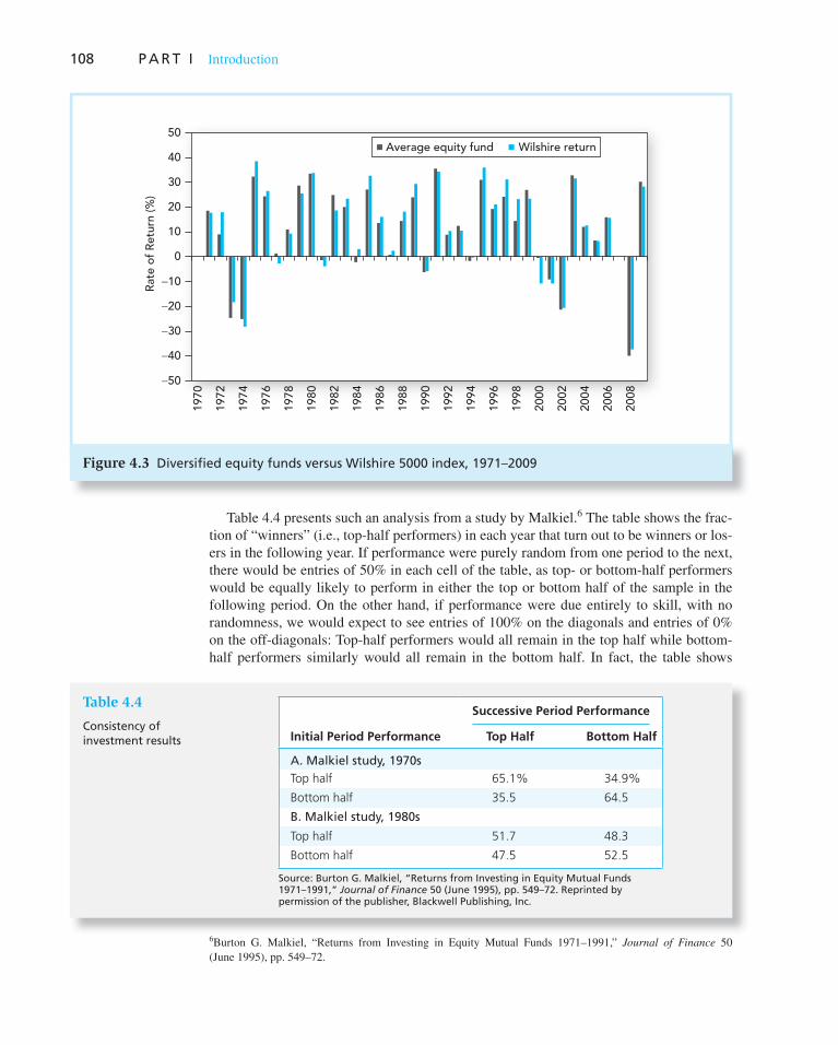
108 P A R T I Introduction
Table 4.4 presents such an analysis from a study by Malkiel. 6 The table shows the frac-tion of “winners” (i.e., top-half performers) in each year that turn out to be winners or los-ers in the following year. If performance were purely random from one period to the next, there would be entries of 50% in each cell of the table, as top- or bottom-half performers would be equally likely to perform in either the top or bottom half of the sample in the following period. On the other hand, if performance were due entirely to skill, with no randomness, we would expect to see entries of 100% on the diagonals and entries of 0% on the off-diagonals: Top-half performers would all remain in the top half while bottom- half performers similarly would all remain in the bottom half. In fact, the table shows
6 Burton G. Malkiel, “Returns from Investing in Equity Mutual Funds 1971–1991,” Journal of Finance 50 (June 1995), pp. 549–72.
Figure 4.3 Diversified equity funds versus Wilshire 5000 index, 1971–2009
−40
−50
−30
−20
−10
0
10
20
30
40
50
1970
1972
1974
1976
1978
1980
1982
1984
1986
1988
1990
1992
1994
1996
1998
2000
2002
2004
2008
2006
Rate
of
Retu
rn (%
)Average equity fund Wilshire return
Table 4.4
Consistency of investment results
Successive Period Performance
Initial Period Performance Top Half Bottom Half
A. Malkiel study, 1970sTop half 65.1% 34.9%
Bottom half 35.5 64.5
B. Malkiel study, 1980s
Top half 51.7 48.3
Bottom half 47.5 52.5
Source: Burton G. Malkiel, “Returns from Investing in Equity Mutual Funds 1971–1991,” Journal of Finance 50 (June 1995), pp. 549–72. Reprinted by permission of the publisher, Blackwell Publishing, Inc.
C H A P T E R 4 Mutual Funds and Other Investment Companies 109
that 65.1% of initial top-half performers fall in the top half of the sample in the following period, while 64.5% of initial bottom-half performers fall in the bottom half in the follow-ing period. This evidence is consistent with the notion that at least part of a fund’s perfor-mance is a function of skill as opposed to luck, so that relative performance tends to persist from one period to the next. 7
On the other hand, this relationship does not seem stable across different sample periods. While initial-year performance predicts subsequent-year performance in the 1970s (panel A), the pattern of persistence in performance virtually disappears in the 1980s (panel B). To summarize, the evidence that performance is consistent from one period to the next is suggestive, but it is inconclusive.
Other studies suggest that bad performance is more likely to persist than good perfor-mance. This makes some sense: It is easy to identify fund characteristics that will result in consistently poor investment performance, notably high expense ratios, and high turnover ratios with associated trading costs. It is far harder to identify the secrets of successful stock picking. (If it were easy, we would all be rich!) Thus the consistency we do observe in fund performance may be due in large part to the poor performers. This suggests that the real value of past performance data is to avoid truly poor funds, even if identifying the future top performers is still a daunting task.
The first place to find information on a mutual fund is in its prospectus. The Securities and Exchange Commission requires that the prospectus describe the fund’s investment objec-tives and policies in a concise “Statement of Investment Objectives” as well as in lengthy discussions of investment policies and risks. The fund’s investment adviser and its port-folio manager are also described. The prospectus also presents the costs associated with purchasing shares in the fund in a fee table. Sales charges such as front-end and back-end loads as well as annual operating expenses such as management fees and 12b-1 fees are detailed in the fee table.
Funds provide information about themselves in two other sources. The Statement of Additional Information or SAI, also known as Part B of the prospectus, includes a list of the securities in the portfolio at the end of the fiscal year, audited financial statements, a list of the directors and officers of the fund—as well as their personal investments in the fund, and data on brokerage commissions paid by the fund. However, unlike the fund prospec-tus, investors do not receive the SAI unless they specifically request it; one industry joke is that SAI stands for “something always ignored.” The fund’s annual report also includes
7 Another possibility is that performance consistency is due to variation in fee structure across funds. We return to this possibility in Chapter 11.
4.8 Information on Mutual Funds
CONCEPT CHECK
4
Suppose you observe the investment performance of 400 portfolio managers and rank them by investment returns during the year. Twenty percent of all managers are truly skilled, and therefore always fall in the top half, but the others fall in the top half purely because of good luck. What fraction of this year’s top-half managers would you expect to be top-half performers next year?

110 P A R T I Introduction
portfolio composition and financial statements, as well as a discussion of the factors that influenced fund performance over the last reporting period.
With more than 8,000 mutual funds to choose from, it can be difficult to find and select the fund that is best suited for a particular need. Several publications now offer “encyclo-pedias” of mutual fund information to help in the search process. Two prominent sources are Wiesenberger’s Investment Companies and Morningstar’s Mutual Fund Sourcebook. Morningstar’s Web site, www.morningstar.com , is another excellent source of informa-tion, as is Yahoo!’s site, finance.yahoo.com/funds . The Investment Company Institute ( www.ici.org ), the national association of mutual funds, closed-end funds, and unit invest-ment trusts, publishes an annual Directory of Mutual Funds that includes information on fees as well as phone numbers to contact funds. To illustrate the range of information avail-able about funds, we consider Morningstar’s report on Fidelity’s Magellan Fund, repro-duced in Figure 4.4 .
Some of Morningstar’s analysis is qualitative. The top box on the left-hand side of the page of the report reproduced in the figure provides a short description of fund strategy, in particular the types of securities in which the fund manager tends to invest. The bottom box on the left (“Morningstar’s Take”) is a more detailed discussion of the fund’s income strategy. The short statement of the fund’s investment policy is in the top right-hand corner: Magellan is a “large growth” fund, meaning that it tends to invest in large firms, with an emphasis on growth over value stocks.
The table on the left in the figure labeled “Performance” reports on the fund’s quarterly returns over the last few years and then over longer periods up to 15 years. Comparisons of returns to relevant indexes, in this case, the S&P 500 and the Russell 1000 indexes, are pro-vided to serve as benchmarks in evaluating the performance of the fund. The values under these columns give the performance of the fund relative to the index. The returns reported for the fund are calculated net of expenses, 12b-1 fees, and any other fees automatically deducted from fund assets, but they do not account for any sales charges such as front-end loads or back-end charges. Next appear the percentile ranks of the fund compared to all other funds with the same investment objective (see column headed by %Rank Cat). A rank of 1 means the fund is a top performer. A rank of 80 would mean that it was beaten by 80% of funds in the comparison group. Finally, growth of $10,000 invested in the fund over various periods ranging from the past 3 months to the past 15 years is given in the last column.
More data on the performance of the fund are provided in the graph near the top of the figure. The line graph compares the growth of $10,000 invested in the fund and the S&P 500 over the last 10 years. Below the graph are boxes for each year that depict the relative performance of the fund for that year. The shaded area on the box shows the quartile in which the fund’s performance falls relative to other funds with the same objective. If the shaded band is at the top of the box, the firm was a top quartile performer in that period, and so on. The table below the bar charts presents historical data on characteristics of the fund such as return data and expense ratios.
The table on the right entitled Portfolio Analysis presents the 20 largest holdings of the portfolio, showing the price–earnings ratio and year-to-date return of each of those securi-ties. Investors can thus get a quick look at the manager’s biggest bets.
Below the portfolio analysis table is a box labeled Current Investment Style. In this box, Morningstar evaluates style along two dimensions: One dimension is the size of the firms held in the portfolio as measured by the market value of outstanding equity; the other dimension is a value/growth measure. Morningstar defines value stocks as those with low ratios of market price per share to various measures of value. It puts stocks on a growth-value continuum based on the ratios of stock price to the firm’s earnings, book value, sales,

C H A P T E R 4 Mutual Funds and Other Investment Companies 111
Figure 4.4 Morningstar report
Source: Morningstar Mutual Funds, © 2007 Morningstar, Inc. All rights reserved. Used with permission.

Vis
it u
s at
ww
w.m
hh
e.co
m/b
km112 P A R T I Introduction
cash flow, and dividends. Value stocks are those with a low price relative to these measures of value. In contrast, growth stocks have high ratios, suggesting that investors in these firms must believe that the firm will experience rapid growth to justify the prices at which the stocks sell. The shaded box for Magellan shows that the portfolio tends to hold larger firms (top row) and growth stocks (right column). A year-by-year history of Magellan’s investment style is presented in the sequence of such boxes at the top of Figure 4.4 .
The center of the figure, labeled Rating and Risk, is one of the more complicated but interesting facets of Morningstar’s analysis. The column labeled Load-Adj Return rates a fund’s return compared to other funds with the same investment policy. Returns for periods ranging from 1 to 10 years are calculated with all loads and back-end fees applicable to that investment period subtracted from total income. The return is then compared to the average return for the comparison group of funds to obtain the Morningstar Return vs. Category. Similarly, risk measures compared to category are computed and reported in the next column.
The last column presents Morningstar’s risk-adjusted rating, ranging from one to five stars. The rating is based on the fund’s return score minus risk score compared to other funds with similar investment styles. To allow funds to be compared to other funds with similar investment styles, Morningstar assigns each fund into one of 48 separate stock and bond fund categories. Of course, we are accustomed to the disclaimer that “past perfor-mance is not a reliable measure of future results,” and this is true as well of the coveted Morningstar 5-star rating. Consistent with the conventional disclaimer, past results have little predictive power for future performance, as we saw in Table 4.4 .
The tax analysis box shown on the left in Figure 4.4 provides some evidence on the tax efficiency of the fund. The after-tax return, given in the first column, is computed based on the dividends paid to the portfolio as well as realized capital gains, assuming the investor is in the maximum federal tax bracket at the time of the distribution. State and local taxes are ignored. The tax efficiency of the fund is measured by the “Tax-Cost Ratio,” which is an estimate of the impact of taxes on the investor’s after-tax return. Morningstar ranks each fund compared to its category for both tax-adjusted return and tax-cost ratio.
The bottom of the page in Figure 4.4 provides information on the expenses and loads associated with investments in the fund, as well as information on the fund’s investment adviser. Thus, Morningstar provides a considerable amount of the information you would need to decide among several competing funds.
1. Unit investment trusts, closed-end management companies, and open-end management compa-nies are all classified and regulated as investment companies. Unit investment trusts are essen-tially unmanaged in the sense that the portfolio, once established, is fixed. Managed investment companies, in contrast, may change the composition of the portfolio as deemed fit by the port-folio manager. Closed-end funds are traded like other securities; they do not redeem shares for their investors. Open-end funds will redeem shares for net asset value at the request of the investor.
2. Net asset value equals the market value of assets held by a fund minus the liabilities of the fund divided by the shares outstanding.
3. Mutual funds free the individual from many of the administrative burdens of owning individual securities and offer professional management of the portfolio. They also offer advantages that are available only to large-scale investors, such as discounted trading costs. On the other hand,
SUMMARY

Vis
it u
s at
ww
w.m
hh
e.co
m/b
km
C H A P T E R 4 Mutual Funds and Other Investment Companies 113
funds are assessed management fees and incur other expenses, which reduce the investor’s rate of return. Funds also eliminate some of the individual’s control over the timing of capital gains realizations.
4. Mutual funds are often categorized by investment policy. Major policy groups include money market funds; equity funds, which are further grouped according to emphasis on income versus growth; fixed-income funds; balanced and income funds; asset allocation funds; index funds; and specialized sector funds.
5. Costs of investing in mutual funds include front-end loads, which are sales charges; back-end loads, which are redemption fees or, more formally, contingent-deferred sales charges; fund oper-ating expenses; and 12b-1 charges, which are recurring fees used to pay for the expenses of mar-keting the fund to the public.
6. Income earned on mutual fund portfolios is not taxed at the level of the fund. Instead, as long as the fund meets certain requirements for pass-through status, the income is treated as being earned by the investors in the fund.
7. The average rate of return of the average equity mutual fund in the last 40 years has been below that of a passive index fund holding a portfolio to replicate a broad-based index like the S&P 500 or Wilshire 5000. Some of the reasons for this disappointing record are the costs incurred by actively managed funds, such as the expense of conducting the research to guide stock-picking activities, and trading costs due to higher portfolio turnover. The record on the consistency of fund performance is mixed. In some sample periods, the better-performing funds continue to perform well in the following periods; in other sample periods they do not.
Related Web sites for this chapter are available at www.mhhe.com/bkm
investment company net asset value (NAV) unit investment trust open-end fund
closed-end fund load hedge fund 12b-1 fees
soft dollars turnover exchange-traded funds
KEY TERMS
1. Would you expect a typical open-end fixed-income mutual fund to have higher or lower operating expenses than a fixed-income unit investment trust? Why?
2. What are some comparative advantages of investing in the following:
a. Unit investment trusts. b. Open-end mutual funds. c. Individual stocks and bonds that you choose for yourself.
3. Open-end equity mutual funds find it necessary to keep a significant percentage of total invest-ments, typically around 5% of the portfolio, in very liquid money market assets. Closed-end funds do not have to maintain such a position in “cash equivalent” securities. What difference between open-end and closed-end funds might account for their differing policies?
4. Balanced funds, life-cycle funds, and asset allocation funds all invest in both the stock and bond markets. What are the differences among these types of funds?
5. Why can closed-end funds sell at prices that differ from net asset value while open-end funds do not?
6. What are the advantages and disadvantages of exchange-traded funds versus mutual funds?
7. An open-end fund has a net asset value of $10.70 per share. It is sold with a front-end load of 6%. What is the offering price?
8. If the offering price of an open-end fund is $12.30 per share and the fund is sold with a front-end load of 5%, what is its net asset value?
PROBLEM SETS
i. Basic
ii. Intermediate

Vis
it u
s at
ww
w.m
hh
e.co
m/b
km114 P A R T I Introduction
9. The composition of the Fingroup Fund portfolio is as follows:
Stock Shares Price
A 200,000 $35
B 300,000 40
C 400,000 20
D 600,000 25
The fund has not borrowed any funds, but its accrued management fee with the portfolio manager currently totals $30,000. There are 4 million shares outstanding. What is the net asset value of the fund?
10. Reconsider the Fingroup Fund in the previous problem. If during the year the portfolio manager sells all of the holdings of stock D and replaces it with 200,000 shares of stock E at $50 per share and 200,000 shares of stock F at $25 per share, what is the portfolio turnover rate?
11. The Closed Fund is a closed-end investment company with a portfolio currently worth $200 million. It has liabilities of $3 million and 5 million shares outstanding.
a. What is the NAV of the fund? b. If the fund sells for $36 per share, what is its premium or discount as a percent of net asset
value?
12. Corporate Fund started the year with a net asset value of $12.50. By year-end, its NAV equaled $12.10. The fund paid year-end distributions of income and capital gains of $1.50. What was the (pretax) rate of return to an investor in the fund?
13. A closed-end fund starts the year with a net asset value of $12.00. By year-end, NAV equals $12.10. At the beginning of the year, the fund was selling at a 2% premium to NAV. By the end of the year, the fund is selling at a 7% discount to NAV. The fund paid year-end distributions of income and capital gains of $1.50.
a. What is the rate of return to an investor in the fund during the year? b. What would have been the rate of return to an investor who held the same securities as the
fund manager during the year?
14 a. Impressive Fund had excellent investment performance last year, with portfolio returns that placed it in the top 10% of all funds with the same investment policy. Do you expect it to be a top performer next year? Why or why not?
b. Suppose instead that the fund was among the poorest performers in its comparison group. Would you be more or less likely to believe its relative performance will persist into the fol-lowing year? Why?
15. Consider a mutual fund with $200 million in assets at the start of the year and with 10 million shares outstanding. The fund invests in a portfolio of stocks that provides dividend income at the end of the year of $2 million. The stocks included in the fund’s portfolio increase in price by 8%, but no securities are sold, and there are no capital gains distributions. The fund charges 12b-1 fees of 1%, which are deducted from portfolio assets at year-end. What is net asset value at the start and end of the year? What is the rate of return for an investor in the fund?
16. The New Fund had average daily assets of $2.2 billion last year. The fund sold $400 million worth of stock and purchased $500 million during the year. What was its turnover ratio?
17. If New Fund’s expense ratio (see the previous problem) was 1.1% and the management fee was .7%, what were the total fees paid to the fund’s investment managers during the year? What were other administrative expenses?
18. You purchased 1,000 shares of the New Fund at a price of $20 per share at the beginning of the year. You paid a front-end load of 4%. The securities in which the fund invests increase in value by 12% during the year. The fund’s expense ratio is 1.2%. What is your rate of return on the fund if you sell your shares at the end of the year?

Vis
it u
s at
ww
w.m
hh
e.co
m/b
km
C H A P T E R 4 Mutual Funds and Other Investment Companies 115
19. Loaded-Up Fund charges a 12b-1 fee of 1.0% and maintains an expense ratio of .75%. Econ-omy Fund charges a front-end load of 2% but has no 12b-1 fee and an expense ratio of .25%. Assume the rate of return on both funds’ portfolios (before any fees) is 6% per year. How much will an investment in each fund grow to after:
a. 1 year. b. 3 years. c. 10 years.
20. City Street Fund has a portfolio of $450 million and liabilities of $10 million.
a. If 44 million shares are outstanding, what is net asset value? b. If a large investor redeems 1 million shares, what happens to the portfolio value, to shares
outstanding, and to NAV?
21. The Investments Fund sells Class A shares with a front-end load of 6% and Class B shares with 12b-1 fees of .5% annually as well as back-end load fees that start at 5% and fall by 1% for each full year the investor holds the portfolio (until the fifth year). Assume the portfolio rate of return net of operating expenses is 10% annually. If you plan to sell the fund after 4 years, are Class A or Class B shares the better choice for you? What if you plan to sell after 15 years?
22. You are considering an investment in a mutual fund with a 4% load and expense ratio of .5%. You can invest instead in a bank CD paying 6% interest.
a. If you plan to invest for 2 years, what annual rate of return must the fund portfolio earn for you to be better off in the fund than in the CD? Assume annual compounding of returns.
b. How does your answer change if you plan to invest for 6 years? Why does your answer change?
c. Now suppose that instead of a front-end load the fund assesses a 12b-1 fee of .75% per year. What annual rate of return must the fund portfolio earn for you to be better off in the fund than in the CD? Does your answer in this case depend on your time horizon?
23. Suppose that every time a fund manager trades stock, transaction costs such as commissions and bid–asked spreads amount to .4% of the value of the trade. If the portfolio turnover rate is 50%, by how much is the total return of the portfolio reduced by trading costs?
24. You expect a tax-free municipal bond portfolio to provide a rate of return of 4%. Management fees of the fund are .6%. What fraction of portfolio income is given up to fees? If the manage-ment fees for an equity fund also are .6%, but you expect a portfolio return of 12%, what frac-tion of portfolio income is given up to fees? Why might management fees be a bigger factor in your investment decision for bond funds than for stock funds? Can your conclusion help explain why unmanaged unit investment trusts tend to focus on the fixed-income market?
25. Suppose you observe the investment performance of 350 portfolio managers for 5 years and rank them by investment returns during each year. After 5 years, you find that 11 of the funds have investment returns that place the fund in the top half of the sample in each and every year of your sample. Such consistency of performance indicates to you that these must be the funds whose man-agers are in fact skilled, and you invest your money in these funds. Is your c onclusion warranted?
iii. Challenge
Choosing a Mutual Fund
Go to finance.yahoo.com . Click on Mutual Funds under the Investing tab. Look for the Mutual Fund Screener. Use the drop-down boxes to select the criteria for mutual funds that are of interest to you. How many funds are shown in your results? If there are no funds or only a few funds that meet your criteria, try loosening your standards. If there are too many funds, try stricter standards. You can click on any column heading in the results list to sort by that criterion.
E-INVEST-MENTS EXERCISES

Vis
it u
s at
ww
w.m
hh
e.co
m/b
km116 P A R T I Introduction
SOLUTIONS TO CONCEPT CHECKS
1. NAV 5$3,035.74 2 $83.08
281.695 $10.48
2. The net investment in the Class A shares after the 4% commission is $9,600. If the fund earns a 10% return, the investment will grow after n years to $9,600 � (1.10) n . The Class B shares have no front-end load. However, the net return to the investor after 12b-1 fees will be only 9.5%. In addition, there is a back-end load that reduces the sales proceeds by a percentage equal to (5 – years until sale) until the fifth year, when the back-end load expires.
Class A Shares Class B Shares
Horizon $9,600 � (1.10)n $10,000 � (1.095)n � (1 � percentage exit fee)
1 year $10,560 $10,000 � (1.095) � (1 � .04) � $10,512
4 years $14,055 $10,000 � (1.095)4 � (1 � .01) � $14,233
10 years $24,900 $10,000 � (1.095)10 � $24,782
For a very short horizon such as 1 year, the Class A shares are the better choice. The front-end and back-end loads are equal, but the Class A shares don’t have to pay the 12b-1 fees. For moder-ate horizons such as 4 years, the Class B shares dominate because the front-end load of the Class A shares is more costly than the 12b-1 fees and the now-smaller exit fee. For long horizons of 10 years or more, Class A again dominates. In this case, the one-time front-end load is less expensive than the continuing 12b-1 fees.
3. a. Turnover � $160,000 in trades per $1 million of portfolio value � 16%.
b. Realized capital gains are $10 � 1,000 � $10,000 on FedEx and $2.50 � 4,000 � $10,000 on Cisco. The tax owed on the capital gains is therefore .20 � $20,000 � $4,000.
4. Twenty percent of the managers are skilled, which accounts for .2 � 400 � 80 of those managers who appear in the top half. There are 120 slots left in the top half, and 320 other managers, so the probability of an unskilled manager “lucking into” the top half in any year is 120/320, or .375. Therefore, of the 120 lucky managers in the first year, we would expect .375 � 120 � 45 to repeat as top-half performers next year. Thus, we should expect a total of 80 � 45 � 125, or 62.5%, of the better initial performers to repeat their top-half performance.

CASUAL OBSERVATION AND formal
research both suggest that investment risk is
as important to investors as expected return.
While we have theories about the relationship
between risk and expected return that would
prevail in rational capital markets, there is no
theory about the levels of risk we should find
in the marketplace. We can at best estimate
the level of risk likely to confront investors by
analyzing historical experience.
This situation is to be expected because
prices of investment assets fluctuate in
response to news about the fortunes of cor-
porations, as well as to macroeconomic devel-
opments that affect interest rates. There is no
theory about the frequency and importance
of such events; hence we cannot determine a
“natural” level of risk.
Compounding this difficulty is the fact
that neither expected returns nor risk are
directly observable. We observe only realized
rates of return after the fact. Hence, to make
forecasts about future expected returns and
risk, we first must learn how to “forecast”
their past values, that is, the expected returns
and risk that investors actually anticipated,
from historical data. (There is an old saying
that forecasting the future is even more dif-
ficult than forecasting the past.) Moreover,
in learning from a historical record we face
what has become known as the “black swan”
problem. 1 No matter how long a histori-
cal record, there is never a guarantee that
it exhibits the worst (and best) that nature
can throw at us in the future. This problem
is particularly daunting when considering the
risk of long-run investments. In this chapter,
we present the essential tools for estimating
expected returns and risk from the histori-
cal record and consider the implications of
this record (and the black swan problem) for
future investments.
We begin by discussing interest rates
and investments in safe assets and examine
the history of risk-free investments in the
U.S over the last 80 years. Moving to risky
assets, we begin with scenario analysis of
risky investments and the data inputs nec-
essary to conduct it. With this in mind, we
develop statistical tools needed to make
inferences from historical time series of
portfolio returns. We present a global view
5 Introduction to Risk, Return, and the Historical Record 5
PAR
T II CHAPTER FIVE
1 Black swans are a metaphor for highly improbable—but highly impactful—events. Until the discovery of Australia, Europeans, having observed only white swans, believed that a black swan was outside the realm of reasonable possibility or, in statistical jargon, an extreme “outlier” relative to their “sample” of observations.

118
(concluded)
of the history of returns from stocks and bonds
in various countries and analyze the historical
record of five broad asset-class portfolios. We
end the chapter with discussions of implications
of the historical record for future investments
and a variety of risk measures commonly used
in the industry.
5.1 Determinants of the Level of Interest Rates
Interest rates and forecasts of their future values are among the most important inputs into an investment decision. For example, suppose you have $10,000 in a savings account. The bank pays you a variable interest rate tied to some short-term reference rate such as the 30-day Treasury bill rate. You have the option of moving some or all of your money into a longer-term certificate of deposit that offers a fixed rate over the term of the deposit.
Your decision depends critically on your outlook for interest rates. If you think rates will fall, you will want to lock in the current higher rates by investing in a relatively long-term CD. If you expect rates to rise, you will want to postpone committing any funds to long-term CDs.
Forecasting interest rates is one of the most notoriously difficult parts of applied macro-economics. Nonetheless, we do have a good understanding of the fundamental factors that determine the level of interest rates:
1. The supply of funds from savers, primarily households.
2. The demand for funds from businesses to be used to finance investments in plant, equipment, and inventories (real assets or capital formation).
3. The government’s net supply of or demand for funds as modified by actions of the Federal Reserve Bank.
Before we elaborate on these forces and resultant interest rates, we need to distinguish real from nominal interest rates.
Real and Nominal Rates of Interest
An interest rate is a promised rate of return denominated in some unit of account (d ollars, yen, euros, or even purchasing power units) over some time period (a month, a year, 20 years, or longer). Thus, when we say the interest rate is 5%, we must specify both the unit of account and the time period.
Assuming there is no default risk, we can refer to the promised rate of interest as a risk-free rate for that particular unit of account and time period. But if an interest rate is risk-free for one unit of account and time period, it will not be risk-free for other units or periods. For example, interest rates that are absolutely safe in dollar terms will be risky when evaluated in terms of purchasing power because of inflation uncertainty.
To illustrate, consider a 1-year dollar (nominal) risk-free interest rate. Suppose exactly 1 year ago you deposited $1,000 in a 1-year time deposit guaranteeing a rate of interest of 10%. You are about to collect $1,100 in cash. What is the real return on your investment? That depends on what money can buy these days, relative to what you could buy a year ago. The consumer price index (CPI) measures purchasing power by averaging the prices of goods and services in the consumption basket of an average urban family of four.
Suppose the rate of inflation (the percent change in the CPI, denoted by i ) for the last year amounted to i � 6%. This tells you that the purchasing power of money is reduced by 6% a year. The value of each dollar depreciates by 6% a year in terms of the goods it can

C H A P T E R 5 Introduction to Risk, Return, and the Historical Record 119
buy. Therefore, part of your interest earnings are offset by the reduction in the purchasing power of the dollars you will receive at the end of the year. With a 10% interest rate, after you net out the 6% reduction in the purchasing power of money, you are left with a net increase in purchasing power of about 4%. Thus we need to distinguish between a nomi-
nal interest rate —the growth rate of your money—and a real interest rate —the growth rate of your purchasing power. If we call R the nominal rate, r the real rate, and i the infla-tion rate, then we conclude
r < R 2 i (5.1)
In words, the real rate of interest is the nominal rate reduced by the loss of purchasing power resulting from inflation. If inflation turns out higher than 6%, your realized real return will be lower than 4%; if inflation is lower, your real rate will be higher.
In fact, the exact relationship between the real and nominal interest rate is given by
1 1 r 51 1 R
1 1 i (5.2)
This is because the growth factor of your purchasing power, 1 � r, equals the growth factor of your money, 1 � R, divided by the growth factor of prices, 1 � i. The exact relationship can be rearranged to
r 5R 2 i
1 1 i (5.3)
which shows that the approximation rule ( Equation 5.1 ) overstates the real rate by the f actor 1 � i.
Before the decision to invest, you should realize that conventional certificates of deposit offer a guaranteed nominal rate of interest. Thus you can only infer the expected real rate on these investments by subtracting your expectation of the rate of inflation.
It is always possible to calculate the real rate after the fact. The inflation rate is pub-lished by the Bureau of Labor Statistics (BLS). The future real rate, however, is unknown, and one has to rely on expectations. In other words, because future inflation is risky, the real rate of return is risky even when the nominal rate is risk-free.
The Equilibrium Real Rate of Interest
Three basic factors—supply, demand, and government actions—determine the real interest rate. The nominal interest rate, which is the rate we actually observe, is the real rate plus the expected rate of inflation. So a fourth factor affecting the interest rate is the expected rate of inflation.
Example 5.1 Approximating the Real Rate
If the nominal interest rate on a 1-year CD is 8%, and you expect inflation to be 5% over the coming year, then using the approximation formula, you expect the real rate of interest to
be r � 8% � 5% � 3%. Using the exact formula, the real rate is r 5.08 2 .05
1 1 .055 .0286,
or 2.86%. Therefore, the approximation rule overstates the expected real rate by only .14% (14 basis points). The approximation rule is more exact for small inflation rates and is per-fectly exact for continuously compounded rates. We discuss further details in the next section.
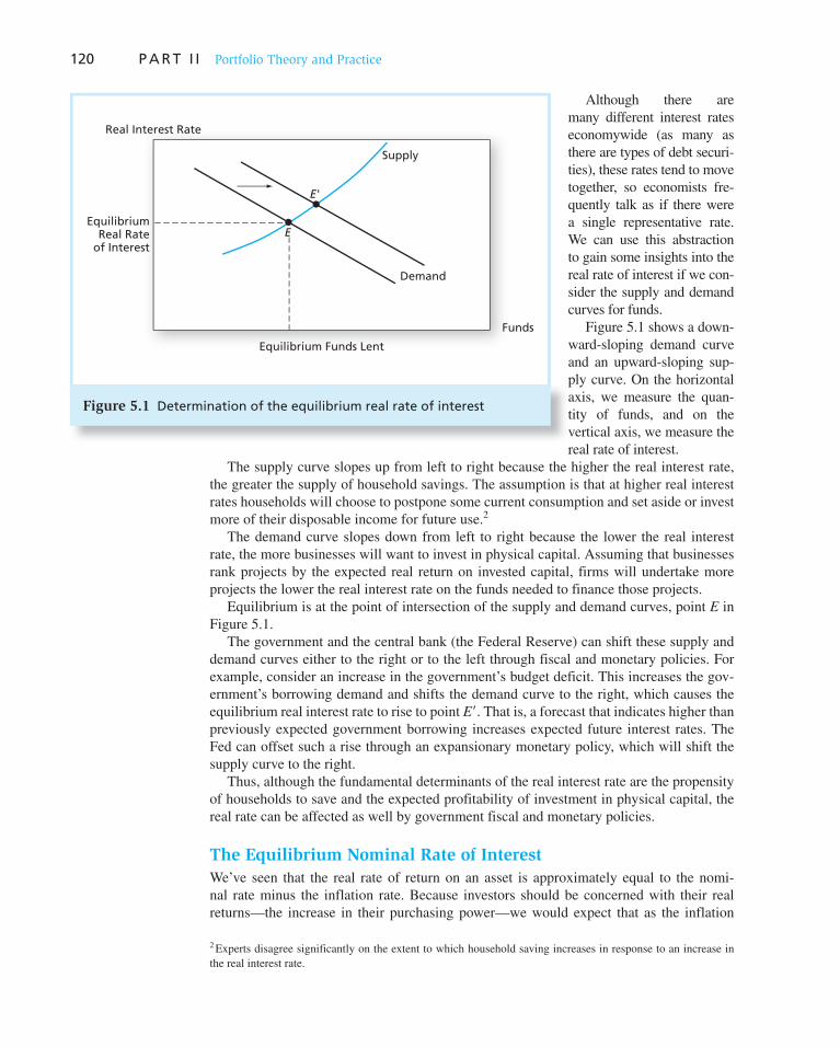
120 P A R T I I Portfolio Theory and Practice
Although there are many different interest rates e conomywide (as many as there are types of debt securi-ties), these rates tend to move together, so economists fre-quently talk as if there were a single representative rate. We can use this abstraction to gain some insights into the real rate of interest if we con-sider the supply and demand curves for funds.
Figure 5.1 shows a down-ward-sloping demand curve and an upward- sloping sup-ply curve. On the horizontal axis, we measure the quan-tity of funds, and on the vertical axis, we measure the real rate of interest.
The supply curve slopes up from left to right because the higher the real interest rate, the greater the supply of household savings. The assumption is that at higher real interest rates households will choose to postpone some current consumption and set aside or invest more of their disposable income for future use. 2
The demand curve slopes down from left to right because the lower the real interest rate, the more businesses will want to invest in physical capital. Assuming that businesses rank projects by the expected real return on invested capital, firms will undertake more projects the lower the real interest rate on the funds needed to finance those projects.
Equilibrium is at the point of intersection of the supply and demand curves, point E in Figure 5.1 .
The government and the central bank (the Federal Reserve) can shift these supply and demand curves either to the right or to the left through fiscal and monetary policies. For example, consider an increase in the government’s budget deficit. This increases the gov-ernment’s borrowing demand and shifts the demand curve to the right, which causes the equilibrium real interest rate to rise to point E � . That is, a forecast that indicates higher than previously expected government borrowing increases expected future interest rates. The Fed can offset such a rise through an expansionary monetary policy, which will shift the supply curve to the right.
Thus, although the fundamental determinants of the real interest rate are the propensity of households to save and the expected profitability of investment in physical capital, the real rate can be affected as well by government fiscal and monetary policies.
The Equilibrium Nominal Rate of Interest
We’ve seen that the real rate of return on an asset is approximately equal to the nomi-nal rate minus the inflation rate. Because investors should be concerned with their real returns—the increase in their purchasing power—we would expect that as the inflation
2 Experts disagree significantly on the extent to which household saving increases in response to an increase in the real interest rate.
Figure 5.1 Determination of the equilibrium real rate of interest
Real Interest Rate
EquilibriumReal Rate
of Interest
Equilibrium Funds Lent
Funds
E
E'
Demand
Supply

C H A P T E R 5 Introduction to Risk, Return, and the Historical Record 121
rate increases, investors will demand higher nominal rates of return on their investments. This higher rate is necessary to maintain the expected real return offered by an investment.
Irving Fisher (1930) argued that the nominal rate ought to increase one-for-one with increases in the expected inflation rate. If we use the notation E ( i ) to denote the current expectation of the inflation rate that will prevail over the coming period, then we can state the so-called Fisher equation formally as
R 5 r 1 E(i) (5.4)
The equation implies that if real rates are reasonably stable, then increases in nominal rates ought to predict higher inflation rates. This relationship has been debated and empirically investigated. The results are mixed; although the data do not strongly support this relation-ship, nominal interest rates seem to predict inflation as well as alternative methods, in part because we are unable to forecast inflation well with any method.
One reason it is difficult to determine the empirical validity of the Fisher hypothesis that changes in nominal rates predict changes in future inflation rates is that the real rate also changes unpredictably over time. Nominal interest rates can be viewed as the sum of the required real rate on nominally risk-free assets, plus a “noisy” forecast of inflation.
In Part Four we discuss the relationship between short- and long-term interest rates. Longer rates incorporate forecasts for long-term inflation. For this reason alone, inter-est rates on bonds of different maturity may diverge. In addition, we will see that prices of longer-term bonds are more volatile than those of short-term bonds. This implies that expected returns on longer-term bonds may include a risk premium, so that the expected real rate offered by bonds of varying maturity also may vary.
Taxes and the Real Rate of Interest
Tax liabilities are based on nominal income and the tax rate determined by the investor’s tax bracket. Congress recognized the resultant “bracket creep” (when nominal income grows due to inflation and pushes taxpayers into higher brackets) and mandated index-linked tax brackets in the Tax Reform Act of 1986.
Index-linked tax brackets do not provide relief from the effect of inflation on the taxa-tion of savings, however. Given a tax rate ( t ) and a nominal interest rate ( R ), the after-tax interest rate is R (1 � t ). The real after-tax rate is approximately the after-tax nominal rate minus the inflation rate:
R(1 2 t) 2 i 5 (r 1 i)(1 2 t) 2 i 5 r (1 2 t) 2 it (5.5)
Thus the after-tax real rate of return falls as the inflation rate rises. Investors suf-fer an inflation penalty equal to the tax rate times the inflation rate. If, for example, you are in a 30% tax bracket and your investments yield 12%, while inflation runs at the rate of 8%, then your before-tax real rate is approximately 4%, and you should, in an inflation-protected tax system, net after taxes a real return of 4%(1 � .3) � 2.8%. But the tax code does not recognize that the first 8% of your return is no more than c ompensation for inflation—not real income—and hence your after-tax return is reduced by 8% � .3 � 2.4%, so that your after-tax real interest rate, at .4%, is almost wiped out.
CONCEPT CHECK
1
a. Suppose the real interest rate is 3% per year and the expected inflation rate is 8%. What is the nominal interest rate?
b. Suppose the expected inflation rate rises to 10%, but the real rate is unchanged. What happens to the nominal interest rate?

122 P A R T I I Portfolio Theory and Practice
5.2 Comparing Rates of Return for Different Holding Periods
Consider an investor who seeks a safe investment, for example, in U.S. Treasury securi-ties. 3 Suppose we observe zero-coupon Treasury securities with several different maturi-ties. Zero-coupon bonds, discussed more fully in Chapter 14, are bonds that are sold at a discount from par value and provide their entire return from the difference between the purchase price and the ultimate repayment of par value. 4 Given the price, P ( T ), of a Treasury bond with $100 par value and maturity of T years, we calculate the total risk-free return available for a horizon of T years as the percentage increase in the value of the investment.
rf (T ) 5
100
P(T )2 1 (5.6)
For T � 1, Equation 5.6 provides the risk-free rate for an investment horizon of 1 year.
Not surprisingly, longer horizons in Example 5.2 provide greater total returns. How should we compare the returns on investments with differing horizons? This requires that we express each total return as a rate of return for a common period. We typically express all investment returns as an effective annual rate (EAR), defined as the percent-age increase in funds invested over a 1-year horizon.
For a 1-year investment, the EAR equals the total return, r f (1), and the gross return, (1 � EAR), is the terminal value of a $1 investment. For investments that last less than 1 year, we compound the per-period return for a full year. For example, for the 6-month bill in Example 5.2 , we compound the 2.71% half-year return for two semiannual periods to obtain a terminal value of 1 � EAR � (1.0271) 2 � 1.0549, implying that EAR � 5.49%.
For investments longer than a year, the convention is to express the EAR as the annual rate that would compound to the same value as the actual investment. For example, the
3 Yields on Treasury bills and bonds of various maturities are widely available on the Web, for example at Yahoo! Finance, MSN Money, or directly from the Federal Reserve.
4 The U.S. Treasury issues T-bills, which are pure discount (or zero-coupon) securities with maturities of up to 1 year. However, financial institutions create zero-coupon Treasury bonds called Treasury strips with maturities up to 30 years by buying coupon-paying T-bonds, “stripping” off the coupon payments, and selling claims to the coupon payments and final payment of face value separately. See Chapter 14 for further details.
Example 5.2 Annualized Rates of Return
Suppose prices of zero-coupon Treasuries with $100 face value and various maturities are as follows. We find the total return of each security by using Equation 5.6 :
Horizon, T Price, P(T ) [100/P(T )] � 1Risk-Free Return
for Given Horizon
Half-year $97.36 100/97.36 � 1 � .0271 rf(.5) � 2.71%
1 year $95.52 100/95.52 � 1 � .0469 rf(1) � 4.69%
25 years $23.30 100/23.30 � 1 � 3.2918 rf(25) � 329.18%

C H A P T E R 5 Introduction to Risk, Return, and the Historical Record 123
investment in the 25-year bond in Example 5.2 grows by its maturity by a factor of 4.2918 (i.e., 1 � 3.2918), so its EAR is
(1 1 EAR)25 5 4.2918
1 1 EAR 5 4.29181/25 5 1.0600
In general, we can relate EAR to the total return, r f ( T ), over a holding period of length T by using the following equation:
1 1 EAR 5 31 1 rf (T ) 41/T (5.7)
We can illustrate with an example.
Annual Percentage Rates
Rates on short-term investments (by convention, T < 1 year) often are annualized using simple rather than compound interest. These are called annual percentage rates, or APRs. For example, the APR corresponding to a monthly rate such as that charged on a credit card is calculated by multiplying the monthly rate by 12. More generally, if there are n compounding periods in a year, and the per-period rate is r f ( T ), then the APR � n � r f ( T ). Conversely, you can find the true per-period rate from the APR as r f ( T ) � T � APR.
Using this procedure, the APR of the 6-month bond in Example 5.2 (which had a 6-month rate of 2.71%) is 2 � 2.71 � 5.42%. To generalize, note that for short-term investments of length T, there are n � 1/ T compounding periods in a year. Therefore, the relationship among the compounding period, the EAR, and the APR is
1 1 EAR 5 31 1 rf (T)4n 5 31 1 rf
(T) 41/T 5 31 1 T 3 APR 41/T (5.8)
Equivalently,
APR 5(1 1 EAR)T 2 1
T
Continuous Compounding
It is evident from Table 5.1 (and Equation 5.8 ) that the difference between APR and EAR grows with the frequency of compounding. This raises the question, How far will these two
Example 5.3 Effective Annual Return versus Total Return
For the 6-month Treasury in Example 5.2 , T � ½, and 1/ T � 2. Therefore,
1 1 EAR 5 (1.0271)2 5 1.0549 and EAR 5 5.49%
For the 25-year Treasury in Example 5.2 , T � 25. Therefore,
1 1 EAR 5 4.29181/25 5 1.060 and EAR 5 6.0%
Example 5.4 EAR versus APR
We use Equation 5.8 to find the APR corresponding to an EAR of 5.8% with various com-mon compounding periods, and, conversely, the values of EAR implied by an APR of 5.8%. The results appear in Table 5.1 .

124 P A R T I I Portfolio Theory and Practice
rates diverge as the compounding frequency continues to grow? Put differently, what is the limit of [1 � T � APR] 1/ T , as T gets ever smaller? As T approaches zero, we effectively approach continuous compounding (CC), and the relation of EAR to the annual percentage rate, denoted by r cc for the continuously compounded case, is given by the exponential function
1 1 EAR 5 exp(rcc) 5 ercc (5.9)
where e is approximately 2.71828. To find r cc from the effective annual rate, we solve Equation 5.9 for r cc as follows:
ln(1 1 EAR) 5 rcc
where ln(•) is the natural logarithm function, the inverse of exp(•). Both the exponen-tial and logarithmic functions are available in Excel, and are called EXP(•) and LN(•), respectively.
While continuous compounding may at first seem to be a mathematical nuisance, work-ing with such rates in many cases can actually simplify calculations of expected return and risk. For example, given a continuously compounded rate, the total return for any period T, r cc ( T ), is simply exp( T � r cc ).
5 In other words, the total return scales up in direct proportion to the time period, T. This is far simpler than working with the exponents that
5 This follows from Equation 5.9. If 1 � EAR � e rcc , then (11 EAR)T 5 erccT.
Example 5.5 Continuously Compounded Rates
The continuously compounded annual percentage rate, r cc , that provides an EAR of 5.8% is 5.638% (see Table 5.1 ). This is virtually the same as the APR for daily compound-ing. But for less frequent compounding, for example, semiannually, the APR necessary to provide the same EAR is noticeably higher, 5.718%. With less frequent compounding, a higher APR is necessary to provide an equivalent effective return.
Compounding Period
EAR � [1 � rf (T )]1/T� 1 � .058 APR � rf (T)*(1/T) � .058
T rf (T) APR � [(1 � EAR)^T � 1]/T rf (T) EAR � (1 � APR*T)^(1/T) � 1
1 year 1.0000 .0580 .05800 .0580 .05800
6 months 0.5000 .0286 .05718 .0290 .05884
1 quarter 0.2500 .0142 .05678 .0145 .05927
1 month 0.0833 .0047 .05651 .0048 .05957
1 week 0.0192 .0011 .05641 .0011 .05968
1 day 0.0027 .0002 .05638 .0002 .05971
Continuous rcc � ln(1 � EAR) � .05638 EAR � exp (rcc) � 1 � .05971
Table 5.1
Annual percentage rates (APR) and effective annual rates (EAR). In the first set of columns, we hold the equivalent annual rate (EAR) fixed at 5.8% and find APR for each holding period. In the second set of columns, we hold APR fixed at 5.8% and solve for EAR.
eXce lPlease visit us at www.mhhe.com/bkm
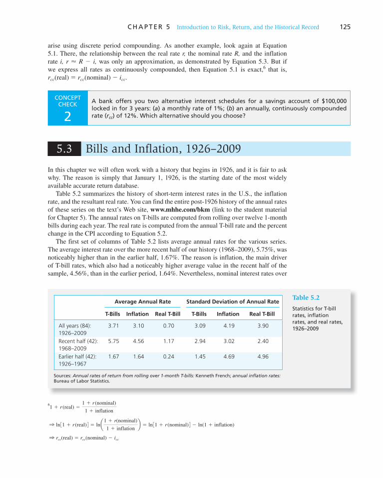
C H A P T E R 5 Introduction to Risk, Return, and the Historical Record 125
arise using discrete period compounding. As another example, look again at Equation 5.1. There, the relationship between the real rate r, the nominal rate R, and the inflation rate i, r � R � i, was only an approximation, as demonstrated by Equation 5.3. But if we express all rates as continuously compounded, then Equation 5.1 is exact, 6 that is, r cc (real) � r cc (nominal) � i cc .
In this chapter we will often work with a history that begins in 1926, and it is fair to ask why. The reason is simply that January 1, 1926, is the starting date of the most widely available accurate return database.
Table 5.2 summarizes the history of short-term interest rates in the U.S., the inflation rate, and the resultant real rate. You can find the entire post-1926 history of the annual rates of these series on the text’s Web site, www.mhhe.com/bkm (link to the student material for Chapter 5). The annual rates on T-bills are computed from rolling over twelve 1-month bills during each year. The real rate is computed from the annual T-bill rate and the percent change in the CPI according to Equation 5.2.
The first set of columns of Table 5.2 lists average annual rates for the various series. The average interest rate over the more recent half of our history (1968–2009), 5.75%, was noticeably higher than in the earlier half, 1.67%. The reason is inflation, the main driver of T-bill rates, which also had a noticeably higher average value in the recent half of the sample, 4.56%, than in the earlier period, 1.64%. Nevertheless, nominal interest rates over
6 1 1 r (real) 51 1 r (nominal)
1 1 inflation
1 ln 31 1 r (real) 4 5 lna1 1 r(nominal)
1 1 inflationb 5 ln 31 1 r (nominal) 4 2 ln(1 1 inflation)
1 rcc(real) 5 rcc(nominal) 2 icc
CONCEPT CHECK
2 A bank offers you two alternative interest schedules for a savings account of $100,000 locked in for 3 years: ( a ) a monthly rate of 1%; ( b ) an annually, continuously compounded rate ( r cc ) of 12%. Which alternative should you choose?
5.3 Bills and Inflation, 1926–2009
Table 5.2
Statistics for T-bill rates, inflation rates, and real rates, 1926–2009
Average Annual Rate Standard Deviation of Annual Rate
T-Bills Inflation Real T-Bill T-Bills Inflation Real T-Bill
All years (84):
1926–2009
3.71 3.10 0.70 3.09 4.19 3.90
Recent half (42):
1968–2009
5.75 4.56 1.17 2.94 3.02 2.40
Earlier half (42):
1926–1967
1.67 1.64 0.24 1.45 4.69 4.96
Sources: Annual rates of return from rolling over 1-month T-bills: Kenneth French; annual inflation rates: Bureau of Labor Statistics.
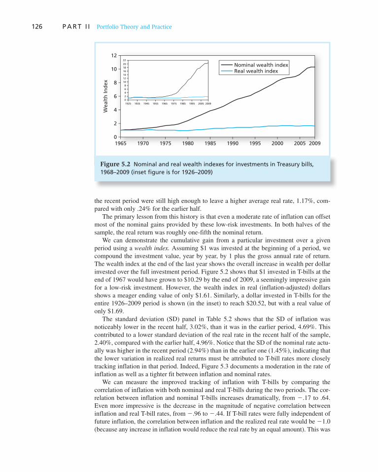
126 P A R T I I Portfolio Theory and Practice
the recent period were still high enough to leave a higher average real rate, 1.17%, com-pared with only .24% for the earlier half.
The primary lesson from this history is that even a moderate rate of inflation can offset most of the nominal gains provided by these low-risk investments. In both halves of the sample, the real return was roughly one-fifth the nominal return.
We can demonstrate the cumulative gain from a particular investment over a given period using a wealth index. Assuming $1 was invested at the beg inning of a period, we compound the investment value, yea r by year, by 1 plus the gross annual rate of return. The wealth index at the end of the last year shows the overall increase in wealth per dollar invested over the full investment period. Figure 5.2 shows that $1 invested in T-bills at the end of 1967 would have grown to $10.29 by the end of 2009, a seemingly impressive gain for a low-risk investment. However, the wealth index in real (inflation-adjusted) dollars shows a meager ending value of only $1.61. Similarly, a dollar invested in T-bills for the entire 1926–2009 period is shown (in the inset) to reach $20.52, but with a real value of only $1.69.
The standard deviation (SD) panel in Table 5.2 shows that the SD of inflation was noticeably lower in the recent half, 3.02%, than it was in the earlier period, 4.69%. This contributed to a lower standard deviation of the real rate in the recent half of the sample, 2.40%, compared with the earlier half, 4.96%. Notice that the SD of the nominal rate actu-ally was higher in the recent period (2.94%) than in the earlier one (1.45%), indicating that the lower variation in realized real returns must be attributed to T-bill rates more closely tracking inflation in that period. Indeed, Figure 5.3 documents a moderation in the rate of inflation as well as a tighter fit between inflation and nominal rates.
We can measure the improved tracking of inflation with T-bills by comparing the correlation of inflation with both nominal and real T-bills during the two periods. The cor-relation between inflation and nominal T-bills increases dramatically, from �.17 to .64. Even more impressive is the decrease in the magnitude of negative correlation between inflation and real T-bill rates, from �.96 to �.44. If T-bill rates were fully independent of future inflation, the correlation between inflation and the realized real rate would be �1.0 (because any increase in inflation would reduce the real rate by an equal amount). This was
Figure 5.2 Nominal and real wealth indexes for investments in Treasury bills, 1968–2009 (inset figure is for 1926–2009)
0
2
4
6
8
10
12
Wealt
h In
dex
1965 1970 1975 1980 1985 1990 1995 2000 2005 2009
0
2
4
6
8
10
12
14
16
18
20
22
1925 1935 1945 1955 1965 1975 1985 1995 2005 2009
Nominal wealth indexReal wealth index
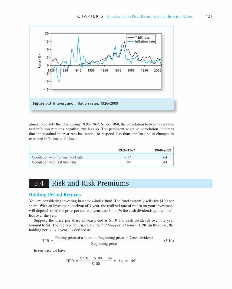
C H A P T E R 5 Introduction to Risk, Return, and the Historical Record 127
almost precisely the case during 1926–1967. Since 1968, the correlation between real rates and inflation remains negative, but less so. The persistent negative correlation indicates that the nominal interest rate has tended to respond less than one-for-one to changes in expected inflation, as follows:
1926–1967 1968–2009
Correlation with nominal T-bill rate �.17 .64
Correlation with real T-bill rate �.96 �.44
Figure 5.3 Interest and inflation rates, 1926–2009
−15
−10
−5
0
5
10
15
20
1946 1956 1966 1976 1986 1996 2006
Rate
s (%
)T-bill rateInflation rate
1926 1936
5.4 Risk and Risk Premiums
Holding-Period Returns
You are considering investing in a stock-index fund. The fund currently sells for $100 per share. With an investment horizon of 1 year, the realized rate of return on your investment will depend on ( a ) the price per share at year’s end and ( b ) the cash dividends you will col-lect over the year.
Suppose the price per share at year’s end is $110 and cash dividends over the year amount to $4. The realized return, called the holding-period return, HPR (in this case, the holding period is 1 year), is defined as
HPR 5Ending price of a share 2 Beginning price 1 Cash dividend
Beginning price (5.10)
In our case we have
HPR 5$110 2 $100 1 $4
$1005 .14, or 14%

128 P A R T I I Portfolio Theory and Practice
This definition of the HPR assumes the dividend is paid at the end of the holding period. To the extent that dividends are received earlier, the HPR ignores reinvestment income between the receipt of the payment and the end of the holding period. The percent return from dividends is called the dividend yield, and so the dividend yield plus the capital gains yield equals the HPR.
Expected Return and Standard Deviation
There is considerable uncertainty about the price of a share plus dividend income 1 year from now, however, so you cannot be sure about your eventual HPR. We can quantify our beliefs about the state of the market and the stock-index fund in terms of four possible scenarios with probabilities as presented in columns A through E of Spreadsheet 5.1 .
How can we evaluate this probability distribution? Throughout this book we will charac-terize probability distributions of rates of return in terms of their expected or mean return, E ( r ), and their standard deviation, � . The expected rate of return is a probability-weighted average of the rates of return in each scenario. Calling p ( s ) the probability of each scenario and r ( s ) the HPR in each scenario, where scenarios are labeled or “indexed” by s, we may write the expected return as
E(r) 5 as
p(s)r(s) (5.11)
Applying this formula to the data in Spreadsheet 5.1 , we find that the expected rate of return on the index fund is
E(r) 5 (.25 3 .31) 1 (.45 3 .14) 1 3.25 3 (2.0675) 4 1 3.05 3 (2.52) 4 5 .0976
Spreadsheet 5.1 shows that this sum can be evaluated easily in Excel, using the SUMPRODUCT function, which first calculates the products of a series of number pairs, and then sums the products. Here, the number pair is the probability of each scenario and the rate of return.
A B C D E F HG I
Purchase Price = $100
State of theMarket ProbabilityExcellentGoodPoor
0.05
0.250.450.25
Expected Value (mean)
Standard Deviation of HPRVariance of HPR
Crash
Year-endPrice
46.00
126.50110.0089.75
2.00
4.504.003.50
−0.5600
0.27000.1000
−0.10750.3815
0.04510.00180.0273
−0.5200
0.31000.1400
−0.0675
CashDividends
T-bill Rate = 0.04
HPR
−0.6176
0.21240.0424
−0.1651
SquaredDeviationsfrom Mean
Deviationsfrom Mean
0.3815
0.04510.00180.0273
0.03800.1949
0.0976
ExcessReturns
SquaredDeviationsfrom Mean
1
2
3
4
5
6
7
8
9
10
11
12
13
14
15
16
SUMPRODUCT(B8:B11, E8:E11) =SUMPRODUCT(B8:B11, G8:G11) =
SQRT(G13) =
0.0576Risk PremiumStandard Deviation of Excess Return 0.1949SQRT(SUMPRODUCT(B8:B11, I8:I11)) =
SUMPRODUCT(B8:B11, H8:H11) =
Spreadsheet 5.1
Scenario analysis of holding period return of the stock-index fund
eXce lPlease visit us at www.mhhe.com/bkm
C H A P T E R 5 Introduction to Risk, Return, and the Historical Record 129
The standard deviation of the rate of return ( � ) is a measure of risk. It is defined as the square root of the variance, which in turn is the expected value of the squared deviations from the expected return. The higher the volatility in outcomes, the higher will be the aver-age value of these squared deviations. Therefore, variance and standard deviation provide one measure of the uncertainty of outcomes. Symbolically,
�2 5 a
s
p(s) 3r(s) 2 E(r)42 (5.12)
Therefore, in our example
�2 5 .25(.31 2 .0976)2 1 .45(.14 2 .0976)2 1 .25(2.0675 2 .0976)2
1 .05(2.52 2 .0976)2 5 .0380
This value is calculated in cell G13 of Spreadsheet 5.1 using the SUMPRODUCT func-tion. The standard deviation is calculated in cell G14 as
� 5 ".0380 5 .1949 5 19.49%
Clearly, what would trouble potential investors in the index fund is the downside risk of a crash or poor market, not the upside potential of a good or excellent market. The stan-dard deviation of the rate of return does not distinguish between good or bad surprises; it treats both simply as deviations from the mean. As long as the probability distribution is more or less symmetric about the mean, � is an adequate measure of risk. In the special case where we can assume that the probability distribution is normal—represented by the well-known bell-shaped curve— E ( r ) and � are perfectly adequate to characterize the distribution.
Excess Returns and Risk Premiums
How much, if anything, should you invest in our index fund? First, you must ask how much of an expected reward is offered for the risk involved in investing money in stocks.
We measure the reward as the difference between the expected HPR on the index stock fund and the risk-free rate, that is, the rate you can earn by leaving money in risk-free assets such as T-bills, money market funds, or the bank. We call this difference the risk
premium on common stocks. The risk-free rate in our example is 4% per year, and the expected index fund return is 9.76%, so the risk premium on stocks is 5.76% per year. The difference in any particular period between the actual rate of return on a risky asset and the actual risk-free rate is called the excess return. Therefore, the risk premium is the expected value of the excess return, and the standard deviation of the excess return is a measure of its risk. (See Spreadsheet 5.1 for these calculations.)
The degree to which investors are willing to commit funds to stocks depends on risk
aversion. Financial analysts generally assume investors are risk averse in the sense that, if the risk premium were zero, people would not be willing to invest any money in stocks. In theory, then, there must always be a positive risk premium on stocks in order to induce risk-averse investors to hold the existing supply of stocks instead of placing all their money in risk-free assets.
Although the scenario analysis illustrates the concepts behind the quantification of risk and return, you may still wonder how to get a more realistic estimate of E ( r ) and � for common stocks and other types of securities. Here, history has insights to offer. Analysis of the historical record of portfolio returns, however, makes use of a variety of concepts and statistical tools, and so we first turn to a preparatory discussion.
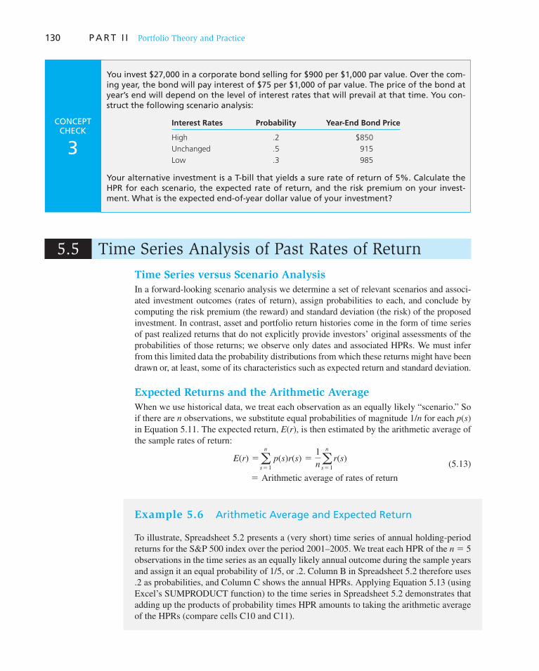
130 P A R T I I Portfolio Theory and Practice
5.5 Time Series Analysis of Past Rates of Return
CONCEPT CHECK
3
You invest $27,000 in a corporate bond selling for $900 per $1,000 par value. Over the com-ing year, the bond will pay interest of $75 per $1,000 of par value. The price of the bond at year’s end will depend on the level of interest rates that will prevail at that time. You con-struct the following scenario analysis:
Interest Rates Probability Year-End Bond Price
High .2 $850
Unchanged .5 915
Low .3 985
Your alternative investment is a T-bill that yields a sure rate of return of 5%. Calculate the HPR for each scenario, the expected rate of return, and the risk premium on your invest-ment. What is the expected end-of-year dollar value of your investment?
Time Series versus Scenario Analysis
In a forward-looking scenario analysis we determine a set of relevant scenarios and associ-ated investment outcomes (rates of return), assign probabilities to each, and conclude by computing the risk premium (the reward) and standard deviation (the risk) of the proposed investment. In contrast, asset and portfolio return histories come in the form of time series of past realized returns that do not explicitly provide investors’ original assessments of the probabilities of those returns; we observe only dates and associated HPRs. We must infer from this limited data the probability distributions from which these returns might have been drawn or, at least, some of its characteristics such as expected return and standard deviation.
Expected Returns and the Arithmetic Average
When we use historical data, we treat each observation as an equally likely “scenario.” So if there are n observations, we substitute equal probabilities of magnitude 1/ n for each p ( s ) in Equation 5.11. The expected return, E ( r ), is then estimated by the arithmetic average of the sample rates of return:
E(r) 5an
s51
p(s)r(s) 51
nan
s51
r(s) (5.13)
5 Arithmetic average of rates of return
Example 5.6 Arithmetic Average and Expected Return
To illustrate, Spreadsheet 5.2 presents a (very short) time series of annual holding-period returns for the S&P 500 index over the period 2001–2005. We treat each HPR of the n � 5 observations in the time series as an equally likely annual outcome during the sample years and assign it an equal probability of 1/5, or .2. Column B in Spreadsheet 5.2 therefore uses .2 as probabilities, and Column C shows the annual HPRs. Applying Equation 5.13 (using Excel’s SUMPRODUCT function) to the time series in Spreadsheet 5.2 demonstrates that adding up the products of probability times HPR amounts to taking the arithmetic average of the HPRs (compare cells C10 and C11).
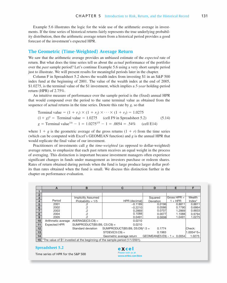
C H A P T E R 5 Introduction to Risk, Return, and the Historical Record 131
Example 5.6 illustrates the logic for the wide use of the arithmetic average in invest-ments. If the time series of historical returns fairly represents the true underlying probabil-ity distribution, then the arithmetic average return from a historical period provides a good forecast of the investment’s expected HPR.
The Geometric (Time-Weighted) Average Return
We saw that the arithmetic average provides an unbiased estimate of the expected rate of return. But what does the time series tell us about the actual performance of the portfolio over the past sample period? Let’s continue Example 5.6 using a very short sample period just to illustrate. We will present results for meaningful periods later in the chapter.
Column F in Spreadsheet 5.2 shows the wealth index from investing $1 in an S&P 500 index fund at the beginning of 2001. The value of the wealth index at the end of 2005, $1.0275, is the terminal value of the $1 investment, which implies a 5 - year holding-period return (HPR) of 2.75%.
An intuitive measure of performance over the sample period is the (fixed) annual HPR that would compound over the period to the same terminal value as obtained from the sequence of actual returns in the time series. Denote this rate by g, so that
Terminal value 5 (1 1 r1) 3 (1 1 r2) 3 . . . 3 (1 1 r5) 5 1.0275
(11 g)n 5 Terminal value 5 1.0275 (cell F9 in Spreadsheet 5.2) (5.14)
g 5 Terminal value1/n 2 1 5 1.02751/5 2 1 5 .0054 5 .54% (cell E14)
where 1 � g is the geometric average of the gross returns (1 � r ) from the time series (which can be computed with Excel’s GEOMEAN function) and g is the annual HPR that would replicate the final value of our investment.
Practitioners of investments call g the time-weighted (as opposed to dollar-weighted) average return, to emphasize that each past return receives an equal weight in the process of averaging. This distinction is important because investment managers often experience significant changes in funds under management as investors purchase or redeem shares. Rates of return obtained during periods when the fund is large produce larger dollar prof-its than rates obtained when the fund is small. We discuss this distinction further in the c hapter on performance evaluation.
123456789
10
11
12
13
14
15
A B C D E F
PeriodImplicitly AssumedProbability = 1/5
SquaredDeviation
Gross HPR =1 + HPR
WealthIndex*
2001 .2 −0.1189 0.01960.05860.07070.0077
0.1774
0.0008
0.1983
0.8811 0.88110.68640.88330.97941.0275
Check:
1.0054^5=
0.77901.28691.10881.0491
0.0054 1.0275
−0.22100.28690.10880.04910.0210
0.0210
HPR (decimal)
.2
.2
.2
.2
2002200320042005
Arithmetic average
Expected HPR SUMPRODUCT(B5:B9, C5:C9) =
SUMPRODUCT(B5:B9, D5:D9)^.5 =
STDEV(C5:C9) =
Geometric average return
*The value of $1 invested at the beginning of the sample period (1/1/2001).
GEOMEAN(E5:E9) − 1 =
Standard deviation
AVERAGE(C5:C9) =
Spreadsheet 5.2
Time series of HPR for the S&P 500
eXce lPlease visit us at www.mhhe.com/bkm

132 P A R T I I Portfolio Theory and Practice
The larger the swings in rates of return, the greater the discrepancy between the arith-metic and geometric averages, that is, between the compound rate earned over the sample period and the average of the annual returns. If returns come from a normal distribution, the expected difference is exactly half the variance of the distribution, that is,
E 3Geometric average4 5 E 3Arithmetic average4 2 1/2 �2 (5.15)
(A warning: to use Equation 5.15 , you must express returns as decimals, not percent-ages.) When returns are approximately normally distributed, Equation 5.15 will be a good approximation.
Variance and Standard Deviation
When thinking about risk, we are interested in the likelihood of deviations from the expected return. In practice, we usually cannot directly observe expectations, so we esti-mate the variance by averaging squared deviations from our estimate of the expected return, the arithmetic average, r. Adapting Equation 5.12 for historic data, we again use equal probabilities for each observation, and use the sample average in place of the unob-servable E ( r ).
Variance 5 Expected value of squared deviations
� 2 5 a p(s) 3r(s) 2 E(r) 42Using historical data with n observations, we could estimate variance as
�̂2 5
1
nan
s51
3r(s) 2 r 42 (5.16)
where �̂ replaces � to denote that it is an estimate.
Example 5.7 Geometric versus Arithmetic Average
The geometric average in Example 5.6 (.54%) is substantially less than the arithmetic a verage (2.10%). This discrepancy sometimes is a source of confusion. It arises from the asymmetric effect of positive and negative rates of returns on the terminal value of the portfolio.
Observe the returns in years 2002 (�.2210) and 2003 (.2869). The arithmetic average return over the 2 years is (�.2210 � .2869)/2 � .03295 (3.295%). However, if you had invested $100 at the beginning of 2002, you would have only $77.90 at the end of the year. In order to simply break even, you would then have needed to earn $21.10 in 2003, which would amount to a whopping return of 27.09% (21.10/77.90). Why is such a high rate necessary to break even, rather than the 22.10% you lost in 2002? The value of your invest-ment in 2003 was much smaller than $100; the lower base means that it takes a greater subsequent percentage gain to just break even. Even a rate as high as the 28.69% realized in 2003 yields a portfolio value in 2003 of $77.90 � 1.2869 � $100.25, barely greater than $100. This implies a 2-year annually compounded rate (the geometric average) of only .12%, significantly less than the arithmetic average of 3.295%.
CONCEPT CHECK
4 You invested $1 million at the beginning of 2008 in an S&P 500 stock-index fund. Given the rate of return for 2008, �38.6%, what rate of return in 2009 would have been necessary for your portfolio to recover to its original value?

C H A P T E R 5 Introduction to Risk, Return, and the Historical Record 133
Example 5.8 Variance and Standard Deviation
Take another look at Spreadsheet 5.2 . Column D shows the square deviations from the arithmetic average, and cell D12 gives the standard deviation as .1774, which is the square root of the sum of products of the (equal) probabilities times the squared deviations.
The variance estimate from Equation 5.16 is biased downward, however. The reason is that we have taken deviations from the sample arithmetic average, r, instead of the unknown, true expected value, E ( r ), and so have introduced a bit of estimation error. This is sometimes called a degrees of freedom bias. We can eliminate the bias by multiplying the arithmetic average of squared deviations by the factor n /( n � 1). The variance and standard deviation then become
�̂ 2 5 a n
n 2 1b 3
1
nan
s51
3r(s) 2 r 42 51
n 2 1an
s51
3r(s) 2 r 42 �̂ 5 Å 1
n 2 1an
s51
3r(s) 2 r 42 (5.17)
Cell D13 shows that the unbiased estimate of the standard deviation is .1983, which is a bit higher than the .1774 value obtained in cell D12.
The Reward-to-Volatility (Sharpe) Ratio
Finally, it is worth noting that investors presumably are interested in the expected excess return they can earn over the T-bill rate by replacing T-bills with a risky portfolio as well as the risk they would thereby incur. While the T-bill rate is not fixed each period, we still know with certainty what rate we will earn if we purchase a bill and hold it to maturity. Other investments typically entail accepting some risk in return for the prospect of earning more than the safe T-bill rate. Investors price risky assets so that the risk premium will be commensurate with the risk of that expected excess return, and hence it’s best to measure risk by the standard deviation of excess, not total, returns.
The importance of the trade-off between reward (the risk premium) and risk (as mea-sured by standard deviation or SD) suggests that we measure the attraction of an invest-ment portfolio by the ratio of its risk premium to the SD of its excess returns.
Sharpe ratio 5Risk premium
SD of excess return (5.18)
This reward-to-volatility measure (first proposed by William Sharpe and hence called the Sharpe ratio ) is widely used to evaluate the performance of investment managers.
Example 5.9 Sharpe Ratio
Take another look at Spreadsheet 5.1 . The scenario analysis for the proposed investment in the stock-index fund resulted in a risk premium of 5.76%, and standard deviation of excess returns of 19.49%. This implies a Sharpe ratio of .30, a value that is in line with perfor-mance of stock-index funds over the past 40 years. We elaborate on this important measure in future chapters and show that while it is an adequate measure of the risk–return trade-off for diversified portfolios (the subject of this chapter), it is inadequate when applied to indi-vidual assets such as shares of stock that may be held as part of larger diversified portfolios.

134 P A R T I I Portfolio Theory and Practice
5.6 The Normal Distribution
CONEPT CHECK
5
Using the annual returns for years 2003–2005 in Spreadsheet 5.2 ,
a. Compute the arithmetic average return.
b. Compute the geometric average return.
c. Compute the standard deviation of returns.
d. Compute the Sharpe ratio assuming the risk-free rate was 6% per year.
The bell-shaped normal distribution appears naturally in many applications. For exam-ple, heights and weights of the population are well described by the normal distribution. In fact, many variables that are the end result of multiple random influences will exhibit a normal distribution, for example, the error of a machine that aims to fill containers with exactly 1 gallon of liquid. By the same logic, if return expectations implicit in asset prices are rational, actual rates of return realized should be normally distributed around these expectations.
To see why the normal curve is “normal,” consider a newspaper stand that turns a profit of $100 on a good day and breaks even on a bad day, with equal probabilities of .5. Thus, the mean daily profit is $50 dollars. We can build a tree that compiles all the possible outcomes at the end of any period. Here is an event tree showing outcomes after 2 days:
Two good days, profit = $200
Two bad days, profit = 0
One good and one bad day, profit = $100
Notice that 2 days can produce three different outcomes and, in general, n days can pro-duce n � 1 possible outcomes. The most likely 2-day outcome is “one good and one bad day,” which can happen in two ways (first a good day, or first a bad day). The probability of this outcome is .5. Less likely are the two extreme outcomes (both good days or both bad days) with probability .25 each.
What is the distribution of profits at the end of many business days? For example, after 200 days, there are 201 possible outcomes and, again, the midrange outcomes are the more likely because there are more sequences that lead to them. For example, while only one sequence can result in 200 consecutive bad days, an enormous number of sequences result in 100 good days and 100 bad days. The probability distribution will eventually take on the
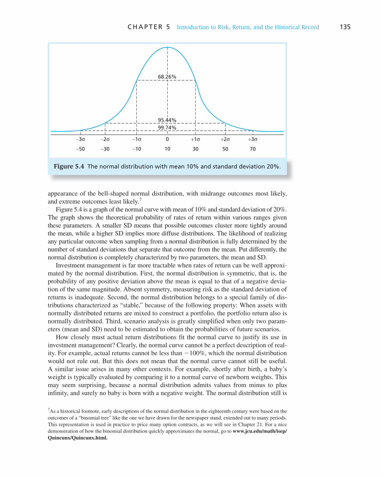
C H A P T E R 5 Introduction to Risk, Return, and the Historical Record 135
appearance of the bell-shaped normal distribution, with midrange outcomes most likely, and extreme outcomes least likely. 7
Figure 5.4 is a graph of the normal curve with mean of 10% and standard deviation of 20%. The graph shows the theoretical probability of rates of return within various ranges given these parameters. A smaller SD means that possible outcomes cluster more tightly around the mean, while a higher SD implies more diffuse distributions. The likelihood of realizing any particular outcome when sampling from a normal distribution is fully determined by the number of standard deviations that separate that outcome from the mean. Put differently, the normal distribution is completely characterized by two parameters, the mean and SD.
Investment management is far more tractable when rates of return can be well approxi-mated by the normal distribution. First, the normal distribution is symmetric, that is, the probability of any positive deviation above the mean is equal to that of a negative devia-tion of the same magnitude. Absent symmetry, measuring risk as the standard deviation of returns is inadequate. Second, the normal distribution belongs to a special family of dis-tributions characterized as “stable,” because of the following property: When assets with normally distributed returns are mixed to construct a portfolio, the portfolio return also is normally distributed. Third, scenario analysis is greatly simplified when only two param-eters (mean and SD) need to be estimated to obtain the probabilities of future scenarios.
How closely must actual return distributions fit the normal curve to justify its use in investment management? Clearly, the normal curve cannot be a perfect description of real-ity. For example, actual returns cannot be less than �100%, which the normal distribution would not rule out. But this does not mean that the normal curve cannot still be useful. A similar issue arises in many other contexts. For example, shortly after birth, a baby’s weight is typically evaluated by comparing it to a normal curve of newborn weights. This may seem surprising, because a normal distribution admits values from minus to plus infinity, and surely no baby is born with a negative weight. The normal distribution still is
7 As a historical footnote, early descriptions of the normal distribution in the eighteenth century were based on the outcomes of a “binomial tree” like the one we have drawn for the newspaper stand, extended out to many periods. This representation is used in practice to price many option contracts, as we will see in Chapter 21. For a nice demonstration of how the binomial distribution quickly approximates the normal, go to www.jcu.edu/math/isep/
Quincunx/Quincunx.html.
Figure 5.4 The normal distribution with mean 10% and standard deviation 20%.
−3σ −2σ −1σ 0 +1σ +2σ +3σ
−50 −30 −10 30 50 70
68.26%
95.44%
99.74%
10

136 P A R T I I Portfolio Theory and Practice
useful in this application because the SD of the weight is small relative to its mean, and the likelihood of a negative weight would be too trivial to matter. 8 In a similar spirit, we must identify criteria to determine the adequacy of the normality assumption for rates of return.
Example 5.10 Normal Distribution Function in Excel
Suppose the monthly rate of return on the S&P 500 is approximately normally distrib-uted with a mean of 1% and standard deviation of 6%. What is the probability that the return on the index in any month will be negative? We can use Excel’s built-in func-tions to quickly answer this question. The probability of observing an outcome less than some cutoff according to the normal distribution function is given as NORMDIST(cutoff, mean, standard deviation, TRUE). In this case, we want to know the probability of an out-come below zero, when the mean is 1% and the standard deviation is 6%, so we compute NORMDIST(0, 1, 6, TRUE) � .4338. We could also use Excel’s built-in standard normal function, NORMSDIST, which uses a mean of 0 and a standard deviation of 1, and ask for the probability of an outcome 1/6 of a standard deviation below the mean. This would be the same: NORMSDIST(�1/6) � .4338.
As we noted earlier (but you can’t repeat it too often!), normality of excess returns hugely simplifies portfolio selection. Normality assures us that standard deviation is a complete measure of risk and hence the Sharpe ratio is a complete measure of portfolio perfor-mance. Unfortunately, many observers today believe that deviations from normality of asset returns are too significant to ignore.
Deviations from normality may be discerned by calculating the higher moments of return distributions. The n th central moment of a distribution of excess returns, R, is esti-
mated as the average value of (R 2 R)n. The first moment ( n � 1) is necessarily zero (the
average deviation from the sample average must be zero). The second moment ( n � 2) is the estimate of the variance of returns, �̂2. 9
8 In fact, the standard deviation is 511 grams while the mean is 3,958 grams. A negative weight would therefore be 7.74 standard deviations below the mean, and according to the normal distribution would have probability of only 4.97 � 10 �15 . The issue of negative birth weight clearly isn’t a practical concern.
9 For distributions that are symmetric about the average, as is the case for the normal distribution, all odd moments ( n � 1, 3, 5, . . .) have expectations of zero. For the normal distribution, the expectations of all higher even moments ( n � 4, 6, . . .) are functions only of the standard deviation, � . For example, the expected fourth moment ( n � 4) is 3 � 4 , and for n � 6, it is 15 � 6 . Thus, for normally distributed returns the standard deviation, � , provides
a complete measure of risk, and portfolio performance may be measured by the Sharpe ratio, R/�. For other distributions, however, asymmetry may be measured by higher nonzero odd moments. Higher even moments (in excess of those consistent with the normal distribution), combined with large, negative odd moments, indicate higher probabilities of extreme negative outcomes.
CONCEPT CHECK
6 What is the probability that the return on the index in Example 5.10 will be below �15%?
5.7 Deviations from Normality and Risk Measures

C H A P T E R 5 Introduction to Risk, Return, and the Historical Record 137
A measure of asymmetry called skew uses the ratio of the average cubed deviations from the average, called the third moment, to the cubed standard deviation to measure any asymmetry or “skewness” of a distribution. Skew is estimated as
Skew 5 Average B (R 2 R)3
�̂3
R (5.19)
Cubing deviations maintains their sign (the cube of a negative number is negative). Thus, if the distribution is “skewed to the right,” as is the dark curve in Figure 5.5A , the extreme positive values, when cubed, will dominate the third moment, resulting in a positive measure of skew. If the distribution is “skewed to the left,” the cubed extreme negative values will dominate, and the skew will be negative.
When the distribution is positively skewed (the skew is greater than zero), the standard devia-tion overestimates risk, because extreme positive deviations from expectation (which are not a source of concern to the investor) nevertheless increase the estimate of volatility. Conversely, and more important, when the distribution is negatively skewed, the SD will underestimate risk.
Another potentially important deviation from nor-mality concerns the likelihood of extreme values on either side of the mean at the expense of a smaller fraction of moderate deviations. Graphically speaking, when the tails of a distribution are “fat,” there is more probability mass in the tails of the distribution than predicted by the normal distribution, at the expense of “slender shoulders,” that is, less probability mass near the center of the distribution. Figure 5.5B super-imposes a “fat-tailed” distribution on a normal with the same mean and SD. Although symmetry is still preserved, the SD will underestimate the likelihood of extreme events: large losses as well as large gains.
Kurtosis is a measure of the degree of fat tails. In this case, we use deviations from the average raised to the fourth power and standardize by dividing by the fourth power of the SD, that is,
Kurtosis 5 Average B (R 2 R)4
�̂4
R 2 3 (5.20)
We subtract 3 from the ratio in Equation 5.20 , because expected Kurtosis for a normal distribution would be 3. Thus, the kurtosis of a normal distribution is defined as zero, and any kurtosis above zero is a sign of fatter tails than would be observed in a normal dis-tribution. The kurtosis of the distribution in Figure 5.5B , which has visible fat tails, is .35.
Higher frequency of extreme negative returns may result from negative skew and/or kur-tosis (fat tails)—an important point. Therefore, we would like a risk measure that indicates
Figure 5.5A Normal and skewed distributions (mean � 6%, SD � 17%)
.00
Rate of Return
.20 .40 .60−.60
Pro
bab
ilit
y
−.40 −.20
.030
.025
.020
.015
.010
.005
.000
Skew = −.75
Skew = .75
Negatively skewed
Normal
Positively skewed
Figure 5.5B Normal and fat-tailed distributions (mean � .1, SD � .2)
−.4 −.2−.6 .2 .4 .60
Rate of Return
Kurtosis=.35
Pro
bab
ilit
y D
en
sity
.8
Normal Fat-tailed
.00
.10
.20
.30
.50
.40
.60
CONCEPT CHECK
7 Estimate the skew and kurtosis of the five rates in Spreadsheet 5.2 .

138 P A R T I I Portfolio Theory and Practice
vulnerability to extreme n egative returns. We discuss three such measures that are most fre-quently used in practice: value at risk, expected shortfall, and lower partial standard deviation.
Value at Risk
The value at risk (denoted VaR to distinguish it from Var, the abbreviation for variance) is the measure of loss most frequently associated with extreme negative returns. VaR is actu-ally written into regulation of banks and closely watched by risk managers. It is another name for quantile of a distribution. The quantile, q, of a distribution is the value below which lies q % of the possible values of that distribution. Thus the median is the q � 50th quantile. Practitioners commonly estimate the 5% VaR, meaning that 95% of returns will exceed the VaR, and 5% will be worse. Therefore, VaR may be viewed as the best rate of return out of the 5% worst-case future scenarios.
When portfolio returns are normally distributed, the VaR may be directly derived from the mean and SD of the distribution. Recalling that �1.65 is the 5th percentile of the stan-dard normal distribution (with mean � 0 and SD � 1), the VaR for the normal distribution is
VaR(.05, normal distribution) 5 Mean 1 (21.65)SD
To obtain a sample estimate of VaR, we sort the observations from high to low. The VaR is the return at the 5th percentile of the sample distribution. Almost always, 5% of the num-ber of observations will not be an integer, and so we must interpolate. Suppose the sample is comprised of 84 annual returns (1926–2009), so that 5% of the number of observa-tions is 4.2. We must interpolate between the fourth and fifth observation from the bottom. Suppose the bottom five returns are
225.03% 225.69% 233.49% 241.03% 245.64%
The VaR is therefore between �25.03% and �25.69% and would be calculated as
VaR 5 .2(225.03) 1 .8(225.69) 5 225.56%
Expected Shortfall
When we assess tail risk by looking at the 5% worst-case scenarios, the VaR is the most optimistic as it takes the highest return (smallest loss) of all these cases. A more realistic view of downside exposure would focus instead on the expected loss given that we find ourselves in one of the worst-case scenarios. This value, unfortunately, has two names: either expected shortfall (ES) or conditional tail expectation (CTE); the latter terminol-ogy emphasizes that this expectation is conditioned on being in the left tail of the distribu-tion. We will use the expected shortfall terminology.
Extending the previous VaR example, we assume equal probabilities for all values. Hence, we need to average across the bottom 5% of the observations. To interpolate as before, we assign the average of the bottom four returns weights of 4/4.2 each, and the fifth value from the bottom a weight of .2/4.2, resulting in a value of ES � �35.94%, signifi-cantly worse than the �25.56% VaR. 10
10 A formula for the ES in the case of normally distributed returns is given in Jonathan Treussard, “The Non-monotonicity of Value-at-Risk and the Validity of Risk Measures over Different Horizons,” IFCAI Journal of
Financial Risk Management, March 2007. The formula is
ES 51
.05 exp(� )N 32� 2 F(.95) 4
where � is the mean of the continuously compounded returns, � is the SD, N(•) is the cumulative standard normal, and F is its inverse. In the sample above, � and � were estimated as 5.47% and 19.54%. Assuming nor-mality, we would have ES � �30.57%, suggesting that this distribution has a larger left tail than the normal. It should be noted, however, that estimates of VaR and ES from historical samples, while unbiased, are subject to large estimation errors.
C H A P T E R 5 Introduction to Risk, Return, and the Historical Record 139
Lower Partial Standard Deviation and the Sortino Ratio
The use of standard deviation as a measure of risk when the return distribution is nonnormal presents three problems: (1) the asymmetry of the distribution suggests we should look at negative outcomes separately; (2) because an alternative to a risky portfolio is a risk-free investment vehicle, we should look at deviations of returns from the risk-free rate rather than from the sample average; and (3) fat tails should be accounted for.
A risk measure that answers the first two of these issues is the lower partial stan-
dard deviation (LPSD), which is computed like the usual standard deviation, but using only “bad” returns. Specifically, it uses only negative deviations from the risk-free rate (rather than negative deviations from the sample average), squares those deviations to obtain an analog to variance, and then takes the square root to obtain a “left-tail standard deviation.” The LPSD is therefore the square root of the average squared deviation, con-
ditional on a negative excess return. Notice that this measure ignores the frequency of negative excess returns, that is, portfolios with the same average squared negative excess returns will yield the same LPSD regardless of the relative frequency of negative excess returns.
Practitioners who replace standard deviation with this LPSD typically also replace the Sharpe ratio (the ratio of average excess return to standard deviation) with the ratio of average excess returns to LPSD. This variant on the Sharpe ratio is called the Sortino
ratio. In the analysis of the history of some popular investment vehicles in the next section
we will show why practitioners need this plethora of statistics and performance measures to analyze risky investments. The nearby box discusses the growing popularity of these measures, and particularly the new focus on fat tails and extreme events.
5.8 Historic Returns on Risky Portfolios: Equities and Long-Term Government Bonds
We can now apply the analytical tools worked out in previous sections to five important risky portfolios:
1. World large stocks. This portfolio includes all available country index portfolios (48 countries in 2009). Each index is composed of that country’s large stocks (e.g., firms in the S&P 500 for the U.S.), each weighted by market capitalization (the market value of all outstanding shares). These country-index portfolios are then weighted by the country market capitalization to form a world stock portfolio.
2. U.S. large stocks. This portfolio is composed of the stocks in the S&P 500 index and is capitalization weighted. These corporations account for about 75% of the market value of all publicly traded stocks in the U.S., and an even larger share of the U.S. GDP.
3. U.S. small stocks. This index measures the return on the smallest quintile (i.e., smallest 20% ranked by capitalization) of U.S. publicly traded stocks.
4. U.S. long-term government bonds. Long-term T-bond returns are measured by the Barclays Capital (formerly Lehman Brothers) value-weighted index of all outstand-ing U.S. government bonds of 10 years and longer maturity.

140
Some Funds Stop Grading on the Curve
In 2008 a typical investment portfolio of 60% stocks and 40% bonds lost roughly a fifth of its value. Standard portfolio-construction tools assume that will happen only once every 111 years. Though mathematicians and many investors have long known market behavior isn’t a pretty picture, standard portfolio construction assumes returns fall along a tidy, bell-curve-shaped distribution. With that approach, a 2008-type decline would fall near the skinny left tail, indicating its rarity.
Recent history would suggest such meltdowns aren’t so rare. In a little more than two decades, investors have been buffeted by the 1987 market crash, the implosion of hedge fund Long-Term Capital Management, the bursting of the tech-stock bubble, and other crises.
Many of Wall Street’s new tools assume market returns fall along a “fat-tailed” distribution, where, say, last year’s nearly 40% stock-market decline would be more com-mon than previously thought. These new assumptions present a far different picture of risk. Consider the 60% stock, 40% bond portfolio that fell about 20% last year. Under the fat-tailed distribution, that should occur once every 40 years, not once every 111 years as assumed under a bell-curve-type distribution. (The last year as bad as 2008 was 1931.)
One potential pitfall: Number-crunchers have a smaller supply of historical observations to construct models
focused on rare events. “Data are intrinsically sparse,” says Lisa Goldberg, executive director of analytic initiatives at MSCI Barra.
Many of the new tools also limit the role of conven-tional risk measures. Standard deviation, proposed as a risk measure by Nobel Prize–winning economist Harry Markowitz in the 1950s, can be used to gauge how much an investment’s returns vary over time. But it is equally affected by upside and downside moves, whereas many investors fear losses much more than they value gains. And it doesn’t fully gauge risk in a fat-tailed world.
A newer measure that has gained prominence in recent decades ignores potential gains and looks at downside risk. That measure, called “value at risk,” might tell you that you have a 5% chance of losing 3% or more in a single day, but it doesn’t home in on the worst downside scenarios.
To focus on extreme risk, many firms have begun using a measure called “expected shortfall” or “conditional value at risk,” which is the expected portfolio loss when value at risk has been breached. Conditional value at risk helps estimate the magnitudes of expected loss on the very bad days. Firms such as J.P. Morgan and MSCI Barra are employing the measure.
Source: Eleanor Laise, “Some Funds Stop Grading on the Curve,” The Wall Street Journal, September 8, 2009, p. C1. Reprinted by permission of The Wall Street Journal, © 2009.
WO
RD
S FR
OM
TH
E ST
REE
T
5. A diversified portfolio. Our most inclusive portfolio is a mixture of the other portfolios with weights of 50% in world large stocks, 20% in U.S. small stocks, and 30% in long-term U.S. government bonds. A common asset allocation s uggested for “average” investors is 70% in stocks and 30% in bonds. In our diversified portfolio, the 70% weight in stocks is placed primarily in world large stocks (of which about half are large U.S. stocks), with 20% allocated to the riskier portfolio of small stocks. Regardless of whether this is an optimal portfolio, it allows us to examine whether diversification beyond the first four portfolios, which are themselves already well diversified, can further enhance the risk–return trade-off.
Figure 5.6 gives a pictorial view of the dispersion of returns of each portfolio, as well as T-bills, over the 84-year period ending in 2009. Clearly, the risk of large losses progres-sively increases as we move from T-bills to long-term bonds, to large stocks, and finally to small stocks. The further diversified Portfolio 5 already emerges as offering a better risk-return trade-off. Interestingly, the superimposed graphs of normal distributions with the same mean and standard deviation as each portfolio shows that exposure to extreme losses greater than those consistent with normality, if they exist at all, are too minor to be discerned with a naked eye.
Table 5.3 summarizes all the relevant statistics for the five risky portfolios from the entire 84-year period (84 observations), as well as for the 42 observations from the more recent period (1968–2009) and earlier (1926–1967) subperiods. The table is quite dense, but we’ll highlight its major implications section by section.

C H A P T E R 5 Introduction to Risk, Return, and the Historical Record 141
Total Returns
One notable feature of total return is the difference between the arithmetic and geometric averages. Recall that Equation 5.15 tells us that for normally distributed returns, the geo-metric average return equals the arithmetic average minus ½ � 2 . With only one exception (small stocks), this relationship is nearly satisfied. While the difference between the geo-metric return and the arithmetic return minus ½ � 2 for small stocks ranges from .29% to 1.91%, for no other portfolio does this difference exceed .17%. This is the first clue that despite the issues raised by the financial crisis of 2008, we will find no strong evidence that the normal distribution fails to adequately describe portfolio returns.
Excess Returns
Our major focus is on excess returns. Average excess returns over the recent half of the history (1968–2009) appear quite different from those of the earlier half period. Except for U.S. long-term government bonds, recent averages are lower, despite the 10 years in the earlier period spanned by the Great Depression. For example, the average excess return of world large stocks fell from 9.02% in the earlier half of the sample to 6.02% in the more
Figure 5.6 Frequency distribution of annual rates of return, 1926–2009
Source: Prepared from data in Table 5.3.
T-Bills
0−90 −60 −30 0 30 60 90
0.1
0.2
0.3
0.4
0.5
0.6
0.7Long-Term T-Bonds
0−90 −60 −30 0 30 60 90
0.1
0.2
0.3
0.4
0
0.1
0.2
0.3
0.4
0
0.1
0.2
0.3
0.4
0
0.1
0.2
0.3
0.4
0
0.1
0.2
0.3
0.4World Stock Portfolio
−90 −60 −30 0 30 60 90
Large U.S. Stocks
−90 −60 −30 0 30 60 90
Small U.S. Stocks
−90 −60 −30 0 30 60 90
Diversified Portfolio
−90 −60 −30 0 30 60 90
Arithmetic Mean = 3.71
Standard Deviation = 3.09
Arithmetic Mean = 11.23
Standard Deviation = 19.27
Arithmetic Mean = 11.63
Standard Deviation = 20.58
Arithmetic Mean = 10.77
Standard Deviation = 16.02
Arithmetic Mean = 17.43
Standard Deviation = 37.18
Arithmetic Mean = 5.60
Standard Deviation = 8.01
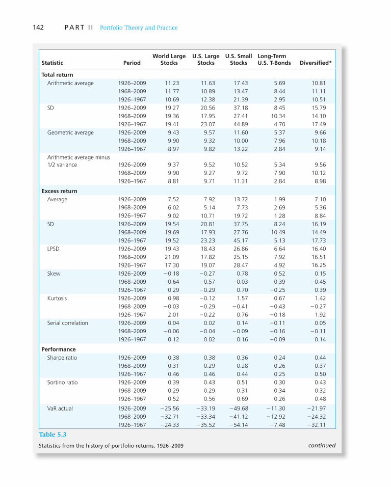
142 P A R T I I Portfolio Theory and Practice
Statistic PeriodWorld Large
StocksU.S. Large
StocksU.S. Small
StocksLong-Term U.S. T-Bonds Diversified*
Total return
Arithmetic average 1926–2009 11.23 11.63 17.43 5.69 10.81
1968–2009 11.77 10.89 13.47 8.44 11.11
1926–1967 10.69 12.38 21.39 2.95 10.51
SD 1926–2009 19.27 20.56 37.18 8.45 15.79
1968–2009 19.36 17.95 27.41 10.34 14.10
1926–1967 19.41 23.07 44.89 4.70 17.49
Geometric average 1926–2009 9.43 9.57 11.60 5.37 9.66
1968–2009 9.90 9.32 10.00 7.96 10.18
1926–1967 8.97 9.82 13.22 2.84 9.14
Arithmetic average minus
1/2 variance 1926–2009 9.37 9.52 10.52 5.34 9.56
1968–2009 9.90 9.27 9.72 7.90 10.12
1926–1967 8.81 9.71 11.31 2.84 8.98
Excess return
Average 1926–2009
1968–2009
1926–1967
7.52 7.92 13.72 1.99 7.10
6.02 5.14 7.73 2.69 5.36
9.02 10.71 19.72 1.28 8.84
SD 1926–2009 19.54 20.81 37.75 8.24 16.19
1968–2009 19.69 17.93 27.76 10.49 14.49
1926–1967 19.52 23.23 45.17 5.13 17.73
LPSD 1926–2009 19.43 18.43 26.86 6.64 16.40
1968–2009 21.09 17.82 25.15 7.92 16.51
1926–1967 17.30 19.07 28.47 4.92 16.25
Skew 1926–2009 �0.18 �0.27 0.78 0.52 0.15
1968–2009 �0.64 �0.57 �0.03 0.39 �0.45
1926–1967 0.29 �0.29 0.70 �0.25 0.39
Kurtosis 1926–2009 0.98 �0.12 1.57 0.67 1.42
1968–2009 �0.03 �0.29 �0.41 �0.43 �0.27
1926–1967 2.01 �0.22 0.76 �0.18 1.92
Serial correlation 1926–2009 0.04 0.02 0.14 �0.11 0.05
1968–2009 �0.06 �0.04 �0.09 �0.16 �0.11
1926–1967 0.12 0.02 0.16 �0.09 0.14
Performance
Sharpe ratio 1926–2009 0.38 0.38 0.36 0.24 0.44
1968–2009 0.31 0.29 0.28 0.26 0.37
1926–1967 0.46 0.46 0.44 0.25 0.50
Sortino ratio 1926–2009 0.39 0.43 0.51 0.30 0.43
1968–2009 0.29 0.29 0.31 0.34 0.32
1926–1967 0.52 0.56 0.69 0.26 0.48
VaR actual 1926–2009 �25.56 �33.19 �49.68 �11.30 �21.97
1968–2009 �32.71 �33.34 �41.12 �12.92 �24.32
1926–1967 �24.33 �35.52 �54.14 �7.48 �32.11
continued
Table 5.3
Statistics from the history of portfolio returns, 1926–2009
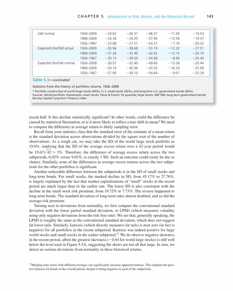
C H A P T E R 5 Introduction to Risk, Return, and the Historical Record 143
recent half. Is this decline statistically significant? In other words, could the difference be caused by statistical fluctuation, or is it more likely to reflect a true shift in mean? We need to compare the difference in average return to likely sampling error.
Recall from your statistics class that the standard error of the estimate of a mean return is the standard deviation across observations divided by the square root of the number of observations. As a rough cut, we may take the SD of the world large stock portfolio as 19.6%, implying that the SD of the average excess return over a 42-year period would
be 19.6/"42 5 3%. Therefore, the difference of average excess return across the two subperiods, 6.02% versus 9.02%, is exactly 1 SD. Such an outcome could easily be due to chance. Similarly, none of the differences in average excess returns across the two subpe-riods for the other portfolios is significant.
Another noticeable difference between the subperiods is in the SD of small stocks and long-term bonds. For small stocks, the marked decline in SD, from 45.17% to 27.76%, is largely explained by the fact that market capitalizations of “small” stocks in the recent period are much larger than in the earlier one. The lower SD is also consistent with the decline in the small stock risk premium, from 19.72% to 7.73%. The reverse happened to long-term bonds. The standard deviation of long-term rates almost doubled, and so did the average risk premium.
Turning next to deviations from normality, we first compare the conventional standard deviation with the lower partial standard deviation, or LPSD (which measures volatility using only negative deviations from the risk-free rate). We see that, generally speaking, the LPSD is roughly the same as the conventional standard deviation, which does not suggest fat lower tails. Similarly, kurtosis (which directly measures fat tails) is near zero (in fact is negative) for all portfolios in the recent subperiod. Kurtosis was indeed positive for large world stocks and small stocks in the earlier subperiod. 11 We do observe negative skewness in the recent period, albeit the greatest skewness (�0.64 for world large stocks) is still well below the level used in Figure 5.5 A, suggesting the skews are not all that large. In sum, we detect no serious deviations from normality in these historical returns.
11 Merging time series with different averages can significantly increase apparent kurtosis. This explains the posi-tive kurtosis for bonds in the overall period, despite it being negative in each of the subperiods.
VaR normal 1926–2009 �24.62 �26.31 �48.37 �11.56 �19.53
1968–2009 �26.36 �24.35 �37.94 �13.58 �19.37
1926–1967 �23.08 �27.51 �54.57 �7.16 �20.32
Expected shortfall actual 1926–2009 �35.94 �38.68 �53.19 �12.32 �27.51
1968–2009 �37.28 �35.40 �42.62 �13.15 �26.70
1926–1967 �30.13 �39.50 �54.58 �8.90 �25.40
Expected shortfall normal 1926–2009 �30.57 �32.40 �49.60 �13.28 �25.44
1968–2009 �33.19 �30.36 �43.25 �16.33 �25.69
1926–1967 �27.95 �34.10 �54.64 �9.07 �25.29
* Portfolio constructed of world large stocks (50%), U. S. small stocks (20%), and long-term U.S. government bonds (30%). Sources: World portfolio: Datastream; small stocks: Fama & French 1st quantile; large stocks: S&P 500; long-term government bonds: Barclay Capital Long-term Treasury index.
Table 5.3 —concluded
Statistics from the history of portfolio returns, 1926–2009

144 P A R T I I Portfolio Theory and Practice
Serial correlation in excess returns (either positive or negative) would suggest that investors can predict future from past returns and profit from reallocating funds across portfolios on the basis of past returns. Hence, we expect serial correlation of returns in well-functioning capital markets to be negligible. Indeed, the low level of serial correlation in the data assures us that investors cannot expect to produce higher returns on the basis of a rule as simple as serial correlation.
Performance
When asset returns are normally distributed, investors may assess performance using the reward-to-volatility ratio, that is, the Sharpe ratio, which divides average excess returns by standard deviation. The investments we are looking at are all passive, broad asset-class portfolios, that is, they are constructed without any special information about potential superior performance of any individual asset or portfolio. Under these circumstances, we would expect better-diversified portfolios to perform better. The Sharpe ratios of the five portfolios live up to this expectation; for the overall period as well as for each subperiod, the “diversified” portfolio shows the highest Sharpe ratio.
The bond portfolio is least diversified, forgoing all stocks. Thus, despite being the least risky, with the lowest SD by far, it has the lowest Sharpe ratio. The small-stock portfolio, with the highest average excess return but also the highest SD, is the next-worst performer since it is not sufficiently diversified. The bond and small-stock portfolios do improve performance, however, when added to the world large-stock portfolio to achieve broader diversification.
The question is whether deviations from normality would reverse this conclusion. Because the LPSD is generally lower than SD, particularly over the earlier period, replac-ing the Sharpe ratio with the Sortino ratio (the ratio of average excess return to LPSD) actually increases the performance measure of the stock portfolios. This leaves us with a conundrum: the recent financial crisis has led some to argue that deviations from normality render portfolios riskier and performance inferior to what we measure with the assumption of normality. But, if anything, these results suggest the opposite.
Nevertheless, turning to risk measures that directly focus directly on extreme outcomes, value at risk (VaR) and expected shortfall (ES), we see from the following tables that esti-mates of these measures for large stocks from the historical record display more extreme losses than would be expected under the assumption of normality. That is, actual VaR values as well as expected shortfall are higher than would be observed under the normal distribution. As neither LPSD nor kurtosis is out of line with normality, it seems that these results must be due to the negative skew of historical returns. We must treat these conclu-sions as tentative, however, since these estimates are measured with considerable impreci-sion. Notice also that for the most diversified portfolio, the differences are smaller, since they are driven by the large-stock portfolios.
Difference between Expected VaR Assuming a Normal Distribution and the Historical VaR
World Large Stocks
U.S. Large Stocks
U.S. Small Stocks
Long-Term U.S. T-Bonds Diversified
1926–2009 0.94 6.88 1.32 �0.26 2.45
1968–2009 6.35 8.99 3.18 �0.67 4.95
1926–1967 1.24 8.02 �0.43 0.33 1.06
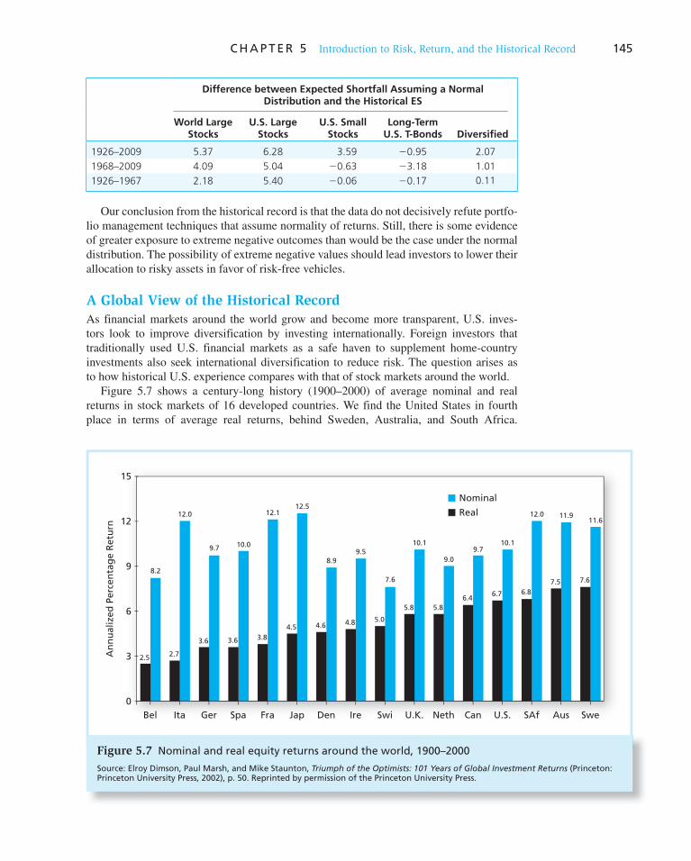
C H A P T E R 5 Introduction to Risk, Return, and the Historical Record 145
Difference between Expected Shortfall Assuming a Normal Distribution and the Historical ES
World Large Stocks
U.S. Large Stocks
U.S. Small Stocks
Long-Term U.S. T-Bonds Diversified
1926–2009 5.37 6.28 3.59 �0.95 2.07
1968–2009 4.09 5.04 �0.63 �3.18 1.01
1926–1967 2.18 5.40 �0.06 �0.17 0.11
Our conclusion from the historical record is that the data do not decisively refute portfo-lio management techniques that assume normality of returns. Still, there is some evidence of greater exposure to extreme negative outcomes than would be the case under the normal distribution. The possibility of extreme negative values should lead investors to lower their allocation to risky assets in favor of risk-free vehicles.
A Global View of the Historical Record
As financial markets around the world grow and become more transparent, U.S. inves-tors look to improve diversification by investing internationally. Foreign investors that t raditionally used U.S. financial markets as a safe haven to supplement home-country investments also seek international diversification to reduce risk. The question arises as to how historical U.S. experience compares with that of stock markets around the world.
Figure 5.7 shows a century-long history (1900–2000) of average nominal and real returns in stock markets of 16 developed countries. We find the United States in fourth place in terms of average real returns, behind Sweden, Australia, and South Africa.
Figure 5.7 Nominal and real equity returns around the world, 1900–2000
Source: Elroy Dimson, Paul Marsh, and Mike Staunton, Triumph of the Optimists: 101 Years of Global Investment Returns (Princeton: Princeton University Press, 2002), p. 50. Reprinted by permission of the Princeton University Press.
An
nu
alize
d P
erc
en
tag
e R
etu
rn
15
Real
Nominal
Bel
2.5
8.2
2.7
12.0
3.6
9.7
3.6
10.0
3.8
12.1
4.5
12.5
4.6
8.9
4.8
9.5
5.0
7.6
5.8
10.1
5.8
9.0
6.4
9.7
6.7
10.1
6.8
12.0
7.5
11.9
7.6
11.6
Ita Ger Spa Fra Jap Den Ire Swi U.K. Neth Can U.S. SAf Aus Swe
12
9
6
3
0

146 P A R T I I Portfolio Theory and Practice
Figure 5.8 shows the standard deviations of real stock and bond returns for these same countries. We find the United States tied with four other countries for third place in terms of lowest standard deviation of real stock returns. So the United States has done well, but not abnormally so, compared with these countries.
One interesting feature of these figures is that the countries with the worst results, mea-sured by the ratio of average real returns to standard deviation, are Italy, Belgium, Germany, and Japan—the countries most devastated by World War II. The top-performing countries are Australia, Canada, and the United States, the countries least devastated by the wars of the twenti-eth century. Another, perhaps more telling feature is the insignificant difference between the real returns in the different countries. The difference between the highest average real rate (Sweden, at 7.6%) and the average return across the 16 countries (5.1%) is 2.5%. Similarly, the difference between the average and the lowest country return (Belgium, at 2.5%) is 2.6%. Using the aver-age standard deviation of 23%, the t -statistic for a difference of 2.6% with 100 observations is
t-Statistic 5Difference in mean
Standard deviation/"n5
2.6
23/"1005 1.3
which is far below conventional levels of statistical significance. We conclude that the U.S. experience cannot be dismissed as an outlier. Hence, using the U.S. stock market as a yard-stick for return characteristics may be reasonable.
These days, practitioners and scholars are debating whether the historical U.S. average risk-premium of large stocks over T-bills of 7.92% ( Table 5.3 ) is a reasonable forecast for the long term. This debate centers around two questions: First, do economic factors that prevailed over that historic period (1926–2009) adequately represent those that may prevail over the forecasting horizon? Second, is the arithmetic average from the available history a good yardstick for long-term forecasts?
Figure 5.8 Standard deviations of real equity and bond returns around the world, 1900–2000
Source: Elroy Dimson, Paul Marsh, and Mike Staunton, Triumph of the Optimists: 101 Years of Global Investment Returns (Princeton: Princeton University Press, 2002), p. 61. Reprinted by permission of the Princeton University Press.
Stan
da
rd D
evi
ati
on
of
An
nu
al R
eal R
etu
rn (
%)
35
Equities
Bonds
Can
17
11
18
13
20
15
20
12
20
10
20
8
21
9
22
12
22
13
23
12
23
11
23
13
23
14
29
14
30
21
32
16
Aus U.K. U.S. Swi Neth Spa Ire Bel SAf Swe Fra Ita Jap GerDen
30
25
20
15
10
5
0

C H A P T E R 5 Introduction to Risk, Return, and the Historical Record 147
5.9 Long-Term Investments *
* The material in this and the next subsection addresses important and ongoing debates about risk and return, but is more challenging. It may be skipped in shorter courses without impairing the ability to understand later chapters.
Consider an investor saving $1 today toward retirement in 25 years, or 300 months. Investing the dollar in a risky stock portfolio (reinvesting dividends until retirement) with an expected rate of return of 1% per month, this retirement “fund” is expected to grow almost 20-fold to a terminal value of (1 � .01) 300 � $19.79 (providing total growth of 1,879%). Compare this impressive result to a 25-year investment in a safe Treasury bond with a monthly return of .5% that grows by retirement to only 1.005300 � $4.46. We see that a monthly risk pre-mium of just .5% produces a retirement fund that is more than four times that of the risk-free alternative. Such is the power of compound interest. Why, then, would anyone invest in the Treasuries? Obviously, this is an issue of trading excess return for risk. What is the nature of this return-to-risk trade-off? The risk of an investment that compounds at fluctuating rates over the long run is important, but is widely misunderstood.
We can construct the probability distribution of the stock-fund terminal value from a bino-mial tree just as we did earlier for the newspaper stand, except that instead of adding monthly profits, the portfolio value compounds monthly by a rate drawn from a given distribution. For example, suppose we can approximate the portfolio monthly distribution as follows: Each month the rate of return is either 5.54% or �3.54%, with equal probabilities of .5. This con-figuration generates an expected return of 1% per month. The portfolio volatility is measured
as the monthly standard deviation: ".5 3 (5.54 2 1)2 1 .5 3 (23.54 2 1)2 5 4.54%. After 2 months, the event tree looks like this:
Portfolio value = $1 × 1.0554 × 1.0554 = $1.1139
Portfolio value = $1 × 1.0554 × .9646 = $1.0180
Portfolio value = $1 × .9646 × .9646 = $.9305
“Growing” the tree for 300 months will result in 301 different possible outcomes. The probability of each outcome can be obtained from Excel’s BINOMDIST function. From the 301 possible outcomes and associated probabilities we compute the mean ($19.79) and the standard deviation ($18.09) of the terminal value. Can we use this standard deviation as a measure of risk to be weighed against the risk premium of 19.79 � 4.29 � 15.5 (1,550%)? Recalling the effect of asymmetry on the validity of standard deviation as a measure of risk, we must first view the shape of the probability distribution at the end of the tree.
Figure 5.9 plots the probability of possible outcomes against the terminal value. The asymmetry of the distribution is striking. The highly positive skewness suggests the stan-dard deviation of terminal value will not be useful in this case. Indeed, the binomial dis-tribution, when period returns compound, converges to a lognormal, rather than a normal, distribution. The lognormal describes the distribution of a variable whose logarithm is normally distributed.
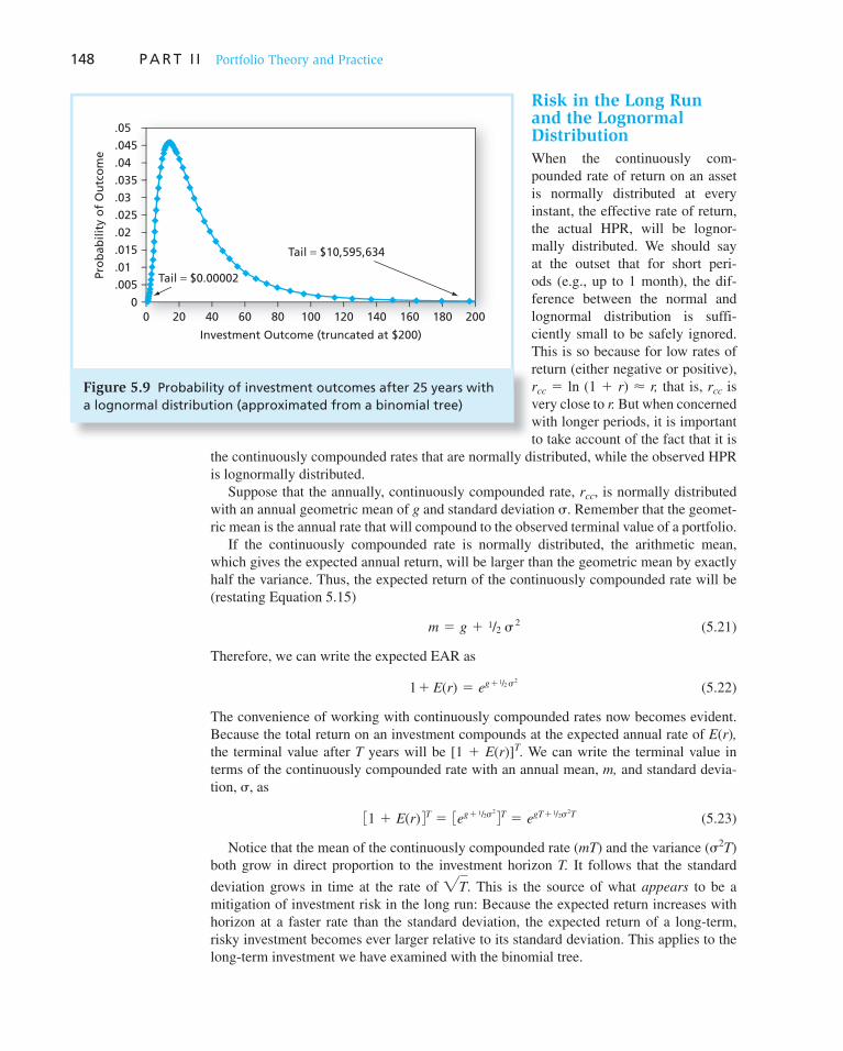
148 P A R T I I Portfolio Theory and Practice
Risk in the Long Run and the Lognormal Distribution
When the continuously com-pounded rate of return on an asset is normally distributed at every instant, the effective rate of return, the actual HPR, will be lognor-mally distributed. We should say at the outset that for short peri-ods (e.g., up to 1 month), the dif-ference between the normal and lognormal distribution is suffi-ciently small to be safely ignored. This is so because for low rates of return (either negative or positive), r cc � ln (1 � r ) � r, that is, r cc is very close to r. But when concerned with longer periods, it is important to take account of the fact that it is
the continuously compounded rates that are normally distributed, while the observed HPR is lognormally distributed.
Suppose that the annually, continuously compounded rate, r cc , is normally distributed with an annual geometric mean of g and standard deviation � . Remember that the geomet-ric mean is the annual rate that will compound to the observed terminal value of a portfolio.
If the continuously compounded rate is normally distributed, the arithmetic mean, which gives the expected annual return, will be larger than the geometric mean by exactly half the variance. Thus, the expected return of the continuously compounded rate will be (restating Equation 5.15 )
m 5 g 1 1/2 � 2 (5.21)
Therefore, we can write the expected EAR as
11 E(r) 5 eg11/2 �2
(5.22)
The convenience of working with continuously compounded rates now becomes evident. Because the total return on an investment compounds at the expected annual rate of E ( r ) ,the terminal value after T years will be [1 � E ( r )] T . We can write the terminal value in terms of the continuously compounded rate with an annual mean, m, and standard devia-tion, � , as
31 1 E(r) 4T 5 3eg11/2�2 4T 5 egT11/2�2T (5.23)
Notice that the mean of the continuously compounded rate ( mT ) and the variance ( � 2 T ) both grow in direct proportion to the investment horizon T. It follows that the standard
deviation grows in time at the rate of "T. This is the source of what appears to be a mitigation of investment risk in the long run: Because the expected return increases with horizon at a faster rate than the standard deviation, the expected return of a long-term, risky investment becomes ever larger relative to its standard deviation. This applies to the long-term investment we have examined with the binomial tree.
Figure 5.9 Probability of investment outcomes after 25 years with a lognormal distribution (approximated from a binomial tree)
0
.005
.01
.015
.02
.025
.03
.035
.04
.045
.05
0 20 40 60 80 100 120 140 160 180 200
Pro
bab
ilit
y o
f O
utc
om
e
Investment Outcome (truncated at $200)
Tail = $0.00002
Tail = $10,595,634
C H A P T E R 5 Introduction to Risk, Return, and the Historical Record 149
Example 5.11 Shortfall Risk in the Short Run and the Long Run
Suppose we wish to estimate the probability that an indexed stock portfolio provides a rate of return less than that on risk-free T-bills. This is called a return shortfall. In line with historical experience, we will assume the monthly HPR on the investment is drawn from a lognormal distribution with an expected continuously compounded rate of rcc � .96% and monthly standard deviation of � � 4.5%. The monthly risk-free rate is taken to be .5%. The index underperforms bills if its return during the month is less than .5%, which is (.96 � .50)/4.5 � .102 standard deviations below its mean. The probability of this event if returns are normally distributed is .46.
Now consider the probability of shortfall for a 25-year (300-month) horizon. The mean 25-year continuously compounded total return is .96 � 300 � 2.88 (i.e., 288%), and
the standard deviation is .045 3 "300 5 .779 (77.9%). At the same time, the monthly risk-free rate of .5% is equivalent to a 25-year continuously compounded total return of 300 � .5% � 150%.
Because the 25-year continuously compounded rate is also normally distributed, we can easily find the probability that the terminal value of the risky portfolio will be below that of the risk-free investment. The expected total return on the index portfolio exceeds that on bills by 288% � 150% � 138%, and the standard deviation of the 25-year return is 77.9%. Therefore, stocks would have to fall short of their expected return by 138/77.9 � 1.722 standard deviations before they would underperform bills. The probability of this outcome is only 3.8%. The far lower probability of a shortfall appears to vindicate those who advo-cate that investment in the stock market is less risky in the long run. After all, the argument goes, 96.2% of the time, the stock fund will outperform the safe investment, while its expected terminal value is almost four times higher.
A warning: The probability of a shortfall is an incomplete measure of investment risk. Such probability does not take into account the size of potential losses, which for some of the possible outcomes (however unlikely) amount to complete ruin. The worst-case scenarios for the 25-year investment are far worse than for the 1-month investment. We demonstrate the buildup of risk over the long run graphically in Figures 5.10 and 5.11 .
A better way to quantify the risk of a long-term investment would be the market price of insuring it against a shortfall. An insurance premium must take into account both the probability of possible losses and the magnitude of these losses. We show in later chapters how the fair market price of portfolio insurance can be estimated from option-pricing models.
Despite the low probability that a portfolio insurance policy would have to pay up (only 3.8% for the 25-year policy), the magnitude and timing 12 of possible losses would make such long-term insurance surprisingly costly. For example, standard option-pricing models suggest that the value of insurance against shortfall risk over a 10-year horizon would cost nearly 20% of the initial value of the portfolio. And contrary to any intuition that a longer horizon reduces shortfall risk, the value of portfolio insurance increases dramatically with the maturity of the contract. For example, a 25-year policy would be about 50% more costly, or about 30% of the initial portfolio value.
12 By “timing,” we mean that a decline in stock prices is associated with a bad economy when extra income would be most important to an investor. The fact that the insurance policy would pay off in these scenarios contributes to its market value.

150 P A R T I I Portfolio Theory and Practice
The Sharpe Ratio Revisited
The Sharpe ratio (the reward-to-volatility ratio) divides average excess return by its stan-dard deviation. You should be aware, however, that the Sharpe ratio has a time dimension, in that the Sharpe ratio for any given portfolio will vary systematically with the assumed investment holding period.
We have seen that as the holding period grows longer, the average continuously com-pounded return grows proportionally to the investment horizon (this is approximately true as well for short-term effective rates). The standard deviation, however, grows at a slower pace, the square root of time. Therefore, the Sharpe ratio grows with the length of the holding period at the rate of the square root of time. Hence, when comparing Sharpe ratios from a series of monthly rates to those from a series of annual rates, we must first multiply the monthly Sharpe ratio by the square root of 12.
Example 5.12 Sharpe Ratios
For the long-term risky portfolio (with a monthly expected return of 1% and standard deviation of 5%), given a risk-free rate of .5%, the Sharpe ratio is (1 � .5)/5 � .10. The expected
annual return would be 12% and annual standard deviation would be 5% 3 "12 5 16.6% so the Sharpe ratio using annual returns would be (12 � 6)/16.6 � .36, similar to values we find in the historical record of well-diversified portfolios.
Simulation of Long-Term Future Rates of Return
The frequency distributions in Figure 5.6 provide only rough descriptions of the nature of the return distributions and are even harder to interpret for long-term investments. A good way to use history to learn about the distribution of long-term future returns is to simulate these future returns from the available sample. A popular method to accomplish this task is called bootstrapping.
Bootstrapping is a procedure that avoids any assumptions about the return distribution, except that all rates of return in the sample history are equally likely. For example, we could simulate a 25-year sample of possible future returns by sampling (with replacement) 25 randomly selected returns from our available 84-year history. We compound those 25 returns to obtain one possible 25-year holding-period return. This procedure is repeated thousands of times to generate a probability distribution of long-term total returns that is anchored in the historical frequency distribution.
The cardinal decision when embarking on a bootstrapping exercise is the choice of how far into the past we should go to draw observations for “future” return sequences. We will use our entire historical sample so that we are more likely to include low-probability events of extreme value.
One important objective of this exercise is to assess the potential effect of deviations from normality on the probability distribution of a long-term investment in U.S. stocks. For this purpose, we simulate a 25-year distribution of annual returns for large and small stocks and contrast these samples to similar samples drawn from normal distributions that (due to compounding) result in lognormally distributed long-term total returns. Results are shown in Figure 5.10 . Panel A shows frequency distributions of large U.S. stocks, c onstructed by sampling both from actual returns and from the normal distribution. Panel B shows the same frequency distributions for small U.S. stocks. The boxes inside Figure 5.10 show the statistics of the distributions.

C H A P T E R 5 Introduction to Risk, Return, and the Historical Record 151
We first review the results for large stocks in panel A. We see that the difference in frequency distributions between the simulated history and the normal curve is small but distinct. Despite the very small differences between the averages of 1-year and 25-year annual returns, as well as between the standard deviations, the small differences in skew-ness and kurtosis combine to produce significant differences in the probabilities of short-falls and losses, as well as in the potential terminal loss. For small stocks, shown in panel B, the smaller differences in skewness and kurtosis lead to almost identical figures for the probability and magnitude of losses.
What about risk for investors with other long-term horizons? Figure 5.11 compares 25-year to 10-year investments in large and small stocks. For an appropriate compari-son, we must account for the fact that the 10-year investment will be supplemented with a 15-year investment in T-bills. To accomplish this comparison, we bootstrap 15-year samples from the 80-year history of T-bill rates and augment each sample with 10 annual rates drawn from the history of the risky investment. Panels A1 and A2 in Figure 5.11 show the comparison for large stocks. The frequency distributions reveal a substantial difference in the risks of the terminal portfolio. This difference is clearly manifested
Figure 5.10 Annually compounded, 25-year HPRs from bootstrapped history and a normal distribution (50,000 observations)
SDMin 25-year HPR
Avg. 1-year HPRAvg. 25-year HPR
Worst-case terminal loss (%)MaxProbability (loss)Probability (shortfall)SkewKurtosis
*Bootstrapped history
Actual*
12.1310.24 10.29
4.27
−11.53
9528.88
.0095
.1044−.0854
.0040
Normal
12.15
4.32
−6.67
8229.32
.0064
.0603
.1135
−.0121
SDMin 25-year HPR
Avg. 1-year HPRAvg. 25-year HPR
Worst-case terminal loss (%)MaxProbability (loss)Probability (shortfall)SkewKurtosis
*Bootstrapped history
Actual*
17.9712.28 12.21
7.28
−17
9947.03
.0415
.1178
.1362
.0678
Normal
17.95
7.41
−14.9
9848.34
.0428
.1232
.2000
.0598
History Normal
0
1
2
3
4
5
6
7
8
9
10
−15 −10 −5 0 5 10 15 20 25 30 35 40 45
Freq
uen
cy
Rate of Return
B: Small Stocks
0
1
2
3
4
5
6
7
8
9
10
−15 −10 −5 0 5 10 15 20 25 30 35 40 45
Freq
uen
cyA: Large Stocks
History Normal

152 P A R T I I Portfolio Theory and Practice
in the portfolio performance statistics. The same picture arises in panels B1 and B2 for small stocks.
Figure 5.12 shows the trajectories of the wealth indexes of possible outcomes of a 25-year investment in large stocks, compared with the wealth index of the average out-come of a T-bill portfolio. The outcomes of the stock portfolio in Figure 5.12 range from the worst, through the bottom 1% and 5% of terminal value, and up to the mean and median terminal values. The bottom 5% still results in a significant shortfall relative to the T-bill portfolio. In sum, the analysis clearly demonstrates that the notion that investments in stocks become less risky in the long run must be rejected.
Yet many practitioners hold on to the view that investment risk is less pertinent to long-term investors. A typical demonstration shown in the nearby box relies on the fact that the standard deviation (or range of likely outcomes) of annualized returns is lower for longer-term horizons. But the demonstration is silent on the range of total returns.
Figure 5.11 Annually compounded, 25-year HPRs from bootstrapped history (50,000 observations)
A1: 25 Years in Large Stocks
B2: 10 Years in Small Stocks and 15 Years in T-bills
A2: 10 Years in Large Stocks and 15 Years in T-bills
B1: 25 Years in Small Stocks
0
2
4
6
8
10
12
14
−15−10 −5 0 5 10 15 20 25 30 35 40 45
Avg. 25-year HPR
Terminal loss (%)
Probability (loss)
Avg. 1-year HPR 12.13
10.24
4.27
−11.5395
28.88
.0095
SD
Min
Max
Freq
uen
cy
0
2
4
6
8
10
12
14
−15−10 −5 0 5 10 15 20 25 30 35 40 45
Avg. 25-year HPR
Terminal loss (%)
Probability (loss)
Avg. 1-year HPR 17.97
12.28
7.28
−17.0099
47.03
.0415
SD
Min
Max
Freq
uen
cy
0
2
4
6
8
10
12
14
−15−10 −5 0 5 10 15 20 25 30 35 40 45
Avg. 25-year HPR
Terminal loss (%)
Probability (loss)
Avg. 1-year HPR 9.40
7.01
4.44
−10.7794
26.63
.0552
SD
Min
Max
Freq
uen
cy
0
2
4
6
8
10
12
14
−15−10 −5 0 5 10 15 20 25 30 35 40 45
Avg. 25-year HPR
Terminal loss (%)
Probability (loss)Avg. 1-year HPR 7.10
6.272.65
−5.3875
16.02.0127
SDMin
Max
Freq
uen
cy
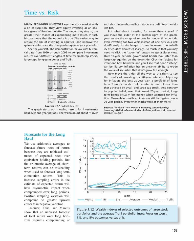
153
Time vs. Risk
MANY BEGINNING INVESTORS eye the stock market with a bit of suspicion. They view equity investing as an anx-ious game of Russian roulette: The longer they stay in, the greater their chance of experiencing more losses. In fact, history shows that the opposite is true. The easiest way to reduce the risk of investing in equities—and improve the gain—is to increase the time you hang on to your portfolio.
See for yourself. The demonstration below uses histori-cal data from 1950 through 2005 to compare investment returns over different lengths of time for small-cap stocks, large caps, long-term bonds and T-bills.
Time vs. Risk
125%100%75%50%25%0%−25%−50%−75%
BondsT–billsLargecap
Smallcap
1–year periodsBest
Average
Worst
zoom in
adjust for inflation
Range of annualized returnsover 1–year periods,
Source: CRSP, Federal Reserve
The graph starts out showing results for investments held over one-year periods. There’s no doubt about it: Over
such short intervals, small-cap stocks are definitely the risk-iest bet.
But what about investing for more than a year? If you move the slider at the bottom right of the graph, you can see the range of returns for longer time periods. Even investing for two years instead of one cuts your risk si gnificantly. As the length of time increases, the volatil-ity of equities decreases sharply—so much so that you may need to click the “zoom in” button to get a closer view. Over 10-year periods, government bonds look safer than large-cap equities on the downside. Click the “adjust for inflation” box, however, and you’ll see that bond “safety” can be illusory. Inflation has an uncanny ability to erode the value of securities that don’t grow fast enough.
Now move the slider all the way to the right to see the results of investing for 20-year intervals. Adjusting for inflation, the best 20-year gain a portfolio of long-term Treasury bonds could muster is much lower than that achieved by small- and large-cap stocks. And contrary to popular belief, over their worst 20-year period, long-term bonds actually lost money when adjusted for infla-tion. Meanwhile, small-cap investors still had gains over a 20-year-period, even when stocks were at their worst.
Source: Abridged from www.smartmoney.com/university/ Investing101/RiskvsReward/index.cfm?story = timevsrisk, accessed October 15, 2007.
WO
RD
S FRO
M TH
E STREET
Figure 5.12 Wealth indexes of selected outcomes of large stock portfolios and the average T-bill portfolio. Inset: Focus on worst, 1%, and 5% outcomes versus bills.
00 5 10 15 20 25
2
4
6
8
10
12
14
16
Worst 1% 5% Average Median T-bills
Years
Wealt
h In
dex
00 5 10 15 20 25
0.5
1
1.5
2
2.5
3
Worst 1% 5% T-bills
Forecasts for the Long Haul
We use arithmetic averages to forecast future rates of return because they are unbiased esti-mates of expected rates over equivalent holding periods. But the arithmetic average of short-term returns can be misleading when used to forecast long-term cumulative returns. This is because sampling errors in the estimate of expected return will have asymmetric impact when compounded over long periods. Positive sampling variation will compound to greater upward errors than negative variation.
Jacquier, Kane, and Marcus show that an unbiased forecast of total return over long hori-zons requires compounding at

Vis
it u
s at
ww
w.m
hh
e.co
m/b
km154 P A R T I I Portfolio Theory and Practice
a weighted average of the arithmetic and geometric historical averages. 13 The proper weight applied to the geometric average equals the ratio of the length of the forecast horizon to the length of the estimation period. For example, if we wish to forecast the cumulative return for a 25-year horizon from a 80-year history, an unbiased estimate would be to compound at a rate of
Geometric average 325
801 Arithmetic average 3
(80 2 25)
80
This correction would take about .6% off the historical arithmetic average risk premium on large stocks and about 2% off the arithmetic average premium of small stocks. A forecast for the next 80 years would require compounding at only the geometric average, and for longer horizons at an even lower number. The forecast horizons that are relevant for cur-rent middle-aged investors would depend on their life expectancies.
13 Eric Jacquier, Alex Kane, and Alan J. Marcus, “Geometric or Arithmetic Means: A Reconsideration,” Financial
Analysts Journal, November/December 2003.
1. The economy’s equilibrium level of real interest rates depends on the willingness of households to save, as reflected in the supply curve of funds, and on the expected profitability of business investment in plant, equipment, and inventories, as reflected in the demand curve for funds. It depends also on government fiscal and monetary policy.
2. The nominal rate of interest is the equilibrium real rate plus the expected rate of inflation. In gen-eral, we can directly observe only nominal interest rates; from them, we must infer expected real rates, using inflation forecasts.
3. The equilibrium expected rate of return on any security is the sum of the equilibrium real rate of interest, the expected rate of inflation, and a security-specific risk premium.
4. Investors face a trade-off between risk and expected return. Historical data confirm our intuition that assets with low degrees of risk provide lower returns on average than do those of higher risk.
5. Assets with guaranteed nominal interest rates are risky in real terms because the future inflation rate is uncertain.
6. Historical rates of return over the twentieth century in developed capital markets suggest the U.S. history of stock returns is not an outlier compared to other countries.
7. Investments in risky portfolios do not become safer in the long run. On the contrary, the longer a risky investment is held, the greater the risk. The basis of the argument that stocks are safe in the long run is the fact that the probability of a shortfall becomes smaller. However, probability of short-fall is a poor measure of the safety of an investment. It ignores the magnitude of possible losses.
8. Historical returns on stocks exhibit more frequent large negative deviations from the mean than would be predicted from a normal distribution. The lower partial standard deviation (LPSD) and the skewness of the actual distribution quantify the deviation from normality. The LPSD, instead of the standard deviation, is sometimes used by practitioners as a measure of risk.
9. Widely used measures of tail risk are value at risk (VaR) and expected shortfall or, equivalently, conditional tail expectations. VaR measures the loss that will be exceeded with a specified prob-ability such as 5%. The VaR does not add new information when returns are normally distributed. When negative deviations from the average are larger and more frequent than the normal distri-bution, the 5% VaR will be more than 1.65 standard deviations below the average return. Con-ditional tail expectations (CTE) measure the expected rate of return conditional on the portfolio falling below a certain value. Thus, 1% CTE is the expected return of all possible outcomes in the bottom 1% of the distribution.
SUMMARY
Related Web sites for this chapter are available at www.mhhe.com/bkm

Vis
it u
s at
ww
w.m
hh
e.co
m/b
km
C H A P T E R 5 Introduction to Risk, Return, and the Historical Record 155
nominal interest rate real interest rate effective annual rate (EAR) annual percentage rate (APR) dividend yield risk-free rate risk premium
excess return risk aversion normal distribution event tree skew kurtosis value at risk (VaR)
expected shortfall (ES) conditional tail expectation
(CTE) lower partial standard
deviation (LPSD) Sortino ratio lognormal distribution
KEY TERMS
1. The Fisher equation tells us that the real interest rate approximately equals the nominal rate minus the inflation rate. Suppose the inflation rate increases from 3% to 5%. Does the Fisher equation imply that this increase will result in a fall in the real rate of interest? Explain.
2. You’ve just stumbled on a new dataset that enables you to compute historical rates of return on U.S. stocks all the way back to 1880. What are the advantages and disadvantages in using these data to help estimate the expected rate of return on U.S. stocks over the coming year?
3. You are considering two alternative 2-year investments: You can invest in a risky asset with a positive risk premium and returns in each of the 2 years that will be identically distributed and uncorrelated, or you can invest in the risky asset for only 1 year and then invest the proceeds in a risk-free asset. Which of the following statements about the first investment alternative (com-pared with the second) are true?
a. Its 2-year risk premium is the same as the second alternative. b. The standard deviation of its 2-year return is the same. c. Its annualized standard deviation is lower. d. Its Sharpe ratio is higher. e. It is relatively more attractive to investors who have lower degrees of risk aversion.
4. You have $5,000 to invest for the next year and are considering three alternatives:
a. A money market fund with an average maturity of 30 days offering a current yield of 6% per year.
b. A 1-year savings deposit at a bank offering an interest rate of 7.5%. c. A 20-year U.S. Treasury bond offering a yield to maturity of 9% per year.
What role does your forecast of future interest rates play in your decisions?
5. Use Figure 5.1 in the text to analyze the effect of the following on the level of real interest rates:
a. Businesses become more pessimistic about future demand for their products and decide to reduce their capital spending.
b. Households are induced to save more because of increased uncertainty about their future Social Security benefits.
c. The Federal Reserve Board undertakes open-market purchases of U.S. Treasury securities in order to increase the supply of money.
6. You are considering the choice between investing $50,000 in a conventional 1-year bank CD offering an interest rate of 5% and a 1-year “Inflation-Plus” CD offering 1.5% per year plus the rate of inflation.
a. Which is the safer investment? b. Which offers the higher expected return? c. If you expect the rate of inflation to be 3% over the next year, which is the better investment?
Why? d. If we observe a risk-free nominal interest rate of 5% per year and a risk-free real rate of 1.5%
on inflation-indexed bonds, can we infer that the market’s expected rate of inflation is 3.5% per year?
PROBLEM SETS
i. Basic
ii. Intermediate

Vis
it u
s at
ww
w.m
hh
e.co
m/b
km156 P A R T I I Portfolio Theory and Practice
7. Suppose your expectations regarding the stock price are as follows:
State of the Market Probability Ending Price HPR (including dividends)
Boom .35 $140 44.5%
Normal growth .30 110 14.0
Recession .35 80 �16.5
Use Equations 5.11 and 5.12 to compute the mean and standard deviation of the HPR on stocks.
8. Derive the probability distribution of the 1-year HPR on a 30-year U.S. Treasury bond with an 8% coupon if it is currently selling at par and the probability distribution of its yield to maturity a year from now is as follows:
State of the Economy Probability YTM
Boom .20 11.0%
Normal growth .50 8.0
Recession .30 7.0
For simplicity, assume the entire 8% coupon is paid at the end of the year rather than every 6 months.
9. What is the standard deviation of a random variable q with the following probability distribution:
Value of q Probability
0 .25
1 .25
2 .50
10. The continuously compounded annual return on a stock is normally distributed with a mean of 20% and standard deviation of 30%. With 95.44% confidence, we should expect its actual return in any particular year to be between which pair of values? Hint: Look again at Figure 5.4 .
a. �40.0% and 80.0% b. �30.0% and 80.0% c. �20.6% and 60.6% d. �10.4% and 50.4%
11. Using historical risk premiums over the 1926–2009 period as your guide, what would be your estimate of the expected annual HPR on the S&P 500 stock portfolio if the current risk-free interest rate is 3%?
12. You can find annual holding-period returns for several asset classes at our Web site ( www.
mhhe.com/bkm ); look for links to Chapter 5. Compute the means, standard deviations, skew-ness, and kurtosis of the annual HPR of large stocks and long-term Treasury bonds using only the 30 years of data between 1980 and 2009. How do these statistics compare with those com-puted from the data for the period 1926–1941? Which do you think are the most relevant statis-tics to use for projecting into the future?
13. During a period of severe inflation, a bond offered a nominal HPR of 80% per year. The infla-tion rate was 70% per year.
a. What was the real HPR on the bond over the year? b. Compare this real HPR to the approximation r � R � i.
14. Suppose that the inflation rate is expected to be 3% in the near future. Using the historical data provided in this chapter, what would be your predictions for:
a. The T-bill rate? b. The expected rate of return on large stocks? c. The risk premium on the stock market?
eXce lPlease visit us at www.mhhe.com/bkm

Vis
it u
s at
ww
w.m
hh
e.co
m/b
km
C H A P T E R 5 Introduction to Risk, Return, and the Historical Record 157
15. An economy is making a rapid recovery from steep recession, and businesses foresee a need for large amounts of capital investment. Why would this development affect real interest rates?
Challenge Problems 16 and 17 are more difficult. You may need to review the defini-tions of call and put options in Chapter 2.
16. You are faced with the probability distribution of the HPR on the stock market index fund given in Spreadsheet 5.1 of the text. Suppose the price of a put option on a share of the index fund with exercise price of $110 and time to expiration of 1 year is $12.
a. What is the probability distribution of the HPR on the put option? b. What is the probability distribution of the HPR on a portfolio consisting of one share of the
index fund and a put option? c. In what sense does buying the put option constitute a purchase of insurance in this case?
17. Take as given the conditions described in the previous problem, and suppose the risk-free inter-est rate is 6% per year. You are contemplating investing $107.55 in a 1-year CD and simultane-ously buying a call option on the stock market index fund with an exercise price of $110 and expiration of 1 year. What is the probability distribution of your dollar return at the end of the year?
iii. Challenge
1. Given $100,000 to invest, what is the expected risk premium in dollars of investing in equities versus risk-free T-bills (U.S. Treasury bills) based on the following table?
Action Probability Expected Return
Invest in equities .6 $50,000
.4 �$30,000
Invest in risk-free T-bill 1.0 $ 5,000
2. Based on the scenarios below, what is the expected return for a portfolio with the following return profile?
Market Condition
Bear Normal Bull
Probability .2 .3 .5
Rate of return �25% 10% 24%
Use the following scenario analysis for Stocks X and Y to answer CFA Problems 3 through 6 (round to the nearest percent).
Bear Market Normal Market Bull Market
Probability 0.2 0.5 0.3
Stock X �20% 18% 50%
Stock Y �15% 20% 10%
3. What are the expected rates of return for Stocks X and Y?
4. What are the standard deviations of returns on Stocks X and Y?
5. Assume that of your $10,000 portfolio, you invest $9,000 in Stock X and $1,000 in Stock Y. What is the expected return on your portfolio?

Vis
it u
s at
ww
w.m
hh
e.co
m/b
km158 P A R T I I Portfolio Theory and Practice
6. Probabilities for three states of the economy and probabilities for the returns on a particular stock in each state are shown in the table below.
State of EconomyProbability of
Economic StateStock Performance
Probability of Stock Performance in Given Economic State
Good .3 Good .6
Neutral .3
Poor .1
Neutral .5 Good .4
Neutral .3
Poor .3
Poor .2 Good .2
Neutral .3
Poor .5
What is the probability that the economy will be neutral and the stock will experience poor performance?
7. An analyst estimates that a stock has the following probabilities of return depending on the state of the economy:
State of Economy Probability Return
Good .1 15%
Normal .6 13
Poor .3 7
What is the expected return of the stock?
Inflation and Rates
The Federal Reserve Bank of St. Louis has information available on interest rates and eco-nomic conditions. A publication called Monetary Trends contains graphs and tables with information about current conditions in the capital markets. Go to the Web site www.
stls.frb.org and click on Economic Research on the menu at the top of the page. Find the most recent issue of Monetary Trends in the Recent Data Publications section and answer these questions.
1. What is the professionals’ consensus forecast for inflation for the next 2 years? (Use the Federal Reserve Bank of Philadelphia line on the graph to answer this.)
2. What do consumers expect to happen to inflation over the next 2 years? (Use the Un iversity of Michigan line on the graph to answer this.)
3. Have real interest rates increased, decreased, or remained the same over the last 2 years?
4. What has happened to short-term nominal interest rates over the last 2 years? What about long-term nominal interest rates?
5. How do recent U.S. inflation and long-term interest rates compare with those of the other countries listed?
6. What are the most recently available levels of 3-month and 10-year yields on Treasury securities?
E-INVEST-MENTS EXERCISES

Vis
it u
s at
ww
w.m
hh
e.co
m/b
km
C H A P T E R 5 Introduction to Risk, Return, and the Historical Record 159
SOLUTIONS TO CONCEPT CHECKS
1. a. 1 1 R 5 (1 1 r)(1 1 i) 5 (1.03)(1.08) 5 1.1124 R 5 11.24%
b. 1 1 R 5 (1.03)(1.10) 5 1.133 R 5 13.3%
2. a. EAR � (1 � .01) 12 � 1 � .1268 � 12.68%
b. EAR � e .12 � 1 � .1275 � 12.75%
Choose the continuously compounded rate for its higher EAR.
3. Number of bonds bought is 27,000/900 � 30
Interest Rates Probability Year-end Bond Price HPR End-of-Year Value
High .2 $850 (75 � 850)/900 � 1 � .0278 (75 � 850)30 � $27,750
Unchanged .5 915 .1000 $29,700
Low .3 985 .1778 $31,800
Expected rate of return .1089
Expected end-of-year
dollar value $29,940
Risk premium .0589
4. (1 1 Required rate)(1 2 .386) 5 1
Required rate 5 .6287, or 62.87%
5. a. Arithmetic return � (1/3)(.2869) � (1/3)(.1088) � (1/3)(0.0491) � .1483 � 14.83%
b. Geometric average 53 "1.2869 3 1.1088 3 1.0491 2 1 5 .1439 5 14.39%
c. Standard deviation � 12.37%
d. Sharpe ratio � (14.83 � 6.0)/12.37 � .71
6. The probability of a more extreme bad month, with return below �15%, is much lower: NORMDIST(�15,1,6,TRUE) � .00383. Alternatively, we can note that �15% is 16/6 standard deviations below the mean return, and use the standard normal function to compute NORMSDIST(�16/6) � .00383.
7. If the probabilities in Spreadsheet 5.2 represented the true return distribution, we would use Equations 5.19 and 5.20 to obtain: Skew � 0.0931; Kurtosis � �1.2081. However, in this case, the data in the table represent a (short) historical sample, and correction for degrees-of-freedom bias is required (in a similar manner to our calculations for standard deviation). You can use Excel functions to obtain: SKEW(C5:C9) � 0.1387; KURT(C5:C9) � �0.2832.

6 6 THE PROCESS OF constructing an investor
portfolio can be viewed as a sequence of
two steps: (1) selecting the composition of
one’s portfolio of risky assets such as stocks
and long-term bonds, and (2) deciding how
much to invest in that risky portfolio versus in
a safe asset such as short-term Treasury bills.
Obviously, an investor cannot decide how to
allocate investment funds between the risk-
free asset and that risky portfolio without
knowing its expected return and degree of
risk, so a fundamental part of the asset alloca-
tion problem is to characterize the risk–return
trade-off for this portfolio.
While the task of constructing an opti-
mal risky portfolio is technically complex, it
can be delegated to a professional because
it largely entails well-defined optimization
techniques. In contrast, the decision of how
much to invest in that portfolio depends
on an investor’s personal preferences about
risk versus expected return, and therefore it
cannot easily be delegated. As we will see
in the chapter on behavioral finance, many
investors stumble over this cardinal step.
We therefore begin our journey into port-
folio theory by establishing a framework to
explore this fundamental decision, namely,
capital allocation between the risk-free and
the risky portfolio.
We begin by introducing two themes in
portfolio theory that are centered on risk.
The first is the tenet that investors will avoid
risk unless they can anticipate a reward for
engaging in risky investments. The second
theme allows us to quantify investors’ per-
sonal trade-offs between portfolio risk and
expected return. To do this we introduce a
personal utility function, which allows each
investor to assign welfare or “utility” scores to
alternative portfolios on the basis of expected
return and risk and choose the portfolio with
the highest score. We elaborate on the histor-
ical and empirical basis for the utility model in
the appendix to this chapter.
Armed with the utility model, we can
resolve the investment decision that is most
consequential to investors, that is, how much
of their wealth to put at risk for the greater
expected return that can thus be achieved. We
assume that the construction of the risky port-
folio from the universe of available risky assets
has already taken place and defer the discus-
sion of how to construct that risky portfolio
to the next chapter. At this point the investor
can assess the expected return and risk of the
overall portfolio. Using the expected return
and risk parameters in the utility model yields
the optimal allocation of capital between the
risky portfolio and risk-free asset.
Risk Aversion and Capital Allocation to Risky Assets
CHAPTER SIX PA
RT
II
C H A P T E R 6 Risk Aversion and Capital Allocation to Risky Assets 161
6.1 Risk and Risk Aversion
In Chapter 5 we introduced the concepts of the holding-period return (HPR) and the excess return over the risk-free rate. We also discussed estimation of the risk premium (the expected excess return) and the standard deviation of the rate of return, which we use as the measure of portfolio risk. We demonstrated these concepts with a scenario analysis of a specific risky portfolio (Spreadsheet 5.1). To emphasize that bearing risk typically must be accompanied by a reward in the form of a risk premium, we first distinguish between speculation and gambling.
Risk, Speculation, and Gambling
One definition of speculation is “the assumption of considerable investment risk to obtain commensurate gain.” Although this definition is fine linguistically, it is useless without first specifying what is meant by “considerable risk” and “commensurate gain.”
By “considerable risk” we mean that the risk is sufficient to affect the decision. An indi-vidual might reject an investment that has a positive risk premium because the potential gain is insufficient to make up for the risk involved. By “commensurate gain” we mean a positive risk premium, that is, an expected profit greater than the risk-free alternative.
To gamble is “to bet or wager on an uncertain outcome.” If you compare this definition to that of speculation, you will see that the central difference is the lack of “commensu-rate gain.” Economically speaking, a gamble is the assumption of risk for no purpose but enjoyment of the risk itself, whereas speculation is undertaken in spite of the risk involved because one perceives a favorable risk–return trade-off. To turn a gamble into a speculative prospect requires an adequate risk premium to compensate risk-averse investors for the risks they bear. Hence, risk aversion and speculation are not inconsistent. Notice that a risky investment with a risk premium of zero, sometimes called a fair game, amounts to a gamble. A risk-averse investor will reject it.
In some cases a gamble may appear to the participants as speculation. Suppose two investors disagree sharply about the future exchange rate of the U.S. dollar against the British pound. They may choose to bet on the outcome. Suppose that Paul will pay Mary $100 if the value of £1 exceeds $1.60 one year from now, whereas Mary will pay Paul if the pound is worth less than $1.60. There are only two relevant outcomes: (1) the pound will exceed $1.60, or (2) it will fall below $1.60. If both Paul and Mary agree on the prob-abilities of the two possible outcomes, and if neither party anticipates a loss, it must be that they assign p � .5 to each outcome. In that case the expected profit to both is zero and each has entered one side of a gambling prospect.
What is more likely, however, is that the bet results from differences in the probabilities that Paul and Mary assign to the outcome. Mary assigns it p > .5, whereas Paul’s assess-ment is p < .5. They perceive, subjectively, two different prospects. Economists call this case of differing beliefs “heterogeneous expectations.” In such cases investors on each side of a financial position see themselves as speculating rather than gambling.
Both Paul and Mary should be asking, Why is the other willing to invest in the side of a risky prospect that I believe offers a negative expected profit? The ideal way to resolve heterogeneous beliefs is for Paul and Mary to “merge their information,” that is, for each party to verify that he or she possesses all relevant information and processes the informa-tion properly. Of course, the acquisition of information and the extensive communication that is required to eliminate all heterogeneity in expectations is costly, and thus up to a point heterogeneous expectations cannot be taken as irrational. If, however, Paul and Mary enter such contracts frequently, they would recognize the information problem in one of

162 P A R T I I Portfolio Theory and Practice
two ways: Either they will realize that they are creating gambles when each wins half of the bets, or the consistent loser will admit that he or she has been betting on the basis of inferior forecasts.
Risk Aversion and Utility Values
The history of rates of return on various asset classes presented in Chapter 5, as well as numerous elaborate empirical studies, leave no doubt that risky assets command a risk pre-mium in the marketplace. This implies that most investors are risk averse.
Investors who are risk averse reject investment portfolios that are fair games or worse. Risk-averse investors are willing to consider only risk-free or speculative prospects with positive risk premiums. Loosely speaking, a risk-averse investor “penalizes” the expected rate of return of a risky portfolio by a certain percentage (or penalizes the expected profit by a dollar amount) to account for the risk involved. The greater the risk, the larger the penalty. One might wonder why we assume risk aversion as fundamental. We believe that most investors would accept this view from simple introspection, but we discuss the ques-tion more fully in Appendix A of this chapter.
To illustrate the issues we confront when choosing among portfolios with varying degrees of risk, consider a specific example. Suppose the risk-free rate is 5% and that an investor considers three alternative risky portfolios with risk premiums, expected returns, and standard deviations as given in Table 6.1 . The risk premiums and degrees of risk (stan-dard deviation, SD) of the portfolios in the table are chosen to represent the properties of low-risk bonds ( L ), high-risk bonds ( M ), and large stocks ( H ). Accordingly, these portfo-lios offer progressively higher risk premiums to compensate for greater risk. How might investors choose among them?
Intuitively, one would rank each portfolio as more attractive when its expected return is higher, and lower when its risk is higher. But when risk increases along with return, the most attractive portfolio is not obvious. How can investors quantify the rate at which they are willing to trade off return against risk?
We will assume that each investor can assign a welfare, or utility, score to competing investment portfolios on the basis of the expected return and risk of those portfolios. Higher utility values are assigned to portfolios with more attractive risk–return profiles. Portfolios receive higher utility scores for higher expected returns and lower scores for higher vola-tility. Many particular “scoring” systems are legitimate. One reasonable f unction that has
CONCEPT CHECK
1
Assume that dollar-denominated T-bills in the United States and pound-denominated bills in the United Kingdom offer equal yields to maturity. Both are short-term assets, and both are free of default risk. Neither offers investors a risk premium. However, a U.S. investor who holds U.K. bills is subject to exchange rate risk, because the pounds earned on the U.K. bills eventually will be exchanged for dollars at the future exchange rate. Is the U.S. investor engaging in speculation or gambling?
Table 6.1
Available risky portfolios (Risk-free rate � 5%)
Portfolio Risk Premium Expected Return Risk (SD)
L (low risk) 2% 7% 5%
M (medium risk) 4 9 10
H (high risk) 8 13 20
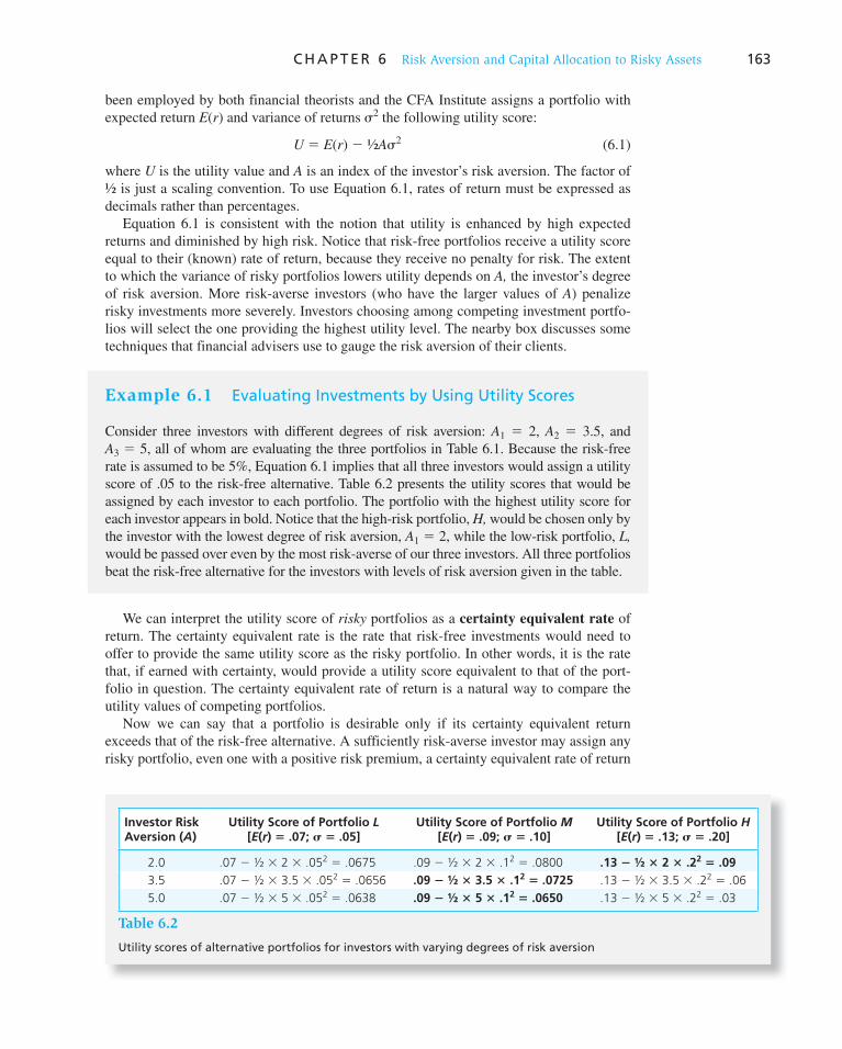
C H A P T E R 6 Risk Aversion and Capital Allocation to Risky Assets 163
been employed by both financial theorists and the CFA Institute assigns a portfolio with expected return E ( r ) and variance of returns � 2 the following utility score:
U 5 E(r) 2 ½A�2 (6.1)
where U is the utility value and A is an index of the investor’s risk aversion. The factor of ½ is just a scaling convention. To use Equation 6.1 , rates of return must be expressed as decimals rather than percentages.
Equation 6.1 is consistent with the notion that utility is enhanced by high expected returns and diminished by high risk. Notice that risk-free portfolios receive a utility score equal to their (known) rate of return, because they receive no penalty for risk. The extent to which the variance of risky portfolios lowers utility depends on A, the investor’s degree of risk aversion. More risk-averse investors (who have the larger values of A ) penalize risky investments more severely. Investors choosing among competing investment portfo-lios will select the one providing the highest utility level. The nearby box discusses some techniques that financial advisers use to gauge the risk aversion of their clients.
Example 6.1 Evaluating Investments by Using Utility Scores
Consider three investors with different degrees of risk aversion: A 1 � 2, A 2 � 3.5, and A 3 � 5, all of whom are evaluating the three portfolios in Table 6.1 . Because the risk-free rate is assumed to be 5%, Equation 6.1 implies that all three investors would assign a utility score of .05 to the risk-free alternative. Table 6.2 presents the utility scores that would be assigned by each investor to each portfolio. The portfolio with the highest utility score for each investor appears in bold. Notice that the high-risk portfolio, H, would be chosen only by the investor with the lowest degree of risk aversion, A 1 � 2, while the low-risk portfolio, L, would be passed over even by the most risk-averse of our three investors. All three portfolios beat the risk-free alternative for the investors with levels of risk aversion given in the table.
We can interpret the utility score of risky portfolios as a certainty equivalent rate of return. The certainty equivalent rate is the rate that risk-free investments would need to offer to provide the same utility score as the risky portfolio. In other words, it is the rate that, if earned with certainty, would provide a utility score equivalent to that of the port-folio in question. The certainty equivalent rate of return is a natural way to compare the utility values of competing portfolios.
Now we can say that a portfolio is desirable only if its certainty equivalent return exceeds that of the risk-free alternative. A sufficiently risk-averse investor may assign any risky portfolio, even one with a positive risk premium, a certainty equivalent rate of return
Table 6.2
Utility scores of alternative portfolios for investors with varying degrees of risk aversion
Investor Risk Aversion (A)
Utility Score of Portfolio L [E(r) � .07; � � .05]
Utility Score of Portfolio M [E(r) � .09; � � .10]
Utility Score of Portfolio H [E(r) � .13; � � .20]
2.0 .07 � ½ � 2 � .052 � .0675 .09 � ½ � 2 � .12 � .0800 .13 � ½ � 2 � .22 � .09
3.5 .07 � ½ � 3.5 � .052 � .0656 .09 � ½ � 3.5 � .12 � .0725 .13 � ½ � 3.5 � .22 � .06
5.0 .07 � ½ � 5 � .052 � .0638 .09 � ½ � 5 � .12 � .0650 .13 � ½ � 5 � .22 � .03

164 P A R T I I Portfolio Theory and Practice
that is below the risk-free rate, which will cause the investor to reject the risky portfolio. At the same time, a less risk-averse investor may assign the same portfolio a certainty equiva-lent rate that exceeds the risk-free rate and thus will prefer the portfolio to the risk-free alternative. If the risk premium is zero or negative to begin with, any downward adjustment to utility only makes the portfolio look worse. Its certainty equivalent rate will be below that of the risk-free alternative for all risk-averse investors.
In contrast to risk-averse investors, risk-neutral investors (with A � 0) judge risky prospects solely by their expected rates of return. The level of risk is irrelevant to the risk-neutral investor, meaning that there is no penalty for risk. For this investor a portfolio’s certainty equivalent rate is simply its expected rate of return.
A risk lover (for whom A < 0) is happy to engage in fair games and gambles; this inves-tor adjusts the expected return upward to take into account the “fun” of confronting the prospect’s risk. Risk lovers will always take a fair game because their upward adjustment of utility for risk gives the fair game a certainty equivalent that exceeds the alternative of the risk-free investment.
We can depict the individual’s trade-off between risk and return by plotting the charac-teristics of potential investment portfolios that the individual would view as equally attrac-tive on a graph with axes measuring the expected value and standard deviation of portfolio returns. Figure 6.1 plots the characteristics of one portfolio denoted P.
Portfolio P, which has expected return E ( r P ) and standard deviation � P , is preferred by risk-averse investors to any portfolio in quadrant IV because it has an expected return equal to or greater than any portfolio in that quadrant and a standard deviation equal to or smaller than any portfolio in that quadrant. Conversely, any portfolio in quadrant I is
CONCEPT CHECK
2 A portfolio has an expected rate of return of 20% and standard deviation of 30%. T-bills offer a safe rate of return of 7%. Would an investor with risk-aversion parameter A � 4 pre-fer to invest in T-bills or the risky portfolio? What if A � 2?
Figure 6.1 The trade-off between risk and return of a potential investment portfolio, P
P
E(rP)
E(r)
σP
σ
I II
III IV
Northwest(preferred direction)
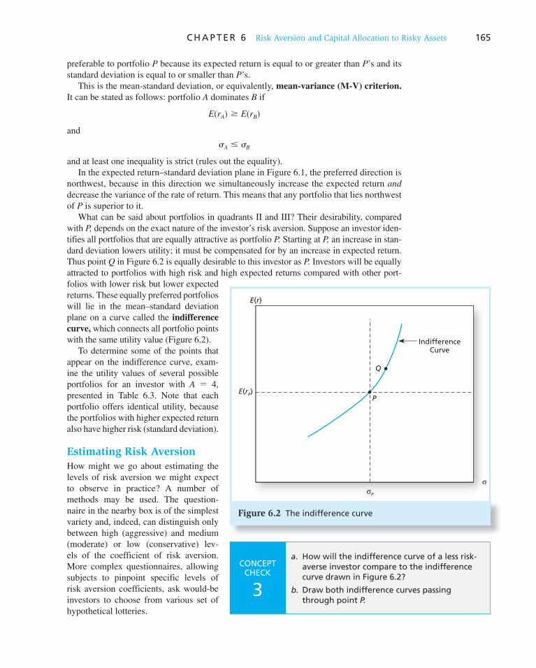
C H A P T E R 6 Risk Aversion and Capital Allocation to Risky Assets 165
preferable to portfolio P because its expected return is equal to or greater than P ’s and its standard deviation is equal to or smaller than P ’s.
This is the mean-standard deviation, or equivalently, mean-variance (M-V) criterion.
It can be stated as follows: portfolio A dominates B if
E(rA) $ E(rB)
and
�A # �B
and at least one inequality is strict (rules out the equality). In the expected return–standard deviation plane in Figure 6.1 , the preferred direction is
northwest, because in this direction we simultaneously increase the expected return and
decrease the variance of the rate of return. This means that any portfolio that lies northwest of P is superior to it.
What can be said about portfolios in quadrants II and III? Their desirability, compared with P, depends on the exact nature of the investor’s risk aversion. Suppose an investor iden-tifies all portfolios that are equally attractive as portfolio P. Starting at P, an increase in stan-dard deviation lowers utility; it must be compensated for by an increase in expected return. Thus point Q in Figure 6.2 is equally desirable to this investor as P. Investors will be equally attracted to portfolios with high risk and high expected returns compared with other port-folios with lower risk but lower expected returns. These equally preferred portfolios will lie in the mean–standard deviation plane on a curve called the indifference
curve, which connects all portfolio points with the same utility value ( Figure 6.2 ).
To determine some of the points that appear on the indifference curve, exam-ine the utility values of several possible portfolios for an investor with A � 4, presented in Table 6.3 . Note that each portfolio offers identical utility, because the portfolios with higher expected return also have higher risk (standard deviation).
Estimating Risk Aversion
How might we go about estimating the levels of risk aversion we might expect to observe in practice? A number of methods may be used. The question-naire in the nearby box is of the simplest variety and, indeed, can distinguish only between high (aggressive) and medium (moderate) or low (conservative) lev-els of the coefficient of risk aversion. More complex questionnaires, allowing subjects to pinpoint specific levels of risk aversion coefficients, ask would-be investors to choose from various set of hypothetical lotteries.
Figure 6.2 The indifference curve
PE(rP)
E(r)
σP
σ
Q
IndifferenceCurve
CONCEPT CHECK
3
a. How will the indifference curve of a less risk-averse investor compare to the indifference curve drawn in Figure 6.2 ?
b. Draw both indifference curves passing through point P.

166
Access to investment accounts of active investors would provide observations of how portfolio composition changes over time. Coupling this information with estimates of the risk–return combinations of these positions would in principle allow us to calculate inves-tors’ implied risk aversion coefficients.
Finally, researchers track behavior of groups of individuals to obtain average degrees of risk aversion. These studies range from observed purchase of insurance policies and durables warranties to labor supply and aggregate consumption behavior.
Table 6.3
Utility values of possible portfolios for investor with risk aversion, A � 4
Expected Return, E(r) Standard Deviation, � Utility � E(r) � ½ A�2
.10 .200 .10 � .5 � 4 � .04 � .02
.15 .255 .15 � .5 � 4 � .065 � .02
.20 .300 .20 � .5 � 4 � .09 � .02
.25 .339 .25 � .5 � 4 � .115 � .02
Time for Investing’s Four-Letter Word
What four-letter word should pop into mind when the stock market takes a harrowing nose dive?
No, not those. R-I-S-K. Risk is the potential for realizing low returns or even
losing money, possibly preventing you from meeting important objectives, like sending your kids to the college of their choice or having the retirement lifestyle you crave.
But many financial advisers and other experts say that when times are good, some investors don’t take the idea of risk as seriously as they should, and overexpose themselves to stocks. So before the market goes down and stays down, be sure that you understand your tolerance for risk and that your portfolio is designed to match it.
Assessing your risk tolerance, however, can be tricky. You must consider not only how much risk you can afford
to take but also how much risk you can stand to take. Determining how much risk you can stand—your tem-
peramental tolerance for risk—is more difficult. It isn’t easy to quantify.
To that end, many financial advisers, brokerage firms and mutual-fund companies have created risk quizzes to help people determine whether they are conservative, mod-erate or aggressive investors. Some firms that offer such quizzes include Merrill Lynch, T. Rowe Price Associates Inc., Baltimore, Zurich Group Inc.’s Scudder Kemper Investments Inc., New York, and Vanguard Group in Malvern, Pa.
Typically, risk questionnaires include seven to 10 ques-tions about a person’s investing experience, financial secu-rity and tendency to make risky or conservative choices.
The benefit of the questionnaires is that they are an objective resource people can use to get at least a rough idea of their risk tolerance. “It’s impossible for someone to assess their risk tolerance alone,” says Mr. Bernstein. “I may say I don’t like risk, yet will take more risk than the average person.”
Many experts warn, however, that the questionnaires should be used simply as a first step to assessing risk toler-ance. “They are not precise,” says Ron Meier, a certified public accountant.
The second step, many experts agree, is to ask yourself some difficult questions, such as: How much you can stand to lose over the long term?
“Most people can stand to lose a heck of a lot tempo-rarily,” says Mr. Schatsky, a financial adviser in New York. The real acid test, he says, is how much of your portfolio’s value you can stand to lose over months or years.
As it turns out, most people rank as middle-of-the-road risk-takers, say several advisers. “Only about 10% to 15% of my clients are aggressive,” says Mr. Roge.
WHAT’S YOUR RISK TOLERANCE? Circle the letter that corresponds to your answer
1. Just 60 days after you put money into an investment, its price falls 20%. Assuming none of the fundamen-tals have changed, what would you do?
a. Sell to avoid further worry and try something else b. Do nothing and wait for the investment to come
back c. Buy more. It was a good investment before; now
it’s a cheap investment, too
2. Now look at the previous question another way. Your investment fell 20%, but it’s part of a portfolio being used to meet investment goals with three different time horizons.
2A. What would you do if the goal were five years away?
a. Sell b. Do nothing c. Buy more
WO
RD
S FR
OM
TH
E ST
REE
T
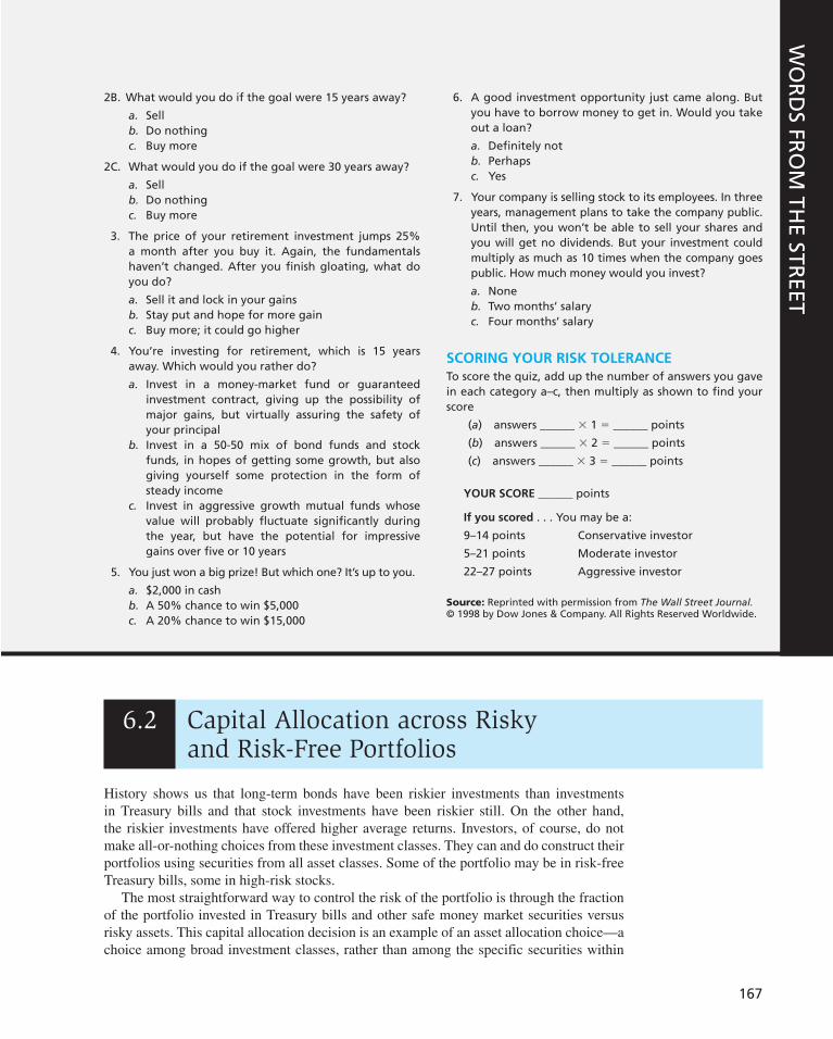
167
6.2 Capital Allocation across Risky and Risk-Free Portfolios
2B. What would you do if the goal were 15 years away?
a. Sell b. Do nothing c. Buy more
2C. What would you do if the goal were 30 years away?
a. Sell b. Do nothing c. Buy more
3. The price of your retirement investment jumps 25% a month after you buy it. Again, the fundamentals haven’t changed. After you finish gloating, what do you do?
a. Sell it and lock in your gains b. Stay put and hope for more gain c. Buy more; it could go higher
4. You’re investing for retirement, which is 15 years away. Which would you rather do?
a. Invest in a money-market fund or guaranteed investment contract, giving up the possibility of major gains, but virtually assuring the safety of your principal
b. Invest in a 50-50 mix of bond funds and stock funds, in hopes of getting some growth, but also giving yourself some protection in the form of steady income
c. Invest in aggressive growth mutual funds whose value will probably fluctuate significantly during the year, but have the potential for impressive gains over five or 10 years
5. You just won a big prize! But which one? It’s up to you.
a. $2,000 in cash b. A 50% chance to win $5,000 c. A 20% chance to win $15,000
6. A good investment opportunity just came along. But you have to borrow money to get in. Would you take out a loan?
a. Definitely not b. Perhaps c. Yes
7. Your company is selling stock to its employees. In three years, management plans to take the company public. Until then, you won’t be able to sell your shares and you will get no dividends. But your investment could multiply as much as 10 times when the company goes public. How much money would you invest?
a. None b. Two months’ salary c. Four months’ salary
SCORING YOUR RISK TOLERANCE To score the quiz, add up the number of answers you gave in each category a–c, then multiply as shown to find your score
( a ) answers ______ � 1 � ______ points
( b ) answers ______ � 2 � ______ points
( c ) answers ______ � 3 � ______ points
YOUR SCORE ______ points
If you scored . . . You may be a:
9–14 points Conservative investor
5–21 points Moderate investor
22–27 points Aggressive investor
Source: Reprinted with permission from The Wall Street Journal. © 1998 by Dow Jones & Company. All Rights Reserved Worldwide.
WO
RD
S FRO
M TH
E STREET
History shows us that long-term bonds have been riskier investments than investments in Treasury bills and that stock investments have been riskier still. On the other hand, the riskier investments have offered higher average returns. Investors, of course, do not make all-or-nothing choices from these investment classes. They can and do construct their portfolios using securities from all asset classes. Some of the portfolio may be in risk-free Treasury bills, some in high-risk stocks.
The most straightforward way to control the risk of the portfolio is through the fraction of the portfolio invested in Treasury bills and other safe money market securities versus risky assets. This capital allocation decision is an example of an asset allocation choice—a choice among broad investment classes, rather than among the specific securities within

168 P A R T I I Portfolio Theory and Practice
each asset class. Most investment professionals consider asset allocation the most impor-tant part of portfolio construction. Consider this statement by John Bogle, made when he was chairman of the Vanguard Group of Investment Companies:
The most fundamental decision of investing is the allocation of your assets: How much should you own in stock? How much should you own in bonds? How much should you own in cash reserves? . . . That decision [has been shown to account] for an astonish-ing 94% of the differences in total returns achieved by institutionally managed pension funds. . . . There is no reason to believe that the same relationship does not also hold true for individual investors. 1
Therefore, we start our discussion of the risk–return trade-off available to investors by examining the most basic asset allocation choice: the choice of how much of the portfolio to place in risk-free money market securities versus other risky asset classes.
We will denote the investor’s portfolio of risky assets as P and the risk-free asset as F. We will assume for the sake of illustration that the risky component of the investor’s over-all portfolio comprises two mutual funds, one invested in stocks and the other invested in long-term bonds. For now, we take the composition of the risky portfolio as given and focus only on the allocation between it and risk-free securities. In the next chapter, we turn to asset allocation and security selection across risky assets.
When we shift wealth from the risky portfolio to the risk-free asset, we do not change the relative proportions of the various risky assets within the risky portfolio. Rather, we reduce the relative weight of the risky portfolio as a whole in favor of risk-free assets.
For example, assume that the total market value of an initial portfolio is $300,000, of which $90,000 is invested in the Ready Asset money market fund, a risk-free asset for practical purposes. The remaining $210,000 is invested in risky securities—$113,400 in equities ( E ) and $96,600 in long-term bonds ( B ). The equities and long bond holdings comprise “the” risky portfolio, 54% in E and 46% in B:
E: wE 5113,400
210,0005 .54
B: wB 596,600
210,0005 .46
The weight of the risky portfolio, P, in the complete portfolio, including risk-free and risky investments, is denoted by y:
y 5210,000
300,0005 .7 (risky assets)
1 2 y 590,000
300,0005 .3 (risky-free assets)
The weights of each asset class in the complete portfolio are as follows:
E: $113,400
$300,0005 .378
B: $96,600
$300,0005 .322
Risky portfolio 5 E 1 B 5 .700
The risky portfolio makes up 70% of the complete portfolio.
1 John C. Bogle, Bogle on Mutual Funds (Burr Ridge, IL: Irwin Professional Publishing, 1994), p. 235.
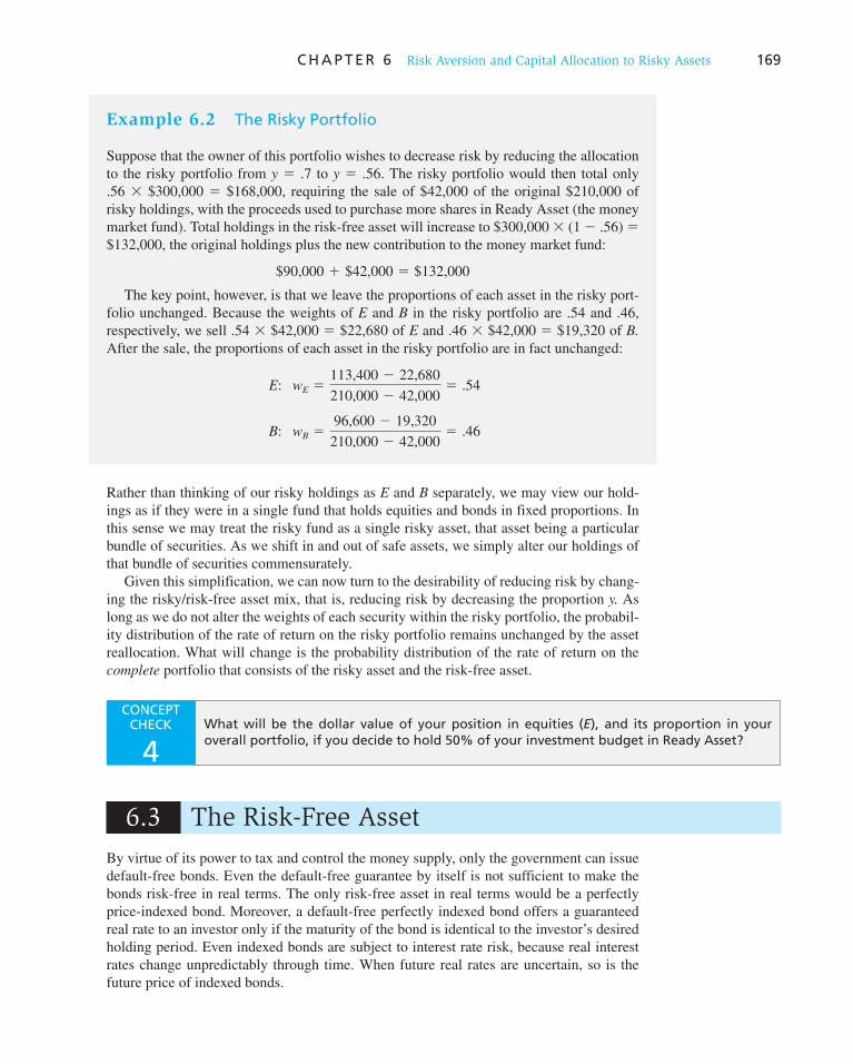
C H A P T E R 6 Risk Aversion and Capital Allocation to Risky Assets 169
Rather than thinking of our risky holdings as E and B separately, we may view our hold-ings as if they were in a single fund that holds equities and bonds in fixed proportions. In this sense we may treat the risky fund as a single risky asset, that asset being a particular bundle of securities. As we shift in and out of safe assets, we simply alter our holdings of that bundle of securities commensurately.
Given this simplification, we can now turn to the desirability of reducing risk by chang-ing the risky/risk-free asset mix, that is, reducing risk by decreasing the proportion y. As long as we do not alter the weights of each security within the risky portfolio, the probabil-ity distribution of the rate of return on the risky portfolio remains unchanged by the asset reallocation. What will change is the probability distribution of the rate of return on the complete portfolio that consists of the risky asset and the risk-free asset.
Example 6.2 The Risky Portfolio
Suppose that the owner of this portfolio wishes to decrease risk by reducing the allocation to the risky portfolio from y � .7 to y � .56. The risky portfolio would then total only .56 � $300,000 � $168,000, requiring the sale of $42,000 of the original $210,000 of risky holdings, with the proceeds used to purchase more shares in Ready Asset (the money market fund). Total holdings in the risk-free asset will increase to $300,000 � (1 � .56) � $132,000, the original holdings plus the new contribution to the money market fund:
$90,000 1 $42,000 5 $132,000
The key point, however, is that we leave the proportions of each asset in the risky port-folio unchanged. Because the weights of E and B in the risky portfolio are .54 and .46, respectively, we sell .54 � $42,000 � $22,680 of E and .46 � $42,000 � $19,320 of B. After the sale, the proportions of each asset in the risky portfolio are in fact unchanged:
E: wE 5113,400 2 22,680
210,000 2 42,0005 .54
B: wB 596,600 2 19,320
210,000 2 42,0005 .46
CONCEPT CHECK
4 What will be the dollar value of your position in equities ( E ), and its proportion in your overall portfolio, if you decide to hold 50% of your investment budget in Ready Asset?
6.3 The Risk-Free Asset
By virtue of its power to tax and control the money supply, only the government can issue default-free bonds. Even the default-free guarantee by itself is not sufficient to make the bonds risk-free in real terms. The only risk-free asset in real terms would be a perfectly price-indexed bond. Moreover, a default-free perfectly indexed bond offers a guaranteed real rate to an investor only if the maturity of the bond is identical to the investor’s desired holding period. Even indexed bonds are subject to interest rate risk, because real interest rates change unpredictably through time. When future real rates are uncertain, so is the future price of indexed bonds.
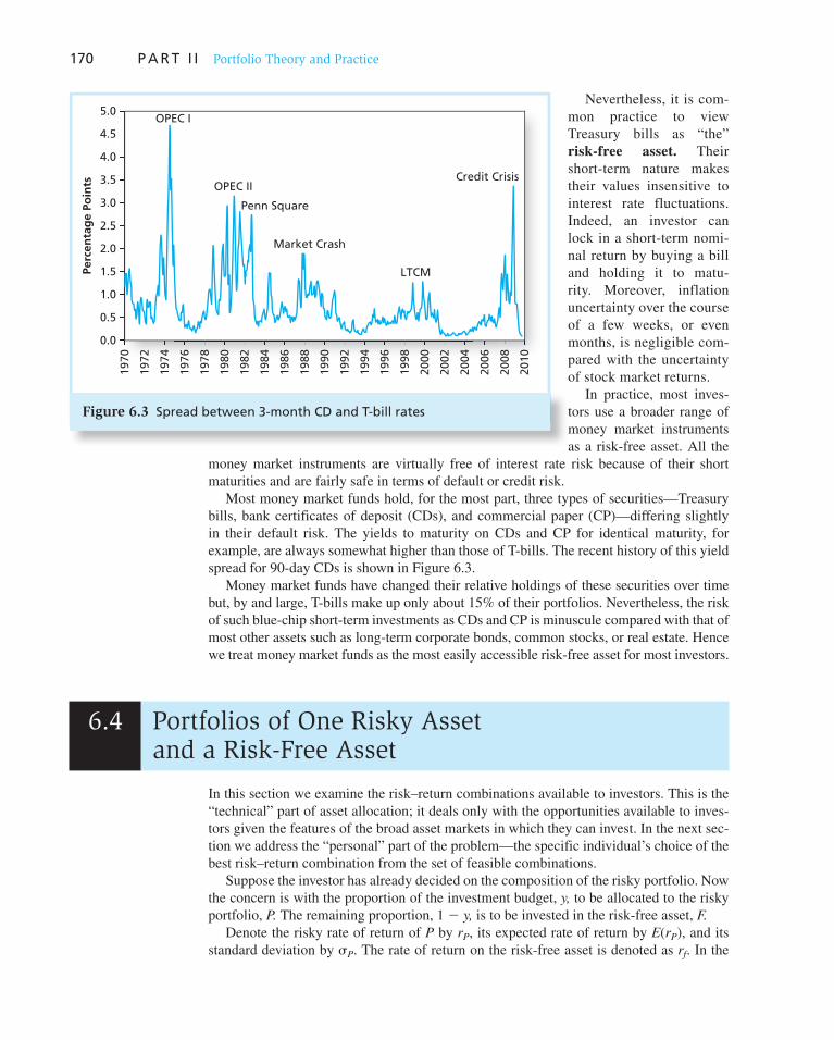
170 P A R T I I Portfolio Theory and Practice
Nevertheless, it is com-mon practice to view Treasury bills as “the” risk-free asset. Their short-term nature makes their values insensitive to interest rate fluctuations. Indeed, an investor can lock in a short-term nomi-nal return by buying a bill and holding it to matu-rity. Moreover, inflation uncertainty over the course of a few weeks, or even months, is negligible com-pared with the uncertainty of stock market returns.
In practice, most inves-tors use a broader range of money market instruments as a risk-free asset. All the
money market instruments are virtually free of interest rate risk because of their short maturities and are fairly safe in terms of default or credit risk.
Most money market funds hold, for the most part, three types of securities—Treasury bills, bank certificates of deposit (CDs), and commercial paper (CP)—differing slightly in their default risk. The yields to maturity on CDs and CP for identical maturity, for example, are always somewhat higher than those of T-bills. The recent history of this yield spread for 90-day CDs is shown in Figure 6.3 .
Money market funds have changed their relative holdings of these securities over time but, by and large, T-bills make up only about 15% of their portfolios. Nevertheless, the risk of such blue-chip short-term investments as CDs and CP is minuscule compared with that of most other assets such as long-term corporate bonds, common stocks, or real estate. Hence we treat money market funds as the most easily accessible risk-free asset for most investors.
Figure 6.3 Spread between 3-month CD and T-bill rates
0.0
0.5
1.0
1.5
2.0
2.5
3.0
3.5
4.0
4.5
5.01970
1972
1974
1976
1978
1980
1982
1984
1986
1988
1990
1992
1994
1996
1998
2000
2002
2004
2006
2008
2010
Perc
en
tag
e P
oin
ts
OPEC I
OPEC II
Penn Square
Market Crash
LTCM
Credit Crisis
6.4 Portfolios of One Risky Asset and a Risk-Free Asset
In this section we examine the risk–return combinations available to investors. This is the “technical” part of asset allocation; it deals only with the opportunities available to inves-tors given the features of the broad asset markets in which they can invest. In the next sec-tion we address the “personal” part of the problem—the specific individual’s choice of the best risk–return combination from the set of feasible combinations.
Suppose the investor has already decided on the composition of the risky portfolio. Now the concern is with the proportion of the investment budget, y, to be allocated to the risky portfolio, P. The remaining proportion, 1 � y, is to be invested in the risk-free asset, F.
Denote the risky rate of return of P by r P , its expected rate of return by E ( r P ), and its standard deviation by � P. The rate of return on the risk-free asset is denoted as r f . In the
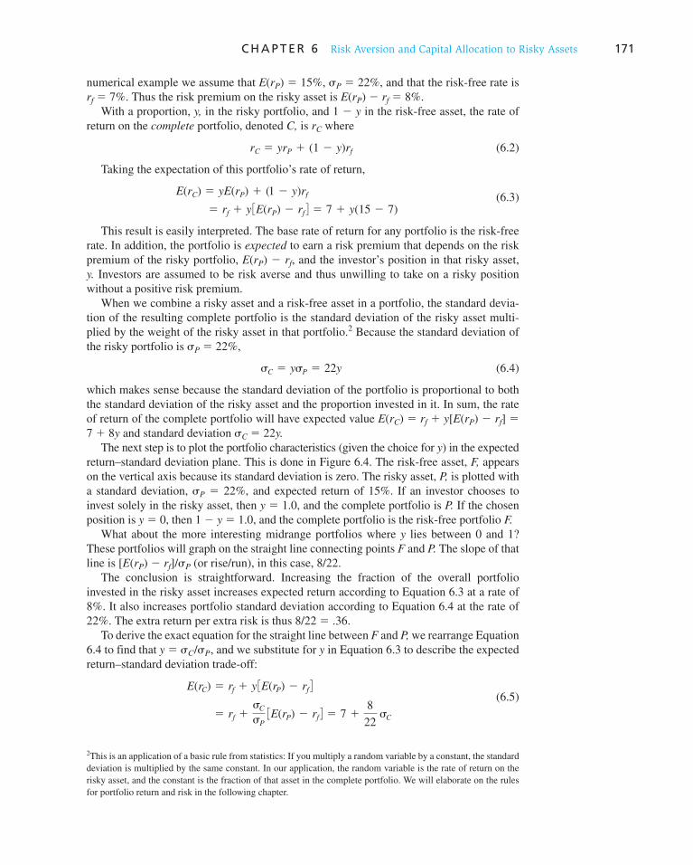
C H A P T E R 6 Risk Aversion and Capital Allocation to Risky Assets 171
numerical example we assume that E ( r P ) � 15%, � P � 22%, and that the risk-free rate is r f � 7%. Thus the risk premium on the risky asset is E ( r P ) � r f � 8%.
With a proportion, y, in the risky portfolio, and 1 � y in the risk-free asset, the rate of return on the complete portfolio, denoted C, is r C where
rC 5 yrP 1 (1 2 y)rf (6.2)
Taking the expectation of this portfolio’s rate of return,
E(rC) 5 yE(rP) 1 (1 2 y)rf
5 rf 1 y 3E(rP) 2 rf 4 5 7 1 y(15 2 7) (6.3)
This result is easily interpreted. The base rate of return for any portfolio is the risk-free rate. In addition, the portfolio is expected to earn a risk premium that depends on the risk premium of the risky portfolio, E ( r P ) � r f , and the investor’s position in that risky asset, y. Investors are assumed to be risk averse and thus unwilling to take on a risky position without a positive risk premium.
When we combine a risky asset and a risk-free asset in a portfolio, the standard devia-tion of the resulting complete portfolio is the standard deviation of the risky asset multi-plied by the weight of the risky asset in that portfolio. 2 Because the standard deviation of the risky portfolio is � P � 22%,
�C 5 y�P 5 22y (6.4)
which makes sense because the standard deviation of the portfolio is proportional to both the standard deviation of the risky asset and the proportion invested in it. In sum, the rate of return of the complete portfolio will have expected value E ( r C ) � r f � y [ E ( r P ) � r f ] � 7 � 8 y and standard deviation � C � 22 y.
The next step is to plot the portfolio characteristics (given the choice for y ) in the expected return–standard deviation plane. This is done in Figure 6.4 . The risk-free asset, F, appears on the vertical axis because its standard deviation is zero. The risky asset, P, is plotted with a standard deviation, � P � 22%, and expected return of 15%. If an investor chooses to invest solely in the risky asset, then y � 1.0, and the complete portfolio is P. If the chosen position is y � 0, then 1 � y � 1.0, and the complete portfolio is the risk-free portfolio F.
What about the more interesting midrange portfolios where y lies between 0 and 1? These portfolios will graph on the straight line connecting points F and P. The slope of that line is [ E ( r P ) � r f ]/ � P (or rise/run), in this case, 8/22.
The conclusion is straightforward. Increasing the fraction of the overall portfolio invested in the risky asset increases expected return according to Equation 6.3 at a rate of 8%. It also increases portfolio standard deviation according to Equation 6.4 at the rate of 22%. The extra return per extra risk is thus 8/22 � .36.
To derive the exact equation for the straight line between F and P, we rearrange Equation 6.4 to find that y � � C / � P , and we substitute for y in Equation 6.3 to describe the expected return–standard deviation trade-off:
E(rC) 5 rf 1 y 3E(rP) 2 rf 4 5 rf 1
�C
�P 3E(rP) 2 rf 4 5 7 1
8
22 �C
(6.5)
2 This is an application of a basic rule from statistics: If you multiply a random variable by a constant, the standard deviation is multiplied by the same constant. In our application, the random variable is the rate of return on the risky asset, and the constant is the fraction of that asset in the complete portfolio. We will elaborate on the rules for portfolio return and risk in the following chapter.

172 P A R T I I Portfolio Theory and Practice
Thus the expected return of the complete portfolio as a function of its standard devia-tion is a straight line, with intercept r f and slope
S 5E(rP) 2 rf
�P5
8
22 (6.6)
Figure 6.4 graphs the investment opportu-
nity set, which is the set of feasible expected return and standard deviation pairs of all portfolios resulting from different values of y.
The graph is a straight line originating at r f and going through the point labeled P.
This straight line is called the capital
allocation line (CAL). It depicts all the risk–return combinations available to inves-tors. The slope of the CAL, denoted S, equals the increase in the expected return of the complete portfolio per unit of addi-tional standard deviation—in other words,
incremental return per incremental risk. For this reason, the slope is called the reward-to-
volatility ratio. It also is called the Sharpe ratio (see Chapter 5). A portfolio equally divided between the risky asset and the risk-free asset, that is, where
y � .5, will have an expected rate of return of E ( r C ) � 7 � .5 � 8 � 11%, implying a risk premium of 4%, and a standard deviation of � C � .5 � 22 � 11%. It will plot on the line FP midway between F and P. The reward-to-volatility ratio is S � 4/11 � .36, precisely the same as that of portfolio P.
What about points on the CAL to the right of portfolio P? If investors can borrow at the (risk-free) rate of r f � 7%, they can construct portfolios that may be plotted on the CAL to the right of P.
Figure 6.4 The investment opportunity set with a risky asset and a risk-free asset in the expected return–standard deviation plane
E(r)
σP = 22%
E(rP) = 15%
σ
rƒ = 7%F
P
E(rP) − rƒ = 8%
CAL = Capital Allocation Line
S = 8/22
CONCEPT CHECK
5 Can the reward-to-volatility (Sharpe) ratio, S � [ E ( r C ) � r f ]/ � C , of any combination of the risky asset and the risk-free asset be different from the ratio for the risky asset taken alone, [ E ( r P ) � r f ]/ � P , which in this case is .36?
Example 6.3 Leverage
Suppose the investment budget is $300,000 and our investor borrows an additional $120,000, investing the total available funds in the risky asset. This is a leveraged position in the risky asset; it is financed in part by borrowing. In that case
y 5420,000
300,0005 1.4
and 1 � y � 1 � 1.4 � � .4, reflecting a short (borrowing) position in the risk-free asset. Rather than lending at a 7% interest rate, the investor borrows at 7%. The distribution of the portfolio rate of return still exhibits the same reward-to-volatility ratio:
E(rC) 5 7% 1 (1.4 3 8%) 5 18.2%

C H A P T E R 6 Risk Aversion and Capital Allocation to Risky Assets 173
Of course, nongovernment investors cannot borrow at the risk-free rate. The risk of a borrower’s default causes lend-ers to demand higher interest rates on loans. Therefore, the nongovernment investor’s borrowing cost will exceed the lending rate of r f � 7%. Suppose the b orrowing rate is rf
B 5 9%. Then in the borrowing range, the reward-to- volatility ratio, the slope of the CAL, will be 3E 1rP 2 2 rf
B 4/�P 5 6/22 5 .27. The CAL will therefore be “kinked” at point P, as shown in Figure 6.5 . To the left of P the investor is lending at 7%, and the slope of the CAL is .36. To the right of P, where y > 1, the investor is borrowing at 9% to finance extra investments in the risky asset, and the slope is .27.
In practice, borrowing to invest in the risky portfolio is easy and straightfor-ward if you have a margin account with a broker. All you have to do is tell your bro-ker that you want to buy “on margin.” Margin purchases may not exceed 50% of the purchase value. Therefore, if your net worth in the account is $300,000, the broker is allowed to lend you up to $300,000 to purchase additional stock. 3 You would then have $600,000 on the asset side of your account and $300,000 on the liability side, resulting in y � 2.0.
3 Margin purchases require the investor to maintain the securities in a margin account with the broker. If the value of the securities declines below a “maintenance margin,” a “margin call” is sent out, requiring a deposit to bring the net worth of the account up to the appropriate level. If the margin call is not met, regulations mandate that some or all of the securities be sold by the broker and the proceeds used to reestablish the required margin. See Chapter 3, Section 3.6, for further discussion. As we will see in Chapter 22, futures contracts also offer leverage. If the risky portfolio is an index fund on which a contract trades, the implicit rate on the loan will be close to the T-bill rate.
�C 5 1.4 3 22% 5 30.8%
S 5E(rC) 2 rf
�C5
18.2 2 7
30.85 .36
As one might expect, the leveraged portfolio has a higher standard deviation than does an unleveraged position in the risky asset.
CONCEPT CHECK
6 Suppose that there is an upward shift in the expected rate of return on the risky asset, from 15% to 17%. If all other parameters remain unchanged, what will be the slope of the CAL for y � 1 and y > 1?
Figure 6.5 The opportunity set with differential borrowing and lending rates
E(r)
E(rP) = 15%
σ
rƒ = 7%
P
σP = 22%
CAL
S(y ≤ 1) = .36rƒ
B = 9%
S(y > 1) = .27

174 P A R T I I Portfolio Theory and Practice
6.5 Risk Tolerance and Asset Allocation
We have shown how to develop the CAL, the graph of all feasible risk–return combina-tions available from different asset allocation choices. The investor confronting the CAL now must choose one optimal portfolio, C, from the set of feasible choices. This choice entails a trade-off between risk and return. Individual investor differences in risk aversion imply that, given an identical opportunity set (that is, a risk-free rate and a reward-to-volatility ratio), different investors will choose different positions in the risky asset. In particular, the more risk-averse investors will choose to hold less of the risky asset and more of the risk-free asset.
An investor who faces a risk-free rate, r f , and a risky portfolio with expected return E ( r P ) and standard deviation � P will find that, for any choice of y, the expected return of the complete portfolio is given by Equation 6.3 :
E(rC) 5 rf 1 y 3E(rP) 2 rf 4From Equation 6.4 , the variance of the overall portfolio is
� C2 5 y2
� P2
Investors attempt to maximize utility by choosing the best allocation to the risky asset, y. The utility function is given by Equation 6.1 as U � E ( r ) � ½ A � 2 . As the allocation to the risky asset increases (higher y ), expected return increases, but so does volatility, so utility can increase or decrease. To illustrate, Table 6.4 shows utility levels corresponding to dif-ferent values of y. Initially, utility increases as y increases, but eventually it declines.
Figure 6.6 is a plot of the utility function from Table 6.4 . The graph shows that utility is highest at y � .41. When y is less than .41, investors are willing to assume more risk to increase expected return. But at higher levels of y, risk is higher, and additional allocations to the risky asset are undesirable—beyond this point, further increases in risk dominate the increase in expected return and reduce utility.
To solve the utility maximization problem more generally, we write the problem as follows:
Max y
U 5 E(rC) 2 A� C
2 5 rf 1 y 3E(rP) 2 rf 4 2 Ay2� P
2½ ½
Table 6.4
Utility levels for various positions in risky assets ( y ) for an investor with risk aversion A � 4
(1) y
(2) E(rC)
(3) �C
(4)U � E(r) � ½ A �2
0 .070 0 .0700
0.1 .078 .022 .0770
0.2 .086 .044 .0821
0.3 .094 .066 .0853
0.4 .102 .088 .0865
0.5 .110 .110 .0858
0.6 .118 .132 .0832
0.7 .126 .154 .0786
0.8 .134 .176 .0720
0.9 .142 .198 .0636
1.0 .150 .220 .0532
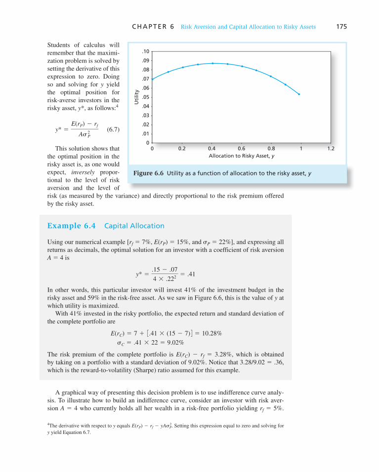
C H A P T E R 6 Risk Aversion and Capital Allocation to Risky Assets 175
Students of calculus will remember that the maximi-zation problem is solved by setting the derivative of this expression to zero. Doing so and solving for y yield the optimal position for risk-averse investors in the risky asset, y * , as follows: 4
y* 5E(rP) 2 rf
A� P2
(6.7)
This solution shows that the optimal position in the risky asset is, as one would expect, inversely propor-tional to the level of risk aversion and the level of risk (as measured by the variance) and directly proportional to the risk premium offered by the risky asset.
Example 6.4 Capital Allocation
Using our numerical example [ r f � 7%, E ( r P ) � 15%, and � P � 22%], and expressing all returns as decimals, the optimal solution for an investor with a coefficient of risk aversion A � 4 is
y* 5.15 2 .07
4 3 .2225 .41
In other words, this particular investor will invest 41% of the investment budget in the risky asset and 59% in the risk-free asset. As we saw in Figure 6.6 , this is the value of y at which utility is maximized.
With 41% invested in the risky portfolio, the expected return and standard deviation of the complete portfolio are
E(rC) 5 7 1 3.41 3 (15 2 7) 4 5 10.28%
�C 5 .41 3 22 5 9.02%
The risk premium of the complete portfolio is E ( r C ) � r f � 3.28%, which is obtained by taking on a portfolio with a standard deviation of 9.02%. Notice that 3.28/9.02 � .36, which is the reward-to-volatility (Sharpe) ratio assumed for this example.
A graphical way of presenting this decision problem is to use indifference curve analy-sis. To illustrate how to build an indifference curve, consider an investor with risk aver-sion A � 4 who currently holds all her wealth in a risk-free portfolio yielding r f � 5%.
4 The derivative with respect to y equals E(rP) 2 rf 2 yA�P2. Setting this expression equal to zero and solving for
y yield Equation 6.7 .
Figure 6.6 Utility as a function of allocation to the risky asset, y
Uti
lity
00
0.2 0.4 0.6
Allocation to Risky Asset, y
0.8 1 1.2
.01
.02
.03
.04
.05
.06
.07
.08
.09
.10

176 P A R T I I Portfolio Theory and Practice
Because the variance of such a portfolio is zero, Equation 6.1 tells us that its utility value is U � .05. Now we find the expected return the investor would require to maintain the same
level of utility when holding a risky portfolio, say, with � � 1%. We use Equation 6.1 to find how much E ( r ) must increase to compensate for the higher value of � :
U 5 E(r) 2 1/2 3 A 3 �2
.05 5 E(r) 2 1/2 3 4 3 .012
This implies that the necessary expected return increases to
Required E(r) 5 .05 1 1/2 3 A 3 �2
5 .05 1 1/2 3 4 3 .012 5 .0502 (6.8)
We can repeat this calculation for many other levels of �, each time finding the value of E ( r ) necessary to maintain U � .05. This process will yield all combinations of expected return and volatility with utility level of .05; plotting these combinations gives us the indif-ference curve.
We can readily generate an investor’s indifference curves using a spreadsheet. Table 6.5 contains risk–return combinations with utility values of .05 and .09 for two investors, one with A � 2 and the other with A � 4. For example, column (2) uses Equation 6.8 to cal-culate the expected return that must be paired with the standard deviation in column (1) for an investor with A � 2 to derive a utility value of U � .05. Column (3) repeats the calculations for a higher utility value, U � .09. The plot of these expected return–standard deviation combinations appears in Figure 6.7 as the two curves labeled A � 2. Notice that the intercepts of the indifference curves are at .05 and .09, exactly the level of utility cor-responding to the two curves.
Given the choice, any investor would prefer a portfolio on the higher indifference curve, the one with a higher certainty equivalent (utility). Portfolios on higher indifference curves offer a higher expected return for any given level of risk. For example, both indifference curves for A � 2 have the same shape, but for any level of volatility, a portfolio on the curve with utility of .09 offers an expected return 4% greater than the corresponding p ortfolio on the lower curve, for which U � .05.
Table 6.5
Spreadsheet cal-culations of indif-ference curves (Entries in columns 2–4 are expected returns necessary to provide specified utility value.)
A � 2 A � 4
� U � .05 U � .09 U � .05 U � .09
0 .0500 .0900 .050 .090
.05 .0525 .0925 .055 .095
.10 .0600 .1000 .070 .110
.15 .0725 .1125 .095 .135
.20 .0900 .1300 .130 .170
.25 .1125 .1525 .175 .215
.30 .1400 .1800 .230 .270
.35 .1725 .2125 .295 .335
.40 .2100 .2500 .370 .410
.45 .2525 .2925 .455 .495
.50 .3000 .3400 .550 .590

C H A P T E R 6 Risk Aversion and Capital Allocation to Risky Assets 177
Columns (4) and (5) of Table 6.5 repeat this analysis for a more risk-averse investor, with A � 4. The resulting pair of indifference curves in Figure 6.7 demonstrates that more risk-averse investors have steeper indifference curves than less risk-averse investors. Steeper curves mean that investors require a greater increase in expected return to com-pensate for an increase in portfolio risk.
Higher indifference curves cor-respond to higher levels of utility. The investor thus attempts to find the complete portfolio on the high-est possible indifference curve. When we superimpose plots of indifference curves on the investment opportunity set represented by the capital allo-cation line as in Figure 6.8 , we can identify the highest possible indiffer-ence curve that still touches the CAL. That indifference curve is tangent to
Figure 6.7 Indifference curves for U � .05 and U � .09 with A � 2 and A � 4
E(r)
0
U = .09
A = 4
A = 4
A = 2
A = 2
U = .05
.10 .20 .30 .40 .50σ
.60
.40
.20
Figure 6.8 Finding the optimal complete portfolio by using indifference curves
σc = .0902 σP = .22
σ
E(r)
E(rP) = .15
E(rc) = .1028
rf = .07
C
P
CAL
0
U = .094U = .08653U = .078U = .07
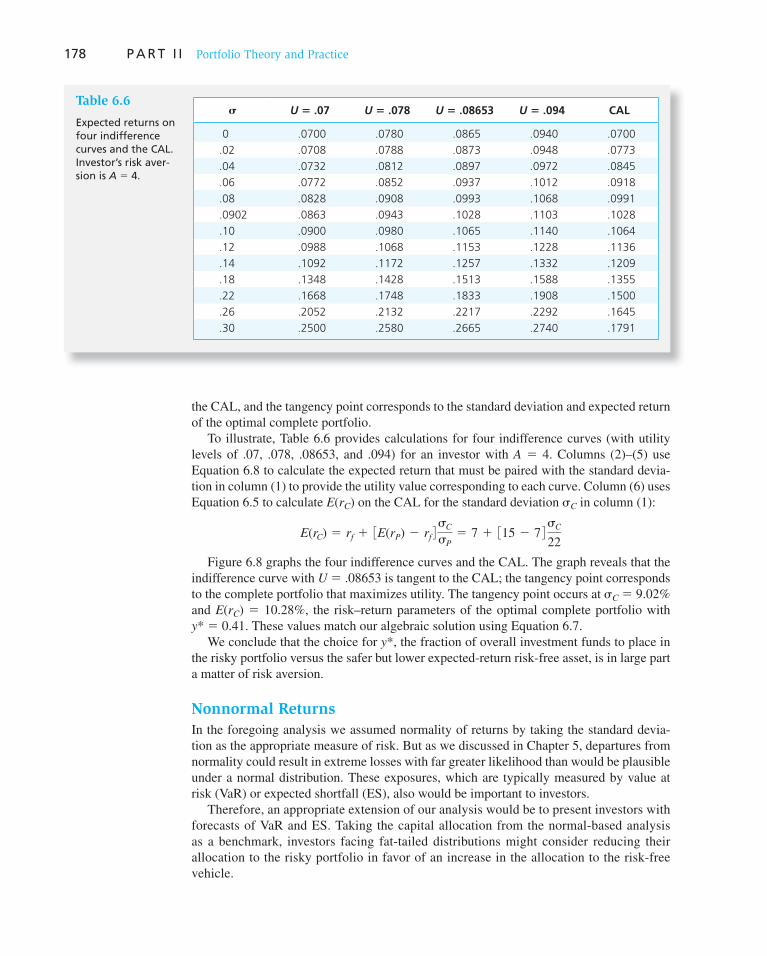
178 P A R T I I Portfolio Theory and Practice
the CAL, and the tangency point corresponds to the standard deviation and expected return of the optimal complete portfolio.
To illustrate, Table 6.6 provides calculations for four indifference curves (with utility levels of .07, .078, .08653, and .094) for an investor with A � 4. Columns (2)–(5) use Equation 6.8 to calculate the expected return that must be paired with the standard devia-tion in column (1) to provide the utility value corresponding to each curve. Column (6) uses Equation 6.5 to calculate E ( r C ) on the CAL for the standard deviation � C in column (1):
E(rC) 5 rf 1 3E(rP) 2 rf 4 �C
�P5 7 1 315 2 7 4 �C
22
Figure 6.8 graphs the four indifference curves and the CAL. The graph reveals that the indifference curve with U � .08653 is tangent to the CAL; the tangency point corresponds to the complete portfolio that maximizes utility. The tangency point occurs at � C � 9.02% and E ( r C ) � 10.28%, the risk–return parameters of the optimal complete portfolio with y * � 0.41. These values match our algebraic solution using Equation 6.7 .
We conclude that the choice for y * , the fraction of overall investment funds to place in the risky portfolio versus the safer but lower expected-return risk-free asset, is in large part a matter of risk aversion.
Nonnormal Returns
In the foregoing analysis we assumed normality of returns by taking the standard devia-tion as the appropriate measure of risk. But as we discussed in Chapter 5, departures from normality could result in extreme losses with far greater likelihood than would be plausible under a normal distribution. These exposures, which are typically measured by value at risk (VaR) or expected shortfall (ES), also would be important to investors.
Therefore, an appropriate extension of our analysis would be to present investors with forecasts of VaR and ES. Taking the capital allocation from the normal-based analysis as a benchmark, investors facing fat-tailed distributions might consider reducing their allocation to the risky portfolio in favor of an increase in the allocation to the risk-free vehicle.
Table 6.6
Expected returns on four indifference curves and the CAL. Investor’s risk aver-sion is A � 4.
� U � .07 U � .078 U � .08653 U � .094 CAL
0 .0700 .0780 .0865 .0940 .0700
.02 .0708 .0788 .0873 .0948 .0773
.04 .0732 .0812 .0897 .0972 .0845
.06 .0772 .0852 .0937 .1012 .0918
.08 .0828 .0908 .0993 .1068 .0991
.0902 .0863 .0943 .1028 .1103 .1028
.10 .0900 .0980 .1065 .1140 .1064
.12 .0988 .1068 .1153 .1228 .1136
.14 .1092 .1172 .1257 .1332 .1209
.18 .1348 .1428 .1513 .1588 .1355
.22 .1668 .1748 .1833 .1908 .1500
.26 .2052 .2132 .2217 .2292 .1645
.30 .2500 .2580 .2665 .2740 .1791

C H A P T E R 6 Risk Aversion and Capital Allocation to Risky Assets 179
6.6 Passive Strategies: The Capital Market Line
CONCEPT CHECK
7
a. If an investor’s coefficient of risk aversion is A � 3, how does the optimal asset mix change? What are the new values of E ( r C ) and � C ?
b. Suppose that the borrowing rate, rfB 5 9% is greater than the lending rate, r f � 7%.
Show graphically how the optimal portfolio choice of some investors will be affected by the higher borrowing rate. Which investors will not be affected by the borrowing rate?
The CAL is derived with the risk-free and “the” risky portfolio, P. Determination of the assets to include in risky portfolio P may result from a passive or an active strategy. A passive strategy describes a portfolio decision that avoids any direct or indirect secu-rity analysis. 5 At first blush, a passive strategy would appear to be naive. As will become apparent, however, forces of supply and demand in large capital markets may make such a strategy the reasonable choice for many investors.
In Chapter 5, we presented a compilation of the history of rates of return on different asset classes. The data are available at Professor Kenneth French’s Web site, mba.tuck
.dartmouth.edu/pages/faculty/ken.french/data_library.html. We can use these data to examine various passive strategies.
A natural candidate for a passively held risky asset would be a well-diversified port-folio of common stocks. Because a passive strategy requires that we devote no resources to acquiring information on any individual stock or group of stocks, we must follow a “neutral” diversification strategy. One way is to select a diversified portfolio of stocks that mirrors the value of the corporate sector of the U.S. economy. This results in a port-folio in which, for example, the proportion invested in Microsoft stock will be the ratio of Microsoft’s total market value to the market value of all listed stocks.
The most popular value-weighted index of U.S. stocks is the Standard & Poor’s Composite Index of 500 large capitalization U.S. corporations (the S&P 500). Table 6.7 summarizes the performance of the S&P 500 portfolio over the 84-year period 1926–2009, as well as for the four 21-year subperiods. Table 6.7 shows the average return for the port-folio, the return on rolling over 1-month T-bills for the same period, as well as the resultant average excess return and its standard deviation. The reward-to-volatility (Sharpe) ratio was .38 for the overall period, 1926–2009. In other words, stock market investors enjoyed a .38% average excess return relative to the T-bill rate for every 1% of standard deviation. The large standard deviation of the excess return (20.81%) is one reason we observe a wide range of average excess returns and reward-to-volatility ratios across subperiods (vary-ing from .21 to .74. Using the statistical distribution of the difference between the Sharpe ratios of two portfolios, we can estimate the probability of observing a deviation of the Sharpe measure for a particular subperiod from that of the overall period, assuming the latter is the true value. The last column of Table 6.7 shows that the probabilities of finding such widely different Sharpe ratios over the subperiods are actually quite substantial.
We call the capital allocation line provided by 1-month T-bills and a broad index of common stocks the capital market line (CML). A passive strategy generates an invest-ment opportunity set that is represented by the CML.
5 By “indirect security analysis” we mean the delegation of that responsibility to an intermediary such as a profes-sional money manager.

180 P A R T I I Portfolio Theory and Practice
How reasonable is it for an investor to pursue a passive strategy? Of course, we cannot answer such a question without comparing the strategy to the costs and benefits accruing to an active portfolio strategy. Some thoughts are relevant at this point, however.
First, the alternative active strategy is not free. Whether you choose to invest the time and cost to acquire the information needed to generate an optimal active portfolio of risky assets, or whether you delegate the task to a professional who will charge a fee, constitution of an active portfolio is more expensive than a passive one. The passive portfolio requires only small commissions on purchases of T-bills (or zero commissions if you purchase bills directly from the government) and management fees to either an exchange-traded fund or a mutual fund company that operates a market index fund. Vanguard, for example, operates the Index 500 Portfolio that mimics the S&P 500 index fund. It purchases shares of the firms constituting the S&P 500 in proportion to the market values of the outstanding equity of each firm, and therefore essentially replicates the S&P 500 index. The fund thus dupli-cates the performance of this market index. It has one of the lowest operating expenses (as a percentage of assets) of all mutual stock funds precisely because it requires minimal managerial effort.
A second reason to pursue a passive strategy is the free-rider benefit. If there are many active, knowledgeable investors who quickly bid up prices of undervalued assets and force down prices of overvalued assets (by selling), we have to conclude that at any time most assets will be fairly priced. Therefore, a well-diversified portfolio of common stock will be a reasonably fair buy, and the passive strategy may not be inferior to that of the average active investor. (We will elaborate on this argument and provide a more comprehensive analysis of the relative success of passive strategies in later chapters.) The nearby box points out that passive index funds have actually outperformed most actively managed funds in the past decades.
To summarize, a passive strategy involves investment in two passive portfolios: virtu-ally risk-free short-term T-bills (or, alternatively, a money market fund) and a fund of com-mon stocks that mimics a broad market index. The capital allocation line representing such a strategy is called the capital market line. Historically, based on 1926 to 2009 data, the passive risky portfolio offered an average risk premium of 7.9% and a standard deviation of 20.8%, resulting in a reward-to-volatility ratio of .38.
Average Annual Returns S&P 500 Portfolio
PeriodS&P 500 Portfolio
1-Month T-Bills Risk Premium
Standard Deviation
Sharpe Ratio (Reward to volatility) Probability*
1926–2009 11.63 3.70 7.93 20.81 .38
1989–2009 10.86 4.02 6.83 19.37 .35 .92
1968–1988 10.91 7.48 3.44 16.71 .21 .53
1947–1967 15.35 2.28 13.08 17.66 .74 .22
1926–1946 9.40 1.04 8.36 27.95 .30 .75
Table 6.7
Average annual return on large stocks and 1-month T-bills; standard deviation and reward-to-volatility ratio of large stocks over time
* The probability that the estimate of the Sharpe ratio over the full 1926–2009 period is accurate and we observe the reported (or even more different) Sharpe ratio for the subperiod due only to sampling variation.

181
Passive investors allocate their investment budgets among instruments according to their degree of risk aversion. We can use our analysis to deduce a typical investor’s risk-aversion parameter. From Table 1.1 in Chapter 1, we estimate that approximately 85% of net worth is invested in a broad array of risky assets. 6 We assume this portfolio has the same reward–risk characteristics that the S&P 500 has exhibited since 1926, as documented in Table 6.7 . Substituting these values in Equation 6.7 , we obtain
y* 5E(rM) 2 rf
A� M2
5.079
A 3 .20825 .85
6 We include in the risky portfolio real assets, half of pension reserves, corporate and noncorporate equity, and half of mutual fund shares. This portfolio sums to $45.18 trillion, which is 85% of household net worth. (See Table 1.1.)
Criticisms of Indexing Don’t Hold Up
Amid the stock market’s recent travails, critics are once again taking aim at index funds. But like the firing squad that stands in a circle, they aren’t making a whole lot of sense.
Indexing, of course, has never been popular in some quarters. Performance-hungry investors loathe the idea of buying index funds and abandoning all chance of beating the market averages. Meanwhile, most Wall Street firms would love indexing to fall from favor because there isn’t much money to be made running index funds.
But the latest barrage of nonsense also reflects today’s peculiar stock market. Here is a look at four recent com-plaints about index funds:
They’re undiversified. Critics charge that the most pop-ular index funds, those that track the Standard & Poor’s 500-stock index, are too focused on a small number of stocks and a single sector, technology.
S&P 500 funds currently have 25.3% of their money in their 10-largest stockholdings and 31.1% of assets in tech-nology companies. This narrow focus made S&P 500 funds especially vulnerable during this year’s market swoon.
But the same complaint could be leveled at actively managed funds. According to Chicago researchers Morningstar Inc., diversified U.S. stock funds have an aver-age 36.2% invested in their 10-largest stocks, with 29.1% in technology.
They’re top-heavy. Critics also charge that S&P 500 funds represent a big bet on big-company stocks. True enough. I have often argued that most folks would be bet-ter off indexing the Wilshire 5000, which includes most regularly traded U.S. stocks, including both large and small companies.
But let’s not get carried away. The S&P 500 isn’t that narrowly focused. After all, it represents some 77.2% of U.S. stock-market value.
Whether you index the S&P 500 or the Wilshire 5000, what you are getting is a fund that pretty much mirrors
the U.S. market. If you think index funds are undiversified and top-heavy, there can only be one reason: The market is undiversified and top heavy.
They’re chasing performance. In the 1990s, the stock market’s return was driven by a relatively small number of sizzling performers. As these hot stocks climbed in value, index funds became more heavily invested in these compa-nies, while lightening up on lackluster performers.
That, complain critics, is the equivalent of buying high and selling low. A devastating criticism? Hardly. This is what all investors do. When Home Depot’s stock climbs 5%, investors collectively end up with 5% more money rid-ing on Home Depot’s shares.
You can do better. Sure, there is always a chance you will get lucky and beat the market. But don’t count on it.
As a group, investors in U.S. stocks can’t outperform the market because, collectively, they are the market. In fact, once you figure in investment costs, active investors are destined to lag behind Wilshire 5000-index funds, because these active investors incur far higher investment costs.
But this isn’t just a matter of logic. The proof is also in the numbers. Over the past decade, only 28% of U.S. stock funds managed to beat the Wilshire 5000, according to Vanguard.
The problem is, the long-term argument for indexing gets forgotten in the rush to embrace the latest, hottest funds. An indexing strategy will beat most funds in most years. But in any given year, there will always be some funds that do better than the index. These winners gar-ner heaps of publicity, which whets investors’ appetites and encourages them to try their luck at beating the market.
Source: Jonathan Clements, “Criticisms of Indexing Don’t Hold Up,” The Wall Street Journal, April 25, 2000. Reprinted by permis-sion of The Wall Street Journal, © 2000 Dow Jones & Company, Inc. All rights reserved worldwide.
WO
RD
S FRO
M TH
E STREET

Vis
it u
s at
ww
w.m
hh
e.co
m/b
kmV
isit
us
at w
ww
.mh
he.
com
/bkm
182 P A R T I I Portfolio Theory and Practice
which implies a coefficient of risk aversion of
A 5.079
.85 3 .20825 2.15
Of course, this calculation is highly speculative. We have assumed that the average investor holds the naive view that historical average rates of return and standard devia-tions are the best estimates of expected rates of return and risk, looking to the future. To the extent that the average investor takes advantage of contemporary information in addi-tion to simple historical data, our estimate of A � 2.15 would be an unjustified inference. Nevertheless, a broad range of studies, taking into account the full range of available assets, places the degree of risk aversion for the representative investor in the range of 2.0 to 4.0. 7
7 See, for example, I. Friend and M. Blume, “The Demand for Risky Assets” American Economic Review 64 (1974); or S. J. Grossman and R. J. Shiller, “The Determinants of the Variability of Stock Market Prices,” American Economic Review 71 (1981).
CONCEPT CHECK
8 Suppose that expectations about the S&P 500 index and the T-bill rate are the same as they were in 2009, but you find that a greater proportion is invested in T-bills today than in 2009. What can you conclude about the change in risk tolerance over the years since 2009?
1. Speculation is the undertaking of a risky investment for its risk premium. The risk premium has to be large enough to compensate a risk-averse investor for the risk of the investment.
2. A fair game is a risky prospect that has a zero risk premium. It will not be undertaken by a risk-averse investor.
3. Investors’ preferences toward the expected return and volatility of a portfolio may be expressed by a utility function that is higher for higher expected returns and lower for higher portfolio variances. More risk-averse investors will apply greater penalties for risk. We can describe these preferences graphically using indifference curves.
4. The desirability of a risky portfolio to a risk-averse investor may be summarized by the certainty equivalent value of the portfolio. The certainty equivalent rate of return is a value that, if it is received with certainty, would yield the same utility as the risky portfolio.
5. Shifting funds from the risky portfolio to the risk-free asset is the simplest way to reduce risk. Other methods involve diversification of the risky portfolio and hedging. We take up these meth-ods in later chapters.
6. T-bills provide a perfectly risk-free asset in nominal terms only. Nevertheless, the standard devia-tion of real rates on short-term T-bills is small compared to that of other assets such as long-term bonds and common stocks, so for the purpose of our analysis we consider T-bills as the risk-free asset. Money market funds hold, in addition to T-bills, short-term relatively safe obligations such as CP and CDs. These entail some default risk, but again, the additional risk is small relative to most other risky assets. For convenience, we often refer to money market funds as risk-free assets.
7. An investor’s risky portfolio (the risky asset) can be characterized by its reward-to-volatility ratio, S � [ E ( r P ) � r f ]/ � P . This ratio is also the slope of the CAL, the line that, when graphed, goes from the risk-free asset through the risky asset. All combinations of the risky asset and the risk-free asset lie on this line. Other things equal, an investor would prefer a steeper-sloping CAL, because that means higher expected return for any level of risk. If the borrowing rate is greater than the lending rate, the CAL will be “kinked” at the point of the risky asset.
SUMMARY

Vis
it u
s at
ww
w.m
hh
e.co
m/b
kmV
isit
us
at w
ww
.mh
he.
com
/bkm
C H A P T E R 6 Risk Aversion and Capital Allocation to Risky Assets 183
8. The investor’s degree of risk aversion is characterized by the slope of his or her indifference curve. Indifference curves show, at any level of expected return and risk, the required risk pre-mium for taking on one additional percentage point of standard deviation. More risk-averse investors have steeper indifference curves; that is, they require a greater risk premium for taking on more risk.
9. The optimal position, y * , in the risky asset, is proportional to the risk premium and inversely proportional to the variance and degree of risk aversion:
y* 5E(rP) 2 rf
A�P2
Graphically, this portfolio represents the point at which the indifference curve is tangent to the CAL.
10. A passive investment strategy disregards security analysis, targeting instead the risk-free asset and a broad portfolio of risky assets such as the S&P 500 stock portfolio. If in 2009 inves-tors took the mean historical return and standard deviation of the S&P 500 as proxies for its expected return and standard deviation, then the values of outstanding assets would imply a degree of risk aversion of about A � 2.15 for the average investor. This is in line with other studies, which estimate typical risk aversion in the range of 2.0 through 4.0.
Related Web sites for this chapter are available at www.mhhe.com/bkm
risk premium fair game risk averse utility certainty equivalent rate
risk neutral risk lover mean-variance (M-V) criterion indifference curve complete portfolio
risk-free asset capital allocation line reward-to-volatility ratio passive strategy capital market line
KEY TERMS
1. Which of the following choices best completes the following statement? Explain. An investor with a higher degree of risk aversion, compared to one with a lower degree, will prefer invest-ment portfolios
a. with higher risk premiums. b. that are riskier (with higher standard deviations). c. with lower Sharpe ratios. d. with higher Sharpe ratios. e. None of the above is true.
2. Which of the following statements are true? Explain.
a. A lower allocation to the risky portfolio reduces the Sharpe (reward-to-volatility) ratio. b. The higher the borrowing rate, the lower the Sharpe ratios of levered portfolios. c. With a fixed risk-free rate, doubling the expected return and standard deviation of the risky
portfolio will double the Sharpe ratio. d. Holding constant the risk premium of the risky portfolio, a higher risk-free rate will increase
the Sharpe ratio of investments with a positive allocation to the risky asset.
3. What do you think would happen to the expected return on stocks if investors perceived higher volatility in the equity market? Relate your answer to Equation 6.7 .
4. Consider a risky portfolio. The end-of-year cash flow derived from the portfolio will be either $70,000 or $200,000 with equal probabilities of .5. The alternative risk-free investment in T-bills pays 6% per year.
a. If you require a risk premium of 8%, how much will you be willing to pay for the portfolio?
b. Suppose that the portfolio can be purchased for the amount you found in ( a ). What will be the expected rate of return on the portfolio?
PROBLEM SETS
i. Basic
ii. Intermediate

Vis
it u
s at
ww
w.m
hh
e.co
m/b
km184 P A R T I I Portfolio Theory and Practice
c. Now suppose that you require a risk premium of 12%. What is the price that you will be willing to pay?
d. Comparing your answers to ( a ) and ( c ), what do you conclude about the relationship between the required risk premium on a portfolio and the price at which the portfolio will sell?
5. Consider a portfolio that offers an expected rate of return of 12% and a standard deviation of 18%. T-bills offer a risk-free 7% rate of return. What is the maximum level of risk aversion for which the risky portfolio is still preferred to bills?
6. Draw the indifference curve in the expected return–standard deviation plane corresponding to a utility level of .05 for an investor with a risk aversion coefficient of 3. ( Hint: Choose sev-eral possible standard deviations, ranging from 0 to .25, and find the expected rates of return providing a utility level of .05. Then plot the expected return–standard deviation points so derived.)
7. Now draw the indifference curve corresponding to a utility level of .05 for an investor with risk aversion coefficient A � 4. Comparing your answer to Problem 6, what do you conclude?
8. Draw an indifference curve for a risk-neutral investor providing utility level .05.
9. What must be true about the sign of the risk aversion coefficient, A, for a risk lover? Draw the indifference curve for a utility level of .05 for a risk lover.
For Problems 10 through 12: Consider historical data showing that the average annual rate of return on the S&P 500 portfolio over the past 80 years has averaged roughly 8% more than the Treasury bill return and that the S&P 500 standard deviation has been about 20% per year. Assume these values are representative of investors’ expec-tations for future performance and that the current T-bill rate is 5%.
10. Calculate the expected return and variance of portfolios invested in T-bills and the S&P 500 index with weights as follows:
W bills W index
0 1.0
0.2 0.8
0.4 0.6
0.6 0.4
0.8 0.2
1.0 0
11. Calculate the utility levels of each portfolio of Problem 10 for an investor with A � 2. What do you conclude?
12. Repeat Problem 11 for an investor with A � 3. What do you conclude?
Use these inputs for Problems 13 through 19: You manage a risky portfolio with expected rate of return of 18% and standard deviation of 28%. The T-bill rate is 8%.
13. Your client chooses to invest 70% of a portfolio in your fund and 30% in a T-bill money market fund. What is the expected value and standard deviation of the rate of return on his portfolio?
14. Suppose that your risky portfolio includes the following investments in the given proportions:
Stock A 25%
Stock B 32%
Stock C 43%
What are the investment proportions of your client’s overall portfolio, including the position in T-bills?
15. What is the reward-to-volatility ratio ( S ) of your risky portfolio? Your client’s?

Vis
it u
s at
ww
w.m
hh
e.co
m/b
km
C H A P T E R 6 Risk Aversion and Capital Allocation to Risky Assets 185
16. Draw the CAL of your portfolio on an expected return–standard deviation diagram. What is the slope of the CAL? Show the position of your client on your fund’s CAL.
17. Suppose that your client decides to invest in your portfolio a proportion y of the total investment budget so that the overall portfolio will have an expected rate of return of 16%.
a. What is the proportion y? b. What are your client’s investment proportions in your three stocks and the T-bill fund? c. What is the standard deviation of the rate of return on your client’s portfolio?
18. Suppose that your client prefers to invest in your fund a proportion y that maximizes the expected return on the complete portfolio subject to the constraint that the complete portfolio’s standard deviation will not exceed 18%.
a. What is the investment proportion, y? b. What is the expected rate of return on the complete portfolio?
19. Your client’s degree of risk aversion is A � 3.5.
a. What proportion, y, of the total investment should be invested in your fund? b. What is the expected value and standard deviation of the rate of return on your client’s opti-
mized portfolio?
20. Look at the data in Table 6.7 on the average risk premium of the S&P 500 over T-bills, and the standard deviation of that risk premium. Suppose that the S&P 500 is your risky portfolio.
a. If your risk-aversion coefficient is A � 4 and you believe that the entire 1926–2009 period is representative of future expected performance, what fraction of your portfolio should be allocated to T-bills and what fraction to equity?
b. What if you believe that the 1968–1988 period is representative? c. What do you conclude upon comparing your answers to ( a ) and ( b )?
21. Consider the following information about a risky portfolio that you manage, and a risk-free asset: E ( r P ) � 11%, � P � 15%, r f � 5%.
a. Your client wants to invest a proportion of her total investment budget in your risky fund to provide an expected rate of return on her overall or complete portfolio equal to 8%. What proportion should she invest in the risky portfolio, P, and what proportion in the risk-free asset?
b. What will be the standard deviation of the rate of return on her portfolio? c. Another client wants the highest return possible subject to the constraint that you limit his
standard deviation to be no more than 12%. Which client is more risk averse?
22. Investment Management Inc. (IMI) uses the capital market line to make asset allocation recom-mendations. IMI derives the following forecasts:
• Expected return on the market portfolio: 12%. • Standard deviation on the market portfolio: 20%. • Risk-free rate: 5%.
Samuel Johnson seeks IMI’s advice for a portfolio asset allocation. Johnson informs IMI that he wants the standard deviation of the portfolio to equal half of the standard deviation for the market portfolio. Using the capital market line, what expected return can IMI provide subject to Johnson’s risk constraint?
For Problems 23 through 26: Suppose that the borrowing rate that your client faces is 9%. Assume that the S&P 500 index has an expected return of 13% and standard deviation of 25%, that r f � 5%, and that your fund has the parameters given in Prob-lem 21.
23. Draw a diagram of your client’s CML, accounting for the higher borrowing rate. Superimpose on it two sets of indifference curves, one for a client who will choose to borrow, and one who will invest in both the index fund and a money market fund.

Vis
it u
s at
ww
w.m
hh
e.co
m/b
km186 P A R T I I Portfolio Theory and Practice
24. What is the range of risk aversion for which a client will neither borrow nor lend, that is, for which y � 1?
25. Solve Problems 23 and 24 for a client who uses your fund rather than an index fund.
26. What is the largest percentage fee that a client who currently is lending ( y < 1) will be willing to pay to invest in your fund? What about a client who is borrowing ( y > 1)?
For Challenge Problems 27 and 28: You estimate that a passive portfolio, that is, one invested in a risky portfolio that mimics the S&P 500 stock index, yields an expected rate of return of 13% with a standard deviation of 25%. You manage an active port-folio with expected return 18% and standard deviation 28%. The risk-free rate is 8%.
27. Draw the CML and your funds’ CAL on an expected return–standard deviation diagram.
a. What is the slope of the CML? b. Characterize in one short paragraph the advantage of your fund over the passive fund.
28. Your client ponders whether to switch the 70% that is invested in your fund to the passive portfolio.
a. Explain to your client the disadvantage of the switch. b. Show him the maximum fee you could charge (as a percentage of the investment in your
fund, deducted at the end of the year) that would leave him at least as well off investing in your fund as in the passive one. ( Hint: The fee will lower the slope of his CAL by reducing the expected return net of the fee.)
29. Consider again the client in Problem 19 with A � 3.5.
a. If he chose to invest in the passive portfolio, what proportion, y, would he select? b. Is the fee (percentage of the investment in your fund, deducted at the end of the year) that
you can charge to make the client indifferent between your fund and the passive strategy affected by his capital allocation decision (i.e., his choice of y )?
iii. Challenge
Use the following data in answering CFA Problems 1–3:
Utility Formula Data
Investment Expected Return, E(r) Standard Deviation, �
1 .12 .30
2 .15 .50
3 .21 .16
4 .24 .21
U � E(r) � ½ A�2, where A � 4
1. On the basis of the utility formula above, which investment would you select if you were risk averse with A � 4?
2. On the basis of the utility formula above, which investment would you select if you were risk neutral?
3. The variable ( A ) in the utility formula represents the:
a. investor’s return requirement. b. investor’s aversion to risk. c. certainty equivalent rate of the portfolio. d. preference for one unit of return per four units of risk.
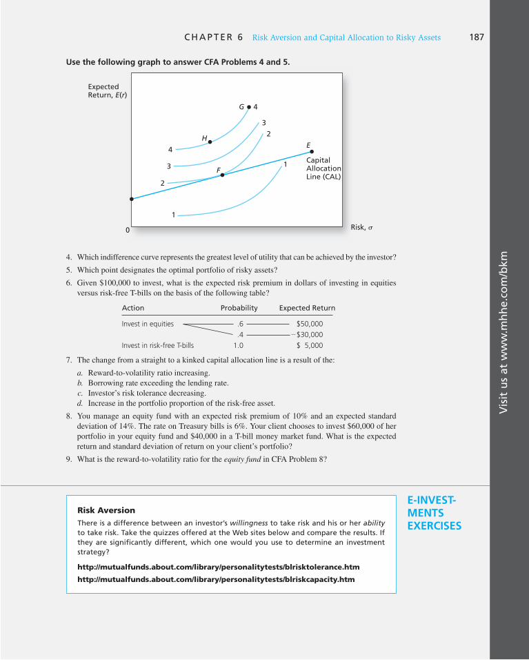
Vis
it u
s at
ww
w.m
hh
e.co
m/b
km
C H A P T E R 6 Risk Aversion and Capital Allocation to Risky Assets 187
Risk,
ExpectedReturn, E(r)
H
G
F
E
CapitalAllocationLine (CAL)
1
1
2
2
3
3
4
4
0
Use the following graph to answer CFA Problems 4 and 5.
4. Which indifference curve represents the greatest level of utility that can be achieved by the investor?
5. Which point designates the optimal portfolio of risky assets?
6. Given $100,000 to invest, what is the expected risk premium in dollars of investing in equities versus risk-free T-bills on the basis of the following table?
Action Probability Expected Return
Invest in equities .6 $50,000
.4 �$30,000
Invest in risk-free T-bills 1.0 $ 5,000
7. The change from a straight to a kinked capital allocation line is a result of the:
a. Reward-to-volatility ratio increasing. b. Borrowing rate exceeding the lending rate. c. Investor’s risk tolerance decreasing. d. Increase in the portfolio proportion of the risk-free asset.
8. You manage an equity fund with an expected risk premium of 10% and an expected standard deviation of 14%. The rate on Treasury bills is 6%. Your client chooses to invest $60,000 of her portfolio in your equity fund and $40,000 in a T-bill money market fund. What is the expected return and standard deviation of return on your client’s portfolio?
9. What is the reward-to-volatility ratio for the equity fund in CFA Problem 8?
Risk Aversion
There is a difference between an investor’s willingness to take risk and his or her ability to take risk. Take the quizzes offered at the Web sites below and compare the results. If they are significantly different, which one would you use to determine an investment strategy?
http://mutualfunds.about.com/library/personalitytests/blrisktolerance.htm
http://mutualfunds.about.com/library/personalitytests/blriskcapacity.htm
E-INVEST-MENTS EXERCISES

Vis
it u
s at
ww
w.m
hh
e.co
m/b
km188 P A R T I I Portfolio Theory and Practice
SOLUTIONS TO CONCEPT CHECKS
1. The investor is taking on exchange rate risk by investing in a pound-denominated asset. If the exchange rate moves in the investor’s favor, the investor will benefit and will earn more from the U.K. bill than the U.S. bill. For example, if both the U.S. and U.K. interest rates are 5%, and the current exchange rate is $2 per pound, a $2 investment today can buy 1 pound, which can be invested in England at a certain rate of 5%, for a year-end value of 1.05 pounds. If the year-end exchange rate is $2.10 per pound, the 1.05 pounds can be exchanged for 1.05 � $2.10 � $2.205 for a rate of return in dollars of 1 � r � $2.205/$2 � 1.1025, or r � 10.25%, more than is available from U.S. bills. Therefore, if the investor expects favorable exchange rate movements, the U.K. bill is a speculative investment. Otherwise, it is a gamble.
2. For the A � 4 investor the utility of the risky portfolio is
U 5 .02 2 (½ 3 4 3 .32 ) 5 .02
while the utility of bills is
U 5 .07 2 (½ 3 4 3 0 ) 5 .07
The investor will prefer bills to the risky portfolio. (Of course, a mixture of bills and the portfolio might be even better, but that is not a choice here.)
Even for the A � 2 investor, the utility of the risky portfolio is
U 5 .20 2 (½ 3 2 3 .32 ) 5 .11
while the utility of bills is again .07. The less risk-averse investor prefers the risky portfolio. 3. The less risk-averse investor has a shallower indifference curve. An increase in risk requires less
increase in expected return to restore utility to the original level.
4. Holding 50% of your invested capital in Ready Assets means that your investment proportion in the risky portfolio is reduced from 70% to 50%.
Your risky portfolio is constructed to invest 54% in E and 46% in B. Thus the proportion of E in your overall portfolio is .5 � 54% � 27%, and the dollar value of your position in E is $300,000 � .27 � $81,000.
PE(rP)
E(r)
P
Less RiskAverse
More RiskAverse

Vis
it u
s at
ww
w.m
hh
e.co
m/b
km
C H A P T E R 6 Risk Aversion and Capital Allocation to Risky Assets 189
5. In the expected return–standard deviation plane all portfolios that are constructed from the same risky and risk-free funds (with various proportions) lie on a line from the risk-free rate through the risky fund. The slope of the CAL (capital allocation line) is the same everywhere; hence the reward-to-volatility ratio is the same for all of these portfolios. Formally, if you invest a proportion, y, in a risky fund with expected return E ( r P ) and standard deviation � P , and the remainder, 1 � y, in a risk-free asset with a sure rate r f , then the portfolio’s expected return and standard deviation are
E(rC) 5 rf 1 y 3E(rP) 2 rf 4�C 5 y�P
and therefore the reward-to-volatility ratio of this portfolio is
SC 5E(rC) 2 rf
�C
5y 3E(rP) 2 rf 4
y�P
5E(rP) 2 rf
�P
which is independent of the proportion y.
6. The lending and borrowing rates are unchanged at rf 5 7%, rfB 5 9%. The standard deviation of
the risky portfolio is still 22%, but its expected rate of return shifts from 15% to 17%.
The slope of the two-part CAL is
E(rP) 2 rf
�P
for the lending range
E(rP) 2 rfB
�P
for the borrowing range
Thus in both cases the slope increases: from 8/22 to 10/22 for the lending range, and from 6/22 to 8/22 for the borrowing range.
7. a. The parameters are r f � .07, E ( r P ) � .15, � P � .22. An investor with a degree of risk aversion A will choose a proportion y in the risky portfolio of
y 5E(rP) 2 rf
A�P2
With the assumed parameters and with A � 3 we find that
y 5.15 2 .07
3 3 .04845 .55
When the degree of risk aversion decreases from the original value of 4 to the new value of 3, investment in the risky portfolio increases from 41% to 55%. Accordingly, both the expected return and standard deviation of the optimal portfolio increase:
E(rC) 5 .07 1 (.55 3 .08) 5 .114 (before: .1028)
�C 5 .55 3 .22 5 .121 (before: .0902)
b. All investors whose degree of risk aversion is such that they would hold the risky portfolio in a proportion equal to 100% or less ( y � 1.00) are lending rather than borrowing, and so are unaffected by the borrowing rate. The least risk-averse of these investors hold 100% in the risky portfolio ( y � 1). We can solve for the degree of risk aversion of these “cut off” investors from the parameters of the investment opportunities:
y 5 1 5E(rP) 2 rf
A�P2
5.08
.0484 A
which implies
A 5.08
.04845 1.65

Vis
it u
s at
ww
w.m
hh
e.co
m/b
km190 P A R T I I Portfolio Theory and Practice
Any investor who is more risk tolerant (that is, A < 1.65) would borrow if the borrowing rate were 7%. For borrowers,
y 5E(rP) 2 rf
B
A�P2
Suppose, for example, an investor has an A of 1.1. When rf 5 rfB 5 7%, this investor chooses to
invest in the risky portfolio:
y 5.08
1.1 3 .04845 1.50
which means that the investor will borrow an amount equal to 50% of her own investment capital. Raise the borrowing rate, in this case to rf
B 5 9%, and the investor will invest less in the risky asset. In that case:
y 5.06
1.1 3 .04845 1.13
and “only” 13% of her investment capital will be borrowed. Graphically, the line from r f to the risky portfolio shows the CAL for lenders. The dashed part would be relevant if the borrowing rate equaled the lending rate. When the borrowing rate exceeds the lending rate, the CAL is kinked at the point corresponding to the risky portfolio.
The following figure shows indifference curves of two investors. The steeper indifference curve portrays the more risk-averse investor, who chooses portfolio C 0 , which involves lending. This investor’s choice is unaffected by the borrowing rate. The more risk-tolerant investor is portrayed by the shallower-sloped indifference curves. If the lending rate equaled the borrowing rate, this investor would choose portfolio C 1 on the dashed part of the CAL. When the borrowing rate goes up, this investor chooses portfolio C 2 (in the borrowing range of the kinked CAL), which involves less borrowing than before. This investor is hurt by the increase in the borrowing rate.
8. If all the investment parameters remain unchanged, the only reason for an investor to decrease the investment proportion in the risky asset is an increase in the degree of risk aversion. If you think that this is unlikely, then you have to reconsider your faith in your assumptions. Perhaps the S&P 500 is not a good proxy for the optimal risky portfolio. Perhaps investors expect a higher real rate on T-bills.
E(r)
E(rP)
rf
C0
C2
C1
rfB
�P
�

APPENDIX A: Risk Aversion, Expected Utility, and the St. Petersburg Paradox
Vis
it u
s at
ww
w.m
hh
e.co
m/b
km
C H A P T E R 6 Risk Aversion and Capital Allocation to Risky Assets 191
We digress in this appendix to examine the rationale behind our contention that investors are risk averse. Recognition of risk aversion as central in investment decisions goes back at least to 1738. Daniel Bernoulli, one of a famous Swiss family of distinguished mathemati-cians, spent the years 1725 through 1733 in St. Petersburg, where he analyzed the follow-ing coin-toss game. To enter the game one pays an entry fee. Thereafter, a coin is tossed until the first head appears. The number of tails, denoted by n, that appears until the first head is tossed is used to compute the payoff, $ R, to the participant, as
R 1n 2 5 2n
The probability of no tails before the first head ( n � 0) is 1/2 and the corresponding payoff is 2 0 � $1. The probability of one tail and then heads ( n � 1) is 1/2 � 1/2 with payoff 2 1 � $2, the probability of two tails and then heads ( n � 2) is 1/2 � 1/2 � 1/2, and so forth.
The following table illustrates the probabilities and payoffs for various outcomes:
Tails Probability Payoff � $ R(n) Probability � Payoff
0 1/2 $1 $1/2
1 1/4 $2 $1/2
2 1/8 $4 $1/2
3 1/16 $8 $1/2
… … … …
n (1/2)n � 1 $2n $1/2
The expected payoff is therefore
E(R) 5 a`
n50
Pr(n)R(n) 5 1@2 1 1@2 1 c5 `
The evaluation of this game is called the “St. Petersburg Paradox.” Although the expected payoff is infinite, participants obviously will be willing to purchase tickets to play the game only at a finite, and possibly quite modest, entry fee.
Bernoulli resolved the paradox by noting that investors do not assign the same value per dollar to all payoffs. Specifically, the greater their wealth, the less their “apprecia-tion” for each extra dollar. We can make this insight mathematically precise by assigning a welfare or utility value to any level of investor wealth. Our utility function should increase as wealth is higher, but each extra dollar of wealth should increase utility by progres-sively smaller amounts. 8 (Modern economists would say that investors exhibit “decreasing marginal utility” from an additional payoff dollar.) One particular function that assigns a subjective value to the investor from a payoff of $ R, which has a smaller value per dollar the greater the payoff, is the function ln( R ) where ln is the natural logarithm function. If this function measures utility values of wealth, the subjective utility value of the game is indeed finite, equal to .693. 9 The certain wealth level necessary to yield this utility value is
8 This utility is similar in spirit to the one that assigns a satisfaction level to portfolios with given risk and return attributes. However, the utility function here refers not to investors’ satisfaction with alternative portfolio choices but only to the subjective welfare they derive from different levels of wealth.
9 If we substitute the “utility” value, ln( R ), for the dollar payoff, R, to obtain an expected utility value of the game (rather than expected dollar value), we have, calling V ( R ) the expected utility,
V(R) 5 a`
n50
Pr(n) ln 3R(n) 4 5 a`
n50
(1/2)n11 ln(2n) 5 .693

Vis
it u
s at
ww
w.m
hh
e.co
m/b
km192 P A R T I I Portfolio Theory and Practice
$2.00, because ln(2.00) � .693. Hence the certainty equivalent value of the risky payoff is $2.00, which is the maximum amount that this investor will pay to play the game.
Von Neumann and Morgenstern adapted this approach to investment theory in a com-plete axiomatic system in 1946. Avoiding unnecessary technical detail, we restrict our-selves here to an intuitive exposition of the rationale for risk aversion.
Imagine two individuals who are identical twins, except that one of them is less fortunate than the other. Peter has only $1,000 to his name while Paul has a net worth of $200,000. How many hours of work would each twin be willing to offer to earn one extra dollar? It is likely that Peter (the poor twin) has more essential uses for the extra money than does Paul. Therefore, Peter will offer more hours. In other words, Peter derives a greater personal wel-fare or assigns a greater “utility” value to the 1,001st dollar than Paul does to the 200,001st. Figure 6A.1 depicts graphically the relationship between the wealth and the utility value of wealth that is consistent with this notion of decreasing marginal utility.
Individuals have different rates of decrease in their marginal utility of wealth. What is constant is the principle that the per-dollar increment to utility decreases with wealth. Functions that exhibit the property of decreasing per-unit value as the number of units grows are called concave. A simple example is the log function, familiar from high school mathematics. Of course, a log function will not fit all investors, but it is consistent with the risk aversion that we assume for all investors.
Now consider the following simple prospect:
Figure 6A.1 Utility of wealth with a log utility function
U (W)
W
$100,000
$150,000
$50,000
p � ½
1 � p � ½

Vis
it u
s at
ww
w.m
hh
e.co
m/b
km
C H A P T E R 6 Risk Aversion and Capital Allocation to Risky Assets 193
This is a fair game in that the expected profit is zero. Suppose, however, that the curve in Figure 6A.1 represents the investor’s utility value of wealth, assuming a log utility func-tion. Figure 6A.2 shows this curve with numerical values marked.
Figure 6A.2 shows that the loss in utility from losing $50,000 exceeds the gain from win-ning $50,000. Consider the gain first. With probability p � .5, wealth goes from $100,000 to $150,000. Using the log utility function, utility goes from ln(100,000) � 11.51 to ln(150,000) � 11.92, the distance G on the graph. This gain is G � 11.92 � 11.51 � .41. In expected utility terms, then, the gain is pG � .5 � .41 � .21.
Now consider the possibility of coming up on the short end of the prospect. In that case, wealth goes from $100,000 to $50,000. The loss in utility, the distance L on the graph, is L � ln(100,000) � ln(50,000) � 11.51 � 10.82 � .69. Thus the loss in expected utility terms is (1 � p ) L � .5 � .69 � .35, which exceeds the gain in expected utility from the possibility of winning the game.
We compute the expected utility from the risky prospect:
E 3U(W) 4 5 pU(W1) 1 (1 2 p)U(W2)
5 1/2 ln(50,000) 1 1/2 ln(150,000) 5 11.37
If the prospect is rejected, the utility value of the (sure) $100,000 is ln(100,000) � 11.51, greater than that of the fair game (11.37). Hence the risk-averse investor will reject the fair game.
Using a specific investor utility function (such as the log utility function) allows us to com-pute the certainty equivalent value of the risky prospect to a given investor. This is the amount that, if received with certainty, she would consider equally attractive as the risky prospect.
If log utility describes the investor’s preferences toward wealth outcomes, then Figure 6A.2 can also tell us what is, for her, the dollar value of the prospect. We ask, What sure level of wealth has a utility value of 11.37 (which equals the expected utility from the prospect)? A horizontal line drawn at the level 11.37 intersects the utility curve at the level of wealth W CE. This means that
ln(WCE) 5 11.37
Figure 6A.2 Fair games and expected utility
Y
G
L
W
U(W) = ln(W)
U(150,000) = 11.92
U(100,000) = 11.51
E[U (W)] = 11.37
U(50,000) = 10.82
E(W) = 100,000W1 = 50,000 WCE W2 = 150,000

APPENDIX B: Utility Functions and Equilibrium Prices of Insurance Contracts
Vis
it u
s at
ww
w.m
hh
e.co
m/b
km194 P A R T I I Portfolio Theory and Practice
which implies that
WCE 5 e11.37 5 $86,681.87
W CE is therefore the certainty equivalent of the prospect. The distance Y in Figure 6A.2 is the penalty, or the downward adjustment, to the expected profit that is attributable to the risk of the prospect.
Y 5 E(W) 2 WCE 5 $100,000 2 $86,681.87 5 $13,318.13
This investor views $86,681.87 for certain as being equal in utility value as $100,000 at risk. Therefore, she would be indifferent between the two.
CONCEPT CHECK
A.1
Suppose the utility function is U(W) � #
a. What is the utility level at wealth levels $50,000 and $150,000?
b. What is expected utility if p still equals .5?
c. What is the certainty equivalent of the risky prospect?
d. Does this utility function also display risk aversion?
e. Does this utility function display more or less risk aversion than the log utility function?
W
The utility function of an individual investor allows us to measure the subjective value the individual would place on a dollar at various levels of wealth. Essentially, a dollar in bad times (when wealth is low) is more valuable than a dollar in good times (when wealth is high).
Suppose that all investors hold the risky S&P 500 portfolio. Then, if the portfolio value falls in a worse-than-expected economy, all investors will, albeit to different degrees, expe-rience a “low-wealth” scenario. Therefore, the equilibrium value of a dollar in the low-wealth economy would be higher than the value of a dollar when the portfolio performs better than expected. This observation helps explain the apparently high cost of portfolio insurance that we encountered when considering long-term investments in the previous chapter. It also helps explain why an investment in a stock portfolio (and hence in individ-ual stocks) has a risk premium that appears to be so high and results in probability of short-fall that is so low. Despite the low probability of shortfall risk, stocks still do not dominate the lower-return risk-free bond, because if an investment shortfall should transpire, it will coincide with states in which the value of dollar returns is high.
Does revealed behavior of investors demonstrate risk aversion? Looking at prices and past rates of return in financial markets, we can answer with a resounding yes. With remarkable consistency, riskier bonds are sold at lower prices than are safer ones with otherwise similar characteristics. Riskier stocks also have provided higher average rates of return over long periods of time than less risky assets such as T-bills. For example, over the 1926 to 2009 period, the average rate of return on the S&P 500 portfolio exceeded the T-bill return by nearly 8% per year.
It is abundantly clear from financial data that the average, or representative, investor exhibits substantial risk aversion. For readers who recognize that financial assets are priced to compensate for risk by providing a risk premium and at the same time feel the urge for

Vis
it u
s at
ww
w.m
hh
e.co
m/b
km
C H A P T E R 6 Risk Aversion and Capital Allocation to Risky Assets 195
some gambling, we have a constructive recommendation: Direct your gambling impulse to investment in financial markets. As Von Neumann once said, “The stock market is a casino with the odds in your favor.” A small risk-seeking investment may provide all the excite-ment you want with a positive expected return to boot!
1. Suppose that your wealth is $250,000. You buy a $200,000 house and invest the remainder in a risk-free asset paying an annual interest rate of 6%. There is a probability of .001 that your house will burn to the ground and its value will be reduced to zero. With a log utility of end-of-year wealth, how much would you be willing to pay for insurance (at the beginning of the year)? (Assume that if the house does not burn down, its end-of-year value still will be $200,000.)
2. If the cost of insuring your house is $1 per $1,000 of value, what will be the certainty equivalent of your end-of-year wealth if you insure your house at:
a. ½ its value. b. Its full value. c. 1½ times its value.
PROBLEMS: APPENDIX
SOLUTIONS TO CONCEPT CHECKS
A.1. a. U(W) 5 "W
U(50,000) 5 "50,000 5 223.61U(150,000) 5 387.30
b. E ( U ) � (.5 � 223.61) � (.5 � 387.30) � 305.45
c. We must find W CE that has utility level 305.45. Therefore
"WCE 5 305.45
WCE 5 305.452 5 $93,301
d. Yes. The certainty equivalent of the risky venture is less than the expected outcome of $100,000.
e. The certainty equivalent of the risky venture to this investor is greater than it was for the log utility investor considered in the text. Hence this utility function displays less risk aversion.

7 7 THE INVESTMENT DECISION can be viewed
as a top-down process: (i) Capital allocation
between the risky portfolio and risk-free
assets, (ii) asset allocation across broad asset
classes (e.g., U.S. stocks, international stocks,
and long-term bonds), and (iii) security selec-
tion of individual assets within each asset class.
Capital allocation, as we saw in Chapter 6,
determines the investor’s exposure to risk.
The optimal capital allocation is determined
by risk aversion as well as expectations for the
risk–return trade-off of the optimal risky port-
folio. In principle, asset allocation and security
selection are technically identical; both aim
at identifying that optimal risky portfolio,
namely, the combination of risky assets that
provides the best risk–return trade-off. In
practice, however, asset allocation and secu-
rity selection are typically separated into two
steps, in which the broad outlines of the port-
folio are established first (asset allocation),
while details concerning specific securities
are filled in later (security selection). After we
show how the optimal risky portfolio may be
constructed, we will consider the costs and
benefits of pursuing this two-step approach.
We first motivate the discussion by illustrat-
ing the potential gains from simple diversifi-
cation into many assets. We then proceed to
examine the process of efficient diversification
from the ground up, starting with an invest-
ment menu of only two risky assets, then add-
ing the risk-free asset, and finally, incorporating
the entire universe of available risky securities.
We learn how diversification can reduce risk
without affecting expected returns. This accom-
plished, we re-examine the hierarchy of capital
allocation, asset allocation, and security selec-
tion. Finally, we offer insight into the power of
diversification by drawing an analogy between
it and the workings of the insurance industry.
The portfolios we discuss in this and the fol-
lowing chapters are of a short-term horizon—
even if the overall investment horizon is long,
portfolio composition can be rebalanced or
updated almost continuously. For these short
horizons, the skewness that characterizes
long-term compounded returns is absent.
Therefore, the assumption of normality is suf-
ficiently accurate to describe holding-period
returns, and we will be concerned only with
portfolio means and variances.
In Appendix A, we demonstrate how con-
struction of the optimal risky portfolio can
easily be accomplished with Excel. Appendix B
provides a review of portfolio statistics with
emphasis on the intuition behind covariance
and correlation measures. Even if you have
had a good quantitative methods course, it
may well be worth skimming.
Optimal Risky Portfolios
CHAPTER SEVEN PA
RT
II
C H A P T E R 7 Optimal Risky Portfolios 197
7.1 Diversification and Portfolio Risk
Suppose your portfolio is composed of only one stock, say, Dell Computer Corporation.
What would be the sources of risk to this “portfolio”? You might think of two broad
sources of uncertainty. First, there is the risk that comes from conditions in the gen-
eral economy, such as the business cycle, inflation, interest rates, and exchange rates.
None of these macroeconomic factors can be predicted with certainty, and all affect
the rate of return on Dell stock. In addition to these macroeconomic factors there
are firm-specific influences, such as Dell’s success in research and development, and
p ersonnel changes. These factors affect Dell without noticeably affecting other firms
in the economy.
Now consider a naive diversification strategy, in which you include additional securi-
ties in your portfolio. For example, place half your funds in ExxonMobil and half in Dell.
What should happen to portfolio risk? To the extent that the firm-specific influences on the
two stocks differ, diversification should reduce portfolio risk. For example, when oil prices
fall, hurting ExxonMobil, computer prices might rise, helping Dell. The two effects are
offsetting and stabilize portfolio return.
But why end diversification at only two stocks? If we diversify into many more secu-
rities, we continue to spread out our exposure to firm-specific factors, and portfolio
volatility should continue to fall. Ultimately, however, even with a large number of
stocks we cannot avoid risk altogether, because virtually all securities are affected by
the common macroeconomic factors. For example, if all stocks are affected by the busi-
ness cycle, we cannot avoid exposure to business cycle risk no matter how many stocks
we hold.
When all risk is firm-specific, as in Figure 7.1 , panel A, diversification can reduce
risk to arbitrarily low levels. The reason is that with all risk sources independent, the
exposure to any particular source of risk is reduced to a negligible level. The reduction
of risk to very low levels in the case of independent risk sources is sometimes called
the insurance principle, because of the notion that an insurance company depends
on the risk reduction achieved through diversification when it writes many policies
insuring against many independent sources of risk, each policy being a small part of
the company’s overall portfolio. (See Section 7.5 for a discussion of the insurance
principle.)
When common sources of risk affect all firms, however, even extensive diversifica-
tion cannot eliminate risk. In Figure 7.1 , panel B, portfolio standard deviation falls as the
number of securities increases, but it cannot be reduced to zero. The risk that remains even
after extensive diversification is called market risk, risk that is attributable to marketwide
risk sources. Such risk is also called systematic risk, or nondiversifiable risk. In contrast,
the risk that can be eliminated by diversification is called unique risk, firm-specific risk,
nonsystematic risk, or diversifiable risk.
This analysis is borne out by empirical studies. Figure 7.2 shows the effect of portfolio
diversification, using data on NYSE stocks. 1 The figure shows the average standard devia-
tion of equally weighted portfolios constructed by selecting stocks at random as a function
of the number of stocks in the portfolio. On average, portfolio risk does fall with diversifi-
cation, but the power of diversification to reduce risk is limited by systematic or common
sources of risk.
1 Meir Statman, “How Many Stocks Make a Diversified Portfolio?” Journal of Financial and Quantitative
Analysis 22 (September 1987).

198 P A R T I I Portfolio Theory and Practice
Figure 7.1 Portfolio risk as a function of the number of stocks in the portfolio Panel A: All risk is firm specific. Panel B: Some risk is systematic, or marketwide.
Panel A
n
Panel B
n
Unique Risk
Market Risk
σ σ
Figure 7.2 Portfolio diversification. The average standard deviation of returns of portfolios composed of only one stock was 49.2%. The average portfolio risk fell rapidly as the number of stocks included in the portfolio increased. In the limit, portfolio risk could be reduced to only 19.2%.
Source: From Meir Statman, “How Many Stocks Make a Diversified Portfolio?” Journal of Financial and Quantitative Analysis 22 (September 1987). Reprinted by permission.
Ave
rag
e P
ort
folio
Sta
nd
ard
Devi
ati
on
(%
)
50
0 2 4 6 8 10 12 14 16 18 20 100 200 300 400 500 600 700 800 900 1,000
0
100
75
5040
Ris
k C
om
pare
d t
o a
On
e-S
tock
Po
rtfo
lio
(%
)
Number of Stocks in Portfolio
4045
353025201510
50

C H A P T E R 7 Optimal Risky Portfolios 199
In the last section we considered naive diversification using equally weighted portfolios
of several securities. It is time now to study efficient diversification, whereby we con-
struct risky portfolios to provide the lowest possible risk for any given level of expected
return.
Portfolios of two risky assets are relatively easy to analyze, and they illustrate the prin-
ciples and considerations that apply to portfolios of many assets. It makes sense to think
about a two-asset portfolio as an asset allocation decision, and so we consider two mutual
funds, a bond portfolio specializing in long-term debt securities, denoted D, and a stock
fund that specializes in equity securities, E. Table 7.1 lists the parameters describing the
rate-of-return distribution of these funds.
A proportion denoted by w D is invested in the bond fund, and the remainder, 1 � w D ,
denoted w E , is invested in the stock fund. The rate of return on this portfolio, r p , will be 2
rp 5 wDrD 1 wErE (7.1)
where r D is the rate of return on the debt fund and r E is the rate of return on the equity fund.
The expected return on the portfolio is a weighted average of expected returns on the
component securities with portfolio proportions as weights:
E(rp) 5 wDE(rD) 1 wEE(rE) (7.2)
The variance of the two-asset portfolio is
� p2 5 wD
2� D
2 1 wE2� E
2 1 2wDwE Cov(rD, rE) (7.3)
Our first observation is that the variance of the portfolio, unlike the expected return, is
not a weighted average of the individual asset variances. To understand the formula for the
portfolio variance more clearly, recall that the covariance of a variable with itself is the
variance of that variable; that is
Cov(rD, rD) 5 ascenarios
Pr(scenario) 3rD 2 E(rD)4 3rD 2 E(rD)45 a
scenarios
Pr(scenario) 3rD 2 E(rD) 42 (7.4)
5 �D2
Therefore, another way to write the variance of the portfolio is
� p2 5 wDwDCov(rD, rD) 1 wEwECov(rE, rE) 1 2wDwECov(rD, rE) (7.5)
2 See Appendix B of this chapter for a review of portfolio statistics.
7.2 Portfolios of Two Risky Assets
Debt Equity
Expected return, E(r) 8% 13%
Standard deviation, � 12% 20%
Covariance, Cov(rD, rE) 72
Correlation coefficient, �DE .30
Table 7.1
Descriptive statistics for two mutual funds

200 P A R T I I Portfolio Theory and Practice
In words, the variance of the portfolio is a weighted sum of covariances, and each weight is
the product of the portfolio proportions of the pair of assets in the covariance term.
Table 7.2 shows how portfolio variance can be calculated from a spreadsheet. Panel A
of the table shows the bordered covariance matrix of the returns of the two mutual funds.
The bordered matrix is the covariance matrix with the portfolio weights for each fund
placed on the borders, that is, along the first row and column. To find portfolio variance,
multiply each element in the covariance matrix by the pair of portfolio weights in its row
and column borders. Add up the resultant terms, and you have the formula for portfolio
variance given in Equation 7.5 .
We perform these calculations in panel B, which is the border-multiplied covariance matrix:
Each covariance has been multiplied by the weights from the row and the column in the bor-
ders. The bottom line of panel B confirms that the sum of all the terms in this matrix (which
we obtain by adding up the column sums) is indeed the portfolio variance in Equation 7.5 .
This procedure works because the covariance matrix is symmetric around the diagonal,
that is, Cov( r D , r E ) � Cov( r E , r D ). Thus each covariance term appears twice.
This technique for computing the variance from the border-multiplied covariance matrix
is general; it applies to any number of assets and is easily implemented on a spreadsheet.
Concept Check 1 asks you to try the rule for a three-asset portfolio. Use this problem to
verify that you are comfortable with this concept.
A. Bordered Covariance Matrix
Portfolio Weights wD wE
wD Cov(rD, rD) Cov(rD, rE)
wE Cov(rE, rD) Cov(rE, rE)
B. Border-Multiplied Covariance Matrix
Portfolio Weights wD wE
wD wDwDCov(rD, rD) wDwECov(rD, rE)
wE wEwDCov(rE, rD) wEwECov(rE, rE)
wD � wE � 1 wDwDCov(rD, rD) � wEwDCov(rE, rD) wDwECov(rD, rE) � wEwECov(rE, rE)
Portfolio variance wDwDCov(rD, rD) � wEwDCov(rE, rD) � wDwECov(rD, rE) � wEwECov(rE, rE)
Table 7.2
Computation of port-folio variance from the covariance matrix
CONCEPT CHECK
1
a. First confirm for yourself that our simple rule for computing the variance of a two-asset portfolio from the bordered covariance matrix is consistent with Equation 7.3 .
b. Now consider a portfolio of three funds, X, Y, Z, with weights w X , w Y , and w Z . Show that the portfolio variance is
wX2 �X
2 1 wY2 �Y
2 1 wZ2 � Z
2 1 2wXwY Cov(rX
, rY)
12wXwZ Cov(rX, rZ) 1 2wY wZCov(rY
, rZ)
Equation 7.3 reveals that variance is reduced if the covariance term is negative. It is
important to recognize that even if the covariance term is positive, the portfolio standard
deviation still is less than the weighted average of the individual security standard devia-
tions, unless the two securities are perfectly positively correlated.

C H A P T E R 7 Optimal Risky Portfolios 201
To see this, notice that the covariance can be computed from the correlation coefficient,
� DE , as
Cov(rD , rE) 5 �DE�D�E (7.6)
Therefore,
�p2 5 wD
2 �D2 1 wE
2 �E2 1 2wDwE�D�E �DE (7.7)
Other things equal, portfolio variance is higher when � DE is higher. In the case of perfect
positive correlation, � DE � 1, the right-hand side of Equation 7.7 is a perfect square and
simplifies to
� p2 5 (wD�D 1 wE�E)2 (7.8)
or
�p 5 wD�D 1 wE�E (7.9)
Therefore, the standard deviation of the portfolio with perfect positive correlation is just
the weighted average of the component standard deviations. In all other cases, the cor-
relation coefficient is less than 1, making the portfolio standard deviation less than the
weighted average of the component standard deviations.
A hedge asset has negative correlation with the other assets in the portfolio. Equation 7.7
shows that such assets will be particularly effective in reducing total risk. Moreover,
Equation 7.2 shows that expected return is unaffected by correlation between returns.
Therefore, other things equal, we will always prefer to add to our portfolios assets with low
or, even better, negative correlation with our existing position.
Because the portfolio’s expected return is the weighted average of its component
expected returns, whereas its standard deviation is less than the weighted average of
the component standard deviations, portfolios of less than perfectly correlated assets
always offer better risk–return opportunities than the individual component securi-
ties on their own. The lower the correlation between the assets, the greater the gain in
efficiency.
How low can portfolio standard deviation be? The lowest possible value of the correla-
tion coefficient is � 1, representing perfect negative correlation. In this case, Equation 7.7
simplifies to
� p2 5 (wD�D 2 wE
�E)2 (7.10)
and the portfolio standard deviation is
�p 5 Absolute value (wD �D 2 wE�E) (7.11)
When � � � 1, a perfectly hedged position can be obtained by choosing the portfolio pro-
portions to solve
wD�D 2 wE�E 5 0
The solution to this equation is
wD 5� E
� D 1 � E
(7.12)
wE 5� D
� D 1 � E
5 1 2 wD
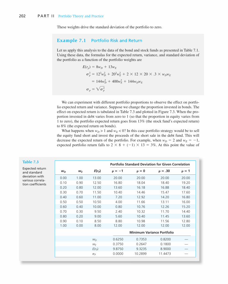
202 P A R T I I Portfolio Theory and Practice
These weights drive the standard deviation of the portfolio to zero.
We can experiment with different portfolio proportions to observe the effect on portfo-
lio expected return and variance. Suppose we change the proportion invested in bonds. The
effect on expected return is tabulated in Table 7.3 and plotted in Figure 7.3 . When the pro-
portion invested in debt varies from zero to 1 (so that the proportion in equity varies from
1 to zero), the portfolio expected return goes from 13% (the stock fund’s expected return)
to 8% (the expected return on bonds).
What happens when w D > 1 and w E < 0? In this case portfolio strategy would be to sell
the equity fund short and invest the proceeds of the short sale in the debt fund. This will
decrease the expected return of the portfolio. For example, when w D � 2 and w E � � 1,
expected portfolio return falls to 2 � 8 � ( � 1) � 13 � 3%. At this point the value of
Example 7.1 Portfolio Risk and Return
Let us apply this analysis to the data of the bond and stock funds as presented in Table 7.1 .
Using these data, the formulas for the expected return, variance, and standard deviation of
the portfolio as a function of the portfolio weights are
E(rp) 5 8wD 1 13wE
� p2 5 122wD
2 1 202wE2 1 2 3 12 3 20 3 .3 3 wDwE
5 144wD2 1 400wE
2 1 144wDwE
� p 5 "� p2
Table 7.3
Expected return and standard deviation with various correla-tion coefficients
Portfolio Standard Deviation for Given Correlation
wD wE E(rP) � � �1 � � 0 � � .30 � � 1
0.00 1.00 13.00 20.00 20.00 20.00 20.00
0.10 0.90 12.50 16.80 18.04 18.40 19.20
0.20 0.80 12.00 13.60 16.18 16.88 18.40
0.30 0.70 11.50 10.40 14.46 15.47 17.60
0.40 0.60 11.00 7.20 12.92 14.20 16.80
0.50 0.50 10.50 4.00 11.66 13.11 16.00
0.60 0.40 10.00 0.80 10.76 12.26 15.20
0.70 0.30 9.50 2.40 10.32 11.70 14.40
0.80 0.20 9.00 5.60 10.40 11.45 13.60
0.90 0.10 8.50 8.80 10.98 11.56 12.80
1.00 0.00 8.00 12.00 12.00 12.00 12.00
Minimum Variance Portfolio
wD 0.6250 0.7353 0.8200 —
wE 0.3750 0.2647 0.1800 —
E(rP) 9.8750 9.3235 8.9000 —
�P 0.0000 10.2899 11.4473 —

C H A P T E R 7 Optimal Risky Portfolios 203
the bond fund in the portfolio is twice the net
worth of the account. This extreme position is
financed in part by short-selling stocks equal in
value to the portfolio’s net worth.
The reverse happens when w D < 0 and
w E > 1. This strategy calls for selling the bond
fund short and using the proceeds to finance
additional purchases of the equity fund.
Of course, varying investment proportions
also has an effect on portfolio standard devia-
tion. Table 7.3 presents portfolio standard
deviations for different portfolio weights cal-
culated from Equation 7.7 using the assumed
value of the correlation coefficient, .30, as well
as other values of � . Figure 7.4 shows the rela-
tionship between standard deviation and port-
folio weights. Look first at the solid curve for
�DE � .30. The graph shows that as the port-
folio weight in the equity fund increases from
zero to 1, portfolio standard deviation first falls
with the initial diversification from bonds into
stocks, but then rises again as the portfolio
becomes heavily concentrated in stocks, and
again is undiversified. This pattern will gener-
ally hold as long as the correlation coefficient
Figure 7.3 Portfolio expected return as a function of investment proportions
Expected Return
13%
8%
Equity Fund
Debt Fund
w (stocks)
w (bonds) = 1 − w (stocks)
− 0.5 0 1.0 2.0
1.5 1.0 0 −1.0
Figure 7.4 Portfolio standard deviation as a function of investment proportions
ρ = .30
−.50 .500 1.501.0
Weight in Stock Fund
Portfolio Standard Deviation (%)
ρ = −1
ρ = 0
ρ = 1
35
30
25
20
15
10
5
0
204 P A R T I I Portfolio Theory and Practice
between the funds is not too high. 3 For a pair of assets with a large positive correlation
of returns, the portfolio standard deviation will increase monotonically from the low-risk
asset to the high-risk asset. Even in this case, however, there is a positive (if small) value
from diversification.
What is the minimum level to which portfolio standard deviation can be held? For the
parameter values stipulated in Table 7.1 , the portfolio weights that solve this minimization
problem turn out to be 4
wMin(D) 5 .82
wMin(E) 5 1 2 .82 5 .18
This minimum-variance portfolio has a standard deviation of
�Min 5 3(.822 3 122) 1 (.182 3 202) 1 (2 3 .82 3 .18 3 72) 41/2 5 11.45%
as indicated in the last line of Table 7.3 for the column � � .30.
The solid colored line in Figure 7.4 plots the portfolio standard deviation when � � .30
as a function of the investment proportions. It passes through the two undiversified port-
folios of w D � 1 and w E � 1. Note that the minimum-variance portfolio has a standard
deviation smaller than that of either of the individual component assets. This illustrates the
effect of diversification.
The other three lines in Figure 7.4 show how portfolio risk varies for other values of the
correlation coefficient, holding the variances of each asset constant. These lines plot the
values in the other three columns of Table 7.3 .
The solid dark straight line connecting the undiversified portfolios of all bonds or all
stocks, w D � 1 or w E � 1, shows portfolio standard deviation with perfect positive correla-
tion, � � 1. In this case there is no advantage from diversification, and the portfolio stan-
dard deviation is the simple weighted average of the component asset standard deviations.
The dashed colored curve depicts portfolio risk for the case of uncorrelated assets,
� � 0. With lower correlation between the two assets, diversification is more effective and
portfolio risk is lower (at least when both assets are held in positive amounts). The mini-
mum portfolio standard deviation when � � 0 is 10.29% (see Table 7.3 ), again lower than
the standard deviation of either asset.
Finally, the triangular broken line illustrates the perfect hedge potential when the
two assets are perfectly negatively correlated ( � � � 1). In this case the solution for the
m inimum-variance portfolio is, by Equation 7.12 ,
wMin(D; � 5 21) 5� E
� D 1 � E
520
12 1 205 .625
wMin(E; � 5 21) 5 1 2 .625 5 .375
and the portfolio variance (and standard deviation) is zero.
We can combine Figures 7.3 and 7.4 to demonstrate the relationship between portfolio
risk (standard deviation) and expected return—given the parameters of the available assets.
3 As long as � < � D / � E , volatility will initially fall when we start with all bonds and begin to move into stocks.
4 This solution uses the minimization techniques of calculus. Write out the expression for portfolio variance from
Equation 7.3 , substitute 1 � w D for w E , differentiate the result with respect to w D , set the derivative equal to zero,
and solve for w D to obtain
wMin(D) 5�E
2 2 Cov(rD, rE)
�D2 1 �E
2 2 2Cov(rD, rE)
Alternatively, with a spreadsheet program such as Excel, you can obtain an accurate solution by using the Solver
to minimize the variance. See Appendix A for an example of a portfolio optimization spreadsheet.
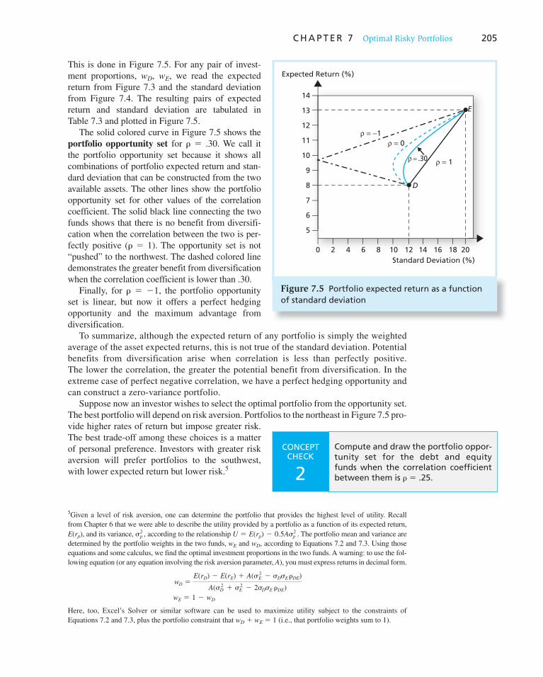
C H A P T E R 7 Optimal Risky Portfolios 205
This is done in Figure 7.5 . For any pair of invest-
ment proportions, w D , w E , we read the expected
return from Figure 7.3 and the standard deviation
from Figure 7.4 . The resulting pairs of expected
return and standard deviation are tabulated in
Table 7.3 and plotted in Figure 7.5 .
The solid colored curve in Figure 7.5 shows the
portfolio opportunity set for � � .30. We call it
the portfolio opportunity set because it shows all
combinations of portfolio expected return and stan-
dard deviation that can be constructed from the two
available assets. The other lines show the portfolio
opportunity set for other values of the correlation
coefficient. The solid black line connecting the two
funds shows that there is no benefit from diversifi-
cation when the correlation between the two is per-
fectly positive ( � � 1). The opportunity set is not
“pushed” to the northwest. The dashed colored line
demonstrates the greater benefit from diversification
when the correlation coefficient is lower than .30.
Finally, for � � � 1, the portfolio opportunity
set is linear, but now it offers a perfect hedging
opportunity and the maximum advantage from
diversification.
To summarize, although the expected return of any portfolio is simply the weighted
average of the asset expected returns, this is not true of the standard deviation. Potential
benefits from diversification arise when correlation is less than perfectly positive.
The lower the correlation, the greater the potential benefit from diversification. In the
extreme case of perfect negative correlation, we have a perfect hedging opportunity and
can construct a zero-variance portfolio.
Suppose now an investor wishes to select the optimal portfolio from the opportunity set.
The best portfolio will depend on risk aversion. Portfolios to the northeast in Figure 7.5 pro-
vide higher rates of return but impose greater risk.
The best trade-off among these choices is a matter
of personal preference. Investors with greater risk
aversion will prefer portfolios to the southwest,
with lower expected return but lower risk. 5
5 Given a level of risk aversion, one can determine the portfolio that provides the highest level of utility. Recall
from Chapter 6 that we were able to describe the utility provided by a portfolio as a function of its expected return,
E ( r p ), and its variance, �p2 , according to the relationship U 5 E(rp) 2 0.5A�p
2 . The portfolio mean and variance are
determined by the portfolio weights in the two funds, w E and w D , according to Equations 7.2 and 7.3 . Using those
equations and some calculus, we find the optimal investment proportions in the two funds. A warning: to use the fol-
lowing equation (or any equation involving the risk aversion parameter, A ), you must express returns in decimal form.
wD 5E(rD) 2 E(rE) 1 A(�E
2 2 �D�E �DE)
A(�D2 1 �E
2 2 2�D�E �DE)
wE 5 1 2 wD
Here, too, Excel’s Solver or similar software can be used to maximize utility subject to the constraints of
Equations 7.2 and 7.3 , plus the portfolio constraint that w D � w E � 1 (i.e., that portfolio weights sum to 1).
Figure 7.5 Portfolio expected return as a function of standard deviation
14
13
12
11
10
9
8
7
6
5
Standard Deviation (%)
0 2 4 6 8 10 12 14 16 18 20
Expected Return (%)
D
E
ρ = −1
ρ = 0
ρ = .30ρ = 1
CONCEPT CHECK
2
Compute and draw the portfolio oppor-tunity set for the debt and equity funds when the correlation coefficient between them is � � .25.

206 P A R T I I Portfolio Theory and Practice
7.3 Asset Allocation with Stocks, Bonds, and Bills
In the previous chapter we examined the capital allocation decision, the choice of how
much of the portfolio to leave in risk-free money market securities versus in a risky portfo-
lio. Now we have taken a further step, specifying that the risky portfolio comprises a stock
and a bond fund. We still need to show how investors can decide on the proportion of their
risky portfolios to allocate to the stock versus the bond market. This is an asset allocation
decision. As the nearby box emphasizes, most investment professionals recognize that “the
really critical decision is how to divvy up your money among stocks, bonds and supersafe
investments such as Treasury bills.”
In the last section, we derived the properties of portfolios formed by mixing two risky
assets. Given this background, we now reintroduce the choice of the third, risk-free, portfo-
lio. This will allow us to complete the basic problem of asset allocation across the three key
asset classes: stocks, bonds, and risk-free money market securities. Once you understand this
case, it will be easy to see how portfolios of many risky securities might best be constructed.
The Optimal Risky Portfolio with Two Risky Assets and a Risk-Free Asset
What if our risky assets are still confined to the bond and stock funds, but now we can also
invest in risk-free T-bills yielding 5%? We start with a graphical solution. Figure 7.6 shows
the opportunity set based on the properties of the bond and stock funds, using the data from
Table 7.1 .
Two possible capital allocation lines (CALs) are drawn from the risk-free rate ( r f � 5%)
to two feasible portfolios. The first possible CAL is drawn through the minimum-variance
portfolio A, which is invested 82% in bonds and 18% in stocks ( Table 7.3 , bottom panel,
last column). Portfolio A ’s expected return is 8.90%, and its standard deviation is 11.45%.
With a T-bill rate of 5%, the reward-to-volatility (Sharpe) ratio, which is the slope of
the CAL combining T-bills and the minimum-
variance portfolio, is
SA 5E(rA) 2 rf
� A5
8.9 2 5
11.455 .34
Now consider the CAL that uses portfolio B
instead of A. Portfolio B invests 70% in bonds and
30% in stocks. Its expected return is 9.5% (a risk
premium of 4.5%), and its standard deviation is
11.70%. Thus the reward-to-volatility ratio on the
CAL that is supported by portfolio B is
SB 59.5 2 5
11.75 .38
which is higher than the reward-to-volatility ratio
of the CAL that we obtained using the minimum-
variance portfolio and T-bills. Hence, portfolio B
dominates A.
But why stop at portfolio B? We can continue
to ratchet the CAL upward until it ultimately
reaches the point of tangency with the investment
opportunity set. This must yield the CAL with the
Figure 7.6 The opportunity set of the debt and equity funds and two feasible CALs
13
12
11
10
9
8
7
6
5
Standard Deviation (%)
0 5 10 15 20 25
Expected Return (%)
D
E
A
B
CAL(A)
CAL(B)
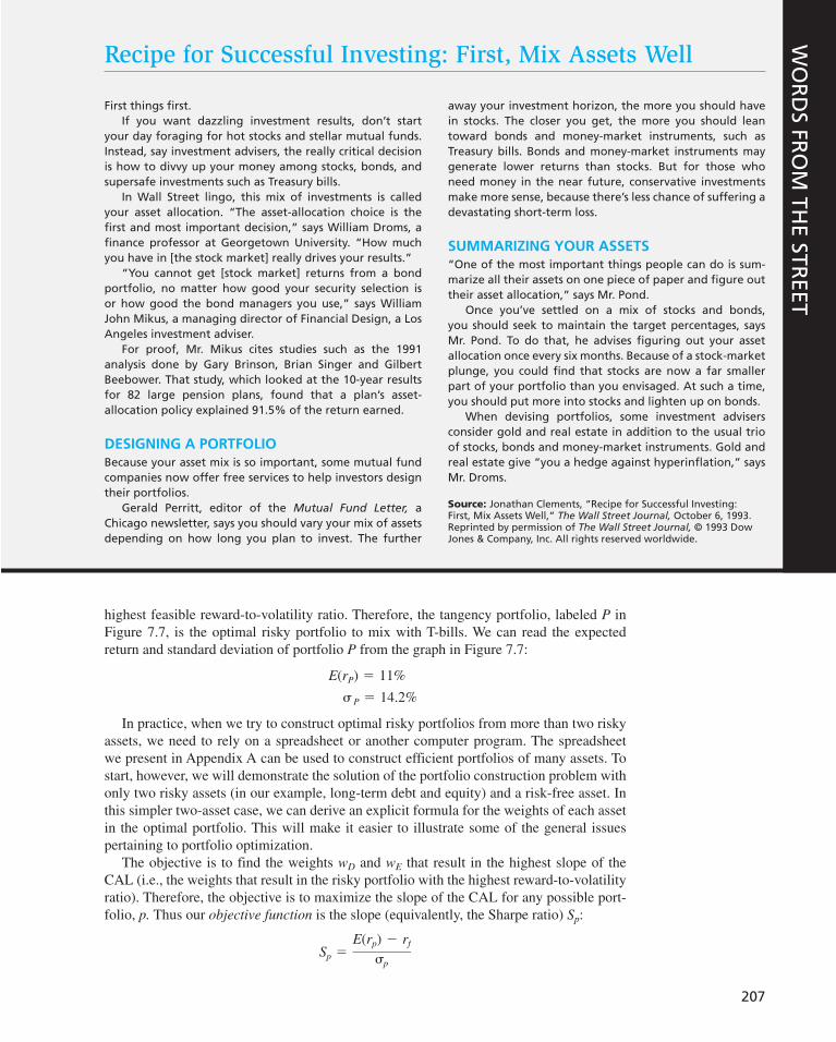
207
Recipe for Successful Investing: First, Mix Assets Well
First things first. If you want dazzling investment results, don’t start
your day foraging for hot stocks and stellar mutual funds. Instead, say investment advisers, the really critical decision is how to divvy up your money among stocks, bonds, and supersafe investments such as Treasury bills.
In Wall Street lingo, this mix of investments is called your asset allocation. “The asset-allocation choice is the first and most important decision,” says William Droms, a finance professor at Georgetown University. “How much you have in [the stock market] really drives your results.”
“You cannot get [stock market] returns from a bond portfolio, no matter how good your security selection is or how good the bond managers you use,” says William John Mikus, a managing director of Financial Design, a Los Angeles investment adviser.
For proof, Mr. Mikus cites studies such as the 1991 analysis done by Gary Brinson, Brian Singer and Gilbert Beebower. That study, which looked at the 10-year results for 82 large pension plans, found that a plan’s asset- allocation policy explained 91.5% of the return earned.
DESIGNING A PORTFOLIO Because your asset mix is so important, some mutual fund companies now offer free services to help investors design their portfolios.
Gerald Perritt, editor of the Mutual Fund Letter, a Chicago newsletter, says you should vary your mix of assets depending on how long you plan to invest. The further
away your investment horizon, the more you should have in stocks. The closer you get, the more you should lean toward bonds and money-market instruments, such as Treasury bills. Bonds and money-market instruments may generate lower returns than stocks. But for those who need money in the near future, conservative investments make more sense, because there’s less chance of suffering a devastating short-term loss.
SUMMARIZING YOUR ASSETS “One of the most important things people can do is sum-marize all their assets on one piece of paper and figure out their asset allocation,” says Mr. Pond.
Once you’ve settled on a mix of stocks and bonds, you should seek to maintain the target percentages, says Mr. Pond. To do that, he advises figuring out your asset allocation once every six months. Because of a stock- market plunge, you could find that stocks are now a far smaller part of your portfolio than you envisaged. At such a time, you should put more into stocks and lighten up on bonds.
When devising portfolios, some investment advisers consider gold and real estate in addition to the usual trio of stocks, bonds and money-market instruments. Gold and real estate give “you a hedge against hyperinflation,” says Mr. Droms.
Source: Jonathan Clements, “Recipe for Successful Investing: First, Mix Assets Well,” The Wall Street Journal, October 6, 1993. Reprinted by permission of The Wall Street Journal, © 1993 Dow Jones & Company, Inc. All rights reserved worldwide.
WO
RD
S FRO
M TH
E STREET
highest feasible reward-to-volatility ratio. Therefore, the tangency portfolio, labeled P in
Figure 7.7 , is the optimal risky portfolio to mix with T-bills. We can read the expected
return and standard deviation of portfolio P from the graph in Figure 7.7 :
E(rP) 5 11%
� P 5 14.2%
In practice, when we try to construct optimal risky portfolios from more than two risky
assets, we need to rely on a spreadsheet or another computer program. The spreadsheet
we present in Appendix A can be used to construct efficient portfolios of many assets. To
start, however, we will demonstrate the solution of the portfolio construction problem with
only two risky assets (in our example, long-term debt and equity) and a risk-free asset. In
this simpler two-asset case, we can derive an explicit formula for the weights of each asset
in the optimal portfolio. This will make it easier to illustrate some of the general issues
pertaining to portfolio optimization.
The objective is to find the weights w D and w E that result in the highest slope of the
CAL (i.e., the weights that result in the risky portfolio with the highest reward-to-volatility
ratio). Therefore, the objective is to maximize the slope of the CAL for any possible port-
folio, p. Thus our objective function is the slope (equivalently, the Sharpe ratio) S p :
Sp 5E(rp) 2 rf
�p

Figure 7.7 The opportunity set of the debt and equity funds with the optimal CAL and the optimal risky portfolio
Standard Deviation (%)
0 5 10 15 20 25 30
Expected Return (%)
D
E
P
rf = 5%
CAL(P)
OpportunitySet of RiskyAssets
2
0
4
6
8
10
12
14
16
18
208 P A R T I I Portfolio Theory and Practice
For the portfolio with two risky assets, the
expected return and standard deviation of portfolio
p are
E(rp) 5 wDE(rD) 1 wEE(rE)
5 8wD 1 13wE
�p 5 3wD2�D
2 1 wE2 �E
2 1 2wDwE Cov(rD, rE)41/2
5 3144wD2 1 400wE
2 1 (2 3 72wDwE)41/2
When we maximize the objective function, Sp ,
we have to satisfy the constraint that the portfolio
weights sum to 1.0 (100%), that is, w D � w E � 1.
Therefore, we solve an optimization problem for-
mally written as
Maxwi
Sp 5E(rp) 2 rf
� p
subject to � w i � 1. This is a maximization prob-
lem that can be solved using standard tools of
calculus.
In the case of two risky assets, the solution for
the weights of the optimal risky portfolio, P, is
given by Equation 7.13 . Notice that the solution
employs excess rates of return (denoted R ) rather
than total returns (denoted r ). 6
wD 5E(RD)� E
2 2 E(RE)Cov(RD, RE)
E(RD)� E2 1 E(RE)� D
2 2 3E(RD) 1 E(RE) 4Cov(RD, RE) (7.13)
wE 5 1 2 wD
6 The solution procedure for two risky assets is as follows. Substitute for E ( r P ) from Equation 7.2 and for � P from
Equation 7.7 . Substitute 1 � w D for w E . Differentiate the resulting expression for S p with respect to w D , set the
derivative equal to zero, and solve for w D .
Example 7.2 Optimal Risky Portfolio
Using our data, the solution for the optimal risky portfolio is
wD 5(8 2 5)400 2 (13 2 5)72
(8 2 5)400 1 (13 2 5)144 2 (8 2 5 1 13 2 5)725 .40
wE 5 1 2 .40 5 .60
The expected return and standard deviation of this optimal risky portfolio are
E(rP) 5 (.4 3 8) 1 (.6 3 13) 5 11%
� P 5 3(.42 3 144) 1 (.62 3 400) 1 (2 3 .4 3 .6 3 72) 41/2 5 14.2%

C H A P T E R 7 Optimal Risky Portfolios 209
In Chapter 6 we found the optimal complete portfolio given an optimal risky portfolio
and the CAL generated by a combination of this portfolio and T-bills. Now that we have
constructed the optimal risky portfolio, P, we can use the individual investor’s degree of
risk aversion, A, to calculate the optimal proportion of the complete portfolio to invest in
the risky component.
Once we have reached this point, generalizing to the case of many risky assets is
straightforward. Before we move on, let us briefly summarize the steps we followed to
arrive at the complete portfolio.
1. Specify the return characteristics of all securities (expected returns, variances,
covariances).
2. Establish the risky portfolio:
a. Calculate the optimal risky portfolio, P ( Equation 7.13 ).
b. Calculate the properties of portfolio P using the weights determined in step ( a )
and Equations 7.2 and 7.3 .
3. Allocate funds between the risky portfolio and the risk-free asset:
a. Calculate the fraction of the complete portfolio allocated to portfolio P (the risky
portfolio) and to T-bills (the risk-free asset) ( Equation 7.14 ).
b. Calculate the share of the complete portfolio invested in each asset and in
T-bills.
7 Notice that we express returns as decimals in Equation 7.14 . This is necessary when using the risk aversion
parameter, A, to solve for capital allocation.
Example 7.3 Optimal Complete Portfolio
An investor with a coefficient of risk aversion A � 4 would take a position in portfolio
P of 7
y 5E(rP) 2 rf
A� P2
5.11 2 .05
4 3 .14225 .7439 (7.14)
Thus the investor will invest 74.39% of his or her wealth in portfolio P and 25.61% in
T-bills. Portfolio P consists of 40% in bonds, so the fraction of wealth in bonds will
be yw D � .4 � .7439 � .2976, or 29.76%. Similarly, the investment in stocks will be
yw E � .6 � .7439 � .4463, or 44.63%. The graphical solution of this asset allocation prob-
lem is presented in Figures 7.8 and 7.9 .
The CAL of this optimal portfolio has a slope of
SP 511 2 5
14.25 .42
which is the reward-to-volatility (Sharpe) ratio of portfolio P. Notice that this slope exceeds
the slope of any of the other feasible portfolios that we have considered, as it must if it is to
be the slope of the best feasible CAL.

210 P A R T I I Portfolio Theory and Practice
Recall that our two risky assets, the bond and stock mutual funds, are already diversified
portfolios. The diversification within each of these portfolios must be credited for a good deal
of the risk reduction compared to undiversified single securities. For example, the standard
deviation of the rate of return on an average stock is about 50% (see Figure 7.2 ). In contrast,
the standard deviation of our stock-index fund is only 20%, about equal to the historical stan-
dard deviation of the S&P 500 portfolio. This is evidence of the importance of diversification
within the asset class. Optimizing the asset allocation between bonds and stocks contributed
incrementally to the improvement in the reward-to-volatility ratio of the complete portfolio.
The CAL using the optimal combination of stocks and bonds (see Figure 7.8) shows that one
can achieve an expected return of 13% (matching that of the stock portfolio) with a standard
deviation of 18%, which is less than the 20% standard deviation of the stock portfolio.
Figure 7.8 Determination of the optimal complete portfolio
Standard Deviation (%)
0 5 10 15 20 25 30
Expected Return (%)
D
C
E
P
CAL(P)
OpportunitySet of RiskyAssets
Optimal RiskyPortfolio
Indifference Curve
OptimalCompletePortfolio
2
0
4
6
8
10
12
14
16
18
rf = 5%
Figure 7.9 The proportions of the optimal complete portfolio
Portfolio P74.39%
Stocks44.63%
Bonds29.76%
T-bills25.61%
CONCEPT CHECK
3
The universe of available securities includes two risky stock funds, A and B, and T-bills. The data for the universe are as follows:
Expected Return Standard Deviation
A 10% 20%
B 30 60
T-bills 5 0
The correlation coefficient between funds A and B is � .2.
a. Draw the opportunity set of funds A and B.
b. Find the optimal risky portfolio, P, and its expected return and standard deviation.
c. Find the slope of the CAL supported by T-bills and portfolio P.
d. How much will an investor with A � 5 invest in funds A and B and in T-bills?

C H A P T E R 7 Optimal Risky Portfolios 211
7.4 The Markowitz Portfolio Selection Model
Figure 7.10 The minimum-variance frontier of risky assets
E(r)
Minimum-Variance Frontier
IndividualAssets
GlobalMinimum-VariancePortfolio
Efficient Frontier
σ
Security Selection
We can generalize the portfolio con-
struction problem to the case of many
risky securities and a risk-free asset.
As in the two risky assets example,
the problem has three parts. First, we
identify the risk–return combinations
available from the set of risky assets.
Next, we identify the optimal portfolio
of risky assets by finding the portfolio
weights that result in the steepest CAL.
Finally, we choose an appropriate com-
plete portfolio by mixing the risk-free
asset with the optimal risky portfolio.
Before describing the process in detail,
let us first present an overview.
The first step is to determine the
risk–return opportunities available to
the investor. These are summarized by
the minimum-variance frontier of
risky assets. This frontier is a graph
of the lowest possible variance that can be attained for a given portfolio expected return.
Given the input data for expected returns, variances, and covariances, we can calculate the
minimum-variance portfolio for any targeted expected return. The plot of these expected
return–standard deviation pairs is presented in Figure 7.10 .
Notice that all the individual assets lie to the right inside the frontier, at least when we
allow short sales in the construction of risky portfolios. 8 This tells us that risky portfolios
comprising only a single asset are inefficient. Diversifying investments leads to portfolios
with higher expected returns and lower standard deviations.
All the portfolios that lie on the minimum-variance frontier from the global minimum-
variance portfolio and upward provide the best risk–return combinations and thus are
candidates for the optimal portfolio. The part of the frontier that lies above the global
minimum-variance portfolio, therefore, is called the efficient frontier of risky assets. For
any portfolio on the lower portion of the minimum-variance frontier, there is a portfolio
with the same standard deviation and a greater expected return positioned directly above it.
Hence the bottom part of the minimum-variance frontier is inefficient.
The second part of the optimization plan involves the risk-free asset. As before, we
search for the capital allocation line with the highest reward-to-volatility ratio (that is, the
steepest slope) as shown in Figure 7.11 .
The CAL that is supported by the optimal portfolio, P, is tangent to the efficient frontier.
This CAL dominates all alternative feasible lines (the broken lines that are drawn through
the frontier). Portfolio P, therefore, is the optimal risky portfolio.
8 When short sales are prohibited, single securities may lie on the frontier. For example, the security with the high-
est expected return must lie on the frontier, as that security represents the only way that one can obtain a return
that high, and so it must also be the minimum-variance way to obtain that return. When short sales are feasible,
however, portfolios can be constructed that offer the same expected return and lower variance. These portfolios
typically will have short positions in low-expected-return securities.

212
Finally, in the last part of the problem the individual investor chooses the appropriate
mix between the optimal risky portfolio P and T-bills, exactly as in Figure 7.8 .
Now let us consider each part of the portfolio construction problem in more detail. In the
first part of the problem, risk–return analysis, the portfolio manager needs as inputs a set of
estimates for the expected returns of each security and a set of estimates for the covariance
matrix. (In Part Five on security analysis we will examine the security valuation techniques
and methods of financial analysis that analysts use. For now, we will assume that ana-
lysts already have spent the time and
resources to prepare the inputs.)
The portfolio manager is now
armed with the n estimates of E ( r i )
and the n � n estimates of the cova-
riance matrix in which the n diagonal
elements are estimates of the vari-
ances, � i2, and the n 2 � n � n ( n � 1)
off-diagonal elements are the estimates
of the covariances between each pair
of asset returns. (You can verify this
from Table 7.2 for the case n � 2.)
We know that each covariance appears
twice in this table, so actually we have
n ( n � 1)/2 different covariance esti-
mates. If our portfolio management
unit covers 50 securities, our security
analysts need to deliver 50 estimates
of expected returns, 50 estimates of
variances, and 50 � 49/2 � 1,225 dif-
ferent estimates of covariances. This is
Figure 7.11 The efficient frontier of risky assets with the optimal CAL
E(r)
CAL(P)Efficient Frontier
P
rf
σ
eXcel APPLICATIONS: Two–Security Model
T he accompanying spreadsheet can be used to mea-sure the return and risk of a portfolio of two risky
assets. The model calculates the return and risk for vary-ing weights of each security along with the optimal risky and minimum-variance portfolio. Graphs are automatically generated for various model inputs. The model allows you
to specify a target rate of return and solves for optimal combinations using the risk-free asset and the optimal risky portfolio. The spreadsheet is constructed with the two-security return data from Table 7.1 . This spreadsheet is available at www.mhhe.com/bkm.
A B C D E F
1
2 Expected Standard Correlation
3 Return Deviation Coefficient Covariance
4 Security 1
5 Security 2
6 T-Bill
7
8 Weight Weight Expected Standard Reward to
9 Security 1 Security 2 Return Deviation Volatility
10
11
12
13
14
Asset Allocation Analysis: Risk and Return
0.08 0.12 0.3 0.0072
0.13 0.2
0.05 0
1 0 0.08000 0.12000 0.25000
0.9 0.1 0.08500 0.11559 0.30281
0.8 0.2 0.09000 0.11454 0.34922
0.7 0.3 0.09500 0.11696 0.38474
0.6 0.4 0.10000 0.407710.12264
0
Standard Deviation (%)
0 5
5
11
10 15 20 25 3530
Expected
Return (%)
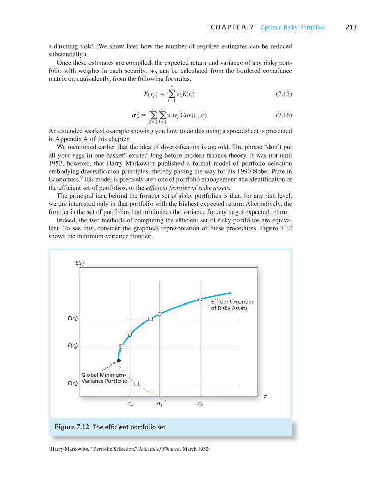
C H A P T E R 7 Optimal Risky Portfolios 213
a daunting task! (We show later how the number of required estimates can be reduced
substantially.)
Once these estimates are compiled, the expected return and variance of any risky port-
folio with weights in each security, w i , can be calculated from the bordered covariance
matrix or, equivalently, from the following formulas:
E(rp) 5 an
i51
wiE(ri) (7.15)
� p2 5 a
n
i51a
n
j51
wiwj Cov(ri, rj) (7.16)
An extended worked example showing you how to do this using a spreadsheet is presented
in Appendix A of this chapter.
We mentioned earlier that the idea of diversification is age-old. The phrase “don’t put
all your eggs in one basket” existed long before modern finance theory. It was not until
1952, however, that Harry Markowitz published a formal model of portfolio selection
embodying diversification principles, thereby paving the way for his 1990 Nobel Prize in
Economics. 9 His model is precisely step one of portfolio management: the identification of
the efficient set of portfolios, or the efficient frontier of risky assets.
The principal idea behind the frontier set of risky portfolios is that, for any risk level,
we are interested only in that portfolio with the highest expected return. Alternatively, the
frontier is the set of portfolios that minimizes the variance for any target expected return.
Indeed, the two methods of computing the efficient set of risky portfolios are equiva-
lent. To see this, consider the graphical representation of these procedures. Figure 7.12
shows the minimum-variance frontier.
9 Harry Markowitz, “Portfolio Selection,” Journal of Finance, March 1952.
Figure 7.12 The efficient portfolio set
E(r)
E(r3)
E(r2)
E(r1)
σA
σB
σC
Efficient Frontierof Risky Assets
Global Minimum-Variance Portfolio
σ

214 P A R T I I Portfolio Theory and Practice
The points marked by squares are the result of a variance-minimization program. We
first draw the constraints, that is, horizontal lines at the level of required expected returns.
We then look for the portfolio with the lowest standard deviation that plots on each hori-
zontal line—we look for the portfolio that will plot farthest to the left (smallest standard
deviation) on that line. When we repeat this for many levels of required expected returns,
the shape of the minimum-variance frontier emerges. We then discard the bottom (dashed)
half of the frontier, because it is inefficient.
In the alternative approach, we draw a vertical line that represents the standard devia-
tion constraint. We then consider all portfolios that plot on this line (have the same stan-
dard deviation) and choose the one with the highest expected return, that is, the portfolio
that plots highest on this vertical line. Repeating this procedure for many vertical lines
(levels of standard deviation) gives us the points marked by circles that trace the upper por-
tion of the minimum-variance frontier, the efficient frontier.
When this step is completed, we have a list of efficient portfolios, because the solution
to the optimization program includes the portfolio proportions, w i , the expected return,
E ( r p ), and the standard deviation, � p .
Let us restate what our portfolio manager has done so far. The estimates generated by
the security analysts were transformed into a set of expected rates of return and a covari-
ance matrix. This group of estimates we shall call the input list. This input list is then fed
into the optimization program.
Before we proceed to the second step of choosing the optimal risky portfolio from the
frontier set, let us consider a practical point. Some clients may be subject to additional
constraints. For example, many institutions are prohibited from taking short positions in
any asset. For these clients the portfolio manager will add to the optimization program
constraints that rule out negative (short) positions in the search for efficient portfolios.
In this special case it is possible that single assets may be, in and of themselves, efficient
risky portfolios. For example, the asset with the highest expected return will be a frontier
portfolio because, without the opportunity of short sales, the only way to obtain that rate of
return is to hold the asset as one’s entire risky portfolio.
Short-sale restrictions are by no means the only such constraints. For example, some cli-
ents may want to ensure a minimal level of expected dividend yield from the optimal port-
folio. In this case the input list will be expanded to include a set of expected dividend yields
d 1 , . . ., d n and the optimization program will include an additional constraint that ensures
that the expected dividend yield of the portfolio will equal or exceed the desired level, d.
Portfolio managers can tailor the efficient set to conform to any desire of the client. Of
course, any constraint carries a price tag in the sense that an efficient frontier constructed
subject to extra constraints will offer a reward-to-volatility ratio inferior to that of a less
constrained one. The client should be made aware of this cost and should carefully con-
sider constraints that are not mandated by law.
Another type of constraint is aimed at ruling out investments in industries or countries
considered ethically or politically undesirable. This is referred to as socially responsible
investing, which entails a cost in the form of a lower reward-to-volatility on the resultant
constrained, optimal portfolio. This cost can be justifiably viewed as a contribution to the
underlying cause.
Capital Allocation and the Separation Property
Now that we have the efficient frontier, we proceed to step two and introduce the risk-
free asset. Figure 7.13 shows the efficient frontier plus three CALs representing various
portfolios from the efficient set. As before, we ratchet up the CAL by selecting d ifferent

215
portfolios until we reach portfolio P, which is the
tangency point of a line from F to the efficient
frontier. Portfolio P maximizes the reward-to-
volatility ratio, the slope of the line from F to
portfolios on the efficient frontier. At this point
our portfolio manager is done. Portfolio P is the
optimal risky portfolio for the manager’s clients.
This is a good time to ponder our results and their
implementation.
The most striking conclusion is that a portfo-
lio manager will offer the same risky portfolio, P,
to all clients regardless of their degree of risk
aversion. 10 The degree of risk aversion of the cli-
ent comes into play only in the selection of the
desired point along the CAL. Thus the only dif-
ference between clients’ choices is that the more
risk-averse client will invest more in the risk-free
asset and less in the optimal risky portfolio than
will a less risk-averse client. However, both will
use portfolio P as their optimal risky investment
vehicle.
This result is called a separation property; it tells us that the portfolio choice problem
may be separated into two independent tasks. 11 The first task, determination of the optimal
10 Clients who impose special restrictions (constraints) on the manager, such as dividend yield, will obtain another
optimal portfolio. Any constraint that is added to an optimization problem leads, in general, to a different and
inferior optimum compared to an unconstrained program. 11 The separation property was first noted by Nobel laureate James Tobin, “Liquidity Preference as Behavior
toward Risk,” Review of Economic Statistics 25 (February 1958), pp. 65–86.
eXcel APPLICATIONS: Optimal Portfolios
A spreadsheet model featuring optimal risky portfolios is available on the Online Learning Center at www.
mhhe.com/bkm. It contains a template that is similar to the template developed in this section. The model can be used to find optimal mixes of securities for targeted levels
of returns for both restricted and unrestricted portfolios. Graphs of the efficient frontier are generated for each set of inputs. The example available at our Web site applies the model to portfolios constructed from equity indexes (called WEBS securities) of several countries.
A B C D E F
1
2
Standard3
Deviation4
5
6
7
8
9
10
11
12
Mean
ReturnWEBS
EWD
EWH
EWI
EWJ
EWL
EWP
EWW
S&P 500
Country
Sweden
Hong Kong
Italy
Japan
Switzerland
Spain
Mexico
15.5393
6.3852
26.5999
1.4133
18.0745
18.6347
16.2243
17.2306
26.4868
41.1475
26.0514
26.0709
21.6916
25.0779
38.7686
17.1944
Efficient Frontier for World Equity Benchmark Securities (WEBS)
Figure 7.13 Capital allocation lines with various portfolios from the efficient set
E(r)
(Global Minimum-Variance Portfolio)
Efficient Frontierof Risky Assets
CAL(P)
CAL(A)
CAL(G)
A
G
P
F
σ

216 P A R T I I Portfolio Theory and Practice
risky portfolio, is purely technical. Given the manager’s input list, the best risky portfolio
is the same for all clients, regardless of risk aversion. The second task, however, allocation
of the complete portfolio to T-bills versus the risky portfolio, depends on personal prefer-
ence. Here the client is the decision maker.
The crucial point is that the optimal portfolio P that the manager offers is the same for
all clients. Put another way, investors with varying degrees of risk aversion would be satis-
fied with a universe of only two mutual funds: a money market fund for risk-free invest-
ments and a mutual fund that holds the optimal risky portfolio, P, on the tangency point
of the CAL and the efficient frontier. This result makes professional management more
efficient and hence less costly. One management firm can serve any number of clients with
relatively small incremental administrative costs.
In practice, however, different managers will estimate different input lists, thus
deriving different efficient frontiers, and offer different “optimal” portfolios to their
clients. The source of the disparity lies in the security analysis. It is worth mentioning
here that the universal rule of GIGO (garbage in–garbage out) also applies to secu-
rity analysis. If the quality of the security analysis is poor, a passive portfolio such
as a market index fund will result in a better CAL than an active portfolio that uses
low-quality security analysis to tilt portfolio weights toward seemingly favorable (mis-
priced) securities.
One particular input list that would lead to a worthless estimate of the efficient fron-
tier is based on recent security average returns. If sample average returns over recent
years are used as proxies for the true expected return on the security, the noise in
those estimates will make the resultant efficient frontier virtually useless for portfolio
construction.
Consider a stock with an annual standard deviation of 50%. Even if one were to use
a 10-year average to estimate its expected return (and 10 years is almost ancient his-
tory in the life of a corporation), the standard deviation of that estimate would still be
50/"10 5 15.8%. The chances that this average represents expected returns for the com-
ing year are negligible. 12 In Chapter 25, we see an example demonstrating that efficient
frontiers constructed from past data may be wildly optimistic in terms of the apparent
opportunities they offer to improve Sharpe ratios.
As we have seen, optimal risky portfolios for different clients also may vary because
of portfolio constraints such as dividend-yield requirements, tax considerations, or other
client preferences. Nevertheless, this analysis suggests that a limited number of portfolios
may be sufficient to serve the demands of a wide range of investors. This is the theoretical
basis of the mutual fund industry.
The (computerized) optimization technique is the easiest part of the portfolio construc-
tion problem. The real arena of competition among portfolio managers is in sophisticated
security analysis. This analysis, as well as its proper interpretation, is part of the art of
portfolio construction. 13
12 Moreover, you cannot avoid this problem by observing the rate of return on the stock more frequently. In
Chapter 5 we pointed out that the accuracy of the sample average as an estimate of expected return depends
on the length of the sample period, and is not improved by sampling more frequently within a given sample
period.
13 You can find a nice discussion of some practical issues in implementing efficient diversification in a white
paper prepared by Wealthcare Capital Management at this address: www.financeware.com/ruminations/WP_
EfficiencyDeficiency.pdf. A copy of the report is also available at the Online Learning Center for this text, www.
mhhe.com/bkm.

C H A P T E R 7 Optimal Risky Portfolios 217
The Power of Diversification
Section 7.1 introduced the concept of diversification and the limits to the benefits of diver-
sification resulting from systematic risk. Given the tools we have developed, we can recon-
sider this intuition more rigorously and at the same time sharpen our insight regarding the
power of diversification.
Recall from Equation 7.16 , restated here, that the general formula for the variance of a
portfolio is
� p2 5 a
n
i51a
n
j51
wiwj Cov(ri, rj) (7.16)
Consider now the naive diversification strategy in which an equally weighted portfolio is
constructed, meaning that w i � 1/ n for each security. In this case Equation 7.16 may be
rewritten as follows, where we break out the terms for which i � j into a separate sum,
noting that Cov 1ri, ri 2 5 � i2:
� p2 5
1na
n
i51
1
n � i
2 1 an
j51j2 i
an
i51
1
n2 Cov(ri, rj) (7.17)
Note that there are n variance terms and n ( n � 1) covariance terms in Equation 7.17 .
If we define the average variance and average covariance of the securities as
� 2 51
nan
i51
� i2 (7.18)
Cov 51
n(n 2 1)an
j51j2 i
an
i51
Cov(ri, rj) (7.19)
we can express portfolio variance as
� p2 5
1
n � 2 1
n 2 1
n Cov (7.20)
Now examine the effect of diversification. When the average covariance among security
returns is zero, as it is when all risk is firm-specific, portfolio variance can be driven to
zero. We see this from Equation 7.20 . The second term on the right-hand side will be zero
CONCEPT CHECK
4
Suppose that two portfolio managers who work for competing investment management houses each employ a group of security analysts to prepare the input list for the Markowitz algorithm. When all is completed, it turns out that the efficient frontier obtained by port-folio manager A seems to dominate that of manager B. By dominate, we mean that A ’s optimal risky portfolio lies northwest of B ’s. Hence, given a choice, investors will all prefer the risky portfolio that lies on the CAL of A.
a. What should be made of this outcome?
b. Should it be attributed to better security analysis by A ’s analysts?
c. Could it be that A ’s computer program is superior?
d. If you were advising clients (and had an advance glimpse at the efficient frontiers of various managers), would you tell them to periodically switch their money to the m anager with the most northwesterly portfolio?

218 P A R T I I Portfolio Theory and Practice
in this scenario, while the first term approaches zero as n becomes larger. Hence when
security returns are uncorrelated, the power of diversification to reduce portfolio risk is
unlimited.
However, the more important case is the one in which economywide risk factors impart
positive correlation among stock returns. In this case, as the portfolio becomes more highly
diversified ( n increases), portfolio variance remains positive. Although firm-specific risk,
represented by the first term in Equation 7.20 , is still diversified away, the second term
simply approaches Cov as n becomes greater. [Note that ( n � 1)/ n � 1 � 1/ n, which
approaches 1 for large n. ] Thus the irreducible risk of a diversified portfolio depends on
the covariance of the returns of the component securities, which in turn is a function of the
importance of systematic factors in the economy.
To see further the fundamental relationship between systematic risk and security corre-
lations, suppose for simplicity that all securities have a common standard deviation, � , and
all security pairs have a common correlation coefficient, � . Then the covariance between
all pairs of securities is � � 2 , and Equation 7.20 becomes
� p2 5
1
n � 2 1
n 2 1
n �� 2 (7.21)
The effect of correlation is now explicit. When � � 0, we again obtain the insurance
principle, where portfolio variance approaches zero as n becomes greater. For � > 0, how-
ever, portfolio variance remains positive. In fact, for � � 1, portfolio variance equals � 2
regardless of n, demonstrating that diversification is of no benefit: In the case of perfect
correlation, all risk is systematic. More generally, as n becomes greater, Equation 7.21
shows that systematic risk becomes � � 2 .
Table 7.4 presents portfolio standard deviation as we include ever-greater numbers of
securities in the portfolio for two cases, � � 0 and � � .40. The table takes � to be 50%. As
one would expect, portfolio risk is greater when � � .40. More surprising, perhaps, is that
portfolio risk diminishes far less rapidly as n increases in the positive correlation case. The
correlation among security returns limits the power of diversification.
Note that for a 100-security portfolio, the standard deviation is 5% in the uncorrelated
case—still significant compared to the potential of zero standard deviation. For � � .40,
the standard deviation is high, 31.86%, yet it is very close to undiversifiable systematic
Table 7.4
Risk reduction of equally weighted portfolios in correlated and uncorrelated universes
� � 0 � � .40
Universe Size n
Portfolio Weights
w � 1/n (%)
Standard Deviation
(%)Reduction
in �Standard
Deviation (%) Reduction in �
1 100 50.00 14.64 50.00 8.17
2 50 35.36 41.83
5 20 22.36 1.95 36.06 0.70
6 16.67 20.41 35.36
10 10 15.81 0.73 33.91 0.20
11 9.09 15.08 33.71
20 5 11.18 0.27 32.79 0.06
21 4.76 10.91 32.73
100 1 5.00 0.02 31.86 0.00
101 0.99 4.98 31.86

C H A P T E R 7 Optimal Risky Portfolios 219
risk in the infinite-sized security universe, "� � 2 5 ".4 3 502 5 31.62%. At this point,
further diversification is of little value.
Perhaps the most important insight from the exercise is this: When we hold diversified
portfolios, the contribution to portfolio risk of a particular security will depend on the
covariance of that security’s return with those of other securities, and not on the security’s
variance. As we shall see in Chapter 9, this implies that fair risk premiums also should
depend on covariances rather than total variability of returns.
CONCEPT CHECK
5
Suppose that the universe of available risky securities consists of a large number of stocks, identically distributed with E ( r ) � 15%, � � 60%, and a common correlation coefficient of � � .5.
a. What are the expected return and standard deviation of an equally weighted risky portfolio of 25 stocks?
b. What is the smallest number of stocks necessary to generate an efficient portfolio with a standard deviation equal to or smaller than 43%?
c. What is the systematic risk in this security universe?
d. If T-bills are available and yield 10%, what is the slope of the CAL?
Asset Allocation and Security Selection
As we have seen, the theories of security selection and asset allocation are identical. Both
activities call for the construction of an efficient frontier, and the choice of a particular
portfolio from along that frontier. The determination of the optimal combination of secu-
rities proceeds in the same manner as the analysis of the optimal combination of asset
classes. Why, then, do we (and the investment community) distinguish between asset allo-
cation and security selection?
Three factors are at work. First, as a result of greater need and ability to save (for col-
lege educations, recreation, longer life in retirement, health care needs, etc.), the demand
for sophisticated investment management has increased enormously. Second, the widening
spectrum of financial markets and financial instruments has put sophisticated investment
beyond the capacity of many amateur investors. Finally, there are strong economies of scale
in investment analysis. The end result is that the size of a competitive investment company
has grown with the industry, and efficiency in organization has become an important issue.
A large investment company is likely to invest both in domestic and international mar-
kets and in a broad set of asset classes, each of which requires specialized expertise. Hence
the management of each asset-class portfolio needs to be decentralized, and it becomes
impossible to simultaneously optimize the entire organization’s risky portfolio in one
stage, although this would be prescribed as optimal on theoretical grounds.
The practice is therefore to optimize the security selection of each asset-class portfolio
independently. At the same time, top management continually updates the asset allocation
of the organization, adjusting the investment budget allotted to each asset-class portfolio.
Optimal Portfolios and Nonnormal Returns
The portfolio optimization techniques we have used so far assume normal distributions of
returns in that standard deviation is taken to be a fully adequate measure of risk. However,
potential nonnormality of returns requires us to pay attention as well to risk measures that
focus on worst-case losses such as value at risk (VaR) or expected shortfall (ES).

220 P A R T I I Portfolio Theory and Practice
In Chapter 6 we suggested that capital allocation to the risky portfolio should be recon-
sidered in the face of fat-tailed distributions that can result in extreme values of VaR and
ES. Specifically, forecasts of greater VaR and ES should encourage more moderate portfo-
lio allocations to the risky portfolio. When we select the composition of the optimal risky
portfolio itself, considering the effect of diversification on VaR and ES would be useful as
well. Unfortunately, the impact of diversification cannot be readily simplified in this case,
as we are able to do when returns are normally distributed.
A practical way to estimate values of VaR and ES in the presence of fat tails is boot-
strapping (described in Section 5.9). We start with a historical sample of returns of each
relevant asset in our investment universe. From this sample, we randomly draw returns
for each of those assets; we can draw as many of these random samples as we wish, for
example, 50,000 observations for each asset. The returns of various portfolios constructed
from this historically based but randomly selected sample can provide a good estimate of
VaR and ES values. The forecasted values for VaR and ES of the mean-variance optimal
portfolio can then be compared to other candidate portfolios. If these other portfolios yield
sufficiently better VaR and ES values, we may prefer one of those to the mean-variance
efficient portfolio given the possibility of fat tails.
7.5 Risk Pooling, Risk Sharing, and the Risk of Long-Term Investments *
Diversification means that we spread our investment budget across a variety of assets and
thus limit overall risk. Sometimes it is argued that spreading investments across time, so
that the average return reflects returns in several investment periods, offers an analogous
benefit dubbed “time diversification,” thus rendering long-term investing safer than short-
term investing.
Is this extension of diversification to investments over time valid? The question of how
risk increases when the horizon of a risky investment lengthens is analogous to risk pool-
ing, the process by which an insurance company aggregates a large portfolio (or pool) of
uncorrelated risks. However, the respective impacts of risk pooling versus risk sharing
(whereby the firm spreads or shares the risk of a fixed portfolio among many owners) are
widely misunderstood, and the common application of “the insurance principle” to long-
term investing is also fraught with widespread misconceptions. In this section, we try to
clarify these issues and explore the appropriate extension of these ideas to risk analysis for
long-term investments.
Risk Pooling and the Insurance Principle
Risk pooling means merging uncorrelated, risky projects as a means to reduce risk.
Applied to the insurance business, risk pooling entails selling many uncorrelated insurance
policies. This application of risk pooling has come to be known as the insurance principle.
Conventional wisdom holds that risk pooling reduces risk, and that such pooling is the
driving force behind risk management for the insurance industry.
But even brief reflection should convince you that risk pooling cannot be the entire
story. How can adding bets that are independent of your other bets reduce your total
*The material in this section is more challenging. It may be skipped without impairing the ability to understand
later chapters.
C H A P T E R 7 Optimal Risky Portfolios 221
e xposure? This would be little different from a gambler in Las Vegas arguing that a few
more trips to the roulette table will reduce his total risk by diversifying his overall “port-
folio” of wagers. You would immediately realize that the gambler now has more money at
stake, and his overall potential swing in wealth is clearly wider: While his average gain or
loss per bet may become more predictable as he repeatedly returns to the table, his total
proceeds become less so. As we will see, the insurance principle is sometimes similarly
misapplied to long-term investments by incorrectly extending what it implies about aver-
age returns to predictions about total returns.
Risk Pooling
We’ve hinted that risk pooling and risk sharing are two complementary, but distinct, tools
in risk management. Let’s try to carefully show how each works. We start with risk pooling.
Imagine a rich investor, Warren, who holds a $1 billion portfolio, P. The fraction of the
portfolio invested in a risky asset, A, is y, leaving the fraction 1 � y invested in the risk-
free rate. Asset A ’s risk premium is R, and its standard deviation is � . From Equations 6.3
and 6.4, the risk premium of the complete portfolio P is R P � yR, its standard deviation is
� P � y � , and the Sharpe ratio is S P � R / � . Now Warren identifies another risky asset, B,
with the same risk premium and standard deviation as A. Warren estimates that the correla-
tion (and therefore covariance) between the two investments is zero, and he is intrigued at
the potential this offers for risk reduction through diversification.
Given the benefits that Warren anticipates from diversification, he decides to take a posi-
tion in asset B equal in size to his existing position in asset A. He therefore transfers another
fraction, y, of wealth from the risk-free asset to asset B. This leaves his total portfolio allo-
cated as follows: the fraction y is still invested in asset A, an additional investment of y is
invested in B, and 1 � 2 y is in the risk-free asset. Notice that this strategy is analogous to
pure risk pooling; Warren has taken on additional risky (albeit uncorrelated) bets, and his
risky portfolio is larger than it was previously. We will denote Warren’s new portfolio as Z.
We can compute the risk premium of portfolio Z from Equation 7.2 , its variance from
Equation 7.3 , and thus its Sharpe ratio. Remember that capital R denotes the excess return
of each asset and the excess return of the risk-free asset is zero. When calculating portfolio
variance, we use the fact that covariance is zero. Thus, for Portfolio Z:
RZ 5 yR 1 yR 1 (1 2 2y)0 5 2yR (double RP)
� Z2 5 y2� 2 1 y2� 2 1 0 5 2y2� 2 (double the variance of P)
�Z 5 "� Z2 5 y�"2 ("2 5 1.41 times the standard deviation of P)
SZ 5 RZ/�Z 5 2yR/y�"2 5 "2R/� ("2 5 1.41 times Sharpe ratio of P)
The good news from these results is that the Sharpe ratio of Z is higher than that of P by
the factor "2. Its excess rate of return is double that of P, yet its standard deviation is only
"2 times larger. The bad news is that by increasing the scale of the risky investment, the
standard deviation of the portfolio also increases by "2.
We might now imagine that instead of two uncorrelated assets, Warren has access to
many. Repeating our analysis, we would find that with n assets the Sharpe ratio under
strategy Z increases (relative to its original value) by a factor of "n to "n 3 R/� . But the
total risk of the pooling strategy Z will increase by the same multiple, to �"n.
This analysis illustrates both the opportunities and limitations of pure risk pooling:
Pooling increases the scale of the risky investment (from y to 2 y ) by adding an additional
position in another, uncorrelated asset. This addition of another risky bet also increases the
222 P A R T I I Portfolio Theory and Practice
size of the risky budget. So risk pooling by itself does not reduce risk, despite the fact that
it benefits from the lack of correlation across policies.
The insurance principle tells us only that risk increases less than proportionally to the
number of policies insured when the policies are uncorrelated; hence profitability—in
this application, the Sharpe ratio—increases. But this effect is not sufficient to actually
reduce risk.
This might limit the potential economies of scale of an ever-growing portfolio such
as that of a large insurer. You can interpret each “asset” in our analysis as one insurance
policy. Each policy written requires the insurance company to set aside additional capital
to cover potential losses. The insurance company invests its capital until it needs to pay out
on claims. Selling more policies entails increasing the total position in risky investments
and therefore the capital that must be allocated to those policies. As the company invests
in more uncorrelated assets (insurance policies), the Sharpe ratio continuously increases
(which is good), but since more funds are invested in risky policies, the overall risk of the
portfolio rises (which is bad). As the number of policies grows, the risk of the pool will
certainly grow—despite “diversification” across policies. Eventually, that growing risk
will overwhelm the company’s available capital.
Insurance analysts often think in terms of probability of loss. Their mathematically
correct interpretation of the insurance principle is that the probability of loss declines
with risk pooling. This interpretation relates to the fact that the Sharpe ratio (profitability)
increases with risk pooling. But to equate the declining probability of loss to reduction in
total risk is erroneous; the latter is measured by overall standard deviation, which increases
with risk pooling. (Again, think about the gambler in Las Vegas. As he returns over and
over again to the roulette table, the probability that he will lose becomes ever more certain,
but the magnitude of potential dollar gains or losses becomes ever greater.) Thus risk pool-
ing allows neither investors nor insurance companies to shed risk. However, the increase in
risk can be overcome when risk pooling is augmented by risk sharing, as discussed in the
next subsection.
Risk Sharing
Now think about a variation on the risk pooling portfolio Z. Imagine that Warren has iden-
tified several attractive insurance policies and wishes to invest in all of them. For simplic-
ity, we will look at the case of two policies, so the pool will have the same properties as
portfolio Z. We saw that if Warren invested in this two-policy pool, his total risk would be
� Z 5 y�"2. But if this is more risk than he is willing to bear, what might he do?
His solution is risk sharing, the act of selling shares in an attractive risky portfolio to
limit risk and yet maintain the Sharpe ratio (profitability) of the resultant position. Suppose
that every time a new risky asset is added to the portfolio, Warren sells off a portion of
his investment in the pool to maintain the total funds invested in risky assets unchanged.
For example, when a second asset is added, he sells half of his position to other investors.
While the total investment budget directed into risky assets is therefore unchanged, it is
equally divided between assets A and B, with weights in each of y /2. In following this strat-
egy, the risk-free component of his complete portfolio remains fixed with weight 1 � y. We
will call this strategy V.
If you compare the risk-pooling strategy Z with the risk-pooling-plus-risk-sharing strat-
egy V, you will notice that they both entail an investment in the pool of two assets; the only
difference between them is that the risk-sharing strategy sells off half the combined pool to
maintain a risky portfolio of fixed size. While the weight of the total risky pool in strategy
Z is 2 y, in the risk-sharing strategy, the risky weight is only one-half that level. Therefore,
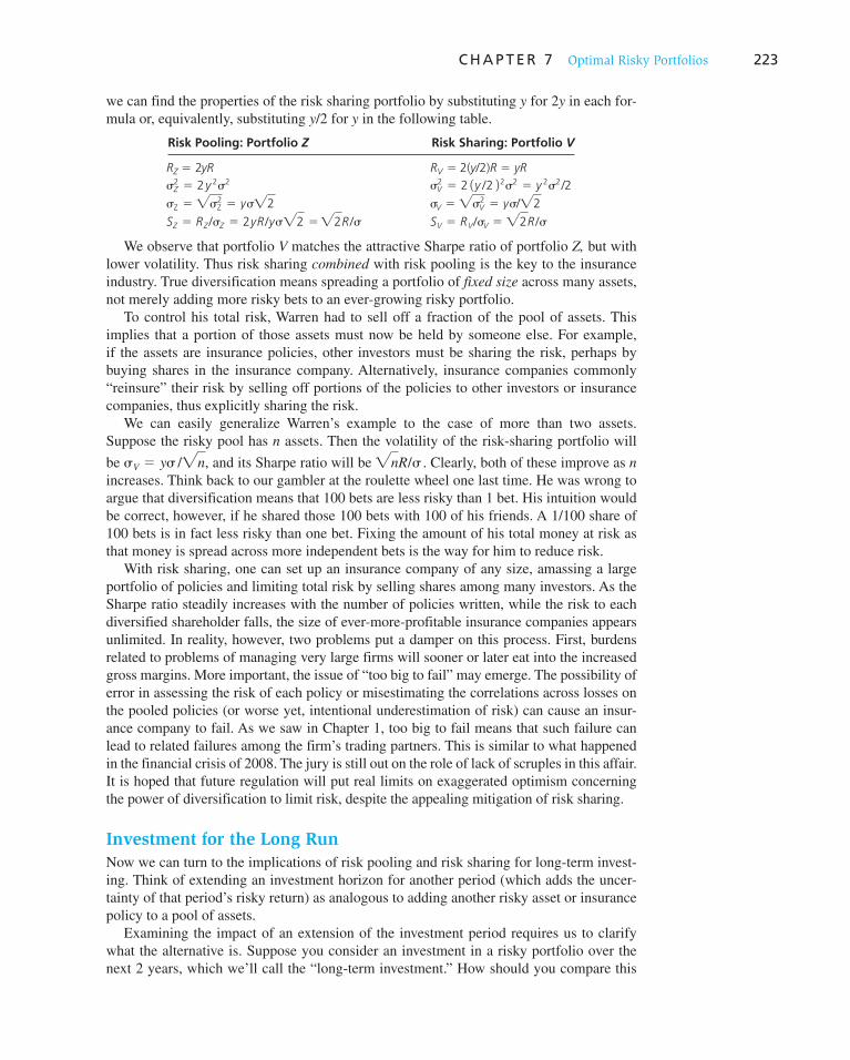
C H A P T E R 7 Optimal Risky Portfolios 223
we can find the properties of the risk sharing portfolio by substituting y for 2 y in each for-
mula or, equivalently, substituting y /2 for y in the following table.
oiloftroP :gnilooP ksiR Z oiloftroP :gnirahS ksiR V
RZ 2 R RV 2(y/2)R yR
Z2 5
5
2y 2 2 V2 5
5
2 1y /2 22 2 5
5
y 2 2 /2
Z 5 " Z2 5 y "2 V 5 " V
2 5 y /"2
SZ 5 RZ / Z 5 2yR /y "2 5"2R / SV 5 RV/ V 5 "2R /
y
We observe that portfolio V matches the attractive Sharpe ratio of portfolio Z, but with
lower volatility. Thus risk sharing combined with risk pooling is the key to the insurance
industry. True diversification means spreading a portfolio of fixed size across many assets,
not merely adding more risky bets to an ever-growing risky portfolio.
To control his total risk, Warren had to sell off a fraction of the pool of assets. This
implies that a portion of those assets must now be held by someone else. For example,
if the assets are insurance policies, other investors must be sharing the risk, perhaps by
buying shares in the insurance company. Alternatively, insurance companies commonly
“reinsure” their risk by selling off portions of the policies to other investors or insurance
companies, thus explicitly sharing the risk.
We can easily generalize Warren’s example to the case of more than two assets.
Suppose the risky pool has n assets. Then the volatility of the risk-sharing portfolio will
be �V 5 y� /"n, and its Sharpe ratio will be "nR/� . Clearly, both of these improve as n
increases. Think back to our gambler at the roulette wheel one last time. He was wrong to
argue that diversification means that 100 bets are less risky than 1 bet. His intuition would
be correct, however, if he shared those 100 bets with 100 of his friends. A 1/100 share of
100 bets is in fact less risky than one bet. Fixing the amount of his total money at risk as
that money is spread across more independent bets is the way for him to reduce risk.
With risk sharing, one can set up an insurance company of any size, amassing a large
portfolio of policies and limiting total risk by selling shares among many investors. As the
Sharpe ratio steadily increases with the number of policies written, while the risk to each
diversified shareholder falls, the size of ever-more-profitable insurance companies appears
unlimited. In reality, however, two problems put a damper on this process. First, burdens
related to problems of managing very large firms will sooner or later eat into the increased
gross margins. More important, the issue of “too big to fail” may emerge. The possibility of
error in assessing the risk of each policy or misestimating the correlations across losses on
the pooled policies (or worse yet, intentional underestimation of risk) can cause an insur-
ance company to fail. As we saw in Chapter 1, too big to fail means that such failure can
lead to related failures among the firm’s trading partners. This is similar to what happened
in the financial crisis of 2008. The jury is still out on the role of lack of scruples in this affair.
It is hoped that future regulation will put real limits on exaggerated optimism concerning
the power of diversification to limit risk, despite the appealing mitigation of risk sharing.
Investment for the Long Run
Now we can turn to the implications of risk pooling and risk sharing for long-term invest-
ing. Think of extending an investment horizon for another period (which adds the uncer-
tainty of that period’s risky return) as analogous to adding another risky asset or insurance
policy to a pool of assets.
Examining the impact of an extension of the investment period requires us to clarify
what the alternative is. Suppose you consider an investment in a risky portfolio over the
next 2 years, which we’ll call the “long-term investment.” How should you compare this

Vis
it u
s at
ww
w.m
hh
e.co
m/b
kmV
isit
us
at w
ww
.mh
he.
com
/bkm
224 P A R T I I Portfolio Theory and Practice
decision to a “short-run investment”? We must compare these two strategies over the same
period, that is, 2 years. The short-term investment therefore must be interpreted as invest-
ing in the risky portfolio over 1 year and in the risk-free asset over the other.
Once we agree on this comparison, and assuming the risky return on the first year is
uncorrelated with that of the second, it becomes clear that the “long-term” strategy is
analogous to portfolio Z. This is because holding on to the risky investment in the sec-
ond year (rather than withdrawing to the risk-free rate) piles up more risk, just as selling
another insurance policy does. Put differently, the long-term investment may be considered
analogous to risk pooling. While extending a risky investment to the long run improves the
Sharpe ratio (as does risk pooling), it also increases risk. Thus “time diversification” is not
really diversification.
An investor can capture the improved Sharpe ratio that accrues from long-term risk tak-
ing and still limit overall risk by reducing the fraction of his portfolio invested in the risky
asset (analogous to Warren selling off a fraction of his insurance pool). Thus a smaller
fraction of the portfolio in the risky asset invested over a longer horizon is preferable to
investing a larger fraction in the same risky investment for a short period and then switch-
ing to the risk-free investment for the remainder of the investment horizon. The emphasis
here is on the reduced fraction that is required for the long-run risky investment, if the risk
is to be limited.
1. The expected return of a portfolio is the weighted average of the component security expected
returns with the investment proportions as weights.
2. The variance of a portfolio is the weighted sum of the elements of the covariance matrix with the
product of the investment proportions as weights. Thus the variance of each asset is weighted by
the square of its investment proportion. The covariance of each pair of assets appears twice in the
covariance matrix; thus the portfolio variance includes twice each covariance weighted by the
product of the investment proportions in each of the two assets.
3. Even if the covariances are positive, the portfolio standard deviation is less than the weighted aver-
age of the component standard deviations, as long as the assets are not perfectly positively corre-
lated. Thus portfolio diversification is of value as long as assets are less than perfectly correlated.
4. The greater an asset’s covariance with the other assets in the portfolio, the more it contributes to
portfolio variance. An asset that is perfectly negatively correlated with a portfolio can serve as a
perfect hedge. The perfect hedge asset can reduce the portfolio variance to zero.
5. The efficient frontier is the graphical representation of a set of portfolios that maximize expected
return for each level of portfolio risk. Rational investors will choose a portfolio on the efficient frontier.
6. A portfolio manager identifies the efficient frontier by first establishing estimates for asset
expected returns and the covariance matrix. This input list is then fed into an optimization pro-
gram that reports as outputs the investment proportions, expected returns, and standard deviations
of the portfolios on the efficient frontier.
7. In general, portfolio managers will arrive at different efficient portfolios because of differences
in methods and quality of security analysis. Managers compete on the quality of their security
analysis relative to their management fees.
8. If a risk-free asset is available and input lists are identical, all investors will choose the same
portfolio on the efficient frontier of risky assets: the portfolio tangent to the CAL. All investors
with identical input lists will hold an identical risky portfolio, differing only in how much each
allocates to this optimal portfolio and to the risk-free asset. This result is characterized as the
separation principle of portfolio construction.
SUMMARY

Vis
it u
s at
ww
w.m
hh
e.co
m/b
kmV
isit
us
at w
ww
.mh
he.
com
/bkm
C H A P T E R 7 Optimal Risky Portfolios 225
9. Diversification is based on the allocation of a fixed portfolio across several assets, limiting the
exposure to any one source of risk. Adding additional risky assets to a portfolio, thereby increas-
ing the total amounts invested, does not reduce dollar risk, even if it makes the rate of return
more predictable. This is because that uncertainty is applied to a larger investment base. Nor
does investing over longer horizons reduce risk. Increasing the investment horizon is analogous
to investing in more assets. It increases total risk. Analogously, the key to the insurance industry
is risk sharing—the spreading of risk across many investors, each of whom takes on only a small
exposure to any given source of risk. Risk pooling—the assumption of ever-more sources of
risk—may increase rate of return predictability, but not the predictability of total dollar returns.
Related Web sites for this chapter are available at www.mhhe.com/bkm
diversification
insurance principle
market risk
systematic risk
nondiversifiable risk
unique risk
firm-specific risk
nonsystematic risk
diversifiable risk
minimum-variance portfolio
portfolio opportunity set
reward-to-volatility ratio
optimal risky portfolio
minimum-variance frontier
efficient frontier of risky
assets
input list
separation property
risk pooling
risk sharing
KEY TERMS
1. Which of the following factors reflect pure market risk for a given corporation?
a. Increased short-term interest rates.
b. Fire in the corporate warehouse.
c. Increased insurance costs.
d. Death of the CEO.
e. Increased labor costs.
2. When adding real estate to an asset allocation program that currently includes only stocks, bonds,
and cash, which of the properties of real estate returns affect portfolio risk? Explain.
a. Standard deviation.
b. Expected return.
c. Correlation with returns of the other asset classes.
3. Which of the following statements about the minimum variance portfolio of all risky securities
are valid? (Assume short sales are allowed.) Explain.
a. Its variance must be lower than those of all other securities or portfolios.
b. Its expected return can be lower than the risk-free rate.
c. It may be the optimal risky portfolio.
d. It must include all individual securities.
The following data apply to Problems 4 through 10 : A pension fund manager is considering three mutual funds. The first is a stock fund, the second is a long-term government and corporate bond fund, and the third is a T-bill money market fund that yields a rate of 8%. The probability distri-bution of the risky funds is as follows:
Expected Return Standard Deviation
Stock fund (S) 20% 30%
Bond fund (B) 12 15
The correlation between the fund returns is .10.
4. What are the investment proportions in the minimum-variance portfolio of the two risky funds,
and what is the expected value and standard deviation of its rate of return?
5. Tabulate and draw the investment opportunity set of the two risky funds. Use investment propor-
tions for the stock fund of zero to 100% in increments of 20%.
PROBLEM SETS
i. Basic
ii. Intermediate

Vis
it u
s at
ww
w.m
hh
e.co
m/b
km226 P A R T I I Portfolio Theory and Practice
6. Draw a tangent from the risk-free rate to the opportunity set. What does your graph show for the
expected return and standard deviation of the optimal portfolio?
7. Solve numerically for the proportions of each asset and for the expected return and standard
deviation of the optimal risky portfolio.
8. What is the reward-to-volatility ratio of the best feasible CAL?
9. You require that your portfolio yield an expected return of 14%, and that it be efficient, on the
best feasible CAL.
a. What is the standard deviation of your portfolio?
b. What is the proportion invested in the T-bill fund and each of the two risky funds?
10. If you were to use only the two risky funds, and still require an expected return of 14%, what
would be the investment proportions of your portfolio? Compare its standard deviation to that of
the optimized portfolio in Problem 9 . What do you conclude?
11. Stocks offer an expected rate of return of 18%, with a standard deviation of 22%. Gold offers an
expected return of 10% with a standard deviation of 30%.
a. In light of the apparent inferiority of gold with respect to both mean return and volatility,
would anyone hold gold? If so, demonstrate graphically why one would do so.
b. Given the data above, reanswer ( a ) with the additional assumption that the correlation coef-
ficient between gold and stocks equals 1. Draw a graph illustrating why one would or would
not hold gold in one’s portfolio. Could this set of assumptions for expected returns, standard
deviations, and correlation represent an equilibrium for the security market?
12. Suppose that there are many stocks in the security market and that the characteristics of stocks
A and B are given as follows:
Stock Expected Return Standard Deviation
A 10% 5%
B 15 10
Correlation � �1
Suppose that it is possible to borrow at the risk-free rate, r f . What must be the value of the risk-
free rate? ( Hint: Think about constructing a risk-free portfolio from stocks A and B. )
13. Assume that expected returns and standard deviations for all securities (including the risk-free
rate for borrowing and lending) are known. In this case all investors will have the same optimal
risky portfolio. (True or false?)
14. The standard deviation of the portfolio is always equal to the weighted average of the standard
deviations of the assets in the portfolio. (True or false?)
15. Suppose you have a project that has a .7 chance of doubling your investment in a year and a
.3 chance of halving your investment in a year. What is the standard deviation of the rate of
return on this investment?
16. Suppose that you have $1 million and the following two opportunities from which to construct
a portfolio:
a. Risk-free asset earning 12% per year.
b. Risky asset with expected return of 30% per year and standard deviation of 40%.
If you construct a portfolio with a standard deviation of 30%, what is its expected rate of return?
The following data are for Problems 17 through 19 : The correlation coefficients between pairs of stocks are as follows: Corr( A, B ) � .85; Corr( A, C ) � .60; Corr( A, D ) � .45. Each stock has an expected return of 8% and a standard deviation of 20%.
17. If your entire portfolio is now composed of stock A and you can add some of only one stock to
your portfolio, would you choose (explain your choice):
a. B.
b. C.
c. D.
d. Need more data.
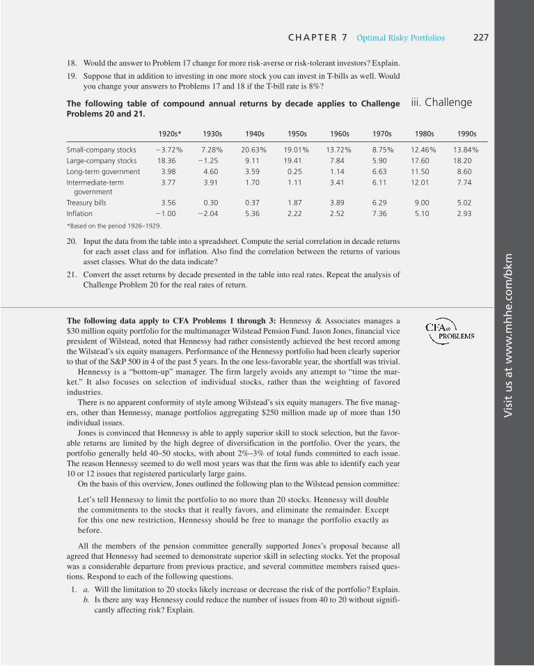
Vis
it u
s at
ww
w.m
hh
e.co
m/b
km
C H A P T E R 7 Optimal Risky Portfolios 227
18. Would the answer to Problem 17 change for more risk-averse or risk-tolerant investors? Explain.
19. Suppose that in addition to investing in one more stock you can invest in T-bills as well. Would
you change your answers to Problems 17 and 18 if the T-bill rate is 8%?
The following table of compound annual returns by decade applies to Challenge Problems 20 and 21 .
1920s* 1930s 1940s 1950s 1960s 1970s 1980s 1990s
Small-company stocks �3.72% 7.28% 20.63% 19.01% 13.72% 8.75% 12.46% 13.84%
Large-company stocks 18.36 �1.25 9.11 19.41 7.84 5.90 17.60 18.20
Long-term government 3.98 4.60 3.59 0.25 1.14 6.63 11.50 8.60
Intermediate-term
government
3.77 3.91 1.70 1.11 3.41 6.11 12.01 7.74
Treasury bills 3.56 0.30 0.37 1.87 3.89 6.29 9.00 5.02
Inflation �1.00 �2.04 5.36 2.22 2.52 7.36 5.10 2.93
* Based on the period 1926–1929.
20. Input the data from the table into a spreadsheet. Compute the serial correlation in decade returns
for each asset class and for inflation. Also find the correlation between the returns of various
asset classes. What do the data indicate?
21. Convert the asset returns by decade presented in the table into real rates. Repeat the analysis of
Challenge Problem 20 for the real rates of return.
iii. Challenge
The following data apply to CFA Problems 1 through 3: Hennessy & Associates manages a
$30 million equity portfolio for the multimanager Wilstead Pension Fund. Jason Jones, financial vice
president of Wilstead, noted that Hennessy had rather consistently achieved the best record among
the Wilstead’s six equity managers. Performance of the Hennessy portfolio had been clearly superior
to that of the S&P 500 in 4 of the past 5 years. In the one less-favorable year, the shortfall was trivial.
Hennessy is a “bottom-up” manager. The firm largely avoids any attempt to “time the mar-
ket.” It also focuses on selection of individual stocks, rather than the weighting of favored
industries.
There is no apparent conformity of style among Wilstead’s six equity managers. The five manag-
ers, other than Hennessy, manage portfolios aggregating $250 million made up of more than 150
individual issues.
Jones is convinced that Hennessy is able to apply superior skill to stock selection, but the favor-
able returns are limited by the high degree of diversification in the portfolio. Over the years, the
portfolio generally held 40–50 stocks, with about 2%–3% of total funds committed to each issue.
The reason Hennessy seemed to do well most years was that the firm was able to identify each year
10 or 12 issues that registered particularly large gains.
On the basis of this overview, Jones outlined the following plan to the Wilstead pension committee:
Let’s tell Hennessy to limit the portfolio to no more than 20 stocks. Hennessy will double
the commitments to the stocks that it really favors, and eliminate the remainder. Except
for this one new restriction, Hennessy should be free to manage the portfolio exactly as
before.
All the members of the pension committee generally supported Jones’s proposal because all
agreed that Hennessy had seemed to demonstrate superior skill in selecting stocks. Yet the proposal
was a considerable departure from previous practice, and several committee members raised ques-
tions. Respond to each of the following questions.
1. a. Will the limitation to 20 stocks likely increase or decrease the risk of the portfolio? Explain.
b. Is there any way Hennessy could reduce the number of issues from 40 to 20 without signifi-
cantly affecting risk? Explain.

Vis
it u
s at
ww
w.m
hh
e.co
m/b
km228 P A R T I I Portfolio Theory and Practice
2. One committee member was particularly enthusiastic concerning Jones’s proposal. He suggested
that Hennessy’s perfoxrmance might benefit further from reduction in the number of issues to 10.
If the reduction to 20 could be expected to be advantageous, explain why reduction to 10 might
be less likely to be advantageous. (Assume that Wilstead will evaluate the Hennessy portfolio
independently of the other portfolios in the fund.)
3. Another committee member suggested that, rather than evaluate each managed portfolio indepen-
dently of other portfolios, it might be better to consider the effects of a change in the Hennessy
portfolio on the total fund. Explain how this broader point of view could affect the committee
decision to limit the holdings in the Hennessy portfolio to either 10 or 20 issues.
4. Which one of the following portfolios cannot lie on the efficient frontier as described by
Markowitz?
Portfolio Expected Return (%) Standard Deviation (%)
a. W 15 36
b. X 12 15
c. Z 5 7
d. Y 9 21
5. Which statement about portfolio diversification is correct?
a. Proper diversification can reduce or eliminate systematic risk.
b. Diversification reduces the portfolio’s expected return because it reduces a portfolio’s total
risk.
c. As more securities are added to a portfolio, total risk typically would be expected to fall at a
decreasing rate.
d. The risk-reducing benefits of diversification do not occur meaningfully until at least 30 indi-
vidual securities are included in the portfolio.
6. The measure of risk for a security held in a diversified portfolio is:
a. Specific risk.
b. Standard deviation of returns.
c. Reinvestment risk.
d. Covariance.
7. Portfolio theory as described by Markowitz is most concerned with:
a. The elimination of systematic risk.
b. The effect of diversification on portfolio risk.
c. The identification of unsystematic risk.
d. Active portfolio management to enhance return.
8. Assume that a risk-averse investor owning stock in Miller Corporation decides to add the stock of
either Mac or Green Corporation to her portfolio. All three stocks offer the same expected return
and total variability. The covariance of return between Miller and Mac is � .05 and between
Miller and Green is � .05. Portfolio risk is expected to:
a. Decline more when the investor buys Mac.
b. Decline more when the investor buys Green.
c. Increase when either Mac or Green is bought.
d. Decline or increase, depending on other factors.
9. Stocks A, B, and C have the same expected return and standard deviation. The following table
shows the correlations between the returns on these stocks.
Stock A Stock B Stock B
Stock A �1.0
Stock B �0.9 �1.0
Stock C �0.1 �0.4 �1.0
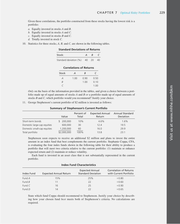
Vis
it u
s at
ww
w.m
hh
e.co
m/b
km
C H A P T E R 7 Optimal Risky Portfolios 229
Given these correlations, the portfolio constructed from these stocks having the lowest risk is a
portfolio:
a. Equally invested in stocks A and B.
b. Equally invested in stocks A and C.
c. Equally invested in stocks B and C.
d. Totally invested in stock C.
10. Statistics for three stocks, A, B, and C, are shown in the following tables.
Standard Deviations of Returns
Stock: A B C
Standard deviation (%): 40 20 40
Correlations of Returns
Stock A B C
A 1.00 0.90 0.50
B 1.00 0.10
C 1.00
Only on the basis of the information provided in the tables, and given a choice between a port-
folio made up of equal amounts of stocks A and B or a portfolio made up of equal amounts of
stocks B and C, which portfolio would you recommend? Justify your choice.
11. George Stephenson’s current portfolio of $2 million is invested as follows:
Summary of Stephenson’s Current Portfolio
ValuePercent of
TotalExpected Annual
ReturnAnnual Standard
Deviation
Short-term bonds $ 200,000 10% 4.6% 1.6%
Domestic large-cap equities 600,000 30 12.4 19.5
Domestic small-cap equities 1,200,000 60 16.0 29.9
Total portfolio $2,000,000 100% 13.8 23.1
Stephenson soon expects to receive an additional $2 million and plans to invest the entire
amount in an index fund that best complements the current portfolio. Stephanie Coppa, CFA,
is evaluating the four index funds shown in the following table for their ability to produce a
portfolio that will meet two criteria relative to the current portfolio: (1) maintain or enhance
expected return and (2) maintain or reduce volatility.
Each fund is invested in an asset class that is not substantially represented in the current
portfolio.
Index Fund Characteristics
Index Fund Expected Annual ReturnExpected Annual
Standard DeviationCorrelation of Returns with Current Portfolio
Fund A 15% 25% �0.80
Fund B 11 22 �0.60
Fund C 16 25 �0.90
Fund D 14 22 �0.65
State which fund Coppa should recommend to Stephenson. Justify your choice by describ-
ing how your chosen fund best meets both of Stephenson’s criteria. No calculations are
required.

Vis
it u
s at
ww
w.m
hh
e.co
m/b
km230 P A R T I I Portfolio Theory and Practice
12. Abigail Grace has a $900,000 fully diversified portfolio. She subsequently inherits ABC Com-
pany common stock worth $100,000. Her financial adviser provided her with the following
forecast information:
Risk and Return Characteristics
Expected Monthly Returns
Standard Deviation of Monthly Returns
Original Portfolio 0.67% 2.37%
ABC Company 1.25 2.95
The correlation coefficient of ABC stock returns with the original portfolio returns is .40.
a. The inheritance changes Grace’s overall portfolio and she is deciding whether to keep the
ABC stock. Assuming Grace keeps the ABC stock, calculate the:
i. Expected return of her new portfolio which includes the ABC stock.
ii. Covariance of ABC stock returns with the original portfolio returns.
iii. Standard deviation of her new portfolio, which includes the ABC stock.
b. If Grace sells the ABC stock, she will invest the proceeds in risk-free government securities
yielding .42% monthly. Assuming Grace sells the ABC stock and replaces it with the gov-
ernment securities, calculate the
i. Expected return of her new portfolio, which includes the government securities.
ii. Covariance of the government security returns with the original portfolio returns.
iii. Standard deviation of her new portfolio, which includes the government securities.
c. Determine whether the systematic risk of her new portfolio, which includes the government
securities, will be higher or lower than that of her original portfolio.
d. On the basis of conversations with her husband, Grace is considering selling the $100,000
of ABC stock and acquiring $100,000 of XYZ Company common stock instead. XYZ
stock has the same expected return and standard deviation as ABC stock. Her husband
comments, “It doesn’t matter whether you keep all of the ABC stock or replace it with
$100,000 of XYZ stock.” State whether her husband’s comment is correct or incorrect.
Justify your response.
e. In a recent discussion with her financial adviser, Grace commented, “If I just don’t lose
money in my portfolio, I will be satisfied.” She went on to say, “I am more afraid of losing
money than I am concerned about achieving high returns.”
i. Describe one weakness of using standard deviation of returns as a risk measure for
Grace.
ii. Identify an alternate risk measure that is more appropriate under the circumstances.
13. Dudley Trudy, CFA, recently met with one of his clients. Trudy typically invests in a master
list of 30 equities drawn from several industries. As the meeting concluded, the client made the
following statement: “I trust your stock-picking ability and believe that you should invest my
funds in your five best ideas. Why invest in 30 companies when you obviously have stronger
opinions on a few of them?” Trudy plans to respond to his client within the context of modern
portfolio theory.
a. Contrast the concepts of systematic risk and firm-specific risk, and give an example of each
type of risk.
b. Critique the client’s suggestion. Discuss how both systematic and firm-specific risk change
as the number of securities in a portfolio is increased.

Vis
it u
s at
ww
w.m
hh
e.co
m/b
km
C H A P T E R 7 Optimal Risky Portfolios 231
SOLUTIONS TO CONCEPT CHECKS
Diversification
Go to the www.investopedia.com/articles/basics/03/050203.asp Web site to learn more about diversification, the factors that influence investors’ risk preferences, and the types of investments that fit into each of the risk categories. Then check out www.
investopedia.com/articles/pf/05/061505.asp for asset allocation guidelines for various types of portfolios from conservative to very aggressive. What do you conclude about your own risk preferences and the best portfolio type for you? What would you expect to hap-pen to your attitude toward risk as you get older? How might your portfolio composition change?
E-INVEST-MENTS EXERCISES
1. a. The first term will be wD 3 wD 3 �D2, because this is the element in the top corner
of the matrix 1�D2 2 times the term on the column border ( w D ) times the term on the row
border ( w D ). Applying this rule to each term of the covariance matrix results in the sum
wD2 �D
2 1 wDwE Cov 1rE, rD 2 1 wEwDCov 1rD, rE 2 1 wE2 �E
2, which is the same as Equation 7.3 ,
because Cov( r E , r D ) � Cov( r D , r E ).
b. The bordered covariance matrix is
wX wY wZ
wX �2x
Cov(rX, rY) Cov(rX, rZ)
wY Cov(rY, rX) �2Y
Cov(rY, rZ)
wZ Cov(rZ, rX) Cov(rZ, rY) �2Z
There are nine terms in the covariance matrix. Portfolio variance is calculated from these nine
terms:
�P2 5 wX
2 �X2 1 wY
2 �Y2 1 wZ
2 �Z2
1 wXwY Cov(rX , rY) 1 wY
wX Cov(rY , rX)
1 wX wZ Cov(rX
, rZ) 1 wZ wX Cov(rZ
, rX)
1 wY wZ Cov (rY
, rZ) 1 wZ wY Cov(rZ
, rY)
5 wX2 �X
2 1 wY2 �Y
2 1 wZ2 �Z
2
1 2wX wY Cov(rX
, rY) 1 2wX wZ Cov(rX
, rZ) 1 2wY wZ Cov(rY
, rZ)
2. The parameters of the opportunity set are E ( r D ) � 8%, E ( r E ) � 13%, � D � 12%, � E � 20%,
and � ( D, E ) � .25. From the standard deviations and the correlation coefficient we generate the
covariance matrix:
Fund D E
D 144 60
E 60 400
The global minimum-variance portfolio is constructed so that
wD 5�E
2 2 Cov(rD, rE)
�D2 1 �E
2 2 2 Cov(rD, rE)
5400 2 60
(144 1 400) 2 (2 3 60)5 .8019
wE 5 1 2 wD 5 .1981

Vis
it u
s at
ww
w.m
hh
e.co
m/b
km232 P A R T I I Portfolio Theory and Practice
Its expected return and standard deviation are
E(rP) 5 (.8019 3 8) 1 (.1981 3 13) 5 8.99%
�P 5 3wD2 �D
2 1 wE2 �E
2 1 2wDwE Cov(rD, rE)41/2
5 3(.80192 3 144) 1 (.19812 3 400) 1 (2 3 .8019 3 .1981 3 60) 41/2
5 11.29%
For the other points we simply increase w D from .10 to .90 in increments of .10; accordingly,
w E ranges from .90 to .10 in the same increments. We substitute these portfolio proportions in
the formulas for expected return and standard deviation. Note that when w E � 1.0, the portfolio
parameters equal those of the stock fund; when w D � 1, the portfolio parameters equal those of
the debt fund.
We then generate the following table:
wE wD E(r) �
0.0 1.0 8.0 12.00
0.1 0.9 8.5 11.46
0.2 0.8 9.0 11.29
0.3 0.7 9.5 11.48
0.4 0.6 10.0 12.03
0.5 0.5 10.5 12.88
0.6 0.4 11.0 13.99
0.7 0.3 11.5 15.30
0.8 0.2 12.0 16.76
0.9 0.1 12.5 18.34
1.0 0.0 13.0 20.00
0.1981 0.8019 8.99 11.29 minimum variance portfolio
You can now draw your graph.
3. a. The computations of the opportunity set of the stock and risky bond funds are like those of
Question 2 and will not be shown here. You should perform these computations, however, in
order to give a graphical solution to part a. Note that the covariance between the funds is
Cov(rA, rB) 5 �(A, B) 3 �A 3 �B
5 2.2 3 20 3 60 5 2240
b. The proportions in the optimal risky portfolio are given by
wA 5(10 2 5)602 2 (30 2 5)(2240)
(10 2 5)602 1 (30 2 5)202 2 30(2240)
5 .6818
wB 5 1 2 wA 5 .3182
The expected return and standard deviation of the optimal risky portfolio are
E(rP) 5 (.6818 3 10) 1 (.3182 3 30) 5 16.36%
�P 5 5(..68182 3 202) 1 (.31822 3 602) 1 32 3 .6818 3 .3182( 2 240) 4 61/2
5 21.13%
Note that portfolio P is not the global minimum-variance portfolio. The proportions of the
latter are given by
wA 5602 2 (2240)
602 1 202 2 2(2240)5 .8571
wB 5 1 2 wA 5 .1429

Vis
it u
s at
ww
w.m
hh
e.co
m/b
km
C H A P T E R 7 Optimal Risky Portfolios 233
With these proportions, the standard deviation of the minimum-variance portfolio is
�(min) 5 (.85712 3 202) 1 (.14292 3 602) 1 32 3 .8571 3 .1429 3 (2240) 41/2
5 17.57%
which is less than that of the optimal risky portfolio.
c. The CAL is the line from the risk-free rate through the optimal risky portfolio. This line
represents all efficient portfolios that combine T-bills with the optimal risky portfolio. The
slope of the CAL is
S 5E(rP) 2 rf
�P
516.36 2 5
21.135 .5376
d. Given a degree of risk aversion, A, an investor will choose a proportion, y, in the optimal risky
portfolio of (remember to express returns as decimals when using A ):
y 5E(rP) 2 rf
A�P2
5.1636 2 .05
5 3 .211325 .5089
This means that the optimal risky portfolio, with the given data, is attractive enough for an
investor with A � 5 to invest 50.89% of his or her wealth in it. Because stock A makes up
68.18% of the risky portfolio and stock B makes up 31.82%, the investment proportions for
this investor are
Stock A: .5089 3 68.18 5 34.70%
Stock B: .5089 3 31.82 5 16.19%
Total 50.89%
4. Efficient frontiers derived by portfolio managers depend on forecasts of the rates of return on
various securities and estimates of risk, that is, the covariance matrix. The forecasts themselves
do not control outcomes. Thus preferring managers with rosier forecasts (northwesterly frontiers)
is tantamount to rewarding the bearers of good news and punishing the bearers of bad news.
What we should do is reward bearers of accurate news. Thus if you get a glimpse of the frontiers
(forecasts) of portfolio managers on a regular basis, what you want to do is develop the track
record of their forecasting accuracy and steer your advisees toward the more accurate forecaster.
Their portfolio choices will, in the long run, outperform the field.
5. The parameters are E ( r ) � 15, � � 60, and the correlation between any pair of stocks is � � .5.
a. The portfolio expected return is invariant to the size of the portfolio because all stocks have
identical expected returns. The standard deviation of a portfolio with n � 25 stocks is
�P 5 3�2/n 1 � 3 �2(n 2 1)/n 41/2
5 3602/25 1 .5 3 602 3 24/25 41/2 5 43.27%
b. Because the stocks are identical, efficient portfolios are equally weighted. To obtain a standard
deviation of 43%, we need to solve for n:
432 5602
n1 .5 3
602(n 2 1)
n
1,849n 5 3,600 1 1,800n 2 1,800
n 51,800
495 36.73
Thus we need 37 stocks and will come in with volatility slightly under the target.
c. As n gets very large, the variance of an efficient (equally weighted) portfolio diminishes,
leaving only the variance that comes from the covariances among stocks, that is
�P 5 "� 3 � 2 5 ".5 3 602 5 42.43%

APPENDIX A: A Spreadsheet Model for Efficient Diversification
Vis
it u
s at
ww
w.m
hh
e.co
m/b
km234 P A R T I I Portfolio Theory and Practice
Note that with 25 stocks we came within .84% of the systematic risk, that is, the nonsystematic
risk of a portfolio of 25 stocks is only .84%. With 37 stocks the standard deviation is 43%, of
which nonsystematic risk is .57%.
d. If the risk-free is 10%, then the risk premium on any size portfolio is 15 � 10 � 5%. The
standard deviation of a well-diversified portfolio is (practically) 42.43%; hence the slope of
the CAL is
S 5 5/42.43 5 .1178
Several software packages can be used to generate the efficient frontier. We will dem-
onstrate the method using Microsoft Excel. Excel is far from the best program for this
purpose and is limited in the number of assets it can handle, but working through a simple
portfolio optimizer in Excel can illustrate concretely the nature of the calculations used in
more sophisticated “black-box” programs. You will find that even in Excel, the computa-
tion of the efficient frontier is fairly easy.
We apply the Markowitz portfolio optimization program to a practical problem of inter-
national diversification. We take the perspective of a portfolio manager serving U.S. cli-
ents, who wishes to construct for the next year an optimal risky portfolio of large stocks
in the U.S and six developed capital markets (Japan, Germany, U.K., France, Canada, and
Australia). First we describe the input list: forecasts of risk premiums and the covariance
matrix. Next, we describe Excel’s Solver, and finally we show the solution to the man-
ager’s problem.
The Covariance Matrix
To capture recent risk parameters the manager compiles an array of 60 recent monthly
(annualized) rates of return, as well as the monthly T-bill rates for the same period.
The standard deviations of excess returns are shown in Table 7A.1 (column C). They
range from 14.93% (U.K. large stocks) to 22.7% (Germany). For perspective on how
these parameters can change over time, standard deviations for the period 1991–2000 are
also shown (column B). In addition, we present the correlation coefficient between large
stocks in the six foreign markets with U.S. large stocks for the same two periods. Here we
see that correlations are higher in the more recent period, consistent with the process of
globalization.
The covariance matrix shown in Table 7A.2 was estimated from the array of 60 returns
of the seven countries using the COVARIANCE function from the dialog box of Data
Analysis in Excel’s Tools menu. Due to a quirk in the Excel software, the covariance matrix
is not corrected for degrees-of-freedom bias; hence, each of the elements in the matrix was
multiplied by 60/59 to eliminate downward bias.
Expected Returns
While estimation of the risk parameters (the covariance matrix) from excess returns is
a simple technical matter, estimating the risk premium (the expected excess return) is a
daunting task. As we discussed in Chapter 5, estimating expected returns using histori-
cal data is unreliable. Consider, for example, the negative average excess returns on U.S.
large stocks over the period 2001–2005 (cell G6) and, more generally, the big differences
in average returns between the 1991–2000 and 2001–2005 periods, as demonstrated in
columns F and G.

Vis
it u
s at
ww
w.m
hh
e.co
m/b
km
C H A P T E R 7 Optimal Risky Portfolios 235
Table 7A.1, 7A.2, 7A.3
Spreadsheet model for international diversification
A B C D E F G H
1
2
7A.1 Country Index Statistics and Forecasts of Excess Returns
Correlation with the
U.S. Average Excess Return Forecast
3
4
Country
−0.0148
0.0094
0.0247
0.0209
0.1225
0.0398
0.1009
0.1108
0.0536
0.0837
0.0473
0.0468
−0.0177
0.0727
1
0.83
0.83
0.85
0.81
0.43
0.79
1
0.64
0.54
0.53
0.52
0.41
0.72
Standard Deviation
1991–2000
0.1295
0.1466
0.1741
0.1538
0.1808
0.2432
0.1687
0.1495
0.1493
0.2008
0.2270
0.1617
0.1878
0.1727
2001–2005 1991–2000 2001–2005
US
UK
France
Germany
Australia
Japan
Canada
5
6
7
8
9
10
11
12
1991–2000 2001–2005 2006
0.0600
0.0530
0.0700
0.0800
0.0580
0.0450
0.0590
A B C D E F G H I
7A.2 The Bordered Covariance Matrix
Portfolio
Weights 1.0000 0.0000 0.0000 0.0000
1.0000
0.0000
0.0000
0.0000
0.0000
0.0000
0.0000
1.0000
0.0600
0.1495
0.4013
Cell A18 - A24 A18 is set arbitrarily to 1 while A19 to A24 are set to 0
Formula in cell C16 =A18 ... Formula in cell I16 =A24
Formula in cell A25 =SUM(A18:A24)
Formula in cell C25 =C16*SUMPRODUCT($A$18:$A$24,C18:C24)
Formula in cell D25-I25 Copied from C25 (note the absolute addresses)
Formula in cell A26 =SUMPRODUCT($A$18:$A$24,H6:H12)
Formula in cell A27 =SUM(C25:I25)^0.5
Formula in cell A28 =A26/A27
0.0224
0.0184
0.0250
0.0288
0.0195
0.0121
0.0205
0.0224
0.0184
0.0223
0.0275
0.0299
0.0204
0.0124
0.0206
0.0000
0.0288
0.0299
0.0438
0.0515
0.0301
0.0183
0.0305
0.0000
0.0121
0.0124
0.0177
0.0183
0.0147
0.0353
0.0158
0.0000
US UK
0.0000
0.0250
0.0275
0.0403
0.0438
0.0259
0.0177
0.0273
0.0000
France Germany
0.0000
0.0195
0.0204
0.0259
0.0301
0.0261
0.0147
0.0234
0.0000
Australia Japan
US
UK
France
Germany
Australia
Japan
Canada
0.0000
0.0205
0.0206
0.0273
0.0305
0.0234
0.0158
0.0298
0.0000
Canada
13
14
15
16
17
18
19
20
21
22
23
24
25
26
27
28
29
30
31
32
33
34
35
36
37
38
A B C D E F G H I J K L
US
Mean
SD 0.1
Min Var Optimum
0.0383
0.1132
0.3386
0.6112
0.8778
−0.2140
−0.5097
0.0695
0.2055
−0.0402
0.0465
0.0400
0.1135
0.3525
0.6195
0.8083
−0.2029
−0.4610
0.0748
0.1987
−0.0374
0.0466
0.0450
0.1168
0.3853
0.6446
0.5992
−0.1693
−0.3144
0.0907
0.1781
−0.0288
0.0480
0.0500
0.1238
0.4037
0.6696
0.3900
−0.1357
−0.1679
0.1067
0.1575
−0.0203
0.0509
0.0550
0.1340
0.4104
0.6947
0.1809
−0.1021
−0.0213
0.1226
0.1369
−0.0118
0.0550
0.0564
0.1374
0.4107
0.7018
0.1214
−0.0926
0.0205
0.1271
0.1311
−0.0093
0.0564
0.0575
0.1401
0.4106
0.7073
0.0758
−0.0852
0.0524
0.1306
0.1266
−0.0075
0.0575
0.0600
0.1466
0.4092
0.7198
−0.0283
−0.0685
0.1253
0.1385
0.1164
−0.0032
0.0602
0.0700
0.1771
0.3953
0.7699
−0.4465
−0.0014
0.4185
0.1704
0.0752
0.0139
0.0727
0.0800
0.2119
0.3774
0.8201
−0.8648
0.0658
0.7117
0.2023
0.0341
0.0309
0.08710.0411
Slope
UK
France
Germany
Australia
Japan
Canada
CAL*
*Risk premium on CAL = SD � slope of optimal risky portfolio
44
45
46
47
48
49
50
51
52
53
54
55
43
Cell to store constraint on risk premium
7A.3 The Efficient Frontier39
40
41
42
0.0400
Mean
SD
Slope
eXce lPlease visit us at www.mhhe.com/bkm

Vis
it u
s at
ww
w.m
hh
e.co
m/b
km236 P A R T I I Portfolio Theory and Practice
In this example, we simply present the manager’s forecasts of future returns as shown in
column H. In Chapter 8 we will establish a framework that makes the forecasting process
more explicit.
The Bordered Covariance Matrix and Portfolio Variance
The covariance matrix in Table 7A.2 is bordered by the portfolio weights, as explained
in Section 7.2 and Table 7.2 . The values in cells A18–A24, to the left of the covariance
matrix, will be selected by the optimization program. For now, we arbitrarily input 1.0
for the U.S. and zero for the others. Cells A16–I16, above the covariance matrix, must be
set equal to the column of weights on the left, so that they will change in tandem as the
column weights are changed by Excel’s Solver. Cell A25 sums the column weights and is
used to force the optimization program to set the sum of portfolio weights to 1.0.
Cells C25–I25, below the covariance matrix, are used to compute the portfolio variance
for any set of weights that appears in the borders. Each cell accumulates the contribution
to portfolio variance from the column above it. It uses the function SUMPRODUCT to
accomplish this task. For example, row 33 shows the formula used to derive the value that
appears in cell C25.
Finally, the short column A26–A28 below the bordered covariance matrix presents
portfolio statistics computed from the bordered covariance matrix. First is the portfolio
risk premium in cell A26, with formula shown in row 35, which multiplies the column
of portfolio weights by the column of forecasts (H6–H12) from Table 7A.1 . Next is the
portfolio standard deviation in cell A27. The variance is given by the sum of cells C25–I25
below the bordered covariance matrix. Cell A27 takes the square root of this sum to pro-
duce the standard deviation. The last statistic is the portfolio Sharpe ratio, cell A28, which
is the slope of the CAL (capital allocation line) that runs through the portfolio constructed
using the column weights (the value in cell A28 equals cell A26 divided by cell A27). The
optimal risky portfolio is the one that maximizes the Sharpe ratio.
Using the Excel Solver
Excel’s Solver is a user-friendly, but quite powerful, optimizer. It has three parts: (1) an
objective function, (2) decision variables, and (3) constraints. Figure 7A.1 shows three
pictures of the Solver. For the current discussion we refer to picture A.
The top panel of the Solver lets you choose a target cell for the “objective function,” that
is, the variable you are trying to optimize. In picture A, the target cell is A27, the portfo-
lio standard deviation. Below the target cell, you can choose whether your objective is to
maximize, minimize, or set your objective function equal to a value that you specify. Here
we choose to minimize the portfolio standard deviation.
The next panel contains the decision variables. These are cells that the Solver can
change in order to optimize the objective function in the target cell. Here, we input cells
A18–A24, the portfolio weights that we select to minimize portfolio volatility.
The bottom panel of the Solver can include any number of constraints. One constraint
that must always appear in portfolio optimization is the “feasibility constraint,” namely,
that portfolio weights sum to 1.0. When we bring up the constraint dialogue box, we spec-
ify that cell A25 (the sum of weights) be set equal to 1.0.
Finding the Minimum Variance Portfolio
It is helpful to begin by identifying the global minimum variance portfolio ( G ). This pro-
vides the starting point of the efficient part of the frontier. Once we input the target cell,

Vis
it u
s at
ww
w.m
hh
e.co
m/b
km
C H A P T E R 7 Optimal Risky Portfolios 237
the decision variable cells, and the feasibility constraint, as in picture A, we can select
“solve” and the Solver returns portfolio G. We copy the portfolio statistics and weights to
our output Table 7A.3 . Column C in Table 7A.3 shows that the lowest standard deviation
(SD) that can be achieved with our input list is 11.32%. Notice that the SD of portfolio
G is considerably lower than even the lowest SD of the individual indexes. From the risk
premium of portfolio G (3.83%) we begin building the efficient frontier with ever-larger
risk premiums.
Charting the Efficient Frontier of Risky Portfolios
We determine the desired risk premiums (points on the efficient frontier) that we wish to
use to construct the graph of the efficient frontier. It is good practice to choose more points
in the neighborhood of portfolio G because the frontier has the greatest curvature in that
region. It is sufficient to choose for the highest point the highest risk premium from the
input list (here, 8% for Germany). You can produce the entire efficient frontier in minutes
following this procedure.
1. Input to the Solver a constraint that says: Cell A26 (the portfolio risk premium)
must equal the value in cell E41. The Solver at this point is shown in picture B of
Figure 7A.1 . Cell E41 will be used to change the required risk premium and thus
generate different points along the frontier.
2. For each additional point on the frontier, you input a different desired risk premium
into cell E41, and ask the Solver to solve again.
3. Every time the Solver gives you a solution to the request in (2), copy the results into
Table 7A.3 , which tabulates the collection of points along the efficient frontier. For
the next step, change cell E41 and repeat from step 2.
Figure 7A.1 Solver dialog box
B
C
A
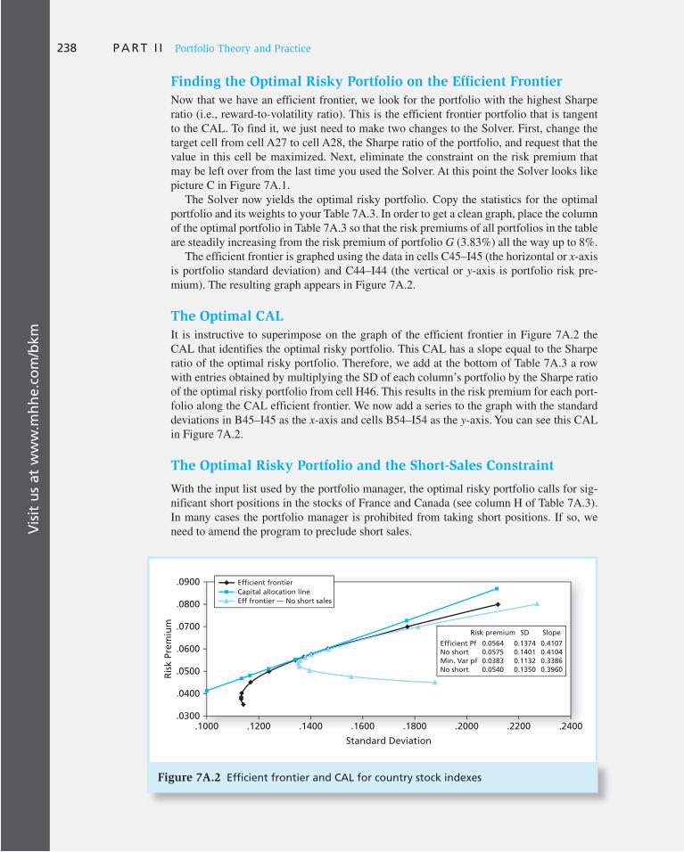
Vis
it u
s at
ww
w.m
hh
e.co
m/b
km238 P A R T I I Portfolio Theory and Practice
Finding the Optimal Risky Portfolio on the Efficient Frontier
Now that we have an efficient frontier, we look for the portfolio with the highest Sharpe
ratio (i.e., reward-to-volatility ratio). This is the efficient frontier portfolio that is tangent
to the CAL. To find it, we just need to make two changes to the Solver. First, change the
target cell from cell A27 to cell A28, the Sharpe ratio of the portfolio, and request that the
value in this cell be maximized. Next, eliminate the constraint on the risk premium that
may be left over from the last time you used the Solver. At this point the Solver looks like
picture C in Figure 7A.1 .
The Solver now yields the optimal risky portfolio. Copy the statistics for the optimal
portfolio and its weights to your Table 7A.3 . In order to get a clean graph, place the column
of the optimal portfolio in Table 7A.3 so that the risk premiums of all portfolios in the table
are steadily increasing from the risk premium of portfolio G (3.83%) all the way up to 8%.
The efficient frontier is graphed using the data in cells C45–I45 (the horizontal or x -axis
is portfolio standard deviation) and C44–I44 (the vertical or y -axis is portfolio risk pre-
mium). The resulting graph appears in Figure 7A.2 .
The Optimal CAL
It is instructive to superimpose on the graph of the efficient frontier in Figure 7A.2 the
CAL that identifies the optimal risky portfolio. This CAL has a slope equal to the Sharpe
ratio of the optimal risky portfolio. Therefore, we add at the bottom of Table 7A.3 a row
with entries obtained by multiplying the SD of each column’s portfolio by the Sharpe ratio
of the optimal risky portfolio from cell H46. This results in the risk premium for each port-
folio along the CAL efficient frontier. We now add a series to the graph with the standard
deviations in B45–I45 as the x -axis and cells B54–I54 as the y -axis. You can see this CAL
in Figure 7A.2 .
The Optimal Risky Portfolio and the Short-Sales Constraint
With the input list used by the portfolio manager, the optimal risky portfolio calls for sig-
nificant short positions in the stocks of France and Canada (see column H of Table 7A.3 ).
In many cases the portfolio manager is prohibited from taking short positions. If so, we
need to amend the program to preclude short sales.
Figure 7A.2 Efficient frontier and CAL for country stock indexes
.0900
.0800
.0700
.0600
.0500
.0400
.0300.1000 .1200 .1400 .1600 .1800 .2000 .2200 .2400
Standard Deviation
Ris
k P
rem
ium
Risk premium SD Slope
Efficient PfNo short
No shortMin. Var pf
0.05640.05750.03830.0540
0.13740.14010.11320.1350
0.41070.41040.33860.3960
Eff frontier — No short sales
Efficient frontier
Capital allocation line

APPENDIX B: Review of Portfolio Statistics
Vis
it u
s at
ww
w.m
hh
e.co
m/b
km
C H A P T E R 7 Optimal Risky Portfolios 239
To accomplish this task, we repeat the exercise, but with one change. We add to the Solver
the following constraint: Each element in the column of portfolio weights, A18–A24, must be
greater than or equal to zero. You should try to produce the short-sale constrained efficient fron-
tier in your own spreadsheet. The graph of the constrained frontier is also shown in Figure 7A.2 .
We base this review of scenario analysis on a two-asset portfolio. We denote the assets D
and E (which you may think of as debt and equity), but the risk and return parameters we
use in this appendix are not necessarily consistent with those used in Section 7.2 .
Expected Returns
We use “expected value” and “mean” interchangeably. For an analysis with n scenarios,
where the rate of return in scenario i is r ( i ) with probability p ( i ), the expected return is
E(r) 5 an
i51
p(i)r(i) (7B.1)
If you were to increase the rate of return assumed for each scenario by some amount ,
then the mean return will increase by . If you multiply the rate in each scenario by a fac-
tor w, the new mean will be multiplied by that factor:
an
i51
p(i) 3 3r (i) 1 D 4 5 an
i51
p(i) 3 r (i) 1 Dan
i51
p(i) 5 E(r) 1 D (7B.2)
an
i51
p(i) 3 3wr(i) 4 5 wan
i51
p(i) 3 r(i) 5 wE(r)
Example 7B.1 Expected Rates of Return
Column C of Table 7B.1 shows scenario rates of return for debt, D. In column D we add 3%
to each scenario return and in column E we multiply each rate by .4. The table shows how we
compute the expected return for columns C, D, and E. It is evident that the mean increases
by 3% (from .08 to .11) in column D and is multiplied by .4 (from .08 to 0.032) in column E.
Table 7B.1
Scenario analysis for bonds
A B C D E GF
1
2
3
4
5
6
7
8
9
10
11
12
Scenario rates of return
rD(i) rD(i) + 0.03 0.4*rD(i)
Mean
Cell C8
−0.10
0.00
0.10
0.32
0.080
=SUMPRODUCT($B$4:$B$7,C4:C7)
−0.07
0.03
0.13
0.35
0.110
−0.040
0.000
0.040
0.128
0.032
0.14
0.36
0.30
0.20
Probability
1
2
3
4
Scenario
eXce lPlease visit us at www.mhhe.com/bkm

Vis
it u
s at
ww
w.m
hh
e.co
m/b
km240 P A R T I I Portfolio Theory and Practice
Now let’s construct a portfolio that invests a fraction of the investment budget, w ( D ), in
bonds and the fraction w ( E ) in stocks. The portfolio’s rate of return in each scenario and its
expected return are given by
rP(i) 5 wDrD(i) 1 wErE(i) (7B.3)
E(rP) 5 a p(i) 3wDrD(i) 1 wErE(i) 4 5 a p(i)wDrD(i) 1 a p(i)wErE(i)
5 wD E(rD) 1 wE
E(rE)
The rate of return on the portfolio in each scenario is the weighted average of the com-
ponent rates. The weights are the fractions invested in these assets, that is, the portfolio
weights. The expected return on the portfolio is the weighted average of the asset means.
Example 7B.2 Portfolio Rate of Return
Table 7B.2 lays out rates of return for both stocks and bonds. Using assumed weights of .4
for debt and .6 for equity, the portfolio return in each scenario appears in column L. Cell L8
shows the portfolio expected return as .1040, obtained using the SUMPRODUCT function,
which multiplies each scenario return (column L) by the scenario probability (column I)
and sums the results.
Variance and Standard Deviation
The variance and standard deviation of the rate of return on an asset from a scenario analy-
sis are given by 14
� 2(r) 5 an
i51
p(i) 3r(i) 2 E(r) 42 (7B.4)
� (r) 5 "� 2(r)
Notice that the unit of variance is percent squared. In contrast, standard deviation, the
square root of variance, has the same dimension as the original returns, and therefore is
easier to interpret as a measure of return variability.
When you add a fixed incremental return, , to each scenario return, you increase the
mean return by that same increment. Therefore, the deviation of the realized return in each
scenario from the mean return is unaffected, and both variance and SD are unchanged. In
contrast, when you multiply the return in each scenario by a factor w, the variance is mul-
tiplied by the square of that factor (and the SD is multiplied by w ):
Var(wr) 5 an
i51
p(i) 3 3wr(i) 2 E(wr) 42 5 w2a
n
i51
p(i) 3r(i) 2 E(r) 42 5 w2� 2
SD(wr) 5 "w2� 2 5 w� (r) (7B.5)
Excel does not have a direct function to compute variance and standard deviation for
a scenario analysis. Its STDEV and VAR functions are designed for time series. We need
14 Variance (here, of an asset rate of return) is not the only possible choice to quantify variability. An alternative
would be to use the absolute deviation from the mean instead of the squared deviation. Thus, the mean absolute
deviation (MAD) is sometimes used as a measure of variability. The variance is the preferred measure for several
reasons. First, working with absolute deviations is mathematically more difficult. Second, squaring deviations
gives more weight to larger deviations. In investments, giving more weight to large deviations (hence, losses) is
compatible with risk aversion. Third, when returns are normally distributed, the variance is one of the two param-
eters that fully characterize the distribution.

Vis
it u
s at
ww
w.m
hh
e.co
m/b
km
C H A P T E R 7 Optimal Risky Portfolios 241
to calculate the probability-weighted squared deviations directly. To avoid having to first
compute columns of squared deviations from the mean, however, we can simplify our
problem by expressing the variance as a difference between two easily computable terms:
� 2(r) 5 E 3r 2 E(r)42 5 E5r2 1 3E(r)42 2 2rE(r)6 5 E(r2) 1 3E(r) 42 2 2E(r)E(r) (7B.6)
5 E(r2) 2 3E(r) 42 5 an
i51
p(i)r(i)2 2 Ban
i51
p(i)r (i)R2
Table 7B.3
Scenario analysis for bonds
A B C D E F G
13
14
15
16
17
18
19
20
21
22
23
24
Scenario rates of return
rD(i) rD(i) + 0.03 0.4*rD(i)
0.14
0.36
0.30
0.20
Mean
Cell C21
Variance
SD
−0.10
0.00
0.10
0.32
0.0800
0.0185
0.1359
=SUMPRODUCT($B$16:$B$19,C16:C19,C16:C19)−C20^2
Cell C22 =C21^0.5
−0.07
0.03
0.13
0.35
0.1100
0.0185
0.1359
−0.040
0.000
0.040
0.128
0.0240
0.0034
0.0584
1
2
3
4
ProbabilityScenario
eXce lPlease visit us at www.mhhe.com/bkm
eXce lPlease visit us at www.mhhe.com/bkm
Table 7B.2
Scenario analysis for bonds and stocks
H I J K L
1
2
3
4
5
6
7
8
9
10
11
12
Scenario rates of return Portfolio return
0.4*rD(i)+0.6*rE(i)rD(i) rE(i)
0.14
0.36
0.30
0.20
−0.10
0.00
0.10
0.32
0.08Mean
Cell L4 =0.4*J4+0.6*K4
Cell L8 =SUMPRODUCT($I$4:$I$7,L4:L7)
−0.35
0.20
0.45
−0.19
0.12
−0.2500
0.1200
0.3100
0.0140
0.1040
1
2
3
4
ProbabilityScenario
Example 7B.3 Calculating the Variance of a Risky Asset in Excel
You can compute the first expression, E ( r 2 ), in Equation 7B.6 using Excel’s SUMPRODUCT
function. For example, in Table 7B.3 , E ( r 2 ) is first calculated in cell C21 by using SUMPROD-
UCT to multiply the scenario probability times the asset return times the asset return again.
Then [ E ( r )] 2 is subtracted (notice the subtraction of C20 2 in cell C21), to arrive at variance.

Vis
it u
s at
ww
w.m
hh
e.co
m/b
km242 P A R T I I Portfolio Theory and Practice
The variance of a portfolio return is not as simple to compute as the mean. The portfolio
variance is not the weighted average of the asset variances. The deviation of the portfolio
rate of return in any scenario from its mean return is
rP 2 E(rP) 5 wDrD(i) 1 wErE(i) 2 3wDE(rD) 1 wEE(rE) 4 5 wD 3rD(i) 2 E(rD) 4 1 wE 3rE(i) 2 E(rE) 4 (7B.7)
5 wDd(i) 1 wEe(i)
where the lowercase variables denote deviations from the mean:
d(i) 5 rD(i) 2 E(rD)
e(i) 5 rE(i) 2 E(rE)
We express the variance of the portfolio return in terms of these deviations from the mean
in Equation 7B.7 :
� P2 5 a
n
i51
p(i) 3rP 2 E(rP) 42 5 an
i51
p(i) 3wD d(i) 1 wEe(i) 42 5 a
n
i51
p(i) 3wD2 d(i)2 1 wE
2 e(i)2 1 2wDwEd(i)e(i) 4 (7B.8)
5 wD2a
n
i51
p(i) d(i)2 1 wE2a
n
i51
p(i)e(i)2 1 2wDwEan
i51
p(i)d(i)e(i)
5 wD2 �D
2 1 wE2 �E
2 1 2wDwEan
i51
p(i)d(i)e(i)
The last line in Equation 7B.8 tells us that the variance of a portfolio is the weighted sum
of portfolio variances (notice that the weights are the squares of the portfolio weights),
plus an additional term that, as we will soon see, makes all the difference.
Notice also that d ( i ) � e ( i ) is the product of the deviations of the scenario returns of the
two assets from their respective means. The probability-weighted average of this product is
its expected value, which is called covariance and is denoted Cov( r D , r E ). The covariance
between the two assets can have a big impact on the variance of a portfolio.
Covariance
The covariance between two variables equals
Cov(rD, rE) 5 E(d 3 e) 5 E5 3rD 2 E(rD) 4 3rE 2 E(rE) 4 6 (7B.9)
5 E(rDrE) 2 E(rD)E(rE)
The covariance is an elegant way to quantify the covariation of two variables. This is easi-
est seen through a numerical example.
Imagine a three-scenario analysis of stocks and bonds as given in Table 7B.4 . In sce-
nario 1, bonds go down (negative deviation) while stocks go up (positive deviation). In
scenario 3, bonds are up, but stocks are down. When the rates move in opposite directions,
as in this case, the product of the deviations is negative; conversely, if the rates moved in
the same direction, the sign of the product would be positive. The magnitude of the product
shows the extent of the opposite or common movement in that scenario. The probability-
weighted average of these products therefore summarizes the average tendency for the
variables to co-vary across scenarios. In the last line of the spreadsheet, we see that the
covariance is � 80 (cell H6).

Vis
it u
s at
ww
w.m
hh
e.co
m/b
km
C H A P T E R 7 Optimal Risky Portfolios 243
Suppose our scenario analysis had envisioned stocks generally moving in the same
direction as bonds. To be concrete, let’s switch the forecast rates on stocks in the first and
third scenarios, that is, let the stock return be � 10% in the first scenario and 30% in the
third. In this case, the absolute value of both products of these scenarios remains the same,
but the signs are positive, and thus the covariance is positive, at � 80, reflecting the ten-
dency for both asset returns to vary in tandem. If the levels of the scenario returns change,
the intensity of the covariation also may change, as reflected by the magnitude of the prod-
uct of deviations. The change in the magnitude of the covariance quantifies the change in
both direction and intensity of the covariation.
If there is no comovement at all, because positive and negative products are equally
likely, the covariance is zero. Also, if one of the assets is risk-free, its covariance with any
risky asset is zero, because its deviations from its mean are identically zero.
The computation of covariance using Excel can be made easy by using the last line in
Equation 7B.9 . The first term, E ( r D � r E ), can be computed in one stroke using Excel’s
SUMPRODUCT function. Specifically, in Table 7B.4 , SUMPRODUCT(A3:A5, B3:B5,
C3:C5) multiplies the probability times the return on debt times the return on equity in
each scenario and then sums those three products.
Notice that adding to each rate would not change the covariance because deviations
from the mean would remain unchanged. But if you multiply either of the variables by a
fixed factor, the covariance will increase by that factor. Multiplying both variables results
in a covariance multiplied by the products of the factors because
Cov(wDrD, wErE) 5 E5 3wDrD 2 wDE(rD) 4 3wErE 2 wEE(rE) 4 6 (7B.10)
5 wDwE Cov(rD, rE)
The covariance in Equation 7B.10 is actually the term that we add (twice) in the last line of
the equation for portfolio variance, Equation 7B.8 . So we find that portfolio variance is the
weighted sum (not average) of the individual asset variances, plus twice their covariance
weighted by the two portfolio weights ( w D � w E ).
Like variance, the dimension (unit) of covariance is percent squared. But here we can-
not get to a more easily interpreted dimension by taking the square root, because the aver-
age product of deviations can be negative, as it was in Table 7B.4 . The solution in this case
is to scale the covariance by the standard deviations of the two variables, producing the
correlation coefficient.
Correlation Coefficient
Dividing the covariance by the product of the standard deviations of the variables will gen-
erate a pure number called correlation. We define correlation as follows:
Corr(rD, rE) 5Cov(rD, rE)
�D�E (7B.11)
Table 7B.4
Three-scenario analysis for stocks and bonds
A
Bonds
Rates of Return Deviation from Mean
Stocks Bonds Stocks
Product of
Deviations
B C D E F G H
1
2
3 0.25
0.50
0.25
Mean:
−2
6
14
6
30
10
−10
10
−8
0
8
0
20
0
−20
0
−160
0
−160
−80
4
5
6
Probability
eXce lPlease visit us at www.mhhe.com/bkm

Vis
it u
s at
ww
w.m
hh
e.co
m/b
km244 P A R T I I Portfolio Theory and Practice
The correlation coefficient must fall within the range [ � 1, 1]. This can be explained as
follows. What two variables should have the highest degree comovement? Logic says a
variable with itself, so let’s check it out.
Cov(rD, rD) 5 E5 3rD 2 E(rD) 4 3 3rD 2 E(rD) 4 6 5 E 3rD 2 E(rD) 42 5 � D
2 (7B.12)
Corr(rD, rD) 5Cov(rD, rD)
�D�D5
� D2
� D2
5 1
Similarly, the lowest (most negative) value of the correlation coefficient is � 1. (Check this
for yourself by finding the correlation of a variable with its own negative.)
An important property of the correlation coefficient is that it is unaffected by both addi-
tion and multiplication. Suppose we start with a return on debt, r D , multiply it by a con-
stant, w D , and then add a fixed amount . The correlation with equity is unaffected:
Corr(D 1 wDrD, rE) 5Cov(D 1 wDrD, rE)
"Var(D 1 wDrD) 3 � E
(7B.13)
5wD Cov(rD, rE)
"wD2 �D
2 3 �E
5wD Cov(rD, rE)
wD�D 3 �E
5 Corr(rD, rE)
Because the correlation coefficient gives more intuition about the relationship between
rates of return, we sometimes express the covariance in terms of the correlation coefficient.
Rearranging Equation 7B.11 , we can write covariance as
Cov(rD, rE) 5 � D�ECorr(rD, rE) (7B.14)
Example 7B.4 Calculating Covariance and Correlation
Table 7B.5 shows the covariance and correlation between stocks and bonds using the same
scenario analysis as in the other examples in this appendix. Covariance is calculated using
Equation 7B.9 . The SUMPRODUCT function used in cell J22 gives us E ( r D � r E ), from
which we subtract E ( r D ) � E ( r E ) (i.e., we subtract J20 � K20). Then we calculate cor-
relation in cell J23 by dividing covariance by the product of the asset standard deviations.
H I J K L M
13
14
15
16
17
18
19
20
21
22
23
24
25
Scenario rates of return
rD(i) rE(i)
0.14
0.36
0.30
0.20
−0.10
0.00
0.10
0.32
0.08
0.1359
−0.0034
−0.0847
Mean
SD
Covariance
Correlation
Cell J22
Cell J23
=SUMPRODUCT(I16:I19,J16:J19,K16:K19)−J20*K20
=J22/(J21*K21)
−0.35
0.20
0.45
−0.19
0.12
0.2918
1
2
3
4
ProbabilityScenario
Table 7B.5
Scenario analysis for bonds and stocks
eXce lPlease visit us at www.mhhe.com/bkm

Vis
it u
s at
ww
w.m
hh
e.co
m/b
km
C H A P T E R 7 Optimal Risky Portfolios 245
Portfolio Variance
We have seen in Equation 7B.8 , with the help of Equation 7B.10 , that the variance of a
two-asset portfolio is the sum of the individual variances multiplied by the square of the
portfolio weights, plus twice the covariance between the rates, multiplied by the product
of the portfolio weights:
� P2 5 wD
2 � D2 1 wE
2� E2 1 2wDwECov(rD, rE) (7B.15)
5 wD2 � D
2 1 wE2�E
2 1 2wDwE�D�ECorr(rD, rE)
Example 7B.5 Calculating Portfolio Variance
We calculate portfolio variance in Table 7B.6 . Notice there that we calculate the portfolio
standard deviation in two ways: once from the scenario portfolio returns (cell E35) and
again (in cell E36) using the first line of Equation 7B.15 . The two approaches yield the
same result. You should try to repeat the second calculation using the correlation coef-
ficient from the second line in Equation 7B.15 instead of covariance in the formula for
portfolio variance.
Suppose that one of the assets, say, E, is replaced with a money market instrument,
that is, a risk-free asset. The variance of E is then zero, as is the covariance with D. In that
case, as seen from Equation 7B.15 , the portfolio standard deviation is just w D � D . In other
words, when we mix a risky portfolio with the risk-free asset, portfolio standard deviation
equals the risky asset’s standard deviation times the weight invested in that asset. This
result was used extensively in Chapter 6.
A B C D E F G
25
26
27
28
29
30
31
32
33
34
35
36
37
38
39
Cell E35 =SUMPRODUCT(B30:B33,E30:E33,E30:E33)−E34^2)^0.5
Cell E36 =(0.4*C35)^2+(0.6*D35)^2+2*0.4*0.6*C36)^0.5
Scenario rates of return Portfolio return
rD(i) rE(i) 0.4*rD(i)+0.6rE(i)
0.14
0.36
0.30
0.20
Mean
SD
Covariance
Correlation
−0.10
0.00
0.10
0.32
0.08
0.1359
−0.0034
−0.0847
−0.35
0.20
0.45
−0.19
0.12
0.2918
SD:
−0.25
0.12
0.31
0.014
0.1040
0.1788
0.1788
1
2
3
4
ProbabilityScenario
Table 7B.6
Scenario analysis for bonds and stocks
eXce lPlease visit us at www.mhhe.com/bkm

8 8 THE MARKOWITZ PROCEDURE introduced
in the preceding chapter suffers from two
drawbacks. First, the model requires a huge
number of estimates to fill the covariance
matrix. Second, the model does not provide
any guideline to the forecasting of the secu-
rity risk premiums that are essential to con-
struct the efficient frontier of risky assets.
Because past returns are unreliable guides to
expected future returns, this drawback can be
telling.
In this chapter we introduce index mod-
els that simplify estimation of the covari-
ance matrix and greatly enhance the analysis
of security risk premiums. By allowing us to
explicitly decompose risk into systematic and
firm-specific components, these models also
shed considerable light on both the power
and the limits of diversification. Further, they
allow us to measure these components of risk
for particular securities and portfolios.
We begin the chapter by describing a
single-factor security market and show how
it can justify a single-index model of security
returns. Once its properties are analyzed, we
proceed to an extensive example of estima-
tion of the single-index model. We review the
statistical properties of these estimates and
show how they relate to the practical issues
facing portfolio managers.
Despite the simplification they offer,
index models remain true to the concepts
of the efficient frontier and portfolio opti-
mization. Empirically, index models are as
valid as the assumption of normality of the
rates of return on available securities. To
the extent that short-term returns are well
approximated by normal distributions, index
models can be used to select optimal port-
folios nearly as accurately as the Markowitz
algorithm. Finally, we examine optimal
risky portfolios constructed using the index
model. While the principles are the same
as those employed in the previous chapter,
the properties of the portfolio are easier
to derive and interpret in this context. We
illustrate how to use the index model by con-
structing an optimal risky portfolio using a
small sample of firms. This portfolio is com-
pared to the corresponding portfolio con-
structed from the Markowitz model. We
conclude with a discussion of several practi-
cal issues that arise when implementing the
index model.
Index Models
CHAPTER EIGHT PA
RT
II
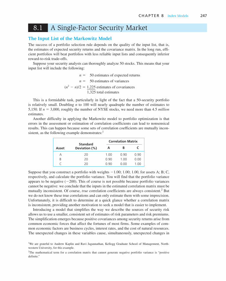
C H A P T E R 8 Index Models 247
8.1 A Single-Factor Security Market
The Input List of the Markowitz Model
The success of a portfolio selection rule depends on the quality of the input list, that is, the estimates of expected security returns and the covariance matrix. In the long run, effi-cient portfolios will beat portfolios with less reliable input lists and consequently inferior reward-to-risk trade-offs.
Suppose your security analysts can thoroughly analyze 50 stocks. This means that your input list will include the following:
n 5 50 estimates of expected returns
n 5 50 estimates of variances
(n2 2 n)/2 5 1,225 estimates of covariances
1,325 total estimates
This is a formidable task, particularly in light of the fact that a 50-security portfolio is relatively small. Doubling n to 100 will nearly quadruple the number of estimates to 5,150. If n � 3,000, roughly the number of NYSE stocks, we need more than 4.5 million estimates.
Another difficulty in applying the Markowitz model to portfolio optimization is that errors in the assessment or estimation of correlation coefficients can lead to nonsensical results. This can happen because some sets of correlation coefficients are mutually incon-sistent, as the following example demonstrates: 1
AssetStandard
Deviation (%)
Correlation Matrix
A B C
A 20 1.00 0.90 0.90
B 20 0.90 1.00 0.00
C 20 0.90 0.00 1.00
Suppose that you construct a portfolio with weights � 1.00; 1.00; 1.00, for assets A; B; C, respectively, and calculate the portfolio variance. You will find that the portfolio variance appears to be negative ( � 200). This of course is not possible because portfolio variances cannot be negative: we conclude that the inputs in the estimated correlation matrix must be mutually inconsistent. Of course, true correlation coefficients are always consistent. 2 But we do not know these true correlations and can only estimate them with some imprecision. Unfortunately, it is difficult to determine at a quick glance whether a correlation matrix is inconsistent, providing another motivation to seek a model that is easier to implement.
Introducing a model that simplifies the way we describe the sources of security risk allows us to use a smaller, consistent set of estimates of risk parameters and risk premiums. The simplification emerges because positive covariances among security returns arise from common economic forces that affect the fortunes of most firms. Some examples of com-mon economic factors are business cycles, interest rates, and the cost of natural resources. The unexpected changes in these variables cause, simultaneously, unexpected changes in
1 We are grateful to Andrew Kaplin and Ravi Jagannathan, Kellogg Graduate School of Management, North-western University, for this example.
2 The mathematical term for a correlation matrix that cannot generate negative portfolio variance is “positive definite.”

248 P A R T I I Portfolio Theory and Practice
the rates of return on the entire stock market. By decomposing uncertainty into these sys-temwide versus firm-specific sources, we vastly simplify the problem of estimating covari-ance and correlation.
Normality of Returns and Systematic Risk
We can always decompose the rate of return on any security, i, into the sum of its expected plus unanticipated components:
ri 5 E(ri) 1 ei (8.1)
where the unexpected return, e i , has a mean of zero and a standard deviation of � i that measures the uncertainty about the security return.
When security returns can be well approximated by normal distributions that are cor-related across securities, we say that they are joint normally distributed. This assumption alone implies that, at any time, security returns are driven by one or more common vari-ables. When more than one variable drives normally distributed security returns, these returns are said to have a multivariate normal distribution. We begin with the simpler case where only one variable drives the joint normally distributed returns, resulting in a single-factor security market. Extension to the multivariate case is straightforward and is discussed in later chapters.
Suppose the common factor, m, that drives innovations in security returns is some macroconomic variable that affects all firms. Then we can decompose the sources of uncertainty into uncertainty about the economy as a whole, which is captured by m, and uncertainty about the firm in particular, which is captured by e i . In this case, we amend Equation 8.1 to accommodate two sources of variation in return:
ri 5 E(ri) 1 m 1 ei (8.2)
The macroeconomic factor, m, measures unanticipated macro surprises. As such, it has a mean of zero (over time, surprises will average out to zero), with standard deviation of � m . In contrast, e i measures only the firm-specific surprise. Notice that m has no subscript because the same common factor affects all securities. Most important is the fact that m and e i are uncorrelated, that is, because e i is firm-specific, it is independent of shocks to the common factor that affect the entire economy. The variance of r i thus arises from two uncorrelated sources, systematic and firm specific. Therefore,
� i2 5 � m
2 1 � 2(ei) (8.3)
The common factor, m, generates correlation across securities, because all securities will respond to the same macroeconomic news, while the firm-specific surprises, captured by e i , are assumed to be uncorrelated across firms. Because m is also uncorrelated with any of the firm-specific surprises, the covariance between any two securities i and j is
Cov(ri , rj) 5 Cov(m 1 ei
, m 1 ej) 5 � m2 (8.4)
Finally, we recognize that some securities will be more sensitive than others to macro-economic shocks. For example, auto firms might respond more dramatically to changes in general economic conditions than pharmaceutical firms. We can capture this refinement by assigning each firm a sensitivity coefficient to macro conditions. Therefore, if we denote the sensitivity coefficient for firm i by the Greek letter beta, � i , we modify Equation 8.2 to obtain the single-factor model:
ri 5 E(ri) 1 �im 1 ei (8.5)

C H A P T E R 8 Index Models 249
Equation 8.5 tells us the systematic risk of security i is determined by its beta coefficient. “Cyclical” firms have greater sensitivity to the market and therefore higher systematic risk. The systematic risk of security i is � i
2�m2 , and its total risk is
� i2 5 �i
2�m2 1 �2(ei) (8.6)
The covariance between any pair of securities also is determined by their betas:
Cov(ri, rj) 5 Cov(�im 1 ei , �j
m 1 ej) 5 �i�j �m
2 (8.7)
In terms of systematic risk and market exposure, this equation tells us that firms are close substitutes. Equivalent beta securities give equivalent market exposures.
Up to this point we have used only statistical implications from the joint normality of security returns. Normality of security returns alone guarantees that portfolio returns are also normal (from the “stability” of the normal distribution discussed in Chapter 5) and that there is a linear relationship between security returns and the common factor. This greatly simplifies portfolio analysis. Statistical analysis, however, does not identify the common factor, nor does it specify how that factor might operate over a longer investment period. However, it seems plausible (and can be empirically verified) that the variance of the com-mon factor usually changes relatively slowly through time, as do the variances of indi-vidual securities and the covariances among them. We seek a variable that can proxy for this common factor. To be useful, this variable must be observable, so we can estimate its volatility as well as the sensitivity of individual securities returns to variation in its value.
8.2 The Single-Index Model
A reasonable approach to making the single-factor model operational is to assert that the rate of return on a broad index of securities such as the S&P 500 is a valid proxy for the common macroeconomic factor. This approach leads to an equation similar to the single-factor model, which is called a single-index model because it uses the market index to proxy for the common factor.
The Regression Equation of the Single-Index Model
Because the S&P 500 is a portfolio of stocks whose prices and rates of return can be observed, we have a considerable amount of past data with which to estimate systematic risk. We denote the market index by M, with excess return of R M � r M � r f , and standard deviation of � M . Because the index model is linear, we can estimate the sensitivity (or beta) coefficient of a security on the index using a single-variable linear regression. We regress the excess return of a security, R i � r i � r f , on the excess return of the index, R M . To esti-mate the regression, we collect a historical sample of paired observations, R i ( t ) and R M ( t ), where t denotes the date of each pair of observations (e.g., the excess returns on the stock and the index in a particular month). 3 The regression equation is
Ri(t) 5 � i 1 �iRM(t) 1 ei(t) (8.8)
The intercept of this equation (denoted by the Greek letter alpha, or � ) is the security’s expected excess return when the market excess return is zero. The slope coefficient, � i , is
3 Practitioners often use a “modified” index model that is similar to Equation 8.8 but that uses total rather than excess returns. This practice is most common when daily data are used. In this case the rate of return on bills is on the order of only about .01% per day, so total and excess returns are almost indistinguishable.
250 P A R T I I Portfolio Theory and Practice
the security beta. Beta is the security’s sensitivity to the index: it is the amount by which the security return tends to increase or decrease for every 1% increase or decrease in the return on the index. e i is the zero-mean, firm-specific surprise in the security return in time t, also called the residual.
The Expected Return–Beta Relationship
Because E ( e i ) � 0, if we take the expected value of E ( R i ) in Equation 8.8 , we obtain the expected return–beta relationship of the single-index model:
E(Ri) 5 � i 1 �iE(RM) (8.9)
The second term in Equation 8.9 tells us that part of a security’s risk premium is due to the risk premium of the index. The market risk premium is multiplied by the relative sensitiv-ity, or beta, of the individual security. We call this the systematic risk premium because it derives from the risk premium that characterizes the entire market, which proxies for the condition of the full economy or economic system.
The remainder of the risk premium is given by the first term in the equation, � . Alpha is a nonmarket premium. For example, � may be large if you think a security is underpriced and therefore offers an attractive expected return. Later on, we will see that when secu-rity prices are in equilibrium, such attractive opportunities ought to be competed away, in which case � will be driven to zero. But for now, let’s assume that each security analyst comes up with his or her own estimates of alpha. If managers believe that they can do a superior job of security analysis, then they will be confident in their ability to find stocks with nonzero values of alpha.
We will see shortly that the index model decomposition of an individual security’s risk premium to market and nonmarket components greatly clarifies and simplifies the opera-tion of macroeconomic and security analysis within an investment company.
Risk and Covariance in the Single-Index Model
Remember that one of the problems with the Markowitz model is the overwhelming number of parameter estimates required to implement it. Now we will see that the index model simplification vastly reduces the number of parameters that must be esti-mated. Equation 8.8 yields the systematic and firm-specific components of the overall risk of each security, and the covariance between any pair of securities. Both variances and covariances are determined by the security betas and the properties of the market index:
Total risk 5 Systematic risk 1 Firm-specific risk
� i2 5 � i
2� M2 1 � 2(ei)
Covariance 5 Product of betas 3 Market index risk
Cov(ri , rj) 5 �i�j�M
2 (8.10)
Correlation 5 Product of correlations with the market index
Corr(ri , rj) 5
�i�j�M2
�i�j5
�i� M2 �j�M
2
�i�M �j
�M5 Corr(ri
, rM) 3 Corr(rj , rM)
Equations 8.9 and 8.10 imply that the set of parameter estimates needed for the single-index model consists of only � , � , and � ( e ) for the individual securities, plus the risk pre-mium and variance of the market index.

C H A P T E R 8 Index Models 251
The Set of Estimates Needed for the Single-Index Model
We summarize the results for the single-index model in the table below.
Symbol
1. The stock’s expected return if the market is neutral, that is, if the market’s
excess return, rM � rf, is zero �i
2. The component of return due to movements in the overall market; �i is the
security’s responsiveness to market movements �i (rM � rf)
3. The unexpected component of return due to unexpected events that
are relevant only to this security (firm specific) ei
4. The variance attributable to the uncertainty of the common
macroeconomic factor �i2 �M
2
5. The variance attributable to firm-specific uncertainty �2(ei)
These calculations show that if we have:
• n estimates of the extra-market expected excess returns, � i
• n estimates of the sensitivity coefficients, � i
• n estimates of the firm-specific variances, � 2 ( e i )
• 1 estimate for the market risk premium, E ( R M )
• 1 estimate for the variance of the (common) macroeconomic factor, � M2
then these (3 n � 2) estimates will enable us to prepare the entire input list for this single-index-security universe. Thus for a 50-security portfolio we will need 152 estimates rather than 1,325; for the entire New York Stock Exchange, about 3,000 securities, we will need 9,002 estimates rather than approximately 4.5 million!
It is easy to see why the index model is such a useful abstraction. For large universes of securities, the number of estimates required for the Markowitz procedure using the index model is only a small fraction of what otherwise would be needed.
Another advantage is less obvious but equally important. The index model abstraction is crucial for specialization of effort in security analysis. If a covariance term had to be calculated directly for each security pair, then security analysts could not specialize by industry. For example, if one group were to specialize in the computer industry and another
CONCEPT CHECK
1
The data below describe a three-stock financial market that satisfies the single-index model.
Stock Capitalization BetaMean Excess
ReturnStandard Deviation
A $3,000 1.0 10% 40%
B $1,940 0.2 2 30
C $1,360 1.7 17 50
The standard deviation of the market index portfolio is 25%.
a. What is the mean excess return of the index portfolio?
b. What is the covariance between stock A and stock B?
c. What is the covariance between stock B and the index?
d. Break down the variance of stock B into its systematic and firm-specific components.
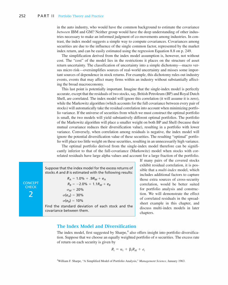
252 P A R T I I Portfolio Theory and Practice
in the auto industry, who would have the common background to estimate the covariance between IBM and GM? Neither group would have the deep understanding of other indus-tries necessary to make an informed judgment of co-movements among industries. In con-trast, the index model suggests a simple way to compute covariances. Covariances among securities are due to the influence of the single common factor, represented by the market index return, and can be easily estimated using the regression Equation 8.8 on p. 249.
The simplification derived from the index model assumption is, however, not without cost. The “cost” of the model lies in the restrictions it places on the structure of asset return uncertainty. The classification of uncertainty into a simple dichotomy—macro ver-sus micro risk—oversimplifies sources of real-world uncertainty and misses some impor-tant sources of dependence in stock returns. For example, this dichotomy rules out industry events, events that may affect many firms within an industry without substantially affect-ing the broad macroeconomy.
This last point is potentially important. Imagine that the single-index model is perfectly accurate, except that the residuals of two stocks, say, British Petroleum (BP) and Royal Dutch Shell, are correlated. The index model will ignore this correlation (it will assume it is zero), while the Markowitz algorithm (which accounts for the full covariance between every pair of stocks) will automatically take the residual correlation into account when minimizing portfo-lio variance. If the universe of securities from which we must construct the optimal portfolio is small, the two models will yield substantively different optimal portfolios. The portfolio of the Markowitz algorithm will place a smaller weight on both BP and Shell (because their mutual covariance reduces their diversification value), resulting in a portfolio with lower variance. Conversely, when correlation among residuals is negative, the index model will ignore the potential diversification value of these securities. The resulting “optimal” portfo-lio will place too little weight on these securities, resulting in an unnecessarily high variance.
The optimal portfolio derived from the single-index model therefore can be signifi-cantly inferior to that of the full-covariance (Markowitz) model when stocks with cor-related residuals have large alpha values and account for a large fraction of the portfolio.
If many pairs of the covered stocks exhibit residual correlation, it is pos-sible that a multi-index model, which includes additional factors to capture those extra sources of cross-security correlation, would be better suited for portfolio analysis and construc-tion. We will demonstrate the effect of correlated residuals in the spread-sheet example in this chapter, and discuss multi-index models in later chapters.
The Index Model and Diversification
The index model, first suggested by Sharpe, 4 also offers insight into portfolio diversifica-tion. Suppose that we choose an equally weighted portfolio of n securities. The excess rate of return on each security is given by
Ri 5 �i 1 �iRM 1 ei
4 William F. Sharpe, “A Simplified Model of Portfolio Analysis,” Management Science, January 1963.
CONCEPT CHECK
2
Suppose that the index model for the excess returns of stocks A and B is estimated with the following results:
RA � 1.0% � .9RM � eA
RB � �2.0% � 1.1RM � eB
�M � 20%
�(eA) � 30%
�(eB) � 10%
Find the standard deviation of each stock and the covariance between them.
C H A P T E R 8 Index Models 253
Similarly, we can write the excess return on the portfolio of stocks as
RP 5 �P 1 �PRM 1 eP (8.11)
We now show that, as the number of stocks included in this portfolio increases, the part of the portfolio risk attributable to nonmarket factors becomes ever smaller. This part of the risk is diversified away. In contrast, market risk remains, regardless of the number of firms combined into the portfolio.
To understand these results, note that the excess rate of return on this equally weighted portfolio, for which each portfolio weight w i � 1/ n, is
RP 5 an
i51
wi Ri 5
1na
n
i51
Ri 51na
n
i51
(� i 1 �iRM 1 ei)
51na
n
i51
�i 1 a1na
n
i51
�ibRM 11na
n
i51
ei
(8.12)
Comparing Equations 8.11 and 8.12 , we see that the portfolio has a sensitivity to the market given by
�P 51na
n
i51
�i (8.13)
which is the average of the individual � i s. It has a nonmarket return component of
�P 51na
n
i51
�i (8.14)
which is the average of the individual alphas, plus the zero mean variable
eP 51na
n
i51
ei (8.15)
which is the average of the firm-specific components. Hence the portfolio’s variance is
�P2 5 �P
2 �M2 1 � 2(eP) (8.16)
The systematic risk component of the portfolio variance, which we defined as the compo-nent that depends on marketwide movements, is �P
2 �M2 and depends on the sensitivity coeffi-
cients of the individual securities. This part of the risk depends on portfolio beta and �M2 and
will persist regardless of the extent of portfolio diversification. No matter how many stocks are held, their common exposure to the market will be reflected in portfolio systematic risk. 5
In contrast, the nonsystematic component of the portfolio variance is � 2 ( e P ) and is attributable to firm-specific components, e i . Because these e i s are independent, and all have zero expected value, the law of averages can be applied to conclude that as more and more stocks are added to the portfolio, the firm-specific components tend to cancel out, resulting in ever-smaller nonmarket risk. Such risk is thus termed diversifiable. To see this more rigorously, examine the formula for the variance of the equally weighted “portfolio” of firm-specific components. Because the e i s are uncorrelated,
� 2(eP) 5 an
i51
a1nb2
� 2(ei) 51n �
– 2(e) (8.17)
where �– 2 1e 2 is the average of the firm-specific variances. Because this average is indepen-dent of n, when n gets large, � 2 ( e P ) becomes negligible.
5 Of course, one can construct a portfolio with zero systematic risk by mixing negative � and positive � assets. The point of our discussion is that the vast majority of securities have a positive � , implying that well-diversified portfolios with small holdings in large numbers of assets will indeed have positive systematic risk.

254 P A R T I I Portfolio Theory and Practice
To summarize, as diversification increases, the total variance of a portfolio approaches the systematic variance, defined as the variance of the market factor multiplied by the square of the portfolio sensitivity coefficient, � P
2. This is shown in Figure 8.1 . Figure 8.1 shows that as more and more securities are combined into a portfolio, the
portfolio variance decreases because of the diversification of firm-specific risk. However, the power of diversification is limited. Even for very large n, part of the risk remains because of the exposure of virtually all assets to the common, or market, factor. Therefore, this systematic risk is said to be nondiversifiable.
This analysis is borne out by empirical evidence. We saw the effect of portfolio diversification on portfo-lio standard deviations in Figure 7.2. These empirical results are similar to the theoretical graph presented here in Figure 8.1 .
Figure 8.1 The variance of an equally weighted portfolio with risk coefficient � P in the single-factor economy
σ2P
n
σ2(eP) � σ
2(e)/n
Diversifiable Risk
Systematic Risk
β2Pσ2
M
CONCEPT CHECK
3
Reconsider the two stocks in Concept Check 2. Sup-pose we form an equally weighted portfolio of A and B. What will be the nonsystematic standard deviation of that portfolio?
8.3 Estimating the Single-Index Model
Armed with the theoretical underpinnings of the single-index model, we now provide an extended example that begins with estimation of the regression equation (8.8) and contin-ues through to the estimation of the full covariance matrix of security returns.
To keep the presentation manageable, we focus on only six large U.S. corporations: Hewlett-Packard and Dell from the information technology (IT) sector of the S&P 500, Target and Walmart from the retailing sector, and British Petroleum and Royal Dutch Shell from the energy sector.
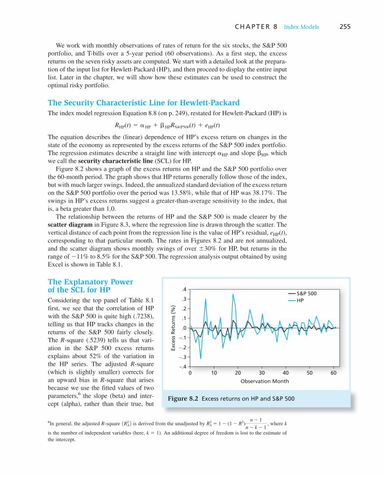
C H A P T E R 8 Index Models 255
We work with monthly observations of rates of return for the six stocks, the S&P 500 portfolio, and T-bills over a 5-year period (60 observations). As a first step, the excess returns on the seven risky assets are computed. We start with a detailed look at the prepara-tion of the input list for Hewlett-Packard (HP), and then proceed to display the entire input list. Later in the chapter, we will show how these estimates can be used to construct the optimal risky portfolio.
The Security Characteristic Line for Hewlett-Packard
The index model regression Equation 8.8 (on p. 249), restated for Hewlett-Packard (HP) is
RHP(t) 5 � HP 1 � HPRS&P500(t) 1 eHP(t)
The equation describes the (linear) dependence of HP’s excess return on changes in the state of the economy as represented by the excess returns of the S&P 500 index portfolio. The regression estimates describe a straight line with intercept � HP and slope � HP , which we call the security characteristic line (SCL) for HP.
Figure 8.2 shows a graph of the excess returns on HP and the S&P 500 portfolio over the 60-month period. The graph shows that HP returns generally follow those of the index, but with much larger swings. Indeed, the annualized standard deviation of the excess return on the S&P 500 portfolio over the period was 13.58%, while that of HP was 38.17%. The swings in HP’s excess returns suggest a greater-than-average sensitivity to the index, that is, a beta greater than 1.0.
The relationship between the returns of HP and the S&P 500 is made clearer by the scatter diagram in Figure 8.3 , where the regression line is drawn through the scatter. The vertical distance of each point from the regression line is the value of HP’s residual, e HP ( t ), corresponding to that particular month. The rates in Figures 8.2 and are not annualized, and the scatter diagram shows monthly swings of over � 30% for HP, but returns in the range of � 11% to 8.5% for the S&P 500. The regression analysis output obtained by using Excel is shown in Table 8.1 .
The Explanatory Power of the SCL for HP
Considering the top panel of Table 8.1 first, we see that the correlation of HP with the S&P 500 is quite high (.7238), telling us that HP tracks changes in the returns of the S&P 500 fairly closely. The R -square (.5239) tells us that vari-ation in the S&P 500 excess returns explains about 52% of the variation in the HP series. The adjusted R -square (which is slightly smaller) corrects for an upward bias in R -square that arises because we use the fitted values of two parameters, 6 the slope (beta) and inter-cept (alpha), rather than their true, but
6 In general, the adjusted R -square 1RA2 2 is derived from the unadjusted by RA
2 5 1 2 (1 2 R2)n 2 1
n 2 k 2 1, where k
is the number of independent variables (here, k � 1). An additional degree of freedom is lost to the estimate of the intercept.
Figure 8.2 Excess returns on HP and S&P 500
−.4
−.3
−.2
−.1
.0
.1
60100 20 30 40 50
.2
.3
.4
Observation Month
Exce
ss R
etu
rns
(%)
S&P 500HP
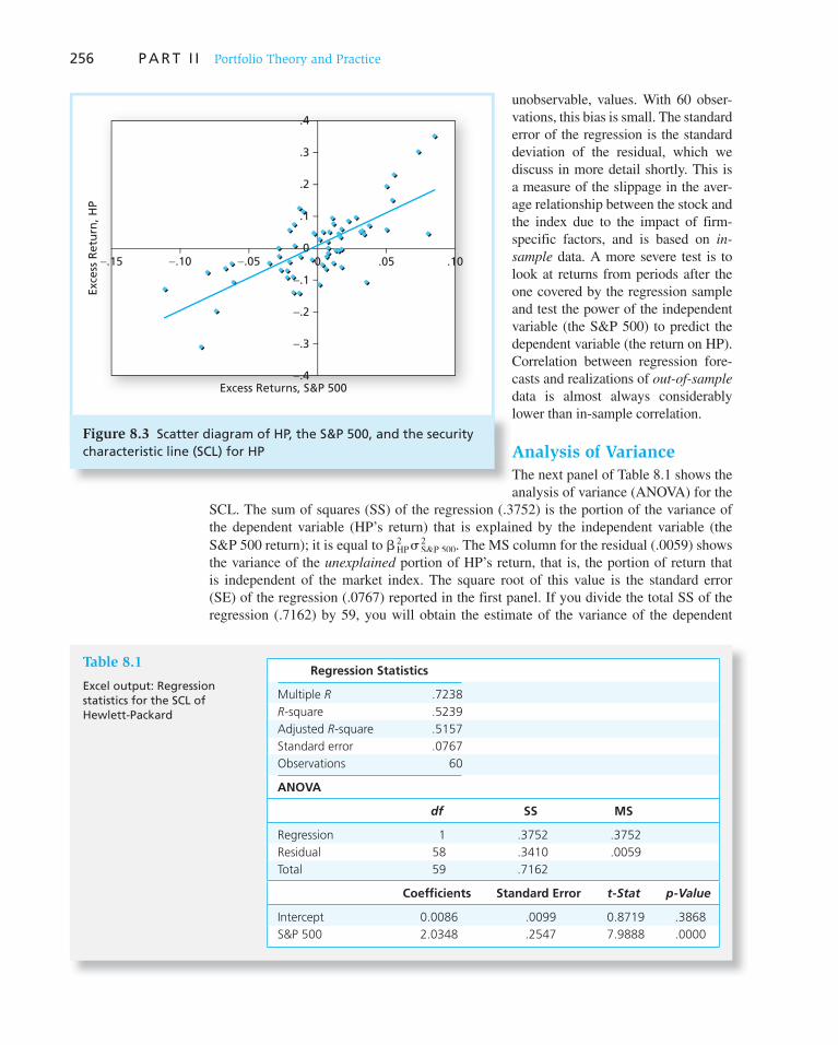
256 P A R T I I Portfolio Theory and Practice
unobservable, values. With 60 obser-vations, this bias is small. The standard error of the regression is the standard deviation of the residual, which we discuss in more detail shortly. This is a measure of the slippage in the aver-age relationship between the stock and the index due to the impact of firm- specific factors, and is based on in-
sample data. A more severe test is to look at returns from periods after the one covered by the regression sample and test the power of the independent variable (the S&P 500) to predict the dependent variable (the return on HP). Correlation between regression fore-casts and realizations of out-of-sample
data is almost always considerably lower than in-sample correlation.
Analysis of Variance
The next panel of Table 8.1 shows the analysis of variance (ANOVA) for the
SCL. The sum of squares (SS) of the regression (.3752) is the portion of the variance of the dependent variable (HP’s return) that is explained by the independent variable (the S&P 500 return); it is equal to � HP
2 � S&P 500
2 . The MS column for the residual (.0059) shows the variance of the unexplained portion of HP’s return, that is, the portion of return that is independent of the market index. The square root of this value is the standard error (SE) of the regression (.0767) reported in the first panel. If you divide the total SS of the regression (.7162) by 59, you will obtain the estimate of the variance of the dependent
Regression Statistics
Multiple R .7238
R-square .5239
Adjusted R-square .5157
Standard error .0767
Observations 60
ANOVA
df SS MS
Regression 1 .3752 .3752
Residual 58 .3410 .0059
Total 59 .7162
Coefficients Standard Error t-Stat p-Value
Intercept 0.0086 .0099 0.8719 .3868
S&P 500 2.0348 .2547 7.9888 .0000
Figure 8.3 Scatter diagram of HP, the S&P 500, and the security characteristic line (SCL) for HP
−.4
−.3
−.2
−.1
0
.1
.2
.3
.4
−.15 −.10 −.05 0 .05 .10
Excess Returns, S&P 500
Exc
ess
Retu
rn, H
P
Table 8.1
Excel output: Regression statistics for the SCL of Hewlett-Packard
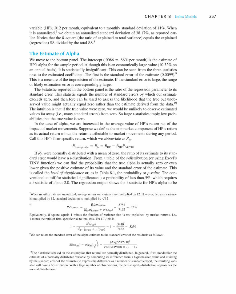
C H A P T E R 8 Index Models 257
variable (HP), .012 per month, equivalent to a monthly standard deviation of 11%. When it is annualized, 7 we obtain an annualized standard deviation of 38.17%, as reported ear-lier. Notice that the R -square (the ratio of explained to total variance) equals the explained (regression) SS divided by the total SS. 8
The Estimate of Alpha
We move to the bottom panel. The intercept (.0086 � .86% per month) is the estimate of HP’s alpha for the sample period. Although this is an economically large value (10.32% on an annual basis), it is statistically insignificant. This can be seen from the three statistics next to the estimated coefficient. The first is the standard error of the estimate (0.0099). 9 This is a measure of the imprecision of the estimate. If the standard error is large, the range of likely estimation error is correspondingly large.
The t -statistic reported in the bottom panel is the ratio of the regression parameter to its standard error. This statistic equals the number of standard errors by which our estimate exceeds zero, and therefore can be used to assess the likelihood that the true but unob-served value might actually equal zero rather than the estimate derived from the data. 10 The intuition is that if the true value were zero, we would be unlikely to observe estimated values far away (i.e., many standard errors) from zero. So large t -statistics imply low prob-abilities that the true value is zero.
In the case of alpha, we are interested in the average value of HP’s return net of the impact of market movements. Suppose we define the nonmarket component of HP’s return as its actual return minus the return attributable to market movements during any period. Call this HP’s firm-specific return, which we abbreviate as R fs .
Rfirm-specific 5 Rfs 5 RHP 2 �HPRS&P500
If R fs were normally distributed with a mean of zero, the ratio of its estimate to its stan-dard error would have a t -distribution. From a table of the t -distribution (or using Excel’s TINV function) we can find the probability that the true alpha is actually zero or even lower given the positive estimate of its value and the standard error of the estimate. This is called the level of significance or, as in Table 8.1 , the probability or p-value. The con-ventional cutoff for statistical significance is a probability of less than 5%, which requires a t -statistic of about 2.0. The regression output shows the t -statistic for HP’s alpha to be
7 When monthly data are annualized, average return and variance are multiplied by 12. However, because variance
is multiplied by 12, standard deviation is multiplied by !12 .
8 R-Square 5
�HP2 �S&P500
2
�HP2 �S&P500
2 1 �2(eHP)5
.3752
.71625 .5239
Equivalently, R -square equals 1 minus the fraction of variance that is not explained by market returns, i.e., 1 minus the ratio of firm-specific risk to total risk. For HP, this is
1 2�2(eHP)
�HP2 �S&P500
2 1 �2(eHP)5 1 2
.3410
.71625 .5239
9 We can relate the standard error of the alpha estimate to the standard error of the residuals as follows:
SE(�HP) 5 �(eHP)Å1n 1
(AvgS&P500)2
Var(S&P500) 3 (n 2 1)
10 The t -statistic is based on the assumption that returns are normally distributed. In general, if we standardize the estimate of a normally distributed variable by computing its difference from a hypothesized value and dividing by the standard error of the estimate (to express the difference as a number of standard errors), the resulting vari-able will have a t -distribution. With a large number of observations, the bell-shaped t -distribution approaches the normal distribution.
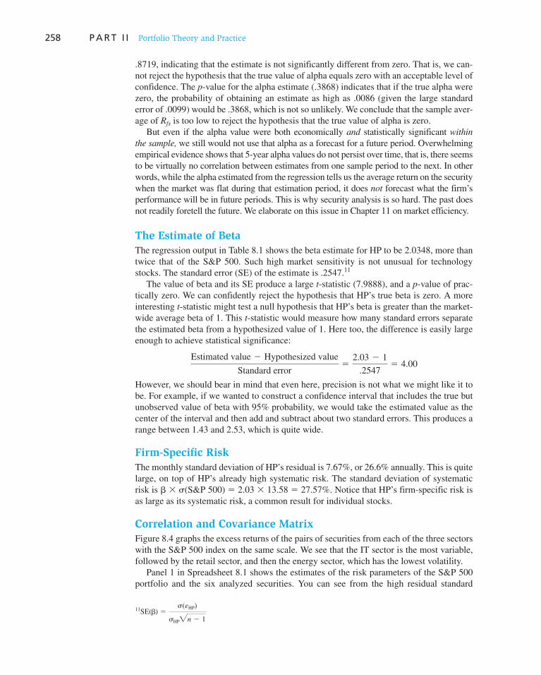
258 P A R T I I Portfolio Theory and Practice
.8719, indicating that the estimate is not significantly different from zero. That is, we can-not reject the hypothesis that the true value of alpha equals zero with an acceptable level of confidence. The p -value for the alpha estimate (.3868) indicates that if the true alpha were zero, the probability of obtaining an estimate as high as .0086 (given the large standard error of .0099) would be .3868, which is not so unlikely. We conclude that the sample aver-age of R fs is too low to reject the hypothesis that the true value of alpha is zero.
But even if the alpha value were both economically and statistically significant within
the sample, we still would not use that alpha as a forecast for a future period. Overwhelming empirical evidence shows that 5-year alpha values do not persist over time, that is, there seems to be virtually no correlation between estimates from one sample period to the next. In other words, while the alpha estimated from the regression tells us the average return on the security when the market was flat during that estimation period, it does not forecast what the firm’s performance will be in future periods. This is why security analysis is so hard. The past does not readily foretell the future. We elaborate on this issue in Chapter 11 on market efficiency.
The Estimate of Beta
The regression output in Table 8.1 shows the beta estimate for HP to be 2.0348, more than twice that of the S&P 500. Such high market sensitivity is not unusual for technology stocks. The standard error (SE) of the estimate is .2547. 11
The value of beta and its SE produce a large t -statistic (7.9888), and a p -value of prac-tically zero. We can confidently reject the hypothesis that HP’s true beta is zero. A more interesting t -statistic might test a null hypothesis that HP’s beta is greater than the market-wide average beta of 1. This t -statistic would measure how many standard errors separate the estimated beta from a hypothesized value of 1. Here too, the difference is easily large enough to achieve statistical significance:
Estimated value 2 Hypothesized value
Standard error5
2.03 2 1
.25475 4.00
However, we should bear in mind that even here, precision is not what we might like it to be. For example, if we wanted to construct a confidence interval that includes the true but unobserved value of beta with 95% probability, we would take the estimated value as the center of the interval and then add and subtract about two standard errors. This produces a range between 1.43 and 2.53, which is quite wide.
Firm-Specific Risk
The monthly standard deviation of HP’s residual is 7.67%, or 26.6% annually. This is quite large, on top of HP’s already high systematic risk. The standard deviation of systematic risk is � � (S&P 500) � 2.03 13.58 � 27.57%. Notice that HP’s firm-specific risk is as large as its systematic risk, a common result for individual stocks.
Correlation and Covariance Matrix
Figure 8.4 graphs the excess returns of the pairs of securities from each of the three sectors with the S&P 500 index on the same scale. We see that the IT sector is the most variable, followed by the retail sector, and then the energy sector, which has the lowest volatility.
Panel 1 in Spreadsheet 8.1 shows the estimates of the risk parameters of the S&P 500 portfolio and the six analyzed securities. You can see from the high residual standard
11 SE(�) 5�(eHP)
�HP"n 2 1
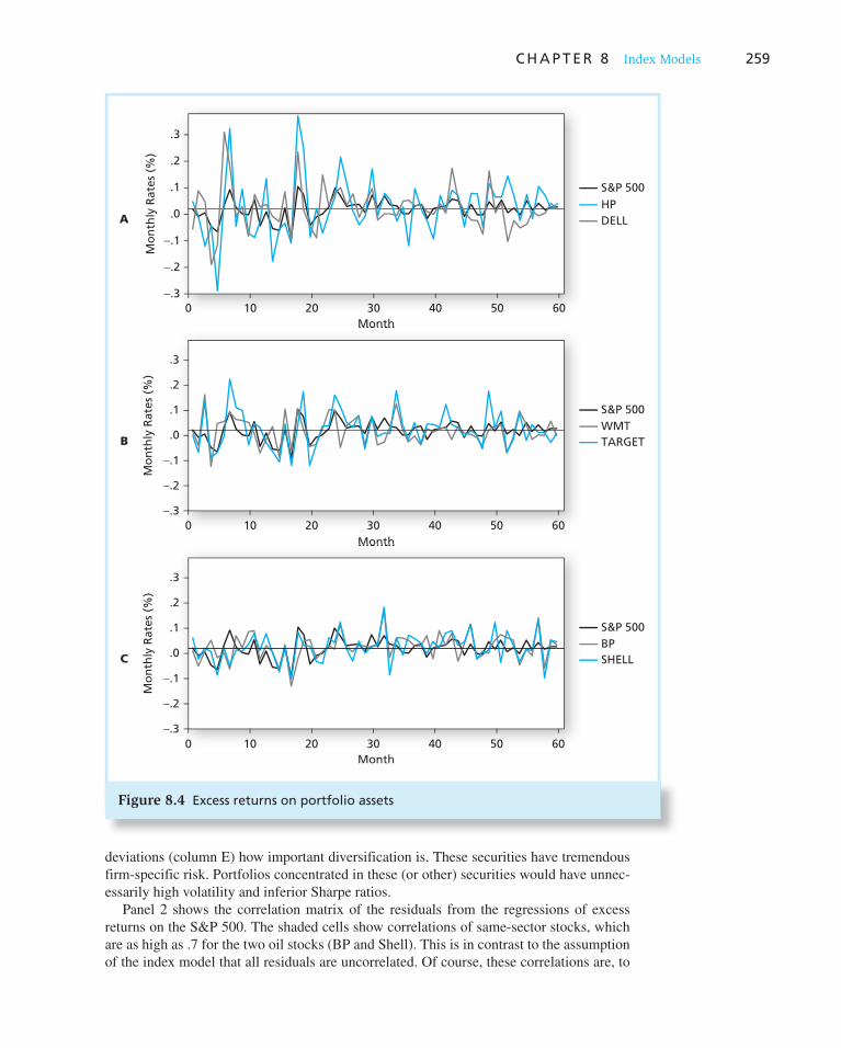
C H A P T E R 8 Index Models 259
Figure 8.4 Excess returns on portfolio assets
−.3
−.2
−.1
.0
.1
.2
.3
0 10 20 30 40 50 60
Month
Mo
nth
ly R
ate
s (%
)
S&P 500
HP
DELL
−.3
−.2
−.1
.0
.1
.2
.3
0 10 20 30 40 50 60
Month
Mo
nth
ly R
ate
s (%
)
S&P 500
WMT
TARGET
−.3
−.2
−.1
.0
.1
.2
.3
0 10 20 30 40 50 60
Month
Mo
nth
ly R
ate
s (%
)
S&P 500
BP
SHELL
A
B
C
deviations (column E) how important diversification is. These securities have tremendous firm-specific risk. Portfolios concentrated in these (or other) securities would have unnec-essarily high volatility and inferior Sharpe ratios.
Panel 2 shows the correlation matrix of the residuals from the regressions of excess returns on the S&P 500. The shaded cells show correlations of same-sector stocks, which are as high as .7 for the two oil stocks (BP and Shell). This is in contrast to the assumption of the index model that all residuals are uncorrelated. Of course, these correlations are, to

Spreadsheet 8.1
Implementing the index model
A B C D E F
1
2
3
4
5
6
0.1358
0.3817
0.2901
0.1935
0.2611
0.1822
0.1988
HP
1.00
7
8
9
10
0.1720 0.1981 0.66
11
0.0634 0.1722 0.35
12
0.0914
0.2762
0.1358
0.1672
0.0841
0.0234
0.0234
0.0086
0.0086
0.0124
0.0150
0.1371
0.5505
1.0000
1.0922
−0.0100
0.0639
−0.0050
0.0322
0.0075
0.0835
0.0025
0.0429
0.012
0.0400
0.0124
0.0375
0.0184
0.0227
0.0227
0.0114
0.0114
0.1780
0.2656
0
0.2392
0.1757
0.46
0.72
0.58
0.43
13
14
15
16
17
18
19
20
21
22
23
24
25
26
27
28
29
30
31
32
33
34
35
36
37
38
39
40
41
42
43
44
45
46
47
48
49
50
51
52
53
54
55
56
57
58
59
G H I J
60
61
SD of
Excess
Return
SD of
Residual
SD of
Systematic
ComponentBeta
Correlation
with the
S&P 500
2.03
1.23
0.62
1.27
0.47
0.67
1.00
1.00
0.0475
0.0475
0.0175
0.0175
0.0253
0.0253
0.0375
0.0462
0.0462
0.0232
0.2126
0.3863
0.1492
0.0705
0.0404
0.1691
0.17180.8282
2.0348
0.1371 0.0639
0.1358
0.0878
0.2497
0.0222
0.1911
0.3472
0.1205
0.0392
0.4045
0.7349
0.5400
0.0297
0.0789
0.1433
0.0205
0.0317
−0.1748
1.2315
0.0322 0.0835
0.6199 1.2672
0.0400
0.4670
0.0429
0.6736
0.0648
0.1422
0.46
1.0158
−0.3176
0.1009
0.0572
−0.1619
−0.2941
0.0865
0.0309
0.0232
0.0288
0.0288
0.0106
0.0106
0.0153
0.01530.0842
0.0141
0.0145
0.0145
0.0053
0.0053
0.0077
0.0077
0.0682
0.0109
0.0109
0.0157
0.0157
0.0332
0.0058
0.0058
0.0395
0.0374
0.0141
2.03Beta
Beta
Risk premium
S&P 500
0.0600
0
S&P 500
2.03
1.23
0.62
1.27
0.47
0.67
0.67
1S&P 500
S&P 500
HP
DELL
WMT
TARGET
BP
SHELL
DELL
WMT
TARGET
BP
SHELL
HP
DELL
WMT
TARGET
BP
SHELL
HP
S&P 500 DELL WMT TARGET BP SHELL Overall PfHPActive Pf A
DELL WMT TARGET BP
HP DELL WMT TARGET BP
1
0.08
−0.34
−0.10
−0.20
−0.06
1
0.17
0.12
−0.28
−0.19
1
1
1
0.50
0.70
0.62 0.47
−0.19
−0.24
−0.13
−0.22
0.1457
SHELL
HP DELL WMT TARGET BP SHELL
1.23 1.27
Off-diagonal cells equal to covariance
multiplies beta from row and column by index variance
formula in cell C26
formula in cell C27
= B4^2
Alpha
Risk premium
σ2(e)
σ2(eA)
αA
α/σ2(e)w0(i)
[w0(i)]2
w0A
w∗(Risky portf)
SD
Sharpe ratio
1
0.06
0.44 0.35
Cells on the diagonal (shadowed) equal to variance
= C$25∗$B27∗$B$4^2
Panel 5: Computation of the Optimal Risky Portfolio
Panel 4: Macro Forecast and Forecasts of Alpha Values
Panel 3: The Index Model Covariance Matrix
Panel 2: Correlation of Residuals
Panel 1: Risk Parameters of the Investable Universe (annualized)
260 P A R T I I Portfolio Theory and Practice
eXce lPlease visit us at www.mhhe.com/bkm

C H A P T E R 8 Index Models 261
a great extent, high by design, because we selected pairs of firms from the same industry. Cross-industry correlations are typically far smaller, and the empirical estimates of corre-lations of residuals for industry indexes (rather than individual stocks in the same industry) would be far more in accord with the model. In fact, a few of the stocks in this sample actu-ally seem to have negatively correlated residuals. Of course, correlation also is subject to statistical sampling error, and this may be a fluke.
Panel 3 produces covariances derived from Equation 8.10 of the single-index model. Variances of the S&P 500 index and the individual covered stocks appear on the diagonal. The variance estimates for the individual stocks equal �i
2�M2 1 �2(ei). The off-diagonal
terms are covariance values and equal �i�j� M2 .
8.4 Portfolio Construction and the Single-Index Model
In this section, we look at the implications of the index model for portfolio construction. 12 We will see that the model offers several advantages, not only in terms of parameter estimation, but also for the analytic simplification and organizational decentralization that it makes possible.
Alpha and Security Analysis
Perhaps the most important advantage of the single-index model is the framework it pro-vides for macroeconomic and security analysis in the preparation of the input list that is so critical to the efficiency of the optimal portfolio. The Markowitz model requires estimates of risk premiums for each security. The estimate of expected return depends on both mac-roeconomic and individual-firm forecasts. But if many different analysts perform security analysis for a large organization such as a mutual fund company, a likely result is incon-sistency in the macroeconomic forecasts that partly underlie expectations of returns across securities. Moreover, the underlying assumptions for market-index risk and return often are not explicit in the analysis of individual securities.
The single-index model creates a framework that separates these two quite different sources of return variation and makes it easier to ensure consistency across analysts. We can lay down a hierarchy of the preparation of the input list using the framework of the single-index model.
1. Macroeconomic analysis is used to estimate the risk premium and risk of the market index.
2. Statistical analysis is used to estimate the beta coefficients of all securities and their residual variances, � 2 ( e i ).
3. The portfolio manager uses the estimates for the market-index risk premium and the beta coefficient of a security to establish the expected return of that security absent any contribution from security analysis. The market-driven expected return is conditional on information common to all securities, not on information gleaned from security analysis of particular firms. This market-driven expected return can be used as a benchmark.
4. Security-specific expected return forecasts (specifically, security alphas) are derived from various security-valuation models (such as those discussed in Part Five). Thus, the alpha value distills the incremental risk premium attributable to private informa-tion developed from security analysis.
12 The use of the index model to construct optimal risky portfolios was originally developed in Jack Treynor and Fischer Black, “How to Use Security Analysis to Improve Portfolio Selection,” Journal of Business, January 1973.

262 P A R T I I Portfolio Theory and Practice
In the context of Equation 8.9 , the risk premium on a security not subject to security analysis would be � i E ( R M ). In other words, the risk premium would derive solely from the security’s tendency to follow the market index. Any expected return beyond this bench-mark risk premium (the security alpha) would be due to some nonmarket factor that would be uncovered through security analysis.
The end result of security analysis is the list of alpha values. Statistical methods of esti-mating beta coefficients are widely known and standardized; hence, we would not expect this portion of the input list to differ greatly across portfolio managers. In contrast, macro and security analysis are far less of an exact science and therefore provide an arena for dis-tinguished performance. Using the index model to disentangle the premiums due to market and nonmarket factors, a portfolio manager can be confident that macro analysts compiling estimates of the market-index risk premium and security analysts compiling alpha values are using consistent estimates for the overall market.
In the context of portfolio construction, alpha is more than just one of the components of expected return. It is the key variable that tells us whether a security is a good or a bad buy. Consider an individual stock for which we have a beta estimate from statistical considerations and an alpha value from security analysis. We easily can find many other securities with identical betas and therefore identical systematic components of their risk premiums. Therefore, what really makes a security attractive or unattractive to a portfolio manager is its alpha value. In fact, we’ve suggested that a security with a positive alpha is providing a premium over and above the premium it derives from its tendency to track the market index. This security is a bargain and therefore should be overweighted in the over-all portfolio compared to the passive alternative of using the market-index portfolio as the risky vehicle. Conversely, a negative-alpha security is overpriced and, other things equal, its portfolio weight should be reduced. In more extreme cases, the desired portfolio weight might even be negative, that is, a short position (if permitted) would be desirable.
The Index Portfolio as an Investment Asset
The process of charting the efficient frontier using the single-index model can be pursued much like the procedure we used in Chapter 7, where we used the Markowitz model to find the optimal risky portfolio. Here, however, we can benefit from the simplification the index model offers for deriving the input list. Moreover, portfolio optimization highlights another advantage of the single-index model, namely, a simple and intuitively revealing representation of the optimal risky portfolio. Before we get into the mechanics of optimization in this setting, however, we start by considering the role of the index portfolio in the optimal portfolio.
Suppose the prospectus of an investment company limits the universe of investable assets to only stocks included in the S&P 500 portfolio. In this case, the S&P 500 index captures the impact of the economy on the large stocks the firm may include in its portfolio. Suppose that the resources of the company allow coverage of only a relatively small subset of this so-called investable universe. If these analyzed firms are the only ones allowed in the portfolio, the portfolio manager may well be worried about limited diversification.
A simple way to avoid inadequate diversification is to include the S&P 500 portfolio as one of the assets of the portfolio. Examination of Equations 8.8 and 8.9 reveals that if we treat the S&P 500 portfolio as the market index, it will have a beta of 1.0 (its sensitivity to itself), no firm-specific risk, and an alpha of zero—there is no nonmarket component in its expected return. Equation 8.10 shows that the covariance of any security, i, with the index is �i�M
2 . To distinguish the S&P 500 from the n securities covered by the firm, we will designate it the ( n � 1)th asset. We can think of the S&P 500 as a passive portfolio that the manager would select in the absence of security analysis. It gives broad market e xposure without the need for expensive security analysis. However, if the manager is willing to
C H A P T E R 8 Index Models 263
engage in such research, she may devise an active portfolio that can be mixed with the index to provide an even better risk–return trade-off.
The Single-Index-Model Input List
If the portfolio manager plans to compile a portfolio from a list of n actively researched firms and a passive market index portfolio, the input list will include the following estimates:
1. Risk premium on the S&P 500 portfolio.
2. Estimate of the standard deviation of the S&P 500 portfolio.
3. n sets of estimates of (a) beta coefficients, (b) stock residual variances, and (c) alpha values. (The alpha values for each security, together with the risk premium of the S&P 500 and the beta of each security, will allow for determination of the expected return on each security.)
The Optimal Risky Portfolio of the Single-Index Model
The single-index model allows us to solve for the optimal risky portfolio directly and to gain insight into the nature of the solution. First we confirm that we easily can set up the optimization process to chart the efficient frontier in this framework along the lines of the Markowitz model.
With the estimates of the beta and alpha coefficients, plus the risk premium of the index portfolio, we can generate the n � 1 expected returns using Equation 8.9 . With the esti-mates of the beta coefficients and residual variances, together with the variance of the index portfolio, we can construct the covariance matrix using Equation 8.10 . Given a col-umn of risk premiums and the covariance matrix, we can conduct the optimization pro-gram described in Chapter 7.
We can take the description of how diversification works in the single-index framework of Section 8.2 a step further. We showed earlier that the alpha, beta, and residual vari-ance of an equally weighted portfolio are the simple averages of those parameters across component securities. Moreover, this result is not limited to equally weighted portfolios. It applies to any portfolio, where we need only replace “simple average” with “weighted average,” using the portfolio weights. Specifically,
�P 5 an11
i51
wi � i and for the index, �n11 5 �M 5 0
�P 5 an11
i51
wi� i and for the index, �n11 5 �M 5 1 (8.18)
� 2(eP) 5 an11
i51
wi2� 2(ei) and for the index, � 2(e n11) 5 � 2(eM) 5 0
The objective is to maximize the Sharpe ratio of the portfolio by using portfolio weights, w 1 , . . ., w n 1 1 . With this set of weights, the expected return, standard deviation, and Sharpe ratio of the portfolio are
E(RP) 5 �P 1 E(RM)�P 5 an11
i51
wi � i 1 E(RM)a
n11
i51
wi�i
�P 5 3�P2�M
2 1 �2(eP)41/2 5 B�M2 ¢a
n11
i51
wi� i≤2
1 an11
i51
wi2� 2(ei)R
1/2
(8.19)
SP 5E(RP)
�P
264 P A R T I I Portfolio Theory and Practice
At this point, as in the standard Markowitz procedure, we could use Excel’s optimization program to maximize the Sharpe ratio subject to the adding-up constraint that the portfo-lio weights sum to 1. However, this is not necessary because the optimal portfolio can be derived explicitly using the index model. Moreover, the solution for the optimal portfolio provides considerable insight into the efficient use of security analysis in portfolio construc-tion. It is instructive to outline the logical thread of the solution. We will not show every algebraic step, but will instead present the major results and interpretation of the procedure.
Before delving into the results, let us first explain the basic trade-off the model reveals. If we were interested only in diversification, we would just hold the market index. Security analysis gives us the chance to uncover securities with a nonzero alpha and to take a differ-ential position in those securities. The cost of that differential position is a departure from efficient diversification, in other words, the assumption of unnecessary firm-specific risk. The model shows us that the optimal risky portfolio trades off the search for alpha against the departure from efficient diversification.
The optimal risky portfolio turns out to be a combination of two component portfolios: (1) an active portfolio, denoted by A, comprised of the n analyzed securities (we call this the active portfolio because it follows from active security analysis), and (2) the market-index portfolio, the ( n � 1)th asset we include to aid in diversification, which we call the passive portfolio and denote by M.
Assume first that the active portfolio has a beta of 1. In that case, the optimal weight in the active portfolio would be proportional to the ratio � A / � 2 ( e A ). This ratio balances the contribution of the active portfolio (its alpha) against its contribution to the portfolio variance (residual variance). The analogous ratio for the index portfolio is E 1RM 2 /� M
2 , and hence the initial position in the active portfolio (i.e., if its beta were 1) is
wA0 5
� A
� A2
E(RM)
� M2
(8.20)
Next, we amend this position to account for the actual beta of the active portfolio. For any level of � A
2, the correlation between the active and passive portfolios is greater when the beta of the active portfolio is higher. This implies less diversification benefit from the passive portfolio and a lower position in it. Correspondingly, the position in the active portfolio increases. The precise modification for the position in the active portfolio is: 13
wA* 5
wA0
1 1 (1 2 �A)wA0 (8.21)
Notice that when �A 5 1, wA* 5 wA
0.
The Information Ratio
Equations 8.20 and 8.21 yield the optimal position in the active portfolio once we know its alpha, beta, and residual variance. With wA
* in the active portfolio and 1 2 wA* invested
in the index portfolio, we can compute the expected return, standard deviation, and Sharpe ratio of the optimal risky portfolio. The Sharpe ratio of an optimally constructed
13 With a little algebraic manipulation, beta can be shown to equal the product of correlation between the index and the active portfolio and the ratio of SD(index)/SD(active portfolio). If � A > 1, then correlation is higher than envisioned in Equation 8.20 , so the diversification value of the index is lower. This requires the modification in Equation 8.21 .

C H A P T E R 8 Index Models 265
risky portfolio will exceed that of the index portfolio (the passive strategy). The exact relationship is
SP2 5 SM
2 1 B � A
� (eA)R 2
(8.22)
Equation 8.22 shows us that the contribution of the active portfolio (when held in its opti-mal weight, wA
* ) to the Sharpe ratio of the overall risky portfolio is determined by the ratio of its alpha to its residual standard deviation. This important ratio is called the informa-
tion ratio. This ratio measures the extra return we can obtain from security analysis com-pared to the firm-specific risk we incur when we over- or underweight securities relative to the passive market index. Equation 8.22 therefore implies that to maximize the overall Sharpe ratio, we must maximize the information ratio of the active portfolio.
It turns out that the information ratio of the active portfolio will be maximized if we invest in each security in proportion to its ratio of � i / � 2 ( e i ). Scaling this ratio so that the total position in the active portfolio adds up to wA
*, the weight in each security is
wi* 5 wA
*
� i
� 2(ei)
an
i51
� i
� 2(ei)
(8.23)
With this set of weights, we find that the contribution of each security to the information ratio of the active portfolio depends on its own information ratio, that is,
B �A
� (eA)R 2
5 an
i51
B � i
� (ei)R 2
(8.24)
The model thus reveals the central role of the information ratio in efficiently taking advantage of security analysis. The positive contribution of a security to the portfolio is made by its addition to the nonmarket risk premium (its alpha). Its negative impact is to increase the portfolio variance through its firm-specific risk (residual variance).
In contrast to alpha, notice that the market (systematic) component of the risk pre-mium, � i E ( R M ), is offset by the security’s nondiversifiable (market) risk, � i
2� M2 , and both
are driven by the same beta. This trade-off is not unique to any security, as any security with the same beta makes the same balanced contribution to both risk and return. Put dif-ferently, the beta of a security is neither vice nor virtue. It is a property that simultaneously affects the risk and risk premium of a security. Hence we are concerned only with the aggregate beta of the active portfolio, rather than the beta of each individual security.
We see from Equation 8.23 that if a security’s alpha is negative, the security will assume a short position in the optimal risky portfolio. If short positions are prohibited, a negative-alpha security would simply be taken out of the optimization program and assigned a port-folio weight of zero. As the number of securities with nonzero alpha values (or the number with positive alphas if short positions are prohibited) increases, the active portfolio will itself be better diversified and its weight in the overall risky portfolio will increase at the expense of the passive index portfolio.
Finally, we note that the index portfolio is an efficient portfolio only if all alpha values are zero. This makes intuitive sense. Unless security analysis reveals that a security has a nonzero alpha, including it in the active portfolio would make the portfolio less attractive. In addition to the security’s systematic risk, which is compensated for by the market risk premium (through beta), the security would add its firm-specific risk to portfolio variance.

266 P A R T I I Portfolio Theory and Practice
With a zero alpha, however, the latter is not compensated by an addition to the nonmarket risk premium. Hence, if all securities have zero alphas, the optimal weight in the active portfolio will be zero, and the weight in the index portfolio will be 1. However, when secu-rity analysis uncovers securities with nonmarket risk premiums (nonzero alphas), the index portfolio is no longer efficient.
Summary of Optimization Procedure
To summarize, once security analysis is complete, and the index-model estimates of secu-rity and market index parameters are established, the optimal risky portfolio can be formed using these steps:
1. Compute the initial position of each security in the active portfolio as wi
0 5 �i/�2(ei).
2. Scale those initial positions to force portfolio weights to sum to 1 by dividing by
their sum, that is, wi 5wi
0
an
i51
wi0
.
3. Compute the alpha of the active portfolio: �A 5 Sni51
wi�i.
4. Compute the residual variance of the active portfolio: � 2(eA) 5 g n
i51 wi2� 2(ei).
5. Compute the initial position in the active portfolio: we
E RA
A
A
M
M
02 ( )
( ).
2
6. Compute the beta of the active portfolio: �A 5 g n
i51 wi�i.
7. Adjust the initial position in the active portfolio: wA* 5
wA0
1 1 (1 2 �A)wA0.
8. Note: the optimal risky portfolio now has weights: wM* 5 1 2 wA
*; wi* 5 wA
*wi.
9. Calculate the risk premium of the optimal risky portfolio from the risk premium of the index portfolio and the alpha of the active portfolio: E(RP) 5 (wM
* 1 wA*�A)E(RM) 1 wA
*� A. Notice that the beta of the risky portfolio is wM
* 1 wA*�A because the beta of the index portfolio is 1.
10. Compute the variance of the optimal risky portfolio from the variance of the index portfolio and the residual variance of the active portfolio: � P
2 5 (wM* 1 wA
*�A)2� M2 1 3wA
*� (eA)42. An Example
We can illustrate the implementation of the index model by constructing an optimal port-folio from the S&P 500 index and the six stocks for which we analyzed risk parameters in Section 8.3 .
This example entails only six analyzed stocks, but by virtue of selecting three pairs of firms from the same industry, it is designed to produce relatively high residual correla-tions. This should put the index model to a severe test, as the model ignores the correla-tion between residuals when producing estimates for the covariance matrix. Therefore, comparison of results from the index model with the full-blown covariance (Markowitz) model should be instructive.

C H A P T E R 8 Index Models 267
Risk Premium Forecasts Panel 4 of Spreadsheet 8.1 contains estimates of alpha and the risk premium for each stock. These alphas ordinarily would be the most important production of the investment company in a real-life procedure. Statistics plays a small role here; in this arena, macro/security analysis is king. In this example, we simply use illustra-tive values to demonstrate the portfolio construction process and possible results. You may wonder why we have chosen such small, forecast alpha values. The reason is that even when security analysis uncovers a large apparent mispricing, that is, large alpha values, these forecasts must be substantially trimmed to account for the fact that such forecasts are subject to large estimation error. We discuss the important procedure of adjusting actual forecasts in Chapter 27.
The Optimal Risky Portfolio Panel 5 of Spreadsheet 8.1 displays calculations for the optimal risky portfolio. They follow the summary procedure of Section 8.4 (you should try to replicate these calculations in your own spreadsheet). In this example we allow short sales. Notice that the weight of each security in the active portfolio (see row 52) has the same sign as the alpha value. Allowing short sales, the positions in the active portfolio are quite large (e.g., the position in BP is .7349); this is an aggressive portfolio. As a result, the alpha of the active portfolio (2.22%) is larger than that of any of the individual alpha forecasts. However, this aggressive stance also results in a large residual variance (.0404, which corresponds to a residual standard deviation of 20%). Therefore, the position in the active portfolio is scaled down (see Equation 8.20 ) and ends up quite modest (.1718; cell C57), reinforcing the notion that diversification considerations are paramount in the opti-mal risky portfolio.
The optimal risky portfolio has a risk premium of 6.48%, standard deviation of 14.22%, and a Sharpe ratio of .46 (cells J58–J61). By comparison, the Sharpe ratio of the index portfolio is .06/.1358 � .44 (cell B61), which is quite close to that of the optimal risky portfolio. The small improvement is a result of the modest alpha forecasts that we used. In Chapter 11 on market efficiency and Chapter 24 on perfor-mance evaluation we demonstrate that such results are common in the mutual fund industry. Of course, some portfolio managers can and do produce portfolios with better performance.
The interesting question here is the extent to which the index model produces results that are inferior to that of the full-covariance (Markowitz) model. Figure 8.5 shows the efficient frontiers from the two models with the example data. We find that the difference is in fact negligible. Table 8.2 compares the compositions and expected performance of the global mini-mum variance ( G ) and the optimal risky portfolios derived from the two models. The significant difference between the two portfolios is limited to the minimum-variance portfolios that are driven only by considerations of variance. As we move up the efficient frontier, the required expected returns obviate the impact of the differ-ences in covariance and the portfolios become similar in performance.
Figure 8.5 Efficient frontiers with the index model and full-covariance matrix
.00
.02
.04
.06
.08
.10
.12
.14
.00 .05 .10 .15 .20 .25 .30 .35 .40
Standard Deviation
Ris
k P
rem
ium
Efficient frontier (full covariance)
Efficient frontier (index model)
S&P 500
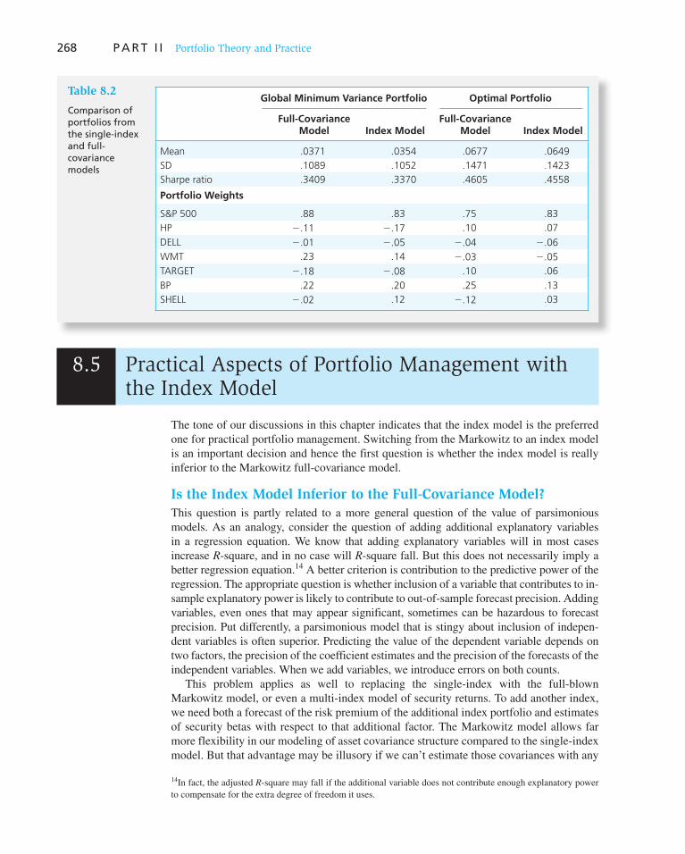
268 P A R T I I Portfolio Theory and Practice
8.5 Practical Aspects of Portfolio Management with the Index Model
Global Minimum Variance Portfolio Optimal Portfolio
Full-Covariance Model Index Model
Full-Covariance Model Index Model
Mean .0371 .0354 .0677 .0649
SD .1089 .1052 .1471 .1423
Sharpe ratio .3409 .3370 .4605 .4558
Portfolio Weights
S&P 500 .88 .83 .75 .83
HP �.11 �.17 .10 .07
DELL �.01 �.05 �.04 �.06
WMT .23 .14 �.03 �.05
TARGET �.18 �.08 .10 .06
BP .22 .20 .25 .13
SHELL �.02 .12 �.12 .03
Table 8.2
Comparison of portfolios from the single-index and full- covariance models
The tone of our discussions in this chapter indicates that the index model is the preferred one for practical portfolio management. Switching from the Markowitz to an index model is an important decision and hence the first question is whether the index model is really inferior to the Markowitz full-covariance model.
Is the Index Model Inferior to the Full-Covariance Model?
This question is partly related to a more general question of the value of parsimonious models. As an analogy, consider the question of adding additional explanatory variables in a regression equation. We know that adding explanatory variables will in most cases increase R -square, and in no case will R -square fall. But this does not necessarily imply a better regression equation. 14 A better criterion is contribution to the predictive power of the regression. The appropriate question is whether inclusion of a variable that contributes to in- sample explanatory power is likely to contribute to out-of-sample forecast precision. Adding variables, even ones that may appear significant, sometimes can be hazardous to forecast precision. Put differently, a parsimonious model that is stingy about inclusion of indepen-dent variables is often superior. Predicting the value of the dependent variable depends on two factors, the precision of the coefficient estimates and the precision of the forecasts of the independent variables. When we add variables, we introduce errors on both counts.
This problem applies as well to replacing the single-index with the full-blown Markowitz model, or even a multi-index model of security returns. To add another index, we need both a forecast of the risk premium of the additional index portfolio and estimates of security betas with respect to that additional factor. The Markowitz model allows far more flexibility in our modeling of asset covariance structure compared to the single-index model. But that advantage may be illusory if we can’t estimate those covariances with any
14 In fact, the adjusted R -square may fall if the additional variable does not contribute enough explanatory power to compensate for the extra degree of freedom it uses.

C H A P T E R 8 Index Models 269
degree of confidence. Using the full-covariance matrix invokes estimation risk of thou-sands of terms. Even if the full Markowitz model would be better in principle, it is very possible that cumulative effect of so many estimation errors will result in a portfolio that is actually inferior to that derived from the single-index model.
Against the potential superiority of the full-covariance model, we have the clear practi-cal advantage of the single-index framework. Its aid in decentralizing macro and security analysis is another decisive advantage.
The Industry Version of the Index Model
Not surprisingly, the index model has attracted the attention of practitioners. To the extent that it is approximately valid, it provides a convenient benchmark for security analysis.
A portfolio manager who has neither special information about a security nor insight that is unavailable to the general public will take the security’s alpha value as zero, and, according to Equation 8.9 , will forecast a risk premium for the security equal to � i R M . If we restate this forecast in terms of total returns, one would expect
E(rHP) 5 rf 1 �HP 3E(rM) 2 rf 4 (8.25)
A portfolio manager who has a forecast for the market index, E ( r M ), and observes the risk-free T-bill rate, r f , can use the model to determine the benchmark expected return for any stock. The beta coefficient, the market risk, � M
2 , and the firm-specific risk, � 2 ( e ), can be estimated from historical SCLs, that is, from regressions of security excess returns on market index excess returns.
There are several proprietary sources for such regression results, sometimes called “beta books”. The Web sites for this chapter at the Online Learning Center ( www.mhhe.com/bkm ) also provide security betas. Table 8.3 is a sample of a typical page from a beta book. Beta books typically use the S&P 500 as the proxy for the market portfolio. They commonly employ the 60 most recent monthly observations to calculate regression parameters, and use total returns, rather than excess returns (deviations from T-bill rates) in the regressions. In this way they estimate a variant of our index model, which is
r 5 a 1 brM 1 e* (8.26)
instead of
r 2 rf 5 � 1 �(rM 2 rf ) 1 e (8.27)
To see the effect of this departure, we can rewrite Equation 8.27 as
r 5 rf 1 � 1 �rM 2 �rf 1 e 5 � 1 rf (1 2 �) 1 �rM 1 e (8.28)
Comparing Equations 8.26 and 8.28 , you can see that if r f is constant over the sample period, both equations have the same independent variable, r M , and residual, e. Therefore, the slope coefficient will be the same in the two regressions. 15
However, the intercept that beta books call ALPHA, as in Table 8.3 , is really an estimate of � � r f (1 � � ). The apparent justification for this procedure is that, on a monthly basis, r f (1 � � ) is small and is likely to be swamped by the volatility of actual stock returns. But it is worth noting that for � 1, the regression intercept in Equation 8.26 will not equal the index model � as it does when excess returns are used as in Equation 8.27 .
15 Actually, r f does vary over time and so should not be grouped casually with the constant term in the regression. However, variations in r f are tiny compared with the swings in the market return. The actual volatility in the T-bill rate has only a small impact on the estimated value of � .
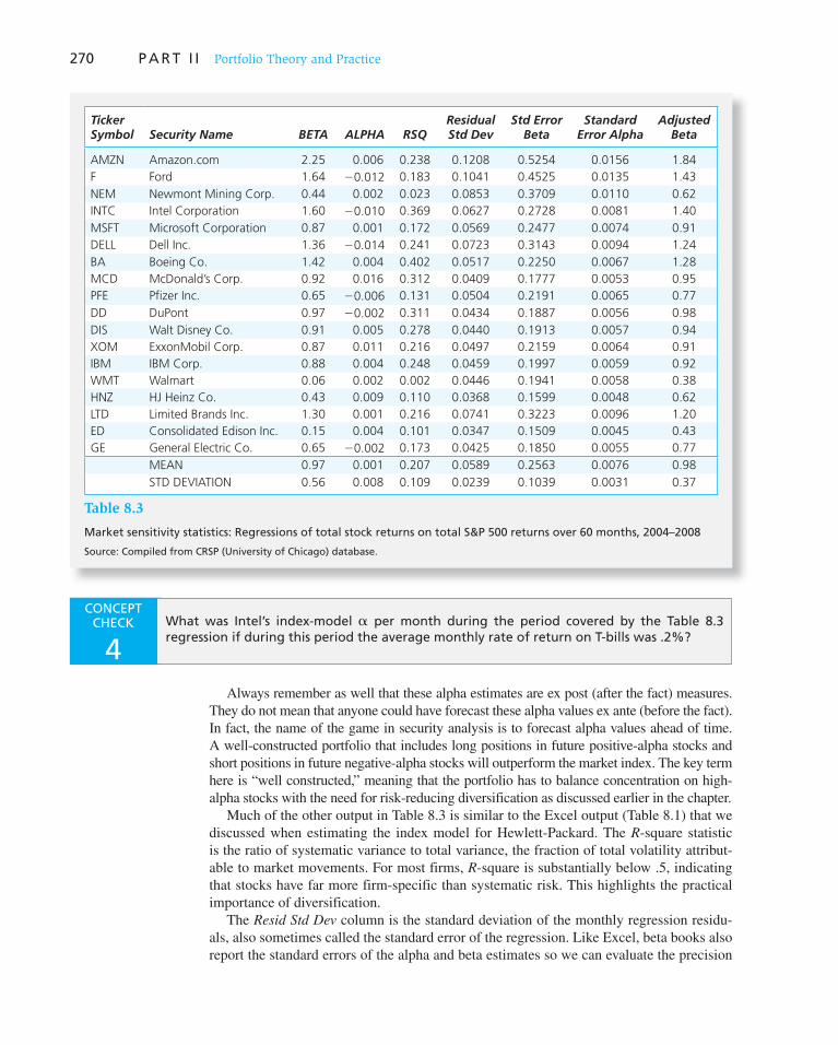
270 P A R T I I Portfolio Theory and Practice
Ticker Symbol Security Name BETA ALPHA RSQ
Residual Std Dev
Std Error Beta
Standard Error Alpha
Adjusted Beta
AMZN Amazon.com 2.25 0.006 0.238 0.1208 0.5254 0.0156 1.84
F Ford 1.64 �0.012 0.183 0.1041 0.4525 0.0135 1.43
NEM Newmont Mining Corp. 0.44 0.002 0.023 0.0853 0.3709 0.0110 0.62
INTC Intel Corporation 1.60 �0.010 0.369 0.0627 0.2728 0.0081 1.40
MSFT Microsoft Corporation 0.87 0.001 0.172 0.0569 0.2477 0.0074 0.91
DELL Dell Inc. 1.36 �0.014 0.241 0.0723 0.3143 0.0094 1.24
BA Boeing Co. 1.42 0.004 0.402 0.0517 0.2250 0.0067 1.28
MCD McDonald’s Corp. 0.92 0.016 0.312 0.0409 0.1777 0.0053 0.95
PFE Pfizer Inc. 0.65 �0.006 0.131 0.0504 0.2191 0.0065 0.77
DD DuPont 0.97 �0.002 0.311 0.0434 0.1887 0.0056 0.98
DIS Walt Disney Co. 0.91 0.005 0.278 0.0440 0.1913 0.0057 0.94
XOM ExxonMobil Corp. 0.87 0.011 0.216 0.0497 0.2159 0.0064 0.91
IBM IBM Corp. 0.88 0.004 0.248 0.0459 0.1997 0.0059 0.92
WMT Walmart 0.06 0.002 0.002 0.0446 0.1941 0.0058 0.38
HNZ HJ Heinz Co. 0.43 0.009 0.110 0.0368 0.1599 0.0048 0.62
LTD Limited Brands Inc. 1.30 0.001 0.216 0.0741 0.3223 0.0096 1.20
ED Consolidated Edison Inc. 0.15 0.004 0.101 0.0347 0.1509 0.0045 0.43
GE General Electric Co. 0.65 �0.002 0.173 0.0425 0.1850 0.0055 0.77
MEAN 0.97 0.001 0.207 0.0589 0.2563 0.0076 0.98
STD DEVIATION 0.56 0.008 0.109 0.0239 0.1039 0.0031 0.37
Table 8.3
Market sensitivity statistics: Regressions of total stock returns on total S&P 500 returns over 60 months, 2004–2008
Source: Compiled from CRSP (University of Chicago) database.
Always remember as well that these alpha estimates are ex post (after the fact) measures. They do not mean that anyone could have forecast these alpha values ex ante (before the fact). In fact, the name of the game in security analysis is to forecast alpha values ahead of time. A well-constructed portfolio that includes long positions in future positive-alpha stocks and short positions in future negative-alpha stocks will outperform the market index. The key term here is “well constructed,” meaning that the portfolio has to balance concentration on high-alpha stocks with the need for risk-reducing diversification as discussed earlier in the chapter.
Much of the other output in Table 8.3 is similar to the Excel output ( Table 8.1 ) that we discussed when estimating the index model for Hewlett-Packard. The R -square statistic is the ratio of systematic variance to total variance, the fraction of total volatility attribut-able to market movements. For most firms, R -square is substantially below .5, indicating that stocks have far more firm-specific than systematic risk. This highlights the practical importance of diversification.
The Resid Std Dev column is the standard deviation of the monthly regression residu-als, also sometimes called the standard error of the regression. Like Excel, beta books also report the standard errors of the alpha and beta estimates so we can evaluate the precision
CONCEPT CHECK
4 What was Intel’s index-model � per month during the period covered by the Table 8.3 regression if during this period the average monthly rate of return on T-bills was .2%?

C H A P T E R 8 Index Models 271
of the estimates. Notice that the standard errors of alpha tend to be far greater multiples of the estimated value of alpha than is the case for beta estimates.
Intel’s Resid Std Dev is 6.27% per month and its R 2 is .369. This tells us that � Intel
2 (e) 5 6.272 5 39.31 and, because R 2 � 1 � � 2 ( e )/ � 2 , we can solve for Intel’s total standard deviation by rearranging as follows:
�Intel 5 B� Intel2 (e)
1 2 R2R1/2
5 a39.31
.631b1/2
5 7.89% per month
This is Intel’s monthly standard deviation for the sample period. Therefore, the annualized
standard deviation for that period was 7.89 !12 5 27.33% The last column is called Adjusted Beta. The motivation for adjusting beta estimates
is that, on average, the beta coefficients of stocks seem to move toward 1 over time. One explanation for this phenomenon is intuitive. A business enterprise usually is established to produce a specific product or service, and a new firm may be more unconventional than an older one in many ways, from technology to management style. As it grows, however, a firm often diversifies, first expanding to similar products and later to more diverse opera-tions. As the firm becomes more conventional, it starts to resemble the rest of the economy even more. Thus its beta coefficient will tend to change in the direction of 1.
Another explanation for this phenomenon is statistical. We know that the average beta over all securities is 1. Thus, before estimating the beta of a security, our best forecast would be that it is 1. When we estimate this beta coefficient over a particular sample period, we sustain some unknown sampling error of the estimated beta. The greater the dif-ference between our beta estimate and 1, the greater is the chance that we incurred a large estimation error and that beta in a subsequent sample period will be closer to 1.
The sample estimate of the beta coefficient is the best guess for that sample period. Given that beta has a tendency to evolve toward 1, however, a forecast of the future beta coefficient should adjust the sample estimate in that direction.
Table 8.3 adjusts beta estimates in a simple way. 16 It takes the sample estimate of beta and averages it with 1, using weights of two-thirds and one-third:
Adjusted beta � 2⁄3 sample beta � 1⁄3 (1) (8.29)
16 A more sophisticated method is described in Oldrich A. Vasicek, “A Note on Using Cross-Sectional Information
in Bayesian Estimation of Security Betas,” Journal of Finance 28 (1973), pp. 1233–39.
Example 8.1 Adjusted Beta
For the 60 months used in Table 8.3, Intel’s beta was estimated at 1.60. Therefore, its adjusted beta is 2⁄3 1.60 � 1⁄3 � 1.40, taking it a third of the way toward 1.
In the absence of special information concerning Intel, if our forecast for the market index is 10% and T-bills pay 4%, we learn from the beta book that the forecast for the rate of return on Intel stock is
E(rIntel) 5 rf 1 Adjusted beta 3 3E(rM) 2 rf 4 5 4 1 1.40(10 2 4) 5 12.40%
The sample period regression alpha is �1.0%. Because Intel’s beta is greater than 1, we know that this means that the estimate of the index model � is somewhat larger. As in
272 P A R T I I Portfolio Theory and Practice
Predicting Betas
Adjusted betas are a simple way to recognize that betas estimated from past data may not be the best estimates of future betas: Betas seem to drift toward 1 over time. This suggests that we might want a forecasting model for beta.
One simple approach would be to collect data on beta in different periods and then esti-mate a regression equation:
Current beta 5 a 1 b (Past beta) (8.30)
Given estimates of a and b, we would then forecast future betas using the rule
Forecast beta 5 a 1 b (Current beta) (8.31)
There is no reason, however, to limit ourselves to such simple forecasting rules. Why not also investigate the predictive power of other financial variables in forecasting beta? For example, if we believe that firm size and debt ratios are two determinants of beta, we might specify an expanded version of Equation 8.30 and estimate
Current beta 5 a 1 b1(Past beta) 1 b2(Firm size) 1 b3(Debt ratio)
Now we would use estimates of a and b 1 through b 3 to forecast future betas. Such an approach was followed by Rosenberg and Guy, 17 who found the following
variables to help predict betas:
1. Variance of earnings.
2. Variance of cash flow.
3. Growth in earnings per share.
4. Market capitalization (firm size).
5. Dividend yield.
6. Debt-to-asset ratio.
Rosenberg and Guy also found that even after controlling for a firm’s financial charac-teristics, industry group helps to predict beta. For example, they found that the beta values of gold mining companies are on average .827 lower than would be predicted based on financial characteristics alone. This should not be surprising; the � .827 “adjustment factor” for the gold industry reflects the fact that gold values are inversely related to market returns.
Table 8.4 presents beta estimates and adjustment factors for a subset of firms in the Rosenberg and Guy study.
17 Barr Rosenberg and J. Guy, “Prediction of Beta from Investment Fundamentals, Parts 1 and 2,” Financial
Analysts Journal, May–June and July–August 1976.
CONCEPT CHECK
5 Compare the first five and last four industries in Table 8.4 . What characteristic seems to determine whether the adjustment factor is positive or negative?
Equation 8.28, we have to subtract (1 � �)rf from the regression alpha to obtain the index model �. In any event, the standard error of the alpha estimate is .81%. The estimate of alpha is far less than twice its standard error. Consequently, we cannot reject the hypothesis that the true alpha is zero.

273
Industry Beta Adjustment Factor
Agriculture 0.99 �.140
Drugs and medicine 1.14 �.099
Telephone 0.75 �.288
Energy utilities 0.60 �.237
Gold 0.36 �.827
Construction 1.27 .062
Air transport 1.80 .348
Trucking 1.31 .098
Consumer durables 1.44 .132
Table 8.4
Industry betas and adjustment factors
Alpha Betting
For those who believe in efficient markets, the recent explosion in the number of exchange-traded funds rep-resents a triumph. ETFs are quoted securities that track a particular index, for a fee that is normally just a fraction of a percentage point. They enable investors to assemble a low-cost portfolio covering a wide range of assets from international equities, through government and corporate bonds, to commodities.
But as fast as the assets of ETFs and index-tracking mutual funds are growing, another section of the indus-try seems to be flourishing even faster. Watson Wyatt, a firm of actuaries, estimates that “alternative asset invest-ment” (ranging from hedge funds through private equity to property) grew by around 20% in 2005, to $1.26 trillion. Investors who take this route pay much higher fees in the hope of better performance. One of the fastest-growing assets, funds of hedge funds, charge some of the highest fees of all.
Why are people paying up? In part, because investors have learned to distinguish between the market return, dubbed beta, and managers’ outperformance, known as alpha. “Why wouldn’t you buy beta and alpha sepa-rately?” asks Arno Kitts of Henderson Global Investors, a fund-management firm. “Beta is a commodity and alpha is about skill.”
Clients have become convinced that no one firm can produce good performance in every asset class. That has led
to a “core and satellite” model, in which part of the port-folio is invested in index trackers with the rest in the hands of specialists. But this creates its own problems. Relations with a single balanced manager are simple. It is much harder to research and monitor the performance of spe-cialists. That has encouraged the middlemen— managers of managers (in the traditional institutional business) and funds-of-funds (in the hedge-fund world), which are usu-ally even more expensive.
That their fees endure might suggest investors can identify outperforming fund managers in advance. However, studies suggest this is extremely hard. And even where you can spot talent, much of the extra per-formance may be siphoned off into higher fees. “A dis-proportionate amount of the benefits of alpha go to the manager, not the client,” says Alan Brown at Schroders, an asset manager.
In any event, investors will probably keep pursuing alpha, even though the cheaper alternatives of ETFs and tracking funds are available. Craig Baker of Watson Wyatt, says that, although above-market returns may not be avail-able to all, clients who can identify them have a “first mover” advantage. As long as that belief exists, managers can charge high fees.
Source: The Economist, September 14, 2006. Copyright © 2007 The Economist Newspaper and The Economist Group. All rights reserved.
WO
RD
S FRO
M TH
E STREET
Index Models and Tracking Portfolios
Suppose a portfolio manager believes she has identified an underpriced portfolio. Her security analysis team estimates the index model equation for this portfolio (using the S&P 500 index) in excess return form and obtains the following estimates:
RP 5 .04 1 1.4RS&P500 1 eP (8.32)

Vis
it u
s at
ww
w.m
hh
e.co
m/b
km274 P A R T I I Portfolio Theory and Practice
Therefore, P has an alpha value of 4% and a beta of 1.4. The manager is confident in the quality of her security analysis but is wary about the performance of the broad market in the near term. If she buys the portfolio, and the market as a whole turns down, she still could lose money on her investment (which has a large positive beta) even if her team is correct that the portfolio is underpriced on a relative basis. She would like a position that takes advantage of her team’s analysis but is independent of the performance of the overall market.
To this end, a tracking portfolio ( T ) can be constructed. A tracking portfolio for port-folio P is a portfolio designed to match the systematic component of P ’s return. The idea is for the portfolio to “track” the market-sensitive component of P ’s return. This means the tracking portfolio must have the same beta on the index portfolio as P and as little nonsys-tematic risk as possible. This procedure is also called beta capture.
A tracking portfolio for P will have a levered position in the S&P 500 to achieve a beta of 1.4. Therefore, T includes positions of 1.4 in the S&P 500 and � .4 in T-bills. Because T is constructed from the index and bills, it has an alpha value of zero.
Now consider buying portfolio P but at the same time offsetting systematic risk by assuming a short position in the tracking portfolio. The short position in T cancels out the systematic exposure of the long position in P: the overall combined position is thus market
neutral. Therefore, even if the market does poorly, the combined position should not be affected. But the alpha on portfolio P will remain intact. The combined portfolio, C, pro-vides an excess return per dollar of
RC 5 RP 2 RT 5 (.04 1 1.4RS&P500 1 eP) 2 1.4RS&P500 5 .04 1 eP (8.33)
While this portfolio is still risky (due to the residual risk, e P ), the systematic risk has been eliminated, and if P is reasonably well-diversified, the remaining nonsystematic risk will be small. Thus the objective is achieved: the manager can take advantage of the 4% alpha without inadvertently taking on market exposure. The process of separating the search for alpha from the choice of market exposure is called alpha transport.
This “long-short strategy” is characteristic of the activity of many hedge funds. Hedge fund managers identify an underpriced security and then try to attain a “pure play” on the perceived underpricing. They hedge out all extraneous risk, focusing the bet only on the perceived “alpha” (see the box on p. 273). Tracking funds are the vehicle used to hedge the exposures to which they do not want exposure. Hedge fund managers use index r egressions such as those discussed here, as well as more-sophisticated variations, to create the tracking portfolios at the heart of their hedging strategies.
1. A single-factor model of the economy classifies sources of uncertainty as systematic (macro-economic) factors or firm-specific (microeconomic) factors. The index model assumes that the macro factor can be represented by a broad index of stock returns.
2. The single-index model drastically reduces the necessary inputs in the Markowitz portfolio selec-tion procedure. It also aids in specialization of labor in security analysis.
3. According to the index model specification, the systematic risk of a portfolio or asset equals
�2�M2 and the covariance between two assets equals � i� j �M
2 .
4. The index model is estimated by applying regression analysis to excess rates of return. The slope of the regression curve is the beta of an asset, whereas the intercept is the asset’s alpha during the sample period. The regression line is also called the security characteristic line.
SUMMARY

Vis
it u
s at
ww
w.m
hh
e.co
m/b
kmV
isit
us
at w
ww
.mh
he.
com
/bkm
C H A P T E R 8 Index Models 275
5. Optimal active portfolios constructed from the index model include analyzed securities in propor-tion to their information ratios. The full risky portfolio is a mixture of the active portfolio and the passive market index portfolio. The index portfolio is used to enhance the diversification of the overall risky position.
6. Practitioners routinely estimate the index model using total rather than excess rates of return. This makes their estimate of alpha equal to � � r f (1 � � ).
7. Betas show a tendency to evolve toward 1 over time. Beta forecasting rules attempt to predict this drift. Moreover, other financial variables can be used to help forecast betas.
Related Web sites for this chapter are available at www.mhhe.com/bkm
single-factor model single-index model regression equation
residuals security characteristic line scatter diagram
information ratio tracking portfolio
KEY TERMS
1. What are the advantages of the index model compared to the Markowitz procedure for obtaining an efficiently diversified portfolio? What are its disadvantages?
2. What is the basic trade-off when departing from pure indexing in favor of an actively managed portfolio?
3. How does the magnitude of firm-specific risk affect the extent to which an active investor will be willing to depart from an indexed portfolio?
4. Why do we call alpha a “nonmarket” return premium? Why are high-alpha stocks desirable investments for active portfolio managers? With all other parameters held fixed, what would hap-pen to a portfolio’s Sharpe ratio as the alpha of its component securities increased?
5. A portfolio management organization analyzes 60 stocks and constructs a mean-variance effi-cient portfolio using only these 60 securities.
a. How many estimates of expected returns, variances, and covariances are needed to optimize this portfolio?
b. If one could safely assume that stock market returns closely resemble a single-index structure, how many estimates would be needed?
6. The following are estimates for two stocks.
Stock Expected Return Beta Firm-Specific Standard Deviation
A 13% 0.8 30%
B 18 1.2 40
The market index has a standard deviations of 22% and the risk-free rate is 8%.
a. What are the standard deviations of stocks A and B? b. Suppose that we were to construct a portfolio with proportions:
Stock A: .30
Stock B: .45
T-bills: .25
Compute the expected return, standard deviation, beta, and nonsystematic standard deviation of the portfolio.
PROBLEM SETS
i. Basic
ii. Intermediate

Vis
it u
s at
ww
w.m
hh
e.co
m/b
km276 P A R T I I Portfolio Theory and Practice
7. Consider the following two regression lines for stocks A and B in the following figure.
rA − r
fr
B − rf
rM − r
fr
M − rf
a. Which stock has higher firm-specific risk? b. Which stock has greater systematic (market) risk? c. Which stock has higher R 2 ? d. Which stock has higher alpha? e. Which stock has higher correlation with the market?
8. Consider the two (excess return) index model regression results for A and B:
R A � 1% � 1.2 R M
R -square � .576
Residual standard deviation � 10.3%
R B � � 2% � .8 R M
R -square � .436
Residual standard deviation � 9.1%
a. Which stock has more firm-specific risk? b. Which has greater market risk? c. For which stock does market movement explain a greater fraction of return variability? d. If r f were constant at 6% and the regression had been run using total rather than excess
returns, what would have been the regression intercept for stock A?
Use the following data for Problems 9 through 14 . Suppose that the index model for stocks A and B is estimated from excess returns with the following results:
RA 5 3% 1 .7RM 1 eA
RB 5 22% 1 1.2RM 1 eB
�M 5 20%; R-squareA 5 .20; R-squareB 5 .12
9. What is the standard deviation of each stock?
10. Break down the variance of each stock to the systematic and firm-specific components.
11. What are the covariance and correlation coefficient between the two stocks?
12. What is the covariance between each stock and the market index?
13. For portfolio P with investment proportions of .60 in A and .40 in B, rework Problems 9, 10, and 12.
14. Rework Problem 13 for portfolio Q with investment proportions of .50 in P, .30 in the market index, and .20 in T-bills.

Vis
it u
s at
ww
w.m
hh
e.co
m/b
km
C H A P T E R 8 Index Models 277
15. A stock recently has been estimated to have a beta of 1.24:
a. What will a beta book compute as the “adjusted beta” of this stock? b. Suppose that you estimate the following regression describing the evolution of beta over
time:
� t 5 .3 1 .7� t21
What would be your predicted beta for next year?
16. Based on current dividend yields and expected growth rates, the expected rates of return on stocks A and B are 11% and 14%, respectively. The beta of stock A is .8, while that of stock B is 1.5. The T-bill rate is currently 6%, while the expected rate of return on the S&P 500 index is 12%. The standard deviation of stock A is 10% annually, while that of stock B is 11%. If you currently hold a passive index portfolio, would you choose to add either of these stocks to your holdings?
17. A portfolio manager summarizes the input from the macro and micro forecasters in the follow-ing table:
Micro Forecasts
Asset Expected Return (%) Beta Residual Standard Deviation (%)
Stock A 20 1.3 58
Stock B 18 1.8 71
Stock C 17 0.7 60
Stock D 12 1.0 55
Macro Forecasts
Asset Expected Return (%) Standard Deviation (%)
T-bills 8 0
Passive equity portfolio 16 23
a. Calculate expected excess returns, alpha values, and residual variances for these stocks. b. Construct the optimal risky portfolio. c. What is Sharpe’s measure for the optimal portfolio and how much of it is contributed by the
active portfolio? d. What should be the exact makeup of the complete portfolio for an investor with a coefficient
of risk aversion of 2.8?
18. Recalculate Problem 17 for a portfolio manager who is not allowed to short sell securities.
a. What is the cost of the restriction in terms of Sharpe’s measure? b. What is the utility loss to the investor ( A � 2.8) given his new complete portfolio?
19. Suppose that on the basis of the analyst’s past record, you estimate that the relationship between forecast and actual alpha is:
Actual abnormal return 5 .3 3 Forecast of alpha
Use the alphas from Problem 17 . How much is expected performance affected by recognizing the imprecision of alpha forecasts?
20. Suppose that the alpha forecasts in row 44 of Spreadsheet 8.1 are doubled. All the other data remain the same. Recalculate the optimal risky portfolio. Before you do any calcula-tions, however, use the Summary of Optimization Procedure to estimate a back-of-the-envelope calculation of the information ratio and Sharpe ratio of the newly optimized portfolio. Then recalculate the entire spreadsheet example and verify your back-of-the-envelope calculation.
iii. Challenge

Vis
it u
s at
ww
w.m
hh
e.co
m/b
km278 P A R T I I Portfolio Theory and Practice
1. When the annualized monthly percentage rates of return for a stock market index were regressed against the returns for ABC and XYZ stocks over a 5-year period ending in 2010, using an ordi-nary least squares regression, the following results were obtained:
Statistic ABC XYZ
Alpha �3.20% 7.3%
Beta 0.60 0.97
R2 0.35 0.17
Residual standard deviation 13.02% 21.45%
Explain what these regression results tell the analyst about risk–return relationships for each stock over the sample period. Comment on their implications for future risk–return relationships, assuming both stocks were included in a diversified common stock portfolio, especially in view of the following additional data obtained from two brokerage houses, which are based on 2 years of weekly data ending in December 2010.
Brokerage House Beta of ABC Beta of XYZ
A .62 1.45
B .71 1.25
2. Assume the correlation coefficient between Baker Fund and the S&P 500 Stock Index is .70. What percentage of Baker Fund’s total risk is specific (i.e., nonsystematic)?
3. The correlation between the Charlottesville International Fund and the EAFE Market Index is 1.0. The expected return on the EAFE Index is 11%, the expected return on Charlottesville Inter-national Fund is 9%, and the risk-free return in EAFE countries is 3%. Based on this analysis, what is the implied beta of Charlottesville International?
4. The concept of beta is most closely associated with:
a. Correlation coefficients. b. Mean-variance analysis. c. Nonsystematic risk. d. Systematic risk.
5. Beta and standard deviation differ as risk measures in that beta measures:
a. Only unsystematic risk, while standard deviation measures total risk. b. Only systematic risk, while standard deviation measures total risk. c. Both systematic and unsystematic risk, while standard deviation measures only unsystematic risk. d. Both systematic and unsystematic risk, while standard deviation measures only systematic risk.
Beta Estimates
Go to http://finance.yahoo.com and click on Stocks link under the Investing tab. Look for the Stock Screener link under Research Tools. The Java Yahoo! Finance Screener lets you create your own screens. In the Click to Add Criteria box, find Trading and Volume on the menu and choose Beta. In the Conditions box, choose < � and in the Values box, enter 1. Hit the Enter key and then request the top 200 matches in the Return Top _M atches box. Click on the Run Screen button.
Select the View Table tab and sort the results to show the lowest betas at the top of the list by clicking on the Beta column header. Which firms have the lowest betas? In which industries do they operate?
Select the View Histogram tab and when the histogram appears, look at the bottom of the screen to see the Show Histogram for box. Use the menu that comes up when you click on the down arrow to select beta. What pattern(s), if any, do you see in the distributions of betas for firms that have betas less than 1?
E-INVEST-MENTS EXERCISES

Vis
it u
s at
ww
w.m
hh
e.co
m/b
km
C H A P T E R 8 Index Models 279
SOLUTIONS TO CONCEPT CHECKS
1. a. Total market capitalization is 3,000 � 1,940 � 1,360 � 6,300. Therefore, the mean excess return of the index portfolio is
3,000
6,3003 10 1
1,940
6,3003 2 1
1,360
6,3003 17 5 9.05% 5 .0905
b. The covariance between stocks A and B equals
Cov(RA, RB) 5 �A�B�M2 5 1 3 .2 3 .252 5 .0125
c. The covariance between stock B and the index portfolio equals
Cov(RB, RM) 5 �B�M2 5 .2 3 .252 5 .0125
d. The total variance of B equals
�B2 5 Var(�BRM 1 eB) 5 �B
2 �M2 1 �2(eB)
Systematic risk equals �B2 �M
2 5 .22 3 .252 5 .0025.
Thus the firm-specific variance of B equals
� 2(eB) 5 �B2 2 �B
2 �M2 5 .302 2 .22 3 .252 5 .0875
2. The variance of each stock is �2�M2 1 �2(e).
For stock A, we obtain
�A2 5 .92(20)2 1 302 5 1,224
�A 5 35%
For stock B,
�B2 5 1.12(20)2 1 102 5 584
�B 5 24%
The covariance is
�A�B �M2 5 .9 3 1.1 3 202 5 396
3. �2(eP) � (1⁄2)2[�2(eA) � �2(eB)]
� 1⁄4 (.302 � .102)
� .0250
Therefore � ( e P ) � .158 � 15.8%
4. The regression ALPHA is related to the index-model � by
ALPHA 5 �index model 1 (1 2 �)rf
For Intel, ALPHA � � 1.0% � � 1.60 and we are told that r f was .2%. Thus
�index model 5 21.0% 2 (1 2 1.60).2% 5 2.88%
Intel’s return was somewhat disappointing. It underperformed its “benchmark” return by an average of .88% per month.
5. The industries with positive adjustment factors are most sensitive to the economy. Their betas would be expected to be higher because the business risk of the firms is higher. In contrast, the industries with negative adjustment factors are in business fields with a lower sensitivity to the economy. Therefore, for any given financial profile, their betas are lower.

9 9 THE CAPITAL ASSET pricing model, almost
always referred to as the CAPM, is a center-
piece of modern financial economics. The
model gives us a precise prediction of the
relationship that we should observe between
the risk of an asset and its expected return.
This relationship serves two vital functions.
First, it provides a benchmark rate of return
for evaluating possible investments. For
example, if we are analyzing securities, we
might be interested in whether the expected
return we forecast for a stock is more or less
than its “fair” return given its risk. Second,
the model helps us to make an educated
guess as to the expected return on assets that
have not yet been traded in the marketplace.
For example, how do we price an initial pub-
lic offering of stock? How will a major new
investment project affect the return inves-
tors require on a company’s stock? Although
the CAPM does not fully withstand empirical
tests, it is widely used because of the insight
it offers and because its accuracy is deemed
acceptable for important applications.
The Capital Asset Pricing Model
CHAPTER NINE PA
RT
III
9.1 The Capital Asset Pricing Model
The capital asset pricing model is a set of predictions concerning equilibrium expected returns on risky assets. Harry Markowitz laid down the foundation of modern portfolio management in 1952. The CAPM was developed 12 years later in articles by William Sharpe, 1 John Lintner, 2 and Jan Mossin. 3 The time for this gestation indicates that the leap from Markowitz’s portfolio selection model to the CAPM is not trivial.
We will approach the CAPM by posing the question “what if,” where the “if” part refers to a simplified world. Positing an admittedly unrealistic world allows a relatively easy leap to the “then” part. Once we accomplish this, we can add complexity to the hypothesized environment one step at a time and see how the conclusions must be amended. This pro-cess allows us to derive a reasonably realistic and comprehensible model.
1 William Sharpe, “Capital Asset Prices: A Theory of Market Equilibrium,” Journal of Finance, September 1964.
2 John Lintner, “The Valuation of Risk Assets and the Selection of Risky Investments in Stock Portfolios and Capital Budgets,” Review of Economics and Statistics, February 1965.
3 Jan Mossin, “Equilibrium in a Capital Asset Market,” Econometrica, October 1966.

C H A P T E R 9 The Capital Asset Pricing Model 281
We summarize the simplifying assumptions that lead to the basic version of the CAPM in the following list. The thrust of these assumptions is that we try to ensure that individu-als are as alike as possible, with the notable exceptions of initial wealth and risk aversion. We will see that conformity of investor behavior vastly simplifies our analysis.
1. There are many investors, each with an endowment (wealth) that is small compared to the total endowment of all investors. Investors are price-takers, in that they act as though security prices are unaffected by their own trades. This is the usual perfect competition assumption of microeconomics.
2. All investors plan for one identical holding period. This behavior is myopic (short-sighted) in that it ignores everything that might happen after the end of the single-period horizon. Myopic behavior is, in general, suboptimal.
3. Investments are limited to a universe of publicly traded financial assets, such as stocks and bonds, and to risk-free borrowing or lending arrangements. This assumption rules out investment in nontraded assets such as education (human capital), private enterprises, and governmentally funded assets such as town halls and international airports. It is assumed also that investors may borrow or lend any amount at a fixed, risk-free rate.
4. Investors pay no taxes on returns and no transaction costs (commissions and service charges) on trades in securities. In reality, of course, we know that investors are in different tax brackets and that this may govern the type of assets in which they invest. For example, tax implications may differ depending on whether the income is from interest, dividends, or capital gains. Furthermore, actual trading is costly, and commissions and fees depend on the size of the trade and the good standing of the individual investor.
5. All investors are rational mean-variance optimizers, meaning that they all use the Markowitz portfolio selection model.
6. All investors analyze securities in the same way and share the same economic view of the world. The result is identical estimates of the probability distribution of future cash flows from investing in the available securities; that is, for any set of security prices, they all derive the same input list to feed into the Markowitz model. Given a set of security prices and the risk-free interest rate, all investors use the same expected returns and covariance matrix of security returns to generate the efficient frontier and the unique optimal risky portfolio. This assumption is often referred to as homogeneous expectations or beliefs.
These assumptions represent the “if” of our “what if ” analysis. Obviously, they ignore many real-world complexities. With these assumptions, however, we can gain some pow-erful insights into the nature of equilibrium in security markets.
We can summarize the equilibrium that will prevail in this hypothetical world of securities and investors briefly. The rest of the chapter explains and elaborates on these implications.
1. All investors will choose to hold a portfolio of risky assets in proportions that duplicate representation of the assets in the market portfolio ( M ), which includes all traded assets. For simplicity, we generally refer to all risky assets as stocks. The proportion of each stock in the market portfolio equals the market value of the stock (price per share multiplied by the number of shares outstanding) divided by the total market value of all stocks.
2. Not only will the market portfolio be on the efficient frontier, but it also will be the tangency portfolio to the optimal capital allocation line (CAL) derived by each and
282 P A R T I I I Equilibrium in Capital Markets
every investor. As a result, the capital market line (CML), the line from the risk-free rate through the market portfolio, M, is also the best attainable capital alloca-tion line. All investors hold M as their optimal risky portfolio, differing only in the amount invested in it versus in the risk-free asset.
3. The risk premium on the market portfolio will be proportional to its risk and the degree of risk aversion of the representative investor. Mathematically,
E(rM ) 2 rf 5 AsM2
where sM2 is the variance of the market portfolio and A is the average degree of risk
aversion across investors. Note that because M is the optimal portfolio, which is efficiently diversified across all stocks, sM
2 is the systematic risk of this universe.
4. The risk premium on individual assets will be proportional to the risk premium on the market portfolio, M, and the beta coefficient of the security relative to the mar-ket portfolio. Beta measures the extent to which returns on the stock and the market move together. Formally, beta is defined as
bi 5Cov(ri
, rM )
sM2
and the risk premium on individual securities is
E(ri) 2 rf 5Cov(ri
, rM)
sM2
3E(rM) 2 rf 45 bi 3E(rM) 2 rf 4 Why Do All Investors Hold the Market Portfolio?
What is the market portfolio? When we sum over, or aggregate, the portfolios of all individual investors, lending and borrowing will cancel out (because each lender has a corresponding borrower), and the value of the aggregate risky portfolio will equal the entire wealth of the economy. This is the market portfolio, M. The proportion of each stock in this portfolio equals the market value of the stock (price per share times num-ber of shares outstanding) divided by the sum of the market values of all stocks. 4 The CAPM implies that as individuals attempt to optimize their personal portfolios, they each arrive at the same portfolio, with weights on each asset equal to those of the market portfolio.
Given the assumptions of the previous section, it is easy to see that all investors will desire to hold identical risky portfolios. If all investors use identical Markowitz analysis (Assumption 5) applied to the same universe of securities (Assumption 3) for the same time horizon (Assumption 2) and use the same input list (Assumption 6), they all must arrive at the same composition of the optimal risky portfolio, the portfolio on the efficient frontier identified by the tangency line from T-bills to that frontier, as in Figure 9.1 . This implies that if the weight of GE stock, for example, in each common risky portfolio is 1%, then GE also will comprise 1% of the market portfolio. The same principle applies to the proportion of any stock in each investor’s risky portfolio. As a result, the optimal risky portfolio of all investors is simply a share of the market portfo-lio in Figure 9.1 .
Now suppose that the optimal portfolio of our investors does not include the stock of some company, such as Delta Airlines. When all investors avoid Delta stock, the demand is zero,
4 As noted previously, we use the term “stock” for convenience; the market portfolio properly includes all assets in the economy.

C H A P T E R 9 The Capital Asset Pricing Model 283
and Delta’s price takes a free fall. As Delta stock gets progressively cheaper, it becomes ever more attrac-tive and other stocks look relatively less attractive. Ultimately, Delta reaches a price where it is attractive enough to include in the optimal stock portfolio.
Such a price adjustment process guarantees that all stocks will be included in the optimal portfolio. It shows that all assets have to be included in the market portfolio. The only issue is the price at which investors will be willing to include a stock in their optimal risky portfolio.
This may seem a roundabout way to derive a sim-ple result: If all investors hold an identical risky port-folio, this portfolio has to be M, the market portfolio. Our intention, however, is to demonstrate a connec-tion between this result and its underpinnings, the equilibrating process that is fundamental to security market operation.
The Passive Strategy Is Efficient
In Chapter 6 we defined the CML (capital market line) as the CAL (capital allocation line) that is constructed from a money market account (or T-bills) and the market portfolio. Perhaps now you can fully appreciate why the CML is an interesting CAL. In the simple world of the CAPM, M is the optimal tangency portfolio on the efficient frontier, as shown in Figure 9.1 .
In this scenario, the market portfolio held by all investors is based on the common input list, thereby incorporating all relevant information about the universe of securities. This means that investors can skip the trouble of doing security analysis and obtain an efficient portfolio simply by holding the market portfolio. (Of course, if everyone were to follow this strategy, no one would perform security analysis and this result would no longer hold. We discuss this issue in greater depth in Chapter 11 on market efficiency.)
Thus the passive strategy of investing in a market index portfolio is efficient. For this reason, we sometimes call this result a mutual fund theorem. The mutual fund theorem is another incarnation of the separation property discussed in Chapter 7. Assuming that all investors choose to hold a market index mutual fund, we can separate portfolio selec-tion into two components—a technical problem, creation of mutual funds by professional managers—and a personal problem that depends on an investor’s risk aversion, allocation of the complete portfolio between the mutual fund and risk-free assets.
In reality, different investment managers do create risky portfolios that differ from the market index. We attribute this in part to the use of different input lists in the formation of the optimal risky portfolio. Nevertheless, the practical significance of the mutual fund theorem is that a passive investor may view the market index as a reasonable first approximation to an efficient risky portfolio.
The nearby box contains a parable illustrating the argument for indexing. If the passive strategy is efficient, then attempts to beat it simply generate trading and research costs with no offsetting ben-efit, and ultimately inferior results.
Figure 9.1 The efficient frontier and the capital market line
E(r)
E(rM)
M
CML
rf
σ
σM
CONCEPT CHECK
1
If there are only a few investors who perform security analysis, and all oth-ers hold the market portfolio, M, would the CML still be the efficient CAL for investors who do not engage in security analysis? Why or why not?
284
The Parable of the Money Managers
Some years ago, in a land called Indicia, revolution led to the overthrow of a socialist regime and the restoration of a system of private property. Former government enterprises were reformed as corporations, which then issued stocks and bonds. These securities were given to a central agency, which offered them for sale to individuals, pension funds, and the like (all armed with newly printed money).
Almost immediately a group of money managers came forth to assist these investors. Recalling the words of a venerated elder, uttered before the previous revolution (“Invest in Corporate Indicia”), they invited clients to give them money, with which they would buy a cross-section of all the newly issued securities. Investors considered this a reasonable idea, and soon everyone held a piece of Corporate Indicia.
Before long the money managers became bored because there was little for them to do. Soon they fell into the habit of gathering at a beachfront casino where they passed the time playing roulette, craps, and similar games, for low stakes, with their own money.
After a while, the owner of the casino suggested a new idea. He would furnish an impressive set of rooms which would be designated the Money Managers’ Club. There the members could place bets with one another about the fortunes of various corporations, industries, the level of the Gross Domestic Product, foreign trade, etc. To make the betting more exciting, the casino owner suggested that the managers use their clients’ money for this purpose.
The offer was immediately accepted, and soon the money managers were betting eagerly with one another. At the end of each week, some found that they had won money for their clients, while others found that they had lost. But the losses always exceeded the gains, for a certain
amount was deducted from each bet to cover the costs of the elegant surroundings in which the gambling took place.
Before long a group of professors from Indicia U. sug-gested that investors were not well served by the activi-ties being conducted at the Money Managers’ Club. “Why pay people to gamble with your money? Why not just hold your own piece of Corporate Indicia?” they said.
This argument seemed sensible to some of the inves-tors, and they raised the issue with their money managers. A few capitulated, announcing that they would henceforth stay away from the casino and use their clients’ money only to buy proportionate shares of all the stocks and bonds issued by corporations.
The converts, who became known as managers of Indicia funds, were initially shunned by those who contin-ued to frequent the Money Managers’ Club, but in time, grudging acceptance replaced outright hostility. The wave of puritan reform some had predicted failed to material-ize, and gambling remained legal. Many managers contin-ued to make their daily pilgrimage to the casino. But they exercised more restraint than before, placed smaller bets, and generally behaved in a manner consonant with their responsibilities. Even the members of the Lawyers’ Club found it difficult to object to the small amount of gam-bling that still went on.
And everyone but the casino owner lived happily ever after.
Source: William F. Sharpe, “The Parable of the Money Managers,” The Financial Analysts’ Journal 32 (July/August 1976), p. 4. Copyright 1976, CFA Institute. Reproduced from The Financial Analysts’ Journal with permission from the CFA Institute. All rights reserved.
WO
RD
S FR
OM
TH
E ST
REE
T
The Risk Premium of the Market Portfolio
In Chapter 6 we discussed how individual investors go about deciding how much to invest in the risky portfolio. Returning now to the decision of how much to invest in portfolio M versus in the risk-free asset, what can we deduce about the equilibrium risk premium of portfolio M?
We asserted earlier that the equilibrium risk premium on the market portfolio, E ( r M ) � r f , will be proportional to the average degree of risk aversion of the investor population and the risk of the market portfolio, sM
2 . Now we can explain this result. Recall that each individual investor chooses a proportion y, allocated to the optimal
portfolio M, such that
y 5E(rM ) 2 rf
AsM2
(9.1)
In the simplified CAPM economy, risk-free investments involve borrowing and lend-ing among investors. Any borrowing position must be offset by the lending position of the creditor. This means that net borrowing and lending across all investors must be zero, and in consequence, substituting the representative investor’s risk aversion, A, for A, the
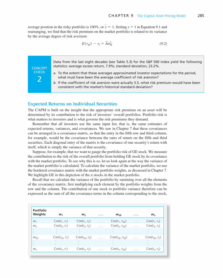
C H A P T E R 9 The Capital Asset Pricing Model 285
average position in the risky portfolio is 100%, or y 5 1. Setting y � 1 in Equation 9.1 and rearranging, we find that the risk premium on the market portfolio is related to its variance by the average degree of risk aversion:
E(rM ) 2 rf 5 AsM2 (9.2)
CONCEPT CHECK
2
Data from the last eight decades (see Table 5.3) for the S&P 500 index yield the following statistics: average excess return, 7.9%; standard deviation, 23.2%.
a. To the extent that these averages approximated investor expectations for the period, what must have been the average coefficient of risk aversion?
b. If the coefficient of risk aversion were actually 3.5, what risk premium would have been consistent with the market’s historical standard deviation?
Expected Returns on Individual Securities
The CAPM is built on the insight that the appropriate risk premium on an asset will be determined by its contribution to the risk of investors’ overall portfolios. Portfolio risk is what matters to investors and is what governs the risk premiums they demand.
Remember that all investors use the same input list, that is, the same estimates of expected returns, variances, and covariances. We saw in Chapter 7 that these covariances can be arranged in a covariance matrix, so that the entry in the fifth row and third column, for example, would be the covariance between the rates of return on the fifth and third securities. Each diagonal entry of the matrix is the covariance of one security’s return with itself, which is simply the variance of that security.
Suppose, for example, that we want to gauge the portfolio risk of GE stock. We measure the contribution to the risk of the overall portfolio from holding GE stock by its covariance with the market portfolio. To see why this is so, let us look again at the way the variance of the market portfolio is calculated. To calculate the variance of the market portfolio, we use the bordered covariance matrix with the market portfolio weights, as discussed in Chapter 7. We highlight GE in this depiction of the n stocks in the market portfolio.
Recall that we calculate the variance of the portfolio by summing over all the elements of the covariance matrix, first multiplying each element by the portfolio weights from the row and the column. The contribution of one stock to portfolio variance therefore can be expressed as the sum of all the covariance terms in the column corresponding to the stock,
Portfolio Weights w1 w2 . . . wGE . . . wn
w1 Cov(r1, r1) Cov(r1, r2) . . . Cov(r1, rGE) . . . Cov(r1, rn)
w2 Cov(r2, r1) Cov(r2, r2) . . . Cov(r2, rGE) . . . Cov(r2, rn)
. . .
. . .
. . .
. . .
. . .
wGE Cov(rGE, r1) Cov(rGE, r2) . . . Cov(rGE, rGE) . . . Cov(rGE, rn)
. . .
. . .
. . .
. . .
. . .
wn Cov(rn, r1) Cov(rn, r2) . . . Cov(rn, rGE) . . . Cov(rn, rn)

286 P A R T I I I Equilibrium in Capital Markets
where each covariance is first multiplied by both the stock’s weight from its row and the weight from its column. 5
For example, the contribution of GE’s stock to the variance of the market portfolio is
wGE 3w1Cov(r1 , rGE) 1 w2Cov(r2
, rGE) 1 . . . 1 wGECov(rGE , rGE) 1 . . .
1wnCov(rn , rGE)]
(9.3)
Equation 9.3 provides a clue about the respective roles of variance and covariance in determining asset risk. When there are many stocks in the economy, there will be many more covariance terms than variance terms. Consequently, the covariance of a particular stock with all other stocks will dominate that stock’s contribution to total portfolio risk.
We will show in a moment that the sum inside the square brackets in Equation 9.3 is the covariance of GE with the market portfolio. In other words, the stock’s contribution to the risk of the market portfolio depends on its covariance with that portfolio:
GE’s contribution to variance 5 wGECov(rGE , rM )
This should not surprise us. For example, if the covariance between GE and the rest of the market is negative, then GE makes a “negative contribution” to portfolio risk: By providing returns that move inversely with the rest of the market, GE stabilizes the return on the overall portfolio. If the covariance is positive, GE makes a positive contribution to overall portfolio risk because its returns reinforce swings in the rest of the portfolio.
To demonstrate this more rigorously, note that the rate of return on the market portfolio may be written as
rM 5 an
k51
wkrk
Therefore, the covariance of the return on GE with the market portfolio is
Cov(rGE , rM ) 5 Cov¢rGE
, an
k51
wkrk≤ 5 an
k51
wkCov(rk , rGE) (9.4)
Notice that the last term of Equation 9.4 is precisely the same as the term in brackets in Equation 9.3 . Therefore, Equation 9.3 , which is the contribution of GE to the vari-ance of the market portfolio, may be simplified to w GE Cov( r GE , r M ). We also observe that the contribution of our holding of GE to the risk premium of the market portfolio is w GE [ E ( r GE ) � r f ].
Therefore, the reward-to-risk ratio for investments in GE can be expressed as
GE’s contribution to risk premium
GE’s contribution to variance5
wGE 3E(rGE) 2 rf 4wGECov(rGE
, rM )5
E(rGE) 2 rf
Cov(rGE , rM )
The market portfolio is the tangency (efficient mean-variance) portfolio. The reward-to-risk ratio for investment in the market portfolio is
Market risk premium
Market variance5
E(rM ) 2 rf
sM2
(9.5)
5 An alternative approach would be to measure GE’s contribution to market variance as the sum of the elements in the row and the column corresponding to GE. In this case, GE’s contribution would be twice the sum in Equation 9.3. The approach that we take in the text allocates contributions to portfolio risk among securities in a convenient man-ner in that the sum of the contributions of each stock equals the total portfolio variance, whereas the alternative mea-sure of contribution would sum to twice the portfolio variance. This results from a type of double-counting, because adding both the rows and the columns for each stock would result in each entry in the matrix being added twice.

C H A P T E R 9 The Capital Asset Pricing Model 287
The ratio in Equation 9.5 is often called the market price of risk 6 because it quantifies the extra return that investors demand to bear portfolio risk. Notice that for components of the efficient portfolio, such as shares of GE, we measure risk as the contribution to portfolio variance (which depends on its covariance with the market). In contrast, for the efficient portfolio itself, its variance is the appropriate measure of risk.
A basic principle of equilibrium is that all investments should offer the same reward-to-risk ratio. If the ratio were better for one investment than another, investors would rearrange their portfolios, tilting toward the alternative with the better trade-off and shying away from the other. Such activity would impart pressure on security prices until the ratios were equalized. Therefore we conclude that the reward-to-risk ratios of GE and the market port-folio should be equal:
E(rGE) 2 rf
Cov(rGE , rM )
5E(rM ) 2 rf
sM2
(9.6)
To determine the fair risk premium of GE stock, we rearrange Equation 9.6 slightly to obtain
E(rGE) 2 rf 5Cov(rGE
, rM )
sM2
3E(rM ) 2 rf 4 (9.7)
The ratio Cov(rGE, rM ) /sM2 measures the contribution of GE stock to the variance of the
market portfolio as a fraction of the total variance of the market portfolio. The ratio is called beta and is denoted by � . Using this measure, we can restate Equation 9.7 as
E(rGE) 5 rf 1 bGE 3E(rM ) 2 rf 4 (9.8)
This expected return–beta relationship is the most familiar expression of the CAPM to practitioners. We will have a lot more to say about the expected return–beta relationship shortly.
We see now why the assumptions that made individuals act similarly are so useful. If everyone holds an identical risky portfolio, then everyone will find that the beta of each asset with the market portfolio equals the asset’s beta with his or her own risky portfolio. Hence everyone will agree on the appropriate risk premium for each asset.
Does the fact that few real-life investors actually hold the market portfolio imply that the CAPM is of no practical importance? Not necessarily. Recall from Chapter 7 that reason-ably well-diversified portfolios shed firm-specific risk and are left with mostly systematic or market risk. Even if one does not hold the precise market portfolio, a well-diversified portfolio will be so highly correlated with the market that a stock’s beta relative to the market will still be a useful risk measure.
In fact, several authors have shown that modified versions of the CAPM will hold true even if we consider differences among individuals leading them to hold different portfo-lios. For example, Brennan 7 examined the impact of differences in investors’ personal tax
6 We open ourselves to ambiguity in using this term, because the market portfolio’s reward-to-volatility ratio
E(rM) 2 rf
sM
sometimes is referred to as the market price of risk. Note that because the appropriate risk measure of GE is its covariance with the market portfolio (its contribution to the variance of the market portfolio), this risk is mea-sured in percent squared. Accordingly, the price of this risk, [E ( r M ) � r f ]/ � 2 , is defined as the percentage expected return per percent square of variance.
7 Michael J. Brennan, “Taxes, Market Valuation, and Corporate Finance Policy,” National Tax Journal, December 1973.

288 P A R T I I I Equilibrium in Capital Markets
rates on market equilibrium, and Mayers 8 looked at the impact of nontraded assets such as human capital (earning power). Both found that although the market portfolio is no longer each investor’s optimal risky portfolio, the expected return–beta relationship should still hold in a somewhat modified form.
If the expected return–beta relationship holds for any individual asset, it must hold for any combination of assets. Suppose that some portfolio P has weight w k for stock k, where k takes on values 1, . . . , n. Writing out the CAPM Equation 9.8 for each stock, and multi-plying each equation by the weight of the stock in the portfolio, we obtain these equations, one for each stock:
w1E(r1 ) 5 w1rf 1 w1b1 3E(rM ) 2 rf 41w2E(r2 ) 5 w2rf 1 w2b2 3E(rM ) 2 rf 41 . . . 5 . . .
1wnE(rn ) 5 wnrf 1 wnbn 3E(rM ) 2 rf 4 E(rP) 5 rf 1 bP 3E(rM ) 2 rf 4
Summing each column shows that the CAPM holds for the overall portfolio because
E ( r P ) � gk
w k E ( r k ) is the expected return on the portfolio, and � P � gk
w k � k is the portfolio
beta. Incidentally, this result has to be true for the market portfolio itself,
E(rM ) 5 rf 1 bM 3E(rM ) 2 rf 4 Indeed, this is a tautology because � M � 1, as we can verify by noting that
bM 5Cov(rM
, rM )
sM2
5sM
2
sM2
This also establishes 1 as the weighted-average value of beta across all assets. If the market beta is 1, and the market is a portfolio of all assets in the economy, the weighted-average beta of all assets must be 1. Hence betas greater than 1 are considered aggressive in that investment in high-beta stocks entails above-average sensitivity to market swings. Betas below 1 can be described as defensive.
A word of caution: We are all accustomed to hearing that well-managed firms will pro-vide high rates of return. We agree this is true if one measures the firm’s return on invest-ments in plant and equipment. The CAPM, however, predicts returns on investments in the securities of the firm.
Let us say that everyone knows a firm is well run. Its stock price will therefore be bid up, and consequently returns to stockholders who buy at those high prices will not be excessive. Security prices, in other words, already reflect public information about a firm’s prospects; therefore only the risk of the company (as measured by beta in the context of the CAPM) should affect expected returns. In a well-functioning market, investors receive high expected returns only if they are willing to bear risk.
Of course, investors do not directly observe or determine expected returns on securities. Rather, they observe security prices and bid those prices up or down. Expected rates of return are determined by the prices investors must pay compared to the cash flows those investments might garner.
8 David Mayers, “Nonmarketable Assets and Capital Market Equilibrium under Uncertainty,” in Studies in the
Theory of Capital Markets, ed. M. C. Jensen (New York: Praeger, 1972). We will look at this model more closely later in the chapter.
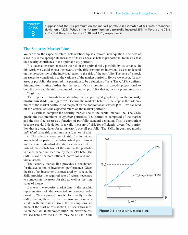
C H A P T E R 9 The Capital Asset Pricing Model 289
The Security Market Line
We can view the expected return–beta relationship as a reward–risk equation. The beta of a security is the appropriate measure of its risk because beta is proportional to the risk that the security contributes to the optimal risky portfolio.
Risk-averse investors measure the risk of the optimal risky portfolio by its variance. In this world we would expect the reward, or the risk premium on individual assets, to depend on the contribution of the individual asset to the risk of the portfolio. The beta of a stock measures its contribution to the variance of the market portfolio. Hence we expect, for any asset or portfolio, the required risk premium to be a function of beta. The CAPM confirms this intuition, stating further that the security’s risk premium is directly proportional to both the beta and the risk premium of the market portfolio; that is, the risk premium equals � [ E ( r M ) � r f ].
The expected return–beta relationship can be portrayed graphically as the security
market line (SML) in Figure 9.2 . Because the market’s beta is 1, the slope is the risk pre-mium of the market portfolio. At the point on the horizontal axis where � � 1, we can read off the vertical axis the expected return on the market portfolio.
It is useful to compare the security market line to the capital market line. The CML graphs the risk premiums of efficient portfolios (i.e., portfolios composed of the market and the risk-free asset) as a function of portfolio standard deviation. This is appropriate because standard deviation is a valid measure of risk for efficiently diversified portfo-lios that are candidates for an investor’s overall portfolio. The SML, in contrast, graphs individual asset risk premiums as a function of asset risk. The relevant measure of risk for individual assets held as parts of well-diversified portfolios is not the asset’s standard deviation or variance; it is, instead, the contribution of the asset to the portfolio variance, which we measure by the asset’s beta. The SML is valid for both efficient portfolios and indi-vidual assets.
The security market line provides a benchmark for the evaluation of investment performance. Given the risk of an investment, as measured by its beta, the SML provides the required rate of return necessary to compensate investors for risk as well as the time value of money.
Because the security market line is the graphic representation of the expected return–beta rela-tionship, “fairly priced” assets plot exactly on the SML; that is, their expected returns are commen-surate with their risk. Given the assumptions we made at the start of this section, all securities must lie on the SML in market equilibrium. Nevertheless, we see here how the CAPM may be of use in the
CONCEPT CHECK
3 Suppose that the risk premium on the market portfolio is estimated at 8% with a standard deviation of 22%. What is the risk premium on a portfolio invested 25% in Toyota and 75% in Ford, if they have betas of 1.10 and 1.25, respectively?
Figure 9.2 The security market line
E(r)
E(rM)
E(rM) – r
f = Slope of SML
SML
rf
βM =1.0
1
β

290
money-management industry. Suppose that the SML relation is used as a benchmark to assess the fair expected return on a risky asset. Then security analysis is performed to calculate the return actually expected. (Notice that we depart here from the simple CAPM world in that some investors now apply their own unique analysis to derive an “input list” that may differ from their competitors’.) If a stock is perceived to be a good buy, or underpriced, it will provide an expected return in excess of the fair return stipu-lated by the SML. Underpriced stocks therefore plot above the SML: Given their betas, their expected returns are greater than dictated by the CAPM. Overpriced stocks plot below the SML.
The difference between the fair and actually expected rates of return on a stock is called the stock’s alpha, denoted by � . For example, if the market return is expected to be 14%, a stock has a beta of 1.2, and the T-bill rate is 6%, the SML would predict an expected return on the stock of 6 � 1.2(14 � 6) � 15.6%. If one believed the stock would provide an expected return of 17%, the implied alpha would be 1.4% (see Figure 9.3 ).
Tales From the Far Side
Financial markets’ evaluation of risk determines the way
firms invest. What if the markets are wrong?
Investors are rarely praised for their good sense. But for the past two decades a growing number of firms have based their decisions on a model which assumes that peo-ple are perfectly rational. If they are irrational, are busi-nesses making the wrong choices?
The model, known as the “capital-asset pricing model,” or CAPM, has come to dominate modern finance. Almost any manager who wants to defend a project—be it a brand, a factory or a corporate merger—must justify his decision partly based on the CAPM. The reason is that the model tells a firm how to calculate the return that its inves-tors demand. If shareholders are to benefit, the returns from any project must clear this “hurdle rate.”
Although the CAPM is complicated, it can be reduced to five simple ideas:
• Investors can eliminate some risks—such as the risk that workers will strike, or that a firm’s boss will quit—by diversifying across many regions and sectors.
• Some risks, such as that of a global recession, cannot be eliminated through diversification. So even a basket of all of the stocks in a stock market will still be risky.
• People must be rewarded for investing in such a risky basket by earning returns above those that they can get on safer assets, such as Treasury bills.
• The rewards on a specific investment depend only on the extent to which it affects the market basket’s risk.
• Conveniently, that contribution to the market basket’s risk can be captured by a single measure—dubbed “beta”—which expresses the relationship between the investment’s risk and the market’s.
Beta is what makes the CAPM so powerful. Although an investment may face many risks, diversified investors should care only about those that are related to the market
basket. Beta not only tells managers how to measure those risks, but it also allows them to translate them directly into a hurdle rate. If the future profits from a project will not exceed that rate, it is not worth shareholders’ money.
The diagram shows how the CAPM works. Safe invest-ments, such as Treasury bills, have a beta of zero. Riskier investments should earn a premium over the risk-free rate which increases with beta. Those whose risks roughly match the market’s have a beta of one, by definition, and should earn the market return.
So suppose that a firm is considering two projects, Aand B. Project A has a beta of ½: when the market rises or falls by 10%, its returns tend to rise or fall by 5%. So its risk premium is only half that of the market. Project B ’s
WO
RD
S FR
OM
TH
E ST
REE
T
Return
MarketReturn
Risk-FreeReturn
A
B
1 2
�
rB
rA
Beta Power
1 2

291
One might say that security analysis (which we treat in Part Five) is about uncovering securities with nonzero alphas. This analysis suggests that the starting point of portfolio management can be a passive market-index portfolio. The portfolio manager will then increase the weights of securities with positive alphas and decrease the weights of securi-ties with negative alphas. We showed one strategy for adjusting the portfolio weights in such a manner in Chapter 8.
The CAPM is also useful in capital budgeting decisions. For a firm considering a new project, the CAPM can provide the required rate of return that the project needs to yield, based on its beta, to be acceptable to investors. Managers can use the CAPM to obtain this cutoff internal rate of return (IRR), or “hurdle rate” for the project.
The nearby box describes how the CAPM can be used in capital budgeting. It also discusses some empirical anomalies concerning the model, which we address in detail in Chapters 11–13. The article asks whether the CAPM is useful for capital budgeting
risk premium is twice that of the market, so it must earn a higher return to justify the expenditure.
NEVER KNOWINGLY UNDERPRICED But there is one small problem with the CAPM: Financial economists have found that beta is not much use for explaining rates of return on firms’ shares. Worse, there appears to be another measure which explains these returns quite well.
That measure is the ratio of a firm’s book value (the value of its assets at the time they entered the balance sheet) to its market value. Several studies have found that, on average, companies that have high book-to-market ratios tend to earn excess returns over long periods, even after adjusting for the risks that are associated with beta.
The discovery of this book-to-market effect has sparked a fierce debate among financial economists. All of them agree that some risks ought to carry greater rewards. But they are now deeply divided over how risk should be mea-sured. Some argue that since investors are rational, the book-to-market effect must be capturing an extra risk fac-tor. They conclude, therefore, that managers should incor-porate the book-to-market effect into their hurdle rates. They have labeled this alternative hurdle rate the “new estimator of expected return,” or NEER.
Other financial economists, however, dispute this approach. Since there is no obvious extra risk associated with a high book-to-market ratio, they say, investors must be mistaken. Put simply, they are underpricing high book-to-market stocks, causing them to earn abnormally high returns. If managers of such firms try to exceed those inflated hurdle rates, they will forgo many profitable investments. With economists now at odds, what is a con-scientious manager to do?
Jeremy Stein, an economist at the Massachusetts Institute of Technology’s business school, offers a p aradoxical
answer. * If investors are rational, then beta cannot be the only measure of risk, so managers should stop using it. Conversely, if investors are irrational, then beta is still the right measure in many cases. Mr. Stein argues that if beta captures an asset’s fundamental risk—that is, its contribu-tion to the market basket’s risk—then it will often make sense for managers to pay attention to it, even if investors are somehow failing to.
Often, but not always. At the heart of Mr. Stein’s argu-ment lies a crucial distinction—that between ( a ) boosting a firm’s long-term value and ( b ) trying to raise its share price. If investors are rational, these are the same thing: any deci-sion that raises long-term value will instantly increase the share price as well. But if investors are making predictable mistakes, a manager must choose.
For instance, if he wants to increase today’s share price—perhaps because he wants to sell his shares, or to fend off a takeover attempt—he must usually stick with the NEER approach, accommodating investors’ mispercep-tions. But if he is interested in long-term value, he should usually continue to use beta. Showing a flair for market-ing, Mr. Stein labels this far-sighted alternative to NEER the “fundamental asset risk”—or FAR—approach.
Mr. Stein’s conclusions will no doubt irritate many com-pany bosses, who are fond of denouncing their investors’ myopia. They have resented the way in which CAPM—with its assumption of investor infallibility—has come to play an important role in boardroom decision-making. But it now appears that if they are right, and their investors are wrong, then those same far-sighted managers ought to be the CAPM’s biggest fans.
*Jeremy Stein, “Rational Capital Budgeting in an Irrational World,” The Journal of Business, October 1996.
Source: “Tales from the FAR Side,” The Economist Group, Inc. November 16, 1996, p. 8. © 1996 The Economist Newspaper Group, Inc. Reprinted with permission. Further reproduction prohibited. www.economist.com . All rights reserved.
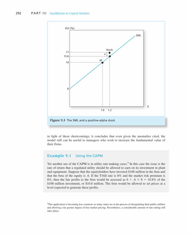
292 P A R T I I I Equilibrium in Capital Markets
in light of these shortcomings; it concludes that even given the anomalies cited, the model still can be useful to managers who wish to increase the fundamental value of their firms.
Example 9.1 Using the CAPM
Yet another use of the CAPM is in utility rate-making cases. 9 In this case the issue is the rate of return that a regulated utility should be allowed to earn on its investment in plant and equipment. Suppose that the equityholders have invested $100 million in the firm and that the beta of the equity is .6. If the T-bill rate is 6% and the market risk premium is 8%, then the fair profits to the firm would be assessed as 6 � .6 � 8 � 10.8% of the $100 million investment, or $10.8 million. The firm would be allowed to set prices at a level expected to generate these profits.
9 This application is becoming less common, as many states are in the process of deregulating their public utilities and allowing a far greater degree of free market pricing. Nevertheless, a considerable amount of rate setting still takes place.
Figure 9.3 The SML and a positive-alpha stock
E(r) (%)
SML
6
14
15.6
1.21.0
17Stock
M
α
β
C H A P T E R 9 The Capital Asset Pricing Model 293
9.2 The CAPM and the Index Model
CONCEPT CHECK
4 and 5
Stock XYZ has an expected return of 12% and risk of � � 1. Stock ABC has expected return of 13% and � � 1.5. The market’s expected return is 11%, and r f � 5%.
a. According to the CAPM, which stock is a better buy?
b. What is the alpha of each stock? Plot the SML and each stock’s risk–return point on one graph. Show the alphas graphically.
The risk-free rate is 8% and the expected return on the market portfolio is 16%. A firm con-siders a project that is expected to have a beta of 1.3.
a. What is the required rate of return on the project?
b. If the expected IRR of the project is 19%, should it be accepted?
Actual Returns versus Expected Returns
The CAPM is an elegant model. The question is whether it has real-world value—whether its implications are borne out by experience. Chapter 13 provides a range of empirical evidence on this point, but for now we focus briefly on a more basic issue: Is the CAPM testable even in principle?
For starters, one central prediction of the CAPM is that the market portfolio is a mean-variance efficient portfolio. Consider that the CAPM treats all traded risky assets. To test the efficiency of the CAPM market portfolio, we would need to construct a value-weighted portfolio of a huge size and test its efficiency. So far, this task has not been feasible. An even more difficult problem, however, is that the CAPM implies relationships among expected returns, whereas all we can observe are actual or realized holding-period returns, and these need not equal prior expectations. Even supposing we could construct a portfolio to repre-sent the CAPM market portfolio satisfactorily, how would we test its mean- variance effi-ciency? We would have to show that the reward-to-volatility ratio of the market portfolio is higher than that of any other portfolio. However, this reward-to-volatility ratio is set in terms of expectations, and we have no way to observe these expectations directly.
The problem of measuring expectations haunts us as well when we try to establish the validity of the second central set of CAPM predictions, the expected return–beta relation-ship. This relationship is also defined in terms of expected returns E ( r i ) and E ( r M ):
E(ri) 5 rf 1 bi 3E(rM ) 2 rf 4 (9.9)
The upshot is that, as elegant and insightful as the CAPM is, we must make additional assumptions to make it implementable and testable.
The Index Model and Realized Returns
We have said that the CAPM is a statement about ex ante or expected returns, whereas in practice all anyone can observe directly are ex post or realized returns. To make the leap from expected to realized returns, we can employ the index model, which we will use in excess return form as
Ri 5 ai 1 bi RM 1 ei (9.10)
294 P A R T I I I Equilibrium in Capital Markets
We saw in Chapter 8 how to apply standard regression analysis to estimate Equation 9.10 using observable realized returns over some sample period. Let us now see how this frame-work for statistically decomposing actual stock returns meshes with the CAPM.
We start by deriving the covariance between the excess returns on stock i and the market index. By definition, the firm-specific or nonsystematic component is independent of the marketwide or systematic component, that is, Cov( R M , e i ) � 0. Therefore, the covariance of the excess rate of return on security i with that of the market index is
Cov(Ri , RM ) 5 Cov(biRM 1 ei
, RM )
5 bi Cov(RM , RM ) 1 Cov(ei
, RM )
5 bi sM
2
Note that we can drop � i from the covariance terms because � i is a constant and thus has zero covariance with all variables.
Because Cov(Ri , RM ) 5 bisM
2 , the sensitivity coefficient, � i , in Equation 9.10 , which is the slope of the regression line representing the index model, equals
bi 5Cov(Ri
, RM )
sM2
The index model beta coefficient turns out to be the same beta as that of the CAPM expected return–beta relationship, except that we replace the (theoretical) market portfolio of the CAPM with the well-specified and observable market index.
The Index Model and the Expected Return–Beta Relationship
Recall that the CAPM expected return–beta relationship is, for any asset i and the (theo-retical) market portfolio,
E(ri) 2 rf 5 bi 3E(rM ) 2 rf 4 where bi 5 Cov(Ri, RM ) /sM
2 . This is a statement about the mean or expected excess returns of assets relative to the mean excess return of the (theoretical) market portfolio.
If the index M in Equation 9.10 represents the true market portfolio, we can take the expectation of each side of the equation to show that the index model specification is
E(ri) 2 rf 5 ai 1 bi 3E(rM ) 2 rf 4 A comparison of the index model relationship to the CAPM expected return–beta rela-
tionship ( Equation 9.9 ) shows that the CAPM predicts that � i should be zero for all assets. The alpha of a stock is its expected return in excess of (or below) the fair expected return as predicted by the CAPM. If the stock is fairly priced, its alpha must be zero.
We emphasize again that this is a statement about expected returns on a security. After the fact, of course, some securities will do better or worse than expected and will have returns higher or lower than predicted by the CAPM; that is, they will exhibit positive or negative alphas over a sample period. But this superior or inferior performance could not have been forecast in advance.
Therefore, if we estimate the index model for several firms, using Equation 9.10 as a regression equation, we should find that the ex post or realized alphas (the regression inter-cepts) for the firms in our sample center around zero. If the initial expectation for alpha were zero, as many firms would be expected to have a positive as a negative alpha for some sample period. The CAPM states that the expected value of alpha is zero for all securities, whereas the index model representation of the CAPM holds that the realized value of alpha

C H A P T E R 9 The Capital Asset Pricing Model 295
should average out to zero for a sample of historical observed returns. Just as important, the sample alphas should be unpredictable, that is, independent from one sample period to the next.
Indirect evidence on the efficiency of the market portfolio can be found in a study by Burton Malkiel, 10 who estimates alpha values for a large sample of equity mutual funds. The results, which appear in Figure 9.4 , show that the distribution of alphas is roughly bell shaped, with a mean that is slightly negative but statistically indistinguishable from zero. On average, it does not appear that mutual funds outperform the market index (the S&P 500) on a risk-adjusted basis. 11
This result is quite meaningful. While we might expect realized alpha values of indi-vidual securities to center around zero, professionally managed mutual funds might be expected to demonstrate average positive alphas. Funds with superior performance (and we do expect this set to be nonempty) should tilt the sample average to a positive value. The small impact of superior funds on this distribution suggests the difficulty in beating the passive strategy that the CAPM deems to be optimal.
There is yet another applicable variation on the intuition of the index model, the market
model. Formally, the market model states that the return “surprise” of any security is pro-portional to the return surprise of the market, plus a firm-specific surprise:
ri 2 E(ri) 5 bi 3rM 2 E(rM ) 4 1 ei
10 Burton G. Malkiel, “Returns from Investing in Equity Mutual Funds 1971–1991,” Journal of Finance 50 (June 1995), pp. 549–72.
11 Notice that the study included all mutual funds with at least 10 years of continuous data. This suggests the average alpha from this sample would be upward biased because funds that failed after less than 10 years were ignored and omitted from the left tail of the distribution. This survivorship bias makes the finding that the average fund underperformed the index even more telling. We discuss survivorship bias further in Chapter 11.
Figure 9.4 Estimates of individual mutual fund alphas, 1972–1991. This is a plot of the frequency distri-bution of estimated alphas for all-equity mutual funds with 10-year continuous records.
Source: Burton G. Malkiel, “Returns from Investing in Equity Mutual Funds 1971–1991,” Journal of Finance 50 (June 1995), pp. 549–72. Reprinted by permission of the publisher, Blackwell Publishing, Inc.
Alpha (%)
Freq
uen
cy
36
32
28
24
16
20
12
8
4
0−3 −2 −1 0 1 2

296 P A R T I I I Equilibrium in Capital Markets
This equation divides returns into firm-specific and systematic components somewhat differently from the index model. If the CAPM is valid, however, you can confirm that, substituting for E ( r i ) from Equation 9.9 , the market model equation becomes identical to the index model. For this reason the terms “index model” and “market model” often are used interchangeably.
9.3 Is the CAPM Practical?
To discuss the role of the CAPM in real-life investments we have to answer two questions. First, even if we all agreed that the CAPM were the best available theoretical model to explain rates of return on risky assets, how would this affect practical investment policy? Second, how can we determine whether the CAPM is in fact the best available model to explain rates of return on risky assets?
Notice the wording of the first question. We don’t pose it as: “Suppose the CAPM per-fectly explains the rates of return on risky assets. . . .” All models, whether in economics or science, are based on simplifications that enable us to come to grips with a complicated reality, which means that perfection is an unreasonable and unusable standard. In our con-text, we must clarify what “perfectly explains” would mean. From the previous section we know that if the CAPM were valid, a single-index model in which the index includes all traded securities (i.e., all risky securities in the investable universe as in Assumption 3) also would be valid. In this case, “perfectly explains” would mean that all alpha values in security risk premiums would be identically zero.
The notion that all alpha values can be identically zero is feasible in principle, but such a configuration cannot be expected to emerge in real markets. This was demonstrated by Grossman and Stiglitz, who showed that such an equilibrium may be one that the real economy can approach, but not necessarily reach. 12 Their basic idea is that the actions of security analysts are the forces that drive security prices to “proper” levels at which alpha is zero. But if all alphas were identically zero, there would be no incentive to engage in such security analysis. Instead, the market equilibrium will be characterized by prices hov-ering “near” their proper values, at which alphas are almost zero, but with enough slippage (and therefore reward for superior insight) to induce analysts to continue their efforts.
A more reasonable standard, that the CAPM is the “best available model to explain rates of return on risky assets,” means that in the absence of security analysis, one should take security alphas as zero. A security is mispriced if and only if its alpha is nonzero— underpriced if alpha is positive and overpriced if alpha is negative—and positive or negative alphas are revealed only by superior security analysis. Absent the investment of significant
12 Sanford J. Grossman and Joseph E. Stiglitz, “On the Impossibility of Informationally Efficient Markets,” American Economic Review 70 (June 1981).
CONCEPT CHECK
6
Can you sort out the nuances of the following maze of models?
a. CAPM
b. Single-factor model
c. Single-index model
d. Market model

C H A P T E R 9 The Capital Asset Pricing Model 297
resources in such analysis, an investor would obtain the best investment portfolio on the assumption that all alpha values are zero. This definition of the superiority of the CAPM over any other model also determines its role in real-life investments.
Under the assumption that the CAPM is the best available model, investors willing to expend resources to construct a superior portfolio must (1) identify a practical index to work with and (2) deploy macro analysis to obtain good forecasts for the index and secu-rity analysis to identify mispriced securities. This procedure was described in Chapter 8 and is further elaborated on in Part Five (Security Analysis) and Part Seven (Applied Portfolio Management).
We will examine several tests of the CAPM in Chapter 13. But it is important to explain the results of these tests and their implications.
Is the CAPM Testable?
Let us consider for a moment what testability means. A model consists of (i) a set of assumptions, (ii) logical/mathematical development of the model through manipulation of those assumptions, and (iii) a set of predictions. Assuming the logical/mathematical manipulations are free of errors, we can test a model in two ways, normative and positive. Normative tests examine the assumptions of the model, while positive tests examine the predictions.
If a model’s assumptions are valid, and the development is error-free, then the pre-dictions of the model must be true. In this case, testing the assumptions is synonymous with testing the model. But few, if any, models can pass the normative test. In most cases, as with the CAPM, the assumptions are admittedly invalid—we recognize that we have simplified reality, and therefore to this extent are relying on “untrue” assumptions. The motivation for invoking unrealistic assumptions is clear; we simply cannot solve a model that is perfectly consistent with the full complexity of real-life markets. As we’ve noted, the need to use simplifying assumptions is not peculiar to economics—it characterizes all of science.
Assumptions are chosen first and foremost to render the model solvable. But we prefer assumptions to which the model is “robust.” A model is robust with respect to an assump-tion if its predictions are not highly sensitive to violation of the assumption. If we use only assumptions to which the model is robust, the model’s predictions will be reason-ably accurate despite its shortcomings. The upshot of all this is that tests of models are almost always positive—we judge a model on the success of its empirical predictions. This standard brings statistics into any science and requires us to take a stand on what are acceptable levels of significance and power. 13 Because the nonrealism of the assumptions
13 To illustrate the meanings of significance and power, consider a test of the efficacy of a new drug. The agency testing the drug may make two possible errors. The drug may be useless (or even harmful), but the agency may conclude that it is useful. This is called a “Type I” error. The significance level of a test is the probability of a Type I error. Typical practice is to fix the level of significance at some low level, for example, 5%. In the case of drug testing, for example, the first goal is to avoid introducing ineffective or harmful treatments. The other possible error is that the drug is actually useful, but the testing procedure concludes it is not. This mistake, called “Type II” error, would lead us to discard a useful treatment. The power of the test is the probability of avoiding Type II error (i.e., one minus the probability of making such an error), that is, the probability of accepting the drug if it is indeed useful. We want tests that, at a given level of significance, have the most power, so we will admit effec-tive drugs with high probability. In social sciences in particular, available tests often have low power, in which case they are susceptible to Type II error and will reject a correct model (a “useful drug”) with high frequency. “The drug is useful” is analogous in the CAPM to alphas being zero. When the test data reject the hypothesis that observed alphas are zero at the desired level of significance, the CAPM fails. However, if the test has low power, the probability that we accept the model when true is not all that high.

298 P A R T I I I Equilibrium in Capital Markets
precludes a normative test, the positive test is really a test of the robustness of the model to its assumptions.
The CAPM implications are embedded in two predictions: (1) the market portfolio is efficient, and (2) the security market line (the expected return–beta relationship) accu-rately describes the risk–return trade-off, that is, alpha values are zero. In fact, the second implication can be derived from the first, and therefore both stand or fall together in a test that the market portfolio is mean-variance efficient. The central problem in testing this pre-diction is that the hypothesized market portfolio is unobservable. The “market portfolio” includes all risky assets that can be held by investors. This is far more extensive than an equity index. It would include bonds, real estate, foreign assets, privately held businesses, and human capital. These assets are often traded thinly or (for example, in the case of human capital) not traded at all. It is difficult to test the efficiency of an observable port-folio, let alone an unobservable one. These problems alone make adequate testing of the model infeasible. 14 Moreover, even small departures from efficiency in the market port-folio can lead to large departures from the expected return–beta relationship of the SML, which would negate the practical usefulness of the model.
The CAPM Fails Empirical Tests
Because the market portfolio cannot be observed, tests of the CAPM revolve around the expected return–beta relationship. The tests use proxies such as the S&P 500 index to stand in for the true market portfolio. These tests therefore appeal to robustness of the assump-tion that the market proxy is sufficiently close to the true, unobservable market portfolio. The CAPM fails these tests, that is, the data reject the hypothesis that alpha values are uniformly zero at acceptable levels of significance. For example, we find that, on average, low-beta securities have positive alphas and high-beta securities have negative alphas.
It is possible that this is a result of a failure of our data, the validity of the market proxy, or statistical method. If so, we would conclude the following: There is no better model out there, but we measure beta and alpha values with unsatisfactory precision. This situation would call for improved technique. But if the rejection of the model is not an artifact of sta-tistical problems, then we must search for extensions to the CAPM, or substitute models. We will consider several extensions of the model later in the chapter.
The Economy and the Validity of the CAPM
For better or worse, some industries are regulated, with rate commissions either setting or approving prices. Imagine a commission pondering a rate case for a regulated utility. The rate commission must decide whether the rates charged by the company are sufficient to grant shareholders a fair rate of return on their investments. The normative framework of the typical rate hearing is that shareholders, who have made an investment in the firm, are entitled to earn a “fair” rate of return on their equity investment. The firm is therefore allowed to charge prices that are expected to generate a profit consistent with that fair rate of return.
The question of fairness of the rate of return to the company shareholders cannot be divorced from the level of risk of these returns. The CAPM provides the commission a
14 The best-known discussion of the difficulty in testing the CAPM is now called “Roll’s critique.” See Richard Roll, “A Critique of the Asset Pricing Theory’s Tests: Part I: On Past and Potential Testability of the Theory,” Journal of Financial Economics 4 (1977). The issue is developed further in Richard Roll and Stephen A. Ross, “On the Cross-Sectional Relation between Expected Return and Betas,” Journal of Finance 50 (1995); and Schmuel Kandel and Robert F. Stambaugh, “Portfolio Inefficiency and the Cross-Section of Expected Returns,” Journal of Finance 50 (1995).

C H A P T E R 9 The Capital Asset Pricing Model 299
clear criterion: If the rates under current regulation are too low, then the rate of return to equity investors would be less than commensurate with risk, and alpha would be negative. As we pointed out in Example 9.1 , the commissioner’s problem may now be organized around arguments about estimates of risk and the security market line.
Similar applications arise in many legal settings. For example, contracts with payoffs that are contingent on a fair rate of return can be based on the index rate of return and the beta of appropriate assets. Many disputes involving damages require that a stream of losses be discounted to a present value. The proper discount rate depends on risk, and disputes about fair compensation to litigants can be (and often are) set on the basis of the SML, using past data that differentiate systematic from firm-specific risk.
It may be surprising to find that the CAPM is an accepted norm in the U.S. and many other developed countries, despite its empirical shortcomings. We can offer a twofold explanation. First, the logic of the decomposition to systematic and firm-specific risk is compelling. Absent a better model to assess nonmarket components of risk premiums, we must use the best method available. As improved methods of generating equilibrium security returns become empirically validated, they gradually will be incorporated into institutional decision making. Such improvements may come either from extensions of the CAPM and its companion, arbitrage pricing theory (discussed in the next chapter), or from a yet-undiscovered new model.
Second, there is impressive, albeit less-formal, evidence that the central conclusion of the CAPM—the efficiency of the market portfolio—may not be all that far from being valid. Thousands of mutual funds within hundreds of investment companies compete for investor money. These mutual funds employ professional analysts and portfolio manag-ers and expend considerable resources to construct superior portfolios. But the number of funds that consistently outperform a simple strategy of investing in passive market index portfolios is extremely small, suggesting that the single-index model with ex ante zero alpha values may be a reasonable working approximation for most investors.
The Investments Industry and the Validity of the CAPM
More than other practitioners, investment firms must take a stand on the validity of the CAPM. If they judge the CAPM invalid, they must turn to a substitute framework to guide them in constructing optimal portfolios.
For example, the CAPM provides discount rates that help security analysts assess the intrinsic value of a firm. If an analyst believes that some actual prices differ from intrin-sic values, then those securities have nonzero alphas, and there is an opportunity to con-struct an active portfolio with a superior risk–return profile. But if the discount rate used to assess intrinsic value is incorrect because of a failure in the CAPM, the estimate of alpha will be biased, and both the Markowitz model of Chapter 7 and the index model of Chapter 8 will actually lead to inferior portfolios. When constructing their presumed optimal risky portfolios, practitioners must be satisfied that the passive index they use for that purpose is satisfactory and that the ratios of alpha to residual variance are appropri-ate measures of investment attractiveness. This would not be the case if the CAPM is invalid. Yet it appears many practitioners do use index models (albeit often with additional indexes) when assessing security prices. The curriculum of the CFA Institute also suggests a widespread acceptance of the CAPM, at least as a starting point for thinking about the risk–return relationship. An explanation similar to the one we offered in the previous sub-section is equally valid here.
The central conclusion from our discussion so far is that, explicitly or implicitly, prac-titioners do use a CAPM. If they use a single-index model and derive optimal portfolios
300 P A R T I I I Equilibrium in Capital Markets
from ratios of alpha forecasts to residual variance, they behave as if the CAPM is valid. 15 If they use a multi-index model, then they use one of the extensions of the CAPM (discussed later in this chapter) or arbitrage pricing theory (discussed in the next chapter). Thus, the-ory and evidence on the CAPM should be of interest to all sophisticated practitioners.
9.4 Econometrics and the Expected Return–Beta Relationship
When assessing the empirical success of the CAPM, we must also consider our econo-metric technique. If our tests are poorly designed, we may mistakenly reject the model. Similarly, some empirical tests implicitly introduce additional assumptions that are not part of the CAPM, for example, that various parameters of the model such as beta or residual variance are constant over time. If these extraneous additional assumptions are too restrictive, we also may mistakenly reject the model.
To begin, notice that all the coefficients of a regression equation are estimated simulta-neously, and these estimates are not independent. In particular, the estimate of the intercept (alpha) of a single- (independent) variable regression depends on the estimate of the slope coefficient. Hence, if the beta estimate is inefficient and/or biased, so will be the estimate of the intercept. Unfortunately, statistical bias is easily introduced.
An example of this hazard was pointed out in an early paper by Miller and Scholes, 16 who demonstrated how econometric problems could lead one to reject the CAPM even if it were perfectly valid. They considered a checklist of difficulties encountered in testing the model and showed how these problems potentially could bias conclusions. To prove the point, they simulated rates of return that were constructed to satisfy the predictions of the CAPM and used these rates to “test” the model with standard statistical techniques of the day. The result of these tests was a rejection of the model that looks surprisingly similar to what we find in tests of returns from actual data—this despite the fact that the “data” were constructed to satisfy the CAPM. Miller and Scholes thus demonstrated that econometric technique alone could be responsible for the rejection of the model in actual tests.
There are several potential problems with the estimation of beta coefficients. First, when residuals are correlated (as is common for firms in the same industry), standard beta esti-mates are not efficient. A simple approach to this problem would be to use statistical tech-niques designed for these complications. For example, we might replace OLS (ordinary least squares) regressions with GLS (generalized least squares) regressions, which account for correlation across residuals. Moreover, both coefficients, alpha and beta, as well as residual variance, are likely time varying. There is nothing in the CAPM that precludes such time variation, but standard regression techniques rule it out and thus may lead to false rejection of the model. There are now well-known techniques to account for time-varying parameters. In fact, Robert Engle won the Nobel Prize for his pioneering work on econometric techniques to deal with time-varying volatility, and a good portion of
15 We need to be a bit careful here. On its face, the CAPM asserts that alpha values will equal zero in security mar-ket equilibrium. But as we argued earlier, consistent with the vast amount of security analysis that actually takes place, a better way to interpret the CAPM is that equilibrium really means that alphas should be taken to be zero in the absence of security analysis. With private information or superior insight one presumably would be able to identify stocks that are mispriced by the market and thus offer nonzero alphas.
16 Merton H. Miller and Myron Scholes, “Rates of Return in Relations to Risk: A Re-examination of Some Recent Findings,” in Studies in the Theory of Capital Markets, Michael C. Jensen, ed. (New York: Praeger, 1972).
C H A P T E R 9 The Capital Asset Pricing Model 301
the applications of these new techniques have been in finance. 17 Moreover, betas may vary not purely randomly over time, but in response to changing economic conditions. A “conditional” CAPM allows risk and return to change with a set of “conditioning variables.” 18
As importantly, Campbell and Vuolteenaho 19 find that the beta of a security can be decomposed into two components, one of which measures sensitivity to changes in cor-porate profitability and another which measures sensitivity to changes in the market’s dis-count rates. These are found to be quite different in many cases. Improved econometric techniques such as those proposed in this short survey may help resolve part of the empiri-cal failure of the simple CAPM.
9.5 Extensions of the CAPM
The CAPM uses a number of simplifying assumptions. We can gain greater predictive accuracy at the expense of greater complexity by relaxing some of those assumptions. In this section, we will consider a few of the more important attempts to extend the model. This discussion is not meant to be exhaustive. Rather, it introduces a few extensions of the basic model to provide insight into the various attempts to improve empirical content.
The Zero-Beta Model
Efficient frontier portfolios have a number of interesting characteristics, independently derived by Merton and Roll. 20 Three of these are
1. Any portfolio that is a combination of two frontier portfolios is itself on the effi-cient frontier.
2. The expected return of any asset can be expressed as an exact linear function of the expected return on any two efficient-frontier portfolios P and Q according to the following equation:
E(ri) 2 E(rQ ) 5 3E(rP) 2 E(rQ )4Cov(ri , rP) 2 Cov(rP
, rQ )
sP2 2 Cov(rP
, rQ ) (9.11)
3. Every portfolio on the efficient frontier, except for the global minimum-variance portfolio, has a “companion” portfolio on the bottom (inefficient) half of the fron-tier with which it is uncorrelated. Because it is uncorrelated, the companion portfo-lio is referred to as the zero-beta portfolio of the efficient portfolio. If we choose the market portfolio M and its zero-beta companion portfolio Z, then Equation 9.11 simplifies to the CAPM-like equation
E(ri) 2 E(rZ ) 5 3E(RM ) 2 E(RZ )4Cov(ri , rM )
sM2
5 bi 3E(rM ) 2 E(rZ )4 (9.12)
17 Engle’s work gave rise to the widespread use of so-called ARCH models. ARCH stands for autoregressive con-ditional heteroskedasticity, which is a fancy way of saying that volatility changes over time, and that recent levels of volatility can be used to form optimal estimates of future volatility.
18 There is now a large literature on conditional models of security market equilibrium. Much of it derives from Ravi Jagannathan and Zhenyu Wang, “The Conditional CAPM and the Cross-Section of Expected Returns,” Journal of Finance 51 (March 1996), pp. 3–53.
19 John Campbell and Tuomo Vuolteenaho, “Bad Beta, Good Beta,” American Economic Review 94 (December 2004), pp. 1249–75.
20 Robert C. Merton, “An Analytic Derivation of the Efficient Portfolio Frontier,” Journal of Financial and
Quantitative Analysis, 1972. Roll, see footnote 14.

302 P A R T I I I Equilibrium in Capital Markets
Equation 9.12 resembles the SML of the CAPM, except that the risk-free rate is replaced with the expected return on the zero-beta companion of the market index portfolio.
Fischer Black used these properties to show that Equation 9.12 is the CAPM equation that results when investors face restrictions on borrowing and/or investment in the risk-free asset. 21 In this case, at least some investors will choose portfolios on the efficient frontier that are not necessarily the market index portfolio. Because average returns on the zero-beta portfolio are greater than observed T-bill rates, the zero-beta model can explain why average estimates of alpha values are positive for low-beta securities and negative for high-beta securities, contrary to the prediction of the CAPM. Despite this, the model is not sufficient to rescue the CAPM from empirical rejection.
Labor Income and Nontraded Assets
An important departure from realism is the CAPM assumption that all risky assets are traded. Two important asset classes that are not traded are human capital and privately held businesses. The discounted value of future labor income exceeds the total market value of traded assets. The market value of privately held corporations and businesses is of the same order of magnitude. Human capital and private enterprises are different types of assets with possibly different implications for equilibrium returns on traded securities.
Privately held business may be the lesser of the two sources of departures from the CAPM. Nontraded firms can be incorporated or sold at will, save for liquidity consid-erations that we discuss in the next section. Owners of private business also can borrow against their value, further diminishing the material difference between ownership of pri-vate and public business. Suppose that privately held business have risk characteristics similar to those of traded assets. In this case, individuals can partially offset the diversifi-cation problems posed by their nontraded entrepreneurial assets by reducing their portfo-lio demand for securities of similar, traded assets. Thus, the CAPM expected return–beta equation may not be greatly disrupted by the presence of entrepreneurial income.
To the extent that risk characteristics of private enterprises differ from those of traded securities, a portfolio of traded assets that best hedges the risk of typical private busi-ness would enjoy excess demand from the population of private business owners. The price of assets in this portfolio will be bid up relative to the CAPM considerations, and the expected returns on these securities will be lower in relation to their systematic risk. Conversely, securities highly correlated with such risk will have high equilibrium risk pre-miums and may appear to exhibit positive alphas relative to the conventional SML. In fact, Heaton and Lucas show that adding proprietary income to a standard asset-pricing model improves its predictive performance. 22
The size of labor income and its special nature is of greater concern for the validity of the CAPM. The possible effect of labor income on equilibrium returns can be appreci-ated from its important effect on personal portfolio choice. Despite the fact that an indi-vidual can borrow against labor income (via a home mortgage) and reduce some of the uncertainty about future labor income via life insurance, human capital is less “portable” across time and may be more difficult to hedge using traded securities than nontraded busi-ness. This may induce pressure on security prices and result in departures from the CAPM
21 Fischer Black, “Capital Market Equilibrium with Restricted Borrowing,” Journal of Business, July 1972.
22 John Heaton and Deborah Lucas, “Portfolio Choice and Asset Prices: The Importance of Entrepreneurial Risk, Journal of Finance 55 (June 2000). This paper offers evidence of the effect of entrepreneurial risk on both port-folio choice and the risk–return relationship.
C H A P T E R 9 The Capital Asset Pricing Model 303
expected return–beta equation. For one example, surely an individual seeking diversifi-cation should avoid investing in his employer’s stock and limit investments in the same industry. Thus, the demand for stocks of labor-intensive firms may be reduced, and these stocks may require a higher expected return than predicted by the CAPM.
Mayers 23 derives the equilibrium expected return–beta equation for an economy in which individuals are endowed with labor income of varying size relative to their nonlabor capital. The resultant SML equation is
E(Ri) 5 E(RM )
Cov(Ri , RM ) 1
PH
PM
Cov(Ri , RH )
sM2 1
PH
PM
Cov(RM , RH )
(9.13)
where P H � value of aggregate human capital
P M � market value of traded assets (market portfolio)
R H � excess rate of return on aggregate human capital
The CAPM measure of systematic risk, beta, is replaced in the extended model by an adjusted beta that also accounts for covariance with the portfolio of aggregate human capi-tal. Notice that the ratio of human capital to market value of all traded assets, P H / P M , may well be greater than 1, and hence the effect of the covariance of a security with labor income, Cov( R i , R H ), relative to the average, Cov( R M , R H ), is likely to be economically significant. When Cov( R i , R H ) is positive, the adjusted beta is greater when the CAPM beta is smaller than 1, and vice versa. Because we expect Cov( R i , R H ) to be positive for the average security, the risk premium in this model will be greater, on average, than pre-dicted by the CAPM for securities with beta less than 1, and smaller for securities with beta greater than 1. The model thus predicts a security market line that is less steep than that of the standard CAPM. This may help explain the average negative alpha of high-beta securities and positive alpha of low-beta securities that lead to the statistical failure of the CAPM equation. In Chapter 13 on empirical evidence we present additional results along these lines.
A Multiperiod Model and Hedge Portfolios
Robert C. Merton revolutionized financial economics by using continuous-time models to extend many of our models of asset pricing. 24 While his (Nobel Prize–winning) contribu-tions to option-pricing theory and financial engineering (along with those of Fischer Black and Myron Scholes) may have had greater impact on the investment industry, his solo con-tribution to portfolio theory was equally important for our understanding of the risk–return relationship.
In his basic model, Merton relaxes the “single-period” myopic assumptions about inves-tors. He envisions individuals who optimize a lifetime consumption/investment plan, and who continually adapt consumption/investment decisions to current wealth and planned retirement age. When uncertainty about portfolio returns is the only source of risk and investment opportunities remain unchanged through time, that is, there is no change in the probability distribution of the return on the market portfolio or individual securities,
23 See footnote 8.
24 Merton’s classic works are collected in Continuous-Time Finance (Oxford, U.K.: Basil Blackwell, 1992).
304 P A R T I I I Equilibrium in Capital Markets
Merton’s so-called intertemporal capital asset pricing model (ICAPM) predicts the same expected return–beta relationship as the single-period equation. 25
But the situation changes when we include additional sources of risk. These extra risks are of two general kinds. One concerns changes in the parameters describing investment opportunities, such as future risk-free rates, expected returns, or the risk of the market port-folio. For example, suppose that the real interest rate may change over time. If it falls in some future period, one’s level of wealth will now support a lower stream of real consump-tion. Future spending plans, for example, for retirement spending, may be put in jeopardy. To the extent that returns on some securities are correlated with changes in the risk-free rate, a portfolio can be formed to hedge such risk, and investors will bid up the price (and bid down the expected return) of those hedge assets. Investors will sacrifice some expected return if they can find assets whose returns will be higher when other parameters (in this case, the real risk-free rate) change adversely.
The other additional source of risk concerns the prices of the consumption goods that can be purchased with any amount of wealth. Consider as an example inflation risk. In addition to the expected level and volatility of their nominal wealth, investors must be concerned about the cost of living—what those dollars can buy. Therefore, inflation risk is an important extramarket source of risk, and investors may be willing to sacrifice some expected return to purchase securities whose returns will be higher when the cost of living changes adversely. If so, hedging demands for securities that help to protect against infla-tion risk would affect portfolio choice and thus expected return. One can push this con-clusion even further, arguing that empirically significant hedging demands may arise for important subsectors of consumer expenditures; for example, investors may bid up share prices of energy companies that will hedge energy price uncertainty. These sorts of effects may characterize any assets that hedge important extramarket sources of risk.
More generally, suppose we can identify K sources of extramarket risk and find K asso-ciated hedge portfolios. Then, Merton’s ICAPM expected return–beta equation would gen-eralize the SML to a multi-index version:
E(Ri) 5 biME(RM ) 1 aK
k51
bikE(Rk) (9.14)
where � iM is the familiar security beta on the market-index portfolio, and � ik is the beta on the k th hedge portfolio.
Other multifactor models using additional factors that do not arise from extramarket sources of risk have been developed and lead to SMLs of a form identical to that of the ICAPM. These models also may be considered extensions of the CAPM in the broad sense. We examine these models in the next chapter.
A Consumption-Based CAPM
The logic of the CAPM together with the hedging demands noted in the previous subsec-tion suggests that it might be useful to center the model directly on consumption. Such models were first proposed by Mark Rubinstein, Robert Lucas, and Douglas Breeden. 26
25 Eugene F. Fama also made this point in “Multiperiod Consumption-Investment Decisions,” American Economic
Review 60 (1970).
26 Mark Rubinstein, “The Valuation of Uncertain Income Streams and the Pricing of Options,” Bell Journal
of Economics and Management Science 7 (1976), pp. 407–25; Robert Lucas, “Asset Prices in an Exchange Economy,” Econometrica 46 (1978), pp. 1429–45; Douglas Breeden, “An Intertemporal Asset Pricing Model with Stochastic Consumption and Investment Opportunities,” Journal of Financial Economics 7 (1979), pp. 265–96.

C H A P T E R 9 The Capital Asset Pricing Model 305
In a lifetime consumption plan, the investor must in each period balance the allocation of current wealth between today’s consumption and the savings and investment that will support future consumption. When optimized, the utility value from an additional dollar of consumption today must be equal to the utility value of the expected future consump-tion that can be financed by that additional dollar of wealth. 27 Future wealth will grow from labor income, as well as returns on that dollar when invested in the optimal complete portfolio.
Suppose risky assets are available and you wish to increase expected consumption growth by allocating some of your savings to a risky portfolio. How would we measure the risk of these assets? As a general rule, investors will value additional income more highly during difficult economic times (when consumption opportunities are scarce) than in afflu-ent times (when consumption is already abundant). An asset will therefore be viewed as riskier in terms of consumption if it has positive covariance with consumption growth—in other words, if its payoff is higher when consumption is already high and lower when con-sumption is relatively restricted. Therefore, equilibrium risk premiums will be greater for assets that exhibit higher covariance with consumption growth. Developing this insight, we can write the risk premium on an asset as a function of its “consumption risk” as follows:
E(Ri) 5 biCRPC (9.15)
where portfolio C may be interpreted as a consumption-tracking portfolio (also called a consumption-mimicking portfolio ), that is, the portfolio with the highest correlation with consumption growth; � iC is the slope coefficient in the regression of asset i ’s excess returns, R i , on those of the consumption-tracking portfolio; and, finally, RP C is the risk premium associated with consumption uncertainty, which is measured by the expected excess return on the consumption-tracking portfolio:
RPC 5 E(RC ) 5 E(rC ) 2 rf (9.16)
Notice how similar this conclusion is to the conventional CAPM. The consumption-tracking portfolio in the CCAPM plays the role of the market portfolio in the conven-tional CAPM. This is in accord with its focus on the risk of consumption opportunities rather than the risk and return of the dollar value of the portfolio. The excess return on the consumption-tracking portfolio plays the role of the excess return on the market portfolio, M. Both approaches result in linear, single-factor models that differ mainly in the identity of the factor they use.
In contrast to the CAPM, the beta of the market portfolio on the market factor of the CCAPM is not necessarily 1. It is perfectly plausible and empirically evident that this beta is substantially greater than 1. This means that in the linear relationship between the mar-ket index risk premium and that of the consumption portfolio,
E(RM ) 5 aM 1 bMC E(RC ) 1 eM (9.17)
where � M and M allow for empirical deviation from the exact model in Equation 9.15 , and � MC is not necessarily equal to 1.
Because the CCAPM is so similar to the CAPM, one might wonder about its usefulness. Indeed, just as the CAPM is empirically flawed because not all assets are traded, so is the
27 Wealth at each point in time equals the market value of assets in the balance sheet plus the present value of future labor income. These models of consumption and investment decisions are often made tractable by assum-ing investors exhibit constant relative risk aversion, or CRRA. CRRA implies that an individual invests a constant proportion of wealth in the optimal risky portfolio regardless of the level of wealth. You might recall that our prescription for optimal capital allocation in Chapter 6 also called for an optimal investment proportion in the risky portfolio regardless of the level of wealth. The utility function we employed there also exhibited CRRA.
306 P A R T I I I Equilibrium in Capital Markets
CCAPM. The attractiveness of this model is in that it compactly incorporates consump-tion hedging and possible changes in investment opportunities, that is, in the parameters of the return distributions in a single-factor framework. There is a price to pay for this compactness, however. Consumption growth figures are published infrequently (monthly at the most) compared with financial assets, and are measured with significant error. Nevertheless, recent empirical research 28 indicates that this model is more successful in explaining realized returns than the CAPM, which is a reason why students of investments should be familiar with it. We return to this issue, as well as empirical evidence concerning the CCAPM, in Chapter 13.
9.6 Liquidity and the CAPM
Standard models of asset pricing (such as the CAPM) assume frictionless markets, mean-ing that securities can be traded costlessly. But these models actually have little to say about trading activity. For example, in the equilibrium of the CAPM, all investors share all available information and demand identical portfolios of risky assets. The awkward impli-cation of this result is that there is no reason for trade. If all investors hold identical port-folios of risky assets, then when new (unexpected) information arrives, prices will change commensurately, but each investor will continue to hold a piece of the market portfolio, which requires no exchange of assets. How do we square this implication with the observa-tion that on a typical day, several billion shares may change hands on the New York Stock Exchange alone? One obvious answer is heterogeneous expectations, that is, beliefs not shared by the entire market. Such private information will give rise to trading as investors attempt to profit by rearranging portfolios in accordance with their now-heterogeneous demands. In reality, trading (and trading costs) will be of great importance to investors.
The liquidity of an asset is the ease and speed with which it can be sold at fair market value. Part of liquidity is the cost of engaging in a transaction, particularly the bid–ask spread. Another part is price impact—the adverse movement in price one would encoun-ter when attempting to execute a larger trade. Yet another component is immediacy—the ability to sell the asset quickly without reverting to fire-sale prices. Conversely, illiquidity can be measured in part by the discount from fair market value a seller must accept if the asset is to be sold quickly. A perfectly liquid asset is one that would entail no illiquidity discount.
Liquidity (or the lack of it) has long been recognized as an important characteristic that affects asset values. For example, in legal cases, courts have routinely applied very steep discounts to the values of businesses that cannot be publicly traded. But liquidity has not always been appreciated as an important factor in security markets, presumably due to the relatively small trading cost per transaction compared with the large costs of trading assets such as real estate. The breakthrough came in the work of Amihud and Mendelson 29 and today, liquidity is increasingly viewed as an important determinant of prices and expected returns. We supply only a brief synopsis of this important topic here and provide empirical evidence in Chapter 13.
28 Ravi Jagannathan and Yong Wang, “Lazy Investors, Discretionary Consumption, and the Cross-Section of Stock Returns,” Journal of Finance 62 (August 2007), pp. 1633–61.
29 Yakov Amihud and Haim Mendelson, “Asset Pricing and the Bid–Ask Spread,” Journal of Financial Economics 17(1986). A summary of the ensuing large body of literature on liquidity can be found in Yakov Amihud, Haim Mendelson, and Lasse Heje Pedersen, “Liquidity and Asset Prices,” Foundations and Trends in Finance 1, no. 4 (2005).

C H A P T E R 9 The Capital Asset Pricing Model 307
Early models of liquidity focused on the inventory management problem faced by secu-rity dealers. Dealers in over-the-counter markets post prices at which they are willing to buy a security (the bid price) or sell it (the ask price). The willingness of security dealers to add to their inventory or sell shares from their inventory makes them crucial contribu-tors to overall market liquidity. The fee they earn for supplying this liquidity is the bid–ask spread. Part of the bid–ask spread may be viewed as compensation for bearing the price risk involved in holding an inventory of securities and allowing their inventory levels to absorb the fluctuations in overall security demand. Assuming the fair price of the stock is the average of the bid and ask prices, an investor pays half the spread upon purchase and the other half upon sale of the stock. A dealer on the other side of the transaction earns these spreads. The spread is one important component of liquidity—it is the cost of trans-acting in a security.
The advent of electronic trading has steadily diminished the role of dealers, but traders still must contend with a bid–ask spread. For example, in electronic markets, the limit-order book contains the “inside spread,” that is, the difference between the highest price at which some investor will purchase any shares and the lowest price at which another investor is willing to sell. The effective bid–ask spread will also depend on the size of the desired transaction. Larger purchases will require a trader to move deeper into the limit-order book and accept less-attractive prices. While inside spreads on electronic mar-kets often appear extremely low, effective spreads can be much larger, because most limit orders are good for only small numbers of shares.
Even without the inventory problems faced by traditional securities dealers, the bid–ask spread persists. There is greater emphasis today on the component of the spread due to asymmetric information. By asymmetric information, we mean the potential for one trader to have private information about the value of the security that is not known to the trading partner. To see why such an asymmetry can affect the market, think about the problems facing someone buying a used car. The seller knows more about the car than the buyer, so the buyer naturally wonders if the seller is trying to get rid of the car because it is a “lemon.” At the least, buyers worried about overpaying will shave the prices they are will-ing to pay for a car of uncertain quality. In extreme cases of asymmetric information, trad-ing may cease altogether. 30 Similarly, traders who post offers to buy or sell at limit prices need to be worried about being picked off by better-informed traders who hit their limit prices only when they are out of line with the intrinsic value of the firm.
Broadly speaking, we may envision investors trading securities for two reasons. Some trades are driven by “noninformational” motives, for example, selling assets to raise cash for a big purchase, or even just for portfolio rebalancing. These sorts of trades, which are not motivated by private information that bears on the value of the traded security, are called noise trades. Security dealers will earn a profit from the bid–ask spread when trans-acting with noise traders (also called liquidity traders because their trades may derive from needs for liquidity, i.e., cash).
Other transactions are motivated by private information known only to the seller or buyer. These transactions are generated when traders believe they have come across infor-mation that a security is mispriced, and try to profit from that analysis. If an information trader identifies an advantageous opportunity, it must be disadvantageous to the other party in the transaction. If private information indicates a stock is overpriced, and the trader
30 The problem of informational asymmetry in markets was introduced by the 2001 Nobel laureate George A. Akerlof and has since become known as the lemons problem. A good introduction to Akerlof’s contribu-tions can be found in George A. Akerlof, An Economic Theorist’s Book of Tales (Cambridge, U.K.: Cambridge University Press, 1984).

308 P A R T I I I Equilibrium in Capital Markets
decides to sell it, a dealer who has posted a bid price or another trader who has posted a limit-buy order and ends up on the other side of the transaction will purchase the stock at what will later be revealed to have been an inflated price. Conversely, when private infor-mation results in a decision to buy, the price at which the security is traded will eventually be recognized as less than fair value.
Information traders impose a cost on both dealers and other investors who post limit orders. Although on average dealers make money from the bid–ask spread when transact-ing with liquidity traders, they will absorb losses from information traders. Similarly, any trader posting a limit order is at risk from information traders. The response is to increase limit-ask prices and decrease limit-bid orders—in other words, the spread must widen. The greater the relative importance of information traders, the greater the required spread to compensate for the potential losses from trading with them. In the end, therefore, liquidity traders absorb most of the cost of the information trades because the bid–ask spread that they must pay on their “innocent” trades widens when informational asymmetry is more severe.
The discount in a security price that results from illiquidity can be surprisingly large, far larger than the bid–ask spread. Consider a security with a bid–ask spread of 1%. Suppose it will change hands once a year for the next 3 years and then will be held forever by the third buyer. For the last trade, the investor will pay for the security 99.5% or .995 of its fair price; the price is reduced by half the spread that will be incurred when the stock is sold. The second buyer, knowing the security will be sold a year later for .995 of fair value, and having to absorb half the spread upon purchase, will be willing to pay .995 � .005/1.05 � .9902 (i.e., 99.02% of fair value), if the spread from fair value is dis-counted at a rate of 5%. Finally, the current buyer, knowing the loss next year, when the stock will be sold for .9902 of fair value (a discount of .0098), will pay for the security only .995 � .0098/1.05 � .9857. Thus the discount has ballooned from .5% to 1.43%. In other words, the present values of all three future trading costs (spreads) are discounted into the current price. 31 To extend this logic, if the security will be traded once a year forever, its current illiquidity cost will equal immediate cost plus the present value of a perpetuity of .5%. At an annual discount rate of 5%, this sum equals .005 � .005/.05 � .105, or 10.5%! Obviously, liquidity is of potentially large value and should not be ignored in deriving the equilibrium value of securities.
As trading costs are higher, the illiquidity discount will be greater. Of course, if some-one can buy a share at a lower price, the expected rate of return will be higher. Therefore, we should expect to see less-liquid securities offer higher average rates of return. But this illiquidity premium need not rise in direct proportion to trading cost. If an asset is less liquid, it will be shunned by frequent traders and held instead by longer term traders who are less affected by high trading costs. Hence in equilibrium, investors with long holding periods will, on average, hold more of the illiquid securities, while short-horizon investors will more strongly prefer liquid securities. This “clientele effect” mitigates the effect of the bid–ask spread for illiquid securities. The end result is that the liquidity premium should increase with trading costs (measured, for example, by the bid–ask spread) at a decreasing rate. Figure 9.5 confirms this prediction.
So far, we have shown that the expected level of liquidity can affect prices, and there-fore expected rates of return. What about unanticipated changes in liquidity? In some cir-cumstances, liquidity can unexpectedly dry up. For example, in the financial crisis of 2008,
31 We will see another instance of such capitalization of trading costs in Chapter 13, where one explanation for large discounts on closed-end funds is the substantial present value of a stream of apparently small per-period expenses.

C H A P T E R 9 The Capital Asset Pricing Model 309
as many investors attempted to reduce leverage and cash out their positions, finding buyers for some assets became difficult. Many mortgage-backed securities stopped trading alto-gether. Liquidity had evaporated. Nor was this an unheard-of phenomenon. The market crash of 1987, as well as the failure of Long-Term Capital Management in 1998, also saw broad declines in liquidity across broad segments of the market.
In fact, several studies have investigated variation in a number of measures of liquidity for large samples of stocks and found that when liquidity in one stock decreases, it tends to decrease in other stocks at the same time; thus liquidity across stocks shows significant correlation. 32 In other words, variation in liquidity seems to have an important systematic component. Not surprisingly, then, investors may demand compensation for their exposure to liquidity risk. The extra expected return they demand for bearing liquidity risk modifies the expected return–beta relationship.
Following up on this insight, other authors have examined whether firms with greater exposure to changes in liquidity offer higher expected returns. For example, Amihud dem-onstrates that firms with greater liquidity uncertainty have higher average returns. 33 Later studies focus on exposure to marketwide liquidity risk, as measured by a “liquidity beta.” Analogously to a traditional market beta, the liquidity beta measures the sensitivity of a firm’s returns to changes in market liquidity (whereas the traditional beta measures return sensitivity to the market return). Firms that provide better returns when market liquidity falls offer some protection against liquidity risk, and thus should be priced higher and offer
32 See, for example, Tarun Chordia, Richard Roll, and Avanidhar Subrahmanyam, “Commonality in Liquidity,” Journal of Financial Economics 56 (2000), pp. 3–28, or J. Hasbrouck and D. H. Seppi, “Common Factors in Prices, Order Flows and Liquidity,” Journal of Financial Economics 59 (2001), pp. 383–411. 33 Yakov Amihud, “Illiquidity and Stock Returns: Cross-Section and Time-Series Effects,” Journal of Financial
Markets 9 (2002), pp. 31–56.
Figure 9.5 The relationship between illiquidity and average returns
Source: Derived from Yakov Amihud and Haim Mendelson, “Asset Pricing and the Bid–Ask Spread,” Journal of Financial Economics 17 (1986), pp. 223–49.
1.2
0 0.5 1 1.5 2 2.5 3 3.5
Bid–AskedSpread (%)
AverageMonthly Return(% per month)
0
0.2
0.4
0.6
0.8
1

Vis
it u
s at
ww
w.m
hh
e.co
m/b
km310 P A R T I I I Equilibrium in Capital Markets
lower expected returns. Conversely, if returns vary positively with liquidity, then liquidity risk is magnified and prices will be lower. In fact, we will see in Chapter 13 that firms with high liquidity betas have offered higher average returns, just as these theories predict. 34 Moreover, the liquidity premium that emerges from these studies appears to be of roughly the same order of magnitude as the market risk premium, suggesting that liquidity should be a first-order consideration when thinking about security pricing. While liquidity risk has until recently not received the same amount of attention as rate-of-return risk, the financial crisis of 2007–2008 highlighted its importance, and it seems clear that liquidity will attract considerably more attention in coming years.
34 See L. Pástor and R. F. Stambaugh, “Liquidity Risk and Expected Stock Returns,” Journal of Political Economy 111 (2003), pp. 642–685, or V. V. Acharya and L. H. Pedersen, “Asset Pricing with Liquidity Risk,” Journal of
Financial Economics 77 (2005), pp. 375–410.
1. The CAPM assumes that investors are single-period planners who agree on a common input list from security analysis and seek mean-variance optimal portfolios.
2. The CAPM assumes that security markets are ideal in the sense that:
a. They are large, and investors are price-takers. b. There are no taxes or transaction costs. c. All risky assets are publicly traded. d. Investors can borrow and lend any amount at a fixed risk-free rate.
3. With these assumptions, all investors hold identical risky portfolios. The CAPM holds that in equilibrium the market portfolio is the unique mean-variance efficient tangency portfolio. Thus a passive strategy is efficient.
4. The CAPM market portfolio is a value-weighted portfolio. Each security is held in a proportion equal to its market value divided by the total market value of all securities.
5. If the market portfolio is efficient and the average investor neither borrows nor lends, then the
risk premium on the market portfolio is proportional to its variance, sM2 , and to the average coef-
ficient of risk aversion across investors, A:
E (rM) 2 rf 5 AsM2
6. The CAPM implies that the risk premium on any individual asset or portfolio is the product of the risk premium on the market portfolio and the beta coefficient:
E (ri) 2 rf 5 bi 3E (rM) 2 rf 4 where the beta coefficient is the covariance of the asset with the market portfolio as a fraction of
the variance of the market portfolio:
bi 5Cov(ri , rM)
sM2
7. When risk-free investments are restricted but all other CAPM assumptions hold, then the sim-ple version of the CAPM is replaced by its zero-beta version. Accordingly, the risk-free rate in the expected return–beta relationship is replaced by the zero-beta portfolio’s expected rate of return:
E (ri) 5 E 3rZ(M) 41 bi E 3rM 2 rZ(M)4
8. The simple version of the CAPM assumes that investors are myopic. When investors are assumed to be concerned with lifetime consumption and bequest plans, but investors’ tastes and security return distributions are stable over time, the market portfolio remains efficient and the
SUMMARY

Vis
it u
s at
ww
w.m
hh
e.co
m/b
kmV
isit
us
at w
ww
.mh
he.
com
/bkm
C H A P T E R 9 The Capital Asset Pricing Model 311
simple version of the expected return–beta relationship holds. But if those distributions change unpredictably, or if investors seek to hedge nonmarket sources of risk to their consumption, the simple CAPM will give way to a multifactor version in which the security’s exposure to these nonmarket sources of risk command risk premiums.
9. The consumption-based capital asset pricing model (CCAPM) is a single-factor model in which the market portfolio excess return is replaced by that of a consumption-tracking port-folio. By appealing directly to consumption, the model naturally incorporates consumption-hedging considerations and changing investment opportunities within a single-factor framework.
10. The security market line of the CAPM must be modified to account for labor income and other significant nontraded assets.
11. Liquidity costs and liquidity risk can be incorporated into the CAPM relationship. Investors demand compensation for expected costs of illiquidity as well as the risk surrounding those costs.
Related Web sites for this chapter are available at www.mhhe.com/bkm
homogeneous expectations market portfolio mutual fund theorem market price of risk beta
expected return–beta relationship
security market line (SML) alpha market model
zero-beta portfolio liquidity illiquidity
KEY TERMS
1. What must be the beta of a portfolio with E ( r P ) � 18%, if r f � 6% and E ( r M ) � 14%?
2. The market price of a security is $50. Its expected rate of return is 14%. The risk-free rate is 6% and the market risk premium is 8.5%. What will be the market price of the security if its correla-tion coefficient with the market portfolio doubles (and all other variables remain unchanged)? Assume that the stock is expected to pay a constant dividend in perpetuity.
3. Are the following true or false? Explain.
a. Stocks with a beta of zero offer an expected rate of return of zero. b. The CAPM implies that investors require a higher return to hold highly volatile securities. c. You can construct a portfolio with beta of .75 by investing .75 of the investment budget in
T-bills and the remainder in the market portfolio.
4. Here are data on two companies. The T-bill rate is 4% and the market risk premium is 6%.
Company $1 Discount Store Everything $5
Forecasted return 12% 11%
Standard deviation of returns 8% 10%
Beta 1.5 1.0
What would be the fair return for each company, according to the capital asset pricing model (CAPM)?
5. Characterize each company in the previous problem as underpriced, overpriced, or properly priced.
6. What is the expected rate of return for a stock that has a beta of 1.0 if the expected return on the market is 15%?
a. 15%. b. More than 15%. c. Cannot be determined without the risk-free rate.
PROBLEM SETS
i. Basic

Vis
it u
s at
ww
w.m
hh
e.co
m/b
km312 P A R T I I I Equilibrium in Capital Markets
7. Kaskin, Inc., stock has a beta of 1.2 and Quinn, Inc., stock has a beta of .6. Which of the follow-ing statements is most accurate?
a. The expected rate of return will be higher for the stock of Kaskin, Inc., than that of Quinn, Inc. b. The stock of Kaskin, Inc., has more total risk than Quinn, Inc. c. The stock of Quinn, Inc., has more systematic risk than that of Kaskin, Inc.
8. You are a consultant to a large manufacturing corporation that is considering a project with the following net after-tax cash flows (in millions of dollars):
Years from Now After-Tax Cash Flow
0 �40
1–10 15
The project’s beta is 1.8. Assuming that r f � 8% and E ( r M ) � 16%, what is the net present value of the project? What is the highest possible beta estimate for the project before its NPV becomes negative?
9. Consider the following table, which gives a security analyst’s expected return on two stocks for two particular market returns:
Market Return Aggressive Stock Defensive Stock
5% �2% 6%
25 38 12
a. What are the betas of the two stocks? b. What is the expected rate of return on each stock if the market return is equally likely to be
5% or 25%? c. If the T-bill rate is 6% and the market return is equally likely to be 5% or 25%, draw the
SML for this economy. d. Plot the two securities on the SML graph. What are the alphas of each? e. What hurdle rate should be used by the management of the aggressive firm for a project with
the risk characteristics of the defensive firm’s stock?
For Problems 10 to 16 : If the simple CAPM is valid, which of the following situations are possible? Explain. Consider each situation independently.
10.
11.
12.
13.
ii. Intermediate
Portfolio Expected Return Beta
A 20 1.4
B 25 1.2
Portfolio Expected ReturnStandard Deviation
A 30 35
B 40 25
Portfolio Expected ReturnStandard Deviation
Risk-free 10 0
Market 18 24
A 16 12
Portfolio Expected ReturnStandard Deviation
Risk-free 10 0
Market 18 24
A 20 22

Vis
it u
s at
ww
w.m
hh
e.co
m/b
km
C H A P T E R 9 The Capital Asset Pricing Model 313
14.
15.
16.
For Problems 17 to 19 assume that the risk-free rate of interest is 6% and the expected rate of return on the market is 16%.
17. A share of stock sells for $50 today. It will pay a dividend of $6 per share at the end of the year. Its beta is 1.2. What do investors expect the stock to sell for at the end of the year?
18. I am buying a firm with an expected perpetual cash flow of $1,000 but am unsure of its risk. If I think the beta of the firm is .5, when in fact the beta is really 1, how much more will I offer for the firm than it is truly worth?
19. A stock has an expected rate of return of 4%. What is its beta?
20. Two investment advisers are comparing performance. One averaged a 19% rate of return and the other a 16% rate of return. However, the beta of the first investor was 1.5, whereas that of the second was 1.
a. Can you tell which investor was a better selector of individual stocks (aside from the issue of general movements in the market)?
b. If the T-bill rate were 6% and the market return during the period were 14%, which investor would be the superior stock selector?
c. What if the T-bill rate were 3% and the market return were 15%?
21. Suppose the rate of return on short-term government securities (perceived to be risk-free) is about 5%. Suppose also that the expected rate of return required by the market for a portfolio with a beta of 1 is 12%. According to the capital asset pricing model:
a. What is the expected rate of return on the market portfolio? b. What would be the expected rate of return on a stock with � � 0? c. Suppose you consider buying a share of stock at $40. The stock is expected to pay $3 divi-
dends next year and you expect it to sell then for $41. The stock risk has been evaluated at � � � .5. Is the stock overpriced or underpriced?
22. Suppose that borrowing is restricted so that the zero-beta version of the CAPM holds. The expected return on the market portfolio is 17%, and on the zero-beta portfolio it is 8%. What is the expected return on a portfolio with a beta of .6?
23. a. A mutual fund with beta of .8 has an expected rate of return of 14%. If r f � 5%, and you expect the rate of return on the market portfolio to be 15%, should you invest in this fund? What is the fund’s alpha?
b. What passive portfolio comprised of a market-index portfolio and a money market account would have the same beta as the fund? Show that the difference between the expected rate of return on this passive portfolio and that of the fund equals the alpha from part ( a ).
24. Outline how you would incorporate the following into the CCAPM:
a. Liquidity. b. Nontraded assets. (Do you have to worry about labor income?)
Portfolio Expected Return Beta
Risk-free 10 0
Market 18 1.0
A 16 1.5
Portfolio Expected Return Beta
Risk-free 10 0
Market 18 1.0
A 16 0.9
Portfolio Expected ReturnStandard Deviation
Risk-free 10 0
Market 18 24
A 16 22
iii. Challenge

Vis
it u
s at
ww
w.m
hh
e.co
m/b
km314 P A R T I I I Equilibrium in Capital Markets
1. a. John Wilson is a portfolio manager at Austin & Associates. For all of his clients, Wilson man-ages portfolios that lie on the Markowitz efficient frontier. Wilson asks Mary Regan, CFA, a managing director at Austin, to review the portfolios of two of his clients, the Eagle Manufac-turing Company and the Rainbow Life Insurance Co. The expected returns of the two portfolios are substantially different. Regan determines that the Rainbow portfolio is virtually identical to the market portfolio and concludes that the Rainbow portfolio must be superior to the Eagle portfolio. Do you agree or disagree with Regan’s conclusion that the Rainbow portfolio is supe-rior to the Eagle portfolio? Justify your response with reference to the capital market line.
b. Wilson remarks that the Rainbow portfolio has a higher expected return because it has greater nonsystematic risk than Eagle’s portfolio. Define nonsystematic risk and explain why you agree or disagree with Wilson’s remark.
2. Wilson is now evaluating the expected performance of two common stocks, Furhman Labs Inc. and Garten Testing Inc. He has gathered the following information:
• The risk-free rate is 5%. • The expected return on the market portfolio is 11.5%. • The beta of Furhman stock is 1.5. • The beta of Garten stock is .8.
Based on his own analysis, Wilson’s forecasts of the returns on the two stocks are 13.25% for Furh-man stock and 11.25% for Garten stock. Calculate the required rate of return for Furhman Labs stock and for Garten Testing stock. Indicate whether each stock is undervalued, fairly valued, or overvalued.
3. The security market line depicts:
a. A security’s expected return as a function of its systematic risk. b. The market portfolio as the optimal portfolio of risky securities. c. The relationship between a security’s return and the return on an index. d. The complete portfolio as a combination of the market portfolio and the risk-free asset.
4. Within the context of the capital asset pricing model (CAPM), assume:
• Expected return on the market � 15%. • Risk-free rate � 8%. • Expected rate of return on XYZ security � 17%. • Beta of XYZ security � 1.25.
Which one of the following is correct?
a. XYZ is overpriced. b. XYZ is fairly priced. c. XYZ’s alpha is � .25%. d. XYZ’s alpha is .25%.
5. What is the expected return of a zero-beta security?
a. Market rate of return. b. Zero rate of return. c. Negative rate of return. d. Risk-free rate of return.
6. Capital asset pricing theory asserts that portfolio returns are best explained by:
a. Economic factors. b. Specific risk. c. Systematic risk. d. Diversification.
7. According to CAPM, the expected rate of return of a portfolio with a beta of 1.0 and an alpha of 0 is:
a. Between r M and r f . b. The risk-free rate, r f . c. � ( r M � r f ). d. The expected return on the market, r M .

Vis
it u
s at
ww
w.m
hh
e.co
m/b
km
C H A P T E R 9 The Capital Asset Pricing Model 315
The following table shows risk and return measures for two portfolios.
PortfolioAverage Annual Rate of Return Standard Deviation Beta
R 11% 10% 0.5
S&P 500 14% 12% 1.0
8. When plotting portfolio R on the preceding table relative to the SML, portfolio R lies:
a. On the SML. b. Below the SML. c. Above the SML. d. Insufficient data given.
9. When plotting portfolio R relative to the capital market line, portfolio R lies:
a. On the CML. b. Below the CML. c. Above the CML. d. Insufficient data given.
10. Briefly explain whether investors should expect a higher return from holding portfolio A versus portfolio B under capital asset pricing theory (CAPM). Assume that both portfolios are fully diversified.
Portfolio A Portfolio B
Systematic risk (beta) 1.0 1.0
Specific risk for each individual security High Low
11. Joan McKay is a portfolio manager for a bank trust department. McKay meets with two clients, Kevin Murray and Lisa York, to review their investment objectives. Each client expresses an interest in changing his or her individual investment objectives. Both clients currently hold well-diversified portfolios of risky assets.
a. Murray wants to increase the expected return of his portfolio. State what action McKay should take to achieve Murray’s objective. Justify your response in the context of the CML.
b. York wants to reduce the risk exposure of her portfolio but does not want to engage in bor-rowing or lending activities to do so. State what action McKay should take to achieve York’s objective. Justify your response in the context of the SML.
12. Karen Kay, a portfolio manager at Collins Asset Management, is using the capital asset pricing model for making recommendations to her clients. Her research department has developed the information shown in the following exhibit.
Forecast Returns, Standard Deviations, and Betas
Forecast Return Standard Deviation Beta
Stock X 14.0% 36% 0.8
Stock Y 17.0 25 1.5
Market index 14.0 15 1.0
Risk-free rate 5.0
a. Calculate expected return and alpha for each stock. b. Identify and justify which stock would be more appropriate for an investor who wants to
i. add this stock to a well-diversified equity portfolio. ii. hold this stock as a single-stock portfolio.

Vis
it u
s at
ww
w.m
hh
e.co
m/b
km316 P A R T I I I Equilibrium in Capital Markets
SOLUTIONS TO CONCEPT CHECKS
Beta and Security Returns
Fidelity provides data on the risk and return of its funds at www.fidelity.com . Click on the Research link, then choose Mutual Funds from the submenu. In the Fund Evaluator section, choose Advanced Search. Scroll down until you find the Risk/ Volatility Measures section and indicate that you want to screen for funds with betas less than or equal to .50. Click Search Funds to see the results. Click on the link that says View All Matching
Fidelity Funds. Select five funds from the resulting list and click Compare. Rank the five funds according to their betas and then according to their standard deviations. Do both lists rank the funds in the same order? How would you explain any difference in the rankings? Note the 1-Year return for one of the funds (use the load-adjusted return if it is available). Repeat the exercise to compare five funds that have betas greater than or equal to 1.50.
E-INVEST-MENTS EXERCISES
1. We can characterize the entire population by two representative investors. One is the “uninformed” investor, who does not engage in security analysis and holds the market portfolio, whereas the other optimizes using the Markowitz algorithm with input from security analysis. The uninformed investor does not know what input the informed investor uses to make portfolio purchases. The uninformed investor knows, however, that if the other investor is informed, the market portfolio proportions will be optimal. Therefore, to depart from these proportions would constitute an uninformed bet, which will, on average, reduce the efficiency of diversification with no compensating improvement in expected returns.
2. a. Substituting the historical mean and standard deviation in Equation 9.2 yields a coefficient of risk aversion of
A 5E (rM) 2 rf
sM2
5.079
.23225 1.47
b. This relationship also tells us that for the historical standard deviation and a coefficient of risk aversion of 3.5 the risk premium would be
E (rM) 2 rf 5 AsM2 5 3.5 3 .2322 5 .188 5 18.8%
3. For these investment proportions, w Ford , w Toyota , the portfolio � is
bP 5 wFordbFord 1 wToyotabToyota
5 ( .75 3 1.25) 1 ( .25 3 1.10) 5 1.2125
As the market risk premium, E ( r M ) � r f , is 8%, the portfolio risk premium will be
E (rP ) 2 rf 5 bP 3E (rM) 2 rf 4 5 1.2125 3 8 5 9.7%
4. The alpha of a stock is its expected return in excess of that required by the CAPM.
a 5 E (r ) 2 5rf 1 b 3E (rM) 2 rf 4 6 aXYZ 5 12 2 35 1 1.0(11 2 5)4 5 1%
aABC 5 13 2 35 1 1.5(11 2 5)4 5 21%
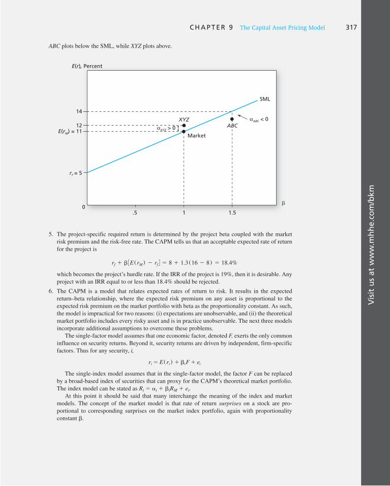
Vis
it u
s at
ww
w.m
hh
e.co
m/b
km
C H A P T E R 9 The Capital Asset Pricing Model 317
5. The project-specific required return is determined by the project beta coupled with the market risk premium and the risk-free rate. The CAPM tells us that an acceptable expected rate of return for the project is
rf 1 b 3E (rM) 2 rf 4 5 8 1 1.3(16 2 8) 5 18.4%
which becomes the project’s hurdle rate. If the IRR of the project is 19%, then it is desirable. Any project with an IRR equal to or less than 18.4% should be rejected.
6. The CAPM is a model that relates expected rates of return to risk. It results in the expected return–beta relationship, where the expected risk premium on any asset is proportional to the expected risk premium on the market portfolio with beta as the proportionality constant. As such, the model is impractical for two reasons: (i) expectations are unobservable, and (ii) the theoretical market portfolio includes every risky asset and is in practice unobservable. The next three models incorporate additional assumptions to overcome these problems.
The single-factor model assumes that one economic factor, denoted F, exerts the only common influence on security returns. Beyond it, security returns are driven by independent, firm-specific factors. Thus for any security, i,
ri 5 E (ri) 1 biF 1 ei
The single-index model assumes that in the single-factor model, the factor F can be replaced by a broad-based index of securities that can proxy for the CAPM’s theoretical market portfolio. The index model can be stated as R i � � i � � i R M � e i .
At this point it should be said that many interchange the meaning of the index and market models. The concept of the market model is that rate of return surprises on a stock are pro-portional to corresponding surprises on the market index portfolio, again with proportionality constant � .
E(r), Percent
�
.5 1 1.5
14
αXYZ > 0
XYZ
Market
SML
0
αABC < 0
E(rM) = 11
rf = 5
ABC12
ABC plots below the SML, while XYZ plots above.

10 THE EXPLOITATION OF security mispricing in
such a way that risk-free profits can be earned
is called arbitrage. It involves the simultane-
ous purchase and sale of equivalent securi-
ties in order to profit from discrepancies in
their prices. Perhaps the most basic principle
of capital market theory is that equilibrium
market prices are rational in that they rule
out arbitrage opportunities. If actual secu-
rity prices allow for arbitrage, the result will
be strong pressure to restore equilibrium.
Therefore, security markets ought to satisfy
a “no-arbitrage condition.” In this chapter,
we show how such no-arbitrage conditions
together with the factor model introduced in
Chapter 8 allow us to generalize the security
market line of the CAPM to gain richer insight
into the risk–return relationship.
We begin by showing how the decompo-
sition of risk into market versus firm- specific
influences that we introduced in earlier
chapters can be extended to deal with the
multifaceted nature of systematic risk. Mul-
tifactor models of security returns can be
used to measure and manage exposure to
each of many economywide factors such as
business-cycle risk, interest or inflation rate
risk, energy price risk, and so on. These mod-
els also lead us to a multifactor version of the
security market line in which risk premiums
derive from exposure to multiple risk sources,
each with their own risk premium.
We show how factor models combined
with a no-arbitrage condition lead to a simple
relationship between expected return and
risk. This approach to the risk–return trade-
off is called arbitrage pricing theory, or APT.
We derive the APT, and show why it implies a
multifactor security market line. We ask next
what factors are likely to be the most impor-
tant sources of risk. These will be the factors
generating substantial hedging demands that
brought us to the multifactor CAPM intro-
duced in Chapter 9. Both the APT and the
CAPM therefore lead to multiple-risk versions
of the security market line, thereby enriching
the insights we can derive about the risk–
return relationship.
Arbitrage Pricing Theory and Multifactor Models of
Risk and Return
CHAPTER TEN 1 PA
RT
III

C H A P T E R 1 0 Arbitrage Pricing Theory and Multifactor Models of Risk and Return 319
The index model introduced in Chapter 8 gave us a way of decomposing stock variability into market or systematic risk, due largely to macroeconomic events, versus firm-specific or idiosyncratic effects that can be diversified in large portfolios. In the index model, the return on the market portfolio summarized the broad impact of macro factors. Sometimes, however, rather than using a market proxy, it is more useful to focus directly on the ultimate sources of risk. This can be useful in risk assessment when measuring one’s exposures to particular sources of uncertainty. Factor models are tools that allow us to describe and quan-tify the different factors that affect the rate of return on a security during any time period.
Factor Models of Security Returns
To illustrate, we will start by examining a single-factor model like the one introduced in Chapter 8. As noted there, uncertainty in asset returns has two sources: a common or macroeconomic factor, and firm-specific events. The common factor is constructed to have zero expected value, because we use it to measure new information concerning the macroeconomy, which, by definition, has zero expected value.
If we call F the deviation of the common factor from its expected value, � i the sensi-tivity of firm i to that factor, and e i the firm-specific disturbance, the factor model states that the actual return on firm i will equal its initially expected return plus a (zero expected value) random amount attributable to unanticipated economywide events, plus another (zero expected value) random amount attributable to firm-specific events.
Formally, the single-factor model is described by Equation 10.1 :
ri 5 E(ri) 1 biF 1 ei (10.1)
where E ( r i ) is the expected return on stock i. Notice that if the macro factor has a value of 0 in any particular period (i.e., no macro surprises), the return on the security will equal its previously expected value, E ( r i ), plus the effect of firm-specific events only. The nonsys-tematic components of returns, the e i s, are assumed to be uncorrelated among themselves and uncorrelated with the factor F.
10.1 Multifactor Models: An Overview
Example 10.1 Factor Models
To make the factor model more concrete, consider an example. Suppose that the macro fac-tor, F, is taken to be news about the state of the business cycle, measured by the unexpected percentage change in gross domestic product (GDP), and that the consensus is that GDP will increase by 4% this year. Suppose also that a stock’s � value is 1.2. If GDP increases by only 3%, then the value of F would be � 1%, representing a 1% disappointment in actual growth versus expected growth. Given the stock’s beta value, this disappointment would translate into a return on the stock that is 1.2% lower than previously expected. This macro surprise, together with the firm-specific disturbance, e i , determine the total depar-ture of the stock’s return from its originally expected value.
CONCEPT CHECK
1 Suppose you currently expect the stock in Example 10.1 to earn a 10% rate of return. Then some macroeconomic news suggests that GDP growth will come in at 5% instead of 4%. How will you revise your estimate of the stock’s expected rate of return?

320 P A R T I I I Equilibrium in Capital Markets
The factor model’s decomposition of returns into systematic and firm-specific compo-nents is compelling, but confining systematic risk to a single factor is not. Indeed, when we motivated the index model in Chapter 8, we noted that the systematic or macro factor sum-marized by the market return arises from a number of sources, for example, uncertainty about the business cycle, interest rates, inflation, and so on. The market return reflects macro factors as well as the average sensitivity of firms to those factors. When we estimate a single-index regression, therefore, we implicitly impose an (incorrect) assumption that each stock has the same relative sensitivity to each risk factor. If stocks actually differ in their betas relative to the various macroeconomic factors, then lumping all systematic sources of risk into one variable such as the return on the market index will ignore the nuances that better explain individual-stock returns.
It stands to reason that a more explicit representation of systematic risk, allowing for the possibility that different stocks exhibit different sensitivities to its various components, would constitute a useful refinement of the single-factor model. It is easy to see that mod-els that allow for several factors— multifactor models —can provide better descriptions of security returns.
Apart from their use in building models of equilibrium security pricing, multifactor models are useful in risk management applications. These models give us a simple way to measure our exposure to various macroeconomic risks, and construct portfolios to hedge those risks.
Let’s start with a two-factor model. Suppose the two most important macroeconomic sources of risk are uncertainties surrounding the state of the business cycle, news of which we will again measure by unanticipated growth in GDP and changes in interest rates. We will denote by IR any unexpected change in interest rates. The return on any stock will respond both to sources of macro risk and to its own firm-specific influences. We therefore can write a two-factor model describing the rate of return on stock i in some time period as follows:
ri 5 E(ri) 1 bi GDPGDP 1 bi IRIR 1 ei (10.2)
The two macro factors on the right-hand side of the equation comprise the system-atic factors in the economy. As in the single-factor model, both of these macro factors have zero expectation: they represent changes in these variables that have not already been anticipated. The coefficients of each factor in Equation 10.2 measure the sensitivity of share returns to that factor. For this reason the coefficients are sometimes called factor
sensitivities, factor loadings, or, equivalently, factor betas. An increase in interest rates is bad news for most firms, so we would expect interest rate betas generally to be negative. As before, e i reflects firm-specific influences.
To illustrate the advantages of multifactor models, consider two firms, one a regulated electric-power utility in a mostly residential area, the other an airline. Because residential demand for electricity is not very sensitive to the business cycle, the utility has a low beta on GDP. But the utility’s stock price may have a relatively high sensitivity to interest rates. Because the cash flow generated by the utility is relatively stable, its present value behaves much like that of a bond, varying inversely with interest rates. Conversely, the performance of the airline is very sensitive to economic activity but is less sensitive to interest rates. It will have a high GDP beta and a lower interest rate beta. Suppose that on a particular day, a news item suggests that the economy will expand. GDP is expected to increase, but so are interest rates. Is the “macro news” on this day good or bad? For the utility, this is bad news: its dominant sensitivity is to rates. But for the airline, which responds more to GDP, this is good news. Clearly a one-factor or single-index model cannot capture such differential responses to varying sources of macroeconomic uncertainty.

C H A P T E R 1 0 Arbitrage Pricing Theory and Multifactor Models of Risk and Return 321
Factor betas can provide a framework for a hedging strategy. The idea for an investor who wishes to hedge a source of risk is to establish an opposite factor exposure to offset that particular source of risk. Often, futures contracts can be used to hedge particular factor exposures. We explore this application in Chapter 22.
A Multifactor Security Market Line
As it stands, the multifactor model is no more than a description of the factors that affect security returns. There is no “theory” in the equation. The obvious question left unan-swered by a factor model like Equation 10.2 is where E ( r ) comes from, in other words, what determines a security’s expected rate of return. This is where we need a theoretical model of equilibrium security returns.
In previous chapters we developed one example of such a model: the security market line (SML) of the capital asset pricing model (CAPM). The CAPM asserts that securi-ties will be priced to give investors an expected return comprised of two components: the risk-free rate, which is compensation for the time value of money, and a risk premium, determined by multiplying a benchmark risk premium (i.e., the risk premium offered by the market portfolio) times the relative measure of risk, beta:
E(r) 5 rf 1 b 3E(rM) 2 rf 4 (10.3)
If we denote the risk premium of the market portfolio by RP M , then a useful way to rewrite Equation 10.3 is
E(r) 5 rf 1 bRPM (10.4)
We pointed out in Chapter 8 that you can think of beta as measuring the exposure of a stock or portfolio to marketwide or macroeconomic risk factors. Therefore, one interpretation of the SML is that investors are rewarded with a higher expected return for their exposure to macro risk, based on the sensitivity to that risk (beta) as well as the compensation for bearing each unit of that source of risk (i.e., the risk premium, RP M ), but are not rewarded for exposure to firm-specific uncertainty (the residual term e i in Equation 10.1 ).
How might this single-factor view of the world generalize once we recognize the pres-ence of multiple sources of systematic risk? We will work out the details of the argument in the next section, but before getting lost in the trees, we will start with the lay of the
Example 10.2 Risk Assessment Using Multifactor Models
Suppose we estimate the two-factor model in Equation 10.2 for Northeast Airlines and find the following result:
r 5 .133 1 1.2(GDP) 2 .3(IR) 1 e
This tells us that based on currently available information, the expected rate of return for Northeast is 13.3%, but that for every percentage point increase in GDP beyond current expectations, the return on Northeast shares increases on average by 1.2%, while for every unanticipated percentage point that interest rates increases, Northeast’s shares fall on aver-age by .3%.
322 P A R T I I I Equilibrium in Capital Markets
forest, motivating intuitively the results that are to come. Perhaps not surprisingly, a mul-tifactor index model gives rise to a multifactor security market line in which the risk pre-mium is determined by the exposure to each systematic risk factor, and by a risk premium associated with each of those factors.
For example, in a two-factor economy in which risk exposures can be measured by Equation 10.2 , we would conclude that the expected rate of return on a security would be the sum of:
1. The risk-free rate of return.
2. The sensitivity to GDP risk (i.e., the GDP beta) times the risk premium for bearing GDP risk.
3. The sensitivity to interest rate risk (i.e., the interest rate beta) times the risk premium for bearing interest rate risk.
This assertion is expressed as follows in Equation 10.5 . In that equation, � GDP denotes the sensitivity of the security return to unexpected changes in GDP growth, and RP GDP is the risk premium associated with “one unit” of GDP exposure, that is, the exposure cor-responding to a GDP beta of 1.0. Here then is a two-factor security market line:
E(r) 5 rf 1 bGDPRPGDP 1 bIRRPIR (10.5)
If you look back at Equation 10.4 , you will see that Equation 10.5 is a generalization of the simple security market line. In the single-factor SML, the benchmark risk premium is given by the market portfolio, RP M � E ( r M ) � r f , but once we generalize to multiple risk sources, each with its own risk premium, we see that the insights are highly similar.
However, one difference between a single- and multiple-factor economy is that a fac-tor risk premium can be negative. For example, a security with a positive interest rate beta performs better when rates increase, and thus would hedge the value of a portfolio against interest rate risk. Investors might well accept a lower rate of return, that is, a negative risk premium, as the cost of this hedging attribute. In contrast, a more typical security that does worse when rates increase (a negative-IR beta) adds to interest rate exposure, and therefore has a higher required rate of return. Equation 10.5 shows that the contribution of interest rate risk to required return for such a security would then be positive, the product of a negative-factor beta times a negative-factor risk premium. 1
We still need to specify how to estimate the risk premium for each factor. Analogously to the simple CAPM, the risk premium associated with each factor can be thought of as the risk premium of a portfolio that has a beta of 1.0 on that particular factor and a beta of zero on all other factors. In other words, it is the risk premium one might expect to earn by taking a “pure play” on that factor. We will return to this below, but for now, let’s just take the factor risk premiums as given and see how a multifactor SML might be used.
1 A warning: predicting the sign of a risk premium can be tricky. For example, taken in isolation, an unantici-pated drop in interest rates could signal a decline in GDP. On this basis, the interest rate factor would proxy for general economic activity and presumably carry a positive risk premium. However, because unexpected changes in GDP are also included in Equation 10.2 , the interest rate beta measures sensitivity to interest rates controlling for surprises in GDP. Therefore, we expect the IR factor to have a negative risk premium. Nevertheless, it is possible that an unanticipated decline in interest rates may signal a fall in GDP in future periods, not captured by the contemporaneous GDP factor. In that case, a positive risk premium still would be possible.
C H A P T E R 1 0 Arbitrage Pricing Theory and Multifactor Models of Risk and Return 323
The multifactor model clearly gives us a much richer way to think about risk exposures and compensation for those exposures than the single-index model or CAPM. Let us now fill in some of the gaps in the argument and more carefully explore the link between multi-factor models of security returns and multifactor security market lines.
Example 10.3 A Multifactor SML
Think about our regression estimates for Northeast Airlines in Example 10.2 . Northeast has a GDP beta of 1.2 and an interest rate beta of � .3. Suppose the risk premium for one unit of exposure to GDP risk is 6%, while the risk premium for one unit of exposure to interest rate risk is � 7%. Then the overall risk premium on the Northeast portfolio should equal the sum of the risk premiums required as compensation for each source of systematic risk.
The risk premium attributable to GDP risk should be the stock’s exposure to that risk multiplied by the risk premium of the first factor portfolio, 6%. Therefore, the por-tion of the firm’s risk premium that is compensation for its exposure to the first fac-tor is 1.2 � 6% � 7.2%. Similarly, the risk premium attributable to interest rate risk is � .3 � ( � 7%) � 2.1%. The total risk premium should be 7.2 � 2.1 � 9.3%. Therefore, if the risk-free rate is 4%, the total return on Northeast Airlines should be
4.0%
1 7.2
1 2.1
13.3%
Risk-free rate
1 Risk premium for exposure to GDP risk
1 Risk premium for exposure to interest rate risk
Total expected return
More concisely, using Equation 10.5 ,
E(r) 5 4% 1 1.2 3 6% 1 (2.3) 3 (27%) 5 13.3%
10.2 Arbitrage Pricing Theory
Stephen Ross developed the arbitrage pricing theory (APT) in 1976. 2 Like the CAPM, the APT predicts a security market line linking expected returns to risk, but the path it takes to the SML is quite different. Ross’s APT relies on three key propositions: (i) secu-rity returns can be described by a factor model; (ii) there are sufficient securities to diver-sify away idiosyncratic risk; and (iii) well-functioning security markets do not allow for the persistence of arbitrage opportunities. We begin with a simple version of Ross’s model, which assumes that only one systematic factor affects security returns. However, the usual discussion of the APT is concerned with the multifactor case, so we treat this more general case as well.
2 Stephen A. Ross, “Return, Risk and Arbitrage,” in I. Friend and J. Bicksler, eds., Risk and Return in Finance (Cambridge, MA: Ballinger, 1976).
CONCEPT CHECK
2 Suppose the factor risk premiums in Example 10.3 were RP GDP � 4% and RP IR � � 2%. What would be the new value for the equilibrium expected rate of return on Northeast Airlines?

324 P A R T I I I Equilibrium in Capital Markets
Arbitrage, Risk Arbitrage, and Equilibrium
An arbitrage opportunity arises when an investor can earn riskless profits without mak-ing a net investment. A trivial example of an arbitrage opportunity would arise if shares of a stock sold for different prices on two different exchanges. For example, suppose IBM sold for $95 on the NYSE but only $93 on NASDAQ. Then you could buy the shares on NASDAQ and simultaneously sell them on the NYSE, clearing a riskless profit of $2 per share without tying up any of your own capital. The Law of One Price states that if two assets are equivalent in all economically relevant respects, then they should have the same market price. The Law of One Price is enforced by arbitrageurs: if they observe a violation of the law, they will engage in arbitrage activity —simultaneously buying the asset where it is cheap and selling where it is expensive. In the process, they will bid up the price where it is low and force it down where it is high until the arbitrage opportunity is eliminated.
The idea that market prices will move to rule out arbitrage opportunities is perhaps the most fundamental concept in capital market theory. Violation of this restriction would indi-cate the grossest form of market irrationality.
The critical property of a risk-free arbitrage portfolio is that any investor, regardless of risk aversion or wealth, will want to take an infinite position in it. Because those large posi-tions will quickly force prices up or down until the opportunity vanishes, security prices should satisfy a “no-arbitrage condition,” that is, a condition that rules out the existence of arbitrage opportunities.
There is an important difference between arbitrage and risk–return dominance argu-ments in support of equilibrium price relationships. A dominance argument holds that when an equilibrium price relationship is violated, many investors will make limited port-folio changes, depending on their degree of risk aversion. Aggregation of these limited portfolio changes is required to create a large volume of buying and selling, which in turn restores equilibrium prices. By contrast, when arbitrage opportunities exist, each inves-tor wants to take as large a position as possible; hence it will not take many investors to bring about the price pressures necessary to restore equilibrium. Therefore, implications for prices derived from no-arbitrage arguments are stronger than implications derived from a risk–return dominance argument.
The CAPM is an example of a dominance argument, implying that all investors hold mean-variance efficient portfolios. If a security is mispriced, then investors will tilt their portfolios toward the underpriced and away from the overpriced securities. Pressure on equilibrium prices results from many investors shifting their portfolios, each by a relatively small dollar amount. The assumption that a large number of investors are mean-variance sensitive is critical. In contrast, the implication of a no-arbitrage condition is that a few investors who identify an arbitrage opportunity will mobilize large dollar amounts and quickly restore equilibrium.
Practitioners often use the terms “arbitrage” and “arbitrageurs” more loosely than our strict definition. “Arbitrageur” often refers to a professional searching for mispriced secu-rities in specific areas such as merger-target stocks, rather than to one who seeks strict (risk-free) arbitrage opportunities. Such activity is sometimes called risk arbitrage to dis-tinguish it from pure arbitrage.
To leap ahead, in Part Four we will discuss “derivative” securities such as futures and options, whose market values are determined by prices of other securities. For example, the value of a call option on a stock is determined by the price of the stock. For such secu-rities, strict arbitrage is a practical possibility, and the condition of no-arbitrage leads to exact pricing. In the case of stocks and other “primitive” securities whose values are not determined strictly by another asset or bundle of assets, no-arbitrage conditions must be obtained by appealing to diversification arguments.
C H A P T E R 1 0 Arbitrage Pricing Theory and Multifactor Models of Risk and Return 325
Well-Diversified Portfolios
Now we look at the risk of a portfolio of stocks. We first show that if a portfolio is well diversified, its firm-specific or nonfactor risk becomes negligible, so that only factor (or systematic) risk remains. If we construct an n -stock portfolio with weights w i , Σ w i � 1, then the rate of return on this portfolio is as follows:
rP 5 E(rP) 1 bP F 1 eP (10.6)
where
bP 5 gwi bi
; E(rP) 5 gwi E(ri)
are the weighted averages of the � i and expected returns of the n securities. The portfolio nonsystematic component (which is uncorrelated with F ) is e P � Σ w i e i , which similarly is a weighted average of the e i of the n securities.
We can divide the variance of this portfolio into systematic and nonsystematic sources, as we saw in Chapter 8. The portfolio variance is
sP2 5 bP
2 sF2 1 s2(eP)
where sF2 is the variance of the factor F and � 2 ( e P ) is the nonsystematic risk of the portfo-
lio, which is given by
s2(eP) 5 Variance(gwiei) 5 gwi2s2(ei)
Note that in deriving the nonsystematic variance of the portfolio, we depend on the fact that the firm-specific e i s are uncorrelated and hence that the variance of the “portfolio” of nonsystematic e i s is the weighted sum of the individual nonsystematic variances with the square of the investment proportions as weights.
If the portfolio were equally weighted, w i � 1/ n, then the nonsystematic variance would be
s2(eP) 5 Variance(gwiei) 5 a a1nb2
s2(ei) 51na
s2(ei)n 5
1n s2(ei)
where the last term is the average value across securities of nonsystematic variance. In words, the nonsystematic variance of the portfolio equals the average nonsystematic vari-ance divided by n. Therefore, when the portfolio gets large in the sense that n is large, its nonsystematic variance approaches zero. This is the effect of diversification.
We conclude that for the equally weighted portfolio, the nonsystematic variance approaches zero as n becomes ever larger. This property is true of portfolios other than the equally weighted one. Any portfolio for which each w i becomes consistently smaller as n gets large (more precisely, for which each wi
2 approaches zero as n increases) will satisfy the condition that the portfolio nonsystematic risk will approach zero. In fact, this property motivates us to define a well-diversified portfolio as one that is diversified over a large enough number of securities, with each weight, w i , small enough that for practical purposes the nonsystematic variance, � 2 ( e P ), is negligible.
Because the expected value of e P for any well-diversified portfolio is zero, and its vari-ance also is effectively zero, we can conclude that any realized value of e P will be virtually zero. Rewriting Equation 10.1 , we conclude that for a well-diversified portfolio, for all practical purposes
rP 5 E(rP) 1 bPF
Large (mostly institutional) investors can hold portfolios of hundreds and even thousands of securities; thus the concept of well-diversified portfolios clearly is operational in con-temporary financial markets.
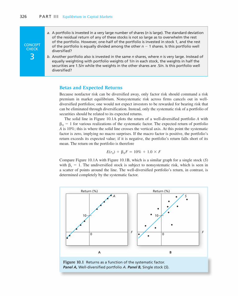
326 P A R T I I I Equilibrium in Capital Markets
Betas and Expected Returns
Because nonfactor risk can be diversified away, only factor risk should command a risk premium in market equilibrium. Nonsystematic risk across firms cancels out in well- diversified portfolios; one would not expect investors to be rewarded for bearing risk that can be eliminated through diversification. Instead, only the systematic risk of a portfolio of securities should be related to its expected returns.
The solid line in Figure 10.1A plots the return of a well-diversified portfolio A with � A � 1 for various realizations of the systematic factor. The expected return of portfolio A is 10%; this is where the solid line crosses the vertical axis. At this point the systematic factor is zero, implying no macro surprises. If the macro factor is positive, the portfolio’s return exceeds its expected value; if it is negative, the portfolio’s return falls short of its mean. The return on the portfolio is therefore
E(rA) 1 bAF 5 10% 1 1.0 3 F
Compare Figure 10.1A with Figure 10.1B , which is a similar graph for a single stock ( S ) with � s � 1. The undiversified stock is subject to nonsystematic risk, which is seen in a scatter of points around the line. The well-diversified portfolio’s return, in contrast, is determined completely by the systematic factor.
CONCEPT CHECK
3
a. A portfolio is invested in a very large number of shares ( n is large). The standard deviation of the residual return of any of these stocks is not so large as to overwhelm the rest of the portfolio. However, one-half of the portfolio is invested in stock 1, and the rest of the portfolio is equally divided among the other n � 1 shares. Is this portfolio well diversified?
b. Another portfolio also is invested in the same n shares, where n is very large. Instead of equally weighting with portfolio weights of 1/ n in each stock, the weights in half the securities are 1.5/ n while the weights in the other shares are .5/ n. Is this portfolio well diversified?
0F
A
10
Return (%)
0F
S
10
Return (%)
A B
Figure 10.1 Returns as a function of the systematic factor. Panel A, Well-diversified portfolio A. Panel B, Single stock ( S ).

C H A P T E R 1 0 Arbitrage Pricing Theory and Multifactor Models of Risk and Return 327
0F (Realization of macro factor)
AB
108
Return (%)
Figure 10.2 Returns as a function of the systematic factor: an arbitrage opportunity
Now consider Figure 10.2 , where the dashed line plots the return on another well- diversified portfolio, portfolio B, with an expected return of 8% and � B also equal to 1. Could portfolios A and B coexist with the return pattern depicted? Clearly not: No matter what the systematic factor turns out to be, portfolio A outperforms portfolio B, leading to an arbitrage opportunity.
If you sell short $1 million of B and buy $1 million of A, a zero net investment strategy, you would have a riskless payoff of $20,000, as follows:
(.10 1 1.0 3 F) 3 $1 million
2(.08 1 1.0 3 F) 3 $1 million
.02 3 $1 million 5 $20,000
from long position in A
from short position in B
net proceeds
Your profit is risk-free because the factor risk cancels out across the long and short posi-tions. Moreover, the strategy requires zero net investment. You should pursue it on an infinitely large scale until the return discrepancy between the two portfolios disappears. Well-diversified portfolios with equal betas must have equal expected returns in market equilibrium, or arbitrage opportunities exist.
What about portfolios with different betas? We show now that their risk premiums must be proportional to beta. To see why, consider Figure 10.3 . Suppose that the risk-free rate is 4% and that a well-diversified portfolio, C, with a beta of .5, has an expected return of 6%. Portfolio C plots below the line from the risk-free asset to portfolio A. Consider, therefore, a new portfolio, D, composed of half of portfolio A and half of the risk-free asset. Portfolio D ’s beta will be (.5 � 0 � .5 � 1.0) � .5, and its expected return will be (.5 � 4 � .5 � 10) � 7%. Now portfolio D has an equal beta but a greater expected return than portfolio C. From our analysis in the previous paragraph we know that this constitutes an arbitrage opportunity.
We conclude that, to preclude arbitrage opportunities, the expected return on all well-diversified portfolios must lie on the straight line from the risk-free asset in Figure 10.3 . The equation of this line will dictate the expected return on all well-diversified portfolios.
Notice in Figure 10.3 that risk premiums are indeed proportional to portfolio betas. The risk premium is depicted by the vertical arrow, which measures the distance between the

328 P A R T I I I Equilibrium in Capital Markets
risk-free rate and the expected return on the portfolio. The risk premium is zero for � � 0 and rises in direct proportion to � .
The One-Factor Security Market Line
Now consider the market index portfolio, M, as a well-diversified portfolio, and let us measure the systematic factor as the unexpected return on that portfolio. Because the index portfolio must be on the line in Figure 10.4 and the beta of the index portfolio is 1, we can
Figure 10.4 The security market line
[E(rM) – rf]
1
M
(With respect tomarket index)
Expected Return (%)
rf
E(rM)
β
rf = 4
β
6
.5 1
10
7
F
C
D
A
RiskPremium
(With respectto macro factor)
Expected Return (%)
Figure 10.3 An arbitrage opportunity
C H A P T E R 1 0 Arbitrage Pricing Theory and Multifactor Models of Risk and Return 329
determine the equation describing that line. As Figure 10.4 shows, the intercept is r f and the slope is E ( r M ) � r f [rise � E ( r M ) � r f ; run � 1], implying that the equation of the line is
E(rP) 5 rf 1 3E(rM) 2 rf 4bP (10.7)
Hence, Figures 10.3 and 10.4 imply an SML relation equivalent to that of the CAPM.
Example 10.4 Arbitrage and the Security Market Line
Suppose the market index is a well-diversified portfolio with expected return 10% and that deviations of its return from expectation (i.e., r M � 10%) can serve as the systematic fac-tor. The T-bill rate is 4%. Then the SML ( Equation 10.7 ) implies that the expected rate of return on well-diversified portfolio E with a beta of 2⁄3 should be 4% � 2⁄3(10 � 4) � 8%. What if its expected return actually is 9%? Then there will be an arbitrage opportunity.
Buy $1 worth of portfolio E and sell $1 of a portfolio that is invested 1⁄3 in T-bills and 2⁄3 in the market. This portfolio by construction has the same beta as portfolio E. The return on this portfolio is 1⁄3 r f � 2⁄3 r M � 1⁄3 � 4% � 2⁄3 r M . The net return on the combined position is:
$1 � [.09 � 2⁄3( r M � .10)] Invest $1 in portfolio E, with expected return 9% and beta of 2⁄3 on surprise in market return.
� $1(1⁄3 � .04 � 2⁄3 r M ) Sell portfolio invested 1⁄3 in T-bills and 2⁄3 in the market index.
$1 � .01 Total
The profit per dollar invested is risk-free and precisely equal to the deviation of the expected return on portfolio E from the SML.
CONCEPT CHECK
4
Continue to use the data in Example 10.4 . Now consider portfolio G, which is well diversi-fied with a beta of 1⁄3 and expected return of 5%. Does an arbitrage opportunity exist? If so, what is the arbitrage strategy? Show that the strategy results in risk-free profits with zero net investment.
We have used the no-arbitrage condition to obtain an expected return–beta relationship identical to that of the CAPM, without the restrictive assumptions of the CAPM. As noted, this derivation depends on three assumptions: a factor model describing security returns, a sufficient number of securities to form well-diversified portfolios, and the absence of arbitrage opportunities. This last restriction gives rise to the name of the approach: arbi-trage pricing theory. Our demonstration suggests that despite its restrictive assumptions, the main conclusion of the CAPM, namely, the SML expected return–beta relationship, should be at least approximately valid.
It is worth noting that in contrast to the CAPM, the APT does not require that the bench-mark portfolio in the SML relationship be the true market portfolio. Any well- diversified portfolio lying on the SML of Figure 10.4 may serve as the benchmark portfolio. For exam-ple, one might define the benchmark portfolio as the well-diversified portfolio most highly correlated with whatever systematic factor is thought to affect stock returns. Accordingly, the APT has more flexibility than does the CAPM because problems associated with an unobservable market portfolio are not a concern.
330 P A R T I I I Equilibrium in Capital Markets
In addition, the APT provides further justification for use of the index model in the practical implementation of the SML relationship. Even if the index portfolio is not a pre-cise proxy for the true market portfolio, which is a cause of considerable concern in the context of the CAPM, we now know that if the index portfolio is sufficiently well diversi-fied, the SML relationship should still hold true according to the APT.
So far we have demonstrated the APT relationship for well-diversified portfolios only. The CAPM expected return–beta relationship applies to single assets, as well as to portfo-lios. In the next section we generalize the APT result one step further.
10.3 Individual Assets and the APT
We have demonstrated that if arbitrage opportunities are to be ruled out, each well- diversified portfolio’s expected excess return must be proportional to its beta. The question is whether this relationship tells us anything about the expected returns on the component stocks. The answer is that if this relationship is to be satisfied by all well-diversified port-folios, it must be satisfied by almost all individual securities, although a full proof of this proposition is somewhat difficult. We can illustrate the argument less formally.
Suppose that the expected return–beta relationship is violated for all single assets. Now create a pair of well-diversified portfolios from these assets. What are the chances that in spite of the fact that for any pair of assets the relationship does not hold, the relationship will hold for both well-diversified portfolios? The chances are small, but it is possible that the relationships among the single securities are violated in offsetting ways so that some-how it holds for the pair of well-diversified portfolios.
Now construct yet a third well-diversified portfolio. What are the chances that the viola-tions of the relationships for single securities are such that the third portfolio also will ful-fill the no-arbitrage expected return–beta relationship? Obviously, the chances are smaller still, but the relationship is possible. Continue with a fourth well-diversified portfolio, and so on. If the no-arbitrage expected return–beta relationship has to hold for infinitely many different, well-diversified portfolios, it must be virtually certain that the relationship holds for all but a small number of individual securities.
We use the term virtually certain advisedly because we must distinguish this conclusion from the statement that all securities surely fulfill this relationship. The reason we cannot make the latter statement has to do with a property of well-diversified portfolios.
Recall that to qualify as well diversified, a portfolio must have very small positions in all securities. If, for example, only one security violates the expected return–beta relation-ship, then the effect of this violation on a well-diversified portfolio will be too small to be of importance for any practical purpose, and meaningful arbitrage opportunities will not arise. But if many securities violate the expected return–beta relationship, the relation-ship will no longer hold for well-diversified portfolios, and arbitrage opportunities will be available. Consequently, we conclude that imposing the no-arbitrage condition on a single-factor security market implies maintenance of the expected return–beta relationship for all well-diversified portfolios and for all but possibly a small number of individual securities.
The APT and the CAPM
The APT serves many of the same functions as the CAPM. It gives us a benchmark for rates of return that can be used in capital budgeting, security valuation, or investment performance evaluation. Moreover, the APT highlights the crucial distinction between

C H A P T E R 1 0 Arbitrage Pricing Theory and Multifactor Models of Risk and Return 331
nondiversifiable risk (factor risk) that requires a reward in the form of a risk premium and diversifiable risk that does not.
The APT is an extremely appealing model. It depends on the assumption that a rational equilibrium in capital markets precludes arbitrage opportunities. A violation of the APT’s pricing relationships will cause extremely strong pressure to restore them even if only a limited number of investors become aware of the disequilibrium. Furthermore, the APT yields an expected return–beta relationship using a well-diversified portfolio that practi-cally can be constructed from a large number of securities.
In contrast, the CAPM is derived assuming an inherently unobservable “market” portfo-lio. The CAPM argument rests on mean-variance efficiency; that is, if any security violates the expected return–beta relationship, then many investors (each relatively small) will tilt their portfolios so that their combined overall pressure on prices will restore an equilib-rium that satisfies the relationship.
In spite of these apparent advantages, the APT does not fully dominate the CAPM. The CAPM provides an unequivocal statement on the expected return–beta relationship for all securities, whereas the APT implies that this relationship holds for all but perhaps a small number of securities. Because it focuses on the no-arbitrage condition, without the further assumptions of the market or index model, the APT cannot rule out a violation of the expected return–beta relationship for any particular asset. For this, we need the CAPM assumptions and its dominance arguments.
10.4 A Multifactor APT
We have assumed so far that only one systematic factor affects stock returns. This simpli-fying assumption is in fact too simplistic. We’ve noted that it is easy to think of several factors driven by the business cycle that might affect stock returns: interest rate fluctua-tions, inflation rates, oil prices, and so on. Presumably, exposure to any of these factors will affect a stock’s risk and hence its expected return. We can derive a multifactor version of the APT to accommodate these multiple sources of risk.
Suppose that we generalize the single-factor model expressed in Equation 10.1 to a two-factor model:
ri 5 E(ri) 1 bi1F1 1 bi2F2 1 ei (10.8)
In Example 10.2 , factor 1 was the departure of GDP growth from expectations, and f actor 2 was the unanticipated change in interest rates. Each factor has zero expected value because each measures the surprise in the systematic variable rather than the level of the variable. Similarly, the firm-specific component of unexpected return, e i , also has zero expected value. Extending such a two-factor model to any number of factors is straightforward.
Establishing a multifactor APT is similar to the one-factor case. But first we must intro-duce the concept of a factor portfolio, which is a well-diversified portfolio constructed to have a beta of 1 on one of the factors and a beta of zero on any other factor. We can think of a factor portfolio as a tracking portfolio. That is, the returns on such a portfolio track the evolution of particular sources of macroeconomic risk but are uncorrelated with other sources of risk. It is possible to form such factor portfolios because we have a large number of securities to choose from, and a relatively small number of factors. Factor portfolios will serve as the benchmark portfolios for a multifactor security market line.

332 P A R T I I I Equilibrium in Capital Markets
To generalize the argument in Example 10.5 , note that the factor exposures of any port-folio, P, are given by its betas, � P 1 and � P 2 . A competing portfolio, Q, can be formed by investing in factor portfolios with the following weights: � P 1 in the first factor portfolio, � P 2 in the second factor portfolio, and 1 � � P 1 � � P 2 in T-bills. By construction, portfolio Q will have betas equal to those of portfolio P and expected return of
E(rQ) 5 bP1E(r1) 1 bP2E(r2) 1 (1 2 bP1 2 bP2)rf
5 rf 1 bP1 3E(r1) 2 rf 4 1 bP2 3E(r2) 2 rf 4 (10.9)
Using the numbers in Example 10.5 :
E(rQ) 5 4 1 .5 3 (10 2 4) 1 .75 3 (12 2 4) 5 13%
Example 10.5 Multifactor SML
Suppose that the two factor portfolios, portfolios 1 and 2, have expected returns E ( r 1 ) � 10% and E ( r 2 ) � 12%. Suppose further that the risk-free rate is 4%. The risk premium on the first factor portfolio is 10% � 4% � 6%, whereas that on the second factor portfolio is 12% � 4% � 8%.
Now consider a well-diversified portfolio, portfolio A, with beta on the first factor, � A 1 � .5, and beta on the second factor, � A 2 � .75. The multifactor APT states that the overall risk premium on this portfolio must equal the sum of the risk premiums required as compensation for each source of systematic risk. The risk premium attributable to risk factor 1 should be the portfolio’s exposure to factor 1, � A 1 , multiplied by the risk pre-mium earned on the first factor portfolio, E ( r 1 ) � r f . Therefore, the portion of portfolio A ’s risk premium that is compensation for its exposure to the first factor is � A 1 [ E ( r 1 ) � r f ] � .5(10% � 4%) � 3%, whereas the risk premium attributable to risk factor 2 is � A 2 [ E ( r 2 ) � r f ] � .75(12% � 4%) � 6%. The total risk premium on the portfolio should be 3 � 6 � 9% and the total return on the portfolio should be 4% � 9% � 13%.
Example 10.6 Mispricing and Arbitrage
Suppose that the expected return on portfolio A from Example 10.5 were 12% rather than 13%. This return would give rise to an arbitrage opportunity. Form a portfolio from the factor portfolios with the same betas as portfolio A. This requires weights of .5 on the first factor portfolio, .75 on the second factor portfolio, and � .25 on the risk-free asset. This portfolio has exactly the same factor betas as portfolio A: It has a beta of .5 on the first fac-tor because of its .5 weight on the first factor portfolio, and a beta of .75 on the second fac-tor. (The weight of � .25 on risk-free T-bills does not affect the sensitivity to either factor.)
Now invest $1 in portfolio Q and sell (short) $1 in portfolio A. Your net investment is zero, but your expected dollar profit is positive and equal to
$1 3 E(rQ) 2 $1 3 E(rA) 5 $1 3 .13 2 $1 3 .12 5 $.01
Moreover, your net position is riskless. Your exposure to each risk factor cancels out because you are long $1 in portfolio Q and short $1 in portfolio A, and both of these well-diversified portfolios have exactly the same factor betas. Thus, if portfolio A ’s expected return differs from that of portfolio Q ’s, you can earn positive risk-free profits on a zero net investment position. This is an arbitrage opportunity.

C H A P T E R 1 0 Arbitrage Pricing Theory and Multifactor Models of Risk and Return 333
Because portfolio Q has precisely the same exposures as portfolio A to the two sources of risk, their expected returns also ought to be equal. So portfolio A also ought to have an expected return of 13%. If it does not, then there will be an arbitrage opportunity. 3
We conclude that any well-diversified portfolio with betas � P 1 and � P 2 must have the return given in Equation 10.9 if arbitrage opportunities are to be precluded. If you compare Equations 10.3 and 10.9 , you will see that Equation 10.9 is simply a generalization of the one-factor SML.
Finally, the extension of the multifactor SML of Equation 10.9 to individual assets is precisely the same as for the one-factor APT. Equation 10.9 cannot be satisfied by every well-diversified portfolio unless it is satisfied by virtually every security taken individu-ally. Equation 10.9 thus represents the multifactor SML for an economy with multiple sources of risk.
We pointed out earlier that one application of the CAPM is to provide “fair” rates of return for regulated utilities. The multifactor APT can be used to the same ends. The nearby box summarizes a study in which the APT was applied to find the cost of capital for regulated electric companies. Notice that empirical estimates for interest rate and inflation risk premi-ums in the box are negative, as we argued was reasonable in our discussion of Example 10.2 .
CONCEPT CHECK
5 Using the factor portfolios of Example 10.5 , find the equilibrium rate of return on a portfolio with � 1 � .2 and � 2 � 1.4.
10.5 Where Should We Look for Factors?
One shortcoming of the multifactor APT is that it gives no guidance concerning the deter-mination of the relevant risk factors or their risk premiums. Two principles guide us when we specify a reasonable list of factors. First, we want to restrict ourselves to a limited num-ber of systematic factors with considerable ability to explain security returns. If our model calls for many explanatory variables, it does little to simplify our description of security returns. Second, we wish to choose factors that seem likely to be important risk factors, that is, factors that concern investors sufficiently that they will demand meaningful risk premiums to bear exposure to those sources of risk. 3
One example of the multifactor approach is the work of Chen, Roll, and Ross, 4 who chose the following set of factors based on the ability of these factors to paint a broad pic-ture of the macroeconomy. Their set is obviously but one of many possible sets that might be considered.
IP � % change in industrial production
EI � % change in expected inflation
UI � % change in unanticipated inflation
CG � excess return of long-term corporate bonds over long-term government bonds
GB � excess return of long-term government bonds over T-bills
3 The risk premium on portfolio A is 9% (more than the historical risk premium of the S&P 500) despite the fact that its betas, which are both below 1, might seem defensive. This highlights another distinction between multi-factor and single-factor models. Whereas a beta greater than 1 in a single-factor market is aggressive, we cannot say in advance what would be aggressive or defensive in a multifactor economy where risk premiums depend on the sum of the contributions of several factors.
4 N. Chen, R. Roll, and S. Ross, “Economic Forces and the Stock Market,” Journal of Business 59 (1986), pp. 383–403.

334
Using the APT to Find Cost of Capital
Elton, Gruber, and Mei * use the APT to derive the cost of capital for electric utilities. They assume that the relevant risk factors are unanticipated developments in the term structure of interest rates, the level of interest rates, infla-tion rates, the business cycle (measured by GDP), foreign exchange rates, and a summary measure they devise to measure other macro factors.
Their first step is to estimate the risk premium associ-ated with exposure to each risk source. They accomplish this in a two-step strategy (which we will describe in con-siderable detail in Chapter 13):
1. Estimate “factor loadings” (i.e., betas) of a large sample
of firms. Regress returns of 100 randomly selected stocks against the systematic risk factors. They use a time-series regression for each stock (e.g., 60 months of data), therefore estimating 100 regressions, one for each stock.
2. Estimate the reward earned per unit of exposure to
each risk factor. For each month, regress the return of each stock against the five betas estimated. The coefficient on each beta is the extra average return earned as beta increases, i.e., it is an estimate of the risk premium for that risk factor from that month’s data. These estimates are of course subject to sam-pling error. Therefore, average the risk premium esti-mates across the 12 months in each year. The average response of return to risk is less subject to sampling error.
The risk premiums are in the middle column of the table at the top of the next column.
Notice that some risk premiums are negative. The interpretation of this result is that risk premium should be positive for risk factors you don’t want exposure to, but negative for factors you do want exposure to. For example, you should desire securities that have higher returns when inflation increases and be willing to accept lower expected returns on such securities; this shows up as a negative risk premium.
FactorFactor Risk Premium
Factor Betas for Niagra Mohawk
Term structure .425 1.0615
Interest rates � .051 �2.4167
Exchange rates �.049 1.3235
Business cycle .041 .1292 Infl ation �.069 �.5220Other macro factors
.530 .3046
Therefore, the expected return on any security should be related to its factor betas as follows:
rf � .425 �term struc � .051 �int rate
�.049 �ex rate � .041 �bus cycle � .069 �inflation � .530 �other
Finally, to obtain the cost of capital for a particular firm, the authors estimate the firm’s betas against each source of risk, multiply each factor beta by the “cost of factor risk” from the table above, sum over all risk sources to obtain the total risk premium, and add the risk-free rate.
For example, the beta estimates for Niagra Mohawk appear in the last column of the table above. Therefore, its cost of capital is
Cost of capital � rf � .425 � 1.0615 � .051(�2.4167) �.049(1.3235) � .041(.1292) �.069(�.5220) � .530(.3046) � rf � .72
In other words, the monthly cost of capital for Niagra Mohawk is .72% above the monthly risk-free rate. Its annu-alized risk premium is therefore .72% � 12 � 8.64%.
*Edwin J. Elton, Martin J. Gruber, and Jianping Mei, “Cost of Capital Using Arbitrage Pricing Theory: A Case Study of Nine New York Utilities,” Financial Markets, Institutions, and Instruments 3 (August 1994), pp. 46–68.
WO
RD
S FR
OM
TH
E ST
REE
T
This list gives rise to the following five-factor model of security returns during holding period t as a function of the change in the set of macroeconomic indicators:
rit 5 ai 1 biIPIPt 1 bi EIEIt 1 bi UIUIt 1 bi CGCGt 1 bi GBGBt 1 eit (10.10)
Equation 10.10 is a multidimensional security characteristic line (SCL), with five fac-tors. As before, to estimate the betas of a given stock we can use regression analysis. Here, however, because there is more than one factor, we estimate a multiple regression of the returns of the stock in each period on the five macroeconomic factors. The residual vari-ance of the regression estimates the firm-specific risk. We discuss the results of this model in Chapter 13, which focuses on empirical evidence on security pricing.

C H A P T E R 1 0 Arbitrage Pricing Theory and Multifactor Models of Risk and Return 335
The Fama-French (FF) Three-Factor Model
An alternative approach to specifying macroeconomic factors as candidates for relevant sources of systematic risk uses firm characteristics that seem on empirical grounds to proxy for exposure to systematic risk. The factors chosen are variables that on past evi-dence seem to predict average returns well and therefore may be capturing risk premiums. One example of this approach is the Fama and French three-factor model, which has come to dominate empirical research and industry applications: 5
rit 5 ai 1 biMRMt 1 biSMBSMBt 1 biHMLHMLt 1 eit (10.11)
where
SMB � Small Minus Big, i.e., the return of a portfolio of small stocks in excess of the return on a portfolio of large stocks.
HML � High Minus Low, i.e., the return of a portfolio of stocks with a high book-to-market ratio in excess of the return on a portfolio of stocks with a low book-to-market ratio.
Note that in this model the market index does play a role and is expected to capture sys-tematic risk originating from macroeconomic factors.
These two firm-characteristic variables are chosen because of long-standing observa-tions that corporate capitalization (firm size) and book-to-market ratio predict deviations of average stock returns from levels consistent with the CAPM. Fama and French jus-tify this model on empirical grounds: While SMB and HML are not themselves obvious candidates for relevant risk factors, the argument is that these variables may proxy for yet-unknown more-fundamental variables. For example, Fama and French point out that firms with high ratios of book-to-market value are more likely to be in financial distress and that small stocks may be more sensitive to changes in business conditions. Thus, these variables may capture sensitivity to risk factors in the macroeconomy. More evidence on the Fama-French model appears in Chapter 13.
The problem with empirical approaches such as the Fama-French model, which use prox-ies for extramarket sources of risk, is that none of the factors in the proposed models can be clearly identified as hedging a significant source of uncertainty. Black 6 points out that when researchers scan and rescan the database of security returns in search of explanatory factors (an activity often called data-snooping), they may eventually uncover past “patterns” that are due purely to chance. Black observes that return premiums to factors such as firm size have proven to be inconsistent since first discovered. However, Fama and French have shown that size and book-to-market ratios have predicted average returns in various time periods and in markets all over the world, thus mitigating potential effects of data-snooping.
The firm-characteristic basis of the Fama-French factors raises the question of whether they reflect an APT model or an approximation to a multi-index ICAPM based on extra-market hedging demands. This is an important distinction for the debate over the proper interpretation of the model, because the validity of FF-style models may constitute either a deviation from rational equilibrium (as there is no rational reason to prefer one or another of these firm characteristics per se), or that firm characteristics identified as empirically associated with average returns are correlated with other (yet unknown) risk factors.
The issue is still unresolved and is discussed in Chapter 13.
5 Eugene F. Fama and Kenneth R. French, “Multifactor Explanations of Asset Pricing Anomalies,” Journal of
Finance 51 (1996), pp. 55–84.
6 Fischer Black, “Beta and Return,” Journal of Portfolio Management 20 (1993), pp. 8–18.

Vis
it u
s at
ww
w.m
hh
e.co
m/b
km336 P A R T I I I Equilibrium in Capital Markets
10.6 The Multifactor CAPM and the APT
It is important to distinguish the multifactor APT from the multi-index CAPM. In the lat-ter, the factors are derived from a multiperiod consideration of a stream of consumption as well as randomly evolving investment opportunities pertaining to the distributions of rates of return. Hence, the hedge index portfolios must be derived from considerations of the utility of consumption, nontraded assets, and changes in investment opportunities.
A multi-index CAPM therefore will inherit its risk factors from sources of risk that a broad group of investors deem important enough to hedge. If hedging demands are com-mon to many investors, the prices of securities with desirable hedging characteristics will be bid up and their expected return reduced. This process requires a multifactor model to explain expected returns, where each factor arises from a particular hedging motive. Risk sources that are “priced” in market equilibrium (that is, are sufficiently important to result in detectable risk premiums) presumably will be systematic sources of uncertainty that affect investors broadly.
In contrast, the APT is largely silent on where to look for priced sources of risk. This lack of guidance is problematic, but by the same token, it accommodates a less structured search for relevant risk factors. These may reflect the concerns of a broader set of inves-tors, including institutions such as endowment or pension funds that may be concerned about exposures to risks that would not be obvious from an examination of individual consumption/investment decisions.
CONCEPT CHECK
6
Consider the following regression results for stock X.
rX � 2% � 1.2 (percentage change in oil prices )
a. If I live in Louisiana, where the local economy is heavily dependent on oil industry profits, does stock X represent a useful asset to hedge my overall economic well-being?
b. What if I live in Massachusetts, where most individuals and firms are energy consumers?
c. If energy consumers are far more numerous than energy producers, will high oil-beta stocks have higher or lower expected rates of return in market equilibrium than low oil-beta stocks?
1. Multifactor models seek to improve the explanatory power of single-factor models by explicitly accounting for the various systematic components of security risk. These models use indicators intended to capture a wide range of macroeconomic risk factors.
2. Once we allow for multiple risk factors, we conclude that the security market line also ought to be multidimensional, with exposure to each risk factor contributing to the total risk premium of the security.
3. A (risk-free) arbitrage opportunity arises when two or more security prices enable investors to construct a zero net investment portfolio that will yield a sure profit. The presence of arbitrage opportunities will generate a large volume of trades that puts pressure on security prices. This pressure will continue until prices reach levels that preclude such arbitrage.
4. When securities are priced so that there are no risk-free arbitrage opportunities, we say that they satisfy the no-arbitrage condition. Price relationships that satisfy the no-arbitrage condition are important because we expect them to hold in real-world markets.
SUMMARY

Vis
it u
s at
ww
w.m
hh
e.co
m/b
km
C H A P T E R 1 0 Arbitrage Pricing Theory and Multifactor Models of Risk and Return 337
5. Portfolios are called “well-diversified” if they include a large number of securities and the invest-ment proportion in each is sufficiently small. The proportion of a security in a well-diversified portfolio is small enough so that for all practical purposes a reasonable change in that security’s rate of return will have a negligible effect on the portfolio’s rate of return.
6. In a single-factor security market, all well-diversified portfolios have to satisfy the expected return–beta relationship of the CAPM to satisfy the no-arbitrage condition. If all well-diversified portfolios satisfy the expected return–beta relationship, then all but a small number of securities also must satisfy this relationship.
7. The APT does not require the restrictive assumptions of the CAPM and its (unobservable) market portfolio. The price of this generality is that the APT does not guarantee this relationship for all securities at all times.
8. A multifactor APT generalizes the single-factor model to accommodate several sources of sys-tematic risk. The multidimensional security market line predicts that exposure to each risk factor contributes to the security’s total risk premium by an amount equal to the factor beta times the risk premium of the factor portfolio that tracks that source of risk.
9. A multifactor extension of the single-factor CAPM, the ICAPM, is a model of the risk–return trade-off that predicts the same multidimensional security market line as the APT. The ICAPM suggests that priced risk factors will be those sources of risk that lead to significant hedging demand by a substantial fraction of investors.
Related Web sites for this chapter are available at www.mhhe.com/bkm
single-factor model multifactor model factor sensitivity factor loading
factor beta arbitrage pricing theory arbitrage Law of One Price
risk arbitrage well-diversified portfolio factor portfolio
KEY TERMS
1. Suppose that two factors have been identified for the U.S. economy: the growth rate of industrial production, IP, and the inflation rate, IR. IP is expected to be 3%, and IR 5%. A stock with a beta of 1 on IP and .5 on IR currently is expected to provide a rate of return of 12%. If industrial production actually grows by 5%, while the inflation rate turns out to be 8%, what is your revised estimate of the expected rate of return on the stock?
2. The APT itself does not provide guidance concerning the factors that one might expect to deter-mine risk premiums. How should researchers decide which factors to investigate? Why, for exam-ple, is industrial production a reasonable factor to test for a risk premium?
3. If the APT is to be a useful theory, the number of systematic factors in the economy must be small. Why?
4. Suppose that there are two independent economic factors, F 1 and F 2 . The risk-free rate is 6%, and all stocks have independent firm-specific components with a standard deviation of 45%. The following are well-diversified portfolios:
Portfolio Beta on F 1 Beta on F 2 Expected Return
A 1.5 2.0 31%
B 2.2 � 0.2 27%
What is the expected return–beta relationship in this economy?
5. Consider the following data for a one-factor economy. All portfolios are well diversified.
Portfolio E ( r ) Beta
A 12% 1.2
F 6% 0.0
PROBLEM SETS
i. Basic
ii. Intermediate

Vis
it u
s at
ww
w.m
hh
e.co
m/b
km338 P A R T I I I Equilibrium in Capital Markets
Suppose that another portfolio, portfolio E, is well diversified with a beta of .6 and expected
return of 8%. Would an arbitrage opportunity exist? If so, what would be the arbitrage strategy?
6. Assume that both portfolios A and B are well diversified, that E ( r A ) � 12%, and E ( r B ) � 9%.
If the economy has only one factor, and � A � 1.2, whereas � B � .8, what must be the risk-free
rate?
7. Assume that stock market returns have the market index as a common factor, and that all stocks
in the economy have a beta of 1 on the market index. Firm-specific returns all have a standard
deviation of 30%.
Suppose that an analyst studies 20 stocks, and finds that one-half have an alpha of � 2%,
and the other half an alpha of –2%. Suppose the analyst buys $1 million of an equally weighted
portfolio of the positive alpha stocks, and shorts $1 million of an equally weighted portfolio of
the negative alpha stocks.
a. What is the expected profit (in dollars) and standard deviation of the analyst’s profit?
b. How does your answer change if the analyst examines 50 stocks instead of 20 stocks?
100 stocks?
8. Assume that security returns are generated by the single-index model,
Ri 5 ai 1 bi RM 1 ei
where R i is the excess return for security i and R M is the market’s excess return. The risk-free
rate is 2%. Suppose also that there are three securities A, B, and C, characterized by the follow-
ing data:
Security � i E ( R i ) � ( e i )
A 0.8 10% 25%
B 1.0 12% 10%
C 1.2 14% 20%
a. If � M � 20%, calculate the variance of returns of securities A, B, and C.
b. Now assume that there are an infinite number of assets with return characteristics identi-
cal to those of A, B, and C, respectively. If one forms a well-diversified portfolio of type A
securities, what will be the mean and variance of the portfolio’s excess returns? What about
portfolios composed only of type B or C stocks?
c. Is there an arbitrage opportunity in this market? What is it? Analyze the opportunity graphically.
9. The SML relationship states that the expected risk premium on a security in a one-factor model
must be directly proportional to the security’s beta. Suppose that this were not the case. For
example, suppose that expected return rises more than proportionately with beta as in the figure
below.
B
C
A
E(r)
β

Vis
it u
s at
ww
w.m
hh
e.co
m/b
km
C H A P T E R 1 0 Arbitrage Pricing Theory and Multifactor Models of Risk and Return 339
a. How could you construct an arbitrage portfolio? ( Hint: Consider combinations of portfolios A and B, and compare the resultant portfolio to C. )
b. Some researchers have examined the relationship between average returns on diversified portfolios and the � and � 2 of those portfolios. What should they have discovered about the effect of � 2 on portfolio return?
10. Consider the following multifactor (APT) model of security returns for a particular stock.
Factor Factor Beta Factor Risk Premium
Inflation 1.2 6%
Industrial production 0.5 8
Oil prices 0.3 3
a. If T-bills currently offer a 6% yield, find the expected rate of return on this stock if the mar-ket views the stock as fairly priced.
b. Suppose that the market expected the values for the three macro factors given in column 1 below, but that the actual values turn out as given in column 2. Calculate the revised expecta-tions for the rate of return on the stock once the “surprises” become known.
Factor Expected Rate of Change Actual Rate of Change
Inflation 5% 4%
Industrial production 3 6
Oil prices 2 0
11. Suppose that the market can be described by the following three sources of systematic risk with associated risk premiums.
Factor Risk Premium
Industrial production ( I ) 6%
Interest rates ( R ) 2
Consumer confidence ( C ) 4
The return on a particular stock is generated according to the following equation:
r 5 15% 1 1.0I 1 .5R 1 .75C 1 e
Find the equilibrium rate of return on this stock using the APT. The T-bill rate is 6%. Is the stock over- or underpriced? Explain.
12. As a finance intern at Pork Products, Jennifer Wainwright’s assignment is to come up with fresh insights concerning the firm’s cost of capital. She decides that this would be a good opportunity to try out the new material on the APT that she learned last semester. She decides that three promising factors would be (i) the return on a broad-based index such as the S&P 500; (ii) the level of interest rates, as represented by the yield to maturity on 10-year Treasury bonds; and (iii) the price of hogs, which are particularly important to her firm. Her plan is to find the beta of Pork Products against each of these factors by using a multiple regression and to estimate the risk premium associated with each exposure factor. Comment on Jennifer’s choice of factors. Which are most promising with respect to the likely impact on her firm’s cost of capital? Can you suggest improvements to her specification?
Use the following information to Answer Problems 13 – 16 : Orb Trust (Orb) has historically leaned toward a passive management style of its portfolios. The only model that Orb’s senior management has promoted in the past is the capital asset pricing model (CAPM). Now Orb’s management has asked one of its analysts, Kevin McCracken, CFA, to investi-gate the use of the arbitrage pricing theory (APT) model.
McCracken believes that a two-factor APT model is adequate, where the factors are the sensitiv-ity to changes in real GDP and changes in inflation. McCracken has concluded that the factor risk

Vis
it u
s at
ww
w.m
hh
e.co
m/b
km340 P A R T I I I Equilibrium in Capital Markets
premium for real GDP is 8% while the factor risk premium for inflation is 2%. He estimates for Orb’s High Growth Fund that the sensitivities to these two factors are 1.25 and 1.5, respectively. Using his APT results, he computes the expected return of the fund. For comparison purposes, he then uses fundamental analysis to also compute the expected return of Orb’s High Growth Fund. McCracken finds that the two estimates of the Orb High Growth Fund’s expected return are equal.
McCracken asks a fellow analyst, Sue Kwon, to provide an estimate of the expected return of Orb’s Large Cap Fund based on fundamental analysis. Kwon, who manages the fund, says that the expected return is 8.5% above the risk-free rate. McCracken then applies the APT model to the Large Cap Fund. He finds that the sensitivities to real GDP and inflation are .75 and 1.25, respectively.
McCracken’s manager at Orb, Jay Stiles, asks McCracken to compose a portfolio that has a unit sensitivity to real GDP growth but is not affected by inflation. McCracken is confident in his APT estimates for the High Growth Fund and the Large Cap Fund. He then computes the sensitivities for a third fund, Orb’s Utility Fund, which has sensitivities equal to 1.0 and 2.0, respectively. McCracken will use his APT results for these three funds to accomplish the task of creating a portfolio with a unit exposure to real GDP and no exposure to inflation. He calls the fund the “GDP Fund.” Stiles says such a GDP Fund would be good for clients who are retirees who live off the steady income of their investments. McCracken says that the fund would be a good choice if upcoming supply side macroeconomic policies of the government are successful.
13. According to the APT, if the risk-free rate is 4%, what should be McCracken’s estimate of the expected return of Orb’s High Growth Fund?
14. With respect to McCracken’s APT model estimate of Orb’s Large Cap Fund and the informa-tion Kwon provides, is an arbitrage opportunity available?
15. The GDP Fund composed from the other three funds would have a weight in Utility Fund equal to ( a ) � 2.2; ( b ) � 3.2; or ( c ) .3.
16. With respect to the comments of Stiles and McCracken concerning for whom the GDP Fund would be appropriate:
a. McCracken was correct and Stiles was wrong. b. Both were correct. c. Stiles was correct and McCracken was wrong.
17. Assume a universe of n (large) securities for which the largest residual variance is of an order
not larger than nsM2 . Construct as many different weighting schemes as you can that generate
well-diversified portfolios.
18. Derive a more general (than the numerical example in the chapter) demonstration of the APT security market line:
a. For a single-factor market. b. For a multifactor market.
19. Small firms will have relatively high loadings (high betas) on the SMB (small minus big) factor.
a. Explain why. b. Now suppose two unrelated small firms merge. Each will be operated as an independent unit
of the merged company. Would you expect the stock market behavior of the merged firm to differ from that of a portfolio of the two previously independent firms? How does the merger affect market capitalization? What is the prediction of the Fama-French model for the risk premium on the combined firm? Do we see here a flaw in the FF model?
iii. Challenge
1. Jeffrey Bruner, CFA, uses the capital asset pricing model (CAPM) to help identify mispriced securities. A consultant suggests Bruner use arbitrage pricing theory (APT) instead. In compar-ing CAPM and APT, the consultant made the following arguments:
a. Both the CAPM and APT require a mean-variance efficient market portfolio. b. Neither the CAPM nor APT assumes normally distributed security returns. c. The CAPM assumes that one specific factor explains security returns but APT does not.

Vis
it u
s at
ww
w.m
hh
e.co
m/b
km
C H A P T E R 1 0 Arbitrage Pricing Theory and Multifactor Models of Risk and Return 341
State whether each of the consultant’s arguments is correct or incorrect. Indicate, for each incor-rect argument, why the argument is incorrect.
2. Assume that both X and Y are well-diversified portfolios and the risk-free rate is 8%.
Portfolio Expected Return Beta
X 16% 1.00
Y 12 0.25
In this situation you would conclude that portfolios X and Y:
a. Are in equilibrium. b. Offer an arbitrage opportunity. c. Are both underpriced. d. Are both fairly priced.
3. A zero-investment portfolio with a positive alpha could arise if:
a. The expected return of the portfolio equals zero. b. The capital market line is tangent to the opportunity set. c. The Law of One Price remains unviolated. d. A risk-free arbitrage opportunity exists.
4. According to the theory of arbitrage:
a. High-beta stocks are consistently overpriced. b. Low-beta stocks are consistently overpriced. c. Positive alpha investment opportunities will quickly disappear. d. Rational investors will pursue arbitrage consistent with their risk tolerance.
5. The arbitrage pricing theory (APT) differs from the single-factor capital asset pricing model (CAPM) because the APT:
a. Places more emphasis on market risk. b. Minimizes the importance of diversification. c. Recognizes multiple unsystematic risk factors. d. Recognizes multiple systematic risk factors.
6. An investor takes as large a position as possible when an equilibrium price relationship is vio-lated. This is an example of:
a. A dominance argument. b. The mean-variance efficient frontier. c. Arbitrage activity. d. The capital asset pricing model.
7. The feature of arbitrage pricing theory (APT) that offers the greatest potential advantage over the simple CAPM is the:
a. Identification of anticipated changes in production, inflation, and term structure of interest rates as key factors explaining the risk–return relationship.
b. Superior measurement of the risk-free rate of return over historical time periods. c. Variability of coefficients of sensitivity to the APT factors for a given asset over time. d. Use of several factors instead of a single market index to explain the risk–return
relationship.
8. In contrast to the capital asset pricing model, arbitrage pricing theory:
a. Requires that markets be in equilibrium. b. Uses risk premiums based on micro variables. c. Specifies the number and identifies specific factors that determine expected returns. d. Does not require the restrictive assumptions concerning the market portfolio.

Vis
it u
s at
ww
w.m
hh
e.co
m/b
km342 P A R T I I I Equilibrium in Capital Markets
Unanticipated Inflation
One of the factors in the APT model specified by Chen, Roll, and Ross is the percent change in unanticipated inflation. Who gains and who loses when inflation change? Go to http://
hussmanfunds.com/rsi/infsurprises.htm to see a graph Inflation Surprise Index and Economists’ Inflation Forecasts.
E-INVEST-MENTS EXERCISES
SOLUTIONS TO CONCEPT CHECKS
1. The GDP beta is 1.2 and GDP growth is 1% better than previously expected. So you will increase your forecast for the stock return by 1.2 � 1% � 1.2%. The revised forecast is for an 11.2% return.
2. With these lower risk premiums, the expected return on the stock will be lower:
E(r) 5 4% 1 1.2 3 4% 1 (2.3) 3 (22%) 5 9.4%
3. a. This portfolio is not well diversified. The weight on the first security does not decline as n increases. Regardless of how much diversification there is in the rest of the portfolio, you will not shed the firm-specific risk of this security.
b. This portfolio is well diversified. Even though some stocks have three times the weight of other stocks (1.5/ n versus .5/ n ), the weight on all stocks approaches zero as n increases. The impact of any individual stock’s firm-specific risk will approach zero as n becomes ever larger.
4. The SML says that the expected return on the portfolio should be 4% � (1⁄3)(10 � 4) � 6%. The return actually expected is only 5%, implying that the stock is overpriced and that there is an
arbitrage opportunity. Buy $1 of a portfolio that is 2⁄3 invested in T-bills and 1⁄3 in the market. The
return on this portfolio is 2⁄3 r f � 1⁄3 r M � 2⁄3 � 4% � 1⁄3 r M . Sell $1 of portfolio G. The net return on the combined position is:
$1 � [2⁄3 � .04 � 1⁄3 r M ] Buy portfolio invested 2⁄3 in T-bills and 1⁄3 in the market index.
� $1 � [.05 � 1⁄3( r M � .10)] Sell $1 in portfolio G, with expected return
of 5% and beta of 1⁄3 on surprise in market return.
$1 � .01 Total
The profit per dollar invested is risk-free and precisely equal to the deviation of expected return from the SML.
5. The equilibrium return is E ( r ) � r f � � P 1 [ E ( r 1 ) � r f ] � � P 2 [ E ( r 2 ) � r f ]. Using the data in Example 10.5 :
E(r) 5 4 1 .2 3 (10 2 4) 1 1.4 3 (12 2 4) 5 16.4%
6. a. For Louisiana residents, the stock is not a hedge. When their economy does poorly (low energy prices), the stock also does poorly, thereby aggravating their problems.
b. For Massachusetts residents, the stock is a hedge. When energy prices increase, the stock will provide greater wealth with which to purchase energy.
c. If energy consumers (who are willing to bid up the price of the stock for its hedge value) dominate the economy, then high oil-beta stocks will have lower expected rates of return than would be predicted by the simple CAPM.
ONE OF THE early applications of comput-
ers in economics in the 1950s was to analyze
economic time series. Business cycle theorists
felt that tracing the evolution of several eco-
nomic variables over time would clarify and
predict the progress of the economy through
boom and bust periods. A natural candidate
for analysis was the behavior of stock market
prices over time. Assuming that stock prices
reflect the prospects of the firm, recurrent
patterns of peaks and troughs in economic
performance ought to show up in those prices.
Maurice Kendall examined this proposi-
tion in 1953. 1 He found to his great surprise
that he could identify no predictable pat-
terns in stock prices. Prices seemed to evolve
randomly. They were as likely to go up as
they were to go down on any particular day,
regardless of past performance. The data pro-
vided no way to predict price movements.
At first blush, Kendall’s results were dis-
turbing to some financial economists. They
seemed to imply that the stock market is
dominated by erratic market psychology, or
“animal spirits”—that it follows no logical
rules. In short, the results appeared to con-
firm the irrationality of the market. On fur-
ther reflection, however, economists came to
reverse their interpretation of Kendall’s study.
It soon became apparent that random
price movements indicated a well-functioning
or efficient market, not an irrational one. In
this chapter we explore the reasoning behind
what may seem a surprising conclusion. We
show how competition among analysts leads
naturally to market efficiency, and we exam-
ine the implications of the efficient market
hypothesis for investment policy. We also con-
sider empirical evidence that supports and
contradicts the notion of market efficiency.
11 The Efficient Market Hypothesis 1
PAR
T III CHAPTER ELEVEN
2
1 Maurice Kendall, “The Analysis of Economic Time Series, Part I: Prices,” Journal of the Royal Statistical Society 96 (1953).
344 P A R T I I I Equilibrium in Capital Markets
11.1 Random Walks and the Efficient Market Hypothesis
Suppose Kendall had discovered that stock prices are predictable. What a gold mine this
would have been. If they could use Kendall’s equations to predict stock prices, investors
would reap unending profits simply by purchasing stocks that the computer model implied
were about to increase in price and by selling those stocks about to fall in price.
A moment’s reflection should be enough to convince yourself that this situation could
not persist for long. For example, suppose that the model predicts with great confidence
that XYZ stock price, currently at $100 per share, will rise dramatically in 3 days to $110.
What would all investors with access to the model’s prediction do today? Obviously, they
would place a great wave of immediate buy orders to cash in on the prospective increase in
stock price. No one holding XYZ, however, would be willing to sell. The net effect would
be an immediate jump in the stock price to $110. The forecast of a future price increase
will lead instead to an immediate price increase. In other words, the stock price will imme-
diately reflect the “good news” implicit in the model’s forecast.
This simple example illustrates why Kendall’s attempt to find recurrent patterns in
stock price movements was likely to fail. A forecast about favorable future performance
leads instead to favorable current performance, as market participants all try to get in on
the action before the price jump.
More generally, one might say that any information that could be used to predict stock
performance should already be reflected in stock prices. As soon as there is any informa-
tion indicating that a stock is underpriced and therefore offers a profit opportunity, inves-
tors flock to buy the stock and immediately bid up its price to a fair level, where only
ordinary rates of return can be expected. These “ordinary rates” are simply rates of return
commensurate with the risk of the stock.
However, if prices are bid immediately to fair levels, given all available information,
it must be that they increase or decrease only in response to new information. New infor-
mation, by definition, must be unpredictable; if it could be predicted, then the prediction
would be part of today’s information. Thus stock prices that change in response to new
(unpredictable) information also must move unpredictably.
This is the essence of the argument that stock prices should follow a random walk, that
is, that price changes should be random and unpredictable. 2 Far from a proof of market
irrationality, randomly evolving stock prices would be the necessary consequence of intel-
ligent investors competing to discover relevant information on which to buy or sell stocks
before the rest of the market becomes aware of that information.
Don’t confuse randomness in price changes with irrationality in the level of prices. If
prices are determined rationally, then only new information will cause them to change.
Therefore, a random walk would be the natural result of prices that always reflect all cur-
rent knowledge. Indeed, if stock price movements were predictable, that would be damn-
ing evidence of stock market inefficiency, because the ability to predict prices would
indicate that all available information was not already reflected in stock prices. Therefore,
2 Actually, we are being a little loose with terminology here. Strictly speaking, we should characterize stock
prices as following a submartingale, meaning that the expected change in the price can be positive, presumably as
compensation for the time value of money and systematic risk. Moreover, the expected return may change over
time as risk factors change. A random walk is more restrictive in that it constrains successive stock returns to be
independent and identically distributed. Nevertheless, the term “random walk” is commonly used in the looser
sense that price changes are essentially unpredictable. We will follow this convention.
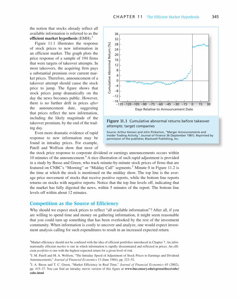
C H A P T E R 1 1 The Efficient Market Hypothesis 345
the notion that stocks already reflect all
available information is referred to as the
efficient market hypothesis (EMH). 3
Figure 11.1 illustrates the response
of stock prices to new information in
an efficient market. The graph plots the
price response of a sample of 194 firms
that were targets of takeover attempts. In
most takeovers, the acquiring firm pays
a substantial premium over current mar-
ket prices. Therefore, announcement of a
takeover attempt should cause the stock
price to jump. The figure shows that
stock prices jump dramatically on the
day the news becomes public. However,
there is no further drift in prices after
the announcement date, suggesting
that prices reflect the new information,
including the likely magnitude of the
takeover premium, by the end of the trad-
ing day.
Even more dramatic evidence of rapid
response to new information may be
found in intraday prices. For example,
Patell and Wolfson show that most of
the stock price response to corporate dividend or earnings announcements occurs within
10 minutes of the announcement. 4 A nice illustration of such rapid adjustment is provided
in a study by Busse and Green, who track minute-by-minute stock prices of firms that are
featured on CNBC’s “Morning” or “Midday Call” segments. 5 Minute 0 in Figure 11.2 is
the time at which the stock is mentioned on the midday show. The top line is the aver-
age price movement of stocks that receive positive reports, while the bottom line reports
returns on stocks with negative reports. Notice that the top line levels off, indicating that
the market has fully digested the news, within 5 minutes of the report. The bottom line
levels off within about 12 minutes.
Competition as the Source of Efficiency
Why should we expect stock prices to reflect “all available information”? After all, if you
are willing to spend time and money on gathering information, it might seem reasonable
that you could turn up something that has been overlooked by the rest of the investment
community. When information is costly to uncover and analyze, one would expect invest-
ment analysis calling for such expenditures to result in an increased expected return.
3 Market efficiency should not be confused with the idea of efficient portfolios introduced in Chapter 7. An infor-
mationally efficient market is one in which information is rapidly disseminated and reflected in prices. An effi-
cient portfolio is one with the highest expected return for a given level of risk. 4 J. M. Patell and M. A. Wolfson, “The Intraday Speed of Adjustment of Stock Prices to Earnings and Dividend
Announcements,” Journal of Financial Economics 13 (June 1984), pp. 223–52. 5 J. A. Busse and T. C. Green, “Market Efficiency in Real Time,” Journal of Financial Economics 65 (2002),
pp. 415–37. You can find an intraday movie version of this figure at www.bus.emory.edu/cgreen/docs/cnbc/
cnbc.html
36
32
28
24
20
16
12
8
4
0
−4
−8
−12
−16−135 −120 −105 −90 −75 −60 −45 −30 −15 0 15 30
Days Relative to Announcement DateC
um
ula
tive
Ab
no
rmal
Ret
urn
(%
)
Figure 11.1 Cumulative abnormal returns before takeover attempts: target companies
Source: Arthur Keown and John Pinkerton, “Merger Announcements and Insider Trading Activity,” Journal of Finance 36 (September 1981). Reprinted by permission of the publisher, Blackwell Publishing, Inc.
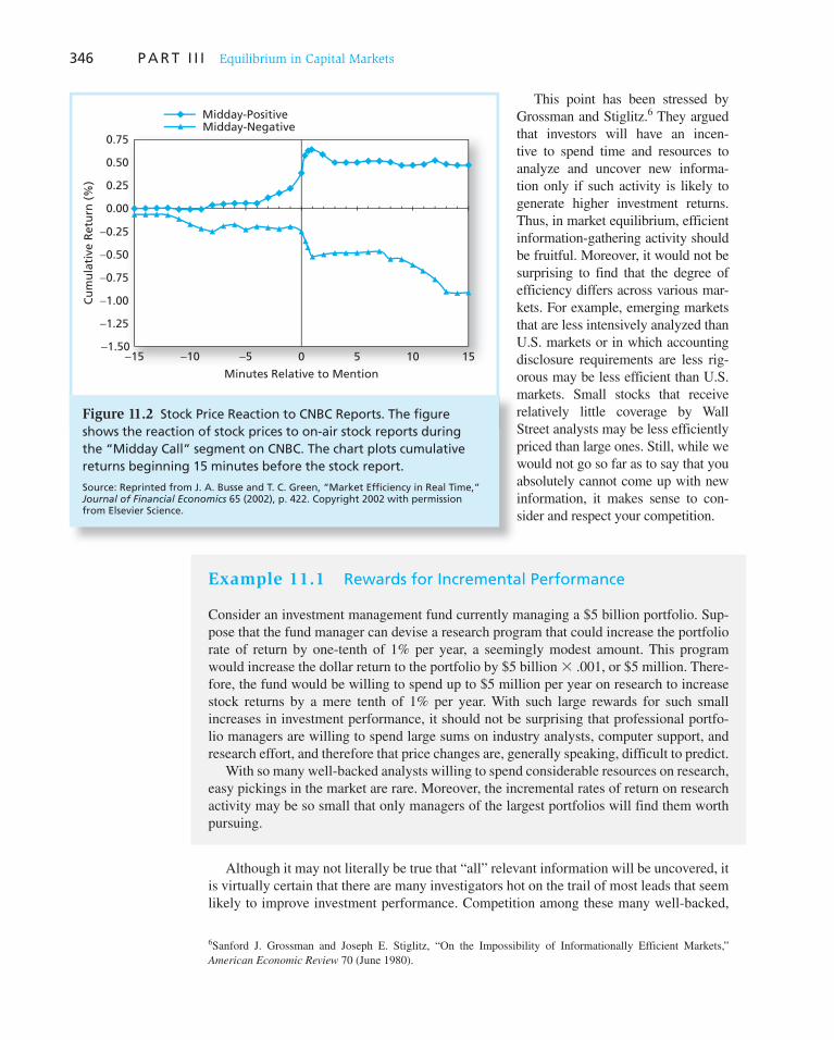
346 P A R T I I I Equilibrium in Capital Markets
This point has been stressed by
Grossman and Stiglitz. 6 They argued
that investors will have an incen-
tive to spend time and resources to
analyze and uncover new informa-
tion only if such activity is likely to
generate higher investment returns.
Thus, in market equilibrium, efficient
information-gathering activity should
be fruitful. Moreover, it would not be
surprising to find that the degree of
efficiency differs across various mar-
kets. For example, emerging markets
that are less intensively analyzed than
U.S. markets or in which accounting
disclosure requirements are less rig-
orous may be less efficient than U.S.
markets. Small stocks that receive
relatively little coverage by Wall
Street analysts may be less efficiently
priced than large ones. Still, while we
would not go so far as to say that you
absolutely cannot come up with new
information, it makes sense to con-
sider and respect your competition.
Example 11.1 Rewards for Incremental Performance
Consider an investment management fund currently managing a $5 billion portfolio. Sup-
pose that the fund manager can devise a research program that could increase the portfolio
rate of return by one-tenth of 1% per year, a seemingly modest amount. This program
would increase the dollar return to the portfolio by $5 billion � .001, or $5 million. There-
fore, the fund would be willing to spend up to $5 million per year on research to increase
stock returns by a mere tenth of 1% per year. With such large rewards for such small
increases in investment performance, it should not be surprising that professional portfo-
lio managers are willing to spend large sums on industry analysts, computer support, and
research effort, and therefore that price changes are, generally speaking, difficult to predict.
With so many well-backed analysts willing to spend considerable resources on research,
easy pickings in the market are rare. Moreover, the incremental rates of return on research
activity may be so small that only managers of the largest portfolios will find them worth
pursuing.
Although it may not literally be true that “all” relevant information will be uncovered, it
is virtually certain that there are many investigators hot on the trail of most leads that seem
likely to improve investment performance. Competition among these many well-backed,
6 Sanford J. Grossman and Joseph E. Stiglitz, “On the Impossibility of Informationally Efficient Markets,”
American Economic Review 70 (June 1980).
−15 −10 −5 0 5 10 15
Minutes Relative to Mention
0.75
0.50
0.25
0.00
−0.25
−0.75
−0.50
−1.00
−1.25
−1.50
Cu
mu
lati
ve R
etu
rn (
%)
Midday-PositiveMidday-Negative
Figure 11.2 Stock Price Reaction to CNBC Reports. The figure shows the reaction of stock prices to on-air stock reports during the “Midday Call” segment on CNBC. The chart plots cumulative returns beginning 15 minutes before the stock report.
Source: Reprinted from J. A. Busse and T. C. Green, “Market Efficiency in Real Time,” Journal of Financial Economics 65 (2002), p. 422. Copyright 2002 with permission from Elsevier Science.

347
“Outsider Trading” and Too Much Information
The Galleon insider-trading case is just the latest chapter in a drama about the proper role of information in driv-ing markets. The story line so far is that Galleon founder Raj Rajaratnam and his colleagues enticed insiders at major corporations into intentionally divulging material nonpub-lic information. If so, these executives would have violated their fiduciary duties to their employers.
There is evidence to support the prosecution case that Galleon analysts knew the information was gathered illegitimately. This includes damning snippets from con-versations captured through wiretaps, such as a Galleon executive telling a source, “You put me in jail if you talk.”
Still, as more facts come out about this case, it will be interesting to see how clear-cut the issues are. In recent decades, these cases have often ended up on murkier ground, raising fundamental questions about how research can be conducted. This is especially true where people are accused of ferreting out too much accurate information. Employees of companies may have clear fiduciary duties to protect corporate secrets, but traders have no such fiduciary obligation. Instead, the Galleon case is about what might be called “outsider trading”—trading by people who gathered information from insiders about company performance or operations, not trading by the insiders themselves.
The reason the U.S. government should tread care-fully in criminalizing outsider trading is that markets run on information, analysis, and the connecting of dots to determine when prices are too high or too low. Economist Milton Friedman once asserted, “You should want more insider trading, not less. You want to give the people most
likely to have knowledge about deficiencies of the com-pany an incentive to make the public aware of that.”
The rules of information engagement for outsiders are especially murky. Information flows these days are increas-ingly about networks. Sophisticated traders such as hedge funds draw on more selected networks such as their inves-tors. As these networks expand, including online through social networking sites, it will become harder to know whether market-moving information originated improp-erly through an insider’s breach or properly through gath-ering of information in other ways.
Stephen Bainbridge, a UCLA law professor, described on his blog this growing conflict between the need for more information to make markets more efficient and prices more accurate versus a regulatory focus on equal access to information. The issue: “Can the SEC prove not just that Rajaratnam had better access to information than the mar-ket generally, but that he got that information by being a participant after the fact in the tipper’s breach of fiduciary duty?”
Until recently, the vagueness of the insider-trading laws was more of an academic topic than a core issue for how markets operate day to day. In today’s world of immediate, global flows of information, markets need greater clarity about how information can be gathered and used. The les-son so far is that knowing when insiders violate their duty is easier than knowing when outsiders go too far in bring-ing accurate information to markets.
Source: L. Gordon Crovitz, “‘Outsider Trading’ and Too Much Information,” The Wall Street Journal, October 26, 2009.
WO
RD
S FRO
M TH
E STREET
highly paid, aggressive analysts ensures that, as a general rule, stock prices ought to reflect
available information regarding their proper levels.
Information is often said to be the most precious commodity on Wall Street, and the com-
petition for it is intense. Sometimes the quest for a competitive advantage can tip over into
a search for illegal inside information. The nearby box reports on a recent insider trading
investigation surrounding the Galleon Group hedge fund but points out that drawing a clear
line between legitimate and prohibited sources of information can be difficult in practice.
Versions of the Efficient Market Hypothesis
It is common to distinguish among three versions of the EMH: the weak, semistrong, and
strong forms of the hypothesis. These versions differ by their notions of what is meant by
the term “all available information.”
The weak-form hypothesis asserts that stock prices already reflect all information that
can be derived by examining market trading data such as the history of past prices, trad-
ing volume, or short interest. This version of the hypothesis implies that trend analysis is
fruitless. Past stock price data are publicly available and virtually costless to obtain. The
weak-form hypothesis holds that if such data ever conveyed reliable signals about future
performance, all investors already would have learned to exploit the signals. Ultimately, the
signals lose their value as they become widely known because a buy signal, for instance,
would result in an immediate price increase.

348 P A R T I I I Equilibrium in Capital Markets
The semistrong-form hypothesis states that all publicly available information regard-
ing the prospects of a firm must be reflected already in the stock price. Such information
includes, in addition to past prices, fundamental data on the firm’s product line, quality
of management, balance sheet composition, patents held, earning forecasts, and account-
ing practices. Again, if investors have access to such information from publicly available
sources, one would expect it to be reflected in stock prices.
Finally, the strong-form version of the efficient market hypothesis states that stock
prices reflect all information relevant to the firm, even including information available
only to company insiders. This version of the hypothesis is quite extreme. Few would
argue with the proposition that corporate officers have access to pertinent information long
enough before public release to enable them to profit from trading on that information.
Indeed, much of the activity of the Securities and Exchange Commission is directed toward
preventing insiders from profiting by exploiting their privileged situation. Rule 10b-5 of
the Security Exchange Act of 1934 sets limits on trading by corporate officers, directors,
and substantial owners, requiring them to report trades to the SEC. These insiders, their
relatives, and any associates who trade on information supplied by insiders are considered
in violation of the law.
Defining insider trading is not always easy, however. After all, stock analysts are in the
business of uncovering information not already widely known to market participants. As
we saw in Chapter 3 as well as in the nearby box, the distinction between private and inside
information is sometimes murky.
CONCEPT CHECK
1
a. Suppose you observed that high-level managers make superior returns on investments in their company’s stock. Would this be a violation of weak-form market efficiency? Would it be a violation of strong-form market efficiency?
b. If the weak form of the efficient market hypothesis is valid, must the strong form also hold? Conversely, does strong-form efficiency imply weak-form efficiency?
11.2 Implications of the EMH
Technical Analysis
Technical analysis is essentially the search for recurrent and predictable patterns in stock
prices. Although technicians recognize the value of information regarding future economic
prospects of the firm, they believe that such information is not necessary for a successful
trading strategy. This is because whatever the fundamental reason for a change in stock
price, if the stock price responds slowly enough, the analyst will be able to identify a trend
that can be exploited during the adjustment period. The key to successful technical analy-
sis is a sluggish response of stock prices to fundamental supply-and-demand factors. This
prerequisite, of course, is diametrically opposed to the notion of an efficient market.
Technical analysts are sometimes called chartists because they study records or charts
of past stock prices, hoping to find patterns they can exploit to make a profit. As an exam-
ple of technical analysis, consider the relative strength approach. The chartist compares
stock performance over a recent period to performance of the market or other stocks in
the same industry. A simple version of relative strength takes the ratio of the stock price
to a market indicator such as the S&P 500 index. If the ratio increases over time, the stock
is said to exhibit relative strength because its price performance is better than that of the

C H A P T E R 1 1 The Efficient Market Hypothesis 349
broad market. Such strength presumably may continue for a long enough period of time to
offer profit opportunities.
One of the most commonly heard components of technical analysis is the notion of
resistance levels or support levels. These values are said to be price levels above which it
is difficult for stock prices to rise, or below which it is unlikely for them to fall, and they
are believed to be levels determined by market psychology.
Example 11.2 Resistance Levels
Consider stock XYZ, which traded for several months at a price of $72, and then declined
to $65. If the stock eventually begins to increase in price, $72 is considered a resistance
level (according to this theory) because investors who bought originally at $72 will be
eager to sell their shares as soon as they can break even on their investment. Therefore,
at prices near $72 a wave of selling pressure would exist. Such activity imparts a type of
“memory” to the market that allows past price history to influence current stock prospects.
The efficient market hypothesis implies that technical analysis is without merit. The past
history of prices and trading volume is publicly available at minimal cost. Therefore, any
information that was ever available from analyzing past prices has already been reflected
in stock prices. As investors compete to exploit their common knowledge of a stock’s price
history, they necessarily drive stock prices to levels where expected rates of return are
exactly commensurate with risk. At those levels one cannot expect abnormal returns.
As an example of how this process works, consider what would happen if the market
believed that a level of $72 truly were a resistance level for stock XYZ in Example 11.2.
No one would be willing to purchase the stock at a price of $71.50, because it would have
almost no room to increase in price, but ample room to fall. However, if no one would
buy it at $71.50, then $71.50 would become a resistance level. But then, using a similar
analysis, no one would buy it at $71, or $70, and so on. The notion of a resistance level is a
logical conundrum. Its simple resolution is the recognition that if the stock is ever to sell at
$71.50, investors must believe that the price can
as easily increase as fall. The fact that investors
are willing to purchase (or even hold) the stock
at $71.50 is evidence of their belief that they can
earn a fair expected rate of return at that price.
An interesting question is whether a techni-
cal rule that seems to work will continue to work in the future once it becomes widely rec-
ognized. A clever analyst may occasionally uncover a profitable trading rule, but the real
test of efficient markets is whether the rule itself becomes reflected in stock prices once its
value is discovered. Once a useful technical rule (or price pattern) is discovered, it ought to
be invalidated when the mass of traders attempts to exploit it. In this sense, price patterns
ought to be self-destructing.
Thus the market dynamic is one of a continual search for profitable trading rules, fol-
lowed by destruction by overuse of those rules found to be successful, followed by more
search for yet-undiscovered rules.
Fundamental Analysis
Fundamental analysis uses earnings and dividend prospects of the firm, expectations
of future interest rates, and risk evaluation of the firm to determine proper stock prices.
CONCEPT CHECK
2 If everyone in the market believes in resis-tance levels, why do these beliefs not become self- fulfilling prophecies?

350 P A R T I I I Equilibrium in Capital Markets
Ultimately, it represents an attempt to determine the present discounted value of all the
payments a stockholder will receive from each share of stock. If that value exceeds the
stock price, the fundamental analyst would recommend purchasing the stock.
Fundamental analysts usually start with a study of past earnings and an examination
of company balance sheets. They supplement this analysis with further detailed economic
analysis, ordinarily including an evaluation of the quality of the firm’s management, the
firm’s standing within its industry, and the prospects for the industry as a whole. The hope
is to attain insight into future performance of the firm that is not yet recognized by the rest
of the market. Chapters 17 through 19 provide a detailed discussion of the types of analy-
ses that underlie fundamental analysis.
Once again, the efficient market hypothesis predicts that most fundamental analysis also
is doomed to failure. If the analyst relies on publicly available earnings and industry infor-
mation, his or her evaluation of the firm’s prospects is not likely to be significantly more
accurate than those of rival analysts. Many well-informed, well-financed firms conduct
such market research, and in the face of such competition it will be difficult to uncover data
not also available to other analysts. Only analysts with a unique insight will be rewarded.
Fundamental analysis is much more difficult than merely identifying well-run firms
with good prospects. Discovery of good firms does an investor no good in and of itself if
the rest of the market also knows those firms are good. If the knowledge is already public,
the investor will be forced to pay a high price for those firms and will not realize a superior
rate of return.
The trick is not to identify firms that are good, but to find firms that are better than
everyone else’s estimate. Similarly, poorly run firms can be great bargains if they are not
quite as bad as their stock prices suggest.
This is why fundamental analysis is difficult. It is not enough to do a good analysis of
a firm; you can make money only if your analysis is better than that of your competitors
because the market price will already reflect all commonly available information.
Active versus Passive Portfolio Management
By now it is apparent that casual efforts to pick stocks are not likely to pay off. Competition
among investors ensures that any easily implemented stock evaluation technique will be
used widely enough so that any insights derived will be reflected in stock prices. Only
serious analysis and uncommon techniques are likely to generate the differential insight
necessary to yield trading profits.
Moreover, these techniques are economically feasible only for managers of large port-
folios. If you have only $100,000 to invest, even a 1% per year improvement in perfor-
mance generates only $1,000 per year, hardly enough to justify herculean efforts. The
billion-dollar manager, however, reaps extra income of $10 million annually from the same
1% increment.
If small investors are not in a favored position to conduct active portfolio management,
what are their choices? The small investor probably is better off investing in mutual funds.
By pooling resources in this way, small investors can gain from economies of scale.
More difficult decisions remain, though. Can investors be sure that even large mutual
funds have the ability or resources to uncover mispriced stocks? Furthermore, will any
mispricing be sufficiently large to repay the costs entailed in active portfolio management?
Proponents of the efficient market hypothesis believe that active management is largely
wasted effort and unlikely to justify the expenses incurred. Therefore, they advocate a pas-
sive investment strategy that makes no attempt to outsmart the market. A passive strategy
aims only at establishing a well-diversified portfolio of securities without attempting to

C H A P T E R 1 1 The Efficient Market Hypothesis 351
find under- or overvalued stocks. Passive management is usually characterized by a buy-
and-hold strategy. Because the efficient market theory indicates that stock prices are at
fair levels, given all available information, it makes no sense to buy and sell securities fre-
quently, which generates large brokerage fees without increasing expected performance.
One common strategy for passive management is to create an index fund, which is a
fund designed to replicate the performance of a broad-based index of stocks. For example,
Vanguard’s 500 Index Fund holds stocks in direct proportion to their weight in the Standard
& Poor’s 500 stock price index. The performance of the 500 Index Fund therefore repli-
cates the performance of the S&P 500. Investors in this fund obtain broad diversification
with relatively low management fees. The fees can be kept to a minimum because Vanguard
does not need to pay analysts to assess stock prospects and does not incur transaction costs
from high portfolio turnover. Indeed, while the typical annual charge for an actively man-
aged equity fund is more than 1% of assets, the expense ratio of the 500 Index Fund is only
.18%. Today, Vanguard’s 500 Index Fund is among the largest equity mutual funds with
$100 billion of assets in May 2010, and about 10%–15% of equity funds are indexed.
Indexing need not be limited to the S&P 500, however. For example, some of the funds
offered by the Vanguard Group track the Wilshire 5000 index, the Salomon Brothers Broad
Investment Grade Bond Index, the MSCI index of small-capitalization U.S. companies, the
European equity market, and the Pacific Basin equity market. Several other mutual fund
complexes have introduced indexed portfolios, but Vanguard dominates the retail market
for indexed products.
Exchange-traded funds, or ETFs, are a close (and often lower-expense) alternative to
indexed mutual funds. As noted in Chapter 4, these are shares in diversified portfolios that
can be bought or sold just like shares of individual stock. ETFs matching several broad stock
market indexes such as the S&P 500 or Wilshire 5000 indexes and dozens of international
and industry stock indexes are available to investors who want to hold a diversified sector
of a market without attempting active security
selection.
A hybrid strategy also is fairly common,
where the fund maintains a passive core, which is
an indexed position, and augments that position
with one or more actively managed portfolios.
The Role of Portfolio Management in an Efficient Market
If the market is efficient, why not pick stocks by throwing darts at The Wall Street Journal
instead of trying rationally to choose a stock portfolio? This is a tempting conclusion to
draw from the notion that security prices are fairly set, but it is far too facile. There is a role
for rational portfolio management, even in perfectly efficient markets.
You have learned that a basic principle in portfolio selection is diversification. Even if
all stocks are priced fairly, each still poses firm-specific risk that can be eliminated through
diversification. Therefore, rational security selection, even in an efficient market, calls for
the selection of a well-diversified portfolio providing the systematic risk level that the
investor wants.
Rational investment policy also requires that tax considerations be reflected in secu-
rity choice. High-tax-bracket investors generally will not want the same securities that low
bracket investors find favorable. At an obvious level, high-bracket investors find it advanta-
geous to buy tax-exempt municipal bonds despite their relatively low pretax yields, whereas
those same bonds are unattractive to low-tax-bracket or tax-exempt investors. At a more sub-
tle level, high-bracket investors might want to tilt their portfolios in the direction of capital
CONCEPT CHECK
3 What would happen to market efficiency if all investors attempted to follow a passive strategy?

352 P A R T I I I Equilibrium in Capital Markets
gains as opposed to interest income, because capital gains are taxed less heavily and because
the option to defer the realization of capital gains income is more valuable the higher the
current tax bracket. Hence these investors may prefer stocks that yield low dividends yet
offer greater expected capital gain income. They also will be more attracted to investment
opportunities for which returns are sensitive to tax benefits, such as real estate ventures.
A third argument for rational portfolio management relates to the particular risk profile
of the investor. For example, a Toyota executive whose annual bonus depends on Toyota’s
profits generally should not invest additional amounts in auto stocks. To the extent that
his or her compensation already depends on Toyota’s well-being, the executive is already
overinvested in Toyota and should not exacerbate the lack of diversification. This lesson
was learned with considerable pain in September 2008 by Lehman Brothers employees
who were famously invested in their own firm when the company failed. Roughly 30% of
the shares in the firm were owned by its 24,000 employees, and their losses on those shares
totaled around $10 billion.
Investors of varying ages also might warrant different portfolio policies with regard
to risk bearing. For example, older investors who are essentially living off savings might
choose to avoid long-term bonds whose market values fluctuate dramatically with changes
in interest rates (discussed in Part Four). Because these investors are living off accumulated
savings, they require conservation of principal. In contrast, younger investors might be
more inclined toward long-term inflation-indexed bonds. The steady flow of real income
over long periods of time that is locked in with these bonds can be more important than
preservation of principal to those with long life expectancies.
In conclusion, there is a role for portfolio management even in an efficient market.
Investors’ optimal positions will vary according to factors such as age, tax bracket, risk
aversion, and employment. The role of the portfolio manager in an efficient market is to
tailor the portfolio to these needs, rather than to beat the market.
Resource Allocation
We’ve focused so far on the investment implications of the efficient market hypothesis.
Deviations from efficiency may offer profit opportunities to better-informed traders at the
expense of less-informed ones.
However, deviations from informational efficiency would also result in a large cost that
will be borne by all citizens, namely, inefficient resource allocation. Recall that in a capital-
ist economy, investments in real assets such as plant, equipment, and know-how are guided
in large part by the prices of financial assets. For example, if the value of telecommunica-
tion capacity reflected in stock market prices exceeds the cost of installing such capacity,
managers might justifiably conclude that telecom investments seem to have positive net
present value. In this manner, capital market prices guide allocation of real resources.
If markets were inefficient and securities commonly mispriced, then resources would
be systematically misallocated. Corporations with overpriced securities would be able to
obtain capital too cheaply, and corporations with undervalued securities might forgo invest-
ment opportunities because the cost of raising capital would be too high. Therefore, ineffi-
cient capital markets would diminish one of the most potent benefits of a market economy.
As an example of what can go wrong, consider the dot-com bubble of the late 1990s,
which sent a strong but, as it turned out, wildly overoptimistic signal about prospects for
Internet and telecommunication firms and ultimately led to substantial over investment in
those industries.
Before writing off markets as a means to guide resource allocation, however, one has
to be reasonable about what can be expected from market forecasts. In particular, you

C H A P T E R 1 1 The Efficient Market Hypothesis 353
shouldn’t confuse an efficient market, where all available information is reflected in prices,
with a perfect foresight market. Even “all available information” is still far from complete
information, and generally rational market forecasts will sometimes be wrong; sometimes,
in fact, they will be very wrong.
11.3 Event Studies
The notion of informationally efficient markets leads to a powerful research methodology.
If security prices reflect all currently available information, then price changes must reflect
new information. Therefore, it seems that one should be able to measure the importance of
an event of interest by examining price changes during the period in which the event occurs.
An event study describes a technique of empirical financial research that enables an
observer to assess the impact of a particular event on a firm’s stock price. A stock market
analyst might want to study the impact of dividend changes on stock prices, for example.
An event study would quantify the relationship between dividend changes and stock returns.
Analyzing the impact of any particular event is more difficult than it might at first
appear. On any day, stock prices respond to a wide range of economic news such as updated
forecasts for GDP, inflation rates, interest rates, or corporate profitability. Isolating the part
of a stock price movement that is attributable to a specific event is not a trivial exercise.
The general approach starts with a proxy for what the stock’s return would have been
in the absence of the event. The abnormal return due to the event is estimated as the
d ifference between the stock’s actual return and this benchmark. Several methodologies for
estimating the benchmark return are used in practice. For example, a very simple approach
measures the stock’s abnormal return as its return minus that of a broad market index. An
obvious refinement is to compare the stock’s return to those of other stocks matched accord-
ing to criteria such as firm size, beta, recent performance, or ratio of price to book value per
share. Another approach estimates normal returns using an asset pricing model such as the
CAPM or one of its multifactor generalizations such as the Fama-French three-factor model.
Many researchers have used a “market model” to estimate abnormal returns. This
approach is based on the index models we introduced in Chapter 9. Recall that a single-
index model holds that stock returns are determined by a market factor and a firm-specific
factor. The stock return, r t , during a given period t, would be expressed mathematically as
rt 5 a 1 brMt 1 et (11.1)
where r Mt is the market’s rate of return during the period and e t is the part of a security’s
return resulting from firm-specific events. The parameter b measures sensitivity to the
market return, and a is the average rate of return the stock would realize in a period with
a zero market return. 7 Equation 11.1 therefore provides a decomposition of r t into market
and firm-specific factors. The firm-specific or abnormal return may be interpreted as the
unexpected return that results from the event.
Determination of the abnormal return in a given period requires an estimate of e t .
Therefore, we rewrite Equation 11.1:
et 5 rt 2 (a 1 brMt) (11.2)
7 We know from Chapter 9 that the CAPM implies that the intercept a in Equation 11.1 should equal r f (1 � � ).
Nevertheless, it is customary to estimate the intercept in this equation empirically rather than imposing the CAPM
value. One justification for this practice is that empirically fitted security market lines seem flatter than predicted
by the CAPM (see Chapter 13), which would make the intercept implied by the CAPM too small.

354 P A R T I I I Equilibrium in Capital Markets
Equation 11.2 has a simple interpretation: The residual, e t , that is, the component presum-
ably due to the event in question, is the stock’s return over and above what one would predict
based on broad market movements in that period, given the stock’s sensitivity to the market.
The market model is a highly flexible tool, because it can be generalized to include
richer models of benchmark returns, for example, by including industry as well as broad
market returns on the right-hand side of Equation 11.1, or returns on indexes constructed
to match characteristic such as firm size. However, one must be careful that regression
parameters in Equation 11.1 (the intercept a and slope b ) are estimated properly. In par-
ticular, they must be estimated using data sufficiently separated in time from the event in
question that they are not affected by event-period abnormal stock performance. In part
because of this vulnerability of the market model, returns on characteristic-matched port-
folios have become more widely used benchmarks in recent years.
Example 11.3 Abnormal Returns
Suppose that the analyst has estimated that a � .05% and b � .8. On a day that the mar-
ket goes up by 1%, you would predict from Equation 11.1 that the stock should rise by
an expected value of .05% � .8 � 1% � .85%. If the stock actually rises by 2%, the
analyst would infer that firm-specific news that day caused an additional stock return of
2% � .85% � 1.15%. This is the abnormal return for the day.
We measure the impact of an event by estimating the abnormal return on a stock (or
group of stocks) at the moment the information about the event becomes known to the
market. For example, in a study of the impact of merger attempts on the stock prices of tar-
get firms, the announcement date is the date on which the public is informed that a merger
is to be attempted. The abnormal returns of each firm surrounding the announcement date
are computed, and the statistical significance and magnitude of the typical abnormal return
are assessed to determine the impact of the newly released information.
One concern that complicates event studies arises from leakage of information. Leakage
occurs when information regarding a relevant event is released to a small group of inves-
tors before official public release. In this case the stock price might start to increase (in the
case of a “good news” announcement) days or weeks before the official announcement
date. Any abnormal return on the announcement date is then a poor indicator of the total
impact of the information release. A better indicator would be the cumulative abnormal
return, which is simply the sum of all abnormal returns over the time period of interest.
The cumulative abnormal return thus captures the total firm-specific stock movement for
an entire period when the market might be responding to new information.
Figure 11.1 (earlier in the chapter) presents the results from a fairly typical event study.
The authors of this study were interested in leakage of information before merger announce-
ments and constructed a sample of 194 firms that were targets of takeover attempts. In
most takeovers, stockholders of the acquired firms sell their shares to the acquirer at sub-
stantial premiums over market value. Announcement of a takeover attempt is good news
for shareholders of the target firm and therefore should cause stock prices to jump.
Figure 11.1 confirms the good-news nature of the announcements. On the announce-
ment day, called day 0, the average cumulative abnormal return (CAR) for the sample of
takeover candidates increases substantially, indicating a large and positive abnormal return
on the announcement date. Notice that immediately after the announcement date the CAR
no longer increases or decreases significantly. This is in accord with the efficient mar-
ket hypothesis. Once the new information became public, the stock prices jumped almost

C H A P T E R 1 1 The Efficient Market Hypothesis 355
immediately in response to the good news. With prices once again fairly set, reflecting the
effect of the new information, further abnormal returns on any particular day are equally
likely to be positive or negative. In fact, for a sample of many firms, the average abnormal
return should be extremely close to zero, and thus the CAR will show neither upward nor
downward drift. This is precisely the pattern shown in Figure 11.1 .
The pattern of returns for the days preceding the public announcement date yields some
interesting evidence about efficient markets and information leakage. If insider trading rules
were perfectly obeyed and perfectly enforced, stock prices should show no abnormal returns
on days before the public release of relevant news, because no special firm-specific infor-
mation would be available to the market before public announcement. Instead, we should
observe a clean jump in the stock price only on the announcement day. In fact, Figure 11.1
shows that the prices of the takeover targets clearly start an upward drift 30 days before the
public announcement. It appears that information is leaking to some market participants who
then purchase the stocks before the public announcement. Such evidence of leakage appears
almost universally in event studies, suggesting at least some abuse of insider trading rules.
Actually, the SEC also can take some comfort from patterns such as that in Figure 11.1 .
If insider trading rules were widely and flagrantly violated, we would expect to see abnor-
mal returns earlier than they appear in these results. For example, in the case of mergers,
the CAR would turn positive as soon as acquiring firms decided on their takeover targets,
because insiders would start trading immediately. By the time of the public announce-
ment, the insiders would have bid up the stock prices of target firms to levels reflecting the
merger attempt, and the abnormal returns on the actual public announcement date would
be close to zero. The dramatic increase in the CAR that we see on the announcement
date indicates that a good deal of these announcements are indeed news to the market
and that stock prices did not already reflect complete knowledge about the takeovers. It
would appear, therefore, that SEC enforcement does have a substantial effect on restricting
insider trading, even if some amount of it still persists.
Event study methodology has become a widely accepted tool to measure the economic
impact of a wide range of events. For example, the SEC regularly uses event studies to
measure illicit gains captured by traders who may have violated insider trading or other
securities laws. 8 Event studies are also used in fraud cases, where the courts must assess
damages caused by a fraudulent activity.
Example 11.4 Using Abnormal Returns to Infer Damages
Suppose the stock of a company with market value of $100 million falls by 4% on the day
that news of an accounting scandal surfaces. The rest of the market, however, generally did
well that day. The market indexes were up sharply, and on the basis of the usual relation-
ship between the stock and the market, one would have expected a 2% gain on the stock.
We would conclude that the impact of the scandal was a 6% drop in value, the difference
between the 2% gain that we would have expected and the 4% drop actually observed. One
might then infer that the damages sustained from the scandal were $6 million, because the
value of the firm (after adjusting for general market movements) fell by 6% of $100 million
when investors became aware of the news and reassessed the value of the stock.
8 For a review of SEC applications of this technique, see Mark Mitchell and Jeffry Netter, “The Role of Financial
Economics in Securities Fraud Cases: Applications at the Securities and Exchange Commission,” The Business
Lawyer 49 (February 1994), pp. 545–90.

356 P A R T I I I Equilibrium in Capital Markets
11.4 Are Markets Efficient?
CONCEPT CHECK
4 Suppose that we see negative abnormal returns (declining CARs) after an announcement date. Is this a violation of efficient markets?
The Issues
Not surprisingly, the efficient market hypothesis does not exactly arouse enthusiasm in the
community of professional portfolio managers. It implies that a great deal of the activity
of portfolio managers—the search for undervalued securities—is at best wasted effort,
and quite probably harmful to clients because it costs money and leads to imperfectly
diversified portfolios. Consequently, the EMH has never been widely accepted on Wall
Street, and debate continues today on the degree to which security analysis can improve
investment performance. Before discussing empirical tests of the hypothesis, we want to
note three factors that together imply that the debate probably never will be settled: the
magnitude issue, the selection bias issue, and the lucky event issue.
The Magnitude Issue We noted that an investment manager overseeing a $5 billion
portfolio who can improve performance by only .1% per year will increase investment
earnings by .001 � $5 billion � $5 million annually. This manager clearly would be worth
her salary! Yet can we, as observers, statistically measure her contribution? Probably not:
A .1% contribution would be swamped by the yearly volatility of the market. Remember,
the annual standard deviation of the well-diversified S&P 500 index has been around 20%.
Against these fluctuations a small increase in performance would be hard to detect.
All might agree that stock prices are very close to fair values and that only managers of
large portfolios can earn enough trading profits to make the exploitation of minor mispric-
ing worth the effort. According to this view, the actions of intelligent investment managers
are the driving force behind the constant evolution of market prices to fair levels. Rather
than ask the qualitative question, Are markets efficient? we ought instead to ask a more
quantitative question: How efficient are markets?
The Selection Bias Issue Suppose that you discover an investment scheme that
could really make money. You have two choices: either publish your technique in The
Wall Street Journal to win fleeting fame, or keep your technique secret and use it to earn
millions of dollars. Most investors would choose the latter option, which presents us with a
conundrum. Only investors who find that an investment scheme cannot generate abnormal
returns will be willing to report their findings to the whole world. Hence opponents of the
efficient markets view of the world always can use evidence that various techniques do
not provide investment rewards as proof that the techniques that do work simply are not
being reported to the public. This is a problem in selection bias; the outcomes we are able
to observe have been preselected in favor of failed attempts. Therefore, we cannot fairly
evaluate the true ability of portfolio managers to generate winning stock market strategies.
The Lucky Event Issue In virtually any month it seems we read an article about some
investor or investment company with a fantastic investment performance over the recent
past. Surely the superior records of such investors disprove the efficient market hypothesis.
Yet this conclusion is far from obvious. As an analogy to the investment game, consider
a contest to flip the most number of heads out of 50 trials using a fair coin. The expected

357
outcome for any person is, of course, 50% heads and 50% tails. If 10,000 people, however,
compete in this contest, it would not be surprising if at least one or two contestants flipped
more than 75% heads. In fact, elementary statistics tells us that the expected number of
contestants flipping 75% or more heads would be two. It would be silly, though, to crown
these people the “head-flipping champions of the world.” Obviously, they are simply the
contestants who happened to get lucky on the day of the event. (See the nearby box.)
The analogy to efficient markets is clear. Under the hypothesis that any stock is fairly
priced given all available information, any bet on a stock is simply a coin toss. There is
equal likelihood of winning or losing the bet. However, if many investors using a variety
of schemes make fair bets, statistically speaking, some of those investors will be lucky and
win a great majority of the bets. For every big winner, there may be many big losers, but we
never hear of these managers. The winners, though, turn up in The Wall Street Journal as
the latest stock market gurus; then they can make a fortune publishing market newsletters.
Our point is that after the fact there will have been at least one successful investment
scheme. A doubter will call the results luck, the successful investor will call it skill. The
proper test would be to see whether the successful investors can repeat their performance
in another period, yet this approach is rarely taken.
With these caveats in mind, we turn now to some of the empirical tests of the efficient
market hypothesis.
CONCEPT CHECK
5
Legg Mason’s Value Trust, managed by Bill Miller, outperformed the S&P 500 in each of the 15 years ending in 2005. Is Miller’s performance sufficient to dissuade you from a belief in efficient markets? If not, would any performance record be sufficient to dissuade you? Now consider that in the next 3 years, the fund dramatically underperformed the S&P 500; by the end of 2008, its cumulative 18-year performance was barely different from the index. Does this affect your opinion?
How to Guarantee a Successful Market Newsletter
Suppose you want to make your fortune publishing a market newsletter. You need first to convince potential subscribers that you have talent worth paying for. But what if you have no talent? The solution is simple: start eight newsletters.
In year 1, let four of your newsletters predict an up- market and four a down-market. In year 2, let half of the originally optimistic group of newsletters continue to pre-dict an up-market and the other half a down-market. Do the same for the originally pessimistic group. Continue in this manner to obtain the pattern of predictions in the table that follows (U � prediction of an up-market, D � prediction of a down-market).
After 3 years, no matter what has happened to the market, one of the newsletters would have had a perfect prediction record. This is because after 3 years there are 2 3 � 8 outcomes for the market, and we have covered all eight possibilities with the eight newsletters. Now, we sim-ply slough off the seven unsuccessful newsletters, and mar-ket the eighth newsletter based on its perfect track record. If we want to establish a newsletter with a perfect track record over a 4-year period, we need 2 4 � 16 newsletters. A 5-year period requires 32 newsletters, and so on.
After the fact, the one newsletter that was always right will attract attention for your uncanny fore-sight and investors will rush to pay large fees for its advice. Your fortune is made, and you have never even researched the market!
WARNING: This scheme is illegal! The point, however, is that with hundreds of market newsletters, you can find one that has stumbled onto an apparently remarkable string of successful predictions without any real degree of skill. After the fact, someone’s prediction history can seem to imply great forecasting skill. This person is the one we will read about in The Wall Street Journal; the others will be forgotten.
Newsletter Predictions
Year 1 2 3 4 5 6 7 8
1 U U U U D D D D
2 U U D D U U D D
3 U D U D U D U D
WO
RD
S FRO
M TH
E STREET
358 P A R T I I I Equilibrium in Capital Markets
Weak-Form Tests: Patterns in Stock Returns
Returns over Short Horizons Early tests of efficient markets were tests of the
weak form. Could speculators find trends in past prices that would enable them to earn
abnormal profits? This is essentially a test of the efficacy of technical analysis.
One way of discerning trends in stock prices is by measuring the serial correlation
of stock market returns. Serial correlation refers to the tendency for stock returns to be
related to past returns. Positive serial correlation means that positive returns tend to fol-
low positive returns (a momentum type of property). Negative serial correlation means
that positive returns tend to be followed by negative returns (a reversal or “correction”
property). Both Conrad and Kaul 9 and Lo and MacKinlay 10 examine weekly returns of
NYSE stocks and find positive serial correlation over short horizons. However, the cor-
relation coefficients of weekly returns tend to be fairly small, at least for large stocks for
which price data are the most reliably up-to-date. Thus, while these studies demonstrate
weak price trends over short periods, 11 the evidence does not clearly suggest the existence
of trading opportunities.
While broad market indexes demonstrate only weak serial correlation, there appears to
be stronger momentum in performance across market sectors exhibiting the best and worst
recent returns. In an investigation of intermediate-horizon stock price behavior (using 3- to
12-month holding periods), Jegadeesh and Titman 12 found a momentum effect in which
good or bad recent performance of particular stocks continues over time. They conclude
that while the performance of individual stocks is highly unpredictable, portfolios of the
best-performing stocks in the recent past appear to outperform other stocks with enough
reliability to offer profit opportunities. Thus, it appears that there is evidence of short- to
intermediate-horizon price momentum in both the aggregate market and cross-sectionally
(i.e., across particular stocks).
Returns over Long Horizons Although studies of short- to intermediate- horizon
returns have detected momentum in stock market prices, tests 13 of long-horizon returns
(i.e., returns over multiyear periods) have found suggestions of pronounced negative
long-term serial correlation in the performance of the aggregate market. The latter result
has given rise to a “fads hypothesis,” which asserts that the stock market might over-
react to relevant news. Such overreaction leads to positive serial correlation (momen-
tum) over short time horizons. Subsequent correction of the overreaction leads to poor
performance following good performance and vice versa. The corrections mean that a
run of positive returns eventually will tend to be followed by negative returns, leading to
9 Jennifer Conrad and Gautam Kaul, “Time-Variation in Expected Returns,” Journal of Business 61 (October
1988), pp. 409–25.
10 Andrew W. Lo and A. Craig MacKinlay, “Stock Market Prices Do Not Follow Random Walks: Evidence from
a Simple Specification Test,” Review of Financial Studies 1 (1988), pp. 41–66.
11 On the other hand, there is evidence that share prices of individual securities (as opposed to broad market
indexes) are more prone to reversals than continuations at very short horizons. See, for example, B. Lehmann,
“Fads, Martingales and Market Efficiency,” Quarterly Journal of Economics 105 (February 1990), pp. 1–28; and
N. Jegadeesh, “Evidence of Predictable Behavior of Security Returns,” Journal of Finance 45 (September 1990),
pp. 881–98. However, as Lehmann notes, this is probably best interpreted as due to liquidity problems after big
movements in stock prices as market makers adjust their positions in the stock.
12 Narasimhan Jegadeesh and Sheridan Titman, “Returns to Buying Winners and Selling Losers: Implications for
Stock Market Efficiency,” Journal of Finance 48 (March 1993), pp. 65–91.
13 Eugene F. Fama and Kenneth R. French, “Permanent and Temporary Components of Stock Prices,” Journal
of Political Economy 96 (April 1988), pp. 24–73; James Poterba and Lawrence Summers, “Mean Reversion in
Stock Prices: Evidence and Implications,” Journal of Financial Economics 22 (October 1988), pp. 27–59.

C H A P T E R 1 1 The Efficient Market Hypothesis 359
negative serial correlation over longer horizons. These episodes of apparent overshoot-
ing followed by correction give the stock market the appearance of fluctuating around
its fair value.
These long-horizon results are dramatic, but the studies offer far from conclusive evi-
dence regarding efficient markets. First, these studies need not be interpreted as evidence for
stock market fads. An alternative interpretation of these results holds that they indicate only
that the market risk premium varies over time. For example, when the risk premium and the
required return on the market rises, stock prices will fall. When the market then rises (on
average) at this higher rate of return, the data convey the impression of a stock price recov-
ery. The apparent overshooting and correction are in fact no more than a rational response of
market prices to changes in discount rates.
In addition to studies suggestive of overreaction in overall stock market returns over
long horizons, many other studies suggest that over long horizons, extreme performance
in particular securities also tends to reverse itself: The stocks that have performed best in
the recent past seem to underperform the rest of the market in following periods, while
the worst past performers tend to offer above-average future performance. DeBondt and
Thaler 14 and Chopra, Lakonishok, and Ritter 15 find strong tendencies for poorly perform-
ing stocks in one period to experience sizable reversals over the subsequent period, while
the best-performing stocks in a given period tend to follow with poor performance in the
following period.
For example, the DeBondt and Thaler study found that if one were to rank the perfor-
mance of stocks over a 5-year period and then group stocks into portfolios based on invest-
ment performance, the base-period “loser” portfolio (defined as the 35 stocks with the
worst investment performance) outperformed the “winner” portfolio (the top 35 stocks) by
an average of 25% (cumulative return) in the following 3-year period. This reversal effect,
in which losers rebound and winners fade back, suggests that the stock market overreacts
to relevant news. After the overreaction is recognized, extreme investment performance is
reversed. This phenomenon would imply that a contrarian investment strategy— investing
in recent losers and avoiding recent winners—should be profitable. Moreover, these returns
seem pronounced enough to be exploited profitably.
Thus it appears that there may be short-run momentum but long-run reversal patterns in
price behavior both for the market as a whole and across sectors of the market. One inter-
pretation of this pattern is that short-run overreaction (which causes momentum in prices)
may lead to long-term reversals (when the market recognizes its past error).
Predictors of Broad Market Returns
Several studies have documented the ability of easily observed variables to predict mar-
ket returns. For example, Fama and French 16 showed that the return on the aggregate
stock market tends to be higher when the dividend/price ratio, the dividend yield, is high.
Campbell and Shiller 17 found that the earnings yield can predict market returns. Keim and
14 Werner F. M. DeBondt and Richard Thaler, “Does the Stock Market Overreact?” Journal of Finance 40 (1985),
pp. 793–805.
15 Navin Chopra, Josef Lakonishok, and Jay R. Ritter, “Measuring Abnormal Performance: Do Stocks Overreact?”
Journal of Financial Economics 31 (1992), pp. 235–68.
16 Eugene F. Fama and Kenneth R. French, “Dividend Yields and Expected Stock Returns,” Journal of Financial
Economics 22 (October 1988), pp. 3–25.
17 John Y. Campbell and Robert Shiller, “Stock Prices, Earnings and Expected Dividends,” Journal of Finance 43
(July 1988), pp. 661–76.
360 P A R T I I I Equilibrium in Capital Markets
Stambaugh 18 showed that bond market data such as the spread between yields on high- and
low-grade corporate bonds also help predict broad market returns.
Again, the interpretation of these results is difficult. On the one hand, they may imply
that stock returns can be predicted, in violation of the efficient market hypothesis. More
probably, however, these variables are proxying for variation in the market risk premium.
For example, given a level of dividends or earnings, stock prices will be lower and divi-
dend and earnings yields will be higher when the risk premium (and therefore the expected
market return) is higher. Thus a high dividend or earnings yield will be associated with
higher market returns. This does not indicate a violation of market efficiency. The predict-
ability of market returns is due to predictability in the risk premium, not in risk-adjusted
abnormal returns.
Fama and French 19 showed that the yield spread between high- and low-grade bonds
has greater predictive power for returns on low-grade bonds than for returns on high-grade
bonds, and greater predictive power for stock returns than for bond returns, suggesting that
the predictability in returns is in fact a risk premium rather than evidence of market inef-
ficiency. Similarly, the fact that the dividend yield on stocks helps to predict bond market
returns suggests that the yield captures a risk premium common to both markets rather
than mispricing in the equity market.
Semistrong Tests: Market Anomalies
Fundamental analysis uses a much wider range of information to create portfolios than
does technical analysis. Investigations of the efficacy of fundamental analysis ask whether
publicly available information beyond the trading history of a security can be used to
improve investment performance, and therefore are tests of semistrong-form market
efficiency. Surprisingly, several easily accessible statistics, for example, a stock’s price–
earnings ratio or its market capitalization, seem to predict abnormal risk-adjusted returns.
Findings such as these, which we will review in the following pages, are difficult to rec-
oncile with the efficient market hypothesis, and therefore are often referred to as efficient
market anomalies.
A difficulty in interpreting these tests is that we usually need to adjust for portfolio
risk before evaluating the success of an investment strategy. Many tests, for example,
have used the CAPM to adjust for risk. However, we know that even if beta is a relevant
descriptor of stock risk, the empirically measured quantitative trade-off between risk as
measured by beta and expected return differs from the predictions of the CAPM. (We
review this evidence in Chapter 13.) If we use the CAPM to adjust portfolio returns for
risk, inappropriate adjustments may lead to the conclusion that various portfolio strate-
gies can generate superior returns, when in fact it simply is the risk adjustment procedure
that has failed.
Another way to put this is to note that tests of risk-adjusted returns are joint tests of the
efficient market hypothesis and the risk adjustment procedure. If it appears that a portfolio
strategy can generate superior returns, we must then choose between rejecting the EMH
and rejecting the risk adjustment technique. Usually, the risk adjustment technique is based
on more-questionable assumptions than is the EMH; by opting to reject the procedure, we
are left with no conclusion about market efficiency.
18 Donald B. Keim and Robert F. Stambaugh, “Predicting Returns in the Stock and Bond Markets,” Journal of
Financial Economics 17 (1986), pp. 357–90.
19 Eugene F. Fama and Kenneth R. French, “Business Conditions and Expected Returns on Stocks and Bonds,”
Journal of Financial Economics 25 (November 1989), pp. 3–22.
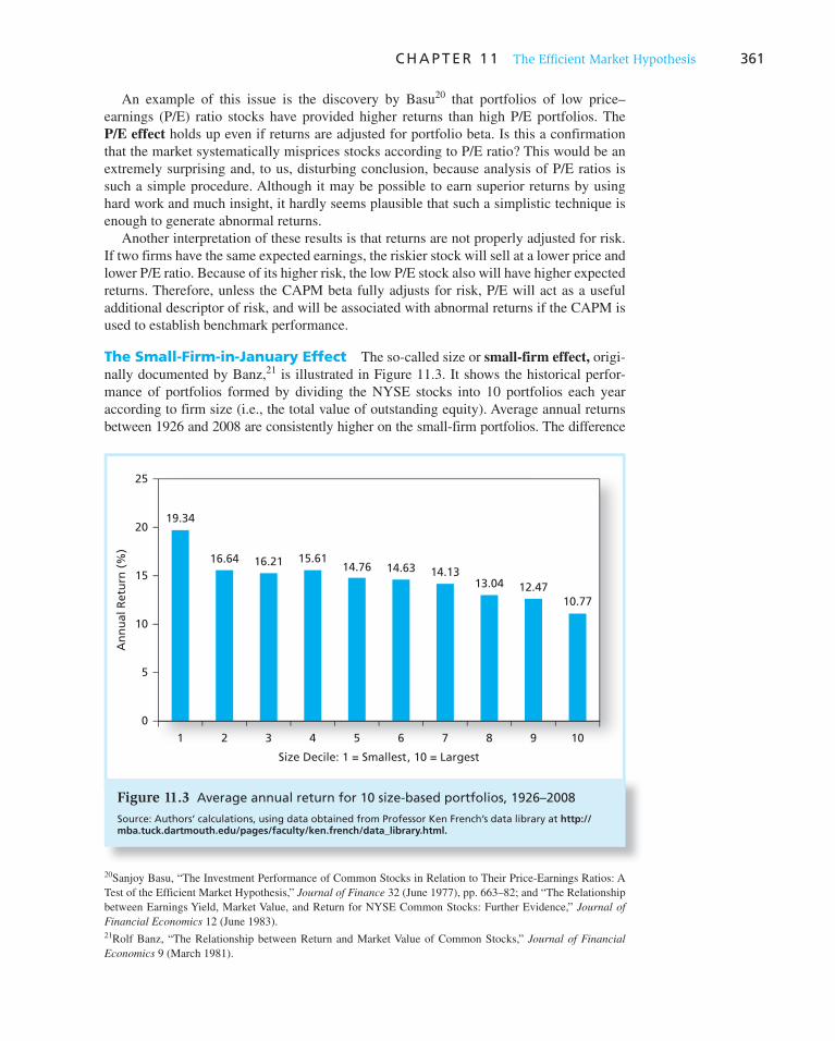
C H A P T E R 1 1 The Efficient Market Hypothesis 361
An example of this issue is the discovery by Basu 20 that portfolios of low price–
e arnings (P/E) ratio stocks have provided higher returns than high P/E portfolios. The
P/E effect holds up even if returns are adjusted for portfolio beta. Is this a confirmation
that the market systematically misprices stocks according to P/E ratio? This would be an
extremely surprising and, to us, disturbing conclusion, because analysis of P/E ratios is
such a simple procedure. Although it may be possible to earn superior returns by using
hard work and much insight, it hardly seems plausible that such a simplistic technique is
enough to generate abnormal returns.
Another interpretation of these results is that returns are not properly adjusted for risk.
If two firms have the same expected earnings, the riskier stock will sell at a lower price and
lower P/E ratio. Because of its higher risk, the low P/E stock also will have higher expected
returns. Therefore, unless the CAPM beta fully adjusts for risk, P/E will act as a useful
additional descriptor of risk, and will be associated with abnormal returns if the CAPM is
used to establish benchmark performance.
The Small-Firm-in-January Effect The so-called size or small-firm effect, origi-
nally documented by Banz, 21 is illustrated in Figure 11.3 . It shows the historical perfor-
mance of portfolios formed by dividing the NYSE stocks into 10 portfolios each year
according to firm size (i.e., the total value of outstanding equity). Average annual returns
between 1926 and 2008 are consistently higher on the small-firm portfolios. The difference
20 Sanjoy Basu, “The Investment Performance of Common Stocks in Relation to Their Price-Earnings Ratios: A
Test of the Efficient Market Hypothesis,” Journal of Finance 32 (June 1977), pp. 663–82; and “The Relationship
between Earnings Yield, Market Value, and Return for NYSE Common Stocks: Further Evidence,” Journal of
Financial Economics 12 (June 1983). 21 Rolf Banz, “The Relationship between Return and Market Value of Common Stocks,” Journal of Financial
Economics 9 (March 1981).
0
5
10
15
20
25
1 2
19.34
16.64 16.21 15.6114.6314.76 14.13
13.04 12.4710.77
3 4 5 6 7 8 9 10
An
nu
al R
etu
rn (
%)
Size Decile: 1 = Smallest, 10 = Largest
Figure 11.3 Average annual return for 10 size-based portfolios, 1926–2008
Source: Authors’ calculations, using data obtained from Professor Ken French’s data library at http://mba.tuck.dartmouth.edu/pages/faculty/ken.french/data_library.html.

362 P A R T I I I Equilibrium in Capital Markets
in average annual return between portfolio 10 (with the largest firms) and portfolio 1 (with
the smallest firms) is 8.57%. Of course, the smaller-firm portfolios tend to be riskier. But
even when returns are adjusted for risk using the CAPM, there is still a consistent premium
for the smaller-sized portfolios.
Imagine earning a premium of this size on a billion-dollar portfolio. Yet it is remarkable
that following a simple (even simplistic) rule such as “invest in low-capitalization stocks”
should enable an investor to earn excess returns. After all, any investor can measure firm
size at little cost. One would not expect such minimal effort to yield such large rewards.
Later studies (Keim, 22 Reinganum, 23 and Blume and Stambaugh 24 ) showed that the
small-firm effect occurs virtually entirely in January, in fact, in the first 2 weeks of January.
The size effect is in fact a “small-firm-in-January” effect.
The Neglected-Firm Effect and Liquidity Effects Arbel and Strebel25 gave
another interpretation of the small-firm-in-January effect. Because small firms tend to be
neglected by large institutional traders, information about smaller firms is less available.
This information deficiency makes smaller firms riskier investments that command higher
returns. “Brand-name” firms, after all, are subject to considerable monitoring from insti-
tutional investors, which promises high-quality information, and presumably investors do
not purchase “generic” stocks without the prospect of greater returns.
As evidence for the neglected-firm effect, Arbel 26 divided firms into highly researched,
moderately researched, and neglected groups based on the number of institutions hold-
ing the stock. The January effect was in fact largest for the neglected firms. An article
by Merton 27 shows that neglected firms might be expected to earn higher equilibrium
returns as compensation for the risk associated with limited information. In this sense the
neglected-firm premium is not strictly a market inefficiency, but is a type of risk premium.
Work by Amihud and Mendelson 28 on the effect of liquidity on stock returns might be
related to both the small-firm and neglected-firm effects. As we noted in Chapter 9, inves-
tors will demand a rate-of-return premium to invest in less-liquid stocks that entail higher
trading costs. In accord with this hypothesis, Amihud and Mendelson showed that these
stocks have a strong tendency to exhibit abnormally high risk-adjusted rates of return.
Because small and less-analyzed stocks as a rule are less liquid, the liquidity effect might
be a partial explanation of their abnormal returns. However, this theory does not explain
why the abnormal returns of small firms should be concentrated in January. In any case,
exploiting these effects can be more difficult than it would appear. The high trading costs
on small stocks can easily wipe out any apparent abnormal profit opportunity.
22 Donald B. Keim, “Size Related Anomalies and Stock Return Seasonality: Further Empirical Evidence,” Journal
of Financial Economics 12 (June 1983).
23 Marc R. Reinganum, “The Anomalous Stock Market Behavior of Small Firms in January: Empirical Tests for
Tax-Loss Effects,” Journal of Financial Economics 12 (June 1983).
24 Marshall E. Blume and Robert F. Stambaugh, “Biases in Computed Returns: An Application to the Size Effect,”
Journal of Financial Economics, 1983.
25 Avner Arbel and Paul J. Strebel, “Pay Attention to Neglected Firms,” Journal of Portfolio Management, Winter
1983.
26 Avner Arbel, “Generic Stocks: An Old Product in a New Package,” Journal of Portfolio Management, Summer
1985. 27 Robert C. Merton, “A Simple Model of Capital Market Equilibrium with Incomplete Information,” Journal of
Finance 42 (1987), pp. 483–510.
28 Yakov Amihud and Haim Mendelson, “Asset Pricing and the Bid–Ask Spread,” Journal of Financial Economics
17 (December 1986), pp. 223–50; and “Liquidity, Asset Prices, and Financial Policy,” Financial Analysts Journal
47 (November/December 1991), pp. 56–66.
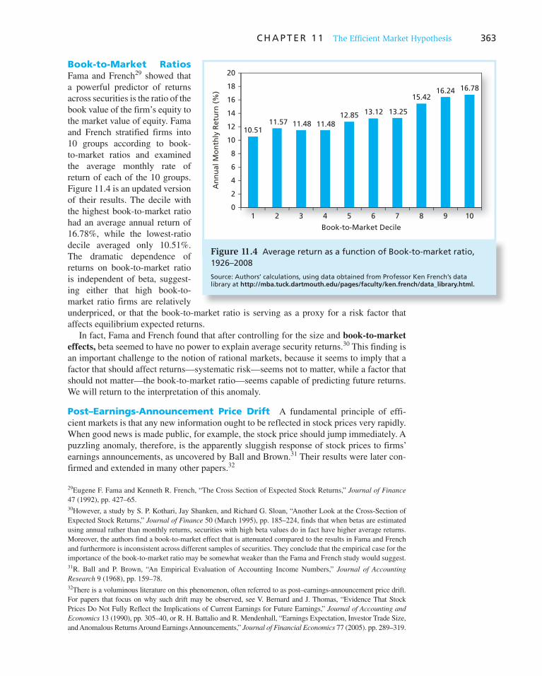
C H A P T E R 1 1 The Efficient Market Hypothesis 363
Book-to-Market Ratios Fama and French 29 showed that
a powerful predictor of returns
across securities is the ratio of the
book value of the firm’s equity to
the market value of equity. Fama
and French stratified firms into
10 groups according to book-
to-market ratios and examined
the average monthly rate of
return of each of the 10 groups.
Figure 11.4 is an updated version
of their results. The decile with
the highest book-to-market ratio
had an average annual return of
16.78%, while the lowest-ratio
decile averaged only 10.51%.
The dramatic dependence of
returns on book-to-market ratio
is independent of beta, suggest-
ing either that high book-to-
market ratio firms are relatively
underpriced, or that the book-to-market ratio is serving as a proxy for a risk factor that
affects equilibrium expected returns.
In fact, Fama and French found that after controlling for the size and book-to-market
effects, beta seemed to have no power to explain average security returns. 30 This finding is
an important challenge to the notion of rational markets, because it seems to imply that a
factor that should affect returns—systematic risk—seems not to matter, while a factor that
should not matter—the book-to-market ratio—seems capable of predicting future returns.
We will return to the interpretation of this anomaly.
Post–Earnings-Announcement Price Drift A fundamental principle of effi-
cient markets is that any new information ought to be reflected in stock prices very rapidly.
When good news is made public, for example, the stock price should jump immediately. A
puzzling anomaly, therefore, is the apparently sluggish response of stock prices to firms’
earnings announcements, as uncovered by Ball and Brown. 31 Their results were later con-
firmed and extended in many other papers. 32
29 Eugene F. Fama and Kenneth R. French, “The Cross Section of Expected Stock Returns,” Journal of Finance
47 (1992), pp. 427–65 . 30 However, a study by S. P. Kothari, Jay Shanken, and Richard G. Sloan, “Another Look at the Cross-Section of
Expected Stock Returns,” Journal of Finance 50 (March 1995), pp. 185–224, finds that when betas are estimated
using annual rather than monthly returns, securities with high beta values do in fact have higher average returns.
Moreover, the authors find a book-to-market effect that is attenuated compared to the results in Fama and French
and furthermore is inconsistent across different samples of securities. They conclude that the empirical case for the
importance of the book-to-market ratio may be somewhat weaker than the Fama and French study would suggest. 31 R. Ball and P. Brown, “An Empirical Evaluation of Accounting Income Numbers,” Journal of Accounting
Research 9 (1968), pp. 159–78. 32 There is a voluminous literature on this phenomenon, often referred to as post–earnings-announcement price drift.
For papers that focus on why such drift may be observed, see V. Bernard and J. Thomas, “Evidence That Stock
Prices Do Not Fully Reflect the Implications of Current Earnings for Future Earnings,” Journal of Accounting and
Economics 13 (1990), pp. 305–40, or R. H. Battalio and R. Mendenhall, “Earnings Expectation, Investor Trade Size,
and Anomalous Returns Around Earnings Announcements,” Journal of Financial Economics 77 (2005). pp. 289–319.
Book-to-Market Decile
An
nu
al M
on
thly
Ret
urn
(%
)
20
18
16
14
12
10
8
6
4
2
01 2 3 4 5 6 7 8 9 10
10.5111.57 11.48 11.48
12.85 13.12 13.25
15.4216.24 16.78
Figure 11.4 Average return as a function of Book-to-market ratio, 1926–2008
Source: Authors’ calculations, using data obtained from Professor Ken French’s data library at http://mba.tuck.dartmouth.edu/pages/faculty/ken.french/data_library.html.
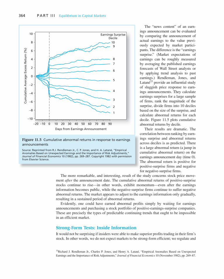
364 P A R T I I I Equilibrium in Capital Markets
The “news content” of an earn-
ings announcement can be evaluated
by comparing the announcement of
actual earnings to the value previ-
ously expected by market partici-
pants. The difference is the “earnings
surprise.” (Market expectations of
earnings can be roughly measured
by averaging the published earnings
forecasts of Wall Street analysts or
by applying trend analysis to past
earnings.) Rendleman, Jones, and
Latané 33 provide an influential study
of sluggish price response to earn-
ings announcements. They calculate
earnings surprises for a large sample
of firms, rank the magnitude of the
surprise, divide firms into 10 deciles
based on the size of the surprise, and
calculate abnormal returns for each
decile. Figure 11.5 plots cumulative
abnormal returns by decile.
Their results are dramatic. The
correlation between ranking by earn-
ings surprise and abnormal returns
across deciles is as predicted. There
is a large abnormal return (a jump in
cumulative abnormal return) on the
earnings announcement day (time 0).
The abnormal return is positive for
positive-surprise firms and negative
for negative-surprise firms.
The more remarkable, and interesting, result of the study concerns stock price move-
ment after the announcement date. The cumulative abnormal returns of positive-surprise
stocks continue to rise—in other words, exhibit momentum—even after the earnings
information becomes public, while the negative-surprise firms continue to suffer negative
abnormal returns. The market appears to adjust to the earnings information only gradually,
resulting in a sustained period of abnormal returns.
Evidently, one could have earned abnormal profits simply by waiting for earnings
announcements and purchasing a stock portfolio of positive-earnings-surprise companies.
These are precisely the types of predictable continuing trends that ought to be impossible
in an efficient market.
Strong-Form Tests: Inside Information
It would not be surprising if insiders were able to make superior profits trading in their firm’s
stock. In other words, we do not expect markets to be strong-form efficient; we regulate and
33 Richard J. Rendleman Jr., Charles P. Jones, and Henry A. Latané, “Empirical Anomalies Based on Unexpected
Earnings and the Importance of Risk Adjustments,” Journal of Financial Economics 10 (November 1982), pp. 269–87.
10
8
6
4
2
0
−2
−4
−6
−8
−10
−20 −10 0 10 20 30 40 50 60 70 80 90
Cu
mu
lati
ve A
vera
ge
Exce
ss R
etu
rn (
%)
Days from Earnings Announcement
109
8
7
6
5
4
3
2
1
Earnings SurpriseDecile
Figure 11.5 Cumulative abnormal returns in response to earnings announcements
Source: Reprinted from R.J. Rendleman Jr., C. P. Jones, and H. A. Latané, “Empirical Anomalies Based on Unexpected Earnings and the Importance of Risk Adjustments,” Journal of Financial Economics 10 (1982), pp. 269–287. Copyright 1982 with permission from Elsevier Science.

C H A P T E R 1 1 The Efficient Market Hypothesis 365
limit trades based on inside information. The ability of insiders to trade profitably in their
own stock has been documented in studies by Jaffe, 34 Seyhun, 35 Givoly and Palmon, 36 and
others. Jaffe’s was one of the earlier studies that documented the tendency for stock prices to
rise after insiders intensively bought shares and to fall after intensive insider sales.
Can other investors benefit by following insiders’ trades? The Securities and Exchange
Commission requires all insiders to register their trading activity and it publishes these
trades in an Official Summary of Security Transactions and Holdings. Since 2002, insiders
must report large trades to the SEC within 2 business days. Once the Official Summary is
published, the trades become public information. At that point, if markets are efficient,
fully and immediately processing the information released in the Official Summary of trad-
ing, an investor should no longer be able to profit from following the pattern of those
trades. Several Internet sites contain information on insider trading. See the Web sites at
our Online Learning Center ( www.mhhe.com/bkm ) for some suggestions.
The study by Seyhun, which carefully tracked the public release dates of the Official
Summary, found that following insider transactions would be to no avail. Although there is
some tendency for stock prices to increase even after the Official Summary reports insider
buying, the abnormal returns are not of sufficient magnitude to overcome transaction costs.
Interpreting the Anomalies
How should we interpret the ever-growing anomalies literature? Does it imply that markets
are grossly inefficient, allowing for simplistic trading rules to offer large profit opportuni-
ties? Or are there other, more-subtle interpretations?
Risk Premiums or Inefficiencies? The price-earnings, small-firm, market-to-
book, momentum, and long-term reversal effects are currently among the most puzzling
phenomena in empirical finance. There are several interpretations of these effects. First note
that to some extent, some of these phenomena may be related. The feature that small firms,
low-market-to-book firms, and recent “losers” seem to have in common is a stock price that
has fallen considerably in recent months or years. Indeed, a firm can become a small firm or
a low-market-to-book firm by suffering a sharp drop in price. These groups therefore may
contain a relatively high proportion of distressed firms that have suffered recent difficulties.
Fama and French 37 argue that these effects can be explained as manifestations of risk
premiums. Using their three-factor model, introduced in the previous chapter, they show
that stocks with higher “betas” (also known as factor loadings) on size or market-to-book
factors have higher average returns; they interpret these returns as evidence of a risk pre-
mium associated with the factor. This model does a much better job than the one-factor
CAPM in explaining security returns. While size or book-to-market ratios per se are obvi-
ously not risk factors, they perhaps might act as proxies for more fundamental determinants
of risk. Fama and French argue that these patterns of returns may therefore be consistent
with an efficient market in which expected returns are consistent with risk. In this regard,
it is worth noting that returns to “style portfolios,” for example, the return on portfolios
constructed based on the ratio of book-to-market value (specifically, the Fama-French high
34 Jeffrey F. Jaffe, “Special Information and Insider Trading,” Journal of Business 47 (July 1974).
35 H. Nejat Seyhun, “Insiders’ Profits, Costs of Trading and Market Efficiency,” Journal of Financial Economics
16 (1986).
36 Dan Givoly and Dan Palmon, “Insider Trading and Exploitation of Inside Information: Some Empirical
Evidence,” Journal of Business 58 (1985).
37 Eugene F. Fama and Kenneth R. French, “Common Risk Factors in the Returns on Stocks and Bonds,” Journal
of Financial Economics 33 (1993), pp. 3–56.
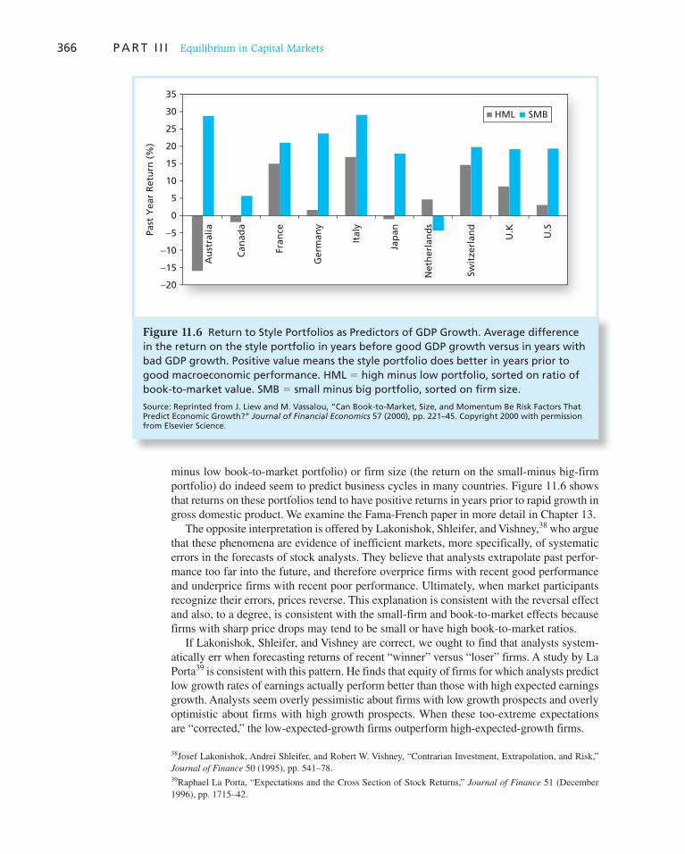
366 P A R T I I I Equilibrium in Capital Markets
minus low book-to-market portfolio) or firm size (the return on the small-minus big-firm
portfolio) do indeed seem to predict business cycles in many countries. Figure 11.6 shows
that returns on these portfolios tend to have positive returns in years prior to rapid growth in
gross domestic product. We examine the Fama-French paper in more detail in Chapter 13.
The opposite interpretation is offered by Lakonishok, Shleifer, and Vishney, 38 who argue
that these phenomena are evidence of inefficient markets, more specifically, of systematic
errors in the forecasts of stock analysts. They believe that analysts extrapolate past perfor-
mance too far into the future, and therefore overprice firms with recent good performance
and underprice firms with recent poor performance. Ultimately, when market participants
recognize their errors, prices reverse. This explanation is consistent with the reversal effect
and also, to a degree, is consistent with the small-firm and book-to-market effects because
firms with sharp price drops may tend to be small or have high book-to-market ratios.
If Lakonishok, Shleifer, and Vishney are correct, we ought to find that analysts system-
atically err when forecasting returns of recent “winner” versus “loser” firms. A study by La
Porta 39 is consistent with this pattern. He finds that equity of firms for which analysts predict
low growth rates of earnings actually perform better than those with high expected earnings
growth. Analysts seem overly pessimistic about firms with low growth prospects and overly
optimistic about firms with high growth prospects. When these too-extreme expectations
are “corrected,” the low-expected-growth firms outperform high-expected-growth firms.
38 Josef Lakonishok, Andrei Shleifer, and Robert W. Vishney, “Contrarian Investment, Extrapolation, and Risk,”
Journal of Finance 50 (1995), pp. 541–78. 39 Raphael La Porta, “Expectations and the Cross Section of Stock Returns,” Journal of Finance 51 (December
1996), pp. 1715–42.
35
30
25
20
15
10
5
0
−5
−10
−15
−20
Past
Yea
r R
etu
rn (
%)
Au
stra
lia
Can
ada
Fran
ce
Ger
man
y
Ital
y
Jap
an
Net
her
lan
ds
Swit
zerl
and
U.K U.S
HML SMB
Figure 11.6 Return to Style Portfolios as Predictors of GDP Growth. Average difference in the return on the style portfolio in years before good GDP growth versus in years with bad GDP growth. Positive value means the style portfolio does better in years prior to good macroeconomic performance. HML � high minus low portfolio, sorted on ratio of book-to-market value. SMB � small minus big portfolio, sorted on firm size.
Source: Reprinted from J. Liew and M. Vassalou, “Can Book-to-Market, Size, and Momentum Be Risk Factors That Predict Economic Growth?” Journal of Financial Economics 57 (2000), pp. 221–45. Copyright 2000 with permission from Elsevier Science.

C H A P T E R 1 1 The Efficient Market Hypothesis 367
Anomalies or Data Mining? We have covered many of the so-called anomalies
cited in the literature, but our list could go on and on. Some wonder whether these anoma-
lies are really unexplained puzzles in financial markets, or whether they instead are an
artifact of data mining. After all, if one reruns the computer database of past returns over
and over and examines stock returns along enough dimensions, simple chance will cause
some criteria to appear to predict returns.
In this regard, it is noteworthy that some anomalies have not shown much staying power
after being reported in the academic literature. For example, after the small-firm effect was
published in the early 1980s, it promptly disappeared for much of the rest of the decade.
Similarly, the book-to-market strategy, which commanded considerable attention in the
early 1990s, was ineffective for the rest of that decade.
Still, even acknowledging the potential for data mining, a common thread seems to
run through many of the anomalies we have considered, lending support to the notion that
there is a real puzzle to explain. Value stocks—defined by low P/E ratio, high book-to-
market ratio, or depressed prices relative to historic levels—seem to have provided higher
average returns than “glamour” or growth stocks.
One way to address the problem of data mining is to find a data set that has not already
been researched and see whether the relationship in question shows up in the new data.
Such studies have revealed size, momentum, and book-to-market effects in other security
markets around the world. While these phenomena may be a manifestation of a systematic
risk premium, the precise nature of that risk is not fully understood.
Bubbles and Market Efficiency
Every so often, asset prices seem (at least in retrospect) to lose their grounding in reality.
For example, in the tulip mania in 17th-century Holland, tulip prices peaked at several
times the annual income of a skilled worker. This episode has become the symbol of a spec-
ulative “bubble” in which prices appear to depart from any semblance of intrinsic value.
Bubbles seem to arise when a rapid run-up in prices creates a widespread expectation that
they will continue to rise. As more and more investors try to get in on the action, they push
prices even further. Inevitably, however, the run-up stalls and the bubble ends in a crash.
Less than a century after tulip mania, the South Sea Bubble in England became almost
as famous. In this episode, the share price of the South Sea Company rose from £128 in
January 1720 to £550 in May, and peaked at around £1,000 in August—just before the
bubble burst and the share price collapsed to £150 in September, leading to widespread
bankruptcies among those who had borrowed to buy shares on credit. In fact, the company
was a major lender of money to investors willing to buy (and thus bid up) its shares. This
sequence may sound familiar to anyone who lived through the dot-com boom and bust of
1995–2002 40 or, more recently, the financial turmoil of 2008, with origins widely attri-
buted to a collapsing housing price bubble.
The position that security prices in these instances represented rational, unbiased assess-
ments of intrinsic value is difficult to defend. And in fact, some economists, most notably
Hyman Minsky, have suggested that bubbles arise naturally. During periods of stability
and rising prices, investors extrapolate that stability into the future and become more will-
ing to take on risk. Risk premiums shrink, leading to further increases in asset prices, and
expectations become even more optimistic in a self-fulfilling cycle. But in the end, pricing
and risk taking become excessive and the bubble bursts. Ironically, the initial period of
stability fosters behavior that ultimately results in instability.
40 The dot-com boom gave rise to the term irrational exuberance. In this vein, consider that one company going
public in the investment boom of 1720 described itself simply as “a company for carrying out an undertaking of
great advantage, but nobody to know what it is.”

368 P A R T I I I Equilibrium in Capital Markets
But beware of jumping to the conclusion that asset prices may generally be thought of
as arbitrary and obvious trading opportunities abundant. First, most bubbles become “obvi-
ous” only in retrospect. At the time, the price run-up often seems to have a defensible ratio-
nale. In the dot-com boom, for example, many contemporary observers rationalized stock
price gains as justified by the prospect of a new and more profitable economy, driven by
technological advances. Even the irrationality of the tulip mania may have been overblown
in its later retelling. 41 In addition, security valuation is intrinsically difficult. Given the
considerable imprecision of estimates of intrinsic value, large bets on perceived mispricing
may entail hubris.
Moreover, even if you suspect that prices are in fact “wrong,” taking advantage of them
can be difficult. We explore these issues in more detail in the following chapter, but for
now, we simply point out some impediments to making aggressive bets against an asset,
among them, the costs of short selling overpriced securities as well as potential problems
obtaining the securities to sell short, and the possibility that even if you are ultimately
correct, the market may disagree and prices still can move dramatically against you in the
short term, thus wiping out your portfolio.
11.5 Mutual Fund and Analyst Performance
We have documented some of the apparent chinks in the armor of efficient market propo-
nents. For investors, the issue of market efficiency boils down to whether skilled investors
can make consistent abnormal trading profits. The best test is to look at the performance
of market professionals to see if they can generate performance superior to that of a pas-
sive index fund that buys and holds the market. We will look at two facets of professional
performance: that of stock market analysts who recommend investment positions and that
of mutual fund managers who actually manage portfolios.
Stock Market Analysts
Stock market analysts historically have worked for brokerage firms, which presents an
immediate problem in interpreting the value of their advice: analysts have tended to be
overwhelmingly positive in their assessment of the prospects of firms. 42 For example, on
a scale of 1 (strong buy) to 5 (strong sell), the average recommendation for 5,628 covered
firms in 1996 was 2.04. 43 As a result, we cannot take positive recommendations (e.g., to
buy) at face value. Instead, we must look at either the relative strength of analyst recommen-
dations compared to those for other firms, or at the change in consensus recommendations.
Womack 44 focuses on changes in analysts’ recommendations and finds that positive
changes are associated with increased stock prices of about 5%, and negative changes
result in average price decreases of 11%. One might wonder whether these price changes
41 For interesting discussions of this possibility, see Peter Garber, Famous First Bubbles: The Fundamentals of
Early Manias (Cambridge: MIT Press, 2000), and Anne Goldgar, Tulipmania: Money, Honor, and Knowledge in
the Dutch Golden Age (Chicago: University of Chicago Press, 2007).
42 This problem may be less severe in the future; one recent reform intended to mitigate the conflict of interest in
having brokerage firms that sell stocks also provide investment advice is to separate analyst coverage from the
other activities of the firm.
43 B. Barber, R. Lehavy, M. McNichols, and B. Trueman, “Can Investors Profit from the Prophets? Security
Analyst Recommendations and Stock Returns,” Journal of Finance 56 (April 2001), pp. 531–63.
44 K. L. Womack, “Do Brokerage Analysts’ Recommendations Have Investment Value?” Journal of Finance 51
(March 1996), pp. 137–67.

C H A P T E R 1 1 The Efficient Market Hypothesis 369
reflect the market’s recognition of analysts’ superior information or insight about firms
or, instead, simply result from new buy or sell pressure brought on by the recommenda-
tions themselves. Womack argues that price impact seems to be permanent, and therefore
consistent with the hypothesis that analysts do in fact reveal new information. Jegadeesh,
Kim, Krische, and Lee 45 also find that changes in consensus recommendations are associ-
ated with price changes, but that the level of consensus recommendations is an inconsistent
predictor of future stock performance.
Barber, Lehavy, McNichols, and Trueman 46 focus on the level of consensus recom-
mendations and show that firms with the most-favorable recommendations outperform
those with the least-favorable recommendations. While their results seem impressive, the
authors note that portfolio strategies based on analyst consensus recommendations would
result in extremely heavy trading activity with associated costs that probably would wipe
out the potential profits from the strategy.
In sum, the literature suggests some value added by analysts, but ambiguity remains.
Are superior returns following analyst upgrades due to revelation of new information or
due to changes in investor demand in response to the changed outlook? Also, are these
results exploitable by investors who necessarily incur trading costs?
Mutual Fund Managers
As we pointed out in Chapter 4, casual evidence does not support the claim that profes-
sionally managed portfolios can consistently beat the market. Figure 4.2 in that chapter
demonstrated that between 1972 and 2009 the returns of a passive portfolio indexed to the
Wilshire 5000 typically would have been better than those of the average equity fund. On
the other hand, there was some (admittedly inconsistent) evidence of persistence in per-
formance, meaning that the better managers in one period tended to be better managers in
following periods. Such a pattern would suggest that the better managers can with some
consistency outperform their competitors, and it would be inconsistent with the notion that
market prices already reflect all relevant information.
The analyses cited in Chapter 4 were based on total returns; they did not properly adjust
returns for exposure to systematic risk factors. In this section we revisit the question of
mutual fund performance, paying more attention to the benchmark against which perfor-
mance ought to be evaluated.
As a first pass, we might examine the risk-adjusted returns (i.e., the alpha, or return in
excess of required return based on beta and the market index return in each period) of a
large sample of mutual funds. But the market index may not be an adequate benchmark
against which to evaluate mutual fund returns. Because mutual funds tend to maintain con-
siderable holdings in equity of small firms, whereas the capitalization-weighted index is
dominated by large firms, mutual funds as a whole will tend to outperform the index when
small firms outperform large ones and underperform when small firms fare worse. Thus a
better benchmark for the performance of funds would be an index that separately incorpo-
rates the stock market performance of smaller firms.
The importance of the benchmark can be illustrated by examining the returns on small
stocks in various subperiods. 47 In the 20-year period between 1945 and 1964, for example,
45 N. Jegadeesh, J. Kim, S. D. Krische, and C. M. Lee, “Analyzing the Analysts: When Do Recommendations Add
Value?” Journal of Finance 59 (June 2004), pp. 1083–124.
46 Barber et al., op. cit.
47 This illustration and the statistics cited are based on E. J. Elton, M. J. Gruber, S. Das, and M. Hlavka, “Efficiency
with Costly Information: A Reinterpretation of Evidence from Managed Portfolios,” Review of Financial
Studies 6 (1993), pp. 1–22, which is discussed shortly.
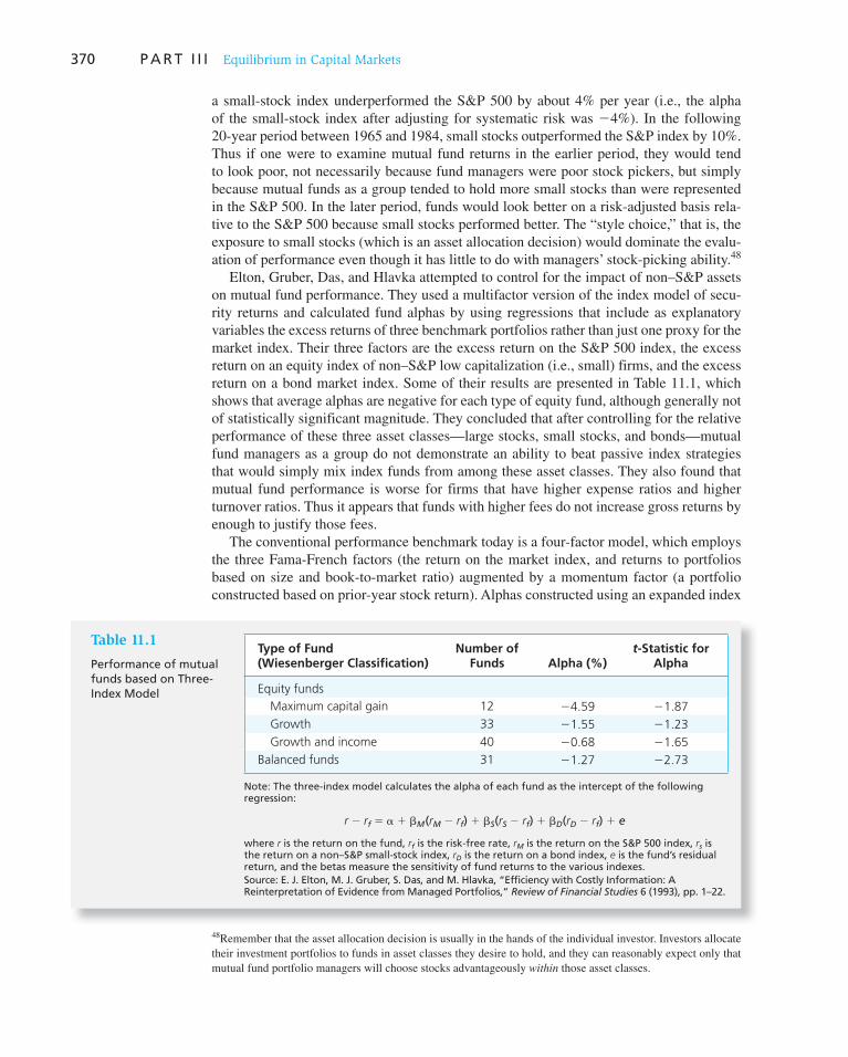
370 P A R T I I I Equilibrium in Capital Markets
a small-stock index underperformed the S&P 500 by about 4% per year (i.e., the alpha
of the small-stock index after adjusting for systematic risk was �4%). In the following
20-year period between 1965 and 1984, small stocks outperformed the S&P index by 10%.
Thus if one were to examine mutual fund returns in the earlier period, they would tend
to look poor, not necessarily because fund managers were poor stock pickers, but simply
because mutual funds as a group tended to hold more small stocks than were represented
in the S&P 500. In the later period, funds would look better on a risk-adjusted basis rela-
tive to the S&P 500 because small stocks performed better. The “style choice,” that is, the
exposure to small stocks (which is an asset allocation decision) would dominate the evalu-
ation of performance even though it has little to do with managers’ stock-picking ability. 48
Elton, Gruber, Das, and Hlavka attempted to control for the impact of non–S&P assets
on mutual fund performance. They used a multifactor version of the index model of secu-
rity returns and calculated fund alphas by using regressions that include as explanatory
variables the excess returns of three benchmark portfolios rather than just one proxy for the
market index. Their three factors are the excess return on the S&P 500 index, the excess
return on an equity index of non–S&P low capitalization (i.e., small) firms, and the excess
return on a bond market index. Some of their results are presented in Table 11.1 , which
shows that average alphas are negative for each type of equity fund, although generally not
of statistically significant magnitude. They concluded that after controlling for the relative
performance of these three asset classes—large stocks, small stocks, and bonds—mutual
fund managers as a group do not demonstrate an ability to beat passive index strategies
that would simply mix index funds from among these asset classes. They also found that
mutual fund performance is worse for firms that have higher expense ratios and higher
turnover ratios. Thus it appears that funds with higher fees do not increase gross returns by
enough to justify those fees.
The conventional performance benchmark today is a four-factor model, which employs
the three Fama-French factors (the return on the market index, and returns to portfolios
based on size and book-to-market ratio) augmented by a momentum factor (a portfolio
constructed based on prior-year stock return). Alphas constructed using an expanded index
48 Remember that the asset allocation decision is usually in the hands of the individual investor. Investors allocate
their investment portfolios to funds in asset classes they desire to hold, and they can reasonably expect only that
mutual fund portfolio managers will choose stocks advantageously within those asset classes.
Table 11.1
Performance of mutual funds based on Three-Index Model
Type of Fund (Wiesenberger Classification)
Number of Funds Alpha (%)
t-Statistic for Alpha
Equity funds
Maximum capital gain 12 �4.59 �1.87
Growth 33 �1.55 �1.23
Growth and income 40 �0.68 �1.65
Balanced funds 31 �1.27 �2.73
Note: The three-index model calculates the alpha of each fund as the intercept of the following regression:
r � rf � � � �M(rM � rf) � �S(rS � rf) � �D(rD � rf) � e
where r is the return on the fund, r f is the risk-free rate, r M is the return on the S&P 500 index, r s is the return on a non–S&P small-stock index, r D is the return on a bond index, e is the fund’s residual return, and the betas measure the sensitivity of fund returns to the various indexes. Source: E. J. Elton, M. J. Gruber, S. Das, and M. Hlavka, “Efficiency with Costly Information: A Reinterpretation of Evidence from Managed Portfolios,” Review of Financial Studies 6 (1993), pp. 1–22.

C H A P T E R 1 1 The Efficient Market Hypothesis 371
model using these four factors control for a wide range of mutual fund style choices that
may affect average returns, for example, an inclination to growth versus value or small-
versus large-capitalization stocks. Figure 11.7 shows a frequency distribution of four-
factor alphas for U.S. domestic equity funds. 49 The results show that the distribution of
alpha is roughly bell shaped, with a slightly negative mean. On average, it does not appear
that these funds outperform their style-adjusted benchmarks.
Carhart 50 reexamines the issue of consistency in mutual fund performance—sometimes
called the “hot hands” phenomenon—using the same four-factor model. He finds that after
controlling for these factors, there is only minor persistence in relative performance across
managers. Moreover, much of that persistence seems due to expenses and transactions
costs rather than gross investment returns.
However, Bollen and Busse 51 do find evidence of performance persistence, at least over
short horizons. They rank mutual fund performance using the four-factor model over a
base quarter, assign funds into one of ten deciles according to base-period alpha, and then
look at performance in the following quarter. Figure 11.8 illustrates their results. The solid
line is the average alpha of funds within each of the deciles in the base period (expressed
on a quarterly basis). The steepness of that curve reflects the considerable dispersion in
performance in the ranking period. The dashed line is the average performance of the funds
in each decile in the following quarter. The shallowness of this curve indicates that most
of the original performance differential disappears. Nevertheless, the plot is still clearly
49 We are grateful to Professor Richard Evans for these data. 50 Mark M. Carhart, “On Persistence in Mutual Fund Performance,” Journal of Finance 52 (1997), pp. 57–82. 51 Nicolas P. B. Bollen and Jeffrey A. Busse, “Short-Term Persistence in Mutual Fund Performance,” Review of
Financial Studies 19 (2004), pp. 569–97.
Alpha (% per month)
Freq
uen
cy
20%
25%
15%
10%
5%
0%
−2.0 −1.67 −1.33 −1.0 −0.67 −0.33 0 0.33 0.67 1.0 1.33 1.67
Figure 11.7 Mutual fund alphas computed using a four-factor model of expected return, 1993–2007. (The best and worst 2.5% of observations are excluded from this distribution.)
Source: Professor Richard Evans, University of Virginia, Darden School of Business.
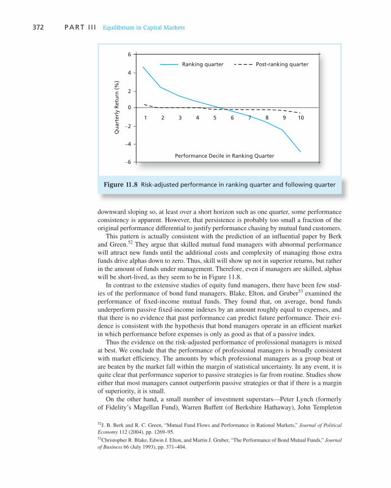
372 P A R T I I I Equilibrium in Capital Markets
downward sloping so, at least over a short horizon such as one quarter, some performance
consistency is apparent. However, that persistence is probably too small a fraction of the
original performance differential to justify performance chasing by mutual fund customers.
This pattern is actually consistent with the prediction of an influential paper by Berk
and Green. 52 They argue that skilled mutual fund managers with abnormal performance
will attract new funds until the additional costs and complexity of managing those extra
funds drive alphas down to zero. Thus, skill will show up not in superior returns, but rather
in the amount of funds under management. Therefore, even if managers are skilled, alphas
will be short-lived, as they seem to be in Figure 11.8 .
In contrast to the extensive studies of equity fund managers, there have been few stud-
ies of the performance of bond fund managers. Blake, Elton, and Gruber 53 examined the
performance of fixed-income mutual funds. They found that, on average, bond funds
underperform passive fixed-income indexes by an amount roughly equal to expenses, and
that there is no evidence that past performance can predict future performance. Their evi-
dence is consistent with the hypothesis that bond managers operate in an efficient market
in which performance before expenses is only as good as that of a passive index.
Thus the evidence on the risk-adjusted performance of professional managers is mixed
at best. We conclude that the performance of professional managers is broadly consistent
with market efficiency. The amounts by which professional managers as a group beat or
are beaten by the market fall within the margin of statistical uncertainty. In any event, it is
quite clear that performance superior to passive strategies is far from routine. Studies show
either that most managers cannot outperform passive strategies or that if there is a margin
of superiority, it is small.
On the other hand, a small number of investment superstars—Peter Lynch (formerly
of Fidelity’s Magellan Fund), Warren Buffett (of Berkshire Hathaway), John Templeton
52 J. B. Berk and R. C. Green, “Mutual Fund Flows and Performance in Rational Markets,” Journal of Political
Economy 112 (2004), pp. 1269–95. 53 Christopher R. Blake, Edwin J. Elton, and Martin J. Gruber, “The Performance of Bond Mutual Funds,” Journal
of Business 66 (July 1993), pp. 371–404.
Qu
arte
rly
Ret
urn
(%
)
−2
−4
−6
0
6
4
2
Performance Decile in Ranking Quarter
Ranking quarter Post-ranking quarter
1 2 3 4 5 6 7 8 9 10
Figure 11.8 Risk-adjusted performance in ranking quarter and following quarter

Vis
it u
s at
ww
w.m
hh
e.co
m/b
km
C H A P T E R 1 1 The Efficient Market Hypothesis 373
(of Templeton Funds), or George Soros among them—have compiled career records that
show a consistency of superior performance hard to reconcile with absolutely efficient
markets. In a careful statistical analysis of mutual fund “stars,” Kosowski, Timmerman,
Wermers, and White 54 conclude that the stock-picking ability of a minority of managers
is sufficient to cover their costs, and that their superior performance tends to persist over
time. However, Nobel Prize–winner Paul Samuelson 55 reviewed this investment hall of
fame and pointed out that the records of the vast majority of professional money manag-
ers offer convincing evidence that there are no easy strategies to guarantee success in the
securities markets.
So, Are Markets Efficient?
There is a telling joke about two economists walking down the street. They spot a $20 bill
on the sidewalk. One stoops to pick it up, but the other one says, “Don’t bother; if the bill
were real someone would have picked it up already.”
The lesson is clear. An overly doctrinaire belief in efficient markets can paralyze the
investor and make it appear that no research effort can be justified. This extreme view is
probably unwarranted. There are enough anomalies in the empirical evidence to justify the
search for underpriced securities that clearly goes on.
The bulk of the evidence, however, suggests that any supposedly superior investment
strategy should be taken with many grains of salt. The market is competitive enough that
only differentially superior information or insight will earn money; the easy pickings have
been picked. In the end it is likely that the margin of superiority that any professional man-
ager can add is so slight that the statistician will not easily be able to detect it.
We conclude that markets are generally very efficient, but that rewards to the especially
diligent, intelligent, or creative may in fact be waiting.
54 R. Kosowski, A. Timmerman, R. Wermers, and H. White. “Can Mutual Fund ‘Stars’ Really Pick Stocks? New
Evidence from a Bootstrap Analysis,” Journal of Finance 61 (December 2006), pp. 2551–95.
55 Paul Samuelson, “The Judgment of Economic Science on Rational Portfolio Management,” Journal of Portfolio
Management 16 (Fall 1989), pp. 4–12.
1. Statistical research has shown that to a close approximation stock prices seem to follow a random
walk with no discernible predictable patterns that investors can exploit. Such findings are now
taken to be evidence of market efficiency, that is, evidence that market prices reflect all cur-
rently available information. Only new information will move stock prices, and this information
is equally likely to be good news or bad news.
2. Market participants distinguish among three forms of the efficient market hypothesis. The weak
form asserts that all information to be derived from past trading data already is reflected in stock
prices. The semistrong form claims that all publicly available information is already reflected.
The strong form, which generally is acknowledged to be extreme, asserts that all information,
including insider information, is reflected in prices.
3. Technical analysis focuses on stock price patterns and on proxies for buy or sell pressure in the
market. Fundamental analysis focuses on the determinants of the underlying value of the firm,
such as current profitability and growth prospects. Because both types of analysis are based on
public information, neither should generate excess profits if markets are operating efficiently.
4. Proponents of the efficient market hypothesis often advocate passive as opposed to active invest-
ment strategies. The policy of passive investors is to buy and hold a broad-based market index.
SUMMARY

Vis
it u
s at
ww
w.m
hh
e.co
m/b
kmV
isit
us
at w
ww
.mh
he.
com
/bkm
374 P A R T I I I Equilibrium in Capital Markets
They expend resources neither on market research nor on frequent purchase and sale of stocks.
Passive strategies may be tailored to meet individual investor requirements.
5. Event studies are used to evaluate the economic impact of events of interest, using abnormal
stock returns. Such studies usually show that there is some leakage of inside information to some
market participants before the public announcement date. Therefore, insiders do seem to be able
to exploit their access to information to at least a limited extent.
6. Empirical studies of technical analysis do not generally support the hypothesis that such analysis
can generate superior trading profits. One notable exception to this conclusion is the apparent
success of momentum-based strategies over intermediate-term horizons.
7. Several anomalies regarding fundamental analysis have been uncovered. These include the P/E
effect, the small-firm-in-January effect, the neglected-firm effect, post–earnings-announcement
price drift, and the book-to-market effect. Whether these anomalies represent market inefficiency
or poorly understood risk premiums is still a matter of debate.
8. By and large, the performance record of professionally managed funds lends little credence to
claims that most professionals can consistently beat the market.
Related Web sites for this chapter are available at www.mhhe.com/bkm
random walk
efficient market hypothesis
weak-form EMH
semistrong-form EMH
strong-form EMH
technical analysis
resistance levels
support levels
fundamental analysis
passive investment strategy
index fund
event study
abnormal return
cumulative abnormal return
momentum effect
reversal effect
anomalies
P/E effect
small-firm effect
neglected-firm effect
book-to-market effect
KEY TERMS
1. If markets are efficient, what should be the correlation coefficient between stock returns for two
non-overlapping time periods?
2. A successful firm like Microsoft has consistently generated large profits for years. Is this a viola-
tion of the EMH?
3. “If all securities are fairly priced, all must offer equal expected rates of return.” Comment.
4. Steady Growth Industries has never missed a dividend payment in its 94-year history. Does this
make it more attractive to you as a possible purchase for your stock portfolio?
5. At a cocktail party, your co-worker tells you that he has beaten the market for each of the last
3 years. Suppose you believe him. Does this shake your belief in efficient markets?
6. “Highly variable stock prices suggest that the market does not know how to price stocks.”
Comment.
7. Why are the following “effects” considered efficient market anomalies? Are there rational expla-
nations for any of these effects?
a. P/E effect.
b. Book-to-market effect.
c. Momentum effect.
d. Small-firm effect.
8. If prices are as likely to increase as decrease, why do investors earn positive returns from the
market on average?
9. Which of the following most appears to contradict the proposition that the stock market is weakly
efficient? Explain.
a. Over 25% of mutual funds outperform the market on average.
b. Insiders earn abnormal trading profits.
c. Every January, the stock market earns abnormal returns.
PROBLEM SETS
i. Basic
ii. Intermediate

Vis
it u
s at
ww
w.m
hh
e.co
m/b
km
C H A P T E R 1 1 The Efficient Market Hypothesis 375
10. Which of the following sources of market inefficiency would be most easily exploited?
a. A stock price drops suddenly due to a large block sale by an institution.
b. A stock is overpriced because traders are restricted from short sales.
c. Stocks are overvalued because investors are exuberant over increased productivity in the
economy.
11. Suppose that, after conducting an analysis of past stock prices, you come up with the following
observations. Which would appear to contradict the weak form of the efficient market hypoth-
esis? Explain.
a. The average rate of return is significantly greater than zero.
b. The correlation between the return during a given week and the return during the following
week is zero.
c. One could have made superior returns by buying stock after a 10% rise in price and selling
after a 10% fall.
d. One could have made higher-than-average capital gains by holding stocks with low dividend
yields.
12. Which of the following statements are true if the efficient market hypothesis holds?
a. It implies that future events can be forecast with perfect accuracy.
b. It implies that prices reflect all available information.
c. It implies that security prices change for no discernible reason.
d. It implies that prices do not fluctuate.
13. Respond to each of the following comments.
a. If stock prices follow a random walk, then capital markets are little different from a casino.
b. A good part of a company’s future prospects are predictable. Given this fact, stock prices
can’t possibly follow a random walk.
c. If markets are efficient, you might as well select your portfolio by throwing darts at the stock
listings in The Wall Street Journal.
14. Which of the following would be a viable way to earn abnormally high trading profits if markets
are semistrong-form efficient?
a. Buy shares in companies with low P/E ratios.
b. Buy shares in companies with recent above-average price changes.
c. Buy shares in companies with recent below-average price changes.
d. Buy shares in companies for which you have advance knowledge of an improvement in the
management team.
15. Suppose you find that prices of stocks before large dividend increases show on average consist-
ently positive abnormal returns. Is this a violation of the EMH?
16. “If the business cycle is predictable, and a stock has a positive beta, the stock’s returns also must
be predictable.” Respond.
17. Which of the following phenomena would be either consistent with or a violation of the effi-
cient market hypothesis? Explain briefly.
a. Nearly half of all professionally managed mutual funds are able to outperform the S&P 500
in a typical year.
b. Money managers that outperform the market (on a risk-adjusted basis) in one year are likely
to outperform in the following year.
c. Stock prices tend to be predictably more volatile in January than in other months.
d. Stock prices of companies that announce increased earnings in January tend to outperform
the market in February.
e. Stocks that perform well in one week perform poorly in the following week.
18. An index model regression applied to past monthly returns in Ford’s stock price produces the
following estimates, which are believed to be stable over time:
rF 5 .10% 1 1.1rM
If the market index subsequently rises by 8% and Ford’s stock price rises by 7%, what is the
abnormal change in Ford’s stock price?

Vis
it u
s at
ww
w.m
hh
e.co
m/b
km376 P A R T I I I Equilibrium in Capital Markets
19. The monthly rate of return on T-bills is 1%. The market went up this month by 1.5%. In addi-
tion, AmbChaser, Inc., which has an equity beta of 2, surprisingly just won a lawsuit that awards
it $1 million immediately.
a. If the original value of AmbChaser equity were $100 million, what would you guess was the
rate of return of its stock this month?
b. What is your answer to ( a ) if the market had expected AmbChaser to win $2 million?
20. In a recent closely contested lawsuit, Apex sued Bpex for patent infringement. The jury came
back today with its decision. The rate of return on Apex was r A � 3.1%. The rate of return on
Bpex was only r B � 2.5%. The market today responded to very encouraging news about the
unemployment rate, and r M � 3%. The historical relationship between returns on these stocks
and the market portfolio has been estimated from index model regressions as:
Apex: rA 5 .2% 1 1.4rM
Bpex: rB 5 2.1% 1 .6rM
On the basis of these data, which company do you think won the lawsuit?
21. Investors expect the market rate of return in the coming year to be 12%. The T-bill rate is 4%.
Changing Fortunes Industries’ stock has a beta of .5. The market value of its outstanding equity
is $100 million.
a. What is your best guess currently as to the expected rate of return on Changing Fortunes’
stock? You believe that the stock is fairly priced.
b. If the market return in the coming year actually turns out to be 10%, what is your best guess
as to the rate of return that will be earned on Changing Fortunes’ stock?
c. Suppose now that Changing Fortunes wins a major lawsuit during the year. The settlement is
$5 million. Changing Fortunes’ stock return during the year turns out to be 10%. What is your
best guess as to the settlement the market previously expected Changing Fortunes to receive
from the lawsuit? (Continue to assume that the market return in the year turned out to be 10%.)
The magnitude of the settlement is the only unexpected firm-specific event during the year.
22. Dollar-cost averaging means that you buy equal dollar amounts of a stock every period, for exam-
ple, $500 per month. The strategy is based on the idea that when the stock price is low, your fixed
monthly purchase will buy more shares, and when the price is high, fewer shares. Averaging over
time, you will end up buying more shares when the stock is cheaper and fewer when it is relatively
expensive. Therefore, by design, you will exhibit good market timing. Evaluate this strategy.
23. We know that the market should respond positively to good news and that good-news events
such as the coming end of a recession can be predicted with at least some accuracy. Why, then,
can we not predict that the market will go up as the economy recovers?
24. You know that firm XYZ is very poorly run. On a scale of 1 (worst) to 10 (best), you would give
it a score of 3. The market consensus evaluation is that the management score is only 2. Should
you buy or sell the stock?
25. Suppose that during a certain week the Fed announces a new monetary growth policy, Congress
surprisingly passes legislation restricting imports of foreign automobiles, and Ford comes out
with a new car model that it believes will increase profits substantially. How might you go about
measuring the market’s assessment of Ford’s new model?
26. Good News, Inc., just announced an increase in its annual earnings, yet its stock price fell. Is
there a rational explanation for this phenomenon?
27. Shares of small firms with thinly traded stocks tend to show positive CAPM alphas. Is this a
violation of the efficient market hypothesis?
28. Examine the accompanying figure, 56 which presents cumulative abnormal returns both before
and after dates on which insiders buy or sell shares in their firms. How do you interpret this
figure? What are we to make of the pattern of CARs before and after the event date?
56 Reprinted from Nejat H. Seyhun, “Insiders, Profits, Costs of Trading and Market Efficiency,” Journal of
Financial Economics 16 (1986). Copyright 1986 with permission from Elsevier Science.
iii. Challenge
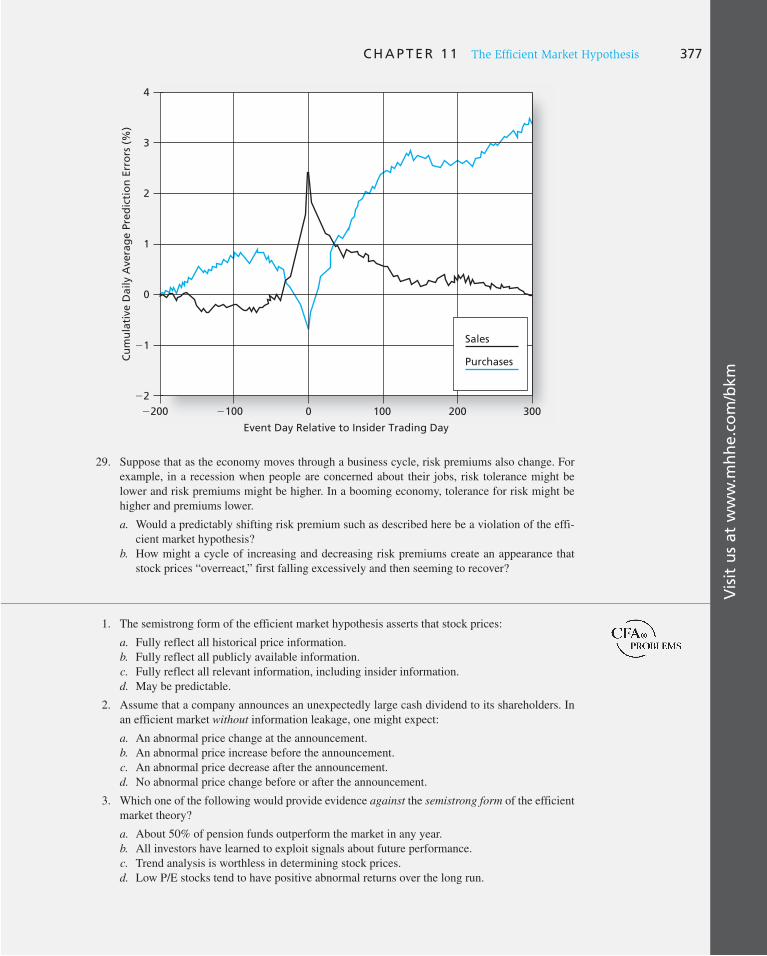
Vis
it u
s at
ww
w.m
hh
e.co
m/b
km
C H A P T E R 1 1 The Efficient Market Hypothesis 377
29. Suppose that as the economy moves through a business cycle, risk premiums also change. For
example, in a recession when people are concerned about their jobs, risk tolerance might be
lower and risk premiums might be higher. In a booming economy, tolerance for risk might be
higher and premiums lower.
a. Would a predictably shifting risk premium such as described here be a violation of the effi-
cient market hypothesis?
b. How might a cycle of increasing and decreasing risk premiums create an appearance that
stock prices “overreact,” first falling excessively and then seeming to recover?
Event Day Relative to Insider Trading Day
Cu
mu
lati
ve D
aily
Ave
rag
e P
red
icti
on
Err
ors
(%
)
200 100 0 100 200 300
Sales
Purchases
2
1
0
1
2
3
4
1. The semistrong form of the efficient market hypothesis asserts that stock prices:
a. Fully reflect all historical price information.
b. Fully reflect all publicly available information.
c. Fully reflect all relevant information, including insider information.
d. May be predictable.
2. Assume that a company announces an unexpectedly large cash dividend to its shareholders. In
an efficient market without information leakage, one might expect:
a. An abnormal price change at the announcement.
b. An abnormal price increase before the announcement.
c. An abnormal price decrease after the announcement.
d. No abnormal price change before or after the announcement.
3. Which one of the following would provide evidence against the semistrong form of the efficient
market theory?
a. About 50% of pension funds outperform the market in any year.
b. All investors have learned to exploit signals about future performance.
c. Trend analysis is worthless in determining stock prices.
d. Low P/E stocks tend to have positive abnormal returns over the long run.

Vis
it u
s at
ww
w.m
hh
e.co
m/b
km378 P A R T I I I Equilibrium in Capital Markets
4. According to the efficient market hypothesis:
a. High-beta stocks are consistently overpriced.
b. Low-beta stocks are consistently overpriced.
c. Positive alphas on stocks will quickly disappear.
d. Negative alpha stocks consistently yield low returns for arbitrageurs.
5. A “random walk” occurs when:
a. Stock price changes are random but predictable.
b. Stock prices respond slowly to both new and old information.
c. Future price changes are uncorrelated with past price changes.
d. Past information is useful in predicting future prices.
6. Two basic assumptions of technical analysis are that security prices adjust:
a. Gradually to new information, and study of the economic environment provides an indica-
tion of future market movements.
b. Rapidly to new information, and study of the economic environment provides an indication
of future market movements.
c. Rapidly to new information, and market prices are determined by the interaction between
supply and demand.
d. Gradually to new information, and prices are determined by the interaction between supply
and demand.
7. When technical analysts say a stock has good “relative strength,” they mean:
a. The ratio of the price of the stock to a market or industry index has trended upward.
b. The recent trading volume in the stock has exceeded the normal trading volume.
c. The total return on the stock has exceeded the total return on T-bills.
d. The stock has performed well recently compared to its past performance.
8. Your investment client asks for information concerning the benefits of active portfolio manage-
ment. She is particularly interested in the question of whether active managers can be expected
to consistently exploit inefficiencies in the capital markets to produce above-average returns
without assuming higher risk.
The semistrong form of the efficient market hypothesis asserts that all publicly available
information is rapidly and correctly reflected in securities prices. This implies that investors
cannot expect to derive above-average profits from purchases made after information has
become public because security prices already reflect the information’s full effects.
a. Identify and explain two examples of empirical evidence that tend to support the EMH
implication stated above.
b. Identify and explain two examples of empirical evidence that tend to refute the EMH impli-
cation stated above.
c. Discuss reasons why an investor might choose not to index even if the markets were, in fact,
semistrong-form efficient.
9. a. Briefly explain the concept of the efficient market hypothesis (EMH) and each of its three
forms—weak, semistrong, and strong—and briefly discuss the degree to which existing
empirical evidence supports each of the three forms of the EMH.
b. Briefly discuss the implications of the efficient market hypothesis for investment policy as it
applies to:
i. Technical analysis in the form of charting.
ii. Fundamental analysis.
c. Briefly explain the roles or responsibilities of portfolio managers in an efficient market
environment.
10. Growth and value can be defined in several ways. “Growth” usually conveys the idea of a
portfolio emphasizing or including only issues believed to possess above-average future rates
of per-share earnings growth. Low current yield, high price-to-book ratios, and high price-to-
earnings ratios are typical characteristics of such portfolios. “Value” usually conveys the idea of

Vis
it u
s at
ww
w.m
hh
e.co
m/b
km
C H A P T E R 1 1 The Efficient Market Hypothesis 379
portfolios emphasizing or including only issues currently showing low price-to-book ratios, low
price-to-earnings ratios, above-average levels of dividend yield, and market prices believed to
be below the issues’ intrinsic values.
a. Identify and provide reasons why, over an extended period of time, value-stock investing
might outperform growth-stock investing.
b. Explain why the outcome suggested in ( a ) should not be possible in a market widely
regarded as being highly efficient.
Earnings Surprises
Several Web sites list information on earnings surprises. Much of the information sup-plied is from Zacks.com . Each day the largest positive and negative surprises are listed. Go to www.zacks.com/research/earnings/today_eps.php and identify the top positive and the top negative earnings surprises for the day. The table will list the time and date of the announcement. Do you notice any difference between the times of day positive announcements tend to be made versus negative announcements?
Identify the tickers for the top three positive surprises. Once you have identified the top surprises, go to finance.yahoo.com. Enter the ticker symbols and obtain quotes for these securities. Examine the 5-day charts for each of the companies. Is the information incorporated into price quickly? Is there any evidence of prior knowledge or anticipation of the disclosure in advance of the trading?
Choose one of the stocks listed and click on its symbol to follow the link for more infor-mation. Click on the link for Interactive Chart that appears under the graph. You can move the cursor over various parts of the graph to investigate what happened to the price and trading volume of the stock on each trading day. Do you notice any patterns?
E-INVEST-MENTS EXERCISES
SOLUTIONS TO CONCEPT CHECKS
1. a. A high-level manager might well have private information about the firm. Her ability to
trade profitably on that information is not surprising. This ability does not violate weak-form
efficiency: The abnormal profits are not derived from an analysis of past price and trading
data. If they were, this would indicate that there is valuable information that can be gleaned
from such analysis. But this ability does violate strong-form efficiency. Apparently, there is
some private information that is not already reflected in stock prices.
b. The information sets that pertain to the weak, semistrong, and strong form of the EMH can be
described by the following illustration:
The weak-form information set includes only the history of prices and volumes. The
semistrong-form set includes the weak form set plus all publicly available information. In
turn, the strong-form set includes the semistrong set plus insiders’ information. It is illegal
Strong-formset
Semistrong-formset
Weak-formset

Vis
it u
s at
ww
w.m
hh
e.co
m/b
km380 P A R T I I I Equilibrium in Capital Markets
to act on this incremental information (insiders’ private information). The direction of valid
implication is
Strong-form EMH 1 Semistrong-form EMH 1 Weak-form EMH
The reverse direction implication is not valid. For example, stock prices may reflect all past price
data (weak-form efficiency) but may not reflect relevant fundamental data (semistrong-form
inefficiency).
2. The point made in the preceding discussion is that the very fact that we observe stock prices near
so-called resistance levels belies the assumption that the price can be a resistance level. If a stock
is observed to sell at any price, then investors must believe that a fair rate of return can be earned
if the stock is purchased at that price. It is logically impossible for a stock to have a resistance
level and offer a fair rate of return at prices just below the resistance level. If we accept that prices
are appropriate, we must reject any presumption concerning resistance levels.
3. If everyone follows a passive strategy, sooner or later prices will fail to reflect new information.
At this point there are profit opportunities for active investors who uncover mispriced securities.
As they buy and sell these assets, prices again will be driven to fair levels.
4. Predictably declining CARs do violate the EMH. If one can predict such a phenomenon, a profit
opportunity emerges: Sell (or short sell) the affected stocks on an event date just before their
prices are predicted to fall.
5. The answer depends on your prior beliefs about market efficiency. Miller’s record through 2005
was incredibly strong. On the other hand, with so many funds in existence, it is less surprising
that some fund would appear to be consistently superior after the fact. Exceptional past
performance of a small number of managers is possible by chance even in an efficient market. A
better test is provided in “continuation studies.” Are better performers in one period more likely
to repeat that performance in later periods? Miller’s record after 2005 fails the continuation or
consistency criterion.

THE EFFICIENT MARKET hypothesis makes
two important predictions. First, it implies
that security prices properly reflect whatever
information is available to investors. A second
implication follows immediately: active trad-
ers will find it difficult to outperform passive
strategies such as holding market indexes. To
do so would require differential insight; this
in a highly competitive market is very hard to
come by.
Unfortunately, it is hard to devise measures
of the “true” or intrinsic value of a security,
and correspondingly difficult to test directly
whether prices match those values. Therefore,
most tests of market efficiency have focused
on the performance of active trading strate-
gies. These tests have been of two kinds. The
anomalies literature has examined strate-
gies that apparently would have provided
superior risk-adjusted returns (e.g., investing
in stocks with momentum or in value rather
than glamour stocks). Other tests have looked
at the results of actual investments by asking
whether professional managers have been
able to beat the market.
Neither class of tests has proven fully con-
clusive. The anomalies literature suggests
that several strategies would have provided
superior returns. But there are questions as to
whether some of these apparent anomalies
reflect risk premiums not captured by simple
models of risk and return, or even if they
merely reflect data mining. Moreover, the
apparent inability of the typical money man-
ager to turn these anomalies into superior
returns on actual portfolios casts additional
doubt on their “reality.”
A relatively new school of thought, behav-
ioral finance, argues that the sprawling litera-
ture on trading strategies has missed a larger
and more important point by overlooking
the first implication of efficient markets—the
correctness of security prices. This may be the
more important implication, because market
economies rely on prices to allocate resources
efficiently. The behavioral school argues that
even if security prices are wrong, to exploit
them still can be difficult and, therefore, the
failure to uncover obviously successful trad-
ing rules or traders cannot be taken as proof
of market efficiency.
Whereas conventional theories presume
that investors are rational, behavioral
finance starts with the assumption that they
might not be. We will examine some of the
information-processing and behavioral irra-
tionalities uncovered by psychologists in
other contexts and show how these tenden-
cies applied to financial markets might result
in some of the anomalies discussed in the
12 Behavioral Finance and Technical Analysis 2
PAR
T III CHAPTER TWELVE

382
(concluded)
previous chapter. We then examine the limita-
tions of strategies designed to take advantage
of behaviorally induced mispricing. If the limits
to such arbitrage activity are severe, mispric-
ing can survive even if some rational investors
attempt to exploit it. We turn next to technical
analysis and show how behavioral models give
some support to techniques that clearly would
be useless in efficient markets. We close the
chapter with a brief survey of some of these
technical strategies.
12.1 The Behavioral Critique
The premise of behavioral finance is that conventional financial theory ignores how real people make decisions and that people make a difference. 1 A growing number of econ-omists have come to interpret the anomalies literature as consistent with several “irra-tionalities” that seem to characterize individuals making complicated decisions. These irrationalities fall into two broad categories: first, that investors do not always process information correctly and therefore infer incorrect probability distributions about future rates of return; and second, that even given a probability distribution of returns, they often make inconsistent or systematically suboptimal decisions.
Of course, the existence of irrational investors would not by itself be sufficient to render capital markets inefficient. If such irrationalities did affect prices, then sharp-eyed arbitra-geurs taking advantage of profit opportunities might be expected to push prices back to their proper values. Thus, the second leg of the behavioral critique is that in practice the actions of such arbitrageurs are limited and therefore insufficient to force prices to match intrinsic value.
This leg of the argument is important. Virtually everyone agrees that if prices are right (i.e., price 5 intrinsic value), then there are no easy profit opportunities. But the reverse is not necessarily true. If behaviorists are correct about limits to arbitrage activity, then the absence of profit opportunities does not necessarily imply that markets are efficient. We’ve noted that most tests of the efficient market hypothesis have focused on the existence of profit opportunities, often as reflected in the performance of money managers. But their failure to systematically outperform passive investment strategies need not imply that mar-kets are in fact efficient.
We will start our summary of the behavioral critique with the first leg of the argument, surveying a sample of the informational processing errors uncovered by psychologists in other areas. We next examine a few of the behavioral irrationalities that seem to character-ize decision makers. Finally, we look at limits to arbitrage activity, and conclude with a tentative assessment of the import of the behavioral debate.
Information Processing
Errors in information processing can lead investors to misestimate the true probabilities of possible events or associated rates of return. Several such biases have been uncovered. Here are four of the more important ones.
1 The discussion in this section is largely based on Nicholas Barberis and Richard Thaler, “A Survey of Behavioral Finance,” in the Handbook of the Economics of Finance, eds. G. M. Constantinides, M. Harris, and R. Stulz (Amsterdam: Elsevier, 2003).

C H A P T E R 1 2 Behavioral Finance and Technical Analysis 383
Forecasting Errors A series of experiments by Kahneman and Tversky 2 indicate that people give too much weight to recent experience compared to prior beliefs when mak-ing forecasts (sometimes dubbed a memory bias ) and tend to make forecasts that are too extreme given the uncertainty inherent in their information. DeBondt and Thaler 3 argue that the P/E effect can be explained by earnings expectations that are too extreme. In this view, when forecasts of a firm’s future earnings are high, perhaps due to favorable recent performance, they tend to be too high relative to the objective prospects of the firm. This results in a high initial P/E (due to the excessive optimism built into the stock price) and poor subsequent performance when investors recognize their error. Thus, high P/E firms tend to be poor investments.
Overconfidence People tend to overestimate the precision of their beliefs or fore-casts, and they tend to overestimate their abilities. In one famous survey, 90% of drivers in Sweden ranked themselves as better-than-average drivers. Such overconfidence may be responsible for the prevalence of active versus passive investment management—itself an anomaly to adherents of the efficient market hypothesis. Despite the growing popularity of indexing, only about 10%–15% of the equity in the mutual fund industry is held in indexed accounts. The dominance of active management in the face of the typical underperfor-mance of such strategies (consider the generally disappointing performance of actively managed mutual funds reviewed in Chapter 4 as well as in the previous chapter) is consis-tent with a tendency to overestimate ability.
An interesting example of overconfidence in financial markets is provided by Barber and Odean, 4 who compare trading activity and average returns in brokerage accounts of men and women. They find that men (in particular, single men) trade far more actively than women, consistent with the greater overconfidence among men well documented in the psychology literature. They also find that trading activity is highly predictive of poor investment performance. The top 20% of accounts ranked by portfolio turnover had aver-age returns 7 percentage points lower than the 20% of the accounts with the lowest turn-over rates. As they conclude, “trading [and by implication, overconfidence] is hazardous to your wealth.”
Conservatism A conservatism bias means that investors are too slow (too conserva-tive) in updating their beliefs in response to new evidence. This means that they might initially underreact to news about a firm, so that prices will fully reflect new information only gradually. Such a bias would give rise to momentum in stock market returns.
Sample Size Neglect and Representativeness The notion of representative-
ness holds that people commonly do not take into account the size of a sample, acting as if a small sample is just as representative of a population as a large one. They may therefore infer a pattern too quickly based on a small sample and extrapolate apparent trends too far into the future. It is easy to see how such a pattern would be consistent with overreac-tion and correction anomalies. A short-lived run of good earnings reports or high stock
2 D. Kahneman and A. Tversky, “On the Psychology of Prediction,” Psychology Review 80 (1973), pp. 237–51, and “Subjective Probability: A Judgment of Representativeness,” Cognitive Psychology 3 (1972), pp. 430–54.
3 W.F.M. De Bondt and R. H. Thaler, “Do Security Analysts Overreact?” American Economic Review 80 (1990), pp. 52–57.
4 Brad Barber and Terrance Odean, “Boys Will Be Boys: Gender, Overconfidence, and Common Stock Investment,” Quarterly Journal of Economics 16 (2001), pp. 262–92, and “Trading Is Hazardous to Your Wealth: The Common Stock Investment Performance of Individual Investors,” Journal of Finance 55 (2000), pp. 773–806.

384 P A R T I I I Equilibrium in Capital Markets
returns would lead such investors to revise their assessments of likely future performance, and thus generate buying pressure that exaggerates the price run-up. Eventually, the gap between price and intrinsic value becomes glaring and the market corrects its initial error. Interestingly, stocks with the best recent performance suffer reversals precisely in the few days surrounding earnings announcements, suggesting that the correction occurs just as investors learn that their initial beliefs were too extreme. 5
Behavioral Biases
Even if information processing were perfect, many studies conclude that individuals would tend to make less-than-fully-rational decisions using that information. These behavioral biases largely affect how investors frame questions of risk versus return, and therefore make risk–return trade-offs.
Framing Decisions seem to be affected by how choices are framed. For example, an individual may reject a bet when it is posed in terms of the risk surrounding possible gains but may accept that same bet when described in terms of the risk surrounding potential losses. In other words, individuals may act risk averse in terms of gains but risk seeking in terms of losses. But in many cases, the choice of how to frame a risky venture—as involv-ing gains or losses—can be arbitrary.
Mental Accounting Mental accounting is a specific form of framing in which peo-ple segregate certain decisions. For example, an investor may take a lot of risk with one investment account, but establish a very conservative position with another account that is dedicated to her child’s education. Rationally, it might be better to view both accounts as part of the investor’s overall portfolio with the risk–return profiles of each integrated into a unified framework. Statman 6 argues that mental accounting is consistent with some investors’ irrational preference for stocks with high cash dividends (they feel free to spend dividend income, but would not “dip into capital” by selling a few shares of another stock with the same total rate of return) and with a tendency to ride losing stock positions for too long (because “behavioral investors” are reluctant to realize losses). In fact, investors
5 N. Chopra, J. Lakonishok, and J. Ritter, “Measuring Abnormal Performance: Do Stocks Overreact?” Journal of
Financial Economics 31 (1992), pp. 235–68.
6 Meir Statman, “Behavioral Finance,” Contemporary Finance Digest 1 (Winter 1997), pp. 5–22.
Example 12.1 Framing
Consider a coin toss with a payoff of $50 for tails. Now consider a gift of $50 that is bun-dled with a bet that imposes a loss of $50 if that coin toss comes up heads. In both cases, you end up with zero for heads and $50 for tails. But the former description frames the coin toss as posing a risky gain while the latter frames the coin toss in terms of risky losses. The difference in framing can lead to different attitudes toward the bet.
CONCEPT CHECK
1 We saw in the last chapter that stocks seem to exhibit a pattern of short- to middle-term momentum, along with long-term reversals. How might this pattern arise from an interplay between the conservatism and representativeness biases?

C H A P T E R 1 2 Behavioral Finance and Technical Analysis 385
are more likely to sell stocks with gains than those with losses, precisely contrary to a tax-minimization strategy. 7
Mental accounting effects also can help explain momentum in stock prices. The house
money effect refers to gamblers’ greater willingness to accept new bets if they currently are ahead. They think of (i.e., frame) the bet as being made with their “winnings account,” that is, with the casino’s and not with their own money, and thus are more willing to accept risk. Analogously, after a stock market run-up, individuals may view investments as largely funded out of a “capital gains account,” become more tolerant of risk, discount future cash flows at a lower rate, and thus further push up prices.
Regret Avoidance Psychologists have found that individuals who make decisions that turn out badly have more regret (blame themselves more) when that decision was more unconventional. For example, buying a blue-chip portfolio that turns down is not as painful as experiencing the same losses on an unknown start-up firm. Any losses on the blue-chip stocks can be more easily attributed to bad luck rather than bad decision making and cause less regret. De Bondt and Thaler 8 argue that such regret avoidance is consistent with both the size and book-to-market effect. Higher book-to-market firms tend to have depressed stock prices. These firms are “out of favor” and more likely to be in a finan-cially precarious position. Similarly, smaller, less well known firms are also less conven-tional investments. Such firms require more “courage” on the part of the investor, which increases the required rate of return. Mental accounting can add to this effect. If investors focus on the gains or losses of individual stocks, rather than on broad portfolios, they can become more risk averse concerning stocks with recent poor performance, discount their cash flows at a higher rate, and thereby create a value-stock risk premium.
Prospect Theory Prospect the ory modifies the analytic description of rational risk-averse investors found in standard financial theory. 9 Figure 12.1 , panel A, illustrates the conventional description of a risk-averse investor. Higher wealth provides higher satisfac-tion, or “ utility,” but at a diminishing rate (the curve flattens as the individual becomes wealthier). This gives rise to risk aversion: A gain of $1,000 increases utility by less than a loss of $1,000 reduces it; therefore, investors will reject risky prospects that don’t offer a risk premium.
Figure 12.1 , panel B, shows a competing description of preferences characterized by “loss aversion.” Utility depends not on the level of wealth as in panel A, but on changes in wealth from current levels. Moreover, to the left of zero (zero denotes no change from current wealth), the curve is convex rather than concave. This has several implications. Whereas many conventional utility functions imply that investors may become less risk averse as wealth increases, the function in panel B always re-centers on current wealth, thereby ruling out such decreases in risk aversion and possibly helping to explain high
7 H. Shefrin and M. Statman, “The Disposition to Sell Winners Too Early and Ride Losers Too Long: Theory and Evidence,” Journal of Finance 40 (July 1985), pp. 777–90; and T. Odean, “Are Investors Reluctant to Realize Their Losses?” Journal of Finance 53 (1998), pp. 1775–98.
8 W.F.M. De Bondt and R. H. Thaler, “Further Evidence on Investor Overreaction and Stock Market Seasonality,” Journal of Finance 42 (1987), pp. 557–81.
9 Prospect theory originated with a highly influential paper about decision making under uncertainty by D. Kahneman and A. Tversky, “Prospect Theory: An Analysis of Decision under Risk,” Econometrica 47 (1979), pp. 263–91.
CONCEPT CHECK
2 How might the P/E effect (discussed in the previous chapter) also be explained as a consequence of regret avoidance?
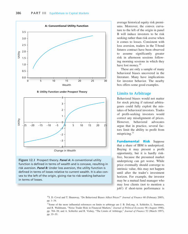
386 P A R T I I I Equilibrium in Capital Markets
average historical equity risk premi-ums. Moreover, the convex curva-ture to the left of the origin in panel B will induce investors to be risk seeking rather than risk averse when it comes to losses. Consistent with loss aversion, traders in the T-bond futures contract have been observed to assume significantly greater risk in afternoon sessions follow-ing morning sessions in which they have lost money. 10
These are only a sample of many behavioral biases uncovered in the literature. Many have implications for investor behavior. The nearby box offers some good examples.
Limits to Arbitrage
Behavioral biases would not matter for stock pricing if rational arbitra-geurs could fully exploit the mis-takes of behavioral investors. Trades of profit-seeking investors would correct any misalignment of prices. However, behavioral advocates argue that in practice, several fac-tors limit the ability to profit from mispricing. 11
Fundamental Risk Suppose that a share of IBM is underpriced. Buying it may present a profit opportunity, but it is hardly risk-free, because the presumed market underpricng can get worse. While price eventually should converge to intrinsic value, this may not happen until after the trader’s investment horizon. For example, the investor may be a mutual fund manager who may lose clients (not to mention a job!) if short-term performance is
10 J. D. Coval and T. Shumway, “Do Behavioral Biases Affect Prices?” Journal of Finance 60 (February 2005), pp. 1–34. 11 Some of the more influential references on limits to arbitrage are J. B. DeLong, A. Schleifer, L. Summers, and R. Waldmann, “Noise Trader Risk in Financial Markets,” Journal of Political Economy 98 (August 1990), pp. 704–38; and A. Schleifer and R. Vishny, “The Limits of Arbitrage,” Journal of Finance 52 (March 1997), pp. 35–55.
Figure 12.1 Prospect theory. Panel A: A conventional utility function is defined in terms of wealth and is concave, resulting in risk aversion. Panel B: Under loss aversion, the utility function is defined in terms of losses relative to current wealth. It is also con-vex to the left of the origin, giving rise to risk-seeking behavior in terms of losses.
A: Conventional Utility Function
0.0
0.5
1.0
1.5
2.0
2.5
3.0
3.5
0 5 10 15 20 25 30
Wealth
Uti
lity
B: Utility Function under Prospect Theory
−3
−2
−1
1
2
3
−20 −15 −10 −5 5 10 15 20
Change in Wealth
Uti
lity
00
4
25
−4
−25

387
Why It’s So Tough to Fix Your Portfolio
If your portfolio is out of whack, you could ask an invest-ment adviser for help. But you might have better luck with your therapist.
It’s a common dilemma: You know you have the wrong mix of investments, but you cannot bring yourself to fix the mess. Why is it so difficult to change? At issue are three mental mistakes.
CHASING WINNERS Looking to lighten up on bonds and get back into stocks? Sure, you know stocks are a long-term investment and, sure, you know they are best bought when cheap.
Yet it’s a lot easier to pull the trigger and buy stocks if the market has lately been scoring gains. “People are influ-enced by what has happened most recently, and then they extrapolate from that,” says Meir Statman, a finance pro-fessor at Santa Clara University in California. “But often, they end up being optimistic and pessimistic at just the wrong time.”
Consider some results from the UBS Index of Investor Optimism, a monthly poll conducted by UBS and the Gallup Organization. Each month, the poll asks investors what gain they expect from their portfolio during the next 12 months. Result? You guessed it: The answers rise and fall with the stock market.
For instance, during the bruising bear market, investors grew increasingly pessimistic, and at the market bottom they were looking for median portfolio gains of just 5%. But true to form, last year’s rally brightened investors’ spir-its and by January they were expecting 10% returns.
GETTING EVEN This year’s choppy stock market hasn’t scared off just bond investors. It has also made it difficult for stock investors to rejigger their portfolios.
Blame it on the old “get even, then get out” syndrome. With stocks treading water, many investors are reluctant to sell, because they are a long way from recovering their bear-market losses. To be sure, investors who bought near the peak are underwater, whether they sell or not. But sell-ing losers is still agonizing, because it means admitting you made a mistake.
“If you’re rational and you have a loss, you sell, take the tax loss and move on,” Prof. Statman says. “But if you’re a normal person, selling at a loss tears your heart out.”
MUSTERING COURAGE Whether you need to buy stocks or buy bonds, it takes con-fidence to act. And right now, investors just aren’t confi-dent. “There’s this status-quo bias,” says John Nofsinger, a finance professor at Washington State University in Pullman, Washington. “We’re afraid to do anything, because we’re afraid we’ll regret it.”
Once again, it’s driven by recent market action When markets are flying high, folks attribute their portfolio’s gains to their own brilliance. That gives them the confi-dence to trade more and to take greater risks Overreacting to short-term market results is, of course, a great way to lose a truckload of money. But with any luck, if you are aware of this pitfall, maybe you will avoid it.
Or maybe [this is] too optimistic. “You can tell some-body that investors have all these behavioral biases,” says Terrance Odean, a finance professor at the University of California at Berkeley. “So what happens? The investor thinks, ‘Oh, that sounds like my husband. I don’t think many investors say, ‘Oh, that sounds like me.’”
Source: Jonathan Clements, The Wall Street Journal Online, June 23, 2004. © 2004 Dow Jones & Company, Inc. All rights reserved worldwide.
WO
RD
S FRO
M TH
E STREET
poor, or a trader who may run through her capital if the market turns against her, even temporarily. A comment often attributed to the famous economist John Maynard Keynes is that “markets can remain irrational longer than you can remain solvent.” The fundamental
risk incurred in exploiting apparent profit opportunities presumably will limit the activity of traders.
Example 12.2 Fundamental Risk
In early 2010, the NASDAQ index fluctuated at a level around 2,300. From that perspec-tive, the value the index had reached in 2000, around 5,000, seemed obviously crazy. Surely some investors living through the Internet “bubble” of the late 1990s must have identified the index as grossly overvalued, suggesting a good selling opportunity. But this hardly would have been a riskless arbitrage opportunity. Consider that NASDAQ may also

388 P A R T I I I Equilibrium in Capital Markets
have been overvalued in 1999 when it first crossed above 3,500 (50% higher than its value in 2010). An investor in 1999 who believed (as it turns out, quite correctly) that NASDAQ was overvalued at 3,500 and decided to sell it short would have suffered enormous losses as the index increased by another 1,500 points before finally peaking at 5,000. While the investor might have derived considerable satisfaction at eventually being proven right about the overpricing, by entering a year before the market “corrected,” he might also have gone broke.
Implementation Costs Exploiting overpricing can be particularly difficult. Short-selling a security entails costs; short-sellers may have to return the borrowed security on little notice, rendering the horizon of the short sale uncertain; other investors such as many pension or mutual fund managers face strict limits on their discretion to short securities. This can limit the ability of arbitrage activity to force prices to fair value.
Model Risk One always has to worry that an apparent profit opportunity is more apparent than real. Perhaps you are using a faulty model to value the security, and the price actually is right. Mispricing may make a position a good bet, but it is still a risky one, which limits the extent to which it will be pursued.
Limits to Arbitrage and the Law of One Price
While one can debate the implications of much of the anomalies literature, surely the Law of One Price (positing that effectively identical assets should have identical prices) should be satisfied in rational markets. Yet there are several instances where the law seems to have been violated. These instances are good case studies of the limits to arbitrage.
“Siamese Twin” Companies 12 In 1907, Royal Dutch Petroleum and Shell Transport merged their operations into one firm. The two original companies, which con-tinued to trade separately, agreed to split all profits from the joint company on a 60/40 basis. Shareholders of Royal Dutch receive 60% of the cash flow, and those of Shell receive 40%. One would therefore expect that Royal Dutch should sell for exactly 60/40 5 1.5 times the price of Shell. But this is not the case. Figure 12.2 shows that the relative value of the two firms has departed considerably from this “parity” ratio for extended periods of time.
Doesn’t this mispricing give rise to an arbitrage opportunity? If Royal Dutch sells for more than 1.5 times Shell, why not buy relatively underpriced Shell and short sell over-priced Royal? This seems like a reasonable strategy, but if you had followed it in February 1993 when Royal sold for about 10% more than its parity value, Figure 12.2 shows that you would have lost a lot of money as the premium widened to about 17% before finally reversing after 1999. As in Example 12.2 , this opportunity posed fundamental risk.
Equity Carve-Outs Several equity carve-outs also have violated the Law of One Price. 13 To illustrate, consider the case of 3Com, which in 1999 decided to spin off its Palm division. It first sold 5% of its stake in Palm in an IPO, announcing that it would distribute the remaining 95% of its Palm shares to 3Com shareholders 6 months later in a spinoff. Each 3Com shareholder would receive 1.5 shares of Palm in the spinoff.
12 This discussion is based on K. A. Froot and E. M. Dabora, “How Are Stock Prices Affected by the Location of Trade?” Journal of Financial Economics 53 (1999), pp. 189–216.
13 O. A. Lamont and R. H. Thaler, “Can the Market Add and Subtract? Mispricing in Tech Carve-outs,” Journal of
Political Economy 111 (2003), pp. 227–68.
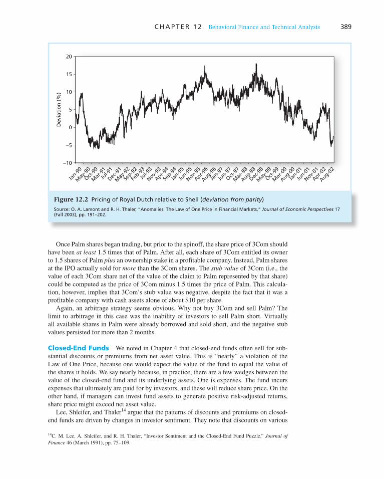
C H A P T E R 1 2 Behavioral Finance and Technical Analysis 389
Once Palm shares began trading, but prior to the spinoff, the share price of 3Com should have been at least 1.5 times that of Palm. After all, each share of 3Com entitled its owner to 1.5 shares of Palm plus an ownership stake in a profitable company. Instead, Palm shares at the IPO actually sold for more than the 3Com shares. The stub value of 3Com (i.e., the value of each 3Com share net of the value of the claim to Palm represented by that share) could be computed as the price of 3Com minus 1.5 times the price of Palm. This calcula-tion, however, implies that 3Com’s stub value was negative, despite the fact that it was a profitable company with cash assets alone of about $10 per share.
Again, an arbitrage strategy seems obvious. Why not buy 3Com and sell Palm? The limit to arbitrage in this case was the inability of investors to sell Palm short. Virtually all available shares in Palm were already borrowed and sold short, and the negative stub values persisted for more than 2 months.
Closed-End Funds We noted in Chapter 4 that closed-end funds often sell for sub-stantial discounts or premiums from net asset value. This is “nearly” a violation of the Law of One Price, because one would expect the value of the fund to equal the value of the shares it holds. We say nearly because, in practice, there are a few wedges between the value of the closed-end fund and its underlying assets. One is expenses. The fund incurs expenses that ultimately are paid for by investors, and these will reduce share price. On the other hand, if managers can invest fund assets to generate positive risk-adjusted returns, share price might exceed net asset value.
Lee, Shleifer, and Thaler 14 argue that the patterns of discounts and premiums on closed-end funds are driven by changes in investor sentiment. They note that discounts on various
14 C. M. Lee, A. Shleifer, and R. H. Thaler, “Investor Sentiment and the Closed-End Fund Puzzle,” Journal of
Finance 46 (March 1991), pp. 75–109.
Figure 12.2 Pricing of Royal Dutch relative to Shell ( deviation from parity )
Source: O. A. Lamont and R. H. Thaler, “Anomalies: The Law of One Price in Financial Markets,” Journal of Economic Perspectives 17 (Fall 2003), pp. 191–202.
Dev
iati
on
(%
) 10
20
15
5
0
−5
−10
Jan-9
0
May
-90
Oct-9
0
Mar
-91
Jul-9
1
Dec-9
1
May
-92
Sep-9
2
Feb-9
3
Jul-9
3
Nov-93
Apr-94
Sep-9
4
Jan-9
5
Jun-9
5
Nov-95
Apr-96
Aug-96
Jan-9
7
Jun-9
7
Oct-9
7
Mar
-98
Aug-98
Dec-9
8
May
-99
Oct-9
9
Mar
-00
Aug-00
Aug-02
Jan-0
1
Jun-0
1
Nov-01
Apr-02
390 P A R T I I I Equilibrium in Capital Markets
funds move together and are correlated with the return on small stocks, suggesting that all are affected by common variation in sentiment. One might consider buying funds selling at a discount from net asset value and selling those trading at a premium, but discounts and pre-miums can widen, subjecting this strategy too to fundamental risk. Pontiff 15 demonstrates that deviations of price from net asset value in closed-end funds tend to be higher in funds that are more difficult to arbitrage, for example, those with more idiosyncratic volatility.
Closed-end fund discounts are a good example of so-called anomalies that also may have rational explanations. Ross demonstrates that they can be reconciled with rational investors even if expenses or fund abnormal returns are modest. 16 He shows that if a fund has a dividend yield of d , an alpha (risk-adjusted abnormal return) of a , and expense ratio of e, then using the constant-growth dividend discount model (see Chapter 18), the premium of the fund over its net asset value will be
Price 2 NAV
NAV5
a 2 e
d 1 e 2 a
If the fund manager’s performance more than compensates for expenses (i.e., if a > e), the fund will sell at a premium to NAV; otherwise it will sell at a discount. For example, suppose a 5 .015, the expense ratio is e 5 .0125, and the dividend yield is d 5 .02. Then the premium will be .14, or 14%. But if the market turns sour on the manager and revises its estimate of a downward to .005, that premium quickly turns into a discount of 27%.
This analysis might explain why closed-end funds often are issued to the public at a premium; if investors do not expect a to exceed e, they won’t purchase shares in the fund. But the fact that most premiums eventually turn into discounts indicates how difficult it is for management to fulfill these expectations. 17
Bubbles and Behavioral Economics
In Example 12.2 above, we pointed out that the stock market run-up of the late 1990s, and even more spectacularly, the run-up of the technology-heavy NASDAQ market, seems in retrospect to have been an obvious bubble. In a 6-year period beginning in 1995, the NASDAQ index increased by a factor of more than 6. Former Fed Chairman Alan Green-span famously characterized the dot-com boom as an example of “irrational exuberance,” and his assessment turned out to be correct: by October 2002, the index fell to less than one-fourth the peak value it had reached only 2½ years earlier. This episode seems to be a case in point for advocates of the behavioral school, exemplifying a market moved by irrational investor sentiment. Moreover, in accord with behavioral patterns, as the dot-com
15 Jeffrey Pontiff, “Costly Arbitrage: Evidence from Closed-End Funds,” Quarterly Journal of Economics 111 (November 1996), pp. 1135–51.
16 S. A. Ross, “Neoclassical Finance, Alternative Finance and the Closed End Fund Puzzle,” European Financial
Management 8 (2002), pp. 129–37, http://ssrn.com/abstract 5 313444.
17 We might ask why this logic of discounts and premiums does not apply to open-end mutual funds because they incur similar expense ratios. Because investors in these funds can redeem shares for NAV, the shares cannot sell at a discount to NAV. Expenses in open-end funds reduce returns in each period rather than being capitalized into price and inducing a discount.
CONCEPT CHECK
3
Fundamental risk may be limited by a “deadline” that forces a convergence between price and intrinsic value. What do you think would happen to a closed-end fund’s discount if the fund announced that it plans to liquidate in 6 months, at which time it will distribute NAV to its shareholders?

C H A P T E R 1 2 Behavioral Finance and Technical Analysis 391
boom developed, it seemed to feed on itself, with investors increasingly confident of their investment prowess (overconfidence bias) and apparently willing to extrapolate short-term patterns into the distant future (representativeness bias).
Only 5 years later, another bubble, this time in housing prices, was under way. As in the dot-com bubble, prospects of further price increases fueled speculative demand by purchasers. Shortly thereafter, of course, housing prices stalled and then fell. The bursting bubble set off the worst financial crisis in 75 years.
Bubbles are a lot easier to identify as such once they are over. While they are going on, it is not as clear that prices are irrationally exuberant and, indeed, many financial commen-tators during the dot-com bubble justified the boom as consistent with glowing forecasts for the “new economy.” A simple example shows how hard it can be to tie down the fair value of stock investments. 18
Still, other evidence seems to tag the dot-com boom as at least partially irrational. Consider, for example, the results of a study documenting that firms adding “.com” to the end of their names during this period enjoyed a meaningful stock price increase. 19 That doesn’t sound like rational valuation to us.
Evaluating the Behavioral Critique
As investors, we are concerned with the existence of profit opportunities. The behavioral explanations of efficient market anomalies do not give guidance as to how to exploit any irrationality. For investors, the question is still whether there is money to be made from mispricing, and the behavioral literature is largely silent on this point.
18 The following example is taken from R. A. Brealey, S. C. Myers, and F. Allen, Principles of Corporate Finance, 8th ed. (New York: McGraw-Hill Irwin, 2006).
19 P. R. Rau, O. Dimitrov, and M. Cooper, “A Rose.com by Any Other Name,” Journal of Finance 56 (2001), pp. 2371–88.
Example 12.3 A Stock Market Bubble?
In 2000, the dividends paid by the firms included in the S&P 500 totaled $154.6 million. If the discount rate for the index was 9.2% and the expected dividend growth rate was 8%, the value of these shares according to the constant-growth dividend discount model (see Chapter 18 for more on this model) would be
Value 5Dividend
Discount rate 2 Growth rate5
$154.6
.092 2 .085 $12,883 million
This was quite close to the actual total value of those firms at the time. But the estimate is highly sensitive to the input values, and even a small reassessment of their prospects would result in a big revision of price. Suppose the expected dividend growth rate fell to 7.4%. This would reduce the value of the index to
Value 5Dividend
Discount rate 2 Growth rate5
$154.6
.092 2 .0745 $8,589 million
which was about the value to which the S&P 500 firms had fallen by October 2002. In light of this example, the run-up and crash of the 1990s seems easier to reconcile with rational behavior.
392 P A R T I I I Equilibrium in Capital Markets
However, as we emphasized above, one of the important implications of the efficient market hypothesis is that security prices serve as reliable guides to the allocation of real capital. If prices are distorted, then capital markets will give misleading signals (and incen-tives) as to where the economy may best allocate resources. In this crucial dimension, the behavioral critique of the efficient market hypothesis is certainly important irrespective of any implication for investment strategies.
There is considerable debate among financial economists concerning the strength of the behavioral critique. Many believe that the behavioral approach is too unstructured, in effect allowing virtually any anomaly to be explained by some combination of irrationali-ties chosen from a laundry list of behavioral biases. While it is easy to “reverse engineer” a behavioral explanation for any particular anomaly, these critics would like to see a consis-tent or unified behavioral theory that can explain a range of behavioral anomalies.
More fundamentally, others are not convinced that the anomalies literature as a whole is a convincing indictment of the efficient market hypothesis. Fama 20 notes that the anoma-lies are inconsistent in terms of their support for one type of irrationality versus another. For example, some papers document long-term corrections (consistent with overreaction) while others document long-term continuations of abnormal returns (consistent with under-reaction). Moreover, the statistical significance of many of these results is less than meets the eye. Even small errors in choosing a benchmark against which to compare returns can cumulate to large apparent abnormalities in long-term returns.
Behavioral finance is still relatively new, however. Its critique of full rationality in inves-tor decision making is well taken, but the extent to which limited rationality affects asset pricing is controversial. Whether or not investor irrationality affects asset prices, however, behavioral finance already makes important points about portfolio management. Investors who are aware of the potential pitfalls in information processing and decision making that seem to characterize their peers should be better able to avoid such errors. Ironically, the insights of behavioral finance may lead to some of the same policy conclusions embraced by efficient market advocates. For example, an easy way to avoid some of the behavioral minefields is to pursue passive, largely indexed, portfolio strategies. It seems that only rare individuals can consistently beat passive strategies; this conclusion may hold true whether your fellow investors are behavioral or rational.
12.2 Technical Analysis and Behavioral Finance
Technical analysis attempts to exploit recurring and predictable patterns in stock prices to generate superior investment performance. Technicians do not deny the value of funda-mental information, but believe that prices only gradually close in on intrinsic value. As fundamentals shift, astute traders can exploit the adjustment to a new equilibrium. 20
For example, one of the best-documented behavioral tendencies is the disposition effect, which refers to the tendency of investors to hold on to losing investments. Behavioral investors seem reluctant to realize losses. This disposition effect can lead to momentum in stock prices even if fundamental values follow a random walk. 21 The fact that the demand of “disposition investors” for a company’s shares depends on the price history of those shares means that prices close in on fundamental values only over time, consistent with the central motivation of technical analysis.
20 E. F. Fama, “Market Efficiency, Long-Term Returns, and Behavioral Finance,” Journal of Financial Economics 49 (September 1998), pp. 283–306.
21 Mark Grinblatt and Bing Han, “Prospect Theory, Mental Accounting, and Momentum,” Journal of Financial
Economics 78 (November 2005), pp. 311–39.

393
Technical Failure
Practical traders, who believe themselves to be quite exempt from any intellectual influences, are usually slaves of some defunct mathematician. That is what Keynes might have said had he considered the faith placed by some investors in the work of Leonardo of Pisa, a 12th and 13th century number-cruncher.
Better known as Fibonacci, Leonardo produced the sequence formed by adding consecutive components of a series—1, 1, 2, 3, 5, 8 and so on. Numbers in this series crop up frequently in nature and the relationship between components tends towards 1.618, a figure known as the golden ratio in architecture and design.
If it works for plants (and appears in “The Da Vinci Code”), why shouldn’t it work for financial markets? Some traders believe that markets will change trend when they reach, say, 61.8% of the previous high, or are 61.8% above their low.
Believers in Fibonacci numbers are part of a school known as technical analysis, or chartism, which believes the future movement of asset prices can be divined from past data. But there is bad news for the numerologists. A new study * by Professor Roy Batchelor and Richard Ramyar of the Cass Business School, finds no evidence that Fibonacci numbers work in American stockmarkets.
This research may well fall on stony ground. Experience suggests that chartists defend their territory with an almost religious zeal. But their arguments are often anecdotal: “If technical analysis doesn’t work, how come so-and-so is a multi-millionaire?” This “survivorship bias” ignores the
many traders whose losses from using charts drive them out of the market. Furthermore, the recommendations of technical analysts can be so hedged about with qualifica-tions that they can validate almost any market outcome.
If the efficient market theory is correct, technical anal-ysis should not work at all; the prevailing market price should reflect all information, including past price move-ments. However, academic fashion has moved in favor of behavioral finance, which suggests that investors may not be completely rational and that their psychological biases could cause prices to deviate from their “correct” level. Technical analysts also make the perfectly fair argument that those who analyze markets on the basis of fundamen-tals (such as economic statistics or corporate profits) are no more successful.
All that talk of long waves is distinctly mystical and seems to take the deterministic view of history that human activity is subject to some pre-ordained pattern. Chartists fall prey to their own behavioral flaw, finding “confir-mation” of patterns everywhere, as if they were reading clouds in their coffee futures.
Besides, technical analysis tends to increase trading activity, creating extra costs. Hedge funds may be able to rise above these costs; small investors will not. As illusion-ists often proclaim, don’t try this at home.
*“No Magic in the Dow—Debunking Fibonacci’s Code,” working paper, Cass Business School, September 2006.
Source: The Economist, September 21, 2006.
WO
RD
S FRO
M TH
E STREET
Behavioral biases may also be consistent with technical analysts’ use of volume data. An important behavioral trait noted above is overconfidence, a systematic tendency to overestimate one’s abilities. As traders become overconfident, they may trade more, induc-ing an association between trading volume and market returns. 22 Technical analysis thus uses volume data as well as price history to direct trading strategy.
Finally, technicians believe that market fundamentals can be perturbed by irrational or behavioral factors, sometimes labeled sentiment variables. More or less random price fluc-tuations will accompany any underlying price trend, creating opportunities to exploit cor-rections as these fluctuations dissipate. The nearby box explores the link between technical analysis and behavioral finance.
Trends and Corrections
Much of technical analysis seeks to uncover trends in market prices. This is in effect a search for momentum. Momentum can be absolute, in which case one searches for upward price trends, or relative, in which case the analyst looks to invest in one sector over another (or even take on a long-short position in the two sectors). Relative strength statistics (see the previous chapter) are designed to uncover these potential opportunities.
22 S. Gervais and T. Odean, “Learning to Be Overconfident,” Review of Financial Studies 14 (2001), pp. 1–27.
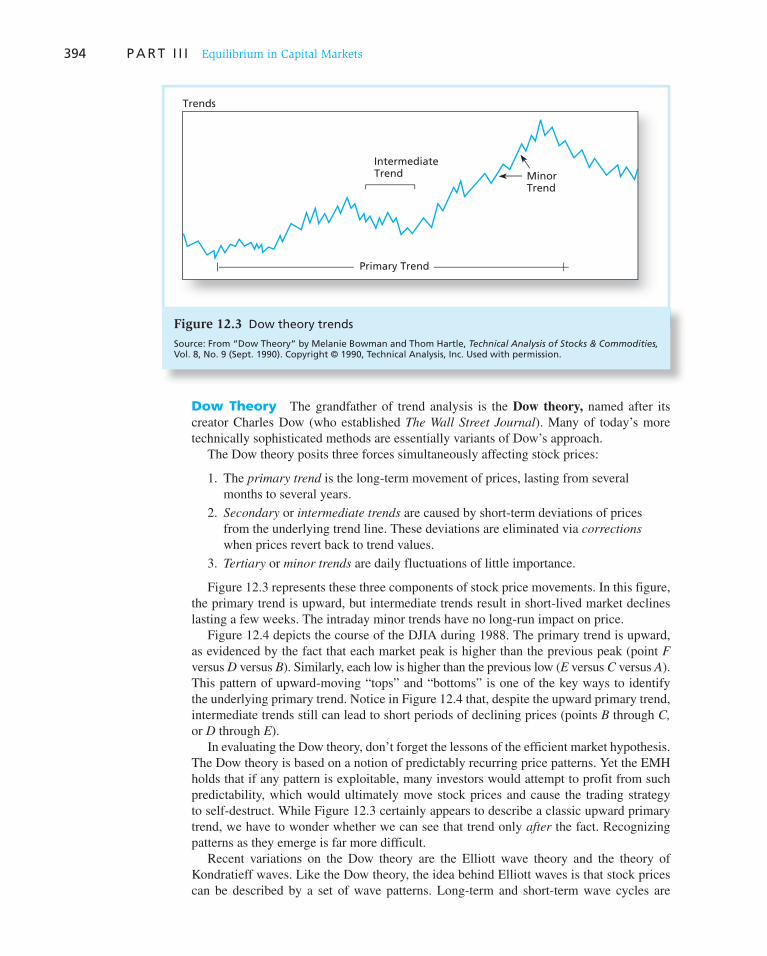
394 P A R T I I I Equilibrium in Capital Markets
Dow Theory The grandfather of trend analysis is the Dow theory, named after its creator Charles Dow (who established The Wall Street Journal ). Many of today’s more technically sophisticated methods are essentially variants of Dow’s approach.
The Dow theory posits three forces simultaneously affecting stock prices:
1. The primary trend is the long-term movement of prices, lasting from several months to several years.
2. Secondary or intermediate trends are caused by short-term deviations of prices from the underlying trend line. These deviations are eliminated via corrections when prices revert back to trend values.
3. Tertiary or minor trends are daily fluctuations of little importance.
Figure 12.3 represents these three components of stock price movements. In this figure, the primary trend is upward, but intermediate trends result in short-lived market declines lasting a few weeks. The intraday minor trends have no long-run impact on price.
Figure 12.4 depicts the course of the DJIA during 1988. The primary trend is upward, as evidenced by the fact that each market peak is higher than the previous peak (point F versus D versus B ). Similarly, each low is higher than the previous low ( E versus C versus A ). This pattern of upward-moving “tops” and “bottoms” is one of the key ways to identify the underlying primary trend. Notice in Figure 12.4 that, despite the upward primary trend, intermediate trends still can lead to short periods of declining prices (points B through C, or D through E ).
In evaluating the Dow theory, don’t forget the lessons of the efficient market hypothesis. The Dow theory is based on a notion of predictably recurring price patterns. Yet the EMH holds that if any pattern is exploitable, many investors would attempt to profit from such predictability, which would ultimately move stock prices and cause the trading strategy to self-destruct. While Figure 12.3 certainly appears to describe a classic upward primary trend, we have to wonder whether we can see that trend only after the fact. Recognizing patterns as they emerge is far more difficult.
Recent variations on the Dow theory are the Elliott wave theory and the theory of Kondratieff waves. Like the Dow theory, the idea behind Elliott waves is that stock prices can be described by a set of wave patterns. Long-term and short-term wave cycles are
Figure 12.3 Dow theory trends
Source: From “Dow Theory” by Melanie Bowman and Thom Hartle, Technical Analysis of Stocks & Commodities,Vol. 8, No. 9 (Sept. 1990). Copyright © 1990, Technical Analysis, Inc. Used with permission.
Trends
IntermediateTrend Minor
Trend
Primary Trend
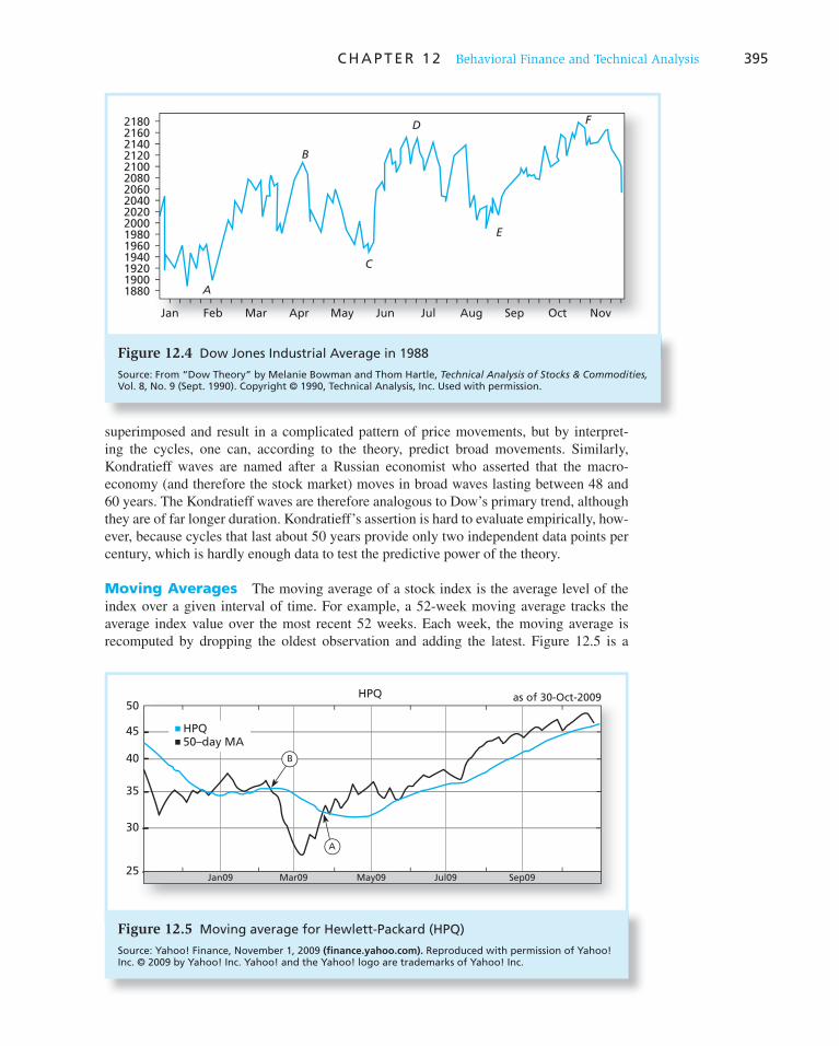
C H A P T E R 1 2 Behavioral Finance and Technical Analysis 395
superimposed and result in a complicated pattern of price movements, but by interpret-ing the cycles, one can, according to the theory, predict broad movements. Similarly, Kondratieff waves are named after a Russian economist who asserted that the macro-economy (and therefore the stock market) moves in broad waves lasting between 48 and 60 years. The Kondratieff waves are therefore analogous to Dow’s primary trend, although they are of far longer duration. Kondratieff’s assertion is hard to evaluate empirically, how-ever, because cycles that last about 50 years provide only two independent data points per century, which is hardly enough data to test the predictive power of the theory.
Moving Averages The moving average of a stock index is the average level of the index over a given interval of time. For example, a 52-week moving average tracks the average index value over the most recent 52 weeks. Each week, the moving average is recomputed by dropping the oldest observation and adding the latest. Figure 12.5 is a
Figure 12.4 Dow Jones Industrial Average in 1988
Source: From “Dow Theory” by Melanie Bowman and Thom Hartle, Technical Analysis of Stocks & Commodities, Vol. 8, No. 9 (Sept. 1990). Copyright © 1990, Technical Analysis, Inc. Used with permission.
Jan Feb Mar Apr May Jun Jul Aug Sep Oct Nov
A
B
C
D
E
F21802160
198019601940192019001880
21402120210020802060204020202000
Figure 12.5 Moving average for Hewlett-Packard (HPQ)
Source: Yahoo! Finance, November 1, 2009 ( finance.yahoo.com ). Reproduced with permission of Yahoo! Inc. © 2009 by Yahoo! Inc. Yahoo! and the Yahoo! logo are trademarks of Yahoo! Inc.
50
45
40
35
30
25
HPQ as of 30-Oct-2009
HPQ50–day MA
Jan09 Mar09 May09 Jul09 Sep09
A
B

396 P A R T I I I Equilibrium in Capital Markets
moving average chart for Hewlett-Packard. Notice that the moving average plot (the col-ored curve) is a “smoothed” version of the original data series (dark curve).
After a period in which prices have generally been falling, the moving average will be above the current price (because the moving average “averages in” the older and higher prices). When prices have been rising, the moving average will be below the current price.
When the market price breaks through the moving average line from below, as at point A in Figure 12.5 , it is taken as a bullish signal because it signifies a shift from a falling trend (with prices below the moving average) to a rising trend (with prices above the moving average). Conversely, when prices fall below the moving average, as at point B, it’s con-sidered time to sell.
There is some variation in the length of the moving average considered most predictive of market movements. Two popular measures are 200-day and 53-week moving averages.
Example 12.4 Moving Averages
Consider the following price data. Each observation represents the closing level of the Dow Jones Industrial Average (DJIA) on the last trading day of the week. The 5-week moving average for each week is the average of the DJIA over the previous 5 weeks. For example, the first entry, for week 5, is the average of the index value between weeks 1 and 5: 10,290, 10,380, 10,399, 10,379, and 10,450. The next entry is the average of the index values between weeks 2 and 6, and so on.
Week DJIA
5-Week Moving Average Week DJIA
5-Week Moving Average
1 10,290 11 10,590 10,555
2 10,380 12 10,652 10,586
3 10,399 13 10,625 10,598
4 10,379 14 10,657 10,624
5 10,450 10,380 15 10,699 10,645
6 10,513 10,424 16 10,647 10,656
7 10,500 10,448 17 10,610 10,648
8 10,565 10,481 18 10,595 10,642
9 10,524 10,510 19 10,499 10,610
10 10,597 10,540 20 10,466 10,563
Figure 12.6 plots the level of the index and the 5-week moving average. Notice that while the index itself moves up and down rather abruptly, the moving average is a rela-tively smooth series, because the impact of each week’s price movement is averaged with that of the previous weeks. Week 16 is a bearish point according to the moving average rule. The price series crosses from above the moving average to below it, signifying the beginning of a downward trend in stock prices.
Breadth The breadth of the market is a measure of the extent to which movement in a market index is reflected widely in the price movements of all the stocks in the market. The most common measure of breadth is the spread between the number of stocks that advance and decline in price. If advances outnumber declines by a wide margin, then the market is

C H A P T E R 1 2 Behavioral Finance and Technical Analysis 397
viewed as being stronger because the rally is widespread. These numbers are reported in The Wall Street Journal
(see Figure 12.7 ). Some analysts cumulate breadth
data each day as in Table 12.1 . The cumulative breadth for each day is obtained by adding that day’s net advances (or declines) to the previous day’s total. The direction of the cumu-lated series is then used to discern broad market trends. Analysts might use a moving average of cumulative breadth to gauge broad trends.
Sentiment Indicators
Trin Statistic Market volume is sometimes used to measure the strength of a market rise or fall. Increased inves-tor participation in a market advance or retreat is viewed as a measure of the significance of the movement. Technicians consider market advances to be a more favorable omen of con-tinued price increases when they are associated with increased trading volume. Similarly, market reversals are considered more bearish when associated with higher volume. The trin statistic is defined as
Trin 5Volume declining/Number declining
Volume advancing/Number advancing
Figure 12.6 Moving averages
10,700
10,600
10,500
10,400
10,300
10,200
10,100
10,000
Week
Do
w J
on
es In
du
stri
al A
vera
ge
1 3 5 7 9 11 13 15 17 19
DJIAMoving Average
Figure 12.7 Market Diary
Source: The Wall Street Journal Online, November 2, 2009. Reprinted by permission of Dow Jones & Company, Inc. via Copyright Clearance Center, Inc. © 2009 Dow Jones & Company, Inc. All Rights Reserved Worldwide.
Issues
AdvancingDecliningunchangedTotal
Issues at
New 52 Week HighNew 52 Week Low
Share Volume
TotalAdvancingDecliningUnchanged
NYSE
1,6041,434
973,135
2814
1,504,894,769795,587,220681,280,499
28,027,050
Amex
234223
67524
410
18,612,6889,216,8887,688,9001,706,900
Nasdaq
1,2771,414
1082,799
2565
2,397,479,9121,226,163,6831,121,231,398
50,084,831
4.02 p.m. EST 11/02/09
Trading Diary: Volume, Advancers, Decliners
Markets Diary

398 P A R T I I I Equilibrium in Capital Markets
Therefore, trin is the ratio of average volume in declining issues to average volume in advancing issues. Ratios above 1.0 are considered bearish because the falling stocks would then have higher average volume than the advancing stocks, indicating net selling pressure. Using the data in Figure 12.7 , trin for the NYSE on this day was
681,280,499/1,434
795,587,220/1,6045 .96
Note, however, that for every buyer, there must be a seller of stock. Rising volume in a rising market should not necessarily indicate a larger imbalance of buyers versus sellers. For example, a trin statistic above 1.0, which is considered bearish, could equally well be interpreted as indicating that there is more buying activity in declining issues.
Confidence Index Barron’s computes a confidence index using data from the bond market. The presumption is that actions of bond traders reveal trends that will emerge soon in the stock market.
The confidence index is the ratio of the average yield on 10 top-rated corporate bonds divided by the average yield on 10 intermediate-grade corporate bonds. The ratio will always be below 100% because higher rated bonds will offer lower promised yields to maturity. When bond traders are optimistic about the economy, however, they might require smaller default premiums on lower rated debt. Hence, the yield spread will narrow, and the confidence index will approach 100%. Therefore, higher values of the confidence index are bullish signals.
Put/Call Ratio Call options give investors the right to buy a stock at a fixed “exercise” price and therefore are a way of betting on stock price increases. Put options give the right to sell a stock at a fixed price and therefore are a way of betting on stock price decreases. 23
The ratio of outstanding put options to outstanding call options is called the put/call ratio.
Typically, the put/call ratio hovers around 65%. Because put options do well in falling markets while call options do well in rising markets, deviations of the ratio from historical norms are considered to be a signal of market sentiment and therefore predictive of market movements.
23 Puts and calls were defined in Chapter 2, Section 2.5. They are discussed more fully in Chapter 20.
Table 12.1
BreadthDay Advances Declines Net Advances Cumulative Breadth
1 1,302 1,248 54 54
2 1,417 1,140 277 331
3 1,203 1,272 269 262
4 1,012 1,622 2610 2348
5 1,133 1,504 2371 2719
Note: The sum of advances plus declines varies across days because some stock prices are unchanged.
CONCEPT CHECK
4 Yields on lower rated debt will rise after fears of recession have spread through the econ-omy. This will reduce the confidence index. Should the stock market now be expected to fall or will it already have fallen?
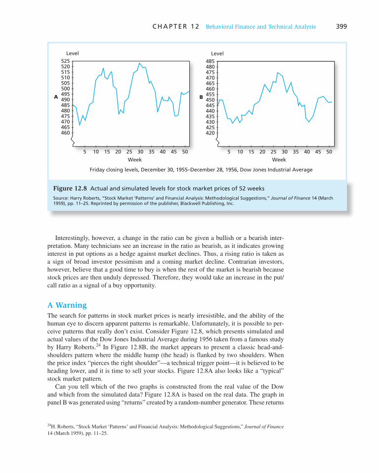
C H A P T E R 1 2 Behavioral Finance and Technical Analysis 399
Interestingly, however, a change in the ratio can be given a bullish or a bearish inter-pretation. Many technicians see an increase in the ratio as bearish, as it indicates growing interest in put options as a hedge against market declines. Thus, a rising ratio is taken as a sign of broad investor pessimism and a coming market decline. Contrarian investors, however, believe that a good time to buy is when the rest of the market is bearish because stock prices are then unduly depressed. Therefore, they would take an increase in the put/call ratio as a signal of a buy opportunity.
A Warning
The search for patterns in stock market prices is nearly irresistible, and the ability of the human eye to discern apparent patterns is remarkable. Unfortunately, it is possible to per-ceive patterns that really don’t exist. Consider Figure 12.8 , which presents simulated and actual values of the Dow Jones Industrial Average during 1956 taken from a famous study by Harry Roberts. 24 In Figure 12.8B , the market appears to present a classic head-and-shoulders pattern where the middle hump (the head) is flanked by two shoulders. When the price index “pierces the right shoulder”—a technical trigger point—it is believed to be heading lower, and it is time to sell your stocks. Figure 12.8A also looks like a “typical” stock market pattern.
Can you tell which of the two graphs is constructed from the real value of the Dow and which from the simulated data? Figure 12.8A is based on the real data. The graph in panel B was generated using “returns” created by a random-number generator. These returns
24 H. Roberts, “Stock Market ‘Patterns’ and Financial Analysis: Methodological Suggestions,” Journal of Finance
14 (March 1959), pp. 11–25.
Figure 12.8 Actual and simulated levels for stock market prices of 52 weeks
Source: Harry Roberts, “Stock Market ‘Patterns’ and Financial Analysis: Methodological Suggestions,” Journal of Finance 14 (March 1959), pp. 11–25. Reprinted by permission of the publisher, Blackwell Publishing, Inc.
Friday closing levels, December 30, 1955–December 28, 1956, Dow Jones Industrial Average
A
5 10 15 20 25 30 35 40 45 50
525520515510505500495490485480475470465460
Level
Week
5 10 15 20 25 30 35 40 45 50
485480475470465460455450445440435430425420
B
Level
Week
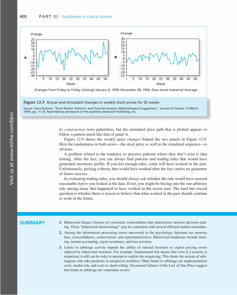
Vis
it u
s at
ww
w.m
hh
e.co
m/b
km400 P A R T I I I Equilibrium in Capital Markets
by construction were patternless, but the simulated price path that is plotted appears to follow a pattern much like that of panel A.
Figure 12.9 shows the weekly price changes behind the two panels in Figure 12.8 . Here the randomness in both series—the stock price as well as the simulated sequence—is obvious.
A problem related to the tendency to perceive patterns where they don’t exist is data mining. After the fact, you can always find patterns and trading rules that would have generated enormous profits. If you test enough rules, some will have worked in the past. Unfortunately, picking a theory that would have worked after the fact carries no guarantee of future success.
In evaluating trading rules, you should always ask whether the rule would have seemed reasonable before you looked at the data. If not, you might be buying into the one arbitrary rule among many that happened to have worked in the recent past. The hard but crucial question is whether there is reason to believe that what worked in the past should continue to work in the future.
Figure 12.9 Actual and simulated changes in weekly stock prices for 52 weeks
Source: Harry Roberts, “Stock Market ‘Patterns’ and Financial Analysis: Methodological Suggestions,” Journal of Finance 14 (March 1959), pp. 11–25. Reprinted by permission of the publisher, Blackwell Publishing, Inc.
Changes from Friday to Friday (closing) January 6, 1956–December 28, 1956, Dow Jones Industrial Average
25201510
50
−5−10−15−20−25−30
1 5 10 15 20 3025 35 40 45 50
Week
A
Change3025201510
50
−5−10−15−20−25
1 5 10 15 20 3025 35 40 45 50
Week
B
Change
1. Behavioral finance focuses on systematic irrationalities that characterize investor decision mak-ing. These “behavioral shortcomings” may be consistent with several efficient market anomalies.
2. Among the information processing errors uncovered in the psychology literature are memory bias, overconfidence, conservatism, and representativeness. Behavioral tendencies include fram-ing, mental accounting, regret avoidance, and loss aversion.
3. Limits to arbitrage activity impede the ability of rational investors to exploit pricing errors induced by behavioral investors. For example, fundamental risk means that even if a security is mispriced, it still can be risky to attempt to exploit the mispricing. This limits the actions of arbi-trageurs who take positions in mispriced securities. Other limits to arbitrage are implementation costs, model risk, and costs to short-selling. Occasional failures of the Law of One Price suggest that limits to arbitrage are sometimes severe.
SUMMARY

Vis
it u
s at
ww
w.m
hh
e.co
m/b
km
C H A P T E R 1 2 Behavioral Finance and Technical Analysis 401
4. The various limits to arbitrage mean that even if prices do not equal intrinsic value, it still may be
difficult to exploit the mispricing. As a result, the failure of traders to beat the market may not be
proof that markets are in fact efficient, with prices equal to intrinsic value.
5. Technical analysis is the search for recurring and predictable patterns in stock prices. It is based
on the premise that prices only gradually close in on intrinsic value. As fundamentals shift, astute
traders can exploit the adjustment to a new equilibrium.
6. Technical analysis also uses volume data and sentiment indicators. These are broadly consistent
with several behavioral models of investor activity.
7. The Dow theory attempts to identify underlying trends in stock indexes. Moving averages, rela-
tive strength, and breadth are used in other trend-based strategies.
8. Some sentiment indicators are the trin statistic, the confidence index, and the put/call ratio.
Related Web sites for this chapter are available at www.mhhe.com/bkm
behavioral finance
conservatism
representativeness
framing
mental accounting
regret avoidance
prospect theory
fundamental risk
disposition effect
Dow theory
breadth
trin statistic
confidence index
put/call ratio
KEY TERMS
1. Explain how some of the behavioral biases discussed in the chapter might contribute to the suc-
cess of technical trading rules.
2. Why would an advocate of the efficient market hypothesis believe that even if many investors
exhibit the behavioral biases discussed in the chapter, security prices might still be set efficiently?
3. What sorts of factors might limit the ability of rational investors to take advantage of any “pricing
errors” that result from the actions of “behavioral investors”?
4. Even if behavioral biases do not affect equilibrium asset prices, why might it still be important for
investors to be aware of them?
5. Some advocates of behavioral finance agree with efficient market advocates that indexing is the
optimal investment strategy for most investors. But their reasons for this conclusion differ greatly.
Compare and contrast the rationale for indexing according to both of these schools of thought.
6. Jill Davis tells her broker that she does not want to sell her stocks that are below the price she paid
for them. She believes that if she just holds on to them a little longer they will recover, at which
time she will sell them. What behavioral characteristic does Davis have as the basis for her deci-
sion making?
a. Loss aversion.
b. Conservatism.
c. Representativeness.
7. After Polly Shrum sells a stock, she avoids following it in the media. She is afraid that it may
subsequently increase in price. What behavioral characteristic does Shrum have as the basis for
her decision making?
a. Fear of regret.
b. Representativeness.
c. Mental accounting.
8. All of the following actions are consistent with feelings of regret except:
a. Selling losers quickly.
b. Hiring a full-service broker.
c. Holding on to losers too long.
PROBLEM SETS
i. Basic

Vis
it u
s at
ww
w.m
hh
e.co
m/b
km402 P A R T I I I Equilibrium in Capital Markets
9. Match each example to one of the following behavioral characteristics.
Example Characteristic
a. Investors are slow to update their beliefs when given new
evidence .
i. Disposition effect.
b. Investors are reluctant to bear losses caused by their
unconventional decisions.
ii. Representativeness bias.
c. Investors exhibit less risk tolerance in their retirement
accounts versus their other stock accounts.
iii. Regret avoidance.
d. Investors are reluctant to sell stocks with “paper” losses. iv. Conservatism bias.
e. Investors disregard sample size when forming views about
the future from the past.
v. Mental accounting.
10. What do we mean by fundamental risk, and why may such risk allow behavioral biases to persist for long periods of time?
11. What is meant by data mining, and why must technical analysts be careful not to engage in it?
12. Even if prices follow a random walk, they still may not be informationally efficient. Explain why this may be true, and why it matters for the efficient allocation of capital in our economy.
13. Use the data from The Wall Street Journal in Figure 12.7 to verify the trin ratio for the NYSE. Is the trin ratio bullish or bearish?
14. Calculate breadth for the NYSE using the data in Figure 12.7 . Is the signal bullish or bearish?
15. Collect data on the DJIA for a period covering a few months. Try to identify primary trends. Can you tell whether the market currently is in an upward or downward trend?
16. Suppose Baa-rated bonds currently yield 6%, while Aa-rated bonds yield 5%. Suppose that due to an increase in the expected inflation rate, the yields on both bonds increase by 1%. What would happen to the confidence index? Would this be interpreted as bullish or bearish by a technical analyst? Does this make sense to you?
17. Table 12A presents price data for Computers, Inc., and a computer industry index. Does Com-puters, Inc., show relative strength over this period?
18. Use again the data in Table 12A to compute a 5-day moving average for Computers, Inc. Can you identify any buy or sell signals?
19. Yesterday, the Dow Jones industrials gained 54 points. However, 1,704 issues declined in price while 1,367 advanced. Why might a technical analyst be concerned even though the market index rose on this day?
20. Table 12B contains data on market advances and declines. Calculate cumulative breadth and decide whether this technical signal is bullish or bearish.
21. If the trading volume in advancing shares on day 1 in the previous problem was 330 million shares, while the volume in declining issues was 240 million shares, what was the trin statistic for that day? Was trin bullish or bearish?
22. Given the following data, is the confidence index rising or falling? What might explain the pattern of yield changes?
This Year Last Year
Yield on top-rated corporate bonds 8% 8.5%
Yield on intermediate-grade
corporate bonds
10.5 10
ii. Intermediate
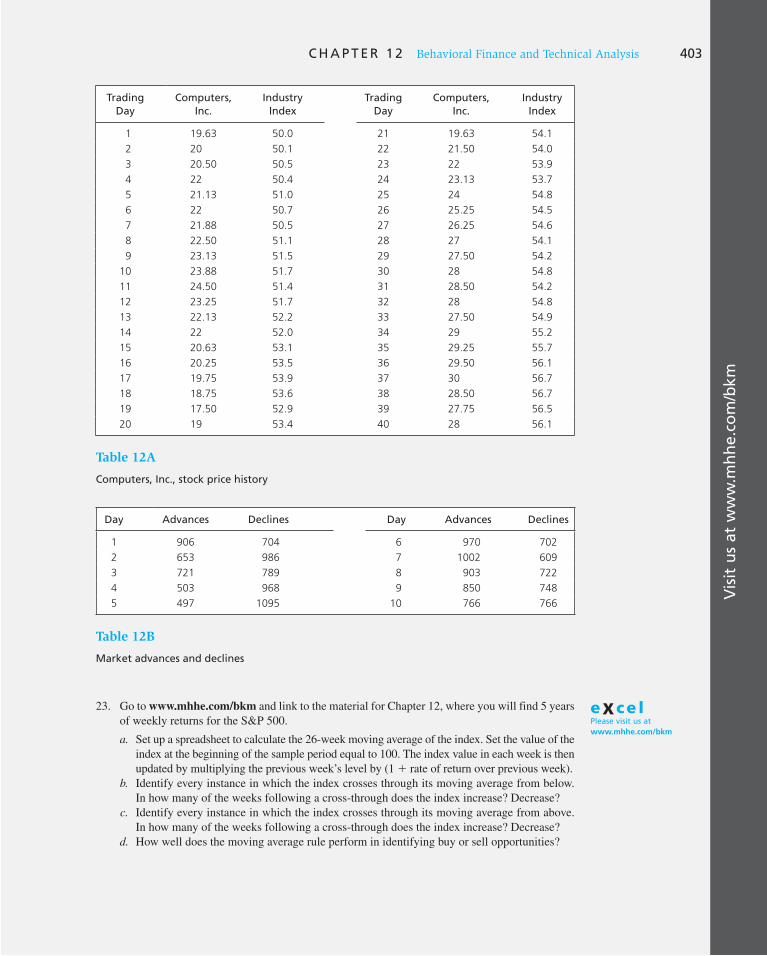
Vis
it u
s at
ww
w.m
hh
e.co
m/b
km
C H A P T E R 1 2 Behavioral Finance and Technical Analysis 403
Trading Day
Computers, Inc.
Industry Index
Trading Day
Computers, Inc.
Industry Index
1 19.63 50.0 21 19.63 54.1
2 20 50.1 22 21.50 54.0
3 20.50 50.5 23 22 53.9
4 22 50.4 24 23.13 53.7
5 21.13 51.0 25 24 54.8
6 22 50.7 26 25.25 54.5
7 21.88 50.5 27 26.25 54.6
8 22.50 51.1 28 27 54.1
9 23.13 51.5 29 27.50 54.2
10 23.88 51.7 30 28 54.8
11 24.50 51.4 31 28.50 54.2
12 23.25 51.7 32 28 54.8
13 22.13 52.2 33 27.50 54.9
14 22 52.0 34 29 55.2
15 20.63 53.1 35 29.25 55.7
16 20.25 53.5 36 29.50 56.1
17 19.75 53.9 37 30 56.7
18 18.75 53.6 38 28.50 56.7
19 17.50 52.9 39 27.75 56.5
20 19 53.4 40 28 56.1
Table 12A
Computers, Inc., stock price history
Day Advances Declines Day Advances Declines
1 906 704 6 970 702
2 653 986 7 1002 609
3 721 789 8 903 722
4 503 968 9 850 748
5 497 1095 10 766 766
Table 12B
Market advances and declines
23. Go to www.mhhe.com/bkm and link to the material for Chapter 12, where you will find 5 years of weekly returns for the S&P 500.
a. Set up a spreadsheet to calculate the 26-week moving average of the index. Set the value of the index at the beginning of the sample period equal to 100. The index value in each week is then updated by multiplying the previous week’s level by (1 1 rate of return over previous week).
b. Identify every instance in which the index crosses through its moving average from below. In how many of the weeks following a cross-through does the index increase? Decrease?
c. Identify every instance in which the index crosses through its moving average from above. In how many of the weeks following a cross-through does the index increase? Decrease?
d. How well does the moving average rule perform in identifying buy or sell opportunities?
eXce lPlease visit us at www.mhhe.com/bkm

Vis
it u
s at
ww
w.m
hh
e.co
m/b
km404 P A R T I I I Equilibrium in Capital Markets
24. Go to www.mhhe.com/bkm and link to the material for Chapter 12, where you will find 5 years of weekly returns for the S&P 500 and Fidelity’s Select Banking Fund (ticker FSRBX).
a. Set up a spreadsheet to calculate the relative strength of the banking sector compared to the broad market. Hint: As in the previous problem, set the initial value of the sector index and the S&P 500 index equal to 100, and use each week’s rate of return to update the level of each index.
b. Identify every instance in which the relative strength ratio increases by at least 5% from its value 5 weeks earlier. In how many of the weeks following a substantial increase in relative strength does the banking sector outperform the S&P 500? In how many of those weeks does the banking sector underperform the S&P 500?
c. Identify every instance in which the relative strength ratio decreases by at least 5% from its value 5 weeks earlier. In how many of the weeks following a substantial decrease in relative strength does the banking sector underperform the S&P 500? In how many of those weeks does the banking sector outperform the S&P 500?
d. How well does the relative strength rule perform in identifying buy or sell opportunities?
25. One seeming violation of the Law of One Price is the pervasive discrepancy of closed-end fund prices from their net asset values. Would you expect to observe greater discrepancies on diversi-fied or less-diversified funds? Why?
eXce lPlease visit us at www.mhhe.com/bkm
iii. Challenge
1. Don Sampson begins a meeting with his financial adviser by outlining his investment philoso-phy as shown below:
Statement Number Statement
1 Investments should offer strong return potential but with very limited risk.
I prefer to be conservative and to minimize losses, even if I miss out on
substantial growth opportunities.
2 All nongovernmental investments should be in industry-leading and
financially strong companies.
3 Income needs should be met entirely through interest income and cash
dividends. All equity securities held should pay cash dividends.
4 Investment decisions should be based primarily on consensus forecasts
of general economic conditions and company-specific growth.
5 If an investment falls below the purchase price, that security should be
retained until it returns to its original cost. Conversely, I prefer to take
quick profits on successful investments.
6 I will direct the purchase of investments, including derivative securities,
periodically. These aggressive investments result from personal research and
may not prove consistent with my investment policy. I have not kept records
on the performance of similar past investments, but I have had some “big
winners.”
Select the statement from the table above that best illustrates each of the following behavioral finance concepts. Justify your selection.
a. Mental accounting. b. Overconfidence (illusion of control). c. Reference dependence (framing).
2. Monty Frost’s tax-deferred retirement account is invested entirely in equity securities. Because the international portion of his portfolio has performed poorly in the past, he has reduced his international equity exposure to 2%. Frost’s investment adviser has recommended an increased international equity exposure. Frost responds with the following comments:

Vis
it u
s at
ww
w.m
hh
e.co
m/b
km
C H A P T E R 1 2 Behavioral Finance and Technical Analysis 405
a. On the basis of past poor performance, I want to sell all my remaining international equity securities once their market prices rise to equal their original cost.
b. Most diversified international portfolios have had disappointing results over the past 5 years. During that time, however, the market in Country XYZ has outperformed all other markets, even our own. If I do increase my international equity exposure, I would prefer that the entire exposure consist of securities from Country XYZ.
c. International investments are inherently more risky. Therefore, I prefer to purchase any international equity securities in my “speculative” account, my best chance at becoming rich. I do not want them in my retirement account, which has to protect me from poverty in my old age.
Frost’s adviser is familiar with behavioral finance concepts but prefers a traditional or standard finance approach (modern portfolio theory) to investments.
Indicate the behavioral finance concept that Frost most directly exhibits in each of his three comments. Explain how each of Frost’s comments can be countered by using an argument from standard finance.
3. Louise and Christopher Maclin live in London, United Kingdom, and currently rent an apart-ment in the metropolitan area. During an initial discussion of the Maclins’ financial plans, Christopher Maclin makes the following statements to the Maclins’ financial adviser, Grant Webb:
a. “I have used the Internet extensively to research the outlook for the housing market over the next 5 years, and I believe now is the best time to buy a house.”
b. “I do not want to sell any bond in my portfolio for a lower price than I paid for the bond.” c. “I will not sell any of my company stock because I know my company and I believe it has
excellent prospects for the future.”
For each statement ( a )–( c ) identify the behavioral finance concept most directly exhibited. Explain how each behavioral finance concept is affecting Maclin’s investment decision making.
4. During an interview with her investment adviser, a retired investor made the following two statements:
a. “I have been very pleased with the returns I’ve earned on Petrie stock over the past 2 years and I am certain that it will be a superior performer in the future.”
b. “I am pleased with the returns from the Petrie stock because I have specific uses for that money. For that reason, I certainly want my retirement fund to continue owning the Petrie stock.”
Identify which principle of behavioral finance is most consistent with each of the investor’s two statements.
5. Claire Pierce comments on her life circumstances and investment outlook:
I must support my parents who live overseas on Pogo Island. The Pogo Island economy has grown rapidly over the past 2 years with minimal inflation, and consensus forecasts call for a continuation of these favorable trends for the foreseeable future. Economic growth has resulted from the export of a natural resource used in an exciting new technology application.
I want to invest 10% of my portfolio in Pogo Island government bonds. I plan to purchase long-term bonds because my parents are likely to live more than 10 years. Experts uniformly do not foresee a resurgence of inflation on Pogo Island, so I am certain that the total returns produced by the bonds will cover my parents’ spending needs for many years to come. There should be no exchange rate risk because the bonds are denominated in local currency. I want to buy the Pogo Island bonds, but am not willing to distort my portfolio’s long-term asset allocation to do so. The overall mix of stocks, bonds, and other investments should not change. Therefore, I am considering selling one of my U.S. bond funds to raise cash to buy the Pogo Island bonds. One possibility is my

Vis
it u
s at
ww
w.m
hh
e.co
m/b
km406 P A R T I I I Equilibrium in Capital Markets
High Yield Bond Fund, which has declined 5% in value year to date. I am not excited about this fund’s prospects; in fact I think it is likely to decline more, but there is a small probability that it could recover very quickly. So I have decided instead to sell my Core Bond Fund that has appreciated 5% this year. I expect this investment to continue to deliver attractive returns, but there is a small chance this year’s gains might disappear quickly.
Once that shift is accomplished, my investments will be in great shape. The sole exception is my Small Company Fund, which has performed poorly. I plan to sell this investment as soon as the price increases to my original cost.
Identify three behavioral finance concepts illustrated in Pierce’s comments and describe each of the three concepts. Discuss how an investor practicing standard or traditional finance would chal-lenge each of the three concepts.
E-INVEST-MENTS EXERCISES
Charting and Technical Analysis
Yahoo! Finance ( finance.yahoo.com ) offers significant capabilities in charting and other technical indicators. Under the charting function, you can specify comparisons between companies by choosing the technical analysis tab. Short interest ratios are found under the company profile report. Prepare charts of moving averages and obtain short interest ratios for GE and SWY. Prepare a 1-year chart of the 50- and 200-day average price of GE, SWY, and the S&P 500 index. Which, if either, of the companies is priced above its 50- and 200-day averages? Would you consider their charts as bullish or bearish? Why? What are the short interest ratios for the two companies? Has short interest displayed any signifi-cant trend?
SOLUTIONS TO CONCEPT CHECKS
1. Conservatism implies that investors will at first respond too slowly to new information, leading to trends in prices. Representativeness can lead them to extrapolate trends too far into the future and overshoot intrinsic value. Eventually, when the pricing error is corrected, we observe a reversal.
2. Out-of-favor stocks will exhibit low prices relative to various proxies for intrinsic value such as earnings. Because of regret avoidance, these stocks will need to offer a more attractive rate of return to induce investors to hold them. Thus, low P/E stocks might on average offer higher rates of return.
3. At liquidation, price will equal NAV. This puts a limit on fundamental risk. Investors need only carry the position for a few months to profit from the elimination of the discount. Moreover, as the liquidation date approaches, the discount should dissipate. This greatly limits the risk that the discount can move against the investor. At the announcement of impending liquidation, the discount should immediately disappear, or at least shrink considerably.
4. By the time the news of the recession affects bond yields, it also ought to affect stock prices. The market should fall before the confidence index signals that the time is ripe to sell.
IN THIS CHAPTER, we consider the empirical
evidence in support of the CAPM and APT. At
the outset, however, it is worth noting that
many of the implications of these models
already have been accepted in widely varying
applications. Consider the following:
1. Many professional portfolio managers use
the expected return–beta relationship of
security returns. Furthermore, many firms
rate the performance of portfolio managers
according to the reward-to-volatility ratios
they maintain and the average rates of return
they realize relative to the CML or SML.
2. Regulatory commissions use the expected
return–beta relationship along with fore-
casts of the market index return as one
factor in determining the cost of capital
for regulated firms.
3. Court rulings on torts cases sometimes
use the expected return–beta relationship
to determine discount rates to evaluate
claims of lost future income.
4. Many firms use the SML to obtain a
benchmark hurdle rate for capital
budgeting decisions.
These practices show that the financial com-
munity has passed a favorable judgment on
the CAPM and the APT, if only implicitly.
In this chapter we consider the evidence
along more explicit and rigorous lines. The
first part of the chapter presents the method-
ology that has been deployed in testing the
single-factor CAPM and APT and assesses the
results. The second part of the chapter pro-
vides an overview of current efforts to estab-
lish the validity of multifactor versions of the
CAPM and APT. In the third part, we discuss
recent literature on so-called anomalies in
patterns of security returns and some of the
responses to these puzzling findings. Finally,
we present interesting research on stock
returns that examines the size of the equity
risk premium. Conventional wisdom has held
for a long time that the history of returns
on equities is quite puzzling. Recent studies
address the puzzle.
Why lump together empirical works on
the CAPM and APT? The CAPM is a theoreti-
cal construct that predicts expected rates of
return on assets, relative to a market portfo-
lio of all risky assets. It is difficult to test these
predictions empirically because expected
returns, covariances, and the exact market
portfolio are unobservable (see Chapter 9). To
overcome this difficulty, a single-factor or mul-
tifactor capital market usually is postulated,
where a broad-based market index p ortfolio
13 Empirical Evidence on Security Returns 3
PAR
T III CHAPTER THIRTEEN

408
(concluded)
(such as the S&P 500) is assumed to represent
the factor, or one of the factors. Furthermore,
to obtain more reliable statistics, most tests have
been conducted with the rates of return on highly
diversified portfolios rather than on individual
securities. For both of these reasons, tests that
have been directed at the CAPM actually have
been more suitable to establish the validity of
the APT. We will see that it is more important to
distinguish the empirical work on the basis of the
factor structure that is assumed or estimated than
to distinguish between tests of the CAPM and
the APT.
13.1 The Index Model and the Single-Factor APT
The Expected Return–Beta Relationship
Recall that if the expected return–beta relationship holds with respect to an observable ex ante efficient index, M, the expected rate of return on any security i is
E(ri) 5 rf 1 bi 3E(rM) 2 rf 4 (13.1)
where b i is defined as Cov(ri , rM)/sM2 .
This is the most commonly tested implication of the CAPM. Early simple tests fol-lowed three basic steps: establishing sample data, estimating the SCL (security character-istic line), and estimating the SML (security market line).
Setting Up the Sample Data Determine a sample period of, for example, 60 monthly holding periods (5 years). For each of the 60 holding periods, collect the rates of return on 100 stocks, a market portfolio proxy (e.g., the S&P 500), and 1-month (risk-free) T-bills. Your data thus consist of
r it 5 Returns on the 100 stocks over the 60-month sample period; i 5 1, . . . , 100, and t 5 1, . . . , 60.
r Mt 5 Returns on the S&P 500 index over the sample period.
r ft 5 Risk-free rate each month.
This constitutes a table of 102 3 60 5 6,120 rates of return.
Estimating the SCL View Equation 13.1 as a security characteristic line (SCL), as in Chapter 8. For each stock, i, you estimate the beta coefficient as the slope of a first-pass
regression equation. (The terminology first-pass regression is due to the fact that the esti-mated coefficients will be used as input into a second-pass regression. )
rit 2 rft 5 ai 1 bi(rMt 2 rft) 1 eit
You will use the following statistics in later analysis:
ri 2 rf 5 Sample averages (over the 60 observations) of the excess return on each of the 100 stocks.
b i 5 Sample estimates of the beta coefficients of each of the 100 stocks.
rM 2 rf 5 Sample average of the excess return of the market index.
s 2 ( e i ) 5 Estimates of the variance of the residuals for each of the 100 stocks.

C H A P T E R 1 3 Empirical Evidence on Security Returns 409
The sample average excess returns on each stock and the market portfolio are taken as estimates of expected excess returns, and the values of b i are estimates of the true beta coefficients for the 100 stocks during the sample period. s 2 ( e i ) estimates the nonsystematic risk of each of the 100 stocks.
CONCEPT CHECK
1
a. How many regression estimates of the SCL do we have from the sample?
b. How many observations are there in each of the regressions?
c. According to the CAPM, what should be the intercept in each of these regressions?
Estimating the SML Now view Equation 13.1 as a security market line (SML) with 100 observations for the stocks in your sample. You can estimate g 0 and g 1 in the following second-pass regression equation with the estimates b i from the first pass as the independent variable:
ri 2 rf 5 g0 1 g1bi i 5 1, c, 100 (13.2)
Compare Equations 13.1 and 13.2; you should conclude that if the CAPM is valid, then g 0 and g 1 should satisfy
g0 5 0 and g1 5 rM 2 rf
In fact, however, you can go a step further and argue that the key property of the expected return–beta relationship described by the SML is that the expected excess return on securi-ties is determined only by the systematic risk (as measured by beta) and should be inde-pendent of the nonsystematic risk, as measured by the variance of the residuals, s 2 ( e i ), which also were estimated from the first-pass regression. These estimates can be added as a variable in Equation 13.2 of an expanded SML that now looks like this:
ri 2 rf 5 g0 1 g1bi 1 g2s2(ei) (13.3)
This second-pass regression equation is estimated with the hypotheses
g0 5 0; g1 5 rM 2 rf ; g2 5 0
The hypothesis that g 2 5 0 is consistent with the notion that nonsystematic risk should not be “priced,” that is, that there is no risk premium earned for bearing nonsystem-atic risk. More generally, according to the CAPM, the risk premium depends only on beta. Therefore, any additional right-hand-side variable in Equation 13.3 beyond beta should have a coefficient that is insignificantly different from zero in the second-pass regression.
Tests of the CAPM
Early tests of the CAPM performed by John Lintner, 1 and later replicated by Merton Miller and Myron Scholes, 2 used annual data on 631 NYSE stocks for 10 years, 1954 to 1963,
1 John Lintner, “Security Prices, Risk and Maximal Gains from Diversification,” Journal of Finance 20 (December 1965).
2 Merton H. Miller and Myron Scholes, “Rate of Return in Relation to Risk: A Reexamination of Some Recent Findings,” in Studies in the Theory of Capital Markets, ed. Michael C. Jensen (New York: Praeger, 1972).

410 P A R T I I I Equilibrium in Capital Markets
and produced the following estimates (with returns expressed as decimals rather than percentages):
Coefficient: g 0 5 .127 g 1 5 .042 g 2 5 .310
Standard error: .006 .006 .026
Sample average: rM 2 rf 5 .165
These results are inconsistent with the CAPM. First, the estimated SML is “too flat”; that is, the g 1 coefficient is too small. The slope should equal rM 2 rf 5 .165 (16.5% per year), but it is estimated at only .042. The difference, .122, is about 20 times the standard error of the estimate, .006, which means that the measured slope of the SML is less than it should be by a statistically significant margin. At the same time, the intercept of the esti-mated SML, g 0 , which is hypothesized to be zero, in fact equals .127, which is more than 20 times its standard error of.006.
The two-stage procedure employed by these researchers (i.e., first estimate security betas using a time-series regression and then use those betas to test the SML relationship between risk and average return) seems straightforward, and the rejection of the CAPM using this approach is disappointing. However, it turns out that there are several difficulties with this approach. First and foremost, stock returns are extremely volatile, which lessens the precision of any tests of average return. For example, the average standard deviation of annual returns of the stocks in the S&P 500 is about 40%; the average standard deviation of annual returns of the stocks included in these tests is probably even higher.
In addition, there are fundamental concerns about the validity of the tests. First, the market index used in the tests is surely not the “market portfolio” of the CAPM. Second, in light of asset volatility, the security betas from the first-stage regressions are necessarily estimated with substantial sampling error and therefore cannot readily be used as inputs to the second-stage regression. Finally, investors cannot borrow at the risk-free rate, as assumed by the simple version of the CAPM. Let us investigate the implications of these problems in turn.
The Market Index
In what has become known as Roll’s critique, Richard Roll 3 pointed out that:
1. There is a single testable hypothesis associated with the CAPM: The market portfolio is mean-variance efficient.
2. All the other implications of the model, the best-known being the linear relation between expected return and beta, follow from the market portfolio’s efficiency and therefore are not independently testable. There is an “if and only if” relation between the expected return–beta relationship and the efficiency of the market portfolio.
3 Richard Roll, “A Critique of the Asset Pricing Theory’s Tests: Part I: On Past and Potential Testability of the Theory,” Journal of Financial Economics 4 (1977).
CONCEPT CHECK
2
a. What is the implication of the empirical SML being “too flat”?
b. Do high- or low-beta stocks tend to outperform the predictions of the CAPM?
c. What is the implication of the estimate of g 2 ?
C H A P T E R 1 3 Empirical Evidence on Security Returns 411
3. In any sample of observations of individual returns there will be an infinite number of ex post (i.e., after the fact) mean-variance efficient portfolios using the sample-period returns and covariances (as opposed to the ex ante expected returns and covariances). Sample betas calculated between each such portfolio and individual assets will be exactly linearly related to sample average returns. In other words, if betas are calculated against such portfolios, they will satisfy the SML relation exactly whether or not the true market portfolio is mean-variance efficient in an ex ante sense.
4. The CAPM is not testable unless we know the exact composition of the true market portfolio and use it in the tests. This implies that the theory is not testable unless all individual assets are included in the sample.
5. Using a proxy such as the S&P 500 for the market portfolio is subject to two difficul-ties. First, the proxy itself might be mean-variance efficient even when the true mar-ket portfolio is not. Conversely, the proxy may turn out to be inefficient, but obviously this alone implies nothing about the true market portfolio’s efficiency. Furthermore, most reasonable market proxies will be very highly correlated with each other and with the true market portfolio whether or not they are mean-variance efficient. Such a high degree of correlation will make it seem that the exact composition of the market portfolio is unimportant, whereas the use of different proxies can lead to quite differ-ent conclusions. This problem is referred to as benchmark error, because it refers to the use of an incorrect benchmark (market proxy) portfolio in the tests of the theory.
Roll and Ross 4 and Kandel and Stambaugh 5 expanded Roll’s critique. Essentially, they argued that tests that reject a positive relationship between average return and beta point to inefficiency of the market proxy used in those tests, rather than refuting the theoretical expected return–beta relationship. They demonstrate that even if the CAPM is true, highly diversified portfolios, such as the value- or equally weighted portfolios of all stocks in the sample, may fail to produce a significant average return–beta relationship.
Kandel and Stambaugh considered the properties of the usual two-pass test of the CAPM in an environment in which borrowing is restricted but the zero-beta version of the CAPM holds. In this case, you will recall that the expected return–beta relationship describes the expected returns on a stock, a portfolio E on the efficient frontier, and that portfolio’s zero-beta companion, Z (see Equation 9.12):
E(ri) 2 E(rZ) 5 bi 3E(rE) 2 E(rZ) 4 (13.4)
where b i denotes the beta of security i on efficient portfolio E. We cannot construct or observe the efficient portfolio E (because we do not know
expected returns and covariances of all assets), and so we cannot estimate Equation 13.4 directly. Kandel and Stambaugh asked what would happen if we followed the common procedure of using a market proxy portfolio M in place of E, and used as well the more efficient generalized least squares regression procedure in estimating the second-pass regression for the zero-beta version of the CAPM, that is,
ri 2 rZ 5 g0 1 g1 3 (Estimated bi)
4 Richard Roll and Stephen A. Ross, “On the Cross-Sectional Relation between Expected Return and Betas,” Journal of Finance 50 (1995), pp. 185–224.
5 Schmuel Kandel and Robert F. Stambaugh, “Portfolio Inefficiency and the Cross-Section of Expected Returns,” Journal of Finance 50 (1995), pp. 185–224; “A Mean-Variance Framework for Tests of Asset Pricing Models,” Review of Financial Studies 2 (1989), pp. 125–56; “On Correlations and Inferences about Mean-Variance Efficiency,” Journal of Financial Economics 18 (1987), pp. 61–90.

412 P A R T I I I Equilibrium in Capital Markets
They showed that the estimated values of g 0 and g 1 will be biased by a term proportional to the relative efficiency of the market proxy. If the market index used in the regression is fully efficient, the test will be well specified. But the second-pass regression will provide a poor test of the CAPM if the proxy for the market portfolio is not efficient. Thus, we still cannot test the model in a meaningful way without a reasonably efficient market proxy. Unfortunately, determining how efficient our market index is relative to the theoretical true market portfolio is difficult, so we cannot tell how good our tests are.
Measurement Error in Beta
Roll’s critique tells us that CAPM tests are handicapped from the outset. But suppose that we could get past Roll’s problem by obtaining data on the returns of the true market portfo-lio. We still would have to deal with the statistical problems caused by measurement error in the estimates of beta from the first-stage regressions.
It is well known in statistics that if the right-hand-side variable of a regression equation is measured with error (in our case, beta is measured with error and is the right-hand-side variable in the second-pass regression), then the slope coefficient of the regression equa-tion will be biased downward and the intercept biased upward. This is consistent with the findings cited above, which found that the estimate of g 0 was higher than predicted by the CAPM and that the estimate of g 1 was lower than predicted.
Indeed, a well-controlled simulation test by Miller and Scholes 6 confirms these argu-ments. In this test a random-number generator simulated rates of return with covariances similar to observed ones. The average returns were made to agree exactly with the CAPM expected return–beta relationship. Miller and Scholes then used these randomly generated rates of return in the tests we have described as if they were observed from a sample of stock returns. The results of this “simulated” test were virtually identical to those reached using real data, despite the fact that the simulated returns were constructed to obey the SML, that is, the true g coefficients were g0 5 0, g1 5 rM 2 rf , and g 2 5 0.
This postmortem of the early test gets us back to square one. We can explain away the disappointing test results, but we have no positive results to support the CAPM-APT implications.
The next wave of tests was designed to overcome the measurement error problem that led to biased estimates of the SML. The innovation in these tests, pioneered by Black, Jensen, and Scholes, 7 was to use portfolios rather than individual securities. Combining securities into portfolios diversifies away most of the firm-specific part of returns, thereby enhancing the precision of the estimates of beta and the expected rate of return of the portfolio of securities. This mitigates the statistical problems that arise from measurement error in the beta estimates.
Obviously, however, combining stocks into portfolios reduces the number of observa-tions left for the second-pass regression. For example, suppose that we group our sample of 100 stocks into five portfolios of 20 stocks each. If the assumption of a single-factor market is reasonably accurate, then the residuals of the 20 stocks in each portfolio will be practically uncorrelated and, hence, the variance of the portfolio residual will be about one-twentieth the residual variance of the average stock. Thus the portfolio beta in the first-pass regression will be estimated with far better accuracy. However, now consider the second-pass regression. With individual securities, we had 100 observations to estimate
6 Miller and Scholes, “Rate of Return in Relation to Risk.”
7 Fischer Black, Michael C. Jensen, and Myron Scholes, “The Capital Asset Pricing Model: Some Empirical Tests,” in Studies in the Theory of Capital Markets, ed. Michael C. Jensen (New York: Praeger, 1972).
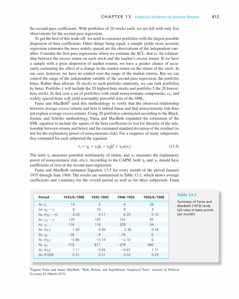
C H A P T E R 1 3 Empirical Evidence on Security Returns 413
the second-pass coefficients. With portfolios of 20 stocks each, we are left with only five observations for the second-pass regression.
To get the best of this trade-off, we need to construct portfolios with the largest possible dispersion of beta coefficients. Other things being equal, a sample yields more accurate regression estimates the more widely spaced are the observations of the independent vari-ables. Consider the first-pass regressions where we estimate the SCL, that is, the relation-ship between the excess return on each stock and the market’s excess return. If we have a sample with a great dispersion of market returns, we have a greater chance of accu-rately estimating the effect of a change in the market return on the return of the stock. In our case, however, we have no control over the range of the market returns. But we can control the range of the independent variable of the second-pass regression, the portfolio betas. Rather than allocate 20 stocks to each portfolio randomly, we can rank portfolios by betas. Portfolio 1 will include the 20 highest-beta stocks and portfolio 5 the 20 lowest-beta stocks. In that case a set of portfolios with small nonsystematic components, e P , and widely spaced betas will yield reasonably powerful tests of the SML.
Fama and MacBeth 8 used this methodology to verify that the observed relationship between average excess returns and beta is indeed linear and that nonsystematic risk does not explain average excess returns. Using 20 portfolios constructed according to the Black, Jensen, and Scholes methodology, Fama and MacBeth expanded the estimation of the SML equation to include the square of the beta coefficient (to test for linearity of the rela-tionship between returns and betas) and the estimated standard deviation of the residual (to test for the explanatory power of nonsystematic risk). For a sequence of many subperiods, they estimated for each subperiod the equation
ri 5 g0 1 g1bi 1 g2bi2 1 g3s(ei) (13.5)
The term g 2 measures potential nonlinearity of return, and g 3 measures the explanatory power of nonsystematic risk, s ( e i ). According to the CAPM, both g 2 and g 3 should have coefficients of zero in the second-pass regression.
Fama and MacBeth estimated Equation 13.5 for every month of the period January 1935 through June 1968. The results are summarized in Table 13.1 , which shows average coefficients and t -statistics for the overall period as well as for three subperiods. Fama
8 Eugene Fama and James MacBeth, “Risk, Return, and Equilibrium: Empirical Tests,” Journal of Political
Economy 81 (March 1973).
Period 1935/6–1968 1935–1945 1946–1955 1956/6–1968
Av. r f 13 2 9 26
Av. g 0 2 r f 8 10 8 5
Av. t ( g 0 2 r f ) 0.20 0.11 0.20 0.10
Av. r M 2 r f 130 195 103 95
Av. g 1 114 118 209 34
Av. t ( g 1 ) 1.85 0.94 2.39 0.34
Av. g 2 226 29 276 0
Av. t ( g 2 ) 20.86 20.14 22.16 0
Av. g 3 516 817 2378 960
Av. t ( g 3 ) 1.11 0.94 20.67 1.11
Av. R -SQR 0.31 0.31 0.32 0.29
Table 13.1
Summary of Fama and MacBeth (1973) study (all rates in basis points per month)

414 P A R T I I I Equilibrium in Capital Markets
and MacBeth observed that the coefficients on residual standard deviation (nonsystematic risk), denoted by g 3 , fluctuate greatly from month to month and were insignificant, consis-tent with the hypothesis that nonsystematic risk is not rewarded by higher average returns. Likewise, the coefficients on the square of beta, denoted by g 2 , were insignificant, consis-tent with the hypothesis that the expected return–beta relationship is linear.
With respect to the expected return–beta relationship, however, the picture is mixed. The estimated SML is too flat, consistent with previous studies, as can be seen from the
fact that g 0 2 r f is positive, and that g 1 is, on average, less than r M 2 r f . On the positive side, the difference does not appear to be significant, so that the CAPM is not clearly rejected.
In conclusion, these tests of the CAPM provide mixed evidence on the validity of the theory. We can summarize the results as follows:
1. The results that support the single-factor CAPM and APT are as follows:
a. Expected rates of return are linear and increase with beta, the measure of systematic risk.
b. Expected rates of return are not affected by nonsystematic risk.
2. However, the single-variable expected return–beta relationship predicted by either the risk-free rate or the zero-beta version of the CAPM is not fully consistent with empirical observation.
Thus, although the CAPM seems qualitatively correct in that b mat-ters and s ( e i ) does not, empirical tests do not validate its quantitative predictions.
The EMH and the CAPM
Roll’s critique also provides a positive avenue to view the empirical content of the CAPM and APT. Recall, as Roll pointed out, that the CAPM and the expected return–beta rela-tionship follow directly from the efficiency of the market portfolio. This means that if we can establish that the market portfolio is efficient, we would have no need to further test the expected return–beta relationship.
As demonstrated in Chapter 11 on the efficient market hypothesis, proxies for the mar-ket portfolio such as the S&P 500 and the NYSE index have proven hard to beat by pro-fessional investors. This is perhaps the strongest evidence for the empirical content of the CAPM and APT.
Accounting for Human Capital and Cyclical Variations in Asset Betas
We are reminded of two important deficiencies of the tests of the single-index models:
1. Only a fraction of the value of assets in the United States is traded in capital markets; perhaps the most important nontraded asset is human capital.
2. There is ample evidence that asset betas are cyclical and that accounting for this cyclicality may improve the predictive power of the CAPM.
CONCEPT CHECK
3 According to the CAPM and the data in Table 13.1 , what are the predicted values of g 0 , g 1 , g 2 , and g 3 in the Fama-MacBeth regressions for the period 1946–1955?
CONCEPT CHECK
4 What would you conclude if you performed the Fama and MacBeth tests and found that the coefficients on b 2 and s ( e ) were positive?
C H A P T E R 1 3 Empirical Evidence on Security Returns 415
One of the CAPM assumptions is that all assets are traded and accessible to all inves-tors. Mayers 9 proposed a version of the CAPM that accounts for a violation of this assump-tion; this requires an additional term in the expected return–beta relationship.
An important nontraded asset that may partly account for the deficiency of standard market proxies such as the S&P 500 is human capital. The value of future wages and com-pensation for skilled services is a significant component of the wealth of investors who expect years of productive careers prior to retirement. Moreover, it is reasonable to expect that changes in human capital are far less than perfectly correlated with asset returns, and hence they diversify the risk of investor portfolios.
Jagannathan and Wang 10 used a proxy for changes in the value of human capital based on the rate of change in aggregate labor income. In addition to the standard security betas estimated using the value-weighted stock market index, which we denote b vw , Jagannathan and Wang also estimated the betas of assets with respect to labor income growth, which we denote b labor . Finally, they considered the possibility that business cycles affect asset betas, an issue that has been examined in a number of other studies. 11 These may be viewed as conditional betas, as their values are conditional on the state of the economy. Jagannathan and Wang used the difference between the yields on low- and high-grade corporate bonds as a proxy for the state of the business cycle and estimate asset betas relative to this busi-ness cycle variable; we denote this beta as b prem . With the estimates of these three betas for several stock portfolios, Jagannathan and Wang estimated a second-pass regression which includes firm size (market value of equity, denoted ME):
E(Ri) 5 c0 1 csize log(ME) 1 cvwbvw 1 cprembprem 1 claborblabor (13.6)
Jagannathan and Wang test their model with 100 portfolios that are designed to spread securities on the basis of size and beta. Stocks are sorted into 10 size portfolios, and the stocks within each size decile are further sorted by beta into 10 subportfolios, resulting in 100 portfolios in total. Table 13.2 shows a subset of the various versions of the second-pass estimates. The first two rows in the table show the coefficients and t -statistics of a test of the CAPM along the lines of the Fama and MacBeth tests introduced in the previous section. The result is a sound rejection of the model, as the coefficient on beta is negative, albeit not significant.
The next two rows show that the model is not helped by the addition of the size factor. The dramatic increase in R -square (from 1.35% to 57%) shows that size explains variations in average returns quite well while beta does not. Substituting the default premium and labor income for size (Panel B) results in a similar increase in explanatory power ( R -square of 55%), but the CAPM expected return–beta relationship is not redeemed. The default premium is significant, while labor income is borderline significant. When we add size as well, in the last two rows, we find it is no longer significant and only marginally increases explanatory power.
9 David Mayers, “Nonmarketable Assets and Capital Market Equilibrium under Uncertainty,” in Studies in the
Theory of Capital Markets, ed. Michael C. Jensen (New York: Praeger, 1972), pp. 223–48.
10 Ravi Jagannathan and Zhenyu Wang, “The Conditional CAPM and the Cross-Section of Expected Returns,” Journal of Finance 51 (March 1996), pp. 3–54.
11 For example, Campbell Harvey, “Time-Varying Conditional Covariances in Tests of Asset Pricing Models,” Journal of Financial Economics 24 (October 1989), pp. 289–317; Wayne Ferson and Campbell Harvey, “The Variation of Economic Risk Premiums,” Journal of Political Economy 99 (April 1991), pp. 385–415; and Wayne Ferson and Robert Korajczyk, “Do Arbitrage Pricing Models Explain the Predictability of Stock Returns?” Journal of Business 68 (July 1995), pp. 309–49.

416 P A R T I I I Equilibrium in Capital Markets
Table 13.2
Evaluation of various CAPM specifications
This table gives the estimates for the cross-sectional regression model
E(Rit) 5 c0 1 csizelog(MEi) 1 cvwbivw 1 cprembi
prem 1 claborbilabor
with either a subset or all of the variables. Here, R it is the return on portfolio i ( i 5 1, 2, . . . , 100) in month t (July 1963–December 1990), Rt
vw is the return on the value-weighted index of stocks, Rt 21prem
is the yield spread between low- and high-grade corporate bonds, and Rt
labor is the growth rate in per capita labor income. The bi
vw is the slope coefficient in the OLS regression of R it on a constant and Rt
vw . The other betas are estimated in a similar way. The portfolio size, log(ME i ), is calculated as the equally weighted average of the logarithm of the market value (in millions of dollars) of the stocks in portfolio i. The regression models are estimated by using the Fama-MacBeth procedure. The “corrected t -values” take sampling errors in the estimated betas into account. All R 2 s are reported as percentages.
Coefficient c0 c vw cprem clabor csize R2
A. The Static CAPM without Human Capital
Estimate 1.24 20.10 1.35
t-value 5.16 20.28
Estimate 2.08 20.32 20.11 57.56
t-value 5.77 20.94 22.30
B. The Conditional CAPM with Human Capital
Estimate 1.24 20.40 0.34 0.22 55.21
t-value 4.10 20.88 1.73 2.31
Estimate 1.70 20.40 0.20 0.10 20.07 64.73
t-value 4.14 21.06 2.72 2.09 21.30
Despite the clear rejection of the CAPM, we do learn two important facts from Table 13.2 . First, conventional first-pass estimates of security betas are greatly deficient. They clearly do not fully capture the cyclicality of stock returns and thus do not accurately measure the systematic risk of stocks. This actually can be interpreted as good news for the CAPM in that it may be possible to replace the simple beta with better estimates of systematic risk and transfer the explanatory power of instrumental variables such as size and the default premium to the index rate of return. Second, and more relevant to the work of Jagannathan and Wang, is the conclusion that human capital will be important in any version of the CAPM that better explains the systematic risk of securities.
Accounting for Nontraded Business
Whereas Jagannathan and Wang focus on labor income, Heaton and Lucas 12 estimate the importance of proprietary business. We expect that private-business owners will reduce demand for traded securities that are positively correlated with their specific entrepreneurial income. If this effect is sufficiently important, aggregate demand for traded securities will be determined in part by the covariance with aggregate noncorporate business income. The risk premium on securities with high covariance with noncorporate business income should be commensurately higher.
12 John Heaton and Debora Lucas, “Portfolio Choice and Asset Prices: The Importance of Entrepreneurial Risk,” Journal of Finance 55, no. 3 (June 2000), pp. 1163–98.

C H A P T E R 1 3 Empirical Evidence on Security Returns 417
Share of Stock in Assets
Stock Relative to Liquid Assets
Stock Relative to Financial Assets
Stock Relative to Total Assets
Intercept 0.71 0.53 0.24
(14.8) (21.28) (10.54)
Total income 3 10210 21.80 2.416 21.72
(20.435) (20.19) (20.85)
Net worth 3 10210 2.75 5.04 7.37
(0.895) (3.156) (5.02)
Relative business 20.14 20.50 20.32
(24.34) (229.31) (220.62)
Age of respondent 27.94 3 1024 26.99 3 1025 2.44 3 1023
(21.26) (20.21) (24.23)
Risk attitude 20.05 20.02 20.02
(24.74) (23.82) (24.23)
Relative mortgage 0.05 0.43 0.30
(1.31) (20.90) (16.19)
Relative pension 0.07 20.41 20.31
(1.10) (211.67) (29.60)
Relative real estate 20.04 20.44 20.31
(21.41) (227.00) (220.37)
Adjusted R-square 0.03 0.48 0.40
Note: t -statistics in parentheses. Source: John Heaton and Debora Lucas, “Portfolio Choice and Asset Prices: The Importance of Entrepreneurial Risk,” Journal of Finance 55, no. 3 (June 2000), pp. 1163–98. Reprinted by permission of the publisher, Blackwell Publishing, Inc.
Table 13.3
Determinants of stockholdings
Consistent with theory, Heaton and Lucas find that households with higher invest-ments in private business do in fact reduce the fraction of total wealth invested in equity. Table 13.3 presents excerpts from their regression analysis, in which allocation of the overall portfolio to stocks is the dependent variable. The share of private business in total wealth (labeled “relative business”) receives negative and statistically significant coeffi-cients in these regressions. Notice also the negative and significant coefficient on risk atti-tude based on a self-reported degree of risk aversion.
Finally, Heaton and Lucas extend Jagannathan and Wang’s equation to include the rate of change in proprietary-business wealth. They find that this variable also is significant and improves the explanatory power of the regression. Here, too, the market rate of return does not help explain the rate of return on individual securities and, hence, this implication of the CAPM still must be rejected.
13.2 Tests of Multifactor CAPM and APT
The multifactor CAPM and APT are elegant theories of how exposure to systematic risk factors should influence expected returns, but they provide little guidance concerning which factors (sources of risk) ought to result in risk premiums. A test of this hypothesis would require three stages:

418 P A R T I I I Equilibrium in Capital Markets
1. Specification of risk factors.
2. Identification of portfolios that hedge these fundamental risk factors.
3. Test of the explanatory power and risk premiums of the hedge portfolios.
A Macro Factor Model
Chen, Roll, and Ross 13 identify several possible variables that might proxy for systematic factors:
IP 5 Growth rate in industrial production.
EI 5 Changes in expected inflation measured by changes in short-term (T-bill) interest rates.
UI 5 Unexpected inflation defined as the difference between actual and expected inflation.
CG 5 Unexpected changes in risk premiums measured by the difference between the returns on corporate Baa-rated bonds and long-term government bonds.
GB 5 Unexpected changes in the term premium measured by the difference between the returns on long- and short-term government bonds.
With the identification of these potential economic factors, Chen, Roll, and Ross skipped the procedure of identifying factor portfolios (the portfolios that have the highest correla-tion with the factors). Instead, by using the factors themselves, they implicitly assumed that factor portfolios exist that can proxy for the factors. They use these factors in a test similar to that of Fama and MacBeth.
A critical part of the methodology is the grouping of stocks into portfolios. Recall that in the single-factor tests, portfolios were constructed to span a wide range of betas to enhance the power of the test. In a multifactor framework the efficient criterion for grouping is less obvious. Chen, Roll, and Ross chose to group the sample stocks into 20 portfolios by size (market value of outstanding equity), a variable that is known to be associated with average stock returns.
They first used 5 years of monthly data to estimate the factor betas of the 20 portfolios in a first-pass regression. This is accomplished by estimating the following regressions for each portfolio:
r 5 a 1 bMrM 1 bIPIP 1 bEIEI 1 bUIUI 1 bCGCG 1 bGBGB 1 e (13.7a)
where M stands for the stock market index. Chen, Roll, and Ross used as the market index both the value-weighted NYSE index (VWNY) and the equally weighted NYSE index (EWNY).
Using the 20 sets of first-pass estimates of factor betas as the independent variables, they now estimated the second-pass regression (with 20 observations, one for each portfolio):
r 5 g0 1 gMbM 1 gIPbIP 1 gEIbEI 1 gUIbUI 1 gCGbCG 1 gGBbGB 1 e (13.7b)
where the gammas become estimates of the risk premiums on the factors. Chen, Roll, and Ross ran this second-pass regression for every month of their sam-
ple period, reestimating the first-pass factor betas once every 12 months. The estimated risk premiums (the values for the parameters, g ) were averaged over all the second-pass regressions.
13 Nai-Fu Chen, Richard Roll, and Stephen Ross, “Economic Forces and the Stock Market,” Journal of Business 59 (1986).
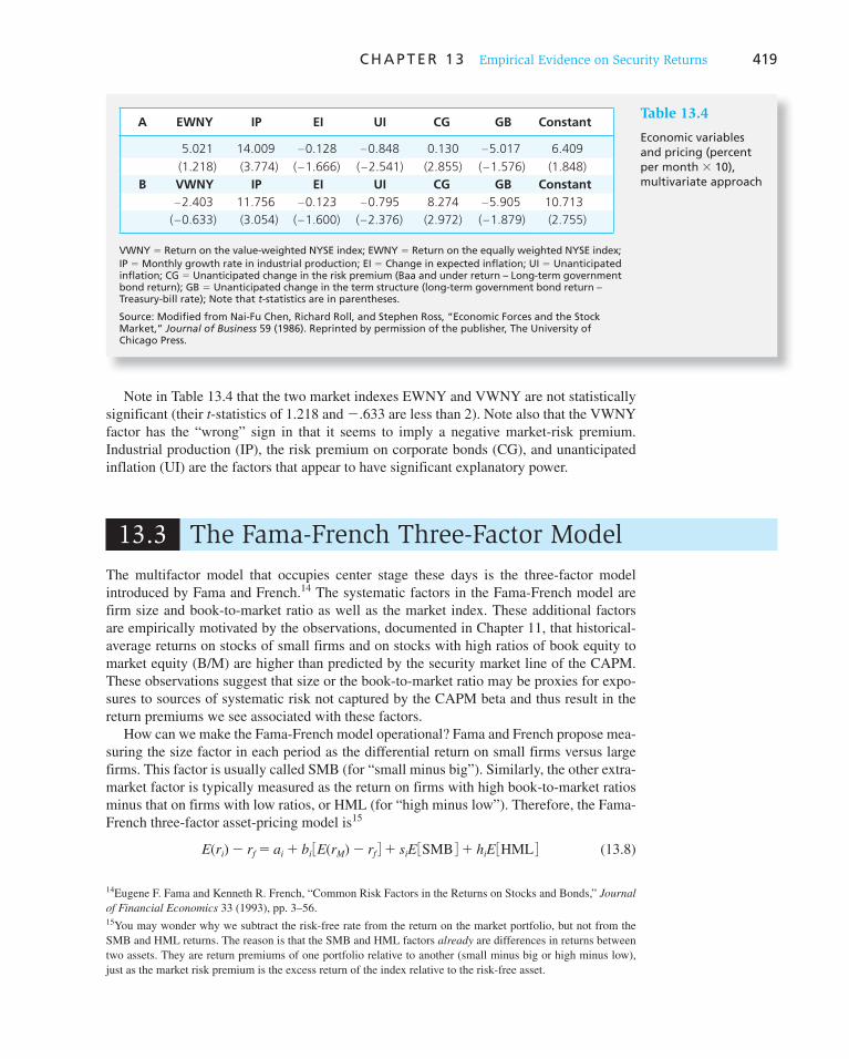
C H A P T E R 1 3 Empirical Evidence on Security Returns 419
A EWNY IP EI UI CG GB Constant
5.021 14.009 20.128 20.848 0.130 25.017 6.409
(1.218) (3.774) (21.666) (22.541) (2.855) (21.576) (1.848)
B VWNY IP EI UI CG GB Constant
22.403 11.756 20.123 20.795 8.274 25.905 10.713
(20.633) (3.054) (21.600) (22.376) (2.972) (21.879) (2.755)
VWNY 5 Return on the value-weighted NYSE index; EWNY 5 Return on the equally weighted NYSE index; IP 5 Monthly growth rate in industrial production; EI 5 Change in expected inflation; UI 5 Unanticipated inflation; CG 5 Unanticipated change in the risk premium (Baa and under return – Long-term government bond return); GB 5 Unanticipated change in the term structure (long-term government bond return – Treasury-bill rate); Note that t -statistics are in parentheses.
Source: Modified from Nai-Fu Chen, Richard Roll, and Stephen Ross, “Economic Forces and the Stock Market,” Journal of Business 59 (1986). Reprinted by permission of the publisher, The University of Chicago Press.
Table 13.4
Economic variables and pricing (percent per month 3 10), multivariate approach
Note in Table 13.4 that the two market indexes EWNY and VWNY are not statistically significant (their t -statistics of 1.218 and 2 .633 are less than 2). Note also that the VWNY factor has the “wrong” sign in that it seems to imply a negative market-risk premium. Industrial production (IP), the risk premium on corporate bonds (CG), and unanticipated inflation (UI) are the factors that appear to have significant explanatory power.
13.3 The Fama-French Three-Factor Model
The multifactor model that occupies center stage these days is the three-factor model introduced by Fama and French. 14 The systematic factors in the Fama-French model are firm size and book-to-market ratio as well as the market index. These additional factors are empirically motivated by the observations, documented in Chapter 11, that historical- average returns on stocks of small firms and on stocks with high ratios of book equity to market equity (B/M) are higher than predicted by the security market line of the CAPM. These observations suggest that size or the book-to-market ratio may be proxies for expo-sures to sources of systematic risk not captured by the CAPM beta and thus result in the return premiums we see associated with these factors.
How can we make the Fama-French model operational? Fama and French propose mea-suring the size factor in each period as the differential return on small firms versus large firms. This factor is usually called SMB (for “small minus big”). Similarly, the other extra-market factor is typically measured as the return on firms with high book-to-market ratios minus that on firms with low ratios, or HML (for “high minus low”). Therefore, the Fama-French three-factor asset-pricing model is 15
E(ri) 2 rf 5 ai 1 bi 3E(rM) 2 rf 41 siE 3SMB 41 hiE 3HML 4 (13.8)
14 Eugene F. Fama and Kenneth R. French, “Common Risk Factors in the Returns on Stocks and Bonds,” Journal
of Financial Economics 33 (1993), pp. 3–56. 15 You may wonder why we subtract the risk-free rate from the return on the market portfolio, but not from the SMB and HML returns. The reason is that the SMB and HML factors already are differences in returns between two assets. They are return premiums of one portfolio relative to another (small minus big or high minus low), just as the market risk premium is the excess return of the index relative to the risk-free asset.
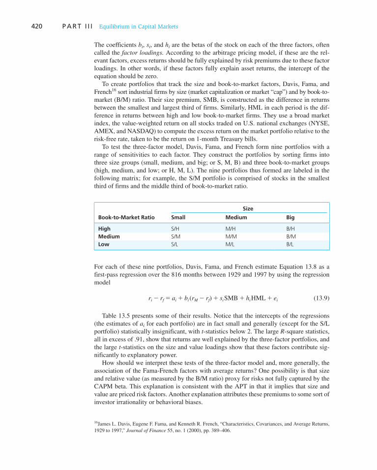
420 P A R T I I I Equilibrium in Capital Markets
The coefficients b i , s i , and h i are the betas of the stock on each of the three factors, often called the factor loadings. According to the arbitrage pricing model, if these are the rel-evant factors, excess returns should be fully explained by risk premiums due to these factor loadings. In other words, if these factors fully explain asset returns, the intercept of the equation should be zero.
To create portfolios that track the size and book-to-market factors, Davis, Fama, and French 16 sort industrial firms by size (market capitalization or market “cap”) and by book-to-market (B/M) ratio. Their size premium, SMB, is constructed as the difference in returns between the smallest and largest third of firms. Similarly, HML in each period is the dif-ference in returns between high and low book-to-market firms. They use a broad market index, the value-weighted return on all stocks traded on U.S. national exchanges (NYSE, AMEX, and NASDAQ) to compute the excess return on the market portfolio relative to the risk-free rate, taken to be the return on 1-month Treasury bills.
To test the three-factor model, Davis, Fama, and French form nine portfolios with a range of sensitivities to each factor. They construct the portfolios by sorting firms into three size groups (small, medium, and big; or S, M, B) and three book-to-market groups (high, medium, and low; or H, M, L). The nine portfolios thus formed are labeled in the following matrix; for example, the S/M portfolio is comprised of stocks in the smallest third of firms and the middle third of book-to-market ratio.
Size
Book-to-Market Ratio Small Medium Big
High S/H M/H B/H
Medium S/M M/M B/M
Low S/L M/L B/L
For each of these nine portfolios, Davis, Fama, and French estimate Equation 13.8 as a first-pass regression over the 816 months between 1929 and 1997 by using the regression model
ri 2 rf 5 ai 1 bi(rM 2 rf) 1 siSMB 1 hiHML 1 ei (13.9)
Table 13.5 presents some of their results. Notice that the intercepts of the regressions (the estimates of a i for each portfolio) are in fact small and generally (except for the S/L portfolio) statistically insignificant, with t -statistics below 2. The large R -square statistics, all in excess of .91, show that returns are well explained by the three-factor portfolios, and the large t -statistics on the size and value loadings show that these factors contribute sig-nificantly to explanatory power.
How should we interpret these tests of the three-factor model and, more generally, the association of the Fama-French factors with average returns? One possibility is that size and relative value (as measured by the B/M ratio) proxy for risks not fully captured by the CAPM beta. This explanation is consistent with the APT in that it implies that size and value are priced risk factors. Another explanation attributes these premiums to some sort of investor irrationality or behavioral biases.
16 James L. Davis, Eugene F. Fama, and Kenneth R. French, “Characteristics, Covariances, and Average Returns, 1929 to 1997,” Journal of Finance 55, no. 1 (2000), pp. 389–406.
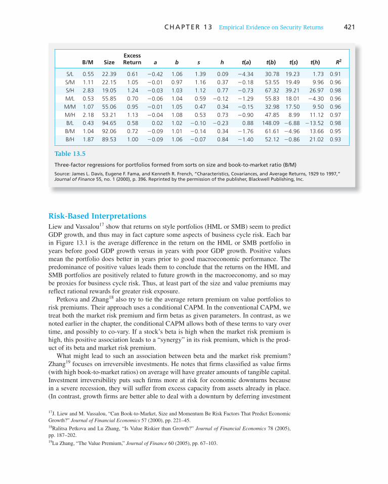
C H A P T E R 1 3 Empirical Evidence on Security Returns 421
B/M SizeExcess Return a b s h t ( a ) t ( b ) t ( s ) t ( h ) R 2
S/L 0.55 22.39 0.61 20.42 1.06 1.39 0.09 24.34 30.78 19.23 1.73 0.91
S/M 1.11 22.15 1.05 20.01 0.97 1.16 0.37 20.18 53.55 19.49 9.96 0.96
S/H 2.83 19.05 1.24 20.03 1.03 1.12 0.77 20.73 67.32 39.21 26.97 0.98
M/L 0.53 55.85 0.70 20.06 1.04 0.59 20.12 21.29 55.83 18.01 24.30 0.96
M/M 1.07 55.06 0.95 20.01 1.05 0.47 0.34 20.15 32.98 17.50 9.50 0.96
M/H 2.18 53.21 1.13 20.04 1.08 0.53 0.73 20.90 47.85 8.99 11.12 0.97
B/L 0.43 94.65 0.58 0.02 1.02 20.10 20.23 0.88 148.09 26.88 213.52 0.98
B/M 1.04 92.06 0.72 20.09 1.01 20.14 0.34 21.76 61.61 24.96 13.66 0.95
B/H 1.87 89.53 1.00 20.09 1.06 20.07 0.84 21.40 52.12 20.86 21.02 0.93
Table 13.5
Three-factor regressions for portfolios formed from sorts on size and book-to-market ratio (B/M)
Source: James L. Davis, Eugene F. Fama, and Kenneth R. French, “Characteristics, Covariances, and Average Returns, 1929 to 1997,” Journal of Finance 55, no. 1 (2000), p. 396. Reprinted by the permission of the publisher, Blackwell Publishing, Inc.
Risk-Based Interpretations
Liew and Vassalou 17 show that returns on style portfolios (HML or SMB) seem to predict GDP growth, and thus may in fact capture some aspects of business cycle risk. Each bar in Figure 13.1 is the average difference in the return on the HML or SMB portfolio in years before good GDP growth versus in years with poor GDP growth. Positive values mean the portfolio does better in years prior to good macroeconomic performance. The predominance of positive values leads them to conclude that the returns on the HML and SMB portfolios are positively related to future growth in the macroeconomy, and so may be proxies for business cycle risk. Thus, at least part of the size and value premiums may reflect rational rewards for greater risk exposure.
Petkova and Zhang 18 also try to tie the average return premium on value portfolios to risk premiums. Their approach uses a conditional CAPM. In the conventional CAPM, we treat both the market risk premium and firm betas as given parameters. In contrast, as we noted earlier in the chapter, the conditional CAPM allows both of these terms to vary over time, and possibly to co-vary. If a stock’s beta is high when the market risk premium is high, this positive association leads to a “synergy” in its risk premium, which is the prod-uct of its beta and market risk premium.
What might lead to such an association between beta and the market risk premium? Zhang 19 focuses on irreversible investments. He notes that firms classified as value firms (with high book-to-market ratios) on average will have greater amounts of tangible capital. Investment irreversibility puts such firms more at risk for economic downturns because in a severe recession, they will suffer from excess capacity from assets already in place. (In contrast, growth firms are better able to deal with a downturn by deferring investment
17 J. Liew and M. Vassalou, “Can Book-to-Market, Size and Momentum Be Risk Factors That Predict Economic Growth?” Journal of Financial Economics 57 (2000), pp. 221–45. 18 Ralitsa Petkova and Lu Zhang, “Is Value Riskier than Growth?” Journal of Financial Economics 78 (2005), pp. 187–202. 19 Lu Zhang, “The Value Premium,” Journal of Finance 60 (2005), pp. 67–103.
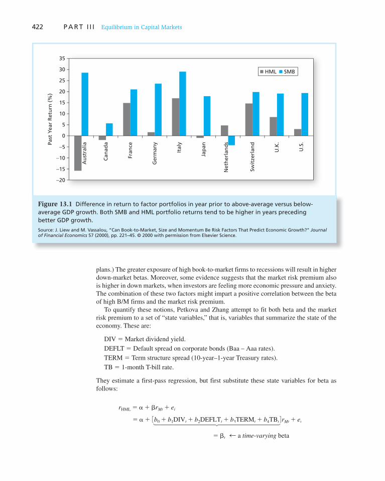
422 P A R T I I I Equilibrium in Capital Markets
plans.) The greater exposure of high book-to-market firms to recessions will result in higher down-market betas. Moreover, some evidence suggests that the market risk premium also is higher in down markets, when investors are feeling more economic pressure and anxiety. The combination of these two factors might impart a positive correlation between the beta of high B/M firms and the market risk premium.
To quantify these notions, Petkova and Zhang attempt to fit both beta and the market risk premium to a set of “state variables,” that is, variables that summarize the state of the economy. These are:
DIV 5 Market dividend yield.
DEFLT 5 Default spread on corporate bonds (Baa – Aaa rates).
TERM 5 Term structure spread (10-year–1-year Treasury rates).
TB 5 1-month T-bill rate.
They estimate a first-pass regression, but first substitute these state variables for beta as follows:
rHML 5 a 1 brMt 1 ei
5 a 1 3b0 1 b1DIVt 1 b2DEFLTt 1 b3TERMt 1 b4TBt 4 rMt 1 ei
5 bt d a time-varying beta
Figure 13.1 Difference in return to factor portfolios in year prior to above-average versus below- average GDP growth. Both SMB and HML portfolio returns tend to be higher in years preceding better GDP growth.
Source: J. Liew and M. Vassalou, “Can Book-to-Market, Size and Momentum Be Risk Factors That Predict Economic Growth?” Journal of Financial Economics 57 (2000), pp. 221–45. © 2000 with permission from Elsevier Science.
−20
−15
−10
−5
0
5
10
15
20
25
30
35
Au
stra
lia
Can
ada
Fran
ce
Ger
man
y
Ital
y
Jap
an
Net
her
lan
ds
Swit
zerl
and
U.K
.
U.S
.Past
Yea
r R
etu
rn (
%)
HML SMB
�������������������
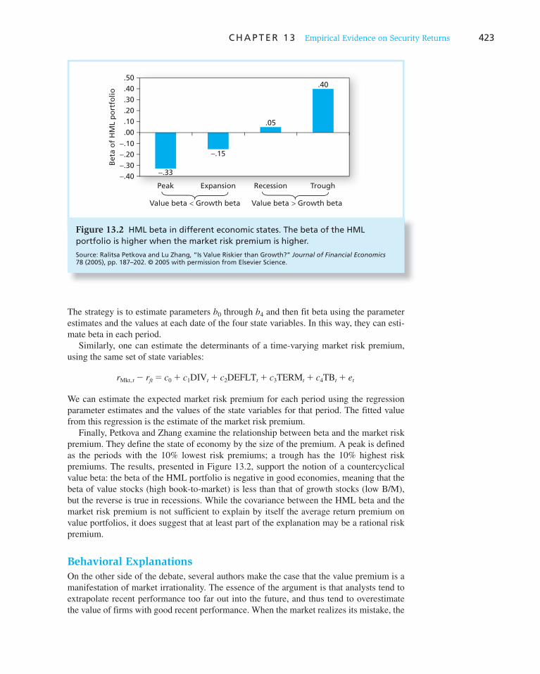
C H A P T E R 1 3 Empirical Evidence on Security Returns 423
The strategy is to estimate parameters b 0 through b 4 and then fit beta using the parameter estimates and the values at each date of the four state variables. In this way, they can esti-mate beta in each period.
Similarly, one can estimate the determinants of a time-varying market risk premium, using the same set of state variables:
rMkt, t 2 rft 5 c0 1 c1DIVt 1 c2DEFLTt 1 c3TERMt 1 c4TBt 1 et
We can estimate the expected market risk premium for each period using the regression parameter estimates and the values of the state variables for that period. The fitted value from this regression is the estimate of the market risk premium.
Finally, Petkova and Zhang examine the relationship between beta and the market risk premium. They define the state of economy by the size of the premium. A peak is defined as the periods with the 10% lowest risk premiums; a trough has the 10% highest risk premiums. The results, presented in Figure 13.2 , support the notion of a countercyclical value beta: the beta of the HML portfolio is negative in good economies, meaning that the beta of value stocks (high book-to-market) is less than that of growth stocks (low B/M), but the reverse is true in recessions. While the covariance between the HML beta and the market risk premium is not sufficient to explain by itself the average return premium on value portfolios, it does suggest that at least part of the explanation may be a rational risk premium.
Behavioral Explanations
On the other side of the debate, several authors make the case that the value premium is a manifestation of market irrationality. The essence of the argument is that analysts tend to extrapolate recent performance too far out into the future, and thus tend to overestimate the value of firms with good recent performance. When the market realizes its mistake, the
Figure 13.2 HML beta in different economic states. The beta of the HML portfolio is higher when the market risk premium is higher.
Source: Ralitsa Petkova and Lu Zhang, “Is Value Riskier than Growth?” Journal of Financial Economics 78 (2005), pp. 187–202. © 2005 with permission from Elsevier Science.
.40
.05
−.33
−.15
−.40
−.30
−.20
−.10
.00
.10
.20
.30
.40
.50
Bet
a o
f H
ML
po
rtfo
lio
Peak Expansion
Value beta < Growth beta
TroughRecession
Value beta > Growth beta
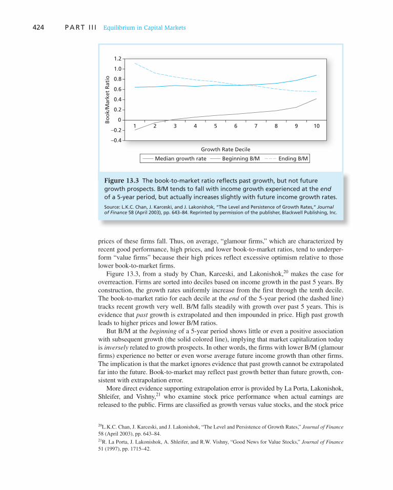
424 P A R T I I I Equilibrium in Capital Markets
prices of these firms fall. Thus, on average, “glamour firms,” which are characterized by recent good performance, high prices, and lower book-to-market ratios, tend to underper-form “value firms” because their high prices reflect excessive optimism relative to those lower book-to-market firms.
Figure 13.3 , from a study by Chan, Karceski, and Lakonishok, 20 makes the case for overreaction. Firms are sorted into deciles based on income growth in the past 5 years. By construction, the growth rates uniformly increase from the first through the tenth decile. The book-to-market ratio for each decile at the end of the 5-year period (the dashed line) tracks recent growth very well. B/M falls steadily with growth over past 5 years. This is evidence that past growth is extrapolated and then impounded in price. High past growth leads to higher prices and lower B/M ratios.
But B/M at the beginning of a 5-year period shows little or even a positive association with subsequent growth (the solid colored line), implying that market capitalization today is inversely related to growth prospects. In other words, the firms with lower B/M (glamour firms) experience no better or even worse average future income growth than other firms. The implication is that the market ignores evidence that past growth cannot be extrapolated far into the future. Book-to-market may reflect past growth better than future growth, con-sistent with extrapolation error.
More direct evidence supporting extrapolation error is provided by La Porta, Lakonishok, Shleifer, and Vishny, 21 who examine stock price performance when actual earnings are released to the public. Firms are classified as growth versus value stocks, and the stock price
20 L.K.C. Chan, J. Karceski, and J. Lakonishok, “The Level and Persistence of Growth Rates,” Journal of Finance
58 (April 2003), pp. 643–84. 21 R. La Porta, J. Lakonishok, A. Shleifer, and R.W. Vishny, “Good News for Value Stocks,” Journal of Finance
51 (1997), pp. 1715–42.
Figure 13.3 The book-to-market ratio reflects past growth, but not future growth prospects. B/M tends to fall with income growth experienced at the end of a 5-year period, but actually increases slightly with future income growth rates.
Source: L.K.C. Chan, J. Karceski, and J. Lakonishok, “The Level and Persistence of Growth Rates,” Journal of Finance 58 (April 2003), pp. 643–84. Reprinted by permission of the publisher, Blackwell Publishing, Inc.
Bo
ok/
Mar
ket
Rat
io
−0.4
−0.2
0
0.2
0.4
0.6
0.8
1.0
1.2
1 2 3 4 5 6 7 8 9 10
Growth Rate Decile
Median growth rate Beginning B/M Ending B/M
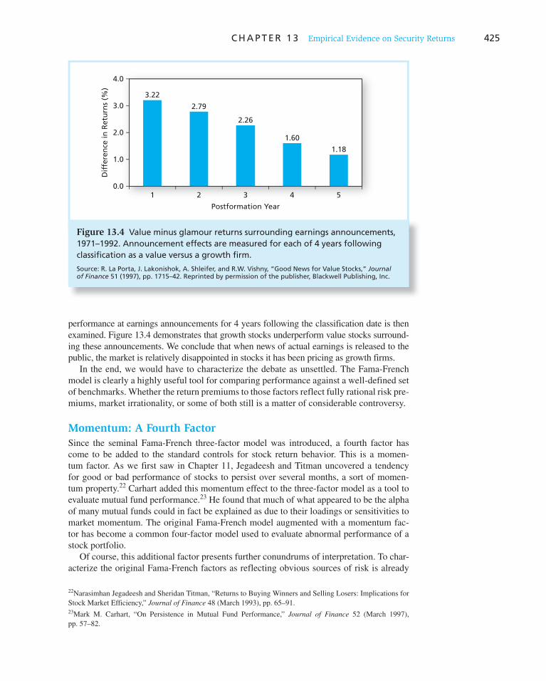
C H A P T E R 1 3 Empirical Evidence on Security Returns 425
performance at earnings announcements for 4 years following the classification date is then examined. Figure 13.4 demonstrates that growth stocks underperform value stocks surround-ing these announcements. We conclude that when news of actual earnings is released to the public, the market is relatively disappointed in stocks it has been pricing as growth firms.
In the end, we would have to characterize the debate as unsettled. The Fama-French model is clearly a highly useful tool for comparing performance against a well-defined set of benchmarks. Whether the return premiums to those factors reflect fully rational risk pre-miums, market irrationality, or some of both still is a matter of considerable controversy.
Momentum: A Fourth Factor
Since the seminal Fama-French three-factor model was introduced, a fourth factor has come to be added to the standard controls for stock return behavior. This is a momen-tum factor. As we first saw in Chapter 11, Jegadeesh and Titman uncovered a tendency for good or bad performance of stocks to persist over several months, a sort of momen-tum property. 22 Carhart added this momentum effect to the three-factor model as a tool to evaluate mutual fund performance. 23 He found that much of what appeared to be the alpha of many mutual funds could in fact be explained as due to their loadings or sensitivities to market momentum. The original Fama-French model augmented with a momentum fac-tor has become a common four-factor model used to evaluate abnormal performance of a stock portfolio.
Of course, this additional factor presents further conundrums of interpretation. To char-acterize the original Fama-French factors as reflecting obvious sources of risk is already
22 Narasimhan Jegadeesh and Sheridan Titman, “Returns to Buying Winners and Selling Losers: Implications for Stock Market Efficiency,” Journal of Finance 48 (March 1993), pp. 65–91. 23 Mark M. Carhart, “On Persistence in Mutual Fund Performance,” Journal of Finance 52 (March 1997), pp. 57–82.
Figure 13.4 Value minus glamour returns surrounding earnings announcements, 1971–1992. Announcement effects are measured for each of 4 years following classification as a value versus a growth firm.
Source: R. La Porta, J. Lakonishok, A. Shleifer, and R.W. Vishny, “Good News for Value Stocks,” Journal of Finance 51 (1997), pp. 1715–42. Reprinted by permission of the publisher, Blackwell Publishing, Inc.
3.22
2.26
1.18
1.60
2.79
0.0
1.0
2.0
3.0
4.0
1 2 3 4 5
Postformation Year
Dif
fere
nce
in R
etu
rns
(%)

426 P A R T I I I Equilibrium in Capital Markets
a bit of a challenge. A momentum factor seems even harder to position as reflecting a risk–return trade-off. But as we saw in Chapter 9, recent work has resulted in a growing appreciation of the importance of liquidity, and particularly an illiquidity premium, in asset pricing. We will see in the next section that a good part of the momentum effect may be related to liquidity.
13.4 Liquidity and Asset Pricing
In Chapter 9 we saw that an important extension of the CAPM incorporates considerations of asset liquidity. Unfortunately, measuring liquidity is far from trivial. We saw in Chapter 9 that the effect of liquidity on an asset’s expected return is composed of two factors:
1. Transaction costs that are dominated by the bid–ask spread that dealers set to compensate for losses incurred when trading with informed traders.
2. Liquidity risk resulting from covariance between changes in asset liquidity cost with both changes in market-index liquidity cost and with market-index rates of return.
Both of these factors are unobservable and their effect on equilibrium rates of return is difficult to estimate.
Liquidity embodies several characteristics such as trading costs, ease of sale, necessary price concessions to effect a quick transaction, market depth, and price predictability. As such, it is difficult to measure with any single statistic. Popular measures of liquidity, or, more precisely, illiquidity, focus on the price impact dimension: What price concession might a seller have to offer in order to accomplish a large sale of an asset or, conversely, what premium must a buyer offer to make a large purchase?
One popular measure of illiquidity is employed by Pástor and Stambaugh, who look for evidence of price reversals, especially following large trades. 24 Their idea is that if stock price movements tend to be partially reversed on the following day, then we can conclude that part of the original price change was not due to perceived changes in intrinsic value (these price changes would not tend to be reversed), but was instead a symptom of price impact associated with the original trade. Reversals suggest that part of the original price change was a concession on the part of trade initiators who needed to offer higher pur-chase prices or accept lower selling prices to complete their trades in a timely manner. Pástor and Stambaugh use regression analysis to show that reversals do in fact tend to be larger when associated with higher trading volume—exactly the pattern that one would expect if part of the price move is a liquidity phenomenon. They run a first-stage regression of returns on lagged returns and trading volume. The coefficient on the latter term measures the tendency of high-volume trades to be accompanied by larger reversals.
Another measure of illiquidity, proposed by Amihud, also focuses on the association between large trades and price movements. 25 His measure is:
ILLIQ 5 Monthly average of daily BAbsolute value (Stock return)
Dollar volumeR
24 L. Pástor and R. F. Stambaugh, “Liquidity Risk and Expected Stock Returns,” Journal of Political Economy 111 (2003), pp. 642–85.
25 Yakov Amihud, “Illiquidity and Stock Returns: Cross-Section and Time-Series Effects,” Journal of Financial
Markets 5 (2002), pp. 31–56.
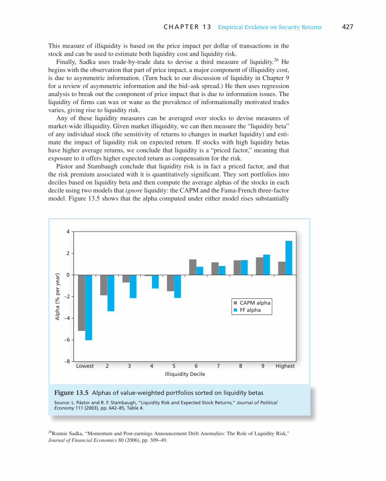
C H A P T E R 1 3 Empirical Evidence on Security Returns 427
This measure of illiquidity is based on the price impact per dollar of transactions in the stock and can be used to estimate both liquidity cost and liquidity risk.
Finally, Sadka uses trade-by-trade data to devise a third measure of liquidity. 26 He begins with the observation that part of price impact, a major component of illiquidity cost, is due to asymmetric information. (Turn back to our discussion of liquidity in Chapter 9 for a review of asymmetric information and the bid–ask spread.) He then uses regression analysis to break out the component of price impact that is due to information issues. The liquidity of firms can wax or wane as the prevalence of informationally motivated trades varies, giving rise to liquidity risk.
Any of these liquidity measures can be averaged over stocks to devise measures of market-wide illiquidity. Given market illiquidity, we can then measure the “liquidity beta” of any individual stock (the sensitivity of returns to changes in market liquidity) and esti-mate the impact of liquidity risk on expected return. If stocks with high liquidity betas have higher average returns, we conclude that liquidity is a “priced factor,” meaning that exposure to it offers higher expected return as compensation for the risk.
Pástor and Stambaugh conclude that liquidity risk is in fact a priced factor, and that the risk premium associated with it is quantitatively significant. They sort portfolios into deciles based on liquidity beta and then compute the average alphas of the stocks in each decile using two models that ignore liquidity: the CAPM and the Fama-French three-factor model. Figure 13.5 shows that the alpha computed under either model rises substantially
26 Ronnie Sadka, “Momentum and Post-earnings Announcement Drift Anomalies: The Role of Liquidity Risk,” Journal of Financial Economics 80 (2006), pp. 309–49.
Figure 13.5 Alphas of value-weighted portfolios sorted on liquidity betas
Source: L. Pástor and R. F. Stambaugh, “Liquidity Risk and Expected Stock Returns,” Journal of Political Economy 111 (2003), pp. 642–85, Table 4.
−2
−4
−6
−8
4
2
Lowest 2 3 4
Illiquidity Decile
5 6 7 8 9 Highest
0
Alp
ha
(% p
er y
ear)
CAPM alphaFF alpha

428 P A R T I I I Equilibrium in Capital Markets
across liquidity-beta deciles, clear evidence that when controlling for other factors, aver-age return rises along with liquidity risk. Not surprisingly, the relationship between liquid-ity risk and alpha across deciles is more regular for the Fama-French model, as it controls for a wider range of other influences on average return.
Acharya and Pedersen use Amihud’s measure to test for price effects associated with the average level of illiquidity as well as a liquidity risk premium. 27 They demonstrate that expected stock returns depend on the average level of illiquidity. (Recall from Chapter 9, Figure 9.5, that Amihud found a similar result.) But Acharya and Pedersen demonstrate that stock returns depend on several liquidity betas as well: the sensitivity of individual stock illiquidity to market illiquidity; the sensitivity of stock returns to market illiquidity; and the sensitivity of stock illiquidity to market return. They conclude that adding these liquidity effects to the conventional CAPM increases our ability to explain expected asset returns.
Liquidity and Efficient Market Anomalies
Pástor and Stambaugh also test the impact of the liquidity beta on alpha computed from a four-factor model (that also controls for momentum), with results extremely similar to those in Figure 9.5. In fact, they suggest that liquidity risk factor may account for a good part of the apparent profitability of the momentum strategy.
Sadka further investigates the connection between liquidity risk and the momentum effect as well as another efficient market anomaly: postearnings announcement drift, the tendency for stock returns to continue to drift up after good earnings news is released or drift down after disappointing releases. (See Chapter 9 for a discussion of this phenom-enon.) He notes that these two anomalies might be particularly sensitive to informational issues: momentum may be viewed as a sluggish reaction to general news about the stock and postearnings announcement drift as a sluggish reaction to earnings news specifically. If these anomalies are news-related, then their returns should be sensitive to the infor-mational portion of marketwide liquidity shocks. In fact, he shows that portfolios built on either momentum or postearnings announcement drift strategies exhibit large betas on marketwide liquidity. Accounting for the liquidity risk premium can explain between 40% and 80% of their apparent abnormal returns.
13.5 Consumption-Based Asset Pricing and the Equity Premium Puzzle
In a classic article, Mehra and Prescott observed that historical excess returns on risky assets in the U.S. are too large to be consistent with economic theory and reasonable levels of risk aversion. 28 This observation has come to be known as the “equity premium puzzle.” The debate about the equity premium puzzle suggests that forecasts of the market risk premium should be lower than historical averages. The question of whether past returns provide a guideline to future returns is sufficiently important to justify stretching the scope of our discussions of equilibrium in capital markets.2728
27 V. V. Acharya and L. H. Pedersen, “Asset Pricing with Liquidity Risk,” Journal of Financial Economics 77 (2005), pp. 375–410.
28 Jarnish Mehra and Edward Prescott, “The Equity Premium: A Puzzle,” Journal of Monetary Economics, March 1985.
C H A P T E R 1 3 Empirical Evidence on Security Returns 429
Consumption Growth and Market Rates of Return
As discussed in Chapter 9, the ICAPM is derived from a lifetime consumption/investment plan of a representative consumer/investor. Each individual’s plan is set to maximize a util-ity function of lifetime consumption, and consumption/investment in each period is based on age and current wealth, as well as the risk-free rate and the market portfolio’s risk and risk premium.
The consumption model implies that what matters to investors is not their wealth per se, but their lifetime flow of consumption. There can be slippage between wealth and con-sumption due to variation in factors such as the risk-free rate, the market portfolio risk premium, or prices of major consumption items. Therefore, a better measure of consumer well-being than wealth is the consumption flow that such wealth can support.
Given this framework, the generalization of the basic CAPM is that instead of measur-ing security risk based on the covariance of returns with the market return (a measure that focuses only on wealth), we are better off using the covariance of returns with aggregate consumption. Hence, we would expect the risk premium of the market index to be related to that covariance as follows:
E(rM) 2 rf 5 ACov(rM , rC) (13.10)
where A depends on the average coefficient of risk aversion and r C is the rate of return on a consumption-tracking portfolio constructed to have the highest possible correlation with growth in aggregate consumption. 29
The first wave of attempts to estimate consumption-based asset pricing models used consumption data directly rather than returns on consumption-tracking portfolios. By and large, these tests found the CCAPM no better than the conventional CAPM in explaining risk premiums. The equity premium puzzle refers to the fact that using reasonable estimates of A, the covariance of consumption growth with the market-index return, Cov( r M , r C ), is far too low to justify observed historical-average excess returns on the market-index port-folio, which may be viewed as an estimate of the left-hand side of Equation 13.10. 30 Thus, the risk premium puzzle says in effect that historical excess returns are too high and/or our usual estimates of risk aversion are too low.
Recent research improves the quality of estimation in several ways. First, rather than using consumption growth directly, it uses consumption-tracking portfolios. The available ( infrequent) data on aggregate consumption is used only to construct the consumption-tracking portfolio. The frequent and accurate data on the return on these port-folios may then be used to test the asset pricing model. (On the other hand, any inaccuracy in the construction of the consumption-mimicking portfolios will muddy the relationship between asset returns and consumption risk.) For example, a study by Jagannathan and Wang focuses on year-over-year fourth-quarter consumption and employs a consumption-tracking portfolio. 31 Table 13.6 , excerpted from their study, shows that the Fama-French
29 This equation is analogous to the equation for the risk premium in the conventional CAPM, i.e., that E ( r M ) 2 r f 5 A Cov( r M , r M ) 5 A Var( r M ). In the multifactor version of the ICAPM, however, the market is no longer mean-variance efficient, so the risk premium of the market index will not be proportional to its variance. The APT also implies a linear relationship between risk premium and covariance with relevant factors, but it is silent about the slope of the relationship because it avoids assumptions about utility.
30 Notice that the conventional CAPM does not pose such problems. In the CAPM, E ( r M ) 2 r f 5 A Var( r M ). A risk premium of .085 (8.5%) and a standard deviation of .20 (20%, or variance of .04) imply a coefficient of risk aver-sion of .085/.04 5 2.125, which is quite plausible.
31 Ravi Jagannathan and Yong Wang, “Lazy Investors, Discretionary Consumption, and the Cross-Section of Stock Returns,” Journal of Finance 62 (August 2006), pp. 1623–61.

430 P A R T I I I Equilibrium in Capital Markets
Book-to-Market
Size Low Medium High
Average annual excess returns* (%)
Small 6.19 12.24 17.19
Medium 6.93 10.43 13.94
Big 7.08 8.52 9.5
Consumption beta*
Small 3.46 4.26 5.94
Medium 2.88 4.35 5.71
Big 3.39 2.83 4.41
Table 13.6
Annual excess returns and consumption betas
*Average annual excess returns on the 25 Fama-French portfolios from 1954 to 2003. Consumption betas estimated by the time series regression
Ri,t 5 ai 1 bi,c gct 1 e i,t ,
where R i, t is the excess return over the risk-free rate, and g ct is annual consumption growth calculated using fourth-quarter consumption data. Source: Ravi Jagannathan and Yong Wang, “Lazy Investors, Discretionary Consumption, and the Cross-Section of Stock Returns,” Journal of Finance 62 (August 2006), pp. 1623–61.
factors are in fact associated with consumption betas as well as excess returns. The top panel contains familiar results: moving across each row, we see that higher book-to-market ratios are associated with higher average returns. Similarly, moving down each column, we see that larger size generally implies lower average returns. The novel results are in
the lower panel: a high book-to-market ratio is associated with higher consump-tion beta, and larger firm size is associ-ated with lower consumption beta. The suggestion is that the explanatory power of the Fama-French factors for average returns may in fact reflect the differ-ing consumption risk of those portfo-lios. Figure 13.6 shows that the average returns of the 25 Fama-French portfo-lios are strongly associated with their consumption betas. Other tests reported by Jagannathan and Wang show that the CCAPM explains returns even bet-ter than the Fama-French three-factor model, which in turn is superior to the single-factor CAPM.
Moreover, the standard CCAPM focuses on a representative consumer/investor, thereby ignoring information about heterogeneous investors with dif-ferent levels of wealth and consumption habits. To improve the model’s power to explain returns, some newer studies
Figure 13.6 Cross section of stock returns: Fama-French 25 portfolios, 1954–2003
Annual excess returns and consumption betas. This figure plots the average annual excess returns on the 25 Fama-French portfolios and their consumption betas. Each two-digit number represents one portfolio. The first digit refers to the size quintile (1 5 smallest, 5 5 largest), and the second digit refers to the book-to-market quintile (1 5 lowest, 5 5 highest).
Exce
ss R
etu
rns
(%)
0 1 2
Consumption Betas
3 4 5 6 7 8
10
8 52413121 11
5142
5322
5455
323343
13 44
3423
24
1425
15
35
1245
6
4
2
0
20
18
16
14
12
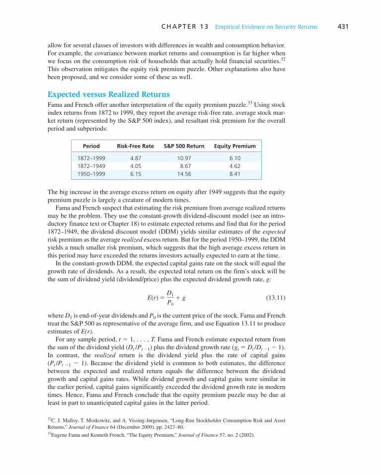
C H A P T E R 1 3 Empirical Evidence on Security Returns 431
allow for several classes of investors with differences in wealth and consumption behavior. For example, the covariance between market returns and consumption is far higher when we focus on the consumption risk of households that actually hold financial securities. 32 This observation mitigates the equity risk premium puzzle. Other explanations also have been proposed, and we consider some of these as well.
Expected versus Realized Returns
Fama and French offer another interpretation of the equity premium puzzle. 33 Using stock index returns from 1872 to 1999, they report the average risk-free rate, average stock mar-ket return (represented by the S&P 500 index), and resultant risk premium for the overall period and subperiods:
Period Risk-Free Rate S&P 500 Return Equity Premium
1872–1999 4.87 10.97 6.10
1872–1949 4.05 8.67 4.62
1950–1999 6.15 14.56 8.41
The big increase in the average excess return on equity after 1949 suggests that the equity premium puzzle is largely a creature of modern times.
Fama and French suspect that estimating the risk premium from average realized returns may be the problem. They use the constant-growth dividend-discount model (see an intro-ductory finance text or Chapter 18) to estimate expected returns and find that for the period 1872–1949, the dividend discount model (DDM) yields similar estimates of the expected risk premium as the average realized excess return. But for the period 1950–1999, the DDM yields a much smaller risk premium, which suggests that the high average excess return in this period may have exceeded the returns investors actually expected to earn at the time.
In the constant-growth DDM, the expected capital gains rate on the stock will equal the growth rate of dividends. As a result, the expected total return on the firm’s stock will be the sum of dividend yield (dividend/price) plus the expected dividend growth rate, g:
E(r) 5D1
P0
1 g (13.11)
where D 1 is end-of-year dividends and P 0 is the current price of the stock. Fama and French treat the S&P 500 as representative of the average firm, and use Equation 13.11 to produce estimates of E(r).
For any sample period, t 5 1, . . . , T, Fama and French estimate expected return from the sum of the dividend yield ( D t / P t 2 1 ) plus the dividend growth rate ( g t 5 D t / D t 2 1 2 1). In contrast, the realized return is the dividend yield plus the rate of capital gains ( P t / P t 2 1 2 1). Because the dividend yield is common to both estimates, the difference between the expected and realized return equals the difference between the dividend growth and capital gains rates. While dividend growth and capital gains were similar in the earlier period, capital gains significantly exceeded the dividend growth rate in modern times. Hence, Fama and French conclude that the equity premium puzzle may be due at least in part to unanticipated capital gains in the latter period.
32 C. J. Malloy, T. Moskowitz, and A. Vissing-Jørgensen, “Long-Run Stockholder Consumption Risk and Asset Returns,” Journal of Finance 64 (December 2009), pp. 2427–80.
33 Eugene Fama and Kenneth French, “The Equity Premium,” Journal of Finance 57, no. 2 (2002).
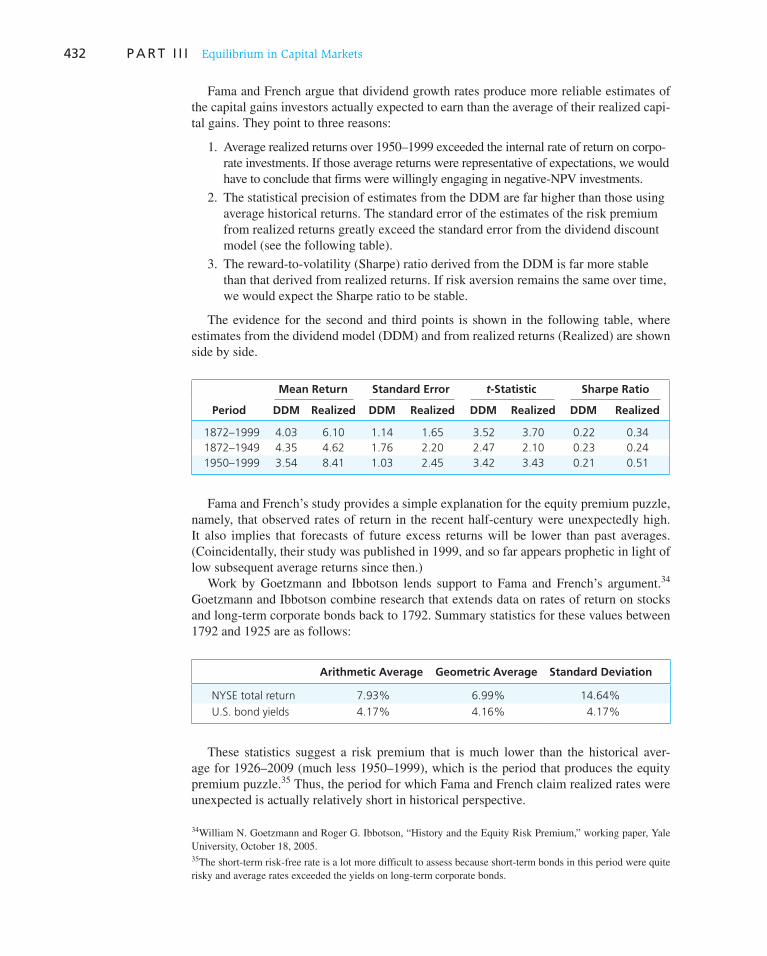
432 P A R T I I I Equilibrium in Capital Markets
Fama and French argue that dividend growth rates produce more reliable estimates of the capital gains investors actually expected to earn than the average of their realized capi-tal gains. They point to three reasons:
1. Average realized returns over 1950–1999 exceeded the internal rate of return on corpo-rate investments. If those average returns were representative of expectations, we would have to conclude that firms were willingly engaging in negative-NPV investments.
2. The statistical precision of estimates from the DDM are far higher than those using average historical returns. The standard error of the estimates of the risk premium from realized returns greatly exceed the standard error from the dividend discount model (see the following table).
3. The reward-to-volatility (Sharpe) ratio derived from the DDM is far more stable than that derived from realized returns. If risk aversion remains the same over time, we would expect the Sharpe ratio to be stable.
The evidence for the second and third points is shown in the following table, where estimates from the dividend model (DDM) and from realized returns (Realized) are shown side by side.
Mean Return Standard Error t-Statistic Sharpe Ratio
Period DDM Realized DDM Realized DDM Realized DDM Realized
1872–1999 4.03 6.10 1.14 1.65 3.52 3.70 0.22 0.34
1872–1949 4.35 4.62 1.76 2.20 2.47 2.10 0.23 0.24
1950–1999 3.54 8.41 1.03 2.45 3.42 3.43 0.21 0.51
Fama and French’s study provides a simple explanation for the equity premium puzzle, namely, that observed rates of return in the recent half-century were unexpectedly high. It also implies that forecasts of future excess returns will be lower than past averages. (Coincidentally, their study was published in 1999, and so far appears prophetic in light of low subsequent average returns since then.)
Work by Goetzmann and Ibbotson lends support to Fama and French’s argument. 34 Goetzmann and Ibbotson combine research that extends data on rates of return on stocks and long-term corporate bonds back to 1792. Summary statistics for these values between 1792 and 1925 are as follows:
Arithmetic Average Geometric Average Standard Deviation
NYSE total return 7.93% 6.99% 14.64%
U.S. bond yields 4.17% 4.16% 4.17%
These statistics suggest a risk premium that is much lower than the historical aver-age for 1926–2009 (much less 1950–1999), which is the period that produces the equity premium puzzle. 35 Thus, the period for which Fama and French claim realized rates were unexpected is actually relatively short in historical perspective.
34 William N. Goetzmann and Roger G. Ibbotson, “History and the Equity Risk Premium,” working paper, Yale University, October 18, 2005.
35 The short-term risk-free rate is a lot more difficult to assess because short-term bonds in this period were quite risky and average rates exceeded the yields on long-term corporate bonds.

C H A P T E R 1 3 Empirical Evidence on Security Returns 433
Survivorship Bias
The equity premium puzzle emerged from long-term averages of U.S. stock returns. There are reasons to suspect that these estimates of the risk pre-mium are subject to survivorship bias, as the United States has arguably been the most successful capitalist system in the world, an outcome that probably would not have been anticipated sev-eral decades ago. Jurion and Goetzmann assembled a database of capital appre-ciation indexes for the stock markets of 39 countries over the period 1921–1996. 36 Figure 13.7 shows that U.S. equities had the highest real return of all countries, at 4.3% annually, versus a median of .8% for other countries. Moreover, unlike the United States, many other countries have had equity markets that actually closed, either permanently or for extended periods of time.
The implication of these results is that using average U.S. data may impart a form of survivorship bias to our estimate of expected returns, because unlike many other countries, the United States has never been a victim of such extreme problems. Estimating risk premiums from the experience of the most successful country and ignoring the evi-dence from stock markets that did not survive for the full sample period will impart an upward bias in estimates of expected returns. The high realized equity premium obtained for the United States may not be indicative of required returns.
As an analogy, think of the effect of survivorship bias in the mutual fund industry. We know that some companies regularly close down their worst-performing mutual funds. If performance studies include only mutual funds for which returns are available during an entire sample period, the average returns of the funds that make it into the sample will be reflective of the performance of long-term survivors only. With the failed funds excluded from the sample, the average measured performance of mutual fund managers will be bet-ter than one could reasonably expect from the full sample of managers. Think back to the box in Chapter 11, “How to Guarantee a Successful Market Newsletter.” If one starts many newsletters with a range of forecasts, and continues only the newsletters that turned out to have successful advice, then it will appear from the sample of survivors that the average newsletter had forecasting skill.
Extensions to the CAPM May Resolve the Equity Premium Puzzle
Constantinides argues that the standard CAPM can be extended to account for observed excess returns by relaxing some of its assumptions, in particular, by recognizing that consumers face uninsurable and idiosyncratic income shocks, for example, the loss of
36 Philippe Jurion and William N. Goetzmann, “Global Stock Markets in the Twentieth Century,” Journal of
Finance 54, no. 3 (June 1999).
Figure 13.7 Real returns on global stock markets. The figure displays average real returns for 39 markets over the period 1921 to 1996. Markets are sorted by years of existence. The graph shows that markets with long histories typically have higher returns. An asterisk indicates that the market suffered a long-term break.
Perc
ent
per
An
nu
m
0 20 40
Years of Existence since Inception
UruguayHungary
CzechoslovakiaIsrael
Brazil
Pakistan
Egypt
Poland
GreeceArgentina*
Philippines
South AfricaVenezuela
India
ColombiaPeru*
Spain*
Portugal* Japan*New Zealand Belgium
ItalyFranceNetherlandsAustria*Ireland
FinlandMexico Denmark
Germany*U.K.Canada
SwitzerlandSweden
Chile*Norway
Australia
60 80 100
U.S.
−6−5−4−3−2−1
6543210

434 P A R T I I I Equilibrium in Capital Markets
employment. 37 The prospect of such events is higher in economic downturns and this observation takes us a long way toward understanding the means and variances of asset returns as well as their variation along the business cycle.
In addition, life-cycle considerations are important and often overlooked. Borrowing constraints become important when placed in the context of the life cycle. The imagi-nary “representative consumer” who holds all stock and bond market wealth does not face borrowing constraints. Young consumers, however, do face meaningful borrowing con-straints. Constantinides traces their impact on the equity premium, the demand for bonds, and on the limited participation of many consumers in the capital markets. Finally, he shows that adding habit formation to the conventional utility function helps explain higher risk premiums than those that would be justified by the covariance of stock returns with aggregate consumption growth. He argues that integrating the notions of habit formation, incomplete markets, the life cycle, borrowing constraints, and other sources of limited stock market participation is a promising vantage point from which to study the prices of assets and their returns, both theoretically and empirically within the class of rational asset-pricing models.
Liquidity and the Equity Premium Puzzle
We’ve seen that liquidity risk is potentially important in explaining the cross section of stock returns. The illiquidity premium may be on the same order of magnitude as the mar-ket risk premium. Therefore, the common practice of treating the average excess return on a market index as an estimate of a risk premium per se is almost certainly too simplistic. Part of that average excess return is almost certainly compensation for liquidity risk rather than just the (systematic) volatility of returns. If this is recognized, the equity premium puzzle may be less of a puzzle than it first appears.
Behavioral Explanations of the Equity Premium Puzzle
Barberis and Huang explain the puzzle as an outcome of irrational investor behavior. 38 The key elements of their approach are loss aversion and narrow framing, two well-known features of decision making under risk in experimental settings. Narrow framing is the idea that investors evaluate every risk they face in isolation. Thus, investors will ignore low correlation of the risk of a stock portfolio with other components of wealth, and therefore require a higher risk premium than rational models would predict. Combined with loss aversion, investor behavior will generate large risk premiums despite the fact that tradition-ally measured risk aversion is plausibly low. (See Chapter 12 for more discussion of such behavioral biases.)
Models that incorporate these effects can generate a large equilibrium equity risk pre-mium and a low and stable risk-free rate, even when consumption growth is smooth and only weakly correlated with the stock market. Moreover, they can do so for parameter values that correspond to plausible predictions about attitudes to independent monetary gambles. The analysis for the equity premium also has implications for a closely related
37 George M. Constantinides, “Understanding the Equity Risk Premium Puzzle,” in Handbooks in Finance:
Handbook of the Equity Risk Premium, ed. Rajnish Mehra (Amsterdam: Elsevier, 2008), pp. 331–59.
38 Nicholas Barberis and Ming Huang, “The Loss Aversion/Narrow Framing Approach to the Equity Premium Puzzle,” in Handbooks in Finance: Handbook of the Equity Risk Premium ed. Rajnish Mehra (Amsterdam: Elsevier, 2008), pp. 199–229.

Vis
it u
s at
ww
w.m
hh
e.co
m/b
km
C H A P T E R 1 3 Empirical Evidence on Security Returns 435
portfolio puzzle, the stock market participation puzzle. They suggest some possible direc-tions for future research.
The approach of Barberis and Huang, when accounting for heterogeneity of prefer-ences, can explain why a segment of the population that one would expect to participate in the stock market still avoids it. Narrow framing also explains the disconnect between consumption growth and market rates of return. The assessment of stock market return in isolation ignores the limited impact on consumption via smoothing and other hedges. Loss aversion that exaggerates disutility of losses relative to a reference point magnifies this effect. The development of empirical literature on the tenets of these theories may deter-mine the validity and implications of the equity premium puzzle.
1. Although the single-factor expected return–beta relationship has not been confirmed by scien-tific standards, its use is already commonplace in economic life.
2. Early tests of the single-factor CAPM rejected the SML, finding that nonsystematic risk was related to average security returns.
3. Later tests controlling for the measurement error in beta found that nonsystematic risk does not explain portfolio returns but also that the estimated SML is too flat compared with what the CAPM would predict.
4. Roll’s critique implied that the usual CAPM test is a test only of the mean-variance efficiency of a prespecified market proxy and therefore that tests of the linearity of the expected return–beta relationship do not bear on the validity of the model.
5. Tests of the mean-variance efficiency of professionally managed portfolios against the bench-mark of a prespecified market index conform with Roll’s critique in that they provide evidence on the efficiency of the prespecific market index.
6. Empirical evidence suggests that most professionally managed portfolios are outperformed by market indexes, which lends weight to acceptance of the efficiency of those indexes and hence the CAPM.
7. Work with economic factors suggests that factors such as unanticipated inflation do play a role in the expected return–beta relationship of security returns.
8. Tests of the single-index model that account for human capital and cyclical variations in asset betas are far more consistent with the single-index CAPM and APT. These tests suggest that macroeconomic variables are not necessary to explain expected returns. Moreover, anom-alies such as effects of size and book-to-market ratios disappear once these variables are accounted for.
9. The equity premium puzzle originates from the observation that equity returns exceeded the risk-free rate to an extent that is inconsistent with reasonable levels of risk aversion—at least when average rates of return are taken to represent expectations. Fama and French show that the puzzle emerges primarily from excess returns over the last 50 years. Alternative estimates of expected returns using the dividend growth model instead of average returns suggest that excess returns on stocks were high because of unexpected large capital gains. The study suggests that future excess returns will be lower than realized in recent decades.
10. Early research on consumption-based capital asset pricing models was disappointing, but more recent work is far more encouraging. In some studies, consumption betas explain average port-folio returns as well as the Fama-French three-factor model. These results support Fama and French’s conjecture that their factors proxy for more fundamental sources of risk.
SUMMARY
Related Web sites for this chapter are available at www.mhhe.com/bkm

Vis
it u
s at
ww
w.m
hh
e.co
m/b
km436 P A R T I I I Equilibrium in Capital Markets
first-pass regression second-pass regression benchmark error KEY TERMS
1. Suppose you find, as research indicates, that in the cross-section regression of the CCAPM, the coefficients of factor loadings on the Fama-French model are significant predictors of average return factors (in addition to consumption beta). How would you explain this phenomenon?
2. Search the Internet for a recent graph of market volatility. What does this history suggest about the history of consumption growth?
The following annual excess rates of return were obtained for nine individual stocks and a market index:
YearMarket Index
Stock Excess Returns (%)
A B C D E F G H I
1 29.65 33.88 225.20 36.48 42.89 239.89 39.67 74.57 40.22 90.19
2 211.91 249.87 24.70 225.11 254.39 44.92 254.33 279.76 271.58 226.64
3 14.73 65.14 225.04 18.91 239.86 23.91 25.69 26.73 14.49 18.14
4 27.68 14.46 238.64 223.31 20.72 23.21 92.39 23.82 13.74 0.09
5 5.18 15.67 61.93 63.95 232.82 44.26 242.96 101.67 24.24 8.98
6 25.97 232.17 44.94 219.56 69.42 90.43 76.72 1.72 77.22 72.38
7 10.64 231.55 274.65 50.18 74.52 15.38 21.95 243.95 213.40 28.95
8 1.02 223.79 47.02 242.28 28.61 217.64 28.83 98.01 28.12 39.41
9 18.82 24.59 28.69 20.54 2.32 42.36 18.93 22.45 37.65 94.67
10 23.92 28.03 48.61 23.65 26.26 23.65 23.31 15.36 80.59 52.51
11 241.61 78.22 285.02 20.79 268.70 285.71 245.64 2.27 272.47 280.26
12 26.64 4.75 42.95 248.60 26.27 13.24 234.34 254.47 21.50 224.46
3. Perform the first-pass regressions and tabulate the summary statistics.
4. Specify the hypotheses for a test of the second-pass regression for the SML.
5. Perform the second-pass SML regression by regressing the average excess return of each port-folio on its beta.
6. Summarize your test results and compare them to the results reported in the text.
7. Group the nine stocks into three portfolios, maximizing the dispersion of the betas of the three resultant portfolios. Repeat the test and explain any changes in the results.
8. Explain Roll’s critique as it applies to the tests performed in Problems 3 to 7.
9. Plot the capital market line (CML), the nine stocks, and the three portfolios on a graph of aver-age returns versus standard deviation. Compare the mean-variance efficiency of the three port-folios and the market index. Does the comparison support the CAPM?
Suppose that, in addition to the market factor that has been considered in Problems 3 to 9, a second factor is considered. The values of this factor for years 1 to 12 were as follows:
Year% Change in Factor Value Year
% Change in Factor Value
1 29.84 7 23.52
2 6.46 8 8.43
3 16.12 9 8.23
4 216.51 10 7.06
5 17.82 11 215.74
6 213.31 12 2.03
PROBLEM SETS
i. Basic
ii. Intermediate

Vis
it u
s at
ww
w.m
hh
e.co
m/b
km
C H A P T E R 1 3 Empirical Evidence on Security Returns 437
10. Perform the first-pass regressions as did Chen, Roll, and Ross and tabulate the relevant sum-mary statistics. ( Hint: Use a multiple regression as in a standard spreadsheet package. Estimate the betas of the 12 stocks on the two factors.)
11. Specify the hypothesis for a test of a second-pass regression for the two-factor SML.
12. Do the data suggest a two-factor economy?
13. Can you identify a factor portfolio for the second factor?
14. Suppose you own your own business, which now makes up about half your net worth. On the basis of what you have learned in this chapter, how would you structure your portfolio of finan-cial assets?
iii. Challenge
1. Identify and briefly discuss three criticisms of beta as used in the capital asset pricing model.
2. Richard Roll, in an article on using the capital asset pricing model (CAPM) to evaluate portfolio performance, indicated that it may not be possible to evaluate portfolio management ability if there is an error in the benchmark used.
a. In evaluating portfolio performance, describe the general procedure, with emphasis on the benchmark employed.
b. Explain what Roll meant by the benchmark error and identify the specific problem with this benchmark.
c. Draw a graph that shows how a portfolio that has been judged as superior relative to a “measured” security market line (SML) can be inferior relative to the “true” SML.
d. Assume that you are informed that a given portfolio manager has been evaluated as superior when compared to the Dow Jones Industrial Average, the S&P 500, and the NYSE Compos-ite Index. Explain whether this consensus would make you feel more comfortable regarding the portfolio manager’s true ability.
e. Although conceding the possible problem with benchmark errors as set forth by Roll, some contend this does not mean the CAPM is incorrect, but only that there is a measurement problem when implementing the theory. Others contend that because of benchmark errors the whole technique should be scrapped. Take and defend one of these positions.
3. Bart Campbell, CFA, is a portfolio manager who has recently met with a prospective client, Jane Black. After conducting a survey market line (SML) performance analysis using the Dow Jones Industrial Average as her market proxy, Black claims that her portfolio has experienced superior performance. Campbell uses the capital asset pricing model as an investment perform-ance measure and finds that Black’s portfolio plots below the SML. Campbell concludes that Black’s apparent superior performance is a function of an incorrectly specified market proxy, not superior investment management. Justify Campbell’s conclusion by addressing the likely effects of an incorrectly specified market proxy on both beta and the slope of the SML.
E-INVEST-MENTS EXERCISES
Mutual Funds and the Index Model
Go to www.morningstar.com and select the Funds tab. When the Mutual Funds page opens, scroll down to the Find a Fund (Fund Screener) section. Get a list of the funds that satisfy specifications of your choosing. Choose three of the listed funds with different investment styles (e.g., small cap, global, precious metals, emerging markets).
For each fund, click on its name to get a Snapshot Report, then click on the link for Risk Measures on the left menu. Identity each fund’s beta, alpha, and R-squared coef-ficients. Compare both the Standard Index and the Best Fit Index. Given the risk levels of the funds, which of them outperformed the market? Which fund had the highest level of risk-adjusted performance?

Vis
it u
s at
ww
w.m
hh
e.co
m/b
km438 P A R T I I I Equilibrium in Capital Markets
SOLUTIONS TO CONCEPT CHECKS
1. The SCL is estimated for each stock; hence we need to estimate 100 equations. Our sample consists of 60 monthly rates of return for each of the 100 stocks and for the market index. Thus each regression is estimated with 60 observations. Equation 13.1 in the text shows that when stated in excess return form, the SCL should pass through the origin, that is, have a zero intercept.
2. When the SML has a positive intercept and its slope is less than the mean excess return on the market portfolio, it is flatter than predicted by the CAPM. Low-beta stocks therefore have yielded returns that, on average, were higher than they should have been on the basis of their beta. Conversely, high-beta stocks were found to have yielded, on average, lower returns than they should have on the basis of their betas. The positive coefficient on g 2 implies that stocks with higher values of firm-specific risk had on average higher returns. This pattern, of course, violates the predictions of the CAPM.
3. According to Equation 13.5, g 0 is the average return earned on a stock with zero beta and zero firm-specific risk. According to the CAPM, this should be the risk-free rate, which for the 1946–1955 period was 9 basis points, or .09% per month (see Table 13.1 ). According to the CAPM, g 1 should equal the average market risk premium, which for the 1946–1955 period was 103 basis points, or 1.03% per month. Finally, the CAPM predicts that g 3 , the coefficient on firm-specific risk, should be zero.
4. A positive coefficient on beta-squared would indicate that the relationship between risk and return is nonlinear. High-beta securities would provide expected returns more than proportional to risk. A positive coefficient on s ( e ) would indicate that firm-specific risk affects expected return, a direct contradiction of the CAPM and APT.

IN THE PREVIOUS chapters on risk and return
relationships, we treated securities at a high
level of abstraction. We assumed implicitly
that a prior, detailed analysis of each security
already had been performed, and that its risk
and return features had been assessed.
We turn now to specific analyses of partic-
ular security markets. We examine valuation
principles, determinants of risk and return,
and portfolio strategies commonly used
within and across the various markets.
We begin by analyzing debt securities. A
debt security is a claim on a specified periodic
stream of income. Debt securities are often
called fixed-income securities because they
promise either a fixed stream of income or a
stream of income that is determined accord-
ing to a specified formula. These securities
have the advantage of being relatively easy
to understand because the payment formu-
las are specified in advance. Risk consider-
ations are minimal as long as the issuer of
the s ecurity is sufficiently creditworthy. That
makes these securities a convenient st arting
point for our analysis of the universe of
potential investment vehicles.
The bond is the basic debt security, and
this chapter starts with an overview of the
universe of bond markets, including Treasury,
corporate, and international bonds. We turn
next to bond pricing, showing how bond
prices are set in accordance with market
interest rates and why bond prices change
with those rates. Given this background, we
can compare the myriad measures of bond
returns such as yield to maturity, yield to call,
holding-period return, or realized compound
rate of return. We show how bond prices
evolve over time, discuss certain tax rules that
apply to debt securities, and show how to cal-
culate after-tax returns. Finally, we consider
the impact of default or credit risk on bond
pricing and look at the determinants of credit
risk and the default premium built into bond
yields. Credit risk is central to both collater-
alized debt obligations and credit default
swaps, so we examine these relatively new
instruments as well.
14 Bond Prices and Yields 4 PA
RT IV
CHAPTER FOURTEEN

440 P A R T I V Fixed-Income Securities
14.1 Bond Characteristics
MATURITYMO/YR
TREASURY NOTES & BONDS
COUPON BID ASKED CHG
ASKYLD
Oct 10 1.500 101:03 101:03 +1 0.39Nov 10 4.500 104:07 104:08 unch. 0.37Apr 11 0.875 100:13 100:14 +3 0.58Oct 11 1.000 100:06 100:06 +5 0.90Feb 12 1.375 100:21 100:22 +7 1.07Jun 12 4.875 109:17 109:18 +7 1.21Nov 12 4.000 107:24 107:25 +10 1.37Dec 13 1.500 98:03 98:04 +15 1.97Jan 14 1.750 98:30 98:30 +17 2.01Oct 14 2.375 100:08 100:09 +18 2.32Sep 16 3.000 100:08 100:09 +23 2.95
MATURITYMO/YR
COUPON BID ASKED CHG
ASKYLD
Oct 16 3.125 100:28 100:28 +43 2.99Feb 17 4.625 110:17 110:18 +26 3.00May 17 4.500 109:17 109:19 +26 3.06Feb 18 3.500 101:29 101:30 +28 3.23Aug 20 8.750 145:27 145:31 +40 3.57Nov 22 7.625 138:06 138:11 +46 3.85Aug 25 6.875 132:18 132:22 +51 4.05Nov 27 6.125 124:23 124:29 +53 4.15Feb 36 4.500 104:13 104:19 +58 4.21May 39 4.250 100:07 100:09 +58 4.23Aug 39 4.500 104:14 104:15 +59 4.23
Treasury note and bond data are representative over-the-counter quotations as of 3pm Eastern time. Figures aftercolons in bid and ask quotes represent 32nds; 101:26 means 101 26/32, or 101.8125% of face value; 99:01means 99 1/32, or 99.03125% of face value. For notes and bonds callable prior to maturity, yields are computedto the earliest call date for issues quoted above par and to the maturity date for issues below par.
U.S. Treasury Quotes
GO TO: Bills
Find Historical Data WHAT’S THIS?Friday, October 30, 2009
Figure 14.1 Listing of Treasury issues
Source: The Wall Street Journal Online, October 30, 2009. Reprinted by permission of Dow Jones & Company, Inc. via Copyright Clearance Center, Inc. © 2009 Dow Jones & Company. All Rights Reserved Worldwide.
A bond is a security that is issued in connection with a borrowing arrangement. The bor-
rower issues (i.e., sells) a bond to the lender for some amount of cash; the bond is the
“IOU” of the borrower. The arrangement obligates the issuer to make specified payments
to the bondholder on specified dates. A typical coupon bond obligates the issuer to make
semiannual payments of interest to the bondholder for the life of the bond. These are called
coupon payments because in precomputer days, most bonds had coupons that investors
would clip off and present to claim the interest payment. When the bond matures, the issuer
repays the debt by paying the bond’s par value (equivalently, its face value ). The coupon
rate of the bond determines the interest payment: The annual payment is the coupon rate
times the bond’s par value. The coupon rate, maturity date, and par value of the bond are
part of the bond indenture, which is the contract between the issuer and the bondholder.
To illustrate, a bond with par value of $1,000 and coupon rate of 8% might be sold to a
buyer for $1,000. The bondholder is then entitled to a payment of 8% of $1,000, or $80 per
year, for the stated life of the bond, say, 30 years. The $80 payment typically comes in two
semiannual installments of $40 each. At the end of the 30-year life of the bond, the issuer
also pays the $1,000 par value to the bondholder.
Bonds usually are issued with coupon rates set just high enough to induce investors to
pay par value to buy the bond. Sometimes, however, zero-coupon bonds are issued that
make no coupon payments. In this case, investors receive par value at the maturity date but
receive no interest payments until then: The bond has a coupon rate of zero. These bonds
are issued at prices considerably below par value, and the investor’s return comes solely
from the difference between issue price and the payment of par value at maturity. We will
return to these bonds later.
Treasury Bonds and Notes
Figure 14.1 is an excerpt from the listing of
Treasury issues. Treasury notes are issued
with original maturities ranging between
1 and 10 years, while Treasury bonds are
issued with maturities ranging from 10 to
30 years. Both bonds and notes may be pur-
chased directly from the Treasury in denomi-
nations of only $100, but denominations of
$1,000 are far more common. Both make
semiannual coupon payments.
The highlighted bond in Figure 14.1
matures in October 2014. Its coupon rate is
2.375%. Par value typically is $1,000; thus the
bond pays interest of $23.75 per year in two
semiannual payments of $11.875. Payments
are made in October and April of each year.
The bid and asked prices 1 are quoted in points
plus fractions of 1⁄32 of a point (the numbers
after the colons are the fractions of a point).
1 Recall that the bid price is the price at which you can sell the bond to a dealer. The asked price, which is slightly
higher, is the price at which you can buy the bond from a dealer.
C H A P T E R 1 4 Bond Prices and Yields 441
Although bonds usually are sold in denominations of $1,000, the prices are quoted as a
percentage of par value. Therefore, the bid price of the bond is 100:08 5 100 8⁄32 5 100.25
of par value, or $1,002.50, whereas the asked price is 1009⁄32% of par, or $1,002.81.
The last column, labeled “Asked yield,” is the yield to maturity on the bond based on
the asked price. The yield to maturity is a measure of the average rate of return to an inves-
tor who purchases the bond for the asked price and holds it until its maturity date. We will
have much to say about yield to maturity below.
Accrued Interest and Quoted Bond Prices The bond prices that you see
quoted in the financial pages are not actually the prices that investors pay for the bond.
This is because the quoted price does not include the interest that accrues between coupon
payment dates.
If a bond is purchased between coupon payments, the buyer must pay the seller for
accrued interest, the prorated share of the upcoming semiannual coupon. For example, if
30 days have passed since the last coupon payment, and there are 182 days in the semian-
nual coupon period, the seller is entitled to a payment of accrued interest of 30/182 of the
semiannual coupon. The sale, or invoice, price of the bond would equal the stated price
plus the accrued interest.
In general, the formula for the amount of accrued interest between two dates is
Accrued interest 5Annual coupon payment
2 3
Days since last coupon payment
Days separating coupon payments
Example 14.1 Accrued Interest
Suppose that the coupon rate is 8%. Then the annual coupon is $80 and the semiannual
coupon payment is $40. Because 30 days have passed since the last coupon payment, the
accrued interest on the bond is $40 3 (30/182) 5 $6.59. If the quoted price of the bond is
$990, then the invoice price will be $990 1 $6.59 5 $996.59.
The practice of quoting bond prices net of accrued interest explains why the price of
a maturing bond is listed at $1,000 rather than $1,000 plus one coupon payment. A pur-
chaser of an 8% coupon bond 1 day before the bond’s maturity would receive $1,040 (par
value plus semiannual interest) on the following day and so should be willing to pay a total
price of $1,040 for the bond. The bond price is quoted net of accrued interest in the finan-
cial pages and thus appears as $1,000. 2
Corporate Bonds
Like the government, corporations borrow money by issuing bonds. Figure 14.2 is a
sample of listings for a few actively traded corporate bonds. Although some bonds trade
electronically on the NYSE Bonds platform, most bonds are traded over-the-counter in
a network of bond dealers linked by a computer quotation system. In practice, the bond
market can be quite “thin,” with few investors interested in trading a particular issue at any
particular time.
2 In contrast to bonds, stocks do not trade at flat prices with adjustments for “accrued dividends.” Whoever owns
the stock when it goes “ex-dividend” receives the entire dividend payment, and the stock price reflects the value
of the upcoming dividend. The price therefore typically falls by about the amount of the dividend on the “ex-day.”
There is no need to differentiate between reported and invoice prices for stocks.

442 P A R T I V Fixed-Income Securities
The bond listings in Figure 14.2 include the coupon, maturity, price, and yield to matu-
rity of each bond. The “rating” column is the estimation of bond safety given by the three
major bond-rating agencies—Moody’s, Standard & Poor’s, and Fitch. Bonds with grada-
tions of A ratings are safer than those with B ratings or below. As a general rule, safer
bonds with higher ratings promise lower yields to maturity than other bonds with similar
maturities. We will return to this topic toward the end of the chapter.
Call Provisions on Corporate Bonds Some corporate bonds are issued with call
provisions allowing the issuer to repurchase the bond at a specified call price before the
maturity date. For example, if a company issues a bond with a high coupon rate when
market interest rates are high, and interest rates later fall, the firm might like to retire the
high-coupon debt and issue new bonds at a lower coupon rate to reduce interest payments.
This is called refunding. Callable bonds typically come with a period of call protection, an
initial time during which the bonds are not callable. Such bonds are referred to as deferred
callable bonds.
The option to call the bond is valuable to the firm, allowing it to buy back the bonds and
refinance at lower interest rates when market rates fall. Of course, the firm’s benefit is the
bondholder’s burden. Holders of called bonds must forfeit their bonds for the call price,
thereby giving up the attractive cou-
pon rate on their original investment.
To compensate investors for this
risk, callable bonds are issued with
higher coupons and promised yields
to maturity than noncallable bonds.
Convertible Bonds Convertible bonds give bondholders an option to exchange
each bond for a specified number of shares of common stock of the firm. The conversion
ratio is the number of shares for which each bond may be exchanged. Suppose a convert-
ible bond is issued at par value of $1,000 and is convertible into 40 shares of a firm’s stock.
The current stock price is $20 per share, so the option to convert is not profitable now.
Should the stock price later rise to $30, however, each bond may be converted profitably
into $1,200 worth of stock. The market conversion value is the current value of the shares
for which the bonds may be exchanged. At the $20 stock price, for example, the bond’s
CONCEPT CHECK
1
Suppose that Verizon issues two bonds with identi-cal coupon rates and maturity dates. One bond is call-able, however, whereas the other is not. Which bond will sell at a higher price?
General Electric Capital GE.HGW 3.000% Dec 2011 Aaa/AAA/− 104.038 103.369 103.730 0.031 1.219Citigroup Funding C.HRU 1.375% May 2011 Aaa/AAA/AAA 101.123 100.770 100.770 0.272 0.869JPMorgan Chase & Co JPM.LVC 6.300% Apr 2019 Aa3/A+/AA− 111.753 109.459 111.045 1.600 4.836Citigroup C.GOS 5.500% Oct 2014 A3/A/A+ 103.497 101.580 101.792 0.425 5.086Goldman Sachs Gp GS.HRH 1.700% Mar 2011 Aaa/AAA/AAA 101.412 101.412 101.412 0.112 0.685Citigroup C.HFV 8.125% Jul 2039 A3/A/A+ 117.308 113.188 116.961 1.711 6.789General Electric Capital GE.HJL 6.000% Aug 2019 Aa2/AA+/− 107.390 103.161 105.010 1.415 5.335Citigroup C.HFF 6.000% Aug 2017 A3/A/A+ 102.250 99.784 100.107 0.536 5.981
YIELD %ISSUER NAME SYMBOL COUPON MATURITY
RATINGMOODY'S/S&P/
FITCH HIGH LOW LAST CHANGE
Figure 14.2 Listing of corporate bonds
Source: The Wall Street Journal Online, October 21, 2009. Reprinted by permission of Dow Jones & Company, Inc. via Copyright Clearance Center, Inc. © 2007 Dow Jones & Company, Inc. All Rights Reserved Worldwide.

C H A P T E R 1 4 Bond Prices and Yields 443
conversion value is $800. The conversion premium is the excess of the bond value over its
conversion value. If the bond were selling currently for $950, its premium would be $150.
Convertible bondholders benefit from price appreciation of the company’s stock.
Again, this benefit comes at a price: Convertible bonds offer lower coupon rates and stated
or promised yields to maturity than do nonconvertible bonds. However, the actual return
on the convertible bond may exceed the stated yield to maturity if the option to convert
becomes profitable.
We discuss convertible and callable bonds further in Chapter 20.
Puttable Bonds While the callable bond gives the issuer the option to extend or retire
the bond at the call date, the extendable or put bond gives this option to the bondholder.
If the bond’s coupon rate exceeds current market yields, for instance, the bondholder will
choose to extend the bond’s life. If the bond’s coupon rate is too low, it will be optimal not to
extend; the bondholder instead reclaims principal, which can be invested at current yields.
Floating-Rate Bonds Floating-rate bonds make interest payments that are tied to
some measure of current market rates. For example, the rate might be adjusted annually
to the current T-bill rate plus 2%. If the 1-year T-bill rate at the adjustment date is 4%, the
bond’s coupon rate over the next year would then be 6%. This arrangement means that the
bond always pays approximately current market rates.
The major risk involved in floaters has to do with changes in the firm’s financial
strength. The yield spread is fixed over the life of the security, which may be many years. If
the financial health of the firm deteriorates, then investors will demand a greater yield pre-
mium than is offered by the security. In this case, the price of the bond will fall. Although
the coupon rate on floaters adjusts to changes in the general level of market interest rates,
it does not adjust to changes in the financial condition of the firm.
Preferred Stock
Although preferred stock strictly speaking is considered to be equity, it often is included in
the fixed-income universe. This is because, like bonds, preferred stock promises to pay a
specified stream of dividends. However, unlike bonds, the failure to pay the promised divi-
dend does not result in corporate bankruptcy. Instead, the dividends owed simply cumulate,
and the common stockholders may not receive any dividends until the preferred stockhold-
ers have been paid in full. In the event of bankruptcy, preferred stockholders’ claims to the
firm’s assets have lower priority than those of bondholders, but higher priority than those
of common stockholders.
Preferred stock commonly pays a fixed dividend. Therefore, it is in effect a perpetuity,
providing a level cash flow indefinitely. In the last two decades, however, adjustable or
floating-rate preferred stock has become popular, in some years accounting for about half
of new issues. Floating-rate preferred stock is much like floating-rate bonds. The divi-
dend rate is linked to a measure of current market interest rates and is adjusted at regular
intervals.
Unlike interest payments on bonds, dividends on preferred stock are not considered
tax-deductible expenses to the firm. This reduces their attractiveness as a source of capital
to issuing firms. On the other hand, there is an offsetting tax advantage to preferred stock.
When one corporation buys the preferred stock of another corporation, it pays taxes on
only 30% of the dividends received. For example, if the firm’s tax bracket is 35%, and
it receives $10,000 in preferred dividend payments, it will pay taxes on only $3,000 of
that income: Total taxes owed on the income will be .35 3 $3,000 5 $1,050. The firm’s

444 P A R T I V Fixed-Income Securities
effective tax rate on preferred dividends is therefore only .30 3 35% 5 10.5%. Given this
tax rule, it is not surprising that most preferred stock is held by corporations.
Preferred stock rarely gives its holders full voting privileges in the firm. However, if
the preferred dividend is skipped, the preferred stockholders may then be provided some
voting power.
Other Issuers
There are, of course, several issuers of bonds in addition to the Treasury and private corpo-
rations. For example, state and local governments issue municipal bonds. The outstanding
feature of these is that interest payments are tax-free. We examined municipal bonds and
the value of the tax exemption in Chapter 2.
Government agencies such as the Federal Home Loan Bank Board, the Farm Credit
agencies, and the mortgage pass-through agencies Ginnie Mae, Fannie Mae, and Freddie
Mac also issue considerable amounts of bonds. These too were reviewed in Chapter 2.
International Bonds
International bonds are commonly divided into two categories, foreign bonds and
Eurobonds. Foreign bonds are issued by a borrower from a country other than the one in
which the bond is sold. The bond is denominated in the currency of the country in which it
is marketed. For example, if a German firm sells a dollar-denominated bond in the United
States, the bond is considered a foreign bond. These bonds are given colorful names based
on the countries in which they are marketed. For example, foreign bonds sold in the United
States are called Yankee bonds. Like other bonds sold in the United States, they are reg-
istered with the Securities and Exchange Commission. Yen-denominated bonds sold in
Japan by non-Japanese issuers are called Samurai bonds. British pound-denominated for-
eign bonds sold in the United Kingdom are called bulldog bonds.
In contrast to foreign bonds, Eurobonds are denominated in one currency, usually that
of the issuer, but sold in other national markets. For example, the Eurodollar market refers
to dollar-denominated bonds sold outside the United States (not just in Europe), although
London is the largest market for Eurodollar bonds. Because the Eurodollar market falls
outside U.S. jurisdiction, these bonds are not regulated by U.S. federal agencies. Similarly,
Euroyen bonds are yen-denominated bonds selling outside Japan, Eurosterling bonds are
pound-denominated Eurobonds selling outside the United Kingdom, and so on.
Innovation in the Bond Market
Issuers constantly develop innovative bonds with unusual features; these issues illustrate
that bond design can be extremely flexible. Here are examples of some novel bonds. They
should give you a sense of the potential variety in security design.
Inverse Floaters These are similar to the floating-rate bonds we described earlier,
except that the coupon rate on these bonds falls when the general level of interest rates
rises. Investors in these bonds suffer doubly when rates rise. Not only does the present
value of each dollar of cash flow from the bond fall as the discount rate rises, but the level
of those cash flows falls as well. Of course, investors in these bonds benefit doubly when
rates fall.
Asset-Backed Bonds Walt Disney has issued bonds with coupon rates tied to the
financial performance of several of its films. Similarly, “David Bowie bonds” have been

C H A P T E R 1 4 Bond Prices and Yields 445
issued with payments that will be tied to royalties on some of his albums. These are exam-
ples of asset-backed securities. The income from a specified group of assets is used to ser-
vice the debt. More conventional asset-backed securities are mortgage-backed securities or
securities backed by auto or credit card loans, as we discussed in Chapter 2.
Catastrophe Bonds Oriental Land Company, which manages Tokyo Disneyland,
issued a bond in 1999 with a final payment that depended on whether there had been an
earthquake near the park. The Swiss insurance firm Winterthur has issued a bond whose
payments will be cut if a severe hailstorm in Switzerland results in extensive payouts on
Winterthur policies. These bonds are a way to transfer “catastrophe risk” from the firm to
the capital markets. Investors in these bonds receive compensation for taking on the risk
in the form of higher coupon rates. But in the event of a catastrophe, the bondholders will
give up all or part of their investments. “Disaster” can be defined by total insured losses or
by criteria such as wind speed in a hurricane or Richter level in an earthquake. Issuance of
catastrophe bonds has surged in recent years as insurers have sought ways to spread their
risks across a wider spectrum of the capital market.
Indexed Bonds Indexed bonds make payments that are tied to a general price index
or the price of a particular commodity. For example, Mexico has issued bonds with pay-
ments that depend on the price of oil. Some bonds are indexed to the general price level.
The United States Treasury started issuing such inflation-indexed bonds in January 1997.
They are called Treasury Inflation Protected Securities (TIPS). By tying the par value of
the bond to the general level of prices, coupon payments as well as the final repayment
of par value on these bonds increase in direct proportion to the Consumer Price Index.
Therefore, the interest rate on these bonds is a risk-free real rate.
To illustrate how TIPS work, consider a newly issued bond with a 3-year maturity,
par value of $1,000, and a coupon rate of 4%. For simplicity, we will assume the bond
makes annual coupon payments. Assume that inflation turns out to be 2%, 3%, and
1% in the next 3 years. Table 14.1 shows how the bond cash flows will be calculated.
The first payment comes at the end of the first year, at t 5 1. Because inflation over
the year was 2%, the par value of the bond increases from $1,000 to $1,020; because
the coupon rate is 4%, the coupon payment is 4% of this amount, or $40.80. Notice
that par value increases by the inflation rate, and because the coupon payments are 4%
of par, they too increase in proportion to the general price level. Therefore, the cash
flows paid by the bond are fixed in real terms. When the bond matures, the investor
receives a final coupon payment of $42.44 plus the (price-level-indexed) repayment of
principal, $1,061.11. 3
3 By the way, total nominal income (i.e., coupon plus that year’s increase in principal) is treated as taxable income
in each year.
Table 14.1
Principal and interest payments for a Treasury Inflation Protected Security
TimeInflation in Year
Just Ended Par ValueCoupon Payment
1Principal
Repayment5
Total Payment
0 $1,000.00
1 2% 1,020.00 $40.80 $ 0 $ 40.80
2 3 1,050.60 42.02 0 42.02
3 1 1,061.11 42.44 1,061.11 1,103.55

446 P A R T I V Fixed-Income Securities
The nominal rate of return on the bond in the first year is
Nominal return 5Interest 1 Price appreciation
Initial price5
40.80 1 20
10005 6.08%
The real rate of return is precisely the 4% real yield on the bond:
Real return 51 1 Nominal return
1 1 Inflation2 1 5
1.0608
1.022 1 5 .04, or 4%
One can show in a similar manner (see Problem 18 in the end-of-chapter problems) that
the rate of return in each of the 3 years is 4% as long as the real yield on the bond remains
constant. If real yields do change, then there will be capital gains or losses on the bond. In
early 2010, the real yield on long-term TIPS bonds was about 1.5%.
14.2 Bond Pricing
Because a bond’s coupon and principal repayments all occur months or years in the future,
the price an investor would be willing to pay for a claim to those payments depends on the
value of dollars to be received in the future compared to dollars in hand today. This “pres-
ent value” calculation depends in turn on market interest rates. As we saw in Chapter 5,
the nominal risk-free interest rate equals the sum of (1) a real risk-free rate of return and (2)
a premium above the real rate to compensate for expected inflation. In addition, because
most bonds are not riskless, the discount rate will embody an additional premium that
reflects bond-specific characteristics such as default risk, liquidity, tax attributes, call risk,
and so on.
We simplify for now by assuming there is one interest rate that is appropriate for dis-
counting cash flows of any maturity, but we can relax this assumption easily. In practice,
there may be different discount rates for cash flows accruing in different periods. For the
time being, however, we ignore this refinement.
To value a security, we discount its expected cash flows by the appropriate discount
rate. The cash flows from a bond consist of coupon payments until the maturity date plus
the final payment of par value. Therefore,
Bond value 5 Present value of coupons 1 Present value of par value
If we call the maturity date T and call the interest rate r, the bond value can be written as
Bond value 5 aT
t51
Coupon
(1 1 r)t1
Par value
(1 1 r)T (14.1)
The summation sign in Equation 14.1 directs us to add the present value of each coupon
payment; each coupon is discounted based on the time until it will be paid. The first term
on the right-hand side of Equation 14.1 is the present value of an annuity. The second term
is the present value of a single amount, the final payment of the bond’s par value.
You may recall from an introductory finance class that the present value of a $1 annu-
ity that lasts for T periods when the interest rate equals r is 1
r B1 2
1
(1 1 r)TR . We call this

C H A P T E R 1 4 Bond Prices and Yields 447
expression the T -period annuity factor for an interest rate of r. 4 Similarly, we call 1
(1 1 r)T
the PV factor, that is, the present value of a single payment of $1 to be received in T peri-
ods. Therefore, we can write the price of the bond as
Price 5 Coupon 31
r B1 2
1
(1 1 r)TR 1 Par value 3
1
(1 1 r)T
(14.2)
5 Coupon 3 Annuity factor(r, T ) 1 Par value 3 PV factor(r, T)
Example 14.2 Bond Pricing
We discussed earlier an 8% coupon, 30-year maturity bond with par value of $1,000 pay-
ing 60 semiannual coupon payments of $40 each. Suppose that the interest rate is 8%
annually, or r 5 4% per 6-month period. Then the value of the bond can be written as
Price 5 a60
t51
$40
(1.04)t1
$1,000
(1.04)60
(14.3)
5 $40 3 Annuity factor(4%, 60) 1 $1,000 3 PV factor(4%, 60)
It is easy to confirm that the present value of the bond’s 60 semiannual coupon
payments of $40 each is $904.94 and that the $1,000 final payment of par value has a
present value of $95.06, for a total bond value of $1,000. You can calculate the value
directly from Equation 14.2 , perform these calculations on any financial calculator, 5
use a spreadsheet program (see the Excel Applications box), or use a set of present
value tables.
In this example, the coupon rate equals the market interest rate, and the bond price
equals par value. If the interest rate were not equal to the bond’s coupon rate, the bond
would not sell at par value. For example, if the interest rate were to rise to 10% (5% per
6 months), the bond’s price would fall by $189.29 to $810.71, as follows:
$40 3 Annuity factor(5%, 60) 1 $1,000 3 PV factor(5%, 60)
5 $757.17 1 $53.54 5 $810.71
5
4 Here is a quick derivation of the formula for the present value of an annuity. An annuity lasting T periods can
be viewed as equivalent to a perpetuity whose first payment comes at the end of the current period less another
perpetuity whose first payment comes at the end of the ( T 1 1)st period. The immediate perpetuity net of the
delayed perpetuity provides exactly T payments. We know that the value of a $1 per period perpetuity is $1/r.
Therefore, the present value of the delayed perpetuity is $1/r discounted for T additional periods, or 1
r3
1
(1 1 r)T .
The present value of the annuity is the present value of the first perpetuity minus the present value of the delayed
perpetuity, or 1
r B1 2
1
(1 1 r)TR .
5 On your financial calculator, you would enter the following inputs: n (number of periods) 5 60; FV (face or
future value) 5 1000; PMT (payment each period) 5 40; i (per period interest rate) 5 4%; then you would
compute the price of the bond (COMP PV or CPT PV). You should find that the price is $1,000. Actually, most
calculators will display the result as negative $1,000. This is because most (but not all) calculators treat the
initial purchase price of the bond as a cash outflow. We will discuss calculators and spreadsheets more fully
in a few pages.
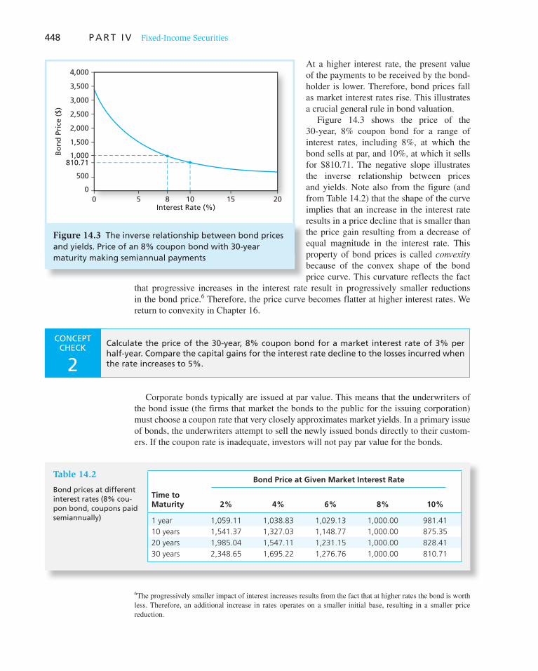
448 P A R T I V Fixed-Income Securities
At a higher interest rate, the present value
of the payments to be received by the bond-
holder is lower. Therefore, bond prices fall
as market interest rates rise. This illustrates
a crucial general rule in bond valuation.
Figure 14.3 shows the price of the
30-year, 8% coupon bond for a range of
interest rates, including 8%, at which the
bond sells at par, and 10%, at which it sells
for $810.71. The negative slope illustrates
the inverse relationship between prices
and yields. Note also from the figure (and
from Table 14.2 ) that the shape of the curve
implies that an increase in the interest rate
results in a price decline that is smaller than
the price gain resulting from a decrease of
equal magnitude in the interest rate. This
property of bond prices is called convexity
because of the convex shape of the bond
price curve. This curvature reflects the fact
that progressive increases in the interest rate result in progressively smaller reductions
in the bond price. 6 Therefore, the price curve becomes flatter at higher interest rates. We
return to convexity in Chapter 16.
Corporate bonds typically are issued at par value. This means that the underwriters of
the bond issue (the firms that market the bonds to the public for the issuing corporation)
must choose a coupon rate that very closely approximates market yields. In a primary issue
of bonds, the underwriters attempt to sell the newly issued bonds directly to their custom-
ers. If the coupon rate is inadequate, investors will not pay par value for the bonds.
6 The progressively smaller impact of interest increases results from the fact that at higher rates the bond is worth
less. Therefore, an additional increase in rates operates on a smaller initial base, resulting in a smaller price
reduction.
0 5 8 10 15 20Interest Rate (%)
Bo
nd
Pri
ce (
$)
0
500
810.711,000
1,500
2,000
2,500
3,000
3,500
4,000
Figure 14.3 The inverse relationship between bond prices and yields. Price of an 8% coupon bond with 30-year maturity making semiannual payments
Bond Price at Given Market Interest Rate
Time to Maturity 2% 4% 6% 8% 10%
1 year 1,059.11 1,038.83 1,029.13 1,000.00 981.41
10 years 1,541.37 1,327.03 1,148.77 1,000.00 875.35
20 years 1,985.04 1,547.11 1,231.15 1,000.00 828.41
30 years 2,348.65 1,695.22 1,276.76 1,000.00 810.71
Table 14.2
Bond prices at different interest rates (8% cou-pon bond, coupons paid semiannually)
CONCEPT CHECK
2 Calculate the price of the 30-year, 8% coupon bond for a market interest rate of 3% per half-year. Compare the capital gains for the interest rate decline to the losses incurred when the rate increases to 5%.

C H A P T E R 1 4 Bond Prices and Yields 449
After the bonds are issued, bondholders may buy or sell bonds in secondary markets. In
these markets, bond prices fluctuate inversely with the market interest rate.
The inverse relationship between price and yield is a central feature of fixed-income
securities. Interest rate fluctuations represent the main source of risk in the fixed-income
market, and we devote considerable attention in Chapter 16 to assessing the sensitivity of
bond prices to market yields. For now, however, it is sufficient to highlight one key factor
that determines that sensitivity, namely, the maturity of the bond.
As a general rule, keeping all other factors the same, the longer the maturity of the
bond, the greater the sensitivity of price to fluctuations in the interest rate. For example,
consider Table 14.2 , which presents the price of an 8% coupon bond at different market
yields and times to maturity. For any departure of the interest rate from 8% (the rate at
which the bond sells at par value), the change in the bond price is greater for longer times
to maturity.
This makes sense. If you buy the bond at par with an 8% coupon rate, and market rates
subsequently rise, then you suffer a loss: You have tied up your money earning 8% when
alternative investments offer higher returns. This is reflected in a capital loss on the bond—
a fall in its market price. The longer the period for which your money is tied up, the greater
the loss, and correspondingly the greater the drop in the bond price. In Table 14.2 , the row
for 1-year maturity bonds shows little price sensitivity—that is, with only 1 year’s earnings
at stake, changes in interest rates are not too threatening. But for 30-year maturity bonds,
interest rate swings have a large impact on bond prices. The force of discounting is greatest
for the longest-term bonds.
This is why short-term Treasury securities such as T-bills are considered to be the s afest.
They are free not only of default risk but also largely of price risk attributable to interest
rate volatility.
Bond Pricing between Coupon Dates
Equation 14.2 for bond prices assumes that the next coupon payment is in precisely one
payment period, either a year for an annual payment bond or 6 months for a semiannual
payment bond. But you probably want to be able to price bonds all 365 days of the year,
not just on the one or two dates each year that it makes a coupon payment!
In principle, the fact that the bond is between coupon dates does not affect the pric-
ing problem. The procedure is always the same: compute the present value of each
remaining payment and sum up. But if you are between coupon dates, there will be
fractional periods remaining until each payment, and this does complicate the arithmetic
computations.
Fortunately, bond pricing functions are included in most spreadsheet programs such
as Excel. The spreadsheet allows you to enter today’s date as well as the maturity date
of the bond, and so can provide prices for bonds at any date. The nearby box shows
you how.
As we pointed out earlier, bond prices are typically quoted net of accrued interest.
These prices, which appear in the financial press, are called flat prices. The actual invoice
price that a buyer pays for the bond includes accrued interest. Thus,
Invoice price 5 Flat price 1 Accrued interest
When a bond pays its coupon, flat price equals invoice price, because at that moment
accrued interest reverts to zero. However, this will be the exceptional case, not the rule.
Excel pricing functions provide the flat price of the bond. To find the invoice price, we
need to add accrued interest. Fortunately, Excel also provides functions that count the days
since the last coupon payment date and thus can be used to compute accrued interest. The

450
eXcel APPLICATIONS: Bond Pricing
E xcel and most other spreadsheet programs provide built-in functions to compute bond prices and yields.
They typically ask you to input both the date you buy the bond (called the settlement date ) and the maturity date of the bond. The Excel function for bond price is
5 PRICE(settlement date, maturity date, annual coupon rate, yield to maturity, redemption value as percent of par value, number of coupon payments per year)
For the 2.375% coupon October 2014 maturity bond high-lighted in Figure 14.1 , we would enter the values in the fol-lowing spreadsheet. Alternatively, we could simply enter the following function in Excel:
5 PRICE(DATE(2009, 10,31), DATE(2014,10,31), .02375, .0232, 100, 2)
The DATE function in Excel, which we use for both the settlement and maturity date, uses the format DATE(year,month,day). The first date is October 31, 2009, when the bond is purchased, and the second is October 31, 2014, when it matures. Most bonds pay coupons on the 15th or the last business day of the month.
Notice that the coupon rate and yield to maturity are expressed as decimals, not percentages. In most cases, redemption value is 100 (i.e., 100% of par value), and the resulting price similarly is expressed as a percent of par value. Occasionally, however, you may encounter bonds that pay off at a premium or discount to par value. One example would be callable bonds, discussed shortly.
The value of the bond returned by the pricing function is 100.258 (cell B12), which matches the price reported in Table 14.1 to the nearest 32nd of a point. This bond has just
paid a coupon. In other words, the settlement date is pre-cisely at the beginning of the coupon period, so no adjust-ment for accrued interest is necessary.
To illustrate the procedure for bonds between cou-pon payments, consider the 3.5% coupon February 2018 bond, also appearing in Figure 14.1 . Using the entries in column D of the spreadsheet, we find in cell D12 that the (flat) price of the bond is 101.946, which matches the price given in the figure except for a few cents’ round-ing error.
What about the bond’s invoice price? Rows 13 through 16 make the necessary adjustments. The function described in cell C13 counts the days since the last coupon. This day count is based on the bond’s settlement date, maturity date, coupon period (1 5 annual; 2 5 semiannual), and day count convention (choice 1 uses actual days). The function described in cell C14 counts the total days in each coupon payment period. Therefore, the entries for accrued inter-est in row 15 are the semiannual coupon multiplied by the fraction of a coupon period that has elapsed since the last payment. Finally, the invoice prices in row 16 are the sum of flat price plus accrued interest.
As a final example, suppose you wish to find the price of the bond in Example 14.2 . It is a 30-year maturity bond with a coupon rate of 8% (paid semiannually). The market interest rate given in the latter part of the example is 10%. However, you are not given a specific settlement or maturity date. You can still use the PRICE function to value the bond. Simply choose an arbitrary settlement date (January 1, 2000, is convenient) and let the maturity date be 30 years hence. The appropriate inputs appear in column F of the spreadsheet, with the resulting price, 81.071% of face value, appearing in cell F16.
eXce lPlease visit us at www.mhhe.com/bkm
A B C D E F G
=B12+B15
Formula in column B
2.375% coupon bond,
maturing Oct 31, 2014
3.5% coupon bond,
maturing Feb 15, 2018
8% coupon bond,
30-year maturity123456789
10111213141516
Settlement dateMaturity dateAnnual coupon rateYield to maturityRedemption value (% of face value)Coupon payments per year
Flat price (% of par)
Invoice priceAccrued interestDays in coupon periodDays since last coupon
= DATE (2009, 10, 31)= DATE (2014, 10, 31)
=PRICE(B4,B5,B6,B7,B8,B9)=COUPDAYBS(B4,B5,2,1)=COUPDAYS(B4,B5,2,1)=(B13/B14)*B6*100/2
10/31/200910/31/2014
0.023750.0232
1002 2 2
0100.258
100.258
181
10/31/20092/15/2018
0.0350.0323
100
101.946
102.679
1840.732
77
1/1/20001/1/2030
0.080.1
100
81.071
81.071
1820
00
nearby box also illustrates how to use these functions. The box provides examples using
bonds that have just paid a coupon and so have zero accrued interest, as well as a bond that
is between coupon dates.
C H A P T E R 1 4 Bond Prices and Yields 451
14.3 Bond Yields
We have noted that the current yield of a bond measures only the cash income provided by
the bond as a percentage of bond price and ignores any prospective capital gains or losses.
We would like a measure of rate of return that accounts for both current income and the
price increase or decrease over the bond’s life. The yield to maturity is the standard mea-
sure of the total rate of return. However, it is far from perfect, and we will explore several
variations of this measure.
Yield to Maturity
In practice, an investor considering the purchase of a bond is not quoted a promised rate
of return. Instead, the investor must use the bond price, maturity date, and coupon pay-
ments to infer the return offered by the bond over its life. The yield to maturity (YTM) is
defined as the interest rate that makes the present value of a bond’s payments equal to its
price. This interest rate is often interpreted as a measure of the average rate of return that
will be earned on a bond if it is bought now and held until maturity. To calculate the yield
to maturity, we solve the bond price equation for the interest rate given the bond’s price.
Example 14.3 Yield to Maturity
Suppose an 8% coupon, 30-year bond is selling at $1,276.76. What average rate of return
would be earned by an investor purchasing the bond at this price? We find the interest rate
at which the present value of the remaining 60 semiannual payments equals the bond price.
This is the rate consistent with the observed price of the bond. Therefore, we solve for r in
the following equation:
$1,276.76 5 a60
t51
$40
(1 1 r)t1
$1,000
(1 1 r)60
or, equivalently,
1,276.76 5 40 3 Annuity factor(r, 60) 1 1,000 3 PV factor(r, 60)
These equations have only one unknown variable, the interest rate, r. You can use a finan-
cial calculator or spreadsheet to confirm that the solution is r 5 .03, or 3%, per half-year. 7
This is the bond’s yield to maturity.
The financial press reports yields on an annualized basis, and annualizes the bond’s
semiannual yield using simple interest techniques, resulting in an annual percentage rate,
or APR. Yields annualized using simple interest are also called “bond equivalent yields.”
Therefore, the semiannual yield would be doubled and reported in the newspaper as a
bond equivalent yield of 6%. The effective annual yield of the bond, however, accounts for
compound interest. If one earns 3% interest every 6 months, then after 1 year, each dollar
invested grows with interest to $1 3 (1.03) 2 5 $1.0609, and the effective annual interest
rate on the bond is 6.09%.
7
7 On your financial calculator, you would enter the following inputs: n 5 60 periods; PV 5 2 1,276.76; FV 5 1000;
PMT 5 40; then you would compute the interest rate (COMP i or CPT i ). Notice that we enter the present value,
or PV, of the bond as minus $1,276.76. Again, this is because most calculators treat the initial purchase price of
the bond as a cash outflow. Spreadsheet 14.1 shows how to find yield to maturity using Excel. Without a financial
calculator or spreadsheet, you still could solve the equation, but you would need to use a trial-and-error approach.

452 P A R T I V Fixed-Income Securities
Excel also provides a function for yield to maturity that is especially useful in-between
coupon dates. It is
5 (YIELD settlement date, maturity date, annual coupon rate, bond price, redemption
value as percent of par value, number of coupon payments per year)
The bond price used in the function should be the reported flat price, without accrued inter-
est. For example, to find the yield to maturity of the bond in Example 14.3 , we would use
column B of Spreadsheet 14.1 . If the coupons were paid only annually, we would change
the entry for payments per year to 1 (see cell D8), and the yield would fall slightly to
5.99%.
The bond’s yield to maturity is the internal rate of return on an investment in the bond.
The yield to maturity can be interpreted as the compound rate of return over the life of the
bond under the assumption that all bond coupons can be reinvested at that yield. 8 Yield to
maturity is widely accepted as a proxy for average return.
Yield to maturity differs from the current yield of a bond, which is the bond’s annual
coupon payment divided by the bond price. For example, for the 8%, 30-year bond cur-
rently selling at $1,276.76, the current yield would be $80/$1,276.76 5 .0627, or 6.27%,
per year. In contrast, recall that the effective annual yield to maturity is 6.09%. For this
bond, which is selling at a premium over par value ($1,276 rather than $1,000), the coupon
rate (8%) exceeds the current yield (6.27%), which exceeds the yield to maturity (6.09%).
The coupon rate exceeds current yield because the coupon rate divides the coupon pay-
ments by par value ($1,000) rather than by the bond price ($1,276). In turn, the current
yield exceeds yield to maturity because the yield to maturity accounts for the built-in capi-
tal loss on the bond; the bond bought today for $1,276 will eventually fall in value to
$1,000 at maturity.
Example 14.3 illustrates a general rule: For premium bonds (bonds selling above
par value), coupon rate is greater than current yield, which in turn is greater than yield
8 If the reinvestment rate does not equal the bond’s yield to maturity, the compound rate of return will differ from
YTM. This is demonstrated in Examples 14.5 and 14.6 .
A B C D E
The formula entered here is: =YIELD(B3,B4,B5,B6,B7,B8)
Annual couponsSemiannual coupons1
2
3
4
5
6
7
8
9
10
12
11
Settlement date
Maturity date
Annual coupon rate
Bond price (flat)
Redemption value (% of face value)
Coupon payments per year
Yield to maturity (decimal)
1/1/2000
1/1/2030
0.08
127.676
100
2
0.0600
1/1/2000
1/1/2030
0.08
127.676
100
1
0.0599
Spreadsheet 14.1
Finding yield to maturity in Excel
eXce lPlease visit us at www.mhhe.com/bkm
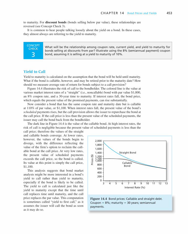
C H A P T E R 1 4 Bond Prices and Yields 453
to maturity. For discount bonds (bonds selling below par value), these relationships are
reversed (see Concept Check 3 ).
It is common to hear people talking loosely about the yield on a bond. In these cases,
they almost always are referring to the yield to maturity.
CONCEPT CHECK
3 What will be the relationship among coupon rate, current yield, and yield to maturity for bonds selling at discounts from par? Illustrate using the 8% (semiannual payment) coupon bond, assuming it is selling at a yield to maturity of 10%.
2,000
5 6 7 8 9 10 11 12 133 4
Interest Rate (%)
Pric
es (
$)
CallableBond
Straight Bond
0
200
400
600
800
1,0001,1001,2001,400
1,600
1,800
Figure 14.4 Bond prices: Callable and straight debt. Coupon 5 8%; maturity 5 30 years; semiannual payments.
Yield to Call
Yield to maturity is calculated on the assumption that the bond will be held until maturity.
What if the bond is callable, however, and may be retired prior to the maturity date? How
should we measure average rate of return for bonds subject to a call provision?
Figure 14.4 illustrates the risk of call to the bondholder. The colored line is the value at
various market interest rates of a “straight” (i.e., noncallable) bond with par value $1,000,
an 8% coupon rate, and a 30-year time to maturity. If interest rates fall, the bond price,
which equals the present value of the promised payments, can rise substantially.
Now consider a bond that has the same coupon rate and maturity date but is callable
at 110% of par value, or $1,100. When interest rates fall, the present value of the bond’s
scheduled payments rises, but the call provision allows the issuer to repurchase the bond at
the call price. If the call price is less than the present value of the scheduled payments, the
issuer may call the bond back from the bondholder.
The dark line in Figure 14.4 is the value of the callable bond. At high interest rates, the
risk of call is negligible because the present value of scheduled payments is less than the
call price; therefore the values of the straight
and callable bonds converge. At lower rates,
however, the values of the bonds begin to
diverge, with the difference reflecting the
value of the firm’s option to reclaim the call-
able bond at the call price. At very low rates,
the present value of scheduled payments
exceeds the call price, so the bond is called.
Its value at this point is simply the call price,
$1,100.
This analysis suggests that bond market
analysts might be more interested in a bond’s
yield to call rather than yield to maturity,
especially if the bond is likely to be called.
The yield to call is calculated just like the
yield to maturity except that the time until
call replaces time until maturity, and the call
price replaces the par value. This computation
is sometimes called “yield to first call,” as it
assumes the issuer will call the bond as soon
as it may do so.

454 P A R T I V Fixed-Income Securities
Example 14.4 Yield to Call
Suppose the 8% coupon, 30-year maturity bond sells for $1,150 and is callable in 10 years
at a call price of $1,100. Its yield to maturity and yield to call would be calculated using
the following inputs:
Yield to Call Yield to Maturity
Coupon payment $40 $40
Number of semiannual periods 20 periods 60 periods
Final payment $1,100 $1,000
Price $1,150 $1,150
Yield to call is then 6.64%. [To confirm this on a calculator, input n 5 20; PV 5 ( 2 )1,150;
FV 5 1100; PMT 5 40; compute i as 3.32%, or 6.64% bond equivalent yield.] Yield to
maturity is 6.82%. [To confirm, input n 5 60; PV 5 ( 2 )1,150; FV 5 1000; PMT 5 40;
compute i as 3.41% or 6.82% bond equivalent yield. In Excel, you can calculate yield to
call as 5 YIELD(DATE(2000,01,01), DATE(2010,01,01), .08, 115, 110, 2). Notice that
redemption value is input as 110, i.e., 110% of par value.]
We have noted that most callable bonds are issued with an initial period of call protec-
tion. In addition, an implicit form of call protection operates for bonds selling at deep dis-
counts from their call prices. Even if interest rates fall a bit, deep-discount bonds still will
sell below the call price and thus will not be subject to a call.
Premium bonds that might be selling near their call prices, however, are especially
apt to be called if rates fall further. If interest rates fall, a callable premium bond is
likely to provide a lower return than could be earned on a discount bond whose poten-
tial price appreciation is not limited by the likelihood of a call. Investors in premium
bonds often are more interested in the bond’s yield to call rather than yield to maturity
as a consequence, because it may appear to them that the bond will be retired at the
call date.
Realized Compound Return versus Yield to Maturity
We have noted that yield to maturity will equal the rate of return realized over the life
of the bond if all coupons are reinvested at an interest rate equal to the bond’s yield to
maturity. Consider, for example, a 2-year bond selling at par value paying a 10% coupon
once a year. The yield to maturity is 10%. If the $100 coupon payment is reinvested at
an interest rate of 10%, the $1,000 investment in the bond will grow after 2 years to
CONCEPT CHECK
4 and 5
4. The yield to maturity on two 10-year maturity bonds currently is 7%. Each bond has a call price of $1,100. One bond has a coupon rate of 6%, the other 8%. Assume for sim-plicity that bonds are called as soon as the present value of their remaining payments exceeds their call price. What will be the capital gain on each bond if the market inter-est rate suddenly falls to 6%?
5. A 20-year maturity 9% coupon bond paying coupons semiannually is callable in 5 years at a call price of $1,050. The bond currently sells at a yield to maturity of 8%. What is the yield to call?

C H A P T E R 1 4 Bond Prices and Yields 455
$1,210, as illustrated in Figure 14.5 , panel A. The
coupon paid in the first year is reinvested and grows
with interest to a second-year value of $110, which
together with the second coupon payment and pay-
ment of par value in the second year results in a total
value of $1,210.
To summarize, the initial value of the investment is
V 0 5 $1,000. The final value in 2 years is V 2 5 $1,210.
The compound rate of return, therefore, is calculated
as follows:
V0(1 1 r)2 5 V2
$1,000(1 1 r)2 5 $1,210
r 5 .10 5 10%
With a reinvestment rate equal to the 10% yield to
maturity, the realized compound return equals yield
to maturity.
But what if the reinvestment rate is not 10%? If the
coupon can be invested at more than 10%, funds will
grow to more than $1,210, and the realized compound
return will exceed 10%. If the reinvestment rate is less
than 10%, so will be the realized compound return.
Consider the following example.
Example 14.5 Realized Compound Return
If the interest rate earned on the first coupon is less than 10%, the final value of the invest-
ment will be less than $1,210, and the realized compound return will be less than 10%. To
illustrate, suppose the interest rate at which the coupon can be invested equals 8%. The
following calculations are illustrated in Figure 14.5 , panel B.
Future value of first coupon payment with interest earnings
1 Cash payment in second year (final coupon plus par value)
5 Total value of investment with reinvested coupons
5 $100 3 1.08 5 $ 108
$1,100
$1,208
The realized compound return is the compound rate of growth of invested funds, assuming
that all coupon payments are reinvested. The investor purchased the bond for par at $1,000,
and this investment grew to $1,208.
V0(1 1 r)2 5 V2
$1,000(1 1 r)2 5 $1,208
r 5 .0991 5 9.91%
Example 14.5 highlights the problem with conventional yield to maturity when rein-
vestment rates can change over time. Conventional yield to maturity will not equal realized
A. Reinvestment Rate = 10%
B. Reinvestment Rate = 8%
FutureValue:
Time:
$1,100
$100Cash Flow:
0
$1,100 = $1,100
100 × 1.10 = $ 110
$1,210
FutureValue:
Time:
$1,100
$100Cash Flow:
0
$1,100 = $1,100
100 × 1.08 = $ 108
$1,208
21
21
Figure 14.5 Growth of invested funds

456 P A R T I V Fixed-Income Securities
compound return. However, in an economy with future interest rate uncertainty, the rates at
which interim coupons will be reinvested are not yet known. Therefore, although realized
compound return can be computed after the investment period ends, it cannot be computed
in advance without a forecast of future reinvestment rates. This reduces much of the attrac-
tion of the realized return measure.
Forecasting the realized compound yield over various holding periods or investment
horizons is called horizon analysis. The forecast of total return depends on your forecasts
of both the price of the bond when you sell it at the end of your horizon and the rate at
which you are able to reinvest coupon income. The sales price depends in turn on the yield
to maturity at the horizon date. With a longer investment horizon, however, reinvested cou-
pons will be a larger component of your final proceeds.
Example 14.6 Horizon Analysis
Suppose you buy a 30-year, 7.5% (annual payment) coupon bond for $980 (when its yield
to maturity is 7.67%) and plan to hold it for 20 years. Your forecast is that the bond’s yield
to maturity will be 8% when it is sold and that the reinvestment rate on the coupons will
be 6%. At the end of your investment horizon, the bond will have 10 years remaining until
expiration, so the forecast sales price (using a yield to maturity of 8%) will be $966.45.
The 20 coupon payments will grow with compound interest to $2,758.92. (This is the
future value of a 20-year $75 annuity with an interest rate of 6%.)
On the basis of these forecasts, your $980 investment will grow in 20 years to $966.45 1
$2,758.92 5 $3,725.37. This corresponds to an annualized compound return of 6.90%:
V0(1 1 r)20 5 V20
$980(1 1 r)20 5 $3,725.37
r 5 .0690 5 6.90%
Examples 14.5 and 14.6 demonstrate that as interest rates change, bond investors are
actually subject to two sources of offsetting risk. On the one hand, when rates rise, bond
prices fall, which reduces the value of the portfolio. On the other hand, reinvested coupon
income will compound more rapidly at those higher rates. This reinvestment rate risk
will offset the impact of price risk. In Chapter 16, we will explore this trade-off in more
detail and will discover that by carefully tailoring their bond portfolios, investors can pre-
cisely balance these two effects for any given investment horizon.
14.4 Bond Prices over Time
As we noted earlier, a bond will sell at par value when its coupon rate equals the market
interest rate. In these circumstances, the investor receives fair compensation for the time
value of money in the form of the recurring coupon payments. No further capital gain is
necessary to provide fair compensation.
When the coupon rate is lower than the market interest rate, the coupon payments alone
will not provide investors as high a return as they could earn elsewhere in the market. To
receive a fair return on such an investment, investors also need to earn price appreciation on
their bonds. The bonds, therefore, would have to sell below par value to provide a “built-in”
capital gain on the investment.

C H A P T E R 1 4 Bond Prices and Yields 457
Example 14.7 Fair Holding-Period Return
To illustrate built-in capital gains or losses, suppose a bond was issued several years ago
when the interest rate was 7%. The bond’s annual coupon rate was thus set at 7%. (We
will suppose for simplicity that the bond pays its coupon annually.) Now, with 3 years
left in the bond’s life, the interest rate is 8% per year. The bond’s market price is the
present value of the remaining annual coupons plus payment of par value. That present
value is 9
$70 3 Annuity factor(8%, 3) 1 $1,000 3 PV factor(8%, 3) 5 $974.23
which is less than par value.
In another year, after the next coupon is paid, the bond would sell at
$70 3 Annuity factor(8%, 2) 1 $1,000 3 PV factor(8%, 2) 5 $982.17
thereby yielding a capital gain over the year of $7.94. If an investor had purchased the
bond at $974.23, the total return over the year would equal the coupon payment plus capi-
tal gain, or $70 1 $7.94 5 $77.94. This represents a rate of return of $77.94/$974.23, or
8%, exactly the current rate of return available elsewhere in the market.
9
When bond prices are set accord-
ing to the present value formula, any
discount from par value provides an
anticipated capital gain that will aug-
ment a below-market coupon rate
just enough to provide a fair total
rate of return. Conversely, if the cou-
pon rate exceeds the market interest
rate, the interest income by itself is greater than that available elsewhere in the market.
Investors will bid up the price of these bonds above their par values. As the bonds
approach maturity, they will fall in value because fewer of these above-market coupon
payments remain. The resulting capital losses offset the large coupon payments so that
the bondholder again receives only a fair rate of return.
Problem 14 at the end of the chapter asks you to work through the case of the high-
coupon bond. Figure 14.6 traces out the price paths of high- and low-coupon bonds (net of
accrued interest) as time to maturity approaches, at least for the case in which the market
interest rate is constant. The low-coupon bond enjoys capital gains, whereas the high-
coupon bond suffers capital losses. 10
We use these examples to show that each bond offers investors the same total rate of
return. Although the capital gain versus income components differ, the price of each bond
is set to provide competitive rates, as we should expect in well-functioning capital markets.
Security returns all should be comparable on an after-tax risk-adjusted basis. It they are
not, investors will try to sell low-return securities, thereby driving down their prices until
9 Using a calculator, enter n 5 3, i 5 8, PMT 5 70, FV 5 1,000, and compute PV.
10 If interest rates are volatile, the price path will be “jumpy,” vibrating around the price path in Figure 14.6
and reflecting capital gains or losses as interest rates fluctuate. Ultimately, however, the price must reach par
value at the maturity date, so the price of the premium bond will fall over time while that of the discount bond
will rise.
CONCEPT CHECK
6
At what price will the bond in Example 14.7 sell in yet another year, when only 1 year remains until maturity? What is the rate of return to an inves-tor who purchases the bond at $982.17 and sells it 1 year hence?

458 P A R T I V Fixed-Income Securities
the total return at the now-lower price
is competitive with other securities.
Prices should continue to adjust until
all securities are fairly priced in that
expected returns are comparable, given
appropriate risk and tax adjustments.
Yield to Maturity versus Holding-Period Return
In Example 14.7 , the holding-period
return and the yield to maturity were
equal. The bond yield started and
ended the year at 8%, and the bond’s
holding-period return also equaled
8%. This turns out to be a general
result. When the yield to maturity is
unchanged over the period, the rate
of return on the bond will equal that
yield. As we noted, this should not be
surprising: The bond must offer a rate
of return competitive with those avail-
able on other securities.
However, when yields fluctuate, so will a bond’s rate of return. Unanticipated changes
in market rates will result in unanticipated changes in bond returns and, after the fact, a
bond’s holding-period return can be better or worse than the yield at which it initially sells.
An increase in the bond’s yield acts to reduce its price, which reduces the holding period
return. In this event, the holding period return is likely to be less than the initial yield to
maturity. 11 Conversely, a decline in yield will result in a holding-period return greater than
the initial yield.
Example 14.8 Yield to Maturity versus Holding-Period Return
Consider a 30-year bond paying an annual coupon of $80 and selling at par value of
$1,000. The bond’s initial yield to maturity is 8%. If the yield remains at 8% over the year,
the bond price will remain at par, so the holding-period return also will be 8%. But if the
yield falls below 8%, the bond price will increase. Suppose the yield falls and the price
increases to $1,050. Then the holding-period return is greater than 8%:
Holding-period return 5$80 1 ($1,050 2 $1,000)
$1,0005 .13, or 13%
11 We have to be a bit careful here. When yields increase, coupon income can be reinvested at higher rates, which
offsets the impact of the initial price decline. If your holding period is sufficiently long, the positive impact of the
higher reinvestment rate can more than offset the initial price decline. But common performance evaluation peri-
ods for portfolio managers are no more than 1 year, and over these shorter horizons the price impact will almost
always dominate the impact of the reinvestment rate. We discuss the trade-off between price risk and reinvest-
ment rate risk more fully in Chapter 16.
4000 5 10 15 20 25 30
Bo
nd
Pri
ce (
$)
Price path for discount bond(selling at yield to maturity = 11.5%)
Price path for premium bondselling for more than face value(at yield to maturity = 4%)
Time (years)
Today Maturity Date
1,400
1,600
1,200
1,000
800
600
Figure 14.6 Prices over time of 30-year maturity, 6.5% coupon bonds. Bond price approaches par value as maturity approaches.

C H A P T E R 1 4 Bond Prices and Yields 459
Here is another way to think about the difference between yield to maturity and
holding-period return. Yield to maturity depends only on the bond’s coupon, current price,
and par value at maturity. All of these values are observable today, so yield to maturity can
be easily calculated. Yield to maturity can be interpreted as a measure of the average rate
of return if the investment in the bond is held until the bond matures. In contrast, holding-
period return is the rate of return over a particular investment period and depends on the
market price of the bond at the end of that holding period; of course this price is not known
today. Because bond prices over the holding period will respond to unanticipated changes
in interest rates, holding-period return can at most be forecast.
Zero-Coupon Bonds and Treasury Strips
Original-issue discount bonds are less common than coupon bonds issued at par. These
are bonds that are issued intentionally with low coupon rates that cause the bond to sell
at a discount from par value. An extreme example of this type of bond is the zero-coupon
bond, which carries no coupons and provides all its return in the form of price apprecia-
tion. Zeros provide only one cash flow to their owners, on the maturity date of the bond.
U.S. Treasury bills are examples of short-term zero-coupon instruments. If the bill has
face value of $10,000, the Treasury issues or sells it for some amount less than $10,000,
agreeing to repay $10,000 at maturity. All of the investor’s return comes in the form of
price appreciation.
Longer-term zero-coupon bonds are commonly created from coupon-bearing notes and
bonds. A bond dealer who purchases a Treasury coupon bond may ask the Treasury to
break down the cash flows to be paid by the bond into a series of independent securities,
where each security is a claim to one of the payments of the original bond. For exam-
ple, a 10-year coupon bond would be “stripped” of its 20 semiannual coupons, and each
coupon payment would be treated as a stand-alone zero-coupon bond. The maturities of
these bonds would thus range from 6 months to 10 years. The final payment of principal
would be treated as another stand-alone zero-coupon security. Each of the payments is
now treated as an independent security and is assigned its own CUSIP number (by the
Committee on Uniform Securities Identification Procedures), the security identifier that
allows for electronic trading over the Fedwire system, a network that connects all Federal
Reserve banks and their branches. The payments are still considered obligations of the
U.S. Treasury. The Treasury program under which coupon stripping is performed is called
STRIPS (Separate Trading of Registered Interest and Principal of Securities), and these
zero-coupon securities are called Treasury strips.
What should happen to prices of zeros as time passes? On their maturity dates, zeros
must sell for par value. Before maturity, however, they should sell at discounts from par,
because of the time value of money. As time passes, price should approach par value. In
fact, if the interest rate is constant, a zero’s price will increase at exactly the rate of interest.
To illustrate, consider a zero with 30 years until maturity, and suppose the market
interest rate is 10% per year. The price of the bond today is $1,000/(1.10) 30 5 $57.31.
Next year, with only 29 years until maturity, if the yield is still 10%, the price will be
CONCEPT CHECK
7
Show that if yield to maturity increases, then holding-period return is less than initial yield. For example, suppose in Example 14.8 that by the end of the first year, the bond’s yield to maturity is 8.5%. Find the 1-year holding-period return and compare it to the bond’s initial 8% yield to maturity.
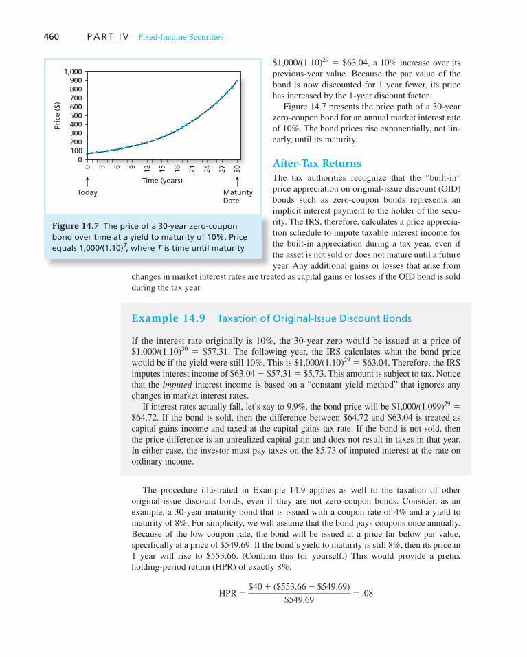
460 P A R T I V Fixed-Income Securities
$1,000/(1.10) 29 5 $63.04, a 10% increase over its
p revious-year value. Because the par value of the
bond is now discounted for 1 year fewer, its price
has increased by the 1-year discount factor.
Figure 14.7 presents the price path of a 30-year
zero-coupon bond for an annual market interest rate
of 10%. The bond prices rise exponentially, not lin-
early, until its maturity.
After-Tax Returns
The tax authorities recognize that the “built-in”
price appreciation on original-issue discount (OID)
bonds such as zero-coupon bonds represents an
implicit interest payment to the holder of the secu-
rity. The IRS, therefore, calculates a price apprecia-
tion schedule to impute taxable interest income for
the built-in appreciation during a tax year, even if
the asset is not sold or does not mature until a future
year. Any additional gains or losses that arise from
changes in market interest rates are treated as capital gains or losses if the OID bond is sold
during the tax year.
Example 14.9 Taxation of Original-Issue Discount Bonds
If the interest rate originally is 10%, the 30-year zero would be issued at a price of
$1,000/(1.10) 30 5 $57.31. The following year, the IRS calculates what the bond price
would be if the yield were still 10%. This is $1,000/(1.10) 29 5 $63.04. Therefore, the IRS
imputes interest income of $63.04 2 $57.31 5 $5.73. This amount is subject to tax. Notice
that the imputed interest income is based on a “constant yield method” that ignores any
changes in market interest rates.
If interest rates actually fall, let’s say to 9.9%, the bond price will be $1,000/(1.099) 29 5
$64.72. If the bond is sold, then the difference between $64.72 and $63.04 is treated as
capital gains income and taxed at the capital gains tax rate. If the bond is not sold, then
the price difference is an unrealized capital gain and does not result in taxes in that year.
In either case, the investor must pay taxes on the $5.73 of imputed interest at the rate on
ordinary income.
The procedure illustrated in Example 14.9 applies as well to the taxation of other
original-issue discount bonds, even if they are not zero-coupon bonds. Consider, as an
example, a 30-year maturity bond that is issued with a coupon rate of 4% and a yield to
maturity of 8%. For simplicity, we will assume that the bond pays coupons once annually.
Because of the low coupon rate, the bond will be issued at a price far below par value,
specifically at a price of $549.69. If the bond’s yield to maturity is still 8%, then its price in
1 year will rise to $553.66. (Confirm this for yourself.) This would provide a pretax
h olding-period return (HPR) of exactly 8%:
HPR 5$40 1 ($553.66 2 $549.69)
$549.695 .08
MaturityDate
Today
Time (years)
Pric
e ($
)
1,000900800700600500400300200100
0
30 6 9 12 15 18 21 24 27 30 Figure 14.7 The price of a 30-year zero-coupon bond over time at a yield to maturity of 10%. Price equals 1,000/(1.10) T , where T is time until maturity.
C H A P T E R 1 4 Bond Prices and Yields 461
CONCEPT CHECK
8
Suppose that the yield to maturity of the 4% coupon, 30-year maturity bond falls to 7% by the end of the first year and that the investor sells the bond after the first year. If the investor’s federal plus state tax rate on interest income is 38% and the combined tax rate on capital gains is 20%, what is the investor’s after-tax rate of return?
The increase in the bond price based on a constant yield, however, is treated as interest
income, so the investor is required to pay taxes on the explicit coupon income, $40, as well
as the imputed interest income of $553.66 2 $549.69 5 $3.97. If the bond’s yield actually
changes during the year, the difference between the bond’s price and the constant-yield
value of $553.66 would be treated as capital gains income if the bond is sold.
14.5 Default Risk and Bond Pricing
Although bonds generally promise a fixed flow of income, that income stream is not risk-
less unless the investor can be sure the issuer will not default on the obligation. While U.S.
government bonds may be treated as free of default risk, this is not true of corporate bonds.
Therefore, the actual payments on these bonds are uncertain, for they depend to some
degree on the ultimate financial status of the firm.
Bond default risk, usually called credit risk, is measured by Moody’s Investor Services,
Standard & Poor’s Corporation, and Fitch Investors Service, all of which provide finan-
cial information on firms as well as quality ratings of large corporate and municipal bond
issues. International sovereign bonds, which also entail default risk, especially in emerging
markets, also are commonly rated for default risk. Each rating firm assigns letter grades to
the bonds of corporations and municipalities to reflect their assessment of the safety of the
bond issue. The top rating is AAA or Aaa, a designation awarded to only about a dozen
firms. Moody’s modifies each rating class with a 1, 2, or 3 suffix (e.g., Aaa1, Aaa2, Aaa3)
to provide a finer gradation of ratings. The other agencies use a 1 or 2 modification.
Those rated BBB or above (S&P, Fitch) or Baa and above (Moody’s) are considered
investment-grade bonds, whereas lower-rated bonds are classified as speculative-grade
or junk bonds. Defaults on low-grade issues are not uncommon. For example, almost half
of the bonds that were rated CCC by Standard & Poor’s at issue have defaulted within
10 years. Highly rated bonds rarely default, but even these bonds are not free of credit risk.
For example, in May 2001 WorldCom sold $11.8 billion of bonds with an investment-
grade rating. Only a year later, the firm filed for bankruptcy and its bondholders lost more
than 80% of their investment. Certain regulated institutional investors such as insurance
companies have not always been allowed to invest in speculative-grade bonds.
Figure 14.8 provides the definitions of each bond rating classification.
Junk Bonds
Junk bonds, also known as high-yield bonds, are nothing more than speculative-grade
(low-rated or unrated) bonds. Before 1977, almost all junk bonds were “fallen angels,” that
is, bonds issued by firms that originally had investment-grade ratings but that had since
been downgraded. In 1977, however, firms began to issue “original-issue junk.”
Much of the credit for this innovation is given to Drexel Burnham Lambert, and espe-
cially its trader Michael Milken. Drexel had long enjoyed a niche as a junk bond trader and
had established a network of potential investors in junk bonds. Firms not able to muster an

462 P A R T I V Fixed-Income Securities
Bond Ratings
Very HighQuality High Quality Speculative Very Poor
Standard & Poor’s AAA AA A BBB BB B CCC D
Moody’s Aaa Aa A Baa Ba B Caa C
At times both Moody’s and Standard & Poor’s have used adjustments to these ratings:S&P uses plus and minus signs: A + is the strongest A rating and A − the weakest.Moody’s uses a 1, 2, or 3 designation, with 1 indicating the strongest.
Moody’s S&P
Aaa AAA Debt rated Aaa and AAA has the highest rating. Capacity to pay interestand principal is extremely strong.
Aa AA Debt rated Aa and AA has a very strong capacity to pay interest and repayprincipal. Together with the highest rating, this group comprises the high-grade bond class.
A A Debt rated A has a strong capacity to pay interest and repay principal,although it is somewhat more susceptible to the adverse effects ofchanges in circumstances and economic conditions than debt inhigher-rated categories.
Baa BBB Debt rated Baa and BBB is regarded as having an adequate capacity topay interest and repay principal. Whereas it normally exhibits adequateprotection parameters, adverse economic conditions or changingcircumstances are more likely to lead to a weakened capacity to payinterest and repay principal for debt in this category than in higher-ratedcategories. These bonds are medium-grade obligations.
Ba BB Debt rated in these categories is regarded, on balance, as predominantlyB B speculative with respect to capacity to pay interest and repay principal inCaa CCC accordance with the terms of the obligation. BB and Ba indicate the lowestCa CC degree of speculation, and CC and Ca the highest degree of speculation.
Although such debt will likely have some quality and protectivecharacteristics, these are outweighed by large uncertainties or major riskexposures to adverse conditions. Some issues may be in default.
C C This rating is reserved for income bonds on which no interest is being paid.
D D Debt rated D is in default, and payment of interest and/or repayment ofprincipal is in arrears.
Figure 14.8 Definitions of each bond rating class
Source: Stephen A. Ross and Randolph W. Westerfield, Corporate Finance, Copyright 1988 (St. Louis: Times Mirror/Mosby College Publishing, reproduced with permission from the McGraw-Hill Companies, Inc.). Data from various editions of Standard & Poor’s Bond Guide and Moody’s Bond Guide.
investment-grade rating were happy to have Drexel (and other investment bankers) market
their bonds directly to the public, as this opened up a new source of financing. Junk issues
were a lower-cost financing alternative than borrowing from banks.
High-yield bonds gained considerable notoriety in the 1980s when they were used as
financing vehicles in leveraged buyouts and hostile takeover attempts. Shortly thereaf-
ter, however, the junk bond market suffered. The legal difficulties of Drexel and Michael
Milken in connection with Wall Street’s insider trading scandals of the late 1980s tainted
the junk bond market.

C H A P T E R 1 4 Bond Prices and Yields 463
At the height of Drexel’s difficulties, the high-yield bond market nearly dried up. Since
then, the market has rebounded dramatically. However, it is worth noting that the average
credit quality of newly issued high-yield debt issued today is higher than the average qual-
ity in the boom years of the 1980s. Of course, in periods of financial stress, junk bonds are
more vulnerable than investment-grade bonds. During the credit crisis of 2008, prices on
these bonds fell dramatically, and their yields to maturity rose equally dramatically. The
spread between yields on junk bonds and Treasuries widened from around 3% in early
2007 to an astonishing 18% by the beginning of 2009.
Determinants of Bond Safety
Bond rating agencies base their quality ratings largely on an analysis of the level and trend
of some of the issuer’s financial ratios. The key ratios used to evaluate safety are
1. Coverage ratios —Ratios of company earnings to fixed costs. For example, the
times-interest-earned ratio is the ratio of earnings before interest payments and
taxes to interest obligations. The fixed-charge coverage ratio includes lease pay-
ments and sinking fund payments with interest obligations to arrive at the ratio of
earnings to all fixed cash obligations (sinking funds are described below). Low or
falling coverage ratios signal possible cash flow difficulties.
2. Leverage ratio, Debt-to-equity ratio —A too-high leverage ratio indicates excessive
indebtedness, signaling the possibility the firm will be unable to earn enough to
satisfy the obligations on its bonds.
3. Liquidity ratios —The two most common liquidity ratios are the current ratio
(current assets/current liabilities) and the quick ratio (current assets excluding
in ventories/current liabilities). These ratios measure the firm’s ability to pay bills
coming due with its most liquid assets.
4. Profitability ratios —Measures of rates of return on assets or equity. Profitabil-
ity ratios are indicators of a firm’s overall financial health. The return on assets
(earnings before interest and taxes divided by total assets) or return on equity (net
income/equity) are the most popular of these measures. Firms with higher returns
on assets or equity should be better able to raise money in security markets because
they offer prospects for better returns on the firm’s investments.
5. Cash flow-to-debt ratio —This is the ratio of total cash flow to outstanding debt.
Standard & Poor’s periodically computes median values of selected ratios for firms in
several rating classes, which we present in Table 14.3 . Of course, ratios must be evalu-
ated in the context of industry standards, and analysts differ in the weights they place on
particular ratios. Nevertheless, Table 14.3 demonstrates the tendency of ratios to improve
along with the firm’s rating class. And default rates vary dramatically with bond rating.
Historically, only about 1% of bonds originally rated AA or better at issuance had defaulted
after 15 years. That ratio is around 7.5% for BBB-rated bonds, and 40% for B-rated bonds.
Credit risk clearly varies dramatically across rating classes.
Many studies have tested whether financial ratios can in fact be used to predict default
risk. One of the best-known series of tests was conducted by Edward Altman, who used
discriminant analysis to predict bankruptcy. With this technique a firm is assigned a score
based on its financial characteristics. If its score exceeds a cut-off value, the firm is deemed
creditworthy. A score below the cut-off value indicates significant bankruptcy risk in the
near future.
To illustrate the technique, suppose that we were to collect data on the return on equity
(ROE) and coverage ratios of a sample of firms, and then keep records of any corporate
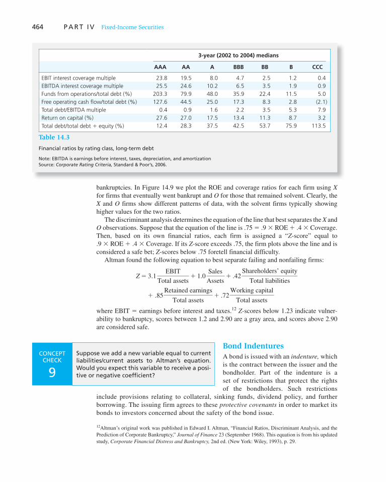
464 P A R T I V Fixed-Income Securities
bankruptcies. In Figure 14.9 we plot the ROE and coverage ratios for each firm using X
for firms that eventually went bankrupt and O for those that remained solvent. Clearly, the
X and O firms show different patterns of data, with the solvent firms typically showing
higher values for the two ratios.
The discriminant analysis determines the equation of the line that best separates the X and
O observations. Suppose that the equation of the line is .75 5 .9 3 ROE 1 .4 3 Coverage.
Then, based on its own financial ratios, each firm is assigned a “ Z -score” equal to
.9 3 ROE 1 .4 3 Coverage. If its Z -score exceeds .75, the firm plots above the line and is
considered a safe bet; Z -scores below .75 foretell financial difficulty.
Altman found the following equation to best separate failing and nonfailing firms:
Z 5 3.1
EBIT
Total assets1 1.0
Sales
Assets1 .42
Shareholders’ equity
Total liabilities
1 .85
Retained earnings
Total assets1 .72
Working capital
Total assets
where EBIT 5 earnings before interest and taxes. 12 Z -scores below 1.23 indicate vulner-
ability to bankruptcy, scores between 1.2 and 2.90 are a gray area, and scores above 2.90
are considered safe.
Bond Indentures
A bond is issued with an indenture, which
is the contract between the issuer and the
bondholder. Part of the indenture is a
set of restrictions that protect the rights
of the bondholders. Such restrictions
include provisions relating to collateral, sinking funds, dividend policy, and further
borrowing. The issuing firm agrees to these protective covenants in order to market its
bonds to investors concerned about the safety of the bond issue.
12 Altman’s original work was published in Edward I. Altman, “Financial Ratios, Discriminant Analysis, and the
Prediction of Corporate Bankruptcy,” Journal of Finance 23 (September 1968). This equation is from his updated
study, Corporate Financial Distress and Bankruptcy, 2nd ed. (New York: Wiley, 1993), p. 29.
CONCEPT CHECK
9
Suppose we add a new variable equal to current liabilities/current assets to Altman’s equation. Would you expect this variable to receive a posi-tive or negative coefficient?
3-year (2002 to 2004) medians
AAA AA A BBB BB B CCC
EBIT interest coverage multiple 23.8 19.5 8.0 4.7 2.5 1.2 0.4
EBITDA interest coverage multiple 25.5 24.6 10.2 6.5 3.5 1.9 0.9
Funds from operations/total debt (%) 203.3 79.9 48.0 35.9 22.4 11.5 5.0
Free operating cash flow/total debt (%) 127.6 44.5 25.0 17.3 8.3 2.8 (2.1)
Total debt/EBITDA multiple 0.4 0.9 1.6 2.2 3.5 5.3 7.9
Return on capital (%) 27.6 27.0 17.5 13.4 11.3 8.7 3.2
Total debt/total debt 1 equity (%) 12.4 28.3 37.5 42.5 53.7 75.9 113.5
Table 14.3
Financial ratios by rating class, long-term debt
Note: EBITDA is earnings before interest, taxes, depreciation, and amortization Source: Corporate Rating Criteria, Standard & Poor’s, 2006.

C H A P T E R 1 4 Bond Prices and Yields 465
Sinking Funds Bonds call for the payment of par value at the end of the bond’s
life. This payment constitutes a large cash commitment for the issuer. To help ensure
the commitment does not create a cash flow crisis, the firm agrees to establish a sinking
fund to spread the payment burden over several years. The fund may operate in one of
two ways:
1. The firm may repurchase a fraction of the outstanding bonds in the open market
each year.
2. The firm may purchase a fraction of the outstanding bonds at a special call price
associated with the sinking fund provision. The firm has an option to purchase the
bonds at either the market price or the sinking fund price, whichever is lower. To
allocate the burden of the sinking fund call fairly among bondholders, the bonds
chosen for the call are selected at random based on serial number. 13
The sinking fund call differs from a conventional bond call in two important ways.
First, the firm can repurchase only a limited fraction of the bond issue at the sinking fund
call price. At best, some indentures allow firms to use a doubling option, which allows
repurchase of double the required number of bonds at the sinking fund call price. Second,
while callable bonds generally have call prices above par value, the sinking fund call price
usually is set at the bond’s par value.
Although sinking funds ostensibly protect bondholders by making principal repay-
ment more likely, they can hurt the investor. The firm will choose to buy back discount
bonds (selling below par) at market price, while exercising its option to buy back pre-
mium bonds (selling above par) at par. Therefore, if interest rates fall and bond prices
rise, firms will benefit from the sinking fund provision that enables them to repurchase
their bonds at below-market prices. In these circumstances, the firm’s gain is the bond-
holder’s loss.
13 Although it is less common, the sinking fund provision also may call for periodic payments to a trustee, with the
payments invested so that the accumulated sum can be used for retirement of the entire issue at maturity.
RO
E
Coverage Ratio
Figure 14.9 Discriminant analysis
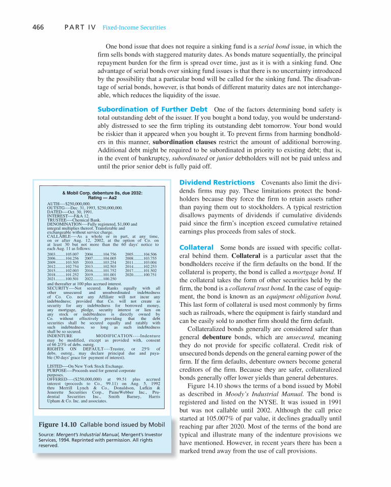
466 P A R T I V Fixed-Income Securities
One bond issue that does not require a sinking fund is a serial bond issue, in which the
firm sells bonds with staggered maturity dates. As bonds mature sequentially, the principal
repayment burden for the firm is spread over time, just as it is with a sinking fund. One
advantage of serial bonds over sinking fund issues is that there is no uncertainty introduced
by the possibility that a particular bond will be called for the sinking fund. The disadvan-
tage of serial bonds, however, is that bonds of different maturity dates are not interchange-
able, which reduces the liquidity of the issue.
Subordination of Further Debt One of the factors determining bond safety is
total outstanding debt of the issuer. If you bought a bond today, you would be understand-
ably distressed to see the firm tripling its outstanding debt tomorrow. Your bond would
be riskier than it appeared when you bought it. To prevent firms from harming bondhold-
ers in this manner, subordination clauses restrict the amount of additional borrowing.
Additional debt might be required to be subordinated in priority to existing debt; that is,
in the event of bankruptcy, subordinated or junior debtholders will not be paid unless and
until the prior senior debt is fully paid off.
Dividend Restrictions Covenants also limit the divi-
dends firms may pay. These limitations protect the bond-
holders because they force the firm to retain assets rather
than paying them out to stockholders. A typical restriction
disallows payments of dividends if cumulative dividends
paid since the firm’s inception exceed cumulative retained
earnings plus proceeds from sales of stock.
Collateral Some bonds are issued with specific collat-
eral behind them. Collateral is a particular asset that the
bondholders receive if the firm defaults on the bond. If the
collateral is property, the bond is called a mortgage bond. If
the collateral takes the form of other securities held by the
firm, the bond is a collateral trust bond. In the case of equip-
ment, the bond is known as an equipment obligation bond.
This last form of collateral is used most commonly by firms
such as railroads, where the equipment is fairly standard and
can be easily sold to another firm should the firm default.
Collateralized bonds generally are considered safer than
general debenture bonds, which are unsecured, meaning
they do not provide for specific collateral. Credit risk of
unsecured bonds depends on the general earning power of the
firm. If the firm defaults, debenture owners become general
creditors of the firm. Because they are safer, collateralized
bonds generally offer lower yields than general debentures.
Figure 14.10 shows the terms of a bond issued by Mobil
as described in Moody’s Industrial Manual. The bond is
registered and listed on the NYSE. It was issued in 1991
but was not callable until 2002. Although the call price
started at 105.007% of par value, it declines gradually until
reaching par after 2020. Most of the terms of the bond are
typical and i llustrate many of the indenture provisions we
have mentioned. However, in recent years there has been a
marked trend away from the use of call provisions.
& Mobil Corp. debenture 8s, due 2032:Rating — Aa2
2003..........105.0072006..........104.2562009..........103.5052012..........102.7542015..........102.0032018..........101.2522021..........100.501
2005..........104.5062008..........103.7552011..........103.0042014..........102.2532017..........101.5022020..........100.751
2004..........104.7562007..........104.0052010..........103.2542013..........102.5032016..........101.7522019..........101.0012022..........100.250
and thereafter at 100 plus accrued interest.SECURITY----Not secured. Ranks equally with allother unsecured and unsubordinated indebtednessof Co. Co. nor any Affiliate will not incur anyindebtedness; provided that Co. will not create assecurity for any indebtedness for borrowed money,any mortgage, pledge, security interest or lien onany stock or indebtedness is directly owned byCo. without effectively providing that the debtsecurities shall be secured equally and ratably withsuch indebtedness. so long as such indebtednessshall be so secured.INDENTURE MODIFICATION----Indenturemay be modified, except as provided with, consentof 66 2/3% of debs. outstg.RIGHTS ON DEFAULT----Trustee, or 25% ofdebs. outstg., may declare principal due and paya-ble (30 days' grace for payment of interest).
LISTED----On New York Stock Exchange.PURPOSE----Proceeds used for general corporatepurposes.OFFERED----($250,000,000) at 99.51 plus accruedinterest (proceeds to Co., 99.11) on Aug. 5, 1992thru Merrill Lynch & Co., Donaldson, Lufkin &Jenerette Securities Corp., PaineWebber Inc., Pru-dential Securities Inc., Smith Barney, HarrisUpham & Co. Inc. and associates.
AUTH----$250,000,000.OUTSTG----Dec. 31, 1993, $250,000,000.DATED----Oct. 30, 1991.INTEREST----F&A 12.TRUSTEE----Chemical Bank.DENOMINATION----Fully registered, $1,000 andintegral multiplies thereof. Transferable andexchangeable without service charge.CALLABLE----As a whole or in part, at any time,on or after Aug. 12, 2002, at the option of Co. onat least 30 but not more than the 60 days' notice toeach Aug. 11 as follows:
Figure 14.10 Callable bond issued by Mobil
Source: Mergent’s Industrial Manual, Mergent’s Investor Services, 1994. Reprinted with permission. All rights reserved.

C H A P T E R 1 4 Bond Prices and Yields 467
Yield to Maturity and Default Risk
Because corporate bonds are subject to default risk, we must distinguish between the
bond’s promised yield to maturity and its expected yield. The promised or stated yield will
be realized only if the firm meets the obligations of the bond issue. Therefore, the stated
yield is the maximum possible yield to maturity of the bond. The expected yield to maturity
must take into account the possibility of a default.
For example, in mid-October 2009, the bank holding company CIT Group faced a wave
of defaults on loans it had extended to many small businesses, and it was quickly approach-
ing its own bankruptcy. Its 6.5% coupon bonds due in 2014 were rated CC and were selling
at about 62% of par value, resulting in a yield to maturity of about 18%. Investors did not
really believe the expected rate of return on these bonds was 18%. They recognized that
bondholders were very unlikely to receive all the payments promised in the bond contract
and that the yield based on expected cash flows was far less than the yield based on prom-
ised cash flows.
Example 14.10 Expected vs. Promised Yield to Maturity
Suppose a firm issued a 9% coupon bond 20 years ago. The bond now has 10 years left
until its maturity date but the firm is having financial difficulties. Investors believe that the
firm will be able to make good on the remaining interest payments, but that at the maturity
date, the firm will be forced into bankruptcy, and bondholders will receive only 70% of par
value. The bond is selling at $750.
Yield to maturity (YTM) would then be calculated using the following inputs:
Expected YTM Stated YTM
Coupon payment $45 $45
Number of semiannual periods 20 periods 20 periods
Final payment $700 $1,000
Price $750 $750
The yield to maturity based on promised payments is 13.7%. Based on the expected pay-
ment of $700 at maturity, however, the yield to maturity would be only 11.6%. The stated
yield to maturity is greater than the yield investors actually expect to receive.
Example 14.10 suggests that when a bond becomes more subject to default risk, its price
will fall, and therefore its promised yield to maturity will rise. Similarly, the default pre-
mium, the spread between the stated yield to maturity and that on otherwise-comparable
Treasury bonds, will rise. However, its expected yield to maturity, which ultimately is tied
to the systematic risk of the bond, will be far less affected. Let’s continue Example 14.10 .
Example 14.11 Default Risk and the Default Premium
Suppose that the condition of the firm in Example 14.10 deteriorates further, and investors
now believe that the bond will pay off only 55% of face value at maturity. Investors now
demand an expected yield to maturity of 12% (i.e., 6% semiannually), which is .4% higher
than in Example 14.10 . But the price of the bond will fall from $750 to $688 [ n 5 20; i 5 6;
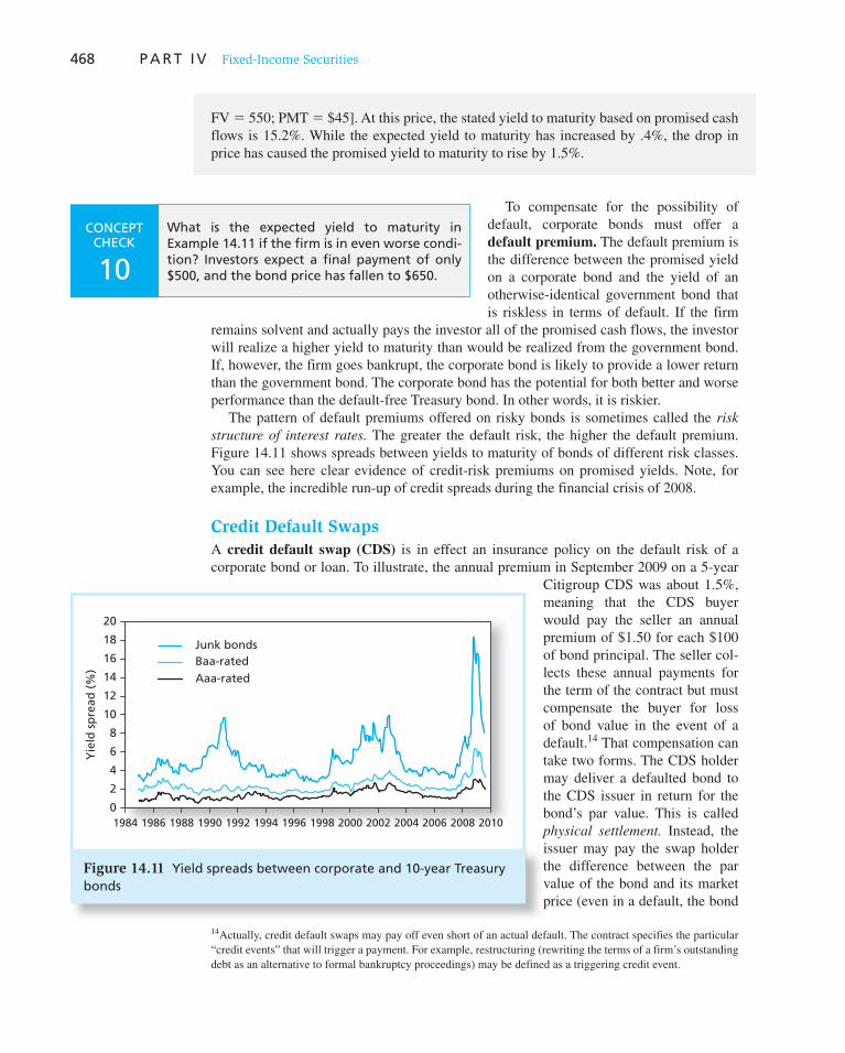
468 P A R T I V Fixed-Income Securities
To compensate for the possibility of
default, corporate bonds must offer a
default premium. The default premium is
the difference between the promised yield
on a corporate bond and the yield of an
otherwise-identical government bond that
is riskless in terms of default. If the firm
remains solvent and actually pays the investor all of the promised cash flows, the investor
will realize a higher yield to maturity than would be realized from the government bond.
If, however, the firm goes bankrupt, the corporate bond is likely to provide a lower return
than the government bond. The corporate bond has the potential for both better and worse
performance than the default-free Treasury bond. In other words, it is riskier.
The pattern of default premiums offered on risky bonds is sometimes called the risk
structure of interest rates. The greater the default risk, the higher the default premium.
Figure 14.11 shows spreads between yields to maturity of bonds of different risk classes.
You can see here clear evidence of credit-risk premiums on promised yields. Note, for
example, the incredible run-up of credit spreads during the financial crisis of 2008.
Credit Default Swaps
A credit default swap (CDS) is in effect an insurance policy on the default risk of a
corporate bond or loan. To illustrate, the annual premium in September 2009 on a 5-year
Citigroup CDS was about 1.5%,
meaning that the CDS buyer
would pay the seller an annual
premium of $1.50 for each $100
of bond principal. The seller col-
lects these annual payments for
the term of the contract but must
compensate the buyer for loss
of bond value in the event of a
default. 14 That compensation can
take two forms. The CDS holder
may deliver a defaulted bond to
the CDS issuer in return for the
bond’s par value. This is called
physical settlement. Instead, the
issuer may pay the swap holder
the difference between the par
value of the bond and its market
price (even in a default, the bond
14 Actually, credit default swaps may pay off even short of an actual default. The contract specifies the particular
“credit events” that will trigger a payment. For example, restructuring (rewriting the terms of a firm’s outstanding
debt as an alternative to formal bankruptcy proceedings) may be defined as a triggering credit event.
20
18
16
14
12
10
8
6
4
2
020102008200620042002200019981996199419921990198819861984
Yie
ld s
pre
ad (
%)
Junk bondsBaa-rated
Aaa-rated
Figure 14.11 Yield spreads between corporate and 10-year Treasury bonds
FV 5 550; PMT 5 $45]. At this price, the stated yield to maturity based on promised cash
flows is 15.2%. While the expected yield to maturity has increased by .4%, the drop in
price has caused the promised yield to maturity to rise by 1.5%.
CONCEPT CHECK
10
What is the expected yield to maturity in Example 14.11 if the firm is in even worse condi-tion? Investors expect a final payment of only $500, and the bond price has fallen to $650.
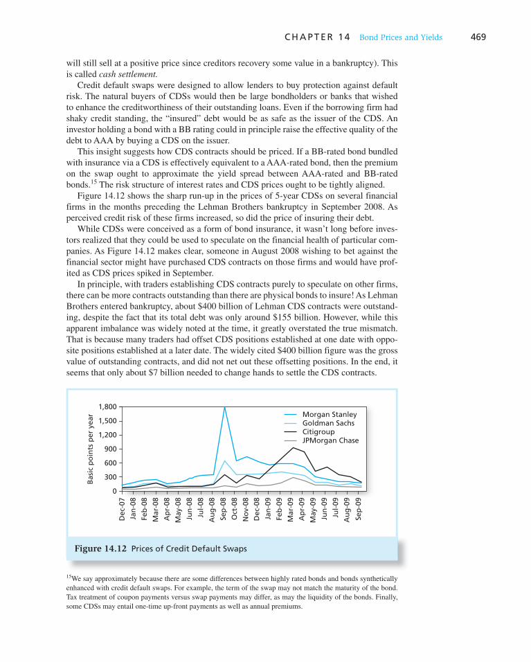
C H A P T E R 1 4 Bond Prices and Yields 469
will still sell at a positive price since creditors recovery some value in a bankruptcy). This
is called cash settlement.
Credit default swaps were designed to allow lenders to buy protection against default
risk. The natural buyers of CDSs would then be large bondholders or banks that wished
to enhance the creditworthiness of their outstanding loans. Even if the borrowing firm had
shaky credit standing, the “insured” debt would be as safe as the issuer of the CDS. An
investor holding a bond with a BB rating could in principle raise the effective quality of the
debt to AAA by buying a CDS on the issuer.
This insight suggests how CDS contracts should be priced. If a BB-rated bond bundled
with insurance via a CDS is effectively equivalent to a AAA-rated bond, then the premium
on the swap ought to approximate the yield spread between AAA-rated and BB-rated
bonds. 15 The risk structure of interest rates and CDS prices ought to be tightly aligned.
Figure 14.12 shows the sharp run-up in the prices of 5-year CDSs on several financial
firms in the months preceding the Lehman Brothers bankruptcy in September 2008. As
perceived credit risk of these firms increased, so did the price of insuring their debt.
While CDSs were conceived as a form of bond insurance, it wasn’t long before inves-
tors realized that they could be used to speculate on the financial health of particular com-
panies. As Figure 14.12 makes clear, someone in August 2008 wishing to bet against the
financial sector might have purchased CDS contracts on those firms and would have prof-
ited as CDS prices spiked in September.
In principle, with traders establishing CDS contracts purely to speculate on other firms,
there can be more contracts outstanding than there are physical bonds to insure! As Lehman
Brothers entered bankruptcy, about $400 billion of Lehman CDS contracts were outstand-
ing, despite the fact that its total debt was only around $155 billion. However, while this
apparent imbalance was widely noted at the time, it greatly overstated the true mismatch.
That is because many traders had offset CDS positions established at one date with oppo-
site positions established at a later date. The widely cited $400 billion figure was the gross
value of outstanding contracts, and did not net out these offsetting positions. In the end, it
seems that only about $7 billion needed to change hands to settle the CDS contracts.
15 We say approximately because there are some differences between highly rated bonds and bonds synthetically
enhanced with credit default swaps. For example, the term of the swap may not match the maturity of the bond.
Tax treatment of coupon payments versus swap payments may differ, as may the liquidity of the bonds. Finally,
some CDSs may entail one-time up-front payments as well as annual premiums.
1,800
1,500
1,200
900
600
300
0
Jul-
09
Au
g-0
9
Sep
-09
Jun
-09
May
-09
Ap
r-09
Mar
-09
Feb
-09
Jan
-09
Dec
-08
No
v-08
Oct
-08
Sep
-08
Au
g-0
8
Jul-
08
Jun
-08
May
-08
Ap
r-08
Mar
-08
Feb
-08
Jan
-08
Dec
-07
Bas
ic p
oin
ts p
er y
ear
JPMorgan Chase
Goldman Sachs Citigroup
Morgan Stanley
Figure 14.12 Prices of Credit Default Swaps
470
Credit Default Swaps, Systemic Risk, and the Credit
Crisis of 2008
The credit crisis of 2008, when lending among banks and other financial institutions effectively seized up, was in large measure a crisis of transparency. The biggest prob-lem was a widespread lack of confidence in the financial standing of counterparties to a trade. If one institution could not be confident that another would remain solvent, it would understandably be reluctant to offer it a loan. When doubt about the credit exposure of customers and trading partners spiked to levels not seen since the Great Depression, the market for loans dried up.
Credit default swaps were particularly cited for foster-ing doubts about counterparty reliability. By August 2008, $63 trillion of such swaps were reportedly outstanding. (By comparison, U.S. gross domestic product in 2008 was about $14 trillion.) As the subprime mortgage market col-lapsed and the economy seemed sure to enter a recession, the potential obligations on these contracts ballooned to levels previously considered unimaginable and the abil-ity of CDS sellers to honor their commitments appeared in doubt. For example, the huge insurance firm AIG alone had sold more than $400 billion of CDS contracts on sub-prime mortgages and other loans and was days from insolvency. But AIG’s insolvency would have triggered the insolvency of other firms that had relied on its promise of protection against loan defaults. These in turn might have triggered further defaults. In the end, the government felt
compelled to rescue AIG to prevent a chain reaction of insolvencies.
Counterparty risk and lax reporting requirements made it effectively impossible to tease out firms’ exposures to credit risk. One problem was that CDS positions do not have to be accounted for on balance sheets. And the possibility of one default setting off a sequence of further defaults means that lenders may be exposed to the default of an institution with which it does not even directly trade. Such knock-on effects create systemic risk, in which the entire financial system can freeze up. With the ripple effects of bad debt extending in ever-widening circles, lending to anyone can seem imprudent.
The aftermath of the credit crisis of 2008 will inevitably bring new regulation and reforms. One proposal calls for a central clearing house for credit derivatives such as CDS contracts. Such a system would foster transparency of posi-tions, would allow the clearing house to replace traders’ offsetting long and short positions with a single net posi-tion, and would require daily recognition of gains or losses on positions through a margin or collateral account. If losses were to mount, positions would have to be unwound before growing to unsustainable levels. Allowing traders to accurately assess counterparty risk, and limiting such risk through margin accounts and the extra back-up of the clearinghouse, would go a long way in limiting systemic risk.
Nevertheless, this episode highlighted the utter lack of transparency about firms’ CDS
obligations. Such uncertainty about firms’ exposures to the credit risk of others gave rise to
doubts about their own financial stability. The nearby box notes that this lack of transpar-
ency was a contributing factor in the credit meltdown of 2008.
Credit Risk and Collateralized Debt Obligations
Collateralized debt obligations, or CDOs, emerged in the last decade as a major mecha-
nism to reallocate credit risk in the fixed-income markets. To create a CDO, a financial
institution, commonly a bank, first would establish a legally distinct entity to buy and
later resell a portfolio of bonds or other loans. A common vehicle for this purpose was the
so-called Structured Investment Vehicle (SIV). 16 An SIV raises funds, often by issuing
short-term commercial paper, and uses the proceeds to buy corporate bonds or other forms
of debt such as mortgage loans or credit card debt. These loans are first pooled together
and then split into a series of classes known as tranches. ( Tranche is the French word for
“slice.”)
Each tranche is given a different level of seniority in terms of its claims on the underly-
ing loan pool, and each can be sold as a stand-alone security. As the loans in the u nderlying
16 The legal separation of the bank from the SIV allows the ownership of the loans to be conducted off the bank’s
balance sheet, and thus avoids capital requirements the bank would otherwise encounter.
WO
RD
S FR
OM
TH
E ST
REE
T

C H A P T E R 1 4 Bond Prices and Yields 471
pool make their interest payments, the proceeds are distributed to pay interest to each
tranche in order of seniority. This priority structure implies that each tranche has a differ-
ent exposure to credit risk.
Figure 14.13 illustrates a typical setup. The senior tranche is on top. Its investors
may account for perhaps 80% of the principal of the entire pool. But it has first claim
on all the debt service. Using our numbers, even if 20% of the debt pool defaults, the
senior tranche can be paid in full. Once the highest seniority tranche is paid off, the next-
lower class (e.g., the mezzanine 1 tranche in Figure 14.13 ) receives the proceeds from the
pool of loans until its claims also are satisfied. Using junior tranches to insulate senior
tranches from credit risk in this manner, one can create Aaa-rated bonds even from a
junk-bond portfolio.
Of course, shielding senior tranches from default risk means that the risk is concen-
trated on the lower tranches. The bottom tranche—called alternatively the equity, first-loss,
or residual tranche—has last call on payments from the pool of loans, or, put differently, is
at the head of the line in terms of absorbing default or delinquency risk.
Not surprisingly, investors in tranches with the greatest exposure to credit risk demand
the highest coupon rates. Therefore, while the lower mezzanine and equity tranches
bear the most risk, they will provide the highest returns if credit experience turns out
favorably.
Mortgage-backed CDOs were an investment disaster in 2007 and 2008. These were
CDOs formed by pooling subprime mortgage loans made to individuals whose credit stand-
ing did not allow them to qualify for conventional mortgages. When home prices stalled
in 2007 and interest rates on these typically adjustable-rate loans reset to market levels,
mortgage delinquencies and home foreclosures soared, and investors in these securities
lost billions of dollars. Even highly rated tranches suffered extreme losses as default rates
turned out to be far higher than anticipated.
Not surprisingly, the rating agencies that had certified these tranches as investment-
grade came under considerable fire. Questions were raised concerning conflicts of inter-
est: Because the rating agencies are paid by bond issuers, the agencies were accused of
responding to pressure to ease their standards.
BankStructuredInvestmentVehicle, SIV
Senior tranche
Senior-SubordinatedTranche Structure
Typical Terms
70–90% of notionalprincipal, coupon similar toAa-Aaa rated bonds
5–15% of principal,investment-grade rating
5–15% of principal, higher-quality junk rating<2%, unrated, coupon ratewith 20% credit spread
Mezzanine 1
Mezzanine 2
Equity/first loss/residual tranche
Figure 14.13 Collateralized debt obligations

Vis
it u
s at
ww
w.m
hh
e.co
m/b
kmV
isit
us
at w
ww
.mh
he.
com
/bkm
472 P A R T I V Fixed-Income Securities
1. Fixed-income securities are distinguished by their promise to pay a fixed or specified stream of
income to their holders. The coupon bond is a typical fixed-income security.
2. Treasury notes and bonds have original maturities greater than 1 year. They are issued at or near
par value, with their prices quoted net of accrued interest.
3. Callable bonds should offer higher promised yields to maturity to compensate investors for the fact
that they will not realize full capital gains should the interest rate fall and the bonds be called away
from them at the stipulated call price. Bonds often are issued with a period of call protection. In
addition, discount bonds selling significantly below their call price offer implicit call protection.
4. Put bonds give the bondholder rather than the issuer the option to terminate or extend the life of
the bond.
5. Convertible bonds may be exchanged, at the bondholder’s discretion, for a specified number of
shares of stock. Convertible bondholders “pay” for this option by accepting a lower coupon rate
on the security.
6. Floating-rate bonds pay a coupon rate at a fixed premium over a reference short-term interest
rate. Risk is limited because the rate is tied to current market conditions.
7. The yield to maturity is the single interest rate that equates the present value of a security’s cash
flows to its price. Bond prices and yields are inversely related. For premium bonds, the coupon
rate is greater than the current yield, which is greater than the yield to maturity. The order of
these inequalities is reversed for discount bonds.
8. The yield to maturity is often interpreted as an estimate of the average rate of return to an inves-
tor who purchases a bond and holds it until maturity. This interpretation is subject to error,
however. Related measures are yield to call, realized compound yield, and expected (versus
promised) yield to maturity.
9. Prices of zero-coupon bonds rise exponentially over time, providing a rate of appreciation equal
to the interest rate. The IRS treats this built-in price appreciation as imputed taxable interest
income to the investor.
10. When bonds are subject to potential default, the stated yield to maturity is the maximum pos-
sible yield to maturity that can be realized by the bondholder. In the event of default, however,
that promised yield will not be realized. To compensate bond investors for default risk, bonds
must offer default premiums, that is, promised yields in excess of those offered by default-free
government securities. If the firm remains healthy, its bonds will provide higher returns than
government bonds. Otherwise the returns may be lower.
11. Bond safety is often measured using financial ratio analysis. Bond indentures are another safe-
guard to protect the claims of bondholders. Common indentures specify sinking fund require-
ments, collateralization of the loan, dividend restrictions, and subordination of future debt.
12. Credit default swaps provide insurance against the default of a bond or loan. The swap buyer
pays an annual premium to the swap seller, but collects a payment equal to lost value if the loan
later goes into default.
13. Collateralized debt obligations are used to reallocate the credit risk of a pool of loans. The pool
is sliced into tranches, with each tranche assigned a different level of seniority in terms of its
claims on the cash flows from the underlying loans. High seniority tranches are usually quite
safe, with credit risk concentrated on the lower level tranches. Each tranche can be sold as a
stand-alone security.
SUMMARY
Related Web sites for this chapter are available at www.mhhe.com/bkm
debt securities
bond
par value
face value
coupon rate
bond indenture
zero-coupon bonds
convertible bonds
put bond
floating-rate bonds
yield to maturity
current yield
KEY TERMS

Vis
it u
s at
ww
w.m
hh
e.co
m/b
km
C H A P T E R 1 4 Bond Prices and Yields 473
premium bonds
discount bonds
realized compound return
horizon analysis
reinvestment rate risk
credit risk
investment-grade bonds
speculative-grade or junk
bonds
sinking fund
subordination clauses
collateral
debenture
default premium
credit default swap (CDS)
collateralized debt obligations
(CDOs)
1. Define the following types of bonds:
a. Catastrophe bond.
b. Eurobond.
c. Zero-coupon bond.
d. Samurai bond.
e. Junk bond.
f. Convertible bond.
g. Serial bond.
h. Equipment obligation bond.
i. Original issue discount bond.
j. Indexed bond.
k. Callable bond.
l. Puttable bond.
2. Two bonds have identical times to maturity and coupon rates. One is callable at 105, the other at
110. Which should have the higher yield to maturity? Why?
3. The stated yield to maturity and realized compound yield to maturity of a (default-free) zero-
coupon bond will always be equal. Why?
4. Why do bond prices go down when interest rates go up? Don’t lenders like high interest rates?
5. A bond with an annual coupon rate of 4.8% sells for $970. What is the bond’s current yield?
6. Which security has a higher effective annual interest rate?
a. A 3-month T-bill selling at $97,645 with par value $100,000.
b. A coupon bond selling at par and paying a 10% coupon semiannually.
7. Treasury bonds paying an 8% coupon rate with semiannual payments currently sell at par value.
What coupon rate would they have to pay in order to sell at par if they paid their coupons annu-
ally? (Hint: What is the effective annual yield on the bond?)
8. Consider a bond with a 10% coupon and with yield to maturity 5 8%. If the bond’s yield to
maturity remains constant, then in 1 year, will the bond price be higher, lower, or unchanged?
Why?
9. Consider an 8% coupon bond selling for $953.10 with 3 years until maturity making annual cou-
pon payments. The interest rates in the next 3 years will be, with certainty, r 1 5 8%, r 2 5 10%,
and r 3 5 12%. Calculate the yield to maturity and realized compound yield of the bond.
10. Assume you have a 1-year investment horizon and are trying to choose among three bonds. All
have the same degree of default risk and mature in 10 years. The first is a zero-coupon bond that
pays $1,000 at maturity. The second has an 8% coupon rate and pays the $80 coupon once per
year. The third has a 10% coupon rate and pays the $100 coupon once per year.
a. If all three bonds are now priced to yield 8% to maturity, what are their prices?
b. If you expect their yields to maturity to be 8% at the beginning of next year, what will their
prices be then? What is your before-tax holding-period return on each bond? If your tax
bracket is 30% on ordinary income and 20% on capital gains income, what will your after-
tax rate of return be on each?
c. Recalculate your answer to ( b ) under the assumption that you expect the yields to maturity
on each bond to be 7% at the beginning of next year.
PROBLEM SETS
i. Basic
ii. Intermediate

Vis
it u
s at
ww
w.m
hh
e.co
m/b
km474 P A R T I V Fixed-Income Securities
11. A 20-year maturity bond with par value of $1,000 makes semiannual coupon payments at a
coupon rate of 8%. Find the bond equivalent and effective annual yield to maturity of the bond
if the bond price is:
a. $950.
b. $1,000.
c. $1,050.
12. Repeat Problem 11 using the same data, but assuming that the bond makes its coupon payments
annually. Why are the yields you compute lower in this case?
13. Fill in the table below for the following zero-coupon bonds, all of which have par values of $1,000.
Price Maturity (years)Bond-Equivalent Yield to Maturity
$400 20 —
$500 20 —
$500 10 —
— 10 10%
— 10 8%
$400 — 8%
14. Consider a bond paying a coupon rate of 10% per year semiannually when the market interest
rate is only 4% per half-year. The bond has 3 years until maturity.
a. Find the bond’s price today and 6 months from now after the next coupon is paid.
b. What is the total (6-month) rate of return on the bond?
15. A bond with a coupon rate of 7% makes semiannual coupon payments on January 15 and
July 15 of each year. The Wall Street Journal reports the asked price for the bond on January 30
at 100:02. What is the invoice price of the bond? The coupon period has 182 days.
16. A bond has a current yield of 9% and a yield to maturity of 10%. Is the bond selling above or
below par value? Explain.
17. Is the coupon rate of the bond in Problem 16 more or less than 9%?
18. Return to Table 14.1 and calculate both the real and nominal rates of return on the TIPS bond in
the second and third years.
19. A newly issued 20-year maturity, zero-coupon bond is issued with a yield to maturity of 8% and face
value $1,000. Find the imputed interest income in the first, second, and last year of the bond’s life.
20. A newly issued 10-year maturity, 4% coupon bond making annual coupon payments is sold to
the public at a price of $800. What will be an investor’s taxable income from the bond over the
coming year? The bond will not be sold at the end of the year. The bond is treated as an original-
issue discount bond.
21. A 30-year maturity, 8% coupon bond paying coupons semiannually is callable in 5 years at a
call price of $1,100. The bond currently sells at a yield to maturity of 7% (3.5% per half-year).
a. What is the yield to call?
b. What is the yield to call if the call price is only $1,050?
c. What is the yield to call if the call price is $1,100, but the bond can be called in 2 years
instead of 5 years?
22. A 10-year bond of a firm in severe financial distress has a coupon rate of 14% and sells for
$900. The firm is currently renegotiating the debt, and it appears that the lenders will allow the
firm to reduce coupon payments on the bond to one-half the originally contracted amount. The
firm can handle these lower payments. What is the stated and expected yield to maturity of the
bonds? The bond makes its coupon payments annually.
23. A 2-year bond with par value $1,000 making annual coupon payments of $100 is priced at
$1,000. What is the yield to maturity of the bond? What will be the realized compound yield to
maturity if the 1-year interest rate next year turns out to be ( a ) 8%, ( b ) 10%, ( c ) 12%?

Vis
it u
s at
ww
w.m
hh
e.co
m/b
km
C H A P T E R 1 4 Bond Prices and Yields 475
24. Suppose that today’s date is April 15. A bond with a 10% coupon paid semiannually every
Ja nuary 15 and July 15 is listed in The Wall Street Journal as selling at an asked price of 101:04.
If you buy the bond from a dealer today, what price will you pay for it?
25. Assume that two firms issue bonds with the following characteristics. Both bonds are issued
at par.
ABC Bonds XYZ Bonds
Issue size $1.2 billion $150 million
Maturity 10 years* 20 years
Coupon 9% 10%
Collateral First mortgage General debenture
Callable Not callable In 10 years
Call price None 110
Sinking fund None Starting in 5 years
*Bond is extendible at the discretion of the bondholder for an additional 10 years.
Ignoring credit quality, identify four features of these issues that might account for the lower
coupon on the ABC debt. Explain.
26. An investor believes that a bond may temporarily increase in credit risk. Which of the following
would be the most liquid method of exploiting this?
a. The purchase of a credit default swap.
b. The sale of a credit default swap.
c. The short sale of the bond.
27. Which of the following most accurately describes the behavior of credit default swaps?
a. When credit risk increases, swap premiums increase.
b. When credit and interest rate risk increases, swap premiums increase.
c. When credit risk increases, swap premiums increase, but when interest rate risk increases,
swap premiums decrease.
28. What would be the likely effect on the yield to maturity of a bond resulting from:
a. An increase in the issuing firm’s times-interest-earned ratio.
b. An increase in the issuing firm’s debt-to-equity ratio.
c. An increase in the issuing firm’s quick ratio.
29. A large corporation issued both fixed and floating-rate notes 5 years ago, with terms given in the
following table:
9% Coupon Notes Floating-Rate Note
Issue size $250 million $280 million
Original maturity 20 years 10 years
Current price (% of par) 93 98
Current coupon 9% 8%
Coupon adjusts Fixed coupon Every year
Coupon reset rule — 1-year T-bill rate 1 2%
Callable 10 years after issue 10 years after issue
Call price 106 102.50
Sinking fund None None
Yield to maturity 9.9% —
Price range since issued $85–$112 $97–$102
a. Why is the price range greater for the 9% coupon bond than the floating-rate note?
b. What factors could explain why the floating-rate note is not always sold at par value?
c. Why is the call price for the floating-rate note not of great importance to investors?

Vis
it u
s at
ww
w.m
hh
e.co
m/b
km476 P A R T I V Fixed-Income Securities
d. Is the probability of a call for the fixed-rate note high or low?
e. If the firm were to issue a fixed-rate note with a 15-year maturity, what coupon rate would it
need to offer to issue the bond at par value?
f. Why is an entry for yield to maturity for the floating-rate note not appropriate?
30. Masters Corp. issues two bonds with 20-year maturities. Both bonds are callable at $1,050. The
first bond is issued at a deep discount with a coupon rate of 4% and a price of $580 to yield
8.4%. The second bond is issued at par value with a coupon rate of 8¾%.
a. What is the yield to maturity of the par bond? Why is it higher than the yield of the discount
bond?
b. If you expect rates to fall substantially in the next 2 years, which bond would you prefer to hold?
c. In what sense does the discount bond offer “implicit call protection”?
31. A newly issued bond pays its coupons once annually. Its coupon rate is 5%, its maturity is
20 years, and its yield to maturity is 8%.
a. Find the holding-period return for a 1-year investment period if the bond is selling at a yield
to maturity of 7% by the end of the year.
b. If you sell the bond after 1 year, what taxes will you owe if the tax rate on interest income is
40% and the tax rate on capital gains income is 30%? The bond is subject to original-issue
discount tax treatment.
c. What is the after-tax holding-period return on the bond?
d. Find the realized compound yield before taxes for a 2-year holding period, assuming that
(1) you sell the bond after 2 years, (2) the bond yield is 7% at the end of the second year, and
(3) the coupon can be reinvested for 1 year at a 3% interest rate.
e. Use the tax rates in ( b ) above to compute the after-tax 2-year realized compound yield.
Remember to take account of OID tax rules.
iii. Challenge
1. Leaf Products may issue a 10-year maturity fixed-income security, which might include a sink-
ing fund provision and either refunding or call protection.
a. Describe a sinking fund provision.
b. Explain the impact of a sinking fund provision on:
i. The expected average life of the proposed security.
ii. Total principal and interest payments over the life of the proposed security.
c. From the investor’s point of view, explain the rationale for demanding a sinking fund provision.
2. Bonds of Zello Corporation with a par value of $1,000 sell for $960, mature in 5 years, and have
a 7% annual coupon rate paid semiannually.
a. Calculate the:
i. Current yield.
ii. Yield to maturity (to the nearest whole percent, i.e., 3%, 4%, 5%, etc.).
iii. Realized compound yield for an investor with a 3-year holding period and a reinvest-
ment rate of 6% over the period. At the end of 3 years the 7% coupon bonds with 2 years
remaining will sell to yield 7%.
b. Cite one major shortcoming for each of the following fixed-income yield measures:
i. Current yield.
ii. Yield to maturity.
iii. Realized compound yield.
3. On May 30, 2008, Janice Kerr is considering one of the newly issued 10-year AAA corporate
bonds shown in the following exhibit.
Description Coupon Price Callable Call Price
Sentinal, due May 30, 2018 6.00% 100 Noncallable NA
Colina, due May 30, 2018 6.20% 100 Currently callable 102

Vis
it u
s at
ww
w.m
hh
e.co
m/b
km
C H A P T E R 1 4 Bond Prices and Yields 477
a. Suppose that market interest rates decline by 100 basis points (i.e., 1%). Contrast the effect of
this decline on the price of each bond.
b. Should Kerr prefer the Colina over the Sentinal bond when rates are expected to rise or to fall?
c. What would be the effect, if any, of an increase in the volatility of interest rates on the prices
of each bond?
4. A convertible bond has the following features:
Coupon 5.25%
Maturity June 15, 2027
Market price of bond $77.50
Market price of underlying common stock $28.00
Annual dividend $1.20
Conversion ratio 20.83 shares
Calculate the conversion premium for this bond.
5. a. Explain the impact on the offering yield of adding a call feature to a proposed bond issue.
b. Explain the impact on the bond’s expected life of adding a call feature to a proposed bond issue.
c. Describe one advantage and one disadvantage of including callable bonds in a portfolio.
6. a. An investment in a coupon bond will provide the investor with a return equal to the bond’s
yield to maturity at the time of purchase if:
i. The bond is not called for redemption at a price that exceeds its par value.
ii. All sinking fund payments are made in a prompt and timely fashion over the life of the issue.
iii. The reinvestment rate is the same as the bond’s yield to maturity and the bond is held until
maturity.
iv. All of the above.
b. A bond with a call feature:
i. Is attractive because the immediate receipt of principal plus premium produces a high return.
ii. Is more apt to be called when interest rates are high because the interest savings will be
greater.
iii. Will usually have a higher yield to maturity than a similar noncallable bond.
iv. None of the above.
c. In which one of the following cases is the bond selling at a discount?
i. Coupon rate is greater than current yield, which is greater than yield to maturity.
ii. Coupon rate, current yield, and yield to maturity are all the same.
iii. Coupon rate is less than current yield, which is less than yield to maturity.
iv. Coupon rate is less than current yield, which is greater than yield to maturity.
d. Consider a 5-year bond with a 10% coupon that has a present yield to maturity of 8%. If inter-
est rates remain constant, 1 year from now the price of this bond will be:
i. Higher.
ii. Lower.
iii. The same.
iv. Par.
E-INVEST-MENTS EXERCISES
Credit Spreads
At www.bondsonline.com review the Industrial Spreads for various ratings (click the links on the left-side menus to follow the links to Today’s Markets, Corporate Bond
Spreads ). These are spreads above U.S. Treasuries of comparable maturities. What factors tend to explain the yield differences? How might these yield spreads differ during an eco-nomic boom versus a recession?

Vis
it u
s at
ww
w.m
hh
e.co
m/b
km478 P A R T I V Fixed-Income Securities
SOLUTIONS TO CONCEPT CHECKS
1. The callable bond will sell at the lower price. Investors will not be willing to pay as much if they
know that the firm retains a valuable option to reclaim the bond for the call price if interest rates
fall.
2. At a semiannual interest rate of 3%, the bond is worth $40 3 Annuity factor (3%, 60) 1
$1,000 3 PV factor(3%, 60) 5 $1,276.76, which results in a capital gain of $276.76. This
exceeds the capital loss of $189.29 (i.e., $1,000 2 $810.71) when the semiannual interest rate
increased to 5%.
3. Yield to maturity exceeds current yield, which exceeds coupon rate. Take as an example the 8%
coupon bond with a yield to maturity of 10% per year (5% per half year). Its price is $810.71, and
therefore its current yield is 80/810.71 5 .0987, or 9.87%, which is higher than the coupon rate
but lower than the yield to maturity.
4. The bond with the 6% coupon rate currently sells for 30 3 Annuity factor (3.5%, 20) 1 1,000 3 PV
factor(3.5%, 20) 5 $928.94. If the interest rate immediately drops to 6% (3% per half-year), the
bond price will rise to $1,000, for a capital gain of $71.06, or 7.65%. The 8% coupon bond
currently sells for $1,071.06. If the interest rate falls to 6%, the present value of the scheduled
payments increases to $1,148.77. However, the bond will be called at $1,100, for a capital gain of
only $28.94, or 2.70%.
5. The current price of the bond can be derived from its yield to maturity. Using your calculator,
set: n 5 40 (semiannual periods); payment 5 $45 per period; future value 5 $1,000; interest
rate 5 4% per semiannual period. Calculate present value as $1,098.96. Now we can calculate
yield to call. The time to call is 5 years, or 10 semiannual periods. The price at which the bond will
be called is $1,050. To find yield to call, we set: n 5 10 (semiannual periods); payment 5 $45 per
period; future value 5 $1,050; present value 5 $1,098.96. Calculate yield to call as 3.72%.
6. Price 5 $70 3 Annuity factor(8%, 1) 1 $1,000 3 PV factor(8%, 1) 5 $990.74
Rate of return to investor 5$70 1 ($990.74 2 $982.17)
$982.175 .080 5 8%
7. By year-end, remaining maturity is 29 years. If the yield to maturity were still 8%, the bond
would still sell at par and the holding-period return would be 8%. At a higher yield, price
and return will be lower. Suppose, for example, that the yield to maturity rises to 8.5%.
With annual payments of $80 and a face value of $1,000, the price of the bond will be
$946.70 [ n 5 29; i 5 8.5%; PMT 5 $80; FV 5 $1,000]. The bond initially sold at $1,000 when
issued at the start of the year. The holding-period return is
HPR 580 1 (946.70 2 1,000)
1,0005 .0267 5 2.67%
which is less than the initial yield to maturity of 8%.
From the home page, select Today’s Markets from the left-side menu and then select the link for Composite Bond Yields. How do the Yield Curves for Treasury, Agency, Corpo-rate, and Municipal bonds compare to each other?

Vis
it u
s at
ww
w.m
hh
e.co
m/b
km
C H A P T E R 1 4 Bond Prices and Yields 479
8. At the lower yield, the bond price will be $631.67 [ n 5 29, i 5 7%, FV 5 $1,000, PMT 5 $40].
Therefore, total after-tax income is
Coupon $40 3 (1 2.38) 5 $24.80
Imputed interest ($553.66 2 $549.69) 3 (1 2 .38) 5 2.46
Capital gains ($631.67 2 $553.66) 3 (1 2 .20) 5 62.41
Total income after taxes $89.67
Rate of return 5 89.67/549.69 5 .163 5 16.3%.
9. It should receive a negative coefficient. A high ratio of liabilities to assets is a poor omen for a
firm that should lower its credit rating.
10. The coupon payment is $45. There are 20 semiannual periods. The final payment is assumed
to be $500. The present value of expected cash flows is $650. The expected yield to maturity is
6.317% semiannual or annualized, 12.63%, bond equivalent yield.
15 1 IN CHAPTER 14 we assumed for the sake
of simplicity that the same constant inter-
est rate is used to discount cash flows of
any maturity. In the real world this is rarely
the case. We have seen, for example, that
in late 2009 short-term Treasury bonds and
notes carried yields to maturity less than 1%
while the longest-term bonds offered yields
of about 4.2%. At the time when these bond
prices were quoted, anyway, the longer-term
securities had higher yields. This, in fact, is
a typical pattern, but as we shall see below,
the relationship between time to maturity
and yield to maturity can vary dramatically
from one period to another. In this chapter
we explore the pattern of interest rates for
different-term assets. We attempt to identify
the factors that account for that pattern and
determine what information may be derived
from an analysis of the so-called term struc-
ture of interest rates, the structure of interest
rates for discounting cash flows of different
maturities.
We demonstrate how the prices of Treasury
bonds may be derived from prices and yields
of stripped zero-coupon Treasury securities.
We also examine the extent to which the term
structure reveals market-consensus forecasts
of future interest rates and how the presence
of interest rate risk may affect those infer-
ences. Finally, we show how traders can use
the term structure to compute forward rates
that represent interest rates on “forward,” or
deferred, loans, and consider the relationship
between forward rates and future interest
rates.
The Term Structure of Interest Rates
CHAPTER FIFTEEN PA
RT
IV
15.1 The Yield Curve
Figure 14.1 demonstrated that bonds of different maturities typically sell at different yields to maturity. When these bond prices and yields were compiled, long-term bonds sold at higher yields than short-term bonds. Practitioners commonly summarize the relation-ship between yield and maturity graphically in a yield curve, which is a plot of yield to maturity as a function of time to maturity. The yield curve is one of the key concerns of fixed-income investors. We will see in this chapter that the yield curve is central to bond valuation and, as well, allows investors to gauge their expectations for future interest rates against those of the market. Such a comparison is often the starting point in the formula-tion of a fixed-income portfolio strategy.
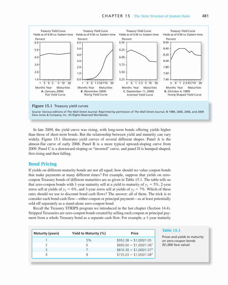
C H A P T E R 1 5 The Term Structure of Interest Rates 481
In late 2009, the yield curve was rising, with long-term bonds offering yields higher than those of short-term bonds. But the relationship between yield and maturity can vary widely. Figure 15.1 illustrates yield curves of several different shapes. Panel A is the almost-flat curve of early 2006. Panel B is a more typical upward-sloping curve from 2009. Panel C is a downward-sloping or “inverted” curve, and panel D is humped-shaped, first rising and then falling.
Bond Pricing
If yields on different-maturity bonds are not all equal, how should we value coupon bonds that make payments at many different times? For example, suppose that yields on zero-coupon Treasury bonds of different maturities are as given in Table 15.1 . The table tells us that zero-coupon bonds with 1-year maturity sell at a yield to maturity of y 1 5 5%, 2-year zeros sell at yields of y 2 5 6%, and 3-year zeros sell at yields of y 3 5 7%. Which of these rates should we use to discount bond cash flows? The answer: all of them. The trick is to consider each bond cash flow—either coupon or principal payment—as at least potentially sold off separately as a stand-alone zero-coupon bond.
Recall the Treasury STRIPS program we introduced in the last chapter (Section 14.4). Stripped Treasuries are zero-coupon bonds created by selling each coupon or principal pay-ment from a whole Treasury bond as a separate cash flow. For example, a 1-year maturity
Treasury Yield CurveYields as of 4:30 P.M. Eastern time
Percent6.0
0.0
2.0
1.0
3.0
4.0
5.0
MaturitiesYearMonthsB. (November 2009)
Rising Yield Curve
Treasury Yield CurveYields as of 4:30 P.M. Eastern time
Treasury Yield CurveYields as of 4:30 P.M. Eastern time
Treasury Yield CurveYields as of 4:30 P.M. Eastern time
Percent6.0
1 3 6 2 5 101.0
2.0
3.0
4.0
5.0
30
MaturitiesYearMonthsD. (October 4, 1989)
Hump-Shaped Yield CurveC. (September 11, 2000)
Inverted Yield CurveA. (January 2006)
Flat Yield Curve
6.50
3 6 1 2 3 5 3010
Percent
Months Year Maturities
5.25
5.50
5.75
6.00
6.25
8.60
3 6 1 2 3 45 710 301 3 6 1 2 56 710 30
Percent
MaturitiesYearMonths
7.40
7.60
7.80
8.00
8.20
8.40
Figure 15.1 Treasury yield curves
Source: Various editions of The Wall Street Journal. Reprinted by permission of The Wall Street Journal, © 1989, 2000, 2006, and 2009 Dow Jones & Company, Inc. All Rights Reserved Worldwide.
Table 15.1
Prices and yields to maturity on zero-coupon bonds ($1,000 face value)
Maturity (years) Yield to Maturity (%) Price
1 5% $952.38 5 $1,000/1.05
2 6 $890.00 5 $1,000/1.062
3 7 $816.30 5 $1,000/1.073
4 8 $735.03 5 $1,000/1.084

482 P A R T I V Fixed-Income Securities
T-bond paying semiannual coupons can be split into a 6-month maturity zero (by selling the first coupon payment as a stand-alone security) and a 12-month zero (corresponding to payment of final coupon and principal). Treasury stripping suggests exactly how to value a coupon bond. If each cash flow can be (and in practice often is) sold off as a separate security, then the value of the whole bond should be the same as the value of its cash flows bought piece by piece in the STRIPS market.
What if it weren’t? Then there would be easy profits to be made. For example, if investment bankers ever noticed a bond selling for less than the amount at which the sum of its parts could be sold, they would buy the bond, strip it into stand-alone zero-coupon s ecurities, sell off the stripped cash flows, and profit by the price difference. If the bond were selling for more than the sum of the values of its individual cash flows, they would run the process in reverse: buy the individual zero-coupon securities in the STRIPS market, reconstitute (i.e., reassemble) the cash flows into a coupon bond, and sell the whole bond for more than the cost of the pieces. Both bond stripping and bond
reconstitution offer opportunities for arbitrage —the exploitation of mispricing among two or more securities to clear a riskless economic profit. Any violation of the Law of One Price, that identical cash flow bundles must sell for identical prices, gives rise to arbitrage opportunities.
Now, we know how to value each stripped cash flow. We simply look up its appropriate discount rate in The Wall Street Journal. Because each coupon payment matures at a dif-ferent time, we discount by using the yield appropriate to its particular maturity—this is the yield on a Treasury strip maturing at the time of that cash flow. We can illustrate with an example.
Example 15.1 Valuing Coupon Bonds
Suppose the yields on stripped Treasuries are as given in Table 15.1 , and we wish to value a 10% coupon bond with a maturity of 3 years. For simplicity, assume the bond makes its payments annually. Then the first cash flow, the $100 coupon paid at the end of the first year, is discounted at 5%; the second cash flow, the $100 coupon at the end of the second year, is discounted at 6%; and the final cash flow consisting of the final coupon plus par value, or $1,100, is discounted at 7%. The value of the coupon bond is therefore
100
1.051
100
1.0621
1100
1.0735 95.238 1 89.000 1 897.928 5 $1,082.17
Calculate the yield to maturity of the coupon bond in Example 15.1 , and you may be sur-prised. Its yield to maturity is 6.88%; so while its maturity matches that of the 3-year zero in Table 15.1 , its yield is a bit lower. 1 This reflects the fact that the 3-year coupon bond may usefully be thought of as a portfolio of three implicit zero-coupon bonds, one corresponding to each cash flow. The yield on the coupon bond is then an amalgam of the yields on each of the three components of the “portfolio.” Think about what this means: If their coupon rates differ, bonds of the same maturity generally will not have the same yield to maturity.
What then do we mean by “the” yield curve? In fact, in practice, traders refer to sev-eral yield curves. The pure yield curve refers to the curve for stripped, or zero-coupon,
1 Remember that the yield to maturity of a coupon bond is the single interest rate at which the present value of cash flows equals market price. To calculate the yield to maturity on this bond on your calculator or spreadsheet, set n 5 3; price 5 1,082.17; future value 5 1,000; payment 5 100. Then compute the interest rate.
C H A P T E R 1 5 The Term Structure of Interest Rates 483
Treasuries. In contrast, the on-the-run yield curve refers to the plot of yield as a function of maturity for recently issued coupon bonds selling at or near par value. As we’ve just seen, there may be significant differences in these two curves. The yield curves published in the financial press, for example, in Figure 15.1 , are typically on-the-run curves. On-the-run Treasuries have the greatest liquidity, so traders have keen interest in their yield curve.
CONCEPT CHECK
1
Calculate the price and yield to maturity of a 3-year bond with a coupon rate of 4% making annual coupon payments. Does its yield match that of either the 3-year zero or the 10% cou-pon bond considered in Example 15.1 ? Why is the yield spread between the 4% bond and the zero smaller than the yield spread between the 10% bond and the zero?
15.2 The Yield Curve and Future Interest Rates
We’ve told you what the yield curve is, but we haven’t yet had much to say about where it comes from. For example, why is the curve sometimes upward-sloping and other times downward-sloping? How do expectations for the evolution of interest rates affect the shape of today’s yield curve?
These questions do not have simple answers, so we will begin with an admittedly ideal-ized framework, and then extend the discussion to more realistic settings. To start, consider a world with no uncertainty, specifically, one in which all investors already know the path of future interest rates.
The Yield Curve under Certainty
If interest rates are certain, what should we make of the fact that the yield on the 2-year zero coupon bond in Table 15.1 is greater than that on the 1-year zero? It can’t be that one bond is expected to provide a higher rate of return than the other. This would not be pos-sible in a certain world—with no risk, all bonds (in fact, all securities!) must offer identical returns, or investors will bid up the price of the high-return bond until its rate of return is no longer superior to that of other bonds.
Instead, the upward-sloping yield curve is evidence that short-term rates are going to be higher next year than they are now. To see why, consider two 2-year bond strategies. The first strategy entails buying the 2-year zero offering a 2-year yield to maturity of y 2 5 6%, and holding it until maturity. The zero with face value $1,000 is purchased today for $1,000/1.06 2 5 $890 and matures in 2 years to $1,000. The total 2-year growth factor for the investment is therefore $1,000/$890 5 1.06 2 5 1.1236.
Now consider an alternative 2-year strategy. Invest the same $890 in a 1-year zero- coupon bond with a yield to maturity of 5%. When that bond matures, reinvest the pro-ceeds in another 1-year bond. Figure 15.2 illustrates these two strategies. The interest rate that 1-year bonds will offer next year is denoted as r 2 .
Remember, both strategies must provide equal returns—neither entails any risk. Therefore, the proceeds after 2 years to either strategy must be equal:
Buy and hold 2-year zero 5 Roll over 1-year bonds
$890 3 1.062 5 $890 3 1.05 3 (1 1 r2)
We find next year’s interest rate by solving 1 1 r 2 5 1.06 2 /1.05 5 1.0701, or r 2 5 7.01%. So while the 1-year bond offers a lower yield to maturity than the 2-year bond (5% versus 6%),
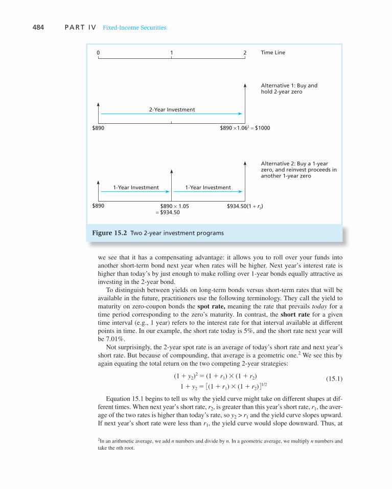
484 P A R T I V Fixed-Income Securities
we see that it has a compensating advantage: it allows you to roll over your funds into another short-term bond next year when rates will be higher. Next year’s interest rate is higher than today’s by just enough to make rolling over 1-year bonds equally attractive as investing in the 2-year bond.
To distinguish between yields on long-term bonds versus short-term rates that will be available in the future, practitioners use the following terminology. They call the yield to maturity on zero-coupon bonds the spot rate, meaning the rate that prevails today for a time period corresponding to the zero’s maturity. In contrast, the short rate for a given time interval (e.g., 1 year) refers to the interest rate for that interval available at different points in time. In our example, the short rate today is 5%, and the short rate next year will be 7.01%.
Not surprisingly, the 2-year spot rate is an average of today’s short rate and next year’s short rate. But because of compounding, that average is a geometric one. 2 We see this by again equating the total return on the two competing 2-year strategies:
(1 1 y2)2 5 (1 1 r1) 3 (1 1 r2) (15.1)
1 1 y2 5 3(1 1 r1) 3 (1 1 r2) 41/2
Equation 15.1 begins to tell us why the yield curve might take on different shapes at dif-ferent times. When next year’s short rate, r 2 , is greater than this year’s short rate, r 1 , the aver-age of the two rates is higher than today’s rate, so y 2 > r 1 and the yield curve slopes upward. If next year’s short rate were less than r 1 , the yield curve would slope downward. Thus, at
2 In an arithmetic average, we add n numbers and divide by n. In a geometric average, we multiply n numbers and take the n th root.
0 1 2 Time Line
Alternative 1: Buy andhold 2-year zero
Alternative 2: Buy a 1-yearzero, and reinvest proceeds inanother 1-year zero
$890
$890 $934.50(1 + r2)
$890 ×1.062 = $1000
2-Year Investment
1-Year Investment 1-Year Investment
$890 × 1.05 = $934.50
Figure 15.2 Two 2-year investment programs

C H A P T E R 1 5 The Term Structure of Interest Rates 485
least in part, the yield curve reflects the market’s assessments of coming interest rates. The following example uses a similar analysis to find the short rate that will prevail in year 3.
Example 15.2 Finding a Future Short Rate
Now we compare two 3-year strategies. One is to buy a 3-year zero, with a yield to matu-rity from Table 15.1 of 7%, and hold it until maturity. The other is to buy a 2-year zero yielding 6%, and roll the proceeds into a 1-year bond in year 3, at the short rate r 3 . The growth factor for the invested funds under each policy will be:
Buy and hold 3-year zero 5 Buy 2-year zero; roll proceeds into 1-year bond
(1 1 y3)3 5 (1 1 y2)
2 3 (1 1 r3)
1.073 5 1.062 3 (1 1 r3)
which implies that r 3 5 1.07 3 /1.06 2 2 1 5 .09025 5 9.025%. Again, notice that the yield on the 3-year bond reflects a geometric average of the discount factors for the next 3 years:
1 1 y3 5 3(1 1 r1) 3 (1 1 r2) 3 (1 1 r3) 41/3
1.07 5 31.05 3 1.0701 3 1.09025 41/3
We conclude that the yield or spot rate on a long-term bond reflects the path of short rates anticipated by the market over the life of the bond.
Figure 15.3 summarizes the results of our analysis and emphasizes the difference between short rates and spot rates. The top line presents the short rates for each year. The lower lines present spot rates—or, equivalently, yields to maturity on zero-coupon bonds for different holding periods—extending from the present to each relevant maturity date.
Holding-Period Returns
We’ve argued that the multiyear cumulative returns on all of our competing bonds ought to be equal. What about holding-period returns over shorter periods such as a year? You might think that bonds selling at higher yields to maturity will offer higher 1-year returns, but this is not the case. In fact, once you stop to think about it, it’s clear that this cannot be true. In a world of certainty, all bonds must offer identical returns, or investors will flock to the higher-return securities, bidding up their prices, and reducing their returns. We can illustrate by using the bonds in Table 15.1 .
CONCEPT CHECK
2 Use Table 15.1 to find the short rate that will prevail in the fourth year. Confirm that the discount factor on the 4-year zero is a geometric average of 11 the short rates in the next 4 years.
Example 15.3 Holding-Period Returns on Zero-Coupon Bonds
The 1-year bond in Table 15.1 can be bought today for $1,000/1.05 5 $952.38 and will mature to its par value in 1 year. It pays no coupons, so total investment income is just its price appreciation, and its rate of return is ($1,000 2 $952.38)/$952.38 5 .05. The 2-year

486 P A R T I V Fixed-Income Securities
Forward Rates
The following equation generalizes our approach to inferring a future short rate from the yield curve of zero-coupon bonds. It equates the total return on two n -year investment strategies: buying and holding an n -year zero-coupon bond versus buying an ( n 2 1)-year zero and rolling over the proceeds into a 1-year bond.
(1 1 yn)n 5 (1 1 yn21)
n21 3 (1 1 rn) (15.2)
where n denotes the period in question, and y n is the yield to maturity of a zero-coupon bond with an n -period maturity. Given the observed yield curve, we can solve Equation 15.2 for the short rate in the last period:
(1 1 rn) 5(1 1 yn)
n
(1 1 yn21)n21
(15.3)
Year
Short Rate in Each Year
Current Spot Rates (Yields to Maturity) for Various Maturities
1-Year Investment
2-Year Investment
3-Year Investment
4-Year Investment
1 2 3 4
r2 = 7.01%r1 = 5% r3 = 9.025% r4 = 11.06%
y1 = 5%
y2 = 6%
y3 = 7%
y4 = 8%
Figure 15.3 Short rates versus spot rates
CONCEPT CHECK
3 Show that the rate of return on the 3-year zero in Table 15.1 also will be 5%. Hint: Next year, the bond will have a maturity of 2 years. Use the short rates derived in Figure 15.3 to compute the 2-year spot rate that will prevail a year from now.
bond can be bought for $1,000/1.06 2 5 $890.00. Next year, the bond will have a remain-ing maturity of 1 year and the 1-year interest rate will be 7.01%. Therefore, its price next year will be $1,000/1.0701 5 $934.49, and its 1-year holding-period rate of return will be ($934.49 2 $890.00)/$890.00 5 .05, for an identical 5% rate of return.

C H A P T E R 1 5 The Term Structure of Interest Rates 487
Equation 15.3 has a simple interpretation. The numerator on the right-hand side is the total growth factor of an investment in an n -year zero held until maturity. Similarly, the denominator is the growth factor of an investment in an ( n 2 1)-year zero. Because the former investment lasts for one more year than the latter, the difference in these growth factors must be the rate of return available in year n when the ( n 2 1)-year zero can be rolled over into a 1-year investment.
Of course, when future interest rates are uncertain, as they are in reality, there is no meaning to inferring “the” future short rate. No one knows today what the future interest rate will be. At best, we can speculate as to its expected value and associated uncertainty. Nevertheless, it still is common to use Equation 15.3 to investigate the implications of the yield curve for future interest rates. Recognizing that future interest rates are uncertain, we call the interest rate that we infer in this matter the forward interest rate rather than the future short rate, because it need not be the interest rate that actually will prevail at the future date.
If the forward rate for period n is denoted f n , we then define f n by the equation
(1 1 fn) 5(1 1 yn)
n
(1 1 yn21)n21
(15.4)
Equivalently, we may rewrite Equation 15.4 as
(1 1 yn)n 5 (1 1 yn21)
n21(1 1 fn) (15.5)
In this formulation, the forward rate is defined as the “break-even” interest rate that equates the return on an n -period zero-coupon bond to that of an ( n 2 1)-period zero-coupon bond rolled over into a 1-year bond in year n. The actual total returns on the two n -year strate-gies will be equal if the short interest rate in year n turns out to equal f n .
Example 15.4 Forward Rates
Suppose a bond trader uses the data presented in Table 15.1 . The forward rate for year 4 would be computed as
1 1 f4 5(1 1 y4)
4
(1 1 y3)3
51.084
1.0735 1.1106
Therefore, the forward rate is f 4 5 .1106, or 11.06%.
We emphasize again that the interest rate that actually will prevail in the future need not equal the forward rate, which is calculated from today’s data. Indeed, it is not even necessarily the case that the forward rate equals the expected value of the future short interest rate. This is an issue that we address in the next section. For now, however, we note that for-ward rates equal future short rates in the special case of interest rate certainty.
CONCEPT CHECK
4 You’ve been exposed to many “rates” in the last few pages. Explain the differences between spot rates, short rates, and forward rates.
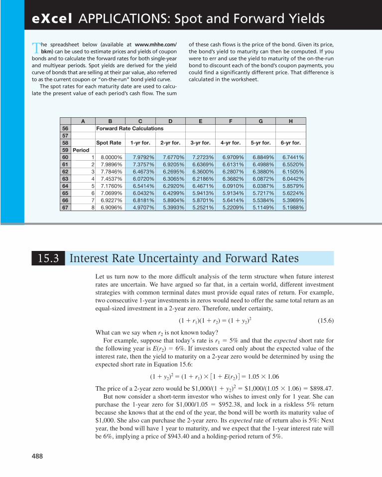
488
15.3 Interest Rate Uncertainty and Forward Rates
eXcel APPLICATIONS: Spot and Forward Yields
T he spreadsheet below (available at www.mhhe.com/
bkm ) can be used to estimate prices and yields of coupon bonds and to calculate the forward rates for both single-year and multiyear periods. Spot yields are derived for the yield curve of bonds that are selling at their par value, also referred to as the current coupon or “on-the-run” bond yield curve.
The spot rates for each maturity date are used to calcu-late the present value of each period’s cash flow. The sum
of these cash flows is the price of the bond. Given its price, the bond’s yield to maturity can then be computed. If you were to err and use the yield to maturity of the on-the-run bond to discount each of the bond’s coupon payments, you could find a significantly different price. That difference is calculated in the worksheet.
Forward Rate Calculations
Spot Rate 1-yr for.
Period
1 8.0000% 7.9792% 7.6770%
2 7.9896% 7.3757% 6.9205%
3 7.7846% 6.4673% 6.2695%
4 7.4537% 6.0720% 6.3065%
5 7.1760% 6.5414% 6.2920%
6 7.0699% 6.0432% 6.4299%
7 6.9227% 6.8181% 5.8904%
8 6.9096% 4.9707% 5.3993%
2-yr for. 3-yr for. 4-yr for. 5-yr for. 6-yr for.
5.2209% 5.1149% 5.1988%
A C D E F G HB
56
57
58
59
60
61
62
63
64
65
66
67
7.2723%
6.6369%
6.3600%
6.2186%
6.4671%
5.9413%
5.8701%
5.2521%
6.9709%
6.6131%
6.2807%
6.3682%
6.0910%
5.9134%
5.6414%
6.8849%
6.4988%
6.3880%
6.0872%
6.0387%
5.7217%
5.5384%
6.7441%
6.5520%
6.1505%
6.0442%
5.8579%
5.6224%
5.3969%
Let us turn now to the more difficult analysis of the term structure when future interest rates are uncertain. We have argued so far that, in a certain world, different investment strategies with common terminal dates must provide equal rates of return. For example, two consecutive 1-year investments in zeros would need to offer the same total return as an equal-sized investment in a 2-year zero. Therefore, under certainty,
(1 1 r1)(1 1 r2) 5 (1 1 y2)2 (15.6)
What can we say when r 2 is not known today? For example, suppose that today’s rate is r 1 5 5% and that the expected short rate for
the following year is E ( r 2 ) 5 6%. If investors cared only about the expected value of the interest rate, then the yield to maturity on a 2-year zero would be determined by using the expected short rate in Equation 15.6 :
(1 1 y2)2 5 (1 1 r1) 3 31 1 E(r2) 45 1.05 3 1.06
The price of a 2-year zero would be $1,000/(1 1 y 2 ) 2 5 $1,000/(1.05 3 1.06) 5 $898.47.
But now consider a short-term investor who wishes to invest only for 1 year. She can purchase the 1-year zero for $1,000/1.05 5 $952.38, and lock in a riskless 5% return because she knows that at the end of the year, the bond will be worth its maturity value of $1,000. She also can purchase the 2-year zero. Its expected rate of return also is 5%: Next year, the bond will have 1 year to maturity, and we expect that the 1-year interest rate will be 6%, implying a price of $943.40 and a holding-period return of 5%.
C H A P T E R 1 5 The Term Structure of Interest Rates 489
But the rate of return on the 2-year bond is risky. If next year’s interest rate turns out to be above expectations, that is, greater than 6%, the bond price will be below $943.40; con-versely if r 2 turns out to be less than 6%, the bond price will exceed $943.40. Why should this short-term investor buy the risky 2-year bond when its expected return is 5%, no better than that of the risk-free 1-year bond? Clearly, she would not hold the 2-year bond unless it offered a higher expected rate of return. This requires that the 2-year bond sell at a price lower than the $898.47 value we derived when we ignored risk.
Example 15.5 Bond Prices and Forward Rates with Interest Rate Risk
Suppose that most investors have short-term horizons and therefore are willing to hold the 2-year bond only if its price falls to $881.83. At this price, the expected holding-period return on the 2-year bond is 7% (because 943.40/881.83 5 1.07). The risk premium of the 2-year bond, therefore, is 2%; it offers an expected rate of return of 7% versus the 5% risk-free return on the 1-year bond. At this risk premium, investors are willing to bear the price risk associated with interest rate uncertainty.
When bond prices reflect a risk premium, however, the forward rate, f 2 , no longer equals the expected short rate, E ( r 2 ). Although we have assumed that E ( r 2 ) 5 6%, it is easy to con-firm that f 2 5 8%. The yield to maturity on the 2-year zeros selling at $881.83 is 6.49%, and
1 1 f2 5(1 1 y2)
2
1 1 y1
51.06492
1.055 1.08
The result in Example 15.5 —that the forward rate exceeds the expected short rate—should not surprise us. We defined the forward rate as the interest rate that would need to prevail in the second year to make the long- and short-term investments equally attractive, ignoring risk. When we account for risk, it is clear that short-term investors will shy away from the long-term bond unless it offers an expected return greater than that of the 1-year bond. Another way of putting this is to say that investors will require a risk premium to hold the longer-term bond. The risk-averse investor would be willing to hold the long-term bond only if the expected value of the short rate is less than the break-even value, f 2 , because the lower the expectation of r 2 , the greater the anticipated return on the long-term bond.
Therefore, if most individuals are short-term investors, bonds must have prices that make f 2 greater than E ( r 2 ). The forward rate will embody a premium compared with the expected future short-interest rate. This liquidity premium compensates short-term inves-tors for the uncertainty about the price at which they will be able to sell their long-term bonds at the end of the year. 3
Perhaps surprisingly, we also can imagine scenarios in which long-term bonds can be perceived by investors to be safer than short-term bonds. To see how, we now consider a “long-term” investor, who wishes to invest for a full 2-year period. Suppose that the investor
3 Liquidity refers to the ability to sell an asset easily at a predictable price. Because long-term bonds have greater price risk, they are considered less liquid in this context and thus must offer a premium.
CONCEPT CHECK
5 Suppose that the required liquidity premium for the short-term investor is 1%. What must E ( r 2 ) be if f 2 is 7%?
490 P A R T I V Fixed-Income Securities
The Expectations Hypothesis
The simplest theory of the term structure is the expectations hypothesis. A common ver-sion of this hypothesis states that the forward rate equals the market consensus expecta-tion of the future short interest rate; that is, f 2 5 E ( r 2 ) and liquidity premiums are zero. If f 2 5 E ( r 2 ), we may relate yields on long-term bonds to expectations of future interest rates. In addition, we can use the forward rates derived from the yield curve to infer market expectations of future short rates. For example, with (1 1 y 2 )
2 5 (1 1 r 1 ) 3 (1 1 f 2 ) from Equation 15.5 , if the expectations hypothesis is correct we may also write that (1 1 y 2 )
2 5 (1 1 r 1 ) 3 [1 1 E ( r 2 )]. The yield to maturity would thus be determined solely by current and expected future one-period interest rates. An upward-sloping yield curve would be clear evidence that investors anticipate increases in interest rates.
can purchase a $1,000 par value 2-year zero-coupon bond for $890 and lock in a guaranteed yield to maturity of y 2 5 6%. Alternatively, the investor can roll over two 1-year invest-ments. In this case an investment of $890 would grow in 2 years to 890 3 1.05 3 (1 1 r 2 ), which is an uncertain amount today because r 2 is not yet known. The break-even year-2 interest rate is, once again, the forward rate, 7.01%, because the forward rate is defined as the rate that equates the terminal value of the two investment strategies.
The expected value of the payoff of the rollover strategy is 890 3 1.05 3 [1 1 E ( r 2 )]. If E ( r 2 ) equals the forward rate, f 2 , then the expected value of the payoff from the rollover strategy will equal the known payoff from the 2-year-maturity bond strategy.
Is this a reasonable presumption? Once again, it is only if the investor does not care about the uncertainty surrounding the final value of the rollover strategy. Whenever that risk is important, the long-term investor will not be willing to engage in the rollover strategy unless its expected return exceeds that of the 2-year bond. In this case the investor would require that
(1.05) 31 1 E(r2) 4. (1.06)2 5 (1.05)(1 1 f2)
which implies that E ( r 2 ) exceeds f 2 . The investor would require that the expected value of next year’s short rate exceed the forward rate.
Therefore, if all investors were long-term investors, no one would be willing to hold short-term bonds unless those bonds offered a reward for bearing interest rate risk. In this situation bond prices would be set at levels such that rolling over short bonds resulted in greater expected return than holding long bonds. This would cause the forward rate to be less than the expected future spot rate.
For example, suppose that in fact E ( r 2 ) 5 8%. The liquidity premium therefore is nega-tive: f 2 2 E ( r 2 ) 5 7.01% 2 8% 5 2 .99%. This is exactly opposite from the conclusion that we drew in the first case of the short-term investor. Clearly, whether forward rates will equal expected future short rates depends on investors’ readiness to bear interest rate risk, as well as their willingness to hold bonds that do not correspond to their investment horizons.
CONCEPT CHECK
6 If the expectations hypothesis is valid, what can we conclude about the premiums necessary to induce investors to hold bonds of differ-ent maturities from their investment horizons?
15.4 Theories of the Term Structure
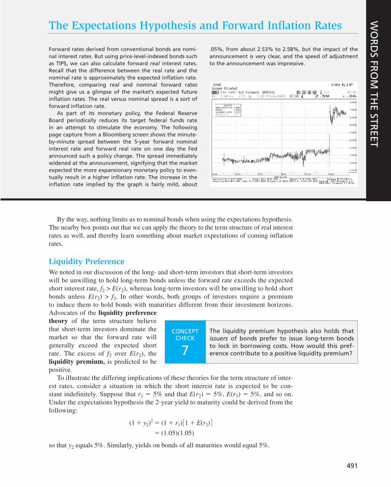
491
CONCEPT CHECK
7
The liquidity premium hypothesis also holds that issuers of bonds prefer to issue long-term bonds to lock in borrowing costs. How would this pref-erence contribute to a positive liquidity premium?
The Expectations Hypothesis and Forward Inflation Rates
Forward rates derived from conventional bonds are nomi-nal interest rates. But using price-level-indexed bonds such as TIPS, we can also calculate forward real interest rates. Recall that the difference between the real rate and the nominal rate is approximately the expected inflation rate. Therefore, comparing real and nominal forward rates might give us a glimpse of the market’s expected future inflation rates. The real versus nominal spread is a sort of forward inflation rate.
As part of its monetary policy, the Federal Reserve Board periodically reduces its target federal funds rate in an attempt to stimulate the economy. The following page capture from a Bloomberg screen shows the minute-by-minute spread between the 5-year forward nominal interest rate and forward real rate on one day the Fed announced such a policy change. The spread immediately widened at the announcement, signifying that the market expected the more expansionary monetary policy to even-tually result in a higher inflation rate. The increase in the inflation rate implied by the graph is fairly mild, about
.05%, from about 2.53% to 2.58%, but the impact of the announcement is very clear, and the speed of adjustment to the announcement was impressive.
WO
RD
S FRO
M TH
E STREET
By the way, nothing limits us to nominal bonds when using the expectations hypothesis. The nearby box points out that we can apply the theory to the term structure of real interest rates as well, and thereby learn something about market expectations of coming inflation rates.
Liquidity Preference
We noted in our discussion of the long- and short-term investors that short-term investors will be unwilling to hold long-term bonds unless the forward rate exceeds the expected short interest rate, f 2 > E ( r 2 ), whereas long-term investors will be unwilling to hold short bonds unless E ( r 2 ) > f 2 . In other words, both groups of investors require a premium to induce them to hold bonds with maturities different from their investment horizons. Advocates of the liquidity preference
theory of the term structure believe that short-term investors dominate the market so that the forward rate will generally exceed the expected short rate. The excess of f 2 over E ( r 2 ), the liquidity premium, is predicted to be positive.
To illustrate the differing implications of these theories for the term structure of inter-est rates, consider a situation in which the short interest rate is expected to be con-stant indefinitely. Suppose that r 1 5 5% and that E ( r 2 ) 5 5%, E ( r 3 ) 5 5%, and so on. Under the expectations hypothesis the 2-year yield to maturity could be derived from the following:
(1 1 y2)2 5 (1 1 r1) 31 1 E(r2) 4 5 (1.05)(1.05)
so that y 2 equals 5%. Similarly, yields on bonds of all maturities would equal 5%.
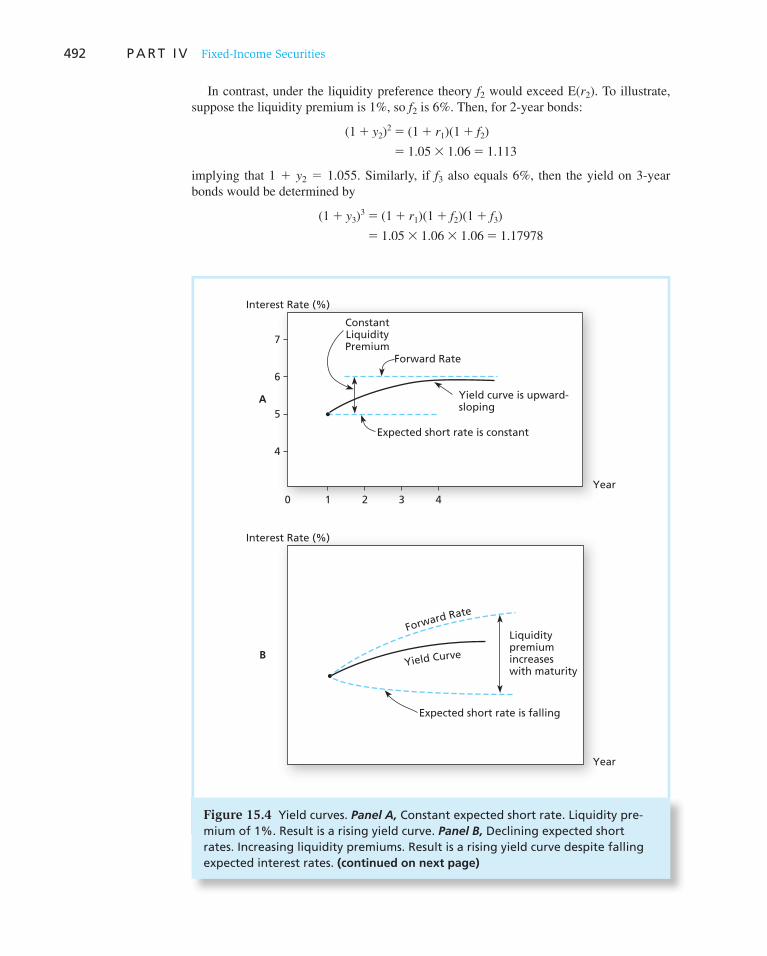
492 P A R T I V Fixed-Income Securities
In contrast, under the liquidity preference theory f 2 would exceed E( r 2 ). To illustrate, suppose the liquidity premium is 1%, so f 2 is 6%. Then, for 2-year bonds:
(1 1 y2)2 5 (1 1 r1)(1 1 f2)
5 1.05 3 1.06 5 1.113
implying that 1 1 y 2 5 1.055. Similarly, if f 3 also equals 6%, then the yield on 3-year bonds would be determined by
(1 1 y3)3 5 (1 1 r1)(1 1 f2)(1 1 f3)
5 1.05 3 1.06 3 1.06 5 1.17978
Forward Rate
Interest Rate (%)
Year
ConstantLiquidityPremium
Forward Rate
Expected short rate is constant
Yield curve is upward-sloping
0 1 2 3 4
Interest Rate (%)
Year
A
BYield Curve
Expected short rate is falling
Liquiditypremiumincreaseswith maturity
7
6
5
4
Figure 15.4 Yield curves. Panel A, Constant expected short rate. Liquidity pre-mium of 1%. Result is a rising yield curve. Panel B, Declining expected short rates. Increasing liquidity premiums. Result is a rising yield curve despite falling expected interest rates. (continued on next page)
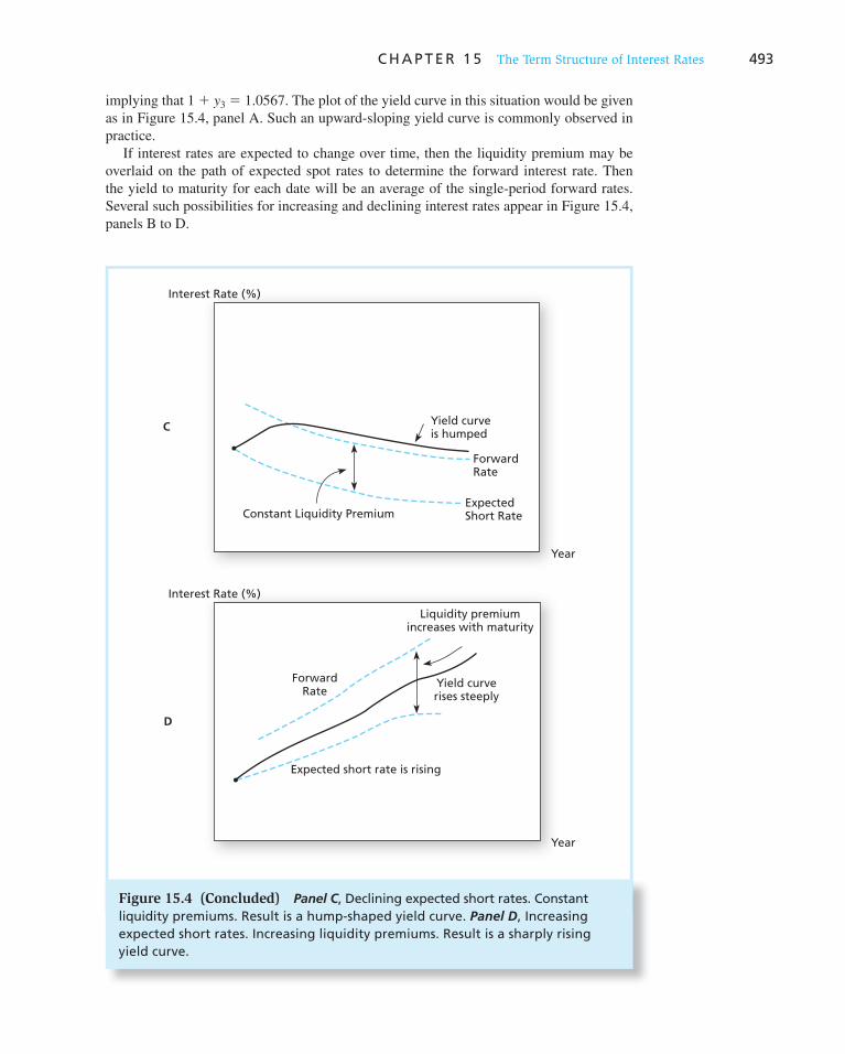
C H A P T E R 1 5 The Term Structure of Interest Rates 493
Interest Rate (%)
D
Expected short rate is rising
Liquidity premiumincreases with maturity
ForwardRate
Yield curverises steeply
Constant Liquidity Premium
Yield curveis humped
ForwardRate
ExpectedShort Rate
C
Interest Rate (%)
Year
Year
Figure 15.4 (Concluded) Panel C , Declining expected short rates. Constant liquidity premiums. Result is a hump-shaped yield curve. Panel D , Increasing expected short rates. Increasing liquidity premiums. Result is a sharply rising yield curve.
implying that 1 1 y 3 5 1.0567. The plot of the yield curve in this situation would be given as in Figure 15.4 , panel A. Such an upward-sloping yield curve is commonly observed in practice.
If interest rates are expected to change over time, then the liquidity premium may be overlaid on the path of expected spot rates to determine the forward interest rate. Then the yield to maturity for each date will be an average of the single-period forward rates. Several such possibilities for increasing and declining interest rates appear in Figure 15.4 , panels B to D.
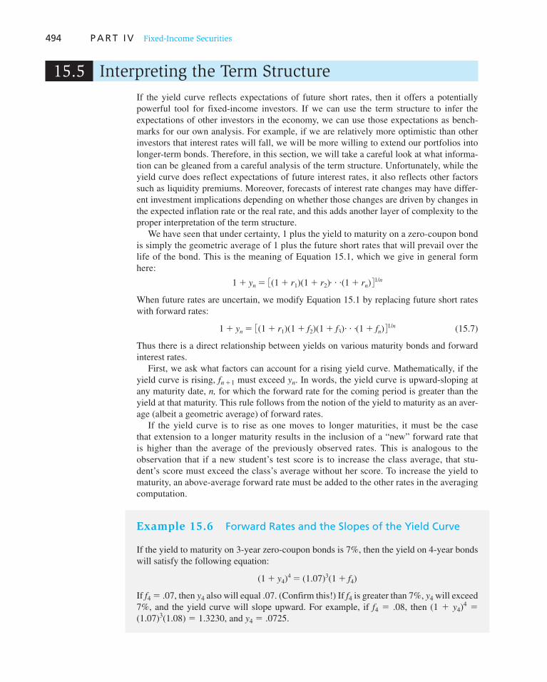
494 P A R T I V Fixed-Income Securities
15.5 Interpreting the Term Structure
If the yield curve reflects expectations of future short rates, then it offers a potentially powerful tool for fixed-income investors. If we can use the term structure to infer the expectations of other investors in the economy, we can use those expectations as bench-marks for our own analysis. For example, if we are relatively more optimistic than other investors that interest rates will fall, we will be more willing to extend our portfolios into longer-term bonds. Therefore, in this section, we will take a careful look at what informa-tion can be gleaned from a careful analysis of the term structure. Unfortunately, while the yield curve does reflect expectations of future interest rates, it also reflects other factors such as liquidity premiums. Moreover, forecasts of interest rate changes may have differ-ent investment implications depending on whether those changes are driven by changes in the expected inflation rate or the real rate, and this adds another layer of complexity to the proper interpretation of the term structure.
We have seen that under certainty, 1 plus the yield to maturity on a zero-coupon bond is simply the geometric average of 1 plus the future short rates that will prevail over the life of the bond. This is the meaning of Equation 15.1 , which we give in general form here:
1 1 yn 5 3(1 1 r1)(1 1 r2)c (1 1 rn) 41/n
When future rates are uncertain, we modify Equation 15.1 by replacing future short rates with forward rates:
1 1 yn 5 3(1 1 r1)(1 1 f2)(1 1 f3)
c(1 1 fn) 41/n (15.7)
Thus there is a direct relationship between yields on various maturity bonds and forward interest rates.
First, we ask what factors can account for a rising yield curve. Mathematically, if the yield curve is rising, f n 1 1 must exceed y n . In words, the yield curve is upward-sloping at any maturity date, n, for which the forward rate for the coming period is greater than the yield at that maturity. This rule follows from the notion of the yield to maturity as an aver-age (albeit a geometric average) of forward rates.
If the yield curve is to rise as one moves to longer maturities, it must be the case that extension to a longer maturity results in the inclusion of a “new” forward rate that is higher than the average of the previously observed rates. This is analogous to the observation that if a new student’s test score is to increase the class average, that stu-dent’s score must exceed the class’s average without her score. To increase the yield to maturity, an above-average forward rate must be added to the other rates in the averaging computation.
Example 15.6 Forward Rates and the Slopes of the Yield Curve
If the yield to maturity on 3-year zero-coupon bonds is 7%, then the yield on 4-year bonds will satisfy the following equation:
(1 1 y4)4 5 (1.07)3(1 1 f4)
If f 4 5 .07, then y 4 also will equal .07. (Confirm this!) If f 4 is greater than 7%, y 4 will exceed 7%, and the yield curve will slope upward. For example, if f 4 5 .08, then (1 1 y 4 )
4 5 (1.07) 3 (1.08) 5 1.3230, and y 4 5 .0725.

C H A P T E R 1 5 The Term Structure of Interest Rates 495
Given that an upward-sloping yield curve is always associated with a forward rate higher than the spot, or current, yield to maturity, we ask next what can account for that higher for-ward rate. Unfortunately, there always are two possible answers to this question. Recall that the forward rate can be related to the expected future short rate according to this equation:
fn 5 E(rn) 1 Liquidity premium (15.8)
where the liquidity premium might be necessary to induce investors to hold bonds of maturities that do not correspond to their preferred investment horizons.
By the way, the liquidity premium need not be positive, although that is the position gen-erally taken by advocates of the liquidity premium hypothesis. We showed previously that if most investors have long-term horizons, the liquidity premium in principle could be negative.
In any case, Equation 15.8 shows that there are two reasons that the forward rate could be high. Either investors expect rising interest rates, meaning that E ( r n ) is high, or they require a large premium for holding longer-term bonds. Although it is tempting to infer from a rising yield curve that investors believe that interest rates will eventually increase, this is not a valid inference. Indeed, panel A in Figure 15.4 provides a simple counter-example to this line of reasoning. There, the short rate is expected to stay at 5% forever. Yet there is a constant 1% liquidity premium so that all forward rates are 6%. The result is that the yield curve continu-ally rises, starting at a level of 5% for 1-year bonds, but eventually approaching 6% for long-term bonds as more and more forward rates at 6% are averaged into the yields to maturity.
Therefore, although it is true that expectations of increases in future interest rates can result in a rising yield curve, the converse is not true: A rising yield curve does not in and of itself imply expectations of higher future interest rates. This is the heart of the difficulty in drawing conclusions from the yield curve. The effects of possible liquidity premiums confound any sim-ple attempt to extract expectations from the term structure. But estimating the market’s expecta-tions is a crucial task, because only by comparing your own expectations to those reflected in market prices can you determine whether you are relatively bullish or bearish on interest rates.
One very rough approach to deriving expected future spot rates is to assume that liquidity premiums are constant. An estimate of that premium can be subtracted from the forward rate to obtain the market’s expected interest rate. For example, again making use of the example plotted in panel A of Figure 15.4 , the researcher would estimate from historical data that a typical liquidity premium in this economy is 1%. After calculating the forward rate from the yield curve to be 6%, the expectation of the future spot rate would be determined to be 5%.
This approach has little to recommend it for two reasons. First, it is next to impossible to obtain precise estimates of a liquidity premium. The general approach to doing so would be to compare forward rates and eventually realized future short rates and to calculate the average difference between the two. However, the deviations between the two values can be quite large and unpredictable because of unanticipated economic events that affect the realized short rate. The data are too noisy to calculate a reliable estimate of the expected premium. Second, there is no reason to believe that the liquidity premium should be con-stant. Figure 15.5 shows the rate of return variability of prices of long-term Treasury bonds since 1971. Interest rate risk fluctuated dramatically during the period. So we might expect risk premiums on various maturity bonds to fluctuate, and empirical evidence suggests that liquidity premiums do in fact fluctuate over time.
Still, very steep yield curves are interpreted by many market professionals as warning signs of impending rate increases. In fact, the yield curve is a good predictor of the business cycle
CONCEPT CHECK
8 Look back at Table 15.1 . Show that y 4 will exceed y 3 if and only if the forward interest rate for period 4 is greater than 7%, which is the yield to maturity on the 3-year bond, y 3 .
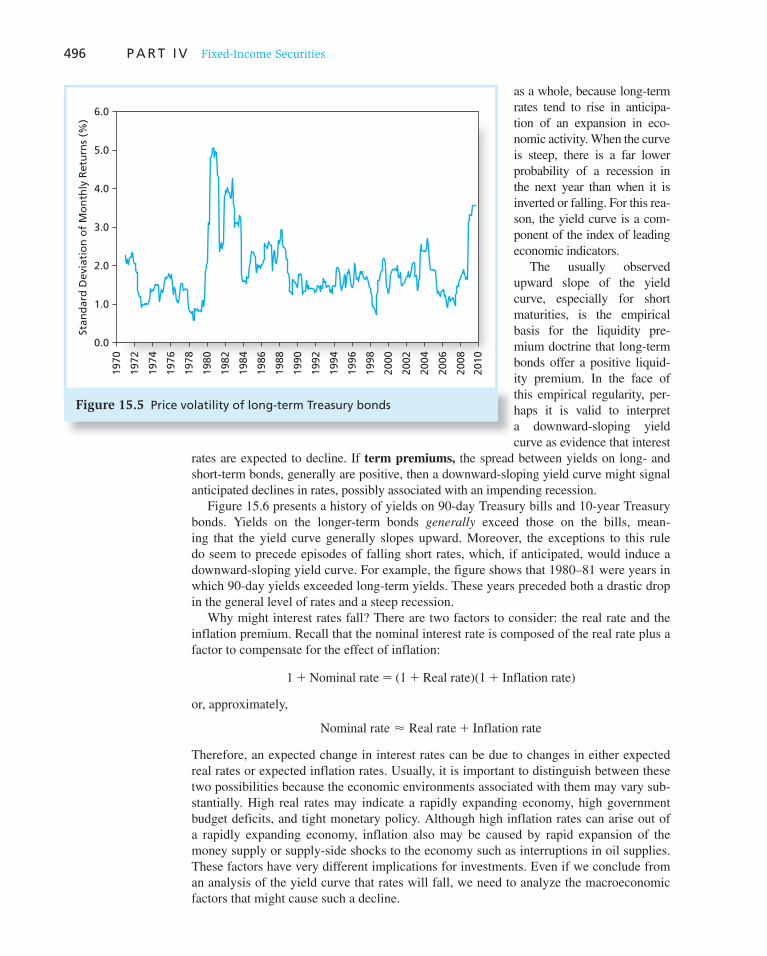
496 P A R T I V Fixed-Income Securities
as a whole, because long-term rates tend to rise in anticipa-tion of an expansion in eco-nomic activity. When the curve is steep, there is a far lower probability of a recession in the next year than when it is inverted or falling. For this rea-son, the yield curve is a com-ponent of the index of leading economic indicators.
The usually observed upward slope of the yield curve, especially for short maturities, is the empirical basis for the liquidity pre-mium doctrine that long-term bonds offer a positive liquid-ity premium. In the face of this empirical regularity, per-haps it is valid to interpret a downward-sloping yield curve as evidence that interest
rates are expected to decline. If term premiums, the spread between yields on long- and short-term bonds, generally are positive, then a downward-sloping yield curve might signal anticipated declines in rates, possibly associated with an impending recession.
Figure 15.6 presents a history of yields on 90-day Treasury bills and 10-year Treasury bonds. Yields on the longer-term bonds generally exceed those on the bills, mean-ing that the yield curve generally slopes upward. Moreover, the exceptions to this rule do seem to precede episodes of falling short rates, which, if anticipated, would induce a downward-sloping yield curve. For example, the figure shows that 1980–81 were years in which 90-day yields exceeded long-term yields. These years preceded both a drastic drop in the general level of rates and a steep recession.
Why might interest rates fall? There are two factors to consider: the real rate and the inflation premium. Recall that the nominal interest rate is composed of the real rate plus a factor to compensate for the effect of inflation:
1 1 Nominal rate 5 (1 1 Real rate)(1 1 Inflation rate)
or, approximately,
Nominal rate < Real rate 1 Inflation rate
Therefore, an expected change in interest rates can be due to changes in either expected real rates or expected inflation rates. Usually, it is important to distinguish between these two possibilities because the economic environments associated with them may vary sub-stantially. High real rates may indicate a rapidly expanding economy, high government budget deficits, and tight monetary policy. Although high inflation rates can arise out of a rapidly expanding economy, inflation also may be caused by rapid expansion of the money supply or supply-side shocks to the economy such as interruptions in oil supplies. These factors have very different implications for investments. Even if we conclude from an analysis of the yield curve that rates will fall, we need to analyze the macroeconomic factors that might cause such a decline.
6.0
5.0
4.0
3.0
2.0
1.0
0.0
1970
1972
1974
1976
1978
1980
1982
1984
1986
1988
1990
1992
1994
1996
1998
2000
2002
2004
2006
2008
2010
Stan
dar
d D
evia
tio
n o
f M
on
thly
Ret
urn
s (%
)
Figure 15.5 Price volatility of long-term Treasury bonds
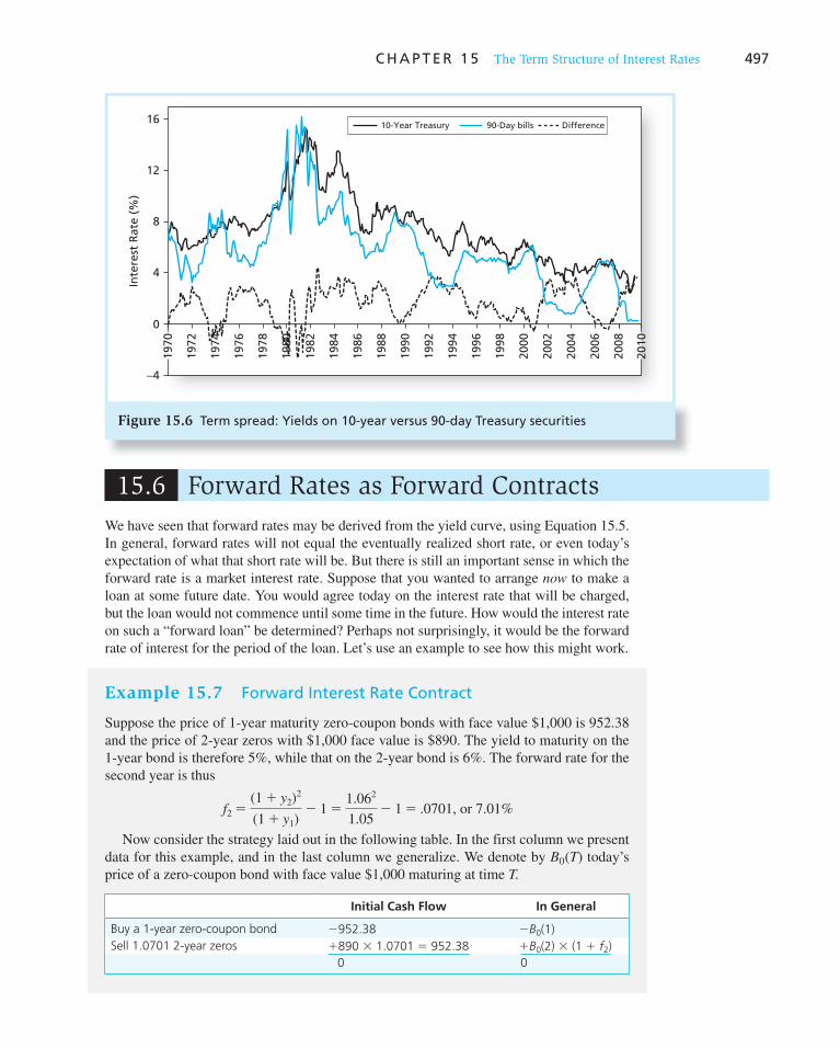
C H A P T E R 1 5 The Term Structure of Interest Rates 497
16
12
8
4
0
−4
Inte
rest
Rat
e (%
)
1972
1974
1976
1978
1980
1982
1984
1986
1988
1990
1992
1994
1996
1998
2000
2002
2004
2006
10-Year Treasury 90-Day bills Difference
2008
1970
2010
Figure 15.6 Term spread: Yields on 10-year versus 90-day Treasury securities
15.6 Forward Rates as Forward Contracts
We have seen that forward rates may be derived from the yield curve, using Equation 15.5 . In general, forward rates will not equal the eventually realized short rate, or even today’s expectation of what that short rate will be. But there is still an important sense in which the forward rate is a market interest rate. Suppose that you wanted to arrange now to make a loan at some future date. You would agree today on the interest rate that will be charged, but the loan would not commence until some time in the future. How would the interest rate on such a “forward loan” be determined? Perhaps not surprisingly, it would be the forward rate of interest for the period of the loan. Let’s use an example to see how this might work.
Example 15.7 Forward Interest Rate Contract
Suppose the price of 1-year maturity zero-coupon bonds with face value $1,000 is 952.38 and the price of 2-year zeros with $1,000 face value is $890. The yield to maturity on the 1-year bond is therefore 5%, while that on the 2-year bond is 6%. The forward rate for the second year is thus
f2 5(1 1 y2)
2
(1 1 y1)2 1 5
1.062
1.052 1 5 .0701, or 7.01%
Now consider the strategy laid out in the following table. In the first column we present data for this example, and in the last column we generalize. We denote by B 0 ( T ) today’s price of a zero-coupon bond with face value $1,000 maturing at time T.
Initial Cash Flow In General
Buy a 1-year zero-coupon bond 2952.38 2B0(1)
Sell 1.0701 2-year zeros 1890 3 1.0701 5 952.38 1B0(2) 3 (1 1 f2)
0 0

498 P A R T I V Fixed-Income Securities
In general, to construct the synthetic forward loan, you sell (1 1 f 2 ) 2-year zeros for every 1-year zero that you buy. This makes your initial cash flow zero because the prices of the 1- and 2-year zeros differ by the factor (1 1 f 2 ); notice that
B0(1) 5$1,000
(1 1 y1) while B0(2) 5
$1,000
(1 1 y2)2
5$1,000
(1 1 y1)(1 1 f2)
Therefore, when you sell (1 1 f 2 ) 2-year zeros you generate just enough cash to buy one 1-year zero. Both zeros mature to a face value of $1,000, so the difference between the cash inflow at time 1 and the cash outflow at time 2 is the same factor, 1 1 f 2 , as illustrated in Figure 15.7 , panel B. As a result, f 2 is the rate on the forward loan.
4 Of course, in reality one cannot sell a fraction of a bond, but you can think of this part of the transaction as fol-lows. If you sold one of these bonds, you would effectively be borrowing $890 for a 2-year period. Selling 1.0701 of these bonds simply means that you are borrowing $890 3 1.0701 5 $952.38.
The initial cash flow (at time 0) is zero. You pay $952.38, or in general B 0 (1), for a zero maturing in 1 year, and you receive $890, or in general B 0 (2), for each zero you sell maturing in 2 years. By selling 1.0701 of these bonds, you set your initial cash flow to zero. 4
At time 1, the 1-year bond matures and you receive $1,000. At time 2, the 2-year maturity zero-coupon bonds that you sold mature, and you have to pay 1.0701 3 $1,000 5 $1,070.10. Your cash flow stream is shown in Figure 15.7 , panel A. Notice that you have created a “synthetic” forward loan: You effectively will borrow $1,000 a year from now, and repay $1,070.10 a year later. The rate on this forward loan is therefore 7.01%, precisely equal to the forward rate for the second year.
−$1,070.10
$1,000
20 1
−$1,000(1 + f2)
$1,000
20 1r1 r2
B. For a General Forward Rate. The short rates in the two periods are r1 (which is observable today) and r2 (which is not). The rate that can be locked in for a one-period-ahead loan is f2.
A. Forward Rate = 7.01%
Figure 15.7 Engineering a synthetic forward loan

Vis
it u
s at
ww
w.m
hh
e.co
m/b
kmV
isit
us
at w
ww
.mh
he.
com
/bkm
C H A P T E R 1 5 The Term Structure of Interest Rates 499
Obviously, you can construct a synthetic forward loan for periods beyond the second year, and you can construct such loans for multiple periods. Challenge Problems 18 and 19 at the end of the chapter lead you through some of these variants.
CONCEPT CHECK
9 Suppose that the price of 3-year zero-coupon bonds is $816.30. What is the forward rate for the third year? How would you construct a synthetic 1-year forward loan that commences at t 5 2 and matures at t 5 3?
1. The term structure of interest rates refers to the interest rates for various terms to maturity embod-ied in the prices of default-free zero-coupon bonds.
2. In a world of certainty all investments must provide equal total returns for any investment period. Short-term holding-period returns on all bonds would be equal in a risk-free economy, and all equal to the rate available on short-term bonds. Similarly, total returns from rolling over short-term bonds over longer periods would equal the total return available from long-maturity bonds.
3. The forward rate of interest is the break-even future interest rate that would equate the total return from a rollover strategy to that of a longer-term zero-coupon bond. It is defined by the equation
(1 1 yn)n(1 1 fn11) 5 (1 1 yn11)
n11
where n is a given number of periods from today. This equation can be used to show that yields to maturity and forward rates are related by the equation
(1 1 yn)n 5 (1 1 r1)(1 1 f2)(1 1 f3)c
(1 1 fn)
4. A common version of the expectations hypothesis holds that forward interest rates are unbiased estimates of expected future interest rates. However, there are good reasons to believe that for-ward rates differ from expected short rates because of a risk premium known as a liquidity pre-
mium. A positive liquidity premium can cause the yield curve to slope upward even if no increase in short rates is anticipated.
5. The existence of liquidity premiums makes it extremely difficult to infer expected future inter-est rates from the yield curve. Such an inference would be made easier if we could assume the liquidity premium remained reasonably stable over time. However, both empirical and theoretical considerations cast doubt on the constancy of that premium.
6. Forward rates are market interest rates in the important sense that commitments to forward (i.e., deferred) borrowing or lending arrangements can be made at these rates.
SUMMARY
Related Web sites for this chapter are available at www.mhhe.com/bkm
term structure of interest rates yield curve bond stripping bond reconstitution pure yield curve
on-the-run yield curve spot rate short rate forward interest rate liquidity premium
expectations hypothesis liquidity preference theory liquidity premium term premiums
KEY TERMS

Vis
it u
s at
ww
w.m
hh
e.co
m/b
km500 P A R T I V Fixed-Income Securities
1. What is the relationship between forward rates and the market’s expectation of future short rates? Explain in the context of both the expectations and liquidity preference theories of the term structure of interest rates.
2. Under the expectations hypothesis, if the yield curve is upward-sloping, the market must expect an increase in short-term interest rates. True/false/uncertain? Why?
3. Under the liquidity preference theory, if inflation is expected to be falling over the next few years, long-term interest rates will be higher than short-term rates. True/false/uncertain? Why?
4. If the liquidity preference hypothesis is true, what shape should the term structure curve have in a period where interest rates are expected to be constant?
a. Upward sloping. b. Downward sloping. c. Flat.
5. Which of the following is true according to the pure expectations theory? Forward rates:
a. Exclusively represent expected future short rates. b. Are biased estimates of market expectations. c. Always overestimate future short rates.
6. Assuming the pure expectations theory is correct, an upward-sloping yield curve implies:
a. Interest rates are expected to increase in the future. b. Longer-term bonds are riskier than short-term bonds. c. Interest rates are expected to decline in the future.
7. The following is a list of prices for zero-coupon bonds of various maturities. Calculate the yields to maturity of each bond and the implied sequence of forward rates.
Maturity (Years) Price of Bond
1 $943.40
2 898.47
3 847.62
4 792.16
8. Assuming that the expectations hypothesis is valid, compute the expected price path of the 4-year bond in the previous problem as time passes. What is the rate of return of the bond in each year? Show that the expected return equals the forward rate for each year.
9. Consider the following $1,000 par value zero-coupon bonds:
Bond Years to Maturity YTM(%)
A 1 5%
B 2 6
C 3 6.5
D 4 7
According to the expectations hypothesis, what is the expected 1-year interest rate 3 years from now?
10. The term structure for zero-coupon bonds is currently:
Maturity (Years) YTM (%)
1 4%
2 5
3 6
PROBLEM SETS
i. Basic
ii. Intermediate

Vis
it u
s at
ww
w.m
hh
e.co
m/b
km
C H A P T E R 1 5 The Term Structure of Interest Rates 501
Next year at this time, you expect it to be:
Maturity (Years) YTM (%)
1 5%
2 6
3 7
a. What do you expect the rate of return to be over the coming year on a 3-year zero-coupon bond? b. Under the expectations theory, what yields to maturity does the market expect to observe on
1- and 2-year zeros at the end of the year? Is the market’s expectation of the return on the 3-year bond greater or less than yours?
11. The yield to maturity on 1-year zero-coupon bonds is currently 7%; the YTM on 2-year zeros is 8%. The Treasury plans to issue a 2-year maturity coupon bond, paying coupons once per year with a coupon rate of 9%. The face value of the bond is $100.
a. At what price will the bond sell? b. What will the yield to maturity on the bond be? c. If the expectations theory of the yield curve is correct, what is the market expectation of the
price that the bond will sell for next year? d. Recalculate your answer to ( c ) if you believe in the liquidity preference theory and you
believe that the liquidity premium is 1%.
12. Below is a list of prices for zero-coupon bonds of various maturities.
Maturity (Years)Price of $1,000 Par Bond
(Zero-Coupon)
1 $943.40
2 873.52
3 816.37
a. An 8.5% coupon $1,000 par bond pays an annual coupon and will mature in 3 years. What should the yield to maturity on the bond be?
b. If at the end of the first year the yield curve flattens out at 8%, what will be the 1-year holding-period return on the coupon bond?
13. Prices of zero-coupon bonds reveal the following pattern of forward rates:
Year Forward Rate
1 5%
2 7
3 8
In addition to the zero-coupon bond, investors also may purchase a 3-year bond making annual payments of $60 with par value $1,000.
a. What is the price of the coupon bond? b. What is the yield to maturity of the coupon bond? c. Under the expectations hypothesis, what is the expected realized compound yield of the
coupon bond? d. If you forecast that the yield curve in 1 year will be flat at 7%, what is your forecast for the
expected rate of return on the coupon bond for the 1-year holding period?
14. You observe the following term structure:
Effective Annual YTM
1-year zero-coupon bond 6.1%
2-year zero-coupon bond 6.2
3-year zero-coupon bond 6.3
4-year zero-coupon bond 6.4

Vis
it u
s at
ww
w.m
hh
e.co
m/b
km502 P A R T I V Fixed-Income Securities
a. If you believe that the term structure next year will be the same as today’s, will the 1-year or the 4-year zeros provide a greater expected 1-year return?
b. What if you believe in the expectations hypothesis?
15. The yield to maturity (YTM) on 1-year zero-coupon bonds is 5% and the YTM on 2-year zeros is 6%. The yield to maturity on 2-year-maturity coupon bonds with coupon rates of 12% (paid annually) is 5.8%. What arbitrage opportunity is available for an investment banking firm? What is the profit on the activity?
16. Suppose that a 1-year zero-coupon bond with face value $100 currently sells at $94.34, while a 2-year zero sells at $84.99. You are considering the purchase of a 2-year-maturity bond making annual coupon payments. The face value of the bond is $100, and the coupon rate is 12% per year.
a. What is the yield to maturity of the 2-year zero? The 2-year coupon bond? b. What is the forward rate for the second year? c. If the expectations hypothesis is accepted, what are (1) the expected price of the coupon
bond at the end of the first year and (2) the expected holding-period return on the coupon bond over the first year?
d. Will the expected rate of return be higher or lower if you accept the liquidity preference hypothesis?
17. The current yield curve for default-free zero-coupon bonds is as follows:
Maturity (Years) YTM (%)
1 10%
2 11
3 12
a. What are the implied 1-year forward rates? b. Assume that the pure expectations hypothesis of the term structure is correct. If market
expectations are accurate, what will be the pure yield curve (that is, the yields to maturity on 1- and 2-year zero coupon bonds) next year?
c. If you purchase a 2-year zero-coupon bond now, what is the expected total rate of return over the next year? What if you purchase a 3-year zero-coupon bond? ( Hint: Compute the current and expected future prices.) Ignore taxes.
d. What should be the current price of a 3-year maturity bond with a 12% coupon rate paid annually? If you purchased it at that price, what would your total expected rate of return be over the next year (coupon plus price change)? Ignore taxes.
18. Suppose that the prices of zero-coupon bonds with various maturities are given in the following table. The face value of each bond is $1,000.
Maturity (Years) Price
1 $925.93
2 853.39
3 782.92
4 715.00
5 650.00
a. Calculate the forward rate of interest for each year. b. How could you construct a 1-year forward loan beginning in year 3? Confirm that the rate on
that loan equals the forward rate. c. Repeat ( b ) for a 1-year forward loan beginning in year 4.
19. Continue to use the data in the preceding problem. Suppose that you want to construct a 2-year maturity forward loan commencing in 3 years.
a. Suppose that you buy today one 3-year maturity zero-coupon bond. How many 5-year matu-rity zeros would you have to sell to make your initial cash flow equal to zero?
b. What are the cash flows on this strategy in each year?
iii. Challenge

Vis
it u
s at
ww
w.m
hh
e.co
m/b
km
C H A P T E R 1 5 The Term Structure of Interest Rates 503
c. What is the effective 2-year interest rate on the effective 3-year-ahead forward loan? d. Confirm that the effective 2-year interest rate equals (1 1 f 4 ) 3 (1 1 f 5 ) 2 1. You therefore
can interpret the 2-year loan rate as a 2-year forward rate for the last 2 years. Alternatively, show that the effective 2-year forward rate equals
(1 1 y5)
5
(1 1 y3)3
2 1
1. Briefly explain why bonds of different maturities have different yields in terms of the expecta-tions and liquidity preference hypotheses. Briefly describe the implications of each hypothesis when the yield curve is (1) upward-sloping and (2) downward-sloping.
2. Which one of the following statements about the term structure of interest rates is true?
a. The expectations hypothesis indicates a flat yield curve if anticipated future short-term rates exceed current short-term rates.
b. The expectations hypothesis contends that the long-term rate is equal to the anticipated short-term rate.
c. The liquidity premium theory indicates that, all else being equal, longer maturities will have lower yields.
d. The liquidity preference theory contends that lenders prefer to buy securities at the short end of the yield curve.
3. The following table shows yields to maturity of zero-coupon Treasury securities.
Term to Maturity (Years) Yield to Maturity (%)
1 3.50%
2 4.50
3 5.00
4 5.50
5 6.00
10 6.60
a. Calculate the forward 1-year rate of interest for year 3. b. Describe the conditions under which the calculated forward rate would be an unbiased esti-
mate of the 1-year spot rate of interest for that year. c. Assume that a few months earlier, the forward 1-year rate of interest for that year had been
significantly higher than it is now. What factors could account for the decline in the forward rate?
4. The 6-month Treasury bill spot rate is 4%, and the 1-year Treasury bill spot rate is 5%. What is the implied 6-month forward rate for 6 months from now?
5. The tables below show, respectively, the characteristics of two annual-pay bonds from the same issuer with the same priority in the event of default, and spot interest rates. Neither bond’s price is consistent with the spot rates. Using the information in these tables, recommend either bond A or bond B for purchase.
Bond Characteristics
Bond A Bond B
Coupons Annual Annual
Maturity 3 years 3 years
Coupon rate 10% 6%
Yield to maturity 10.65% 10.75%
Price 98.40 88.34
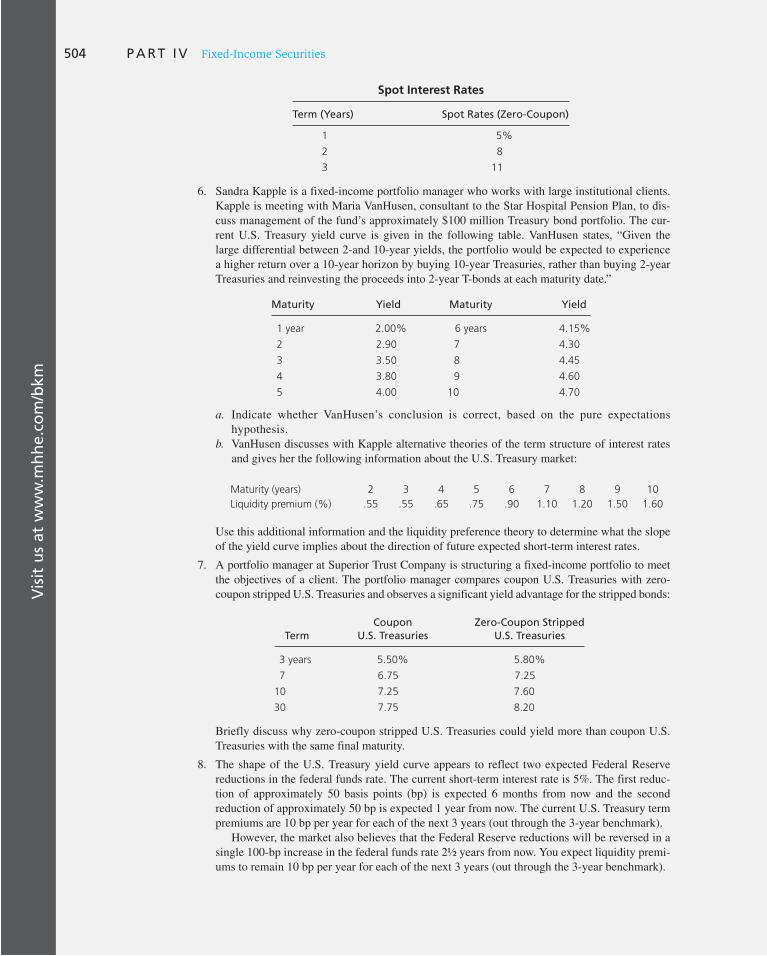
Vis
it u
s at
ww
w.m
hh
e.co
m/b
km504 P A R T I V Fixed-Income Securities
Spot Interest Rates
Term (Years) Spot Rates (Zero-Coupon)
1 5%
2 8
3 11
6. Sandra Kapple is a fixed-income portfolio manager who works with large institutional clients. Kapple is meeting with Maria VanHusen, consultant to the Star Hospital Pension Plan, to dis-cuss management of the fund’s approximately $100 million Treasury bond portfolio. The cur-rent U.S. Treasury yield curve is given in the following table. VanHusen states, “Given the large differential between 2-and 10-year yields, the portfolio would be expected to experience a higher return over a 10-year horizon by buying 10-year Treasuries, rather than buying 2-year Treasuries and reinvesting the proceeds into 2-year T-bonds at each maturity date.”
Maturity Yield Maturity Yield
1 year 2.00% 6 years 4.15%
2 2.90 7 4.30
3 3.50 8 4.45
4 3.80 9 4.60
5 4.00 10 4.70
a. Indicate whether VanHusen’s conclusion is correct, based on the pure expectations hypothesis.
b. VanHusen discusses with Kapple alternative theories of the term structure of interest rates and gives her the following information about the U.S. Treasury market:
Maturity (years) 2 3 4 5 6 7 8 9 10
Liquidity premium (%) .55 .55 .65 .75 .90 1.10 1.20 1.50 1.60
Use this additional information and the liquidity preference theory to determine what the slope of the yield curve implies about the direction of future expected short-term interest rates.
7. A portfolio manager at Superior Trust Company is structuring a fixed-income portfolio to meet the objectives of a client. The portfolio manager compares coupon U.S. Treasuries with zero- coupon stripped U.S. Treasuries and observes a significant yield advantage for the stripped bonds:
TermCoupon
U.S. TreasuriesZero-Coupon Stripped
U.S. Treasuries
3 years 5.50% 5.80%
7 6.75 7.25
10 7.25 7.60
30 7.75 8.20
Briefly discuss why zero-coupon stripped U.S. Treasuries could yield more than coupon U.S. Treasuries with the same final maturity.
8. The shape of the U.S. Treasury yield curve appears to reflect two expected Federal Reserve reductions in the federal funds rate. The current short-term interest rate is 5%. The first reduc-tion of approximately 50 basis points (bp) is expected 6 months from now and the second reduction of approximately 50 bp is expected 1 year from now. The current U.S. Treasury term premiums are 10 bp per year for each of the next 3 years (out through the 3-year benchmark).
However, the market also believes that the Federal Reserve reductions will be reversed in a single 100-bp increase in the federal funds rate 2½ years from now. You expect liquidity premi-ums to remain 10 bp per year for each of the next 3 years (out through the 3-year benchmark).

Vis
it u
s at
ww
w.m
hh
e.co
m/b
km
C H A P T E R 1 5 The Term Structure of Interest Rates 505
Describe or draw the shape of the Treasury yield curve out through the 3-year bench-mark. Which term structure theory supports the shape of the U.S. Treasury yield curve you’ve described?
9. U.S. Treasuries represent a significant holding in many pension portfolios. You decide to ana-lyze the yield curve for U.S. Treasury notes.
a. Using the data in the table below, calculate the 5-year spot and forward rates assuming annual compounding. Show your calculations.
U.S. Treasury Note Yield Curve Data
Years to MaturityPar Coupon
Yield to MaturityCalculated Spot Rates
Calculated Forward Rates
1 5.00 5.00 5.00
2 5.20 5.21 5.42
3 6.00 6.05 7.75
4 7.00 7.16 10.56
5 7.00 ? ?
b. Define and describe each of the following three concepts:
i. Short rate ii. Spot rate iii. Forward rate
Explain how these concepts are related. c. You are considering the purchase of a zero-coupon U.S. Treasury note with 4 years to matu-
rity. On the basis of the above yield-curve analysis, calculate both the expected yield to maturity and the price for the security. Show your calculations.
10. The spot rates of interest for five U.S. Treasury Securities are shown in the following exhibit. Assume all securities pay interest annually.
Spot Rates of Interest
Term to Maturity Spot Rate of Interest
1 year 13.00%
2 12.00
3 11.00
4 10.00
5 9.00
a. Compute the 2-year implied forward rate for a deferred loan beginning in 3 years. b. Compute the price of a 5-year annual-pay Treasury security with a coupon rate of 9% by
using the information in the exhibit.
E-INVEST-MENTS EXERCISES
The Yield Curve
Go to www.smartmoney.com . Access the Living Yield Curve (look for the Economy
and Bonds tab), a moving picture of the yield curve. Is the yield curve usually upward- or downward-sloping? What about today’s yield curve? How much does the slope of the curve vary? Which varies more: short-term or long-term rates? Can you explain why this might be the case?

Vis
it u
s at
ww
w.m
hh
e.co
m/b
km506 P A R T I V Fixed-Income Securities
SOLUTIONS TO CONCEPT CHECKS
1. The price of the 3-year bond paying a $40 coupon is
40
1.051
40
1.0621
1040
1.0735 38.095 1 35.600 1 848.950 5 $922.65
At this price, the yield to maturity is 6.945% [ n 5 3; PV 5 ( 2 )922.65; FV 5 1,000; PMT 5 40]. This bond’s yield to maturity is closer to that of the 3-year zero-coupon bond than is the yield to maturity of the 10% coupon bond in Example 15.1 . This makes sense: this bond’s coupon rate is lower than that of the bond in Example 15.1 . A greater fraction of its value is tied up in the final payment in the third year, and so it is not surprising that its yield is closer to that of a pure 3-year zero-coupon security.
2. We compare two investment strategies in a manner similar to Example 15.2 :
Buy and hold 4-year zero 5 Buy 3-year zero; roll proceeds into 1-year bond
(1 1 y4)4 5 (1 1 y3)
3 3 (1 1 r4)
1.084 5 1.073 3 (1 1 r4)
which implies that r 4 5 1.08 4 /1.07 3 2 1 5 .11056 5 11.056%. Now we confirm that the yield on the 4-year zero is a geometric average of the discount factors for the next 3 years:
1 1 y4 5 3(1 1 r1) 3 (1 1 r2) 3 (1 1 r3) 3 (1 1 r4) 41/4
1.08 5 31.05 3 1.0701 3 1.09025 3 1.11056 41/4
3. The 3-year bond can be bought today for $1,000/1.07 3 5 $816.30. Next year, it will have a remaining maturity of 2 years. The short rate in year 2 will be 7.01% and the short rate in year 3 will be 9.025%. Therefore, the bond’s yield to maturity next year will be related to these short rates according to
(1 1 y2)2 5 1.0701 3 1.09025 5 1.1667
and its price next year will be $1,000/(1 1 y 2 ) 2 5 $1,000/1.1667 5 $857.12. The 1-year holding-
period rate of return is therefore ($857.12 2 $816.30)/$816.30 5 .05, or 5%.
4. The n -period spot rate is the yield to maturity on a zero-coupon bond with a maturity of n periods. The short rate for period n is the one-period interest rate that will prevail in period n. Finally, the forward rate for period n is the short rate that would satisfy a “break-even condition” equating the total returns on two n -period investment strategies. The first strategy is an investment in an n -period zero-coupon bond; the second is an investment in an n 2 1 period zero-coupon bond “rolled over” into an investment in a one-period zero. Spot rates and forward rates are observable today, but because interest rates evolve with uncertainty, future short rates are not. In the special
case in which there is no uncertainty in future interest rates, the forward rate calculated from the yield curve would equal the short rate that will prevail in that period.
5. 7% 2 1% 5 6%.
6. The risk premium will be zero.
7. If issuers prefer to issue long-term bonds, they will be willing to accept higher expected interest costs on long bonds over short bonds. This willingness combines with investors’ demands for higher rates on long-term bonds to reinforce the tendency toward a positive liquidity premium.
8. In general, from Equation 15.5 , (1 1 y n ) n 5 (1 1 y n 2 1 )
n 2 1 3 (1 1 f n ). In this case, (1 1 y 4 )
4 5 (1.07) 3 3 (1 1 f 4 ). If f 4 5 .07, then (1 1 y 4 ) 4 5 (1.07) 4 and y 4 5 .07. If f 4 is greater
than .07, then y 4 also will be greater, and conversely if f 4 is less than .07, then y 4 will be as well.

Vis
it u
s at
ww
w.m
hh
e.co
m/b
km
C H A P T E R 1 5 The Term Structure of Interest Rates 507
9. The 3-year yield to maturity is a 1,000
816.30b1/3
2 1 5 .07 5 7.0%
The forward rate for the third year is therefore
f3 5(1 1 y3)
3
(1 1 y2)2
2 1 51.073
1.0622 1 5 .0903 5 9.03%
(Alternatively, note that the ratio of the price of the 2-year zero to the price of the 3-year zero is 1 1 f 3 5 1.0903.) To construct the synthetic loan, buy one 2-year maturity zero, and sell 1.0903 3-year maturity zeros. Your initial cash flow is zero, your cash flow at time 2 is 1 $1,000, and your cash flow at time 3 is 2 $1,090.30, which corresponds to the cash flows on a 1-year forward loan commencing at time 2 with an interest rate of 9.03%.

16 1 CHAPTER SIXTEEN
IN THIS CHAPTER we turn to various strate-
gies that bond portfolio managers can pur-
sue, making a distinction between passive
and active strategies. A passive investment
strategy takes market prices of securities as
set fairly. Rather than attempting to beat
the market by exploiting superior infor-
mation or insight, passive managers act to
maintain an appropriate risk–return balance
given market opportunities. One special
case of passive management is an immuni-
zation strategy that attempts to insulate or
immunize the portfolio from interest rate
risk. In contrast, an active investment strat-
egy attempts to achieve returns greater than
those commensurate with the risk borne. In
the context of bond management this style
of management can take two forms. Active
managers use either interest rate forecasts
to predict movements in the entire bond
market or some form of intramarket analy-
sis to identify particular sectors of the mar-
ket or particular bonds that are relatively
mispriced.
Because interest rate risk is crucial to for-
mulating both active and passive strategies,
we begin our discussion with an analysis of
the sensitivity of bond prices to interest rate
fluctuations. This sensitivity is measured by
the duration of the bond, and we devote con-
siderable attention to what determines bond
duration. We discuss several passive invest-
ment strategies, and show how duration-
matching techniques can be used to immunize
the holding-period return of a portfolio from
interest rate risk. After examining the broad
range of applications of the duration mea-
sure, we consider refinements in the way that
interest rate sensitivity is measured, focusing
on the concept of bond convexity. Duration
is important in formulating active investment
strategies as well, and we conclude the chap-
ter with a discussion of active fixed-income
strategies. These include policies based on
interest rate forecasting as well as intramar-
ket analysis that seeks to identify relatively
attractive sectors or securities within the
fixed-income market.
Managing Bond Portfolios
PAR
T IV

C H A P T E R 1 6 Managing Bond Portfolios 509
We have seen already that an inverse relationship exists between bond prices and yields, and we know that interest rates can fluctuate substantially. As interest rates rise and fall, bondholders experience capital losses and gains. These gains or losses make fixed-income investments risky, even if the coupon and principal payments are guaranteed, as in the case of Treasury obligations.
Why do bond prices respond to interest rate fluctuations? Remember that in a competi-tive market all securities must offer investors fair expected rates of return. If a bond is issued with an 8% coupon when competitive yields are 8%, then it will sell at par value. If the market rate rises to 9%, however, who would purchase an 8% coupon bond at par value? The bond price must fall until its expected return increases to the competitive level of 9%. Conversely, if the market rate falls to 7%, the 8% coupon on the bond is attrac-tive compared to yields on alternative investments. In response, investors eager for that return would bid the bond price above its par value until the total rate of return falls to the market rate.
Interest Rate Sensitivity
The sensitivity of bond prices to changes in market interest rates is obviously of great concern to investors. To gain some insight into the determinants of interest rate risk, turn to Figure 16.1 , which presents the percentage change in price corresponding to changes in yield to maturity for four bonds that differ according to coupon rate, initial yield to maturity, and time to maturity. All four bonds illustrate that bond prices decrease when yields rise, and that the price curve is convex, meaning that decreases in yields have bigger
Perc
enta
ge
Ch
ang
e in
Bo
nd
Pri
ce
Change in Yield to Maturity (%)
DCB
A
A
B
C
D
5
−5
−4
−3
−2
−1 0 1 2 3 4
200
150
100
50
0
−50
InitialBond Coupon Maturity YTM
A 12% 5 years 10%B 12% 30 years 10%C 3% 30 years 10%D 3% 30 years 6%
Figure 16.1 Change in bond price as a function of change in yield to maturity
16.1 Interest Rate Risk

510 P A R T I V Fixed-Income Securities
impacts on price than increases in yields of equal magnitude. We summarize these obser-vations in the following two propositions:
1. Bond prices and yields are inversely related: as yields increase, bond prices fall; as
yields fall, bond prices rise.
2. An increase in a bond’s yield to maturity results in a smaller price change than a
decrease in yield of equal magnitude.
Now compare the interest rate sensitivity of bonds A and B, which are identical except for maturity. Figure 16.1 shows that bond B, which has a longer maturity than bond A, exhibits greater sensitivity to interest rate changes. This illustrates another general property:
3. Prices of long-term bonds tend to be more sensitive to interest rate changes than
prices of short-term bonds.
This is not surprising. If rates increase, for example, the bond is less valuable as its cash flows are discounted at a now-higher rate. The impact of the higher discount rate will be greater as that rate is applied to more-distant cash flows.
Notice that while bond B has six times the maturity of bond A, it has less than six times the interest rate sensitivity. Although interest rate sensitivity seems to increase with matu-rity, it does so less than proportionally as bond maturity increases. Therefore, our fourth property is that:
4. The sensitivity of bond prices to changes in yields increases at a decreasing rate
as maturity increases. In other words, interest rate risk is less than proportional
to bond maturity.
Bonds B and C, which are alike in all respects except for coupon rate, illustrate another point. The lower-coupon bond exhibits greater sensitivity to changes in interest rates. This turns out to be a general property of bond prices:
5. Interest rate risk is inversely related to the bond’s coupon rate. Prices of
low-coupon bonds are more sensitive to changes in interest rates than prices
of high-coupon bonds.
Finally, bonds C and D are identical except for the yield to maturity at which the bonds currently sell. Yet bond C, with a higher yield to maturity, is less sensitive to changes in yields. This illustrates our final property:
6. The sensitivity of a bond’s price to a change in its yield is inversely related to the
yield to maturity at which the bond currently is selling.
The first five of these general properties were described by Malkiel 1 and are sometimes known as Malkiel’s bond-pricing relationships. The last property was demonstrated by Homer and Liebowitz. 2
Maturity is a major determinant of interest rate risk. However, maturity alone is not suf-ficient to measure interest rate sensitivity. For example, bonds B and C in Figure 16.1 have the same maturity, but the higher-coupon bond has less price sensitivity to interest rate changes. Obviously, we need to know more than a bond’s maturity to quantify its interest rate risk.
1Burton G. Malkiel, “Expectations, Bond Prices, and the Term Structure of Interest Rates,” Quarterly Journal of
Economics 76 (May 1962), pp. 197–218.
2 Sidney Homer and Martin L. Liebowitz, Inside the Yield Book: New Tools for Bond Market Strategy (Englewood Cliffs, NJ: Prentice Hall, 1972).
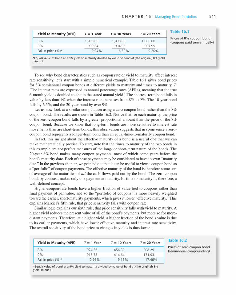
C H A P T E R 1 6 Managing Bond Portfolios 511
To see why bond characteristics such as coupon rate or yield to maturity affect interest rate sensitivity, let’s start with a simple numerical example. Table 16.1 gives bond prices for 8% semiannual coupon bonds at different yields to maturity and times to maturity, T.
[The interest rates are expressed as annual percentage rates (APRs), meaning that the true 6-month yield is doubled to obtain the stated annual yield.] The shortest-term bond falls in value by less than 1% when the interest rate increases from 8% to 9%. The 10-year bond falls by 6.5%, and the 20-year bond by over 9%.
Let us now look at a similar computation using a zero-coupon bond rather than the 8% coupon bond. The results are shown in Table 16.2 . Notice that for each maturity, the price of the zero-coupon bond falls by a greater proportional amount than the price of the 8% coupon bond. Because we know that long-term bonds are more sensitive to interest rate movements than are short-term bonds, this observation suggests that in some sense a zero-coupon bond represents a longer-term bond than an equal-time-to-maturity coupon bond.
In fact, this insight about the effective maturity of a bond is a useful one that we can make mathematically precise. To start, note that the times to maturity of the two bonds in this example are not perfect measures of the long- or short-term nature of the bonds. The 20-year 8% bond makes many coupon payments, most of which come years before the bond’s maturity date. Each of these payments may be considered to have its own “maturity date.” In the previous chapter, we pointed out that it can be useful to view a coupon bond as a “portfolio” of coupon payments. The effective maturity of the bond is therefore some sort of average of the maturities of all the cash flows paid out by the bond. The zero-coupon bond, by contrast, makes only one payment at maturity. Its time to maturity is, therefore, a well-defined concept.
Higher-coupon-rate bonds have a higher fraction of value tied to coupons rather than final payment of par value, and so the “portfolio of coupons” is more heavily weighted toward the earlier, short-maturity payments, which gives it lower “effective maturity.” This explains Malkiel’s fifth rule, that price sensitivity falls with coupon rate.
Similar logic explains our sixth rule, that price sensitivity falls with yield to maturity. A higher yield reduces the present value of all of the bond’s payments, but more so for more-distant payments. Therefore, at a higher yield, a higher fraction of the bond’s value is due to its earlier payments, which have lower effective maturity and interest rate sensitivity. The overall sensitivity of the bond price to changes in yields is thus lower.
Table 16.1
Prices of 8% coupon bond (coupons paid semiannually)
Yield to Maturity (APR) T 5 1 Year T 5 10 Years T 5 20 Years
8% 1,000.00 1,000.00 1,000.00
9% 990.64 934.96 907.99
Fall in price (%)* 0.94% 6.50% 9.20%
*Equals value of bond at a 9% yield to maturity divided by value of bond at (the original) 8% yield, minus 1.
Yield to Maturity (APR) T 5 1 Year T 5 10 Years T 5 20 Years
8% 924.56 456.39 208.29
9% 915.73 414.64 171.93
Fall in price (%)* 0.96% 9.15% 17.46%
*Equals value of bond at a 9% yield to maturity divided by value of bond at (the original) 8% yield, minus 1.
Table 16.2
Prices of zero-coupon bond (semiannual compounding)

512 P A R T I V Fixed-Income Securities
Duration
To deal with the ambiguity of the “maturity” of a bond making many payments, we need a measure of the average maturity of the bond’s promised cash flows. We would like also to use such an effective maturity measure as a guide to the sensitivity of a bond to interest rate changes, because we have noted that price sensitivity tends to increase with time to maturity.
Frederick Macaulay 3 termed the effective maturity concept the duration of the bond. Macaulay’s duration equals the weighted average of the times to each coupon or princi-pal payment. The weight associated with each payment time clearly should be related to the “importance” of that payment to the value of the bond. In fact, the weight applied to each payment time is the proportion of the total value of the bond accounted for by that payment, that is, the present value of the payment divided by the bond price.
We define the weight, w t , associated with the cash flow made at time t (denoted CF t ) as:
wt 5CFt / (1 1 y)
t
Bond price
where y is the bond’s yield to maturity. The numerator on the right-hand side of this equa-tion is the present value of the cash flow occurring at time t while the denominator is the value of all the bond’s payments. These weights sum to 1.0 because the sum of the cash flows discounted at the yield to maturity equals the bond price.
Using these values to calculate the weighted average of the times until the receipt of each of the bond’s payments, we obtain Macaulay’s duration formula:
D 5 aT
t51
t 3 wt (16.1)
As an example of the application of Equation 16.1 , we derive in Spreadsheet 16.1 the durations of an 8% coupon and zero-coupon bond, each with 2 years to maturity. We
3 Frederick Macaulay, Some Theoretical Problems Suggested by the Movements of Interest Rates, Bond Yields,
and Stock Prices in the United States since 1856 (New York: National Bureau of Economic Research, 1938).
Spreadsheet 16.1
Calculating the duration of two bonds
Column sums subject to rounding error.
eXce lPlease visit us at www.mhhe.com/bkm
A C D E F G
Time until PV of CF Column (C)
Payment (Discount rate = times
Period (Years) Cash Flow 5% per period) Weight* Column (F)
A. 8% coupon bond 1 0.5 38.095 0.0395
2 1.0 36.281 0.0376 0.03763 1.5 34.554 0.0358 0.0537
4 2.0 855.611 0.8871 1.7741
Sum: 964.540 1.0000 1.8852
B. Zero-coupon 1 0.5 0.000 0.0000 0.0000
2 1.0 0.000 0.0000 0.0000
3 1.5 0.000 0.0000 0.0000
4 2.0 822.702 1.0000 2.0000
Sum: 822.702 1.0000 2.0000
Semiannual int rate:
0.0197
*Weight = Present value of each payment (column E) divided by the bond price.
1
2
3
4
5
6
7
8
9
10
11
12
13
14
15
16
17
18
B
40
40
40
1040
0
0
0
1000
0.05

C H A P T E R 1 6 Managing Bond Portfolios 513
assume that the yield to maturity on each bond is 10%, or 5% per half-year. The present value of each payment is discounted at 5% per period for the number of (semiannual) peri-ods shown in column B. The weight associated with each payment time (column F) is the present value of the payment for that period (column E) divided by the bond price (the sum of the present values in column E).
The numbers in column G are the products of time to payment and payment weight. Each of these products corresponds to one of the terms in Equation 16.1. According to that equation, we can calculate the duration of each bond by adding the numbers in column G.
The duration of the zero-coupon bond is exactly equal to its time to maturity, 2 years. This makes sense, because with only one payment, the average time until payment must be the bond’s maturity. In contrast, the 2-year coupon bond has a shorter duration of 1.8852 years.
Spreadsheet 16.2 shows the spreadsheet formulas used to produce the entries in Spreadsheet 16.1 . The inputs in the spreadsheet—specifying the cash flows the bond will pay—are given in columns B–D. In column E we calculate the present value of each cash flow using the assumed yield to maturity, in column F we calculate the weights for Equation 16.1 , and in column G we compute the product of time to payment and payment weight. Each of these terms corresponds to one of the values that is summed in Equation 16.1. The sums computed in cells G8 and G14 are therefore the durations of each bond. Using the spreadsheet, you can easily answer several “what if” questions such as the one in Concept Check 1.
CONCEPT CHECK
1Suppose the interest rate decreases to 9% as an annual percentage rate. What will happen to the prices and durations of the two bonds in Spreadsheet 16.1?
Duration is a key concept in fixed-income portfolio management for at least three rea-sons. First, as we have noted, it is a simple summary statistic of the effective average matu-rity of the portfolio. Second, it turns out to be an essential tool in immunizing portfolios
Spreadsheet 16.2
Spreadsheet formulas for calculating duration
eXce lPlease visit us at www.mhhe.com/bkm
1
2
3
4
5
6
7
8
9
10
11
12
13
14
15
16
Time until PV of CF Column (C)
Payment (Discount rate = times
Period (Years) Cash Flow 5% per period) Weight Column (F)
A. 8% coupon bond 1
2
3
4
Sum:
B. Zero-coupon 1
2
3
4
0.5
1
1.5
2
0.5
1
1.5
2
Sum:
=D4/(1+$B$16)^B4
=D5/(1+$B$16)^B5
=D6/(1+$B$16)^B6
=D7/(1+$B$16)^B7
=SUM(E4:E7)
=D10/(1+$B$16)^B10
=D11/(1+$B$16)^B11
=D12/(1+$B$16)^B12
=D13/(1+$B$16)^B13
=SUM(E10:E13)
=E4/E$8
=E5/E$8
=E6/E$8
=E7/E$8
=SUM(F4:F7)
=E10/E$14
=E11/E$14
=E12/E$14
=E13/E$14
=SUM(F10:F13)
Semiannual int rate:
=F5*C5
=F6*C6
=F7*C7
=SUM(G4:G7)
=F10*C10
=F11*C11
=F12*C12
=F13*C13
=SUM(G10:G13)
=F4*C4
A C D E F GB
40
40
40
1040
0
0
0
1000
0.05

514 P A R T I V Fixed-Income Securities
from interest rate risk. We explore this application in Section 16.3 . Third, duration is a measure of the interest rate sensitivity of a portfolio, which we explore here.
We have seen that long-term bonds are more sensitive to interest rate movements than are short-term bonds. The duration measure enables us to quantify this relationship. Specifically, it can be shown that when interest rates change, the proportional change in a bond’s price can be related to the change in its yield to maturity, y, according to the rule
DP
P5 2D 3 BD(1 1 y)
1 1 yR (16.2)
The proportional price change equals the proportional change in 1 plus the bond’s yield times the bond’s duration.
Practitioners commonly use Equation 16.2 in a slightly different form. They define modi-
fied duration as D * 5 D /(1 1 y ), note that D(1 1 y ) 5 D y, and rewrite Equation 16.2 as
DP
P5 2D *Dy (16.3)
The percentage change in bond price is just the product of modified duration and the change in the bond’s yield to maturity. Because the percentage change in the bond price is proportional to modified duration, modified duration is a natural measure of the bond’s exposure to changes in interest rates. Actually, as we will see below, Equation 16.2 , or equivalently 16.3, is only approximately valid for large changes in the bond’s yield. The approximation becomes exact as one considers smaller, or localized, changes in yields. 4
4 Students of calculus will recognize that modified duration is proportional to the derivative of the bond’s price with respect to changes in the bond’s yield. For small changes in yield, Equation 16.3 can be restated as
D* 5 21
P dP
dy
As such, it gives a measure of the slope of the bond price curve only in the neighborhood of the current price. In fact, Equation 16.3 can be derived by differentiating the following bond pricing equation with respect to y:
P 5 aT
t51
CFt
(1 1 y)t
where CF t is the cash flow paid to the bondholder at date t; CF t represents either a coupon payment before matu-rity or final coupon plus par value at the maturity date.
Example 16.1 Duration
Consider the 2-year maturity, 8% coupon bond in Spreadsheet 16.1 making semiannual coupon payments and selling at a price of $964.540, for a yield to maturity of 10%. The duration of this bond is 1.8852 years. For comparison, we will also consider a zero-coupon bond with maturity and duration of 1.8852 years. As we found in Spreadsheet 16.1 , because the coupon bond makes payments semiannually, it is best to treat one “period” as a half-year. So the duration of each bond is 1.8852 3 2 5 3.7704 (semiannual) periods, with a per period interest rate of 5%. The modified duration of each bond is therefore 3.7704/1.05 5 3.591 periods.
Suppose the semiannual interest rate increases from 5% to 5.01%. According to Equation 16.3 , the bond prices should fall by
DP / P 5 2D *Dy 5 23.591 3 .01% 5 2.03591%

C H A P T E R 1 6 Managing Bond Portfolios 515
What Determines Duration?
Malkiel’s bond price relations, which we laid out in the previous section, characterize the determinants of interest rate sensitivity. Duration allows us to quantify that sensitiv-ity, which greatly enhances our ability to formulate investment strategies. For example, if we wish to speculate on interest rates, duration tells us how strong a bet we are making. Conversely, if we wish to remain “neutral” on rates, and simply match the interest rate sensitivity of a chosen bond-market index, duration allows us to measure that sensitivity and mimic it in our own portfolio. For these reasons, it is crucial to understand the deter-minants of duration. Therefore, in this section, we present several “rules” that summarize most of its important properties. These rules are also illustrated in Figure 16.2 , where dura-tions of bonds of various coupon rates, yields to maturity, and times to maturity are plotted.
We have already established:
Rule 1 for Duration The duration of a zero-coupon bond equals its time to maturity.
We have also seen that a coupon bond has a lower duration than a zero with equal matu-rity because coupons early in the bond’s life lower the bond’s weighted average time until payments. This illustrates another general property:
Rule 2 for Duration Holding maturity constant, a bond’s duration is lower when the coupon rate is higher.
This property corresponds to Malkiel’s fifth relationship and is attributable to the impact of early coupon payments on the weighted-average maturity of a bond’s payments. The higher these coupons, the higher the weights on the early payments and the lower is the weighted average maturity of the payments. In other words, a higher fraction of the total value of the bond is tied up in the (earlier) coupon payments whose values are relatively insensitive to yields rather than the (later and more yield-sensitive) repayment of par value. Compare the plots in Figure 16.2 of the durations of the 3% coupon and 15% coupon bonds, each with identical yields of 15%. The plot of the duration of the 15% coupon bond lies below the corresponding plot for the 3% coupon bond.
CONCEPT CHECK
2
a. In Concept Check 1, you calculated the price and duration of a 2-year maturity, 8% cou-pon bond making semiannual coupon payments when the market interest rate is 9%. Now suppose the interest rate increases to 9.05%. Calculate the new value of the bond and the percentage change in the bond’s price.
b. Calculate the percentage change in the bond’s price predicted by the duration formula in Equation 16.2 or 16.3. Compare this value to your answer for ( a ).
Now compute the price change of each bond directly. The coupon bond, which ini-tially sells at $964.540, falls to $964.1942 when its yield increases to 5.01%, which is a percentage decline of .0359%. The zero-coupon bond initially sells for $1,000/1.05 3.7704 5 831.9704. At the higher yield, it sells for $1,000/1.0501 3.7704 5 831.6717. This price also falls by .0359%.
We conclude that bonds with equal durations do in fact have equal interest rate sensitiv-ity and that (at least for small changes in yields) the percentage price change is the modi-fied duration times the change in yield.
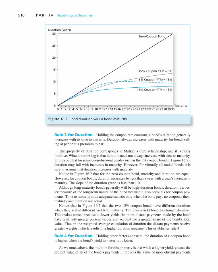
516 P A R T I V Fixed-Income Securities
Rule 3 for Duration Holding the coupon rate constant, a bond’s duration generally increases with its time to maturity. Duration always increases with maturity for bonds sell-ing at par or at a premium to par.
This property of duration corresponds to Malkiel’s third relationship, and it is fairly intuitive. What is surprising is that duration need not always increase with time to maturity. It turns out that for some deep-discount bonds (such as the 3% coupon bond in Figure 16.2 ), duration may fall with increases in maturity. However, for virtually all traded bonds it is safe to assume that duration increases with maturity.
Notice in Figure 16.2 that for the zero-coupon bond, maturity and duration are equal. However, for coupon bonds, duration increases by less than a year with a year’s increase in maturity. The slope of the duration graph is less than 1.0.
Although long-maturity bonds generally will be high-duration bonds, duration is a bet-ter measure of the long-term nature of the bond because it also accounts for coupon pay-ments. Time to maturity is an adequate statistic only when the bond pays no coupons; then, maturity and duration are equal.
Notice also in Figure 16.2 that the two 15% coupon bonds have different durations when they sell at different yields to maturity. The lower-yield bond has longer duration. This makes sense, because at lower yields the more distant payments made by the bond have relatively greater present values and account for a greater share of the bond’s total value. Thus in the weighted-average calculation of duration the distant payments receive greater weights, which results in a higher duration measure. This establishes rule 4:
Rule 4 for Duration Holding other factors constant, the duration of a coupon bond is higher when the bond’s yield to maturity is lower.
As we noted above, the intuition for this property is that while a higher yield reduces the present value of all of the bond’s payments, it reduces the value of more-distant payments
Duration (years)
Zero-Coupon Bond
15% Coupon YTM = 15%
3% Coupon YTM = 15%
15% Coupon YTM = 6%
0 1 2 3 4 5 6 7 8 9 10 11 12 13 14 15 16 17 18 19 20 21 22 23 24 25 26 27 28 29 30Maturity
30
25
20
15
10
5
0
Figure 16.2 Bond duration versus bond maturity

C H A P T E R 1 6 Managing Bond Portfolios 517
by a greater proportional amount. Therefore, at higher yields a higher fraction of the total value of the bond lies in its earlier payments, thereby reducing effective maturity. Rule 4, which is the sixth bond-pricing relationship above, applies to coupon bonds. For zeros, of course, duration equals time to maturity, regardless of the yield to maturity.
Finally, we present a formula for the duration of a perpetuity. This rule is derived from and consistent with the formula for duration given in Equation 16.1 but may be easier to use for infinitely lived bonds.
Rule 5 for Duration The duration of a level perpetuity is
Duration of perpetuity 51 1 y
y (16.4)
For example, at a 10% yield, the duration of a perpetuity that pays $100 once a year forever is 1.10/.10 5 11 years, but at an 8% yield it is 1.08/.08 5 13.5 years.
CONCEPT CHECK
3Show that the duration of the perpetuity increases as the interest rate decreases in accor-dance with rule 4.
Equation 16.4 makes it obvious that maturity and duration can differ substantially. The maturity of the perpetuity is infinite, whereas the duration of the instrument at a 10% yield is only 11 years. The present-value-weighted cash flows early on in the life of the perpetu-ity dominate the computation of duration.
Notice from Figure 16.2 that as their maturities become ever longer, the durations of the two coupon bonds with yields of 15% both converge to the duration of the perpetuity with the same yield, 7.67 years.
The equations for the durations of coupon bonds are somewhat tedious and spread-sheets like Spreadsheet 16.1 are cumbersome to modify for different maturities and cou-pon rates. Moreover, they assume that the bond is at the beginning of a coupon payment period. Fortunately, spreadsheet programs such as Excel come with generalizations of these equations that can accommodate bonds between coupon payment dates. Spreadsheet 16.3 illustrates how to use Excel to compute duration. The spreadsheet uses many of the same conventions as the bond-pricing spreadsheets described in Chapter 14.
Spreadsheet 16.3
Using Excel functions to compute duration
eXce lPlease visit us at www.mhhe.com/bkm
1
2
3
4
5
6
7
8
9
10
A B C
Inputs
Settlement date
Formula in column B
Modified duration
Macaulay duration
Outputs
Coupons per year
Yield to maturity
Coupon rate
Maturity date
=MDURATION(B2,B3,B4,B5,B6)
=DURATION(B2,B3,B4,B5,B6)
2
0.10
0.08
=DATE(2002,1,1)
=DATE(2000,1,1)1/1/2000
1.7955
1.8852
2
0.10
1/1/2002
0.08

518 P A R T I V Fixed-Income Securities
The settlement date (i.e., today’s date) and maturity date are entered in cells B2 and B3 using Excel’s date function, DATE(year, month, day). The coupon and maturity rates are entered as decimals in cells B4 and B5, and the payment periods per year are entered in cell B6. Macaulay and modified duration appear in cells B9 and B10. The spreadsheet confirms that the duration of the bond we looked at in Spreadsheet 16.1 is indeed 1.8852 years. For this 2-year maturity bond, we don’t have a specific settlement date. We arbitrarily set the settlement date to January 1, 2000, and use a maturity date precisely 2 years later.
CONCEPT CHECK
4
Use Spreadsheet 16.3 to test some of the rules for duration presented a few pages ago. What happens to duration when you change the coupon rate of the bond? The yield to maturity? The maturity? What happens to duration if the bond pays its coupons annually rather than semiannually? Why intuitively is duration shorter with semiannual coupons?
Durations can vary widely among traded bonds. Table 16.3 presents durations com-puted from Spreadsheet 16.3 for several bonds all paying semiannual coupons and yielding 4% per half-year. Notice that duration decreases as coupon rates increase, and increases with time to maturity. According to Table 16.3 and Equation 16.2 , if the interest rate were to increase from 8% to 8.1%, the 6% coupon 20-year bond would fall in value by about 10.922 3 .1%/1.04 5 1.05%, whereas the 10% coupon 1-year bond would fall by only .976 3 .1%/1.04 5 .094%. 5 Notice also from Table 16.3 that duration is independent of coupon rate only for perpetuities.
16.2 Convexity
As a measure of interest rate sensitivity, duration clearly is a key tool in fixed-income portfolio management. Yet the duration rule for the impact of interest rates on bond prices is only an approximation. Equation 16.2 , or its equivalent, 16.3, which we repeat here, states that the percentage change in the value of a bond approximately equals the product of modified duration times the change in the bond’s yield:
DP
P5 2D *Dy
This equation asserts that the percentage price change is directly proportional to the change in the bond’s yield. If this were exactly so, however, a graph of the percentage
5 Notice that because the bonds pay their coupons semiannually, we calculate modified duration using the semian-nual yield to maturity, 4%, in the denominator.
Coupon Rates (per Year)
Years to Maturity 6% 8% 10% 12%
1 0.985 0.981 0.976 0.972
5 4.361 4.218 4.095 3.990
10 7.454 7.067 6.772 6.541
20 10.922 10.292 9.870 9.568
Infinite (perpetuity) 13.000 13.000 13.000 13.000
Table 16.3
Bond durations (yield to maturity 5 8% APR; semiannual coupons)

C H A P T E R 1 6 Managing Bond Portfolios 519
change in bond price as a func-tion of the change in its yield would plot as a straight line, with slope equal to 2 D *. Yet Figure 16.1 makes it clear that the relationship between bond prices and yields is not linear. The duration rule is a good approximation for small changes in bond yield, but it is less accu-rate for larger changes.
Figure 16.3 illustrates this point. Like Figure 16.1 , the figure presents the percentage change in bond price in response to a change in the bond’s yield to maturity. The curved line is the percentage price change for a 30-year maturity, 8% annual payment coupon bond, selling at an initial yield to maturity of 8%. The straight line is the percent-age price change predicted by the duration rule. The slope of the straight line is the modi-fied duration of the bond at its initial yield to maturity. The modified duration of the bond at this yield is 11.26 years, so the straight line is a plot of 2 D *D y 5 2 11.26 3 D y. Notice that the two plots are tangent at the initial yield. Thus for small changes in the bond’s yield to maturity, the duration rule is quite accurate. However, for larger changes in yield, there is progressively more “daylight” between the two plots, demonstrating that the duration rule becomes progressively less accurate.
Notice from Figure 16.3 that the duration approximation (the straight line) always understates the value of the bond; it underestimates the increase in bond price when the yield falls, and it overestimates the decline in price when the yield rises. This is due to the curvature of the true price-yield relationship. Curves with shapes such as that of the price-yield relationship are said to be convex, and the curvature of the price-yield curve is called the convexity of the bond.
We can quantify convexity as the rate of change of the slope of the price-yield curve, expressed as a fraction of the bond price. 6 As a practical rule, you can view bonds with higher convexity as exhibiting higher curvature in the price-yield relationship. The convex-ity of noncallable bonds such as that in Figure 16.3 is positive: The slope increases (i.e., becomes less negative) at higher yields.
6 We pointed out in footnote 4 that Equation 16.3 for modified duration can be written as dP / P 5 2 D * dy. Thus D * 5 1/ P 3 dP / dy is the slope of the price-yield curve expressed as a fraction of the bond price. Similarly, the convexity of a bond equals the second derivative (the rate of change of the slope) of the price-yield curve divided by bond price: Convexity 5 1/ P 3 d 2 P / dy 2 . The formula for the convexity of a bond with a maturity of T years making annual coupon payments is
Convexity 51
P 3 (1 1 y)2aT
t51
B CFt
(1 1 y)t (t2 1 t)R
where CF t is the cash flow paid to the bondholder at date t; CF t represents either a coupon payment before matu-rity or final coupon plus par value at the maturity date.
Perc
enta
ge
Ch
ang
e in
Bo
nd
Pri
ce
Change in Yield to Maturity (%)
Actual Price Change
100
80
60
40
20
0
−20
−40
−60−5
−4
−3
−2
−1 0 1 2 3 4 5
Duration Approximation
Figure 16.3 Bond price convexity: 30-year maturity, 8% coupon bond; initial yield to maturity 5 8%

520 P A R T I V Fixed-Income Securities
Convexity allows us to improve the duration approximation for bond price changes. Accounting for convexity, Equation 16.3 can be modified as follows: 7
�
�� �y � � � (�P
PD y* )2Convexity 1 2 (16.5)
The first term on the right-hand side is the same as the duration rule, Equation 16.3. The second term is the modification for convexity. Notice that for a bond with positive convex-ity, the second term is positive, regardless of whether the yield rises or falls. This insight corresponds to the fact noted just above that the duration rule always underestimates the new value of a bond following a change in its yield. The more accurate Equation 16.5 , which accounts for convexity, always predicts a higher bond price than Equation 16.2. Of course, if the change in yield is small, the convexity term, which is multiplied by (D y ) 2 in Equation 16.5 , will be extremely small and will add little to the approximation. In this case, the linear approximation given by the duration rule will be sufficiently accurate. Thus con-vexity is more important as a practical matter when potential interest rate changes are large.
7To use the convexity rule, you must express interest rates as decimals rather than percentages.
Example 16.2 Convexity
The bond in Figure 16.3 has a 30-year maturity, an 8% coupon, and sells at an initial yield to maturity of 8%. Because the coupon rate equals yield to maturity, the bond sells at par value, or $1,000. The modified duration of the bond at its initial yield is 11.26 years, and its convex-ity is 212.4, which can be verified using the formula in footnote 6. (You can find a spreadsheet to calculate the convexity of a 30-year bond at the Online Learning Center at www.mhhe
.com/bkm. ) If the bond’s yield increases from 8% to 10%, the bond price will fall to $811.46, a decline of 18.85%. The duration rule, Equation 16.2 , would predict a price decline of
DP
P5 2D * Dy 5 211.26 3 .02 5 2.2252, or 222.52%
which is considerably more than the bond price actually falls. The duration-with-convexity rule, Equation 16.4 , is far more accurate:
��� �y � � � (�
�� � �
P
PD y* )
.11 26 .02 �
2Convexity
2212 4 02 18272. (. ) . ,� �� or �18.27%
1 2
1 2
which is far closer to the exact change in bond price. (Notice that when we use Equation 16.5 , we must express interest rates as decimals rather than percentages. The change in rates from 8% to 10% is represented as D y 5 .02.)
If the change in yield were smaller, say, .1%, convexity would matter less. The price of the bond actually would fall to $988.85, a decline of 1.115%. Without accounting for convexity, we would predict a price decline of
DP
P5 2D * Dy 5 211.26 3 .001 5 2.01126, or 21.126%
Accounting for convexity, we get almost the precisely correct answer:
��� � � � ��
P
P11 26 001 � 212 4 001 011152. . . (. ) . , or ��1 115. %1 2
Nevertheless, the duration rule is quite accurate in this case, even without accounting for convexity.

C H A P T E R 1 6 Managing Bond Portfolios 521
Why Do Investors Like Convexity?
Convexity is generally consid-ered a desirable trait. Bonds with greater curvature gain more in price when yields fall than they lose when yields rise. For example, in Figure 16.4 bonds A and B have the same duration at the initial yield. The plots of their proportional price changes as a function of inter-est rate changes are tangent, meaning that their sensitivities to changes in yields at that point are equal. However, bond A is more convex than bond B. It enjoys greater price increases and smaller price decreases when interest rates fluctuate by larger amounts. If interest rates are volatile, this is an attractive asymmetry that increases the expected return on the bond, because bond A will benefit more from rate decreases and suffer less from rate increases. Of course, if convexity is desirable, it will not be available for free: investors will have to pay higher prices and accept lower yields to maturity on bonds with greater convexity.
Duration and Convexity of Callable Bonds
Look at Figure 16.5 , which depicts the price-yield curve for a callable bond. When inter-est rates are high, the curve is convex, as it would be for a straight bond. For example, at an interest rate of 10%, the price-yield curve lies above its tangency line. But as rates fall, there is a ceiling on the possible price: The bond cannot be worth more than its call price. So as rates fall, we sometimes say that the bond is subject to price compression—its value is “compressed” to the call price. In this region, for example at an interest rate of 5%, the price-yield curve lies below its tangency line, and the curve is said to have negative
convexity. 8 Notice that in the region of negative convexity, the price-yield curve exhibits an
unattractive asymmetry. Interest rate increases result in a larger price decline than the price gain corresponding to an interest rate decrease of equal magnitude. The asym-metry arises from the fact that the bond issuer has retained an option to call back the bond. If rates rise, the bondholder loses, as would be the case for a straight bond. But if rates fall, rather than reaping a large capital gain, the investor may have the bond called back from her. The bondholder is thus in a “heads I lose, tails I don’t win” position. Of course, she was compensated for this unattractive situation when she purchased the bond. Callable bonds sell at lower initial prices (higher initial yields) than otherwise comparable straight bonds.
8 If you’ve taken a calculus course, you will recognize that the curve is concave in this region. However, rather than saying that these bonds exhibit concavity, bond traders prefer the terminology “negative convexity.”
Perc
enta
ge
Ch
ang
e in
Bo
nd
Pri
ce
Change in Yield to Maturity (%)
Bond A
Bond B
100
80
60
40
20
0
−20
−40
−60−5
−4
−3
−2
−1 0 1 2 3 4 5
Figure 16.4 Convexity of two bonds

522 P A R T I V Fixed-Income Securities
The effect of negative convexity is highlighted in Equation 16.5. When convexity is negative, the second term on the right-hand side is necessarily negative, meaning that bond price performance will be worse than would be predicted by the duration approximation. However, callable bonds or, more generally, bonds with “embedded options,” are diffi-cult to analyze in terms of Macaulay’s duration. This is because in the presence of such options, the future cash flows provided by the bonds are no longer known. If the bond may be called, for example, its cash flow stream may be terminated and its principal repaid earlier than was initially anticipated. Because cash flows are random, we can hardly take a weighted average of times until each future cash flow, as would be necessary to compute Macaulay’s duration.
The convention on Wall Street is to compute the effective duration of bonds with embedded options. Effective duration cannot be computed with a simple formula such as 16.1 that requires known cash flows. Instead, more complex bond valuation approaches that account for the embedded options are used, and effective duration is defined as the proportional change in the bond price per unit change in market interest rates:
Effective duration 5 2DP / P
Dr (16.6)
This equation seems merely like a slight manipulation of the modified duration formula 16.3. However, there are important differences. First, note that we do not compute effec-tive duration relative to a change in the bond’s own yield to maturity. (The denominator is D r, not D y. ) This is because for bonds with embedded options, which may be called early, the yield to maturity is often not a relevant statistic. Instead, we calculate price change relative to a shift in the level of the term structure of interest rates. Second, the effective duration formula relies on a pricing methodology that accounts for embedded options.
Bond Price
Region of Negative Convexity(Price-yield curve is below its tangency line.)
Region of PositiveConvexity
05% 10%
Interest Rate
CallPrice
Figure 16.5 Price-yield curve for a callable bond

C H A P T E R 1 6 Managing Bond Portfolios 523
This means that the effective duration will be a function of variables that would not matter to conventional duration, for example, the volatility of interest rates. In contrast, modified or Macaulay duration can be computed directly from the promised bond cash flows and yield to maturity.
Duration and Convexity of Mortgage-Backed Securities
In practice, the biggest market for which call provisions are important is the market for mortgage-backed securities. In recent years, firms have been less apt to issue bonds with call provisions, and the number of outstanding callable corporate bonds has steadily declined. In contrast, the mortgage-backed market grew rapidly over the last two decades. In 2009, the mortgage-backed securities market included about $5.1 trillion of agency-backed pass-throughs and $2.4 trillion of private-label pass-throughs, making it consider-ably larger than the entire corporate bond market ($4.0 trillion).
As described in Chapter 1, lenders that originate mortgage loans commonly sell those loans to federal agencies such as the Federal National Mortgage Association (FNMA, or Fannie Mae) or the Federal Home Loan Mortgage Corporation (FHLMC, or Freddie Mac). The original borrowers (the homeowners) continue to make their monthly payments to their lenders, but the lenders pass these payments along to the agency that has purchased the loan. In turn, the agencies may combine many mortgages into a pool called a mortgage-backed security, and then sell that security in the fixed-income market. These securities are called pass-throughs because the cash flows from the borrowers are first passed through to the agency (Fannie Mae or Freddie Mac) and then passed through again to the ultimate purchaser of the mortgage-backed security. There is also a very large market among private
CONCEPT CHECK
5 What are the differences between Macaulay duration, modified duration, and effective duration?
Example 16.3 Effective Duration
Suppose that a callable bond with a call price of $1,050 is selling today for $980. If the yield curve shifts up by .5%, the bond price will fall to $930. If it shifts down by .5%, the bond price will rise to $1,010. To compute effective duration, we compute:
Dr 5 Assumed increase in rates 2 Assumed decrease in rates
5 .5% 2 (2.5%) 5 1% 5 .01
DP 5 Price at .5% increase in rates 2 Price at .5% decrease in rates
5 $930 2 $1,010 5 2$80
Then the effective duration of the bond is
Effective duration 5 2DP / P
Dr5 2
2$80 / $980
.015 8.16 years
In other words, the bond price changes by 8.16% for a 1 percentage point swing in rates around current values.
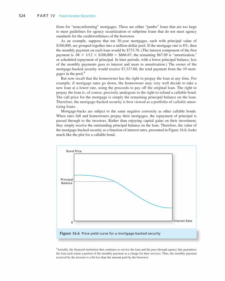
524 P A R T I V Fixed-Income Securities
firms for “nonconforming” mortgages. These are either “jumbo” loans that are too large to meet guidelines for agency securitization or subprime loans that do not meet agency standards for the creditworthiness of the borrower.
As an example, suppose that ten 30-year mortgages, each with principal value of $100,000, are grouped together into a million-dollar pool. If the mortgage rate is 8%, then the monthly payment on each loan would be $733.76. (The interest component of the first payment is .08 3 1/12 3 $100,000 5 $666.67; the remaining $67.09 is “amortization,” or scheduled repayment of principal. In later periods, with a lower principal balance, less of the monthly payments goes to interest and more to amortization.) The owner of the mortgage-backed security would receive $7,337.60, the total payment from the 10 mort-gages in the pool. 9
But now recall that the homeowner has the right to prepay the loan at any time. For example, if mortgage rates go down, the homeowner may very well decide to take a new loan at a lower rate, using the proceeds to pay off the original loan. The right to prepay the loan is, of course, precisely analogous to the right to refund a callable bond. The call price for the mortgage is simply the remaining principal balance on the loan. Therefore, the mortgage-backed security is best viewed as a portfolio of callable amor-tizing loans.
Mortgage-backs are subject to the same negative convexity as other callable bonds. When rates fall and homeowners prepay their mortgages, the repayment of principal is passed through to the investors. Rather than enjoying capital gains on their investment, they simply receive the outstanding principal balance on the loan. Therefore, the value of the mortgage-backed security as a function of interest rates, presented in Figure 16.6 , looks much like the plot for a callable bond.
9 Actually, the financial institution that continues to service the loan and the pass-through agency that guarantees the loan each retain a portion of the monthly payment as a charge for their services. Thus, the monthly payment received by the investor is a bit less than the amount paid by the borrower.
Bond Price
0 Interest Rate
PrincipalBalance
Figure 16.6 Price-yield curve for a mortgage-backed security

C H A P T E R 1 6 Managing Bond Portfolios 525
There are some differences between the mortgage-backs and callable corporate bonds, however. For example, you will commonly find mortgage-backs selling for more than their principal balance. This is because homeowners do not refinance their loans as soon as interest rates drop. Some homeowners do not want to incur the costs or hassles of refi-nancing unless the benefit is great enough, others may decide not to refinance if they are planning to move shortly, and others may simply be unsophisticated in making the refi-nancing decision. Therefore, while the mortgage-backed security exhibits negative con-vexity at low rates, its implicit call price (the principal balance on the loan) is not a firm ceiling on its value.
Simple mortgage-backs have also given rise to a rich set of mortgage-backed deriva-tives. For example, a CMO (collateralized mortgage obligation) further redirects the cash flow stream of the mortgage-backed security to several classes of derivative securities called “tranches.” These tranches may be designed to allocate interest rate risk to investors most willing to bear that risk. 10
The following table is an example of a very simple CMO structure. The underlying mortgage pool is divided into three tranches, each with a different effective maturity and therefore interest rate risk exposure. Suppose the original pool has $10 million of 15-year-maturity mortgages, each with an interest rate of 10.5%, and is subdivided into three tranches as follows:
Tranche A 5 $4 million principal “Short-pay” tranche
Tranche B 5 $3 million principal “Intermediate-pay” tranche
Tranche C 5 $3 million principal “Long-pay” tranche
Suppose further that in each year, 8% of outstanding loans in the pool prepay. Then total cash flows in each year to the whole mortgage pool are given in panel A of Figure 16.7. Total payments shrink by 8% each year, as that percentage of the loans in the original pool is paid off. The light portions of each bar represent interest payments, while the dark portions are principal payments, including both loan amortization and prepayments.
In each period, each tranche receives the interest owed it based on the promised coupon rate and outstanding principal balance. But initially, all principal payments, both prepay-ments and amortization, go to tranche A ( Figure 16.7 , panel B). Notice from panels C and D that tranches B and C receive only interest payments until tranche A is retired. Once tranche A is fully paid off, all principal payments go to tranche B. Finally, when B is retired, all principal payments go to C. This makes tranche A a “short-pay” class, with the lowest effective duration, while tranche C is the longest-pay tranche. This is therefore a relatively simple way to allocate interest rate risk among tranches.
Many variations on the theme are possible and employed in practice. Different tranches may receive different coupon rates. Some tranches may be given preferential treatment in terms of uncertainty over mortgage prepayment speeds. Complex formulas may be used to dictate the cash flows allocated to each tranche. In essence, the mortgage pool is treated as a source of cash flows that can be reallocated to different investors in accordance with the tastes of different investors.
10 In Chapter 14, we examined how collateralized debt obligations or CDOs used tranche structures to reallocate credit risk among different classes. Credit risk in agency-sponsored mortgage-backed securities is not really an issue because the mortgage payments are guaranteed by the agency, and for now, the federal government; in the CMO market, tranche structure is used to allocate interest rate risk rather than credit risk across classes.
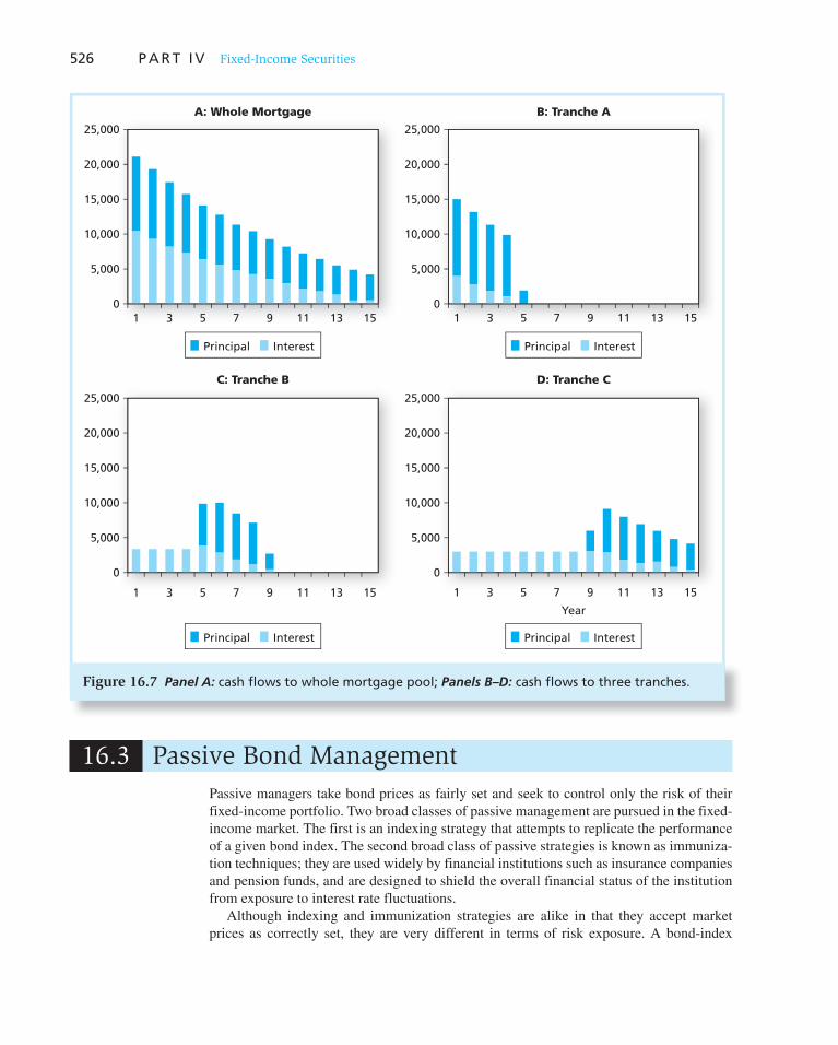
526 P A R T I V Fixed-Income Securities
16.3 Passive Bond Management
Passive managers take bond prices as fairly set and seek to control only the risk of their fixed-income portfolio. Two broad classes of passive management are pursued in the fixed-income market. The first is an indexing strategy that attempts to replicate the performance of a given bond index. The second broad class of passive strategies is known as immuniza-tion techniques; they are used widely by financial institutions such as insurance companies and pension funds, and are designed to shield the overall financial status of the institution from exposure to interest rate fluctuations.
Although indexing and immunization strategies are alike in that they accept market prices as correctly set, they are very different in terms of risk exposure. A bond-index
25,000
20,000
15,000
10,000
5,000
01 3 5 7 9 11 13 15
Principal Interest
A: Whole Mortgage
20,000
25,000
15,000
10,000
5,000
01 3 5 7 9 11 13 15
Principal Interest
B: Tranche A
Principal Interest
1 3 5 7 9 11 13 15
15,000
20,000
25,000
10,000
5,000
0
C: Tranche B
15,000
20,000
25,000
10,000
5,000
0
Principal Interest
1 3 5 7 9 11 13 15
D: Tranche C
Year
Figure 16.7 Panel A: cash flows to whole mortgage pool; Panels B–D: cash flows to three tranches.

C H A P T E R 1 6 Managing Bond Portfolios 527
portfolio will have the same risk–reward profile as the bond market index to which it is tied. In contrast, immunization strategies seek to establish a virtually zero-risk profile, in which interest rate movements have no impact on the value of the firm. We discuss both types of strategies in this section.
Bond-Index Funds
In principle, bond market indexing is similar to stock market indexing. The idea is to create a portfolio that mirrors the composition of an index that measures the broad market. In the U.S. equity market, for example, the S&P 500 is the most commonly used index for stock-index funds, and these funds simply buy shares of each firm in the S&P 500 in proportion to the market value of outstanding equity. A similar strategy is used for bond-index funds, but as we shall see shortly, several modifications are required because of difficulties unique to the bond market and its indexes.
Three major indexes of the broad bond market are the Barclays Capital U.S. (formerly Lehman) Aggregate Bond Index, the Salomon Broad Investment Grade (BIG) Index, and the Merrill Lynch Domestic Master index. All are market-value-weighted indexes of total returns. All three include government, corporate, mortgage-backed, and Yankee bonds in their universes. (Yankee bonds are dollar-denominated, SEC-registered bonds of foreign issuers sold in the United States.)
The first problem that arises in the formation of an indexed bond portfolio arises from the fact that these indexes include thousands of securities, making it quite difficult to pur-chase each security in the index in proportion to its market value. Moreover, many bonds are very thinly traded, meaning that identifying their owners and purchasing the securities at a fair market price can be difficult.
Bond-index funds also face more difficult rebalancing problems than do stock-index funds. Bonds are continually dropped from the index as their maturities fall below 1 year. Moreover, as new bonds are issued, they are added to the index. Therefore, in contrast to equity indexes, the securities used to compute bond indexes constantly change. As they do, the manager must update or rebalance the portfolio to ensure a close match between the composition of the portfolio and the bonds included in the index. The fact that bonds generate considerable interest income that must be reinvested further complicates the job of the index fund manager.
In practice, it is infeasible to precisely replicate the broad bond indexes. Instead, a stratified sampling or cellular approach is often pursued. Figure 16.8 illustrates the idea behind the cellular approach. First, the bond market is stratified into several subclasses. Figure 16.8 shows a simple two-way breakdown by maturity and issuer; in practice, how-ever, criteria such as the bond’s coupon rate or the credit risk of the issuer also would be used to form cells. Bonds falling within each cell are then considered reasonably homo-geneous. Next, the percentages of the entire universe (i.e., the bonds included in the index that is to be matched) falling within each cell are computed and reported, as we have done for a few cells in Figure 16.8. Finally, the portfolio manager establishes a bond portfolio with representation for each cell that matches the representation of that cell in the bond universe. In this way, the characteristics of the portfolio in terms of maturity, coupon rate, credit risk, industrial representation, and so on, will match the characteristics of the index, and the performance of the portfolio likewise should match the index.
Retail investors can buy mutual funds or exchange-traded funds that track the broad bond market. For example, Vanguard’s Total Bond Market Index Fund and Barclays Aggregate Bond Fund iShare (ticker AGG) both track the Barclays index.

528 P A R T I V Fixed-Income Securities
Immunization
In contrast to indexing strategies, many institutions try to insulate their portfolios from interest rate risk altogether. Generally, there are two ways of viewing this risk. Some insti-tutions, such as banks, are concerned with protecting current net worth or net market value against interest rate fluctuations. Other investors, such as pension funds, may face an obli-gation to make payments after a given number of years. These investors are more con-cerned with protecting the future values of their portfolios.
What is common to both investors is interest rate risk. The net worth of the firm or the ability to meet future obligations fluctuates with interest rates. Immunization techniques refer to strategies used by such investors to shield their overall financial status from expo-sure to interest rate fluctuations.
Many banks and thrift institutions have a natural mismatch between asset and liability maturity structures. Bank liabilities are primarily the deposits owed to customers, most of which are very short-term in nature and, consequently, of low duration. Bank assets by contrast are composed largely of outstanding commercial and consumer loans or mort-gages. These assets are of longer duration, and their values are correspondingly more sensitive to interest rate fluctuations. When interest rates increase unexpectedly, banks can suffer serious decreases in net worth—their assets fall in value by more than their liabilities.
Similarly, a pension fund may have a mismatch between the interest rate sensitivity of the assets held in the fund and the present value of its liabilities—the promise to make pay-ments to retirees. The nearby box illustrates the dangers that pension funds face when they neglect to consider the interest rate exposure of both assets and liabilities. For example, in some recent years pension funds lost ground despite the fact that they enjoyed excellent investment returns. As interest rates fell, the value of their liabilities grew even faster than the value of their assets. The lesson is that funds should match the interest rate exposure of assets and liabilities so that the value of assets will track the value of liabilities whether rates rise or fall. In other words, the financial manager might want to immunize the fund against interest rate volatility.
TreasurySector
Termto Maturity
Agency Mortgage-backed
Industrial Finance Utility Yankee
12.1%
4.1%
9.2%
0.1%
3.4%
<1 year
1–3 years
3–5 years
5–7 years
7–10 years
10–15 years
15–30 years
30+ years
5.4%
Figure 16.8 Stratification of bonds into cells
529
Pension funds are not alone in this concern. Any institution with a future fixed obliga-tion might consider immunization a reasonable risk management policy. Insurance compa-nies, for example, also pursue immunization strategies. In fact, the notion of immunization was introduced by F. M. Redington, 11 an actuary for a life insurance company. The idea is that duration-matched assets and liabilities let the asset portfolio meet the firm’s obliga-tions despite interest rate movements.
Consider, for example, an insurance company that issues a guaranteed investment contract, or GIC, for $10,000. (Essentially, GICs are zero-coupon bonds issued by the insurance company to its customers. They are popular products for individuals’ retirement-savings accounts.) If the GIC has a 5-year maturity and a guaranteed interest rate of 8%, the insurance company promises to pay $10,000 3 (1.08) 5 5 $14,693.28 in 5 years.
Suppose that the insurance company chooses to fund its obligation with $10,000 of 8% annual coupon bonds, selling at par value, with 6 years to maturity. As long as the market interest rate stays at 8%, the company has fully funded the obligation, as the present value of the obligation exactly equals the value of the bonds.
Table 16.4A shows that if interest rates remain at 8%, the accumulated funds from the bond will grow to exactly the $14,693.28 obligation. Over the 5-year period, year-end coupon income of $800 is reinvested at the prevailing 8% market interest rate. At the end of the period, the bonds can be sold for $10,000; they still will sell at par value because the coupon rate still equals the market interest rate. Total income after 5 years from reinvested coupons and the sale of the bond is precisely $14,693.28.
If interest rates change, however, two offsetting influences will affect the ability of the fund to grow to the targeted value of $14,693.28. If interest rates rise, the fund will suffer a capital loss, impairing its ability to satisfy the obligation. The bonds will be worth less in 5 years than if interest rates had remained at 8%. However, at a higher interest rate, rein-vested coupons will grow at a faster rate, offsetting the capital loss. In other words, fixed-income investors face two offsetting types of interest rate risk: price risk and reinvestment
rate risk. Increases in interest rates cause capital losses but at the same time increase the rate at which reinvested income will grow. If the portfolio duration is chosen appropriately,
11 F. M. Redington, “Review of the Principle of Life-Office Valuations,” Journal of the Institute of Actuaries 78 (1952).
Pension Funds Lost Ground Despite
Broad Market Gains
With the S&P 500 providing a rate of return in excess of 25%, 2003 was a banner year for the stock market. Not surprisingly, this performance showed up in the balance sheets of U.S. pension funds: assets in these funds rose by more than $100 billion. Despite this boost, pension funds actually lost ground in 2003, with the gap between assets and liabilities growing by about $45 billion.
How could this happen? Blame the decline in inter-est rates during the year that were in large part the force behind the stock market gains. As rates fell dur-ing the year, the present value of pension obligations to retirees rose even faster than the value of the assets backing those promises. It turns out that the value of pension liabilities is more sensitive to interest rate
changes than the value of the typical assets held in those funds. So even though falling rates tend to pump up asset returns, they pump up liabilities even more so. In other words, the duration of fund investments tends to be shorter than the duration of its obligations. This duration mismatch makes funds vulnerable to interest rate declines.
Why don’t funds better match asset and liability durations? One reason is that fund managers are often evaluated based on their performance relative to stan-dard bond market indexes. Those indexes tend to have far shorter durations than pension fund liabilities. So to some extent, managers may be keeping their eyes on the wrong ball, one with the wrong interest rate sensitivity.
WO
RD
S FRO
M TH
E STREET
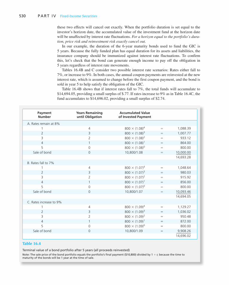
530 P A R T I V Fixed-Income Securities
these two effects will cancel out exactly. When the portfolio duration is set equal to the investor’s horizon date, the accumulated value of the investment fund at the horizon date will be unaffected by interest rate fluctuations. For a horizon equal to the portfolio’s dura-
tion, price risk and reinvestment risk exactly cancel out. In our example, the duration of the 6-year maturity bonds used to fund the GIC is
5 years. Because the fully funded plan has equal duration for its assets and liabilities, the insurance company should be immunized against interest rate fluctuations. To confirm this, let’s check that the bond can generate enough income to pay off the obligation in 5 years regardless of interest rate movements.
Tables 16.4B and C consider two possible interest rate scenarios: Rates either fall to 7%, or increase to 9%. In both cases, the annual coupon payments are reinvested at the new interest rate, which is assumed to change before the first coupon payment, and the bond is sold in year 5 to help satisfy the obligation of the GIC.
Table 16.4B shows that if interest rates fall to 7%, the total funds will accumulate to $14,694.05, providing a small surplus of $.77. If rates increase to 9% as in Table 16.4C , the fund accumulates to $14,696.02, providing a small surplus of $2.74.
Payment Number
Years Remaining until Obligation
Accumulated Value of Invested Payment
A. Rates remain at 8%
1 4 800 3 (1.08)4 5 1,088.39
2 3 800 3 (1.08)3 5 1,007.77
3 2 800 3 (1.08)2 5 933.12
4 1 800 3 (1.08)1 5 864.00
5 0 800 3 (1.08)0 5 800.00
Sale of bond 0 10,800/1.08 5 10,000.00
14,693.28
B. Rates fall to 7%
1 4 800 3 (1.07)4 5 1,048.64
2 3 800 3 (1.07)3 5 980.03
3 2 800 3 (1.07)2 5 915.92
4 1 800 3 (1.07)1 5 856.00
5 0 800 3 (1.07)0 5 800.00
Sale of bond 0 10,800/1.07 5 10,093.46
14,694.05
C. Rates increase to 9%
1 4 800 3 (1.09)4 5 1,129.27
2 3 800 3 (1.09)3 5 1,036.02
3 2 800 3 (1.09)2 5 950.48
4 1 800 3 (1.09)1 5 872.00
5 0 800 3 (1.09)0 5 800.00
Sale of bond 0 10,800/1.09 5 9,908.26
14,696.02
Table 16.4
Terminal value of a bond portfolio after 5 years (all proceeds reinvested) Note: The sale price of the bond portfolio equals the portfolio’s final payment ($10,800) divided by 1 1 r, because the time to maturity of the bonds will be 1 year at the time of sale.
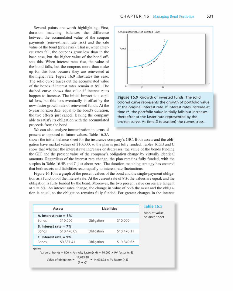
C H A P T E R 1 6 Managing Bond Portfolios 531
Several points are worth highlighting. First, duration matching balances the difference between the accumulated value of the coupon payments (reinvestment rate risk) and the sale value of the bond (price risk). That is, when inter-est rates fall, the coupons grow less than in the base case, but the higher value of the bond off-sets this. When interest rates rise, the value of the bond falls, but the coupons more than make up for this loss because they are reinvested at the higher rate. Figure 16.9 illustrates this case. The solid curve traces out the accumulated value of the bonds if interest rates remain at 8%. The dashed curve shows that value if interest rates happen to increase. The initial impact is a capi-tal loss, but this loss eventually is offset by the now-faster growth rate of reinvested funds. At the 5-year horizon date, equal to the bond’s duration, the two effects just cancel, leaving the company able to satisfy its obligation with the accumulated proceeds from the bond.
We can also analyze immunization in terms of present as opposed to future values. Table 16.5A shows the initial balance sheet for the insurance company’s GIC. Both assets and the obli-gation have market values of $10,000, so the plan is just fully funded. Tables 16.5B and C show that whether the interest rate increases or decreases, the value of the bonds funding the GIC and the present value of the company’s obligation change by virtually identical amounts. Regardless of the interest rate change, the plan remains fully funded, with the surplus in Table 16.5B and C just about zero. The duration-matching strategy has ensured that both assets and liabilities react equally to interest rate fluctuations.
Figure 16.10 is a graph of the present values of the bond and the single-payment obliga-tion as a function of the interest rate. At the current rate of 8%, the values are equal, and the obligation is fully funded by the bond. Moreover, the two present value curves are tangent at y 5 8%. As interest rates change, the change in value of both the asset and the obliga-tion is equal, so the obligation remains fully funded. For greater changes in the interest
Accumulated Value of Invested Funds
0 t* D
t
Funds
Figure 16.9 Growth of invested funds. The solid colored curve represents the growth of portfolio value at the original interest rate. If interest rates increase at time t *, the portfolio value initially falls but increases thereafter at the faster rate represented by the broken curve. At time D (duration) the curves cross.
Table 16.5
Market value balance sheet
Assets Liabilities
A. Interest rate 5 8%
Bonds $10,000 Obligation $10,000
B. Interest rate 5 7%
Bonds $10,476.65 Obligation $10,476.11
C. Interest rate 5 9%
Bonds $9,551.41 Obligation $ 9,549.62
Notes:Value of bonds 5 800 3 Annuity factor(r, 6) 1 10,000 3 PV factor (r, 6)
Value of obligation 514,693.28
(1 1 r)55 14,693.28 3 PV factor (r,5)
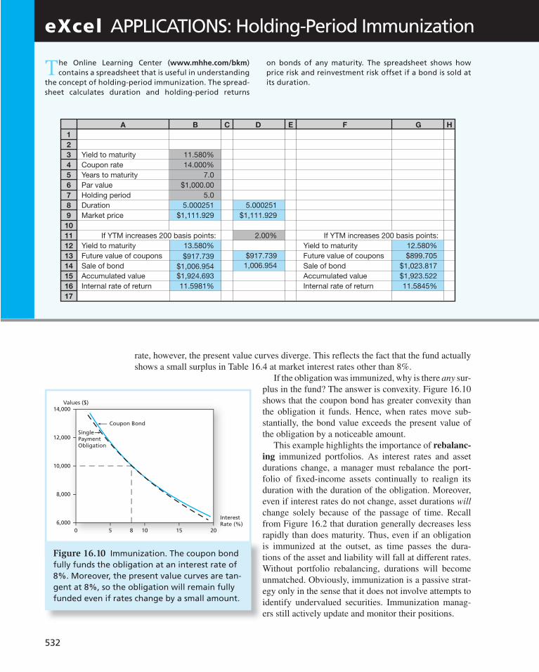
532
rate, however, the present value curves diverge. This reflects the fact that the fund actually shows a small surplus in Table 16.4 at market interest rates other than 8%.
If the obligation was immunized, why is there any sur-plus in the fund? The answer is convexity. Figure 16.10 shows that the coupon bond has greater convexity than the obligation it funds. Hence, when rates move sub-stantially, the bond value exceeds the present value of the obligation by a noticeable amount.
This example highlights the importance of rebalanc-
ing immunized portfolios. As interest rates and asset durations change, a manager must rebalance the port-folio of fixed-income assets continually to realign its duration with the duration of the obligation. Moreover, even if interest rates do not change, asset durations will
change solely because of the passage of time. Recall from Figure 16.2 that duration generally decreases less rapidly than does maturity. Thus, even if an obligation is immunized at the outset, as time passes the dura-tions of the asset and liability will fall at different rates. Without portfolio rebalancing, durations will become unmatched. Obviously, immunization is a passive strat-egy only in the sense that it does not involve attempts to identify undervalued securities. Immunization manag-ers still actively update and monitor their positions.
Values ($)
6,000
Coupon Bond
SinglePaymentObligation
InterestRate (%)
0 5 8 10 15 20
14,000
12,000
10,000
8,000
Figure 16.10 Immunization. The coupon bond fully funds the obligation at an interest rate of 8%. Moreover, the present value curves are tan-gent at 8%, so the obligation will remain fully funded even if rates change by a small amount.
1
2
3
4
5
6
7
8
9
10
11
12
13
14
15
16
17
If YTM increases 200 basis points: If YTM increases 200 basis points:
A B DC E F G H
Yield to maturity
Internal rate of return
Accumulated value
Sale of bond
Future value of coupons
Yield to maturity
Market price
Duration
Holding period
Par value
Years to maturity
Coupon rate
11.580%
11.5981%
$1,924.693
$1,006.954
$917.739
13.580%
$1,111.929
5.000251
5.0
$1,000.00
7.0
14.000%
1,006.954
$917.739
2.00%
$1,111.929
5.000251
Internal rate of return
Yield to maturity
Future value of coupons
Sale of bond
Accumulated value
12.580%
11.5845%
$1,923.522
$1,023.817
$899.705
eXcel APPLICATIONS: Holding-Period Immunization
T he Online Learning Center ( www.mhhe.com/bkm ) contains a spreadsheet that is useful in understanding
the concept of holding-period immunization. The spread-sheet calculates duration and holding-period returns
on bonds of any maturity. The spreadsheet shows how price risk and reinvestment risk offset if a bond is sold at its duration.

C H A P T E R 1 6 Managing Bond Portfolios 533
Even if a position is immunized, however, the portfolio manager still cannot rest. This is because of the need for rebalancing in response to changes in interest rates. Moreover, even if rates do not change, the passage of time also will affect duration and require rebal-ancing. Let us continue Example 16.4 and see how the portfolio manager can maintain an immunized position.
Example 16.5 Rebalancing
Suppose that 1 year has passed, and the interest rate remains at 10%. The portfolio man-ager of Example 16.4 needs to reexamine her position. Is the position still fully funded? Is it still immunized? If not, what actions are required?
First, examine funding. The present value of the obligation will have grown to $11,000, as it is 1 year closer to maturity. The manager’s funds also have grown to $11,000: The zero-coupon bonds have increased in value from $5,000 to $5,500 with the passage of time, while the perpetuity has paid its annual $500 coupons and remains worth $5,000. Therefore, the obligation is still fully funded.
Example 16.4 Constructing an Immunized Portfolio
An insurance company must make a payment of $19,487 in 7 years. The market interest rate is 10%, so the present value of the obligation is $10,000. The company’s portfolio manager wishes to fund the obligation using 3-year zero-coupon bonds and perpetuities paying annual coupons. (We focus on zeros and perpetuities to keep the algebra simple.) How can the manager immunize the obligation?
Immunization requires that the duration of the portfolio of assets equal the duration of the liability. We can proceed in four steps:
1. Calculate the duration of the liability. In this case, the liability duration is simple to compute. It is a single-payment obligation with duration of 7 years.
2. Calculate the duration of the asset portfolio. The portfolio duration is the weighted average of duration of each component asset, with weights proportional to the funds placed in each asset. The duration of the zero-coupon bond is simply its maturity, 3 years. The duration of the perpetuity is 1.10/.10 5 11 years. Therefore, if the fraction of the portfolio invested in the zero is called w and the fraction invested in the perpetuity is (1 2 w ), the portfolio duration will be
Asset duration 5 w 3 3 years 1 (1 2 w) 3 11 years
3. Find the asset mix that sets the duration of assets equal to the 7-year duration of
liabilities. This requires us to solve for w in the following equation:
w 3 3 years 1 (1 2 w) 3 11 years 5 7 years
This implies that w 5 ½. The manager should invest half the portfolio in the zero and half in the perpetuity. This will result in an asset duration of 7 years.
4. Fully fund the obligation. Because the obligation has a present value of $10,000, and the fund will be invested equally in the zero and the perpetuity, the manager must purchase $5,000 of the zero-coupon bond and $5,000 of the perpetuity. (Note that the face value of the zero will be $5,000 3 (1.10) 3 5 $6,655.)

534 P A R T I V Fixed-Income Securities
Of course, rebalancing of the portfolio entails transaction costs as assets are bought or sold, so one cannot rebalance continuously. In practice, an appropriate compromise must be established between the desire for perfect immunization, which requires continual rebalancing, and the need to control trading costs, which dictates less frequent rebalancing.
CONCEPT CHECK
6Look again at Example 16.5. What would be the immunizing weights in the second year if the interest rate had fallen to 8%?
Cash Flow Matching and Dedication
The problems associated with immunization seem to have a simple solution. Why not simply buy a zero-coupon bond that provides a payment in an amount exactly sufficient to cover the projected cash outlay? If we follow the principle of cash flow matching we automatically immunize the portfolio from interest rate movement because the cash flow from the bond and the obligation exactly offset each other.
Cash flow matching on a multiperiod basis is referred to as a dedication strategy. In this case, the manager selects either zero-coupon or coupon bonds that provide total cash flows in each period that match a series of obligations. The advantage of dedication is that it is a once-and-for-all approach to eliminating interest rate risk. Once the cash flows are matched, there is no need for rebalancing. The dedicated portfolio provides the cash neces-sary to pay the firm’s liabilities regardless of the eventual path of interest rates.
Cash flow matching is not more widely pursued probably because of the constraints that it imposes on bond selection. Immunization or dedication strategies are appealing to firms that do not wish to bet on general movements in interest rates, but these firms may want to immunize using bonds that they perceive are undervalued. Cash flow matching, however, places so many more constraints on the bond selection process that it can be impossible to pursue a dedication strategy using only “underpriced” bonds. Firms looking for under-priced bonds give up exact and easy dedication for the possibility of achieving superior returns from the bond portfolio.
Sometimes, cash flow matching is simply not possible. To cash flow match for a pen-sion fund that is obligated to pay out a perpetual flow of income to current and future retirees, the pension fund would need to purchase fixed-income securities with maturities ranging up to hundreds of years. Such securities do not exist, making exact dedication infeasible.
The portfolio weights must be changed, however. The zero-coupon bond now will have a duration of 2 years, while the perpetuity duration remains at 11 years. The obligation is now due in 6 years. The weights must now satisfy the equation
w 3 2 1 (1 2 w) 3 11 5 6
which implies that w 5 5/9. To rebalance the portfolio and maintain the duration match, the manager now must invest a total of $11,000 3 5/9 5 $6,111.11 in the zero-coupon bond. This requires that the entire $500 coupon payment be invested in the zero, with an addi-tional $111.11 of the perpetuity sold and invested in the zero-coupon bond.
C H A P T E R 1 6 Managing Bond Portfolios 535
Other Problems with Conventional Immunization
If you look back at the definition of duration in Equation 16.1 , you note that it uses the bond’s yield to maturity to calculate the weight applied to the time until each coupon payment. Given this definition and limitations on the proper use of yield to maturity, it is perhaps not surprising that this notion of duration is strictly valid only for a flat yield curve for which all payments are discounted at a common interest rate.
If the yield curve is not flat, then the definition of duration must be modified and CF t /(1 1 y ) t replaced with the present value of CF t , where the present value of each cash flow is calculated by discounting with the appropriate spot interest rate from the zero-coupon yield curve corresponding to the date of the particular cash flow, instead of by discounting with the bond’s yield to maturity. Moreover, even with this modification, dura-tion matching will immunize portfolios only for parallel shifts in the yield curve. Clearly, this sort of restriction is unrealistic. As a result, much work has been devoted to general-izing the notion of duration. Multifactor duration models have been developed to allow for tilts and other distortions in the shape of the yield curve, in addition to shifts in its level. However, the added complexity of such models does not appear to pay off in terms of sub-stantially greater effectiveness. 12
Finally, immunization can be an inappropriate goal in an inflationary environment. Immunization is essentially a nominal notion and makes sense only for nominal liabili-ties. It makes no sense to immunize a projected obligation that will grow with the price level using nominal assets such as bonds. For example, if your child will attend college in 15 years and if the annual cost of tuition is expected to be $40,000 at that time, immunizing your portfolio at a locked-in terminal value of $40,000 is not necessarily a risk-reducing strategy. The tuition obligation will vary with the realized inflation rate, whereas the asset portfolio’s final value will not. In the end, the tuition obligation will not necessarily be matched by the value of the portfolio.
16.4 Active Bond Management
Sources of Potential Profit
Broadly speaking, there are two sources of potential value in active bond management. The first is interest rate forecasting, which tries to anticipate movements across the entire spectrum of the fixed-income market. If interest rate declines are anticipated, managers will increase portfolio duration (and vice versa). The second source of potential profit is identification of relative mispricing within the fixed-income market. An analyst, for example, might believe that the default premium on one particular bond is unnecessarily large and therefore that the bond is underpriced.
These techniques will generate abnormal returns only if the analyst’s information or insight is superior to that of the market. You cannot profit from knowledge that rates are about to fall if prices already reflect this information. You know this from our discussion
12 G. O. Bierwag, G. C. Kaufman, and A. Toevs, eds., Innovations in Bond Portfolio Management: Duration
Analysis and Immunization (Greenwich, CT: JAI Press, 1983).
CONCEPT CHECK
7 How would an increase in trading costs affect the attractiveness of dedication versus immunization?

536 P A R T I V Fixed-Income Securities
of market efficiency. Valuable information is differential information. In this context it is worth noting that interest rate forecasters have a notoriously poor track record. If you con-sider this record, you will approach attempts to time the bond market with caution.
Homer and Liebowitz (see footnote 2) coined a popular taxonomy of active bond port-folio strategies. They characterize portfolio rebalancing activities as one of four types of bond swaps. In the first two swaps the investor typically believes that the yield relation-ship between bonds or sectors is only temporarily out of alignment. When the aberration is eliminated, gains can be realized on the underpriced bond. The period of realignment is called the workout period.
1. The substitution swap is an exchange of one bond for a nearly identical substitute. The substituted bonds should be of essentially equal coupon, maturity, quality, call features, sinking fund provisions, and so on. This swap would be motivated by a belief that the market has temporarily mispriced the two bonds, and that the discrepancy between the prices of the bonds represents a profit opportunity.
An example of a substitution swap would be a sale of a 20-year maturity, 8% coupon Toyota bond that is priced to provide a yield to maturity of 8.05%, coupled with a purchase of an 8% coupon Honda bond with the same time to maturity that yields 8.15%. If the bonds have about the same credit rating, there is no apparent reason for the Honda bonds to provide a higher yield. Therefore, the higher yield actually available in the market makes the Honda bond seem relatively attractive. Of course, the equality of credit risk is an important condition. If the Honda bond is in fact riskier, then its higher yield does not represent a bargain.
2. The intermarket spread swap is pursued when an investor believes that the yield spread between two sectors of the bond market is temporarily out of line. For example, if the current spread between corporate and government bonds is consid-ered too wide and is expected to narrow, the investor will shift from government bonds into corporate bonds. If the yield spread does in fact narrow, corporates will outperform governments. For example, if the yield spread between 10-year Trea-sury bonds and 10-year Baa-rated corporate bonds is now 3%, and the historical spread has been only 2%, an investor might consider selling holdings of Treasury bonds and replacing them with corporates. If the yield spread eventually narrows, the Baa-rated corporate bonds will outperform the Treasuries.
Of course, the investor must consider carefully whether there is a good reason that the yield spread seems out of alignment. For example, the default premium on corporate bonds might have increased because the market is expecting a severe recession. In this case, the wider spread would not represent attractive pricing of corporates relative to Treasuries, but would simply be an adjustment for a perceived increase in credit risk.
3. The rate anticipation swap is pegged to interest rate forecasting. In this case if investors believe that rates will fall, they will swap into bonds of longer duration. Conversely, when rates are expected to rise, they will swap into shorter dura-tion bonds. For example, the investor might sell a 5-year maturity Treasury bond, replacing it with a 25-year maturity Treasury bond. The new bond has the same lack of credit risk as the old one, but has longer duration.
4. The pure yield pickup swap is pursued not in response to perceived mispricing, but as a means of increasing return by holding higher-yield bonds. When the yield curve is upward-sloping, the yield pickup swap entails moving into longer-term bonds. This must be viewed as an attempt to earn an expected term premium in higher-yield bonds. The investor is willing to bear the interest rate risk that this

C H A P T E R 1 6 Managing Bond Portfolios 537
strategy entails. The investor who swaps the shorter-term bond for the longer one will earn a higher rate of return as long as the yield curve does not shift up dur-ing the holding period. Of course if it does, the longer-duration bond will suffer a greater capital loss.
We can add a fifth swap, called a tax swap, to this list. This simply refers to a swap to exploit some tax advantage. For example, an investor may swap from one bond that has decreased in price to another if realization of capital losses is advantageous for tax purposes.
Horizon Analysis
One form of interest rate forecasting, which we encountered in Chapter 14, is called horizon analysis. The analyst using this approach selects a particular holding period and predicts the yield curve at the end of that period. Given a bond’s time to maturity at the end of the holding period, its yield can be read from the predicted yield curve and its end-of-period price calculated. Then the analyst adds the coupon income and prospective capital gain of the bond to obtain the total return on the bond over the holding period.
CONCEPT CHECK
8 What will be the rate of return in Example 16.6 if the manager forecasts that in 2 years the yield on 18-year bonds will be 10%, and that the reinvestment rate for coupons will be 8%?
Example 16.6 Horizon Analysis
A 20-year maturity bond with a 10% coupon rate (paid annually) currently sells at a yield to maturity of 9%. A portfolio manager with a 2-year horizon needs to forecast the total return on the bond over the coming 2 years. In 2 years, the bond will have an 18-year maturity. The analyst forecasts that 2 years from now, 18-year bonds will sell at yields to maturity of 8%, and that coupon payments can be reinvested in short-term securities over the coming 2 years at a rate of 7%.
To calculate the 2-year return on the bond, the analyst would perform the following calculations:
1. Current price 5 $100 3 Annuity factor (9%, 20 years)
1 $1,000 3 PV factor (9%, 20 years)
5 $1,091.29
2. Forecast price 5 $100 3 Annuity factor (8%, 18 years)
1 $1,000 3 PV factor (8%, 18 years)
5 $1,187.44
3. The future value of reinvested coupons will be ($100 3 1.07) 1 $100 5 $207
4. The 2-year return is $207 1 ($1,187.44 2 $1,091.29)
$1,091.295 0.278, or 27.8%
The annualized rate of return over the 2-year period would then be (1.278) 1/2 2 1 5 0.13, or 13%.

Vis
it u
s at
ww
w.m
hh
e.co
m/b
km538 P A R T I V Fixed-Income Securities
1. Even default-free bonds such as Treasury issues are subject to interest rate risk. Longer-term bonds generally are more sensitive to interest rate shifts than are short-term bonds. A measure of the average life of a bond is Macaulay’s duration, defined as the weighted average of the times until each payment made by the security, with weights proportional to the present value of the payment.
2. Duration is a direct measure of the sensitivity of a bond’s price to a change in its yield. The pro-portional change in a bond’s price equals the negative of duration multiplied by the proportional change in 1 1 y.
3. Convexity refers to the curvature of a bond’s price-yield relationship. Accounting for convexity can substantially improve on the accuracy of the duration approximation for the response of bond price to changes in yield.
4. Immunization strategies are characteristic of passive fixed-income portfolio management. Such strategies attempt to render the individual or firm immune from movements in interest rates. This may take the form of immunizing net worth or, instead, immunizing the future accumulated value of a fixed-income portfolio.
5. Immunization of a fully funded plan is accomplished by matching the durations of assets and liabilities. To maintain an immunized position as time passes and interest rates change, the port-folio must be periodically rebalanced. Classic immunization also depends on parallel shifts in a flat yield curve. Given that this assumption is unrealistic, immunization generally will be less than complete. To mitigate the problem, multifactor duration models can be used to allow for variation in the shape of the yield curve.
6. A more direct form of immunization is dedication, or cash flow matching. If a portfolio is per-fectly matched in cash flow with projected liabilities, rebalancing will be unnecessary.
7. Active bond management consists of interest rate forecasting techniques and intermarket spread analysis. One popular taxonomy classifies active strategies as substitution swaps, intermarket spread swaps, rate anticipation swaps, or pure yield pickup swaps.
8. Horizon analysis is a type of interest rate forecasting. In this procedure the analyst forecasts the position of the yield curve at the end of some holding period, and from that yield curve predicts corresponding bond prices. Bonds then can be ranked according to expected total returns (coupon plus capital gain) over the holding period.
SUMMARY
Related Web sites for this chapter are available at www.mhhe.com/bkm
Macaulay’s duration modified duration convexity effective duration immunization
rebalancing cash flow matching dedication strategy substitution swap intermarket spread swap
rate anticipation swap pure yield pickup swap tax swap horizon analysis
KEY TERMS
1. Prices of long-term bonds are more volatile than prices of short-term bonds. However, yields to maturity of short-term bonds fluctuate more than yields of long-term bonds. How do you recon-cile these two empirical observations?
2. How can a perpetuity, which has an infinite maturity, have a duration as short as 10 or 20 years?
3. A 9-year bond has a yield of 10% and a duration of 7.194 years. If the market yield changes by 50 basis points, what is the percentage change in the bond’s price?
4. Find the duration of a 6% coupon bond making annual coupon payments if it has 3 years until maturity and has a yield to maturity of 6%. What is the duration if the yield to maturity is 10%?
5. Find the duration of the bond in Problem 4 if the coupons are paid semiannually.
PROBLEM SETS
i. Basic
ii. Intermediate

Vis
it u
s at
ww
w.m
hh
e.co
m/b
km
C H A P T E R 1 6 Managing Bond Portfolios 539
6. The historical yield spread between AAA bonds and Treasury bonds widened dramatically in 2008. If you believe the spread will soon return to more typical historical levels, what should you do? This would be an example of what sort of bond swap?
7. You predict that interest rates are about to fall. Which bond will give you the highest capital gain?
a. Low coupon, long maturity. b. High coupon, short maturity. c. High coupon, long maturity. d. Zero coupon, long maturity.
8. Rank the durations or effective durations of the following pairs of bonds:
a. Bond A is an 8% coupon bond, with a 20-year time to maturity selling at par value. Bond B is an 8% coupon bond, with a 20-year maturity time selling below par value.
b. Bond A is a 20-year noncallable coupon bond with a coupon rate of 8%, selling at par. Bond B is a 20-year callable bond with a coupon rate of 9%, also selling at par.
9. An insurance company must make payments to a customer of $10 million in 1 year and $4 million in 5 years. The yield curve is flat at 10%.
a. If it wants to fully fund and immunize its obligation to this customer with a single issue of a zero-coupon bond, what maturity bond must it purchase?
b. What must be the face value and market value of that zero-coupon bond?
10. Long-term Treasury bonds currently are selling at yields to maturity of nearly 8%. You expect interest rates to fall. The rest of the market thinks that they will remain unchanged over the com-ing year. In each question, choose the bond that will provide the higher holding-period return over the next year if you are correct. Briefly explain your answer.
a. i. A Baa-rated bond with coupon rate 8% and time to maturity 20 years. ii. An Aaa-rated bond with coupon rate of 8% and time to maturity 20 years.
b. i. An A-rated bond with coupon rate 4% and maturity 20 years, callable at 105. ii. An A-rated bond with coupon rate 8% and maturity 20 years, callable at 105.
c. i. A 6% coupon noncallable T-bond with maturity 20 years and YTM 5 8%. ii. A 9% coupon noncallable T-bond with maturity 20 years and YTM 5 8%.
11. Currently, the term structure is as follows: 1-year bonds yield 7%, 2-year bonds yield 8%, 3-year bonds and longer-maturity bonds all yield 9%. An investor is choosing between 1-, 2-, and 3-year maturity bonds all paying annual coupons of 8%, once a year. Which bond should you buy if you strongly believe that at year-end the yield curve will be flat at 9%?
12. You will be paying $10,000 a year in tuition expenses at the end of the next 2 years. Bonds cur-rently yield 8%.
a. What is the present value and duration of your obligation? b. What maturity zero-coupon bond would immunize your obligation? c. Suppose you buy a zero-coupon bond with value and duration equal to your obligation. Now
suppose that rates immediately increase to 9%. What happens to your net position, that is, to the difference between the value of the bond and that of your tuition obligation? What if rates fall to 7%?
13. Pension funds pay lifetime annuities to recipients. If a firm will remain in business indefinitely, the pension obligation will resemble a perpetuity. Suppose, therefore, that you are managing a pension fund with obligations to make perpetual payments of $2 million per year to beneficiar-ies. The yield to maturity on all bonds is 16%.
a. If the duration of 5-year maturity bonds with coupon rates of 12% (paid annually) is 4 years and the duration of 20-year maturity bonds with coupon rates of 6% (paid annually) is 11 years, how much of each of these coupon bonds (in market value) will you want to hold to both fully fund and immunize your obligation?
b. What will be the par value of your holdings in the 20-year coupon bond?
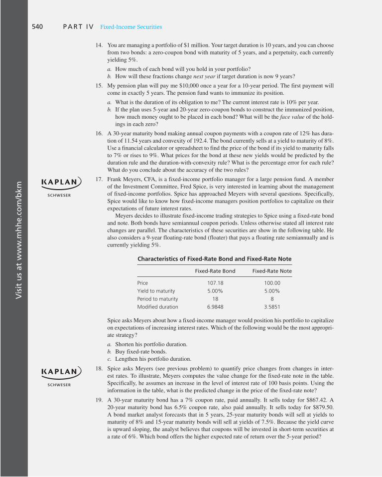
Vis
it u
s at
ww
w.m
hh
e.co
m/b
km540 P A R T I V Fixed-Income Securities
14. You are managing a portfolio of $1 million. Your target duration is 10 years, and you can choose from two bonds: a zero-coupon bond with maturity of 5 years, and a perpetuity, each currently yielding 5%.
a. How much of each bond will you hold in your portfolio? b. How will these fractions change next year if target duration is now 9 years?
15. My pension plan will pay me $10,000 once a year for a 10-year period. The first payment will come in exactly 5 years. The pension fund wants to immunize its position.
a. What is the duration of its obligation to me? The current interest rate is 10% per year. b. If the plan uses 5-year and 20-year zero-coupon bonds to construct the immunized position,
how much money ought to be placed in each bond? What will be the face value of the hold-ings in each zero?
16. A 30-year maturity bond making annual coupon payments with a coupon rate of 12% has dura-tion of 11.54 years and convexity of 192.4. The bond currently sells at a yield to maturity of 8%. Use a financial calculator or spreadsheet to find the price of the bond if its yield to maturity falls to 7% or rises to 9%. What prices for the bond at these new yields would be predicted by the duration rule and the duration-with-convexity rule? What is the percentage error for each rule? What do you conclude about the accuracy of the two rules?
17. Frank Meyers, CFA, is a fixed-income portfolio manager for a large pension fund. A member of the Investment Committee, Fred Spice, is very interested in learning about the management of fixed-income portfolios. Spice has approached Meyers with several questions. Specifically, Spice would like to know how fixed-income managers position portfolios to capitalize on their expectations of future interest rates.
Meyers decides to illustrate fixed-income trading strategies to Spice using a fixed-rate bond and note. Both bonds have semiannual coupon periods. Unless otherwise stated all interest rate changes are parallel. The characteristics of these securities are show in the following table. He also considers a 9-year floating-rate bond (floater) that pays a floating rate semiannually and is currently yielding 5%.
Characteristics of Fixed-Rate Bond and Fixed-Rate Note
Fixed-Rate Bond Fixed-Rate Note
Price 107.18 100.00
Yield to maturity 5.00% 5.00%
Period to maturity 18 8
Modified duration 6.9848 3.5851
Spice asks Meyers about how a fixed-income manager would position his portfolio to capitalize on expectations of increasing interest rates. Which of the following would be the most appropri-ate strategy?
a. Shorten his portfolio duration. b. Buy fixed-rate bonds. c. Lengthen his portfolio duration.
18. Spice asks Meyers (see previous problem) to quantify price changes from changes in inter-est rates. To illustrate, Meyers computes the value change for the fixed-rate note in the table. Specifically, he assumes an increase in the level of interest rate of 100 basis points. Using the information in the table, what is the predicted change in the price of the fixed-rate note?
19. A 30-year maturity bond has a 7% coupon rate, paid annually. It sells today for $867.42. A 20-year maturity bond has 6.5% coupon rate, also paid annually. It sells today for $879.50. A bond market analyst forecasts that in 5 years, 25-year maturity bonds will sell at yields to maturity of 8% and 15-year maturity bonds will sell at yields of 7.5%. Because the yield curve is upward sloping, the analyst believes that coupons will be invested in short-term securities at a rate of 6%. Which bond offers the higher expected rate of return over the 5-year period?

Vis
it u
s at
ww
w.m
hh
e.co
m/b
km
C H A P T E R 1 6 Managing Bond Portfolios 541
20. a. Use a spreadsheet to calculate the durations of the two bonds in Spreadsheet 16.1 if the annual interest rate increases to 12%. Why does the duration of the coupon bond fall while that of the zero remains unchanged? ( Hint: Examine what happens to the weights computed in column F.)
b. Use the same spreadsheet to calculate the duration of the coupon bond if the coupon were 12% instead of 8% and the semiannual interest rate is again 5%. Explain why duration is lower than in Spreadsheet 16.1 . (Again, start by looking at column F.)
21. a. Footnote 6 presents the formula for the convexity of a bond. Build a spreadsheet to calculate the convexity of a 5-year, 8% coupon bond making annual payments at the initial yield to maturity of 10%.
b. What is the convexity of a 5-year zero-coupon bond?
22. A 12.75-year maturity zero-coupon bond selling at a yield to maturity of 8% (effective annual yield) has convexity of 150.3 and modified duration of 11.81 years. A 30-year maturity 6% cou-pon bond making annual coupon payments also selling at a yield to maturity of 8% has nearly identical duration—11.79 years—but considerably higher convexity of 231.2.
a. Suppose the yield to maturity on both bonds increases to 9%. What will be the actual per-centage capital loss on each bond? What percentage capital loss would be predicted by the duration-with-convexity rule?
b. Repeat part ( a ), but this time assume the yield to maturity decreases to 7%. c. Compare the performance of the two bonds in the two scenarios, one involving an increase
in rates, the other a decrease. Based on the comparative investment performance, explain the attraction of convexity.
d. In view of your answer to ( c ), do you think it would be possible for two bonds with equal duration but different convexity to be priced initially at the same yield to maturity if the yields on both bonds always increased or decreased by equal amounts, as in this example? Would anyone be willing to buy the bond with lower convexity under these circumstances?
23. A newly issued bond has a maturity of 10 years and pays a 7% coupon rate (with coupon pay-ments coming once annually). The bond sells at par value.
a. What are the convexity and the duration of the bond? Use the formula for convexity in footnote 6. b. Find the actual price of the bond assuming that its yield to maturity immediately increases
from 7% to 8% (with maturity still 10 years). c. What price would be predicted by the duration rule ( Equation 16.3 )? What is the percentage
error of that rule? d. What price would be predicted by the duration-with-convexity rule ( Equation 16.5 )? What is
the percentage error of that rule?
iii. Challenge
1. a. Explain the impact on the offering yield of adding a call feature to a proposed bond issue. b. Explain the impact on both effective bond duration and convexity of adding a call feature to
a proposed bond issue.
2. a. A 6% coupon bond paying interest annually has a modified duration of 10 years, sells for $800, and is priced at a yield to maturity of 8%. If the YTM increases to 9%, what is the predicted change in price using the duration concept?
b. A 6% coupon bond with semiannual coupons has a convexity (in years) of 120, sells for 80% of par, and is priced at a yield to maturity of 8%. If the YTM increases to 9.5%, what is the predicted contribution to the percentage change in price due to convexity?
c. A bond with annual coupon payments has a coupon rate of 8%, yield to maturity of 10%, and Macaulay duration of 9 years. What is the bond’s modified duration?
d. When interest rates decline, the duration of a 30-year bond selling at a premium:
i. Increases. ii. Decreases. iii. Remains the same. iv. Increases at first, then declines.

Vis
it u
s at
ww
w.m
hh
e.co
m/b
km542 P A R T I V Fixed-Income Securities
e. If a bond manager swaps a bond for one that is identical in terms of coupon rate, maturity, and credit quality but offers a higher yield to maturity, the swap is:
i. A substitution swap. ii. An interest rate anticipation swap. iii. A tax swap. iv. An intermarket spread swap.
f. Which bond has the longest duration?
i. 8-year maturity, 6% coupon. ii. 8-year maturity, 11% coupon. iii. 15-year maturity, 6% coupon. iv. 15-year maturity, 11% coupon.
3. A newly issued bond has the following characteristics:
Coupon Yield to Maturity Maturity Macaulay Duration
8% 8% 15 years 10 years
a. Calculate modified duration using the information above. b. Explain why modified duration is a better measure than maturity when calculating the
bond’s sensitivity to changes in interest rates. c. Identify the direction of change in modified duration if:
i. The coupon of the bond were 4%, not 8%. ii. The maturity of the bond were 7 years, not 15 years.
d. Define convexity and explain how modified duration and convexity are used to approximate the bond’s percentage change in price, given a change in interest rates.
4. Bonds of Zello Corporation with a par value of $1,000 sell for $960, mature in 5 years, and have a 7% annual coupon rate paid semiannually.
a. Calculate each of the following yields:
i. Current yield. ii. Yield to maturity (to the nearest whole percent, i.e., 3%, 4%, 5%, etc.). iii. Horizon yield (also called total compound return) for an investor with a 3-year hold-
ing period and a reinvestment rate of 6% over the period. At the end of 3 years the 7% coupon bonds with 2 years remaining will sell to yield 7%.
b. Cite a major shortcoming for each of the following fixed-income yield measures:
i. Current yield. ii. Yield to maturity. iii. Horizon yield (also called total compound return).
5. Sandra Kapple presents Maria VanHusen with a description, given in the following table, of the bond portfolio held by the Star Hospital Pension Plan. All securities in the bond portfolio are noncallable U.S. Treasury securities.
Price If Yields Change
Par Value (U.S. $)
Treasury Security
Market Value
(U.S. $)Current
Price
Up 100 Basis
Points
Down 100 Basis
PointsEffective Duration
48,000,000 2.375% due 2011 48,667,680 101.391 99.245 103.595 2.15
50,000,000 4.75% due 2036 50,000,000 100.000 86.372 116.887 —
98,000,000 Total Bond Portfolio 98,667,680 — — — —
a. Calculate the effective duration of each of the following:
i. The 4.75% Treasury security due 2036. ii. The total bond portfolio.

Vis
it u
s at
ww
w.m
hh
e.co
m/b
km
C H A P T E R 1 6 Managing Bond Portfolios 543
b. VanHusen remarks to Kapple, “If you changed the maturity structure of the bond portfolio to result in a portfolio duration of 5.25, the price sensitivity of that portfolio would be identical to the price sensitivity of a single, noncallable Treasury security that has a duration of 5.25.” In what circumstance would VanHusen’s remark be correct?
6. One common goal among fixed-income portfolio managers is to earn high incremental returns on corporate bonds versus government bonds of comparable durations. The approach of some corporate-bond portfolio managers is to find and purchase those corporate bonds having the largest initial spreads over comparable-duration government bonds. John Ames, HFS’s fixed-income manager, believes that a more rigorous approach is required if incremental returns are to be maximized.
The following table presents data relating to one set of corporate/government spread rela-tionships present in the market at a given date:
Bond RatingInitial Spread over
GovernmentsExpected
Horizon Spread Initial DurationExpected Duration 1 Year from Now
Aaa 31 b.p. 31 b.p. 4 years 3.1 years
Aa 40 b.p. 50 b.p. 4 years 3.1 years
Note: 1 b.p. means 1 basis point, or .01%.
a. Recommend purchase of either Aaa or Aa bonds for a 1-year investment horizon given a goal of maximizing incremental returns.
b. Ames chooses not to rely solely on initial spread relationships. His analytical framework considers a full range of other key variables likely to impact realized incremental returns, including call provisions and potential changes in interest rates. Describe variables, in addi-tion to those identified above, that Ames should include in his analysis and explain how each of these could cause realized incremental returns to differ from those indicated by initial spread relationships.
7. Patrick Wall is considering the purchase of one of the two bonds described in the following table. Wall realizes his decision will depend primarily on effective duration, and he believes that interest rates will decline by 50 basis points at all maturities over the next 6 months.
Characteristic CIC PTR
Market price 101.75 101.75
Maturity date June 1, 2022 June 1, 2022
Call date Noncallable June 1, 2017
Annual coupon 5.25% 6.35%
Interest payment Semiannual Semiannual
Effective duration 7.35 5.40
Yield to maturity 5.02% 6.10%
Credit rating A A
a. Calculate the percentage price change forecasted by effective duration for both the CIC and PTR bonds if interest rates decline by 50 basis points over the next 6 months.
b. Calculate the 6-month horizon return (in percent) for each bond, if the actual CIC bond price equals 105.55 and the actual PTR bond price equals 104.15 at the end of 6 months.
c. Wall is surprised by the fact that although interest rates fell by 50 basis points, the actual price change for the CIC bond was greater than the price change forecasted by effective duration, whereas the actual price change for the PTR bond was less than the price change forecasted by effective duration. Explain why the actual price change would be greater for the CIC bond and the actual price change would be less for the PTR bond.

Vis
it u
s at
ww
w.m
hh
e.co
m/b
km544 P A R T I V Fixed-Income Securities
8. You are the manager for the bond portfolio of a pension fund. The policies of the fund allow for the use of active strategies in managing the bond portfolio.
It appears that the economic cycle is beginning to mature, inflation is expected to acceler-ate, and in an effort to contain the economic expansion, central bank policy is moving toward constraint. For each of the situations below, state which one of the two bonds you would prefer. Briefly justify your answer in each case.
a. Government of Canada (Canadian pay) 4% due in 2014 and priced at 98.75 to yield 4.50% to maturity.
or
Government of Canada (Canadian pay) 4% due in 2024 and priced at 91.75 to yield 5.19% to maturity.
b. Texas Power and Light Co. 5½ due in 2019, rated AAA, and priced at 90 to yield 7.02% to maturity.
or
Arizona Public Service Co. 5.45 due in 2019, rated A–, and priced at 85 to yield 8.05% to maturity.
c. Commonwealth Edison 2¾ due in 2018, rated Baa, and priced at 81 to yield 7.2% to maturity.
or
Commonwealth Edison 93/8 due in 2018, rated Baa, and priced at 114.40 to yield 7.2% to maturity.
d. Shell Oil Co. 6½ sinking fund debentures due in 2023, rated AAA (sinking fund begins September 2010 at par), and priced at 89 to yield 7.1% to maturity.
or
Warner-Lambert 67/8 sinking fund debentures due in 2023, rated AAA (sinking fund begins April 2017 at par), and priced at 89 to yield 7.1% to maturity.
e. Bank of Montreal (Canadian pay) 5% certificates of deposit due in 2012, rated AAA, and priced at 100 to yield 5% to maturity.
or
Bank of Montreal (Canadian pay) floating-rate note due in 2016, rated AAA. Coupon currently set at 3.7% and priced at 100 (coupon adjusted semiannually to .5% above the 3-month Government of Canada Treasury bill rate).
9. A member of a firm’s investment committee is very interested in learning about the manage-ment of fixed-income portfolios. He would like to know how fixed-income managers position portfolios to capitalize on their expectations concerning three factors which influence interest rates:
a. Changes in the level of interest rates. b. Changes in yield spreads across/between sectors. c. Changes in yield spreads as to a particular instrument.
Formulate and describe a fixed-income portfolio management strategy for each of these factors that could be used to exploit a portfolio manager’s expectations about that factor. ( Note: Three strategies are required, one for each of the listed factors.)
10. Carol Harrod is the investment officer for a $100 million U.S. pension fund. The fixed-income portion of the portfolio is actively managed, and a substantial portion of the fund’s large capi-talization U.S. equity portfolio is indexed and managed by Webb Street Advisors.
Harrod has been impressed with the investment results of Webb Street’s equity index strat-egy and is considering asking Webb Street to index a portion of the actively managed fixed-income portfolio.
a. Describe advantages and disadvantages of bond indexing relative to active bond management. b. Webb Street manages indexed bond portfolios. Discuss how an indexed bond portfolio is
constructed under stratified sampling (cellular) methods. c. Describe the main source of tracking error for the cellular method.

Vis
it u
s at
ww
w.m
hh
e.co
m/b
km
C H A P T E R 1 6 Managing Bond Portfolios 545
11. Janet Meer is a fixed-income portfolio manager. Noting that the current shape of the yield curve is flat, she considers the purchase of a newly issued, 7% coupon, 10-year maturity, option-free corporate bond priced at par. The bond has the following features:
Change in Yields
Up 10 Basis Points Down 10 Basis Points
Price 99.29 100.71
Convexity measure 35.00
Convexity adjustment 0.0035
a. Calculate the modified duration of the bond. b. Meer is also considering the purchase of a newly issued, 7.25% coupon, 12-year maturity
option-free corporate bond. She wants to evaluate this second bond’s price sensitivity to an instantaneous, downward parallel shift in the yield curve of 200 basis points. Based on the following data, what will be its price change in this yield-curve scenario?
c. Meer asks her assistant to analyze several callable bonds, given the expected downward parallel shift in the yield curve. Meer’s assistant argues that if interest rates fall enough, convexity for a callable bond will become negative. Is the assistant’s argument correct?
12. Noah Kramer, a fixed-income portfolio manager based in the country of Sevista, is consider-ing the purchase of a Sevista government bond. Kramer decides to evaluate two strategies for implementing his investment in Sevista bonds. Table 16A gives the details of the two strategies, and Table 16B contains the assumptions that apply to both strategies.
Before choosing one of the two bond-investment strategies, Kramer wants to analyze how the market value of the bonds will change if an instantaneous interest rate shift occurs immediately after his investment. The details of the interest rate shift are shown in Table 16C . Calculate, for the instantaneous interest rate shift shown in Table 16C , the percent change in the market value of the bonds that will occur under each strategy.
Original issue price Par value, to yield 7.25%
Modified duration (at original price) 7.90
Convexity measure 41.55
Convexity adjustment (yield change of 200 basis points) 1.66
Table 16A
Investment strategies (amounts are market value invested) Strategy
5-Year Maturity (Modified
Duration 5 4.83)
15-Year Maturity (Modified
Duration 5 14.35)
25-Year Maturity (Modified
Duration 5 23.81)
I $5 million 0 $5 million
II 0 $10 million 0
Market value of bonds $10 million
Bond maturities 5 and 25 years or 15 years
Bond coupon rates 0.00% (zero coupon)
Target modified duration 15 years
Table 16B
Investment strategy assumptions
Maturity Interest Rate Change
5 year Down 75 basis points (bps)
15 year Up 25 bps
25 year Up 50 bps
Table 16C
Instantaneous interest rate shift immediately after investment

Vis
it u
s at
ww
w.m
hh
e.co
m/b
km546 P A R T I V Fixed-Income Securities
13. As part of your analysis of debt issued by Monticello Corporation, you are asked to evaluate two of its bond issues, shown in the following table.
Bond A (Callable)
Bond B(Noncallable)
Maturity 2020 2020
Coupon 11.50% 7.25%
Current price 125.75 100.00
Yield to maturity 7.70% 7.25%
Modified duration to maturity 6.20 6.80
Call date 2014 —
Call price 105 —
Yield to call 5.10% —
Modified duration to call 3.10 —
a. Using the duration and yield information in the table above, compare the price and yield behavior of the two bonds under each of the following two scenarios:
i. Strong economic recovery with rising inflation expectations. ii. Economic recession with reduced inflation expectations.
b. Using the information in the table, calculate the projected price change for bond B if its yield to maturity falls by 75 basis points.
c. Describe the shortcoming of analyzing bond A strictly to call or to maturity.
E-INVEST-MENTS EXERCISES
Duration and Convexity Calculators
Go to www.investinginbonds.com/story.asp?id 5 207. Choose the link for the general-purpose bond calculator. The calculator provides yield to maturity, modified duration, and bond convexity as the bond’s price changes. Experiment by trying different inputs. What happens to duration and convexity as coupon increases? As maturity increases? As price increases (holding coupon fixed)?
SOLUTIONS TO CONCEPT CHECKS
1. Use Spreadsheet 16.1 with a semiannual discount rate of 4.5%.
Period
Time until Payment (Years) Cash Flow
PV of CF (Discount rate 5 4.5% per
period) Weight Weight 3 Time
A. 8% coupon bond 1 0.5 40 38.278 0.0390 0.0195
2 1.0 40 36.629 0.0373 0.0373
3 1.5 40 35.052 0.0357 0.0535
4 2.0 1040 872.104 0.8880 1.7761
Sum: 982.062 1.0000 1.8864
B. Zero-coupon 1 0.5 0 0.000 0.0000 0.0000
2 1.0 0 0.000 0.0000 0.0000
3 1.5 0 0.000 0.0000 0.0000
4 2.0 1000 838.561 1.0000 2.0000
Sum: 838.561 1.0000 2.0000

Vis
it u
s at
ww
w.m
hh
e.co
m/b
km
C H A P T E R 1 6 Managing Bond Portfolios 547
The duration of the 8% coupon bond increases to 1.8864 years. Price increases to $982.062. The duration of the zero-coupon bond is unchanged at 2 years, although its price also increases (to $838.561) when the interest rate falls.
2. a. If the interest rate increases from 9% to 9.05%, the bond price falls from $982.062 to $981.177. The percentage change in price is 2 0.0901%.
b. Using the initial semiannual rate of 4.5%, duration is 1.8864 years (see Concept Check 1), so the duration formula would predict a price change of
2
1.8864
1.0453 .0005 5 2.000903 5 2.0903%
which is almost the same answer that we obtained from direct computation in part ( a ).
3. The duration of a level perpetuity is (1 1 y )/ y or 1 1 1/ y, which clearly falls as y increases. Tabulating duration as a function of y we get
y D
.01 101 years
.02 51
.05 21
.10 11
.20 6
.25 5
.40 3.5
4. In accord with the duration rules presented in the chapter, you should find that duration is shorter when the coupon rate or yield to maturity is higher. Duration increases with maturity for most bonds. Duration is shorter when coupons are paid semiannually rather than annually because on average, payments come earlier. Instead of waiting until year-end to receive the annual coupon, investors receive half the coupon midyear.
5. Macaulay’s duration is defined as the weighted average of the time until receipt of each bond payment. Modified duration is defined as Macaulay’s duration divided by 1 1 y (where y is yield per payment period, e.g., a semiannual yield if the bond pays semiannual coupons). One can demonstrate that for a straight bond, modified duration approximately equals the percentage change in bond price per change in yield. Effective duration captures this last property of modified duration. It is defined as percentage change in bond price per change in market interest rates. Effective duration for a bond with embedded options requires a valuation method that allows for such options in computing price changes. Effective duration cannot be related to a weighted average of times until payments, because those payments are themselves uncertain.
6. The perpetuity’s duration now would be 1.08/.08 5 13.5. We need to solve the following equation for w:
w 3 2 1 (1 2 w) 3 13.5 5 6
Therefore w 5 .6522.
7. Dedication would be more attractive. Cash flow matching eliminates the need for rebalancing and thus saves transaction costs.
8. Current price 5 $1,091.29
Forecasted price 5 $100 3 Annuity factor (10%, 18years) 1 $1,000 3 PV factor (10%, 18 years)
5 $1,000
The future value of reinvested coupons will be ($100 3 1.08) 1 $100 5 $208
The 2-year return is $208 1 ($1,000 2 $1,091.29)
$1,091.295 0.107, or 10.7%
The annualized rate of return over the 2-year period would then be (1.107) 1/2 2 1 5 .052, or 5.2%.

TO DETERMINE A proper price for a firm’s
stock, the security analyst must forecast the
dividend and earnings that can be expected
from the firm. This is the heart of fundamen-
tal analysis —that is, the analysis of the deter-
minants of value such as earnings prospects.
Ultimately, the business success of the firm
determines the dividends it can pay to share-
holders and the price it will command in the
stock market. Because the prospects of the
firm are tied to those of the broader econ-
omy, however, fundamental analysis must
consider the business environment in which
the firm operates. For some firms, macroeco-
nomic and industry circumstances might have
a greater influence on profits than the firm’s
relative performance within its industry. In
other words, investors need to keep the big
economic picture in mind.
Therefore, in analyzing a firm’s prospects
it often makes sense to start with the broad
economic environment, examining the state
of the aggregate economy and even the inter-
national economy. From there, one considers
the implications of the outside environment
on the industry in which the firm operates.
Finally, the firm’s position within the industry
is examined.
This chapter treats the broad-based aspects
of fundamental analysis—macroeconomic and
industry analysis. The two chapters following
cover firm-specific analysis. We begin with a
discussion of international factors relevant to
firm performance, and move on to an over-
view of the significance of the key variables
usually used to summarize the state of the
macroeconomy. We then discuss government
macroeconomic policy. We conclude the anal-
ysis of the macroenvironment with a discus-
sion of business cycles. Finally, we move to
industry analysis, treating issues concerning
the sensitivity of the firm to the business cycle,
the typical life cycle of an industry, and stra-
tegic issues that affect industry performance.
17 Macroeconomic and Industry Analysis
CHAPTER SEVENTEEN 1 PA
RT
V

C H A P T E R 1 7 Macroeconomic and Industry Analysis 549
17.1 The Global Economy
Stock Market Return, 2009 (%)
Local Currency U.S. DollarsForecasted growth in GDP, 2010 (%)
Brazil 81.9 142.6 3.8
Britain 2.6 39.9 1.3
Canada 30.2 51.8 2.4
China 76.2 76.1 8.6
France 23.1 29.1 1.3
Germany 25.0 31.1 1.6
India 80.4 88.3 6.3
Japan 20.1 21.5 1.5
Mexico 45.8 59.1 3.0
Russia 126.4 128.7 2.5
Singapore 62.9 68.3 3.8
South Korea 48.7 60.8 2.8
Thailand 64.9 72.8 3.3
U.S. 24.7 24.7 2.7
Venezuela 57.0 69.0 –3.4
Source: The Economist, December 30, 2009.
Table 17.1
Economic performance
A top-down analysis of a firm’s prospects must start with the global economy. The inter-national economy might affect a firm’s export prospects, the price competition it faces from competitors, or the profits it makes on investments abroad. Table 17.1 shows the importance of the global macroeconomy to firms’ prospects. As fears of global depression subsided following the financial crisis of 2008, stock markets around the world responded in unison, with annual returns commonly greater than 30%.
Despite the obvious importance of a global economic factor, economic performance across countries also varies considerably. For example, while the Chinese economy was forecast at the beginning of 2010 to grow by 8.6% in that year, that of Venezuela was projected to shrink by 3.4%. Stock market returns also display considerable dispersion. While the Russian mar-ket rose by 128.7% in 2009 (with returns measured in U.S. dollars), presumably due to its close connection to surging oil prices, the Japanese market rose by only 21.5%.
These data illustrate that the national economic environment can be a crucial determi-nant of industry performance. It is far harder for businesses to succeed in a contracting economy than in an expanding one. This observation highlights the role of a big-picture macroeconomic analysis as a fundamental part of the investment process.
In addition, the global environment presents political risks of far greater magnitude than are typically encountered in U.S.-based investments. In the last decade, we have seen several instances where political developments had major impacts on economic prospects. For example, the biggest international economic story in late 1997 and 1998 was the tur-moil in several Asian economies, notably Thailand, Indonesia, and South Korea. The close interplay between politics and economics was also highlighted by these episodes, as both currency and stock values swung with enormous volatility in response to developments concerning the prospects for aid from the International Monetary Fund. In August 1998, the shockwaves following Russia’s devaluation of the ruble and its default on some of its
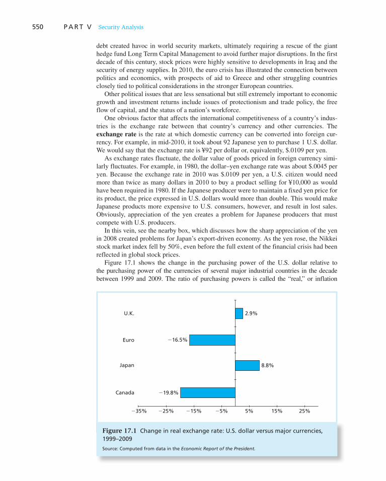
550 P A R T V Security Analysis
debt created havoc in world security markets, ultimately requiring a rescue of the giant hedge fund Long Term Capital Management to avoid further major disruptions. In the first decade of this century, stock prices were highly sensitive to developments in Iraq and the security of energy supplies. In 2010, the euro crisis has illustrated the connection between politics and economics, with prospects of aid to Greece and other struggling countries closely tied to political considerations in the stronger European countries.
Other political issues that are less sensational but still extremely important to economic growth and investment returns include issues of protectionism and trade policy, the free flow of capital, and the status of a nation’s workforce.
One obvious factor that affects the international competitiveness of a country’s indus-tries is the exchange rate between that country’s currency and other currencies. The exchange rate is the rate at which domestic currency can be converted into foreign cur-rency. For example, in mid-2010, it took about 92 Japanese yen to purchase 1 U.S. dollar. We would say that the exchange rate is ¥92 per dollar or, equivalently, $.0109 per yen.
As exchange rates fluctuate, the dollar value of goods priced in foreign currency simi-larly fluctuates. For example, in 1980, the dollar–yen exchange rate was about $.0045 per yen. Because the exchange rate in 2010 was $.0109 per yen, a U.S. citizen would need more than twice as many dollars in 2010 to buy a product selling for ¥10,000 as would have been required in 1980. If the Japanese producer were to maintain a fixed yen price for its product, the price expressed in U.S. dollars would more than double. This would make Japanese products more expensive to U.S. consumers, however, and result in lost sales. Obviously, appreciation of the yen creates a problem for Japanese producers that must compete with U.S. producers.
In this vein, see the nearby box, which discusses how the sharp appreciation of the yen in 2008 created problems for Japan’s export-driven economy. As the yen rose, the Nikkei stock market index fell by 50%, even before the full extent of the financial crisis had been reflected in global stock prices.
Figure 17.1 shows the change in the purchasing power of the U.S. dollar relative to the purchasing power of the currencies of several major industrial countries in the decade between 1999 and 2009. The ratio of purchasing powers is called the “real,” or inflation
Figure 17.1 Change in real exchange rate: U.S. dollar versus major currencies, 1999–2009
Source: Computed from data in the Economic Report of the President.
�19.8%
8.8%
�16.5%
2.9%
�25%�35% �15% �5% 5% 15% 25%
U.K.
Euro
Japan
Canada
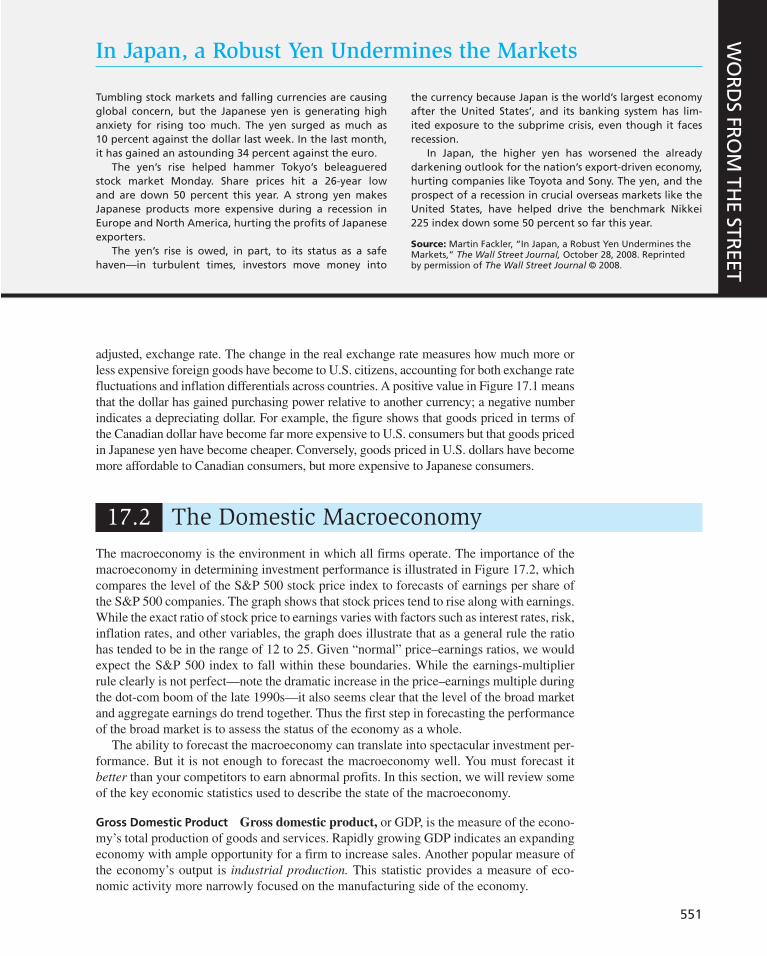
551
In Japan, a Robust Yen Undermines the Markets
Tumbling stock markets and falling currencies are causing global concern, but the Japanese yen is generating high anxiety for rising too much. The yen surged as much as 10 percent against the dollar last week. In the last month, it has gained an astounding 34 percent against the euro.
The yen’s rise helped hammer Tokyo’s beleaguered stock market Monday. Share prices hit a 26-year low and are down 50 percent this year. A strong yen makes Japanese products more expensive during a recession in Europe and North America, hurting the profits of Japanese exporters.
The yen’s rise is owed, in part, to its status as a safe haven—in turbulent times, investors move money into
the currency because Japan is the world’s largest economy after the United States’, and its banking system has lim-ited exposure to the subprime crisis, even though it faces recession.
In Japan, the higher yen has worsened the already darkening outlook for the nation’s export-driven economy, hurting companies like Toyota and Sony. The yen, and the prospect of a recession in crucial overseas markets like the United States, have helped drive the benchmark Nikkei 225 index down some 50 percent so far this year.
Source: Martin Fackler, “In Japan, a Robust Yen Undermines the Markets,” The Wall Street Journal, October 28, 2008. Reprinted by permission of The Wall Street Journal © 2008.
WO
RD
S FRO
M TH
E STREET
adjusted, exchange rate. The change in the real exchange rate measures how much more or less expensive foreign goods have become to U.S. citizens, accounting for both exchange rate fluctuations and inflation differentials across countries. A positive value in Figure 17.1 means that the dollar has gained purchasing power relative to another currency; a negative number indicates a depreciating dollar. For example, the figure shows that goods priced in terms of the Canadian dollar have become far more expensive to U.S. consumers but that goods priced in Japanese yen have become cheaper. Conversely, goods priced in U.S. dollars have become more affordable to Canadian consumers, but more expensive to Japanese consumers.
17.2 The Domestic Macroeconomy
The macroeconomy is the environment in which all firms operate. The importance of the macroeconomy in determining investment performance is illustrated in Figure 17.2 , which compares the level of the S&P 500 stock price index to forecasts of earnings per share of the S&P 500 companies. The graph shows that stock prices tend to rise along with earnings. While the exact ratio of stock price to earnings varies with factors such as interest rates, risk, inflation rates, and other variables, the graph does illustrate that as a general rule the ratio has tended to be in the range of 12 to 25. Given “normal” price–earnings ratios, we would expect the S&P 500 index to fall within these boundaries. While the earnings-multiplier rule clearly is not perfect—note the dramatic increase in the price–earnings multiple during the dot-com boom of the late 1990s—it also seems clear that the level of the broad market and aggregate earnings do trend together. Thus the first step in forecasting the performance of the broad market is to assess the status of the economy as a whole.
The ability to forecast the macroeconomy can translate into spectacular investment per-formance. But it is not enough to forecast the macroeconomy well. You must forecast it better than your competitors to earn abnormal profits. In this section, we will review some of the key economic statistics used to describe the state of the macroeconomy.
Gross Domestic Product Gross domestic product , or GDP, is the measure of the econo-my’s total production of goods and services. Rapidly growing GDP indicates an expanding economy with ample opportunity for a firm to increase sales. Another popular measure of the economy’s output is industrial production. This statistic provides a measure of eco-nomic activity more narrowly focused on the manufacturing side of the economy.
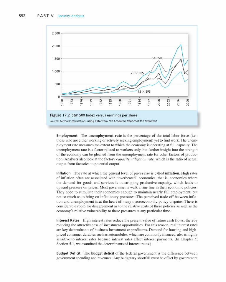
552 P A R T V Security Analysis
Employment The unemployment rate is the percentage of the total labor force (i.e., those who are either working or actively seeking employment) yet to find work. The unem-ployment rate measures the extent to which the economy is operating at full capacity. The unemployment rate is a factor related to workers only, but further insight into the strength of the economy can be gleaned from the unemployment rate for other factors of produc-tion. Analysts also look at the factory capacity utilization rate, which is the ratio of actual output from factories to potential output.
Inflation The rate at which the general level of prices rise is called inflation . High rates of inflation often are associated with “overheated” economies, that is, economies where the demand for goods and services is outstripping productive capacity, which leads to upward pressure on prices. Most governments walk a fine line in their economic policies. They hope to stimulate their economies enough to maintain nearly full employment, but not so much as to bring on inflationary pressures. The perceived trade-off between infla-tion and unemployment is at the heart of many macroeconomic policy disputes. There is considerable room for disagreement as to the relative costs of these policies as well as the economy’s relative vulnerability to these pressures at any particular time.
Interest Rates High interest rates reduce the present value of future cash flows, thereby reducing the attractiveness of investment opportunities. For this reason, real interest rates are key determinants of business investment expenditures. Demand for housing and high-priced consumer durables such as automobiles, which are commonly financed, also is highly sensitive to interest rates because interest rates affect interest payments. (In Chapter 5, Section 5.1, we examined the determinants of interest rates.)
Budget Deficit The budget deficit of the federal government is the difference between government spending and revenues. Any budgetary shortfall must be offset by government
Figure 17.2 S&P 500 Index versus earnings per share
Source: Authors’ calculations using data from The Economic Report of the President.
2,500
2,000
1,500
1,000
500
0
S&P 500
25 � EPS
12 � EPS
1970
1973
1976
1979
1982
1985
1988
1991
1994
1997
2000
2003
2006
2009
18 � EPS
C H A P T E R 1 7 Macroeconomic and Industry Analysis 553
borrowing. Large amounts of government borrowing can force up interest rates by increas-ing the total demand for credit in the economy. Economists generally believe excessive government borrowing will “crowd out” private borrowing and investing by forcing up interest rates and choking off business investment.
Sentiment Consumers’ and producers’ optimism or pessimism concerning the economy is an important determinant of economic performance. If consumers have confidence in their future income levels, for example, they will be more willing to spend on big-ticket items. Similarly, businesses will increase production and inventory levels if they anticipate higher demand for their products. In this way, beliefs influence how much consumption and investment will be pursued and affect the aggregate demand for goods and services.
CONCEPT CHECK
1
Consider an economy where the dominant industry is automobile production for domes-tic consumption as well as export. Now suppose the auto market is hurt by an increase in the length of time people use their cars before replacing them. Describe the probable effects of this change on ( a ) GDP, ( b ) unemployment, ( c ) the government budget deficit, and ( d ) interest rates.
17.3 Demand and Supply Shocks
A useful way to organize your analysis of the factors that might influence the macro-economy is to classify any impact as a supply or demand shock. A demand shock is an event that affects the demand for goods and services in the economy. Examples of positive demand shocks are reductions in tax rates, increases in the money supply, increases in government spending, or increases in foreign export demand. A supply shock is an event that influences production capacity and costs. Examples of supply shocks are changes in the price of imported oil; freezes, floods, or droughts that might destroy large quantities of agricultural crops; changes in the educational level of an economy’s workforce; or changes in the wage rates at which the labor force is willing to work.
Demand shocks are usually characterized by aggregate output moving in the same direction as interest rates and inflation. For example, a big increase in government spend-ing will tend to stimulate the economy and increase GDP. It also might increase interest rates by increasing the demand for borrowed funds by the government as well as by busi-nesses that might desire to borrow to finance new ventures. Finally, it could increase the inflation rate if the demand for goods and services is raised to a level at or beyond the total productive capacity of the economy.
Supply shocks are usually characterized by aggregate output moving in the opposite direc-tion of inflation and interest rates. For example, a big increase in the price of imported oil will be inflationary because costs of production will rise, which eventually will lead to increases in prices of finished goods. The increase in inflation rates over the near term can lead to higher nominal interest rates. Against this background, aggregate output will be falling. With raw materials more expensive, the productive capacity of the economy is reduced, as is the ability of individuals to purchase goods at now-higher prices. GDP, therefore, tends to fall.
How can we relate this framework to investment analysis? You want to identify the industries that will be most helped or hurt in any macroeconomic scenario you envision. For example, if you forecast a tightening of the money supply, you might want to avoid industries such as automobile producers that might be hurt by the likely increase in interest

554 P A R T V Security Analysis
rates. We caution you again that these forecasts are no easy task. Macroeconomic predic-tions are notoriously unreliable. And again, you must be aware that in all likelihood your forecast will be made using only publicly available information. Any investment advantage you have will be a result only of better analysis—not better information.
17.4 Federal Government Policy
As the previous section would suggest, the government has two broad classes of macro-economic tools—those that affect the demand for goods and services and those that affect the supply. For much of postwar history, demand-side policy was of primary interest. The focus was on government spending, tax levels, and monetary policy. Since the 1980s, how-ever, increasing attention has been focused on supply-side economics. Broadly interpreted, supply-side concerns have to do with enhancing the productive capacity of the economy, rather than increasing the demand for the goods and services the economy can produce. In practice, supply-side economists have focused on the appropriateness of the incentives to work, innovate, and take risks that result from our system of taxation. However, issues such as national policies on education, infrastructure (such as communication and trans-portation systems), and research and development also are properly regarded as part of supply-side macroeconomic policy.
Fiscal Policy
Fiscal policy refers to the government’s spending and tax actions and is part of “demand-side management.” Fiscal policy is probably the most direct way either to stimulate or to slow the economy. Decreases in government spending directly deflate the demand for goods and services. Similarly, increases in tax rates immediately siphon income from con-sumers and result in fairly rapid decreases in consumption.
Ironically, although fiscal policy has the most immediate impact on the economy, the formulation and implementation of such policy is usually painfully slow and involved. This is because fiscal policy requires enormous amounts of compromise between the exec-utive and legislative branches. Tax and spending policy must be initiated and voted on by Congress, which requires considerable political negotiations, and any legislation passed must be signed by the president, requiring more negotiation. Thus, although the impact of fiscal policy is relatively immediate, its formulation is so cumbersome that fiscal policy cannot in practice be used to fine-tune the economy.
Moreover, much of government spending, such as that for Medicare or Social Security, is nondiscretionary, meaning that it is determined by formula rather than policy and cannot be changed in response to economic conditions. This places even more rigidity into the formulation of fiscal policy.
A common way to summarize the net impact of government fiscal policy is to look at the government’s budget deficit or surplus, which is simply the difference between rev-enues and expenditures. A large deficit means the government is spending considerably more than it is taking in by way of taxes. The net effect is to increase the demand for goods (via spending) by more than it reduces the demand for goods (via taxes), thereby stimulat-ing the economy.
Monetary Policy
Monetary policy refers to the manipulation of the money supply to affect the macro-economy and is the other main leg of demand-side policy. Monetary policy works largely through its impact on interest rates. Increases in the money supply lower short-term interest

C H A P T E R 1 7 Macroeconomic and Industry Analysis 555
rates, ultimately encouraging investment and consumption demand. Over longer periods, however, most economists believe a higher money supply leads only to a higher price level and does not have a permanent effect on economic activity. Thus the monetary authorities face a difficult balancing act. Expansionary monetary policy probably will lower interest rates and thereby stimulate investment and some consumption demand in the short run, but these circumstances ultimately will lead only to higher prices. The stimulation/inflation trade-off is implicit in all debate over proper monetary policy.
Fiscal policy is cumbersome to implement but has a fairly direct impact on the economy, whereas monetary policy is easily formulated and implemented but has a less immediate impact. Monetary policy is determined by the Board of Governors of the Federal Reserve System. Board members are appointed by the president for 14-year terms and are reason-ably insulated from political pressure. The board is small enough, and often sufficiently dominated by its chairperson, that policy can be formulated and modulated relatively easily.
Implementation of monetary policy also is quite direct. The most widely used tool is the open market operation, in which the Fed buys or sells bonds for its own account. When the Fed buys securities, it simply “writes a check,” thereby increasing the money supply. (Unlike us, the Fed can pay for the securities without drawing down funds at a bank account.) Conversely, when the Fed sells a security, the money paid for it leaves the money supply. Open market operations occur daily, allowing the Fed to fine-tune its monetary policy.
Other tools at the Fed’s disposal are the discount rate, which is the interest rate it charges banks on short-term loans, and the reserve requirement, which is the fraction of deposits that banks must hold as cash on hand or as deposits with the Fed. Reductions in the dis-count rate signal a more expansionary monetary policy. Lowering reserve requirements allows banks to make more loans with each dollar of deposits and stimulates the economy by increasing the effective money supply.
While the discount rate is under the direct control of the Fed, it is changed relatively infrequently. The federal funds rate is by far the better guide to Federal Reserve policy. The federal funds rate is the interest rate at which banks make short-term, usually overnight, loans to each other. These loans occur because some banks need to borrow funds to meet reserve requirements, while other banks have excess funds. Unlike the discount rate, the fed funds rate is a market rate, meaning that it is determined by supply and demand rather than being set administratively. Nevertheless, the Federal Reserve Board targets the fed funds rate, expanding or contracting the money supply through open market operations as it nudges the fed funds rate to its targeted value. This is the benchmark short-term U.S. interest rate, and as such has considerable influence on other interest rates in the United States and the rest of the world.
Monetary policy affects the economy in a more roundabout way than fiscal policy. Whereas fiscal policy directly stimulates or dampens the economy, monetary policy works largely through its impact on interest rates. Increases in the money supply lower interest rates, which stimulates investment demand. As the quantity of money in the economy increases, investors will find that their portfolios of assets include too much money. They will rebalance their portfolios by buying securities such as bonds, forcing bond prices up and interest rates down. In the longer run, individuals may increase their holdings of stocks as well and ultimately buy real as-sets, which stimulates consumption demand directly. The ultimate effect of monetary policy on investment and consumption demand, however, is less immediate than that of fiscal policy.
CONCEPT CHECK
2
Suppose the government wants to stimulate the econ-omy without increasing interest rates. What combina-tion of fiscal and monetary policy might accomplish this goal?
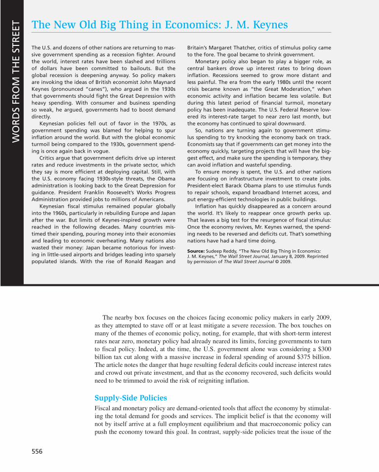
556
The New Old Big Thing in Economics: J. M. Keynes
The U.S. and dozens of other nations are returning to mas-sive government spending as a recession fighter. Around the world, interest rates have been slashed and trillions of dollars have been committed to bailouts. But the global recession is deepening anyway. So policy makers are invoking the ideas of British economist John Maynard Keynes (pronounced “canes”), who argued in the 1930s that governments should fight the Great Depression with heavy spending. With consumer and business spending so weak, he argued, governments had to boost demand directly.
Keynesian policies fell out of favor in the 1970s, as government spending was blamed for helping to spur inflation around the world. But with the global economic turmoil being compared to the 1930s, government spend-ing is once again back in vogue.
Critics argue that government deficits drive up interest rates and reduce investments in the private sector, which they say is more efficient at deploying capital. Still, with the U.S. economy facing 1930s-style threats, the Obama administration is looking back to the Great Depression for guidance. President Franklin Roosevelt’s Works Progress Administration provided jobs to millions of Americans.
Keynesian fiscal stimulus remained popular globally into the 1960s, particularly in rebuilding Europe and Japan after the war. But limits of Keynes-inspired growth were reached in the following decades. Many countries mis-timed their spending, pouring money into their economies and leading to economic overheating. Many nations also wasted their money: Japan became notorious for invest-ing in little-used airports and bridges leading into sparsely populated islands. With the rise of Ronald Reagan and
Britain’s Margaret Thatcher, critics of stimulus policy came to the fore. The goal became to shrink government.
Monetary policy also began to play a bigger role, as central bankers drove up interest rates to bring down inflation. Recessions seemed to grow more distant and less painful. The era from the early 1980s until the recent crisis became known as “the Great Moderation,” when economic activity and inflation became less volatile. But during this latest period of financial turmoil, monetary policy has been inadequate. The U.S. Federal Reserve low-ered its interest-rate target to near zero last month, but the economy has continued to spiral downward.
So, nations are turning again to government stimu-lus spending to try knocking the economy back on track. Economists say that if governments can get money into the economy quickly, targeting projects that will have the big-gest effect, and make sure the spending is temporary, they can avoid inflation and wasteful spending.
To ensure money is spent, the U.S. and other nations are focusing on infrastructure investment to create jobs. President-elect Barack Obama plans to use stimulus funds to repair schools, expand broadband Internet access, and put energy-efficient technologies in public buildings.
Inflation has quickly disappeared as a concern around the world. It’s likely to reappear once growth perks up. That leaves a big test for the resurgence of fiscal stimulus: Once the economy revives, Mr. Keynes warned, the spend-ing needs to be reversed and deficits cut. That’s something nations have had a hard time doing.
Source: Sudeep Reddy, “The New Old Big Thing in Economics: J. M. Keynes,” The Wall Street Journal, January 8, 2009. Reprinted by permission of The Wall Street Journal © 2009.
WO
RD
S FR
OM
TH
E ST
REE
T
The nearby box focuses on the choices facing economic policy makers in early 2009, as they attempted to stave off or at least mitigate a severe recession. The box touches on many of the themes of economic policy, noting, for example, that with short-term interest rates near zero, monetary policy had already neared its limits, forcing governments to turn to fiscal policy. Indeed, at the time, the U.S. government alone was considering a $300 billion tax cut along with a massive increase in federal spending of around $375 billion. The article notes the danger that huge resulting federal deficits could increase interest rates and crowd out private investment, and that as the economy recovered, such deficits would need to be trimmed to avoid the risk of reigniting inflation.
Supply-Side Policies
Fiscal and monetary policy are demand-oriented tools that affect the economy by stimulat-ing the total demand for goods and services. The implicit belief is that the economy will not by itself arrive at a full employment equilibrium and that macroeconomic policy can push the economy toward this goal. In contrast, supply-side policies treat the issue of the
C H A P T E R 1 7 Macroeconomic and Industry Analysis 557
productive capacity of the economy. The goal is to create an environment in which work-ers and owners of capital have the maximum incentive and ability to produce and develop goods.
Supply-side economists also pay considerable attention to tax policy. Whereas demand-siders look at the effect of taxes on consumption demand, supply-siders focus on incen-tives and marginal tax rates. They argue that lowering tax rates will elicit more investment and improve incentives to work, thereby enhancing economic growth. Some go so far as to claim that reductions in tax rates can lead to increases in tax rev-enues because the lower tax rates will cause the economy and the revenue tax base to grow by more than the tax rate is reduced.
CONCEPT CHECK
3
Large tax cuts in 2001 were followed by relatively rapid growth in GDP. How would demand-side and supply-side economists differ in their interpretations of this phenomenon?
17.5 Business Cycles
We’ve looked at the tools the government uses to fine-tune the economy, attempting to maintain low unemployment and low inflation. Despite these efforts, economies repeat-edly seem to pass through good and bad times. One determinant of the broad asset alloca-tion decision of many analysts is a forecast of whether the macroeconomy is improving or deteriorating. A forecast that differs from the market consensus can have a major impact on investment strategy.
The Business Cycle
The economy recurrently experiences periods of expansion and contraction, although the length and depth of those cycles can be irregular. This recurring pattern of recession and recovery is called the business cycle . Figure 17.3 presents graphs of several measures of production and output. The production series all show clear variation around a gener-ally rising trend. The bottom graph of capacity utilization also evidences a clear cyclical (although irregular) pattern.
The transition points across cycles are called peaks and troughs, indicated by the left and right edges of the shaded regions in Figure 17.3 . A peak is the transition from the end of an expansion to the start of a contraction. A trough occurs at the bottom of a recession just as the economy enters a recovery. The shaded areas in Figure 17.3 therefore all repre-sent periods of recession.
As the economy passes through different stages of the business cycle, the relative per-formance of different industry groups might be expected to vary. For example, at a trough, just before the economy begins to recover from a recession, one would expect that cyclical
industries , those with above-average sensitivity to the state of the economy, would tend to outperform other industries. Examples of cyclical industries are producers of durable goods such as automobiles. Because purchases of these goods can be deferred during a recession, sales are particularly sensitive to macroeconomic conditions. Other cyclical industries are producers of capital goods, that is, goods used by other firms to produce their own products. When demand is slack, few companies will be expanding and purchasing capital goods. Therefore, the capital goods industry bears the brunt of a slowdown but does well in an expansion.
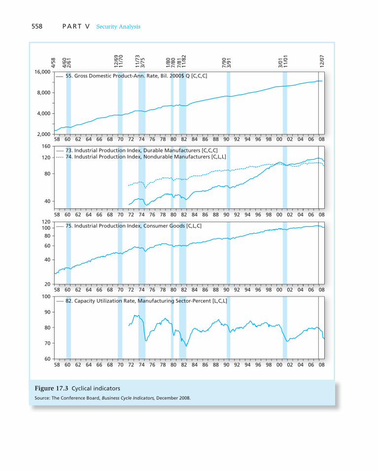
558 P A R T V Security Analysis
Figure 17.3 Cyclical indicators
Source: The Conference Board, Business Cycle Indicators, December 2008.
16,000
4/58
4/60
2/61
12/6
911
/70
11/7
33/
75
1/80
7/80
7/81
11/8
2
7/90
3/91
3/01
11/0
1
12/0
7
8,000
4,000
2,00058 60 62 64 66 68 70 72 74 76 78 80 82 84 86 88 90 92 94 96 98 00 02 04 06 08
06 08
06 08
06 08
58 60 62 64 66 68 70 72 74 76 78 80 82 84 86 88 90 92 94 96 98 00 02 04
58 60 62 64 66 68 70 72 74 76 78 80 82 84 86 88 90 92 94 96 98 00 02 04
58 60 62 64 66 68 70 72 74 76 78 80 82 84 86 88 90 92 94 96 98 00 02 04
160
120
80
40
120100
80
60
40
20
100
90
80
70
60
55. Gross Domestic Product-Ann. Rate, Bil. 2000$ Q [C,C,C]
73. Industrial Production Index, Durable Manufacturers [C,C,C]74. Industrial Production Index, Nondurable Manufacturers [C,L,L]
75. Industrial Production Index, Consumer Goods [C,L,C]
82. Capacity Utilization Rate, Manufacturing Sector-Percent [L,C,L]

C H A P T E R 1 7 Macroeconomic and Industry Analysis 559
In contrast to cyclical firms, defensive industries have little sensitivity to the business cycle. These are industries that produce goods for which sales and profits are least sensi-tive to the state of the economy. Defensive industries include food producers and proces-sors, pharmaceutical firms, and public utilities. These industries will outperform others when the economy enters a recession.
The cyclical/defensive classification corresponds well to the notion of systematic or market risk introduced in our discussion of portfolio theory. When perceptions about the health of the economy become more optimistic, for example, the prices of most stocks will increase as forecasts of profitability rise. Because the cyclical firms are most sensitive to such developments, their stock prices will rise the most. Thus firms in cyclical industries will tend to have high-beta stocks. In general, then, stocks of cyclical firms will show the best results when economic news is positive but the worst results when that news is bad. Conversely, defensive firms will have low betas and performance that is relatively unaf-fected by overall market conditions.
If your assessments of the state of the business cycle were reliably more accurate than those of other investors, you would simply choose cyclical industries when you are rela-tively more optimistic about the economy and defensive firms when you are relatively more pessimistic. Unfortunately, it is not so easy to determine when the economy is passing through a peak or a trough. It if were, choosing between cyclical and defensive industries would be easy. As we know from our discussion of efficient markets, how-ever, attractive investment choices will rarely be obvious. It usually is not apparent that a recession or expansion has started or ended until several months after the fact. With hindsight, the transitions from expansion to recession and back might be apparent, but it is often quite difficult to say whether the economy is heating up or slowing down at any moment.
Economic Indicators
Given the cyclical nature of the business cycle, it is not surprising that to some extent the cycle can be predicted. A set of cyclical indicators computed by the Conference Board helps forecast, measure, and interpret short-term fluctuations in economic activity. Leading
economic indicators are those economic series that tend to rise or fall in advance of the rest of the economy. Coincident and lagging indicators, as their names suggest, move in tandem with or somewhat after the broad economy.
Ten series are grouped into a widely followed composite index of leading economic indicators. Similarly, four coincident and seven lagging indicators form separate indexes. The composition of these indexes appears in Table 17.2 .
Figure 17.4 graphs these three series. The dates at the top of the chart correspond to turning points between expansions and contractions. The chart shows that the index of leading indicators consistently turns before the rest of the economy, but its lead time is somewhat erratic. Moreover, the lead time for peaks is consistently longer than that for troughs.
The stock market price index is a leading indicator. This is as it should be, as stock prices are forward-looking predictors of future profitability. Unfortunately, this makes the series of leading indicators much less useful for investment policy—by the time the series predicts an upturn, the market has already made its move. Although the business cycle may be somewhat predictable, the stock market may not be. This is just one more manifestation of the efficient markets hypothesis.

560 P A R T V Security Analysis
A. Leading indicators
1. Average weekly hours of production workers (manufacturing)
2. Initial claims for unemployment insurance
3. Manufacturers’ new orders (consumer goods and materials industries)
4. Fraction of companies reporting slower deliveries
5. New orders for nondefense capital goods
6. New private housing units authorized by local building permits
7. Yield curve slope: 10-year Treasury minus federal funds rate
8. Stock prices, 500 common stocks
9. Money supply (M2) growth rate
10. Index of consumer expectations
B. Coincident indicators
1. Employees on nonagricultural payrolls
2. Personal income less transfer payments
3. Industrial production
4. Manufacturing and trade sales
C. Lagging indicators
1. Average duration of unemployment
2. Ratio of trade inventories to sales
3. Change in index of labor cost per unit of output
4. Average prime rate charged by banks
5. Commercial and industrial loans outstanding
6. Ratio of consumer installment credit outstanding to personal income
7. Change in consumer price index for services
Table 17.2
Indexes of economic indicators
Source: The Conference Board, Business Cycle Indicators, February 2010.
The money supply is another leading indicator. This makes sense in light of our earlier discussion concerning the lags surrounding the effects of monetary policy on the economy. An expansionary monetary policy can be observed fairly quickly, but it might not affect the economy for several months. Therefore, today’s monetary policy might well predict future economic activity.
Other leading indicators focus directly on decisions made today that will affect produc-tion in the near future. For example, manufacturers’ new orders for goods, contracts and orders for plant and equipment, and housing starts all signal a coming expansion in the economy.
A wide range of economic indicators is released to the public on a regular “economic calendar.” Table 17.3 is an “economic calendar,” listing the public announcement dates and sources for about 20 statistics of interest. These announcements are reported in the financial press, for example, The Wall Street Journal, as they are released. They also are available at many sites on the Web, for example, at the Yahoo! Finance Web site. Figure 17.5 is a brief excerpt from the Economic Calendar page at Yahoo! The page gives a list of the announcements released the week of January 4, 2010. Notice that recent forecasts of each variable are provided along with the actual value of each sta-tistic. This is useful, because in an efficient market, security prices already will reflect
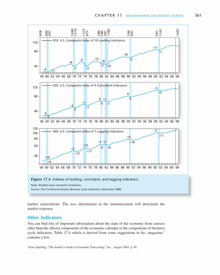
C H A P T E R 1 7 Macroeconomic and Industry Analysis 561
Figure 17.4 Indexes of leading, coincident, and lagging indicators
Note: Shaded areas represent recessions.
Source: The Conference Board, Business Cycle Indicators, December 2008.
120
100
80
60
40
58 646260 66 7068 7472 807876 8482 908886 969492 0098 08060402
920. U.S. Composite Index of 4 Coincident Indicators120
80
400
0
−2+1
+3
+15
+13+3 +2
+3 +6
+6
+16
+11
+10
+6
+1+1
+3
+1
0
−3
00
58 646260 66 7068 7472 807876 8482 908886 969492 0098 08060402
930. U.S. Composite Index of 7 Lagging Indicators
+17
−3
58 646260 66 7068 7472 807876 8482 908886 969492 0098 08060402
12/6
911
/70
11/7
33/
75
1/80
7/80
7/81
11/8
2
7/90
3/91
3/01
11/0
1
12/0
7
910. U.S. Composite Index of 10 Leading Indicators120
80
40
4/58
4/60
2/61
−9−11
−8−9 −15
−11
−7
−2
−10−2−7
−2−8
−18
0
0
market expectations. The new information in the announcement will determine the market response.
Other Indicators
You can find lots of important information about the state of the economy from sources other than the official components of the economic calendar or the components of business cycle indicators. Table 17.4 which is derived from some suggestions in Inc. magazine, 1
contains a few.
1 Gene Sperling, “The Insider’s Guide to Economic Forecasting,” Inc., August 2003, p. 96.

562 P A R T V Security Analysis
Statistic Release Date* Source Web Site
Auto and truck sales 2nd of month Commerce Department commerce.gov
Business inventories 15th of month Commerce Department commerce.gov
Construction spending 1st business day of month Commerce Department commerce.gov
Consumer confidence Last Tuesday of month Conference Board conference-board.org
Consumer credit 5th business day of month Federal Reserve Board federalreserve.gov
Consumer price index (CPI) 13th of month Bureau of Labor Statistics bls.gov
Durable goods orders 26th of month Commerce Department commerce.gov
Employment cost index End of first month of quarter Bureau of Labor Statistics bls.gov
Employment record
(unemployment, average
workweek, nonfarm payrolls)
1st Friday of month Bureau of Labor Statistics bls.gov
Existing home sales 25th of month National Association of
Realtors
realtor.org
Factory orders 1st business day of month Commerce Department commerce.gov
Gross domestic product 3rd–4th week of month Commerce Department commerce.gov
Housing starts 16th of month Commerce Department commerce.gov
Industrial production 15th of month Federal Reserve Board federalreserve.gov
Initial claims for jobless
benefits
Thursdays Department of Labor dol.gov
International trade balance 20th of month Commerce Department commerce.gov
Index of leading economic
indicators
Beginning of month Conference Board conference-board.org
Money supply Thursdays Federal Reserve Board federalreserve.gov
New home sales Last business day of month Commerce Department commerce.gov
Producer price index 11th of month Bureau of Labor Statistics bls.gov
Productivity and costs 2nd month in quarter
(approx. 7th day of month)
Bureau of Labor Statistics bls.gov
Retail sales 13th of month Commerce Department commerce.gov
Survey of purchasing
managers
1st business day of month Institute for Supply
Management
ism.ws
Table 17.3
Economic calendar *Many of these release dates are approximate.
17.6 Industry Analysis
Industry analysis is important for the same reason that macroeconomic analysis is. Just as it is difficult for an industry to perform well when the macroeconomy is ailing, it is unusual for a firm in a troubled industry to perform well. Similarly, just as we have seen that eco-nomic performance can vary widely across countries, performance also can vary widely across industries. Figure 17.6 illustrates the dispersion of industry performance. It shows return on equity based on 2009 profitability for several major industry groups. ROE ranged from 7.6% for oil and gas companies to 34.9% for the computer systems industry.
Given the wide variation in profitability, it is not surprising that industry groups exhibit considerable dispersion in their stock market performance. Figure 17.7 presents the stock

C H A P T E R 1 7 Macroeconomic and Industry Analysis 563
Figure 17.5 Economic calendar at Yahoo!, week of January 4, 2010
Source: Yahoo! Finance, biz.yahoo.com . Reproduced by permission of Yahoo! Inc. © 2010 by Yahoo! Inc. Yahoo! and the Yahoo! logo are trademarks of Yahoo! Inc.
Jan4 Nov
Dec
Nov
Nov
Jan4
Jan5
Jan5
PriorActualForStatisticDate
Last Week
Institute for SupplyManagement Index
Factory Orders
10:00 AM
10:00 AM
10:00 AM
10:00 AM
8:15 AM
8:30 AM
Dec
01/02
–0.6%
–16.0%
55.9
1.1%
–84K
–0.1%
55.3
0.1%
2.0%
−125K
455K
–0.5%
54.3
0.5%
–2.0%
−75K
439K 433K
–0.5%
3.9%
53.6
0.8%
−145KJan6
Jan7
ADP Employment Report
Initial Claims
Pending Home Sales
Time(ET)
BriefingForecast
MarketExpects
Construction Spending
434K
Economic Calendar Week of January 4, 2010
CEO polls
www.businessroundtable.org
The business roundtable surveys CEOs about
planned capital spending, a good measure of
their optimism about the economy.
Temp jobs
(search for “Temporary Help Services”)
www.bls.gov
A useful leading indicator. Businesses often hire
temporary workers as the economy first picks
up, until it is clear that an upturn is going to be
sustained. This series is available at the Bureau
of Labor Statistics Web site.
Walmart sales
www.walmartstores.com
Walmart sales are a good indicator of the retail
sector. It publishes its same-store sales weekly.
Commercial and industrial loans
www.federalreserve.gov
These loans are used by small and medium-sized
firms. Information is published weekly by the
Federal Reserve.
Semiconductors
www.semi.org
The book-to-bill ratio (i.e., new sales versus
actual shipments) indicates whether demand in
the technology sector is increasing (ratio . 1) or
falling. This ratio is published by Semiconductor
Equipment and Materials International.
Commercial structures
http://bea.doc.gov
Investment in structures is an indicator of busi-
nesses’ forecasts of demand for their products
in the near future. This series is compiled by the
Bureau of Economic Analysis as part of its GDP
series.
Table 17.4
Useful economic indicators
market performance of several industries during 2009. Stock returns that year were gener-ally excellent, as fears of a widespread depression receded. Nevertheless, the spread in performance across industries is remarkable, ranging from a 209.8% return for travel and tourism firms to a 14.9% loss in renewable energy.

564 P A R T V Security Analysis
Figure 17.6 Return on equity by industry, 2009
Source: Yahoo! Finance, January 8, 2010. finance.yahoo.com. Reproduced with permission of Yahoo! Inc. © 2010 by Yahoo! Inc. Yahoo! and the Yahoo! logo are trademarks of Yahoo! Inc.
Computer Systems
Application Software
Discount Stores
Pollution Control
Tobacco Products
Chemical Products
Electric Utilities
Pharmaceuticals
Business Software
Telecom Services
Food
Integrated Oil & Gas 7.6
0 5 10 15 20 25 30
Rate of Return (%)
35
10.0
10.1
12.1
12.7
13.8
14.0
14.0
14.2
14.6
18.1
21.6
22.6
23.6
25.934.9
Restaurants
Industrial Metals & Minerals
Hospitals
Aerospace/Defense
Defining an Industry
Although we know what we mean by an “industry,” deciding where to draw the line between one industry and another can be difficult in practice. Consider, for example, one of the industries depicted in Figure 17.6 , application software firms. Industry ROE in 2009 was 25.9%. But there is substantial variation within this group by focus, and one might well be justified in further dividing these firms into distinct subindustries. Their differ-ences may result in considerable dispersion in financial performance. Figure 17.8 shows ROE for a sample of the firms included in this industry, confirming that 2009 performance did indeed vary widely: from 8.3% for Adobe to 41.6% for VeriSign.
A useful way to define industry groups in practice is given by the North American Industry Classification System, or NAICS codes . 2 These are codes assigned to group firms for statistical analysis. The first two digits of the NAICS codes denote very broad industry classifications. For example, Table 17.5 shows that the codes for all construction firms start with 23. The next digits define the industry grouping more narrowly. For example, codes
2 These codes are used for firms operating inside the NAFTA (North American Free Trade Agreement) region, which includes the U.S., Mexico, and Canada. NAICS codes replaced the Standard Industry Classification or SIC codes previously used in the U.S.
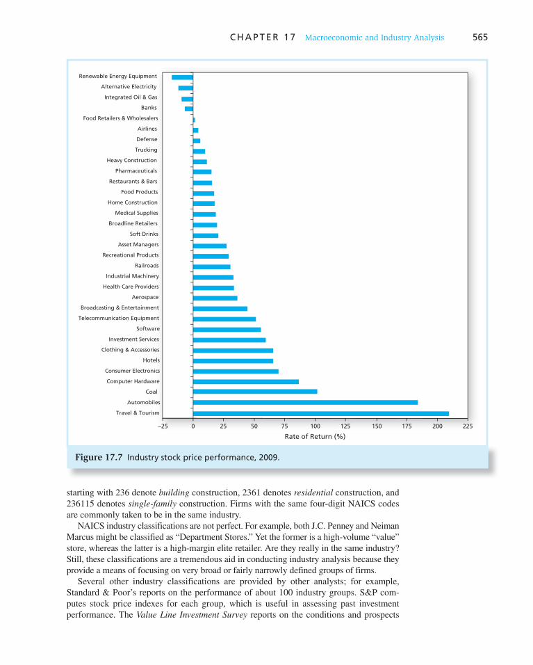
C H A P T E R 1 7 Macroeconomic and Industry Analysis 565
Figure 17.7 Industry stock price performance, 2009.
Rate of Return (%)
0−25 25 50 75 100 125 150 175 200 225
Medical Supplies
Industrial Machinery
Health Care Providers
Renewable Energy Equipment
Alternative Electricity
Integrated Oil & Gas
Banks
Food Retailers & Wholesalers
Airlines
Defense
Trucking
Heavy Construction
Pharmaceuticals
Restaurants & Bars
Food Products
Home Construction
Broadline Retailers
Soft Drinks
Asset Managers
Recreational Products
Railroads
Aerospace
Broadcasting & Entertainment
Telecommunication Equipment
Software
Investment Services
Clothing & Accessories
Hotels
Consumer Electronics
Computer Hardware
Coal
Automobiles
Travel & Tourism
starting with 236 denote building construction, 2361 denotes residential construction, and 236115 denotes single-family construction. Firms with the same four-digit NAICS codes are commonly taken to be in the same industry.
NAICS industry classifications are not perfect. For example, both J.C. Penney and Neiman Marcus might be classified as “Department Stores.” Yet the former is a high-volume “value” store, whereas the latter is a high-margin elite retailer. Are they really in the same industry? Still, these classifications are a tremendous aid in conducting industry analysis because they provide a means of focusing on very broad or fairly narrowly defined groups of firms.
Several other industry classifications are provided by other analysts; for example, Standard & Poor’s reports on the performance of about 100 industry groups. S&P com-putes stock price indexes for each group, which is useful in assessing past investment performance. The Value Line Investment Survey reports on the conditions and prospects

566 P A R T V Security Analysis
Figure 17.8 ROE of major software development firms
Source: Yahoo! Finance, January 15, 2010. finance.yahoo.com . Reproduced with permisssion of Yahoo! © 2010 by Yahoo! Inc. Yahoo! and the Yahoo! logo are trademarks of Yahoo! Inc.
ROE (%)
0 10 20 30 40 50
8.3
15.9
23.1
27.0
36.8
41.6
Adobe
CA (Computer Assoc)
Oracle
SAP
Microsoft
VeriSign
of about 1,700 firms, grouped into about 90 industries. Value Line’s analysts prepare fore-casts of the performance of industry groups as well as of each firm.
Sensitivity to the Business Cycle
Once the analyst forecasts the state of the macroeconomy, it is necessary to determine the implication of that forecast for specific industries. Not all industries are equally sensitive to the business cycle.
For example, Figure 17.9 plots changes in retail sales (year over year) in two industries: jewelry and grocery stores. Clearly, sales of jewelry, which is a luxury good, fluctuate
NAICS Code NAICS Title
23 Construction
236 Construction of Buildings
2361 Residential Building Construction
23611 Residential Building Construction
236115 New Single-Family Housing Construction
236116 New Multifamily Housing Construction
236117 New Housing Operative Builders
236118 Residential Remodelers
2362 Nonresidential Building Construction
23621 Industrial Building Construction
236210 Industrial Building Construction
23622 Commercial and Institutional Building Construction
236220 Commercial and Institutional Building Construction
Table 17.5
Examples of NAICS industry codes

C H A P T E R 1 7 Macroeconomic and Industry Analysis 567
more widely than those of grocer-ies. The dramatic downturns in jew-elry sales in the recessions of 2001 and 2008 are notable. In contrast, sales growth in the grocery industry is relatively stable, with no years in which sales decline. These patterns reflect the fact that jewelry is a dis-cretionary good, whereas most gro-cery products are staples for which demand will not fall significantly even in hard times.
Three factors will determine the sensitivity of a firm’s earnings to the business cycle. First is the sensitivity of sales. Necessities will show little sensitivity to business conditions. Examples of industries in this group are food, drugs, and medical services. Other industries with low sensitivity are those for which income is not a crucial determinant of demand. Tobacco products are an example of this type of industry. Another industry in this group is movies, because consumers tend to substitute movies for more expensive sources of entertainment when income levels are low. In contrast, firms in industries such as machine tools, steel, autos, and transportation are highly sensitive to the state of the economy.
The second factor determining business cycle sensitivity is operating leverage, which refers to the division between fixed and variable costs. (Fixed costs are those the firm incurs regardless of its production levels. Variable costs are those that rise or fall as the firm produces more or less product.) Firms with greater amounts of variable as opposed to fixed costs will be less sensitive to business conditions. This is because in economic downturns, these firms can reduce costs as output falls in response to falling sales. Profits for firms with high fixed costs will swing more widely with sales because costs do not move to offset revenue variability. Firms with high fixed costs are said to have high oper-ating leverage, because small swings in business conditions can have large impacts on profitability.
Figure 17.9 Industry cyclicality
GroceryJewelry
1994
An
nu
al S
ales
Gro
wth
(%
)
1995
1996
1997
1998
1999
2000
2001
0
−2
−4
−6
−8
2
4
6
8
10
12
1993
2002
2003
2004
2005
2006
2007
2008
Example 17.1 Operating Leverage
Consider two firms operating in the same industry with identical revenues in all phases of the business cycle: recession, normal, and expansion. Firm A has short-term leases on most of its equipment and can reduce its lease expenditures when production slackens. It has fixed costs of $5 million and variable costs of $1 per unit of output. Firm B has long-term leases on most of its equipment and must make lease payments regardless of eco-nomic conditions. Its fixed costs are higher, $8 million, but its variable costs are only $.50 per unit. Table 17.6 shows that Firm A will do better in recessions than Firm B, but not as well in expansions. A’s costs move in conjunction with its revenues to help performance in downturns and impede performance in upturns.
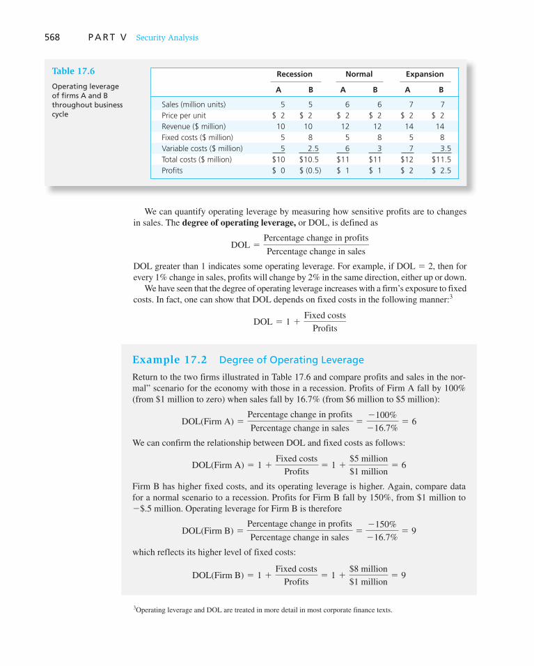
568 P A R T V Security Analysis
We can quantify operating leverage by measuring how sensitive profits are to changes in sales. The degree of operating leverage , or DOL, is defined as
DOL 5Percentage change in profits
Percentage change in sales
DOL greater than 1 indicates some operating leverage. For example, if DOL 5 2, then for every 1% change in sales, profits will change by 2% in the same direction, either up or down.
We have seen that the degree of operating leverage increases with a firm’s exposure to fixed costs. In fact, one can show that DOL depends on fixed costs in the following manner: 3
DOL 5 1 1Fixed costs
Profits
3 Operating leverage and DOL are treated in more detail in most corporate finance texts.
Recession Normal Expansion
A B A B A B
Sales (million units) 5 5 6 6 7 7
Price per unit $ 2 $ 2 $ 2 $ 2 $ 2 $ 2
Revenue ($ million) 10 10 12 12 14 14
Fixed costs ($ million) 5 8 5 8 5 8
Variable costs ($ million) 5 2.5 6 3 7 3.5
Total costs ($ million) $10 $10.5 $11 $11 $12 $11.5
Profits $ 0 $ (0.5) $ 1 $ 1 $ 2 $ 2.5
Table 17.6
Operating leverage of firms A and B throughout business cycle
Example 17.2 Degree of Operating Leverage
Return to the two firms illustrated in Table 17.6 and compare profits and sales in the nor-mal” scenario for the economy with those in a recession. Profits of Firm A fall by 100% (from $1 million to zero) when sales fall by 16.7% (from $6 million to $5 million):
DOL(Firm A) 5Percentage change in profits
Percentage change in sales5
2100%
216.7%5 6
We can confirm the relationship between DOL and fixed costs as follows:
DOL(Firm A) 5 1 1Fixed costs
Profits5 1 1
$5 million
$1 million5 6
Firm B has higher fixed costs, and its operating leverage is higher. Again, compare data for a normal scenario to a recession. Profits for Firm B fall by 150%, from $1 million to 2 $.5 million. Operating leverage for Firm B is therefore
DOL(Firm B) 5Percentage change in profits
Percentage change in sales5
2150%
216.7%5 9
which reflects its higher level of fixed costs:
DOL(Firm B) 5 1 1Fixed costs
Profits5 1 1
$8 million
$1 million5 9
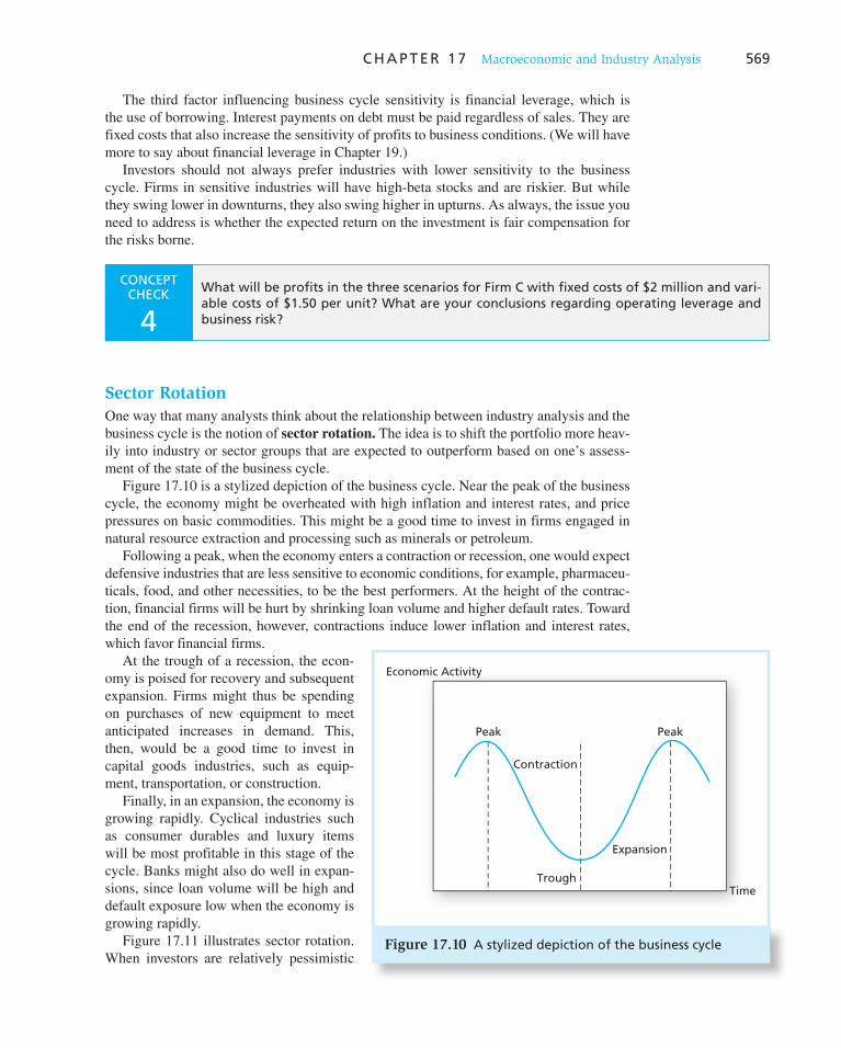
C H A P T E R 1 7 Macroeconomic and Industry Analysis 569
The third factor influencing business cycle sensitivity is financial leverage, which is the use of borrowing. Interest payments on debt must be paid regardless of sales. They are fixed costs that also increase the sensitivity of profits to business conditions. (We will have more to say about financial leverage in Chapter 19.)
Investors should not always prefer industries with lower sensitivity to the business cycle. Firms in sensitive industries will have high-beta stocks and are riskier. But while they swing lower in downturns, they also swing higher in upturns. As always, the issue you need to address is whether the expected return on the investment is fair compensation for the risks borne.
CONCEPT CHECK
4 What will be profits in the three scenarios for Firm C with fixed costs of $2 million and vari-able costs of $1.50 per unit? What are your conclusions regarding operating leverage and business risk?
Sector Rotation
One way that many analysts think about the relationship between industry analysis and the business cycle is the notion of sector rotation . The idea is to shift the portfolio more heav-ily into industry or sector groups that are expected to outperform based on one’s assess-ment of the state of the business cycle.
Figure 17.10 is a stylized depiction of the business cycle. Near the peak of the business cycle, the economy might be overheated with high inflation and interest rates, and price pressures on basic commodities. This might be a good time to invest in firms engaged in natural resource extraction and processing such as minerals or petroleum.
Following a peak, when the economy enters a contraction or recession, one would expect defensive industries that are less sensitive to economic conditions, for example, pharmaceu-ticals, food, and other necessities, to be the best performers. At the height of the contrac-tion, financial firms will be hurt by shrinking loan volume and higher default rates. Toward the end of the recession, however, contractions induce lower inflation and interest rates, which favor financial firms.
At the trough of a recession, the econ-omy is poised for recovery and subsequent expansion. Firms might thus be spending on purchases of new equipment to meet anticipated increases in demand. This, then, would be a good time to invest in capital goods industries, such as equip-ment, transportation, or construction.
Finally, in an expansion, the economy is growing rapidly. Cyclical industries such as consumer durables and luxury items will be most profitable in this stage of the cycle. Banks might also do well in expan-sions, since loan volume will be high and default exposure low when the economy is growing rapidly.
Figure 17.11 illustrates sector rotation. When investors are relatively pessimistic
Figure 17.10 A stylized depiction of the business cycle
Economic Activity
Time
Peak
Trough
Expansion
Contraction
Peak

570 P A R T V Security Analysis
about the economy, they will shift into noncyclical industries such as consumer staples or health care. When anticipating an expansion, they will prefer more cyclical industries such as materials and technology.
Let us emphasize again that sector rotation, like any other form of market timing, will be successful only if one anticipates the next stage of the business cycle better than other investors. The business cycle depicted in Figure 17.10 is highly stylized. In real life, it is never as clear how long each phase of the cycle will last, nor how extreme it will be. These forecasts are where analysts need to earn their keep.
CONCEPT CHECK
5
In which phase of the business cycle would you expect the following industries to enjoy their best performance?
a. Newspapers
b. Machine tools
c. Beverages
d. Timber
Industry Life Cycles
Examine the biotechnology industry and you will find many firms with high rates of invest-ment, high rates of return on investment, and low dividend payout rates. Do the same for the public utility industry and you will find lower rates of return, lower investment rates, and higher dividend payout rates. Why should this be?
The biotech industry is still new. Recently, available technologies have created opportu-nities for highly profitable investment of resources. New products are protected by patents, and profit margins are high. With such lucrative investment opportunities, firms find it advantageous to put all profits back into the firm. The companies grow rapidly on average.
Eventually, however, growth must slow. The high profit rates will induce new firms to enter the industry. Increasing competition will hold down prices and profit margins.
New technologies become proven and more predict-able, risk levels fall, and entry becomes even easier. As internal investment opportunities become less attractive, a lower fraction of profits is reinvested in the firm. Cash dividends increase.
Ultimately, in a mature industry, we observe “cash cows,” firms with stable dividends and cash flows and little risk. Growth rates might be similar to that of the overall economy. Industries in early states of their life cycles offer high-risk/high-potential-return invest-ments. Mature industries offer lower-risk, lower-return profiles.
This analysis suggests that a typical industry life
cycle might be described by four stages: a start-up stage, characterized by extremely rapid growth; a con-solidation stage, characterized by growth that is less rapid but still faster than that of the general economy; a maturity stage, characterized by growth no faster than the general economy; and a stage of relative decline, in which the industry grows less rapidly than the rest
Figure 17.11 Sector rotation
Source: Sam Stovall, BusinessWeek Online, “A Cyclical Take on Performance.” Reprinted with special permission from the July 8, 2004, issue of BusinessWeek. © 2004 McGraw-Hill Companies, Inc.
Energy
Health Care
Consumer Staples
Utilities
FinancialsTechnology
Consumer
Discretionary
Materials
Industrials
Expan
sion
Typical Sector RotationThrough an Average
Economic Cycle
Contr
acti
on
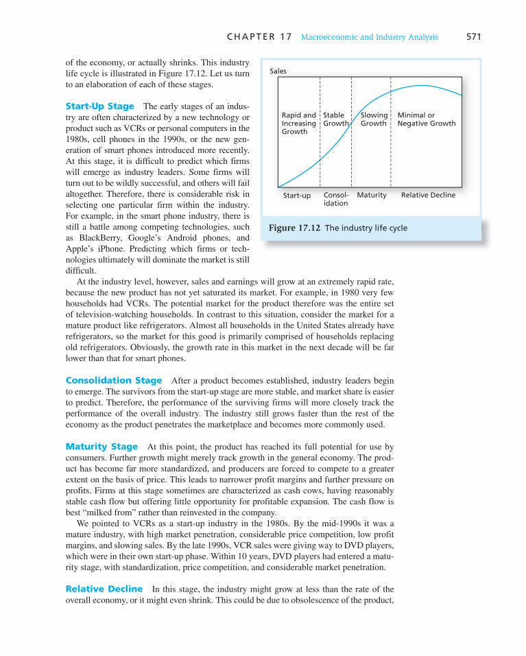
C H A P T E R 1 7 Macroeconomic and Industry Analysis 571
of the economy, or actually shrinks. This industry life cycle is illustrated in Figure 17.12 . Let us turn to an elaboration of each of these stages.
Start-Up Stage The early stages of an indus-try are often characterized by a new technology or product such as VCRs or personal computers in the 1980s, cell phones in the 1990s, or the new gen-eration of smart phones introduced more recently. At this stage, it is difficult to predict which firms will emerge as industry leaders. Some firms will turn out to be wildly successful, and others will fail altogether. Therefore, there is considerable risk in selecting one particular firm within the industry. For example, in the smart phone industry, there is still a battle among competing technologies, such as BlackBerry, Google’s Android phones, and Apple’s iPhone. Predicting which firms or tech-nologies ultimately will dominate the market is still difficult.
At the industry level, however, sales and earnings will grow at an extremely rapid rate, because the new product has not yet saturated its market. For example, in 1980 very few households had VCRs. The potential market for the product therefore was the entire set of television-watching households. In contrast to this situation, consider the market for a mature product like refrigerators. Almost all households in the United States already have refrigerators, so the market for this good is primarily comprised of households replacing old refrigerators. Obviously, the growth rate in this market in the next decade will be far lower than that for smart phones.
Consolidation Stage After a product becomes established, industry leaders begin to emerge. The survivors from the start-up stage are more stable, and market share is easier to predict. Therefore, the performance of the surviving firms will more closely track the performance of the overall industry. The industry still grows faster than the rest of the economy as the product penetrates the marketplace and becomes more commonly used.
Maturity Stage At this point, the product has reached its full potential for use by consumers. Further growth might merely track growth in the general economy. The prod-uct has become far more standardized, and producers are forced to compete to a greater extent on the basis of price. This leads to narrower profit margins and further pressure on profits. Firms at this stage sometimes are characterized as cash cows, having reasonably stable cash flow but offering little opportunity for profitable expansion. The cash flow is best “milked from” rather than reinvested in the company.
We pointed to VCRs as a start-up industry in the 1980s. By the mid-1990s it was a mature industry, with high market penetration, considerable price competition, low profit margins, and slowing sales. By the late 1990s, VCR sales were giving way to DVD players, which were in their own start-up phase. Within 10 years, DVD players had entered a matu-rity stage, with standardization, price competition, and considerable market penetration.
Relative Decline In this stage, the industry might grow at less than the rate of the overall economy, or it might even shrink. This could be due to obsolescence of the product,
Figure 17.12 The industry life cycle
Sales
Start-up Consol-idation
Maturity Relative Decline
Rapid andIncreasingGrowth
StableGrowth
SlowingGrowth
Minimal orNegative Growth

572 P A R T V Security Analysis
competition from new low-cost suppliers, or competition from new products, as illustrated by the steady displacement of VCRs by DVD players.
At which stage in the life cycle are investments in an industry most attractive? Conventional wisdom is that investors should seek firms in high-growth industries. This recipe for success is simplistic, however. If the security prices already reflect the likeli-hood for high growth, then it is too late to make money from that knowledge. Moreover, high growth and fat profits encourage competition from other producers. The exploitation of profit opportunities brings about new sources of supply that eventually reduce prices, profits, investment returns, and finally growth. This is the dynamic behind the progression from one stage of the industry life cycle to another. The famous portfolio manager Peter Lynch makes this point in One Up on Wall Street:
Many people prefer to invest in a high-growth industry, where there’s a lot of sound and fury. Not me. I prefer to invest in a low-growth industry. . . . In a low-growth industry, especially one that’s boring and upsets people [such as funeral homes or the oil-drum retrieval business], there’s no problem with competition. You don’t have to protect your flanks from potential rivals . . . and this gives you the leeway to continue to grow. 4
In fact, Lynch uses an industry classification system in a very similar spirit to the life-cycle approach we have described. He places firms in the following six groups:
Slow Growers Large and aging companies that will grow only slightly faster than the broad economy. These firms have matured from their earlier fast-growth phase. They usu-ally have steady cash flow and pay a generous dividend, indicating that the firm is generat-ing more cash than can be profitably reinvested in the firm.
Stalwarts Large, well-known firms like Coca-Cola, Hershey’s, or Colgate-Palmolive. They grow faster than the slow growers, but are not in the very rapid growth start-up stage. They also tend to be in noncyclical industries that are relatively unaffected by recessions.
Fast Growers Small and aggressive new firms with annual growth rates in the neigh-borhood of 20% to 25%. Company growth can be due to broad industry growth or to an increase in market share in a more mature industry.
Cyclicals These are firms with sales and profits that regularly expand and contract along with the business cycle. Examples are auto companies, steel companies, or the construction industry.
Turnarounds These are firms that are in bankruptcy or soon might be. If they can recover from what might appear to be imminent disaster, they can offer tremendous investment returns. A good example of this type of firm would be Chrysler in 1982, when it required a government guarantee on its debt to avoid bankruptcy. The stock price rose fifteenfold in the next 5 years.
Asset Plays These are firms that have valuable assets not currently reflected in the stock price. For example, a company may own or be located on valuable real estate that is worth as much as or more than the company’s business enterprises. Sometimes the hidden asset can be tax-loss carryforwards. Other times the assets may be intangible. For example, a cable company might have a valuable list of cable subscribers. These assets do not immediately generate cash flow, and so may be more easily overlooked by other analysts attempting to value the firm.
4 Peter Lynch with John Rothchild, One Up on Wall Street (New York: Penquin, p. 131).
C H A P T E R 1 7 Macroeconomic and Industry Analysis 573
Industry Structure and Performance
The maturation of an industry involves regular changes in the firm’s competitive environment. As a final topic, we examine the relationship among industry structure, competitive strat-egy, and profitability. Michael Porter has highlighted these five determinants of competition: threat of entry from new competitors, rivalry between existing competitors, price pressure from substitute products, bargaining power of buyers, and bargaining power of suppliers. 5
Threat of Entry New entrants to an industry put pressure on price and profits. Even if a firm has not yet entered an industry, the potential for it to do so places pressure on prices, because high prices and profit margins will encourage entry by new competitors. Therefore, barriers to entry can be a key determinant of industry profitability. Barriers can take many forms. For example, existing firms may already have secure distribution channels for their products based on long-standing relationships with customers or sup-pliers that would be costly for a new entrant to duplicate. Brand loyalty also makes it difficult for new entrants to penetrate a market and gives firms more pricing discretion. Proprietary knowledge or patent protection also may give firms advantages in serving a market. Finally, an existing firm’s experience in a market may give it cost advantages due to the learning that takes place over time.
Rivalry between Existing Competitors When there are several competitors in an industry, there will generally be more price competition and lower profit margins as competitors seek to expand their share of the market. Slow industry growth contributes to this competition, because expansion must come at the expense of a rival’s market share. High fixed costs also create pressure to reduce prices, because fixed costs put greater pres-sure on firms to operate near full capacity. Industries producing relatively homogeneous goods are also subject to considerable price pressure, because firms cannot compete on the basis of product differentiation.
Pressure from Substitute Products Substitute products means that the industry faces competition from firms in related industries. For example, sugar producers compete with corn syrup producers. Wool producers compete with synthetic fiber producers. The availability of substitutes limits the prices that can be charged to customers.
Bargaining Power of Buyers If a buyer purchases a large fraction of an industry’s output, it will have considerable bargaining power and can demand price concessions. For example, auto producers can put pressure on suppliers of auto parts. This reduces the prof-itability of the auto parts industry.
Bargaining Power of Suppliers If a supplier of a key input has monopolistic control over the product, it can demand higher prices for the good and squeeze profits out of the industry. One special case of this issue pertains to organized labor as a supplier of a key input to the production process. Labor unions engage in collective bargaining to increase the wages paid to workers. When the labor market is highly unionized, a signifi-cant share of the potential profits in the industry can be captured by the workforce.
The key factor determining the bargaining power of suppliers is the availability of sub-stitute products. If substitutes are available, the supplier has little clout and cannot extract higher prices.
5 Michael Porter, Competitive Advantage: Creating and Sustaining Superior Performance (New York: Free Press, 1985).

Vis
it u
s at
ww
w.m
hh
e.co
m/b
km574 P A R T V Security Analysis
1. Macroeconomic policy aims to maintain the economy near full employment without aggravat-ing inflationary pressures. The proper trade-off between these two goals is a source of ongoing debate.
2. The traditional tools of macropolicy are government spending and tax collection, which com-prise fiscal policy, and manipulation of the money supply via monetary policy. Expansionary fiscal policy can stimulate the economy and increase GDP but tends to increase interest rates. Expansionary monetary policy works by lowering interest rates.
3. The business cycle is the economy’s recurring pattern of expansions and recessions. Leading economic indicators can be used to anticipate the evolution of the business cycle because their values tend to change before those of other key economic variables.
4. Industries differ in their sensitivity to the business cycle. More sensitive industries tend to be those producing high-priced durable goods for which the consumer has considerable discretion as to the timing of purchase. Examples are jewelry, automobiles, or consumer durables. Other sensitive industries are those that produce capital equipment for other firms. Operating leverage and financial leverage increase sensitivity to the business cycle.
SUMMARY
Related Web sites for this chapter are available at www.mhhe.com/bkm
fundamental analysis exchange rate gross domestic product unemployment rate inflation budget deficit demand shock
supply shock fiscal policy monetary policy business cycle peak trough cyclical industries
defensive industries leading economic indicators NAICS codes degree of operating leverage sector rotation industry life cycle
KEY TERMS
1. What monetary and fiscal policies might be prescribed for an economy in a deep recession?
2. If you believe the U.S. dollar will depreciate more dramatically than do other investors, what will be your stance on investments in U.S. auto producers?
3. Choose an industry and identify the factors that will determine its performance in the next 3 years. What is your forecast for performance in that time period?
4. What are the differences between bottom-up and top-down approaches to security valuation? What are the advantages of a top-down approach?
5. What characteristics will give firms greater sensitivity to business cycles?
6. Unlike other investors, you believe the Fed is going to loosen monetary policy. What would be your recommendations about investments in the following industries?
a. Gold mining b. Construction
7. According to supply-side economists, what will be the long-run impact on prices of a reduction in income tax rates?
8. Which of the following is consistent with a steeply upwardly sloping yield curve?
a. Monetary policy is expansive and fiscal policy is expansive. b. Monetary policy is expansive while fiscal policy is restrictive. c. Monetary policy is restrictive and fiscal policy is restrictive.
9. Which of the following is not a governmental structural policy that supply-side economists believe would promote long-term growth in an economy?
a. A redistributive tax system. b. A promotion of competition. c. Minimal government interference in the economy.
PROBLEM SETS
i. Basic
ii. Intermediate

Vis
it u
s at
ww
w.m
hh
e.co
m/b
km
C H A P T E R 1 7 Macroeconomic and Industry Analysis 575
10. Consider two firms producing smart phones. One uses a highly automated robotics process, whereas the other uses workers on an assembly line and pays overtime when there is heavy production demand.
a. Which firm will have higher profits in a recession? In a boom? b. Which firm’s stock will have a higher beta?
11. Here are four industries and four forecasts for the macroeconomy. Match the industry to the scenario in which it is likely to be the best performer.
Industry Economic Forecast
a. Housing construction (i) Deep recession: falling inflation, interest rates, and GDP
b. Health care
c. Gold mining
(ii) Superheated economy: rapidly rising GDP, increasing inflation
and interest rates
d. Steel production (iii) Healthy expansion: rising GDP, mild inflation, low
unemployment
(iv) Stagflation: falling GDP, high inflation
12. In which stage of the industry life cycle would you place the following industries?
( Note: There is considerable room for disagreement concerning the “correct” answers to this question.)
a. Oil well equipment. b. Computer hardware. c. Computer software. d. Genetic engineering. e. Railroads.
13. For each pair of firms, choose the one that you think would be more sensitive to the business cycle.
a. General Autos or General Pharmaceuticals. b. Friendly Airlines or Happy Cinemas.
14. Why do you think the index of consumer expectations is a useful leading indicator of the macro-economy? (See Table 17.2 .)
15. Why do you think the change in the index of labor cost per unit of output is a useful lagging indicator of the macroeconomy? (See Table 17.2 .)
16. General Weedkillers dominates the chemical weed control market with its patented product Weed-ex. The patent is about to expire, however. What are your forecasts for changes in the industry? Specifically, what will happen to industry prices, sales, the profit prospects of General Weedkillers, and the profit prospects of its competitors? What stage of the industry life cycle do you think is relevant for the analysis of this market?
17. Your business plan for your proposed start-up firm envisions first-year revenues of $120,000, fixed costs of $30,000, and variable costs equal to one-third of revenue.
a. What are expected profits based on these expectations? b. What is the degree of operating leverage based on the estimate of fixed costs and expected
profits? c. If sales are 10% below expectation, what will be the decrease in profits? d. Show that the percentage decrease in profits equals DOL times the 10% drop in sales. e. Based on the DOL, what is the largest percentage shortfall in sales relative to original expec-
tations that the firm can sustain before profits turn negative? What are break-even sales at this point?
f. Confirm that your answer to ( e ) is correct by calculating profits at the break-even level of sales.

Vis
it u
s at
ww
w.m
hh
e.co
m/b
km576 P A R T V Security Analysis
Use the following case in answering Problems 18–21: Institutional Advisors for All Inc., or IAAI, is a consulting firm that primarily advises all types of institutions such as foundations, endowments, pension plans, and insurance companies. IAAI also provides advice to a select group of individual investors with large portfolios. One of the claims the firm makes in its advertising is that IAAI devotes considerable resources to forecasting and determining long-term trends; then it uses com-monly accepted investment models to determine how these trends should affect the performance of various investments. The members of the research department of IAAI recently reached some con-clusions concerning some important macroeconomic trends. For instance, they have seen an upward trend in job creation and consumer confidence and predict that this should continue for the next few years. Other domestic leading indicators that the research department at IAAI wishes to consider are industrial production, average weekly hours in manufacturing, S&P 500 stock prices, M2 money supply, and the index of consumer expectations.
In light of the predictions for job creation and consumer confidence, the investment advisers at IAAI want to make recommendations for their clients. They use established theories that relate job creation and consumer confidence to inflation and interest rates, and then incorporate the forecasted movements in inflation and interest rates into established models for explaining asset prices. Their primary concern is to forecast how the trends in job creation and consumer confidence should affect bond prices and how those trends should affect stock prices.
The members of the research department at IAAI also note that stocks have been trending up in the past year, and this information is factored into the forecasts of the overall economy that they deliver. The researchers consider an upward-trending stock market a positive economic indicator in itself; however, they disagree as to the reason this should be the case.
18. The researchers at IAAI have forecasted positive trends for both job creation and consumer confidence. Which, if either, of these trends should have a positive affect on stock prices?
19. Stock prices are useful as a leading indicator. To explain this phenomenon, which of the follow-ing is most accurate? Stock prices:
a. Predict future interest rates and reflect the trends in other indicators. b. Do not predict future interest rates, nor are they correlated with other leading indicators; the
usefulness of stock prices as a leading indicator is a mystery. c. Reflect the trends in other leading indicators only, and do not have predictive power of their
own.
20. Which of the domestic series that the IAAI research department listed for use as leading indica-tors is least appropriate?
a. Industrial production. b. Manufacturing average weekly hours. c. M2 money supply.
21. IAAI uses primarily historical data in its calculations and forecasts. Which of the following regarding the actions of IAAI is most accurate?
a. Credit risk premiums may be useful to IAAI because they are based on actual market expectations.
b. IAAI should use a moving average of recent stock returns when times are bad because it will result in a high expected equity risk premium.
c. Long time spans should be used so that regime changes can be factored into the forecasts.
Use the following case in answering Problems 22–25: Mary Smith, a Level II CFA candidate, was recently hired for an analyst position at the Bank of Ireland. Her first assignment is to examine the competitive strategies employed by various French wineries.
Smith’s report identifies four wineries that are the major players in the French wine industry. Key characteristics of each are cited in Table 17A . In the body of Smith’s report, she includes a discus-sion of the competitive structure of the French wine industry. She notes that over the past 5 years, the French wine industry has not responded to changing consumer tastes. Profit margins have declined steadily and the number of firms representing the industry has decreased from 10 to 4. It appears that participants in the French wine industry must consolidate in order to survive.

Vis
it u
s at
ww
w.m
hh
e.co
m/b
km
C H A P T E R 1 7 Macroeconomic and Industry Analysis 577
Smith’s report notes that French consumers have strong bargaining power over the industry. She supports this conclusion with five key points, which she labels “Bargaining Power of Buyers”:
• Many consumers are drinking more beer than wine with meals and at social occasions. • Increasing sales over the Internet have allowed consumers to better research the wines, read
opinions from other customers, and identify which producers have the best prices. • The French wine industry is consolidating and consists of only 4 wineries today compared to
10 wineries 5 years ago. • More than 65% of the business for the French wine industry consists of purchases from res-
taurants. Restaurants typically make purchases in bulk, buying four to five cases of wine at a time.
• Land where the soil is fertile enough to grow grapes necessary for the wine production pro-cess is scarce in France.
After completing the first draft of her report, Smith takes it to her boss, RonVanDriesen, to review. VanDriesen tells her that he is a wine connoisseur himself, and often makes purchases from the South Winery. Smith tells VanDriesen, “In my report I have classified the South Winery as a stuck-in-the-middle firm. It tries to be a cost leader by selling its wine at a price that is slightly below the other firms, but it also tries to differentiate itself from its competitors by producing wine in bottles with curved necks, which increases its cost structure. The end result is that the South Winery’s profit margin gets squeezed from both sides. VanDriesen replies, “I have met members of the management team from the South Winery at a couple of the wine conventions I have attended. I believe that the South Winery could succeed at following both a cost leadership and a differentiation strategy if its operations were separated into distinct operating units, with each unit pursuing a different competitive strategy.” Smith makes a note to do more research on generic competitive strategies to verify VanDriesen’s assertions before publishing the final draft of her report.
22. If the French home currency were to greatly appreciate in value compared to the English cur-rency, what is the likely impact on the competitive position of the East Winery?
a. Make the firm less competitive in the English market. b. No impact, since the major market for East Winery is England, not France. c. Make the firm more competitive in the English market.
23. Which of Smith’s points effectively support the conclusion that consumers have strong bargain-ing power over the industry?
24. Smith notes in her report that the West Winery might differentiate its wine product on attributes that buyers perceive to be important. Which of the following attributes would be the most likely area of focus for the West Winery to create a differentiated product?
a. The method of delivery for the product. b. The price of the product. c. A focus on customers aged 30 to 45.
25. Smith knows that a firm’s generic strategy should be the centerpiece of a firm’s strategic plan. On the basis of a compilation of research and documents, Smith makes three observations about the North Winery and its strategic planning process:
South Winery North Winery East Winery West Winery
Founding date 1750 1903 1812 1947
Generic competitive strategy ? Cost leadership Cost leadership Cost leadership
Major customer market
(more than 80% concentration)France France England U.S.
Production site France France France France
Table 17A
Characteristics of Four Major French Wineries

Vis
it u
s at
ww
w.m
hh
e.co
m/b
km578 P A R T V Security Analysis
i. North Winery’s price and cost forecasts account for future changes in the structure of the French wine industry.
ii. North Winery places each of its business units into one of three categories: build, hold, or harvest.
iii. North Winery uses market share as the key measure of its competitive position.
Which of these observation(s) least support the conclusion that the North Winery’s strategic plan-ning process is guided and informed by its generic competitive strategy?
1. Briefly discuss what actions the U.S. Federal Reserve would likely take in pursuing an expan-
sionary monetary policy using each of the following three monetary tools:
a. Reserve requirements. b. Open market operations. c. Discount rate.
2. An unanticipated expansionary monetary policy has been implemented. Indicate the impact of this policy on each of the following four variables:
a. Inflation rate. b. Real output and employment. c. Real interest rate. d. Nominal interest rate.
3. Universal Auto is a large multinational corporation headquartered in the United States. For segment reporting purposes, the company is engaged in two businesses: production of motor vehicles and information processing services.
The motor vehicle business is by far the larger of Universal’s two segments. It consists mainly of domestic U.S. passenger car production, but it also includes small truck manufac-turing operations in the United States and passenger car production in other countries. This segment of Universal has had weak operating results for the past several years, including a large loss in 2009. Although the company does not reveal the operating results of its domestic passenger car segments, that part of Universal’s business is generally believed to be primarily responsible for the weak performance of its motor vehicle segment.
Idata, the information processing services segment of Universal, was started by Universal about 15 years ago. This business has shown strong, steady growth that has been entirely inter-nal; no acquisitions have been made.
An excerpt from a research report on Universal prepared by Paul Adams, a CFA candidate, states: “Based on our assumption that Universal will be able to increase prices significantly on U.S. passenger cars in 2010, we project a multibillion dollar profit improvement.”
a. Discuss the concept of an industrial life cycle by describing each of its four phases. b. Identify where each of Universal’s two primary businesses—passenger cars and information
processing—is in such a cycle. c. Discuss how product pricing should differ between Universal’s two businesses, based on the
location of each in the industrial life cycle.
4. Adams’s research report (see the preceding problem) continued as follows: “With a business recovery already under way, the expected profit surge should lead to a much higher price for Universal Auto stock. We strongly recommend purchase.”
a. Discuss the business cycle approach to investment timing. (Your answer should describe actions to be taken on both stocks and bonds at different points over a typical business cycle.)
b. Assuming Adams’s assertion is correct (that a business recovery is already under way), evaluate the timeliness of his recommendation to purchase Universal Auto, a cyclical stock, based on the business cycle approach to investment timing.
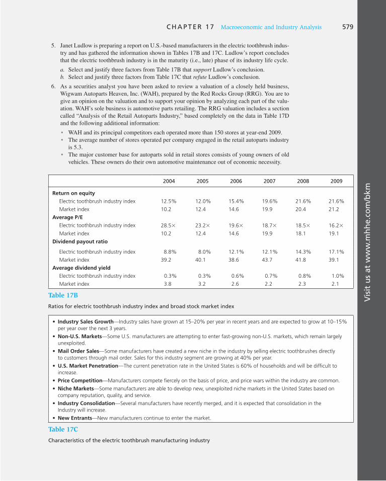
Vis
it u
s at
ww
w.m
hh
e.co
m/b
km
C H A P T E R 1 7 Macroeconomic and Industry Analysis 579
5. Janet Ludlow is preparing a report on U.S.-based manufacturers in the electric toothbrush indus-try and has gathered the information shown in Tables 17B and 17C . Ludlow’s report concludes that the electric toothbrush industry is in the maturity (i.e., late) phase of its industry life cycle.
a. Select and justify three factors from Table 17B that support Ludlow’s conclusion. b. Select and justify three factors from Table 17C that refute Ludlow’s conclusion.
6. As a securities analyst you have been asked to review a valuation of a closely held business, Wigwam Autoparts Heaven, Inc. (WAH), prepared by the Red Rocks Group (RRG). You are to give an opinion on the valuation and to support your opinion by analyzing each part of the valu-ation. WAH’s sole business is automotive parts retailing. The RRG valuation includes a section called “Analysis of the Retail Autoparts Industry,” based completely on the data in Table 17D and the following additional information:
• WAH and its principal competitors each operated more than 150 stores at year-end 2009. • The average number of stores operated per company engaged in the retail autoparts industry
is 5.3. • The major customer base for autoparts sold in retail stores consists of young owners of old
vehicles. These owners do their own automotive maintenance out of economic necessity.
2004 2005 2006 2007 2008 2009
Return on equity
Electric toothbrush industry index 12.5% 12.0% 15.4% 19.6% 21.6% 21.6%
Market index 10.2 12.4 14.6 19.9 20.4 21.2
Average P/E
Electric toothbrush industry index 28.53 23.23 19.63 18.73 18.53 16.23
Market index 10.2 12.4 14.6 19.9 18.1 19.1
Dividend payout ratio
Electric toothbrush industry index 8.8% 8.0% 12.1% 12.1% 14.3% 17.1%
Market index 39.2 40.1 38.6 43.7 41.8 39.1
Average dividend yield
Electric toothbrush industry index 0.3% 0.3% 0.6% 0.7% 0.8% 1.0%
Market index 3.8 3.2 2.6 2.2 2.3 2.1
Table 17B
Ratios for electric toothbrush industry index and broad stock market index
• Industry Sales Growth—Industry sales have grown at 15–20% per year in recent years and are expected to grow at 10–15%
per year over the next 3 years.
• Non-U.S. Markets—Some U.S. manufacturers are attempting to enter fast-growing non-U.S. markets, which remain largely
unexploited.
• Mail Order Sales—Some manufacturers have created a new niche in the industry by selling electric toothbrushes directly
to customers through mail order. Sales for this industry segment are growing at 40% per year.
• U.S. Market Penetration—The current penetration rate in the United States is 60% of households and will be difficult to
increase.
• Price Competition—Manufacturers compete fiercely on the basis of price, and price wars within the industry are common.
• Niche Markets—Some manufacturers are able to develop new, unexploited niche markets in the United States based on
company reputation, quality, and service.
• Industry Consolidation—Several manufacturers have recently merged, and it is expected that consolidation in the
Industry will increase.
• New Entrants—New manufacturers continue to enter the market.
Table 17C
Characteristics of the electric toothbrush manufacturing industry
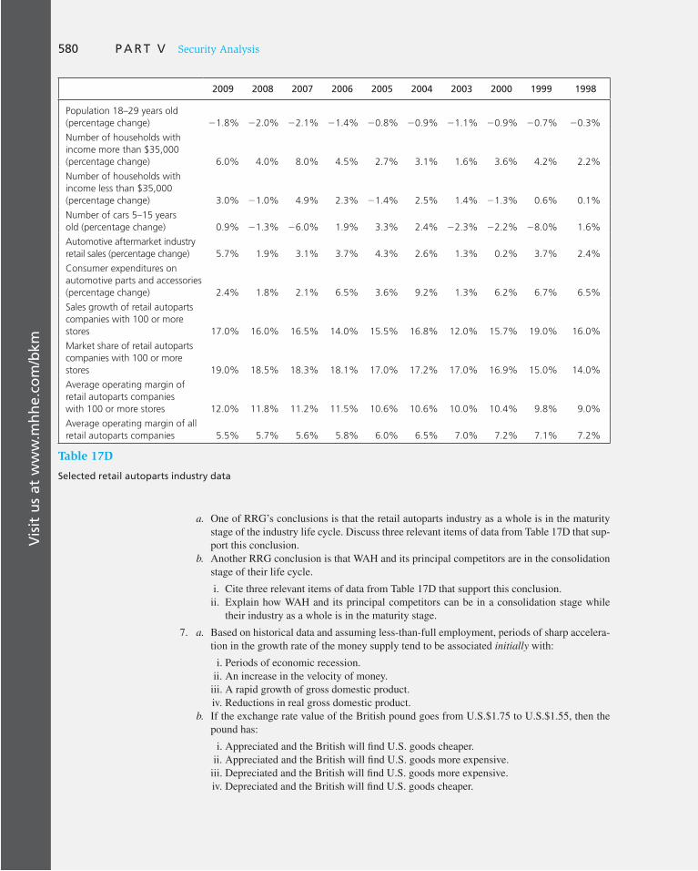
Vis
it u
s at
ww
w.m
hh
e.co
m/b
km580 P A R T V Security Analysis
a. One of RRG’s conclusions is that the retail autoparts industry as a whole is in the maturity stage of the industry life cycle. Discuss three relevant items of data from Table 17D that sup-port this conclusion.
b. Another RRG conclusion is that WAH and its principal competitors are in the consolidation stage of their life cycle.
i. Cite three relevant items of data from Table 17D that support this conclusion. ii. Explain how WAH and its principal competitors can be in a consolidation stage while
their industry as a whole is in the maturity stage.
7. a. Based on historical data and assuming less-than-full employment, periods of sharp accelera-tion in the growth rate of the money supply tend to be associated initially with:
i. Periods of economic recession. ii. An increase in the velocity of money. iii. A rapid growth of gross domestic product. iv. Reductions in real gross domestic product.
b. If the exchange rate value of the British pound goes from U.S.$1.75 to U.S.$1.55, then the pound has:
i. Appreciated and the British will fi nd U.S. goods cheaper. ii. Appreciated and the British will fi nd U.S. goods more expensive. iii. Depreciated and the British will fi nd U.S. goods more expensive. iv. Depreciated and the British will fi nd U.S. goods cheaper.
2009 2008 2007 2006 2005 2004 2003 2000 1999 1998
Population 18–29 years old
(percentage change) 21.8% 22.0% 22.1% 21.4% 20.8% 20.9% 21.1% 20.9% 20.7% 20.3%
Number of households with
income more than $35,000
(percentage change) 6.0% 4.0% 8.0% 4.5% 2.7% 3.1% 1.6% 3.6% 4.2% 2.2%
Number of households with
income less than $35,000
(percentage change) 3.0% 21.0% 4.9% 2.3% 21.4% 2.5% 1.4% 21.3% 0.6% 0.1%
Number of cars 5–15 years
old (percentage change) 0.9% 21.3% 26.0% 1.9% 3.3% 2.4% 22.3% 22.2% 28.0% 1.6%
Automotive aftermarket industry
retail sales (percentage change) 5.7% 1.9% 3.1% 3.7% 4.3% 2.6% 1.3% 0.2% 3.7% 2.4%
Consumer expenditures on
automotive parts and accessories
(percentage change) 2.4% 1.8% 2.1% 6.5% 3.6% 9.2% 1.3% 6.2% 6.7% 6.5%
Sales growth of retail autoparts
companies with 100 or more
stores 17.0% 16.0% 16.5% 14.0% 15.5% 16.8% 12.0% 15.7% 19.0% 16.0%
Market share of retail autoparts
companies with 100 or more
stores 19.0% 18.5% 18.3% 18.1% 17.0% 17.2% 17.0% 16.9% 15.0% 14.0%
Average operating margin of
retail autoparts companies
with 100 or more stores 12.0% 11.8% 11.2% 11.5% 10.6% 10.6% 10.0% 10.4% 9.8% 9.0%
Average operating margin of all
retail autoparts companies 5.5% 5.7% 5.6% 5.8% 6.0% 6.5% 7.0% 7.2% 7.1% 7.2%
Table 17D
Selected retail autoparts industry data

Vis
it u
s at
ww
w.m
hh
e.co
m/b
km
C H A P T E R 1 7 Macroeconomic and Industry Analysis 581
c. Changes in which of the following are likely to affect interest rates?
i. Infl ation expectations. ii. Size of the federal defi cit. iii. Money supply.
d. According to the supply-side view of fiscal policy, if the impact on total tax revenues is the same, does it make any difference whether the government cuts taxes by either reducing marginal tax rates or increasing the personal exemption allowance?
i. No, both methods of cutting taxes will exert the same impact on aggregate supply. ii. No, people in both cases will increase their saving, expecting higher future taxes, and
thereby offset the stimulus effect of lower current taxes. iii. Yes, the lower marginal tax rates alone will increase the incentive to earn marginal in-
come and thereby stimulate aggregate supply. iv. Yes, interest rates will increase if marginal tax rates are lowered, whereas they will tend
to decrease if the personal exemption allowance is raised.
E-INVEST-MENTS EXERCISES
Economic Indicators
1. Locate the Conference Board’s ( www.conference-board.org/economics/bci ) latest monthly release of U.S. Leading Index. The link is located under the heading Latest
Releases, or on the left-side menu under Business Cycle Indicators. Review the latest report. What 10 economic and fi nancial statistics does the Conference Board use in its Leading Indicators series? Which factors contributed positively to the Leading Index; which ones contributed negatively? Why is each of these factors useful when attempt-ing to forecast future economic activity? Answer the same questions for the factors that are coincident indicators and lagging indicators.
2. Is the U.S. economy in a recession or not? Check the “offi cial” opinion at the National Bureau of Economic Research (NBER) at www.nber.org/data . Link to the Offi cial
Business Cycle Dates. How does the NBER select the beginning or end of a recession (follow the available link for a discussion of this topic)? What period in U.S. economic history was the longest expansion? Contraction? Look at the Announcement Dates sec-tion toward the bottom of the page. How much of a time lag is there between when a peak or a trough occurs and when it is announced? What implication does this have for investors?
SOLUTIONS TO CONCEPT CHECKS
1. The downturn in the auto industry will reduce the demand for the product of this economy. The economy will, at least in the short term, enter a recession. This would suggest that:
a. GDP will fall. b. The unemployment rate will rise. c. The government deficit will increase. Income tax receipts will fall, and government
expenditures on social welfare programs probably will increase. d. Interest rates should fall. The contraction in the economy will reduce the demand for credit.
Moreover, the lower inflation rate will reduce nominal interest rates.
2. Expansionary fiscal policy coupled with expansionary monetary policy will stimulate the econ-omy, with the loose monetary policy keeping down interest rates.
3. A traditional demand-side interpretation of the tax cuts is that the resulting increase in after-tax income increased consumption demand and stimulated the economy. A supply-side interpretation

Vis
it u
s at
ww
w.m
hh
e.co
m/b
km582 P A R T V Security Analysis
is that the reduction in marginal tax rates made it more attractive for businesses to invest and for individuals to work, thereby increasing economic output.
4. Firm C has the lowest fixed cost and highest variable costs. It should be least sensitive to the business cycle. In fact, it is. Its profits are highest of the three firms in recessions but lowest in expansions.
Recession Normal Expansion
Revenue $10 $12 $14
Fixed cost 2 2 2
Variable cost 7.5 9 10.5
Profits $ 0.5 $ 1 $ 1.5
5. a. Newspapers will do best in an expansion when advertising volume is increasing. b. Machine tools are a good investment at the trough of a recession, just as the economy is
about to enter an expansion and firms may need to increase capacity. c. Beverages are defensive investments, with demand that is relatively insensitive to the
business cycle. Therefore, they are relatively attractive investments if a recession is forecast. d. Timber is a good investment at a peak period, when natural resource prices are high and the
economy is operating at full capacity.

AS OUR DISCUSSION of market efficiency
indicated, finding undervalued securities
is hardly easy. At the same time, there are
enough chinks in the armor of the efficient
market hypothesis that the search for such
securities should not be dismissed out of
hand. Moreover, it is the ongoing search for
mispriced securities that maintains a nearly
efficient market. Even minor mispricing
would allow a stock market analyst to earn
his salary.
This chapter describes the valuation mod-
els that stock market analysts use to uncover
mispriced securities. The models presented
are those used by fundamental analysts,
those analysts who use information concern-
ing the current and prospective profitability
of a company to assess its fair market value.
We start with a discussion of alternative mea-
sures of the value of a company. From there,
we progress to quantitative tools called divi-
dend discount models, which security ana-
lysts commonly use to measure the value of
a firm as an ongoing concern. Next we turn
to price–earnings, or P/E, ratios, explaining
why they are of such interest to analysts but
also highlighting some of their shortcomings.
We explain how P/E ratios are tied to dividend
valuation models and, more generally, to the
growth prospects of the firm.
We close the chapter with a discussion and
extended example of free cash flow models
used by analysts to value firms based on fore-
casts of the cash flows that will be generated
from the firms’ business endeavors. Finally,
we apply the several valuation tools covered
in the chapter to a real firm and find some
disparity in their conclusions—a conundrum
that will confront any security analyst—and
consider reasons for these discrepancies.
18 Equity Valuation Models 8 PA
RT V
CHAPTER EIGHTEEN
18.1 Valuation by Comparables
The purpose of fundamental analysis is to identify stocks that are mispriced relative to some measure of “true” value that can be derived from observable financial data. There are many convenient sources of such data. For U.S. companies, the Securities and Exchange Commission provides information at its EDGAR Web site, www.sec.gov/edgar.shtml. The SEC requires all public companies (except foreign companies and companies with less than $10 million in assets

584 P A R T V Security Analysis
and 500 shareholders) to file registration statements, periodic reports, and other forms electronically through EDGAR. Anyone can access and download this information.
Many Web sites provide analysis of the data. An example is Standard & Poor’s Market Insight service, which includes COMPUSTAT. Table 18.1 shows COMPUSTAT’s selec-tion of financial highlights for Microsoft Corporation on January 13, 2010.
The price of a share of Microsoft common stock on that day is shown as $30.07, and the total market value of all 8,900 million shares outstanding was $267,623 million. Under the heading Valuation, Table 18.1 reports the ratios of Microsoft’s stock price to four different items taken from its latest financial statements (each divided by the number of outstanding shares): operating earnings, book value, sales revenue, and cash flow. Microsoft’s price-to-earnings (P/E) ratio is 19.0, the price-to-book value is 6.5, and price-to-sales is 4.8. Such comparative valuation ratios are used to assess the valuation of one firm versus others in the same industry. In the column to the right in Table 18.1 are comparable ratios for the average firm in the PC software industry.
For example, an analyst might compare the price/cash flow ratio for Microsoft—16.3, to the industry average ratio of 20.9. By comparison with this standard, Microsoft appears to be underpriced. On the other hand, the market price of a share of Microsoft stock was 6.5 times its book value. Book value is the net worth of a company as reported on its
Source: COMPUSTAT Company Profiles, January 13, 2010. Copyright © 2010 Standard & Poor’s, a division of the McGraw-Hill Companies, Inc. All rights reserved.
Current Qtr Ended: Sep. 2009 Current Year Ended: Jun. 2009
Miscellaneous
Current price 30.070000 Comn sharehldrs (actual) 142468
Comn shares outstdg (mil) 8900.000 Employees (actual) 93000
Market capitalization (mil) 267623.000 S&P issuer credit rating AAA
Latest 12 Months Company 1-Yr Chng (%)
Sales (mil) 56296.000 28.8
EBITDA (mil) 21799.000 216.5
Net Income (mil) 13770.000 222.5
EPS from Ops 1.58 218.6
Dividends/Share 0.520000 18.2
Valuation Company Industry Avg
Price/EPS from Ops 19.0 20.4
Price/Book 6.5 4.6
Price/Sales 4.8 3.9
Price/Cash Flow 16.3 20.9
Profitability (%)
Return on equity 33.4 14.4
Return on assets 16.9 7.1
Oper profit margin 34.1 31.6
Net profit margin 24.5 12.4
Financial Risk
Debt/Equity 14.5 29.6
Cash Flow/Share 1.8 27.6
Table 18.1
Financial highlights for Microsoft Corporation, January 13, 2010

C H A P T E R 1 8 Equity Valuation Models 585
balance sheet. For the average firm in the PC software industry it was 4.6. By comparison with this standard, Microsoft seems a bit overvalued. Microsoft’s price-to-sales ratio also was somewhat higher than the industry average. The price-to-sales ratio is useful for firms and industries that are in a start-up phase. Earnings figures for start-up firms are often negative and not reported, so analysts shift their focus from earnings per share to sales revenue per share.
Limitations of Book Value Shareholders in a firm are sometimes called “residual claimants,” which means that the value of their stake is what is left over when the liabilities of the firm are subtracted from its assets. Shareholders’ equity is this net worth. However, the values of both assets and liabilities recognized in financial statements are based on historical—not current—values. For example, the book value of an asset equals the original cost of acquisition less some adjustment for depreciation, even if the market price of that asset has changed over time. Moreover, depreciation allowances are used to allocate the original cost of the asset over several years, but do not reflect loss of actual value.
Whereas book values are based on original cost, market values measure current values of assets and liabilities. The market value of the shareholders’ equity investment equals the difference between the current values of all assets and liabilities. (The stock price is just the market value of shareholders’ equity divided by the number of outstanding shares.) We’ve emphasized that current values generally will not match historical ones. Equally or even more important, many assets, for example, the value of a good brand name or special-ized expertise developed over many years, may not even be included on the financial state-ments. Market prices therefore reflect the value of the firm as a going concern. It would be unusual if the market price of a stock were exactly equal to its book value.
Can book value represent a “floor” for the stock’s price, below which level the market price can never fall? Although Microsoft’s book value per share in 2010 was less than its market price, other evidence disproves this notion. While it is not common, there are always some firms selling at a market price below book value. In early 2010, for example, such troubled firms included Sprint/Nextel, Citigroup, Mitsubishi, E*trade, and AOL.
A better measure of a floor for the stock price is the firm’s liquidation value per share. This represents the amount of money that could be realized by breaking up the firm, selling its assets, repaying its debt, and distributing the remainder to the shareholders. The reason-ing behind this concept is that if the market price of equity drops below liquidation value, the firm becomes attractive as a takeover target. A corporate raider would find it profitable to buy enough shares to gain control and then actually to liquidate.
Another approach to valuing a firm is the replacement cost of its assets less its liabili-ties. Some analysts believe the market value of the firm cannot remain for long too far above its replacement cost because if it did, competitors would try to replicate the firm. The competitive pressure of other similar firms entering the same industry would drive down the market value of all firms until they came into equality with replacement cost.
This idea is popular among economists, and the ratio of market price to replacement cost is known as Tobin’s q, after the Nobel Prize–winning economist James Tobin. In the long run, according to this view, the ratio of market price to replacement cost will tend toward 1, but the evidence is that this ratio can differ significantly from 1 for very long periods.
Although focusing on the balance sheet can give some useful information about a firm’s liquidation value or its replacement cost, the analyst must usually turn to expected future cash flows for a better estimate of the firm’s value as a going concern. We now examine the quantitative models that analysts use to value common stock in terms of the future earnings and dividends the firm will yield.

586 P A R T V Security Analysis
18.2 Intrinsic Value versus Market Price
The most popular model for assessing the value of a firm as a going concern starts from the observation that an investor in stock expects a return consisting of cash dividends and capital gains or losses. We begin by assuming a 1-year holding period and supposing that ABC stock has an expected dividend per share, E ( D 1 ), of $4, the current price of a share, P 0 , is $48, and the expected price at the end of a year, E ( P 1 ), is $52. For now, don’t worry about how you derive your forecast of next year’s price. At this point we ask only whether the stock seems attractively priced today given your forecast of next year’s price.
The expected holding-period return is E ( D 1 ) plus the expected price appreciation, E ( P 1 ) 2 P 0 , all divided by the current price, P 0 :
Expected HPR 5 E(r) 5E(D1) 1 3E(P1) 2 P0 4
P0
54 1 (52 2 48)
485 .167, or 16.7%
Thus, the stock’s expected holding-period return is the sum of the expected dividend yield, E ( D 1 )/ P 0 , and the expected rate of price appreciation, the capital gains yield, [ E ( P 1 ) 2 P 0 ]/ P 0 .
But what is the required rate of return for ABC stock? The CAPM states that when stock market prices are at equilibrium levels, the rate of return that investors can expect to earn on a security is r f 1 b [ E ( r M ) 2 r f ]. Thus, the CAPM may be viewed as providing an estimate of the rate of return an investor can expect to earn on a security given its risk as measured by beta. This is the return that investors will require of any other investment with equivalent risk. We will denote this required rate of return as k. If a stock is priced “correctly,” it will offer investors a “fair” return, that is, its expected return will equal its required return. Of course, the goal of a security analyst is to find stocks that are mis-priced. For example, an underpriced stock will provide an expected return greater than the required return.
Suppose that r f 5 6%, E ( r M ) 2 r f 5 5%, and the beta of ABC is 1.2. Then the value of k is
k 5 6% 1 1.2 3 5% 5 12%
The expected holding-period return, 16.7%, therefore exceeds the required rate of return based on ABC’s risk by a margin of 4.7%. Naturally, the investor will want to include more of ABC stock in the portfolio than a passive strategy would indicate.
Another way to see this is to compare the intrinsic value of a share of stock to its market price. The intrinsic value, denoted V 0 , is defined as the present value of all cash payments to the investor in the stock, including dividends as well as the proceeds from the ultimate sale of the stock, discounted at the appropriate risk-adjusted interest rate, k. If the intrinsic value, or the investor’s own estimate of what the stock is really worth, exceeds the market price, the stock is considered undervalued and a good investment. In the case of ABC, using a 1-year investment horizon and a forecast that the stock can be sold at the end of the year at price P 1 5 $52, the intrinsic value is
V0 5E(D1) 1 E(P1)
1 1 k5
$4 1 $52
1.125 $50
Equivalently, at a price of $50, the investor would derive a 12% rate of return—just equal to the required rate of return—on an investment in the stock. However, at the current
C H A P T E R 1 8 Equity Valuation Models 587
price of $48, the stock is underpriced compared to intrinsic value. At this price, it provides better than a fair rate of return relative to its risk. In other words, using the terminology of the CAPM, it is a positive-alpha stock, and investors will want to buy more of it than they would following a passive strategy.
If the intrinsic value turns out to be lower than the current market price, investors should buy less of it than under the passive strategy. It might even pay to go short on ABC stock, as we discussed in Chapter 3.
In market equilibrium, the current market price will reflect the intrinsic value estimates of all market participants. This means the individual investor whose V 0 estimate differs from the market price, P 0 , in effect must disagree with some or all of the market consensus estimates of E ( D 1 ), E ( P 1 ), or k. A common term for the market consensus value of the required rate of return, k, is the market capitalization rate, which we use often through-out this chapter.
CONCEPT CHECK
1
You expect the price of IBX stock to be $59.77 per share a year from now. Its current market price is $50, and you expect it to pay a dividend 1 year from now of $2.15 per share.
a. What is the stock’s expected dividend yield, rate of price appreciation, and holding-period return?
b. If the stock has a beta of 1.15, the risk-free rate is 6% per year, and the expected rate of return on the market portfolio is 14% per year, what is the required rate of return on IBX stock?
c. What is the intrinsic value of IBX stock, and how does it compare to the current market price?
18.3 Dividend Discount Models
Consider an investor who buys a share of Steady State Electronics stock, planning to hold it for 1 year. The intrinsic value of the share is the present value of the dividend to be received at the end of the first year, D 1 , and the expected sales price, P 1 . We will henceforth use the simpler notation P 1 instead of E ( P 1 ) to avoid clutter. Keep in mind, though, that future prices and dividends are unknown, and we are dealing with expected values, not certain values. We’ve already established
V0 5D1 1 P1
1 1 k (18.1)
Although this year’s dividends are fairly predictable given a company’s history, you might ask how we can estimate P 1 , the year-end price. According to Equation 18.1 , V 1 (the year-end intrinsic value) will be
V1 5D2 1 P2
1 1 k
If we assume the stock will be selling for its intrinsic value next year, then V 1 5 P 1 , and we can substitute this value for P 1 into Equation 18.1 to find
V0 5D1
1 1 k1
D2 1 P2
(1 1 k)2

588 P A R T V Security Analysis
This equation may be interpreted as the present value of dividends plus sales price for a 2-year holding period. Of course, now we need to come up with a forecast of P 2 . Continuing in the same way, we can replace P 2 by ( D 3 1 P 3 )/(1 1 k ), which relates P 0 to the value of dividends plus the expected sales price for a 3-year holding period.
More generally, for a holding period of H years, we can write the stock value as the present value of dividends over the H years, plus the ultimate sale price, P H :
V0 5D1
1 1 k1
D2
(1 1 k)21c1
DH 1 PH
(1 1 k)H (18.2)
Note the similarity between this formula and the bond valuation formula developed in Chapter 14. Each relates price to the present value of a stream of payments (coupons in the case of bonds, dividends in the case of stocks) and a final payment (the face value of the bond, or the sales price of the stock). The key differences in the case of stocks are the uncertainty of dividends, the lack of a fixed maturity date, and the unknown sales price at the horizon date. Indeed, one can continue to substitute for price indefinitely, to conclude
V0 5D1
1 1 k1
D2
(1 1 k)21
D3
(1 1 k)31c (18.3)
Equation 18.3 states that the stock price should equal the present value of all expected future dividends into perpetuity. This formula is called the dividend discount model
(DDM) of stock prices. It is tempting, but incorrect, to conclude from Equation 18.3 that the DDM focuses
exclusively on dividends and ignores capital gains as a motive for investing in stock. Indeed, we assume explicitly in Equation 18.1 that capital gains (as reflected in the expected sales price, P 1 ) are part of the stock’s value. Our point is that the price at which you can sell a stock in the future depends on dividend forecasts at that time.
The reason only dividends appear in Equation 18.3 is not that investors ignore capital gains. It is instead that those capital gains will be determined by dividend forecasts at the time the stock is sold. That is why in Equation 18.2 we can write the stock price as the present value of dividends plus sales price for any horizon date. P H is the present value at time H of all dividends expected to be paid after the horizon date. That value is then discounted back to today, time 0. The DDM asserts that stock prices are determined ulti-mately by the cash flows accruing to stockholders, and those are dividends. 1
The Constant-Growth DDM
Equation 18.3 as it stands is still not very useful in valuing a stock because it requires dividend forecasts for every year into the indefinite future. To make the DDM practical, we need to introduce some simplifying assumptions. A useful and common first pass at the problem is to assume that dividends are trending upward at a stable growth rate that we will call g. Then if g 5 .05, and the most recently paid dividend was D 0 5 3.81, expected future dividends are
D1 5 D0(1 1 g) 5 3.81 3 1.05 5 4.00
D2 5 D0(1 1 g)2 5 3.81 3 (1.05)2 5 4.20
D3 5 D0(1 1 g)3 5 3.81 3 (1.05)3 5 4.41
1 If investors never expected a dividend to be paid, then this model implies that the stock would have no value. To reconcile the DDM with the fact that non-dividend-paying stocks do have a market value, one must assume that investors expect that some day it may pay out some cash, even if only a liquidating dividend.

C H A P T E R 1 8 Equity Valuation Models 589
and so on. Using these dividend forecasts in Equation 18.3 , we solve for intrinsic value as
V0 5D0(1 1 g)
1 1 k1
D0(1 1 g)2
(1 1 k)21
D0(1 1 g)3
(1 1 k)31c
This equation can be simplified to 2
V0 5D0(1 1 g)
k 2 g5
D1
k 2 g (18.4)
Note in Equation 18.4 that we divide D 1 (not D 0 ) by k 2 g to calculate intrinsic value. If the market capitalization rate for Steady State is 12%, now we can use Equation 18.4 to show that the intrinsic value of a share of Steady State stock is
$3.81(1 1 .05)
.12 2 .05 5
$4.00
.12 2 .055 $57.14
Equation 18.4 is called the constant-growth DDM, or the Gordon model, after Myron J. Gordon, who popularized the model. It should remind you of the formula for the pres-ent value of a perpetuity. If dividends were expected not to grow, then the dividend stream would be a simple perpetuity, and the valuation formula would be 3 V 0 5 D 1 / k. Equation 18.4 is a generalization of the perpetuity formula to cover the case of a growing perpetuity. As g increases (for a given value of D 1 ), the stock price also rises.
Example 18.1 Preferred Stock and the DDM
Preferred stock that pays a fixed dividend can be valued using the constant-growth divi-dend discount model. The constant-growth rate of dividends is simply zero. For example, to value a preferred stock paying a fixed dividend of $2 per share when the discount rate is 8%, we compute
V0 5$2
.08 2 05 $25
2 We prove that the intrinsic value, V 0 , of a stream of cash dividends growing at a constant rate g is equal to D1
k 2 g
as follows. By definition,
V0 5D1
1 1 k1
D1(1 1 g)
(1 1 k)21
D1(1 1 g)2
(1 1 k)31c (a)
Multiplying through by (1 1 k )/(1 1 g ), we obtain
(1 1 k)
(1 1 g) V0 5
D1
(1 1 g)1
D1
(1 1 k)1
D1(1 1 g)
(1 1 k)21c (b)
Subtracting equation (a) from equation (b) , we find that
1 1 k
1 1 g V0 2 V0 5
D1
(1 1 g)
which implies
(k 2 g)V0
(1 1 g)5
D1
(1 1 g)
V0 5D1
k 2 g
3 Recall from introductory finance that the present value of a $1 per year perpetuity is 1/ k. For example, if k 5 10%, the value of the perpetuity is $1/.10 5 $10. Notice that if g 5 0 in Equation 18.4 , the constant-growth DDM formula is the same as the perpetuity formula.

590 P A R T V Security Analysis
Example 18.2 The Constant-Growth DDM
High Flyer Industries has just paid its annual dividend of $3 per share. The dividend is expected to grow at a constant rate of 8% indefinitely. The beta of High Flyer stock is 1.0, the risk-free rate is 6%, and the market risk premium is 8%. What is the intrinsic value of the stock? What would be your estimate of intrinsic value if you believed that the stock was riskier, with a beta of 1.25?
Because a $3 dividend has just been paid and the growth rate of dividends is 8%, the forecast for the year-end dividend is $3 3 1.08 5 $3.24. The market capitalization rate is 6% 1 1.0 3 8% 5 14%. Therefore, the value of the stock is
V0 5D1
k 2 g5
$3.24
.14 2 .085 $54
If the stock is perceived to be riskier, its value must be lower. At the higher beta, the market capitalization rate is 6% 3 1.25 3 8% 5 16%, and the stock is worth only
$3.24
.16 2 .085 $40.50
The constant-growth DDM is valid only when g is less than k. If dividends were expected to grow forever at a rate faster than k, the value of the stock would be infinite. If an analyst derives an estimate of g that is greater than k, that growth rate must be unsus-tainable in the long run. The appropriate valuation model to use in this case is a multistage DDM such as those discussed below.
The constant-growth DDM is so widely used by stock market analysts that it is worth exploring some of its implications and limitations. The constant-growth rate DDM implies that a stock’s value will be greater:
1. The larger its expected dividend per share.
2. The lower the market capitalization rate, k.
3. The higher the expected growth rate of dividends.
Another implication of the constant-growth model is that the stock price is expected to grow at the same rate as dividends. To see this, suppose Steady State stock is selling at its intrinsic value of $57.14, so that V 0 5 P 0 . Then
P0 5D1
k 2 g
Note that price is proportional to dividends. Therefore, next year, when the dividends paid to Steady State stockholders are expected to be higher by g 5 5%, price also should increase by 5%. To confirm this, note
D2 5 $4(1.05) 5 $4.20
P1 5D2
k 2 g5
$4.20
.12 2 .055 $60.00
which is 5% higher than the current price of $57.14. To generalize,
P1 5D2
k 2 g5
D1(1 1 g)
k 2 g5
D1
k 2 g(1 1 g) 5 P0(1 1 g)

C H A P T E R 1 8 Equity Valuation Models 591
Therefore, the DDM implies that in the case of constant growth of dividends, the rate of price appreciation in any year will equal that constant-growth rate, g. Note that for a stock whose market price equals its intrinsic value ( V 0 5 P 0 ), the expected holding-period return will be
E(r) 5 Divided yield 1 Capital gains yield
5D1
P0
1P1 2 P0
P0
5D1
P0
1 g (18.5)
This formula offers a means to infer the market capitalization rate of a stock, for if the stock is selling at its intrinsic value, then E ( r ) 5 k, implying that k 5 D 1 / P 0 1 g. By observing the dividend yield, D 1 / P 0 , and estimating the growth rate of dividends, we can compute k. This equation is also known as the discounted cash flow (DCF) formula.
This is an approach often used in rate hearings for regulated public utilities. The regula-tory agency responsible for approving utility pricing decisions is mandated to allow the firms to charge just enough to cover costs plus a “fair” profit, that is, one that allows a competitive return on the investment the firm has made in its productive capacity. In turn, that return is taken to be the expected return investors require on the stock of the firm. The D 1 / P 0 1 g formula provides a means to infer that required return.
Example 18.3 The Constant-Growth Model
Suppose that Steady State Electronics wins a major contract for its new computer chip. The very profitable contract will enable it to increase the growth rate of dividends from 5% to 6% without reducing the current dividend from the projected value of $4.00 per share. What will happen to the stock price? What will happen to future expected rates of return on the stock?
The stock price ought to increase in response to the good news about the contract, and indeed it does. The stock price jumps from its original value of $57.14 to a postannounce-ment price of
D1
k 2 g5
$4.00
.12 2 .065 $66.67
Investors who are holding the stock when the good news about the contract is announced will receive a substantial windfall.
On the other hand, at the new price the expected rate of return on the stock is 12%, just as it was before the new contract was announced.
E(r) 5D1
P0
1 g 5$4.00
$66.671 .06 5 .12, or 12%
This result makes sense. Once the news about the contract is reflected in the stock price, the expected rate of return will be consistent with the risk of the stock. Because the risk of the stock has not changed, neither should the expected rate of return.
CONCEPT CHECK
2
a. IBX’s stock dividend at the end of this year is expected to be $2.15, and it is expected to grow at 11.2% per year forever. If the required rate of return on IBX stock is 15.2% per year, what is its intrinsic value?
b. If IBX’s current market price is equal to this intrinsic value, what is next year’s expected price?
c. If an investor were to buy IBX stock now and sell it after receiving the $2.15 dividend a year from now, what is the expected capital gain (i.e., price appreciation) in percentage terms? What is the dividend yield, and what would be the holding-period return?

592 P A R T V Security Analysis
Convergence of Price to Intrinsic Value
Now suppose that the current market price of ABC stock is only $48 per share and, there-fore, that the stock now is undervalued by $2 per share. In this case the expected rate of price appreciation depends on an additional assumption about whether the discrepancy between the intrinsic value and the market price will disappear, and if so, when.
One fairly common assumption is that the discrepancy will never disappear and that the market price will trend upward at rate g forever. This implies that the discrepancy between intrinsic value and market price also will grow at the same rate. In our example:
Now Next Year
V0 5 $50 V1 5 $50 3 1.04 5 $52
P0 5 $48 P1 5 $48 3 1.04 5 $49.92
V0 2 P0 5 $2 V1 2 P1 5 $2 3 1.04 5 $2.08
Under this assumption the expected HPR will exceed the required rate, because the dividend yield is higher than it would be if P 0 were equal to V 0 . In our example the divi-dend yield would be 8.33% instead of 8%, so that the expected HPR would be 12.33% rather than 12%:
E(r) 5D1
P0
1 g 5$4
$481 .04 5 .0833 1 .04 5 .1233
An investor who identifies this undervalued stock can get an expected dividend that exceeds the required yield by 33 basis points. This excess return is earned each year, and the market price never catches up to intrinsic value.
An alternative assumption is that the gap between market price and intrinsic value will disappear by the end of the year. In that case we would have P 1 5 V 1 5 $52, and
E(r) 5D1
P0
1P1 2 P0
P0
54
481
52 2 48
485 .0833 1 .0833 5 .1667
The assumption of complete catch-up to intrinsic value produces a much larger 1-year HPR. In future years, however, the stock is expected to generate only fair rates of return.
Many stock analysts assume that a stock’s price will approach its intrinsic value gradu-ally over time—for example, over a 5-year period. This puts their expected 1-year HPR somewhere between the bounds of 12.33% and 16.67%.
Stock Prices and Investment Opportunities
Consider two companies, Cash Cow, Inc., and Growth Prospects, each with expected earn-ings in the coming year of $5 per share. Both companies could in principle pay out all of these earnings as dividends, maintaining a perpetual dividend flow of $5 per share. If the market capitalization rate were k 5 12.5%, both companies would then be valued at D 1 / k 5 $5/.125 5 $40 per share. Neither firm would grow in value, because with all earn-ings paid out as dividends, and no earnings reinvested in the firm, both companies’ capital stock and earnings capacity would remain unchanged over time; earnings 4 and dividends would not grow.
4 Actually, we are referring here to earnings net of the funds necessary to maintain the productivity of the firm’s capital, that is, earnings net of “economic depreciation.” In other words, the earnings figure should be interpreted as the maximum amount of money the firm could pay out each year in perpetuity without depleting its productive capacity. For this reason, the net earnings number may be quite different from the accounting earnings figure that the firm reports in its financial statements. We explore this further in the next chapter.
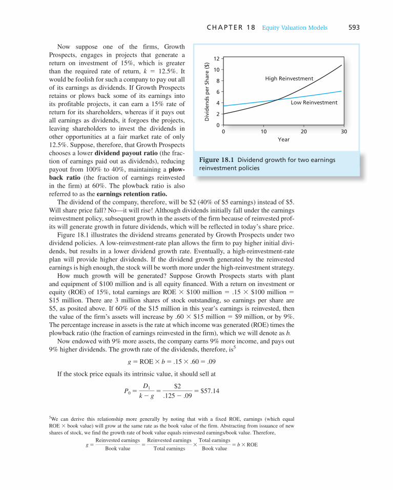
C H A P T E R 1 8 Equity Valuation Models 593
Now suppose one of the firms, Growth Prospects, engages in projects that generate a return on investment of 15%, which is greater than the required rate of return, k 5 12.5%. It would be foolish for such a company to pay out all of its earnings as dividends. If Growth Prospects retains or plows back some of its earnings into its profitable projects, it can earn a 15% rate of return for its shareholders, whereas if it pays out all earnings as dividends, it forgoes the projects, leaving shareholders to invest the dividends in other opportunities at a fair market rate of only 12.5%. Suppose, therefore, that Growth Prospects chooses a lower dividend payout ratio (the frac-tion of earnings paid out as dividends), reducing payout from 100% to 40%, maintaining a plow-
back ratio (the fraction of earnings reinvested in the firm) at 60%. The plowback ratio is also referred to as the earnings retention ratio.
The dividend of the company, therefore, will be $2 (40% of $5 earnings) instead of $5. Will share price fall? No—it will rise! Although dividends initially fall under the earnings reinvestment policy, subsequent growth in the assets of the firm because of reinvested prof-its will generate growth in future dividends, which will be reflected in today’s share price.
Figure 18.1 illustrates the dividend streams generated by Growth Prospects under two dividend policies. A low-reinvestment-rate plan allows the firm to pay higher initial divi-dends, but results in a lower dividend growth rate. Eventually, a high-reinvestment-rate plan will provide higher dividends. If the dividend growth generated by the reinvested earnings is high enough, the stock will be worth more under the high-reinvestment strategy.
How much growth will be generated? Suppose Growth Prospects starts with plant and equipment of $100 million and is all equity financed. With a return on investment or equity (ROE) of 15%, total earnings are ROE 3 $100 million 5 .15 3 $100 million 5$15 million. There are 3 million shares of stock outstanding, so earnings per share are $5, as posited above. If 60% of the $15 million in this year’s earnings is reinvested, then the value of the firm’s assets will increase by .60 3 $15 million 5 $9 million, or by 9%. The percentage increase in assets is the rate at which income was generated (ROE) times the plowback ratio (the fraction of earnings reinvested in the firm), which we will denote as b.
Now endowed with 9% more assets, the company earns 9% more income, and pays out 9% higher dividends. The growth rate of the dividends, therefore, is 5
g 5 ROE 3 b 5 .15 3 .60 5 .09
If the stock price equals its intrinsic value, it should sell at
P0 5D1
k 2 g5
$2
.125 2 .095 $57.14
5 We can derive this relationship more generally by noting that with a fixed ROE, earnings (which equal ROE 3 book value) will grow at the same rate as the book value of the firm. Abstracting from issuance of new shares of stock, we find the growth rate of book value equals reinvested earnings/book value. Therefore,
g 5Reinvested earnings
Book value5
Reinvested earnings
Total earnings3
Total earnings
Book value5 b 3 ROE
Div
iden
ds
per
Sh
are
($)
Year
12
0 302010
Low Reinvestment
High Reinvestment
0
2
4
6
8
10
Figure 18.1 Dividend growth for two earnings r einvestment policies
594 P A R T V Security Analysis
When Growth Prospects pursued a no-growth policy and paid out all earnings as divi-dends, the stock price was only $40. Therefore, you can think of $40 as the value per share of the assets the company already has in place.
When Growth Prospects decided to reduce current dividends and reinvest some of its earnings in new investments, its stock price increased. The increase in the stock price reflects the fact that the planned investments provide an expected rate of return greater than the required rate. In other words, the investment opportunities have positive net present value. The value of the firm rises by the NPV of these investment opportunities. This net present value is also called the present value of growth opportunities, or PVGO.
Therefore, we can think of the value of the firm as the sum of the value of assets already in place, or the no-growth value of the firm, plus the net present value of the future invest-ments the firm will make, which is the PVGO. For Growth Prospects, PVGO 5 $17.14 per share:
Price 5 No-growth value per share 1 PVGO
P0 5E1
k1 PVGO
57.14 5 40 1 17.14
(18.6)
We know that in reality, dividend cuts almost always are accompanied by steep drops in stock prices. Does this contradict our analysis? Not necessarily: Dividend cuts are usu-ally taken as bad news about the future prospects of the firm, and it is the new information about the firm—not the reduced dividend yield per se—that is responsible for the stock price decline.
In one well-known case, Florida Power & Light announced a cut in its dividend, not because of financial distress but because it wanted to better position itself for a period of deregulation. At first, the stock market did not believe this rationale—the stock price dropped 14% on the day of the announcement. But within a month, the market became convinced that the firm had in fact made a strategic decision that would improve growth prospects, and the share price actually rose above its preannouncement value. Even includ-ing the initial price drop, the share price outperformed both the S&P 500 and the S&P util-ity index in the year following the dividend cut.
It is important to recognize that growth per se is not what investors desire. Growth enhances company value only if it is achieved by investment in projects with attractive profit opportunities (i.e., with ROE > k ). To see why, let’s now consider Growth Prospects’s unfortunate sister company, Cash Cow, Inc. Cash Cow’s ROE is only 12.5%, just equal to the required rate of return, k. The net present value of its investment opportunities is zero. We’ve seen that following a zero-growth strategy with b 5 0 and g 5 0, the value of Cash Cow will be E 1 / k 5 $5/.125 5 $40 per share. Now suppose Cash Cow chooses a plowback ratio of b 5 .60, the same as Growth Prospects’s plowback. Then g would increase to
g 5 ROE 3 b 5 .125 3 .60 5 .075
but the stock price is still
P0 5D1
k 2 g5
$2
.125 2 .0755 $40
which is no different from the no-growth strategy. In the case of Cash Cow, the dividend reduction used to free funds for reinvest-
ment in the firm generates only enough growth to maintain the stock price at the cur-rent level. This is as it should be: If the firm’s projects yield only what investors can

C H A P T E R 1 8 Equity Valuation Models 595
earn on their own, shareholders cannot be made better off by a high-reinvestment-rate policy. This demonstrates that “growth” is not the same as growth opportunities. To jus-tify reinvestment, the firm must engage in projects with better prospective returns than those shareholders can find elsewhere. Notice also that the PVGO of Cash Cow is zero: PVGO 5 P 0 2 E 1 / k 5 40 2 40 5 0. With ROE 5 k, there is no advantage to plowing funds back into the firm; this shows up as PVGO of zero. In fact, this is why firms with considerable cash flow but limited investment prospects are called “cash cows.” The cash these firms generate is best taken out of, or “milked from,” the firm.
Example 18.4 Growth Opportunities
Takeover Target is run by entrenched management that insists on reinvesting 60% of its earnings in projects that provide an ROE of 10%, despite the fact that the firm’s capitaliza-tion rate is k 5 15%. The firm’s year-end dividend will be $2 per share, paid out of earn-ings of $5 per share. At what price will the stock sell? What is the present value of growth opportunities? Why would such a firm be a takeover target for another firm?
Given current management’s investment policy, the dividend growth rate will be
g 5 ROE 3 b 5 10% 3 .60 5 6%
and the stock price should be
P0 5$2
.15 2 .065 $22.22
The present value of growth opportunities is
PVGO 5 Price per share 2 No-growth value per share
5 $22.22 2 E1/k 5 $22.22 2 $5/.15 5 2$11.11
PVGO is negative. This is because the net present value of the firm’s projects is negative: The rate of return on those assets is less than the opportunity cost of capital.
Such a firm would be subject to takeover, because another firm could buy the firm for the market price of $22.22 per share and increase the value of the firm by chang-ing its investment policy. For example, if the new management simply paid out all earnings as dividends, the value of the firm would increase to its no-growth value, E 1 / k 5 $5/.15 5 $33.33.
CONCEPT CHECK
3
a. Calculate the price of a firm with a plowback ratio of .60 if its ROE is 20%. Current ea rnings, E 1 , will be $5 per share, and k 5 12.5%.
b. What if ROE is 10%, which is less than the market capitalization rate? Compare the firm’s price in this instance to that of a firm with the same ROE and E 1 , but a plowback ratio of b 5 0.
Life Cycles and Multistage Growth Models
As useful as the constant-growth DDM formula is, you need to remember that it is based on a simplifying assumption, namely, that the dividend growth rate will be constant for-ever. In fact, firms typically pass through life cycles with very different dividend profiles in

596 P A R T V Security Analysis
different phases. In early years, there are ample opportunities for profitable reinvestment in the company. Payout ratios are low, and growth is correspondingly rapid. In later years, the firm matures, production capacity is sufficient to meet market demand, competitors enter the market, and attractive opportunities for reinvestment may become harder to find. In this mature phase, the firm may choose to increase the dividend payout ratio, rather than retain earnings. The dividend level increases, but thereafter it grows at a slower rate because the company has fewer growth opportunities.
Table 18.2 illustrates this pattern. It gives Value Line’s forecasts of return on assets, dividend payout ratio, and 3-year projected growth rate in earnings per share for a sample of the firms included in the computer software industry versus those of East Coast electric utilities. (We compare return on assets rather than return on equity because the latter is affected by leverage, which tends to be far greater in the electric utility industry than in the software industry. Return on assets measures operating income per dollar of total assets, regardless of whether the source of the capital supplied is debt or equity. We will return to this issue in the next chapter.)
By and large, the software firms have attractive investment opportunities. The median return on assets of these firms is forecast to be 16.5%, and the firms have responded with high plowback ratios. Most of these firms pay no dividends at all. The high return on assets and high plowback result in rapid growth. The median projected growth rate of earnings per share in this group is 14.5%.
Return on Assets (%)
Payout Ratio (%)
Growth Rate 2010–2013
Computer software
Adobe Systems 12.5% 0.0% 17.0%
Cognizant 16.5 0.0 14.5
Compuware 11.5 0.0 10.9
Intuit 17.0 0.0 9.8
Microsoft 35.5 30.0 15.9
Oracle 29.5 14.0 12.0
Red Hat 12.0 0.0 23.6
Parametric Tech 14.0 0.0 39.2
SAP 20.0 28.0 9.7
Median 16.5% 0.0% 14.5%
Electric utilities
Central Hudson G&E 5.5% 73.0% 6.3%
Central Vermont 5.0 51.0 3.9
Consolidated Edison 6.0 63.0 6.4
Duke Energy 5.5 78.0 5.3
Northeast Utilities 5.5 53.0 4.9
NStar 9.5 61.0 8.4
Pennsylvania Power (PPL) 10.5 50.0 5.4
Public Services Enter 10.5 44.0 4.9
United Illuminating 6.5 76.0 4.0
Median 6.0% 61.0% 5.3%
Source: Value Line Investment Survey, November 2009. Reprinted with permission of Value Line Investment Survey. © 2009 Value Line Publishing, Inc. All rights reserved.
Table 18.2
Financial ratios in two industries

C H A P T E R 1 8 Equity Valuation Models 597
In contrast, the electric utilities are more representative of mature firms. Their median return on assets is lower, 6%; dividend payout is higher, 61%; and median growth is lower, 5.3%.
We conclude that the higher payouts of the electric utilities reflect their more limited opportunities to reinvest earnings at attractive rates of return. For example, Microsoft’s announcement in 2004 that it would sharply increase its dividend and initiate multi-billion-dollar stock buybacks was widely seen as an indication that the firm was maturing into a lower-growth stage. It was generating far more cash than it had the opportunity to invest attractively, and so was paying out that cash to its shareholders.
To value companies with temporarily high growth, analysts use a multistage version of the dividend discount model. Dividends in the early high-growth period are forecast and their combined present value is calculated. Then, once the firm is projected to settle down to a steady-growth phase, the constant-growth DDM is applied to value the remaining stream of dividends.
We can illustrate this with a real-life example. Figure 18.2 is a Value Line Investment Survey report on Honda Motor Co. Some of the relevant information for late 2009 is highlighted.
Honda’s beta appears at the circled A, its recent stock price at the B, the per-share dividend payments at the C, the ROE (referred to as “return on shareholder equity”) at the D, and the dividend payout ratio (referred to as “all dividends to net profits”) at the E. 6 The rows ending at C, D, and E are historical time series. The boldfaced, italicized entries under 2010 are estimates for that year. Similarly, the entries in the far right column (labeled 12–14) are forecasts for some time between 2012 and 2014, which we will take to be 2013.
Value Line projects rapid growth in the near term, with dividends rising from $.50 in 2010 to $1.00 in 2013. This rapid growth rate cannot be sustained indefinitely. We can obtain dividend inputs for this initial period by using the explicit forecasts for 2010 and 2013 and linear interpolation for the years between:
2010 $.50 2012 $ .83
2011 $.66 2013 $1.00
Now let us assume the dividend growth rate levels off in 2013. What is a good guess for that steady-state growth rate? Value Line forecasts a dividend payout ratio of .30 and an ROE of 11%, implying long-term growth will be
g 5 ROE 3 b 5 11.0% 3 (1 2 .30) 5 7.70%
Our estimate of Honda’s intrinsic value using an investment horizon of 2013 is therefore obtained from Equation 18.2 , which we restate here:
V2009 5D2010
1 1 k1
D2011
(1 1 k)21
D2012
(1 1 k)31
D2013 1 P2013
(1 1 k)4
5.50
1 1 k1
.66
(1 1 k)21
.83
(1 1 k)31
1.00 1 P2013
(1 1 k)4
6 Because Honda is a Japanese firm, Americans would hold its shares via ADRs, or American Depository Receipts. ADRs are not shares of the firm, but are claims to shares of the underlying foreign stock that are then traded in U.S. security markets. Value Line notes that each Honda ADR is a claim on one common share, but in other cases, each ADR may represent a claim to multiple shares or even fractional shares.
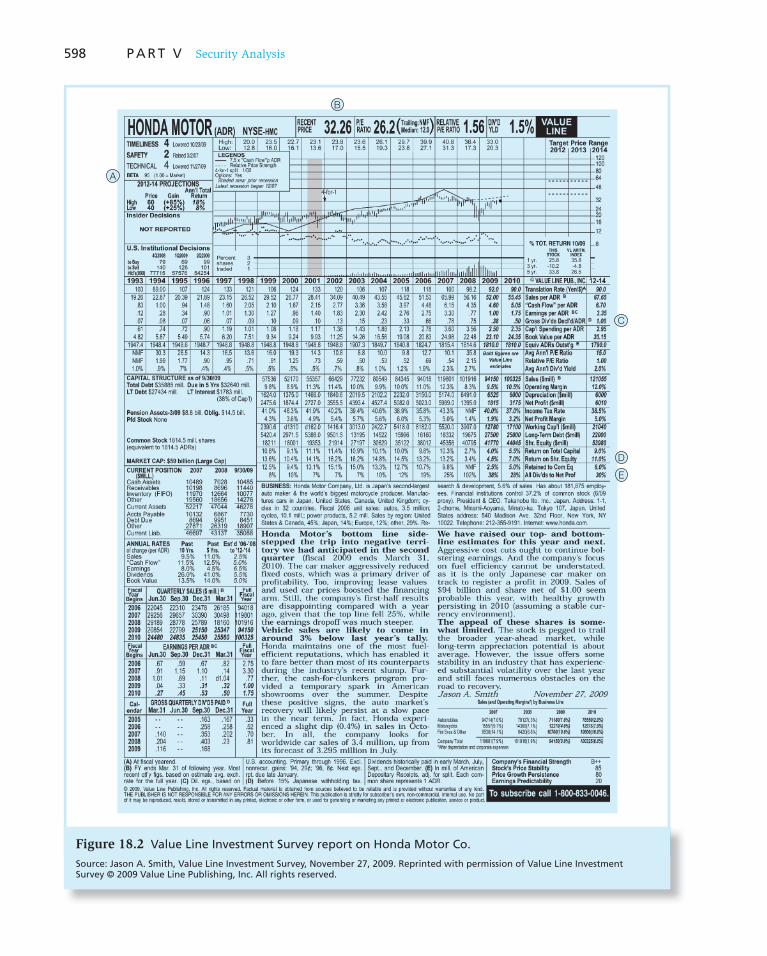
598 P A R T V Security Analysis
B
A
C
D
E
Figure 18.2 Value Line Investment Survey report on Honda Motor Co.
Source: Jason A. Smith, Value Line Investment Survey, November 27, 2009. Reprinted with permission of Value Line Investment Survey © 2009 Value Line Publishing, Inc. All rights reserved.

C H A P T E R 1 8 Equity Valuation Models 599
Here, P 2013 represents the forecast price at which we can sell our shares at the end of 2013, when dividends are assumed to enter their constant-growth phase. That price, according to the constant-growth DDM, should be
P2013 5D2014
k 2 g5
D2013(1 1 g)
k 2 g5
1.00 3 1.077
k 2 .077
The only variable remaining to be determined to calculate intrinsic value is the market capitalization rate, k.
One way to obtain k is from the CAPM. Observe from the Value Line report that Honda’s beta is .95. The risk-free rate on Treasury bonds at the end of 2009 was about 3.5%. Suppose that the market risk premium were forecast at 8%, roughly in line with its historical average. This would imply that the forecast for the market return was
Risk-free rate 1 Market risk premium 5 3.5% 1 8% 5 11.5%
Therefore, we can solve for the market capitalization rate as
k 5 rf 1 b 3E(rM) 2 rf 45 3.5% 1 .95(11.5 2 3.5) 5 11.1%
Our forecast for the stock price in 2013 is thus
P2013 5$1.00 3 1.077
.111 2 .0775 $31.68
And today’s estimate of intrinsic value is
V2009 5.50
1.1111
.66
(1.111)21
.83
(1.111)31
1.00 1 31.68
(1.111)45 $23.04
We know from the Value Line report that Honda’s actual price was $32.26 (at the circled B). Our intrinsic value analysis indicates that the stock was overpriced. Should we increase our holdings?
Perhaps. But before betting the farm, stop to consider how firm our estimate is. We’ve had to guess at dividends in the near future, the ultimate growth rate of those dividends, and the appropriate discount rate. Moreover, we’ve assumed Honda will follow a relatively simple two-stage growth process. In practice, the growth of dividends can follow more complicated patterns. Even small errors in these approximations could upset a conclusion.
For example, suppose that we have underestimated Honda’s growth prospects and that the actual ROE in the post-2013 period will be 13% rather than 11%. Using the higher return on equity in the dividend discount model would result in an intrinsic value in 2009 of $38.05, which is more than the stock price. Our conclusion regarding intrinsic value versus price is reversed.
The exercise also highlights the importance of performing sensitivity analysis when you attempt to value stocks. Your estimates of stock values are no better than your assumptions. Sensitivity analysis will highlight the inputs that need to be most carefully examined. For example, even modest changes in the estimated ROE for the post-2013 period can result in big changes in intrinsic value. Similarly, small changes in the assumed capitalization rate would change intrinsic value substantially. On the other hand, reasonable changes in the dividends forecast between 2010 and 2013 would have a small impact on intrinsic value.
CONCEPT CHECK
4 Confirm that the intrinsic value of Honda using ROE 5 13% is $38.05. ( Hint: First calculate the stock price in 2013. Then calculate the present value of all interim dividends plus the present value of the 2013 sales price.)

600 P A R T V Security Analysis
Multistage Growth Models
The two-stage growth model that we just considered for Honda is a good start toward realism, but clearly we could do even better if our valuation model allowed for more flexible patterns of growth. Multistage growth models allow dividends per share to grow at several different rates as the firm matures. Many analysts use three-stage growth mod-els. They may assume an initial period of high dividend growth (or instead make year-by-year forecasts of dividends for the short term), a final period of sustainable growth, and a transition period between, during which dividend growth rates taper off from the initial rapid rate to the ultimate sustainable rate. These models are conceptually no harder to work with than a two-stage model, but they require many more calculations and can be tedious to do by hand. It is easy, however, to build an Excel spreadsheet for such a model.
Spreadsheet 18.1 is an example of such a model. Column B contains the inputs we have used so far for Honda. Column E contains dividend forecasts. In cells E2 through E5 we present the Value Line estimates for the next 4 years. Dividend growth in this period is rapid, about 26% annually. Rather than assume a sudden transition to constant dividend growth starting in 2013, we assume instead that the dividend growth rate in 2013 will be 26% and that it will decline steadily through 2024, finally reaching the constant terminal growth rate of 7.7% (see column F). Each dividend in the transition period is the previous year’s dividend times that year’s growth rate. Terminal value once the firm enters a constant-growth stage (cell G17) is computed from the constant-growth DDM. Finally, investor cash flow in each period (column H) equals dividends in each year plus the terminal value in 2024. The present value of these cash flows is computed in cell H19 as $49.44, about double the value we found from the two-stage model. We obtain a greater intrinsic value in this case because we assume that dividend growth, which at its current value of 26% per year is extremely rapid, only gradually declines to its steady-state value.
Spreadsheet 18.1
A three-stage growth model for Honda Motor Co.
eXce lPlease visit us at www.mhhe.com/bkm
A B C D E F G H I
1
2
3
4
5
6
7
8
9
10
11
12
13
14
15
16
17
18
19
20
21
Inputs
beta
mkt_prem
rf
k_equity
plowback
roe
term_gwth
Value line
annual dividends
forecasts of
Transitional period
with slowing dividend
growth
Beginning of constant
growth period
0.95
0.08
0.035
0.111
0.7
0.11
0.077
Year
2009
2010
2011
2012
2013
2014
2015
2016
2017
2018
2019
2020
2021
2022
2023
2024
Dividend Div growth Term value Investor CF
0.50
0.67
0.83
1.00
1.26
1.56
1.91
2.31
2.74
3.20
3.68
4.16
4.64
5.08
5.47
5.89
0.2599
0.2416
0.2233
0.2050
0.1868
0.1685
0.1502
0.1319
0.1136
0.0953
0.0770
0.0770 186.57
0.50
0.67
0.83
1.00
1.26
1.56
1.91
2.31
2.74
3.20
3.68
4.16
4.64
5.08
5.47
192.46
E17*(1+F17)/(B5−F17)
49.44
NPV(B5,H2:H17)
= PV of CF
C H A P T E R 1 8 Equity Valuation Models 601
18.4 Price–Earnings Ratio
The Price–Earnings Ratio and Growth Opportunities
Much of the real-world discussion of stock market valuation concentrates on the firm’s price–earnings multiple, the ratio of price per share to earnings per share, commonly called the P/E ratio. Our discussion of growth opportunities shows why stock market analysts focus on the P/E ratio. Both companies considered, Cash Cow and Growth Prospects, had earnings per share (EPS) of $5, but Growth Prospects reinvested 60% of earnings in prospects with an ROE of 15%, whereas Cash Cow paid out all earnings as dividends. Cash Cow had a price of $40, giving it a P/E multiple of 40/5 5 8.0, whereas Growth Prospects sold for $57.14, giving it a multiple of 57.14/5 5 11.4. This observa-tion suggests the P/E ratio might serve as a useful indicator of expectations of growth opportunities.
We can see how growth opportunities are reflected in P/E ratios by rearranging Equation 18.6 to
P0
E1
51
k ¢1 1
PVGO
E/k≤ (18.7)
When PVGO 5 0, Equation 18.7 shows that P 0 5 E 1 / k. The stock is valued like a non-growing perpetuity of E 1 , and the P/E ratio is just 1/ k. However, as PVGO becomes an increasingly dominant contributor to price, the P/E ratio can rise dramatically.
The ratio of PVGO to E / k has a simple interpretation. It is the ratio of the compo-nent of firm value due to growth opportunities to the component of value due to assets already in place (i.e., the no-growth value of the firm, E / k ). When future growth oppor-tunities dominate the estimate of total value, the firm will command a high price relative to current earnings. Thus a high P/E multiple indicates that a firm enjoys ample growth opportunities.
Let’s see if P/E multiples do vary with growth prospects. Between 1992 and 2009, for example, McDonald’s P/E ratio averaged about 19.0 while Consolidated Edison’s (an electric utility) average P/E was only about two-thirds of that. These numbers do not nec-essarily imply that McDonald’s was overpriced compared to Con Ed. If investors believed McDonald’s would grow faster than Con Ed, the higher price per dollar of earnings would be justified. That is, an investor might well pay a higher price per dollar of current earn-ings if he or she expects that earnings stream to grow more rapidly. In fact, McDonald’s growth rate has been consistent with its higher P/E multiple. Over this period, its earnings per share grew at 11.0% per year while Con Ed’s earnings growth rate was only 1.2%. Figure 18.4 (page 607) shows the EPS history of the two companies.
Clearly, differences in expected growth opportunities are responsible for differences in P/E ratios across firms. The P/E ratio actually is a reflection of the market’s optimism concerning a firm’s growth prospects. In their use of a P/E ratio, analysts must decide whether they are more or less optimistic than the market. If they are more optimistic, they will recommend buying the stock.
There is a way to make these insights more precise. Look again at the constant-growth DDM formula, P 0 5 D 1 /( k 2 g ). Now recall that dividends equal the earnings that are not reinvested in the firm: D 1 5 E 1 (1 2 b ). Recall also that g 5 ROE 3 b. Hence, substituting for D 1 and g, we find that
P0 5E1(1 2 b)
k 2 ROE 3 b

602 P A R T V Security Analysis
implying the P/E ratio is
P0
E1
51 2 b
k 2 ROE 3 b (18.8)
It is easy to verify that the P/E ratio increases with ROE. This makes sense, because high-ROE projects give the firm good opportunities for growth. 7 We also can verify that the P/E ratio increases for higher plowback, b, as long as ROE exceeds k. This too makes sense. When a firm has good investment opportunities, the market will reward it with a higher P/E multiple if it exploits those opportunities more aggressively by plowing back more earn-ings into those opportunities.
Remember, however, that growth is not desirable for its own sake. Examine Table 18.3 where we use Equation 18.8 to compute both growth rates and P/E ratios for different com-binations of ROE and b. Although growth always increases with the plowback rate (move across the rows in Panel A), the P/E ratio does not (move across the rows in panel B). In the top row of Panel B, the P/E falls as the plowback rate increases. In the middle row, it is unaffected by plowback. In the third row, it increases.
This pattern has a simple interpretation. When the expected ROE is less than the required return, k, investors prefer that the firm pay out earnings as dividends rather than reinvest earnings in the firm at an inadequate rate of return. That is, for ROE lower than k, the value of the firm falls as plowback increases. Conversely, when ROE exceeds k, the firm offers attractive investment opportunities, so the value of the firm is enhanced as those opportunities are more fully exploited by increasing the plowback rate.
Finally, where ROE just equals k, the firm offers “break-even” investment opportuni-ties with a fair rate of return. In this case, investors are indifferent between reinvestment of earnings in the firm or elsewhere at the market capitalization rate, because the rate of return in either case is 12%. Therefore, the stock price is unaffected by the plowback rate.
We conclude that the higher the plowback rate, the higher the growth rate, but a higher plowback rate does not necessarily mean a higher P/E ratio. Higher plowback increases P/E only if investments undertaken by the firm offer an expected rate of return greater than the market capitalization rate. Otherwise, increasing plowback hurts investors because more money is sunk into projects with inadequate rates of return.
7 Note that Equation 18.8 is a simple rearrangement of the DDM formula, with ROE 3 b 5 g. Because that formula requires that g < k, Equation 18.8 is valid only when ROE 3 b < k.
Table 18.3
Effect of ROE and plowback on growth and the P/E ratio
Plowback Rate (b)
0 .25 .50 .75
ROE A. Growth rate, g
10% 0 2.5% 5.0% 7.5%
12 0 3.0 6.0 9.0
14 0 3.5 7.0 10.5
B. P/E ratio
10% 8.33 7.89 7.14 5.56
12 8.33 8.33 8.33 8.33
14 8.33 8.82 10.00 16.67
Assumption: k 5 12% per year.

C H A P T E R 1 8 Equity Valuation Models 603
Notwithstanding these fine points, P/E ratios frequently are taken as proxies for the expected growth in dividends or earnings. In fact, a common Wall Street rule of thumb is that the growth rate ought to be roughly equal to the P/E ratio. In other words, the ratio of P/E to g, often called the PEG ratio, should be about 1.0. Peter Lynch, the famous portfolio manager, puts it this way in his book One Up on Wall Street:
The P/E ratio of any company that’s fairly priced will equal its growth rate. I’m talking here about growth rate of earnings here. . . . If the P/E ratio of Coca Cola is 15, you’d expect the company to be growing at about 15% per year, etc. But if the P/E ratio is less than the growth rate, you may have found yourself a bargain.
Example 18.5 P/E Ratio versus Growth Rate
Let’s try Lynch’s rule of thumb. Assume that
rf 5 8% (roughly the value when Peter Lynch was writing)
rM 2 rf 5 8% (about the historical average market risk premium)
b 5 .4 (a typical value for the plowback ratio in the United States)
Therefore, r M 5 r f 1 market risk premium 5 8% 1 8% 5 16%, and k 5 16% for an aver-age ( b 5 1) company. If we also accept as reasonable that ROE 5 16% (the same value as the expected return on the stock), we conclude that
g 5 ROE 3 b 5 16% 3 .4 5 6.4%
and
P
E5
1 2 .4
.16 2 .0645 6.26
Thus, the P/E ratio and g are about equal using these assumptions, consistent with the rule of thumb.
However, note that this rule of thumb, like almost all others, will not work in all circum-stances. For example, the value of r f today is more like 3.5%, so a comparable forecast of r M today would be
rf 1 Market risk premium 5 3.5% 1 8% 5 11.5%
If we continue to focus on a firm with b 5 1, and if ROE still is about the same as k, then
g 5 11.5% 3 .4 5 4.6%
while
P
E5
1 2 .4
.115 2 .0465 8.70
The P/E ratio and g now diverge and the PEG ratio is now 1.9. Nevertheless, lower-than-average PEG ratios are still widely seen as signaling potential underpricing.
The importance of growth opportunities is most evident in the valuation of start-up firms. For example, in the dot-com boom of the late 1990s, many companies that had yet to turn a profit were valued by the market at billions of dollars. The perceived value of these companies was exclusively as growth opportunities. For example, the online auction firm eBay had 1998 profits of $2.4 million, far less than the $45 million profit earned by the
604 P A R T V Security Analysis
traditional auctioneer Sotheby’s; yet eBay’s market value was more than 10 times greater: $22 billion versus $1.9 billion. (As it turns out, the market was quite right to value eBay so much more aggressively than Sotheby’s. By 2006, eBay’s net income was over $1 billion, more than 10 times that of Sotheby’s, and despite setbacks since then, its income in 2009 was still several multiples of Sotheby’s.
Of course, when company valuation is determined primarily by growth opportunities, those values can be very sensitive to reassessments of such prospects. When the market became more skeptical of the business prospects of most Internet retailers at the close of the 1990s, that is, as it revised the estimates of growth opportunities downward, their stock prices plummeted.
As perceptions of future prospects wax and wane, share price can swing wildly. Growth prospects are intrinsically difficult to tie down; ultimately, however, those prospects drive the value of the most dynamic firms in the economy.
CONCEPT CHECK
5
ABC stock has an expected ROE of 12% per year, expected earnings per share of $2, and expected dividends of $1.50 per share. Its market capitalization rate is 10% per year.
a. What are its expected growth rate, its price, and its P/E ratio?
b. If the plowback ratio were .4, what would be the expected dividend per share, the growth rate, price, and the P/E ratio?
The nearby box is an example of a valuation analysis based on the P/E ratio. The article points out that in early 2010, P/E ratios in emerging markets were lower than in developed ones, making stocks in the emerging markets appear comparatively attractive. The article also notes that P/E multiples are especially attractive in terms of the high growth rates of earnings expected for some markets.
P/E Ratios and Stock Risk
One important implication of any stock-valuation model is that (holding all else equal) riskier stocks will have lower P/E multiples. We can see this quite easily in the context of the constant-growth model by examining the formula for the P/E ratio ( Equation 18.8 ):
P
E5
1 2 b
k 2 g
Riskier firms will have higher required rates of return, that is, higher values of k. Therefore, the P/E multiple will be lower. This is true even outside the context of the constant-growth model. For any expected earnings and dividend stream, the present value of those cash flows will be lower when the stream is perceived to be riskier. Hence the stock price and the ratio of price to earnings will be lower.
Of course, you can find many small, risky, start-up companies with very high P/E mul-tiples. This does not contradict our claim that P/E multiples should fall with risk; instead it is evidence of the market’s expectations of high growth rates for those companies. This is why we said that high-risk firms will have lower P/E ratios holding all else equal. Given a growth projection, the P/E multiple will be lower when risk is perceived to be higher.
Pitfalls in P/E Analysis
No description of P/E analysis is complete without mentioning some of its pitfalls. First, consider that the denominator in the P/E ratio is accounting earnings, which are i nfluenced by somewhat arbitrary accounting rules such as the use of historical cost in depreciation

605
Picking Your Shots Overseas
Stocks in developed international markets, such as Western Europe, Canada and Australia, trade at roughly 14.4 times expected 2010 earnings, according to MSCI Barra data. That’s only slightly less than the S&P 500, which currently trades at about 15 times consensus 2010 earnings.
Emerging markets as a group trade at an even lower P/E ratio, just 10.2, though they generated some of the most robust returns in 2009. Even though smaller markets are trading at relatively low P/E ratios, those ratios have in many cases more than doubled from crisis lows. As a result, “more emerging-market stocks are hitting our sell targets, and fewer are coming onto our bargain list,” says Templeton’s Ms. Sweeting.
By and large, today’s P/E ratios in much of the world seem cheap compared with earnings growth that, at this point, looks to be strong in 2010. Consensus estimates have earnings growing at 28% for developed markets and 26% for emerging markets. U.S. earnings growth is projected at 27%. Of course, there’s always the chance analysts could begin tempering expectations when first-quarter results arrive and company executives have a better view on the rest of the year.
Source: Jeff D. Opdyke, “Picking Your Shots Overseas,” The Wall Street Journal, January 5, 2010. Reprinted by permission of The Wall Street Journal © 2010.
WO
RD
S FRO
M TH
E STREET
and inventory valuation. In times of high inflation, historic cost depreciation and inven-tory costs will tend to underrepresent true economic values, because the replacement cost of both goods and capital equipment will rise with the general level of prices. As Figure 18.3 demonstrates, P/E ratios fell dramatically in the 1970s when inflation spiked. This reflected the market’s assessment that earnings in these periods were of “lower quality,” artificially distorted by inflation, and warranting lower P/E ratios.
Earnings management is the practice of using flexibility in accounting rules to improve the apparent profitability of the firm. We will have much to say on this topic in the next chapter on interpreting financial statements. A version of earnings management that became common in the 1990s was the reporting of “pro forma earnings” measures.
P/E Ratio
1955
1958
1961
1964
1967
1970
1973
1976
1979
1982
1985
1988
1991
1994
1997
2003
2000
2006
2009
Inflation
40
35
30
25
20
15
10
5
0
Figure 18.3 P/E ratios of the S&P 500 Index and inflation
606 P A R T V Security Analysis
Pro forma earnings are calculated ignoring certain expenses, for example, restructur-ing charges, stock-option expenses, or write-downs of assets from continuing operations. Firms argue that ignoring these expenses gives a clearer picture of the underlying profit-ability of the firm. Comparisons with earlier periods probably would make more sense if those costs were excluded.
But when there is too much leeway for choosing what to exclude, it becomes hard for investors or analysts to interpret the numbers or to compare them across firms. The lack of standards gives firms considerable leeway to manage earnings.
Even GAAP allows firms considerable discretion to manage earnings. For example, in the late 1990s, Kellogg took restructuring charges, which are supposed to be one-time events, nine quarters in a row. Were these really one-time events, or were they more appro-priately treated as ordinary expenses? Given the available leeway in managing earnings, the justified P/E multiple becomes difficult to gauge.
Another confounding factor in the use of P/E ratios is related to the business cycle. We were careful in deriving the DDM to define earnings as being net of economic deprecia-tion, that is, the maximum flow of income that the firm could pay out without depleting its productive capacity. But reported earnings are computed in accordance with generally accepted accounting principles and need not correspond to economic earnings. Beyond this, however, notions of a normal or justified P/E ratio, as in Equations 18.7 or 18.8 , assume implicitly that earnings rise at a constant rate, or, put another way, on a smooth trend line. In contrast, reported earnings can fluctuate dramatically around a trend line over the course of the business cycle.
Another way to make this point is to note that the “normal” P/E ratio predicted by Equation 18.8 is the ratio of today’s price to the trend value of future earnings, E 1 . The P/E ratio reported in the financial pages of the newspaper, by contrast, is the ratio of price to the most recent past accounting earnings. Current accounting earnings can differ con-siderably from future economic earnings. Because ownership of stock conveys the right to future as well as current earnings, the ratio of price to most recent earnings can vary sub-stantially over the business cycle, as accounting earnings and the trend value of economic earnings diverge by greater and lesser amounts.
As an example, Figure 18.4 graphs the earnings per share of McDonald’s and Con Ed since 1992. Note that McDonald’s EPS is far more variable. Because the market values the entire stream of future dividends generated by the company, when earnings are temporar-ily depressed, the P/E ratio should tend to be high—that is, the denominator of the ratio responds more sensitively to the business cycle than the numerator. This pattern is borne out well.
Figure 18.5 graphs the P/E ratios of the two firms. McDonald’s has greater earn-ings volatility and more v ariability in its P/E ratio. Its clearly higher average growth rate shows up in its generally higher P/E ratio. The only period in which Con Ed’s ratio exceeded McDonald’s was in 2003–2005, a period when Con Ed’s earnings temporarily dipped below their trend line and McDonald’s earnings rose faster than their trend. The market seems to have recognized that these were both temporary conditions; prices did not respond dramati-cally to these fluctuations in earnings, so Con Ed’s P/E ratio rose and McDonald’s fell.
This example shows why analysts must be careful in using P/E ratios. There is no way to say P/E ratio is overly high or low without referring to the company’s long-run growth prospects, as well as to current earnings per share relative to the long-run trend line.
Nevertheless, Figures 18.4 and 18.5 demonstrate a clear relation between P/E ratios and growth. Despite considerable short-run fluctuations, McDonald’s EPS clearly trended upward over the period. Con Ed’s earnings were essentially flat. McDonald’s growth pros-pects are reflected in its consistently higher P/E multiple.

C H A P T E R 1 8 Equity Valuation Models 607
This analysis suggests that P/E ratios should vary across industries, and in fact they do. Figure 18.6 shows P/E ratios in early 2010 for a sample of industries. Notice that the industries with the highest multiples—such as business software or pollu-tion control—have attrac-tive investment opportunities and relatively high growth rates, whereas the indus-tries with the lowest ratios—tobacco products or computer manufacturers—are in more mature industries with lim-ited growth prospects. The relationship between P/E and growth is not perfect, which is not surprising in light of the pitfalls discussed in this section, but as a general rule, the P/E multiple does track growth opportunities.
Combining P/E Analysis and the DDM
Some analysts use P/E ratios in conjunction with e arnings forecasts to estimate the price of a stock at an i nvestor’s horizon date. The Honda analysis in Figure 18.2 shows that Value Line forecast a P/E ratio for 2013 of 15. EPS for 2013 were forecast at $3.35, implying a price in 2013 of 15 3 $3.35 5 $50.25. Given an estimate of $50.25 for the 2013 sales price, we would compute intrinsic value in 2009 as
V2009 5.50
1.1111
.66
(1.111)21
.83
(1.111)31
1.00 1 50.25
(1.111)45 $35.23
Other Comparative Valuation Ratios
The price–earnings ratio is an example of a comparative valuation ratio. Such ratios are used to assess the valuation of one firm versus another based on a fundamental indicator
5
0
10
15
P/E
Rat
io
1992
1994
1993
1995
1996
1997
1998
1999
2000
2004
2005
2006
2007
2008
2003
2002
2001
2009
Con Ed
McDonald’s
35
30
25
20
Figure 18.5 Price–earnings ratios
Earn
ing
s p
er S
har
e (1
992
= 1
)
1992
1994
1993
1995
1996
1997
1998
1999
2000
2004
2005
2006
2007
2008
2003
2002
2001
2009
Con Ed
McDonald’s
0
1
2
6
5
4
3
Figure 18.4 Earnings growth for two companies
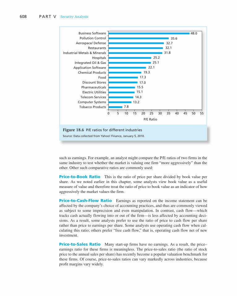
608 P A R T V Security Analysis
such as earnings. For example, an analyst might compare the P/E ratios of two firms in the same industry to test whether the market is valuing one firm “more aggressively” than the other. Other such comparative ratios are commonly used:
Price-to-Book Ratio This is the ratio of price per share divided by book value per share. As we noted earlier in this chapter, some analysts view book value as a useful measure of value and therefore treat the ratio of price to book value as an indicator of how aggressively the market values the firm.
Price-to-Cash-Flow Ratio Earnings as reported on the income statement can be affected by the company’s choice of accounting practices, and thus are commonly viewed as subject to some imprecision and even manipulation. In contrast, cash flow—which tracks cash actually flowing into or out of the firm—is less affected by accounting deci-sions. As a result, some analysts prefer to use the ratio of price to cash flow per share rather than price to earnings per share. Some analysts use operating cash flow when cal-culating this ratio; others prefer “free cash flow,” that is, operating cash flow net of new investment.
Price-to-Sales Ratio Many start-up firms have no earnings. As a result, the price–earnings ratio for these firms is meaningless. The price-to-sales ratio (the ratio of stock price to the annual sales per share) has recently become a popular valuation benchmark for these firms. Of course, price-to-sales ratios can vary markedly across industries, because profit margins vary widely.
Business Software
35.632.732.1
31.8
25.2
25.1
22.1
19.3
17.3
17.0
Chemical Products
Food
Telecom Services
Computer Systems
Tobacco Products
15.515.1
14.3
13.27.8
0 5 10 15 20 25 30 35 40 45 50 55
P/E Ratio
Discount Stores
Pharmaceuticals
Electric Utilities
Pollution Control
Aerospace/ Defense
Restaurants
Industrial Metals & Minerals
Hospitals
Integrated Oil & Gas
Application Software
48.0
Figure 18.6 P/E ratios for different industries
Source: Data collected from Yahoo! Finance, January 5, 2010.
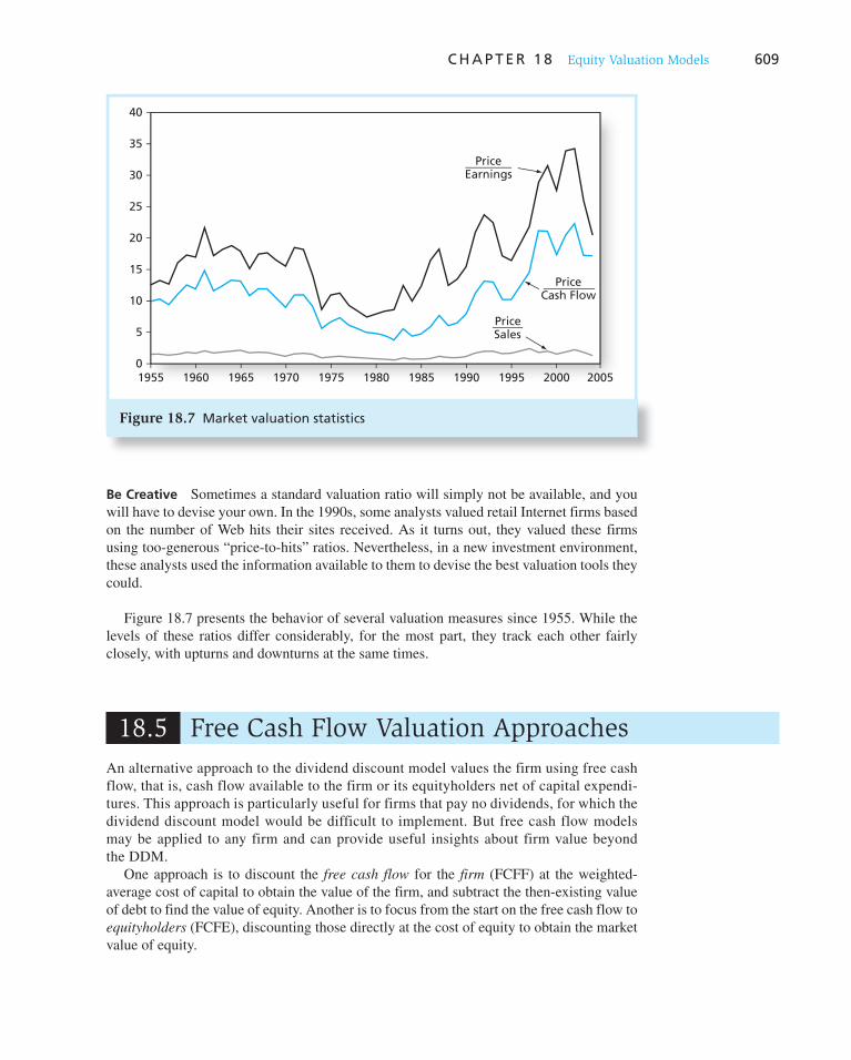
C H A P T E R 1 8 Equity Valuation Models 609
Be Creative Sometimes a standard valuation ratio will simply not be available, and you will have to devise your own. In the 1990s, some analysts valued retail Internet firms based on the number of Web hits their sites received. As it turns out, they valued these firms using too-generous “price-to-hits” ratios. Nevertheless, in a new investment environment, these analysts used the information available to them to devise the best valuation tools they could.
Figure 18.7 presents the behavior of several valuation measures since 1955. While the levels of these ratios differ considerably, for the most part, they track each other fairly closely, with upturns and downturns at the same times.
PriceSales
PriceCash Flow
PriceEarnings
40
35
30
25
20
15
10
5
01955 1960 1965 1970 1975 1980 1985 1990 1995 2000 2005
Figure 18.7 Market valuation statistics
18.5 Free Cash Flow Valuation Approaches
An alternative approach to the dividend discount model values the firm using free cash flow, that is, cash flow available to the firm or its equityholders net of capital expendi-tures. This approach is particularly useful for firms that pay no dividends, for which the dividend discount model would be difficult to implement. But free cash flow models may be applied to any firm and can provide useful insights about firm value beyond the DDM.
One approach is to discount the free cash flow for the firm (FCFF) at the weighted-average cost of capital to obtain the value of the firm, and subtract the then-existing value of debt to find the value of equity. Another is to focus from the start on the free cash flow to equityholders (FCFE), discounting those directly at the cost of equity to obtain the market value of equity.

610 P A R T V Security Analysis
The free cash flow to the firm is the after-tax cash flow that accrues from the firm’s operations, net of investments in capital and net working capital. It includes cash flows available to both debt- and equityholders. 8 It is given as follows:
FCFF 5 EBIT (1 2 tc) 1 Depreciation 2 Capital expenditures 2 Increase in NWC (18.9)
where
EBIT 5 earnings before interest and taxes
t c 5 the corporate tax rate
NWC 5 net working capital
Alternatively, we can focus on cash flow available to equityholders. This will differ from free cash flow to the firm by after-tax interest expenditures, as well as by cash flow associated with net issuance or repurchase of debt (i.e., principal repayments minus pro-ceeds from issuance of new debt).
FCFE 5 FCFF 2 Interest expense 3 (1 2 tc) 1 Increases in net debt (18.10)
The free cash flow to the firm approach discounts year-by-year cash flows plus some estimate of terminal value, V T . In Equation 18.11 , we use the constant-growth model to estimate terminal value and discount at the weighted-average cost of capital.
Firm value 5 aT
t51
FCFFt
(1 1 WACC)t1
VT
(1 1 WACC)T , where VT 5
FCFFT11
WACC 2 g (18.11)
To find equity value, we subtract the existing market value of debt from the derived value of the firm.
Alternatively, we can discount free cash flows to equity (FCFE) at the cost of equity, k E .
Market value of equity 5 aT
t51
FCFEt
(1 1 kE)t1
VT
(1 1 kE)T , where VT 5
FCFET11
kE 2 g (18.12)
As in the dividend discount model, free cash flow models use a terminal value to avoid adding the present values of an infinite sum of cash flows. That terminal value may simply be the present value of a constant-growth perpetuity (as in the formulas above) or it may be based on a multiple of EBIT, book value, earnings, or free cash flow. As a general rule, estimates of intrinsic value depend critically on terminal value.
Spreadsheet 18.2 presents a free cash flow valuation of Honda using the data supplied by Value Line in Figure 18.2 . We start with the free cash flow to the firm approach given in Equation 18.9 . Panel A of the spreadsheet lays out values supplied by Value Line. Entries for middle years are interpolated from beginning and final values. Panel B calculates free cash flow. The sum of after-tax profits in row 11 (from Value Line) plus after-tax interest payments in row 12 [i.e., interest expense 3 (1 2 t c )] equals EBIT(1 2 t c ). In row 13 we subtract the change in net working capital, in row 14 we add back depreciation, and in row 15 we subtract capital expenditures. The result in row 17 is the free cash flow to the firm, FCFF, for each year between 2010 and 2013.
To find the present value of these cash flows, we will discount at WACC, which is calculated in panel C. WACC is the weighted average of the after-tax cost of debt and the
8 This is firm cash flow assuming all-equity financing. Any tax advantage to debt financing is recognized by using an after-tax cost of debt in the computation of weighted-average cost of capital. This issue is discussed in any introductory corporate finance text.

C H A P T E R 1 8 Equity Valuation Models 611
cost of equity in each year. When computing WACC, we must account for the change in leverage forecast by Value Line. To compute the cost of equity, we will use the CAPM as in our earlier (dividend discount model) valuation exercise, but accounting for the fact that equity beta will decline each year as the firm reduces leverage. 9
9Call b L the firm’s equity beta at the initial level of leverage as provided by Value Line. Equity betas reflect both business risk and financial risk. When a firm changes its capital structure (debt/equity mix), it changes financial risk, and therefore equity beta changes. How should we recognize the change in financial risk? As you may remember from an introductory corporate finance class, you must first unleverage beta. This leaves us with business risk. We use the following formula to find unleveraged beta, b U (where D / E is the firm’s current debt-equity ratio):
bU 5bL
1 1 (D/E)(1 2 tc)
Then, we re-leverage beta in any particular year using the forecast capital structure for that year (which reintro-duces the financial risk associated with that year’s capital structure):
bL 5 bU 31 1 (D/E)(1 2 tc) 4
Spreadsheet 18.2
Free cash flow valuation of Honda Motor Co.
eXce lPlease visit us at www.mhhe.com/bkm
1
2
3
4
5
6
7
8
9
10
11
12
13
14
15
16
17
18
19
20
21
22
23
24
25
26
27
28
29
30
31
32
33
34
35
36
37
38
2009 2010 2011 2012 2013
A. Input data
P/E 30.00
2.50
27500
1810
1.00
12780
1815.0
761.1
26.25 22.50 18.75 15.00
Cap spending/shr 2.35 2.55 2.75 2.95
LT Debt 25000 24000 23000 22000
Shares 1810 1803 1797 1790
EPS 1.75 2.28 2.82 3.35
Working Capital
17100 18413 19727 21040
B. Cash flow calculations
Profits (after tax) 3175.0 4120.0 5065.0 6010.0
Interest (after tax) 691.9 664.2 636.5 608.9 = (1-tax_rate) × r_debt × LT Debt
Chg Working Cap 4320.0 1313.3 1313.3 1313.3
Depreciation 6000.0 6000.0 6000.0 6000.0
Cap Spending 4253.5 4595.8 4938.2 5280.5
Terminal value
FCFF 1293.4 4875.0 5450.0 6025.0 108545.5
FCFE –1898.5 3210.8 3813.5 4416.2 87296.9
C. Discount rate calculations
Current beta 0.95 from Value Line
from Value Line
assumes fixed debt ratio after 2013
Unlevered beta 0.725 current beta/[1 + (1-tax)*debt/equity)]
terminal growth 0.03
tax_rate 0.385
r_debt 0.045 YTM in 2010 on A+ rated LT debt
risk-free rate 0.035
market risk prem 0.08
MV equity 54450
0.34
0.950
0.111
0.083
90150 Row 3 × Row 11
Debt/Value 0.30 0.27 0.23 0.20 linear trend from initial to final value
Levered beta 0.917 0.886 0.859 0.834 unlevered beta × [1 + (1-tax)*debt/equity]
k_equity 0.108 0.106 0.104 0.102 0.102 from CAPM and levered beta
WACC 0.084 0.085 0.086 0.087 0.087 (1-t)*r_debt*D/V + k_equity*(1-D/V)
PV factor for FCFF 1.000 0.922 0.850 0.783 0.720 0.720 Discount each year at WACC
PV factor for FCFE 1.000 0.902 0.816 0.739 0.671 0.671 Discount each year at k_equity
D. Present values Intrinsic val Equity val Intrin/share
PV(FCFF) 1193 4144 4266 4338 78145 92085 64585 35.68
PV(FCFE) –1713 2620 2819 2963 58574 65262 65262 36.06
IA C D E F G H J LK MB

612 P A R T V Security Analysis
To find Honda’s cost of debt, we note that its long-term bonds were rated A 1 in early 2010 and that yields to maturity on this quality debt at the time were about 4.5%. Honda’s debt-to-value ratio in 2009 was .34 (row 29). On the basis of Value Line fore-casts, it will fall to .20 by 2013. We interpolate the debt-to-value ratio for the interme-diate years. WACC is computed in row 32. WACC increases slightly over time as the debt-to-value ratio declines between 2009 and 2013. The present value factor for cash flows accruing in each year is the previous year’s factor divided by (1 1 WACC) for that year. The present value of each cash flow (row 37) is the free cash flow times the cumulative discount factor.
The terminal value of the firm (cell H17) is computed from the constant-growth model as FCFF 2013 3 (1 1 g )/(WACC 2013 2 g ), where g (cell B23) is the assumed value for the steady growth rate. We assume in the spreadsheet that g 5 .03, roughly in line with the long-run growth rate of the broad economy. 10 Terminal value is also discounted back to 2009 (cell H37), and the intrinsic value of the firm is thus found as the sum of discounted free cash flows between 2010 and 2013 plus the discounted terminal value. Finally, the value of debt in 2009 is subtracted from firm value to arrive at the intrinsic value of equity in 2009 (cell K37), and value per share is calculated in cell L37 as equity value divided by number of shares in 2009.
The free cash flow to equity approach yields a similar intrinsic value for the stock. 11 FCFE (row 18) is obtained from FCFF by subtracting after-tax interest expense and net debt repurchases. The cash flows are then discounted at the equity rate. Like WACC, the cost of equity changes each period as leverage changes. The present value factor for equity cash flows is presented in row 34. Equity value is reported in cell J38, which is put on a per share basis in cell L38.
Spreadsheet 18.2 is available at the Online Learning Center for this text, www.mhhe
.com/bkm .
Comparing the Valuation Models
In principle, the free cash flow approach is fully consistent with the dividend discount model and should provide the same estimate of intrinsic value if one can extrapolate to a period in which the firm begins to pay dividends growing at a constant rate. This was demonstrated in two famous papers by Modigliani and Miller. 12 However, in practice, you will find that values from these models may differ, sometimes substantially. This is due to the fact that in practice, analysts are always forced to make simplifying assumptions. For example, how long will it take the firm to enter a constant-growth stage? How should depreciation best be treated? What is the best estimate of ROE? Answers to questions like these can have a big impact on value, and it is not always easy to maintain consistent assumptions across the models.
10 In the long run a firm can’t grow forever at a rate higher than the aggregate economy. So by the time we assert that growth is in a stable stage, it seems reasonable that the growth rate should not be significantly greater than that of the overall economy (although it can be less if the firm is in a declining industry).
11 Over the 2010–2013 period, Value Line predicts that Honda will retire a considerable fraction of its outstand-ing debt. The implied debt repurchases are a use of cash and reduce the cash flow available to equity. Such repurchases cannot be sustained indefinitely, however, for debt outstanding would soon be run down to zero. Therefore, in our estimate of the terminal value of equity, we compute the final cash flow assuming that starting in 2013 Honda will begin issuing enough debt to maintain its debt-to-value ratio. This approach is consistent with the assumption of constant growth and constant discount rates after 2013.
12 Franco Modigliani and M. Miller, “The Cost of Capital, Corporation Finance, and the Theory of Investment,” American Economic Review, June 1958, and “Dividend Policy, Growth, and the Valuation of Shares,” Journal of
Business, October 1961.

C H A P T E R 1 8 Equity Valuation Models 613
We have now valued Honda using several approaches, with estimates of intrinsic value as follows:
Model Intrinsic Value
Two-stage dividend discount model $23.04
DDM with earnings multiple terminal value 35.23
Three-stage DDM 49.44
Free cash flow to the firm 35.68
Free cash flow to equity 36.06
Market price (from Value Line) 32.26
What should we make of these differences? All but the two-stage dividend discount model estimates are somewhat higher than Honda’s actual stock price, perhaps indicat-ing that they use an unrealistically high value for the ultimate constant growth rate. For example, in the long run, it seems unlikely that Honda will be able to grow as rapidly as Value Line’s forecast for 2013 growth, 7.7%. The two-stage dividend discount model is the most conservative of the estimates, largely because it assumes that Honda’s dividend growth rate will fall to its terminal value after only 3 years. In contrast, the three-stage DDM allows growth to taper off over a longer period. Its considerably higher estimate of intrinsic value compared to the other models suggests that dividend growth will fall from its currently rapid rate more quickly than envisioned in Spreadsheet 18.1 . The DDM with a terminal value provided by the earnings multiple results in the estimate of intrinsic value closest to Honda’s actual stock price. On the other hand, given the consistency with which these estimates exceed market price, perhaps the stock is indeed slightly underpriced com-pared to its intrinsic value.
This valuation exercise shows that finding bargains is not as easy as it seems. While these models are easy to apply, establishing proper inputs is more of a challenge. This should not be surprising. In even a moderately efficient market, finding profit opportunities will be more involved than analyzing Value Line data for a few hours. These models are extremely useful to analysts, however, because they provide ballpark estimates of intrinsic value. More than that, they force rigorous thought about underlying assumptions and highlight the vari-ables with the greatest impact on value and the greatest payoff to further analysis.
18.6 The Aggregate Stock Market
Explaining Past Behavior
It has been well documented that the stock market is a leading economic indicator. This means that it tends to fall before a recession and to rise before an economic recovery. However, the relationship is far from perfectly reliable.
Most scholars and serious analysts would agree that, although the stock market some-times appears to have a substantial life of its own, responding perhaps to bouts of mass euphoria and then panic, economic events and the anticipation of such events do have a substantial effect on stock prices. Perhaps the two factors with the greatest impact are interest rates and corporate profits.
Figure 18.8 shows the behavior of the earnings-to-price ratio (i.e., the earnings yield) of the S&P 500 stock index versus the yield to maturity on long-term Treasury bonds since 1955. Clearly, the two series track each other quite closely. This is to be expected: The two variables that affect a firm’s value are earnings (and implicitly the dividends they can
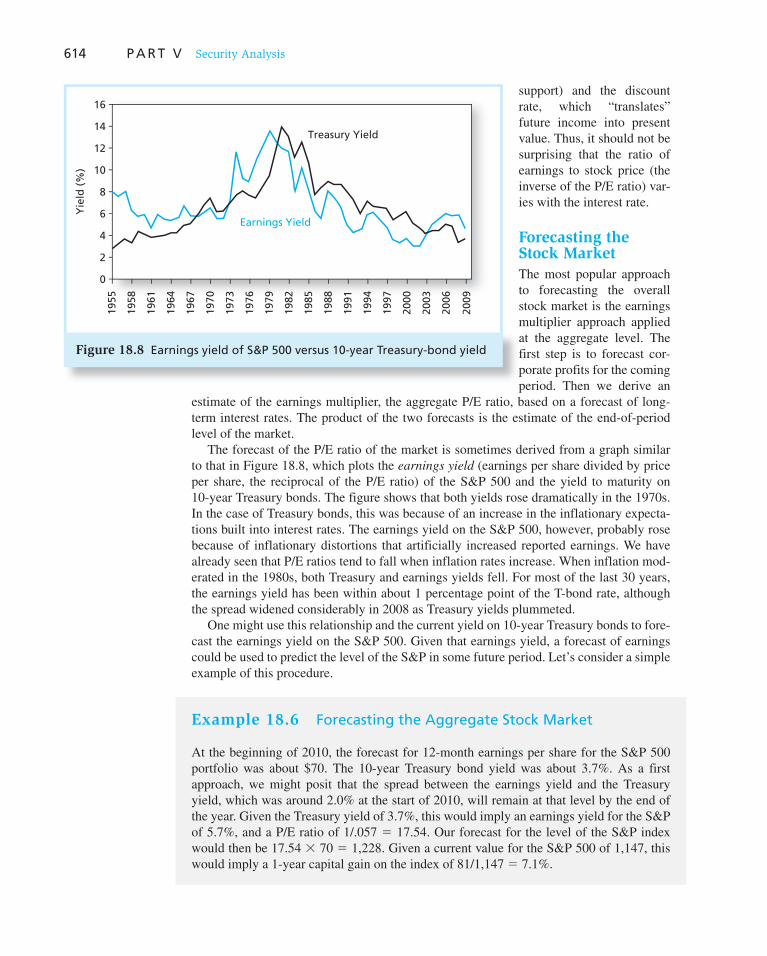
614 P A R T V Security Analysis
support) and the discount rate, which “translates” future income into present value. Thus, it should not be surprising that the ratio of earnings to stock price (the inverse of the P/E ratio) var-ies with the interest rate.
Forecasting the Stock Market
The most popular approach to forecasting the overall stock market is the earnings multiplier approach applied at the aggregate level. The first step is to forecast cor-porate profits for the coming period. Then we derive an
estimate of the earnings multiplier, the aggregate P/E ratio, based on a forecast of long-term interest rates. The product of the two forecasts is the estimate of the end-of-period level of the market.
The forecast of the P/E ratio of the market is sometimes derived from a graph similar to that in Figure 18.8 , which plots the earnings yield (earnings per share divided by price per share, the reciprocal of the P/E ratio) of the S&P 500 and the yield to maturity on 10-year Treasury bonds. The figure shows that both yields rose dramatically in the 1970s. In the case of Treasury bonds, this was because of an increase in the inflationary expecta-tions built into interest rates. The earnings yield on the S&P 500, however, probably rose because of inflationary distortions that artificially increased reported earnings. We have already seen that P/E ratios tend to fall when inflation rates increase. When inflation mod-erated in the 1980s, both Treasury and earnings yields fell. For most of the last 30 years, the earnings yield has been within about 1 percentage point of the T-bond rate, although the spread widened considerably in 2008 as Treasury yields plummeted.
One might use this relationship and the current yield on 10-year Treasury bonds to fore-cast the earnings yield on the S&P 500. Given that earnings yield, a forecast of earnings could be used to predict the level of the S&P in some future period. Let’s consider a simple example of this procedure.
0
1955
1958
1961
1964
1967
1970
1973
1976
1979
1982
1985
1988
1991
1994
1997
2000
2003
2006
2009
Treasury Yield
Earnings Yield
16
14
12
10
8
6
4
2
Yie
ld (
%)
Figure 18.8 Earnings yield of S&P 500 versus 10-year Treasury-bond yield
Example 18.6 Forecasting the Aggregate Stock Market
At the beginning of 2010, the forecast for 12-month earnings per share for the S&P 500 portfolio was about $70. The 10-year Treasury bond yield was about 3.7%. As a first approach, we might posit that the spread between the earnings yield and the Treasury yield, which was around 2.0% at the start of 2010, will remain at that level by the end of the year. Given the Treasury yield of 3.7%, this would imply an earnings yield for the S&P of 5.7%, and a P/E ratio of 1/.057 5 17.54. Our forecast for the level of the S&P index would then be 17.54 3 70 5 1,228. Given a current value for the S&P 500 of 1,147, this would imply a 1-year capital gain on the index of 81/1,147 5 7.1%.
Vis
it u
s at
ww
w.m
hh
e.co
m/b
km
C H A P T E R 1 8 Equity Valuation Models 615
Some analysts use an aggregate version of the dividend discount model rather than an earnings multiplier approach. All of these models, however, rely heavily on forecasts of such macroeconomic variables as GDP, interest rates, and the rate of inflation, which are difficult to predict accurately.
Because stock prices reflect expectations of future dividends, which are tied to the eco-nomic fortunes of firms, it is not surprising that the performance of a broad-based stock index like the S&P 500 is taken as a leading economic indicator, that is, a predictor of the performance of the aggregate economy. Stock prices are viewed as embodying consen-sus forecasts of economic activity and are assumed to move up or down in anticipation of movements in the economy. The government’s index of leading economic indicators, which is taken to predict the progress of the business cycle, is made up in part of recent stock market performance. However, the predictive value of the market is far from perfect. A well-known joke, often attributed to Paul Samuelson, is that the market has forecast eight of the last five recessions.
Table 18.4
S&P 500 price fore-casts under various scenarios
Most Likely Scenario
Pessimistic Scenario
Optimistic Scenario
Treasury bond yield 3.70% 4.70% 2.70%
Earnings yield 5.70% 6.70% 4.70%
Resulting P/E ratio 17.54 14.93 21.28
EPS forecast 70 70 70
Forecast for S&P 500 1,228 1,045 1,489
Forecast for the earnings yield on the S&P 500 equals Treasury bond yield plus 2%. The P/E ratio is the reciprocal of the forecast earnings yield.
1. One approach to firm valuation is to focus on the firm’s book value, either as it appears on the balance sheet or as adjusted to reflect current replacement cost of assets or liquidation value. Another approach is to focus on the present value of expected future dividends.
2. The dividend discount model holds that the price of a share of stock should equal the present value of all future dividends per share, discounted at an interest rate commensurate with the risk of the stock.
3. Dividend discount models give estimates of the intrinsic value of a stock. If price does not equal intrinsic value, the rate of return will differ from the equilibrium return based on the stock’s risk. The actual return will depend on the rate at which the stock price is predicted to revert to its intrinsic value.
SUMMARY
Of course, there is uncertainty regarding all three inputs into this analysis: the actual earnings on the S&P 500 stocks, the level of Treasury yields at year-end, and the spread between the Treasury yield and the earnings yield. One would wish to perform sensitivity or scenario analysis to examine the impact of changes in all of these variables. To illus-trate, consider Table 18.4 , which shows a simple scenario analysis treating possible effects of variation in the Treasury bond yield. The scenario analysis shows that forecast level of the stock market varies inversely and with dramatic sensitivity to interest rate changes.

Vis
it u
s at
ww
w.m
hh
e.co
m/b
kmV
isit
us
at w
ww
.mh
he.
com
/bkm
616 P A R T V Security Analysis
4. The constant-growth version of the DDM asserts that if dividends are expected to grow at a constant rate forever, the intrinsic value of the stock is determined by the formula
V0 5D1
k 2 g
This version of the DDM is simplistic in its assumption of a constant value of g. There are more-sophisticated multistage versions of the model for more-complex environments. When the constant-growth assumption is reasonably satisfied and the stock is selling for its intrinsic value, the formula can be inverted to infer the market capitalization rate for the stock:
k 5D1
P0
1 g
5. The constant-growth dividend discount model is best suited for firms that are expected to exhibit stable growth rates over the foreseeable future. In reality, however, firms progress through life cycles. In early years, attractive investment opportunities are ample and the firm responds with high plowback ratios and rapid dividend growth. Eventually, however, growth rates level off to more sustainable values. Three-stage growth models are well suited to such a pattern. These models allow for an initial period of rapid growth, a final period of steady dividend growth, and a middle, or transition, period in which the dividend growth rate declines from its initial high rate to the lower sustainable rate.
6. Stock market analysts devote considerable attention to a company’s price-to-earnings ratio. The P/E ratio is a useful measure of the market’s assessment of the firm’s growth opportunities. Firms with no growth opportunities should have a P/E ratio that is just the reciprocal of the capi-talization rate, k. As growth opportunities become a progressively more important component of the total value of the firm, the P/E ratio will increase.
7. The expected growth rate of earnings is related both to the firm’s expected profitability and to its dividend policy. The relationship can be expressed as
g 5 (ROE on new investment) 3 (1 2 Dividend payout ratio)
8. You can relate any DDM to a simple capitalized earnings model by comparing the expected ROE on future investments to the market capitalization rate, k. If the two rates are equal, then the stock’s intrinsic value reduces to expected earnings per share (EPS) divided by k.
9. Many analysts form their estimates of a stock’s value by multiplying their forecast of next year’s EPS by a predicted P/E multiple. Some analysts mix the P/E approach with the dividend discount model. They use an earnings multiplier to forecast the terminal value of shares at a future date, and add the present value of that terminal value with the present value of all interim dividend payments.
10. The free cash flow approach is the one used most often in corporate finance. The analyst first estimates the value of the entire firm as the present value of expected future free cash flows to the entire firm and then subtracts the value of all claims other than equity. Alternatively, the free cash flows to equity can be discounted at a discount rate appropriate to the risk of the stock.
11. The models presented in this chapter can be used to explain and forecast the behavior of the aggregate stock market. The key macroeconomic variables that determine the level of stock prices in the aggregate are interest rates and corporate profits.
Related Web sites for this chapter are available at www.mhhe.com/bkm
book value liquidation value replacement cost Tobin’s q intrinsic value
market capitalization rate dividend discount model (DDM) constant-growth DDM dividend payout ratio plowback ratio
earnings retention ratio present value of growth
o pportunities (PVGO) price–earnings multiple earnings management
KEY TERMS

Vis
it u
s at
ww
w.m
hh
e.co
m/b
km
C H A P T E R 1 8 Equity Valuation Models 617
1. In what circumstances would you choose to use a dividend discount model rather than a free cash flow model to value a firm?
2. In what circumstances is it most important to use multistage dividend discount models rather than constant-growth models?
3. If a security is underpriced (i.e., intrinsic value > price), then what is the relationship between its market capitalization rate and its expected rate of return?
4. Deployment Specialists pays a current (annual) dividend of $1.00 and is expected to grow at 20% for 2 years and then at 4% thereafter. If the required return for Deployment Specialists is 8.5%, what is the intrinsic value of Deployment Specialists stock?
5. Jand, Inc., currently pays a dividend of $1.22, which is expected to grow indefinitely at 5%. If the current value of Jand’s shares based on the constant-growth dividend discount model is $32.03, what is the required rate of return?
6. A firm pays a current dividend of $1.00 which is expected to grow at a rate of 5% indefinitely. If current value of the firm’s shares is $35.00, what is the required return applicable to the invest-ment based on the constant-growth dividend discount model (DDM)?
7. Tri-coat Paints has a current market value of $41 per share with earnings of $3.64. What is the present value of its growth opportunities (PVGO) if the required return is 9%?
8. a. Computer stocks currently provide an expected rate of return of 16%. MBI, a large co mputer company, will pay a year-end dividend of $2 per share. If the stock is selling at $50 per share, what must be the market’s expectation of the growth rate of MBI dividends?
b. If dividend growth forecasts for MBI are revised downward to 5% per year, what will hap-pen to the price of MBI stock? What (qualitatively) will happen to the company’s price–earnings ratio?
9. a. MF Corp. has an ROE of 16% and a plowback ratio of 50%. If the coming year’s earnings are expected to be $2 per share, at what price will the stock sell? The market capitalization rate is 12%. b. What price do you expect MF shares to sell for in 3 years?
10. The market consensus is that Analog Electronic Corporation has an ROE 5 9%, has a beta of 1.25, and plans to maintain indefinitely its traditional plowback ratio of 2/3. This year’s earn-ings were $3 per share. The annual dividend was just paid. The consensus estimate of the com-ing year’s market return is 14%, and T-bills currently offer a 6% return.
a. Find the price at which Analog stock should sell. b. Calculate the P/E ratio. c. Calculate the present value of growth opportunities. d. Suppose your research convinces you Analog will announce momentarily that it will immediately
reduce its plowback ratio to 1/3. Find the intrinsic value of the stock. The market is still una-ware of this decision. Explain why V 0 no longer equals P 0 and why V 0 is greater or less than P 0 .
11. The FI Corporation’s dividends per share are expected to grow indefinitely by 5% per year.
a. If this year’s year-end dividend is $8 and the market capitalization rate is 10% per year, what must the current stock price be according to the DDM?
b. If the expected earnings per share are $12, what is the implied value of the ROE on future investment opportunities?
c. How much is the market paying per share for growth opportunities (i.e., for an ROE on future investments that exceeds the market capitalization rate)?
12. The stock of Nogro Corporation is currently selling for $10 per share. Earnings per share in the coming year are expected to be $2. The company has a policy of paying out 50% of its earn-ings each year in dividends. The rest is retained and invested in projects that earn a 20% rate of return per year. This situation is expected to continue indefinitely.
a. Assuming the current market price of the stock reflects its intrinsic value as computed using the constant-growth DDM, what rate of return do Nogro’s investors require?
PROBLEM SETS
i. Basic
ii. Intermediate

Vis
it u
s at
ww
w.m
hh
e.co
m/b
km618 P A R T V Security Analysis
b. By how much does its value exceed what it would be if all earnings were paid as dividends and nothing were reinvested?
c. If Nogro were to cut its dividend payout ratio to 25%, what would happen to its stock price? What if Nogro eliminated the dividend?
13. The risk-free rate of return is 8%, the expected rate of return on the market portfolio is 15%, and the stock of Xyrong Corporation has a beta coefficient of 1.2. Xyrong pays out 40% of its earnings in dividends, and the latest earnings announced were $10 per share. Dividends were just paid and are expected to be paid annually. You expect that Xyrong will earn an ROE of 20% per year on all reinvested earnings forever.
a. What is the intrinsic value of a share of Xyrong stock? b. If the market price of a share is currently $100, and you expect the market price to be equal
to the intrinsic value 1 year from now, what is your expected 1-year holding-period return on Xyrong stock?
14. The Digital Electronic Quotation System (DEQS) Corporation pays no cash dividends currently and is not expected to for the next 5 years. Its latest EPS was $10, all of which was reinvested in the company. The firm’s expected ROE for the next 5 years is 20% per year, and during this time it is expected to continue to reinvest all of its earnings. Starting in year 6, the firm’s ROE on new investments is expected to fall to 15%, and the company is expected to start paying out 40% of its earnings in cash dividends, which it will continue to do forever after. DEQS’s market capitalization rate is 15% per year.
a. What is your estimate of DEQS’s intrinsic value per share? b. Assuming its current market price is equal to its intrinsic value, what do you expect to hap-
pen to its price over the next year? The year after? c. What effect would it have on your estimate of DEQS’s intrinsic value if you expected DEQS
to pay out only 20% of earnings starting in year 6?
15. Recalculate the intrinsic value of Honda in each of the following scenarios by using the three-stage growth model of Spreadsheet 18.1 (available at www.mhhe.com/bkm; link to Chapter 18 material). Treat each scenario independently.
a. ROE in the constant-growth period will be 10%. b. Honda’s actual beta is 1.0. c. The market risk premium is 8.5%.
16. Recalculate the intrinsic value of Honda shares using the free cash flow model of Spread-sheet 18.2 (available at www.mhhe.com/bkm; link to Chapter 18 material) under each of the following assumptions. Treat each scenario independently.
a. Honda’s P/E ratio starting in 2013 will be 16. b. Honda’s unlevered beta is 0.8. c. The market risk premium is 9%.
17. The Duo Growth Company just paid a dividend of $1 per share. The dividend is expected to grow at a rate of 25% per year for the next 3 years and then to level off to 5% per year forever. You think the appropriate market capitalization rate is 20% per year.
a. What is your estimate of the intrinsic value of a share of the stock? b. If the market price of a share is equal to this intrinsic value, what is the expected dividend yield? c. What do you expect its price to be 1 year from now? Is the implied capital gain consistent
with your estimate of the dividend yield and the market capitalization rate?
18. The Generic Genetic (GG) Corporation pays no cash dividends currently and is not expected to for the next 4 years. Its latest EPS was $5, all of which was reinvested in the company. The firm’s expected ROE for the next 4 years is 20% per year, during which time it is expected to continue to reinvest all of its earnings. Starting in year 5, the firm’s ROE on new investments is expected to fall to 15% per year. GG’s market capitalization rate is 15% per year.
a. What is your estimate of GG’s intrinsic value per share? b. Assuming its current market price is equal to its intrinsic value, what do you expect to
happen to its price over the next year?
eXce lPlease visit us at www.mhhe.com/bkm
eXce lPlease visit us at www.mhhe.com/bkm

Vis
it u
s at
ww
w.m
hh
e.co
m/b
km
C H A P T E R 1 8 Equity Valuation Models 619
19. The MoMi Corporation’s cash flow from operations before interest and taxes was $2 million in the year just ended, and it expects that this will grow by 5% per year forever. To make this happen, the firm will have to invest an amount equal to 20% of pretax cash flow each year. The tax rate is 35%. Depreciation was $200,000 in the year just ended and is expected to grow at the same rate as the operating cash flow. The appropriate market capitalization rate for the unlever-aged cash flow is 12% per year, and the firm currently has debt of $4 million outstanding. Use the free cash flow approach to value the firm’s equity.
20. Chiptech, Inc., is an established computer chip firm with several profitable existing products as well as some promising new products in development. The company earned $1 a share last year, and just paid out a dividend of $.50 per share. Investors believe the company plans to maintain its dividend payout ratio at 50%. ROE equals 20%. Everyone in the market expects this situation to persist indefinitely.
a. What is the market price of Chiptech stock? The required return for the computer chip industry is 15%, and the company has just gone ex-dividend (i.e., the next dividend will be paid a year from now, at t 5 1).
b. Suppose you discover that Chiptech’s competitor has developed a new chip that will elimi-nate Chiptech’s current technological advantage in this market. This new product, which will be ready to come to the market in 2 years, will force Chiptech to reduce the prices of its chips to remain competitive. This will decrease ROE to 15%, and, because of falling demand for its product, Chiptech will decrease the plowback ratio to .40. The plowback ratio will be decreased at the end of the second year, at t 5 2: The annual year-end dividend for the second year (paid at t 5 2) will be 60% of that year’s earnings. What is your estimate of Chiptech’s intrinsic value per share? ( Hint: Carefully prepare a table of Chiptech’s earnings and dividends for each of the next 3 years. Pay close attention to the change in the payout ratio in t 5 2.)
c. No one else in the market perceives the threat to Chiptech’s market. In fact, you are confident that no one else will become aware of the change in Chiptech’s competitive status until the competitor firm publicly announces its discovery near the end of year 2. What will be the rate of return on Chiptech stock in the coming year (i.e., between t 5 0 and t 5 1)? In the second year (between t 5 1 and t 5 2)? The third year (between t 5 2 and t 5 3)? ( Hint: Pay attention to when the mar-
ket catches on to the new situation. A table of dividends and market prices over time might help.)
iii. Challenge
1. At Litchfield Chemical Corp. (LCC), a director of the company said that the use of dividend discount models by investors is “proof” that the higher the dividend, the higher the stock price.
a. Using a constant-growth dividend discount model as a basis of reference, evaluate the direc-tor’s statement.
b. Explain how an increase in dividend payout would affect each of the following (holding all other factors constant):
i. Sustainable growth rate. ii. Growth in book value.
2. Helen Morgan, CFA, has been asked to use the DDM to determine the value of Sundanci, Inc. Morgan anticipates that Sundanci’s earnings and dividends will grow at 32% for 2 years and 13% thereafter. Calculate the current value of a share of Sundanci stock by using a two-stage dividend discount model and the data from Tables 18A and 18B .
3. Abbey Naylor, CFA, has been directed to determine the value of Sundanci’s stock using the Free Cash Flow to Equity (FCFE) model. Naylor believes that Sundanci’s FCFE will grow at 27% for 2 years and 13% thereafter. Capital expenditures, depreciation, and working capital are all expected to increase proportionately with FCFE.
a. Calculate the amount of FCFE per share for the year 2008, using the data from Table 18A . b. Calculate the current value of a share of Sundanci stock based on the two-stage FCFE model. c. i. Describe one limitation of the two-stage DDM model that is addressed by using the two-
stage FCFE model. ii. Describe one limitation of the two-stage DDM model that is not addressed by using the
two-stage FCFE model.

Vis
it u
s at
ww
w.m
hh
e.co
m/b
km620 P A R T V Security Analysis
4. Christie Johnson, CFA, has been assigned to analyze Sundanci using the constant dividend growth price/earnings (P/E) ratio model. Johnson assumes that Sundanci’s earnings and divi-dends will grow at a constant rate of 13%.
a. Calculate the P/E ratio based on information in Tables 18A and 18B and on Johnson’s assumptions for Sundanci.
b. Identify, within the context of the constant dividend growth model, how each of the follow-ing factors would affect the P/E ratio.
• Risk (beta) of Sundanci. • Estimated growth rate of earnings and dividends. • Market risk premium.
5. Dynamic Communication is a U.S. industrial company with several electronics divisions. The company has just released its 2010 annual report. Tables 18C and 18D present a summary of Dynamic’s financial statements for the years 2009 and 2010. Selected data from the financial statements for the years 2006 to 2008 are presented in Table 18E .
a. A group of Dynamic shareholders has expressed concern about the zero growth rate of divi-dends in the last 4 years and has asked for information about the growth of the company. Calculate Dynamic’s sustainable growth rates in 2007 and 2010. Your calculations should use beginning-of-year balance sheet data.
b. Determine how the change in Dynamic’s sustainable growth rate (2010 compared to 2007) was affected by changes in its retention ratio and its financial leverage. ( Note: Your calcula-tions should use beginning-of-year balance sheet data.)
Table 18A
Sundanci actual 2007 and 2008 financial statements for fiscal years ending May 31 ($ million, except per-share data)
Income Statement 2007 2008
Revenue $ 474 $ 598
Depreciation 20 23
Other operating costs 368 460
Income before taxes 86 115
Taxes 26 35
Net income 60 80
Dividends 18 24
Earnings per share $0.714 $0.952
Dividend per share $0.214 $0.286
Common shares outstanding (millions) 84.0 84.0
Balance Sheet 2007 2008
Current assets $ 201 $ 326
Net property, plant and equipment 474 489
Total assets 675 815
Current liabilities 57 141
Long-term debt 0 0
Total liabilities 57 141
Shareholders’ equity 618 674
Total liabilities and equity 675 815
Capital expenditures 34 38
Required rate of return on equity 14%
Growth rate of industry 13%
Industry P/E ratio 26
Table 18B
Selected financial information
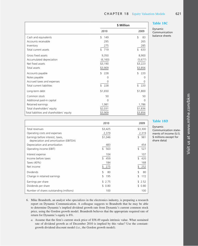
Vis
it u
s at
ww
w.m
hh
e.co
m/b
km
C H A P T E R 1 8 Equity Valuation Models 621
$ Million
2010 2009
Cash and equivalents $ 149 $ 83
Accounts receivable 295 265
Inventory 275 285
Total current assets $ 719 $ 633
Gross fixed assets 9,350 8,900
Accumulated depreciation (6,160) (5,677)
Net fixed assets $3,190 $3,223
Total assets $3,909 $3,856
Accounts payable $ 228 $ 220
Notes payable 0 0
Accrued taxes and expenses 0 0
Total current liabilities $ 228 $ 220
Long-term debt $1,650 $1,800
Common stock 50 50
Additional paid-in capital 0 0
Retained earnings 1,981 1,786
Total shareholders’ equity $2,031 $1,836
Total liabilities and shareholders’ equity $3,909 $3,856
Table 18C
Dynamic Communication b alance sheets
2010 2009
Total revenues $3,425 $3,300
Operating costs and expenses 2,379 2,319
Earnings before interest, taxes,
depreciation and amortization (EBITDA)
$1,046 $ 981
Depreciation and amortization 483 454
Operating income (EBIT) $ 563 $ 527
Interest expense 104 107
Income before taxes $ 459 $ 420
Taxes (40%) 184 168
Net income $ 275 $ 252
Dividends $ 80 $ 80
Change in retained earnings $ 195 $ 172
Earnings per share $ 2.75 $ 2.52
Dividends per share $ 0.80 $ 0.80
Number of shares outstanding (millions) 100 100
Table 18D
Dynamic Communication state-ments of income (U.S. $ millions except for share data)
6. Mike Brandreth, an analyst who specializes in the electronics industry, is preparing a research report on Dynamic Communication. A colleague suggests to Brandreth that he may be able to determine Dynamic’s implied dividend growth rate from Dynamic’s current common stock price, using the Gordon growth model. Brandreth believes that the appropriate required rate of return for Dynamic’s equity is 8%.
a. Assume that the firm’s current stock price of $58.49 equals intrinsic value. What sustained rate of dividend growth as of December 2010 is implied by this value? Use the constant-growth dividend discount model (i.e., the Gordon growth model).
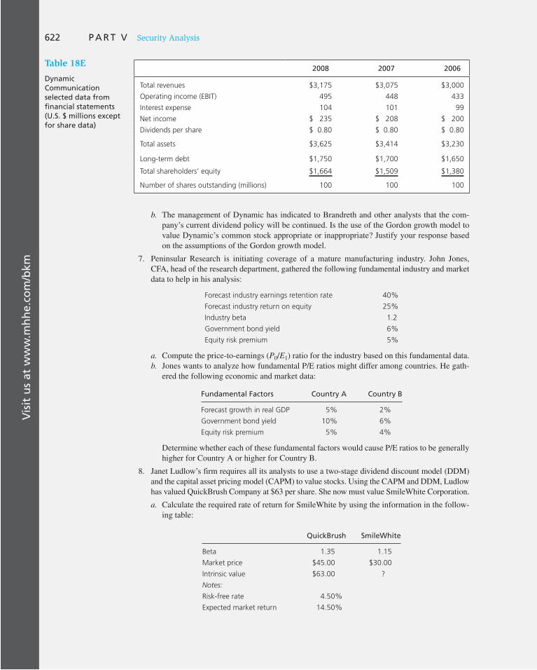
Vis
it u
s at
ww
w.m
hh
e.co
m/b
km622 P A R T V Security Analysis
b. The management of Dynamic has indicated to Brandreth and other analysts that the com-pany’s current dividend policy will be continued. Is the use of the Gordon growth model to value Dynamic’s common stock appropriate or inappropriate? Justify your response based on the assumptions of the Gordon growth model.
7. Peninsular Research is initiating coverage of a mature manufacturing industry. John Jones, CFA, head of the research department, gathered the following fundamental industry and market data to help in his analysis:
Forecast industry earnings retention rate 40%
Forecast industry return on equity 25%
Industry beta 1.2
Government bond yield 6%
Equity risk premium 5%
a. Compute the price-to-earnings ( P 0 / E 1 ) ratio for the industry based on this fundamental data. b. Jones wants to analyze how fundamental P/E ratios might differ among countries. He gath-
ered the following economic and market data:
Fundamental Factors Country A Country B
Forecast growth in real GDP 5% 2%
Government bond yield 10% 6%
Equity risk premium 5% 4%
Determine whether each of these fundamental factors would cause P/E ratios to be generally higher for Country A or higher for Country B.
8. Janet Ludlow’s firm requires all its analysts to use a two-stage dividend discount model (DDM) and the capital asset pricing model (CAPM) to value stocks. Using the CAPM and DDM, Ludlow has valued QuickBrush Company at $63 per share. She now must value SmileWhite Corporation.
a. Calculate the required rate of return for SmileWhite by using the information in the follow-ing table:
QuickBrush SmileWhite
Beta 1.35 1.15
Market price $45.00 $30.00
Intrinsic value $63.00 ?
Notes:
Risk-free rate 4.50%
Expected market return 14.50%
2008 2007 2006
Total revenues $3,175 $3,075 $3,000
Operating income (EBIT) 495 448 433
Interest expense 104 101 99
Net income $ 235 $ 208 $ 200
Dividends per share $ 0.80 $ 0.80 $ 0.80
Total assets $3,625 $3,414 $3,230
Long-term debt $1,750 $1,700 $1,650
Total shareholders’ equity $1,664 $1,509 $1,380
Number of shares outstanding (millions) 100 100 100
Table 18E
Dynamic Communication selected data from financial statements (U.S. $ millions except for share data)

Vis
it u
s at
ww
w.m
hh
e.co
m/b
km
C H A P T E R 1 8 Equity Valuation Models 623
b. Ludlow estimates the following EPS and dividend growth rates for SmileWhite:
First 3 years 12% per year
Years thereafter 9% per year
Estimate the intrinsic value of SmileWhite by using the table above, and the two-stage DDM. Dividends per share in the most recent year were $1.72.
c. Recommend QuickBrush or SmileWhite stock for purchase by comparing each company’s intrinsic value with its current market price.
d. Describe one strength of the two-stage DDM in comparison with the constant-growth DDM. Describe one weakness inherent in all DDMs.
9. Rio National Corp. is a U.S.-based company and the largest competitor in its industry. Tables 18F–18I present financial statements and related information for the company. Table 18J presents relevant industry and market data.
Revenue $300.80
Total operating expenses (173.74)
Operating profit 127.06
Gain on sale 4.00
Earnings before interest, taxes, depreciation &
amortization (EBITDA)
131.06
Depreciation and amortization (71.17)
Earnings before interest & taxes (EBIT) 59.89
Interest (16.80)
Income tax expense (12.93)
Net income $ 30.16
Table 18G
Rio National Corp. summary income statement for the year ended December 31, 2010 (U.S. $ millions)
2010 2009
Cash $ 13.00 $ 5.87
Accounts receivable 30.00 27.00
Inventory 209.06 189.06
Current assets $252.06 $221.93
Gross fixed assets 474.47 409.47
Accumulated depreciation (154.17) (90.00)
Net fixed assets 320.30 319.47
Total assets $572.36 $541.40
Accounts payable $ 25.05 $ 26.05
Notes payable 0.00 0.00
Current portion of long-term debt 0.00 0.00
Current liabilities $ 25.05 $ 26.05
Long-term debt 240.00 245.00
Total liabilities $265.05 $271.05
Common stock 160.00 150.00
Retained earnings 147.31 120.35
Total shareholders’ equity $307.31 $270.35
Total liabilities and shareholders’ equity $572.36 $541.40
Table 18F
Rio National Corp. summary year-end balance sheets (U.S. $ millions)
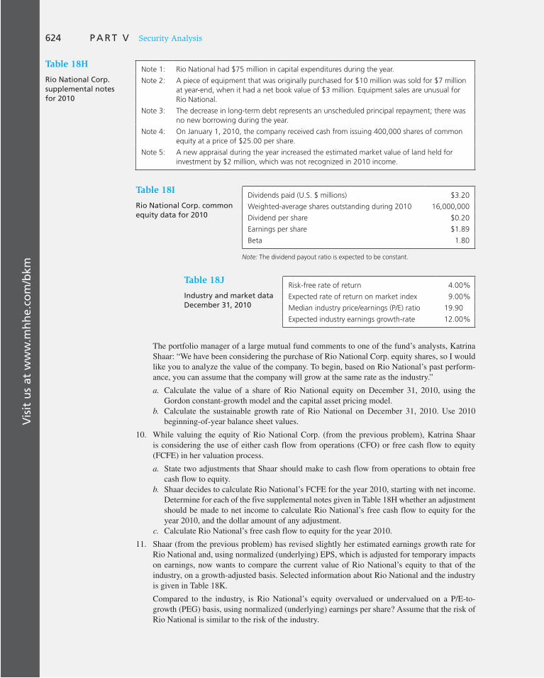
Vis
it u
s at
ww
w.m
hh
e.co
m/b
km624 P A R T V Security Analysis
The portfolio manager of a large mutual fund comments to one of the fund’s analysts, Katrina Shaar: “We have been considering the purchase of Rio National Corp. equity shares, so I would like you to analyze the value of the company. To begin, based on Rio National’s past perform-ance, you can assume that the company will grow at the same rate as the industry.”
a. Calculate the value of a share of Rio National equity on December 31, 2010, using the G ordon constant-growth model and the capital asset pricing model.
b. Calculate the sustainable growth rate of Rio National on December 31, 2010. Use 2010 beginning-of-year balance sheet values.
10. While valuing the equity of Rio National Corp. (from the previous problem), Katrina Shaar is considering the use of either cash flow from operations (CFO) or free cash flow to equity (FCFE) in her valuation process.
a. State two adjustments that Shaar should make to cash flow from operations to obtain free cash flow to equity.
b. Shaar decides to calculate Rio National’s FCFE for the year 2010, starting with net income. Determine for each of the five supplemental notes given in Table 18H whether an adjustment should be made to net income to calculate Rio National’s free cash flow to equity for the year 2010, and the dollar amount of any adjustment.
c. Calculate Rio National’s free cash flow to equity for the year 2010.
11. Shaar (from the previous problem) has revised slightly her estimated earnings growth rate for Rio National and, using normalized (underlying) EPS, which is adjusted for temporary impacts on earnings, now wants to compare the current value of Rio National’s equity to that of the industry, on a growth-adjusted basis. Selected information about Rio National and the industry is given in Table 18K .
Compared to the industry, is Rio National’s equity overvalued or undervalued on a P/E-to-growth (PEG) basis, using normalized (underlying) earnings per share? Assume that the risk of Rio National is similar to the risk of the industry.
Table 18H
Rio National Corp. supplemental notes for 2010
Note 1: Rio National had $75 million in capital expenditures during the year.
Note 2: A piece of equipment that was originally purchased for $10 million was sold for $7 million
at year-end, when it had a net book value of $3 million. Equipment sales are unusual for
Rio National.
Note 3: The decrease in long-term debt represents an unscheduled principal repayment; there was
no new borrowing during the year.
Note 4: On January 1, 2010, the company received cash from issuing 400,000 shares of common
equity at a price of $25.00 per share.
Note 5: A new appraisal during the year increased the estimated market value of land held for
investment by $2 million, which was not recognized in 2010 income.
Table 18J
Industry and market data December 31, 2010
Risk-free rate of return 4.00%
Expected rate of return on market index 9.00%
Median industry price/earnings (P/E) ratio 19.90
Expected industry earnings growth-rate 12.00%
Dividends paid (U.S. $ millions) $3.20
Weighted-average shares outstanding during 2010 16,000,000
Dividend per share $0.20
Earnings per share $1.89
Beta 1.80
Table 18I
Rio National Corp. c ommon equity data for 2010
Note: The dividend payout ratio is expected to be constant.

Vis
it u
s at
ww
w.m
hh
e.co
m/b
km
C H A P T E R 1 8 Equity Valuation Models 625
Rio National
Estimated earnings growth rate 11.00%
Current share price $25.00
Normalized (underlying) EPS for 2008 $1.71
Weighted-average shares outstanding during 2008 16,000,000
Industry
Estimated earnings growth rate 12.00%
Median price/earnings (P/E) ratio 19.90
Table 18K
Rio National Corp. vs. industry
E-INVEST-MENTS EXERCISES
Equity Valuation
Go to the MoneyCentral Investor page at moneycentral.msn.com/investor/home.asp. Use the Research Wizard function under Guided Research to obtain fundamentals, price history, price target, catalysts, and comparison for Walmart (WMT). For comparison, use Target (TGT), BJ’s Wholesale Club (BJ), and the Industry.
1. What has been the 1-year sales and income growth for Walmart?
2. What has been the company’s 5-year profit margin? How does that compare with the other two firms’ profit margins and the industry’s profit margin?
3. What have been the percentage price changes for the last 3, 6, and 12 months? How do they compare with the other firms’ price changes and the industry’s price changes?
4. What are the estimated high and low prices for Walmart for the coming year based on its current P/E multiple?
5. Compare the price performance of Walmart with that of Target and BJ’s. Which of the companies appears to be the most expensive in terms of current earnings? Which of the companies is the least expensive in terms of current earnings?
6. What are the firms’ Stock Scouter Ratings? How are these ratings interpreted?
SOLUTIONS TO CONCEPT CHECKS
1. a. Dividend yield 5 $2.15/$50 5 4.3%. Capital gains yield 5 (59.77 2 50)/50 5 19.54%. Total return 5 4.3% 1 19.54% 5 23.84%.
b. k 5 6% 1 1.15(14% 2 6%) 5 15.2%.
c. V 0 5 ($2.15 1 $59.77)/1.152 5 $53.75, which exceeds the market price. This would indicate a “buy” opportunity.
2. a. D 1 /( k 2 g ) 5 $2.15/(.152 2 .112) 5 $53.75.
b. P 1 5 P 0 (1 1 g ) 5 $53.75(1.112) 5 $59.77.
c. The expected capital gain equals $59.77 2 $53.75 5 $6.02, for a percentage gain of 11.2%. The dividend yield is D 1 / P 0 5 2.15/53.75 5 4%, for a holding-period return of 4% 1 11.2% 5 15.2%.
3. a. g 5 ROE 3 b 5 20% 3 .60 5 12%.
D 1 5 .4 3 E 1 5 .4 3 $5 5 $2. P 0 5 2/(.125 2 .12) 5 400.

Vis
it u
s at
ww
w.m
hh
e.co
m/b
km626 P A R T V Security Analysis
b. When the firm invests in projects with ROE less than k, its stock price falls. If b 5 .60, then g 5 10% 3 .60 5 6% and P 0 5 $2/(.125 2 .06) 5 $30.77. In contrast, if b 5 0, then P 0 5 $5/.125 5 $40.
4. V2009 5.50
(1.111)1
.66
(1.111)21
.83
(1.111)31
1.00 1 P2013
(1.111)4
Now compute the sales price in 2013 using the constant-growth dividend discount model. The growth rate will be g 5 ROE 3 b 5 13% 3 .70 5 9.10%.
P2013 51.00 3 (1 1 g)
k 2 g5
$1.00 3 1.091
.111 2 .0915 $54.55
Therefore, V 2009 5 $38.05.
5. a. ROE 5 12%. b 5 $.50/$2.00 5 .25. g 5 ROE 3 b 5 12% 3 .25 5 3%. P 0 5 D 1 /( k 2 g) 5 $1.50/(.10 2 .03) 5 $21.43. P 0 / E 1 5 $21.43/$2.00 5 10.71.
b. If b 5 .4, then .4 3 $2 5 $.80 would be reinvested and the remainder of earnings, or $1.20, would be paid as dividends.
g 5 12% 3 .4 5 4.8%. P 0 5 D 1 /( k 2 g ) 5 $1.20/(.10 2 .048) 5 $23.08. P 0 / E 1 5 $23.08/$2.00 5 11.54.
199 PA
RT V
IN THE PREVIOUS chapter, we explored
equity valuation techniques. These tech-
niques take the firm’s dividends and earnings
prospects as inputs. Although the valuation
analyst is interested in economic earnings
streams, only financial accounting data are
readily available. What can we learn from a
company’s accounting data that can help us
estimate the intrinsic value of its common
stock? In this chapter, we show how inves-
tors can use financial data as inputs into stock
valuation analysis. We start by reviewing
the basic sources of such data—the income
statement, the balance sheet, and the state-
ment of cash flows. We next discuss the dif-
ference between economic and accounting
earnings. Although economic earnings are
more important for issues of valuation, we
examine evidence suggesting that, whatever
their shortcomings, accounting data still are
useful in assessing the economic prospects of
the firm. We show how analysts use finan-
cial ratios to explore the sources of a firm’s
profitability and evaluate the “quality” of
its earnings in a systematic fashion. We also
examine the impact of debt policy on various
financial ratios. Finally, we conclude with a
discussion of the challenges you will encoun-
ter when using financial statement analysis
as a tool in uncovering mispriced securities.
Some of these issues arise from differences in
firms’ accounting procedures. Others are due
to inflation-induced distortions in accounting
numbers.
Financial Statement Analysis
CHAPTER NINETEEN
19.1 The Major Financial Statements
The Income Statement
The income statement is a summary of the profitability of the firm over a period of time, such as a year. It presents revenues generated during the operating period, the expenses incurred during that same period, and the company’s net earnings or profits, which are simply the difference between revenues and expenses.
It is useful to distinguish four broad classes of expenses: cost of goods sold, which is the direct cost attributable to producing the product sold by the firm; general and adminis-trative expenses, which correspond to overhead expenses, salaries, advertising, and other costs of operating the firm that are not directly attributable to production; interest expense on the firm’s debt; and taxes on earnings owed to federal and local governments.

628 P A R T V Security Analysis
Table 19.1 presents a 2009 income statement for Hewlett-Packard. At the top are the company’s revenues from operations. Next come operating expenses, the costs incurred in the course of generating those revenues, including a depreciation allowance. The differ-ence between operating revenues and operating costs is called operating income. Income or expenses from other, primarily nonrecurring, sources are then added or subtracted to obtain earnings before interest and taxes (EBIT), which is what the firm would have earned if not for obligations to its creditors and the tax authorities. EBIT is a measure of the profit-ability of the firm’s operations, ignoring any interest burden attributable to debt financing. The income statement then goes on to subtract net interest expense from EBIT to arrive at taxable income. Finally, the income tax due the government is subtracted to arrive at net income, the “bottom line” of the income statement.
Analysts also commonly prepare a common-size income statement, in which all items on the income statement are expressed as a fraction of total revenue. This makes it easier to compare firms of different sizes. The right-hand column of Table 19.1 is HP’s common-size income statement.
The Balance Sheet
While the income statement provides a measure of profitability over a period of time, the balance sheet provides a “snapshot” of the financial condition of the firm at a particular moment. The balance sheet is a list of the firm’s assets and liabilities at that moment. The difference in assets and liabilities is the net worth of the firm, also called shareholders’ or stockholders’ equity. Like income statements, balance sheets are reasonably standardized in presentation. Table 19.2 is HP’s balance sheet for 2009.
Note: Sums subject to rounding error. Source: Hewlett-Packard Annual Report, year ending October 2009. © 2009 Hewlett-Packard Development Company, L.P.
$ MillionPercent of Revenue
Operating revenues
Net sales $114,552 100.0%
Operating expenses
Cost of goods sold 82,751 72.2
Selling, general & administrative expenses 11,613 10.1
Research & development expenses 2,819 2.5
Depreciation 4,773 4.2
Operating income 12,596 11.0
Other income (expense) (2,460) 22.1
Earnings before interest and income taxes $10,136 8.8%
Interest expense 721 0.6
Taxable income $ 9,415 8.2%
Taxes 1,755 1.5
Net income $7,660 6.7%
Allocation of net income
Dividends 766 0.7
Addition to retained earnings 6,894 6.0
Table 19.1
Consolidated statement of income for Hewlett-Packard, 2009
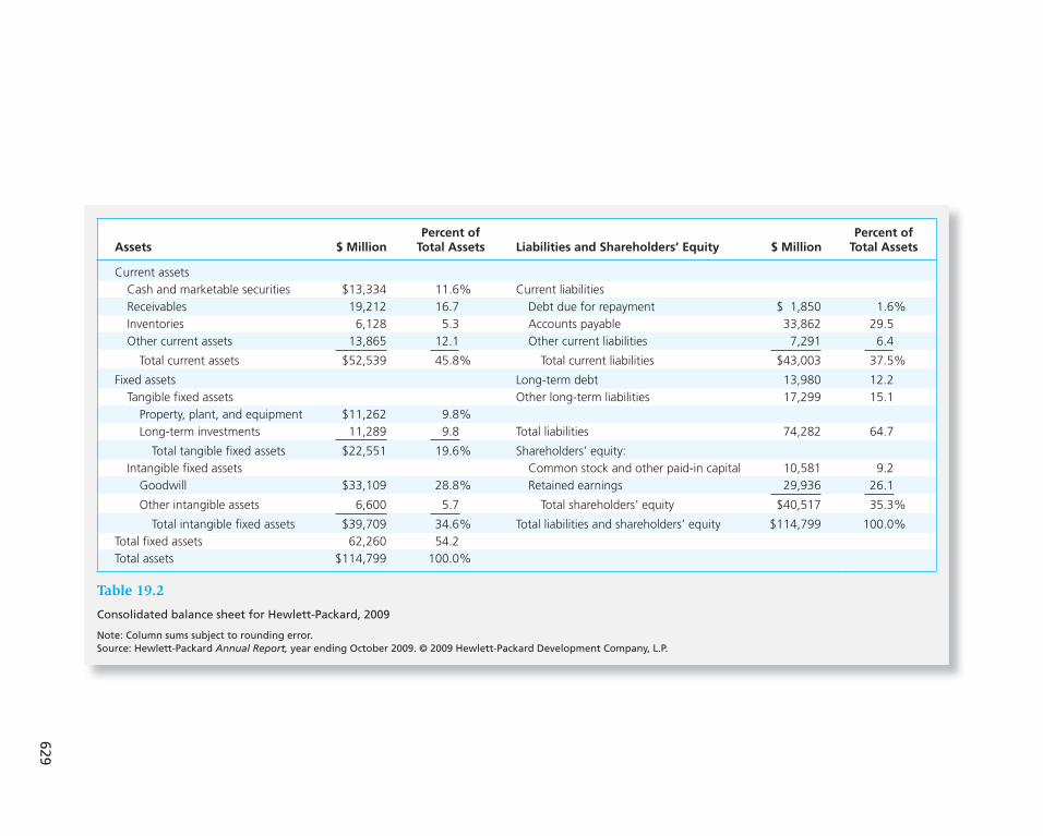
629
Assets $ MillionPercent of
Total Assets Liabilities and Shareholders’ Equity $ MillionPercent of
Total Assets
Current assets
Cash and marketable securities $13,334 11.6% Current liabilities
Receivables 19,212 16.7 Debt due for repayment $ 1,850 1.6%
Inventories 6,128 5.3 Accounts payable 33,862 29.5
Other current assets 13,865 12.1 Other current liabilities 7,291 6.4
Total current assets $52,539 45.8% Total current liabilities $43,003 37.5%
Fixed assets Long-term debt 13,980 12.2
Tangible fixed assets Other long-term liabilities 17,299 15.1
Property, plant, and equipment $11,262 9.8%
Long-term investments 11,289 9.8 Total liabilities 74,282 64.7
Total tangible fixed assets $22,551 19.6% Shareholders’ equity:
Intangible fixed assets Common stock and other paid-in capital 10,581 9.2
Goodwill $33,109 28.8% Retained earnings 29,936 26.1
Other intangible assets 6,600 5.7 Total shareholders’ equity $40,517 35.3%
Total intangible fixed assets $39,709 34.6% Total liabilities and shareholders’ equity $114,799 100.0%
Total fixed assets 62,260 54.2
Total assets $114,799 100.0%
Table 19.2
Consolidated balance sheet for Hewlett-Packard, 2009
Note: Column sums subject to rounding error. Source: Hewlett-Packard Annual Report, year ending October 2009. © 2009 Hewlett-Packard Development Company, L.P.

630 P A R T V Security Analysis
The first section of the balance sheet gives a listing of the assets of the firm. Current assets are presented first. These are cash and other items such as accounts receivable or inventories that will be converted into cash within 1 year. Next comes a listing of long-term or “fixed” assets. Tangible fixed assets are items such as buildings, equipment, or vehicles. HP also has several intangible assets such as a respected brand name and expertise. But accountants generally are reluctant to include these assets on the balance sheet, as they are so hard to value. However, when one firm purchases another for a premium over its book value, that difference, called “goodwill,” is listed on the balance sheet as an intan-
gible fixed asset. HP has unusually high goodwill because of its acquisition of Compaq Computer several years ago. 1 The sum of current and fixed assets is total assets, the last line of the assets section of the balance sheet.
The liability and shareholders’ equity (also called stockholders’ equity) section is arranged similarly. First come short-term, or “current,” liabilities such as accounts pay-able, accrued taxes, and debts that are due within 1 year. Following this is long-term debt and other liabilities due in more than 1 year. The difference between total assets and total liabilities is stockholders’ equity. This is the net worth, or book value, of the firm. Stockholders’ equity is divided into par value of stock, additional paid-in capital, and retained earnings, although this division is usually unimportant. Briefly, par value plus additional paid-in capital represent the proceeds realized from the sale of stock to the pub-lic, whereas retained earnings represent the buildup of equity from profits plowed back into the firm. Even if the firm issues no new equity, book value typically will increase each year due to reinvested earnings.
The first panel in the balance sheet in Table 19.2 presents the dollar value of each asset. Just as they compute common-size income statements, however, analysts also find it con-venient to use common-size balance sheets when comparing firms of different sizes. Each item is expressed as a percentage of total assets. These entries appear in the right columns of Table 19.2 .
The Statement of Cash Flows
The income statement and balance sheets are based on accrual methods of accounting, which means that revenues and expenses are recognized at the time of a sale even if no cash has yet been exchanged. In contrast, the statement of cash flows tracks the cash implications of transactions. For example, if goods are sold now, with payment due in 60 days, the income statement will treat the revenue as generated when the sale occurs, and the balance sheet will be immediately augmented by accounts receivable, but the statement of cash flows will not show an increase in available cash until the bill is paid.
Table 19.3 is the 2009 statement of cash flows for HP. The first entry listed under cash flows from operations is net income. The next entries modify that figure for components of income that have been recognized but for which cash has not yet changed hands. For example, HP’s accounts receivable increased by $549 million in 2009. This portion of sales was claimed on the income statement, but the cash had not yet been collected. Increases in accounts receivable are in effect an investment in working capital, and therefore reduce the cash flows realized from operations. Similarly, increases in accounts payable mean that expenses have been recognized, but cash has not yet left the firm. Any payment delay increases the company’s net cash flows in this period.
1 Firms are required to test their goodwill assets for “impairment” each year. If the value of the acquired firm is clearly less than its purchase price, that amount must be charged off as an expense. AOL Time Warner set a record when it recognized an impairment of $99 billion in 2002 following the January 2001 merger of Time Warner with AOL.
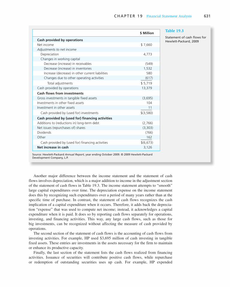
C H A P T E R 1 9 Financial Statement Analysis 631
Another major difference between the income statement and the statement of cash flows involves depreciation, which is a major addition to income in the adjustment section of the statement of cash flows in Table 19.3 . The income statement attempts to “smooth” large capital expenditures over time. The depreciation expense on the income statement does this by recognizing such expenditures over a period of many years rather than at the specific time of purchase. In contrast, the statement of cash flows recognizes the cash implication of a capital expenditure when it occurs. Therefore, it adds back the deprecia-tion “expense” that was used to compute net income; instead, it acknowledges a capital expenditure when it is paid. It does so by reporting cash flows separately for operations, investing, and financing activities. This way, any large cash flows, such as those for big investments, can be recognized without affecting the measure of cash provided by operations.
The second section of the statement of cash flows is the accounting of cash flows from investing activities. For example, HP used $3,695 million of cash investing in tangible fixed assets. These entries are investments in the assets necessary for the firm to maintain or enhance its productive capacity.
Finally, the last section of the statement lists the cash flows realized from financing activities. Issuance of securities will contribute positive cash flows, while repurchase or redemption of outstanding securities uses up cash. For example, HP expended
Source: Hewlett-Packard Annual Report, year ending October 2009. © 2009 Hewlett-Packard Development Company, L.P.
$ Million
Cash provided by operations
Net income $ 7,660
Adjustments to net income
Depreciation 4,773
Changes in working capital
Decrease (increase) in receivables (549)
Decrease (increase) in inventories 1,532
Increase (decrease) in other current liabilities 580
Changes due to other operating activities (617)
Total adjustments $ 5,719
Cash provided by operations 13,379
Cash flows from investments
Gross investments in tangible fixed assets (3,695)
Investments in other fixed assets 104
Investment in other assets 11
Cash provided by (used for) investments $(3,580)
Cash provided by (used for) financing activities
Additions to (reductions in) long-term debt (2,766)
Net issues (repurchases of) shares (3,303)
Dividends (766)
Other 162
Cash provided by (used for) financing activities $(6,673)
Net increase in cash 3,126
Table 19.3
Statement of cash flows for Hewlett-Packard, 2009
632 P A R T V Security Analysis
$3,303 million to repurchase shares of its stock in 2009, which was a major use of cash. Its dividend payments, $766 million, also used cash. In total, HP’s financing activities in 2009 absorbed $6,673 million.
To summarize, HP’s operations generated a cash flow of $13,379 million. Some of that cash flow, $3,580 million, went to pay for new investments. Another part, $6,673 mil-lion, went to pay dividends and retire outstanding securities. HP’s cash holdings therefore increased by $13,379 2 $3,580 2 $6,673 5 $3,126 million. This is reported on the last line of Table 19.3 .
The statement of cash flows provides important evidence on the well-being of a firm. If a company cannot pay its dividends and maintain the productivity of its capital stock out of cash flow from operations, for example, and it must resort to borrowing to meet these demands, this is a serious warning that the firm cannot maintain the dividend payout at its current level in the long run. The statement of cash flows will reveal this developing problem when it shows that cash flow from operations is inadequate and that borrowing is being used to maintain dividend payments at unsustainable levels.
19.2 Accounting versus Economic Earnings
We’ve seen that stock valuation models require a measure of economic earnings —the sustainable cash flow that can be paid out to stockholders without impairing the produc-tive capacity of the firm. In contrast, accounting earnings are affected by several con-ventions regarding the valuation of assets such as inventories (e.g., LIFO versus FIFO treatment), and by the way some expenditures such as capital investments are recognized over time (as depreciation expenses). We discuss problems with some of these account-ing conventions in greater detail later in the chapter. In addition to these accounting issues, as the firm makes its way through the business cycle, its earnings will rise above or fall below the trend line that might more accurately reflect sustainable economic earn-ings. This introduces an added complication in interpreting net income figures. One might wonder how closely accounting earnings approximate economic earnings and, correspondingly, how useful accounting data might be to investors attempting to value the firm.
In fact, the net income figure on the firm’s income statement does convey considerable information concerning a firm’s prospects. We see this in the fact that stock prices tend to increase when firms announce earnings greater than market analysts or investors had anticipated.
19.3 Profitability Measures
Profitability measures focus on the firm’s earnings. To facilitate comparisons across firms, total earnings are expressed on a per-dollar-invested basis. So return on equity (ROE), which measures profitability for contributors of equity capital, is defined as (after-tax) profits divided by the book value of equity. Similarly, return on assets (ROA), which measures profitability for all contributors of capital, is defined as earnings before interest and taxes divided by total assets. Not surprisingly, ROA and ROE are linked, but as we will see shortly, the relationship between them is affected by the firm’s financial policies.

C H A P T E R 1 9 Financial Statement Analysis 633
Past versus Future ROE
We noted in Chapter 18 that return on equity (ROE) is one of the two basic factors in determining a firm’s growth rate of earnings. Sometimes it is reasonable to assume that future ROE will approximate its past value, but a high ROE in the past does not necessarily imply a firm’s future ROE will be high. A declining ROE, on the other hand, is evidence that the firm’s new investments have offered a lower ROE than its past investments. The vital point for a security analyst is not to accept historical values as indicators of future values. Data from the recent past may provide information regarding future performance, but the analyst should always keep an eye on the future. Expectations of future dividends and earnings determine the intrinsic value of the company’s stock.
Financial Leverage and ROE
An analyst interpreting the past behavior of a firm’s ROE or forecasting its future value must pay careful attention to the firm’s debt-equity mix and to the interest rate on its debt. An example will show why. Suppose Nodett is a firm that is all-equity financed and has total assets of $100 million. Assume it pays corporate taxes at the rate of 40% of taxable earnings.
Table 19.4 shows the behavior of sales, earnings before interest and taxes, and net prof-its under three scenarios representing phases of the business cycle. It also shows the behav-ior of two of the most commonly used profitability measures: operating return on assets
(ROA), which equals EBIT/assets, and ROE, which equals net profits/equity. Somdett is an otherwise identical firm to Nodett, but $40 million of its $100 million
of assets are financed with debt bearing an interest rate of 8%. It pays annual interest expenses of $3.2 million. Table 19.5 shows how Somdett’s ROE differs from Nodett’s.
Note that annual sales, EBIT, and therefore ROA for both firms are the same in each of the three scenarios; that is, business risk for the two companies is identical. But their financial risk differs. Although Nodett and Somdett have the same ROA in each scenario, Somdett’s ROE exceeds that of Nodett in normal and good years and is lower in bad years.
ScenarioSales
($ millions)EBIT
($ millions)ROA
(% per year)Net Profit
($ millions)ROE
(% per year)
Bad year 80 5 5 3 3
Normal year 100 10 10 6 6
Good year 120 15 15 9 9
Table 19.4
Nodett’s profitability over the business cycle
Nodett Somdett
ScenarioEBIT
($ millions)Net Profits ($ millions)
ROE (%)
Net Profit* ($ millions)
ROE† (%)
Bad year 5 3 3 1.08 1.8
Normal year 10 6 6 4.08 6.8
Good year 15 9 9 7.08 11.8
*Somdett’s after-tax profits are given by .6(EBIT 2 $3.2 million). † ROE 5 net profit/equity. Somdett’s equity is only $60 million.
Table 19.5
Impact of financial leverage on ROE
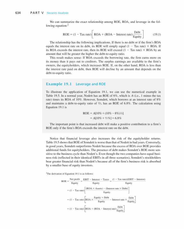
Example 19.1 Leverage and ROE
To illustrate the application of Equation 19.1 , we can use the numerical example in Table 19.5 . In a normal year, Nodett has an ROE of 6%, which is .6 (i.e., 1 minus the tax rate) times its ROA of 10%. However, Somdett, which borrows at an interest rate of 8% and maintains a debt-to-equity ratio of 2/3, has an ROE of 6.8%. The calculation using Equation 19.1 is
ROE 5 1 2
5 1 5
. [ % ( % %) ]
. [ % %] . %
6 10 10 8
6 10 6 8
2 3
4 3
The important point is that increased debt will make a positive contribution to a firm’s ROE only if the firm’s ROA exceeds the interest rate on the debt.
634 P A R T V Security Analysis
We can summarize the exact relationship among ROE, ROA, and leverage in the fol-lowing equation: 2
ROE 5 (1 2 Tax rate) BROA 1 (ROA 2 Interest rate)
Debt
EquityR (19.1)
The relationship has the following implications. If there is no debt or if the firm’s ROA equals the interest rate on its debt, its ROE will simply equal (1 2 Tax rate) 3 ROA. If its ROA exceeds the interest rate, then its ROE will exceed (1 2 Tax rate) 3 ROA by an amount that will be greater the higher the debt-to-equity ratio.
This result makes sense: If ROA exceeds the borrowing rate, the firm earns more on its money than it pays out to creditors. The surplus earnings are available to the firm’s owners, the equityholders, which increases ROE. If, on the other hand, ROA is less than the interest rate paid on debt, then ROE will decline by an amount that depends on the debt-to-equity ratio.
Notice that financial leverage also increases the risk of the equityholder returns. Table 19.5 shows that ROE of Somdett is worse than that of Nodett in bad years. Conversely, in good years, Somdett outperforms Nodett because the excess of ROA over ROE provides additional funds for equityholders. The presence of debt makes Somdett’s ROE more sen-sitive to the business cycle than Nodett’s. Even though the two companies have equal busi-ness risk (reflected in their identical EBITs in all three scenarios), Somdett’s stockholders bear greater financial risk than Nodett’s because all of the firm’s business risk is absorbed by a smaller base of equity investors.
2 The derivation of Equation 19.1 is as follows:
ROE 5Net profit
Equity5
EBIT 2 Interest 2 Taxes
Equity5
(1 2 Tax rate)(EBIT 2 Interest)
Equity
5 (1 2 Tax rate) B(ROA 3 Assets) 2 (Interest rate 3 Debt)
Equity R
5 (1 2 Tax rate) BROA 3Equity 1 Debt
Equity2 Interest rate 3
Debt
EquityR
5 (1 2 Tax rate) BROA 1 (ROA 2 Interest rate)
Debt
EquityR
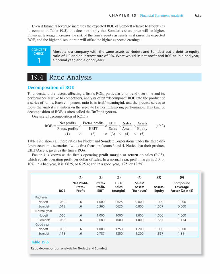
C H A P T E R 1 9 Financial Statement Analysis 635
Even if financial leverage increases the expected ROE of Somdett relative to Nodett (as it seems to in Table 19.5 ), this does not imply that Somdett’s share price will be higher. Financial leverage increases the risk of the firm’s equity as surely as it raises the expected ROE, and the higher discount rate will offset the higher expected earnings.
19.4 Ratio Analysis
Decomposition of ROE
To understand the factors affecting a firm’s ROE, particularly its trend over time and its performance relative to competitors, analysts often “decompose” ROE into the product of a series of ratios. Each component ratio is in itself meaningful, and the process serves to focus the analyst’s attention on the separate factors influencing performance. This kind of decomposition of ROE is often called the DuPont system.
One useful decomposition of ROE is
ROE 5Net profits
Pretax profits3
Pretax profits
EBIT3
EBIT
Sales3
Sales
Assets3
Assets
Equity
(1) 3 (2) 3 (3) 3 (4) 3 (5)
(19.2)
Table 19.6 shows all these ratios for Nodett and Somdett Corporations under the three dif-ferent economic scenarios. Let us first focus on factors 3 and 4. Notice that their product, EBIT/Assets, gives us the firm’s ROA.
Factor 3 is known as the firm’s operating profit margin or return on sales (ROS), which equals operating profit per dollar of sales. In a normal year, profit margin is .10, or 10%; in a bad year, it is .0625, or 6.25%; and in a good year, .125, or 12.5%.
CONCEPT CHECK
1 Mordett is a company with the same assets as Nodett and Somdett but a debt-to-equity ratio of 1.0 and an interest rate of 9%. What would its net profit and ROE be in a bad year, a normal year, and a good year?
ROE
(1)
Net Profit/Pretax Profit
(2)
Pretax Profit/EBIT
(3)
EBIT/Sales
(margin)
(4)
Sales/Assets
(Turnover)
(5)
Assets/Equity
(6)
Compound Leverage
Factor (2) 3 (5)
Bad year
Nodett .030 .6 1.000 .0625 0.800 1.000 1.000
Somdett .018 .6 0.360 .0625 0.800 1.667 0.600
Normal year
Nodett .060 .6 1.000 .1000 1.000 1.000 1.000
Somdett .068 .6 0.680 .1000 1.000 1.667 1.134
Good year
Nodett .090 .6 1.000 .1250 1.200 1.000 1.000
Somdett .118 .6 0.787 .1250 1.200 1.667 1.311
Table 19.6
Ratio decomposition analysis for Nodett and Somdett

636 P A R T V Security Analysis
Factor 4, the ratio of sales to total assets, is known as total asset turnover (ATO). It indicates the efficiency of the firm’s use of assets in the sense that it measures the annual sales generated by each dollar of assets. In a normal year, ATO for both firms is 1.0 per year, meaning that sales of $1 per year were generated per dollar of assets. In a bad year, this ratio declines to .8 per year, and in a good year, it rises to 1.2 per year.
Comparing Nodett and Somdett, we see that factors 3 and 4 do not depend on a firm’s financial leverage. The firms’ ratios are equal to each other in all three scenarios.
Similarly, factor 1, the ratio of net income after taxes to pretax profit, is the same for both firms. We call this the tax-burden ratio. Its value reflects both the government’s tax code and the policies pursued by the firm in trying to minimize its tax burden. In our example it does not change over the business cycle, remaining a constant .6.
Although factors 1, 3, and 4 are not affected by a firm’s capital structure, factors 2 and 5 are. Factor 2 is the ratio of pretax profits to EBIT. The firm’s pretax profits will be great-est when there are no interest payments to be made to debtholders. In fact, another way to express this ratio is
Pretax profits
EBIT5
EBIT 2 Interest expense
EBIT
We will call this factor the interest-burden ratio. It takes on its highest possible value, 1, for Nodett, which has no financial leverage. The higher the degree of financial leverage, the lower the interest burden ratio. Nodett’s ratio does not vary over the business cycle. It is fixed at 1.0, reflecting the total absence of interest payments. For Somdett, however, because interest expense is fixed in a dollar amount while EBIT varies, the interest burden ratio varies from a low of .36 in a bad year to a high of .787 in a good year.
A closely related statistic to the interest burden ratio is the interest coverage ratio, or times interest earned. The ratio is defined as
Interest coverage 5 EBIT/Interest expense
A high coverage ratio indicates that the likelihood of bankruptcy is low because annual earnings are significantly greater than annual interest obligations. It is widely used by both lenders and borrowers in determining the firm’s debt capacity and is a major determinant of the firm’s bond rating.
Factor 5, the ratio of assets to equity, is a measure of the firm’s degree of financial lever-age. It is called the leverage ratio and is equal to 1 plus the total debt-to-equity ratio. 3 In our numerical example in Table 19.6 , Nodett has a leverage ratio of 1, while Somdett’s is 1.667.
From our discussion in Section 19.2 , we know that financial leverage helps boost ROE only if ROA is greater than the interest rate on the firm’s debt. How is this fact reflected in the ratios of Table 19.6 ?
The answer is that to measure the full impact of leverage in this framework, the analyst must take the product of the interest burden and leverage ratios (i.e., factors 2 and 5, shown in Table 19.6 as column 6). For Nodett, factor 6, which we call the compound leverage
factor, remains a constant 1.0 under all three scenarios. But for Somdett, we see that the compound leverage factor is greater than 1 in normal years (1.134) and in good years (1.311), indicating the positive contribution of financial leverage to ROE. It is less than 1 in bad years, reflecting the fact that when ROA falls below the interest rate, ROE falls with increased use of debt.
3 Assets
Equity5
Equity 1 Debt
Equity5 1 1
Debt
Equity
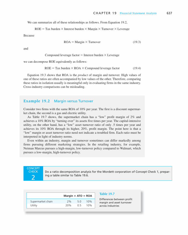
Example 19.2 Margin versus Turnover
Consider two firms with the same ROA of 10% per year. The first is a discount supermar-ket chain, the second is a gas and electric utility.
As Table 19.7 shows, the supermarket chain has a “low” profit margin of 2% and achieves a 10% ROA by “turning over” its assets five times per year. The capital-intensive utility, on the other hand, has a “low” asset turnover ratio of only .5 times per year and achieves its 10% ROA through its higher, 20%, profit margin. The point here is that a “low” margin or asset turnover ratio need not indicate a troubled firm. Each ratio must be interpreted in light of industry norms.
Even within an industry, margin and turnover sometimes can differ markedly among firms pursuing different marketing strategies. In the retailing industry, for example, Neiman Marcus pursues a high-margin, low-turnover policy compared to Walmart, which pursues a low-margin, high-turnover policy.
C H A P T E R 1 9 Financial Statement Analysis 637
We can summarize all of these relationships as follows. From Equation 19.2 ,
ROE 5 Tax burden 3 Interest burden 3 Margin 3 Turnover 3 Leverage
Because
ROA 5 Margin 3 Turnover (19.3)
and
Compound leverage factor 5 Interest burden 3 Leverage
we can decompose ROE equivalently as follows:
ROE 5 Tax burden 3 ROA 3 Compound leverage factor (19.4)
Equation 19.3 shows that ROA is the product of margin and turnover. High values of one of these ratios are often accompanied by low values of the other. Therefore, comparing these ratios in isolation usually is meaningful only in evaluating firms in the same industry. Cross-industry comparisons can be misleading.
CONCEPT CHECK
2 Do a ratio decomposition analysis for the Mordett corporation of Concept Check 1, prepar-ing a table similar to Table 19.6 .
Margin 3 ATO 5 ROA
Supermarket chain 2% 5.0 10%
Utility 20% 0.5 10%
Table 19.7
Differences between profit margin and asset turnover across industries

638 P A R T V Security Analysis
Turnover and Other Asset Utilization Ratios
It is often helpful in understanding a firm’s ratio of sales to assets to compute comparable efficiency-of-utilization, or turnover, ratios for subcategories of assets. For example, we can think about turnover relative to fixed rather than total assets:
Fixed-asset turnover 5Sales
Fixed assets
This ratio measures sales per dollar of the firm’s money tied up in fixed assets. To illustrate how you can compute this and other ratios from a firm’s financial state-
ments, consider Growth Industries, Inc. (GI). GI’s historical income statement and opening and closing balance sheets for the years 2008, 2009, and 2010 appear in Table 19.8 .
GI’s total asset turnover in 2010 was .303, which was below the industry average of .4. To understand better why GI underperformed, we can compute asset utilization ratios separately for fixed assets, inventories, and accounts receivable.
GI’s sales in 2010 were $144 million. Its only fixed assets were plant and equip-ment, which were $216 million at the beginning of the year and $259.2 million at year’s end. Average fixed assets for the year were, therefore, $237.6 million [($216 mil-lion 1 $259.2 million)/2]. GI’s fixed-asset turnover for 2010 therefore was $144 million
2007 2008 2009 2010
Income statements
Sales revenue $100,000 $120,000 $144,000
Cost of goods sold (including depreciation) 55,000 66,000 79,200
Depreciation 15,000 18,000 21,600
Selling and administrative expenses 15,000 18,000 21,600
Operating income 30,000 36,000 43,200
Interest expense 10,500 19,095 34,391
Taxable income 19,500 16,905 8,809
Income tax (40% rate) 7,800 6,762 3,524
Net income $ 11,700 $ 10,143 $ 5,285
Balance sheets (end of year)
Cash and marketable securities $ 50,000 $ 60,000 $ 72,000 $ 86,400
Accounts receivable 25,000 30,000 36,000 43,200
Inventories 75,000 90,000 108,000 129,600
Net plant and equipment 150,000 180,000 216,000 259,200
Total assets $300,000 $360,000 $432,000 $518,400
Accounts payable $ 30,000 $ 36,000 $ 43,200 $ 51,840
Short-term debt 45,000 87,300 141,957 214,432
Long-term debt (8% bonds maturing in 2025) 75,000 75,000 75,000 75,000
Total liabilities $150,000 $198,300 $260,157 $341,272
Shareholders’ equity (1 million shares outstanding) $150,000 $161,700 $171,843 $177,128
Other data
Market price per common share at year-end $ 93.60 $ 61.00 $ 21.00
Table 19.8
Growth Industries financial statements, 2007–2010 ($ thousand)

C H A P T E R 1 9 Financial Statement Analysis 639
per year/$237.6 million 5 .606 per year. In other words, for every dollar of fixed assets, there were $.606 in sales during the year 2010.
Comparable figures for the fixed-asset turnover ratio for 2008 and 2009 and the 2010 industry average are
2008 2009 2010 2010 Industry Average
.606 .606 .606 .700
GI’s fixed asset turnover has been stable over time and below the industry average. Notice that when a financial ratio includes one item from the income statement, which
covers a period of time, and another from a balance sheet, which is a “snapshot” at a par-ticular time, common practice is to take the average of the beginning and end-of-year bal-ance sheet figures. Thus in computing the fixed-asset turnover ratio we divided sales (from the income statement) by average fixed assets (from the balance sheet).
Another widely followed turnover ratio is the inventory turnover ratio, which is the ratio of cost of goods sold per dollar of average inventory. (We use the cost of goods sold instead of sales revenue in the numerator to maintain consistency with inventory, which is valued at cost). This ratio measures the speed with which inventory is turned over.
In 2008, GI’s cost of goods sold (excluding depreciation) was $40 million, and its average inventory was $82.5 million [($75 million 1 $90 million)/2]. Its inventory turn-over was .485 per year ($40 million/$82.5 million). In 2009 and 2010, inventory turnover remained the same, which was below the industry average of .5 per year. In other words, GI was burdened with a higher level of inventories per dollar of sales than its competitors. This higher investment in working capital in turn resulted in a higher level of assets per dollar of sales or profits, and a lower ROA than its competitors.
Another aspect of efficiency surrounds management of accounts receivable, which is often measured by days sales in receivables, that is, the average level of accounts receiv-able expressed as a multiple of daily sales. It is computed as average accounts receivable/sales 3 365 and may be interpreted as the number of days’ worth of sales tied up in accounts receivable. You can also think of it as the average lag between the date of sale and the date payment is received, and is therefore also called the average collection period.
For GI in 2010 the average collection period was 100.4 days:
($36 million 1 $43.2 million)/2
$144 million3 365 5 100.4 days
The industry average was only 60 days. This statistic tells us that GI’s average receivables per dollar of sales exceeds that of its competitors. Again, this implies a higher required investment in working capital, and ultimately a lower ROA.
In summary, these ratios show us that GI’s poor total asset turnover relative to the indus-try is in part caused by lower-than-average fixed-asset turnover and inventory turnover and higher-than-average days receivables. This suggests GI may be having problems with excess plant capacity along with poor inventory and receivables management practices.
Liquidity Ratios
Liquidity and interest coverage ratios are of great importance in evaluating the riskiness of a firm’s securities. They aid in assessing the financial strength of the firm. Liquidity ratios include the current ratio, quick ratio, and interest coverage ratio.
1. Current ratio: Current assets/current liabilities. This ratio measures the ability of the firm to pay off its current liabilities by liquidating its current assets (i.e., turning

640 P A R T V Security Analysis
them into cash). It indicates the firm’s ability to avoid insolvency in the short run. GI’s current ratio in 2008, for example, was (60 1 30 1 90)/(36 1 87.3) 5 1.46. In other years, it was
2008 2009 2010 2010 Industry Average
1.46 1.17 .97 2.0
This represents an unfavorable time trend and poor standing relative to the indus-try. This troublesome pattern is not surprising given the working capital burden resulting from GI’s subpar performance with respect to receivables and inventory management.
2. Quick ratio: (Cash 1 marketable securities 1 receivables)/current liabilities. This ratio is also called the acid test ratio. It has the same denominator as the current ratio, but its numerator includes only cash, cash equivalents, and receivables. The quick ratio is a better measure of liquidity than the current ratio for firms whose inventory is not readily convertible into cash. GI’s quick ratio shows the same disturbing trends as its current ratio:
2008 2009 2010 2010 Industry Average
.73 .58 .49 1.0
3. Cash ratio. A company’s receivables are less liquid than its holdings of cash and marketable securities. Therefore, in addition to the quick ratio, analysts also compute a firm’s cash ratio, defined as
Cash ratio 5Cash 1 marketable securities
Current liabilities
GI’s cash ratios are
2008 2009 2010 2010 Industry Average
.487 .389 .324 .70
GI’s liquidity ratios have fallen dramatically over this 3-year period, and by 2010, its liquidity measures are far below industry averages. The decline in the liquidity ratios com-bined with the decline in coverage ratio (you can confirm that times interest earned has also fallen over this period) suggests that its credit rating has been declining as well, and, no doubt, GI is considered a relatively poor credit risk in 2010.
Market Price Ratios: Growth versus Value
The market–book-value ratio (P/B) equals the market price of a share of the firm’s common stock divided by its book value, that is, shareholders’ equity per share. Some analysts consider the stock of a firm with a low market–book value to be a “safer” invest-ment, seeing the book value as a “floor” supporting the market price. These analysts pre-sumably view book value as the level below which market price will not fall because the firm always has the option to liquidate, or sell, its assets for their book values. However, this view is questionable. In fact, the previous chapter provided examples of firms
C H A P T E R 1 9 Financial Statement Analysis 641
selling below book value in early 2010, for example, Bank of America and Citigroup. Nevertheless, a low market–book-value ratio is seen by some as providing a “margin of safety,” and some analysts will screen out or reject high-P/B firms in their stock selection process.
In fact, a better interpretation of the market-price-to-book ratio is as a measure of growth opportunities. Recall from the previous chapter that we may view the two com-ponents of firm value as assets in place and growth opportunities. As the next example illustrates, firms with greater growth opportunities will tend to exhibit higher multiples of market-price-to-book value.
Another measure used to place firms along a growth versus value spectrum is the price–earnings (P/E) ratio. In fact, we saw in the last chapter that the ratio of the present value of growth options to the value of assets in place largely determines the P/E multiple. While low-P/E stocks allow you to pay less per dollar of current earnings, the high-P/E stock may still be a better bargain if its earnings are expected to grow quickly enough. 4
Many analysts nevertheless believe that low-P/E stocks are more attractive than high-P/E stocks. And in fact, low-P/E stocks have generally been positive-alpha investments using the CAPM as a return benchmark. But an efficient market adherent would discount this track record, arguing that such a simplistic rule could not really generate abnormal returns, and that the CAPM may not be a good benchmark for returns in this case.
In any event, the important points to remember are that ownership of the stock conveys the right to future as well as current earnings and, therefore, that a high P/E ratio may best be interpreted as a signal that the market views the firm as enjoying attractive growth opportunities.
4 Remember, though, P/E ratios reported in the financial pages are based on past earnings, while price is deter-mined by the firm’s prospects of future earnings. Therefore, reported P/E ratios may reflect variation in current earnings around a trend line.
Example 19.3 Price to Book and Growth Options
Consider two firms, both with book value per share of $10, both with a market capitaliza-tion rate of 15%, and both with plowback ratios of .60.
Bright Prospects has an ROE of 20%, which is well in excess of the market capital-ization rate; this ROE implies that the firm is endowed with ample growth opportunities. With ROE 5 .20, Bright Prospects will earn $2 per share this year. With its plowback ratio of .60, it pays out a dividend of D 1 5 (1 2 .6) 3 $2 5 $.80, has a growth rate of g 5 b 3 ROE 5 .60 3 .20 5 .12, and a stock price of D 1 /( k 2 g ) 5 $.80/(.15 2 .12) 5 $26.67. Its price–book ratio is 26.67/10 5 2.667.
In contrast, Past Glory has an ROE of only 15%, just equal to the market capital-ization rate. It therefore will earn $1.50 per share this year and will pay a dividend of D 1 5 .4 3 $1.50 5 $.60. Its growth rate is g 5 b 3 ROE 5 .60 3 .15 5 .09, and its stock price is D 1 /( k 2 g ) 5 $.60/(.15 2 .09) 5 $10. Its price–book ratio is $10/$10 5 1.0. Not surprisingly, a firm that earns just the required rate of return on its investments will sell for book value, and no more.
We conclude that the market-price-to-book-value ratio is determined in large part by growth prospects.

642 P A R T V Security Analysis
Before leaving the P/B and P/E ratios, it is worth pointing out an important relationship between them:
ROE 5Earnings
Book value5
Market price
Book value4
Market price
Earnings (19.5)
5 P/B ratio 4 P/E ratio
By rearranging the terms, we find that a firm’s P/E ratio equals its price-to-book ratio divided by ROE:
P
E5
P/B
ROE
Thus a company with a high P/B ratio nevertheless can have a relatively low P/E if its ROE is high enough.
Wall Street often distinguishes between “good firms” and “good investments.” A good firm may be highly profitable, with a correspondingly high ROE. But if its stock price is bid up to a level commensurate with this ROE, its P/B ratio will also be high, and the stock price may be a relatively large multiple of earnings, thus reducing its attractiveness as an investment. The high ROE of the firm does not by itself imply that the stock is a good investment. Conversely, troubled firms with low ROEs can be good investments if their prices are low enough.
Table 19.9 summarizes the ratios reviewed in this section.
CONCEPT CHECK
3What were GI’s ROE, P/E, and P/B ratios in the year 2010? How do they compare to the indus-try average ratios, which were: ROE 5 8.64%; P/E 5 8; P/B 5 .69? How does GI’s earnings yield in 2010 compare to the industry average?
Choosing a Benchmark
We have discussed how to calculate the principal financial ratios. To evaluate the per-formance of a given firm, however, you need a benchmark to which you can compare its ratios. One obvious benchmark is the ratio for the same company in earlier years. For example, Figure 19.1 shows HP’s return on assets, profit margin, and asset turnover ratio for the last few years. You can see there that most of the variation in HP’s return on assets has been driven by the considerable variation in its asset turnover ratio. In contrast, HP’s profit margin has been relatively stable.
It is also helpful to compare financial ratios to those of other firms in the same industry. Financial ratios for industries are published by the U.S. Department of Commerce (see Table 19.10 ), Dun & Bradstreet ( Industry Norms and Key Business Ratios ), and the Risk Management Association, or RMA ( Annual Statement Studies ). A broad range of financial ratios is also easily accessible on the Web.
Table 19.10 presents ratios for a sample of major industry groups to give you a feel for some of the differences across industries. You should note that while some ratios such as asset turnover or total debt ratio tend to be relatively stable over time, others such as return on assets or equity will be more sensitive to current business conditions. Observe, for example, the negative profitability measures for the motor vehicle industry in 2009.
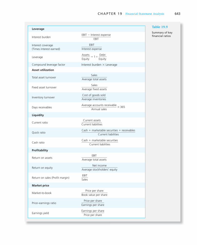
C H A P T E R 1 9 Financial Statement Analysis 643
Leverage
Interest burdenEBIT 2 Interest expense
EBIT
Interest coverage
(Times interest earned)
EBIT
Interest expense
LeverageAssets
Equity
Debt
Equity5 11
Compound leverage factor Interest burden 3 Leverage
Asset utilization
Total asset turnoverSales
Average total assets
Fixed asset turnoverSales
Average fixed assets
Inventory turnoverCost of goods sold
Average inventories
Days receivablesAverage accounts receivable
Annual sales3 365
Liquidity
Current ratioCurrent assets
Current liabilities
Quick ratioCash 1 marketable securities 1 receivables
Current liabilities
Cash ratioCash 1 marketable securities
Current liabilities
Profitability
Return on assetsEBIT
Average total assets
Return on equityNet income
Average stockholders’ equity
Return on sales (Profit margin)EBIT
Sales
Market price
Market-to-bookPrice per share
Book value per share
Price–earnings ratioPrice per share
Earnings per share
Earnings yieldEarnings per share
Price per share
Table 19.9
Summary of key financial ratios

644 P A R T V Security Analysis
19.5 Economic Value Added
One common use of financial ratios is to evaluate the performance of the firm. While prof-itability is typically used to measure that performance, profitability is really not enough. A firm should be viewed as successful only if the return on its projects is better than the rate investors could expect to earn for themselves (on a risk-adjusted basis) in the capital mar-ket. Plowing back funds into the firm increases stock price only if the firm earns a higher rate of return on the reinvested funds than the opportunity cost of capital, that is, the market capitalization rate. To account for this opportunity cost, we might measure the success of
Figure 19.1 DuPont decomposition for Hewlett-Packard
1998 1999 2000 2001 2002 2003 2004 2005 2006 200920082007
ROA
Turnover 3 10
30
25
20
15
10
5
0
Rat
ioProfit Margin
LT DebtAssets
InterestCoverage
CurrentRatio
Quick Ratio
AssetTurnover
Profit Margin (%)
Return onAssets (%)
Return on Equity (%)
All manufacturing 0.22 2.51 1.36 0.96 0.74 6.10 4.54 9.15
Food products 0.24 3.74 1.39 0.86 1.11 7.57 8.44 14.10
Clothing 0.22 5.29 1.28 0.43 1.73 4.43 7.65 10.93
Printing/publishing 0.41 1.71 1.23 0.96 1.27 5.40 6.83 7.22
Chemicals 0.27 3.89 1.36 1.05 0.50 13.97 7.04 19.00
Drugs 0.27 5.49 1.52 1.25 0.40 20.03 8.07 22.90
Machinery 0.18 3.62 1.25 0.81 0.77 7.28 5.60 9.96
Electrical 0.13 5.43 1.14 0.70 0.60 9.77 5.88 9.76
Motor vehicles 0.26 20.92 0.75 0.56 0.79 26.03 24.78 NMF*
Computer and electronic 0.16 1.35 1.73 1.44 0.57 2.16 1.22 5.27
Table 19.10
Financial Ratios for Major Industry Groups
*No meaningful figure because shareholders’ equity was negative. Source: U.S. Department of Commerce, Quarterly Financial Report for Manufacturing, Mining and Trade Corporations, second quarter 2009.

C H A P T E R 1 9 Financial Statement Analysis 645
the firm using the difference between the return on assets, ROA, and the opportunity cost of capital, k. Economic value added is the spread between ROA and k multiplied by the capital invested in the firm. It therefore measures the dollar value of the firm’s return in excess of its opportunity cost. Another term for EVA (the term coined by Stern Stewart, a consulting firm that has promoted its use) is residual income.
Table 19.11 shows EVA for a small sample of firms. The EVA leader in this sample was Walmart. Notice that Walmart’s EVA was far greater than GlaxoSmithKline’s, despite a smaller margin between its ROA and the cost of capital. This is because Walmart applied its margin to a much larger capital base. At the other extreme, AT&T earned less than its opportunity cost on a very large capital base, which resulted in a large, negative EVA.
Notice that even the EVA “losers” in Table 19.11 reported positive accounting profits. For example, by conventional standards, AT&T was solidly profitable in 2009, with an ROA of 4.9%. But its cost of capital was 7.8%. By this standard, it did not cover its oppor-tunity cost of capital, and returned a negative EVA in 2009. EVA treats the opportunity cost of capital as a real cost that, like other costs, should be deducted from revenues to arrive at a more meaningful “bottom line.” A firm that is earning profits but is not covering its opportunity cost might be able to redeploy its capital to better uses. Therefore, a growing number of firms now calculate EVA and tie managers’ compensation to it.
Source: Authors’ calculations using data from finance.yahoo.com. Actual EVA estimates reported by Stern Stewart differ from the values in Table 19.11 because of adjustments to the accounting data involving issues such as treatment of research and development expenses, taxes, advertising expenses, and depreciation. The estimates in Table 19.11 are designed to show the logic behind EVA but must be taken as imprecise.
Table 19.11
Economic value added, 2009
EVA ($ billion)
Capital ($ billion) ROA (%)
Cost of Capital (%)
Walmart $4.25 $115.03 9.6% 5.9%
GlaxoSmithKline 3.53 41.94 15.5 7.1
Amgen 0.66 34.28 9.1 7.2
ExxonMobil 0.58 115.97 7.2 6.7
Intel 0.20 42.04 10.4 9.9
Motorola 20.06 13.53 7.8 8.2
Hewlett-Packard 20.59 54.79 6.0 7.1
AT&T 24.94 171.21 4.9 7.8
Example 19.4 Economic Value Added
In 2009, Walmart had a weighted-average cost of capital of 5.9% (based on its cost of debt, its capital structure, its equity beta, and estimates derived from the CAPM for the cost of equity). Its return on assets was 9.6%, fully 3.7% greater than the opportunity cost of capital on its investments in plant, equipment, and know-how. In other words, each dol-lar invested by Walmart earned about 3.7 cents more than the return that investors could have anticipated by investing in equivalent-risk stocks. Walmart earned this superior rate of return on a capital base of $115 billion. Its economic value added, that is, its return in excess of opportunity cost, was therefore (.096 2 .059) 3 $115 5 $4.25 billion.
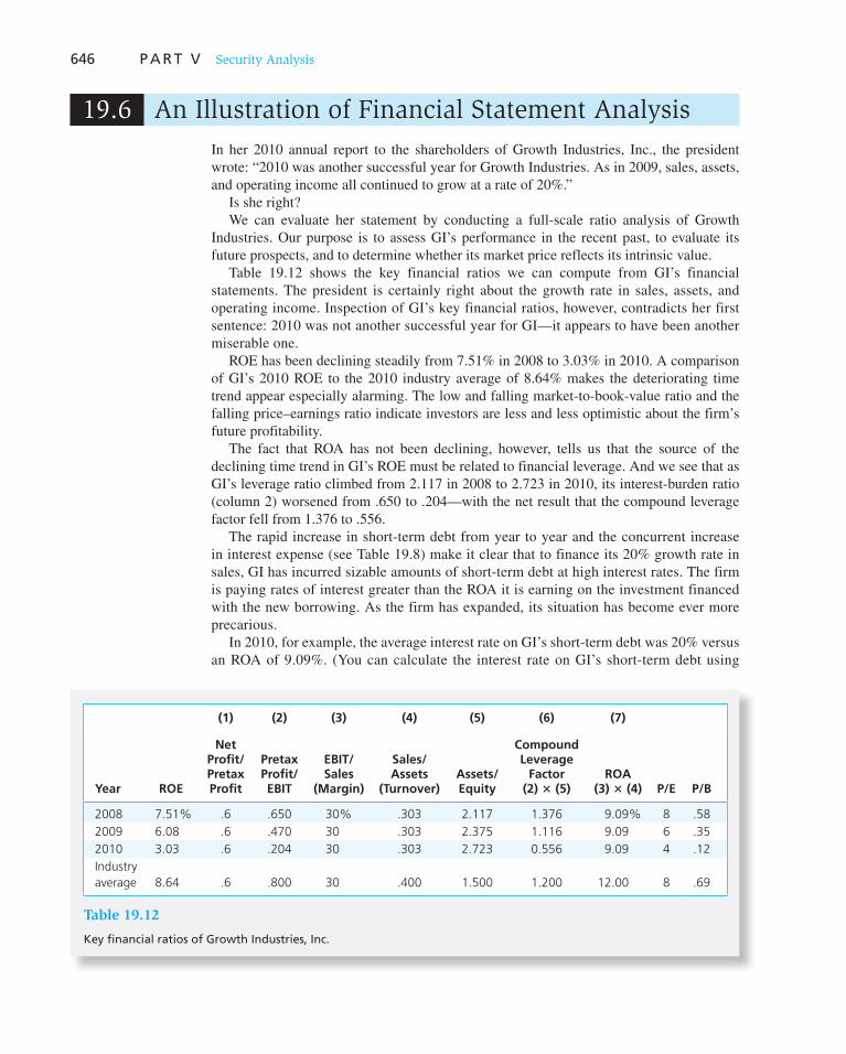
646 P A R T V Security Analysis
19.6 An Illustration of Financial Statement Analysis
In her 2010 annual report to the shareholders of Growth Industries, Inc., the president wrote: “2010 was another successful year for Growth Industries. As in 2009, sales, assets, and operating income all continued to grow at a rate of 20%.”
Is she right? We can evaluate her statement by conducting a full-scale ratio analysis of Growth
Industries. Our purpose is to assess GI’s performance in the recent past, to evaluate its future prospects, and to determine whether its market price reflects its intrinsic value.
Table 19.12 shows the key financial ratios we can compute from GI’s financial statements. The president is certainly right about the growth rate in sales, assets, and operating income. Inspection of GI’s key financial ratios, however, contradicts her first sentence: 2010 was not another successful year for GI—it appears to have been another miserable one.
ROE has been declining steadily from 7.51% in 2008 to 3.03% in 2010. A comparison of GI’s 2010 ROE to the 2010 industry average of 8.64% makes the deteriorating time trend appear especially alarming. The low and falling market-to-book-value ratio and the falling price–earnings ratio indicate investors are less and less optimistic about the firm’s future profitability.
The fact that ROA has not been declining, however, tells us that the source of the declining time trend in GI’s ROE must be related to financial leverage. And we see that as GI’s leverage ratio climbed from 2.117 in 2008 to 2.723 in 2010, its interest-burden ratio (column 2) worsened from .650 to .204—with the net result that the compound leverage factor fell from 1.376 to .556.
The rapid increase in short-term debt from year to year and the concurrent increase in interest expense (see Table 19.8 ) make it clear that to finance its 20% growth rate in sales, GI has incurred sizable amounts of short-term debt at high interest rates. The firm is paying rates of interest greater than the ROA it is earning on the investment financed with the new borrowing. As the firm has expanded, its situation has become ever more precarious.
In 2010, for example, the average interest rate on GI’s short-term debt was 20% versus an ROA of 9.09%. (You can calculate the interest rate on GI’s short-term debt using
(1) (2) (3) (4) (5) (6) (7)
Year ROE
Net Profit/Pretax Profit
Pretax Profit/EBIT
EBIT/Sales
(Margin)
Sales/Assets
(Turnover)Assets/Equity
Compound Leverage
Factor (2) 3 (5)
ROA (3) 3 (4) P/E P/B
2008 7.51% .6 .650 30% .303 2.117 1.376 9.09% 8 .58
2009 6.08 .6 .470 30 .303 2.375 1.116 9.09 6 .35
2010 3.03 .6 .204 30 .303 2.723 0.556 9.09 4 .12
Industry
average 8.64 .6 .800 30 .400 1.500 1.200 12.00 8 .69
Table 19.12
Key financial ratios of Growth Industries, Inc.
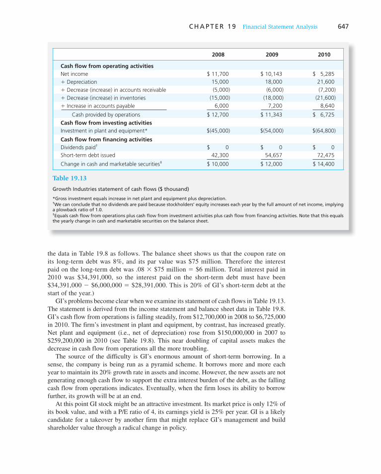
C H A P T E R 1 9 Financial Statement Analysis 647
the data in Table 19.8 as follows. The balance sheet shows us that the coupon rate on its long-term debt was 8%, and its par value was $75 million. Therefore the interest paid on the long-term debt was .08 3 $75 million 5 $6 million. Total interest paid in 2010 was $34,391,000, so the interest paid on the short-term debt must have been $34,391,000 2 $6,000,000 5 $28,391,000. This is 20% of GI’s short-term debt at the start of the year.)
GI’s problems become clear when we examine its statement of cash flows in Table 19.13 . The statement is derived from the income statement and balance sheet data in Table 19.8 . GI’s cash flow from operations is falling steadily, from $12,700,000 in 2008 to $6,725,000 in 2010. The firm’s investment in plant and equipment, by contrast, has increased greatly. Net plant and equipment (i.e., net of depreciation) rose from $150,000,000 in 2007 to $259,200,000 in 2010 (see Table 19.8 ). This near doubling of capital assets makes the decrease in cash flow from operations all the more troubling.
The source of the difficulty is GI’s enormous amount of short-term borrowing. In a sense, the company is being run as a pyramid scheme. It borrows more and more each year to maintain its 20% growth rate in assets and income. However, the new assets are not generating enough cash flow to support the extra interest burden of the debt, as the falling cash flow from operations indicates. Eventually, when the firm loses its ability to borrow further, its growth will be at an end.
At this point GI stock might be an attractive investment. Its market price is only 12% of its book value, and with a P/E ratio of 4, its earnings yield is 25% per year. GI is a likely candidate for a takeover by another firm that might replace GI’s management and build shareholder value through a radical change in policy.
2008 2009 2010
Cash flow from operating activities
Net income $ 11,700 $ 10,143 $ 5,285
1 Depreciation 15,000 18,000 21,600
1 Decrease (increase) in accounts receivable (5,000) (6,000) (7,200)
1 Decrease (increase) in inventories (15,000) (18,000) (21,600)
1 Increase in accounts payable 6,000 7,200 8,640
Cash provided by operations $ 12,700 $ 11,343 $ 6,725
Cash flow from investing activities
Investment in plant and equipment* $(45,000) $(54,000) $(64,800)
Cash flow from financing activities
Dividends paid† $ 0 $ 0 $ 0
Short-term debt issued 42,300 54,657 72,475
Change in cash and marketable securities‡ $ 10,000 $ 12,000 $ 14,400
Table 19.13
Growth Industries statement of cash flows ($ thousand)
*Gross investment equals increase in net plant and equipment plus depreciation. † We can conclude that no dividends are paid because stockholders’ equity increases each year by the full amount of net income, implying a plowback ratio of 1.0. ‡ Equals cash flow from operations plus cash flow from investment activities plus cash flow from financing activities. Note that this equals the yearly change in cash and marketable securities on the balance sheet.

648 P A R T V Security Analysis
19.7 Comparability Problems
Financial statement analysis gives us a good amount of ammunition for evaluating a com-pany’s performance and future prospects. But comparing financial results of different com-panies is not so simple. There is more than one acceptable way to represent various items of revenue and expense according to generally accepted accounting principles (GAAP). This means two firms may have exactly the same economic income yet very different accounting incomes.
Furthermore, interpreting a single firm’s performance over time is complicated when inflation distorts the dollar measuring rod. Comparability problems are especially acute in this case because the impact of inflation on reported results often depends on the par-ticular method the firm adopts to account for inventories and depreciation. The security analyst must adjust the earnings and the financial ratio figures to a uniform standard before attempting to compare financial results across firms and over time.
Comparability problems can arise out of the flexibility of GAAP guidelines in account-ing for inventories and depreciation and in adjusting for the effects of inflation. Other important potential sources of noncomparability include the capitalization of leases and other expenses, the treatment of pension costs, and allowances for reserves.
Inventory Valuation
There are two commonly used ways to value inventories: LIFO (last-in first-out) and FIFO (first-in first-out). We can explain the difference using a numerical example.
Suppose Generic Products, Inc. (GPI), has a constant inventory of 1 million units of generic goods. The inventory turns over once per year, meaning the ratio of cost of goods sold to inventory is 1.
The LIFO system calls for valuing the million units used up during the year at the cur-rent cost of production, so that the last goods produced are considered the first ones to be sold. They are valued at today’s cost.
The FIFO system assumes that the units used up or sold are the ones that were added to inventory first, and goods sold should be valued at original cost.
If the price of generic goods has been constant, at the level of $1, say, the book value of inventory and the cost of goods sold would be the same, $1 million under both systems. But suppose the price of generic goods rises by 10 cents per unit during the year as a result of general inflation.
CONCEPT CHECK
4
You have the following information for IBX Corporation for the years 2010 and 2012 (all figures are in $ million):
2010 2012
Net income $ 253.7 $ 239.0
Pretax income 411.9 375.6
EBIT 517.6 403.1
Average assets 4,857.9 3,459.7
Sales 6,679.3 4,537.0
Shareholders’ equity 2,233.3 2,347.3
What is the trend in IBX’s ROE; how can you account for it in terms of tax burden, margin, turnover, and financial leverage?
C H A P T E R 1 9 Financial Statement Analysis 649
LIFO accounting would result in a cost of goods sold of $1.1 million, whereas the end-of-year balance sheet value of the 1 million units in inventory remains $1 million. The balance sheet value of inventories is given as the cost of the goods still in inventory. Under LIFO the last goods produced are assumed to be sold at the current cost of $1.10; the goods remaining are the previously produced goods, at a cost of only $1. You can see that although LIFO accounting accurately measures the cost of goods sold today, it understates the current value of the remaining inventory in an inflationary environment.
In contrast, under FIFO accounting, the cost of goods sold would be $1 million, and the end-of-year balance sheet value of the inventory would be $1.1 million. The result is that the LIFO firm has both a lower reported profit and a lower balance sheet value of invento-ries than the FIFO firm.
LIFO is preferred over FIFO in computing economic earnings (i.e., real sustainable cash flow) because it uses up-to-date prices to evaluate the cost of goods sold. However, LIFO accounting induces balance sheet distortions when it values investment in invento-ries at original cost. This practice results in an upward bias in ROE because the investment base on which return is earned is undervalued.
Depreciation
Another source of problems is the measurement of depreciation, which is a key factor in computing true earnings. The accounting and economic measures of depreciation can dif-fer markedly. According to the economic definition, depreciation is the amount of a firm’s operating cash flow that must be reinvested in the firm to sustain its real productive capac-ity at the current level.
The accounting measurement is quite different. Accounting depreciation is the amount of the original acquisition cost of an asset that is allocated to each accounting period over an arbitrarily specified life of the asset. This is the figure reported in financial statements.
Assume, for example, that a firm buys machines with a useful economic life of 20 years at $100,000 apiece. In its financial statements, however, the firm can depreciate the machines over 10 years using the straight-line method, for $10,000 per year in depre-ciation. Thus after 10 years a machine will be fully depreciated on the books, even though it remains a productive asset that will not need replacement for another 10 years.
In computing accounting earnings, this firm will overestimate depreciation in the first 10 years of the machine’s economic life and underestimate it in the last 10 years. This will cause reported earnings to be understated compared with economic earnings in the first 10 years and overstated in the last 10 years.
Depreciation comparability problems add one more wrinkle. A firm can use different depreciation methods for tax purposes than for other reporting purposes. Most firms use accelerated depreciation methods for tax purposes and straight-line depreciation in pub-lished financial statements. There also are differences across firms in their estimates of the depreciable life of plant, equipment, and other depreciable assets.
Another complication arises from inflation. Because conventional depreciation is based on historical costs rather than on the current replacement cost of assets, measured depreci-ation in periods of inflation is understated relative to replacement cost, and real economic income (sustainable cash flow) is correspondingly overstated.
For example, suppose Generic Products, Inc., has a machine with a 3-year useful life that originally cost $3 million. Annual straight-line depreciation is $1 million, regardless of what happens to the replacement cost of the machine. Suppose inflation in the first year turns out to be 10%. Then the true annual depreciation expense is $1.1 million in current terms, whereas conventionally measured depreciation remains fixed at $1 million per year. Accounting income overstates real economic income by $.1 million.
Example 19.5 Inflation and Real Income
Suppose Generic Products has debt outstanding with a face value of $10 million at an interest rate of 10% per year. Interest expense as conventionally measured is $1 million per year. However, suppose inflation during the year is 6%, so that the real interest rate is 4%. Then $.6 million of what appears as interest expense on the income statement is really an inflation premium, or compensation for the anticipated reduction in the real value of the $10 million principal; only $.4 million is real interest expense. The $.6 million reduction in the purchasing power of the outstanding principal may be thought of as repayment of principal, rather than as an interest expense. Real income of the firm is, therefore, under-stated by $.6 million.
650 P A R T V Security Analysis
Inflation and Interest Expense
Although inflation can cause distortions in the measurement of a firm’s inventory and depreciation costs, it has perhaps an even greater effect on calculation of real interest expense. Nominal interest rates include an inflation premium that compensates the lender for inflation-induced erosion in the real value of principal. From the perspective of both lender and borrower, therefore, part of what is conventionally measured as interest expense should be treated more properly as repayment of principal.
Mismeasurement of real interest means inflation deflates the computation of real income. The effects of inflation on the reported values of inventories and depreciation that we have discussed work in the opposite direction.
Fair Value Accounting
Many major assets and liabilities are not traded in financial markets and do not have eas-ily observable values. For example, we cannot simply look up the values of employee stock options, health care benefits for retired employees, or buildings and other real estate. While the true financial status of a firm may depend critically on these values, which can swing widely over time, common practice has been to simply value them at historic cost. Proponents of fair value accounting, also known as mark-to-market accounting, argue that financial statements would give a truer picture of the firm if they better reflected the current market values of all assets and liabilities.
The Financial Accounting Standards Board’s Statement No. 157 on fair value account-ing places assets in one of three “buckets.” Level 1 assets are traded in active markets and therefore should be valued at their market price. Level 2 assets are not actively traded, but their values still may be estimated using observable market data on similar assets. Level 3 assets can be valued only with inputs that are difficult to observe. Level 2 and 3 assets may be valued using pricing models, for example, based on a theoretical price derived from a computer model. Rather than mark to market, these values are often called “mark to model,” although they are also disparagingly known as mark-to-make believe, as the estimates are so prone to manipulation by creative use of model inputs.
CONCEPT CHECK
5
In a period of rapid inflation, companies ABC and XYZ have the same reported earnings. ABC uses LIFO inventory accounting, has relatively fewer depreciable assets, and has more debt than XYZ. XYZ uses FIFO inventory accounting. Which company has the higher real income, and why?

651
Critics of fair value accounting argue that it relies too heavily on estimates. Such esti-mates potentially introduce considerable noise in firms’ accounts and can induce great profit volatility as fluctuations in asset valuations are recognized. Even worse, subjective valuations may offer management a tempting tool to manipulate earnings or the appar-ent financial condition of the firm at opportune times. As just one example, Bergstresser, Desai, and Rauth 5 find that firms make more aggressive assumptions about returns on defined benefit pension plans (which lowers the computed present value of pension obliga-tions) during periods in which executives are actively exercising their stock options.
A contentious debate over the application of fair value accounting to troubled financial institutions erupted in 2008 when even values of financial securities such as subprime mortgage pools and derivative contracts backed by these pools came into question as trad-ing in these instruments dried up. Without well-functioning markets, estimating (much less observing) market values was, at best, a precarious exercise.
Some felt that mark-to-market accounting exacerbated the financial meltdown by forcing banks to excessively write down asset values; others felt that a failure to mark would have been tantamount to willfully ignoring reality and abdicating the responsibility to redress problems at nearly or already insolvent banks. The nearby box discusses the debate.
5 D. Bergstresser, M. Desai, and J. Rauh, “Earnings Manipulation, Pension Assumptions, and Managerial Investment Decisions,” Quarterly Journal of Economics 121 (2006), pp. 157–95.
Mark-to-Market Accounting: Cure or Disease?
As banks and other institutions holding mortgage-backed securities revalued their portfolios throughout 2008, their net worth fell along with the value of those securities. The losses on these securities were painful enough, but their knock-on effects only increased the banks’ woes. For example, banks are required to maintain adequate levels of capital relative to assets. If capital reserves decline, a bank may be forced to shrink until its remaining capital is once again adequate compared to its asset base. But such shrinkage may require the bank to cut back on its lending, which restricts its customers’ access to credit. It may also require asset sales, and if many banks attempt to shrink their portfolios at once, waves of forced sales may put fur-ther pressure on prices, resulting in additional write-downs and reductions to capital in a self-feeding cycle. Critics of mark-to-market accounting therefore contend that it has exacerbated the problems of an already reeling economy.
Advocates, however, argue that the critics confuse the message with the messenger. Mark-to-market accounting makes transparent losses that have already been incurred, but it does not cause those losses. Critics retort that when markets are faltering, market prices may be unreliable. If trading activity has largely broken down, and assets can be sold only at fire-sale prices, then those prices may no longer be indicative of fundamental value. Markets can-not be efficient if they are not even functioning. In the turmoil surrounding the defaulted mortgages weighing down bank portfolios, one of the early proposals of then–Treasury secretary Henry Paulson was for the government
to buy bad assets at “hold to maturity” prices based on estimates of intrinsic value in a normally functioning mar-ket. In that spirit, FASB approved new guidelines in 2009 allowing valuation based on an estimate of the price that would prevail in an orderly market rather than the one that could be received in a forced liquidation.
Waiving write-down requirements may best be viewed as thinly veiled regulatory forbearance. Regulators know that losses have been incurred and that capital has been impaired. But by allowing firms to carry assets on their books at model rather than market prices, the unpleas-ant implications of that fact for capital adequacy may be politely ignored for a time. Even so, if the goal is to avoid forced sales in a distressed market, transparency may nev-ertheless be the best policy. Better to acknowledge losses and explicitly modify capital regulations to help institu-tions recover their footing in a difficult economy than to deal with losses by ignoring them. After all, why bother preparing financial statements if they are allowed to obscure the true condition of the firm?
Before abandoning fair value accounting, it would be prudent to consider the alternative. Traditional historic-cost accounting, which would allow firms to carry assets on the books at their original purchase price, has even less to recommend it. It would leave investors without an accu-rate sense of the condition of shaky institutions, and by the same token lessen the pressure on those firms to get their houses in order. Dealing with losses must surely require acknowledging them.
WO
RD
S FRO
M TH
E STREET
652 P A R T V Security Analysis
Quality of Earnings
Many firms will make accounting choices that present their financial statements in the best possible light. The different choices that firms can make give rise to the comparabil-ity problems we have discussed. As a result, earnings statements for different companies may be more or less rosy presentations of true economic earnings—sustainable cash flow that can be paid to shareholders without impairing the firm’s productive capacity. Analysts commonly evaluate the quality of earnings reported by a firm. This concept refers to the realism and conservatism of the earnings number, in other words, the extent to which we might expect the reported level of earnings to be sustained.
Examples of the types of factors that influence quality of earnings are:
• Allowance for bad debt. Most firms sell goods using trade credit and must make an allowance for bad debt. An unrealistically low allowance reduces the quality of reported earnings.
• Nonrecurring items. Some items that affect earnings should not be expected to recur regularly. These include asset sales, effects of accounting changes, effects of exchange rate movements, or unusual investment income. For example, in years with large stock market returns, some firms enjoy large capital gains on securities held. These contribute to that year’s earnings, but should not be expected to repeat regularly. They would be considered a “low-quality” component of earnings. Similarly, investment gains in corporate pension plans generated large but one-off contributions to reported earnings.
• Earnings smoothing. In 2003, Freddie Mac was the subject of an accounting scandal, when it emerged that it had improperly reclassified mortgages held in its portfolio in an attempt to reduce its current earnings. Similarly, in the 1990s, W.R. Grace chose to offset high earnings in one of its subsidiaries by setting aside extra reserves. Why would these firms take such actions? Because later, if earnings turned down, they could “release” earnings by reversing these transactions, and thereby create the appearance of steady earnings growth. Indeed, almost until its sudden collapse in 2008, Freddie Mac’s nickname on Wall Street was “Steady Freddie.” Wall Street likes strong, steady earnings, but these firms planned to provide such growth only cosmetically, through earnings management.
• Revenue recognition. Under GAAP accounting, a firm is allowed to recognize a sale before it is paid. This is why firms have accounts receivable. But sometimes it can be hard to know when to recognize sales. For example, suppose a computer firm signs a contract to provide products and services over a 5-year period. Should the projected revenue be booked immediately or spread out over 5 years? A more extreme version of this problem is called “channel stuffing,” in which firms “sell” large quantities of goods to customers, but give them the right to later either refuse delivery or return the product. The revenue from the “sale” is booked now, but the likely returns are not recognized until they occur (in a future accounting period). According to the SEC, Sunbeam, which filed for bankruptcy in 2001, generated $60 million in fraudulent profits in 1999 using this technique. If you see accounts receivable increasing far faster than sales, or becoming a larger percentage of total assets, beware of these practices. Given the wide latitude firms have in how they recognize revenue, many analysts choose instead to concentrate on cash flow, which is far harder for a company to manipulate.
• Off-balance-sheet assets and liabilities. Suppose that one firm guarantees the outstanding debt of another firm, perhaps a firm in which it has an ownership stake. That obligation ought to be disclosed as a contingent liability, because it
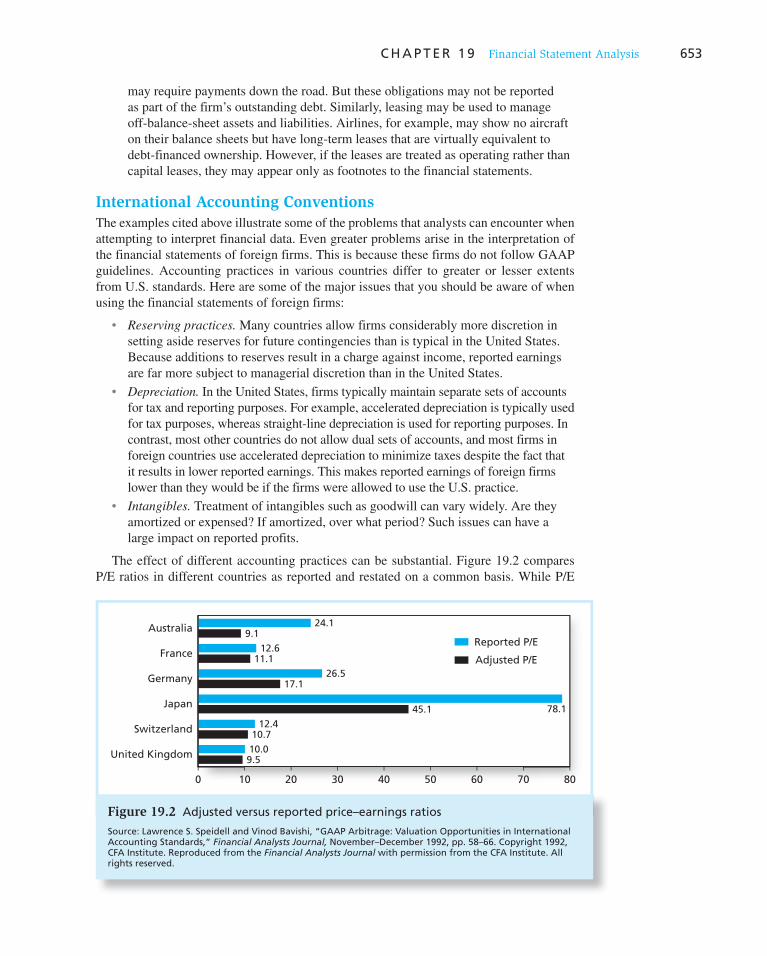
C H A P T E R 1 9 Financial Statement Analysis 653
Australia
0 8070605040302010
Reported P/E
24.19.1
12.611.1
26.517.1
78.145.1
12.410.7
10.09.5United Kingdom
Switzerland
Japan
Germany
FranceAdjusted P/E
Figure 19.2 Adjusted versus reported price–earnings ratios
Source: Lawrence S. Speidell and Vinod Bavishi, “GAAP Arbitrage: Valuation Opportunities in International Accounting Standards,” Financial Analysts Journal, November–December 1992, pp. 58–66. Copyright 1992, CFA Institute. Reproduced from the Financial Analysts Journal with permission from the CFA Institute. All rights reserved.
may require payments down the road. But these obligations may not be reported as part of the firm’s outstanding debt. Similarly, leasing may be used to manage off-balance-sheet assets and liabilities. Airlines, for example, may show no aircraft on their balance sheets but have long-term leases that are virtually equivalent to debt-financed ownership. However, if the leases are treated as operating rather than capital leases, they may appear only as footnotes to the financial statements.
International Accounting Conventions
The examples cited above illustrate some of the problems that analysts can encounter when attempting to interpret financial data. Even greater problems arise in the interpretation of the financial statements of foreign firms. This is because these firms do not follow GAAP guidelines. Accounting practices in various countries differ to greater or lesser extents from U.S. standards. Here are some of the major issues that you should be aware of when using the financial statements of foreign firms:
• Reserving practices. Many countries allow firms considerably more discretion in setting aside reserves for future contingencies than is typical in the United States. Because additions to reserves result in a charge against income, reported earnings are far more subject to managerial discretion than in the United States.
• Depreciation. In the United States, firms typically maintain separate sets of accounts for tax and reporting purposes. For example, accelerated depreciation is typically used for tax purposes, whereas straight-line depreciation is used for reporting purposes. In contrast, most other countries do not allow dual sets of accounts, and most firms in foreign countries use accelerated depreciation to minimize taxes despite the fact that it results in lower reported earnings. This makes reported earnings of foreign firms lower than they would be if the firms were allowed to use the U.S. practice.
• Intangibles. Treatment of intangibles such as goodwill can vary widely. Are they amortized or expensed? If amortized, over what period? Such issues can have a large impact on reported profits.
The effect of different accounting practices can be substantial. Figure 19.2 compares P/E ratios in different countries as reported and restated on a common basis. While P/E
654 P A R T V Security Analysis
multiples have changed considerably since this study was published, these results illustrate how different accounting rules can have a big impact on these ratios.
Such differences in international accounting standards become more of a problem as the drive to globally integrated capital markets progresses. For example, many foreign firms would like to list their shares on the New York Stock Exchange to more easily tap U.S. equity markets, and the NYSE would like to have those firms listed. But the SEC did not until recently allow such shares to be listed unless the firms prepared their financial state-ments in accordance with U.S. GAAP standards. This policy limited listing of non-U.S. companies dramatically.
In contrast, the European Union has moved to institute common international finan-
cial reporting standards (IFRS) across the EU. IFRS seem on their way to becoming global standards, even outside the European Union. By 2008, more than 100 countries had adopted them, and they are making inroads even in the United States. In November 2007, the SEC began allowing foreign firms to issue securities in the U.S. if their financial statements are prepared using IFRS. The SEC noted that the goal of its new ruling was to encourage the development of IFRS as a uniform global standard to enhance consistency and comparability. The SEC went even further when it proposed allowing large U.S. mul-tinational firms to report earnings using IFRS rather than GAAP starting in 2010, with all U.S. firms to follow by 2014.
The major difference between IFRS and GAAP has to do with “principles”- versus “rules”-based standards. U.S. rules are detailed, explicit, and lengthy. European rules are more flex-ible, but firms must be prepared to demonstrate that they have conformed to general principles meant to ensure that financial accounts faithfully reflect the actual status of the firm.
19.8 Value Investing: The Graham Technique
No presentation of fundamental security analysis would be complete without a discussion of the ideas of Benjamin Graham, the greatest of the investment “gurus.” Until the evolu-tion of modern portfolio theory in the latter half of the 20th century, Graham was the single most important thinker, writer, and teacher in the field of investment analysis. His influ-ence on investment professionals remains very strong.
Graham’s magnum opus is Security Analysis, written with Columbia Professor David Dodd in 1934. Its message is similar to the ideas presented in this chapter. Graham believed careful analysis of a firm’s financial statements could turn up bargain stocks. Over the years, he developed many different rules for determining the most important financial ratios and the critical values for judging a stock to be undervalued. Through many editions, his book has been so influential and successful that widespread adoption of Graham’s tech-niques has led to elimination of the very bargains they are designed to identify.
In a 1976 seminar Graham said: 6
I am no longer an advocate of elaborate techniques of security analysis in order to find superior value opportunities. This was a rewarding activity, say, forty years ago, when our textbook “Graham and Dodd” was first published; but the situation has changed a good deal since then. In the old days any well-trained security analyst could do a good professional job of selecting undervalued issues through detailed studies; but in the light of the enormous amount of research now being carried on, I doubt whether in most cases such extensive efforts will generate sufficiently superior selections to justify their cost. To that very limited extent I’m on the side of the “efficient market” school of thought now generally accepted by the professors.
6 As cited by John Train in Money Masters (New York: Harper & Row, 1987).

Vis
it u
s at
ww
w.m
hh
e.co
m/b
km
C H A P T E R 1 9 Financial Statement Analysis 655
Nonetheless, in that same seminar, Graham suggested a simplified approach to identify-ing bargain stocks:
My first, more limited, technique confines itself to the purchase of common stocks at less than their working-capital value, or net current-asset value, giving no weight to the plant and other fixed assets, and deducting all liabilities in full from the current assets. We used this approach extensively in managing investment funds, and over a 30-odd-year period we must have earned an average of some 20 percent per year from this source. I consider it a foolproof method of systematic investment—once again, not on the basis of individual results but in terms of the expectable group income.
There are two convenient sources of information for those interested in trying out the Graham technique: Both Standard & Poor’s Outlook and The Value Line Investment Survey carry lists of stocks selling below net working capital value.
1. The primary focus of the security analyst should be the firm’s real economic earnings rather than its reported earnings. Accounting earnings as reported in financial statements can be a biased estimate of real economic earnings, although empirical studies reveal that reported earn-ings convey considerable information concerning a firm’s prospects.
2. A firm’s ROE is a key determinant of the growth rate of its earnings. ROE is affected pro-foundly by the firm’s degree of financial leverage. An increase in a firm’s debt-to-equity ratio will raise its ROE and hence its growth rate only if the interest rate on the debt is less than the firm’s return on assets.
3. It is often helpful to the analyst to decompose a firm’s ROE ratio into the product of several accounting ratios and to analyze their separate behavior over time and across companies within an industry. A useful breakdown is
ROE 5Net profits
Pretax profits3
Pretax profits
EBIT3
EBIT
Sales3
Sales
Assets3
Assets
Equity
4. Other accounting ratios that have a bearing on a firm’s profitability and/or risk are fixed-asset turnover, inventory turnover, and the current, quick, and interest coverage ratios.
5. Two ratios that make use of the market price of the firm’s common stock in addition to its finan-cial statements are the ratios of market to book value and price to earnings. Analysts sometimes take low values for these ratios as a margin of safety or a sign that the stock is a bargain.
6. Good firms are not necessarily good investments. Stock market prices of successful firms may be bid up to levels that reflect that success. If so, the price of these firms relative to their earn-ings prospects may not constitute a bargain.
7. A major problem in the use of data obtained from a firm’s financial statements is comparabil-ity. Firms have a great deal of latitude in how they choose to compute various items of revenue and expense. It is, therefore, necessary for the security analyst to adjust accounting earnings and financial ratios to a uniform standard before attempting to compare financial results across firms.
8. Comparability problems can be acute in a period of inflation. Inflation can create distortions in accounting for inventories, depreciation, and interest expense.
9. Fair value or mark-to-market accounting requires that most assets be valued at current market value rather than historical cost. This policy has proven to be controversial because ascertaining true market value in many instances is difficult, and critics contend that financial statements are therefore unduly volatile. Advocates argue that financial statements should reflect the best estimate of current asset values.
10. International financial reporting standards have become progressively accepted throughout the world, including the United States. They differ from traditional U.S. GAAP procedures in that they are “principles based” rather than rules based.
SUMMARY
Related Web sites for this chapter are available at www.mhhe.com/bkm
Vis
it u
s at
ww
w.m
hh
e.co
m/b
km656 P A R T V Security Analysis
1. What is the major difference in approach of international financial reporting standards and U.S. GAAP accounting? What are the advantages and disadvantages of each?
2. If markets are truly efficient, does it matter whether firms engage in earnings management? On the other hand, if firms manage earnings, what does that say about management’s view on effi-cient markets?
3. What financial ratios would a credit rating agency such as Moody’s or Standard & Poor’s be most interested in? Which ratios would be of most interest to a stock market analyst deciding whether to buy a stock for a diversified portfolio?
4. The Crusty Pie Co., which specializes in apple turnovers, has a return on sales higher than the industry average, yet its ROA is the same as the industry average. How can you explain this?
5. The ABC Corporation has a profit margin on sales below the industry average, yet its ROA is above the industry average. What does this imply about its asset turnover?
6. Firm A and firm B have the same ROA, yet firm A ’s ROE is higher. How can you explain this?
7. Use the DuPont system and the following data to find return on equity.
Leverage ratio (assets/equity) 2.2
Total asset turnover 2.0
Net profit margin 5.5%
Dividend payout ratio 31.8%
8. Recently, Galaxy Corporation lowered its allowance for doubtful accounts by reducing bad debt expense from 2% of sales to 1% of sales. Ignoring taxes, what are the immediate effects on ( a ), operating income and ( b ) operating cash flow?
Use the following case in answering Problems 9–11: Hatfield Industries is a large manufacturing conglomerate based in the United States with annual sales in excess of $300 million. Hatfield is cur-rently under investigation by the Securities and Exchange Commission (SEC) for accounting irregu-larities and possible legal violations in the presentation of the company’s financial statements. A due diligence team from the SEC has been sent to Hatfield’s corporate headquarters in Philadelphia for a complete audit in order to further assess the situation.
Several unique circumstances at Hatfield are discovered by the SEC due diligence team during the course of the investigation:
• Management has been involved in ongoing negotiations with the local labor union, of which approximately 40% of its full-time labor force are members. Labor officials are seeking increased wages and pension benefits, which Hatfield’s management states is not possible at this time due to decreased profitability and a tight cash flow situation. Labor officials have accused Hatfield’s management of manipulating the company’s financial statements to justify not granting any concessions during the course of negotiations.
PROBLEM SETS
i. Basic
ii. Intermediate
income statement balance sheet statement of cash flows economic earnings accounting earnings return on equity return on assets DuPont system profit margin return on sales total asset turnover
interest coverage ratio times interest earned leverage ratio inventory turnover ratio average collection period current ratio quick ratio acid test ratio cash ratio market–book-value ratio price–earnings (P/E) ratio
economic value added residual income LIFO FIFO fair value accounting mark-to-market accounting quality of earnings international financial
reporting standards
KEY TERMS

Vis
it u
s at
ww
w.m
hh
e.co
m/b
km
C H A P T E R 1 9 Financial Statement Analysis 657
• All new equipment obtained over the past several years has been established on Hatfield’s books as operating leases, although past acquisitions of similar equipment were nearly always classified as capital leases. Financial statements of industry peers indicate that capital leases for this type of equipment are the norm. The SEC wants Hatfield’s management to provide justification for this apparent deviation from “normal” accounting practices.
• Inventory on Hatfield’s books has been steadily increasing for the past few years in compari-son to sales growth. Management credits improved operating efficiencies in its production methods that have contributed to boosts in overall production. The SEC is seeking evidence that Hatfield somehow may have manipulated its inventory accounts.
The SEC due diligence team is not necessarily searching for evidence of fraud but of possible manip-ulation of accounting standards for the purpose of misleading shareholders and other interested par-ties. Initial review of Hatfield’s financial statements indicates that at a minimum, certain practices have resulted in low-quality earnings.
9. Labor officials believe that the management of Hatfield is attempting to understate its net income to avoid making any concessions in the labor negotiations. Which of the following actions by management will most likely result in low-quality earnings?
a. Lengthening the life of a depreciable asset in order to lower the depreciation expense. b. Lowering the discount rate used in the valuation of the company’s pension obligations. c. The recognition of revenue at the time of delivery rather than when payment is received.
10. Hatfield has begun recording all new equipment leases on its books as operating leases, a change from its consistent past use of capital leases, in which the present value of lease payments is classified as a debt obligation. What is the most likely motivation behind Hatfield’s change in accounting methodology? Hatfield is attempting to:
a. Improve its leverage ratios and reduce its perceived leverage. b. Reduce its cost of goods sold and increase it profitability. c. Increase its operating margins relative to industry peers.
11. The SEC due diligence team is searching for the reason behind Hatfield’s inventory build-up relative to its sales growth. One way to identify a deliberate manipulation of financial results by Hatfield is to search for:
a. A decline in inventory turnover. b. Receivables that are growing faster than sales. c. A delay in the recognition of expenses.
12. A firm has an ROE of 3%, a debt-to-equity ratio of .5, a tax rate of 35%, and pays an interest rate of 6% on its debt. What is its operating ROA?
13. A firm has a tax burden ratio of .75, a leverage ratio of 1.25, an interest burden of .6, and a return on sales of 10%. The firm generates $2.40 in sales per dollar of assets. What is the firm’s ROE?
14. Use the following cash flow data for Rocket Transport to find Rocket’s
a. Net cash provided by or used in investing activities. b. Net cash provided by or used in financing activities. c. Net increase or decrease in cash for the year.
Cash dividend $ 80,000
Purchase of bus $ 33,000
Interest paid on debt $ 25,000
Sales of old equipment $ 72,000
Repurchase of stock $ 55,000
Cash payments to suppliers $ 95,000
Cash collections from customers $300,000
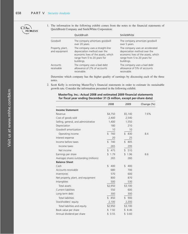
Vis
it u
s at
ww
w.m
hh
e.co
m/b
km658 P A R T V Security Analysis
1. The information in the following exhibit comes from the notes to the financial statements of QuickBrush Company and SmileWhite Corporation:
Determine which company has the higher quality of earnings by discussing each of the three notes.
2. Scott Kelly is reviewing MasterToy’s financial statements in order to estimate its sustainable growth rate. Consider the information presented in the following exhibit.
MasterToy, Inc.: Actual 2008 and estimated 2009 financial statements for fiscal year ending December 31 ($ million, except per-share data)
2008 2009 Change (%)
Income Statement
Revenue $4,750 $5,140 7.6%
Cost of goods sold 2,400 2,540
Selling, general, and administrative 1,400 1,550
Depreciation 180 210
Goodwill amortization 10 10
Operating income $ 760 $ 830 8.4
Interest expense 20 25
Income before taxes $ 740 $ 805
Income taxes 265 295
Net income $ 475 $ 510
Earnings per share $ 1.79 $ 1.96 8.6
Averages shares outstanding (millions) 265 260
Balance Sheet
Cash $ 400 $ 400
Accounts receivable 680 700
Inventories 570 600
Net property, plant, and equipment 800 870
Intangibles 500 530
Total assets $2,950 $3,100
Current liabilities 550 600
Long-term debt 300 300
Total liabilities $ 850 $ 900
Stockholders’ equity 2,100 2,200
Total liabilities and equity $2,950 $3,100
Book value per share $ 7.92 $ 8.46
Annual dividend per share $ 0.55 $ 0.60
QuickBrush SmileWhite
Goodwill The company amortizes goodwill
over 20 years.
The company amortizes goodwill
over 5 years.
Property, plant,
and equipment
The company uses a straight-line
depreciation method over the
economic lives of the assets, which
range from 5 to 20 years for
buildings.
The company uses an accelerated
depreciation method over the
economic lives of the assets, which
range from 5 to 20 years for
buildings.
Accounts
receivable
The company uses a bad debt
allowance of 2% of accounts
receivable.
The company uses a bad debt
allowance of 5% of accounts
receivable.

Vis
it u
s at
ww
w.m
hh
e.co
m/b
km
C H A P T E R 1 9 Financial Statement Analysis 659
a. Identify and calculate the components of the DuPont formula. b. Calculate the ROE for 2009 using the components of the DuPont formula. c. Calculate the sustainable growth rate for 2009 from the firm’s ROE and plowback ratios.
3. This problem should be solved using the following data:
Cash payments for interest $(12)
Retirement of common stock (32)
Cash payments to merchandise suppliers (85)
Purchase of land (8)
Sale of equipment 30
Payments of dividends (37)
Cash payment for salaries (35)
Cash collection from customers 260
Purchase of equipment (40)
a. What are cash flows from operating activities? b. Using the data above, calculate cash flows from investing activities. c. Using the data above, calculate cash flows from financing activities.
4. Janet Ludlow is a recently hired analyst. After describing the electric toothbrush industry, her first report focuses on two companies, QuickBrush Company and SmileWhite Corporation, and concludes:
QuickBrush is a more profitable company than SmileWhite, as indicated by the 40% sales growth and substantially higher margins it has produced over the last few years. SmileWhite’s sales and earnings are growing at a 10% rate and pro-duce much lower margins. We do not think SmileWhite is capable of growing faster than its recent growth rate of 10% whereas QuickBrush can sustain a 30% long-term growth rate.
a. Criticize Ludlow’s analysis and conclusion that QuickBrush is more profitable, as defined by return on equity (ROE), than SmileWhite and that it has a higher sustainable growth rate. Use only the information provided in Tables 19A and 19B . Support your criticism by calculating and analyzing:
• The five components that determine ROE. • The two ratios that determine sustainable growth: ROE and plowback.
b. Explain how QuickBrush has produced an average annual earnings per share (EPS) growth rate of 40% over the last 2 years with an ROE that has been declining. Use only the informa-tion provided in Table 19A .
Use the following in answering CFA Problems 5–8: Eastover Company (EO) is a large, diversified forest products company. Approximately 75% of its sales are from paper and forest products, with the remainder from financial services and real estate. The company owns 5.6 million acres of timber-land, which is carried at very low historical cost on the balance sheet.
Peggy Mulroney, CFA, is an analyst at the investment counseling firm of Centurion Investments. She is assigned the task of assessing the outlook for Eastover, which is being considered for pur-chase, and comparing it to another forest products company in Centurion’s portfolios, Southampton Corporation (SHC). SHC is a major producer of lumber products in the United States. Building products, primarily lumber and plywood, account for 89% of SHC’s sales, with pulp accounting for the remainder. SHC owns 1.4 million acres of timberland, which is also carried at historical cost on the balance sheet. In SHC’s case, however, that cost is not as far below current market as Eastover’s.
Mulroney began her examination of Eastover and Southampton by looking at the five compo-nents of return on equity (ROE) for each company. For her analysis, Mulroney elected to define equity as total shareholders’ equity, including preferred stock. She also elected to use year-end data rather than averages for the balance sheet items.
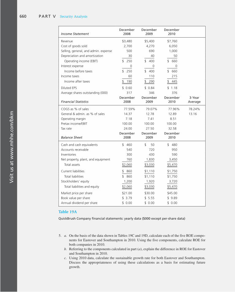
Vis
it u
s at
ww
w.m
hh
e.co
m/b
km660 P A R T V Security Analysis
5. a. On the basis of the data shown in Tables 19C and 19D , calculate each of the five ROE compo-nents for Eastover and Southampton in 2010. Using the five components, calculate ROE for both companies in 2010.
b. Referring to the components calculated in part ( a ), explain the difference in ROE for Eastover and Southampton in 2010.
c. Using 2010 data, calculate the sustainable growth rate for both Eastover and Southampton. Discuss the appropriateness of using these calculations as a basis for estimating future growth.
Income Statement
December 2008
December 2009
December 2010
Revenue $3,480 $5,400 $7,760
Cost of goods sold 2,700 4,270 6,050
Selling, general, and admin. expense 500 690 1,000
Depreciation and amortization 30 40 50
Operating income (EBIT) $ 250 $ 400 $ 660
Interest expense 0 0 0
Income before taxes $ 250 $ 400 $ 660
Income taxes 60 110 215
Income after taxes $ 190 $ 290 $ 445
Diluted EPS $ 0.60 $ 0.84 $ 1.18
Average shares outstanding (000) 317 346 376
Financial Statistics
December 2008
December 2009
December 2010
3-Year Average
COGS as % of sales 77.59% 79.07% 77.96% 78.24%
General & admin. as % of sales 14.37 12.78 12.89 13.16
Operating margin 7.18 7.41 8.51
Pretax income/EBIT 100.00 100.00 100.00
Tax rate 24.00 27.50 32.58
Balance Sheet
December 2008
December 2009
December 2010
Cash and cash equivalents $ 460 $ 50 $ 480
Accounts receivable 540 720 950
Inventories 300 430 590
Net property, plant, and equipment 760 1,830 3,450
Total assets $2,060 $3,030 $5,470
Current liabilities $ 860 $1,110 $1,750
Total liabilities $ 860 $1,110 $1,750
Stockholders’ equity 1,200 1,920 3,720
Total liabilities and equity $2,060 $3,030 $5,470
Market price per share $21.00 $30.00 $45.00
Book value per share $ 3.79 $ 5.55 $ 9.89
Annual dividend per share $ 0.00 $ 0.00 $ 0.00
Table 19A
QuickBrush Company financial statements: yearly data ($000 except per-share data)
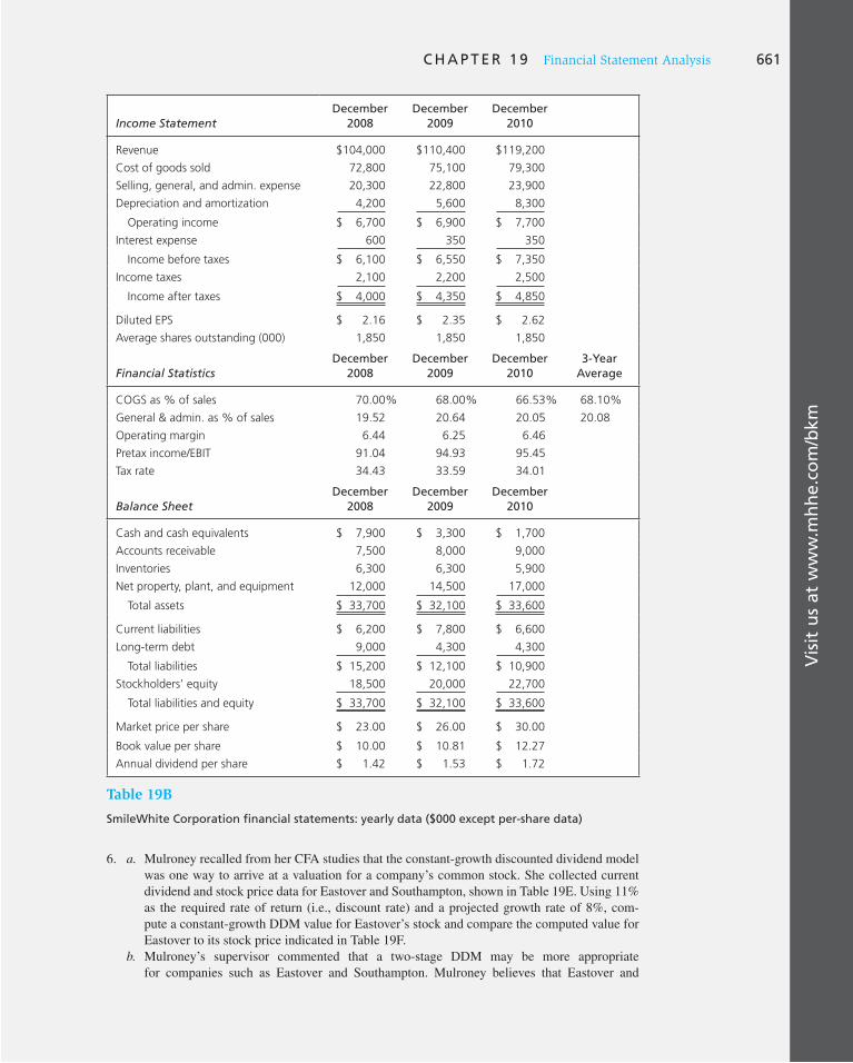
Vis
it u
s at
ww
w.m
hh
e.co
m/b
km
C H A P T E R 1 9 Financial Statement Analysis 661
6. a. Mulroney recalled from her CFA studies that the constant-growth discounted dividend model was one way to arrive at a valuation for a company’s common stock. She collected current dividend and stock price data for Eastover and Southampton, shown in Table 19E . Using 11% as the required rate of return (i.e., discount rate) and a projected growth rate of 8%, com-pute a constant-growth DDM value for Eastover’s stock and compare the computed value for Eastover to its stock price indicated in Table 19F .
b. Mulroney’s supervisor commented that a two-stage DDM may be more appropriate for companies such as Eastover and Southampton. Mulroney believes that Eastover and
Income Statement
December 2008
December 2009
December 2010
Revenue $104,000 $110,400 $119,200
Cost of goods sold 72,800 75,100 79,300
Selling, general, and admin. expense 20,300 22,800 23,900
Depreciation and amortization 4,200 5,600 8,300
Operating income $ 6,700 $ 6,900 $ 7,700
Interest expense 600 350 350
Income before taxes $ 6,100 $ 6,550 $ 7,350
Income taxes 2,100 2,200 2,500
Income after taxes $ 4,000 $ 4,350 $ 4,850
Diluted EPS $ 2.16 $ 2.35 $ 2.62
Average shares outstanding (000) 1,850 1,850 1,850
Financial Statistics
December 2008
December 2009
December 2010
3-Year Average
COGS as % of sales 70.00% 68.00% 66.53% 68.10%
General & admin. as % of sales 19.52 20.64 20.05 20.08
Operating margin 6.44 6.25 6.46
Pretax income/EBIT 91.04 94.93 95.45
Tax rate 34.43 33.59 34.01
Balance Sheet
December 2008
December 2009
December 2010
Cash and cash equivalents $ 7,900 $ 3,300 $ 1,700
Accounts receivable 7,500 8,000 9,000
Inventories 6,300 6,300 5,900
Net property, plant, and equipment 12,000 14,500 17,000
Total assets $ 33,700 $ 32,100 $ 33,600
Current liabilities $ 6,200 $ 7,800 $ 6,600
Long-term debt 9,000 4,300 4,300
Total liabilities $ 15,200 $ 12,100 $ 10,900
Stockholders’ equity 18,500 20,000 22,700
Total liabilities and equity $ 33,700 $ 32,100 $ 33,600
Market price per share $ 23.00 $ 26.00 $ 30.00
Book value per share $ 10.00 $ 10.81 $ 12.27
Annual dividend per share $ 1.42 $ 1.53 $ 1.72
Table 19B
SmileWhite Corporation financial statements: yearly data ($000 except per-share data)
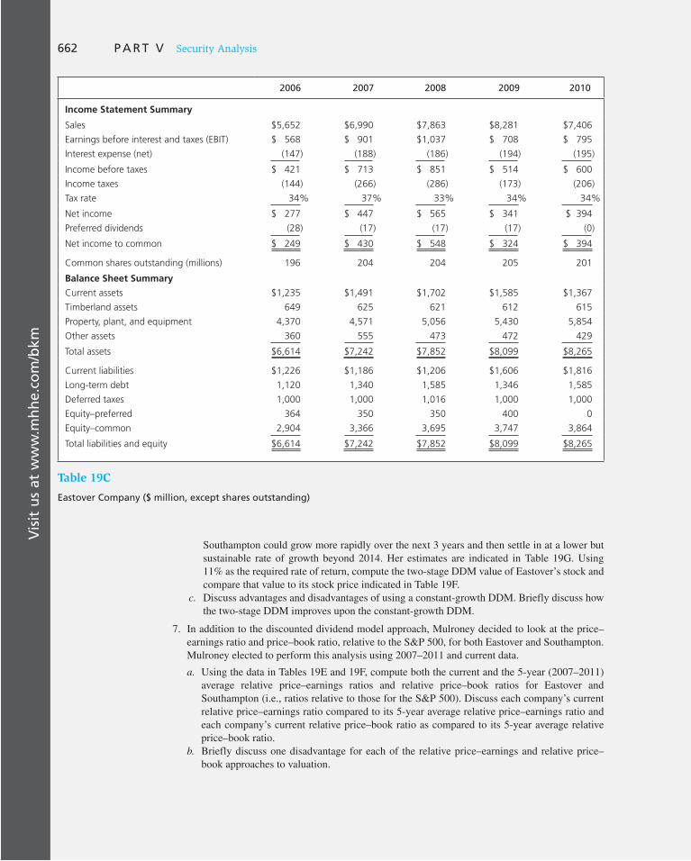
Vis
it u
s at
ww
w.m
hh
e.co
m/b
km662 P A R T V Security Analysis
2006 2007 2008 2009 2010
Income Statement Summary
Sales $5,652 $6,990 $7,863 $8,281 $7,406
Earnings before interest and taxes (EBIT) $ 568 $ 901 $1,037 $ 708 $ 795
Interest expense (net) (147) (188) (186) (194) (195)
Income before taxes $ 421 $ 713 $ 851 $ 514 $ 600
Income taxes (144) (266) (286) (173) (206)
Tax rate 34% 37% 33% 34% 34%
Net income $ 277 $ 447 $ 565 $ 341 $ 394
Preferred dividends (28) (17) (17) (17) (0)
Net income to common $ 249 $ 430 $ 548 $ 324 $ 394
Common shares outstanding (millions) 196 204 204 205 201
Balance Sheet Summary
Current assets $1,235 $1,491 $1,702 $1,585 $1,367
Timberland assets 649 625 621 612 615
Property, plant, and equipment 4,370 4,571 5,056 5,430 5,854
Other assets 360 555 473 472 429
Total assets $6,614 $7,242 $7,852 $8,099 $8,265
Current liabilities $1,226 $1,186 $1,206 $1,606 $1,816
Long-term debt 1,120 1,340 1,585 1,346 1,585
Deferred taxes 1,000 1,000 1,016 1,000 1,000
Equity–preferred 364 350 350 400 0
Equity–common 2,904 3,366 3,695 3,747 3,864
Total liabilities and equity $6,614 $7,242 $7,852 $8,099 $8,265
Table 19C
Eastover Company ($ million, except shares outstanding)
Southampton could grow more rapidly over the next 3 years and then settle in at a lower but sustainable rate of growth beyond 2014. Her estimates are indicated in Table 19G . Using 11% as the required rate of return, compute the two-stage DDM value of Eastover’s stock and compare that value to its stock price indicated in Table 19F .
c. Discuss advantages and disadvantages of using a constant-growth DDM. Briefly discuss how the two-stage DDM improves upon the constant-growth DDM.
7. In addition to the discounted dividend model approach, Mulroney decided to look at the price–earnings ratio and price–book ratio, relative to the S&P 500, for both Eastover and Southampton. Mulroney elected to perform this analysis using 2007–2011 and current data.
a. Using the data in Tables 19E and 19F , compute both the current and the 5-year (2007–2011) average relative price–earnings ratios and relative price–book ratios for Eastover and Southampton (i.e., ratios relative to those for the S&P 500). Discuss each company’s current relative price–earnings ratio compared to its 5-year average relative price–earnings ratio and each company’s current relative price–book ratio as compared to its 5-year average relative price–book ratio.
b. Briefly discuss one disadvantage for each of the relative price–earnings and relative price–book approaches to valuation.

Vis
it u
s at
ww
w.m
hh
e.co
m/b
km
C H A P T E R 1 9 Financial Statement Analysis 663
8. Mulroney previously calculated a valuation for Southampton for both the constant-growth and two-stage DDM as shown below:
Constant-Growth Approach Two-Stage Approach
$29 $35.50
Using only the information provided and your answers to CFA Problems 5–7, select the stock (EO or SHC) that Mulroney should recommend as the better value, and justify your selection.
9. In reviewing the financial statements of the Graceland Rock Company, you note that net income increased while cash flow from operations decreased from 2010 to 2011.
a. Explain how net income could increase for Graceland Rock Company while cash flow from operations decreased. Give some illustrative examples.
b. Explain why cash flow from operations may be a good indicator of a firm’s “quality of earnings.”
10. A firm has net sales of $3,000, cash expenses (including taxes) of $1,400, and depreciation of $500. If accounts receivable increase over the period by $400, what would be cash flow from operations?
11. A company’s current ratio is 2.0. Suppose the company uses cash to retire notes payable due within 1 year. What would be the effect on the current ratio and asset turnover ratio?
12. Jones Group has been generating stable after-tax return on equity (ROE) despite declining oper-ating income. Explain how it might be able to maintain its stable after-tax ROE.
2006 2007 2008 2009 2010
Income Statement Summary
Sales $1,306 $1,654 $1,799 $2,010 $1,793
Earnings before interest and taxes (EBIT) $ 120 $ 230 $ 221 $ 304 $ 145
Interest expense (net) (13) (36) (7) (12) (8)
Income before taxes $ 107 $ 194 $ 214 $ 292 $ 137
Income taxes (44) (75) (79) (99) (46)
Tax rate 41% 39% 37% 34% 34%
Net income $ 63 $ 119 $ 135 $ 193 $ 91
Common shares outstanding (millions) 38 38 38 38 38
Balance Sheet Summary
Current assets $487 $ 504 $ 536 $ 654 $ 509
Timberland assets 512 513 508 513 518
Property, plant, and equipment 648 681 718 827 1,037
Other assets 141 151 34 38 40
Total assets $1,788 $1,849 $1,796 $2,032 $2,104
Current liabilities $ 185 $ 176 $ 162 $ 180 $ 195
Long-term debt 536 493 370 530 589
Deferred taxes 123 136 127 146 153
Equity 944 1,044 1,137 1,176 1,167
Total liabilities and equity $1,788 $1,849 $1,796 $2,032 $2,104
Table 19D
Southampton Corporation ($ million, except shares outstanding)

Vis
it u
s at
ww
w.m
hh
e.co
m/b
km664 P A R T V Security Analysis
2006 2007 2008 2009 2010 20115-Year Average
(2007–2011)
Eastover Company
Earnings per share $ 1.27 $ 2.12 $ 2.68 $ 1.56 $ 1.87 $ 0.90
Dividends per share 0.87 0.90 1.15 1.20 1.20 1.20
Book value per share 14.82 16.54 18.14 18.55 19.21 17.21
Stock price
High 28 40 30 33 28 30
Low 20 20 23 25 18 20
Close 25 26 25 28 22 27
Average P/E 18.9 14.2 9.9 18.6 12.3 27.8
Average P/B 1.6 1.8 1.5 1.6 1.2 1.5
Southampton Corporation
Earnings per share $ 1.66 $ 3.13 $ 3.55 $ 5.08 $ 2.46 $ 1.75
Dividends per share 0.77 0.79 0.89 0.98 1.04 1.08
Book value per share 24.84 27.47 29.92 30.95 31.54 32.21
Stock price
High 34 40 38 43 45 46
Low 21 22 26 28 20 26
Close 31 27 28 39 27 44
Average P/E 16.6 9.9 9.0 7.0 13.2 20.6
Average P/B 1.1 1.1 1.1 1.2 1.0 1.1
S&P 500
Average P/E 15.8 16.0 11.1 13.9 15.6 19.2 15.2
Average P/B 1.8 2.1 1.9 2.2 2.1 2.3 2.1
Table 19E
Valuation of Eastover Company and Southampton Corporation compared to S&P 500
Current Share Price
Current Dividends Per Share
2012 EPS Estimate
Current Book Value Per Share
Eastover $ 28 $ 1.20 $ 1.60 $ 17.32
Southampton 48 1.08 3.00 32.21
S&P 500 1660 48.00 82.16 639.32
Table 19F
Current information
Next 3 Years (2012, 2013, 2014) Growth Beyond 2014
Eastover 12% 8%
Southampton 13% 7%
Table 19G
Projected growth rates as of year-end 2011

Vis
it u
s at
ww
w.m
hh
e.co
m/b
km
C H A P T E R 1 9 Financial Statement Analysis 665
13. The DuPont formula defines the net return on shareholders’ equity as a function of the follow-ing components:
• Operating margin. • Asset turnover. • Interest burden. • Financial leverage. • Income tax rate.
Using only the data in Table 19H :
a. Calculate each of the five components listed above for 2007 and 2011, and calculate the return on equity (ROE) for 2007 and 2011, using all of the five components.
b. Briefly discuss the impact of the changes in asset turnover and financial leverage on the change in ROE from 2007 to 2011.
2007 2011
Income Statement Data
Revenues $542 $979
Operating income 38 76
Depreciation and amortization 3 9
Interest expense 3 0
Pretax income 32 67
Income taxes 13 37
Net income after tax 19 30
Balance Sheet Data
Fixed assets $ 41 $ 70
Total assets 245 291
Working capital 123 157
Total debt 16 0
Total shareholders’ equity 159 220
Table 19H
Income statements and balance sheets
E-INVEST-MENTS EXERCISES
Performance Measurement
This chapter introduced the idea of economic value added (EVA) as a means to measure firm performance. A related measure is market value added (MVA), which is the difference between the market value of a firm and its book value. You can find the firms with the best such measures at www.evadimensions.com . You will see there that EVA leaders do not necessarily have the highest return on capital. Why not? Are the EVA leaders also the MVA leaders? Why not?
SOLUTIONS TO CONCEPT CHECKS
1. A debt-to-equity ratio of 1 implies that Mordett will have $50 million of debt and $50 million of equity. Interest expense will be .09 3 $50 million, or $4.5 million per year. Mordett’s net profits and ROE over the business cycle will therefore be
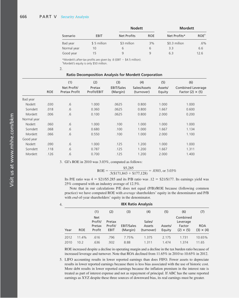
Vis
it u
s at
ww
w.m
hh
e.co
m/b
km666 P A R T V Security Analysis
Nodett Mordett
Scenario EBIT Net Profits ROE Net Profits* ROE†
Bad year $ 5 million $3 million 3% $0.3 million .6%
Normal year 10 6 6 3.3 6.6
Good year 15 9 9 6.3 12.6
*Mordett’s after-tax profits are given by .6 (EBIT 2 $4.5 million).†Mordett’s equity is only $50 million.
2.
Ratio Decomposition Analysis for Mordett Corporation
(1) (2) (3) (4) (5) (6)
ROENet Profit/
Pretax ProfitPretax
Profit/EBITEBIT/Sales (Margin)
Sales/Assets (turnover)
Assets/Equity
Combined Leverage Factor (2) 3 (5)
Bad year
Nodett .030 .6 1.000 .0625 0.800 1.000 1.000
Somdett .018 .6 0.360 .0625 0.800 1.667 0.600
Mordett .006 .6 0.100 .0625 0.800 2.000 0.200
Normal year
Nodett .060 .6 1.000 .100 1.000 1.000 1.000
Somdett .068 .6 0.680 .100 1.000 1.667 1.134
Mordett .066 .6 0.550 .100 1.000 2.000 1.100
Good year
Nodett .090 .6 1.000 .125 1.200 1.000 1.000
Somdett .118 .6 0.787 .125 1.200 1.667 1.311
Mordett .126 .6 0.700 .125 1.200 2.000 1.400
3. GI’s ROE in 2010 was 3.03%, computed as follows:
ROE 5$5,285
.5($171,843 1 $177,128)5 .0303, or 3.03%
Its P/E ratio was 4 5 $21/$5.285 and its P/B ratio was .12 5 $21/$177. Its earnings yield was 25% compared with an industry average of 12.5%.
Note that in our calculations P/E does not equal (P/B)/ROE because (following common practice) we have computed ROE with average shareholders’ equity in the denominator and P/B with end-of-year shareholders’ equity in the denominator.
4. IBX Ratio Analysis
(1) (2) (3) (4) (5) (6) (7)
Year ROE
Net Profit/Pretax Profit
Pretax Profit/EBIT
EBIT/Sales (Margin)
Sales/Assets
(turnover)Assets/Equity
Combined Leverage
Factor (2) 3 (5)
ROA (3) 3 (4)
2012 11.4% .616 .796 7.75% 1.375 2.175 1.731 10.65%
2010 10.2 .636 .932 8.88 1.311 1.474 1.374 11.65
ROE increased despite a decline in operating margin and a decline in the tax burden ratio because of increased leverage and turnover. Note that ROA declined from 11.65% in 2010 to 10.65% in 2012.
5. LIFO accounting results in lower reported earnings than does FIFO. Fewer assets to depreciate results in lower reported earnings because there is less bias associated with the use of historic cost. More debt results in lower reported earnings because the inflation premium in the interest rate is treated as part of interest expense and not as repayment of principal. If ABC has the same reported earnings as XYZ despite these three sources of downward bias, its real earnings must be greater.

DERIVATIVE SECURITIES, OR more simply
derivatives, play a large and increasingly
important role in financial markets. These are
securities whose prices are determined by,
or “derive from,” the prices of other securi-
ties. These assets are also called contingent
claims because their payoffs are contingent
on the prices of other securities. Options and
futures contracts are both derivative securi-
ties. We will see that their payoffs depend on
the value of other securities. Swaps, which we
will discuss in Chapter 23, also are derivatives.
Because the value of derivatives depends
on the value of other securities, they can be
powerful tools for both hedging and specula-
tion. We will investigate these applications in
the next four chapters, starting in this chapter
with options.
Trading of standardized options contracts
on a national exchange started in 1973 when
the Chicago Board Options Exchange (CBOE)
began listing call options. These contracts
were almost immediately a great success,
crowding out the previously existing over-the-
counter trading in stock options. Option con-
tracts are traded now on several exchanges.
They are written on common stock, stock
indexes, foreign exchange, agricultural com-
modities, precious metals, and interest rate
futures. In addition, the over-the-counter
market has enjoyed a tremendous resurgence
in recent years as trading in custom-tailored
options has exploded. Popular and potent
tools in modifying portfolio characteristics,
options have become essential tools a portfo-
lio manager must understand.
This chapter is an introduction to options
markets. It explains how puts and calls work
and examines their investment characteris-
tics. Popular option strategies are considered
next. Finally, we examine a range of securities
with embedded options such as callable or
convertible bonds, and we take a quick look
at some so-called exotic options.
20 Options Markets: Introduction 0
PAR
T VI
CHAPTER TWENTY

668 P A R T V I Options, Futures, and Other Derivatives
20.1 The Option Contract
Example 20.1 Profits and Losses on a Call Option
Consider the January 2010 expiration call option on a share of IBM with an exercise price of $130 that was selling on December 2, 2009, for $2.18. Exchange-traded options expire on the third Friday of the expiration month, which for this option was January 15, 2010. Until the expiration date, the purchaser of the calls may buy shares of IBM for $130. On December 2, IBM sells for $127.21. Because the stock price is currently less than $130 a share, exercising the option to buy at $130 clearly would make no sense at that moment. Indeed, if IBM remains below $130 by the expiration date, the call will be left to expire worthless. On the other hand, if IBM is selling above $130 at expiration, the call holder will find it optimal to exercise. For example, if IBM sells for $132 on January 15, the option will be exercised, as it will give its holder the right to pay $130 for a stock worth $132. The value of the option on the expiration date would then be
Value at expiration 5 Stock price 2 Exercise price 5 $132 2 $130 5 $2
Despite the $2 payoff at expiration, the call holder still realizes a loss of $.18 on the invest-ment because the initial purchase price was $2.18:
Profit 5 Final value 2 Original investment 5 $2.00 2 $2.18 5 2$.18
A call option gives its holder the right to purchase an asset for a specified price, called the exercise, or strike, price, on or before some specified expiration date. For example, a January call option on IBM stock with exercise price $130 entitles its owner to purchase IBM stock for a price of $130 at any time up to and including the expiration date in January. The holder of the call is not required to exercise the option. The holder will choose to exer-cise only if the market value of the underlying asset exceeds the exercise price. In that case, the option holder may “call away” the asset for the exercise price. Otherwise, the option may be left unexercised. If it is not exercised before the expiration date of the contract, a call option simply expires and no longer has value. Therefore, if the stock price is greater than the exercise price on the expiration date, the value of the call option equals the differ-ence between the stock price and the exercise price; but if the stock price is less than the exercise price at expiration, the call will be worthless. The net profit on the call is the value of the option minus the price originally paid to purchase it.
The purchase price of the option is called the premium. It represents the compensation the purchaser of the call must pay for the right to exercise the option if exercise becomes profitable.
Sellers of call options, who are said to write calls, receive premium income now as pay-ment against the possibility they will be required at some later date to deliver the asset in return for an exercise price less than the market value of the asset. If the option is left to expire worthless, however, then the writer of the call clears a profit equal to the premium income derived from the initial sale of the option. But if the call is exercised, the profit to the option writer is the premium income derived when the option was initially sold minus the difference between the value of the stock that must be delivered and the exercise price that is paid for those shares. If that difference is larger than the initial premium, the writer will incur a loss.

C H A P T E R 2 0 Options Markets: Introduction 669
Nevertheless, exercise of the call is optimal at expiration if the stock price exceeds the exercise price because the exercise proceeds will offset at least part of the cost of the option. The investor in the call will clear a profit if IBM is selling above $132.18 at the expiration date. At that stock price, the proceeds from exercise will just cover the origi-nal cost of the call.
Example 20.2 Profits and Losses on a Put Option
Now consider the January 2010 expiration put option on IBM with an exercise price of $130, selling on December 2, 2009, for $4.79. It entitled its owner to sell a share of IBM for $130 at any time until January 15. If the holder of the put buys a share of IBM and imme-diately exercises the right to sell at $130, net proceeds will be $130 2 $127.21 5 $2.79. Obviously, an investor who pays $4.79 for the put has no intention of exercising it imme-diately. If, on the other hand, IBM sells for $123 at expiration, the put turns out to be a profitable investment. Its value at expiration would be
Value at expiration 5 Exercise price 2 Stock price 5 $130 2 $123 5 $7
and the investor’s profit would be $7.00 2 $4.79 5 $2.21. This is a holding period return of $2.21/$4.79 5 .461, or 46.1%—over only 44 days! Apparently, put option sellers on December 2 (who were on the other side of the transaction) did not consider this outcome very likely.
A put option gives its holder the right to sell an asset for a specified exercise or strike price on or before some expiration date. A January expiration put on IBM with exercise price $130 entitles its owner to sell IBM stock to the put writer at a price of $130 at any time before expiration in January even if the market price of IBM is less than $130. While profits on call options increase when the asset increases in value, profits on put options increase when the asset value falls. A put will be exercised only if the exercise price is greater than the price of the underlying asset, that is, only if its holder can deliver for the exercise price an asset with market value less than the exercise price. (One doesn’t need to own the shares of IBM to exercise the IBM put option. Upon exercise, the investor’s broker purchases the necessary shares of IBM at the market price and immediately delivers, or “puts them,” to an option writer for the exercise price. The owner of the put profits by the difference between the exercise price and market price.)
An option is described as in the money when its exercise would produce profits for its holder. An option is out of the money when exercise would be unprofitable. Therefore, a call option is in the money when the asset price is greater than the exercise price. It is out of the money when the asset price is less than the exercise price; no one would exercise the right to purchase for the strike price an asset worth less than that price. Conversely, put options are in the money when the exercise price exceeds the asset’s value, because delivery of the lower-valued asset in exchange for the exercise price is profitable for the holder. Options are at the money when the exercise price and asset price are equal.

670 P A R T V I Options, Futures, and Other Derivatives
Options Trading
Some options trade on over-the-counter markets. The OTC market offers the advantage that the terms of the option contract—the exercise price, expiration date, and number of shares committed—can be tai-lored to the needs of the traders. The costs of estab-lishing an OTC option contract, however, are higher than for exchange-traded options.
Options contracts traded on exchanges are stan-dardized by allowable expiration dates and exercise prices for each listed option. Each stock option con-tract provides for the right to buy or sell 100 shares of stock (except when stock splits occur after the contract is listed and the contract is adjusted for the terms of the split).
Standardization of the terms of listed option con-tracts means all market participants trade in a lim-ited and uniform set of securities. This increases the depth of trading in any particular option, which low-ers trading costs and results in a more competitive market. Exchanges, therefore, offer two important benefits: ease of trading, which flows from a central marketplace where buyers and sellers or their repre-
sentatives congregate; and a liquid secondary market where buyers and sellers of options can transact quickly and cheaply.
Until recently, most options trading in the United States took place on the Chicago Board Options Exchange. However, by 2003 the International Securities Exchange, an electronic exchange based in New York, displaced the CBOE as the largest options market. Options trading in Europe is uniformly transacted in electronic exchanges.
Figure 20.1 is a selection of listed stock option quotations for IBM. The last recorded price on the New York Stock Exchange for IBM shares was $127.21 per share. 1 Options are reported on IBM at exercise prices of $120 through $135.
The exercise (or strike) prices bracket the stock price. While exercise prices generally are set at five-point intervals, larger intervals sometimes are set for stocks selling above $100, and intervals of $2.50 may be used for stocks selling at low prices. If the stock price moves outside the range of exercise prices of the existing set of options, new options with appropriate exercise prices may be offered. Therefore, at any time, both in-the-money and out-of-the-money options will be listed, as in this example.
Figure 20.1 shows both call and put options listed for each expiration date and exercise price. The three sets of columns for each option report closing price, trading volume in contracts, and open interest (number of outstanding contracts). When we compare prices of call options with the same expiration date but different exercise prices in Figure 20.1 , we see that the value of a call is lower when the exercise price is higher. This makes sense, because the right to purchase a share at a lower exercise price is more valuable than the right to purchase at a higher price. Thus the January expiration IBM call option with strike
1 Occasionally, this price may not match the closing price listed for the stock on the stock market page. This is because some NYSE stocks also trade on exchanges that close after the NYSE, and the stock pages may reflect the more recent closing price. The options exchanges, however, close with the NYSE, so the closing NYSE stock price is appropriate for comparison with the closing option price.
PRICES AT CLOSE DECEMBER 02, 2009
Expiration
Dec 2009Jan 2010Apr 2010Jul 2010Dec 2009Jan 2010Apr 2010Jul 2010Dec 2009Jan 2010Apr 2010Jul 2010Dec 2009Jan 2010Apr 2010Jul 2010
120120120120125125125125130130130130135135135135
7.758.63
11.2513.30
3.254.757.90
10.050.772.185.497.750.110.843.455.67
197130
4334
416278
697
21083489
2931
214176126
6
237021884
1705108
1441914180
3652150
1103319278
2773111
895524556
3798140
0.261.184.206.701.022.446.058.853.554.798.50
11.307.657.75
11.5013.80
6441267
331
18721060
8215
8441986685862445
1
880688711903
34920390941122215
423332731312228631776433113
Call Put
I B M (IBM) Underlying Stock Price: 127.21
Strike Last VolumeOpen
Interest Last VolumeOpen
Interest
Figure 20.1 Stock options on IBM Closing prices as of December 2, 2009
Source: The Wall Street Journal Online, December 3, 2009.

C H A P T E R 2 0 Options Markets: Introduction 671
price $130 sells for $2.18 whereas the $135 exercise price January call sells for only $.84. Conversely, put options are worth more when the exercise price is higher: You would rather have the right to sell shares for $135 than for $130, and this is reflected in the prices of the puts. The January expiration put option with strike price $135 sells for $7.75, whereas the $130 exercise price January put sells for only $4.79.
If an option does not trade on a given day, three dots will appear in the volume and price columns. Because trading is infrequent, it is not unusual to find option prices that appear out of line with other prices. You might see, for example, two calls with different exercise prices that seem to sell for the same price. This discrepancy arises because the last trades for these options may have occurred at different times during the day. At any moment, the call with the lower exercise price must be worth more than an otherwise-identical call with a higher exercise price.
Expirations of most exchange-traded options tend to be fairly short, ranging up to only several months. For larger firms and several stock indexes, however, longer-term options are traded with expirations ranging up to several years. These options are called LEAPS (for L ong- T erm E quity A ntici P ation S ecurities).
CONCEPT CHECK
1
a. What will be the proceeds and net profits to an investor who purchases the January expiration IBM calls with exercise price $125 if the stock price at expiration is $135? What if the stock price at expiration is $115?
b. Now answer part ( a ) for an investor who purchases a January expiration IBM put option with exercise price $125.
American and European Options
An American option allows its holder to exercise the right to purchase (if a call) or sell (if a put) the underlying asset on or before the expiration date. European options allow for exercise of the option only on the expiration date. American options, because they allow more leeway than their European counterparts, generally will be more valuable. Virtually all traded options in the United States are American style. Foreign currency options and stock index options are notable exceptions to this rule, however.
Adjustments in Option Contract Terms
Because options convey the right to buy or sell shares at a stated price, stock splits would radically alter their value if the terms of the options contract were not adjusted to account for the stock split. For example, reconsider the IBM call options in Figure 20.1 . If IBM were to announce a 2-for-1 split, its share price would fall from about $127 to about $63.50. A call option with exercise price $130 would be just about worthless, with virtually no possibility that the stock would sell at more than $130 before the options expired.
To account for a stock split, the exercise price is reduced by a factor of the split, and the number of options held is increased by that factor. For example, each original call option with exercise price of $130 would be altered after a 2-for-1 split to 2 new options, with each new option carrying an exercise price of $65. A similar adjustment is made for stock dividends of more than 10%; the number of shares covered by each option is increased in proportion to the stock dividend, and the exercise price is reduced by that proportion.

672 P A R T V I Options, Futures, and Other Derivatives
In contrast to stock dividends, cash dividends do not affect the terms of an option con-tract. Because payment of a cash dividend reduces the selling price of the stock without inducing offsetting adjustments in the option contract, the value of the option is affected by dividend policy. Other things being equal, call option values are lower for high-dividend payout policies, because such policies slow the rate of increase of stock prices; conversely, put values are higher for high-dividend payouts. (Of course, the option values do not nec-essarily rise or fall on the dividend payment or ex-dividend dates. Dividend payments are anticipated, so the effect of the payment already is built into the original option price.)
CONCEPT CHECK
2
Suppose that IBM’s stock price at the exercise date is $140, and the exercise price of the call is $130. What is the payoff on one option contract? After a 2-for-1 split, the stock price is $70, the exercise price is $65, and the option holder now can purchase 200 shares. Show that the split leaves the payoff from the option unaffected.
The Options Clearing Corporation
The Options Clearing Corporation (OCC), the clearinghouse for options trading, is jointly owned by the exchanges on which stock options are traded. Buyers and sellers of options who agree on a price will strike a deal. At this point, the OCC steps in. The OCC places itself between the two traders, becoming the effective buyer of the option from the writer and the effective writer of the option to the buyer. All individuals, therefore, deal only with the OCC, which effectively guarantees contract performance.
When an option holder exercises an option, the OCC arranges for a member firm with clients who have written that option to make good on the option obligation. The mem-ber firm selects from its clients who have written that option to fulfill the contract. The selected client must deliver 100 shares of stock at a price equal to the exercise price for each call option contract written or must purchase 100 shares at the exercise price for each put option contract written.
Because the OCC guarantees contract performance, option writers are required to post margin to guarantee that they can fulfill their contract obligations. The margin required is determined in part by the amount by which the option is in the money, because that value is an indicator of the potential obligation of the option writer. When the required margin exceeds the posted margin, the writer will receive a margin call. In contrast, the holder of the option need not post margin because the holder will exercise the option only if it is profitable to do so. After purchase of the option, no further money is at risk.
Margin requirements are determined in part by the other securities held in the investor’s portfolio. For example, a call option writer owning the stock against which the option is written can satisfy the margin requirement simply by allowing a broker to hold that stock in the brokerage account. The stock is then guaranteed to be available for delivery should the call option be exercised. If the underlying security is not owned, however, the margin requirement is determined by the value of the underlying security as well as by the amount by which the option is in or out of the money. Out-of-the-money options require less mar-gin from the writer, for expected payouts are lower.
Other Listed Options
Options on assets other than stocks are also widely traded. These include options on mar-ket indexes and industry indexes, on foreign currency, and even on the futures prices of agricultural products, gold, silver, fixed-income securities, and stock indexes. We will dis-cuss these in turn.

C H A P T E R 2 0 Options Markets: Introduction 673
Index Options An index option is a call or put based on a stock market index such as the S&P 500 or the NASDAQ 100. Index options are traded on several broad-based indexes as well as on several industry-specific indexes and even commodity price indexes. We discussed many of these indexes in Chapter 2.
The construction of the indexes can vary across contracts or exchanges. For example, the S&P 100 index is a value-weighted average of the 100 stocks in the Standard & Poor’s 100 stock group. The weights are proportional to the market value of outstanding equity for each stock. The Dow Jones Industrial Index, by contrast, is a price-weighted average of 30 stocks.
Option contracts on many foreign stock indexes also trade. For example, options on the (Japanese) Nikkei Stock Index trade on the Chicago Mercantile Exchange, and options on the Eurotop 100 and Japan indexes trade on the American Stock Exchange. The Chicago Board Options Exchange, as well as the Amex, lists options on industry indexes such as the biotech or financial industries.
In contrast to stock options, index options do not require that the call writer actually “deliver the index” upon exercise or that the put writer “purchase the index.” Instead, a cash settlement procedure is used. The payoff that would accrue upon exercise of the option is calculated, and the option writer simply pays that amount to the option holder. The payoff is equal to the difference between the exercise price of the option and the value of the index. For example, if the S&P index is at 1100 when a call option on the index with exercise price 1090 is exercised, the holder of the call receives a cash payment of the dif-ference, 1100 2 1090, times the contract multiplier of $100, or $1,000 per contract.
Options on the major indexes, that is, the S&P 100 (often called the OEX after its ticker symbol), the S&P 500 (the SPX), the NASDAQ 100 (the NDX), and the Dow Jones Industrials (the DJX), are the most actively traded contracts on the CBOE. Together, these contracts dominate CBOE volume.
Futures Options Futures options give their holders the right to buy or sell a speci-fied futures contract, using as a futures price the exercise price of the option. Although the delivery process is slightly complicated, the terms of futures options contracts are designed in effect to allow the option to be written on the futures price itself. The option holder receives upon exercise a net payoff equal to the difference between the current futures price on the specified asset and the exercise price of the option. Thus if the futures price is, say, $37, and the call has an exercise price of $35, the holder who exercises the call option on the futures gets a payoff of $2.
Foreign Currency Options A currency option offers the right to buy or sell a quan-tity of foreign currency for a specified amount of domestic currency. Currency option con-tracts call for purchase or sale of the currency in exchange for a specified number of U.S. dollars. Contracts are quoted in cents or fractions of a cent per unit of foreign currency.
There is an important difference between currency options and currency futures options. The former provide payoffs that depend on the difference between the exercise price and the exchange rate at maturity. The latter are foreign exchange futures options that provide payoffs that depend on the difference between the exercise price and the exchange rate futures price at maturity. Because exchange rates and exchange rate futures prices gener-ally are not equal, the options and futures-options contracts will have different values, even with identical expiration dates and exercise prices. Trading volume in currency futures options dominates by far trading in currency options.
Interest Rate Options Options are traded on Treasury notes and bonds, Treasury bills, certificates of deposit, GNMA pass-through certificates, and yields on Treasury and Eurodollar securities of various maturities. Options on several interest rate futures
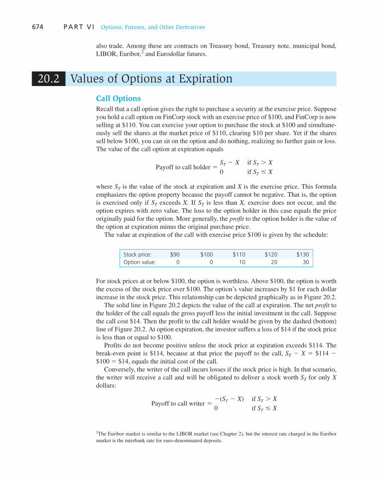
674 P A R T V I Options, Futures, and Other Derivatives
also trade. Among these are contracts on Treasury bond, Treasury note, municipal bond, LIBOR, Euribor, 2 and Eurodollar futures.
20.2 Values of Options at Expiration
Call Options
Recall that a call option gives the right to purchase a security at the exercise price. Suppose you hold a call option on FinCorp stock with an exercise price of $100, and FinCorp is now selling at $110. You can exercise your option to purchase the stock at $100 and simultane-ously sell the shares at the market price of $110, clearing $10 per share. Yet if the shares sell below $100, you can sit on the option and do nothing, realizing no further gain or loss. The value of the call option at expiration equals2
Payoff to call holder 5ST 2 X if ST . X
0 if ST # X
where S T is the value of the stock at expiration and X is the exercise price. This formula emphasizes the option property because the payoff cannot be negative. That is, the option is exercised only if S T exceeds X. If S T is less than X, exercise does not occur, and the option expires with zero value. The loss to the option holder in this case equals the price originally paid for the option. More generally, the profit to the option holder is the value of the option at expiration minus the original purchase price.
The value at expiration of the call with exercise price $100 is given by the schedule:
Stock price: $90 $100 $110 $120 $130
Option value: 0 0 10 20 30
For stock prices at or below $100, the option is worthless. Above $100, the option is worth the excess of the stock price over $100. The option’s value increases by $1 for each dollar increase in the stock price. This relationship can be depicted graphically as in Figure 20.2 .
The solid line in Figure 20.2 depicts the value of the call at expiration. The net profit to the holder of the call equals the gross payoff less the initial investment in the call. Suppose the call cost $14. Then the profit to the call holder would be given by the dashed (bottom) line of Figure 20.2 . At option expiration, the investor suffers a loss of $14 if the stock price is less than or equal to $100.
Profits do not become positive unless the stock price at expiration exceeds $114. The break-even point is $114, because at that price the payoff to the call, S T 2 X 5 $114 2 $100 5 $14, equals the initial cost of the call.
Conversely, the writer of the call incurs losses if the stock price is high. In that scenario, the writer will receive a call and will be obligated to deliver a stock worth S T for only X dollars:
Payoff to call writer 52(ST 2 X) if ST . X
0 if ST # X
2 The Euribor market is similar to the LIBOR market (see Chapter 2), but the interest rate charged in the Euribor market is the interbank rate for euro-denominated deposits.

C H A P T E R 2 0 Options Markets: Introduction 675
The call writer, who is exposed to losses if the stock price increases, is willing to bear this risk in return for the option premium.
Figure 20.3 depicts the payoff and profit diagrams for the call writer. These are the mirror images of the corresponding dia-grams for call holders. The break-even point for the option writer also is $114. The (negative) payoff at that point just offsets the premium originally received when the option was written.
Put Options
A put option is the right to sell an asset at the exercise price. In this case, the holder will not exercise the option unless the asset is worth less than the exercise price. For example, if FinCorp shares were to fall to $90, a put option with exercise price $100 could be exercised to clear $10 for its holder. The holder would purchase a share for $90 and simultaneously deliver it to the put option writer for the exercise price of $100.
The value of a put option at expiration is
Payoff to put holder 50 if ST $ X
X 2 ST if ST , X
The solid line in Figure 20.4 illustrates the payoff at expiration to the holder of a put option on FinCorp stock with an exercise price of $100. If the stock price at expiration is above $100, the put has no value, as the right to sell the shares at $100 would not be exercised. Below a price of $100, the put value at expiration increases by $1 for each dollar the stock price falls. The dashed line in Figure 20.4 is a graph of the put option owner’s profit at expiration, net of the initial cost of the put.
Writing puts naked (i.e., writing a put without an offsetting short position in the stock for hedging purposes) exposes the writer to losses if the market falls. Writing naked out-of-the-money puts was once con-sidered an attractive way to generate income, as it was believed that as long as the market did not fall sharply before the option expira-tion, the option premium could be collected without the put holder ever exercising the option against the writer. Because only sharp drops in the market could result in losses to the put writer, the strategy was not viewed as overly risky. However, in the wake of the market crash of October 1987, such put writ-ers suffered huge losses. Participants now perceive much greater risk to this strategy.
$30
ST
80 90 100 110 120Cost of Option Profit
Payoff = Value at Expiration
−$14
−$10
0
$10
$20
Figure 20.2 Payoff and profit to call option at expiration
$14
0$100 $114
Profit
Payoff
ST
Figure 20.3 Payoff and profit to call writers at expiration
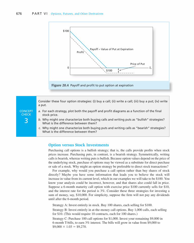
676 P A R T V I Options, Futures, and Other Derivatives
Option versus Stock Investments
Purchasing call options is a bullish strategy; that is, the calls provide profits when stock prices increase. Purchasing puts, in contrast, is a bearish strategy. Symmetrically, writing calls is bearish, whereas writing puts is bullish. Because option values depend on the price of the underlying stock, purchase of options may be viewed as a substitute for direct purchase or sale of a stock. Why might an option strategy be preferable to direct stock transactions?
For example, why would you purchase a call option rather than buy shares of stock directly? Maybe you have some information that leads you to believe the stock will increase in value from its current level, which in our examples we will take to be $100. You know your analysis could be incorrect, however, and that shares also could fall in price. Suppose a 6-month maturity call option with exercise price $100 currently sells for $10, and the interest rate for the period is 3%. Consider these three strategies for investing a sum of money, say, $10,000. For simplicity, suppose the firm will not pay any dividends until after the 6-month period.
Strategy A: Invest entirely in stock. Buy 100 shares, each selling for $100.
Strategy B: Invest entirely in at-the-money call options. Buy 1,000 calls, each selling for $10. (This would require 10 contracts, each for 100 shares.)
Strategy C: Purchase 100 call options for $1,000. Invest your remaining $9,000 in 6-month T-bills, to earn 3% interest. The bills will grow in value from $9,000 to $9,000 3 1.03 5 $9,270.
Figure 20.4 Payoff and profit to put option at expiration
Payoff = Value of Put at ExpirationProfit
$100
$1000
Price of PutST
CONCEPT CHECK
3
Consider these four option strategies: (i) buy a call; (ii) write a call; (iii) buy a put; (iv) write a put.
a. For each strategy, plot both the payoff and profit diagrams as a function of the final stock price.
b. Why might one characterize both buying calls and writing puts as “bullish” strategies? What is the difference between them?
c. Why might one characterize both buying puts and writing calls as “bearish” strategies? What is the difference between them?

C H A P T E R 2 0 Options Markets: Introduction 677
Let us trace the possible values of these three portfolios when the options expire in 6 months as a function of the stock price at that time:
Stock Price
Portfolio $95 $100 $105 $110 $115 $120
Portfolio A: All stock $9,500 $10,000 $10,500 $11,000 $11,500 $12,000
Portfolio B: All options 0 0 5,000 10,000 15,000 20,000
Portfolio C: Call plus bills 9,270 9,270 9,770 10,270 10,770 11,270
Portfolio A will be worth 100 times the share price. Portfolio B is worthless unless shares sell for more than the exercise price of the call. Once that point is reached, the portfolio is worth 1,000 times the excess of the stock price over the exercise price. Finally, portfolio Cis worth $9,270 from the investment in T-bills plus any profits from the 100 call options. Remember that each of these portfolios involves the same $10,000 initial investment. The rates of return on these three portfolios are as follows:
Stock Price
Portfolio $95 $100 $105 $110 $115 $120
Portfolio A: All stock 25.0% 0.0% 5.0% 10.0% 15.0% 20.0%
Portfolio B: All options 2100.0 2100.0 250.0 0.0 50.0 100.0
Portfolio C: Call plus bills 27.3 27.3 22.3 2.7 7.7 12.7
These rates of return are graphed in Figure 20.5 . Comparing the returns of portfolios B and C to those of the simple investment in stock
represented by portfolio A, we see that options offer two interesting features. First, an option offers leverage. Compare the returns of portfolios B and A. Unless the stock increases from its initial value of $100, the value of portfolio B falls precipitously to zero—a rate of return of negative 100%. Conversely, modest increases in the rate of return on the stock result in dispro-portionate increases in the option rate of return. For example, a 4.3% increase in the stock price from $115 to $120 would increase the rate of return on the call from 50% to 100%. In this sense, calls are a levered investment on the stock. Their values respond more than propor-tionately to changes in the stock value.
Figure 20.5 vividly illustrates this point. The slope of the all-option port-folio is far steeper than that of the all-stock portfolio, reflecting its greater proportional sensitivity to the value of the underlying security. The leverage factor is the reason investors (illegally) exploiting inside information com-monly choose options as their invest-ment vehicle.
Rat
e o
f R
etu
rn (
%)
100
ST
−120
−100
−80
−60
−40
−20
0
20
40
60
80
86 88 90 92 94 96 98 100
102
104
106
108
110
112
114
116
118
120
A: All Stocks
C: Call Plus Bills
B: All Options
84
Figure 20.5 Rate of return to three strategies

678 P A R T V I Options, Futures, and Other Derivatives
The potential insurance value of options is the second interesting feature, as portfolio C shows. The T-bill-plus-option portfolio cannot be worth less than $9,270 after 6 months, as the option can always be left to expire worthless. The worst possible rate of return on portfolio C is 2 7.3%, compared to a (theoretically) worst possible rate of return on the stock of 2 100% if the company were to go bankrupt. Of course, this insurance comes at a price: When the share price increases, portfolio C, the option-plus-bills portfolio, does not perform as well as portfolio A, the all-stock portfolio.
This simple example makes an important point. Although options can be used by specu-lators as effectively leveraged stock positions, as in portfolio B, they also can be used by investors who desire to tailor their risk exposures in creative ways, as in portfolio C. For example, the call-plus-bills strategy of portfolio C provides a rate of return profile quite unlike that of the stock alone. The absolute limitation on downside risk is a novel and attractive feature of this strategy. We next discuss several option strategies that provide other novel risk profiles that might be attractive to hedgers and other investors.
20.3 Option Strategies
An unlimited variety of payoff patterns can be achieved by combining puts and calls with various exercise prices. We explain in this section the motivation and structure of some of the more popular ones.
Protective Put
Imagine you would like to invest in a stock, but you are unwilling to bear potential losses beyond some given level. Investing in the stock alone seems risky to you because in prin-ciple you could lose all the money you invest. You might consider instead investing in stock and purchasing a put option on the stock. Table 20.1 shows the total value of your portfolio at option expiration: Whatever happens to the stock price, you are guaranteed a payoff at least equal to the put option’s exercise price because the put gives you the right to sell your shares for that price.
Example 20.3 Protective Put
Suppose the strike price is X 5 $100 and the stock is selling at $97 at option expiration. Then the value of your total portfolio is $100. The stock is worth $97 and the value of the expiring put option is
X 2 ST 5 $100 2 $97 5 $3
Another way to look at it is that you are holding the stock and a put contract giving you the right to sell the stock for $100. The right to sell locks in a minimum portfolio value of $100. On the other hand, if the stock price is above $100, say, $104, then the right to sell a share at $100 is worthless. You allow the put to expire unexercised, ending up with a share of stock worth S T 5 $104.
Figure 20.6 illustrates the payoff and profit to this protective put strategy. The solid line in Figure 20.6 C is the total payoff. The dashed line is displaced downward by the cost of establishing the position, S 0 1 P. Notice that potential losses are limited.

C H A P T E R 2 0 Options Markets: Introduction 679
Table 20.1
Value of a protective put portfolio at option expiration
S T # X S T . X
Stock S T S T
1 Put X 2 S T 0
5 TOTAL X S T
Figure 20.6 Value of a protective put position at option expiration
ST
ST
ST
Payoff of Stock
Payoff of Option
Payoff ofProtective Put
Payoff
Profit
X
X
X
X
X − (S0 + P)
A: Stock
+ B: Put
= C: Protective Put
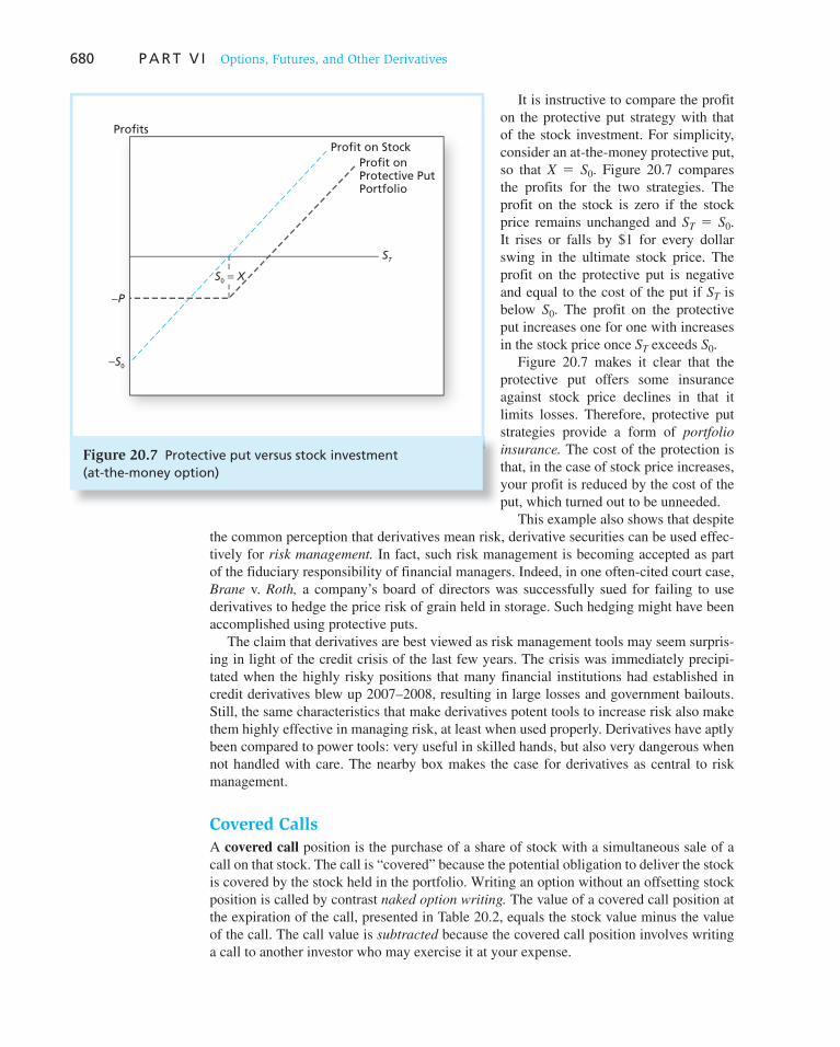
680 P A R T V I Options, Futures, and Other Derivatives
It is instructive to compare the profit on the protective put strategy with that of the stock investment. For simplicity, consider an at-the-money protective put, so that X 5 S 0 . Figure 20.7 compares the profits for the two strategies. The profit on the stock is zero if the stock price remains unchanged and S T 5 S0 . It rises or falls by $1 for every dollar swing in the ultimate stock price. The profit on the protective put is negative and equal to the cost of the put if S T is below S 0 . The profit on the protective put increases one for one with increases in the stock price once S T exceeds S 0 .
Figure 20.7 makes it clear that the protective put offers some insurance against stock price declines in that it limits losses. Therefore, protective put strategies provide a form of portfolio
insurance. The cost of the protection is that, in the case of stock price increases, your profit is reduced by the cost of the put, which turned out to be unneeded.
This example also shows that despite the common perception that derivatives mean risk, derivative securities can be used effec-tively for risk management. In fact, such risk management is becoming accepted as part of the fiduciary responsibility of financial managers. Indeed, in one often-cited court case, Brane v. Roth, a company’s board of directors was successfully sued for failing to use derivatives to hedge the price risk of grain held in storage. Such hedging might have been accomplished using protective puts.
The claim that derivatives are best viewed as risk management tools may seem surpris-ing in light of the credit crisis of the last few years. The crisis was immediately precipi-tated when the highly risky positions that many financial institutions had established in credit derivatives blew up 2007–2008, resulting in large losses and government bailouts. Still, the same characteristics that make derivatives potent tools to increase risk also make them highly effective in managing risk, at least when used properly. Derivatives have aptly been compared to power tools: very useful in skilled hands, but also very dangerous when not handled with care. The nearby box makes the case for derivatives as central to risk management.
Covered Calls
A covered call position is the purchase of a share of stock with a simultaneous sale of a call on that stock. The call is “covered” because the potential obligation to deliver the stock is covered by the stock held in the portfolio. Writing an option without an offsetting stock position is called by contrast naked option writing. The value of a covered call position at the expiration of the call, presented in Table 20.2 , equals the stock value minus the value of the call. The call value is subtracted because the covered call position involves writing a call to another investor who may exercise it at your expense.
Profits
Profit on Stock
ST
Profit onProtective PutPortfolio
−P
−S0
S0 = X
Figure 20.7 Protective put versus stock investment (at-the-money option)

681
The Case for Derivatives
They’ve been dubbed financial weapons of mass destruc-tion, attacked for causing the financial turmoil sweeping the nation and identified as the kryptonite that brought down the global economy. Yet few Main Streeters really know what derivatives are—namely, financial contracts between a buyer and a seller that derive value from an underlying asset, such as a mortgage or a stock. There seems to be near consensus that derivatives were a source of undue risk.
And then there’s Robert Shiller. The Yale economist believes just the opposite is true. A champion of financial innovation and an expert in management of risk, Shiller contends that derivatives, far from being a problem, are actually the solution. Derivatives, Shiller says, are merely a risk-management tool the same way insurance is. “You pay a premium and if an event happens, you get a pay-ment.” That tool can be used well or, as happened recently, used badly. Shiller warns that banishing the tool gets us nowhere.
For all the trillions in derivative trading, there were very few traders. Almost all the subprime mortgages that were bundled and turned into derivatives were sold by a hand-ful of Wall Street institutions, working with a small num-ber of large institutional buyers. It was a huge but illiquid and opaque market.
Meanwhile, the system was built on the myriad deci-sions of individual homeowners and lenders around the world. None of them, however, could hedge their bets the way large institutions can. Those buying a condo in Miami had no way to protect themselves if the market went down.
Derivatives, according to Shiller, could be used by homeowners—and, by extension, lenders—to insure themselves against falling prices. In Shiller’s scenario, you would be able to go to your broker and buy a new type of financial instrument, perhaps a derivative that is inversely related to a regional home-price index. If the value of
houses in your area declined, the financial instrument would increase in value, offsetting the loss. Lenders could do the same thing, which would help them hedge against foreclosures. The idea is to make the housing market more liquid. More buyers and sellers mean that markets stay liquid and functional even under pressure.
Some critics dismiss Shiller’s basic premise that more derivatives would make the housing market more liquid and more stable. They point out that futures contracts haven’t made equity markets or commodity markets immune from massive moves up and down. They add that a ballooning world of home-based derivatives wouldn’t lead to homeowners’ insurance: it would lead to a new playground for speculators.
In essence, Shiller is laying the intellectual ground-work for the next financial revolution. We are now suffer-ing through the first major crisis of the Information Age economy. Shiller’s answers may be counterintuitive, but no more so than those of doctors and scientists who centu-ries ago recognized that the cure for infectious diseases was not flight or quarantine, but purposely infecting more people through vaccinations. “We’ve had a major glitch in derivatives and securitization,” says Shiller. “The Titanic sank almost a century ago, but we didn’t stop sailing across the Atlantic.”
Of course, people did think twice about getting on a ship, at least for a while. But if we listen only to our fears, we lose the very dynamism that has propelled us this far. That is the nub of Shiller’s call for more derivatives and more innovation. Shiller’s appeal is a tough sell at a time when derivatives have produced so much havoc. But he reminds us that the tools that got us here are not to blame; they can be used badly and they can be used well. And trying to stem the ineffable tide of human creativity is a fool’s errand.
Source: Zachary Karabell, “The Case for Derivatives,” Newsweek, February 2, 2009.
WO
RD
S FRO
M TH
E STREET
The solid line in Figure 20.8 C illustrates the payoff pattern. You see that the total posi-tion is worth S T when the stock price at time T is below X and rises to a maximum of X when S T exceeds X. In essence, the sale of the call options means the call writer has sold the claim to any stock value above X in return for the initial premium (the call price). Therefore, at expiration, the position is worth at most X. The dashed line of Figure 20.8 C is the net profit to the covered call.
Writing covered call options has been a popular investment strategy among institutional investors. Consider the managers of a fund invested largely in stocks. They might find it appealing to write calls on some or all of the stock in order to boost income by the premi-ums collected. Although they thereby forfeit potential capital gains should the stock price rise above the exercise price, if they view X as the price at which they plan to sell the stock anyway, then the call may be viewed as a kind of “sell discipline.” The written call guaran-tees the stock sale will occur as planned.
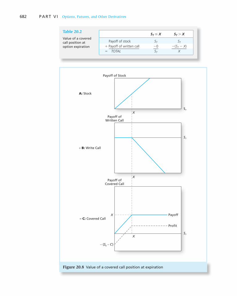
682 P A R T V I Options, Futures, and Other Derivatives
Table 20.2
Value of a covered call position at option expiration
S T # X S T . X
Payoff of stock S T S T
1 Payoff of written call 20 2( S T 2 X )
5 TOTAL S T X
Figure 20.8 Value of a covered call position at expiration
ST
Payoff of Stock
Payoff ofWritten Call
Payoff ofCovered Call
Payoff
Profit
X
A: Stock
+ B: Write Call
= C: Covered Call
ST
ST
X
X
X
– (S0 – C)

683
eXcel APPLICATIONS: Spreads and Straddles
U sing spreadsheets to analyze combinations of options is very helpful. Once the basic models are built, it is
easy to extend the analysis to different bundles of options. The Excel model “Spreads and Straddles” shown below can
be used to evaluate the profitability of different strate-gies. You can find a link to this spreadsheet at www.mhhe.
com/bkm .
12345678910111213141516171819202122232425
Stock Prices
Buying Options:Call Options Strike
Put Options Strike
Straddle
Spreads and Straddles
Payoff
Payoff
Payoff
Profit
Profit
Profit
Return %
Return %
Return %
Ending EndingX 120 StraddleX 110 Straddle
A B C D E F G H I J K L
Beginning Market PriceEnding Market Price
116.5130
120110
130120110
140
170160150
180
210200190
1009080706050
130120110
140
170160150
180
210200190
1009080706050
130120110
140
130140
130120110
140
22.80
0.000.000.00
10.00
20.0010.000.00
10.00
16.8013.6010.30
12.6017.2023.6030.50
35.4034.0037.2040.80
−12.60−17.20−23.60−20.50
−15.40−24.00
−15.4024.60
24.6034.6044.6054.6064.60
14.60
14.60
4.60
4.60
−5.40−15.40−25.40−35.40−25.40−15.40
−5.40
−24.0036.00
16.0026.0036.0046.0056.00
26.00
6.00
16.00
−4.00
6.00−4.00
−14.00−24.00−34.00−24.00−14.00
−37.20−30.80
−100.00%−100.00%−100.00%
−67.21%
−43.50%−70.59%
−100.00%−75.49%
Price
Price
Price
Stock PriceProfit
Stock PriceProfit
20.0010.000.000.00
−2.80−6.80
−13.60−10.30
−12.28%−40.48%
−100.00%−100.00%
Example 20.4 Covered Call
Assume a pension fund holds 1,000 shares of stock, with a current price of $100 per share. Suppose the portfolio manager intends to sell all 1,000 shares if the share price hits $110, and a call expiring in 60 days with an exercise price of $110 currently sells for $5. By writ-ing 10 call contracts (for 100 shares each) the fund can pick up $5,000 in extra income. The fund would lose its share of profits from any movement of the stock price above $110 per share, but given that it would have sold its shares at $110, it would not have realized those profits anyway.
Straddle
A long straddle is established by buying both a call and a put on a stock, each with the same exercise price, X, and the same expiration date, T. Straddles are useful strategies for investors who believe a stock will move a lot in price but are uncertain about the direction of the move. For example, suppose you believe an important court case that will make or break a company is about to be settled, and the market is not yet aware of the situation. The stock will either double in value if the case is settled favorably or will drop by half if the settlement goes against the company. The straddle position will do well regardless of the outcome because its value is highest when the stock price makes extreme upward or downward moves from X.
The worst-case scenario for a straddle is no movement in the stock price. If S T equals X, both the call and the put expire worthless, and the investor’s outlay for the purchase of both options is lost. Straddle positions, therefore, are bets on volatility. An investor

684 P A R T V I Options, Futures, and Other Derivatives
who establishes a straddle must view the stock as more volatile than the market does. Conversely, investors who write straddles—selling both a call and a put—must believe the stock is less volatile. They accept the option premiums now, hoping the stock price will not change much before option expiration.
The payoff to a straddle is presented in Table 20.3 . The solid line of Figure 20.9 C illus-trates this payoff. Notice the portfolio payoff is always positive, except at the one point where the portfolio has zero value, S T 5 X. You might wonder why all investors don’t pursue such a seemingly “no-lose” strategy. The reason is that the straddle requires that both the put and call be purchased. The value of the portfolio at expiration, while never negative, still must exceed the initial cash outlay for a straddle investor to clear a profit.
The dashed line of Figure 20.9 C is the profit to the straddle. The profit line lies below the payoff line by the cost of purchasing the straddle, P 1 C. It is clear from the diagram that the straddle position generates a loss unless the stock price deviates substantially from X. The stock price must depart from X by the total amount expended to purchase the call and the put for the straddle to clear a profit.
Strips and straps are variations of straddles. A strip is two puts and one call on a security with the same exercise price and maturity date. A strap is two calls and one put.
Spreads
A spread is a combination of two or more call options (or two or more puts) on the same stock with differing exercise prices or times to maturity. Some options are bought, whereas others are sold, or written. A money spread involves the purchase of one option and the simultaneous sale of another with a different exercise price. A time spread refers to the sale and purchase of options with differing expiration dates.
Consider a money spread in which one call option is bought at an exercise price X 1 , whereas another call with identical expiration date, but higher exercise price, X 2 , is written. The payoff to this position will be the difference in the value of the call held and the value of the call written, as in Table 20.4 .
There are now three instead of two outcomes to distinguish: the lowest-price region where S T is below both exercise prices, a middle region where S T is between the two exer-cise prices, and a high-price region where S T exceeds both exercise prices. Figure 20.10 illustrates the payoff and profit to this strategy, which is called a bullish spread because the payoff either increases or is unaffected by stock price increases. Holders of bullish spreads benefit from stock price increases.
One motivation for a bullish spread might be that the investor thinks one option is over-priced relative to another. For example, an investor who believes an X 5 $100 call is cheap compared to an X 5 $110 call might establish the spread, even without a strong desire to take a bullish position in the stock.
Collars
A collar is an options strategy that brackets the value of a portfolio between two bounds. Suppose that an investor currently is holding a large position in FinCorp stock, which is currently selling at $100 per share. A lower bound of $90 can be placed on the value of the portfolio by buying a protective put with exercise price $90. This protection, however, requires that the investor pay the put premium. To raise the money to pay for the put, the investor might write a call option, say, with exercise price $110. The call might sell for
CONCEPT CHECK
4 Graph the profit and payoff diagrams for strips and straps.
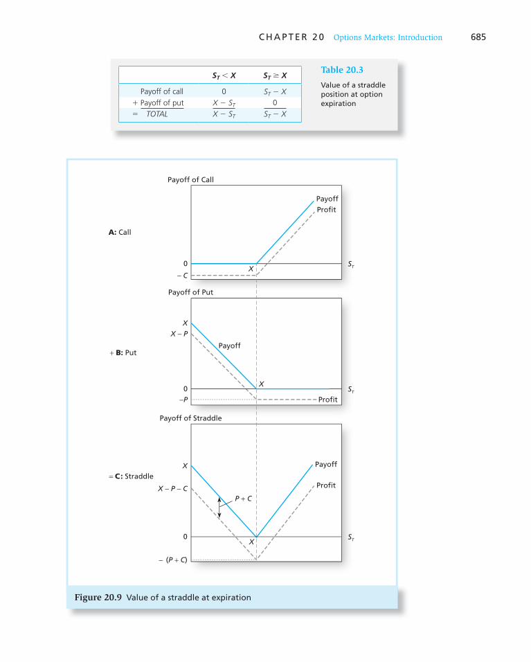
C H A P T E R 2 0 Options Markets: Introduction 685
Table 20.3
Value of a straddle position at option expiration
S T , X S T $ X
Payoff of call 0 S T 2 X
1 Payoff of put X 2 S T 0
5 TOTAL X 2 S T S T 2 X
Figure 20.9 Value of a straddle at expiration
ST
Payoff of Call
Payoff of Put
Payoff of Straddle
Payoff
Profit
X
X
A: Call
+ B: Put
= C: Straddle
ST
ST
Profit
Profit
Payoff
P + C
Payoff
X
X
X − P
− C
−P
0
0
X
X − P − C
− (P + C)
0
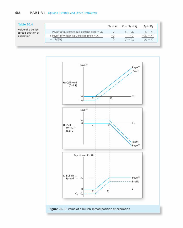
686 P A R T V I Options, Futures, and Other Derivatives
Table 20.4
Value of a bullish spread position at expiration
S T # X 1 X 1 , S T # X 2 ST $ X 2
Payoff of purchased call, exercise price 5 X 1 0 S T 2 X 1 S T 2 X 11 Payoff of written call, exercise price 5 X 2 20 20 2( S T 2 X 2 )
5 TOTAL 0 S T 2 X 1 X 2 2 X 1
Figure 20.10 Value of a bullish spread position at expiration
ST
Payoff
Payoff and Profit
Payoff
X1
X2 − X1
C2 − C1
Profit
ST
ST
Payoff
Profit
Payoff
Profit
Payoff
X2
A: Call Held(Call 1)
B: Call Written (Call 2)
− C1
X1 X2
X1
C2
0
0
C: BullishSpread
0
X2

C H A P T E R 2 0 Options Markets: Introduction 687
roughly the same price as the put, meaning that the net outlay for the two options positions is approximately zero. Writing the call limits the portfolio’s upside potential. Even if the stock price moves above $110, the investor will do no better than $110, because at a higher price the stock will be called away. Thus the investor obtains the downside protection rep-resented by the exercise price of the put by selling her claim to any upside potential beyond the exercise price of the call.
Example 20.5 Collars
A collar would be appropriate for an investor who has a target wealth goal in mind but is unwilling to risk losses beyond a certain level. If you are contemplating buying a house for $220,000, for example, you might set this figure as your goal. Your current wealth may be $200,000, and you are unwilling to risk losing more than $20,000. A collar established by (1) purchasing 2,000 shares of stock currently selling at $100 per share, (2) purchas-ing 2,000 put options (20 options contracts) with exercise price $90, and (3) writing 2,000 calls with exercise price $110 would give you a good chance to realize the $20,000 capital gain without risking a loss of more than $20,000.
CONCEPT CHECK
5 Graph the payoff diagram for the collar described in Example 20.5 .
20.4 The Put-Call Parity Relationship
We saw in the previous section that a protective put portfolio, comprising a stock position and a put option on that position, provides a payoff with a guaranteed minimum value, but with unlimited upside potential. This is not the only way to achieve such protection, however. A call-plus-bills portfolio also can provide limited downside risk with unlimited upside potential.
Consider the strategy of buying a call option and, in addition, buying Treasury bills with face value equal to the exercise price of the call, and with maturity date equal to the expira-tion date of the option. For example, if the exercise price of the call option is $100, then each option contract (which is written on 100 shares) would require payment of $10,000 upon exercise. Therefore, you would purchase a T-bill with a maturity value of $10,000. More generally, for each option that you hold with exercise price X, you would purchase a risk-free zero-coupon bond with face value X.
Examine the value of this position at time T, when the options expire and the zero-coupon bond matures:
S T # X S T . X
Value of call option 0 ST 2 X
Value of riskless bond X X
TOTAL X ST
If the stock price is below the exercise price, the call is worthless, but the riskless bond matures to its face value, X. The bond therefore provides a floor value to the portfolio. If
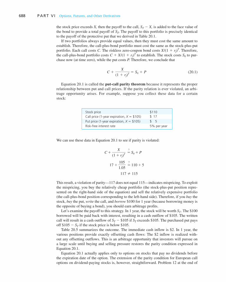
688 P A R T V I Options, Futures, and Other Derivatives
the stock price exceeds X, then the payoff to the call, S T 2 X, is added to the face value of the bond to provide a total payoff of S T . The payoff to this portfolio is precisely identical to the payoff of the protective put that we derived in Table 20.1 .
If two portfolios always provide equal values, then they must cost the same amount to establish. Therefore, the call-plus-bond portfolio must cost the same as the stock-plus-put portfolio. Each call costs C. The riskless zero-coupon bond costs X /(1 1 r f )
T . Therefore, the call-plus-bond portfolio costs C 1 X /(1 1 r f )
T to establish. The stock costs S 0 to pur-chase now (at time zero), while the put costs P. Therefore, we conclude that
C 1X
(1 1 rf)T
5 S0 1 P (20.1)
Equation 20.1 is called the put-call parity theorem because it represents the proper relationship between put and call prices. If the parity relation is ever violated, an arbi-trage opportunity arises. For example, suppose you collect these data for a certain stock:
Stock price $110
Call price (1-year expiration, X 5 $105) $ 17
Put price (1-year expiration, X 5 $105) $ 5
Risk-free interest rate 5% per year
We can use these data in Equation 20.1 to see if parity is violated:
C 1X
(1 1 rf)T 5
?S0 1 P
17 1105
1.05 5
?110 1 5
117 2 115
This result, a violation of parity—117 does not equal 115—indicates mispricing. To exploit the mispricing, you buy the relatively cheap portfolio (the stock-plus-put position repre-sented on the right-hand side of the equation) and sell the relatively expensive portfolio (the call-plus-bond position corresponding to the left-hand side). Therefore, if you buy the stock, buy the put, write the call, and borrow $100 for 1 year (because borrowing money is the opposite of buying a bond), you should earn arbitrage profits.
Let’s examine the payoff to this strategy. In 1 year, the stock will be worth S T . The $100 borrowed will be paid back with interest, resulting in a cash outflow of $105. The written call will result in a cash outflow of S T 2 $105 if S T exceeds $105. The purchased put pays off $105 2 S T if the stock price is below $105.
Table 20.5 summarizes the outcome. The immediate cash inflow is $2. In 1 year, the various positions provide exactly offsetting cash flows: The $2 inflow is realized with-out any offsetting outflows. This is an arbitrage opportunity that investors will pursue on a large scale until buying and selling pressure restores the parity condition expressed in Equation 20.1 .
Equation 20.1 actually applies only to options on stocks that pay no dividends before the expiration date of the option. The extension of the parity condition for European call options on dividend-paying stocks is, however, straightforward. Problem 12 at the end of

C H A P T E R 2 0 Options Markets: Introduction 689
the chapter leads you through the extension of the parity relationship. The more general formulation of the put-call parity condition is
P 5 C 2 S0 1 PV(X) 1 PV(dividends) (20.2)
where PV(dividends) is the present value of the dividends that will be paid by the stock during the life of the option. If the stock does not pay dividends, Equation 20.2 becomes identical to Equation 20.1 .
Notice that this generalization would apply as well to European options on assets other than stocks. Instead of using dividend income in Equation 20.2 , we would let any income paid out by the underlying asset play the role of the stock dividends. For example, European put and call options on bonds would satisfy the same parity relationship, except that the bond’s coupon income would replace the stock’s dividend payments in the parity formula.
Even this generalization, however, applies only to European options, as the cash flow streams from the two portfolios represented by the two sides of Equation 20.2 will match only if each position is held until expiration. If a call and a put may be optimally exercised at different times before their common expiration date, then the equality of payoffs cannot be assured, or even expected, and the portfolios will have different values.
Table 20.5
Arbitrage strategy
Immediate Cash Flow
Cash Flow in 1 Year
Position S T , 105 S T $ 105
Buy stock 2110 ST ST
Borrow $105/1.05 5 $100 1100 2105 2105
Sell call 117 0 2( ST 2 105)
Buy put 25 105 2 ST 0
TOTAL 2 0 0
Example 20.6 Put-Call Parity
Let’s see how well parity works using real data on the IBM options in Figure 20.1 . The January expiration call with exercise price $130 and time to expiration of 44 days cost $2.18 while the corresponding put option cost $4.79. IBM was selling for $127.21, and the annualized short-term interest rate on this date was .2%. No dividends will be paid between the date of the listing, December 2, and the option expiration date. According to parity, we should find that
P 5 C 1 PV(X) 2 S0 1 PV(dividends)
4.79 5 2.18 1130
(1.002)44/3652 127.21 1 0
4.79 5 2.18 1 129.97 2 127.21
4.79 5 4.94
So parity is violated by about $.15 per share. Is this a big enough difference to exploit? Probably not. You have to weigh the potential profit against the trading costs of the call, put, and stock. More important, given the fact that options trade relatively infrequently, this deviation from parity might not be “real,” but may instead be attributable to “stale” (i.e., out-of-date) price quotes at which you cannot actually trade.

690 P A R T V I Options, Futures, and Other Derivatives
20.5 Option-like Securities
Suppose you never traded an option directly. Why do you need to appreciate the properties of options in formulating an investment plan? Many financial instruments and agreements have features that convey implicit or explicit options to one or more parties. If you are to value and use these securities correctly, you must understand these embedded option attributes.
Callable Bonds
You know from Chapter 14 that many corporate bonds are issued with call provisions enti-tling the issuer to buy bonds back from bondholders at some time in the future at a speci-fied call price. A call provision conveys a call option to the issuer, where the exercise price is equal to the price at which the bond can be repurchased. A callable bond arrangement is essentially a sale of a straight bond (a bond with no option features such as callability or convertibility) to the investor and the concurrent issuance of a call option by the investor to the bond-issuing firm.
There must be some compensation for conveying this implicit call option to the firm. If the callable bond were issued with the same coupon rate as a straight bond, it would sell at a lower price than the straight bond: the price difference would equal the value of the call. To sell callable bonds at par, firms must issue them with coupon rates higher than the coupons on straight debt. The higher coupons are the investor’s compensation for the call option retained by the issuer. Coupon rates usually are selected so that the newly issued bond will sell at par value.
Figure 20.11 illustrates this optionlike property. The horizontal axis is the value of a straight bond with otherwise identical terms to the callable bond. The dashed 45-degree line represents the value of straight debt. The solid line is the value of the callable bond, and the dotted line is the value of the call option retained by the firm. A callable bond’s potential for capital gains is limited by the firm’s option to repurchase at the call price.
CONCEPT CHECK
7 Suppose the period of call protection is extended. How will the cou-pon rate the company needs to offer on its bonds change to enable the issuer to sell the bonds at par value?
CONCEPT CHECK
6 How is a callable bond similar to a covered call strategy on a straight bond?
The option inherent in callable bonds actually is more complex than an ordinary call option, because usually it may be exercised only after some initial period of call protection. The price at which the bond is callable may change over time also. Unlike exchange-listed options, these features are defined in the initial bond covenant and will depend on the needs of the issuing firm and its perception of the market’s tastes.
Convertible Securities
Convertible bonds and convertible preferred stock convey options to the holder of the secu-rity rather than to the issuing firm. A convertible security typically gives its holder the right

C H A P T E R 2 0 Options Markets: Introduction 691
to exchange each bond or share of preferred stock for a fixed number of shares of common stock, regardless of the market prices of the securities at the time.
For example, a bond with a con-
version ratio of 10 allows its holder to convert one bond of par value $1,000 into 10 shares of common stock. Alternatively, we say the conversion
price in this case is $100: To receive 10 shares of stock, the investor sacri-fices bonds with face value $1,000 or, put another way, $100 of face value per share. If the present value of the bond’s scheduled payments is less than 10 times the value of one share of stock, it may pay to convert; that is, the conversion option is in the money. A bond worth $950 with a conversion ratio of 10 could be converted prof-itably if the stock were selling above $95, as the value of the 10 shares received for each bond surrendered would exceed $950. Most convertible bonds are issued “deep out of the money.” That is, the issuer sets the conversion ratio so that conversion will not be profitable unless there is a substantial increase in stock prices and/or decrease in bond prices from the time of issue.
A bond’s conversion value equals the value it would have if you converted it into stock immediately. Clearly, a bond must sell for at least its conversion value. If it did not, you could purchase the bond, convert it, and clear an immediate profit. This condition could never persist, for all investors would pursue such a strategy and ultimately would bid up the price of the bond.
The straight bond value, or “bond floor,” is the value the bond would have if it were not convertible into stock. The bond must sell for more than its straight bond value because a convertible bond has more value; it is in fact a straight bond plus a valuable call option. Therefore, the convertible bond has two lower bounds on its market price: the conversion value and the straight bond value.
Value of Straight Debt
Value of Callable Bond
Call Price
Value of Firm’sCall Option
Value ofStraight Debt
Figure 20.11 Values of callable bonds compared with straight bonds
CONCEPT CHECK
8 Should a convertible bond issued at par value have a higher or lower coupon rate than a nonconvertible bond at par?
Figure 20.12 illustrates the optionlike properties of the convertible bond. Figure 20.12 A shows the value of the straight debt as a function of the stock price of the issuing firm. For healthy firms, the straight debt value is almost independent of the value of the stock because default risk is small. However, if the firm is close to bankruptcy (stock prices are low), default risk increases, and the straight bond value falls. Panel B shows the conversion value of the bond. Panel C compares the value of the convertible bond to these two lower bounds.
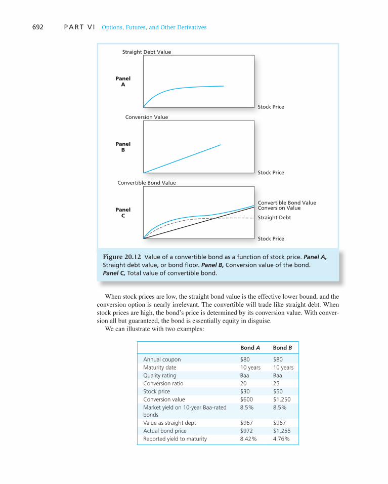
692 P A R T V I Options, Futures, and Other Derivatives
Bond A Bond B
Annual coupon $80 $80
Maturity date 10 years 10 years
Quality rating Baa Baa
Conversion ratio 20 25
Stock price $30 $50
Conversion value $600 $1,250
Market yield on 10-year Baa-rated
bonds
8.5% 8.5%
Value as straight dept $967 $967
Actual bond price $972 $1,255
Reported yield to maturity 8.42% 4.76%
Figure 20.12 Value of a convertible bond as a function of stock price. Panel A, Straight debt value, or bond floor. Panel B, Conversion value of the bond. Panel C, Total value of convertible bond.
Straight Debt Value
Stock Price
PanelA
Conversion Value
Stock Price
PanelB
Convertible Bond Value
Straight Debt
Conversion ValueConvertible Bond Value
Stock Price
PanelC
When stock prices are low, the straight bond value is the effective lower bound, and the conversion option is nearly irrelevant. The convertible will trade like straight debt. When stock prices are high, the bond’s price is determined by its conversion value. With conver-sion all but guaranteed, the bond is essentially equity in disguise.
We can illustrate with two examples:

C H A P T E R 2 0 Options Markets: Introduction 693
Bond A has a conversion value of only $600. Its value as straight debt, in contrast, is $967. This is the present value of the coupon and principal payments at a market rate for straight debt of 8.5%. The bond’s price is $972, so the premium over straight bond value is only $5, reflecting the low probability of conversion. Its reported yield to maturity based on scheduled coupon payments and the market price of $972 is 8.42%, close to that of straight debt.
The conversion option on bond B is in the money. Conversion value is $1,250, and the bond’s price, $1,255, reflects its value as equity (plus $5 for the protection the bond offers against stock price declines). The bond’s reported yield is 4.76%, far below the compa-rable yield on straight debt. The big yield sacrifice is attributable to the far greater value of the conversion option.
In theory, we could value convertible bonds by treating them as straight debt plus call options. In practice, however, this approach is often impractical for several reasons:
1. The conversion price frequently increases over time, which means the exercise price of the option changes.
2. Stocks may pay several dividends over the life of the bond, further complicating the option-valuation analysis.
3. Most convertibles also are callable at the discretion of the firm. In essence, both the investor and the issuer hold options on each other. If the issuer exercises its call option to repurchase the bond, the bondholders typically have a month during which they still can convert. When issuers use a call option, knowing bondholders will choose to convert, the issuer is said to have forced a
conversion. These conditions together mean the actual maturity of the bond is indeterminate.
Warrants
Warrants are essentially call options issued by a firm. One important difference between calls and warrants is that exercise of a warrant requires the firm to issue a new share of stock—the total number of shares outstanding increases. Exercise of a call option requires only that the writer of the call deliver an already-issued share of stock to discharge the obligation. In that case, the number of shares outstanding remains fixed. Also unlike call options, warrants result in a cash flow to the firm when the warrant holder pays the exercise price. These differences mean that warrant values will differ somewhat from the values of call options with identical terms.
Like convertible debt, warrant terms may be tailored to meet the needs of the firm. Also like convertible debt, warrants generally are protected against stock splits and dividends in that the exercise price and the number of warrants held are adjusted to offset the effects of the split.
Warrants are often issued in conjunction with another security. Bonds, for example, may be packaged together with a warrant “sweetener,” frequently a warrant that may be sold separately. This is called a detachable warrant.
Issue of warrants and convertible securities creates the potential for an increase in out-standing shares of stock if exercise occurs. Exercise obviously would affect financial sta-tistics that are computed on a per-share basis, so annual reports must provide earnings per share figures under the assumption that all convertible securities and warrants are exer-cised. These figures are called fully diluted earnings per share. 3
3 We should note that the exercise of a convertible bond need not reduce EPS. Diluted EPS will be less than undi-luted EPS only if interest saved (per share) on the convertible bonds is less than the prior EPS.

694 P A R T V I Options, Futures, and Other Derivatives
The executive and employee stock options that became so popular in the last decade actually were warrants. Some of these grants were huge, with payoffs to top executives in excess of $100 million. Yet firms almost uniformly chose not to acknowledge these grants as expenses on their income statements until new reporting rules that took effect in 2006 required such recognition.
Collateralized Loans
Many loan arrangements require that the borrower put up collateral to guarantee the loan will be paid back. In the event of default, the lender takes possession of the collateral. A nonrecourse loan gives the lender no recourse beyond the right to the collateral. That is, the lender may not sue the borrower for further payment if the collateral turns out not to be valuable enough to repay the loan.
This arrangement gives an implicit call option to the borrower. Assume the borrower is obligated to pay back L dollars at the maturity of the loan. The collateral will be worth S T dollars at maturity. (Its value today is S 0 .) The borrower has the option to wait until loan maturity and repay the loan only if the collateral is worth more than the L dollars necessary to satisfy the loan. If the collateral is worth less than L, the borrower can default on the loan, discharging the obligation by forfeiting the collateral, which is worth only S T .
4 Another way of describing such a loan is to view the borrower as turning over the col-
lateral to the lender but retaining the right to reclaim it by paying off the loan. The transfer of the collateral with the right to reclaim it is equivalent to a payment of S 0 dollars, less a simultaneous recovery of a sum that resembles a call option with exercise price L. In effect, the borrower turns over collateral but keeps an option to “repurchase” it for L dollars at the maturity of the loan if L turns out to be less than S T . This is a call option.
A third way to look at a collateralized loan is to assume that the borrower will repay the L dollars with certainty but also retain the option to sell the collateral to the lender for L dollars, even if S T is less than L. In this case, the sale of the collateral would generate the cash necessary to satisfy the loan. The ability to “sell” the collateral for a price of L dollars represents a put option, which guarantees the borrower can raise enough money to satisfy the loan simply by turning over the collateral.
It is perhaps surprising to realize that we can describe the same loan as involving either a put option or a call option, as the payoffs to calls and puts are so different. Yet the equivalence of the two approaches is nothing more than a reflection of the put-call parity relationship. In our call-option description of the loan, the value of the borrower’s liability is S 0 2 C: The borrower turns over the asset, which is a transfer of S 0 dollars, but retains a call worth C dollars. In the put-option description, the borrower is obligated to pay L dollars but retains the put, which is worth P: The present value of this net obligation is L /(1 1 r f )
T 2 P. Because these alternative descriptions are equivalent ways of viewing the same loan, the value of the obligations must be equal:
S0 2 C 5L
(1 1 rf)T
2 P (20.3)
Treating L as the exercise price of the option, Equation 20.3 is simply the put-call parity relationship.
4 In reality, of course, defaulting on a loan is not so simple. There are losses of reputation involved as well as considerations of ethical behavior. This is a description of a pure nonrecourse loan where both parties agree from the outset that only the collateral backs the loan and that default is not to be taken as a sign of bad faith if the col-lateral is insufficient to repay the loan.

C H A P T E R 2 0 Options Markets: Introduction 695
Figure 20.13 illustrates this fact. Figure 20.13 A is the value of the payment to be received by the lender, which equals the minimum of S T or L. Panel B shows that this amount can be expressed as S T minus the payoff of the call implicitly written by the lender and held by the borrower. Panel C shows it also can be viewed as a receipt of L dollars minus the proceeds of a put option.
Figure 20.13 Collateralized loan. Panel A, Payoff to collateralized loan. Panel B, Lender can be viewed as collecting the collateral from the borrower, but issuing an option to the borrower to call back the collateral for the face value of the loan. Panel C, Lender can be viewed as collecting a risk-free loan from the borrower, but issuing a put to the borrower to sell the collateral for the face value of the loan.
L
L
ST
L dollars minus the payoff to the implicit put option
Payoff to a put withexercise price L
Payoff
L
L
ST
ST dollars minus the payoffto the implicit call option
Payoff to call with exercise price L
Payoff
PanelA
PanelB
PanelC
Payoff
L
LST
Payoff to lender
When ST exceeds L, the loan is repaid and the collateral is reclaimed. Otherwise,the collateral is forfeited and the total loan repayment is worth only ST

696 P A R T V I Options, Futures, and Other Derivatives
Levered Equity and Risky Debt
Investors holding stock in incorporated firms are protected by limited liability, which means that if the firm cannot pay its debts, the firm’s creditors may attach only the firm’s assets, not sue the corporation’s equityholders for further payment. In effect, any time the corporation borrows money, the maximum possible collateral for the loan is the total of the firm’s assets. If the firm declares bankruptcy, we can interpret this as an admission that the assets of the firm are insufficient to satisfy the claims against it. The corporation may discharge its obligations by transferring ownership of the firm’s assets to the creditors.
Just as is true for nonrecourse collateralized loans, the required payment to the credi-tors represents the exercise price of the implicit option, while the value of the firm is the underlying asset. The equityholders have a put option to transfer their ownership claims on the firm to the creditors in return for the face value of the firm’s debt.
Alternatively, we may view the equityholders as retaining a call option. They have, in effect, already transferred their ownership claim to the firm to the creditors but have retained the right to reacquire that claim by paying off the loan. Hence the equityholders have the option to “buy back” the firm for a specified price: They have a call option.
The significance of this observation is that analysts can value corporate bonds using option-pricing techniques. The default premium required of risky debt in principle can be estimated by using option-valuation models. We consider some of these models in the next chapter.
20.6 Financial Engineering
One of the attractions of options is the ability they provide to create investment positions with payoffs that depend in a variety of ways on the values of other securities. We have seen evidence of this capability in the various options strategies examined in Section 20.4 .
Options also can be used to custom-design new securities or portfolios with desired patterns of exposure to the price of an underlying security. In this sense, options (and futures contracts, to be discussed in Chapters 22 and 23) provide the ability to engage in financial engineering, the cre-ation of portfolios with specified payoff patterns.
A simple example of a prod-uct engineered with options is the index-linked certificate of deposit. Index-linked CDs enable retail investors to take small posi-tions in index options. Unlike conventional CDs, which pay a fixed rate of interest, these CDs pay depositors a specified frac-tion of the rate of return on a mar-ket index such as the S&P 500,
Rate of Return on Index-Linked CD
Slope = .7
rM = Market Rateof Return
Figure 20.14 Return on index-linked CD

C H A P T E R 2 0 Options Markets: Introduction 697
while guaranteeing a minimum rate of return should the market fall. For example, the index-linked CD may offer 70% of any market increase, but protect its holder from any market decrease by guaranteeing at least no loss.
The index-linked CD is clearly a type of call option. If the market rises, the depositor profits according to the participation rate or multiplier, in this case 70%; if the market falls, the investor is insured against loss. Just as clearly, the bank offering these CDs is in effect writing call options and can hedge its position by buying index calls in the options market. Figure 20.14 shows the nature of the bank’s obligation to its depositors.
How might the bank set the appropriate multiplier? To answer this, note various fea-tures of the option:
1. The price the depositor is paying for the options is the forgone interest on the conventional CD that could be purchased. Because interest is received at the end of the period, the present value of the interest payment on each dollar invested is r f /(1 1 r f ). Therefore, the depositor trades a sure payment with present value per dollar invested of r f /(1 1 r f ) for a return that depends on the market’s performance. Conversely, the bank can fund its obligation using the interest that it would have paid on a conventional CD.
2. The option we have described is an at-the-money option, meaning that the exercise price equals the current value of the stock index. The option goes into the money as soon as the market index increases from its level at the inception of the contract.
3. We can analyze the option on a per-dollar-invested basis. For example, the option costs the depositor r f /(1 1 r f ) dollars per dollar placed in the index-linked CD. The market price of the option per dollar invested is C / S 0 : The at-the-money option costs C dollars and is written on one unit of the market index, currently at S 0 .
Now it is easy to determine the multiplier that the bank can offer on the CDs. It receives from its depositors a “payment” of r f /(1 1 r f ) per dollar invested. It costs the bank C / S 0 to purchase the call option on a $1 investment in the market index. Therefore, if r f /(1 1 r f ) is, for example, 70% of C / S 0 , the bank can purchase at most .7 call option on the $1 invest-ment and the multiplier will be .7. More generally, the break-even multiplier on an index-linked CD is r f /(1 1 r f ) divided by C / S 0 .
Example 20.7 Indexed-Linked CDs
Suppose that r f 5 6% per year, and that 6-month maturity at-the-money calls on the market index currently cost $50. The index is at 1,000. Then the option costs 50/1,000 5 $.05 per dollar of market value. The CD rate is 3% per 6 months, meaning that r f /(1 1 r f ) 5 .03/1.03 5 .0291. Therefore, the multiplier would be .0291/.05 5 .5825.
The index-linked CD has several variants. Investors can purchase similar CDs that guar-antee a positive minimum return if they are willing to settle for a smaller multiplier. In this case, the option is “purchased” by the depositor for ( r f 2 r min )/(1 1 r f ) dollars per dol-lar invested, where r min is the guaranteed minimum return. Because the purchase price is lower, fewer options can be purchased, which results in a lower multiplier. Another variant of the “bullish” CD we have described is the bear CD, which pays depositors a fraction of any fall in the market index. For example, a bear CD might offer a rate of return of .6 times any percentage decline in the S&P 500.

698 P A R T V I Options, Futures, and Other Derivatives
20.7 Exotic Options
CONCEPT CHECK
9 Continue to assume that r f 5 3% per half-year, that at-the-money calls sell for $50, and that the market index is at 1,000. What would be the multiplier for 6-month bullish equity-linked CDs offering a guaranteed minimum return of .5% over the term of the CD?
Options markets have been tremendously successful. Investors clearly value the portfolio strategies made possible by trading options; this is reflected in the heavy trading volume in these markets. Success breeds imitation, and in recent years we have witnessed con-siderable innovation in the range of option instruments available to investors. Part of this innovation has occurred in the market for customized options, which now trade in active over-the-counter markets. Many of these options have terms that would have been highly unusual even a few years ago; they are therefore called “exotic options.” In this section we survey some of the more interesting variants of these new instruments.
Asian Options
You already have been introduced to American- and European-style options. Asian-style options are options with payoffs that depend on the average price of the underlying asset during at least some portion of the life of the option. For example, an Asian call option may have a payoff equal to the average stock price over the last 3 months minus the strike price if that value is positive, and zero otherwise. These options may be of interest, for example, to firms that wish to hedge a profit stream that depends on the average price of a commodity over some period of time.
Barrier Options
Barrier options have payoffs that depend not only on some asset price at option expiration, but also on whether the underlying asset price has crossed through some “barrier.” For example, a down-and-out option is one type of barrier option that automatically expires worthless if and when the stock price falls below some barrier price. Similarly, down-and-in options will not provide a payoff unless the stock price does fall below some barrier at least once during the life of the option. These options also are referred to as knock-out and knock-in options.
Lookback Options
Lookback options have payoffs that depend in part on the minimum or maximum price of the underlying asset during the life of the option. For example, a lookback call option might provide a payoff equal to the maximum stock price during the life of the option minus the exercise price, instead of the final stock price minus the exercise price. Such an option provides (for a price, of course) a form of perfect market timing, providing the call holder with a payoff equal to the one that would accrue if the asset were purchased for X dollars and later sold at what turns out to be its high price.
Currency-Translated Options
Currency-translated options have either asset or exercise prices denominated in a foreign currency. A good example of such an option is the quanto, which allows an investor to fix

Vis
it u
s at
ww
w.m
hh
e.co
m/b
km
C H A P T E R 2 0 Options Markets: Introduction 699
in advance the exchange rate at which an investment in a foreign currency can be converted back into dollars. The right to translate a fixed amount of foreign currency into dollars at a given exchange rate is a simple foreign exchange option. Quantos are more interesting, however, because the amount of currency that will be translated into dollars depends on the investment performance of the foreign security. Therefore, a quanto in effect provides a random number of options.
Digital Options
Digital options, also called binary or “bet” options, have fixed payoffs that depend on whether a condition is satisfied by the price of the underlying asset. For example, a digital call option might pay off a fixed amount of $100 if the stock price at maturity exceeds the exercise price.
1. A call option is the right to buy an asset at an agreed-upon exercise price. A put option is the right to sell an asset at a given exercise price.
2. American-style options allow exercise on or before the expiration date. European options allow exercise only on the expiration date. Most traded options are American in nature.
3. Options are traded on stocks, stock indexes, foreign currencies, fixed-income securities, and sev-eral futures contracts.
4. Options can be used either to lever up an investor’s exposure to an asset price or to provide insur-ance against volatility of asset prices. Popular option strategies include covered calls, protective puts, straddles, spreads, and collars.
5. The put-call parity theorem relates the prices of put and call options. If the relationship is vio-lated, arbitrage opportunities will result. Specifically, the relationship that must be satisfied is
P 5 C 2 S0 1 PV(X) 1 PV(dividends)
where X is the exercise price of both the call and the put options, PV( X ) is the present value of a claim to X dollars to be paid at the expiration date of the options, and PV(dividends) is the present value of dividends to be paid before option expiration.
6. Many commonly traded securities embody option characteristics. Examples of these securities are callable bonds, convertible bonds, and warrants. Other arrangements such as collateralized loans and limited-liability borrowing can be analyzed as conveying implicit options to one or more parties.
7. Trading in so-called exotic options now takes place in an active over-the-counter market.
SUMMARY
Related Web sites for this chapter are available at www.mhhe.com/bkm
call option exercise or strike price premium put option in the money out of the money
at the money American option European option protective put covered call
straddle spread collar put-call parity theorem warrant
KEY TERMS

Vis
it u
s at
ww
w.m
hh
e.co
m/b
km700 P A R T V I Options, Futures, and Other Derivatives
1. We said that options can be used either to scale up or reduce overall portfolio risk. What are some examples of risk-increasing and risk-reducing options strategies? Explain each.
2. What are the trade-offs facing an investor who is considering buying a put option on an existing portfolio?
3. What are the trade-offs facing an investor who is considering writing a call option on an existing portfolio?
4. Why do you think the most actively traded options tend to be the ones that are near the money?
5. Turn back to Figure 20.1 , which lists prices of various IBM options. Use the data in the figure to calculate the payoff and the profits for investments in each of the following January expiration options, assuming that the stock price on the expiration date is $125.
a. Call option, X 5 $120. b. Put option, X 5 $120. c. Call option, X 5 $125. d. Put option, X 5 $125. e. Call option, X 5 $130. f. Put option, X 5 $130.
6. Suppose you think Walmart stock is going to appreciate substantially in value in the next 6 months. Say the stock’s current price, S 0 , is $100, and the call option expiring in 6 months has an exercise price, X, of $100 and is selling at a price, C, of $10. With $10,000 to invest, you are considering three alternatives.
a. Invest all $10,000 in the stock, buying 100 shares. b. Invest all $10,000 in 1,000 options (10 contracts). c. Buy 100 options (one contract) for $1,000, and invest the remaining $9,000 in a money mar-
ket fund paying 4% in interest over 6 months (8% per year).
What is your rate of return for each alternative for the following four stock prices 6 months from now? Summarize your results in the table and diagram below.
Price of Stock 6 Months from Now
$80 $100 $110 $120
a. All stocks (100 shares)
b. All options (1,000 shares)
c. Bills 1 100 options
PROBLEM SETS
i. Basic
ii. Intermediate
ST0
Rate of Return
7. The common stock of the P.U.T.T. Corporation has been trading in a narrow price range for the past month, and you are convinced it is going to break far out of that range in the next 3 months. You do not know whether it will go up or down, however. The current price of the stock is $100 per share, and the price of a 3-month call option at an exercise price of $100 is $10.
a. If the risk-free interest rate is 10% per year, what must be the price of a 3-month put option on P.U.T.T. stock at an exercise price of $100? (The stock pays no dividends.)

Vis
it u
s at
ww
w.m
hh
e.co
m/b
km
C H A P T E R 2 0 Options Markets: Introduction 701
b. What would be a simple options strategy to exploit your conviction about the stock price’s future movements? How far would it have to move in either direction for you to make a profit on your initial investment?
8. The common stock of the C.A.L.L. Corporation has been trading in a narrow range around $50 per share for months, and you believe it is going to stay in that range for the next 3 months. The price of a 3-month put option with an exercise price of $50 is $4.
a. If the risk-free interest rate is 10% per year, what must be the price of a 3-month call option on C.A.L.L. stock at an exercise price of $50 if it is at the money? (The stock pays no dividends.)
b. What would be a simple options strategy using a put and a call to exploit your conviction about the stock price’s future movement? What is the most money you can make on this position? How far can the stock price move in either direction before you lose money?
c. How can you create a position involving a put, a call, and riskless lending that would have the same payoff structure as the stock at expiration? What is the net cost of establishing that position now?
9. You are a portfolio manager who uses options positions to customize the risk profile of your clients. In each case, what strategy is best given your client’s objective?
a. • Performance to date: Up 16%. • Client objective: Earn at least 15%. • Your scenario: Good chance of large gains or large losses between now and end of year.
i. Long straddle. ii. Long bullish spread. iii. Short straddle.
b. • Performance to date: Up 16%. • Client objective: Earn at least 15%. • Your scenario: Good chance of large losses between now and end of year.
i. Long put options. ii. Short call options. iii. Long call options.
10. An investor purchases a stock for $38 and a put for $.50 with a strike price of $35. The inves-tor sells a call for $.50 with a strike price of $40. What is the maximum profit and loss for this position? Draw the profit and loss diagram for this strategy as a function of the stock price at expiration.
11. Imagine that you are holding 5,000 shares of stock, currently selling at $40 per share. You are ready to sell the shares but would prefer to put off the sale until next year for tax reasons. If you continue to hold the shares until January, however, you face the risk that the stock will drop in value before year end. You decide to use a collar to limit downside risk without laying out a good deal of additional funds. January call options with a strike of $35 are selling at $2, and January puts with a strike price of $45 are selling at $3. What will be the value of your portfolio in January (net of the proceeds from the options) if the stock price ends up at: ( a ) $30, ( b ) $40, or ( c ) $50? Compare these proceeds to what you would realize if you simply continued to hold the shares.
12. In this problem, we derive the put-call parity relationship for European options on stocks that pay dividends before option expiration. For simplicity, assume that the stock makes one divi-dend payment of $ D per share at the expiration date of the option.
a. What is the value of a stock-plus-put position on the expiration date of the option? b. Now consider a portfolio comprising a call option and a zero-coupon bond with the same
maturity date as the option and with face value ( X 1 D ). What is the value of this portfolio on the option expiration date? You should find that its value equals that of the stock-plus-put portfolio regardless of the stock price.
c. What is the cost of establishing the two portfolios in parts ( a ) and ( b )? Equate the costs of these portfolios, and you will derive the put-call parity relationship, Equation 20.2 .

Vis
it u
s at
ww
w.m
hh
e.co
m/b
km702 P A R T V I Options, Futures, and Other Derivatives
13. a. A butterfly spread is the purchase of one call at exercise price X 1 , the sale of two calls at exercise price X 2 , and the purchase of one call at exercise price X 3 . X 1 is less than X 2 , and X 2 is less than X 3 by equal amounts, and all calls have the same expiration date. Graph the payoff diagram to this strategy.
b. A vertical combination is the purchase of a call with exercise price X 2 and a put with exercise price X 1 , with X 2 greater than X 1 . Graph the payoff to this strategy.
14. A bearish spread is the purchase of a call with exercise price X 2 and the sale of a call with exercise price X 1 , with X 2 greater than X 1 . Graph the payoff to this strategy and compare it to Figure 20.10 .
15. Joseph Jones, a manager at Computer Science, Inc. (CSI), received 10,000 shares of company stock as part of his compensation package. The stock currently sells at $40 a share. Joseph would like to defer selling the stock until the next tax year. In January, however, he will need to sell all his holdings to provide for a down payment on his new house. Joseph is worried about the price risk involved in keeping his shares. At current prices, he would receive $400,000 for the stock. If the value of his stock holdings falls below $350,000, his ability to come up with the necessary down payment would be jeopardized. On the other hand, if the stock value rises to $450,000, he would be able to maintain a small cash reserve even after making the down pay-ment. Joseph considers three investment strategies:
a. Strategy A is to write January call options on the CSI shares with strike price $45. These calls are currently selling for $3 each.
b. Strategy B is to buy January put options on CSI with strike price $35. These options also sell for $3 each.
c. Strategy C is to establish a zero-cost collar by writing the January calls and buying the January puts.
Evaluate each of these strategies with respect to Joseph’s investment goals. What are the advan-tages and disadvantages of each? Which would you recommend?
16. Use the spreadsheet from the Excel Application boxes on spreads and straddles (available at www.mhhe.com/bkm ; link to Chapter 20 material) to answer these questions.
a. Plot the payoff and profit diagrams to a straddle position with an exercise (strike) price of $130. Assume the options are priced as they are in the Excel Application.
b. Plot the payoff and profit diagrams to a bullish spread position with exercise (strike) prices of $120 and $130. Assume the options are priced as they are in the Excel Application.
17. The agricultural price support system guarantees farmers a minimum price for their output. Describe the program provisions as an option. What is the asset? The exercise price?
18. In what ways is owning a corporate bond similar to writing a put option? A call option?
19. An executive compensation scheme might provide a manager a bonus of $1,000 for every dollar by which the company’s stock price exceeds some cutoff level. In what way is this arrangement equivalent to issuing the manager call options on the firm’s stock?
20. Consider the following options portfolio. You write a January expiration call option on IBM with exercise price 130. You write a January IBM put option with exercise price 125.
a. Graph the payoff of this portfolio at option expiration as a function of IBM’s stock price at that time.
b. What will be the profit/loss on this position if IBM is selling at 128 on the option expiration date? What if IBM is selling at 135? Use The Wall Street Journal listing from Figure 20.1 to answer this question.
c. At what two stock prices will you just break even on your investment? d. What kind of “bet” is this investor making; that is, what must this investor believe about
IBM’s stock price to justify this position?
21. Consider the following portfolio. You write a put option with exercise price 90 and buy a put option on the same stock with the same expiration date with exercise price 95.
a. Plot the value of the portfolio at the expiration date of the options. b. On the same graph, plot the profit of the portfolio. Which option must cost more?
eXce lPlease visit us at www.mhhe.com/bkm

Vis
it u
s at
ww
w.m
hh
e.co
m/b
km
C H A P T E R 2 0 Options Markets: Introduction 703
22. A Ford put option with strike price 60 trading on the Acme options exchange sells for $2. To your amazement, a Ford put with the same maturity selling on the Apex options exchange but with strike price 62 also sells for $2. If you plan to hold the options positions to maturity, devise a zero-net-investment arbitrage strategy to exploit the pricing anomaly. Draw the profit diagram at maturity for your position.
23. Assume a stock has a value of $100. The stock is expected to pay a dividend of $2 per share at year-end. An at-the-money European-style put option with one-year maturity sells for $7. If the annual interest rate is 5%, what must be the price of a 1-year at-the-money European call option on the stock?
24. You buy a share of stock, write a 1-year call option with X 5 $10, and buy a 1-year put option with X 5 $10. Your net outlay to establish the entire portfolio is $9.50. What is the risk-free interest rate? The stock pays no dividends.
25. You write a put option with X 5 100 and buy a put with X 5 110. The puts are on the same stock and have the same expiration date.
a. Draw the payoff graph for this strategy. b. Draw the profit graph for this strategy. c. If the underlying stock has positive beta, does this portfolio have positive or negative beta?
26. Joe Finance has just purchased a stock index fund, currently selling at $400 per share. To pro-tect against losses, Joe also purchased an at-the-money European put option on the fund for $20, with exercise price $400, and 3-month time to expiration. Sally Calm, Joe’s financial adviser, points out that Joe is spending a lot of money on the put. She notes that 3-month puts with strike prices of $390 cost only $15, and suggests that Joe use the cheaper put.
a. Analyze Joe’s and Sally’s strategies by drawing the profit diagrams for the stock-plus-put positions for various values of the stock fund in 3 months.
b. When does Sally’s strategy do better? When does it do worse? c. Which strategy entails greater systematic risk?
27. You write a call option with X 5 50 and buy a call with X 5 60. The options are on the same stock and have the same expiration date. One of the calls sells for $3; the other sells for $9.
a. Draw the payoff graph for this strategy at the option expiration date. b. Draw the profit graph for this strategy. c. What is the break-even point for this strategy? Is the investor bullish or bearish on the stock?
28. Devise a portfolio using only call options and shares of stock with the following value (payoff) at the option expiration date. If the stock price is currently 53, what kind of bet is the investor making?
50
50 60 110
Payoff
ST
29. You are attempting to formulate an investment strategy. On the one hand, you think there is great upward potential in the stock market and would like to participate in the upward move if it materializes. However, you are not able to afford substantial stock market losses and so cannot run the risk of a stock market collapse, which you think is also a possibility. Your investment adviser suggests a protective put position: Buy both shares in a market index stock fund and put options on those shares with 3-month expiration and exercise price of $780. The stock index
iii. Challenge

Vis
it u
s at
ww
w.m
hh
e.co
m/b
km704 P A R T V I Options, Futures, and Other Derivatives
fund is currently selling for $900. However, your uncle suggests you instead buy a 3-month call option on the index fund with exercise price $840 and buy 3-month T-bills with face value $840.
a. On the same graph, draw the payoffs to each of these strategies as a function of the stock fund value in 3 months. ( Hint: Think of the options as being on one “share” of the stock index fund, with the current price of each share of the fund equal to $900.)
b. Which portfolio must require a greater initial outlay to establish? ( Hint: Does either portfo-lio provide a final payout that is always at least as great as the payoff of the other portfolio?)
c. Suppose the market prices of the securities are as follows:
Stock fund $900
T-bill (face value $840) $810
Call (exercise price $840) $120
Put (exercise price $780) $ 6
Make a table of the profits realized for each portfolio for the following values of the stock price in 3 months: S T 5 $700, $840, $900, $960.
Graph the profits to each portfolio as a function of S T on a single graph. d. Which strategy is riskier? Which should have a higher beta? e. Explain why the data for the securities given in part ( c ) do not violate the put-call parity
relationship.
30. Using the IBM option prices in Figure 20.1 , calculate the market price of a riskless zero-coupon bond with face value $125 that matures in January on the same date as the listed options.
31. Demonstrate that an at-the-money call option on a given stock must cost more than an at-the-money put option on that stock with the same maturity. The stock will pay no dividends until after the expiration date. ( Hint: Use put-call parity.)
1. Donna Donie, CFA, has a client who believes the common stock price of TRT Materials (cur-rently $58 per share) could move substantially in either direction in reaction to an expected court decision involving the company. The client currently owns no TRT shares, but asks Donie for advice about implementing a strangle strategy to capitalize on the possible stock price movement. A strangle is a portfolio of a put and a call with different exercise prices but the same expiration date. Donie gathers the TRT option-pricing data:
Characteristic Call Option Put Option
Price $ 5 $ 4
Strike price $60 $55
Time to expiration 90 days from now 90 days from now
a. Recommend whether Donie should choose a long strangle strategy or a short strangle strat-egy to achieve the client’s objective.
b. Calculate, at expiration for the appropriate strangle strategy in part ( a ), the:
i. Maximum possible loss per share. ii. Maximum possible gain per share. iii. Break-even stock price(s).
2. Martin Bowman is preparing a report distinguishing traditional debt securities from structured note securities. Discuss how the following structured note securities differ from a traditional debt security with respect to coupon and principal payments:
a. Equity index-linked notes. b. Commodity-linked bear bond.

Vis
it u
s at
ww
w.m
hh
e.co
m/b
km
C H A P T E R 2 0 Options Markets: Introduction 705
3. Suresh Singh, CFA, is analyzing a convertible bond. The characteristics of the bond and the underlying common stock are given in the following exhibit:
Convertible Bond Characteristics
Par value $1,000
Annual coupon rate (annual pay) 6.5%
Conversion ratio 22
Market price 105% of par value
Straight value 99% of par value
Underlying Stock Characteristics
Current market price $40 per share
Annual cash dividend $1.20 per share
Compute the bond’s:
a. Conversion value. b. Market conversion price.
4. Rich McDonald, CFA, is evaluating his investment alternatives in Ytel Incorporated by analyz-ing a Ytel convertible bond and Ytel common equity. Characteristics of the two securities are given in the following exhibit:
Characteristics Convertible Bond Common Equity
Par value $1,000 —
Coupon (annual payment) 4% —
Current market price $980 $35 per share
Straight bond value $925 —
Conversion ratio 25 —
Conversion option At any time —
Dividend — $0
Expected market price in 1 year $1,125 $45 per share
a. Calculate, based on the exhibit, the:
i. Current market conversion price for the Ytel convertible bond. ii. Expected 1-year rate of return for the Ytel convertible bond. iii. Expected 1-year rate of return for the Ytel common equity.
One year has passed and Ytel’s common equity price has increased to $51 per share. Also, over the year, the interest rate on Ytel’s nonconvertible bonds of the same maturity increased, while credit spreads remained unchanged.
b. Name the two components of the convertible bond’s value. Indicate whether the value of each component should decrease, stay the same, or increase in response to the:
i. Increase in Ytel’s common equity price. ii. Increase in interest rates.
5. a. Consider a bullish spread option strategy using a call option with a $25 exercise price priced at $4 and a call option with a $40 exercise price priced at $2.50. If the price of the stock increases to $50 at expiration and each option is exercised on the expiration date, the net profit per share at expiration (ignoring transaction costs) is:
i. $8.50 ii. $13.50 iii. $16.50 iv. $23.50

Vis
it u
s at
ww
w.m
hh
e.co
m/b
km706 P A R T V I Options, Futures, and Other Derivatives
b. A put on XYZ stock with a strike price of $40 is priced at $2.00 per share, while a call with a strike price of $40 is priced at $3.50. What is the maximum per-share loss to the writer of the uncovered put and the maximum per-share gain to the writer of the uncovered call?
Maximum Loss to Put Writer
Maximum Gain to Call Writer
i. $38.00 $ 3.50
ii. $38.00 $36.50
iii. $40.00 $ 3.50
iv. $40.00 $40.00
E-INVEST-MENTS EXERCISES
The Options Clearing Corporation
Most of your education in finance and financial markets focuses on the “front office” activities of investment analysis, trading, and broker or dealer interaction with invest-ing customers. For every trade there is a “clearing” and a few days later, a “settlement.” This “back office” area of financial markets, though not in the spotlight, is an enormous operation, and a source of considerable employment opportunities. The Options Clearing Corporation discussed in this chapter is an excellent example. Go to the OCC home page ( www.optionsclearing.com ) and answer the following questions:
1. Click on the Volume Statistics link. How many equity option contracts were cleared by the OCC yesterday? How does this fi gure compare with the year-to-date (YTD) average daily volume?
2. Click the link for Historical Volume Statistics. For each of the most recent 3 months, calculate the percentages of total contract clearings that were equity contracts, index contracts, currency contracts, and futures contracts. Is there much variation among the months’ percentages?
3. Back on the home page, examine the Who We Are link under the About OCC menu. What is the mission of the OCC?
4. Click on the Read More link at the bottom of the Who We Are page. How does the “Three Tiered Backup System” provide the OCC with a AAA rating? What programs does the OCC employ to promote liquidity for its members?
5. Go back to the home page and visit the Career Center. Where is the OCC located? What are the current employment opportunities with the OCC?
SOLUTIONS TO CONCEPT CHECKS
1. a. Denote the stock price at option expiration by S T , and the exercise price by X. Value at expi-ration 5 S T 2 X 5 S T 2 $100 if this value is positive; otherwise the call expires worthless.
Profit 5 Final value 2 Price of call option 5 Proceeds 2 $6.00.
S T 5 $115 S T 5 $135
Proceeds $0 $10
Profits 2$4.75 $ 5.25

Vis
it u
s at
ww
w.m
hh
e.co
m/b
km
C H A P T E R 2 0 Options Markets: Introduction 707
b. Value at expiration 5 X 2 S T 5 $100 2 S T if this value is positive; otherwise the put expires worthless.
Profit 5 Final value 2 Price of put option 5 Proceeds 2 $1.25.
S T 5 $115 S T 5 $135
Proceeds $10 $0
Profits 2$ 7.56 2$ 2.44
2. Before the split, the final payoff would have been 100 3 ($140 2 $130) 5 $1,000. After the split, the payoff is 200 3 ($70 2 $65) 5 $1,000. The payoff is unaffected.
3. a.
SPayoff
Profit
Buy Call
SPayoff
Profit
Write Put
S
Payoff
Profit
Write Call
SPayoff
Profit
Buy Put
b. The payoffs and profits to both buying calls and writing puts generally are higher when the stock price is higher. In this sense, both positions are bullish. Both involve potentially taking delivery of the stock. However, the call holder will choose to take delivery when the stock price is high, while the put writer is obligated to take delivery when the stock price is low.
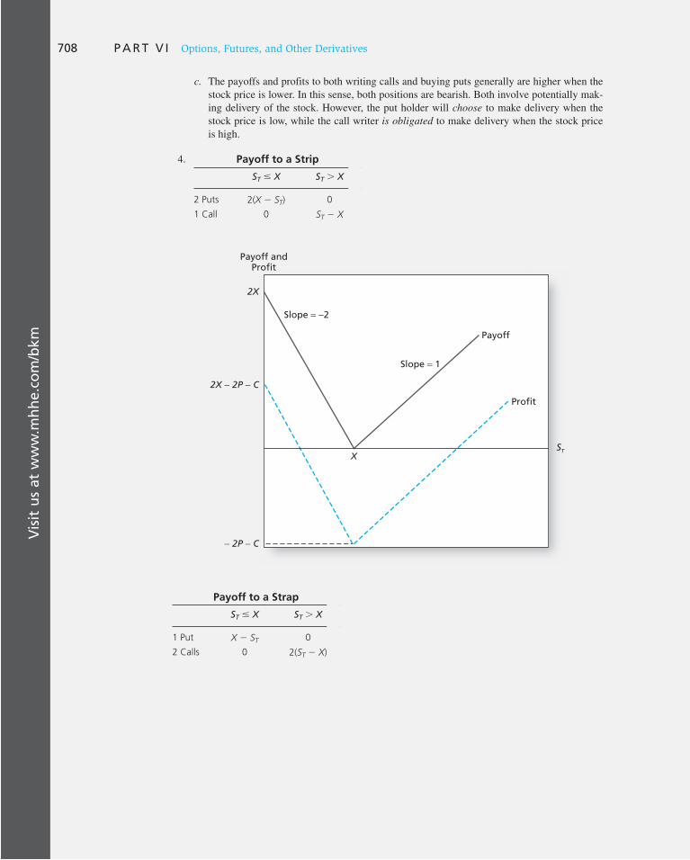
Vis
it u
s at
ww
w.m
hh
e.co
m/b
km708 P A R T V I Options, Futures, and Other Derivatives
c. The payoffs and profits to both writing calls and buying puts generally are higher when the stock price is lower. In this sense, both positions are bearish. Both involve potentially mak-ing delivery of the stock. However, the put holder will choose to make delivery when the stock price is low, while the call writer is obligated to make delivery when the stock price is high.
4. Payoff to a Strip
ST # X ST . X
2 Puts 2(X 2 ST) 0
1 Call 0 ST 2 X
Slope 2
Slope 1
Payoff andProfit
Payoff
Profit
2P C
2X 2P C
X
2X
ST
Payoff to a Strap
ST # X ST . X
1 Put X 2 ST 0
2 Calls 0 2(ST 2 X)

Vis
it u
s at
ww
w.m
hh
e.co
m/b
km
C H A P T E R 2 0 Options Markets: Introduction 709
Slope 1
Slope 2
Payoff andProfit
Payoff
Profit
P 2C
X P 2C
X
ST
X
5. The payoff table on a per-share basis is as follows:
ST # 90 90 # ST # 110 ST . 110
Buy put (X 5 90) 90 2 ST 0 0
Share ST ST ST
Write call (X 5 110) 0 0 2(ST 2 110)
TOTAL 90 ST 110
The graph of the payoff is as follows. If you multiply the per-share values by 2,000, you will see that the collar provides a minimum payoff of $180,000 (representing a maximum loss of $20,000) and a maximum payoff of $220,000 (which is the cost of the house).

Vis
it u
s at
ww
w.m
hh
e.co
m/b
km710 P A R T V I Options, Futures, and Other Derivatives
6. The covered call strategy would consist of a straight bond with a call written on the bond. The value of the strategy at option expiration as a function of the value of the straight bond is given by the solid colored payoff line in the figure following, which is virtually identical to Figure 20.11 .
Value of Straight Bond
Call Written
Value of Straight Bond
Payoff of Covered Call
X
7. The call option is worth less as call protection is expanded. Therefore, the coupon rate need not be as high.
8. Lower. Investors will accept a lower coupon rate in return for the conversion option.
9. The depositor’s implicit cost per dollar invested is now only ($.03 2 $.005)/1.03 5 $.02427 per 6-month period. Calls cost 50/1,000 5 $.05 per dollar invested in the index. The multiplier falls to .02427/.05 5 .4854.
$90
$110
$90 $110
Collar
Payoff
ST

IN THE PREVIOUS chapter we examined option
markets and strategies. We noted that many
securities contain embedded options that affect
both their values and their risk–return charac-
teristics. In this chapter, we turn our attention
to option-valuation issues. To understand most
option-valuation models requires considerable
mathematical and statistical background. Still,
many of the ideas and insights of these models
can be demonstrated in simple examples, and
we will concentrate on these.
We start with a discussion of the factors
that ought to affect option prices. After
this discussion, we present several bounds
within which option prices must lie. Next we
turn to quantitative models, starting with a
simple “two-state” option-valuation model,
and then showing how this approach can be
generalized into a useful and accurate pric-
ing tool. We then move on to one particular
valuation formula, the famous Black-Scholes
model, one of the most significant break-
throughs in finance theory in several decades.
Finally, we look at some of the more impor-
tant applications of option-pricing theory in
portfolio management and control.
Option-pricing models allow us to “back
out” market estimates of stock-price volatil-
ity, and we will examine these measures of
implied volatility. Next we turn to some of
the more important applications of option-
pricing theory in risk management. Finally, we
take a brief look at some of the empirical evi-
dence on option pricing, and the implications
of that evidence concerning the li mitations of
the Black-Scholes model.
21 Option Valuation 1 PA
RT V
I CHAPTER TWENTY-ONE
21.1 Option Valuation: Introduction
Intrinsic and Time Values
Consider a call option that is out of the money at the moment, with the stock price below the exercise price. This does not mean the option is valueless. Even though immediate exercise today would be unprofitable, the call retains a positive value because there is always a chance the stock price will increase sufficiently by the expiration date to allow for profitable exercise. If not, the worst that can happen is that the option will expire with zero value.

712 P A R T V I Options, Futures, and Other Derivatives
The value S 0 2 X is sometimes called the intrinsic value of in-the-money call options because it gives the payoff that could be obtained by immediate exercise. Intrinsic value is set equal to zero for out-of-the-money or at-the-money options. The difference between the actual call price and the intrinsic value is commonly called the time value of the option.
“Time value” is an unfortunate choice of terminology, because it may confuse the option’s time value with the time value of money. Time value in the options context refers simply to the difference between the option’s price and the value the option would have if it were expiring immediately. It is the part of the option’s value that may be attributed to the fact that it still has positive time to expiration.
Most of an option’s time value typically is a type of “volatility value.” Because the option holder can choose not to exercise, the payoff cannot be worse than zero. Even if a call option is out of the money now, it still will sell for a positive price because it offers the potential for a profit if the stock price increases, while imposing no risk of additional loss should the stock price fall. The volatility value lies in the value of the right not to exercise the call if that action would be unprofitable. The option to exercise, as opposed to the obli-gation to exercise, provides insurance against poor stock price performance.
As the stock price increases substantially, it becomes likely that the call option will be exercised by expiration. Ultimately, with exercise all but assured, the volatility value becomes minimal. As the stock price gets ever larger, the option value approaches the “adjusted” intrinsic value, the stock price minus the present value of the exercise price, S 0 2 PV( X ).
Why should this be? If you are virtually certain the option will be exercised and the stock purchased for X dollars, it is as though you own the stock already. The stock cer-tificate, with a value today of S 0 , might as well be sitting in your safe-deposit box now, as it will be there in only a few months. You just haven’t paid for it yet. The present value of your obligation is the present value of X, so the net value of the call option is S 0 2 PV( X ). 1
Figure 21.1 illustrates the call option valuation function. The value curve shows that when the stock price is very low, the option is nearly worthless, because there is almost no chance that it will be exercised. When the stock price is very high, the option value approaches adjusted intrinsic value. In the midrange case, where the option is approxi-mately at the money, the option curve diverges from the straight lines corresponding to adjusted intrinsic value. This is because although exercise today would have a negligible (or negative) payoff, the volatility value of the option is quite high in this region.
The call always increases in value with the stock price. The slope is greatest, however, when the option is deep in the money. In this case, exercise is all but assured, and the option increases in price one-for-one with the stock price.
Determinants of Option Values
We can identify at least six factors that should affect the value of a call option: the stock price, the exercise price, the volatility of the stock price, the time to expiration, the inter-est rate, and the dividend rate of the stock. The call option should increase in value with the stock price and decrease in value with the exercise price because the payoff to a call,
1 This discussion presumes that the stock pays no dividends until after option expiration. If the stock does pay dividends before expiration, then there is a reason you would care about getting the stock now rather than at expiration—getting it now entitles you to the interim dividend payments. In this case, the adjusted intrinsic value of the option must subtract the value of the dividends the stock will pay out before the call is exercised. Adjusted intrinsic value would more generally be defined as S 0 2 PV( X ) 2 PV( D ), where D is the dividend to be paid before option expiration.

C H A P T E R 2 1 Option Valuation 713
if exercised, equals S T 2 X. The magnitude of the expected payoff from the call increases with the difference S 0 2 X.
Call option values also increase with the volatility of the underlying stock price. To see why, consider circumstances where possible stock prices at expiration may range from $10 to $50 compared to a situation where stock prices may range only from $20 to $40. In both cases, the expected, or average, stock price will be $30. Suppose the exercise price on a call option is also $30. What are the option payoffs?
High-Volatility Scenario
Stock price $10 $20 $30 $40 $50
Option payoff 0 0 0 10 20
Low-Volatility Scenario
Stock price $20 $25 $30 $35 $40
Option payoff 0 0 0 5 10
If each outcome is equally likely, with probability .2, the expected payoff to the option under high-volatility conditions will be $6, but under low-volatility conditions the expected payoff to the call option is half as much, only $3.
Despite the fact that the average stock price in each scenario is $30, the average option payoff is greater in the high-volatility scenario. The source of this extra value is the limited loss an option holder can suffer, or the volatility value of the call. No matter how far below
Option Value
Out of theMoney
In the Money
S0
Time Value
PV(X) X
Value of Call OptionS0 – PV(X)
Value of optionif now atexpiration = S – X =Intrinsic value
Figure 21.1 Call option value before expiration
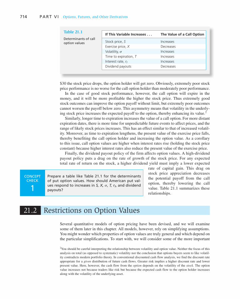
714 P A R T V I Options, Futures, and Other Derivatives
$30 the stock price drops, the option holder will get zero. Obviously, extremely poor stock price performance is no worse for the call option holder than moderately poor performance.
In the case of good stock performance, however, the call option will expire in the money, and it will be more profitable the higher the stock price. Thus extremely good stock outcomes can improve the option payoff without limit, but extremely poor outcomes c annot worsen the payoff below zero. This asymmetry means that volatility in the underly-ing stock price increases the expected payoff to the option, thereby enhancing its value. 2
Similarly, longer time to expiration increases the value of a call option. For more distant expiration dates, there is more time for unpredictable future events to affect prices, and the range of likely stock prices increases. This has an effect similar to that of increased volatil-ity. Moreover, as time to expiration lengthens, the present value of the exercise price falls, thereby benefiting the call option holder and increasing the option value. As a corollary to this issue, call option values are higher when interest rates rise (holding the stock price constant) because higher interest rates also reduce the present value of the exercise price.
Finally, the dividend payout policy of the firm affects option values. A high-dividend payout policy puts a drag on the rate of growth of the stock price. For any expected total rate of return on the stock, a higher dividend yield must imply a lower expected
rate of capital gain. This drag on stock price appreciation decreases the potential payoff from the call option, thereby lowering the call value. Table 21.1 summarizes these relationships.
Several quantitative models of option pricing have been devised, and we will examine some of them later in this chapter. All models, however, rely on simplifying assumptions. You might wonder which properties of option values are truly general and which depend on the particular simplifications. To start with, we will consider some of the more im portant
2 You should be careful interpreting the relationship between volatility and option value. Neither the focus of this analysis on total (as opposed to systematic) volatility nor the conclusion that options buyers seem to like volatil-ity contradicts modern portfolio theory. In conventional discounted cash flow analysis, we find the discount rate appropriate for a given distribution of future cash flows. Greater risk implies a higher discount rate and lower present value. Here, however, the cash flow from the option depends on the volatility of the stock. The option value increases not because traders like risk but because the expected cash flow to the option holder increases along with the volatility of the underlying asset.
If This Variable Increases . . . The Value of a Call Option
Stock price, S Increases
Exercise price, X Decreases
Volatility, s Increases
Time to expiration, T Increases
Interest rate, rf Increases
Dividend payouts Decreases
Table 21.1
Determinants of call option values
CONCEPT CHECK
1
Prepare a table like Table 21.1 for the determinants of put option values. How should American put val-ues respond to increases in S, X, s, T, r f , and dividend payouts?
21.2 Restrictions on Option Values

C H A P T E R 2 1 Option Valuation 715
general properties of option prices. Some of these properties have important implications for the effect of stock dividends on option values and the possible profitability of early exercise of an American option.
Restrictions on the Value of a Call Option
The most obvious restriction on the value of a call option is that its value cannot be nega-tive. Because the option need not be exercised, it cannot impose any liability on its holder; moreover, as long as there is any possibility that at some point the option can be exercised profitably, the option will command a positive price. Its payoff is zero at worst, and pos-sibly positive, so that investors are willing to pay some amount to purchase it.
We can place another lower bound on the value of a call option. Suppose that the stock will pay a dividend of D dollars just before the expiration date of the option, denoted by T (where today is time 0). Now compare two portfolios, one consisting of a call option on one share of stock and the other a leveraged equity position consisting of that share and borrowing of ( X 1 D )/(1 1 r f )
T dollars. The loan repayment is X 1 D dollars, due on the expiration date of the option. For example, for a half-year maturity option with exercise price $70, dividends to be paid of $5, and effective annual interest of 10%, you would pur-chase one share of stock and borrow $75/(1.10) 1/2 5 $71.51. In 6 months, when the loan matures, the payment due is $75.
At that time, the payoff to the leveraged equity position would be
In General Our Numbers
Stock value ST 1 D ST 1 5
2 Payback of loan 2(X 1 D) 275
TOTAL ST 2 X ST 2 70
where S T denotes the stock price at the option expiration date. Notice that the payoff to the stock is the ex-dividend stock value plus dividends received. Whether the total payoff to the stock-plus-borrowing position is positive or negative depends on whether S T exceeds X. The net cash outlay required to establish this leveraged equity position is S 0 2 $71.51, or, more generally, S 0 2 ( X 1 D )/(1 1 r f )
T , that is, the current price of the stock, S 0 , less the initial cash inflow from the borrowing position.
The payoff to the call option will be S T 2 X if the option expires in the money and zero otherwise. Thus the option payoff is equal to the leveraged equity payoff when that payoff is positive and is greater when the leveraged equity position has a negative payoff. Because the option payoff is always greater than or equal to that of the leveraged equity position, the option price must exceed the cost of establishing that position.
Therefore, the value of the call must be greater than S 0 2 ( X 1 D )/(1 1 r f ) T , or, more
generally,
C $ S0 2 PV(X) 2 PV(D)
where PV( X ) denotes the present value of the exercise price and PV( D ) is the present value of the dividends the stock will pay at the option’s expiration. More generally, we can inter-pret PV( D ) as the present value of any and all dividends to be paid prior to the option expi-ration date. Because we know already that the value of a call option must be nonnegative, we may conclude that C is greater than the maximum of either 0 or S 0 2 PV( X ) 2 PV( D ).
We also can place an upper bound on the possible value of the call; this bound is simply the stock price. No one would pay more than S 0 dollars for the right to purchase a stock currently worth S 0 dollars. Thus C # S 0 .

716 P A R T V I Options, Futures, and Other Derivatives
Figure 21.2 demonstrates graphically the range of prices that is ruled out by these upper and lower bounds for the value of a call option. Any option value outside the shaded area is not possible according to the restric-tions we have derived. Before expiration, the call option value normally will be within the allowable range, touching neither the upper nor lower bound, as in Figure 21.3 .
Early Exercise and Dividends
A call option holder who wants to close out that position has two choices: exercise the call or sell it. If the holder exercises at time t, the call will provide a payoff of S t 2 X, assuming, of course, that the option is in the money. We have just seen that the option can be sold for at least S t 2 PV( X ) 2 PV ( D ). Therefore, for an option on a non-dividend-paying stock, C is greater than S t 2 PV ( X ). Because the present value of X is less than X itself, it follows that
C $ St 2 PV(X) . St 2 X
The implication here is that the proceeds from a sale of the option (at price C ) must exceed the proceeds from an exercise ( S t 2 X ). It is economically more attractive to sell the call, which keeps it alive, than to exercise and thereby end the option. In other words, calls on non-dividend-paying stocks are “worth more alive than dead.”
If it never pays to exercise a call option before expiration, the right to exercise early actually must be valueless. The right to exer-cise an American call early is irrelevant because it will never pay to exercise early. We therefore conclude that the values of otherwise identical American and European call options on stocks paying no dividends are equal. If we can find the value for the European call, we also will have found the value of the American call. This simplifies matters, because any valu-ation formula that applies to the European call, for which only one exercise date need be con-sidered, also must apply to an American call.
As most stocks do pay dividends, you may wonder whether this result is just a theoreti-cal curiosity. It is not: Reconsider our argument and you will see that all that we really require is that the stock pay no dividends until the option expires. This condition will be true for many real-world options.
Call Value
Lower Bound� Adjusted intrinsic value� S0 � PV(X) � PV(D)
Upper
Bound �
S 0
Allo
wab
le R
ange
PV(X) � PV(D)S0
Figure 21.2 Range of possible call option values
Value of Call forGiven Stock Price
C
S0
PV(X) � PV(D)
Figure 21.3 Call option value as a function of the c urrent stock price

C H A P T E R 2 1 Option Valuation 717
Early Exercise of American Puts
For American put options, the optimality of early exercise is most definitely a possibil-ity. To see why, consider a simple example. Suppose that you purchase a put option on a stock. Soon the firm goes bankrupt, and the stock price falls to zero. Of course you want to exercise now, because the stock price can fall no lower. Immediate exercise gives you immediate receipt of the exercise price, which can be invested to start generating income. Delay in exercise means a time-value-of-money cost. The right to exercise a put option before expiration must have value.
Now suppose instead that the firm is only nearly bankrupt, with the stock selling at just a few cents. Immediate exercise may still be optimal. After all, the stock price can fall by only a very small amount, meaning that the proceeds from future exercise cannot be more than a few cents greater than the proceeds from immediate exercise. Against this possibil-ity of a tiny increase in proceeds must be weighed the time-value-of-money cost of defer-ring exercise. Clearly, there is some stock price below which early exercise is optimal.
This argument also proves that the American put must be worth more than its European counterpart. The American put allows you to exercise anytime before expiration. Because the right to exercise early may be useful in some circumstances, it will command a pre-mium in the capital market. The American put therefore will sell for a higher price than a European put with otherwise identical terms.
Figure 21.4 A illustrates the value of an American put option as a function of the current stock price, S 0 . Once the stock price drops below a critical value, denoted S * in the figure, exercise becomes optimal. At that point the option-pricing curve is tangent to the straight line depicting the intrinsic value of the option. If and when the stock price reaches S *, the put option is exercised and its payoff equals its intrinsic value.
In contrast, the value of the European put, which is graphed in Figure 21.4 B, is not asymptotic to the intrinsic value line. Because early exercise is prohibited, the maximum value of the European put is PV( X ), which occurs at the point S 0 5 0. Obviously, for a long enough horizon, PV( X ) can be made arbitrarily small.
A. American Put Value B. European Put Value
X X
S* X XPV(X)S0 S0
PV(X)Put Value
TimeValue
Figure 21.4 Put option values as a function of the current stock price
CONCEPT CHECK
2 In light of this discussion, explain why the put-call parity relationship is valid only for E uropean options on non-dividend-paying stocks. If the stock pays no dividends, what inequality for American options would correspond to the parity theorem?

718 P A R T V I Options, Futures, and Other Derivatives
21.3 Binomial Option Pricing
Two-State Option Pricing
A complete understanding of commonly used option-valuation formulas is difficult with-out a substantial mathematics background. Nevertheless, we can develop valuable insight into option valuation by considering a simple special case. Assume that a stock price can take only two possible values at option expiration: The stock will either increase to a given higher price or decrease to a given lower price. Although this may seem an extreme simpli-fication, it allows us to come closer to understanding more complicated and realistic mod-els. Moreover, we can extend this approach to describe far more reasonable specifications of stock price behavior. In fact, several major financial firms employ variants of this simple model to value options and securities with optionlike features.
Suppose the stock now sells at S 0 5 $100, and the price will either increase by a factor of u 5 1.20 to $120 ( u stands for “up”) or fall by a factor of d 5 .9 to $90 ( d stands for “down”) by year-end. A call option on the stock might specify an exercise price of $110 and a time to expiration of 1 year. The interest rate is 10%. At year-end, the payoff to the holder of the call option will be either zero, if the stock falls, or $10, if the stock price goes to $120.
These possibilities are illustrated by the following value “trees”:
120 10
100 C
90 0 Stock price Call option value
Compare the payoff of the call to that of a portfolio consisting of one share of the stock and borrowing of $81.82 at the interest rate of 10%. The payoff of this portfolio also depends on the stock price at year-end:
Value of stock at year-end $90 $120
2 Repayment of loan with interest 290 290
TOTAL $ 0 $ 30
We know the cash outlay to establish the portfolio is $18.18: $100 for the stock, less the $81.82 proceeds from borrowing. Therefore the portfolio’s value tree is
30
18.18
0
The payoff of this portfolio is exactly three times that of the call option for either value of the stock price. In other words, three call options will exactly replicate the payoff to the portfolio; it follows that three call options should have the same price as the cost of estab-lishing the portfolio. Hence the three calls should sell for the same price as this replicating
portfolio. Therefore,
3C 5 $18.18
or each call should sell at C 5 $6.06. Thus, given the stock price, exercise price, interest rate, and volatility of the stock price (as represented by the magnitude of the up or down movements), we can derive the fair value for the call option.
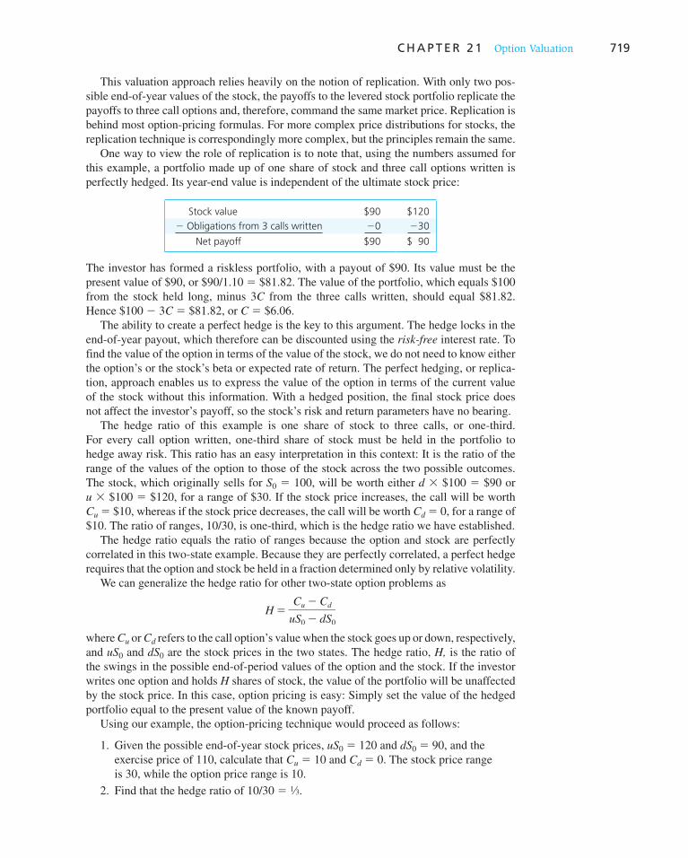
C H A P T E R 2 1 Option Valuation 719
This valuation approach relies heavily on the notion of replication. With only two pos-sible end-of-year values of the stock, the payoffs to the levered stock portfolio replicate the payoffs to three call options and, therefore, command the same market price. Replication is behind most option-pricing formulas. For more complex price distributions for stocks, the replication technique is correspondingly more complex, but the principles remain the same.
One way to view the role of replication is to note that, using the numbers assumed for this example, a portfolio made up of one share of stock and three call options written is perfectly hedged. Its year-end value is independent of the ultimate stock price:
Stock value $90 $120
2 Obligations from 3 calls written 20 230
Net payoff $90 $ 90
The investor has formed a riskless portfolio, with a payout of $90. Its value must be the present value of $90, or $90/1.10 5 $81.82. The value of the portfolio, which equals $100 from the stock held long, minus 3 C from the three calls written, should equal $81.82. Hence $100 2 3 C 5 $81.82, or C 5 $6.06.
The ability to create a perfect hedge is the key to this argument. The hedge locks in the end-of-year payout, which therefore can be discounted using the risk-free interest rate. To find the value of the option in terms of the value of the stock, we do not need to know either the option’s or the stock’s beta or expected rate of return. The perfect hedging, or replica-tion, approach enables us to express the value of the option in terms of the current value of the stock without this information. With a hedged position, the final stock price does not affect the investor’s payoff, so the stock’s risk and return parameters have no bearing.
The hedge ratio of this example is one share of stock to three calls, or one-third. For every call option written, one-third share of stock must be held in the portfolio to hedge away risk. This ratio has an easy interpretation in this context: It is the ratio of the range of the values of the option to those of the stock across the two possible outcomes. The stock, which originally sells for S 0 5 100, will be worth either d 3 $100 5 $90 or u 3 $100 5 $120, for a range of $30. If the stock price increases, the call will be worth C u 5 $10, whereas if the stock price decreases, the call will be worth C d 5 0, for a range of $10. The ratio of ranges, 10/30, is one-third, which is the hedge ratio we have established.
The hedge ratio equals the ratio of ranges because the option and stock are perfectly correlated in this two-state example. Because they are perfectly correlated, a perfect hedge requires that the option and stock be held in a fraction determined only by relative volatility.
We can generalize the hedge ratio for other two-state option problems as
H 5Cu 2 Cd
uS0 2 dS0
where C u or C d refers to the call option’s value when the stock goes up or down, r espectively, and uS 0 and dS 0 are the stock prices in the two states. The hedge ratio, H, is the ratio of the swings in the possible end-of-period values of the option and the stock. If the investor writes one option and holds H shares of stock, the value of the portfolio will be unaffected by the stock price. In this case, option pricing is easy: Simply set the value of the hedged portfolio equal to the present value of the known payoff.
Using our example, the option-pricing technique would proceed as follows:
1. Given the possible end-of-year stock prices, uS 0 5 120 and dS 0 5 90, and the e xercise price of 110, calculate that C u 5 10 and C d 5 0. The stock price range is 30, while the option price range is 10.
2. Find that the hedge ratio of 10/30 5 1⁄3.

720 P A R T V I Options, Futures, and Other Derivatives
3. Find that a portfolio made up of 1⁄3 share with one written option would have an end-of-year value of $30 with certainty.
4. Show that the present value of $30 with a 1-year interest rate of 10% is $27.27.
5. Set the value of the hedged position to the present value of the certain payoff:
1@3 S0 2 C0 5 $27.27
$33.33 2 C0 5 $27.27
6. Solve for the call’s value, C 0 5 $6.06.
What if the option is overpriced, perhaps selling for $6.50? Then you can make arbi-trage profits. Here is how:
Cash Flow in 1 Year for Each Possible Stock Price
Initial Cash Flow S1 5 90 S1 5 120
1. Write 3 options $ 19.50 $ 0 $230
2. Purchase 1 share 2100 90 120
3. Borrow $80.50 at 10% interest
Repay in 1 year
80.50 288.55 288.55
TOTAL $ 0 $ 1.45 $ 1.45
Although the net initial investment is zero, the payoff in 1 year is positive and riskless. If the option were underpriced, one would simply reverse this arbitrage strategy: Buy the option, and sell the stock short to eliminate price risk. Note, by the way, that the present value of the profit to the arbitrage strategy above exactly equals three times the amount by which the option is overpriced. The present value of the risk-free profit of $1.45 at a 10% interest rate is $1.318. With three options written in the strategy above, this translates to a profit of $.44 per option, exactly the amount by which the option was overpriced: $6.50 versus the “fair value” of $6.06.
CONCEPT CHECK
3
Suppose the call option had been underpriced, selling at $5.50. Formulate the arbitrage strategy to exploit the mispricing, and show that it provides a riskless cash flow in 1 year of $.6167 per option purchased. Compare the present value of this cash flow to the option mispricing.
Generalizing the Two-State Approach
Although the two-state stock price model seems simplistic, we can generalize it to incor-porate more realistic assumptions. To start, suppose we were to break up the year into two 6-month segments, and then assert that over each half-year segment the stock price could take on two values. We will say it can increase 10% (i.e., u 5 1.10) or decrease 5% (i.e., d 5 .95). A stock initially selling at 100 could follow these possible paths over the course of the year:
121 110 100 104.50 95
90.25

C H A P T E R 2 1 Option Valuation 721
The midrange value of 104.50 can be attained by two paths: an increase of 10% followed by a decrease of 5%, or a decrease of 5% followed by a 10% increase.
There are now three possible end-of-year values for the stock and three for the option:
Cuu
Cu
C Cud 5 Cdu
Cd
Cdd
Using methods similar to those we followed above, we could value C u from know-ledge of C uu and C ud , then value C d from knowledge of C du and C dd , and finally value C from knowledge of C u and C d . And there is no reason to stop at 6-month intervals. We could next break the year into four 3-month units, or twelve 1-month units, or 365 1-day units, each of which would be posited to have a two-state process. Although the calcula-tions become quite numerous and correspondingly tedious, they are easy to program into a computer, and such computer programs are used widely by participants in the options market.
Example 21.1 Binomial Option Pricing
Suppose that the risk-free interest rate is 5% per 6-month period and we wish to value a call option with exercise price $110 on the stock described in the two-period price tree just above. We start by finding the value of C u . From this point, the call can rise to an expiration-date value of C uu 5 $11 (because at this point the stock price is u 3 u 3 S 0 5 $121) or fall to a final value of C ud 5 0 (because at this point, the stock price is u 3 d 3 S 0 5 $104.50, which is less than the $110 exercise price). Therefore the hedge ratio at this point is
H 5Cuu 2 Cud
uuS0 2 udS0
5$11 2 0
$121 2 104.505
2
3
Thus, the following portfolio will be worth $209 at option expiration regardless of the ultimate stock price:
udS 5 $104.50 uuS0 5 $121
Buy 2 shares at price uS0 5 $110 $209 $242
Write 3 calls at price Cu 0 233
TOTAL $209 $209
The portfolio must have a current market value equal to the present value of $209:
2 3 110 2 3Cu 5 $209/1.05 5 $199.047
Solve to find that C u 5 $6.984. Next we find the value of C d . It is easy to see that this value must be zero. If we reach
this point (corresponding to a stock price of $95), the stock price at option expiration will be either $104.50 or $90.25; in either case, the option will expire out of the money. (More formally, we could note that with C ud 5 C dd 5 0, the hedge ratio is zero, and a portfolio of zero shares will replicate the payoff of the call!)
Finally, we solve for C using the values of C u and C d . Concept Check 4 leads you through the calculations that show the option value to be $4.434.

722 P A R T V I Options, Futures, and Other Derivatives
As we break the year into progressively finer subintervals, the range of possible year-end stock prices expands and, in fact, will ultimately take on a familiar bell-shaped distri-bution. This can be seen from an analysis of the event tree for the stock for a period with three subintervals:
u3S0
u2S0
uS0 u2dS0
S0 udS0
dS0 ud2S0
d2S0
d3S0
First, notice that as the number of subintervals increases, the number of possible stock prices also increases. Second, notice that extreme events such as u 3 S 0 or d 3 S 0 are relatively rare, as they require either three consecutive increases or decreases in the three subinter-vals. More moderate, or midrange, results such as u 2 dS 0 can be arrived at by more than one path—any combination of two price increases and one decrease will result in stock price u 2 dS 0 . Thus the midrange values will be more likely. The probability of each outcome is described by the binomial distribution, and this multiperiod approach to option pricing is therefore called the binomial model.
For example, using an initial stock price of $100, equal probability of stock price increases or decreases, and three intervals for which the possible price increase is 20% and decrease is 10%, we can obtain the probability distribution of stock prices from the following calculations. There are eight possible combinations for the stock price move-ments in the three periods: uuu, uud, udu, duu, udd, dud, ddu, ddd. Each has probability of 1⁄8. Therefore, the probability distribution of stock prices at the end of the last interval would be:
Event Probability Final Stock Price
3 up movements 1/8 100 3 1.203 5 72.90
2 up and 1 down 3/8 100 3 1.202 3 .90 5 97.20
1 up and 2 down 3/8 100 3 1.20 3 .902 5 129.60
3 down movements 1/8 100 3 .903 5 172.80
Notice that the midrange values are three times as likely to occur as the extreme values. Figure 21.5 A is a graph of the frequency distribution for this example. Suppose now that we were to take the full holding period and divide it into six subintervals instead of
CONCEPT CHECK
4
Show that the initial value of the call option in Example 21.1 is $4.434.
a. Confirm that the spread in option values is C u 2 C d 5 $6.984.
b. Confirm that the spread in stock values is uS 0 2 dS 0 5 $15.
c. Confirm that the hedge ratio is .4656 shares purchased for each call written.
d. Demonstrate that the value in one period of a portfolio comprised of .4656 shares and one call written is riskless.
e. Calculate the present value of this payoff.
f. Solve for the option value.
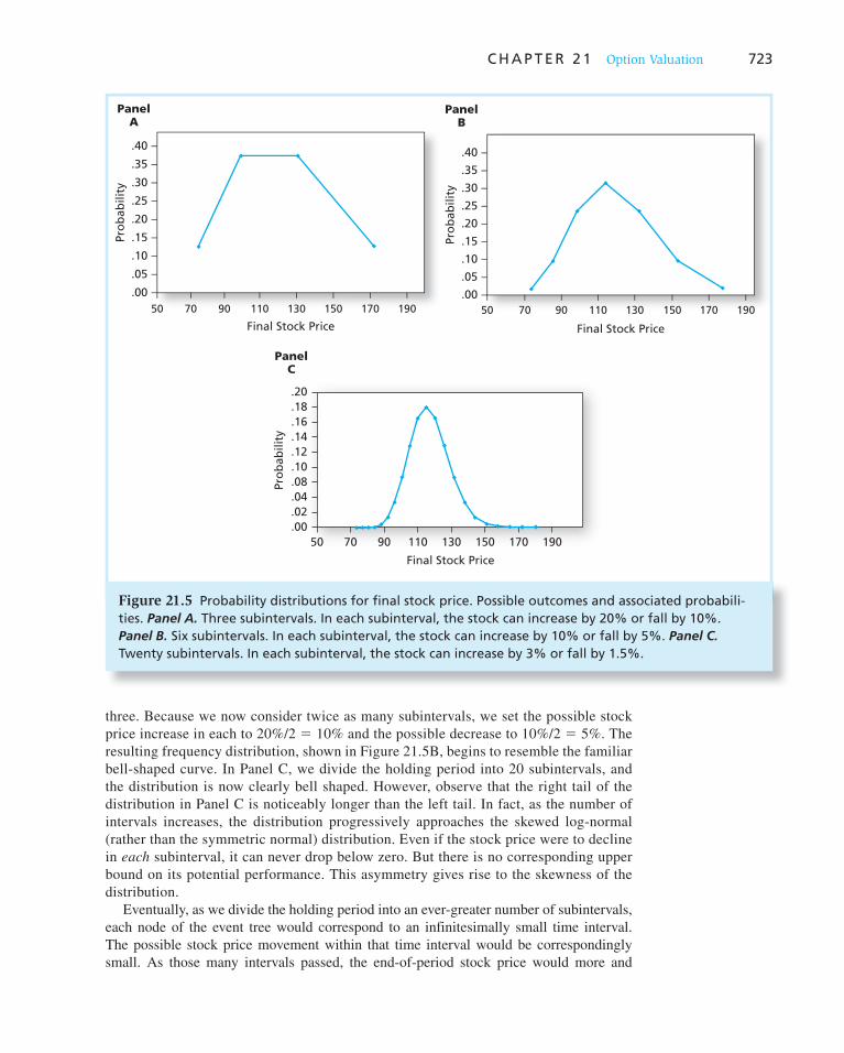
C H A P T E R 2 1 Option Valuation 723
three. Because we now consider twice as many subintervals, we set the possible stock price increase in each to 20%/2 5 10% and the possible decrease to 10%/2 5 5%. The resulting frequency distribution, shown in Figure 21.5 B, begins to resemble the familiar bell-shaped curve. In Panel C, we divide the holding period into 20 subintervals, and the distribution is now clearly bell shaped. However, observe that the right tail of the distribution in Panel C is noticeably longer than the left tail. In fact, as the number of intervals increases, the distribution progressively approaches the skewed log-normal (rather than the symmetric normal) distribution. Even if the stock price were to decline in each subinterval, it can never drop below zero. But there is no corresponding upper bound on its potential performance. This asymmetry gives rise to the skewness of the distribution.
Eventually, as we divide the holding period into an ever-greater number of subintervals, each node of the event tree would correspond to an infinitesimally small time interval. The possible stock price movement within that time interval would be correspondingly small. As those many intervals passed, the end-of-period stock price would more and
PanelA
.40
.35
.30
.25
.20
.15
.10
.05
.00
50 70 90 110 130 150 170 190
Final Stock Price
Pro
bab
ilit
yPanel
B
.40
.35
.30
.25
.20
.15
.10
.05
.00
50 70 90 110 130 150 170 190
Final Stock Price
Pro
bab
ilit
y
PanelC
.20
.18
.16
.14
.12
.10
.08
.04
.02
.00
50 70 90 110 130 150 170 190
Pro
bab
ilit
y
Final Stock Price
Figure 21.5 Probability distributions for final stock price. Possible outcomes and associated probabili-ties. Panel A. Three subintervals. In each subinterval, the stock can increase by 20% or fall by 10%. Panel B. Six subintervals. In each subinterval, the stock can increase by 10% or fall by 5%. Panel C. Twenty subintervals. In each subinterval, the stock can increase by 3% or fall by 1.5%.

724 P A R T V I Options, Futures, and Other Derivatives
more closely resemble a lognormal distribution. 3 Thus the apparent oversimplification of the two-state model can be overcome by progressively subdividing any period into many subperiods.
At any node, one still could set up a portfolio that would be perfectly hedged over the next tiny time interval. Then, at the end of that interval, on reaching the next node, a new hedge ratio could be computed and the portfolio composition could be revised to remain hedged over the coming small interval. By continuously revising the hedge posi-tion, the portfolio would remain hedged and would earn a riskless rate of return over each interval. This is called dynamic hedging, the continued updating of the hedge ratio as time passes. As the dynamic hedge becomes ever finer, the resulting option-valuation procedure becomes more precise.
Although the binomial model we have described is extremely flexible, a computer is needed for it to be useful in actual trading. An option-pricing formula would be far easier to use than the complex algorithm involved in the binomial model. It turns out that such a formula can be derived if one is willing to make just two more assumptions: that both the risk-free interest rate and stock price volatility are constant over the life of the option. In this case, as the time to expiration is divided into ever-more subperiods, the distribution of the stock price at expiration progressively approaches the lognormal distribution, as suggested by Figure 21.5 . When the stock price distribution is actually lognormal, we can derive an exact option-pricing formula.
The Black-Scholes Formula
Financial economists searched for years for a workable option-pricing model before Black and Scholes 4 and Merton 5 derived a formula for the value of a call option. Scholes and Merton shared the 1997 Nobel Prize in Economics for their accomplishment. 6 Now
3 Actually, more complex considerations enter here. The limit of this process is lognormal only if we assume also that stock prices move continuously, by which we mean that over small time intervals only small price movements can occur. This rules out rare events such as sudden, extreme price moves in response to dramatic information (like a takeover attempt). For a treatment of this type of “jump process,” see John C. Cox and Stephen A. Ross, “The Valuation of Options for Alternative Stochastic Processes,” Journal of Financial Economics 3 (January–March 1976), pp. 145–66, or Robert C. Merton, “Option Pricing When Underlying Stock Returns Are Discontinuous,” Journal of Financial Economics 3 (January–March 1976), pp. 125–44.
4 Fischer Black and Myron Scholes, “The Pricing of Options and Corporate Liabilities,” Journal of Political
Economy 81 (May–June 1973).
5 Robert C. Merton, “Theory of Rational Option Pricing,” Bell Journal of Economics and Management Science 4 (Spring 1973).
6 Fischer Black died in 1995.
CONCEPT CHECK
5
Would you expect the hedge ratio to be higher or lower when the call option is more in the money? (Hint: Remember that the hedge ratio is the change in the option price divided by the change in the stock price. When is the option price most sensitive to the stock price?)
21.4 Black-Scholes Option Valuation

C H A P T E R 2 1 Option Valuation 725
widely used by options market participants, the Black-Scholes pricing formula for a call option is
C0 5 S0N(d1) 2 Xe2r TN(d2) (21.1)
where
d1 5ln(S0 / X) 1 (r 1 s2 / 2)T
s"T
d2 5 d1 2 s"T
and
C 0 5 Current call option value.
S0 5 Current stock price.
N ( d ) 5 The probability that a random draw from a standard normal distribution will be less than d. This equals the area under the normal curve up to d, as in the shaded area of Figure 21.6 . In Excel, this function is called NORMSDIST( ).
X 5 Exercise price.
e 5 The base of the natural log function, approximately 2.71828. In Excel, e x can be evaluated using the function EXP( x ).
r 5 Risk-free interest rate (the annualized continuously compounded rate on a safe asset with the same maturity as the expiration date of the option, which is to be distinguished from r f , the discrete period interest rate).
T 5 Time to expiration of option, in years.
ln 5 Natural logarithm function. In Excel, ln( x ) can be calculated as LN( x ).
s 5 Standard deviation of the annualized continuously compounded rate of return of the stock.
Notice a surprising feature of Equation 21.1 : The option value does not depend on the expected rate of return on the stock. In a sense, this information is already built into the formula with the inclusion of the stock price, which itself depends on the stock’s risk and return characteristics. This version of the Black-Scholes formula is predicated on the assumption that the stock pays no dividends.
Although you may find the Black-Scholes formula intimidating, we can explain it at a somewhat intuitive level. The trick is to view the N ( d ) terms (loosely) as risk-adjusted probabilities that the call option will expire in the money. First, look at Equation 21.1 assuming both N ( d ) terms are close to 1.0, that is, when there is a very high probability the option will be exercised. Then the call option value is equal to S 0 2 Xe 2 rT , which is what we called earlier the adjusted intrin-sic value, S 0 2 PV( X ). This makes sense; if exercise is certain, we have a claim on a stock with c urrent value S 0 , and an obligation with p resent value PV( X ), or, with continuous com-pounding, Xe 2 rT .
N(d) = Shaded area
d0
Figure 21.6 A standard normal curve

726 P A R T V I Options, Futures, and Other Derivatives
Now look at Equation 21.1 assuming the N ( d ) terms are close to zero, meaning the option almost certainly will not be exercised. Then the equation confirms that the call is worth nothing. For middle-range values of N ( d ) between 0 and 1, Equation 21.1 tells us that the call value can be viewed as the present value of the call’s potential payoff adjusting for the probability of in-the-money expiration.
How do the N ( d ) terms serve as risk-adjusted probabilities? This question quickly leads us into advanced statistics. Notice, however, that ln( S 0 / X ), which appears in the numera-tor of d 1 and d 2 , is approximately the percentage amount by which the option is currently in or out of the money. For example, if S 0 5 105 and X 5 100, the option is 5% in the money, and ln(105/100) 5 .049. Similarly, if S 0 5 95, the option is 5% out of the money,
and ln(95/100) 5 2 .051. The denominator, s"T, adjusts the amount by which the option is in or out of the money for the volatility of the stock price over the remaining life of the option. An option in the money by a given percent is more likely to stay in the money if both stock price volatility and time to expiration are low. Therefore, N ( d 1 ) and N ( d 2 ) increase with the probability that the option will expire in the money.
Example 21.2 Black-Scholes Valuation
You can use the Black-Scholes formula fairly easily. Suppose you want to value a call option under the following circumstances:
Stock price: S 0 5 100
Exercise price: X 5 95
Interest rate: r 5 .10 (10% per year)
Time to expiration: T 5 .25 (3 months or one-quarter of a year)
Standard deviation: s 5 .50 (50% per year)
First calculate
d1 5ln(100 / 95) 1 (.10 1 .52 / 2).25
.5".255 .43
d2 5 .43 2 .5".25 5 .18
Next find N ( d 1 ) and N ( d 2 ). The values of the normal distribution are tabulated and may be found in many statistics textbooks. A table of N ( d ) is provided here as Table 21.2 . The normal distribution function, N ( d ), is also provided in any spreadsheet program. In Microsoft Excel, for example, the function name is NORMSDIST. Using either Excel or Table 21.2 we find that
N(.43) 5 .6664
N(.18) 5 .5714
Thus the value of the call option is
C 5 100 3 .6664 2 95e2.103.25 3 .5714
5 66.64 2 52.94 5 $13.70
CONCEPT CHECK
6 Recalculate the value of the call option in Example 21.2 using a standard deviation of .6 instead of .5. Confirm that the option is worth more using the higher stock-return volatility.

C H A P T E R 2 1 Option Valuation 727
d N(d ) d N(d ) d N(d ) d N(d ) d N(d ) d N(d )
23.00 .0013 21.58 .0571 20.76 .2236 0.06 .5239 0.86 .8051 1.66 .9515
22.95 .0016 21.56 .0594 20.74 .2297 0.08 .5319 0.88 .8106 1.68 .9535
22.90 .0019 21.54 .0618 20.72 .2358 0.10 .5398 0.90 .8159 1.70 .9554
22.85 .0022 21.52 .0643 20.70 .2420 0.12 .5478 0.92 .8212 1.72 .9573
22.80 .0026 21.50 .0668 20.68 .2483 0.14 .5557 0.94 .8264 1.74 .9591
22.75 .0030 21.48 .0694 20.66 .2546 0.16 .5636 0.96 .8315 1.76 .9608
22.70 .0035 21.46 .0721 20.64 .2611 0.18 .5714 0.98 .8365 1.78 .9625
22.65 .0040 21.44 .0749 20.62 .2676 0.20 .5793 1.00 .8414 1.80 .9641
22.60 .0047 21.42 .0778 20.60 .2743 0.22 .5871 1.02 .8461 1.82 .9656
22.55 .0054 21.40 .0808 20.58 .2810 0.24 .5948 1.04 .8508 1.84 .9671
22.50 .0062 21.38 .0838 20.56 .2877 0.26 .6026 1.06 .8554 1.86 .9686
22.45 .0071 21.36 .0869 20.54 .2946 0.28 .6103 1.08 .8599 1.88 .9699
22.40 .0082 21.34 .0901 20.52 .3015 0.30 .6179 1.10 .8643 1.90 .9713
22.35 .0094 21.32 .0934 20.50 .3085 0.32 .6255 1.12 .8686 1.92 .9726
22.30 .0107 21.30 .0968 20.48 .3156 0.34 .6331 1.14 .8729 1.94 .9738
22.25 .0122 21.28 .1003 20.46 .3228 0.36 .6406 1.16 .8770 1.96 .9750
22.20 .0139 21.26 .1038 20.44 .3300 0.38 .6480 1.18 .8810 1.98 .9761
22.15 .0158 21.24 .1075 20.42 .3373 0.40 .6554 1.20 .8849 2.00 .9772
22.10 .0179 21.22 .1112 20.40 .3446 0.42 .6628 1.22 .8888 2.05 .9798
22.05 .0202 21.20 .1151 20.38 .3520 0.44 .6700 1.24 .8925 2.10 .9821
22.00 .0228 21.18 .1190 20.36 .3594 0.46 .6773 1.26 .8962 2.15 .9842
21.98 .0239 21.16 .1230 20.34 .3669 0.48 .6844 1.28 .8997 2.20 .9861
21.96 .0250 21.14 .1271 20.32 .3745 0.50 .6915 1.30 .9032 2.25 .9878
21.94 .0262 21.12 .1314 20.30 .3821 0.52 .6985 1.32 .9066 2.30 .9893
21.92 .0274 21.10 .1357 20.28 .3897 0.54 .7054 1.34 .9099 2.35 .9906
21.90 .0287 21.08 .1401 20.26 .3974 0.56 .7123 1.36 .9131 2.40 .9918
21.88 .0301 21.06 .1446 20.24 .4052 0.58 .7191 1.38 .9162 2.45 .9929
21.86 .0314 21.04 .1492 20.22 .4129 0.60 .7258 1.40 .9192 2.50 .9938
21.84 .0329 21.02 .1539 20.20 .4207 0.62 .7324 1.42 .9222 2.55 .9946
21.82 .0344 21.00 .1587 20.18 .4286 0.64 .7389 1.44 .9251 2.60 .9953
21.80 .0359 20.98 .1635 20.16 .4365 0.66 .7454 1.46 .9279 2.65 .9960
21.78 .0375 20.96 .1685 20.14 .4443 0.68 .7518 1.48 .9306 2.70 .9965
21.76 .0392 20.94 .1736 20.12 .4523 0.70 .7580 1.50 .9332 2.75 .9970
21.74 .0409 20.92 .1788 20.10 .4602 0.72 .7642 1.52 .9357 2.80 .9974
21.72 .0427 20.90 .1841 20.08 .4681 0.74 .7704 1.54 .9382 2.85 .9978
21.70 .0446 20.88 .1894 20.06 .4761 0.76 .7764 1.56 .9406 2.90 .9981
21.68 .0465 20.86 .1949 20.04 .4841 0.78 .7823 1.58 .9429 2.95 .9984
21.66 .0485 20.84 .2005 20.02 .4920 0.80 .7882 1.60 .9452 3.00 .9986
21.64 .0505 20.82 .2061 0.00 .5000 0.82 .7939 1.62 .9474 3.05 .9989
21.62 .0526 20.80 .2119 0.02 .5080 0.84 .7996 1.64 .9495
21.60 .0548 20.78 .2177 0.04 .5160
Table 21.2
Cumulative normal distribution

728 P A R T V I Options, Futures, and Other Derivatives
What if the option price in Example 21.2 were $15 rather than $13.70? Is the option mispriced? Maybe, but before betting your fortune on that, you may want to reconsider the valuation analysis. First, like all models, the Black-Scholes formula is based on some simplifying abstractions that make the formula only approximately valid.
Some of the important assumptions underlying the formula are the following:
1. The stock will pay no dividends until after the option expiration date.
2. Both the interest rate, r, and variance rate, s 2 , of the stock are constant (or in slightly more general versions of the formula, both are known functions of time—any changes are perfectly predictable).
3. Stock prices are continuous, meaning that sudden extreme jumps such as those in the aftermath of an announcement of a takeover attempt are ruled out.
Variants of the Black-Scholes formula have been developed to deal with many of these limitations.
Second, even within the context of the Black-Scholes model, you must be sure of the accuracy of the parameters used in the formula. Four of these— S 0 , X, T, and r —are straightforward. The stock price, exercise price, and time to expiration are readily deter-mined. The interest rate used is the money market rate for a maturity equal to that of the option, and the dividend payout is reasonably predictable, at least over short horizons.
The last input, though, the standard deviation of the stock return, is not directly observ-able. It must be estimated from historical data, from scenario analysis, or from the prices of other options, as we will describe momentarily.
We saw in Chapter 5 that the historical variance of stock market returns can be calcu-lated from n observations as follows:
s2 5n
n 2 1an
t51
(rt 2 r )2
n
where r is the average return over the sample period. The rate of return on day t is defined to be consistent with continuous compounding as r t 5 ln( S t / S t 2 1 ). [We note again that the natural logarithm of a ratio is approximately the percentage difference between the numerator and denominator so that ln( S t / S t 2 1 ) is a measure of the rate of return of the stock from time t 2 1 to time t. ] Historical variance commonly is computed using daily returns over periods of several months. Because the volatility of stock returns must be estimated, however, it is always possible that discrepancies between an option price and its Black-Scholes value are simply artifacts of error in the estimation of the stock’s volatility.
In fact, market participants often give the option-valuation problem a different twist. Rather than calculating a Black-Scholes option value for a given stock’s standard devia-tion, they ask instead: What standard deviation would be necessary for the option price that I observe to be consistent with the Black-Scholes formula? This is called the implied vola-
tility of the option, the volatility level for the stock implied by the option price. 7 Investors can then judge whether they think the actual stock standard deviation exceeds the implied volatility. If it does, the option is considered a good buy; if actual volatility seems greater than the implied volatility, its fair price would exceed the observed price.
Another variation is to compare two options on the same stock with equal expiration dates but different exercise prices. The option with the higher implied volatility would be
7 This concept was introduced in Richard E. Schmalensee and Robert R. Trippi, “Common Stock Volatility Expectations Implied by Option Premia,” Journal of Finance 33 (March 1978), pp. 129–47.

C H A P T E R 2 1 Option Valuation 729
considered relatively expensive, because a higher standard deviation is required to justify its price. The analyst might consider buying the option with the lower implied volatility and writing the option with the higher implied volatility.
The Black-Scholes valuation formula, as well as implied volatilities, are easily calcu-lated using an Excel spreadsheet like Spreadsheet 21.1 . The model inputs are provided in column B, and the outputs are given in column E. The formulas for d 1 and d 2 are provided in the spreadsheet, and the Excel formula NORMSDIST( d 1 ) is used to calculate N ( d 1 ). Cell E6 contains the Black-Scholes formula. (The formula in the spreadsheet actually includes an adjustment for dividends, as described in the next section.)
To compute an implied volatility, we can use the Goal Seek command from the Tools menu in Excel. See Figure 21.7 for an illustration. Goal Seek asks us to change the value of one cell to make the value of another cell (called the target cell) equal to a specific value. For example, if we observe a call option selling for $7 with other inputs as given in the spreadsheet, we can use Goal Seek to change the value in cell B2 (the standard deviation of the stock) to set the option value in cell E6 equal to $7. The target cell, E6, is the call price, and the spreadsheet manipulates cell B2. When you click “OK,” the spreadsheet finds that
Spreadsheet 21.1
Spreadsheet to calculate Black-Scholes call option values
eXce lPlease visit us at www.mhhe.com/bkm
A C D E
1
2
3
4
5
6
7
B
INPUTS
Standard deviation (annual)
Maturity (in years)
Risk-free rate (annual)
Stock price
Exercise price
Dividend yield (annual)
FORMULA FOR OUTPUT IN COLUMN E
(LN(B5/B6)+(B4–B7+.5*B2^2)*B3)/(B2*SQRT(B3))
E2–B2*SQRT(B3)
NORMSDIST(E2)
NORMSDIST(E3)
B5*EXP(–B7*B3)*E4–B6*EXP(–B4*B3)*E5
B6*EXP(–B4*B3)*(1–E5)–B5*EXP(–B7*B3)*(1–E4)
OUTPUTS
d1
d2
N(d1)
N(d2)
B/S call value
B/S put value
0.2783
0.5
0.06
100
105
0
F G H I J
0.0029
–0.1939
0.5012
0.4231
7.0000
8.8968
A
Standard deviation (annual)
Maturity (in years)
Risk-free rate (annual)
Stock price
Exercise price
Dividend yield (annual)
0.2783
0.5
0.06
100
105
0
0.0029
�0.1939
0.5012
0.4231
7.0000
8.8968
(LN(B5/B6)�(B4�B7�.5*B2^2)*B3)/(B2*SQRT(B3))
E2�B2*SQRT(B3)
NORMSDIST(E2)
NORMSDIST(E3)
B5*EXP(�B7*B3)*E4�B6*EXP(�B4*B3)*E5
B6*EXP(�B4*B3)*(1�E5) � B5*EXP(�B7*B3)*(1�E4)
d1
d2
N(d1)
N(d2)
B/S call value
B/S put value
1
2
3
4
5
6
7
8
9
10
11
12
13
14
15
16
17
B C D E F G H I J K
OUTPUTS FORMULA FOR OUTPUT IN COLUMN EINPUTS
Figure 21.7 Using Goal Seek to find implied volatility eXce lPlease visit us at www.mhhe.com/bkm
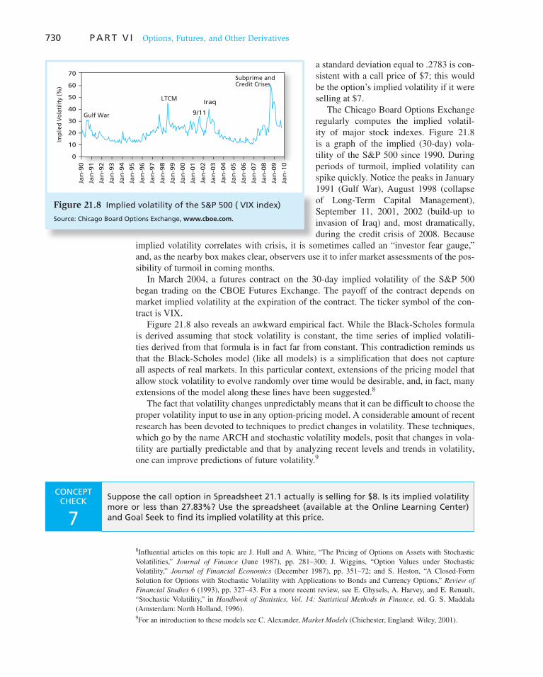
730 P A R T V I Options, Futures, and Other Derivatives
a standard deviation equal to .2783 is con-sistent with a call price of $7; this would be the option’s implied volatility if it were selling at $7.
The Chicago Board Options Exchange regularly computes the implied volatil-ity of major stock indexes. Figure 21.8 is a graph of the implied (30-day) vola-tility of the S&P 500 since 1990. During periods of turmoil, implied volatility can spike quickly. Notice the peaks in January 1991 (Gulf War), August 1998 (collapse of Long-Term Capital Management), September 11, 2001, 2002 (build-up to invasion of Iraq) and, most dramatically, during the credit crisis of 2008. Because
implied volatility correlates with crisis, it is sometimes called an “investor fear gauge,” and, as the nearby box makes clear, observers use it to infer market assessments of the pos-sibility of turmoil in coming months.
In March 2004, a futures contract on the 30-day implied volatility of the S&P 500 began trading on the CBOE Futures Exchange. The payoff of the contract depends on market implied volatility at the expiration of the contract. The ticker symbol of the con-tract is VIX.
Figure 21.8 also reveals an awkward empirical fact. While the Black-Scholes formula is derived assuming that stock volatility is constant, the time series of implied volatili-ties derived from that formula is in fact far from constant. This contradiction reminds us that the Black-Scholes model (like all models) is a simplification that does not capture all aspects of real markets. In this particular context, extensions of the pricing model that allow stock volatility to evolve randomly over time would be desirable, and, in fact, many extensions of the model along these lines have been suggested. 8
The fact that volatility changes unpredictably means that it can be difficult to choose the proper volatility input to use in any option-pricing model. A considerable amount of recent research has been devoted to techniques to predict changes in volatility. These techniques, which go by the name ARCH and stochastic volatility models, posit that changes in vola-tility are partially predictable and that by analyzing recent levels and trends in volatility, one can improve predictions of future volatility. 9
8 Influential articles on this topic are J. Hull and A. White, “The Pricing of Options on Assets with Stochastic Volatilities,” Journal of Finance (June 1987), pp. 281–300; J. Wiggins, “Option Values under Stochastic Volatility,” Journal of Financial Economics (December 1987), pp. 351–72; and S. Heston, “A Closed-Form Solution for Options with Stochastic Volatility with Applications to Bonds and Currency Options,” Review of
Financial Studies 6 (1993), pp. 327–43. For a more recent review, see E. Ghysels, A. Harvey, and E. Renault, “Stochastic Volatility,” in Handbook of Statistics, Vol. 14: Statistical Methods in Finance, ed. G. S. Maddala (Amsterdam: North Holland, 1996). 9 For an introduction to these models see C. Alexander, Market Models (Chichester, England: Wiley, 2001).
LTCM
Gulf War
Jan
-90
Jan
-91
Jan
-92
Jan
-93
Jan
-94
Jan
-95
Jan
-96
Jan
-97
Jan
-98
Jan
-00
Jan
-01
Jan
-02
Jan
-03
Jan
-04
Jan
-05
Jan
-06
Jan
-07
Jan
-08
Jan
-09
Jan
-10
Jan
-99
Subprime andCredit Crises
70
60
50
40
30
20
10
0
Imp
lied
Vo
lati
lity
(%)
Iraq
9/11
Figure 21.8 Implied volatility of the S&P 500 ( VIX index)
Source: Chicago Board Options Exchange, www.cboe.com.
CONCEPT CHECK
7 Suppose the call option in Spreadsheet 21.1 actually is selling for $8. Is its implied volatility more or less than 27.83%? Use the spreadsheet (available at the Online Learning Center) and Goal Seek to find its implied volatility at this price.

731
Dividends and Call Option Valuation
We noted earlier that the Black-Scholes call option formula applies to stocks that do not pay dividends. When dividends are to be paid before the option expires, we need to adjust the formula. The payment of dividends raises the possibility of early exercise, and for most realistic dividend payout schemes the valuation formula becomes significantly more com-plex than the Black-Scholes equation.
We can apply some simple rules of thumb to approximate the option value, however. One popular approach, originally suggested by Black, calls for adjusting the stock price downward by the present value of any dividends that are to be paid before option expi-ration. 10 Therefore, we would simply replace S 0 with S 0 2 PV(dividends) in the Black-Scholes formula. Such an adjustment will take dividends into account by reflecting their eventual impact on the stock price. The option value then may be computed as before, assuming that the option will be held to expiration.
In one special case, the dividend adjustment takes a simple form. Suppose the underly-ing asset pays a continuous flow of income. This might be a reasonable assumption for options on a stock index, where different stocks in the index pay dividends on different days, so that dividend income arrives in a more or less continuous flow. If the dividend yield, denoted d, is constant, one can show that the present value of that dividend flow accruing until the option expiration date is S 0 (1 2 e 2 d T ). (For intuition, notice that e 2 d T approximately equals 1 2 d T, so the value of the dividend is approximately d TS 0 .) In this case, S 0 2 PV(Div) 5 S 0 e 2 d T , and we can derive a Black-Scholes call option formula on the dividend-paying asset simply by substituting S 0 e 2 d T for S 0 in the original formula. This approach is used in Spreadsheet 21.1 .
These procedures yield a very good approximation of option value for European call options that must be held until expiration, but they do not allow for the fact that the holder of an American call option might choose to exercise the option just before a dividend. The current value of a call option, assuming that the option will be exercised just before the ex-dividend date, might be greater than the value of the option assuming it will be held until expiration. Although holding the option until expiration allows greater effective time to
10 Fischer Black, “Fact and Fantasy in the Use of Options,” Financial Analysts Journal 31 (July–August 1975).
The “Fear” Gauge Is Flashing Complacency
Stock-market volatility is back to normal. That could imply more gains ahead, but more likely it means investors have gotten complacent.
The most closely watched volatility measure, the Chicago Board Options Exchange’s VIX index, closed on Friday at 21.25, near its lowest level since August 2008 and near its historical average of 20.28. The VIX, which tracks volatility in S&P 500 options, spiked to more than 80 at the worst of the Lehman Brothers crisis, implying volatility unseen since at least the Great Depression.
A rising VIX is usually associated with falling stock prices, one reason it is often called the “fear” index. It has retreated as the market has soared this year, and it could fall further in the short run.
But volatility lives. One thing apparently bothering traders was the possibility that a stronger job market could lead the Federal Reserve to raise interest rates sooner than expected, snuffing this year’s easy-money-fueled market gains.
But higher rates are only one of many threats to peace and quiet in the coming year. Among others: rising bank losses in commercial real estate and consumer credit, a housing market still oozing foreclosures, municipal and sovereign debt worries, soaring commodities prices and an economic recovery hampered by persistent unemployment and cautious consumer spending.
Stocks can rise amid all kinds of turmoil. But the VIX appears to believe that things have returned to normal, and that is a stretch.
“We’re going to have a sustained level of volatility going forward,” says Milton Balbuena, co–chief investment strategist at Contango Capital Advisors in San Francisco. “Rallies and meltdowns will be part of the process.”
Source: Mark Gongloff, “The ‘Fear’ Gauge Is Flashing Complacency,” The Wall Street Journal, December 7, 2009. Reprinted by permission of The Wall Street Journal, © 2009.
WO
RD
S FRO
M TH
E STREET
732 P A R T V I Options, Futures, and Other Derivatives
expiration, which increases the option value, it also entails more dividend payments, low-ering the expected stock price at expiration and thereby lowering the current option value.
For example, suppose that a stock selling at $20 will pay a $1 dividend in 4 months, whereas the call option on the stock does not expire for 6 months. The effective annual interest rate is 10%, so that the present value of the dividend is $1/(1.10) 1/3 5 $0.97. Black suggests that we can compute the option value in one of two ways:
1. Apply the Black-Scholes formula assuming early exercise, thus using the actual stock price of $20 and a time to expiration of 4 months (the time until the dividend payment).
2. Apply the Black-Scholes formula assuming no early exercise, using the dividend-adjusted stock price of $20 2 $.97 5 $19.03 and a time to expiration of 6 months.
The greater of the two values is the estimate of the option value, recognizing that early exercise might be optimal. In other words, the so-called pseudo-American call
option value is the maximum of the value derived by assuming that the option will be held until expiration and the value derived by assuming that the option will be exercised just before an ex-dividend date. Even this technique is not exact, however, for it assumes that the option holder makes an irrevocable decision now on when to exercise, when in fact the decision is not binding until exercise notice is given. 11
Put Option Valuation
We have concentrated so far on call option valuation. We can derive Black-Scholes European put option values from call option values using the put-call parity theorem. To value the put option, we simply calculate the value of the corresponding call option in Equation 21.1 from the Black-Scholes formula, and solve for the put option value as
P 5 C 1 PV(X) 2 S0
5 C 1 Xe2rT 2 S0 (21.2)
We must calculate the present value of the exercise price using continuous compounding to be consistent with the Black-Scholes formula.
Sometimes, it is easier to work with a put option valuation formula directly. If we sub-stitute the Black-Scholes formula for a call in Equation 21.2 , we obtain the value of a European put option as
P 5 Xe2rT 31 2 N(d2) 42 S0 31 2 N(d1) 4 (21.3)
11 An exact formula for American call valuation on dividend-paying stocks has been developed in Richard Roll, “An Analytic Valuation Formula for Unprotected American Call Options on Stocks with Known Dividends,” Journal of Financial Economics 5 (November 1977). The technique has been discussed and revised in Robert Geske, “A Note on an Analytical Formula for Unprotected American Call Options on Stocks with Known Dividends,” Journal of Financial Economics 7 (December 1979), and Robert E. Whaley, “On the Valuation of American Call Options on Stocks with Known Dividends,” Journal of Financial Economics 9 (June 1981). These are difficult papers, however.
Example 21.3 Black-Scholes Put Valuation
Using data from Example 21.2 ( C 5 $13.70, X 5 $95, S 5 $100, r 5 .10, s 5 .50, and T 5 .25), Equation 21.3 implies that a European put option on that stock with identical exercise price and time to expiration is worth
$95e2.103.25(1 2 .5714) 2 $100(1 2 .6664) 5 $6.35

C H A P T E R 2 1 Option Valuation 733
Dividends and Put Option Valuation
Equation 21.2 or 21.3 is valid for European puts on non-dividend-paying stocks. As we did for call options, if the underlying asset pays a dividend, we can find European put values by substituting S 0 2 PV(Div) for S 0 . Cell E7 in Spreadsheet 21.1 allows for a continuous dividend flow with a dividend yield of d. In that case S 0 2 PV(Div) 5 S 0 e 2 d T .
However, listed put options on stocks are American options that offer the opportunity of early exercise, and we have seen that the right to exercise puts early can turn out to be valu-able. This means that an American put option must be worth more than the corresponding European option. Therefore, Equation 21.2 or 21.3 describes only the lower bound on the true value of the American put. However, in many applications the approximation is very accurate. 12
21.5 Using the Black-Scholes Formula
Hedge Ratios and the Black-Scholes Formula
In the last chapter, we considered two investments in FinCorp stock: 100 shares or 1,000 call options. We saw that the call option position was more sensitive to swings in the stock price than was the all-stock position. To analyze the overall exposure to a stock price more precisely, however, it is necessary to quantify these relative sensitivities. A tool that enables us to summarize the overall exposure of portfolios of options with various exercise prices and times to expiration is the hedge ratio. An option’s hedge ratio is the change in the price of an option for a $1 increase in the stock price. A call option, therefore, has a positive hedge ratio and a put option a negative hedge ratio. The hedge ratio is commonly called the option’s delta.
If you were to graph the option value as a function of the stock value, as we have done for a call option in Figure 21.9 , the hedge ratio is simply the slope of the value curve evalu-ated at the current stock price. For example, suppose the slope of the curve at S 0 5 $120 equals .60. As the stock increases in value by $1, the option increases by approximately $.60, as the figure shows.
For every call option written, .60 share of stock would be needed to hedge the investor’s portfolio. For example, if one writes 10 options and holds six shares of stock, according to the hedge ratio of .6, a $1 increase in stock price will result in a gain of $6 on the stock holdings, whereas the loss on the 10 options written will be 10 3 $.60, an equivalent $6. The stock price movement leaves total wealth unaltered, which is what a hedged position is intended to do. The investor holding the stock and options in proportions dictated by their relative price movements hedges the portfolio.
12 For a more complete treatment of American put valuation, see R. Geske and H. E. Johnson, “The American Put
Valued Analytically,” Journal of Finance 39 (December 1984), pp. 1511–24.
Notice that this value is consistent with put-call parity:
P 5 C 1 PV(X) 2 S0 5 13.70 1 95e2.103.25 2 100 5 6.35
As we noted traders can do, we might then compare this formula value to the actual put price as one step in formulating a trading strategy.

734 P A R T V I Options, Futures, and Other Derivatives
Black-Scholes hedge ratios are particu-larly easy to compute. The hedge ratio for a call is N ( d 1 ), whereas the hedge ratio for a put is N ( d 1 ) 2 1. We defined N ( d 1 ) as part of the Black-Scholes formula in Equation 21.1 . Recall that N ( d ) stands for the area under the standard normal curve up to d. Therefore, the call option hedge ratio must be positive and less than 1.0, whereas the put option hedge ratio is negative and of smaller absolute value than 1.0.
Figure 21.9 verifies the insight that the slope of the call option valuation function is less than 1.0, approaching 1.0 only as the stock price becomes much greater than the exercise price. This tells us that option values change less than one-for-one with changes in stock prices. Why should this be? Suppose an option is so far in the money that you are absolutely certain it will be exercised. In that
case, every dollar increase in the stock price would increase the option value by $1. But if there is a reasonable chance the call option will expire out of the money, even after a moderate stock price gain, a $1 increase in the stock price will not necessarily increase the ultimate payoff to the call; therefore, the call price will not respond by a full dollar.
The fact that hedge ratios are less than 1.0 does not contradict our earlier observation that options offer leverage and are sensitive to stock price movements. Although dollar
movements in option prices are less than dollar movements in the stock price, the rate of
return volatility of options remains greater than stock return volatility because options sell at lower prices. In our example, with the stock selling at $120, and a hedge ratio of .6, an option with exercise price $120 may sell for $5. If the stock price increases to $121, the call price would be expected to increase by only $.60 to $5.60. The percentage increase in the option value is $.60/$5.00 5 12%, however, whereas the stock price increase is only $1/$120 5 .83%. The ratio of the percentage changes is 12%/.83% 5 14.4. For every 1% increase in the stock price, the option price increases by 14.4%. This ratio, the percentage change in option price per percentage change in stock price, is called the option elasticity.
The hedge ratio is an essential tool in portfolio management and control. An example will show why.
Value of a Call (C)
S0
40
20
0
120
Slope 5 .6
Figure 21.9 Call option value and hedge ratio
Example 21.4 Hedge Ratios
Consider two portfolios, one holding 750 IBM calls and 200 shares of IBM and the other holding 800 shares of IBM. Which portfolio has greater dollar exposure to IBM price movements? You can answer this question easily by using the hedge ratio.
Each option changes in value by H dollars for each dollar change in stock price, where H stands for the hedge ratio. Thus, if H equals .6, the 750 options are equivalent to .6 3 750 5 450 shares in terms of the response of their market value to IBM stock price movements. The first portfolio has less dollar sensitivity to stock price change because the 450 share-equivalents of the options plus the 200 shares actually held are less than the 800 shares held in the second portfolio.

735
This is not to say, however, that the first portfolio is less sensitive to the stock’s rate of return. As we noted in discussing option elasticities, the first portfolio may be of lower total value than the second, so despite its lower sensitivity in terms of total market value, it might have greater rate of return sensitivity. Because a call option has a lower market value than the stock, its price changes more than proportionally with stock price changes, even though its hedge ratio is less than 1.0.
eXcel APPLICATIONS: Black-Scholes Option Valuation
T he spreadsheet below can be used to determine option values using the Black-Scholes model. The inputs are
the stock price, standard deviation, expiration of the option, exercise price, risk-free rate, and dividend yield. The call option is valued using Equation 21.1 and the put is valued using Equation 21.3 . For both calls and puts, the dividend-adjusted Black-Scholes formula substitutes Se 2 d T
for S, as outlined on page 731. The model also calculates the intrinsic and time value for both puts and calls.
Further, the model presents sensitivity analysis using the one-way data table. The first workbook presents the analysis of calls while the second workbook presents simi-lar analysis for puts. You can find these spreadsheets at the Online Learning Center at www.mhhe.com/bkm.
1
2
3
4
5
6
7
8
9
10
11
12
13
14
15
16
17
18
19
20
21
22
23
24
25
Chapter 21- Black-Scholes Option Pricing
Call Valuation & Call Time Premiums
Standard deviation (s)
Variance (annual, s2)
Time to expiration (years, T)
Risk-free rate (annual, r)
Current stock price (S0)
Exercise price (X)
Dividend yield (annual, d)
d1
d2
N(d1)
N(d2)
Black-Scholes call value
Black-Scholes put value
Intrinsic value of call
Time value of call
Intrinsic value of put
Time value of put
0.27830
0.07745
0.50
6.00%
$100.00
$105.00
0.00%
0.0029095
—0.193878
0.50116
0.42314
$6.99992
$8.89670
$0.00000
6.99992
$5.00000
3.89670
A B C D
Standard
Deviation
Call
Option
Value
0.15
0.18
0.20
0.23
0.25
0.28
0.30
0.33
0.35
0.38
0.40
0.43
0.45
0.48
0.50
E
7.000
3.388
4.089
4.792
5.497
6.202
6.907
7.612
8.317
9.022
9.726
10.429
11.132
11.834
12.536
13.236
F G
Standard
Deviation
Call
Time
Value
H I J
Stock
Price
Call
Option
Value
$60
$65
$70
$75
$80
$85
$90
$95
$100
$105
$110
$115
$120
$125
$130
$135.00
K
7.000
0.017
0.061
0.179
0.440
0.935
1.763
3.014
4.750
7.000
9.754
12.974
16.602
20.572
24.817
29.275
33.893
L M
Stock
Price
Call
Time
Value
$60
$65
$70
$75
$80
$85
$90
$95
$100
$105
$110
$115
$120
$125
$130
$135
N
7.000
0.017
0.061
0.179
0.440
0.935
1.763
3.014
4.750
7.000
9.754
7.974
6.602
5.572
4.817
4.275
3.893
0.150
0.175
0.200
0.225
0.250
0.275
0.300
0.325
0.350
0.375
0.400
0.425
0.450
0.475
0.500
7.000
3.388
4.089
4.792
5.497
6.202
6.907
7.612
8.317
9.022
9.726
10.429
11.132
11.834
12.536
13.236
LEGEND:
Enter data
Value calculated
See comment
Portfolio Insurance
In Chapter 20, we showed that protec-tive put strategies offer a sort of insur-ance policy on an asset. The protective put has proven to be extremely popular with investors. Even if the asset price falls, the put conveys the right to sell the asset for the exercise price, which is a way to lock in a minimum portfolio value. With an at-the-money put ( X 5 S 0 ), the maximum loss that can be realized is the cost of the put. The asset can be sold for X, which equals its original value, so even if the asset price falls, the investor’s net loss over the period is just the cost of the put. If the asset value increases, however,
CONCEPT CHECK
8 What is the elasticity of a put option currently sell-ing for $4 with exercise price $120 and hedge ratio 2 .4 if the stock price is currently $122?

736 P A R T V I Options, Futures, and Other Derivatives
upside potential is unlimited. Figure 21.10 graphs the profit or loss on a protective put position as a function of the change in the value of the underlying asset, P.
While the protective put is a simple and convenient way to achieve portfolio insurance, that is, to limit the worst-case portfo-lio rate of return, there are practi-cal difficulties in trying to insure a portfolio of stocks. First, unless the investor’s portfolio corre-sponds to a standard market index for which puts are traded, a put option on the portfolio will not be available for purchase. And if index puts are used to protect a non-indexed portfolio, tracking error can result. For example, if the portfolio falls in value while
the market index rises, the put will fail to provide the intended protection. Tracking error limits the investor’s freedom to pursue active stock selection because such error will be greater as the managed portfolio departs more substantially from the market index.
Here is the general idea behind portfolio insurance programs. Even if a put option on the desired portfolio does not exist, a theoretical option-pricing model (such as the Black-Scholes model) can be used to determine how that option’s price would respond to the portfolio’s value if it did trade. For example, if stock prices were to fall, the put option would increase in value. The option model could quantify this relationship. The net expo-sure of the (hypothetical) protective put portfolio to swings in stock prices is the sum of the exposures of the two components of the portfolio, the stock and the put. The net exposure of the portfolio equals the equity exposure less the (offsetting) put option exposure.
We can create “synthetic” protective put positions by holding a quantity of stocks with the same net exposure to market swings as the hypothetical protective put position. The key to this strategy is the option delta, or hedge ratio, that is, the change in the price of the protective put option per change in the value of the underlying stock portfolio.
Change in Valueof Protected Position
Change in Valueof Underlying Asset
�P
00
Cost of Put
Figure 21.10 Profit on a protective put strategy
Example 21.5 Synthetic Protective Put Options
Suppose a portfolio is currently valued at $100 million. An at-the-money put option on the portfolio might have a hedge ratio or delta of 2 .6, meaning the option’s value swings $.60 for every dollar change in portfolio value, but in an opposite direction. Suppose the stock portfolio falls in value by 2%. The profit on a hypothetical protective put position (if the put existed) would be as follows (in millions of dollars):
Loss on stocks: 2% of $100 5 $2.00
Gain on put: .6 3 $2.00 5 1.20
Net loss 5 $ .80

C H A P T E R 2 1 Option Valuation 737
The difficulty with this procedure is that deltas constantly change. Figure 21.11 shows that as the stock price falls, the magnitude of the appropriate hedge ratio increases. Therefore, market declines require extra hedging, that is, additional conversion of equity into cash. This constant updating of the hedge ratio is called dynamic hedging (alterna-tively, delta hedging).
Dynamic hedging is one reason portfolio insurance has been said to contribute to mar-ket volatility. Market declines trigger additional sales of stock as portfolio insurers strive to increase their hedging. These additional sales are seen as reinforcing or exaggerating market downturns.
In practice, portfolio insurers do not actually buy or sell stocks directly when they update their hedge positions. Instead, they minimize trading costs by buying or selling stock index futures as a substitute for sale of the stocks themselves. As you will see in the next chapter, stock prices and index futures prices usually are very tightly linked by cross-market arbitra-geurs so that futures transactions can be used as reliable proxies for stock transac-tions. Instead of selling equities based on the put option’s delta, insurers will sell an equivalent number of futures contracts. 13
Several portfolio insurers suffered great setbacks during the market crash of October 19, 1987, when the market suffered an unprecedented 1-day loss of about 20%. A description of what
13 Notice, however, that the use of index futures reintroduces the problem of tracking error between the portfolio and the market index.
We create the synthetic option position by selling a proportion of shares equal to the put option’s delta (i.e., selling 60% of the shares) and placing the proceeds in risk-free T-bills. The rationale is that the hypothetical put option would have off-set 60% of any change in the stock portfolio’s value, so one must reduce portfolio risk directly by selling 60% of the equity and putting the proceeds into a risk-free asset. Total return on a synthetic protective put position with $60 million in risk-free investments such as T-bills and $40 million in equity is
Loss on stocks: 2% of $40 5 $.80
1 Loss on bills: 5 0
Net loss 5 $.80
The synthetic and actual protective put positions have equal returns. We conclude that if you sell a proportion of shares equal to the put option’s delta and place the proceeds in cash equivalents, your exposure to the stock market will equal that of the desired protective put position.
0
Value of a Put (P)
S0
Low slope 5Low hedge ratio
Higher slope �High hedge ratio
Figure 21.11 Hedge ratios change as the stock price fluctuates
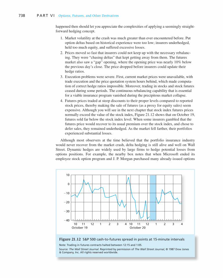
738 P A R T V I Options, Futures, and Other Derivatives
h appened then should let you appreciate the complexities of applying a seemingly straight-forward hedging concept.
1. Market volatility at the crash was much greater than ever encountered before. Put option deltas based on historical experience were too low; insurers underhedged, held too much equity, and suffered excessive losses.
2. Prices moved so fast that insurers could not keep up with the necessary rebalanc-ing. They were “chasing deltas” that kept getting away from them. The futures market also saw a “gap” opening, where the opening price was nearly 10% below the previous day’s close. The price dropped before insurers could update their hedge ratios.
3. Execution problems were severe. First, current market prices were unavailable, with trade execution and the price quotation system hours behind, which made computa-tion of correct hedge ratios impossible. Moreover, trading in stocks and stock futures ceased during some periods. The continuous rebalancing capability that is essential for a viable insurance program vanished during the precipitous market collapse.
4. Futures prices traded at steep discounts to their proper levels compared to reported stock prices, thereby making the sale of futures (as a proxy for equity sales) seem expensive. Although you will see in the next chapter that stock index futures prices normally exceed the value of the stock index, Figure 21.12 shows that on October 19, futures sold far below the stock index level. When some insurers gambled that the futures price would recover to its usual premium over the stock index, and chose to defer sales, they remained underhedged. As the market fell farther, their portfolios experienced substantial losses.
Although most observers at the time believed that the portfolio insurance industry would never recover from the market crash, delta hedging is still alive and well on Wall Street. Dynamic hedges are widely used by large firms to hedge potential losses from options positions. For example, the nearby box notes that when Microsoft ended its employee stock option program and J. P. Morgan purchased many already-issued options
0
10
�10
�20
�30
�4010 11 12 1 2 3 4 10 11 12 1 2 3 4
October 19 October 20
Figure 21.12 S&P 500 cash-to-futures spread in points at 15-minute intervals
Note: Trading in futures contracts halted between 12:15 and 1:05.
Source: The Wall Street Journal. Reprinted by permission of The Wall Street Journal, © 1987 Dow Jones & Company, Inc. All rights reserved worldwide.

739
J. P. Morgan Rolls Dice on Microsoft Options
Microsoft, in a shift that could be copied throughout the technology business, said yesterday that it plans to stop issuing stock options to its employees, and instead will pro-vide them with restricted stock.
The deal could portend a seismic shift for Microsoft’s Silicon Valley rivals, and it could well have effects on Wall Street. Though details of the plan still aren’t clear, J. P. Morgan effectively plans to buy the options from Microsoft employees who opt for restricted stock instead. Employee stock options are granted as a form of compensation and allow employees the right to exchange the options for shares of company stock.
The price offered to employees for the options presum-ably will be lower than the current value, giving J. P. Morgan a chance to make a profit on the deal. Rather than hold-ing the options, and thus betting Microsoft’s stock will rise, people familiar with the bank’s strategy say J. P. Morgan probably will match each option it buys from the company’s employees with a separate trade in the stock market that both hedges the bet and gives itself a margin of profit.
For Wall Street’s so-called rocket scientists who do com-plicated financial transactions such as this one, the strategy behind J. P. Morgan’s deal with Microsoft isn’t particularly unique or sophisticated. They add that the bank has sev-eral ways to deal with the millions of Microsoft options that could come its way.
The bank, for instance, could hedge the options by shorting, or betting against, Microsoft stock. Microsoft has the largest market capitalization of any stock in the mar-ket, and its shares are among the most liquid, meaning it would be easy to hedge the risk of holding those options.
J. P. Morgan also could sell the options to investors, much as they would do with a syndicated loan, thereby spreading the risk. During a conference call with investors, Mr. Ballmer said employees could sell their options to “a third party or set of third parties,” adding that the com-pany was still working out the details with J. P. Morgan and the SEC.
Source: The Wall Street Journal, July 9, 2003. © 2003 Dow Jones & Company, Inc. All rights reserved.
WO
RD
S FRO
M TH
E STREET
of Microsoft employees, it was widely expected that Morgan would protect its options position by selling shares in Microsoft in accord with a delta hedging strategy.
Hedging Bets on Mispriced Options
Suppose you believe that the standard deviation of IBM stock returns will be 35% over the next few weeks, but IBM put options are selling at a price consistent with a volatility of 33%. Because the put’s implied volatility is less than your forecast of the stock volatility, you believe the option is underpriced. Using your assessment of volatility in an option-pricing model like the Black-Scholes formula, you would estimate that the fair price for the puts exceeds the actual price.
Does this mean that you ought to buy put options? Perhaps it does, but by doing so, you risk losses if IBM stock performs well, even if you are correct about the volatility. You would like to separate your bet on volatility from the “attached” bet inherent in purchasing a put that IBM’s stock price will fall. In other words, you would like to speculate on the option mispricing by purchasing the put option, but hedge the resulting exposure to the performance of IBM stock.
The option delta can be interpreted as a hedge ratio that can be used for this purpose. The delta was defined as
Delta 5Change in value of option
Change in value of stock
Therefore, delta is the slope of the option-pricing curve. This ratio tells us precisely how many shares of stock we must hold to offset our expo-
sure to IBM. For example, if the delta is 2 .6, then the put will fall by $.60 in value for every one-point increase in IBM stock, and we need to hold .6 share of stock to hedge each put. If we purchase 10 option contracts, each for 100 shares, we would need to buy 600 shares of stock. If the stock price rises by $1, each put option will decrease in value by $.60, resulting in a loss of $600. However, the loss on the puts will be offset by a gain on the stock holdings of $1 per share 3 600 shares.
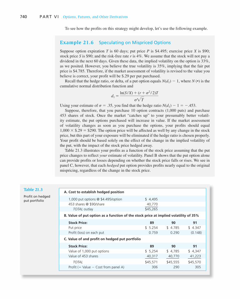
740 P A R T V I Options, Futures, and Other Derivatives
To see how the profits on this strategy might develop, let’s use the following example.
Example 21.6 Speculating on Mispriced Options
Suppose option expiration T is 60 days; put price P is $4.495; exercise price X is $90; stock price S is $90; and the risk-free rate r is 4%. We assume that the stock will not pay a dividend in the next 60 days. Given these data, the implied volatility on the option is 33%, as we posited. However, you believe the true volatility is 35%, implying that the fair put price is $4.785. Therefore, if the market assessment of volatility is revised to the value you believe is correct, your profit will be $.29 per put purchased.
Recall that the hedge ratio, or delta, of a put option equals N ( d 1 ) 2 1, where N (•) is the cumulative normal distribution function and
d1 5ln(S / X) 1 (r 1 s2 / 2)T
s"T
Using your estimate of s 5 .35, you find that the hedge ratio N ( d 1 ) 2 1 5 2 .453. Suppose, therefore, that you purchase 10 option contracts (1,000 puts) and purchase
453 shares of stock. Once the market “catches up” to your presumably better volatil-ity estimate, the put options purchased will increase in value. If the market assessment of volatility changes as soon as you purchase the options, your profits should equal 1,000 3 $.29 5 $290. The option price will be affected as well by any change in the stock price, but this part of your exposure will be eliminated if the hedge ratio is chosen properly. Your profit should be based solely on the effect of the change in the implied volatility of the put, with the impact of the stock price hedged away.
Table 21.3 illustrates your profits as a function of the stock price assuming that the put price changes to reflect your estimate of volatility. Panel B shows that the put option alone can provide profits or losses depending on whether the stock price falls or rises. We see in panel C, however, that each hedged put option provides profits nearly equal to the original mispricing, regardless of the change in the stock price.
Table 21.3
Profit on hedged put portfolio
A. Cost to establish hedged position
1,000 put options @ $4.495/option $ 4,495
453 shares @ $90/share 40,770
TOTAL outlay $45,265
B. Value of put option as a function of the stock price at implied volatility of 35%
Stock Price: 89 90 91
Put price $ 5.254 $ 4.785 $ 4.347
Profit (loss) on each put 0.759 0.290 (0.148)
C. Value of and profit on hedged put portfolio
Stock Price: 89 90 91
Value of 1,000 put options $ 5,254 $ 4,785 $ 4,347
Value of 453 shares 40,317 40,770 41,223
TOTAL $45,571 $45,555 $45,570
Profit (5 Value 2 Cost from panel A) 306 290 305

C H A P T E R 2 1 Option Valuation 741
Notice in Example 21.6 that the profit is not exactly independent of the stock price. This is because as the stock price changes, so do the deltas used to calculate the hedge ratio. The hedge ratio in principle would need to be continually adjusted as deltas evolve. The sensitivity of the delta to the stock price is called the gamma of the option. Option gammas are analogous to bond convexity. In both cases, the curvature of the value function means that hedge ratios or durations change with market conditions, making rebalancing a necessary part of hedging strategies.
A variant of the strategy in Example 21.6 involves cross-option speculation. Suppose you observe a 45-day expiration call option on IBM with strike price 95 selling at a price consistent with a volatility of s 5 33% while another 45-day call with strike price 90 has an implied volatility of only 27%. Because the underlying asset and expiration date are identical, you conclude that the call with the higher implied volatility is relatively over-priced. To exploit the mispricing, you might buy the cheap calls (with strike price 90 and implied volatility of 27%) and write the expensive calls (with strike price 95 and implied volatility 33%). If the risk-free rate is 4% and IBM is selling at $90 per share, the calls purchased will be priced at $3.6202 and the calls written will be priced at $2.3735.
Despite the fact that you are long one call and short another, your exposure to IBM stock-price uncertainty will not be hedged using this strategy. This is because calls with different strike prices have different sensitivities to the price of the underlying asset. The lower-strike-price call has a higher delta and therefore greater exposure to the price of IBM. If you take an equal number of positions in these two options, you will inadvertently establish a bullish position in IBM, as the calls you purchase have higher deltas than the calls you write. In fact, you may recall from Chapter 20 that this portfolio (long call with low exercise price and short call with high exercise price) is called a bullish spread.
To establish a hedged position, we can use the hedge ratio approach as follows. Consider the 95-strike-price options you write as the asset that hedges your exposure to the 90-strike-price options you purchase. Then the hedge ratio is
H 5Change in value of 90-strike-price call for $1 change in IBM
Change in value of 95-strike-price call for $1 change in IBM
5Delta of 90-strike-price call
Delta of 95-strike-price call. 1
You need to write more than one call with the higher strike price to hedge the purchase of each call with the lower strike price. Because the prices of higher-strike-price calls are less sensitive to IBM prices, more of them are required to offset the exposure.
Suppose the true annual volatility of the stock is midway between the two implied vola-tilities, so s 5 30%. We know that the delta of a call option is N ( d 1 ). Therefore, the deltas of the two options and the hedge ratio are computed as follows:
Option with strike price 90:
d1 5ln(90 / 90) 1 (.04 1 .302 / 2) 3 45 / 365
.30"45 / 3655 .0995
N(d1) 5 .5396
CONCEPT CHECK
9
Suppose you bet on volatility by purchasing calls instead of puts. How would you hedge your expo-sure to stock-price fluctuations? What is the hedge ratio?
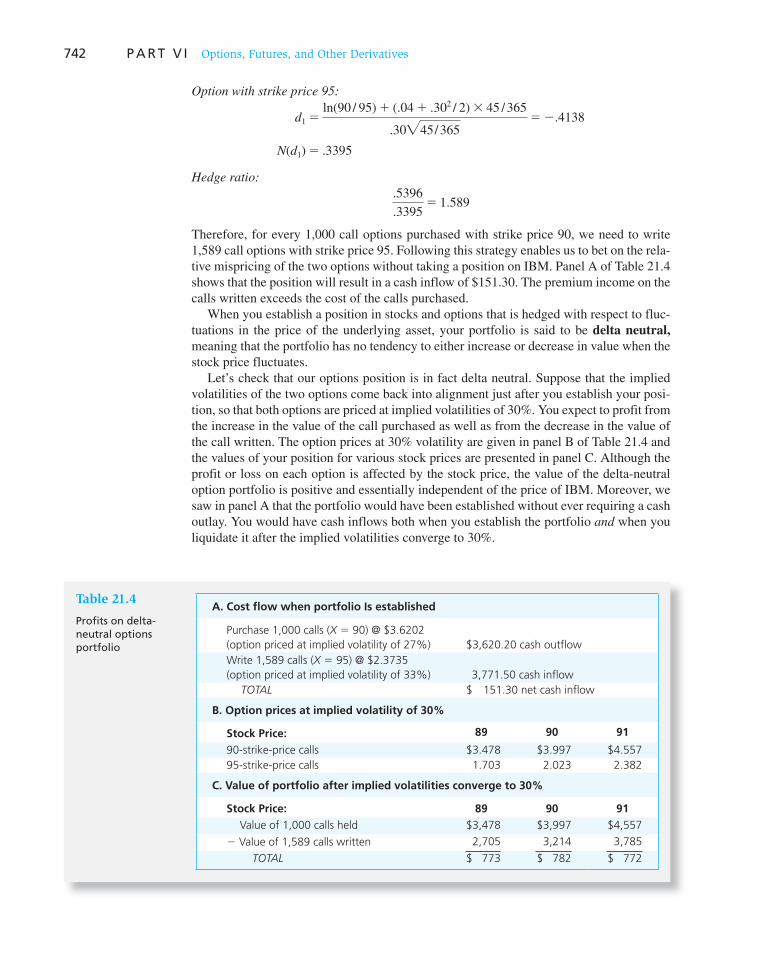
742 P A R T V I Options, Futures, and Other Derivatives
Option with strike price 95:
d1 5ln(90 / 95) 1 (.04 1 .302 / 2) 3 45 / 365
.30"45/ 3655 2.4138
N(d1) 5 .3395
Hedge ratio: .5396
.33955 1.589
Therefore, for every 1,000 call options purchased with strike price 90, we need to write 1,589 call options with strike price 95. Following this strategy enables us to bet on the rela-tive mispricing of the two options without taking a position on IBM. Panel A of Table 21.4 shows that the position will result in a cash inflow of $151.30. The premium income on the calls written exceeds the cost of the calls purchased.
When you establish a position in stocks and options that is hedged with respect to fluc-tuations in the price of the underlying asset, your portfolio is said to be delta neutral, meaning that the portfolio has no tendency to either increase or decrease in value when the stock price fluctuates.
Let’s check that our options position is in fact delta neutral. Suppose that the implied volatilities of the two options come back into alignment just after you establish your posi-tion, so that both options are priced at implied volatilities of 30%. You expect to profit from the increase in the value of the call purchased as well as from the decrease in the value of the call written. The option prices at 30% volatility are given in panel B of Table 21.4 and the values of your position for various stock prices are presented in panel C. Although the profit or loss on each option is affected by the stock price, the value of the delta-neutral option portfolio is positive and essentially independent of the price of IBM. Moreover, we saw in panel A that the portfolio would have been established without ever requiring a cash outlay. You would have cash inflows both when you establish the portfolio and when you liquidate it after the implied volatilities converge to 30%.
Table 21.4
Profits on delta- neutral options portfolio
A. Cost flow when portfolio Is established
Purchase 1,000 calls (X 5 90) @ $3.6202
(option priced at implied volatility of 27%) $3,620.20 cash outflow
Write 1,589 calls (X 5 95) @ $2.3735
(option priced at implied volatility of 33%) 3,771.50 cash inflow
TOTAL $ 151.30 net cash inflow
B. Option prices at implied volatility of 30%
Stock Price: 89 90 91
90-strike-price calls $3.478 $3.997 $4.557
95-strike-price calls 1.703 2.023 2.382
C. Value of portfolio after implied volatilities converge to 30%
Stock Price: 89 90 91
Value of 1,000 calls held $3,478 $3,997 $4,557
2 Value of 1,589 calls written 2,705 3,214 3,785
TOTAL $ 773 $ 782 $ 772

C H A P T E R 2 1 Option Valuation 743
This unusual profit opportunity arises because you have identified prices out of align-ment. Such opportunities could not arise if prices were at equilibrium levels. By exploiting the pricing discrepancy using a delta-neutral strategy, you should earn profits regardless of the price movement in IBM stock.
Delta-neutral hedging strategies are also subject to practical problems, the most impor-tant of which is the difficulty in assessing the proper volatility for the coming period. If the volatility estimate is incorrect, so will be the deltas, and the overall position will not truly be hedged. Moreover, option or option-plus-stock positions generally will not be neutral with respect to changes in volatility. For example, a put option hedged by a stock might be delta neutral, but it is not volatility neutral. Changes in the market assessments of volatility will affect the option price even if the stock price is unchanged.
These problems can be serious, because volatility estimates are never fully reliable. First, volatility cannot be observed directly and must be estimated from past data which imparts measurement error to the forecast. Second, we’ve seen that both historical and implied volatilities fluctuate over time. Therefore, we are always shooting at a moving target. Although delta-neutral positions are hedged against changes in the price of the underlying asset, they still are subject to volatility risk, the risk incurred from unpre-dictable changes in volatility. The sensitivity of an option price to changes in volatility is called the option’s vega. Thus, although delta-neutral option hedges might eliminate exposure to risk from fluctuations in the value of the underlying asset, they do not elimi-nate volatility risk.
21.6 Empirical Evidence on Option Pricing
The Black-Scholes option-pricing model has been subject to an enormous number of empirical tests. For the most part, the results of the studies have been positive in that the Black-Scholes model generates option values fairly close to the actual prices at which options trade. At the same time, some regular empirical failures of the model have been noted.
Whaley 14 examined the performance of the Black-Scholes formula relative to that of more complicated option formulas that allow for early exercise. His findings indicate that formulas allowing for the possibility of early exercise do better at pricing than the Black-Scholes formula. The Black-Scholes formula seems to perform worst for options on stocks with high dividend payouts. The true American call option formula, on the other hand, seems to fare equally well in the prediction of option prices on stocks with high or low dividend payouts.
Rubinstein has emphasized a more serious problem with the Black-Scholes model. 15 If the model were accurate, the implied volatility of all options on a particular stock with the same expiration date would be equal—after all, the underlying asset and expiration date are the same for each option, so the volatility inferred from each also ought to be the same. But in fact, when one actually plots implied volatility as a function of exercise price, the typical results appear as in Figure 21.13 , which treats S&P 500 index options as the underlying asset. Implied volatility steadily falls as the exercise price rises. Clearly, the Black-Scholes model is missing something.
14 Robert E. Whaley, “Valuation of American Call Options on Dividend-Paying Stocks: Empirical Tests,” Journal
of Financial Economics 10 (1982).
15 Mark Rubinstein, “Implied Binomial Trees,” Journal of Finance 49 (July 1994), pp. 771–818.
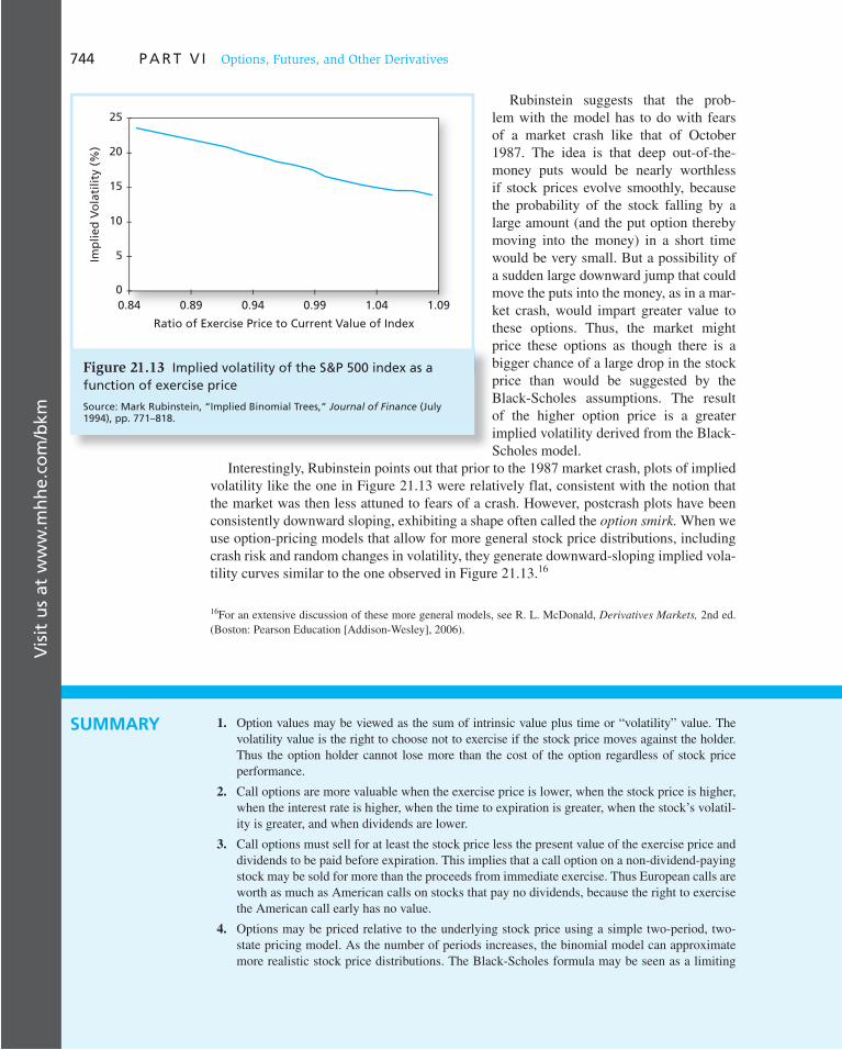
Vis
it u
s at
ww
w.m
hh
e.co
m/b
km744 P A R T V I Options, Futures, and Other Derivatives
Rubinstein suggests that the prob-lem with the model has to do with fears of a market crash like that of October 1987. The idea is that deep out-of-the-money puts would be nearly worthless if stock prices evolve smoothly, because the probability of the stock falling by a large amount (and the put option thereby moving into the money) in a short time would be very small. But a possibility of a sudden large downward jump that could move the puts into the money, as in a mar-ket crash, would impart greater value to these options. Thus, the market might price these options as though there is a bigger chance of a large drop in the stock price than would be suggested by the Black-Scholes assumptions. The result of the higher option price is a greater implied volatility derived from the Black-Scholes model.
Interestingly, Rubinstein points out that prior to the 1987 market crash, plots of implied volatility like the one in Figure 21.13 were relatively flat, consistent with the notion that the market was then less attuned to fears of a crash. However, postcrash plots have been consistently downward sloping, exhibiting a shape often called the option smirk. When we use option-pricing models that allow for more general stock price distributions, including crash risk and random changes in volatility, they generate downward-sloping implied vola-tility curves similar to the one observed in Figure 21.13 . 16
16 For an extensive discussion of these more general models, see R. L. McDonald, Derivatives Markets, 2nd ed. (Boston: Pearson Education [Addison-Wesley], 2006).
0.84 0.89 0.94 0.99 1.04 1.09
Imp
lied
Vo
lati
lity
(%
)
Ratio of Exercise Price to Current Value of Index
25
20
15
10
5
0
Figure 21.13 Implied volatility of the S&P 500 index as a function of exercise price
Source: Mark Rubinstein, “Implied Binomial Trees,” Journal of Finance (July 1994), pp. 771–818.
1. Option values may be viewed as the sum of intrinsic value plus time or “volatility” value. The volatility value is the right to choose not to exercise if the stock price moves against the holder. Thus the option holder cannot lose more than the cost of the option regardless of stock price performance.
2. Call options are more valuable when the exercise price is lower, when the stock price is higher, when the interest rate is higher, when the time to expiration is greater, when the stock’s volatil-ity is greater, and when dividends are lower.
3. Call options must sell for at least the stock price less the present value of the exercise price and dividends to be paid before expiration. This implies that a call option on a non-dividend-paying stock may be sold for more than the proceeds from immediate exercise. Thus European calls are worth as much as American calls on stocks that pay no dividends, because the right to exercise the American call early has no value.
4. Options may be priced relative to the underlying stock price using a simple two-period, two-state pricing model. As the number of periods increases, the binomial model can approximate more realistic stock price distributions. The Black-Scholes formula may be seen as a limiting
SUMMARY

Vis
it u
s at
ww
w.m
hh
e.co
m/b
kmV
isit
us
at w
ww
.mh
he.
com
/bkm
C H A P T E R 2 1 Option Valuation 745
case of the binomial option model, as the holding period is divided into progressively smaller subperiods when the interest rate and stock volatility are constant.
5. The Black-Scholes formula applies to options on stocks that pay no dividends. Dividend adjust-ments may be adequate to price European calls on dividend-paying stocks, but the proper treat-ment of American calls on dividend-paying stocks requires more complex formulas.
6. Put options may be exercised early, whether the stock pays dividends or not. Therefore, American puts generally are worth more than European puts.
7. European put values can be derived from the call value and the put-call parity relationship. This technique cannot be applied to American puts for which early exercise is a possibility.
8. The implied volatility of an option is the standard deviation of stock returns consistent with an option’s market price. It can be backed out of an option-pricing model by finding the stock volatility that makes the option’s value equal to its observed price.
9. The hedge ratio is the number of shares of stock required to hedge the price risk involved in writing one option. Hedge ratios are near zero for deep out-of-the-money call options and approach 1.0 for deep in-the-money calls.
10. Although hedge ratios are less than 1.0, call options have elasticities greater than 1.0. The rate of return on a call (as opposed to the dollar return) responds more than one-for-one with stock price movements.
11. Portfolio insurance can be obtained by purchasing a protective put option on an equity position. When the appropriate put is not traded, portfolio insurance entails a dynamic hedge strategy where a fraction of the equity portfolio equal to the desired put option’s delta is sold and placed in risk-free securities.
12. The option delta is used to determine the hedge ratio for options positions. Delta-neutral portfo-lios are independent of price changes in the underlying asset. Even delta-neutral option portfo-lios are subject to volatility risk, however.
13. Empirically, implied volatilities derived from the Black-Scholes formula tend to be lower on options with higher exercise prices. This may be evidence that the option prices reflect the pos-sibility of a sudden dramatic decline in stock prices. Such “crashes” are inconsistent with the Black-Scholes assumptions.
Related Web sites for this chapter are available at www.mhhe.com/bkm
intrinsic value time value binomial model Black-Scholes pricing formula implied volatility
pseudo-American call option value
hedge ratio delta option elasticity
portfolio insurance dynamic hedging gamma delta neutral vega
KEY TERMS
1. We showed in the text that the value of a call option increases with the volatility of the stock. Is this also true of put option values? Use the put-call parity theorem as well as a numerical exam-ple to prove your answer.
2. Would you expect a $1 increase in a call option’s exercise price to lead to a decrease in the option’s value of more or less than $1?
3. Is a put option on a high-beta stock worth more than one on a low-beta stock? The stocks have identical firm-specific risk.
4. All else equal, is a call option on a stock with a lot of firm-specific risk worth more than one on a stock with little firm-specific risk? The betas of the two stocks are equal.
5. All else equal, will a call option with a high exercise price have a higher or lower hedge ratio than one with a low exercise price?
PROBLEM SETS
i. Basic

Vis
it u
s at
ww
w.m
hh
e.co
m/b
km746 P A R T V I Options, Futures, and Other Derivatives
6. In each of the following questions, you are asked to compare two options with parameters as given. The risk-free interest rate for all cases should be assumed to be 6%. Assume the stocks on which these options are written pay no dividends.
a.
Which put option is written on the stock with the lower price?
i. A. ii. B. iii. Not enough information.
b.
Which put option must be written on the stock with the lower price?
i. A. ii. B. iii. Not enough information.
c.
Which call option must have the lower time to expiration?
i. A. ii. B. iii. Not enough information.
d.
Which call option is written on the stock with higher volatility?
i. A. ii. B. iii. Not enough information.
e.
Which call option is written on the stock with higher volatility?
i. A. ii. B. iii. Not enough information.
7. Reconsider the determination of the hedge ratio in the two-state model (see page 719), where we showed that one-third share of stock would hedge one option. What would be the hedge ratio for the following exercise prices: 120, 110, 100, 90? What do you conclude about the hedge ratio as the option becomes progressively more in the money?
8. Show that Black-Scholes call option hedge ratios also increase as the stock price increases. Con-sider a 1-year option with exercise price $50, on a stock with annual standard deviation 20%. The T-bill rate is 3% per year. Find N ( d 1 ) for stock prices $45, $50, and $55.
ii. Intermediate
Put T X s Price of Option
A .5 50 .20 $10
B .5 50 .25 $10
Put T X s Price of Option
A .5 50 .2 $10
B .5 50 .2 $12
Call S X s Price of Option
A 50 50 .20 $12
B 55 50 .20 $10
Call T X S Price of Option
A .5 50 55 $10
B .5 50 55 $12
Call T X S Price of Option
A .5 50 55 $10
B .5 50 55 $ 7

Vis
it u
s at
ww
w.m
hh
e.co
m/b
km
C H A P T E R 2 1 Option Valuation 747
9. We will derive a two-state put option value in this problem. Data: S 0 5 100; X 5 110; 1 1 r 5 1.10. The two possibilities for S T are 130 and 80.
a. Show that the range of S is 50, whereas that of P is 30 across the two states. What is the hedge ratio of the put?
b. Form a portfolio of three shares of stock and five puts. What is the (nonrandom) payoff to this portfolio? What is the present value of the portfolio?
c. Given that the stock currently is selling at 100, solve for the value of the put.
10. Calculate the value of a call option on the stock in the previous problem with an exercise price of 110. Verify that the put-call parity theorem is satisfied by your answers to Problems 9 and 10 . (Do not use continuous compounding to calculate the present value of X in this example because we are using a two-state model here, not a continuous-time Black-Scholes model.)
11. Use the Black-Scholes formula to find the value of a call option on the following stock:
Time to expiration 6 months
Standard deviation 50% per year
Exercise price $50
Stock price $50
Interest rate 3%
12. Find the Black-Scholes value of a put option on the stock in the previous problem with the same exercise price and expiration as the call option.
13. Recalculate the value of the call option in Problem 11 , successively substituting one of the changes below while keeping the other parameters as in Problem 11 :
a. Time to expiration 5 3 months. b. Standard deviation 5 25% per year. c. Exercise price 5 $55. d. Stock price 5 $55. e. Interest rate 5 5%.
Consider each scenario independently. Confirm that the option value changes in accordance with the prediction of Table 21.1 .
14. A call option with X 5 $50 on a stock currently priced at S 5 $55 is selling for $10. Using a volatility estimate of s 5 .30, you find that N ( d 1 ) 5 .6 and N ( d 2 ) 5 .5. The risk-free interest rate is zero. Is the implied volatility based on the option price more or less than .30? Explain.
15. What would be the Excel formula in Spreadsheet 21.1 for the Black-Scholes value of a straddle position?
Use the following case in answering Problems 16–21: Mark Washington, CFA, is an analyst with BIC. One year ago, BIC analysts predicted that the U.S. equity market would most likely experience a slight downturn and suggested delta-hedging the BIC portfolio. As predicted, the U.S. equity markets did indeed experience a downturn of approximately 4% over a 12-month period. However, portfolio performance for BIC was disappointing, lagging its peer group by nearly 10%. Washington has been told to review the options strategy to determine why the hedged portfolio did not perform as expected.
16. Which of the following best explains a delta-neutral portfolio? A delta-neutral portfolio is per-fectly hedged against:
a. Small price changes in the underlying asset. b. Small price decreases in the underlying asset. c. All price changes in the underlying asset.
17. After discussing the concept of a delta-neutral portfolio, Washington determines that he needs to further explain the concept of delta. Washington draws the value of an option as a function of the underlying stock price. Using this diagram, indicate how delta is interpreted. Delta is the:
a. Slope in the option price diagram. b. Curvature of the option price graph. c. Level in the option price diagram.

Vis
it u
s at
ww
w.m
hh
e.co
m/b
km748 P A R T V I Options, Futures, and Other Derivatives
18. Washington considers a put option that has a delta of 20.65. If the price of the underlying asset decreases by $6, then what is the best estimate of the change in option price?
19. BIC owns 51,750 shares of Smith & Oates. The shares are currently priced at $69. A call option on Smith & Oates with a strike price of $70 is selling at $3.50 and has a delta of .69 What is the number of call options necessary to create a delta-neutral hedge?
20. Return to the previous problem. Will the number of call options written for a delta-neutral hedge increase or decrease if the stock price falls?
21. Which of the following statements regarding the goal of a delta-neutral portfolio is most accu-rate? One example of a delta-neutral portfolio is to combine a:
a. Long position in a stock with a short position in call options so that the value of the portfolio does not change with changes in the value of the stock.
b. Long position in a stock with a short position in a call option so that the value of the portfo-lio changes with changes in the value of the stock.
c. Long position in a stock with a long position in call options so that the value of the portfolio does not change with changes in the value of the stock.
22. Should the rate of return of a call option on a long-term Treasury bond be more or less sensitive to changes in interest rates than is the rate of return of the underlying bond?
23. If the stock price falls and the call price rises, then what has happened to the call option’s implied volatility?
24. If the time to expiration falls and the put price rises, then what has happened to the put option’s implied volatility?
25. According to the Black-Scholes formula, what will be the value of the hedge ratio of a call option as the stock price becomes infinitely large? Explain briefly.
26. According to the Black-Scholes formula, what will be the value of the hedge ratio of a put option for a very small exercise price?
27. The hedge ratio of an at-the-money call option on IBM is .4. The hedge ratio of an at-the-money put option is 2 .6. What is the hedge ratio of an at-the-money straddle position on IBM?
28. Consider a 6-month expiration European call option with exercise price $105. The underlying stock sells for $100 a share and pays no dividends. The risk-free rate is 5%. What is the implied volatility of the option if the option currently sells for $8? Use Spreadsheet 21.1 (available at www.mhhe.com/bkm; link to Chapter 21 material) to answer this question.
a. Go to the Tools menu of the spreadsheet and select Goal Seek. The dialog box will ask you for three pieces of information. In that dialog box, you should set cell E6 to value 8 by changing cell B2. In other words, you ask the spreadsheet to find the value of standard deviation (which appears in cell B2) that forces the value of the option (in cell E6) equal to $8. Then click OK, and you should find that the call is now worth $8, and the entry for standard deviation has been changed to a level consistent with this value. This is the call’s implied standard deviation at a price of $8.
b. What happens to implied volatility if the option is selling at $9? Why has implied volatility increased?
c. What happens to implied volatility if the option price is unchanged at $8, but option expira-tion is lower, say, only 4 months? Why?
d. What happens to implied volatility if the option price is unchanged at $8, but the exercise price is lower, say, only $100? Why?
e. What happens to implied volatility if the option price is unchanged at $8, but the stock price is lower, say, only $98? Why?
29. A collar is established by buying a share of stock for $50, buying a 6-month put option with exercise price $45, and writing a 6-month call option with exercise price $55. On the basis of the volatility of the stock, you calculate that for a strike price of $45 and expiration of 6 months, N ( d 1 ) 5 .60, whereas for the exercise price of $55, N ( d 1 ) 5 .35.
a. What will be the gain or loss on the collar if the stock price increases by $1? b. What happens to the delta of the portfolio if the stock price becomes very large? Very small?
eXce lPlease visit us at www.mhhe.com/bkm

Vis
it u
s at
ww
w.m
hh
e.co
m/b
km
C H A P T E R 2 1 Option Valuation 749
30. These three put options are all written on the same stock. One has a delta of 2 .9, one a delta of 2 .5, and one a delta of 2 .1. Assign deltas to the three puts by filling in this table.
Put X Delta
A 10
B 20
C 30
31. You are very bullish (optimistic) on stock EFG, much more so than the rest of the market. In each question, choose the portfolio strategy that will give you the biggest dollar profit if your bullish forecast turns out to be correct. Explain your answer.
a. Choice A: $10,000 invested in calls with X 5 50. Choice B: $10,000 invested in EFG stock. b. Choice A: 10 call option contracts (for 100 shares each), with X 5 50. Choice B: 1,000 shares of EFG stock.
32. You would like to be holding a protective put position on the stock of XYZ Co. to lock in a guar-anteed minimum value of $100 at year-end. XYZ currently sells for $100. Over the next year the stock price will increase by 10% or decrease by 10%. The T-bill rate is 5%. Unfortunately, no put options are traded on XYZ Co.
a. Suppose the desired put option were traded. How much would it cost to purchase? b. What would have been the cost of the protective put portfolio? c. What portfolio position in stock and T-bills will ensure you a payoff equal to the payoff that
would be provided by a protective put with X 5 100? Show that the payoff to this portfolio and the cost of establishing the portfolio matches that of the desired protective put.
33. Return to Example 21.1 . Use the binomial model to value a 1-year European put option with exercise price $110 on the stock in that example. Does your solution for the put price satisfy put-call parity?
34. Suppose that the risk-free interest rate is zero. Would an American put option ever be exercised early? Explain.
35. Let p ( S, T, X ) denote the value of a European put on a stock selling at S dollars, with time to maturity T, and with exercise price X, and let P ( S, T, X ) be the value of an American put.
a. Evaluate p (0, T, X ). b. Evaluate P (0, T, X ). c. Evaluate p ( S, T, 0). d. Evaluate P ( S, T, 0). e. What does your answer to ( b ) tell you about the possibility that American puts may be exer-
cised early?
36. You are attempting to value a call option with an exercise price of $100 and 1 year to expiration. The underlying stock pays no dividends, its current price is $100, and you believe it has a 50% chance of increasing to $120 and a 50% chance of decreasing to $80. The risk-free rate of inter-est is 10%. Calculate the call option’s value using the two-state stock price model.
37. Consider an increase in the volatility of the stock in the previous problem. Suppose that if the stock increases in price, it will increase to $130, and that if it falls, it will fall to $70. Show that the value of the call option is now higher than the value derived in the previous problem.
38. Calculate the value of a put option with exercise price $100 using the data in Problem 36 . Show that put-call parity is satisfied by your solution.
39. XYZ Corp. will pay a $2 per share dividend in 2 months. Its stock price currently is $60 per share. A call option on XYZ has an exercise price of $55 and 3-month time to expiration. The risk-free interest rate is .5% per month, and the stock’s volatility (standard deviation) 5 7% per month. Find the pseudo-American option value. (Hint: Try defining one “period” as a month, rather than as a year.)
40. “The beta of a call option on General Electric is greater than the beta of a share of General Elec-tric.” True or false?

Vis
it u
s at
ww
w.m
hh
e.co
m/b
km750 P A R T V I Options, Futures, and Other Derivatives
41. “The beta of a call option on the S&P 500 index with an exercise price of 1,130 is greater than the beta of a call on the index with an exercise price of 1,140.” True or false?
42. What will happen to the hedge ratio of a convertible bond as the stock price becomes very large?
43. Goldman Sachs believes that market volatility will be 20% annually for the next 3 years. Three-year at-the-money call and put options on the market index sell at an implied volatility of 22%. What options portfolio can Goldman establish to speculate on its volatility belief without taking a bullish or bearish position on the market? Using Goldman’s estimate of volatility, 3-year at-the-money options have N ( d 1 ) 5 .6.
44. You are holding call options on a stock. The stock’s beta is .75, and you are concerned that the stock market is about to fall. The stock is currently selling for $5 and you hold 1 million options on the stock (i.e., you hold 10,000 contracts for 100 shares each). The option delta is .8. How much of the market index portfolio must you buy or sell to hedge your market exposure?
45. Imagine you are a provider of portfolio insurance. You are establishing a 4-year program. The portfolio you manage is currently worth $100 million, and you hope to provide a minimum return of 0%. The equity portfolio has a standard deviation of 25% per year, and T-bills pay 5% per year. Assume for simplicity that the portfolio pays no dividends (or that all dividends are reinvested).
a. How much should be placed in bills? How much in equity? b. What should the manager do if the stock portfolio falls by 3% on the first day of trading?
46. Suppose that call options on ExxonMobil stock with time to expiration 3 months and strike price $60 are selling at an implied volatility of 30%. ExxonMobil stock currently is $60 per share, and the risk-free rate is 4%. If you believe the true volatility of the stock is 32%, how can you trade on your belief without taking on exposure to the performance of ExxonMobil? How many shares of stock will you hold for each option contract purchased or sold?
47. Using the data in the previous problem, suppose that 3-month put options with a strike price of $60 are selling at an implied volatility of 34%. Construct a delta-neutral portfolio comprising positions in calls and puts that will profit when the option prices come back into alignment.
48. Suppose that JPMorgan Chase sells call options on $1.25 million worth of a stock portfolio with beta 5 1.5. The option delta is .8. It wishes to hedge out its resultant exposure to a market advance by buying a market index portfolio.
a. How many dollars worth of the market index portfolio should it purchase to hedge its position? b. What if it instead uses market index puts to hedge its exposure? Should it buy or sell puts?
Each put option is on 100 units of the index, and the index at current prices represents $1,000 worth of stock.
iii. Challenge
1. The board of directors of Abco Company is concerned about the downside risk of a $100 million equity portfolio in its pension plan. The board’s consultant has proposed temporarily (for 1 month) hedging the portfolio with either futures or options. Referring to the following table, the consultant states:
a. “The $100 million equity portfolio can be fully protected on the downside by selling (short-ing) 4,000 futures contracts.”
b. “The cost of this protection is that the portfolio’s expected rate of return will be zero percent.”
Market, Portfolio, and Contract Data
Equity index level 99.00
Equity futures price 100.00
Futures contract multiplier $250
Portfolio beta 1.20
Contract expiration (months) 3
Critique the accuracy of each of the consultant’s two statements.

Vis
it u
s at
ww
w.m
hh
e.co
m/b
km
C H A P T E R 2 1 Option Valuation 751
2. Michael Weber, CFA, is analyzing several aspects of option valuation, including the determinants of the value of an option, the characteristics of various models used to value options, and the potential for divergence of calculated option values from observed market prices.
a. What is the expected effect on the value of a call option on common stock if the volatility of the underlying stock price decreases? If the time to expiration of the option increases?
b. Using the Black-Scholes option-pricing model, Weber calculates the price of a 3-month call option and notices the option’s calculated value is different from its market price. With respect to Weber’s use of the Black-Scholes option-pricing model,
i. Discuss why the calculated value of an out-of-the-money European option may differ from its market price.
ii. Discuss why the calculated value of an American option may differ from its market price.
3. Joel Franklin is a portfolio manager responsible for derivatives. Franklin observes an American-style option and a European-style option with the same strike price, expiration, and underly-ing stock. Franklin believes that the European-style option will have a higher premium than the American-style option.
a. Critique Franklin’s belief that the European-style option will have a higher premium. Franklin is asked to value a 1-year European-style call option for Abaco Ltd. common stock, which last traded at $43.00. He has collected the information in the following table.
Closing stock price $43.00
Call and put option exercise price 45.00
1-year put option price 4.00
1-year Treasury bill rate 5.50%
Time to expiration One year
b. Calculate, using put-call parity and the information provided in the table, the European-style call option value.
c. State the effect, if any, of each of the following three variables on the value of a call option. (No calculations required.)
i. An increase in short-term interest rate. ii. An increase in stock price volatility. iii. A decrease in time to option expiration.
4. A stock index is currently trading at 50. Paul Tripp, CFA, wants to value 2-year index options using the binomial model. The stock will either increase in value by 20% or fall in value by 20%. The annual risk-free interest rate is 6%. No dividends are paid on any of the underlying securities in the index.
a. Construct a two-period binomial tree for the value of the stock index. b. Calculate the value of a European call option on the index with an exercise price of 60. c. Calculate the value of a European put option on the index with an exercise price of 60. d. Confirm that your solutions for the values of the call and the put satisfy put-call parity.
5. Ken Webster manages a $200 million equity portfolio benchmarked to the S&P 500 index. Webster believes the market is overvalued when measured by several traditional fundamental/e conomic indicators. He is concerned about potential losses but recognizes that the S&P 500 index could nevertheless move above its current 1136 level. Webster is considering the following option collar strategy:
• Protection for the portfolio can be attained by purchasing an S&P 500 index put with a strike price of 1130 (just out of the money).
• The put can be financed by selling two 1150 calls (farther out-of-the-money) for every put purchased.
• Because the combined delta of the two calls (see following table) is less than 1 (that is, 2 3 .36 5 .72), the options will not lose more than the underlying portfolio will gain if the market advances.

Vis
it u
s at
ww
w.m
hh
e.co
m/b
km752 P A R T V I Options, Futures, and Other Derivatives
The information in the following table describes the two options used to create the collar.
Characteristics 1150 Call 1130 Put
Option price $8.60 $16.10
Option implied volatility 22% 24%
Option’s delta 0.36 20.44
Contracts needed for collar 602 301
Notes:• Ignore transaction costs.• S&P 500 historical 30-day volatility 5 23%.• Time to option expiration 5 30 days.
a. Describe the potential returns of the combined portfolio (the underlying portfolio plus the option collar) if after 30 days the S&P 500 index has:
i. risen approximately 5% to 1193. ii. remained at 1136 (no change). iii. declined by approximately 5% to 1080. (No calculations are necessary.)
b. Discuss the effect on the hedge ratio (delta) of each option as the S&P 500 approaches the level for each of the potential outcomes listed in part ( a ).
c. Evaluate the pricing of each of the following in relation to the volatility data provided:
i. the put ii. the call
E-INVEST-MENTS EXERCISES
Option Price Differences
Select a stock for which options are listed on the CBOE Web site ( www.cboe.com ). The price data for captions can be found on the “delayed quotes” menu option. Enter a ticker symbol for a stock of your choice and pull up its option price data.
Using daily price data from finance.yahoo.com calculate the annualized standard deviation of the daily percentage change in the stock price. Create a Black-Scholes option-pricing model in a spreadsheet, or use our Spreadsheet 21.1 , available at www.mhhe
.com/bkm with Chapter 21 material. Using the standard deviation and a risk-free rate found at www.bloomberg.com/markets/rates/index.html , calculate the value of the call options.
How do the calculated values compare to the market prices of the options? On the basis of the difference between the price you calculated using historical volatility and the actual price of the option, what do you conclude about expected trends in market volatility?

Vis
it u
s at
ww
w.m
hh
e.co
m/b
km
C H A P T E R 2 1 Option Valuation 753
SOLUTIONS TO CONCEPT CHECKS 1.
*For American puts, increase in time to expiration must increase value. One can always choose to exercise early if this is optimal; the longer expiration date simply expands the range of alternatives open to the option holder which must make the option more valuable. For a European put, where early exercise is not allowed, longer time to expiration can have an indeterminate effect. Longer expiration increases volatility value because the final stock price is more uncertain, but it reduces the present value of the exercise price that will be received if the put is exercised. The net effect on put value is ambiguous.
To understand the impact of higher volatility, consider the same scenarios as for the call. The low-volatility scenario yields a lower expected payoff.
High Stock price $10 $20 $30 $40 $50
volatility Put payoff $20 $10 $ 0 $ 0 $ 0
Low Stock price $20 $25 $30 $35 $40
volatility Put payoff $10 $ 5 $ 0 $ 0 $ 0
2. The parity relationship assumes that all options are held until expiration and that there are no cash flows until expiration. These assumptions are valid only in the special case of European options on non-dividend-paying stocks. If the stock pays no dividends, the American and European calls are equally valuable, whereas the American put is worth more than the European put. Therefore, although the parity theorem for European options states that
P 5 C 2 S0 1 PV(X) in fact, P will be greater than this value if the put is American.
3. Because the option now is underpriced, we want to reverse our previous strategy.
Cash Flow in 1 Year for Each Possible Stock Price
Initial Cash Flow S 5 90 S 5 120
Buy 3 options 216.50 0 30
Short-sell 1 share; repay in 1 year 100 290 2120
Lend $83.50 at 10% interest rate 283.50 91.85 91.85
TOTAL 0 1.85 1.85
The riskless cash flow in 1 year per option is $1.85/3 5 $.6167, and the present value is $.6167/1.10 5 $.56, precisely the amount by which the option is underpriced.
4. a. C u 2 C d 5 $6.984 2 0
b. uS 0 2 dS 0 5 $110 2 $95 5 $15
c. 6.984/15 5 .4656
d.
If This Variable Increases . . . The Value of a Put Option
S Decreases
X Increases
s Increases
T Increases*
rf Decreases
Dividend payouts Increases
Value in Next Period as Function of Stock Price
Action Today (time 0) dS0 5 $95 uS0 5 $110
Buy .4656 shares at price S0 5 $100 $44.232 $51.216
Write 1 call at price C0 0 26.984
TOTAL $44.232 $44.232

Vis
it u
s at
ww
w.m
hh
e.co
m/b
km754 P A R T V I Options, Futures, and Other Derivatives
The portfolio must have a market value equal to the present value of $44.232.
e. $44.232/1.05 5 $42.126
f. .4656 3 $100 2 C 0 5 $42.126
C 0 5 $46.56 2 $42.126 5 $4.434
5. Higher. For deep out-of-the-money call options, an increase in the stock price still leaves the option unlikely to be exercised. Its value increases only fractionally. For deep in-the-money options, exercise is likely, and option holders benefit by a full dollar for each dollar increase in the stock, as though they already own the stock.
6. Because s 5 .6, s 2 5 .36.
d1 5ln(100 / 95) 1 (.10 1 .36 / 2).25
.6".255 .4043
d2 5 d1 2 .6".25 5 .1043 Using Table 21.2 and interpolation, or from a spreadsheet function:
N(d1) 5 .6570
N(d2) 5 .5415
C 5 100 3 .6570 2 95e2.103.25 3 .5415 5 15.53 7. Implied volatility exceeds .2783. Given a standard deviation of .2783, the option value is $7.
A higher volatility is needed to justify an $8 price. Using Spreadsheet 21.1 and Goal Seek, you can confirm that implied volatility at an option price of $8 is .3138.
8. A $1 increase in stock price is a percentage increase of 1/122 5 .82%. The put option will fall by (.4 3 $1) 5 $.40, a percentage decrease of $.40/$4 5 10%. Elasticity is 2 10/.82 5 2 12.2.
9. The delta for a call option is N ( d 1 ), which is positive, and in this case is .547. Therefore, for every 10 option contracts purchased, you would need to short 547 shares of stock.

FUTURES AND FORWARD contracts are
like options in that they specify purchase or
sale of some underlying security at some
fu ture date. The key difference is that the
holder of an option is not compelled to
buy or sell, and will not do so if the trade
is unprofitable. A futures or forward con-
tract, however, carries the obligation to go
through with the agreed-upon transaction.
A forward contract is not an investment in
the strict sense that funds are paid for an asset.
It is only a commitment today to transact in
the future. Forward arrangements are part of
our study of investments, however, because
they offer powerful means to hedge other
investments and generally modify portfolio
characteristics.
Forward markets for future delivery of
various commodities go back at least to
ancient Greece. Organized futures markets,
though, are a relatively modern develop-
ment, dating only to the 19th century. Futures
markets replace informal forward contracts
with highly standardized, exchange-traded
securities.
While futures markets have their roots in
agricultural products and commodities, the
markets today are dominated by trading in
financial futures such as those on stock indi-
ces, interest-rate-dependent securities such
as government bonds, and foreign exchange.
The markets themselves also have changed,
with trading today largely taking place in
electronic markets.
This chapter describes the workings of
futures markets and the mechanics of trading
in these markets. We show how futures con-
tracts are useful investment vehicles for both
hedgers and speculators and how the futures
price relates to the spot price of an asset. We
also show how futures can be used in several
risk-management applications. This chapter
deals with general principles of future mar-
kets. Chapter 23 describes specific futures
markets in greater detail.
22 Futures Markets 2 PA
RT V
I CHAPTER TWENTY-TWO

756 P A R T V I Options, Futures, and Other Derivatives
To see how futures and forwards work and how they might be useful, consider the port-folio diversification problem facing a farmer growing a single crop, let us say wheat. The entire planting season’s revenue depends critically on the highly volatile crop price. The farmer can’t easily diversify his position because virtually his entire wealth is tied up in the crop.
The miller who must purchase wheat for processing faces a portfolio problem that is the mirror image of the farmer’s. He is subject to profit uncertainty because of the unpredict-able future cost of the wheat.
Both parties can reduce this source of risk if they enter into a forward contract requir-ing the farmer to deliver the wheat when harvested at a price agreed upon now, regardless of the market price at harvest time. No money need change hands at this time. A forward contract is simply a deferred-delivery sale of some asset with the sales price agreed on now. All that is required is that each party be willing to lock in the ultimate price for delivery of the commodity. A forward contract protects each party from future price fluctuations.
Futures markets formalize and standardize forward contracting. Buyers and sellers trade in a centralized futures exchange. The exchange standardizes the types of contracts that may be traded: It establishes contract size, the acceptable grade of commodity, con-tract delivery dates, and so forth. Although standardization eliminates much of the flex-ibility available in forward contracting, it has the offsetting advantage of liquidity because many traders will concentrate on the same small set of contracts. Futures contracts also differ from forward contracts in that they call for a daily settling up of any gains or losses on the contract. By contrast, with forward contracts, no money changes hands until the delivery date.
The centralized market, standardization of contracts, and depth of trading in each con-tract allows futures positions to be liquidated easily rather than personally renegotiated with the other party to the contract. Because the exchange guarantees the performance of each party to the contract, costly credit checks on other traders are not necessary. Instead, each trader simply posts a good-faith deposit, called the margin, in order to guarantee contract performance.
The Basics of Futures Contracts
The futures contract calls for delivery of a commodity at a specified delivery or maturity date, for an agreed-upon price, called the futures price, to be paid at contract maturity. The contract specifies precise requirements for the commodity. For agricultural commodities, the exchange sets allowable grades (e.g., No. 2 hard winter wheat or No. 1 soft red wheat). The place or means of delivery of the commodity is specified as well. Delivery of agri-cultural commodities is made by transfer of warehouse receipts issued by approved ware-houses. For financial futures, delivery may be made by wire transfer; for index futures, delivery may be accomplished by a cash settlement procedure such as those for index options. Although the futures contract technically calls for delivery of an asset, delivery rarely occurs. Instead, parties to the contract much more commonly close out their posi-tions before contract maturity, taking gains or losses in cash.
Because the futures exchange specifies all the terms of the contract, the traders need bargain only over the futures price. The trader taking the long position commits to pur-chasing the commodity on the delivery date. The trader who takes the short position com-mits to delivering the commodity at contract maturity. The trader in the long position is said to “buy” a contract; the short-side trader “sells” a contract. The words buy and sell
22.1 The Futures Contract

C H A P T E R 2 2 Futures Markets 757
are figurative only, because a contract is not really bought or sold like a stock or bond; it is entered into by mutual agreement. At the time the contract is entered into, no money changes hands.
Figure 22.1 shows prices for several futures contracts as they appear in The Wall Street
Journal. The boldface heading lists in each case the commodity, the exchange where the futures contract is traded in parentheses, the contract size, and the pricing unit. The first agricultural contract listed is for corn, traded on the Chicago Board of Trade (CBT). (The CBT merged with the Chicago Mercantile Exchange in 2007, but for now, maintains a separate identity.) Each contract calls for delivery of 5,000 bushels, and prices in the entry are quoted in cents per bushel.
The next several rows detail price data for contracts expiring on various dates. The March 2010 maturity corn contract, for example, opened during the day at a futures price of 404 cents per bushel. The highest futures price during the day was 410, the lowest was 399.50, and the settlement price (a representative trading price during the last few minutes of trading) was 408.50. The settlement price increased by 4 cents from the previous trading day. Finally, open interest, or the number of outstanding contracts, was 497,859. Similar information is given for each maturity date.
The trader holding the long position, that is, the person who will purchase the good, profits from price increases. Suppose that when the contract matures in March, the price of corn turns out to be 413.50 cents per bushel. The long-position trader who entered the contract at the futures price of 408.50 cents therefore earns a profit of 5 cents per bushel. As each contract calls for delivery of 5,000 bushels, the profit to the long position equals 5,000 3 $.05 5 $250 per contract. Conversely, the short position loses 5 cents per bushel. The short position’s loss equals the long position’s gain.
To summarize, at maturity:
Profit to long 5 Spot price at maturity 2 Original futures price
Profit to short 5 Original futures price 2 Spot price at maturity
where the spot price is the actual market price of the commodity at the time of the delivery. The futures contract is, therefore, a zero-sum game, with losses and gains netting out to
zero. Every long position is offset by a short position. The aggregate profits to futures trad-ing, summing over all investors, also must be zero, as is the net exposure to changes in the commodity price. For this reason, the establishment of a futures market in a commodity should not have a major impact on prices in the spot market for that commodity.
Figure 22.2 , panel A, is a plot of the profits realized by an investor who enters the long side of a futures contract as a function of the price of the asset on the maturity date. Notice that profit is zero when the ultimate spot price, P T , equals the initial futures price, F 0 . Profit per unit of the underlying asset rises or falls one-for-one with changes in the final spot price. Unlike the payoff of a call option, the payoff of the long futures position can be negative: This will be the case if the spot price falls below the original futures price. Unlike the holder of a call, who has an option to buy, the long futures position trader can-not simply walk away from the contract. Also unlike options, in the case of futures there is no need to distinguish gross payoffs from net profits. This is because the futures contract is not purchased; it is simply a contract that is agreed to by two parties. The futures price adjusts to make the present value of entering into a new contract equal to zero.
The distinction between futures and options is highlighted by comparing panel A of Figure 22.2 to the payoff and profit diagrams for an investor in a call option with exercise price, X, chosen equal to the futures price F 0 (see panel C). The futures investor is exposed to considerable losses if the asset price falls. In contrast, the investor in the call cannot lose more than the cost of the option.
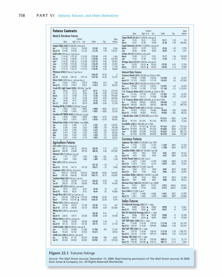
758 P A R T V I Options, Futures, and Other Derivatives
Copper-High (CMX)-25,000 IBS; cents per IbDec 311.00 313.65 310.00 313.00 2.00 2,436March’10 314.00 316.00 311.05 315.20 1.90 110,415
Gold (CMX)-100 troy oz; $ per troy ozDec 1114.50 1127.50 1114.50 1123.30 3.90 1,606Feb’10 1114.60 1128.90 1111.70 1123.80 3.90 337,982April 1116.70 1130.10 1113.00 1125.10 3.90 50,967June 1119.00 1131.00 1115.60 1126.30 4.00 23,452Aug 1115.90 1130.00 1115.90 1127.60 4.00 11,720Dec 1119.10 1135.10 1119.10 1130.90 4.20 20,860
Platinum (NYM)-50 troy oz; $ per troy ozDec 1446.20 24.50 0Jan’10 1432.00 1455.10 1421.20 1447.00 24.30 22,475
Silver (CMX)-5,000 troy oz ; cents per troy ozDec 1734.0 1734.5 1727.0 1732.6 24.2 470March’10 1714.0 1744.5 1709.5 1134.0 25.0 80,332
Crude Oil, Light Sweet (NYM)-1,000 bbls; $ per bblJan 69.63 70.22 68.59 69.51 �0.36 172,256Feb 71.70 72.54 70.83 71.86 �0.09 231,544March 73.27 74.08 72.45 73.46 �0.08 149,509June 75.48 76.51 75.00 75.97 �0.02 105,906Dec 78.40 79.77 78.40 79.22 �0.01 131,615Dec’12 84.85 85.15 84.70 84.82 �0.06 57,590
Heating Oil No.2 (NYM)-42,000 gal; $ per galJan 1.9036 1.9261 1.8956 1.9082 �.0003 58,173Feb 1.9309 1.9474 1.9250 1.9307 �.0003 55,705
Gasoline-NY RBOB (NYM)-42,000 gal; $ per galJan 1.8396 1.8495 1.8240 1.8267 �.0149 54,284Feb 1.8657 1.8775 1.8522 1.8550 �.0139 48,965
Natural Gas (NYM)-10,000 MMBtu; $ per MMBtuJan 5.235 5.409 5.191 5.332 .169 118,292Feb 5.296 5.469 5.262 5.402 .170 98,108March 5.349 5.490 5.303 5.437 .163 120,570April 5.419 5.502 5.323 5.452 .153 68,250May 5.494 5.545 5.357 5.494 .151 36,786Oct 5.875 5.945 5.774 5.892 .143 33,425
Agriculture FuturesCorn (CBT)-5,000 bu; cents per buDec 387.25 395.25 385.00 392.00 2.75 3,791March’10 404.00 410.00 399.50 408.50 4.00 497,859
Ethanol (CBT)-29,000 gal; $ per galJan 1.917 1.917 1.870 1.881 �.031 729March 1.810 1.810 1.800 1.809 �.023 1,168
Oats (CBT)-5,000 bu; cents per buDec 247.50 �.50 4March’10 257.50 261.75 257.50 258.75 �.25 9,406
Soybeans (CBT)-5,000 bu; cents per buJan 1032.75 1059.00 1023.50 1055.00 20.00 143,687March 1041.00 1066.00 1032.00 1061.75 18.75 163,832
Soybean Meal (CBT)-100 tons; $ per tonDec 315.30 335.00 314.50 326.50 12.00 570Jan’10 306.30 317.00 303.00 316.20 9.70 49,468
Soybean Oil (CBT)-60,000 lbs; cents per lbDec 39.01 39.45 39.01 39.40 .18 677March’10 40.03 40.25 39.61 40.04 .05 94,008
Rough Rice (CBT)-2,000 cwt; cents per cwtJan 1563.50 1598.50 1555.50 1598.00 32.00 6,014March 1594.50 1627.00 1594.00 1626.50 32.00 9,295
Wheat (CBT)-5,000 bu; cents per buDec 517.00 529.25 517.00 525.00 5.75 657March’10 537.50 548.00 531.50 543.50 6.00 185,083
Wheat (KC)-5,000 bu; cents per buDec 526.00 8.75 3March’10 528.25 539.25 523.00 534.00 6.50 59,698
Wheat (MPLS)-5,000 bu; cents per buDec 533.00 533.00 533.00 533.00 5.50 12March’10 541.25 551.25 537.50 547.75 5.25 21,743
Cattle-Feeder (CME)-50,000 lbs; cents per lbJan 91.775 92.050 91.600 91.900 .325 12,247March 92.650 92.750 92.250 92.375 10,954
Cattle-Live (CME)-40,000 lbs; cents per lbDec 80.400 81.125 80.225 81.050 .900 8,823Feb’10 83.450 84.050 83.350 83.950 .675 139,326
Sugar-World (ICE-US)-112,000 lbs; cents per IbJan 23.45 24.61 23.45 24.71 1.28 153March 24.07 25.40 24.00 25.28 1.28 340,446
Sugar-Domestic (ICE-US)-112,000 lbs; cents per IbMarch 33.99 33.99 33.95 33.96 �.09 2.994July 30.00 30.00 30.00 30.00 �.23 1,591
Cotton (ICE-US)-50,000 Ibs; cents per IbMarch 74.00 76.13 73.81 75.77 1.46 128,590July 75.45 77.30 75.45 77.00 1.19 19,815
Orange Juice (ICE-US)-15,000 Ibs; cents per IbJan 126.90 134.35 126.85 132.90 6.05 12,786March 130.70 138.35 130.60 136.80 6.10 14,863
Interest Rate FuturesTreasury Bonds (CBT)-$100,000; pts 32nds of 100%Dec 119-030 119-090 118-220 119-030 6.0 23,707March’10 117-210 118-070 117-170 118-010 6.0 677,820
Treasury Notes (CBT)-$100,000; pts 32nds of 100%Dec 119-060 119-120 118-270 118-295 �3.0 22,449March’10 117-190 117-290 117-150 117-180 �3.5 1,159,873
5 Yr. Treasury Notes (CBT)-$100,000; pts 32nds of 100%Dec 117-142 117-190 117-047 117-062 �8.2 42,355March’10 116-057 116-117 115-280 115-300 �8.7 775,051
2 Yr. Treasury Notes (CBT)-$200,000; pts 32 nds of 100%Dec 109-065 109-065 109-035 109-040 �2.2 13,210March’10 108-220 108-235 108-182 108-192 �2.7 899,750
30 Day Federal Funds (CBT)-$5,00,000; 100-daily avgDec 99.870 99.873 99.868 99.870 �.002 78,058March’10 99.820 99.820 99.810 99,820 �.005 80,726
1 Month Libor (CME)-$3,000,000; pts of 100%Dec 99.7675 �.0025 15,944Feb’10 99.7225 99.7225 99.7150 99.7175 �.0050 12,456
Eurodollar (CME)-$1,000,000; pts of 100%Dec 99.7475 99.7475 99.7425 99.7462 .0037 972,556March’10 99.5950 99.6100 99.5750 99.6000 .0050 1,124,481June 99.3800 99.4100 99.3550 99.3650 �.0150 882,123Dec 98.7450 98.7900 98.6900 98.7050 �.0400 787,484
Currency FuturesJapanese Yen (CME)-¥12,500,000; $ per 100¥Dec 1.1196 1.1322 1.1195 1.1304 .0092 51,224March’10 1.1209 1.1330 1.1203 1.1288 .0069 89,721
Canadian Dollar (CME)-CAD 100,000; $ per CADDec .9422 .9462 .9378 .9437 .0009 34,162March’10 .9423 .9464 .9378 .9437 .0009 76,148
British Pound (CME)-£62,500; $ per £Dec 1.6222 1.6324 1.6190 1.6242 .0002 31,720March’10 1.6214 1.6316 1.6179 1.6294 .0063 72,201
Swiss Franc (CME)-CHF 125,000; $ per CHFDec .9660 .9712 .9658 .9687 .0019 18,007March’10 .9663 .9720 .9663 .9696 .0022 33,394
Australian Dollar (CME)-AUD 100,000; $ per AUDDec .9107 .9126 .9053 .9121 .0013 51,404March’10 .9021 .9090 .8967 .9080 .0058 98,513
Mexican Peso (CME)-MXN 500,000; $ per 10MXNDec .77575 .78075 .77375 .77925 .00325 90,956March’10 .76900 .77750 .76425 .77275 .00475 115,004
Euro (CME)-€125,000; $ per € Dec 1.4617 1.4686 1.4606 1.4641 .0022 76,982March’10 1.4611 1.4682 1.4599 1.4643 .0029 126,868
Index FuturesDJ Industrial Average (CBT)-$10 � indexDec 10480 10567 10460 10498 14 13,861March’10 10422 10507 10397 10437 14 2,010
Mini DJ Industrial Average (CBT)-$5 � indexDec 10486 10571 10458 10498 14 53,788March’10 10421 10510 10395 10437 14 29,508
S&P 500 Index (CME)-$250 � indexDec 1114.00 1114.90 1109.50 1113.40 5.40 241,769March’10 1102.60 1113.00 1099.80 1108.60 5.40 186,747
Mini S&P 500 (CME)-$50 � indexDec 1107.50 1118.00 1104.50 1113.50 5.50 1,783,101March’10 1102.50 1113.00 1099.75 1108.50 5.25 1,315,764
Nasdaq 100 (CME)-$100 � indexDec 1804.00 1811.00 1795.00 1809.75 15.75 22,119March’10 1793.00 1810.00 1787.25 1807.75 15.75 2,660
Open Settle ChgOpen
interestHigh hi lo lowContract
Open Settle ChgOpen
interestHigh hi lo lowContract
Metal & Petroleum Futures
Futures Contracts
Figure 22.1 Futures listings
Source: The Wall Street Journal, December 15, 2009. Reprinted by permission of The Wall Street Journal, © 2009 Dow Jones & Company, Inc. All Rights Reserved Worldwide.

C H A P T E R 2 2 Futures Markets 759
Figure 22.2 , panel B, is a plot of the profits realized by an investor who enters the short side of a futures contract. It is the mirror image of the profit diagram for the long position.
Payoff
Profit
C. Buy a call option
XPT
Profit
B. Short futures profit = F0 – PT
F0
PT
Profit
A. Long futures profit = PT – F0
F0
PT
Figure 22.2 Profits to buyers and sellers of futures and options contracts
CONCEPT CHECK
1
a. Compare the profit diagram in Figure 22.2 B to the payoff diagram for a long position in a put option. Assume the exercise price of the option equals the initial futures price.
b. Compare the profit diagram in Figure 22.2 B to the payoff diagram for an investor who writes a call option.
Existing Contracts
Futures and forward contracts are traded on a wide variety of goods in four broad catego-ries: agricultural commodities, metals and minerals (including energy commodities), for-eign currencies, and financial futures (fixed-income securities and stock market indexes). In addition to indexes on broad stock indexes, one can now trade single-stock futures on individual stocks and narrowly based indexes. OneChicago (a joint venture of the Chicago Board Options Exchange and the Chicago Mercantile Exchange) has operated an entirely electronic market in single-stock futures since 2002. The exchange maintains futures mar-kets in actively traded stocks with the most liquidity as well as in some popular ETFs such as those on the S&P 500 (ticker SPY), the NASDAQ-100 (QQQQ), and the Dow Jones Industrial Average (DIA). However, trading volume in this market has to date been some-what disappointing.
Table 22.1 enumerates some of the various contracts trading in 2010. Contracts now trade on items that would not have been considered possible only a few years ago, such as electricity as well as weather futures and options contracts. Weather derivatives (which trade on the Chicago Mercantile Exchange) have payoffs that depend on average weather conditions, for example, the number of degree-days by which the temperature in a region exceeds or falls short of 65 degrees Fahrenheit. The potential use of these derivatives in managing the risk surrounding electricity or oil and natural gas use should be evident.

760 P A R T V I Options, Futures, and Other Derivatives
While Table 22.1 includes many contracts, the large and ever-growing array of markets makes this list necessarily incomplete. The nearby box discusses some comparatively fan-ciful futures markets, sometimes called prediction markets, in which payoffs may be tied to the winner of presidential elections, the box office receipts of a particular movie, or anything else in which participants are willing to take positions.
Outside the futures markets, a well-developed network of banks and brokers has estab-lished a forward market in foreign exchange. This forward market is not a formal exchange in the sense that the exchange specifies the terms of the traded contract. Instead, participants in a forward contract may negotiate for delivery of any quantity of goods, whereas in the formal futures markets contract size and delivery dates are set by the exchange. In forward arrange-ments, banks and brokers simply negotiate contracts for clients (or themselves) as needed.
Foreign Currencies Agricultural
Metals and Energy Interest Rate Futures Equity Indexes
British pound Corn Copper Eurodollars S&P 500 index
Canadian dollar Oats Aluminum Euroyen Dow Jones Industrials
Japanese yen Soybeans Gold Euro-denominated bond S&P Midcap 400
Euro Soybean meal Platinum Euroswiss NASDAQ 100
Swiss franc Soybean oil Palladium Sterling NYSE index
Australian dollar Wheat Silver British government bond Russell 2000 index
Mexican peso Barley Crude oil German government bond Nikkei 225 (Japanese)
Brazilian real Flaxseed Heating oil Italian government bond FTSE index (British)
Canola Gas oil Canadian government bond CAC-40 (French)
Rye Natural gas Treasury bonds DAX-30 (German)
Cattle Gasoline Treasury notes All ordinary (Australian)
Hogs Propane Treasury bills Toronto 35 (Canadian)
Pork bellies Commodity index LIBOR Dow Jones Euro STOXX 50
Cocoa Electricity EURIBOR Industry indexes, e.g.,
Coffee Weather Euroswiss Banking
Cotton Municipal bond index Telecom
Milk Federal funds rate Utilities
Orange juice Bankers’ acceptance Health care
Sugar Interest rate swaps Technology
Lumber
Rice
Table 22.1
Sample of futures contracts
22.2 Trading Mechanics
The Clearinghouse and Open Interest
Until about 10 years ago, most futures trades in the United States occurred among floor traders in the “trading pit” for each contract. Participants there use voice or hand signals to signify their desire to buy or sell and locate a trader willing to accept the opposite side of

Closing Price: 61 Vol: 80
Nov 08 Dec Jan 09 Feb Mar Apr May Jun Jul Aug Sep Oct Nov Dec
80
75
70
65
60
55
50
Pri
ce (
% o
f fa
ce v
alu
e)
Source: www.intrade.com, downloaded December 17, 2009.
761
a trade. Today, however, trading is conducted primarily over electronic networks, particu-larly for financial futures.
The impetus for this shift originated in Europe, where electronic trading is the norm. Eurex, which is jointly owned by the Deutsche Börse and Swiss exchange, is among the world’s largest derivatives exchanges. It operates a fully electronic trading and clearing platform and, in 2004, received clearance from regulators to list contracts in the U.S. In response, the Chicago Board of Trade adopted an electronic platform provided by Eurex’s European rival Euronext.liffe, 1 and the great majority of the CBOT’s Treasury contracts are traded electronically. The Chicago Mercantile Exchange maintains another electronic trading system called Globex.
1 Euronext.liffe is the international derivatives market of Euronext. It resulted from Euronext’s purchase of LIFFE (the London International Financial Futures and Options Exchange) and a merger with the Lisbon exchange in 2002. Euronext was itself the result of a 2000 merger of the exchanges of Amsterdam, Brussels, and Paris.
Prediction Markets
If you find S&P 500 or T-bond contracts a bit dry, perhaps you’d be interested in futures contacts with payoffs that depend on the winner of the next presidential election, or the severity of the next influenza season, or the host city of the 2016 Olympics. You can now find “futures markets” in these events and many others.
For example, both Intrade ( www.intrade.com ) and Iowa Electronic Markets ( www.biz.uiowa.edu/iem ) main-tain presidential futures markets. In 2009–2010, you could buy a contract that will pay off $10 in 2012 if the eventual Democratic candidate for president wins that year’s elec-tion. The contract price (expressed as a percentage of face value) therefore may be viewed as the probability of the party’s electoral success, at least according to the consensus view of the participants in the market.
If you wish to bet on a Democratic victory, you would purchase one of these contracts. Each contract will pay
$10 if Democratic nominee wins the election and nothing if that candidate loses. If you believe the probability of a Democratic victory in 2012 is 55%, you will be prepared to pay up to $5.50 for the contract. Alternatively, if you wish to bet against the Democrats, you can sell the contract.
The accompanying figure shows the price of the Democratic-victory contract through the end of 2009. Notice the dramatic increase in its price following the 2008 election, when Barack Obama’s victory in 2008 por-tended a higher probability of Democratic success in the 2012 election. As the economy continued to weaken in the early months of 2009, however, the contract price fell. The price clearly tracks the perceived prospects of the party.
WO
RD
S FRO
M TH
E STREET
Presidential Futures Contract. Contract pays $10 if the Democrats win the 2012 election. Price is expressed as a percentage of face value.
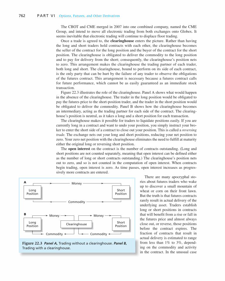
762 P A R T V I Options, Futures, and Other Derivatives
The CBOT and CME merged in 2007 into one combined company, named the CME Group, and intend to move all electronic trading from both exchanges onto Globex. It seems inevitable that electronic trading will continue to displace floor trading.
Once a trade is agreed to, the clearinghouse enters the picture. Rather than having the long and short traders hold contracts with each other, the clearinghouse becomes the seller of the contract for the long position and the buyer of the contract for the short position. The clearinghouse is obligated to deliver the commodity to the long position and to pay for delivery from the short; consequently, the clearinghouse’s position nets to zero. This arrangement makes the clearinghouse the trading partner of each trader, both long and short. The clearinghouse, bound to perform on its side of each contract, is the only party that can be hurt by the failure of any trader to observe the obligations of the futures contract. This arrangement is necessary because a futures contract calls for future performance, which cannot be as easily guaranteed as an immediate stock transaction.
Figure 22.3 illustrates the role of the clearinghouse. Panel A shows what would happen in the absence of the clearinghouse. The trader in the long position would be obligated to pay the futures price to the short-position trader, and the trader in the short position would be obligated to deliver the commodity. Panel B shows how the clearinghouse becomes an intermediary, acting as the trading partner for each side of the contract. The clearing-house’s position is neutral, as it takes a long and a short position for each transaction.
The clearinghouse makes it possible for traders to liquidate positions easily. If you are currently long in a contract and want to undo your position, you simply instruct your bro-ker to enter the short side of a contract to close out your position. This is called a reversing
trade. The exchange nets out your long and short positions, reducing your net position to zero. Your zero net position with the clearinghouse eliminates the need to fulfill at maturity either the original long or reversing short position.
The open interest on the contract is the number of contracts outstanding. (Long and short positions are not counted separately, meaning that open interest can be defined either as the number of long or short contracts outstanding.) The clearinghouse’s position nets out to zero, and so is not counted in the computation of open interest. When contracts begin trading, open interest is zero. As time passes, open interest increases as progres-sively more contracts are entered.
There are many apocryphal sto-ries about futures traders who wake up to discover a small mountain of wheat or corn on their front lawn. But the truth is that futures contracts rarely result in actual delivery of the underlying asset. Traders establish long or short positions in contracts that will benefit from a rise or fall in the futures price and almost always close out, or reverse, those positions before the contract expires. The fraction of contracts that result in actual delivery is estimated to range from less than 1% to 3%, depend-ing on the commodity and activity in the contract. In the unusual case
A Money
Commodity
LongPosition
B Money
Commodity
Money
Commodity
LongPosition Clearinghouse
ShortPosition
ShortPosition
Figure 22.3 Panel A, Trading without a clearinghouse. Panel B, Trading with a clearinghouse.
C H A P T E R 2 2 Futures Markets 763
of actual deliveries of commodities, they occur via regular channels of supply, most often warehouse receipts.
You can see the typical pattern of open interest in Figure 22.1 . In the gold contract, for example, the December delivery contract is approaching maturity, and open interest is small; most contracts have been reversed already. The greatest open interest is in the February contract. The more-distant maturity contracts have less open interest, as they have been available only recently, and few participants have yet traded. For other contracts, for example, cotton, for which the nearest maturity date isn’t until March, open interest is typically highest in the nearest contract.
The Margin Account and Marking to Market
The total profit or loss realized by the long trader who buys a contract at time 0 and closes, or reverses, it at time t is just the change in the futures price over the period, F t 2 F 0 . Symmetrically, the short trader earns F 0 2 F t .
The process by which profits or losses accrue to traders is called marking to market. At initial execution of a trade, each trader establishes a margin account. The margin is a secu-rity account consisting of cash or near-cash securities, such as Treasury bills, that ensures the trader is able to satisfy the obligations of the futures contract. Because both parties to a futures contract are exposed to losses, both must post margin. To illustrate, return to the first corn contract listed in Figure 22.1 . If the initial required margin on corn, for example, is 10%, then the trader must post $1,960 per contract of the margin account. This is 10% of the value of the contract, $3.92 per bushel 3 5,000 bushels per contract.
Because the initial margin may be satisfied by posting interest-earning securities, the requirement does not impose a significant opportunity cost of funds on the trader. The ini-tial margin is usually set between 5% and 15% of the total value of the contract. Contracts written on assets with more volatile prices require higher margins.
On any day that futures contracts trade, futures prices may rise or may fall. Instead of wait-ing until the maturity date for traders to realize all gains and losses, the clearinghouse requires all positions to recognize profits as they accrue daily. If the futures price of corn rises from 392 to 394 cents per bushel, the clearinghouse credits the margin account of the long position for 5,000 bushels times 2 cents per bushel, or $100 per contract. Conversely, for the short position, the clearinghouse takes this amount from the margin account for each contract held.
This daily settling is called marking to market. It means the maturity date of the contract does not govern realization of profit or loss. Marking to market ensures that, as futures prices change, the proceeds accrue to the trader’s margin account immediately. We will provide a more detailed example of this process shortly.
Marking to market is the major way in which futures and forward contracts differ, besides contract standardization. Futures follow this pay-(or receive-)as-you-go method. Forward contracts are simply held until maturity, and no funds are transferred until that date, although the contracts may be traded.
If a trader accrues sustained losses from daily marking to market, the margin account may fall below a critical value called the maintenance margin. If the value of the account falls below this value, the trader receives a margin call. Margins and margin calls safeguard the position of the clearinghouse. Positions are closed out before the margin account is exhausted—the trader’s losses are covered, and the clearinghouse is not put at risk.
CONCEPT CHECK
2 What must be the net inflow or outlay from marking to market for the clearinghouse?

764 P A R T V I Options, Futures, and Other Derivatives
Example 22.1 Maintenance Margin
Suppose the maintenance margin is 5% while the initial margin was 10% of the value of the corn, or $1,960. Then a margin call will go out when the original margin account has fallen in half, by about $980. Each 1-cent decline in the corn price results in a $50 loss to the long position. Therefore, the futures price need only fall by 20 cents to trigger a margin call. Either new funds must be transferred into the margin account or the broker will close out enough of the trader’s account to re-establish the required margin for the position.
On the contract maturity date, the futures price will equal the spot price of the com-modity. As a maturing contract calls for immediate delivery, the futures price on that day must equal the spot price—the cost of the commodity from the two competing sources is equalized in a competitive market. 2 You may obtain delivery of the commodity either by purchasing it directly in the spot market or by entering the long side of a futures contract.
A commodity available from two sources (spot or futures market) must be priced identi-cally, or else investors will rush to purchase it from the cheap source in order to sell it in the high-priced market. Such arbitrage activity could not persist without prices adjusting to eliminate the arbitrage opportunity. Therefore, the futures price and the spot price must converge at maturity. This is called the convergence property.
For an investor who establishes a long position in a contract now (time 0) and holds that position until maturity (time T ), the sum of all daily settlements will equal F T 2 F 0 , where F T stands for the futures price at contract maturity. Because of convergence, however, the futures price at maturity, F T , equals the spot price, P T , so total futures profits also may be expressed as P T 2 F 0 . Thus we see that profits on a futures contract held to maturity per-fectly track changes in the value of the underlying asset.
2 Small differences between the spot and futures price at maturity may persist because of transportation costs, but this is a minor factor.
Example 22.2 Marking to Market
Assume the current futures price for silver for delivery 5 days from today is $17.10 per ounce. Suppose that over the next 5 days, the futures price evolves as follows:
Day Futures Price
0 (today) $17.10
1 17.20
2 17.25
3 17.18
4 17.18
5 (delivery) 17.21
The spot price of silver on the delivery date is $17.21: The convergence property implies that the price of silver in the spot market must equal the futures price on the delivery day.

C H A P T E R 2 2 Futures Markets 765
Cash versus Actual Delivery
Most futures contracts call for delivery of an actual commodity such as a particular grade of wheat or a specified amount of foreign currency if the contract is not reversed before maturity. For agricultural commodities, where quality of the delivered good may vary, the exchange sets quality standards as part of the futures contract. In some cases, contracts may be settled with higher- or lower-grade commodities. In these cases, a premium or dis-count is applied to the delivered commodity to adjust for the quality difference.
Some futures contracts call for cash settlement. An example is a stock index futures con-tract where the underlying asset is an index such as the Standard & Poor’s 500 or the New York Stock Exchange Index. Delivery of every stock in the index clearly would be impracti-cal. Hence the contract calls for “delivery” of a cash amount equal to the value that the index attains on the maturity date of the contract. The sum of all the daily settlements from mark-ing to market results in the long position realizing total profits or losses of S T 2 F 0 , where S T is the value of the stock index on the maturity date T and F 0 is the original futures price. Cash settlement closely mimics actual delivery, except the cash value of the asset rather than the asset itself is delivered by the short position in exchange for the futures price.
More concretely, the S&P 500 index contract calls for delivery of $250 times the value of the index. At maturity, the index might list at 1,100, the market-value-weighted index of the prices of all 500 stocks in the index. The cash settlement contract calls for delivery of $250 3 1,100, or $275,000 cash in return for $250 times the futures price. This yields exactly the same profit as would result from directly purchasing 250 units of the index for $275,000 and then delivering it for $250 times the original futures price.
Regulations
Futures markets are regulated by the federal Commodities Futures Trading Commission. The CFTC sets capital requirements for member firms of the futures exchanges, authorizes trading in new contracts, and oversees maintenance of daily trading records.
The daily mark-to-market settlements for each contract held by the long position will be as follows:
Day Profit (Loss) per Ounce 3 5,000 Ounces/Contract 5 Daily Proceeds
1 17.20 2 17.10 5 .10 $500
2 17.25 2 17.20 5 .05 250
3 17.18 2 17.25 5 2.07 2350
4 17.18 2 17.18 5 0 0
5 17.21 2 17.18 5 .03 150
Sum 5 $550
The profit on Day 1 is the increase in the futures price from the previous day, or ($17.20 2 $17.10) per ounce. Because each silver contract on the Commodity Exchange (CMX) calls for purchase and delivery of 5,000 ounces, the total profit per contract is 5,000 times $.10, or $500. On Day 3, when the futures price falls, the long position’s mar-gin account will be debited by $350. By Day 5, the sum of all daily proceeds is $550. This is exactly equal to 5,000 times the difference between the final futures price of $17.21 and original futures price of $17.10. Thus the sum of all the daily proceeds (per ounce of silver held long) equals P T 2 F 0 .

766 P A R T V I Options, Futures, and Other Derivatives
The futures exchange may set limits on the amount by which futures prices may change from one day to the next. For example, if the price limit on silver contracts traded on the Chicago Board of Trade is $1 and silver futures close today at $17.10 per ounce, then trades in silver tomorrow may vary only between $18.10 and $16.10 per ounce. The exchanges may increase or reduce price limits in response to perceived changes in price volatility of the contract. Price limits are often eliminated as contracts approach maturity, usually in the last month of trading.
Price limits traditionally are viewed as a means to limit violent price fluctuations. This reasoning seems dubious. Suppose an international monetary crisis overnight drives up the spot price of silver to $20.00. No one would sell silver futures at prices for future delivery as low as $17.10. Instead, the futures price would rise each day by the $1 limit, although the quoted price would represent only an unfilled bid order—no contracts would trade at the low quoted price. After several days of limit moves of $1 per day, the futures price would finally reach its equilibrium level, and trading would occur again. This process means no one could unload a position until the price reached its equilibrium level. We con-clude that price limits offer no real protection against fluctuations in equilibrium prices.
Taxation
Because of the mark-to-market procedure, investors do not have control over the tax year in which they realize gains or losses. Instead, price changes are realized gradually, with each daily settlement. Therefore, taxes are paid at year-end on cumulated profits or losses regardless of whether the position has been closed out. As a general rule, 60% of futures gains or losses are treated as long term, and 40% as short term.
22.3 Futures Markets Strategies
Hedging and Speculation
Hedging and speculating are two polar uses of futures markets. A speculator uses a futures contract to profit from movements in futures prices, a hedger to protect against price movement.
If speculators believe prices will increase, they will take a long position for expected profits. Conversely, they exploit expected price declines by taking a short position.
Example 22.3 Speculating with Oil Futures
Suppose that at the end of 2009 you believed that crude oil prices would increase, and therefore decided to purchase crude oil futures. Each contract calls for delivery of 1,000 barrels of oil. Figure 22.1 shows that the futures price for delivery in February 2010 is $71.86 per barrel. For every dollar increase in the futures price of crude, the long position gains $1,000 and the short position loses that amount.
Conversely, suppose you think that prices are heading lower and therefore sell a con-tract. If crude oil prices do in fact fall, then you will gain $1,000 per contract for every dollar that prices decline.
If crude oil is selling at the contract maturity date for $73.86, which is $2 more than the initial futures price, the long side will profit by $2,000 per contract purchased. The short side will lose an identical amount on each contract sold. On the other hand, if oil has fallen to $69.86, the long side will lose, and the short side will gain, $2,000 per contract.

C H A P T E R 2 2 Futures Markets 767
Why does a speculator buy a futures contract? Why not buy the underlying asset directly? One reason lies in transaction costs, which are far smaller in futures markets.
Another important reason is the leverage that futures trading provides. Recall that futures contracts require traders to post margin considerably less than the value of the asset underlying the contract. Therefore, they allow speculators to achieve much greater lever-age than is available from direct trading in a commodity.
Example 22.4 Futures and Leverage
Suppose the initial margin requirement for the oil contract is 10%. At a current futures price of $71.86, and contract size of 1,000 barrels, this would require margin of .10 3 71.86 3 1,000 5 $7,186. A $2 jump in oil prices represents an increase of 2.78%, and results in a $2,000 gain on the contract for the long position. This is a percentage gain of 27.8% in the $7,186 posted as margin, precisely 10 times the percentage increase in the oil price. The 10-to-1 ratio of percentage changes reflects the leverage inherent in the futures position, because the contract was established with an initial margin of one-tenth the value of the underlying asset.
Hedgers, by contrast, use futures to insulate themselves against price movements. A firm planning to sell oil, for example, might anticipate a period of market volatility and wish to protect its revenue against price fluctuations. To hedge the total revenue derived from the sale, the firm enters a short position in oil futures. As the following example illus-trates, this locks in its total proceeds (i.e., revenue from the sale of the oil plus proceeds from its futures position).
Example 22.5 Hedging with Oil Futures
Consider an oil distributor planning to sell 100,000 barrels of oil in February that wishes to hedge against a possible decline in oil prices. Because each contract calls for delivery of 1,000 barrels, it would sell 100 contracts that mature in February. Any decrease in prices would then generate a profit on the contracts that would offset the lower sales revenue from the oil.
To illustrate, suppose that the only three possible prices for oil in February are $69.86, $71.86, and $73.86 per barrel. The revenue from the oil sale will be 100,000 times the price per barrel. The profit on each contract sold will be 1,000 times any decline in the futures price. At maturity, the convergence property ensures that the final futures price will equal the spot price of oil. Therefore, the profit on the 100 contracts sold will equal 100,000 3 ( F 0 2 P T ), where P T is the oil price on the delivery date, and F 0 is the original futures price, $71.86.
Now consider the firm’s overall position. The total revenue in February can be com-puted as follows:
Oil Price in February, PT
$69.86 $71.86 $73.86
Revenue from oil sale: 100,000 3 PT $6,986,000 $7,186,000 $7,386,000
1 Profit on futures: 100,000 3 (F0 2 PT) 200,000 0 2200,000
TOTAL PROCEEDS $7,186,000 $7,186,000 $7,186,000

768 P A R T V I Options, Futures, and Other Derivatives
Figure 22.4 illustrates the nature of the hedge in Example 22.5 . The upward-sloping line is the revenue from the sale of oil. The downward-sloping line is the profit on the futures contract. The horizontal line is the sum of sales revenue plus futures profits. This line is flat, as the hedged position is independent of oil prices.
To generalize Example 22.5 , note that oil will sell for P T per barrel at the maturity of the contract. The profit per barrel on the futures will be F 0 2 P T . Therefore, total revenue is P T 1 ( F 0 2 P T ) 5 F 0 , which is independent of the eventual oil price.
The oil distributor in Example 22.5 engaged in a short hedge, taking a short futures position to offset risk in the sales price of a particular asset. A long hedge is the analogous hedge for someone who wishes to eliminate the risk of an uncertain purchase price. For example, suppose a power supplier planning to purchase oil is afraid that prices might rise by the time of the purchase. As the following Concept Check illustrates, the supplier might buy oil futures to lock in the net purchase price at the time of the transaction.
The revenue from the oil sale plus the proceeds from the contracts equals the current futures price, $71.86 per barrel. The variation in the price of the oil is precisely offset by the profits or losses on the futures position. For example, if oil falls to $69.86 a barrel, the short futures position generates $200,000 profit, just enough to bring total revenues to $7,186,000. The total is the same as if one were to arrange today to sell the oil in February at the futures price.
CONCEPT CHECK
3
Suppose as in Example 22.5 that oil will be selling in February for $69.86, $71.86, or $73.86 per barrel. Consider a firm such as an electric utility that plans to buy 100,000 barrels of oil in February. Show that if the firm buys 100 oil contracts today, its net expenditures in February will be hedged and equal to $7,186,000.
Sales Revenue per Barrel Futures Profits per Barrel Total Proceeds
100
80
Hedged revenues are constant at $71.86 per barrel,equal to the futures price
60
40
20
065 70 75
71.8685
�20
Pro
ceed
s (p
er
barr
el)
Oil Price
Sales revenue increases with oil price
Profit on short futures position falls with oil price
80
Figure 22.4 Hedging revenues using futures, Example 22.5 (Futures price 5 $71.86)

C H A P T E R 2 2 Futures Markets 769
Exact futures hedging may be impossible for some goods because the necessary futures contract is not traded. For example, a portfolio manager might want to hedge the value of a diversified, actively managed portfolio for a period of time. However, futures con-tracts are listed only on indexed portfolios. Nevertheless, because returns on the manag-er’s diversified portfolio will have a high correlation with returns on broad-based indexed portfolios, an effective hedge may be established by selling index futures contracts. Hedging a position using futures on another asset is called cross-hedging.
Basis Risk and Hedging
The basis is the difference between the futures price and the spot price. 3 As we have noted, on the maturity date of a contract, the basis must be zero: The convergence property implies that F T 2 P T 5 0. Before maturity, however, the futures price for later delivery may differ substantially from the current spot price.
In Example 22.5 we discussed the case of a short hedger who manages risk by entering a short position to deliver oil in the future. If the asset and futures contract are held until maturity, the hedger bears no risk. Risk is eliminated because the futures price and spot price at contract maturity must be equal: Gains and losses on the futures and the com-modity position will exactly cancel. However, if the contract and asset are to be liquidated early, before contract maturity, the hedger bears basis risk, because the futures price and spot price need not move in perfect lockstep at all times before the delivery date. In this case, gains and losses on the contract and the asset may not exactly offset each other.
Some speculators try to profit from movements in the basis. Rather than betting on the direction of the futures or spot prices per se, they bet on the changes in the difference between the two. A long spot–short futures position will profit when the basis narrows.
Example 22.6 Speculating on the Basis
Consider an investor holding 100 ounces of gold, who is short one gold-futures contract. Suppose that gold today sells for $991 an ounce, and the futures price for June delivery is $996 an ounce. Therefore, the basis is currently $5. Tomorrow, the spot price might increase to $995, while the futures price increases to $999, so the basis narrows to $4.
The investor’s gains and losses are as follows:
Gain on holdings of gold (per ounce): $995 2 $991 5 $4
Loss on gold futures position (per ounce): $999 2 $996 5 $3
The net gain is the decrease in the basis, or $1 per ounce.
A related strategy is a calendar spread position, where the investor takes a long posi-tion in a futures contract of one maturity and a short position in a contract on the same commodity, but with a different maturity. 4 Profits accrue if the difference in futures prices
3 Usage of the word basis is somewhat loose. It sometimes is used to refer to the futures-spot difference F 2 P, and sometimes to the spot-futures difference P 2 F. We will consistently call the basis F 2 P.
4 Yet another strategy is an intercommodity spread, in which the investor buys a contract on one commodity and sells a contract on a different commodity.
CONCEPT CHECK
4 What are the sources of risk to an investor who uses stock index futures to hedge an actively managed stock portfolio?
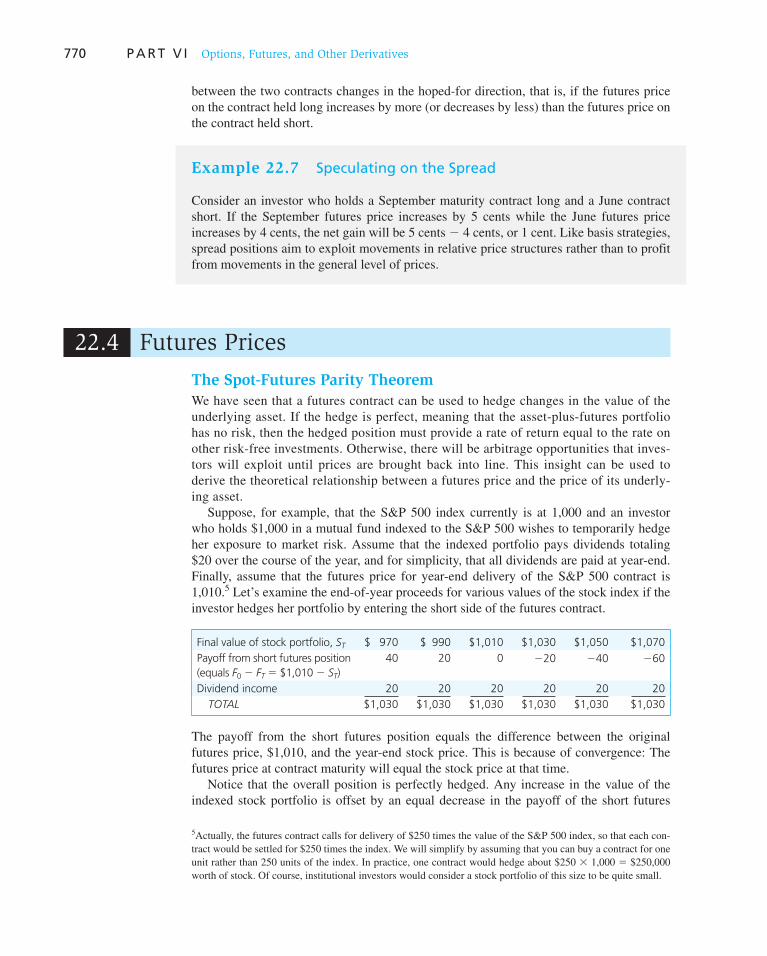
770 P A R T V I Options, Futures, and Other Derivatives
between the two contracts changes in the hoped-for direction, that is, if the futures price on the contract held long increases by more (or decreases by less) than the futures price on the contract held short.
Example 22.7 Speculating on the Spread
Consider an investor who holds a September maturity contract long and a June contract short. If the September futures price increases by 5 cents while the June futures price increases by 4 cents, the net gain will be 5 cents 2 4 cents, or 1 cent. Like basis strategies, spread positions aim to exploit movements in relative price structures rather than to profit from movements in the general level of prices.
22.4 Futures Prices
The Spot-Futures Parity Theorem
We have seen that a futures contract can be used to hedge changes in the value of the underlying asset. If the hedge is perfect, meaning that the asset-plus-futures portfolio has no risk, then the hedged position must provide a rate of return equal to the rate on other risk-free investments. Otherwise, there will be arbitrage opportunities that inves-tors will exploit until prices are brought back into line. This insight can be used to derive the theoretical relationship between a futures price and the price of its underly-ing asset.
Suppose, for example, that the S&P 500 index currently is at 1,000 and an investor who holds $1,000 in a mutual fund indexed to the S&P 500 wishes to temporarily hedge her exposure to market risk. Assume that the indexed portfolio pays dividends totaling $20 over the course of the year, and for simplicity, that all dividends are paid at year-end. Finally, assume that the futures price for year-end delivery of the S&P 500 contract is 1,010. 5 Let’s examine the end-of-year proceeds for various values of the stock index if the investor hedges her portfolio by entering the short side of the futures contract.
Final value of stock portfolio, ST $ 970 $ 990 $1,010 $1,030 $1,050 $1,070
Payoff from short futures position
(equals F0 2 FT 5 $1,010 2 ST)
40 20 0 220 240 260
Dividend income 20 20 20 20 20 20
TOTAL $1,030 $1,030 $1,030 $1,030 $1,030 $1,030
The payoff from the short futures position equals the difference between the original futures price, $1,010, and the year-end stock price. This is because of convergence: The futures price at contract maturity will equal the stock price at that time.
Notice that the overall position is perfectly hedged. Any increase in the value of the indexed stock portfolio is offset by an equal decrease in the payoff of the short futures
5 Actually, the futures contract calls for delivery of $250 times the value of the S&P 500 index, so that each con-tract would be settled for $250 times the index. We will simplify by assuming that you can buy a contract for one unit rather than 250 units of the index. In practice, one contract would hedge about $250 3 1,000 5 $250,000 worth of stock. Of course, institutional investors would consider a stock portfolio of this size to be quite small.

C H A P T E R 2 2 Futures Markets 771
position, resulting in a final value independent of the stock price. The $1,030 total payoff is the sum of the current futures price, F 0 5 $1,010, and the $20 dividend. It is as though the investor arranged to sell the stock at year-end for the current futures price, thereby eliminating price risk and locking in total proceeds equal to the sales price plus dividends paid before the sale.
What rate of return is earned on this riskless position? The stock investment requires an initial outlay of $1,000, whereas the futures position is established without an initial cash outflow. Therefore, the $1,000 portfolio grows to a year-end value of $1,030, providing a rate of return of 3%. More generally, a total investment of S 0 , the current stock price, grows to a final value of F 0 1 D, where D is the dividend payout on the portfolio. The rate of return is therefore
Rate of return on perfectly hedged stock portfolio 5(F0 1 D) 2 S0
S0
This return is essentially riskless. We observe F 0 at the beginning of the period when we enter the futures contract. While dividend payouts are not perfectly riskless, they are highly predictable over short periods, especially for diversified portfolios. Any uncertainty is extremely small compared to the uncertainty in stock prices.
Presumably, 3% must be the rate of return available on other riskless investments. If not, then investors would face two competing risk-free strategies with different rates of return, a situation that could not last. Therefore, we conclude that
(F0 1 D) 2 S0
S0
5 rf
Rearranging, we find that the futures price must be
F0 5 S0(1 1 rf) 2 D 5 S0(1 1 rf 2 d) (22.1)
where d is the dividend yield on the stock portfolio, defined as D / S 0 . This result is called the spot-futures parity theorem. It gives the normal or theoretically correct relationship between spot and futures prices. Any deviation from parity would give rise to risk-free arbitrage opportunities.
Example 22.8 Futures Market Arbitrage
Suppose that parity were violated. For example, suppose the risk-free interest rate in the economy were only 1% so that according to Equation 22.1 , the futures price should be $1,000(1.01) 2 $20 5 $990. The actual futures price, F 0 5 $1,010, is $20 higher than its “appropriate” value. This implies that an investor can make arbitrage profits by shorting the relatively overpriced futures contract and buying the relatively underpriced stock port-folio using money borrowed at the 1% market interest rate. The proceeds from this strategy would be as follows:
Action Initial Cash Flow Cash Flow in 1 Year
Borrow $1,000, repay with interest in 1 year 11,000 21,000(1.01) 5 2$1,010
Buy stock for $1,000 21,000 ST 1 $20 dividend
Enter short futures position (F0 5 $1,010) 0 $1,010 2 ST
TOTAL 0 $20
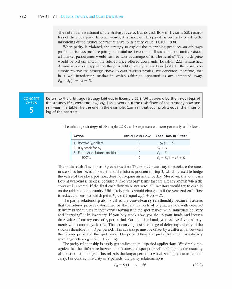
772 P A R T V I Options, Futures, and Other Derivatives
The arbitrage strategy of Example 22.8 can be represented more generally as follows:
Action Initial Cash Flow Cash Flow in 1 Year
1. Borrow S0 dollars S0 2S0 (1 1 rf)
2. Buy stock for S0 2S0 ST 1 D
3. Enter short futures position 0 F0 2 ST
TOTAL 0 F0 2 S0(1 1 rf) 1 D
The initial cash flow is zero by construction: The money necessary to purchase the stock in step 1 is borrowed in step 2, and the futures position in step 3, which is used to hedge the value of the stock position, does not require an initial outlay. Moreover, the total cash flow at year-end is riskless because it involves only terms that are already known when the contract is entered. If the final cash flow were not zero, all investors would try to cash in on the arbitrage opportunity. Ultimately prices would change until the year-end cash flow is reduced to zero, at which point F 0 would equal S 0 (1 1 r f ) 2 D.
The parity relationship also is called the cost-of-carry relationship because it asserts that the futures price is determined by the relative costs of buying a stock with deferred delivery in the futures market versus buying it in the spot market with immediate delivery and “carrying” it in inventory. If you buy stock now, you tie up your funds and incur a time-value-of-money cost of r f per period. On the other hand, you receive dividend pay-ments with a current yield of d. The net carrying cost advantage of deferring delivery of the stock is therefore r f 2 d per period. This advantage must be offset by a differential between the futures price and the spot price. The price differential just offsets the cost-of-carry advantage when F 0 5 S 0 (1 1 r f 2 d ).
The parity relationship is easily generalized to multiperiod applications. We simply rec-ognize that the difference between the futures and spot price will be larger as the maturity of the contract is longer. This reflects the longer period to which we apply the net cost of carry. For contract maturity of T periods, the parity relationship is
F0 5 S0(1 1 rf 2 d)T (22.2)
The net initial investment of the strategy is zero. But its cash flow in 1 year is $20 regard-less of the stock price. In other words, it is riskless. This payoff is precisely equal to the mispricing of the futures contract relative to its parity value, 1,010 2 990.
When parity is violated, the strategy to exploit the mispricing produces an arbitrage profit—a riskless profit requiring no initial net investment. If such an opportunity existed, all market participants would rush to take advantage of it. The results? The stock price would be bid up, and/or the futures price offered down until Equation 22.1 is satisfied. A similar analysis applies to the possibility that F 0 is less than $990. In this case, you simply reverse the strategy above to earn riskless profits. We conclude, therefore, that in a well-functioning market in which arbitrage opportunities are competed away, F 0 5 S 0 (1 1 r f ) 2 D.
CONCEPT CHECK
5
Return to the arbitrage strategy laid out in Example 22.8 . What would be the three steps of the strategy if F 0 were too low, say, $980? Work out the cash flows of the strategy now and in 1 year in a table like the one in the example. Confirm that your profits equal the mispric-ing of the contract.
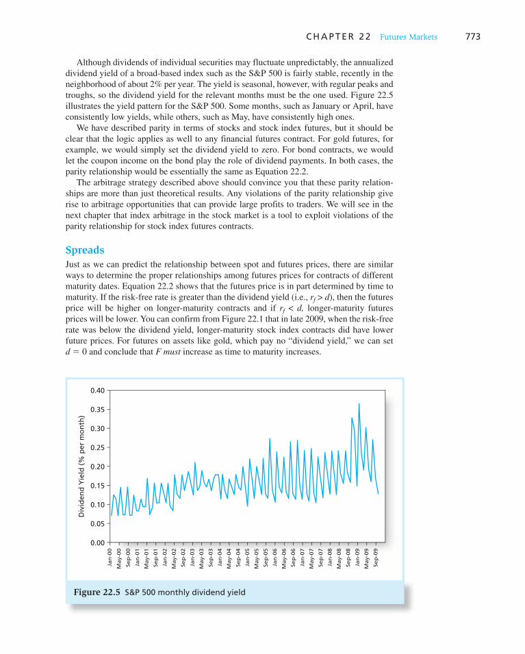
C H A P T E R 2 2 Futures Markets 773
Although dividends of individual securities may fluctuate unpredictably, the annualized dividend yield of a broad-based index such as the S&P 500 is fairly stable, recently in the neighborhood of about 2% per year. The yield is seasonal, however, with regular peaks and troughs, so the dividend yield for the relevant months must be the one used. Figure 22.5 illustrates the yield pattern for the S&P 500. Some months, such as January or April, have consistently low yields, while others, such as May, have consistently high ones.
We have described parity in terms of stocks and stock index futures, but it should be clear that the logic applies as well to any financial futures contract. For gold futures, for example, we would simply set the dividend yield to zero. For bond contracts, we would let the coupon income on the bond play the role of dividend payments. In both cases, the parity relationship would be essentially the same as Equation 22.2 .
The arbitrage strategy described above should convince you that these parity relation-ships are more than just theoretical results. Any violations of the parity relationship give rise to arbitrage opportunities that can provide large profits to traders. We will see in the next chapter that index arbitrage in the stock market is a tool to exploit violations of the parity relationship for stock index futures contracts.
Spreads
Just as we can predict the relationship between spot and futures prices, there are similar ways to determine the proper relationships among futures prices for contracts of different maturity dates. Equation 22.2 shows that the futures price is in part determined by time to maturity. If the risk-free rate is greater than the dividend yield (i.e., r f > d ), then the futures price will be higher on longer-maturity contracts and if r f < d, longer-maturity futures prices will be lower. You can confirm from Figure 22.1 that in late 2009, when the risk-free rate was below the dividend yield, longer-maturity stock index contracts did have lower future prices. For futures on assets like gold, which pay no “dividend yield,” we can set d 5 0 and conclude that F must increase as time to maturity increases.
0.40
0.35
0.30
0.25
0.20
0.15
0.10
0.05
0.00
Jan
-00
May-0
0
Sep
-00
Jan
-01
May-0
1
Sep
-01
Jan
-02
May-0
2
Sep
-02
Jan
-03
May-0
3
Sep
-03
Jan
-04
May-0
4
Sep
-04
Jan
-05
May-0
5
Jan
-06
Sep
-05
Jan
-07
May-0
7
Sep
-07
Jan
-08
May-0
8
Sep
-08
Jan
-09
May-0
9
Sep
-09
Sep
-06
May-0
6
Div
iden
d Y
ield
(%
per
mo
nth
)
Figure 22.5 S&P 500 monthly dividend yield

774 P A R T V I Options, Futures, and Other Derivatives
To be more precise about spread pricing, call F ( T 1 ) the current futures price for delivery at date T 1 , and F ( T 2 ) the futures price for delivery at T 2 . Let d be the dividend yield of the stock. We know from the parity Equation 22.2 that
F (T1) 5 S0 (1 1 rf 2 d )T1
F (T2) 5 S0 (1 1 rf 2 d )T2
As a result,
F (T2) /F (T1) 5 (1 1 rf 2 d )(T22T1)
Therefore, the basic parity relationship for spreads is
F (T2) 5 F (T1)(1 1 rf 2 d )(T22T1) (22.3)
Equation 22.3 should remind you of the spot-futures parity relationship. The major differ-ence is in the substitution of F ( T 1 ) for the current spot price. The intuition is also similar. Delaying delivery from T 1 to T 2 provides the long position the knowledge that the stock will be purchased for F ( T 2 ) dollars at T 2 but does not require that money be tied up in the stock until T 2 . The savings realized are the net cost of carry between T 1 and T 2 . Delaying delivery from T 1 until T 2 frees up F ( T 1 ) dollars, which earn risk-free interest at r f . The delayed delivery of the stock also results in the lost dividend yield between T 1 and T 2 . The net cost of carry saved by delaying the delivery is thus r f 2 d. This gives the proportional increase in the futures price that is required to compensate market participants for the delayed delivery of the stock and postponement of the payment of the futures price. If the parity condition for spreads is violated, arbitrage opportunities will arise. ( Problem 19 at the end of the chapter explores this possibility.)
Example 22.9 Spread Pricing
To see how to use Equation 22.3 , consider the following data for a hypothetical contract:
Contract Maturity Data Futures Price
January 15 $105.00
March 15 105.10
Suppose that the effective annual T-bill rate is expected to persist at 3% and that the divi-dend yield is 2% per year. The “correct” March futures price relative to the January price is, according to Equation 22.3 ,
105(1 1 .03 2 .02)1/6 5 105.174
The actual March futures price is 105.10, meaning that the March futures price is slightly underpriced compared to the January futures and that, aside from transaction costs, an arbitrage opportunity seems to be present.
Equation 22.3 shows that futures prices should all move together. Actually, it is not surprising that futures prices for different maturity dates move in unison, because all are linked to the same spot price through the parity relationship. Figure 22.6 plots futures prices on gold for three maturity dates. It is apparent that the prices move in virtual lockstep and that the more distant delivery dates command higher futures prices, as Equation 22.3 predicts.
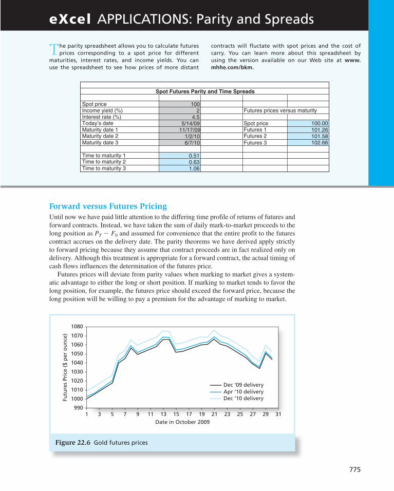
Spot Futures Parity and Time Spreads
Spot priceIncome yield (%)Interest rate (%)Today’s dateMaturity date 1Maturity date 2Maturity date 3
Time to maturity 1Time to maturity 2Time to maturity 3
100
100.00101.26101.58102.66
24.5
5/14/0911/17/09
1/2/106/7/10
0.510.631.06
Futures prices versus maturity
Spot priceFutures 1Futures 2Futures 3
775
Forward versus Futures Pricing
Until now we have paid little attention to the differing time profile of returns of futures and forward contracts. Instead, we have taken the sum of daily mark-to-market proceeds to the long position as P T 2 F 0 and assumed for convenience that the entire profit to the futures contract accrues on the delivery date. The parity theorems we have derived apply strictly to forward pricing because they assume that contract proceeds are in fact realized only on delivery. Although this treatment is appropriate for a forward contract, the actual timing of cash flows influences the determination of the futures price.
Futures prices will deviate from parity values when marking to market gives a system-atic advantage to either the long or short position. If marking to market tends to favor the long position, for example, the futures price should exceed the forward price, because the long position will be willing to pay a premium for the advantage of marking to market.
eXcel APPLICATIONS: Parity and Spreads
T he parity spreadsheet allows you to calculate futures prices corresponding to a spot price for different
maturities, interest rates, and income yields. You can use the spreadsheet to see how prices of more distant
c ontracts will fluctate with spot prices and the cost of carry. You can learn more about this spreadsheet by using the version available on our Web site at www.
mhhe.com/bkm .
1 3 5 7 9 11 13 15 17 19 21 23 25 27 29 31990
1000
1010
1020
1030
1040
1050
1060
1070
1080
Futu
res
Pri
ce (
$ p
er
ou
nce
)
Date in October 2009
Apr ‘10 deliveryDec ‘10 delivery
Dec ‘09 delivery
Figure 22.6 Gold futures prices

776 P A R T V I Options, Futures, and Other Derivatives
When will marking to market favor either a long or short trader? A trader will ben-efit if daily settlements are received when the interest rate is high and are paid when the interest rate is low. Receiving payments when the interest rate is high allows investment of proceeds at a high rate. Because long positions will benefit if futures prices tend to rise when interest rates are high, these investors will be willing to accept a higher futures price. Therefore, a positive correlation between interest rates and changes in futures prices implies that the “fair” futures price will exceed the forward price. Conversely, a negative correlation means that marking to market favors the short position and implies that the equilibrium futures price should be below the forward price.
For most contracts, the covariance between futures prices and interest rates is so low that the difference between futures and forward prices will be negligible. However, con-tracts on long-term fixed-income securities are an important exception to this rule. In this case, because prices have a high correlation with interest rates, the covariance can be large enough to generate a meaningful spread between forward and future prices.
22.5 Futures Prices versus Expected Spot Prices
So far we have considered the relationship between futures prices and the current spot price. One of the oldest controversies in the theory of futures pricing concerns the rela-tionship between the futures price and the expected value of the spot price of the com-modity at some future date. In other words, how well does the futures price forecast the ultimate spot price? Three traditional theories have been put forth: the expecta-tions hypothesis, normal backwardation, and contango. Today’s consensus is that all of these traditional hypotheses are subsumed by the insights provided by modern port-folio theory. Figure 22.7 shows the expected path of futures under the three traditional hypotheses.
Expectations Hypothesis
The expectations hypothesis is the simplest theory of futures pricing. It states that the futures price equals the expected value of the future spot price of the asset: F 0 5 E ( P T ). Under this theory the expected profit to either position of a futures contract would equal zero: The short position’s expected profit is F 0 2 E ( P T ), whereas the long’s is E ( P T ) 2 F 0 . With F 0 5 E ( P T ), the expected profit to either side is zero. This hypothesis relies on a notion of risk neutrality. If all market participants are risk neutral, they should agree on a futures price that provides an expected profit of zero to all parties.
The expectations hypothesis bears a resemblance to market equilibrium in a world with no uncertainty; that is, if prices of goods at all future dates are currently known, then the futures price for delivery at any particular date would equal the currently known future spot price for that date. It is a tempting but incorrect leap to then assert that under uncertainty the futures price should equal the currently expected spot price. This view ignores the risk premiums that must be built into futures prices when ultimate spot prices are uncertain.
Normal Backwardation
This theory is associated with the famous British economists John Maynard Keynes and John Hicks. They argued that for most commodities there are natural hedgers who wish to shed risk. For example, wheat farmers desire to shed the risk of uncertain wheat prices. These farmers will take short positions to deliver wheat in the future at
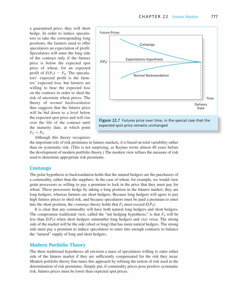
C H A P T E R 2 2 Futures Markets 777
a guaranteed price; they will short hedge. In order to induce specula-tors to take the corresponding long positions, the farmers need to offer speculators an expectation of profit. Speculators will enter the long side of the contract only if the futures price is below the expected spot price of wheat, for an expected profit of E ( P T ) 2 F 0 . The specula-tors’ expected profit is the farm-ers’ expected loss, but farmers are willing to bear the expected loss on the contract in order to shed the risk of uncertain wheat prices. The theory of normal backwardation thus suggests that the futures price will be bid down to a level below the expected spot price and will rise over the life of the contract until the maturity date, at which point F T 5 P T .
Although this theory recognizes the important role of risk premiums in futures markets, it is based on total variability rather than on systematic risk. (This is not surprising, as Keynes wrote almost 40 years before the development of modern portfolio theory.) The modern view refines the measure of risk used to determine appropriate risk premiums.
Contango
The polar hypothesis to backwardation holds that the natural hedgers are the purchasers of a commodity, rather than the suppliers. In the case of wheat, for example, we would view grain processors as willing to pay a premium to lock in the price that they must pay for wheat. These processors hedge by taking a long position in the futures market; they are long hedgers, whereas farmers are short hedgers. Because long hedgers will agree to pay high futures prices to shed risk, and because speculators must be paid a premium to enter into the short position, the contango theory holds that F 0 must exceed E ( P T ).
It is clear that any commodity will have both natural long hedgers and short hedgers. The compromise traditional view, called the “net hedging hypothesis,” is that F 0 will be less than E ( P T ) when short hedgers outnumber long hedgers and vice versa. The strong side of the market will be the side (short or long) that has more natural hedgers. The strong side must pay a premium to induce speculators to enter into enough contracts to balance the “natural” supply of long and short hedgers.
Modern Portfolio Theory
The three traditional hypotheses all envision a mass of speculators willing to enter either side of the futures market if they are sufficiently compensated for the risk they incur. Modern portfolio theory fine-tunes this approach by refining the notion of risk used in the determination of risk premiums. Simply put, if commodity prices pose positive systematic risk, futures prices must be lower than expected spot prices.
Future Prices
Expectations Hypothesis
Contango
Normal Backwardation
Time
E(PT)
DeliveryDate
Figure 22.7 Futures price over time, in the special case that the expected spot price remains unchanged

Vis
it u
s at
ww
w.m
hh
e.co
m/b
km778 P A R T V I Options, Futures, and Other Derivatives
As an example of the use of modern portfolio theory to determine the equilibrium futures price, consider once again a stock paying no dividends. If E ( P T ) denotes today’s expectation of the time T price of the stock, and k denotes the required rate of return on the stock, then the price of the stock today must equal the present value of its expected future payoff as follows:
P0 5E(PT)
(1 1 k)T (22.4)
We also know from the spot-futures parity relationship that
P0 5F0
(1 1 rf)T (22.5)
Therefore, the right-hand sides of Equations 22.4 and 22.5 must be equal. Equating these terms allows us to solve for F 0 :
F0 5 E(PT)¢ 1 1 rf
1 1 k≤T
(22.6)
You can see immediately from Equation 22.6 that F 0 will be less than the expectation of P T whenever k is greater than r f , which will be the case for any positive-beta asset. This means that the long side of the contract will make an expected profit [ F 0 will be lower than E ( P T )] when the commodity exhibits positive systematic risk ( k is greater than r f ).
Why should this be? A long futures position will provide a profit (or loss) of P T 2 F 0 . If the ultimate realization of P T involves positive systematic risk, the profit to the long posi-tion also involves such risk. Speculators with well-diversified portfolios will be willing to enter long futures positions only if they receive compensation for bearing that risk in the form of positive expected profits. Their expected profits will be positive only if E ( P T ) is greater than F 0 . The converse is that the short position’s profit is the negative of the long’s and will have negative systematic risk. Diversified investors in the short position will be willing to suffer an expected loss in order to lower portfolio risk and will be willing to enter
the contract even when F 0 is less than E ( P T ). Therefore, if P T has positive beta, F 0 must be less than the expec-tation of P T . The analysis is reversed for negative-beta commodities.
CONCEPT CHECK
6 What must be true of the risk of the spot price of an asset if the futures price is an unbiased estimate of the ultimate spot price?
1. Forward contracts are arrangements that call for future delivery of an asset at a currently agreed-on price. The long trader is obligated to purchase the good, and the short trader is obligated to deliver it. If the price of the asset at the maturity of the contract exceeds the forward price, the long side benefits by virtue of acquiring the good at the contract price.
2. A futures contract is similar to a forward contract, differing most importantly in the aspects of standardization and marking to market, which is the process by which gains and losses on futures contract positions are settled daily. In contrast, forward contracts call for no cash transfers until contract maturity.
3. Futures contracts are traded on organized exchanges that standardize the size of the contract, the grade of the deliverable asset, the delivery date, and the delivery location. Traders negotiate only over the contract price. This standardization creates increased liquidity in the marketplace and means that buyers and sellers can easily find many traders for a desired purchase or sale.
SUMMARY

Vis
it u
s at
ww
w.m
hh
e.co
m/b
kmV
isit
us
at w
ww
.mh
he.
com
/bkm
C H A P T E R 2 2 Futures Markets 779
4. The clearinghouse acts as an intermediary between each pair of traders, acting as the short posi-tion for each long and as the long position for each short. In this way traders need not be con-cerned about the performance of the trader on the opposite side of the contract. In turn, traders post margins to guarantee their own performance on the contracts.
5. The gain or loss to the long side for the futures contract held between time 0 and time t is F t 2 F 0 . Because F T 5 P T , the long’s profit if the contract is held until maturity is P T 2 F 0 , where P T is the spot price at time T and F 0 is the original futures price. The gain or loss to the short position is F 0 2 P T .
6. Futures contracts may be used for hedging or speculating. Speculators use the contracts to take a stand on the ultimate price of an asset. Short hedgers take short positions in contracts to offset any gains or losses on the value of an asset already held in inventory. Long hedgers take long posi-tions to offset gains or losses in the purchase price of a good.
7. The spot-futures parity relationship states that the equilibrium futures price on an asset providing no service or payments (such as dividends) is F 0 5 P 0 (1 1 r f )
T . If the futures price deviates from this value, then market participants can earn arbitrage profits.
8. If the asset provides services or payments with yield d, the parity relationship becomes F 0 5 P 0 (1 1 r f 2 d ) T . This model is also called the cost-of-carry model, because it states that futures price must exceed the spot price by the net cost of carrying the asset until maturity date T.
9. The equilibrium futures price will be less than the currently expected time T spot price if the spot price exhibits systematic risk. This provides an expected profit for the long position who bears the risk and imposes an expected loss on the short position who is willing to accept that expected loss as a means to shed systematic risk.
Related Web sites for this chapter are available at www.mhhe.com/bkm
forward contract futures price long position short position single-stock futures clearinghouse
open interest marking to market maintenance margin convergence property cash settlement basis
basis risk calendar spread spot-futures parity theorem cost-of-carry relationship
KEY TERMS
1. Why is there no futures market in cement?
2. Why might individuals purchase futures contracts rather than the underlying asset?
3. What is the difference in cash flow between short-selling an asset and entering a short futures position?
4. Are the following statements true or false? Why?
a. All else equal, the futures price on a stock index with a high dividend yield should be higher than the futures price on an index with a low dividend yield.
b. All else equal, the futures price on a high-beta stock should be higher than the futures price on a low-beta stock.
c. The beta of a short position in the S&P 500 futures contract is negative.
5. What is the difference between the futures price and the value of the futures contract?
6. Evaluate the criticism that futures markets siphon off capital from more productive uses.
7. a. Turn to the S&P 500 contract in Figure 22.1 . If the margin requirement is 10% of the futures price times the multiplier of $250, how much must you deposit with your broker to trade the March maturity contract?
b. If the March futures price were to increase to 1,150, what percentage return would you earn on your net investment if you entered the long side of the contract at the price shown in the figure?
c. If the March futures price falls by 1%, what is your percentage return?
PROBLEM SETS
i. Basic
ii. Intermediate

Vis
it u
s at
ww
w.m
hh
e.co
m/b
km780 P A R T V I Options, Futures, and Other Derivatives
8. a. A single-stock futures contract on a non-dividend-paying stock with current price $150 has a maturity of 1 year. If the T-bill rate is 3%, what should the futures price be?
b. What should the futures price be if the maturity of the contract is 3 years? c. What if the interest rate is 6% and the maturity of the contract is 3 years?
9. How might a portfolio manager use financial futures to hedge risk in each of the following circumstances:
a. You own a large position in a relatively illiquid bond that you want to sell. b. You have a large gain on one of your Treasuries and want to sell it, but you would like to
defer the gain until the next tax year. c. You will receive your annual bonus next month that you hope to invest in long-term corpo-
rate bonds. You believe that bonds today are selling at quite attractive yields, and you are concerned that bond prices will rise over the next few weeks.
10. Suppose the value of the S&P 500 stock index is currently 1,100. If the 1-year T-bill rate is 3% and the expected dividend yield on the S&P 500 is 2%, what should the 1-year maturity futures price be? What if the T-bill rate is less than the dividend yield, for example, 1%?
11. Consider a stock that pays no dividends on which a futures contract, a call option, and a put option trade. The maturity date for all three contracts is T, the exercise price of the put and the call are both X, and the futures price is F. Show that if X 5 F, then the call price equals the put price. Use parity conditions to guide your demonstration.
12. It is now January. The current interest rate is 5%. The June futures price for gold is $946.30, whereas the December futures price is $960.00. Is there an arbitrage opportunity here? If so, how would you exploit it?
13. OneChicago has just introduced a single-stock futures contract on Brandex stock, a company that currently pays no dividends. Each contract calls for delivery of 1,000 shares of stock in 1 year. The T-bill rate is 6% per year.
a. If Brandex stock now sells at $120 per share, what should the futures price be? b. If the Brandex price drops by 3%, what will be the change in the futures price and the change
in the investor’s margin account? c. If the margin on the contract is $12,000, what is the percentage return on the investor’s position?
14. The multiplier for a futures contract on a stock market index is $250. The maturity of the contract is 1 year, the current level of the index is 1,300, and the risk-free interest rate is .5% per month. The dividend yield on the index is .2% per month. Suppose that after 1 month, the stock index is at 1,320.
a. Find the cash flow from the mark-to-market proceeds on the contract. Assume that the parity condition always holds exactly.
b. Find the holding-period return if the initial margin on the contract is $13,000.
15. You are a corporate treasurer who will purchase $1 million of bonds for the sinking fund in 3 months. You believe rates will soon fall, and you would like to repurchase the company’s sinking fund bonds (which currently are selling below par) in advance of requirements. Unfor-tunately, you must obtain approval from the board of directors for such a purchase, and this can take up to 2 months. What action can you take in the futures market to hedge any adverse move-ments in bond yields and prices until you can actually buy the bonds? Will you be long or short? Why? A qualitative answer is fine.
16. The S&P portfolio pays a dividend yield of 1% annually. Its current value is 1,300. The T-bill rate is 4%. Suppose the S&P futures price for delivery in 1 year is 1,330. Construct an arbitrage strategy to exploit the mispricing and show that your profits 1 year hence will equal the mispric-ing in the futures market.
17. The Excel Application box in the chapter (available at www.mhhe.com/bkm ; link to Chapter 22 material) shows how to use the spot-futures parity relationship to find a “term structure of futures prices,” that is, futures prices for various maturity dates.
a. Suppose that today is January 1, 2011. Assume the interest rate is 3% per year and a stock index currently at 1,500 pays a dividend yield of 1.5%. Find the futures price for contract maturity dates of February 14, 2011, May 21, 2011, and November 18, 2011.
eXce lPlease visit us at www.mhhe.com/bkm

Vis
it u
s at
ww
w.m
hh
e.co
m/b
km
C H A P T E R 2 2 Futures Markets 781
b. What happens to the term structure of futures prices if the dividend yield is higher than the risk-free rate? For example, what if the dividend yield is 4%?
18. a. How should the parity condition ( Equation 22.2 ) for stocks be modified for futures contracts on Treasury bonds? What should play the role of the dividend yield in that equation?
b. In an environment with an upward-sloping yield curve, should T-bond futures prices on more-distant contracts be higher or lower than those on near-term contracts?
c. Confirm your intuition by examining Figure 22.1 .
19. Consider this arbitrage strategy to derive the parity relationship for spreads: (1) enter a long futures position with maturity date T 1 and futures price F ( T 1 ); (2) enter a short position with maturity T 2 and futures price F ( T 2 ); (3) at T 1 , when the first contract expires, buy the asset and borrow F ( T 1 ) dollars at rate r f ; (4) pay back the loan with interest at time T 2 .
a. What are the total cash flows to this strategy at times 0, T 1 , and T 2 ? b. Why must profits at time T 2 be zero if no arbitrage opportunities are present? c. What must the relationship between F ( T 1 ) and F ( T 2 ) be for the profits at T 2 to be equal to
zero? This relationship is the parity relationship for spreads.
iii. Challenge
1. Joan Tam, CFA, believes she has identified an arbitrage opportunity for a commodity as indi-cated by the following information:
Spot price for commodity $120
Futures price for commodity expiring in 1 year $125
Interest rate for 1 year 8%
a. Describe the transactions necessary to take advantage of this specific arbitrage opportunity. b. Calculate the arbitrage profit.
2. Michelle Industries issued a Swiss franc–denominated 5-year discount note for SFr200 million. The proceeds were converted to U.S. dollars to purchase capital equipment in the United States. The company wants to hedge this currency exposure and is considering the following alternatives:
• At-the-money Swiss franc call options. • Swiss franc forwards. • Swiss franc futures.
a. Contrast the essential characteristics of each of these three derivative instruments. b. Evaluate the suitability of each in relation to Michelle’s hedging objective, including both
advantages and disadvantages.
3. Identify the fundamental distinction between a futures contract and an option contract, and briefly explain the difference in the manner that futures and options modify portfolio risk.
4. Maria VanHusen, CFA, suggests that using forward contracts on fixed income securities can be used to protect the value of the Star Hospital Pension Plan’s bond portfolio against the pos-sibility of rising interest rates. VanHusen prepares the following example to illustrate how such protection would work:
• A 10-year bond with a face value of $1,000 is issued today at par value. The bond pays an annual coupon.
• An investor intends to buy this bond today and sell it in 6 months. • The 6-month risk-free interest rate today is 5% (annualized). • A 6-month forward contract on this bond is available, with a forward price of $1,024.70. • In 6 months, the price of the bond, including accrued interest, is forecast to fall to
$978.40 as a result of a rise in interest rates.
a. Should the investor buy or sell the forward contract to protect the value of the bond against rising interest rates during the holding period?
b. Calculate the value of the forward contract for the investor at the maturity of the forward contract if VanHusen’s bond-price forecast turns out to be accurate.
c. Calculate the change in value of the combined portfolio (the underlying bond and the appro-priate forward contract position) 6 months after contract initiation.
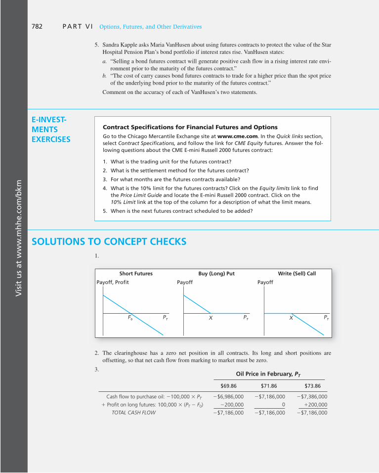
Vis
it u
s at
ww
w.m
hh
e.co
m/b
km782 P A R T V I Options, Futures, and Other Derivatives
5. Sandra Kapple asks Maria VanHusen about using futures contracts to protect the value of the Star Hospital Pension Plan’s bond portfolio if interest rates rise. VanHusen states:
a. “Selling a bond futures contract will generate positive cash flow in a rising interest rate envi-ronment prior to the maturity of the futures contract.”
b. “The cost of carry causes bond futures contracts to trade for a higher price than the spot price of the underlying bond prior to the maturity of the futures contract.”
Comment on the accuracy of each of VanHusen’s two statements.
E-INVEST-MENTS EXERCISES
Contract Specifications for Financial Futures and Options
Go to the Chicago Mercantile Exchange site at www.cme.com . In the Quick links section, select Contract Specifications, and follow the link for CME Equity futures. Answer the fol-lowing questions about the CME E-mini Russell 2000 futures contract:
1. What is the trading unit for the futures contract?
2. What is the settlement method for the futures contract?
3. For what months are the futures contracts available?
4. What is the 10% limit for the futures contracts? Click on the Equity limits link to find the Price Limit Guide and locate the E-mini Russell 2000 contract. Click on the 10% Limit link at the top of the column for a description of what the limit means.
5. When is the next futures contract scheduled to be added?
SOLUTIONS TO CONCEPT CHECKS
1.
2. The clearinghouse has a zero net position in all contracts. Its long and short positions are offsetting, so that net cash flow from marking to market must be zero.
3. Oil Price in February, PT
$69.86 $71.86 $73.86
Cash flow to purchase oil: 2100,000 3 PT 2$6,986,000 2$7,186,000 2$7,386,000
1 Profit on long futures: 100,000 3 (PT 2 F0) 2200,000 0 1200,000
TOTAL CASH FLOW 2$7,186,000 2$7,186,000 2$7,186,000
Payoff, Profit
Short Futures
F0 PT
Payoff
Buy (Long) Put
X PT
Payoff
Write (Sell) Call
X PT

Vis
it u
s at
ww
w.m
hh
e.co
m/b
km
C H A P T E R 2 2 Futures Markets 783
4. The risk would be that the index and the portfolio do not move perfectly together. Thus basis risk involving the spread between the futures price and the portfolio value could persist even if the index futures price were set perfectly relative to the index itself.
5. The futures price, $980, is $10 below the parity value of $990. The cash flow to the following strategy is riskless and equal to this mispricing.
Action Initial Cash Flow Cash Flow in 1 Year
Lend S0 dollars 21,000 1,000(1.01) 5 1,010
Sell stock short 11,000 2ST 2 20
Long futures 0 ST 2 980
TOTAL 0 $10 risklessly
6. It must have zero beta. If the futures price is an unbiased estimator, then we infer that it has a zero risk premium, which means that beta must be zero.

23 THE PREVIOUS CHAPTER provided a basic
introduction to the operation of futures mar-
kets and the principles of futures pricing. This
chapter explores both pricing and risk man-
agement in selected futures markets in more
depth. Most of the growth has been in finan-
cial futures, which dominate trading, so we
emphasize these contracts.
Hedging refers to techniques that offset
particular sources of risk, rather than as a
more ambitious search for an optimal risk-
return profile for an entire portfolio. Because
futures contracts are written on particular
quantities such as stock index values, foreign
exchange rates, commodity prices, and so
on, they are ideally suited for these applica-
tions. In this chapter we will consider several
hedging applications, illustrating general
principles using a variety of contracts. We also
show how hedging strategies can be used to
isolate bets on perceived profit opportunities.
We begin with foreign exchange futures,
where we show how forward exchange rates
are determined by interest rate differentials
across countries, and examine how firms can
use futures to manage exchange rate risk. We
then move on to stock-index futures, where
we focus on program trading and index
arbitrage. Next we turn to the most actively
traded markets, those for interest rate
futures. We also examine commodity futures
pricing. Finally, we turn to swaps markets in
foreign exchange and fixed-income securities.
We will see that swaps can be interpreted as
portfolios of forward contracts and valued
accordingly.
Futures, Swaps, and Risk Management
CHAPTER TWENTY-THREE 2 PA
RT
VI 23.1 Foreign Exchange Futures
The Markets
Exchange rates between currencies vary continually and often substantially. This vari-ability can be a source of concern for anyone involved in international business. A U.S. exporter who sells goods in England, for example, will be paid in British pounds, and the dollar value of those pounds depends on the exchange rate at the time payment is made.
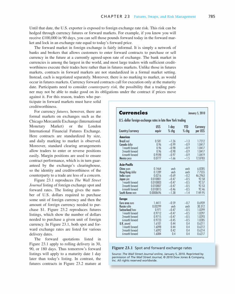
C H A P T E R 2 3 Futures, Swaps, and Risk Management 785
Americas Brazil real 0.581 −1.26 −1.3 1.7212 Canada dollar 0.96 −0.99 −0.9 1.0417 1-month forward 0.96 −0.98 −0.9 1.0417 3-month forward 0.96 −0.98 −0.9 1.0417 6-month forward 0.9598 −0.97 −0.9 1.0419 Mexico peso 0.0777 −1.66 −1.5 12.8783
US$equiv
1-day% chg
YTD% chg
Currencyper US$ Country/currency
U.S.-dollar foreign-exchange rates in late New York trading
Currencies January 5, 2010
Asia-Pacific China yuan 0.1464 unch unch 6.8285 Hong Kong dollar 0.1289 unch unch 7.7555 India rupee 0.0216 −0.69 −0.2 46.2963 Japan yen 0.010801 −0.47 −0.5 92.58 1-month forward 0.010803 −0.47 −0.5 92.57 3-month forward 0.010807 −0.47 −0.5 92.53 6-month forward 0.010815 −0.46 −0.5 92.46 South Korea won 0.0008696 −1.38 −1.4 1149.95
Europe Euro area euro 1.4411 −0.59 −0.7 0.6939 Russia ruble 0.03299 unch unch 30.312 Switzerland franc 0.971 −0.47 −0.5 1.0299 1-month forward 0.9712 −0.47 −0.5 1.0297 3-month forward 0.9715 −0.47 −0.5 1.0293 6-month forward 0.9723 −0.45 −0.5 1.0285 U.K. pound 1.6101 0.44 0.4 0.6211 1-month forward 1.6098 0.44 0.4 0.6212 3-month forward 1.6092 0.42 0.4 0.6214 6-month forward 1.6084 0.4 0.4 0.6217
Figure 23.1 Spot and forward exchange rates
Source: The Wall Street Journal online, January 5, 2010. Reprinted by permission of The Wall Street Journal, © 2010 Dow Jones & Company, Inc. All rights reserved worldwide.
Until that date, the U.S. exporter is exposed to foreign exchange rate risk. This risk can be hedged through currency futures or forward markets. For example, if you know you will receive £100,000 in 90 days, you can sell those pounds forward today in the forward mar-ket and lock in an exchange rate equal to today’s forward price.
The forward market in foreign exchange is fairly informal. It is simply a network of banks and brokers that allows customers to enter forward contracts to purchase or sell currency in the future at a currently agreed-upon rate of exchange. The bank market in currencies is among the largest in the world, and most large traders with sufficient credit-worthiness execute their trades here rather than in futures markets. Unlike those in futures markets, contracts in forward markets are not standardized in a formal market setting. Instead, each is negotiated separately. Moreover, there is no marking to market, as would occur in futures markets. Currency forward contracts call for execution only at the maturity date. Participants need to consider counterparty risk, the possibility that a trading part-ner may not be able to make good on its obligations under the contract if prices move against it. For this reason, traders who par-ticipate in forward markets must have solid creditworthiness.
For currency futures, however, there are formal markets on exchanges such as the Chicago Mercantile Exchange (International Monetary Market) or the London International Financial Futures Exchange. Here contracts are standardized by size, and daily marking to market is observed. Moreover, standard clearing arrangements allow traders to enter or reverse positions easily. Margin positions are used to ensure contract performance, which is in turn guar-anteed by the exchange’s clearinghouse, so the identity and creditworthiness of the counterparty to a trade are less of a concern.
Figure 23.1 reproduces The Wall Street
Journal listing of foreign exchange spot and forward rates. The listing gives the num-ber of U.S. dollars required to purchase some unit of foreign currency and then the amount of foreign currency needed to pur-chase $1. Figure 23.2 reproduces futures listings, which show the number of dollars needed to purchase a given unit of foreign currency. In Figure 23.1 , both spot and for-ward exchange rates are listed for various delivery dates.
The forward quotations listed in Figure 23.1 apply to rolling delivery in 30, 90, or 180 days. Thus tomorrow’s forward listings will apply to a maturity date 1 day later than today’s listing. In contrast, the futures contracts in Figure 23.2 mature at

786 P A R T V I Options, Futures, and Other Derivatives
specified dates in March, June, September, and December; these are the only four dates each year when futures con-tracts settle.
Interest Rate Parity
As is true of stocks and stock futures, there is a spot-futures exchange rate relationship that will prevail in well- functioning markets. Should this so-called interest
rate parity relationship be violated, arbitrageurs will be able to make risk-free profits in foreign exchange markets with zero net investment. Their actions will force futures and spot exchange rate back into alignment. Another term for interest rate parity is the covered interest arbitrage
relationship. We can illustrate the interest rate parity theorem by
using two currencies, the U.S. dollar and the British (U.K.) pound. Call E 0 the current exchange rate between the two
currencies, that is, E 0 dollars are required to purchase one pound. F 0 , the forward price, is the number of dollars that is agreed to today for purchase of one pound at time T in the future. Call the risk-free rates in the United States and United Kingdom r US and r UK , respectively.
The interest rate parity theorem then states that the proper relationship between E 0 and F 0 is given as
F0 5 E0 ¢ 1 1 rUS
1 1 rUK
≤T
(23.1)
For example, if r US 5 .04 and r UK 5 .05 annually, while E 0 5 $2 per pound, then the proper futures price for a 1-year contract would be
$2.00¢ 1.04
1.05≤ 5 $1.981 per pound
Consider the intuition behind this result. If r US is less than r UK , money invested in the United States will grow at a slower rate than money invested in the United Kingdom. If this is so, why wouldn’t all investors decide to invest their money in the United Kingdom? One important reason why not is that the dollar may be appreciating relative to the pound. Although dollar investments in the United States grow slower than pound investments in the United Kingdom, each dollar would then be worth progressively more pounds as time passes. Such an effect will exactly offset the advantage of the higher U.K. interest rate.
To complete the argument, we need only determine how an appreciating dollar will show up in Equation 23.1 . If the dollar is appreciating, meaning that progressively fewer dollars are required to purchase each pound, then the forward exchange rate F 0 (which equals the dollars required to purchase one pound for delivery in 1 year) must be less than E 0 , the current exchange rate. This is exactly what Equation 23.1 tells us: When r US is less than r UK , F 0 must be less than E 0 . The appreciation of the dollar embodied in the ratio of F 0to E 0 exactly compensates for the difference in interest rates available in the two countries. Of course, the argument also works in reverse: If r US is greater than r UK , then F 0 is greater than E 0 .
Japanese Yen(CME) -¥12,500,000; $ per 100¥March 1.0763 1.0852 1.0731 1.0804 .0064 100,677June 1.0787 1.0858 1.0743 1.0812 .0063 360
Canadian Dollar (CME) - CAD 100,000; $ per CADMarch .9549 .9660 .9508 .9594 .0032 100,156June .9557 .9657 .9509 .9593 .0032 1,376
British Pound (CME) - £62,500; $ per £ March 1.6118 1.6235 1.6052 1.6085 �.0061 81,371June 1.6132 1.6224 1.6045 1.6077 �.0061 501
Swiss Franc (CME) - CHF125,000; $ per CHFMarch .9677 .9748 .9600 .9720 .0051 35,932June .9709 .9755 .9612 .9728 .0051 62
Open Settle ChgOpen
interestHigh hi lo lowContract
Figure 23.2 Foreign exchange futures
Source: The Wall Street Journal, January 5, 2010. Reprinted by permission of The Wall Street Journal, © 2010 Dow Jones & Company, Inc. All rights reserved worldwide.

C H A P T E R 2 3 Futures, Swaps, and Risk Management 787
To generalize the strategy in Example 23.1 :
Action Initial CF ($) CF in 1 Year ($)
1. Borrow 1 U.K. pound in London. Convert to dollars. $E 0 2$E1(1 1 rUK)
2. Use proceeds of borrowing in London to lend in
the U.S.
2$E 0 $E 0(1 1 rUS)
3. Enter (1 1 rUK) futures positions to purchase
1 pound for F0 dollars. 0 (1 1 rUK)(E1 2 F0)
TOTAL 0 E0(1 1 rUS) 2 F0(1 1 rUK)
Let us again review the stages of the arbitrage operation. The first step requires borrow-ing one pound in the United Kingdom. With a current exchange rate of E 0 , the one pound is converted into E 0 dollars, which is a cash inflow. In 1 year the British loan must be paid off with interest, requiring a payment in pounds of (1 1 r UK ), or in dollars of E 1 (1 1 r UK ). In the second step the proceeds of the British loan are invested in the United States. This involves an initial cash outflow of $ E 0 , and a cash inflow of $ E 0 (1 1 r US ) in 1 year. Finally, the exchange risk involved in the British borrowing is hedged in step 3. Here, the (1 1 r UK ) pounds that will need to be delivered to satisfy the British loan are purchased ahead in the futures contract.
The net proceeds to the arbitrage portfolio are risk-free and given by E 0 (1 1 r US ) 2 F 0 (1 1 r UK ). If this value is positive, borrow in the United Kingdom, lend in the
Example 23.1 Covered Interest Arbitrage
What if the interest rate parity relationship were violated? For example, suppose the futures price is $1.97/£ instead of $1.981/£. You could adopt the following strategy to reap arbitrage profits. In this example let E 1 denote the exchange rate ($/£) that will prevail in 1 year. E 1 is, of course, a random variable from the perspective of today’s investors.
Action Initial Cash Flow ($) CF in 1 Year ($)
1. Borrow 1 U.K. pound in London. Convert to
dollars. Repay £1.05 at year-end.
2.00 2E1(£ 1.05)
2. Lend $2.00 in the United States. 22.00 $ 2.00(1.04)
3. Enter a contract to purchase £1.05 at a
(futures) price of F0 5 $1.97/£ 0 £ 1.05(E1 2 $1.97/£)
TOTAL 0 $.0115
In step 1, you exchange the one pound borrowed in the United Kingdom for $2 at the current exchange rate. After 1 year you must repay the pound borrowed with interest. Because the loan is made in the United Kingdom at the U.K. interest rate, you would repay £1.05, which would be worth E 1 (1.05) dollars. The U.S. loan in step 2 is made at the U.S. interest rate of 4%. The futures position in step 3 results in receipt of £1.05, for which you would pay $1.97 each, and then convert into dollars at exchange rate E 1 .
Note that the exchange rate risk here is exactly offset between the pound obligation in step 1 and the futures position in step 3. The profit from the strategy is therefore risk-free and requires no net investment.

788 P A R T V I Options, Futures, and Other Derivatives
United States, and enter a long futures position to eliminate foreign exchange risk. If the value is negative, borrow in the United States, lend in the United Kingdom, and take a short position in pound futures. When prices preclude arbitrage opportunities, the expres-sion must equal zero. This no-arbitrage condition implies that
F0 51 1 rUS
1 1 rUK
E0 (23.2)
which is the interest rate parity theorem for a 1-year horizon.
Example 23.2 Covered Interest Arbitrage
Ample empirical evidence bears out the interest rate parity relationship. For exam-ple, on January 4, 2010, the dollar-denominated LIBOR interest rate with maturity of 3 months was .26%, while the comparable U.K. pound-denominated rate was .61%. The spot exchange rate was $1.6101/£. Using these values, we find that interest rate parity implies that the forward exchange rate for delivery in 3 months should have been 1.6101 3 (1.0026/1.0061) ¼ 5 $1.6087/£. The actual forward rate was $1.6092/£, which was so close to the parity value that transaction costs would have prevented arbitrageurs from profiting from the discrepancy.
Direct versus Indirect Quotes
The exchange rate in Examples 23.1 and 23.2 is expressed as dollars per pound. This is an example of a direct exchange rate quote. The euro-dollar exchange rate is also typically expressed as a direct quote. In contrast, exchange rates for other currencies such as the Japanese yen or Swiss franc are typically expressed as indirect quotes, that is, as units of foreign currency per dollar, for example, 92 yen per dollar. For currencies expressed as indirect quotes, depreciation of the dollar would result in a decrease in the quoted exchange rate ($1 buys fewer yen); in contrast, dollar depreciation versus the pound would show up as a higher exchange rate (more dollars are required to buy £1). When the exchange rate is quoted as foreign currency per dollar, the domestic and foreign exchange rates in Equation 23.2 must be switched: in this case the equation becomes
F0 (foreign currency/$) 51 1 rforeign
1 1 rUS
3 E0 (foreign currency/$)
If the interest rate in the U.S. is higher than in Japan, the dollar will sell in the forward market at a lower price (will buy fewer yen) than in the spot market.
Using Futures to Manage Exchange Rate Risk
Consider a U.S. firm that exports most of its product to Great Britain. The firm is vulner-able to fluctuations in the dollar/pound exchange rate for several reasons. First, the dollar value of the pound-denominated revenue derived from its customers will fluctuate with the exchange rate. Second, the pound price that the firm can charge its customers in the United
CONCEPT CHECK
1 What would be the arbitrage strategy and associated profits in Example 23.1 if the initial futures price were F 0 5 $2.01/pound?

C H A P T E R 2 3 Futures, Swaps, and Risk Management 789
Kingdom will itself be affected by the exchange rate. For example, if the pound depreci-ates by 10% relative to the dollar, the firm would need to increase the pound price of its goods by 10% in order to maintain the dollar-equivalent price. However, the firm might not be able to raise the price by 10% if it faces competition from British producers, or if it believes the higher pound-denominated price would reduce demand for its product.
To offset its foreign exchange exposure, the firm might engage in transactions that bring it profits when the pound depreciates. The lost profits from business operations resulting from a depreciation will then be offset by gains on its financial transactions. Suppose, for exam-ple, that the firm enters a futures contract to deliver pounds for dollars at an exchange rate agreed to today. Therefore, if the pound depreciates, the futures position will yield a profit.
For example, suppose that the futures price is currently $2 per pound for delivery in 3 months. If the firm enters a futures contract with a futures price of $2.00 per pound, and the exchange rate in 3 months is $1.90 per pound, then the profit on the transaction is $.10 per pound. The futures price converges at the maturity date to the spot exchange rate of $1.90 and the profit to the short position is therefore F 0 2 F T 5 $2.00 2 $1.90 5 $.10 per pound.
How many pounds should be sold in the futures market to most fully offset the expo-sure to exchange rate fluctuations? Suppose the dollar value of profits in the next quar-ter will fall by $200,000 for every $.10 depreciation of the pound. To hedge, we need a futures position that provides a $200,000 profit for every $.10 that the pound depreciates. Therefore, we need a futures position to deliver £2,000,000. As we have just seen, the profit per pound on the futures contract equals the difference in the current futures price and the ultimate exchange rate; therefore, the foreign exchange profits resulting from a $.10 depreciation 1 will equal $.10 3 2,000,000 5 $200,000.
The proper hedge position in pound futures is independent of the actual depreciation in the pound as long as the relationship between profits and exchange rates is approximately linear. For example, if the pound depreciates by only half as much, $.05, the firm would lose only $100,000 in operating profits. The futures position would also return half the profits: $.05 3 2,000,000 5 $100,000, again just offsetting the operating exposure. If the pound appreciates, the hedge position still (unfortunately in this case) offsets the operat-ing exposure. If the pound appreciates by $.05, the firm might gain $100,000 from the enhanced value of the pound; however, it will lose that amount on its obligation to deliver the pounds for the original futures price.
The hedge ratio is the number of futures positions necessary to hedge the risk of the unprotected portfolio, in this case the firm’s export business. In general, we can think of the hedge ratio as the number of hedging vehicles (e.g., futures contracts) one would establish to offset the risk of a particular unprotected position. The hedge ratio, H, in this case is
H 5Change in value of unprotected position for a given change in exchange rate
Profit derived from one futures position for the same change in exchange rate
5$200,000 per $.10 change in $/£ exchange rate
$.10 profit per pound delivered per $.10 change in $/£ exchange rate
5 20,000,000 pounds to be delivered
Because each pound-futures contract on the International Monetary Market (a division of the Chicago Mercantile Exchange) calls for delivery of 62,500 pounds, you would need to sell 2,000,000/62,500 per contract 5 32 contracts.
1 Actually, the profit on the contract depends on the changes in the futures price, not the spot exchange rate. For simplicity, we call the decline in the futures price the depreciation in the pound.

790 P A R T V I Options, Futures, and Other Derivatives
One interpretation of the hedge ratio is as a ratio of sensitivities to the underlying source of uncertainty. The sensitivity of operating profits is $200,000 per swing of $.10 in the exchange rate. The sensitivity of futures profits is $.10 per pound to be delivered per swing of $.10 in the exchange rate. Therefore, the hedge ratio is 200,000/.10 5 2,000,000 pounds.
We could just as easily have defined the hedge ratio in terms of futures contracts. Because each contract calls for delivery of 62,500 pounds, the profit on each contract per swing of $.10 in the exchange rate is $6,250. Therefore, the hedge ratio defined in units of futures contracts is $200,000/$6,250 5 32 contracts, as derived above.
CONCEPT CHECK
2
Suppose a multinational firm is harmed when the dollar depreciates. Specifically, suppose that its profits decrease by $200,000 for every $.05 rise in the dollar/pound exchange rate. How many contracts should the firm enter? Should it take the long side or the short side of the contracts?
Given the sensitivity of the unhedged position to changes in the exchange rate, calculat-ing the risk-minimizing hedge position is easy. Estimating that sensitivity is much harder. For the exporting firm, for example, a naive view might focus only on the expected pound-denominated revenue, and then contract to deliver that number of pounds in the futures or forward market. This approach, however, fails to recognize that pound revenue is itself a function of the exchange rate because the U.S. firm’s competitive position in the United Kingdom is determined in part by the exchange rate.
One approach relies, in part, on historical relationships. Suppose, for example, that the firm prepares a scatter diagram as in Figure 23.3 that relates its business profits (mea-sured in dollars) in each of the last 40 quarters to the dollar/pound exchange rate in that
Figure 23.3 Profits as a function of the exchange rate
Profits perQuarter
$2.2 million
$2.0 million
$2.00/£$1.90/£Exchange Rate
Slope = 2 million

C H A P T E R 2 3 Futures, Swaps, and Risk Management 791
quarter. Profits generally are lower when the exchange rate is lower, that is, when the pound depreciates. To quantify that sensitivity, we might estimate the following regres-sion equation:
Profits 5 a 1 b($/£ exchange rate)
The slope of the regression, the estimate of b, is the sensitivity of quarterly profits to the exchange rate. For example, if the estimate of b turns out to be 2,000,000, as in Figure 23.3 , then on average, a $1 increase in the value of the pound results in a $2,000,000 increase in quarterly profits. This, of course, is the sensitivity we posited when we asserted that a $.10 drop in the dollar/pound exchange rate would decrease profits by $200,000.
Of course, one must interpret regression output with care. For example, one would not want to extrapolate the historical relationship between profitability and exchange rates exhibited in a period when the exchange rate hovered between $1.80 and $2.10 per pound to scenarios in which the exchange rate might be forecast at below $1.40 per pound or above $2.50 per pound.
In addition, one always must use care when extrapolating past relationships into the future. We saw in Chapter 8 that regression betas from the index model tend to vary over time; such problems are not unique to the index model. Moreover, regression estimates are just that—estimates. Parameters of a regression equation are sometimes measured with considerable imprecision.
Still, historical relationships are often a good place to start when looking for the average sensitivity of one variable to another. These slope coefficients are not perfect, but they are still useful indicators of hedge ratios.
CONCEPT CHECK
3
United Millers purchases corn to make cornflakes. When the price of corn increases, the cost of making cereal increases, resulting in lower profits. Historically, profits per quarter have been related to the price of corn according to the equation: Profits 5 $8 million 2 1 million 3 price per bushel. How many bushels of corn should United Millers purchase in the corn futures market to hedge its corn-price risk?
23.2 Stock-Index Futures
The Contracts
In contrast to most futures contracts, which call for delivery of a specified commodity, stock-index contracts are settled by a cash amount equal to the value of the stock index in question on the contract maturity date times a multiplier that scales the size of the contract. The total profit to the long position is S T 2 F 0 , where S T is the value of the stock index on the maturity date. Cash settlement avoids the costs that would be incurred if the short trader had to purchase the stocks in the index and deliver them to the long position, and if the long position then had to sell the stocks for cash. Instead, the long trader receives S T 2 F 0 dollars, and the short trader F 0 2 S T dollars. These profits duplicate those that would arise with actual delivery.
There are several stock-index futures contracts currently traded. Table 23.1 lists some of the major ones, showing under contract size the multiplier used to calculate contract settle-ments. An S&P 500 contract, for example, with a futures price of 1,100 and a final index

792 P A R T V I Options, Futures, and Other Derivatives
value of 1,105 would result in a profit for the long side of $250 3 (1,105 2 1,100) 5 $1,250. The S&P contract by far dominates the market in U.S. stock index futures. 2
The broad-based stock market indexes are all highly correlated. Table 23.2 presents a correlation matrix for the major U.S. indexes. Notice that the correlations among the Dow Jones Industrial Average, the New York Stock Exchange Index, and the S&P 500 are all well above .9. The NASDAQ Composite index, which is dominated by technology firms, and the Russell 2000 index of smaller capitalization firms have smaller correlations with the large-cap indexes and with each other, but for the most part, even these are above .8.
Creating Synthetic Stock Positions: An Asset Allocation Tool
One reason stock-index futures are so popular is that they can substitute for holdings in the underlying stocks themselves. Index futures let investors participate in broad market movements without actually buying or selling large amounts of stock.
Because of this, we say futures represent “synthetic” holdings of the market portfolio. Instead of holding the market directly, the investor takes a long futures position in the index. Such a strategy is attractive because the transaction costs involved in establish-ing and liquidating futures positions are much lower than taking actual spot positions. Investors who wish to frequently buy and sell market positions find it much less costly to play the futures market rather than the underlying spot market. “Market timers,” who speculate on broad market moves rather than on individual securities, are large players in stock-index futures for this reason.
2 We should point out that while the multipliers on these contracts may make the resulting positions too large for many small investors, there are effectively equivalent futures contracts with smaller multipliers (typically one-fifth the value of the standard contract) called E-Minis that are traded on the Chicago Mercantile Exchange’s Globex electronic exchange. The exchange offers E-Mini contracts in several stock indexes as well as foreign currencies.
Contract Underlying Market Index Contract Size Exchange
S&P 500 Standard & Poor’s 500 index. $250 times Chicago Mercantile Exchange
A value-weighted arithmetic
average of 500 stocks.
S&P 500 index
Dow Jones Industrial Dow Jones Industrial Average. $10 times index Chicago Board of Trade
Average (DJIA) Price-weighted average of 30
firms.
Russell 2000 Index of 2,000 smaller firms. $100 times index Intercontinental Exchange (ICE)
NASDAQ 100 Value-weighted arithmetic
average of 100 of the largest
over-the-counter stocks.
$100 times index Chicago Mercantile Exchange
Nikkei Nikkei 225 stock average. $5 times Nikkei Index Chicago Mercantile Exchange
FTSE 100 Financial Times Stock Exchange
Index of 100 U.K. firms.
£10 times FTSE Index London International Financial
Futures Exchange
DAX-30 Index of 30 German stocks. 25 euros times index Eurex
CAC-40 Index of 40 French stocks. 10 euros times index Euronext Paris
DJ Euro Stoxx-50 Index of 50 large stocks in
Euro-zone.
10 euros times index Eurex
Table 23.1
Sample of stock-index futures
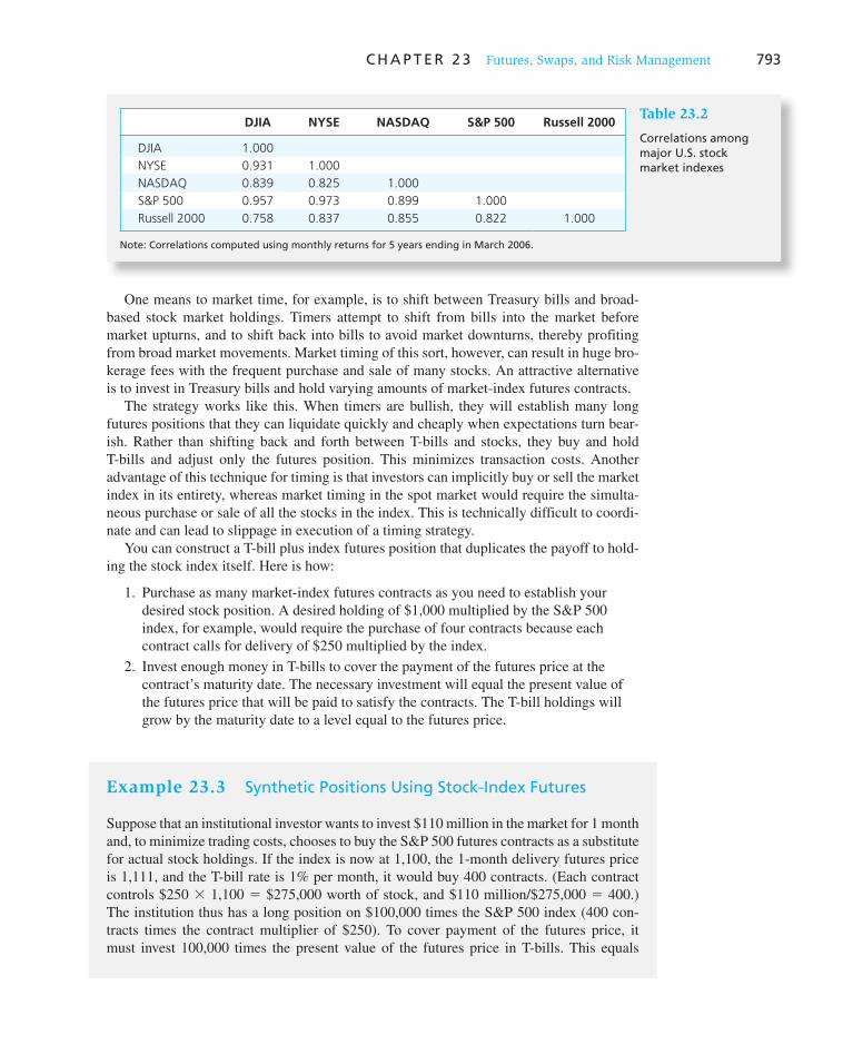
C H A P T E R 2 3 Futures, Swaps, and Risk Management 793
One means to market time, for example, is to shift between Treasury bills and broad-based stock market holdings. Timers attempt to shift from bills into the market before market upturns, and to shift back into bills to avoid market downturns, thereby profiting from broad market movements. Market timing of this sort, however, can result in huge bro-kerage fees with the frequent purchase and sale of many stocks. An attractive alternative is to invest in Treasury bills and hold varying amounts of market-index futures contracts.
The strategy works like this. When timers are bullish, they will establish many long futures positions that they can liquidate quickly and cheaply when expectations turn bear-ish. Rather than shifting back and forth between T-bills and stocks, they buy and hold T-bills and adjust only the futures position. This minimizes transaction costs. Another advantage of this technique for timing is that investors can implicitly buy or sell the market index in its entirety, whereas market timing in the spot market would require the simulta-neous purchase or sale of all the stocks in the index. This is technically difficult to coordi-nate and can lead to slippage in execution of a timing strategy.
You can construct a T-bill plus index futures position that duplicates the payoff to hold-ing the stock index itself. Here is how:
1. Purchase as many market-index futures contracts as you need to establish your desired stock position. A desired holding of $1,000 multiplied by the S&P 500 index, for example, would require the purchase of four contracts because each contract calls for delivery of $250 multiplied by the index.
2. Invest enough money in T-bills to cover the payment of the futures price at the contract’s maturity date. The necessary investment will equal the present value of the futures price that will be paid to satisfy the contracts. The T-bill holdings will grow by the maturity date to a level equal to the futures price.
Example 23.3 Synthetic Positions Using Stock-Index Futures
Suppose that an institutional investor wants to invest $110 million in the market for 1 month and, to minimize trading costs, chooses to buy the S&P 500 futures contracts as a substitute for actual stock holdings. If the index is now at 1,100, the 1-month delivery futures price is 1,111, and the T-bill rate is 1% per month, it would buy 400 contracts. (Each contract controls $250 3 1,100 5 $275,000 worth of stock, and $110 million/$275,000 5 400.) The institution thus has a long position on $100,000 times the S&P 500 index (400 con-tracts times the contract multiplier of $250). To cover payment of the futures price, it must invest 100,000 times the present value of the futures price in T-bills. This equals
DJIA NYSE NASDAQ S&P 500 Russell 2000
DJIA 1.000
NYSE 0.931 1.000
NASDAQ 0.839 0.825 1.000
S&P 500 0.957 0.973 0.899 1.000
Russell 2000 0.758 0.837 0.855 0.822 1.000
Table 23.2
Correlations among major U.S. stock market indexes
Note: Correlations computed using monthly returns for 5 years ending in March 2006.
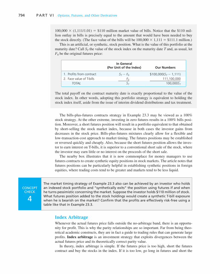
794 P A R T V I Options, Futures, and Other Derivatives
The bills-plus-futures contracts strategy in Example 23.3 may be viewed as a 100% stock strategy. At the other extreme, investing in zero futures results in a 100% bills posi-tion. Moreover, a short futures position will result in a portfolio equivalent to that obtained by short-selling the stock market index, because in both cases the investor gains from decreases in the stock price. Bills-plus-futures mixtures clearly allow for a flexible and low-transaction-cost approach to market timing. The futures positions may be established or reversed quickly and cheaply. Also, because the short futures position allows the inves-tor to earn interest on T-bills, it is superior to a conventional short sale of the stock, where the investor may earn little or no interest on the proceeds of the short sale.
The nearby box illustrates that it is now commonplace for money managers to use futures contracts to create synthetic equity positions in stock markets. The article notes that futures positions can be particularly helpful in establishing synthetic positions in foreign equities, where trading costs tend to be greater and markets tend to be less liquid.
100,000 3 (1,111/1.01) 5 $110 million market value of bills. Notice that the $110 mil-lion outlay in bills is precisely equal to the amount that would have been needed to buy the stock directly. (The face value of the bills will be 100,000 3 1,111 5 $111.1 million.)
This is an artificial, or synthetic, stock position. What is the value of this portfolio at the maturity date? Call S T the value of the stock index on the maturity date T and, as usual, let F 0 be the original futures price:
In General (Per Unit of the Index) Our Numbers
1. Profits from contract S T 2 F0 $100,000(S T 2 1,111)
2. Face value of T-bills F0 111,100,000
TOTAL S T 100,000S T
The total payoff on the contract maturity date is exactly proportional to the value of the stock index. In other words, adopting this portfolio strategy is equivalent to holding the stock index itself, aside from the issue of interim dividend distributions and tax treatment.
CONCEPT CHECK
4
The market timing strategy of Example 23.3 also can be achieved by an investor who holds an indexed stock portfolio and “synthetically exits” the position using futures if and when he turns pessimistic concerning the market. Suppose the investor holds $110 million of stock. What futures position added to the stock holdings would create a synthetic T-bill exposure when he is bearish on the market? Confirm that the profits are effectively risk-free using a table like that in Example 23.3 .
Index Arbitrage
Whenever the actual futures price falls outside the no-arbitrage band, there is an opportu-nity for profit. This is why the parity relationships are so important. Far from being theo-retical academic constructs, they are in fact a guide to trading rules that can generate large profits. Index arbitrage is an investment strategy that exploits divergences between the actual futures price and its theoretically correct parity value.
In theory, index arbitrage is simple. If the futures price is too high, short the futures contract and buy the stocks in the index. If it is too low, go long in futures and short the

795
Got a Bundle to Invest Fast? Think Stock-Index Futures
As investors go increasingly global and market turbulence grows, stock-index futures are emerging as the favorite way for nimble money managers to deploy their funds. Indeed, in most major markets, trading in stock futures now exceeds the buying and selling of actual shares.
What’s the big appeal? Speed, ease and cheapness. For most major markets, stock futures not only boast greater liquidity but also lower transaction costs than traditional trading methods.
“When I decide it’s time to move into France, Germany or Britain, I don’t necessarily want to wait around until I find exactly the right stocks,” says Fabrizio Pierallini, man-ager of New York–based Vontobel Ltd.’s Euro Pacific Fund.
Mr. Pierallini says he later fine-tunes his market picks by gradually shifting out of futures into favorite stocks. To the extent Mr. Pierallini’s stocks outperform the mar-ket, futures provide a means to preserve those gains, even while hedging against market declines.
For instance, by selling futures equal to the value of the underlying portfolio, a manager can almost completely insulate a portfolio from market moves. Say a manager suc-ceeds in outperforming the market, but still loses 3% while the market as a whole falls 10%. Hedging with futures would capture that margin of out-performance, transform-ing the loss into a profit of roughly 7%.
Among futures-intensive strategies is “global tactical asset allocation,” which involves trading whole markets worldwide as traditional managers might trade stocks. The growing popularity of such asset-allocation strategies has given futures a big boost in recent years.
To capitalize on global market swings, “futures do the job for us better than stocks, and they’re cheaper,” said Jarrod Wilcox, director of global investments at PanAgora Asset Management, a Boston-based asset allocator. Even when PanAgora does take positions in individual stocks, it often employs futures to modify its position, such as by hedging part of its exposure to that particular stock market.
When it comes to investing overseas, Mr. Wilcox noted, futures are often the only vehicle that makes sense from a cost standpoint. Abroad, transaction taxes and sky-high commissions can wipe out more than 1% of the money deployed on each trade. By contrast, a comparable trade in futures costs as little as 0.05%.
Source: Abridged from Suzanne McGee, “Got a Bundle to Invest Fast? Think Stock-Index Futures,” The Wall Street Journal, February 21, 1995. Reprinted by permission of The Wall Street Journal, © 1995 Dow Jones & Company, Inc. All rights reserved worldwide.
WO
RD
S FRO
M TH
E STREET
stocks. You can perfectly hedge your position and should earn arbitrage profits equal to the mispricing of the contract.
In practice, however, index arbitrage is difficult to implement. The problem lies in buy-ing “the stocks in the index.” Selling or purchasing shares in all 500 stocks in the S&P 500 is impractical for two reasons. The first is transaction costs, which may outweigh any profits to be made from the arbitrage. Second, it is extremely difficult to buy or sell stock of 500 different firms simultaneously, and any lags in the execution of such a strategy can destroy the effectiveness of a plan to exploit temporary price discrepancies.
Arbitrageurs need to trade an entire portfolio of stocks quickly and simultaneously if they hope to exploit disparities between the futures price and its corresponding stock index. For this they need a coordinated trading program; hence the term program trading, which refers to purchases or sales of entire portfolios of stocks. Electronic trading enables traders to submit coordinated buy or sell programs to the stock market at once.
The success of these arbitrage positions and associated program trades depends on only two things: the relative levels of spot and futures prices and synchronized trading in the two markets. Because arbitrageurs exploit disparities in futures and spot prices, absolute price levels are unimportant.
Using Index Futures to Hedge Market Risk
How might a portfolio manager use futures to hedge market exposure? Suppose, for exam-ple, that you manage a $30 million portfolio with a beta of .8. You are bullish on the market over the long term, but you are afraid that over the next 2 months, the market is vulnerable
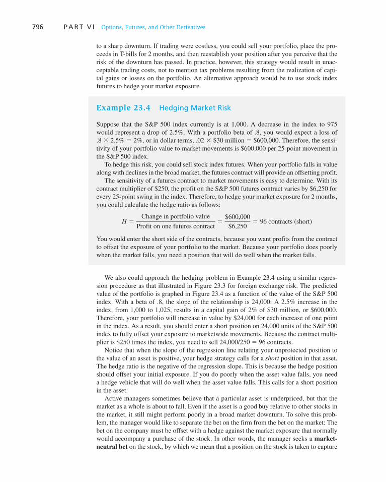
796 P A R T V I Options, Futures, and Other Derivatives
to a sharp downturn. If trading were costless, you could sell your portfolio, place the pro-ceeds in T-bills for 2 months, and then reestablish your position after you perceive that the risk of the downturn has passed. In practice, however, this strategy would result in unac-ceptable trading costs, not to mention tax problems resulting from the realization of capi-tal gains or losses on the portfolio. An alternative approach would be to use stock index futures to hedge your market exposure.
Example 23.4 Hedging Market Risk
Suppose that the S&P 500 index currently is at 1,000. A decrease in the index to 975 would represent a drop of 2.5%. With a portfolio beta of .8, you would expect a loss of .8 3 2.5% 5 2%, or in dollar terms, .02 3 $30 million 5 $600,000. Therefore, the sensi-tivity of your portfolio value to market movements is $600,000 per 25-point movement in the S&P 500 index.
To hedge this risk, you could sell stock index futures. When your portfolio falls in value along with declines in the broad market, the futures contract will provide an offsetting profit.
The sensitivity of a futures contract to market movements is easy to determine. With its contract multiplier of $250, the profit on the S&P 500 futures contract varies by $6,250 for every 25-point swing in the index. Therefore, to hedge your market exposure for 2 months, you could calculate the hedge ratio as follows:
H 5Change in portfolio value
Profit on one futures contract5
$600,000
$6,2505 96 contracts (short)
You would enter the short side of the contracts, because you want profits from the contract to offset the exposure of your portfolio to the market. Because your portfolio does poorly when the market falls, you need a position that will do well when the market falls.
We also could approach the hedging problem in Example 23.4 using a similar regres-sion procedure as that illustrated in Figure 23.3 for foreign exchange risk. The predicted value of the portfolio is graphed in Figure 23.4 as a function of the value of the S&P 500 index. With a beta of .8, the slope of the relationship is 24,000: A 2.5% increase in the index, from 1,000 to 1,025, results in a capital gain of 2% of $30 million, or $600,000. Therefore, your portfolio will increase in value by $24,000 for each increase of one point in the index. As a result, you should enter a short position on 24,000 units of the S&P 500 index to fully offset your exposure to marketwide movements. Because the contract multi-plier is $250 times the index, you need to sell 24,000/250 5 96 contracts.
Notice that when the slope of the regression line relating your unprotected position to the value of an asset is positive, your hedge strategy calls for a short position in that asset. The hedge ratio is the negative of the regression slope. This is because the hedge position should offset your initial exposure. If you do poorly when the asset value falls, you need a hedge vehicle that will do well when the asset value falls. This calls for a short position in the asset.
Active managers sometimes believe that a particular asset is underpriced, but that the market as a whole is about to fall. Even if the asset is a good buy relative to other stocks in the market, it still might perform poorly in a broad market downturn. To solve this prob-lem, the manager would like to separate the bet on the firm from the bet on the market: The bet on the company must be offset with a hedge against the market exposure that normally would accompany a purchase of the stock. In other words, the manager seeks a market-
neutral bet on the stock, by which we mean that a position on the stock is taken to capture
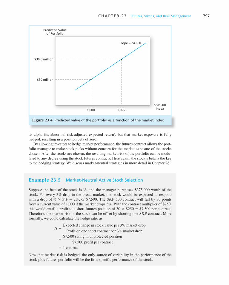
C H A P T E R 2 3 Futures, Swaps, and Risk Management 797
its alpha (its abnormal risk-adjusted expected return), but that market exposure is fully hedged, resulting in a position beta of zero.
By allowing investors to hedge market performance, the futures contract allows the port-folio manager to make stock picks without concern for the market exposure of the stocks chosen. After the stocks are chosen, the resulting market risk of the portfolio can be modu-lated to any degree using the stock futures contracts. Here again, the stock’s beta is the key to the hedging strategy. We discuss market-neutral strategies in more detail in Chapter 26.
Figure 23.4 Predicted value of the portfolio as a function of the market index
Predicted Valueof Portfolio
Slope = 24,000
S&P 500Index
$30.6 million
$30 million
1,000 1,025
Example 23.5 Market-Neutral Active Stock Selection
Suppose the beta of the stock is 2⁄3, and the manager purchases $375,000 worth of the stock. For every 3% drop in the broad market, the stock would be expected to respond with a drop of 2⁄3 3 3% 5 2%, or $7,500. The S&P 500 contract will fall by 30 points from a current value of 1,000 if the market drops 3%. With the contract multiplier of $250, this would entail a profit to a short futures position of 30 3 $250 5 $7,500 per contract. Therefore, the market risk of the stock can be offset by shorting one S&P contract. More formally, we could calculate the hedge ratio as
H 5Expected change in stock value per 3% market drop
Profit on one short contract per 3% market drop
5$7,500 swing in unprotected position
$7,500 profit per contract
5 1 contract
Now that market risk is hedged, the only source of variability in the performance of the stock-plus-futures portfolio will be the firm-specific performance of the stock.

798 P A R T V I Options, Futures, and Other Derivatives
23.3 Interest Rate Futures
Hedging Interest Rate Risk
Like equity managers, fixed-income managers also sometimes desire to hedge market risk, in this case resulting from movements in the entire structure of interest rates. Consider, for example, these problems:
1. A fixed-income manager holds a bond portfolio on which considerable capital gains have been earned. She foresees an increase in interest rates but is reluctant to sell her portfolio and replace it with a lower-duration mix of bonds because such rebal-ancing would result in large trading costs as well as realization of capital gains for tax purposes. Still, she would like to hedge her exposure to interest rate increases.
2. A corporation plans to issue bonds to the public. It believes that now is a good time to act, but it cannot issue the bonds for another 3 months because of the lags inher-ent in SEC registration. It would like to hedge the uncertainty surrounding the yield at which it eventually will be able to sell the bonds.
3. A pension fund will receive a large cash inflow next month that it plans to invest in long-term bonds. It is concerned that interest rates may fall by the time it can make the investment and would like to lock in the yield currently available on long-term issues.
In each of these cases, the investment manager wishes to hedge interest rate uncertainty. To illustrate the procedures that might be followed, we will focus on the first example, and suppose that the portfolio manager has a $10 million bond portfolio with a modified dura-tion of 9 years. 3 If, as feared, market interest rates increase and the bond portfolio’s yield also rises, say, by 10 basis points (.10%), the fund will suffer a capital loss. Recall from Chapter 16 that the capital loss in percentage terms will be the product of modified dura-tion, D *, and the change in the portfolio yield. Therefore, the loss will be
D* 3 Dy 5 9 3 .10% 5 .90%
or $90,000. This establishes that the sensitivity of the value of the unprotected portfolio to changes in market yields is $9,000 per 1 basis point change in the yield. Market practitioners call this ratio the price value of a basis point, or PVBP. The PVBP represents the sensitiv-ity of the dollar value of the portfolio to changes in interest rates. Here, we’ve shown that
PVBP 5Change in portfolio value
Predicted change in yield5
$90,000
10 basis points5 $9,000 per basis point
One way to hedge this risk is to take an offsetting position in an interest rate futures con-tract. The Treasury bond contract is the most widely traded contract. The bond nominally calls for delivery of $100,000 par value T-bonds with 6% coupons and 20-year maturity. In practice, the contract delivery terms are fairly complicated because many bonds with different coupon rates and maturities may be substituted to settle the contract. However, we will assume that the bond to be delivered on the contract already is known and has a modified duration of 10 years. Finally, suppose that the futures price currently is $90 per $100 par value. Because the contract requires delivery of $100,000 par value of bonds, the contract multiplier is $1,000.
3 Recall that modified duration, D *, is related to duration, D, by the formula D * 5 D /(1 1 y ), where y is the bond’s yield to maturity. If the bond pays coupons semiannually, then y should be measured as a semiannual yield. For simplicity, we will assume annual coupon payments, and treat y as the effective annual yield to maturity.
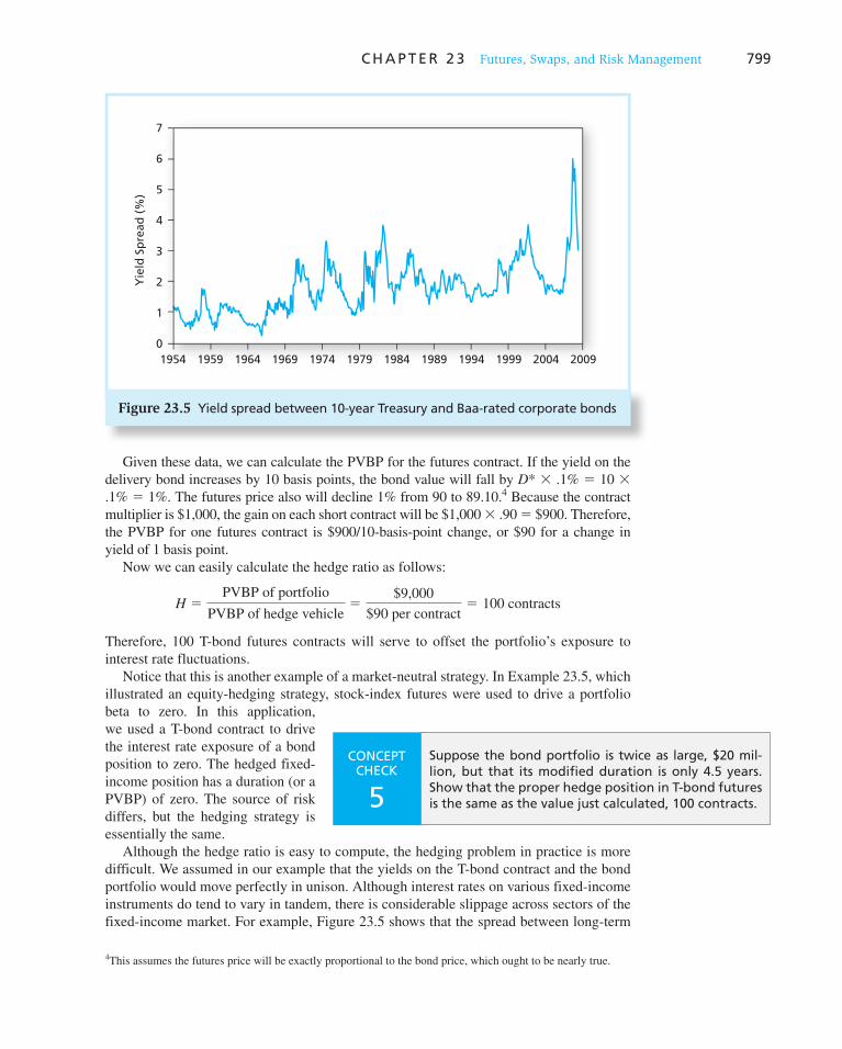
C H A P T E R 2 3 Futures, Swaps, and Risk Management 799
Given these data, we can calculate the PVBP for the futures contract. If the yield on the delivery bond increases by 10 basis points, the bond value will fall by D * 3 .1% 5 10 3.1% 5 1%. The futures price also will decline 1% from 90 to 89.10. 4 Because the contract multiplier is $1,000, the gain on each short contract will be $1,000 3 .90 5 $900. Therefore, the PVBP for one futures contract is $900/10-basis-point change, or $90 for a change in yield of 1 basis point.
Now we can easily calculate the hedge ratio as follows:
H 5PVBP of portfolio
PVBP of hedge vehicle5
$9,000
$90 per contract5 100 contracts
Therefore, 100 T-bond futures contracts will serve to offset the portfolio’s exposure to interest rate fluctuations.
Notice that this is another example of a market-neutral strategy. In Example 23.5 , which illustrated an equity-hedging strategy, stock-index futures were used to drive a portfolio beta to zero. In this application, we used a T-bond contract to drive the interest rate exposure of a bond position to zero. The hedged fixed-income position has a duration (or a PVBP) of zero. The source of risk differs, but the hedging strategy is essentially the same.
Although the hedge ratio is easy to compute, the hedging problem in practice is more difficult. We assumed in our example that the yields on the T-bond contract and the bond portfolio would move perfectly in unison. Although interest rates on various fixed-income instruments do tend to vary in tandem, there is considerable slippage across sectors of the fixed-income market. For example, Figure 23.5 shows that the spread between long-term
4 This assumes the futures price will be exactly proportional to the bond price, which ought to be nearly true.
Figure 23.5 Yield spread between 10-year Treasury and Baa-rated corporate bonds
7
5
4
3
2
1
01954 1959 1964 1969 1974 1979 1984 1989 1994 1999 2004 2009
Yie
ld S
pre
ad (
%)
6
CONCEPT CHECK
5
Suppose the bond portfolio is twice as large, $20 mil-lion, but that its modified duration is only 4.5 years. Show that the proper hedge position in T-bond futures is the same as the value just calculated, 100 contracts.

800 P A R T V I Options, Futures, and Other Derivatives
corporate and 10-year Treasury bond yields has fluctuated considerably over time. Our hedging strategy would be fully effective only if the yield spread across the two sectors of the fixed-income market were constant (or at least perfectly predictable) so that yield changes in both sectors were equal.
This problem highlights the fact that most hedging activity is in fact cross-hedging, meaning that the hedge vehicle is a different asset than the one to be hedged. To the extent that there is slippage between prices or yields of the two assets, the hedge will not be per-fect. Cross-hedges can eliminate a large fraction of the total risk of the unprotected portfo-lio, but you should be aware that they typically are far from risk-free positions.
23.4 Swaps
Swaps are multiperiod extensions of forward contracts. For example, rather than agreeing to exchange British pounds for U.S. dollars at an agreed-upon forward price at one single date, a foreign exchange swap would call for an exchange of currencies on several future dates. The parties might exchange $2 million for £1 million in each of the next 5 years. Similarly, interest rate swaps call for the exchange of a series of cash flows proportional to a given interest rate for a corresponding series of cash flows proportional to a floating inter-est rate. 5 One party might exchange a variable cash flow equal to $1 million times a short-term interest rate for $1 million times a fixed interest rate of 8% for each of the next 7 years.
The swap market is a huge component of the derivatives market, with well over $500 trillion in swap agreements outstanding. We will illustrate how these contracts work by using a simple interest rate swap as an example. 6
5 Interest rate swaps have nothing to do with the Homer-Liebowitz bond swap taxonomy described in Chapter 16.
6 The participants to the swap do not loan each other money. They agree only to exchange a fixed cash flow for a variable cash flow that depends on the short-term interest rate. This is why the principal is described as notional. The notional principal is simply a way to describe the size of the swap agreement. In this example, the parties to the swap exchange a 7% fixed rate for the LIBOR rate; the difference between LIBOR and 7% is multiplied by notional principal to determine the cash flow exchanged by the parties.
Example 23.6 Interest Rate Swap
Consider the manager of a large portfolio that currently includes $100 million par value of long-term bonds paying an average coupon rate of 7%. The manager believes interest rates are about to rise. As a result, he would like to sell the bonds and replace them with either short-term or floating-rate issues. However, it would be exceedingly expensive in terms of transaction costs to replace the portfolio every time the forecast for interest rates is updated. A cheaper and more flexible way to modify the portfolio is to “swap” the $7 million a year in interest income the portfolio currently generates for an amount of money that is tied to the short-term interest rate. That way, if rates do rise, so will the portfolio’s interest income.
A swap dealer might advertise its willingness to exchange, or “swap,” a cash flow based on the 6-month LIBOR rate for one based on a fixed rate of 7%. (The LIBOR, or Lon-don Interbank Offered Rate, is the interest rate at which banks borrow from each other in the Eurodollar market. It is the most commonly used short-term interest rate in the swap market.) The portfolio manager would then enter into a swap agreement with the dealer to pay 7% on notional principal of $100 million and receive payment of the LIBOR rate on that amount of notional principal. 6 In other words, the manager swaps a payment of
C H A P T E R 2 3 Futures, Swaps, and Risk Management 801
Swaps and Balance Sheet Restructuring
Example 23.6 illustrates why swaps have tremendous appeal to fixed-income managers. These contracts provide a means to quickly, cheaply, and anonymously restructure the balance sheet. Suppose a corporation that has issued fixed-rate debt believes that interest rates are likely to fall; it might prefer to have issued floating-rate debt. In principle, it could issue floating-rate debt and use the proceeds to buy back the outstanding fixed-rate debt. But it is faster and easier to convert the outstanding fixed-rate debt into synthetic floating-rate debt by entering a swap to receive a fixed interest rate (offsetting its fixed-rate coupon obligation) and paying a floating rate.
Conversely, a bank that pays current market interest rates to its depositors, and thus is exposed to increases in rates, might wish to convert some of its financing to a fixed-rate basis. It would enter a swap to receive a floating rate and pay a fixed rate on some amount of notional principal. This swap position, added to its floating-rate deposit liability, would result in a net liability of a fixed stream of cash. The bank might then be able to invest in long-term fixed-rate loans without encountering interest rate risk.
For another example, consider a fixed-income portfolio manager. Swaps enable the manager to switch back and forth between a fixed- or floating-rate profile quickly and cheaply as forecast for interest rate changes. A manager who holds a fixed-rate portfolio can transform it into a synthetic floating-rate portfolio by entering a pay fixed–receive floating swap and can later transform it back by entering the opposite side of a similar swap.
Foreign exchange swaps also enable the firm to quickly and cheaply restructure its bal-ance sheet. Suppose, for example, that a firm issues $10 million in debt at an 8% coupon rate, but actually prefers that its interest obligations be denominated in British pounds. For example, the issuing firm might be a British corporation that perceives advantageous financing opportunities in the United States but prefers pound-denominated liabilities. Then the firm, whose debt currently obliges it to make dollar-denominated payments
.07 3 $100 million for a payment of LIBOR 3 $100 million. The manager’s net cash flow from the swap agreement is therefore (LIBOR 2 .07) 3 $100 million. Note that the swap arrangement does not mean that a loan has been made. The participants have agreed only to exchange a fixed cash flow for a variable one.
Now consider the net cash flow to the manager’s portfolio in three interest rate scenarios:
LIBOR Rate
6.5% 7.0% 7.5%
Interest income from bond portfolio
(5 7% of $100 million bond portfolio) $7,000,000 $7,000,000 $7,000,000
Cash flow from swap
[5 (LIBOR 2 7%) 3 notional principal of $100 million] (500,000) 0 500,000
Total (5 LIBOR 3 $100 million) $6,500,000 $7,000,000 $7,500,000
Notice that the total income on the overall position—bonds plus swap agreement—is now equal to the LIBOR rate in each scenario times $100 million. The manager has, in effect, converted a fixed-rate bond portfolio into a synthetic floating-rate portfolio.
802 P A R T V I Options, Futures, and Other Derivatives
of $800,000, can agree to swap a given number of pounds each year for $800,000. By so doing, it effectively covers its dollar obligation and replaces it with a new pound- denominated obligation.
The Swap Dealer
What about the swap dealer? Why is the dealer, which is typically a financial intermediary such as a bank, willing to take on the opposite side of the swaps desired by these partici-pants in these hypothetical swaps?
Consider a dealer who takes on one side of a swap, let’s say paying LIBOR and receiv-ing a fixed rate. The dealer will search for another trader in the swap market who wishes to receive a fixed rate and pay LIBOR. For example, Company A may have issued a 7% coupon fixed-rate bond that it wishes to convert into synthetic floating-rate debt, while Company B may have issued a floating-rate bond tied to LIBOR that it wishes to convert into synthetic fixed-rate debt. The dealer will enter a swap with Company A in which it pays a fixed rate and receives LIBOR, and will enter another swap with Company B in which it pays LIBOR and receives a fixed rate. When the two swaps are combined, the dealer’s position is effectively neutral on interest rates, paying LIBOR on one swap and receiving it on another. Similarly, the dealer pays a fixed rate on one swap and receives it on another. The dealer becomes little more than an intermediary, funneling payments from one party to the other. 7 The dealer finds this activity profitable because it will charge a bid–asked spread on the transaction.
This rearrangement is illustrated in Figure 23.6 . Company A has issued 7% fixed-rate debt (the leftmost arrow in the figure) but enters a swap to pay the dealer LIBOR and receive a 6.95% fixed rate. Therefore, the company’s net payment is 7% 1 (LIBOR 2 6.95%) 5 LIBOR 1 .05%. It has thus transformed its fixed-rate debt into synthetic floating-rate debt. Conversely, Company B has issued floating-rate debt paying LIBOR (the rightmost arrow), but enters a swap to pay a 7.05% fixed rate in return for LIBOR. Therefore, its net payment is LIBOR 1 (7.05% 2 LIBOR) 5 7.05%. It has thus trans-formed its floating-rate debt into synthetic fixed-rate debt. The bid–asked spread, the source of the dealer’s profit, in the example illustrated in Figure 23.6 is .10% of notional principal each year.
7 Actually, things are a bit more complicated. The dealer is more than just an intermediary because it bears the credit risk that one or the other of the parties to the swap might default on the obligation. Referring to Figure 23.6 , if firm A defaults on its obligation, for example, the swap dealer still must maintain its commitment to firm B. In this sense, the dealer does more than simply pass through cash flows to the other swap participants.
CONCEPT CHECK
7
A pension fund holds a portfolio of money market securities that the manager believes are paying excellent yields compared to other comparable-risk short-term securities. However, the manager believes that interest rates are about to fall. What type of swap will allow the fund to continue to hold its portfolio of short-term securities while at the same time ben-efiting from a decline in rates?
CONCEPT CHECK
6 Show how a firm that has issued a floating-rate bond with a coupon equal to the LIBOR rate can use swaps to convert that bond into synthetic fixed-rate debt. Assume the terms of the swap allow an exchange of LIBOR for a fixed rate of 8%.
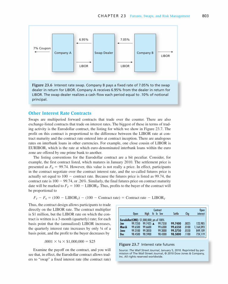
C H A P T E R 2 3 Futures, Swaps, and Risk Management 803
Other Interest Rate Contracts
Swaps are multiperiod forward contracts that trade over the counter. There are also exchange-listed contracts that trade on interest rates. The biggest of these in terms of trad-ing activity is the Eurodollar contract, the listing for which we show in Figure 23.7 . The profit on this contract is proportional to the difference between the LIBOR rate at con-tract maturity and the contract rate entered into at contract inception. There are analogous rates on interbank loans in other currencies. For example, one close cousin of LIBOR is EURIBOR, which is the rate at which euro-denominated interbank loans within the euro zone are offered by one prime bank to another.
The listing conventions for the Eurodollar contract are a bit peculiar. Consider, for example, the first contract listed, which matures in January 2010. The settlement price is presented as F 0 5 99.74. However, this value is not really a price. In effect, participants in the contract negotiate over the contract interest rate, and the so-called futures price is actually set equal to 100 2 contract rate. Because the futures price is listed as 99.74, the contract rate is 100 2 99.74, or .26%. Similarly, the final futures price on contract maturity date will be marked to F T 5 100 2 LIBOR T . Thus, profits to the buyer of the contract will be proportional to
FT 2 F0 5 (100 2 LIBORT) 2 (100 2 Contract rate) 5 Contract rate 2 LIBORT
Thus, the contract design allows participants to trade directly on the LIBOR rate. The contract multiplier is $1 million, but the LIBOR rate on which the con-tract is written is a 3-month (quarterly) rate; for each basis point that the (annualized) LIBOR increases, the quarterly interest rate increases by only ¼ of a basis point, and the profit to the buyer decreases by
.0001 3 ¼ 3 $1,000,000 5 $25
Examine the payoff on the contract, and you will see that, in effect, the Eurodollar contract allows trad-ers to “swap” a fixed interest rate (the contract rate)
Figure 23.6 Interest rate swap. Company B pays a fixed rate of 7.05% to the swap dealer in return for LIBOR. Company A receives 6.95% from the dealer in return for LIBOR. The swap dealer realizes a cash flow each period equal to .10% of notional principal.
Company A Swap Dealer Company B
LIBOR
6.95% 7.05%
7% Coupon
LIBOR
LIBOR
Figure 23.7 Interest rate futures
Source: The Wall Street Journal, January 5, 2010. Reprinted by per-mission of The Wall Street Journal, © 2010 Dow Jones & Company, Inc. All rights reserved worldwide.
Open High Settle ChgOpen
interestContract
hi lo low
Eurodollar(CME) - $1,000,000; pts of 100%Jan 99.7350 99.7425 99.7350 99.7400 .0025 123,985March 99.6500 99.6600 99.6300 99.6550 .0100 1,164,093June 99.3100 99.3850 99.3000 99.3750 .0550 849,109Dec 98.4500 98.5900 98.4300 98.5800 .1100 724,119
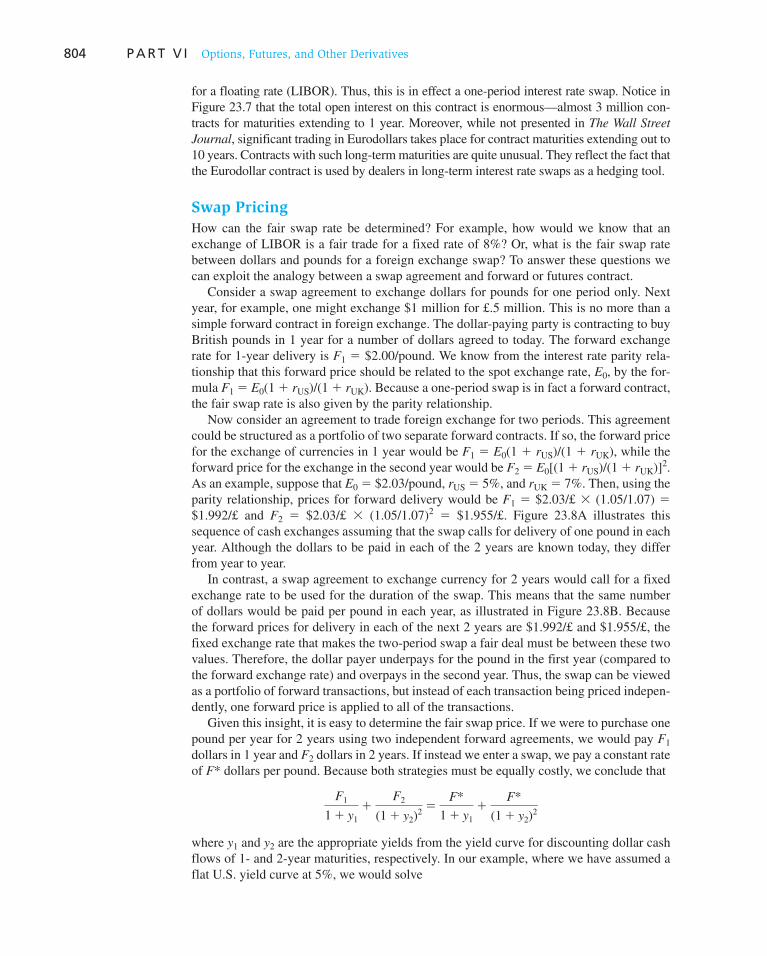
804 P A R T V I Options, Futures, and Other Derivatives
for a floating rate (LIBOR). Thus, this is in effect a one-period interest rate swap. Notice in Figure 23.7 that the total open interest on this contract is enormous—almost 3 million con-tracts for maturities extending to 1 year. Moreover, while not presented in The Wall Street
Journal, significant trading in Eurodollars takes place for contract maturities extending out to 10 years. Contracts with such long-term maturities are quite unusual. They reflect the fact that the Eurodollar contract is used by dealers in long-term interest rate swaps as a hedging tool.
Swap Pricing
How can the fair swap rate be determined? For example, how would we know that an exchange of LIBOR is a fair trade for a fixed rate of 8%? Or, what is the fair swap rate between dollars and pounds for a foreign exchange swap? To answer these questions we can exploit the analogy between a swap agreement and forward or futures contract.
Consider a swap agreement to exchange dollars for pounds for one period only. Next year, for example, one might exchange $1 million for £.5 million. This is no more than a simple forward contract in foreign exchange. The dollar-paying party is contracting to buy British pounds in 1 year for a number of dollars agreed to today. The forward exchange rate for 1-year delivery is F 1 5 $2.00/pound. We know from the interest rate parity rela-tionship that this forward price should be related to the spot exchange rate, E 0 , by the for-mula F 1 5 E 0 (1 1 r US )/(1 1 r UK ). Because a one-period swap is in fact a forward contract, the fair swap rate is also given by the parity relationship.
Now consider an agreement to trade foreign exchange for two periods. This agreement could be structured as a portfolio of two separate forward contracts. If so, the forward price for the exchange of currencies in 1 year would be F 1 5 E 0 (1 1 r US )/(1 1 r UK ), while the forward price for the exchange in the second year would be F 2 5 E 0 [(1 1 r US )/(1 1 r UK )] 2 . As an example, suppose that E 0 5 $2.03/pound, r US 5 5%, and r UK 5 7%. Then, using the parity relationship, prices for forward delivery would be F 1 5 $2.03/£ 3 (1.05/1.07) 5 $1.992/£ and F 2 5 $2.03/£ 3 (1.05/1.07) 2 5 $1.955/£. Figure 23.8A illustrates this sequence of cash exchanges assuming that the swap calls for delivery of one pound in each year. Although the dollars to be paid in each of the 2 years are known today, they differ from year to year.
In contrast, a swap agreement to exchange currency for 2 years would call for a fixed exchange rate to be used for the duration of the swap. This means that the same number of dollars would be paid per pound in each year, as illustrated in Figure 23.8B . Because the forward prices for delivery in each of the next 2 years are $1.992/£ and $1.955/£, the fixed exchange rate that makes the two-period swap a fair deal must be between these two values. Therefore, the dollar payer underpays for the pound in the first year (compared to the forward exchange rate) and overpays in the second year. Thus, the swap can be viewed as a portfolio of forward transactions, but instead of each transaction being priced indepen-dently, one forward price is applied to all of the transactions.
Given this insight, it is easy to determine the fair swap price. If we were to purchase one pound per year for 2 years using two independent forward agreements, we would pay F 1 dollars in 1 year and F 2 dollars in 2 years. If instead we enter a swap, we pay a constant rate of F * dollars per pound. Because both strategies must be equally costly, we conclude that
F1
1 1 y1
1F2
(1 1 y2)2
5F*
1 1 y1
1F*
(1 1 y2)2
where y 1 and y 2 are the appropriate yields from the yield curve for discounting dollar cash flows of 1- and 2-year maturities, respectively. In our example, where we have assumed a flat U.S. yield curve at 5%, we would solve
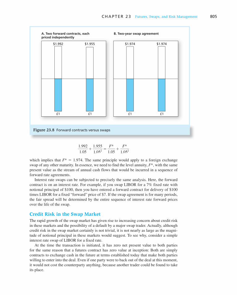
C H A P T E R 2 3 Futures, Swaps, and Risk Management 805
1.992
1.051
1.955
1.0525
F*
1.051
F*
1.052
which implies that F * 5 1.974. The same principle would apply to a foreign exchange swap of any other maturity. In essence, we need to find the level annuity, F *, with the same present value as the stream of annual cash flows that would be incurred in a sequence of forward rate agreements.
Interest rate swaps can be subjected to precisely the same analysis. Here, the forward contract is on an interest rate. For example, if you swap LIBOR for a 7% fixed rate with notional principal of $100, then you have entered a forward contract for delivery of $100 times LIBOR for a fixed “forward” price of $7. If the swap agreement is for many periods, the fair spread will be determined by the entire sequence of interest rate forward prices over the life of the swap.
Credit Risk in the Swap Market
The rapid growth of the swap market has given rise to increasing concern about credit risk in these markets and the possibility of a default by a major swap trader. Actually, although credit risk in the swap market certainly is not trivial, it is not nearly as large as the magni-tude of notional principal in these markets would suggest. To see why, consider a simple interest rate swap of LIBOR for a fixed rate.
At the time the transaction is initiated, it has zero net present value to both parties for the same reason that a futures contract has zero value at inception: Both are simply contracts to exchange cash in the future at terms established today that make both parties willing to enter into the deal. Even if one party were to back out of the deal at this moment, it would not cost the counterparty anything, because another trader could be found to take its place.
Figure 23.8 Forward contracts versus swaps
A. Two forward contracts, eachpriced independently
$1.992 $1.955
£1 £1
B. Two-year swap agreement
$1.974 $1.974
£1 £1
806 P A R T V I Options, Futures, and Other Derivatives
Once interest or exchange rates change, however, the situation is not as simple. Suppose, for example, that interest rates increase shortly after an interest-rate swap agreement has begun. The floating-rate payer therefore suffers a loss, while the fixed-rate payer enjoys a gain. If the floating-rate payer reneges on its commitment at this point, the fixed-rate payer suffers a loss. However, that loss is not as large as the notional principal of the swap, for the default of the floating-rate payer relieves the fixed-rate payer from its obligation as well. The loss is only the difference between the values of the fixed-rate and floating-rate obliga-tions, not the total value of the payments that the floating-rate payer was obligated to make.
Example 23.7 Credit Risk in Swaps
Consider a swap written on $1 million of notional principal that calls for exchange of LIBOR for a fixed rate of 8% for 5 years. Suppose, for simplicity, that the yield curve is currently flat at 8%. With LIBOR thus equal to 8%, no cash flows will be exchanged unless interest rates change. But now suppose that the yield curve immediately shifts up to 9%. The floating-rate payer now is obligated to pay a cash flow of (.09 2 .08) 3 $1 million 5 $10,000 each year to the fixed-rate payer (as long as rates remain at 9%). If the floating-rate payer defaults on the swap, the fixed-rate payer loses the prospect of that 5-year annuity. The present value of that annuity is $10,000 3 Annuity factor(9%, 5 years) 5 $38,897. This loss may not be trivial, but it is less than 4% of notional principal. We conclude that the credit risk of the swap is far less than notional principal. Again, this is because the default by the floating-rate payer costs the counterparty only the difference between the LIBOR rate and the fixed rate.
Credit Default Swaps
Despite the similarity in names, a credit default swap, or CDS, is not the same type of instrument as interest rate or currency swaps. As we saw in Chapter 14, payment on a CDS is tied to the financial status of one or more reference firms; the CDS therefore allows two counterparties to take positions on the credit risk of those firms. When a particular “credit event” is triggered, say, default on an outstanding bond or failure to pay interest, the seller of protection is expected to cover the loss in the market value of the bond. For example, the swap seller may be obligated to pay par value to take delivery of the defaulted bond (in which case the swap is said to entail physical settlement) or may instead pay the swap buyer the difference between the par value and market value of the bond (termed cash settlement). The swap purchaser pays a periodic fee to the seller for this protection against credit events.
Unlike interest rate swaps, credit default swaps do not entail periodic netting of one reference rate against another. They are in fact more like insurance policies written on par-ticular credit events. Bondholders may buy these swaps to transfer their credit risk expo-sure to the swap seller, effectively enhancing the credit quality of their portfolios. Unlike insurance policies, however, the swap holder need not hold the bonds underlying the CDS contract; therefore, credit default swaps can be used purely to speculate on changes in the credit standing of the reference firms.
23.5 Commodity Futures Pricing
Commodity futures prices are governed by the same general considerations as stock futures. One difference, however, is that the cost of carrying commodities, especially those subject to spoilage, is greater than the cost of carrying financial assets. The underlying
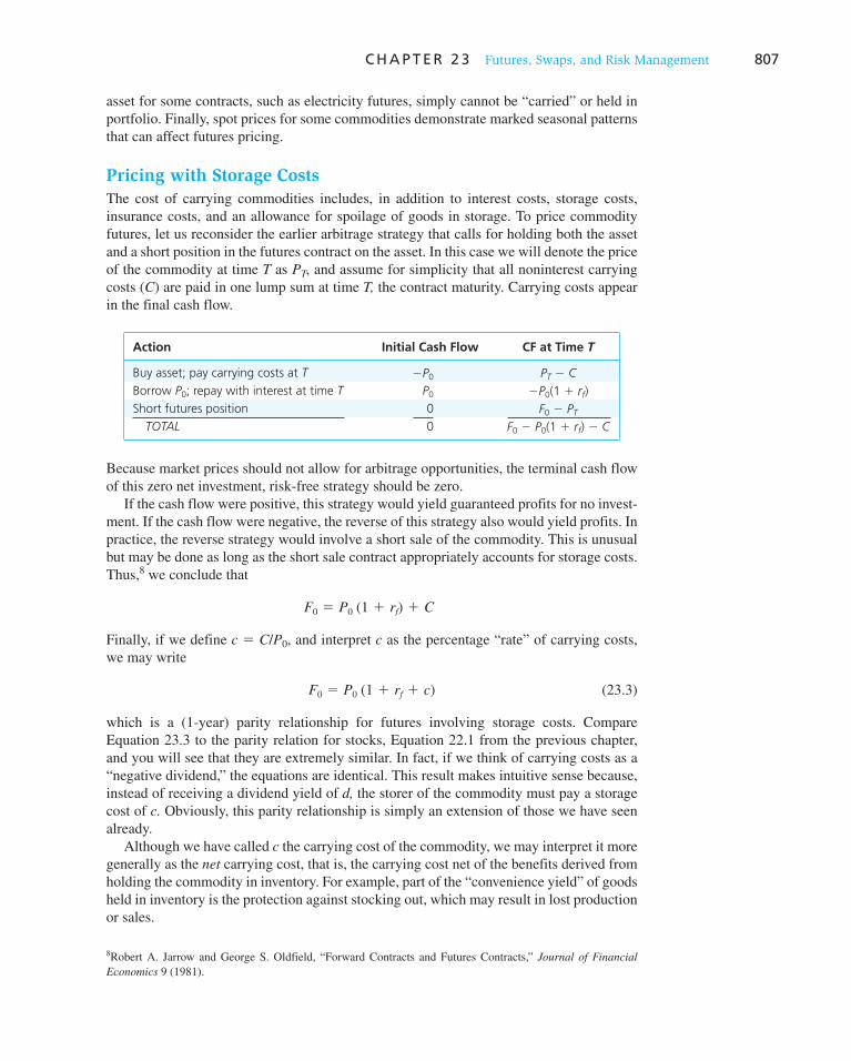
C H A P T E R 2 3 Futures, Swaps, and Risk Management 807
asset for some contracts, such as electricity futures, simply cannot be “carried” or held in portfolio. Finally, spot prices for some commodities demonstrate marked seasonal patterns that can affect futures pricing.
Pricing with Storage Costs
The cost of carrying commodities includes, in addition to interest costs, storage costs, insurance costs, and an allowance for spoilage of goods in storage. To price commodity futures, let us reconsider the earlier arbitrage strategy that calls for holding both the asset and a short position in the futures contract on the asset. In this case we will denote the price of the commodity at time T as P T , and assume for simplicity that all noninterest carrying costs ( C ) are paid in one lump sum at time T, the contract maturity. Carrying costs appear in the final cash flow.
Action Initial Cash Flow CF at Time T
Buy asset; pay carrying costs at T 2P0 PT 2 C
Borrow P0; repay with interest at time T P0 2P0(1 1 rf)
Short futures position 0 F0 2 PT
TOTAL 0 F0 2 P0(1 1 rf) 2 C
Because market prices should not allow for arbitrage opportunities, the terminal cash flow of this zero net investment, risk-free strategy should be zero.
If the cash flow were positive, this strategy would yield guaranteed profits for no invest-ment. If the cash flow were negative, the reverse of this strategy also would yield profits. In practice, the reverse strategy would involve a short sale of the commodity. This is unusual but may be done as long as the short sale contract appropriately accounts for storage costs. Thus, 8 we conclude that
F0 5 P0 (1 1 rf) 1 C
Finally, if we define c 5 C / P 0 , and interpret c as the percentage “rate” of carrying costs, we may write
F0 5 P0 (1 1 rf 1 c) (23.3)
which is a (1-year) parity relationship for futures involving storage costs. Compare Equation 23.3 to the parity relation for stocks, Equation 22.1 from the previous chapter, and you will see that they are extremely similar. In fact, if we think of carrying costs as a “negative dividend,” the equations are identical. This result makes intuitive sense because, instead of receiving a dividend yield of d, the storer of the commodity must pay a storage cost of c. Obviously, this parity relationship is simply an extension of those we have seen already.
Although we have called c the carrying cost of the commodity, we may interpret it more generally as the net carrying cost, that is, the carrying cost net of the benefits derived from holding the commodity in inventory. For example, part of the “convenience yield” of goods held in inventory is the protection against stocking out, which may result in lost production or sales.
8 Robert A. Jarrow and George S. Oldfield, “Forward Contracts and Futures Contracts,” Journal of Financial
Economics 9 (1981).

808 P A R T V I Options, Futures, and Other Derivatives
It is vital to note that we derive Equation 23.3 assuming that the asset will be bought and stored; it therefore applies only to goods that currently are being stored. Two kinds of com-modities cannot be expected to be stored. The first kind is commodities for which storage is technologically not feasible, such as electricity. The second includes goods that are not stored for economic reasons. For example, it would be foolish to buy an agricultural commodity now, planning to store it for ultimate use in 3 years. Instead, it is clearly preferable to delay the pur-chase until after the harvest of the third year, and avoid paying storage costs. Moreover, if the crop in the third year is comparable to this year’s, you could obtain it at roughly the same price as you would pay this year. By waiting to purchase, you avoid both interest and storage costs.
Because storage across harvests is costly, Equation 23.3 should not be expected to apply for holding periods that span harvest times, nor should it apply to perishable goods that are available only “in season.” Whereas the futures
price for gold, which is a stored commodity, increases steadily with the maturity of the contract, the futures price for wheat is seasonal; its futures price typically falls across har-vests between March and July as new supplies become available.
Figure 23.9 is a stylized version of the seasonal price pattern for an agricultural product. Clearly this pattern differs from financial assets such as stocks or gold for which there is no seasonal price movement. Financial assets are priced so that holding them in portfo-lio produces a fair expected return. Agricultural prices, in contrast, are subject to steep periodic drops as each crop is harvested, which makes storage across harvests generally unprofitable.
Futures pricing across seasons therefore requires a different approach that is not based on storage across harvest periods. In place of general no-arbitrage restrictions we rely instead on risk premium theory and discounted cash flow (DCF) analysis.
Price
Time
FirstHarvest
SecondHarvest
ThirdHarvest
Figure 23.9 Typical agricultural price pattern over the season. Prices adjusted for inflation.
CONCEPT CHECK
8
People are willing to buy and “store” shares of stock despite the fact that their purchase ties up capital. Most people, however, are not willing to buy and store soybeans. What is the difference in the properties of the expected evolution of stock prices versus soybean prices that accounts for this result?
Discounted Cash Flow Analysis for Commodity Futures
Given the current expectation of the spot price of the commodity at some future date and a measure of the risk characteristics of that price, we can measure the present value of a claim to receive the commodity at that future date. We simply calculate the appropriate risk premium from a model such as the CAPM or APT and discount the expected spot price at the appropriate risk-adjusted interest rate, as illustrated in the following example.

C H A P T E R 2 3 Futures, Swaps, and Risk Management 809
Example 23.8 Commodity Futures Pricing
Table 23.3 , which presents betas on a variety of commodities, shows that the beta of orange juice, for example, was estimated to be .117 over the period. If the T-bill rate is currently 5% and the historical market risk premium is about 8%, the appropriate discount rate for orange juice would be given by the CAPM as
5% 1 .117 3 8% 5 5.94%
If the expected spot price for orange juice 6 months from now is $1.45 per pound, the present value of a 6-month deferred claim to a pound of orange juice is simply
$1.45 / (1.0594)1/2 5 $1.409
What would the proper futures price for orange juice be? The contract calls for the ultimate exchange of orange juice for the futures price. We have just shown that the pres-ent value of the juice is $1.409. This should equal the present value of the futures price that will be paid for the juice. A commitment to a payment of F 0 dollars in 6 months has a present value of F 0 /(1.05) 1/2 5 .976 3 F 0 . (Note that the discount rate is the risk-free rate of 5%, because the promised payment is fixed and therefore independent of market conditions.)
To equate the present values of the promised payment of F 0 and the promised receipt of orange juice, we would set
.976F0 5 $1.409
or F 0 5 $1.444.
Table 23.3
Commodity betas Commodity Beta Commodity Beta
Wheat 20.370 Orange juice 0.117
Corn 20.429 Propane 23.851
Oats 0.000 Cocoa 20.291
Soybeans 20.266 Silver 20.272
Soybean oil 20.650 Copper 0.005
Soybean meal 0.239 Cattle 0.365
Broilers 21.692 Hogs 20.148
Plywood 0.660 Pork bellies 20.062
Potatoes 20.610 Egg 20.293
Platinum 0.221 Lumber 20.131
Wool 0.307 Sugar 22.403
Cotton 20.015
Source: Zvi Bodie and Victor Rosansky, “Risk and Return in Commodity Futures,” Financial Analysts Journal 36 (May–June 1980). Copyright 1980, CFA Institute. Reproduced from the Financial Analysts Journal with permission from the CFA Institute. All rights reserved.

Vis
it u
s at
ww
w.m
hh
e.co
m/b
km810 P A R T V I Options, Futures, and Other Derivatives
The general rule, then, to determine the appropriate futures price is to equate the present value of the future payment of F 0 and the present value of the commodity to be received. This gives us
F0
(1 1 rf)T
5E(PT)
(1 1 k)T
or
F0 5 E(PT) ¢ 1 1 rf
1 1 k≤T
(23.4)
where k is the required rate of return on the commodity, which may be obtained from a model of asset market equilibrium such as the CAPM.
Note that Equation 23.4 is perfectly consistent with the spot-futures parity relationship. For example, apply Equation 23.4 to the futures price for a stock paying no dividends. Because the entire return on the stock is in the form of capital gains, the expected rate of capital gains must equal k, the required rate of return on the stock. Consequently, the expected price of the stock will be its current price times (1 1 k ) T , or E ( P T ) 5 P 0 (1 1 k ) T . Substituting this expression into Equation 23.4 results in F 0 5 P 0 (1 1 r f )
T , which is exactly the parity relationship. This equilibrium derivation of the parity relationship simply rein-forces the no-arbitrage restrictions we derived earlier. The spot-futures parity relationship may be obtained from the equilibrium condition that all portfolios earn fair expected rates of return.
CONCEPT CHECK
9 Suppose that the systematic risk of orange juice were to increase, holding the expected time T price of juice constant. If the expected spot price is unchanged, would the futures price change? In what direction? What is the intuition behind your answer?
1. Foreign exchange futures trade on several foreign currencies, as well as on a European currency index. The interest rate parity relationship for foreign exchange futures is
F0 5 E0 ¢ 1 1 rUS
1 1 rforeign
≤T
with exchange rates quoted as dollars per foreign currency. Deviations of the futures price from this value imply an arbitrage opportunity. Empirical evidence, however, suggests that generally the parity relationship is satisfied.
2. Futures contracts calling for cash settlement are traded on various stock market indexes. The con-tracts may be mixed with Treasury bills to construct artificial equity positions, which makes them potentially valuable tools for market timers. Market index contracts are used also by arbitrageurs who attempt to profit from violations of the stock-futures parity relationship.
3. Hedging requires investors to purchase assets that will offset the sensitivity of their portfolios to particular sources of risk. A hedged position requires that the hedging vehicle provide profits that vary inversely with the value of the position to be protected.
4. The hedge ratio is the number of hedging vehicles such as futures contracts required to offset the risk of the unprotected position. The hedge ratio for systematic market risk is proportional to the size and beta of the underlying stock portfolio. The hedge ratio for fixed-income portfolios is
SUMMARY

Vis
it u
s at
ww
w.m
hh
e.co
m/b
kmV
isit
us
at w
ww
.mh
he.
com
/bkm
C H A P T E R 2 3 Futures, Swaps, and Risk Management 811
proportional to the price value of a basis point, which in turn is proportional to modified duration
and the size of the portfolio.
5. Many investors such as hedge funds use hedging strategies to create market-neutral bets on per-
ceived instances of relative mispricing between two or more securities. They are not arbitrage
strategies, but pure plays on a particular perceived profit opportunity.
6. Interest rate futures contracts may be written on the prices of debt securities (as in the case
of Treasury-bond futures contracts) or on interest rates directly (as in the case of Eurodollar
contracts).
7. Commodity futures pricing is complicated by costs for storage of the underlying commodity.
When the asset is willingly stored by investors, the storage costs net of convenience yield enter
the futures pricing equation as follows:
F0 5 P0 (1 1 rf 1 c)
The non–interest net carrying costs, c, play the role of a “negative dividend” in this context.
8. When commodities are not stored for investment purposes, the correct futures price must be
determined using general risk–return principles. In this event,
F0 5 E(PT) ¢1 1 rf
1 1 k≤T
The equilibrium (risk–return) and the no-arbitrage predictions of the proper futures price are
consistent with one another for stored commodities.
9. Swaps, which call for the exchange of a series of cash flows, may be viewed as portfolios of
forward contracts. Each transaction may be viewed as a separate forward agreement. However,
instead of pricing each exchange independently, the swap sets one “forward price” that applies
to all of the transactions. Therefore, the swap price will be an average of the forward prices that
would prevail if each exchange were priced separately.
Related Web sites for this chapter are available at www.mhhe.com/bkm
hedging
interest rate parity relationship
covered interest arbitrage
relationship
hedge ratio
index arbitrage
program trading
market-neutral bet
price value of a basis point
cross-hedging
foreign exchange swap
interest rate swap
notional principal
credit default swap
KEY TERMS
1. A stock’s beta is a key input to hedging in the equity market. A bond’s duration is key in fixed-
income hedging. How are they used similarly? Are there any differences in the calculations nec-
essary to formulate a hedge position in each market?
2. A U.S. exporting firm may use foreign exchange futures to hedge its exposure to exchange rate
risk. Its position in futures will depend in part on currently outstanding bills to its customers
denominated in foreign currency. In general, however, should its position in futures be more or
less than the number of contracts necessary to hedge these bills? What other considerations might
enter into the hedging strategy?
3. Both gold-mining firms and oil-producing firms might choose to use futures to hedge uncertainty
in future revenues due to price fluctuations. But trading activity sharply tails off for maturities
beyond 1 year. Suppose a firm wishes to use available (short maturity) contracts to hedge com-
modity prices at a more distant horizon, say, 4 years from now. Do you think the hedge will be
more effective for the oil- or the gold-producing firm?
PROBLEM SETS
i. Basic

Vis
it u
s at
ww
w.m
hh
e.co
m/b
km812 P A R T V I Options, Futures, and Other Derivatives
4. You believe that the spread between municipal bond yields and U.S. Treasury bond yields is going to narrow in the coming month. How can you profit from such a change using the munici-pal bond and T-bond futures contracts?
5. Consider the futures contract written on the S&P 500 index and maturing in 6 months. The interest rate is 3% per 6-month period, and the future value of dividends expected to be paid over the next 6 months is $15. The current index level is 1,425. Assume that you can short sell the S&P index.
a. Suppose the expected rate of return on the market is 6% per 6-month period. What is the expected level of the index in 6 months?
b. What is the theoretical no-arbitrage price for a 6-month futures contract on the S&P 500 stock index?
c. Suppose the futures price is 1,422. Is there an arbitrage opportunity here? If so, how would you exploit it?
6. Suppose that the value of the S&P 500 stock index is 1,150.
a. If each futures contract costs $25 to trade with a discount broker, how much is the transac-tion cost per dollar of stock controlled by the futures contract?
b. If the average price of a share on the NYSE is about $40, how much is the transaction cost per “typical share” controlled by one futures contract?
c. For small investors, a typical transaction cost per share in stocks directly is about 15 cents per share. How many times the transactions costs in futures markets is this?
7. You manage an $11.5 million portfolio, currently all invested in equities, and believe that the market is on the verge of a big but short-lived downturn. You would move your portfolio tempo-rarily into T-bills, but you do not want to incur the transaction costs of liquidating and reestab-lishing your equity position. Instead, you decide to temporarily hedge your equity holdings with S&P 500 index futures contracts.
a. Should you be long or short the contracts? Why? b. If your equity holdings are invested in a market-index fund, into how many contracts should
you enter? The S&P 500 index is now at 1,150 and the contract multiplier is $250. c. How does your answer to ( b ) change if the beta of your portfolio is .6?
8. A manager is holding a $1 million stock portfolio with a beta of 1.25. She would like to hedge the risk of the portfolio using the S&P 500 stock index futures contract. How many dollars’ worth of the index should she sell in the futures market to minimize the volatility of her position?
9. Suppose that the relationship between the rate of return on IBM stock, the market index, and a computer industry index can be described by the following regression equation: r IBM 5 .5 r M 1 .75 r Industry . If a futures contract on the computer industry is traded, how would you hedge the exposure to the systematic and industry factors affecting the performance of IBM stock? How many dollars’ worth of the market and industry index contracts would you buy or sell for each dollar held in IBM?
10. Suppose that the spot price of the euro is currently $1.50. The 1-year futures price is $1.55. Is the interest rate higher in the United States or the euro zone?
11. a. The spot price of the British pound is currently $2.00. If the risk-free interest rate on 1-year government bonds is 4% in the United States and 6% in the United Kingdom, what must be the forward price of the pound for delivery 1 year from now?
b. How could an investor make risk-free arbitrage profits if the forward price were higher than the price you gave in answer to ( a )? Give a numerical example.
12. Consider the following information:
rUS 5 4%; rUK 5 7%
E0 5 2.00 dollars per pound
F0 5 1.98(1-year delivery)
ii. Intermediate

Vis
it u
s at
ww
w.m
hh
e.co
m/b
km
C H A P T E R 2 3 Futures, Swaps, and Risk Management 813
where the interest rates are annual yields on U.S. or U.K. bills. Given this information:
a. Where would you lend? b. Where would you borrow? c. How could you arbitrage?
13. Farmer Brown grows Number 1 red corn and would like to hedge the value of the coming har-vest. However, the futures contract is traded on the Number 2 yellow grade of corn. Suppose that yellow corn typically sells for 90% of the price of red corn. If he grows 100,000 bushels, and each futures contract calls for delivery of 5,000 bushels, how many contracts should Farmer Brown buy or sell to hedge his position?
14. Return to Figure 23.7 . Suppose the LIBOR rate when the first listed Eurodollar contract matures in January is .40%. What will be the profit or loss to each side of the Eurodollar contract?
15. Yields on short-term bonds tend to be more volatile than yields on long-term bonds. Suppose that you have estimated that the yield on 20-year bonds changes by 10 basis points for every 15-basis-point move in the yield on 5-year bonds. You hold a $1 million portfolio of 5-year maturity bonds with modified duration 4 years and desire to hedge your interest rate exposure with T-bond futures, which currently have modified duration 9 years and sell at F 0 5 $95. How many futures contracts should you sell?
16. A manager is holding a $1 million bond portfolio with a modified duration of 8 years. She would like to hedge the risk of the portfolio by short-selling Treasury bonds. The modified duration of T-bonds is 10 years. How many dollars’ worth of T-bonds should she sell to mini-mize the variance of her position?
17. A corporation plans to issue $10 million of 10-year bonds in 3 months. At current yields the bonds would have modified duration of 8 years. The T-note futures contract is selling at F 0 5 100 and has modified duration of 6 years. How can the firm use this futures contract to hedge the risk surrounding the yield at which it will be able to sell its bonds? Both the bond and the contract are at par value.
18. If the spot price of gold is $980 per troy ounce, the risk-free interest rate is 4%, and storage and insurance costs are zero, what should the forward price of gold be for delivery in 1 year? Use an arbitrage argument to prove your answer. Include a numerical example showing how you could make risk-free arbitrage profits if the forward price exceeded its upper bound value.
19. If the corn harvest today is poor, would you expect this fact to have any effect on today’s futures prices for corn to be delivered (postharvest) 2 years from today? Under what circumstances will there be no effect?
20. Suppose that the price of corn is risky, with a beta of .5. The monthly storage cost is $.03, and the current spot price is $2.75, with an expected spot price in 3 months of $2.94. If the expected rate of return on the market is 1.8% per month, with a risk-free rate of 1% per month, would you store corn for 3 months?
21. Suppose the U.S. yield curve is flat at 4% and the euro yield curve is flat at 3%. The current exchange rate is $1.50 per euro. What will be the swap rate on an agreement to exchange cur-rency over a 3-year period? The swap will call for the exchange of 1 million euros for a given number of dollars in each year.
22. Firm ABC enters a 5-year swap with firm XYZ to pay LIBOR in return for a fixed 8% rate on notional principal of $10 million. Two years from now, the market rate on 3-year swaps is LIBOR for 7%; at this time, firm XYZ goes bankrupt and defaults on its swap obligation.
a. Why is firm ABC harmed by the default? b. What is the market value of the loss incurred by ABC as a result of the default? c. Suppose instead that ABC had gone bankrupt. How do you think the swap would be treated
in the reorganization of the firm?
23. Suppose that at the present time, one can enter 5-year swaps that exchange LIBOR for 8%. An off-market swap would then be defined as a swap of LIBOR for a fixed rate other than 8%. For example, a firm with 10% coupon debt outstanding might like to convert to synthetic

Vis
it u
s at
ww
w.m
hh
e.co
m/b
km814 P A R T V I Options, Futures, and Other Derivatives
floating-rate debt by entering a swap in which it pays LIBOR and receives a fixed rate of 10%. What up-front payment will be required to induce a counterparty to take the other side of this swap? Assume notional principal is $10 million.
24. Suppose the 1-year futures price on a stock-index portfolio is 1,218, the stock index currently is 1,200, the 1-year risk-free interest rate is 3%, and the year-end dividend that will be paid on a $1,200 investment in the market index portfolio is $15.
a. By how much is the contract mispriced? b. Formulate a zero-net-investment arbitrage portfolio and show that you can lock in riskless
profits equal to the futures mispricing. c. Now assume (as is true for small investors) that if you short sell the stocks in the market
index, the proceeds of the short sale are kept with the broker, and you do not receive any interest income on the funds. Is there still an arbitrage opportunity (assuming that you don’t already own the shares in the index)? Explain.
d. Given the short-sale rules, what is the no-arbitrage band for the stock-futures price relation-ship? That is, given a stock index of 1,200, how high and how low can the futures price be without giving rise to arbitrage opportunities?
25. Consider these futures market data for the June delivery S&P 500 contract, exactly 6 months hence. The S&P 500 index is at 1,350, and the June maturity contract is at F 0 5 1,351.
a. If the current interest rate is 2.2% semiannually, and the average dividend rate of the stocks in the index is 1.2% semiannually, what fraction of the proceeds of stock short sales would need to be available to you to earn arbitrage profits?
b. Suppose that you in fact have access to 90% of the proceeds from a short sale. What is the lower bound on the futures price that rules out arbitrage opportunities? By how much does the actual futures price fall below the no-arbitrage bound? Formulate the appropriate arbi-trage strategy, and calculate the profits to that strategy.
iii. Challenge
1. Donna Doni, CFA, wants to explore potential inefficiencies in the futures market. The TOBEC stock index has a spot value of 185. TOBEC futures contracts are settled in cash and underlying contract values are determined by multiplying $100 times the index value. The current annual risk-free interest rate is 6.0%.
a. Calculate the theoretical price of the futures contract expiring 6 months from now, using the cost-of-carry model. The index pays no dividends.
The total (round-trip) transaction cost for trading a futures contract is $15. b. Calculate the lower bound for the price of the futures contract expiring 6 months from now.
2. Suppose your client says, “I am invested in Japanese stocks but want to eliminate my exposure to this market for a period of time. Can I accomplish this without the cost and inconvenience of selling out and buying back in again if my expectations change?”
a. Briefly describe a strategy to hedge both the local market risk and the currency risk of invest-ing in Japanese stocks.
b. Briefly explain why the hedge strategy you described in part ( a ) might not be fully effective.
3. René Michaels, CFA, plans to invest $1 million in U.S. government cash equivalents for the next 90 days. Michaels’s client has authorized her to use non–U.S. government cash equiva-lents, but only if the currency risk is hedged to U.S. dollars by using forward currency contracts.
a. Calculate the U.S. dollar value of the hedged investment at the end of 90 days for each of the two cash equivalents in the table below. Show all calculations.
b. Briefly explain the theory that best accounts for your results. c. On the basis of this theory, estimate the implied interest rate for a 90-day U.S. government
cash equivalent.

Vis
it u
s at
ww
w.m
hh
e.co
m/b
km
C H A P T E R 2 3 Futures, Swaps, and Risk Management 815
Interest Rates 90-Day Cash Equivalents
Japanese government 7.6%
Swiss government 8.6%
Exchange Rates Currency Units per U.S. Dollar
Spot 90-Day Forward
Japanese yen 133.05 133.47
Swiss franc 1.5260 1.5348
4. After studying Iris Hamson’s credit analysis, George Davies is considering whether he can increase the holding-period return on Yucatan Resort’s excess cash holdings (which are held in pesos) by investing those cash holdings in the Mexican bond market. Although Davies would be investing in a peso-denominated bond, the investment goal is to achieve the highest holding-period return, measured in U.S. dollars, on the investment.
Davies finds the higher yield on the Mexican 1-year bond, which is considered to be free of credit risk, to be attractive, but he is concerned that depreciation of the peso will reduce the holding-period return, measured in U.S. dollars. Hamson has prepared the following selected financial data to help Davies make the decision:
Selected Economic and Financial Data
U.S. 1-year Treasury bond yield 2.5%
Mexican 1-year bond yield 6.5%
Nominal Exchange Rates
Spot 9.5000 Pesos 5 U.S. $1.00
1-year forward 9.8707 Pesos 5 U.S. $1.00
Hamson recommends buying the Mexican 1-year bond and hedging the foreign currency expo-sure using the 1-year forward exchange rate. Calculate the U.S. dollar holding-period return that would result from the transaction recommended by Hamson. Is the U.S. dollar holding-period return resulting from the transaction more or less than that available in the U.S.?
5. a. Pamela Itsuji, a currency trader for a Japanese bank, is evaluating the price of a 6-month Japanese yen/U.S. dollar currency futures contract. She gathers the following currency and interest rate data:
Japanese yen/U.S. dollar spot currency exchange rate ¥124.30/$1.00
6-month Japanese interest rate 0.10%
6-month U.S. interest rate 3.80%
Calculate the theoretical price for a 6-month Japanese yen/U.S. dollar currency futures con-tract, using the data above.
b. Itsuji is also reviewing the price of a 3-month Japanese yen/U.S. dollar currency futures con-tract, using the currency and interest rate data shown below. Because the 3-month Japanese interest rate has just increased to .50%, Itsuji recognizes that an arbitrage opportunity exists
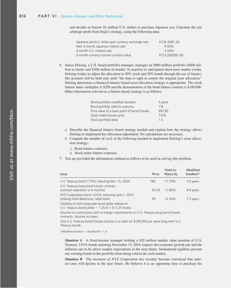
Vis
it u
s at
ww
w.m
hh
e.co
m/b
km816 P A R T V I Options, Futures, and Other Derivatives
and decides to borrow $1 million U.S. dollars to purchase Japanese yen. Calculate the yen arbitrage profit from Itsuji’s strategy, using the following data:
Japanese yen/U.S. dollar spot currency exchange rate ¥124.30/$1.00
New 3-month Japanese interest rate 0.50%
3-month U.S. interest rate 3.50%
3-month currency futures contract value ¥123.2605/$1.00
6. Janice Delsing, a U.S.-based portfolio manager, manages an $800 million portfolio ($600 mil-lion in stocks and $200 million in bonds). In reaction to anticipated short-term market events, Delsing wishes to adjust the allocation to 50% stock and 50% bonds through the use of futures. Her position will be held only until “the time is right to restore the original asset allocation.” Delsing determines a financial futures–based asset allocation strategy is appropriate. The stock futures index multiplier is $250 and the denomination of the bond futures contract is $100,000. Other information relevant to a futures-based strategy is as follows:
Bond portfolio modified duration 5 years
Bond portfolio yield to maturity 7%
Price value of a basis point of bond futures $97.85
Stock-index futures price 1378
Stock portfolio beta 1.0
a. Describe the financial futures–based strategy needed and explain how the strategy allows Delsing to implement her allocation adjustment. No calculations are necessary.
b. Compute the number of each of the following needed to implement Delsing’s asset alloca-tion strategy:
i. Bond futures contracts. ii. Stock-index futures contracts.
7. You are provided the information outlined as follows to be used in solving this problem.
Issue PriceYield to Maturity
Modified Duration*
U.S. Treasury bond 11¾% maturing Nov. 15, 2024 100 11.75% 7.6 years
U.S. Treasury long bond futures contract
(contract expiration in 6 months) 63.33 11.85% 8.0 years
XYZ Corporation bond 12½% maturing June 1, 2015
(sinking fund debenture, rated AAA) 93 13.50% 7.2 years
Volatility of AAA corporate bond yields relative to
U.S. Treasury bond yields 5 1.25 to 1.0 (1.25 times)
Assume no commission and no margin requirements on U.S. Treasury long bond futures
contracts. Assume no taxes.
One U.S. Treasury bond futures contract is a claim on $100,000 par value long-term U.S.
Treasury bonds.
*Modified duration 5 Duration/(1 1 y).
Situation A A fixed-income manager holding a $20 million market value position of U.S. Treasury 11¾% bonds maturing November 15, 2024, expects the economic growth rate and the inflation rate to be above market expectations in the near future. Institutional rigidities prevent any existing bonds in the portfolio from being sold in the cash market.
Situation B The treasurer of XYZ Corporation has recently become convinced that inter-est rates will decline in the near future. He believes it is an opportune time to purchase his

Vis
it u
s at
ww
w.m
hh
e.co
m/b
km
C H A P T E R 2 3 Futures, Swaps, and Risk Management 817
company’s sinking fund bonds in advance of requirements because these bonds are trading at a discount from par value. He is preparing to purchase in the open market $20 million par value XYZ Corporation 12½% bonds maturing June 1, 2015. A $20 million par value position of these bonds is currently offered in the open market at 93. Unfortunately, the treasurer must obtain approval from the board of directors for such a purchase, and this approval process can take up to 2 months. The board of directors’ approval in this instance is only a formality.
For each of these two situations, demonstrate how interest rate risk can be hedged using the Trea-sury bond futures contract. Show all calculations, including the number of futures contracts used.
8. You ran a regression of the yield of KC Company’s 10-year bond on the 10-year U.S. Treasury benchmark’s yield using month-end data for the past year. You found the following result:
YieldKC 5 0.54 1 1.22 YieldTreasury
where Yield KC is the yield on the KC bond and Yield Treasury is the yield on the U.S. Treasury bond. The modified duration on the 10-year U.S. Treasury is 7.0 years, and modified duration on the KC bond is 6.93 years.
a. Calculate the percentage change in the price of the 10-year U.S. Treasury, assuming a 50-basis-point change in the yield on the 10-year U.S. Treasury.
b. Calculate the percentage change in the price of the KC bond, using the regression equation above, assuming a 50-basis-point change in the yield on the 10-year U.S. Treasury.
E-INVEST-MENTS EXERCISES
Foreign Currency Futures
Go to the Chicago Mercantile Exchange Web site (www.cme.com) and link to the tab for Trade CME Products, then Foreign Exchange. Link to the Canadian Dollar contracts and answer the following questions about the futures contract:
What is the size (units of $CD) of each contract?
What is the maximum daily price fl uctuation?
What time period during the day is the contract traded?
If the delivery option is exercised, when and where does delivery take place?
SOLUTIONS TO CONCEPT CHECKS
1. According to interest rate parity, F 0 should be $1.981. Because the futures price is too high, we should reverse the arbitrage strategy just considered.
CF Now ($) CF in 1 Year
1. Borrow $2.00 in the U.S. Convert to 1 U.K. pound. 12.00 22.00(1.04)
2. Lend the 1 pound in the U.K. 22.00 1.05E1
3. Enter a contract to sell 1.05 pounds at a futures
price of $2.01/£. 0 (£1.05)($2.01/£ 2 E1)
TOTAL 0 $.0305
2. Because the firm does poorly when the dollar depreciates, it hedges with a futures contract that will provide profits in that scenario. It needs to enter a long position in pound futures, which means that it will earn profits on the contract when the futures price increases, that is, when more dollars are required to purchase one pound. The specific hedge ratio is determined by

Vis
it u
s at
ww
w.m
hh
e.co
m/b
km818 P A R T V I Options, Futures, and Other Derivatives
noting that if the number of dollars required to buy one pound rises by $.05, profits decrease by $200,000 at the same time that the profit on a long future contract would increase by $.05 3 62,500 5 $3,125. The hedge ratio is
$200,000 per $.05 depreciation in the dollar
$3,125 per contract per $.05 depreciation5 64 contracts long
3. Each $1 increase in the price of corn reduces profits by $1 million. Therefore, the firm needs to enter futures contracts to purchase 1 million bushels at a price stipulated today. The futures position will profit by $1 million for each increase of $1 in the price of corn. The profit on the contract will offset the lost profits on operations.
4. In General (per unit of index) Our Numbers
Hold 100,000 units of indexed stock portfolio with
S0 5 1,400. ST 100,000 ST
Sell 400 contracts. F0 2 ST 400 3 $250 3 (1,111 2 ST)
TOTAL F0 $111,100,000
The net cash flow is riskless, and provides a 1% monthly rate of return, equal to the risk-free rate.
5. The price value of a basis point is still $9,000, as a 1-basis-point change in the interest rate reduces the value of the $20 million portfolio by .01% 3 4.5 5 .045%. Therefore, the number of futures needed to hedge the interest rate risk is the same as for a portfolio half the size with double the modified duration.
6. LIBOR
7% 8% 9%
As debt payer (LIBOR 3 $10 million) 2700,000 2800,000 2900,000
As fixed payer receives $10 million 3 (LIBOR 2 .08) 2100,000 0 1100,000
Net cash flow 2800,000 2800,000 2800,000
Regardless of the LIBOR rate, the firm’s net cash outflow equals .08 3 principal, just as if it had issued a fixed-rate bond with a coupon of 8%.
7. The manager would like to hold on to the money market securities because of their attractive relative pricing compared to other short-term assets. However, there is an expectation that rates will fall. The manager can hold this particular portfolio of short-term assets and still benefit from the drop in interest rates by entering a swap to pay a short-term interest rate and receive a fixed interest rate. The resulting synthetic fixed-rate portfolio will increase in value if rates do fall.
8. Stocks offer a total return (capital gain plus dividends) large enough to compensate investors for the time value of the money tied up in the stock. Agricultural prices do not necessarily increase over time. In fact, across a harvest, crop prices will fall. The returns necessary to make storage economically attractive are lacking.
9. If systematic risk were higher, the appropriate discount rate, k, would increase. Referring to Equation 23.4 , we conclude that F 0 would fall. Intuitively, the claim to 1 pound of orange juice is worth less today if its expected price is unchanged, while the risk associated with the value of that claim increases. Therefore, the amount investors are willing to pay today for future delivery is lower.

244PA
RT V
II
HOW CAN WE evaluate the performance of
a portfolio manager? It turns out that even
average portfolio return is not as straight-
forward to measure as it might seem. In
addition, adjusting average returns for risk
presents a host of other problems. We begin
with the measurement of portfolio returns.
From there we move on to conventional
approaches to risk adjustment. We identify
the problems with these approaches when
applied in various real-life situations. We then
turn to some practical procedures for perfor-
mance evaluation in the field such as style
analysis, the Morningstar Star Ratings, and in-
house performance attribution.
Portfolio Performance Evaluation
CHAPTER TWENTY-FOUR
24.1 The Conventional Theory of Performance Evaluation
Average Rates of Return
We defined the holding-period return (HPR) in Section 5.1 of Chapter 5 and explained the differences between arithmetic and geometric averages. Suppose we evaluate the per-formance of a portfolio over a period of 5 years from 20 quarterly rates of return. The arithmetic average of this sample of returns would be the best estimate of the expected rate of return of the portfolio for the next quarter. In contrast, the geometric average is the constant quarterly return over the 20 quarters that would yield the same total or cumulative return. Therefore, the geometric average is defined by
(1 1 rG)20 5 (1 1 r1)(1 1 r2) c
(1 1 r20)
The right-hand side of this equation is the compounded final value of a $1 investment earn-ing the 20 quarterly rates of return over the 5-year observation period. The left-hand side is the compounded value of a $1 investment earning r G each quarter. We solve for 1 1 r G as
1 1 rG 5 [(1 1 r1)(1 1 r2) c
(1 1 r20)]1/20
Each return has an equal weight in the geometric average. For this reason, the geometric average is referred to as a time-weighted average.

820 P A R T V I I Applied Portfolio Management
To set the stage for discussing the more subtle issues that follow, let us start with a trivial example. Consider a stock paying a dividend of $2 annually that currently sells for $50. You purchase the stock today, collect the $2 dividend, and then sell the stock for $53 at year-end. Your rate of return is
Total proceeds
Initial investment5
Income 1 Capital gain
505
2 1 3
505 .10, or 10%
Another way to derive the rate of return that is useful in the more difficult multiperiod case is to set up the investment as a discounted cash flow problem. Call r the rate of return that equates the present value of all cash flows from the investment with the initial outlay. In our example the stock is purchased for $50 and generates cash flows at year-end of $2 (dividend) plus $53 (sale of stock). Therefore, we solve 50 5 (2 1 53)/(1 1 r ) to find again that r 5 10%.
Time-Weighted Returns versus Dollar-Weighted Returns
When we consider investments over a period during which cash was added to or with-drawn from the portfolio, measuring the rate of return becomes more difficult. To continue our example, suppose that you were to purchase a second share of the same stock at the end of the first year, and hold both shares until the end of year 2, at which point you sell each share for $54.
Total cash outlays are
Time Outlay
0 $50 to purchase first share
1 $53 to purchase second share a year later
Proceeds
1 $2 dividend from initially purchased share
2 $4 dividend from the 2 shares held in the second year, plus
$108 received from selling both shares at $54 each
Using the discounted cash flow (DCF) approach, we can solve for the average return over the 2 years by equating the present values of the cash inflows and outflows:
50 153
1 1 r5
2
1 1 r1
112
(1 1 r)2
resulting in r 5 7.117%. This value is called the internal rate of return, or the dollar-weighted rate of return on
the investment. It is “dollar weighted” because the stock’s performance in the second year, when two shares of stock are held, has a greater influence on the average overall return than the first-year return, when only one share is held.
The time-weighted (geometric average) return is 7.81%:
r1 553 1 2 2 50
505 .10 5 10% r2 5
54 1 2 2 53
535 .0566 5 5.66%
rG 5 (1.10 3 1.0566)1/2 2 1 5 .0781 5 7.81%
The dollar-weighted average is less than the time-weighted average in this example because the return in the second year, when more money was invested, is lower.

C H A P T E R 2 4 Portfolio Performance Evaluation 821
Adjusting Returns for Risk
Evaluating performance based on average return alone is not very useful. Returns must be adjusted for risk before they can be compared meaningfully. The simplest and most popular way to adjust returns for portfolio risk is to compare rates of return with those of other investment funds with similar risk characteristics. For example, high-yield bond portfolios are grouped into one “universe,” growth stock equity funds are grouped into another universe, and so on. Then the (usually time-weighted) average returns of each fund within the universe are ordered, and each portfolio manager receives a percentile ranking depending on relative performance with the comparison universe. For example, the manager with the ninth-best performance in a universe of 100 funds would be the 90th percentile manager: Her performance was better than 90% of all competing funds over the evaluation period. 1
These relative rankings are usually displayed in a chart such as that in Figure 24.1 . The chart summarizes performance rankings over four periods: 1 quarter, 1 year, 3 years, and 5 years. The top and bottom lines of each box are drawn at the rate of return of the 95th and 5th percentile managers. The three dashed lines correspond to the rates of return of the 75th, 50th (median), and 25th percentile managers. The diamond is drawn at the average return of a particular fund and the square is drawn at the return of a benchmark index such as the S&P 500. The placement of the diamond within the box is an easy-to-read repre-sentation of the performance of the fund relative to the comparison universe.
This comparison of performance with other managers of similar investment style is a useful first step in evaluating performance. However, such rankings can be misleading. Within a particular universe, some managers may con-centrate on particular subgroups, so that port-folio characteristics are not truly comparable.
1 In previous chapters (particularly in Chapter 11 on the efficient market hypothesis), we have examined whether actively managed portfolios can outperform a passive index. For this purpose we looked at the distribution of alpha values for samples of mutual funds. We noted that any conclusion from such samples was subject to error due to survivorship bias if funds that failed during the sample period were excluded from the sample. In this chap-ter, we are interested in how to assess the performance of individual funds (or other portfolios) of interest. When a particular portfolio is chosen today for inspection of its returns going forward, survivorship bias is not an issue. However, comparison groups must be free of survivorship bias. A sample comprised only of surviving funds will bias upward the return of the benchmark group.
CONCEPT CHECK
1
Shares of XYZ Corp. pay a $2 dividend at the end of every year on December 31. An investor buys two shares of the stock on January 1 at a price of $20 each, sells one of those shares for $22 a year later on the next January 1, and sells the second share an additional year later for $19. Find the dollar- and time-weighted rates of return on the 2-year investment.
30
1 Quarter 1 Year 3 Years 5 Years
S&P 500The Markowill Group
Rate of Return (%)
5
10
15
20
25
Figure 24.1 Universe comparison. Periods ending December 31, 2010

822 P A R T V I I Applied Portfolio Management
For example, within the equity universe, one manager may concentrate on high-beta or aggressive growth stocks. Similarly, within fixed-income universes, durations can vary across managers. These considerations suggest that a more precise means for risk adjust-ment is desirable.
Methods of risk-adjusted performance evaluation using mean-variance criteria came on stage simultaneously with the capital asset pricing model. Jack Treynor, 2 William Sharpe, 3 and Michael Jensen 4 recognized immediately the implications of the CAPM for rating the performance of managers. Within a short time, academicians were in command of a battery of performance measures, and a bounty of scholarly investigation of mutual fund performance was pouring from ivory towers. Shortly thereafter, agents emerged who were willing to supply rating services to portfolio managers and their clients.
But while widely used, risk-adjusted performance measures each have their own limita-tions. Moreover, their reliability requires quite a long history of consistent management with a steady level of performance and a representative sample of investment environ-ments, for example, bull as well as bear markets. In practice, we may need to make deci-sions before the necessary data are available.
For now, however, we start by cataloging some possible risk-adjusted performance measures for a portfolio, P, and examine the circumstances in which each measure might be most relevant.
1. Sharpe measure: (rP 2 rf)/sP
Sharpe’s measure divides average portfolio excess return over the sample period by the standard deviation of returns over that period. It measures the reward to (total) volatility trade-off. 5
2. Treynor measure: (rP 2 rf)/bP
Like Sharpe’s, Treynor’s measure gives excess return per unit of risk, but it uses systematic risk instead of total risk.
3. Jensen measure (portfolio alpha): aP 5 rP 2 [rf 1 bP (rM 2 rf)]
Jensen’s measure is the average return on the portfolio over and above that predicted by the CAPM, given the portfolio’s beta and the average market return. Jensen’s measure is the portfolio’s alpha value.
4. Information ratio: a P / s ( e P )
The information ratio divides the alpha of the portfolio by the nonsystematic risk of the portfolio, called “tracking error” in the industry. It measures abnormal return per unit of risk that in principle could be diversified away by holding a market index portfolio.
Each measure has some appeal. But each does not necessarily provide consistent assessments of performance, because the risk measures used to adjust returns differ substantially.
2 Jack L. Treynor, “How to Rate Management Investment Funds,” Harvard Business Review 43 (January–February 1966).
3 William F. Sharpe, “Mutual Fund Performance,” Journal of Business 39 (January 1966).
4 Michael C. Jensen, “The Performance of Mutual Funds in the Period 1945–1964,” Journal of Finance, May 1968; and “Risk, the Pricing of Capital Assets, and the Evaluation of Investment Portfolios,” Journal of Business, April 1969.
5 We place bars over r f as well as r P to denote the fact that because the risk-free rate may not be constant over the measurement period, we are taking a sample average, just as we do for r P . Equivalently, we may simply compute sample average excess returns.
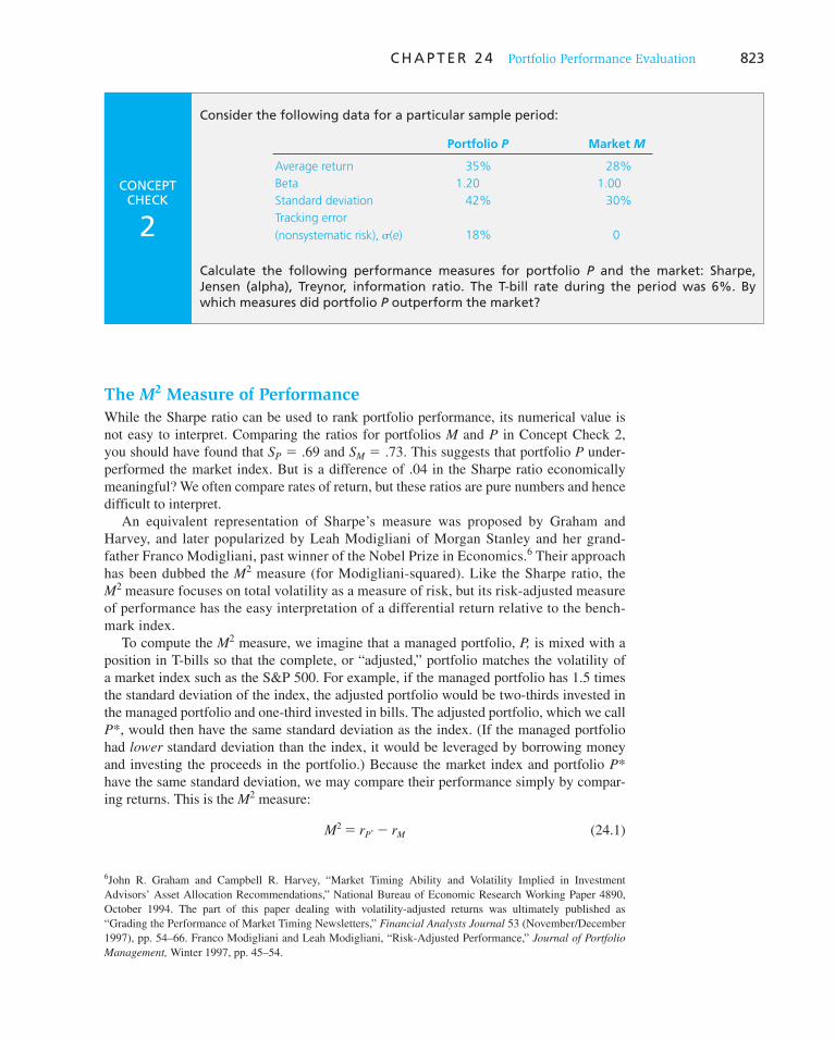
C H A P T E R 2 4 Portfolio Performance Evaluation 823
The M 2 Measure of Performance
While the Sharpe ratio can be used to rank portfolio performance, its numerical value is not easy to interpret. Comparing the ratios for portfolios M and P in Concept Check 2, you should have found that S P 5 .69 and S M 5 .73. This suggests that portfolio P under-performed the market index. But is a difference of .04 in the Sharpe ratio economically meaningful? We often compare rates of return, but these ratios are pure numbers and hence difficult to interpret.
An equivalent representation of Sharpe’s measure was proposed by Graham and Harvey, and later popularized by Leah Modigliani of Morgan Stanley and her grand-father Franco Modigliani, past winner of the Nobel Prize in Economics. 6 Their approach has been dubbed the M 2 measure (for Modigliani-squared). Like the Sharpe ratio, the M 2 measure focuses on total volatility as a measure of risk, but its risk-adjusted measure of performance has the easy interpretation of a differential return relative to the bench-mark index.
To compute the M 2 measure, we imagine that a managed portfolio, P, is mixed with a position in T-bills so that the complete, or “adjusted,” portfolio matches the volatility of a market index such as the S&P 500. For example, if the managed portfolio has 1.5 times the standard deviation of the index, the adjusted portfolio would be two-thirds invested in the managed portfolio and one-third invested in bills. The adjusted portfolio, which we call P *, would then have the same standard deviation as the index. (If the managed portfolio had lower standard deviation than the index, it would be leveraged by borrowing money and investing the proceeds in the portfolio.) Because the market index and portfolio P * have the same standard deviation, we may compare their performance simply by compar-ing returns. This is the M 2 measure:
M2 5 rP* 2 rM (24.1)
6 John R. Graham and Campbell R. Harvey, “Market Timing Ability and Volatility Implied in Investment Advisors’ Asset Allocation Recommendations,” National Bureau of Economic Research Working Paper 4890, October 1994. The part of this paper dealing with volatility-adjusted returns was ultimately published as “Grading the Performance of Market Timing Newsletters,” Financial Analysts Journal 53 (November/December 1997), pp. 54–66. Franco Modigliani and Leah Modigliani, “Risk-Adjusted Performance,” Journal of Portfolio
Management, Winter 1997, pp. 45–54.
CONCEPT CHECK
2
Consider the following data for a particular sample period:
Portfolio P Market M
Average return 35% 28%
Beta 1.20 1.00
Standard deviation 42% 30%
Tracking error
(nonsystematic risk), s(e) 18% 0
Calculate the following performance measures for portfolio P and the market: Sharpe, Jensen (alpha), Treynor, information ratio. The T-bill rate during the period was 6%. By which measures did portfolio P outperform the market?

824 P A R T V I I Applied Portfolio Management
Example 24.1 M 2 Measure
Using the data of Concept Check 2, P has a standard deviation of 42% versus a market standard deviation of 30%. Therefore, the adjusted portfolio P * would be formed by mix-ing bills and portfolio P with weights 30/42 5 .714 in P and 1 2 .714 5 .286 in bills. The return on this portfolio would be (.286 3 6%) 1 (.714 3 35%) 5 26.7%, which is 1.3% less than the market return. Thus portfolio P has an M 2 measure of 2 1.3%.
A graphical representation of the M 2 measure appears in Figure 24.2 . We move down the capital allocation line corresponding to portfolio P (by mixing P with T-bills) until we reduce the standard deviation of the adjusted portfolio to match that of the market index. The M 2 measure is then the vertical distance (i.e., the difference in expected returns) between portfolios P * and M. You can see from Figure 24.2 that P will have a negative M 2 measure when its capital allocation line is less steep than the capital market line, that is, when its Sharpe ratio is less than that of the market index. 7
Sharpe’s Measure as the Criterion for Overall Portfolios
Suppose that Jane Close constructs a portfolio and holds it for a considerable period of time. She makes no changes in portfolio composition during the period. In addition, sup-pose that the daily rates of return on all securities have constant means, variances, and covariances. These assumptions are unrealistic, but they make it easier to highlight impor-tant issues. They are also crucial to understanding the shortcoming of conventional appli-cations of performance measurement.
Now we want to evaluate the performance of Jane’s portfolio. Has she made a good choice of securities? This is really a three-pronged question. First, “good choice” com-
pared with what alternatives? Second, in choosing between two dis-tinct alternative portfolios, what are the appropriate criteria to evaluate performance? Finally, the performance criteria having been identified, is there a rule that will separate basic ability from the random luck of the draw?
Earlier chapters of this text help to determine portfolio choice cri-teria. If investor preferences can be summarized by a mean-variance utility function such as that introduced in Chapter 6, we can arrive at a relatively simple criterion. The particular utility function that we used is
U 5 E(rP) 2 ½ AsP2
where A is the coefficient of risk aversion. With mean-variance pref-erences, Jane wants to maximize the Sharpe measure (i.e., the reward-to-volatility ratio [ E ( r P ) 2 r f ]/ s P ). Recall that this criterion led to the selection of the tangency portfolio in Chapter 7. Jane’s problem reduces to the search for the portfolio with the highest possible Sharpe ratio.
7 In fact you can use Figure 24.2 to show that the M 2 and Sharpe measures are directly related. Letting R denote excess returns and S denote Sharpe measures, the geometry of the figure implies that Rp* 5 SPsM, and therefore that
M2 5 rp* 2 rM 5 Rp* 2 RM 5 SPsM 2 SMsM 5 (SP 2 SM)sM
E(r)
CAL(P)
CML
P*P
M
F
M2
σM σP
σ
Figure 24.2 M 2 of portfolio P
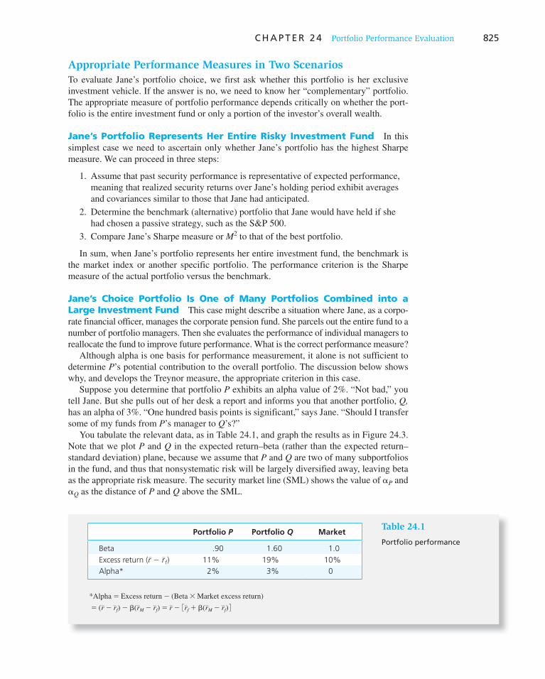
C H A P T E R 2 4 Portfolio Performance Evaluation 825
Appropriate Performance Measures in Two Scenarios
To evaluate Jane’s portfolio choice, we first ask whether this portfolio is her exclusive investment vehicle. If the answer is no, we need to know her “complementary” portfolio. The appropriate measure of portfolio performance depends critically on whether the port-folio is the entire investment fund or only a portion of the investor’s overall wealth.
Jane’s Portfolio Represents Her Entire Risky Investment Fund In this simplest case we need to ascertain only whether Jane’s portfolio has the highest Sharpe measure. We can proceed in three steps:
1. Assume that past security performance is representative of expected performance, meaning that realized security returns over Jane’s holding period exhibit averages and covariances similar to those that Jane had anticipated.
2. Determine the benchmark (alternative) portfolio that Jane would have held if she had chosen a passive strategy, such as the S&P 500.
3. Compare Jane’s Sharpe measure or M 2 to that of the best portfolio.
In sum, when Jane’s portfolio represents her entire investment fund, the benchmark is the market index or another specific portfolio. The performance criterion is the Sharpe measure of the actual portfolio versus the benchmark.
Jane’s Choice Portfolio Is One of Many Portfolios Combined into a Large Investment Fund This case might describe a situation where Jane, as a corpo-rate financial officer, manages the corporate pension fund. She parcels out the entire fund to a number of portfolio managers. Then she evaluates the performance of individual managers to reallocate the fund to improve future performance. What is the correct performance measure?
Although alpha is one basis for performance measurement, it alone is not sufficient to determine P ’s potential contribution to the overall portfolio. The discussion below shows why, and develops the Treynor measure, the appropriate criterion in this case.
Suppose you determine that portfolio P exhibits an alpha value of 2%. “Not bad,” you tell Jane. But she pulls out of her desk a report and informs you that another portfolio, Q,
has an alpha of 3%. “One hundred basis points is significant,” says Jane. “Should I transfer some of my funds from P ’s manager to Q ’s?”
You tabulate the relevant data, as in Table 24.1 , and graph the results as in Figure 24.3 . Note that we plot P and Q in the expected return–beta (rather than the expected return–standard deviation) plane, because we assume that P and Q are two of many subportfolios in the fund, and thus that nonsystematic risk will be largely diversified away, leaving beta as the appropriate risk measure. The security market line (SML) shows the value of a P and a Q as the distance of P and Q above the SML.
Portfolio P Portfolio Q Market
Beta .90 1.60 1.0
Excess return (r 2 rf ) 11% 19% 10%
Alpha* 2% 3% 0
Table 24.1
Portfolio performance
*Alpha 5 Excess return 2 (Beta 3 Market excess return)
5 (r 2 rf) 2 b(rM 2 rf) 5 r 2 3rf 1 b(rM 2 rf) 4
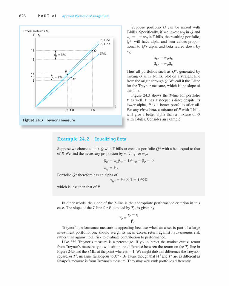
826 P A R T V I I Applied Portfolio Management
Suppose portfolio Q can be mixed with T-bills. Specifically, if we invest w Q in Q and w F 5 1 2 w Q in T-bills, the resulting port folio, Q *, will have alpha and beta values propor-tional to Q ’s alpha and beta scaled down by w Q :
aQ* 5 wQaQ
bQ* 5 wQbQ
Thus all portfolios such as Q *, generated by mixing Q with T-bills, plot on a straight line from the origin through Q. We call it the T-line for the Treynor measure, which is the slope of this line.
Figure 24.3 shows the T -line for portfolio P as well. P has a steeper T -line; despite its lower alpha, P is a better portfolio after all. For any given beta, a mixture of P with T-bills will give a better alpha than a mixture of Q with T-bills. Consider an example.
Example 24.2 Equalizing Beta
Suppose we choose to mix Q with T-bills to create a portfolio Q * with a beta equal to that of P. We find the necessary proportion by solving for w Q :
bQ* 5 wQbQ 5 1.6wQ 5 bP 5 .9
wQ 5 9⁄16
Portfolio Q * therefore has an alpha ofaQ* 5 9⁄16 3 3 5 1.69%
which is less than that of P.
In other words, the slope of the T -line is the appropriate performance criterion in this case. The slope of the T -line for P, denoted by T P , is given by
TP 5rP 2 rf
bP
Treynor’s performance measure is appealing because when an asset is part of a large investment portfolio, one should weigh its mean excess return against its systematic risk rather than against total risk to evaluate contribution to performance.
Like M 2 , Treynor’s measure is a percentage. If you subtract the market excess return from Treynor’s measure, you will obtain the difference between the return on the T P line in Figure 24.3 and the SML, at the point where b 5 1. We might dub this difference the Treynor-square, or T 2 , measure (analogous to M 2 ). Be aware though that M 2 and T 2 are as different as Sharpe’s measure is from Treynor’s measure. They may well rank portfolios differently.
.9 1.0 1.6
19
16
11109
QSML
Tp LineTQ Line
Excess Return (%)r − rf
P
M
β
αQ = 3%
αp = 2%
Figure 24.3 Treynor’s measure

827
The Role of Alpha in Performance Measures
With some algebra we can derive the relationship between the various performance mea-sures that we’ve introduced above. The following table shows some of these relationships.
Treynor (TP) Sharpe* (SP)
Relation to alpha E(rP) 2 rf
bP
5aP
bP
1 TM
E(rP) 2 rf
sP
5aP
sP
1 rSM
Deviation from market performance T 2P 5 TP 2 TM 5
aP
bP
S P 2 SM 5aP
sP
1 (r 2 1)SM
*r denotes the correlation coefficient between portfolio P and the market, and is less than 1.
All of these models are consistent in that superior performance requires a positive alpha. Hence, alpha is the most widely used performance measure. However, the Treynor and Sharpe measures make different uses of alpha and can therefore rank portfolios dif-ferently. A positive alpha alone cannot guarantee a better Sharpe measure of a portfolio, because taking advantage of security mispricing means departing from full diversification, which entails a cost (notice in the table that r 2 1 is negative, so that the Sharpe measure can actually fall).
Actual Performance Measurement: An Example Now that we have examined possible criteria for performance evaluation, we need to deal with a statistical issue: Can we assess the quality of ex ante decisions using ex post data? Before we plunge into a discussion of this problem, let us look at the rate of return on Jane’s portfolio over the last 12 months. Table 24.2 shows the excess return recorded each month for Jane’s portfolio P, one of her alternative portfolios Q, and the benchmark index portfolio M. The last rows in Table 24.2 give sample average and standard devia-tions. From these, and regressions of P and Q on M, we obtain the necessary performance statistics.
eXcel APPLICATIONS: Performance Measurement
T he following performance measurement spread-sheet computes all the performance measures
discussed in this section. You can see how relative
ranking differs according to the criterion selected. This Excel model is available at the Online Learning Center ( www.mhhe.com/bkm ).
21
34567891011121314151617181920
21
A B C D E F G H I J K
Non-Average Beta systematic Sharpe's Treynor's Jensen's M2 T2 Appraisal
Fund Return Deviation Coefficient Risk Measure Measure Measure Measure Measure RatioAlpha 28.00% 27.00% 1.7000 5.00% 0.8148 0.1294 −0.0180 −0.0015 −0.0106 −0.3600Omega 31.00% 26.00% 1.6200 6.00% 0.9615 0.1543 0.0232 0.0235 0.0143 0.3867Omicron 22.00% 21.00% 0.8500 2.00% 0.7619 0.1882 0.0410 −0.0105 0.0482 2.0500Millennium 40.00% 33.00% 2.5000 27.00% 1.0303 0.1360 −0.0100 0.0352 −0.0040 −0.0370Big Value 15.00% 13.00% 0.9000 3.00% 0.6923 0.1000 −0.0360 −0.0223 −0.0400 −1.2000Momentum Watcher 29.00% 24.00% 1.4000 16.00% 0.9583 0.1643 0.0340 0.0229 0.0243 0.2125Big Potential 15.00% 11.00% 0.5500 1.50% 0.8182 0.1636 0.0130 −0.0009 0.0236 0.8667S & P Index Return 20.00% 17.00% 1.0000 0.00% 0.8235 0.1400 0.0000 0.0000 0.0000 0.0000T-Bill Return 6.00% 0.0000
Non-Average Beta systematic Sharpe's Treynor's Jensen's M2 T2 Appraisal
Fund Return Deviation Coefficient Risk Measure Measure Measure Measure Measure Ratio
Enter dataLEGEND
Value calculatedSee comment
Ranking By Sharpe's Measure
Performance Measurement
Standard
Standard
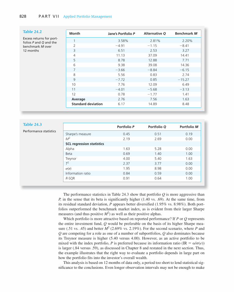
828 P A R T V I I Applied Portfolio Management
The performance statistics in Table 24.3 show that portfolio Q is more aggressive than P, in the sense that its beta is significantly higher (1.40 vs. .69). At the same time, from its residual standard deviation, P appears better diversified (1.95% vs. 8.98%). Both port-folios outperformed the benchmark market index, as is evident from their larger Sharpe measures (and thus positive M 2 ) as well as their positive alphas.
Which portfolio is more attractive based on reported performance? If P or Q represents the entire investment fund, Q would be preferable on the basis of its higher Sharpe mea-sure (.51 vs. .45) and better M 2 (2.69% vs. 2.19%). For the second scenario, where P and Q are competing for a role as one of a number of subportfolios, Q also dominates because its Treynor measure is higher (5.40 versus 4.00). However, as an active portfolio to be mixed with the index portfolio, P is preferred because its information ratio (IR 5 a / s ( e )) is larger (.84 versus .59), as discussed in Chapter 8 and restated in the next section. Thus, the example illustrates that the right way to evaluate a portfolio depends in large part on how the portfolio fits into the investor’s overall wealth.
This analysis is based on 12 months of data only, a period too short to lend statistical sig-nificance to the conclusions. Even longer observation intervals may not be enough to make
Table 24.2
Excess returns for port-folios P and Q and the benchmark M over 12 months
Month Jane’s Portfolio P Alternative Q Benchmark M
1 3.58% 2.81% 2.20%
2 24.91 21.15 28.41
3 6.51 2.53 3.27
4 11.13 37.09 14.41
5 8.78 12.88 7.71
6 9.38 39.08 14.36
7 23.66 28.84 26.15
8 5.56 0.83 2.74
9 27.72 0.85 215.27
10 7.76 12.09 6.49
11 24.01 25.68 23.13
12 0.78 21.77 1.41
Average 2.76 7.56 1.63
Standard deviation 6.17 14.89 8.48
Table 24.3
Performance statistics Portfolio P Portfolio Q Portfolio M
Sharpe’s measure 0.45 0.51 0.19
M2 2.19 2.69 0.00
SCL regression statistics
Alpha 1.63 5.28 0.00
Beta 0.69 1.40 1.00
Treynor 4.00 5.40 1.63
T2 2.37 3.77 0.00
s(e) 1.95 8.98 0.00
Information ratio 0.84 0.59 0.00
R-SQR 0.91 0.64 1.00

C H A P T E R 2 4 Portfolio Performance Evaluation 829
the decision clear-cut, which represents a further problem. A model that calculates these performance measures is available on the Online Learning Center ( www.mhhe.com/bkm ).
Realized Returns versus Expected Returns
When evaluating a portfolio, the evaluator knows neither the portfolio manager’s original expectations nor whether those expectations made sense. One can only observe perfor-mance after the fact and hope that random results are neither taken for, nor hide, true underlying ability. But risky asset returns are “noisy,” which complicates the inference problem. To avoid making mistakes, we have to determine the “significance level” of a performance measure to know whether it reliably indicates ability.
Consider Joe Dart, a portfolio manager. Suppose that his portfolio has an alpha of 20 basis points per month, which makes for a hefty 2.4% per year before compounding. Let us assume that the return distribution of Joe’s portfolio has constant mean, beta, and alpha, a heroic assumption, but one that is in line with the usual treatment of performance measure-ment. Suppose that for the measurement period Joe’s portfolio beta is 1.2 and the monthly standard deviation of the residual (nonsystematic risk) is .02 (2%). With a market index stan-dard deviation of 6.5% per month (22.5% per year), Joe’s portfolio systematic variance is
b2sM2 5 1.22 3 6.52 5 60.84
and hence the correlation coefficient between his portfolio and the market index is
r 5 B b2sM2
b2sM2 1 s2 (e)
R 1/2
5 B 60.84
60.84 1 4R 1/2
5 .97
which shows that his portfolio is quite well diversified. To estimate Joe’s portfolio alpha from the security characteristic line (SCL), we regress
the portfolio excess returns on the market index. Suppose that we are in luck and the regres-sion estimates yield precisely the true parameters. That means that our SCL estimates for the N months are
â 5 .2%, b̂ 5 1.2, ŝ(e) 5 2%
The evaluator who runs such a regression, however, does not know the true values, and hence must compute the t -statistic of the alpha estimate to determine whether to reject the hypothesis that Joe’s alpha is zero, that is, that he has no superior ability.
The standard error of the alpha estimate in the SCL regression is approximately
ŝ(a) 5ŝ(e)
"N
where N is the number of observations and ŝ(e) is the sample estimate of nonsystematic risk. The t -statistic for the alpha estimate is then
t(â) 5â
ŝ(a)5
â"N
ŝ(e) (24.2)
Suppose that we require a significance level of 5%. This requires a t(â) value of 1.96 if N is large. With â 5 .2 and ŝ(e) 5 2, we solve Equation 24.2 for N and find that
1.96 5.2"N
2
N 5 384 months
or 32 years!

830 P A R T V I I Applied Portfolio Management
What have we shown? Here is an analyst who has very substantial ability. The example is biased in his favor in the sense that we have assumed away statistical complications. Nothing changes in the parameters over a long period of time. Furthermore, the sample period “behaves” perfectly. Regression estimates are all perfect. Still, it will take Joe’s entire working career to get to the point where statistics will confirm his true ability. We have to conclude that the problem of statistical inference makes performance evaluation extremely difficult in practice.
Now add to the imprecision of performance estimates the fact that the average tenure of a fund manager is only about 4.5 years. By the time you are lucky enough to find a fund whose historic superior performance you are confident of, its manager is likely to be about to move, or has already moved elsewhere. The nearby box explores this topic further.
CONCEPT CHECK
3 Suppose an analyst has a measured alpha of .2% with a standard error of 2%, as in our example. What is the probability that the positive alpha is due to luck of the draw and that true ability is zero?
24.2 Performance Measurement for Hedge Funds
In describing Jane’s portfolio performance evaluation we left out one scenario that may well be the most relevant.
Suppose Jane has been satisfied with her well-diversified mutual fund, but now she stumbles upon information on hedge funds. Hedge funds are rarely designed as candidates for an investor’s overall portfolio. Rather than focusing on Sharpe ratios, which would entail establishing an attractive trade-off between expected return and overall volatility, these funds tend to concentrate on opportunities offered by temporarily mispriced securi-ties, and show far less concern for broad diversification. In other words, these funds are alpha driven, and best thought of as possible additions to core positions in more traditional portfolios established with concerns of diversification in mind.
In Chapter 8, we considered precisely the question of how best to mix an actively man-aged portfolio with a broadly diversified core position. We saw that the key statistic for this mixture is the information ratio of the actively managed portfolio; this ratio, therefore, becomes the active fund’s appropriate performance measure.
To briefly review, call the active portfolio established by the hedge fund H, and the investor’s baseline passive portfolio M. Then the optimal position of H in the overall port-folio, denoted P *, would be
wH 5wH
0
1 1 (1 2 bH)wH0
wH0 5
aH
s2(eH)
E(RM)
sM2
(24.3)

831
Should You Follow Your Fund Manager?
The whole idea of investing in a mutual fund is to leave the stock and bond picking to the professionals. But fre-quently, events don’t turn out quite as expected—the manager resigns, gets transferred or dies. A big part of the investor’s decision to buy a managed fund is based on the manager’s record, so changes like these can come as an unsettling surprise.
There are no rules about what happens in the wake of a manager’s departure. It turns out, however, that there is strong evidence to suggest that the managers’ real con-tribution to fund performance is highly overrated. For example, research company Morningstar compared funds that experienced management changes between 1990 and 1995 with those that kept the same managers. In the five years ending in June 2000, the top-performing funds of the previous five years tended to keep beating their peers—despite losing any fund managers. Those funds that per-formed badly in the first half of the 1990s continued to do badly, regardless of management changes. While mutual fund management companies will undoubtedly continue to create star managers and tout their past records, inves-tors should stay focused on fund performance.
Funds are promoted on their managers’ track records, which normally span a three- to five-year period. But per-formance data that goes back only a few years is hardly a valid measure of talent. To be statistically sound, evidence of a manager’s track record needs to span, at a minimum, 10 years or more.
The mutual fund industry may look like a merry-go-round of managers, but that shouldn’t worry most inves-tors. Many mutual funds are designed to go through little or no change when a manager leaves. That is because,
according to a strategy designed to reduce volatility and succession worries, mutual funds are managed by teams of stock pickers, who each run a portion of the assets, rather than by a solo manager with co-captains. Meanwhile, even so-called star managers are nearly always surrounded by researchers and analysts, who can play as much of a role in performance as the manager who gets the headlines.
Don’t forget that if a manager does leave, the invest-ment is still there. The holdings in the fund haven’t changed. It is not the same as a chief executive leaving a company whose share price subsequently falls. The best thing to do is to monitor the fund more closely to be on top of any changes that hurt its fundamental investment qualities.
In addition, don’t underestimate the breadth and depth of a fund company’s “managerial bench.” The larger, established investment companies generally have a large pool of talent to draw on. They are also well aware that investors are prone to depart from a fund when a manage-rial change occurs.
Lastly, for investors who worry about management changes, there is a solution: index funds. These mutual funds buy stocks and bonds that track a benchmark index like the S&P 500 rather than relying on star managers to actively pick securities. In this case, it doesn’t really matter if the manager leaves. At the same time, index investors don’t have to pay tax bills that come from switching out of funds when managers leave. Most importantly, index fund investors are not charged the steep fees that are needed to pay star management salaries.
Source: Shauna Carther, “Should You Follow Your Fund Manager?” Investopedia.com, March 3, 2010. Provided by Forbes.
WO
RD
S FRO
M TH
E STREET
As we saw in Chapter 8, when the hedge fund is optimally combined with the baseline portfolio using Equation 24.3 , the improvement in the Sharpe measure will be determined by its information ratio a H / s ( e H ), according to
SP*2 5 SM
2 1 B aH
s(eH)R 2
(24.4)
Equation 24.4 tells us that the appropriate performance measure for the hedge fund is its information ratio (IR).
Looking back at Table 24.3 , we can calculate the IR of portfolios P and Q as
IRP 5aP
s(eP)5
1.63
1.955 .84
IRQ 55.28
8.985 .59
(24.5)
If we were to interpret P and Q as hedge funds, the low beta of P, .69, could result from short positions the fund holds in some assets. The relatively high beta of Q, 1.40, might result from leverage that would also increase the firm-specific risk of the fund, s ( e Q ).

832
Using these calculations, Jane would favor hedge fund P with the higher information ratio.
In practice, evaluating hedge funds poses considerable practical challenges. We will discuss many of these in Chapter 26, which is devoted to these funds. But for now we can briefly mention a few of the difficulties:
1. The risk profile of hedge funds (both total volatility and exposure to relevant systematic factors) may change rapidly. Hedge funds have far greater leeway than mutual funds to change investment strategy opportunistically. This instability makes it hard to measure exposure at any given time.
2. Hedge funds tend to invest in illiquid assets. We therefore must disentangle liquid-ity premiums from true alpha to properly assess their performance. Moreover, it can be difficult to accurately price inactively traded assets, and correspondingly difficult to measure rates of return.
3. Many hedge funds pursue strategies that may provide apparent profits over long periods of time, but expose the fund to infrequent but severe losses. Therefore, very long time periods may be required to formulate a realistic picture of their true risk–return trade-off.
4. When hedge funds are evaluated as a group, survivorship bias can be a major consideration, because turnover in this industry is far higher than for investment companies such as mutual funds.
The nearby box discusses some of the misuses of conventional performance measures in evaluating hedge funds.
Sharpe Point: Risk Gauge is Misused
William F. Sharpe was probably the biggest expert in the room when economists from around the world gathered to hash out a pressing problem: How to gauge hedge-fund risk. About 40 years ago, Dr. Sharpe created a simple cal-culation for measuring the return that investors should expect for the level of volatility they are accepting. In other words: How much money do they stand to make compared with the size of the up-and-down swings they will lose sleep over?
The so-called Sharpe Ratio became a cornerstone of modern finance, as investors used it to help select money managers and mutual funds. But the use of the ratio has been criticized by many prominent academics—including Dr. Sharpe himself.
The ratio is commonly used—“misused,” Dr. Sharpe says—for promotional purposes by hedge funds. Hedge funds, loosely regulated private investment pools, often use complex strategies that are vulnerable to surprise events and elude any simple formula for measuring risk. “Past average experience may be a terrible predictor of future performance,” Dr. Sharpe says.
Dr. Sharpe designed the ratio to evaluate portfolios of stocks, bonds, and mutual funds. The higher the Sharpe
Ratio, the better a fund is expected to perform over the long term. However, at a time when smaller investors and pension funds are pouring money into hedge funds, the ratio can foster a false sense of security.
Dr. Sharpe says the ratio doesn’t foreshadow hedge-fund woes because “no number can.” The formula can’t predict such troubles as the inability to sell off invest-ments quickly if they start to head south, nor can it account for extreme unexpected events. Long-Term Capital Management, a huge hedge fund in Connecticut, had a glowing Sharpe Ratio before it abruptly collapsed in 1998 when Russia devalued its currency and defaulted on debt. Plus, hedge funds are generally secretive about their strat-egies, making it difficult for investors to get an accurate picture of risk.
Another problem with the Sharpe Ratio is that it is designed to evaluate the risk-reward profile of an inves-tor’s entire portfolio, not small pieces of it. This shortcom-ing is particularly telling for hedge funds.
Source: Ianthe Jeanne Dugan, “Sharpe Point: Risk Gauge is Misused,” The Wall Street Journal, August 31, 2005, p. C1. © 2005 Dow Jones & Company, Inc. All rights reserved worldwide.
WO
RD
S FR
OM
TH
E ST
REE
T

C H A P T E R 2 4 Portfolio Performance Evaluation 833
24.3 Performance Measurement with Changing Portfolio Composition
We have seen already that the volatility of stock returns requires a very long observation period to determine performance levels with any precision, even if portfolio returns are distributed with constant mean and variance. Imagine how this problem is compounded when portfolio return distributions are constantly changing.
It is acceptable to assume that the return distributions of passive strategies have constant mean and variance when the measurement interval is not too long. However, under an active strategy return distributions change by design, as the portfolio manager updates the portfolio in accordance with the dictates of financial analysis. In such a case, estimating various statistics from a sample period assuming a constant mean and variance may lead to substantial errors. Let us look at an example.
Example 24.3 Changing Portfolio Risk
Suppose that the Sharpe measure of the market index is .4. Over an initial period of 52 weeks, the portfolio manager executes a low-risk strategy with an annualized mean excess return of 1% and standard deviation of 2%. This makes for a Sharpe measure of .5, which beats the passive strategy. Over the next 52-week period this manager finds that a high -risk strategy is optimal, with an annual mean excess return of 9% and standard devia-tion of 18%. Here, again, the Sharpe measure is .5. Over the 2-year period our manager maintains a better-than-passive Sharpe measure.
Figure 24.4 shows a pattern of (annualized) quarterly returns that are consistent with our description of the manager’s strategy of 2 years. In the first four quarters the excess returns are 2 1%, 3%, 2 1%, and 3%, making for an average of 1% and standard deviation of 2%. In the next four quarters the returns are 2 9%, 27%, 2 9%, 27%, making for an average of 9% and standard deviation of 18%. Thus both years exhibit a Sharpe measure of .5. However, over the eight-quarter sequence the mean and standard deviation are 5% and 13.42%, respec-tively, making for a Sharpe measure of only .37, apparently inferior to the passive strategy!
What happened in Example 24.3 ? The shift of the mean from the first four quar-ters to the next was not recognized as a shift in strategy. Instead, the difference in mean returns in the 2 years added to the appear-
ance of volatility in portfolio returns. The active strategy with shifting means appears riskier than it really is and biases the esti-mate of the Sharpe measure downward. We conclude that for actively managed portfo-lios it is helpful to keep track of portfolio composition and changes in portfolio mean and risk. We will see another example of this problem in the next section, which deals with market timing.
Rate of Return (%)
Quarter
27
3−1
−9
Figure 24.4 Portfolio returns. Returns in last four quarters are more variable than in the first four.
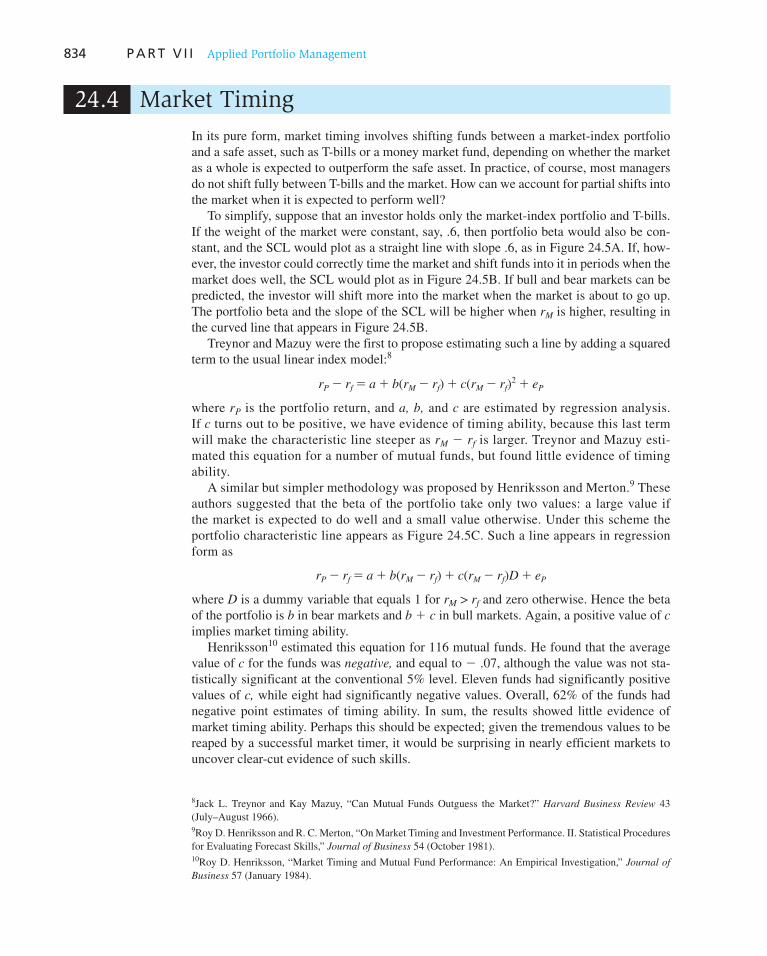
834 P A R T V I I Applied Portfolio Management
24.4 Market Timing
In its pure form, market timing involves shifting funds between a market-index portfolio and a safe asset, such as T-bills or a money market fund, depending on whether the market as a whole is expected to outperform the safe asset. In practice, of course, most managers do not shift fully between T-bills and the market. How can we account for partial shifts into the market when it is expected to perform well?
To simplify, suppose that an investor holds only the market-index portfolio and T-bills. If the weight of the market were constant, say, .6, then portfolio beta would also be con-stant, and the SCL would plot as a straight line with slope .6, as in Figure 24.5 A. If, how-ever, the investor could correctly time the market and shift funds into it in periods when the market does well, the SCL would plot as in Figure 24.5 B. If bull and bear markets can be predicted, the investor will shift more into the market when the market is about to go up. The portfolio beta and the slope of the SCL will be higher when r M is higher, resulting in the curved line that appears in Figure 24.5 B.
Treynor and Mazuy were the first to propose estimating such a line by adding a squared term to the usual linear index model: 8
rP 2 rf 5 a 1 b(rM 2 rf) 1 c(rM 2 rf)2 1 eP
where r P is the portfolio return, and a, b, and c are estimated by regression analysis. If c turns out to be positive, we have evidence of timing ability, because this last term will make the characteristic line steeper as r M 2 r f is larger. Treynor and Mazuy esti-mated this equation for a number of mutual funds, but found little evidence of timing ability.
A similar but simpler methodology was proposed by Henriksson and Merton. 9 These authors suggested that the beta of the portfolio take only two values: a large value if the market is expected to do well and a small value otherwise. Under this scheme the portfolio characteristic line appears as Figure 24.5C. Such a line appears in regression form as
rP 2 rf 5 a 1 b(rM 2 rf) 1 c(rM 2 rf)D 1 eP
where D is a dummy variable that equals 1 for r M > r f and zero otherwise. Hence the beta of the portfolio is b in bear markets and b 1 c in bull markets. Again, a positive value of c implies market timing ability.
Henriksson 10 estimated this equation for 116 mutual funds. He found that the average value of c for the funds was negative, and equal to 2 .07, although the value was not sta-tistically significant at the conventional 5% level. Eleven funds had significantly positive values of c, while eight had significantly negative values. Overall, 62% of the funds had negative point estimates of timing ability. In sum, the results showed little evidence of market timing ability. Perhaps this should be expected; given the tremendous values to be reaped by a successful market timer, it would be surprising in nearly efficient markets to uncover clear-cut evidence of such skills.
8 Jack L. Treynor and Kay Mazuy, “Can Mutual Funds Outguess the Market?” Harvard Business Review 43 (July–August 1966).
9 Roy D. Henriksson and R. C. Merton, “On Market Timing and Investment Performance. II. Statistical Procedures for Evaluating Forecast Skills,” Journal of Business 54 (October 1981).
10 Roy D. Henriksson, “Market Timing and Mutual Fund Performance: An Empirical Investigation,” Journal of
Business 57 (January 1984).
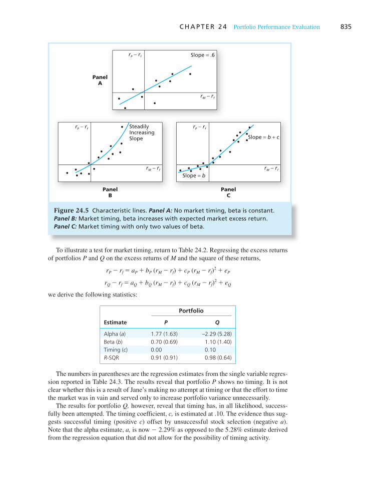
C H A P T E R 2 4 Portfolio Performance Evaluation 835
To illustrate a test for market timing, return to Table 24.2 . Regressing the excess returns of portfolios P and Q on the excess returns of M and the square of these returns,
rP 2 rf 5 aP 1 bP (rM 2 rf) 1 cP (rM 2 rf)2 1 eP
rQ 2 rf 5 aQ 1 bQ (rM 2 rf) 1 cQ (rM 2 rf)2 1 eQ
we derive the following statistics:
Portfolio
Estimate P Q
Alpha (a) 1.77 (1.63) –2.29 (5.28)
Beta (b) 0.70 (0.69) 1.10 (1.40)
Timing (c) 0.00 0.10
R-SQR 0.91 (0.91) 0.98 (0.64)
The numbers in parentheses are the regression estimates from the single variable regres-sion reported in Table 24.3 . The results reveal that portfolio P shows no timing. It is not clear whether this is a result of Jane’s making no attempt at timing or that the effort to time the market was in vain and served only to increase portfolio variance unnecessarily.
The results for portfolio Q, however, reveal that timing has, in all likelihood, success-fully been attempted. The timing coefficient, c, is estimated at .10. The evidence thus sug-gests successful timing (positive c ) offset by unsuccessful stock selection (negative a ). Note that the alpha estimate, a, is now 2 2.29% as opposed to the 5.28% estimate derived from the regression equation that did not allow for the possibility of timing activity.
Slope = b
rM − rf
Slope = b + c
rP − rfSteadilyIncreasingSlope
rP − rf
rM − rf
rM − rf
Slope = .6rP − rf
PanelA
PanelB
PanelC
Figure 24.5 Characteristic lines. Panel A: No market timing, beta is constant. Panel B: Market timing, beta increases with expected market excess return. Panel C: Market timing with only two values of beta.
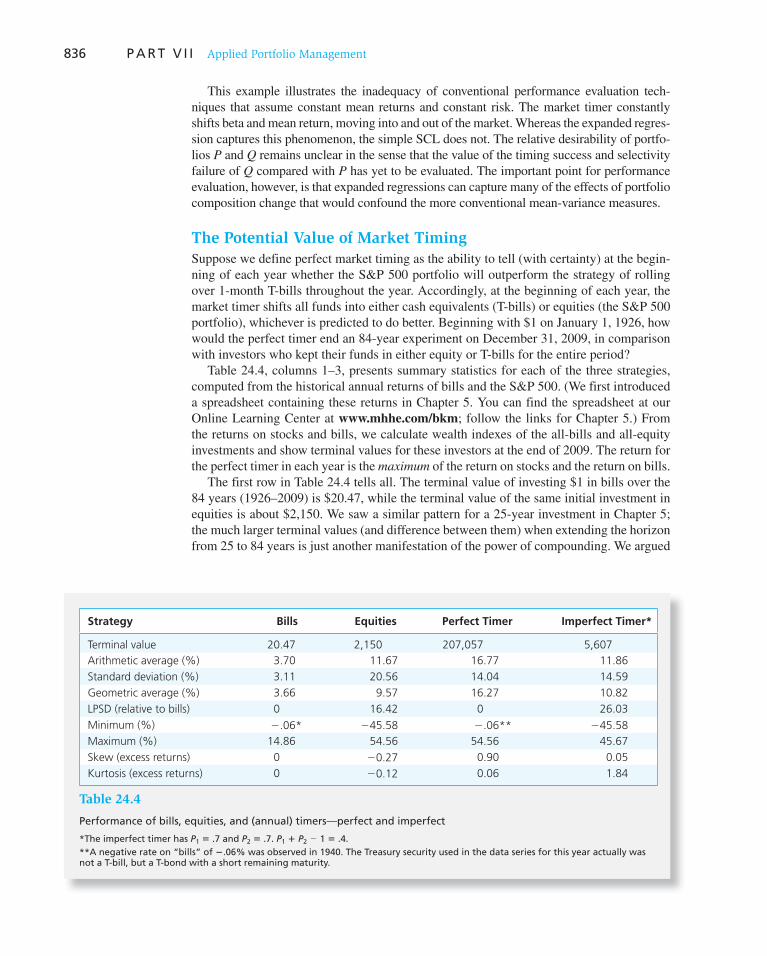
836 P A R T V I I Applied Portfolio Management
This example illustrates the inadequacy of conventional performance evaluation tech-niques that assume constant mean returns and constant risk. The market timer constantly shifts beta and mean return, moving into and out of the market. Whereas the expanded regres-sion captures this phenomenon, the simple SCL does not. The relative desirability of portfo-lios P and Q remains unclear in the sense that the value of the timing success and selectivity failure of Q compared with P has yet to be evaluated. The important point for performance evaluation, however, is that expanded regressions can capture many of the effects of portfolio composition change that would confound the more conventional mean-variance measures.
The Potential Value of Market Timing
Suppose we define perfect market timing as the ability to tell (with certainty) at the begin-ning of each year whether the S&P 500 portfolio will outperform the strategy of rolling over 1-month T-bills throughout the year. Accordingly, at the beginning of each year, the market timer shifts all funds into either cash equivalents (T-bills) or equities (the S&P 500 portfolio), whichever is predicted to do better. Beginning with $1 on January 1, 1926, how would the perfect timer end an 84-year experiment on December 31, 2009, in comparison with investors who kept their funds in either equity or T-bills for the entire period?
Table 24.4 , columns 1–3, presents summary statistics for each of the three strategies, computed from the historical annual returns of bills and the S&P 500. (We first introduced a spreadsheet containing these returns in Chapter 5. You can find the spreadsheet at our Online Learning Center at www.mhhe.com/bkm; follow the links for Chapter 5.) From the returns on stocks and bills, we calculate wealth indexes of the all-bills and all-equity investments and show terminal values for these investors at the end of 2009. The return for the perfect timer in each year is the maximum of the return on stocks and the return on bills.
The first row in Table 24.4 tells all. The terminal value of investing $1 in bills over the 84 years (1926–2009) is $20.47, while the terminal value of the same initial investment in equities is about $2,150. We saw a similar pattern for a 25-year investment in Chapter 5; the much larger terminal values (and difference between them) when extending the horizon from 25 to 84 years is just another manifestation of the power of compounding. We argued
Table 24.4
Performance of bills, equities, and (annual) timers—perfect and imperfect
*The imperfect timer has P 1 5 .7 and P 2 5 .7. P 1 1 P 2 2 1 5 .4. ** A negative rate on “bills” of 2 .06% was observed in 1940. The Treasury security used in the data series for this year actually was not a T-bill, but a T-bond with a short remaining maturity.
Strategy Bills Equities Perfect Timer Imperfect Timer*
Terminal value 20.47 2,150 207,057 5,607
Arithmetic average (%) 3.70 11.67 16.77 11.86
Standard deviation (%) 3.11 20.56 14.04 14.59
Geometric average (%) 3.66 9.57 16.27 10.82
LPSD (relative to bills) 0 16.42 0 26.03
Minimum (%) 2.06* 245.58 2.06** 245.58
Maximum (%) 14.86 54.56 54.56 45.67
Skew (excess returns) 0 20.27 0.90 0.05
Kurtosis (excess returns) 0 20.12 0.06 1.84

C H A P T E R 2 4 Portfolio Performance Evaluation 837
in Chapter 5 that as impressive as the difference in terminal values is, it is best interpreted as no more than fair compensation for the risk borne by equity investors. Notice that the standard deviation of the all-equity investor was a hefty 20.56%. This is also why the geo-metric average of large stocks for the period is “only” 9.57%, compared with the arithmetic average of 11.67%. (Remember that the geometric average is less than the arithmetic aver-age and that the difference between the two increases with the volatility of returns.)
Now observe that the terminal value of the perfect timer is about $207,000, a 96-fold increase over the already large terminal value of the all-equity strategy! In fact, this result is even better than it looks, because the return to the market timer is truly risk-free. This is the classic case where a large standard deviation (14.04%) has nothing to do with risk. Because the timer never delivers a return below the risk-free rate, the standard deviation is a measure of good surprises only. The positive skew of the distribution (compared with the small neg-ative skew of equities) is a manifestation of the fact that the extreme values are all positive. Another indication of this stellar performance is the minimum and maximum returns—the minimum return equals the minimum return on bills (in 1940) and the maximum return is that of equities (in 1933)—so that all negative returns on equities (as low as –45.58% in 1931) were avoided by the timer. Finally, the best indication of the performance of the timer is a lower partial standard deviation, LPSD, in which we calculate the (square root of the) average squared deviation below the risk-free rate (rather than below the mean). 11 The LPSD of the all-equity portfolio is only slightly less than the conventional standard devia-tion, but it is necessarily zero for the perfect timer.
If we interpret the terminal value of the all-equity portfolio in excess of the value of the T-bill portfolio entirely as a risk premium commensurate with investment risk, we must conclude that the risk-adjusted equivalent value of the all-equity terminal value is the same as that of the T-bill portfolio, $20.47. 12 In contrast, the perfect timer’s portfolio has no risk, and so receives no discount for risk. Hence, it is fair to say that the forecasting ability of the perfect timer converts an $20.47 final value to a value of $207,057 for free.
Valuing Market Timing as a Call Option
The key to valuing market timing ability is to recognize that perfect foresight is equivalent to holding a call option on the equity portfolio. The perfect timer invests 100% in either the safe asset or the equity portfolio, whichever will provide the higher return. The rate of return is at least the risk-free rate. This is shown in Figure 24.6 .
To see the value of information as an option, suppose that the market index currently is at S 0 and that a call option on the index has an exercise price of X 5 S 0 (1 1 r f ). If the market outper-forms bills over the coming period, S T will exceed X, whereas it will be less than X otherwise. Now look at the payoff to a portfolio consisting of this option and S 0 dollars invested in bills:
ST , X ST $ X
Bills S0(1 1 rf) S0(1 1 rf)
Option 0 ST 2 X
Total S0(1 1 rf) ST
11 The conventional LPSD is based on the average squared deviation below the mean. Because the threshold performance in this application is the risk-free rate, we modify the LPSD for this discussion by taking squared deviations from that rate.
12 It may seem hard to attribute such a big difference in final outcome solely to risk aversion. But think of it this way: the final value of the equity position is about 105 times that of the bills position ($2,150 versus $20.47). Over 84 years, this implies a reasonable annualized risk premium of 5.7%: 105 1/84 5 1.057.
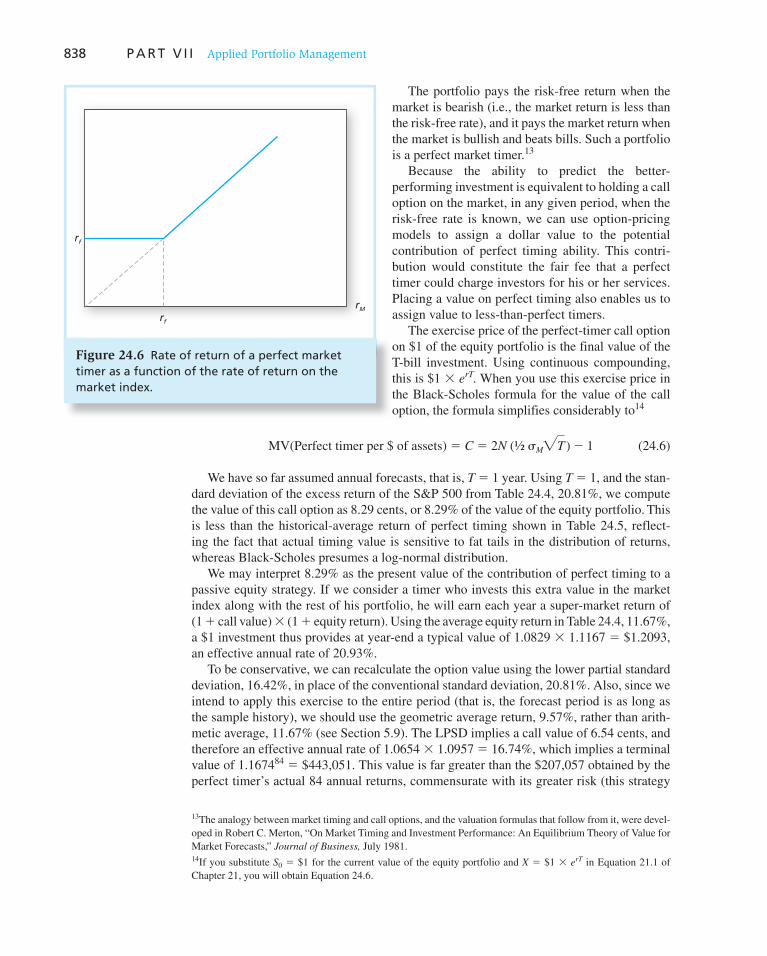
838 P A R T V I I Applied Portfolio Management
The portfolio pays the risk-free return when the market is bearish (i.e., the market return is less than the risk-free rate), and it pays the market return when the market is bullish and beats bills. Such a portfolio is a perfect market timer. 13
Because the ability to predict the better- performing investment is equivalent to holding a call option on the market, in any given period, when the risk-free rate is known, we can use option- pricing models to assign a dollar value to the potential contribution of perfect timing ability. This contri-bution would constitute the fair fee that a perfect timer could charge investors for his or her services. Placing a value on perfect timing also enables us to assign value to less-than-perfect timers.
The exercise price of the perfect-timer call option on $1 of the equity portfolio is the final value of the T-bill investment. Using continuous compounding, this is $1 3 e rT . When you use this exercise price in the Black-Scholes formula for the value of the call option, the formula simplifies considerably to 14
MV(Perfect timer per $ of assets) 5 C 5 2N (½ sM"T ) 2 1 (24.6)
We have so far assumed annual forecasts, that is, T 5 1 year. Using T 5 1, and the stan-dard deviation of the excess return of the S&P 500 from Table 24.4, 20.81%, we compute the value of this call option as 8.29 cents, or 8.29% of the value of the equity portfolio. This is less than the historical-average return of perfect timing shown in Table 24.5, reflect-ing the fact that actual timing value is sensitive to fat tails in the distribution of returns, whereas Black-Scholes presumes a log-normal distribution.
We may interpret 8.29% as the present value of the contribution of perfect timing to a passive equity strategy. If we consider a timer who invests this extra value in the market index along with the rest of his portfolio, he will earn each year a super-market return of (1 1 call value) 3 (1 1 equity return). Using the average equity return in Table 24.4, 11.67%, a $1 investment thus provides at year-end a typical value of 1.0829 3 1.1167 5 $1.2093, an effective annual rate of 20.93%.
To be conservative, we can recalculate the option value using the lower partial standard deviation, 16.42%, in place of the conventional standard deviation, 20.81%. Also, since we intend to apply this exercise to the entire period (that is, the forecast period is as long as the sample history), we should use the geometric average return, 9.57%, rather than arith-metic average, 11.67% (see Section 5.9). The LPSD implies a call value of 6.54 cents, and therefore an effective annual rate of 1.0654 3 1.0957 5 16.74%, which implies a terminal value of 1.167484 5 $443,051. This value is far greater than the $207,057 obtained by the perfect timer’s actual 84 annual returns, commensurate with its greater risk (this strategy
13 The analogy between market timing and call options, and the valuation formulas that follow from it, were devel-oped in Robert C. Merton, “On Market Timing and Investment Performance: An Equilibrium Theory of Value for Market Forecasts,” Journal of Business, July 1981. 14 If you substitute S 0 5 $1 for the current value of the equity portfolio and X 5 $1 3 e rT in Equation 21.1 of Chapter 21, you will obtain Equation 24.6 .
rf
rf
rM
Figure 24.6 Rate of return of a perfect market timer as a function of the rate of return on the market index.

C H A P T E R 2 4 Portfolio Performance Evaluation 839
is always fully invested in the market, whereas the timer is sometimes invested in bills). It would be fair, however, to compare it to the equal-risk passive equity strategy that yielded a terminal value of $2,150.
If the timer could make the correct choice every month instead of every year, the value of the forecasts would dramatically increase. Of course, making perfect forecasts more frequently requires even better powers of prediction. As the frequency of such perfect predictions increases without bound, the value of the services will increase without bound as well.
Suppose the perfect timer could make perfect forecasts every month. In this case, each forecast would be for a shorter interval, and the value of each individual forecast would be lower, but there would be 12 times as many forecasts, each of which could be val-ued as another call option. The net result is a big increase in total value. With monthly
predictions, the value of the call will be 2N (½ 3 .1642 3"1/12 ) 2 1 5 .0189. Using a monthly T-bill rate of 3.7%/12, the present value of a 1-year string of such monthly calls, each worth $.0189, is $.21. Thus, the annual value of the monthly perfect timer is 21 cents on the dollar, compared to 6.54 cents for an annual timer. For an investment period of 84 years, the forecast future value of a $1 investment would be a far greater [(1 1 .21) 3 (1 1 .0957/12)]84 5 $17.5 million.
The Value of Imperfect Forecasting
Unfortunately, managers are not perfect forecasters. It seems pretty obvious that if manag-ers are right most of the time, they are doing very well. However, when we say “most of the time,” we cannot mean merely the percentage of the time a manager is right. The weather forecaster in Tucson, Arizona, who always predicts no rain, may be right 90% of the time. But a high success rate for a “stopped-clock” strategy is not evidence of forecasting ability.
Similarly, the appropriate measure of market forecasting ability is not the overall pro-portion of correct forecasts. If the market is up 2 days out of 3 and a forecaster always predicts market advance, the two-thirds success rate is not a measure of forecasting abil-ity. We need to examine the proportion of bull markets ( r M > r f ) correctly forecast and the proportion of bear markets ( r M > r f ) correctly forecast.
If we call P 1 the proportion of the correct forecasts of bull markets and P 2 the propor-tion for bear markets, then P 5 P 1 1 P 2 2 1 is the correct measure of timing ability. For example, a forecaster who always guesses correctly will have P 1 5 P 2 5 1, and will show ability of 1 (100%). An analyst who always bets on a bear market will mispredict all bull markets ( P 1 5 0), will correctly “predict” all bear markets ( P 2 5 1), and will end up with timing ability of P 5 P 1 1 P 2 2 1 5 0.
The accuracy of a market timer in terms of guessing correctly bull and bear mar-kets can be estimated from data that include predictions and realizations. When tim-ing is imperfect, Merton shows that if we measure overall accuracy by the statistic P 5 P 1 1 P 2 2 1, the market value of the services of an imperfect timer is simply
MV(Imperfect timer) 5 P 3 C 5(P1 1 P2 2 1) [2N (½ sM"T) 2 1] (24.7)
CONCEPT CHECK
4 What is the market timing score of someone who flips a fair coin to predict the market?

840 P A R T V I I Applied Portfolio Management
The last column in Table 24.4 provides an assessment of the imperfect market-timer in two ways. To simulate the performance of an imperfect timer, we drew random numbers for predictions in each year (assuming that both P 1 and P 2 5 .7) and compiled results for the 84 years of history. 15 The statistics of this exercise resulted in a terminal value for the timer of “only” $5,607, compared with $2,150 for the all-equity investments. Here, too, Equation 24.7 allows for a better comparison of timing versus passive investment. With timing ability measured by P1 1 P2 2 1 5 .4, the value of the imperfect timer’s call option is .4 3 6.54 5 2.616 cents. Recalculating the timer’s terminal value yields (1.02616 3 1.0957)84 5 $18,887, still far superior to the $2,150 value of the equity portfolio.16
A further variation on the valuation of market timing is a case in which the timer does not shift fully from one asset to the other. In particular, if the timer knows her forecasts are imperfect, one would not expect her to shift fully between markets. She presumably would moderate her positions. Suppose that she shifts a fraction v of the portfolio between T-bills and equities. In that case, Equation 24.7 can be generalized as follows:
MV(Imperfect timer) 5 v 3 P 3 C 5 v(P1 1 P2 2 1)[2N(sM"T) 2 1]
For example, if the shift is v 5 .50 (50% of the portfolio), the timer’s value will be one-half of the value we would obtain for full shifting, for which v 5 1.0.
24.5 Style Analysis
Style analysis was introduced by Nobel laureate William Sharpe. 17 The popularity of the concept was aided by a well-known study 18 concluding that 91.5% of the variation in returns of 82 mutual funds could be explained by the funds’ asset allocation to bills, bonds, and stocks. Later studies that considered asset allocation across a broader range of asset classes found that as much as 97% of fund returns can be explained by asset allocation alone.
Sharpe’s idea was to regress fund returns on indexes representing a range of asset classes. The regression coefficient on each index would then measure the fund’s implicit allocation to that “style.” Because funds are barred from short positions, the regression coefficients are constrained to be either zero or positive and to sum to 100%, so as to rep-resent a complete asset allocation. The R -square of the regression would then measure the percentage of return variability attributable to style or asset allocation, while the remainder of return variability would be attributable either to security selection or to market timing by periodic changes in the asset-class weights.
15 In each year, we started with the correct forecast, but then used a random number generator to occasionally change the timer’s forecast to an incorrect prediction. We set the probability that the timer’s forecast would be correct equal to .70 for both up and down markets.
16 Notice that Equation 24.7 implies that an investor with a value of P 5 0 who attempts to time the market would add zero value. The shifts across markets would be no better than a random decision concerning asset allocation.
17 William F. Sharpe, “Asset Allocation: Management Style and Performance Evaluation,” Journal of Portfolio
Management, Winter 1992, pp. 7–19.
18 Gary Brinson, Brian Singer, and Gilbert Beebower, “Determinants of Portfolio Performance,” Financial
Analysts Journal, May/June 1991.
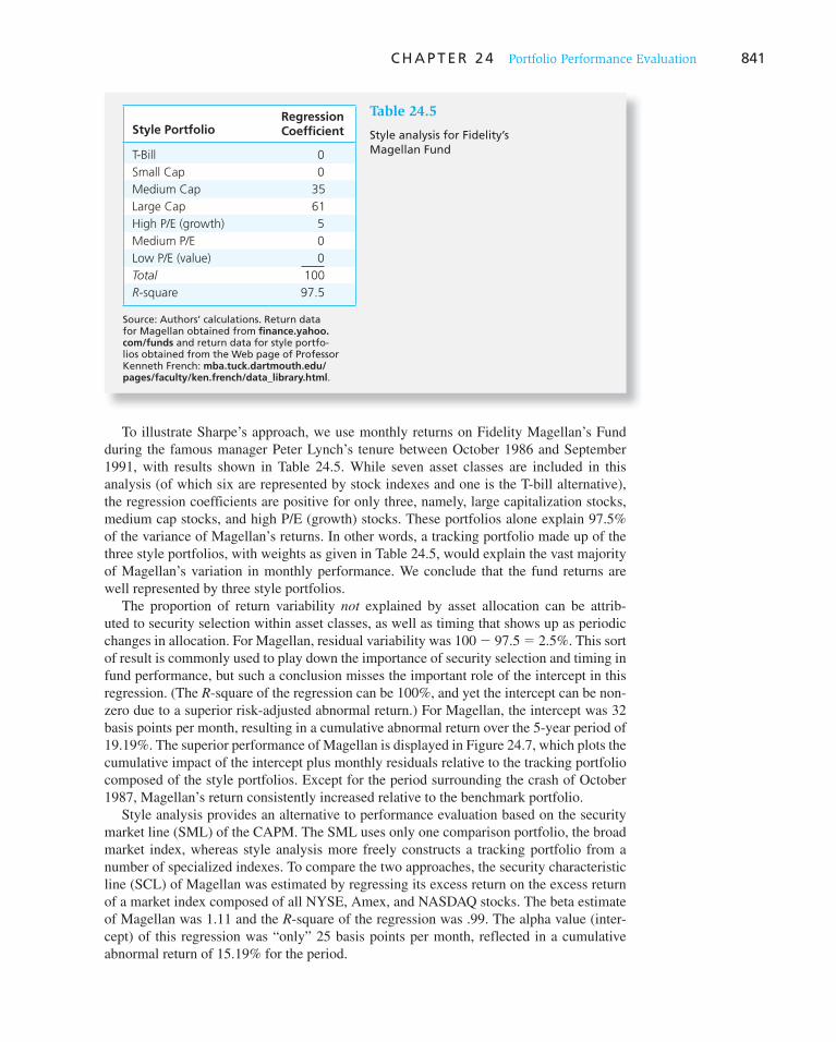
C H A P T E R 2 4 Portfolio Performance Evaluation 841
To illustrate Sharpe’s approach, we use monthly returns on Fidelity Magellan’s Fund during the famous manager Peter Lynch’s tenure between October 1986 and September 1991, with results shown in Table 24.5 . While seven asset classes are included in this analysis (of which six are represented by stock indexes and one is the T-bill alternative), the regression coefficients are positive for only three, namely, large capitalization stocks, medium cap stocks, and high P/E (growth) stocks. These portfolios alone explain 97.5% of the variance of Magellan’s returns. In other words, a tracking portfolio made up of the three style portfolios, with weights as given in Table 24.5 , would explain the vast majority of Magellan’s variation in monthly performance. We conclude that the fund returns are well represented by three style portfolios.
The proportion of return variability not explained by asset allocation can be attrib-uted to security selection within asset classes, as well as timing that shows up as periodic changes in allocation. For Magellan, residual variability was 100 2 97.5 5 2.5%. This sort of result is commonly used to play down the importance of security selection and timing in fund performance, but such a conclusion misses the important role of the intercept in this regression. (The R -square of the regression can be 100%, and yet the intercept can be non-zero due to a superior risk-adjusted abnormal return.) For Magellan, the intercept was 32 basis points per month, resulting in a cumulative abnormal return over the 5-year period of 19.19%. The superior performance of Magellan is displayed in Figure 24.7 , which plots the cumulative impact of the intercept plus monthly residuals relative to the tracking portfolio composed of the style portfolios. Except for the period surrounding the crash of October 1987, Magellan’s return consistently increased relative to the benchmark portfolio.
Style analysis provides an alternative to performance evaluation based on the security market line (SML) of the CAPM. The SML uses only one comparison portfolio, the broad market index, whereas style analysis more freely constructs a tracking portfolio from a number of specialized indexes. To compare the two approaches, the security characteristic line (SCL) of Magellan was estimated by regressing its excess return on the excess return of a market index composed of all NYSE, Amex, and NASDAQ stocks. The beta estimate of Magellan was 1.11 and the R -square of the regression was .99. The alpha value (inter-cept) of this regression was “only” 25 basis points per month, reflected in a cumulative abnormal return of 15.19% for the period.
Style PortfolioRegression Coefficient
T-Bill 0
Small Cap 0
Medium Cap 35
Large Cap 61
High P/E (growth) 5
Medium P/E 0
Low P/E (value) 0
Total 100
R-square 97.5
Table 24.5
Style analysis for Fidelity’s Magellan Fund
Source: Authors’ calculations. Return data for Magellan obtained from finance.yahoo.com/funds and return data for style portfo-lios obtained from the Web page of Professor Kenneth French: mba.tuck.dartmouth.edu/pages/faculty/ken.french/data_library.html .
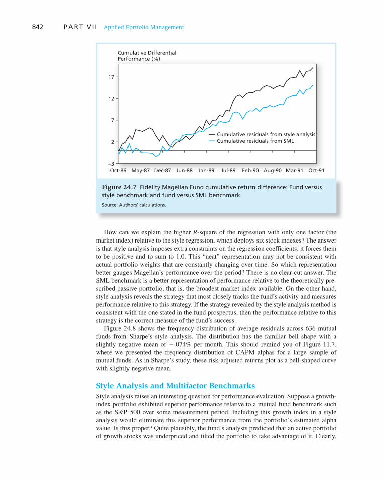
842 P A R T V I I Applied Portfolio Management
How can we explain the higher R -square of the regression with only one factor (the market index) relative to the style regression, which deploys six stock indexes? The answer is that style analysis imposes extra constraints on the regression coefficients: it forces them to be positive and to sum to 1.0. This “neat” representation may not be consistent with actual portfolio weights that are constantly changing over time. So which representation better gauges Magellan’s performance over the period? There is no clear-cut answer. The SML benchmark is a better representation of performance relative to the theoretically pre-scribed passive portfolio, that is, the broadest market index available. On the other hand, style analysis reveals the strategy that most closely tracks the fund’s activity and measures performance relative to this strategy. If the strategy revealed by the style analysis method is consistent with the one stated in the fund prospectus, then the performance relative to this strategy is the correct measure of the fund’s success.
Figure 24.8 shows the frequency distribution of average residuals across 636 mutual funds from Sharpe’s style analysis. The distribution has the familiar bell shape with a slightly negative mean of 2 .074% per month. This should remind you of Figure 11.7, where we presented the frequency distribution of CAPM alphas for a large sample of mutual funds. As in Sharpe’s study, these risk-adjusted returns plot as a bell-shaped curve with slightly negative mean.
Style Analysis and Multifactor Benchmarks
Style analysis raises an interesting question for performance evaluation. Suppose a growth-index portfolio exhibited superior performance relative to a mutual fund benchmark such as the S&P 500 over some measurement period. Including this growth index in a style analysis would eliminate this superior performance from the portfolio’s estimated alpha value. Is this proper? Quite plausibly, the fund’s analysts predicted that an active portfolio of growth stocks was underpriced and tilted the portfolio to take advantage of it. Clearly,
Oct-86 May-87 Dec-87 Jun-88 Jan-89 Jul-89 Feb-90 Aug-90 Mar-91 Oct-91−3
2
7
12
17
Cumulative DifferentialPerformance (%)
Cumulative residuals from style analysisCumulative residuals from SML
Figure 24.7 Fidelity Magellan Fund cumulative return difference: Fund versus style benchmark and fund versus SML benchmark
Source: Authors’ calculations.

C H A P T E R 2 4 Portfolio Performance Evaluation 843
the contribution of this decision to an alpha value relative to the benchmark is a legitimate part of the overall alpha value of the fund, and should not be elimi-nated by style analysis. This brings up a related question.
Chapter 11 pointed out that the conventional performance benchmark today is a four-factor model, which employs the three Fama-French factors (the return on the market index, and returns to portfolios based on size and book-to-market ratio) augmented by a momentum factor (a portfolio con-structed based on prior-year stock return). Alphas estimated from these four factor portfolios control for a wide range of style choices that may affect average returns. But using alpha values from a multi-factor model presupposes that a passive strategy would include the aforementioned factor portfolios. When is this reasonable?
Use of any benchmark other than the fund’s single-index benchmark is legitimate only if we assume that the factor portfolios in question are part of the fund’s alternative passive strategy. This assumption may be unrealistic in many cases where a single-index bench-mark is used for performance evaluation even if research shows a multifactor model better explains asset returns. In Section 24.8 on performance attribution we show how portfolio managers attempt to uncover which decisions contributed to superior performance. This performance attribution procedure starts with benchmark allocations to various indexes and attributes performance to asset allocation on the basis of deviation of actual from benchmark allocations. The performance benchmark may be and often is specified in advance without regard to any particular style portfolio.
Style Analysis in Excel
Style analysis has become very popular in the investment management industry and has spawned quite a few variations on Sharpe’s methodology. Many portfolio managers utilize Web sites that help investors identify their style and stock selection performance.
You can do style analysis with Excel’s Solver. The strategy is to regress a fund’s rate of return on those of a number of style portfolios (as in Table 24.5 ). The style portfolios are passive (index) funds that represent a style alternative to asset allocation. Suppose you choose three style portfolios, labeled 1–3. Then the coefficients in your style regres-sion are alpha (the intercept that measures abnormal performance) and three slope coefficients, one for each style index. The slope coefficients reveal how sensitively the performance of the fund follows the return of each passive style portfolio. The residuals from this re gression, e ( t ), represent “noise,” that is, fund performance at each date, t, that
−1.
00
−0.
50
0.00
0.50
1.00
Average Tracking Error (%/month)
0
10
20
30
40
50
60
70
80
90
Figure 24.8 Average tracking error for 636 mutual funds, 1985–1989
Source: William F. Sharpe, “Asset Allocation: Management Style and Performance Evaluation,” Journal of Portfolio Management, Winter 1992, pp. 7–19. Copyrighted material is reprinted with permission from Institutional Investor, 225 Park Avenue South, NewYork NY 10003.
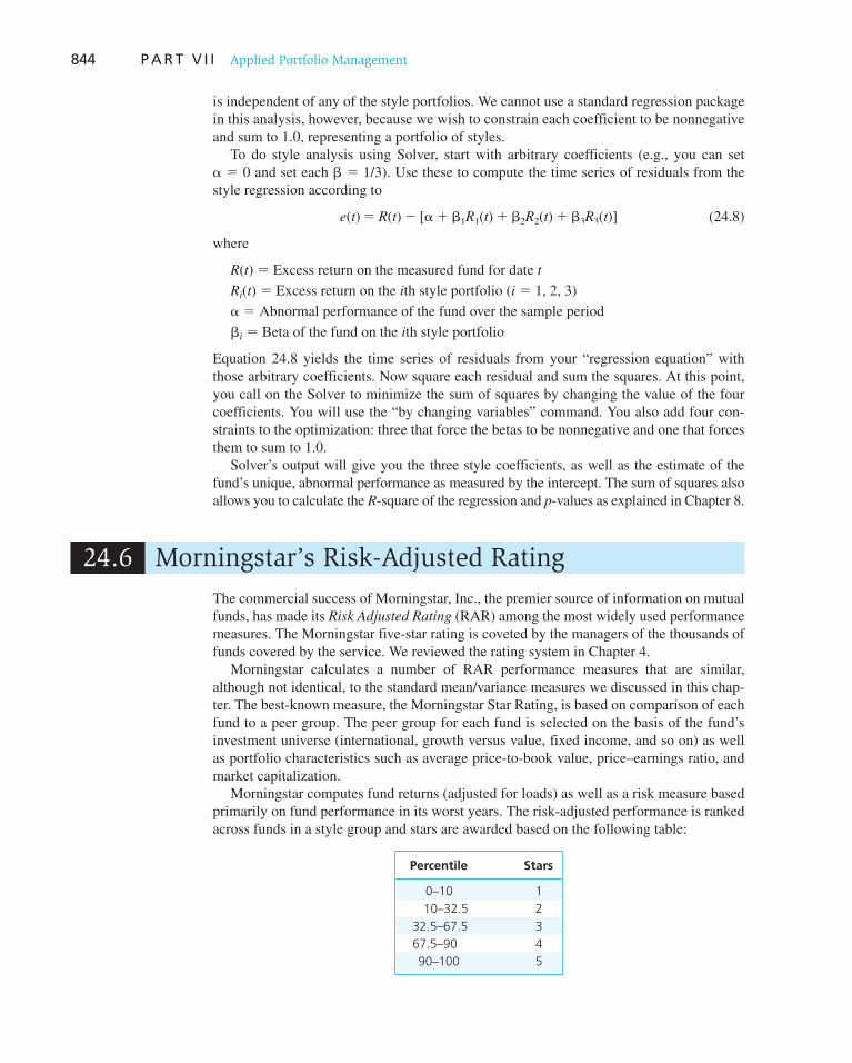
844 P A R T V I I Applied Portfolio Management
is i ndependent of any of the style portfolios. We cannot use a standard regression package in this analysis, however, because we wish to constrain each coefficient to be nonnegative and sum to 1.0, representing a portfolio of styles.
To do style analysis using Solver, start with arbitrary coefficients (e.g., you can set a 5 0 and set each b 5 1/3). Use these to compute the time series of residuals from the style regression according to
e(t) 5 R(t) 2 [a 1 b1R1(t) 1 b2R2(t) 1 b3R3(t)] (24.8)
where
R ( t ) 5 Excess return on the measured fund for date t
R i ( t ) 5 Excess return on the i th style portfolio ( i 5 1, 2, 3)
a 5 Abnormal performance of the fund over the sample period
b i 5 Beta of the fund on the i th style portfolio
Equation 24.8 yields the time series of residuals from your “regression equation” with those arbitrary coefficients. Now square each residual and sum the squares. At this point, you call on the Solver to minimize the sum of squares by changing the value of the four coefficients. You will use the “by changing variables” command. You also add four con-straints to the optimization: three that force the betas to be nonnegative and one that forces them to sum to 1.0.
Solver’s output will give you the three style coefficients, as well as the estimate of the fund’s unique, abnormal performance as measured by the intercept. The sum of squares also allows you to calculate the R -square of the regression and p -values as explained in Chapter 8.
24.6 Morningstar’s Risk-Adjusted Rating
The commercial success of Morningstar, Inc., the premier source of information on mutual funds, has made its Risk Adjusted Rating (RAR) among the most widely used performance measures. The Morningstar five-star rating is coveted by the managers of the thousands of funds covered by the service. We reviewed the rating system in Chapter 4.
Morningstar calculates a number of RAR performance measures that are similar, although not identical, to the standard mean/variance measures we discussed in this chap-ter. The best-known measure, the Morningstar Star Rating, is based on comparison of each fund to a peer group. The peer group for each fund is selected on the basis of the fund’s investment universe (international, growth versus value, fixed income, and so on) as well as portfolio characteristics such as average price-to-book value, price–earnings ratio, and market capitalization.
Morningstar computes fund returns (adjusted for loads) as well as a risk measure based primarily on fund performance in its worst years. The risk-adjusted performance is ranked across funds in a style group and stars are awarded based on the following table:
Percentile Stars
0–10 1
10–32.5 2
32.5–67.5 3
67.5–90 4
90–100 5

C H A P T E R 2 4 Portfolio Performance Evaluation 845
The Morningstar RAR method produces results that are similar but not identical to that of the mean/variance-based Sharpe ratios. Figure 24.9 demonstrates the fit between rank-ing by RAR and by Sharpe ratios from the performance of 1,286 diversified equity funds over the period 1994–1996. Sharpe notes that this period is characterized by high returns that contribute to a good fit.
24.7 Evaluating Performance Evaluation
Performance evaluation has two very basic problems:
1. Many observations are needed for significant results even when portfolio mean and variance are constant.
2. Shifting parameters when portfolios are actively managed makes accurate perfor-mance evaluation all the more elusive.
Although these objective difficulties cannot be overcome completely, it is clear that to obtain reasonably reliable performance measures we need to do the following:
1. Maximize the number of observations by taking more frequent return readings.
2. Specify the exact makeup of the portfolio to obtain better estimates of the risk parameters at each observation period.
Suppose an evaluator knows the exact portfolio composition at the opening of each day. Because the daily return on each security is available, the total daily return on the portfolio can be calculated. Furthermore, the exact portfolio composition allows the evaluator to estimate the risk characteristics (variance, beta, residual variance) for each day. Thus daily risk-adjusted rates of return can be obtained. Although a performance measure for 1 day is statistically unreliable, the number of days with such rich data accumulates quickly. Performance evaluation that accounts for frequent revision in portfolio co mposition is
0 0.2 0.4 0.6 0.8 1
Sharpe RatioPercentile in Category
Category RARPercentile inCategory
���������������������������������������������������������
����������������������������
�����������������������������������
��������������
������������������������������������������
����������������������������������
������������������������������������������������
����������������������������������
��������������������������������������������
�����������������������������������
��������������
��������������������������
������������������������������
������������������������������������������������
����������������������������������������
����������������������������������
�����������������������������������
��������������
��������������������������
������������������������������
������������������������������������������������
��� ���������������������������
��������������
����������������������������
�����������������������������������������������������
����������������������������������
�����������������
��������������������������
��������������������������������������������
������������������������������������
�������������������������
������������������
��������������������������������������������������������������
�����������������������
�����������������������������
������������������������������������
�������������������������
������������������
��������������������������������������������������������������
��
���������������������
�����������������������������
������������������������������������
�������������������������
������������������
��������������������������������������������������������������
�����������������������
�����������������������������
� ����������������
������������������������
�������������������������
������������������
���������������������������������������������������
�������
�����
������
�����������������������������������
�����������������������
�����������������������������
������������������������������������
�������������������������
������������������
��������������������������������������������������������������
��
���������������������
�����������������������������
������������������������������������
�������������������������
������������������
��������������������������������������������������������������
�����������������������
�����������������������������
������������������������������������
�������������������������
������������������
���������������������������������������
�������������������
����������
���������������������
��������������������
��������������������������
��������
�����
�������������
�����
�����������������������
�������
�����
�����������������
�������
�����������������������
���
�����������������
����������������������
�����������
��
���
������������������
��������������������
�����
������������� ����������
�����
����
�������
���������
�����
�
�����
���
�����
���������������������������
���
�������
������������
�����������
��������
�����
������
����
�
�
���
�
� ��
��
�
��
�
��� �
��
�����
����
���
���
����
�
��
�
���
���
�� �
� ��
���
0
0.2
0.4
0.6
0.8
1
Figure 24.9 Rankings based on Morningstar’s category RARs and excess return Sharpe ratios
Source: William F. Sharpe, “Morningstar Performance Measures,” www.wsharpe.com. Used by permission of William F. Sharpe.
846 P A R T V I I Applied Portfolio Management
superior by far to evaluation that assumes constant risk characteristics over the entire mea-surement period.
What sort of evaluation takes place in practice? Performance reports for portfolio manag-ers traditionally have been based on quarterly data over 5 to 10 years. Currently, managers of mutual funds are required to disclose the exact composition of their portfolios only quar-terly. Trading activity that immediately precedes the reporting date is known as “window dressing.” Window dressing involves changes in portfolio composition to make it look as if the manager chose successful stocks. If IBM performed well over the quarter, for example, a portfolio manager might make sure that his or her portfolio includes a lot of IBM on the reporting date whether or not it did during the quarter and whether or not IBM is expected to perform as well over the next quarter. Of course, portfolio managers deny such activity, and we know of no published evidence to substantiate the allegation. However, if window dressing is quantitatively significant, even the reported quarterly composition data can be misleading. Mutual funds publish portfolio values on a daily basis, which means the rate of return for each day is publicly available, but portfolio composition is not.
Still, even with more data, an insidious problem that will continue to complicate perfor-mance evaluation is survivorship bias. Because poorly performing mutual funds are regu-larly closed down, sample data will include only surviving funds, which correspondingly tend to be the more successful ones. At the same time, survivorship bias also affects broad-market indexes used as benchmark portfolios and generates upward-biased returns that are harder to beat. Several providers supply returns for various indexes that are adjusted for survivorship bias. These providers also attempt to adjust returns for cross-holdings of shares that can distort the appropriate weights in the index.
24.8 Performance Attribution Procedures
Rather than focus on risk-adjusted returns, practitioners often want simply to ascertain which decisions resulted in superior or inferior performance. Superior investment performance depends on an ability to be in the “right” securities at the right time. Such timing and selec-tion ability may be considered broadly, such as being in equities as opposed to fixed-income securities when the stock market is performing well. Or it may be defined at a more detailed level, such as choosing the relatively better-performing stocks within a particular industry.
Portfolio managers constantly make broad-brush asset allocation decisions as well as more detailed sector and security allocation decisions within asset classes. Performance attribution studies attempt to decompose overall performance into discrete components that may be identified with a particular level of the portfolio selection process.
Attribution studies start from the broadest asset allocation choices and progressively focus on ever-finer details of portfolio choice. The difference between a managed port-folio’s performance and that of a benchmark portfolio then may be expressed as the sum of the contributions to performance of a series of decisions made at the various levels of the portfolio construction process. For example, one common attribution system decom-poses performance into three components: (1) broad asset market allocation choices across equity, fixed-income, and money markets; (2) industry (sector) choice within each market; and (3) security choice within each sector.
The attribution method explains the difference in returns between a managed portfo-lio, P, and a selected benchmark portfolio, B, called the bogey. Suppose that the universe of assets for P and B includes n asset classes such as equities, bonds, and bills. For each asset class, a benchmark index portfolio is determined. For example, the S&P 500 may
C H A P T E R 2 4 Portfolio Performance Evaluation 847
be c hosen as a benchmark for equities. The bogey portfolio is set to have fixed weights in each asset class, and its rate of return is given by
rB 5 an
i51
wBirBi
where w Bi is the weight of the bogey in asset class i, and r Bi is the return on the benchmark portfolio of that class over the evaluation period. The portfolio managers choose weights in each class, w Pi , based on their capital market expectations, and they choose a portfolio of the securities within each class based on their security analysis, which earns r Pi over the evaluation period. Thus the return of the managed portfolio will be
rP 5 an
i51
wPirPi
The difference between the two rates of return, therefore, is
rP 2 rB 5 an
i51
wPirPi 2 an
i51
wBirBi 5 an
i51
(wPirPi 2 wBirBi) (24.9)
Each term in the summation of Equation 24.9 can be rewritten in a way that shows how asset allocation decisions versus security selection decisions for each asset class contrib-uted to overall performance. We decompose each term of the summation into a sum of two terms as follows. Note that the two terms we label as contribution from asset allocation and contribution from security selection in the following decomposition do in fact sum to the total contribution of each asset class to overall performance.
Contribution from asset allocation (wPi 2 wBi)rBi
1 Contribution from security selection wPi (rPi 2 rBi)
5 Total contribution from asset class i wPirPi 2 wBirBi
The first term of the sum measures the impact of asset allocation because it shows how deviations of the actual weight from the benchmark weight for that asset class multiplied by the index return for the asset class added to or subtracted from total performance. The second term of the sum measures the impact of security selection because it shows how the manager’s excess return within the asset class compared to the benchmark return for that class multiplied by the portfolio weight for that class added to or subtracted from total performance. Figure 24.10 presents a graphical interpretation of the attribution of overall performance into security selection versus asset allocation.
To illustrate this method, consider the attribution results for a hypothetical portfolio. The portfolio invests in stocks, bonds, and money market securities. An attribution analy-sis appears in Tables 24.6 through 24.9 . The portfolio return over the month is 5.34%.
The first step is to establish a benchmark level of performance against which perfor-mance ought to be compared. This benchmark, again, is called the bogey. It is designed to measure the returns the portfolio manager would earn if he or she were to follow a com-pletely passive strategy. “Passive” in this context has two attributes. First, it means that the allocation of funds across broad asset classes is set in accord with a notion of “usual,” or neutral, allocation across sectors. This would be considered a passive asset-market alloca-tion. Second, it means that within each asset class, the portfolio manager holds an indexed portfolio such as the S&P 500 index for the equity sector. In such a manner, the passive strategy used as a performance benchmark rules out asset allocation as well as security selection decisions. Any departure of the manager’s return from the passive benchmark must be due to either asset allocation bets (departures from the neutral allocation across markets) or security selection bets (departures from the passive index within asset classes).

848 P A R T V I I Applied Portfolio Management
While we have already discussed in earlier chapters the justification for indexing within sectors, it is worth briefly explaining the determination of the neutral allocation of funds across the broad asset classes. Weights that are designated as “neutral” will depend on the risk tolerance of the investor and must be determined in consultation with the cli-ent. For example, risk-tolerant clients may place a large fraction of their portfolio in the equity market, perhaps directing the fund manager to set neutral weights of 75% equity, 15% bonds, and 10% cash equivalents. Any deviation from these weights must be justified by a belief that one or another market will either over- or underperform its usual risk–return profile. In contrast, more risk-averse clients may set neutral weights of 45%/35%/20% for the three markets. Therefore, their portfolios in normal circumstances will be exposed to less risk than that of the risk-tolerant client. Only intentional bets on market performance will result in departures from this profile.
In Table 24.6 , the neutral weights have been set at 60% equity, 30% fixed income, and 10% cash (money market securities). The bogey portfolio, comprised of investments in each index with the 60/30/10 weights, returned 3.97%. The managed portfolio’s mea-sure of performance is positive and equal to its actual return less the return of the bogey: 5.34 2 3.97 5 1.37%. The next step is to allocate the 1.37% excess return to the separate decisions that contributed to it.
Asset Allocation Decisions
Our hypothetical managed portfolio is invested in the equity, fixed-income, and money markets with weights of 70%, 7%, and 23%, respectively. The portfolio’s performance could have to do with the departure of this weighting scheme from the benchmark 60/30/10 weights and/or to superior or inferior results within each of the three broad markets.
rPi
rBi
wPiwBi
wi
Return in Asset Class
Mixed Origin(attributed toselection)
Weight in Asset Class
Bogey returnfrom ith assetclass = rBiwBi
Allo
cation
Added by Selection
Figure 24.10 Performance attribution of i th asset class. Enclosed area indicates total rate of return.
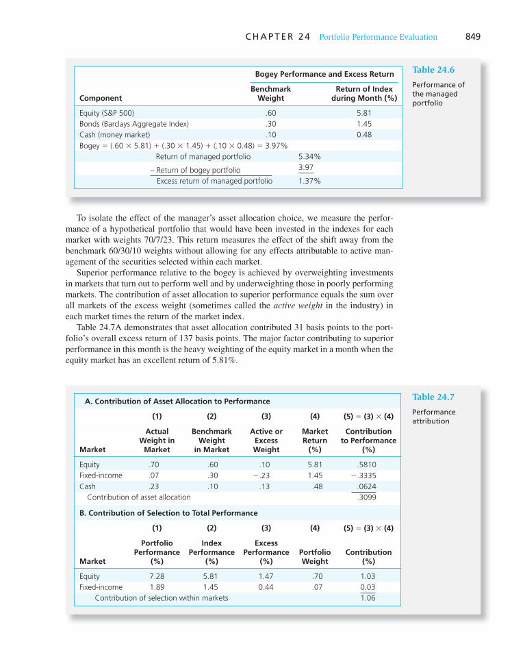
C H A P T E R 2 4 Portfolio Performance Evaluation 849
To isolate the effect of the manager’s asset allocation choice, we measure the perfor-mance of a hypothetical portfolio that would have been invested in the indexes for each market with weights 70/7/23. This return measures the effect of the shift away from the benchmark 60/30/10 weights without allowing for any effects attributable to active man-agement of the securities selected within each market.
Superior performance relative to the bogey is achieved by overweighting investments in markets that turn out to perform well and by underweighting those in poorly performing markets. The contribution of asset allocation to superior performance equals the sum over all markets of the excess weight (sometimes called the active weight in the industry) in each market times the return of the market index.
Table 24.7 A demonstrates that asset allocation contributed 31 basis points to the port-folio’s overall excess return of 137 basis points. The major factor contributing to superior performance in this month is the heavy weighting of the equity market in a month when the equity market has an excellent return of 5.81%.
Bogey Performance and Excess Return
ComponentBenchmark
WeightReturn of Index
during Month (%)
Equity (S&P 500) .60 5.81
Bonds (Barclays Aggregate Index) .30 1.45
Cash (money market) .10 0.48
Bogey 5 (.60 3 5.81) 1 (.30 3 1.45) 1 (.10 3 0.48) 5 3.97%
Return of managed portfolio 5.34%
– Return of bogey portfolio 3.97
Excess return of managed portfolio 1.37%
Table 24.6
Performance of the managed portfolio
A. Contribution of Asset Allocation to Performance
(1) (2) (3) (4) (5) 5 (3) 3 (4)
Market
Actual Weight in
Market
Benchmark Weight
in Market
Active or Excess Weight
Market Return
(%)
Contribution to Performance
(%)
Equity .70 .60 .10 5.81 .5810
Fixed-income .07 .30 2.23 1.45 2.3335
Cash .23 .10 .13 .48 .0624
Contribution of asset allocation .3099
B. Contribution of Selection to Total Performance
(1) (2) (3) (4) (5) 5 (3) 3 (4)
Market
Portfolio Performance
(%)
Index Performance
(%)
Excess Performance
(%)Portfolio Weight
Contribution (%)
Equity 7.28 5.81 1.47 .70 1.03
Fixed-income 1.89 1.45 0.44 .07 0.03
Contribution of selection within markets 1.06
Table 24.7
Performance attribution
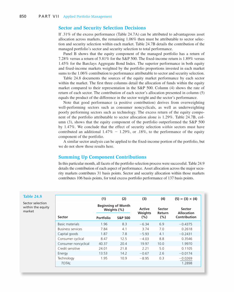
850 P A R T V I I Applied Portfolio Management
Sector and Security Selection Decisions
If .31% of the excess performance ( Table 24.7 A) can be attributed to advantageous asset allocation across markets, the remaining 1.06% then must be attributable to sector selec-tion and security selection within each market. Table 24.7 B details the contribution of the managed portfolio’s sector and security selection to total performance.
Panel B shows that the equity component of the managed portfolio has a return of 7.28% versus a return of 5.81% for the S&P 500. The fixed-income return is 1.89% versus 1.45% for the Barclays Aggregate Bond Index. The superior performance in both equity and fixed-income markets weighted by the portfolio proportions invested in each market sums to the 1.06% contribution to performance attributable to sector and security selection.
Table 24.8 documents the sources of the equity market performance by each sector within the market. The first three columns detail the allocation of funds within the equity market compared to their representation in the S&P 500. Column (4) shows the rate of return of each sector. The contribution of each sector’s allocation presented in column (5) equals the product of the difference in the sector weight and the sector’s performance.
Note that good performance (a positive contribution) derives from overweighting well-performing sectors such as consumer noncyclicals, as well as underweighting poorly performing sectors such as technology. The excess return of the equity compo-nent of the portfolio attributable to sector allocation alone is 1.29%. Table 24.7 B, col-umn (3), shows that the equity component of the portfolio outperformed the S&P 500 by 1.47%. We conclude that the effect of security selection within sectors must have contributed an additional 1.47% 2 1.29%, or .18%, to the performance of the equity component of the portfolio.
A similar sector analysis can be applied to the fixed-income portion of the portfolio, but we do not show those results here.
Summing Up Component Contributions
In this particular month, all facets of the portfolio selection process were successful. Table 24.9 details the contribution of each aspect of performance. Asset allocation across the major secu-rity markets contributes 31 basis points. Sector and security allocation within those markets contributes 106 basis points, for total excess portfolio performance of 137 basis points.
(1) (2) (3) (4) (5) 5 (3) 3 (4)
Beginning of Month Weights (%)
Portfolio S&P 500Sector
Active Weights
(%)
Sector Return
(%)
Sector Allocation
Contribution
Basic materials 1.96 8.3 26.34 6.9 20.4375
Business services 7.84 4.1 3.74 7.0 0.2618
Capital goods 1.87 7.8 25.93 4.1 20.2431
Consumer cyclical 8.47 12.5 24.03 8.8 0.3546
Consumer noncyclical 40.37 20.4 19.97 10.0 1.9970
Credit sensitive 24.01 21.8 2.21 5.0 0.1105
Energy 13.53 14.2 20.67 2.6 20.0174
Technology 1.95 10.9 28.95 0.3 20.0269
TOTAL 1.2898
Table 24.8
Sector selection within the equity market

851
The sector and security allocation of 106 basis points can be partitioned further. Sector allocation within the equity market results in excess performance of 129 basis points, and security selection within sectors contributes 18 basis points. (The total equity excess perfor-mance of 147 basis points is multiplied by the 70% weight in equity to obtain contribution to portfolio performance.) Similar partitioning could be done for the fixed-income sector.
eXcel APPLICATIONS: Performance Attribution
T he performance attribution spreadsheet develops the attribution analysis that is presented in this section.
Additional data can be used in the analysis of performance for other sets of portfolios. The model can be used to ana-
lyze performance of mutual funds and other managed portfolios.
You can find this Excel model on the Online Learning Center at www.mhhe.com/bkm.
A B C D E F
Bogey
Portfolio
Component
Equity
Bonds
Cash
Index
S&P 500
Barclays Index
Money Market
Benchmark
Weight
0.60
0.30
0.10
Return on
Index
5.8100%
1.4500%
0.4800%
Portfolio
Return
Portfolio
Weight
0.70
0.07
0.23
Actual
Return
5.8100%
1.4500%
0.4800%
Portfolio
Return
Managed
Portfolio
Component
Equity
Bonds
Cash
Performance Attribution
Return on Bogey
Return on Managed
Excess Return
5.0960%
0.1323%
0.1104%
5.3387%
1.3697%
3.4860%
0.4350%
0.0480%
3.9690%
19
18
17
16
15
14
13
12
11
10
9
8
7
6
5
4
3
2
1
CONCEPT CHECK
5
a. Suppose the benchmark weights is Table 24.7 had been set at 70% equity, 25% fixed-income, and 5% cash equivalents. What would have been the contributions of the manager’s asset allocation choices?
b. Suppose the S&P 500 return is 5%. Compute the new value of the manager’s security selection choices.
Contribution (basis points)
1. Asset allocation 31
2. Selection
a. Equity excess return (basis points)
i. Sector allocation 129
ii. Security selection 18
147 3 .70 (portfolio weight) 5 102.9
b. Fixed-income excess return 44 3 .07 (portfolio weight) 5 3.1
Total excess return of portfolio 137.0
Table 24.9
Portfolio attribution: summary

Vis
it u
s at
ww
w.m
hh
e.co
m/b
kmV
isit
us
at w
ww
.mh
he.
com
/bkm
852 P A R T V I I Applied Portfolio Management
1. The appropriate performance measure depends on the role of the portfolio to be evaluated. Appro-priate performance measures are as follows:
a. Sharpe: when the portfolio represents the entire investment fund.
b. Information ratio: when the portfolio represents the active portfolio to be optimally mixed with the passive portfolio.
c. Treynor or Jensen: when the portfolio represents one subportfolio of many.
2. Many observations are required to eliminate the effect of the “luck of the draw” from the evalua-tion process because portfolio returns commonly are very “noisy.”
3. Hedge funds or other active positions meant to be mixed with a passive indexed portfolio should be evaluated based on their information ratio.
4. The shifting mean and variance of actively managed portfolios make it even harder to assess per-formance. A typical example is the attempt of portfolio managers to time the market, resulting in ever-changing portfolio betas.
5. A simple way to measure timing and selection success simultaneously is to estimate an expanded security characteristic line, with a quadratic term added to the usual index model. Another way to evaluate timers is based on the implicit call option embedded in their performance.
6. Style analysis uses a multiple regression model where the factors are category (style) portfolios such as bills, bonds, and stocks. A regression of fund returns on the style portfolio returns gener-ates residuals that represent the value added of stock selection in each period. These residuals can be used to gauge fund performance relative to similar-style funds.
7. The Morningstar Star Rating method compares each fund to a peer group represented by a style portfolio within four asset classes. Risk-adjusted ratings (RAR) are based on fund returns relative to the peer group and used to award each fund one to five stars based on the rank of its RAR.
8. Common attribution procedures partition performance improvements to asset allocation, sector selection, and security selection. Performance is assessed by calculating departures of portfolio composition from a benchmark or neutral portfolio.
SUMMARY
Related Web sites for this chapter are available at www.mhhe.com/bkm
time-weighted average dollar-weighted rate of return comparison universe
Sharpe’s measure Treynor’s measure Jensen’s measure
information ratio bogey
KEY TERMS
1. Is it possible that a positive alpha will be associated with inferior performance? Explain.
2. We know that the geometric average (time-weighted return) on a risky investment is always lower than the corresponding arithmetic average. Can the IRR (the dollar-weighted return) similarly be ranked relative to these other two averages?
3. We have seen that market timing has tremendous potential value. Would it therefore be wise to shift resources to timing at the expense of security selection?
4. Consider the rate of return of stocks ABC and XYZ.
Year rABC rXYZ
1 20% 30%
2 12 12
3 14 18
4 3 0
5 1 –10
PROBLEM SETS
i. Basic
ii. Intermediate

Vis
it u
s at
ww
w.m
hh
e.co
m/b
km
C H A P T E R 2 4 Portfolio Performance Evaluation 853
a. Calculate the arithmetic average return on these stocks over the sample period. b. Which stock has greater dispersion around the mean? c. Calculate the geometric average returns of each stock. What do you conclude? d. If you were equally likely to earn a return of 20%, 12%, 14%, 3%, or 1%, in each year (these
are the five annual returns for stock ABC), what would be your expected rate of return? What if the five possible outcomes were those of stock XYZ?
5. XYZ stock price and dividend history are as follows:
Year Beginning-of-Year Price Dividend Paid at Year-End
2007 $100 $4
2008 120 4
2009 90 4
2010 100 4
An investor buys three shares of XYZ at the beginning of 2007, buys another two shares at the beginning of 2008, sells one share at the beginning of 2009, and sells all four remaining shares at the beginning of 2010.
a. What are the arithmetic and geometric average time-weighted rates of return for the investor? b. What is the dollar-weighted rate of return? ( Hint: Carefully prepare a chart of cash flows
for the four dates corresponding to the turns of the year for January 1, 2007, to January 1, 2010. If your calculator cannot calculate internal rate of return, you will have to use trial and error.)
6. A manager buys three shares of stock today, and then sells one of those shares each year for the next 3 years. His actions and the price history of the stock are summarized below. The stock pays no dividends.
Time Price Action
0 $ 90 Buy 3 shares
1 100 Sell 1 share
2 100 Sell 1 share
3 100 Sell 1 share
a. Calculate the time-weighted geometric average return on this “portfolio.” b. Calculate the time-weighted arithmetic average return on this portfolio. c. Calculate the dollar-weighted average return on this portfolio.
7. Based on current dividend yields and expected capital gains, the expected rates of return on port-folios A and B are 12% and 16%, respectively. The beta of A is .7, while that of B is 1.4. The T-bill rate is currently 5%, whereas the expected rate of return of the S&P 500 index is 13%. The standard deviation of portfolio A is 12% annually, that of B is 31%, and that of the S&P 500 index is 18%.
a. If you currently hold a market-index portfolio, would you choose to add either of these port-folios to your holdings? Explain.
b. If instead you could invest only in T-bills and one of these portfolios, which would you choose?
8. Consider the two (excess return) index-model regression results for stocks A and B. The risk-free rate over the period was 6%, and the market’s average return was 14%. Performance is measured using an index model regression on excess returns.
Stock A Stock B
Index model regression estimates 1% 1 1.2(rM – rf) 2% 1 .8(rM – rf)
R-square .576 .436
Residual standard deviation, s(e) 10.3% 19.1%
Standard deviation of excess returns 21.6% 24.9%

Vis
it u
s at
ww
w.m
hh
e.co
m/b
km854 P A R T V I I Applied Portfolio Management
a. Calculate the following statistics for each stock:
i. Alpha ii. Information ratio iii. Sharpe measure iv. Treynor measure
b. Which stock is the best choice under the following circumstances?
i. This is the only risky asset to be held by the investor. ii. This stock will be mixed with the rest of the investor’s portfolio, currently composed
solely of holdings in the market index fund. iii. This is one of many stocks that the investor is analyzing to form an actively managed
stock portfolio.
9. Evaluate the market timing and security selection abilities of four managers whose perform-ances are plotted in the accompanying diagrams.
CC
rP− rf
AA
rP − rf
DrM − rf
DrM r
rP − rf
B
rM − rf
B
rM r
rP − rf
rM − rf
rM − rf
10. Consider the following information regarding the performance of a money manager in a recent month. The table represents the actual return of each sector of the manager’s portfolio in col-umn 1, the fraction of the portfolio allocated to each sector in column 2, the benchmark or neu-tral sector allocations in column 3, and the returns of sector indices in column 4.
Actual Return Actual Weight Benchmark Weight Index Return
Equity 2% .70 .60 2.5% (S&P 500)
Bonds 1 .20 .30 1.2 (Salomon Index)
Cash 0.5 .10 .10 0.5
a. What was the manager’s return in the month? What was her overperformance or underperformance?
b. What was the contribution of security selection to relative performance? c. What was the contribution of asset allocation to relative performance? Confirm that the sum of
selection and allocation contributions equals her total “excess” return relative to the bogey.

Vis
it u
s at
ww
w.m
hh
e.co
m/b
km
C H A P T E R 2 4 Portfolio Performance Evaluation 855
11. A global equity manager is assigned to select stocks from a universe of large stocks through-out the world. The manager will be evaluated by comparing her returns to the return on the MSCI World Market Portfolio, but she is free to hold stocks from various countries in whatever proportions she finds desirable. Results for a given month are contained in the fol-lowing table:
CountryWeight In
MSCI IndexManager’s
WeightManager’s Return
in CountryReturn of Stock Index
for That Country
U.K. .15 .30 20% 12%
Japan .30 .10 15 15
U.S. .45 .40 10 14
Germany .10 .20 5 12
a. Calculate the total value added of all the manager’s decisions this period. b. Calculate the value added (or subtracted) by her country allocation decisions. c. Calculate the value added from her stock selection ability within countries. Confirm that the
sum of the contributions to value added from her country allocation plus security selection decisions equals total over- or underperformance.
12. Conventional wisdom says that one should measure a manager’s investment performance over an entire market cycle. What arguments support this convention? What arguments con-tradict it?
13. Does the use of universes of managers with similar investment styles to evaluate relative invest-ment performance overcome the statistical problems associated with instability of beta or total variability?
14. During a particular year, the T-bill rate was 6%, the market return was 14%, and a portfolio manager with beta of .5 realized a return of 10%.
a. Evaluate the manager based on the portfolio alpha. b. Reconsider your answer to part ( a ) in view of the Black-Jensen-Scholes finding that the
security market line is too flat. Now how do you assess the manager’s performance?
15. Bill Smith is evaluating the performance of four large-cap equity portfolios: Funds A, B, C, and D. As part of his analysis, Smith computed the Sharpe ratio and the Treynor measure for all four funds. Based on his finding, the ranks assigned to the four funds are as follows:
Fund Treynor Measure Rank Sharpe Ratio Rank
A 1 4
B 2 3
C 3 2
D 4 1
The difference in rankings for Funds A and D is most likely due to:
a. A lack of diversification in Fund A as compared to Fund D. b. Different benchmarks used to evaluate each fund’s performance. c. A difference in risk premiums.
Use the following information to answer Problems 16–19: Primo Management Co. is look-ing at how best to evaluate the performance of its managers. Primo has been hearing more and more about benchmark portfolios and is interested in trying this approach. As such, the com-pany hired Sally Jones, CFA, as a consultant to educate the managers on the best methods for constructing a benchmark portfolio, how best to choose a benchmark, whether the style of the fund under management matters, and what they should do with their global funds in terms of benchmarking.
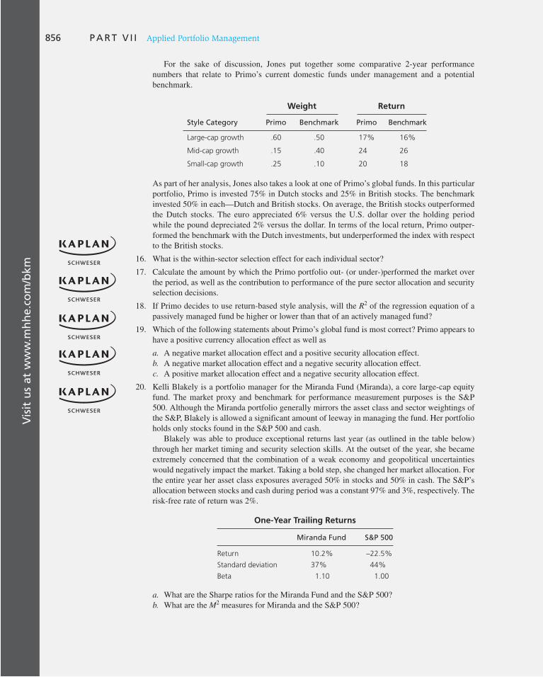
Vis
it u
s at
ww
w.m
hh
e.co
m/b
km856 P A R T V I I Applied Portfolio Management
For the sake of discussion, Jones put together some comparative 2-year performance numbers that relate to Primo’s current domestic funds under management and a potential benchmark.
Weight Return
Style Category Primo Benchmark Primo Benchmark
Large-cap growth .60 .50 17% 16%
Mid-cap growth .15 .40 24 26
Small-cap growth .25 .10 20 18
As part of her analysis, Jones also takes a look at one of Primo’s global funds. In this particular portfolio, Primo is invested 75% in Dutch stocks and 25% in British stocks. The benchmark invested 50% in each—Dutch and British stocks. On average, the British stocks outperformed the Dutch stocks. The euro appreciated 6% versus the U.S. dollar over the holding period while the pound depreciated 2% versus the dollar. In terms of the local return, Primo outper-formed the benchmark with the Dutch investments, but underperformed the index with respect to the British stocks.
16. What is the within-sector selection effect for each individual sector?
17. Calculate the amount by which the Primo portfolio out- (or under-)performed the market over the period, as well as the contribution to performance of the pure sector allocation and security selection decisions.
18. If Primo decides to use return-based style analysis, will the R 2 of the regression equation of a passively managed fund be higher or lower than that of an actively managed fund?
19. Which of the following statements about Primo’s global fund is most correct? Primo appears to have a positive currency allocation effect as well as
a. A negative market allocation effect and a positive security allocation effect. b. A negative market allocation effect and a negative security allocation effect. c. A positive market allocation effect and a negative security allocation effect.
20. Kelli Blakely is a portfolio manager for the Miranda Fund (Miranda), a core large-cap equity fund. The market proxy and benchmark for performance measurement purposes is the S&P 500. Although the Miranda portfolio generally mirrors the asset class and sector weightings of the S&P, Blakely is allowed a significant amount of leeway in managing the fund. Her portfolio holds only stocks found in the S&P 500 and cash.
Blakely was able to produce exceptional returns last year (as outlined in the table below) through her market timing and security selection skills. At the outset of the year, she became extremely concerned that the combination of a weak economy and geopolitical uncertainties would negatively impact the market. Taking a bold step, she changed her market allocation. For the entire year her asset class exposures averaged 50% in stocks and 50% in cash. The S&P’s allocation between stocks and cash during period was a constant 97% and 3%, respectively. The risk-free rate of return was 2%.
One-Year Trailing Returns
Miranda Fund S&P 500
Return 10.2% –22.5%
Standard deviation 37% 44%
Beta 1.10 1.00
a. What are the Sharpe ratios for the Miranda Fund and the S&P 500? b. What are the M 2 measures for Miranda and the S&P 500?
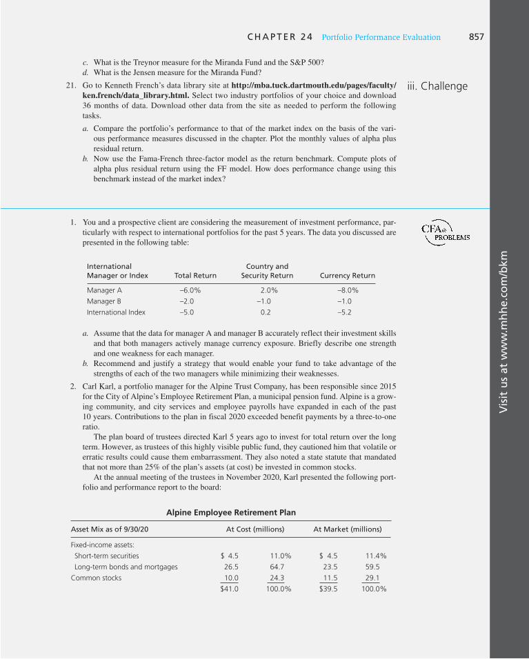
Vis
it u
s at
ww
w.m
hh
e.co
m/b
km
C H A P T E R 2 4 Portfolio Performance Evaluation 857
c. What is the Treynor measure for the Miranda Fund and the S&P 500? d. What is the Jensen measure for the Miranda Fund?
21. Go to Kenneth French’s data library site at http://mba.tuck.dartmouth.edu/pages/faculty/
ken.french/data_library.html. Select two industry portfolios of your choice and download 36 months of data. Download other data from the site as needed to perform the following tasks.
a. Compare the portfolio’s performance to that of the market index on the basis of the vari-ous performance measures discussed in the chapter. Plot the monthly values of alpha plus residual return.
b. Now use the Fama-French three-factor model as the return benchmark. Compute plots of alpha plus residual return using the FF model. How does performance change using this benchmark instead of the market index?
iii. Challenge
1. You and a prospective client are considering the measurement of investment performance, par-ticularly with respect to international portfolios for the past 5 years. The data you discussed are presented in the following table:
International Manager or Index Total Return
Country and Security Return Currency Return
Manager A –6.0% 2.0% –8.0%
Manager B –2.0 –1.0 –1.0
International Index –5.0 0.2 –5.2
a. Assume that the data for manager A and manager B accurately reflect their investment skills and that both managers actively manage currency exposure. Briefly describe one strength and one weakness for each manager.
b. Recommend and justify a strategy that would enable your fund to take advantage of the strengths of each of the two managers while minimizing their weaknesses.
2. Carl Karl, a portfolio manager for the Alpine Trust Company, has been responsible since 2015 for the City of Alpine’s Employee Retirement Plan, a municipal pension fund. Alpine is a grow-ing community, and city services and employee payrolls have expanded in each of the past 10 years. Contributions to the plan in fiscal 2020 exceeded benefit payments by a three-to-one ratio.
The plan board of trustees directed Karl 5 years ago to invest for total return over the long term. However, as trustees of this highly visible public fund, they cautioned him that volatile or erratic results could cause them embarrassment. They also noted a state statute that mandated that not more than 25% of the plan’s assets (at cost) be invested in common stocks.
At the annual meeting of the trustees in November 2020, Karl presented the following port-folio and performance report to the board:
Alpine Employee Retirement Plan
Asset Mix as of 9/30/20 At Cost (millions) At Market (millions)
Fixed-income assets:
Short-term securities $ 4.5 11.0% $ 4.5 11.4%
Long-term bonds and mortgages 26.5 64.7 23.5 59.5
Common stocks 10.0 24.3 11.5 29.1
$41.0 100.0% $39.5 100.0%
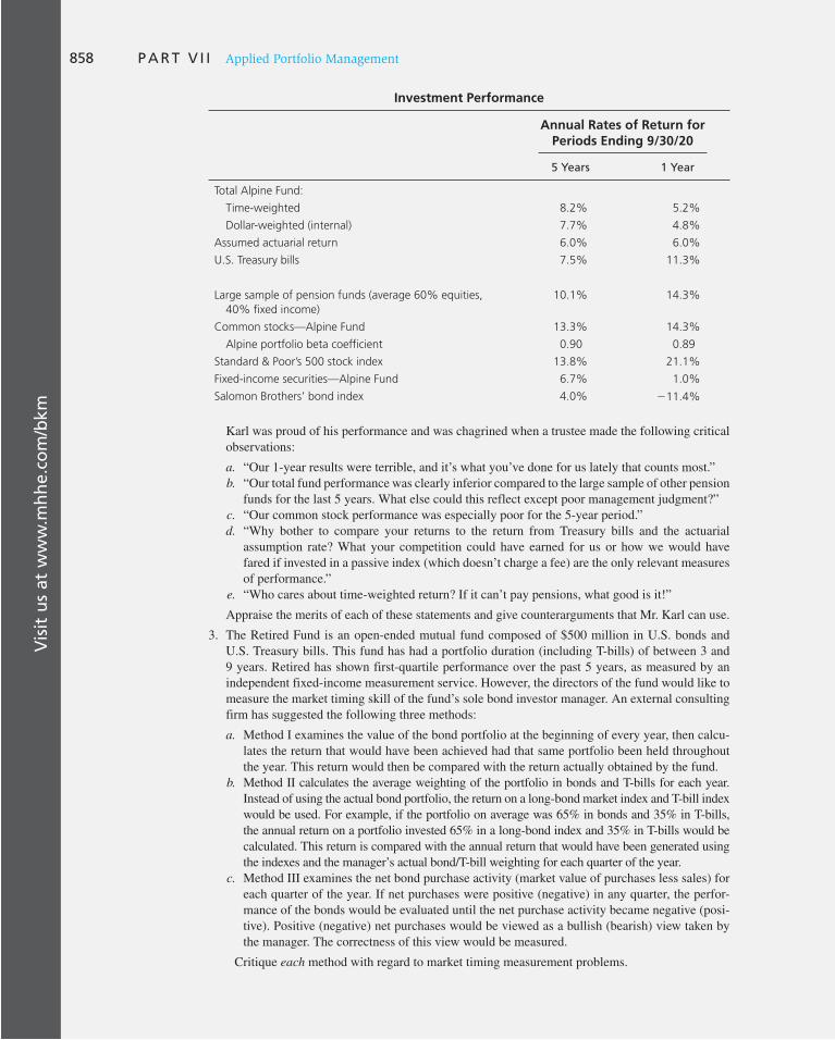
Vis
it u
s at
ww
w.m
hh
e.co
m/b
km858 P A R T V I I Applied Portfolio Management
Investment Performance
Annual Rates of Return for P eriods Ending 9/30/20
5 Years 1 Year
Total Alpine Fund:
Time-weighted 8.2% 5.2%
Dollar-weighted (internal) 7.7% 4.8%
Assumed actuarial return 6.0% 6.0%
U.S. Treasury bills 7.5% 11.3%
Large sample of pension funds (average 60% equities,
40% fixed income)
10.1% 14.3%
Common stocks—Alpine Fund 13.3% 14.3%
Alpine portfolio beta coefficient 0.90 0.89
Standard & Poor’s 500 stock index 13.8% 21.1%
Fixed-income securities—Alpine Fund 6.7% 1.0%
Salomon Brothers’ bond index 4.0% 211.4%
Karl was proud of his performance and was chagrined when a trustee made the following critical observations:
a. “Our 1-year results were terrible, and it’s what you’ve done for us lately that counts most.” b. “Our total fund performance was clearly inferior compared to the large sample of other pension
funds for the last 5 years. What else could this reflect except poor management judgment?” c. “Our common stock performance was especially poor for the 5-year period.” d. “Why bother to compare your returns to the return from Treasury bills and the actuarial
assumption rate? What your competition could have earned for us or how we would have fared if invested in a passive index (which doesn’t charge a fee) are the only relevant measures of performance.”
e. “Who cares about time-weighted return? If it can’t pay pensions, what good is it!”
Appraise the merits of each of these statements and give counterarguments that Mr. Karl can use.
3. The Retired Fund is an open-ended mutual fund composed of $500 million in U.S. bonds and U.S. Treasury bills. This fund has had a portfolio duration (including T-bills) of between 3 and 9 years. Retired has shown first-quartile performance over the past 5 years, as measured by an independent fixed-income measurement service. However, the directors of the fund would like to measure the market timing skill of the fund’s sole bond investor manager. An external consulting firm has suggested the following three methods:
a. Method I examines the value of the bond portfolio at the beginning of every year, then calcu-lates the return that would have been achieved had that same portfolio been held throughout the year. This return would then be compared with the return actually obtained by the fund.
b. Method II calculates the average weighting of the portfolio in bonds and T-bills for each year. Instead of using the actual bond portfolio, the return on a long-bond market index and T-bill index would be used. For example, if the portfolio on average was 65% in bonds and 35% in T-bills, the annual return on a portfolio invested 65% in a long-bond index and 35% in T-bills would be calculated. This return is compared with the annual return that would have been generated using the indexes and the manager’s actual bond/T-bill weighting for each quarter of the year.
c. Method III examines the net bond purchase activity (market value of purchases less sales) for each quarter of the year. If net purchases were positive (negative) in any quarter, the perfor-mance of the bonds would be evaluated until the net purchase activity became negative (posi-tive). Positive (negative) net purchases would be viewed as a bullish (bearish) view taken by the manager. The correctness of this view would be measured.
Critique each method with regard to market timing measurement problems.

Vis
it u
s at
ww
w.m
hh
e.co
m/b
km
C H A P T E R 2 4 Portfolio Performance Evaluation 859
Use the following data to solve CFA Problems 4–6: The administrator of a large pension fund wants to evaluate the performance of four portfolio managers. Each portfolio manager invests only in U.S. common stocks. Assume that during the most recent 5-year period, the average annual total rate of return including dividends on the S&P 500 was 14%, and the aver-age nominal rate of return on government Treasury bills was 8%. The following table shows risk and return measures for each portfolio:
Portfolio Average Annual Rate of Return Standard Deviation Beta
P 17% 20% 1.1
Q 24 18 2.1
R 11 10 0.5
S 16 14 1.5
S&P 500 14 12 1.0
4. What is the Treynor performance measure for portfolio P?
5. What is the Sharpe performance measure for portfolio Q?
6. An analyst wants to evaluate portfolio X, consisting entirely of U.S. common stocks, using both the Treynor and Sharpe measures of portfolio performance. The following table provides the average annual rate of return for portfolio X, the market portfolio (as measured by the S&P 500), and U.S. Treasury bills during the past 8 years:
Average Annual Rate of Return Standard Deviation of Return Beta
Portfolio X 10% 18% 0.60
S&P 500 12 13 1.00
T-bills 6 N/A N/A
a. Calculate the Treynor and Sharpe measures for both portfolio X and the S&P 500. Briefly explain whether portfolio X underperformed, equaled, or outperformed the S&P 500 on a risk-adjusted basis using both the Treynor measure and the Sharpe measure.
b. On the basis of the performance of portfolio X relative to the S&P 500 calculated in part ( a ), briefly explain the reason for the conflicting results when using the Treynor measure versus the Sharpe measure.
7. Assume you invested in an asset for 2 years. The first year you earned a 15% return, and the second year you earned a negative 10% return. What was your annual geometric return?
8. A portfolio of stocks generates a 2 9% return in 2008, a 23% return in 2009, and a 17% return in 2010. What is the annualized return (geometric mean) for the entire period?
9. A 2-year investment of $2,000 results in a cash flow of $150 at the end of the first year and another cash flow of $150 at the end of the second year, in addition to the return of the original investment. What is the internal rate of return on the investment?
10. In measuring the performance of a portfolio, the time-weighted rate of return is superior to the dollar-weighted rate of return because:
a. When the rate of return varies, the time-weighted return is higher. b. The dollar-weighted return assumes all portfolio deposits are made on day 1. c. The dollar-weighted return can only be estimated. d. The time-weighted return is unaffected by the timing of portfolio contributions and
withdrawals.
11. A pension fund portfolio begins with $500,000 and earns 15% the first year and 10% the second year. At the beginning of the second year, the sponsor contributes another $500,000. What were the time-weighted and dollar-weighted rates of return?

Vis
it u
s at
ww
w.m
hh
e.co
m/b
km860 P A R T V I I Applied Portfolio Management
12. During the annual review of Acme’s pension plan, several trustees questioned their investment consultant about various aspects of performance measurement and risk assessment.
a. Comment on the appropriateness of using each of the following benchmarks for perfor-mance evaluation:
• Market index.
• Benchmark normal portfolio.
• Median of the manager universe.
b. Distinguish among the following performance measures:
• The Sharpe ratio.
• The Treynor measure.
• Jensen’s alpha.
i. Describe how each of the three performance measures is calculated. ii. State whether each measure assumes that the relevant risk is systematic, unsystematic, or
total. Explain how each measure relates excess return and the relevant risk.
13. Trustees of the Pallor Corp. pension plan ask consultant Donald Millip to comment on the fol-lowing statements. What should his response be?
a. Median manager benchmarks are statistically unbiased measures of performance over long periods of time.
b. Median manager benchmarks are unambiguous and are therefore easily replicated by man-agers wishing to adopt a passive/indexed approach.
c. Median manager benchmarks are not appropriate in all circumstances because the median manager universe encompasses many investment styles.
14. James Chan is reviewing the performance of the global equity managers of the Jarvis University endowment fund. Williamson Capital is currently the endowment fund’s only large- capitalization global equity manager. Performance data for Williamson Capital are shown in Table 24A .
Chan also presents the endowment fund’s investment committee with performance informa-tion for Joyner Asset Management, which is another large-capitalization global equity manager. Performance data for Joyner Asset Management are shown in Table 24B . Performance data for the relevant risk-free asset and market index are shown in Table 24C .
a. Calculate the Sharpe ratio and Treynor measure for both Williamson Capital and Joyner Asset Management.
b. The Investment Committee notices that using the Sharpe ratio versus the Treynor measure produces different performance rankings of Williamson and Joyner. Explain why these crite-ria may result in different rankings.
Table 24A
Williamson capital performance data, 1999–2010
Average annual rate of return 22.1%
Beta 1.2
Standard deviation of returns 16.8%
Table 24B
Joyner asset management performance data 1999–2010
Average annual rate of return 24.2%
Beta 0.8
Standard deviation of returns 20.2%
Table 24C
Relevant risk-free asset and market index p erformance data, 1999–2010
Risk-Free Asset
Average annual rate of return 5.0%
Market Index
Average annual rate of return 18.9%
Standard deviation of returns 13.8%

Vis
it u
s at
ww
w.m
hh
e.co
m/b
km
C H A P T E R 2 4 Portfolio Performance Evaluation 861
SOLUTIONS TO CONCEPT CHECKS
E-INVEST-MENTS EXERCISES
Performance of Mutual Funds
Several popular finance-related Web sites offer mutual fund screeners. Go to moneycentral
.msn.com and click on the Investing link on the top menu. Choose Funds from the sub-menu, then look for the Easy Screener link on the left-side menu. Before you start to specify your preferences using the drop-down boxes, look for the Show More Options link toward the bottom of the page and select it. When all of the options are shown, devise a screen for funds that meet the following criteria: 5-star Morningstar Overall Rating, a Minimum Initial Investment as low as possible, Low Morningstar Risk, No Load, Manager Tenure of at least 5 years, Morningstar Overall Return high, 12b-1 fees as low as possible, and Expense Ratio as low as possible. Click on the Find Funds link to run the screen.
When you get the list of results, you can sort them according to any one criterion that interests you by clicking on its column heading. Are there any funds you would rule out based on what you see? If you want to rerun the screen with different choices click on the Change Criteria link toward the top of the page and make the changes. Click on Find
Funds again to run the new screen. You can click on any fund symbol to get more informa-tion about it.
Are any of these funds of interest to you? How might your screening choices differ if you were choosing funds for various clients?
1.
a. Dollar-weighted return:
240 126
1 1 r1
21
(1 1 r)25 0
r 5 .1191, or 11.91%
b. Time-weighted return: The rates of return on the stock in the 2 years were:
r1 52 1 (22 2 20)
205 .20
r2 52 1 (19 2 22)
225 2.045
(r1 1 r2)/2 5 .077, or 7.7%
2. Sharpe: (r 2 rf)/s
SP 5 (35 2 6)/42 5 .69
SM 5 (28 2 6)/30 5 .733
Alpha: r 2 [rf 1 b(rM 2 rf)]
aP 5 35 2 [6 1 1.2(28 2 6)] 5 2.6
aM 5 0
Time Action Cash Flow
0 Buy two shares 240
1 Collect dividends; then sell one of the shares 4 1 22
2 Collect dividend on remaining share, then sell it 2 1 19

Vis
it u
s at
ww
w.m
hh
e.co
m/b
km862 P A R T V I I Applied Portfolio Management
Treynor: (r 2 rf)/b
TP 5 (35 2 6)/1.2 5 24.2
TM 5 (28 2 6)/1.0 5 22
Information ratio: a / s ( e )
IP 5 2.6/18 5 .144
IM 5 0
3. The alpha exceeds zero by .2/2 5 .1 standard deviations. A table of the normal distribution (or, somewhat more appropriately, the distribution of the t-statistic) indicates that the probability of such an event is approximately 46%.
4. The timer will guess bear or bull markets completely randomly. One-half of all bull markets will be preceded by a correct forecast, and similarly for bear markets. Hence P 1 1 P 2 2 1 5 ½ 1 ½ 2 1 5 0.
5. First compute the new bogey performance as (.70 3 5.81) 1 (.25 3 1.45) 1 (.05 3 .48) 5 4.45.
a. Contribution of asset allocation to performance:
Market
(1) Actual
Weight in Market
(2) Benchmark Weight in
Market
(3) Active
or Excess Weight
(4) Market Return
(%)
(5) 5 (3) 3 (4) Contribution to
Performance (%)
Equity .70 .70 .00 5.81 .00
Fixed-income .07 .25 2.18 1.45 2.26
Cash .23 .05 .18 0.48 .09
Contribution of asset allocation 2.17
b. Contribution of selection to total performance:
Market
(1) Portfolio
Performance (%)
(2) Index
Performance (%)
(3) Excess
Performance (%)
(4)
Portfolio Weight
(5) 5 (3) 3 (4) Contribution (%)
Equity 7.28 5.00 2.28 .70 1.60
Fixed-income 1.89 1.45 0.44 .07 0.03
Contribution of selection within markets 1.63

ALTHOUGH WE IN the United States cus-
tomarily use a broad index of U.S. equities
as the market-index portfolio, the practice is
increasingly inappropriate. U.S. equities rep-
resent less than 40% of world equities and
a far smaller fraction of total world wealth.
In this chapter, we look beyond domestic
markets to survey issues of international
and extended diversification. In one sense,
international investing may be viewed as
no more than a straightforward generaliza-
tion of our earlier treatment of portfolio
selection with a larger menu of assets from
which to construct a portfolio. Similar issues
of diversification, security analysis, security
selection, and asset allocation face the inves-
tor. On the other hand, international invest-
ments pose some problems not encountered
in domestic markets. Among these are the
presence of exchange rate risk, restrictions
on capital flows across national boundar-
ies, an added dimension of political risk and
country- specific regulations, and differing
accounting practices in different countries.
Therefore, in this chapter we review the
major topics covered in the rest of the book,
emphasizing their international aspects. We
start with the central concept of portfo-
lio theory—diversification. We will see that
global diversification offers opportunities for
improving portfolio risk–return trade-offs.
We also will see how exchange rate fluctua-
tions and political risk affect the risk of inter-
national investments. We next turn to passive
and active investment styles in the interna-
tional context. We will consider some of the
special problems involved in the interpreta-
tion of passive index portfolios, and we will
show how active asset allocation can be gen-
eralized to incorporate country and currency
choices in addition to traditional domestic
asset class choices. Finally, we demonstrate
performance attribution for international
investments.
25 International Diversification 5
PAR
T VII
CHAPTER TWENTY-FIVE

864 P A R T V I I Applied Portfolio Management
25.1 Global Markets for Equities
Developed Countries
To appreciate the myopia of an exclusive investment focus on U.S. stocks and bonds, con-sider the data in Table 25.1 . The U.S. accounts for only about a third of world stock market capitalization. Clearly, investors can attain better risk–return trade-offs if they extend their search for attractive securities to both developed and emerging markets. Developed coun-tries have broad stock indexes that are generally less risky than those of emerging markets, but both offer opportunities for improved diversification. 1 Developed countries made up 68% of world gross domestic product in 2009. Our list also includes 20 emerging markets that make up 16.2% of the market capitalization of the world stock markets.
The first six columns of Table 25.1 show market capitalization over the years 2004–2009 for developed markets. The first line is capitalization for all world exchanges, show-ing total capitalization of corporate equity in 2009 as $37.2 trillion, of which U.S. stock exchanges made up $12.3 trillion (33.1%). The next three columns of Table 25.1 show country equity capitalization as a percentage of the world’s in 2004 and 2009 and the growth in capitalization over the period. The large volatility of country stock indexes resulted in significant changes in relative size. For example, the U.S. weight in the world equity portfolio decreased from 42% in 2004 to 33% in 2009. The weights of the five larg-est countries behind the U.S. (Japan, U.K., France, Hong Kong and Canada) added up to 29% in 2009, so that in the universe of these six countries alone, the weight of the U.S. was only 54%. Clearly, U.S. stocks may not comprise a fully diversified portfolio of equities.
The last three columns of Table 25.1 show GDP, per capita GDP, and equity capitaliza-tion as a percentage of GDP for the year 2009. As we would expect, per capita GDP in developed countries is not as variable across countries as total GDP, which is determined in part by total population. But market capitalization as a percentage of GDP is quite variable, suggesting widespread differences in economic structure even across developed countries. We return to this issue in the next section.
Emerging Markets
For a passive strategy one could argue that a portfolio of equities of just the six countries with the largest capitalization would make up 61.7% (in 2009) of the world portfolio and may be sufficiently diversified. This argument will not hold for active portfolios that seek to tilt investments toward promising assets. Active portfolios will naturally include many stocks or even indexes of emerging markets.
Table 25.2 makes the point. Surely, active portfolio managers must prudently scour stocks in markets such as the so-called BRIC nations (Brazil, Russia, India, China). Table 25.2 shows data from the 20 largest emerging markets, the most notable of which is China with growth of 874% over the 5 years ending in 2009. But managers also would not want to have missed a market like Colombia (.36% of world capitalization) with a growth of 569% over the same years.
These 20 emerging markets make up 24% of the world GDP and 16% of world market capitalization. Per capita GDP in these countries in 2009 was quite variable, ranging from $954 (Pakistan) to $18.576 (Czech Republic). Market capitalization as a perc entage of GDP
1 FTSE Index Co. [the sponsor of the British FTSE (Financial Times Share Exchange) stock market index] uses 14 specific criteria to divide countries into “developed” and “emerging” lists. Our list of developed countries includes all 25 countries that appear on FTSE’s list.
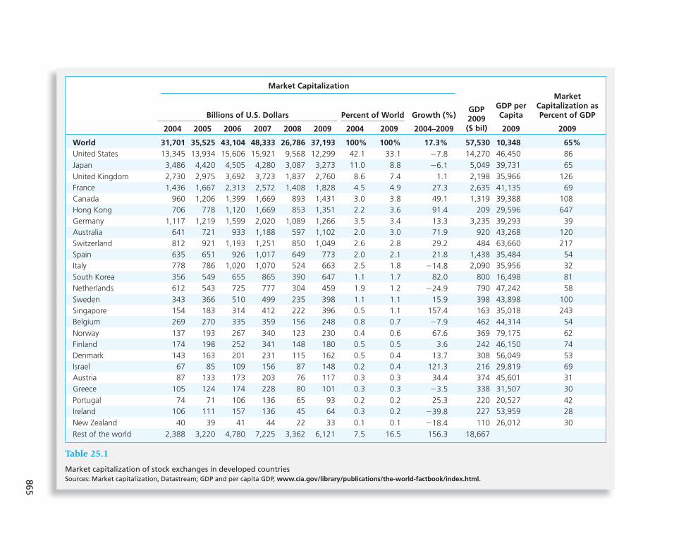
865
Market Capitalization
Billions of U.S. Dollars Percent of World Growth (%)GDP2009($ bil)
GDP per Capita
Market Capitalization as Percent of GDP
2004 2005 2006 2007 2008 2009 2004 2009 2004–2009 2009 2009
World 31,701 35,525 43,104 48,333 26,786 37,193 100% 100% 17.3% 57,530 10,348 65%
United States 13,345 13,934 15,606 15,921 9,568 12,299 42.1 33.1 27.8 14,270 46,450 86
Japan 3,486 4,420 4,505 4,280 3,087 3,273 11.0 8.8 26.1 5,049 39,731 65
United Kingdom 2,730 2,975 3,692 3,723 1,837 2,760 8.6 7.4 1.1 2,198 35,966 126
France 1,436 1,667 2,313 2,572 1,408 1,828 4.5 4.9 27.3 2,635 41,135 69
Canada 960 1,206 1,399 1,669 893 1,431 3.0 3.8 49.1 1,319 39,388 108
Hong Kong 706 778 1,120 1,669 853 1,351 2.2 3.6 91.4 209 29,596 647
Germany 1,117 1,219 1,599 2,020 1,089 1,266 3.5 3.4 13.3 3,235 39,293 39
Australia 641 721 933 1,188 597 1,102 2.0 3.0 71.9 920 43,268 120
Switzerland 812 921 1,193 1,251 850 1,049 2.6 2.8 29.2 484 63,660 217
Spain 635 651 926 1,017 649 773 2.0 2.1 21.8 1,438 35,484 54
Italy 778 786 1,020 1,070 524 663 2.5 1.8 214.8 2,090 35,956 32
South Korea 356 549 655 865 390 647 1.1 1.7 82.0 800 16,498 81
Netherlands 612 543 725 777 304 459 1.9 1.2 224.9 790 47,242 58
Sweden 343 366 510 499 235 398 1.1 1.1 15.9 398 43,898 100
Singapore 154 183 314 412 222 396 0.5 1.1 157.4 163 35,018 243
Belgium 269 270 335 359 156 248 0.8 0.7 27.9 462 44,314 54
Norway 137 193 267 340 123 230 0.4 0.6 67.6 369 79,175 62
Finland 174 198 252 341 148 180 0.5 0.5 3.6 242 46,150 74
Denmark 143 163 201 231 115 162 0.5 0.4 13.7 308 56,049 53
Israel 67 85 109 156 87 148 0.2 0.4 121.3 216 29,819 69
Austria 87 133 173 203 76 117 0.3 0.3 34.4 374 45,601 31
Greece 105 124 174 228 80 101 0.3 0.3 23.5 338 31,507 30
Portugal 74 71 106 136 65 93 0.2 0.2 25.3 220 20,527 42
Ireland 106 111 157 136 45 64 0.3 0.2 239.8 227 53,959 28
New Zealand 40 39 41 44 22 33 0.1 0.1 218.4 110 26,012 30
Rest of the world 2,388 3,220 4,780 7,225 3,362 6,121 7.5 16.5 156.3 18,667
Table 25.1
Market capitalization of stock exchanges in developed countries Sources: Market capitalization, Datastream; GDP and per capita GDP, www.cia.gov/library/publications/the-world-factbook/index.html.
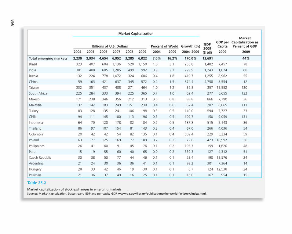
866
Market Capitalization
Billions of U.S. Dollars Percent of World Growth (%)GDP2009($ bil)
GDP per Capita
Market Capitalization as Percent of GDP
2004 2005 2006 2007 2008 2009 2004 2009 2004–2009 2009 2009
Total emerging markets 2,230 2,934 4,654 6,952 3,285 6,022 7.0% 16.2% 170.0% 13,691 44%
Brazil 323 407 604 1,136 520 1,150 1.0 3.1 255.8 1,482 7,457 78
India 301 408 605 1,285 499 992 0.9 2.7 229.9 1,243 1,074 80
Russia 132 224 778 1,072 324 686 0.4 1.8 419.7 1,255 8,962 55
China 59 163 421 637 345 572 0.2 1.5 874.4 4,758 3,554 12
Taiwan 332 351 437 488 271 464 1.0 1.2 39.8 357 15,552 130
South Africa 225 284 333 394 225 365 0.7 1.0 62.4 277 5,655 132
Mexico 171 238 346 356 212 313 0.5 0.8 83.8 866 7,790 36
Malaysia 137 142 183 249 151 230 0.4 0.6 67.4 207 8,065 111
Turkey 83 128 135 241 106 198 0.3 0.5 140.0 594 7,727 33
Chile 94 111 145 180 113 196 0.3 0.5 109.7 150 9,059 131
Indonesia 64 70 120 178 82 184 0.2 0.5 187.8 515 2,143 36
Thailand 86 97 107 154 81 143 0.3 0.4 67.0 266 4,036 54
Colombia 20 42 42 54 82 135 0.1 0.4 569.4 229 5,234 59
Poland 63 77 125 169 77 109 0.2 0.3 72.6 423 10,992 26
Philippines 26 41 60 91 45 76 0.1 0.2 193.7 159 1,620 48
Peru 15 19 55 60 40 65 0.0 0.2 339.3 127 4,312 51
Czech Republic 30 38 50 77 44 46 0.1 0.1 53.4 190 18,576 24
Argentina 21 24 30 36 36 41 0.1 0.1 98.2 301 7,364 14
Hungary 28 33 42 46 19 30 0.1 0.1 6.7 124 12,538 24
Pakistan 21 36 37 49 16 25 0.1 0.1 16.0 167 954 15
Table 25.2
Market capitalization of stock exchanges in emerging markets Sources: Market capitalzation, Datastream; GDP and per capita GDP, www.cia.gov/library/publications/the-world-factbook/index.html.

C H A P T E R 2 5 International Diversification 867
ranges from 12% (China) to 132% (South Africa), suggesting that these markets are expected to show significant growth over the coming years, even absent spectacular growth in GDP.
The growth of capitalization in emerging markets over 2004–2009 was very large (170%) and much more volatile than growth in developed countries, suggest-ing that both risk and rewards in this segment of the globe may be substantial.
Market Capitalization and GDP
The contemporary view of eco-nomic development (see, for example, deSoto) 2 holds that a major requirement for economic advancement is a developed code of business laws, institu-tions, and regulation that allows citizens to legally own, capitalize, and trade capital assets. As a corollary, we expect that development of equity markets will serve as a catalyst for enrichment of the population, that is, that countries with larger relative capitalization of equities will tend to be richer. Work by La Porta, Lopez-De-Silvanes, Shleifer, and Vishny indicates that, other things equal, market value of corporations is higher in countries with better protection of minority shareholders. 3
Figure 25.1 is a simple (perhaps simplistic, because other relevant explanatory vari-ables are omitted) rendition of the argument that a developed market for corporate equity contributes to the enrichment of the population. The slope of the regression line shown in Figure 25.1 is .45, suggesting that an increase of 1% in the ratio of market capitalization to GDP is associated with an increase in per capita GDP of .45%. It is remarkable that only 2 of the 25 developed countries lie below the regression line; only 2 of 20 low-income emerging markets lie above the line. A country like Norway that lies above the line, that is, exhibits higher per capita GDP than predicted by the regression, enjoys oil wealth that contributes to population income. Countries below the line, such as Pakistan, suffered from deterioration of the business environment due to political strife and/or government policies that restricted the private sector.
Home-Country Bias
One would expect that most investors, particularly institutional and professional investors, would be aware of the opportunities offered by international investing. Yet in p ractice,
2 Hernando de Soto, The Mystery of Capital (New York: Basic Books, 2000). 3 Rafael La Porta, Florencio Lopez-De-Silvanes, Andrei Shleifer, and Robert Vishny, “Investor Protection and Corporate Valuation,” Journal of Finance 57 (June 2002).
100
1,000
10,000
100,000
1 10 100 1,000
Per
Cap
ita
GD
P ($
)
Developed countries Emerging markets Regression line
PakistanIndia
ChileS. Korea
Japan
IrelandNorway
U.S.
U.K.
Hungary
Czech Rep.
Switzerland
HongKong
Brazil
Russia
China
Market Capitalization (% of GDP)
Figure 25.1 Per capita GDP and market capitalization as percent of GDP, 2009 (log scale)
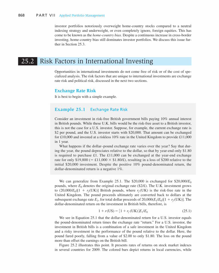
868 P A R T V I I Applied Portfolio Management
investor portfolios notoriously overweight home-country stocks compared to a neutral indexing strategy and underweight, or even completely ignore, foreign equities. This has come to be known as the home-country bias. Despite a continuous increase in cross-border investing, home-country bias still dominates investor portfolios. We discuss this issue fur-ther in Section 25.3.
25.2 Risk Factors in International Investing
Opportunities in international investments do not come free of risk or of the cost of spe-cialized analysis. The risk factors that are unique to international investments are exchange rate risk and political risk, discussed in the next two sections.
Exchange Rate Risk
It is best to begin with a simple example.
Example 25.1 Exchange Rate Risk
Consider an investment in risk-free British government bills paying 10% annual interest in British pounds. While these U.K. bills would be the risk-free asset to a British investor, this is not the case for a U.S. investor. Suppose, for example, the current exchange rate is $2 per pound, and the U.S. investor starts with $20,000. That amount can be exchanged for £10,000 and invested at a riskless 10% rate in the United Kingdom to provide £11,000 in 1 year.
What happens if the dollar–pound exchange rate varies over the year? Say that dur-ing the year, the pound depreciates relative to the dollar, so that by year-end only $1.80 is required to purchase £1. The £11,000 can be exchanged at the year-end exchange rate for only $19,800 ( 5 £11,000 3 $1.80/£), resulting in a loss of $200 relative to the initial $20,000 investment. Despite the positive 10% pound-denominated return, the dollar-denominated return is a negative 1%.
We can generalize from Example 25.1. The $20,000 is exchanged for $20,000/ E 0 pounds, where E 0 denotes the original exchange rate ($2/£). The U.K. investment grows to (20,000/ E 0 )[1 1 r f (UK)] British pounds, where r f (UK) is the risk-free rate in the United Kingdom. The pound proceeds ultimately are converted back to dollars at the subsequent exchange rate E 1 , for total dollar proceeds of 20,000( E 1 / E 0 )[1 1 r f (UK)]. The dollar-denominated return on the investment in British bills, therefore, is
1 1 r (US) 5 31 1 rf (UK) 4E1/E0 (25.1)
We see in Equation 25.1 that the dollar-denominated return for a U.S. investor equals the pound-denominated return times the exchange rate “return.” For a U.S. investor, the investment in British bills is a combination of a safe investment in the United Kingdom and a risky investment in the performance of the pound relative to the dollar. Here, the pound fared poorly, falling from a value of $2.00 to only $1.80. The loss on the pound more than offset the earnings on the British bill.
Figure 25.2 illustrates this point. It presents rates of returns on stock market indexes in several countries for 2009. The colored bars depict returns in local currencies, while

C H A P T E R 2 5 International Diversification 869
the dark bars depict returns in dollars, adjusted for exchange rate movements. It’s clear that exchange rate fluctuations over this period had large effects on dollar-denominated returns in several countries.
Pure exchange rate risk is the risk borne by investments in foreign safe assets. The investor in U.K. bills of Example 25.1 bears the risk of the U.K./U.S. exchange rate only. We can assess the magnitude of exchange rate risk by examining historical rates of change in various exchange rates and their correlations.
Table 25.3 A shows historical exchange rate risk measured from monthly percentage changes in the exchange rates of major currencies over the period 2000–2009. The data show that currency risk can be quite high. The annualized standard deviation of the per-centage changes in the exchange rate ranged from 9.65% (Canadian dollar) to 13.84% (Australian dollar). The annualized standard deviation of returns on U.S. stocks for the same period was 17.08%. Hence, currency exchange risk alone would amount to between 57% and 81% of the risk on U.S. stocks. Clearly, an active investor who believes that Australian stocks are underpriced, but has no information about any m ispricing of the
9.212.7
0 10 20 40 5030 60 70 80 90 100
Taiwan
Hong Kong
Norway
Spain
Netherlands
Australia
Canada
Denmark
France
U.K.
Italy
Germany
New Zealand
Ireland
Japan
Finland
%
Return (in U.S.$)Return (in local currency)
75.780.2
60.260.2
55.688.6
40.645.1
38.643.0
37.076.8
33.657.4
32.837.1
29.133.3
27.743.4
24.028.0
22.626.6
21.951.7
9.412.9
9.36.4
Figure 25.2 Stock market returns in U.S. dollars and local currencies, 2009
CONCEPT CHECK
1
Using the data in Example 25.1 , calculate the rate of return in dollars to a U.S. investor hold-ing the British bill if the year-end exchange rate is: ( a ) E1 5 $2.00/£; ( b ) E1 5 $2.20/£.
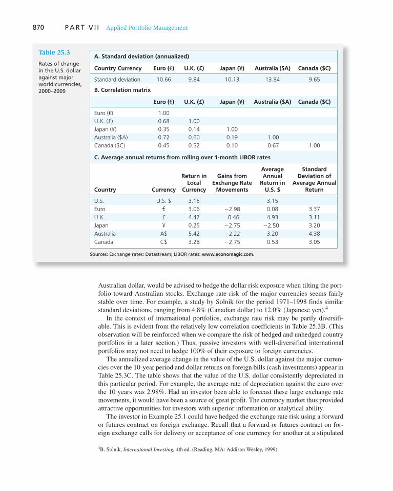
870 P A R T V I I Applied Portfolio Management
Australian dollar, would be advised to hedge the dollar risk exposure when tilting the port-folio toward Australian stocks. Exchange rate risk of the major currencies seems fairly stable over time. For example, a study by Solnik for the period 1971–1998 finds similar standard deviations, ranging from 4.8% (Canadian dollar) to 12.0% (Japanese yen). 4
In the context of international portfolios, exchange rate risk may be partly diversifi-able. This is evident from the relatively low correlation coefficients in Table 25.3B . (This observation will be reinforced when we compare the risk of hedged and unhedged country portfolios in a later section.) Thus, passive investors with well-diversified international portfolios may not need to hedge 100% of their exposure to foreign currencies.
The annualized average change in the value of the U.S. dollar against the major curren-cies over the 10-year period and dollar returns on foreign bills (cash investments) appear in Table 25.3C . The table shows that the value of the U.S. dollar consistently depreciated in this particular period. For example, the average rate of depreciation against the euro over the 10 years was 2.98%. Had an investor been able to forecast these large exchange rate movements, it would have been a source of great profit. The currency market thus provided attractive opportunities for investors with superior information or analytical ability.
The investor in Example 25.1 could have hedged the exchange rate risk using a forward or futures contract on foreign exchange. Recall that a forward or futures contract on for-eign exchange calls for delivery or acceptance of one currency for another at a stipulated
4 B. Solnik, International Investing, 4th ed. (Reading, MA: Addison Wesley, 1999).
A. Standard deviation (annualized)
Country Currency Euro (€) U.K. ( £) Japan ( ¥ ) Australia ($A) Canada ($C)
Standard deviation 10.66 9.84 10.13 13.84 9.65
B. Correlation matrix
Euro (€) U.K. ( £) Japan ( ¥ ) Australia ($A) Canada ($C)
Euro (€) 1.00
U.K. (£) 0.68 1.00
Japan (¥) 0.35 0.14 1.00
Australia ($A) 0.72 0.60 0.19 1.00
Canada ($C) 0.45 0.52 0.10 0.67 1.00
C. Average annual returns from rolling over 1-month LIBOR rates
Country Currency
Return in Local
Currency
Gains from Exchange Rate
Movements
Average Annual
Return in U.S. $
Standard Deviation of
Average Annual Return
U.S. U.S. $ 3.15 3.15
Euro € 3.06 22.98 0.08 3.37
U.K. £ 4.47 0.46 4.93 3.11
Japan ¥ 0.25 22.75 22.50 3.20
Australia A$ 5.42 22.22 3.20 4.38
Canada C$ 3.28 22.75 0.53 3.05
Sources: Exchange rates: Datastream; LIBOR rates: www.economagic.com.
Table 25.3
Rates of change in the U.S. d ollar against major world currencies, 2000–2009

C H A P T E R 2 5 International Diversification 871
exchange rate. Here, the U.S. investor would agree to deliver pounds for dollars at a fixed exchange rate, thereby eliminating the risk involved with conversion of the pound invest-ment back into dollars.
Example 25.2 Hedging Exchange Rate Risk
If the forward exchange rate in Example 25.1 had been F 0 5 $1.93/£ when the investment was made, the U.S. investor could have assured a riskless dollar-denominated return by arranging to deliver the £11,000 at the forward exchange rate of $1.93/£. In this case, the riskless U.S. return would then have been 6.15%:
31 1 rf (UK) 4F0 /E0 5 (1.10)1.93 / 2.00 5 1.0615
You may recall that the hedge underlying Example 25.2 is the same type of hedging strategy at the heart of the spot-futures parity relationship first discussed in Chapter 22. In both instances, futures or forward markets are used to eliminate the risk of holding another asset. The U.S. investor can lock in a riskless dollar-denominated return either by investing in United Kingdom bills and hedging exchange rate risk or by investing in riskless U.S. assets. Because investments in two riskless strategies must provide equal returns, we con-clude that [1 1 r f (UK)] F 0 / E 0 5 1 1 r f (US), which can be rearranged to
F0
E0
51 1 rf (US)
1 1 rf (UK) (25.2)
This relationship is called the interest rate parity relationship or covered interest arbi-
trage relationship, which we first encountered in Chapter 23. Unfortunately, such perfect exchange rate hedging usually is not so easy. In our exam-
ple, we knew exactly how many pounds to sell in the forward or futures market because the pound-denominated return in the United Kingdom was riskless. If the U.K. investment had not been in bills, but instead had been in risky U.K. equity, we would have known neither the ultimate value in pounds of our U.K. investment nor how many pounds to sell forward. The hedging opportunity offered by foreign exchange forward contracts would thus be imperfect.
To summarize, the generalization of Equation 25.1 for unhedged investments is that
1 1 r (US) 5 31 1 r (foreign) 4E1 /
E0 (25.3)
where r (foreign) is the possibly risky return earned in the currency of the foreign invest-ment. You can set up a perfect hedge only in the special case that r (foreign) is itself a known number. In that case, you know you must sell in the forward or futures market an amount of foreign currency equal to [1 1 r (foreign)] for each unit of that currency you pur-chase today.
Political Risk
In principle, security analysis at the macroeconomic, industry, and firm-specific level is similar in all countries. Such analysis aims to provide estimates of expected returns and risk of individual assets and portfolios. However, to achieve the same quality of in formation
CONCEPT CHECK
2 How many pounds would the investor in Example 25.2 need to sell forward to hedge exchange rate risk if: ( a ) r (UK) 5 20%; and ( b ) r (UK) 5 30%?
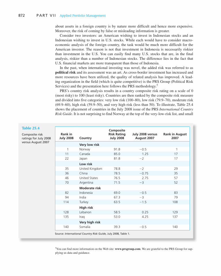
872 P A R T V I I Applied Portfolio Management
about assets in a foreign country is by nature more difficult and hence more expensive. Moreover, the risk of coming by false or misleading information is greater.
Consider two investors: an American wishing to invest in Indonesian stocks and an Indonesian wishing to invest in U.S. stocks. While each would have to consider macro-economic analysis of the foreign country, the task would be much more difficult for the American investor. The reason is not that investment in Indonesia is necessarily riskier than investment in the U.S. You can easily find many U.S. stocks that are, in the final analysis, riskier than a number of Indonesian stocks. The difference lies in the fact that U.S. financial markets are more transparent than those of Indonesia.
In the past, when international investing was novel, the added risk was referred to as political risk and its assessment was an art. As cross-border investment has increased and more resources have been utilized, the quality of related analysis has improved. A lead-ing organization in the field (which is quite competitive) is the PRS Group (Political Risk Services) and the presentation here follows the PRS methodology. 5
PRS’s country risk analysis results in a country composite risk rating on a scale of 0 (most risky) to 100 (least risky). Countries are then ranked by the composite risk measure and divided into five categories: very low risk (100–80), low risk (79.9–70), moderate risk (69.9–60), high risk (59.9–50), and very high risk (less than 50). To illustrate, Table 25.4 shows the placement of countries in the July 2008 issue of the PRS International Country
Risk Guide. It is not surprising to find Norway at the top of the very-low-risk list, and small
5 You can find more information on the Web site: www.prsgroup.com. We are grateful to the PRS Group for sup-plying us data and guidance.
Rank in July 2008 Country
Composite Risk Rating July 2008
July 2008 versus August 2007
Rank in August 2007
Very low risk
1 Norway 91.8 20.5 1
11 Canada 85.0 1.25 17
22 Japan 81.8 22 17
Low risk
35 United Kingdom 78.8 22 29
36 China 78.5 20.75 35
46 United States 76.5 2.75 57
70 Argentina 71.5 23 52
Moderate risk
82 Indonesia 69.0 20.5 83
94 India 67.3 23 79
114 Turkey 63.5 21.5 108
High risk
128 Lebanon 58.5 0.25 129
135 Iraq 53.0 4.25 137
Very high risk
140 Somalia 39.3 20.5 140
Source: International Country Risk Guide, July 2008, Table 1.
Table 25.4
Composite risk ratings for July 2008 versus August 2007

C H A P T E R 2 5 International Diversification 873
emerging markets at the bottom, with Somalia (ranked 140) closing the list. What may be surprising is the fairly mediocre ranking of the U.S. (ranked 46), comparable to China (36) and the U.K. (35), all three appearing in the low-risk category.
The composite risk rating is a weighted average of three measures: political risk, finan-cial risk, and economic risk. Political risk is measured on a scale of 100–0, while financial and economic risk are measured on a scale of 50–0. The three measures are added and divided by two to obtain the composite rating. The variables used by PRS to determine the composite risk rating from the three measures are shown in Table 25.5 .
Table 25.6 shows the three risk measures for five of the countries in Table 25.4 , in order of the July 2008 ranking of the composite risk ratings. The table shows that by politi-cal risk, the United States ranked second among these five countries. But in the finan-cial risk measure, the U.S. ranked last among the five. The surprisingly poor performance of the U.S. in this dimension was probably due to its exceedingly large government and balance-of-trade deficits, which put considerable pressure on its exchange rate. Exchange
Political Risk Variables Financial Risk Variables Economic Risk Variables
Government stability Foreign debt (% of GDP) GDP per capita
Socioeconomic conditions Foreign debt service (% of GDP) Real annual GDP growth
Investment profile Current account (% of exports) Annual inflation rate
Internal conflicts Net liquidity in months of imports Budget balance (% of GDP)
External conflicts Exchange rate stability Current account balance (% GDP)
Corruption
Military in politics
Religious tensions
Law and order
Ethnic tensions
Democratic accountability
Bureaucracy quality
Table 25.5
Variables used in PRS’s political risk score
Composite Ratings Current Ratings
Country August 2007 July 2008Political Risk
July 2008Financial Risk
July 2008Economic Risk
July 2008
Canada 83.75 85 86 42 42
Japan 83.75 81.75 77.5 46 40
China 80.5 78.5 67.5 48 41.5
United States 73.5 76.5 81 32 40
India 71 67.25 60.5 43.5 30.5
Table 25.6
Current risk ratings and composite risk forecasts
Source: International Country Risk Guide, July 2008, Table 2B.

874 P A R T V I I Applied Portfolio Management
A. Composite risk forecasts
One Year Ahead Five Years Ahead
CountryCurrent Rating
July 2008Worst Case
Best Case
Risk Stability
Worst Case
Best Case
Risk Stability
Canada 85.0 80.8 87.8 7.0 78.0 90.8 12.8
Japan 81.8 78.3 85.0 6.8 75.5 89.0 13.5
China 78.5 72.3 80.3 8.0 63.3 83.3 20.0
United States 76.5 74.8 82.0 7.3 71.0 84.3 13.3
India 67.3 63.8 71.3 7.5 61.8 76.3 14.5
B. Political Risk Forecasts
One Year Ahead Five Years Ahead
CountryCurrent Rating
July 2008Worst Case
Best Case
Risk Stability
Worst Case
Best Case
Risk Stability
Canada 86.0 83.5 88.5 5.0 83.0 92.5 9.5
Japan 77.5 75.0 83.0 8.0 74.0 89.0 15.0
China 67.5 63.5 70.5 7.0 60.5 77.0 16.5
United States 81.0 79.0 87.0 8.0 77.0 87.5 10.5
India 60.5 59.0 65.5 6.5 61.0 72.5 11.5
Table 25.7
Composite and political risk forecasts
Sources: A: International Country Risk Guide, July 2008, Table 2C; B: International Country Risk Guide, July 2008, Table 3C.
rate stability, foreign trade imbalance, and foreign indebtedness all enter PRS’s computa-tion of financial risk. The financial crisis that began in August of 2008 was a striking vin-dication of PRS’s judgment; our initial surprise at the rank of the U.S. arose from a failure to carefully consider the underpinnings of their methodology.
Country risk is captured in greater depth by scenario analysis for the composite mea-sure and each of its components. Table 25.7 (A and B) shows 1- and 5-year worst-case and best-case scenarios for the composite ratings and for the political risk measure. Risk stabil-ity is based on the difference in the rating between the best- and worst-case scenarios and is quite large in most cases. The worst-case scenario can move a country to a higher risk category. For example, Table 25.7 B shows that in the worst-case five-year scenario, India was particularly vulnerable to deterioration in the political environment.
Finally, Table 25.8 shows ratings of political risk by each of its 12 components. Corruption (variable F) in Japan is rated worse than in the U.S. but better than in China and India. In democratic accountability (variable K), China ranked worst, and the United States, Canada, and India best, while China ranked best in government stability (variable A).
Each monthly issue of the International Country Risk Guide of the PRS Group includes great detail and holds some 250 pages. Other organizations compete in supplying such evaluations. The result is that today’s investor can become well equipped to properly assess the risk involved in international investing.
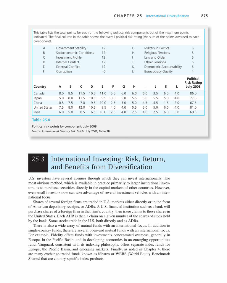
C H A P T E R 2 5 International Diversification 875
25.3 International Investing: Risk, Return, and Benefits from Diversification
This table lists the total points for each of the following political risk components out of the maximum points
indicated. The final column in the table shows the overall political risk rating (the sum of the points awarded to each
component).
A Government Stability 12 G Military in Politics 6
B Socioeconomic Conditions 12 H Religious Tensions 6
C Investment Profile 12 I Law and Order 6
D Internal Conflict 12 J Ethnic Tensions 6
E External Conflict 12 K Democratic Accountability 6
F Corruption 6 L Bureaucracy Quality 4
Country A B C D E F G H I J K L
Political Risk Rating July 2008
Canada 8.0 8.5 11.5 10.5 11.0 5.0 6.0 6.0 6.0 3.5 6.0 4.0 86.0
Japan 5.0 8.0 11.5 10.5 9.5 3.0 5.0 5.5 5.0 5.5 5.0 4.0 77.5
China 10.5 7.5 7.0 9.5 10.0 2.5 3.0 5.0 4.5 4.5 1.5 2.0 67.5
United States 7.5 8.0 12.0 10.5 9.5 4.0 4.0 5.5 5.0 5.0 6.0 4.0 81.0
India 6.0 5.0 8.5 6.5 10.0 2.5 4.0 2.5 4.0 2.5 6.0 3.0 60.5
Table 25.8
Political risk points by component, July 2008
Source: International Country Risk Guide, July 2008, Table 3B.
U.S. investors have several avenues through which they can invest internationally. The most obvious method, which is available in practice primarily to larger institutional inves-tors, is to purchase securities directly in the capital markets of other countries. However, even small investors now can take advantage of several investment vehicles with an inter-national focus.
Shares of several foreign firms are traded in U.S. markets either directly or in the form of American depository receipts, or ADRs. A U.S. financial institution such as a bank will purchase shares of a foreign firm in that firm’s country, then issue claims to those shares in the United States. Each ADR is then a claim on a given number of the shares of stock held by the bank. Some stocks trade in the U.S. both directly and as ADRs.
There is also a wide array of mutual funds with an international focus. In addition to single-country funds, there are several open-end mutual funds with an international focus. For example, Fidelity offers funds with investments concentrated overseas, generally in Europe, in the Pacific Basin, and in developing economies in an emerging opportunities fund. Vanguard, consistent with its indexing philosophy, offers separate index funds for Europe, the Pacific Basin, and emerging markets. Finally, as noted in Chapter 4, there are many exchange-traded funds known as iShares or WEBS (World Equity Benchmark Shares) that are country-specific index products.
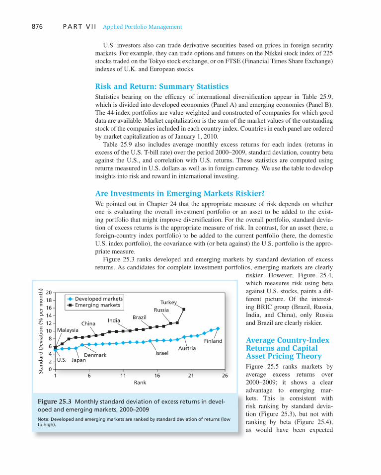
876 P A R T V I I Applied Portfolio Management
U.S. investors also can trade derivative securities based on prices in foreign security markets. For example, they can trade options and futures on the Nikkei stock index of 225 stocks traded on the Tokyo stock exchange, or on FTSE (Financial Times Share Exchange) indexes of U.K. and European stocks.
Risk and Return: Summary Statistics
Statistics bearing on the efficacy of international diversification appear in Table 25.9 , which is divided into developed economies (Panel A) and emerging economies (Panel B). The 44 index portfolios are value weighted and constructed of companies for which good data are available. Market capitalization is the sum of the market values of the outstanding stock of the companies included in each country index. Countries in each panel are ordered by market capitalization as of January 1, 2010.
Table 25.9 also includes average monthly excess returns for each index (returns in excess of the U.S. T-bill rate) over the period 2000–2009, standard deviation, country beta against the U.S., and correlation with U.S. returns. These statistics are computed using returns measured in U.S. dollars as well as in foreign currency. We use the table to develop insights into risk and reward in international investing.
Are Investments in Emerging Markets Riskier?
We pointed out in Chapter 24 that the appropriate measure of risk depends on whether one is evaluating the overall investment portfolio or an asset to be added to the exist-ing portfolio that might improve diversification. For the overall portfolio, standard devia-tion of excess returns is the appropriate measure of risk. In contrast, for an asset (here, a foreign-country index portfolio) to be added to the current portfolio (here, the domestic U.S. index portfolio), the covariance with (or beta against) the U.S. portfolio is the appro-priate measure.
Figure 25.3 ranks developed and emerging markets by standard deviation of excess returns. As candidates for complete investment portfolios, emerging markets are clearly
riskier. However, Figure 25.4 , which measures risk using beta against U.S. stocks, paints a dif-ferent picture. Of the interest-ing BRIC group (Brazil, Russia, India, and China), only Russia and Brazil are clearly riskier.
Average Country-Index Returns and Capital Asset Pricing Theory
Figure 25.5 ranks markets by average excess returns over 2000–2009; it shows a clear advantage to emerging mar-kets. This is consistent with risk ranking by standard devia-tion ( Figure 25.3 ), but not with ranking by beta ( Figure 25.4 ), as would have been expected
0
2
4
6
8
10
12
14
16
18
20
1 6 11 16 21 26Rank
Stan
dar
d D
evia
tio
n (
% p
er m
on
th)
Developed marketsEmerging markets
U.S. JapanDenmark Israel
AustriaFinland
TurkeyRussia
BrazilIndia
ChinaMalaysia
Figure 25.3 Monthly standard deviation of excess returns in devel-oped and emerging markets, 2000–2009
Note: Developed and emerging markets are ranked by standard deviation of returns (low to high).

877
CountryWorld
Capitalization*
Excess Returns (% per Month in U.S. Dollars) Excess Returns (% per Month in Local Currency)
Average Std. Dev. Beta/U.S. Corr./U.S. Average Std./Dev. Beta/U.S. Corr./U.S.
World 37,193 20.01 5.34 1.00 0.97 20.01 5.34 1.00 0.97
A. Developed countries
U.S. 12,299 20.20 5.14 1.00 1.00 20.20 5.14 1.00 1.00
Japan 3,273 20.38 5.52 0.66 0.61 20.46 5.34 0.62 0.60
U.K. 2,760 0.04 5.45 0.92 0.87 20.01 4.54 0.77 0.87
France 1,828 0.21 6.55 1.09 0.85 20.15 5.59 0.90 0.82
Canada 1,431 0.76 7.11 1.15 0.83 0.38 5.32 0.86 0.84
Hong Kong 1,351 0.35 6.74 0.85 0.65 0.35 6.73 0.85 0.65
Germany 1,266 0.24 7.82 1.28 0.84 20.13 6.91 1.09 0.81
Australia 1,102 1.00 6.66 1.03 0.79 0.60 4.09 0.58 0.73
Switzerland 1,049 0.35 5.48 0.86 0.81 20.05 4.83 0.74 0.79
Spain 773 0.71 7.12 1.11 0.80 0.34 6.12 0.91 0.77
Italy 663 0.18 6.81 1.02 0.77 20.18 5.75 0.84 0.75
Korea 647 1.05 10.23 1.47 0.74 0.90 8.33 1.04 0.64
Netherlands 459 0.19 6.98 1.14 0.84 20.16 6.27 0.96 0.79
Sweden 398 0.36 8.83 1.38 0.80 0.10 7.47 1.01 0.70
Singapore 396 0.47 7.56 1.08 0.74 0.27 6.76 0.95 0.72
Belgium 248 0.11 7.64 1.11 0.75 20.27 6.58 0.93 0.73
Norway 230 1.13 8.73 1.29 0.76 0.74 7.38 1.09 0.76
Finland 180 20.12 10.68 1.43 0.69 20.45 10.32 1.24 0.62
Denmark 162 0.71 6.48 1.00 0.79 0.36 5.83 0.81 0.72
Israel 148 0.69 7.49 0.82 0.56 0.55 6.86 0.63 0.47
Greece 117 20.10 9.45 1.12 0.61 20.46 8.44 0.93 0.57
Austria 101 0.80 8.50 1.18 0.71 0.39 7.19 1.00 0.71
Portugal 93 0.27 6.58 0.80 0.62 20.09 5.52 0.61 0.57
Ireland 64 20.54 7.59 1.08 0.73 20.86 7.23 0.90 0.64
New Zealand 33 0.56 7.12 0.95 0.68 0.14 4.66 0.49 0.54
Table 25.9
Risk and return across the globe, 2000–2009 continued
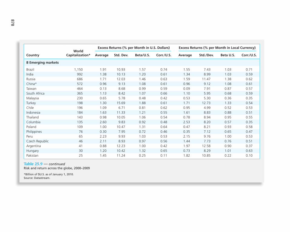
878
CountryWorld
Capitalization*
Excess Returns (% per Month in U.S. Dollars) Excess Returns (% per Month in Local Currency)
Average Std. Dev. Beta/U.S. Corr./U.S. Average Std./Dev. Beta U.S. Corr./U.S.
B Emerging markets
Brazil 1,150 1.91 10.93 1.57 0.74 1.55 7.43 1.03 0.71
India 992 1.38 10.13 1.20 0.61 1.34 8.99 1.03 0.59
Russia 686 1.71 12.03 1.46 0.63 1.59 11.47 1.38 0.62
China* 572 0.96 9.13 1.08 0.61 0.96 9.12 1.08 0.61
Taiwan 464 0.13 8.68 0.99 0.59 0.09 7.91 0.87 0.57
South Africa 365 1.13 8.42 1.07 0.66 1.10 5.95 0.68 0.59
Malaysia 230 0.65 5.78 0.48 0.42 0.53 5.30 0.36 0.35
Turkey 198 1.30 15.69 1.88 0.61 1.71 12.73 1.33 0.54
Chile 196 1.09 6.71 0.81 0.62 0.95 4.99 0.52 0.53
Indonesia 184 1.63 11.33 1.21 0.55 1.61 8.83 0.88 0.51
Thailand 143 0.98 10.05 1.06 0.54 0.78 8.94 0.95 0.55
Columbia 135 2.60 9.83 0.92 0.48 2.53 8.20 0.57 0.35
Poland 109 1.00 10.47 1.31 0.64 0.47 8.21 0.93 0.58
Philippines 76 0.30 7.95 0.72 0.46 0.35 7.12 0.65 0.47
Peru 65 2.23 9.93 1.03 0.53 2.15 9.76 1.00 0.53
Czech Republic 46 2.11 8.93 0.97 0.56 1.44 7.73 0.76 0.51
Argentina 41 0.88 12.23 1.00 0.42 1.97 12.58 0.90 0.37
Hungary 30 1.20 10.42 1.32 0.65 0.73 8.29 1.01 0.63
Pakistan 25 1.45 11.24 0.25 0.11 1.82 10.85 0.22 0.10
Table 25.9 — continuedRisk and return across the globe, 2000–2009
*Billion of $U.S. as of January 1, 2010.Source: Datastream.
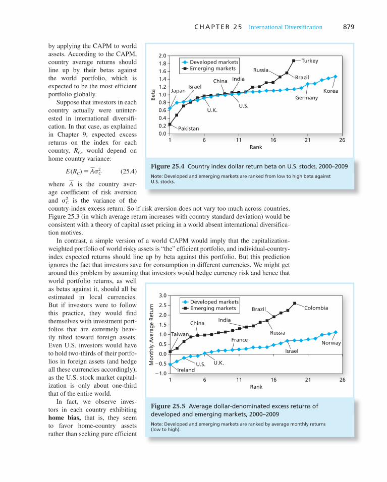
C H A P T E R 2 5 International Diversification 879
by applying the CAPM to world assets. According to the CAPM, country average returns should line up by their betas against the world portfolio, which is expected to be the most efficient portfolio globally.
Suppose that investors in each country actually were uninter-ested in international diversifi-cation. In that case, as explained in Chapter 9, expected excess returns on the index for each country, R C , would depend on home country variance:
E (RC) 5 AsC2 (25.4)
where A is the country aver-age coefficient of risk aversion and sC
2 is the variance of the country-index excess return. So if risk aversion does not vary too much across countries, Figure 25.3 (in which average return increases with country standard deviation) would be consistent with a theory of capital asset pricing in a world absent international diversifica-tion motives.
In contrast, a simple version of a world CAPM would imply that the capitalization-weighted portfolio of world risky assets is “the” efficient portfolio, and individual-country-index expected returns should line up by beta against this portfolio. But this prediction ignores the fact that investors save for consumption in different currencies. We might get around this problem by assuming that investors would hedge currency risk and hence that world portfolio returns, as well as betas against it, should all be estimated in local currencies. But if investors were to follow this practice, they would find themselves with investment port-folios that are extremely heav-ily tilted toward foreign assets. Even U.S. investors would have to hold two-thirds of their portfo-lios in foreign assets (and hedge all these currencies accordingly), as the U.S. stock market capital-ization is only about one-third that of the entire world.
In fact, we observe inves-tors in each country exhibiting home bias, that is, they seem to favor home-country assets rather than seeking pure efficient
�1.0
�0.5
0.0
0.5
1.0
1.5
2.0
2.5
3.0
Mo
nth
ly A
vera
ge
Ret
urn
Developed marketsEmerging markets
IrelandU.S. U.K.
France
Israel
Norway
ColombiaBrazil
Russia
IndiaChina
Taiwan
1 6 11 16 21 26Rank
Figure 25.5 Average dollar-denominated excess returns of developed and emerging markets, 2000–2009
Note: Developed and emerging markets are ranked by average monthly returns (low to high).
0.0
0.2
0.4
0.6
0.8
1.0
1.2
1.4
1.6
1.8
2.0
1 6 11 16 21 26Rank
Bet
a
Developed marketsEmerging markets
Pakistan
U.K.U.S.
Germany
Turkey
BrazilRussia
IndiaChinaIsrael
Japan Korea
Figure 25.4 Country index dollar return beta on U.S. stocks, 2000–2009
Note: Developed and emerging markets are ranked from low to high beta against U.S. stocks.

880 P A R T V I I Applied Portfolio Management
d iversification. In addition to issues of psychology, regulation, and extra expense, home bias may also arise from the following motivation. 6 Investors evaluate their standard of living against a reference group that is most likely to consist primarily of their compatriots. This alone is a reason to tie portfolio returns to the success of home firms that supply the labor/management income of the reference group.
On these grounds, we expect that country-index expected returns would be influenced by both beta against the world portfolio and the variance of home country returns. In addi-tion to these two variables, we might also consider country size (capitalization) as another variable that explains returns, since larger markets tend to exhibit better regulation and transparency.
Unfortunately, a regression of average country return on beta, variance, and size poses problems in implementation. First, statistical imprecision in estimates of beta and vari-ance degrades the regression estimates. Precision also suffers from the small number of countries (40–50) that offer sufficient data. The results of such regressions using data from Table 25.9 are shown in Table 25.10 . The first column includes all countries, and the coef-ficient on return variance is the only one to attain statistical significance. In this regression, the coefficient on beta actually has the “wrong” sign, implying that returns fall with beta. Separate regressions for developed and emerging markets in the next two columns suggest these populations exhibit different behavior. Here, the coefficients on beta are positive, but neither is significant. Country size, measured by log of capitalization, has the expected sign in both regressions, but neither is significant. All we can conclude from these regres-sions is that neither model adequately explains the data.
Country return variance, rather than beta, may well be the dominant variable, suggest-ing the importance of home bias. Notice that we used returns measured in U.S. dollars in the regressions of Table 25.10 , so the returns would apply most directly to U.S. investors. Investors in other countries would have to translate all returns to the home currency.
6 For a formal analysis of this idea see Peter M. De Marzo, Ron Kaniel, and Ilan Kremer, “Diversification as a Public Good: Community Effects in Portfolio Choice,” Journal of Finance 59 (August 2004).
Markets
All Countries Developed Emerging
Coeffients Intercept
Ln(size)
Beta on U.S.
Variance
0.67 0.00 1.16
20.05 20.06 20.08
20.33 0.95 0.34
0.94 20.50 0.15
t-statistic Intercept
Ln(size)
Beta on U.S.
Variance
1.26 0.00 1.41
20.60 20.79 20.45
20.75 1.15 0.50
2.94 20.60 0.30
R-square 0.30 0.31 0.28
Observations 44 25 19
Table 25.10
Regressions of country average monthly excess returns on size, beta, and return variance, 2000–2009

881
Benefits from International Diversification
Table 25.11 presents correlations between returns on stock and long-term bond portfolios in various countries. Panel A shows correlation of returns in U.S. dollars, that is, returns to a U.S. investor when currency risk is not hedged. Panel B shows correlation of returns in local currencies, that is, returns to a U.S. investor when the exchange risk is hedged. First and foremost, these correlations as a whole suggest that international diversification should be considered, at least for active investors. Although correlations between most of the country stock portfolios shown in Table 25.11 are quite high, a few are low enough to imply meaningful benefits from diversification, particularly among bond portfolios and stock/bond portfolios.
Comparison of correlations between currency-hedged and unhedged portfolios shows that, at least for U.S. investors, some currencies should be hedged while some hedges are better forgone. Clearly, taking full account of currency risk would make construction of optimal diversified international portfolios cumbersome and expensive. This brings up a more basic question: Will passive investors benefit from international diversification in the future? We see in Table 25.12 that globalization seems to have encouraged a trend toward higher cross-country correlations. (This trend is the subject of the nearby box.) The lowest correlations are exhibited by emerging markets, but these too have been rising steadily. Since emerging markets are also more volatile (higher standard deviations), lower correla-tions are needed to achieve significant benefits.
The observed high correlation across markets calls into question the common claim of large diversification benefits from international investing. This conventional wisdom is depicted in Figure 25.6 , which is based on data for the period 1961–1975. It suggests that international diversification can reduce the standard deviation of a domestic portfolio by as much as half (from about 27% of the standard deviation of a single stock to about 12%). This improvement may well be exaggerated if correlation across markets has markedly increased, as data from recent years suggest, while standard deviations of country indexes have actually decreased. Still, while benefits from international diversification may be sig-nificant, we first need to dispose of a misleading, yet widespread, representation of poten-tial benefits from diversification.
Investors’ Challenge: Markets Seem Too Linked
It’s one of the golden rules of investing: Reduce risk by diversifying your money into a variety of holdings—stock funds, bonds, commodities—that don’t move in lockstep with one another. And it’s a rule that’s getting tougher to obey.
According to recent research, an array of investments whose prices used to rise and fall independently are now increasingly correlated. For an example, look no fur-ther than the roller coaster in emerging-markets stocks of recent weeks. The MSCI EAFE index, which measures emerging markets, now shows .96 correlation to the S&P, up from just .32 six years ago.
For investors, that poses a troubling issue: how to main-tain a portfolio diversified enough so all the pieces don’t tank at once.
The current correlation trend doesn’t mean investors should go out and ditch their existing investments. It’s just that they may not be “getting the same di versification”
they thought if the investment decisions were made some time ago, says Mr. Ezrati, chief economist at money- management firm Lord Abbett & Co. He adds that over long periods of time, going back decades, sometimes var-ied asset classes tend to converge.
One explanation for today’s higher correlation is increased globalization, which has made the economies of various countries more interdependent. International stocks, even with their higher correlations at present, deserve some allocation in a long-term investor’s hold-ings, says Jeff Tjornehoj, an analyst at data firm Lipper Inc. Mr. Tjornehoj is among those who believe these correla-tions are a temporary phenomenon, and expects that the diversity will return some time down the line—a year or few years.
Source: Shefali Anand, “Investors Challenge: Markets Seem Too Linked,” The Wall Street Journal, June 2, 2006, p. C1. © 2006 Dow Jones & Company, Inc. All rights reserved worldwide.
WO
RD
S FRO
M TH
E STREET
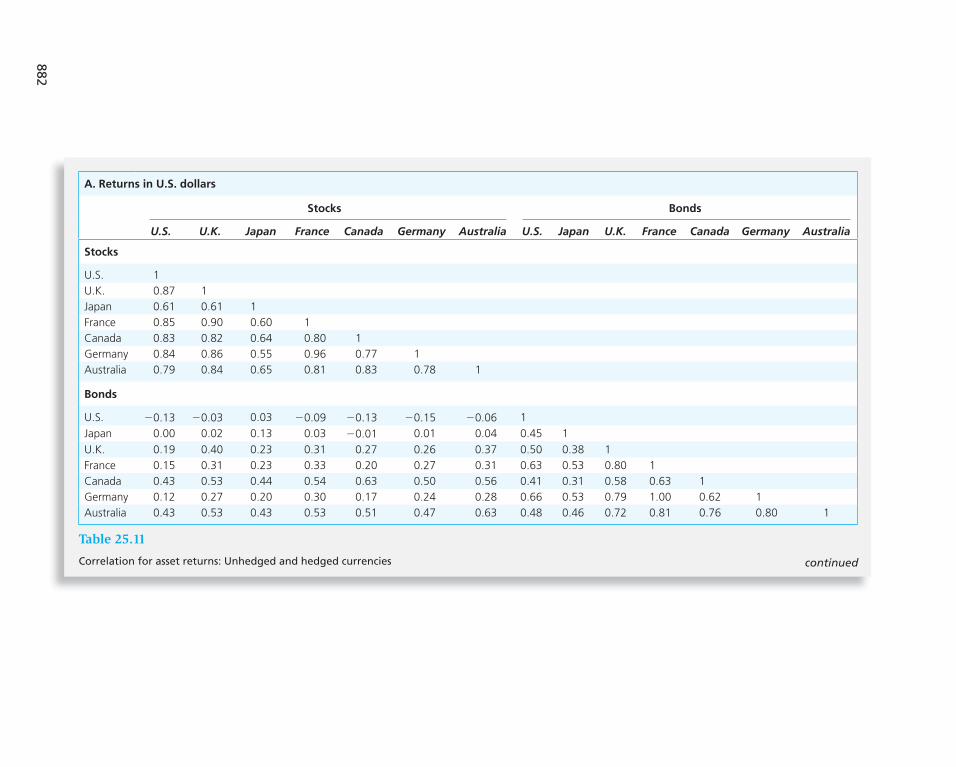
882
A. Returns in U.S. dollars
Stocks Bonds
U.S. U.K. Japan France Canada Germany Australia U.S. Japan U.K. France Canada Germany Australia
Stocks
U.S. 1
U.K. 0.87 1
Japan 0.61 0.61 1
France 0.85 0.90 0.60 1
Canada 0.83 0.82 0.64 0.80 1
Germany 0.84 0.86 0.55 0.96 0.77 1
Australia 0.79 0.84 0.65 0.81 0.83 0.78 1
Bonds
U.S. 20.13 20.03 0.03 20.09 20.13 20.15 20.06 1
Japan 0.00 0.02 0.13 0.03 20.01 0.01 0.04 0.45 1
U.K. 0.19 0.40 0.23 0.31 0.27 0.26 0.37 0.50 0.38 1
France 0.15 0.31 0.23 0.33 0.20 0.27 0.31 0.63 0.53 0.80 1
Canada 0.43 0.53 0.44 0.54 0.63 0.50 0.56 0.41 0.31 0.58 0.63 1
Germany 0.12 0.27 0.20 0.30 0.17 0.24 0.28 0.66 0.53 0.79 1.00 0.62 1
Australia 0.43 0.53 0.43 0.53 0.51 0.47 0.63 0.48 0.46 0.72 0.81 0.76 0.80 1
Table 25.11
Correlation for asset returns: Unhedged and hedged currencies continued

883
B. Returns in local currency (eqivalent to U.S. dollar returns plus fully hedged currency risk)
Stocks Bonds
U.S. Japan U.K. France Canada Germany Australia U.S. Japan U.K. France Canada Germany Australia
Stocks
U.S. 1
Japan 0.60 1
U.K. 0.87 0.59 1
France 0.82 0.63 0.89 1
Canada 0.84 0.61 0.74 0.74 1
Germany 0.81 0.57 0.84 0.95 0.70 1
Australia 0.73 0.64 0.74 0.74 0.68 0.69 1
Bonds
U.S. 20.13 20.16 20.13 20.25 20.11 20.28 20.18 1
Japan 20.03 20.27 20.05 20.16 20.14 20.12 20.09 0.36 1
U.K. 20.06 20.13 20.01 20.13 20.08 20.15 20.07 0.79 0.38 1
France 20.18 20.19 20.10 20.21 20.20 20.24 20.19 0.77 0.32 0.77 1
Canada 20.04 20.09 0.01 20.07 0.01 20.12 20.12 0.83 0.38 0.77 0.74 1
Germany 20.21 20.22 20.12 20.22 20.22 20.25 20.21 0.75 0.31 0.76 0.99 0.74 1
Australia 20.23 20.30 20.20 20.27 20.24 20.33 20.27 0.78 0.39 0.71 0.72 0.75 0.71 1
Table 25.11—concluded
Correlation for asset returns: Unhedged and hedged currencies
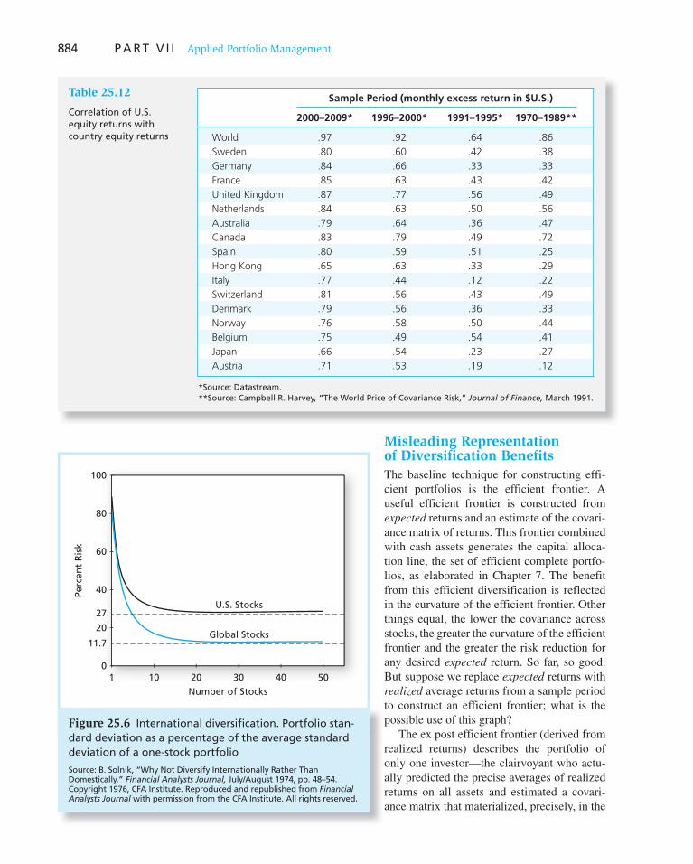
884 P A R T V I I Applied Portfolio Management
Misleading Representation of Diversification Benefits
The baseline technique for constructing effi-cient portfolios is the efficient frontier. A useful efficient frontier is constructed from expected returns and an estimate of the covari-ance matrix of returns. This frontier combined with cash assets generates the capital alloca-tion line, the set of efficient complete portfo-lios, as elaborated in Chapter 7. The benefit from this efficient diversification is reflected in the curvature of the efficient frontier. Other things equal, the lower the covariance across stocks, the greater the curvature of the efficient frontier and the greater the risk reduction for any desired expected return. So far, so good. But suppose we replace expected returns with realized average returns from a sample period to construct an efficient frontier; what is the possible use of this graph?
The ex post efficient frontier (derived from realized returns) describes the portfolio of only one investor—the clairvoyant who actu-ally predicted the precise averages of realized returns on all assets and estimated a covari-ance matrix that m aterialized, precisely, in the
27
11.7
1 10 20 30 40 50
U.S. Stocks
Global Stocks
Number of Stocks
Perc
ent
Ris
k
0
20
40
60
80
100
Figure 25.6 International diversification. Portfolio stan-dard deviation as a percentage of the average standard deviation of a one-stock portfolio
Source: B. Solnik, “Why Not Diversify Internationally Rather Than Domestically.” Financial Analysts Journal, July/August 1974, pp. 48–54. Copyright 1976, CFA Institute. Reproduced and republished from Financial Analysts Journal with permission from the CFA Institute. All rights reserved.
Table 25.12
Correlation of U.S. equity returns with country equity returns
Sample Period (monthly excess return in $U.S.)
2000–2009* 1996–2000* 1991–1995* 1970–1989**
World .97 .92 .64 .86
Sweden .80 .60 .42 .38
Germany .84 .66 .33 .33
France .85 .63 .43 .42
United Kingdom .87 .77 .56 .49
Netherlands .84 .63 .50 .56
Australia .79 .64 .36 .47
Canada .83 .79 .49 .72
Spain .80 .59 .51 .25
Hong Kong .65 .63 .33 .29
Italy .77 .44 .12 .22
Switzerland .81 .56 .43 .49
Denmark .79 .56 .36 .33
Norway .76 .58 .50 .44
Belgium .75 .49 .54 .41
Japan .66 .54 .23 .27
Austria .71 .53 .19 .12
*Source: Datastream.**Source: Campbell R. Harvey, “The World Price of Covariance Risk,” Journal of Finance, March 1991.

C H A P T E R 2 5 International Diversification 885
actual realizations of the sample period returns on all assets. Obviously, we are talking about a slim to empty set of investors. For all other, less-than-clairvoyant investors, such a frontier may have value only for purposes of performance evaluation.
In the world of volatile stocks, some stocks are bound to realize large, unexpected
average returns. This will be reflected in ex post efficient frontiers of enormous apparent “potential.” They will, however, suggest exaggerated diversification benefits. Such (elu-sive) potential was enumerated in Chapter 24 on performance evaluation. It has no mean-ing as a tool to discuss the potential for future investments for real-life investors.
Realistic Benefits from International Diversification
While recent realized returns can be highly misleading estimates of expected future returns, they are more useful for measuring prospective risk. There are two compelling reasons for this. First, market efficiency (or even near efficiency) implies that stock prices will be difficult to predict with any accuracy, but no such implication applies to risk measures. Second, it is a statistical fact that errors in estimates of standard deviation and correlation from realized data are of a lower order of magnitude than estimates of expected returns. For these reasons, using risk estimates from realized returns does not bias assessments of the potential benefits from diversification.
Figure 25.7 shows the efficient frontier using realized average monthly returns on the stock indexes of the 25 developed countries, with and without short sales. Even when the (ex post) efficient frontier is constrained to preclude short sales, it greatly exaggerates the benefits from diversification. Unfortunately, such misleading efficient frontiers are still presented in articles and texts on the benefits of diversification.
A more reasonable description of diversification is achievable only when we input rea-sonable equilibrium expected returns. Absent superior information, such expected returns are best based on appropriate risk measures of the assets. The capital asset pricing model (CAPM) suggests using the beta of the stock against the world portfolio. To generate expected excess returns (over the risk-free rate) for all assets, we specify the expected
World
AustriaKorea
New Zealand
−0.5
0.0
0.5
1.0
1.5
2.0
2.5
3.0
0 2 4 6
U.S.
8 10 12
Standard Deviation (% per month)
Rea
lized
Ave
rag
e M
on
thly
Exc
ess
Ret
urn
(%
)
Efficient frontier with short salesEfficient frontier w/ no short salesCountry portfolios
Figure 25.7 Ex post efficient frontier of country portfolios, 2001–2005

886 P A R T V I I Applied Portfolio Management
excess return on the world portfolio. We obtain the expected excess return on each asset by multiplying the beta of the asset by the world portfolio expected excess return. This procedure presupposes that the world portfolio will lie on the efficient frontier, at the point of tangency with the world capital market line. The curvature of the efficient frontier will not be affected by the estimate of the world portfolio excess return. A higher estimate will simply shift the curve upward.
We perform this procedure with risk measures estimated from actual returns and fur-ther impose the likely applicable constraint on short sales. We use the betas to compute the expected return on individual markets, assuming the expected excess return on the world port-folio is .6% per month. This excess return is in line with the average return over the previous 50 years. Varying this estimate would not qualitatively affect the results shown in Figure 25.8 (which is drawn on the same scale as Figure 25.7 ). The figure shows a realistic assessment that reveals modest but significant benefits from international diversification using only devel-oped markets. Incorporating emerging markets would further increase these benefits.
Are Benefits from International Diversification Preserved in Bear Markets?
Some studies suggest that correlation in country portfolio returns increases during peri-ods of turbulence in capital markets. 7 If so, benefits from diversification would be lost exactly when they are needed the most. For example, a study by Roll of the crash of
7 F. Longin and B. Solnik, “Is the Correlation in International Equity Returns Constant: 1960–1990?” Journal of
International Money and Finance 14 (1995), pp. 3–26; and Eric Jacquier and Alan Marcus, “Asset Allocation Models and Market Volatility,” Financial Analysts Journal 57 (March/April 2001), pp. 16–30.
World
U.S.
0.0
0.2
0.4
0.6
0.8
1.0
1.2
0 2 4 6 8 10 12Standard Deviation (% per month)
Exp
ecte
d M
on
thly
Exc
ess
Ret
urn
(%
) World CMLEfficient frontier w/ no short salesEfficient frontier w/ short salesCountry portfolios
Figure 25.8 Efficient frontier of country portfolios (world expected excess return 5 .6% per month)

C H A P T E R 2 5 International Diversification 887
October 1987 shows that all 23 country indexes studied declined over the crash period of October 12–26. 8 This correlation is reflected in the movements of regional indexes depicted in Figure 25.9 . Roll found that the beta of a country index on the world index (estimated prior to the crash) was the best predictor of that index’s response to the October crash of the U.S. stock market. This suggests a common factor underlying the movement of stocks around the world. This model predicts that a macroeconomic shock would affect all countries and that diversification can only mitigate country-specific events.
The 2008 crash of stock markets around the world allows us to test Roll’s prediction. The data in Figure 25.10 include average monthly rates of return for both the 10-year period 1999–2008 and the crisis period corresponding to the last 4 months of 2008, as well as the beta on the U.S. market and monthly standard deviation for several portfolios. The graph shows that both beta against the U.S. and the country-index standard deviation explain the difference between crisis period returns and overall period averages. Market behavior during the 1987 crisis, that is, larger correlations in extreme bad times, repeated itself in the crisis of 2008, vindicating Roll’s prediction.
8 Richard Roll, “The International Crash of October 1987,” Financial Analysts Journal, September–October 1988.
Value of One Currency Unit
1.05
Tick Marks on October Date, 4:00 P.M., U.S. Eastern Standard Time
12 14 16 18 20 22 24 26
Symbols positionedat market closelocal time
North America
0.65
0.7
0.75
0.8
0.85
0.9
0.95
1
Australia/New ZealandAsiaSmall EuropeLarge EuropeIreland, So. Africa, U.K.
Figure 25.9 Regional indexes around the crash, October 14–October 26, 1987
Source: From Richard Roll, “The International Crash of October 1987,” Financial Analysts Journal, September–October 1988. Copyright 1998, CFA Institute. Reproduced from Financial Analysts Journal with permission from the CFA Institute. All rights reserved.
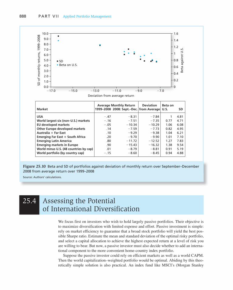
888 P A R T V I I Applied Portfolio Management
25.4 Assessing the Potential of International Diversification
10.0
9.0
8.0
7.0
6.0
5.0
4.0SDBeta on U.S.
3.0
2.0
1.0
0.0�17.0
SD o
f m
on
thly
ret
urn
s, 1
999–
2008
�15.0 �13.0
Deviation from average return
�11.0 �9.0 �7.00
0.2
Bet
a ag
ain
st U
.S.
0.4
0.6
0.8
1
1.2
1.4
1.6
Market
USA �.47 �8.31 �7.84 1 4.81World largest six (non–U.S.) markets �.16 �7.51 �7.35 0.77 4.71EU developed markets �.05 �10.34 �10.29 1.06 6.08Other Europe developed markets .14 �7.59 �7.73 0.82 4.95Australia � Far East .10 �9.29 �9.38 1.04 6.21Emerging Far East � South Africa .20 �9.70 �9.90 1.01 7.10Emerging Latin America .80 �11.72 �12.52 1.27 7.83Emerging markets in Europe .90 �15.43 �16.32 1.38 9.54World minus U.S. (48 countries by cap) .01 �8.79 �8.81 0.91 5.19World portfolio (by country cap) �.15 �8.60 �8.45 0.94 4.88
1999–2008 2008: Sept.–Dec.Average Monthly Return Deviation
from AverageBeta onU.S. SD
Figure 25.10 Beta and SD of portfolios against deviation of monthly return over September–December 2008 from average return over 1999–2008
Source: Authors’ calculations.
We focus first on investors who wish to hold largely passive portfolios. Their objective is to maximize diversification with limited expense and effort. Passive investment is simple: rely on market efficiency to guarantee that a broad stock portfolio will yield the best pos-sible Sharpe ratio. Estimate the mean and standard deviation of the optimal risky portfolio, and select a capital allocation to achieve the highest expected return at a level of risk you are willing to bear. But now, a passive investor must also decide whether to add an interna-tional component to the more convenient home-country index portfolio.
Suppose the passive investor could rely on efficient markets as well as a world CAPM. Then the world capitalization–weighted portfolio would be optimal. Abiding by this theo-retically simple solution is also practical. An index fund like MSCI’s (Morgan Stanley
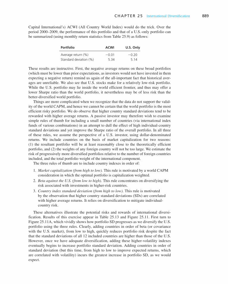
C H A P T E R 2 5 International Diversification 889
Capital International’s) ACWI (All Country World Index) would do the trick. Over the period 2000–2009, the performance of this portfolio and that of a U.S.-only portfolio can be summarized (using monthly return statistics from Table 25.9 ) as follows:
Portfolio ACWI U.S. Only
Average return (%) 20.01 20.20
Standard deviation (%) 5.34 5.14
These results are instructive. First, the negative average returns on these broad portfolios (which must be lower than prior expectations, as investors would not have invested in them expecting a negative return) remind us again of the all-important fact that historical aver-ages are unreliable. We also see that U.S. stocks make for a relatively low-risk portfolio. While the U.S. portfolio may lie inside the world efficient frontier, and thus may offer a lower Sharpe ratio than the world portfolio, it nevertheless may be of less risk than the better-diversified world portfolio.
Things are more complicated when we recognize that the data do not support the valid-ity of the world CAPM, and hence we cannot be certain that the world portfolio is the most efficient risky portfolio. We do observe that higher country standard deviations tend to be rewarded with higher average returns. A passive investor may therefore wish to examine simple rules of thumb for including a small number of countries (via international index funds of various combinations) in an attempt to dull the effect of high individual-country standard deviations and yet improve the Sharpe ratio of the overall portfolio. In all three of these rules, we assume the perspective of a U.S. investor, using dollar- denominated returns. We include countries on the basis of market capitalization for two reasons: (1) the resultant portfolio will be at least reasonably close to the theoretically efficient portfolio, and (2) the weights of any foreign country will not be too large. We estimate the risk of progressively more diversified portfolios relative to the number of foreign countries included, and the total portfolio weight of the international component.
The three rules of thumb are to include country indexes in order of:
1. Market capitalization (from high to low). This rule is motivated by a world CAPM consideration in which the optimal portfolio is capitalization weighted.
2. Beta against the U.S. (from low to high). This rule concentrates on diversifying the risk associated with investments in higher-risk countries.
3. Country index standard deviation (from high to low). This rule is motivated by the observation that higher country standard deviations (SDs) are correlated with higher average returns. It relies on diversification to mitigate individual-country risk.
These alternatives illustrate the potential risks and rewards of international diversi-fication. Results of this exercise appear in Table 25.13 and Figure 25.11 . First turn to Figure 25.11 A, which vividly shows how portfolio SD progresses as we diversify the U.S. portfolio using the three rules. Clearly, adding countries in order of beta (or covariance with the U.S. market), from low to high, quickly reduces portfolio risk despite the fact that the standard deviations of all 12 included countries are higher than those of the U.S. However, once we have adequate diversification, adding these higher-volatility indexes eventually begins to increase portfolio standard deviation. Adding countries in order of standard deviation (but this time, from high to low to improve expected returns, which are correlated with volatility) incurs the greatest increase in portfolio SD, as we would expect.
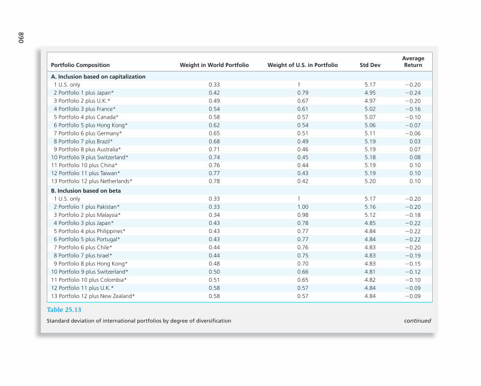
890
Portfolio Composition Weight in World Portfolio Weight of U.S. in Portfolio Std DevAverageReturn
A. Inclusion based on capitalization
1 U.S. only 0.33 1 5.17 20.20
2 Portfolio 1 plus Japan* 0.42 0.79 4.95 20.24
3 Portfolio 2 plus U.K.* 0.49 0.67 4.97 20.20
4 Portfolio 3 plus France* 0.54 0.61 5.02 20.16
5 Portfolio 4 plus Canada* 0.58 0.57 5.07 20.10
6 Portfolio 5 plus Hong Kong* 0.62 0.54 5.06 20.07
7 Portfolio 6 plus Germany* 0.65 0.51 5.11 20.06
8 Portfolio 7 plus Brazil* 0.68 0.49 5.19 0.03
9 Portfolio 8 plus Australia* 0.71 0.46 5.19 0.07
10 Portfolio 9 plus Switzerland* 0.74 0.45 5.18 0.08
11 Portfolio 10 plus China* 0.76 0.44 5.19 0.10
12 Portfolio 11 plus Taiwan* 0.77 0.43 5.19 0.10
13 Portfolio 12 plus Netherlands* 0.78 0.42 5.20 0.10
B. Inclusion based on beta
1 U.S. only 0.33 1 5.17 20.20
2 Portfolio 1 plus Pakistan* 0.33 1.00 5.16 20.20
3 Portfolio 2 plus Malaysia* 0.34 0.98 5.12 20.18
4 Portfolio 3 plus Japan* 0.43 0.78 4.85 20.22
5 Portfolio 4 plus Philippines* 0.43 0.77 4.84 20.22
6 Portfolio 5 plus Portugal* 0.43 0.77 4.84 20.22
7 Portfolio 6 plus Chile* 0.44 0.76 4.83 20.20
8 Portfolio 7 plus Israel* 0.44 0.75 4.83 20.19
9 Portfolio 8 plus Hong Kong* 0.48 0.70 4.83 20.15
10 Portfolio 9 plus Switzerland* 0.50 0.66 4.81 20.12
11 Portfolio 10 plus Colombia* 0.51 0.65 4.82 20.10
12 Portfolio 11 plus U.K.* 0.58 0.57 4.84 20.09
13 Portfolio 12 plus New Zealand* 0.58 0.57 4.84 20.09
Table 25.13
Standard deviation of international portfolios by degree of diversification continued
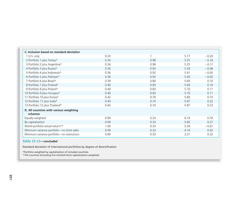
891
C. Inclusion based on standard deviation
1 U.S. only 0.33 1 5.17 20.20
2 Portfolio 1 plus Turkey* 0.34 0.98 5.25 20.18
3 Portfolio 2 plus Argentina* 0.34 0.98 5.25 20.17
4 Portfolio 3 plus Russia* 0.36 0.93 5.39 20.08
5 Portfolio 4 plus Indonesia* 0.36 0.92 5.41 20.05
6 Portfolio 5 plus Pakistan* 0.36 0.92 5.40 20.05
7 Portfolio 6 plus Brazil* 0.39 0.84 5.66 0.10
8 Portfolio 7 plus Finland* 0.40 0.83 5.69 0.10
9 Portfolio 8 plus Poland* 0.40 0.83 5.70 0.11
10 Portfolio 9 plus Hungary* 0.40 0.83 5.70 0.11
11 Portfolio 10 plus Korea* 0.42 0.79 5.80 0.15
12 Portfolio 11 plus India* 0.44 0.74 5.87 0.22
13 Portfolio 12 plus Thailand* 0.45 0.74 5.87 0.23
D. All countries with various weighting
schemes
Equally weighted 0.99 0.33 6.14 0.76
By capitalization 0.99 0.33 5.60 0.27
World portfolio actual return** 1.00 0.33 5.34 20.01
Minimum variance portfolio—no short sales 0.99 0.33 4.14 0.02
Minimum variance portfolio—no restrictions 0.99 0.33 2.21 0.32
Table 25.13 —concluded
Standard deviation of international portfolios by degree of diversification
*Portfolio weighted by capitalization of included countries.**All countries (including five omitted here) capitalization-weighted.

892 P A R T V I I Applied Portfolio Management
Figure 25.11 B confirms the observations we made from the regressions in Table 25.10 .
Inclusion in order of standard deviations also increases average returns. Inclusion by beta
also increases average returns, at least for low-beta countries, suggesting that at least at a
qualitative level, international CAPM issues affect asset pricing.
4.60
4.80
5.00
5.20
5.40
5.60
5.80
5.85
0.30 0.35 0.40 0.45 0.50 0.55 0.60 0.700.65 0.75 0.80Fraction of World Portfolio Capitalization
Stan
dar
d D
evia
tio
n (
% p
er m
on
th) Inclusion in order of market capitalization
Inclusion in order of betaInclusion in order of SD
�0.30
�0.20
�0.10
0.00
0.10
0.20
0.30
0.40
0.30 0.35 0.40 0.45 0.50 0.55 0.60 0.700.65 0.75 0.80Fraction of World Portfolio Capitalization
Ave
rag
e R
etu
rn (
% p
er m
on
th)
Inclusion in order of market capitalizationInclusion in order of betaInclusion in order of standard deviation
Figure 25.11 Risks and rewards of international portfolios, 2000–2009. Panel A, Standard deviations for international portfolios; Panel B, Average return of i nternational portfolios.
C H A P T E R 2 5 International Diversification 893
Broadly speaking, these results are consistent with logic of the previous chapters. First, diversification pays, and risk is rewarded. Second, even with strong home-country bias, covariance risk still plays a role internationally. We also see that when confined to domes-tic markets, risk aversion across the world is not too different: higher country standard deviations match up with higher average returns.
In Panel D of Table 25.13 , we examine risk and reward from fuller international diversi-fication. Observe first that an equally weighted portfolio of all countries is the riskiest in the group. At the same time, because this portfolio assigns much larger weights to the smaller, high-volatility–high-return countries, it also provides a higher average return. At the other extreme, consider the minimum-variance portfolios, with and without short-sale constraints. Without the short-sale restriction, the minimum-variance portfolio attains the amazingly low SD of 2.21%, less than half that of the lowest-SD country (the U.S.). However, this portfolio is probably not practical, including 22 short positions, the largest being 215% (in Sweden). When short sales are disallowed, the SD is far higher, 4.14%, offering much less improve-ment over the capitalization-weighted portfolio. Moreover, these portfolio weights also would be impractical, with the largest weight in Malaysia (29%), and only 7% in the U.S.
One puzzling and instructive feature of the results in Table 25.13 is the lower average return on the actual world portfolio (ACWI) compared with the 44-country portfolios. The difference arises because MSCI country-index portfolios are not capitalization-weighted portfolios. MSCI uses industry-weighted portfolios, which places greater weights on the larger stocks in each country. Since small stocks performed better over 2000–2009, the ACWI portfolio had a lower average return. This pattern is not guaranteed, or necessarily even likely, to apply to future returns.
25.5 International Investing and Performance Attribution
The benefits from international diversification may be modest for passive investors but for active managers international investing offers greater opportunities. International investing calls for specialization in additional fields of analysis: currency, country and worldwide industry, as well as a greater universe for stock selection.
Constructing a Benchmark Portfolio of Foreign Assets
Active international investing, as well as passive, requires a benchmark portfolio (the bogey). One widely used index of non-U.S. stocks is the Europe, Australasia, Far East
(EAFE) index computed by Morgan Stanley Capital International. Additional indexes of world equity performance are published by Morgan Stanley Capital International Indices, Credit Suisse First Boston, and Goldman Sachs. Portfolios designed to mirror or even replicate the country, currency, and company representation of these indexes would be the obvious generalization of the purely domestic passive equity strategy.
An issue that sometimes arises in the international context is the appropriateness of market-capitalization weighting schemes in the construction of international indexes. Capitalization weighting is far and away the most common approach. However, some argue that it might not be the best weighting scheme in an international context. This is in part because different countries have differing proportions of their corporate sector orga-nized as publicly traded firms.
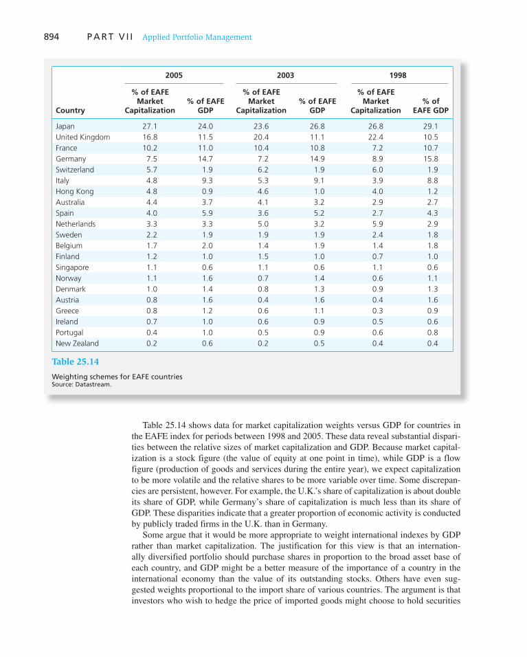
894 P A R T V I I Applied Portfolio Management
Table 25.14 shows data for market capitalization weights versus GDP for countries in the EAFE index for periods between 1998 and 2005. These data reveal substantial dispari-ties between the relative sizes of market capitalization and GDP. Because market capital-ization is a stock figure (the value of equity at one point in time), while GDP is a flow figure (production of goods and services during the entire year), we expect capitalization to be more volatile and the relative shares to be more variable over time. Some discrepan-cies are persistent, however. For example, the U.K.’s share of capitalization is about double its share of GDP, while Germany’s share of capitalization is much less than its share of GDP. These disparities indicate that a greater proportion of economic activity is conducted by publicly traded firms in the U.K. than in Germany.
Some argue that it would be more appropriate to weight international indexes by GDP rather than market capitalization. The justification for this view is that an internation-ally diversified portfolio should purchase shares in proportion to the broad asset base of each country, and GDP might be a better measure of the importance of a country in the international economy than the value of its outstanding stocks. Others have even sug-gested weights proportional to the import share of various countries. The argument is that investors who wish to hedge the price of imported goods might choose to hold securities
2005 2003 1998
Country
% of EAFE Market
Capitalization% of EAFE
GDP
% of EAFE Market
Capitalization% of EAFE
GDP
% of EAFE Market
Capitalization% of
EAFE GDP
Japan 27.1 24.0 23.6 26.8 26.8 29.1
United Kingdom 16.8 11.5 20.4 11.1 22.4 10.5
France 10.2 11.0 10.4 10.8 7.2 10.7
Germany 7.5 14.7 7.2 14.9 8.9 15.8
Switzerland 5.7 1.9 6.2 1.9 6.0 1.9
Italy 4.8 9.3 5.3 9.1 3.9 8.8
Hong Kong 4.8 0.9 4.6 1.0 4.0 1.2
Australia 4.4 3.7 4.1 3.2 2.9 2.7
Spain 4.0 5.9 3.6 5.2 2.7 4.3
Netherlands 3.3 3.3 5.0 3.2 5.9 2.9
Sweden 2.2 1.9 1.9 1.9 2.4 1.8
Belgium 1.7 2.0 1.4 1.9 1.4 1.8
Finland 1.2 1.0 1.5 1.0 0.7 1.0
Singapore 1.1 0.6 1.1 0.6 1.1 0.6
Norway 1.1 1.6 0.7 1.4 0.6 1.1
Denmark 1.0 1.4 0.8 1.3 0.9 1.3
Austria 0.8 1.6 0.4 1.6 0.4 1.6
Greece 0.8 1.2 0.6 1.1 0.3 0.9
Ireland 0.7 1.0 0.6 0.9 0.5 0.6
Portugal 0.4 1.0 0.5 0.9 0.6 0.8
New Zealand 0.2 0.6 0.2 0.5 0.4 0.4
Table 25.14
Weighting schemes for EAFE countriesSource: Datastream.

895
in foreign firms in proportion to the goods imported from those countries. The nearby box considers the question of global asset allocation for investors seeking effective interna-tional diversification.
Performance Attribution
We can measure the contribution of each of these factors following a manner similar to the performance attribution techniques introduced in Chapter 24.
1. Currency selection measures the contribution to total portfolio performance attrib-utable to exchange rate fluctuations relative to the investor’s benchmark currency, which we will take to be the U.S. dollar. We might use a benchmark like the EAFE index to compare a portfolio’s currency selection for a particular period to a passive
International Investing Raises Questions
As Yogi Berra might say, the problem with international investing is that it’s so darn foreign.
Currency swings? Hedging? International diversifica-tion? What’s that?
Here are answers to five questions that I’m often asked:
• Foreign stocks account for some 60% of world stock market value, so shouldn’t you have 60% of your stock market money overseas?
The main reason to invest abroad isn’t to replicate the global market or to boost returns. Instead, “what we’re trying to do by adding foreign stocks is to reduce volatil-ity,” explains Robert Ludwig, chief investment officer at money manager SEI Investments.
Foreign stocks don’t move in sync with U.S. shares and, thus, they may provide offsetting gains when the U.S. mar-ket is falling. But to get the resulting risk reduction, you don’t need anything like 60% of your money abroad.
• So, how much foreign exposure do you need to get decent diversification?
“Based on the volatility of foreign markets and the cor-relation between markets, we think an optimal portfolio is 70% in the U.S., 20% in developed foreign markets, and 10% in emerging markets,” Mr. Ludwig says.
Even with a third of your stock market money in foreign issues, you may find that the risk-reduction benefits aren’t all that reliable. Unfortunately, when U.S. stocks get really pounded, it seems foreign shares also tend to tumble.
• Can U.S. companies with global operations give you international diversification?
“When you look at these multinationals, the factor that drives their performance is their home market,” says Mark Riepe, a vice president with Ibbotson Associates, a Chicago research firm.
How come? U.S. multinationals tend to be owned by U.S. investors, who will be swayed by the ups and downs of the U.S. market. In addition, Mr. Riepe notes that while multinationals may derive substantial profits and revenue abroad, most of their costs—especially labor costs—will be incurred in the U.S.
• Does international diversification come from the for-eign stocks or the foreign currency?
“It comes from both in roughly equal pieces,” Mr. Riepe says. “Those who choose to hedge their foreign currency raise the correlation with U.S. stocks, and so the diversifica-tion benefit won’t be nearly as great.”
Indeed, you may want to think twice before investing in a foreign-stock fund that frequently hedges its currency exposure in an effort to mute the impact of—and make money from—changes in foreign-exchange rates.
“The studies that we’ve done show that stock managers have hurt themselves more than they’ve helped themselves by actively managing currencies,” Mr. Ludwig says.
• Should you divvy up your money among foreign coun-tries depending on the size of each national stock market?
At issue is the nagging question of how much to put in Japan. If you replicated the market weightings of Morgan Stanley Capital International’s Europe, Australasia and Far East index, you would currently have around a third of your overseas money in Japan.
That’s the sort of weighting you find in international funds, which seek to track the performance of the EAFE or similar international indexes. Actively managed f oreign-stock funds, by contrast, pay less attention to market weights and on average, these days have just 14% in Japan.
If your focus is risk reduction rather than performance, the index—and the funds that track it—are the clear win-ners. Japan performs quite unlike the U.S. market, so it provides good diversification for U.S. investors, says Tricia Rothschild, international editor at Morningstar Mutual Funds, a Chicago newsletter.
“But correlations aren’t static,” she adds. “There’s always a problem with taking what happened over the past 20 years and projecting it out over the next 20 years.”
Source: Jonathan Clements, “International Investing Raises Questions on Allocation, Diversification, Hedging,” The Wall Street Journal, July 29, 1997. Excerpted by permission of The Wall Street Journal. © 1997 Dow Jones & Company, Inc. All rights reserved worldwide.
WO
RD
S FRO
M TH
E STREET

896
eXcel APPLICATIONS: International Portfolios
T his Excel model provides an efficient frontier analysis similar to that in Chapter 6. In Chapter 6 the frontier
was based on individual securities, whereas this model examines the returns on international exchange–traded
funds and enables us to analyze the benefits of interna-tional diversification. Go to the Online Learning Center at www.mhhe.com/bkm.
58
59
60
61
62
63
64
65
66
67
68
69
70
71
72
73
74
75
76
77
78
79
80
81
82
83
84
85
86
87
A B C D E F G H I J
Bordered Covariance Matrix for Target Return Portfolio
EWD EWH EWI EWJ EWL EWP EWW SP 500
Weights 0.00 0.00 0.08 0.38 0.02 0.00 0.00 0.520.0000 0.00 0.00 0.00 0.00 0.00 0.00 0.00 0.000.0000 0.00 0.00 0.00 0.00 0.00 0.00 0.00 0.000.0826 0.00 0.00 4.63 3.21 0.55 0.00 0.00 7.690.3805 0.00 0.00 3.21 98.41 1.82 0.00 0.00 53.790.0171 0.00 0.00 0.55 1.82 0.14 0.00 0.00 2.090.0000 0.00 0.00 0.00 0.00 0.00 0.00 0.00 0.000.0000 0.00 0.00 0.00 0.00 0.00 0.00 0.00 0.000.5198 0.00 0.00 7.69 53.79 2.09 0.00 0.00 79.901.0000 0.00 0.00 16.07 157.23 4.59 0.00 0.00 143.47
Port Via 321.36Port S.D. 17.93Port Mean 12.00
Weights
Mean St. Dev EWD EWH EWI EWJ EWL EWP EWW SP 500
6 21.89 0.02 0.00 0.00 0.71 0.00 0.02 0.00 0.269 19.66 0.02 0.00 0.02 0.53 0.02 0.00 0.00 0.41
12 17.93 0.00 0.00 0.08 0.38 0.02 0.00 0.00 0.5215 16.81 0.00 0.00 0.14 0.22 0.02 0.00 0.00 0.6218 16.46 0.00 0.00 0.19 0.07 0.02 0.00 0.00 0.7321 17.37 0.00 0.00 0.40 0.00 0.00 0.00 0.00 0.6024 21.19 0.00 0.00 0.72 0.00 0.00 0.00 0.00 0.2827 26.05 0.00 0.00 1.00 0.00 0.00 0.00 0.00 0.00
CONCEPT CHECK
3
Using the data in Table 25.15 , compute the man-ager’s country and currency selection if portfolio weights had been 40% in Europe, 20% in Aus-tralia, and 40% in the Far East.
benchmark. EAFE currency selection would be computed as the weighted average of the currency appreciation of the currencies represented in the EAFE portfolio using as weights the fraction of the EAFE portfolio invested in each currency.
2. Country selection measures the contribution to performance attributable to invest-ing in the better-performing stock markets of the world. It can be measured as the weighted average of the equity index returns of each country using as weights the share of the manager’s portfolio in each country. We use index returns to abstract from the effect of security selection within countries. To measure a manager’s contribution relative to a passive strategy, we might compare country selection to the weighted average across countries of equity index returns using as weights the share of the EAFE portfolio in each country.
3. Stock selection ability may, as in Chapter 24, be measured as the weighted average of equity returns in excess of the equity index in each country. Here, we would use local currency returns and use as weights the investments in each country.
4. Cash/bond selection may be measured as the excess return derived from weight-ing bonds and bills differently from some benchmark weights.
Table 25.15 gives an example of how to mea-sure the contribution of the decisions an interna-tional portfolio manager might make.

Vis
it u
s at
ww
w.m
hh
e.co
m/b
kmV
isit
us
at w
ww
.mh
he.
com
/bkm
C H A P T E R 2 5 International Diversification 897
1. U.S. assets are only a part of the world portfolio. International capital markets offer important
opportunities for portfolio diversification with enhanced risk–return characteristics.
2. Exchange rate risk imparts an extra source of uncertainty to investments denominated in foreign
currencies. Much of that risk can be hedged in foreign exchange futures or forward markets, but
a perfect hedge is not feasible unless the foreign currency rate of return is known.
3. Several world market indexes can form a basis for passive international investing. Active interna-
tional management can be partitioned into currency selection, country selection, stock selection,
and cash/bond selection.
SUMMARY
Related Web sites for this chapter are available at www.mhhe.com/bkm
EAFE Weight
Return on Equity Index
Currency Appreciation
E1/E0 2 1Manager’s
WeightManager’s
Return
Europe 0.30 10% 10% 0.35 8%
Australia 0.10 5 210 0.10 7
Far East 0.60 15 30 0.55 18
Overall performance (dollar return 5 return on index 1 currency appreciation)
EAFE: .30(10 1 10) 1 .10(5 2 10) 1 .60(15 1 30) 5 32.5%
Manager: .35(8 1 10) 1 .10(7 2 10) 1 .55(18 1 30) 5 32.4%
Loss of .10% relative to EAFE
Currency selection
EAFE: (0.30 3 10%) 1 (0.10 3 (210%)) 1 (0.60 3 30%) 5 20% appreciation
Manager: (0.35 3 10%) 1 (0.10 3 (210%)) 1 (0.55 3 30%) 5 19% appreciation
Loss of 1% relative to EAFE
Country selection
EAFE: (0.30 3 10%) 1 (0.10 3 5%) 1 (0.60 3 15%) 5 12.5%
Manager: (0.35 3 10%) 1 (0.10 3 5%) 1 (0.55 3 15%) 5 12.25%
Loss of 0.25% relative to EAFE
Stock selection
(8% 2 10%)0.35 1 (7% 2 5%)0.10 1 (18% 2 15%)0.55 5 1.15%
Contribution of 1.15% relative to EAFE
Sum of attributions (equal to overall performance)
Currency (21%) 1 country (2.25%) 1 selection (1.15%) 5 2.10%
Table 25.15
Example of p erformance attribu-tion: international
exchange rate risk
interest rate parity relationship
covered interest arbitrage
relationship
political risk
home bias
Europe, Australasia, Far East
(EAFE) index
currency selection
country selection
stock selection
cash/bond selection
KEY TERMS
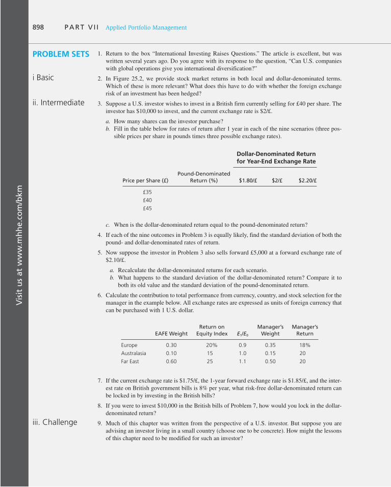
Vis
it u
s at
ww
w.m
hh
e.co
m/b
km898 P A R T V I I Applied Portfolio Management
1. Return to the box “International Investing Raises Questions.” The article is excellent, but was written several years ago. Do you agree with its response to the question, “Can U.S. companies with global operations give you international diversification?”
2. In Figure 25.2 , we provide stock market returns in both local and dollar-denominated terms. Which of these is more relevant? What does this have to do with whether the foreign exchange risk of an investment has been hedged?
3. Suppose a U.S. investor wishes to invest in a British firm currently selling for £40 per share. The investor has $10,000 to invest, and the current exchange rate is $2/£.
a. How many shares can the investor purchase? b. Fill in the table below for rates of return after 1 year in each of the nine scenarios (three pos-
sible prices per share in pounds times three possible exchange rates).
Dollar-Denominated Return for Year-End Exchange Rate
Price per Share (£)Pound-Denominated
Return (%) $1.80/£ $2/£ $2.20/£
£35
£40
£45
c. When is the dollar-denominated return equal to the pound-denominated return?
4. If each of the nine outcomes in Problem 3 is equally likely, find the standard deviation of both the pound- and dollar-denominated rates of return.
5. Now suppose the investor in Problem 3 also sells forward £5,000 at a forward exchange rate of $2.10/£.
a. Recalculate the dollar-denominated returns for each scenario. b. What happens to the standard deviation of the dollar-denominated return? Compare it to
both its old value and the standard deviation of the pound-denominated return.
6. Calculate the contribution to total performance from currency, country, and stock selection for the manager in the example below. All exchange rates are expressed as units of foreign currency that can be purchased with 1 U.S. dollar.
EAFE WeightReturn on
Equity Index E1/E0
Manager’s Weight
Manager’s Return
Europe 0.30 20% 0.9 0.35 18%
Australasia 0.10 15 1.0 0.15 20
Far East 0.60 25 1.1 0.50 20
7. If the current exchange rate is $1.75/£, the 1-year forward exchange rate is $1.85/£, and the inter-est rate on British government bills is 8% per year, what risk-free dollar-denominated return can be locked in by investing in the British bills?
8. If you were to invest $10,000 in the British bills of Problem 7, how would you lock in the dollar-denominated return?
9. Much of this chapter was written from the perspective of a U.S. investor. But suppose you are advising an investor living in a small country (choose one to be concrete). How might the lessons of this chapter need to be modified for such an investor?
PROBLEM SETS
i Basic
ii. Intermediate
iii. Challenge

Vis
it u
s at
ww
w.m
hh
e.co
m/b
km
C H A P T E R 2 5 International Diversification 899
1. You are a U.S. investor who purchased British securities for £2,000 one year ago when the British pound cost U.S.$1.50. What is your total return (based on U.S. dollars) if the value of the securi-ties is now £2,400 and the pound is worth $1.75? No dividends or interest were paid during this period.
2. The correlation coefficient between the returns on a broad index of U.S. stocks and the returns on indexes of the stocks of other industrialized countries is mostly ________ , and the correla-tion coefficient between the returns on various diversified portfolios of U.S. stocks is mostly ________ .
a. less than .8; greater than .8. b. greater than .8; less than .8. c. less than 0; greater than 0. d. greater than 0; less than 0.
3. An investor in the common stock of companies in a foreign country may wish to hedge against the ________ of the investor’s home currency and can do so by ________ the foreign currency in the forward market.
a. depreciation; selling. b. appreciation; purchasing. c. appreciation; selling. d. depreciation; purchasing.
4. John Irish, CFA, is an independent investment adviser who is assisting Alfred Darwin, the head of the Investment Committee of General Technology Corporation, to establish a new pension fund. Darwin asks Irish about international equities and whether the Investment Committee should consider them as an additional asset for the pension fund.
a. Explain the rationale for including international equities in General’s equity portfolio. Identify and describe three relevant considerations in formulating your answer.
b. List three possible arguments against international equity investment and briefly discuss the significance of each.
c. To illustrate several aspects of the performance of international securities over time, Irish shows Darwin the accompanying graph of investment results experienced by a U.S. pen-sion fund in the recent past. Compare the performance of the U.S. dollar and non-U.S. dollar equity and fixed-income asset categories, and explain the significance of the result of the account performance index relative to the results of the four individual asset class indexes.
10 20 30 40
6
0
1
2
3
4
5
Annualized Historical Performance Data(%)
Variability(standarddeviation)
U.S. $BondsNon-U.S. $Bonds
EAFE IndexAccount Performance Index
S&P Index
Real Returns (%)

Vis
it u
s at
ww
w.m
hh
e.co
m/b
km900 P A R T V I I Applied Portfolio Management
5. You are a U.S. investor considering purchase of one of the following securities. Assume that the currency risk of the Canadian government bond will be hedged, and the 6-month discount on Canadian dollar forward contracts is 2 .75% versus the U.S. dollar.
Bond Maturity Coupon Price
U.S. government 6 months 6.50% 100.00
Canadian government 6 months 7.50% 100.00
Calculate the expected price change required in the Canadian government bond that would result in the two bonds having equal total returns in U.S. dollars over a 6-month horizon. Assume that the yield on the U.S. bond is expected to remain unchanged.
6. A global manager plans to invest $1 million in U.S. government cash equivalents for the next 90 days. However, she is also authorized to use non-U.S. government cash equivalents, as long as the currency risk is hedged to U.S. dollars using forward currency contracts.
a. What rate of return will the manager earn if she invests in money market instruments in either Canada or Japan and hedges the dollar value of her investment? Use the data in the following tables.
b. What must be the approximate value of the 90-day interest rate available on U.S. government securities?
Interest Rates (APR) 90-Day Cash Equivalents
Japanese government 2.52%
Canadian government 6.74%
Exchange Rates Dollars per Unit of Foreign Currency
Spot 90-Day Forward
Japanese yen .0119 .0120
Canadian dollar .7284 .7269
7. The Windsor Foundation, a U.S.-based, not-for-profit charitable organization, has a diversified investment portfolio of $100 million. Windsor’s board of directors is considering an initial invest-ment in emerging market equities. Robert Houston, treasurer of the foundation, has made the fol-lowing four comments:
a. “For an investor holding only developed market equities, the existence of stable emerging market currencies is one of several preconditions necessary for that investor to realize strong emerging market performance.”
b. “Local currency depreciation against the dollar has been a frequent occurrence for U.S. inves-tors in emerging markets. U.S. investors have consistently seen large percentages of their returns erased by currency depreciation. This is true even for long-term investors.”
c. “Historically, the addition of emerging market stocks to a U.S. equity portfolio such as the S&P 500 index has reduced volatility; volatility has also been reduced when emerg-ing market stocks are combined with an international portfolio such as the MSCI EAFE index.”
d. “Although correlations among emerging markets can change over the short term, such correla-tions show evidence of stability over the long term. Thus, an emerging markets portfolio that lies on the efficient frontier in one period tends to remain close to the frontier in subsequent periods.”
Discuss whether each of Houston’s four comments is correct or incorrect.
8. After much research on the developing economy and capital markets of the country of Otunia, your firm, GAC, has decided to include an investment in the Otunia stock market in its Emerging

Vis
it u
s at
ww
w.m
hh
e.co
m/b
km
C H A P T E R 2 5 International Diversification 901
Markets Commingled Fund. However, GAC has not yet decided whether to invest actively or by indexing. Your opinion on the active versus indexing decision has been solicited. The following is a summary of the research findings:
Otunia’s economy is fairly well diversified across agricultural and natural resources, manufacturing (both consumer and durable goods), and a grow-ing finance sector. Transaction costs in securities markets are relatively large in Otunia because of high commissions and government “stamp taxes” on securi-ties trades. Accounting standards and disclosure regulations are quite detailed, resulting in wide public availability of reliable information about companies’ financial performance.
Capital flows into and out of Otunia, and foreign ownership of Otunia secu-rities is strictly regulated by an agency of the national government. The settle-ment procedures under these ownership rules often cause long delays in settling trades made by nonresidents. Senior finance officials in the government are working to deregulate capital flows and foreign ownership, but GAC’s political consultant believes that isolationist sentiment may prevent much real progress in the short run.
a. Briefly discuss aspects of the Otunia environment that favor investing actively, and aspects that favor indexing.
b. Recommend whether GAC should invest in Otunia actively or by indexing. Justify your rec-ommendation based on the factors identified in part ( a ).
E-INVEST-MENTS EXERCISES
International Investing
Go to the Morgon Stanley Global Economic Forum (GEF) archives at www.morganstanley
.com/views/gef. Look for the link to the GEF archive, and click on a recent date to see the report for that day. Choose a company from those listed and read the section that dis-cusses the country’s current economic situation. What factors are cited as significant? How would each of the factors affect your decision about whether to include securities from this country in your portfolio?
Return to the archives page and choose another report approximately 1 year older than the one you just reviewed. Find the report for the same country (you might have to check a few surrounding dates to find the same country). Compare the issues that were listed a year ago to those you found in the recent report. Is there any overlap or are they completely different?
SOLUTIONS TO CONCEPT CHECKS
1. 1 1 r (US) 5 [1 1 r f (UK)] 3 ( E 1 / E 0 )
a. 1 1 r (US) 5 1.1 3 1.0 5 1.10. Therefore, r (US) 5 10%. b. 1 1 r (US) 5 1.1 3 1.1 5 1.21. Therefore, r (US) 5 21%.
2. You must sell forward the number of pounds you will end up with at the end of the year. This value cannot be known with certainty, however, unless the rate of return of the pound-denominated investment is known.
a. 10,000 3 1.20 5 12,000 pounds. b. 10,000 3 1.30 5 13,000 pounds.

Vis
it u
s at
ww
w.m
hh
e.co
m/b
km902 P A R T V I I Applied Portfolio Management
3. Country selection:
(0.40 3 10%) 1 (0.20 3 5%) 1 (0.40 3 15%) 5 11%
This is a loss of 1.5% (11% versus 12.5%) relative to the EAFE passive benchmark.
Currency selection:
(0.40 3 10%) 1 (0.20 3 (210%)) 1 (0.40 3 30%) 5 14%
This is a loss of 6% (14% versus 20%) relative to the EAFE benchmark.

WHILE MUTUAL FUNDS are still the domi-
nant form of investing in securities markets
for most individuals, hedge funds enjoyed
far greater growth rates in the last decade,
with assets under management increasing
from around $200 billion in 1997 to nearly
$2 trillion before declining asset prices and
hefty withdrawals during the market down-
turn of 2008 reduced that value to around
$1.5 trillion in late 2009. Like mutual funds,
hedge funds allow private investors to pool
assets to be invested by a fund manager.
Unlike mutual funds, however, they are com-
monly organized as private partnerships and
thus not subject to many SEC regulations.
They typically are open only to wealthy or
institutional investors.
Hedge funds touch on virtually every
issue discussed in the earlier chapters of the
text, including liquidity, security analysis,
market efficiency, portfolio analysis, hedg-
ing, and option pricing. For example, these
funds often bet on relative mispricing of
specific securities, but hedge broad market
exposure. This sort of pure “alpha seeking”
behavior requires a procedure for optimally
mixing a hedge fund position with a more
traditional portfolio. Other funds engage in
aggressive market timing; their risk profiles
can shift rapidly and substantially, raising dif-
ficult questions for performance evaluation.
Many hedge funds take extensive deriva-
tives positions. Even those funds that do
not trade derivatives charge incentive fees
that resemble the payoff to a call option; an
option-pricing background therefore is neces-
sary to interpret both hedge fund strategies
and costs. In short, hedge funds raise the full
range of issues that one might confront in
active portfolio management.
We begin with a survey of various hedge
fund orientations. We devote considerable
attention to the classic “market-neutral” or
hedged strategies that historically gave hedge
funds their name. We move on to evidence on
hedge fund performance, and the difficul-
ties in evaluating that performance. Finally,
we consider the implications of their unusual
fee structure for investors in and managers of
such funds.
26 Hedge Funds 6 PA
RT V
II CHAPTER TWENTY-SIX
904 P A R T V I I Applied Portfolio Management
26.1 Hedge Funds versus Mutual Funds
Like mutual funds, the basic idea behind hedge funds is investment pooling. Investors buy shares in these funds, which then invest the pooled assets on their behalf. The net asset value of each share represents the value of the investor’s stake in the portfolio. In this regard, hedge funds operate much like mutual funds. However, there are important differ-ences between the two.
Transparency Mutual funds are subject to the Securities Act of 1933 and the Investment Company Act of 1940 (designed to protect unsophisticated investors), which require trans-parency and predictability of strategy. They periodically must provide the public with information on portfolio composition. In contrast, hedge funds usually are set up as limited liability partnerships, and provide minimal information about portfolio composition and strategy to their investors only.
Investors Hedge funds traditionally have no more than 100 “sophisticated” investors, in practice usually defined by minimum net worth and income requirements. They do not advertise to the general public, although the recent trend is to market as well to ever-smaller and less sophisticated investors. Minimum investments for some new funds are as low as $25,000, compared to traditional $250,000–$1 million minimums.
Investment Strategies Mutual funds lay out their general investment approach (e.g., large, value stock orientation versus small-cap growth orientation) in their prospectus. They face pressure to avoid style drift (departures from their stated investment orientation), especially given the importance of retirement funds such as 401(k) plans to the industry, and the demand of such plans for predictable strategies. Most mutual funds promise to limit their use of short-selling and leverage, and their use of derivatives is highly restricted. In recent years, some so-called 130/30 mutual funds 1 have opened, primarily for institutional clients, with prospectuses that explicitly allow for more active short-selling and derivatives positions, but even these have less flexibility than hedge funds. In contrast, hedge funds may effectively partake in any investment strategy and may act opportunistically as con-ditions evolve. For this reason, viewing hedge funds as anything remotely like a uniform asset class would be a mistake. Hedge funds by design are empowered to invest in a wide range of investments, with various funds focusing on derivatives, distressed firms, currency speculation, convertible bonds, emerging markets, merger arbitrage, and so on. Other funds may jump from one asset class to another as perceived investment opportunities shift.
Liquidity Hedge funds often impose lock-up periods, that is, periods as long as several years in which investments cannot be withdrawn. Many also employ redemption notices that require investors to provide notice weeks or months in advance of their desire to redeem funds. These restrictions limit the liquidity of investors but in turn enable the funds to invest in illiquid assets where returns may be higher, without worrying about meeting unanticipated demands for redemptions.
Compensation Structure Hedge funds also differ from mutual funds in their fee struc-ture. Whereas mutual funds assess management fees equal to a fixed percentage of assets, for example, between .5% and 1.5% annually for typical equity funds, hedge funds charge a management fee, usually between 1% and 2% of assets, plus a substantial incentive fee
1 These are funds that may sell short up to 30% of the value of their portfolios, using the proceeds of the sale to increase their positions in invested assets. So for every $100 in net assets, the fund could sell short $30, investing the proceeds to increase its long positions to $130. This gives rise to the 130/30 moniker.

C H A P T E R 2 6 Hedge Funds 905
equal to a fraction of any investment profits beyond some benchmark. The incentive fee typically is 20%, but is sometimes higher. The threshold return to earn the incentive fee is often a money market rate such as LIBOR. Indeed, some observers only half-jokingly characterize hedge funds as “a compensation scheme masquerading as an asset class.”
26.2 Hedge Fund Strategies
Table 26.1 lists most of the common investment themes found in the hedge fund industry. The list contains a wide diversity of styles and suggests how hard it can be to speak generi-cally about hedge funds as a group. We can, however, divide hedge fund strategies into two general categories: directional and nondirectional.
Directional and Nondirectional Strategies
Directional strategies are easy to understand. They are simply bets that one sector or another will outperform other sectors of the market.
In contrast, nondirectional strategies are usually designed to exploit temporary mis-alignments in security valuations. For example, if the yield on mortgage-backed securities seems abnormally high compared to that on Treasury bonds, the hedge fund would buy mortgage-backed and short sell Treasury securities. Notice that the fund is not betting on
Convertible arbitrage Hedged investing in convertible securities, typically long convertible bonds and short stock.
Dedicated short bias Net short position, usually in equities, as opposed to pure short exposure.
Emerging markets Goal is to exploit market inefficiencies in emerging markets. Typically long-only
because short-selling is not feasible in many of these markets.
Equity market neutral Commonly uses long/short hedges. Typically controls for industry, sector, size, and
other exposures, and establishes market-neutral positions designed to exploit some
market inefficiency. Commonly involves leverage.
Event driven Attempts to profit from situations such as mergers, acquisitions, restructuring,
bankruptcy, or reorganization.
Fixed-income arbitrage Attempts to profit from price anomalies in related interest rate securities. Includes
interest rate swap arbitrage, U.S. versus non-U.S. government bond arbitrage,
yield-curve arbitrage, and mortgage-backed arbitrage.
Global macro Involves long and short positions in capital or derivative markets across the world.
Portfolio positions reflect views on broad market conditions and major economic trends.
Long/Short equity hedge Equity-oriented positions on either side of the market (i.e., long or short), depend-
ing on outlook. Not meant to be market neutral. May establish a concentrated focus
regionally (e.g., U.S. or Europe) or on a specific sector (e.g., tech or health care
stocks). Derivatives may be used to hedge positions.
Managed futures Uses financial, currency, or commodity futures. May make use of technical
trading rules or a less structured judgmental approach.
Multistrategy Opportunistic choice of strategy depending on outlook.
Fund of funds Fund allocates its cash to several other hedge funds to be managed.
Table 26.1
Hedge fund styles
CS/TASS (Credit Suisse/Tremont Advisors Shareholder Services) maintains one of the most comprehensive databases on hedge fund performance. It categorizes hedge funds into these 11 different investment styles.

906 P A R T V I I Applied Portfolio Management
broad movements in the entire bond market: it buys one type of bond and sells another. By taking a long mortgage–short Treasury position, the fund hedges its interest rate expo-sure while making a bet on the relative valuation across the two sectors. The idea is that when yield spreads revert back to their “normal” relationship, the fund will profit from the realignment regardless of the general trend in the level of interest rates. In this respect, it strives to be market neutral, or hedged with respect to the direction of interest rates, which gives rise to the term “hedge fund.”
Nondirectional strategies are sometimes further divided into convergence or relative
value positions. The difference between convergence and relative value is a time horizon at which one can say with confidence that any mispricing ought to be resolved. An example of a convergence strategy would entail mispricing of a futures contract that must be cor-rected by the time the contract matures. In contrast, the mortgage versus Treasury spread we just discussed would be a relative value strategy, because there is no obvious horizon during which the yield spread would “correct” from unusual levels.
Long-short positions such as in Example 26.1 are characteristic of hedged strategies. They are designed to isolate a bet on some mispricing without taking on market exposure. Profits are made regardless of broad market movements once prices “converge” or return to their “proper” levels. Hence, use of short positions and derivatives are part and parcel of the industry.
A more complex long-short strategy is convertible bond arbitrage, one of the more prominent sectors of the hedge-fund universe. Noting that a convertible bond may be viewed as a straight bond plus a call option on the underlying stock, the market-neutral strategy in this case involves a position in the bond offset by an opposite position in the stock. For example, if the convertible is viewed as underpriced, the fund will buy it and offset its resultant exposure to declines in the stock price by shorting the stock.
Although these market-neutral positions are hedged, we emphasize that they are not risk-free arbitrage strategies. Rather they should be viewed as pure plays, that is, bets on particular (perceived) mispricing between two sectors or securities, with extraneous sources of risk such as general market exposure hedged away. Moreover, because the funds often operate with considerable leverage, returns can be quite volatile.
Example 26.1 Market-Neutral Positions
We can illustrate a market-neutral position with a strategy used extensively by several hedge funds, which have observed that newly issued or “on-the-run” 30-year Treasury bonds regularly sell at higher prices (lower yields) than 29½-year bonds with almost iden-tical duration. The yield spread presumably is a premium due to the greater liquidity of the on-the-run bonds. Hedge funds, which have relatively low liquidity needs, therefore buy the 29½-year bond and sell the 30-year bond. This is a hedged, or market-neutral, position that will generate a profit whenever the yields on the two bonds converge, as typically hap-pens when the 30-year bonds age, are no longer the most liquid on-the-run bond, and are no longer priced at a premium.
Notice that this strategy should generate profits regardless of the general direction of interest rates. The long-short position will return a profit as long as the 30-year bonds underperform the 29½-year bonds, as they should when the liquidity premium dissipates. Because the pricing dis-crepancies between these two securities almost necessarily must disappear at a given date, this strategy is an example of convergence arbitrage. While the convergence date in this application is not quite as definite as the maturity of a futures contract, one can be sure that the currently on-the-run T-bonds will lose that status by the time the Treasury next issues 30-year bonds.

C H A P T E R 2 6 Hedge Funds 907
CONCEPT CHECK
1
Classify each of the following strategies as directional or nondirectional.
a. The fund buys shares in the India Investment Fund, a closed-end fund that is selling at a discount to net asset value, and sells the MSCI India Index Swap.
b. The fund buys shares in Petrie Stores and sells Toys “R” Us, which is a major component of Petrie’s balance sheet.
c. The fund buys shares in Generic Pharmaceuticals betting that it will be acquired at a premium by Pfizer.
Statistical Arbitrage
Statistical arbitrage is a version of a market-neutral strategy, but one that merits its own discussion. It differs from pure arbitrage in that it does not seek out risk-free positions based on unambiguous mispricing (such as index arbitrage). Instead, it uses quantitative and often automated trading systems that seek out many temporary and modest misalign-ments in prices among securities. By taking relatively small positions in many of these opportunities, the law of averages would make the probability of profiting from the col-lection of ostensibly positive-value bets very high, ideally almost a “statistical certainty.” Of course, this strategy presumes that the fund’s modeling techniques can actually identify reliable, if small, market inefficiencies. The law of averages will work for the fund only if the expected return is positive!
Statistical arbitrage often involves trading in hundreds of securities a day with holding periods that can be measured in minutes or less. Such rapid and heavy trading requires extensive use of quantitative tools such as automated trading and mathematical algorithms to identify profit opportunities and efficient diversification across positions. These strate-gies try to profit from the smallest of perceived mispricing opportunities, and require the fastest trading technology and the lowest possible trading costs. They would not be pos-sible without the electronic communication networks discussed in Chapter 3.
A particular form of statistical arbitrage is pairs trading, in which stocks are paired up based on an analysis of either fundamental similarities or market exposures (betas). The general approach is to pair up similar companies whose returns are highly correlated but where one company seems to be priced more aggressively than the other. 2 Market-neutral positions can be formed by buying the relatively cheap firm and selling the expensive one. Many such pairs comprise the hedge fund’s overall portfolio. Each pair may have an uncer-tain outcome, but with many such matched pairs, the presumption is that the large number of long-short bets will provide a very high probability of a positive abnormal return. More general versions of pairs trading allow for positions in clusters of stocks that may be rela-tively mispriced.
Statistical arbitrage is commonly associated with data mining, which refers to sort-ing through huge amounts of historical data to uncover systematic patterns in returns that can be exploited by traders. The risk of data mining, and statistical arbitrage in general, is that historical relationships may break down when fundamental economic conditions change or, indeed, that the apparent patterns in the data may be due to pure chance. Enough analysis applied to enough data is sure to produce apparent patterns that do not reflect real relationships that can be counted on to persist in the future.
2 Rules for deciding relative “aggressiveness” of pricing may vary. In one approach, a computer scans for stocks whose prices historically have tracked very closely but have recently diverged. If the differential in cumulative return typically dissipates, the fund will buy the recently underperforming stock and sell the outperforming one. In other variants, pricing aggressiveness may be determined by evaluating the stocks based on some measure of price to intrinsic value.

908 P A R T V I I Applied Portfolio Management
26.3 Portable Alpha
An important implication of the market-neutral pure play is the notion of portable alpha. Suppose that you wish to speculate on a stock that you think is underpriced, but you think that the market is about to fall. Even if you are right about the stock being relatively under-priced, it still might decline in response to declines in the broad market. You would like to separate the stock-specific bet from the implicit asset allocation bet on market perfor-mance that arises because the stock’s beta is positive. The solution is to buy the stock and eliminate the resultant market exposure by selling enough index futures to drive beta to zero. This long stock–short futures strategy gives you a pure play or, equivalently, a market-neutral position on the stock.
More generally, you might wish to separate asset allocation from security selection. The idea is to invest wherever you can “find alpha.” You would then hedge the system-atic risk of that investment to isolate its alpha from the asset market where it was found. Finally, you establish exposure to desired market sectors by using passive products such as indexed mutual funds or ETFs. In other words, you have created portable alpha that can be mixed with an exposure to whatever sector of the market you choose. This procedure is also called alpha transfer, because you transfer alpha from the sector where you find it to the asset class in which you ultimately establish exposure. Finding alpha requires skill. By contrast, beta, or market exposure, is a “commodity” that can be supplied cheaply through index funds or ETFs, and offers little value added.
An Example of a Pure Play
Suppose you manage a $1.2 million portfolio. You believe that the alpha of the portfolio is positive, a > 0, but also that the market is about to fall, that is, that r M < 0. You would therefore try to establish a pure play on the perceived mispricing.
The return on portfolio over the next month may be described by Equation 26.1 , which states that the portfolio return will equal its “fair” CAPM return (the first two terms on the right-hand side), plus firm-specific risk reflected in the “residual,” e, plus an alpha that reflects perceived mispricing:
rportfolio 5 rf 1 b(rM 2 rf) 1 e 1 a (26.1)
To be concrete, suppose that b 5 1.20, a 5 .02, r f 5 .01, the current value of the S&P 500 index is S 0 5 1,152, and, for simplicity, that the portfolio pays no dividends. You want to capture the positive alpha of 2% per month, but you don’t want the positive beta that the stock entails because you are worried about a market decline. So you choose to hedge your exposure by selling S&P 500 futures contracts.
Because the S&P contracts have a multiplier of $250, and the portfolio has a beta of 1.20, your stock position can be hedged for 1 month by selling five futures contracts : 3
Hedge ratio 5$1,200,000
1,152 3 $2503 1.20 5 5 contracts
3 We simplify here by assuming that the maturity of the futures contract precisely equals the hedging horizon, in this case, 1 month. If the contract maturity were longer, one would have to slightly reduce the hedge ratio in a process called “tailing the hedge.”

C H A P T E R 2 6 Hedge Funds 909
The dollar value of your portfolio after 1 month will be
$1,200,000 3 (1 1 rportfolio) 5 $1,200,000 31 1 .01 1 1.20 (rM 2 .01) 1 .02 1 e 4 5 $1,221,600 1 $1,440,000 3 rM 1 $1,200,000 3 e
The dollar proceeds from your futures position will be:
5 3 $250 3 ( F 0 2 F 1 ) Mark to market on 5 contracts sold
5 $1,250 3 [ S 0 (1.01) 2 S 1 ] Substitute for futures prices from parity relationship
5 $1,250 3 S 0 [1.01 2 (1 1 r M )] Because S 1 5 S 0 (1 1 r M ) when no dividends are paid
5 $1,250 3 [ S 0 (.01 2 r M )] Simplify
5 $14,400 2 $1,440,000 3 r M Because S 0 5 1,152
The total value of the stock plus futures position at month’s end will be the sum of the portfolio value plus the futures proceeds, which equals
Hedged proceeds 5 $1,236,000 1 $1,200,000 3 e (26.2)
Notice that the dollar exposure to the market from your futures position precisely off-sets your exposure from the stock portfolio. In other words, you have reduced beta to zero. Your investment is $1.2 million, so your total monthly rate of return is 3% plus the remaining nonsystematic risk (the second term of Equation 26.2 ). The fair or equi-librium expected rate of return on such a zero-beta position is the risk-free rate, 1%, so you have preserved your alpha of 2%, while eliminating the market exposure of the stock portfolio.
This is an idealized example of a pure play. In particular, it simplifies by assuming a known and fixed portfolio beta, but it illustrates that the goal is to speculate on the stock while hedging out the undesired market exposure. Once this is accomplished, you can establish any desired exposure to other sources of systematic risk by buying indexes or entering index futures contracts in those markets. Thus, you have made alpha portable.
Figure 26.1 is a graphical analysis of this pure play. Panel A shows the excess returns to betting on a positive-alpha stock portfolio “naked,” that is, unhedged. Your expected return is better than an equilibrium return given your risk, but because of your market exposure you still can lose if the market declines. Panel B shows the characteristic line for the posi-tion with systematic risk hedged out. There is no market exposure.
A warning: Even market-neutral positions are still bets, and they can go wrong. This is not true arbitrage because your profits still depend on whether your analysis (your per-ceived alpha) is correct. Moreover, you can be done in by simple bad luck, that is, your analysis may be correct but a bad realization of idiosyncratic risk (negative values of e in Equation 26.1 or 26.2 ) can still result in losses.
CONCEPT CHECK
2
What would be the dollar value and rate of return on the market-neutral position if the value of the residual turns out to be 2 4%? If the market return in that month is 5%, where would the plot of the strategy return lie in each panel of Figure 26.1 ?
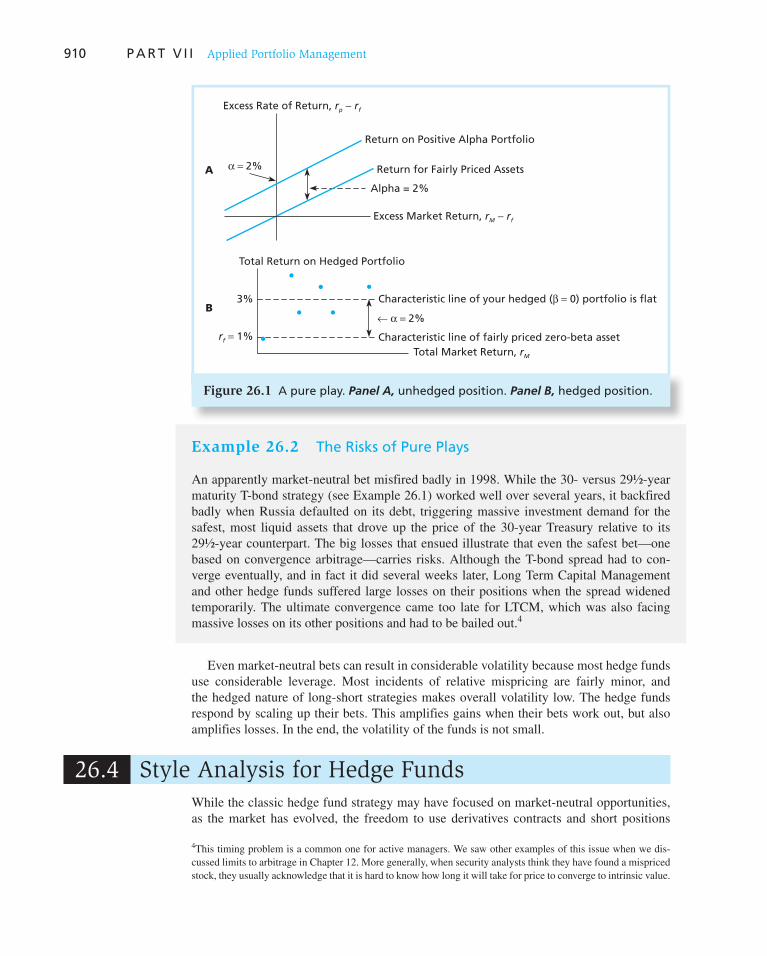
910 P A R T V I I Applied Portfolio Management
Example 26.2 The Risks of Pure Plays
An apparently market-neutral bet misfired badly in 1998. While the 30- versus 29½-year maturity T-bond strategy (see Example 26.1 ) worked well over several years, it backfired badly when Russia defaulted on its debt, triggering massive investment demand for the safest, most liquid assets that drove up the price of the 30-year Treasury relative to its 29½-year counterpart. The big losses that ensued illustrate that even the safest bet—one based on convergence arbitrage—carries risks. Although the T-bond spread had to con-verge eventually, and in fact it did several weeks later, Long Term Capital Management and other hedge funds suffered large losses on their positions when the spread widened temporarily. The ultimate convergence came too late for LTCM, which was also facing massive losses on its other positions and had to be bailed out. 4
Figure 26.1 A pure play. Panel A, unhedged position. Panel B, hedged position.
Return on Positive Alpha Portfolio
Return for Fairly Priced Assets
Alpha = 2%
Excess Market Return, rM − rf
Excess Rate of Return, rp − rf
α = 2%
Characteristic line of your hedged (β = 0) portfolio is flat
Characteristic line of fairly priced zero-beta assetTotal Market Return, rM
Total Return on Hedged Portfolio
← α = 2%
rf = 1%
3%
A
B
Even market-neutral bets can result in considerable volatility because most hedge funds use considerable leverage. Most incidents of relative mispricing are fairly minor, and the hedged nature of long-short strategies makes overall volatility low. The hedge funds respond by scaling up their bets. This amplifies gains when their bets work out, but also amplifies losses. In the end, the volatility of the funds is not small. 4
While the classic hedge fund strategy may have focused on market-neutral opportunities, as the market has evolved, the freedom to use derivatives contracts and short positions
4 This timing problem is a common one for active managers. We saw other examples of this issue when we dis-cussed limits to arbitrage in Chapter 12. More generally, when security analysts think they have found a mispriced
stock, they usually acknowledge that it is hard to know how long it will take for price to converge to intrinsic value.
26.4 Style Analysis for Hedge Funds

C H A P T E R 2 6 Hedge Funds 911
means that hedge funds can in effect follow any investment strategy. While many hedge funds pursue market-neutral strategies, a quick glance at the range of investment styles in Table 26.1 should convince you that many, if not most, funds pursue directional strategies. In these cases, the fund makes an outright bet, for example, on currency movements, the outcome of a takeover attempt, or the performance of an investment sector. These funds are most certainly not hedged, despite their name.
In Chapter 24, we introduced you to style analysis, which uses regression analysis to measure the exposure of a portfolio to various factors or asset classes. The analysis thus measures the implicit asset class exposure of a portfolio. The betas on a series of factors measure the fund’s exposure to each source of systematic risk. A market-neutral fund will have no sensitivity to an index for that market. In contrast, directional funds will exhibit significant betas, often called loadings in this context, on whatever factors the fund tends to bet on. Observers attempting to measure investment style can use these factor loadings to impute exposures to a range of variables.
We present a simple style analysis for the hedge fund indexes in Table 26.2 . The four systematic factors we consider are:
• Interest rates: the return on long-term U.S. Treasury bonds.
• Equity markets: the return on the S&P 500.
• Credit conditions: the difference in the return on Baa-rated bonds over Treasury bonds.
• Foreign exchange: the percentage change in the value of the U.S. dollar against a basket of foreign currencies.
The returns on hedge fund index i in month t may be statistically described by 5
Rit 5 ai 1 bi1 Factor1t 1c1 bi4 Factor4t 1 eit (26.3)
The betas (equivalently, factor loadings) measure the sensitivity to each factor. As usual, the residual, e it , measures nonsystematic risk that is uncorrelated with the set of explan-atory factors, and the intercept, a i , measures average performance of fund i net of the impact of these systematic factors.
Table 26.2 presents factor exposure estimates for 13 hedge fund indexes. The results confirm that most funds are in fact directional with very clear exposures to one or more of the four factors. Moreover, the estimated factor betas seem reasonable in terms of the funds’ stated style. For example:
• The equity market–neutral funds have uniformly low and statistically insignificant factor betas, as one would expect of a market-neutral posture.
• Dedicated short bias funds exhibit substantial negative betas on the S&P index.
• Distressed firm funds have significant exposure to credit conditions (more positive credit spreads in this table indicate better economic conditions) as well as to the S&P 500. This exposure arises because restructuring activities often depend on access to borrowing, and successful restructuring depends on the state of the economy.
• Global macro funds show negative exposure to a stronger U.S. dollar, which would make the dollar value of foreign investments less valuable.
We conclude that, by and large, most hedge funds are making very explicit directional bets on a wide array of economic factors.
5 This analysis differs in two important respects from style analysis for mutual funds introduced in Chapter 24. First, in this application, factor loadings are not constrained to be non-negative. This is because, unlike mutual funds, hedge funds easily can take on short positions in various asset classes. Second, portfolio weights are not constrained to sum to 1.0. Again, unlike mutual funds, hedge funds can operate with considerable leverage.
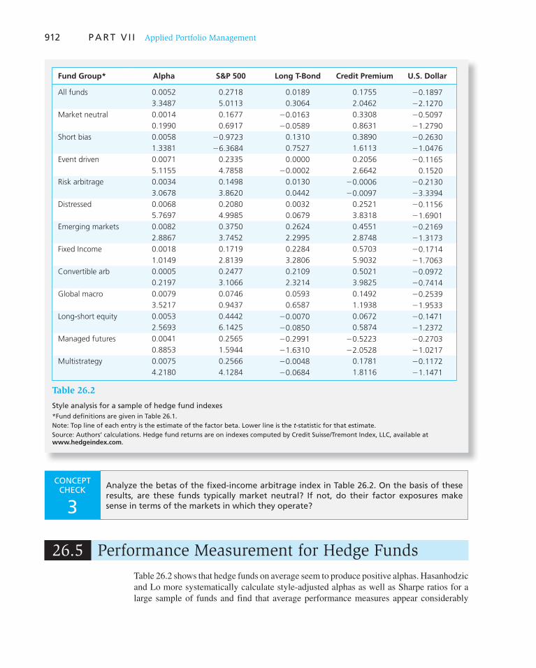
912 P A R T V I I Applied Portfolio Management
Fund Group* Alpha S&P 500 Long T-Bond Credit Premium U.S. Dollar
All funds 0.0052
3.3487
0.2718
5.0113
0.0189
0.3064
0.1755
2.0462
20.1897
22.1270
Market neutral 0.0014
0.1990
0.1677
0.6917
20.0163
20.0589
0.3308
0.8631
20.5097
21.2790
Short bias 0.0058
1.3381
20.9723
26.3684
0.1310
0.7527
0.3890
1.6113
20.2630
21.0476
Event driven 0.0071
5.1155
0.2335
4.7858
0.0000
20.0002
0.2056
2.6642
20.1165
0.1520
Risk arbitrage 0.0034
3.0678
0.1498
3.8620
0.0130
0.0442
20.0006
20.0097
20.2130
23.3394
Distressed 0.0068
5.7697
0.2080
4.9985
0.0032
0.0679
0.2521
3.8318
20.1156
21.6901
Emerging markets 0.0082
2.8867
0.3750
3.7452
0.2624
2.2995
0.4551
2.8748
20.2169
21.3173
Fixed Income 0.0018
1.0149
0.1719
2.8139
0.2284
3.2806
0.5703
5.9032
20.1714
21.7063
Convertible arb 0.0005
0.2197
0.2477
3.1066
0.2109
2.3214
0.5021
3.9825
20.0972
20.7414
Global macro 0.0079
3.5217
0.0746
0.9437
0.0593
0.6587
0.1492
1.1938
20.2539
21.9533
Long-short equity 0.0053
2.5693
0.4442
6.1425
20.0070
20.0850
0.0672
0.5874
20.1471
21.2372
Managed futures 0.0041
0.8853
0.2565
1.5944
20.2991
21.6310
20.5223
22.0528
20.2703
21.0217
Multistrategy 0.0075
4.2180
0.2566
4.1284
20.0048
20.0684
0.1781
1.8116
20.1172
21.1471
Table 26.2
Style analysis for a sample of hedge fund indexes *Fund definitions are given in Table 26.1 . Note: Top line of each entry is the estimate of the factor beta. Lower line is the t -statistic for that estimate. Source: Authors’ calculations. Hedge fund returns are on indexes computed by Credit Suisse/Tremont Index, LLC, available at www.hedgeindex.com.
CONCEPT CHECK
3 Analyze the betas of the fixed-income arbitrage index in Table 26.2 . On the basis of these results, are these funds typically market neutral? If not, do their factor exposures make sense in terms of the markets in which they operate?
26.5 Performance Measurement for Hedge Funds
Table 26.2 shows that hedge funds on average seem to produce positive alphas. Hasanhodzic and Lo more systematically calculate style-adjusted alphas as well as Sharpe ratios for a large sample of funds and find that average performance measures appear considerably
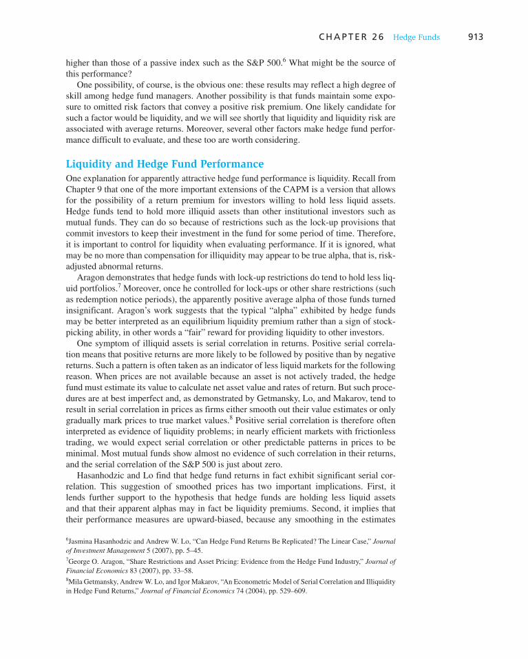
C H A P T E R 2 6 Hedge Funds 913
higher than those of a passive index such as the S&P 500. 6 What might be the source of this performance?
One possibility, of course, is the obvious one: these results may reflect a high degree of skill among hedge fund managers. Another possibility is that funds maintain some expo-sure to omitted risk factors that convey a positive risk premium. One likely candidate for such a factor would be liquidity, and we will see shortly that liquidity and liquidity risk are associated with average returns. Moreover, several other factors make hedge fund perfor-mance difficult to evaluate, and these too are worth considering.
Liquidity and Hedge Fund Performance
One explanation for apparently attractive hedge fund performance is liquidity. Recall from Chapter 9 that one of the more important extensions of the CAPM is a version that allows for the possibility of a return premium for investors willing to hold less liquid assets. Hedge funds tend to hold more illiquid assets than other institutional investors such as mutual funds. They can do so because of restrictions such as the lock-up provisions that commit investors to keep their investment in the fund for some period of time. Therefore, it is important to control for liquidity when evaluating performance. If it is ignored, what may be no more than compensation for illiquidity may appear to be true alpha, that is, risk-adjusted abnormal returns.
Aragon demonstrates that hedge funds with lock-up restrictions do tend to hold less liq-uid portfolios. 7 Moreover, once he controlled for lock-ups or other share restrictions (such as redemption notice periods), the apparently positive average alpha of those funds turned insignificant. Aragon’s work suggests that the typical “alpha” exhibited by hedge funds may be better interpreted as an equilibrium liquidity premium rather than a sign of stock-picking ability, in other words a “fair” reward for providing liquidity to other investors.
One symptom of illiquid assets is serial correlation in returns. Positive serial correla-tion means that positive returns are more likely to be followed by positive than by negative returns. Such a pattern is often taken as an indicator of less liquid markets for the following reason. When prices are not available because an asset is not actively traded, the hedge fund must estimate its value to calculate net asset value and rates of return. But such proce-dures are at best imperfect and, as demonstrated by Getmansky, Lo, and Makarov, tend to result in serial correlation in prices as firms either smooth out their value estimates or only gradually mark prices to true market values. 8 Positive serial correlation is therefore often interpreted as evidence of liquidity problems; in nearly efficient markets with frictionless trading, we would expect serial correlation or other predictable patterns in prices to be minimal. Most mutual funds show almost no evidence of such correlation in their returns, and the serial correlation of the S&P 500 is just about zero.
Hasanhodzic and Lo find that hedge fund returns in fact exhibit significant serial cor-relation. This suggestion of smoothed prices has two important implications. First, it lends further support to the hypothesis that hedge funds are holding less liquid assets and that their apparent alphas may in fact be liquidity premiums. Second, it implies that their performance measures are upward-biased, because any smoothing in the estimates
6 Jasmina Hasanhodzic and Andrew W. Lo, “Can Hedge Fund Returns Be Replicated? The Linear Case,” Journal
of Investment Management 5 (2007), pp. 5–45.
7 George O. Aragon, “Share Restrictions and Asset Pricing: Evidence from the Hedge Fund Industry,” Journal of
Financial Economics 83 (2007), pp. 33–58.
8 Mila Getmansky, Andrew W. Lo, and Igor Makarov, “An Econometric Model of Serial Correlation and Illiquidity in Hedge Fund Returns,” Journal of Financial Economics 74 (2004), pp. 529–609.

914 P A R T V I I Applied Portfolio Management
of portfolio value will reduce total volatility (increasing the Sharpe ratio) as well as covariances and therefore betas with systematic factors (increasing risk-adjusted alphas). In fact, Figure 26.2 shows that hedge fund serial correlations are highly associated with their apparent Sharpe ratios.
Whereas Aragon focuses on the average level of liquidity, Sadka addresses the liquidity risk
of hedge funds. 9 He shows that exposure to unexpected declines in market liquidity is an impor-tant determinant of average hedge fund returns, and that the spread in average returns across the funds with the highest and lowest liquid-ity exposure may be as much as 6% annually. Hedge fund perfor-mance may therefore reflect sig-nificant compensation for liquidity risk. Figure 26.3 , constructed from data reported in his study, is a scatter diagram relating average return for the hedge funds in each style group of Table 26.2 to the liquidity-risk beta for that group. Average return clearly rises with exposure to changes in market liquidity.
Returns can be even more dif-ficult to interpret if a hedge fund takes advantage of illiquid markets to manipulate returns by purposely misvaluing illiquid assets. In this regard, it is worth noting a Santa
effect: hedge funds report average returns in December that are substantially greater than their average returns in other months. 10 The pattern is stronger for funds that are near or beyond the threshold return at which performance incentive fees kick in and suggests that illiquid assets are more generously valued in December, when annual performance relative to benchmarks is being calculated. In fact, it seems that the December spike in returns is stronger for lower-liquidity funds. If funds take advantage of illiquid markets to manage returns, then accurate performance measurement becomes almost impossible.
9 Ronnie Sadka, “Liquidity Risk and the Cross-Section of Hedge-Fund Returns,” Journal of Financial Economics,
forthcoming. 10 Vikas Agarwal, Naveen D. Daniel, and Narayan Y. Naik, “Why Is Santa So Kind to Hedge Funds? The December Return Puzzle!” March 29, 2007, http://ssrn.com/abstract 5 891169.
Figure 26.2 Hedge funds with higher serial correlation in returns, an indicator of illiquid portfolio holdings, exhibit higher Sharpe ratios.
Source: Plotted from data in Hasanhodzic and Lo, “Can Hedge Funds Be Replicated?”
3.0
2.5
2.0
1.5
1.0
0.5
0.0
Shar
pe
Rat
io
0.0 0.1 0.2
Serial Correlation
0.3 0.4 0.5
Figure 26.3 Average hedge fund returns as a function of liquidity risk
Source: Plotted from data in Sadka, “Liquidity Risk and the Cross-Section of Hedge-Fund Returns.”
0 0.5
Liquidity Beta
1 1.5
0.1
0.2
0.3
0.4
0.5
Ave
rag
e Ex
cess
Ret
urn
(%
/mo
nth
)
−0.5
0.6
0

C H A P T E R 2 6 Hedge Funds 915
Hedge Fund Performance and Survivorship Bias
We already know that survivorship bias (when only successful funds are included in a database) can affect the estimated performance of a sample of mutual funds. The same problems, as well as related ones, apply to hedge funds. Backfill bias arises because hedge funds report returns to database publishers only if they choose to. Funds started with seed capital will open to the public and therefore enter standard databases only if their past performance is deemed sufficiently successful to attract clients. Therefore, the prior per-formance of funds that are eventually included in the sample may not be representative of typical performance. Survivorship bias arises when unsuccessful funds that cease opera-tion stop reporting returns and leave a database, leaving behind only the successful funds. Malkiel and Saha find that attrition rates for hedge funds are far higher than for mutual funds—in fact, commonly more than double the attrition rate of mutual funds—making this an important issue to address. 11 Estimates of survivorship bias in various studies are typically substantial, in the range of 2–4%. 12
Hedge Fund Performance and Changing Factor Loadings
In Chapter 24, we pointed out that an important assumption underlying conventional per-formance evaluation is that the portfolio manager maintains a reasonably stable risk profile over time. But hedge funds are designed to be opportunistic and have considerable flex-ibility to change that profile. This too can make performance evaluation tricky. If risk is not constant, then estimated alphas will be biased if we use a standard, linear index model. And if the risk profile changes in systematic manner with the expected return on the mar-ket, performance evaluation is even more difficult.
To see why, look at Figure 26.4 , which illustrates the characteristic line of a perfect market timer (see Chapter 24, Section 24.4) who engages in no security selection but moves funds from T-bills into the market portfolio only when the market will outperform bills. The characteristic line is nonlinear, with a slope of 0 when the market’s excess return is negative, and a slope of 1 when it is positive. But a naïve attempt to estimate a regression equation from this pattern would result in a fitted line with a slope between 0 and 1, and a positive alpha. Neither statistic accurately describes the fund.
As we noted in Chapter 24, and as is evident from Figure 26.4 , an ability to conduct per-fect market timing is much like obtaining a call option on the underlying portfolio without having to pay for it. Similar nonlinearities would arise if the fund actually buys or writes options. Figure 26.5 A illustrates the case of a fund that holds a stock portfolio and writes put options on it, and panel B illustrates the case of a fund that holds a stock portfolio and writes call options. In both cases, the characteristic line is steeper when portfolio returns are poor—in other words, the fund has greater sensitivity to the market when it is falling than when it is rising. This is the opposite profile that would arise from timing ability, which is much like acquiring rather than writing options, and therefore would give the fund greater sensitivity to market advances. 13
11 Burton G. Malkiel and Atanu Saha, “Hedge Funds: Risk and Return,” Financial Analysts Journal 61 (2005), pp. 80–88.
12 For example, Malkiel and Saha estimate the bias at 4.4%; G. Amin and H. Kat, “Stocks, Bonds and Hedge Funds: Not a Free Lunch!” Journal of Portfolio Management 29 (Summer 2003), pp. 113–20, find a bias of about 2%; and William Fung and David Hsieh, “Performance Characteristics of Hedge Funds and CTA Funds: Natural versus Spurious Biases,” Journal of Financial and Quantitative Analysis 35 (2000), pp. 291–307, find a bias of about 3.6%.
13 But the fund that writes options would at least receive fair compensation for the unattractive shape of its char-acteristic line in the form of the premium received when it writes the options.
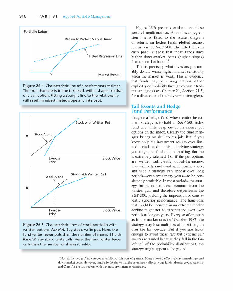
916 P A R T V I I Applied Portfolio Management
Figure 26.6 presents evidence on these sorts of nonlinearities. A nonlinear regres-sion line is fitted to the scatter diagram of returns on hedge funds plotted against returns on the S&P 500. The fitted lines in each panel suggest that these funds have higher down-market betas (higher slopes) than up-market betas. 14
This is precisely what investors presum-ably do not want: higher market sensitivity when the market is weak. This is evidence that funds may be writing options, either explicitly or implicitly through dynamic trad-ing strategies (see Chapter 21, Section 21.5, for a discussion of such dynamic strategies).
Tail Events and Hedge Fund Performance
Imagine a hedge fund whose entire invest-ment strategy is to hold an S&P 500 index fund and write deep out-of-the-money put options on the index. Clearly the fund man-ager brings no skill to his job. But if you knew only his investment results over lim-ited periods, and not his underlying strategy, you might be fooled into thinking that he is extremely talented. For if the put options are written sufficiently out-of-the-money, they will only rarely end up imposing a loss, and such a strategy can appear over long periods—even over many years—to be con-sistently profitable. In most periods, the strat-egy brings in a modest premium from the written puts and therefore outperforms the S&P 500, yielding the impression of consis-tently superior performance. The huge loss that might be incurred in an extreme market decline might not be experienced even over periods as long as years. Every so often, such as in the market crash of October 1987, the strategy may lose multiples of its entire gain over the last decade. But if you are lucky enough to avoid these rare but extreme tail
events (so named because they fall in the far-left tail of the probability distribution), the strategy might appear to be gilded.
14 Not all the hedge fund categories exhibited this sort of pattern. Many showed effectively symmetric up- and down-market betas. However, Figure 26.6 A shows that the asymmetry affects hedge funds taken as group. Panels B and C are for the two sectors with the most prominent asymmetries.
Figure 26.4 Characteristic line of a perfect market timer. The true characteristic line is kinked, with a shape like that of a call option. Fitting a straight line to the relationship will result in misestimated slope and intercept.
Return to Perfect Market Timer
Fitted Regression Line
Portfolio Return
Market Returnrf
Figure 26.5 Characteristic lines of stock portfolio with written options. Panel A, Buy stock, write put. Here, the fund writes fewer puts than the number of shares it holds. Panel B, Buy stock, write calls. Here, the fund writes fewer calls than the number of shares it holds.
Stock Alone
Stock Alone
A
B
ExercisePrice
Stock Value
ExercisePrice
Stock Value
Stock with Written Put
Stock with Written Call

917
5%0%−5%−10%−15%
5%
−5%
0%R
etu
rn o
n B
road
Hed
ge
Fun
d In
dex
S&P 500 Return
10%
−10%
−20% 10%A
B
5%0%−5%−10%−15%
−5%
0%
Ret
urn
on
Fix
ed-I
nco
me
Arb
itra
ge
Fun
ds
S&P 500 Return
−10%
−15%
−20% 10%
5%
C5%0%−5%−10%−15%
5%
−5%
−10%
0%
Ret
urn
on
Eve
nt-
Dri
ven
Fu
nd
s
S&P 500 Return
10%
−15%
−20% 10%
Figure 26.6 Monthly return on hedge fund indexes versus return on the S&P 500, 1993–2009. Panel A, hedge fund index. Panel B, fixed-income arbitrage funds. Panel C, event-driven funds.
Source: Constructed from data downloaded from www.hedgeindex.com and finance.yahoo.com.
918 P A R T V I I Applied Portfolio Management
The evidence in Figure 26.6 indicating that hedge funds are at least implicitly option writers should make us nervous about taking their measured performance at face value. The problem in interpreting strategies with exposure to extreme tail events (such as short options positions) is that these events by definition occur very infrequently, so decades of results may be needed to fully appreciate their true risk and reward attributes. In two influential books, Nassim Taleb, who is a hedge fund operator himself, makes the case that many hedge funds are analogous to our hypothetical manager, racking up fame and fortune through strat-egies that make money most of the time but expose investors to rare but extreme losses. 15
Taleb uses the metaphor of the black swan to discuss the importance of highly improb-able, but highly impactful, events. Until the discovery of Australia, Europeans believed that all swans were white: they had never encountered swans that were not white. In their experi-ence, the black swan was outside the realm of reasonable possibility, in statistical jargon, an extreme outlier relative to their sample of observations. Taleb argues that the world is filled with black swans, deeply important developments that simply could not have been predicted from the range of accumulated experience to date. While we can’t predict which black swans to expect, we nevertheless know that some black swan may be making an appearance at any moment. The October 1987 crash, when the market fell by more than 20% in 1 day, might be viewed as a black swan—an event that had never taken place before, one that most market observers would have dismissed as impossible and certainly not worth modeling, but with high impact. These sorts of events seemingly come out of the blue, and they caution us to show great humility when we use past experience to evaluate the future risk of our actions. With this in mind, consider again the example of Long Term Capital Management.
15 Nassim N. Taleb, Fooled by Randomness: The Hidden Role of Chance in Life and in the Markets (New York: TEXERE (Thomson), 2004); Nassim N. Taleb, The Black Swan: The Impact of the Highly Improbable (New York: Random House, 2007).
Example 26.3 Tail Events and Long-Term Capital Management
In the late 1990s, Long Term Capital Management was widely viewed as the most suc-cessful hedge fund in history. It had consistently provided double-digit returns to its inves-tors, and it had earned hundreds of millions of dollars in incentive fees for its managers. The firm used sophisticated computer models to estimate correlations across assets and believed that its capital was almost 10 times the annual standard deviation of its portfolio returns, presumably enough to withstand any “possible” shock to capital (at least, assum-ing normal distributions!). But in the summer of 1998, things went badly. On August 17, 1998, Russia defaulted on its sovereign debt and threw capital markets into chaos. LTCM’s 1-day loss on August 21 was $550 million (approximately nine times its estimated monthly standard deviation). Total losses in August were about $1.3 billion, despite the fact that LTCM believed that the great majority of its positions were market-neutral relative-value trades. Losses accrued on virtually all of its positions, flying in the face of the presumed diversification of the overall portfolio.
How did this happen? The answer lies in the massive flight to quality and, even more so, to liquidity that was set off by the Russian default. LTCM was typically a seller of liquid-ity (holding less liquid assets, selling more liquid assets with lower yields, and earning the yield spread) and suffered huge losses. This was a different type of shock from those that appeared in its historical sample/modeling period. In the liquidity crisis that engulfed asset markets, the unexpected commonality of liquidity risk across ostensibly uncorrelated asset classes became obvious. Losses that seemed statistically impossible on past experience had in fact come to pass; LTCM fell victim to a black swan.

C H A P T E R 2 6 Hedge Funds 919
26.6 Fee Structure in Hedge Funds
The typical hedge fund fee structure is a management fee of 1% to 2% of assets plus an incentive fee equal to 20% of investment profits beyond a stipulated benchmark perfor-mance, annually. Incentive fees are effectively call options on the portfolio with a strike price equal to current portfolio value times 1 1 benchmark return. The manager gets the fee if the portfolio value rises sufficiently, but loses nothing if it falls. Figure 26.7 illus-trates the incentive fee for a fund with a 20% incentive fee and a hurdle rate equal to the money market rate, r f . The current value of the portfolio is denoted S 0 and the year-end value is S T . The incentive fee is equivalent to .20 call options on the portfolio with exercise price S 0 (1 1 r f ).
Example 26.4 Black-Scholes Valuation of Incentive Fees
Suppose the standard deviation of a hedge fund’s annual rate of return is 30% and the incentive fee is 20% of any investment return over the risk-free money market rate. If the portfolio currently has a net asset value of $100 per share, and the effective annual risk-free rate is 5% (or 4.88% expressed as a continuously compounded rate), then the implicit exercise price on the incentive fee is $105. The Black-Scholes value of a call option with S 0 5 100, X 5 105, s 5 .30, r 5 .0488, T 5 1 year is $11.92, just a shade below 12% of net asset value. Because the incentive fee is worth 20% of the call option, its value is just about 2.4% of net asset value. Together with a typical management fee of 2% of net asset value, the investor in the fund pays fees with a total value of 4.4%.
Figure 26.7 Incentive fees as a call option. The current value of the portfolio is denoted S 0 and its year-end value is S T . The incentive fee is equivalent to .20 call options on the portfolio with exercise price S 0 (1 1 r f ).
S0(1 + rf) ST
Incentive Fee
Slope = .20
The major complication to this description of the typical compensation structure is the high water mark. If a fund experiences losses, it may not be able to charge an incentive fee unless and until it recovers to its previous higher value. With large losses, this may be dif-ficult. High water marks therefore give managers an incentive to shut down funds that have performed poorly, and likely are a cause of the high attrition rate for funds noted above.
One of the fastest-growing sectors in the hedge fund universe has been in funds of
funds. These are hedge funds that invest in one or more other hedge funds. Funds of funds are also called feeder funds, because they feed assets from the original investor to the ultimate hedge fund. They are marketed as providing investors the capability to diversify across funds, and also as providing the due diligence involved in screening funds for investment worthiness. In principle, this can be a valuable service because many hedge funds are opaque and feeder funds may have greater insight than typical outsiders. However, when Bernard Madoff was arrested in December 2008 after admitting to a massive Ponzi scheme, many large feeder funds were found to be among his biggest clients, and their “due diligence” may have been, to put it mildly, lack-ing. At the head of the list was Fairfield Greenwich Advisors, with exposure reported at $7.5 billion, but several other feeder funds and asset management firms around the world were also on the hook for amounts greater than $1 billion, among them Tremont Group Holdings, Banco Santander (a Spanish bank, one of the largest in the euro area), Ascot Partners, and

920
The Bernard Madoff Scandal
On December 13, 2008, Bernard Madoff reportedly con-fessed to his two sons that he had for years been operat-ing a Ponzi scheme, one that had reached a staggering $60 billion. A Ponzi scheme is an investment fraud in which a manager collects funds from clients, claims to invest those funds on the clients’ behalf, reports extremely favorable investment returns, but in fact uses the funds for his own purposes. (The schemes are named after Charles Ponzi, whose success with this scheme in the early 1900s made him notorious throughout the United States.) Early investors who ask to redeem their investments are paid back with the funds coming in from new investors rather than with true earnings. The scheme can continue as long as new investors provide enough funds to cover the redemption requests of the earlier ones—and these inflows are attracted by the superior returns “earned” by early investors as well as their apparent ability to redeem funds as requested.
As a highly respected member of the Wall Street estab-lishment, Madoff was in a perfect position to perpetrate such a fraud. He was a pioneer in electronic trading and had served as chairman of the NASDAQ Stock Market. Aside from its trading operations, Bernard L. Madoff Investment Securities LLC also acted as a money manager, and it claimed to achieve highly consistent annual returns, between 10% and 12% in good markets as well as bad. Its strategy was supposedly based on option hedging strat-egies, but Madoff was never precise about his approach. Still, his stature on Wall Street and the prestige of his client list seemed to testify to his legitimacy. Moreover, he played hard to attract new investors, and the appearance that one needed connections to join the fund only increased its appeal. The scheme seems to have operated for decades, but in the 2008 stock market downturn, several large cli-ents requested redemptions totaling around $7 billion.
With far less than $1 billion of assets left in the firm, the scheme collapsed.
Not everyone was fooled, and in retrospect, several red flags should have aroused suspicion. For example, some institutional investors shied away from the fund, objecting to its unusual opacity. Given the magnitude of the assets supposedly under management, the option hedging trades purportedly at the heart of Madoff’s investment strategy should have dominated options market trading volume, yet there was no evidence of their execution. Moreover, Madoff’s auditor, a small firm with only three employees (including only one active accountant!), seemed grossly inadequate to audit such a large and complex operation. In addition, Madoff’s fee structure was highly unusual. Rather than acting as a hedge fund that would charge a per-centage of assets plus incentive fees, he claimed to profit instead through trading commissions on the account—if true, this would have been a colossal price break to cli-ents. Finally, rather than placing assets under management with a custodial bank as most funds do, Madoff claimed to keep the funds in house, which meant that no one could independently verify their existence. In 2000, the SEC received a letter from an industry professional named Harry Markopolos concluding that “Madoff Securities is the world’s largest Ponzi scheme,” but Madoff continued to operate unimpeded.
Several questions remain unanswered. How much help did Madoff have from others? How much money was actu-ally lost? Much of the “lost” funds represented fictitious earnings on invested money, and some was returned to early investors. Where did the money go? Was it lost to bad trades, or was it skimmed off to support Madoff’s life style? And why did the red flags and early warnings not prompt a more aggressive response from regulators?
WO
RD
S FR
OM
TH
E ST
REE
T
Access International Advisors. In the end, it appears that some funds had in effect become little more than marketing agents for Madoff. The nearby box presents further discussion of the Madoff affair.
The option-like nature of compensation can have a big impact on expected fees in funds of funds. This is because the fund of funds pays an incentive fee to each underlying fund that outperforms its benchmark, even if the aggregate performance of the fund of funds is poor. In this case, diversification can hurt you! 16
16 S. J. Brown, W. N. Goetzmann, and B. Liang, “Fees on Fees in Funds of Funds,” Journal of Investment
Management 2 (2004), pp. 39–56.
Example 26.5 Incentive Fees in Funds of Funds
Suppose a fund of funds is established with $1 million invested in each of three hedge funds. For simplicity, we will ignore the asset-value-based portion of fees (the manage-ment fee) and focus only on the incentive fee. Suppose that the hurdle rate for the incentive
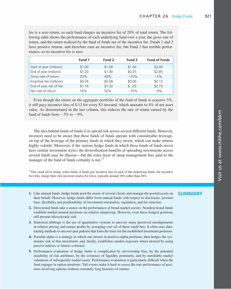
Vis
it u
s at
ww
w.m
hh
e.co
m/b
km
C H A P T E R 2 6 Hedge Funds 921
1. Like mutual funds, hedge funds pool the assets of several clients and manage the pooled assets on their behalf. However, hedge funds differ from mutual funds with respect to disclosure, investor base, flexibility and predictability of investment orientation, regulation, and fee structure.
2. Directional funds take a stance on the performance of broad market sectors. Nondirectional funds establish market-neutral positions on relative mispricing. However, even these hedged positions still present idiosyncratic risk.
3. Statistical arbitrage is the use of quantitative systems to uncover many perceived misalignments in relative pricing and ensure profits by averaging over all of these small bets. It often uses data- mining methods to uncover past patterns that form the basis for the established investment positions.
4. Portable alpha is a strategy in which one invests in positive-alpha positions, then hedges the sys-tematic risk of that investment, and, finally, establishes market exposure where desired by using passive indexes or futures contracts.
5. Performance evaluation of hedge funds is complicated by survivorship bias, by the potential instability of risk attributes, by the existence of liquidity premiums, and by unreliable market valuations of infrequently traded assets. Performance evaluation is particularly difficult when the fund engages in option positions. Tail events make it hard to assess the true performance of posi-tions involving options without extremely long histories of returns.
SUMMARY
The idea behind funds of funds is to spread risk across several different funds. However, investors need to be aware that these funds of funds operate with considerable leverage, on top of the leverage of the primary funds in which they invest, which can make returns highly volatile. Moreover, if the various hedge funds in which these funds of funds invest have similar investment styles, the diversification benefits of spreading investments across several funds may be illusory—but the extra layer of steep management fees paid to the manager of the fund of funds certainly is not. 17
17 One small silver lining: while funds of funds pay incentive fees to each of the underlying funds, the incentive fees they charge their own investors tend to be lower, typically around 10% rather than 20%.
fee is a zero return, so each fund charges an incentive fee of 20% of total return. The fol-lowing table shows the performance of each underlying fund over a year, the gross rate of return, and the return realized by the fund of funds net of the incentive fee. Funds 1 and 2 have positive returns, and therefore earn an incentive fee, but Fund 3 has terrible perfor-mance, so its incentive fee is zero.
Fund 1 Fund 2 Fund 3 Fund of Funds
Start of year (millions) $1.00 $1.00 $1.00 $3.00
End of year (millions) $1.20 $1.40 $0.25 $2.85
Gross rate of return 20% 40% 275% 25%
Incentive fee (millions) $0.04 $0.08 $0.00 $0.12
End of year, net of fee $1.16 $1.32 $ .25 $2.73
Net rate of return 16% 32% 275% 29%
Even though the return on the aggregate portfolio of the fund of funds is negative 5%, it still pays incentive fees of $.12 for every $3 invested, which amounts to 4% of net asset value. As demonstrated in the last column, this reduces the rate of return earned by the fund of funds from 2 5% to 2 9%.
Vis
it u
s at
ww
w.m
hh
e.co
m/b
kmV
isit
us
at w
ww
.mh
he.
com
/bkm
922 P A R T V I I Applied Portfolio Management
6. Hedge funds typically charge investors both a management fee and an incentive fee equal to a
percentage of profits beyond some threshold value. The incentive fee is akin to a call option on
the portfolio. Funds of hedge funds pay the incentive fee to each underlying fund that beats its
hurdle rate, even if the overall performance of the portfolio is poor.
Related Web sites for this chapter are available at www.mhhe.com/bkm
hedge funds
lock-up periods
directional strategy
nondirectional strategy
market neutral
pure plays
statistical arbitrage
pairs trading
data mining
portable alpha
alpha transfer
backfill bias
survivorship bias
incentive fee
high water mark
funds of funds
KEY TERMS
1. Would a market-neutral hedge fund be a good candidate for an investor’s entire retirement port-
folio? If not, would there be a role for the hedge fund in the overall portfolio of such an investor?
2. How might the incentive fee of a hedge fund affect the manager’s proclivity to take on high-risk
assets in the portfolio?
3. Why is it harder to assess the performance of a hedge fund portfolio manager than that of a typi-
cal mutual fund manager?
4. Which of the following is most accurate in describing the problems of survivorship bias and
backfill bias in the performance evaluation of hedge funds?
a. Survivorship bias and backfill bias both result in upwardly biased hedge fund index returns.
b. Survivorship bias and backfill bias both result in downwardly biased hedge fund index returns.
c. Survivorship bias results in upwardly biased hedge fund index returns, but backfill bias
results in downwardly biased hedge fund index returns.
5. Which of the following would be the most appropriate benchmark to use for hedge fund evaluation?
a. A multifactor model.
b. The S&P 500.
c. The risk-free rate.
6. With respect to hedge fund investing, the net return to an investor in a fund of funds would be
lower than that earned from an individual hedge fund because of:
a. Both the extra layer of fees and the higher liquidity offered.
b. No reason; fund of funds earn returns that are equal to those of individual hedge funds.
c. The extra layer of fees only.
7. Which of the following hedge fund types is most likely to have a return that is closest to risk-free?
a. A market-neutral hedge fund.
b. An event-driven hedge fund.
c. A long/short hedge fund.
8. Is statistical arbitrage true arbitrage? Explain.
9. A hedge fund with $1 billion of assets charges a management fee of 2% and an incentive fee of
20% of returns over a money market rate, which currently is 5%. Calculate total fees, both in
dollars and as a percent of assets under management, for portfolio returns of:
a. 2 5%
b. 0
c. 5%
d. 10%
10. A hedge fund with net asset value of $62 per share currently has a high water mark of $66. Is the
value of its incentive fee more or less than it would be if the high water mark were $67?
PROBLEM SETS
i. Basic
ii. Intermediate

Vis
it u
s at
ww
w.m
hh
e.co
m/b
km
C H A P T E R 2 6 Hedge Funds 923
11. Reconsider the hedge fund in the previous problem. Suppose it is January 1, the standard devia-tion of the fund’s annual returns is 50%, and the risk-free rate is 4%. The fund has an incentive fee of 20%, but its current high water mark is $66, and net asset value is $62.
a. What is the value of the annual incentive fee according to the Black-Scholes formula? b. What would the annual incentive fee be worth if the fund had no high water mark and it
earned its incentive fee on its total return? c. What would the annual incentive fee be worth if the fund had no high water mark and it
earned its incentive fee on its return in excess of the risk-free rate? (Treat the risk-free rate as a continuously compounded value to maintain consistency with the Black-Scholes formula.)
d. Recalculate the incentive fee value for part ( b ) now assuming that an increase in fund lever-age increases volatility to 60%.
12. Go to the Online Learning Center at www.mhhe.com/bkm, link to Chapter 26, and find there a spreadsheet containing monthly values of the S&P 500 index. Suppose that in each month you had written an out-of-the-money put option on one unit of the index with an exercise price 5% lower than the current value of the index.
a. What would have been the average value of your gross monthly payouts on the puts over the 10-year period October 1977–September 1987? The standard deviation?
b. Now extend your sample by 1 month to include October 1987, and recalculate the average payout and standard deviation of the put-writing strategy. What do you conclude about tail risk in naked put writing?
13. Suppose a hedge fund follows the following strategy. Each month it holds $100 million of an S&P 500 index fund and writes out-of-the-money put options on $100 million of the index with exercise price 5% lower than the current value of the index. Suppose the premium it receives for writing each put is $.25 million, roughly in line with the actual value of the puts.
a. Calculate the Sharpe ratio the fund would have realized in the period October 1982– September 1987. Compare its Sharpe ratio to that of the S&P 500. Use the data from the previous prob-lem, available at the Online Learning Center, and assume the monthly risk-free interest rate over this period was .7%.
b. Now calculate the Sharpe ratio the fund would have realized if we extend the sample period by 1 month to include October 1987. What do you conclude about performance evaluation and tail risk for funds pursuing option-like strategies?
14. The following is part of the computer output from a regression of monthly returns on Water-works stock against the S&P 500 index. A hedge fund manager believes that Waterworks is underpriced, with an alpha of 2% over the coming month.
Beta R-squareStandard Deviation
of Residuals
.75 .65 .06 (i.e., 6% monthly)
a. If he holds a $2 million portfolio of Waterworks stock, and wishes to hedge market exposure for the next month using 1-month maturity S&P 500 futures contracts, how many contracts should he enter? Should he buy or sell contracts? The S&P 500 currently is at 1,000 and the contract multiplier is $250.
b. What is the standard deviation of the monthly return of the hedged portfolio? c. Assuming that monthly returns are approximately normally distributed, what is the prob-
ability that this market-neutral strategy will lose money over the next month? Assume the risk-free rate is .5% per month.
15. Return to the previous problem.
a. Suppose you hold an equally weighted portfolio of 100 stocks with the same alpha, beta, and residual standard deviation as Waterworks. Assume the residual returns (the e terms in Equations 26.1 and 26.2 ) on each of these stocks are independent of each other. What is the residual standard deviation of the portfolio?
eXce lPlease visit us at www.mhhe.com/bkm
eXce lPlease visit us at www.mhhe.com/bkm
iii. Challenge

Vis
it u
s at
ww
w.m
hh
e.co
m/b
km924 P A R T V I I Applied Portfolio Management
b. Recalculate the probability of a loss on a market-neutral strategy involving equally weighted, market-hedged positions in the 100 stocks over the next month.
16. Return again to Problem 14. Now suppose that the manager misestimates the beta of Water-works stock, believing it to be .50 instead of .75. The standard deviation of the monthly market rate of return is 5%.
a. What is the standard deviation of the (now improperly) hedged portfolio? b. What is the probability of incurring a loss over the next month if the monthly market return
has an expected value of 1% and a standard deviation of 5%? Compare your answer to the probability you found in Problem 14.
c. What would be the probability of a loss using the data in Problem 15 if the manager simi-larly misestimated beta as .50 instead of .75? Compare your answer to the probability you found in Problem 14.
d. Why does the misestimation of beta matter so much more for the 100-stock portfolio than it does for the 1-stock portfolio?
17. Here are data on three hedge funds. Each fund charges its investors an incentive fee of 20% of total returns. Suppose initially that a fund of funds (FF) manager buys equal amounts of each of these funds, and also charges its investors a 20% incentive fee. For simplicity, assume also that management fees other than incentive fees are zero for all funds.
Hedge Fund 1
Hedge Fund 2
Hedge Fund 3
Start of year value (millions) $100 $100 $100
Gross portfolio rate of return 20% 10% 30%
a. Compute the rate of return after incentive fees to an investor in the fund of funds. b. Suppose that instead of buying shares in each of the three hedge funds, a stand-alone (SA)
hedge fund purchases the same portfolio as the three underlying funds. The total value and composition of the SA fund is therefore identical to the one that would result from aggregating the three hedge funds. Consider an investor in the SA fund. After paying 20% incentive fees, what would be the value of the investor’s portfolio at the end of the year?
c. Confirm that the investor’s rate of return in SA is higher than in FF by an amount equal to the extra layer of fees charged by the fund of funds.
d. Now suppose that the return on the portfolio held by hedge fund 3 were 2 30% rather than 1 30%. Recalculate your answers to parts ( a ) and ( b ). Will either FF or SA charge an incentive fee in this scenario? Why then does the investor in FF still do worse than the investor in SA?
E-INVEST-MENTS EXERCISES
Hedge Fund Styles and Results
Log on to www.hedgeindex.com, a site run by Credit Suisse/Tremont, which maintains the TASS Hedge Funds Data Base of the performance of more than 2,000 hedge funds, and produces indexes of investment performance for several hedge fund classes. Click the Downloads tab (free registration is required for access to this part of the Web site). From the Downloads page, you can access historical rates of return on each of the hedge fund subclasses (e.g., market neutral, event-driven, dedicated short bias, and so on). Download 5 years of monthly returns for each subclass and download returns on the S&P 500 for the same period from finance.yahoo.com. Calculate the beta of the equity-market-neutral and dedicated short bias funds. Do the results seem reasonable in terms of the orientation of these funds? Next, look at the year-by-year performance of each hedge fund class. How does the variability of performance results in different years compare to that of the S&P 500?

Vis
it u
s at
ww
w.m
hh
e.co
m/b
km
C H A P T E R 2 6 Hedge Funds 925
SOLUTIONS TO CONCEPT CHECKS
1. a. Nondirectional. The shares in the fund and the short position in the index swap constitute a hedged position. The hedge fund is betting that the discount on the closed-end fund will shrink and that it will profit regardless of the general movements in the Indian market.
b. Nondirectional. The value of both positions is driven by the value of Toys “R” Us. The hedge fund is betting that the market is undervaluing Petri relative to Toys “R” Us, and that as the relative values of the two positions come back into alignment, it will profit regardless of the movements in the underlying shares.
c. Directional. This is an outright bet on the price that Generic Pharmaceuticals will eventually command at the conclusion of the predicted takeover attempt.
2. The expected rate of return on the position (in the absence of any knowledge about idiosyncratic risk reflected in the residual) is 3%. If the residual turns out to be 2 4%, then the position will lose 1% of its value over the month and fall to $1.188 million. The excess return on the market in this month over T-bills would be 5% 2 1% 5 4%, while the excess return on the hedged strategy would be 2 1% 2 1% 5 2 2%, so the strategy would plot in panel A as the point (4%, 2 2%). In panel B, which plots total returns on the market and the hedge position, the strategy would plot as the point (5%, 2 1%).
3. Fixed-income arbitrage portfolios show positive exposure to the long bond and to the credit spread. This pattern suggests that these are not hedged arbitrage portfolios, but in fact are direc-tional portfolios.
THIS CHAPTER CONSIDERS the practical
process of constructing optimal portfolios
that an active portfolio manager can offer cli-
ents. It might seem that the word “theory” in
the chapter title is inconsistent with this prac-
tical goal, and that the foregoing chapters
must already have exhausted the knowledge
that theorists can impart to those who prac-
tice portfolio management in the field—the
rest would be up to the investment managers
in the trenches.
We will see, however, that theory has a
significant contribution to offer even when
it comes to the daily grind of putting it all
together. We begin with another look at the
portfolio optimization procedure using the
single-index model proposed by Treynor and
Black, first presented in Chapter 8. We discuss
practical problems that arise from the prop-
erties of the solution and how to effectively
handle them. We discuss the critical issue of
how to handle the limited accuracy of alpha
forecasts when implementing the Treynor-
Black model. Armed with these insights, we
present a prototype organizational chart and
discuss the efficacy of fitting the organization
to the theoretical underpinning of portfolio
management.
In the next section, we present the Black-
Litterman model that allows flexible views
about the expected returns of asset classes to
improve asset allocation. Finally, we look into
the potential profitability of security analysis
and end with concluding remarks. An appen-
dix to the chapter presents the mathematics
underlying the Black-Litterman model.
27 2 PA
RT
VII
The Theory of Active Portfolio Management
CHAPTER TWENTY-SEVEN
27.1 Optimal Portfolios and Alpha Values
In Chapter 8 we showed how to form an optimal risky portfolio with a single-index model. Table 27.1 summarizes the steps in this optimization, commonly known as the Treynor-Black model. The outlined procedure uses the index model that ignores nonzero covariance values across residuals. This is sometimes called the diagonal model, because it assumes that the covariance matrix of residuals has nonzero entries only on the diagonals. While the diagonal model is a special case that offers considerable simplification, we know from Chapter 7 that, if necessary, we always can resort to the full-blown Markowitz algorithm that allows for correlation among residuals. Moreover, we saw that despite the significant

C H A P T E R 2 7 The Theory of Active Portfolio Management 927
correlation between some pairs of residuals in the portfolio construction example we used in Chapter 8, for example, between Shell and BP, the efficient frontiers formed from the index model and the Markowitz model were barely distinguishable (see Figure 8.5 of Chapter 8).
For illustration, in this chapter we continue with the example employed in Chapter 8. Spreadsheet 27.1 recaps the data and results of this exercise. Table D in the spreadsheet shows the improvement in the Sharpe ratio over the passive market index portfolio
offered by adding the active portfolio to the mix. To better appreciate this improvement we have included the M -square measure of performance. M -square is the incremental expected return of the optimized portfolio compared to the passive alternative once the active portfolio is mixed with bills to provide the same total volatility as the index portfolio (for a review, see Chapter 24).
Forecasts of Alpha Values and Extreme Portfolio Weights
The overriding impression from Spreadsheet 27.1 is the apparently meager performance improvement: Table D of the spreadsheet shows that M -square increases by only 19 basis points (equivalent to an improvement of .0136 in the Sharpe ratio). Notice that the Sharpe
Table 27.1
Construction and properties of the optimal risky portfolio
1. Initial position of security i in the active
portfoliow i
0 5ai
s2(ei)
2. Scaled initial positions w i 5w
0i
an
i51
ai
s2(ei)
3. Alpha of the active portfolio aA 5 an
i51
wi ai
4. Residual variance of the active portfolio s2(eA) 5 an
i51
w i2s2(ei)
5. Initial position in the active portfoliowA
0 5
aA
s2(eA)
E(RM)
sM2
6. Beta of the active portfolio bA 5 an
i51
wi bi
7. Adjusted (for beta) position in the active
portfolio wA* 5
wA0
1 1 (1 2 bA)wA0
8. Final weights in passive portfolio and
in security iwM
* 5 1 2 wA* ; wi
* 5 wA*wi
9. The beta of the optimal risky portfolio
and its risk premium
bP 5 wM* 1 wA
*bA 5 1 2 wA*(1 2 bA)
E(RP) 5 bP E(RM) 1 wA
* aA
10. The variance of the optimal risky portfolio sP2 5 bP
2 sM2 1 3wA
* s(eA) 42 11. Sharpe ratio of the risky portfolio
SP2 5 SM
2 1 an
i51
¢ ai
s(ei)≤
2

928 P A R T V I I Applied Portfolio Management
ratio of the active portfolio is inferior to that of the passive portfolio (due to its large stan-dard deviation) and hence its M -square is actually negative. But remember that the active portfolio is mixed with the passive portfolio, so total volatility is not its appropriate mea-sure of risk. When combined with the passive portfolio, it does offer some improvement in performance, although such improvement is quite modest. This is the best that can be had given the alpha values uncovered by the security analysts (see Table C). Notice that the position in the active portfolio amounts to 17%, financed in part by a combined short position in Dell and Walmart of about 10%. Because the figures in Spreadsheet 27.1 are annualized, this performance is equivalent to a 1-year holding-period return (HPR).
The alpha values we used in Spreadsheet 27.1 are actually small by the standard of typi-cal analysts’ forecasts. On June 1, 2006, we downloaded the current prices of the six stocks in the example, as well as analysts’ 1-year target prices for each firm. These data and the
σ2(e)
α/σ2(e)
w0(i)
[w0(i)]2
αA
σ2(eA)
w0
w*
1
2
3
4
5678910111213
14
15
16
171819202122232425
26
27
28
29
303132
3334
35
36
37
38
39
40
41
42
43
44
45
46
47
48
49
A C D E F G H I J
Table A: Risk Parameters of the Investable Universe (annualized)
SD of Excess Return Beta
SD of Systematic Component
SD of Residual
Correlation with the S&P
500
S&P 500 0.1358 1.00 0.1358 0 1HP 0.3817 2.03 0.2762 0.2656 0.72
DELL 0.2901 1.23 0.1672 0.2392 0.58WMT 0.1935 0.62 0.0841 0.1757 0.43
TARGET 0.2611 1.27 0.1720 0.1981 0.66BP 0.1822 0.47 0.0634 0.1722 0.35
SHELL 0.1988 0.67 0.0914 0.1780 0.46
Table B: The Index Model Covariance Matrix
SP 500 HP DELL WMT TARGET BP SHELL
Beta 1.00 2.03 1.23 0.62 1.27 0.47 0.67S&P 500 1.00 0.0184 0.0375 0.0227 0.0114 0.0234 0.0086 0.0124
HP 2.03 0.0375 0.1457 0.0462 0.0232 0.0475 0.0175 0.0253DELL 1.23 0.0227 0.0462 0.0842 0.0141 0.0288 0.0106 0.0153WMT 0.62 0.0114 0.0232 0.0141 0.0374 0.0145 0.0053 0.0077
TARGET 1.27 0.0234 0.0475 0.0288 0.0145 0.0682 0.0109 0.0157BP 0.47 0.0086 0.0175 0.0106 0.0053 0.0109 0.0332 0.0058
SHELL 0.67 0.0124 0.0253 0.0153 0.0077 0.0157 0.0058 0.0395
Table C: Macro Forecast (S&P 500) and Forecasts of Alpha Values
SP 500 HP DELL WMT TARGET BP SHELL
Alpha 0 0.0150 −0.0100 −0.0050 0.0075 0.012 0.0025Risk premium 0.0600 0.1371 0.0639 0.0322 0.0835 0.0400 0.0429
Table D: Computation of the Optimal Risky Portfolio
S&P 500 Active Pf A HP DELL WMT TARGET BP SHELL
0.0705 0.0572 0.0309 0.0392 0.0297 0.0317
0.5505 0.2126 −0.1748 −0.1619 0.1911 0.4045 0.0789
1.0000 0.3863 −0.3176 −0.2941 0.3472 0.7349 0.1433
0.1492 0.1009 0.0865 0.1205 0.5400 0.0205
0.0222
0.0404
0.1691 Overall
0.8282 0.1718 Portfolio 0.0663 −0.0546 −0.0505 0.0596 0.1262 0.0246
Beta 1 1.0922 1.0158 0.0663 −0.0546 −0.0505 0.0596 0.1262 0.0246Risk premium 0.06 0.0878 0.0648 0.0750 0.1121 0.0689 0.0447 0.0880 0.0305SD 0.1358 0.2497 0.1422 0.3817 0.2901 0.1935 0.2611 0.1822 0.1988Sharpe ratio 0.44 0.35 0.4556M-square 0 −0.0123 0.0019
Benchmark risk 0.0346
B
Spreadsheet 27.1
Active portfolio management with a universe of six stocks
eXce lPlease visit us at www.mhhe.com/bkm

C H A P T E R 2 7 The Theory of Active Portfolio Management 929
implied annual alpha values are shown in Table 27.2 . Notice that all alphas are positive, indicating an optimistic view for this group of stocks. Figure 27.1 shows the graphs of the stock prices, as well as the S&P 500 index (ticker 5 GSPC), for the previous year, June 2005–May 2006. The graph shows that the optimistic views in Table 27.2 are not a result of extrapolating rates from the past.
Table 27.3 shows the optimal portfolio using the analysts’ forecasts rather than the orig-inal alpha values in Table D in Spreadsheet 27.1 . The difference in performance is striking. The Sharpe ratio of the new optimal portfolio has increased from the benchmark’s .44 to 2.32, amounting to a huge risk-adjusted return advantage. This shows up in an M -square of 25.53%! However, these results also expose the potential major problem with the Treynor-Black model. The optimal portfolio calls for extreme long/short positions that are simply infeasible for a real-world portfolio manager. For example, the model calls for a position of 5.79 (579%) in the active portfolio, largely financed by a short position of 2 4.79 in the S&P 500 index. Moreover, the standard deviation of this optimal portfolio is 52.24%, a level of risk that only extremely aggressive hedge funds would be willing to bear. It is important to notice that this risk is largely nonsystematic because the beta of the active portfolio, at .95, is less than 1.0, and the beta of the overall risky portfolio is even lower, only .73, because of the short position in the passive portfolio. Only hedge funds may still be interested in this portfolio.
One approach to this problem is to restrict extreme portfolio positions, beginning with short sales. When the short position in the S&P 500 index is eliminated, forcing us to con-strain the position in the active portfolio to be no more than 1.0, the position in the passive portfolio (the S&P 500) is zero, and the active portfolio comprises the entire risky p osition. Table 27.4 shows that the optimal portfolio now has a standard deviation of 15.68%, not
Stock HP Dell WMT Target BP Shell
Current price 32.15 25.39 48.14 49.01 70.8 68.7
Target price 36.88 29.84 57.44 62.8 83.52 71.15
Implied alpha 0.1471 0.1753 0.1932 0.2814 0.1797 0.0357
Table 27.2
Stock prices and analysts’ target prices for June 1, 2006
Figure 27.1 Rates of return on the S&P 500 (GSPC) and the six stocks, June 2005–May 2006
+60
HP
BPRDS-BGSPCWMTTGT
DELL
+40
+20
−20
−40
−60Jul. 05 Sep. 05
Rat
e o
f R
etu
rn (
%)
Nov. 05 Jan. 06 Mar. 06 May 06
0
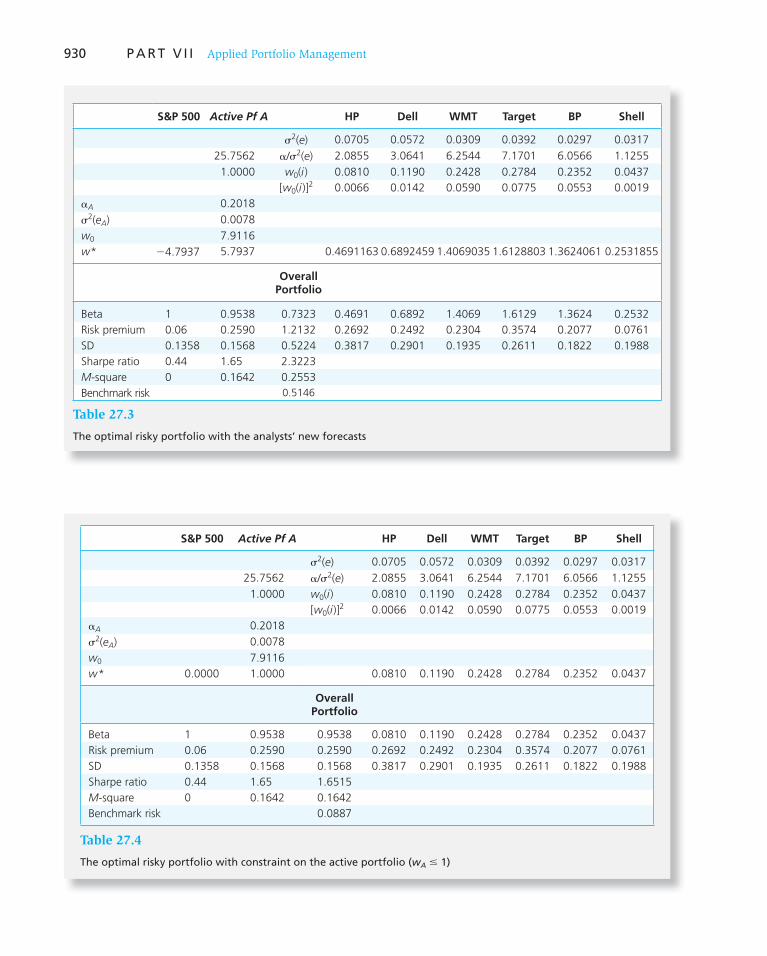
930 P A R T V I I Applied Portfolio Management
Table 27.3
The optimal risky portfolio with the analysts’ new forecasts
S&P 500 Active Pf A HP Dell WMT Target BP Shell
s2(e) 0.0705 0.0572 0.0309 0.0392 0.0297 0.0317
25.7562 a/s2(e) 2.0855 3.0641 6.2544 7.1701 6.0566 1.1255
1.0000 w0(i) 0.0810 0.1190 0.2428 0.2784 0.2352 0.0437
[w0(i)]2 0.0066 0.0142 0.0590 0.0775 0.0553 0.0019
aA 0.2018
s2(eA) 0.0078
w0 7.9116
w* 24.7937 5.7937 0.4691163 0.6892459 1.4069035 1.6128803 1.3624061 0.2531855
Overall Portfolio
Beta 1 0.9538 0.7323 0.4691 0.6892 1.4069 1.6129 1.3624 0.2532
Risk premium 0.06 0.2590 1.2132 0.2692 0.2492 0.2304 0.3574 0.2077 0.0761
SD 0.1358 0.1568 0.5224 0.3817 0.2901 0.1935 0.2611 0.1822 0.1988
Sharpe ratio 0.44 1.65 2.3223
M-square 0 0.1642 0.2553
Benchmark risk 0.5146
Table 27.4
The optimal risky portfolio with constraint on the active portfolio ( w A # 1)
S&P 500 Active Pf A HP Dell WMT Target BP Shell
s2(e) 0.0705 0.0572 0.0309 0.0392 0.0297 0.0317
25.7562 a/s2(e) 2.0855 3.0641 6.2544 7.1701 6.0566 1.1255
1.0000 w0(i) 0.0810 0.1190 0.2428 0.2784 0.2352 0.0437
[w0(i)]2 0.0066 0.0142 0.0590 0.0775 0.0553 0.0019
aA 0.2018
s2(eA) 0.0078
w0 7.9116
w* 0.0000 1.0000 0.0810 0.1190 0.2428 0.2784 0.2352 0.0437
Overall Portfolio
Beta 1 0.9538 0.9538 0.0810 0.1190 0.2428 0.2784 0.2352 0.0437
Risk premium 0.06 0.2590 0.2590 0.2692 0.2492 0.2304 0.3574 0.2077 0.0761
SD 0.1358 0.1568 0.1568 0.3817 0.2901 0.1935 0.2611 0.1822 0.1988
Sharpe ratio 0.44 1.65 1.6515
M-square 0 0.1642 0.1642
Benchmark risk 0.0887
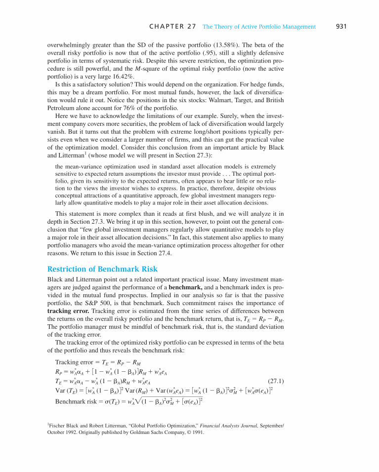
C H A P T E R 2 7 The Theory of Active Portfolio Management 931
overwhelmingly greater than the SD of the passive portfolio (13.58%). The beta of the overall risky portfolio is now that of the active portfolio (.95), still a slightly defensive portfolio in terms of systematic risk. Despite this severe restriction, the optimization pro-cedure is still powerful, and the M -square of the optimal risky portfolio (now the active portfolio) is a very large 16.42%.
Is this a satisfactory solution? This would depend on the organization. For hedge funds, this may be a dream portfolio. For most mutual funds, however, the lack of diversifica-tion would rule it out. Notice the positions in the six stocks: Walmart, Target, and British Petroleum alone account for 76% of the portfolio.
Here we have to acknowledge the limitations of our example. Surely, when the invest-ment company covers more securities, the problem of lack of diversification would largely vanish. But it turns out that the problem with extreme long/short positions typically per-sists even when we consider a larger number of firms, and this can gut the practical value of the optimization model. Consider this conclusion from an important article by Black and Litterman 1 (whose model we will present in Section 27.3):
the mean-variance optimization used in standard asset allocation models is extremely sensitive to expected return assumptions the investor must provide . . . The optimal port-folio, given its sensitivity to the expected returns, often appears to bear little or no rela-tion to the views the investor wishes to express. In practice, therefore, despite obvious conceptual attractions of a quantitative approach, few global investment managers regu-larly allow quantitative models to play a major role in their asset allocation decisions.
This statement is more complex than it reads at first blush, and we will analyze it in depth in Section 27.3. We bring it up in this section, however, to point out the general con-clusion that “few global investment managers regularly allow quantitative models to play a major role in their asset allocation decisions.” In fact, this statement also applies to many portfolio managers who avoid the mean-variance optimization process altogether for other reasons. We return to this issue in Section 27.4.
Restriction of Benchmark Risk
Black and Litterman point out a related important practical issue. Many investment man-agers are judged against the performance of a benchmark, and a benchmark index is pro-vided in the mutual fund prospectus. Implied in our analysis so far is that the passive portfolio, the S&P 500, is that benchmark. Such commitment raises the importance of tracking error. Tracking error is estimated from the time series of differences between the returns on the overall risky portfolio and the benchmark return, that is, T E 5 R P 2 R M . The portfolio manager must be mindful of benchmark risk, that is, the standard deviation of the tracking error.
The tracking error of the optimized risky portfolio can be expressed in terms of the beta of the portfolio and thus reveals the benchmark risk:
Tracking error 5 T E 5 R P 2 R M
RP 5 wA*aA 1 31 2 wA
* (1 2 bA) 4RM 1 wA*eA
TE 5 wA*aA 2 wA
* (1 2 bA)RM 1 wA*eA (27.1)
Var (TE) 5 3wA* (1 2 bA) 42 Var (RM) 1 Var (wA
*eA) 5 3wA* (1 2 bA) 42sM
2 1 3wA*s(eA) 42
Benchmark risk 5 s(TE) 5 wA*"(1 2 bA)2sM
2 1 3s(eA) 42 1 Fischer Black and Robert Litterman, “Global Portfolio Optimization,” Financial Analysts Journal, September/October 1992. Originally published by Goldman Sachs Company, © 1991.
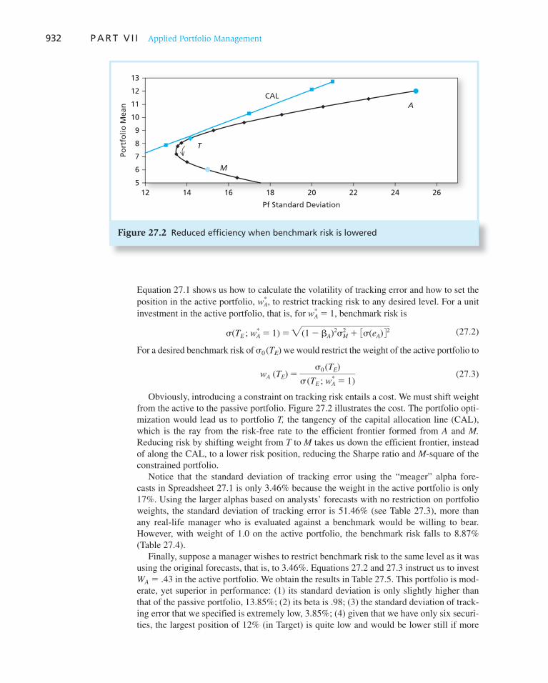
932 P A R T V I I Applied Portfolio Management
Equation 27.1 shows us how to calculate the volatility of tracking error and how to set the position in the active portfolio, wA
*, to restrict tracking risk to any desired level. For a unit investment in the active portfolio, that is, for wA
* 5 1, benchmark risk is
s(TE ; wA
* 5 1) 5"(1 2 bA)2sM2 1 3s(eA) 42 (27.2)
For a desired benchmark risk of s 0 ( T E ) we would restrict the weight of the active portfolio to
wA (TE) 5s0 (TE)
s(TE ; wA
* 5 1) (27.3)
Obviously, introducing a constraint on tracking risk entails a cost. We must shift weight from the active to the passive portfolio. Figure 27.2 illustrates the cost. The portfolio opti-mization would lead us to portfolio T, the tangency of the capital allocation line (CAL), which is the ray from the risk-free rate to the efficient frontier formed from A and M. Reducing risk by shifting weight from T to M takes us down the efficient frontier, instead of along the CAL, to a lower risk position, reducing the Sharpe ratio and M -square of the constrained portfolio.
Notice that the standard deviation of tracking error using the “meager” alpha fore-casts in Spreadsheet 27.1 is only 3.46% because the weight in the active portfolio is only 17%. Using the larger alphas based on analysts’ forecasts with no restriction on portfolio weights, the standard deviation of tracking error is 51.46% (see Table 27.3 ), more than any real-life manager who is evaluated against a benchmark would be willing to bear. However, with weight of 1.0 on the active portfolio, the benchmark risk falls to 8.87% ( Table 27.4 ).
Finally, suppose a manager wishes to restrict benchmark risk to the same level as it was using the original forecasts, that is, to 3.46%. Equations 27.2 and 27.3 instruct us to invest W A 5 .43 in the active portfolio. We obtain the results in Table 27.5 . This portfolio is mod-erate, yet superior in performance: (1) its standard deviation is only slightly higher than that of the passive portfolio, 13.85%; (2) its beta is .98; (3) the standard deviation of track-ing error that we specified is extremely low, 3.85%; (4) given that we have only six securi-ties, the largest position of 12% (in Target) is quite low and would be lower still if more
Figure 27.2 Reduced efficiency when benchmark risk is lowered
M
CAL
T
A
5
6
7
8
9
10
11
12
13
12 14 16 18 20 22 24 26
Pf Standard Deviation
Port
folio
Mea
n
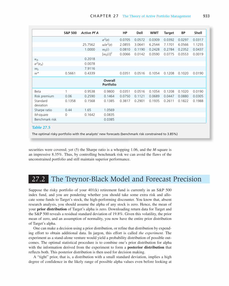
C H A P T E R 2 7 The Theory of Active Portfolio Management 933
securities were covered; yet (5) the Sharpe ratio is a whopping 1.06, and the M -square is an impressive 8.35%. Thus, by controlling benchmark risk we can avoid the flaws of the unconstrained portfolio and still maintain superior performance.
Table 27.5
The optimal risky portfolio with the analysts’ new forecasts (benchmark risk constrained to 3.85%)
27.2 The Treynor-Black Model and Forecast Precision
Suppose the risky portfolio of your 401(k) retirement fund is currently in an S&P 500 index fund, and you are pondering whether you should take some extra risk and allo-cate some funds to Target’s stock, the high-performing discounter. You know that, absent research analysis, you should assume the alpha of any stock is zero. Hence, the mean of your prior distribution of Target’s alpha is zero. Downloading return data for Target and the S&P 500 reveals a residual standard deviation of 19.8%. Given this volatility, the prior mean of zero, and an assumption of normality, you now have the entire prior distribution of Target’s alpha.
One can make a decision using a prior distribution, or refine that distribution by expend-ing effort to obtain additional data. In jargon, this effort is called the experiment. The experiment as a stand-alone venture would yield a probability distribution of possible out-comes. The optimal statistical procedure is to combine one’s prior distribution for alpha with the information derived from the experiment to form a posterior distribution that reflects both. This posterior distribution is then used for decision making.
A “tight” prior, that is, a distribution with a small standard deviation, implies a high degree of confidence in the likely range of possible alpha values even before looking at
S&P 500 Active Pf A HP Dell WMT Target BP Shell
s2(e) 0.0705 0.0572 0.0309 0.0392 0.0297 0.0317
25.7562 a/s2(e) 2.0855 3.0641 6.2544 7.1701 6.0566 1.1255
1.0000 w0(i ) 0.0810 0.1190 0.2428 0.2784 0.2352 0.0437
[w0(i )]2 0.0066 0.0142 0.0590 0.0775 0.0553 0.0019
aA 0.2018
s2(eA) 0.0078
w0 7.9116
w* 0.5661 0.4339 0.0351 0.0516 0.1054 0.1208 0.1020 0.0190
Overall Portfolio
Beta 1 0.9538 0.9800 0.0351 0.0516 0.1054 0.1208 0.1020 0.0190
Risk premium 0.06 0.2590 0.1464 0.0750 0.1121 0.0689 0.0447 0.0880 0.0305
Standard
deviation
0.1358 0.1568 0.1385 0.3817 0.2901 0.1935 0.2611 0.1822 0.1988
Sharpe ratio 0.44 1.65 1.0569
M-square 0 0.1642 0.0835
Benchmark risk 0.0385

934 P A R T V I I Applied Portfolio Management
the data. In this case, the experiment may not be sufficiently convincing to affect your beliefs, meaning that the posterior will be little changed from the prior. 2 In the con-text of the present discussion, an active forecast of alpha and its precision provides the experiment that may induce you to update your prior beliefs about its value. The role of the portfolio manager is to form a posterior distribution of alpha that serves portfolio construction.
Adjusting Forecasts for the Precision of Alpha
Imagine it is June 1, 2006, and you have just downloaded from Yahoo! Finance the analysts’ forecasts we used in the previous section, implying that Target’s alpha is 28.1%. Should you conclude that the optimal position in Target, before adjusting for beta, is a / s 2 ( e ) 5 .281/.198 2 5 7.17 (717%)? Naturally, before committing to such an extreme position, any reasonable manager would first ask: “How accurate is this forecast?” and “How should I adjust my position to take account of forecast imprecision?”
Treynor and Black 3 asked this question and supplied an answer. The logic of the answer is quite straightforward; you must quantify the uncertainty about this forecast, just as you would the risk of the underlying asset or portfolio. A Web surfer may not have a way to assess the precision of a downloaded forecast, but the employer of the analyst who issued the forecast does. How? By examining the forecasting record of previous forecasts issued by the same forecaster.
Suppose that a security analyst provides the portfolio manager with forecasts of alpha at regular intervals, say, the beginning of each month. The investor portfolio is updated using the forecast and held until the update of next month’s forecast. At the end of each month, T, the realized abnormal return of Target’s stock is the sum of alpha plus a residual:
u(T) 5 RTGT (T) 2 bRM
(T) 5 a(T) 1 e(T) (27.4)
where beta is estimated from Target’s security characteristic line (SCL) using data for periods prior to T,
SCL: RTGT(t) 5 a 1 bRM(t) 1 e(t), t , T (27.5)
The 1-month, forward-looking forecast a f ( T ) issued by the analyst at the beginning of month T is aimed at the abnormal return, u ( T ), in Equation 27.4. In order to decide on how to use the forecast for month T, the portfolio manager uses the analyst’s forecasting record. The analyst’s record is the paired time series of all past forecasts, a f ( t ), and realizations, u ( t ). To assess forecast accuracy, that is, the relationship between forecast and realized alphas, the manager uses this record to estimate the regression:
u(t) 5 a0 1 a1af(t) 1 e(t) (27.6)
Our goal is to adjust alpha forecasts to properly account for their imprecision. We will form an adjusted alpha forecast a ( T ) for the coming month by using the original forecasts a f ( T ) and applying the estimates from the regression Equation 27.6, that is,
a(T) 5 a0 1 a1af(T) (27.7)
The properties of the regression estimates assure us that the adjusted forecast is the “best linear unbiased estimator” of the abnormal return on Target in the coming month, T.
2 In application to debates about social issues, you might define a fanatic as one who enters the debate with a prior that is so tight that no argument will influence his posterior, making the debate altogether a waste of time.
3 Jack Treynor and Fischer Black, “How to Use Security Analysis to Improve Portfolio Selection,” Journal of
Business, January 1973.
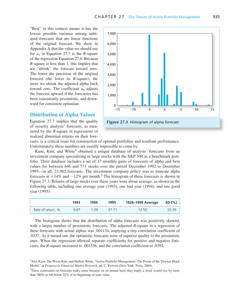
C H A P T E R 2 7 The Theory of Active Portfolio Management 935
“Best” in this context means it has the lowest possible variance among unbi-ased forecasts that are linear functions of the original forecast. We show in Appendix A that the value we should use for a 1 in Equation 27.7 is the R -square of the regression Equation 27.6. Because R -square is less than 1, this implies that we “shrink” the forecast toward zero. The lower the precision of the original forecast (the lower its R -square), the more we shrink the adjusted alpha back toward zero. The coefficient a 0 adjusts the forecast upward if the forecaster has been consistently pessimistic, and down-ward for consistent optimism.
Distribution of Alpha Values
Equation 27.7 implies that the quality of security analysts’ forecasts, as mea-sured by the R -square in regressions of realized abnormal returns on their fore-casts, is a critical issue for construction of optimal portfolios and resultant performance. Unfortunately, these numbers are usually impossible to come by.
Kane, Kim, and White 4 obtained a unique database of analysts’ forecasts from an investment company specializing in large stocks with the S&P 500 as a benchmark port-folio. Their database includes a set of 37 monthly pairs of forecasts of alpha and beta values for between 646 and 771 stocks over the period December 1992 to December 1995—in all, 23,902 forecasts. The investment company policy was to truncate alpha forecasts at 1 14% and 2 12% per month. 5 The histogram of these forecasts is shown in Figure 27.3 . Returns of large stocks over these years were about average, as shown in the following table, including one average year (1993), one bad year (1994), and one good year (1995):
1993 1994 1995 1926–1999 Average SD (%)
Rate of return, % 9.87 1.29 37.71 12.50 20.39
The histogram shows that the distribution of alpha forecasts was positively skewed, with a larger number of pessimistic forecasts. The adjusted R -square in a regression of these forecasts with actual alphas was .001134, implying a tiny correlation coefficient of .0337. As it turned out, the optimistic forecasts were of superior quality to the pessimistic ones. When the regression allowed separate coefficients for positive and negative fore-casts, the R -square increased to .001536, and the correlation coefficient to .0392.
4 Alex Kane, Tae-Hwan Kim, and Halbert White, “Active Portfolio Management: The Power of the Treynor-Black Model,” in Progress in Financial Market Research, ed. C. Kyrtsou (New York: Nova, 2004). 5 These constraints on forecasts make sense because on an annual basis they imply a stock would rise by more than 380% or fall below 22% of its beginning-of-year value.
Figure 27.3 Histogram of alpha forecast
−15 −10 −5 0 5 10 150
4,000
3,000
2,000
1,000
6,000
5,000
7,000
936 P A R T V I I Applied Portfolio Management
These results contain “good” and “bad” news. The “good” news is that after adjusting even the wildest forecast, say, an alpha of 12% for the next month, the value to be used by a forecaster when R -square is .001 would be .012%, just 1.2 basis points per month. On an annual basis, this would amount to .14%, which is of the order of the alpha forecasts of the example in Spreadsheet 27.1 . With forecasts of this small magnitude, the problem of extreme portfolio weights would never arise. The bad news arises from the same data: the performance of the active portfolio will be no better than in our example—implying an M -square of only 19 basis points.
An investment company that delivers such limited performance will not be able to cover its cost. However, this performance is based on an active portfolio that includes only six stocks. As we show in Section 27.5, even small information ratios of individual stocks can add up (see line 11 in Table 27.1 ). Thus, when many forecasts of even low precision are used to form a large active portfolio, large profits can be made.
So far we have assumed that forecast errors of various stocks are independent, an assumption that may not be valid. When forecasts are correlated across stocks, precision is measured by a covariance matrix of forecasting errors, which can be estimated from past forecasts. While the necessary adjustment to the forecasts in this case is algebraically messy, it is just a technical detail. As we might guess, correlations among forecast errors will call for us to further shrink the adjusted forecasts toward zero.
Organizational Structure and Performance
The mathematical property of the optimal risky portfolio reveals a central feature of invest-ment companies, namely, economies of scale. From the Sharpe measure of the optimized portfolio shown in Table 27.1 , it is evident that performance as measured by the Sharpe ratio and M -square grows monotonically with the squared information ratio of the active portfolio (see Equation 8.22, Chapter 8, for a review), which in turn is the sum of the squared information ratios of the covered securities (see Equation 8.24). Hence, a larger force of security analysts is sure to improve performance, at least before adjustment for cost. Moreover, a larger universe will also improve the diversification of the active port-folio and mitigate the need to hold positions in the neutral passive portfolio, perhaps even allowing a profitable short position in it. Additionally, a larger universe allows for an increase in the size of the fund without the need to trade larger blocks of single securities. Finally, as we will show in some detail in Section 27.5, increasing the universe of securi-ties creates another diversification effect, that of forecasting errors by analysts.
The increases in the universe of the active portfolio in pursuit of better performance naturally come at a cost, because security analysts of quality do not come cheap. However, the other units of the organization can handle increased activity with little increase in cost. All this suggests economies of scale for larger investment companies provided the organi-zational structure is efficient.
Optimizing the risky portfolio entails a number of tasks of different nature in terms of expertise and need for independence. As a result, the organizational chart of the portfolio management outfit requires a degree of decentralization and proper controls. Figure 27.4 shows an organizational chart designed to achieve these goals. The figure is largely self-explanatory and the structure is consistent with the theoretical considerations worked out in previous chapters. It can go a long way in forging sound underpinnings to the daily work of portfolio management. A few comments are in order, though.
The control units responsible for forecasting records and determining forecast adjust-ments will directly affect the advancement and bonuses of security analysts and estimation experts. This implies that these units must be independent and insulated from organiza-tional pressures.
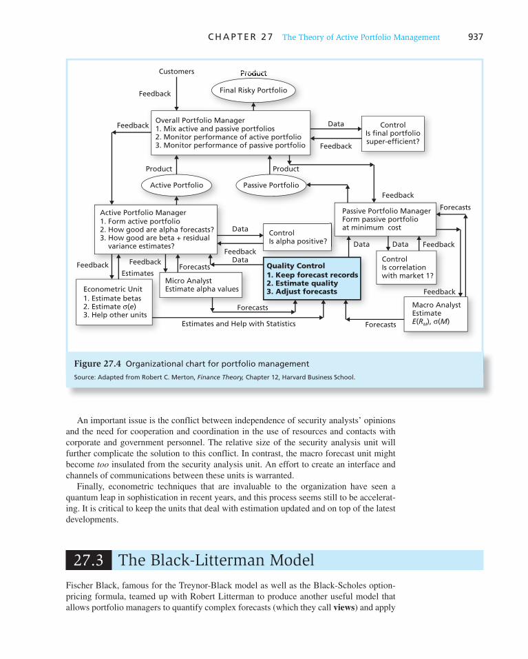
C H A P T E R 2 7 The Theory of Active Portfolio Management 937
An important issue is the conflict between independence of security analysts’ opinions and the need for cooperation and coordination in the use of resources and contacts with corporate and government personnel. The relative size of the security analysis unit will further complicate the solution to this conflict. In contrast, the macro forecast unit might become too insulated from the security analysis unit. An effort to create an interface and channels of communications between these units is warranted.
Finally, econometric techniques that are invaluable to the organization have seen a quantum leap in sophistication in recent years, and this process seems still to be accelerat-ing. It is critical to keep the units that deal with estimation updated and on top of the latest developments.
Figure 27.4 Organizational chart for portfolio management
Source: Adapted from Robert C. Merton, Finance Theory, Chapter 12, Harvard Business School.
Product
Final Risky Portfolio
Customers
ControlIs final portfoliosuper-efficient?
Product
Active Portfolio
Product
Passive Portfolio
Data
Feedback
Feedback
Feedback
ControlIs alpha positive?
Data
FeedbackData
Passive Portfolio ManagerForm passive portfolioat minimum cost
Feedback
ControlIs correlationwith market 1?
Feedback
Feedback
Data
Macro AnalystEstimateE(RM), σ(M)
Forecasts
Quality Control
1. Keep forecast records2. Estimate quality3. Adjust forecasts
Micro AnalystEstimate alpha valuesEconometric Unit
1. Estimate betas2. Estimate σ(e)3. Help other units
Forecasts
Forecasts
Data
ForecastsEstimates
Estimates and Help with Statistics
Feedback Feedback
Overall Portfolio Manager1. Mix active and passive portfolios2. Monitor performance of active portfolio3. Monitor performance of passive portfolio
1. Form active portfolio2. How good are alpha forecasts?3. How good are beta + residual variance estimates?
Active Portfolio Manager
27.3 The Black-Litterman Model
Fischer Black, famous for the Treynor-Black model as well as the Black-Scholes option-pricing formula, teamed up with Robert Litterman to produce another useful model that allows portfolio managers to quantify complex forecasts (which they call views ) and apply
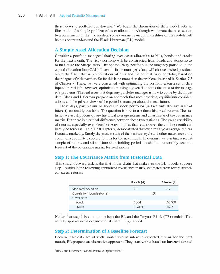
938 P A R T V I I Applied Portfolio Management
these views to portfolio construction. 6 We begin the discussion of their model with an illustration of a simple problem of asset allocation. Although we devote the next section to a comparison of the two models, some comments on commonalities of the models will help us better understand the Black-Litterman (BL) model.
A Simple Asset Allocation Decision
Consider a portfolio manager laboring over asset allocation to bills, bonds, and stocks for the next month. The risky portfolio will be constructed from bonds and stocks so as to maximize the Sharpe ratio. The optimal risky portfolio is the tangency portfolio to the capital allocation line (CAL). Investors in the manager’s fund will choose desired positions along the CAL, that is, combinations of bills and the optimal risky portfolio, based on their degree of risk aversion. So far this is no more than the problem described in Section 7.3 of Chapter 7. There, we were concerned with optimizing the portfolio given a set of data inputs. In real life, however, optimization using a given data set is the least of the manag-er’s problems. The real issue that dogs any portfolio manager is how to come by that input data. Black and Litterman propose an approach that uses past data, equilibrium consider-ations, and the private views of the portfolio manager about the near future.
These days, past returns on bond and stock portfolios (in fact, virtually any asset of interest) are readily available. The question is how to use those historical returns. The sta-tistics we usually focus on are historical average returns and an estimate of the covariance matrix. But there is a critical difference between these two statistics. The great variability of returns, especially over short horizons, implies that returns over the coming month can barely be forecast. Table 5.2 (Chapter 5) demonstrated that even multiyear average returns fluctuate markedly. Surely the present state of the business cycle and other macroeconomic conditions dominate expected returns for the next month. In contrast, we can take a recent sample of returns and slice it into short holding periods to obtain a reasonably accurate forecast of the covariance matrix for next month.
Step 1: The Covariance Matrix from Historical Data
This straightforward task is the first in the chain that makes up the BL model. Suppose step 1 results in the following annualized covariance matrix, estimated from recent histori-cal excess returns:
Bonds (B) Stocks (S)
Standard deviation .08 .17
Correlation (bonds/stocks) .3
Covariance
Bonds .0064 .00408
Stocks .00408 .0289
Notice that step 1 is common to both the BL and the Treynor-Black (TB) models. This activity appears in the organizational chart in Figure 27.4 .
Step 2: Determination of a Baseline Forecast
Because past data are of such limited use in inferring expected returns for the next month, BL propose an alternative approach. They start with a baseline forecast derived
6 Black and Litterman, “Global Portfolio Optimization.”
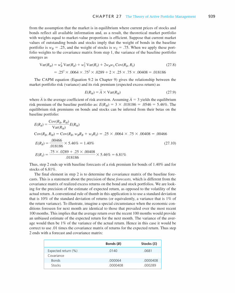
C H A P T E R 2 7 The Theory of Active Portfolio Management 939
from the assumption that the market is in equilibrium where current prices of stocks and bonds reflect all available information and, as a result, the theoretical market portfolio with weights equal to market-value proportions is efficient. Suppose that current market values of outstanding bonds and stocks imply that the weight of bonds in the baseline portfolio is w B 5 .25, and the weight of stocks is w S 5 .75. When we apply these port-folio weights to the covariance matrix from step 1, the variance of the baseline portfolio emerges as
Var(RM) 5 wB2 Var(RB) 1 wS
2 Var(RS) 1 2wBwS Cov(RB, RS) (27.8)
5 .252 3 .0064 3 .752 3 .0289 1 2 3 .25 3 .75 3 .00408 5 .018186
The CAPM equation (Equation 9.2 in Chapter 9) gives the relationship between the market portfolio risk (variance) and its risk premium (expected excess return) as
E(RM) 5 A 3 Var(RM) (27.9)
where A is the average coefficient of risk aversion. Assuming A 5 3 yields the equilibrium risk premium of the baseline portfolio as: E ( R M ) 5 3 3 .018186 5 .0546 5 5.46%. The equilibrium risk premiums on bonds and stocks can be inferred from their betas on the baseline portfolio:
E(RB) 5Cov(RB, RM)
Var(RM) E(RM)
Cov( R B , R M ) 5 Cov( R B , w B R B 1 w S R S ) 5 .25 3 .0064 3 .75 3 .00408 5 .00466
E(RB) 5.00466
.0181863 5.46% 5 1.40% (27.10)
E(RS) 5.75 3 .0289 1 .25 3 .00408
.0181863 5.46% 5 6.81%
Thus, step 2 ends up with baseline forecasts of a risk premium for bonds of 1.40% and for stocks of 6.81%.
The final element in step 2 is to determine the covariance matrix of the baseline fore-casts. This is a statement about the precision of these forecasts, which is different from the covariance matrix of realized excess returns on the bond and stock portfolios. We are look-ing for the precision of the estimate of expected return, as opposed to the volatility of the actual return. A conventional rule of thumb in this application is to use a standard deviation that is 10% of the standard deviation of returns (or equivalently, a variance that is 1% of the return variance). To illustrate, imagine a special circumstance when the economic con-ditions foreseen for next month are identical to those that prevailed over the most recent 100 months. This implies that the average return over the recent 100 months would provide an unbiased estimate of the expected return for the next month. The variance of the aver-age would then be 1% of the variance of the actual return. Hence in this case it would be correct to use .01 times the covariance matrix of returns for the expected return. Thus step 2 ends with a forecast and covariance matrix:
Bonds (B) Stocks (S)
Expected return (%) .0140 .0681
Covariance
Bonds .000064 .0000408
Stocks .0000408 .000289

940 P A R T V I I Applied Portfolio Management
Now that we have backed out market expectations, it is time to integrate the manager’s private views into our analysis.
Step 3: Integrating the Manager’s Private Views
The BL model allows the manager to introduce any number of views about the baseline forecasts into the optimization process. Appended to the views, the manager specifies his degree of confidence in them. Views in the BL model are expressed as values of various linear combinations of excess returns, and confidence in them as a covariance matrix of errors in these values.
Example 27.1 Views in the Black-Litterman Model
Suppose the manager takes a contrarian’s view concerning the baseline forecasts, that is, he believes that in the next month bonds will outperform stocks by .5%. The following equation expresses this view:
1 3 RB 1 (21) 3 RS 5 .5%
More generally, any view that is a linear combination of the relevant excess returns can be presented as an array (in Excel, an array would be a column of numbers) that multiplies another array (column) of excess returns. In this case, the array of weights is P 5 (1, 2 1) and the array of excess returns is ( R B , R S ). (We can perform the multiplication in Excel by applying the SUMPRODUCT function to the two arrays.) The value of this linear combi-nation, denoted Q, reflects the manager’s view. In this case, Q 5 .5% will be taken into account in optimizing the portfolio.
A view must come with a degree of confidence, that is, a standard deviation to measure the precision of Q. In other words, the manager’s view is really Q 1 á, where á represents zero-mean “noise” surrounding the view with a standard deviation that reflects the man-ager’s confidence. Noticing that the variance of the difference between the expected rates on stocks and bonds is 2.7% (calculated below in Equation 27.13), suppose that the man-ager assigns a value of s (á) 5 1.73%. To summarize, if we denote the array of returns by R 5 ( R B , R S ), then the manager’s view, P, applied to these returns is
PR r5 Q 1 e
P 5 (1, 21)
R 5 (RB, RS) (27.11)
Q 5 .5% 5 .005
s2(e) 5 .01732 5 .0003
Step 4: Revised (Posterior) Expectations
The baseline forecasts of expected returns derived from market values and their covari-ance matrix comprise the prior distribution of the rates of return on bonds and stocks. The manager’s view, together with its confidence measure, provides the probability distribution arising from the “experiment,” that is, the additional information that must be optimally integrated with the prior distribution. The result is a new set of expected returns, condi-tioned on the manager’s views.

C H A P T E R 2 7 The Theory of Active Portfolio Management 941
To acquire intuition about the solution, consider what the baseline expected returns imply about the view. The expectations derived from market data were that the expected return on bonds is 1.40% and on stocks 6.81%. Therefore, the baseline view is that R B 2 R S 5 2 5.41%. In contrast, the manager thinks this difference is Q 5 R B 2 R S 5 .5%. Using the BL linear-equation notation for market expectations:
QE 5 PRrE
P 5 (1, 21)
RE 5 3E(RB), E(RS) 45 (1.40%, 6.81%) (27.12)
QE 5 1.40 2 6.81 5 25.41%
Thus, the baseline “view” is 2 5.41% (i.e., stocks will outperform bonds), which is vastly different from the manager’s view. The difference, D, is
D 5 Q 2 QE 5 .005 2 (2.0541) 5 .0591
s2(D) 5 s2(e) 1 s2(QE) 5 .0003 1 s2(QE)
s2(QE) 5 Var 3E(RB) 2 E(RS) 45 sE(RB)2 1 sE(RS)
2 2 2Cov 3E(RB), E(RS) 4 (27.13)
5 .000064 1 .000289 2 2 3 .0000408 5 .0002714
s2(D) 5 .0003 1 .0002714 5 .0005714
Given the large difference between the manager’s and the baseline expectations, we expect a significant change in the conditional expectations from those of the baseline and, as result, a very different optimal portfolio.
The change in expected returns is a function of four elements: the baseline expectations, E ( R ); the difference, D, between the manager’s view and the baseline view (see Equation 27.13); the variance of E ( R ); and the variance of D. Using the BL updating formulas given the baseline and manager’s views and their precision, we get
E(RB | P) 5 E(RB) 1D5sE(RB)
2 2 Cov 3E(RB), E(RS) 4 6sD
2
5 .0140 1.0591(.000064 2 .0000408)
.00057145 .0140 1 .0024 5 .0164
E(RS | P) 5 E(RS) 1D5Cov 3E(RB), E(RS) 42 sE(RS)
2 6sD
2 (27.14)
5 .0681 1.0591(.0000408 2 .000289)
.00057145 .0681 2 .0257 5 .0424
We see that the manager increases his expected returns on bonds by .24% to 1.64%, and reduces his expected return on stocks by 2.57% to 4.24%. The difference between the expected returns on stocks and bonds is reduced from 5.41% to 2.60%. While this is a very large change, we also realize that the manager’s private view that Q 5 .5% has been greatly tempered by the prior distribution to a value roughly halfway between his private view and the baseline view. In general, the degree of compromise between views will depend on the precision assigned to them.
The example we have described contains only two assets and one view. It can easily be generalized to any number of assets with any number of views about future returns. The views can be more complex than a simple difference between a pair of returns. Views can

942 P A R T V I I Applied Portfolio Management
assign a value to any linear combination of the assets in the universe, and the confidence level (the covariance matrix of the set of á values of the views) can allow for dependence across views. This flexibility gives the model great potential by quantifying a rich set of information that is unique to a portfolio manager. Appendix B to the chapter presents the general BL model.
Step 5: Portfolio Optimization
At this point, the portfolio optimization follows the Markowitz procedure of Chapter 7, with an input list that replaces baseline expectations with the conditional expectations aris-ing from the manager’s view.
Spreadsheet 27.2 presents the calculations of the BL model. Table 1 of the spreadsheet shows the calculation of the benchmark forecasts and Table 2 incorporates a view to arrive at the revised (conditional) expectations. We show these for various degrees of confidence in the view. Figure 27.5 shows properties of the optimal portfolio for the various levels of confidence on the assumption that the view is correct. Figure 27.6 conducts the same sen-sitivity analysis when the view is wrong. Figures 27.5 and 27.6 illustrate the important role that confidence plays in the performance of the BL portfolio. In the next section we discuss the implication of these results.
1
2
3
4
5
6
7
8
9
10
11
12
13
14
15
16
17
18
19
20
21
22
23
24
2526
27
28
29
30
31
32
33
34
35
36
Table 1: Bordered Covariance Matrix Based on Historical Excess Returns
and Market-Value Weights and Calculation of Baseline Forecasts
Bonds StocksWeights 0.25 0.75
BondsStocks
sumproduct 0.001165 0.017021Market portfolio variance V(M) = sum(c11:d11) =
Coefficient of risk aversion of representative investor =Baseline market portfolio risk premium = A × V(M) =
Covariance with RM
Baseline risk premiums
Proportion of covariance attributed to expected returns: 0.01Covariance matrix of expected returns
Bonds Stocks
BondsStocks
Table 2: Views, Confidence and Revised (Posterior) Expectations
View: Difference between returns on bonds and stocks, Q =
View embedded in baseline forecasts QE =
Variance of QE = Var(RB − RS)
Var[E(RB)] − Cov[E(RB),E(RS)] =
Cov[E(RB),E(RS)] − Var[E(RB)] =
Difference between view and baseline data, D =Confidence measured by standard deviation of view Q
Possible SD 0 0.0100 0.0173 0.0300 0.0600
Variance 0 0.0015 0.0003 0.0009 0.0036 BaselineE(RB|P) 0.0190 0.0148 0.0164 0.0152 0.0143 0.0140E(RS|P) 0.0140 0.0598 0.0424 0.0556 0.0643 0.0681
A C D E F G H IB
0.25 0.006400 0.0040800.75 0.004080 0.028900
0.00466 0.022695
0.01 0.07
0.000064 0.00004080.0000408 0.000289
0.0050−0.0541
0.000271
0.000023
−0.000248
0.0591
0.0181863
0.0546
Spreadsheet 27.2
Sensitivity of the Black-Litterman portfolio to confidence in views
eXce lPlease visit us at www.mhhe.com/bkm
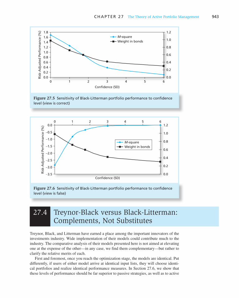
C H A P T E R 2 7 The Theory of Active Portfolio Management 943
27.4 Treynor-Black versus Black-Litterman: Complements, Not Substitutes
Figure 27.5 Sensitivity of Black-Litterman portfolio performance to confidence level (view is correct)
0.0
0.2
0.4
0.6
0.8
1.0
1.2
1.4
1.6
1.8
0 1 2 3 4 5 6
Confidence (SD)
Ris
k-A
dju
sted
Per
form
ance
(%
)
0.0
0.2
0.4
0.6
0.8
1.0
1.2M-squareWeight in bonds
Figure 27.6 Sensitivity of Black-Litterman portfolio performance to confidence level (view is false)
−3.5
−3.0
−2.5
−2.0
−1.5
−1.0
−0.5
0.00 1 2 3 4 5 6
Confidence (SD)
Ris
k-A
dju
sted
Per
form
ance
(%
)
0.0
0.2
0.4
0.6
0.8
1.0
1.2
M-squareWeight in bonds
Treynor, Black, and Litterman have earned a place among the important innovators of the investments industry. Wide implementation of their models could contribute much to the industry. The comparative analysis of their models presented here is not aimed at elevating one at the expense of the other—in any case, we find them complementary—but rather to clarify the relative merits of each.
First and foremost, once you reach the optimization stage, the models are identical. Put differently, if users of either model arrive at identical input lists, they will choose identi-cal portfolios and realize identical performance measures. In Section 27.6, we show that these levels of performance should be far superior to passive strategies, as well as to active

944 P A R T V I I Applied Portfolio Management
s trategies that do not take advantage of the quantitative techniques of these models. The models differ primarily in the way they arrive at the input list, and analysis of these differ-ences shows that the models are true complements and are best used in tandem.
The BL Model as Icing on the TB Cake
The Treynor-Black (TB) model is really oriented to individual security analysis. This can be seen from the way the active portfolio is constructed. The alpha values assigned to securities must be determined relative to the passive portfolio. This portfolio is the one that would be held if all alpha values turned out to be zero. Now suppose an investment com-pany prospectus mandates a portfolio invested 70% in a U.S. universe of large stocks, say, the S&P 500, and 30% in a well-defined universe of large European stocks. In that case, the macro analysis of the organization would have to be split, and the TB model would have to be run as two separate divisions. In each division, security analysts would compile values of alpha relative to their own passive portfolio. The product of this organization would thus include four portfolios, two passive and two active. This scheme is workable only when the portfolios are optimized separately. That is, the parameters (alpha, beta, and residual variance) of U.S. securities are estimated relative to the U.S. benchmark, while the parameters of European stocks are estimated relative to the European benchmark. Then the final portfolio would be constructed as a standard problem in asset allocation.
The resulting portfolio could be improved using the BL approach. First, views about the relative performance of the U.S. and European markets can be expected to add information to the independent macro forecasts for the two economies. For reasons of specialization, the U.S. and European macro analysts must focus on their respective economies. Obviously, when more country or regional portfolios are added to the company’s universe, the need for decentralization becomes more compelling, and the potential of applying the BL model to the TB product greater. Moreover, the foreign-stock portfolios will result in various positions in local currencies. This is a clear area of international finance and the only way to import fore-casts from this analysis is with the BL technique. 7
Why Not Replace the Entire TB Cake with the BL Icing?
This question is raised by the need to use the BL technique if the overall portfolio is to include forecasts from comparative economic and international finance analyses. It is indeed possible to use the BL model for the entire process of constructing the efficient portfolio. The reason is that the alpha compiled for the TB model can be replaced with BL views. To take a simple example, suppose only one security makes up the active portfolio. With the TB model, we have macro forecasts, E ( R M ) and s M , as well as alpha, beta, and residual variance for the active portfolio. This input list also can be represented in the fol-lowing form, along the lines of the BL framework:
R 5 3E(RM), E(RA) 5 bAE(RM) 4 P 5 ¢0, 1 1
aA
bAE(RM)≤
PR r5 Q 1 e 5 aA 1 e
QE 5 0 (27.15)
D 5 aA
s2(e) 5 Var(forecasting error) in Equation 27.6
s2(D) 5 s2(e) 1 s2(e)
7 The BL model can also be used to introduce views about relative performance of various U.S and foreign corporations.

C H A P T E R 2 7 The Theory of Active Portfolio Management 945
where e is the residual in the SCL regression of Equation 27.5. Calculation of the condi-tional expectations from Equation 27.15 as in Equation 27.13 will bring us to the same adjusted alpha as in Equation 27.7 of the TB model.
In this light, the BL model can be viewed as a generalization of the TB model. The BL model allows you to adjust expected return from views about alpha values as in the TB model, but it also allows you to express views about relative performance that cannot be incorporated in the TB model.
However, this conclusion might produce a false impression that is consequential to investment management. To understand the point, we first discuss the degree of confi-dence, which is essential to fully represent a view in the BL model. Spreadsheet 27.2 and Figures 27.5 and 27.6 illustrate that the optimal portfolio weights and performance are highly sensitive to the degree of confidence in the BL views. Thus, the validity of the model rests in large part on the way the confidence about views is arrived at.
When a BL view is structured to replace a direct alpha estimate in a TB framework, we must use the variance of the forecasting error taken from Equation 27.7 and applied to Equation 27.15. This is how “confidence” is quantified in the BL model. Whereas in the TB framework one can measure forecast accuracy by computing the correlation between analysts’ alpha forecasts and subsequent realizations, such a procedure is not as easily applied to BL views about relative performance. Managers’ views may be expressed about different quantities in different time periods, and, therefore, we will not have long forecast histories on a particular variable with which to assess accuracy. To our knowledge, no promotion of any kind of how to quantify “confidence” appears in academic or industry publications about the BL model.
This raises the issue of adjusting forecasts in the TB model. We have never seen evi-dence that analysts’ track records are systematically compiled and used to adjust alpha forecasts, although we cannot assert that such effort is nowhere expended. However, indi-rect evidence confirms the impression that alphas are usually not adjusted, specifically, the common “complaint” that the TB model is not applied in the field because it results in “wild” portfolio weights. Yet, as we saw in Section 27.3, those wild portfolio weights are a consequence of failing to adjust alpha values to reflect forecast precision. Any realistic R -square that can be obtained even by excellent forecasters will result in moderate portfo-lio weights. Even when “wild” weights do occasionally materialize, they can be “tamed” by a straightforward restriction on benchmark risk.
It is therefore useful to keep the two models separate and distinct; the TB model for the management of security analysis with proper adjustment of forecasts and the BL model for asset allocation where views about relative performance are useful despite the fact that the degree of confidence must in practice be inaccurately estimated.
27.5 The Value of Active Management
We showed in Chapter 24 that the value of successful market timing is enormous. Even a forecaster with far-from-perfect predictive power would contribute significant value. Nevertheless, active portfolio management based on security analysis has even far greater potential. Even if each individual security analyst has only modest forecasting power, the power of a portfolio of analysts is potentially unbounded.
A Model for the Estimation of Potential Fees
The value of market timing was derived from the value of an equivalent number of call options that mimic the return to the timer’s portfolio. Thus, we were able to derive an unambiguous market value to timing ability, that is, we could price the implicit call in the
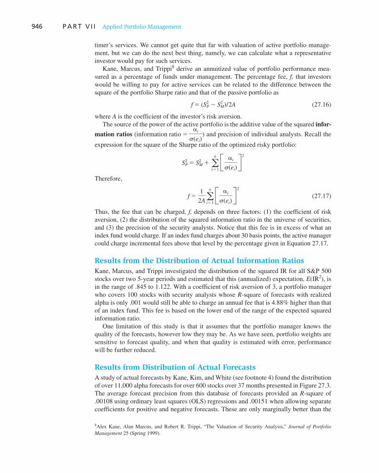
946 P A R T V I I Applied Portfolio Management
timer’s services. We cannot get quite that far with valuation of active portfolio manage-ment, but we can do the next best thing, namely, we can calculate what a representative investor would pay for such services.
Kane, Marcus, and Trippi 8 derive an annuitized value of portfolio performance mea-sured as a percentage of funds under management. The percentage fee, f, that investors would be willing to pay for active services can be related to the difference between the square of the portfolio Sharpe ratio and that of the passive portfolio as
f 5 (SP2 2 SM
2 )/2A (27.16)
where A is the coefficient of the investor’s risk aversion. The source of the power of the active portfolio is the additive value of the squared infor-
mation ratios (information ratio 5ai
s(ei)) and precision of individual analysts. Recall the
expression for the square of the Sharpe ratio of the optimized risky portfolio:
SP2 5 SM
2 1 an
i51
B ai
s(ei)R 2
Therefore,
f 51
2Aan
i51
B ai
s(ei)R 2
(27.17)
Thus, the fee that can be charged, f, depends on three factors: (1) the coefficient of risk aversion, (2) the distribution of the squared information ratio in the universe of securities, and (3) the precision of the security analysts. Notice that this fee is in excess of what an index fund would charge. If an index fund charges about 30 basis points, the active manager could charge incremental fees above that level by the percentage given in Equation 27.17.
Results from the Distribution of Actual Information Ratios
Kane, Marcus, and Trippi investigated the distribution of the squared IR for all S&P 500 stocks over two 5-year periods and estimated that this (annualized) expectation, E (IR 2 ), is in the range of .845 to 1.122. With a coefficient of risk aversion of 3, a portfolio manager who covers 100 stocks with security analysts whose R -square of forecasts with realized alpha is only .001 would still be able to charge an annual fee that is 4.88% higher than that of an index fund. This fee is based on the lower end of the range of the expected squared information ratio.
One limitation of this study is that it assumes that the portfolio manager knows the quality of the forecasts, however low they may be. As we have seen, portfolio weights are sensitive to forecast quality, and when that quality is estimated with error, performance will be further reduced.
Results from Distribution of Actual Forecasts
A study of actual forecasts by Kane, Kim, and White (see footnote 4) found the distribution of over 11,000 alpha forecasts for over 600 stocks over 37 months presented in Figure 27.3 . The average forecast precision from this database of forecasts provided an R -square of .00108 using ordinary least squares (OLS) regressions and .00151 when allowing separate coefficients for positive and negative forecasts. These are only marginally better than the
8 Alex Kane, Alan Marcus, and Robert R. Trippi, “The Valuation of Security Analysis,” Journal of Portfolio
Management 25 (Spring 1999).

C H A P T E R 2 7 The Theory of Active Portfolio Management 947
precision used to interpret the Kane, Marcus, and Trippi study of the distribution of real-ized information value. Kane, Kim, and White use these R -squares to adjust the forecasts in their database and form optimal portfolios from 105 stocks selected randomly from the 646 covered by the investment company.
Kane, Kim, and White assume that forecast quality is the same each month for all alpha forecasts for the 105 stocks, but act as though they do not know that quality. Thus, the adjustment process is performed each month by using past forecasts. This introduces another source of estimation error that compounds the difficulty of low forecast quality. To dull the impact of this real-life difficulty, the estimation of forecast quality adopts improved econometric technique. They find that least absolute deviation (LAD) regressions perform uniformly better than OLS regressions. The optimization model used both the diagonal index model (as in TB) as well as the full-covariance model (the Markowitz algorithm).
The annualized M -square measures of performance are shown in Table 27.6 . The M -square values, which range from 2.67% to 6.31%, are quite impressive. The results in Table 27.6 also show that using the residual covariance matrix can significantly improve performance when many stocks are covered, contrary to the small difference when only six stocks are covered, as in Spreadsheet 8.1 of Chapter 8.
Results with Reasonable Forecasting Records
To investigate the role of the forecasting record in performance with low-quality forecasts, Kane, Kim, and White simulate a market with the S&P 500 index portfolio as bench-mark and 500 stocks with the same characteristics as the S&P 500 universe. 9 Various sizes of active portfolios are constructed by selecting stocks randomly from this universe with available forecasting records of only 36 to 60 months. To avoid estimation techniques that may not be available to portfolio managers, all estimates in this study are obtained from OLS regressions.
The portfolio manager in the simulation must deploy a full-blown “organizational struc-ture” to capture performance under realistic conditions. At any point, the manager uses only past returns and past forecast records to produce forward-looking estimates which include (1) the benchmark risk premium and standard deviation, (2) beta coefficients for the stocks in the active portfolio, and (3) the forecasting quality of each security analyst. At this point, the manager receives a set of alpha forecasts from the security analysts and pro-ceeds to construct the optimal portfolio. The portfolio is optimized on the basis of macro forecasts for the benchmark portfolio, and alpha forecasts adjusted for quality using the past record of performance for each analyst. Finally, the next month returns are simulated and the performance of the portfolio is recorded.
Table 27.7 summarizes the results for portfolios when, unbeknownst to the portfolio manager, security-analyst forecasts are generated with an R -square of .001. M -square
9 Alex Kane, Tae-Hwan Kim, and Halbert White, “Forecast Precision and Portfolio Performance,” UCSD working paper, University of California–San Diego, April 2006.
Forecast Adjustment Diagonal Model Covariance Model
Line* 2.67 3.01
Kinked** 4.25 6.31
Table 27.6
M -square for the portfolio, actual forecasts
*Same coefficients for positive and negative forecasts. **Different coefficients for positive and negative forecasts.

948 P A R T V I I Applied Portfolio Management
clearly increases when performance records are longer. The results also show that, in gen-eral, performance improves with the size of the portfolio.
The results of all three studies show that even the smallest forecast ability can result in greatly improved performance. Moreover, with better estimation techniques, perfor-mance can be further enhanced. We believe that one reason the proposed procedures are not widely used in the industry is that security analysts believe that low individual correla-tions imply low aggregate forecasting value and thus wish to avoid the estimation of their abilities. We hope that results of studies of the type discussed here will lure investment companies to adopt these techniques and move the industry to new levels of performance.
Forecast Record (months)
Stocks in Portfolio 36 48 60
100 0.96 3.12 6.36
300 0.60 5.88 12.72
500 3.00 5.88 15.12
Table 27.7
M -square of simulated portfolios
27.6 Concluding Remarks on Active Management
A common concern of students of investments who encounter a heavy dose of theory laced with math and statistics is whether the analytical approach is necessary or even useful. Here are some observations that should allay any such concern. Investment theory has developed in recent decades at a galloping pace. Yet, perhaps surprisingly, the distance between the basic science of investments and industry practice, one that exists in any field, has actually narrowed in recent years. This satisfying trend is due at least in part to the vig-orous growth of the CFA Institute. The CFA designation has become nearly a prerequisite to success in the industry, and the number of individuals seeking it already exceeds that of finance-major MBAs. They continuously contribute to the proximity between investments science and the industry.
Even more important is the zeal of the Institute in advancing and enriching the cur-riculum of the CFA degree and taking it ever closer to contemporary investment theory. Indeed, finance professors indirectly benefit from this curriculum, because they can argue the practicality of the text material by pointing out that it is part of the body of knowledge required of CFA candidates.
Yet there is one area in which practice still lags far behind theory, and that is the subject of this chapter—this despite the fact that TB and BL models have been around since 1973 and 1992, respectively. Yet, as we have seen, these models have to date failed to materially penetrate the industry. We speculated on the reason for this failure in the previous section. We hope, however, that we will be forced to discard this paragraph from future editions due to obsolescence.
Finally, there is little time in the already dense investments curriculum to discuss the welfare implication of nearly efficient security prices. Prices can reach such levels only when investors optimize portfolios with high-quality analysis and implementation. The value of nearly efficient prices to the welfare of the economy is enormous, competing in importance with advances in technology. High-quality active management therefore can contribute to society even as it enriches its practitioners.

Vis
it u
s at
ww
w.m
hh
e.co
m/b
kmV
isit
us
at w
ww
.mh
he.
com
/bkm
C H A P T E R 2 7 The Theory of Active Portfolio Management 949
1. Treynor-Black portfolio weights are sensitive to large alpha values, which can result in practically infeasible long/short portfolio positions.
2. Benchmark portfolio risk, the variance of the return difference between the portfolio and the benchmark, can be constrained to keep the TB portfolio within reasonable weights.
3. Alpha forecasts must be shrunk (adjusted toward zero) to account for less-than-perfect forecast-ing quality. Compiling past analyst forecasts and subsequent realizations allows one to estimate the correlation between realizations and forecasts. Regression analysis can be used to measure the forecast quality and guide the proper adjustment of future forecasts. When alpha forecasts are scaled back to account for forecast imprecision, the resulting portfolio positions become far more moderate.
4. The Black-Litterman model allows the private views of the portfolio manager to be incorporated with market data in the optimization procedure.
5. The Treynor-Black and Black-Litterman models are complementary tools. Both should be used: the TB model is more geared toward security analysis while the BL model more naturally fits asset allocation problems.
6. Even low-quality forecasts are valuable. Imperceptible R -squares of only .001 in regressions of realizations on analysts’ forecasts can be used to substantially improve portfolio performance.
SUMMARY
Related Web sites for this chapter are available at www.mhhe.com/bkm
passive portfolio active portfolio alpha values benchmark portfolio tracking error
prior distribution posterior distribution forecasting records adjusted alphas views
asset allocation baseline forecasts information ratio
KEY TERMS
1. How would the application of the BL model to a stock and bond portfolio (as the example in the text) affect security analysis? What does this suggest about the hierarchy of use of the BL and TB models?
2. Figure 27.4 includes a box for the econometrics unit. Item (3) is to “help other units.” What sorts of specific tasks might this entail?
3. Make up new alpha forecasts and replace those in Spreadsheet 27.1 in Section 27.1. Find the optimal portfolio and its expected performance.
4. Make up a view and replace the one in Spreadsheet 27.2 in Section 27.3. Recalculate the optimal asset allocation and portfolio expected performance.
5. Suppose that sending an analyst to an executive education program will raise the precision of the analyst’s forecasts as measured by R -square by .01. How might you put a dollar value on this improvement? Provide a numerical example.
PROBLEM SETS
i. Basic
ii. Intermediate
eXce lPlease visit us at www.mhhe.com/bkm
iii. Challenge
Tracking Errors
Visit www.jpmorganfunds.com/pdfs/other/Tracking_Error.pdf for a discussion about the measurement of tracking error. What factors are mentioned as possible causes of high tracking error? What is the relationship between high tracking error and a manager’s gen-eration of high positive alphas? How can the tracking error measurement and the Sharpe ratio be used to assess a manager’s performance?
E-INVEST-MENTS EXERCISES

APPENDIX A: Forecasts and Realizations of Alpha
APPENDIX B: The General Black-Litterman Model
Vis
it u
s at
ww
w.m
hh
e.co
m/b
km950 P A R T V I I Applied Portfolio Management
A linear representation of the process that generates forecasts from the (yet unknown) future values of alpha would be
a f(t) 5 b0 1 b1u(t) 1 h(t) (27A.1)
where h ( t ) is the forecasting error and is uncorrelated with the actual u ( t ). Notice that when the forecast is optimized as in Equation 27.7, the error of the adjusted forecast, á( t ) in Equation 27.6, is uncorrelated with the optimally adjusted forecast a ( T ). The coeffi-cients b 0 and b 1 are shift and scale biases in the forecast. Unbiased forecasts would result in b 0 5 0 (no shift) and b 1 5 1 (no scale bias).
We can derive both the variance of the forecast and the covariance between the forecast and realization from Equation 27A.1:
s2(a f) 5 b12 3 s2(u) 1 s2(h)
Cov(a f, u) 5 b1 3 s2(u) (27A.2)
Therefore the slope coefficient, a 1 , in Equation 27.6 is
a1 5Cov(u, a f)
s2(a f )5
b1 3 s2(u)
b12 3 s2(u) 1 s2(h)
(27A.3)
When the forecast has no scale bias, that is, when b 1 5 1, a 1 equals the R -square of the regression of forecasts on realizations in Equation 27A.1, which also equals the R -square of the regression of realizations on forecasts in Equation 27.6. When b 1 is different from 1.0, we must adjust the coefficient a 1 to account for the scale bias. Notice also that with this adjustment, a 0 5 2 b 0 .
The BL model is easiest to write using matrix notation. We describe the model according to the steps in Section 27.3.
Steps 1 and 2: The Covariance Matrix and Baseline Forecasts
A sample of past excess returns of the universe of n assets is used to estimate the n 3 n cova-riance matrix, denoted by Σ. It is assumed that the excess returns are normally distributed.
Market values of the universe assets are obtained and used to compute the 1 3 n vector of weights w M in the baseline equilibrium portfolio. The variance of the baseline portfolio is calculated from
sM2 5 wM gwrM (27B.1)
A coefficient of risk aversion for the representative investor in the economy, A, is applied to the CAPM equation to obtain the baseline macro forecast for the market portfolio risk premium,
E(RM) 5 AsM2 (27B.2)

Vis
it u
s at
ww
w.m
hh
e.co
m/b
km
C H A P T E R 2 7 The Theory of Active Portfolio Management 951
The 1 3 n vector of baseline forecasts for the universe securities risk premiums, R, is com-puted from the macro forecast and the covariance matrix by
E(Rr) 5 E(RM)gw rM (27B.3)
The data so far describe the prior (baseline) distribution of the rates of return of the asset universe by
R| , N 3E(R), g 4 (27B.4)
The n 3 n covariance matrix of the baseline expected returns, t Σ, is assumed proportional to the covariance matrix, Σ, by the scalar t .
Step 3: The Manager’s Private Views
The k 3 n matrix of views, P, includes k views. The i th view is a 1 3 k vector that mul-
tiplies the 1 3 n vector of returns, R|, to obtain the value of the view, Q i , with forecasting error á i . The entire vector of view values and their forecasting errors is given by
RP 5 Q 1 e (27B.5)
The confidence of the manager in the views is given by the k 3 k covariance matrix, V, of the vector of errors in views, á. The views embedded in the baseline forecast, R, are given by Q E ,
RP 5 QE
Thus, the 1 3 k vector of deviation of the view from the baseline view (forecasts) and its covariance matrix S D is
D 5 QE 2 Q
SD 5 tPgP r1 V (27B.6)
Step 4: Revised (Posterior) Expectations
The 1 3 n vector of posterior (revised) expectations conditional on the views is given by
R* 5 R | P 5 R 1 tDSD21gP r (27B.7)
Step 5: Portfolio Optimization
The vector of revised expectations is used in conjunction with the covariance matrix of excess returns to produce the optimal portfolio weights with the Markowitz algorithm.

28 2 TRANSLATING THE ASPIRATIONS and cir-
cumstances of diverse households into appro-
priate investment decisions is a daunting task.
The task is equally difficult for institutions,
most of which have many stakeholders and
often are regulated by various authorities.
The investment process is not easily reduced
to a simple or mechanical algorithm.
While many principles of investments are
quite general and apply to virtually all inves-
tors, some issues are peculiar to the specific
investor. For example, tax bracket, age, risk
tolerance, wealth, job prospects, and uncer-
tainties make each investor’s circumstances
somewhat unique. In this chapter we focus on
the process by which investors systematically
review their particular objectives, constraints,
and circumstances. Along the way, we sur-
vey some of the major classes of institutional
investors and examine the special issues they
must confront.
Of course, there is no unique “ correct”
investment process. However, some approaches
are better than others, and it can be helpful
to take one high-quality approach as a useful
case study. For this reason, we will examine
the systematic approach suggested by the CFA
Institute. Among other things, the Institute
administers examinations to certify invest-
ment professionals as Chartered Financial
Analysts. Therefore, the approach we outline
is also one that a highly respected professional
group endorses through the curriculum that it
requires investment practitioners to master.
The basic framework involves dividing the
investment process into four stages: specify-
ing objectives, specifying constraints, for-
mulating policy, and later monitoring and
updating the portfolio as needed. We will
treat each of these activities in turn. We start
with a description of the major types of inves-
tors, both individual and institutional, as well
as their special objectives. We turn next to the
constraints or circumstances peculiar to each
investor class, and we consider some of the
investment policies that each can choose.
We will examine how the special circum-
stances of both individuals as well as institu-
tions such as pension funds affect investment
decisions. We also will see how the tax system
can impart a substantial effect on investment
decisions.
Investment Policy and the Framework of the CFA
Institute
CHAPTER TWENTY-EIGHT PA
RT
VII

C H A P T E R 2 8 Investment Policy and the Framework of the CFA Institute 953
28.1 The Investment Management Process
The CFA Institute divides the process of investment management into three main elements that constitute a dynamic feedback loop: planning, execution, and feedback. Figure 28.1 and Table 28.1 describe the steps in that process. As shorthand, you might think of plan-
ning as focused largely on establishing all the inputs necessary for decision making. These include data about the client as well as the capital market, resulting in very broad policy guidelines (the strategic asset allocation). Execution fleshes out the details of optimal asset allocation and security selection. Finally, feedback is the process of adapting to changes in expectations and objectives as well as to changes in portfolio composition that result from changes in market prices.
The result of this analysis can be summarized in an Investment Policy Statement addressing the topics specified in Table 28.2 . In the next sections we elaborate on the steps leading to such an Investment Policy Statement. We start with the planning phase, panel A of Table 28.1 .
Objectives
Table 28.1 indicates that the management planning process starts off by analyzing one’s investment clients—in particular, by considering the objectives and constraints that gov-ern their decisions. Portfolio objectives center on the risk–return trade-off between the expected return the investors want ( return requirements in the first column of Table 28.3 ) and how much risk they are willing to assume ( risk tolerance ). Investment managers must know the level of risk that can be tolerated in the pursuit of a higher expected rate of return.
Figure 28.1 CFA Institute investment management process
Portfolio policies
and strategies
Capital market expectations
Planning Execution Feedback
Specification and quantification of
investor objectives, constraints,
and preferences
Relevant economic,
social, political, and
sector considerations
Portfolio construction
and revision
Asset allocation,
portfolio optimization,
security selection,
implementation, and
execution
Monitoring economic
and market input
factors
Monitoring investor-
related input factors
Attainment of
investor
objectives
Performance
measurement

954
Risk Tolerance Questionnaire
Here is an example of a short quiz which may be used by financial institutions to help estimate risk tolerance.
WO
RD
S FR
OM
TH
E ST
REE
T
Question 1 Point 2 Points 3 Points 4 Points
1. I plan on using the
money I am investing:
Within 6 months. Within the next
3 years.
Between 3 and 6 years. No sooner than
7 years from now.
2. My investments make
up this share of assets
(excluding home):
More than 75%. 50% or more but
less than 75%.
25% or more but less
than 50%.
Less than 25%.
3. I expect my future
income to:
Decrease. Remain the same
or grow slowly.
Grow faster than the rate
of inflation.
Grow quickly.
4. I have emergency
savings:
No. — Yes, but less than I’d like
to have.
Yes.
5. I would risk this share
in exchange for the
same probability of
doubling my money:
Zero. 10%. 25%. 50%.
6. I have invested in
stocks and stock
mutual funds:
— Yes, but I was uneasy
about it.
No, but I look forward
to it.
Yes, and I was
c omfortable with it.
7. My most important
investment goal is to:
Preserve my original
investment.
Receive some growth
and provide income.
Grow faster than in flation
but still provide some
income.
Grow as fast as
possible. Income is
not important today.
Add the number of points for all seven questions. Add one point if you choose the first answer, two if you choose the second answer, and so on. If you score between 25 and 28 points, consider yourself an aggressive investor. If you score between 20 and 24 points, your risk tolerance is above average. If you score between 15 and 19 points, consider
yourself a moderate investor. This means you are willing to accept some risk in exchange for a potential higher rate of return. If you score fewer than 15 points, consider yourself a conservative investor. If you have fewer than 10 points, you may consider yourself a very conservative investor.
Source: Securities Industry and Financial Markets Association.
The nearby box is an illustration of a questionnaire designed to assess an investor’s risk tolerance. Table 28.4 lists factors governing return requirements and risk attitudes for each of the seven major investor categories we will discuss.
Individual Investors
The basic factors affecting individual investor return requirements and risk tolerance are life-cycle stage and individual preferences. A middle-aged tenured professor will have a different set of needs and preferences from a retired widow, for example. We will have much more to say about individual investors later in this chapter.
Personal Trusts
Personal trusts are established when an individual confers legal title to property to another person or institution (the trustee) to manage that property for one or more ben-eficiaries. Beneficiaries customarily are divided into income beneficiaries, who receive the interest and dividend income from the trust during their lifetimes, and remainder-
men, who receive the principal of the trust when the income beneficiary dies and the trust is dissolved. The trustee is usually a bank, a savings and loan association, a lawyer, or

C H A P T E R 2 8 Investment Policy and the Framework of the CFA Institute 955
an investment pr ofessional. Investment of a trust is subject to trust laws, as well as “pru-dent investor” rules that limit the types of allowable trust investment to those that a prudent person would select.
Objectives for personal trusts normally are more limited in scope than those of the indi-vidual investor. Because of their fiduciary responsibility, personal trust managers typically
I. Planning
A. Identifying and specifying the investor’s objectives and constraints
B. Creating the Investment Policy Statement (See Table 28.2.)
C. Forming capital market expectations
D. Creating the strategic asset allocation (target minimum and maximum class weights)
II. Execution: Portfolio construction and revision
A. Asset allocation (including tactical) and portfolio optimization (combining assets to meet risk and return objectives)
B. Security selection
C. Implementation and execution
III. Feedback
A. Monitoring (investor, economic, and market input factors)
B. Rebalancing
C. Performance evaluation
Table 28.1
Components of the investment management process
Source: John L. Maginn, Donald L. Tuttle, Dennis W. McLeavey, and Jerald E. Pinto, “The Portfolio Management Process and the Investment Policy Statement,” in Managing Investment Portfolios: A Dynamic Process, 3rd ed . (CFA Institute, 2007) and co rrespondence with Tom Robinson, head of educational content.
Table 28.2
Components of the investment policy statement
1. Brief client description
2. Purpose of establishing policies and guidelines
3. Duties and investment responsibilities of parties involved
4. Statement of investment goals, objectives, and constraints
5. Schedule for review of investment performance and the IPS
6. Performance measures and benchmarks
7. Any considerations in developing strategic asset allocation
8. Investment strategies and investment styles
9. Guidelines for rebalancing
Table 28.3
Determination of portfolio policies
Objectives Constraints Policies
Return requirements Liquidity Asset allocation
Risk tolerance Horizon Diversification
Regulations Risk positioning
Taxes Tax positioning
Unique needs Income generation

956 P A R T V I I Applied Portfolio Management
are more risk averse than are individual investors. Certain asset classes such as options and futures contracts, for example, and strategies such as short-selling or buying on margin are ruled out.
Mutual Funds
Mutual funds are pools of investors’ money. They invest in ways specified in their pro-spectuses and issue shares to investors entitling them to a pro rata portion of the income generated by the funds. The objectives of a mutual fund are spelled out in its prospectus. We discussed mutual funds in detail in Chapter 4.
Pension Funds
Pension fund objectives depend on the type of pension plan. There are two basic types: defined contribution plans and defined benefit plans. Defined contribution plans are in effect tax-deferred retirement savings accounts established by the firm in trust for its employees, with the employee bearing all the risk and receiving all the return from the plan’s assets.
The largest pension funds, however, are defined benefit plans. In these plans the assets serve as collateral for the liabilities that the firm sponsoring the plan owes to plan benefi-ciaries. The liabilities are life annuities, earned during the employee’s working years, that start at the plan participant’s retirement. Thus it is the sponsoring firm’s shareholders who bear the risk in a defined benefit pension plan. We discuss pension plans more fully later in this chapter.
Endowment Funds
Endowment funds are organizations chartered to use their money for specific nonprofit purposes. They are financed by gifts from one or more sponsors and are typically managed by educational, cultural, and charitable organizations or by independent foundations estab-lished solely to carry out the fund’s specific purposes. Generally, the investment objectives of an endowment fund are to produce a steady flow of income subject to only a moderate
Table 28.4
Matrix of objectives
Type of Investor Return Requirement Risk Tolerance
Individual and personal trusts Life cycle (education, children, retirement) Life cycle (younger are more risk
tolerant)
Mutual funds Variable Variable
Pension funds Assumed actuarial rate Depends on proximity of payouts
Endowment funds Determined by current income needs and
need for asset growth to maintain real value
Generally conservative
Life insurance companies Should exceed new money rate by sufficient
margin to meet expenses and profit
objectives; also actuarial rates important
Conservative
Non–life insurance companies No minimum Conservative
Banks Interest spread Variable

C H A P T E R 2 8 Investment Policy and the Framework of the CFA Institute 957
degree of risk. Trustees of an endowment fund, however, can specify other objectives as dictated by the circumstances of the particular endowment fund.
Life Insurance Companies
Life insurance companies generally try to invest so as to hedge their liabilities, which are defined by the policies they write. Thus there are as many objectives as there are distinct types of policies. Until the 1980s, there were for all practical purposes only two types of life insurance policies available for individuals: whole-life and term.
A whole-life insurance policy combines a death benefit with a kind of savings plan that provides for a gradual buildup of cash value that the policyholder can withdraw at a later point in life, usually at age 65. Term insurance, on the other hand, provides death benefits only, with no buildup of cash value.
The interest rate that is embedded in the schedule of cash value accumulation promised under a whole-life policy is a fixed rate, and life insurance companies try to hedge this liability by investing in long-term bonds. Often the insured individual has the right to bor-row at a prespecified fixed interest rate against the cash value of the policy.
During the inflationary years of the 1970s and early 1980s, when many older whole-life policies carried contractual borrowing rates as low as 4% or 5% per year, policyholders borrowed heavily against the cash value to invest in money market mutual funds paying double-digit yields. In response to these developments the insurance industry came up with two new policy types: variable life and universal life. Under a variable life policy the insured’s premium buys a fixed death benefit plus a cash value that can be invested in a variety of mutual funds from which the policyholder can choose. With a universal life policy, policyholders can increase or reduce the premium or death benefit according to their needs. Furthermore, the interest rate on the cash value component changes with mar-ket interest rates. The great advantage of variable and universal life insurance policies is that earnings on the cash value are not taxed until the money is withdrawn.
Non–Life Insurance Companies
Non–life insurance companies such as property and casualty insurers have investable funds primarily because they pay claims after they collect policy premiums. Typically, they are conservative in their attitude toward risk. As with life insurers, non–life insurance compa-nies can be either stock companies or mutual companies.
Banks
The defining characteristic of banks is that most of their investments are loans to busi-nesses and consumers and most of their liabilities are accounts of depositors. As investors, the objective of banks is to try to match the risk of assets to liabilities while earning a prof-itable spread between the lending and borrowing rates.
28.2 Constraints
Both individuals and institutional investors restrict their choice of investment assets. These restrictions arise from their specific circumstances. Identifying these restrictions/c onstraints will affect the choice of investment policy. Five common types of constraints are described below. Table 28.5 presents a matrix summarizing the main constraints in each category for each of the seven types of investors.

958 P A R T V I I Applied Portfolio Management
Liquidity
Liquidity is the ease (and speed) with which an asset can be sold and still fetch a fair price. It is a relationship between the time dimension (how long will it take to sell) and the price dimension (any discount from fair market price) of an investment asset. (See the discussion of liquidity in Chapter 9.)
When an actual concrete measure of liquidity is necessary, one thinks of the discount when an immediate sale is unavoidable. Cash and money market instruments such as Treasury bills and commercial paper, where the bid–asked spread is a small fraction of 1%, are the most liquid assets, and real estate is among the least liquid. Office buildings and manufacturing structures can potentially experience a 50% liquidity discount.
Both individual and institutional investors must consider how likely they are to dispose of assets at short notice. From this likelihood, they establish the minimum level of liquid assets they want in the investment portfolio.
Investment Horizon
This is the planned liquidation date of the investment or substantial part of it. Examples of an individual investment horizon could be the time to fund a child’s college education or the retirement date for a wage earner. For a university endowment, an investment horizon could relate to the time to fund a major campus construction project. Horizon needs to be considered when investors choose between assets of various maturities, such as bonds, which pay off at specified future dates.
Regulations
Only professional and institutional investors are constrained by regulations. First and foremost is the prudent investor rule. That is, professional investors who manage other people’s money have a fiduciary responsibility to restrict investment to assets that would have been approved by a prudent investor. The law is purposefully nonspecific. Every pro-fessional investor must stand ready to defend an investment policy in a court of law, and interpretation may differ according to the standards of the times.
Also, specific regulations apply to various institutional investors. For instance, U.S. mutual funds (institutions that pool individual investor money under professional management) may not hold more than 5% of the shares of any publicly traded corporation. This regulation keeps professional investors from getting involved in the actual management of corporations.
Table 28.5
Matrix of constraints
Type of Investor Liquidity Horizon Regulations Taxes
Individuals and personal trusts Variable Life cycle None Variable
Mutual funds High Variable Few None
Pension funds Young, low; mature, high Long ERISA None
Endowment funds Low Long Few None
Life insurance companies Low Long Complex Yes
Non–life insurance companies High Short Few Yes
Banks High Short Changing Yes

C H A P T E R 2 8 Investment Policy and the Framework of the CFA Institute 959
Tax Considerations
Tax consequences are central to investment decisions. The performance of any investment strategy is measured by how much it yields after taxes. For household and institutional investors who face significant tax rates, tax sheltering and deferral of tax obligations may be pivotal in their investment strategy.
Unique Needs
Virtually every investor faces special circumstances. Imagine husband-and-wife aeronauti-cal engineers holding high-paying jobs in the same aerospace corporation. The entire human capital of that household is tied to a single player in a rather cyclical industry. This couple would need to hedge the risk of a deterioration of the economic well-being of the aerospace industry by investing in assets that will yield more if such deterioration materializes.
Similar issues would confront an executive on Wall Street who owns an apartment near work. Because the value of the home in that part of Manhattan probably depends on the vitality of the securities industry, the individual is doubly exposed to the vagaries of the stock market. Because both job and home already depend on the fortunes of Wall Street, the purchase of a typical diversified stock portfolio would actually increase the exposure to the stock market.
These examples illustrate that the job is often the primary “investment” of an individual, and the unique risk profile that results from employment can play a big role in determining a suitable investment portfolio.
Other unique needs of individuals often center around their stage in the life cycle, as dis-cussed below. Retirement, housing, and children’s education constitute three major demands for funds, and investment policy will depend in part on the proximity of these expenditures.
Institutional investors also face unique needs. For example, pension funds will differ in their investment policy, depending on the average age of plan participants. Another exam-ple of a unique need for an institutional investor would be a university whose trustees allow the administration to use only cash income from the endowment fund. This constraint would translate into a preference for high-dividend-paying assets.
28.3 Policy Statements 1
An investment policy statement (IPS) serves as a strategic guide to the planning and imple-mentation of an investment program. When implemented successfully, the IPS anticipates issues related to governance of the investment program, planning for appropriate asset allocation, implementing an investment program with internal and/or external managers, moni toring the results, risk management, and appropriate reporting. The IPS also estab-lishes accountability for the various entities that may work on behalf of an investor. Perhaps most important, the IPS serves as a policy guide that can offer an objective course of action to be followed during periods of disruption when emotional or instinctive responses might otherwise motivate less prudent actions.
The nearby box suggests desirable components of an Investment Policy Statement for use with individual and/or high net worth investors. Not every component will be appropri-ate for every investor or every situation, and there may be other components that are desir-able for inclusion reflecting unique investor circumstances.
1 This section is adapted from documents of the CFA Institute that were made available to the authors in draft form on February 19, 2010. They may differ from the final published documents.
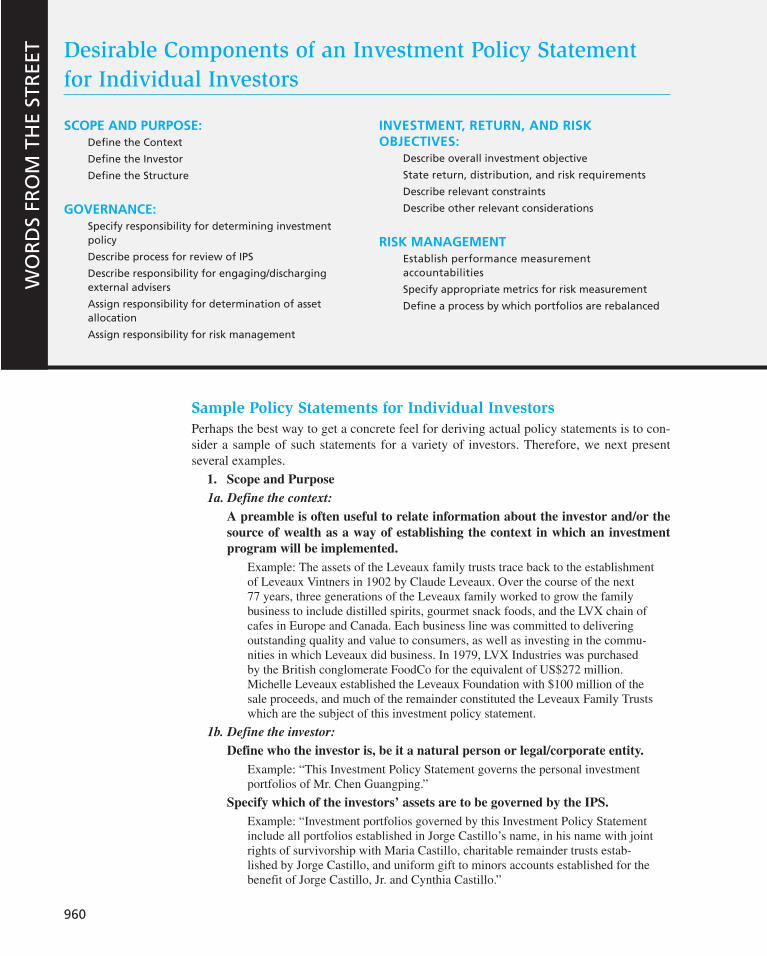
SCOPE AND PURPOSE: Define the Context
Define the Investor
Define the Structure
GOVERNANCE: Specify responsibility for determining investment policy
Describe process for review of IPS
Describe responsibility for engaging/discharging external advisers
Assign responsibility for determination of asset allocation
Assign responsibility for risk management
INVESTMENT, RETURN, AND RISK OBJECTIVES:
Describe overall investment objective
State return, distribution, and risk requirements
Describe relevant constraints
Describe other relevant considerations
RISK MANAGEMENT Establish performance measurement accountabilities
Specify appropriate metrics for risk measurement
Define a process by which portfolios are rebalanced
960
Desirable Components of an Investment Policy Statement
for Individual Investors
WO
RD
S FR
OM
TH
E ST
REE
T
Sample Policy Statements for Individual Investors
Perhaps the best way to get a concrete feel for deriving actual policy statements is to con-sider a sample of such statements for a variety of investors. Therefore, we next present several examples.
1. Scope and Purpose
1a. Define the context:
A preamble is often useful to relate information about the investor and/or the
source of wealth as a way of establishing the context in which an investment
program will be implemented.
Example: The assets of the Leveaux family trusts trace back to the establishment of Leveaux Vintners in 1902 by Claude Leveaux. Over the course of the next 77 years, three generations of the Leveaux family worked to grow the family business to include distilled spirits, gourmet snack foods, and the LVX chain of cafes in Europe and Canada. Each business line was committed to delivering outstanding quality and value to consumers, as well as investing in the commu-nities in which Leveaux did business. In 1979, LVX Industries was purchased by the British conglomerate FoodCo for the equivalent of US$272 million. Michelle Leveaux established the Leveaux Foundation with $100 million of the sale proceeds, and much of the remainder constituted the Leveaux Family Trusts which are the subject of this investment policy statement.
1b. Define the investor:
Define who the investor is, be it a natural person or legal/corporate entity.
Example: “This Investment Policy Statement governs the personal investment portfolios of Mr. Chen Guangping.”
Specify which of the investors’ assets are to be governed by the IPS.
Example: “Investment portfolios governed by this Investment Policy Statement include all portfolios established in Jorge Castillo’s name, in his name with joint rights of survivorship with Maria Castillo, charitable remainder trusts estab-lished by Jorge Castillo, and uniform gift to minors accounts established for the benefit of Jorge Castillo, Jr. and Cynthia Castillo.”

C H A P T E R 2 8 Investment Policy and the Framework of the CFA Institute 961
1c. Define the structure:
Set forth key responsibilities and actors.
Example: “Janice Jones, as financial advisor to Sam and Mary Smith, is responsible for coordinating updates to the Investment Policy, including soliciting input from the designated tax and legal advisors to Sam and Mary Smith. Ms. Jones is also responsible for monitoring application of the Investment Policy Statement, and shall promptly notify Sam and Mary Smith of the need for updates to the Policy and/or violations of the Policy in implementation. Sam and Mary Smith shall be r esponsible for approving the Investment Policy Statement and all subsequent revisions to it.”
Set forth a “standard of care” for those serving as advisor. Regulations in different jurisdictions may allow for advisors to abide by different standards depending on their preferences, business models, and client preferences. Fiduciary standards generally require that advisors always hold client interests as foremost, whereas suitability stan-dards require recommendations that are suitable for an investor based on the advisor’s knowledge of that investor’s circumstances. Investors may not perceive or understand the distinction in the absence of addressing the issue in the Investment Policy Statement.
Example: “Fuji Advisors acts as a fiduciary in its capacity as advisor to the Takesumi Family Accounts, and acknowledges that all advice and decisions ren-dered must reflect first and foremost the best interests of its clients. Fuji Advi-sors also affirms its compliance as a firm with the CFA Institute Asset Manager Code of Professional Conduct.”
Identify an organizational structure for investing.
Example: “The trustees of the Wei Family Trust shall designate an investment advisor who shall have exclusive discretionary authority to invest on behalf of the Trust consistent with the policies set forth in the Investment Policy Statement, except that the portfolio established at ZZZ Trust Company identified as “Wei Trust Discretionary Portfolio 1” shall be managed exclusively by Mr. Wei Zhang.”
Identify a risk management structure applicable to investing.
Example: “Susan Smith, as investment advisor to Russell Roberts, is responsible for monitoring investment risks and reporting them to Russell Roberts in the reporting format that has been agreed to, a sample of which is presented in Appendix XX.”
Assign responsibility for monitoring and reporting.
Example: “The HHH Trust Company will provide custody services and is responsible for rendering a monthly financial report for the Devereaux Trust. The HHH Trust Company report shall be considered to be the official record for the Trust accounts, and shall be the basis for the risk review to be performed by Judith Jones as advisor to the Trust.”
Document acceptance of the Investment Policy Statement.
Example: “By their signatures below, the Xien Trust trustees and LLL Investment Counsel acknowledge both receipt of this document and acceptance of its content.”
2. Governance
2a. Specify who is responsible for determining investment policy, executing invest-
ment policy, and monitoring the results of implementation of the policy. The IPS documents accountability for all stages of investment policy development and implementation. It can reinforce the obligations of advisors to offer counsel and principals to ultimately approve or disapprove of the policy.
Example: “As trustee for the Charitable Remainder Trust, Nigel Brown is responsible for approval of the investment policy and any subsequent changes to it. In their capacity as counselors to the Trust, Tower Advisors shall counsel the trustee as to development of the Investment Policy, suggest appropriate revisions
962 P A R T V I I Applied Portfolio Management
to the Investment Policy on an ongoing basis, and monitor and report on results achieved from implementation of the Policy on no less than a monthly basis.”
2b. Describe the process for review and updating of the IPS. A process for refreshing
the IPS as investor circumstances and/or market conditions change should be
clearly identified in advance.
Example: “Wanda Wood is responsible for monitoring the investing require-ments of Sam and Susan Smith as well as investment and economic issues, and for suggesting changes to the IPS as necessary. Wanda Wood shall review the IPS no less frequently than annually with Sam and Susan Smith.”
2c. Describe the responsibilities for engaging or discharging external advisors. The IPS should set forth who is responsible for hiring and firing external money manag-ers, consultants, or other vendors associated with the investment assets.
Example: “Marcel Perrold delegates exclusive authority to his financial advisor Francois Finault to retain and dismiss individuals and/or firms to manage his investment assets. Francois Finault shall, prior to hiring any external investment manager, disclose in writing to Marcel Perrold any compensation or other con-sideration received or due to be received from the external investment manager.”
2d. Assign responsibility for determination of asset allocation, including inputs used
and criteria for development of input assumptions. An asset allocation framework provides strategic context to many of the more tactical investment decisions. Asset allocation policies are likely to change over time as characteristics of the investor change and as market circumstances vary. Accordingly, the IPS may reference an Asset Allocation Policy as an appendix, which can be revised without requiring approval of an entirely new IPS. It is appropriate for the IPS to address the assump-tions used in developing and selecting inputs to the asset allocation decision process.
Example: “At least annually, Tower Advisors shall review the asset allocation of the Family Investment Accounts, and suggest revisions for final approval by James and Jennifer Jensen. The asset allocation plan is incorporated as Appendix A to this Investment Policy Statement, and shall consider the proportions of investments in cash equivalents, municipal securities, US fixed income obligations, US large capitalization equities, US small capitalization equities, and American Depositary Receipts (ADRs). Tower Advisors shall consider expected returns and correlation of returns for a broad representation of asset classes in the US capital markets, as well as anticipated changes in the rate of inflation, and changes in marginal tax rates.”
2e. Assign responsibility for risk management, monitoring, and reporting. The IPS should document who is responsible for setting risk policy, monitoring the risk pro-file of the investment portfolio, and reporting on portfolio risk.
Example: “As investment advisor, Tower Capital is responsible for using the statements prepared by CCC Brokerage as a basis for evaluating the risk profile of the Jorge Luiz account, consistent with the risk management policies approved and adopted by Jorge Luiz (see Appendix ZZZ). Tower Capital shall be responsible for identifying variances in risk positions that exceed tolerable limits as specified in the risk management policies, and taking prompt correc-tive action. No less than quarterly, Tower Capital shall provide to Jorge Luiz a reporting of the all such variances in the prior quarter.”
3. Investment, Return, and Risk Objectives
3a. Describe overall investment objective. The IPS should relate the purpose of the assets being invested to a broad investment objective.
Example: “The investment program governed by the IPS is intended to supple-ment the earned income of Marcel Perrold in satisfying ongoing living expenses as well as to provide for funds upon his retirement in 2016.”

C H A P T E R 2 8 Investment Policy and the Framework of the CFA Institute 963
3b. State the return, distribution, and risk requirements.
State the overall investment performance objective. Careful specification of the overall investment performance objective is likely to incorporate descriptions of general funding needs as well as relations to key factors (such as inflation, spending rate, etc.)
Example: “The financial plan developed for Margarita Mendez indicates a required real growth rate of 4% to satisfy her future obligations and allow her to retire in 2017 as planned.”
Identify performance objectives for each asset class eligible for investment. The Investment Policy Statement should set forth all permissible asset classes in which the portfolio may be invested. Some investors may find benefit in employing techniques to risk-adjust the benchmark return and portfolio return for purposes of comparison. Note that some asset classes may not be employed at all times, but they should still be identified in the IPS. For each asset class, a brief description of the class should be provided, and a benchmark for performance identified. Within each asset class, there may be sub-asset classes (for example, US Large Cap equity as a sub-asset class of US equity). Descriptions and benchmarks for sub-asset classes may be identified in the IPS, or reserved for an Asset Allocation Plan that may be attached as an appendix.
Example: “The Family Trust accounts may invest in US equity, US fixed income, US money market, and Developed Country international equity securi-ties. The following benchmarks have been selected for comparison to each asset class: US equity: Russell 3000 index. US fixed income: Barclays US Aggregate Index. US money market: Lipper US Government Money Market Average. Developed Country international equity securities: MSCI EAFE index.
Define distribution/spending assumptions or policies. Spending or distributions from the portfolio should be defined. Often, a “spending calculus” that reconciles investment return objectives, fees, taxes, inflation, and anticipated spending is use-ful to document as a guide to realistic assumptions. Distributions may be character-ized as a percentage of portfolio market value or as a specific cash value.
Example: “Based on the overall expected portfolio return of 7.5%, fees of 1.2%, inflation of 2.8%, and an effective tax rate of 32% of total appreciation, the Linzer Trust Portfolio may support an annual spending rate of 1.2% of the portfolio mar-ket value while retaining potential for capital preservation or nominal growth.”
Define a policy portfolio to serve as a basis for performance and risk assess-
ments. An asset allocation policy should designate target allocations to each asset class, with allowable ranges around the targets. Similar targets and ranges may be specified for sub-asset classes. Overall fund returns, weighted according to stra-tegic target allocations, may be constructed and compared to overall actual fund performance. Similarly, some insight as to risk exposures may be developed from examining deviations from target allocations and violations of acceptable ranges of deviation.
Example: “An asset allocation plan for the Mendez Charitable Trust is attached as Exhibit ZZZ, and shall be subject to periodic review and change under the sole authority of Jose Carrios as trustee. For each asset class, a target allocation has been established that reflects the optimized asset allocation study conducted by Hill Counsel as investment advisors, as well as allowable ranges from which actual allocations to each asset class may vary. The investment advisor is responsible for adhering to the asset allocation plan and for maintaining actual allocations to asset classes within the ranges established. Each quarterly report by the investment manager to the trustee shall confirm actual asset allocations as of the end of the quarter, and shall also confirm that allocations during the quarter were within allowable ranges.”

964 P A R T V I I Applied Portfolio Management
3c. Define the risk tolerance of the investor.
Describe the investor’s general philosophy regarding tolerance of risk. The IPS should acknowledge the assumption of risk, and the potential for returns associ-ated with risk to be both positive and negative over time. Relevant risks are usually myriad, and may include liquidity, legal, political, regulatory, longevity, mortality, business, and/or health risks. Beyond specifying relevant risks, defining acceptable paths of risk may also be important: volatility as a descriptive measure of risk may be irrelevant beyond an absolute level of loss that completely derails an investment portfolio given personal (i.e., loss of job, disability, lifecycle stage) risks.
For individuals, assessing risk tolerance may be difficult and subjective. Where possible, the IPS should account for known liabilities to lend some quantitative basis to the risk tolerance assessment. Individual investors may also require assessment of intellectual and emotional tolerance for potential losses associated with risks, using interviews or questionnaires. More nuanced approaches may attempt to define multiple levels of risks associated with avoiding financial catastrophe, maintaining a current standard of living, or developing significant further wealth. The results of this sort of analysis may suggest boundaries for tolerance for risk and associ-ated policies (for example, stop-loss or rebalancing policies.) Such policies may be incorporated by reference in an Appendix.
Example: “James and Jennifer Jensen seek to generate investment returns that are proportionate to the risks assumed in the Family Trust portfolios, understand-ing that the very nature of risk is uncertainty about the future, and specifically, the uncertainty as to future investment returns. Tower Advisors, as investment advisor, seeks to implement an investment strategy that balances the need to grow the Family Trust assets consistent with the objectives identified in the 2009 Financial Plan with the risks associated with that strategy. Based on the April 12, 2009 Risk Assessment interview with James and Jennifer Jensen, Tower Advi-sors understands that an absolute loss in any 12 month period of more than -33% is intolerable, and policies and procedures to minimize subsequent risk of further loss should be implemented by Tower Advisors at that threshold.”
3d. Describe relevant constraints. Investors must address a variety of constraints that affect their investment programs. Such constraints may reflect legal or regulatory imperatives, or may reflect internal policies. Often, such constraints are closely linked to particular risks that are relevant to the investor.
Define an evaluation horizon for achievement of performance objectives. Although relatively short time periods may be used for monitoring performance, establishing a minimum time horizon for achievement of performance objectives makes clearer when action may need to be taken to resolve underperformance issues.
Example: “The investment advisor will provide the Family Trust trustees with a quarterly report that summarizes the performance of each investment manager, each asset class, and the Family Trust in its entirety. Although such quarterly reports are essential for monitoring purposes, the basis for evaluation of relative success in achieving investment objectives will be on a rolling 8-quarter basis.”
Identify any requirements for maintaining liquidity. Investors may have short or medium term needs for cash, which should be specified in the IPS if they are ongo-ing requirements.
Example: “All dividend and interest income will be transferred to the James Jensen checking account at the end of each month. In addition, up to 15% of the market value of the portfolio should be invested such that it could be liquidated upon 5 days’ notice without suffering capital depreciation.”

C H A P T E R 2 8 Investment Policy and the Framework of the CFA Institute 965
Identify to what extent, if any, tax considerations shall affect investment
d ecision-making. In some instances, the tax consequences of an investment deci-sion may significantly change the desirability of the proposed transaction. The investor’s general tax situation as well as specific tax issues should be accounted for in the Investment Policy Statement.
Example: “In general, it will be the investment policy for the Wen portfolios to invest for appreciation in the taxable individual accounts, and invest for dividend and interest income in the individual retirement accounts. In addition, the investment advisor shall consider tax harvesting of existing high-basis hold-ings as holdings in similar industries or sectors are considered, secondary to the primary investment objective of the purchase/sale decision.”
Identify any relevant legal constraints.
Example: “Management of the Aquilla Family Foundation account is subject to the provisions of the Uniform Prudent Investor Act.”
Specify any policies related to leverage. The ability to leverage portfolios may be constrained by policy or relevant statute. Any such constraints should be identified. In addition, to the extent that different manager portfolios and/or different asset classes have different leverage allowances, accountability for monitoring overall leverage should be defined.
Example: “At the discretion of Tower Advisors as investment manager, the Xie Weng portfolio may be margined up to 50% of its value.”
Identify any restrictions on investment in foreign securities or i nvestments.
Some investors may choose to limit their exposure to investments outside of their home country because of economic or investment reasons; others may choose to impose constraints to manage administrative burdens and costs.
Example for an Individual Investor: “Investments in issuers of securities that are not denominated in yen and/or are not traded on the Tokyo Stock Exchange shall be limited to those available by participation in commingled trusts which are custodied domestically and denominated in yen.”
If relevant, specify a policy on foreign currency management. If investments in foreign assets are permissible, the Investment Policy Statement should address management of foreign currency.
Example for an Individual Investor: “To the extent that payments of interest, dividends, or principal occur in any currency other than the Canadian dollar, the investment advisor will be responsible for arranging conversion of the foreign currency to Canadian dollars immediately upon receipt at the prevailing spot rates.”
3e. Describe other considerations relevant to investment strategy.
State the investment philosophy. The IPS should document the investor’s phil-osophical approach to investing, which may include such dimensions as market efficiency; the degree of opportunism anticipated; desirability for inclusion of envi-ronmental, social, and/or governance factors in decisionmaking; etc.
Example for an Individual Investor: “James and Judy Jensen have as a philo-sophical basis for investment the conviction that markets are efficient, and thus active management of assets is unlikely to add value beyond the short term net of investment costs. Further, James and Judy Jensen believe in a long term orientation to their investment program and do not intend to seek to exploit investment opportunities that may exist in the very short term, given their belief in their inability to consistently do so profitably.”

966 P A R T V I I Applied Portfolio Management
Identify a proxy voting policy. The ability to exert shareowner rights may con-tribute to the value of investments. A policy for establishing responsibility and processes for proxy voting should be specified in the Investment Policy Statement, although the detailed policy may be reserved for an appendix. Generally, the advisor and/or the investor will retain responsibility for proxy voting decisions, but other parties (such as brokers, custodian banks, consultants) may also have roles that should be acknowledged in the IPS.
Example for an Individual Investor: “Tower Advisors as investment advisor to the Family Trust shall be responsible for voting all proxies in a timely manner in a way that maximizes the value of the Trust’s underlying investments. Upon timely notification to Tower Advisors, the Family Trust trustees may provide voting instructions to be executed.”
Identify constraints on participation in securities lending programs. Securities lending programs have developed to offer investors incremental income on their portfolios. Participation in such programs does create some degree of collateral investment and counterparty risk, however, and a policy should be set forth govern-ing participation.
Example for an Individual Investor: “Except for the margin account established at GGG Securities, no Charitable Remainder Trust securities shall be lent or otherwise hypothecated.”
Identify special factors to be used in including or excluding potential invest-
ments from the portfolio. Investors may choose to impose limits on certain investments, consistent with their beliefs in extrafinancial factor effects on secu-rities prices, a desire to avoid concentrated risks in a particular industry, or to be consistent with their philosophical or political orientation of the organization. In particular, use of Environmental, Social, or Governance (ESG) factors is increas-ingly common, and such use should be explicitly allowed or disallowed in the Investment Policy Statement. Islamic clients may choose to restrict investment activity to shariah-compliant investments.
Example for an Individual Investor: “Consistent with her personal beliefs, no investments in companies that derive revenue from products or services that are contrary to the teachings of the Catholic Church will be made for Jennifer Jensen’s account. The investment advisor will be responsible for reviewing the portfolio monthly to assure that this requirement is satisfied, and shall immedi-ately dispose of any portfolio holding found to be in violation of this policy.”
4. Risk Management
4a. Establish performance measurement and reporting accountabilities. The IPS should establish an objective, reliable mechanism for reporting on investment performance.
Example for an Individual Investor: “Hill Counsel, as investment advisor to the Charitable Remainder Trust, will calculate the performance of each investment account under its supervision and report to the trustees by the 15th day of the new quarter. Calculations will be performed consistent with the Global Invest-ment Performance Standards published by CFA Institute. Hill Counsel will also provide a reconciliation of their records with the brokerage statement provided by CCC as part of the performance report.”
4b. Specify appropriate metrics for risk measurement and evaluation. Consistent use of metrics to assess and evaluate the risk profile of investment portfolios is impor-tant to allow for meaningful comparisons over time and avoid inappropriate use of different metrics to highlight or disguise certain risks. There is reasonable debate

C H A P T E R 2 8 Investment Policy and the Framework of the CFA Institute 967
over the suitability of various metrics, and continued review of the choice of metrics is recommended as a strategic imperative.
Example for an Individual Investor: “In addition to performance reporting, Tower Capital shall report to the Marcel Family Trust trustees on a quarterly basis indicative risk metrics, calculated as the annualized standard deviation of portfolio returns relative to each portfolio’s specified benchmark; and the infor-mation ratio for each portfolio based on annualized returns for the portfolio and benchmark as of the end of each quarter.”
4c. Define a process by which portfolios are rebalanced to target allocations. Outside boundaries of acceptable variations from target, or another target rebalancing point should be documented in the Investment Policy Statement. The rebalancing mecha-nism may be integrated with the risk management system in some cases, in which case a brief description of the rebalancing policy with reference to the risk manage-ment process in a separate Appendix is likely to be appropriate. If the policy is not to rebalance, this should also be documented in the IPS.
Example for an Individual Investor: “On the first business day of each new quar-ter, the investment advisor for the Jensen personal accounts will propose rebal-ancing transactions to return the accounts to their target allocations, and shall execute these transactions within two business days of receiving authorization from the Investment Committee, except that if the principal value of a proposed rebalancing transaction is less than $50,000, that rebalancing transaction will be deferred indefinitely. ”
28.4 Asset Allocation
Consideration of their objectives and constraints leads investors to a set of investment poli-cies. The policies column in Table 28.3 lists the various dimensions of portfolio manage-ment policymaking—asset allocation, diversification, risk and tax positioning, and income generation. By far the most important part of policy determination is asset allocation, that is, deciding how much of the portfolio to invest in each major asset category.
We can view the process of asset allocation as consisting of the following steps:
1. Specify asset classes to be included in the portfolio. The major classes usually c onsidered are the following:
a. Money market instruments (usually called cash ).
b. Fixed-income securities (usually called bonds ).
c. Stocks.
d. Real estate.
e. Precious metals.
f. Other.
Institutional investors will rarely invest in more than the first four categories, whereas individual investors may include precious metals and other more exotic types of investments in their portfolios.
2. Specify capital market expectations. This step consists of using both historical data and economic analysis to determine your expectations of future rates of return over the relevant holding period on the assets to be considered for inclusion in the portfolio.

968
Looking to Lower Your Risk? Just Add More
If you’re like a lot of investors these days, you’re looking to make your portfolio “less risky.”
The way to do that is by adding more risk, or at least more types of risk. That strange twist—adding more to get less—is why risk is one of the hardest elements of investing to understand.
The first rule in risk is the hardest for many investors to accept: There is no such thing as a “risk-free investment.”
Avoiding one form of risk means embracing another; the safest of investments generally come with the lowest returns, while the biggest potential gainers bring larger potential losses.
The primary risks in fund investing include the following.
Market risk: This is the big one, also known as princi-pal risk, and it’s the chance that downturn chews up your money.
Purchasing power risk: Sometimes called “inflation risk,” this is the “risk of avoiding risk,” and it’s at the oppo-site end of the spectrum from market risk. In a nutshell, this is the possibility that you are too conservative and your money won’t grow fast enough to keep pace with inflation.
Interest-rate risk: This is a key factor in an environ-ment of declining rates, where you face potential income declines when a bond or certificate of deposit matures and you need to reinvest the money.
Goosing returns using higher-yielding, longer-term securities creates the potential to get stuck losing ground to inflation if the rate trend changes again.
Timing risk: This is another highly individual factor, revolving around your personal time horizon. Simply put, the chance of stock mutual funds making money over the
next 20 years is high; the prospects for the next 18 months are murky.
If you need money at a certain time, this risk must be factored into your asset allocation.
Liquidity risk: Another risk heightened by current ten-sions, it affects everything from junk bonds to foreign stocks. If world events were to alter the flow of money in credit markets or to close some foreign stock exchanges for an extended period, your holdings in those areas could be severely hurt.
Political risk: This is the prospect that government deci-sions will affect the value of your investments. Given the current environment, it is probably a factor in all forms of investing, whether you are looking at stocks or bonds.
Societal risk: Call this “world-event risk.” It was evident when the first anthrax scares sent markets reeling briefly. Some businesses are more susceptible (airlines, for exam-ple), though virtually all types of investing have some con-cerns here.
Even after all of those risks, some investments face cur-rency risk, credit risk, and more. Every type of risk deserves some consideration as you build your holdings.
Ultimately, by making sure that your portfolio addresses all types of risk—heavier on the ones you prefer and lighter on those that make you queasy—you ensure that no one type of risk can wipe you out.
That’s something that a “less risky” portfolio may not be able to achieve.
Source: Abridged from Charles A. Jaffee’s article of the same title, Boston Sunday Globe, October 21, 2001. BOSTON SUNDAY GLOBE (“GLOBE STAFF”/“CONTRIBUTING REPORTER” PRODUCED COPY ONLY) by CHARLES A. JAFFEE. Copyright 2001 by GLOBE NEWSPAPER CO (MA). Reproduced with permission of GLOBE NEWSPAPER CO (MA) in the format Textbook via Copyright Clearance Center.
WO
RD
S FR
OM
TH
E ST
REE
T
3. Derive the efficient portfolio frontier. This step consists of finding portfolios that achieve the maximum expected return for any given degree of risk.
4. Find the optimal asset mix. This step consists of selecting the efficient portfolio that best meets your risk and return objectives while satisfying the constraints you face.
Taxes and Asset Allocation
Until this point we have glossed over the issue of income taxes in discussing asset alloca-tion. Of course, to the extent that you are a tax-exempt investor such as a pension fund, or if all of your investment portfolio is in a tax-sheltered account such as an individual retire-ment account (IRA), then taxes are irrelevant to your portfolio decisions.
But let us say that at least some of your investment income is subject to income taxes at the highest rate under current U.S. law. You are interested in the after-tax holding-period return (HPR) on your portfolio. At first glance it might appear to be a simple matter to fig-ure out what the after-tax HPRs on stocks, bonds, and cash are if you know what they are before taxes. However, there are several complicating factors.
The first is the fact that you can choose between tax-exempt and taxable bonds. We discussed this issue in Chapter 2 and concluded there that you will choose to invest in
C H A P T E R 2 8 Investment Policy and the Framework of the CFA Institute 969
tax-exempt bonds (i.e., municipal bonds) if your personal tax rate is such that the after-tax rate of interest on taxable bonds is less than the interest rate on “munis.”
Because we are assuming that you are in the highest tax bracket, it is fair to assume that you will prefer to invest in munis for both the short maturities (cash) and the long maturities (bonds). As a practical matter, this means that cash for you will probably be a tax-exempt money market fund.
The second complication is not quite so easy to deal with. It arises from the fact that part of your HPR is in the form of a capital gain or loss. Under the current tax system you pay income taxes on a capital gain only if you realize it by selling the asset during the holding period. This applies to bonds as well as stocks, and it makes the after-tax HPR a function of whether the security will actually be sold at the end of the holding period. Sophisticated investors time the realization of their sales of securities to minimize their tax burden. This often calls for selling securities that are losing money at the end of the tax year and holding on to those that are making money.
Furthermore, because cash dividends on stocks are fully taxable and capital gains taxes can be deferred by not selling stocks that appreciate in value, the after-tax HPR on stocks will depend on the dividend payout policies of the corporations that issued the stock.
These tax complications make the process of portfolio selection for a taxable inves-tor a lot harder than for the tax-exempt investor. There is a whole branch of the money management industry that deals with ways to defer or avoid paying taxes through special investment strategies. Unfortunately, many of these strategies conflict with the principles of efficient diversification.
We will discuss these and related issues in greater detail later in this chapter.
28.5 Managing Portfolios of Individual Investors
The overriding consideration in individual investor goal-setting is one’s stage in the life cycle. Most young people start their adult lives with only one asset—their earning power. In this early stage of the life cycle an individual may not have much interest in investing in stocks and bonds. The needs for liquidity and preserving safety of principal dictate a conservative policy of putting savings in a bank or a money market fund. If and when a person gets married, the purchase of life and disability insurance will be required to protect the value of human capital.
When a married couple’s labor income grows to the point at which insurance and hous-ing needs are met, the couple may start to save for any children’s college education and their own retirement, especially if the government provides tax incentives for retirement savings. Retirement savings typically constitute a family’s first pool of investable funds. This is money that can be invested in stocks, bonds, and real estate (other than the primary home).
Human Capital and Insurance
The first significant investment decision for most individuals concerns education, building up their human capital. The major asset most people have during their early working years is the earning power that draws on their human capital. In these circumstances, the risk of illness or injury is far greater than the risk associated with financial wealth.
The most direct way of hedging human capital risk is to purchase insurance. With the combination of your labor income and a disability insurance policy viewed as a portfolio,

970 P A R T V I I Applied Portfolio Management
the rate of return on this portfolio is less risky than the labor income by itself. Life insur-ance is a hedge against the complete loss of income as a result of death of any of the family’s income earners.
Investment in Residence
The first major economic asset many people acquire is their own house. Deciding to buy rather than rent a residence qualifies as an investment decision.
An important consideration in assessing the risk and return aspects of this investment is the value of a house as a hedge against two kinds of risk. The first kind is the risk of increases in rental rates. If you own a house, any increase in rental rates will increase the return on your investment.
The second kind of risk is that the particular house or apartment where you live may not always be available to you. By buying, you guarantee its availability.
Saving for Retirement and the Assumption of Risk
People save and invest money to provide for future consumption and leave an estate. The primary aim of lifetime savings is to allow maintenance of the customary standard of liv-ing after retirement. As Figure 28.2 suggests, your retirement consumption depends on your life expectancy at that time. Life expectancy, when one makes it to retirement at age 65, approximates 85 years, so the average retiree needs to prepare a 20-year nest egg and sufficient savings to cover unexpected health care costs. Investment income may also increase the welfare of one’s heirs, favorite charity, or both.
Questionnaires suggest that attitudes shift away from risk tolerance and toward risk aversion as investors near retirement age. With age, individuals lose the potential to recover from a disastrous investment performance. When they are young, investors can respond to a loss by working harder and saving more of their income. But as retire-ment approaches, investors realize there will be less time to recover. Hence the shift to safe assets.
Retirement Planning Models
In recent years, investment companies and finan-cial advisory firms have created a variety of “user-friendly” interactive tools and models for retirement planning. Although they vary in detail, the essential structure behind most of them can be explained using The American Saving Education Council’s “Ballpark Estimate” worksheet (See Figure 28.3 ). The work-sheet assumes you’ll need 70% of current income, that you’ll live to age 87, and you’ll realize a constant real rate of return of 3% after inflation. For example, let’s say Jane is a 35-year-old working woman with two children, earning $30,000 per year. Seventy percent of Jane’s current annual income ($30,000) is $21,000. Jane would then subtract the income she expects to receive from Social Security ($12,000 in her case) from $21,000, equaling $9,000. This is how much Jane needs to make up for each retirement year. Jane expects to retire at age 65, so (using panel 3 of
Figure 28.2 Long life expectancy is a double-edged sword
Source: www.glasbergen.com . Copyright 2000 by Randy Glasbergen. Reprinted by permission of Randy Glasbergen.
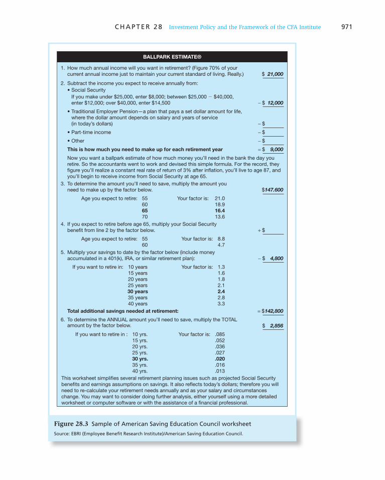
C H A P T E R 2 8 Investment Policy and the Framework of the CFA Institute 971
Figure 28.3 Sample of American Saving Education Council worksheet
Source: EBRI (Employee Benefit Research Institute)/American Saving Education Council.
1. How much annual income will you want in retirement? (Figure 70% of your current annual income just to maintain your current standard of living. Really.) $ 21,000
2. Subtract the income you expect to receive annually from:
• Social Security
If you make under $25,000, enter $8,000; between $25,000 � $40,000,enter $12,000; over $40,000, enter $14,500 − $ 12,000
• Traditional Employer Pension—a plan that pays a set dollar amount for life, where the dollar amount depends on salary and years of service (in today’s dollars) − $
• Part-time income − $
• Other − $
This is how much you need to make up for each retirement year = $ 9,000
Now you want a ballpark estimate of how much money you’ll need in the bank the day youretire. So the accountants went to work and devised this simple formula. For the record, theyfigure you’ll realize a constant real rate of return of 3% after inflation, you’ll live to age 87, andyou’ll begin to receive income from Social Security at age 65.
3. To determine the amount you’ll need to save, multiply the amount you need to make up by the factor below. $147.600
Age you expect to retire: 55 Your factor is: 21.060 18.965 16.4
70 13.6
4. If you expect to retire before age 65, multiply your Social Security benefit from line 2 by the factor below. + $
Age you expect to retire: 55 Your factor is: 8.860 4.7
5. Multiply your savings to date by the factor below (include money accumulated in a 401(k), IRA, or similar retirement plan): − $ 4,800
If you want to retire in: 10 years Your factor is: 1.315 years 1.620 years 1.825 years 2.130 years 2.4
35 years 2.840 years 3.3
Total additional savings needed at retirement: = $142,800
6. To determine the ANNUAL amount you’ll need to save, multiply the TOTALamount by the factor below. $ 2,856
If you want to retire in : 10 yrs. Your factor is: .08515 yrs. .05220 yrs. .03625 yrs. .02730 yrs. .020
35 yrs. .01640 yrs. .013
BALLPARK ESTIMATE®
This worksheet simplifies several retirement planning issues such as projected Social Security benefits and earnings assumptions on savings. It also reflects today’s dollars; therefore you will need to re-calculate your retirement needs annually and as your salary and circumstances change. You may want to consider doing further analysis, either yourself using a more detailed worksheet or computer software or with the assistance of a financial professional.

972 P A R T V I I Applied Portfolio Management
the worksheet) she multiplies $9,000 3 16.4 equaling $147,600. Jane has already saved $2,000 in her 401(k) plan. She plans to retire in 30 years so (from panel 4) she multiplies $2,000 3 2.4 equaling $4,800. She subtracts that from her total, making her projected total savings needed at retirement $142,800. Jane then multiplies $142,800 3 .020 5 $2,856 (panel 6). This is the amount Jane will need to save annually for her retirement.
CONCEPT CHECK
1
a. Think about the financial circumstances of your closest relative in your parents’ generation (preferably your parents’ household if you are fortunate enough to have them around). Write down the objectives and constraints for their investment decisions.
b. Now consider the financial situation of your closest relative who is in his or her 30s. Write down the objectives and constraints that would fit his or her investment decision.
c. How much of the difference between the two statements is due to the age of the investors?
Manage Your Own Portfolio or Rely on Others?
Lots of people have assets such as Social Security benefits, pension and group insurance plans, and savings components of life insurance policies. Yet they exercise limited control, if any, on the investment decisions of these plans. The funds that secure pension and life insurance plans are managed by institutional investors.
Outside the “forced savings” plans, however, individuals can manage their own invest-ment portfolios. As the population grows richer, more and more people face this decision.
Managing your own portfolio appears to be the lowest-cost solution. Conceptually, there is little difference between managing one’s own investments and professional finan-cial planning/investment management.
Against the fees and charges that financial planners and professional investment manag-ers impose, you will want to offset the value of your time and energy expended on diligent portfolio management. People with a suitable background may even look at investment as recreation. Most of all, you must recognize the potential difference in investment results.
Besides the need to deliver better-performing investments, professional managers face two added difficulties. First, getting clients to communicate their objectives and constraints requires considerable skill. This is not a one-time task because objectives and constraints are forever changing. Second, the professional needs to articulate the financial plan and keep the client abreast of outcomes. Professional management of large portfolios is com-plicated further by the need to set up an efficient organization where decisions can be decentralized and information properly disseminated.
The task of life cycle financial planning is a formidable one for most people. It is not surprising that a whole industry has sprung up to provide personal financial advice.
Tax Sheltering
In this section we explain three important tax sheltering options that can radically affect opti-mal asset allocation for individual investors. The first is the tax-deferral option, which arises from the fact that you do not have to pay tax on a capital gain until you choose to realize the gain. The second is tax-deferred retirement plans such as individual retirement accounts, and the third is tax-deferred annuities offered by life insurance companies. Not treated here at all is the possibility of investing in the tax-exempt instruments discussed in Chapter 2.
The Tax-Deferral Option A fundamental feature of the U.S. Internal Revenue Code is that tax on a capital gain on an asset is payable only when the asset is sold; this is its tax-deferral option. The investor therefore can control the timing of the tax payment. This conveys a benefit to stock investments.

C H A P T E R 2 8 Investment Policy and the Framework of the CFA Institute 973
To see this, compare IBM stock with an IBM bond. Suppose both offer an expected total return of 12%. The stock has a dividend yield of 4% and expected price appreciation of 8%, whereas the bond pays an interest rate of 12%. The bond investor must pay tax on the bond’s interest in the year it is earned, whereas the stockholder pays tax only on the dividend and defers paying capital gains tax until the stock is sold.
Suppose one invests $1,000 for 5 years. Although in reality interest is taxed as ordi-nary income while capital gains and dividends are taxed at a rate of only 15% for most investors,2 to isolate the benefit of tax deferral, we will assume that all investment income is taxed at 15%. The bond will earn an after-tax return of 12% 3 (1 2 .15) 5 10.2%. The after-tax accumulation at the end of 5 years is
$1,000 3 1.1025 5 $1,625.20
For the stock, the dividend yield after taxes is 4% 3 (1 2 .15) 5 3.4%. Because no taxes are paid on the 8% annual capital gain until year 5, the before-tax accumulation will be
$1,000 3 (1 1 .034 1 .08)5 5 1,000(1.114)5 5 $1,715.64
In year 5, when the stock is sold, the (now-taxable) capital gain is
$1,715.64 2 $1,000(1.034)5 5 1,715.64 2 1,181.96 5 $533.68
Taxes due are $80.05, leaving $1,635.59, which is $10.39 more than the bond investment yields. Deferral of the capital gains tax allows the investment to compound at a faster rate until the tax is actually paid. Note that the more of one’s total return that is in the form of price appreciation, the greater the value of the tax-deferral option.
Tax-Deferred Retirement Plans Recent years have seen increased use of tax-
deferred retirement plans in which investors can choose how to allocate assets. Such plans include traditional IRAs, Keogh plans, and employer-sponsored “tax-qualified” defined contribution plans such as 401 (k) plans. A feature they have in common is that contributions and earnings are not subject to federal income tax until the individual with-draws them as benefits.
Typically, an individual may have some investment in the form of such qualified retire-ment accounts and some in the form of ordinary taxable accounts. The basic investment principle that applies is to hold whatever bonds you want to hold in the retirement account while holding equities in the ordinary account. You maximize the tax advantage of the retirement account by holding it in the security that is the least tax advantaged.
To see this point, consider an investor who has $200,000 of wealth, $100,000 of it in a tax-qualified retirement account. She currently invests half of her wealth in bonds and half in stocks, so she allocates half of her retirement account and half of her nonretirement funds to each. She could reduce her tax bill with no change in before-tax returns simply by shifting her bonds into the retirement account and holding all her stocks outside the retire-ment account.
2These tax rates are likely to change in 2011, with the rate on capital gains rising to 20%, and dividends taxed as ordinary income.
CONCEPT CHECK
2
Suppose our investor earns a 10% per year rate of interest on bonds and 15% per year on stocks, all in the form of price appreciation. In 5 years she will withdraw all her funds and spend them. By how much will she increase her final accumulation if she shifts all bonds into the retirement account and holds all stocks outside the retirement account? She is in a 28% tax bracket for ordinary income, and her capital gains income is taxed at 15%.

974 P A R T V I I Applied Portfolio Management
Deferred Annuities Deferred annuities are essentially tax-sheltered accounts offered by life insurance companies. They combine deferral of taxes with the option of withdrawing one’s funds in the form of a life annuity. Variable annuity contracts offer the additional advantage of mutual fund investing. One major difference between an IRA and a variable annuity contract is that whereas the amount one can contribute to an IRA is tax-deductible and extremely limited as to maximum amount, the amount one can contribute to a deferred annuity is unlimited, but not tax-deductible.
The defining characteristic of a life annuity is that its payments continue as long as the recipient is alive, although virtually all deferred annuity contracts have several withdrawal options, including a lump sum of cash paid out at any time. You need not worry about running out of money before you die. Like Social Security, therefore, life annuities offer longevity insurance and thus would seem to be an ideal asset for someone in the retirement years. Indeed, theory suggests that where there are no bequest motives, it would be optimal for people to invest heavily in actuarially fair life annuities. 3
There are two types of life annuities, fixed annuities and variable annuities. A fixed annuity pays a fixed nominal sum of money per period (usually each month), whereas a variable annuity pays a periodic amount linked to the investment performance of some underlying portfolio.
In pricing annuities, insurance companies use mortality tables that show the probabili-ties that individuals of various ages will die within a year. These tables enable the insurer to compute with reasonable accuracy how many of a large number of people in a given age group will die in each future year. If it sells life annuities to a large group, the insurance company can estimate fairly accurately the amount of money it will have to pay in each future year to meet its obligations.
Variable annuities are structured so that the investment risk of the underlying asset port-folio is passed through to the recipient, much as shareholders bear the risk of a mutual fund. There are two stages in a variable annuity contract: an accumulation phase and a payout phase. During the accumulation phase, the investor contributes money periodically to one or more open-end mutual funds and accumulates shares. The second, or payout, stage usually starts at retirement, when the investor typically has several options, including the following:
1. Taking the market value of the shares in a lump sum payment.
2. Receiving a fixed annuity until death.
3. Receiving a variable amount of money each period that depends on the investment performance of the portfolio.
Variable and Universal Life Insurance Variable life insurance is another tax-deferred investment vehicle offered by the life insurance industry. A variable life insurance policy combines life insurance with the tax-deferred annuities described earlier.
To invest in this product, you pay either a single premium or a series of premiums. In each case there is a stated death benefit, and the policyholder can allocate the money invested to several portfolios, which generally include a money market fund, a bond fund, and at least one common stock fund. The allocation can be changed at any time.
Variable life insurance policies offer a death benefit that is the greater of the stated face value or the market value of the investment base. In other words, the death benefit may rise with favorable investment performance, but it will not go below the guaranteed face value. Furthermore, the surviving beneficiary is not subject to income tax on the death benefit.
3 For an elaboration of this point see Laurence J. Kotlikoff and Avia Spivak, “The Family as an Incomplete Annuities Market,” Journal of Political Economy 89 (April 1981).
C H A P T E R 2 8 Investment Policy and the Framework of the CFA Institute 975
The policyholder can choose from a number of income options to convert the policy into a stream of income, either on surrender of the contract or as a partial withdrawal. In all cases income taxes are payable on the part of any distribution representing investment gains.
The insured can gain access to the investment without having to pay income tax by bor-rowing against the cash surrender value. Policy loans of up to 90% of the cash value are available at any time at a contractually specified interest rate.
A universal life insurance policy is similar to a variable life policy except that, instead of having a choice of portfolios to invest in, the policyholder earns a rate of interest that is set by the insurance company and changed periodically as market conditions change. The disadvantage of universal life insurance is that the company controls the rate of return to the policyholder, and, although companies may change the rate in response to competitive pressures, changes are not automatic. Different companies offer different rates, so it often pays to shop around for the best.
28.6 Pension Funds
By far the most important institution in the retirement income system is the employer-sponsored pension plan. These plans vary in form and complexity, but they all share certain common elements in every country. In general, investment strategy depends on the type of plan.
Pension plans are defined by the terms specifying the “who,” “when,” and “how much,” for both the plan benefits and the plan contributions used to pay for those benefits. The pension fund of the plan is the cumulation of assets created from contributions and the investment earnings on those contributions, less any payments of benefits from the fund. In the United States, contributions to the fund by either employer or employee are tax- deductible, and investment income of the fund is not taxed. Distributions from the fund, whether to the employer or the employee, are taxed as ordinary income. There are two “pure” types of pension plans: defined contribution and defined benefit.
Defined Contribution Plans
In a defined contribution plan, a formula specifies contributions but not benefit payments. Contribution rules usually are specified as a predetermined fraction of salary (e.g., the employer contributes 10% of the employee’s annual wages to the plan), although that frac-tion need not be constant over the course of an employee’s career. The pension fund con-sists of a set of individual investment accounts, one for each employee. Pension benefits are not specified, other than that at retirement the employee may apply that total accumu-lated value of contributions and earnings on those contributions to purchase an annuity. The employee often has some choice over both the level of contributions and the way the account is invested.
In principle, contributions could be invested in any security, although in practice most plans limit investment choices to bond, stock, and money market funds. The employee bears all the investment risk; the retirement account is, by definition, fully funded by the contributions, and the employer has no legal obligation beyond making its periodic contributions.
For defined contribution plans, investment policy is essentially the same as for a tax-qualified individual retirement account. Indeed, the main providers of investment products for these plans are the same institutions such as mutual funds and insurance companies

976 P A R T V I I Applied Portfolio Management
that serve the general investment needs of individuals. Therefore, in a defined contribution plan much of the task of setting and achieving the income-replacement goal falls on the employee.
CONCEPT CHECK
3
An employee is 45 years old. Her salary is $40,000 per year, and she has $100,000 accumulated in her self-directed defined contribution pension plan. Each year she contributes 5% of her salary to the plan, and her employer matches it with another 5%. She plans to retire at age 65. The plan offers a choice of two funds: a guaranteed return fund that pays a risk-free real interest rate of 3% per year and a stock index fund that has an expected real rate of return of 6% per year and a standard deviation of 20%. Her current asset mix in the plan is $50,000 in the guaranteed fund and $50,000 in the stock index fund. She plans to reinvest all investment earnings in each fund in that same fund and to allocate her annual contribution equally between the two funds. If her salary grows at the same rate as the cost of living, how much can she expect to have at retirement? How much can she be sure of having?
Defined Benefit Plans
In a defined benefit plan, a formula specifies benefits, but not the manner, including con-tributions, in which these benefits are funded. The benefit formula typically takes into account years of service for the employer and level of wages or salary (e.g., an employer might pay an employee for life, beginning at age 65, a yearly amount equal to 1% of his final annual wage for each year of service). The employer (called the “plan sponsor”) or an insurance company hired by the sponsor guarantees the benefits and thus absorbs the investment risk. The obligation of the plan sponsor to pay the promised benefits is like a long-term debt liability of the employer.
As measured both by number of plan participants and the value of total pension liabili-ties, the defined benefit form still dominates in most countries around the world. However, the strong trend since the mid-1970s has been for sponsors to choose the defined contri-bution form when starting new plans. But the two plan types are not mutually exclusive. Many sponsors adopt defined benefit plans as their primary plan, in which participation is mandatory, and supplement them with voluntary defined contribution plans.
With defined benefit plans, there is an important distinction between the pension plan and the pension fund. The plan is the contractual arrangement setting out the rights and obligations of all parties; the fund is a separate pool of assets set aside to provide collateral for the promised benefits. In defined contribution plans, by definition, the value of the benefits equals that of the assets, so the plan is always fully funded. But in defined benefit plans, there is a continuum of possibilities. There may be no separate fund, in which case the plan is said to be unfunded. When there is a separate fund with assets worth less than the present value of the promised benefits, the plan is underfunded. And if the plan’s assets have a market value that exceeds the present value of the plan’s liabilities, it is said to be overfunded.
Alternative Perspectives on Defined Benefit Pension Obligations
As previously described, in a defined benefit plan, the pension benefit is determined by a formula that takes into account the employee’s history of service and wages or salary. The plan sponsor provides this benefit regardless of the investment performance of the pension fund assets. The annuity promised to the employee is therefore the employer’s liability. What is the nature of this liability?

C H A P T E R 2 8 Investment Policy and the Framework of the CFA Institute 977
There is a widespread belief that pension benefits in final-pay formula plans are pro-tected against inflation at least up to the date of retirement. But this is a misperception. Unlike Social Security benefits, whose starting value is indexed to a general index of wages, pension benefits even in final-pay private-sector plans are “indexed” only to the extent that (1) the employee continues to work for the same employer, (2) the employee’s own wage or salary keeps pace with the general price index, and (3) the employer contin-ues to maintain the same plan. Very few private corporations in the United States offer pen-sion benefits that are automatically indexed for inflation; thus workers who change jobs wind up with lower pension benefits at retirement than otherwise identical workers who stay with the same employer, even if the employers have defined benefit plans with the same final-pay benefit formula. This is referred to as the portability problem.
Both the rule-making body of the accounting profession (the Financial Accounting Standards Board) and Congress have adopted the present value of the nominal benefits as the appropriate measure of a sponsor’s pension liability. FASB Statement 87 specifies that the measure of corporate pension liabilities to be used on the corporate balance sheet in external reports is the accumulated benefit obligation (ABO)—that is, the present value of pension benefits owed to employees under the plan’s benefit formula absent any salary projections and discounted at a nominal rate of interest. Similarly, in its Omnibus Budget Reconciliation Act (OBRA) of 1987, Congress defined the current liability as the measure of a corporation’s pension liability and set limits on the amount of tax-qualified contribu-tions a corporation could make as a proportion of the current liability. OBRA’s definition of the current liability is essentially the same as FASB Statement 87’s definition of the ABO.
The ABO is thus a key element in a pension fund’s investment strategy. It affects a c orporation’s reported balance sheet liabilities; it also reflects economic reality.
Statement 87, however, recognizes an additional measure of a defined benefit plan’s liability: the projected benefit obligation (PBO). The PBO is a measure of the sponsor’s pension liability that includes projected increases in salary up to the expected age of retire-ment. Statement 87 requires corporations to use the PBO in computing pension expense reported in their income statements. This is perhaps useful for financial analysts, in that the amount may help them to derive an appropriate estimate of expected future labor costs for discounted cash flow valuation models of the firm as a going concern. The PBO is not, however, an appropriate measure of the benefits that the employer has explicitly guaran-teed. The difference between the PBO and the ABO should not be treated as a liability of the firm, because these additional pension costs will be realized only if the employees continue to work in the future. If these future contingent labor costs are to be treated as a liability of the firm, then why not book the entire future wage bill as a liability? If this is done, then shouldn’t one add as an asset the present value of future revenues generated by these labor activities? It is indeed difficult to see either the accounting or economic logic for using the PBO as a measure of pension liabilities.
CONCEPT CHECK
4 An employee is 40 years old and has been working for the firm for 15 years. If normal retire-ment age is 65, the interest rate is 8%, and the employee’s life expectancy is 80, what is the present value of the accrued pension benefit?
Pension Investment Strategies
The special tax status of pension funds creates the same incentive for both defined contri-bution and defined benefit plans to tilt their asset mix toward assets with the largest spread between pretax and after-tax rates of return. In a defined contribution plan, because the

978 P A R T V I I Applied Portfolio Management
participant bears all the investment risk, the optimal asset mix also depends on the risk tolerance of the participant.
In defined benefit plans, optimal investment policy may be different because the spon-sor absorbs the investment risk. If the sponsor has to share some of the upside potential of the pension assets with plan participants, there is an incentive to eliminate all investment risk by investing in securities that match the promised benefits. If, for example, the plan sponsor has to pay $100 per year for the next 5 years, it can provide this stream of benefit payments by buying a set of five zero-coupon bonds each with a face value of $100 and maturing sequentially. By so doing, the sponsor eliminates the risk of a shortfall. This is an example of immunization of the pension liability.
If a corporate pension fund has an ABO that exceeds the market value of its assets, FASB Statement 87 requires that the corporation recognize the unfunded liability on its balance sheet. If, however, the pension assets exceed the ABO, the corporation cannot include the surplus on its balance sheet. This asymmetric accounting treatment expresses a deeply held view about defined benefit pension funds. Representatives of organized labor, some politicians, and even a few pension professionals believe that the sponsoring corporation, as guarantor of the accumulated pension benefits, is liable for pension asset shortfalls but does not have a clear right to the entire surplus in case of pension overfunding.
If the pension fund is overfunded, then a 100% fixed-income portfolio is no longer required to minimize the cost of the corporate pension guarantee. Management can invest surplus pension assets in equities, provided it reduces the proportion so invested when the market value of pension assets comes close to the value of the ABO.
Investing in Equities If the only goal guiding corporate pension policy were share-holder wealth maximization, it is hard to understand why a financially sound pension sponsor would invest in equities at all. A policy of 100% bond investment would minimize the cost of guaranteeing the defined benefits.
In addition to the reasons given for a fully funded pension plan to invest only in fixed income securities, there is a tax reason for doing so too. The tax advantage of a pension fund stems from the ability of the sponsor to earn the pretax interest rate on pension invest-ments. To maximize the value of this tax shelter, it is necessary to invest entirely in assets offering the highest pretax interest rate. Because capital gains on stocks can be deferred and dividends are taxed at a lower rate than interest on bonds, corporate pension funds should invest entirely in taxable bonds and other fixed-income investments.
Yet we know that in general pension funds invest from 40% to 60% of their portfolios in equity securities. Even a casual perusal of the practitioner literature suggests that they do so for a variety of reasons—some right and some wrong. There are three possible correct reasons.
The first is that corporate management views the pension plan as a trust for the employ-ees and manages fund assets as if it were a defined contribution plan. It believes that a suc-cessful policy of investment in equities might allow it to pay extra benefits to employees and is therefore worth taking the risk.
The second possible correct reason is that management believes that through superior market timing and security selection it is possible to create value in excess of management fees and expenses. Many executives in nonfinancial corporations are used to creating value in excess of cost in their businesses. They assume that it can also be done in the area of portfolio management. Of course, if that is true, then one must ask why they do not do it on their corporate account rather than in the pension fund. That way they could have their tax shelter “cake” and eat it too. It is important to realize, however, that to accomplish this feat, the plan must beat the market, not merely match it.
C H A P T E R 2 8 Investment Policy and the Framework of the CFA Institute 979
Note that a very weak form of the efficient markets hypothesis would imply that man-agement cannot create shareholder value simply by shifting the pension portfolio out of bonds and into stocks. Even when the entire pension surplus belongs to the shareholders, investing in stocks just moves the shareholders along the capital market line (the market trade-off between risk and return for passive investors) and does not create value. When the net cost of providing plan beneficiaries with shortfall risk insurance is taken into account, increasing the pension fund equity exposure reduces shareholder value unless the equity investment can put the firm above the capital market line. This implies that it makes sense for a pension fund to invest in equities only if it intends to pursue an active strategy of beat-ing the market either through superior timing or security selection. A completely passive strategy will add no value to shareholders.
For an underfunded plan of a corporation in financial distress there is another pos-sible reason for investing in stocks and other risky assets—federal pension insurance. Firms in financial distress have an incentive to invest pension fund money in the risk-iest assets, just as troubled thrift institutions insured by the Federal Savings and Loan Insurance Corporation (FSLIC) in the 1980s had similar motivation with respect to their loan portfolios.
Wrong Reasons to Invest in Equities The wrong reasons for a pension fund to invest in equities stem from interrelated fallacies. The first is the notion that stocks are not risky in the long run. This fallacy was discussed at length in Chapter 5. Another related fallacy is the notion that stocks are a hedge against inflation. The reasoning behind this fal-lacy is that stocks are an ownership claim over real physical capital. Real profits are either unaffected or enhanced when there is unanticipated inflation, so owners of real capital should not be hurt by it.
Let us assume that this proposition is true, and that the real rate of return on stocks is uncorrelated or slightly positively correlated with inflation. If stocks are to be a good hedge against inflation risk in the conventional sense, however, the nominal return on stocks has to be highly positively correlated with inflation. However, empirical studies show that stock returns have been negatively correlated with inflation in the past with a low R 2 . Thus even in the best of circumstances, stocks can offer only a limited hedge against inflation risk.
28.7 Investments for the Long Run
As the aged population around the world grows more rapidly than any other age group, issues of saving for the long run, for the most part surrounding retirement, have come to the fore of the investments industry. Traditionally, the advice for the long run could be summa-rized by rules of thumb concerning various rates of gradual, age-determined shifts in asset allocation from risky to safe assets. Implications of “modern” portfolio management, now more than 30 years old, originated from Merton’s lifetime consumption/investment model (ICAPM) suggesting that one consider hedge assets to account for extramarket sources of risk, such as inflation, and needs emanating from uncertain longevity.
In previous sections, we presented the CFA Institute process of devising investment programs for individual investments, as well as for concerns of various institutions. Here we emphasize two important aspects of investment for the long run based on insights from recent research, namely, duration matching and the term structure of volatilities.

980 P A R T V I I Applied Portfolio Management
Advice from the Mutual Fund Industry
Many employees don’t know the basics of how to invest wisely, despite the wealth of infor-mation on the Internet and countless books and magazines freely available at libraries. The mutual fund industry’s list of basic investing rules includes the following:
• Don’t try to outguess the market by pulling money out or putting it in just because the market is suddenly up or down. The long-term trend for the market is up (the market risk premium is positive); buying and holding generally pays off.
• Diversify investments to spread risk.
• Put portions of the money into stocks, bonds, and money-market funds. Within these categories there are additional choices to help further diversify, for example, corporate bonds, government bonds, municipal bonds.
• Avoid keeping 401(k) money in a company’s default investment scheme. It’s usually a low-risk fund with a correspondingly low rate of return.
• Be wary of investing a large percentage of your 401(k) in your company’s stock. If your company falters, you could lose your job and your nest egg at once.
As useful as it is, this list neglects some important fundamentals.
Target Investing and the Term Structure of Bonds
Interest rates usually vary by maturity. For example, a person considering investing money in an insured certificate of deposit or a Treasury security will observe that the interest rate she can earn depends on its maturity. Thus, for any given target date there is a different risk-free interest rate. Each investor, with a unique horizon, therefore has his or her own risk-free asset. For Mr. Short it is bills and for Ms. Long it is bonds. Thus, to accommodate investors with different time horizons, there must be a menu of choices that has a term structure of risk-free investments. The principle of duration matching means matching one’s assets to one’s objectives (liabilities) and is equivalent to the immunization strategy for pension funds that we examined in Chapter 16.
In what unit of account should the risk-free term structure be denominated? This is a critical issue because a bond is risk-free only in terms of a specified numeraire (unit of account), such as dollars, yen, and so on. Thus, if a bond promises to pay $100 two years from now, its payoff in terms of yen depends on the dollar price of the yen 2 years from now, and vice versa. Thus even a zero-coupon bond with no default risk can still be very risky if it is denominated in a unit of account (such as a foreign currency) that does not match the investor’s goal. This type of risk is called “basis risk.”
To illustrate, assume the goal is retirement. If the goal is specified as a level of real wealth at the retirement date, then the unit of account should be consumption units. The risk-free asset in this case would be a bond with a payoff linked to an index of consumer prices, such as the CPI. However, if the index chosen does not truly reflect the specific investor’s future cost of living, there will be some risk. If the goal is to maintain a certain standard of living for the rest of one’s life, then instead of a fixed level of retirement wealth in terms of consumption units, a more appropriate unit of account would be a lifetime flow of real consumption. This can be computed by divid-ing dollar amounts by the market price of a lifetime real annuity that starts paying benefits at the target retirement date. The term structure is then given by the prices of lifetime real annuities with different starting dates. Similarly, education bonds that
C H A P T E R 2 8 Investment Policy and the Framework of the CFA Institute 981
are linked to the cost of college education provide the appropriate unit of account for children’s college funds.
Making Simple Investment Choices
A target-date retirement fund (TDRF) is a fund of funds diversified across stocks and bonds with the feature that the proportion invested in stocks is automatically reduced as time passes. 4 TDRFs are often advocated as the simple solution to the complex task of determining the appropriate asset allocation among funds in 401(k) plans, IRAs, and other personal investment accounts. TDRFs are marketed as enabling investors to put their investment plans on autopilot. Once you choose a fund with a target year matching your horizon, the life cycle manager moves some of your money out of stocks and into bonds as your retirement date nears. But this will be optimal only for individuals with “typical” human capital risk and tolerance for market risk.
An improved design for TDRFs would offer at least one additional fund to each age cohort of life cycle investors: a risk-free investment portfolio with a matching investment horizon. Individuals could mix the TDRF and the risk-free fund depending on their personal charac-teristics. Under such a portfolio policy, the individual continues to be exposed to equity risk via human capital risk. Directing individuals based on their personal characteristics to either the TDRF and/or the risk-free fund matching their investment horizon would add an addi-tional degree of freedom that generates economically significant individual welfare gains. 5
Inflation Risk and Long-Term Investors
While inflation risk is usually low for short horizons, it is a first-order source of risk for retirement planning, where horizons may be extremely long. An inflation “shock” may last for many years, and impart substantial uncertainty to the purchasing power of any dollar you (or your client) have saved for retirement.
A conventional answer to the problem of inflation risk is to invest in price-indexed bonds such as TIPS (see Chapter 14 for a review). This is a good first step but is not a full answer to inflation risk. A zero-coupon priced-indexed bond with maturity equal to an investor’s horizon would be a riskless investment in terms of purchasing power. This can be achieved with CPI-indexed savings bonds, but the government limits the amount of such bonds one may buy in any year. Unfortunately, market-traded TIPS bonds are not risk-free. As the (real) interest rate changes, the value of those bonds will fluctuate. Moreover, these bonds pay coupons, so the accumulated (real) value of the portfolio is sub-ject to reinvestment-rate risk. These issues should remind you of our discussion of bond risk in Chapter 16. In this context too, one must balance price risk with reinvestment rate risk by tailoring the duration of the bond portfolio to the investment horizon. But in this case, we need to calculate duration using the real interest rate and focus on real payoffs from our investments.
4 Vanguard describes its TDRFs as follows: “With Target Retirement Funds, you have only one decision to make: when you plan to retire. Your Target Retirement Fund automatically grows more conservative as your retire-ment date nears. When you are ready to draw income in your retirement, your Target Retirement Fund has a stable, income-oriented mix of assets.” From “Choose a Simple Solution: Vanguard Target Retirement Funds,” www.vanguard.com/jumppage/retire.
5 The model is detailed in Zvi Bodie and Jonathan Treussard, “Making Investment Choices as Simple as Possible but Not Simpler,” Financial Analysts Journal 63 (May–June 2007).

Vis
it u
s at
ww
w.m
hh
e.co
m/b
km982 P A R T V I I Applied Portfolio Management
1. When the principles of portfolio management are discussed, it is useful to distinguish among seven classes of investors:
a. Individual investors and personal trusts. b. Mutual funds. c. Pension funds. d. Endowment funds. e. Life insurance companies. f. Non–life insurance companies. g. Banks.
In general, these groups have somewhat different investment objectives, constraints, and portfolio policies.
2. To some extent, most institutional investors seek to match the risk-and-return characteristics of their investment portfolios to the characteristics of their liabilities.
3. The process of asset allocation consists of the following steps:
a. Specifying the asset classes to be included. b. Defining capital market expectations. c. Finding the efficient portfolio frontier. d. Determining the optimal mix.
4. People living on money-fixed incomes are vulnerable to inflation risk and may want to hedge against it. The effectiveness of an asset as an inflation hedge is related to its correlation with unanticipated inflation.
5. For investors who must pay taxes on their investment income, the process of asset allocation is complicated by the fact that they pay income taxes only on certain kinds of investment income. Interest income on munis is exempt from tax, and high-tax-bracket investors will prefer to hold them rather than short- and long-term taxable bonds. However, the really difficult part of the tax effect to deal with is the fact that capital gains are taxable only if realized through the sale of an asset during the holding period. Investment strategies designed to avoid taxes may conflict with the principles of efficient diversification.
6. The life cycle approach to the management of an individual’s investment portfolio views the individual as passing through a series of stages, becoming more risk averse in later years. The rationale underlying this approach is that as we age, we use up our human capital and have less time remaining to recoup possible portfolio losses through increased labor supply.
7. People buy life and disability insurance during their prime earning years to hedge against the risk associated with loss of their human capital, that is, their future earning power.
8. There are three ways to shelter investment income from federal income taxes besides investing in tax-exempt bonds. The first is by investing in assets whose returns take the form of appreciation in value, such as common stocks or real estate. As long as capital gains taxes are not paid until the asset is sold, the tax can be deferred indefinitely.
The second way of tax sheltering is through investing in tax-deferred retirement plans such as IRAs. The general investment rule is to hold the least tax-advantaged assets in the plan and the most tax-advantaged assets outside of it.
The third way of sheltering is to invest in the tax-advantaged products offered by the life insurance industry—tax-deferred annuities and variable and universal life insurance. They com-bine the flexibility of mutual fund investing with the tax advantages of tax deferral.
9. Pension plans are either defined contribution plans or defined benefit plans. Defined contribution plans are in effect retirement funds held in trust for the employee by the employer. The employees in such plans bear all the risk of the plan’s assets and often have some choice in the allocation of those assets. Defined benefit plans give the employees a claim to a money-fixed annuity at r etirement. The annuity level is determined by a formula that takes into account years of service and the employee’s wage or salary history.
SUMMARY

Vis
it u
s at
ww
w.m
hh
e.co
m/b
kmV
isit
us
at w
ww
.mh
he.
com
/bkm
C H A P T E R 2 8 Investment Policy and the Framework of the CFA Institute 983
10. If the only goal guiding corporate pension policy were shareholder wealth maximization, it would be hard to understand why a financially sound pension sponsor would invest in equities at all. A policy of 100% bond investment would both maximize the tax advantage of funding the pension plan and minimize the costs of guaranteeing the defined benefits.
11. If sponsors viewed their pension liabilities as indexed for inflation, then the appropriate way for them to minimize the cost of providing benefit guarantees would be to hedge using securities whose returns are highly correlated with inflation. Common stocks would not be an appropriate hedge because they have a low correlation with inflation.
Related Web sites for this chapter are available at www.mhhe.com/bkm
risk–return trade-off personal trusts income beneficiaries remaindermen defined contribution plans defined benefit plans endowment funds
whole-life insurance policy term insurance variable life universal life liquidity investment horizon prudent investor rule
tax-deferral option tax-deferred retirement plans deferred annuities fixed annuities variable annuities mortality tables immunization
KEY TERMS
1. Your neighbor has heard that you successfully completed a course in investments and has come to seek your advice. She and her husband are both 50 years old. They just finished making their last payments for their condominium and their children’s college education and are planning for retirement. What advice on investing their retirement savings would you give them? If they are very risk averse, what would you advise?
2. What is the least-risky asset for each of the following investors?
a. A person investing for her 3-year-old child’s college tuition. b. A defined benefit pension fund with benefit obligations that have an average duration of
10 years. The benefits are not inflation-protected. c. A defined benefit pension fund with benefit obligations that have an average duration of
10 years. The benefits are inflation-protected.
3. George More is a participant in a defined contribution pension plan that offers a fixed-income fund and a common stock fund as investment choices. He is 40 years old and has an accumula-tion of $100,000 in each of the funds. He currently contributes $1,500 per year to each. He plans to retire at age 65, and his life expectancy is age 80.
a. Assuming a 3% per year real earnings rate for the fixed-income fund and 6% per year for common stocks, what will be George’s expected accumulation in each account at age 65?
b. What will be the expected real retirement annuity from each account, assuming these same real earnings rates?
c. If George wanted a retirement annuity of $30,000 per year from the fixed-income fund, by how much would he have to increase his annual contributions?
4. The difference between a Roth IRA and a conventional IRA is that in a Roth IRA taxes are paid on the income that is contributed but the withdrawals at retirement are tax-free. In a conventional IRA, however, the contributions reduce your taxable income, but the withdrawals at retirement are taxable. Try using the Excel spreadsheet introduced in the Appendix to answer these questions.
a. Which of these two types provides higher after-tax benefits? b. Which provides better protection against tax rate uncertainty?
PROBLEM SETS
i. Basic
ii. Intermediate
1. Angus Walker, CFA, is reviewing the defined benefit pension plan of Acme Industries. Based in London, Acme has operations in North America, Japan, and several European countries. Next month, the retirement age for full benefits under the plan will be lowered from age 60 to age 55.

Vis
it u
s at
ww
w.m
hh
e.co
m/b
km984 P A R T V I I Applied Portfolio Management
The median age of Acme’s workforce is 49 years. Walker is responsible for the pension plan’s investment policy and strategic asset allocation decisions. The goals of the plan include achiev-ing a minimum expected return of 8.4% with expected standard deviation no greater than 16.0%.
Walker is evaluating the current asset allocation ( Table 28A ) and selected financial informa-tion for the company ( Table 28B ). There is an ongoing debate within Acme Industries about the pension plan’s investment policy statement (IPS). Two investment policy statements under consideration are shown in Table 28C .
a. Determine, for each of the following components, whether IPS X or IPS Y (see Table 28C ) has the appropriate language for the pension plan of Acme Industries. Justify each response with one reason.
i. Return requirement ii. Risk tolerance iii. Time horizon iv. Liquidity
Note: Some components of IPS X may be appropriate, while other components of IPS Y may be appropriate.
International Equities (MSCI World, excluding U.K.) 10%
U.K. bonds 42
U.K. small capitalization equities 13
U.K. large capitalization equities 30
Cash 5
Table 28A
Acme pension plan: Current asset allocation
Acme Industries total assets £ 16,000
Pension plan data:
Plan assets 6,040
Plan liabilities 9,850
Table 28B
Acme Industries selected financial information (in millions)
IPS X IPS Y
Return requirement Plan’s objective is to outperform
the relevant benchmark return by a
substantial margin.
Plan’s objective is to match the
relevant benchmark return.
Risk tolerance Plan has a high risk tolerance
because of the long-term nature of
the plan and its liabilities.
Plan has a low risk tolerance
because of its limited ability to
assume substantial risk.
Time horizon Plan has a very long time horizon
because of the plan’s infinite life.
Plan has a shorter time horizon
than in the past because of plan
demographics.
Liquidity Plan needs moderate level of liquidity
to fund monthly benefit payments.
Plan has minimal liquidity needs.
Table 28C
Investment policy statements

Vis
it u
s at
ww
w.m
hh
e.co
m/b
km
C H A P T E R 2 8 Investment Policy and the Framework of the CFA Institute 985
b. To assist Walker, Acme has hired two pension consultants, Lucy Graham and Robert Michael. Graham believes that the pension fund must be invested to reflect a low risk tolerance, but Michael believes the pension fund must be invested to achieve the highest possible returns. The fund’s current asset allocation and the allocations recommended by Graham and Michael are shown in Table 28D . Select which of the three asset allocations in Table 28D is most appropriate for Acme’s pension plan. Explain how your selection meets each of the following objectives or constraints for the plan:
i. Return requirement ii. Risk tolerance iii. Liquidity
2. Your client says, “With the unrealized gains in my portfolio, I have almost saved enough money for my daughter to go to college in 8 years, but educational costs keep going up.” On the basis of this statement alone, which one of the following appears to be least important to your client’s investment policy?
a. Time horizon. b. Purchasing power risk. c. Liquidity. d. Taxes.
3. The aspect least likely to be included in the portfolio management process is
a. Identifying an investor’s objectives, constraints, and preferences. b. Organizing the management process itself. c. Implementing strategies regarding the choice of assets to be used. d. Monitoring market conditions, relative values, and investor circumstances.
4. Sam Short, CFA, has recently joined the investment management firm of Green, Spence, and Smith (GSS). For several years, GSS has worked for a broad array of clients, including employee benefit plans, wealthy individuals, and charitable organizations. Also, the firm expresses exper-tise in managing stocks, bonds, cash reserves, real estate, venture capital, and international secu-rities. To date, the firm has not utilized a formal asset allocation process but instead has relied on the individual wishes of clients or the particular preferences of its portfolio managers. Short recommends to GSS management that a formal asset allocation process would be beneficial and emphasizes that a large part of a portfolio’s ultimate return depends on asset allocation. He is asked to take his conviction an additional step by making a proposal to executive management.
a. Recommend and justify an approach to asset allocation that could be used by GSS. b. Apply the approach to a middle-aged, wealthy individual characterized as a fairly conserva-
tive investor (sometimes referred to as a “guardian investor”).
5. Jarvis University (JU) is a private, multiprogram U.S. university with a $2 billion endowment fund as of fiscal year-end May 31, 2009. With little government support, JU is heavily d ependent
Current Graham Michael
U.K. large capitalization equities 30 20 40
U.K. small capitalization equities 13 8 20
International equities (MSCI World ex-U.K.) 10 10 18
U.K. bonds 42 52 17
Cash 5 10 5
Total 100 100 100
Expected portfolio return (%) 9.1 8.2 10.6
Expected portfolio volatility (standard deviation in %) 16.1 12.8 21.1
Table 28D
Asset allocations (in %)

Vis
it u
s at
ww
w.m
hh
e.co
m/b
km986 P A R T V I I Applied Portfolio Management
on its endowment fund to support ongoing expenditures, especially because the university’s enrollment growth and tuition revenue have not met expectations in recent years. The endowment fund must make a $126 million annual contribution, which is indexed to inflation, to JU’s general operating budget. The U.S. Consumer Price Index is expected to rise 2.5% annually and the U.S. higher education cost index is anticipated to rise 3% annually. The endowment has also budgeted $200 million due on January 31, 2010, representing the final payment for construction of a new main library.
In a recent capital campaign, JU only met its fund-raising goal with the help of one very suc-cessful alumna, Valerie Bremner, who donated $400 million of Bertocchi Oil and Gas common stock at fiscal year-end May 31, 2009. Bertocchi Oil and Gas is a large-capitalization, publicly traded U.S. company. Bremner donated the stock on the condition that no more than 25% of the initial number of shares may be sold in any fiscal year. No substantial additional donations are expected in the future.
Given the large contribution to and distributions from the endowment fund, the endowment fund’s investment committee has decided to revise the fund’s investment policy statement. The investment committee also recognizes that a revised asset allocation may be warranted. The asset allocation in place for the JU endowment fund as of May 31, 2009, is given in Table 28E .
a. Prepare the components of an appropriate investment policy statement for the Jarvis Univer-sity endowment fund as of June 1, 2009, based only on the information given.
Note: Each component in your response must specifically address circumstances of the JU endowment fund.
b. Determine the most appropriate revised allocation percentage for each asset in Table 28E as of June 1, 2009. Justify each revised allocation percentage.
6. Susan Fairfax is president of Reston Industries, a U.S.-based company whose sales are entirely domestic and whose shares are listed on the New York Stock Exchange. The following are addi-tional facts concerning her current situation:
• Fairfax is single, aged 58. She has no immediate family, no debts, and does not own a r esidence. She is in excellent health and covered by Reston-paid health insurance that co ntinues after her expected retirement at age 65.
• Her base salary of $500,000/year, inflation-protected, is sufficient to support her present lifestyle but can no longer generate any excess for savings.
• She has $2,000,000 of savings from prior years held in the form of short-term instruments. • Reston rewards key employees through a generous stock-bonus incentive plan but provides
no pension plan and pays no dividend. • Fairfax’s incentive plan participation has resulted in her ownership of Reston stock worth
$10 million (current market value). The stock, received tax-free but subject to tax at a 35% rate (on entire proceeds) if sold, is expected to be held at least until her retirement.
Asset
Current Allocation (millions)
Current Allocation Percentage
Current Yield
Expected Annual Return
Standard Deviation of Returns
U.S. money market bond fund $ 40 2% 4.0% 4.0% 2.0%
Intermediate global bond fund 60 3 5.0 5.0 9.0
Global equity fund 300 15 1.0 10.0 15.0
Bertocchi Oil and Gas common stock 400 20 0.1 15.0 25.0
Direct real estate 700 35 3.0 11.5 16.5
Venture capital 500 25 0.0 20.0 35.0
TOTAL $2,000 100%
Table 28E
Jarvis University endowment fund asset allocation as of May 31, 2009

Vis
it u
s at
ww
w.m
hh
e.co
m/b
km
C H A P T E R 2 8 Investment Policy and the Framework of the CFA Institute 987
• Her present level of spending and the current annual inflation rate of 4% are expected to continue after her retirement.
• Fairfax is taxed at 35% on all salary, investment income, and realized capital gains. Assume her composite tax rate will continue at this level indefinitely.
Fairfax’s orientation is patient, careful, and conservative in all things. She has stated that an annual after-tax real total return of 3% would be completely acceptable to her if it was achieved in a context where an investment portfolio created from her accumulated savings was not subject to a decline of more than 10% in nominal terms in any given 12-month period. To obtain the benefits of professional assistance, she has approached two investment advisory firms—HH Counselors (“HH”) and Coastal Advisors (“Coastal”)—for recommendations on allocation of the investment portfolio to be created from her existing savings assets (the “Savings Portfolio”) as well as for advice concerning investing in general.
a. Create and justify an investment policy statement for Fairfax based only on the information provided thus far. Be specific and complete in presenting objectives and constraints. (An asset allocation is not required in answering this question.)
b. Coastal has proposed the asset allocation shown in Table 28F for investment of Fairfax’s $2 million of savings assets. Assume that only the current yield portion of projected total return (comprised of both investment income and realized capital gains) is taxable to Fairfax and that the municipal bond income is entirely tax-exempt.
Critique the Coastal proposal. Include in your answer three weaknesses in the Coastal proposal from the standpoint of the investment policy statement you created for her in ( a ).
c. HH Counselors has developed five alternative asset allocations (shown in Table 28G ) for cli-ent portfolios. Answer the following questions based on Table 28G and the investment policy statement you created for Fairfax in ( a ).
i. Determine which of the asset allocations in Table 28G meet or exceed Fairfax’s stated return objective.
ii. Determine the three asset allocations in Table 28G that meet Fairfax’s risk tolerance crite-rion. Assume a 95% confidence interval is required, with 2 standard deviations serving as an approximation of that requirement.
d. Assume that the risk-free rate is 4.5%.
i. Calculate the Sharpe ratio for Asset Allocation D. ii. Determine the two asset allocations in Table 28G having the best risk-adjusted returns,
based only on the Sharpe ratio measure. e. Recommend and justify the one asset allocation in Table 28G you believe would be the best
model for Fairfax’s savings portfolio.
Asset ClassProposed
Allocation (%)Current
Yield (%)Projected Total
Return (%)
Cash equivalents 15.0 4.5 4.5
Corporate bonds 10.0 7.5 7.5
Municipal bonds 10.0 5.5 5.5
Large-cap U.S. stocks 0.0 3.5 11.0
Small-cap U.S. stocks 0.0 2.5 13.0
International stocks (EAFE) 35.0 2.0 13.5
Real estate investment trusts (REITs) 25.0 9.0 12.0
Venture capital 5.0 0.0 20.0
TOTAL 100.0 4.9 10.7
Inflation (CPI), projected 4.0
Table 28F
Susan Fairfax proposed asset allocation, prepared by Coastal Advisors
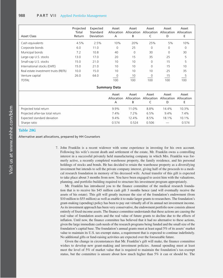
Vis
it u
s at
ww
w.m
hh
e.co
m/b
km988 P A R T V I I Applied Portfolio Management
7. John Franklin is a recent widower with some experience in investing for his own account. Following his wife’s recent death and settlement of the estate, Mr. Franklin owns a controlling interest in a successful privately held manufacturing company in which Mrs. Franklin was for-merly active, a recently completed warehouse property, the family residence, and his personal holdings of stocks and bonds. He has decided to retain the warehouse property as a diversifying investment but intends to sell the private company interest, giving half of the proceeds to a medi-cal research foundation in memory of his deceased wife. Actual transfer of this gift is expected to take place about 3 months from now. You have been engaged to assist him with the valuations, planning, and portfolio building required to structure his investment program appropriately.
Mr. Franklin has introduced you to the finance committee of the medical research founda-tion that is to receive his $45 million cash gift 3 months hence (and will eventually receive the assets of his estate). This gift will greatly increase the size of the foundation’s endowment (from $10 million to $55 million) as well as enable it to make larger grants to researchers. The foundation’s grant-making (spending) policy has been to pay out virtually all of its annual net investment income. As its investment approach has been very conservative, the endowment portfolio now consists almost entirely of fixed-income assets. The finance committee understands that these actions are causing the real value of foundation assets and the real value of future grants to decline due to the effects of inflation. Until now, the finance committee has believed that it had no alternative to these actions, given the large immediate cash needs of the research programs being funded and the small size of the foundation’s capital base. The foundation’s annual grants must at least equal 5% of its assets’ market value to maintain its U.S. tax-exempt status, a requirement that is expected to continue indefinitely. No additional gifts or fund-raising activities are expected over the foreseeable future.
Given the change in circumstances that Mr. Franklin’s gift will make, the finance committee wishes to develop new grant-making and investment policies. Annual spending must at least meet the level of 5% of market value that is required to maintain the foundation’s tax-exempt status, but the committee is unsure about how much higher than 5% it can or should be. The
Asset Class
Projected Total
Return
Expected Standard Deviation
Asset Allocation
A
Asset Allocation
B
Asset Allocation
C
Asset Allocation
D
Asset Allocation
E
Cash equivalents 4.5% 2.5% 10% 20% 25% 5% 10%
Corporate bonds 6.0 11.0 0 25 0 0 0
Municipal bonds 7.2 10.8 40 0 30 0 30
Large-cap U.S. stocks 13.0 17.0 20 15 35 25 5
Small-cap U.S. stocks 15.0 21.0 10 10 0 15 5
International stocks (EAFE) 15.0 21.0 10 10 0 15 10
Real estate investment trusts (REITs) 10.0 15.0 10 10 10 25 35
Venture capital 26.0 64.0 0 10 0 15 5
TOTAL 100 100 100 100 100
Summary Data
Asset Allocation
A
Asset Allocation
B
Asset Allocation
C
Asset Allocation
D
Asset Allocation
E
Projected total return 9.9% 11.0% 8.8% 14.4% 10.3%
Projected after-tax total return 7.4% 7.2% 6.5% 9.4% 7.4%
Expected standard deviation 9.4% 12.4% 8.5% 18.1% 10.1%
Sharpe ratio 0.574 0.524 0.506 — 0.574
Table 28G
Alternative asset allocations, prepared by HH Counselors

Vis
it u
s at
ww
w.m
hh
e.co
m/b
km
C H A P T E R 2 8 Investment Policy and the Framework of the CFA Institute 989
committee wants to pay out as much as possible because of the critical nature of the research being funded; however, it understands that preserving the real value of the foundation’s assets is equally important in order to preserve its future grant-making capabilities. You have been asked to assist the committee in developing appropriate policies.
a. Identify and briefly discuss the three key elements that should determine the foundation’s grant-making (spending) policy.
b. Formulate and justify an investment policy statement for the foundation, taking into account the increased size of its assets arising from Mr. Franklin’s gift. Your policy statement must encom-pass all relevant objectives, constraints, and the key elements identified in your answer to part ( a ).
c. Recommend and justify a long-term asset allocation that is consistent with the investment policy statement you created in part ( b ). Explain how your allocation’s expected return meets the requirements of a feasible grant-making (spending) policy for the foundation. ( Hint: Your allocation must sum to 100% and should use the economic/market data pre-sented in Table 28H and your knowledge of historical asset-class characteristics.)
8. Christopher Maclin, aged 40, is a supervisor at Barnett Co. and earns an annual salary of £80,000 before taxes. Louise Maclin, aged 38, stays home to care for their newborn twins. She recently inherited £900,000 (after wealth-transfer taxes) in cash from her father’s estate. In addition, the Maclins have accumulated the following assets (current market value):
• £5,000 in cash. • £160,000 in stocks and bonds. • £220,000 in Barnett common stock.
The value of their holdings in Barnett stock has appreciated substantially as a result of the com-pany’s growth in sales and profits during the past 10 years. Christopher Maclin is confident that the company and its stock will continue to perform well.
The Maclins need £30,000 for a down payment on the purchase of a house and plan to make a £20,000 non–tax deductible donation to a local charity in memory of Louise Maclin’s father. The Maclins’ annual living expenses are £74,000. After-tax salary increases will offset any future increases in their living expenses.
During their discussions with Grant Webb, the Maclins’ express concern about achieving their educational goals for their children and their own retirement goals. The Maclins tell Webb:
• They want to have sufficient funds to retire in 18 years when their children begin their 4 years of university education.
• They have been unhappy with the portfolio volatility they have experienced in recent years and they do not want to experience a loss greater than 12% in any one year.
• They do not want to invest in alcohol and tobacco stocks. • They will not have any additional children.
Historic Averages
Intermediate Term Consensus Forecast
U.S. Treasury bills 3.7% 4.2%
Intermediate-term U.S. T-bonds 5.2 5.8
Long-term U.S. T-bonds 4.8 7.7
U.S. corporate bonds (AAA) 5.5 8.8
Non-U.S. bonds (AAA) N/A 8.4
U.S. common stocks (all) 10.3 9.0
U.S. common stocks (small-cap) 12.2 12.0
Non-U.S. common stocks (all) N/A 10.1
U.S. inflation 3.1 3.5
Table 28H
Capital markets annnualized return data

Vis
it u
s at
ww
w.m
hh
e.co
m/b
km990 P A R T V I I Applied Portfolio Management
After their discussions, Webb calculates that in 18 years the Maclins will need £2 million to meet their educational and retirement goals. Webb suggests that their portfolio be structured to limit shortfall risk (defined as expected total return minus two standard deviations) to no lower than a 2 12% return in any one year. Maclin’s salary and all capital gains and investment income are taxed at 40% and no tax-sheltering strategies are available. Webb’s next step is to formulate an investment policy statement for the Maclins.
a. Formulate the risk objective of an investment policy statement for the Maclins. b. Formulate the return objective of an investment policy statement for the Maclins. Calculate
the pretax rate of return that is required to achieve this objective. Show your calculations. c. Formulate the constraints portion of an investment policy statement for the Maclins, address-
ing each of the following:
i. Time horizon ii. Liquidity requirements iii. Tax concerns iv. Unique circumstances
9. Louise and Christopher Maclin have purchased their house and made the donation to the local charity. Now that an investment policy statement has been prepared for the Maclins, Grant Webb recommends that they consider the strategic asset allocation described in Table 28I .
a. Identify aspects of the recommended asset allocation in Table 28I that are inconsistent with the Maclins’ investment objectives and constraints. Support your responses.
b. After further discussion, Webb and the Maclins agree that any suitable strategic asset alloca-tion will include 5 to 10% in U.K. small-capitalization equities and 10 to 15% in U.K. large-capitalization equities. For the remainder of the portfolio, Webb is considering the asset class ranges described in Table 28J .
Asset ClassRecommended
Allocation Current Yield
Projected Annualized Pretax
Total Return
Expected Standard Deviation
Cash 15.0% 1.0% 1.0% 2.5%
U.K. corporate bonds 55.0 4.0 5.0 11.0
U.K. small-capitalization equities 0.0 0.0 11.0 25.0
U.K. large-capitalization equities 10.0 2.0 9.0 21.0
U.S. equities* 5.0 1.5 10.0 20.0
Barnett Co. common stock 15.0 1.0 16.0 48.0
Total portfolio 100.0 — 6.7 12.4
Table 28I
Louise and Christopher Maclin’s recommended strategic asset allocation
*U.S. equity data are in British pound terms.
Asset Class Allocation Ranges
Cash 0%–3% 5%–10% 15%–20%
U.K. corporate bonds 10%–20% 30%–40% 50%–60%
U.S. equities 0%–5% 10%–15% 20%–25%
Barnett Co. common stock 0%–5% 10%–15% 20%–25%
Table 28J
Louise and Christopher Maclin’s asset class ranges

Vis
it u
s at
ww
w.m
hh
e.co
m/b
km
C H A P T E R 2 8 Investment Policy and the Framework of the CFA Institute 991
E-INVEST-MENTS EXERCISES
Asset Allocation and Financial Planning
Visit the Asset Allocation Wizard site, which provides suggestions about portfolio asset proportions based on your time frame and attitude toward risk: http://cgi.money.cnn
.com/tools/assetallocwizard/assetallocwizard.html . After you run the calculator with your preferences, change your inputs slightly to see what effect that would have on the results. For a comprehensive retirement planning calculator, go to http://cgi.money.cnn.com/
tools/retirementplanner/retirementplanner.jsp . After you specify your current income and savings habits, your attitude toward risk, and other relevant information, the calculator will tell you the probability of successfully meeting your goals. It also offers suggestions for future savings plans and a graph of probabilities for several possible outcomes.
Recommend the most appropriate allocation range for each of the asset classes in Table 28J . Justify each appropriate allocation range with a reason based on the Maclins’ investment objectives and constraints. Note: No calculations are required.
SOLUTIONS TO CONCEPT CHECKS
1. Identify the elements that are life cycle–driven in the two schemes of objectives and constraints.
2. If the investor keeps her present asset allocation, she will have the following amounts to spend after taxes 5 years from now:
Tax-qualified account:
Bonds: $50,000(1.1) 5 3 .72 5 $ 57,978.36
Stocks: $50,000(1.15) 5 3 .72 5 $ 72,408.86
Subtotal $130,387.22
Nonretirement account:
Bonds: $50,000[1 1 (.10 3 .85)] 5 5 $ 75,182.83
Stocks: $50,000(1.15) 5 2 .15 3 [50,000(1.15) 5 2 50,000] 5 $ 92,982.68
Subtotal $ 168,165.51
Total $298,552.73
If she shifts all of the bonds into the retirement account and all of the stock into the nonretirement account, she will have the following amounts to spend after taxes 5 years from now:
Tax-qualified account:
Bonds: $100,000(1.1) 5 3 .72 5 $115,956.72
Nonretirement account:
Stocks: $100,000(1.15) 5 2 .15 3 [100,000(1.15) 5 2 100,000] 5 $185,965.36
Total 5 $301,922.08
Her spending budget will increase by $3,369.35.

Vis
it u
s at
ww
w.m
hh
e.co
m/b
km992 P A R T V I I Applied Portfolio Management
3. The contribution to each fund will be $2,000 per year (i.e., 5% of $40,000) in constant dollars. At retirement she will have in her guaranteed return fund:
$50,000 3 1.0320 1 $2,000 3 Annuity factor (3%, 20 years) 5 $144,046
That is the amount she will have for sure.
In addition the expected future value of her stock account is:
$50,000 3 1.0620 1 $2,000 3 Annuity factor (6%, 20 years) 5 $233,928
4. He has accrued an annuity of .01 3 15 3 15,000 5 $2,250 per year for 15 years, starting in 25 years. The present value of this annuity is $2,812.13:
PV 5 2,250 3 Annuity factor (8%, 15) 3 PV factor (8%, 25) 5 2,812.13

993
References to CFA Problems
Each end-of-chapter CFA question is reprinted with permission from the CFA Institute, Charlottesville, VA. Following is a list of the CFA questions in the end-of-chapter material and the exams and study guides from which they were taken and updated.
9. 1994 Level I CFA Study Guide, © 1994 10. 1994 Level I CFA Study Guide, © 1994 11. 2002 Level II CFA Study Guide, © 2002 12. 2000 Level II CFA Study Guide, © 2000
Chapter 10
1. 2001 Level II CFA Study Guide, © 2001 2–8. 1991–1993 Level I CFA Study Guides
Chapter 11
1–5. 1993 Level I CFA Study Guide, © 1993 6. 1992 Level I CFA Study Guide, © 1992 7. 1992 Level I CFA Study Guide, © 1992 8–10. 1996 Level III CFA Study Guide,
© 1996
Chapter 12
1. 2000 Level III CFA Study Guide, © 2000 2. 2001 Level III CFA Study Guide, © 2001 3. 2004 Level III CFA Study Guide, © 2004 4. 2003 Level III CFA Study Guide, © 2003 5. 2002 Level III CFA Study Guide, © 2002
Chapter 13
1. 1993 Level I CFA Study Guide, © 1993 2. 1993 Level I CFA Study Guide, © 1993 3. 2002 Level II CFA Study Guide, © 2002
Chapter 14
1. 1993 Level I CFA Study Guide, © 1993 2. 1994 Level I CFA Study Guide, © 1994 3. 1999 Level II CFA Study Guide, © 1999 4. 1992 Level II CFA Study Guide, © 1992 5. 1993 Level I CFA Study Guide, © 1993 6. 1992 Level I CFA Study Guide, © 1992
Chapter 15
1. 1993 Level II CFA Study Guide, © 1993 2. 1993 Level I CFA Study Guide, © 1993 3. 1993 Level II CFA Study Guide, © 1993 4. 1994 Level I CFA Study Guide, © 1994 5. 1994 Level II CFA Study Guide, © 1994 6. 2004 Level II CFA Study Guide, © 2004 7. 1999 Level II CFA Study Guide, © 1999 8. 2000 Level II CFA Study Guide, © 2000 9. 1996 Level II CFA Study Guide, © 1996 10. 2000 Level II CFA Study Guide, © 2000
Chapter 2
1–3. 1996 Level I CFA Study Guide, © 1996 4. 1994 Level I CFA Study Guide, © 1994 5. 1994 Level I CFA Study Guide, © 1994
Chapter 3
1. 1986 Level I CFA Study Guide, © 1986 2–3. 1986 Level I CFA Study Guide, © 1986
Chapter 5
1. 1992 Level I CFA Study Guide, © 1992 2. 1992 Level I CFA Study Guide, © 1992 3–7. 1993 Level I CFA Study Guide, © 1993
Chapter 6
1–3. 1991 Level I CFA Study Guide, © 1991 4–5. 1991 Level I CFA Study Guide, © 1991 6. 1991 Level I CFA Study Guide, © 1991 7–9. 1993 Level I CFA Study Guide, © 1993 10. 1991 Level I CFA Study Guide, © 1991
Chapter 7
1–3. 1982 Level III CFA Study Guide, © 1982
4. 1993 Level I CFA Study Guide, © 1993 5. 1993 Level I CFA Study Guide, © 1993 6. 1992 Level I CFA Study Guide, © 1992 7. 1992 Level I CFA Study Guide, © 1992 8–10. 1994 Level I CFA Study Guide, © 1994 11. 2001 Level III CFA Study Guide, © 2001 12. 2001 Level II CFA Study Guide, © 2001 13. 2000 Level II CFA Study Guide, © 2000
Chapter 8
1. 1982 Level I CFA Study Guide, © 1982 2. 1993 Level I CFA Study Guide, © 1993 3. 1993 Level I CFA Study Guide, © 1993 4. 1993 Level I CFA Study Guide, © 1993 5. 1994 Level I CFA Study Guide, © 1994
Chapter 9
1. 2002 Level I CFA Study Guide, © 2002 2. 2002 Level I CFA Study Guide, © 2002 3–5. 1993 Level I CFA Study Guide, © 1993 6. 1992 Level I CFA Study Guide, © 1992 7. 1994 Level I CFA Study Guide, © 1994 8. 1993 Level I CFA Study Guide, © 1993
Chapter 16
1. 1993 Level II CFA Study Guide, © 1993 2. 1992–1994 Level I CFA study guides 3. 1993 Level I CFA Study Guide, © 1993 4. 1993 Level I CFA Study Guide, © 1993 5. 2004 Level II CFA Study Guide, © 2004 6. 1996 Level III CFA Study Guide, © 1996 7. 1998 Level II CFA Study Guide, © 1998 8. From various Level I study guides 9. 1994 Level III CFA Study Guide, © 1994 10. 2000 Level III CFA Study Guide, © 2000 11. 2003 Level II CFA Study Guide, © 2003 12. 2001 Level II CFA Study Guide, © 2001 13. 1992 Level II CFA Study Guide, © 1992
Chapter 17
1. 1993 Level I CFA Study Guide, © 1993 2. 1993 Level I CFA Study Guide, © 1993 3. 1993 Level II CFA Study Guide, © 1993 4. 1993 Level II CFA Study Guide, © 1993 5. 1998 Level II CFA Study Guide, © 1998 6. 1995 Level II CFA Study Guide, © 1995 7. 2004 Level II CFA Study Guide, © 2004 8. 1993 Level I CFA Study Guide, © 1993
Chapter 18
1. 1995 Level II CFA Study Guide, © 1995 2. 2001 Level II CFA Study Guide, © 2001 3. 2001 Level II CFA Study Guide, © 2001 4. 2001 Level II CFA Study Guide, © 2001 5–6. 2004 Level II CFA Study Guide,
© 2004 7. 2001 Level II CFA Study Guide, © 2001 8. 1993 Level I CFA Study Guide, © 1993 9. 2003 Level I CFA Study Guide, © 2003 10. 2003 Level I CFA Study Guide, © 2003 11. 2003 Level II CFA Study Guide, © 2003
Chapter 19
1. 1998 Level II CFA Study Guide, © 1998 2. 1998 Level II CFA Study Guide, © 1998 3. 1999 Level II CFA Study Guide, © 1999 4. 1992 Level I CFA Study Guide, © 1992 5. 1994 Level I CFA Study Guide, © 1994 6. 1998 Level II CFA Study Guide, © 1998 7–10. 1992 Level I CFA Study Guide,
© 1992

REFERENCES TO CFA QUESTIONS
994
11. 1998 Level I CFA Study Guide, © 1998 12. 1994 Level I CFA Study Guide, © 1994 13. 1992 Level I CFA Study Guide, © 1992 14. 1993 Level II CFA Study Guide, © 1993 15. 1993 Level II CFA Study Guide, © 1993 16. 2002 Level II CFA Study Guide, © 2002 17. 1990 Level II CFA Study Guide, © 1990
Chapter 20
1. 2002 Level II CFA Study Guide, © 2002 2. 2000 Level II CFA Study Guide, © 2000 3. 2001 Level II CFA Study Guide, © 2001 4. 2002 Level II CFA Study Guide, © 2002 5. From various Level I study guides
Chapter 21
1. 1998 Level II CFA Study Guide, © 1998 2. 2003 Level II CFA Study Guide, © 2003 3. 1998 Level II CFA Study Guide, © 1998 4. 2000 Level II CFA Study Guide, © 2000 5. 1997 Level III CFA Study Guide, © 1997
14. 2001 Level III CFA Study Guide, © 2001 15. 2000 Level III CFA Study Guide, © 2000 16. 2002 Level III CFA Study Guide, © 2002
Chapter 25
1–3. From various Level I CFA study guides
4. 1986 Level III CFA Study Guide, © 1986 5. 1991 Level II CFA Study Guide, © 1991 6. 1995 Level II CFA Study Guide, © 1995 7. 2003 Level III CFA Study Guide, © 2003 8. 1998 Level II CFA Study Guide, © 1998
Chapter 28
1. 2001 Level III CFA Study Guide, © 2001 2–4. 1988 Level I CFA Study Guide, © 1988 5. 2002 Level III CFA Study Guide, © 2002 6. 1996 Level III CFA Study Guide, © 1996 7. 1993 Level III CFA Study Guide, © 1993 8. 2004 Level III CFA Study Guide, © 2004 9. 2004 Level III CFA Study Guide, © 2004
Chapter 22
1. 2000 Level II CFA Study Guide, © 2000 2. 1993 Level II CFA Study Guide, © 1993 3. 1986 Level III CFA Study Guide, © 1986 4. 2004 Level II CFA Study Guide, © 2004 5. 2004 Level II CFA Study Guide, © 2004
Chapter 23
1. 2001 Level II CFA Study Guide, © 2001 2. 1995 Level III CFA Study Guide, © 1995 3. 1991 Level III CFA Study Guide, © 1991 4–5. 2003 Level II CFA Study Guide, © 2003 6. 2000 Level III CFA Study Guide, © 2000 7. 1985 Level III CFA Study Guide, © 1985 8. 1996 Level II CFA Study Guide, © 1996
Chapter 24
1. 1995 Level III CFA Study Guide, © 1995 2. 1981 Level I CFA Study Guide, © 1981 3. 1986 Level II CFA Study Guide, © 1986 4–11. From various Level I CFA study guides

G-1
Glossary
A
abnormal return Return on a stock beyond what would be predicted by market movements alone. Cumulative abnor-mal return (CAR) is the total abnormal return for the period surrounding an announcement or the release of information.
accounting earnings Earnings of a firm as reported on its income statement.
acid test ratio See quick ratio.
active management Attempts to achieve portfolio returns more than commensurate with risk, either by forecasting broad market trends or by identifying particular mispriced sectors of a market or securities in a market.
active portfolio In the context of the Treynor-Black model, the portfolio formed by mixing analyzed stocks of perceived nonzero alpha values. This portfolio is ultimately mixed with the passive market index portfolio.
adjusted alphas Forecasts for alpha that are modulated to account for statistical imprecision in the analyst’s estimate.
agency problem Conflicts of interest among stockholders, bondholders, and managers.
alpha The abnormal rate of return on a security in excess of what would be predicted by an equilibrium model like CAPM or APT.
American depository receipts (ADRs) Domestically traded securities representing claims to shares of foreign stocks.
American option An American option can be exercised before and up to its expiration date. Compare with a European option, which can be exercised only on the expiration date.
announcement date Date on which particular news concerning a given company is announced to the public. Used in event studies, which researchers use to evaluate the economic impact of events of interest.
annual percentage rate (APR) Interest rate is annualized using simple rather than compound interest.
anomalies Patterns of returns that seem to contradict the efficient market hypothesis.
appraisal ratio The signal-to-noise ratio of an analyst’s forecasts. The ratio of alpha to residual standard deviation.
arbitrage A zero-risk, zero-net investment strategy that still generates profits.
arbitrage pricing theory An asset pricing theory that is derived from a factor model, using diversification and arbitrage arguments. The theory describes the relationship between expected returns on securities, given that there are no opportunities to create wealth through risk-free arbitrage investments.
asked price The price at which a dealer will sell a security.
asset allocation Choosing among broad asset classes such as stocks versus bonds.
at the money When the exercise price and asset price of an option are equal.
auction market A market where all traders in a good meet at one place to buy or sell an asset. The NYSE is an example.
average collection period, or days’ receivables The ratio of accounts receivable to sales, or the total amount of credit extended per dollar of daily sales (average AR/sales 3 365).
B
backfill bias Bias in the average returns of a sample of funds induced by including past returns on funds that entered the sample only if they happened to be successful.
balance sheet An accounting statement of a firm’s financial position at a specified time.
bank discount yield An annualized interest rate assuming simple interest, a 360-day year, and using the face value of the security rather than purchase price to compute return per dollar invested.
banker’s acceptance A money market asset consisting of an order to a bank by a customer to pay a sum of money at a future date.
baseline forecasts Forecast of security returns derived from the assumption that the market is in equilibrium where current prices reflect all available information.
basis The difference between the futures price and the spot price.
basis risk Risk attributable to uncertain movements in the spread between a futures price and a spot price.
behavioral finance Models of financial markets that emphasize implications of psychological factors affecting investor behavior.
benchmark error Use of an inappropriate proxy for the true market portfolio.
benchmark portfolio Portfolio against which a manager is to be evaluated.
beta The measure of the systematic risk of a security. The tendency of a security’s returns to respond to swings in the broad market.
bid–asked spread The difference between a dealer’s bid and asked price.
bid price The price at which a dealer is willing to purchase a security.

Glossary
G-2
C
calendar spread Buy one option, and write another with a different expiration date.
callable bond A bond that the issuer may repurchase at a given price in some specified period.
call option The right to buy an asset at a specified exercise price on or before a specified expiration date.
call protection An initial period during which a callable bond may not be called.
capital allocation decision Allocation of invested funds between risk-free assets versus the risky portfolio.
capital allocation line (CAL) A graph showing all feasible risk–return combinations of a risky and risk-free asset.
capital gains The amount by which the sale price of a security exceeds the purchase price.
capital market line (CML) A capital allocation line provided by the market index portfolio.
capital markets Includes longer-term, relatively riskier securities.
cash/bond selection Asset allocation in which the choice is between short-term cash equivalents and longer-term bonds.
cash equivalents Short-term money-market securities.
cash flow matching A form of immunization, matching cash flows from a bond portfolio with an obligation.
cash ratio Measure of liquidity of a firm. Ratio of cash and marketable securities to current liabilities.
cash settlement The provision of some futures contracts that requires not delivery of the underlying assets (as in agri-cultural futures) but settlement according to the cash value of the asset.
certainty equivalent rate The certain return providing the same utility as a risky portfolio.
certificate of deposit A bank time deposit.
clearinghouse Established by exchanges to facilitate transfer of securities resulting from trades. For options and futures contracts, the clearinghouse may interpose itself as a middleman between two traders.
closed-end (mutual) fund A fund whose shares are traded through brokers at market prices; the fund will not redeem shares at their net asset value. The market price of the fund can differ from the net asset value.
collar An options strategy that brackets the value of a portfolio between two bounds.
collateral A specific asset pledged against possible default on a bond. Mortgage bonds are backed by claims on prop-erty. Collateral trust bonds are backed by claims on other securities. Equipment obligation bonds are backed by claims on equipment.
collateralized debt obligation (CDO) A pool of loans sliced into several tranches with different levels of risk.
binomial model An option-valuation model predicated on the assumption that stock prices can move to only two values over any short time period.
Black-Scholes formula An equation to value a call option that uses the stock price, the exercise price, the risk-free interest rate, the time to maturity, and the standard deviation of the stock return.
block sale A transaction of more than 10,000 shares of stock.
block transactions Large transactions in which at least 10,000 shares of stock are bought or sold. Brokers or “block houses” often search directly for other large traders rather than bringing the trade to the stock exchange.
bogey The return an investment manager is compared to for performance evaluation.
bond A security issued by a borrower that obligates the issuer to make specified payments to the holder over a specific period. A coupon bond obligates the issuer to make interest payments called coupon payments over the life of the bond, then to repay the face value at maturity.
bond equivalent yield Bond yield calculated on an annual percentage rate method. Differs from effective annual yield.
bond indenture The contract between the issuer and the bondholder.
bond reconstitution Combining stripped Treasury securi-ties to re-create the original cash flows of a Treasury bond.
bond stripping Selling bond cash flows (either coupon or principal payments) as stand-alone zero-coupon securities.
book-to-market effect The tendency for stocks of firms with high ratios of book-to-market value to generate abnor-mal returns.
book value An accounting measure describing the net worth of common equity according to a firm’s balance sheet.
breadth The extent to which movements in the broad mar-ket index are reflected widely in movements of individual stock prices.
brokered market A market where an intermediary (a broker) offers search services to buyers and sellers.
budget deficit The amount by which government spending exceeds government revenues.
bull CD, bear CD A bull CD pays its holder a specified percentage of the increase in return on a specified market index while guaranteeing a minimum rate of return. A bear CD pays the holder a fraction of any fall in a given market index.
bullish, bearish Words used to describe investor attitudes. Bullish means optimistic; bearish means pessimistic. Also used in bull market and bear market.
bundling, unbundling A trend allowing creation of secu-rities either by combining primitive and derivative securities into one composite hybrid or by separating returns on an asset into classes.
business cycle Repetitive cycles of recession and recovery.

Glossary
G-3
country selection A type of active international manage-ment that measures the contribution to performance attribut-able to investing in the better-performing stock markets of the world.
coupon rate A bond’s interest payments per dollar of par value.
covariance A measure of the degree to which returns on two risky assets move in tandem. A positive covariance means that asset returns move together. A negative covari-ance means they vary inversely.
covered call A combination of selling a call on a stock together with buying the stock.
covered interest arbitrage relation See interest rate parity relation .
credit default swap (CDS) A derivative contract in which one party sells insurance concerning the credit risk of another firm.
credit enhancement Purchase of the financial guarantee of a large insurance company to raise funds.
credit risk Default risk.
cross-hedge Hedging a position in one asset using futures on another commodity.
cumulative abnormal return See abnormal return.
currency selection Asset allocation in which the inves-tor chooses among investments denominated in different currencies.
current ratio A ratio representing the ability of the firm to pay off its current liabilities by liquidating current assets (current assets/current liabilities).
current yield A bond’s annual coupon payment divided by its price. Differs from yield to maturity.
cyclical industries Industries with above-average sensitiv-ity to the state of the economy.
D
data mining Sorting through large amounts of historical data to uncover systematic patterns that can be exploited.
day order A buy order or a sell order expiring at the close of the trading day.
days’ receivables See average collection period.
dealer market A market where traders specializing in particular commodities buy and sell assets for their own accounts. The OTC market is an example.
debenture or unsecured bond A bond not backed by specific collateral.
debt securities Bonds; also called fixed-income securities.
dedication strategy Refers to multiperiod cash flow matching.
default premium A differential in promised yield that compensates the investor for the risk inherent in purchasing a corporate bond that entails some risk of default.
collateralized mortgage obligation (CMO) A mortgage pass-through security that partitions cash flows from under-lying mortgages into classes called tranches that receive principal payments according to stipulated rules.
commercial paper Short-term unsecured debt issued by large corporations.
common stock Equities, or equity securities, issued as ownership shares in a publicly held corporation. Shareholders have voting rights and may receive dividends based on their proportionate ownership.
comparison universe The collection of money managers of similar investment style used for assessing relative perfor-mance of a portfolio manager.
complete portfolio The entire portfolio, including risky and risk-free assets.
conditional tail expectation Expectation of a random variable conditional on its falling below some threshold value. Often used as a measure of down side risk.
confidence index Ratio of the yield of top-rated corporate bonds to the yield on intermediate-grade bonds.
conservativism Notion that investors are too slow to update their beliefs in response to new evidence.
constant-growth model A form of the dividend discount model that assumes dividends will grow at a constant rate.
contango theory Holds that the futures price must exceed the expected future spot price.
contingent claim Claim whose value is directly depen-dent on or is contingent on the value of some underlying assets.
contingent immunization A mixed passive-active strategy that immunizes a portfolio if necessary to guarantee a minimum acceptable return but otherwise allows active management.
convergence arbitrage A bet that two or more prices are out of alignment and that profits can be made when the prices converge back to proper relationship.
convergence property The convergence of futures prices and spot prices at the maturity of the futures contract.
convertible bond A bond with an option allowing the bondholder to exchange the bond for a specified number of shares of common stock in the firm. A conversion ratio specifies the number of shares. The market conversion price is the current value of the shares for which the bond may be exchanged. The conversion premium is the excess of the bond’s value over the conversion price.
convexity The curvature of the price-yield relationship of a bond.
corporate bonds Long-term debt issued by private corpo-rations typically paying semiannual coupons and returning the face value of the bond at maturity.
correlation coefficient A statistic in which the covariance is scaled to a value between 2 1 (perfect negative correla-tion) and 1 1 (perfect positive correlation).
cost-of-carry relationship See spot-futures parity theorem.

Glossary
G-4
DuPont system Decomposition of firm profitability measures into the underlying factors that determine such profitability.
duration A measure of the average life of a bond, defined as the weighted average of the times until each payment is made, with weights proportional to the present value of the payment.
dynamic hedging Constant updating of hedge positions as market conditions change.
E
EAFE index The Europe, Australasia, Far East index, computed by Morgan Stanley, is a widely used index of non-U.S. stocks.
earnings management The practice of using flexibility in accounting rules to improve the apparent profitability of the firm.
earnings retention ratio Plowback ratio.
earnings yield The ratio of earnings to price, E/P.
economic earnings The real flow of cash that a firm could pay out forever in the absence of any change in the firm’s productive capacity.
economic value added (EVA) The spread between ROA and cost of capital multiplied by the capital invested in the firm. It measures the dollar value of the firm’s return in excess of its opportunity cost.
effective annual rate (EAR) Interest rate annualized using compound rather than simple interest.
effective annual yield Annualized interest rate on a security computed using compound interest techniques.
effective duration Percentage change in bond price per change in the level of market interest rates.
efficient diversification The organizing principle of mod-ern portfolio theory, which maintains that any risk-averse investor will search for the highest expected return for any level of portfolio risk.
efficient frontier Graph representing a set of portfolios that maximize expected return at each level of portfolio risk.
efficient frontier of risky assets The portion of the minimum-variance frontier that lies above the global minimum-variance portfolio.
efficient market hypothesis The prices of securities fully reflect available information. Investors buying securities in an efficient market should expect to obtain an equilibrium rate of return. Weak-form EMH asserts that stock prices already reflect all information contained in the history of past prices. The semistrong-form hypothesis asserts that stock prices already reflect all publicly available information. The strong-form hypothesis asserts that stock prices reflect all relevant information including insider information.
elasticity (of an option) Percentage change in the value of an option accompanying a 1% change in the value of a stock.
defensive industries Industries with little sensitivity to the state of the economy.
deferred annuities Tax-advantaged life insurance product. Deferred annuities offer deferral of taxes with the option of withdrawing one’s funds in the form of a life annuity.
defined benefit plans Pension plans in which retirement benefits are set according to a fixed formula.
defined contribution plans Pension plans in which the employer is committed to making contributions according to a fixed formula.
degree of operating leverage Percentage change in profits for a 1% change in sales.
delta (of option) See hedge ratio.
delta neutral The value of the portfolio is not affected by changes in the value of the asset on which the options are written.
demand shock An event that affects the demand for goods and services in the economy.
derivative asset/contingent claim Securities provid-ing payoffs that depend on or are contingent on the values of other assets such as commodity prices, bond and stock prices, or market index values. Examples are futures and options.
derivative security A security whose payoff depends on the value of other financial variables such as stock prices, interest rates, or exchange rates.
direct search market Buyers and sellers seek each other directly and transact directly.
directional strategy Speculation that one sector or another will outperform other sectors of the market.
discount bonds Bonds selling below par value.
discretionary account An account of a customer who gives a broker the authority to make buy and sell decisions on the customer’s behalf.
diversifiable risk Risk attributable to firm-specific risk, or nonmarket risk. Nondiversifiable risk refers to systematic or market risk.
diversification Spreading a portfolio over many invest-ments to avoid excessive exposure to any one source of risk.
dividend discount model (DDM) A formula stating that the intrinsic value of a firm is the present value of all expected future dividends.
dividend payout ratio Percentage of earnings paid out as dividends.
dividend yield The percent rate of return provided by a stock’s dividend payments.
dollar-weighted rate of return The internal rate of return on an investment.
doubling option A sinking fund provision that may allow repurchase of twice the required number of bonds at the sinking fund call price.
Dow theory A technical analysis technique that seeks to discern long- and short-term trends in security prices.

Glossary
G-5
factor loading See factor beta.
factor model A way of decomposing the factors that influence a security’s rate of return into common and firm-specific influences.
factor portfolio A well-diversified portfolio constructed to have a beta of 1.0 on one factor and a beta of 0 on any other factor.
factor sensitivity See factor beta.
fair game An investment prospect that has a zero risk premium.
fair value accounting Use of current values rather than historic cost in the firm’s financial statements.
federal funds Funds in a bank’s reserve account.
FIFO The first-in first-out accounting method of inventory valuation.
financial assets Financial assets such as stocks and bonds are claims to the income generated by real assets or claims on income from the government.
financial engineering Creating and designing securities with custom-tailored characteristics.
financial intermediary An institution such as a bank, mutual fund, investment company, or insurance company that serves to connect the household and business sectors so households can invest and businesses can finance production.
firm-specific risk See diversifiable risk.
first-pass regression A time series regression to estimate the betas of securities or portfolios.
fiscal policy The use of government spending and taxing for the specific purpose of stabilizing the economy.
fixed annuities Annuity contracts in which the insurance company pays a fixed dollar amount of money per period.
fixed-charge coverage ratio Ratio of earnings to all fixed cash obligations, including lease payments and sinking fund payments.
fixed-income security A security such as a bond that pays a specified cash flow over a specific period.
flight to quality Describes the tendency of investors to require larger default premiums on investments under uncer-tain economic conditions.
floating-rate bond A bond whose interest rate is reset periodically according to a specified market rate.
forced conversion Use of a firm’s call option on a callable convertible bond when the firm knows that bondholders will exercise their option to convert.
forecasting records The historical record of the forecast-ing errors of a security analyst.
foreign exchange market An informal network of banks and brokers that allows customers to enter forward con-tracts to purchase or sell currencies in the future at a rate of exchange agreed upon now.
foreign exchange swap An agreement to exchange stipu-lated amounts of one currency for another at one or more future dates.
electronic communication network (ECN) A computer-operated trading network offering an alternative to formal stock exchanges or dealer markets for trading securities.
endowment funds Organizations chartered to invest money for specific purposes.
equities Ownership shares in a firm.
equity Ownership in a firm. Also, the net worth of a margin account.
equivalent taxable yield The pretax yield on a taxable bond providing an after-tax yield equal to the rate on a tax-exempt municipal bond.
Eurodollars Dollar-denominated deposits at foreign banks or foreign branches of American banks.
Europe, Australasia, Far East (EAFE) index A widely used index of non-U.S. stocks computed by Morgan Stanley.
European option A European option can be exercised only on the expiration date. Compare with an American option, which can be exercised before, up to, and on its expi-ration date.
event study Research methodology designed to measure the impact of an event of interest on stock returns.
event tree Depicts all possible sequences of events.
excess return Rate of return in excess of the risk-free rate.
exchange rate Price of a unit of one country’s currency in terms of another country’s currency.
exchange rate risk The uncertainty in asset returns due to movements in the exchange rates between the dollar and foreign currencies.
exchange-traded funds (ETFs) Offshoots of mutual funds that allow investors to trade portfolios of securities just as they do shares of stock.
exchanges National or regional auction markets providing a facility for members to trade securities. A seat is a mem-bership on an exchange.
exercise or strike price Price set for calling (buying) an asset or putting (selling) an asset.
expectations hypothesis (of interest rates) Theory that forward interest rates are unbiased estimates of expected future interest rates.
expected return The probability-weighted average of the possible outcomes.
expected return–beta relationship Implication of the CAPM that security risk premiums (expected excess returns) will be proportional to beta.
expected shortfall The expected loss on a security conditional on returns being in the left tail of the probability distribution.
F
face value The maturity value of a bond.
factor beta Sensitivity of security returns to changes in a systematic factor. Alternatively, factor loading; factor sensitivity.

Glossary
G-6
hedge ratio (for an option) The number of stocks required to hedge against the price risk of holding one option. Also called the option’s delta.
hedging Investing in an asset to reduce the overall risk of a portfolio.
hedging demands Demands for securities to hedge par-ticular sources of consumption risk, beyond the usual mean variance diversification motivation.
high water mark The previous value of a portfolio that must be reattained before a hedge fund can charge incentive fees.
holding-period return The rate of return over a given period.
homogenous expectations The assumption that all investors use the same expected returns and covariance matrix of security returns as inputs in security analysis.
horizon analysis Forecasting the realized compound yield over various holding periods or investment horizons.
home bias The tendency of investers to allocate a greater share of their portfolios to domestic securities than would be the case under neutral diversification.
I
illiquidity Difficulty, cost, and/or delay in selling an asset on short notice without offering substantial price concessions.
illiquidity cost Costs due to imperfect liquidity of some security.
illiquidity premium Extra expected return as compensa-tion for limited liquidity.
immunization A strategy that matches durations of assets and liabilities so as to make net worth unaffected by interest rate movements.
implied volatility The standard deviation of stock returns that is consistent with an option’s market value.
incentive fee A fee charged by hedge funds equal to a share of any investment returns beyond a stipulated bench-mark performance.
income beneficiary One who receives income from a trust.
income statement A financial statement showing a firm’s revenues and expenses during a specified period.
indenture The document defining the contract between the bond issuer and the bondholder.
index arbitrage An investment strategy that exploits divergences between actual futures prices and their theoreti-cally correct parity values to make a profit.
index fund A mutual fund holding shares in proportion to their representation in a market index such as the S&P 500.
index model A model of stock returns using a market index such as the S&P 500 to represent common or systematic risk factors.
index option A call or put option based on a stock market index.
forward contract An agreement calling for future delivery of an asset at an agreed-upon price. Also see futures contract.
forward interest rate Rate of interest for a future period that would equate the total return of a long-term bond with that of a strategy of rolling over shorter-term bonds. The forward rate is inferred from the term structure.
framing Decisions are affected by how choices are described, for example, whether uncertainty is posed as potential gains from a low baseline level, or as losses from a higher baseline value.
fully diluted earnings per share Earnings per share expressed as if all outstanding convertible securities and warrants have been exercised.
fundamental analysis Research to predict stock value that focuses on such determinants as earnings and dividends prospects, expectations for future interest rates, and risk evaluation of the firm.
fundamental risk Risk that even if an asset is mispriced, there is still no arbitrage opportunity, because the mispricing can widen before price eventually converges to intrinsic value.
funds of funds Hedge funds that invest in several other hedge funds.
futures contract Obliges traders to purchase or sell an asset at an agreed-upon price on a specified future date. The long position is held by the trader who commits to purchase. The short position is held by the trader who commits to sell. Futures differ from forward contracts in their standardiza-tion, exchange trading, margin requirements, and daily settling (marking to market).
futures option The right to enter a specified futures con-tract at a futures price equal to the stipulated exercise price.
futures price The price at which a futures trader commits to make or take delivery of the underlying asset.
G
gamma The curvature of an option pricing function (as a function of the value of the underlying asset).
geometric average The n th root of the product of n num-bers. It is used to measure the compound rate of return over time.
globalization Tendency toward a worldwide investment environment, and the integration of national capital markets.
gross domestic product (GDP) The market value of goods and services produced over time including the income of foreign corporations and foreign residents working in the United States, but excluding the income of U.S. residents and corporations overseas.
H
hedge fund A private investment pool, open to institu-tional or wealthy investors, that is largely exempt from SEC regulation and can pursue more speculative policies than mutual funds.

Glossary
G-7
investment Commitment of current resources in the expectation of deriving greater resources in the future.
investment bankers Firms specializing in the sale of new securities to the public, typically by underwriting the issue.
investment company Firm managing funds for investors. An investment company may manage several mutual funds.
investment-grade bond Bond rated BBB and above or Baa and above. Lower-rated bonds are classified as speculative-grade or junk bonds.
investment horizon Time horizon for purposes of investment decisions.
investment portfolio Set of securities chosen by an investor.
J
Jensen’s measure The alpha of an investment.
junk bond See speculative-grade bond.
K
kurtosis Measure of the fatness of the tails of a probability distribution. Indicates probability of observing extreme high or low values.
L
Law of One Price The rule stipulating that equivalent securities or bundles of securities must sell at equal prices to preclude arbitrage opportunities.
leading economic indicators Economic series that tend to rise or fall in advance of the rest of the economy.
leverage ratio Ratio of debt to total capitalization of a firm.
LIFO The last-in first-out accounting method of valuing inventories.
limited liability The fact that shareholders have no personal liability to the creditors of the corporation in the event of bankruptcy.
limit order An order specifying a price at which an investor is willing to buy or sell a security.
liquidation value Net amount that could be realized by selling the assets of a firm after paying the debt.
liquidity Liquidity refers to the speed and ease with which an asset can be converted to cash.
liquidity preference theory Theory that the forward rate exceeds expected future interest rates.
liquidity premium Forward rate minus expected future short interest rate.
load Sales charge on the purchase of some mutual funds.
load fund A mutual fund with a sales commission, or load.
lock-up period Period in which investors cannot redeem investments in the hedge fund.
indifference curve A curve connecting all portfolios with the same utility according to their means and standard deviations.
industry life cycle Stages through which firms typically pass as they mature.
inflation The rate at which the general level of prices for goods and services is rising.
information ratio Ratio of alpha to the standard deviation of diversifiable risk.
initial public offering Stock issued to the public for the first time by a formerly privately owned company.
input list List of parameters such as expected returns, variances, and covariances necessary to determine the optimal risky portfolio.
inside information Nonpublic knowledge about a cor-poration possessed by corporate officers, major owners, or other individuals with privileged access to information about a firm.
insider trading Trading by officers, directors, major stock-holders, or others who hold private inside information allow-ing them to benefit from buying or selling stock.
insurance principle The law of averages. The average outcome for many independent trials of an experiment will approach the expected value of the experiment.
interest coverage ratio Measure of financial leverage. Earnings before interest and taxes as a multiple of interest expense.
interest coverage ratio, or times interest earned A finan-cial leverage measure (EBIT divided by interest expense).
interest rate The number of dollars earned per dollar invested per period.
interest rate parity relation (theorem) The spot-futures exchange rate relationship that prevails in well-functioning markets.
interest rate swaps A method to manage interest rate risk where parties trade the cash flows corresponding to different securities without actually exchanging securities directly.
intermarket spread swap Switching from one segment of the bond market to another (from Treasuries to corporates, for example).
in the money In the money describes an option whose exercise would produce profits. Out of the money describes an option where exercise would not be profitable.
international financial reporting standards Accounting standards used in many non-U.S. markets that rely more on principles and less on rules than U.S. standards.
intrinsic value (of a firm) The present value of a firm’s expected future net cash flows discounted by the required rate of return.
intrinsic value of an option Stock price minus exercise price, or the profit that could be attained by immediate exercise of an in-the-money option.
inventory turnover ratio Cost of goods sold as a multiple of average inventory.

Glossary
G-8
market-value-weighted index An index of a group of securities computed by calculating a weighted average of the returns of each security in the index, with weights proportional to outstanding market value.
marking to market Describes the daily settlement of obligations on futures positions.
mean-variance analysis Evaluation of risky prospects based on the expected value and variance of possible outcomes.
mean-variance criterion The selection of portfolios based on the means and variances of their returns. The choice of the higher expected return portfolio for a given level of variance or the lower variance portfolio for a given expected return.
mental accounting Individuals mentally segregate assets into independent accounts rather than viewing them as part of a unified portfolio.
minimum-variance frontier Graph of the lowest possible portfolio variance that is attainable for a given portfolio expected return.
minimum-variance portfolio The portfolio of risky assets with lowest variance.
modern portfolio theory (MPT) Principles underlying analysis and evaluation of rational portfolio choices based on risk–return trade-offs and efficient diversification.
modified duration Macaulay’s duration divided by 1 1 yield to maturity. Measures interest rate sensitivity of bonds.
momentum effect The tendency of poorly performing stocks and well-performing stocks in one period to continue that abnormal performance in following periods.
monetary policy Actions taken by the Board of Governors of the Federal Reserve System to influence the money supply or interest rates.
money market Includes short-term, highly liquid, and relatively low-risk debt instruments.
mortality tables Tables of probability that individuals of various ages will die within a year.
mortgage-backed security Ownership claim in a pool of mortgages or an obligation that is secured by such a pool. Also called a pass-through, because payments are passed along from the mortgage originator to the purchaser of the mortgage-backed security.
multifactor CAPM Generalization of the basic CAPM that accounts for extra-market hedging demands.
multifactor models Model of security returns positing that returns respond to several systematic factors.
municipal bonds Tax-exempt bonds issued by state and local governments, generally to finance capital improvement projects. General obligation bonds are backed by the general taxing power of the issuer. Revenue bonds are backed by the proceeds from the project or agency they are issued to finance.
mutual fund A firm pooling and managing funds of investors.
mutual fund theorem A result associated with the CAPM, asserting that investors will choose to invest their entire risky portfolio in a market-index mutual fund.
lognormal distribution The log of the variable has a normal (bell-shaped) distribution.
London Interbank Offered Rate (LIBOR) Rate that most creditworthy banks charge one another for large loans of Eurodollars in the London market.
long position hedge Hedging the future cost of a pur-chase by taking a long futures position to protect against changes in the price of the asset.
lower partial standard deviation Standard deviation computed using only the portion of the probability distribution below the mean of the variable.
M
Macaulay’s duration Effective maturity of bond, equal to weighted average of the times until each payment, with weights proportional to the present value of the payment.
maintenance, or variation, margin An established value below which a trader’s margin cannot fall. Reaching the maintenance margin triggers a margin call.
margin Describes securities purchased with money borrowed from a broker. Current maximum margin is 50%.
market–book-value ratio Ratio of price per share to book value per share.
market capitalization rate The market-consensus estimate of the appropriate discount rate for a firm’s cash flows.
market model Another version of the index model that breaks down return uncertainty into systematic and nonsystematic components.
market neutral A strategy designed to exploit relative mispricing within a market, but which is hedged to avoid taking a stance on the direction of the broad market.
market order A buy or sell order to be executed immediately at current market prices.
market or systematic risk, firm-specific risk Market risk is risk attributable to common macroeconomic factors. Firm-specific risk reflects risk peculiar to an individual firm that is independent of market risk.
market portfolio The portfolio for which each security is held in proportion to its market value.
market price of risk A measure of the extra return, or risk premium, that investors demand to bear risk. The reward-to-risk ratio of the market portfolio.
market risk See systematic risk.
market segmentation The theory that long- and short-maturity bonds are traded in essentially distinct or segmented markets and that prices in one market do not affect those in the other.
market timer An investor who speculates on broad market moves rather than on specific securities.
market timing Asset allocation in which the investment in the market is increased if one forecasts that the market will outperform T-bills.

Glossary
G-9
P
pairs trading Stocks are paired up based on underlying similarities, and long/short positions are established to exploit any relative mispricing between each pair.
par value The face value of the bond.
passive investment strategy See passive management.
passive management Buying a well-diversified portfolio to represent a broad-based market index without attempting to search out mispriced securities.
passive portfolio A market index portfolio.
passive strategy See passive management.
pass-through security Pools of loans (such as home mort-gage loans) sold in one package. Owners of pass-throughs receive all principal and interest payments made by the borrowers.
peak The transition from the end of an expansion to the start of a contraction.
P/E effect That portfolios of low P/E stocks have exhibited higher average risk-adjusted returns than high P/E stocks.
personal trust An interest in an asset held by a trustee for the benefit of another person.
plowback ratio The proportion of the firm’s earnings that is reinvested in the business (and not paid out as dividends). The plowback ratio equals 1 minus the dividend payout ratio.
political risk Possibility of the expropriation of assets, changes in tax policy, restrictions on the exchange of foreign currency for domestic currency, or other changes in the business climate of a country.
portable alpha; alpha transfer A strategy in which you invest in positive alpha positions, then hedge the systematic risk of that investment, and, finally, establish market exposure where you want it by using passive indexes.
portfolio insurance The practice of using options or dynamic hedge strategies to provide protection against investment losses while maintaining upside potential.
portfolio management Process of combining securities in a portfolio tailored to the investor’s preferences and needs, monitoring that portfolio, and evaluating its performance.
portfolio opportunity set The expected return–standard deviation pairs of all portfolios that can be constructed from a given set of assets.
posterior distribution Probability distribution for a variable after adjustment for empirical evidence on its likely value.
preferred habitat theory Holds that investors prefer specific maturity ranges but can be induced to switch if risk premiums are sufficient.
preferred stock Nonvoting shares in a corporation, paying a fixed or variable stream of dividends.
premium The purchase price of an option.
premium bonds Bonds selling above par value.
N
NAICS codes North American Industrial Classification System codes that use numerical values to identify industries.
naked option writing Writing an option without an offsetting stock position.
NASDAQ The automated quotation system for the OTC market, showing current bid–asked prices for thousands of stocks.
neglected-firm effect That investments in stock of less well-known firms have generated abnormal returns.
net asset value (NAV) The value of each share expressed as assets minus liabilities on a per-share basis.
nominal interest rate The interest rate in terms of nominal (not adjusted for purchasing power) dollars.
nondirectional strategy A position designed to exploit temporary misalignments in relative pricing. Typically involves a long position in one security hedged with a short position in a related security.
nondiversifiable risk See systematic risk.
nonsystematic risk Nonmarket or firm-specific risk factors that can be eliminated by diversification. Also called unique risk or diversifiable risk. Systematic risk refers to risk factors common to the entire economy.
normal distribution Bell-shaped probability distribution that characterizes many natural phenomena.
notional principal Principal amount used to calculate swap payments.
O
on the run Recently issued bond, selling at or near par value.
on-the-run yield curve Relationship between yield to maturity and time to maturity for newly issued bonds selling at par.
open-end (mutual) fund A fund that issues or redeems its own shares at their net asset value (NAV).
open interest The number of futures contracts outstanding.
optimal risky portfolio An investor’s best combination of risky assets to be mixed with safe assets to form the complete portfolio.
option elasticity The percentage increase in an option’s value given a 1% change in the value of the underlying security.
original issue discount bond A bond issued with a low coupon rate that sells at a discount from par value.
out of the money Out of the money describes an option where exercise would not be profitable. In the money describes an option where exercise would produce profits.
over-the-counter market An informal network of brokers and dealers who negotiate sales of securities (not a formal exchange).

Glossary
G-10
pure plays Bets on particular mispricing across two or more securities, with extraneous sources of risk such as general market exposure hedged away.
pure yield curve Refers to the relationship between yield to maturity and time to maturity for zero-coupon bonds.
pure yield pickup swap Moving to higher-yield bonds.
put bond A bond that the holder may choose either to exchange for par value at some date or to extend for a given number of years.
put-call parity theorem An equation representing the proper relation between put and call prices. Violation of parity allows arbitrage opportunities.
put/call ratio Ratio of put options to call options outstanding on a stock.
put option The right to sell an asset at a specified exercise price on or before a specified expiration date.
Q
quality of earnings The realism and conservatism of the earnings number and the extent to which we might expect the reported level of earnings to be sustained.
quick ratio A measure of liquidity similar to the current ratio except for exclusion of inventories (cash plus receiv-ables divided by current liabilities).
R
random walk Describes the notion that stock price changes are random and unpredictable.
rate anticipation swap A switch made in response to forecasts of interest rates.
real assets, financial assets Real assets are land, buildings, and equipment that are used to produce goods and services. Financial assets are claims such as securities to the income generated by real assets.
real interest rate The excess of the interest rate over the inflation rate. The growth rate of purchasing power derived from an investment.
realized compound return Yield assuming that coupon payments are invested at the going market interest rate at the time of their receipt and rolled over until the bond matures.
rebalancing Realigning the proportions of assets in a portfolio as needed.
registered bond A bond whose issuer records ownership and interest payments. Differs from a bearer bond, which is traded without record of ownership and whose possession is its only evidence of ownership.
regression equation An equation that describes the average relationship between a dependent variable and a set of explanatory variables.
regret avoidance Notion from behavioral finance that individuals who make decisions that turn out badly will have more regret when that decision was more unconventional.
present value of growth opportunities (PVGO) Net present value of a firm’s future investments.
price–earnings multiple See price–earnings ratio.
price–earnings (P/E) ratio The ratio of a stock’s price to its earnings per share. Also referred to as the P/E multiple.
price value of a basis point The change in the value of a fixed-income asset resulting from a 1 basis point change in the asset’s yield to maturity.
price-weighted average Weighted average with weights proportional to security prices rather than total capitalization.
primary market New issues of securities are offered to the public here.
primitive security, derivative security A primitive security is an instrument such as a stock or bond for which payments depend only on the financial status of its issuer. A derivative security is created from the set of primitive securities to yield returns that depend on factors beyond the characteristics of the issuer and that may be related to prices of other assets.
principal The outstanding balance on a loan.
prior distribution Probability distribution for a variable before adjusting for empirical evidence on its likely value.
private placement Primary offering in which shares are sold directly to a small group of institutional or wealthy investors.
profit margin See return on sales.
program trading Coordinated buy orders and sell orders of entire portfolios, usually with the aid of computers, often to achieve index arbitrage objectives.
prospect theory Behavioral (as opposed to rational) model of investor utility. Investor utility depends on changes in wealth rather than levels of wealth.
prospectus A final and approved registration statement including the price at which the security issue is offered.
protective covenant A provision specifying requirements of collateral, sinking fund, dividend policy, etc., designed to protect the interests of bondholders.
protective put Purchase of stock combined with a put option that guarantees minimum proceeds equal to the put’s exercise price.
proxy An instrument empowering an agent to vote in the name of the shareholder.
prudent investor rule An investment manager must act in accord with the actions of a hypothetical prudent investor.
pseudo-American call option value The maximum of the value derived by assuming that an option will be held until expiration and the value derived by assuming that the option will be exercised just before an ex-dividend date.
public offering, private placement A public offering consists of bonds sold in the primary market to the general public; a private placement is sold directly to a limited number of institutional investors.

Glossary
G-11
risk-free rate The interest rate that can be earned with certainty.
risk lover See risk-averse.
risk-neutral See risk-averse.
risk premium An expected return in excess of that on risk-free securities. The premium provides compensation for the risk of an investment.
risk–return trade-off If an investor is willing to take on risk, there is the reward of higher expected returns.
risky asset An asset with an uncertain rate of return.
risk pooling Investing the portfolio in many risky assets.
risk sharing Sharing the risk of a portfolio of given size among many investers.
S
scatter diagram Plot of returns of one security versus returns of another security. Each point represents one pair of returns for a given holding period.
seasoned new issue Stock issued by companies that already have stock on the market.
secondary market Already existing securities are bought and sold on the exchanges or in the OTC market.
second-pass regression A cross-sectional regression of portfolio returns on betas. The estimated slope is the measurement of the reward for bearing systematic risk during the period.
sector rotation An investment strategy which entails shifting the portfolio into industry sectors that are forecast to outperform others based on macroeconomic forecasts.
securitization Pooling loans for various purposes into standardized securities backed by those loans, which can then be traded like any other security.
security analysis Determining correct value of a security in the marketplace.
security characteristic line A plot of the excess return on a security over the risk-free rate as a function of the excess return on the market.
security market line Graphical representation of the expected return–beta relationship of the CAPM.
security selection See security selection decision.
security selection decision Choosing the particular securities to include in a portfolio.
semistrong-form EMH See efficient market hypothesis.
separation property The property that portfolio choice can be separated into two independent tasks: (1) determina-tion of the optimal risky portfolio, which is a purely techni-cal problem, and (2) the personal choice of the best mix of the risky portfolio and the risk-free asset.
Sharpe’s measure Reward-to-volatility ratio; ratio of portfolio excess return to standard deviation.
shelf registration Advance registration of securities with the SEC for sale up to 2 years following initial registration.
reinvestment rate risk The uncertainty surrounding the cumulative future value of reinvested bond coupon payments.
REIT Real estate investment trust, which is similar to a closed-end mutual fund. REITs invest in real estate or loans secured by real estate and issue shares in such investments.
remainderman One who receives the principal of a trust when it is dissolved.
replacement cost Cost to replace a firm’s assets. “Reproduction” cost.
representativeness bias People seem to believe that a small sample is just as representative of a broad population as a large one and therefore infer patterns too quickly.
repurchase agreements (repos) Short-term, often over-night, sales of government securities with an agreement to repurchase the securities at a slightly higher price. A reverse repo is a purchase with an agreement to resell at a specified price on a future date.
residual claim Refers to the fact that shareholders are at the bottom of the list of claimants to assets of a corporation in the event of failure or bankruptcy.
residual income See economic value added (EVA).
residuals Parts of stock returns not explained by the explan-atory variable (the market-index return). They measure the impact of firm-specific events during a particular period.
resistance level A price level above which it is supposedly difficult for a stock or stock index to rise.
return on assets (ROA) A profitability ratio; earnings before interest and taxes divided by total assets.
return on equity (ROE) An accounting ratio of net profits divided by equity.
return on sales (ROS), or profit margin The ratio of oper-ating profits per dollar of sales (EBIT divided by sales).
reversal effect The tendency of poorly performing stocks and well-performing stocks in one period to experience reversals in following periods.
reversing trade Entering the opposite side of a currently held futures position to close out the position.
reward-to-volatility ratio Ratio of excess return to portfolio standard deviation.
riding the yield curve Buying long-term bonds in anticipation of capital gains as yields fall with the declining maturity of the bonds.
risk arbitrage Speculation on perceived mispriced secu-rities, usually in connection with merger and acquisition targets.
risk-averse, risk-neutral, risk lover A risk-averse investor will consider risky portfolios only if they provide compensation for risk via a risk premium. A risk-neutral investor finds the level of risk irrelevant and considers only the expected return of risk prospects. A risk lover is willing to accept lower expected returns on prospects with higher amounts of risk.
risk-free asset An asset with a certain rate of return; often taken to be short-term T-bills.

Glossary
G-12
statement of cash flows A financial statement showing a firm’s cash receipts and cash payments during a specified period.
statistical arbitrage Use of quantitative systems to uncover many perceived misalignments in relative pricing and ensure profit by averaging over all of these small bets.
stock exchanges Secondary markets where already-issued securities are bought and sold by members.
stock selection An active portfolio management technique that focuses on advantageous selection of particular stocks rather than on broad asset allocation choices.
stock split Issue by a corporation of a given number of shares in exchange for the current number of shares held by stockholders. Splits may go in either direction, either increasing or decreasing the number of shares outstanding. A reverse split decreases the number outstanding.
stop-loss order A sell order to be executed if the price of the stock falls below a stipulated level.
stop orders Order to trade contingent on security price designed to limit losses if price moves against the trader.
straddle A combination of buying both a call and a put on the same asset, each with the same exercise price and expi-ration date. The purpose is to profit from expected volatility.
straight bond A bond with no option features such as callability or convertibility.
street name Describes securities held by a broker on behalf of a client but registered in the name of the firm.
strike price See exercise price.
strip, strap Variants of a straddle. A strip is two puts and one call on a stock; a strap is two calls and one put, both with the same exercise price and expiration date.
stripped of coupons Describes the practice of some investment banks that sell “synthetic” zero-coupon bonds by marketing the rights to a single payment backed by a coupon-paying Treasury bond.
strong-form EMH See efficient market hypothesis.
subordination clause A provision in a bond indenture that restricts the issuer’s future borrowing by subordinating the new leaders’ claims on the firm to those of the existing bond holders. Claims of subordinated or junior debtholders are not paid until the prior debt is paid.
substitution swap Exchange of one bond for a bond with similar attributes but more attractively priced.
supply shock An event that influences production capacity and costs in the economy.
support level A price level below which it is supposedly difficult for a stock or stock index to fall.
survivorship bias Bias in the average returns of a sample of funds induced by excluding past returns on funds that left the sample because they happened to be unsuccessful.
swaption An option on a swap.
systematic risk Risk factors common to the whole economy, nondiversifiable risk; also called market risk.
short position or hedge Protecting the value of an asset held by taking a short position in a futures contract.
short rate A one-period interest rate.
short sale The sale of shares not owned by the investor but borrowed through a broker and later repurchased to replace the loan. Profit is earned if the initial sale is at a higher price than the repurchase price.
single-factor model A model of security returns that acknowledges only one common factor. See factor model.
single-index model A model of stock returns that decomposes influences on returns into a systematic factor, as measured by the return on a broad market index, and firm-specific factors.
single-stock futures Futures contracts on single stock rather than an index.
sinking fund A procedure that allows for the repayment of principal at maturity by calling for the bond issuer to repurchase some proportion of the outstanding bonds either in the open market or at a special call price associated with the sinking fund provision.
skew Measure of the asymmetry of a probability distribution.
small-firm effect That investments in stocks of small firms appear to have earned abnormal returns.
soft dollars The value of research services that brokerage houses supply to investment managers “free of charge” in exchange for the investment managers’ business.
Sortino ratio: Excess return divided by lower partial standard deviation.
specialist A trader who makes a market in the shares of one or more firms and who maintains a “fair and orderly market” by dealing personally in the stock.
speculation Undertaking a risky investment with the objective of earning a greater profit than an investment in a risk-free alternative (a risk premium).
speculative-grade bond Bond rated Ba or lower by Moody’s, or BB or lower by Standard & Poor’s, or an unrated bond.
spot-futures parity theorem, or cost-of-carry relationship Describes the theoretically correct relationship between spot and futures prices. Violation of the parity relationship gives rise to arbitrage opportunities.
spot rate The current interest rate appropriate for discounting a cash flow of some given maturity.
spread (futures) Taking a long position in a futures contract of one maturity and a short position in a contract of different maturity, both on the same commodity.
spread (options) A combination of two or more call options or put options on the same stock with differing exer-cise prices or times to expiration. A money spread refers to a spread with different exercise price; a time spread refers to differing expiration date.
standard deviation Square root of the variance.

Glossary
G-13
trough The transition point between recession and recovery.
turnover The ratio of the trading activity of a portfolio to the assets of the portfolio.
12b-1 fees Annual fees charged by a mutual fund to pay for marketing and distribution costs.
U
unbundling See bundling.
underwriters Investment bankers who help companies issue their securities to the public.
underwriting, underwriting syndicate Underwriters (investment bankers) purchase securities from the issuing company and resell them. Usually a syndicate of investment bankers is organized behind a lead firm.
unemployment rate The ratio of the number of people classified as unemployed to the total labor force.
unique risk See diversifiable risk.
unit investment trust Money invested in a portfolio whose composition is fixed for the life of the fund. Shares in a unit trust are called redeemable trust certificates, and they are sold at a premium above net asset value.
universal life policy An insurance policy that allows for a varying death benefit and premium level over the term of the policy, with an interest rate on the cash value that changes with market interest rates.
utility The measure of the welfare or satisfaction of an investor.
utility value The welfare a given investor assigns to an investment with a particular return and risk.
V
value at risk Measure of downside risk. The loss that will be incurred in the event of an extreme adverse price change with some given, typically low, probability.
variable annuities Annuity contracts in which the insur-ance company pays a periodic amount linked to the invest-ment performance of an underlying portfolio.
variable life policy An insurance policy that provides a fixed death benefit plus a cash value that can be invested in a variety of funds from which the policyholder can choose.
variance A measure of the dispersion of a random variable. Equals the expected value of the squared deviation from the mean.
variation margin See maintenance margin.
vega Response of option price to change in standard deviation of underlying asset.
views An analyst’s opinion on the likely performance of a stock or sector compared to the market-consensus expectation.
volatility risk The risk in the value of options portfolios due to unpredictable changes in the volatility of the underlying asset.
T
tax anticipation notes Short-term municipal debt to raise funds to pay for expenses before actual collection of taxes.
tax deferral option The feature of the U.S. Internal Revenue Code that the capital gains tax on an asset is payable only when the gain is realized by selling the asset.
tax-deferred retirement plans Employer-sponsored and other plans that allow contributions and earnings to be made and accumulate tax-free until they are paid out as benefits.
tax swap Swapping two similar bonds to receive a tax benefit.
technical analysis Research to identify mispriced securi-ties that focuses on recurrent and predictable stock price pat-terns and on proxies for buy or sell pressure in the market.
tender offer An offer from an outside investor to share-holders of a company to purchase their shares at a stipulated price, usually substantially above the market price, so that the investor may amass enough shares to obtain control of the company.
term insurance Provides a death benefit only, no build-up of cash value.
term premiums Excess of the yields to maturity on long-term bonds over those of short-term bonds.
term structure of interest rates The pattern of interest rates appropriate for discounting cash flows of various maturities.
times interest earned Ratio of profits to interest expense.
time value (of an option) The part of the value of an option that is due to its positive time to expiration. Not to be confused with present value or the time value of money.
time-weighted average An average of the period-by-period holding-period returns of an investment.
Tobin’s q. Ratio of market value of the firm to replacement cost.
total asset turnover The annual sales generated by each dollar of assets (sales/assets).
tracking error The difference between the return on a specified portfolio and that of a benchmark portfolio designed to mimic that portfolio.
tracking portfolio A portfolio constructed to have returns with the highest possible correlation with a systematic risk factor.
tranche See collateralized mortgage obligation.
Treasury bill Short-term, highly liquid government securities issued at a discount from the face value and returning the face amount at maturity.
Treasury bond or note Debt obligations of the federal government that make semiannual coupon payments and are issued at or near par value.
Treynor’s measure Ratio of excess return to beta.
trin statistic Ratio of average trading volume in declining stocks to average volume in advancing stocks. Used in technical analysis.

Glossary
G-14
Y
yield curve A graph of yield to maturity as a function of time to maturity.
yield to maturity A measure of the average rate of return that will be earned on a bond if held to maturity.
Z
zero-beta portfolio The minimum-variance portfolio uncorrelated with a chosen efficient portfolio.
zero-coupon bond A bond paying no coupons that sells at a discount and provides payment of face value only at maturity.
zero-investment portfolio A portfolio of zero net value, established by buying and shorting component securities, usually in the context of an arbitrage strategy.
W
warrant An option issued by the firm to purchase shares of the firm’s stock.
weak-form EMH See efficient market hypothesis.
well-diversified portfolio A portfolio spread out over many securities in such a way that the weight in any security is close to zero.
whole-life insurance policy Provides a death benefit and a kind of savings plan that builds up cash value for possible future withdrawal.
workout period Realignment period of a temporary misaligned yield relationship.
world investable wealth The part of world wealth that is traded and is therefore accessible to investors.
writing a call Selling a call option.


I-1
Goldgar, Anne, 368Gongloff, Mark, 731Gordon, Myron J., 589Graham, Benjamin, 654–655Graham, John R., 823Green, T. C., 345, 346n, 372Greenspan, Alan, 390Grinblatt, Mark, 392nGrossman, Sanford J., 182n, 296, 346Gruber, Martin J., 334, 369–370, 372Guy, J., 272
HHan, Bing, 392nHarris, M., 382nHartle, Thom, 394–395Harvey, A., 730nHarvey, Campbell R., 415, 823, 884Hasanhodzic, Jasmina, 912–913Hasbrouck, J., 309nHeaton, John, 302n, 416–417Henriksson, Roy D., 834Heston, S., 730nHicks, John, 776Hlavka, M., 369–370Homer, Sidney, 510, 536Hsieh, David, 915Huang, Ming, 434–435Hull, J., 730n
I
Ibbotson, Roger G., 432Icahn, Carl, 7
J
Jacquier, Eric, 153, 154n, 886Jaffee, Charles A., 968Jaffee, Jeffrey F., 86n, 365Jagannathan, Ravi, 247n, 301n, 306n, 415, 417,
429–430Jarrow, Robert A., 807nJegadeesh, Narasimhan, 358, 369, 425Jensen, Michael C., 288n, 300n, 412, 415, 822Johnson, H. E., 733nJones, C., 83Jones, Charles P., 364nJurion, Philippe, 433
K
Kahneman, D., 383, 385nKandel, Schmuel, 298n, 411Kane, Alex, 153, 154n, 935, 946
Chopra, Navin, 359, 384nChordia, Tarun, 309nClements, Jonathan, 181n, 207, 387, 895Conrad, Jennifer, 358Constantinides, George M., 382n, 434Cooper, M., 391nCoval, J. D., 386nCrovitz, L. Gordon, 347
DDabora, E. M., 388nDaniel, Naveen D., 914Das, S., 369–370Davis, James L., 420, 421nDe Marzo, Peter M., 880de Soto, Hernando, 867DeBondt, Werner F. M., 359, 383, 385DeLong, J. B., 386nDesai, M., 651Dimitrov, O., 391nDimson, Elroy, 145n–146nDodd, David, 654Dow, Charles, 394Droms, William, 207Dugan, Ianthe Jeanne, 832
EElton, Edwin J., 334, 369–370, 372Engle, Robert, 300, 301nEvans, Richard, 371n
FFackler, Martin, 551nFama, Eugene F., 304n, 335, 358n, 359–360, 363,
365, 392, 413, 416n, 419–420, 421n, 430–432
Ferson, Wayne, 415Fisher, Irving, 121French, Kenneth R., 125n, 179, 335, 358n, 359–
360, 361n, 363, 365, 419–420, 421n, 430–432
Friedman, Milton, 347Friend, I., 182n, 323nFroot, K. A., 388nFung, William, 915
GGarber, Peter, 368Gervais, S., 393nGeske, Robert, 732–733nGetmansky, Mila, 913Ghysels, E., 730nGivoly, Dan, 365Goetzmann, William N., 432–433, 920
AAcharya, V. V., 310n, 428Agarwal, Vikas, 914Akerlof, George A., 397nAlexander, C., 730nAllen, F., 391nAltman, Edward I., 463, 464nAmihud, Yakov, 306, 309, 362, 426Amin, G., 915Anand, Shefali, 881Aragon, George O., 913–914Arbel, Avner, 362
BBainbridge, Stephen, 347Baker, Craig, 273Balbuena, Milton, 731Ball, R., 363Banz, Rolf, 361nBarber, Brad, 359, 368, 383Barberis, Nicholas, 382n, 434–435Basu, Sanjoy, 361Batchelor, Roy, 393Battalio, R. H., 363Bavishi, Vinod, 653nBeebower, Gilbert, 207, 840nBenveniste, Lawrence, 62nBergstresser, D., 651Berk, J. B., 372Bernard, V., 363Bernoulli, Daniel, 191Bicksler, J., 323nBierwag, G. O., 535nBlack, Fischer, 302–303, 335, 412, 731n, 931,
934, 938Blake, Christopher R., 372Blume, Marshall E., 182n, 362Bodie, Zvi, 809n, 981Bogle, John C., 168Bollen, Nicholas P. B., 371Bowman, Melanie, 394–395Brealey, R. A., 391nBreeden, Douglas, 304Brennan, Michael J., 287Brinson, Gary, 207, 840nBrown, Alan, 273Brown, P., 363Brown, S. J., 920Buffett, Warren, 372Busse, Jeffrey A., 345, 346n, 371
CCampbell, John Y., 301, 359Carhart, Mark M., 371, 425Carther, Shauna, 831Chan, L. K. C., 424Chen, Nai-Fu, 333, 418, 419n
Name Index
Page numbers followed by n refer to footnotes.

Name Index
I-2
Kaniel, Ron, 880Kaplin, Andrew, 247nKarabell, Zachary, 681Karceski, J., 424Kat, H., 915Kaufman, G. C., 535nKaul, Gautam, 358Keim, Donald B., 359–360, 362Kendall, Maurice, 343–344Keynes, John Maynard, 387, 393, 556, 776Kim, J., 369Kim, Tae-Hwan, 935Kitts, Arno, 273Korajczyk, Robert, 415Kosowski, R., 373Kothari, S. P., 363Kotlikoff, Laurence J., 974Kremer, Ilan, 880Krische, S. D., 369
LLa Porta, Rafael, 366n., 424, 425n, 867Laise, Eleanor, 140nLakonishok, Josef, 359, 366n, 384n, 424, 425nLamont, O. A., 83, 388–389nLatané, Henry A., 364nLee, C. M., 369, 389Lehavy, R., 368Lehmann, B., 358nLiang, B., 920Liebowitz, Martin L., 510, 536Liew, J., 366n, 421, 422nLintner, John, 280, 409Litterman, Robert, 931, 938Lo, Andrew W., 358, 912–913Longin, F., 886Lopez-De-Silvanes, Florencio, 867Loughran, T., 62Lucas, Deborah, 302n, 416–417Lucas, Robert, 304Ludwig, Robert, 895Lynch, Peter, 372, 572, 603
MMacaulay, Frederick, 512MacBeth, James, 413, 416nMacKinlay, A. Craig, 358Maddala, G. S., 730nMadoff, Bernard, 919–920Makarov, Igor, 913Malkiel, Burton G., 108, 295, 510, 515–516, 915Malloy, C. J., 431Marcus, Alan J., 153, 154n, 886, 946Markopolos, Harry, 920Markowitz, Harry, 10, 213, 280Marsh, Paul, 145n–146nMayers, David, 288, 303, 415Mazuy, Kay, 834McDonald, R. L., 744nMcGee, Suzanne, 795McNichols, M., 368Mehra, Jarnish, 428Mei, Jianping, 334Mendelhall, R., 363Mendelson, Haim, 306, 309n, 362
Merton, Robert C., 301, 303–304, 362, 834, 838, 937Mikus, William John, 207Milken, Michael, 461–462Miller, Merton H., 300, 409, 412, 612nMinsky, Hyman, 367Mitchell, Mark, 355nModigliani, Franco, 612n, 823Modigliani, Leah, 823Morgenstern, J., 192Moskowitz, T., 431Mossin, Jan, 280Myers, S. C., 391n
NNaik, Narayan Y., 914Netter, Jeffry, 355nNofsinger, John, 387
OObama, Barack, 556Odean, Terrance, 383, 385n, 387, 393nOldfield, George S., 807nOpdyke, Jeff D., 605n
PPalmon, Dan, 365Pástor, L., 310n, 426–427Patell, J. M., 345Patterson, Scott, 73Paulson, Henry, 651Pedersen, Lasse Heje, 306n, 310n, 428Perritt, Gerald, 207Petkova, Ralitsa, 421–423Pierallini, Fabrizio, 795Pontiff, Jeffrey, 95, 390Poterba, James, 358nPrescott, Edward, 428
RRajaratnam, Raj, 347Ramyar, Richard, 393Rau, P. R., 391nRauh, J., 651Reagan, Ronald, 556Reddy, Sudeep, 556Redington, F. M., 529Reinganum, Marc R., 362Renault, E., 730nRendleman, R. J., Jr., 364Riepe, Mark, 895Ritter, Jay R., 62, 359, 384nRoberts, Harry, 399, 400nRobinstein, Mark, 304Roll, Richard, 298n, 301, 309n, 333, 410–411,
418–419, 732n, 887Roosevelt, Franklin, 556Rosansky, Victor, 809nRosenberg, Barr, 272Ross, Stephen A., 298n, 323, 333, 390n, 411,
418–419, 462n
Rothchild, John, 572nRothschild, Tricia, 895Rubinstein, Mark, 743–744Rydqvist, K., 62
SSadka, Ronnie, 427, 914Sahan, Atanu, 915Samuelson, Paul, 373, 615Schleifer, A., 386nSchmalensee, Richard E., 728nScholes, Myron, 300, 303, 409, 412Seppi, D. H., 309nSeyhun, Nejat H., 365, 376nShanken, Jay, 363Sharpe, William F., 10, 252, 280, 284, 822, 832,
840, 845Shefrin, H., 385nShiller, Robert J., 182n, 359, 681Shleifer, Andrei, 366n, 389, 424, 425n, 867Shumway, T., 386nSinger, Brian, 207, 840nSloan, Richard G., 363Solnik, B., 870n, 884, 886Soros, George, 373Speidell, Lawrence S., 653nSperling, Gene, 561nSpivak, Avia, 974Stambaugh, R. F., 310n, 426–427Stambaugh, Robert F., 298n, 360, 362, 411Statman, Meir, 197–198n, 384, 385n, 387Staunton, Mike, 145n–146nStein, Jeremy, 291Stiglitz, Joseph E., 296, 346Strebel, Paul J., 362Stulz, R., 382nSubrahmanyam, Avanidhar, 309nSummers, Lawrence, 358n, 386n
TTaleb, Nassim N., 918Templeton, John, 372Thaler, Richard H., 359, 382n, 383, 385, 388–389Thatcher, Margaret, 556Thomas, J., 363Timmerman, A., 373Titman, Sheridan, 358, 425Tjornehoj, Jeff, 881Tobin, James, 215n, 585Toevs, A., 535nTrain, John, 654nTreussard, Jonathan, 138n, 981Treynor, Jack L., 822, 834, 934Trippi, Robert R., 728n, 946Trueman, B., 368Tversky, A., 383, 385n
V
Vasicek, Oldrich A., 271nVassalou, M., 366n, 421, 422nVishny, Robert W., 366n, 386n, 424, 425n, 867Vissing-Jorgensen, A., 431

Name Index
I-3
Von Neumann, O., 192, 195Vuolteenaho, Tuomo, 301
W
Waldman, R., 386nWang, Yong, 306n, 429–430Wang, Zhenyu, 301n, 415, 417
Wermers, R., 373Westerfield, Randolph W., 462nWhaley, Robert E., 732n, 743White, A., 730nWhite, Halbert, 373, 935Wiggins, J., 730nWilcox, Jarrod, 795Wilhelm, William, 62nWolfson, M. A., 345Womack, K. L., 368
YYang, Jerry, 7
ZZhang, Lu, 421–423

I-4
international diversification; see International diversification
performance attribution and, 848–849policy statements, 959–967risk tolerance and, 174–178risky and risk-free portfolios, 167–169security selection and, 219steps in, 967–969stock, bonds, and bills, 206–210successful investing and, 207synthetic stock positions, 792–794taxes and, 968–969
Asset-backed bonds, 444–445Asset-backed commercial paper, 31Asset-backed securities, 445
amount outstanding (1996–2009), 41Asset betas, 414–416Asset plays, 572Asset pricing models; see Arbitrage pricing
theory (APT); Capital asset pricing model (CAPM)
Asset utilization ratios, 638–639, 643Assets; see also Derivative assets; Financial assets
asset classes; see Financial instrumentsindividual assets and ATP, 330–331nontraded assets, 302–303real assets vs. financial assets, 203risk-free asset, 169–170
Asymmetric information, 307At the money, 669Auction markets, 64Average collection period, 639Average rates of return, 819–820
BBack-end load, 100Backfill bias, 915Bad debt allowance, 652Balance sheet, 628–630
commercial banks (2009), 13common-size balance sheets, 630Hewlett-Packard example, 629nonfinancial U.S. business (2009), 13restructurings and swaps, 801–802U.S. households (2009), 3
Balanced funds, 97Bank of America, 14, 21, 73Bank-discount method, 29Bankers’ acceptances, 31Banks, 957Barclays Capital U.S. (formerly Lehman)
Aggregate Bond Index, 527Barclay’s Global Investors, 106Bargaining power of buyers/suppliers, 573Barrier options, 698Barron’s, 398Baseline forecast, 938–939Basis, 769
Alpha seeking behavior, 903, 908Alpha transfer, 908Alpha transport, 274Alpha values, 928Altman’s Z score, 463–464American Depository Receipts (ADRs), 44, 875American option, 671, 717, 732American Saving Education Council, “Ballpark
Estimate” retirement planning worksheet, 970–971
Analysis of variance (ANOVA), 256–257Annual percentage rates (APRs), 34, 123
effective annual rate (EAR) vs., 123Annuities, 974Annuity factor, 447Anomalies, 360, 381; see also Market anomaliesArbitrage, 324
covered interest arbitrage, 786–788, 871fundamental risk, 386–387futures markets, 771–772implementation costs, 388index arbitrage, 794–795law of one price and, 324, 388–390limits to, 386–388mispricing and, 332model risk, 388security market line and, 329systematic factor and, 327
Arbitrage pricing theory (APT), 318, 323–330, 407betas and expected returns, 326–328CAPM and, 330–331cost of capital and, 334equilibrium and, 324Fama and French (FF) three-factor model, 335,
419–420index model and single-factor ATP, 408–417individual assets and, 330–331multifactor APT, 331–335multifactor CAPM and, 336one-factor security market line, 328–329risk arbitrage and, 324security market line, 329tests of, 407, 417–419well-diversified portfolios, 325
ArcaEx, 72ARCH (autoregressive conditional heteroskedastic-
ity) models, 301n, 730Archipelago exchange, 65, 70, 75Arithmetic average
expected return and, 130–131geometric vs., 132
Arthur Andersen, 8Asian options, 698Asked price, 29, 64–65, 440nAsked yield, 441Asset allocation, 8, 28, 98, 160, 168, 196, 991; see
also Capital allocationBlack-Litterman model, 938flexible funds and, 98global tactical asset allocation, 795
AAbnormal return, 353
cumulative abnormal returns, 354event studies, 353market model to estimate, 353to infer damages, 355
Accounting earnings, 627, 632economic earnings vs., 632
Accrued interest, 441Accumulated benefit obligation (ABO), 977Accumulation phase, 974Acid test ratio, 640Active bond management, 508, 535–537
hedging interest rate risk, 798–800horizon analysis, 537intermarket spread swap, 536pure yield pickup swap, 536–537rate anticipation swap, 536sources of profit, 535–537substitution swap, 536tax swap, 537
Active portfolio, 264, 927Active portfolio management; see also Black-
Litterman model; Treynor-Black modelalphas values, forecasts of, 926–931imperfect forecasting and, 839–840information ratio and, 946manager’s private views, 940market timing, 834–840optimal portfolios and alpha values, 926–933passive portfolio management vs., 350–361restriction of benchmark risk, 931–933value of, 945–948
Actual delivery, 765Adjustable-rate mortgages (ARMs), 18Adjusted alpha, 934Adjusted beta, 271After-tax returns, OID bond, 460Agency problems, 6, 19, 42Aggregate stock market, 613–615
explaining past behavior, 613–614forecasting of, 614–615
Aggressive investor, 954Agricultural futures, 760AIG, 21Aite Group, 73Allowance for bad debt, 652Alpha, 249–250, 270, 290
adjusting forecasts, 934–935alpha betting, 273distribution of alpha values, 935–936estimate of, 257–258forecasts and extreme portfolio weights, 927–931forecasts and realizations of, 950multifactor model and, 843mutual fund alphas (1972–1991), 295optimal portfolios and, 926–933performance measures and, 827portable alpha, 908–910
Subject Index
Page numbers followed by n refer to footnotes.

Subject Index
I-5
Bonds, 440; see also Active bond management; Fixed income capital market; Interest rates; Term structure of interest rates; Yield curve
accrued interest, 441after-tax returns, 469asset allocation with, 206–210asset-backed bonds, 444–445call provisions, 442callable bonds, 39catastrophe bonds, 445characteristics of, 440–446collateral, 466convertible bonds, 39, 442–443convexity; see Convexitycorporate bonds, 38–39, 441–442coupon rate, 440current yield, 452default risk; see Default riskdividend restrictions, 466floating-rate bonds, 4, 443indentures, 440, 464indexed bonds, 445–446inflation-linked bonds, 57, 445–446innovations in bond market, 444–446international bonds, 444inverse floaters, 444junk bonds, 461–463other issuers of, 444par/face value, 440pricing; see Bond pricingprotective covenants, 464puttable bonds, 443quoted bond prices, 441ratings, 442, 462safety, determinants of, 463–464secured bonds, 38sinking funds, 465–466subordination clauses, 466trading of, 73unsecured bonds, 466yield to call, 453–454yield to maturity; see Yield to maturityzero-coupon bonds; see Zero-coupon bonds
Book and bookbuilding, 61Book-to-market effects, 363Book-to-market ratios, 291, 363, 424Book value, 584, 640
limitations of, 585Bootstrapping, 150Border-multiplied covariance matrix, 200, 236Bordered covariance matrix, 200Bottom-up strategy, 9Bracket creep, 121Brane v. Roth, 680Breadth, 396–397BRIC nations (Brazil, Russia, India, China), 864,
876Brokered markets, 64Broker’s call loans, 76Brokers’ calls, 32Bubbles, 367–368, 390–391Budget deficit, 552–553Bulldog bonds, 444Bullish spread, 684, 686, 741Bureau of Economic Research (NBER), 581Bureau of Labor Statistics (BLS), 119Business cycles, 557–562, 569
cyclical indicators, 558defensive industries, 559
hedge ratios and, 733–735hedging bets on mispriced options, 739–743implied volatility, 728, 730incentive fees, 919portfolio insurance, 735–736pseudo-American call option value, 732put option valuation, 732–733synthetic protective put options, 736
Black swan event, 117, 918BlackRock, 106Block houses, 64, 71Block sales/transactions, 71Blue sky laws, 84Bogey, 846Bond-equivalent yield, 30, 34Bond funds, 97Bond indentures, 440, 464
collateral, 466dividend restrictions, 466sinking funds, 465–466subordination clauses, 466
Bond-index funds, 527Bond market, 34–41
corporate bonds, 38–39federal agency debt, 35inflation-protected Treasury bonds, 35innovations, 444–445international bonds, 35mortgages and mortgage-backed securities, 39–41municipal bonds, 35–38tax-exempt debt outstanding (1979–2009), 36Treasury notes and bonds, 34
Bond market indexes, 50–51Bond portfolios; see Active bond management;
Passive bond managementBond pricing, 439, 446–450
callable and straight debt, 453coupon bonds, 449between coupon dates, 449default risk and, 461–471Excel application for, 450forward rates with interest rate risk, 489interest rate sensitivity, 448Malkiel’s bond-pricing relationships, 510price/yield relationship, 448–449, 509prices over time, 456–461quoted bond prices, 441yield curve and, 481–483
Bond ratings, definitions of class, 462Bond reconstitution, 482Bond safety
Altman’s Z, 463–464cash flow-to-debt ratio, 463coverage ratios, 463determinants of, 463–464leverage ratio, 463liquidity ratios, 463profitability ratios, 463
Bond stripping, 482Bond swap, 536–537; see also Active bond
managementBond trading, 73Bond yields, 451–456
current yield, 452effective annual yield, 451realized compound yield vs. yield to maturity,
454–455yield to call, 453–454yield to maturity (YTM), 451–453
vs. holding period return, 458
Basis risk, 769BATS, 72Bear markets, international diversification and,
886–888Bear Stearns, 14, 21, 83Behavioral biases, 384–388, 393
framing, 384mental accounting, 384–385prospect theory, 385–386regret avoidance, 385
Behavioral economics, 390–391Behavioral finance, 381–392
bubbles and behavioral economics, 390–391disposition effect, 392equity premium puzzle, 434–435evaluation of, 391–392information processing, 382–384limits to arbitrage, 386–388mental accounting, 384–385technical analysis and, 392–400value premium, 423–425warnings on, 399–400
Benchmark error, 411Benchmark risk, 931–932Benchmarks, 931
for mutual funds, 107for ratio analysis, 642style analysis and multifactor benchmarks,
842–843Beta, 250
adjusted beta, 271commodity betas, 809consumption betas, 430defined, 282equalizing beta, 826estimate of, 258, 278expected return-beta relationship, 250, 287
econometrics and, 300–301index model and, 408–409
expected returns and, 250, 326–328factor betas, 320–321human capital and cyclical variations, 414–416as hurdle rate, 290–291, 407liquidity betas, 309, 427measurement error in, 412–414predicting betas, 272security returns and, 316zero-beta model, 301–302
Beta books, 269–270Beta capture, 274Bid-asked spread, 29, 65, 307–308, 426Bid price, 29, 64–65, 440nBinomial option pricing, 718–724
example of, 721two-state option pricing, 718–720
Black-Litterman model, 937–943asset allocation decision, 938baseline forecast, 938–940, 950covariance matrix from historical data, 938, 950manager’s private views and, 940, 951portfolio optimization, 942–943, 951revised (posterior) expectations, 940–942, 951steps in, 938–942Treynor-Black vs., 943–945
Black-Scholes pricing formula, 724–733assumptions of, 728dividends and call options, 731–732dividends and put option valuation, 733example of, 726Excel model for, 729, 735

Subject Index
I-6
Commodity Futures Trading Commission (CFTC), 83, 765
Common-size balance sheets, 630Common-size income statement, 628Common stock, 4, 41; see also Equity securities
characteristics of, 42limited liability of, 42as ownership shares, 41–42as residual claim, 42
Comparability problems, 648–654depreciation, 649fair value accounting, 650–651financial statement analysis, 648–654inflation and interest expense, 650international accounting conventions, 653–654inventory valuation, 648–649quality of earnings, 652–653
Comparison universe, 821Competition
in financial markets, 9–11Porter’s five determinants of, 573rivalry between competitors, 573as source of efficiency, 345–347
Complete portfolio, 168, 171, 283optimal complete portfolio, 209–210proportions of, 210steps to, 209
Compound leverage factor, 636, 643COMPUSTAT Company Profiles, 584Conditional tail expectation (CTE), 138Conference Board, 581Confidence index, 398Conforming mortgages, 18, 39Conservatism, 383Conservative investor, 954Conservatorship, 40nConsolidated Tape, 72Consolidation stage, 571Consolidation of stock markets, 75Constant-growth dividend discount model,
588–591Constant relative risk aversion (CRRA), 305nConstraints; see Investment constraintsConsumer Price Index (CPI), 35, 118Consumption-based asset pricing, 428–435Consumption-based CAPM, 304–306, 430
market rates of return and, 429–431Consumption-mimicking portfolio, 305Consumption risk, 305Consumption timing, 5Consumption-tracking portfolio, 305Contango, 777Contingent claims, 667Contingent deferred sales charges, 100Contingent liability, 652Continuous compounding, 123–125Contract, 52Convergence arbitrage, 906Convergence property, 764Conversion premium, 443Conversion price, 691Conversion ratio, 442, 691Conversion value, 691Convertible bonds, 39, 442–443
convertible bond arbitrage, 905, 906value as function of stock price, 692
Convertible securities, 690–693Convexity, 448, 518–526, 546
callable bonds and, 521–523as desirable trait for investors, 521
multifactor CAPM and APT, 336multiperiod model, 303–304passive strategy as efficient, 283as practical, 296–297required rate of return, 291, 810risk premium of market portfolio, 284–285Roll’s critique, 298n, 410–412security market line (SML), 289–292tests of, 293, 297–298, 409–410, 414utility rate-making cases and, 292, 407world portfolio, 879, 885, 893zero-beta model, 301–302
Capital gains, 43Capital market line (CML), 179–182, 282
efficient frontier and, 283Capital markets, 4, 28CAPM; see Capital asset pricing model (CAPM)Case-Shiller index of U.S. housing prices
(1987–2009), 16Cash, 28
cash/bond selection, 896Cash cows, 571Cash equivalents, 28Cash flow matching, 534Cash flow-to-debt ratio, 463Cash ratio, 640, 643Cash settlement, 469, 765Catastrophe bonds, 445CDA Wiesenberger Investment Companies
Services, 99Cellular approach (stratified sampling), 527–528Certainty equivalent rate, 163Certificates of deposit (CDs), 4, 30, 170
index-linked CDs, 696–6973-month CD/T-bill spread (1970–2009), 33
CFA (Chartered Financial Analysts) Institute, 84, 299
investment management process, 953–957standards of professional conduct, 85
CFA Institute, 84, 948, 952Charting, 406Chartists, 348, 393Chicago Board Options Exchange (CBOE), 70,
667, 730–731Chicago Board of Trade (CBOT), 53, 70, 75, 757,
761–762Chicago Mercantile Exchange (CME), 70, 75, 757,
762, 782, 785, 817Clearinghouse, 760–763Clientele effect, 308Closed-end funds, 94, 308n, 389–390CME Group, 762Coincident indicators, 559–561Collars, 684, 687Collateral, 466Collateral trust bond, 466Collateralized debt obligations (CDOs),
18–19, 471credit risk and, 470–471
Collateralized loans, 694–695Collateralized mortgage obligation (CMO), 525Commercial banks, balance sheet (2009), 12Commercial paper (CP), 30–31, 170Commingled funds, 95Commodities, 5Commodity betas, 809Commodity futures
discounted cash flow analysis, 808–810pricing of, 806–807, 809pricing with storage costs, 807–808
Business cycles—Cont.
degree of operating leverage, 567–569economic indicators, 559–561Great Moderation, 16, 556other indicators, 561peaks/troughs, 557sector rotation and, 569–570sensitivity to, 566–569
Buying on margin; see Margin
CCalendar spread, 769Call option, 4n, 51, 668
corporate bonds (callable), 690covered calls, 680–683current stock price and, 716determinants of value, 714dividends and, 716, 731early exercises and dividends, 716hedge ratio and, 734incentive fee as, 919market timing valued as, 837–839profits and losses on, 668, 759pseudo-American call option value, 732put/call ratio, 398–399restrictions on value of, 715–716values at expiration, 674–675values before expiration, 713
Call price, 442Call provisions, 442Callable bonds, 39, 466, 522, 690
duration and convexity of, 521–523mortgage-backs vs., 525negative convexity, 522values vs. straight bonds, 691yield to call, 453–454
Capacity utilization rate, 552, 557–558Capital allocation, 196; see also Asset allocation
risk tolerance and, 174–178risky and risk-free portfolios, 160, 167–169, 175separation property and, 214–216
Capital allocation line (CAL), 172, 206, 212, 238, 938
Capital asset pricing model (CAPM), 280–292, 407
actual vs. expected returns, 293arbitrage pricing theory (APT), 330–331assumptions of, 281average country-index returns, 876–880capital budgeting decisions and, 291consumption-based CAPM, 304–306economy and validity of, 298–299EMH and, 414empirical tests of, 298, 407, 414expected return-beta relationship, 300–301,
408–409expected returns on individual securities,
285–288extensions of, 301–306, 433–434hedge portfolios, 303–304homogeneous expectations, 281hurdle rate, 290ICAPM (intertemporal CAPM), 304index model and, 293–296investment industry and, 299–300labor income and nontraded assets, 302–303liquidity and, 306–310, 426–428market portfolio (M) and, 281–283, 298

Subject Index
I-7
misleading representation of benefits, 884–885portfolio risk and, 197–198power of, 217–219well-diversified portfolios, 325
Dividend discount models (DDM), 431–432, 583, 587–600
constant-growth (Gordon model) DDM, 588–591
convergence of price to intrinsic value, 592life cycles and, 595–599multistage growth models, 600P/E analysis and, 607preferred stock and, 589stock prices and investment opportunities,
592–595Dividend payout ratio, 593Dividend yield, 128Dividends, 548
call option valuation, 716, 731cumulative dividends, 43growth rate of dividends, 593put option valuation, 733restrictions on, 466
Dollar-weighted rate of return, 820Domestic macroeconomy, 551–553
budget deficit, 552–553employment, 552gross domestic product (GDP), 551inflation, 552interest rates, 552sentiment, 553
Domestic net worth, 3Dot-com boom, 367–368Doubling option, 465Dow Jones Industrial Average (DJIA), 44–47, 395
composition 1928/2010, 47Friday closing levels (1956), 399–400moving averages, 397as price-weighted average, 44–45splits and, 45–46
Dow theory, 394–395Drexel Burnham Lambert, 461–463Dreyfus, 96Dun & Bradstreet Industry Norms and Key
Business Ratios, 642DuPont system, 635, 644Duration, 512–515, 546
bond maturity vs., 516callable bonds, 521–523determinants of, 515–518effective duration, 522–523Excel application for, 513, 517as key concept, 513–514Macaulay’s duration, 512, 522modified duration, 514mortgage-backed securities, 523–525rules for, 515–517
Dynamic hedging, 724, 737
EE-Minis, 792nEarly exercise, 716Earnings
accounting vs. economic earnings, 632fully diluted earnings per share, 693quality of, 652–653
Earnings before interest and taxes (EBIT), 628Earnings management, 605–606
DAX index (Germany), 49Days sales in receivables, 639, 643Dealer markets, 64, 66–67Debenture bonds, 466Debentures, 38Debt securities, 4, 439Debt-to-equity ratio, 463Dedicated short bias, 905Dedication strategy, 534Default premium, 467–468Default risk
bond pricing and, 461–471corporate bonds, 38default premium and, 467–468financial ratios as predictors, 463yield to maturity and, 467
Defensive industries, 559Deferred annuities, 974Deferred callable bonds, 442Defined benefit pension obligations, 976–977Defined benefit plans, 976Defined contribution plans, 975–976Degree of operating leverage (DOL), 568Degrees of freedom bias, 133Deleveraging, 21Delta, 733Delta hedging, 737Delta neutral, 742Demand shock, 553Department of Housing and Urban Development
(HUD), 40Depository receipts, 44Depreciation, 631
accounting vs. economic definition of, 649comparability problems of, 649international accounting conventions, 653
Derivative assets, 51; see also Options; Swapsfutures contracts, 53options, 51–52, 668–669
Derivative markets, 51–53mortgage derivatives and 2008 crisis, 18–19
Derivative securities, 4, 667, 681Detachable warrant, 693Deutsche Börse, 761Developed countries, 864
market capitalization of stock exchanges, 74, 865
Diagonal model, 926Digital options, 699Direct Edge, 72Direct quotes, 788Direct search markets, 64Directional strategies, 905DirectPlus/Direct+, 71Discount bonds, 453Discount brokers, 76Discounted cash flow (DCF), 591
commodity futures pricing, 808–810Discounted cash flow (DCF) formula, 591Discretionary account, 76Discriminant analysis, 465Disposition effect, 392Diversifiable risk, 197, 254Diversification, 10, 197, 213, 231; see also
International diversificationbenefits over time, 220efficient diversification, 196, 199index model and, 252–254insurance principle and, 197investment companies, 93
mortgage-backed securities, 523–525negative convexity, 521n, 522
Corporate bonds, 38–39, 441–442; see also Bondscallable bonds, 39, 442convertible bonds, 39, 442–443debentures, 38default risk, 38floating-rate bonds, 443pricing of, 448puttable bonds, 443secured bonds, 38subordinated debentures, 38
Corporate ethics, 7–8Corporate governance, 7–8Correlation coefficient, 201, 243–245, 258–261,
881–883Cost of capital, 407
using APT to find, 334Cost-of-carry relationship, 772Counterparty risk, 470, 785Country indexes, 889Country risk, 874Country selection, 896Coupon bonds
pricing of, 449valuing of, 482
Coupon payments, 34, 440Coupon rate, 440Covariance, 219, 242–244
border-multiplied covariance, 200bordered covariance matrix, 200single-index model and, 250
Covariance matrix, 200, 246correlation and, 258–259from historical data, 938spreadsheet model, 234
Coverage ratios, 463Covered calls, 680–683
value at expiration, 682Covered interest arbitrage relationship, 786–788, 871Covering the short position, 80Credit default swaps (CDS), 19–20, 468–470, 806Credit risk, 461, 525n
collateralized debt obligations and, 470–41in swap market, 805–806
Credit spreads, 477Cross-hedging, 769, 800Crowding out, 553Cumulative abnormal return, 354Cumulative dividends, 43Currency futures, 785; see also Foreign exchange
futuresCurrency futures options, 673Currency options, 673Currency selection, 895–896Currency-translated options, 698–699Current ratio, 463, 639, 643Current yield, 452CUSIP number (Committee on Uniform Securities
Identification Procedures), 459Cyclical firms, 249Cyclical indicators, 558Cyclical industries, 249, 557, 567Cyclicals, 572
DData mining, 367, 381, 907“David Bowie bonds,” 444

Subject Index
I-8
Event studies, 353–355Event tree, 134Excel Solver, 236–237, 843–844Excess returns, 129, 259
developed/emerging markets, 876risk premiums and, 129–130on risky portfolios (1926–2009), 141–144
Exchange rate, 550, 784Exchange rate risk, 785, 869
futures and, 788–791hedging exchange rate risk, 789–790, 871international investing and, 868–875
Exchange-traded funds (ETFs), 49, 104–106, 273, 351, 759, 875
advantages/disadvantages of, 106growth of (1998–2008), 105sponsors and products, 105
Execution, 953Exercise price, 51, 668Exit fees, 100Exotic options, 698–699
Asian options, 698barrier options, 698currency-translated options, 698–699digital options, 699lookback options, 698
Expectations hypothesis, 490–491forward inflation rates, 491futures pricing, 776
Expected holding-period return, 586Expected return, 9n, 117, 239–240
actual return vs., 293arithmetic average and, 130–131beta and, 250, 326–328expected holding-period return, 586expected vs. promised YTM, 467expected return-beta relationship, 294–296, 407
econometrics and, 300–301index model and, 294–296index model and single-factor APT, 408–417
individual securities and, 285–288portfolio expected return, 203realized return vs., 293–294, 431–432, 829–930spreadsheet model for, 234–235, 239standard deviation and, 128–129, 202, 205
Expected shortfall (ES), 138, 144–145, 178, 219–220Expected utility, 191–194Extendable (put) bond, 443
FFace value, 440Factor betas, 320–321Factor loadings, 320, 334, 365, 420, 915–916Factor models of security returns, 319–320; see
also Multifactor modelsFactor portfolio, 331Factor sensitivities, 320Fads hypothesis, 358Fair game, 161, 193Fair value accounting, 650–651Fallen angels, 461Fama and French (FF) three-factor model, 335,
419–426behavioral explanations, 423–425momentum as fourth factor, 425–426risk-based interpretations, 421–423
Fannie Mae; see Federal National Mortgage Association (FNMA or Fannie Mae)
versions of, 347–348weak-form of, 347, 358–360
Electronic communication networks (ECNs), 67, 72
Electronic trading, 71Elliott wave theory, 394Emerging market funds, 97Emerging markets, 864–867, 905
market capitalization of stock exchanges, 866P/E ratios in, 605risk and return in, 876
Employment, 552Endowment funds, 956–957Enron, 8, 83Equally-weighted indexes, 49Equilibrium, 324Equipment obligation bond, 466Equity, 4; see also Equity securities
levered equity, 696Equity carve-outs, 388–389Equity funds, 97Equity indexes, 760Equity market neutral, 905Equity premium, 428, 433–434
behavioral explanations of, 434–435consumption growth and market rates of return,
429–431expected vs. realized returns, 431–432extensions to CAPM, 433–434liquidity and, 434survivorship bias, 433
Equity securities, 41–44asset allocation with, 206–210characteristics of, 42common stock as ownership shares, 41–42depository receipts, 44developed countries, 864emerging markets, 864–867global markets for, 864–868home-country bias, 867–868options vs. stock investments, 676–678pension investment strategies and, 978–979preferred stock, 43–44stock market listings, 42–43synthetic stock positions, 792–794
Equity trusts, 95Equity valuation models, 583
aggregate stock market, 613–615comparison of models, 612–613dividend discount model; see Dividend discount
model (DDM)free cash flow approaches, 609–612intrinsic value vs. market price, 586–587price-earnings analysis and DDM, 608valuation by comparables, 583–585
Equivalent taxable yield, 37ETFs; see Exchange-traded funds (ETFs)Ethics
CFA standards of professional conduct, 85corporate ethics, 7–8
Eurex, 761EURIBOR (European Interbank Offered Rate), 32Eurobonds, 35, 444Eurodollars, 31Euronext, 74–75Euronext.liffe, 761Europe, Australasian, Far East (EAFE) index,
893–894European options, 671Event driven, 905
Earnings retention ratio, 593Earnings smoothing, 652Earnings surprises, 364, 379Earnings yield, 643Econometrics, expected return-beta relationship,
300–301Economic calendar, 560, 562–563Economic depreciation, 592n, 606Economic earnings, 627, 632
accounting earnings vs., 632Economic indicators, 559–561
coincident/lagging indicators, 560–561leading economic indicators, 559–561other indicators, 561–563
Economic value added, 644–645, 665Economies of scale, 13Economy; see also Business cycles;
Macroeconomic analysisconsumption timing, 5domestic macroeconomy, 551–553financial markets and, 5–8global economy, 549–551separation of ownership and management, 6–7systemic risk and real economy, 22–23validity of CAPM and, 298–299
Effective annual rate (EAR), 122annual percentage rates (APRs) vs., 123total return vs., 123
Effective duration, 522–523Efficient diversification, 196, 199
spreadsheet model for, 234–239Efficient frontier of risky assets, 211–213
capital market line and, 212, 283charting of, 237country portfolios, 885–886spreadsheet model for, 234–239
Efficient market hypothesis (EMH), 10–11, 343–345, 381, 392, 394
abnormal returns, 353–355active vs. passive portfolio management, 10,
350–251book-to-market ratios, 363bubbles, 367–368CAPM and, 414competition as source, 345–347data mining, 367event studies, 353–355fundamental analysis, 349–350implications of, 348–353inside information, 85, 364–365liquidity effects, 362, 428lucky event issue, 356–357magnitude issue, 356market anomalies, 356, 360–362mutual fund managers, 369–373neglected-firm effect, 362portfolio management and, 351–352post-earnings-announcement price drift,
363–364predictors of broad market returns, 359–360random walks and, 344–348resource allocation, 352–353returns over short/long horizons, 358–359risk premiums, 365–355selection bias issue, 356semistrong form of, 348, 360–364small-firm-in-January effect, 361–362stock market analysts, 368–369strong-form of, 348, 364–365technical analysis and, 348–349

Subject Index
I-9
convertible bonds, 442–443corporate bonds, 441–442floating-rate bonds, 443innovations in, 444–445international bonds, 444levered equity and risky debt, 696preferred stock, 443–444puttable bonds, 443Treasury bonds and notes, 440–441
Flash trading, 72–73Flat prices, 449Flexible funds, 98Float securities, 59Floating-rate bonds, 4, 443Floor broker, 69–70Forecasting
active portfolio management, 946–948long horizons, 153–154risk premium forecasts, 246, 267stock market, 614–615value of imperfect forecasting, 839–840
Forecasting errors, 383Forecasting record, 934Foreign bonds, 444Foreign currency options, 673Foreign exchange futures, 760, 784–791, 817
covered interest arbitrage, 786–788direct vs. indirect quotes, 788interest rate parity, 786–788managing exchange rate risk, 788–791the markets, 784–786
Foreign exchange swap, 800Foreign stock market indexes, 49Foreign stocks; see Global equity marketsForward contract, 755–756
forward rates as, 497–499futures pricing vs., 775–776swaps vs., 805synthetic forward loan, 498
Forward interest rate, 486–487as forward contracts, 497–499interest rate risk, 489interest rate uncertainty and, 488–490slopes of yield curve, 494
Forward interest rate contract, 497Framing, 384Freddie Mac; see Federal Home Loan Mortgage
Corporation (FHLMC or Freddie Mac)Free cash flow for the firm (FCFF), 609–612Free cash flow to equityholders (FCFE), 609Free cash flow valuation approaches, 609–613Free float, 48Free-rider benefit, 180Front-end load, 100FTSE (Financial Times) index (UK), 44, 49, 74,
864Full-covariance model; see also Markowitz
portfolio selection modelindex model vs., 268–269
Full-service brokers, 76Fully diluted earnings per share, 693Fund of funds, 905, 919–921Fundamental analysis, 349–350, 548Fundamental analysts, 583Fundamental risk, 386–387Futures contracts, 53, 667, 755–760, 782
basics of, 756–759cash vs. actual delivery, 765existing contracts, 759–760leverage and, 767
Financial leveragebusiness cycle sensitivity, 566–569ROE and, 633–635
Financial marketsallocation of risk, 5–6capital markets, 28as competitive, 9–11consumption timing, 5corporate governance/ethics, 7–8economy and, 5–8as efficient, 10–11financial intermediaries in, 11–13firms as net borrowers, 11government’s role in, 11households as net savers, 11information role of, 5investment bankers and, 13–14major players in, 11–14money markets, 28risk-return trade-off, 9–10separation of ownership and management, 6–7
Financial planning, 991Financial ratio analysis; see Ratio analysisFinancial statement analysis, 627
accounting vs. economic earnings, 627, 632balance sheet, 628–630comparability problems, 648–654depreciation, 649economic value added, 644–654fair value accounting, 650–651financial leverage and ROE, 633–635illustration of use, 646–647income statement, 627–628inflation and interest expense, 650international accounting conventions, 653–654inventory valuation, 648–649profitability measures, 632–635quality of earnings, 652–653ratio analysis; see Ratio analysisreturn on equity, 633–635statement of cash flows, 630–632value investing (Graham technique), 654–655
Financial supermarkets, 99Firm commitment, 60Firm-specific risk, 197–198, 258First-pass regression, 408Fiscal policy, 554Fitch Investors Services, 19, 442, 461Fixed annuities, 974Fixed asset, 630Fixed-asset turnover, 636, 643Fixed-charge coverage ratio, 463Fixed-income arbitrage, 905Fixed-income capital market, 34; see also Bonds;
Money market; Treasury billscorporate bonds, 38–39, 441–442federal agency debt, 35inflation-protected Treasury bonds, 35international bonds, 35mortgages and mortgage-backed securities,
39–41municipal bonds, 35–38, 444preferred stock, 443–444Treasury notes and bonds, 34, 440–441
Fixed-income portfolio management; see Active bond management
Fixed-income securities, 4, 439; see also Bonds; Money market
bond market innovation, 444–445collateralized loan, 694–695
Farm Credit agencies, 444Fast growers, 572Federal agency debt, 35Federal Deposit Insurance Corporation (FDIC), 30Federal funds (fed funds), 32, 555Federal government policy, 554–557
fiscal policy, 554monetary policy, 554–556supply-side policies, 556–557
Federal Home Loan Bank (FHLB), 35, 444Federal Home Loan Mortgage Corporation
(FHLMC or Freddie Mac), 35, 39, 523, 652
failure of, 40financial crisis of 2008, 17–18, 21
Federal National Mortgage Association (FNMA or Fannie Mae), 35, 39, 444, 523
failure of, 40financial crisis of 2008, 17–18, 21
Federal Reserve Bank of St. Louis, 158Federal Reserve Board
federal funds rate targeting, 555margin limits, 77monetary policy, 555
Federal Savings and Loan Insurance Corporation (FSLIC), 979
Fedwire, 459Feedback, 953Feeder funds, 919Fees
active management, 945–946hedge funds, 919–921mutual funds, 99–102
Fibonacci numbers, 393Fidelity’s Magellan Fund, 111, 841–482FIFO (first-in first-out), 648Financial Accounting Standards Board (FASB)
Statement No. 87, 977Statement No. 157, 650
Financial assets, 2, 4–5balance sheet of U.S. households, 3derivatives, 4equity, 4fixed-income or debt securities, 4real assets vs., 2–3separation of ownership/management, 6–7
Financial crisis of 2008, 14–23, 309antecedents of, 15–17changes in housing finance, 17–18credit default swaps, 19–20, 470money market for short-term lending, 22, 33mortgage derivatives, 18–19, 471peak of crisis, 21–22real economy and, 22–23systemic risk, 20–23
Financial engineering, 696–698; see also Derivative assets
index-linked CDs, 696–697Financial Industry Regulatory Authority
(FINRA), 84Financial instruments
bond market, 34–41derivative markets, 51–53equity securities, 41–44money market, 28–33stock and bond market indexes, 44–51
Financial intermediaries, 11–14investment bankers, 13–14investment companies, 12role of, 11–14

Subject Index
I-10
cross-hedging, 769, 800dynamic hedging, 724, 737exchange rate risk, 871factor betas and, 321futures markets and, 766–770index futures and market risk, 795–797interest rate risk, 798–800long/short hedge, 768mispriced options and, 739–743oil futures, 767–768profit on hedged put portfolio, 740speculation and, 766–769
Heterogeneous expectations, 161Hewlett-Packard
balance sheet, 629DuPont decomposition for, 644income statement, 628moving average chart (2009), 395–396security characteristic line (SCL), 255–256statement of cash flows, 631
High water mark, 919High-yield bonds, 4, 461–463Historic returns on risky portfolios, 139–146
diversified portfolio, 140–143excess returns, 141–144expected shortfall (ES), 144–145global view of, 145–146performance, 144–145total return, 141U.S. large stocks, 139, 141–143U.S. long-term government bonds, 131,
139–143U.S. small stocks, 139, 141–143U.S. T-bills, 141–143value at risk (VaR), 144–145world large stocks, 139, 141–143
Holding-period return (HPR), 127–128, 457, 819after-tax holding-period return, 968expected holding period return, 586original-issues discount bonds, 460simulation of long-term future rates of return,
150–152yield to maturity vs., 458zero-coupon bonds, 485–486
Home bias, 879Home-country bias, 867–868Homogeneous expectations, 281Horizon analysis, 456, 537“Hot hands” phenomenon, 371House money effect, 385Households
balance sheet of (2009), 3domestic net worth, 3household wealth, 2as net savers, 11
Housing finance, changes in, 17–18Human capital, 969
asset betas, 414–416insurance and, 969–970
Hurdle rate, 290–291, 407
IIlliquidity, 306, 426–427, 913
asset pricing and, 306–309average returns and, 309
Immunization, 528–534cash flow matching and dedication, 534–535constructing a portfolio, 533holding period immunization, 532
Global funds, 97Global macro style, 905Global tactical asset allocation, 795Globalization, of stock markets, 75Globex, 761–762, 792nGoldman Sachs, 14, 73Goodwill, 630Gordon model, 588–591Government, in financial markets, 11; see also
Federal government policyGovernment National Mortgage Association
(GNMA or Ginnie Mae), 35, 444Graham technique, 654–655Great Moderation, 16, 556Gross domestic product (GDP), 551, 558
market capitalization and, 867Growth funds, 97Growth opportunities, 595
present value of growth opportunities (PVGO), 594
price-earnings ratio and, 601–604price to book, 641
Growth rate of dividends, 593Growth stocks, 112Guaranteed investment contract (GIC), 529
HHang Seng (Hong Kong) index, 49HealthSouth, 8Hedge fund performance, 830–832, 912–918
changing factor loadings, 915–916liquidity and, 904, 913–914Long-Term Capital Management example, 918problems in evaluation, 832survivorship bias and, 915tail events and, 916–918
Hedge fund strategies, 274, 904–907directional strategies, 905long-short strategy, 274market neutral, 905, 906market-neutral positions, 903, 905, 906, 908nondirectional strategies, 905–906portable alpha, 908–910pure play, 906statistical arbitrage, 907styles of, 905, 924
Hedge funds, 96, 903compensation structure, 904–905fee structure in, 919–921investors in, 904liquidity issues in, 904long-short strategy, 906mutual funds vs., 96, 904–905performance measurement for, 830–832,
912–918portable alpha, 908strategies of, 904style analysis for, 910–912transparency, 904
Hedge portfolios, 303–304Hedge ratio, 733, 742
Black-Scholes formula and, 733–735call option value, 734dynamic hedging, 724, 737exchange rate risk, 789–790stock price fluctuations, 737two-state option, 718–720
Hedging, 766, 784basis risk and, 769
Futures contracts—Cont.
maintenance margin, 763–764margin account, 763–764marking to market, 763–765oil futures, 766–769profit to buyers/sellers, 759sample of, 760as zero-sum game, 757
Futures markets, 755, 784arbitrage, 771–772basis risk and hedging, 769–770clearinghouse, 760–763currency futures, 785exchange rate risk, 788–791foreign exchange futures, 760, 817, 874–791forward vs. futures pricing, 775–776future vs. expected spot price, 776–778hedging and speculation, 766–770interest rate futures, 760, 798–800interest rate parity, 786–788, 871leverage and, 767mechanics of trading in, 760–766open interest, 760–763presidential/other prediction futures, 760–761regulations, 765–766spot-futures parity theorem, 770–773stock-index futures, 791–797strategies for, 766–770taxation, 766trading mechanics, 760–770
Futures options, 673Futures prices, 756, 770–776
contango, 777cost-of-carry relationship, 772expectations hypothesis, 776expected spot prices vs., 776–778forward vs., 775–776future market arbitrage, 771–772modern portfolio theory and, 777–778normal backwardation, 776–777parity and spreads (Excel), 775spot-futures parity theorem, 770–771spreads, 773–774
GGalleon Group insider-trading case, 347Gambling, 161–162Gamma, 741General Electric (GE), 42–43General obligation bonds, 36Generally accepted accounting principles (GAAP),
648, 654Geometric (time-weighted) average return,
131–132arithmetic average vs., 132
Ginnie Mae; see Government National Mortgage Association (GNMA or Ginnie Mae)
Glass-Steagall Act, 14Global Crossing, 8Global economy, 549–551Global equity markets, 864–868; see also
International investingdeveloped countries, 864emerging markets, 864–867home-country bias, 867–868market capitalization and GDP, 867market capitalization of world stock
exchanges, 74stock market return (2009), 549

Subject Index
I-11
maturity and, 510sensitivity to, 509–518
Interest rate swap, 800, 803balance sheet restructuring, 801–802other contracts, 803–804swap dealer, 802
Interest rates; see also Term structure of interest rates
approximating the real rate, 119determinants of level of, 118–121equilibrium nominal rate, 120–121equilibrium real rate, 119–120factors that determine, 118inflation and (1926–2009), 127macroeconomy and, 552nominal rate, 118–119real interest rate, 118–119risk structure of interest rates, 468taxes and, 121yield curve and future rates, 483–487
Intermarket spread swap, 536Intermediate trends, 394Internal rate of return (IRR), 291International accounting conventions, 653–654
depreciation, 653intangibles, 653reserving practices, 653
International bonds, 35, 444International diversification, 863
assessing potential of, 888–893bear markets and, 886–888benefits from, 881–886efficient diversification, 196, 199exchange rate risk, 868–871global equity markets, 864–867home-country bias, 867–868market capitalization and GDP, 867misleading representation of benefits, 884–885performance attribution and, 893–897political risk, 871–875risk factors in, 868–875risk, return, and benefits from, 875–880spreadsheet model for, 235
International financial reporting standards (IFRS), 654
International funds, 97International investing
cash/bond selection, 896country selection, 896country-specific risk, 874currency selection, 895–896emerging market risk, 876Excel application, 896exchange rate risk, 868–871performance attribution and, 893–897political risk, 871–875risk factors in, 868–875risk, return, and benefits of diversification,
875–876stock selection, 896
International Monetary Fund, 549International Securities Exchange, 70International stock market indexes, 49Intertemporal capital asset pricing model
(ICAPM), 304, 429Intrade, 761Intrinsic value, 586, 711–712
convergence of price to, 592market price vs., 586–587
Inventory turnover ratio, 639, 643Inventory valuation, 648–649
return on equity by industry (2009), 564rivalry between competitors, 573sector rotation, 569–570structure and performance, 573substitute products, 573threat of entry, 573
Industry life cycles, 570–572asset plays, 572consolidation stage, 571cyclicals, 572fast growers, 572maturity stage, 571relative decline, 571–572slow growers, 572stalwarts, 572start-up stage, 571turnarounds, 572
Inflation, 158, 552interest expense and, 650long-term investing and, 981real income and, 650T-bills (1926–2009) and, 125–127unanticipated inflation, 342
Inflation-linked bonds, 57Inflation-protected treasury bonds, 35, 445–446Inflation rate, forward rates and expectations
hypothesis, 491Information
asymmetric information, 307insider/outsider trading, 347leakage of, 354on mutual funds, 109–112role of financial markets, 5
Information processing, 382–384conservatism, 383forecasting errors, 383overconfidence, 383sample size neglect/representativeness,
383–384Information ratio, 264–266, 822, 831, 946Informational asymmetry, 307nInitial public offerings (IPOs), 59, 61
average initial returns, 62long-term relative performance of, 63pricing of, 62
Input list, 214, 247–248Inside information, 85, 364–365Inside quotes, 65, 69Inside spread, 307Insider trading, 85–86, 347–348, 355Insurance, 969–970Insurance contracts, equilibrium prices of,
194–195Insurance principle, 197, 220–221
diversification and, 197risk-pooling and, 220–221risk-sharing and, 222–224
Intangible fixed asset, 630Intangibles, 653Intel Corp., 52, 65Intercommodity spread, 769nInterest-burden ratio, 636, 643Interest coverage ratio, 636, 643Interest expense, inflation and, 650Interest rate futures, 760, 798–800Interest rate options, 673–674Interest rate parity, 786–788, 871Interest rate risk, 509–518, 525, 968
bond prices and forward rates, 489duration, 512–518hedging of, 798–800
pension liability, 529, 978problems of, 535rebalancing portfolios, 532–534
Implementation costs, 388Implied volatility, 728, 730In the money, 669In-sample data, 256Incentive fee, 904, 919, 920–921Income beneficiaries, 954Income funds, 97Income statement, 627–628
common-size income statement, 628Hewlett-Packard example, 628
Indenture; see Bond indenturesIndex arbitrage, 794–795Index funds, 49, 98, 351
bond-index funds, 527criticisms of, 181to hedge market risk, 795–797
Index futures; see also Stock-index futuresto hedge market risk, 795–797
Index-linked CDs, 696–697Index model, 246; see also Single-index model
betas and, 272CAPM and, 293–296diversification and, 252–254example of, 266–268expected return-beta relationship, 250,
294–296, 408full-covariance model vs., 268–269implementation of, 260industry version of, 269–272as investment asset, 262–263market model, 295–296mutual funds and, 437portfolio management with, 268–274realized returns and, 293–294single-factor APT and, 408–417single-factor security market, 247–249tracking portfolios, 273–274
Index options, 673Indexed bonds, 445–446Indifference curve, 165, 176–178Indirect quotes, 778Indirect security analysis, 179nIndividual investors, 969–975; see also Behavioral
financedeferred annuities, 974human capital and insurance, 969–970life cycles and, 954managing portfolios of, 969–975professional services or self-management, 972residence as investment, 970retirement planning models, 970–972risk tolerance, 970saving for retirement, 970tax-deferral option, 972–973tax-deferred retirement plans, 973tax sheltering, 972–973variable and universal life insurance, 974–975
Industrial development bond, 36, 36nIndustrial production, 551Industrial production index, 558Industry analysis, 562–573
bargaining power of buyers/suppliers, 573business cycle sensitivity, 566–567defining an industry, 564–566degree of operating leverage (DOL), 567–568industry cyclicality (example), 567industry stock price performance (2009), 565Porter’s competitive analysis, 573

Subject Index
I-12
Life-cycles, 434; see also Industry life cycles multistage growth models, 595–599
Life expectancy, 970Life insurance companies, 957LIFO (last-in first-out), 648–649Limit order book, 65Limit orders, 65Limited liability, 42Liquidation value, 585Liquidity, 20, 306–307, 489n, 643
asset pricing and, 426–428CAPM and, 306–310efficient market anomalies and, 428equity premium puzzle, 434hedge funds and, 904, 913–914as investment constraint, 958
Liquidity beta, 309Liquidity effects, 362Liquidity preference theory, 491–493Liquidity premium, 489, 491Liquidity ratios, 463, 639–640Liquidity risk, 309–310, 968Liquidity traders, 307Lloyd’s of London, 63Load, 95Loadings, 911Lock-up periods, 96, 904, 913Lognormal distribution, 147
risk in the long run, 148–149London Interbank Offered Rate (LIBOR), 15, 32, 800
TED spread (1988–2009), 15, 22, 33London International Financial Futures Exchange,
785London Stock Exchange, 74
SEAQ (Stock Exchange Automated Quotations), 74
SETS (Stock Exchange Electronic Trading Service), 74
Long hedge, 768Long position, 53, 756Long-short equity hedge, 905Long-short strategy, 274Long-Term Capital Management, 32, 140, 309,
550, 730, 832, 910, 918Long-term investments, 147–154, 223–224
advice from mutual fund industry, 980forecasts for, 153–154inflation risk and, 981lognormal distribution, 147–149risk in long run, 148–149Sharpe ratio and, 150simulation of future rates of return, 150–152target date retirement fund (TDRF), 981
Lookback options, 698Loss aversion, 385–386Low-load funds, 100Lower partial standard deviation, 139Lucky event issue, 356–357
MM2 measure of performance, 823–824, 927Macaulay’s duration, 512, 522Macroeconomic analysis
budget deficit, 552–553business cycles, 557–559demand shocks, 553–554domestic macroeconomy, 551–553economic indicators, 559–562
Investment policy statements, 953, 959–967components of, 955, 960governance, 960–966investment, return, and risk, 960risk management, 960, 966–967sample statement, 960–967scope and purpose, 960–961
Investment process, 8–9; see also Portfolio management
asset allocation decisions, 8bottom-up strategy, 9security analysis, 9security selection decision, 8top-down portfolio construction, 9
Investor fear gauge, 730–731Invoice price, 441, 449Iowa Electronic Markets, 761IPOs; see Initial public offeringsIrrational exuberance, 367niShares, 106, 875
JJapanese Yen, 551Jensen’s measure, 822J.P. Morgan, 739JPMorgan Chase, 14, 21Junk bonds, 4, 98, 461–463
KKondratieff waves, 394–395Kurtosis, 137, 143n
LLabor income, 302–303Lagging indicators, 559–561Late trading, 103LavaFlow, 72Law of one price, 324, 388–390, 482
closed-end funds, 389–390equity carve-outs, 388–389limits to arbitrate and, 388–390“Siamese Twin” companies, 388
Leading economic indicators, 559–561Leakage of information, 354LEAPS (Long-Term Equity AnticiPation
Securities), 671Lehman Brothers, 14, 20–22, 33, 83, 97n, 469Lemons problem, 307Level of significance, 257Leverage, 172, 643
compound leverage factor, 643degree of operating leverage (DOL), 568financial leverage and business cycle,
566–569futures and, 767key financial ratios, 643operating leverage, 567–568return on equity (ROE) and, 634
Leverage ratio, 14n, 463, 636Levered equity and risky debt, 696LIBOR; see London Interbank Offered Rate
(LIBOR)Life-cycle funds, 97
Inverse floaters, 444Inverted yield curve, 481Investing; see Investment decisions; Investment
processInvestment, 1, 8–9Investment bankers, 13–14; see also Financial
crisis of 2008Investment banking, 60Investment companies, 12–13, 92–93; see also
Mutual fundsclosed-end funds, 94commingled funds, 95functions performed, 92–93hedge funds, 96managed investment companies, 94–95open-end funds, 94other organizations, 95–96real estate investment trusts (REITs), 95types of, 93–96unit investment trusts, 93–94
Investment Company Act of 1940, 93, 904Investment Company Institute, Directory of Mutual
Funds, 110Investment constraints, 957–959
investment horizon, 958liquidity, 958matrix of constraints, 958regulations, 958tax considerations, 959unique needs, 959
Investment decisions; see also Long-term investments
banks, 957endowment funds, 956–957individual investors; see Individual investorslife insurance companies, 957mutual funds, 956non-life insurance companies, 957objectives, 953–954, 956pension funds, 956personal trusts, 954–956
Investment environment, validity of CAPM, 299–300
Investment-grade bonds, 461Investment horizon, 958Investment management process, 953–957
banks, 957components of, 955constraints, 957–959endowment funds, 956–957execution, 953feedback, 953individual investors, 954investments for long run, 979–981life insurance companies, 957mutual funds, 956non-life insurance companies, 957objectives of, 953–954, 956pension funds, 956personal trusts, 954–956planning, 953risk tolerance questionnaire, 954
Investment opportunities, stock prices and, 592–595
Investment opportunity set, 172Investment performance
business cycle sensitivity, 566–569fees and mutual fund returns, 101–102international investments, 893–897mutual funds, 106–109

Subject Index
I-13
Treasury bills, 29–30yields on, 32–33
Money market funds, 33, 96–97Money spread, 684Moody’s Investor Services, 19, 442, 461
Moody’s Industrial Manual, 466Morgan Stanley Capital International (MSCI), 893
country indexes, 49–50EAFE index, 893–894
Morgan Stanley Global Economic Forum (GEF), 901
Morningstar’s Mutual Fund Sourcebook, 99, 110–111, 831
Morningstar’s Risk-Adjusted Rating (RAR), 844–845
Mortality tables, 974Mortgage-backed securities; see Mortgages and
mortgage-backed securitiesMortgage bond, 466Mortgage derivatives, 18–19Mortgage pass-through security, cash flows in, 17Mortgage trusts, 95Mortgages and mortgage-backed securities, 38–41
adjustable-rate mortgage (ARMs), 18callable corporate bonds vs., 525conforming/conventional mortgages, 18, 39duration and convexity of, 523–526failures of Freddie Mac and Fannie Mae, 40housing finance changes pre-2008 crisis,
17–18price-yield curve, 524securities outstanding (1979–2009), 39subprime mortgages, 18, 39–40
Moving averages, 395–397Multi-index model, 252Multifactor APT, 331–333, 336Multifactor benchmarks, style analysis and,
842–843Multifactor CAPM
APT and, 336macro factor model, 418–419test of, 417–419
Multifactor models, 318–843determination of factors, 333–335factor models of security returns, 319–320Fama and French (FF) three-factor model, 335,
419–420mispricing and arbitrage, 332multifactor security market line, 321–323, 332overview of, 319–323risk assessment using, 321two-factor model, 320, 322
Multifactor security market line, 321–323Multiperiod CAPM model, 303–304Multiplier, 697Multistage growth models, 595–600
Excel application, 600life cycles and, 595–599
Multistrategy style, 905Municipal bonds, 35–38, 444
equivalent taxable yield, 37general obligation bonds, 36industrial development bond, 36ratio of yields vs. corporate debt (1953–2009), 38revenue bonds, 36tax anticipation notes, 36tax-exempt debt outstanding (1979–2009), 36
Mutual fund fees, 99–102Mutual fund managers, 369–373, 831Mutual fund theorem, 283
Market psychology; see Behavioral financeMarket risk, 197, 968
hedging with index futures, 795–797Market timing, 834–840
imperfect forecasting, 839–840mutual funds, 103potential value of, 836–837security characteristics lines, 834–835valuing as a call option, 837–839
Market value added (MVA), 665Market-value-weighted index, 48Markets
auction markets, 64brokered markets, 64as competitive, 9–11dealer markets, 64direct search markets, 64efficient markets, 10–11, 356–357risk-return trade-off, 9–10types of, 63–64
Markets and instrumentsbond market, 34–41derivative markets, 51–53equity securities, 41–44money market, 28–33stock and bond market indexes, 44–51
Marketwide liquidity risk, 309Marking to market, 763–765Markowitz portfolio selection model, 211–220,
264, 281asset allocation and security selection, 219capital allocation and separation property,
214–216diversification, power of, 217–219drawbacks of, 246efficient frontier with index model, 267index model vs., 268–269input list of, 214, 247–248optimal portfolios and nonnormal returns,
219–220security selection, 211–214
Maturity stage, 571Mean absolute deviation (MAD), 240nMean-variance (M-V) criterion, 165Memory bias, 383Mental accounting, 384–385Merrill Lynch, 14, 20–21, 73Merrill Lynch Domestic Master Index, 527Metal and energy futures, 760Microsoft Corporation, 7, 584, 739Minimum-variance portfolio, 204, 211, 236–237Minor trends, 394Model investor, 954Model risk, 388Modern portfolio theory, 10, 777–778Modified duration, 514, 798Modified index model, 249nMomentum effect, 358, 425–426Monetary policy, 554–556Money market, 4, 28–33
bankers’ acceptances, 31brokers’ calls, 32certificates of deposit (CD), 30commercial paper, 30–31crisis of 2008, 22, 33Eurodollars, 31federal funds, 32LIBOR market, 32major components of, 30repos and reverses, 31
employment/unemployment rate, 552federal government policy, 554–557global economy, 549–550gross domestic product (GDP), 551inflation, 552interest rates, 552sentiment, 553supply shocks, 553–554
Madoff scandal, 920Magnitude issue, 356Maintenance margin, 77–78, 173n, 763–764Malkiel’s bond-pricing relationships, 510Managed futures, 905Managed investment companies, 94–95Margin, 20, 76–79, 173, 756
example of, 77Excel applications, 78maintenance margin, 77–78margin call, 77, 82, 173nturnover vs., 637
Margin account, 763–764Margin call, 77, 82, 173nMark-to-market accounting, 650–651Market anomalies, 360, 381; see also Efficient
market hypothesis (EMH)book-to-market ratios, 363data mining, 367, 381inside information, 364–365interpretation of, 365–366mutual fund and analyst performance, 369–373neglected-firm and liquidity effects, 362P/E effect, 361post-earnings-announcement price drift,
363–364risk premiums vs. inefficiencies, 365–355semistrong tests, 360–361small-firm-in-January effect, 361–362strong-form tests, 364–365
Market-book-value ratio (P/B), 640–641, 643Market capitalization, 867
developed countries, 875emerging markets, 866
Market capitalization rate, 587, 599Market conversion value, 442Market efficiency; see also Efficient market
hypothesis (EMH)broad market returns, 359–360bubbles and, 367–368competition as source of, 345–347lucky event issues, 356–357magnitude issues, 356market anomalies, 360–361portfolio management in, 351–352random walk and, 344–345returns over long horizons, 358–359returns over short horizons, 358selection bias issue, 356semistrong tests, 360–364strong-form tests, 364–365weak-form tests of, 358–360
Market index (Roll’s critique), 410–412Market model, 295–296, 353Market neutral, 274, 796, 903, 905, 906, 908Market-neutral active stock selection, 797Market orders, 65Market portfolio (M), 281–283, 298, 410
reward-to-risk ratio, 286–287risk premium of, 282, 284–285
Market price ratios, 643Market price of risk, 287

Subject Index
I-14
collateralized loans, 694–695convertible bonds, 39, 690–693convertible securities, 690–683levered equity and risky debt, 696warrants, 693–694
Option smirk, 744Options, 51–52
adjustments in contract terms, 671–672American options, 671call options; see Call optionscollars, 684, 687covered calls, 680–683embedded options, 522European option, 671exercise (strike) price, 51exotic options; see Exotic optionsforeign currency options, 673futures options, 673index options, 673interest rate options, 673–674levered equity and risk debt, 696option contract, 668–674other listed options, 672–674protective put, 678–680put-call parity relationship, 687–689put options; see Put optionsspreads, 683–684, 686stock investments vs., 676–678straddles, 683–685strategies, 678–687trading options, 670–671values at expiration, 674–678
Options Clearing Corporation (OCC), 672, 706Options valuation, 611–712
binomial option pricing, 718–724Black-Scholes model, 724–733
assumptions of, 728dividends and call/put options, 731–733empirical evidence on, 743–744Excel model for, 729, 735formula for, 724–730hedge ratios and, 733–734, 737hedging bets on mispriced options, 739–743implied volatility, 728portfolio insurance, 735–736pricing formula, 725pseudo-American call option value, 732put option valuation, 732–733synthetic protective put options, 736–737
Black-Scholes model, example of, 726call option, 674–675determinants of, 712–714early exercise and dividends, 716empirical evidence on, 743–744hedging bets on mispriced options, 739–743intrinsic and time values, 711–712profits on delta-neutral portfolio, 742put options, 675–676, 732–733restrictions on option values, 714–717
call option, 715–716early exercise of American puts, 717early exercise and dividends, 716time value, 712
two-state option pricing, 718–721volatility and, 714n
Order types, 64–66limit orders, 65market orders, 65price-contingent orders, 65–66stop orders, 66
Noise traders, 307Nominal interest rate, 118–119, 446
equilibrium nominal rate of interest, 120–121Non-life insurance companies, 957Non-normal distributions
conditional tail expectation (CTE), 138expected shortfall, 138lower partial standard deviation (LPSD), 139Sortino ratio, 139value at risk (VaR), 138
Nonconforming “subprime” loans/mortgages, 18, 524Nondirectional strategies, 905–906Nondiversifiable risk, 197–198Nonnormal returns, 178, 219–220Nonrecurring items, 652Nonsystematic risk, 197, 326Nontraded assets, 302–303Nontraded business, 416–417Nonvoting stock, 41nNormal backwardation, 776–777Normal distribution, 134–136; see also
Non-normal distributionsdeviations from, 136–139in Excel, 136skewed distributions and, 137
North American Industry Classification System (NAICS codes), 564, 566
Notional principal, 800
OOff-balance-sheet assets/liabilities, 652–653Oil futures, 766–767Omnibus Budget Reconciliation Act (OBRA) of
1987, 977On-the-run yield curve, 483One-factor security market line, 328–330130/30 mutual funds, 904One Up on Wall Street (Lynch), 572, 603OneChicago, 759Open-end funds, 94Open-end investment companies, 92Open interest, 760–763Operating expenses, mutual funds, 99Operating income, 628Operating leverage, 567–568Optimal complete portfolio, 168, 171, 209
determination of, 210indifference curves and, 177proportions of, 210
Optimal risky portfolio, 196, 208–209alpha values and, 926–933construction and properties of, 927diversification and portfolio risk, 197–198nonnormal returns, 219–220optimization procedure, 266short sales and, 238–239single-index model, 263–264, 268spreadsheet (Excel) model, 215, 238, 267–268two risky assets, 206–210two risky assets and a risk-free asset, 206–210
Optimizationexample using Excel Solver, 236portfolio optimization, 942summary of procedure, 266
Option elasticity, 734Option-like securities, 690–696
bonds with embedded options, 522callable bonds, 39, 690
Mutual funds, 13, 92, 96–99, 903, 956asset allocation and flexible funds, 98back-end load, 100balanced funds, 97basic investing rules, 980bond funds, 97costs of investing in, 99–103equity funds, 97exchange-traded funds (ETFs), 104–106fee structure, 99–102front-end load, 100hedge funds vs., 96, 904–905how sold, 99index funds, 98index model and, 437information on, 109–112international funds, 97investment performance, 106–109investment policies, 96–98late trading and market timing, 103money market funds, 33, 96–97net asset value (NAV), 93, 103130/30 funds, 904operating expenses, 99performance of, 368–373, 851returns and fees, 101–102sector funds, 97soft dollars, 102survivorship bias, 433taxation of income on, 103–104turnover, 10412b-1 charges, 100–101
NNAFTA (North American Free Trade Agreement),
564n, 566NAICS codes, 564Naked access, 72–73Naked option writing, 680Naked puts, 675Naked short-selling, 80nNASDAQ Stock Market (NASDAQ), 66, 68–69, 75
level of subscribers, 69listing requirements, 69Nasdaq Market Center, 69, 72Pink Link, 68–69
National Association of Securities Dealers Automatic Quotations System (NASDAQ), 66–68
National market system, 72–73National wealth, 2Negative convexity, 521n, 522Negative correlation, 201Neglected-firm effect, 362Net asset value (NAV), 93, 103New York Stock Exchange (NYSE), 43, 64, 66,
69–72block sales, 71Direct Plus/Direct+, 71listing requirements, 70NYSE Euronext, 70program trade, 71self-regulation of, 84settlement, 71–72specialist, 67, 70SuperDot and electronic trading, 71
Nikkei Average (Tokyo), 44, 49, 75No-load funds, 100

Subject Index
I-15
Portfolio variance, 200, 245border-multiplied covariance matrix, 200, 236bordered covariance matrix, 200spreadsheet model, 236
Post-earnings-announcement price drift, 363–364Posterior distribution, 933Prediction markets, 760–61Preferred stock, 43–44, 443–444
cumulative dividends, 43DDM and, 589redeemable preferred stock, 44
Premium, 668; see also Equity premium; Risk premiums
Premium bonds, 452Present value, 446–447Present value of growth opportunities (PVGO), 594Price-contingent orders, 65–66Price continuity, 68Price-earnings (P/E) ratio, 43, 601–609, 641, 643,
653DDM and, 607earnings management and, 605–606effect of ROE and plowback, 602growth opportunities and, 601–604growth rate vs. (PEG ratio), 603industry comparisons, 608pitfalls in analysis, 604–607stock risk and, 604
Price risk, 529–530Price-to-book ratio, 608, 640–642
growth options and, 641Price-to-cash-flow ratio, 608Price-to-sales ratio, 608Price value of a basis point (PVBP), 798Price-weighted average, 44–46
splits and, 45–46Primary market, 14, 59, 64Primary trend, 394Primitive securities, 324Prior distribution, 933Private placement, 60–61Pro forma earnings, 605–606Profit margin, 635Profitability measures, 632–635, 643
financial leverage and ROE, 633–635key financial ratios of, 643past vs. future ROE, 6533
Profitability ratios, 643Program trade, 71Program trading, 795Projected benefit obligation (PBO), 977Prospect theory, 385–386Prospectus, 60Protectionism, 550Protective covenants, 464Protective put, 678–680, 736
stock investment vs., 680Proxy, 42Proxy contest, 7PRS Group (Political Group Services)
International Country Risk Guide, 872–875
Prudent investor rules, 955, 958Pseudo-American call option value, 732Public offering, 60Purchasing power risk, 968Pure plays, 322
examples of, 908–909risks of, 910
Pure yield curve, 482–483
Ponzi schemes, 919–920Portability problem, 977Portable alpha, 908–910Porter’s competitive analysis, 573Portfolio, 8
complete portfolio, 209–210hedge portfolios, 303–304market portfolio (M), 281–283one risky and a risk-free asset, 170–173replicating portfolio, 718–719tracking portfolio, 273–274well-diversified portfolio, 325–326
Portfolio allocationMarkowitz portfolio selection model, 211–220minimum-variance portfolio, 204one risky asset and risk-free asset, 170–173two risky assets, 199–205well-diversified portfolios, 325–326
Portfolio insurance, 680, 735–739Portfolio management; see also Active portfolio
managementindex model and, 268–274individual investors, 954investment decisions; see Investment
decisionsorganizational chart for, 937role in efficient market, 351–352
Portfolio opportunity set, 205Portfolio performance evaluation, 819–830
alpha and, 827average rates of return, 819–820changing portfolio composition, 833dollar-weighted returns, 820equalizing beta, 826evaluating performance, 845–846example of, 825–829Excel example, 827hedge funds, 830–832, 912–918historic returns on risky portfolios, 144–145information ratio, 822, 946international investing, 893–897Jensen’s measure, 822M2 measure of performance, 823–824market timing, 834–840Morningstar’s Risk Adjusted Rating (RAR),
844–845mutual funds, 368–373, 861performance attribution procedures, 846–851realized return vs. expected return, 829–830risk-adjusted measures, 821–822Sharpe’s measure, 822, 824style analysis, 840–844time-weighted returns, 820Treynor’s measure, 822, 826two scenarios for, 825–826value of imperfect forecasting, 839–840
Portfolio risk, 285diversification and, 197–198performance measurement and, 833return and, 202
Portfolio statistics, 199ncorrelation coefficient, 243–244covariance, 242–243expected returns, 239–240portfolio rate of return, 240portfolio variance, 245review of, 239–245variance and standard deviation, 240–241
Portfolio theory; see also Capital allocationrisk and risk aversion, 161–166
Organizational structure and performance, 936–937
Oriental Land Company, 445Original-issue discount bonds, 459–460Original-issue junk (junk bonds), 461Out of the money, 669Out-of-sample data, 256Outsider trading, 347Over-the-counter (OTC) market, 66Overconfidence, 383
PP-value, 257–258P/E effect, 361P/E ratio; see Price-earnings (P/E) ratioPairs trading, 907Par value, 440Parmalat, 8Participation rate, 697Pass-throughs, 18, 39, 103, 523Passive bond management, 508, 526–535
bond-index funds, 527cash flow matching and dedication, 534immunization, 528–534rebalancing, 532–534
Passive core, 351Passive management, 10Passive market index portfolio, 927Passive portfolio, 264Passive strategy, 179–180, 508
active vs., 350–351capital market line and (CML), 179–183as efficient, 283index funds, 98, 351
Peak, 557PEG ratio, 603Penn Square bank, 32Pension funds, 956, 975–979
defined benefit pension obligations, 976–977defined benefit plans, 956, 976defined contribution plans, 956, 975–976equity investments, 978–979immunization, 978investment strategies, 977–978portability problem, 977
Pension liability, 529Performance attribution procedures, 846–851,
896–897asset allocation decisions, 848–849cash/bond selection, 896component contributions, 850–851country selection, 896currency selection, 895–896Excel application for, 851, 896international investing and, 897sector and security selection, 850stock selection, 896
Performance measurement; see Portfolio perfor-mance evaluation
Personal residence, 970Personal trusts, 954–956Physical settlement, 468Piggyback loans, 18Pink Link, 68Pinksheets.com, 68Planning, 953Plowback ratio, 593Political risk, 871–875, 968

Subject Index
I-16
Revenue bonds, 36Revenue recognition, 652Revenue sharing, 99Reversal effect, 359Reverse repo, 31Reversing trade, 762Reward-to-risk ratio for market portfolio (M),
286–287Reward-to-volatility ratio, 172, 206–209, 407; see
also Sharpe ratioRisk; see also Portfolio risk
adjusting returns for, 821–822allocation of, 5–6basis risk, 769benchmark risk, 931–933consumption risk, 305counterparty risk, 785country-specific risk, 874credit risk, 461, 525n, 805–806default risk; see Default riskdiversifiable risk, 197exchange rate risk, 868–871firm-specific, 197–198, 258fundamental risk, 386–387individual investors, 970interest rate risk; see Interest rate riskinternational investing and, 868–875investment risk, 117liquidity risk, 309–310, 968in long run, 148–149market price of risk, 287market risk, 197, 795–797, 968model risk, 388Morningstar’s risk-adjusted rating, 844–845nondiversifiable risk, 197–198nonsystematic risk, 197, 326political risk, 871–875, 968portfolio risk; see Portfolio riskprice risk, 529–530purchasing power risk, 968pure play, 910reinvestment rate risk, 456, 529–530risk aversion and, 161–166risk premiums; see Risk premiumsrisk–return trade-off, 9–10shortfall risk, 149single-index model, 250societal risk, 968speculation and gambling, 1161–162stock risk, 604systematic risk, 197systemic risk, 15time vs., 153, 968unique risk, 197value at risk (VaR), 99, 138, 140, 144–145, 178,
219–220volatility risk, 743
Risk arbitrage, 324Risk assessment, multifactor models, 321Risk aversion, 129, 162, 187, 205
estimation of, 165–166expected utility, 191–194speculation and, 161utility values and, 162–165
Risk-free asset, 169–170risky asset and, 206–210two risky assets and, 206–210
Risk-free portfolios, capital allocation and, 167–169Risk-free rate, 129Risk lover, 164
price-to-sales ratio, 608profitability, 643summary of key ratios, 643turnover/other utilization ratios, 638–639two-industry comparison, 596
Real assets, 2financial assets vs., 2–3
Real estate, 5, 970Real estate investment trusts (REITs), 95Real income, inflation and, 650Real interest rate, 118–119
approximation of, 119equilibrium real rate of interest, 119–120taxes and, 121
Realized compound return, 455yield to maturity vs., 454–455
Realized returnexpected return vs., 431–432, 829–830index model and, 293–294
Rebalancing, 532–534Red herring, 60Redeemable preferred stock, 44Redeemable trust certificates, 94Redemption fees, 100Refunding, 442Regional funds, 97Regression equation, 249Regret avoidance, 385Regulation of securities market, 82–86; see also
Securities and Exchange Commission (SEC)
futures market, 765–766insider trading, 85–86as investment constraint, 958prudent investor rule, 955, 958Sarbanes-Oxley Act, 84–85self-regulation, 84
Reinvestment rate risk, 456, 529–530Relative decline stage, 571–572Relative strength approach, 348Relative value positions, 906Remaindermen, 954Replacement cost, 585Replicating portfolio, 718–719Repos (repurchase agreements), 31Representativeness, 383–384Repurchase agreements (repos), 31Required rate of return, 291, 587, 810Reserve Primary Money Market Fund, 22, 33, 97nReserving practices, 653Residual, 250Residual claim, 42Residual claimants, 585Residual income, 645Resistance levels, 349Resource allocation, 352–353Retirement assets; see Individual investors;
Pension fundsRetirement planning models, 970–972Retirement savings, 970Return on assets (ROA), 463, 632–633, 643Return on equity (ROE), 463, 632–635, 642–643
decomposition of, 635–637financial leverage and, 633–634industry comparison (2009), 564major software development firms (example),
566past vs. future ROE, 633
Return requirements, 953Return on sales (ROS), 635, 643
Pure yield pickup swap, 536Put bond, 443Put-call parity relationship, 687–689Put/call ratio, 398–399Put options, 51, 669
Black-Scholes put valuation, 732current stock price and, 717dividends and, 733early excise of American put, 717naked puts, 675profits and losses on, 669protective put, 678–680, 736synthetic protective put, 736–737values at expiration, 675–676
Putman Prime Money Market Fund, 33Puttable bonds, 443PV factor, 447
QQuanto, 698Quartile of a distribution, 138Quick ratio, 463, 640, 643Qwest Communications, 8
RRandom walk, 344–345, 392Rate anticipation swap, 536Rate of return; see also Historic returns on risky
portfolioannual percentage rates (APRs), 123annualized rates of return, 122consumption growth and market rates of return,
429–431continuous compounding, 123–125different holding periods, 122–125effective annual rate (EAR), 122expected returns and arithmetic average,
130–131geometric (time-weighted) average return,
131–132nominal and real rate of return (bond), 446normality of returns and systematic risk,
248–249portfolio rate of return, 240required rate of return, 291, 587, 810reward-to-volatility (Sharpe) ratio, 172,
206–209, 407simulation of long-term future rates, 150–152time series vs. scenario analysis, 130
Ratio analysis, 635–644; see also Price-earnings (P/E) ratio
asset utilization, 638–639benchmark for, 642comparative valuation ratios, 607–608decomposition of ROE, 635–637as default risk predictors, 463economic value added, 644–645leverage, 636liquidity ratios, 639–640major industry groups, 644margin vs. turnover, 637market price ratios, 640–642market valuation statistics (1955–2005), 609price-to-book ratio, 608price-to-cash-flow ratio, 608

Subject Index
I-17
short sales, 66, 79–83specialists markets, 67–68stop orders, 66SuperDOT system, 71Tokyo Stock Exchange, 75trading costs, 76trading mechanisms, 66–68types of markets, 63–64types of orders, 64–66
Securitization, 17, 41Security analysis, 9Security Analysis (Graham and Dodd), 654Security characteristic line (SCL), 255, 334
analysis of variance, 256–257estimation of, 408–409explanatory power of, 255–256Hewlett-Packard example, 255–256market timing and, 834–935
Security market line (SML), 289–293, 407arbitrage and, 329estimation of, 409multifactor SML, 321–323, 332one-factor SML, 328–330positive-alpha stock and, 292style analysis vs., 841–482
Security returnsbeta and, 316empirical evidence on, 407–408factor models of, 319–321
Security selection, 8, 28, 196asset allocation and, 219efficient frontier of risky assets, 211–213Markowitz portfolio selection model,
211–214Security selection decisions, 850Selection bias issue, 356Self-regulation in securities market, 84Semistrong-form hypothesis, 348Semistrong tests, 360–365Sentiment/sentiment indicators, 397–399, 553
confidence index, 398put/call ratio, 398–399trin statistic, 397–398
Separation of ownership/management, 6–7Separation property, 214–216Serial bond issue, 466Serial correlation, 358, 913Settlement, 71–72Shareholders, 628Shareholders’ equity, 628Sharpe ratio, 133, 136, 172, 206–209, 263,
822–823hedge funds and, 913–914historical record of, 144–145long-term horizon, 150overall portfolios, 824
Shelf registration, 60Shell Transport, 388–389Short hedge, 768Short position, 53, 756Short rate, 484–485Short sales, 66, 79–83
cash flows from purchasing vs., 80example of, 81Excel application, 80margin calls on, 82optimal risky portfolio and, 238–239
“Siamese Twin” companies, 388Significance level of the test, 297nSingle-factor model, 319
investment banking and, 60private placements, 61shelf registration, 60trading; see Securities trading
Securities Act of 1933, 82, 84, 904Securities Act Amendments of 1975, 72Securities Exchange Act of 1934, 82, 348Securities and Exchange Commission (SEC), 83
consolidated tape, 72EDGAR Web site, 583–584electronic communication networks, 67, 72insider trading, 355national market system, 72Official Summary of Securities Transactions
and Holdings, 86, 365prospectus disclosure, 109public offerings, 60Rule 10b-5, 348Rule 144A (private placements), 61Rule 415 (shelf registration), 60soft dollar arrangements, 102trade-through rule, 72–7312b-1 charges, 100–101
Securities Investor Protection Act of 1970, 83Securities Investor Protection Corporation
(SIPC), 83Securities markets; see also Markets and
instrumentsbond trading, 73as competitive, 9–11electronic communication networks (ECNs),
72globalization and consolidation of, 75insider trading, 85–86Nasdaq, 68–69national market system, 72–73New York Stock Exchange, 69–70in other countries, 74–75regulation of, 82–86Sarbanes-Oxley Act, 84–85self-regulation of, 84trading mechanisms, 66–68types of markets, 63–64types of orders, 64–66U.S. securities markets, 68–73
Securities trading, 59, 63–68auction markets, 64block sales, 64, 71bond trading, 73brokered markets, 64dealer markets, 64, 66–67direct search markets, 64electronic communication networks (ECNs),
67, 71–72Euronext, 74globalization and consolidation, 75insider trading, 85–86late trading in mutual funds, 103London Stock Exchange, 74margin buying, 76–79market orders, 65naked access, 73National Market system, 72–73in other countries, 74–75over-the-counter (OTC) market, 66price-contingent orders, 65–66program trade, 71, 795regulation of markets, 82–86self-regulation, 84settlement and, 71–72
Risk management, 680multifactor models in, 321
Risk Management Association (RMA) Annual
Statement Studies, 642Risk-neutral, 164Risk pooling, 220–222
insurance principle and, 220–221investment for the long run, 223–224
Risk premiums, 127–130, 161, 333excess returns and, 129–130expected return and standard deviation,
128–129, 202, 205forecasts of, 246, 267holding-period returns, 127–128inefficiencies vs., 365–366market portfolio, 282, 284
Risk-return trade-off, 9–10, 164emerging markets, 876international investing, 876–878portfolio objectives, 953–954, 956
Risk sharing, 222–224Risk structure of interest rates, 468Risk tolerance, 953
asset allocation and, 174–178questionnaire for, 166–167, 187, 954
Risky assetscapital allocation and, 167–169efficient frontier of, 211–213leverage position in, 172levered equity and risky debt, 696optimal risky portfolio with, 206–210portfolios of two risky assets, 199–205risk-free asset and, 206–210two-security Excel model, 212variance of, 241
Risky portfolios, 169; see also Optimal risky portfolio
charting the efficient frontier of, 237historic returns on, 139–146
Rite Aid, 8Rivalry between competitors, 573Road shows, 61Roll’s critique, 298n, 410–412Royal Dutch Petroleum, 388–389
SSafe investing; see Bond safetySt. Petersburg Paradox, 191–193Salomon Broad Investment Grade (BIG) Index, 527Sample size neglect, 383–384Samurai bonds, 35, 444Santa effect, 914Sarbanes-Oxley Act, 8, 84Savings, 8–9Scatter diagram, 255–256Scenario analysis, 130, 161, 241Seasoned equity offerings, 59Second-pass regression, 408–409Secondary market, 14, 59Secondary trend, 394Sector funds, 97Sector rotation, 569–570Sector selection decisions, 850Secured bonds, 38Securities; see also Convertible securities; Equity
securitieshow firms issue, 59–63initial public offerings, 61–63

Subject Index
I-18
Strips, 684STRIPS (Separate Trading of Registered Interest
and Principal of Securities), 459, 481–482Strong-form hypothesis, 348Strong-form tests, 364–365Structure Investment Vehicle (SIV), 470Structured products, 19nStub value, 389Style analysis, 840–844
in Excel, 843–844Fidelity’s Magellan Fund (example), 841–842hedge funds, 910–912multifactor benchmarks, 842–843security market line (SML) vs., 841–842
Style drift, 904Style portfolios, 365–366, 421Subordinated debentures, 38Subordination clauses, 466Subprime mortgages, 18, 39–40Substitute products, 573Substitution swap, 536Sunbeam, 652SuperDot, 71Supply shock, 553Supply-side policies, 556–557Support levels, 349Survivorship bias, 295n, 393, 433, 821n, 915Swap dealer, 802Swaps, 667, 800–806
balance sheet restructuring and, 801–802bond swap, 536–537credit default swaps (CDS), 19–20, 806credit risk in, 805–806foreign exchange swap, 800forward contract vs., 805interest rate swap, 800–801, 803other interest rate contracts, 803–804pricing of, 804–805swap dealer, 802
Synthetic forward loan, 498Synthetic protective put, 736–737Synthetic stock positions, 792–794Systematic risk, 197–198, 250, 254, 826
factor models, 327normality of returns and, 248–249
Systemic risk, 15, 21, 470financial crisis of 2008, 20–21real economy and, 22–23
T
T-statistic, 257nTail events, hedge fund performance and, 916–918Tailing the hedge, 908nTangible fixed assets, 630Target-date retirement fund (TDRF), 981Target investing, 980Targeted-maturity funds, 97Tax anticipation notes, 36Tax-burden ratio, 636Tax-deferral option, 972–973Tax-deferred retirement plans, 973Tax-exempt debt outstanding (1979–2009), 36Tax policy, 557Tax Reform Act of 1986, 121Tax sheltering, 972–975
deferred annuities, 974tax-deferral option, 972–973
as market-value-weighted index, 48monthly dividend yield, 773
Standard & Poor’s Corporationbond ratings, 442, 461, 463credit ratings, 19indexes, 48–49Market Insight service, 584Outlook, 655
Standard deviationexpected return and, 128–129, 202, 205historical record of returns, 145international portfolios by diversification,
890–891investment proportions and, 203lower partial standard deviation (LPSD), 139minimum-variance portfolio, 204variance and, 132–133, 240–242
Start-up stage, 571Statement of cash flows, 630–632
Hewlett-Packard example, 631Statistical arbitrage, 907Stern Stewart, 645Stochastic volatility models, 730Stock exchange, 69Stock-index futures, 791–797
contracts, 791–792hedging market risk, 795–797index arbitrage, 704–795major contracts, 792synthetic stock positions, 792–794
Stock investments, option vs., 676–678, 680Stock market
aggregate stock market, 613–615consolidation of, 75explaining past behavior, 613–614forecasting of, 614–615globalization of, 75listing standards, 90as self-regulating, 84
Stock market analysts, 368–369Stock market bubble, 368, 391Stock market indexes, 44–50
correlations among major, 793Dow Jones averages, 44–47equally weighted indexes, 49foreign and international indexes, 49market-value-weighted indexes, 48other U.S. market-value indexes, 49price-weighted average, 44–46Standard & Poor’s indexes, 48–49value-weighted index, 48
Stock market listings, 42–43Stock prices
convergence to intrinsic value, 592convertible bond and, 692industry stock price performance (2009), 565investment opportunities and, 592–595random walk argument, 344–345, 392
Stock risk, P/E ratios and, 604Stock selection, 896Stop-buy orders, 66Stop-loss orders, 66Stop orders, 66Storage costs, 807–808Straddles, 683–685Straight bond, 690Straps, 684Stratified sampling (cellular approach), 527–528Street name, 72Strike price, 51, 668
Single-factor security market, 247–249input list of Markowitz model, 247–248normality of returns and systematic risk,
248–249Single-index model, 249–254
analysis of variance, 256–257correlation and covariance matrix, 258–261diversification and, 252–254estimate of alpha, 257–258estimate of beta, 258estimates needed for, 251–252estimating the model (example), 254–261expected return-beta relationship, 250firm-specific risk, 258human capital and cyclical asset betas,
414–416nontraded business, 416–417portfolio construction and, 261–268
alpha and security analysis, 261–262example of, 266–268information ratio, 264–266input list, 263optimal risky portfolio, 263–264optimization summary, 266risk premium forecasts, 267
regression equation of, 249–250risk and covariance in, 250security characteristic line, 255–256
Single-stock futures, 759Sinking funds, 465–466Skew, 137Slow growers, 572Small-firm effect, 361Small-firm-in-January effect, 361–362Socially responsible investing, 214Societal risk, 968Soft dollars, 102Sortino ratio, 139SPDR (Standard & Poor’s Depository Receipt),
104Special-purpose entities, 8Specialist, 67, 70Specialist markets, 67–68Speculation, 161–162
on the basis, 769–770hedging and, 766–767mispriced options, 740oil futures, 766on the spread, 770
Speculative-grade bonds, 461Spinning IPOs, 62Spot-futures parity theorem, 770–773Spot rate, 484, 486, 488Spreads, 684, 773–774
bullish spread, 684, 686Excel application, 683futures, 769parity and, 775speculating on, 770spread pricing, 774
Stalwarts, 572Standard & Poor’s 500 stock price index, 98,
179–180, 351average annual returns, 180cash-to-futures spread (Oct 19 and 20), 738cumulative returns (1980–2009), 16earnings per share vs. (1970–2009), 552earnings yield vs. 10-year Treasury yield
(1955–2009), 614implied volatility and exercise price, 744

Subject Index
I-19
VVA Linux, 61, 61nValue at risk (VaR), 138, 140, 144–145, 178,
219–220Value investing (Graham technique), 654–655Value Line Investment Survey, 565, 598, 655Value stocks, 110Value-weighted indexes, 48Vanguard Group, 96, 98, 168, 351
Vanguard 500 Index Fund, 98, 351Vanguard Total Stock Market Index portfolio, 107
Variable annuities, 974Variable life, 957Variable life insurance, 974–975Variance
portfolio variance, 200, 245risky asset, 241standard deviation and, 132–133, 240–242
Vega, 743Views, 937Volatility, 714n
CBOE’s VIX index as fear gauge, 730–731dynamic hedging and, 724implied volatility, 728
Volatility risk, 743
WWall Street Journal Online
CBOT corn futures, 53closed-end mutual funds, 94corporate bonds, 442foreign exchange futures, 786futures listings, 758interest rate futures, 803market diaries, volume, advancers, decliners, 397spot/forward prices in foreign exchange, 785stock market listings, 43stock options on IBM, 670trading on Intel options, 52Treasury bill yields, 29Treasury bonds and notes, 34Treasury issues, 440
Walmart, 645Walt Disney, 444Warrants, 693–694Weak-form tests, 347, 358–360Wealth, 305nWealth index, 126Wealthcare Capital Management, 216nWeather derivatives, 759Well-diversified portfolio, 325–326Whole-life insurance policy, 957Wiesenberger’s Investment Companies, 110Wilshire 5000 index, 49, 107–108, 181, 351
diversified equity funds vs. (1971–2009), 108Window dressing, 846Winterthur, 445Workout period, 536WorldCom, 7, 83, 461W.R. Grace, 652
YYahoo!, 7, 110, 115, 563Yankee bonds, 35, 444
Trading mechanisms, 66–68; see also Securities trading
dealer markets, 66–67electronic communication networks (ECNs), 67futures markets, 760–766options trading, 670–671specialist markets, 67–68
Trading pit, 760Tranches, 19, 470, 525–526Transactions costs, 426Transparency, 23, 904Treasury bills (T-bills), 4, 29, 459
asset allocation with, 206–210bank-discount method, 29bond-equivalent yield, 30inflation and (1926–2009), 125–127nominal and real wealth indexes (1968–2009),
126as risk-free asset, 170statistics for (1926–2009), 125three-mo. CD spread vs. (1970–2009), 33
Treasury Inflation Protected Securities (TIPS), 445, 981
Treasury notes and bonds, 34, 440–441inflation-protected Treasury bonds, 35
Treasury strips, 459–460, 481–482Trends and corrections, 393Treynor-Black model, 926, 933–937
Black-Litterman vs., 943–945distribution of alpha values, 935–936forecast precision of alpha, 934–935organizational structure and performance,
936–937Treynor’s measure, 822, 826Trin statistic, 397–398Trough, 557TSX (Canada), 49Tulip mania, 367Turnarounds, 572Turnover, 104, 637–63912b-1 charges, 100–102Two-state option pricing, 718–721Tyco, 83Type I and Type II errors, 297n
UUnanticipated inflation, 342Underwriters, 13, 60Unemployment rate, 552Uniform Securities Act (1956), 84Unique needs, 959Unique risk, 197Unit investment trusts, 93–94U.S. Department of Commerce, 642Units, 95Universal banks, 14Universal life insurance, 957, 974–975Unmanaged trusts, 94Unsecured bonds, 466Utility, 162, 205, 385Utility function, 160, 386
allocation to risky asset, 174–178expected utility, 191–194insurance contracts, 194–195prospect theory and, 385–386
Utility rate-making and CAPM, 292Utility scores, evaluating investments by, 163Utility values, risk aversion, 162–166
tax-deferred retirement plans, 973variable and universal life insurance, 974–975
Tax swap, 537Taxes
asset allocation and, 968–969futures and, 766investment considerations and, 959mutual fund income, 103–104OID bonds, 460real rate of interest and, 121tax sheltering, 972–975taxable vs. tax-exempt yields, 38
Technical analysis, 381, 406behavioral finance and, 392–400breadth, 396–397cautions on use of, 399–400confidence index, 398Dow theory, 394–395implications of EMH, 348–349moving averages, 395–396put/call ratio, 398–399resistance/support levels, 349sentiment indicators, 397–399trends and corrections, 393trin statistic, 397–398
TED (Treasury-Eurodollar) spread, 15, 22, 33Term insurance, 957Term premiums, 496Term repo, 31Term spread, 497Term structure of interest rates, 480, 490–493,
980expectations hypothesis, 490–491forward inflation rates and, 491interpretation of, 494–497liquidity preference, 491–493theories of, 490–493uncertainty and forward rates, 488–490
Tertiary trends, 394Threat of entry, 5733Com, 388–389Time diversification, 220Time series analysis
expected returns and arithmetic average, 130–131
geometric (time-weighted) average return, 131–132
reward-to-volatility (Sharpe) ratio, 133scenario analysis vs., 130variance and standard deviation, 132–133
Time spread, 684Time value, 711–712Time-weighted (geometric) average return,
131–132, 819Time-weighted returns vs. dollar-weighted returns,
820Times-interest-earned, 463, 636, 643Timing risk, 968TIPS (Treasury Inflation-Protected Securities),
35Tobin’s q, 585Tokyo Stock Exchange (TSE), 75Too big to fail, 223Top-down portfolio construction, 9, 196Total asset turnover (ATO), 636, 643Tracking error, 822, 931, 949Tracking portfolios, 273–274, 331Trade policy, 550Trade-through rule, 72–73Trading costs, 76

Subject Index
I-20
spread between 10-year Treasury and Baa-rated corporate, 799
taxable vs. tax-exempt, 38
Z
Z-score, 464Zero-beta model, 301–302Zero-coupon bonds (zeros), 440, 459–460Zero-sum game, 757
Yield to call, 453–454Yield to maturity (YTM), 34, 451
default risk and, 467Excel function for, 452expected vs. promised YTM, 467holding period return vs., 458realized compound return vs., 454–455
Yields, 29, 439; see also Bond yieldsbank-discount method, 29bond-equivalent yield, 30, 34equivalent taxable yield, 37money market instruments, 32–33
Yield curve, 480–483, 492–493, 505bond pricing, 481–482forward rates, 486–485future interest rates and, 483–487holding-period returns, 485–486inverted yield curve, 481on-the-run yield curve, 483, 488pure yield curve, 482–483slopes of, 492–494spot and forward yields, 488Treasury yield curves, 481under certainty, 483–485

Commonly Used Notation
b Retention or plowback ratio
C Call option value
CF Cash flow
D Duration
E Exchange rate
E(x) Expected value of random variable x
F Futures price
e 2.718, the base for the natural
logarithm, used for continuous
compounding
ei t The firm-specific return, also calledthe residual return, of security i in
period t
f Forward rate of interest
g Growth rate of dividends
H Hedge ratio for an option,sometimes called the option’s delta
i Inflation rate
k Market capitalization rate, the
required rate of return on a firm’s
stock
ln Natural logarithm function
M The market portfolio
N(d) Cumulative normal function, the
probability that a standard normal
random variable will have value lessthan d
p Probability
P Put value
PV Present value
P/E Price-to-earnings multiple
r Rate of return on a security; for
fixed-income securities, r may
denote the rate of interest for a
particular period
rf The risk-free rate of interest
rM The rate of return on the market
portfolio
ROE Return on equity, incremental
economic earnings per dollar
reinvested in the firm
Sp Reward-to-volatility ratio of a
portfolio, also called Sharpe’s
measure; the excess expected return
divided by the standard deviation
t Time
Tp Treynor’s measure for a portfolio,
excess expected return divided by
beta
V Intrinsic value of a firm, the present
value of future dividends per share
X Exercise price of an option
y Yield to maturity
Rate of return beyond the value that
would be forecast from the market’s
return and the systematic risk of thesecurity
Systematic or market risk of a
security
i j Correlation coefficient between
returns on securities i and j
Standard deviation
2 Variance
Cov(ri , rj) Covariance between returns on
securities i and j