Thermo-mechanical fatigue of cast iron for engine applications
70
Thermo-mechanical fatigue of cast iron for engine applications NIKLAS COLLIN Master of Science Thesis Stockholm, Sweden 2014
-
Upload
khangminh22 -
Category
Documents
-
view
0 -
download
0
Transcript of Thermo-mechanical fatigue of cast iron for engine applications

Thermo-mechanical fatigue of cast iron for engine applications
NIKLAS COLLIN
Master of Science Thesis Stockholm, Sweden 2014

2 (70)
3 (70)
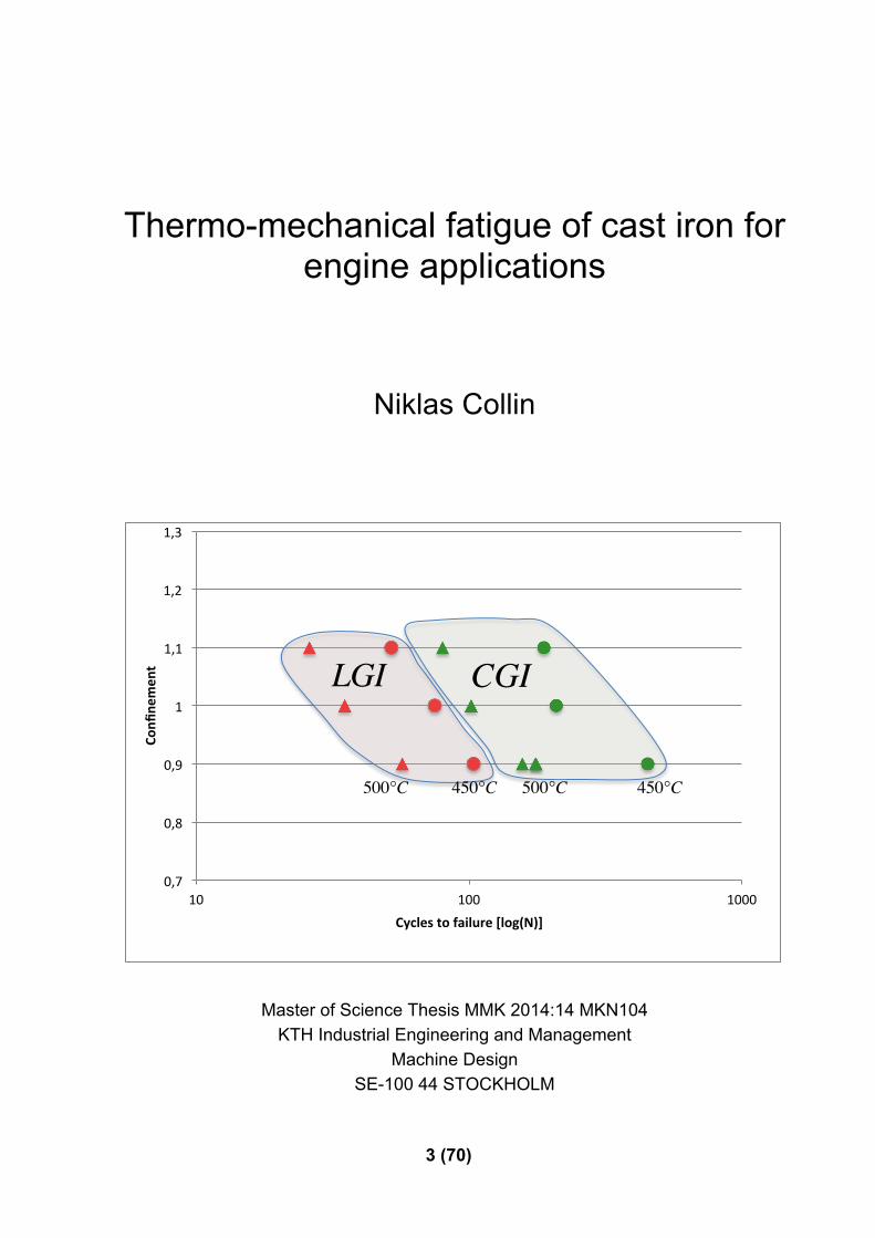
Thermo-mechanical fatigue of cast iron for engine applications
Niklas Collin
Master of Science Thesis MMK 2014:14 MKN104 KTH Industrial Engineering and Management
Machine Design SE-100 44 STOCKHOLM
0,7
0,8
0,9
1
1,1
1,2
1,3
10 100 1000
Confi
nemen
t
Cycles to failure [log(N)]
CGILGI
450°C500°C450°C500°C

4 (70)

5 (70)
Master of Science Thesis MMK 2014:14 MKN104
Thermo-mechanical fatigue of cast iron for engine applications
Niklas Collin
Godkänt
2014-06-02
Examinator
Ulf Sellgren
Handledare
Ulf Sellgren Uppdragsgivare
Scania Kontaktperson
Peter Skoglund
Abstract In an engine component the repeated start-stop cycles cause temporal and local inhomogeneous temperatures, which in turn lead to a type of low-frequency loading, plastic deformation and eventually failure due to thermo-mechanical fatigue. Simultaneously, high-frequency mechanical loading arises from the cyclic combustion pressure and from road induced vibrations. These types of loadings that mainly are in the elastic region are usually denoted high cycle fatigue (HCF). In order to improve efficiency, power density and to reduce emissions, future truck engines will be subjected to higher temperatures and higher combustion pressures which will affect the service life of the different engine components. As a consequence, there is a need to determine the limitations of the used alloys under these service conditions as exactly as possible. In this master thesis work the fatigue properties of one grey iron (EN-GJL 250) and one compacted graphite iron (EN-GJV 400) has been investigated under realistic loading conditions. The results show that a change from the grey iron to the compacted graphite iron will result in a significant increase of the fatigue life. The investigation also reveal that the life will increase significantly if the maximum temperature can be decreased tens of degrees. Further, the results indicate that addition of a relatively small HCF load may give a large decrease of the fatigue life. Keywords: Thermo-mechanical fatigue, TMF, CGI, LGI, fatigue, thermal strain.

6 (70)
7 (70)
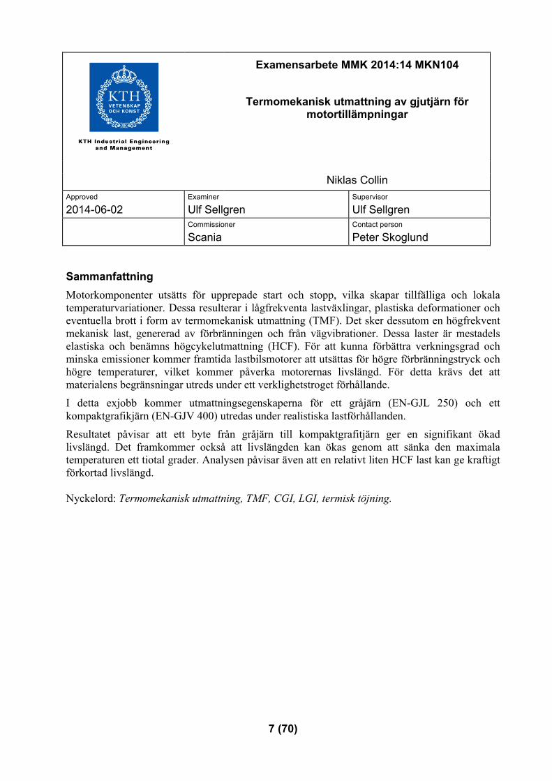
Examensarbete MMK 2014:14 MKN104
Termomekanisk utmattning av gjutjärn för motortillämpningar
Niklas Collin
Approved
2014-06-02 Examiner
Ulf Sellgren Supervisor
Ulf Sellgren Commissioner
Scania Contact person
Peter Skoglund
Sammanfattning Motorkomponenter utsätts för upprepade start och stopp, vilka skapar tillfälliga och lokala temperaturvariationer. Dessa resulterar i lågfrekventa lastväxlingar, plastiska deformationer och eventuella brott i form av termomekanisk utmattning (TMF). Det sker dessutom en högfrekvent mekanisk last, genererad av förbränningen och från vägvibrationer. Dessa laster är mestadels elastiska och benämns högcykelutmattning (HCF). För att kunna förbättra verkningsgrad och minska emissioner kommer framtida lastbilsmotorer att utsättas för högre förbränningstryck och högre temperaturer, vilket kommer påverka motorernas livslängd. För detta krävs det att materialens begränsningar utreds under ett verklighetstroget förhållande. I detta exjobb kommer utmattningsegenskaperna för ett gråjärn (EN-GJL 250) och ett kompaktgrafikjärn (EN-GJV 400) utredas under realistiska lastförhållanden. Resultatet påvisar att ett byte från gråjärn till kompaktgrafitjärn ger en signifikant ökad livslängd. Det framkommer också att livslängden kan ökas genom att sänka den maximala temperaturen ett tiotal grader. Analysen påvisar även att en relativt liten HCF last kan ge kraftigt förkortad livslängd. Nyckelord: Termomekanisk utmattning, TMF, CGI, LGI, termisk töjning.

8 (70)

9 (70)
NOMENCLATURE
CGI – Compacted graphite iron FGI – Flake graphite iron SGI – Spherical graphite iron TMF – Thermo-mechanical fatigue HCF – High cycle fatigue LCF – Low cycle fatigue LGI – Lamellar graphite iron, synonymous with FGI

10 (70)

11 (70)
Table of Contents
Nomenclature .............................................................................................................................................. 9
1. Introduction ........................................................................................................................................ 13
1.1 Background ...................................................................................................................................... 13
1.2 Research question ........................................................................................................................... 13
1.3 Delimitations .................................................................................................................................... 13
1.4 Research methodology .................................................................................................................... 13
2. Frame of reference ............................................................................................................................. 15
2.1 Static behavior ................................................................................................................................. 15
2.2 Fatigue ............................................................................................................................................. 16
2.3 Damage mechanisms ....................................................................................................................... 22
2.4 Cast iron ........................................................................................................................................... 26
2.5 The test rig ....................................................................................................................................... 33
2.6 Factorial design ................................................................................................................................ 37
3. Thermo-‐mechanical fatigue testing ................................................................................................... 39
3.1 The test rig ....................................................................................................................................... 39
3.2 The test specimens .......................................................................................................................... 40
3.3 Temperature gradient ...................................................................................................................... 42
3.4 Chemical composition ...................................................................................................................... 43
3.5 Microscopy ...................................................................................................................................... 43
3.6 Test setup ........................................................................................................................................ 44
4. Result ..................................................................................................................................................... 51
4.1 Test result ........................................................................................................................................ 51
4.2 Analysis of thermal expansion and Young’s modulus ...................................................................... 59
5. Discussion .............................................................................................................................................. 61
6. Conclusion ............................................................................................................................................. 65
7. Recommendation and future work ........................................................................................................ 65
8. References ............................................................................................................................................. 67
9. Appendix ................................................................................................................................................ 69

12 (70)
13 (70)
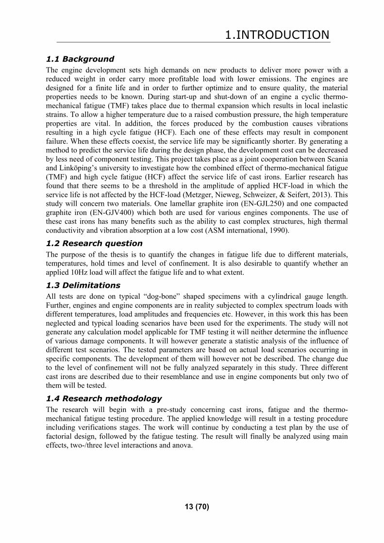
1. INTRODUCTION
1.1 Background The engine development sets high demands on new products to deliver more power with a reduced weight in order carry more profitable load with lower emissions. The engines are designed for a finite life and in order to further optimize and to ensure quality, the material properties needs to be known. During start-up and shut-down of an engine a cyclic thermo-mechanical fatigue (TMF) takes place due to thermal expansion which results in local inelastic strains. To allow a higher temperature due to a raised combustion pressure, the high temperature properties are vital. In addition, the forces produced by the combustion causes vibrations resulting in a high cycle fatigue (HCF). Each one of these effects may result in component failure. When these effects coexist, the service life may be significantly shorter. By generating a method to predict the service life during the design phase, the development cost can be decreased by less need of component testing. This project takes place as a joint cooperation between Scania and Linköping’s university to investigate how the combined effect of thermo-mechanical fatigue (TMF) and high cycle fatigue (HCF) affect the service life of cast irons. Earlier research has found that there seems to be a threshold in the amplitude of applied HCF-load in which the service life is not affected by the HCF-load (Metzger, Nieweg, Schweizer, & Seifert, 2013). This study will concern two materials. One lamellar graphite iron (EN-GJL250) and one compacted graphite iron (EN-GJV400) which both are used for various engines components. The use of these cast irons has many benefits such as the ability to cast complex structures, high thermal conductivity and vibration absorption at a low cost (ASM international, 1990).
1.2 Research question The purpose of the thesis is to quantify the changes in fatigue life due to different materials, temperatures, hold times and level of confinement. It is also desirable to quantify whether an applied 10Hz load will affect the fatigue life and to what extent.
1.3 Delimitations All tests are done on typical “dog-bone” shaped specimens with a cylindrical gauge length. Further, engines and engine components are in reality subjected to complex spectrum loads with different temperatures, load amplitudes and frequencies etc. However, in this work this has been neglected and typical loading scenarios have been used for the experiments. The study will not generate any calculation model applicable for TMF testing it will neither determine the influence of various damage components. It will however generate a statistic analysis of the influence of different test scenarios. The tested parameters are based on actual load scenarios occurring in specific components. The development of them will however not be described. The change due to the level of confinement will not be fully analyzed separately in this study. Three different cast irons are described due to their resemblance and use in engine components but only two of them will be tested.
1.4 Research methodology The research will begin with a pre-study concerning cast irons, fatigue and the thermo-mechanical fatigue testing procedure. The applied knowledge will result in a testing procedure including verifications stages. The work will continue by conducting a test plan by the use of factorial design, followed by the fatigue testing. The result will finally be analyzed using main effects, two-/three level interactions and anova.

14 (70)

15 (70)
2. FRAME OF REFERENCE
2.1 Static behavior Stress, σ is expressed as applied force divided by the cross section. This stress is often related to the strain by a stress-strain diagram. This curve can be identified as either engineer or true stress depending whither the original or the actual cross section area (due to necking) is used, see Figure 1. This study will exclusively use the methodology with engineering stress-strain curves.
Figure 1, shows the difference between true and engineering stress strain curves.
Elasto-plastic materials such as iron-based alloys have an elastic and a plastic region depending on the applied stress, as seen in Figure 1. The elastic region is characterized by a linear reversible elastic behavior between stress and strain seen below the yield strength, when the stress in released, the strain will return. The derivative of the linear region is a function defined by Hooke’s law seen in Equation 1.
E = σε
(1)
σ is the applied stress and ε is the resulting strain. If the stress has reached the yield strength and entered the plastic region, only the elastic section will return when released. The ultimate strength is the maximum force the material can withstand.

16 (70)
2.2 Fatigue Fatigue is progressive structural changes that appear in materials due to repeated strains. This may induce cracks and crack propagation with subsequent failure even though the stress is far below the static yield strength.
2.2.1 Wöhler curve Mechanical fatigue is often characterized as either high or low cycle fatigue. For high cycle fatigue (HCF), the strain only occurs in the elastic region, see Figure 2. For a specific level of applied stress, namely the fatigue limit, a fatigue failure may not occur. For low cycle fatigue (LCF), the stress is located in the plastic region and result in a fatigue life significantly shorter than for HCF. (DeLuca, 2014) Mechanical testing can be performed at various temperatures and in different medias.
Figure 2, shows the difference between HCF and LCF.
It has for a long time been known that components fail due to fatigue. One of the first fatigue investigations was performed in 1829 by a German mining engineer named W. Albert in order to determine the service life on iron chains (MSC software, 2014). When the railway was expanded in the middle of the nineteenth century, a man named A. Wöhler took interest in investigating the service life of train axles and generated what we know today as the Wöhler curve (S/N-curve). The Wöhler-curve compared the nominal stress amplitude and the cycles to failure. He conducted full-scaled and small-scaled tests using a rotational four point bending test rig (MSC software, 2014). Fatigue testing can be performed in various temperatures, atmospheres and medias. All experiments can however be classified into two different categories: (Weronski & Hejwowski, 1991)
1. Using a load controlled test in which the load amplitude is set either constant or using spectrum loads. This can be performed using uniaxial or multiaxial loadings is torsion, bending or push-pull setups. This is most commonly used for HCF-tests.
2. Using a strain controlled system with an extensometer measuring the deformation and keeps it at a certain range. The load is therefore allowed to change during the test. This is most commonly used for tests in the plastic region of the material and when considering thermal strains.

17 (70)
In the case where spectrum loads are used, the spectrum is often recorded beforehand (while in actual use) and then applied on the tested component in a laboratory environment. (Weronski & Hejwowski, 1991). The experimental setup usually have a few parameters in common such as the ratio between the applied compression and. This is characterized by the R-value as seen in Equation 2.
R = σ min
σ max
(2)
Depending on the R-value, the material will be subjected to pure tensile, pure compression or a combination between tension and compression as seen in Figure 3.
Figure 3, shows how different R values affect the loading scenario .
The stress range and stress amplitude is characterized as seen in Figure 3. For strain controlled testing, the same methodology can be used but with the strain, as seen in in Equation 3.
R = εminεmax
(3)
Higher level of compression usually results in a longer fatigue life, this can be further studied in section 2.3.1 Mechanical properties. An example of the effect from different R-values can be seen in Figure 4.
Maximum stress
Minimum stress
Stress amplitude
Stre
ss
Time
Stress range

18 (70)
Figure 4, shows the influence of different R-values for the fatigue life (Svensk Standard 112370).
2.2.2 Low cycle fatigue (LCF) Since LCF scenarios enter the plastic strains of the material, the hysteresis loop acts differently compared with only elastic strains. Figure 5 shows an example of kinematic hardening where the length of the elastic region remains constant. When the strained material pass the yield strength in point A, the material will plasticize and when released return to zero stress in point B but with a retained elongation. During the following compression the proportional limit is found in point C and if the stress is increased further, plastic deformation will occur. When released the material will return to point D, resulting in a permanent contraction.
Figure 5, shows the cyclic behavior of a stress strain curve.
Different materials can show different characteristics during strain controlled cyclic behavior, as seen in Figure 6. Crystal hardening will increase the elastic section and stress level by the number of cycles and cyclic softening will decrease the elastic section and the stress level.
Cycles to failure [N]
Stre
ss ra
nge
[MPa
]

19 (70)
Figure 6, shows how cyclic hardening and softening behaviour works, (MSC software, 2014)
Since the strength of a material often is reduced at elevated temperatures (Weronski & Hejwowski, 1991). There are reasons to investigate a material using different temperatures, either isothermal or by the use of thermo-mechanical testing.
2.2.3 Thermo-mechanical fatigue (TMF) TMF-testing is characterized by a cyclic temperature load with the presence of mechanical loadings. When performing TMF testing, strain controlled load scenarios is used and there are three different strains that needs to be considered as seen in Equation 4 below:
εtot = εme + εth (4)
These are the total strain, which is measured by an extensometer. The thermal strain that is a result from the thermal expansion and the mechanical strain defined as stress divided by the material stiffness. These strains can be studied separately in Figure 7.

20 (70)
Figure 7, shows the difference between thermal and mechanical strain.
The thermal strain does not itself give any stresses in the material and components subjected to only thermal strains are therefore assumed to have an infinite life in the absence of mechanical strains. The ratio between mechanical strain and negative thermal strain is the level of confinement. For elastic behavior this can be seen in Equation 5.
x = − εmeεth
= − σ Eα ⋅ΔT
(5)
Here, α is the thermal expansion coefficient of the specimen. ΔT is the temperature difference, E is the Young’s modulus. The thermal expansion coefficient and Young’s modulus are not constants since these changes with temperature, this is furthered explained in section 3.6 Test setup. When x in equation 5 is zero, the specimen can expand freely due to temperature changes. When x equals one, it is fully confined and the thermal expansion generates stresses in the material. When x is between zero and one, the material is only partly confined and may expand slightly as the temperature increases. In some applications, x can be far more than one, resulting in a compression that increases with higher temperatures (Löhe, 2008). This can for example take place if surrounding components is subjected to a higher thermal expansion. TMF is often divided into either in-phase (IP) and out-of-phase (OP). For positive x-values, it is OP and characterizes by that the maximum temperature and the maximum compression occurs simultaneously (efatigue, 2014). For negative x-values it is called in-phase (IP) and the maximum tension will occur simultaneously as the maximum temperature (efatigue, 2014), see Figure 8. A confinement typically appears in a component due to assembly fixations or by thermal gradients (Nieweg, B; Seifert, T; Metzger, M, 2011).

21 (70)
Figure 8, shows the difference between OP and IP for TMF testing.
When a material is subjected to thermo-mechanical strains, there are certain properties that affect the result more than others. A high thermal conductivity will reduce the thermal gradients and make the specimen more uniform in temperature. A high thermal gradient may lead to high internal stresses that may damage the material. In a similar way, the Young’s modulus should be low since that allows more flexibility of the material and reduces stresses while confined. The thermal expansion coefficient and thermal conductivity for some common materials can be seen in Figure 9.
Figure 9, shows the thermal conductivity and thermal expansion for some metals at room temperature. (Extracted from
CES edupack)
2.2.4 Combined TMF and HCF Engine components are often subjected to TMF cycles due to start and stop of the vehicle. It is also subjected to HCF-loading due to the combustion and road induced vibrations. When combining these effects earlier studies have shown that the TMF fatigue life decreases with applied HCF-loads (Nieweg, Seifert & Metzger, 2011). The HCF-load can vary in amplitude as well as in frequency. There appears as there is a threshold in HCF-strain that significantly changes the influence of the combined effects (Schweizer, Seifert, Nieweg, Hartrott, & Riedel,
Stre
ss
Mechanical strain
Tmax
Tmin Out-‐of-‐phase
Stre
ss
Mechanical strain
Tmin
Tmax
In-‐phase

22 (70)
2011). For the nickel-based Inconel 617 the effect from increased HCF-load and frequency can be seen in Figure 10.
Figure 10, shows the effect of HCF-load and frequency for Inconel 617, (Beck, Henne, & Löhe, 2008)
The result implies that not only the amplitude but also the frequency of the HCF-load affects the fatigue life. There are however large differences between cast iron and Inconel.
2.3 Damage mechanisms There are usually three major damage mechanisms to consider in TMF, the severity of these often depends whether OP or IP-loadings are present, (Sehitoglu, 1992). One commonly used model for the life assessment is the damage accumulation model. It describes the influence of the different mechanisms on the overall fatigue life, as seen Equation 6 below. (Nieweg, B; Seifert, T; Metzger, M, 2011).
1N f
= 1N f
fatigue +1
N foxidation +
1N f
creep (6)
Where the total fatigue life depends on mechanical fatigue, oxidation and creep properties of the material. The individual parts do however contain many different material properties that need to be determined in order to being able to use the model. For cast iron, the fatigue damage is assumed to be the dominating factor (Nieweg, B; Seifert, T; Metzger, M, 2011)
23 (70)
2.3.1 The fatigue damage Fatigue takes place as an action from simultaneous cyclic stress, tensile stress and plastic strain. All these components must be present in order to initiate and propagate a crack. The analogy from LCF can be used, with the addition of that the material strength is reduced by higher temperatures. The presence of plastic strain initiates the crack and the tensile stress will propagate the crack growth. Compressive loads does not increase the crack by itself, it can however generate local tensile stresses that will propagate the crack. Local plastic strains can occur at low level of stresses, even though the material otherwise appear fully elastic (ASM international, handbook, 1996, pp. 63-72).
2.3.2 The oxidation damage The oxidation failure mechanism is generally not the dominating factor in TMF testing (efatigue, 2014). It does however affect more severely during OP loading than IP. If the TMF-loading is OP, an oxide often grows at high temperature when the specimen is in compression. When the temperature decreases the oxide becomes brittle and cracks when the specimen is subjected to tensile stresses. This results that new virgin material is exposed. (efatigue, 2014). During IP loadings, an oxide film occurs at high temperature during tension and crack once cooled and compressed (efatigue, 2014). The oxide film properties are highly material dependent and may occur faster at higher temperatures. The level of induced micro cracks is highly depending on the experienced strain range and not the induced stress (efatigue, 2014). The oxidation mechanism can be minimized by the use of low temperatures, non-oxidizing atmosphere or short expose times.
2.3.3 The creep damage Creep is defined as a time-dependent and permanent deformation when subjected to a load (Callister & Rethwisch, 2009). This characteristic failure component can be observed in most materials and are divided into three regions seen in Figure 11. At first there is a primary creep that consists of an elastic deformation. The secondary phase consists of a constant increase of the strain. This part is often the dominating section with the longest duration (Callister & Rethwisch, 2009). The reason for the increased strain is a balance between strain hardening and recovery that slowly allows the material to strain. The final step called tertiary creep is characterized by an accelerated strain growth ending with an ultimate failure. The reason for this is mostly imbedded in the micro structural change as for example grain boundary separation. When by tension a neck is produced resulting in a smaller cross section and an increase of strain rate (Callister & Rethwisch, 2009). An approximation for metals is that creep damage occurs at temperatures above 40% of the absolute melting temperature (Tm), as seen in Figure 11 (Callister & Rethwisch, 2009). For LGI and CGI which have Tm at approximately 1400K. The creep behavior should therefore be taken account for above approximately 300ºC.

24 (70)
Figure 11, shows the dependency of temperature on creep behavior (Callister & Rethwisch, 2009).
The creep occurring in TMF testing is more complex than for constant load scenarios. Since the strain and temperature varies, the creep only occurs at certain sections of the test. For OP the creep occurs in compression and reduces the stress as seen in Figure 12. The level of decrease is beside the temperature highly dependent on the hold time.
Figure 12, shows how the creep occurs in TMF testing.
In general a good creep resistant material have a high melting point, a high Young’s modulus and consist of large grains (Callister & Rethwisch, 2009).
2.3.4 Failure mechanism The failure characteristics of cast iron vary from the one seen in steel because cast iron have a soft graphite phase and a steel matrix while steel only consist of a more homogeneous steel phase. For steel there are three characteristic steps which take place: crack initiation, where a micro crack form in the material due to local plastic deformation between the slip planes within the atomic structure and results in micro cracks and stress concentrations, see Figure 13 (1). This can occur on either the surface or internally, (Callister & Rethwisch, 2009). These micro cracks
Stress
Mechanical strain
Tmax
Tmin
Creep

25 (70)
may have occurred prior to any loading by for e.g. welding or by a scratched surface. For cast irons the crack initiation is dominated by the separation of the steel matrix and the weak graphite phase and may take place at several places simultaneously, this is further explained in section 2.4 Cast iron. The second step is the crack propagation where the crack gradually increases in size with each load cycle. The propagation continues until a critical crack size occurs. For steel, this step can often be identified by beach marks (4) shown in Figure 13. For cast iron, the many micro cracks propagate separately and eventually forms macro cracks. The third step is the final fracture (7) and takes place as a rapid fracture once the crack(s) have reached a critical limit.
Figure 13, shows a typical fatigue failure cross section for steel (Weronski & Hejwowski, 1991).

26 (70)
2.4 Cast iron Cast iron is a family of ferrous alloys primarily containing iron, carbon and silicon. The carbon and silicon content is higher than for steel, which results in a carbon rich phase named graphite. By adding carbon it is possible to reduce the melting point. This makes it easier to use in manufacturing and decrease the cooling shrinking. Some other basic properties are good flow-ability, making it easy to cast. It has a high heat conductivity, good machinability at a low cost (Angus, 1960). Historically, cast irons were divided in two types depending on whether the fracture surface was white or grey, namely white iron and grey iron. A more commonly used methods today is to divide depending on the metallographic properties. The graphite shape is one of the classifications and is divided in spheroidal graphite (SGI), compacted (vermicular) graphite (CGI) and lamellar graphite (LGI) also known as flake graphite, as seen in Figure 14.
Figure 14, shows the different orientation for the graphite for SGI (A), CGI (B) and LGI (C), (ASM international, 1990).
All these three material classes are used for engine applications, the analysis will however only focus on two specific alloys, one is a LGI (EN-GJL250) with a ultimate strength larger than 250 MPa and a CGI (EN-GJV400) with an ultimate strength larger than 400 MPa. The main characteristic between different cast iron mainly depends on:
• Chemical composition • Cooling rate • Liquid treatment • Heat treatment
2.4.1 Chemical composition Typical alloy contents for the three presented cast irons can be seen in Table 1.
Table 1, chemical composition of LGI and CGI (ASM international, 1990).
Material class Composition, wt% C Si Mn P S
LGI 2.5-4.0 1.0-3.0 0.2-1.0 0.002-1.0 0.02-0.25 CGI 2.5-4.0 1.0-3.0 0.2-1.0 0.01-0.1 0.01-0.03 SGI 3.0-4.0 1.8-2.8 0.1-1.0 0.01-0.1 0.01-0.03
For a cast iron without silicon, the eutectic point is positioned at 4.3% as seen in Figure 15. By adding additional alloys such as phosphorous and silicon the eutectic point will be affected according to the carbon equivalent. There are however many different ways to calculate the carbon equivalent. The relation used by Scania is showed in Equation 7 (Scania).
CE = Cc +Cp
2+ Csi
4 (7)
A B C
27 (70)
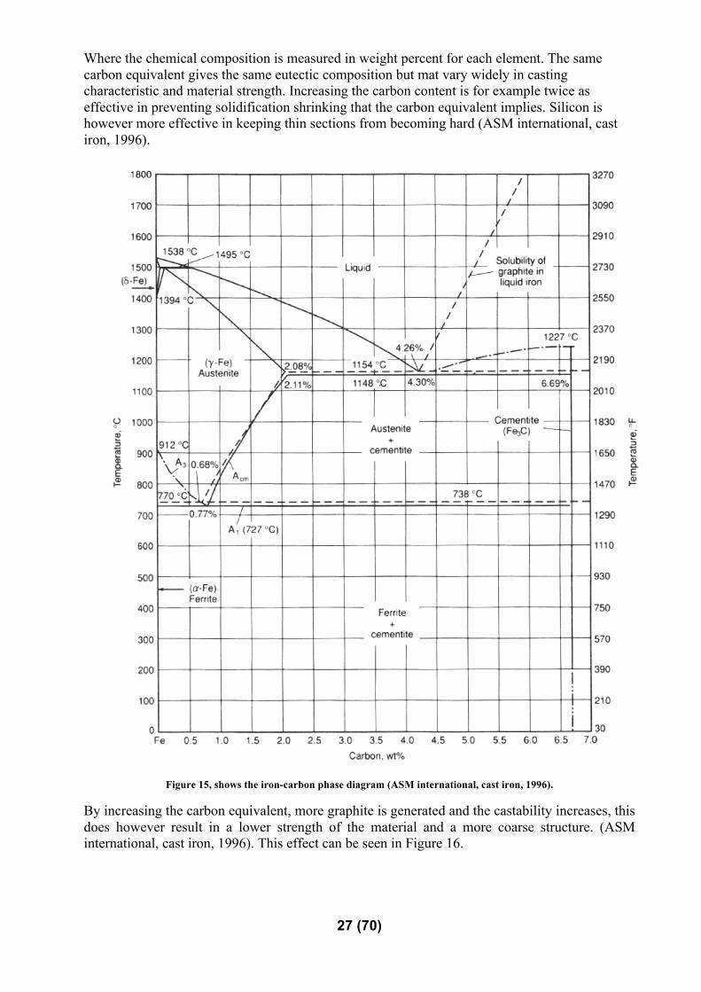
Where the chemical composition is measured in weight percent for each element. The same carbon equivalent gives the same eutectic composition but mat vary widely in casting characteristic and material strength. Increasing the carbon content is for example twice as effective in preventing solidification shrinking that the carbon equivalent implies. Silicon is however more effective in keeping thin sections from becoming hard (ASM international, cast iron, 1996).
Figure 15, shows the iron-carbon phase diagram (ASM international, cast iron, 1996).
By increasing the carbon equivalent, more graphite is generated and the castability increases, this does however result in a lower strength of the material and a more coarse structure. (ASM international, cast iron, 1996). This effect can be seen in Figure 16.

28 (70)
Figure 16, shows how the tensile strength depends on the carbon equivalent, (ASM international, cast iron, 1996).
2.4.2 Cooling rate The cooling rate is highly depending on the section thickness of the cast. A higher thickness results in a slower cooling rate. A higher cooling rate generates higher strength and hardness of the material compared to a slow due to an increased nucleation, see Figure 17. If the cooling rate is high enough, the graphite can however transform from graphite to cementite. Resulting in a white cast iron which is a brittle phase with high hardness. (ASM international, cast iron, 1996).

29 (70)
Figure 17, shows how the strength influences by the section thickness, (ASM international, cast iron, 1996).
2.4.3 Liquid treatment The liquid treatment is a process called inoculation where minor alloy elements are added to the cast before pouring. By doing this it is possible to drastically change the nucleation and growth condition during solidification. The process increases the graphitization potential and might reduce the transformation of cementite. Due to the changes in nucleation, a less coarse structure in the matrix is generated with higher strength as a result, (ASM international, cast iron, 1996). A general result for inoculating can be seen in Figure 18.
Figure 18, shows how inoculated effect the material strength, (ASM international, cast iron, 1996).
The inoculating has a very large influence in whether LGI or CGI is generated since they have similar chemical composition and the major difference lies in the shape of the graphite. In Figure 19 it is seen how adding magnesium affect the graphite structure.

30 (70)
Figure 19, shows how the graphite shape is affected by inoculation by magnesium, (ASM international, cast iron, 1996).
2.4.4 Heat treatment Heat treatment can change the matrix structure, but the graphite will remain unaffected. This can be used as stress relief or annealing to reduce hardness but are rarely used for gray iron and compacted graphite iron but is essential for spherical graphite iron, (ASM international, cast iron, 1996).
2.4.5 Mechanical properties The general characteristic tensile strength for LGI, CGI and SGI can be seen in Figure 20.
31 (70)
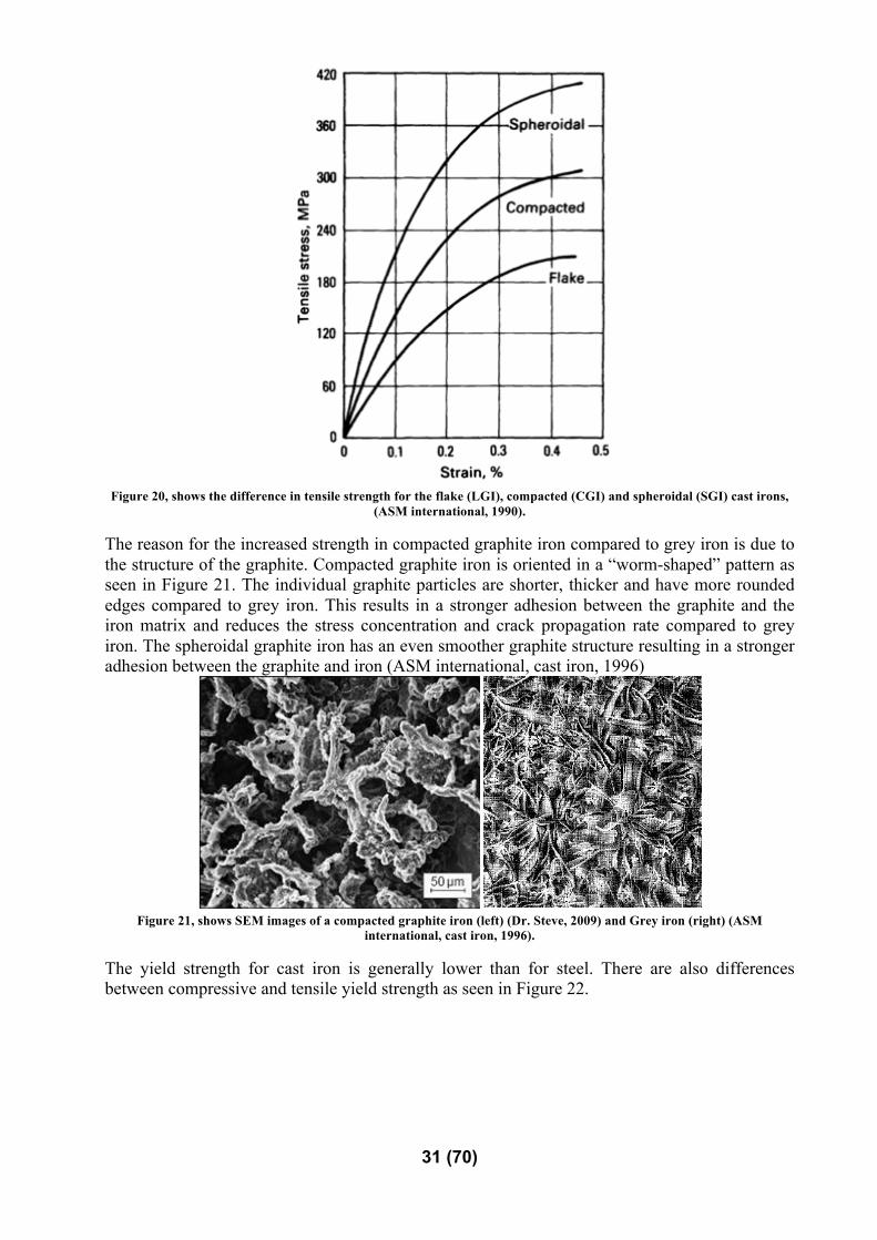
Figure 20, shows the difference in tensile strength for the flake (LGI), compacted (CGI) and spheroidal (SGI) cast irons,
(ASM international, 1990).
The reason for the increased strength in compacted graphite iron compared to grey iron is due to the structure of the graphite. Compacted graphite iron is oriented in a “worm-shaped” pattern as seen in Figure 21. The individual graphite particles are shorter, thicker and have more rounded edges compared to grey iron. This results in a stronger adhesion between the graphite and the iron matrix and reduces the stress concentration and crack propagation rate compared to grey iron. The spheroidal graphite iron has an even smoother graphite structure resulting in a stronger adhesion between the graphite and iron (ASM international, cast iron, 1996)
Figure 21, shows SEM images of a compacted graphite iron (left) (Dr. Steve, 2009) and Grey iron (right) (ASM
international, cast iron, 1996).
The yield strength for cast iron is generally lower than for steel. There are also differences between compressive and tensile yield strength as seen in Figure 22.

32 (70)
Figure 22, shows how the difference in strength varies with compression and tension (ASM international, cast iron, 1996).
The graphite is weaker than the steel matrix and will therefore allow less elastic motion compared to solid steel. The graphite particles will also initiate cracks easier than steel due to the sharp graphite particles. The crack initiation phase of cast iron takes place as a separation between graphite particles and the iron matrix and does often occur at low loadings. When comparing the compacted graphite iron against grey iron, there are several general advantages to consider. CGI has:
• Higher ductility and toughness • Higher yield strength at the same carbon equivalent which reduces the need of expensive
alloying • Less sensitivity to oxidization. • Less sensitivity to section thickness.
There are however also several disadvantages of changing from LGI to CGI: CGI has:
• Lower damping properties compared to LGI • Lower castability • Higher thermal expansion • Lower conductivity • Lower machinability
(ASM international, cast iron, 1996)
33 (70)
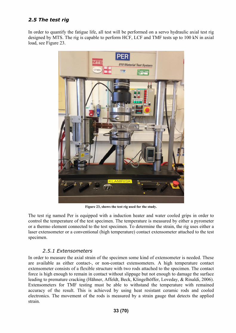
2.5 The test rig In order to quantify the fatigue life, all test will be performed on a servo hydraulic axial test rig designed by MTS. The rig is capable to perform HCF, LCF and TMF tests up to 100 kN in axial load, see Figure 23.
Figure 23, shows the test rig used for the study.
The test rig named Per is equipped with a induction heater and water cooled grips in order to control the temperature of the test specimen. The temperature is measured by either a pyrometer or a thermo element connected to the test specimen. To determine the strain, the rig uses either a laser extensometer or a conventional (high temperature) contact extensometer attached to the test specimen.
2.5.1 Extensometers In order to measure the axial strain of the specimen some kind of extensometer is needed. These are available as either contact-, or non-contact extensometers. A high temperature contact extensometer consists of a flexible structure with two rods attached to the specimen. The contact force is high enough to remain in contact without slippage but not enough to damage the surface leading to premature cracking (Hähner, Affeldt, Beck, Klingelhöffer, Loveday, & Rinaldi, 2006). Extensometers for TMF testing must be able to withstand the temperature with remained accuracy of the result. This is achieved by using heat resistant ceramic rods and cooled electronics. The movement of the rods is measured by a strain gauge that detects the applied strain.

34 (70)
A non-contact extensometer detects the strain by a image recognition. A laser light illuminates the specimen and the resulting reflected speckle pattern is recorded using digital cameras, see Figure 24.
Figure 24, shows the generated speckle pattern using a laser extensometer, (based on Zwick/Roell).
The length between two defined points can be tracked digitally and allow slow changes within the material due to oxidation with an accurate result. One problem with image recognition is that it requires large computational resources to use the required sample rate needed for fast movements, as discovered by initial testing.
2.5.2 Temperature control A typical TMF test contains of a cyclic behavior between two temperatures. To create this some temperature control system is needed including heating and cooling devices. There are several different methods used to control the temperature in TMF testing. Induction heating is often used for ferrous metals (Hähner, Affeldt, Beck, Klingelhöffer, Loveday, & Rinaldi, 2006) but there are also possibilities to use convection ovens or the use of resistance heating. The advantage with induction heating is that it is fast and allows a more precise heating compared to convection that normally is used for isothermal testing at elevated temperatures. The induction coil can be modified in order to better correspond to the requested testing, see Figure 25. The disadvantage with the induction coil is that is can be difficult to access the specimen with for i.e. extensometers. It is recommended to not heat solid specimens in a rate higher than 5ºC/s (Hähner, Affeldt, Beck, Klingelhöffer, Loveday, & Rinaldi, 2006) in order to avoid large radial gradients.
L

35 (70)
Figure 25, shows different setups for the induction coil (Hähner, Affeldt, Beck, Klingelhöffer, Loveday, & Rinaldi, 2006).
An induction heater is a non-contact process using a high frequency current in order to generate a alternating magnetic field. This generates a current within the specimen which in turn generates heat.
Figure 26, shows the basic principle for induction heating, [www.induction-heating.com].
Since the induction heater only heats a small part of the specimen, it is important to verify that the temperature gradient is at reasonable levels over the specimen. This can easily be tested by attaching several thermoelements on the specimen and measure the difference. In order to decrease the temperature in the specimen there are two commonly used methods, sometimes used together. Either it is possible to use water-cooled grips that cools the specimen ends and/or use convection through an increased airflow during the cooling sequence of the cycle. Convection has the advantages that the thermal gradient decreases in the specimen. The water-cooled grips do not take any extra space and may provide a faster cooling rate than convection. The temperature in the specimen must be controlled using some kind of thermometer. Either using a pyrometer or by attaching thermo elements on the specimen. A pyrometer is a contact-free method to measure temperatures using the radiation emitted from the surface. The use of a pyrometer generates less delay than a regular contact thermometer since there is less inertia to consider. (IMPAC Infrared GmbH, 2004). The basic principle is that different wavelengths are emitted at different temperatures which can be converted to a temperature as seen in Figure 27.

36 (70)
Figure 27, shows the emitted wavelength emitted from a black–body, [www.wikipedia.com].
The properties do however change with the object itself depending on the different reflection, absorption and transmission abilities. Figure 27 shows the spectral radiant emittance for an ideal black body with 100% absorption rate and 0% reflection and transmission rate. (IMPAC Infrared GmbH, 2004). In order to use a pyrometer, the emissivity coefficients must be set prior to the test. A problem that occur in TMF testing is that the emissivity properties changes over time because of the surface oxidation. It is however possible to paint the specimen with black paint to decrease the changes (IMPAC Infrared GmbH, 2004) but this may however affect the surface oxidation. The alternative is the use of thermoelement that are soldered or clamped to the specimen. The thermo element contains two cables made of two different metal alloys. When these are subjected to a thermal gradient an electric voltage is generated (pentronic, 2014), as seen in Figure 28.
Figure 28, shows how a thermo element works, [www.spintronics-info].
This voltage can be converted to a temperature. By solder the element on the specimen, a good thermal conduction is generated that minimizes the response time. These thermoelements are however generating a very low voltage of approximately 40µV and makes the system highly sensitive to electromagnetic interference (Smalcerz & Przylucki, 2013). Smalcerz revealed that the temperature in worst case scenarios differs up to tens of percent when the induction coil is active but returns to correct values as soon as the induction is turned. This error can be minimized by the use of small thermoelements with less mass and induction frequencies adjusted to the test setup. This study uses the code of practice for TMF testing (Hähner, Affeldt, Beck, Klingelhöffer, Loveday, & Rinaldi, 2006) which for i.e. have recommendations for the use of thermoelements.
37 (70)
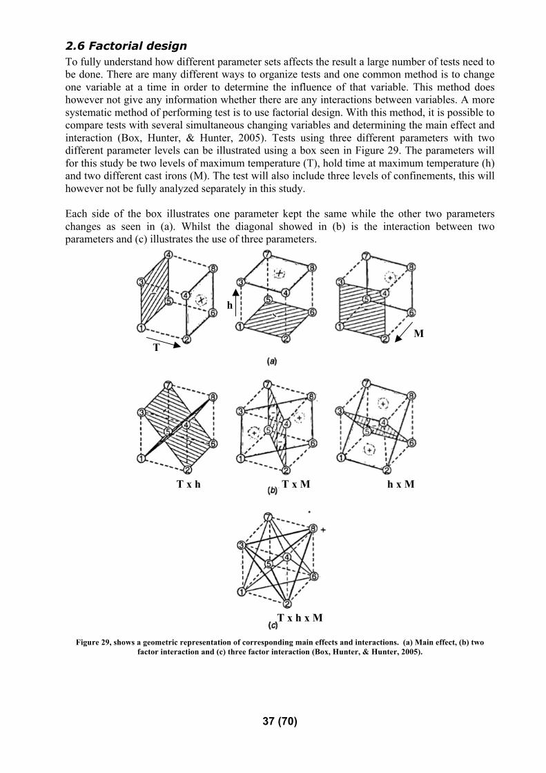
2.6 Factorial design To fully understand how different parameter sets affects the result a large number of tests need to be done. There are many different ways to organize tests and one common method is to change one variable at a time in order to determine the influence of that variable. This method does however not give any information whether there are any interactions between variables. A more systematic method of performing test is to use factorial design. With this method, it is possible to compare tests with several simultaneous changing variables and determining the main effect and interaction (Box, Hunter, & Hunter, 2005). Tests using three different parameters with two different parameter levels can be illustrated using a box seen in Figure 29. The parameters will for this study be two levels of maximum temperature (T), hold time at maximum temperature (h) and two different cast irons (M). The test will also include three levels of confinements, this will however not be fully analyzed separately in this study. Each side of the box illustrates one parameter kept the same while the other two parameters changes as seen in (a). Whilst the diagonal showed in (b) is the interaction between two parameters and (c) illustrates the use of three parameters.
Figure 29, shows a geometric representation of corresponding main effects and interactions. (a) Main effect, (b) two
factor interaction and (c) three factor interaction (Box, Hunter, & Hunter, 2005).
T x h T x M h x M
T x h x M
T
h
M
38 (70)
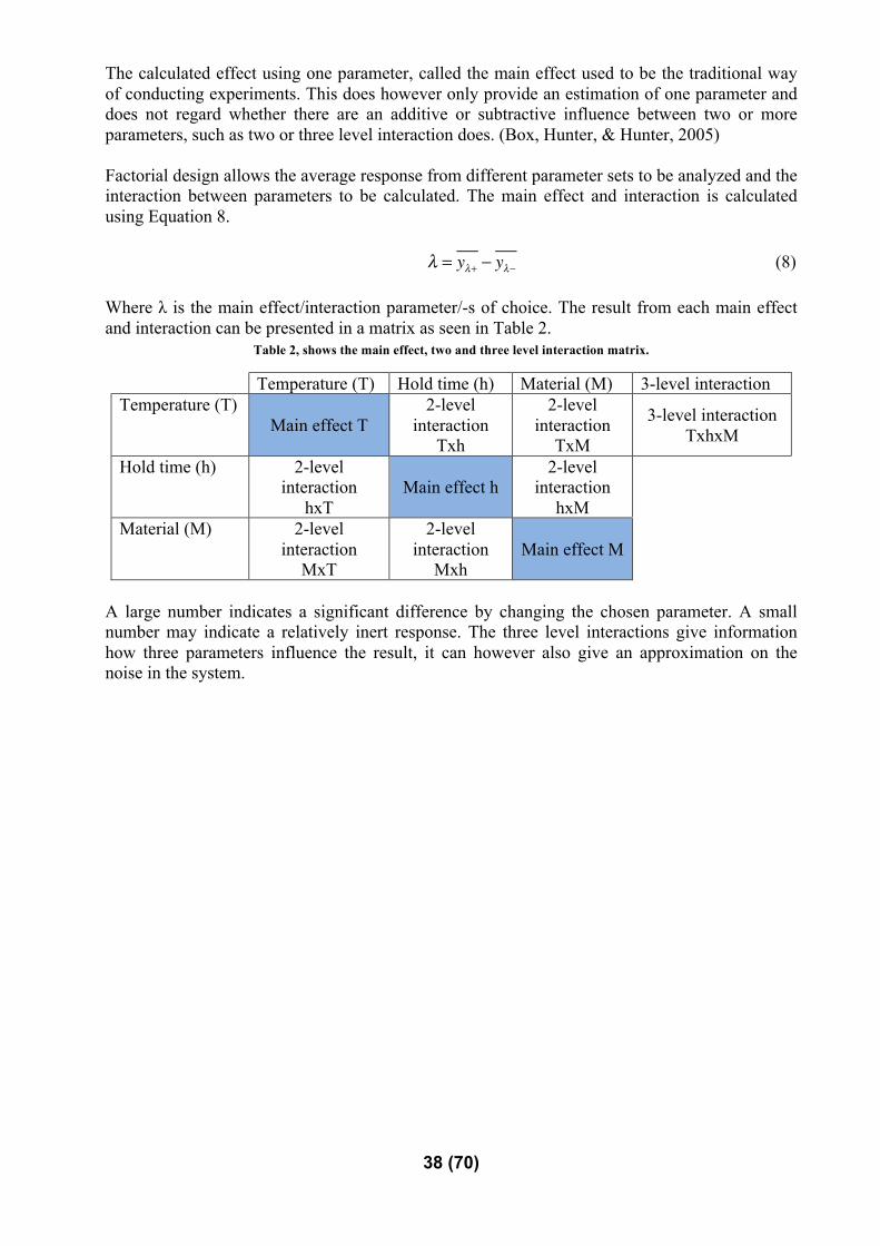
The calculated effect using one parameter, called the main effect used to be the traditional way of conducting experiments. This does however only provide an estimation of one parameter and does not regard whether there are an additive or subtractive influence between two or more parameters, such as two or three level interaction does. (Box, Hunter, & Hunter, 2005) Factorial design allows the average response from different parameter sets to be analyzed and the interaction between parameters to be calculated. The main effect and interaction is calculated using Equation 8.
λ = yλ+ − yλ− (8) Where λ is the main effect/interaction parameter/-s of choice. The result from each main effect and interaction can be presented in a matrix as seen in Table 2.
Table 2, shows the main effect, two and three level interaction matrix.
Temperature (T) Hold time (h) Material (M) 3-level interaction Temperature (T)
Main effect T 2-level
interaction Txh
2-level interaction
TxM
3-level interaction TxhxM
Hold time (h) 2-level interaction
hxT Main effect h
2-level interaction
hxM
Material (M) 2-level interaction
MxT
2-level interaction
Mxh Main effect M
A large number indicates a significant difference by changing the chosen parameter. A small number may indicate a relatively inert response. The three level interactions give information how three parameters influence the result, it can however also give an approximation on the noise in the system.

39 (70)
3. THERMO-MECHANICAL FATIGUE TESTING
3.1 The test rig The test rig will for this study is equipped with an high temperature extensometer and thermoelements will be attached by spot welding in the middle of the test specimen as seen in Figure 30.
Figure 30, shows the attached components on the test rig.
Water-cooled grips
Extensometer
Induction heater
Thermoelement
Specimen
40 (70)
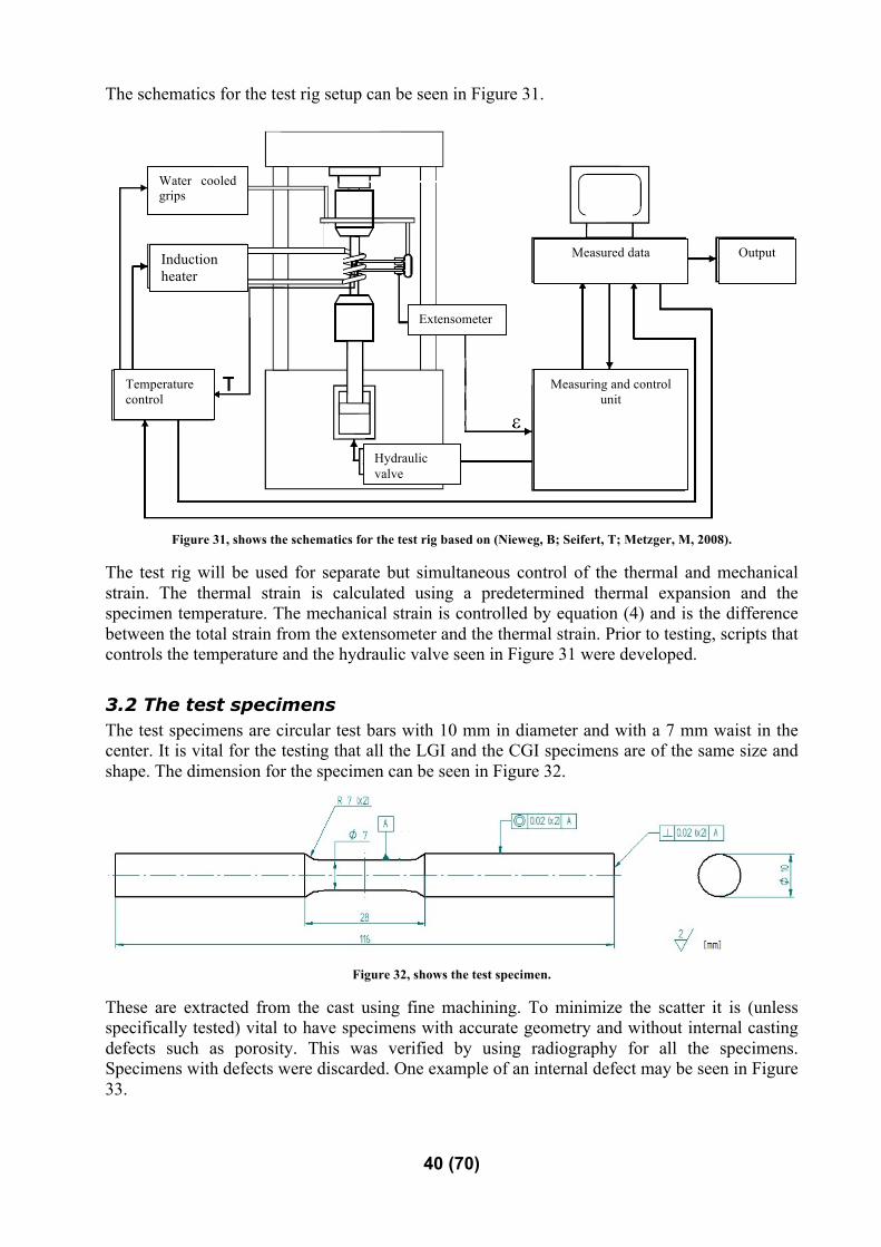
The schematics for the test rig setup can be seen in Figure 31.
Figure 31, shows the schematics for the test rig based on (Nieweg, B; Seifert, T; Metzger, M, 2008).
The test rig will be used for separate but simultaneous control of the thermal and mechanical strain. The thermal strain is calculated using a predetermined thermal expansion and the specimen temperature. The mechanical strain is controlled by equation (4) and is the difference between the total strain from the extensometer and the thermal strain. Prior to testing, scripts that controls the temperature and the hydraulic valve seen in Figure 31 were developed.
3.2 The test specimens The test specimens are circular test bars with 10 mm in diameter and with a 7 mm waist in the center. It is vital for the testing that all the LGI and the CGI specimens are of the same size and shape. The dimension for the specimen can be seen in Figure 32.
Figure 32, shows the test specimen.
These are extracted from the cast using fine machining. To minimize the scatter it is (unless specifically tested) vital to have specimens with accurate geometry and without internal casting defects such as porosity. This was verified by using radiography for all the specimens. Specimens with defects were discarded. One example of an internal defect may be seen in Figure 33.
Output Measured data
Measuring and control unit
Induction heater
Temperature control
Water cooled grips
Extensometer
Hydraulic valve

41 (70)
Figure 33, shows a possible cast defect in the waist of one specimen.
To verify that the specimens were correctly manufactured within the given surface roughness, one LGI and one CGI specimen were measured accordingly to standards for Ra and Rz, as seen in Figure 34.
Figure 34, shows the surface roughness for one CGI and LGI sample.
Figure 35, shows that the edge of a cross section of the stressed surface contains of several graphite particles.
3.2.1 Static strength To verify that the materials were produced according to the strength specifications. Some standardized strain-stress tests was performed. The CGI specified as minimum ultimate strength of 400MPa gave a result of 470MPa. The LGI had a tensile strength of 270MPa and fulfilled the specified requirement.
CGI Ra 1,8 Rz 10,5
LGI Ra 1,7 Rz 10,5

42 (70)
Prior to TMF testing the hardness of each material were measured according to Brinell testing using a 2,5 mm indenter and an applied force on 1850N, see Figure 36.
Figure 36, shows the Brinell harness testing [Substech].
The hardness for the LGI material was 196 HBW and 251 HBW for CGI. After running a TMF test using 500ºC and hold time 25s, the hardness decreased to 188 HBW for LGI and 236 HBW for CGI.
3.3 Temperature gradient The test subject is attached in the hydraulic grips using a pair of three section clamps. The induction heater is positioned concentric on the specimen with one thermo element soldered in the middle of the gauge length. The thermoelement have manually been positioned in the same relative angle to the induction heater. To verify that the temperature gradient over the specimen is within reasonable limits, two specimens were produced with three thermoelements evenly divided within the gauge length of 12 mm. Ideally according to a European code of practice (Hähner, Affeldt, Beck, Klingelhöffer, Loveday, & Rinaldi, 2006), the gradient should not exceed 10ºC within the gauge length as seen in Figure 37. In the event that it is not achieved, the result should clearly state this. The result from this test can be seen in Table 3.
Figure 37, show the thermal profile for the test specimen.

43 (70)
Table 3, shows the difference of temperature within the gauge length.
Thermo element Temp 1 [°C] Temp 2 [°C] Temp 3 [°C] Temp 4 [°C] Temp 5 [°C]
T1 91 185 278 371 464 T2 100 200 300 400 500 T3 90 184 277 368 462 The deviation varies between 10-38°C over the gauge length depending on the temperature and exceeds the recommendation in the code of practice. The thermal gradient may be reduced by careful adjustments of the size and position of the induction heater. This was however not possible due to access of the used extensometer.
3.4 Chemical composition The chemical analysis of the two alloys is showed in Table 4.
Table 4, shows the alloy content of the two different cast iron used.
CGI LGI C 3.51 3.26 wt% Si 1.98 1.81 wt% Cu 0.97 0.31 wt% Mn 0.39 0.65 wt% Ni 0.051 <0.05 wt% Cr 0.025 0.226 wt% P 0.016 0.024 wt% S 0.008 0.072 wt% Sn 0.076 <0.01 wt% Al 0.003 <0.001 wt% As <0.01 <0.001 wt% Mo <0.01 0.013 wt% Ti <0.01 <0.01 wt% V <0.01 0.012 wt% Pb <0.00
1 <0.001 wt%
B <70 <70 ppm CE (Carbon Equivalent) 4.0 3.7 -
The chemical contents are within the requested ranges.
3.5 Microscopy To verify that the graphite structure correspond the selected material, microscopic investigations was performed for one LGI and CGI specimen prior and after TMF testing. In Figure 41 the untested structure can be seen.

44 (70)
Figure 38, shows the microscopic structure for LGI (left) and CGI (right) at 100x magnification.
The dark sections are graphite and the bright sections are the iron matrix. The same material after the TMF testing can be seen in Figure 39.
Figure 39, the microscopic structure for LGI (left) and CGI (right) at 100x magnification after TMF testing.
The LGI material shows in magnification micro cracks between individual graphite particles as shown in Figure 40. This behavior is also expected in the CGI material.
Figure 40, shown micro cracks initiated by graphite particles in LGI.
3.6 Test setup The entire test series are conducted using OP-TMF loading conditions since this is a common and critical loading case fore many engine components. To achieve comparable result to other studies, the test procedure is based on a code of practice for TMF testing, (Hähner, Affeldt, Beck, Klingelhöffer, Loveday, & Rinaldi, 2006). To control the mechanical strain in the test, the thermal expansion and Young’s modulus needs to be determined for each specimen prior to testing. Due to material differences, this must be done for every specimen.

45 (70)
The test scenario does therefore consist of 5 different steps:
1. Determine the temperature dependency of the thermal expansion coefficient, α. 2. Determine the temperature dependency of Young’s modulus, E. 3. Check the error of α. 4. Check the error of E. 5. Perform the TMF testing.
The thermal strain depends on the change in temperature, ΔT and the thermal expansion coefficient, α. By performing several temperature cycles in the temperature range used in the TMF testing on a free expanding test specimen, the thermal strain can be determined, as seen Figure 41.
Figure 41, shows how the thermal expansion is determined.
The result can be fitted to a second degree polynomial which will generate the constants A0, A1 and A2 for the thermal expansion, the different coefficients measured for all specimens can be seen in appendix A. The procedure must be repeated several times until a dynamic steady state has been achieved and the expansion converge to a stabile value as seen in Figure 42.
Figure 42, shows approximations of the thermal coefficient for different cycle numbers.
As seen in Figure 42, small changes in the thermal expansion may be seen during repeated measurements, due to the development of a dynamic steady state. It is therefore important that
100 200 300 400 500
Ther
mal
str
ain
[%]
Temperature [°C]
A2x2 + A1X + A0
See figure 42 0.6 0.5 0.4 0.3 0.2 0.1 0
450 455 460 465 470 475 480 485 490 495 500
Thermal Strain [%
]
Temperature [ºC]
0.60 0.59 0.58 0.57 0.57 0.56 0.55 0.54 0.53 0.52
Cycle: 1 5 10 15 20

46 (70)
the entire test is performed as soon as possible to maintain the steady state behavior with a minimized error. For the first half of the test plan, the expansion was determined as an approximation using of only the second cycle. By that time the convergence study was initiated and for the remaining samples an average of cycle two to ten was used. To be able to separate the level of strain characterized as elastic and plastic, the Young’s modulus, E needs to be known. This will however not be used for this test but may be used in further analysis.
εme = εmeelastic + εme
plastic (8)
The Young’s modulus is determined by applying known elastic strain amplitude of 0.05% to a test subject and measure the required force. Since the Young’s modulus is temperature dependent, the test will be repeated for eight different temperatures evenly divided within the temperature range 20-500ºC and fitted to a second degree polynomial to determine the constants B0, B1 and B2, see Figure 43
Figure 43, shows the temperature dependency of Young's modulus.
As a final verification that the thermal expansion has been detected correctly, a test is performed with a controlled temperature cycle using zero load. If the thermal expansion values are correct, the test specimen will be subjected to zero mechanical strain, as seen in Figure 44.
100
120
140
160
180
0 100 200 300 400 500
E-m
odul
us [G
Pa]
Temperature [°C]
B2x2 + B1X + B0

47 (70)
Figure 44, shows the error in the approximation of thermal expansion.
A second verification test using the same temperature cycle and applying zero mechanical strain gives the stress seen in Figure 45. If the thermal expansion coefficients are correct the stress will equal zero.
Figure 45, shows the error in the approximation of the thermal expansion.
Errors less than 5% of the mechanical strain and stress applied in the testing is assumed to be acceptable. (Hähner, Affeldt, Beck, Klingelhöffer, Loveday, & Rinaldi, 2006). The typical example seen in Figure 44-45 gives error of about 1% and 3% respectably. The TMF testing will be divided in two different test series. One using TMF and one using a combined load of TMF and HCF. These test series will be using factorial design methodology. The tests are designed to determine the difference in fatigue life for various parameter settings. The maximum tensile stress for each cycle will increase during the initially cycles. Eventually the fatigue cracks will propagate and result in a decreased stress range. The test is terminated and assumed as fractured when the tensile stress get less than 90% of the maximum stress during the test, as seen in Figure 46.
-‐0,00020
-‐0,00010
0,00000
0,00010
0,00020
0 200 400 600
Mecha
nical strain [m
m/m
m]
Temperature [°C] 0
100
200
300
400
500
600
0 100 200 300 400 500
Tempe
rature [°C]
Time [s]
-‐20
-‐15
-‐10
-‐5
0
5
10
15
20
0 100 200 300 400 500 600
Stress [M
Pa]
Temperature [°C]
0
100
200
300
400
500
600
0 100 200 300 400 500
Tempe
rature [°C]
Ame [s]

48 (70)
Figure 46, shows the fracture criteria used.
This procedure will be using a MATLAB-script to minimize the human influence of the result and to make it visual detectable if the result may be unreliable.
3.6.1 Test series one Test series will be designed as a full factorial design experiment with three different parameters using two levels and one parameter using three levels, see
Table 5. The main interest is to investigate how the fatigue life changes for the two cast irons due to different maximum temperatures, hold time at high temperature and for different confinements that are based on the nominal mechanical strain and Equation 5, see Figure 47. The parameters have been chosen in order to simulate the loadings occurring at specific places in engine applications and the test cycle in which these are tested in. The cycle will always contain of 200s of heating and cooling and a hold time at the minimum temperature of 25s.
-‐400
-‐300
-‐200
-‐100
0
100
200
300
400
0 50 100 150 200 250
Stress ra
nge [M
Pa]
TMF cycle N [-‐]
90% of maximum stress
FaVg
ue failure Maximum tensile stress for each TMF cycle
Maximum compressive stress for each TMF cycle

49 (70)
Figure 47, shows the test scenario for the first test series.
Table 5, shows the full factorial design used for the test.
Test: Material: Temperature: Hold time: Confinement: 1 + (CGI) + (500ºC) - (25s) - (X 0.9) 2 + + - 0 (X 1.0) 3 + + - + (X 1.1) 4 + + + (250s) - 5 + + + 0 6 + + + + 7 + - (450ºC) - - 8 + - - 0 9 + - - + 10 + - + - 11 + - + 0 12 + - + + 13 - (LGI) + - - 14 - + - 0 15 - + - + 16 - + + - 17 - + + 0 18 - + + + 19 - - - - 20 - - - 0 21 - - - + 22 - - + - 23 - - + 0 24 - - + + This test series will also contain a few randomly selected replicate runs in order to verify the stability of the tests.

50 (70)
3.6.2 Test series two As a second test series, the influence of HCF-load combined with TMF testing will be investigated. Due to limitations in time and test specimens, this test series will be using a smaller test matrix using three parameters with two levels each (23 factorial design) concerning the factors temperature, material and HCF-load, see Figure 48. The test matrix can be seen in Table 6. The result will be compared with the result generated from test series 1. In order to determine the influence of the fatigue life.
Figure 48, shows the test scenario used for the second test series.
Table 6, shows the second test series using a combined TMF and HCF-load scenario.
Test: Hold time: HCF amplitude: Temperature: Material: Confinement: 1 + (250s) - (0.05%) +(500ºC) + CGI 1(X 1.0) 2 + +(0.1%) + + 1 3 - (25s) - + + 1 4 - + + + 1 5 + - -(450ºC) + 1 6 + + - + 1 7 - - - + 1 8 - + - + 1
The HCF-load will be tested at a frequency of 10 Hz and correlates well against the HCF-load situated in the engine at nominal 1200 rpm.

51 (70)
4. RESULT
4.1 Test result The result from the TMF testing will be presented as plots, statistic analysis using unpaired T-tests and analysis of main effect/interaction. The analysis will mainly focus on the change in fatigue life as a function of confinement since this is a versatile method used when designing engine components. The analysis will also partially consider the change in fatigue life as a function of the mechanical strain, since this is more relevant for material development. All test results are available in appendix B.
4.1.1 Main effect (TMF) When only considering the change of material in the complete first test series, the main effect can be seen in Figure 49 below. Green represents CGI and red LGI.
Figure 49, shows the main effect of the two different cast iron materials as a function of TMF cycles to fatigue and
confinement.
It is clear that the compacted graphite iron has a longer fatigue life, regardless of the temperature and hold time. The average fatigue life decrease with 70% by the use of LGI instead of CGI, seemingly increased at lower confinements. Using a T-test and a 95% confidence interval, the
0,4
0,5
0,6
0,7
0,8
0,9
1
1,1
0 100 200 300 400 500
Confi
nemen
t
TMF cycles to failure
CGI, Tmax 450C, 25s LGI, Tmax 450C, 25s
0,4
0,5
0,6
0,7
0,8
0,9
1
1,1
0 100 200 300 400
Confi
nemen
t
TMF cycles to failure
CGI, Tmax 450C, 250s LGI, Tmax 450C, 250s
0,4
0,5
0,6
0,7
0,8
0,9
1
1,1
0 50 100 150 200
Confi
nemen
t
TMF cycles to failure
CGI, Tmax 500C, 25s LGI, Tmax 500C, 25s
0,4
0,5
0,6
0,7
0,8
0,9
1
1,1
0 50 100 150
Confi
nemen
t
TMF cycles to failure
CGI, Tmax 500C, 250s LGI, Tmax 500C, 250s

52 (70)
P95% value equals 0.001 and it is therefore statistic significant that the CGI material has a longer fatigue life compared to LGI. When only considering the change in the maximum temperature, the main effect can be seen in Figure 50. Green represents 450°C and red 500°C.
Figure 50, shows the main effect of the different maximum temperatures as a function of TMF cycles to fatigue and
confinement.
It is here possible to determine that a higher maximum temperature decrease the fatigue life, with an average of 48% when using 500°C instead of 450°C. The change increases at lower confinements. When only considering the main effect from different maximum temperatures, the P95% value from the T-test equals 0.040. This implies a statistic significant change in fatigue life.
0,4
0,5
0,6
0,7
0,8
0,9
1
1,1
0 100 200 300 400 500
Confi
nemen
t
TMF cycles to failure
CGI, Tmax 450C, 25s CGI, Tmax 500C, 25s
0,4
0,5
0,6
0,7
0,8
0,9
1
1,1
0 100 200 300 400
Confi
nemen
t
TMF cycles to failure
CGI, Tmax 450C, 250s CGI, Tmax 500C, 250s
0,4
0,5
0,6
0,7
0,8
0,9
1
1,1
0 50 100 150
Confi
nemen
t
TMF cycles to failure
LGI, Tmax 450C, 25s LGI, Tmax 500C, 25s
0,4
0,5
0,6
0,7
0,8
0,9
1
1,1
0 20 40 60 80
Confi
nemen
t
TMF cycles to failure
LGI, Tmax 450C, 250s LGI, Tmax 500C, 250s

53 (70)
The main effect from only changing the hold time from 25 to 250 seconds can be seen in Figure 51. Green represents 25 seconds hold time and red 250 seconds.
Figure 51, shows the main effect of the different hold times as a function of TMF cycles to fatigue and confinement.
This result indicates that the increased hold time from 25 to 250 seconds decreases the fatigue life by an average of 27%, seemingly increased at lower confinements. The P95% for the main effect of hold time equals 0.290 and will not be considered as statistic significant.
0,4
0,5
0,6
0,7
0,8
0,9
1
1,1
0 100 200 300 400 500
Confi
nemen
t
TMF cycles to failure
CGI, Tmax 450C, 25s CGI, Tmax 450C, 250s
0,4
0,5
0,6
0,7
0,8
0,9
1
1,1
0 50 100 150 200
Confi
nemen
t
TMF cycles to failure
CGI, Tmax 500C, 25s CGI, Tmax 500C, 250s
0,4 0,5 0,6 0,7 0,8 0,9 1
1,1
0 50 100 150
Confi
nemen
t
TMF cycles to failure
LGI, Tmax 450C, 25s LGI, Tmax 450C, 250s
0,4 0,5 0,6 0,7 0,8 0,9 1
1,1
0 20 40 60
Confem
ent
TMF cycles to failure
LGI, Tmax 500C, 25s LGI, Tmax 500C, 250s

54 (70)
4.1.2 2-level interaction (TMF) When considering a simultaneous change in two parameters the 2-level interaction can be seen in Figure 52-Figure 54.
Figure 52, shows the two level interactions between temperature and material as a function of TMF cycles to fatigue and
confinement.
While changing the material and the maximum temperature simultaneously, the CGI material is seen to have longer fatigue life than LGI independent of the applied temperature. The four different sets are clearly separated and provide all p95% within the statistic significant range as seen in Table 7.
Table 7, shows the statistically significant probability for material and maximum temperature. Statistically significant data are characterized by green cells and have a p95% below 0.05.
Material CGI CGI LGI LGI Tmax 500 450 500 450 CGI 500 - 0.006 0.001 0.0028 CGI 450 0.006 - 0.001 0.003 LGI 500 0.001 0.001 - 0.006 LGI 450 0.0028 0.003 0.006 -
Figure 53, shows the two level interactions between hold time and material as a function of TMF cycles to fatigue and
confinement.
0,4
0,5
0,6
0,7
0,8
0,9
1
1,1
0 100 200 300 400 500
Confi
nemen
t
TMF cycles to failure
CGI, Tmax 450C, 25s LGI, Tmax 450C, 25s CGI, Tmax 500C, 25s LGI, Tmax 500C, 25s
0,4
0,5
0,6
0,7
0,8
0,9
1
1,1
0 100 200 300 400
Confi
nemen
t
TMF cycles to failure
CGI, Tmax 450C, 250s LGI, Tmax 500C, 250s CGI, Tmax 450C, 250s LGI, Tmax 500C, 250s
0,4
0,5
0,6
0,7
0,8
0,9
1
1,1
0 100 200 300 400 500
Confi
nemen
t
TMF cycles to failure
CGI, Tmax 450C, 25s LGI, Tmax 450C, 25s CGI, Tmax 450C, 250s LGI, Tmax 450C, 250s
0,4
0,5
0,6
0,7
0,8
0,9
1
1,1
0 50 100 150 200
Confi
nemen
t
TMF cycles to failure
CGI, Tmax 500C, 25s LGI, Tmax 500C, 25s CGI, Tmax 500C, 250s LGI, Tmax 500C, 250s

55 (70)
For a simultaneous change in material and hold time, the fatigue life remains higher for CGI than for LGI independent of the hold time. The change in material provides statistic significance. The sets can however not be separated within the different hold times, as seen in Table 8.
Table 8, shows the statistically significant probability for material and hold times. Statistically significant data are characterized by green cells and have a p95% below 0.05.
Material CGI CGI LGI LGI thold 25 250 25 250 CGI 25 - 0.317 0.020 0.011 CGI 250 0.317 - 0.037 0.015 LGI 25 0.020 0.037 - 0.293 LGI 250 0.011 0.015 0.293 -
Figure 54, shows the two level interactions between temperature and hold time as a function of TMF cycles to fatigue and
confinement.
When considering a simultaneous change within temperature and hold time, no statistic significant conclusion can be drawn, as seen in Table 9.
Table 9, shows the statistically significant probability for maximum temperature and hold time. Statistically significant data are characterized by green cells and have a p95% below 0.05.
Tmax 500 450 500 450 thold 25 250 25 250 500 25 - 0.193 0.154 0.433 450 250 0.193 - 0.061 0.544 500 25 0.154 0.061 - 0.082 450 250 0.433 0.544 0.082 -
0,4
0,5
0,6
0,7
0,8
0,9
1
1,1
0 200 400 600
Confi
nemen
t
TMF cycles to failure
CGI, Tmax 450C, 25s CGI, Tmax 500C, 25s CGI, Tmax 450C, 250s CGI, Tmax 500C, 250s
0,4
0,5
0,6
0,7
0,8
0,9
1
1,1
0 50 100 150
Confi
nemen
t
TMF cycles to failure
LGI, Tmax 450C, 25s LGI, Tmax 500C, 25s LGI, Tmax 450C, 250s LGI, Tmax 500C, 250s

56 (70)
4.1.3 3-level interaction (TMF) When considering a simultaneous change in all three parameters, the 3-level interaction can be seen in Figure 55.
Figure 55, shows the three level interactions shown as a function of TMF cycles to failure and confinement.
When considering the simultaneous change within three parameters, eight different sets are acquired. When considering the statistical significance using a T-test matrix, the result can be seen in Table 10 and shows that approximately 50% of the sets are statistically separable.
Table 10, shows the statistically significant probability for the three level interactions. Statistically significant data are characterized by green cells and have a p95% below 0.05.
Material CGI CGI CGI CGI LGI LGI LGI LGI Tmax 500 500 450 450 500 500 450 450 thold 25 250 25 250 25 250 25 250 CGI 500 25 - 0.069 0.075 0.112 0.011 0.006 0.077 0.024 CGI 500 250 0.069 - 0.041 0.017 0.023 0.005 0.629 0.086 CGI 450 250 0.075 0.041 - 0.492 0.046 0.040 0.075 0.057 CGI 450 25 0.112 0.017 0.492 - 0.014 0.011 0.036 0.020 LGI 500 250 0.011 0.023 0.046 0.014 - 0.305 0.100 0.162 LGI 500 25 0.006 0.005 0.040 0.011 0.305 - 0.033 0.010 LGI 450 250 0.077 0.629 0.075 0.036 0.100 0.033 - 0.305 LGI 450 25 0.024 0.086 0.057 0.020 0.162 0.10 0.305 - The approach described in 2.6 Factorial design using the main effect, two and three level interaction calculated with Equation 8 shows similar results on the fatigue life as calculated using the T-tests as seen in Table 7-10.
0,7
0,8
0,9
1
1,1
10 100
Confi
nemen
t [-‐]
TMF cycles to failure [log(N)]
CGI, Tmax 500C, 25s CGI, Tmax 500C, 250s
CGI, Tmax 450C, 25s CGI, Tmax 450C, 250s
LGI, Tmax 500C, 25s LGI, Tmax 500C, 250s
LGI, Tmax 450C, 25s LGI, Tmax 450C, 250s

57 (70)
Table 11, shows the main effect, two and three level interaction affect on the fatigue life.
Temperature Hold time Material 3-level interaction Temperature 75 0.4 35 3 Hold time 0.4 40 26 Material 35 26 117
It is possible to state that the change in material stands for the most significant change in fatigue life followed by the change in temperature. The hold time stands for a much smaller difference. The two and three level interactions are even smaller.
4.1.4 Main effect (TMF+HCF) The fatigue life can for the fully constrained (x=1) samples be seen in Figure 56. It is clear that the fatigue life decreases significantly with an applied HCF-load. The fatigue life decreases with an average of 40% when applying a 0.05% HCF-load and 90% with 0.1% HCF-load.
Figure 56, shows the result from test series two as a function of confinement.
The fatigue life as a function of the mechanical strain range can be seen in Figure 57. The result includes three different levels of HCF-load, 0% generated from test series one, 0.05% and 0.1% generated from test series two.
0,9
1
1,1
0 50 100 150 200
Con
finem
ent
TMF cycles to failure
CGI T500 h25 HCF 0,05 25s 500C HCF 0,1 25s 500C CGI T450 h25 HCF 0,05 25s 450C HCF 0,1 25s 450C CGI T500 h250 HCF 0,05 250s 500C HCF 0,1 250s 500C CGI T450 h250 HCF 0,05 250s 450C HCF 0,1 250s 450C

58 (70)
Figure 57, shows the result from the second test series.
The fatigue life is always shorter for the load cases with an applied HCF-load. They are however generated at a higher mechanical strain range, see Figure 58. The data shown in Figure 57 indicates that at HCF-loadings of 0.05% there is no synergetic effect between the HCF and TMF-load. However, at a HCF-load of 0.1% the fatigue life is significantly shorter than expected, indicating a combined effect between the HCF and TMF-loads.
0,4
0,5
0,6
0,7
0,8
0,9
1 10 100 1000
Mecha
nical strain range [%
]
Logaritmic TMF cycles to failure
CGI, Tmax 450C, 25s
450 25 0 450 25 0,0005 450 25 0,001 0,4
0,5
0,6
0,7
0,8
0,9
1 10 100 1000
Mecha
nical strain range [%
]
Logaritmic TMF cycles to failure
CGI, Tmax 500C, 25s
500 25 0 500 25 0.0005 500 25 0.001
0,4
0,5
0,6
0,7
0,8
0,9
1 10 100 1000
Mecha
nical strain range [%
]
Logaritmic TMF cycles to failure
CGI, Tmax 450C, 250s
450 250 0 450 250 0,0005 450 250 0,001 0,4
0,5
0,6
0,7
0,8
0,9
1 10 100 1000
Mecha
nical strain range [%
]
Logaritmic TMF cycles to failure
CGI, Tmax 500C, 250s
500 250 0 500 250 0.0005 500 250 0,001
HCF 0% HCF 0.05% HCF 0.1%
HCF 0% HCF 0.05% HCF 0.1%
HCF 0% HCF 0.05% HCF 0.1%
HCF 0% HCF 0.05% HCF 0.1%

59 (70)
Figure 58, shows the difference between mechanical and mean strain range.
4.2 Analysis of thermal expansion and Young’s modulus The mean values and standard deviations for the thermal expansion and Young’s modulus at 500ºC can be seen in Table 12. This can be further studied in appendix A.
Table 12, shows the mean and standard deviation for the thermal expansion and Young's modulus at 100 and 500ºC.
Mean εth [%]
Standard deviation εth [%]
Mean E [GPa]
Standard deviation E [GPa]
100 ºC 500 ºC 100 ºC 500 ºC 100 ºC 500 ºC 100 ºC 500 ºC LGI 0.09
0.65
0.0098
0.10
123 105.0 2.2 3.5
CGI 0.08
0.64 0.0042
0.11 149 126.0 4.0 7.1

60 (70)

61 (70)
5. DISCUSSION
Main effects and interaction Using equation 8, the main effect, two and three level interaction is calculated according to Table 11. Where large values characterize larger influences of the parameters. For the number of cycles, the three level interactions shows very small values and may therefore be considered as noise in the analysis. The largest value (showed in green) shows that the use of CGI material is the most effective way to increase the number of cycles. Followed by the change in temperature. The two level interactions show a smaller effect. The performed T-tests shows similar results and reveals that the changes related to hold time may not be of statistic significance. It is also possible to state that the difference in fatigue life increases with a lower confinement. This indicates that the fatigue damage is the dominating source of damage and that the creep and oxidation damages may be secondary. The second test series implies a large reduction in fatigue life when the HCF-load approaches 0.1% for fully constrained specimens, see Figure 56-57. This is strengthened by other performed studies (Nieweg, B; Seifert, T; Metzger, M, 2011). The result indicates that there may be a threshold between an HCF-load between 0.05-0.1%. Above the threshold, the fatigue life is significantly decreased. Similar result is however harder to detect when considering the mechanical strain range as seen in Figure 57. Here it is possible to detect a large change due to the 0.1% load but not by the 0.05%. This is probably due to the increased mechanical strain range generated by the HCF-load, as seen in figure 58. The difference will affect the mechanical strain as seen in Figure 59 and shows a much more clear difference in fatigue life. It would therefore be interesting to investigate how this difference HCF-loads affects the fatigue life.

62 (70)
Figure 59, shows the difference between mechanical strain range/mean range for CGI, Tmax 450C, 250s.
Thermoelements As seen in 2.5.2 Temperature control, the thermoelements may be sensitive to the electromagnetic field from the induction heater. This effect has not been further studied but may affect the test results. The process is however similar to all tests and should not influence the comparability of the tests itself. The thermoelements are welded onto the specimen, welding usually results in heat-affected zones with changed material properties. The crack did however not start in thermoelement for any sample and the effect is therefore neglected.
Surface roughness Measured surface roughness is 1,8 (Ra) for CGI and 1,7 (Ra) for LGI. Since these are similar it is assumed that the surface roughness not affect the result significantly. Especially since the graphite phase acts as a premature crack initiation in the material, as seen in Figure 39-40.
Ramp time dependency During the test series it was discovered that the heating ramp time for the first cycle was significantly shorter (30s) than for the following heating cycles (200s). A comparison between these ramp times was performed using as seen in Figure 60.
0,4
0,5
0,6
0,7
0,8
0 50 100 150 200 250 300 350
Mecha
nical strain range/mean range [%
]
TMF cycles to failure
Mean range
Range
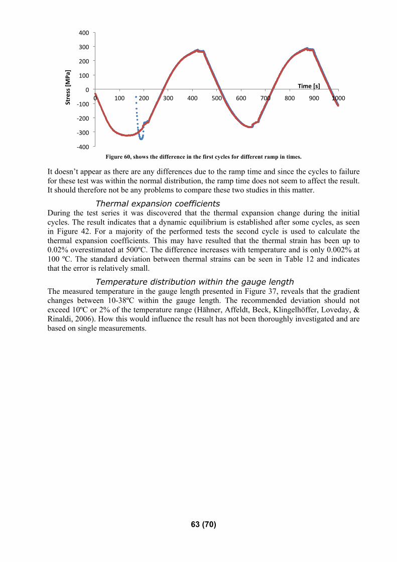
63 (70)
Figure 60, shows the difference in the first cycles for different ramp in times.
It doesn’t appear as there are any differences due to the ramp time and since the cycles to failure for these test was within the normal distribution, the ramp time does not seem to affect the result. It should therefore not be any problems to compare these two studies in this matter.
Thermal expansion coefficients During the test series it was discovered that the thermal expansion change during the initial cycles. The result indicates that a dynamic equilibrium is established after some cycles, as seen in Figure 42. For a majority of the performed tests the second cycle is used to calculate the thermal expansion coefficients. This may have resulted that the thermal strain has been up to 0.02% overestimated at 500ºC. The difference increases with temperature and is only 0.002% at 100 ºC. The standard deviation between thermal strains can be seen in Table 12 and indicates that the error is relatively small.
Temperature distribution within the gauge length The measured temperature in the gauge length presented in Figure 37, reveals that the gradient changes between 10-38ºC within the gauge length. The recommended deviation should not exceed 10ºC or 2% of the temperature range (Hähner, Affeldt, Beck, Klingelhöffer, Loveday, & Rinaldi, 2006). How this would influence the result has not been thoroughly investigated and are based on single measurements.
-‐400
-‐300
-‐200
-‐100
0
100
200
300
400
0 100 200 300 400 500 600 700 800 900 1000
Stress [M
Pa]
Time [s]

64 (70)

65 (70)
6. CONCLUSION
The conclusions possible to draw from this study are: • The fatigue life will decrease with an average of about 70% if LGI is used instead of
CGI for the tested parameters. • The fatigue life will decrease with an average of about 48% if the maximum temperature
is increased to 500°C from 450°C. • The fatigue life may increase if the time at high temperature decreases. • It is possible to state that the difference in fatigue life increases with a lower confinement
and/or mechanical strain. • When applying a superimposed 10Hz strain of 0.1% in addition with the thermo-
mechanical load, the fatigue life can be significantly decreased.
7. RECOMMENDATION AND FUTURE WORK
It would be advised to continue with the testing to further investigate the influence between the TMF and HCF-loads since it may have a large influence of the fatigue life. It is further recommended to investigate the presence of a threshold in applied HCF-load as studied by (Nieweg, Siefert and Metzger, 2011). That study claims there is a certain level that not results in any major decrease in the fatigue life. It would simplify the requirement specification if a maximum HCF-load can be specified. It would also be of great benefit to investigate how the fatigue life is affected by other parameters such as the minimum temperature, cycle time and spectral loads.

66 (70)

67 (70)
8. REFERENCES
Angus, H. T. (1960). Physical and engineering properties of cast iron. Alvechurch, England: The british cast iron reasearch association. ASM international. (1990). ASM handbook, Properties and Selection: Irons, Steels, and High-Performance Alloys (Vol. 1). ASM international. ASM international, cast iron. (1996). ASM speciality handbook - cast irons. ASM international, handbook. (1996). ASM handbook, volyme 19, Fatigue Failure in Metals, Fatigue and Fracture (Vol. 19). Beck, T., Henne, I., & Löhe, D. (2008). Lifetime of cast ALSI6Cu4 under superimposed thermal-mechanical fatigue and high-cycle fatigue loading. Materials Science and engineering, 382-386. Box, G. E., Hunter, J. S., & Hunter, W. G. (2005). Statistics for experimenters. New Jersey: John Wileys & sons. Callister, W. D., & Rethwisch, D. G. (2009). Material science and engineering an introduction (8:th ed.). DeLuca, D. Understanding fatigue, ASME.org. Retrieved 2014-01-13 from files.asme.org/IGTI/Knowledge/Articles/13048.pdf Dr. Steve, D. (2009). Compacted graphite iron – A material solution for modern diesel engine cylinder blocks and heads. China foundary , 6 (3), 241-246. efatigue. Retrieved 2014-01-10 from https://www.efatigue.com/hightemp/background/tmf.html Hähner, P., Affeldt, E., Beck, T., Klingelhöffer, H., Loveday, M., & Rinaldi, C. (2006). Validated Code-of-Practice for Strain-Controlled Thermo-Mechanical Fatigue Testing. European Commission. IMPAC Infrared GmbH. (2004). Pyrometer handbook. Frankfurt am Main: IMPAC Infrared GmbH. Löhe, D. (2008). Thermomechanical Fatigue: The Basics. Karlsruhe. Metzger, M., Nieweg, B., Schweizer, C., & Seifert, T. (2013). Lifetime prediction of cast iron materials under combined thermomechanical. International Journal of Fatigue , 53, 58-66. MSC software. www.mscsoftware.com. Retrieved 2014-01-13 from http://www.mscsoftware.com/training_videos/patran/Reverb_help/index.html#page/Fatigue%2520Users%2520Guide/fat_theory.15.1.html#ww60609 Nieweg, B; Seifert, T; Metzger, M. (2008). Rechenmodelle zur Lebensdauervorhersage von Motorbauteilen unter thermomechanischer. Nieweg, B; Seifert, T; Metzger, M. (2011). Rechenmodelle zur Lebensdauervorhersage von Motorbauteilen unter thermomechanischer. 947. Pentronic. Retrieved 2014-03-05, from http://www.pentronic.se/start/temperaturgivare/teori-om-givare/teori-om-termoelement.aspx Schweizer, C., Seifert, T., Nieweg, B., Hartrott, P. v., & Riedel, H. (2011). Mechanisms and modelling of fatigue crack growth under combined low and high cycle fatigue loading. International Journal of Fatigue , 33, 194-202. Sehitoglu, S. (1992). Thermo-Mechanical Fatigue Life Prediction Methods; Advances in Fatigue Life Predictive Techniques. ASTM STP 1122. Smalcerz, A., & Przylucki, R. (2013). Impact of electromagnetic field upon temperature measurement of induction heated charges. International journal of thermophysics, 34, 667-679. SS 11 23 70. (n.d.). Svensk Standard. Weronski, A., & Hejwowski, T. (1991). Thermal fatigue of metals. Dekker.

68 (70)

69 (70)
9. APPENDIX
Appendix A, Thermal expansion coefficient and Young’s modulus
Table 13, Shows the coefficients used to approximate the thermal expansion and the Young's modulus.
Test specimen A2 A1 A0 B2 B1 B0 NC003CGI 5.06E-09 1.09E-05 -2.97E-04 -0.0504 -17.9729 155613 NC004CGI 4.33E-09 1.09E-05 -3.24E-04 -0.0105 -35.4297 152532 NC005CGI 4.60E-09 1.11E-05 -3.62E-04 -0.0662 -15.5091 150819 NC006CGI 4.92E-09 1.10E-05 -2.83E-04 -0.0457 -21.7578 153483 NC007CGI 5.06E-09 1.10E-05 -2.50E-04 -0.0773 -7.9826 152266 NC008 CGI 5.31E-09 1.08E-05 -2.59E-04 -0.0993 -1.4551 148205 NC009 CGI 4.38E-09 1.12E-05 -3.23E-04 -0.1379 -12.4215 149423 NC010 CGI 5.35E-09 1.09E-05 -3.03E-04 -0.0557 -17.0235 149975 NC011 CGI 4.21E-09 1.14E-05 -2.48E-04 -0.0922 0.3340 147307 NC026 CGI 5.09E-09 1.10E-05 -3.33E-04 -0.1005 -7.6599 152824
NC027 CGI 5.20E-09 1.07E-05 -3.16E-04 -0.0325 -33.7477 157326 NC028 CGI 5.24E-09 1.12E-05 -3.22E-04 -0.021 -33.4858 155830 NC029 CGI 5.46E-09 1.11E-05 -3.27E-04 -0.0613 -14.1717 148574 NC030 CGI 5.63E-09 1.09E-05 -3.02E-04 -0.1316 17.5119 136240 NC031 CGI 5.43E-09 1.09E-05 -2.17E-04 -0.0079 -58.3563 154345 NC032 CGI 4.85E-09 1.12E-05 -3.58E-04 -0.0247 -44.6342 156469 NC001 LGI 3.92E-09 1.15E-05 -2.16E-04 -0.0627 -7.2143 123999 NC002 LGI 3.80E-09 1.15E-05 -9.91E-05 0.0037 -58.9750 130098 NC003 LGI 3.93E-09 1.16E-05 -3.76E-04 -0.1817 49.4750 119563 NC004 LGI 4.15E-09 1.15E-05 -3.17E-04 -0.0467 -16.7596 126844 NC005 LGI 3.66E-09 1.21E-05 -4.71E-04 -0.0743 10.4133 117826 NC006 LGI 3.88E-09 1.19E-05 -3.91E-04 -0.0086 -42.2785 129109 NC007 LGI 4.00E-09 1.15E-05 -3.33E-04 0.003 -35.5442 126153 NC008 LGI 4.39E-09 1.15E-05 -3.83E-04 NC009 LGI 3.97E-09 1.22E-05 -3.49E-04 -0.0098 -33.8941 128211

70 (70)
Appendix B, Test result Table 14, shows the result from test series one.
Test: Material: Temperature: Hold time: Confinement: TMF cycles to failure: [N]
1 + (CGI) + (500ºC) - (25s) - (X 0.9) 157 1,1 + + - - 175 1,2 + + - - 176 2 + + - 0 (X 1.0) 102 3 + + - + (X 1.1) 80 4 + + + (250s) - 102 4,1 + + + - 90 5 + + + 0 96 6 + + + + 56 7 + - (450ºC) - - 452 8 + - - 0 209 9 + - - + 188 10 + - + - 289 11 + - + 0 196 12 + - + + 151 13 - (LGI) + - - 59 14 - + - 0 35 15 - + - + 26 16 - + + - 33 17 - + + 0 28 18 - + + + 23 19 - - - - 104 20 - - - 0 75 21 - - - + 52 22 - - + - 69 23 - - + 0 56 24 - - + + 49
Table 15, shows the result from test series two.
Test:
Hold time:
HCF amplitude:
Temperature: Material: Confinement: TMF cycles to failure:
1 + (250s) - (0.05%) +(500ºC) + CGI 1(X 1.0) 43 2 + +(0.1%) + + 1 3 3 - (25s) - + + 1 65 4 - + + + 1 11 5 + - -(450ºC) + 1 115 6 + + - + 1 15 7 - - - + 1 114 8 - + - + 1 15