Capturing Binary Graphs - HAL-LAAS

HAL Id: tel-02298644https://hal.laas.fr/tel-02298644

Submitted on 27 Sep 2019

HAL is a multi-disciplinary open accessarchive for the deposit and dissemination of sci-entific research documents, whether they are pub-lished or not. The documents may come fromteaching and research institutions in France orabroad, or from public or private research centers.

L’archive ouverte pluridisciplinaire HAL, estdestinée au dépôt et à la diffusion de documentsscientifiques de niveau recherche, publiés ou non,émanant des établissements d’enseignement et derecherche français ou étrangers, des laboratoirespublics ou privés.

Capturing Binary GraphsGilles Trédan

To cite this version:Gilles Trédan. Capturing Binary Graphs. Computer Science [cs]. Institut National Polytechnique deToulouse (INPT), 2019. tel-02298644

https://hal.laas.fr/tel-02298644

https://hal.archives-ouvertes.fr

MEMOIREMEMOIREEn vue de l’obtention de l’

Habilitation à diriger les recherchesDélivré par : l’Institut National Polytechnique de Toulouse (INP Toulouse)

Présenté et soutenu le 21 Juin 2019 par :Gilles Tredan

Capturing Binary Graphs

JURYValérie Issarny Directrice de Recherches, Inria Paris RapporteurMatthieu Latapy Directeur de Recherches, Lip6 RapporteurPascal Felber Professeur, Université de Neuchâtel RapporteurFrançois Taïani Directeur de Recherches, Irisa ExaminateurMohamed Kaâniche Directeur de Recherches, LAAS Directeur

Unité de Recherche :LAAS - UPR 8001

Correspondant :Mohamed Kaâniche

The economic anarchy of capitalist society as it exists today is, in my opinion, the realsource of the evil. (...) We see before us a huge community of producers the members ofwhich are unceasingly striving to deprive each other of the fruits of their collective labor.

Unlimited competition leads to a huge waste of labor, and to that crippling of the socialconsciousness of individuals (...).This crippling of individuals I consider the worst evil ofcapitalism.

—Albert Einstein, Monthly Review, 1949

RemerciementsJe tiens à remercier l’ensemble des personnes ayant contribué à l’élaboration de ce document et à la

conduite des recherches présentées ici.En premier, je remercie mes rapporteurs Valérie Issarny, Pascal Felber et Matthieu Latapy pour avoir

accepté d’évaluer mes travaux et permis la reconnaissance de ces pages en tant que diplôme universitaire.Avec François Taiani, examinateur mobilisé et pertinent, ils ont formé un jury avec lequel j’ai appris etpris plaisir à échanger.

Je remercie chaleureusement Mohamed Kaâniche, qui m’a soutenu dans ces travaux à la fois scien-tifiquement en tant que directeur de mémoire, et économiquement en tant que directeur d’équipe. Sanslui je n’aurais probablement jamais vu le bout de cette fastidieuse quête de qualification administrative.

Bien sûr, tous les travaux présentés dans ce document sont le fruit de collaborations. Le parcourstransformant une idée en papier et un papier en une ligne sur dblp est escarpé. Je suis heureux d’avoirpartagé ces aventures avec mes co-auteurs, et les remercie pour les joies, les déceptions, les raisons et lespassions que nous avons rencontrées sur le chemin. Mersi da Erwan ma ankouezet ar wech diwezhan.

Parce que je ne travaille pas qu’avec des co-auteurs, et qu’ils façonnent l’environnement dont je suisle produit, je tiens à remercier tous ceux avec qui je travaille mais ne publie pas. Je pense à l’équipeTSF, et plus généralement aux collègues du LAAS. Je pense aussi au CRCA et au LPT (avec qui j’espèrequand même publier un jour), à Maria Barthélémy et René Sultra.

Merci enfin à ceux avec qui je vis mais ne travaille pas. Ma famille étendue, Anne-Isa, Bébéchat etMifou. Ils méritent une gratitude que je ne saurais exprimer dans ce document.

Contents

I Introduction 1

II Is network tomography a good idea ? 11

1 Modeling the impact of traceroute stars 131.1 Context: Complex Networks arising from networking . . . . . . . . . . . . . . . . . . . . . 13

1.1.1 Related Work . . . . . . . . . . . . . . . . . . . . . . . . . . . . . . . . . . . . . . . 131.1.2 Contributions . . . . . . . . . . . . . . . . . . . . . . . . . . . . . . . . . . . . . . . 14

1.2 Model . . . . . . . . . . . . . . . . . . . . . . . . . . . . . . . . . . . . . . . . . . . . . . . 151.3 Inferrable Topologies . . . . . . . . . . . . . . . . . . . . . . . . . . . . . . . . . . . . . . . 18

1.3.1 Basic Observations . . . . . . . . . . . . . . . . . . . . . . . . . . . . . . . . . . . . 181.4 Properties and Full Exploration . . . . . . . . . . . . . . . . . . . . . . . . . . . . . . . . . 211.5 Conclusion . . . . . . . . . . . . . . . . . . . . . . . . . . . . . . . . . . . . . . . . . . . . 22

2 Mapping virtual clouds 232.1 Context: Virtualized Networks . . . . . . . . . . . . . . . . . . . . . . . . . . . . . . . . . 232.2 Model . . . . . . . . . . . . . . . . . . . . . . . . . . . . . . . . . . . . . . . . . . . . . . . 25

2.2.1 VNet Embedding . . . . . . . . . . . . . . . . . . . . . . . . . . . . . . . . . . . . . 252.2.2 Request Complexity . . . . . . . . . . . . . . . . . . . . . . . . . . . . . . . . . . . 262.2.3 Additional Complexities . . . . . . . . . . . . . . . . . . . . . . . . . . . . . . . . . 272.2.4 Terminology and Notation . . . . . . . . . . . . . . . . . . . . . . . . . . . . . . . . 27

2.3 Adversarial Topology Discovery . . . . . . . . . . . . . . . . . . . . . . . . . . . . . . . . . 282.3.1 Trees . . . . . . . . . . . . . . . . . . . . . . . . . . . . . . . . . . . . . . . . . . . . 282.3.2 Arbitrary Graphs . . . . . . . . . . . . . . . . . . . . . . . . . . . . . . . . . . . . . 29

2.4 Motif Framework . . . . . . . . . . . . . . . . . . . . . . . . . . . . . . . . . . . . . . . . . 302.5 Simulations . . . . . . . . . . . . . . . . . . . . . . . . . . . . . . . . . . . . . . . . . . . . 312.6 Related Work . . . . . . . . . . . . . . . . . . . . . . . . . . . . . . . . . . . . . . . . . . . 332.7 Conclusion . . . . . . . . . . . . . . . . . . . . . . . . . . . . . . . . . . . . . . . . . . . . 34

III Data-oriented approaches 35

1 Souk and Loca: inferring social networks from position information 391.1 Context . . . . . . . . . . . . . . . . . . . . . . . . . . . . . . . . . . . . . . . . . . . . . . 39

1.1.1 Typical Mobility and Interaction Analyses . . . . . . . . . . . . . . . . . . . . . . . 401.2 Souk: the Experimental Platform . . . . . . . . . . . . . . . . . . . . . . . . . . . . . . . 40

1.2.1 Position capture platform . . . . . . . . . . . . . . . . . . . . . . . . . . . . . . . . 411.2.2 Mobility model framework . . . . . . . . . . . . . . . . . . . . . . . . . . . . . . . . 421.2.3 Analysis pipeline . . . . . . . . . . . . . . . . . . . . . . . . . . . . . . . . . . . . . 42

1.3 Experimental Deployments . . . . . . . . . . . . . . . . . . . . . . . . . . . . . . . . . . . 431.3.1 Experimental setup . . . . . . . . . . . . . . . . . . . . . . . . . . . . . . . . . . . . 431.3.2 General characteristics . . . . . . . . . . . . . . . . . . . . . . . . . . . . . . . . . . 44

E

F CONTENTS

1.3.3 Constructing Interaction Graphs . . . . . . . . . . . . . . . . . . . . . . . . . . . . 441.4 Reality Against Models . . . . . . . . . . . . . . . . . . . . . . . . . . . . . . . . . . . . . 461.5 Conclusion . . . . . . . . . . . . . . . . . . . . . . . . . . . . . . . . . . . . . . . . . . . . 47

2 Loca: Inferring Social Networks from Sparse Traces 492.1 Context . . . . . . . . . . . . . . . . . . . . . . . . . . . . . . . . . . . . . . . . . . . . . . 492.2 Model and Algorithms . . . . . . . . . . . . . . . . . . . . . . . . . . . . . . . . . . . . . . 50

2.2.1 Attacker Model . . . . . . . . . . . . . . . . . . . . . . . . . . . . . . . . . . . . . . 502.2.2 Transformation Algorithms . . . . . . . . . . . . . . . . . . . . . . . . . . . . . . . 51

2.3 Experimental Results . . . . . . . . . . . . . . . . . . . . . . . . . . . . . . . . . . . . . . . 532.3.1 Datasets . . . . . . . . . . . . . . . . . . . . . . . . . . . . . . . . . . . . . . . . . . 532.3.2 Metrics and Methods . . . . . . . . . . . . . . . . . . . . . . . . . . . . . . . . . . . 542.3.3 Sensors Deployment Strategies . . . . . . . . . . . . . . . . . . . . . . . . . . . . . 552.3.4 Quality of the Virtual Mapping . . . . . . . . . . . . . . . . . . . . . . . . . . . . . 552.3.5 Results . . . . . . . . . . . . . . . . . . . . . . . . . . . . . . . . . . . . . . . . . . 56

2.4 Related Works . . . . . . . . . . . . . . . . . . . . . . . . . . . . . . . . . . . . . . . . . . 592.5 Mitigation strategies . . . . . . . . . . . . . . . . . . . . . . . . . . . . . . . . . . . . . . . 602.6 Conclusion . . . . . . . . . . . . . . . . . . . . . . . . . . . . . . . . . . . . . . . . . . . . 60

IV A model of G for dynamic graphs 631.1 Context . . . . . . . . . . . . . . . . . . . . . . . . . . . . . . . . . . . . . . . . . . . . . . 641.2 Preliminaries . . . . . . . . . . . . . . . . . . . . . . . . . . . . . . . . . . . . . . . . . . . 661.3 Centrality Distance . . . . . . . . . . . . . . . . . . . . . . . . . . . . . . . . . . . . . . . . 671.4 Methodology . . . . . . . . . . . . . . . . . . . . . . . . . . . . . . . . . . . . . . . . . . . 691.5 Experimental Case Studies . . . . . . . . . . . . . . . . . . . . . . . . . . . . . . . . . . . 69

1.5.1 Centrality Distances over Time . . . . . . . . . . . . . . . . . . . . . . . . . . . . . 711.5.2 Dynamics Signature . . . . . . . . . . . . . . . . . . . . . . . . . . . . . . . . . . . 72

1.6 Related Work . . . . . . . . . . . . . . . . . . . . . . . . . . . . . . . . . . . . . . . . . . . 731.7 Conclusion . . . . . . . . . . . . . . . . . . . . . . . . . . . . . . . . . . . . . . . . . . . . 74

V Conclusion and Future Works 771.1 Some shortcomings of this document . . . . . . . . . . . . . . . . . . . . . . . . . . . . . . 781.2 Future works . . . . . . . . . . . . . . . . . . . . . . . . . . . . . . . . . . . . . . . . . . . 79

1.2.1 Theory . . . . . . . . . . . . . . . . . . . . . . . . . . . . . . . . . . . . . . . . . . 791.2.2 Applications . . . . . . . . . . . . . . . . . . . . . . . . . . . . . . . . . . . . . . . 80

List of Figures

1 Euler’s first Graph (1736): abstracting islands as vertices, and bridges as edges. . . . . . . 22 Ernst-Reuter-Platz pedestrian domain abstracted as a graph. Vertices represent pedestri-

ans waiting spots, sidewalks connect those as black edges, while inbound (resp. outbound)traffic lane pedestrian crossing are represented by orange (resp. green) edges. . . . . . . . 3

3 Link activation pattern due to traffic lights: while it is always possible to walk on sidewalks,it is only possible to cross inbound traffic lanes (green links) two thirds of the time, andoutbound traffic (orange links) one third of the time. Those possibilities are regulated bytraffic lights that cycle through 3 distinct states. . . . . . . . . . . . . . . . . . . . . . . . 4

4 A recurring illustration of G. . . . . . . . . . . . . . . . . . . . . . . . . . . . . . . . . . . 65 Illustration of Chapter II.1 approach. . . . . . . . . . . . . . . . . . . . . . . . . . . . . . . 76 Illustration of Chapter II.2 approach. Arrows symbolise the 7→ embedding relation. . . . . 77 Illustration of Part III approaches: models and reality are compared by sampling. . . . . . 88 Illustration of Part IV approach. . . . . . . . . . . . . . . . . . . . . . . . . . . . . . . . . 99 An example of Internet map produced by Matt Britt and based on traceroute measurements. 12

10 Model parameters in currently available trace sets. . . . . . . . . . . . . . . . . . . . . . . 1611 Two non-isomorphic inferred topologies . . . . . . . . . . . . . . . . . . . . . . . . . . . . 1712 Summary of bounds on inferrable topologies . . . . . . . . . . . . . . . . . . . . . . . . . . 22

13 Embedding process illustration. . . . . . . . . . . . . . . . . . . . . . . . . . . . . . . . . . 2414 Algorithm Dict overview . . . . . . . . . . . . . . . . . . . . . . . . . . . . . . . . . . . . 3015 Results of Dict when run on different Internet and power grid topologies . . . . . . . . . 3216 The AS-4755 network . . . . . . . . . . . . . . . . . . . . . . . . . . . . . . . . . . . . . . 3317 One of the first social networks, representing here the affinities in a kindergarten. Trian-

gular and circular nodes correspond to girls and boys, respectively. The criteria for a linkis "Studying and playing in proximity, actually sitting beside" [93] . . . . . . . . . . . . . 36

18 Illustrations extracted from Milgram’s small world experiment (1967) [128] . . . . . . . . 3719 Different souk deployments . . . . . . . . . . . . . . . . . . . . . . . . . . . . . . . . . . . 38

20 Each participant carries two lightweight tags, clamped on clothes on her/his shoulders. . . 4121 Overview of the Souk processing pipeline . . . . . . . . . . . . . . . . . . . . . . . . . . . 4222 Layout of the experimental areas . . . . . . . . . . . . . . . . . . . . . . . . . . . . . . . . 4423 Number of users in each trace. . . . . . . . . . . . . . . . . . . . . . . . . . . . . . . . . . 4424 Movement patterns for the souk dataset. . . . . . . . . . . . . . . . . . . . . . . . . . . . . 4525 Temporal movement characteristics . . . . . . . . . . . . . . . . . . . . . . . . . . . . . . . 4526 Broadcast time on datasets and synthetic traces. . . . . . . . . . . . . . . . . . . . . . . . 4727 Digging into social interactions . . . . . . . . . . . . . . . . . . . . . . . . . . . . . . . . . 47

28 Possible attack surfaces represented by red arrows. . . . . . . . . . . . . . . . . . . . . . . 5029 (a) Deployment of 15 sensors in SOUK cocktail-room according to the Density strat-

egy. (b) Representation of the Transition Matrix as a weighted graph laid out using theFruchterman and Reingold algorithm. . . . . . . . . . . . . . . . . . . . . . . . . . . . . . 54

30 AUC results of the (a) SOUK and (b) MILANO datasets for different deployment strategies. 56

G

H LIST OF FIGURES

31 Impact of Kin on SOUK (a) and MILANO (b) datasets, considering a deployment of 15sensors with a 1m range. . . . . . . . . . . . . . . . . . . . . . . . . . . . . . . . . . . . . 57

32 Detailed ROC for the SOUK dataset using 15 sensors: True Positive Rate (TPR) as afunction of False Positive Rate (FRP). . . . . . . . . . . . . . . . . . . . . . . . . . . . . . 58

33 Impact of sensors range on inference accuracy for 15 sensors evenly distributed in space. 5834 Probability to have exactly x out of 10 best friends correctly identified by Loca using 15

sensors of 1m range. . . . . . . . . . . . . . . . . . . . . . . . . . . . . . . . . . . . . . . . 5935 Local/Global scenario: G1 is a line graph, G2 and G3 differ from G1 by only one link. . . 6536 Two evolutionary paths from a line graph GL to a shell graph GS . . . . . . . . . . . . . . 6637 The graph-of-graph G connects named networks (represented as stars). Two networks are

neighboring iff they differ by a graph edit distance of one. The centrality distance definesa distance for each pair of neighboring graphs. . . . . . . . . . . . . . . . . . . . . . . . . 67

38 Number of edges and graph edit distance GED in the network traces. . . . . . . . . . . . 7039 Example centrality distances against null model . . . . . . . . . . . . . . . . . . . . . . . . 7240 Histogram representation of the different facets of graph dynamics . . . . . . . . . . . . . 73

Part IIntroduction

Summary of the thesisThis thesis regroups a set of algorithmical approaches related to the problem of graph metrology. Graphsare an abstraction representing a set of entities along with their interactions. As such, it is widely used asa tool to model real-life homogeneous systems. However, when using graphs to represent actual systems,a central question is "How to accurately represent these systems using graphs ?".

Indeed, when using Graphs as an abstraction to represent a real interaction system, accurately ob-taining the set of interactions is sometimes difficult. This is often due to standard phenomena likedynamism (entities and interactions evolve over time), or difficulties in accurately measuring pairwiseinteractions among entities that will result in noisy or erroneous measurements and missing information.Consider for instance social networks: while those networks have largely been studied, and assuming"social interaction" would find a consensual definition among the community, measuring the presence orthe absence of such interaction remains an error-prone process.

More precisely, fix a set of entities V : each set of possible symmetric binary interactions E among theelements of V defines a graph G. Let G the set of possible such graphs. Assume the system of interestis perfectly represented by an ideal graph G that has to be captured through an imperfect process. As aresult a graph G′ is obtained. This thesis presents different perspectives on the relation between G andG′.

While physics have developed a strong metrological framework to harness such uncertainty in con-tinuous models, the discrete nature of graphs along with the huge size of the possible graph space isproblematic. To illustrate this, we show in the first part of this manuscript that some theoretical analy-ses of graph capture approaches provide bad pessimistic answers. In particular, we show in a first studyon Traceroute that missing information has a very bad impact on the accuracy of graph capture. Wealso show in the context of virtual networks that capture algorithms are by nature expensive.

Nevertheless, while capturing graphs is in theory inacurrate and expensive, it is often efficient inpractice. There is a gap between the worst case on any possible graph, and the average case on realgraphs. Such a gap between theoretical analyses and practical usefulness provides a hint. Somehow,the approach of characterising for a given function f the worst case difference maxG,G′∈G |f(G)−f(G′)|does not match the classical use context of those topologies that could be in a nutshell representedby EG,G′∈Greal

|f(G)− f(G′)|. This formulation highlights two complementary approaches to fill thisgap: i) focus on the relation between G and Greal in order to reduce the gap between maxG,G′∈G andmaxG,G′∈Greal

; ii) characterise the distance between G and G′ and seek for properties of f allowing torelate d(G,G′) and f (e.g. continuity transposed to the discrete set of graphs).

The second part of this manuscript focuses on modeling real graphs to provide an approach to thisquestion in the context of human mobility. By extensively collecting data on interacting humans in acrowd, we collect instances of G′ ∈ Greal that highlight the importance of the link creation mechanism:there is some correlation between G and G′. We also show that current mobility models fail to reproduceimportant properties of real graphs. However, we show that such interaction structures can still provevery usefull even when constructed from very sparse information.

The last part of this manuscript takes a step back on these analyses by providing some tools to chartthe space of possible graphs. While theory tells that graphs are extremely noise-sensitive, practice showsthat in general the noise does not matter. The angle pursued in this part is to provide useful distanceson G, that more precisely allow to differentiate errors that matter and errors that don’t. We define anew family of distances on G, and illustrate their use in the context of dynamic graphs.

The selection of works presented in this thesis has for objective to shed different lights to the problemof graph capture. However, the big picture still has many holes. The final part provides some intuitionabout possible directions to fill them.

1

Part I/

From Königsberg to BerlinThe first system modeled as a graph was probably the islands of the city of Königsberg and its bridges. Itwas introduced in 1736 by Euler. Since then, this abstraction has found vast application arrays, rangingfrom sociology to computer science through physics, mathematics or epidemiology.

Figure 1: Euler’s first Graph (1736): abstracting islandsas vertices, and bridges as edges.

Although the original article has for sub-ject what is now known as "Euler’s 7 bridgesproblem", its deepest contribution perhapsdoes not lie in the solution to the problem,but rather in the introduction of a novel ab-straction that will both support deep theory(e.g. graph minors well-quasi-ordering [112])and experimental approaches ([128]). Such aversatility is probably due to the simplicityof the abstraction: it only requires the def-inition of what is an entity or a vertex andof what is an interaction or an edge betweenthese entities.

In this first graph abstraction ever de-fined, entities were islands defined by theriver Pregel (that will later inspire the nameof google’s large graph mining system[88]). The interactions modeled between the islands were thebridges. The illustration of his original article is reproduced Figure 1: it contained 4 vertices, and7 edges. In the remainder of this document, we will refer to such graphs as binary graphs: graphscomposed of symmetric and unvalued edges that could be represented by symmetric binary adjacencymatrices.

The Binary graph representation is a good tool to abstract a set of islands connected by bridges.Many reasons, often kept implicit, can justify this choice:

• it is impossible to change island without using bridge for a normal citizen having a walk in thecity;

• once on a island it is possible to reach any bridge of that island;

• bridges do not change often; it is easy to decide whether there is a bridge between two given islands;

• bridges always connect two distinct islands and can be crossed both ways;

• no hidden or fake bridge exists.

In other words, binary graphs were the right tool to strip down the real city from all its complexity (roadnetwork, shops, individuals, districts) to only keep the structure of the island network. Let us howeverobserve that such approach is only useful if the problem of interest relates to this island network.

Euler’s original question is "is there a walk that would cross each bridge exactly once ?". This problemonly involves bridges, and as such, a binary graph modeling the island and bridges network is sufficient toprovide an answer to this question. That is, abstracting the city of Königsber by a binary graph removedlots of information but not what is required to answer the Euler’s question. To state the obvious, suchmodel would not necessarily be sufficient to answer other questions, for instance: "where is the best barof the city ?".

In short, the binary graph abstraction fits very well this use-case. Since defining entities and inter-actions is a rather easy task, this graph model quickly grew in popularity. However, abstracting a reallife problem by a binary graph is not always so simple or fruitful. I like to illustrate this point usingan apparently very close problem that arised while I was working as a PostDoc in the FG-Inet groupof TU-Berlin. The group was located in the Tel building, on the Ernst-Reuter-Platz roundabout. Thisroundabout is a major intersection of Berlin, connecting 5 major 4-lane streets. The roundabout has adiameter of roughly 150m, and circumventing it as a pedestrian takes a long time.

2

Part I/

The limits of binary graphsIf we want to model (pedestrian) walks along this roundabout, we can model it using Euler’s approach:like the bridges connecting islands on the Pregel river, pedestrian crossings would be the edges connectingthe different sidewalks. The Ernst-Reuter place and its abstraction as a graph are represented Figure 2.However, to cope with the intense vehicle traffic of the German capital, the flow of cars and pedestrians isorchestrated by a set of traffic lights. Pedestrians cannot cross the links at arbitrary times. More precisely,these lights follow a particular 3-stage pattern: during first stage, all lights are red for pedestrians andit is impossible to cross any road. During the second stage, traffic lights stop the cars entering theroundabout, allowing the pedestrian to cross the green links. During the last stage, traffic lights alsostop the cars leaving the roundabout, allowing pedestrian to cross both green and orange links. Thislink activation pattern is represented in Figure 3.

Since the 4-lane streets are rather wide, crossing a street as a pedestrian takes a handful of seconds. Itis therefore only possible to cross one link during each stage. The intriguing consequence of this timingis the following: as a pedestrian it is a lot easier to circle the roundabout anti-clockwise rather thanclockwise. Consider for instance the path from i to g: regardless of the stage at which I reach i, I canreach g in 2 to 4 stages. However, on the other direction I need at most 5 stages (and at least 3) toreach i. Asymmetry, the consequence of this timing, interestingly arises even despite the very symmetricnature of link crossing: it takes exactly the same time to cross a link in both directions.

a

b

c

d

e

f

g h

i

j

k

l

mno

Figure 2: Ernst-Reuter-Platz pedestrian domain abstracted as a graph. Vertices represent pedestrianswaiting spots, sidewalks connect those as black edges, while inbound (resp. outbound) traffic lanepedestrian crossing are represented by orange (resp. green) edges.

Can I use a static and binary graph model to think about the experience of a pedestrian on thisroundabout ? The answer is in general no, as symmetric networks are by nature completely unable tocapture the asymmetries of Ernst Reuter Platz. So despite the similarities of my problem comparedto Königsberg 7 bridges, and despite that the edges (pedestrian crossings) are symmetric by nature,the activation patterns of the links combined with their topological arrangements have generated anasymmetric situation that I cannot capture with my symmetric graph model.

Of course, depending on the nature of the question, this abstraction will sometimes be useful. Abinary representation will for example be enough to represent where should pedestrian crossings bepainted. However, the topological shortest path from a to g will not represent the shortest journey [28].

3

Part I/

Stage

Links

orange

green

sidewalk

0 1 2 3 4 5 6 7 8 9

Figure 3: Link activation pattern due to traffic lights: while it is always possible to walk on sidewalks, itis only possible to cross inbound traffic lanes (green links) two thirds of the time, and outbound traffic(orange links) one third of the time. Those possibilities are regulated by traffic lights that cycle through3 distinct states.

Sampling and modelingImagine now one wants to create a map of Berlin walking times: given the roundabout problem, we nowunderstand it is a difficult problem. Since the walking times on the roundabout change depending onthe direction travelled and the departure time, establishing an accurate map would require many mea-surements. Since Berlin is a big city, its architecture constantly changes for instance due to constructionand road works, therefore such a map would need to be constantly updated to produce accurate answers.Another, more realistic approach, would be to measure the distance on the ground, that is unlikely tochange a lot over time, and to account for delays at the crossings while simply ignoring the synchronizedroundabouts like Ernst-Reuter-Platz. This map would be less accurate, but far easier to establish andmaintain.

Does it matter ? This central question implies that inaccurate maps might be useful provided they areaccurate enough for a purpose. An intuitive reasoning for the Ernst-Reuter-Platz case would probablylead to the conclusion that such configurations are relatively rare in a city, and that the impact ofclockwise vs. anti-clockwise travel is not important enough to justify using a more complex model, suchas asymmetric graphs.

To provide a theoretical answer to this problem would however require some work. For instanceto capture that such configurations are relatively rare, one would probably require a model of urbanpedestrian navigability graphs in general, and show that roundabouts rarely serve more than a fixedamount of streets, and that few other situations can create this problem, and so on.

The objective of these two introductory examples is to illustrate the necessity of a reasoning on theaccuracy of our modeling operations and their impact. As we abstract the reality with models, we omitpart of the reality. The consequences of these omissions are that the considered graph does not accuratelydescribe the real situation. In short, these examples illustrate the necessity of a metrological reasoningabout the graph objects as well.

This observation is not new. As we will see throughout this document, scientists worry since longago about the potential biases introduced by their observation methodology of a given network. In 2005,[60] called for a metrological perspective on the problem of sampling complex networks. It is to ourknowledge the earliest call for a more systematic approach on the problem introduced by representingreal systems with networks. This thesis attemps to provide a perspective on the authors’ works thatconcurs this objective.

Table I synthetises the different works presented in this thesis under the metrology perspective. Errorsoriginate from two sources: the inaccuracies of the link observation process, and the unstability of thesystem over time. While these both sources have different nature, they both have for consequence amismatch between the real system and its graph abstraction. One might observe that this approach is

4

Part I/

Section Entity Edge/Interaction Measurement methodIntro Königsberg Islands Bridges City MapII.1 WAN Routers IP (Layer 3) communication Traceroute TomographyII.2 Hosts Communication Embedding requestsIII.* Individuals Social contact Position information

ProximityIV Any fixed set of nodes Any binary pairwise relation Any method

../..

Section Error Sources Algorithmic Perspective Quality MeasureIntro ∅ ∅ ∅II.1 Router Anonymity

TimeWorst case analysis of graph propertiesModel Assumption

Property distribution rangeNone

II.2 Only binary answersTime

Algorithms to greedily span a topologyModel Assumption

Strict EqualityNone

III.* Inference process,Elusive edge definition

Filtering, dry-runsExtrapolation Algorithm

Comparison against models"Arbitrary" ground truth

IV DynamismLink Sampling errors

Definition of distance functions Comparison against a nullmodel

Table 1: This table summarises the different graphs and metrology difficulties encountered throughoutthis document.

consistent with "traditional" metrology. Standards are for instance chosen to allow a precise measurement(e.g. the original definition of the second (s) depended on the length standard earth day has beenabandonned because this earth day length is impacted by water tides) that is stable over time (e.g.the Kilogram reference is being abandoned because of its unstability over time despite all precautions).Interestingly, the concept of failures, particularly relevant when studying the resilience of man-madenetworks, can also be considered from this metrology perspective as a specific type of dynamism.

In summary, modeling a system by a graph is an operation that abstracts a real and complex setof intertwined elements into a pure structural representation of entities and interactions. Doing so isattractive if the seeked answers lie within the structure of the system, but in practice, finding the abstractgraph that corresponds to a real system is often problematic: interactions often evolve in reality, andcapturing those interactions is often not trivial. As a result, the observed/captured graph does not alwaysaccurately represent the real system. Understanding and mitigating the effect of these inaccuracies is therecurring angle of this thesis. The next chapter will focus on providing an overview of these approaches.

5

Part I/

A visual perspective on this thesisThroughout this thesis, a useful perspective will be the one of the set of all possible graphs over V namednodes, noted GV :

Definition:(G) Let V a finite set of elements. Let GV the set of all possible symmetric binary graphsbetween these n= |V | elements. Let P (X) the power set of a setX. Then for each possible E ∈P (V ×V ),there exists a unique graph G ∈ GV such that G= (V,E).

When the context is clear, we will write G. One first observation is that we choose here to explicitelyrefer to "named" elements in V . This means that in particular that isometric graphs are considereddifferent: G1 ∈ isom(G2) 6⇒G1 =G2. This distinction is important because it allows to test for equalityat a small computational cost. However, this dooms us to only compare graphs among identical sets ofnodes. For instance, the distances we will develop hereafter can only compute distances within a givenset GV , and it is correct to write ∀G1,G2 ∈ GV ,d(G1,G2) but not d(G1,H1) with G1 ∈ GV and H1 ∈ GV

′ .This approach however carries the natural meaning we usually have when graphs are applied to

everyday objects ("Alice plays with Carl while Denise stays alone" does not mean the same as "Aliceplays with Denise while Carl stays alone"). Moreover, in most of the presented works, V is easily known.

A second observation concerns the enormous size of this set. Its size is 2(n2). There are 1024 different

possible graphs of 5 elements, and more than 68 billion possibilities with 9 elements. A most tragicconsequence of this size is to forbid any enumerative approach. Yet it reamins a nice thought experiment,which I believe is very useful to apprehend (and spatialize) many of the problems presented in this thesis.

G

?G

planar →

tree →

Figure 4: A recurring illustration of G.

In the following I will represent G in two dimensions by a shapeless circuit set like in Figure 4.Each element in this shape is a binary symmetric graph, like G. Although the positions of the pointsrepresenting the graphs within the shape are completely arbitrary, the representation of a set is usefulto represent partitions and subsets of G. In this context, Figure 4 would represent G as a planar graphthat is not a tree.

In the first chapter, we study the properties of the set of graphs reconstructed from a given trace τ(using Algorithm 1). More precisely, since each trace τ defines a set of possible graphs on which τ canbe captured, we try to estimate the possible range of some properties of G (abstractly noted prop(G) onFigure 5). This approach is done by worst case, by exhibiting couples of graphs G1,G2 that present themost different values of prop(G). We believe this information is more important than the mere numberof members of Gτ : if the distribution of values is narrow (possibly even a point), then this means thattraceroute tomography allows to precisely estimate the value of this property. An (obvious) example ofsuch property would be the number of connected components (under already good covering hypothesesfor τ , see Chapter 1 for more details).

In Chapter 2, we use another tomographic approach. In the context of Virtual Networks (VNETs),we can request to embed a graph G in a target host H. Informally, the maximal graph G (in terms ofsize and density) that we can embed in H is reached when G=H, and reaching this limit in the fewest

6

Part I/

G

Gττ

Algorithm 1

X

P(prop(G)) =X

prop(G1) prop(G2)

?

?

Figure 5: Illustration of Chapter II.1 approach.

possible attempts is the objective of our approach. To achieve this, we first observe that (under somemild conditions), the embedding relation (written 7→) defines a partial order relation on the set of graphsthat we could embed in H: (H, 7→) is a poset (partially ordered set). We then exploit this relation bydefining greedy algorithms that, starting from the empty graph ∅, iteratively grow the structure G untilH is reached, as illustrated in Figure 6. Note that only part of the poset structure is represented. Inaddition, we try to reduce the considerable cost of exploring this poset structure by reducing the problemto standard graph classes, such as Trees or Cacti where they become much more tractable.

*

*

G

H

∅

G,s.t. G 7→H

Trees→

Figure 6: Illustration of Chapter II.2 approach. Arrows symbolise the 7→ embedding relation.

The conclusion of Chapter 2 is that reducing the search space to subsets of G (like the space of graphsconstructed from few motifsH) is an efficient approach. The popularity of traceroute-based measurementstudies hint that the worst cases identified in Chapter 1 probably never happen in practice. Together,those conclusions illustrate the need for a more precise modeling of the graphs encountered "in practice".In other words, a better modeling of the reality is needed.

The notion of graph model is rather standard in the complex network community. Famous modelssuch as Erdos-Renyi, Barabasi-Albert or Watts-Strogatz have driven the general understanding of pro-cesses on graphs. From G’s perspective, a graph model is a probability distribution: let m be a model,then implicitely m defines a probability distribution M : G 7→ [0,1] that associates with each graph itsprobability to be generated by model m.

7

Part I/

While graph classes are subsets of G, here the boundaries of a model are relatively soft: for instance,whatever the parameter p > 0 of an Erdos-Renyi (aka uniform) random graph model, all events of G havea non-negative probability of occurrence. That is, even Kn the densest graph has a small probability(pn(n−1)/2 > 0) to appear. For practical reasons however, we will represent models in the same way asclasses, by delimiting a subregion of the original G shape.

In Part III we focus our approach on observing such "practical" graphs. More precisely, we focusour study on graphs that are generated from humans moving in the two dimensional plane. How toestimate whether our synthetic mobility models do a good job in reproducing likely observable graphs ?One possibility is to collect many observations, and generate many samples, and use the approach ofChapter 1: compare and average the natural and artificial samples along some standard graph properties.Although this approach has been presented in other publications (see e.g. [70, 99]) it is not the approachpresented in this manuscript.

Indeed, doing so would neglect an important relation that binds all measured graphs: time. Thecaptured and generated graphs are not static, they evolve as the individuals (or agents simulating in-dividuals) move in the experience space. When I capture the evolving social network of a crowd, Iobtain a set of graphs Gi0<i<end. However, it is important to realise that the order matters (thatis G1,G2, . . . ,Gend−1 in this specific order). For instance, the connectivity of vertices is bound by thephysical location of the individuals they represent. Since those individuals cannot teleport, graphs evolverather smoothly. Using standard graph properties has this limitation: it considers each single graph inisolation.

To illustrate this idea, consider a captured dynamic graph DG= Gi0<i<end. One can compute itsaverage diameter E[diam(DG)] = 1

(end−1)∑i diam(Gi). Imagine an arbitrary permutation of order of

the graphs σ: letDG′= Gσ(i). Of course reordering the snapshots will not change the average diameterE[diam(DG)] =E[diam(DG′)]. From the diameter perspective, DG and DG′ are strictly identical, andsince DG is a real graph, this would push us to conclude that DG′ is a realistic trace. Imagine howeverthe real social event corresponding to DG′. It is probably not a very likely dynamic graph: people wouldleave and return to the event continuously, would not stay within a social circle for long, and so on.

This observation also holds for comparing models and real traces: while static graph measures alreadyprovide a hint on the quality of the model, the temporal dimension shall not be overlooked. This is whywe chose to focus on an application primitive (being more interested in the capacity of synthetic modelsto be useful to the distributed application programmer), the broadcast. In the case of a broadcast timecomputed directly by simulation on dynamic graphs, it is easy to observe that re-ordering the snapshotswill likely change the result.

G

model→reality→

?

??

??

??

??

X

P(prop(G)) =X

?

??

Figure 7: Illustration of Part III approaches: models and reality are compared by sampling.

8

Part I/

Finally, Chapter IV seeks to provide a more general structuring framework to G in the context ofdynamic graphs. Indeed, as illustrated through Figures 5- 7, a common feature of these approaches is toimpose some structure to the "flat" set G. The structures built are however highly application-dependent:different axioms would lead to different results in Chapter 1, a different embedding model would changethe results of Chapter 2. A recurring question of these works is "how different/similar are these twographs" ?

Chapter IV observes G as a graph, and shows it is possible to exploit this graph structure to constructdistances on the space G. The literature offers surprisingly few distance functions to compare two graphs.To alleviate this, we exploit centralities, a well known tool to capture the importance of nodes in graphs.We show that most standard centralities can be transformed into distances on G. Such distance wouldcapture the impact of a change in the topology on the roles of the nodes constituting this topology –where role is implicitely defined by the notion of importance each centrality exploits.

G

a

b c

d e

f g

h

i

j

k

a

b c

d e

f g

78

59

75

156

89

11

2

4

125

12

3

5

Figure 8: Illustration of Part IV approach.

This approach is illustrated Figure 8: each star a−k is one topological configuration, one possiblegraph over the elements V . The edges of G are established by connecting each graph with the othergraphs from which it only differs by one edge. The benefits of this approach is to allow representingdynamic graphs: they define trajectories in G provided the sampling resolution of the dynamic graphallows to observe each individual edge evolution (symbolized in red on the drawing). This approach alsoprovides a very particular structure to the graph G (coined graph-of-graphs): it is bipartite (as opposedto what is represented) and n(n−1)/2 regular. By measuring the individual nodes centrality variations,we are able to decorate the constructed edges with weights. Each centrality defines a different weightdistribution, and therefore a different perspective on the cost of the evolutionary path defined by thedynamic graph.

Interestingly, by exploiting the introduced distances, we also show in Chapter IV that "real" dynamicgraphs (like those generated from human mobility) tend to minimise the variation (they define trajectoriesof low weight) compared to different randomized null models. In other words, the captured dynamicnetworks evolve less than expected (given the raw number of topological updates); roles of the nodes inthose dynamic networks are more stable than expected. Sadly we do not know yet how to exploit theseobservations, for instance by leveraging the stability of information flows to improve the coordinationcapacities of a dynamic distributed system.

9

Part IIIs network tomography a good idea ?

In this part, I will present two rather theoretical approaches to network tomography. The centralquestion that will structure these approaches is how to "capture" a topology ? The first study focuses onthe Internet IP level routing, while the second focuses on Virtualized Network Infrastructures (VNETs).More precisely, the complete version of the presented results spans the following two papers :

• Misleading Stars: What Cannot Be Measured in the Internet? In Journal DistributedComputing 26(4): 209-222 (2013). with Yvonne-Anne Pignolet and Stefan Schmid

• Adversarial Topology Discovery in Network Virtualization Environments: A Threatfor ISPs? In Journal Distributed Computing (DIST), Springer, 2014. with Yvonne-Anne Pignoletand Stefan Schmid

Both follow the same objective: study the performance of algorithms that produce a graph repre-senting the target topology. The first chapter presents an offline algorithm (that works on a given inputtrace set), while the second chapter studies an "online" algorithm (generating requests depending on theanswers of an online service). Hence these works have also different optimisation objectives: while the on-line algo optimises the number of issued requests, the first one studies the impact of missing information(namely, some node names) on the fidelity of reconstructed topologies.

In a nutshell, both theoretical studies bring bad news. In the context of VNETs, inferring densetopologies requires a large amount of requests. For instance, an optimal algorithm requires o(n2) requeststo infer an n node graph in general (see more details in section 2.3.2). In the context of traceroute, missingnode names can have a drastic impact on the accuracy of the inferred topologies. For instance, we showthat even with the maximum of possible information available, the presence of s anonymous nodes cangenerate a quadratic uncertainty on the number of triangles (see more details in section 1.5). Theseresults are however not very surprising, given the pessimistic nature of worst case approaches considered,and given the enormous size of G.

Despite these theoretical barriers, the other interesting aspect of both studies is their relative praticalrelevance. In section 2.5 we present simulations conducted on real internet topologies: due to theirsparsity and relative regularity, they can be efficiently explored. Regarding the traceroute study, thelarge popularity of this approach to map the Internet such as the one on Figure 9 is also an argument ofpractical relevance: if people trust these maps despite their probable inaccuracy, it is probably becausethey find some use to it. In this case however, other factors such as the absence of more accurate andefficient alternatives to traceroute is probably also a main explanation parameter of traceroute popularity.

This common gap between the bad theoretical results and the good practical performance of thepresented methods nicely introduces the need for models. The whole graph space G is too big for mostexplorations, and worst case approaches rather inaccurately reflect the practical performance of themethods. Models allow to circumvent both limitations: they reduce the graph space to a subset thatmore closely captures recurring aspects of the reality. Models also temper the worst case effect by againfocusing the search on subsets of the graph space that are of practical relevance.

11

Part II/

Figure 9: An example of Internet map produced by Matt Britt and based on traceroute measurements.

12

Chapter 1

Modeling the impact of traceroutestars

This chapter explores the relations between T , the set of collected traces, and GT , the set of topologies onwhich it is possible to observe T . It is known that even if T is of high quality (this notion of quality willbe described hereafter), the presence of some anonymous routers in the trace can trigger the exponentialgrowth of the possible candidates sets GT . This work builds on the observation that the mere numberof inferrable topologies alone does not contradict the usefulness or feasibility of topology inference; ifthe set of inferrable topologies GT is homogeneous in the sense that the different topologies share manyimportant properties, the generation of all possible graphs can be avoided: an arbitrary representativemay characterize the underlying network accurately. Therefore, we identify important topological metricssuch as diameter or maximal node degree and examine how “close” the possible inferred topologies arewith respect to these metrics.

1.1 Context: Complex Networks arising from networkingThe classic tool to study topological properties of the Internet (at the IP level) is traceroute. Tracerouteallows us to collect traces from a given source node to a set of specified destination nodes. A tracebetween two nodes contains a sequence of identifiers describing a route between source and destination.

However, using traceroute to tomography IP-level topologies is error-prone. One of the major prob-lems of traceroute based sampling is the presence of stars: not every node along a sampled path isconfigured to answer with its identifier. Rather, some nodes may be anonymous in the sense that theyappear as stars (‘∗’) in a trace. Anonymous nodes exacerbate the exploration of a topology becausealready a small number of anonymous nodes may increase the spectrum of inferrable topologies thatcorrespond to a trace set T .

1.1.1 Related WorkArguably one of the most influential measurement studies on the Internet topology was conducted by theFaloutsos brothers [50] who show that the Internet exhibits a skewed structure: the nodes’ out-degreefollows a power-law distribution. Moreover, this property seems to be invariant over time. These resultscomplement discoveries of similar distributions of communication traffic which is often self-similar, andof the topologies of natural networks such as human respiratory systems. The power-law property allowsus to give good predictions not only on node degree distributions but also, e.g., on the expected numberof nodes at a given hop-distance. Since [50] was published, many additional results have been obtained,e.g., [4, 5, 42, 80], also by conducting a distributed computing approach to increase the number ofmeasurement points [27]. However, our understanding of the Internet’s structure remains preliminary,and the topic continues to attract much attention from the scientific communities. In contrast to these

13

Part II/ 1.1. CONTEXT: COMPLEX NETWORKS ARISING FROM NETWORKING

measurement studies, we pursue a more formal approach, and a complete review of the empirical resultsobtained over the last years is beyond the scope of this chapter.

The tool traceroute has been developed to investigate the routing behavior of the internet. [27, 57, 79,102, 127] Paxson [102] used traceroute to analyze pathological conditions, routing stability, and routingsymmetry. Another study by Gill et al. [57] demonstrates that large content providers (e.g., Google,Microsoft, Yahoo!) are deploying their own wide-area networks, bringing their networks closer to users,and bypassing Tier-1 ISPs on many routing paths.

Traceroute is also used to discover Internet topologies [32]. Unfortunately, there are several problemswith this approach that render topology inference difficult, such as aliasing (a node appears with differentidentifiers on different interfaces) or load-balancing, which has motivated researchers to develop new toolssuch as Paris Traceroute [11, 68].

There are several results on traceroute sampling and its limitations. In their famous papers, Lakhinaet al. [80] (by simulation) and Achlioptas et al. [4] (mathematically) have shown that the degree distribu-tion under traceroute sampling exhibits a power law even if the underlying degree distribution is Poisson.Dall’Asta et al. [42] show that the edge and vertex detection probability depends on the betweennesscentrality of each element and they propose improved mapping strategies. Another interesting resultis due to Barford et al. [15] who experimentally show that when performing traceroute-like methods toinfer network topologies, it is more useful to increase the number of destinations than the number oftrace sources.

A drawback of using traceroute to determine the network topology stems from the fact that routersmay appear as stars (i.e., anonymous nodes) in the trace since they are overloaded or since they areconfigured not to send out any ICMP responses. [134] The lack of complete information in the trace setrenders the accurate characterization of Internet topologies difficult. This chapter attends to the problemof what information on the underlying topology can be inferred despite anonymous nodes and assumes aconservative, “worst-case” perspective that does not rely on any assumptions on the underlying network.Other work on this subject includes e.g., [134] by Yao et al. studying possible candidate topologies for agiven trace set and computing the minimal topology, that is, the topology with the minimal number ofanonymous nodes. Answering this question turns out to be NP-hard. Subsequently, different heuristicsaddressing this problem have been proposed [61, 68].

Our work is motivated by a series of papers by Acharya and Gouda. In [3], a network tracing theorymodel is introduced where nodes are “irregular” in the sense that each node appears in at least onetrace with its real identifier. In [1], hardness results on finding the minimal topology are derived for thismodel. However, as pointed out by the authors themselves, the irregular node model—where nodes areanonymous due to high loads—is less relevant in practice and hence they consider strictly anonymousnodes in their follow-up studies [2]. As proved in [2], the problem is still hard (in the sense that thereare many minimal networks corresponding to a trace set), even for networks with only two anonymousnodes, symmetric routing and without aliasing.

In contrast to the line of research on cardinalities of minimal networks, we are interested in the networkproperties of inferrable topologies. If the inferred topologies share the most important characteristics,the negative results on cardinalities in [1, 2] may be of little concern. Moreover, we believe that a studylimited to minimal topologies only may miss important redundancy aspects of the Internet. Unlike [1, 2],our work is constructive in the sense that algorithms can be derived to compute inferred topologies.

Our work is also related to the field of end-to-end network tomography, where topologies are exploredusing pairwise measurements, without the cooperation of nodes along these paths. For a good discussionof this approach as well as results for a routing model along shortest and second shortest paths see [9]. Forexample, [9] shows that for sparse random graphs, a relatively small number of cooperating participantsis sufficient to determine the network topology fairly well.

1.1.2 ContributionsThis chapter reports on the study and characterization of topologies that can be inferred from a giventrace set computed with the traceroute tool. While existing literature assuming a worst-case perspectivehas mainly focused on the cardinality of minimal topologies, we go one step further and examine specifictopological graph properties.

14

Part II/ 1.2. MODEL

We introduce a formal theory of topology inference by proposing basic axioms (i.e., assumptionson the trace set) that are used to guide the inference process. We present a novel definition for theisomorphism of inferred topologies which is aware of traffic paths; it is motivated by the observation thatalthough two topologies look equivalent up to a renaming of anonymous nodes, the same trace set mayresult in different paths. Moreover, we propose the study of two extremes: in the first scenario, we onlyrequire that each link appears at least once in the trace set; interestingly, however, it turns out thatthis is often not sufficient, and we propose a “best case” scenario where the trace set is, in some sense,complete: it contains paths between all pairs of non-anonymous nodes.

The main result of this chapter is a negative one. It is shown that already a small number ofanonymous nodes in the network renders topology inference difficult. In particular, we prove that ingeneral, the possible inferrable topologies differ in many crucial aspects, e.g., the maximal node degree,the diameter, the stretch, the number of triangles and the number of connected components.

We introduce the concept of the star graph of a trace set that is useful for the characterization ofinferred topologies. In particular, colorings of the star graphs allow us to constructively derive inferredtopologies. (Although the general problem of computing the set of inferrable topologies is related toNP-hard problems such as minimal graph coloring and graph isomorphism, some important instancesof inferrable topologies can be computed efficiently.) The chromatic number (i.e., the number of colorsin the minimal proper coloring) of the star graph defines a lower bound on the number of anonymousnodes from which the stars in the traces could originate from. And the number of possible colorings ofthe star graph—a function of the chromatic polynomial of the star graph—gives an upper bound on thenumber of inferrable topologies. We show that this bound is tight in the sense that trace sets with thatmany inferrable topologies indeed exist. In particular, there are problem instances where the cardinalityof the set of inferrable topologies equals the Bell number. This insight complements existing cardinalityresults and generalizes topology inference to arbitrary, not only minimal, inferrable topologies.

Finally, we examine the scenario of fully explored networks for which “complete” trace sets are avail-able. As expected, the inferrable topologies are more homogeneous in this case and can be characterizedwell with respect to many properties such as the distances between nodes. However, we also find thatsome other properties are inherently difficult to estimate. Interestingly, our results indicate that fullexploration is often useful to derive bounds on global properties (such as connectivity) while it does nothelp much for bounds on more local properties (such as node degrees).

1.2 ModelLet T denote the set of traces obtained from probing (e.g., by traceroute) a network G0 = (V0,E0) withnodes or vertices V0 (the set of routers) and undirected links or edges E0. We assume that G0 is staticduring the probing time (or that probing is instantaneous), but we do not require that G0 is connected.Each trace T (u,v) ∈ T describes a path connecting two nodes u,v ∈ V0; when u and v do not matteror are clear from the context, we simply write T . Moreover, let dT (u,v) denote the distance (numberof hops) between two nodes u and v in trace T . We define dG0(u,v) to be the corresponding shortestpath distance in G0. Note that a trace between two nodes u and v may not describe the shortest pathbetween u and v in G0.

The nodes in V0 fall into two categories: anonymous nodes and non-anonymous (or shorter: named)nodes. As it is the case in most related literature, we assume these categories to be permanent over timeand traces: a node is either consistently anonymous or consistently non-anonymous. This is motivatedby the fact that while sometimes nodes can be anonymous due to temporary events such as high loads,most of the time the cause are static configurations, see [134]: Some routers are configured to not sendout ICMP responses while others use the destination addresses of traceroute packets instead of their ownaddresses as source addresses for outgoing ICMPv6 packets.

Therefore, each trace T ∈ T describes a sequence of symbols representing anonymous and non-anonymous nodes. We make the natural assumption that the first and the last node in each traceT are non-anonymous. Moreover, we assume that traces are given in a form where non-anonymousnodes appear with a unique, anti-aliased identifier (i.e., the multiple IP addresses corresponding to dif-ferent interfaces of a node are resolved to one identifier); an anonymous node is represented as ∗ (“star”)

15

Part II/ 1.2. MODEL14

data # traces n s # edges # named edges # src-dst pairs avg trace lengthroutes1 [21] 6219 746 513 2372 1576 893 14.81routes2 [21] 27510 1077 4571 10011 2243 1417 15.57xprobes [21] 6407 909 631 2688 1512 905 15.69

xroutes.1 [21] 615 673 62 1026 906 273 15.83PAM [14] 372 1511 279 2685 2153 372 12.25

Table 1 This table gives an overview of the order of magnitudes of our model parameters in real life data. The number of edges refers to thenumber of edges in the trace set (the underlying graphs are unknown). The number of named edges counts the number of edges between namednodes. Some trace sets contain multiple queries for the same source-destination pairs, whereas others consist of one trace per pair.

Figure 10: This table gives an overview of the order of magnitudes of our model parameters in real lifedata. The number of edges refers to the number of edges in the trace set (the underlying graphs areunknown). The number of named edges counts the number of edges between named nodes. Some tracesets contain multiple queries for the same source-destination pairs, whereas others consist of one traceper pair.

in the traces. For our formal analysis, we assign to each star in a trace set T a unique identifier i: ∗i.(Note that except for the numbering of the stars, we allow identical copies of T in T , and we do not makeany assumptions on the implications of identical traces: they may or may not describe the same paths.)Thus, a trace T ∈ T is a sequence of symbols taken from an alphabet Σ = ID∪(

⋃i∗i), where ID is the

set of non-anonymous node identifiers (IDs): Σ is the union of the (anti-aliased) non-anonymous nodesand the set of all stars (with their unique identifiers) appearing in a trace set. The main challenge intopology inference is to determine which stars in the traces may originate from which anonymous nodes.

Henceforth, let n= |ID| denote the number of non-anonymous nodes and let s= |⋃i ∗i| be the number

of stars in T ; similarly, let a denote the number of anonymous nodes in a topology. Let N = n+s= |Σ|be the total number of symbols occurring in T .

Table 10 gives some statistics for our variables from other studies [102, 57]: the number of traces |T |is between 372 and 27510, the number of named nodes n is between 615 and 1077, the number of starss is between 62 and 4571, and the number of edges in the trace set varies between 1026 and 10011. (SeeSection 1.1.1 for a short summary on the studies collecting these trace sets.)

Clearly, the process of topology inference depends on the assumptions on the measurements. Inthe following, we postulate the fundamental axioms that guide the reconstruction. First, we make theassumption that each link of G0 is visited by the measurement process, i.e., it appears as a transition inthe trace set T . In other words, we are only interested in inferring the (sub-)graph for which measurementdata is available.

Axiom 0 (Complete Cover): Each edge of G0 appears at least once in some trace in T .

The next fundamental axiom assumes that traces always represent paths on G0.

Axiom 1 (Reality Sampling): For every trace T ∈ T , if the distance between two symbols σ1,σ2 ∈ T isdT (σ1,σ2) = k, then there exists a path (i.e., a walk without cycles) of length k connecting two (namedor anonymous) nodes σ1 and σ2 in G0.

The following axiom captures the consistency of the routing protocol on which the traceroute probingrelies. In the current Internet, policy routing is known to have an impact both on the route length [127]and on the convergence time [79].

Axiom 2 (α-(Routing) Consistency): There exists an α ∈ (0,1] such that, for every trace T ∈ T , ifdT (σ1,σ2) = k for two entries σ1,σ2 in trace T , then the shortest path connecting the two (named oranonymous) nodes corresponding to σ1 and σ2 in G0 has distance at least dαke.

Note that if α= 1, the routing is a shortest path routing. Moreover, note that if α= 0, there can be loopsin the paths, and there are hardly any topological constraints, rendering almost any topology inferrable.(For example, the complete graph with one anonymous router is always a solution.)

Any topology G which is consistent with these axioms (when applied to T ) is called inferrable fromT .

Definition 1.2.1 (Inferrable Topologies). A topology G is (α-consistently) inferrable from a trace setT if axioms Axiom 0, Axiom 1, and Axiom 2 (with parameter α) are fulfilled.

16

Part II/ 1.2. MODEL

u v

*12

*34

u v

*14

*23

Figure 11: Two non-isomorphic inferred topologies, i.e., different mapping functions lead to these topolo-gies.

We will refer by GT to the set of topologies inferrable from T . Please note the following importantobservation.Remark 1.2.2. In the absence of anonymous nodes, it holds that G0 ∈ GT , since T was generated fromG0 and Axiom 0, Axiom 1, and Axiom 2 are fulfilled by definition. However, there are instances wherean α-consistent trace set for G0 contradicts Axiom 0: as trace needs to start and end with a namednode, some edges cannot appear in an α-consistent trace set T . In the following, we will only considersettings where G0 ∈ GT .

The main objective of a topology inference algorithm Alg is to compute topologies which are con-sistent with these axioms. Concretely, Alg’s input is the trace set T together with the parameter αspecifying the assumed routing consistency. Essentially, the goal of any topology inference algorithmAlg is to compute a mapping of the symbols Σ (appearing in T ) to nodes in an inferred topology G;or, in case the input parameters α and T are contradictory, reject the input. This mapping of symbolsto nodes implicitly describes the edge set of G as well: the edge set is unique as all the transitions of thetraces in T are now unambiguously tied to two nodes.

So far, we have ignored an important and non-trivial question: When are two topologies G1,G2 ∈ GTdifferent ? In this chapter, we pursue the following approach: We are not interested in purely topologicalisomorphisms, but we care about the identifiers of the non-anonymous nodes, i.e., we are interested inthe locations of the non-anonymous nodes and their distance to other nodes. For anonymous nodes,the situation is slightly more complicated: one might think that as the nodes are anonymous, their“names” do not matter. Consider however the example in Figure 11: the two inferrable topologies havetwo anonymous nodes, one where ∗1,∗2 plus ∗3,∗4 are merged into one node each in the inferrabletopology and one where ∗1,∗4 plus ∗2,∗3 are merged into one node each in the inferrable topology.In this chapter, we regard the two topologies as different, for the following reason: Assume that thereare two paths in the network, one u ∗2 v (e.g., during day time) and one u ∗3 v (e.g., at night);clearly, this traffic has different consequences and hence we want to be able to distinguish between thetwo topologies described above. In other words, our notion of isomorphism of inferred topologies ispath-aware.

It is convenient to introduce the following Map function. Essentially, an inference algorithm computessuch a mapping.Definition 1.2.3 (Mapping Function Map). Let G = (V,E) ∈ GT be a topology inferrable from T . Atopology inference algorithm describes a surjective mapping function Map : Σ→ V . For the set of non-anonymous nodes in Σ, the mapping function is bijective; and each star is mapped to exactly one nodein V , but multiple stars may be assigned to the same node. Note that for any σ ∈ Σ, Map(σ) uniquelyidentifies a node v ∈ V . More specifically, we assume that Map assigns labels to the nodes in V : in caseof a named node, the label is simply the node’s identifier; in case of anonymous nodes, the label is ∗β ,where β is the concatenation of the sorted indices of the stars which are merged into node ∗β .

With this definition, two topologies G1,G2 ∈ GT differ if and only if they do not describe the identical(Map-) labeled topology. We will use this Map function also for G0, i.e., we will write Map(σ) to referto a symbol σ’s corresponding node in G0.

17

Part II/ 1.3. INFERRABLE TOPOLOGIES

Axiom 1 implies a natural way to merge traces to derive additional bounds on path lengths.

Lemma 1.2.4. For two traces T1,T2 ∈T for which ∃σ1,σ2,σ3, where σ2 refers to a named node, such thatdT1(σ1,σ2) = i and dT2(σ2,σ3) = j, it holds that the distance between two nodes u and v correspondingto σ1 and σ3, respectively, in G0, is at most dG0(σ1,σ3)≤ i+ j.

Proof. Let T be a trace set, and G ∈ GT . Let σ1,σ2,σ3 s.t. ∃T1,T2 ∈ T with σ1 ∈ T1,σ3 ∈ T2 andσ2 ∈ T1∩T2. Let i = dT1(σ1,σ2) and j = dT2(σ1,σ3). Since any inferrable topology G fulfills Axiom 1,there is a path π1 of length at most i between the nodes corresponding to σ1 and σ2 in G and a path π2of length at most j between the nodes corresponding to σ2 and σ3 in G. The combined path can onlybe shorter, and hence the claim follows.

In this work we will often assume that Axiom 0 is given. Thus, to prove that a topology is inferrablefrom a trace set it is sufficient to show that Axiom 1 and Axiom 2 are satisfied.

1.3 Inferrable TopologiesWhat insights can be obtained from topology inference with minimal assumptions, i.e., with our axioms?Or what is the structure of the inferrable topology set GT ? We first make some general observations andthen examine different graph metrics in more detail.

1.3.1 Basic ObservationsAlthough the generation of the entire topology set GT may be computationally hard, some instances ofGT can be computed efficiently. The simplest possible inferrable topology is the so-called canonic graphGC : the topology which assumes that all stars in the traces refer to different anonymous nodes. In otherwords, if a trace set T contains n= |ID| named nodes and s stars, GC will contain |V (GC)|=N = n+snodes.

Definition 1.3.1 (Canonic Graph GC). The canonic graph is defined by GC(VC ,EC) where VC = Σis the set of (anti-aliased) nodes appearing in T (where each star is considered a unique anonymousnode) and where σ1,σ2 ∈ EC ⇔ ∃T ∈ T ,T = (. . . ,σ1,σ2, . . .), i.e., σ1 follows after σ2 in some trace T(σ1,σ2 ∈ T can be either non-anonymous nodes or stars). Let dC(σ1,σ2) denote the canonic distancebetween two nodes, i.e., the length of a shortest path in GC between the nodes σ1 and σ2.

Note that GC is indeed one inferrable topology. In this case, Map : Σ→ Σ is the identity function.

Theorem 1.3.2. GC is inferrable from T .

Proof. Fix T . We have to prove that GC fulfills Axiom 0, Axiom 1 and Axiom 2.Axiom 0: The axiom holds trivially: only edges from the traces are used in GC .Axiom 1: Let T ∈ T and σ1,σ2 ∈ T . Let k = dT (σ1,σ2). We show that GC fulfills Axiom 1, namely,

there exists a path of length k in GC . Induction on k: (k = 1:) By the definition of GC , σ1,σ2 ∈ ECthus there exists a path of length one between σ1 and σ2. (k > 1:) Suppose Axiom 1 holds up to k−1.Let σ′1, . . . ,σ′k−1 be the intermediary nodes between σ1 and σ2 in T : T = (. . . ,σ1,σ

′1, . . . ,σ

′k−1,σ2, . . .).

By the induction hypothesis, in GC there is a path of length k−1 between σ1 and σ′k−1. Let π be thispath. By definition of GC , σ′k−1,σ2 ∈ EC . Thus appending (σ′k−1,σ2) to π yields the desired path oflength k linking σ1 and σ2: Axiom 1 thus holds up to k.

Axiom 2: We have to show that dT (σ1,σ2) = k⇒ dC(σ1,σ2) ≥ dα · ke. By contradiction, supposethat GC does not fulfill Axiom 2 with respect to α. So there exists k′ < dα · ke and σ1,σ2 ∈ VC suchthat dC(σ1,σ2) = k′. Let π be a shortest path between σ1 and σ2 in GC . Let (T1, . . . ,T`) be thecorresponding (maybe repeating) traces covering this path π in GC . Let Ti ∈ (T1, . . . ,T`), and let siand ei be the corresponding start and end nodes of π in Ti. We will show that this path π implies theexistence of a path in G0 which violates α-consistency. Since G0 is inferrable, G0 fulfills Axiom 2, thus wehave: dC(σ1,σ2) =

∑ì=1 dTi

(si,ei) = k′ < dα ·ke ≤ dG0(σ1,σ2) since G0 is α-consistent. However, G0 alsofulfills Axiom 1, thus dTi

(si,ei)≥ dG0(si,ei). Thus∑ì=1 dG0(si,ei)≤

∑ì=1 dTi

(si,ei)<dG0(σ1,σ2): we

18


have constructed a path from σ1 to σ2 in G0 whose length is shorter than the distance between σ1 andσ2 in G0, leading to the desired contradiction.

Theorem 1 implies that with our axioms the canonic graph is one of the possible topologies thatcould lead to a given trace set. However, it does not imply that the stars of traces from a given topologyrepresent different nodes.

GC can be computed efficiently from T : represent each non-anonymous node and star as a separatenode, and for any pair of consecutive entries (i.e., nodes) in a trace, add the corresponding link. Thetime complexity of this construction is linear in the size of T . Also note that there is no inferrable graphin GT having a larger diameter than GC .

With the definition of the canonic graph, we can derive the following lemma which establishes anecessary condition when two stars cannot represent the same node in G0 from constraints on therouting paths. This is useful for the characterization of inferred topologies.

Lemma 1.3.3. Let ∗1,∗2 be two stars occurring in some traces in T . ∗1,∗2 cannot be mapped to thesame node, i.e., Map(∗1) 6= Map(∗2), without violating the axioms in the following conflict situations:

(i) if ∗1 ∈ T1 and ∗2 ∈ T2, and T1 describes a path that is too long between anonymous node Map(∗1)and non-anonymous node u, i.e., dα ·dT1(∗1,u)e> dC(u,∗2).

(ii) if ∗1 ∈ T1 and ∗2 ∈ T2, and there exists a trace T that contains a path between two non-anonymousnodes u and v and dα ·dT (u,v)e> dC(u,∗1) +dC(v,∗2).

Lemma 1.3.3 can be applied to show that a topology is not inferrable from a given trace set becauseit merges (i.e., maps to the same node) two stars in a manner that violates the axioms. Let us introducea useful concept for our analysis: the star graph that describes the conflicts between stars.

Definition 1.3.4 (Star Graph G∗). The star graph G∗(V∗,E∗) consists of vertices V∗ representing starsin traces, i.e., V∗ =

⋃i∗i. Two vertices are connected if and only if they must differ according to

Lemma 1.3.3, i.e., ∗1,∗2 ∈ E∗ if and only if at least one of the conditions of Lemma 1.3.3 hold for∗1,∗2.

Note that the star graph G∗ is unique and can be computed efficiently for a given trace set T :Conditions (i) and (ii) can be checked by computing GC . However, note that while G∗ specifies somestars which cannot be merged, the construction is not sufficient: as Lemma 1.3.3 is based on GC ,additional links might be needed to characterize the set of inferrable and α-consistent topologies GTexactly. In other words, a topology G obtained by merging stars that are adjacent in G∗ is neverinferrable (G 6∈ GT ); however, merging non-adjacent stars does not guarantee that the resulting topologyis inferrable.

What do star graphs look like? The answer is arbitrarily: the following lemma states that the set ofpossible star graphs is equivalent to the class of general graphs. This claim holds for any α.

Lemma 1.3.5. For any graph G= (V,E), there exists a trace set T such that G is the star graph for T .

The problem of computing inferrable topologies is related to the vertex colorings of the star graphs.We will use the following definition which relates a vertex coloring of G∗ to an inferrable topology G bycontracting independent stars in G∗ to become one anonymous node in G. For example, observe that amaximum coloring treating every star in the trace as a separate anonymous node describes the inferrabletopology GC .

Definition 1.3.6 (Coloring-Induced Graph). Let γ denote a coloring of G∗ which assigns colors 1, . . . ,kto the vertices of G∗: γ : V∗→1, . . . ,k. We require that γ is a proper coloring of G∗, i.e., that differentanonymous nodes are assigned different colors: u,v ∈E∗⇒ γ(u) 6= γ(v). Gγ is defined as the topologyinduced by γ. Gγ describes the graph GC where nodes of the same color are contracted: two vertices uand v represent the same node in Gγ , i.e., Map(∗i) = Map(∗j), if and only if γ(∗i) = γ(∗j).

19


The following two lemmas establish an intriguing relationship between colorings of G∗ and inferrabletopologies. Also note that Definition 1.3.6 implies that two different colorings of G∗ define two non-isomorphic inferrable topologies.

We first show that while a coloring-induced topology always fulfills Axiom 1, the routing consistencyis sacrificed.

Lemma 1.3.7. Let γ be a proper coloring of G∗. The coloring-induced topology Gγ is a topologyfulfilling Axiom 2 with a routing consistency of α′ > 0, for an arbitrarily small α′.

Proof available in the original paper [104].An inferrable topology always defines a proper coloring on G∗.

Lemma 1.3.8. Let T be a trace set and G∗ its corresponding star graph. If a topology G is inferrablefrom T , then G induces a proper coloring on G∗.

Proof. For any α-consistent inferrable topology G there exists some mapping function Map that assignseach symbol of T to a corresponding node in G (cf Definition 1.2.3), and this mapping function givesa coloring on G∗ (i.e., merged stars appear as nodes of the same color in G∗). The coloring must beproper: due to Lemma 1.3.3, an inferrable topology can never merge adjacent nodes of G∗.

The colorings of G∗ allow us to derive an upper bound on the cardinality of GT .

Theorem 1.3.9. Given a trace set T sampled from a network G0 and GT , the set of topologies inferrablefrom T , it holds that:

|V∗|∑k=γ(G∗)

P (G∗,k)/k!≥ |GT |,

where γ(G∗) is the chromatic number of G∗ and P (G∗,k) is the number of colorings of G∗ with k colors(known as the chromatic polynomial of G∗).

Proof. The proof follows directly from Lemma 1.3.8 which shows that each inferred topology has propercolorings, and the fact that a coloring of G∗ cannot result in two different inferred topologies, as thecoloring uniquely describes which stars to merge (Lemma 1.3.7). In order to account for isomorphiccolorings, we need to divide by the number of color permutations.

Note that the fact that G∗ can be an arbitrary graph (Lemma 1.3.5) implies that we cannot exploitsome special properties of G∗ to compute colorings of G∗ and γ(G∗). Also note that the exact compu-tation of the upper bound is hard, since the minimal coloring as well as the chromatic polynomial of G∗(in P]) is needed. To complement the upper bound, we note that star graphs with a small number ofconflict edges can indeed result in a large number of inferred topologies.

Theorem 1.3.10. Regardless of α > 0, there is a trace set for which the number of non-isomorphiccolorings of G∗ equals |GT | ≤ Bs, where GT is the set of inferrable and α-consistent topologies, s is thenumber of stars in T , and Bs is the Bell number of s. Such a trace set can originate from a G0 networkwith one anonymous node only.

Proof is available in the original publication [103]Using these observations it is now possible to design an algorithm extracting GT : first, i) construct

Gc and G∗ using T and the parameter α. Then, ii) compute all the non isomorphic proper colorings ofG∗. Each such coloring γ defines which vertices to merge in Gc to obtain a color-induced topology Gγ .Finally, iii) for each color-induced graph Gγ , test whether it is α-consistent with respect to T . Notethat each color of a proper coloring γ yields an anonymous router in Gγ . Thus, if one is only interestedin minimal topologies, it is possible to compute only the minimal colorings of G∗ on step ii). Moreformally, Algorithm 1 summarizes the steps required to produce the set of all inferrable topologies GT .

20

Part II/ 1.4. PROPERTIES AND FULL EXPLORATION

Algorithm 1 Given traces T :1: Compute G∗ and GC2: GT ←∅3: for all proper colorings γ of G∗ do4: Gγ ←GC5: for all pairs ∗i,∗j do6: if γ(∗i) = γ(∗i) then7: merge ∗i and ∗j in Gγ8: GT ←GT ∪Gγ9: return GT

1.4 Properties and Full ExplorationEven if the number of inferrable topologies is large, studying trace sets can still be useful if one ismainly interested in some properties of G0 and if the ensemble GT is homogeneous with respect to theseproperties; for example, if “most” of the instances in GT the properties are close to G0, it may be anoption to conduct an efficient sampling analysis on random representatives. Therefore, in the following,we will take a closer look on how much the members of GT differ in various aspects.

Important metrics to characterize inferrable topologies are, for instance, the graph size, the diameterDiam(·), the number of triangles C3(·) of G. In the following, let G1 = (V1,E1),G2 = (V2,E2) ∈ GT betwo arbitrary representatives of GT . Inferrable topologies can also differ in the number of connectedcomponents. This implies that the shortest distance between two named nodes can differ arbitrarilybetween two representatives in GT .

Another aspect of the usefulness of topology inference depends on the distortion of shortest paths.

Definition 1.4.1 (Stretch). The maximal ratio of the distance of two non-anonymous nodes in G0 anda connected topology G is called the stretch ρ:

ρ= maxu,v∈ID(G0)

maxdG0(u,v)dG(u,v) ,

dG(u,v)dG0(u,v)

.

So far, we assumed that the trace set T contains each node and link of G0 at least once. At firstsight, this seems to be the best we can hope for. However, sometimes traces exploring the vicinityof anonymous nodes in more than one trace yield additional information that help to characterize GTbetter.

This section introduces the concept of fully explored networks: A trace set T fully explores a networkif it contains sufficiently many traces such that the distances between non-anonymous nodes can beestimated accurately.

Definition 1.4.2 (Fully Explored Topologies). A topology G0 is fully explored by a trace set T if itcontains all nodes and links ofG0 and for each pair u,v of non-anonymous nodes in the same componentof G0 there exists a trace T ∈ T containing both nodes u ∈ T and v ∈ T .

A trace set for a fully explored network is the optimal input for generic topology inference in thesense that aspects that cannot be inferred well in a fully explored topology model are infeasible to inferwithout additional assumptions on G0. Put differently, a fully exploring set of traces has the propertythat adding any additional traces does not change the set of topologies which are consistent with thegiven traces. Thus, the full exploration hypothesis provides “upper bounds” on what can be learnedfrom topology inference.

Using these definitions and Algorithm 1, it is possible to compute worst case scenarios in which wemaximise the difference between a property of interest on G0 and its value obtained on a topology inferredfrom G0. Figure 12 presents these results for standard properties on both fully explored and arbitrarytraces. While full exploration provide guarantees on the global accuracy of the inference (number ofcomponents, stretch), it does not prevent arbitrarily bad reconstruction of local properties of G0 (e.g.triangles).

21

Part II/ 1.5. CONCLUSION

2

This article focuses on the most basic characteristic of the network: its topology. Theclassic tool to study topological properties is traceroute. Traceroute allows us to collecttraces from a given source node to a set of specified destination nodes. A trace betweentwo nodes contains a sequence of identifiers describing a route between source and destina-tion. However, not every node along such a path is configured to answer with its identifier.Rather, some nodes may be anonymous in the sense that they appear as stars (‘∗’) in a trace.Anonymous nodes exacerbate the exploration of a topology because already a small numberof anonymous nodes may increase the spectrum of inferrable topologies that correspond toa trace set T .

This article is motivated by the observation that the mere number of inferrable topolo-gies alone does not contradict the usefulness or feasibility of topology inference; if theset of inferrable topologies is homogeneous in the sense that the different topologies sharemany important properties, the generation of all possible graphs can be avoided: an arbitraryrepresentative may characterize the underlying network accurately. Therefore, we identifyimportant topological metrics such as diameter or maximal node degree and examine how“close” the possible inferred topologies are with respect to these metrics.

Property/Scenario Arbitrary Fully Explored (α = 1)G1 −G2 G1/G2 G1 −G2 G1/G2

# of nodes ≤ s− γ(G∗) ≤ (n+ s)/(n+ γ(G∗)) ≤ s− γ(G∗) ≤ (n+ s)/(n+ γ(G∗))# of links ≤ 2(s− γ(G∗)) ≤ (ν + 2s)/(ν + 2) ≤ 2(s− γ(G∗)) ≤ (ν + 2s)/(ν + 2)# of connected components ≤ n/2 ≤ n/2 = 0 = 1Stretch - ≤ (N − 1)/2 - = 1Diameter ≤ (s− 1)/s · (N − 1) ≤ s ≤ s/2 ≤ 2Max. Deg. ≤ 2(s− γ(G∗)) ≤ s− γ(G∗) + 1 ≤ 2(s− γ(G∗)) ≤ s− γ(G∗) + 1Triangles ≤ 2s(s− 1) ∞ ≤ 2s(s− 1)/2 ∞

References

1. H. Acharya and M. Gouda. The weak network tracing problem. In Proc. Int. Conference on DistributedComputing and Networking (ICDCN), pages 184–194, 2010.

2. H. Acharya and M. Gouda. On the hardness of topology inference. In Proc. Int. Conference on Dis-tributed Computing and Networking (ICDCN), pages 251–262, 2011.

3. H. B. Acharya and M. G. Gouda. A theory of network tracing. In Proc. 11th International Symposiumon Stabilization, Safety, and Security of Distributed Systems (SSS), pages 62–74, 2009.

4. D. Achlioptas, A. Clauset, D. Kempe, and C. Moore. On the bias of traceroute sampling: or, power-lawdegree distributions in regular graphs. In Proc. 37th Annual ACM Symposium on Theory of Computing(STOC), pages 694–703, 2005.

5. N. Alon, Y. Emek, M. Feldman, and M. Tennenholtz. Economical graph discovery. In Proc. 2nd Sym-posium on Innovations in Computer Science (ICS), 2011.

6. A. Anandkumar, A. Hassidim, and J. Kelner. Topology discovery of sparse random graphs with fewparticipants. In Proc. SIGMETRICS, 2011.

7. B. Augustin, X. Cuvellier, B. Orgogozo, F. Viger, T. Friedman, M. Latapy, C. Magnien, and R. Teix-eira. Avoiding traceroute anomalies with paris traceroute. In Proc. 6th ACM SIGCOMM Conference onInternet Measurement (IMC), pages 153–158, 2006.

8. P. Barford, A. Bestavros, J. Byers, and M. Crovella. On the marginal utility of network topology mea-surements. In Proc. 1st ACM SIGCOMM Workshop on Internet Measurement (IMW), pages 5–17, 2001.

9. A. Bestavros, J. W. Byers, and K. A. Harfoush. Inference and labeling of metric-induced network topolo-gies. IEEE Trans. Parallel Distrib. Syst., 16:1053–1065, 2005.

10. M. Buchanan. Data-bots chart the internet. Science, 813(3), 2005.11. B. Cheswick, H. Burch, and S. Branigan. Mapping and visualizing the internet. In Proc. USENIX Annual

Technical Conference (ATEC), 2000.12. M. Faloutsos, P. Faloutsos, and C. Faloutsos. On power-law relationships of the internet topology. In

Proc. SIGCOMM, pages 251–262, 1999.13. M. Gunes and K. Sarac. Resolving anonymous routers in internet topology measurement studies. In

Proc. INFOCOM, 2008.

Figure 12: Summary of our bounds on the properties of inferrable topologies. s denotes the numberof stars in the traces, n is the number of named nodes, N = n+ s, and ν denotes the number of linksbetween named nodes. Note that trace sets meeting these bounds exist for all properties for which wehave upper bounds.

1.5 ConclusionOur work is to be viewed as a first step to shed light onto the similarity of inferrable topologies if thetrace sets are based on very basic axioms and no assumptions on the underlying network are taken (e.g.,assumptions on power-law properties of the degree distribution). In other words, we consider the worstcase: arbitrary networks. Using our formal framework we show that the topologies for a given traceset may differ significantly. Thus, it is impossible to accurately characterize topological properties ofcomplex networks. Note that while this is a negative result from the perspective of application designerswho may want to exploit the topology, certain players in the Internet (e.g., ISPs) are interested in keepingtheir topology as a business secret. [107]

To complement the general analysis, we propose the notion of fully explored networks or trace sets,as a “best possible scenario”. As expected, we find that fully exploring traces allow us to determineseveral properties of the network more accurately; however, it also turns out that even in this scenario,other topological properties are inherently hard to compute. Our results are summarized in Figure 12.

Our work opens several directions for future research. So far we have only investigated fully explorednetworks with short path routing (α= 1), and a scenario with suboptimal routes might lead to differentresults. One may also study whether the minimal inferrable topologies considered in, e.g., [1, 2], sharemore similarities than the whole set of inferrable graphs. More importantly, while this work merelypresented bounds for the general worst-case, it is of great interest to devise (efficient) algorithms thatcompute, for a given trace set, worst-case bounds for the properties under consideration. For example,such approximate bounds would be helpful to decide whether additional measurements are needed.Moreover, such algorithms may even give advice on the locations at which such measurements wouldbe most useful. Finally, it would also be interesting to study whether the additional knowledge that anetwork must belong to a certain graph family (e.g., types of backbone networks) may render inferencemore efficient and accurate.

22

Chapter 2

Mapping virtual clouds

2.1 Context: Virtualized NetworksVirtualization has arguably been one of the main innovation motors of today’s Internet. Already a decadeago, node virtualization revamped the server business, and today’s datacenters host thousands of virtualmachines. But also links become more virtualized, e.g., through the introduction of Software-DefinedNetworking [89] technology.

After the virtualization of nodes and links, the industry as well as the academia discusses the virtu-alization of entire networks: network virtualization [34, 62] envisions an Internet where customers (e.g.,a startup company or a content distribution provider) can request virtual networks (VNets) on short no-tice and with arbitrary specifications on the required node resources and their connectivity. Indeed, firstprototypes have emerged (e.g., in the European CHANGE and UNIFY projects, the American GENIproject or the Asian AKARI project). Network virtualization is particularly attractive for Internet Ser-vice Providers (ISPs): ISPs benefit from the improved resource utilization as well as from the possibilityto introduce new services. [116]

While the last chapter relied on a rather standard link tomography technique (namely traceroute)to capture the IP-level networking infrastructure, this chapter explores a more exotic technique fortomography. Interestingly here, we follow the original paper angle which takes the ISP’s perspectiveand argues that the network virtualization trend also comes with certain threats. In particular, weshow that critical information about the ISP’s network infrastructure and its properties can be learnedfrom answers to VNet embedding requests. Given that the resource network constitutes a competitiveadvantage and is a business secret, this is problematic; moreover, the discovery of, e.g., bottlenecks, maybe exploited for attacks or bad publicity. Hence, providers around the world are often reluctant to openthe infrastructure to novel technologies and applications that might lead to information leaks.

Background on VNets and Embeddings. Basically, a VNet defines a graph (henceforth: theguest graph): a set of virtual nodes (e.g., virtual machines) which need to be interconnected via virtuallinks according to the specified VNet topology. This graph is often realized over a physical resourcenetwork (also called the substrate network or host graph): the virtual nodes must be mapped to physicalnodes and the virtual links must be mapped to physical paths (e.g. realized by OpenFlow [89]).

We consider VNet requests which do not impose any location constraints on where the virtual nodesare mapped to: for example, a computational VNet to process large amounts of scientific data, a data-center VNet, or a testbed VNet such as Planetlab to experiment with novel networking protocols maynot require specific locations. This flexibility in the VNet specification can be exploited to optimize theVNet embedding.

VNets can come in different flavors and with different specifications, and can also provide QoSguarantees such as a minimal bandwidth (given that corresponding traffic shaping and reservation policiesare in place). Although VNets appear as dedicated and “real” networks to their users, several VNets canbe embedded (i.e., realized) over the same infrastructure network (referred to as the substrate network);network virtualization technology therefore enables resource reuse. We will prefer the term substrate to

23

Part II/ 2.1. CONTEXT: VIRTUALIZED NETWORKS

the term infrastructure as the substrate network may not necessarily be a physical network, but a virtualnetwork itself. [116]

Figure 13 illustrates the VNet embedding problem.

Figure 13: In order to embed a VNet (i.e., a guest graph G) with unit link and node demands forming atriangle (left) in the substrate network (i.e., a host graph H, in the middle), resources along four links areallocated in the substrate network (right). In the right graph, solid lines represent virtual links mappedon single substrate links, solid curves are virtual links mapped on multiple substrate links, dotted linesare substrate links implementing a multihop virtual link, and dashed lines are unused substrate links.

Contributions.This chapter reports on the following main contributions:

• We introduce a formal model to study the problem of VNet topology inference. This modelallows a customer or attacker to issue the following types of requests: Is graph G (the VNet)embeddable in graph H (the substrate)?

To measure how quickly a topology can be disclosed, we define the notion of request complexity:the number of VNet requests needed to disclose a substrate topology in the worst-case. Our modeldiffers from existing topology discovery problems (such as, e.g., graph tomography, see Section 2.6)in that the requests come in the form of entire graphs instead of paths only.

An important assumption used in our work is the honesty of the provider, i.e., we assume that theprovider will always accept a VNet request if it has sufficient resources for the embedding.

We show that we can profit from the poset (partially ordered set) properties of the VNet embeddingrelation, and present algorithms achieving an optimal request complexity for different settings andsubstrate topologies.

• We derive request complexity bounds for different graph classes. This constitutes a different ap-proach compared to Chapter 1, where we did not exploit particular graph classes. In particular, weshow that the request complexity of trees is O(n), while arbitrary graphs have a request complexityof O(n2), where n is the number of nodes in the substrate. In addition we provide matching lowerbounds for these complexities.

• Moreover, we introduce a generalized graph inference framework based on the concept of so-calledmotifs that describes a graph based on components that are glued together. This framework servesas a transition towards the practical approaches presented in the next chapter: although it providesno theoretical guarantees, it performs greatly on the real topologies as those exhibit regularities(motifs) that can be efficiently leverage to speed up the discovery process.

In general, we understand our work as a first step towards a better understanding of the security aspectsof VNet embeddings, and believe that our work opens interesting directions for future research.

24

Part II/ 2.2. MODEL

2.2 ModelWe first introduce the VNet topology discovery problem and subsequently describe our algorithmicapproach.

2.2.1 VNet EmbeddingOur formal setting consists of two entities: a customer (the “adversary”) that issues virtual network(VNet) requests and a provider (a virtual network or infrastructure provider [116]) that performs theaccess control and the embedding of VNets. We model the virtual network requests as simple, undirectedgraphs G= (V,E,w) (the so-called guest graphs) where V denotes the virtual nodes, E denotes the virtualedges connecting nodes in V , and w denotes the resource requirements of the node resp. link: the weightw(v) describes the demand of node v ∈ V for, e.g., computation or storage, and w(e) describes thebandwidth demand of edge e ∈ E. Similarly, the infrastructure network is given as an undirected graphH = (V,E,w) (the so-called host graph or substrate) as well, where V denotes the set of substrate nodesand E is the set of substrate links. Again, a weight function w can describe the available resources on agiven node or edge.

Without loss of generality, we assume that neither the VNet nor the substrate topologies containparallel edges or self-loops, and that H is connected. (As we will see, if H consists of multiple connectedcomponents, these components can be processed sequentially with our algorithms by keeping the VNetembedding in an already discovered component in order to focus on the next component.) Moreover inthis chapter, in order to focus on the topological aspects, we will typically consider host graphs withunit capacities only, i.e., we will assume that w ≡ 1. As we will see, for substrate networks with unitcapacities, we can also make the guest graph unweighted: all graph classes considered in this chaptercan be inferred with an asymptotically optimal complexity using unweighted VNets only.

We also assume that besides the resource demands, the VNet requests do not impose any mappingrestrictions, i.e., a virtual node can be mapped to any substrate node, and we assume that a virtual linkconnecting two substrate nodes can be mapped to an entire (but single) path on the substrate as long asthe demanded capacity is available. These assumptions are common for virtual networks. [34]

A virtual link which is mapped to more than one substrate link however can entail certain costs atthe relay nodes, the substrate nodes which do not constitute endpoints of the virtual link and merelyserve for forwarding. For example, this cost may represent a header lookup cost and may be a functionof the packet rate. However, depending on the application, the cost can also be more complex, e.g., incase of a VNet which requires additional functionality at the backbone routers, e.g., to implement anintrusion detection system. We model these kinds of costs with a parameter ε > 0 (per link). Moreover,we also allow multiple virtual nodes to be mapped to the same substrate node if the node capacity allowsit; we assume that if two virtual nodes are mapped to the same substrate node, the cost of a virtual linkbetween them is zero.

Armed with these definitions, we can formalize our VNet embedding problem.

Definition 2.2.1 (Embedding π, Validity Properties, Embedding Relation 7→). An embedding of a graphA= (VA,EA,wA) to a graph B = (VB ,EB ,wB) is a mapping π :A→B where every node of A is mappedto exactly one node of B, and every edge of A is mapped to a path of B. That is, π consists of a nodemapping πV : VA→ VB and an edge mapping πE :EA→ PB , where PB denotes the set of paths. We willrefer to the set of virtual nodes embedded on a node vB ∈ VB by π−1

V (vB); similarly, π−1E (eB) describes

the set of virtual links passing through eB ∈EB and π−1E (vB) describes the virtual links passing through

vB ∈ VB with vB serving as a relay node.To be valid, the embedding π has to fulfill the following four properties: (i) Each node vA ∈ VA is

mapped to exactly one node vB ∈ VB (but given sufficient capacities, vB can host multiple nodes fromVA). (ii) Links are mapped consistently, i.e., for two nodes vA,v′A ∈ VA, if eA = vA,v′A ∈ EA then eAis mapped to a single (possibly empty and undirected) path in B connecting nodes π(vA) and π(v′A). Alink eA cannot be split into multiple paths. (iii) The capacities of substrate nodes are not exceeded: forall vB ∈ VB :

∑u∈π−1

V(vB)w(u) + ε · |π−1

E (vB)| ≤ w(vB). (iv) The capacities in EB are respected as well,i.e., for all eB ∈ EB :

∑e∈π−1

E(eB)w(e)≤ w(eB).

25

Part II/ 2.2. MODEL

If there exists such a valid embedding π, we say that graph A can be embedded in B, indicated byA 7→B. Hence, 7→ denotes the VNet embedding relation.

Definition 2.2.2 (Embedding Cost). The cost associated with an embedding π is denoted by

Cost(π) =∑

vA∈VA

w(vA) +∑

eA∈EA

w(eA) · |π−1(eA)| (2.1)

+ ε ·∑

vB∈VB

|π−1E (vB)| (2.2)

The provider has a flexible choice where to embed a VNet as long as a valid mapping is chosen.In order to design topology discovery algorithms, we can exploit the poset property of the embeddingrelation. The proof of the following lemma appears in the original paper.

Lemma 2.2.3. The embedding relation 7→ applied to any graph family G (short: (G, 7→)), forms apartially ordered set (a poset), i.e., it satisfies reflexivity, antisymmetry and transitivity.

Observe that even though the VNet embedding is similar to the minor graph relation, there are someimportant differences. The following lemma shows that the minor graph relation and the embeddingrelation do not imply each other. The proof appears in the appendix.

Lemma 2.2.4. Given two graphs A, B ∈ G with unit capacity it holds that (i) A 7→ B implies that Ais a minor of B for ε > 0.5. (ii) For smaller ε it holds that A may be embeddable in B even if A is not aminor of B. (iii) Not every minor A of a graph B can be embedded in A.

2.2.2 Request Complexity

We assume the perspective of a customer (an “adversary”) that seeks to disclose the (fixed) infrastructuretopology of a provider with a minimal number of requests. These requests (and the answers to them)are the only means of obtaining information. As a performance measure, we introduce the notion ofrequest complexity, i.e., the number of VNet requests which have to be issued until a given networkis fully discovered, i.e., all vertices, edges and capacities are known to the adversary. The motivationfor focusing on a request measure is based on the fact that a request constitutes the natural unit ofnegotiation between customer and provider, and issuing a request entails a certain overhead for bothsides. In particular a situation where after the provider’s answers, the customer repeatedly revokes herrequest, can be perceived as a denial-of-service attack. Algorithms achieving a low request complexityhence also ensure that adversarial information discovery activities remain hidden.

We are interested in algorithms that “guess” the target topology H (the host graph) among the set Hof possible substrate topologies allowed by the model. Concretely, we assume that given a VNet requestG (a guest graph), the substrate provider always responds with an honest (binary) reply R informingthe customer whether the requested VNet G is embeddedable on the substrate H. In the following, wewill use the notation request(G,H) to denote such an embedding request of G to H, and the providerwill answer with the binary information whether G is embeddable in H (short: G 7→H). Based on thisreply, the customer may then decide to ask the provider to embed the corresponding VNet G on H, orit may not embed it and continue asking for other VNets.

Let Alg be an algorithm that issues a series of requests G1, . . . ,Gt each consisting of a request graphto reveal H.

Definition 2.2.5 (Request Complexity). The request complexity to infer the topology is measured inthe number of requests t (in the worst case) until Alg issues a request Gt which is isomorphic to H andterminates (i.e., Alg knows that H =Gt and does not issue any further requests).

26

Part II/ 2.2. MODEL

2.2.3 Additional ComplexitiesDepending on the perspective, our model can be regarded as overly conservative or overly optimistic,in the sense that in reality, the request complexity may likely be lower or higher. In the following, weelaborate on some of our assumptions and discuss their implications.

Recall that we assume that the attacker only gets a binary response, whether the VNet can beembedded or not: thus, minimal information about the provider network is revealed, entailing a highrequest complexity. Alternative models may reduce the number of requests needed to infer the topology.For example, a plausible alternative may be a “valued reply model” where the provider returns theembedding cost Cost(request(G,H)). (The binary reply model can be emulated with this model byusing the variable (Cost(request(G,H))<∞).)

Moreover, we rely on the assumption that the provider always gives an honest answer. While thereare algorithms to compute such honest answers [115], the problem is related to graph isomorphism testingand is generally NP-hard (see e.g., [8]). Thus, in practice, a provider may use approximation algorithmsand heuristics to embed VNets (see e.g. [34]), and may not accept a VNet although it is theoreticallyembeddable. In addition, a provider being aware of potential attacks may proactively randomize itsresponses.

In other words, by focussing on the idealized case where providers answer embedding requests correctlyand honestly, we investigate a worst case situation for the provider. Hence the results of this workdetermine how quickly and how much information on the host network can be revealed in circumstancesthat are ideal for attackers. These findings can help providers to decide on the tradeoff of a comprehensiveclient offering and the cost/benefit of attack countermeasures.

Besides the request complexity and the embedding complexity, there is a third relevant complexitywhich has not been discussed so far: the complexity of generating the attack sequence, i.e., generatingthe request Gi+1 out of Gi given the provider answer. We will refer to this complexity as the generationcomplexity. While the generation complexity plays a secondary role in this approach, all presentedalgorithms are essentially greedy and efficient; an exception is the dictionary framework which relies ona pre-computed directed acyclic graph.

2.2.4 Terminology and NotationThe algorithms presented in this chapter are often based on simple graphs (so-called motifs) such as achain, a virtual link connecting two virtual nodes, or a cycle, three virtual nodes connected as a triangle.

Definition 2.2.6 (Chain C, Cycle Y , Diamond D, Bipartite Motif Kx,y, Cliques Kx). The motif Cdenotes a Chain graph, a virtual edge that maps to a path on the substrate: C = (V = u,v,E =u,v). Motif Y is a cY cle, i.e., a virtual triangle that maps to a cycle in the substrate: Y = (V =u,v,w,E = u,v,u,w,w,v). The Diamond motif D is a complete graph over four nodes withone missing link. Finally, Kx,y is a complete bipartite graph with x+y nodes, and Kx is a clique withx nodes.

These basic motifs are then attached to each other to grow more complex VNet requests. We willoften make use of a graph grammars notation [29] in order to describe the graph exploration iteratively.

When two motifs are attached to each other we use the term concatenation to describe that two motifsare glued to each other selecting one of the nodes of each of them as attachment points and mergingthem.

Definition 2.2.7 (Concatenation, prefix, postfix). We will use the notation M j to denote the con-catenation of j motifsM (where the attachment points must be clear from the context). Moreover, giventwo graphs G1 and G2 containing nodes u,v, the notation G1vG2(u) denotes a graph where the nodev ∈G1 is merged with the node u ∈G2, i.e., the edges of G2 are added to the set of G1’s edges and thecorresponding nodes to the set of G1’s nodes; the node u∈G1 is optional if clear from the context. Givena sequence S of motifs attached to each other, and a particular motifM belonging to this sequence, thenprefix(M,S) and postfix(M,S) denote the subsequences of S before and after this motif M .

27

Part II/ 2.3. ADVERSARIAL TOPOLOGY DISCOVERY

2.3 Adversarial Topology DiscoveryThis section presents tight bounds for the discovery of trees and general graphs.

2.3.1 TreesWe start with a simple observation: it is easy to decide whether the host graph forms a tree or not. Atopology discovery algorithm Alg can test if the substrate H ∈H is tree-like using a single request: Algsimply asks for a triangle network (i.e., a complete graph K3 consisting of three virtual nodes, with unitvirtual node and link capacities). The triangle can be embedded if and only if H contains a cycle. Onceit is known that the set of possible infrastructure topologies (or host graphs) H is restricted to trees, thealgorithm described in this section can be used to discover them. Moreover, as we will see, the algorithmpresented in this section has the property that if H ∈H does contain cycles, it automatically computesa spanning tree of H.

The tree discovery algorithm Tree (see Algorithm 2 for the formal listing) described in the followingis based on the idea of incrementally growing the request graph by adding longest chains (i.e., “branches”of the tree). Intuitively, such a longest chain of virtual nodes will serve as an “anchor” for extendingfurther branches in future requests: since the chain is maximal and no more nodes can be embedded, thenumber of virtual nodes along the chain must equal the number of substrate nodes on the correspondingsubstrate path. The endpoints of the chain thus cannot have any additional neighbors and must betree leafs (we will call these nodes explored), and we can recursively explore the longest branches of theso-called pending nodes discovered along the chain.

More concretely, Tree first discovers the overall longest (cycle-free) chain of nodes in the substratetree by performing binary search on the length of the maximal embeddable path. This is achieved byrequesting, in request Ri, a VNet of 2i linearly connected virtual nodes (of unit node and link capacities);in Algorithm 2, we refer to a single virtual link connecting two virtual nodes by a chain C, and a sequenceof j chains by Cj . The first time a path of the double length 2i is not embeddable, Tree asks for thelongest embeddable chain with 2i−1 to 2i−1 virtual nodes; and so on. Once the longest chain is found,its end nodes are considered explored (they cannot have any additional neighbors due to the longestchain property), and all remaining virtual nodes along the longest chain are considered pending (set P):their tree branches still need to be explored. Tree then picks an arbitrary pending node v and seeks toattach a maximal chain (“branch”) analogously to the procedure above, except for that the node at thechain’s origin is left pending until no more branches can be added. The scheme is repeated recursivelyuntil there are no pending nodes left. Formally, in Algorithm 2, we write GvC to denote that a chain Cis added to an already discovered graph G at the virtual node v.

Algorithm 2 Tree Discovery: Tree1: G := v,∅ /* current request graph */2: P := v /* pending set of unexplored nodes*/3: while P 6= ∅ do4: choose v ∈ P, S :=exploreSequence(v)5: if S 6= ∅ then6: G :=GvS, add all nodes of S to P7: else8: remove v from P

exploreSequence(v)

1: S := ∅2: if request(GvC,H) then3: find max j s.t. GvCj 7→H (binary search)4: S := Cj

5: return S

28

Part II/ 2.3. ADVERSARIAL TOPOLOGY DISCOVERY

Theorem 2.3.1. Algorithm Tree is correct and has a request complexity of O(n), where n is thenumber of substrate nodes. This is asymptotically optimal in the sense that any algorithm needs Ω(n)requests in the worst case.

Proof. Correctness: Since the substrate network is connected, each node can be reached by a path fromany other node. As the algorithm explores each path attached to a discovered node until no more nodescan be added, every node is eventually found. Since a tree is cycle-free, this also implies that the set ofdiscovered edges is complete.

Complexity (upper bound): We observe that our algorithm has the property that at time t, it alwaysasks for a VNet which is a strict super graph of any embeddable graph asked at time t′ < t (positiveanswer from the provider). Moreover, due to the exponential binary search construction, Tree issuesO(log`) requests to discover a chain consisting of ` links. The cost of exploring a path can be distributedamong its constituting links, thus we have an accounting scheme which shows that the amortized cost perlink is constant: As there are at most n−1 links in a tree, the total number of requests due to the linkdiscovery is linear in n as well. In order to account for requests at nodes that do not have any unexploredneighbors and lead to marking a node explored (at most one request per node), O(n) requests need tobe added.

Complexity (lower bound): The lower bound follows from the cardinality of the set of non-isomorphictrees, which is in the order of 2.96n/n5/2 [106]. Since any discovery algorithm can only obtain a binaryinformation for each request issued, a request cuts the remaining search space in (at most) half. Therefore,the request complexity of any algorithm is at least Ω(log(2.96n/n5/2)) = Ω(n).

Although Tree looks simple, one has to be careful to avoid pitfalls when trying to design treediscovery algorithms. For instance, consider a scheme where instead of searching for longest chains, wewant to find the nodes of largest degree, e.g., by performing binary search on the neighborhood size ofa given virtual node, and then recursively explore the discovered pending nodes by adding newly foundnodes to the pending set: Since pending nodes are connected by virtual links to each other, they mayphysically be separated by many hops, and one has to ensure that the substrate nodes along these pathsare not forgotten. Although these problems can be handled within the same asymptotical complexity,we do not elaborate on these directions more here.

Observe that Tree has the nice property that if H is not a tree, Tree simply computes a spanningtree of H by extending maximal (cycle-free) branches from the nodes.

Corollary 2.3.2. Tree determines a spanning tree of any graph with request complexity O(n).

2.3.2 Arbitrary GraphsLet us now turn to the general problem of inferring arbitrary substrate topologies. First note that even ifthe total number of substrate nodes is known, the adversary cannot simply compute the substrate edgesby testing each virtual link between the node pairs: the fact that the corresponding virtual link canbe embedded does not imply that a corresponding substrate link exists, because the virtual link mightbe mapped across an entire substrate path. Nevertheless, we will show in the following that a requestcomplexity of O(n2) can be achieved; this is asymptotically optimal.

The main idea of our algorithm Gen is to build upon the Tree algorithm to first find a spanning tree(see Corollary 2.3.2). This spanning tree (consisting of pending nodes only) “reserves” the resources onthe substrate nodes, such that they cannot serve as relay nodes for virtual links passing through them.Subsequently, we try to extend the spanning tree with additional edges. An arbitrary pending node u ischosen, and we try to add an edge to any other pending node v in the spanning tree. After looping overall pending nodes and adding the corresponding links, u is marked explored. Gen terminates when nomore pending nodes are left.

Theorem 2.3.3. A general graph can be discovered with request complexity O(n2). This is asymptot-ically optimal.

Proof. Upper bound: According to Corollary 2.3.1, computing a spanning tree G using Tree requiresO(n) requests. Subsequently, Gen asks for each pair of pending nodes if an edge between them can be

29

Part II/ 2.4. MOTIF FRAMEWORK

added without destroying embeddability. Since the spanning tree is used as a basis, and since ε > 0,two nodes can be connected if and only if there is a direct substrate link between them; otherwise, thecapacity constraints would be violated. Thus one request per possible substrate link is sufficient, whichresults in at most O(n2) requests.

Lower bound: The number an of non-isomorphic simple graphs on n vertices satisfies 2(n2)/n!≤ an ≤

2(n2). By the same argument as for the lower bound of the request complexity for trees, Ω(logan) = Ω(n2)

requests are necessary in the worst case.

2.4 Motif FrameworkWe have shown that tree graphs can be discovered in time O(n), while general graphs require timeO(n2). This raises the question whether there exist additional graph families, which still allow for asub-quadratic complexity. In the original paper, we answer this question affirmatively using a frameworkfor arbitrary graph inference. The framework is based on three principles: (1) growing request graphsiteratively, (2) using simple motifs to reserve entire subgraphs while exploring the detailed structure ofthe subgraph only later, (3) requesting more highly connected motifs first.

Concretely, our algorithm Dict is based on the observation that given a spanning tree, it is very costlyto discover additional edges between nodes in 2-connected components: essentially, finding a single suchedge requires testing all possible node pair combinations, which is quadratic in the component size.Thus, our algorithm iteratively first explores the basic “knitting” of the topology, i.e., it discovers first asequence of maximal minors which are at least 2-connected (the motifs). Dict maintains the invariantthat there are never two nodes u,v which are not k-connected in the currently requested graph H ′ whilethey are k-connected in H; no path relevant for the connectivity of the current component is overlookedand needs to be found later. Subsequently, nodes and edges which are not contributing to the connectivityof the current component can then be discovered by (1) edge expansion where additional nodes of degreetwo are added along a motif edge, and by (2) adding sequences of motifs to the nodes iteratively withthe same process.

Figure 2.4 gives a simplified overview of our discovery strategy: in a first phase, we seek to discover thehighly connected parts of the physical network (and reserve the corresponding resources); this is achievedby trying to embed sequences of so-called “motifs” of the highest connectivity and subsequently shiftingtoward less connected motifs. Nodes of degree two are found using edge expansion, that iteratively triesto reserve as many node as possible along each identified edge.

Knitting Expand Links Repeat

Figure 14: Algorithm Dict first discovers and reserves sequences of highly connected parts of the hostgraph. Then, less connected parts are discovered by edge expansion and then the process is repeateduntil no additional nodes and edges can be found.

With the above intuition in mind, we give a short overview of this approach and emphasize its relevant

30

Part II/ 2.5. SIMULATIONS

aspects with respect to graph tomography. The interested reader is referred to the original paper for amore detailed presentation of the Dict algorithm.

Some sparse graph classes can be described using only motifs. For example, for a tree graph we onlyneed a single motif, the chain C (two nodes connected by a link); since there are no 2-connected motifsin a tree, it can be discovered by attaching chains C to each other.

Another interesting graph family are cactus graphs: connected graphs in which any two simple cycleshave at most one vertex in common. Cactus graphs are interesting in the sense that many backbone orcore networks are reminiscent of cacti (see, e.g., the topologies collected in the Rocketfuel project [122]).In terms of motifs, since a cactus graph may contain cycles, besides the chain C we also need a cyclemotif Y : three nodes connected in a triangle manner; however, C and Y are also sufficient to discoverall cactus graphs.

More complicated graphs which include higher connected parts may require, e.g., motifs describingdiamonds D or cliques K4. A method extracting motifs for a given graph family is provided in theoriginal paper.

The first idea behind our algorithm Dict is that once a motif is embedded, it occupies resources onthe entire host subgraph, and the discovery of the remaining parts of the subgraph where the motif isembedded can be postponed to some later point: For example, Figure 2.4 (left) shows a motif occupyingresources on the subgraph at the top; additional nodes (Figure 2.4 (middle)) and edges (Figure 2.4(right)) can be discovered later.

However, in order to discover entire graphs, multiple motifs are needed: motifs must be attached toeach other; accordingly, we introduce the concept of motif sequences and attachment points. Moreover,for Dict to be correct, it is important that more highly connected motifs are embedded first: a lessconnected motif may be embeddable on a subgraph but may “overlook” (i.e., not allocate resources on)some links. The situation is complicated by the fact that a graph A may not be embeddable on graphB and vice versa, but A may be embeddable on two graphs B which are attached to each other. Thismotivates the dictionary concept where motifs are organized in an acyclic directed graph.

Our main result shows that Dict correctly discovers a given topology by respecting the order of thedictionary of the corresponding graph family.

2.5 SimulationsTo complement our theoretical results and to validate our framework on real network topologies, wedissected the ISP topologies provided by the Rocketfuel [122] mapping engine. In particular, given thehigh execution times of Dict in the worst-case and for complex motif sets, we were interested in (1)the structure and complexity of the motif sets of these topologies, and in (2) the question whether anefficient and approximate variant of Dict could be used in practice to infer large parts of the networkin linear time.

For this purpose, we implemented our motif extraction algorithm. Concretely, for each Rocketfueltopology, we first isolate the subgraphs that are trees (i.e., the 1-connected subgraphs), by recursivelyremoving leaf-nodes. The remainder of the topology is then simplified by contracting degree-2 nodes thatwould be detected during the algorithms’ edge expansion phases. The result is a topology only containingmotifs connected by “articulation vertices”, which provide us with a mean to distinguish motifs. Finally,the extracted motifs are compared pairwise to distinguish between isomorphic and non-isomorphic ones.

Figure 15 a) provides some statistics about the considered AS router-level topologies: their overallsize, the number of nodes belonging to a 1-connected subgraph, the number of nodes belonging to amotif, and the number of nodes belonging to the largest motif of each topology. For instance, the figureshows that the AS 1221 topology contains 2669 nodes, but only 310 nodes are part of a bi-connectedcomponent. Among those nodes, 47 are expanded degree-2 nodes, and 48 are part of motifs containingonly 3 or 4 nodes. The remaining 215 nodes compose the “network heart” (containing 716 edges out ofthe topologies’ 3175 edges): such a single highly-connected motif is typical and appears for many AStopologies. One takeaway from this plot is that, since most Rocketfuel networks are built of simple motifsand since Dict discovers both tree and relay nodes easily, most of each topology could be discovered

31

Part II/ 2.5. SIMULATIONS

a)

0

2500

5000

7500

1221

1239

1755

2914

3257

3356

3967

4755

7018

Topology

Num

ber

of n

odes or

igin

altr

eeed

geE

xpbi

gges

t

b)

c)

0.00

0.25

0.50

0.75

1.00

1221

1239

1755

2914

3257

3356

3967

4755

7018

Topology

Rat

io o

f nod

es d

isco

vere

d

d)

Figure 15: Results of Dict when run on different Internet and power grid topologies. a) Number ofnodes in different autonomous systems (AS). We computed the set of motifs of these graphs and countedthe number of remaining nodes after removing the nodes that : (i) belong to a tree structure at the“fringe” of the network, (ii) have degree 2 and belong to two-connected motifs, and finally (iii) are partof the largest motif. b) The 19-motif dictionary built from the dataset. c) The fraction of nodes thatcan be discovered with the dictionary. d) Most frequent motifs encountered in the dataset.

quickly with an approximate Dict algorithm containing merely the basic motifs: only the few morecomplex motifs in the network heart require an exhaustive link exploration. In other words, the vastmajority of the topology can be discovered in linear time.

Figures 15 b) and c) further explore the fraction of nodes that can be discovered by Dict restrictedto a small motif set. For this purpose, we built a dictionary containing all the motifs identified in ourdataset, and removed the biggest motif of each topology (the “network heart”). The remaining 19 motifsare depicted Figure 15 b): they are surprisingly simple and symmetric. Figure 15 c) shows the fractionof nodes in perfectly inferred subgraphs: we see that a 19-motifs dictionary is sufficient to explore from37 to 92% of the nine considered AS topologies. Figure 15 d) represents the frequency distribution ofthe most common motifs in the nine topologies. Note that interestingly, motif Y only comes third, with11 occurrences across the dataset.

To conclude our glimpse into ISP network motifs, Figure 16 shows an example how the motifs covera specific AS topology (namely AS-4755).

32

Part II/ 2.6. RELATED WORK

Figure 16: Representation of the AS-4755 network where tree nodes are colored yellow, relay-nodes aregreen, attachment point nodes are red, cYcle motifs nodes are purple and the maximal motif nodes areblue.

2.6 Related WorkOur work is motivated by the virtualization trend in today’s Internet and especially network virtualiza-tion. For a general introduction and a good survey, we refer the reader to [34]. Our model differentiatesbetween a customer (e.g., a service provider requesting VNets) and a substrate provider (e.g., a physicalinfrastructure provider or a virtual network provider). In the terminology of [116], our customer is theSP, and the provider may either be the PIP or the VNP.

VNet Embedding. The embeddings of VNets is an intensively studied problem and there exists alarge body of literature (e.g., [51, 86, 135]), and there also exist distributed computing approaches [64]and online algorithms [13, 48]. Our work is orthogonal to this line of literature in the sense that weassume that an (arbitrary and not necessarily resource-optimal) embedding algorithm is given. Rather,we focus on the question of how the feedback obtained through these algorithms can be exploited, andwe study the implications on the information which can be obtained about a provider’s infrastructure.

Topology Inference. Our work studies a new kind of topology inference problems. Traditionally,much graph discovery research has been conducted in the context of today’s complex networks such asthe Internet which have fascinated scientists for many years, and there exists a wealth of results on thetopic. One of the most influential measurement studies on the Internet topology was conducted by theFaloutsos brothers [50], and their work has subsequently been intensively discussed both in practical [80]and theoretical [4] papers. The classic instrument to discover Internet topologies is traceroute [32], but aswe’ve seen in Chapter 1, stars (i.e., anonymous nodes) renders the accurate characterization of Internettopologies difficult [2, 104, 134]. Network tomography is another important field of topology discovery.In network tomography, topologies are explored using pairwise end-to-end measurements, without thecooperation of nodes along these paths. This approach is quite flexible and applicable in various contexts,e.g., in social networks. For a good discussion of this approach as well as results for a routing modelalong shortest and second shortest paths see [9]. For example, [9] shows that for sparse random graphs,a relatively small number of cooperating participants is sufficient to discover a network fairly well.

Both the traceroute and the network tomography problems differ from our virtual network topologydiscovery problem in that the exploration there is inherently path-based while we can ask for entirevirtual graphs.

Virtualization and Security. The benefits and threats of virtualization are extensively studiedbut still not well-understood. A complete review of the research is beyond the scope of this document,

33

Part II/ 2.7. CONCLUSION

and we refer the reader to the recent literature, e.g., on virtual machine collocation attacks [111].Graph Grammars and Mining. We decided to describe our algorithms using a graph grammar

formalism, and indeed, some graph grammar problems share commonalities with our work. Graphgrammars are a powerful tool to generate and characterize topologies, and we refer the interested readerto, e.g., [29]. More remotely, our work also has connections with graph data mining [131]. For instance,in [37], an algorithm is presented to search subsequences which can best compress an input graphbased on a minimum description length principle. Although these algorithms pursue a different goal,the computationally-constrained beam search is reminiscent of some of our techniques as nodes areincrementally (and greedily) expanded.

2.7 ConclusionThis chapter has provided an algorithmic perspective on topology discovery in network virtualizationenvironments. We presented tight bounds for three important graph classes. We understand our resultsas a first step to shed light on possible security threats of the virtualization technology.

We find that the topology of typical sparse backbone networks such as tree or cactus graphs canbe discovered relatively fast (request complexity O(n)). However, the motif-based topology discoveryframework we sketched suggests that the request complexity for denser graphs is higher, as the numberof graph knittings can grow combinatorially, and one has to resort to testing edges individually (aftercomputing a spanning tree) which yields a quadratic request complexity.

These results open several interesting directions for future research. First, more work is needed tounderstand the implications of the framework on other important graph classes, such as different typesof planar graphs: in order to beat the trivial O(n2) upper bound on the request complexity, additionaldictionary properties must be exploited.

Moreover, in the context of Tree we have seen that if the host graph is not a tree, running Treewill simply result in a spanning tree. This raises the question whether similar spanning structures canbe computed with incomplete motif sets, resulting in the “densest spanning structures” given these motifsets. For example, when applying Cactus to a general graph, which fraction of edges will be discovered?

While our work so far has focused on discovering the entire topology, specific graph properties maybe inferred much more efficiently. For instance, identifying a minimal cut efficiently would have strongimplications in the security domain.

Finally, a benefit of these algorithms is to allow the precise targeting of nodes, which could beexploited to infer non-topological properties of the network such as latency, throughput, etc.

34

Part IIIData-oriented approaches

In the introduction, we presented graph as a fruitful abstraction to represent real systems. However,the first part of this thesis, dedicated to a theoretical modeling of some graph observation processes,mostly brought bad news. Indeed, we’ve shown both that tomographying a graph is difficult, and thatmeasurement errors can have a strong influence on the properties of the considered graph.

In other words it is, at least from a worst case perspective, very easy to draw wrong conclusions froma graph that inadequately represents the (real) system of interest. On the other hand, the widespreaduse of graphs by the scientific community suggests that sampling errors are in practice either very rare(that is, the studied fault model is too strong compared to reality), or that those errors do not impedethe practical relevance of these models (that is, the resulting error bounds are too pessimistic).

Bottom-up versus Top-down in graph metrologyTo understand a bit more the relation between systems, their abstraction as graphs, and the applicationof those, I believe it is important to see a concrete example of modeling of a system by graphs, and theirapplications. Such approach can be seen as complementing the "top-down" theoretical study of the firstchapters, with a "bottom-up" practical aspect, that aims at producing graphs based on data collectedabout a system.

This data-based approach has some other advantages beyond its complementarity with a theoreticalanalysis. First, I believe practice is an important dimension of metrology: if one wants to measurethe impact of errors in the process of measuring something, understanding how this measurement isconcretely carried out and what are its objectives is essential.

Second, the landscape of the eternal struggle between theory-based and data-based approaches incomputer science has evolved. The growing abundance of data impacts science both by increasing thedemands of the scientific community in terms of experimental justifications – therefore impacting thetools one has to use to produce accepted science, but also by changing the scientific methodology itself.Indeed data is not a clue one has to collect to support a predefined theory anymore: the wealth of datareadily available allows more explorative approaches.

Capturing social networksWhile providing a different perspective on graph metrology, this part also tackles the construction andthe inference of a particular type of graphs: social networks. Indeed, while the introduction and the firstchapter exploited graphs to represent man-made systems, graphs are also commonly used to capturenatural systems. Arguably one of the most studied of such systems is the social structure of humans.

The notion of social network as we know it today seems to originate from J.L. Moreno in his 1934book "Who shall survive" [93], where he represented the social relations between childen of a publicschool (see Figure 17) as a graph. Since then, many sociological studies focused on the structure ofhuman interaction networks.

One of the most notable success of this thread of research is probably Milgram’s letter experiment,that led to the notion of small world effect and the world’s "six degrees of separation". Figures 18a and18b are extracted for the original publication in 1967 [128].

Social networks are an interesting subject in the context of graph metrology due to the elusive andplastic definition of interaction. Indeed, in most of these studies, the individuals (vertices of the graph)are easily identified. However, characterizing the existence of an edge within the graph that correspondsto a social interaction between the individuals is a difficult task. First, one has to agree on a definitionof social interaction and second, one has to be able to measure it. These difficulties directly impact theexistence and availability of a ground truth, which would be in our context a consensual and provablereference social network against which we can compare our inferred networks to measure the quality ofthe inference.

In the context of computer networks, due to the declarative nature of those networks, such groundtruth often exists even if it cannot be accessed in practice: for instance, in the context of Chapter 1,

35

Part III/

the ground truth can be extracted from the union of each individual router’s configuration. Note thatin cases where the ground truth is easily available, the interest of developing inference algorithms isminored: one just has to assess the ground truth.

Regarding social networks, first there is no consensual way to project the hole complexity of interper-sonnal relationships on a binary notion (link/no link). There is for instance a large thread of research onthe notion of (social) "tie" strength [59]. Second, assuming one settles on a consensual notion of sociallink, there is generally no easy way to assess it. While interviews are considered the gold standard bysome sociologists, those still suffer a number of shortcomings (see e.g. [114]). Moreover, those networksare dynamic, and one has to design an experimental setup where the action of measuring the networkdoes not influence the network itself.

Interestingly, in [128] Travers and Milgram apply a tomography technique that is very similar to theone studied in Chapter 1: by capturing only some paths of the global social structure of the USA, hecollected enough data to support a general theory about the organisation of networks that has foundapplications way beyond social networks.

Figure 17: One of the first social networks, representing here the affinities in a kindergarten. Triangularand circular nodes correspond to girls and boys, respectively. The criteria for a link is "Studying andplaying in proximity, actually sitting beside" [93]

Social Networks and graph metrology

In the context of this thesis, this part focuses on exploring parts of G that represent human interactiongraphs extracted from proximity information.

One first observation is that those graphs are tied to a geography. More precisely, in all the graphsconsidered in this part, the nodes also have a physical location, and the existence of an interactionbetween two nodes is related to their respective location: these are geometric graphs. As a result, allthese graphs only span a small subpart of G: for instance in practice, they are all sparse and usually havea high clustering coefficient. Moreover, theory shows that if the existence of an interaction is decidedby a fixed distance interval between the corresponding nodes (that is, there exists two bounds dmin anddmax s.t. (i, j) ∈ E iff dmin ≤ d2(i, j)≤ dmax), we can derive an upper bound on the chromatic numberof the resulting graphs (for instance if dmin = dmax, we fall in the Hadwiger–Nelson problem, resultinggraphs are 7-colorable at most [120]).

However, these properties concerning geometric graphs are probably not enough to precisely define

36

Part III/

(a) "Random dispersement of people in the small world" (b) "The network spreads, with complicated inter-connections"

Figure 18: Illustrations extracted from Milgram’s small world experiment (1967) [128]

the subspace of G containing human interaction graphs. Using such analytical approach, we can in thegood cases come up with a list of properties those graphs have to satisfy, but it is difficult to evaluatethe coverage of such approach: namely, how precise is my characterisation. In addition, entanglementof geometry and graphs quickly renders analytical approaches difficult. To complement this approach,a common methodology is to i) collect many such graphs, and study their common properties to thenii) devise a model that recreates the observed behaviors. Along the process, comparing the propertiesdistribution of the synthetic (i.e. from a model) and real (i.e. from measurements) graphs allow toevaluate the accuracy of the approach.

The first chapter shows that the observed graphs are radically different from what one could createusing synthetic mobility models – therefore indicating that human interaction graphs are more thansimple objects randomly moving on the euclidean plane. The second chapter on the other hand showsthat with sparse information about the position of the individuals, it is possible to infer the socialnetwork of interactions that happened during an event. The combination of these observations in myhumble opinion suggest a strong entanglement between social and physical proximity –that may beillustrated by the expression "close friends".This is not new: for instance Moreno itself introduced thenotion of psychogeography to refer to the relation between physical distance and social relations. Thisalso suggests that using mobility models to create synthetic interaction graphs is not the most efficientapproach, and that directly creating dynamic interaction models would be more efficient.

The Souk experimental platformThis part presents the works conducted around the Souk experimental platform. Souk is sought as atool to capture interactions in crowds. More precisely, Souk captures the positions of individuals in aroom. Based on those positions, it is possible to construct a certain number of graphs. In the followingchapter, we will briefly present the physical platform and present two use-cases.

I believe it is important to emphasize the considerable amount of time needed for those measurementcampaigns. The radically different approach (compared to theoretical approaches), and the necessity tomanipulate large amounts of data in rather explorative approaches, were the opportunity to learn a largearray of new techniques and methods. Moreover, Souk, thought initially as a demonstrator to allow thepublic to more concretely visualise graphs, has generated a wide thread of interedisciplinary research.

Although the results of these interdisciplinary experiences still need to be published, it led us toconstruct projects with physicists, ethologists, biologists, herdsmen and dancers. I believe the mostprofitable outcome of Souk is this generation of data in interdisciplinary fields.

Nevertheless, Souk raised some interest inside the computer science community, and this part is basedon the following papers:

• Souk: Spatial Observation of hUman Kinetics In Computer Networks, Elsevier, 2016. with

37

Part III/

(a) Measuring the interactions of a herd and a dog during sheep-herd trials

(b) Art and Science project Stromo, an attempt to measureharmony

Figure 19: Different souk deployments

Marc-Olivier Killijian, Roberto Pasqua, Matthieu Roy and Christophe Zanon

• Loca: A Location-Oblivious Co-location Attack in Crowds In the 2016 ACM InternationalJoint Conference on Pervasive and Ubiquitous Computing, Ubicomp 2016 with Roberto Pasquaand Matthieu Roy.

Contributions We introduce Souk, a platform to capture the behavior of a crowd at an unprecedentedresolution. Traces captured using this platform allow access to both the position and the social contactsof individuals, allowing precise simulation of any Short Range Communication topology.

We showcase our approach by comparing standard mobility models against data collected duringexperimental deployments of the platform during multiple social events. Although the shortcomings ofmodels such as the random waypoint model have already been pinpointed before, the comparison is onlypresented to demonstrate how the proposed approach allows to easily compare a given model againstreality.

In the second chapter, we exploit Souk traces to show that co-location attacks can be performedwithout any information on the location of users or sniffing devices. More precisely, we show that it isindeed possible to perform location-oblivious co-location attacks, putting emphasis on the possible risksinvolved by the deployment of cheap and ubiquitous objects, as advocated by the envisioned Internet ofThings. We provide an algorithm named Loca that implements this attack, identify the key parametersinfluencing the attack accuracy and evaluate our approach on different datasets. This evaluation showsthat our approach is efficient on data captured using different technologies and on synthetic datasets.We also compare Loca with existing work.

38

Chapter 1

Souk and Loca: inferring socialnetworks from position information

1.1 Context

During the past two decades, the problem of understanding human mobility has received a growingattention from the research community. Thanks to the widespread use of mobile handheld devices, largescale datasets have been produced and successfully exploited to provide a wealth of results characterizinghuman mobility patterns. Applications are multiple: from street planning to epidemics modeling, everyhint about how humans move is a powerful ally for designing tomorrow’s information society.

Indeed, one of the most crucial parameters of a ubiquitous system that relies on the network formedby users’s devices —often referred to as Mobile Opportunistic Networking, or Mobile Networking inProximity (MNP)— is its users contact model. Available mobility traces are usually coarse grainedand do not allow to precisely emulate short range communication topologies. Contact traces exist, butthese are usually established using wireless technologies themselves. The problem of such approachesis genericity: how to simulate a Bluetooth communication topology using an RFID contact trace, andvice-versa? Due to the wide variety of wireless technologies and their rapid evolution, it is of primeimportance to establish datasets that are technology independent.

The idea that users’ mobility and social ties (e.g. friends, foes, acquaintances) are connected hasrecently given rise to the development of mobility models taking these two dynamics in consideration.But in the absence of traces capturing both interactions and movements, such models remain onlypartially validated.

One of the fundamental question that is left unanswered is “what is a good analytical model for crowdconnectivity, required to implement the MNP paradigm?”, and, as a corollary, “how to validate models?”.

To that end, we present Souk— Social Observation of hUman Kinetics. This platform allows theprecise capture, in real time, of both the position and the orientation of individuals in a dense region. Toachieve this, each individual is equipped with two lightweight wireless tags that are localized with a 15cmaccuracy using a network of sensors. More precisely, we present Souk as a means to test the realism ofexisting and future human mobility models. Moreover, by assessing directly positions independently of agiven NMP communication protocol, the same dataset can be used reproduced communication networksproduced by virtually any NMP communication technology.

The level of accuracy attained when capturing localization and orientation data allows Souk to inferinteractions between users in a crowd. The dynamic network of social interactions arising during thesocial event can thus be computed, exposed in real-time and logged for off-line analysis. To the best ofour knowledge, this is the first time that both social interactions and movements are assessed at such afine granularity and at such a scale.

39

Part III/ 1.2. SOUK: THE EXPERIMENTAL PLATFORM

1.1.1 Typical Mobility and Interaction AnalysesThe CRAWDAD project1 regroups several mobility data collection campaigns. Table 1.1 presents aselection of datasets that include some flavor of mobility in captured data. These campaigns use Off-The-Shelf hardware, such as smartphones, to capture information, thus their localization source is eithera GPS system or based on wireless interfaces.

Compared to the datasets we capture, the major difference lies in the scale: Souk’s dataset has asmaller scale (i.e., building-wise vs. town-wise, and short term vs. long-term) but provides a higheraccuracy (i.e., in the order of 10cm vs. 10−100m) and includes users orientation, thus enabling a precisecapture of social interactions between users.

Since Souk aims at capturing micro-mobility whereas all other datasets in Table 1.1 are interestedin macro-mobility, these two types of datasets are complementary: on the one hand, understandingmicro-mobility and fine-grained interactions between users requires the accuracy offered by a localizationsystem similar to the one we used, and allows a better understanding of connectivity patterns withina pedestrian-carried mobile system. On the other hand, long-term evolution of systems and recurrentbehaviors can only be captured on platforms that are large scale both in terms of time and space [12].

Dataset Users Duration ResolutionYellow cabs 100 1 month GPS: 1/minReality Mining 100 9 months BlueTooth: 12/hUIUC-UIM 28 3 weeks BlueTooth: 1/min, WiFi: 1/hNokia 200 1 year GPS: user-defined frequencyYonsei/Lifemap 8 2 months GPS, WiFi 12−30/hSouk 50 1.5h Ultra-Wide Band: 10cm at 1Hz

Table 1.1: Typical available mobility/interaction datasets

Indoor positioning has been a very active area of research in ubiquitous and pervasive computing.Much effort has been spent on developing indoor localization technologies: from the original Cricketsystem [108] that used both radio and ultrasonic signals, to more recent systems using power lines [101],Ultra-Wide Band signals [6], digital cameras and SLAMs [74], CDMA mobile phone fingerprinting [130],resonant magnetic coupling [105], etc.

The study, and modeling, of the relationship between human mobility and social aspects of humanbehavior has recently gained a lot of attention. In particular, much effort is spent in developing sociallyinspired mobility or propagation models [63, 94, 23, 21, 100, 124]. In these works, positioning is notnecessarily of primary interest but, rather, access to data concerning contacts or proximity betweenthe individuals is necessary. Several technologies and methods have been used to collect or infer socialcontacts. Bluetooth and WiFi networks were used in various environments : in offices [81, 31], confer-ences [65], during a roller trip [16], on a campus [45] or in shopping malls [54]. The main limitation ofthese experiments lies in the fact that contacts are inferred when two devices are co-located or in com-munication range. Accuracy of this inference can be questioned. In the same manner, dead reckoningcan be used to estimate relative positions between individuals [69] but has the same drawbacks. RFIDsmay be used to record contacts when individuals are engaged in face-to-face interaction [124], withoutknowing users positions — notice that tags have to really face each other for a long enough period oftime and thus, some interactions can be missed.

Recent works have focused on analyzing interactions in crowds [26, 25]. Yet, to the best of ourknowledge, this is the first time that such an accurate and precise framework for capturing both positionsand contacts is produced in the context of dense populations.

1.2 Souk: the Experimental PlatformSouk consists of three parts: an experimental platform to capture the position and orientation of mobile

1The CRAWDAD project: crawdad.cs.dartmouth.edu

40

crawdad.cs.dartmouth.edu


individuals through wireless tags, a framework to develop mobility models, and a software system thatexploits the output of either the capture process or model-generated traces. In a nutshell, both mobilitymodels and the experimental platform can feed a database that is then accessed by the software pipeline.The use of a database between the production and the exploitation of positions ensures the repeatabilityof the experiments, and a certain degree of genericity: any model or positioning system can be used, forreal-time exploitation of data or for later off-line analysis.

1.2.1 Position capture platformThe experimental platform relies on two types of elements: a sensor network, and a set of tags. Currently,Souk relies on a Ultra Wide Band (UWB) based localization system developed by Ubisense [129]. Thewhole system can be deployed within a day, and the UWB technology allows Souk to work seamlessly incrowded environments. The precise whereabouts concerning the hardware system are of little interest tothis thesis: any system providing a similar localization accuracy would fit. However, to allow a generalunderstanding of the process we hereafter briefly present the system.

Tags

A tag is localized by the system in a three dimensional space. Each participant is equipped with twotags, so that along with the position of the participant, we are able to compute the orientation of hisbody.

Each tag dimension is approximately 4×4×1.5cm and weighs 25g, hence users tend to forget aboutthem and the impact of wearing the tags on users behaviors is rather limited.

Tags communicate with sensors using UWB wave trains, and although these wave trains can traversethe human body to a certain extent, we chose to locate the tags on participants’ shoulders to limitobstacles, as shown on Figure 20.

Moreover, since tag localization accuracy is about 15cm (symbolized by the red halos on Figure 20),it is important to put sensors as far apart as possible from each other, in order to attain a sufficientlyreliable orientation.

Sensors

Figure 20: Each partici-pant carries two lightweighttags, clamped on clothes onher/his shoulders.

Each tag periodically beacons a UWB pulse train. Sensors, which havefixed positions in the environment, locate the tag using both the angle ofarrival and the time difference of arrival principles. Therefore, sensors needto be tightly synchronized together, and precisely positioned and orientedin space. The practical range of a sensor is a cone of 90 and 25m depth.At least two sensors are required to provide an accurate position, but, inpractice, the more sensors that compute the localization, the more preciseand robust the position is (in our current setting, we use a set of 6 sensors).

Sensors use a Time Division Multiple Access (TDMA) channel accessmethod. Indeed, both UWB and traditional WiFi signals are used toprovide synchronization in the system. WiFi is used to negotiate theTDMA slots allocated to tags: every tag communicates using 802.11 signals with a master sensor thatprovides it with a unique TDMA slot. As soon as a tag gets allocated a TDMA slot, it starts to beaconpulse trains in its slot in the UWB range.

The number of TDMA slots per second is a fixed parameter given a set of sensors: let c be the numberof communication slots per second, n the number of attendees in the monitored event (requiring 2×ntags), and f the position refresh frequency, in Hertz. All these parameters are bound by the relation:f ≤ c

2n . In our setup, the highest rate available on the system is c= 128. As a consequence, to obtain aposition refresh rate of 1Hz, we limit to at most 64 participants. Notice that breaking this 64 participantsbarrier is just a matter of resources: duplication of sensors doubles the systems capacity; more generally,the cost of the system is linear with respect to the number of equipped participants. As of 2016, theprice of the position capturing system for n users is roughly dn/64e×20k$.

41


1.2.2 Mobility model frameworkWhen devising a mobility model for humans, it is fundamental to question its accuracy. To that aim,we provide researchers with a large generic toolbox of metrics that can characterize both models andexperiments. Souk allows using this toolbox regardless of the model-generated or experimental natureof the data, allowing a fair comparison between models and experiments.

In the framework, it is simple to develop a mobility model to use it as an input of the analysis process.It is thus possible to check generated traces against real, captured ones. More interestingly, it is possibleto use model-generated traces as an input of the analysis pipeline, and make comparisons on higher levelmetrics, as we show in the next subsection, rather on low-level traces that cannot be easily compared.

Practically, developing a new mobility model is as simple as extending the provided random way-pointmodel.

1.2.3 Analysis pipelineThis part constitutes the heart of Souk. It consists of a set of software bricks that dynamically retrievedata from the database, filter results, infer contacts, and maintain various statistics. Figure 21 illustratesthe information processing pipeline used in Souk. The layered approach used allows partitioning theanalysis in different bricks that are detailed below.

Figure 21: Overview of the Souk processing pipeline

Snapshot creation

The localization system produces a flow of tag positions (more precisely, (tagId, x, y, z, timestamp)tuples) that need to be transformed into participants position/orientation couples. This is the role ofthe snapshot creation module, that periodically polls the database for new data, associates sensor pairsto each participant, and computes participants orientation.

Snapshot is an important abstraction in Souk. Intuitively, it provides a series of “pictures” of thesystem as if it were periodically frozen. Such a discretization of system states dramatically simplifiesdata processing.

An important feature of this mechanism is to handle possible missed position reports. Indeed, due tothe high contention on the wireless medium, or to possible obstructions, some position reports might bemissed. As a result, one of the two tags locating a participant may have no position known at a givenround. The snapshot creation module implements a synchronization and filtering policy to handle suchcases: periodically, when a snapshot is created, the last known position is used for every tag, mitigatedby a classical aging policy — when a tag has no position known for ∆ time units, it is considered tobe out of the system. From our first experiments, we found that setting ∆ = 3s provides good filteringproperties while still guaranteeing sufficient temporal and spatial accuracy.

Contact extraction

Every snapshot is then transferred to the contact extraction module. Its role is to decide whether twogiven participants (or the devices they carry) a and b are potentially engaged in a contact. This decisionis based on the analysis of participants respective positions and orientations, and depends on the natureof the contact that one seeks to capture, and therefore on the finality of the study.

42

Part III/ 1.3. EXPERIMENTAL DEPLOYMENTS

In this paper, we present two different contract extractions, corresponding to two different use casesfor Souk. One extracts the communication topology of devices carried by users and communicatingwirelessly at short range. The other extracts social contact between users. Although defining what isa social contact is far from being trivial —several definitions can coexist— Souk modular architectureallows to implement and test heuristics corresponding to those different definitions. In the next section,we showcase different techniques: a device-based unit-disc graph wireless contact extraction, and a twouser-based social contact extraction techniques.

Interaction extraction

Once contacts have been extracted, they are exploited by the interaction module to decide whether aand b are engaged in an interaction. The interaction module keeps an history of the previous contactgraphs, and uses information filtering techniques to transform contact graphs into an interaction graph.

This step is very important for two reasons. First, recall that information about tags positioningis noisy, and therefore contact graphs might be biased. Therefore this information filtering step allowsto remove spurious interactions caused, for instance, by inaccurate participant orientation. Second, acontact is not necessarily the beginning of an interaction: two people crossing each other because theytravel opposite directions in the same corridor will appear for a short period of time as being in contact,but this scenario cannot be considered as an interaction.

Finally, each pipeline step can be decorated with observers that perform additional functions. Weused this feature to export topologies to a database and to the ns-2 simulator, to stream the graph to agraph rendering software in real-time for visualization purposes, and to compute statistics.

1.3 Experimental Deployments

1.3.1 Experimental setup

We present here three measurement studies, named souk, milano and cap2. All experiments wereconducted in roughly the same context: a social event where attendees are free to move and socialize.Souk and cap2 were conducted in Toulouse while milano was conducted in Italy. The first deployment,souk, was conducted during the social event consecutive to the inauguration of a new building in theLAAS laboratory. The attendance mixed lab members, officials and representatives of the local andnational science communities. The second deployment, milano, took place after a science and artproject in which Souk was used to measure the movements of a group of amateur dancers. We recordedparticipants positions during the closing cocktail. Similarly in Cap2, the recording took place during aclosing cocktail after a measurement study where Souk was deployed for an experimental project withbiologists.

Table 1.2 reports on the physical setup of the campaigns.

Date Name Experimental room size (m2) Maximal number of participants Trace length (minutes)

05-07-2012 souk 110 45 4403-05-2015 milano 225 64 11718-09-2015 cap2 100 56 101

Table 1.2: General statistics regarding the reported deployments.

The physical layout of the rooms is presented Figure) 22.In the 3 deployments, we equipped the vast majority of participants. However, the open nature of

these events prevented us from ensuring that 100% of the social event attendees had tags. In soukone participant refused to equip for privacy reasons. Moreover, the number of users in the dataset alsodeclines through time as attendees leave the cocktail. Figure 23 plots the evolution of the number ofcaptured users over time.

43


Exit

Exit

Visualisation

Exit

Exit

Buffet 1

Buffet2

x

y

(0,0)

(a) Souk room map

Exit

Exit

Exit

Buffet1

Buffet2

Visualisation

(0,0)

y

x

(b) Milano room map

Exit Work station

Buffet2

x

y

(0,0)

Buffet1

Buffet 3

Buffet 4

Scene

(c) Cap2 room map

Figure 22: Layout of the experimental areas

cap2 milano souk

20

40

60

12:15

12:30

12:45

13:00

13:15

13:30

13:45

16:00

16:30

17:00

17:30

18:00

19:00

19:10

19:20

19:30

19:40

Time

Num

ber

of u

sers

Figure 23: Number of users in each trace.

1.3.2 General characteristicsWhile the goal of this section is not to get in details through each of the datasets, we here reproduce somenotable characteristics. First, all datasets exhibited very irregular movement patterns. For instance, thedensity of reports is not homogeneous in the experimental area as attendees like to flock and to grouparound points of interest such as bars. Attendees also exhibited a wide range of total distance walked.Figure 24 plots those distributions for the souk deployments.

Our framework also enables to monitor attendee’s movement patterns through time. Figure 25 plotssome results: since it is possible to detect attendee’s immobility with a good accuracy, we can partitiontheir mobility pattern in 3 broad classes (moving, stop, out –that is, they are outside, out of rangeof the system). One can observe a median walking speed of 0.5m.s−1 (1.8km.h−1), a fairly low valuethat however fits the idea of range at which and individual can evole in a crowded place. The milanodeployment has a relatively lower density, which might explain the large fract of speeds above 0.8m.s−1.

1.3.3 Constructing Interaction GraphsWe here explore three simple models of what a contact is. Defining social contacts is far beyond the scopeof this thesis, but we provide these examples in order to illustrate the potential uses of the platform.Thanks to the raw nature of the data – that is, it contains positions rather than contacts directly–incorporating a new contact model to Souk is a matter of minutes, the only limitation being that sucha contact model has to be solely based on position and orientation of individuals.

44


0

100

200

300

1 2 3 4 5 6 7 8 9 10 11 12 13 14 15 16 17 18 19 20 21 22 23 24 25 26 27 28 29 30 31 32 33 34 35 36 37 38 39 40 41 42 43 44 45 46 47 48 49

Node (ordered by distance walked)

Dis

tanc

e w

alke

d (in

m)

(a) Distance walked by each attendee

0

2000

4000

6000

8000

10000

12000

2000 4000 6000 8000 10000X

Y

050100150

(b) Number of position reports for each area

Figure 24: Movement patterns for the souk dataset.

0%

25%

50%

75%

100%

cap2 milano soukDataset

Fra

ctio

n tim

e

Stateoutstopwalk

(a) Fraction of time attendees are walking/stopped/out

0.00

0.25

0.50

0.75

1.00

0.4 0.6 0.8 1.0Speed (m/s)

CD

F

Datasetcap2milanosouk

(b) Cumulative Distribution Function of walking speeds

Figure 25: Temporal movement characteristics

The first two models are based on the simple distance between the users. More precisely, we considertwo individuals are in contact iff the euclidean distance between them is less than x meters. This contactmodel mimics the traditional Unit Disk Graph model well known to the distributed sensor networkcommunity (see e.g. [76]). A use case for this model is to model the communication network of usercarried devices. In the following we consider contact ranges of 1 and 2 meters.

The third model carries a sociological dimension. Based on an agglomerative clustering, it tries toidentify clusters of individuals with the objective to capture social groups gathered to exchange. In anutshell, the algorithm works as follows: each individual initially belongs to his own cluster. At eachstep, the algorithm merges the two clusters that are closest to each other, until the minimal distancebetween two clusters reaches a defined distance. The maximal distance we considered is 1.5m betweentwo clusters, where the distance between two clusters is defined as the euclidean distance between thebarycenters of each cluster. All the individuals belonging to the same cluster are then considered incontact with this model named face-to-face (ftf) hereafter.

To construct our graphs, we first construct snapshots of individuals positions at each second of eachdataset. We then transform each of these snapshots in a graph using the desired link creation model,yielding for each dataset a dynamic graph Gt0<t<end.

45

Part III/ 1.4. REALITY AGAINST MODELS

1.4 Reality Against ModelsThanks to the collected experimental data, we can now inspect dynamic interactions graphs. We hereonly illustrate one potential usecases of such data: we will focus on comparing the constructed "real"interaction graphs with those generated using state-of-the-art mobility models.

To achieve this, we relied on André Panisson’s Pymobility framework2 that can generate mobilitytraces from 7 different mobility models. To ensure a fair comparison, we parametrized each of thesemodels as close as possible to our traces (same number of nodes, room size, flight lenght, pause time,etc.).

Obviously, the generated networks will be different, but how to measure such differences ? Oneapproach would be, like in Chapter 1, to compare the distributions of synthetic graph properties likediameter, connected components, and so on.

However, since the orginal objective of these works was to enable novel MNP approaches, we here takethe MNP application developer viewpoint. If this developer relies on models to simulate its applicationdeployment, a central question he faces is: "will my application behave the same on synthetic tracesand in reality" ? While it is difficult to test all possible applications, we chose to implement a centralprimitive of MNP (and, in a larger extent, distributed) system: the broadcast time.

We argue this broadcast time is a good proxy to capture the efficiency of information diffusion inthose networks. More precisely, we measure the time needed for a node to send a (multi-hop) networkto reach a majority (i.e. bn/2c+ 1) of other nodes for two reasons:

• It is the time needed to reach a standard quorum, on which many distributed agreement problemsare based

• As some attendees can get out, measuring the time needed to reach the hole population (n) isnoisy: the absence of a single node will delay the completion of all broadcast, and the resultingmeasure is not stable enough to bring information.

The implemented broadcast algorithm is a simple flooding: for each new encounter, send all previouslyreceived messages. Since we actually only simulate such flooding, the classical problems of collisionsand saturation of the network can easily be avoided. In practice, a more subtle algorithm should beimplemented (like Lightweight Probabilistic Broadcast [47]). However, flooding provides a lower boundon the time (as any congestion control mechanism or any collision would only increase the broadcasttime).

Figure 26 summarises the obtained results. In short, all models systematically underestimate thetime needed to reach half of the population. While the difference is small with a 2m range becausethe diameter of the communication graph is low anyway, this difference is considerable in the two othermodels where the median time is sometimes twice lower in the synthetic traces compared to the collecteddata. Moreover, it is also much more uniform in the models.

Why such a difference ? Figure 27a provides hints about the answer. It represents for the souk de-ployment the weight distribution of the cumulated interaction graph. That is, ∀i, j ∈ V 2,wij =

∑t 1V t

i(j),

where 1V ti

(j) = 1 iff (i, j) ∈ Et. This not surprisingly skewed distribution in the souk case translates aknown behaviour: we are not uniformly random in the time we spend with other, we spend much timewith few people, and few or no time with many people. For comparison, the same weight distribution isrepresented for the random waypoint (rwp) model: it exhibits a standard binomial distribution, trans-lating the fact that our random agents have no social preferences and "spend time" with anyone with thesame probability.

It is possible to imagine the impact of these differences on a broadcast time: since random agentsmeet equally likely, they quickly propagate the info. On the other hand, the social preferences of realindividuals lead them to spend most of their time with the same few individuals, from which they do notlearn as much. This effect is further reinforced by the strong clustering effect of real networks (the friendsof my friends are my friends): Figure 27b presents a layout of the weighted graph; colors correspondto communities detected using the standard Louvain Method [20]. This relatively strong community

2https://github.com/panisson/pymobility

46

https://github.com/panisson/pymobility

Part III/ 1.5. CONCLUSION

1m 2m ftf

0

10

20

30

souk

milano

cap2 gm rd

rpgm rw rw

p tlw trw souk

milano

cap2 gm rd

rpgm rw rw

p tlw trw souk

milano

cap2 gm rd

rpgm rw rw

p tlw trw

Dataset

Tim

e to

rea

ch h

alf o

f the

pop

ulat

ion

(sec

.)

Tracesrealsynt

Figure 26: Broadcast time on datasets and synthetic traces.

structure of the interaction network allows a broadcasts to quickly spread within a community, butextends the time needed to reach the majority of nodes.

0

50

100

150

200

250

0 50 100 150 200 250Number of contacts within trace

Num

ber

of n

ode

pairs

Configuration

ubrwp

(a) Weight distributions of the wireless contact graphsgenerated from the (user-based, ub) collected data, andfrom the (random waypoint, rwp) model.

(b) Layout of the final interaction graph.

Figure 27: Digging into social interactions

1.5 ConclusionIn this chapter, we introduced the Souk experimental platform, designed to capture the position of acrowd in order to infer its connectivity. As a validation process, we then compared our results with stateof the art mobility models, both from an application perspective (based on the broadcast primitive), andfrom the infered graph properties.

The conclusion we can draw from this comparison of Souk against a palette of mobility models is thatthey fail to produce realistic graphs at least from an information diffusion perspective. Interestingly, this

47


process fails despite the fact that mobility models and collected data both generate geometric graphs thatall share the desired properties (like sparsity and clustering) listed in the introduction of this part (sectionIII). While the limitations of mobility models are well known, such failure brings to the conclusion thatmobility models fail to capture a part of reality that plays an important role in the establishment ofthose contact graphs.

The last observations led us to suspect the social preferences as such missing element: somehow,mobility traces embed social preferences while most models ignore this dimension. The next chapterwill focus on exploiting this relation between social preferences and position information. More preciselyit focuses on exploiting mobility traces to extract social preferences, a problem that currently findsapplications in privacy.

48

Chapter 2

Loca: Inferring Social Networksfrom Sparse Traces

2.1 ContextThe massive diffusion of GPS-equipped smart phones and the tremendous growth of the data marketraised concerns about the privacy of users. The balance between the benefits in terms of service, and thedrawbacks in terms of exposed private information is now better understood. To achieve this understand-ing, a decisive step was to assess the amount of private information that was enclosed in mobility tracesof users. We know that the location of individuals can reveal much about their activities, lifestyle, jobsatisfaction [44] or even social contacts. As such, the recognition that mobility traces represent sensitiveinformation has widened.

In this context, co-location attacks have demonstrated the danger of implicitly revealing social net-works by exploiting the geographical proximity of located users and translating them in terms of “socialproximity” [40]. The work carried out in [40] exploits a set of GPS-geo-tagged pictures. It dividesEarth in a roughly 80km sided grid and correlates users’ co-locations on this grid. Due to the huge timeand space span of the dataset, accidental co-locations are extremely rare, and users being repeatedlyco-located are often socially tied, as they explain: “two people have almost a 60% chance —nearly 5,000times the baseline probability— of having a social tie on Flickr when they have five co-occurrences at atemporal range of a day in distinct cells”.

Their work highlights the following principle: if users can be repeatedly located (either directlyusing a GPS device, or indirectly by revealing their proximity to a located device), an attacker canisolate recurring physical proximities between users, and derive localized social contacts, that are in turncorrelated to general social interactions. Hence, to be effective, the attacker needs to have access toprecise location information of equipment, be they user-carried or fixed.

The requirement of a good location accuracy in order to infer social ties as been relaxed in [19] wherethe authors assume an attacker able to trilaterate mobile phone users. To that end, they assume theattacker knows the position of 37 Access Points (APs) in a Wifi mesh over a 130m×250m campus region.They also assume the attacker is able to sniff some of the packets exchanged between the APs. Thisallows them to trilaterate mobile users based on APs positions and the sniffed RSSI values (used as aproxy for AP-user distance). Then, they exploit the obtained positions using a probabilistic framework toinfer relationships among the targeted users. Finally, they swiftly exploit the specificities of the academicstructure (i.e. students divided in classes) to improve the attack results using a community detectionalgorithm.

Thanks to the awareness raised by the location-privacy research thread, location is now generallyconsidered as sensitive information. The corresponding attack surface is shrinking as users are moreaware of the threat and take actions to hide their location information. Yet, the expected massivedeployment of small connected objects that are not located due to cost reasons gives attackers accessto huge amount of data collected on users possibly without their consent. Consider the following two

49

Part III/ 2.2. MODEL AND ALGORITHMS

scenarios:

Sniffing Smart Dust UHF RFID readers can read passive tags at a range of 1m [95] while cheapmicro-controllers with Bluetooth Low Energy client capabilities and low power consumption cost around$30 (e.g. RFduino). An attacker can deploy many such sensors for a relatively low price, and thisdeployment can be done quickly as no positioning of the sensor is required. Such sensors have a very lowpower consumption and need only to be fitted with an RTC clock and some storage capacity to log theencountered MAC addresses.

Network-based Eavesdropper An attacker spies on the network activity generated by users’ smartphones reacting to the proximity of IoT objects such as iBeacons from Apple, Eddystone from Google,BLE tags, or reactive advertising platforms.

Consider for instance iBeacons scattered in the environment (say, a shop) that interact with users’smart phones to provide users with an enriched experience [66]. This is typically done by “binding” a tagto some digital content on the cloud. Therefore, these interactions typically involve a network fetch fromthe smart phone of the user (e.g., a web page, a price). The tuple (smart phone IP, tag url, time-stamp)can be monitored at various levels of the network infrastructure.

These scenarios show that a huge number of day-to-day activities of users, including users’ colocations,are or will soon be available to potential attackers. Although such personal information on users doesnot include location data, the main threat of these scenarios is the impossibility for users to even noticethe data collection, hence to take action against this collection, and the ubiquitous nature of such datacollection campaigns.

In this chapter, we go beyond location-based co-location attacks by providing a method to interpolatesocial interactions from a co-location attack performed on location-oblivious activity traces gathered inone of the scenarios exemplified above. Removing the dependence on the knowledge of location toconduct co-location attacks clearly extends their threat and scope. Indeed, this implies that cheap IoTobjects represent a potential support of such attacks. Moreover, such an attack can be conducted withoutknowing the geographical layout of the targeted area, or even knowing where the targeted area is: it canbe based on monitoring co-locations, independently of where they happen, provided that co-occurrencesof users detected by a device represent a real co-location of users.

The principle of this attack is as follows: we assume we are able to collect the proximity of each userto a fixed set of K sensors for which we do not know any information apart from that they have uniqueidentifiers. We use proximity data of users in two ways: first we exploit the recorded proximities of allusers as a whole, and use them to construct a virtual map of the sensed space. Then we exploit “trajec-tories” of users in this virtual space to conduct a standard co-location attack. Through simulation onboth real and synthetic datasets, we show that in dense enough environments, such a virtual cartographyis accurate enough to reveal social contacts of users and preferences.

2.2 Model and Algorithms2.2.1 Attacker Model

userIDIoT_ID

(a) IoT device under control

request(IoT_ID, userID)

IoT_ID

(b) Compromised infrastructure or service provider

Figure 28: Possible attack surfaces represented by red arrows.

50


Algorithm 3 ComputeSimilarityMatrixhistk1: Require K sensor logs histk /*For brevity, the case of overlapping sensors/virtual sensors creation

is omitted*/

2: int P [1 . . .N,1 . . .T ] = 0 /*Proximity logs for users, initially null*/3: int R[1 . . .K,1 . . .K] = 0 /*Transition matrix on sensors, initially null*/4: int M [1 . . .N,1 . . .N ] = 0 /*Interaction matrix between users, initially null*/

5: for t= 1 . . .T /*First step: compute proximity logs*/ do6: for k = 1 . . .K do7: for all i ∈ histk(t) do8: P [i, t]← k

9: for i= 1 . . .N /*Second step: compute transitions*/ do10: for t= 1 . . .T −1 do11: if P [i, t] 6= 0 /*User i is detected at time t:*/ then12: if t′ > t,P [i, t′] 6= 0 6= ∅ /*If user i is detected after t,*/ then13: let ti = mint′ > t,P [i, t′] 6= 014: R[P [i, t],P [i, ti]]←R[P [i, t],P [i, ti]] + 1 /*then update transition matrix accordingly.*/15: for k,k′ = 1 . . .K do16: R[k,k′]←R[k,k′]/

∑t∈T |histk(t)| /*Normalize transitions*/

17: for i= 1 . . .N do18: for j = i+ 1 . . .N do19: score← 020: for t= 1 . . .T do21: score← score+R[P [i, t]],P [j, t]] /*Third step: compute interactions based on similarity*/22: M [i, j]← score23: M [j, i]← score24: Return M /*Output interaction matrix*/

We assume that an attacker has access to a set of proximity logs, captured by wireless equippedobjects. More precisely, information available to the attacker has the following properties:

• Every user sensed by the objects has a unique identifier, e.g., a physical address or a cookie,

• Proximity logs contain timestamped detection of users’ identifiers.

We do not assume a particular model for the attacker to get such information. As depicted inFigure 28, proximity logs may come from the objects themselves, if the attacker has physical access toIoT objects. It may also be eavesdropped in the network infrastructure, if the attacker controls a set ofnetworks links. Additionally, proximity logs may come from the IoT service provider if the attacker isan insider —or if the service provider has been compromised.

From these logs, the attacker computes the number of users N , and the time span of the attack T ,transforming proximity logs into a sequence snapshots for all time instants t ∈ 1, . . . ,T. We considerthat the attacker has K distinct proximity logs, coming from immobile sensors deployed in a given area.Each sensor is unaware of its position and is able to detect any subset of the N users that pass in itsvicinity at each discrete instant t ∈ 1, . . . ,T. Consequently, the total amount of information that isavailable is a set of K logs (histk)k=1..K output by sensors, each one providing a set of detected users atevery time instant (histk : [1,T ]→ 2[1,N ]).

2.2.2 Transformation AlgorithmsIn order to exploit low-level information histk, Loca proceeds in three steps: 1) we compute aggre-

gated proximity logs for each user, that provide the sequence of encountered sensors for each user duringan experiment, 2) we construct a transition matrix that evaluates the flow of users between sensors

51


during the experiment, and 3) we compute an interaction matrix that quantifies interactions betweenpairs of users, i.e., we generate the co-location events for each pair of users in the dataset.

Physical sensors: proximity logs The following definitions formalize these steps, and the Locaalgorithm is described in Algorithm 3.

Definition 2.2.1 (Proximity Log). Given a set of histories histk, the proximity log pi for user i(i ∈ 1 . . .N) is defined as:

pi : [1,T ]→ [1,K]

t 7→k if i ∈ histk(t)

0 otherwise

In this definition, we assume that sensors have non-overlapping range of detection. Such an assump-tion greatly simplifies presentation of later steps of the transformation algorithm.

Virtual sensors Yet, in real systems, assuming that sensors shall not overlap is not realistic and toorestrictive. As we will see later, our real attack algorithm does take into account sensors overlapping bymeans of virtual sensors. When two sensors overlap effectively, i.e. when two (or more) sensors detectthe same user simultaneously, we assign this detection to a virtual sensor defined as the intersectionof sensors that detected a user simultaneously. Notice that such a virtual sensors creation scheme isoblivious to the position of sensors, and is solely based on simultaneous detection of a user by differentphysical sensors.

Transition matrix: users flows Starting from proximity logs of users, we can compute the TransitionMatrix R that evaluates the transition of users between different sensors. Its elements rk,k′ measure theflow of users that move from sensor k to sensor k′.

Definition 2.2.2 (Transition Matrix). For every (k,k′) ∈ [1,K]2, the element rk,k′ of the TransitionMatrix R is computed as follows:

rk,k′ = 1σk

∑i∈[1,N ]

|(i, t, t′) s.t. pi(t) = k∧pi(t′) = k′∧pi(t′′) = 0,∀t′′ ∈]t, t′[|

with σk =∑i∈[1,N ],t∈[1,T ] δk,pi(t), where δ is the Kronecker delta: δi,j = 1 iff i= j, 0 otherwise.

Due to physical constraints, the Transition Matrix is a non symmetric sparse matrix that containsan indirect estimation of real sensors distance, corresponding to “virtual distance”.

Users’ similarity score To quantify interactions between two users and evaluate their co-locationprofile, we compute the similarity between their trajectories. We define the similarity index as

∀(i, j) ∈ [1,N ]2,score(i, j) =∑

t∈[1,T ]rpi(t),pj(t).

The definition above shows that similarity index is based on the virtual distance between sensorsdefined through the Transition Matrix.

Interaction matrix: co-locations Finally, in order to study interactions between each pair of users,we define the Interaction Matrix M , a symmetric matrix that measures how two given users interact.This matrix is the result of the co-location inference attack and contains the whole amount of co-locationevents detected during the experiment.

Definition 2.2.3 (Interaction Matrix). Element mi,j of the Interaction Matrix M is defined as:

mi,j =mj,i =

score(i, j) if i 6= j.0 if i= j.

(2.1)

52

Part III/ 2.3. EXPERIMENTAL RESULTS

Algorithm 3 describes the complete code used to compute the interaction matrix.To sum up, Loca exploits proximity logs in two complementary ways. First, to compute similarity

between users, in a quite classical way. Second, to establish a virtual “map” between sensors: as we willsee in the next Section, this map is an estimation of sensors distance that is sufficient to conduct anefficient colocation attack.

2.3 Experimental ResultsIn this section, we present simulation results quantifying the accuracy and sensitivity of Loca, as pre-sented in Section 2.2.2.

2.3.1 DatasetsThe Loca algorithm has been tested on three real-world datasets and a set of synthetic ones, describedhereafter. Each dataset consists of two parts: a) a set of users location traces and b) a ground truthrepresenting for the real number of social interactions of each pair of users. The difficulty of acquiringdatasets that contain both position information and social contacts severely constrained the number ofdatasets that could be exploited.

Space [m] Nodes StepName Width Length N vmin vmax T

HD 10 10 40 0.01m/s 0.5m/s 1000LD 30 30 40 0.01m/s 0.5m/s 1000

Table 2.1: Input parameters.

Synthetic We first test the accuracy of the inference on a broad range of synthetic datasets generatedthanks to the pymobility generator [10]. Table 2.1 contains the settings used to configure the differentmodels to generate the datasets. For mobility models featuring a varying node speed, we chose 0.01m.s−1

as the minimal speed (some models require a strictly positive value), and 0.5m.s−1 as the maximum speed(picked according to our measurements). We configure pymobility to simulate two types of gatherings,one corresponding to a High Density situation (hereafter, HD) with 40 individuals in a 100m2 area, andone representing a Low Density situation (hereafter, LD) with again 40 individuals in a 900m2 area.For both gatherings, we generate 10 independent mobility traces of 1000 seconds using Random Walk(rw), Random Waypoint (rwp), Random Direction (rd), Truncated Levy Walk (tlw), Gauss-Markov(gm), Reference Point Group Mobility model (rpgm), Time-variant Community (trw). For each of thesetraces, we also generate the corresponding contact traces using a distance-based interaction model asour ground truth, adapted from [72].

Real/SOUK The SOUK data set contains precise trajectories of 45 users during a 45 minutes cocktailparty [71], captured using ultra-wide band real-time location technology in a 100m2 (10m×10m) closedspace. The ground truth consists of detected social interactions using the algorithm provided in [71].Both dataset and algorithms can be freely downloaded [113].

Real/MILANO The MILANO data set is similar to the SOUK dataset. It was captured using asimilar technology and contains trajectories of 64 users during a 45 minutes cocktail party in a 225m2

(15m × 15m) closed space. The ground truth consists of detected social interactions using the algorithmprovided in [71, 113].

53


Real/Badges The Badge dataset [43] contains trajectories of 39 employees equipped with active socio-metric badges in an office environment during approximately one month. The considered ground truthconsists of the cumulated face-to-face interaction time as recorded by the RFID badges. Even thoughin total 39 employees were equipped with badges, not all employees were present everyday. We onlyretained days where strictly more than 20 employees were present.

2.3.2 Metrics and Methods

1

2

3

4

5

6

78

9

10

11

12

13

14

15

0

3000

6000

9000

12000

0 2500 5000 7500 10000x

y

(a) Physical sensors deployment: Density (b) Computed virtual map —virtual sensors in-dicated in yellow are labelled with intersectingphysical sensors label set.

Figure 29: (a) Deployment of 15 sensors in SOUK cocktail-room according to the Density strategy.(b) Representation of the Transition Matrix as a weighted graph laid out using the Fruchterman andReingold algorithm.

For each dataset, we virtually “deployed” a set of K co-location sensors in the experimental space.The set ofK proximity traces extracted from each sensor is then the only input of the inference algorithm:we exploit the sensor traces without relying at any point on their location. To measure the accuracyof the attack, we compare the results obtained from the attack represented by an interaction matrix Mwith the ground truth matrix G obtained from the original datasets. The ground truth matrix is similarto the interaction matrix M in the sense that it contains the real interaction behavior for each pair ofusers.

To measure the accuracy of the inference, we rely on two metrics:

1. Global Social Network Inference: We measure the accuracy at which the attack identifies thestrongest social ties of the ground truth social network G. To do so, we only target the Kin pairsof G having the highest number of interactions.We use Receiver Operating Characteristic (hereafter, ROC curves) analysis to compare differentmodels by representing the evolution of the true positive rate (in our case: the predicted user pairis indeed one of the Kin strongest social ties) as a function of the false positive rate (in our case:the predicted user pair is not one of the Kin strongest ties).The Area Under the Receiver Operating Characteristic curve (or Area Under Curve, hereafterdenoted as AUC) summarizes the obtained inference results. It can be interpreted as the probabilityof Loca to assign a higher score to a randomly chosen user pair in Kin than to a randomly chosenuser pair not in Kin. This methodology is commonly used in classification analysis to determinewhich of the studied models has the best prediction capabilities.

54


We typically set Kin = 3N to obtain a connected social network with an average degree equal to 3.Yet, due to the different levels of social activity of the nodes, we often observe a huge bias towardsmore social nodes.

2. Local Best Friend Inference: For each node i ∈ [1,N ], we measure the size of the intersectionbetween lists of i’s 10 best friends (i.e. strongest social ties) in G and in M : this is the recall@10for each user. This is a tougher test for Loca inference since we remove the bias toward moresocial individuals to also target weakly socialized users for which data is mechanically sparser.

To provide a comparison baseline, we also assessed the accuracy of the co-location attack presentedin [19]. As this work is, to the best of our knowledge, the closest to our proposal to date, we implementedtheir approach to compare it against our algorithm. In the following, we refer to this approach as theState of the Art (SoA), obtained using the full trajectories. The gap between SoA and Loca inferenceaccuracy therefore measures the added cost of having no position information.

2.3.3 Sensors Deployment StrategiesTwo parameters greatly impact the inference accuracy: the number of sensors K, and their range. Thesetwo parameters indirectly define the area covered by sensors. Intuitively, and as experiments will confirm,the higher the coverage achieved by sensors, the more accurate the attack is.

But another important parameter influencing the attack success is the density of users: sensors shouldbe placed in dense areas in order to gather as many records as possible. Yet, adversary’s control overthis parameter is limited as he might have no control over sensors placement, or might not know a prioriwhere users will densely regroup. We therefore study the following strategies:

• Grid: sensors are deployed along a regular grid starting from the center of the area.

• Density: sensors are placed using a priori knowledge of high-density areas (i.e. where peoplewill gather and where social interactions are more likely to happen). This deployment representsthe best possible situation and provides an upper bound of the sensor placement impact. Suchinformation could have been obtained through observation of previous similar gatherings or exteriorknowledge (e.g. metro platforms rather that metro corridors), or by targeting Points of Interest.

• Spiral: sensors are placed starting from the center of the area, following a counter-clockwise spiralextending up to the periphery of the area.

• Random: in this strategy, sensors are randomly located in the experimental area.

Note that the impact of poor sensor placement on Loca is twofold: first, badly located sensors willprovide very few co-locations, hindering the score computation, and second badly located sensors willdegrade the relation between the virtual distances matrix of sensors (the Transition matrix) and theactual physical distances of sensors.

The last parameter conditioning the covered area is the sensors detection radius. A 100cm rangecould for instance represent the immediate range of an iBeacon device or a very conservative read rangefor an UHF RFID passive tag reader [95], whereas BLE range can be set by the programmer for up to50cm in practical contexts. The impact of range is detailed in Section 2.3.5.

2.3.4 Quality of the Virtual MappingAt the heart of our approach is the exploitation of users’ sensor to sensor flows to estimate the distancebetween sensors through the construction of the Transition Matrix. Implicitly, we assume that thenumber of individuals going from one sensor to another is related to the distance between sensors.

Figure 29 illustrates the correlation between the real positions of sensors (Figure 29(a) – left) and thevirtual positions obtained using the Transition Matrix values, represented using a Fruchterman-Reingoldlayout algorithm (Figure 29(b) – right). One can globally observe a good match: close sensors have high

55


0.4

0.5

0.6

0.7

0.8

0.9

1.0

0 10 20 30 40 50K (number of sensors)

AU

C

Strategies

Grid

Spiral

Density

Random

SoA

(a) SOUK

0.4

0.5

0.6

0.7

0.8

0.9

1.0

0 10 20 30 40 50K (number of sensors)

AU

C

Strategies

Grid

Spiral

Density

Random

SoA

(b) MILANO

Figure 30: AUC results of the (a) SOUK and (b) MILANO datasets for different deployment strategies.

values in the transition matrix (symbolized by bold lines on the right representation), and therefore endup with a low “virtual distance” when computing the Loca interaction matrix. Figure 29(b) depicts anexample of virtual sensors as created by the Loca algorithm in the case two sensors overlap (the samestrategy is applied for overlapping of more than two sensors). The virtual sensors are named after theconcatenation of identifiers of intersecting sensors (e.g., 3−9 corresponds to the overlapping of sensors3 and 9).

2.3.5 Results

StrategyModel Config Grid Spiral Density Randomgm HD 0.651 0.719 0.790 0.703gm LD 0.523 0.540 0.553 0.551rd HD 0.663 0.738 0.840 0.752rd LD 0.529 0.553 0.555 0.557rpgm HD 0.834 0.872 0.922 0.870rpgm LD 0.696 0.700 0.798 0.762rw HD 0.696 0.766 0.916 0.820rw LD 0.524 0.545 0.722 0.658rwp HD 0.685 0.735 0.785 0.698rwp LD 0.557 0.604 0.580 0.547tlw HD 0.665 0.723 0.850 0.753tlw LD 0.520 0.534 0.600 0.561trw HD 0.837 0.874 0.898 0.860trw LD 0.650 0.685 0.770 0.748

Table 2.2: Global network inference using Loca on synthetic dataset: AUC of the inference accuracyusing 15 sensors of 1m range.

Synthetic/global Table 2.2 summarizes the inference accuracy AUC for the different considered syn-thetic models. High density setups perform consistently better. This is explained by the relative areacovered with sensors: the HD setup area is 9 times smaller than the LD area, resulting in a highercoverage with the same number of sensors. A high coverage provides a wealth of data to accuratelyestimate relative distance of sensors and ensures that most of the interactions are captured.

56


Not surprisingly, models where social interactions have an impact on the physical proximity of theusers (namely trw and rpgm) are more accurately inferred than purely random ones, even in the worstcase of a random deployment strategy.

Real/global Figure 30 presents the AUC results for SOUK and MILANO datasets global inferenceusing the different strategies and a varying number of sensors. It reads the following: for K = 15 sensorsdeployed during the SOUK cocktail, the AUC of Loca inference is 66% for the Random strategy, 72% forthe Grid strategy, 76% for the Spiral strategy and 89% for the Density strategy. Colored areas representthe standard deviation of the corresponding randomized strategies assessed over 10 independent runs.Since the SoA attack relies on full trajectories, it is not impacted by K, and yields 88% and 84%accuracies on SOUK and MILANO respectively.

On both datasets, the impact of K is clear: more sensors improve the inference accuracy. The onlyexception to this trend is the Density strategy on SOUK: it peaks quickly with surprisingly few sensors:16 sensors (AUC is 93.14%) only cover about 12% of the 100m2 of the room, yet allow to identify thequasi-totality of the 150 most important social links. The slight decrease in the accuracy when moresensors are added is explained by the virtual sensor creation mechanism: as more sensors are only addedin the densest areas, many sensing radii tend to overlap, leading to the creation of many “virtual sensors”that each contain little information. This globally degrades the quality of the Transition Matrix andtherefore the quality of the inference.

The Spiral strategy follows the Density results: this translates the fact that most of the socialinteractions happened in the center of the room on both datasets. Covering the SOUK area with 36sensors (28% of the room covered) yields a 83% accuracy. To completely cover the SOUK area, 120sensors are required for 89.2% accuracy (point not shown on picture), slightly less than Density strategyoptimum. This again illustrates the fact that too many sensors add much noise to the process thatcan impede the detection with spurious proximities. The Random strategy is only efficient when manysensors are available, but yet yields accuracies close to the SoA on MILANO.

0.5

0.6

0.7

0.8

0.9

250 500 750Kin

AUC

Strategies

Grid

Spiral

Density

Random

(a) SOUK

0.7

0.8

0.9

250 500 750Kin

AU

C

Strategies

Grid

Spiral

Density

Random

(b) MILANO

Figure 31: Impact of Kin on SOUK (a) and MILANO (b) datasets, considering a deployment of 15 sensorswith a 1m range.

Figure 32 zooms on the accuracy results by presenting the ROC curves of the Loca global networkinference forK = 15 on the SOUK dataset. The Density strategy quickly identifies 50% of the 150 targetedlinks with a low false positive rate, similarly to the SoA approach. Both Grid and Random strategiesprovide the same detection performance with 12% false positives. The random strategy identifies someof the targeted links early on, but then performs no better than a purely random classifier.

Sensitivity analysis/global Figure 31 illustrates the sensitivity of Loca to the targeted social tiestrength. The left-hand side of the picture, SOUK, considers 45 participants, therefore the number ofpossible social links is almost 1000. In Figure 31(a), Kin = 250 corresponds to the detection of the 25%strongest social ties. Similarly, on the right-hand side of the figure, MILANO contains 64 users, resulting

57


0.00

0.25

0.50

0.75

1.00

0.00 0.25 0.50 0.75 1.00FPR

TPR

Strategies

Grid

Spiral

Density

Random

SoA

Figure 32: Detailed ROC for the SOUK dataset using 15 sensors: True Positive Rate (TPR) as a functionof False Positive Rate (FRP).

in slightly more than 2000 possible links. Hence, in Figure 31(b), Kin = 250 corresponds to the detectionof the first eighth of social ties.

As Kin grows, we measure the ability of Loca to detect weaker social ties. As stronger ties are easierto detect than weaker ones, the global inference accuracy decreases when Kin grows. The hierarchy ofstrategies (e.g. density is more efficient than random) is globally unchanged, whatever Kin.

0.4

0.5

0.6

0.7

0.8

0.9

1.0

1000 2000 3000 4000 5000Radius

AUC

Dataset

MILANO

SOUK

Figure 33: Impact of sensors range on inference accuracy for 15 sensors evenly distributed in space.

Figure 33 evaluates the impact of range on detection accuracy. Due to the different sizes of SOUKand MILANO experimental spaces, the peak accuracy is achieved at different ranges: 2.6m for SOUKand 1.7m for MILANO. One can observe that 3m range sensors perform poorly on the MILANO dataset.

This fact is partly explained by the combined effect of our virtual sensors creation scheme and thedifferent density of users. In the SOUK experiment, the spatial density is higher than in the MILANOexperiment, reducing the coverage of the assumption that co-locations and interactions are correlated.From this observation, one may intuitively assume the optimal range would be smaller for SOUK thanfor MILANO. Let us now consider our virtual sensor definition strategy: if (at least) two sensors overlapand (at least) one co-location happens in an intersection, then we create a virtual sensor whose sensingarea is the intersection of the overlapping sensors. If sensors are densely deployed, many ranges willoverlap, and therefore many virtual sensors will be created. If too many of these virtual sensors arecreated, each will end up with a little fraction of the (finite) localisation events, leading to a relativelypoor distance estimation. Hence, the optimal range for a scattered social event is finally lower than theoptimal range we measured in a dense social event.

Badges/global Table 2.3 presents the AUC results for the Badges dataset. In this dataset, due to thespecificities of the office environment, we chose to place sensors near points of interests only: coffee and

58

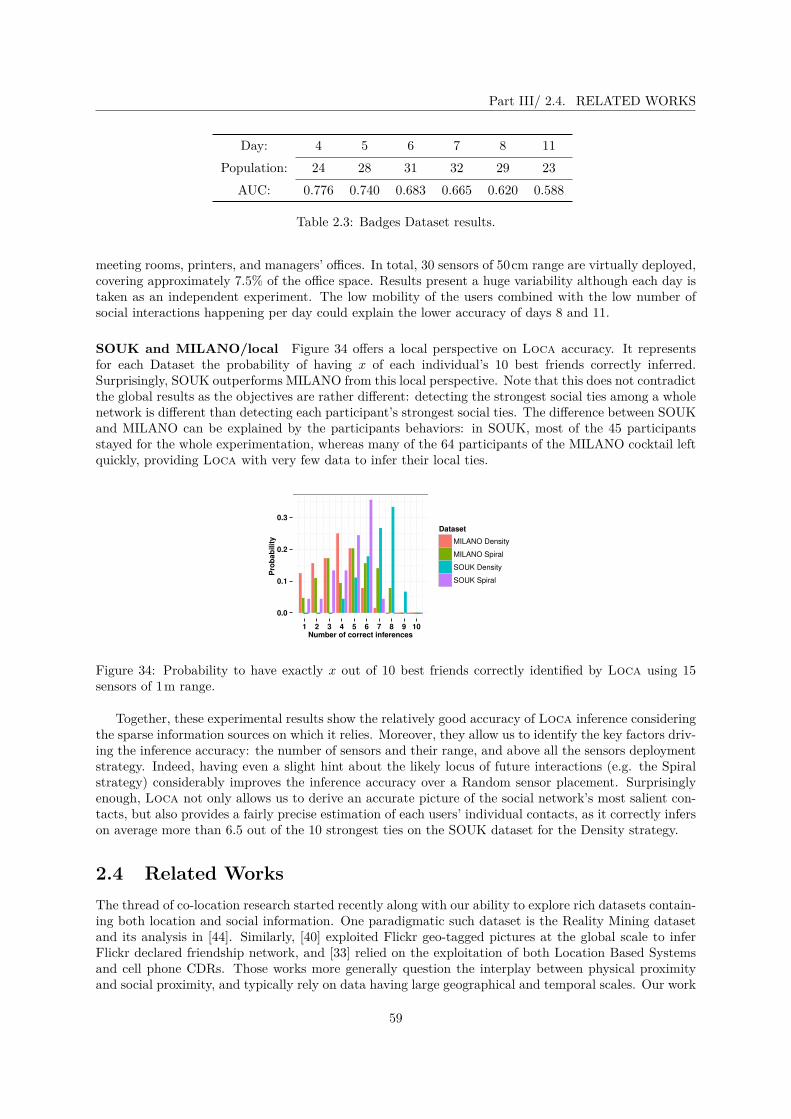
Part III/ 2.4. RELATED WORKS

Day: 4 5 6 7 8 11Population: 24 28 31 32 29 23

AUC: 0.776 0.740 0.683 0.665 0.620 0.588

Table 2.3: Badges Dataset results.

meeting rooms, printers, and managers’ offices. In total, 30 sensors of 50cm range are virtually deployed,covering approximately 7.5% of the office space. Results present a huge variability although each day istaken as an independent experiment. The low mobility of the users combined with the low number ofsocial interactions happening per day could explain the lower accuracy of days 8 and 11.

SOUK and MILANO/local Figure 34 offers a local perspective on Loca accuracy. It representsfor each Dataset the probability of having x of each individual’s 10 best friends correctly inferred.Surprisingly, SOUK outperforms MILANO from this local perspective. Note that this does not contradictthe global results as the objectives are rather different: detecting the strongest social ties among a wholenetwork is different than detecting each participant’s strongest social ties. The difference between SOUKand MILANO can be explained by the participants behaviors: in SOUK, most of the 45 participantsstayed for the whole experimentation, whereas many of the 64 participants of the MILANO cocktail leftquickly, providing Loca with very few data to infer their local ties.

0.0

0.1

0.2

0.3

1 2 3 4 5 6 7 8 9 10Number of correct inferences

Pro

bab

ility

Dataset

MILANO Density

MILANO Spiral

SOUK Density

SOUK Spiral

Figure 34: Probability to have exactly x out of 10 best friends correctly identified by Loca using 15sensors of 1m range.

Together, these experimental results show the relatively good accuracy of Loca inference consideringthe sparse information sources on which it relies. Moreover, they allow us to identify the key factors driv-ing the inference accuracy: the number of sensors and their range, and above all the sensors deploymentstrategy. Indeed, having even a slight hint about the likely locus of future interactions (e.g. the Spiralstrategy) considerably improves the inference accuracy over a Random sensor placement. Surprisinglyenough, Loca not only allows us to derive an accurate picture of the social network’s most salient con-tacts, but also provides a fairly precise estimation of each users’ individual contacts, as it correctly inferson average more than 6.5 out of the 10 strongest ties on the SOUK dataset for the Density strategy.

2.4 Related WorksThe thread of co-location research started recently along with our ability to explore rich datasets contain-ing both location and social information. One paradigmatic such dataset is the Reality Mining datasetand its analysis in [44]. Similarly, [40] exploited Flickr geo-tagged pictures at the global scale to inferFlickr declared friendship network, and [33] relied on the exploitation of both Location Based Systemsand cell phone CDRs. Those works more generally question the interplay between physical proximityand social proximity, and typically rely on data having large geographical and temporal scales. Our work

59

Part III/ 2.5. MITIGATION STRATEGIES

focuses on local observation of users’ behaviors (as opposed to, say, day and country-wide CDR-baseduser tracking) in order to stick to the IoT-based sensor use case.

More recent studies exploit the connection of proximity and social ties with a privacy angle [19, 96].These landmark works evaluate the privacy implications of wireless communications in office environ-ments. Having equipped for 3 months a set of 80 university users with tracked mobile phones, the authorsuse the campus Wifi map to locate users and infer, from an eavesdropper perspective, the social contactsof the users as captured by the tracked mobile phone. Their attack assumes the adversary is able to“trilaterate” mobile phones by using both Access Point positions and exfiltered RSSI values. In [96],the authors study the impact of obfuscated location information on co-location attack accuracy. Ourapproach is both more localized in time and space, and assumes that no location information is availableat all.

A closely related study [41] exploits another wireless-related information dataset to infer social con-tacts: the list of known SSIDs often broadcasted by smart phones to speedup the link establishment toAPs. The authors exploit the similarity of SSID lists to infer social proximity. In this approach, the vastvariety of encountered SSIDs allows them to efficiently fingerprint users. In contrast, our approach isgeneric as it does not depend on the specificities of one wireless protocol, and exploits only proximities.

2.5 Mitigation strategiesWe here present some suggestions to mitigate the success of Loca-like attacks. Those strategies areknown: in that respect Loca simply extends the scope of co-location attacks against which strategieshave already been elaborated.

A first step is to prevent Loca from following the same individual when he/she moves across differentsensors. This can be achieved for instance by mix-zones [17], by extending the scope of traditionalLocation Privacy Protection Mechanisms [119, 55], or by simply relying on the use of many pseudonyms—this last solution applies only if the traceability of a user across different sensors is not an importantfeature for the provided services.

Another mitigation is to limit the attack surface of such systems, by avoiding network operations,especially if they contain identifying information. One strategy is to design “silent protocols” such thatthe carried device cannot be inadvertently detected by an eavesdropping device. Since RFIDs can bepassively read at distance, the users can store them in shielded wallets that are available on the market.

2.6 ConclusionIn this part, we presented a framework to capture and analyze mobility data as a tool to extract interac-tion networks. We show that this tool enables to assess the realism and generality of models and traces,allowing us to better understand and simulate human-centered Short Range Communication-based sys-tems for instance.

To the best of our knowledge the dynamics of such a dense crowd had never been assessed thatprecisely before. Analysis reveals that crowd behavior is all but random, demonstrating the need of abetter model toolbox to design and test mobility-resilient software systems.

On the practical side, the Souk platform, which is mostly open source, has been designed as ascalable solution towards analysis of large crowds: although the results presented here are illustrated onan experiment involving 50 persons, the hardware cost and the complexity of software analysis (usingVoronoï-based approach) are both linear with respect to the number of tracked individuals.

One of the applications of Souk is Loca, a simple co-location inference algorithm that has theparticularity of not relying on positioning information. Instead, it uses sensed data to estimate thephysical distance between sensors. The so-constructed virtual distances are then used to conduct theco-location inference attack. Experimental results show that Loca inference remains accurate even ifthe monitored space is sparsely covered, and highlights the importance of the sensor placement strategyin such contexts.

60


Loca shows that location is not required to conduct co-location attacks. This conclusion strikes thepotential privacy issue of trending IoT devices that could become potential attack surfaces for co-locationattacks. Such attacks could be conducted either by directly monitoring users’ proximity (i.e., altering thedevice’s firmware to report nearby users), or for instance by monitoring the web page requests generatedby close users’ smart phones as Loca requires no information about the sensors themselves.

Going further users’ privacy, Loca demonstrates a potential risk for service providers in the Internetof Things ecosystem: even though service providers may not store positioning information of deployedcommunicating objects, performing Loca on the logs of users-objects interaction will provide lots ofinformation on objects physical repartition. As such, by raising this issue over exploitation of users-objects interaction logs, we advocate the deployment of more decentralized architectures for sustainableubiquitous systems deployment.

This part only spans the first results obtained around the Souk platform. Many research directionsopened around these original works. Among those directions, one is to design models that reflect moreclosely crowd connectivity dynamics. Another direction is to study this evolving connectivity following agraph-theoretic perspective: like most observed static interaction networks that exhibit scale-free prop-erties, we conjecture that the dynamics of interactions in human-carried mobile networks should havecommon properties tied to the geographical and social distribution of users.

61

Part IVA model of G for dynamic graphs

This part is based on the following article:

• The many faces of graph dynamics In Journal of Statistical Mechanics: Theory and Experi-ment, Volume 2017, June 2017 with Yvonne Anne Pignolet, Matthieu Roy, Stefan Schmid.

While the previous chapters provided Gwith some structure depending on some application objectives,this part designs a general structure for G. The goal is to provide a framework in which to represent andimagine many different problems related to a graph G ∈ G and its many different variations (be they dueto noisy measurements or to the intrinsic dynamism of G).

It is interestingly the paper we had most troubles to publish, and what I paradoxically consider so faras my most interesting production. This is probably due to the type of contribution, as it is an articlethat provides many questions and a few answers. Moreover, it is a paper that brings together practicaland theoretical approaches, and that also brought together co-authors from Part II and Part III for themost fruitful interactions.

In the previous part of this document, we focused on the process of measuring graphs based onexperimental data. More precisely, Souk by essence produces dynamic graphs, rather than uniquegraphs. And although the first part provides bad news on the exploitability of observed graphs, the lastchapter provided us with interesting applications around the graph observation that seem to resist thisfirsthand analysis.

One way to explain the quality of the obtained results lies perhaps in the dynamic nature of thegraph observation which is implicitely exploited by Loca :all the graphs composing the observation ofone dynamic graph contain noise but the repeated observation allows to average it out for instance whenextracting a social network from these observations.

Another, maybe more pessimistic analysis of the Souk related results would also reveal that whenjustifying the accuracy of the observations, we never directly compare to some ground truth, eitherbecause it is not available, or because the accuracy of the process is measured using other methods: forinstance, in Loca we only compare local neighborhoods, a measure that does not reflect the quality ofthe global inference. This last point illustrates the importance of an application-related perspective tometrology.

In this last part, we take a more general perspective on both graph metrology and the dynamic graphs.We argue that while both may seem unrelated, the theoretical toolbox to study them both involve thesame essential tool: a distance function. Indeed, both require quantifying the difference between onegraph and another, either because they represent the same process at different instants, or because oneis the noisy observation of the other.

More precisely, this part is dedicated to presenting a family of such distances for the space of graphs.This is achieved by establishing a link between (inter-graph) distances, and centralities, a family ofmeasures that aim at capturing the importance of a given node in a graph. Because the notion ofimportance is not consensual –and is application dependent–, by allowing the transposition of centralitiesto graph distances we allow the distances to also transport application-dependent flavours into thedynamic graph analysis.

63

Part IV/ 1.1. CONTEXT

1.1 ContextHow do real-world networks evolve with time? While empirical studies provide many intuitions andexpectations, many questions remain open. In particular, we lack tools to characterize and quantita-tively compare temporal graph dynamics. In turn, such tools require good observables to quantify the(temporal) relationships between networks.

A natural prerequisite to measure evolutionary distances are good metrics to compare graphs. Theclassic similarity measure for graphs is the Graph Edit Distance (GED) [56]: the graph edit dis-tance dGED(G1,G2) between two graphs G1 and G2 is defined as the minimal number of graph editoperations that are needed to transform G1 into G2. The specific set of allowed graph edit operationsdepends on the context, but typically includes node and link insertions and deletions. While graph editdistance metrics play an important role in computer graphics and are widely applied to pattern analysisand recognition, GED is not well-suited for measuring similarities of networks in other contexts [50]: theset of graphs at a certain graph edit distance d from a given graph G exhibit very diverse characteristicsand seem unrelated.

A similarity measure that takes into account the inherent structure of a graph may however havemany important applications. A large body of work on graph similarities focusing on a variety of usecases have been developed in the past (see our discussion in Section 1.6). Depending on the context inwhich they are to be used, one or another is more suitable. In particular, we argue that graph similaritiesand graph distance measures are also an excellent tool for the analysis, comparison and prediction oftemporal network traces, allowing us to answer questions such as: Do these two networks have a commonancestor? Are two evolution patterns similar? or What is a likely successor network for a given network?However, we argue that in terms of graph similarity measures, there is no panacea: rather, graphs andtheir temporal patterns, come with many faces. Accordingly, we propose to use a parametric, centrality-based approach to measure graph similarities and distances, which in turn can be used to study theevolution of networks.

More than one century ago, Camille Jordan introduced the first graph centrality measure in hisattempt to capture “the center of a graph”. Since then the family of centrality measures has grown largerand is commonly employed in many graph-related studies. All major graph-processing libraries commonlyexport functionality for degree, closeness, betweenness, clustering, pagerank and eigenvector centralities.In the context of static graphs, centralities have proven to be a powerful tool to extract meaningfulinformation on the structure of the networks, and more precisely on the role every participant (node)has in the network. In social network analysis, centralities are widely used to measure the importanceof nodes, e.g., to determine key players in social networks, or main actors in the propagation of diseases,etc.

Today, there is no consensus on “good" and “bad" centralities: each centrality captures a particularangle of a node’s topological role, some of which can be either crucial or insignificant, depending onthe application. Am I important because I have many friends, because I have important friends, orbecause without me, my friends could not communicate together? The answer to this question is clearlycontext-dependent.

We argue that the perceived quality of network similarities or distances measuring the differencebetween two networks depends on the focus and application just as much. Instead of debating theadvantages and disadvantages of a set of similarities and distances, we provide a framework to applythem to characterize network evolution from different perspectives. In particular, we leverage centralitiesto provide a powerful tool to quantify network changes. The intuition is simple: to measure how anetwork evolves, we measure the change of the nodes’ roles and importance in the network, by leavingthe responsibility to quantify node importance to centralities.

Contributions This work is motivated by the observation that centralities can be useful to studythe dynamics of networks over time, taking into account the individual roles of nodes (in contrast to,e.g., isomorphism-based measures, as they are used in the context of anonymous graphs), as well as thecontext and semantics (in contrast to, e.g., graph edit distances). In particular, we introduce the notionof centrality distance dC(G1,G2) for two graphs G1,G2, a graph similarity measure based on a nodecentrality C.

64

Part IV/ 1.1. CONTEXT

We demonstrate the usefulness of our approach to identify and characterize the different faces of graphdynamics. To this end, we study five generative graph models and seven dynamic real world networksin more details. Our evaluation methodology comparing the quality of different similarity measures to arandom baseline using data from actual graph evolutions, may be of independent interest.

In particular, we demonstrate how centrality distances provide interesting insights into the struc-tural evolution of these networks and show that actual evolutionary paths are far from being random.Moreover, we build upon the centrality distance concept to construct dynamic graph signatures. Theintuition is simple: we measure the probability of an update to be considered as an outlier compared toa uniformly random evolution. This allows us to quantify the deviation of a given dynamic network froma purely random evolution (our null-model) of the same structure for a set of centrality distances. Thesignature consisting of the resulting deviation values enables the comparison of different dynamisms ona fair basis, independently from scale and sampling considerations. Indeed, each signature is establishedby comparing a dynamic graph against its corresponding null model generated with same scale, samesampling rate: signatures hide those scale and sampling differences by only capturing deviations from areference model.

Examples To motivate the need for tools to analyse network evolution, we consider two simple exam-ples.

Example 1. [Local/Global Scenario] Consider the three graphs G1, G2, G3 of Figure 35 over fivenodes v1,v2, . . . ,v5: G1 is a line, where vi and vi+1 are connected; G2 is a cycle, i.e., G1 with anadditional link v1,v5; and G3 is G1 with an additional link v2,v4. In this example, we first observethat G2 and G3 have the same graph edit distance to G1: dGED(G1,G2) = dGED(G1,G3) = 1, as theycontain one additional edge. However, in a social network context, one would intuitively expect G3 tobe closer to G1 than G2. For example, in a friendship network a short-range “triadic closure” [75] linkmay be more likely to emerge than a long-range link: friends of friends may be more likely to becomefriends themselves in the future. Moreover, more local changes are also expected in mobile environments(e.g., under bounded human mobility and speed). As we will see, the centrality distance concept of thischapter can capture such differences.

v1 v2 v3 v5

G1: v4

v1 v2 v3 v5

G2: v4

v1 v2 v3 v5

G3: v4

Figure 35: Local/Global scenario: G1 is a line graph, G2 and G3 differ from G1 by only one link.

Example 2. [Evolution Scenario] As a second synthetic example, consider two graphs GL and GS ,where GL is a line topology and GS is a “shell network” (see also Figure 36). How can we characterizeevolutionary paths leading from the GL topology to GS? Note that the graph edit distance does notprovide us with any information about the likelihood or the role changes of evolutionary paths from GLto GS , i.e., on the order of edge insertions: there are many possible orders in which the missing linkscan be added to GL, and these orders do not differ in any way when comparing them with the graphedit distance. In reality, however, we often have some expectations on how a graph may have evolvedbetween two given snapshots GL and GS . For example, applying the triadic closure principle to ourexample, we would expect that the missing links are introduced one-by-one, from left to right.

The situation may look different in technological, man-made networks. Adding links from left toright only slowly improves the “routing efficiency” of the network: after the addition of t edges from left

65

Part IV/ 1.2. PRELIMINARIES

Figure 36: Two evolutionary paths from a line graph GL to a shell graph GS .

to right, the longest shortest path is n− t hops, for t < n−1. A more efficient evolution of the networkis obtained by connecting v1 to the furthest node, adding links to the middle of the network, resultingin a faster distance reduction: after t edge insertions, the distance is roughly reduced by a factor t.

Thus, different network evolution patterns can be observed in real networks. Instead of definingapplication-dependent similarities with design choices focusing on which evolution patterns are moreexpected from a certain network, we provide a framework that allows the joint characterization of graphdynamics along different axes.

1.2 PreliminariesWe here focus on labeled graphs G= (V,E), where vertices v ∈V have unique identifiers and are connectedvia undirected edges e ∈ E. In the following, we denote as Γ(v) the set of neighbors of node v: Γ(v) =w ∈ V s.t. v,w ∈ E. A temporal network trace is a sequence T = [G0,G1, . . . ,Gl], where Gi(V,Ei)represents the network at the ith snapshot.

We focus on node centralities, a centrality being a real-valued function assigning “importance values”to nodes. Obviously, the notion of importance is context-dependent, which has led to many differentdefinitions of centralities. We refer to [22] for a thorough and formal discussion on centralities.

Definition 1.2.1 (Centrality). A centrality C is a function C : (G,v)→R+ that, given a graphG= (V,E)and a vertex v ∈ V (G), returns a non-negative value C(G,v). The centrality function is defined over allvertices V (G) of a given graph G.

By convention, we define the centrality of a node without edges to be 0. We write C(G) to refer tothe vector in (R+)n where the ith element is C(G,vi) for a given order of the identifiers.

Centralities are a common way to characterize networks and their vertices. Frequently studied cen-tralities include the degree centrality (DC), the betweenness centrality (BC), the closeness centrality(CC), and the pagerank centrality (PC) among many more. A node is DC-central if it has many edges:the degree centrality is simply the node degree; a node is BC-central if it is on many shortest paths: thebetweenness centrality is the number of shortest paths going through the node; a node is CC-central ifit is close to many other nodes: the closeness centrality measures the inverse of the distances to all othernodes; and a node is PC-central if the probability that a random walk on G visits this node is high. Weuse the classical definitions for centralities, and the exact formulas are presented in Section 1.5.1 for thesake of completeness.

66

Part IV/ 1.3. CENTRALITY DISTANCE

Finally, we define the graph edit distance GED between two graphs G1 and G2 as the minimumnumber of operations to transform G1 into G2 (or vice versa), where an operation is one of the following:link insertion and link removal.

1.3 Centrality DistanceThe canonical distance measure is the graph edit distance, GED. However, GED often provides limitedinsights into the graph dynamics in practice. Figure 36 shows an example with two evolutionary paths:an incremental (left) and a binary (right) path that go from GL to GS . With respect to GED, thereare many equivalent shortest paths for moving from GL to GS . However, intuitively, not all tracesare equally likely for dynamic networks, as the structural roles that nodes in networks have are oftenpreserved and do not change arbitrarily. Clearly, studying graph evolution with GED thus cannot helpus to understand how structural properties of graphs evolve.

We now introduce our centrality-based graph similarity measure. We will refer to the set of allpossible topologies by G, and we will sometimes think of G being a graph itself: the “graph-of-graphs”which connects graphs with graph edit distance 1. Figure 36 illustrates the concept.

G2

G1

Gi

Figure 37: The graph-of-graph G connects named networks (represented as stars). Two networks areneighboring iff they differ by a graph edit distance of one. The centrality distance defines a distance foreach pair of neighboring graphs.

Definition 1.3.1 (Centrality Distance). Given a centrality C, we define the centrality distance dC(G1,G2)between two neighboring graphs as the component-wise difference:

∀(G1,G2) ∈ E(G),dC(G1,G2) =∑v∈V|C(G1,v)−C(G2,v)|.

This definition extends naturally for non-neighboring graph couples: the distance dC(G1,G2) betweenG1 and G2 is simply the graph-induced distance.

∀G1,G2 ∈ G2,dC(G1,G2) = minP∈PG1,G2

|P |−1∑i=1

dC(P [i],P [i+ 1]),

where PG1,G2 represents the set of all possible paths between G1 and G2 in G and P [i] represents theith graph on path P .

As we will see, the distance axioms are indeed fulfilled for the major centralities. The resultingstructure supports the formal study with existing algorithmic tools. Let us first define the notion ofsensitivity.Definition 1.3.2 (Sensitive Centrality). A centrality C is sensitive if any single edge modification ofany graph G changes the centrality value of at least one node of G. Formally, a centrality C is sensitiveiff

∀G ∈ G,∀e ∈ E(G),∃v ∈ V (G) s.t. C(G,v) 6= C(G\e,v),where G\e is the result of removing edge e from G.

67

Part IV/ 1.3. CENTRALITY DISTANCE

Lemma 1.3.3. DC, BC and CC are sensitive centralities.

Proof. Let G ∈ G, and e= (u,v) ∈ E(G).

Degree centrality: DC(G,u) = DC(G\e,u) + 1: DC is sensitive.

Betweenness centrality: Recall our slightly changed definition of betweenness. Now, BC(G,u) =∑x,w∈V σu(x,w)/σ(x,w).

In G\e, all shortest paths are at least as long as in G, and the shortest path between u and vhas increased at least one unit: BC is sensitive.

Closeness centrality: CC(G,u) =∑w∈V \u 2−d(u,w). In G\e, all distances are greater or equal than

in G, and strictly greater for the couple (u,v): CC is sensitive.

It is easy to see that also other centralities, such as cluster centralities and Page Rank centralitiesare sensitive. The distance axioms now follow directly from the graph-induced distance.

Theorem 1.3.4. For any centrality C, dC is a distance on G iff C is sensitive.

Proof. We show that dC is a metric on G:

Separation ∀G1,G2 ∈ G,dC(G1,G2)≥ 0 since all summands are non-negative.

Coincidence If G1 = G2, we have∑v∈V |C1(v)−C1(v)| = 0. If G1 6= G2 and C is sensitive, since

∀G∈N(G1),dC(G1,G)> 0, necessarily dC(G1,G2)> 0. For the sake of contradiction, assume C isnot sensitive: ∃G∈ G,e∈E(G) s.t. ∀v ∈G,C(G,v) =C(G\e,v), and therefore dC(G,G\e) = 0with G 6=G\e: dC is not a metric.

Symmetry Straightforward since |C(G2,v)−C(G1,v)|= |C(G1,v)−C(G2,v)|.

Triangle inequality Observe that the neighbor-based dC definition associates each edge of G with astrictly positive weight. The multi-hop distance dC is the weighted shortest path in G given thoseweights. Since the weighted shortest path obeys the triangle inequality for strictly positive weights,dC does as well.

The centrality distance metric of Definition 1.3.1 however comes with a major drawback: it is impos-sible to compute in practice. Thus, we propose the following approximate version:

Definition 1.3.5 (Approximate Centrality Distance). Given a centrality C, we define the approximatecentrality distance dC(G1,G2) between any two graphs as the component-wise difference:

∀(G1,G2), dC(G1,G2) =∑v∈V|C(G1,v)−C2(G2,v)|.

Note that dC ≤ dC always holds. While the approximate distance can be far from the exact one inthe worst case, it features some interesting properties.

We conclude by noting that given two centralities C1 and C2 and two arbitrary graphs G1 and G2with n nodes, the respective distances are typically different, i.e., dC1(G1,G2) 6= dC2(G1,G2). Hence,using a set of different centrality distances, we can explore the variation of the graph dynamics in morethan one “dimension”.

68

Part IV/ 1.4. METHODOLOGY

1.4 MethodologyIn order to characterize the different faces of graph dynamics and to study the benefits of centrality-basedmeasures, we propose a simple methodology. Intuitively, given a centrality capturing well the roles ofdifferent nodes in a real-world setting, we expect the centrality distance between two consecutive graphsnapshots Gt and Gt+1 to be smaller than the typical distance from Gt to other graphs that have thesame GED.

To verify this intuition, we define a null model for evolution. A null model generates networks usingpatterns and randomization, i.e., certain elements are held constant and others are allowed to varystochastically. Ideally, the randomization is designed to mimic the outcome of a random process thatwould be expected in the absence of a particular mechanism [58]. Applied to our case, this means thatstarting from a given snapshot Gt that represents the fixed part of the null model, if the evolution followsa null model, then any graph randomly generated from Gt at the given GED is evenly likely to appear.

Concretely, for all consecutive graph pairs Gt and Gt+1 of a network trace, we determine the graphedit distance (or “radius”) R = dGED(Gt,Gt+1). Then, we generate a set St+1 of k = 100 samplegraphs (Hi)i=1..k at the same GED R from Gt uniformly at random. That is, to create Hi, we first startfrom a copy of Gt and select R node pairs, (ul,wl) ∈ V 2,1 ≤ l ≤ R, uniformly at random. For each ofthese pairs (ul,wl) we add the edge (ul,wl) to Hi if it does not exist in Gt or we remove it if it wasin Gt originally. Such randomly built sample graphs at the same graph edit distance allow us to assessthe impact of a uniformly random evolution of the same magnitude from the same starting graph Gt:∀Hi ∈ St+1,dGED(Gt,Hi) = dGED(Gt,Gt+1). In other words, Gt is the pattern and the evolution to Hiat graph edit distance R is the randomized part of the null model1.

As a next step, given a centrality C, we compare Gt+1 with the set St+1 that samples the evolutionfollowing the null model. We consider that Gt+1 does not follow the null model if it is an outlier inthe set St+1 for the centrality C. Practically, Gt+1 is considered an outlier if the absolute value of itsdistance from Gt minus the mean distance of St+1 to Gt is at least twice the standard deviation, i.e., if

|dC(Gt,Gt+1)− µ(dC(Gt,x),x ∈ St+1)| > 2σ(dC(Gt,x),x ∈ St+1).

Given a temporal trace T , we define pC,T as the fraction of outliers in the trace for centrality C. Anensemble of such values pCi,T for a set of centralities C = C1, . . . ,Ck is called a dynamic signature ofT .

1.5 Experimental Case StudiesBased on our centrality framework and methodology, we can now shed some light on the different facesof graph dynamics, using real world data sets.

• Caida (AS): This data captures the Autonomous Systems relationships as captured by the Caidaproject. Each of the 400 snapshots represents the daily interactions of the 1000 first AS identifiersfrom August 1997 until December 1998 [78].

• ICDCS (ICDCS): We extracted the most prolific authors in the ICDCS conference (IEEE Inter-national Conference on Distributed Computing Systems) and the co-author graph they form fromthe DBLP publication database (http://dblp.uni-trier.de). This trace contains 33 snapshotsof 691 nodes and 1076 collaboration edges. The timestamp assigned to an edge corresponds to thefirst ICDCS paper the authors wrote together. Clearly, the co-authorship graph is characterizedby a strictly monotonic densification over time.

• UCI Social network (UCI): The third case study is based on a publicly available dataset [97],capturing all the messages exchanges realized on an online Facebook-like social network between1882 students at University of California, Irvine over 7 months. We discretized the data into adynamic graph of 187 time steps representing the daily message exchanges among users.

1This is the least constrained randomization of network evolution w.r.t. the graph edit distance. More refined nullmodels may preserve other structural graph properties in the sample graphs, e.g., their densities. The original publicationalso describes results obtained for a null model that guarantees the average degree of Gt+1 in the sample graphs.

69

http://dblp.uni-trier.de

Part IV/ 1.5. EXPERIMENTAL CASE STUDIES

• Hypertext (HT): Face-to-face interactions of the ACM Hypertext 2009 conference attendees. 113participants were equipped with RFID tags. Each snapshot represents one hour of interactions [78].

• Infectious (IN): Face-to-face interactions of the “Infectious: Stay away” exhibition held in 2009.410 Participants were equipped with RFID tags. Each snapshot represents 5 minutes of the busiestexhibition day [78].

• Manufacture (MA): Daily internal email exchange network of a medium-size manufacturingcompany (167 nodes) over 9 months of 2010 [78].

• Souk (SK): This dataset captures the social interactions of 45 individuals during a cocktail,see [71] for more details. The dataset consists of 300 snapshots, describing the dynamic interactiongraph between the participants, one time step every 3 seconds [71].

05000

1000015000

0300600900

0

1000

2000

0100200300400

050

100150200

0

200

400

0204060

0 100 200 300 400 0 10 20 30

0 50 100 150 0 10 20 30 40

0 25 50 75 100 0 50 100 150 200

0 100 200 300t

Number of edges GED

CAIDA ICDCS

UCI HyperText

Infectious Manufacturing

Souk

Figure 38: Number of edges and graph edit distance GED in the network traces.

Figure 38 provides a temporal overview on the evolution of the number of edges in the network andthe GED between consecutive snapshots. Some of the seven datasets exhibit very different dynamics:one can observe the time-of-day effect of attendees interactions on Hypertext, and the day-of-week effecton Manufacture. UCI, Hypertext, Infectious and Manufacture all exhibit a high level of dynamics withrespect to their number of links. This is expected for Infectious, as visitors come and leave regularly andrarely stay for long, but rather surprising for Manufacture.

The density of Caida slowly increases, and with a steady GED. Similarly, the number of co-authoredges of ICDCS steadily increases over the years, while the number of new edges per year is relativelystable. The number of days of the conference Hypertext and the fact that conference participants sleepduring the night and do not engage in social activity is evident in the second trace. The dynamic patternof the online social network UCI has two regimes: it has a high dynamics for the first 50 timestamps,and is then relatively stable, whereas Souk exhibits a more regular dynamics. Generally, note that GEDcan be at most twice as high as the maximal edge count of two consecutive snapshots.

70


1.5.1 Centrality Distances over TimeTo instanciate our framework, we picked a standard set of centralities:Degree Centrality DC: Recall that Γ(v) is the set of neighbors of a node v. The degree centrality isdefined as:

DC(G,v) = |Γ(v)|.

Betweenness Centrality BC: Given a pair (v,w)∈ V (G)2, let σ(v,w) be the number of shortest pathsbetween v and w, and σx(v,w) be the number of shortest paths between v and w that pass through x∈ V .The betweenness centrality is:

BC(G,v) =∑

x,w∈Vσv(x,w)/σ(x,w).

For consistency reasons, we consider that a node is on its own shortest path, i.e., σv(v,w)/σ(v,w) = 1,and, by convention, σv(v,v)/σ(v,v) = 0. If G is not connected, each connected component is treatedindependently (σ(x,w) = 0⇒∀v,σv(x,w)/σ(x,w) = 0).Ego Centrality EC: Let Gv be the subgraph of G induced by (Γ(v)∪v). The ego centrality is:

EC(G,v) =BC(Gv,v).

Closeness Centrality CC: Let δG(a,b) be the length of a shortest path between vertices a and b in G.The closeness centrality is defined as:

CC(G,v) =∑

w∈V \v

2−δG(v,w).

Pagerank Centrality PC: Let 0 < α < 1 be a damping factor (i.e. the probability for the randomwalk to stop [98]). The pagerank centrality of G is defined as:

PC(G,v) = 1−αn

+α∑

w∈V \v

PC(G,w)|Γ(w)| .

Cluster Centrality KC: The cluster centrality of a node v is the cluster coefficient of v, i.e., thenumber of triangles in which v is involved divided by all possible triangles in v’s neighborhood. Byconvention, KC(G,v) = 0 for |Γ(v)|= 0, and KC(G,v) = 1 for |Γ(v)|= 1. For higher degrees:

KC(G,v) = 2|j,k s.t. (j,k) ∈ Γ(v)2,(j,k) ∈ E||Γ(v)|(|Γ(v)|−1) .

Figure 39 presents examples of the results of our comparison of random graphs with the same graphedit distance GED as real-world network traces. The red dashed lines represent the centrality distancesof Gt and Gt+1. The distribution of dC values from Gt to the 100 randomly sampled graphs of St+1 isrepresented as follows: the blue line is the median, while the gray lines represent the 2σ outlier detectionwindow.

For most graphs under investigation and for most centralities it holds that the induced centralitydistance between Gt and Gt+1 is often lower than between Gt and an arbitrary other graph with thesame distance. There are however a few noteworthy details.

Hypertext and Infectious exhibit very similar dynamics compared from a GED perspective as shownin Figure 38. Yet from the other centralities’ perspective, their dynamism is very different. Consider forinstance Infectious for PC, where the measured distance is consistently an order of magnitude less thanthe sampled one. This can be understood from the link creation mechanics: in Infectious, visitors atdifferent time periods never meet. By connecting these in principle very remote visitors, the null modeldynamics creates highly important links. This does not happen in Hypertext where the same group ofresearchers meet repeatedly. In the monotonically growing co-authorship network of ICDCS, we canobserve that closeness and (ego) betweenness distances grow over time, which is not the case for theother networks in Figure 39.

71


101

102

103

110

103104

10-610

-3101

100.610

101.6

10-1110

EC

BC

CC

KC

PC

0 10 20 30 40

Distance

10

102

103

110103105

107106

103

10

102

1

10

EC

BC

CC

KC

PC

0 25 50 75round

Distance

10

102103

10

103106

10-7

10-5

10-3

1010102

10101.5

EC

BC

CC

KC

PC

0 10 20 30

Distance

1.5

Hypertext Infectious ICDCS

Figure 39: Centrality distance between Gt and Gt+1 in dashed red lines and between Gt and 100 graphswith the same GED as Gt and Gt+1 in solid blue lines representing the median, 2σ bars in grey. EC: Egocentrality, BC: Betweenness centrality, CC: Closeness centrality, KC: Cluster centrality, PC: Pagerankcentrality.

When looking at other centrality distances, we observe that even though the local structure changes, adifferent set of properties remains mostly unaltered across different networks. Moreover, for some (graph,distance) pairs, like KC on ICDCS, CC on Hypertext, or PC on Infectious, the measured distance is ordersof magnitude lower than the median of the sampled ones. This underlines a clear difference betweenrandom evolution and the observed one from this centrality perspective: the link update dynamics isbiased.

1.5.2 Dynamics Signature

Figure 40 summarizes the pC,G signatures for C ∈ CC,EC,BC,PC,KC applied to 7 real and 5 syntheticgraphs in the form of a histogram chart—for synthetic graphs, each point is the average of 50 independentrealizations of the model, and |St|= 100. That is, each chart represents the probability of having graphevolutions being outliers with respect to the null model for the corresponding centralities. Interestingly,this “distinction ratio” is not uniform among datasets. On Caida, Infectious and UCI, the ratio is highfor local centralities such as PageRank and Clustering, and low for global centralities such as Closenessor Betweenness. On the contrary, Hypertext and Manufacture exhibit large ratios for global centralitiesand small ratios for local centralities. Both local and global centralities perform well on Souk. Thedifference of these behaviors show that these graphs adhere to different types of dynamics.

To complement our observations on real networks with graph snapshots produced according to amodel, we investigated graph traces generated by some of the most well-known models: Erdős-RényiER [46], random regular RR [123], Barabasi-Albert BA [14] and preferential attachment [35] graphs withan equal number of node and edge events (CMHALF) and with the number of node events dependinglogarithmically on the time (CMLOG). Perhaps the most striking observation is that all tested dynamicnetwork models have low pC,T values for all C. This is partly due to the fact that the graph edit distancebetween two subsequent snapshots is one and thus the centrality vectors do not vary as much as betweenthe snapshots and the sampled graphs of the same graph edit distance for the real networks. Moreover,these randomized synthetic models are closer to the null model, and lack some of the characteristics (likelink locality) of real world networks. Furthermore, we observe that each random network model exhibitsdistinct dynamics signatures, with ER being closest to the null model.

72

Part IV/ 1.6. RELATED WORK

BA CMHALF CMLOG ER

HT IN MA SK

0.00

0.25

0.50

0.75

1.00

0.00

0.25

0.50

0.75

1.00

0.00

0.25

0.50

0.75

1.00

PC KC EC BC CC PC KC EC BC CC PC KC EC BC CC PC KC EC BC CC

P(C

,G)

RR CA ICDCS UCI

Figure 40: Histogram representation of the different facets of graph dynamics, the dynamics signatures.For each data set, a histogram chart for the different centralities is depicted, showing pC,T , the probabilitythat Gt+1 is an outlier w.r.t. the null model for the corresponding centrality. Synthetic scenarios aredepicted in blue, real scenarios in red. The black line at 5% represents the null model, i.e., the fractionof graphs that are at distance at least 2σ from the mean in a normal distribution. Synthetic datasets:BA: Barabasi-Albert, CMHALF: Preferential attachment—equiprobable nodes and edge events CMLOG:Preferential attachement—node events decay in log, ER: Erdös-Rényi, RR: Random Regular. Real-lifedatasets: CA: Caida, ICDCS: ICDCS co-authors, UCI: Online social network of UCI, HT: Hypertextconference, IN: Infectious MA: Manufacture mails, SK: Souk cocktail.

1.6 Related WorkTo the best of our knowledge, this approach is the first to combine the concepts of centralities and graphdistances. In the following, we review related work in the two fields in turn, and subsequently discussadditional literature on dynamic graphs.

Graph characterizations and centralities. Graph structures are often characterized by thefrequency of small patterns called motifs [92, 117, 132], also known as graphlets [109], or structural signa-tures [36]. Another important graph characterization, which is studied in this paper, are centralities [24].Dozens of different centrality indices have been defined over the last years, and their study is still on-going, with no unified theory yet. We believe that our centrality distance framework can provide newinputs for this discussion.

Indeed, one of the recurring critics about centralities is that they lack a formal specification. Forinstance [22] says: "While many measures of centrality have been proposed, the category itself is notwell defined (..). The one thing that all agree on is that centrality is a node-level construct. But whatspecifically defines the category?". Our approach, by connecting both concepts, could allow for a differenttake on the problem and structure the space of centralities by exploring the properties of the distancesthey define.

Graph similarities and distances. Graph edit distances have been used extensively in the contextof inexact graph matchings in the field of pattern analysis. We refer the reader to the good survey byGao et al. [56]. Soundarajan et al [121] compare twenty network similarities for anonymous networks.

73

Part IV/ 1.7. CONCLUSION

They distinguish between comparison levels (node, community, network level) and identify vector-based,classifier-based, and matching-based methods. Surprisingly they are able to show that the results ofmany methods are highly correlated. NetSimile [18] allows to assess the similarity between k networks,possibly with different sizes and no overlaps in nodes or links. NetSimile uses different social theories tocompute similarity scores that are size-invariant, enabling mining tasks such as clustering, visualization,discontinuity detection, network transfer learning, and re-identification across networks. The Deltaconmethod [49] is based on the normed difference of node-to-node affinity according to a Belief Propagationmethod. More precisely, the similarity between two graphs is the Root Euclidean Distance of theirtwo affinity matrices or an approximation thereof. The authors provide three axioms that similaritiesshould satisfy and demonstrate using examples and simulations that their similarity features the desiredproperties of graph similarity functions. Our work can be understood as an attempt to generalize theinteresting approach by Faloutsos et al. in [49], which derives a distance from a normed matrix difference,where each element depends on the relationships among the nodes. In particular, we argue that there isno one-size-fits-it-all measure, and propose an approach parametrized by centralities.

Dynamic graphs. Among the most well-known evolutionary patterns are the shrinking diameterand densification [83]. A lot of recent work studies link prediction algorithms [7, 84, 133]. Others focuson methods for finding frequent, coherent or dense temporal structures [67, 118, 125], or the evolutionof communities and user behavior [52, 136].

Another line of research attempts to extend the concept of centralities to dynamic graphs [38, 73, 82,126]. Some researchers study how the importance of nodes changes over time in dynamic networks [126].Others define temporal centralities to rank nodes in dynamic networks and study their distribution overtime [73, 82]. Time centralities which describe the relative importance of time instants in dynamicnetworks are proposed in [38]. In contrast to this existing body of work, our goal is to facilitate thedirect comparison of entire networks and their dynamics, not only parts thereof.

A closely related work but using a different approach is by Kunegis [77]. Kunegis studies the evolutionof networks from a spectral graph theory perspective. He argues that the graph spectrum describes anetwork on the global level, whereas eigenvectors describe a network at the local level, and uses theseresults to devise link prediction algorithms.

1.7 ConclusionThis work proposes a centrality-based distance measure, and introduces a simple methodology to studythe different faces of graph dynamics. Motivated by the observation that in terms of graph similaritymeasures, there is no “one size fits it all”, our experiments confirm that the evolution patterns of dynamicnetworks are not universal, and different networks need different centrality distances to describe theirbehavior.

We observe that the edges in networks represent structural characteristics that are inherently con-nected to the roles of the nodes in these networks. These structures are maintained under changes, whichexplains the inertia of centrality distance which capture these properties. This behavior can be used todistinguish between natural and random network evolution.

We believe that this work opens a rich field for future research. We focused on five well-knowncentralities and their induced distances, and showed that they feature interesting properties when appliedto the use case of dynamic social networks. However, we regard our approach as a distance framework,which can be configured with various additional centralities and metrics, which may not even be restrictedby distance metrics, but can be based on the angles between centrality vectors or use existing correlationmetrics (e.g., Pearson correlation, Tanimoto coefficient, log likelihood). Finally, exploiting the propertiesof centrality distances, especially their ability to distinguish and quantify between similar evolutionarytraces, also opens the door to new applications, such as graph interpolation (what is a likely graphsequence between two given snapshots of a trace) and extrapolation, i.e., for link prediction algorithmsbased on centralities.

While these works were mostly presented under the perspective of dynamic networks, recent works[53] expose their transposability to the problem of network sampling. Indeed the authors exploit the samemodel of dynamic graphs containing labelled nodes, and exploit distances on G to study the convergence

74


of sampling processes before exploring higher-level operations like Principal Component Analysis. Thebeauty of the distance abstraction is indeed its capacity to provide tools for analysing graph variationsthat apply both to metrology and dynamism by considering both as processes that will slightly changea graph.

75


76

Part VConclusion and Future Works

It is now time to conclude this document. I will here first recall the different sections and their relationto our tour on graphs metrology, before higlighting some of the shortcomings of this thesis. Lastly, I willpresent some research directions that might provide interesting perspectives on the subject.

In the introduction, we presented the binary graph notion and its application to model real-worldinteracting systems. We have seen that this modeling operation is error-prone, and advocated for ametrological perspective on this operation. Moreover, in the introduction we mostly focused on thegeneral approach: how to represent my system using a binary graph, and what are the impacts of suchapproach ? While this abstraction has originally been applied to systems where interactions and entitiesare reasonably well defined, we have seen that the graph abstraction is today applied to models whereinteractions might be hard to capture, or evolve over time, or both. This introduction presented graphcapture (i.e. matching a real system with its graph abstraction) as a central problem of this abstractionprocess.

The first chapter presents a theoretical perspective on one method to capture graphs (that is, to matchreal systems with their binary graph abstraction): tomography. We studied algorithmic properties oftwo such tomography approaches yielding mostly negative results: in theory tomography is costly anderror-prone. This raised a structuring contradiction: why are graphs so successful even though the meansof observing these is in theory inaccurate and expensive ?

In the second part, we focused on one family of graphs: the social interaction networks. We presenteda platform named Souk to experimentally capture such graphs, and analysed the obtained results. Then,in the context of privacy, we presented another method to capture such graphs, namely inference basedon co-location information. This part introduced the important notion of models, that can from a high-level perspective be seen as particular sub-regions of the space of possible graphs G that concentrate theobservables of one particular process. We have also illustrated through the privacy part that the needfor accuracy can be relaxed depending on the context: identifying 60% of the links of a graph can beseen as successful in some contexts. Finally, this part led us to consider the temporal dimension of theproblem: by repeatedly capturing the interactions of a real system, it is possible to extract meaningfulglobal trends and average out some of the noise introduced by the graph-level sampling. As a result, itis possible to extract useful information out of rather noisy measurements.

These results point a source of this contraction between the practical use and the theoretical analysisof graph abstractions: real systems exhibit some internal and temporal coherence that is not accountedfor in the theoretical studies. The necessity of developing theoretical tools to assess this coherence servesas a transition towards the next part.

In the last part, we provide a framework that could host observations regarding noise, graph dy-namism, and more generally the coherence of graph objects over time. By considering dynamic graphsas trajectories in the space of all possible graphs, and by providing this space with adequate distancemeasures, we observe interesting results. Indeed, the inspected dynamic graphs evolve very differentlyand in a more deterministic fashion than our random models. The consequences of such observationsare twofold: first, these bring some hope to circumvent sensitivity of individual graphs to errors of thesampling process by exploiting the temporal coherence of these observations. Second, by allowing suchreflexions, it suggests that this broader perspective of dynamic graphs and trajectories in the space ofgraphs is a good abstraction that could prove fruitful.

77

Part V/ 1.1. SOME SHORTCOMINGS OF THIS DOCUMENT

1.1 Some shortcomings of this documentIn this section, we elaborate on the limits of this thesis.

Delimiting the boundaries of these worksThe ambition of this document is to concatenate different publications produced for different audiencesinto a single document coherently adressing one scientific question. While the diversity of these docu-ments helps to broaden the picture around the problem of graph capture, focusing on specific problemsmostly provides detailed perspectives that are arguably weakly inter-related.

Circumventing this effect could be achieved using two concurrent approaches: on one hand, findinga common system model (that would for instance precisely define what is meant by "real interactingsystem"), while on the other hand convince that the proposed conclusions hold at this common systemmodel.

While the last part of this manuscript achieves so by considering "dynamic graphs" at large, suchapproach would require an extensive additionnal work for the two first parts.

Graph TheoryMoreover, by focusing right away our study on graphs representing "real" systems, we implicitely eludea huge branch of graph theory. Indeed, not all graphs are meant to be the direct abstraction of somereal interaction network (consider for instance infinite graphs and grammars [30]).

This frontier is however arbitrary, and while the question of "what is real" is beyond the horizon ofthis document, precisely delimiting the scope of the presented results (i.e. clarifying where those resultsdo not apply) would have improved the contribution. An important observation to nuance this aspect isto observe that generally we manipulate labelled graphs, a practical difference that mechanically excludesa large body of theoretic research on isomorphic graphs.

In addition, this document mixes conclusions driven by theoretical studies (Part 1) and experimentalobservations (Part 2,3) without much distinction. The goal is to provide arguments from both approachesin hope to find a middle ground between the top-down (Theory to practice) and the bottom-up (Practiceto theory) methodologies. However, by doing so we implicitly put correctness (theory’s quality criteria)and representativity (experience quality criteria) at the same level, which is misleading.

A more precise modelling of use casesThe introduction clearly presented the final application as one of the pillars of a metrology study. Beyondpointing inaccuracies, the goal of a metrological reasoning is to assess whether the phenomena aremeasured precisely enough for the considered application, hence the necessity of having the target usecase correctly defined. There is no such attempt to chart the space of possible applications in thisdocument. Indeed, these works usually pursue another approach by abstracting the use case. Forinstance, instead of trying to model all distributed applications in Part 2, we abstract the notion ofapplication arbitrarily by a broadcast, arguing that most applications rely at some point on broadcast.

First, this opinion might not be consensual. Another approach that could for instance be based onsome paradigmatic applications, but again establishing a consensus on the set of paradigmatic applica-tions is difficult.

A more subtle downside of the "abstractive approach" (i.e. most applications rely on broadcast)is to make the contributions more abstract, which in turn reduces their impact on potentially inter-ested audiences. For instance, the distributed application developer would probably have an easier timetransposing his problem onto a couple of concrete applications.

Pipes and flowsWhen capturing interaction structures, the goal is often to infine provide information about the flows(be they information, contagion, data packet). However, all the thinking and modelling is done at thelink (pipe)-level, exploiting the intuition that flows need to be carried along pipes. While this seems tobe an interesting distinction, it is not carried throughout the document. For instance, tomography inPart 1 relies on flows to establish the pipe network, while Souk somewhat directly infers links at thepipe level.

While this confusion is common in other academic works, I believe it is problematic to maintain itthroughout the document. Lifting such confusion would however require a broad exploration of the largebody of graph-related works trying to identify patterns that belong predominantly to either flow-basedor link-based approaches.

78

Part V/ 1.2. FUTURE WORKS

Machine LearningThis manuscript tackles networks, models and notions like inference, accuracy without ever looking atmachine learning. While some machine learning techniques (especially neural networks) could have beeneither used as tools, either analysed as research objects in these works, it is also important to observethat neural networks have little to do with the networks of this document.

Neural networks typically represent a corner case of "real" networks – as these networks arguably donot represent reality, but are built as simple regressions of one phenomenon of the real world that canhypothetically be represented as a function. Moreover, they represent a very particular type of network(they are weighted, directed, and most importantly cycle-free), which would not fit the scope of thisdocument.

This family of networks however represent a very interesting research subject, as those networks are atthe focal point of an ever growing attention from the scientific and industrial community. One particularlyinteresting aspect of neural networks is their use as recommenders. Take for instance Youtube: therecommendations produced by its neural network [39] translate into hyperlinks on webpages that can beseen as a graph that one could call a recommendation network. Investigating on the connections betweenthe nature of the recommender, the input data and the resulting recommendation network ends up (inmy humble opinion) being very close to for instance the problem of monitoring network infrastructures.Both networks are the product of artifacts (in its sociological meaning) that roughly involve algorithmsand distributed input, and end up being complex objects for which no easy description exists. Finally,recommendation networks are also difficult to capture because of their scale (which typically only allowpartial exploration), their dynamism, so that their capture and exploitation raises problems that couldfall in the scope of this document.

1.2 Future works

1.2.1 Theory

Dynamic graphsThis approach of dynamics and tomography on G allows to develop some interesting perspectives. Per-haps the most pressing need is for models of dynamic graphs. Such models would allow for instance todirectly generate connection patterns without the intermediary step of generating node positions, butalso maybe capture the effects of slow sampling, or alleviate problems of iid link measurement errors.

We’ve seen that each static graph model m defines a probability distribution on G: they associateeach G∈ G with a probability pm(G). Chapter IV interprets G as a graph, considering each G as a vertexof G, each link of G capturing an atomic topology evolution. This view exhibited a link between thesimplest graph distance (the graph edit distance) and the simplest centrality (the degree centrality).

Since dynamic graphs define trajectories in G, let us consider trajectories using a standard tool:random walks. The simplest form of random walk, the uniform random walk u: since G is regular, thestationary distribution of G is uniform (see e.g. [87]): ∀G ∈ G,pu(G) = 1/|G|. Consider now the simpleststatic graph model, the Erdos-Renyi (uniform) graph model er. It has one parameter, p, the probabilityof each individual link. If p= 1/2, it is relatively easy to see that per = pu: pick a graph G, fix one edgee, the probabilty to generate a graph having e is 1/2 (same with non-edges). Therefore the probabilityto obtain exactly G is (1/2)n(n−1)/2. In other words, there is a direct connection between the weightsin G, and random graph models. I believe it is important to explore this intriguing yet natural relationand try to transpose it to other models.

Indeed since our centrality-induced distances decorate the edges of G with weights, and since thoseweights could be used to bias random walks, each centrality induced distance would then be translatedin a static graph model. This connection would work both ways: the standard, from the edge weights(centralities) to stationary distribution (static graph models), and the inverse: from the static graphmodels to graph distances and centralities. Note however that due to the enormous dimensions of G, thisquestion is mostly of theoretical interest. The very particular structure of G however probably enablesmany optimisations and simplifications that might help.

79


In addition to connecting static graph models and distances, this random walk approach also bringsdynamic models as a bonus: each sequence of random walk steps is a dynamic graph. Interestingly,dynamic graphs generated by this model would in addition comply with the experimental observationsof Chapter IV: random walks would statistically minimise the induced distance compared to uniformwalks. Moreover, this connects with the intuition: all we know about real graphs is through the captureof such objects. But these objects (consider for instance a social network) existed long before themeasurement and continue existing after: as if we captured them at a random time of their existence.In that sense it is exactly the definition of a stationary distribution.

Finally, I also believe the quality of a model also resides in its acceptance by the community. Con-structing new models by bringing a temporal depth to static models (static graph models and dynamicgraph models) like this seems more promising than producing new models in the hope they encountersuccess in the scientific community. Such approach would indeed have the benefit of not re-inventingnew models –which would have to be sold to the community, as it would instead allow the transpositionsof old models already accepted by the community.

Link creation mechanismsAnother common pattern of our approaches is the discrete yet important role of the link creation mech-anism: the function responsible of the knitting of our topology. Usually, it is part of the model, like theset of axioms for traceroute, the vnet embedding model, or the hypothesis that individuals are in theplane. I believe an important approach would be to formalise the role of this link creation mechanism, asit implicitely regroups many distinct phenomena that do not necessarily share the same characteristics.For instance, a computer network, a predator/prey network or an author collaboration graph can all beabstracted by a graph, but the underlying dynamics (what leads two nodes to be connected or not) seemradically different. It is surprising that these differences do not translate into topological properties.

Chapter 1 provides interesting observations of the link creation mechanism in the case of individualsin the 2d plane. Indeed, we have seen that simulating random agents moving on the plane providesnot so convincing results, hinting that geographical positions play a secondary role in this link creation.However, the Loca approach constructs a (fairly) good inference graph by reconstructing an approximategeographic map of the physical layout of the problem. In other words, to conduct co-location attackswithout location information, the Loca first reconstructs (virtual) location information. The ambiguousrole of geometry in this example should be investigated. Moreover, while this relation between linksand geometric positions was explored (in the context of Unit Disk Graphs, see e.g. [76]), the dynamicsof an evolving Unit Disk Graph (UDG) have not been studied. That is, given a dynamic graph DG =G1, . . .GT , I cannot precisely answer to the question "can DG be generated from moving individualsin the plane ?". I can verify whether a particular Gi represents a UDG, but not whether DG can begenerated by points moving all along the same UDG.

More generally on the relation between graphs and euclidean spaces, Linial, London and Rabinovichhave this very interesting sentence [85]: "Many combinatorial and algorithmic problems concern eitherdirectly or implicitly the distance, or metric on the vertices of a possibly weighted graph. It is, therefore,natural to look for connections between such questions and classical geometric structures. " I believeour capacity to alternate between discrete representations of networks (graphs) and continuous ones(euclidean embeddings) is a key to fast approximations algorithms, and beyond this, a key to modellingthe dynamism of interaction structures: euclidean spaces enriched with a temporal dimension are acentral tool of physics. There is hence a large toolbox available (notions of speed, acceleration, differentialequations, etc.) that would probably greatly benefit the dynamic graphs analysis.

To summarise, we have seen in this document there is a gap between the practical relevance of graph,and the theoretical analysis of its accuracy. This observation calls for new theoretical tools to graspthis paradox, either from a global perpective based on the study of G, either from a local perspectiveexploring the properties of link creation mechanisms.

1.2.2 Applications

Transparency

80


Another attractive field for understanding link creation dynamics is the algorithmic transparency.Indeed, the Web as we users explore it is in great part constructed by algorithms: filtering and recom-mendation algorithms that choose which information to present, ranking algorithms that select whichinformation to present first, etc. Since the Web is a graph, observing the dynamics of such network canprovide important informations on the internals of these algorithms [90, 91]. Moreover, while modellingsocial networks is intrinsically difficult because of the many parameters that influence each individual’sown decisions, modelling algorithm-produced graphs can be easily done in-vitro with a complete con-trol over simulation parameters. The interest I see in algorithmic transparency is therefore to combinea certain experimental ease (for collecting information and devising models) with an extreme societalimportance.

Indeed, the position of some algorithms in the society’s information flows is now very central. Wecannot leave the full control over these algorithms to some firms led by objectives that will necessarilyat some point conflict with a notion of fair treatment of the information.

Networking and shortest pathsAnother interesting research direction relates to the distinction between flow and pipes. A class of

systems in which this study could start are the graphs used as abstraction of (computer) networkingsystems.

This abstraction is very commonly used to represent datacenter flows, virtual networks, infrastruc-tures, and so on. In some of these approaches, we model the infrastructure as a proxy to model theinformation flows. Information flows are then interpolated as travelling the shortest paths of the infras-tructure. However, multiple shortest paths are very common (in non-tree topologies). Therefore, whenproblems like load balancing or network tomography –that directly relate to information flows– comewith the input of a graph, they are underspecified: the choice of the actual shortest path is not defined.

It seems that refining this view (by formalising some properties on the set of shortest paths of anetwork) can provide considerable improvements in the complexity of the related problems. The relativelyrecent trend of Software Defined Networks, that continue to blur the (artificial) frontier between systemsand networks, constitutes an exciting use-case for such graph-related approaches on networking.

Data collectionFinally, I’d like to stress the importance of data collection approaches. Theory can provide a powerful

framework to abstract and manipulate reality, but in the context of graphs we have seen the primeimportance of models: G is in general a too broad model of reality. Identifying and focusing on subpartsof G is the key to accurate and efficient algorithmic approaches. To achieve this, we need to capture andconstitute databases of dynamic interaction networks.

This task has largely been empowered by the digitalisation of our daily lives. Many of our activitiesare logged, recorded, analysed, generating an ever growing amount of data on our behaviours, ideasand opinions. However, it is important to realise that a large fraction of this data does not meet thestandards of scientific data: it is only accessible to a small part of the community (through collaborationwith firms), and it is collected through rather opaque means (e.g. smartphone applications). It is verydifficult to estimate the biases introduced by the collection (who has a smartphone, which mechanicalTurk users were directed to my ad) and by the collaboration (will I still get data from company X if I saythis about their users). For these reasons, I believe we ought to design open data collection campaigns,and construct datasets allowing researchers to explore in complete freedom and produce reproductibleresearch.

Of course, the constitution of such open data sets raises a number of privacy challenges. Those areimportant challenges that must be addressed. However, there is a huge gap between how privacy isofficially considered in our society and the large scale tracking and personal data open bar organised bythe major data brokers: this question is also a political one [110].

81

Bibliography

[1] H. Acharya and M. Gouda. The weak network tracing problem. In Proc. Int. Conference onDistributed Computing and Networking (ICDCN), pages 184–194, 2010.

[2] H. Acharya and M. Gouda. On the hardness of topology inference. In Proc. Int. Conference onDistributed Computing and Networking (ICDCN), pages 251–262, 2011.

[3] M. Acharya, H. a nd Gouda. A theory of network tracing. In Proc. 11th International Symposiumon Stabilization, Safety, and Security of Distributed Systems (SSS), pages 62–74, 2009.

[4] D. Achlioptas, A. Clauset, D. Kempe, and C. Moore. On the bias of traceroute sampling: or, power-law degree distributions in regular graphs. In Proc. 37th Annual ACM Symposium on Theory ofComputing (STOC), pages 694–703, 2005.

[5] B. Ager, N. Chatzis, A. Feldmann, N. Sarrar, S. Uhlig, and W. Willinger. Anatomy of a largeeuropean ixp. In Proc. ACM SIGCOMM, 2012.

[6] R. Aipperspach, T. Rattenbury, A. Woodruff, and J. Canny. A quantitative method for revealingand comparing places in the home. In Procs. of UbiComp’06, pages 1–18. Springer, 2006.

[7] O. Allali, C. Magnien, and M. Latapy. Internal link prediction: A new approach for predictinglinks in bipartite graphs. Intelligent Data Analysis, 17(1):5–25, 2013.

[8] C. Ambühl, M. Mastrolilli, and O. Svensson. Inapproximability results for maximum edge biclique,minimum linear arrangement, and sparsest cut. SIAM J. Comput., 40(2):567–596, Apr. 2011.

[9] A. Anandkumar, A. Hassidim, and J. Kelner. Topology discovery of sparse random graphs withfew participants. In Proc. SIGMETRICS, 2011.

[10] André Panisson. pymobility: python implementation of mobility models. https://github.com/panisson/pymobility, 2015.

[11] B. Augustin, X. Cuvellier, B. Orgogozo, F. Viger, T. Friedman, M. Latapy, C. Magnien, andR. Teixeira. Avoiding traceroute anomalies with paris traceroute. In Proc. 6th ACM SIGCOMMConference on Internet Measurement (IMC), pages 153–158, 2006.

[12] A. J. Aviv, M. Sherr, M. Blaze, and J. M. Smith. Evading cellular data monitoring with humanmovement networks. In Proc. 5th USENIX Workshop Hot Topics on Security, 2010.

[13] N. Bansal, K.-W. Lee, V. Nagarajan, and M. Zafer. Minimum congestion mapping in a cloud. InProc. 30th PODC, pages 267–276, 2011.

[14] A.-L. Barabási and R. Albert. Emergence of Scaling in Random Networks. Science, 286, 1999.

[15] P. Barford, A. Bestavros, J. Byers, and M. Crovella. On the marginal utility of network topologymeasurements. In Proc. 1st ACM SIGCOMM Workshop on Internet Measurement (IMW), pages5–17, 2001.

83



Part V/ BIBLIOGRAPHY

[16] F. Benbadis, J. Leguay, V. Borrel, M. Amorim, and T. Friedman. Millipede: a rollerblade posi-tioning system. In Procs. of ACM WiNTECH’06, pages 117–118. ACM, 2006.

[17] A. R. Beresford and F. Stajano. Location privacy in pervasive computing. IEEE Pervasive com-puting, 1:46–55, 2003.

[18] M. Berlingerio, D. Koutra, T. Eliassi-Rad, and C. Faloutsos. Network similarity via multiple socialtheories. In Proc. IEEE/ACM International Conference on Advances in Social Networks Analysisand Mining (ASONAM), pages 1439–1440, 2013.

[19] I. Bilogrevic, K. Huguenin, M. Jadliwala, F. Lopez, J.-P. Hubaux, P. Ginzboorg, and V. Niemi.Inferring social ties in academic networks using short-range wireless communications. In Proceedingsof the 12th ACM workshop on Workshop on privacy in the electronic society, pages 179–188. ACM,2013.

[20] V. D. Blondel, J.-L. Guillaume, R. Lambiotte, and E. Lefebvre. Fast unfolding of communities inlarge networks. Journal of statistical mechanics: theory and experiment, 2008(10):P10008, 2008.

[21] C. Boldrini, M. Conti, and A. Passarella. The sociable traveller: human travelling patterns insocial-based mobility. In Procs. of ACM MobiWAC’09, pages 34–41. ACM, 2009.

[22] S. Borgatti and M. Everett. A graph-theoretic perspective on centrality. Social Networks, 28(4):466–484, 2006.

[23] V. Borrel, F. Legendre, M. D. De Amorim, and S. Fdida. Simps: using sociology for personalmobility. IEEE/ACM Trans. Netw., 17(3):831–842, June 2009.

[24] U. Brandes and T. Erlebach. Network Analysis: Methodological Foundations. LNCS 3418, Springer-Verlag New York, Inc., 2005.

[25] C. Brown, C. Efstratiou, I. Leontiadis, D. Quercia, and C. Mascolo. Tracking serendipitous in-teractions: How individual cultures shape the office. In Proceedings of the ACM Conference onComputer Supported Cooperative Work and Social Computing (CSCW 2014), 2014.

[26] C. Brown, C. Efstratiou, I. Leontiadis, D. Quercia, C. Mascolo, J. Scott, and P. Key. The architec-ture of innovation: Tracking face-to-face interactions with ubicomp technologies. In Proceedings ofthe ACM International Joint Conference on Pervasive and Ubiquitous Computing (Ubicomp 2014),2014.

[27] M. Buchanan. Data-bots chart the internet. Science, 813(3), 2005.

[28] A. Casteigts, P. Flocchini, W. Quattrociocchi, and N. Santoro. Time-varying graphs and dynamicnetworks. International Journal of Parallel, Emergent and Distributed Systems, 27(5):387–408,2012.

[29] D. Caucal. Deterministic graph grammars. Logic and Automata, pages 169–250, 2008.

[30] D. Caucal. On cayley graphs of algebraic structures. arXiv preprint arXiv:1803.08518, 2018.

[31] A. Chaintreau, P. Hui, J. Crowcroft, C. Diot, R. Gass, and J. Scott. Impact of human mobilityon opportunistic forwarding algorithms. IEEE Transactions on Mobile Computing, 6(6):606–620,June 2007.

[32] B. Cheswick, H. Burch, and S. Branigan. Mapping and visualizing the internet. In Proc. USENIXAnnual Technical Conference (ATEC), 2000.

[33] E. Cho, S. A. Myers, and J. Leskovec. Friendship and mobility: user movement in location-basedsocial networks. In Proceedings of the 17th ACM SIGKDD international conference on Knowledgediscovery and data mining, pages 1082–1090. ACM, 2011.

84


[34] M. K. Chowdhury and R. Boutaba. A survey of network virtualization. Elsevier Computer Net-works, 54(5), 2010.

[35] F. R. Chung and L. Lu. Complex graphs and networks, volume 107. American mathematical societyProvidence, 2006.

[36] N. S. Contractor, S. Wasserman, and K. Faust. Testing multitheoretical organizational networks:An analytic framework and empirical example. Academy of Management Review, 2006.

[37] D. J. Cook and L. B. Holder. Substructure discovery using minimum description length andbackground knowledge. J. Artif. Int. Res., 1:231–255, 1994.

[38] E. C. Costa, A. B. Vieira, K. Wehmuth, A. Ziviani, and A. P. C. da Silva. Time centrality indynamic complex networks. arXiv preprint arXiv:1504.00241, 2015.

[39] P. Covington, J. Adams, and E. Sargin. Deep neural networks for youtube recommendations. InRecSys, 2016.

[40] D. J. Crandall, L. Backstrom, D. Cosley, S. Suri, D. Huttenlocher, and J. Kleinberg. Inferring socialties from geographic coincidences. Proceedings of the National Academy of Sciences, 107(52):22436–22441, 2010.

[41] M. Cunche, M.-A. Kaafar, and R. Boreli. Linking wireless devices using information contained inwi-fi probe requests. Pervasive and Mobile Computing, 11:56–69, 2014.

[42] L. Dall’Asta, I. Alvarez-Hamelin, A. Barrat, A. Vázquez, and A. Vespignani. Exploring networkswith traceroute-like probes: Theory and simulations. Theoretical Computer Science, 355(1):6–24,2006.

[43] W. Dong, D. Olguin-Olguin, B. Waber, T. Kim, and A. S. Pentland. Mapping organizationaldynamics with body sensor networks. In International Workshop on Wearable and ImplantableBody Sensor Networks, volume 0, pages 130–135, Los Alamitos, CA, USA, 2012. IEEE ComputerSociety.

[44] N. Eagle, A. S. Pentland, and D. Lazer. Inferring friendship network structure by using mobilephone data. Proceedings of the National Academy of Sciences, 106(36):15274–15278, 2009.

[45] N. Eagle and A. (Sandy) Pentland. Reality mining: sensing complex social systems. PersonalUbiquitous Comput., 10(4):255–268, Mar. 2006.

[46] P. Erdős and A. Rényi. On the evolution of random graphs. Publ. Math. Inst. Hungar. Acad. Sci,5:17–61, 1960.

[47] P. T. Eugster, R. Guerraoui, S. B. Handurukande, P. Kouznetsov, and A.-M. Kermarrec.Lightweight probabilistic broadcast. ACM Transactions on Computer Systems (TOCS), 21(4):341–374, 2003.

[48] G. Even, M. Medina, G. Schaffrath, and S. Schmid. Competitive and deterministic embeddings ofvirtual networks. In Proc. ICDCN, 2012.

[49] C. Faloutsos, D. Koutra, and J. T. Vogelstein. DELTACON: A principled massive-graph similarityfunction. In Proc. 13th SIAM International Conference on Data Mining (SDM), pages 162–170,2013.

[50] M. Faloutsos, P. Faloutsos, and C. Faloutsos. On power-law relationships of the internet topology.In Proc. SIGCOMM, pages 251–262, 1999.

[51] J. Fan and M. H. Ammar. Dynamic topology configuration in service overlay networks: A studyof reconfiguration policies. In Proc. IEEE INFOCOM, 2006.

85


[52] J. Ferlez, C. Faloutsos, J. Leskovec, D. Mladenic, and M. Grobelnik. Monitoring network evolutionusing mdl. In International Conference on Data Engineering (ICDE), pages 1328–1330, 2008.

[53] D. Fraiman, N. Fraiman, and R. Fraiman. Nonparametric statistics of dynamic networks withdistinguishable nodes. Test, 26(3):546–573, 2017.

[54] A. Galati and C. Greenhalgh. Human mobility in shopping mall environments. In Proceedings ofthe Second International Workshop on Mobile Opportunistic Networking, MobiOpp ’10, pages 1–7.ACM, 2010.

[55] S. Gao, J. Ma, W. Shi, and G. Zhan. Ltppm: a location and trajectory privacy protection mech-anism in participatory sensing. Wireless Communications and Mobile Computing, 15(1):155–169,2015.

[56] X. Gao, B. Xiao, D. Tao, and X. Li. A survey of graph edit distance. Pattern Anal. Appl.,13(1):113–129, 2010.

[57] P. Gill, M. Arlitt, Z. Li, and A. Mahanti. The flattening internet topology: Natural evolution,unsightly barnacles or contrived collapse? Passive and Active Network Measurement, pages 1–10,2008.

[58] N. J. Gotelli and G. R. Graves. Null models in ecology. online resources, 1996.

[59] M. S. Granovetter. The strength of weak ties. In Social networks, pages 347–367. Elsevier, 1977.

[60] J.-L. Guillaume and M. Latapy. Complex network metrology. Complex systems, 16(1):83, 2005.

[61] M. Gunes and K. Sarac. Resolving anonymous routers in internet topology measurement studies.In Proc. INFOCOM, 2008.

[62] A. Haider, R. Potter, and A. Nakao. Challenges in resource allocation in network virtualization.In Proc. ITC Specialist Seminar on Network Virtualization, 2009.

[63] K. Herrmann. Modeling the sociological aspects of mobility in ad hoc networks. In Procs. of ACMMSWIM’03, pages 128–129. ACM, 2003.

[64] I. Houidi, W. Louati, and D. Zeghlache. A distributed virtual network mapping algorithm. InProc. IEEE ICC, 2008.

[65] P. Hui, A. Chaintreau, J. Scott, R. Gass, J. Crowcroft, and C. Diot. Pocket switched networks andhuman mobility in conference environments. In Procs. of WDTN’05, pages 244–251. ACM, 2005.

[66] E. Inc. Estimote beacons. http://www.estimote.com, 2016.

[67] R. Jin, C. Wang, D. Polshakov, S. Parthasarathy, and G. Agrawal. Discovering frequent topologicalstructures from graph datasets. In Proc. ACM SIGKDD, pages 606–611. ACM, 2005.

[68] X. Jin, W.-P. Yiu, S.-H. Chan, and Y. Wang. Network topology inference based on end-to-endmeasurements. IEEE Journal on Selected Areas in Communications, 24(12):2182 –2195, 2006.

[69] D. Kamisaka, T. Watanabe, S. Muramatsu, A. Kobayashi, and H. Yokoyama. Estimating positionrelation between two pedestrians using mobile phones. In Procs. of Pervasive Computing’12, pages307–324. Springer Berlin Heidelberg, 2012.

[70] M.-O. Killijian, R. Pasqua, M. Roy, G. Trédan, and C. Zanon. Souk: Spatial observation of humankinetics. Computer Networks, 111:109–119, 2016.

[71] M.-O. Killijian, M. Roy, G. Trédan, and C. Zanon. Souk: social observation of human kinetics. InProceedings of the 2013 ACM international joint conference on Pervasive and ubiquitous computing,pages 193–196. ACM, 2013.

86

http://www.estimote.com


[72] B. Kim, J.-Y. Ha, S. Lee, S. Kang, Y. Lee, Y. Rhee, L. Nachman, and J. Song. Adnext: a visit-pattern-aware mobile advertising system for urban commercial complexes. In Proceedings of the12th Workshop on Mobile Computing Systems and Applications, pages 7–12. ACM, 2011.

[73] H. Kim and R. Anderson. Temporal node centrality in complex networks. Physical Review E,85(2):026107, 2012.

[74] M. Köhler, S. N. Patel, J. W. Summet, E. P. Stuntebeck, and G. D. Abowd. Tracksense: infrastruc-ture free precise indoor positioning using projected patterns. In Procs. of Pervasive computing’07,pages 334–350. Springer-Verlag, 2007.

[75] G. Kossinets and D. J. Watts. Empirical analysis of an evolving social network. Science,311(5757):88–90, 2006.

[76] F. Kuhn, T. Moscibroda, and R. Wattenhofer. Unit disk graph approximation. In Proceedings ofthe 2004 Joint Workshop on Foundations of Mobile Computing, DIALM-POMC ’04, pages 17–23,New York, NY, USA, 2004. ACM.

[77] J. Kunegis. On the spectral evolution of large networks. PhD thesis, 2011.

[78] J. Kunegis. KONECT – The Koblenz Network Collection. In Proc. Int. Conf. on World Wide WebCompanion, pages 1343–1350, 2013.

[79] C. Labovitz, A. Ahuja, S. Venkatachary, and R. Wattenhofer. The impact of internet policy andtopology on delayed routing convergence. In Proc. 20th IEEE INFOCOM, volume 1, pages 537–546,2001.

[80] A. Lakhina, J. Byers, M. Crovella, and P. Xie. Sampling biases in ip topology measurements. InProc. 22nd IEEE INFOCOM, volume 1, pages 332 – 341, 2003.

[81] V. Lenders, J. Wagner, and M. May. Analyzing the impact of mobility in ad hoc networks. InProcs. of ACM RealMan’06, pages 39–46. ACM, 2006.

[82] K. Lerman, R. Ghosh, and J. H. Kang. Centrality metric for dynamic networks. In Mining andLearning with Graphs, 2010.

[83] J. Leskovec, J. Kleinberg, and C. Faloutsos. Graph evolution: Densification and shrinking diame-ters. ACM Transactions on Knowledge Discovery from Data (TKDD), 1(1):2, 2007.

[84] D. Liben-Nowell and J. Kleinberg. The link prediction problem for social networks. In Proc. 12thInternational Conference on Information and Knowledge Management (CIKM), 2003.

[85] N. Linial, E. London, and Y. Rabinovich. The geometry of graphs and some of its algorithmicapplications. Combinatorica, 15(2):215–245, 1995.

[86] J. Lischka and H. Karl. A virtual network mapping algorithm based on subgraph isomorphismdetection. In Proc. ACM SIGCOMM VISA, 2009.

[87] L. Lovasz. Random walks on graphs: A survey. Combinatorics, Paul Erdos in Eighty, 2, 1993.

[88] G. Malewicz, M. H. Austern, A. J. Bik, J. C. Dehnert, I. Horn, N. Leiser, and G. Czajkowski.Pregel: a system for large-scale graph processing. In Proceedings of the 2010 ACM SIGMODInternational Conference on Management of data, pages 135–146. ACM, 2010.

[89] N. McKeown, T. Anderson, H. Balakrishnan, G. Parulkar, L. Peterson, J. Rexford, S. Shenker, andJ. Turner. Openflow: enabling innovation in campus networks. SIGCOMM Comput. Commun.Rev., 38:69–74, 2008.

[90] E. L. Merrer and G. Trédan. The topological face of recommendation: models and application tobias detection. CoRR, abs/1704.08991, 2017.

87


[91] E. L. Merrer and G. Trédan. Uncovering influence cookbooks: Reverse engineering the topologicalimpact in peer ranking services. In Proceedings of the 2017 ACM Conference on Computer Sup-ported Cooperative Work and Social Computing, CSCW 2017, Portland, OR, USA, February 25 -March 1, 2017, pages 1413–1418, 2017.

[92] R. Milo, S. Shen-Orr, S. Itzkovitz, N. Kashtan, D. Chklovskii, and U. Alon. Network motifs: Simplebuilding blocks of complex networks. In SCIENCE, 2001.

[93] J. L. Moreno, H. H. Jennings, et al. Who shall survive? Nervous and mental disease publishingco., 1934.

[94] M. Musolesi and C. Mascolo. Designing mobility models based on social network theory. SIGMO-BILE Mob. Comput. Commun. Rev., 11(3):59–70, July 2007.

[95] P. V. Nikitin and K. Rao. Performance limitations of passive uhf rfid systems. In IEEE Antennasand Propagation Society International Symposium, volume 1011, 2006.

[96] A.-M. Olteanu, K. Huguenin, R. Shokri, and J.-P. Hubaux. Quantifying the effect of co-locationinformation on location privacy. In Privacy Enhancing Technologies, pages 184–203. Springer,2014.

[97] T. Opsahl and P. Panzarasa. Clustering in weighted networks. Social networks, 31(2):155–163,2009.

[98] L. Page, S. Brin, R. Motwani, and T. Winograd. The pagerank citation ranking: Bringing orderto the web. Technical report, Stanford InfoLab, 1999.

[99] R. Pasqua. Inference and models of personal data : social mobility, spatial proximity. Theses,Université Paul Sabatier - Toulouse III, Nov. 2016.

[100] A. Passarella, M. Conti, C. Boldrini, and R. I. Dunbar. Modelling inter-contact times in socialpervasive networks. In Proc. ACM MSWiM ’11, pages 333–340. ACM, 2011.

[101] S. Patel, K. Truong, and G. Abowd. Powerline positioning: A practical sub-room-level indoor loca-tion system for domestic use. In Procs. of UbiComp’06, pages 441–458. Springer Berlin Heidelberg,2006.

[102] V. Paxson. End-to-end routing behavior in the internet. In ACM SIGCOMM Computer Commu-nication Review, volume 26, pages 25–38. ACM, 1996.

[103] Y.-A. Pignolet, S. Schmid, and G. Tredan. Misleading stars: what cannot be measured in theinternet? Distributed computing, 26(4):209–222, 2013.

[104] Y. A. Pignolet, G. Tredan, and S. Schmid. Misleading Stars: What Cannot Be Measured in theInternet? In Proc. DISC, 2011.

[105] G. Pirkl and P. Lukowicz. Robust, low cost indoor positioning using magnetic resonant coupling.In Procs. of ACM UbiComp’12, pages 431–440. ACM, 2012.

[106] J. M. Plotkin and J. W. Rosenthal. How to obtain an asymptotic expansion of a sequence from ananalytic identity satisfied by its generating function. J. Austral. Math. Soc. Ser. A, 1994.

[107] I. Poese, B. Frank, B. Ager, G. Smaragdakis, and A. Feldmann. Improving content delivery usingprovider-aided distance information. In Proc. ACM IMC, 2010.

[108] N. B. Priyantha, A. Chakraborty, and H. Balakrishnan. The cricket location-support system. InProcs. of ACM Mobicom’00, pages 32–43. ACM, 2000.

[109] N. Przulj. Biological network comparison using graphlet degree distribution. Bioinformatics, 2007.

88


[110] P. Rimbert. Données personnelles, une affaire politique (in french). In Le Monde diplomatique –Septembre, page 3, 2016.

[111] T. Ristenpart, E. Tromer, H. Shacham, and S. Savage. Hey, you, get off of my cloud: exploringinformation leakage in third-party compute clouds. In Proc. 16th ACM CCS, pages 199–212, 2009.

[112] N. Robertson and P. Seymour. Graph minors. xx. wagner’s conjecture. Journal of CombinatorialTheory, Series B, 92(2):325 – 357, 2004. Special Issue Dedicated to Professor W.T. Tutte.

[113] M. Roy, G. Tredan, and C. Zanon. Souk: Social & spatial observation of human kinetics. http://projects.laas.fr/souk/software, 2016.

[114] L. Ryan, J. Mulholland, and A. Agoston. Talking ties: Reflecting on network visualisation andqualitative interviewing. Sociological Research Online, 19(2):1–12, 2014.

[115] G. Schaffrath, S. Schmid, and A. Feldmann. Optimizing long-lived cloudnets with migrations. InProc. IEEE/ACM UCC, 2012.

[116] G. Schaffrath, C. Werle, P. Papadimitriou, A. Feldmann, R. Bless, A. Greenhalgh, A. Wundsam,M. Kind, O. Maennel, and L. Mathy. Network virtualization architecture: Proposal and initialprototype. In Proc. ACM SIGCOMM VISA, 2009.

[117] F. Schreiber and H. Schwöbbermeyer. Frequency concepts and pattern detection for the analysisof motifs in networks. Transactions on Computational Systems Biology, 3:89–104, 2005.

[118] N. Shah, D. Koutra, T. Zou, B. Gallagher, and C. Faloutsos. Timecrunch: Interpretable dynamicgraph summarization. In Proc. ACM SIGKDD, pages 1055–1064. ACM, 2015.

[119] R. Shokri, G. Theodorakopoulos, J.-Y. Le Boudec, and J.-P. Hubaux. Quantifying location privacy.In 2011 IEEE Symposium on Security and Privacy, pages 247–262. IEEE, 2011.

[120] A. Soifer, B. Grünbaum, P. Johnson, and C. Rousseau. The Mathematical Coloring Book: Mathe-matics of Coloring and the Colorful Life of its Creators. Springer New York, 2008.

[121] S. Soundarajan, T. Eliassi-Rad, and B. Gallagher. A guide to selecting a network similarity method.In Proc. SIAM International Conference on Data Mining, 2014.

[122] N. Spring, R. Mahajan, D. Wetherall, and T. Anderson. Measuring isp topologies with rocketfuel.IEEE/ACM Trans. Netw., 12(1):2–16, 2004.

[123] A. Steger and N. C. Wormald. Generating random regular graphs quickly. Combinatorics, Proba-bility and Computing, 8(04), 1999.

[124] J. Stehlé, N. Voirin, A. Barrat, C. Cattuto, L. Isella, J.-F. Pinton, M. Quaggiotto, W. Van denBroeck, C. Régis, B. Lina, and P. Vanhems. High-resolution measurements of face-to-face contactpatterns in a primary school. PLoS ONE, 6(8), 08 2011.

[125] J. Sun, C. Faloutsos, S. Papadimitriou, and P. S. Yu. Graphscope: parameter-free mining of largetime-evolving graphs. In Proc. ACM SIGKDD, pages 687–696. ACM, 2007.

[126] T. M. Tabirca, K. N. Brown, and C. J. Sreenan. Snapshot centrality indices in dynamic fifonetworks. Journal of Mathematical Modelling and Algorithms, 10(4):371–391, 2011.

[127] H. Tangmunarunkit, R. Govindan, S. Shenker, and D. Estrin. The impact of routing policy oninternet paths. In Proc. 21st IEEE INFOCOM, volume 2, pages 736–742, 2002.

[128] J. Travers and S. Milgram. The small world problem. Psychology Today, 1(1):61–67, 1967.

[129] Ubisense. Series 7000 ip sensors. ubisense.net/en/media/pdfs/factsheets_pdf/83188_series_7000_ip_sensors.pdf.

89

http://projects.laas.fr/souk/software

http://projects.laas.fr/souk/software

ubisense.net/en/media/pdfs/factsheets_pdf/83188_series_7000_ip_sensors.pdf

ubisense.net/en/media/pdfs/factsheets_pdf/83188_series_7000_ip_sensors.pdf


[130] W. ur Rehman, E. de Lara, and S. Saroiu. Cilos: a cdma indoor localization system. In Procs. ofACM UbiComp’08, pages 104–113. ACM, 2008.

[131] T. Washio and H. Motoda. State of the art of graph-based data mining. SIGKDD Explor. Newsl.,5:59–68, 2003.

[132] S. Wernicke. Efficient detection of network motifs. IEEE/ACM Trans. Comput. Biol. Bioinfor-matics, 3(4):347–359, Oct. 2006.

[133] S. H. Yang, B. Long, A. Smola, N. Sadagopan, Z. Zheng, and H. Zha. Like like alike: joint friendshipand interest propagation in social networks. In Conference on World Wide Web (WWW), 2011.

[134] B. Yao, R. Viswanathan, F. Chang, and D. Waddington. Topology inference in the presence ofanonymous routers. In Proc. 22nd IEEE INFOCOM, pages 353–363, 2003.

[135] S. Zhang, Z. Qian, J. Wu, and S. Lu. An opportunistic resource sharing and topology-awaremapping framework for virtual networks. In Proc. IEEE INFOCOM, 2012.

[136] X. Zhao, A. Sala, C. Wilson, X. Wang, S. Gaito, H. Zheng, and B. Y. Zhao. Multi-scale dynamicsin a massive online social network. In Proc. ACM IMC, 2012.

90

Capturing Binary Graphs - HAL-LAAS

Documents

Transcript of Capturing Binary Graphs - HAL-LAAS