Physics-based Quadratic Deformation UsingElastic Weighting

Ran Luo, Weiwei Xu, Member, IEEE , Huamin Wang, Member, IEEE , Kun Zhou,Fellow, IEEE ,and Yin Yang, Member, IEEE

Abstract—This paper presents a spatial reduction framework for simulating nonlinear deformable objects interactively. This reducedmodel is built using a small number of overlapping quadratic domains as we notice that incorporating high-order degrees of freedom(DOFs) is important for the simulation quality. Departing from existing multi-domain methods in graphics, our method interpretsdeformed shapes as blended quadratic transformations from nearby domains. Doing so avoids expensive safeguards against thedomain coupling and improves the numerical robustness under large deformations. We present an algorithm that efficiently computesweight functions for reduced DOFs in a physics-aware manner. Inspired by the well-known multi-weight enveloping technique, ourframework also allows subspace tweaking based on a few representative deformation poses. Such elastic weighting mechanismsignificantly extends the expressivity of the reduced model with light-weight computational efforts. Our simulator is versatile and can bewell interfaced with many existing techniques. It also supports local DOF adaption to incorporate novel deformations (i.e. induced bythe collision). The proposed algorithm complements state-of-the-art model reduction and domain decomposition methods by seekingfor good trade-offs among animation quality, numerical robustness, pre-computation complexity, and simulation efficiency from analternative perspective.

Index Terms—Quadratic deformation, FEM, Model reduction, Domain decomposition, Weight function.

�

1 INTRODUCTION

REalistically simulating nonlinear deformable objects is

known to be expensive, which drives a great amount of

research efforts for developing accelerating techniques. An intu-

itive thought is to leverage the fact that deformations in reality

are often of low rank, as elastic material models themselves

effectively penalize high-frequency shape variations. Speedups of

orders of magnitude can be obtained by removing less important

degrees of freedom (DOFs). The core question for such modelreduction method is how to utilize limited DOFs to achieve a

better deformation expressivity. This objective is often dealt with

either spectrally or spatially.

Spectral subspace methods assign each DOF with a global

representative modal shape or mode, often obtained using PCA or

modal analysis [3], [4]. They rely on a dedicated pre-computation

to select key modes. Some recent research further accelerates the

pre-computation [5], [6] nevertheless, it is still at the order of

O(rN2), where r stands for the number of modes and N is the size

of the input model. It is also known that a globally constructed

modal subspace lacks the capability of capturing local defor-

mations. To remedy this limitation, the domain decomposition

method (DDM) trends to be a more attractive option. It allows

a domain-level mode customization and makes the local pre-

computation much more efficient (i.e. O(rN2/d) for d domains,

which is parallelizable and re-usable if domains are of the same

• R. Luo and Y. Yang are with the Department of Electrical and ComputerEngineering, University of New Mexico, NM, 87131.E-mail: {luoran|yangy}@unm.edu

• W. Xu and K. Zhou are with State Key Lab of CAD&CG at ZhejiangUniversity, China.E-mail: weiwei.xu.g@gmail.com;kunzhou@acm.org

• H. Wang is with Department of Computer Science and Engineering, OhioState University, OH, 43210.E-mail: whmin@cse.ohio-state.edu

1 0.3

Fig. 1: Overlapping quadratic domains make the simulation robust

even under large deformations. The one-inch-tall bunny model is

forced to pass a funnel whose inner diameter is only 0.3 inch.

Our method yields plausible animations (the red bunny) at an

interactive rate comparable to the fullspace simulation (the blue

bunny). Most existing non-overlapping multi-domain simulators

(i.e. [1], [2]) fail in this challenging test. Indeed, our simulator

remains stable even when the funnel’s diameter is reduced to

0.2 inch (Fig. 16). Please refer to the supplementary video and

executables for more details.

geometry). When domains are non-overlapping, the influence of

domain’s subspace is analogous to the nodal shape function in

the finite element method (FEM), which evaluates 1 locally and

0 elsewhere. As an unpleasant consequence, domains need to be

explicitly coupled due to such boundary discontinuity. This gives

rise to another concern regarding the simulation robustness under

large deformations. Highly deformed domain interfaces could

fail most coupling methods adopted in existing nonlinear multi-

domain simulators like rigid binding [1], damped springs [7], or

coupling elements [2].

Another collection of acceleration techniques, referred to as

spatial reduction here, scatters DOFs sparsely over the deformable

body and utilizes blending functions to express the deformation

2

in between, similar to the Cage-based [8] or the Free-from [9]

schemes widely used for shape modeling. Here, the concept of

DOF is not limited to the nodal displacement. It could be a

linear transformation field [10], a local coordinate frame [11], or

an integration unit [12]. The adopted blend or weight functionssmoothly mix deformations across domains and unnecessitate an

explicit domain coupling. As a result, the spatial reduction behaves

more stably against extreme deformations. This framework is also

better suited for local adaptivity and refinement [13], [14] than

the spectral method. On the downside, since weight functions are

typically calculated geometrically, they do not accommodate real

material parameters like the Young’s modulus and the Poisson’s

ratio. The deviation of the resulting deformation from the fullspace

standard is often visually noticeable.

Single-domainspectral reduction

Multi-domainspectral reduction

Spatial reduction Our method

Fast pre-computationGood nonlinear

expressivityRobust under

large deformationGood localadaptivity

Fig. 2: Pros and cons of existing single- and multi-domain reduc-

tion techniques for nonlinear deformable models.

As outlined in Fig. 2, our method supplements state-of-the-art

spatial reduction techniques and tries to provide better answers to

following three important how-tos:

• How to choose suitable deformation DOFs?

• How to assign limited DOFs in a more profitable way?

• How to design a good weight function?

We show that it is essential, for nonlinear models, to employ

high-order DOFs in the spatial reduction, and we build our reduced

simulator using overlapping quadratic domains so that it remains

stable even under extreme-scale deformations. Orthogonal to ex-

isting geometric weighting methods, we propose a new physics-

based strategy yielding local, smooth and material-respecting

weight functions. We borrow the idea of multi-weight enveloping

(MWE) for animation skinning [15] and fine-tune weight functions

based on a few given representative deformations. Experiments

(i.e. an example is given in Fig. 1) show that such augmentation

enhances the expressivity of the reduced model significantly even

with few input poses. This elastic weighting mechanism is efficient

and adaptable so that adding new quadratic DOFs at the simulation

runtime is possible.

2 RELATED WORK

Physics-based deformable model has been extensively studied

in computer graphics. We refer readers to excellent review arti-

cles [16], [17] for a comprehensive overview of classic deformable

simulation algorithms. Speeding up a deformable simulation can

be achieved using dedicated numerical treatments like the multi-

grid method [18], [19], an incremental matrix update [20], or

parallelizable nonlinear solvers [21], [22]. These methods focus

on improving the performance for the fullspace nonlinear op-

timization without condensing simulation DOFs. On the other

hand, spectral reduction methods remove less important DOFs and

create a reduced or subspace representation of fullspace DOFs (i.e.

u = Uq). Modal analysis [3], [23], [24] and its first-order modal

derivatives [4] are often considered as the most effective way for

the spectral subspace construction. Yang and colleagues [6] used

Krylov iteration with reduced orthogonalization to further speed

up this calculation. Displacement vectors from recent fullspace

simulations can also be utilized as subspace bases [25].

Earlier spectral reduction techniques compute U globally,

which become a bit awkward when localized deformations are

desired unless the user includes a large number of modal bases. As

a response to this limitation, domain decomposition methods, orig-

inally designed for large-scale numerical partial differential equa-

tions (PDEs), have been imported to graphics. As subspaces are

constructed at domains, local deformations can be better handled.

Many existing multi-domain solvers are non-overlapping. Conse-

quently – domains must be explicitly constrained at boundaries,

which stands as a primary challenge for state-of-the-art multi-

domain deformable models. Roughly speaking, domain coupling

can be achieved either geometrically [1], [26] by enforcing the

shape continuity at the interface, or physically [2], [7] by plugging

in coupling forces between adjacent domains. Recently, overlap-

ping domain decomposition has also been explored in graphics.

Xu and Barbic [27] used bounded bi-harmonics weights (BBW)

to blend local modal derivative bases for localized deformations.

While targeting on character skinning, it implies that overlapping

domain decomposition is a feasible solution for local deformation

effects. Following this direction, our method can also be consid-

ered as an overlapping domain decomposition system. Unlike [27],

which geometrically blends physically-computed subspace bases,

our method physically blends geometrically-constructed bases.

Alternatives are also possible for local deformations. For

instance, Harmon and Zorin [28] made the fast simulation of

contact-trigger deformations possible by adding local modal sub-

spaces based on the Boussinesq solution. However, this method

becomes less powerful when handling other types of local defor-

mations. Teng and colleagues [29] extended the linear condensa-

tion to handle unpredicted deformations by evoking the fullspace

simulation locally.

Our algorithm falls into another category of spatial reduction

methods. Inspired by the superior accuracy of the higher-order fi-

nite element method [30], [31], we choose to build our deformable

model based on overlapping quadratic domains, and each domain

can be considered as a generalized super element. Our method also

shares similar spirits of the shape match method [32]. Unlike shape

matching however, our dynamics formulation is fully physics-

based. Material parameters are fully incorporated in our reduced

representation. This is achieved by encoding physically calculated

shape functions, which is referred to as elastic weighting in

this article. Calculating weight functions for shape interpolation

has been widely studied in computer animation (see e.g. [33]).

The harmonic coordinate [34], radial basis function (RBF) [35]

and mean value coordinate (MVC) [36], [37] are a few classic

paradigms. Similar techniques are also used in meshless simula-

tions: Martin and colleagues [12] used the generalized moving

least square (GMLS) for local deformation gradient evaluation.

Gilles and colleagues [11] used harmonic kernels to blend rigid

body motions for a skinning-like simulation.

We are not the first trying to accommodate material-awareness

in the weight function calculation. Faure and colleagues [10] built

shape functions using stiffness-scaled distance or the compliance

3

distance. However, the other important material parameter of

Poisson’s ratio is disregarded. Nesme and colleagues [38] used

static analysis to compute the weight function, which is similar to

our approach. Yet, it is not clear how boundary conditions should

be imposed. Meanwhile, it is difficult to rely on a single weight

function to describe complex nonlinear deformations across the

deformable body. Consequently, we calculate supplementary dif-

ferential weight functions for quadratic DOFs based on few given

representative deformation poses. This approach is similar to the

multi-weight enveloping [15], [39].

3 QUADRATIC DOFS

Rest shapeShear lock withLinear DOFs Quadratic DOFs

Before starting a

detailed discussion

of our overlapping

multi-domain simu-

lator, we first show that quadratic DOFs are important in spatial

reduction. Illustrated as the inset, think of simulating a simple

2D square under the pure bending using quadrilateral elements.

Because only bending moments are applied, the angle α should

be unchanged and retain right during the bending. Unfortunately,

if the local subspace (i.e. shape functions of the quad-element)

is linear, straight lines stay straight, and an artificial shear stress

will be produced because α cannot be a right angle. More

importantly, the shearing energy often increases one- or even two-

order (depends on the element’s geometry) faster than the real

bending energy, which stiffens the deformable body. This artifact

is known as the shear locking of linear elements. Shear locking

is suppressed when the elements arrangement is dense as in most

FEM based graphics simulations. However when simulation DOFs

are spatially sparse (i.e. in our case), the locking issue becomes

much more severe if we only have affine/linear [10] or rigid [11]

DOFs.

To further illustrate this issue, we show

an extreme example with side-by-side compar-

isons among several popular choices for local

DOFs in Fig. 3. The beam model undergoes

a pure bending test, where external forces applied are always

perpendicular to its neutral axis. The force magnitude linearly

varies along the neutral axis (as shown on the left). Under this

circumstance, the deformable object will only have nonlinear

bending deformation. This simulation is particularly challenging

for linear elements. As shown in the figure, even with the cor-

rection of the invertible finite element (IFE) method [40], the

fullspace simulation using linear tetrahedral elements still fails

this test. While quadratic 10-node tetrahedral elements produce a

convincing ground truth result (with the cost of a much slower

simulation). We evaluate the bending quality by examining the

shearing angle as marked in the figure. A single quadratic do-

main (30 DOFs) captures the bending better than three affine

domains [10] (36 DOFs) and five rigid domains [11] (30 DOFs).

4 DEFORMABLE QUADRATIC MODEL

We design our reduced model using overlapping quadratic do-

mains. Each domain houses 30 DOFs grouped into 3 translation

DOFs, 9 affine DOFs, 9 quadratic homogenous DOFs, as well as

9 quadratic heterogenous DOFs. The kinematics of an individual

domain is the same as in [12]. A domain only influences a local

region, and the global deformation is obtained by combining

contributions from multiple nearby domains.

Time step

Shea

r ang

les 110°

90°

100°

Quadratic fullspace Our method Affine DOFsLinear fullspace Rigid DOFs

Fig. 3: We apply pure bending moments along the neutral axis

of the beam model. The bending quality is measured using the

maximum shearing angle along the neutral axis. Our method yields

a much smaller shearing locking artifact than other competitors

including affine DOFs [10], and rigid DOFs [11]. The ground

truth is the result using fullspace quadratic tetrahedral elements.

Under such challenging bending test, even fullspace simulation

using linear elements will fail.

Kinematics For a given material point P on the deformable

body, we denote x = [x1,x2,x3]� and u = [u1,u2,u3]

� as its

rest shape position and displacement. A nearby domain imposes

a quadratic influence to its displacement components such that

ui = x�Qix+ a�i x+ ti for i = 1,2,3. Qi ∈ R3×3 is a symmetric

tensor encoding the iso-quadratic DOFs. We put its three diagonal

DOFs into a vector qoi = [Q11,Q22,Q33]� and name it as ho-

mogenous DOFs. Similarly, the vector qei = [2Q12,2Q23,2Q13]�

containing off-diagonal entries of Qi is referred to as heterogenousDOFs. The affine DOF a ∈ R

3 describes how ui is linearly related

to its rest position, and ti is a translation DOF. Each type of

deformable DOFs from different domains are convexly combined,

and the ith displacement component of P can be written as:

ui = ∑j

w j(

t ji +a j�

i x+q j�oi

x+q j�ei

x), (1)

where w j is the location-dependent weight coefficient indicating

how much domain j affects the displacement of P. x= [x21,x

22,x

23]�

and x = [x1x2,x2x3,x1x3]� are second-order homogenous and

heterogenous vectors of P. By stacking all the DOFs from

the jth domain into a single vector q j ∈ R30 such that q j =

[t j� ,a j�1 ,a j�

2 ,a j�3 ,q j�

o1,q j�

o2,q j�

o3,q j�

e1,q j�

e2,q j�

e3]�, the displacement

of P can be concisely expressed as a matrix-vector product:

u = G jq j =[G j

t |G ja|G j

o|G je

]q j, (2)

where

G jt = w jI, G j

a = w jI⊗x�, G jo = w jI⊗ x�, G j

e = w jI⊗ x�.

We call matrix G j the geometric displacement matrix, and the

generalized coordinate q j prescribes P’s kinematic configuration

as:

u = ∑j

G jq j, u = ∑j

G jq j. (3)

Reduced dynamics Let ei denote canonical basis vectors of R3,

and we drop the domain superscript [·] j for succincter notations.

Based on Eq.(1), each row of the deformation gradient tensor F =

4

[F1,F2,F3]� ∈ R

3×3 can be written as Fi = Fti +Fai +Foi +Fei +ei, where

Fti = ∑∇wti, Fai = ∑a�i x∇w+wa�i ,Foi = ∑q�

oix∇w+wq�

oiX, Fei = ∑q�

eix∇w+wq�

eiX,

and

X =

⎡⎣ x2 x1 0

0 x3 x2

x3 0 x1

⎤⎦ , X =

⎡⎣ 2x1 0 0

0 2x2 0

0 0 2x3

⎤⎦ .

Here we assume that ∇w is a column 3-vector. On the top of

F, one can evaluate the nonlinear Green strain, E = 12 (F

�F− I),and proceed to express the strain energy density Ψ as well as

the first Piola-Kirchhoff stress tensor (PK1) based on the chosen

material model. Our framework works with most hyperelastic

materials, and in this paper we choose to use the St. Venant-

Kirchhoff (StVK) model since it is capable of producing most

desired deformation effects for computer animation. With the

StVK model, the energy density and PK1 are formulated as:

Ψ = μE : E + λ2 tr2(E) and P = F[2μE + λ tr(E)I] respectively,

where λ and μ are the Lamé parameters. The per-domain reduced

internal force fint and its gradient ∂ fint/∂q are computed as:

fint =−∫

P :∂F∂q

dV, (4)

and∂ fint

∂q=−

∫ (∂P∂F

:∂F∂q

)�:

∂F∂q

dV. (5)

Here, ∂F/∂q ∈ R3×3×30 is a block-sparse 3-tensor, which can be

itFt

iaFa

i

o

oFq

ie

e

Fq

iFq

1i2i3i

understood as the superposition of

three layers as shown on the right.

The ith layer represents the ma-

trix ∂Fi/∂q and it hosts four sub-

matrices: ∂Fti/∂ t, ∂Fai/∂a, ∂Foi/∂qoand ∂Fei/∂ae. These sub-matrices are

block-sparse as the partial derivative

is nonzero only when subscripts of generalized coordinates agree

with each other. Each nonzero block can be easily calculated as:

∂Fti∂ ti

= ∇w,∂Fai

∂ai= ∇w⊗x+wI,

∂Foi

∂qoi

= ∇w⊗ x+wX�,∂Fei

∂qei

= ∇w⊗ x+wX�.(6)

Applying temporal discretization using the implicit Euler in-

tegration leads to the final nonlinear system to be solved at each

time step:

(M−hC−h2 ∂ fint

∂q)Δq = hfext +h2 ∂ fint

∂qq, (7)

where M is the reduced mass matrix, which can be evaluated

block-wisely: Mi j =∫

ρGi�G jdV ; fext is the generalized external

force; h is the time step size; and C is the reduced damping matrix.

5 PHYSICS-BASED ELASTIC WEIGHTING

Analogous to FEM shape functions that blend nodal quantities

volumetrically within an element, the weight function w(x) in-

terpolates local quadratic transformations to produce the final

global result. An ideal weighting mechanism should be material-customized so that sparsely allocated DOFs well capture the

nonlinear dynamics. To this end, we utilize the per-domain static

equilibrium to retrieve the most physically meaningful weight

distribution with carefully prescribed boundary conditions. It may

be difficult to depict complex deformations with a single weight

function. To address this challenge, we use a method similar to

the multi-weight enveloping [15] to customize weight distributions

for quadratic DOFs using an alternating optimization. The block-

sparse matrix brought by decomposed domains allows a block-

Jacobi solver to update weight coefficients efficiently.

D1: + +D2: + +D3: + +D4: + +

Voronoisegmentation

Connectivitygraph

Final domaindecomposition

Fig. 4: Decompose a deformable body into four domains.

Domain decomposition The input tetrahedral mesh is de-

composed into overlapping domains. As illustrated in Fig. 4,

the domain decomposition starts with subdividing the mesh into

non-overlapping segments as in [10], [11]. While many well-

established mesh segmentation algorithms are available [41], we

found that a centroid Voronoi tessellation typically suffices. Initial

seeds of each Voronoi cell are obtained by a regular sampling

within the bounding box of the input model, followed by a few

Lloyd iterations [42]. Users are allowed to manually specify seg-

ments with the provided interface too. After that, we can extract an

undirected graph G(V ,E) encoding the connectivity information

of the resulting Voronoi segmentation such that each vertex vi ∈ Von the graph represents a Voronoi cell and 〈vi,v j〉 ∈ E iff vi and v jshare at least a triangle face. Finally, a domain is defined as a set of

face-connected tetrahedrons from the ones in vi and vi’s adjacent

segments, and its seed is the seed of vi. Note that it is possible

that domains have the same collection of elements. For instance

in Fig. 5 the red and purple, and the blue and green domains

coincide with each other entirely, but they have complimentary

weight functions.

Fig. 5: The Voronoi segmentation and corresponding domain

decomposition of the bunny model.

Principal direction The weight function of a domain ought to

comply with the pattern describing how the deformation amplitude

dissipates from its seed, where the maximum local displacement

occurs. Following this thought, a reasonable way is to solve a

static equilibrium [10], [38], by imposing an external nodal force

fs at the seed while retaining other neighbor seeds and domain’s

boundary. Unfortunately, this solution is ill-defined as we have

infinite numbers of choices for applying fs – obviously they lead

to different weight distributions especially when the domain’s

geometry and material are irregular.

We resolve this ambiguity by restricting fs along the principaldirection p. It can be understood as the most deformable directionsuch that domain’s displacement is maximized when fs = p. Let

[·]s and [·]n denote domain’s (three) seed DOFs and non-seed

5

DOFs1. We partition domain’s stiffness matrix accordingly and

the principal direction of the domain can be mathematically for-

mulated as a quadratically constrained quadratic program (QCQP)

problem:

argmaxp

‖u‖

subject to

⎡⎣ Kss Ksn 0

K�sn Knn C�

0 C 0

⎤⎦

︸ ︷︷ ︸K

⎡⎣ us

unλ

⎤⎦=

⎡⎣ p

0n0λ

⎤⎦ ,

and ‖p‖= 1.

(8)

Here λ is the unknown multiplier vector. C is a constraint

matrix prescribing necessary boundary conditions, which in-

clude: 1) user specified constraints like anchor nodes; 2) seeds

of neighbor Voronoi cells; and 3) domain’s boundary DOFs

(as shown on the right). Doing so makes the resulting weight

function always evaluate 1 at its own seed and 0 at others’.

It is also local and has a vanished influence outside the do-

main. K is the domain’s stiffness matrix (using linear elements).

User-specified constraint

Neighbor seeds

Domain boundary

Boundary cond. for + +

In general, QCQP is NP-hard [43].

However as Eq. (8) only activates

low-dimensional equality constraints,

it can be efficiently solved. To do so,

we first rewrite the linear constraint

term in Eq. (8) using partitioned com-pliance matrix L (i.e. L � K−1) as:⎡

⎣ usunλ

⎤⎦=

⎡⎣ Lss Lsn Lsλ

L�sn Lnn Lnλ

L�sλ L�

nλ Lλλ

⎤⎦⎡⎣ p

0n0λ

⎤⎦ ,

which leads to

u =

[usun

]=

[LssL�

sn

]p � Lp. (9)

While evaluating the full L matrix is expensive, L only has three

columns and it can be quickly computed by solving:

K

⎡⎣ Lss

L�sn

L�sλ

⎤⎦=

⎡⎣ Is

0n0λ

⎤⎦ . (10)

Recalling that KL = I, it is easy to understand that the right hand

side of Eq. (10) is simply the first three column of the identity

matrix. After that, the target function to be maximized becomes:

‖u‖=√

p�Bp, B = L�L. (11)

B is a symmetric positive definite (SPD) matrix and can be

diagonalized with the eigenvalue decomposition as: B = R�ΣR,

where Σ = diag(d1,d2,d3), d1 ≤ d2 ≤ d3 is the diagonal matrix

of eigenvalues. R is an orthonormal matrix. Substituting B by

R�ΣR in Eq. (11) yields:

‖u‖=√

(Rp)�diag(d1,d2,d3)(Rp)≤√

d3. (12)

It shows that ‖u‖ reaches the maximum value√

d3 when p is the

eigenvector of B corresponding to its largest eigenvalue.

1. Seed DOFs are the x, y, and z displacement freedoms of the domain’sseed node while non-seed DOFs are the DOFs of the non-seed nodes.

Neighbor seedsBoundaries

Local seed(a)

(b)

Fig. 6: (a) Anchoring bound-

ary nodes completely re-

sults in weight damping. (b)

Principal projection yields

smoother weight functions.

Principal weight & principleprojection After p is ready, one

can solve domain’s static equilib-

rium prescribing p as the seed dis-

placement and use the norm of the

corresponding nodal displacement

as its weight coefficient. Unfor-

tunately, the resulting weight dis-

tribution leads to noticeable lock-

ing artifacts. Reasons are twofold.

First, using the displacement norm

as weight coefficients rules out the

possibility of negative weight val-

ues, which are essential for high-

order overlapping shape/weight functions. Second, when nodes are

completely fixed, weight distributions among them are damped (as

shown in Fig. 6 (a)) making the corresponding region artificially

stiffened. The solution is simple: since the principal direction

reveals the most deformable direction of the domain, we should

only consider the displacement along it other than incorporating

information from “less important” directions.

Following this rationale, we allow all the constrained nodes

to move on a plane perpendicular to the principal direction and

only restrict their displacements along p. The resulting per-node

equilibrium displacement is also projected on p as the final prin-cipal weight. As illustrated in Fig. 6 (b), such principal projection

is able to produce a natural and smooth weight distribution with

necessary negative values across the domain. Clearly, the principal

direction plays an essential role forming the principal weight

function. Since different deformations propagate over the domain

with different patterns, the principal direction effectively captures

the most dominant one. Thus, animations produced using the

principal weight are often distinguishably better. A simple test

shown in Fig. 7 validates the importance of principal direction.

In this test, the beam model only has one domain seeded at the

middle. The principal direction is vertical to its neutral axis. We

compare its deformation using weight functions calculated under

a direction that is gradually away from the principal one (from 0◦to 90◦ as shown in the figure). It can be clearly seen that the more

it diverges from the principal direction, the more locking artifacts

are observed.

Elastic weighting encodes both domain’s material and geom-

etry information. Our experiment shows that the principal weight

yields more realistic animations compared with geometry-based

weights (e.g. harmonic coordinate [34], RBF [35] or MVC [36],

[37]) especially when the material of the deformable body is

heterogeneous (e.g. see §7, Fig. 12).

Elastic multi-weight enveloping While the principal weight

function captures most visible deformations and produces natural

results in general, the expressivity of our reduced model can be

further enriched by using more customized weight functions at

high-order DOFs, given a few representative shapes. Our method

is similar to the multi-weight enveloping method [15], and we

name this approach as elastic multi-weight enveloping (EMWE).

Since the Cubature scheme [44] is also used for a fast runtime

integration. Such shapes can be picked out of the Cubature training

pose set if not specially provided.

We split domain’s geometric displacement matrix G (i.e.

Eq. (2)) into two sub-matrices G = [Y|Z] defined as Y = [Gt |Ga]and Z= [Go|Ge] housing the linear and quadratic parts of G matrix

6

0° 30° 60° 90°0

0.5

1

1.5

Rel

ativ

e er

rors

(a) (b) (c) (d)

Principal direction

Ground truth

Fig. 7: Computing weight function along different directions other

than the principal direction leads to locking artifacts. (a) shows

the rest shape of the beam, whose principal direction is along

the y axis. We show its equilibrium shapes under the gravity

using weight functions calculated with directions further and

further away from the principal direction. The resulting shapes

are aggregated for the comparison. The ground truth is also given

in (c). In (d) we plot the relative shape difference for different

directions.

respectively. Similarly, we subdivide domain’s reduced coordinate

into y = [t�,a�1 ,a�2 ,a

�3 ]

� and z = [q�o1,q�

o2,q�

o3,q�

e1,q�

e2,q�

e3]� so

that u = Gq = Yy+Zz.

Y matrix is constructed using the principal weight function

discussed previously. For a given exemplar shape uk, we compute

its residual error vector as:

Δuk �(

I−Y(Y�Y)−1Y�)

uk, (13)

which is a difference vector between the shape uk and its best-

fitting reduced representation in the column space of Y (i.e.

(YY�)−1Y�uk). Our goal is to minimize ‖Δuk−Zz‖ by assigning

each quadratic DOF an independent isotropic weight function so

that uk can be well expressed in the subspace. Mathematically, this

reflects an updated formulation for Go and Ge:

Go = I⊗(

w�o diag(x)

)Ge = I⊗

(w�

e diag(x)), (14)

where wo,we ∈R3 are weight coefficients for homogenous (x2

1, x22,

x23) and heterogenous (x1x2, x2x3, x1x3) quadratic DOFs. We split

Zz into homogenous and heterogenous parts as Zz=Gozo+Geze.

A few manipulations extract the homogenous weight vector as:

Gozo =[I⊗ (w�

o diag(x))]

zo= (I⊗ x�)(I⊗diag(wo))zo

= (I⊗ x�)[diag(qo1

)|diag(qo2)|diag(qo3

)]�︸ ︷︷ ︸

Wo

wo.

(15)

Together with We =(I⊗ x�)[diag(qe1

)|diag(qe2)|diag(qe3

)]�

,

we construct the matrix W = [Wo|We] such that Zz = Ww, where

w = [w�o ,w�

e ]� is the quadratic weight vector. Clearly, both

z and w are unknown and final weight coefficients should be

calculated alternatingly. We initialize w as the principal weight,

fix it, and compute the current optimal z using least square as:

z ← (Z�Z)−1Z�Δuk. Afterwards, z is fixed, and we compute

the optimal w respecting the updated z. The iteration stops when

‖Δuk −Ww‖ converges.

To avoid irregular weight distributions, we also added a

penalty term when solving w. Let L ∈ R6N×6N be a graph-

Laplacian matrix computing the weight difference between a node

and its local average. The augmented optimization for w becomes:

argminw

‖Δuk −Ww‖+α‖Lw‖, (16)

which leads to the final weight update as w ← (αL�L +W�W)−1W�Δuk. Here, we set α = 0.1 in all of our experiments.

αL�L+W�W∈R6N×6N is a big matrix and explicitly factorizing

it is expensive. Fortunately, it is also block dominant since W�W

frame 50 frame 100 frame 150 frame 200

Fullspace groundtruth10,800 DOFs

Our methodwithout EMWEsingle domain30 DOFs

Modal derivativesingle domain60 DOFs

Our methodwith EMWEsingle domain30 DOFs

Affine frames3 frames 36 DOFs

frame 0 frame 200Training poses

Fig. 8: Comparative simulation of a winding snake.

0 10 20 30Number of alternating

0

0.05

0.1

0.15

Rel

ativ

e er

rors bunny

snakeis block diagonal. As a result,

we use the iterative block-Jacobi

solver to solve w efficiently. For in-

stance for the bunny model, block-

Jacobi can complete one weight

update within tens of milliseconds

while the Pardiso solver takes

several seconds. As shown on the left, few (3 to 5 iterations)

alternations are sufficient to produce good quadratic weights.

EMWE enriches the expressivity of the geometric displace-

ment matrix and allows interesting deformable effects that could

be challenging for exiting methods with similar numbers of sim-

ulation DOFs. Fig. 8 reports snapshots from a set of comparative

simulations of a winding snake model. A circular force field is

applied and the fullspace simulation with 10,800 DOFs winds

the snake for about 800◦ (i.e. 360◦ + 360◦ + 180◦) as shown in

the first row in the figure. Applying the principal weight for all

the 30 DOFs only yields a 360-degree wind (second row in the

figure). This result is similar to what one could obtain using modalderivatives [4] with 30 modal bases. However, EMWE using only

three poses is able to improve the resulting animation making it

visually similar to the fullspace result (third row in the figure).

This result is even more plausible than modal derivatives with

60 bases (forth row in the figure). Notice that training poses

used are quite different from the final frame of the fullspace

simulation. Indeed, these poses simply imply that larger weights

should be assigned to quadratic DOFs at the middle part of the

snake. The entire EMWE training takes less than 300 ms. Results

using multiple domains but with only affine transformations as

in [10] are also reported in the bottom row. Clearly our method

outperforms the spatial reduction using linear DOFs.

6 ADAPTABILITY AND EXTENSIBILITY

Assembling G only needs to solve domain’s rest-shape stiffness

matrix (i.e. for handling Eq. (10) and computing the principal

7

weight), which is efficient and allows an interactive DOF adaption

during the simulation runtime to incorporate novel deforma-

tions, for example induced by collisions. Besides, the locality

of domain’s subspace also makes the Cubature training orders

of magnitude faster and parallelizable at each Voronoi segment.

Overlapping domains do not need an explicit domain coupling

treatment. Therefore, our method is able to simulate extreme-

scale deformations robustly even when the mesh geometry is

degenerated.

Runtime domain adaption It is known that geometrically con-

structed shape functions can be conveniently altered and adapted

at the run time to accommodate new deformations [10], [45]. Our

elastic weighting function also possesses this property. Suppose a

novel deformation is triggered by a local contact on the deformable

body. A reasonable reaction is to add a new domain Da seeded at

the node where the deepest inter-penetration is found. Due to the

presence of Da, weight functions of existing domains that overlap

with Da need to be updated.

Consider a 1D example shown in Fig. 9. The original weight

function of an existing domain D seeded at S, as well as the newly-

plugged domains Da seeded at Sa are known. The weight interpo-

lating property requires that the updated weight w′ of D must have

Domain seed

Domain boundary

s as

New domain seed

( )aw S

waw

' ( )a aw w w S w

Bs as Bs B

Weight of Weight of a Updated weight of

Fig. 9: Left: the initial weight distribution w of an existing domain

seeded at S. Mid: the weighting function of a newly inserted

domain wa. Right: the updated weighting function w′ can be fast

obtained as the linear combination of w and wa.

vanished values at both B (the original domain boundary) and Sawhile remaining 1 at its own seed S. In other words, we seek

for a smooth function to offset w such that it becomes 0 at Sawhile its original values at S and B are unchanged. Interestingly,

wa serves this purpose perfectly as it evaluates 0 at both S and Bso that stacking wa over w will not change w’s original boundary

conditions. As a result, the updated weight function of D, after

Da is inserted, can be instantly obtained without resorting to the

re-computation from scratch as:

w′ = w−w(Sa) ·wa. (17)

It is noteworthy that such combination of weight functions

also agrees with the superposition principle of linear elasticity. If

principal directions of D and Da align each other, it can be shown

that the updated weight distribution w′ is identical to the fresh-

calculated elastic weight, under new boundary conditions. Eq. (17)

also implies that the new weight from Da supplements existing

subspaces rather than replacing them. In the example shown in

Fig. 10, a concentrated external force is applied at the facet center

of a rubber brick. Inserting a new domain correspondingly yields a

natural denting effect. The updated weight functions on the surface

are also plotted.

Parallelized local Cubature An efficient integration to com-

pute the reduced internal force and its gradient is important for

interactive deformable models. Barbic and James [4] found that

entries of f and K are low-degree polynomials of the reduced

displacement for StVK materials, whose coefficients can be pre-

computed. Another more general solution named Cubature [44]

uses 3D quadrature to approximate the internal force at a few

Cubature elements. Cubature was originally adopted for model

reduction using global bases, and we notice that this procedure

can be significantly accelerated under our framework due to the

locality of the per-domain subspace.

Fig. 10: Adding new do-

main produces natural dent-

ing effects on the brick.

It is clear that (i.e. in Fig. 4) el-

ements in the same Voronoi segment

are affected by the same subset of re-

duced DOFs from adjacent domains.

As a result, the Cubature training

can be carried out segment by seg-

ment. Such local training is indepen-

dent and can be trivially accelerated

with multi-threading. More impor-

tantly because a segment has much

fewer (typically less than 20) Cu-

bature points, the associated NNLS

(non-negative least square) solves run much faster than the

global Cubature training. For instance, training the bunny model

would take more than three hours with global bases, which

is only less than two minutes when domain-decomposed. Af-

ter the Cubature training is finished, the runtime evaluation of

force and force gradient is simplified as: fint ≈ ∑l ηlPl∂Fl∂q and

K≈∑l ηl(∂Fl∂q )�( ∂Pl

∂Fl)� ∂Fl

∂q , where ηl is the non-negative Cubature

weight at the element l.

Recovering domain degeneration Some materials such as the

StVK model suffer the stability issue under a large compression.

This is because the constitutive law does not produce necessary

resisting forces to restore the volume from degeneration. This

issue is often invisible for spectral reduction methods as the high-

frequency displacements are already filtered by the subspace. Un-

fortunately, we do not have any mechanism preventing a domain

from inversion. To deal with the domain degeneration, we trans-

plant the invertible finite element or IFE method [40], [46] into our

framework. IFE alters singular values of F if they are smaller than

a certain threshold so that an element always produces restoring

internal forces. Doing so modifies the differential relation between

PK1 and the deformation gradient. We follow the formulation

in [47] to update ∂P/∂F. While F is linearly related to the reduced

coordinate, clamping its singular values does not alter this relation.

Therefore, ∂F/∂q remains unchanged.

Fig. 11: Use reduced IFE simulation to imitate the inflation of a

hot-air balloon. In this example, we simply use Cubature points as

restorative elements. Three domains are defined.

In general, IFE is slow because the deformation gradient at

each element must be checked and adjusted if necessary. This

leads to O(N) runtime efforts, and an interactive IFE simulation is

hardly possible for large meshes, where N stands for the total

8

0

0.04

0.08

0.12

0.16

0.2

Rel

ativ

e er

ror

Our m

ethod[N

esme et al. 2009]

[Gilles et al. 2011]

[Carr et al. 2001]

[Ju et al. 2005]

Our method [Gilles et al. 2011] [Carr et al. 2001] [Ju et al. 2005] [Nesme et al. 2009]

Youn

g's m

odul

us

10,0001,000

1 1

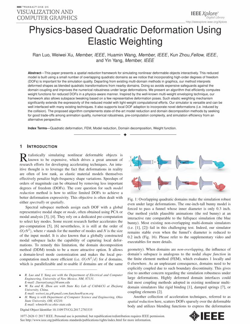
Fig. 12: Compare different weighting algorithms with a cylinder beam of heterogenous materials: the Young’s modulus of the beam

varies along its neutral axis. Two quadratic domains are set. The weight distributions from different algorithms are also plotted.

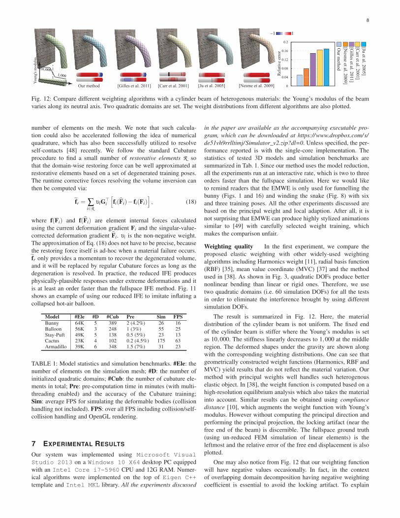
number of elements on the mesh. We note that such calcula-

tion could also be accelerated following the idea of numerical

quadrature, which has also been successfully utilized to resolve

self-contacts [48] recently. We follow the standard Cubature

procedure to find a small number of restorative elements R so

that the domain-wise restoring force can be well approximated at

restorative elements based on a set of degenerated training poses.

The runtime corrective forces resolving the volume inversion can

then be computed via:

fr = ∑i∈R

υiG�i

[fi(Fi)− fi(Fi)

], (18)

where f(Fi) and f(Fi) are element internal forces calculated

using the current deformation gradient Fi and the singular-value-

corrected deformation gradient Fi. υi is the non-negative weight.

The approximation of Eq. (18) does not have to be precise, because

the restoring force itself is ad-hoc when a material failure occurs.

fr only provides a momentum to recover the degenerated volume,

and it will be replaced by regular Cubature forces as long as the

degeneration is resolved. In practice, the reduced IFE produces

physically-plausible responses under extreme deformations and it

is at least an order faster than the fullspace IFE method. Fig. 11

shows an example of using our reduced IFE to imitate inflating a

collapsed hot-air balloon.

Model #Ele #D #Cub Pre Sim FPSBunny 64K 5 389 2 (4.2%) 26 16Balloon 56K 3 248 1 (3%) 55 25Stay-Puft 49K 5 138 0.5 (5%) 23 13Cactus 23K 4 102 0.2 (4.5%) 175 63Armadillo 39K 6 348 1.5 (7%) 31 23

TABLE 1: Model statistics and simulation benchmarks. #Ele: the

number of elements on the simulation mesh; #D: the number of

initialized quadratic domains; #Cub: the number of cubature ele-

ments in total; Pre: pre-computation time in minutes (with multi-

threading enabled) and the accuracy of the Cubature training;

Sim: average FPS for simulating the deformable bodies (collision

handling not included). FPS: over all FPS including collision/self-

collision handling and OpenGL rendering.

7 EXPERIMENTAL RESULTS

Our system was implemented using Microsoft VisualStudio 2013 on a Windows 10 X64 desktop PC equipped

with an Intel Core i7-5960 CPU and 12G RAM. Numer-

ical algorithms were implemented on the top of Eigen C++template and Intel MKL library. All the experiments discussed

in the paper are available as the accompanying executable pro-gram, which can be downloaded at https://www.dropbox.com/s/de51vh9rrlltimj/Simulator_v2.zip?dl=0. Unless specified, the per-

formance reported is with the single-core implementation. The

statistics of tested 3D models and simulation benchmarks are

summarized in Tab. 1. Since our method uses the model reduction,

all the experiments run at an interactive rate, which is two to three

orders faster than the fullspace simulation. Here we would like

to remind readers that the EMWE is only used for funnelling the

bunny (Figs. 1 and 16) and winding the snake (Fig. 8) with six

and three training poses. All the other experiments discussed are

based on the principal weight and local adaption. After all, it is

not surprising that EMWE can produce highly stylized animations

similar to [49] with carefully selected weight training, which

makes the comparison unfair.

Weighting quality In the first experiment, we compare the

proposed elastic weighting with other widely-used weighting

algorithms including Harmonics weight [11], radial basis function

(RBF) [35], mean value coordinate (MVC) [37] and the method

used in [38]. As shown in Fig. 3, quadratic DOFs produce better

nonlinear bending than linear or rigid ones. Therefore, we use

two quadratic domains (i.e. 60 simulation DOFs) for all the tests

in order to eliminate the interference brought by using different

simulation DOFs.

The result is summarized in Fig. 12. Here, the material

distribution of the cylinder beam is not uniform. The fixed end

of the cylinder beam is stiffer where the Young’s modulus is set

as 10,000. The stiffness linearly decreases to 1,000 at the middle

region. The deformed shapes under the gravity are shown along

with the corresponding weighting distributions. One can see that

geometrically constructed weight functions (Harmonics, RBF and

MVC) yield results that do not reflect the material variation. Our

method with principal weights well handles such heterogenous

elastic object. In [38], the weight function is computed based on a

high-resolution equilibrium analysis which also takes the material

into account. Similar results can be obtained using compliancedistance [10], which augments the weight function with Young’s

modulus. However without computing the principal direction and

performing the principal projection, the locking artifact (near the

free end of the beam) is discernible. The fullspace ground truth

(using un-reduced FEM simulation of linear elements) is the

leftmost and the relative error of the free end displacement is also

plotted.

One may also notice from Fig. 12 that our weighting function

will have negative values occasionally. In fact, in the context

of overlapping domain decomposition having negative weighting

coefficient is essential to avoid the locking artifact. To explain

9

A B A B A B

CC

Fig. 13: Shape functions of a simple 1D element.

this argument, let us look at an illustrative toy example of a

1D element with two nodes A and B. Under this configuration,

only interpolation is needed as shown in the leftmost subfigure

of Fig. 13. Here, interpolation means A’s weighting function WAis defined within its nearest boundary condition: WA(B) = 0, and

negative weight should be avoided. When a new node C is inserted

into this 1D element between A and B2, it induces a new boundary

condition: WA(C) = 0. That also means WA need to be extrapolatedbeyond its nearest boundary condition in order to allow A to

influence the entire element. If one chooses to design a smooth

shape function, in order to incorporate boundary conditions at Band C, the lowest-degree polynomial solution is a quadratic curve

with negative values after C (the rightmost subfigure in Fig. 13).

If one chooses to clamp the functions values as the bounded

biharmonic weights (BBW) [50], the weighting function becomes

discontinuous and locking artifacts could occur (mid sugfigure in

Fig. 13). In this case, the element is degenerated to be a linear

one. Without negative weight values, no smooth shape functions

can satisfy both boundary conditions at B and C simultaneous.

+2

-2

0

-5 0 5-1

0

1

2

Wei

ght

Seed 0 Seed 1

-5 0 50

0.5

1

Wei

ght Seed 1Seed 0

Our weight [Jacobson et al. 2011]

Fig. 14: BBW may induce locking artifacts.

Whether or not we should have negative weighting functions

depends on whether or not the weighting function needs to be

extrapolated beyond its nearest boundary conditions. In many

existing graphics literature, weighting functions are not supposed

to influence areas outside of its neighboring boundary conditions.

As a result, such blending is just interpolation and should be

convex. However, our system is designed for the overlapping

domain decomposition and negative weights become essential.

Fig. 14 gives a 3D example. The beam model has two domains

both covering the entire model. Their seeds are at the 1/4 and 3/4

along the neutral axis of the beam. If BBW is used, weight values

of both domains at nodes right to seed 1 will be 1 and 0. This

2. Doing so actually makes this element nonlinear.

Fullspace Our method

[Barbic and Zhao 2011] [Wu et al. 2015]v

Fig. 15: Simulate a swinging cactus using deformation substruc-

turing [1], unified domain decomposition [2], our method, and the

fullspace solver.

leads to locking effect. However, our method does not have such

problem.

Robust nonlinear expressivity Next, we evaluate the capability

of the proposed simulator capturing large nonlinear deformations.

We compare our method with two paradigmatic state-of-the-art

multi-domain nonlinear simulators using deformation substructur-

ing [1] and coupling elements [2]. As shown in Fig. 15, the cactus

model is decomposed into four domains. The Voronoi segments

(left in the figure) are used for the non-overlapping domain de-

composition for [1] and [2] with 30 modal derivatives per domain.

Therefore all the reduced models have 120 simulation DOFs. From

snapshots reported in the figure and the supplementary video,

we can see that all the simulators produce plausible deformable

animations comparable to the fullspace result.

Fullspace

Our method

[Barbic and Zhao 2011]v

[Wu et al. 2015]

0.4

0.2

Fig. 16: Drag the bunny through a thin funnel (available as the

supplementary executable too).

On the other hand, our method does not require an explicit

domain coupling. This advantage makes our system robust against

10

Fig. 17: Our solver remains stable under severe geometry con-

straints.

large-scale deformations. Figs. 1 and 16 show snapshots of a

challenging scenario: a one-inch-tall bunny model is forced to

pass through a thin funnel. The Young’s modulus of the bunny is

500 and the Poisson’s ratio is 0.4. Five domains are used in this

example and all the solvers use 150 simulation DOFs. When the

funnel is relatively wide (i.e. 0.4) as shown in Fig. 16 top, all the

simulators produce plausible and interesting animations. However,

if we reduce the size of the funnel to 0.3, non-overlapping solvers

fail. This is because when domains’ interfaces are highly distorted,

the rigid interface assumption [1] does not hold and the coupling

elements [2] are degenerated. Our method is still able to produce a

similar animation compared with the fullspace simulation (Fig. 1)

and remains stable even the funnel is further shrunk to 0.2 (Fig. 16

bottom).

A more extreme case highlighting the robustness of our solver

is shown in Fig. 17. In this test, we collapse the Armadillo model

into a small 2D disk initially. When this strong geometry constraint

is released, our method quickly restores the model back to the rest

shape with the help of reduced IFE simulation. While the IFE

contributes the calculation of necessary internal forces, the main

reason behind such good numerical stability is the overlapping

domain decomposition. A fullspace IFE [40] simulated animation

is also available in the video for readers’ reference.

Local adaptivity Lastly, we test the adaptivity of our algorithm.

Fig. 18 reports results using our method, local subspace [28]

and the fullspace solver when we push the Stay-Puft with a

spiky board. The Stay-Puft model originally has five domains

and extra two domains are inserted corresponding to the external

collision with spikes. We can see from the figure that, newly-added

domains provide necessary deformable freedoms to simulate local

deformation, and realistic results comparative to the fullspace

ground truth are produced.

Fullspace [Harmon and Zorin 2013]

Our method without local adaption Our method with local adaption

Fig. 18: Adding new domains according to the contacts from a

moving spike board greatly enriches detailed local deformation.

It is noteworthy that similar denting effects can also be ob-

AdaptiveNon-adaptive

Non-adaptive Adaptive

Non

-ada

ptiv

eA

dapt

ive

Fig. 19: Runtine domain adaption does not only yield better

denting effects on the bunny, but also enriches local deformations

at the lollipop.

tained by building a local subspace using Boussinesq equation [28]

as shown in Fig. 18. However, our method is able to deal with a

much wider range types of deformation. As shown in Fig. 19, the

falling bunny hits an elastic lollipop. The local domain insertion

does not only help for a better denting effect on the bunny’s body,

it also enriches the local deformation for the lollipop. Initially,

the bunny has five domains and the lollipop has only one domain

seeded at the middle.

8 LIMITATION AND FUTURE WORK

We present a new spatially reduced deformable simulator us-

ing overlapping quadratic domains. The incorporated high-order

DOFs enhance the expressivity of the reduced model for non-

linear deformations. Besides, we also design an elastic multi-

weight enveloping scheme assigning customized weight functions

for quadratic DOFs. Augmented with the accelerated invertible

finite element method and runtime domain addition, our method

simulates challenging large-scale nonlinear deformations at an

interactive rate.

Our method also has several limitations, which leave us many

interesting research directions for future work. While quadratic

transformations provide plenty of nonlinear freedoms, they could

also inject excessive DOFs for modest deformations. As a result,

placing a lot of quadratic domains (i.e. over hundreds of domains

as in [1]) will quickly drop simulation FPS. A possible solution

is to explore the geometric symmetry/degeneration hidden in the

deformable body to further condense the domain’s DOFs (i.e.

downgrade entries in the geometry matrix to linear DOFs that

are perpendicular to the neutral axis of a beam, where we have

limited nonlinear deformations). Another possible treatment is

to use mixed domains, like affine [10] or rigid [11] domains.

Adding new domains during the simulation runtime alters the

subspace matrix and popping artifacts are possible if the time

step size is aggressive. For instance in [28], the time step is set

conservatively at the order of 1e−4 to 1e−6 to alleviate the issue.

Another limitation lies in the fact that our weight function is

still computed based on the linear elasticity and the rest shape

stiffness matrix. Under large deformations, the weight distribution

is likely to change too. We will look into the possibility of

calculating the spatial weight derivative similar to the modal

derivative [4] to better incorporate such nonlinearity. Augmenting

modal deformations with elastic weighting is also an interesting

future work for us. In order to do so, we need to carefully design

11

local boundary conditions to construct modal bases and couple

them with local rigid body transformations. Of course, doing so

will induce more freedoms to the simulator putting us back to the

original question for the reduced simulation: how to find the best

balance between simulation speed and quality?

Acknowledgement We would like to thank TVCG editors and

reviewers for their constructive and detailed comments. Huamin

Wang is partially supported by NSF IIS-1524992 and gift

grant from Adobe and nVidia. Yin Yang and Ran Luo are

partially supported by NSF CHS-1464306, CHS-1717972,CNS-1637092 and nVidia GPU grant. Weiwei Xu is partially

supported by NSFC 61732016 and the Fundamental Research

Funds for the Central Universities (2017XZZX009-03).

REFERENCES

[1] J. Barbic and Y. Zhao, “Real-time large-deformation substructuring,” ser.SIGGRAPH ’11, 2011, pp. 91:1–91:8.

[2] X. Wu, R. Mukherjee, and H. Wang, “A unified approach for subspacesimulation of deformable bodies in multiple domains,” ACM Trans.Graph., vol. 34, no. 6, pp. 241:1–241:9, Oct. 2015.

[3] A. Pentland and J. Williams, “Good vibrations: Modal dynamics forgraphics and animation,” ser. SIGGRAPH ’89, 1989, pp. 215–222.

[4] J. Barbic and D. L. James, “Real-time subspace integration for st. venant-kirchhoff deformable models,” ser. SIGGRAPH ’05, 2005, pp. 982–990.

[5] C. von Tycowicz, C. Schulz, H.-P. Seidel, and K. Hildebrandt, “Anefficient construction of reduced deformable objects,” ACM Transactionson Graphics (TOG), vol. 32, no. 6, p. 213, 2013.

[6] Y. Yang, D. Li, W. Xu, Y. Tian, and C. Zheng, “Expediting precompu-tation for reduced deformable simulation,” ACM Trans. Graph., vol. 34,no. 6, pp. 243:1–243:13, Oct. 2015.

[7] T. Kim and D. L. James, “Physics-based character skinning using multi-domain subspace deformations,” ser. SCA ’11, 2011, pp. 63–72.

[8] F. G. García, T. Paradinas, N. Coll, and G. Patow, “Cages:: A multilevel,multi-cage-based system for mesh deformation,” ACM Trans. Graph.,vol. 32, no. 3, pp. 24:1–24:13, Jul. 2013.

[9] T. W. Sederberg and S. R. Parry, “Free-form deformation of solidgeometric models,” in Proceedings of the 13th Annual Conference onComputer Graphics and Interactive Techniques, ser. SIGGRAPH ’86,1986, pp. 151–160.

[10] F. Faure, B. Gilles, G. Bousquet, and D. K. Pai, “Sparse meshless modelsof complex deformable solids,” ser. SIGGRAPH ’11, 2011, pp. 73:1–73:10.

[11] B. Gilles, G. Bousquet, F. Faure, and D. K. Pai, “Frame-based elasticmodels,” ACM Trans. Graph., vol. 30, no. 2, pp. 15:1–15:12, Apr. 2011.

[12] S. Martin, P. Kaufmann, M. Botsch, E. Grinspun, and M. Gross, “Unifiedsimulation of elastic rods, shells, and solids,” ACM Trans. Graph.,vol. 29, no. 4, pp. 39:1–39:10, Jul. 2010.

[13] S. Capell, S. Green, B. Curless, T. Duchamp, and Z. Popovic, “Amultiresolution framework for dynamic deformations,” in Proceedingsof the 2002 ACM SIGGRAPH/Eurographics Symposium on ComputerAnimation, ser. SCA ’02. ACM, 2002, pp. 41–47.

[14] E. Grinspun, P. Krysl, and P. Schröder, “Charms: A simple frameworkfor adaptive simulation,” in Proceedings of the 29th Annual Conferenceon Computer Graphics and Interactive Techniques, ser. SIGGRAPH ’02.ACM, 2002, pp. 281–290.

[15] X. C. Wang and C. Phillips, “Multi-weight enveloping: Least-squaresapproximation techniques for skin animation,” ser. SCA ’02, 2002, pp.129–138.

[16] A. Nealen, M. Müller, R. Keiser, E. Boxerman, and M. Carlson, “Phys-ically based deformable models in computer graphics,” in ComputerGraphics Forum, vol. 25, no. 4, 2006, pp. 809–836.

[17] E. Sifakis and J. Barbic, “Fem simulation of 3d deformable solids: Apractitioner’s guide to theory, discretization and model reduction,” inACM SIGGRAPH 2012 Courses, ser. SIGGRAPH ’12, 2012, pp. 20:1–20:50.

[18] Y. Zhu, E. Sifakis, J. Teran, and A. Brandt, “An efficient multigrid methodfor the simulation of high-resolution elastic solids,” ACM Trans. Graph.,vol. 29, no. 2, pp. 16:1–16:18, Apr. 2010.

[19] R. Tamstorf, T. Jones, and S. F. McCormick, “Smoothed aggregationmultigrid for cloth simulation,” ACM Trans. Graph., vol. 34,no. 6, pp. 245:1–245:13, Oct. 2015. [Online]. Available: http://doi.acm.org/10.1145/2816795.2818081

[20] F. Hecht, Y. J. Lee, J. R. Shewchuk, and J. F. O’Brien, “Updated sparsecholesky factors for corotational elastodynamics,” ACM Transactions onGraphics, vol. 31, no. 5, pp. 123:1–13, Oct. 2012.

[21] M. Fratarcangeli, V. Tibaldo, and F. Pellacini, “Vivace: a practical gauss-seidel method for stable soft body dynamics,” ACM Transactions onGraphics (TOG), vol. 35, no. 6, p. 214, 2016.

[22] H. Wang and Y. Yang, “Descent methods for elastic body simulation onthe gpu,” ACM Transactions on Graphics (TOG), vol. 35, no. 6, p. 212,2016.

[23] K. K. Hauser, C. Shen, and J. F. O’Brien, “Interactive deformation usingmodal analysis with constraints,” in Graphics Interface, Jun. 2003, pp.247–256.

[24] M. G. Choi and H.-S. Ko, “Modal warping: Real-time simulation oflarge rotational deformation and manipulation,” IEEE Transactions onVisualization and Computer Graphics, vol. 11, no. 1, pp. 91–101, Jan.2005.

[25] T. Kim and D. L. James, “Skipping steps in deformable simulation withonline model reduction,” ACM Trans. Graph., vol. 28, no. 5, pp. 123:1–123:9, Dec. 2009.

[26] Y. Yang, W. Xu, X. Guo, K. Zhou, and B. Guo, “Boundary-aware mul-tidomain subspace deformation,” Visualization and Computer Graphics,IEEE Transactions on, vol. 19, no. 10, pp. 1633–1645, 2013.

[27] H. Xu and J. Barbic, “Pose-space subspace dynamics,” ACM Transac-tions on Graphics (TOG), vol. 35, no. 4, p. 35, 2016.

[28] D. Harmon and D. Zorin, “Subspace integration with local deformations,”ACM Trans. Graph., vol. 32, no. 4, pp. 107:1–107:10, Jul. 2013.

[29] Y. Teng, M. Meyer, T. DeRose, and T. Kim, “Subspace condensation:Full space adaptivity for subspace deformations,” ACM Trans. Graph.,vol. 34, no. 4, pp. 76:1–76:9, Jul. 2015.

[30] J. Mezger, B. Thomaszewski, S. Pabst, and W. Straber, “Interactivephysically-based shape editing,” Computer Aided Geometric Design,vol. 26, no. 6, pp. 680 – 694, 2009.

[31] A. W. Bargteil and E. Cohen, “Animation of deformable bodies withquadratic bÉzier finite elements,” ACM Trans. Graph., vol. 33, no. 3, pp.27:1–27:10, Jun. 2014.

[32] M. Müller, B. Heidelberger, M. Teschner, and M. Gross, “Meshlessdeformations based on shape matching,” ACM transactions on graphics(TOG), vol. 24, no. 3, pp. 471–478, 2005.

[33] A. Jacobson, Z. Deng, L. Kavan, and J. P. Lewis, “Skinning: Real-timeshape deformation (full text not available),” in ACM SIGGRAPH 2014Courses, ser. SIGGRAPH ’14, 2014, pp. 24:1–24:1.

[34] P. Joshi, M. Meyer, T. DeRose, B. Green, and T. Sanocki, “Harmoniccoordinates for character articulation,” ACM Trans. Graph., vol. 26, no. 3,Jul. 2007.

[35] J. C. Carr, R. K. Beatson, J. B. Cherrie, T. J. Mitchell, W. R. Fright,B. C. McCallum, and T. R. Evans, “Reconstruction and representation of3d objects with radial basis functions,” ser. SIGGRAPH ’01, 2001, pp.67–76.

[36] M. S. Floater, “Mean value coordinates,” Comput. Aided Geom. Des.,vol. 20, no. 1, pp. 19–27, Mar. 2003.

[37] T. Ju, S. Schaefer, and J. Warren, “Mean value coordinates for closedtriangular meshes,” ACM Trans. Graph., vol. 24, no. 3, pp. 561–566, Jul.2005.

[38] M. Nesme, P. G. Kry, L. Jerábková, and F. Faure, “Preserving topologyand elasticity for embedded deformable models,” ser. SIGGRAPH ’09,2009, pp. 52:1–52:9.

[39] Y. Wang, A. Jacobson, J. Barbic, and L. Kavan, “Linear subspace designfor real-time shape deformation,” ACM Transactions on Graphics (TOG),vol. 34, no. 4, p. 57, 2015.

[40] G. Irving, J. Teran, and R. Fedkiw, “Invertible finite elements for robustsimulation of large deformation,” ser. SCA ’04, 2004, pp. 131–140.

[41] A. Shamir, “A survey on mesh segmentation techniques,” in Computergraphics forum, vol. 27, no. 6. Wiley Online Library, 2008, pp. 1539–1556.

[42] S. Lloyd, “Least squares quantization in pcm,” IEEE Trans. Inf. Theor.,vol. 28, no. 2, pp. 129–137, Sep. 1982.

[43] S. Boyd and L. Vandenberghe, Convex optimization. Cambridgeuniversity press, 2004.

[44] S. S. An, T. Kim, and D. L. James, “Optimizing cubature for efficientintegration of subspace deformations,” ser. SIGGRAPH Asia ’08, 2008,pp. 165:1–165:10.

[45] M. Tournier, M. Nesme, F. Faure, and B. Gilles, “Velocity-based adaptiv-ity of deformable models,” Computers & Graphics, vol. 45, pp. 75–85,2014.

[46] A. Stomakhin, R. Howes, C. Schroeder, and J. M. Teran, “Energeticallyconsistent invertible elasticity,” ser. SCA ’12, 2012, pp. 25–32.

12

[47] F. Sin, Y. Zhu, Y. Li, and D. Schroeder, “Invertible isotropic hyperelas-ticity using svd gradients,” in SCA’11 (Posters, 2011.

[48] Y. Teng, M. A. Otaduy, and T. Kim, “Simulating articulated subspaceself-contact,” ACM Trans. Graph., vol. 33, no. 4, pp. 106:1–106:9, Jul.2014. [Online]. Available: http://doi.acm.org/10.1145/2601097.2601181

[49] S. Martin, B. Thomaszewski, E. Grinspun, and M. Gross, “Example-based elastic materials,” ACM Trans. Graph., vol. 30, no. 4, pp.72:1–72:8, Jul. 2011. [Online]. Available: http://doi.acm.org/10.1145/2010324.1964967

[50] A. Jacobson, I. Baran, J. Popovic, and O. Sorkine, “Bounded biharmonicweights for real-time deformation.” ACM Trans. Graph., vol. 30, no. 4,pp. 78–1, 2011.

Ran Luo received the bachelor degree in Bei-hang University, previously known as BeijingUniversity of Aeronautics and Astronautics, in2014. He is currently pursuing the Ph.D. de-gree in Computer Engineering at the Univer-sity of New Mexico(UNM), Albuquerque, NewMexico. His research interests include physics-based animation/simulation, virtual reality, ma-chine learning and related topics. He is currentlya Research Assistant with the Department ofElectrical and Computer Engineering at UNM.

Weiwei Xu is a Researcher in State Key Labof CAD & CG, College of Computer Science atZhejiang University, awardee of NSFC ExcellentYoung Scholars Program in 2013. His main re-search interests are digital geometry process-ing, physical simulation and virtual reality. Hehas published around 60 papers on internationalgraphics journals and conferences, including 16papers on ACM TOG.

Huamin Wang is an Associate Professor in thedepartment of Computer Science and Engineer-ing at the Ohio State University. Before joiningOSU, he was a postdoctoral researcher in thedepartment of Electrical Engineering and Com-puter Sciences at the University of California,Berkeley. He received his Ph.D. degree in Com-puter Science from Gerogia Institute of Tech-nology in 2009, his M.S. degree from StanfordUniversity in 2004, and his B.Eng. degree fromZhejiang University in 2002.

Kun Zhou is a Cheung Kong Professor in theComputer Science Department of Zhejiang Uni-versity, and the Director of the State Key Labof CAD&CG. Prior to joining Zhejiang Universityin 2008, Dr. Zhou was a Leader Researcher ofthe Internet Graphics Group at Microsoft Re-search Asia. He received his B.S. degree andPh.D. degree in computer science from ZhejiangUniversity in 1997 and 2002, respectively. Hisresearch interests are in visual computing, paral-lel computing, human computer interaction, and

virtual reality. He currently serves on the editorial/advisory boards ofACM Transactions on Graphics and IEEE Spectrum. He is a Fellow ofIEEE.

Yin Yang received his Ph.D. degree in computerscience from the University of Texas at Dallasin 2013. He is an Assistant Professor in De-partment of Electrical Computer Engineering atthe University of New Mexico, Albuquerque. Hisresearch interests include physics-based anima-tion/simulation and related applications, scien-tific visualization and medical imaging analysis.