Mixing ratios and eddy covariance flux measurements of ...

Atmos. Chem. Phys., 9, 1971–1987, 2009www.atmos-chem-phys.net/9/1971/2009/© Author(s) 2009. This work is distributed underthe Creative Commons Attribution 3.0 License.

AtmosphericChemistry

and Physics

Mixing ratios and eddy covariance flux measurements of volatileorganic compounds from an urban canopy (Manchester, UK)

B. Langford1, B. Davison1, E. Nemitz2, and C. N. Hewitt1

1Lancaster Environment Centre, Lancaster University, Lancaster, LA1 4YQ, UK2Centre for Ecology & Hydrology (CEH) Edinburgh, Bush Estate, Penicuik, EH26 0QB, UK

Received: 13 November 2007 – Published in Atmos. Chem. Phys. Discuss.: 8 January 2008Revised: 17 February 2009 – Accepted: 24 February 2009 – Published: 19 March 2009

Abstract. Mixing ratios and fluxes of six selected volatileorganic compounds (VOCs) were measured above the cityof Manchester (UK) during the summer of 2006. A protontransfer reaction-mass spectrometer was used for the mea-surement of mixing ratios, and fluxes were calculated fromthese using both the disjunct and the virtual disjunct eddy co-variance techniques. The two flux systems, which operatedin alternate half hours, showed good agreement, withR2 val-ues ranging between 0.74 and 0.9 for the individual analytes.On average, fluxes measured in the disjunct mode were ap-proximately 20% lower than those measured in the virtualmode. This difference is due to both the dampening of theVOC signal by the disjunct flux sampler and carry over fromone sample to the next. Correcting for these effects reducedthe difference to less than 7%. Observed fluxes are thought tobe largely controlled by anthropogenic sources, with vehicleemissions the major contributor. However, both evaporativeand biogenic emissions may account for some of the VOCspresent. Concentrations and fluxes of the oxygenated com-pounds were highest on average, ranging between 0.15 to1 mg m−2 h−1; the fluxes of aromatic compounds were lower,between 0.12 to 0.28 mg m−2 h−1. The observed fluxes wereup-scaled to give city wide emission estimates for each com-pound and the results compared to estimates made by the Na-tional Atmospheric Emission Inventory (NAEI) for the sameflux footprint. Fluxes of toluene and benzene compared mostclosely differing by approximately 50%, while in contrast theoxygenated fluxes were found to be between 3.6–6.3 timeslarger than the annual average predicted by the NAEI.

Correspondence to:C. N. Hewitt([email protected])

1 Introduction

The compilation of spatially and temporally detailed invento-ries for the emission of anthropogenic volatile organic com-pounds (VOCs) from urban areas is a necessary requirementfor air quality regulatory purposes, effects assessment andresearch. Current emission estimates are associated withlarge degrees of uncertainty (Friedrich and Obermeier, 1999)which may limit their usefulness. Much of this uncertaintycan be attributed to the large variety of different source cate-gories which contribute to urban VOC emissions, which canbe difficult to characterise and validate. Rather than takinga “bottom-up” inventory approach, an alternative is to makedirect micrometeorologically based measurements which canintegrate observations of wind speed and scalar concentra-tions to give a city-wide estimate of pollutant emission rates(Nemitz et al., 2002; Dorsey et al., 2002; Velasco et al, 2005;Martin et al., 2008; Famulari et al., 2009).

Currently, the eddy covariance (EC) technique is con-sidered the most direct micrometeorological method avail-able for estimating surface/atmosphere exchange fluxes, as itmeasures the turbulent flux directly, without reliance on anyempirical parameterisations. This approach requires highfrequency measurements (typically in the order of 5–20 Hz)of both vertical wind speed and concentration (or mixing ra-tios) to resolve all eddies that contribute to vertical transport(Lenschow, 1995). Although this technique is now well es-tablished for the measurement of some trace gases, such asCO2 and H2O (Aubinet et al., 2001), its application to VOCfluxes has been restricted because of the slow response timesof most VOC sensors.

A number of alternative micrometeorological approacheshave been developed which relax the demands placed uponinstrument response times. The technique most com-monly applied to VOCs is the relaxed eddy accumulation

Published by Copernicus Publications on behalf of the European Geosciences Union.

http://creativecommons.org/licenses/by/3.0/

1972 B. Langford et al.: Eddy covariance flux measurements of VOC from a city

method (REA), a conditional sampling technique where sam-ples of air are directed into an up or down draught reservoiraccording to the sign of the vertical wind velocity at the timeof sampling (Businger and Oncley, 1990). Air from eachreservoir is subsequently analysed off-line and a flux is calcu-lated from the difference in concentration generated betweenthe two reservoirs. Unlike the eddy covariance method, REAis not a direct measure of the flux as it relies on empiricalparameterisation. Furthermore, there is no scope for retro-spective corrections to the coordinate frame (Bowling et al.,1998). Despite these drawbacks, the REA method has beensuccessfully applied to a range of vegetation types includinggrass land (Olofsson et al., 2003), forests (Schween et al.,1997; Gallagher et al., 2000; Tani et al., 2002; Greenberg etal., 2003; Ciccioli et al., 2003; Friedrichs et al., 1999) andlately in an urban study (Park et al., 2008).

More recently a second technique, disjunct eddy covari-ance (DEC) (Rinne et al., 2001; Warneke et al., 2002;Turnipseed et al., 2009), has been developed for “relaxed”flux measurement. Rather than measuring at high frequen-cies as in EC, in DEC the flux is calculated using a sub-setof a continuous time series. In order to retain the flux con-tributions carried by small scale eddies, DEC utilises near-instantaneous grab samples of air which are aspirated intoa storage reservoir at regular intervals. The “dead” time be-tween the sampling periods is then used to analyse the air at arate suitable for the gas analyser. The discontinuous datasetgenerated can be used to give high precision flux informa-tion, which is numerically similar to the EC approach, butwith reduced statistics (Grabmer et al., 2004). The DEC ap-proach is particularly useful for sensors with a response timeof 1 to 20 s.

With the advent of quadrupole mass spectrometers (QMS)for the use of atmospheric composition measurements, arange of analysers is now becoming available that can pro-vide fast measurements (as determined by the dwell time on agivenm/z), which is nevertheless discontinuous (as the QMSscans through a range ofm/z’s). One such instrument is theproton transfer reaction-mass spectrometer (PTR-MS; Ioni-con GmbH; Innsbruck, Austria) which allows for the mea-surement of most VOCs with good sensitivity (10 ppt) andfast response times (200 ms–1 s).

The quadrupole mass spectrometer in the PTR-MS can beprogrammed to scan over a small suite of masses in what istermed a scan cycle. Although in theory the instrument hasa sufficient response time to be compatible with the eddy co-variance method, in reality the quadrupole can only scan onemass at a time; therefore the dataset returned on completionof each duty cycle is in effect disjunct.

To optimise flux measurement approaches for these kindof data, the DEC concept has been developed further to cal-culate fluxes from the discontinuous time-series at eachm/z

by pairing up each concentration measurement with the as-sociated wind measurement in software, a process knownas virtual disjunct eddy covariance (vDEC) (Karl et al.,

2001, 2002; Spirig et al., 2005; Lee et al., 2006; Ammann etal., 2006; Brunner et al., 2007). The advantage of this tech-nique is that air can be sampled directly into the instrument,as individual masses are measured at a sufficiently fast rate:therefore no additional sampling system is required. Further-more, analysis times are shorter than in DEC, allowing moredata points to be collected during each averaging period andreducing the statistical uncertainty associated with the use ofa discontinuous time series by averaging over a larger num-ber of eddy motions. However, shorter dwell times can leadto increased random error in individual concentration mea-surements, therefore a balance must be found between anal-ysis times and measurement frequency.

The vDEC method has been successfully applied to giveVOC flux estimates over vegetation canopies, includinggrassland (Karl et al., 2001; Ammann et al., 2006; Brunneret al., 2007), forests (Karl et al., 2002; Spirig et al., 2005;Lee et al., 2006), and over an urban environment (Velasco etal., 2005).

In the current study we deployed both the DEC and vDECtechniques for the measurement of a range of VOCs abovethe city of Manchester (UK). The recorded data were thenused to calculate city-wide emission fluxes which were com-pared to the UK National Atmospheric Emission Inventory(NAEI) for Manchester (http://www.naei.org.uk/datachunk.php?fdatachunkid=174).

The NAEI, as with most emission inventories, is com-piled using a bottom-up approach, where combinations of re-ported and estimated emissions across numerous source sec-tors are used to provide a spatially disaggregated (1×1 km)emission inventory. The uncertainty associated with theseestimates is dependent on the ratio of reported to estimated(modelled) data, and hence for compounds such as VOCs,where reported emissions are limited and uncertainty levelsare high, micrometeorological methods offer a useful alter-native and/or validation.

2 Methods

2.1 Measurement site and general setup

The work presented here formed part of the UK CityFluxproject, which aimed to (i) directly measure pollutant emis-sions from urban areas, (ii) investigate controls of theseemissions, (iii) derive emission factors relative to CO2 andCO and (iv) study pollutant transformation by comparingfluxes at the plume, street canyon and urban canopy scale.During the summer of 2006, micrometeorological measure-ments of VOC emissions were made over the city of Manch-ester, together with measurements of fluxes and concentra-tions of VOCs, aerosols, O3, CO2 and H2O, as well as mo-bile measurements with a mobile laboratory, measurementsin a street canyon, tracer releases and aircraft-borne mea-surements. The VOC flux measurements were taken from

Atmos. Chem. Phys., 9, 1971–1987, 2009 www.atmos-chem-phys.net/9/1971/2009/

http://www.naei.org.uk/datachunk.php?f_datachunk_id=174


B. Langford et al.: Eddy covariance flux measurements of VOC from a city 1973

the roof of Portland Tower (53◦28′41′′ N; 2◦14′18′′ W), an80 m tall, rectangular (46 m×16 m) office block, which is lo-cated in central Manchester. The building is situated on Port-land Street, which is approximately 600 m distance from theArndale centre, (the city’s principal shopping district) 475 mfrom Piccadilly railway station, (the north-west’s busiest sta-tion), and 100 m from the China Town district (a concen-trated area of restaurants). The office block is surrounded bytrafficked streets on three sides and a multi-storey car parkon the other. The buildings in the immediate vicinity of thetower are predominately commercial thus giving the site anurban classification of 2 according to the criteria described byOke (2006) (intensively developed high density urban areawith 2–5 storey, attached or very close-set buildings often ofbrick or stone, e.g. old city core).

The roof of Portland Tower is not uniformly flat but hasthree levels. On the lowest level a small shed was erectedwhich housed the PTR-MS. The second level, 2 m above,contained a utility substation (20 m×10 m) which was usedto house the sonic anemometer signal box. The roof of thesubstation was used as the foundation for a 15 m mast whichwas fitted to the north west facing wall and instrumentedwith a sonic anemometer (Solent Research R3, Gill Instru-ments Ltd, Lymington, Hants, UK) and Teflon gas inlet line(1/2′′ OD; 0.38′′ ID). The mast was erected to get above thewake effects generated from both the edges of the buildingand the inhomogeneous roof surface and increased the ef-fective measurement height to 95 m above street level. Theanemometer and sample inlet were therefore 13 m above thehighest part of the roof. Particle number fluxes from this sitehave been presented by Martin et al. (2008).

Fluxes were measured between 5 and 20 June 2006. Dur-ing the first few days of measurements (5th–10th) a highpressure system was centred over Northern Ireland whichdominated the weather during this period, with mostly dryconditions, clear skies and temperatures between 16–30◦C.Between 13th–16th a cold front slowly moved across South-ern England and during this time temperatures at the mea-surement tower dropped to a maximum of 24◦C and a min-imum of 14◦C on 16th. For the later part of the cam-paign, temperatures slowly increased as a high pressure ridgemoved in behind the cold front, increasing the average tem-perature to 21◦C. Throughout the campaign the wind direc-tion shifted between SW and NNE, but also came from theSEE at certain times. The wind speed ranged between 0.4–11.2 m s−1, with an average of 3.3 m s−1 (based on 30-minaverages).

2.2 The proton transfer reaction mass spectrometer(PTR-MS)

A PTR-MS instrument (Ionicon Analytik, Austria) wasused for the measurement of VOC concentrations. De-tailed descriptions of this instrument can be found elsewhere(Lindinger et al., 1998; Hayward et al., 2003; de Gouw and

Warneke., 2007), therefore only a brief account of the instru-ment and setup will be given here.

The PTR-MS used was an Ionicon standard model, con-taining two turbo-molecular pumps, a 9.6 cm long drift tube(stainless steel rings) and heated silico-steel inlet, whichdrew air at a rate of 0.15 l min−1. The quadrupole was pro-grammed to sequentially scan through a suite of six pro-tonated target compounds: methanol (m/z 33), acetalde-hyde (m/z 45), acetone (m/z 59), isoprene/furan (m/z 69),benzene (m/z 79) and toluene (m/z 93). In additionto these compounds, the primary ion count, measured atm/z 21 (H18

3 O+) and two reagent cluster ions,m/z 37(H16

3 O+ (H162 O+)) andm/z 55 (H16

3 O+ (H162 O+)2) were also

recorded. A further mass,m/z 25, was used at the start ofeach measurement cycle as a spacer to ensure the monitoredair did not contain residues from the previous sample.

During the measurement period drift tube parameters pres-sure, temperature and voltage were held constant at 2 mbar,45 ◦C and 600 V, respectively, to achieve an E/N ratio ofapproximately 125 Td. The primary ion count ranged be-tween (2.2–3.6)×106 with an average of 2.8×106. Thereagent ions ranged between (1.07–2.62)×105 with a meanof 1.69×105 which represented 6% of the primary ion sig-nal. Average normalised counts ranged between 3 (benzene)and 72 [ncps] (methanol) with instrument sensitivities in therange of 4.3 (isoprene)–13.3 (benzene) ncps ppbv−1.

A VOC gas standard was not available for on-site cal-ibration of the PTR-MS, hence mixing ratios were calcu-lated using the instrument specific transmission coefficientsand reaction times taken from Zhao and Zhang (2004). Thetransmission coefficients were calculated experimentally un-der laboratory conditions using a range of gas standards andthe method used has been described in detail by Wilkin-son (2006). Despite the careful calculation of coefficients,previous studies (de Gouw and Warneke, 2007) have sug-gested mixing ratios calculated using this approach can havelarge systematic errors, therefore some systematic bias inmixing ratios cannot be ruled out here. It should be notedthat a systematic offset in the VOC mixing ratio due to theinstrument background will not affect the measured fluxes.

Additional uncertainties in PTR-MS measurements arisedue to the limitations of the mass filter, which can only re-solve ion counts with a resolution of one atomic mass unit.Therefore attributing ion counts to individual VOC speciescan be difficult, especially in the urban environment wherenumerous emission sources give rise to air masses containinga wide variety of compounds, several of which may have thesame integer molecular weight. Interference from other ionsat m/z 33, 45, 79 and 93 has been shown to be insignificantin previous studies (de Gouw et al., 2007), but both acetoneand propanal have been detected at amu 59. Although thiscan generate some uncertainty in the measurement of ace-tone, the signal of acetone is often dominant in ambient air(Kato et al., 2004), therefore ion counts recorded atm/z 59

www.atmos-chem-phys.net/9/1971/2009/ Atmos. Chem. Phys., 9, 1971–1987, 2009


were ascribed solely to acetone in the present study. Sim-ilarly m/z 69 may be isoprene and/or furan, although thelatter is normally present at very low concentrations in am-bient air (Christian et al., 2004). Despite this, in the urbanatmosphere, contributions from unknown compounds suchas alkenes cannot be ruled out and thereforem/z 69 was ten-tatively attributed entirely to isoprene.

2.3 Flux measurements

During the campaign, two flux measurement techniques(DEC and vDEC) were employed to measure surface layerfluxes of VOCs from the urban canopy. As both techniquesutilised a single PTR-MS instrument to give VOC concentra-tions, it was not possible to operate the systems simultane-ously, and therefore fluxes were measured by the two meth-ods in alternate half hours. A Teflon 3-way solenoid valve(001-0017-900, Parker Hannifin) sat in line and enabled thePTR-MS to switch between the two systems. Flux measure-ments in each mode were averaged over a 25 min period andthe remaining 5 min of each half hour were used to scan theentire mass spectrum (m/z 21–146) to give basic ambientconcentration information on a wider range of VOCs. Thisinformation is to be presented elsewhere. Figure 1 shows atypical PTR-MS operating sequence during 1 h of measure-ments and includes the PTR-MS scan cycles for each fluxmode.

2.3.1 Virtual disjunct eddy covariance sampling system(vDEC)

During the first period of each hour, the 3-way solenoid valvewas triggered to enable the PTR-MS to sub-sample directlyfrom the main sample line in a virtual disjunct eddy covari-ance mode. The quadrupole was set to scan each mass ata rate of 20 ms, allowing sample air to be purged directlyinto the instrument without the use of an additional samplingsystem. The inlet for the sample line was mounted a shortdistance below the sonic anemometer, as vertical displace-ment has been shown to result in the smallest flux losses(Kristensen et al., 1997). In order to maintain a turbulentflow through the sample line, and thus avoid dampening ofthe VOC signal, a flow rate of approximately 60 l min−1 wasused. Upon the completion of each PTR-MS scan cycle,data were exported to a LabVIEW logging program using theMicrosoft Windows “dynamic data exchange” (DDE) pro-tocol, which stored the data alongside those from the sonicanemometer.

2.3.2 Disjunct flux sampling system (DFS)

A disjunct flux sampling system was deployed on the roofof the building to monitor the VOC fluxes for the second pe-riod of each hour. The schematic and operating sequence ofthe DFS are depicted in Fig. 2. The sampler comprised twoone litre stainless steel canisters, which act as intermediate

storage reservoirs (ISR) for sampled air. Fast switching highflow conductance valves (Lucifer E121K45) were mountedto the inlet of each canister, enabling the ISR to take a fastgrab sample once activated. Each ISR was coiled with heatercable and insulated with aluminium foil to maintain an inter-nal temperature of 40◦C. This, combined with the cylindricalshape of the canisters which reduced relative surface area,helped to minimise loss of VOCs to walls, and minimisedcondensation and the formation of liquid water, which canremove soluble compounds such as methanol from the gasphase.

Before grab samples of air were taken, each ISR was firstevacuated to a pressure of 250 mbar. The time taken to evac-uate the canister, 12 s, was determined by the efficiency ofthe pump and proved to be the limiting factor in determin-ing the length of time between sampling. By contrast, thetime taken to fully pressurise the ISRs, 0.5 s, proved to bethe limiting factor in determining sampling times. This valueis more than double that of previous studies (Grabmer et al2004; Rinne et al., 2000, 2001; Warneke et al., 2002) andis thought to be a consequence of the flow resistance of thesample tube, and the reduced pressure in the 1/2′′ inlet tube(see below). This considered, the overall effective responsetime of the DFS setup is about 0.5 s, which is sufficient toresolve turbulent fluctuations of up to 1 Hz. In comparison,the effective response time of the vDEC system, which islimited by the response time of the PTR-MS and not sampleintegration time, was approximately 1 s. Therefore, despitethe shorter dwell time used in vDEC (20 ms) the effectiveresponse time was longer than in DEC, allowing turbulentfluctuations of up to 0.5 Hz to be resolved. At a measure-ment height of 95 m the portion of the total flux carried in thesub 1 s range is negligible (estimated from Horst, 1997) andtherefore no explicit corrections were applied. Simulations,using the sensible heat flux data, indicate that on average 5%of the heat flux were carried by frequencies between 0.5 and1 Hz. The effect is discussed below.

Grab samples of air acquired by the DFS were analysedfor VOCs using the PTR-MS, which was connected to theDFS via a 4 m length of 1/8′′ PFA tubing. The rate at whichthe PTR-MS draws air from the ISR is important as a vacuumis gradually generated as air is sampled. This back-pressurecan affect the pressure in the drift tube, which can lead tosmall changes in the E/N ratio of the instrument. In orderto prevent this problem, the flow rate of the PTR-MS wasreduced from 300 ml min−1 to 150 ml min−1.

The PTR-MS was housed some distance from the sonicanemometer. Thus the sampling line between ISRs and PTR-MS would have been too long for the DFS to be mounted onthe anemometer mast. Instead it was located at the base of thetower, with each sample valve connected via a “T-piece” intothe 1/2′′ OD sampling line. This setup had three drawbacks:firstly, the sample line is subject to a pressure drop of approx-imately 200 mbar, caused by the high flow rates used. Con-sequently, upon activation of sample valves each ISR could



0 5 30 35 60

MS MSvDEC DEC

Time [min]

Flux measurement sequence

vDEC Duty Cycle

0 40 80 120 160 200 240

M 25

Time [ms]

M 21 M 37 M 55 M 33 M 45 M 59 M 69 M 79 M93

M 25 M 21 M 37 M 55 M 33 M 45 M 59 M 69 M 79 M 93

0 2 4 6 8 10 12Time [s]

DEC Duty Cycle

Fig. 1. Representation of the PTR-MS measurement sequence used at Portland Tower. When operating in vDEC mode the scan cycle lastedfor a total of 200 ms, whereas in DEC mode dwell times were increased and a 12-s scan cycle was used.

only pressurise to 800 mbar, increasing their effective car-ryover between samples from 25% under normal operatingconditions (at 1000 mbar) to∼31%. Secondly, air for anal-ysis by the PTR-MS had to travel through an additional 4 mof 1/8′′ tubing which may have resulted in the dampening ofthe VOC signal. Finally, the additional inlet lines results in atime lag between the wind measurement and the filling of theISR which had to be corrected for, similar to the correctionin the vDEC approach. This correction is not required if theDFS can be mounted next to the anemometer.

The sequence of valve switching used to control both thesample and analysis phases of the DFS, which, combinedwith valve switching, pressure recording, sonic anemometerand PTR-MS data recording, were all coordinated using Lab-VIEW software (National Instruments – v6.1). The valveswere controlled through a multifunction IO card (6071E, Na-tional Instruments), which also recorded the analogue signalsfrom the pressure sensors of the ISR (OMEGA, Stamford,Connecticut, PX137-015DV).

2.3.3 Flux calculations

In the eddy covariance technique, the flux of an atmosphericscalar is calculated using the covariance between continuoustime series of vertical wind speed and scalar concentration ata fixed point in space over a statistically representative timeperiod. Since the data generated by the disjunct flux systemsare simply a sub-set of the continuous time series, the flux

Pump

ISR 1

ISR 2

PTR-MS

Pump

To Sonic Anemometer

½” PFA

DFS Operating Sequence

ISR 1

ISR 2

ISR 1

ISR 2

ISR 1

ISR 2

ISR 1

ISR 2

0.5 s 12 s 0.5 s 12 s

V V

1/8” PFA

Pump

ISR 1

ISR 2

ISR 1

ISR 2

PTR-MS

Pump

To Sonic Anemometer

½” PFA

DFS Operating Sequence

ISR 1

ISR 2

ISR 1

ISR 2

ISR 1

ISR 2

ISR 1

ISR 2

ISR 1

ISR 2

ISR 1

ISR 2

ISR 1

ISR 2

ISR 1

ISR 2

ISR 1

ISR 2

0.5 s 12 s 0.5 s 12 s

Valve ClosedValve OpenValve ClosedValve Open

1/8” PFA

Fig. 2. Schematic of the experimental setup used at Portland tower.The inset diagram shows the operating sequence of solenoid valveswhich controlled the sample and analysis phase of the disjunct fluxsampler (DFS). ISR=Intermediate storage reservoir.

may be calculated in the same way; thus observations of ver-tical wind velocity (w) were paired with the corresponding



Table 1. Summary of VOC mixing ratios and flux measurementsbetween 5 and 20 June 2006, in Manchester (UK).

Concen- Methanol Acetal- Acetone Isoprene Benzene Toluenetrations dehyde

[ppb] (m/z 33) (m/z 45) (m/z 59) (m/z 69) (m/z 79) (m/z 93)

Mean 3.10 1.20 1.10 0.30 0.10 0.20Median 2.92 1.14 1.00 0.29 0.08 0.14Percentiles

- 5th 1.77 0.63 0.52 0.13 0.03 0.06- 95th 5.25 1.83 1.94 0.50 0.14 0.35

SD 1.15 0.41 0.48 0.12 0.04 0.10Geo SD 1.40 1.40 1.50 1.60 – 1.70N 354 354 354 353 353 354

Fluxes[mg m−2 h−1

]

Mean 0.54 0.38 0.53 – 0.12 0.28Median 0.49 0.39 0.51 – 0.12 0.24Percentiles

- 5th −0.74 −0.82 −0.69 – −0.19 −0.48- 95th 1.25 1.05 1.55 – 0.37 0.74

SD 0.71 0.68 0.66 – 0.18 0.41N 200 200 195 – 186 200

PTR-MS data (χ ) to give a flux as follows:

Fχ (1t) =1

N

N∑i=1

w′(i − 1t/1tw)χ ′(i) (1)

where primes indicate instantaneous fluctuations about themean vertical wind and VOC concentration measurements(i.e. w′

=w−w), 1t represents the variable lag time that ex-ists between wind and PTR-MS measurements,1tw is thesampling interval of the vertical wind velocity measurements(0.05 s) andN gives the number of PTR-MS measurementsduring each 25 min averaging period (7500 for vDEC and125 for DEC).

Values of1t were calculated by finding the maximum incovariance function between values ofw′ andχ ’ within a settime window. The lag time was not constant due to fluctua-tions in temperature and pressure and the performance of thepump which varied over time. For vDEC measurements thepeak was typically found between 10 and 20 seconds whereasDEC lag times were much longer, 40–50 s, due to the cyclingdelay of the DEC system (12 s) and an increased length ofsample tubing.

Standard rotations of the coordinate frame were applied tocorrect for tilting of the sonic anemometer. The vertical ro-tation angle showed a clear relationship with wind direction,with maximum values of up to 15◦. This is similar to otherflux measurements in the urban environment (e.g. Nemitz etal., 2002) and suggests that, although the mean airflow at theanemometer is affected by the building, the influence can becompensated by standard rotational corrections.

Calculated fluxes were subject to a post-processing algo-rithm which filtered and removed data that failed to meetspecified quality controls. These included removal of largespikes in vertical wind speed or VOC concentration and the

omission of data where the friction velocity (u∗) dropped be-low 0.15 m s−1. This latter QA procedure resulted in the lossof 7% of the flux data.

In addition, during post-processing of the data, it wasfound that the inlet pump was occasionally shut down byits thermal trip. The affected time periods were filtered andthe spikes removed, affected averaging periods were not in-cluded in the final flux analysis. This meant approximately31% of measured flux data was deemed unusable and are notincluded in the analysis here.

3 Results and discussion

3.1 VOC mixing ratios

Mixing ratios of VOCs measured by the PTR-MS are sum-marised in Table 1 and the 25 min average values are plottedalongside temperature and wind direction in Fig. 3. The oxy-genated compounds, methanol, acetone and acetaldehyde,were the most abundant (methanol 1.3–8 ppbv; acetone 0.3–4.4 ppbv; acetaldehyde 0.44–3.2 ppbv). The higher mixingratios of methanol compared with the other analytes are typi-cal for urban VOC composition measurements and can be at-tributed to its relatively low photochemical reactivity (Atkin-son, 2000) and the numerous anthropogenic/biogenic sourceswhich contribute to its emissions both in and outside of thecity (de Gouw et al., 2003). Comparisons of methanol con-centrations with previous studies shows the values observedhere to be within the lower range of concentrations mea-sured in Barcelona (Filella and Penuelas, 2006) and withinthe range of values recorded in Innsbruck (Holzinger et al.,2001). The concentrations of the other two oxygenated com-pounds, acetone and acetaldehyde, both lie within the rangeof data reported from other major conurbations such as Rome(Possanzini et al., 1996), Los Angeles (Grosjean et al., 1996)and Rio de Janiero (Grosjean et al., 2002).‘

Concentrations of isoprene ranged between 0.07–0.75 ppbv, which is consistent with values obtainedfrom the national air quality monitoring network(http://www.airquality.co.uk/archive/reports/cat13/0602011042q3 2005 rat rep issue1v5.pdf) for otherUK cities, including Bristol and London. The aromaticcompounds, benzene and toluene, were the least abun-dant of the VOCs measured, ranging between 0.02–0.2and 0.03–0.73 ppbv respectively. These values also com-pared well with data obtained from the national network(www.airquality.co.uk) automatic monitoring station onMarylebone Road, London although, on average, concen-trations from the London site were higher, presumably dueto the kerbside location of the sampler, compared with asampling height of 95 m for the concentrations reportedhere.

Linear relationships were observed between the concen-trations of each of the measured VOCs, withR2 values rang-


http://www.airquality.co.uk/archive/reports/cat13/0602011042_q3_2005_rat_rep_issue1_v5.pdf

http://www.airquality.co.uk/archive/reports/cat13/0602011042_q3_2005_rat_rep_issue1_v5.pdf

www.airquality.co.uk


7.) Figure 8 caption. Please change “u*” to “u*” Black box 1 = the year submitted was 2009 Black box 2 = word labelling has been enlarged and the updated figure is pasted below. Please let me know if you require this in pdf format.

Tem

pera

ture

[o C]

10

15

20

25

30

Time & Date [UTC]

Tue 06 00:00 Thu 08 00:00 Sat 10 00:00 Mon 12 00:00 Wed 14 00:00 Fri 16 00:00 Sun 18 00:00 Tue 20 00:00

Win

d D

irect

ion

[o]

0

90180270360 Wind Direction

1.5

3.0

4.5

Temperature

VOC

Con

cent

ratio

n [p

pb]

0.2

0.4

0.6

0.8Isoprene (m/z 69)

0.05

0.10

0.15

0.20 Benzene (m/z 79)

Time & Date [UTC]

Tue 06 00:00 Thu 08 00:00 Sat 10 00:00 Mon 12 00:00 Wed 14 00:00 Fri 16 00:00 Sun 18 00:00 Tue 20 00:000.0

0.3

0.6

0.9Toluene (m/z 93)

2

4

6

8 Methanol (m/z 33)

1

2

3 Acetaldehyde (m/z 45)

Win

d Sp

eed

[m s

-1]

3

6

9Wind speed

Acetone (m/z 59)

Fig. 3. Plot showing 30 min average wind direction, wind speed and temperature as recorded by the sonic anemometer and the 25 min averageconcentrations of VOCs measured by the PTR-MS between 5 and 20 June.

ing between 0.24 and 0.85, suggesting some commonalitybetween the sources of emission for each of the compounds.

Clear day-night trends in mixing ratios were not alwaysapparent, with maxima occasionally observed at night time(Thursday 8th, Saturday 11th), whereas on other days (Sat-urday 17th–Tuesday 20th) they tended to peak during the lateafternoon. Spikes were frequently observed in the concentra-tion of methanol during the early morning. This often corre-sponded to lower temperatures and low wind speed in theearly morning and is consistent with previous urban VOC

studies which have attributed this trend to condensation pro-cesses (Fiella and Penuelas, 2006). The nocturnal increasein concentrations for the other compounds is unclear, but islikely a combination of small night-time emissions accumu-lating in the shallow nocturnal boundary layer, the dynamicsof which differed between the different nights. These emis-sions may include combustion and fugitive emissions fromindustrial activity outside the flux footprint, on the outskirtsof the city.



0.30

0.25

0.20

0.15

0.10

0.05

0.00

m/z

79

[ppb

]

1.00.80.60.40.20.0m/z 93 [ppb]

0.7

0.6

0.5

0.4

0.3

0.2

0.1

0.0

m/z

69

[ppb

]

0.200.150.100.050.00m/z 79 [ppb]

0.7

0.6

0.5

0.4

0.3

0.2

0.1

0.0

m/z

69

[ppb

]

0.60.40.20.0m/z 93 [ppb]

4

3

2

1

0

m/z

59

[ppb

]

0.200.150.100.050.00m/z 79 [ppb]

4

3

2

1

0

m/z

59

[ppb

]

0.60.40.20.0m/z 93 [ppb]

4

3

2

1

0

m/z

59

[ppb

]

0.60.40.20.0m/z 69 [ppb]

3.0

2.5

2.0

1.5

1.0

0.5

0.0

m/z

45

[ppb

]

0.60.40.20.0m/z 93 [ppb]

3.0

2.5

2.0

1.5

1.0

0.5

0.0

m/z

45

[pbb

]

0.200.150.100.050.00m/z 79 [pbb]

3.0

2.5

2.0

1.5

1.0

0.5

0.0

m/z

45

[ppb

]

0.60.40.20.0m/z 69 [ppb]

8

6

4

2

0

m/z

33

[ppb

]

0.200.150.100.050.00m/z 79 [ppb]

8

6

4

2

0

m/z

33

[ppb

]

0.60.40.20.0m/z 93 [ppb]

8

6

4

2

0

m/z

33

[ppb

]

0.60.40.20.0m/z 69 [ppb]

A B C

D E F

G H I

J K L

302826242220181614

Temperature [oC]

Ace

tone

(m/z

59) [

ppb]

Ace

tone

(m/z

59) [

ppb]

Ace

tone

(m/z

59) [

ppb]

Ace

tald

ehyd

e (m

/z45

) [pp

b]A

ceto

ne (m

/z59

) [pp

b]

Ace

tald

ehyd

e (m

/z45

) [pp

b]

Ace

tald

ehyd

e (m

/z45

) [pp

b]

Met

hano

l (m

/z33

) [pp

b]

Met

hano

l (m

/z33

) [pp

b]

Met

hano

l (m

/z33

) [pp

b]

Isop

rene

(m/z

69) [

ppb]

Isop

rene

(m/z

69) [

ppb]

Isoprene (m/z 69) [ppb]Toluene (m/z 93) [ppb]

Toluene (m/z 93) [ppb] Toluene (m/z 93) [ppb]Benzene (m/z 79) [ppb]

Benzene (m/z 79) [ppb]

Benzene (m/z 79) [ppb] Isoprene (m/z 69) [ppb]

Isoprene (m/z 69) [ppb]Benzene (m/z 79) [ppb]

Toluene (m/z 93) [ppb]


Ben

zene

(m

/z79

) [pp

b]

0.30

0.25

0.20

0.15

0.10

0.05

0.00

m/z

79

[ppb

]

1.00.80.60.40.20.0m/z 93 [ppb]

0.7

0.6

0.5

0.4

0.3

0.2

0.1

0.0

m/z

69

[ppb

]

0.200.150.100.050.00m/z 79 [ppb]

0.7

0.6

0.5

0.4

0.3

0.2

0.1

0.0

m/z

69

[ppb

]

0.60.40.20.0m/z 93 [ppb]

4

3

2

1

0

m/z

59

[ppb

]

0.200.150.100.050.00m/z 79 [ppb]

4

3

2

1

0

m/z

59

[ppb

]

0.60.40.20.0m/z 93 [ppb]

4

3

2

1

0

m/z

59

[ppb

]

0.60.40.20.0m/z 69 [ppb]

3.0

2.5

2.0

1.5

1.0

0.5

0.0

m/z

45

[ppb

]

0.60.40.20.0m/z 93 [ppb]

3.0

2.5

2.0

1.5

1.0

0.5

0.0

m/z

45

[pbb

]

0.200.150.100.050.00m/z 79 [pbb]

3.0

2.5

2.0

1.5

1.0

0.5

0.0

m/z

45

[ppb

]

0.60.40.20.0m/z 69 [ppb]

8

6

4

2

0

m/z

33

[ppb

]

0.200.150.100.050.00m/z 79 [ppb]

8

6

4

2

0

m/z

33

[ppb

]

0.60.40.20.0m/z 93 [ppb]

8

6

4

2

0

m/z

33

[ppb

]

0.60.40.20.0m/z 69 [ppb]

A B C

D E F

G H I

J K L

302826242220181614

Temperature [oC]

Ace

tone

(m/z

59) [

ppb]

Ace

tone

(m/z

59) [

ppb]

Ace

tone

(m/z

59) [

ppb]

Ace

tald

ehyd

e (m

/z45

) [pp

b]A

ceto

ne (m

/z59

) [pp

b]

Ace

tald

ehyd

e (m

/z45

) [pp

b]

Ace

tald

ehyd

e (m

/z45

) [pp

b]

Met

hano

l (m

/z33

) [pp

b]

Met

hano

l (m

/z33

) [pp

b]

Met

hano

l (m

/z33

) [pp

b]

Isop

rene

(m/z

69) [

ppb]

Isop

rene

(m/z

69) [

ppb]

Isoprene (m/z 69) [ppb]Toluene (m/z 93) [ppb]

Toluene (m/z 93) [ppb] Toluene (m/z 93) [ppb]Benzene (m/z 79) [ppb]

Benzene (m/z 79) [ppb]

Benzene (m/z 79) [ppb] Isoprene (m/z 69) [ppb]

Isoprene (m/z 69) [ppb]Benzene (m/z 79) [ppb]



Ben

zene

(m

/z79

) [pp

b]

Fig. 4. Scatter plots of VOC concentrations measured at Portland Tower, Manchester. Colour bar corresponds to ambient air temperature atthe time of sampling.



Additional spikes in VOC concentrations can be observedin Fig. 3. While some of these can be ascribed to changesin wind direction, such as those observed inm/z 59 on the14th, others, as seen inm/z 93 on the 16th cannot.

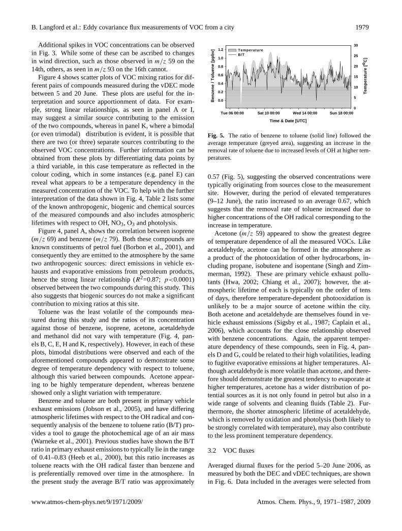
Figure 4 shows scatter plots of VOC mixing ratios for dif-ferent pairs of compounds measured during the vDEC modebetween 5 and 20 June. These plots are useful for the in-terpretation and source apportionment of data. For exam-ple, strong linear relationships, as seen in panel A or I,may suggest a similar source contributing to the emissionof the two compounds, whereas in panel K, where a bimodal(or even trimodal) distribution is evident, it is possible thatthere are two (or three) separate sources contributing to theobserved VOC concentrations. Further information can beobtained from these plots by differentiating data points bya third variable, in this case temperature as reflected in thecolour coding, which in some instances (e.g. panel E) canreveal what appears to be a temperature dependency in themeasured concentration of the VOC. To help with the furtherinterpretation of the data shown in Fig. 4, Table 2 lists someof the known anthropogenic, biogenic and chemical sourcesof the measured compounds and also includes atmosphericlifetimes with respect to OH, NO3, O3 and photolysis.

Figure 4, panel A, shows the correlation between isoprene(m/z 69) and benzene (m/z 79). Both these compounds areknown constituents of petrol fuel (Borbon et al., 2001), andconsequently they are emitted to the atmosphere by the sametwo anthropogenic sources: direct emissions in vehicle ex-hausts and evaporative emissions from petroleum products,hence the strong linear relationship (R2=0.87; p<0.0001)observed between the two compounds during this study. Thisalso suggests that biogenic sources do not make a significantcontribution to mixing ratios at this site.

Toluene was the least volatile of the compounds mea-sured during this study and the ratios of its concentrationagainst those of benzene, isoprene, acetone, acetaldehydeand methanol did not vary with temperature (Fig. 4, pan-els B, C, E, H and K, respectively). However, in each of theseplots, bimodal distributions were observed and each of theaforementioned compounds appeared to demonstrate somedegree of temperature dependency with respect to toluene,although this varied between compounds. Acetone appear-ing to be highly temperature dependent, whereas benzeneshowed only a slight variation with temperature.

Benzene and toluene are both present in primary vehicleexhaust emissions (Jobson et al., 2005), and have differingatmospheric lifetimes with respect to the OH radical and con-sequently analysis of the benzene to toluene ratio (B/T) pro-vides a tool to gauge the photochemical age of an air mass(Warneke et al., 2001). Previous studies have shown the B/Tratio in primary exhaust emissions to typically lie in the rangeof 0.41–0.83 (Heeb et al., 2000), but this ratio increases astoluene reacts with the OH radical faster than benzene andis preferentially removed over time in the atmosphere. Inthe present study the average B/T ratio was approximately

Time & Date [UTC]

Tue 06 00:00 Sat 10 00:00 Wed 14 00:00 Sun 18 00:00

Tem

pera

ture

[oC

]

0

5

10

15

20

25

30

Ben

zene

/ To

luen

e [p

pbv]

0.0

0.2

0.4

0.6

0.8

1.0

1.2 TemperatureB/T

Fig. 5. The ratio of benzene to toluene (solid line) followed theaverage temperature (greyed area), suggesting an increase in theremoval rate of toluene due to increased levels of OH at higher tem-peratures.

0.57 (Fig. 5), suggesting the observed concentrations weretypically originating from sources close to the measurementsite. However, during the period of elevated temperatures(9–12 June), the ratio increased to an average 0.67, whichsuggests that the removal rate of toluene increased due tohigher concentrations of the OH radical corresponding to theincrease in temperature.

Acetone (m/z 59) appeared to show the greatest degreeof temperature dependence of all the measured VOCs. Likeacetaldehyde, acetone can be formed in the atmosphere asa product of the photooxidation of other hydrocarbons, in-cluding propane, isobutene and isopentane (Singh and Zim-merman, 1992). These are primary vehicle exhaust pollu-tants (Hwa, 2002; Chiang et al., 2007); however, the at-mospheric lifetime of each is typically on the order of tensof days, therefore temperature-dependent photooxidation isunlikely to be a major source of acetone within the city.Both acetone and acetaldehyde are themselves found in ve-hicle exhaust emissions (Sigsby et al., 1987; Caplain et al.,2006), which accounts for the close relationship observedwith benzene concentrations. Again, the apparent temper-ature dependency of these compounds, seen in Fig. 4, pan-els D and G, could be related to their high volatilities, leadingto fugitive evaporative emissions at higher temperatures. Al-though acetaldehyde is more volatile than acetone, and there-fore should demonstrate the greatest tendency to evaporate athigher temperatures, acetone has a wider distribution of po-tential sources as it is not only found in petrol but also in awide range of solvents and cleaning fluids (Table 2). Fur-thermore, the shorter atmospheric lifetime of acetaldehyde,which is removed by oxidation and photolysis (both likely tobe strongly correlated with temperature), may also contributeto the less prominent temperature dependency.

3.2 VOC fluxes

Averaged diurnal fluxes for the period 5–20 June 2006, asmeasured by both the DEC and vDEC techniques, are shownin Fig. 6. Data included in the averages were selected from



Table 2. List of biogenic, anthropogenic and secondary atmospheric chemistry sources of VOCs and atmospheric lifetimes with respect toOH, NO3, O3 and photolysis. The temperature dependency (TD) of each source is listed, where 5 stars represent a very high dependencyand 1 star a very low dependency.

Sources Methanol TD? Acetaldehyde TD? Acetone TD? Isoprene TD? Benzene TD? Toluene TD?

[m/z 33] [m/z 45] [m/z 59] [m/z 69] [m/z 79] [m/z 93]

Biogenic Direct Biomass burning Wetting of dried Emission No Noemissions (Lipari et al., 1984; leaf litter which from ∗∗∗∗∗ known knownfrom plants: Hurst et al., 1994). has been ∗∗∗ plants sources sources

subjected to highdaytime temperatures

- Plant defence. ∗ Direct emissions (Warneke et al., 1999).- Cut and drying from plants:of vegetation ∗ - Leakage from(Guenther stomata during - Plant defenceet al., 2000). oxidation of ethanol - Cut and drying

(Kreuzwieser et al., of vegetation ∗

1999). (Guenther et al.,- Leaf decomposition ∗∗ 2000)(Fall, 2003; Warnekeet al., 1999).- Leaf wounding(de Gouw et al., ∗

2000).- Light darktransition emission(Holzinger et al., 2000;Karl et al., 2002).

- Plant defence. ∗

- Cut and dryingof vegetation ∗

(Guenther et al., 2000).

Anthro- Primarily used as Fossil fuel combustion Produced in industry∗∗∗∗ Tail pipe emissions Tail pipe emissions Tail pipe emissionspogenic an industrial ∗∗∗∗ (Anderson et al., 1996). for use as a solvent. (Borbon et al., 2001).∗ (Borbon et al., 2001). ∗ (Borbon et al., 2001). ∗

solvent –inks,adhesives, dyes, Tail pipe emissionspaint andvarnish remover. Tail pipe emissions

∼0.5% of carbon (Sigsby et al., 1987) 1.6–15.3 mg km−1 5.87–12.2 mg km−1 29 mg km−1

Ingredient of is emitted as estimated total ∗ (Chiang et al., 2007). (Chiang et al., 2007; (Chiang et al.,gasoline where it ∗∗∗ Acetaldehyde ∗ emission∼1% of total Hwa, 2002). 2007; Hwa, 2002).is used as an (Sigsby et al., 1987). pipe total exhaust. ∗∗

antifreeze and Evaporative Solvents –octane booster. Exhaust emission Evaporative emissions.∗∗∗∗∗ emissions – Paint thinners ∗

Likely to become in urban areas ∗ petrol Ink and paint ∗

an important 1.4 mg km−1 station manufacture ∗

source (petrol) and forecourts. Printing and ∗

in the future. 4.4 mg km−1 publishing ∗

(diesel) (Caplain Evaporative ∗

et al., 2006). emissions – ∗

Antifreeze. ∗∗∗

Evaporativeemissions. ∗∗∗∗∗

Atmo- Oxidation of Oxidation ofspheric hydrocarbons propane (which haschemistry (Grosjean et al., 2003). an atmospheric

lifetime with>C1 alkanes respect to OH of ∗∗∗∗

(e.g. ethane, 10 days), isobutenepropane,n-butane) and isopentaneand>C2 alkenes (Singh et al., 1994).(propene, 2-butene)form acetaldehyde Propaneas an intermediate (0.2–2.4 mg km−1;oxidation product. Hwa, 2002;

Chiang et al., 2007),isobutene(5.6 mg km−1;Hwa, 2002) andisopentane(40.1 mg km−1;Chiang et al., 2007)have all been shownto be emittedin vehicle exhaust.

Atmosphericlifetime withrespect to:OH1, 12 day 8.8 h 53 days 1.4 h 9.4 day 1.9 dayNO1

3, 1 yr 17 day >11 yr 50 min >4 years 1.9 yrO1

3, – >4.5 yr – 1.3 day >4.5 years >4.5 yrPhotolysis∗. – 6 day – –

1 Atmospheric lifetimes of VOCs are taken from Atkinson (2000).



My list of amendments 1.) Page 2, column 2, line 27, add “with” - “The NAEI, as with most emission nventories….” 2.) Page 4, column 1, last sentence of section 2.3, change “duty cycles” to “scan cycles”. 3.) Figure 1 caption. Change “duty cycle” to “scan cycle” (two corrections needed). 4.) Equation 1. Replace with the following corrected equation

)(')/('1)(1

ittiwN

tFN

iw χχ ∑

=

ΔΔ−=Δ

5.) Figure 3 caption. Please replace the caption with the following…”Plot showing 30 min average wind direction, wind speed and temperature as recorded by the sonic anemometer and the 25 min average concentrations of VOCs measured by the PTR-MS between 5 and 20 June.” 6.) Figure 6. Panels E and J overlap. A corrected version of this figure is pasted below. Please let me know if you require this as a pdf.

Benzene [uncorrected]

f = 7.03 + 0.858 * xR2 = 0.85, p = < 0.0001

vDEC [μg m-2 h-1]

0 100 200 300

DEC

[ μg

m-2

h-1

]

0

100

200

300Hour [UTC]

00 02 04 06 08 10 12 14 16 18 20 22 00

Met

hano

l Flu

x [ μ

g m

-2 h

-1]

0

200

400

600

800

1000vDECDEC [uncorrected]DEC [corrected]

Hour [UTC] 00 02 04 06 08 10 12 14 16 18 20 22 00

Tolu

ene

Flux

[ μg

m-2

h-1

]

0

100

200

300

400

500

600

vDECDEC [uncorrected]DEC [corrected]

Benzene [corrected]

f = -6.803 + 1.367 * xR2 = 0.90, p = < 0.0001

Hour [UTC] 00 02 04 06 08 10 12 14 16 18 20 22 00

Acet

one

Flux

[ μg

m-2

h-1

]

-200

0

200

400

600

800

1000

1200

1400vDECDEC [uncorrected]DEC [corrected] Acetone [corrected]

f =-157.55 + 1.323 * xR2 = 0.76, p = < 0.0001

Hour [UTC]

00 02 04 06 08 10 12 14 16 18 20 22 00

Ben

zene

Flu

x [ μ

g m

-2 h

-1]

0

100

200


Acetone [uncorrected]

f =-138.17 + 1.108 * xR2 = 0.83, p = < 0.0001

vDEC [μg m-2 h-1]100 200 300 400 500 600 700 800 900

DEC

[ μg

m-2

h-1

]

100

200

300

400

500

600

700

800

900

Acetone [corrected]

f =-157.55 + 1.323 * xR2 = 0.76, p = < 0.0001

Hour [UTC] 00 02 04 06 08 10 12 14 16 18 20 22 00

Acet

alde

hyde

Flu

x [ μ

g m

-2 h

-1]

-200

0

200

400

600

800


vDEC [μg m-2 h-1]0 200 400 600

DEC

[ μg

m-2

h-1

]

0

200

400

600

Acetaldehyde [uncorrected]

f = -218.5 + 0.946 * xR2 = 0.77, p = < 0.0001

Acetaldehyde [corrected]

f = -111.532 + 1.212 * xR2 = 0.95, p = < 0.0001

Toluene [uncorrected]

f= -55.143 + 1.11 * xR2 = 0.9, p = < 0.0001

vDEC [μg m-2 h-1]100 200 300 400 500 600

DEC

[ μg

m-2

h-1

]

100

200

300

400

500

600

Toluene [corrected]

f = -80.823 + 1.416 * xR2 = 0.82, p = < 0.0001

A F

C H

E

D

J

B G

I

Methanol [corrected]

f=-333.316 + 1.631 * xR2 = 0.76, p = < 0.0001

Methanol [uncorrected]

f=-71.3 + 0.92 * xR2 = 0.74, p = < 0.0001

vDEC [μg m-2 h-1]300 400 500 600 700 800

DEC

[ μg

m-2

h-1

]

300

400

500

600

700

Methanol [corrected]

f=-333.316 + 1.631 * xR2 = 0.76, p = < 0.0001

F

Fig. 6. PanelsA, B, C, D andE show the average daily fluxes for methanol, acetone, benzene and toluene measured by the DEC andvDEC techniques. The error bars represent 1 standard error of the averages of the vDEC flux. PanelsF, G, H andI show the correspondingregression plots for both corrected (closed circles, dashed line) and uncorrected DEC fluxes (open circles, solid line), where the correctiontakes into account the carry over between subsequent samples in the ISRs.

time periods where measurements from both systems wereavailable. Despite some variability between the two systems,both techniques show VOC fluxes to have a clear diurnaltrend, with fluxes at their largest in the mid to late afternoonand lowest in the early hours of the morning. On average,fluxes were positive for most of the day, indicating the city tobe acting as a net source of VOC to the atmosphere, althoughdeposition was observed for short periods at night. On aver-age, fluxes of methanol were the largest (0.54 mg m−2 h−1),followed by acetone, (0.53 mg m−2 h−1) and acetaldehyde,(0.38 mg m−2 h−1), whereas fluxes of the aromatic com-pounds benzene and toluene were lower (0.12 mg m−2 h−1

and 0.28 mg m−2 h−1, respectively). Isoprene fluxes wereomitted from the final analysis, as significant differenceswere observed between the two techniques, indicating a pos-sible source of contamination in one or other of the systems.

Panel A, Fig. 6, shows the average daily flux of methanol.Typically, fluxes of methanol started to increase at around06:00, rising steadily until a broad evening maximum wasreached between 16:00 and 21:00 GMT. At this time fluxesdropped off sharply before levelling and reaching a minimumduring the early morning. Acetaldehyde fluxes (panel B) alsohad a broad daytime peak, but in contrast to methanol, fluxestended to be larger in the late morning and early afternoon.

The remaining three compounds each shared a similartrend that saw emissions rise between 05:00 and 06:00,reaching a broad peak between 14:00 and 19:00 GMT. Thisafternoon maximum was reflected in measurements of trafficdensity (Fig. 7) taken on Oxford Road, a busy street adjacentto Portland Street. Measurements from this location providea good proxy for the relative change of the diurnal trafficpattern in the area. They also indicate a clear morning rushhour peak which is not reflected in the observed fluxes. The



Hour [UTC]

00 02 04 06 08 10 12 14 16 18 20 22 00

Traf

fic D

ensi

ty [V

ehic

les

h-1]

0

200

400

600

800

1000WeekdayWeekend

Fig. 7. Traffic density measured on Oxford Road (street adjacent toPortland Street). This provides a good proxy for the relative changeof traffic activity in the local area.

absence of this peak in the flux measurements is not uniqueto this site (Nemitz et al., 2002) and is thought to relate toa number of factors: firstly, flux measurements represent theaverage surface exchange occurring over a large area, thusrush hour trends which may be more apparent on some roads(e.g. bus routes such as Oxford road) than others, becomesmeared. Secondly, during the day there is more stationarytraffic, due to loading/unloading and congestion. Thirdly, formeasurements of VOCs which might partially be under tem-perature control, fugitive emission may become an impor-tant source at midday when temperatures are warmest andconsequently any rush hour trend within the data becomessmoothed. Furthermore the use of products (e.g. cleaningproducts, solvents) is not likely to be linked to traffic counts.Finally, the fluxes presented here are an average of bothweekday and weekend fluxes, which, as shown by Fig. 7,may also dampen any rush hour trend in the data.

Regardless of these factors it is still possible that some ofthe flux is missed by the measurement systems, as duringstable night-time conditions and on calm mornings/eveningsthe measurement site may become decoupled from the streetcanyon below. Although this may result in damping of sometemporal features, the effect is somewhat reduced throughnocturnal heat output from the city and the relatively windylocation and therefore the average daily fluxes presented hereshould provide a robust estimate of the total exchange occur-ring throughout the day.

The similarities between traffic counts and VOC fluxessuggest vehicle emissions to be the dominant source formost VOCs, but not all. Methanol and acetaldehyde emis-

sions showed some similarities with traffic density but werebroader over the day, consistent with a large contributionfrom fugitive sources that are coupled to a combination oftemperature and non-traffic anthropogenic activity such assolvent use.

In order to compare data from the two flux techniques,which did not measure simultaneously, the average dailyfluxes were used, thus avoiding uncertainties associated witha changing atmosphere. Despite the indirect nature of thecomparison, the two flux measurement systems showed goodagreement, with measured fluxes falling within the rangeof the standard error (σ /

√N) of hourly fluxes. The high-

est observed correlations between the DEC and vDEC tech-niques were observed in the fluxes of toluene and benzene,which hadR2 values of 0.9 (p<0.0001; N=24) and 0.85(p<0.0001), respectively. Acetone (R2=0.83 p<0.0001)and acetaldehyde (R2=0.77p<0.0001) also compared well,as did methanol (R2=0.74p<0.0001).

The regression plots that accompany Fig. 6 clearly showan offset between the two techniques, with the vDEC fluxmeasurements consistently higher than those made by DEC.The offset was highest for acetaldehyde (46%) and lowestfor benzene (6%) with an average deviation of 20%. Partof this offset may relate to the tendency of the VOC to ad-sorb to the surfaces of the DFS, meaning the signal of the“stickier” compounds such as methanol is dampened. Themain cause however, is thought to relate to the carry-overof air from one DEC sample to the next, caused by the in-complete evacuation of the canister. The carry-over for oursystem was much larger than that reported in previous studies(Rinne et al., 2001) and therefore an alternative data analysiswas carried out, incorporating the following correction forcarry-over:

χcorr =(χ × p1 − χold × p2)

(p1 − p2). (2)

Hereχ is the VOC concentration within the ISR,χold is theprevious concentration of the same ISR,p1 is the ISR pres-sure when full andp2 is the ISR pressure after evacuation.The correction increases the amplitude of the PTR-MS dataand consequently gives larger flux values, as can be seen inFig. 6. After the correction was applied the average offset be-tween the two systems was reduced to less than 7%. Despitethis correction, DECcorr values remained lower than vDECfluxes at night-time. This is thought to relate to the very shortdwell times chosen for the vDEC method, which can resultin limited counting statistics.

Counting statistics cause uncertainty in the flux and theerror is inversely proportional toN0.5, whereN is the totalnumber of ion counts during a (25 min) flux averaging period(Fairall, 1984).N remains similar, independent of whethera concentration is measured frequently with a short dwelltime, or less often with a longer dwell time, except for the in-creased relative dead time associated with switching betweenm/z more rapidly. However, reducing the error associated



with individual count rates on the raw DEC and vDEC datapoints is important as it can impact upon the cross-correlationfunction used to calculate1t and may thus affect the overallprecision of the flux measurement. When the random erroris high, the cross-correlation becomes noisier and more dif-ficult to interpret, reducing the measurement precision. Bylooking for the time lag that maximises the cross correlation,fluxes may be systematically biased towards extreme values,which would be more important the noisier the time-seriesand the smaller the flux (i.e. during night-time). Calculatingthe flux limit of detection by taking the standard deviationof the covariance function at distances far from the true lagwould help to eliminate such periods in the future. It shouldbe noted that, where a constant time-lag can be used, a sys-tematic bias should not occur.

During the daytime, corrected DEC fluxes were larger thanvDEC fluxes. Some of this difference can be explained by thefaster response time of the DEC system, which could resolveturbulent fluctuations of up to 1 Hz as opposed to 0.5Hz forthe vDEC system. Analysis of the sensible heat flux, whichwe assume to show identical frequency behaviour as the mea-sured VOC, demonstrated that approximately 5% of the fluxwas carried in this frequency range.

The uncertainty of flux estimates due to the disjunct sam-pling protocol was estimated for each system using the ap-proach of Lenschow et al. (1994). Integral time scales (lws)ranged between 10–20 s, our averaging period (T ) was 1500 sand our sampling intervals (1x) were∼0.2 s and 12 s respec-tively for the vDEC and DEC techniques. Sampling errorswere found to be<1% for the vDEC technique and between6 and 13% for the DEC mode. These errors are comparablysmall when considering uncertainties associated with geo-physical variability. Errors associated with both unstable andneutral conditions were calculated following the method ofWesley and Hart (1985) and were found to be 47% and 61%,respectively.

3.3 Comparison of measured VOC fluxes with NAEIestimates

Measured VOC fluxes were up-scaled and comparedagainst the most recent (2006) emission estimate forManchester taken from the UK National AtmosphericEmission Inventory (http://www.naei.org.uk/datachunk.php?f datachunkid=174). The flux estimates from the DECcorrsystem were used for the comparison as they did not suf-fer from the attenuation of high frequency flux contributions.In order to compare the up-scaled fluxes with the inventoryit was first necessary to calculate the approximate flux footprint (surface area contributing to the flux) so that the appro-priate NAEI grid(s) could be selected for comparison.

Footprints were calculated using a simple parameterisa-tion model developed by Kljun et al. (2004) which was runusing typical urban meteorology to give footprints under sta-ble, neutral and convectively unstable atmospheric condi-

tions. This model is designed for dynamically homogenousterrain, therefore its application to the urban environment isnot ideal; however there are few if any operational footprintmodels designed for this type of environment. Therefore theflux footprints obtained are treated as a first-order estimateonly. The following parameters were used in the model: stan-dard deviation of vertical wind velocityσw=0.3 m s−1; fric-tion velocity u∗=0.3 m s−1 (average measurement period);measurement heightzm=95 m; roughness lengthz0=1.5 m(estimated as 1/10th of the average building height, 15 m);and boundary layer heighth=2000 m. The results are shownin Fig. 8 and list the distance at which the maximum contri-bution to the flux can be expected (Xmax) and the distancewhich 80% of the flux is contained (Xr ). A circular fluxfootprint (radius=Xr ) was then superimposed over a map ofNAEI grid squares and the entrained grids averaged using aweighting factor to account for the measured wind directionduring the measurement period.

In order to calculate an emission estimate for the fluxfootprint using these data, it was assumed that the observedaverage fluxes were representative of VOC emission ratesoccurring throughout the year (although the emission ratesare likely to show some seasonality, with increased vehicleuse during the winter months causing higher direct emis-sions; this may be balanced by increased fugitive emissionsin the summer months). Therefore the measured averagetotal daily flux of benzene for example (2.87 mg m−2 d−1

(DECcorr)) was extrapolated to give an annual emission es-timate of 1.0 t km−2 yr−1. This value is 1.5 times greaterthan that predicted by the NAEI (0.69 t km−2 yr−1) for thesame flux footprint during 2006. However, the NAEI esti-mate falls inside the overall error bounds of the measure-ment (Fig. 9). Fluxes of toluene compared similarly, witha 1.5 times difference between measurements and inventory.In contrast, fluxes of the oxygenated compounds methanol(×3.6), acetaldehyde (×6.3) and acetone (×4.7) were con-siderably larger than the emission inventory. This outcomesuggests the NAEI is accurately characterising the sourcesof the aromatic compounds, whose emission is dominatedby a single source, in this case road transport. Yet, for theoxygenated VOCs, such as methanol or acetaldehyde, whoseemissions may be dominated by numerous diffuse sources, itperforms less well. In such instances direct “top-down” fluxmeasurements may provide a more robust approach.

Published VOC fluxes from the urban environment arelimited, but fluxes have been measured above MexicoCity using a vDEC approach as part of the Mexico CityMetropolitan Area 2003 field campaign. Average fluxes ofmethanol (1.0 mg m−2 h−1), toluene (0.83 mg m−2 h−1) andacetone (0.39 mg m−2 h−1) were found to be up to threetimes higher than those observed in Manchester (Velasco etal., 2005). This is unsurprising given the much older vehi-cle fleet, less dominance of catalytic converters and poorerfuel quality in Mexico City, where vehicle emissions are notregulated by the Geneva (UN ECE, 1991) and Gothenburg





0

0.0001

0.0002

0.0003

0.0004

0.0005

0.0006

0.0007

0.0008

0.0009

-1500 0 1500 3000 4500 6000X [m]

fy [m

-1] (

Cro

ssw

ind

inte

grat

ed f)

u* = 0.35u* = 0.2 u* = 0.75

X max Xr [80%]

742 m 1623 m

536 m 1174 m

1544 m 3378 m

Fig. 8. Predicted one-dimensional flux footprint from PortlandTower, Manchester, where the solid, dashed and dotted lines rep-resent the predicted footprint for u* values of 0.2 (minimum ob-served), 0.35 (average for campaign) and 0.75 m s−1 (maximumobserved).

0

1

2

3

4

5

6

7

8

Methan

ol

Acetal

dehy

de

Aceton

e

Benze

ne

Toluen

e

VOC

em

issi

on e

stim

ate

[t k

m-2

yr-1

]

DECDEC CorrectedvDECNAEI

Fig. 9. Emission estimates for Manchester city centre based onup-scaled flux measurements. The emission estimate for benzene(DECcorr) and toluene compared closely to that predicted by thenational atmospheric emission inventory. Error bars show the un-certainty of the emission estimate based on the standard error of theflux averages.

(UN ECE, 1999) multi-pollutant protocols as is the case inthe UK. By comparison, recent measurements of VOC fluxesby REA over Houston, Texas, (Park et al., 2008) derivedfluxes in the range−0.36 to 3.1 mg m−2 h−1 for benzene and−0.47 to 5.04 mg m−2 h−1 for toluene.

4 Conclusions

In the past the virtual and disjunct eddy covariance tech-niques have been successfully applied to give flux informa-tion from a range of vegetation canopies. In the present studywe have shown that these techniques can be extended to theurban environment provided a measurement site with suit-able elevation above street level can be found. We have alsodemonstrated the effectiveness and limitations of each ap-proach. The vDEC technique is thought to be more suitedfor urban flux work due to its relative simplicity, althoughlonger dwell times are needed to avoid errors associated withlimited counting statistics.

Emission estimates derived from flux data demonstrate thepotential of using VOC flux measurements in determiningemission estimates on a city wide scale. Although emis-sion estimates obtained in this study are based on a “snapshot” of the total annual emission, they demonstrate the po-tential of the technique, which, if deployed on a longer timescale, such as a year, could give very detailed information onurban-scale emissions, including both spatial and, more im-portantly, temporal trends, which are currently not accountedfor in the NAEI emission estimates.

Acknowledgements.We thank Bruntwood Estates Ltd for allowingaccess to Portland Tower and for the cooperation and support oftheir staff. The work was funded by the UK Natural EnvironmentalResearch Council through the “CityFlux” grant and an NCASstudentship and by the ESF VOCBAS programme. We thankIan Longley (Manchester University) who was responsible forthe organisation and logistics of the campaign, Gavin Phillips(CEH Edinburgh) for his help transporting the instrumentation andMalcolm Possell (Lancaster University) for helpful discussion.

Edited by: A. B. Guenther

References

Ammann, C., Brunner, A., Spirig, C., and Neftel, A.: Technicalnote: Water vapour concentration and flux measurements withPTR-MS, Atmos. Chem. Phys., 6, 4643–4651, 2006,http://www.atmos-chem-phys.net/6/4643/2006/.

Anderson, L. G., Lanning, J. A., Barrell, R., Miyagishima, J., Jones,R. H., and Wolfe, P.: Sources and sinks of formaldehyde and ac-etaldehyde: An analysis of Denver’s ambient concentration data,Atmos. Environ., 30, 2113–2123, 1996.

Atkinson, R.: Atmospheric chemistry of VOC and NOx, Atmos.Environ., 34, 2063–2101, 2000.


http://www.atmos-chem-phys.net/6/4643/2006/


Aubinet, M., Chermanne, B., Vandenhaute, M., Longdoz, B., Yer-naux, M., and Laitat, E.: Long term carbon dioxide exchangeabove a mixed forest in the Belgian Ardennes, Agr. Forest Mete-orol., 108, 293–315, 2001.

Borbon, A., Fontaine, H., Veillerot, M., Locoge, N., Galloo, J. C.,and Guillermo, R.: An investigation into the traffic-related frac-tion of isoprene at an urban location, Atmos. Environ., 35, 3749–3760, 2001.

Bowling, D. R., Turnipseed, A. A., Delany, A. C., Baldocchi, D.D., Greenberg, J. P., and Monson, R. K.: The use of relaxededdy accumulation to measure biosphere-atmosphere exchangeof isoprene and of other biological trace gases, Oecologia, 116,306–315, 1998.

Brunner, A., Ammann, C., Neftel, A., and Spirig, C.: Methanol ex-change between grassland and the atmosphere, Biogeosciences,4, 395–410, 2007,http://www.biogeosciences.net/4/395/2007/.

Businger, J. A. and Oncley, S. P.: Flux measurement with condi-tional sampling, J. Atmos. Ocean. Tech., 7, 349–352, 1990.

Caplain, I., Cazier, F., Nouali, H., Mercier, A., Dechaux, J. C., Nol-let, V., Journard, R., Andre, J. M., and Vidon, R.: Emissions ofunregulated pollutants from European gasoline and diesel pas-senger cars, Atmos. Environ., 40, 5954–5966, 2006.

Chiang, H. L., Hwu, C. S., Chen, S. Y., Wu, M. C., Ma, S. Y.,and Huang, Y. S.: Emission factors and characteristics of criteriapollutants and volatile organic compounds (VOCs) in a freewaytunnel study, Sci. Total Environ., 381, 200–211, 2007.

Christian, T. J., Kleiss, B., Yokelson, R. J., Holzinger, R., Crutzen,P. J., Hao, W. M., Shirai, T., and Blake, D. R.: Com-prehensive laboratory measurements of biomass-burning emis-sions: 2. First intercomparison of open-path FTIR, PTR-MS,and GC-MS/FID/ECD, J. Geophys. Res.-Atmos., 109, D02311,doi:10.1029/2003JD003874, 2004.

Ciccioli, P., Brancaleoni, E., Frattoni, M., Marta, S., Brachetti, A.,Vitullo, M., Tirone, G., and Valentini, R.: Relaxed eddy accumu-lation, a new technique for measuring emission and depositionfluxes of volatile organic compounds by capillary gas chromatog-raphy and mass spectrometry, J. Chromatogr. A, 985, 283–296,2003.

de Gouw, J. and Warneke, C.: Measurements of volatile organiccompounds in the Earth’s atmosphere using proton-transfer-reaction mass spectrometry, Mass Spectrom. Rev., 26, 223–257,2007.

de Gouw, J., Warneke, C., Karl, T., Eerdekens, G., van der Veen,C., and Fall, R.: Sensitivity and specificity of atmospheric tracegas detection by proton-transfer-reaction mass spectrometry, Int.J. Mass Spectrom., 223, 365–382, 2003.

de Gouw, J. A., Howard, C. J., Custer, T. G., Baker, B. M., andFall, R.: Proton-transfer chemical-ionization mass spectrome-try allows real-time analysis of volatile organic compounds re-leased from cutting and drying of crops, Environ. Sci. Technol.,34, 2640–2648, 2000.

Dollard, G. J., Dumitrean, P., Telling, S., Dixon, J., and Derwent,R. G.: Observed trends in ambient concentrations of C-2-C-8hydrocarbons in the United Kingdom over the period from 1993to 2004, Atmos. Environ., 41, 2559–2569, 2007.

Dorsey, J. R., Nemitz, E., Gallagher, M. W., Fowler, D., Williams,P. I., Bower, K. N., and Beswick, K. M.: Direct measurementsand parameterisation of aerosol flux, concentration and emission

velocity above a city, Atmos. Environ., 36, 791–800, 2002.Fairall, C. W.: Interpretation of eddy-correlation measurements

of particulate deposition and aerosol flux, Atmos. Environ., 18,1329–1337, 1984.

Famulari, D., Nemitz, E., Di Marco, C., Phillips, G. J., Thomas,R., House, E., and Fowler, D.: Eddy-covariance measurementsof nitrous oxide fluxes above a city, Agr. Forest Meteorol., inreview, 2009.

Filella, I. and Penuelas, J.: Daily, weekly, and seasonal time coursesof VOC concentrations in a semi-urban area near Barcelona, At-mos. Environ., 40, 7752–7769, 2006.

Friedrich, R. and Obermeier, A.: Anthropogenic Emissions ofVolatile Organic Compounds, in: Reactive Hydrocarbons in theAtmosphere, edited by: Hewitt, C. N., Academic Press, Califor-nia, 1–39, 1999.

Gallagher, M. W., Clayborough, R., Beswick, K. M., Hewitt, C.N., Owen, S., Moncrieff, J., and Pilegaard, K.: Assessment ofa relaxed eddy accumulation for measurements of fluxes of bio-genic volatile organic compounds: Study over arable crops and amature beech forest, Atmos. Environ., 34, 2887–2899, 2000.

Grabmer, W., Graus, M., Lindinger, C., Wisthaler, A., Rap-pengluck, B., Steinbrecher, R., and Hansel, A.: Disjunct eddycovariance measurements of monoterpene fluxes from a norwayspruce forest using PTR-MS, Int. J. Mass Spectrom., 239, 111–115, 2004.

Greenberg, J. P., Guenther, A., Harley, P., Otter, L., Veenendaal,E. M., Hewitt, C. N., James, A. E., and Owen, S. M.: Eddyflux and leaf-level measurements of biogenic VOC emissionsfrom mopane woodland of Botswana, J. Geophys. Res.-Atmos.,108(D13), 8466, doi:10.1029/2002JD002317, 2003.

Grosjean, D., Grosjean, E., and Moreira, L. F. R.: Speciated ambi-ent carbonyls in Rio de Janeiro, Brazil, Environ. Sci. Technol.,36, 1389-1395, 2002.

Grosjean, E., Grosjean, D., Fraser, M. P., and Cass, G. R.: Air qual-ity model evaluation data for organics. 2. C-1-C-14 carbonyls inLos Angeles air, Environ. Sci. Technol., 30, 2687–2703, 1996.

Guenther, A., Geron, C., Pierce, T., Lamb, B., Harley, P., andFall, R.: Natural emissions of non-methane volatile organic com-pounds; carbon monoxide, and oxides of nitrogen from NorthAmerica, Atmos. Environ., 34, 2205–2230, 2000.

Hayward, S., Hewitt, C. N., Sartin, J. H., and Owen, S. M.: Per-formance characteristics and applications of a proton transferreaction-mass spectrometer for measuring volatile organic com-pounds in ambient air, Environ. Sci. Technol., 36, 1554–1560,2002.

Heeb, N. V., Forss, A. M., Bach, C., Reimann, S., Herzog, A.,and Jackle, H. W.: A comparison of benzene, toluene and C-2-benzenes mixing ratios in automotive exhaust and in the sub-urban atmosphere during the introduction of catalytic convertertechnology to the Swiss car fleet, Atmos. Environ., 34, 3103–3116, 2000.

Holzinger, R., Jordan, A., Hansel, A., and Lindinger, W.:Methanol measurements in the lower troposphere near Innsbruck(047◦16′ N; 011◦24′ E), Austria, Atmos. Environ., 35, 2525–2532, 2001.

Horst, T. W.: A simple formula for attenuation of eddy fluxes mea-sured with first-order-response scalar sensors, Bound.-Lay. Me-teorol., 82, 219–233, 1997.

Hurst, D. F., Griffith, D. W. T., and Cook, G. D.: Trace gas emis-


http://www.biogeosciences.net/4/395/2007/


sions from biomass burning in tropical Australian savannas, J.Geophys. Res.-Atmos., 99, 16 441–16 456, 1994.

Hwa, M. Y., Hsieh, C. C., Wu, T. C., and Chang, L. F. W.: Real-world vehicle emissions and VOCs profile in the Taipei tunnellocated at Taiwan Taipei area, Atmos. Environ., 36, 1993–2002,2002.

Jobson, B. T., Alexander, M. L., Maupin, G. D., and Muntean, G.G.: On-line analysis of organic compounds in diesel exhaust us-ing a proton transfer reaction mass spectrometer (PTR-MS), Int.J. Mass Spectrom., 245, 78–89, 2005.

Karl, T. G., Spirig, C., Rinne, J., Stroud, C., Prevost, P., Green-berg, J., Fall, R., and Guenther, A.: Virtual disjunct eddy covari-ance measurements of organic compound fluxes from a subalpineforest using proton transfer reaction mass spectrometry, Atmos.Chem. Phys., 2, 279–291, 2002,http://www.atmos-chem-phys.net/2/279/2002/.

Karl, T., Guenther, A., Lindinger, C., Jordan, A., Fall, R., andLindinger, W.: Eddy covariance measurements of oxygenatedvolatile organic compound fluxes from crop harvesting using aredesigned proton-transfer-reaction mass spectrometer, J. Geo-phys. Res.-Atmos., 106, 24 157–24 167, 2001.

Kato, S., Miyakawa, Y., Kaneko, T., and Kajii, Y.: Urban air mea-surements using PTR-MS in Tokyo area and comparison withGC-FID measurements, Int. J. Mass Spectrom., 235, 103–110,2004.

Kljun, N., Calanca, P., Rotachhi, M. W., and Schmid, H. P.: A sim-ple parameterisation for flux footprint predictions, Bound.-Lay.Meteorol., 112, 503–523, 2004.

Kreuzwieser, J., Scheerer, U., and Rennenberg, H.: Metabolic ori-gin of acetaldehyde emitted by Poplar (Populus tremulax P-alba) trees, J. Exp. Bot., 50, 757–765, 1999.

Kristensen, L., Mann, J., Oncley, S. P., and Wyngaard, J. C.: Howclose is close enough when measuring scalar fluxes with dis-placed sensors?, J. Atmos. Ocean. Tech., 14, 814–821, 1997.

Lee, A., Schade, G. W., Holzinger, R., and Goldstein, A. H.: Acomparison of new measurements of total monoterpene flux withimproved measurements of speciated monoterpene flux, Atmos.Chem. Phys., 5, 505–513, 2005,http://www.atmos-chem-phys.net/5/505/2005/.

Lenschow, D. H., Mann, J., and Kristensen, L.: How long is longenough when measuring fluxes and other turbulence statistics, J.Atmos. Ocean. Tech., 11, 661–673, 1994.

Lenschow, D. H.: Micrometeorological techniques for measuringbiosphere-atmosphere trace gas exchangei in: Biogenic TraceGases: Measuring Emissions from Soil and Water, edited by:Matson, P. A., London, Blackwell, 126–163, 1995.

Lindinger, W., Hansel, A., and Jordan, A.: Proton-transfer-reactionmass spectrometry (PTR-MS): On-line monitoring of volatile or-ganic compounds at pptv levels, Chem. Soc. Rev., 27, 347–354,1998.

Lipari, F., Dasch, J. M., and Scruggs, W. F.: Aldehyde emissionsfrom wood-burning fireplaces, Environ. Sci. Technol., 18, 326–330, 1984.

Martin, C. L., Longley, I. D., Dorsey, J. R., Thomas, R. M.,Gallagher M. W., and Nemitz, E.: Ultrafine particle fluxesabove four major European cities, Atmos. Environ., in press,doi:10.1016/j.atmosenv.2008.10.009, 2008.

Nemitz, E., Hargreaves, K. J., McDonald, A. G., Dorsey, J. R., andFowler, D.: Meteorological measurements of the urban heat bud-

get and CO2 emissions on a city scale, Environ. Sci. Technol.,36, 3139–3146, 2002.

Oke, T. R.: Towards better scientific communication in urban cli-mate, Theor. Appl. Climatol., 84, 179–190, 2006.

Olofsson, M., Ek-Olausson, B., Ljungstrom, E., and Langer, S.:Flux of organic compounds from grass measured by relaxed eddyaccumulation technique, J. Environ. Monitor., 5, 963–970, 2003.

Park, C., Schade, G., and Boedeker, I.: VOC flux measurementsusing a novel relaxed eddy accumulation GC-FID system in ur-ban Houston, Texas, Eos Trans. AGU, 89(53), Fall Meet. Suppl.,Abstract A41F-0178, 2008.

Possanzini, M., Dipalo, V., Petricca, M., Fratarcangeli, R., andBrocco, D.: Measurements of lower carbonyls in Rome ambi-ent air, Atmos. Environ., 30, 3757–3764, 1996.

Rinne, H. J. I., Delany, A. C., Greenberg, J. P., and Guenther, A.B.: A true eddy accumulation system for trace gas fluxes usingdisjunct eddy sampling method, J. Geophys. Res.-Atmos., 105,24 791–24 798, 2000.

Rinne, H. J. I., Guenther, A. B., Warneke, C., de Gouw, J. A., andLuxembourg, S. L.: Disjunct eddy covariance technique for tracegas flux measurements, Geophys. Res. Lett., 28, 3139–3142,2001.

Schween, J. H., Dlugi, R., Hewitt, C. N., and Foster, P.: Determi-nation and accuracy of VOC-fluxes above the pine/oak forest atCastelporziano, Atmos. Environ., 31, 199–215, 1997.

Sigsby, J. E., Tejada, S., Ray, W., Lang, J. M., and Duncan, J. W.:Volatile organic-compound emissions from 46 in-use passengercars, Environ. Sci. Technol., 21, 466–475, 1987.

Singh, H. B., Ohara, D., Herlth, D., Sachse, W., Blake, D. R., Brad-shaw, J. D., Kanakidou, M., and Crutzen, P. J.: Acetone in theatmosphere – distribution, sources, and sinks, J. Geophys. Res.-Atmos., 99, 1805–1819, 1994.

Spirig, C., Neftel, A., Ammann, C., Dommen, J., Grabmer, W.,Thielmann, A., Schaub, A., Beauchamp, J., Wisthaler, A., andHansel, A.: Eddy covariance flux measurements of biogenicVOCs during ECHO 2003 using proton transfer reaction massspectrometry, Atmos. Chem. Phys., 5, 465–481, 2005,http://www.atmos-chem-phys.net/5/465/2005/.

Tani, A., Nozoe, S., Aoki, M., and Hewitt, C. N.: Monoterpenefluxes measured above a Japanese red pine forest at Oshibaplateau, Japan, Atmos. Environ., 36, 3391–3402, 2002.

Turnipseed, A. A., Pressley, S. N., Karl, T., Lamb, B., Nemitz, E.,Allwine, E., Cooper, W. A., Shertz, S., and Guenther, A. B.: Theuse of disjunct eddy sampling methods for the determination ofecosystem level fluxes of trace gases, Atmos. Chem. Phys., 9,981–994, 2009,http://www.atmos-chem-phys.net/9/981/2009/.

Velasco, E., Lamb, B., Pressley, S., Allwine, E., Westberg, H.,Jobson, B. T., Alexander, M., Prazeller, P., Molina, L., andMolina, M.: Flux measurements of volatile organic compoundsfrom an urban landscape, Geophys. Res. Lett., 32, L20802,doi:10.1029/2005GL023356, 2005.

Warneke, C., van der Veen, C., Luxembourg, S., de Gouw, J. A.,and Kok, A.: Measurements of benzene and toluene in ambi-ent air using proton-transfer-reaction mass spectrometry: Cali-bration, humidity dependence, and field intercomparison, Int. J.Mass Spectrom., 207, 167–182, 2001.

Warneke, C., Luxembourg, S. L., de Gouw, J. A., Rinne, H. J. I.,Guenther, A. B., and Fall, R.: Disjunct eddy covariance measure-







ments of oxygenated volatile organic compounds fluxes from analfalfa field before and after cutting, J. Geophys. Res.-Atmos.,107(D8), 4067, doi:10.1029/2001JD000594, 2002.

Warneke, C., Karl, T., Judmaier, H., Hansel, A., Jordan, A.,Lindinger, W., and Crutzen, P. J.: Acetone, methanol, and otherpartially oxidized volatile organic emissions from dead plantmatter by abiological processes: Significance for atmosphericHOx chemistry, Global Biogeochem. Cy., 13, 9–17, 1999.

Wesely, M. L. and Hart, R. L.: Variability of short term eddy-covariance estimates of mass exchange, in: The forest atmo-sphere interactions, edited by: Hutchison, B. and Hicks, B.,D. Reidel publishing Company, Dortrecht, The Netherlands,591–612, 1985

Wilkinson, M. J.: Circadian control of isoprene emissions from oilpalm, Ph.D. thesis, Lancaster University, 2006.

UN ECE: Protocol to the 1979 Convention on Long-Range Trans-boundary Air Pollution Concerning the Control of Emissionsof Volatile Organic Compounds on their Transboundary Fluxes,ECE/EB.AIR/30, United Nations Economic Commission for Eu-rope, Geneva, Switzerland, 1991.

UN ECE: Protocol to the 1979 Convention on Long-range Trans-boundary Air Pollution to Abate Acidification, Eutrophicationand Ground-level Ozone, United Nations Economic Commissionfor Europe, Geneva, Switzerland, 1999.

Zhao, J. and Zhang, R. Y.: Proton transfer reaction rate constantsbetween hydronium ion (H3O(+)) and volatile organic com-pounds, Atmos. Environ., 38, 2177–2185, 2004.


Mixing ratios and eddy covariance flux measurements of ...

Documents

Transcript of Mixing ratios and eddy covariance flux measurements of ...