arX

iv:1

404.

7080

v1 [

mat

h.ST

] 2

8 A

pr 2

014

A test for the equality of covariance operators

Graciela Boente, Daniela Rodriguez and Mariela Sued

Facultad de Ciencias Exactas y Naturales, Universidad de Buenos Aires and CONICET, Argentina

e–mail: gboente@dm.uba.ar drodrig@dm.uba.ar msued@dm.uba.ar

Abstract

In many situations, when dealing with several populations, equality of the covarianceoperators is assumed. An important issue is to study if this assumption holds beforemaking other inferences. In this paper, we develop a test for comparing covarianceoperators of several functional data samples. The proposed test is based on the squarednorm of the difference between the estimated covariance operators of each population.We derive the asymptotic distribution of the test statistic under the null hypothesis andfor the situation of two samples, under a set of contiguous alternatives related to thefunctional common principal component model. Since the null asymptotic distributiondepends on parameters of the underlying distribution, we also propose a bootstrap test.

1 Introduction

In many applications, we study phenomena that are continuous in time or space and can beconsidered as smooth curves or functions. On the other hand, when working with more thanone population, as in the finite dimensional case, the equality of the covariance operatorsassociated with each population is often assumed. In the case of finite-dimensional data,tests for equality of covariance matrices have been extensively studied, see for exampleSeber (1984) and Gupta and Xu (2006). This problem has been considered even for highdimensional data, i.e., when the sample size is smaller than the number of variables understudy; we refer among others to Ledoit and Wolf (2002) and Schott (2007).

For functional data, most of the literature on hypothesis testing deals with tests on themean function including the functional linear model, see, for instance, Fan and Lin (1998),Cardot et al. (2003), Cuevas et al. (2004) and Shen and Faraway (2004). Tests on thecovariance operators related to serial correlation were considered by Gabrys and Kokoszka(2007), Gabrys et al. (2010) and Horvath et al. (2010). On the other hand, Benkoet al. (2009) proposed two-sample bootstrap tests for specific aspects of the spectrum offunctional data, such as the equality of a subset of eigenfunctions while Ferraty et al. (2007)considered tests for comparison of groups of curves based on comparison of their covariances.The hypothesis tested by the later are that of equality, proportionality and others basedon the spectral decomposition of the covariances. Their approach is high dimensional sincethey either approximate the curves over a grid of points, or use a projection approach. More

1

recently, Panaretos et al. (2010) considered the problem of testing whether two samples ofcontinuous zero mean i.i.d. Gaussian processes share or not the same covariance structure.

In this paper, we go one step further and consider the functional setting. Our goalis to provide a test statistic to test the hypothesis that the covariance operators of severalindependent samples are equal in a fully functional setting. To fix ideas, we will first describethe two sample situation. Let us assume that we have two independent populations withcovariance operators Γ1 and Γ2. Denote by Γ1 and Γ2 consistent estimators of Γ1 and Γ2,respectively, such as the sample covariance estimators studied in Dauxois et al. (1982).It is clear that under the standard null hypothesis Γ1 = Γ2, the difference between thecovariance operator estimators should be small. For that reason, a test statistic based onthe norm of Γ1 − Γ2 may be helpful to study the hypothesis of equality.

The paper is organized as follows. Section 2 introduce the notation and review somebasic concepts which are used in later sections. Section 3 introduces the test statistics forthe two sample problem. Its asymptotic distribution under the null hypothesis is establishedin Section 3.1 while a bootstrap test is described in Section 3.2. An important issue is todescribe the set of alternatives that the proposed statistic is able to detect. For that purpose,the asymptotic distribution under a set of contiguous alternatives based on the functionalcommon principal component model is studied in Section 3.3. Finally, an extension toseveral populations is provided in Section 4. Proofs are relegated to the Appendix.

2 Preliminaries and notation

Let us consider independent random elements X1, . . . ,Xk in a separable Hilbert space H(often L2(I)) with inner product 〈·, ·〉 and norm ‖u‖ = 〈u, u〉1/2 and assume that E‖Xi‖2 <∞. Denote by µi ∈ H the mean of Xi, µi = E(Xi) and by Γi : H → H the covarianceoperator of Xi. Let ⊗ stand for the tensor product on H, e.g., for u, v ∈ H, the operatoru⊗v : H → H is defined as (u⊗v)w = 〈v,w〉u. With this notation, the covariance operatorΓi can be written as Γi = E{(Xi − µi)⊗ (Xi − µi)}. The operator Γi is linear, self-adjointand continuous.

In particular, if H = L2(I) and 〈u, v〉 =∫I u(s)v(s)ds, the covariance operator is defined

through the covariance function of Xi, γi(s, t) = cov(Xi(s),Xi(t)), s, t ∈ I as (Γiu)(t) =∫I γi(s, t)u(s)ds. It is usually assumed that ‖γi‖2 =

∫I∫I γ2i (t, s)dtds < ∞ hence, Γi

is a Hilbert-Schmidt operator. Hilbert–Schmidt operators have a countable number ofeigenvalues, all of them being real.

Let F denote the Hilbert space of Hilbert–Schmidt operators with inner product de-

fined by 〈H1,H2〉F = trace(H1H2) =∑∞

ℓ=1〈H1uℓ,H2uℓ〉 and norm ‖H‖F = 〈H,H〉1/2F ={∑∞

ℓ=1 ‖Huℓ‖2}1/2, where {uℓ : ℓ ≥ 1} is any orthonormal basis of H, while H1, H2 and H

are Hilbert-Schmidt operators, i.e., such that ‖H‖F < ∞. Choosing an orthonormal basis{φi,ℓ : ℓ ≥ 1} of eigenfunctions of Γi related to the eigenvalues {λi,ℓ : ℓ ≥ 1} such thatλi,ℓ ≥ λi,ℓ+1, we get ‖Γi‖2F =

∑∞ℓ=1 λ

2i,ℓ. In particular, if H = L2(I), we have ‖Γi‖F = ‖γi‖.

Our goal is to test whether the covariance operators Γi of several populations are equal

2

or not. For that purpose, let us consider independent samples of each population, thatis, let us assume that we have independent observations Xi,1, · · · ,Xi,ni

, 1 ≤ i ≤ k, withXi,j ∼ Xi. A natural way to estimate the covariance operators Γi, for 1 ≤ i ≤ k, is through

their empirical versions. The sample covariance operator Γi is defined as

Γi =1

ni

ni∑

j=1

(Xi,j −Xi

)⊗(Xi,j −X i

),

where Xi = 1/ni∑ni

j=1Xi,j. Dauxois et al. (1982) obtained the asymptotic behaviour of

Γi. In particular, they have shown that, when E(‖Xi,1‖4) < ∞,√ni

(Γi − Γi

)converges in

distribution to a zero mean Gaussian random element of F , Ui, with covariance operatorΥi given by

Υi =∑

m,r,o,p

simsirsiosipE[fimfirfiofip]φi,m ⊗ φi,r⊗φi,o ⊗ φi,p

−∑

m,r

λimλir φi,m ⊗ φi,m⊗φi,r ⊗ φi,r (1)

where ⊗ stands for the tensor product in F and, as mentioned above, {φi,ℓ : ℓ ≥ 1} is anorthonormal basis of eigenfunctions of Γi with associated eigenvalues {λi,ℓ : ℓ ≥ 1} such thatλi,ℓ ≥ λi,ℓ+1. The coefficients sim are such that s2im = λi,m, while fim are the standardized

coordinates of Xi − µi on the basis {φi,ℓ : ℓ ≥ 1}, that is, fim = 〈Xi − µi, φi,m〉/λ1

2

i,m.Note that E(fim) = 0. Using that cov (〈u,Xi − µi〉, 〈v,Xi − µi〉) = 〈u,Γiv〉, we get thatE(f2

im) = 1, E(fim fis) = 0 for m 6= s. In particular, the Karhunen-Loeve expansion leadsto

Xi = µi +∞∑

ℓ=1

λ1

2

i,ℓ fiℓ φi,ℓ . (2)

It is worth noticing that E‖Ui‖2F < ∞ so, the sum of the eigenvalues of Υi is finite, implyingthat Υi is a linear operator over F which is Hilbert Schmidt. Thus, any linear combinationof the operators Υi, Υ =

∑ki=1 aiΥi, with ai ≥ 0, will be a Hilbert Schmidt operator.

Therefore, if {θℓ}ℓ≥1 stand for the eigenvalues of Υ ordered in decreasing order, θℓ ≥ 0 and∑ℓ≥1 θℓ < ∞. This property will be used later in Theorem 3.1.

When H = L2(I), smooth estimators, Γi,h, of the covariance operators were studied inBoente and Fraiman (2000). The smoothed operator is the operator induced by the smoothcovariance function

γi,h(t, s) =1

n1

ni∑

j=1

(Xi,j,h(t)−X i,h(t)

) (Xi,j,h(s)−X i,h(s)

),

where Xi,j,h(t) =∫I Kh(t − x)Xi,j are the smoothed trajectories, Kh(·) = h−1K(·/h) is a

nonnegative kernel function, and h a smoothing parameter. Boente and Fraiman (2000)have shown that, under mild conditions, the smooth estimators have the same asymptoticdistribution that the empirical version.

3

3 Test statistics for two–sample problem

We first consider the problem of testing the hypothesis

H0 : Γ1 = Γ2 against H1 : Γ1 6= Γ2 . (3)

A natural approach is to consider Γi as the empirical covariance operators of each popula-tion and construct a statistic Tn based on the difference between the covariance operatorsestimators, i.e., to define Tn = n‖Γ1 − Γ2‖2F , where n = n1 + n2.

3.1 The null asymptotic distribution of the test statistic

The following result allows to study the asymptotic behaviour of Tn = n‖Γ1 − Γ2‖2F whenΓ1 = Γ2 and thus, to construct a test for the hypothesis (3.1) of equality of covarianceoperators.

Theorem 3.1. Let Xi,1, · · · ,Xi,ni, for i = 1, 2, be independent observations from two

independent samples in H with mean µi and covariance operator Γi. Let n = n1 + n2 andassume also that ni/n → τi with τi ∈ (0, 1). Let Γi, i = 1, 2, be independent estimators

of the i−th population covariance operator such that√ni

(Γi − Γi

)D−→ Ui, with Ui a

zero mean Gaussian random element with covariance operator Υi. Denote by {θℓ}ℓ≥1 theeigenvalues of the operator Υ = τ1

−1Υ1 + τ2−1Υ2 with

∑ℓ≥1 θℓ < ∞. Then,

n‖(Γ1 − Γ1)− (Γ2 − Γ2)‖2FD−→∑

ℓ≥1

θℓZ2ℓ , (4)

where Zℓ are i.i.d. standard normal random variables. In particular, if Γ1 = Γ2 we have

that n‖Γ1 − Γ2‖2FD−→∑

ℓ≥1 θℓZ2ℓ .

Remark 3.1.

a) The results in Theorem 3.1 apply in particular, when considering the sample covari-

ance operator, i.e., when Γi = Γi. Effectively, when E(‖Xi,1‖4) < ∞,√ni

(Γi − Γi

)

converges in distribution to a zero mean Gaussian random element Ui of F with co-variance operator Υi given by (1). As mentioned in the Introduction, the fact thatE(‖Xi,1‖4) < ∞ entails that

∑ℓ≥1 θℓ < ∞.

b) It is worth noting that if qn is a sequence of integers such that qn → ∞, the factthat

∑ℓ≥1 θℓ < ∞ implies that the sequence Un =

∑qnℓ=1 θℓZ

2i is Cauchy in L2 and

therefore, the limit U =∑

ℓ≥1 θℓZ2ℓ is well defined. In fact, analogous arguments to

those considered in Neuhaus (1980) allow to show that the series converges almostsurely. Moreover, since Z2

1 ∼ χ21, U has a continuous distribution function FU and

so FUn, the distribution functions of Un, converge to the FU uniformly, as shown in

Lemma 2.11 in Van der Vaart (2000).

4

Remark 3.2. Theorem 3.1 implies that, under the null hypothesis H0 : Γ1 = Γ2, we

have that Tn = n‖Γ1 − Γ2‖2FD−→ U =

∑ℓ≥1 θℓZ

2ℓ , hence an asymptotic test based on

Tn rejecting for large values of Tn allows to test H0. To obtain the critical value, thedistribution of U and thus, the eigenvalues of τ−1

1 Υ1 + τ−12 Υ2 need to be estimated. As

mentioned in Remark 3.1 the distribution function of U can be uniformly approximated bythat of Un and so, the critical values can be approximated by the (1−α)−percentile of Un.Gupta and Xu (2006) provide an approximation for the distribution function of any finitemixture of χ2

1 independent random variables that can be used in the computation of the

(1 − α)−percentile of∑qn

ℓ=1 θℓZ2ℓ where θℓ are estimators of θℓ. It is also, worth noticing

that under H0 : Γ1 = Γ2, we have that for i = 1, 2, Υi given in (1) reduces to

Υi=∑

m,r,o,p

smsrsospE[fimfirfiofip]φm ⊗ φr⊗φo ⊗ φp−∑

m,r

λmλr φm ⊗ φm⊗φr ⊗ φr

where for the sake of simplicity we have eliminated the subscript 1 and simply denote as

sm = λ1/2m with λm the m−th largest eigenvalue of Γ1 and φm its corresponding eigenfunc-

tion. In particular, if all the populations have the same underlying distribution except forthe mean and covariance operator, as it happens when comparing the covariance operatorsof Gaussian processes, the random function f2m has the same distribution as f1m and so,Υ1 = Υ2.

The previous comments motivate the use of the bootstrap methods, due the fact that theasymptotic distribution obtained in (4) depends on the unknown eigenvalues θℓ. It is clearthat when the underlying distribution of the processXi is assumed to be known, for instance,if both samples correspond to Gaussian processes differing only on their mean and covarianceoperators, a parametric bootstrap can be implemented. Effectively, denote by Gi,µi,Γi

thedistribution of Xi where the parameters µi and Γi are explicit for later convenience. Foreach 1 ≤ i ≤ k, generate bootstrap samples X⋆

i,j, 1 ≤ j ≤ ni, with distribution Gi,0,Γi

. Notethat the samples can be generated with mean 0 since our focus is on covariance operators.Besides, the sample covariance operator Γi is a finite range operator, hence the Karhunen–Loeve expansion (2) allows to generate X⋆

i,j knowing the distribution of the random variables

fiℓ, the eigenfunctions φi,ℓ of Γi and its related eigenvalues λi,ℓ, 1 ≤ ℓ ≤ ni, that is,

the estimators of the first principal components of the process. Define Γ⋆

i as the sample

covariance operator of X⋆i,j , 1 ≤ j ≤ ni and further, let T ⋆

n = n‖Γ⋆

1 − Γ⋆

2‖2F . By replicatingNboot times, we obtain Nboot values T ⋆

n that allow easily to construct a bootstrap test.

The drawback of the above described procedure, it that it assumes that the underlyingdistribution is known hence, it cannot be applied in many situations. For that reason, wewill consider a bootstrap calibration for the distribution of the test that can be describedas follows,

Step 1 Given a sample Xi,1, · · · ,Xi,ni, let Υi be consistent estimators of Υi for

i = 1, 2. Define Υ = τ −11 Υ1 + τ −1

2 Υ2 with τi = ni/(n1 + n2).

Step 2 For 1 ≤ ℓ ≤ qn denote by θℓ the positive eigenvalues of Υ.

5

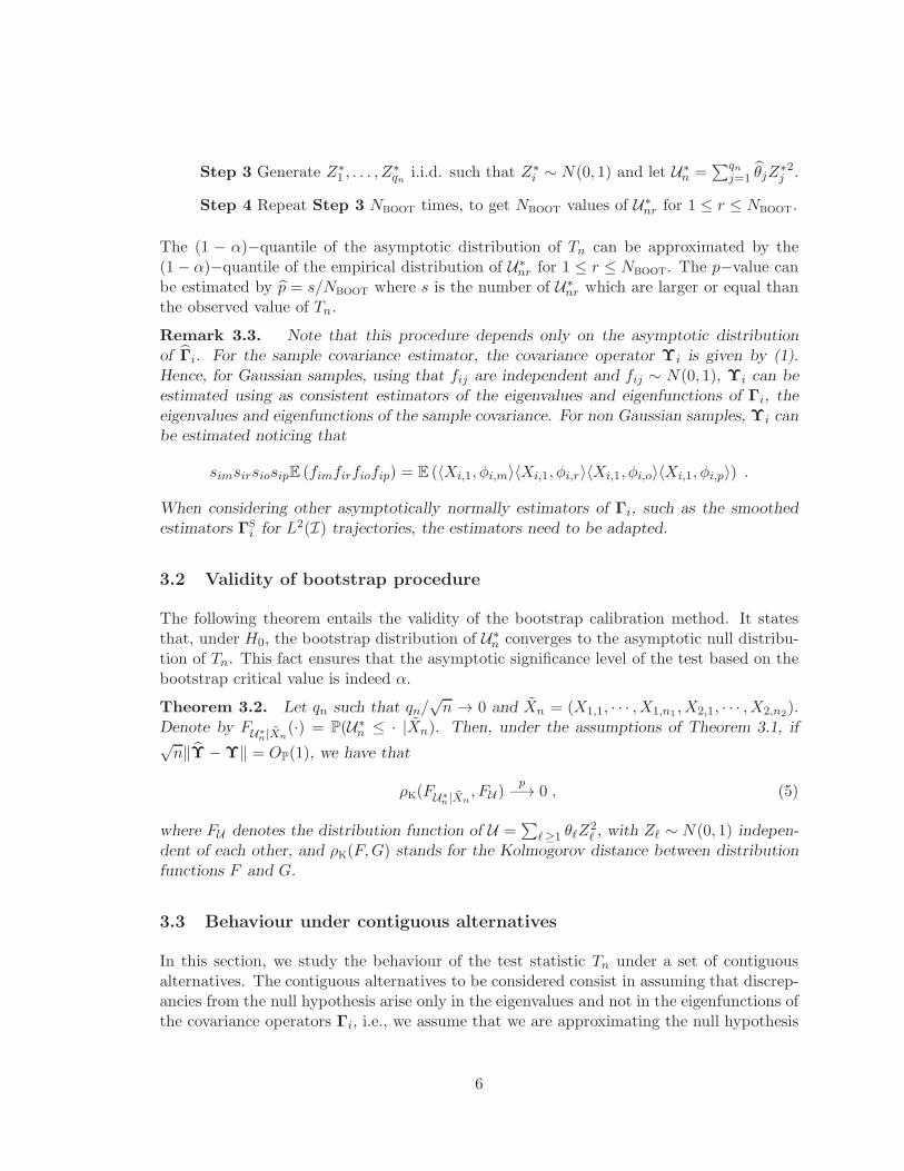
Step 3 Generate Z∗1 , . . . , Z

∗qn i.i.d. such that Z∗

i ∼ N(0, 1) and let U∗n =

∑qnj=1 θjZ

∗j2.

Step 4 Repeat Step 3 Nboot times, to get Nboot values of U∗nr for 1 ≤ r ≤ Nboot.

The (1 − α)−quantile of the asymptotic distribution of Tn can be approximated by the(1− α)−quantile of the empirical distribution of U∗

nr for 1 ≤ r ≤ Nboot. The p−value canbe estimated by p = s/Nboot where s is the number of U∗

nr which are larger or equal thanthe observed value of Tn.

Remark 3.3. Note that this procedure depends only on the asymptotic distributionof Γi. For the sample covariance estimator, the covariance operator Υi is given by (1).Hence, for Gaussian samples, using that fij are independent and fij ∼ N(0, 1), Υi can beestimated using as consistent estimators of the eigenvalues and eigenfunctions of Γi, theeigenvalues and eigenfunctions of the sample covariance. For non Gaussian samples, Υi canbe estimated noticing that

simsirsiosipE (fimfirfiofip) = E (〈Xi,1, φi,m〉〈Xi,1, φi,r〉〈Xi,1, φi,o〉〈Xi,1, φi,p〉) .

When considering other asymptotically normally estimators of Γi, such as the smoothedestimators Γs

i for L2(I) trajectories, the estimators need to be adapted.

3.2 Validity of bootstrap procedure

The following theorem entails the validity of the bootstrap calibration method. It statesthat, under H0, the bootstrap distribution of U∗

n converges to the asymptotic null distribu-tion of Tn. This fact ensures that the asymptotic significance level of the test based on thebootstrap critical value is indeed α.

Theorem 3.2. Let qn such that qn/√n → 0 and Xn = (X1,1, · · · ,X1,n1

,X2,1, · · · ,X2,n2).

Denote by FU∗

n|Xn(·) = P(U∗

n ≤ · |Xn). Then, under the assumptions of Theorem 3.1, if√n‖Υ−Υ‖ = OP(1), we have that

ρk(FU∗

n|Xn, FU )

p−→ 0 , (5)

where FU denotes the distribution function of U =∑

ℓ≥1 θℓZ2ℓ , with Zℓ ∼ N(0, 1) indepen-

dent of each other, and ρk(F,G) stands for the Kolmogorov distance between distributionfunctions F and G.

3.3 Behaviour under contiguous alternatives

In this section, we study the behaviour of the test statistic Tn under a set of contiguousalternatives. The contiguous alternatives to be considered consist in assuming that discrep-ancies from the null hypothesis arise only in the eigenvalues and not in the eigenfunctions ofthe covariance operators Γi, i.e., we assume that we are approximating the null hypothesis

6

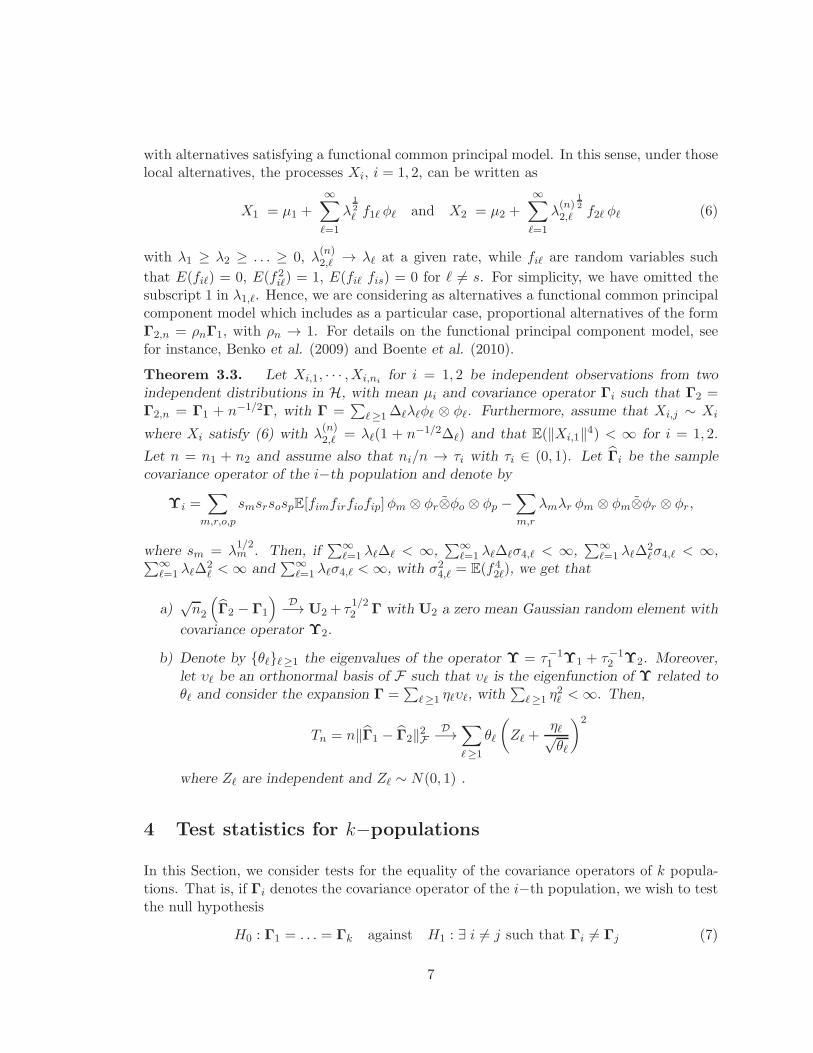
with alternatives satisfying a functional common principal model. In this sense, under thoselocal alternatives, the processes Xi, i = 1, 2, can be written as

X1 = µ1 +∞∑

ℓ=1

λ1

2

ℓ f1ℓ φℓ and X2 = µ2 +∞∑

ℓ=1

λ(n)2,ℓ

1

2 f2ℓ φℓ (6)

with λ1 ≥ λ2 ≥ . . . ≥ 0, λ(n)2,ℓ → λℓ at a given rate, while fiℓ are random variables such

that E(fiℓ) = 0, E(f2iℓ) = 1, E(fiℓ fis) = 0 for ℓ 6= s. For simplicity, we have omitted the

subscript 1 in λ1,ℓ. Hence, we are considering as alternatives a functional common principalcomponent model which includes as a particular case, proportional alternatives of the formΓ2,n = ρnΓ1, with ρn → 1. For details on the functional principal component model, seefor instance, Benko et al. (2009) and Boente et al. (2010).

Theorem 3.3. Let Xi,1, · · · ,Xi,nifor i = 1, 2 be independent observations from two

independent distributions in H, with mean µi and covariance operator Γi such that Γ2 =Γ2,n = Γ1 + n−1/2Γ, with Γ =

∑ℓ≥1∆ℓλℓφℓ ⊗ φℓ. Furthermore, assume that Xi,j ∼ Xi

where Xi satisfy (6) with λ(n)2,ℓ = λℓ(1 + n−1/2∆ℓ) and that E(‖Xi,1‖4) < ∞ for i = 1, 2.

Let n = n1 + n2 and assume also that ni/n → τi with τi ∈ (0, 1). Let Γi be the samplecovariance operator of the i−th population and denote by

Υi =∑

m,r,o,p

smsrsospE[fimfirfiofip]φm ⊗ φr⊗φo ⊗ φp −∑

m,r

λmλr φm ⊗ φm⊗φr ⊗ φr,

where sm = λ1/2m . Then, if

∑∞ℓ=1 λℓ∆ℓ < ∞,

∑∞ℓ=1 λℓ∆ℓσ4,ℓ < ∞,

∑∞ℓ=1 λℓ∆

2ℓσ4,ℓ < ∞,∑∞

ℓ=1 λℓ∆2ℓ < ∞ and

∑∞ℓ=1 λℓσ4,ℓ < ∞, with σ2

4,ℓ = E(f42ℓ), we get that

a)√n2

(Γ2 − Γ1

)D−→ U2 + τ

1/22 Γ with U2 a zero mean Gaussian random element with

covariance operator Υ2.

b) Denote by {θℓ}ℓ≥1 the eigenvalues of the operator Υ = τ−11 Υ1 + τ−1

2 Υ2. Moreover,let υℓ be an orthonormal basis of F such that υℓ is the eigenfunction of Υ related toθℓ and consider the expansion Γ =

∑ℓ≥1 ηℓυℓ, with

∑ℓ≥1 η

2ℓ < ∞. Then,

Tn = n‖Γ1 − Γ2‖2FD−→∑

ℓ≥1

θℓ

(Zℓ +

ηℓ√θℓ

)2

where Zℓ are independent and Zℓ ∼ N(0, 1) .

4 Test statistics for k−populations

In this Section, we consider tests for the equality of the covariance operators of k popula-tions. That is, if Γi denotes the covariance operator of the i−th population, we wish to testthe null hypothesis

H0 : Γ1 = . . . = Γk against H1 : ∃ i 6= j such that Γi 6= Γj (7)

7

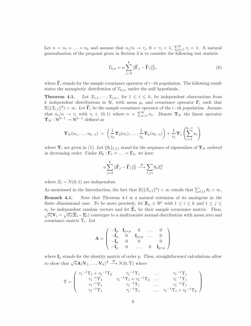
Let n = n1 + . . . + nk and assume that ni/n → τi, 0 < τi < 1,∑k

i=1 τi = 1. A naturalgeneralization of the proposal given in Section 3 is to consider the following test statistic

Tk,n = nk∑

j=2

‖Γj − Γ1‖2F , (8)

where Γi stands for the sample covariance operator of i−th population. The following resultstates the asymptotic distribution of Tk,n, under the null hypothesis.

Theorem 4.1. Let Xi,1, · · · ,Xi,ni, for 1 ≤ i ≤ k, be independent observations from

k independent distributions in H, with mean µi and covariance operator Γi such thatE(‖Xi,1‖4) < ∞. Let Γi be the sample covariance operator of the i−th population. Assume

that ni/n → τi with τi ∈ (0, 1) where n =∑k

i=1 ni. Denote Υw the linear operatorΥw : Hk−1 → Hk−1 defined as

Υw(u1, . . . , uk−1) =

(1

τ2Υ2(u1), . . . ,

1

τkΥk(uk−1)

)+

1

τ1Υ1

(k−1∑

i=1

ui

)

where Υi are given in (1). Let {θℓ}ℓ≥1 stand for the sequence of eigenvalues of Υw orderedin decreasing order. Under H0 : Γ1 = . . . = Γk, we have

n

k∑

j=2

‖Γj − Γ1‖2FD−→∑

ℓ≥1

θℓZ2ℓ

where Zℓ ∼ N(0, 1) are independent.

As mentioned in the Introduction, the fact that E(‖Xi,1‖4) < ∞ entails that∑

ℓ≥1 θℓ < ∞.

Remark 4.1. Note that Theorem 4.1 is a natural extension of its analogous in thefinite–dimensional case. To be more precisely, let Zij ∈ R

p with 1 ≤ i ≤ k and 1 ≤ j ≤ni be independent random vectors and let Σi be their sample covariance matrix. Then,√niVi =

√ni(Σi−Σi) converges to a multivariate normal distribution with mean zero and

covariance matrix Υi. Let

A =

−Ip Ip×p 0 . . . 0−Ip 0 Ip×p . . . 0−Ip 0 0 0−Ip 0 . . . 0 Ip×p

where Ip stands for the identity matrix of order p. Then, straightforward calculations allow

to show that√nA(V1, . . . ,Vk)

t D−→ N(0,Υ) where

Υ =

τ1−1Υ1 + τ2

−1Υ2 τ1−1Υ1 . . . τ1

−1Υ1

τ1−1Υ1 τ1

−1Υ1 + τ3−1Υ3 . . . τ1

−1Υ1

τ1−1Υ1 τ1

−1Υ1 . . . τ1−1Υ1

τ1−1Υ1 τ1

−1Υ1 . . . τ1−1Υ1 + τk

−1Υk

8

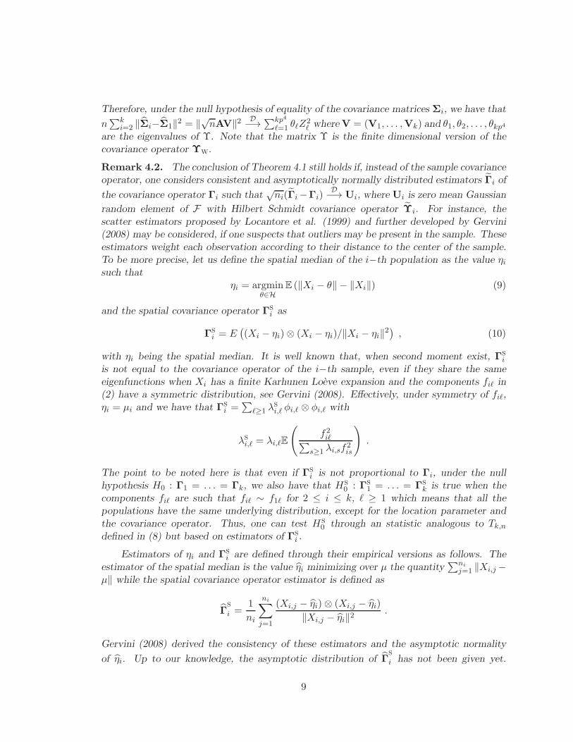
Therefore, under the null hypothesis of equality of the covariance matrices Σi, we have that

n∑k

i=2 ‖Σi−Σ1‖2 = ‖√nAV‖2 D−→∑kp4

ℓ=1 θℓZ2ℓ whereV = (V1, . . . ,Vk) and θ1, θ2, . . . , θkp4

are the eigenvalues of Υ. Note that the matrix Υ is the finite dimensional version of thecovariance operator Υw.

Remark 4.2. The conclusion of Theorem 4.1 still holds if, instead of the sample covarianceoperator, one considers consistent and asymptotically normally distributed estimators Γi of

the covariance operator Γi such that√ni(Γi−Γi)

D−→ Ui, where Ui is zero mean Gaussian

random element of F with Hilbert Schmidt covariance operator Υi. For instance, thescatter estimators proposed by Locantore et al. (1999) and further developed by Gervini(2008) may be considered, if one suspects that outliers may be present in the sample. Theseestimators weight each observation according to their distance to the center of the sample.To be more precise, let us define the spatial median of the i−th population as the value ηisuch that

ηi = argminθ∈H

E (‖Xi − θ‖ − ‖Xi‖) (9)

and the spatial covariance operator Γs

i as

Γs

i = E((Xi − ηi)⊗ (Xi − ηi)/‖Xi − ηi‖2

), (10)

with ηi being the spatial median. It is well known that, when second moment exist, Γs

i

is not equal to the covariance operator of the i−th sample, even if they share the sameeigenfunctions when Xi has a finite Karhunen Loeve expansion and the components fiℓ in(2) have a symmetric distribution, see Gervini (2008). Effectively, under symmetry of fiℓ,ηi = µi and we have that Γs

i =∑

ℓ≥1 λs

i,ℓ φi,ℓ ⊗ φi,ℓ with

λsi,ℓ = λi,ℓE

(f2iℓ∑

s≥1 λi,sf2is

).

The point to be noted here is that even if Γs

i is not proportional to Γi, under the nullhypothesis H0 : Γ1 = . . . = Γk, we also have that Hs

0 : Γs

1 = . . . = Γs

k is true when thecomponents fiℓ are such that fiℓ ∼ f1ℓ for 2 ≤ i ≤ k, ℓ ≥ 1 which means that all thepopulations have the same underlying distribution, except for the location parameter andthe covariance operator. Thus, one can test Hs

0 through an statistic analogous to Tk,n

defined in (8) but based on estimators of Γs

i .

Estimators of ηi and Γs

i are defined through their empirical versions as follows. Theestimator of the spatial median is the value ηi minimizing over µ the quantity

∑ni

j=1 ‖Xi,j −µ‖ while the spatial covariance operator estimator is defined as

Γs

i =1

ni

ni∑

j=1

(Xi,j − ηi)⊗ (Xi,j − ηi)

‖Xi,j − ηi‖2.

Gervini (2008) derived the consistency of these estimators and the asymptotic normality

of ηi. Up to our knowledge, the asymptotic distribution of Γs

i has not been given yet.

9

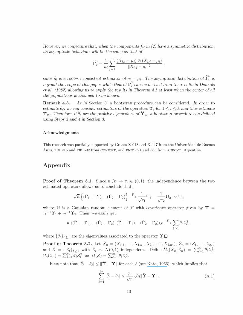
However, we conjecture that, when the components fiℓ in (2) have a symmetric distribution,its asymptotic behaviour will be the same as that of

Γs

i =1

ni

ni∑

j=1

(Xi,j − µi)⊗ (Xi,j − µi)

‖Xi,j − µi‖2.

since ηi is a root−n consistent estimator of ηi = µi. The asymptotic distribution of Γs

i is

beyond the scope of this paper while that of Γs

i can be derived from the results in Dauxoiset al. (1982) allowing us to apply the results in Theorem 4.1 at least when the center of allthe populations is assumed to be known.

Remark 4.3. As in Section 3, a bootstrap procedure can be considered. In order toestimate θℓ, we can consider estimators of the operators Υi for 1 ≤ i ≤ k and thus estimateΥw. Therefore, if θℓ are the positive eigenvalues of Υw, a bootstrap procedure can definedusing Steps 3 and 4 in Section 3.

Acknowledgments

This research was partially supported by Grants X-018 and X-447 from the Universidad de Buenos

Aires, pid 216 and pip 592 from conicet, and pict 821 and 883 from anpcyt, Argentina.

Appendix

Proof of Theorem 3.1. Since ni/n → τi ∈ (0, 1), the independence between the twoestimated operators allows us to conclude that,

√n{(Γ1 − Γ1)− (Γ2 − Γ2)

} D−→ 1√τ1U1 −

1√τ2U2 ∼ U ,

where U is a Gaussian random element of F with covariance operator given by Υ =τ1

−1Υ1 + τ2−1Υ2. Then, we easily get

n 〈(Γ1 − Γ1)− (Γ2 − Γ2), (Γ1 − Γ1)− (Γ2 − Γ2)〉F D−→∑

ℓ≥1

θℓZ2ℓ ,

where {θℓ}ℓ≥1 are the eigenvalues associated to the operator Υ.

Proof of Theorem 3.2. Let Xn = (X1,1, · · · ,X1,n1,X2,1, · · · ,X2,n2

), Zn = (Z1, · · · , Zqn)

and Z = {Zℓ}ℓ≥1 with Zi ∼ N(0, 1) independent. Define Un(Xn, Zn) =∑qn

ℓ=1 θℓZ2ℓ ,

Un(Zn) =∑qn

ℓ=1 θℓZ2ℓ and U(Z) =

∑∞ℓ=1 θℓZ

2ℓ .

First note that |θℓ − θℓ| ≤ ‖Υ−Υ‖ for each ℓ (see Kato, 1966), which implies that

qn∑

ℓ=1

|θℓ − θℓ| ≤qn√n

√n‖Υ−Υ‖ . (A.1)

10

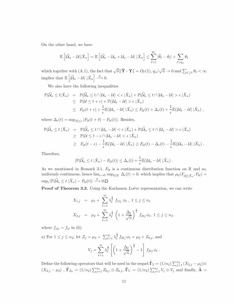
On the other hand, we have

E

[|Un − U||Xn

]= E

[|Un − Un + Un − U| |Xn

]≤

qn∑

ℓ=1

|θℓ − θℓ|+∑

ℓ>qn

θℓ

which together with (A.1), the fact that√n‖Υ−Υ‖ = OP(1), qn/

√n → 0 and

∑ℓ≥1 θℓ < ∞

implies that E[|Un − U| |Xn

]p−→ 0.

We also have the following inequalities

P(Un ≤ t|Xn) = P(Un ≤ t ∩ |Un − U| < ǫ |Xn) + P(Un ≤ t ∩ |Un − U| > ǫ |Xn)

≤ P(U ≤ t+ ǫ) + P(|Un − U| > ǫ |Xn)

≤ FU (t+ ǫ) +1

ǫE(|Un − U| |Xn) ≤ FU (t) + ∆ǫ(t) +

1

ǫE(|Un − U| |Xn) ,

where ∆ǫ(t) = sup|δ|≤ǫ |FU (t+ δ) − FU (t)|. Besides,

P(Un ≤ t |Xn) = P(Un ≤ t ∩ |Un − U| < ǫ |Xn) + P(Un ≤ t ∩ |Un − U| > ǫ |Xn)

≥ P(U ≤ t− ǫ ∩ |Un − U| < ǫ |Xn)

≥ FU (t− ǫ)− 1

ǫE(|Un − U| |Xn) ≥ FU (t)−∆ǫ(t)−

1

ǫE(|Un − U| |Xn) .

Therefore,

|P(Un ≤ t |Xn)− FU (t)| ≤ ∆ǫ(t) +1

ǫE(|Un − U| |Xn) .

As we mentioned in Remark 3.1, FU is a continuous distribution function on R and so,uniformly continuous, hence limǫ→0 supt∈R ∆ǫ(t) = 0, which implies that ρk(FU∗

n|Xn, FU ) =

supt |P(Un ≤ t |Xn)− FU (t)|p−→ 0.

Proof of Theorem 3.3. Using the Karhunen–Loeve representation, we can write

X1,j = µ1 +∞∑

ℓ=1

λ1

2

ℓ f1ℓj φℓ , 1 ≤ j ≤ n1

X2,j = µ2 +

∞∑

ℓ=1

λ1

2

ℓ

(1 +

∆ℓ√n

) 1

2

f2ℓj φℓ, 1 ≤ j ≤ n2 .

where fiℓj ∼ fiℓ in (6).

a) For 1 ≤ j ≤ n2, let Zj = µ2 +∑∞

ℓ=1 λ1

2

ℓ f2ℓj φℓ = µ2 + Z0,j, and

Vj =

∞∑

ℓ=1

λ1

2

ℓ

[(1 +

∆ℓ√n

) 1

2

− 1

]f2ℓj φℓ .

Define the following operators that will be used in the sequel Γ2 = (1/n2)∑n2

j=1 (X2,j − µ2)⊗(X2,j − µ2) , ΓZ0

= (1/n2)∑n2

j=1 Z0,j ⊗ Z0,j , ΓV = (1/n2)∑n2

j=1 Vj ⊗ Vj and finally, A =

11

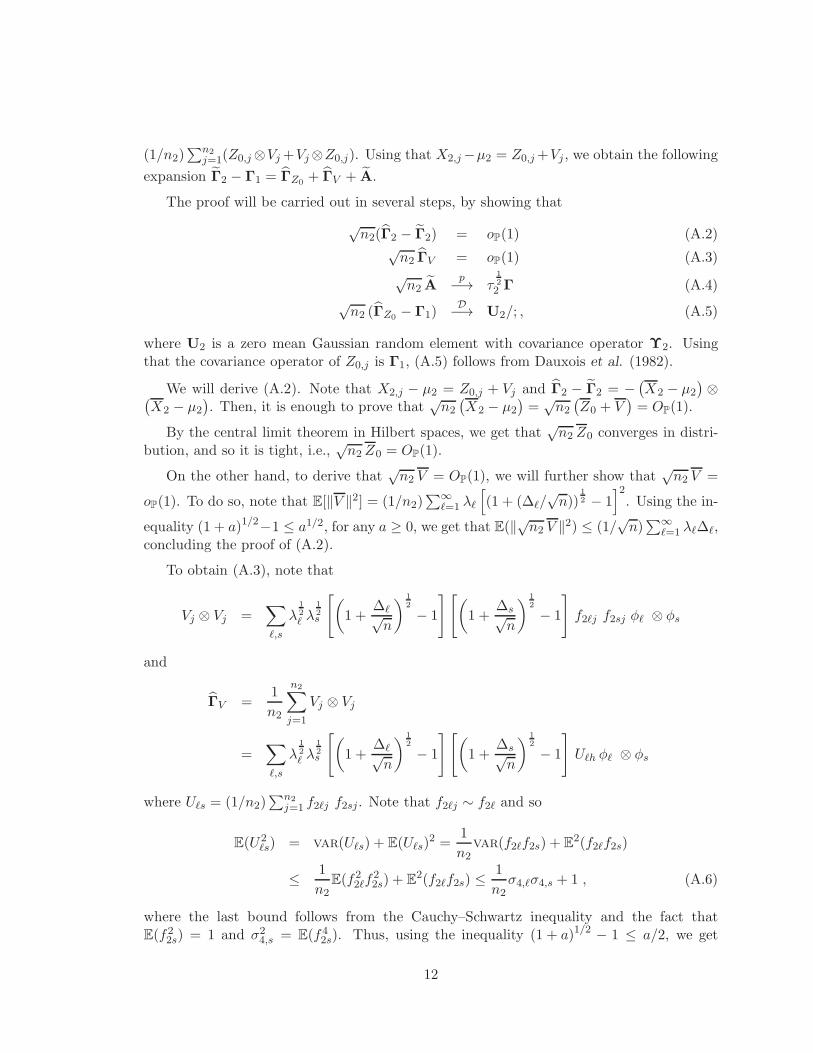
(1/n2)∑n2

j=1(Z0,j⊗Vj+Vj⊗Z0,j). Using that X2,j−µ2 = Z0,j+Vj , we obtain the following

expansion Γ2 − Γ1 = ΓZ0+ ΓV + A.

The proof will be carried out in several steps, by showing that

√n2(Γ2 − Γ2) = oP(1) (A.2)

√n2 ΓV = oP(1) (A.3)√n2 A

p−→ τ1

2

2 Γ (A.4)√n2 (ΓZ0

− Γ1)D−→ U2/; , (A.5)

where U2 is a zero mean Gaussian random element with covariance operator Υ2. Usingthat the covariance operator of Z0,j is Γ1, (A.5) follows from Dauxois et al. (1982).

We will derive (A.2). Note that X2,j − µ2 = Z0,j + Vj and Γ2 − Γ2 = −(X2 − µ2

)⊗(

X2 − µ2

). Then, it is enough to prove that

√n2

(X2 − µ2

)=

√n2

(Z0 + V

)= OP(1).

By the central limit theorem in Hilbert spaces, we get that√n2 Z0 converges in distri-

bution, and so it is tight, i.e.,√n2 Z0 = OP(1).

On the other hand, to derive that√n2 V = OP(1), we will further show that

√n2 V =

oP(1). To do so, note that E[‖V ‖2] = (1/n2)∑∞

ℓ=1 λℓ

[(1 + (∆ℓ/

√n))

1

2 − 1]2. Using the in-

equality (1 + a)1/2−1 ≤ a1/2, for any a ≥ 0, we get that E(‖√n2 V ‖2) ≤ (1/√n)∑∞

ℓ=1 λℓ∆ℓ,concluding the proof of (A.2).

To obtain (A.3), note that

Vj ⊗ Vj =∑

ℓ,s

λ1

2

ℓ λ1

2s

[(1 +

∆ℓ√n

) 1

2

− 1

][(1 +

∆s√n

) 1

2

− 1

]f2ℓj f2sj φℓ ⊗ φs

and

ΓV =1

n2

n2∑

j=1

Vj ⊗ Vj

=∑

ℓ,s

λ1

2

ℓ λ1

2s

[(1 +

∆ℓ√n

) 1

2

− 1

][(1 +

∆s√n

) 1

2

− 1

]Uℓh φℓ ⊗ φs

where Uℓs = (1/n2)∑n2

j=1 f2ℓj f2sj. Note that f2ℓj ∼ f2ℓ and so

E(U2ℓs) = var(Uℓs) + E(Uℓs)

2 =1

n2var(f2ℓf2s) + E

2(f2ℓf2s)

≤ 1

n2E(f2

2ℓf22s) + E

2(f2ℓf2s) ≤1

n2σ4,ℓσ4,s + 1 , (A.6)

where the last bound follows from the Cauchy–Schwartz inequality and the fact thatE(f2

2s) = 1 and σ24,s = E(f4

2s). Thus, using the inequality (1 + a)1/2 − 1 ≤ a/2, we get

12

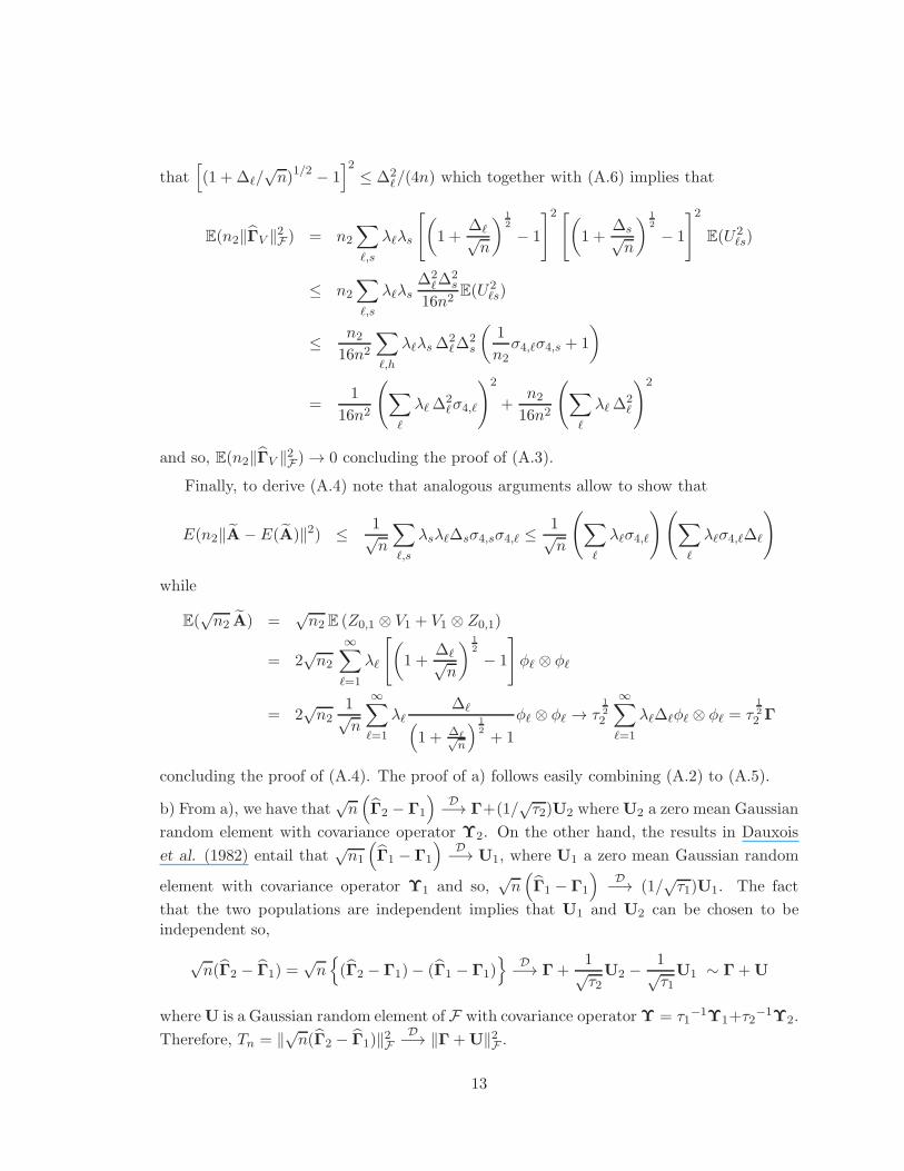
that[(1 + ∆ℓ/

√n)

1/2 − 1]2

≤ ∆2ℓ/(4n) which together with (A.6) implies that

E(n2‖ΓV ‖2F ) = n2

∑

ℓ,s

λℓλs

[(1 +

∆ℓ√n

)1

2

− 1

]2 [(1 +

∆s√n

) 1

2

− 1

]2E(U2

ℓs)

≤ n2

∑

ℓ,s

λℓλs∆2

ℓ∆2s

16n2E(U2

ℓs)

≤ n2

16n2

∑

ℓ,h

λℓλs∆2ℓ∆

2s

(1

n2σ4,ℓσ4,s + 1

)

=1

16n2

(∑

ℓ

λℓ∆2ℓσ4,ℓ

)2

+n2

16n2

(∑

ℓ

λℓ∆2ℓ

)2

and so, E(n2‖ΓV ‖2F ) → 0 concluding the proof of (A.3).

Finally, to derive (A.4) note that analogous arguments allow to show that

E(n2‖A− E(A)‖2) ≤ 1√n

∑

ℓ,s

λsλℓ∆sσ4,sσ4,ℓ ≤1√n

(∑

ℓ

λℓσ4,ℓ

)(∑

ℓ

λℓσ4,ℓ∆ℓ

)

while

E(√n2 A) =

√n2 E (Z0,1 ⊗ V1 + V1 ⊗ Z0,1)

= 2√n2

∞∑

ℓ=1

λℓ

[(1 +

∆ℓ√n

) 1

2

− 1

]φℓ ⊗ φℓ

= 2√n2

1√n

∞∑

ℓ=1

λℓ∆ℓ

(1 + ∆ℓ√

n

) 1

2

+ 1

φℓ ⊗ φℓ → τ1

2

2

∞∑

ℓ=1

λℓ∆ℓφℓ ⊗ φℓ = τ1

2

2 Γ

concluding the proof of (A.4). The proof of a) follows easily combining (A.2) to (A.5).

b) From a), we have that√n(Γ2 − Γ1

)D−→ Γ+(1/

√τ2)U2 whereU2 a zero mean Gaussian

random element with covariance operator Υ2. On the other hand, the results in Dauxois

et al. (1982) entail that√n1

(Γ1 − Γ1

) D−→ U1, where U1 a zero mean Gaussian random

element with covariance operator Υ1 and so,√n(Γ1 − Γ1

)D−→ (1/

√τ1)U1. The fact

that the two populations are independent implies that U1 and U2 can be chosen to beindependent so,

√n(Γ2 − Γ1) =

√n{(Γ2 − Γ1)− (Γ1 − Γ1)

} D−→ Γ+1√τ2U2 −

1√τ1U1 ∼ Γ+U

whereU is a Gaussian random element of F with covariance operatorΥ = τ1−1Υ1+τ2

−1Υ2.

Therefore, Tn = ‖√n(Γ2 − Γ1)‖2FD−→ ‖Γ+U‖2F .

13

To conclude the proof, we have to obtain the distribution of ‖Γ + U‖2F . Since U isa zero mean Gaussian random element of F with covariance operator Υ, we have that

U can be written as∑

ℓ≥1 θ1/2ℓ Zℓυℓ where Zℓ are i.i.d. random variables such that Zℓ ∼

N(0, 1). Hence, Γ+U =∑

ℓ≥1

(ηℓ + θ

1/2ℓ Zℓ

)υℓ and so, ‖Γ+U‖2F =

∑ℓ≥1

(ηℓ + θ

1/2ℓ Zℓ

)2=

∑ℓ≥1 θℓ

(ηℓ/θ

1/2ℓ + Zℓ

)2concluding the proof.

Proof of Theorem 4.1. Consider the process Vk,n = {√n(Γi − Γi)}1≤i≤k. The indepen-dence of the samples and among populations together with the results stated in Dauxoiset al. (1982), allow to show that Vk,n converges in distribution to a zero mean Gaussianrandom element U of Fk with covariance operator Υ. More precisely, we get that

{√n(Γi − Γi)}1≤i≤k

D−→ U = (U1, · · · ,Uk)

whereU1, · · · ,Uk are independent random processes of F with covariance operators τi−1Υi,

respectively.

Let A : Fk → Fk−1 be a linear operator given by A(V1, · · · , Vk) = (V2−V1, · · · , Vk−V1).

The continuous map Theorem guarantees that A(√n(Γ1 − Γ1), · · · ,

√n(Γk − Γk))

D−→ W ,where W is a zero mean Gaussian random element of Fk−1 with covariance operator Υw =AΥA∗ where A∗ denote the adjoint operator of A. It is easy to see that the adjoint operatorA∗ : Fk−1 → Fk is given by A∗(u1, . . . , uk−1) = (−∑k−1

i=1 ui, u1, . . . , uk−1). Hence, asU1, · · · ,Uk are independent, we conclude that

Υw(u1, . . . , uk−1) =

(1

τ2Υ2(u1), . . . ,

1

τkΥk(uk−1)

)+

1

τ1Υ1

(k−1∑

i=1

ui

).

Finally,

Tk,n = n

k∑

j=2

‖Γj − Γ1‖2FD−→∑

ℓ≥1

θℓZ2ℓ

where Zℓ are i.i.d standard normal random variables and θℓ are the eigenvalues of theoperator Υw.

References

[1] Benko, M., Hardle, P. & Kneip, A. (2009). Common Functional Principal Components.Annals of Statistics, 37, 1-34.

[2] Boente, G. & Fraiman, R. (2000). Kernel-based functional principal components.Statistics and Probabability Letters, 48 , 335-345.

[3] Boente, G., Rodriguez, D. & Sued, M. (2010). Inference under functional proportionaland common principal components models. Journal of Multivariate Analysis, 101, 464-475.

14

[4] Cardot, H., Ferraty, F., Mas, A. & Sarda, P. (2003). Testing hypotheses in the func-tional linear model. Scandinavian Journal of Statistics, 30, 241255.

[5] Cuevas, A., Febrero, M. & Fraiman, R. (2004). An anova test for functional data.Computational Statistics & Data Analysis, 47, 111122.

[6] Dauxois, J., Pousse, A. & Romain, Y. (1982). Asymptotic theory for the principal com-ponent analysis of a vector random function: Some applications to statistical inference.Journal of Multivariate Analysis, 12, 136-154.

[7] Gabrys, R. & Kokoszka, P. (2007), Portmanteau Test of Independence for FunctionalObservations. Journal of the American Statistical Association, 102, 13381348.

[8] Gabrys, R., Horvath, L. & Kokoszka, P. (2010). Tests for error correlation in thefunctional linear model. Journal of the American Statistical Association, 105, 1113-1125.

[9] Fan, J. & Lin, S.-K. (1998). Tests of significance when the data are curves. Journal ofthe American Statistical Association, 93, 10071021.

[10] Ferraty, F., Vieu, Ph. & Viguier–Pla, S. (2007). Factor-based comparison of groups ofcurves. Computational Statistics & Data Analysis, 51, 4903-4910.

[11] Gupta, A. & Xu, J. (2006). On some tests of the covariance matrix under generalconditions. Annals of the Institute of Statistical Mathematics, 58, 101114.

[12] Horvath, L., Huskova, M. & Kokoszka, P. (2010). Testing the stability of the functionalautoregressive process. Journal of Multivariate Analysis, 101, 352367.

[13] Kato, T. (1966). Perturbation Theory for Linear Operators. Springer-Verlag, New York.

[14] Ledoit, O. & Wolf, M. (2002). Some hypothesis tests for the covariance matrix when thedimension is large compared to the sample size. Annals of Statistics, 30, 4, 1081-1102.

[15] Neuhaus, G. (1980). A note on computing the distribution of the norm of Hilbert spacevalued gaussian random variables. Journal of Multivariate Analysis, 10, 19-25.

[16] Panaretos, V. M., Kraus, D. & Maddocks, J. H. (2010). Second-Order Comparison ofGaussian Random Functions and the Geometry of DNA Minicircles. Journal of theAmerican Statistical Association, 105, 670682.

[17] Schott, J. (2007). A test for the equality of covariance matrices when the dimensionis large relative to the sample sizes.Computational Statistics & Data Analysis, 51, 12,6535-6542.

[18] Seber, G. (1984) Multivariate Observations. John Wiley and Sons.

[19] Shen, Q. & Faraway, J. (2004). An F-test for Linear models with functional responses.Statistica Sinica, 14, 12391257.

[20] Van der Vaart, A. (2000). Asymptotic Statistics. Cambridge University Press.

15