Comparison between tower and aircraft-based eddy covariance fluxes in five European regions

www.elsevier.com/locate/agrformet

Agricultural and Forest Meteorology 127 (2004) 1–16

Comparison between tower and aircraft-based eddy covariance

fluxes in five European regions

Beniamino Giolia,*, Franco Migliettaa, Biagio De Martinoa, Ronald W.A. Hutjesb,Han A.J. Dolmanc, Anders Lindrothd, Marcus Schumachere, Maria Jose Sanzf,

Giovanni Mancag, Alessandro Peressottih, Edward J. Dumasi

aIBIMET-CNR, Istituto di Biometeorologia, Consiglio Nazionale delle Ricerche, Via G. Caproni 8, 50145 Firenze, ItalybAlterra, Duivendaal 2, 6701 AP Wageningen, The Netherlands

cDepartment of Geo-Environmental Sciences, Faculty of Earth and Life Sciences, Vrije Universiteit,

de Boelelaan 1085, 1081 HV Amsterdam, The NetherlandsdSweden Department of Physical Geography and Ecosystems Analysis, Lund University,

Solvegatan 12, 223 62 Lund, SwedeneMax-Planck-Institut fur Biogeochemie, Carl-Zeiss-Promenade 10, 07745 Jena, GermanyfCEAM, Parque Tecnologico, c/Charles H. Darwin 14, 46980 Paterna (Valencia), Spain

gDepartment of Forest Science and Environment, University of Tuscia, Via de Lellis, 01100 Viterbo, ItalyhDipartimento Produzione Vegetale e Tecnologie Agrarie, Universita di Udine,

Via delle Scienze 208, 33100 Udine, ItalyiNOAA, Atmospheric Turbulence and Diffusion Division, 456 S. Illinois Ave, Oak Ridge, TN, USA

Received 1 December 2003; received in revised form 10 August 2004; accepted 12 August 2004

Abstract

Airborne eddy covariance measurements provide a unique opportunity to directly measure surface energy, mass and

momentum fluxes at the regional scale. This offers the possibility to complement the data that are obtained by the ground-based

eddy covariance networks and to validate estimates of the surface fluxes that can be obtained by means of satellite products and

models. The overall accuracy and the reliability of airborne eddy covariance measurements have already been assessed in the

past for different platforms. More recently an international collaboration between several research laboratories and a European

aeronautical manufacturer led to the development of a new small environmental research aircraft, called the Sky Arrow ERA

(Environmental Research Aircraft). This aircraft has been used in the framework of the European Research Project RECAB

(Regional Assessment and Modelling of the Carbon Balance in Europe), that is part of the CarboEurope projects cluster, to

measure surface mass and energy exchange at five different European locations. An extensive comparison between airborne and

ground-based flux data at seven flux measurement sites, showed the overall matching between airborne and tower data. While

friction velocity and latent heat flux estimates made by airborne and tower data were comparable at all sites and under whatever

* Corresponding author. Tel.: +39 0 5530 33711; fax: +39 0 5530 8910.

E-mail address: [email protected] (B. Gioli).

0168-1923/$ – see front matter # 2004 Elsevier B.V. All rights reserved.

doi:10.1016/j.agrformet.2004.08.004

B. Gioli et al. / Agricultural and Forest Meteorology 127 (2004) 1–162

conditions, substantial and consistent underestimation of CO2 (28% on average) and sensible heat fluxes (35% on average) was

observed. Differences in the aircraft and tower footprint and flux divergence with height explained most of the discrepancies.

# 2004 Elsevier B.V. All rights reserved.

Keywords: Aircraft flux measurements; Area-averaged fluxes; Regional ecosystem exchange; Flux divergence

1. Introduction

Global environmental change is likely to affect the

magnitude and the dynamics of the exchange of energy,

mass and momentum occurring between the land

surface and the atmosphere. Such a change may directly

and indirectly have effects on the global climate. The

gas composition of the atmosphere also depends on

positive and negative biogenic fluxes of vegetated and

oceanic surfaces. It has been calculated that the

exchange of carbon between the terrestrial biosphere

and the atmosphere is on the order of 120 Gt of carbon

per year (Schimel et al., 1995), with an estimated

terrestrial biospheric sink of 2.3 Gt of carbon per year

(Bousquet et al., 1999). Such a large sink represents, at

present, 15–30% of the annual global emissions of

carbon from fossil fuels and industrial activity and plays

an important role in the regulation of greenhouse gas

concentrations in the atmosphere. The introduction of

the notion of ‘‘biospheric sinks’’ in policies (i.e. the

Kyoto Protocol) governing reductions in greenhouse

gas emissions (Schulze et al., 2002) has recently

highlighted the importance of a better understanding of

mechanisms that are at the base of global carbon uptake

and accumulation by forests and soils. For this, a series

of co-ordinated efforts to come up with a better

quantification of those carbon fluxes has been

established (Baldocchi et al., 2001). The choice of

appropriate temporal and spatial scales to monitor and

interpret those fluxes is important. A mismatch exists

between our understanding of ecosystem–atmosphere

exchange of CO2 at local and at continental scales.

Studies based on the use of ground-based eddy

covariance techniques can explain temporal and diurnal

local variations in the fluxes thus helping our under-

standing of the interactions between environmental

conditions and carbon uptake (Falge et al., 2002). On

the other hand, inversion based on atmospheric

transport can provide useful indications of the

magnitude of the terrestrial carbon sink at the

continental and global scales (Ciais et al., 2000; Fan

et al., 1998), with obvious limitations in the under-

standing of the mechanisms or the exact geographical

location of the sinks and the sources.

Airborne eddy covariance has recently been

proposed as a tool to measure energy and carbon

dioxide exchange at the ‘‘regional scale’’ (e.g. several

hundreds square kilometres) where the atmospheric

boundary layer plays a crucial role as mediator

between the surface fluxes and the atmosphere (Stull,

1988; Culf et al., 1997; Millan et al., 1996; Lloyd et

al., 1996). Our capability to understand and measure

the magnitude of the different contributions that occur

at such a scale needs to be brought to a level where we

can make realistic assessments of the atmospheric

carbon balance, thus bridging the gap between the

local scale of ground-based flux measurements and the

continental scale of atmospheric inversion methods.

The idea of using aircraft to measure gas exchange

between the land surface and the atmosphere was

developed more than 20 years ago (Lenschow et al.,

1981; Desjardins et al., 1982). Airborne eddy flux

observations with modern instruments properly

installed and operated on appropriate aircraft may

give results no less accurate than from a careful flux-

tower operation, while the primary difference is in

how the data must be interpreted (Mahrt, 1998). Tower

data form a time series relying on mean wind to advect

the turbulence past the sensors, while an aircraft,

because of its speed, experiences turbulence more as a

space series. While on towers the Taylor hypothesis of

‘frozen turbulence’ has to be invoked to use the time

averages as ensemble averages for eddy covariance

computations (Kaimal and Finnigan, 1994), aircraft

can really measure turbulence in space within very

short amount of time. These measurements provide an

almost ‘instantaneous’ picture of the turbulence field

over an area and are not affected by temporal trends

and non-stationary effects like those experienced by

towers. On the other hand, spatial homogeneity over

large areas is a crucial requirement for successful

aircraft flux measurements.

B. Gioli et al. / Agricultural and Forest Meteorology 127 (2004) 1–16 3

Despite initial successes (Oechel et al., 1998) and

continuing technological improvements, such a novel

technique still requires large scale validation to better

understand its reliability in regional flux estimates

(Oechel et al., 1998; Doran et al., 1992; Crawford et

al., 1996a, 1996b; Desjardins et al., 1995, 1997). The

occurrence of substantial differences in the fluxes of

scalars measured by airborne and ground-based eddy

covariance has been observed and discussed at several

occasions (Desjardins et al., 1989; Kelly et al., 1992;

Crawford et al., 1996a, 1996b; Isaac et al., 2004).

Those differences were attributed to systematic

instrumental and/or methodological errors, inherent

properties of the planetary boundary layer, or to the

fact that towers and aircraft are not measuring the

same thing (e.g. different footprints). Footprint

differences are rather obvious between towers and

airborne measurements as aircraft operate generally at

higher altitudes than towers and the fluxes measured

by aircraft integrate contributions originating from

different zones. Vertical flux divergence may also

contribute (Mahrt, 1998; Desjardins et al., 1989), as

the net flux measured at different heights within the

planetary boundary layer (PBL) depends on the

relative magnitude of the flux at the surface, on one

side, and at the entrainment/subsidence zone of the

PBL, on the other (Samulesson and Tjernstrom,

1999).

The Sky Arrow ERA (Environmental Research

Aircraft) is a new platform that has been recently

developed in the frame of an international colla-

boration. This aircraft has been used in the European

Research Project RECAB (Regional Assessment and

Modelling of the Carbon Balance in Europe) to

measure surface fluxes at the regional scale in

selected regions of Europe. To assess the accuracy

and the reliability of those measurements, an

extensive comparison between airborne fluxes and

observations made on the ground by conventional

eddy covariance towers has been also made. This

paper reports the results of such multi-site compar-

ison that included five study areas in Spain, Italy,

Germany, The Netherlands and Sweden (Hutjes et

al., 2002). This aircraft–tower comparison study

encompassed a wide range of land uses and climatic

conditions from agricultural fields to coniferous and

broadleaf forests during campaigns that were made

both in winter and in summer.

2. Materials and methods

2.1. Description of the Sky Arrow ERA

The aerial platform that was developed for flux

measurements within RECAB is based on the certified

aircraft Sky Arrow 650 ERA (Environmental

Research Aircraft), a commercially produced, certi-

fied small aircraft equipped with sensors to measure

three-dimensional wind and turbulence together with

gas concentrations and other atmospheric parameters

at high frequency. It is a two seat aircraft made of

carbon fibre and epoxy resin, powered by 75 kW

engine. It has a wingspan of 9.6 m, a length of 8.2 m, a

wing area of 13.1 m2, and a maximum takeoff mass of

648.6 kg (Fig. 1). The aircraft has a cruise flight speed

of 45 m s�1 with an endurance of 3.5 h, allowing it to

cover flight distances of up to 500 km. Operating

altitudes can range from 10 m above ground level to

more than 3500 m above sea level. The aircraft was re-

engineered in 1999 to host the mobile flux platform

(MFP), which consists of a set of sensors for

atmospheric measurements. The installation was

certified to operate under both FAA (Federal Aviation

Administration, USA) and JAR (Joint Aviation

Regulations, EU) aeronautical regulations. Atmo-

spheric turbulence measurements are made with the

‘‘Best Aircraft Turbulence’’ (BAT) probe, developed

by NOAA-ATDD and ARA Australia.

In brief, the BAT probe measures the velocity of air

with respect to aircraft using a hemispheric nine-hole

pressure sphere that records static and dynamic

pressures by means of four differential pressure

transducers (Crawford and Dobosy, 1992). The Sky

Arrow engine is mounted in a pusher configuration,

allowing the BAT probe to be installed directly on the

aircraft’s nose, thus reducing most of airflow

contamination due to upwash and sidewash generated

by the wing (Crawford et al., 1996a, 1996b). The

actual wind components (horizontal U, V and vertical

W) relative to the ground are calculated introducing

corrections for three-dimensional velocity, pitch, roll

and heading of the aircraft. Those corrections are

made using a combination of GPS velocity measure-

ments and data from two sets of three orthogonal

accelerometers mounted at the centre of gravity of the

aircraft and in the centre of the hemisphere. Aircraft

velocity relative to the ground is measured by means


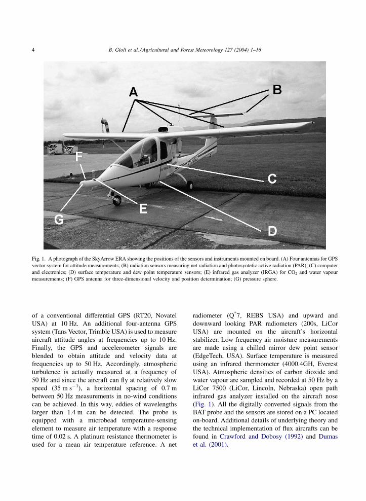
Fig. 1. A photograph of the SkyArrow ERA showing the positions of the sensors and instruments mounted on board. (A) Four antennas for GPS

vector system for attitude measurements; (B) radiation sensors measuring net radiation and photosyntetic active radiation (PAR); (C) computer

and electronics; (D) surface temperature and dew point temperature sensors; (E) infrared gas analyzer (IRGA) for CO2 and water vapour

measurements; (F) GPS antenna for three-dimensional velocity and position determination; (G) pressure sphere.

of a conventional differential GPS (RT20, Novatel

USA) at 10 Hz. An additional four-antenna GPS

system (Tans Vector, Trimble USA) is used to measure

aircraft attitude angles at frequencies up to 10 Hz.

Finally, the GPS and accelerometer signals are

blended to obtain attitude and velocity data at

frequencies up to 50 Hz. Accordingly, atmospheric

turbulence is actually measured at a frequency of

50 Hz and since the aircraft can fly at relatively slow

speed (35 m s�1), a horizontal spacing of 0.7 m

between 50 Hz measurements in no-wind conditions

can be achieved. In this way, eddies of wavelengths

larger than 1.4 m can be detected. The probe is

equipped with a microbead temperature-sensing

element to measure air temperature with a response

time of 0.02 s. A platinum resistance thermometer is

used for a mean air temperature reference. A net

radiometer (Q*7, REBS USA) and upward and

downward looking PAR radiometers (200s, LiCor

USA) are mounted on the aircraft’s horizontal

stabilizer. Low frequency air moisture measurements

are made using a chilled mirror dew point sensor

(EdgeTech, USA). Surface temperature is measured

using an infrared thermometer (4000.4GH, Everest

USA). Atmospheric densities of carbon dioxide and

water vapour are sampled and recorded at 50 Hz by a

LiCor 7500 (LiCor, Lincoln, Nebraska) open path

infrared gas analyzer installed on the aircraft nose

(Fig. 1). All the digitally converted signals from the

BAT probe and the sensors are stored on a PC located

on-board. Additional details of underlying theory and

the technical implementation of flux aircrafts can be

found in Crawford and Dobosy (1992) and Dumas

et al. (2001).


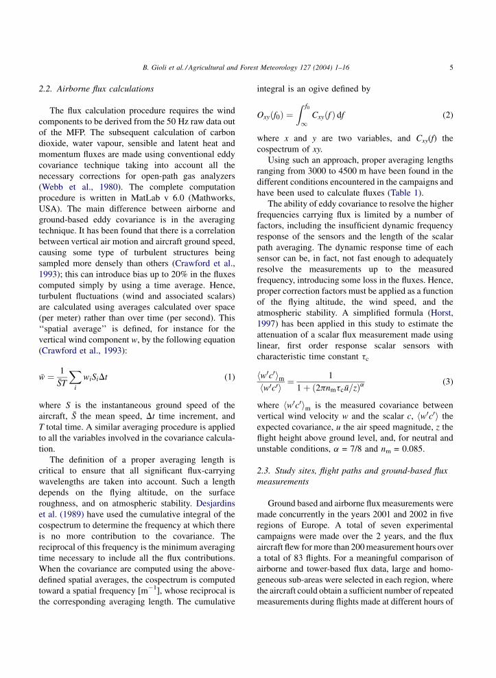
2.2. Airborne flux calculations

The flux calculation procedure requires the wind

components to be derived from the 50 Hz raw data out

of the MFP. The subsequent calculation of carbon

dioxide, water vapour, sensible and latent heat and

momentum fluxes are made using conventional eddy

covariance technique taking into account all the

necessary corrections for open-path gas analyzers

(Webb et al., 1980). The complete computation

procedure is written in MatLab v 6.0 (Mathworks,

USA). The main difference between airborne and

ground-based eddy covariance is in the averaging

technique. It has been found that there is a correlation

between vertical air motion and aircraft ground speed,

causing some type of turbulent structures being

sampled more densely than others (Crawford et al.,

1993); this can introduce bias up to 20% in the fluxes

computed simply by using a time average. Hence,

turbulent fluctuations (wind and associated scalars)

are calculated using averages calculated over space

(per meter) rather than over time (per second). This

‘‘spatial average’’ is defined, for instance for the

vertical wind component w, by the following equation

(Crawford et al., 1993):

w ¼ 1

ST

Xi

wiSiDt (1)

where S is the instantaneous ground speed of the

aircraft, S the mean speed, Dt time increment, and

T total time. A similar averaging procedure is applied

to all the variables involved in the covariance calcula-

tion.

The definition of a proper averaging length is

critical to ensure that all significant flux-carrying

wavelengths are taken into account. Such a length

depends on the flying altitude, on the surface

roughness, and on atmospheric stability. Desjardins

et al. (1989) have used the cumulative integral of the

cospectrum to determine the frequency at which there

is no more contribution to the covariance. The

reciprocal of this frequency is the minimum averaging

time necessary to include all the flux contributions.

When the covariance are computed using the above-

defined spatial averages, the cospectrum is computed

toward a spatial frequency [m�1], whose reciprocal is

the corresponding averaging length. The cumulative

integral is an ogive defined by

Oxyðf0Þ ¼Z f0

1Cxyðf Þ df (2)

where x and y are two variables, and Cxy(f) the

cospectrum of xy.

Using such an approach, proper averaging lengths

ranging from 3000 to 4500 m have been found in the

different conditions encountered in the campaigns and

have been used to calculate fluxes (Table 1).

The ability of eddy covariance to resolve the higher

frequencies carrying flux is limited by a number of

factors, including the insufficient dynamic frequency

response of the sensors and the length of the scalar

path averaging. The dynamic response time of each

sensor can be, in fact, not fast enough to adequately

resolve the measurements up to the measured

frequency, introducing some loss in the fluxes. Hence,

proper correction factors must be applied as a function

of the flying altitude, the wind speed, and the

atmospheric stability. A simplified formula (Horst,

1997) has been applied in this study to estimate the

attenuation of a scalar flux measurement made using

linear, first order response scalar sensors with

characteristic time constant tc

hw0c0im

hw0c0i ¼ 1

1 þ ð2pnmtcu=zÞa (3)

where hw0c0im is the measured covariance between

vertical wind velocity w and the scalar c, hw0c0i the

expected covariance, u the air speed magnitude, z the

flight height above ground level, and, for neutral and

unstable conditions, a = 7/8 and nm = 0.085.

2.3. Study sites, flight paths and ground-based flux

measurements

Ground based and airborne flux measurements were

made concurrently in the years 2001 and 2002 in five

regions of Europe. A total of seven experimental

campaigns were made over the 2 years, and the flux

aircraft flew for more than 200 measurement hours over

a total of 83 flights. For a meaningful comparison of

airborne and tower-based flux data, large and homo-

geneous sub-areas were selected in each region, where

the aircraft could obtain a sufficient number of repeated

measurements during flights made at different hours of


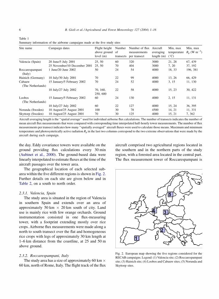
Table 1

Summary information of the airborne campaigns made at the five study sites

Site name Campaign dates Flight height

above ground

level (m)

Number

of

transects

Number of flux

measurements

per transect

Aircraft

averaging

length (m)

Min, max

temperature

(8C)

Min, max

Rp (W m�2)

Valencia (Spain) 20 June/5 July 2001 25, 50 60 320 3000 21, 28 67, 439

25 November/10 December 2001 25, 50 70 404 3000 7, 20 37, 192

Roccarespampani

(Italy)

1 June/20 June 2002 50 24 54 4000 18, 33 196, 381

Hainich (Germany) 10 July/30 July 2001 70 22 99 4000 13, 26 66, 429

Cabauw

(The Netherlands)

15 January/5 February 2002 70 24 52 4000 3, 15 11, 130

10 July/27 July 2002 70, 160,

250, 600

22 58 4000 15, 23 30, 422

Loobos

(The Netherlands)

15 January/5 February 2002 60 24 130 4000 2, 15 11, 131

10 July/27 July 2002 60 22 127 4000 15, 24 36, 395

Norunda (Sweden) 10 August/25 August 2001 100 30 78 4500 14, 21 11, 331

Skyttorp (Sweden) 10 August/25 August 2001 70 30 125 4000 15, 21 7, 362

Aircraft averaging length is the ‘‘spatial average’’ used for individual airborne flux calculations. The number of transects indicates the number of

mean aircraft flux measurements that were compared with corresponding time interpolated half-hourly tower measurements. The number of flux

measurements per transect indicates how many ‘‘spatially averaged’’ aircraft fluxes were used to calculate those means. Maximum and minimum

temperature and photosyntetically active radiation Rp in the last two columns correspond to the two extreme observations that were made by the

aircraft during each campaign.

Fig. 2. European map showing the five regions considered for the

RECAB campaigns. Legend: (1) Valencia site; (2) Roccarespampani

site; (3) Hainich site; (4) Loobos and Cabauw sites; (5) Norunda and

Skyttorp sites.

the day. Eddy covariance towers were available on the

ground providing flux calculations every 30 min

(Aubinet et al., 2000). The ground-based data were

linearly interpolated to estimate fluxes at the time of the

aircraft passages over the tower area.

The geographical location of each selected sub-

area within the five different regions is shown in Fig. 2.

Further details on each site are given below and in

Table 2, on a south to north order.

2.3.1. Valencia, Spain

The study area is situated in the region of Valencia

in southern Spain and extends over an area of

approximately 50 km 20 km south of city. Land

use is mainly rice with few orange orchards. Ground

instrumentation consisted in one flux-measuring

tower, with a footprint extending mostly over rice

crops. Airborne flux measurements were made along a

north to south transect over the flat and homogeneous

rice crops with legs of approximately 30 km length at

1–6 km distance from the coastline, at 25 and 50 m

above ground.

2.3.2. Roccarespampani, Italy

The study area has a size of approximately 60 km 60 km, north of Rome, Italy. The flight track of the flux

aircraft comprised two agricultural regions located in

the southern and in the northern parts of the study

region, with a forested area located in the central part.

The flux measurement tower of Roccarespampani is


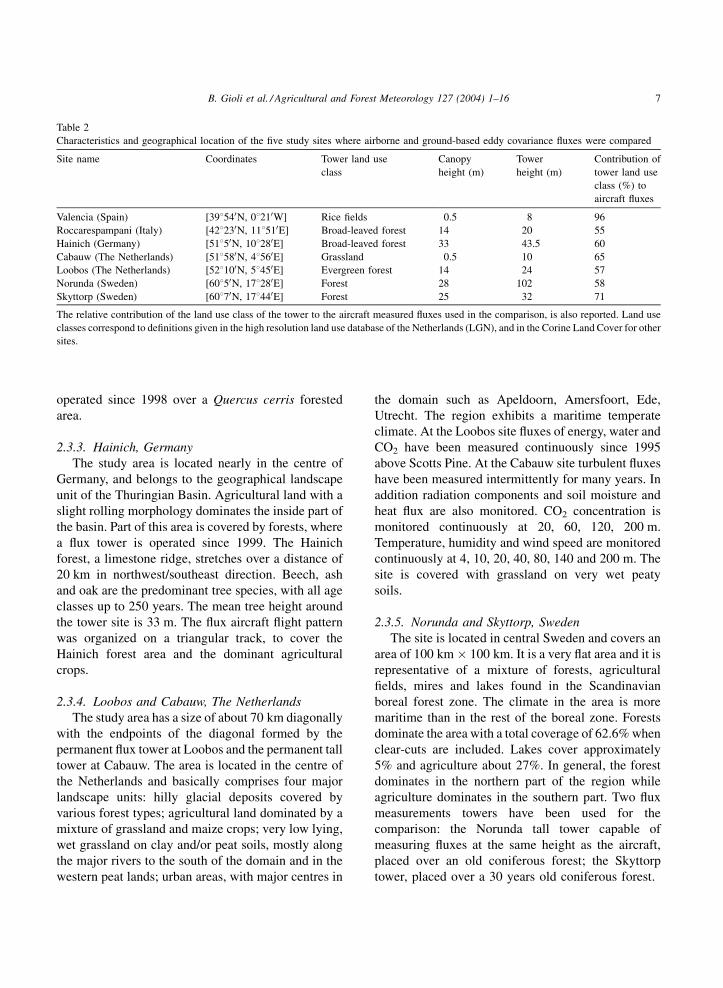
Table 2

Characteristics and geographical location of the five study sites where airborne and ground-based eddy covariance fluxes were compared

Site name Coordinates Tower land use

class

Canopy

height (m)

Tower

height (m)

Contribution of

tower land use

class (%) to

aircraft fluxes

Valencia (Spain) [398540N, 08210W] Rice fields 0.5 8 96

Roccarespampani (Italy) [428230N, 118510E] Broad-leaved forest 14 20 55

Hainich (Germany) [51850N, 108280E] Broad-leaved forest 33 43.5 60

Cabauw (The Netherlands) [518580N, 48560E] Grassland 0.5 10 65

Loobos (The Netherlands) [528100N, 58450E] Evergreen forest 14 24 57

Norunda (Sweden) [60850N, 178280E] Forest 28 102 58

Skyttorp (Sweden) [60870N, 178440E] Forest 25 32 71

The relative contribution of the land use class of the tower to the aircraft measured fluxes used in the comparison, is also reported. Land use

classes correspond to definitions given in the high resolution land use database of the Netherlands (LGN), and in the Corine Land Cover for other

sites.

operated since 1998 over a Quercus cerris forested

area.

2.3.3. Hainich, Germany

The study area is located nearly in the centre of

Germany, and belongs to the geographical landscape

unit of the Thuringian Basin. Agricultural land with a

slight rolling morphology dominates the inside part of

the basin. Part of this area is covered by forests, where

a flux tower is operated since 1999. The Hainich

forest, a limestone ridge, stretches over a distance of

20 km in northwest/southeast direction. Beech, ash

and oak are the predominant tree species, with all age

classes up to 250 years. The mean tree height around

the tower site is 33 m. The flux aircraft flight pattern

was organized on a triangular track, to cover the

Hainich forest area and the dominant agricultural

crops.

2.3.4. Loobos and Cabauw, The Netherlands

The study area has a size of about 70 km diagonally

with the endpoints of the diagonal formed by the

permanent flux tower at Loobos and the permanent tall

tower at Cabauw. The area is located in the centre of

the Netherlands and basically comprises four major

landscape units: hilly glacial deposits covered by

various forest types; agricultural land dominated by a

mixture of grassland and maize crops; very low lying,

wet grassland on clay and/or peat soils, mostly along

the major rivers to the south of the domain and in the

western peat lands; urban areas, with major centres in

the domain such as Apeldoorn, Amersfoort, Ede,

Utrecht. The region exhibits a maritime temperate

climate. At the Loobos site fluxes of energy, water and

CO2 have been measured continuously since 1995

above Scotts Pine. At the Cabauw site turbulent fluxes

have been measured intermittently for many years. In

addition radiation components and soil moisture and

heat flux are also monitored. CO2 concentration is

monitored continuously at 20, 60, 120, 200 m.

Temperature, humidity and wind speed are monitored

continuously at 4, 10, 20, 40, 80, 140 and 200 m. The

site is covered with grassland on very wet peaty

soils.

2.3.5. Norunda and Skyttorp, Sweden

The site is located in central Sweden and covers an

area of 100 km 100 km. It is a very flat area and it is

representative of a mixture of forests, agricultural

fields, mires and lakes found in the Scandinavian

boreal forest zone. The climate in the area is more

maritime than in the rest of the boreal zone. Forests

dominate the area with a total coverage of 62.6% when

clear-cuts are included. Lakes cover approximately

5% and agriculture about 27%. In general, the forest

dominates in the northern part of the region while

agriculture dominates in the southern part. Two flux

measurements towers have been used for the

comparison: the Norunda tall tower capable of

measuring fluxes at the same height as the aircraft,

placed over an old coniferous forest; the Skyttorp

tower, placed over a 30 years old coniferous forest.


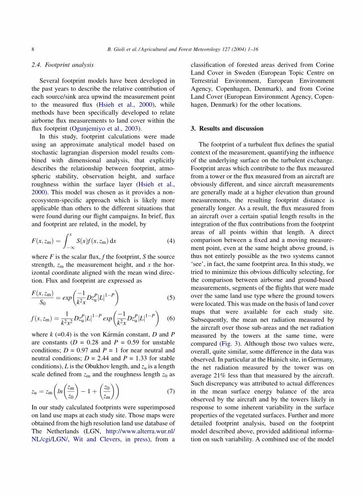
2.4. Footprint analysis

Several footprint models have been developed in

the past years to describe the relative contribution of

each source/sink area upwind the measurement point

to the measured flux (Hsieh et al., 2000), while

methods have been specifically developed to relate

airborne flux measurements to land cover within the

flux footprint (Ogunjemiyo et al., 2003).

In this study, footprint calculations were made

using an approximate analytical model based on

stochastic lagrangian dispersion model results com-

bined with dimensional analysis, that explicitly

describes the relationship between footprint, atmo-

spheric stability, observation height, and surface

roughness within the surface layer (Hsieh et al.,

2000). This model was chosen as it provides a non-

ecosystem-specific approach which is likely more

applicable than others to the different situations that

were found during our flight campaigns. In brief, flux

and footprint are related, in the model, by

Fðx; zmÞ ¼Z x

�1SðxÞf ðx; zmÞ dx (4)

where F is the scalar flux, f the footprint, S the source

strength, zm the measurement height, and x the hor-

izontal coordinate aligned with the mean wind direc-

tion. Flux and footprint are expressed as

Fðx; zmÞS0

¼ exp�1

k2xDzP

u jLj1�P

� �(5)

1 P 1�P �1 P 1�P

� �
f ðx; zmÞ ¼
k2x2Dzu jLj exp

k2xDzu jLj (6)

where k (=0.4) is the von Karman constant, D and P

are constants (D = 0.28 and P = 0.59 for unstable

conditions; D = 0.97 and P = 1 for near neutral and

neutral conditions; D = 2.44 and P = 1.33 for stable

conditions), L is the Obukhov length, and zu is a length

scale defined from zm and the roughness length z0 as

zu ¼ zm lnzm

z0

� �� 1 þ z0

zm

� �� (7)

In our study calculated footprints were superimposed

on land use maps at each study site. Those maps were

obtained from the high resolution land use database of

The Netherlands (LGN, http://www.alterra.wur.nl/

NL/cgi/LGN/, Wit and Clevers, in press), from a

classification of forested areas derived from Corine

Land Cover in Sweden (European Topic Centre on

Terrestrial Environment, European Environment

Agency, Copenhagen, Denmark), and from Corine

Land Cover (European Environment Agency, Copen-

hagen, Denmark) for the other locations.

3. Results and discussion

The footprint of a turbulent flux defines the spatial

context of the measurement, quantifying the influence

of the underlying surface on the turbulent exchange.

Footprint areas which contribute to the flux measured

from a tower or the flux measured from an aircraft are

obviously different, and since aircraft measurements

are generally made at a higher elevation than ground

measurements, the resulting footprint distance is

generally longer. As a result, the flux measured from

an aircraft over a certain spatial length results in the

integration of the flux contributions from the footprint

areas of all points within that length. A direct

comparison between a fixed and a moving measure-

ment point, even at the same height above ground, is

thus not entirely possible as the two systems cannot

‘see’, in fact, the same footprint area. In this study, we

tried to minimize this obvious difficulty selecting, for

the comparison between airborne and ground-based

measurements, segments of the flights that were made

over the same land use type where the ground towers

were located. This was made on the basis of land cover

maps that were available for each study site.

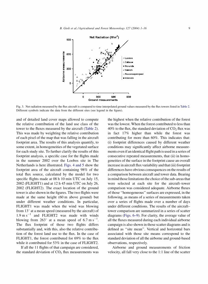
Subsequently, the mean net radiation measured by

the aircraft over those sub-areas and the net radiation

measured by the towers at the same time, were

compared (Fig. 3). Although those two values were,

overall, quite similar, some difference in the data was

observed. In particular at the Hainich site, in Germany,

the net radiation measured by the tower was on

average 21% less than that measured by the aircraft.

Such discrepancy was attributed to actual differences

in the mean surface energy balance of the area

observed by the aircraft and by the towers likely in

response to some inherent variability in the surface

properties of the vegetated surfaces. Further and more

detailed footprint analysis, based on the footprint

model described above, provided additional informa-

tion on such variability. A combined use of the model

http://www.alterra.wur.nl/NL/cgi/LGN/

http://www.alterra.wur.nl/NL/cgi/LGN/


Fig. 3. Net radiation measured by the flux aircraft is compared to time interpolated ground values measured by the flux towers listed in Table 2.

Different symbols indicate the data from the different sites (see legend in the figure).

and of detailed land cover maps allowed to compute

the relative contribution of the land use class of the

tower to the fluxes measured by the aircraft (Table 2).

This was made by weighting the relative contribution

of each pixel of the map that was falling in the aircraft

footprint area. The results of this analysis quantify, to

some extent, in homogeneities of the vegetated surface

for each study site. To further clarify the results of this

footprint analysis, a specific case for the flights made

in the summer 2002 over the Loobos site in The

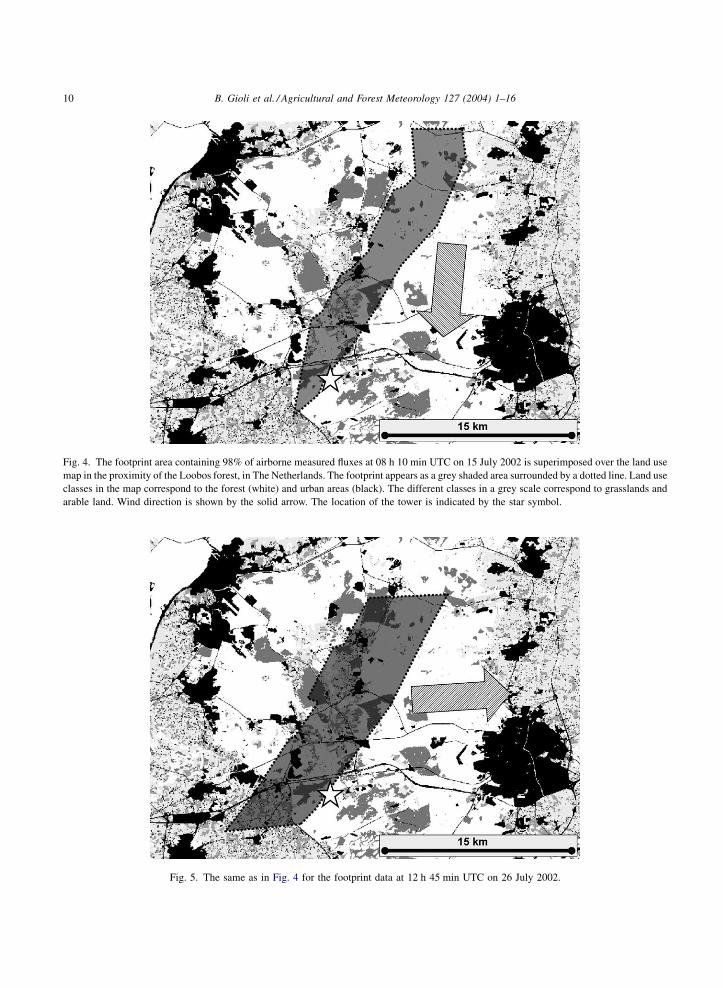
Netherlands is here illustrated. Figs. 4 and 5 show the

footprint area of the aircraft containing 98% of the

total flux source, calculated by the model for two

specific flights made at 08 h 10 min UTC on July 15,

2002 (FLIGHT1) and at 12 h 45 min UTC on July 26,

2002 (FLIGHT2). The exact location of the ground

tower is also shown in the figures. The two flights were

made at the same height (60 m above ground) but

under different weather conditions. In particular,

FLIGHT1 was made when the wind was blowing

from 138 at a mean speed (measured by the aircraft) of

1.9 m s�1 and FLIGHT2 was made with winds

blowing from 2638 at a mean speed of 6.7 m s�1.

The flux footprint of those two flights differs

substantially and, with this, also the relative contribu-

tion of the forest land use to the flux. In the case of

FLIGHT1, the forest contributed for 69% to the flux

while it contributed for 53% in the case of FLIGHT2.

If all the 11 flights of that campaign are considered,

the standard deviation of CO2 flux measurements was

the highest when the relative contribution of the forest

was the lowest. When the forest contributed to less than

40% to the flux, the standard deviation of CO2 flux was

in fact 17% higher than while the forest was

contributing for more than 60%. This indicates that:

(i) footprint differences caused by different weather

conditions may significantly affect airborne measure-

ments even if an identical flight path is used in a series of

consecutive repeated measurements, that (ii) in homo-

geneities of the surface in the footprint cause an overall

increase in aircraft flux variability and that (iii) footprint

differences have obvious consequences on the results of

a comparison between aircraft and tower data. Bearing

in mind those limitations the choice of the sub-areas that

were selected at each site for the aircraft–tower

comparison was considered adequate. Airborne fluxes

of those ‘‘homogeneous’’ surfaces are expressed, in the

following, as means of a series of measurements taken

over a series of flights made over a number of days

under different conditions. The results of the aircraft–

tower comparison are summarized in a series of scatter

diagrams (Figs. 6–9). For clarity, the average value of

all the fluxes measured during each individual airborne

campaign is also shown in those scatter diagrams and is

defined as ‘‘site mean’’. Vertical and horizontal bars

associated with those site means correspond to the

standard deviation of all the airborne and ground-based

observations, respectively.

Airborne and ground measurements of friction

velocity, all fall very close to the 1:1 line of the scatter


Fig. 4. The footprint area containing 98% of airborne measured fluxes at 08 h 10 min UTC on 15 July 2002 is superimposed over the land use

map in the proximity of the Loobos forest, in The Netherlands. The footprint appears as a grey shaded area surrounded by a dotted line. Land use

classes in the map correspond to the forest (white) and urban areas (black). The different classes in a grey scale correspond to grasslands and

arable land. Wind direction is shown by the solid arrow. The location of the tower is indicated by the star symbol.

Fig. 5. The same as in Fig. 4 for the footprint data at 12 h 45 min UTC on 26 July 2002.


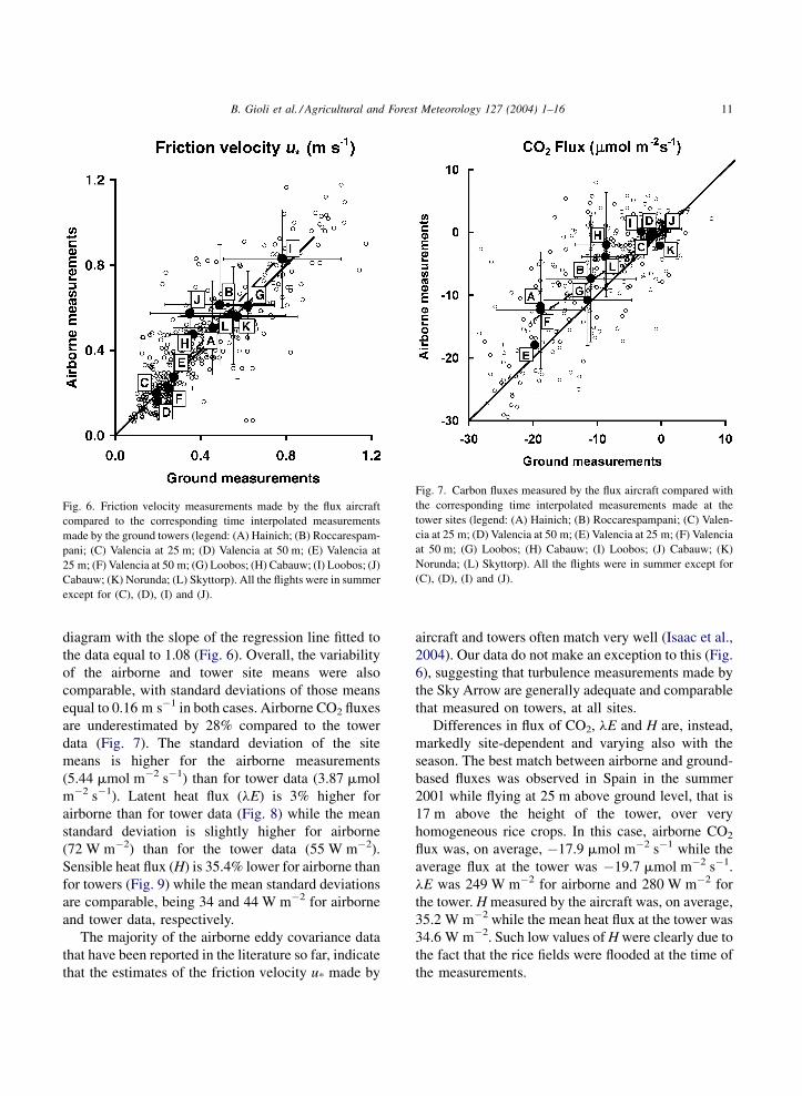
Fig. 6. Friction velocity measurements made by the flux aircraft

compared to the corresponding time interpolated measurements

made by the ground towers (legend: (A) Hainich; (B) Roccarespam-

pani; (C) Valencia at 25 m; (D) Valencia at 50 m; (E) Valencia at

25 m; (F) Valencia at 50 m; (G) Loobos; (H) Cabauw; (I) Loobos; (J)

Cabauw; (K) Norunda; (L) Skyttorp). All the flights were in summer

except for (C), (D), (I) and (J).

Fig. 7. Carbon fluxes measured by the flux aircraft compared with

the corresponding time interpolated measurements made at the

tower sites (legend: (A) Hainich; (B) Roccarespampani; (C) Valen-

cia at 25 m; (D) Valencia at 50 m; (E) Valencia at 25 m; (F) Valencia

at 50 m; (G) Loobos; (H) Cabauw; (I) Loobos; (J) Cabauw; (K)

Norunda; (L) Skyttorp). All the flights were in summer except for

(C), (D), (I) and (J).

diagram with the slope of the regression line fitted to

the data equal to 1.08 (Fig. 6). Overall, the variability

of the airborne and tower site means were also

comparable, with standard deviations of those means

equal to 0.16 m s�1 in both cases. Airborne CO2 fluxes

are underestimated by 28% compared to the tower

data (Fig. 7). The standard deviation of the site

means is higher for the airborne measurements

(5.44 mmol m�2 s�1) than for tower data (3.87 mmol

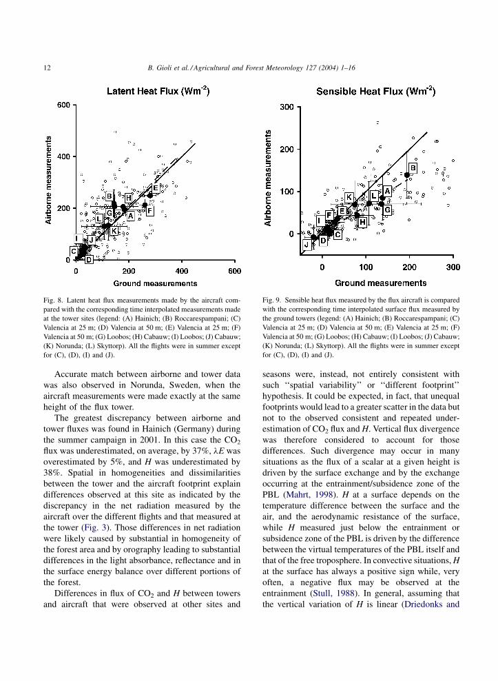
m�2 s�1). Latent heat flux (lE) is 3% higher for

airborne than for tower data (Fig. 8) while the mean

standard deviation is slightly higher for airborne

(72 W m�2) than for the tower data (55 W m�2).

Sensible heat flux (H) is 35.4% lower for airborne than

for towers (Fig. 9) while the mean standard deviations

are comparable, being 34 and 44 W m�2 for airborne

and tower data, respectively.

The majority of the airborne eddy covariance data

that have been reported in the literature so far, indicate

that the estimates of the friction velocity u* made by

aircraft and towers often match very well (Isaac et al.,

2004). Our data do not make an exception to this (Fig.

6), suggesting that turbulence measurements made by

the Sky Arrow are generally adequate and comparable

that measured on towers, at all sites.

Differences in flux of CO2, lE and H are, instead,

markedly site-dependent and varying also with the

season. The best match between airborne and ground-

based fluxes was observed in Spain in the summer

2001 while flying at 25 m above ground level, that is

17 m above the height of the tower, over very

homogeneous rice crops. In this case, airborne CO2

flux was, on average, �17.9 mmol m�2 s�1 while the

average flux at the tower was �19.7 mmol m�2 s�1.

lE was 249 W m�2 for airborne and 280 W m�2 for

the tower. H measured by the aircraft was, on average,

35.2 W m�2 while the mean heat flux at the tower was

34.6 W m�2. Such low values of H were clearly due to

the fact that the rice fields were flooded at the time of

the measurements.


Fig. 8. Latent heat flux measurements made by the aircraft com-

pared with the corresponding time interpolated measurements made

at the tower sites (legend: (A) Hainich; (B) Roccarespampani; (C)

Valencia at 25 m; (D) Valencia at 50 m; (E) Valencia at 25 m; (F)

Valencia at 50 m; (G) Loobos; (H) Cabauw; (I) Loobos; (J) Cabauw;

(K) Norunda; (L) Skyttorp). All the flights were in summer except

for (C), (D), (I) and (J).

Fig. 9. Sensible heat flux measured by the flux aircraft is compared

with the corresponding time interpolated surface flux measured by

the ground towers (legend: (A) Hainich; (B) Roccarespampani; (C)

Valencia at 25 m; (D) Valencia at 50 m; (E) Valencia at 25 m; (F)

Valencia at 50 m; (G) Loobos; (H) Cabauw; (I) Loobos; (J) Cabauw;

(K) Norunda; (L) Skyttorp). All the flights were in summer except

for (C), (D), (I) and (J).

Accurate match between airborne and tower data

was also observed in Norunda, Sweden, when the

aircraft measurements were made exactly at the same

height of the flux tower.

The greatest discrepancy between airborne and

tower fluxes was found in Hainich (Germany) during

the summer campaign in 2001. In this case the CO2

flux was underestimated, on average, by 37%, lE was

overestimated by 5%, and H was underestimated by

38%. Spatial in homogeneities and dissimilarities

between the tower and the aircraft footprint explain

differences observed at this site as indicated by the

discrepancy in the net radiation measured by the

aircraft over the different flights and that measured at

the tower (Fig. 3). Those differences in net radiation

were likely caused by substantial in homogeneity of

the forest area and by orography leading to substantial

differences in the light absorbance, reflectance and in

the surface energy balance over different portions of

the forest.

Differences in flux of CO2 and H between towers

and aircraft that were observed at other sites and

seasons were, instead, not entirely consistent with

such ‘‘spatial variability’’ or ‘‘different footprint’’

hypothesis. It could be expected, in fact, that unequal

footprints would lead to a greater scatter in the data but

not to the observed consistent and repeated under-

estimation of CO2 flux and H. Vertical flux divergence

was therefore considered to account for those

differences. Such divergence may occur in many

situations as the flux of a scalar at a given height is

driven by the surface exchange and by the exchange

occurring at the entrainment/subsidence zone of the

PBL (Mahrt, 1998). H at a surface depends on the

temperature difference between the surface and the

air, and the aerodynamic resistance of the surface,

while H measured just below the entrainment or

subsidence zone of the PBL is driven by the difference

between the virtual temperatures of the PBL itself and

that of the free troposphere. In convective situations, H

at the surface has always a positive sign while, very

often, a negative flux may be observed at the

entrainment (Stull, 1988). In general, assuming that

the vertical variation of H is linear (Driedonks and


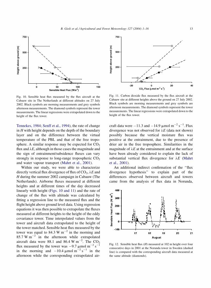
Fig. 10. Sensible heat flux measured by the flux aircraft at the

Cabauw site in The Netherlands at different altitudes on 27 July

2002. Black symbols are morning measurements and grey symbols

afternoon measurements. The diamond symbols represent the tower

measurements. The linear regressions were extrapolated down to the


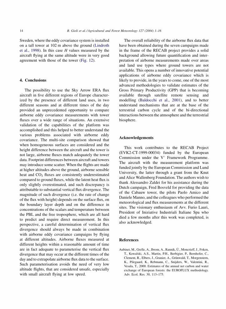
Fig. 11. Carbon dioxide flux measured by the flux aircraft at the

Cabauw site at different heights above the ground on 27 July 2002.

Black symbols are morning measurements and grey symbols are

afternoon measurements. The diamond symbols represent the tower

measurements. The linear regressions were extrapolated down to the


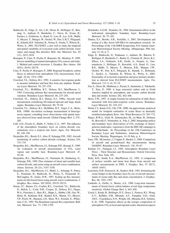
Fig. 12. Sensible heat flux (H) measured at 102 m height over four

consecutive days in 2001 at the Norunda tower in Sweden (dashed

line) is compared with the corresponding aircraft data measured at

the same altitude (diamonds).

Tennekes, 1984; Senff et al., 1994), the rate of change

in H with height depends on the depth of the boundary

layer and on the difference between the virtual

temperature of the PBL and that of the free tropo-

sphere. A similar response may be expected for CO2

flux and lE, although in those cases the magnitude and

the sign of entrainment/subsidence fluxes can vary

strongly in response to long-range tropospheric CO2

and water vapour transport (Mahrt et al., 2001).

Within our study, we were able to characterize

directly vertical flux divergence of flux of CO2, lE and

H during the summer 2002 campaign in Cabauw (The

Netherlands). Airborne fluxes measured at different

heights and at different times of the day decreased

linearly with height (Figs. 10 and 11) and the rate of

change of the flux with altitude was calculated by

fitting a regression line to the measured flux and the

flight height above ground level data. Using regression

equations it was then possible to extrapolate the fluxes

measured at different heights to the height of the eddy

covariance tower. Time interpolated values from the

tower and aircraft data extrapolated to the height of

the tower matched. Sensible heat flux measured by the

tower was equal to 84.3 W m�2 in the morning and

85.7 W m�2 in the afternoon while extrapolated

aircraft data were 88.1 and 86.4 W m�2. The CO2

flux measured by the tower was �9.7 mmol m�2 s�1

in the morning and �10.4 mmol m�2 s�1 in the

afternoon while the corresponding extrapolated air-

craft data were �11.3 and �14.9 mmol m�2 s�1. Flux

divergence was not observed for lE (data not shown)

possibly because the vertical moisture flux was

positive at the entrainment, due to the presence of

drier air in the free troposphere. Similarities in the

magnitude of lE at the entrainment and at the surface

have been already considered to explain the lack of

substantial vertical flux divergence for lE (Mahrt

et al., 2001).

An additional indirect confirmation of the ‘‘flux

divergence hypothesis’’ to explain part of the

differences observed between aircraft and towers

came from the analysis of flux data in Norunda,


Sweden, where the eddy covariance system is installed

on a tall tower at 102 m above the ground (Lindroth

et al., 1998). In this case H values measured by the

aircraft flying at the same altitude were in very good

agreement with those of the tower (Fig. 12).

4. Conclusions

The possibility to use the Sky Arrow ERA flux

aircraft in five different regions of Europe character-

ized by the presence of different land uses, in two

different seasons and at different times of the day

provided an unprecedented opportunity to compare

airborne eddy covariance measurements with tower

fluxes over a wide range of situations. An extensive

validation of the capabilities of the platform was

accomplished and this helped to better understand the

various problems associated with airborne eddy

covariance. The multi-site comparison showed that

when homogeneous surfaces are considered and the

height difference between the aircraft and the tower is

not large, airborne fluxes match adequately the tower

data. Footprint differences between aircraft and towers

may introduce some scatter. When the flights are made

at higher altitudes above the ground, airborne sensible

heat and CO2 fluxes are consistently underestimated

compared to ground fluxes, while the latent heat flux is

only slightly overestimated, and such discrepancy is

attributable to substantial vertical flux divergence. The

magnitude of such divergence (i.e. the rate of change

of the flux with height) depends on the surface flux, on

the boundary layer depth and on the difference in

concentrations of the scalars and temperature between

the PBL and the free troposphere, which are all hard

to predict and require direct measurement. In this

perspective, a careful determination of vertical flux

divergence should always be made in combination

with airborne eddy covariance campaigns by flying

at different altitudes. Airborne fluxes measured at

different heights within a reasonable amount of time

are in fact adequate to parameterise the vertical flux

divergence that may occur at the different times of the

day and to extrapolate airborne flux data to the surface.

Such parameterisation avoids the need of very low

altitude flights, that are considered unsafe, especially

with small aircraft flying at low speed.

The overall reliability of the airborne flux data that

have been obtained during the seven campaigns made

in the frame of the RECAB project provides a solid

background allowing future quantification and inter-

pretation of airborne measurements made over areas

and land use types where ground towers are not

available. This opens a number of innovative potential

applications of airborne eddy covariance which is

likely to provide, in the years to come, one of the most

advanced methodologies to validate estimates of the

Gross Primary Productivity (GPP) that is becoming

available through satellite remote sensing and

modelling (Baldocchi et al., 2001), and to better

understand mechanisms that are at the base of the

terrestrial carbon cycle and of the bi-directional

interactions between the atmosphere and the terrestrial

biosphere.

Acknowledgements

This work contributes to the RECAB Project

(EVK2-CT-1999-00034) funded by the European

Commission under the V8 Framework Programme.

The aircraft with the measurement platform was

funded jointly by the European Commission and Lund

University, the latter through a grant from the Knut

and Alice Wallenberg Foundation. The authors wish to

thank Alessandro Zaldei for his assistance during the

Dutch campaign, Fred Bosveld for providing the data

of the Cabauw tower, the pilots Paolo Amico and

Daniele Manno, and the colleagues who performed the

meteorological and flux measurements at the different

sites. The visionary enthusiasm of Avv. Furio Lauri,

President of Iniziative Industriali Italiane Spa who

died a few months after this work was completed, is

also acknowledged.

References

Aubinet, M., Grelle, A., Ibrom, A., Rannik, U., Moncrieff, J., Foken,

T., Kowalski, A.S., Martin, P.H., Berbigier, P., Bernhofer, C.,

Clement, R., Elbers, J., Granier, A., Grunwald, T., Morgenstern,

K., Pilegaard, K., Rebmann, C., Snijders, W., Valentini, R.,

Vesala, T., 2000. Estimates of the annual net carbon and water

exchange of European forests: the EUROFLUX methodology.

Adv. Ecol. Res. 30, 113–175.


Baldocchi, D., Falge, E., Gu, L.H., Olson, R., Hollinger, D., Run-

ning, S., Anthoni, P., Bernhofer, C., Davis, K., Evans, R.,

Fuentes, J., Goldstein, A., Katul, G., Law, B., Lee, X.H., Malhi,

Y., Meyers, T., Munger, W., Oechel, W., Paw, U.K.T., Pilegaard,

K., Schmid, H.P., Valentini, R., Verma, S., Vesala, T., Wilson, K.,

Wofsy, S., 2001. FLUXNET: a new tool to study the temporal

and spatial variability of ecosystem-scale carbon dioxide, water

vapor, and energy flux densities. Bull. Am. Meteorol. Soc. 82

(11), 2415–2434.

Bousquet, P., Ciais, P., Peylin, P., Ramonet, M., Monfray, P., 1999.

Inverse modelling of annual atmospheric CO2 sources and sinks.

1. Method and control inversion. J. Geophys. Res.-Atmos. 104

(D21), 26161–26178.

Ciais, P., Peylin, P., Bousquet, P., 2000. Regional biospheric carbon

fluxes as inferred from atmospheric CO2 measurements. Ecol.

Appl. 10 (6), 1574–1589.

Crawford, T.L., Dobosy, R.J., 1992. A sensitive fast response probe

to measure turbulence and heat flux from any airplane. Bound-

ary-Layer Meteorol. 59, 257–278.

Crawford, T.L., McMillen, R.T., Dobosy, R.J., MacPherson, I.,

1993. Correcting airborne flux measurements for aircraft speed

variation. Boundary-Layer Meteorol. 66, 237–245.

Crawford, T.L., Dobosy, R.J., Dumas, E.J., 1996a. Aircraft wind

measurement considering lift-induced upwash and large attack

angles. Boundary-Layer Meteorol. 80, 79–94.

Crawford, T.L., Dobosy, R.J., McMillen, R.T., Vogel, C.A., Hicks,

B.B., 1996b. Air-surface exchange measurement in heteroge-

neous regions: extending tower observations with spatial struc-

ture observed from small aircraft. Global Change Biol. 2, 275–

285.

Culf, A.D., Fiosch, G., Mahli, Y., Nobre, C.A., 1997. The influence

of the atmospheric boundary layer on carbon dioxide con-

centrations over a tropical rain forest. Agric. For. Meteorol.

85, 149–158.

Desjardins, R.L., Brach, E.J., Alno, P., Schuepp, P.H., 1982. Aircraft

monitoring of surface carbon dioxide exchange. Science 216,

733–735.

Desjardins, R.L., MacPherson, J.I., Schuepp, P.H., Karanji, F., 1989.

An evaluation of aircraft measurements of CO2, water

vapour and sensible heat. Boundary-Layer Meteorol. 47,

55–69.

Desjardins, R.L., MacPherson, J.I., Neumann, H., Denhartog, G.,

Schuepp, P.H., 1995. Flux estimates of latent and sensible heat,

carbon-dioxide, and ozone using an aircraft–tower combination.

Atmos. Environ. 29 (21), 3147–3158.

Desjardins, R.L., MacPherson, J.I., Mahrt, L., Schuepp, P., Pattey,

E., Neumann, H., Baldocchi, D., Wofsy, S., Fitzjarrald, D.,

McCaughey, H., Joiner, D.W., 1997. Scaling up flux measure-

ments for the boreal forest using aircraft–tower combinations. J.

Geophys. Res.-Atmos. 102 (D24), 29125–29133.

Doran, J.C., Barnes, F.J., Coulter, R.L., Crawford, T.L., Baldocchi,

D., Balick, L., Cook, D.R., Cooper, D., Dobosy, R.J., Dugas,

W.A., Fritschen, L., Hart, R.L., Hipps, L., Hubbe, J.M., Gao, W.,

Hicks, R., Kirkham, R.R., Kunkel, K.E., Martin, T.J., Meyers,

T.P., Porch, W., Shannon, J.D., Shaw, W.J., Swiatek, E., White-

man, C.D., 1992. The Boardman regional flux experiment. Bull.

Am. Meteorol. Soc. 73, 1785–1795.

Driedonks, A.G.M., Tennekes, H., 1984. Entrainment effects in the

well-mixed atmospheric boundary layer. Boundary-Layer

Meteorol. 30, 75–105.

Dumas, E.J., Brooks, S.B., Verfaillie, J., 2001. Development and

testing of a Sky Arrow 650 ERA for atmospheric research. In:

Proceedings of the 11th SMOI Symposium, 81st Annual Amer-

ican Meteorological Society Meeting. Albuquerque, NM, Jan-

uary 13–18, p. 5.

Falge, E., Baldocchi, D., Tenhunen, J., Aubinet, M., Bakwin, P.,

Berbigier, P., Bernhofer, C., Burba, G., Clement, R., Davis, K.J.,

Elbers, J.A., Goldstein, A.H., Grelle, A., Granier, A., Guo-

mundsson, J., Hollinger, D., Kowalski, A.S., Katul, G., Law,

B.E., Malhi, Y., Meyers, T., Monson, R.K., Munger, J.W.,

Oechel, W., Paw, K.T., Pilegaard, K., Rannik, U., Rebmann,

C., Suyker, A., Valentini, R., Wilson, K., Wofsy, S., 2002.

Seasonality of ecosystem respiration and gross primary produc-

tion as derived from FLUXNET measurements. Agric. For.

Meteorol. 113 (1–4), 53–74.

Fan, S., Gloor, M., Mahlman, J., Pacala, S., Sarmiento, J., Takahashi,

T., Tans, P., 1998. A large terrestrial carbon sink in North

America implied by atmospheric and oceanic carbon dioxide

data and model. Science 282, 442–446.

Horst, T.W., 1997. A simple formula for attenuation of eddy fluxes

measured with first-order-response scalar sensors. Boundary-

Layer Meteorol. 82, 219–233.

Hsieh, C.I., Katul, G.G., Chi, T.W., 2000. An approximate analytical

model for footprint estimation of scalar fluxes in thermally

stratified atmospheric flows. Adv. Water Resources 23, 765–772.

Hutjes, R.W.A., Gioli, B., Schumacher, M., ter Maat, H., Dolman,

H., Bosveld, F., Vermeulen, A., Vila, J., 2002. Integrating surface

and boundary layer observations of CO2 exchange in hetero-

geneous landscapes: experiences from the RECAB campaign in

the Netherlands. In: Proceedings of the 15th Conference on

Boundary Layer and Turbulence, American Meteorological

Society Meeting. Wageningen, 14–19 July, p. 4.

Isaac, P.R., McAneney, J., Coppin, P., Hacker, J., 2004. Comparison

of aircraft and ground-based flux measurements during

OASIS95. Boundary-Layer Meteorol. 110, 39–67.

Kaimal, J.C., Finnigan, J.J., 1994. Atmospheric Boundary Layer

Flows – Their Structure and Measurement. Oxford University

Press, New York, NY.

Kelly, R.D., Smith, E.A., MacPherson, J.I., 1992. A comparison

of surface sensible and latent heat fluxes from aircraft and

surface measurements in FIFE. J. Geophys. Res. 97 (D17),

18445–18453.

Lenschow, D.H., Pearson Jr., R., Stankov, B.B., 1981. Estimating the

ozone budget in the boundary layer by use of aircraft measure-

ments of ozone eddy flux and mean concentration. J. Geophys.

Res. 86, 7291–7297.

Lindroth, A., Grelle, A., Moren, A.S., 1998. Long-term measure-

ments of boreal forest carbon balance reveal large temperature

sensitivity. Global Change Biol. 4, 443–450.

Lloyd, J., Kruijt, B., Hollinger, D.Y., Grace, J., Francey, R.J., Wong,

S.-C., Kelliher, F.M., Miranda, A.C., Farquhar, G.D., Gash,

J.H.C., Vygodskaya, N.N., Wright, I.R., Miranda, H.S., Schulze,

E.-D., 1996. Vegetation effects on the isotopic composition of

atmospheric CO2 at local and regional scales: theoretical aspects


and a comparison between rain forest in amazonia and a boreal

forest in Siberia. Aust. J. Plant Physiol. 23, 371–399.

Mahrt, L., 1998. Flux sampling errors for aircraft and towers. J.

Atmos. Oceanic Technol. 15, 416–429.

Mahrt, L., Vickers, D., Sun, J., 2001. Spatial variations of surface

moisture flux from aircraft data. Adv. Water Resources 24,

1133–1141.

Millan, M., Salvador, R., Mantilla, E., Artinano, B., 1996. Meteor-

ology and photochemical air pollution in southern Europe:

experimental results from EC research projects. Atmos. Environ.

30 (12), 1909–1924.

Oechel, W.C., Vourlitis, G.L., Brooks, S.B., Crawford, T.L., Dumas,

E.J., 1998. Intercomparison between chamber, tower, and air-

craft net CO2 exchange and energy fluxes measured during the

Arctic system sciences land–atmosphere–ice interaction

(ARCSS-LAII) flux study. J. Geophys. Res. 103, 28993–

29003.

Ogunjemiyo, S.O., Kaharabata, S.K., Schuepp, P.H., MacPherson,

I.J., Desjardins, R.L., Roberts, D.A., 2003. Methods of estimat-

ing CO2, latent heat and sensible heat fluxes from estimates of

land cover fractions in the flux footprint. Agric. For. Meteorol.

117 (3–4), 125–144.

Samulesson, P., Tjernstrom, M., 1999. Airborne flux measurements

in NOPEX: comparison with footprint estimated surface heat

fluxes. Agric. For. Meteorol. 98–99, 205–225.

Schimel, D., Enting, I.G., Heimann, M., Wigley, T.M.L., Raynaud,

D., Alves, D., Siegenthaler, U., 1995. CO2 and the carbon

cycle. In: Houghton et al. (Ed.), Radiative Forcing of Climate

Change and an Evaluation of the IPCC IS92 Emission Scenarios.

Cambridge University Press, Cambridge, UK, pp. 35–71.

Schulze, E.D., Valentini, R., Sanz, M.J., 2002. The long way from

Kyoto to Marrakesh: implications of the Kyoto Protocol nego-

tiations for global ecology. Global Change Biol. 8 (6), 505–518.

Stull, R.B., 1988. An Introduction to Boundary Layer Meteorology.

Kluwer Academic Publishers, Dordrecht.

Senff, C., Bosenberg, J., Peters, G., 1994. Measurement of water-

vapor flux profiles in the convective boundary-layer with LIDAR

and RADAR-RASS. J. Atmos. Oceanic Technol. 11 (1), 85–93.

Webb, E.K., Pearman, G.I., Leuning, R., 1980. Correction of flux

measurements for density effects due to heat and water vapor

transfer. Quart. J. Roy. Meteorol. Soc. 106, 85–100.

Wit, A.J.W.de, Clevers, J.P.W., in press. Efficiency and accuracy of

per-field classification for operational crop mapping. Int. J. Rem.

Sens.

Comparison between tower and aircraft-based eddy covariance fluxes in five European regions

Documents

Transcript of Comparison between tower and aircraft-based eddy covariance fluxes in five European regions