The Eddy Currents - BSP Books

The Eddy Currents 5

I The Eddy Currents

GENERAL Eddy currents, also known as Foucault currents1, manifest as induced currents in nearly all metallic conducting media – magnetic or non-magnetic – exposed to time-varying magnetic fields. The currents are so-called owing to their nature of flow as closed, circuital currents in the media, in many cases analogous to “swirls” or “eddies” formed in water due to air disturbance of some kind. The simplest case is that of swirling water in a pond following a disturbance. For example, as a simple case, if a pebble or stone is thrown in the water, swirls or eddies are formed at a given instant as depicted in Fig.1.1. When viewed in the plan, the eddies are clearly seen to be closed ‘paths’ – an essential feature of eddy currents in electrical circuits, comprising paths of induced currents in the metallic media or regions. Also, analogous to swirls in water, eddy currents may either ‘persist’ as long as the cause is present or ‘perish’ or die owing to various damping effects.

INDUCTION OF CURRENTS Apart from other factors such as physical properties of the media, the essential requirement of production of eddy currents involves

(a) a relative movement of the medium in space with respect to a magnetic field from a suitable source; for example a permanent magnet of given specification, of constant or varying magnitude and direction

or

1Named after the French physicist, Leon Foucault who first ‘discovered’ the phenomenon due to eddy currents around 1855. Historically, the first person credited with ‘observing’ eddy currents was Franscois Arago – another French physicist and mathematician.

Fig.1.1: Swirls or eddies in water

Finite Element Analyses of Eddy Current Effects in Turbogenerators 6

(b) the exposure of the metallic medium to a magnetic field that is changing or varying with time in a particular manner, that is, of a given waveform and frequency.

The examples of the two cases are shown in Fig.1.2.

Fig.1.2: Production of eddy currents

In the first case, the to and fro lateral motion of a permanent magnet with respect to a stationary metal disc (of copper or aluminium) results in induction of EMFs in the disc, leading to closed eddy currents. The same effect will ensue if the magnet were held stationary and the disc moved to and fro relative to the magnet. In either case the magnetic field is constant in magnitude and unidirectional, not changing with time. Alternatively, the disc could be arranged to rotate in the airgap of the poles of a stationary permanent magnet, leading to induction of eddy currents in the disc, but of a different distribution. The second case pertains to the disc being impinged by a magnetic field, produced by an iron-core solenoid, the winding of which is excited by an alternating current that is varying in magnitude with time; this situation being frequently encountered in most AC machines, devices and equipment.

The Eddy Currents 7

Basic Principle of Eddy Current Production The production of eddy currents is based on the fundamental laws of electromagnetic induction, enunciated by Michael Faraday1, a British scientist, in 1831. The laws state that

(i) a changing magnetic field induces an electromagnetic force, the EMF, in a conductor or an electrically conducting medium;

(ii) the EMF so induced is proportional to the rate of change of the field (with time); and (iii) the direction of the induced EMF depends on the orientation of the field.

The motionally induced EMF When the induced EMF in the medium, for example in the metal disc in Fig.1.2(a), is due to relative motion of the field and with respect to the medium, the EMF is termed to be motional. In place of the simple action indicated in the figure, suppose the medium to be a conductor of length l (m), ‘cutting’ a uniform magnetic field of flux density B (T) with a linear, constant velocity v (m/s), all of these being mutually perpendicular, as shown in Fig.1.3, an EMF given by e = B l v V (1.1) will be induced in the conductor, and if the ends of the conductor are ‘short circuited’, a current given by

i = eR

A (1.2)

will result where R is the resistance of the “closed” circuit comprising the conductor and the shorting link.

The expression for the EMF above is also explained by applying the well-known “Fleming’s2 Right Hand Rule” depicted by the diagram of Fig.1.4. It is important that the magnetic field and motion are at right angles; if not, the magnitude of the induced EMF will be correspondingly reduced considering appropriate trigonometric expression to account for the relative inclination. The phenomenon of induced eddy currents in a variety of cases in practice, for example that in Fig.1.2(a), may not be as straight forward as expressed by the EMF relationship stated above; however, two aspects are basic to the phenomenon:

1Michael Faraday: 1791-1867. 2Alexander Fleming: 1881-1955.

Fig.1.3: Production of motional EMF

Fig.1.4: Fleming’s right-hand rule


(a) the relative motion induces EMFs in the conducting medium according to Faraday’s law(s); and

(b) the induced EMFs manifest as closed, circuital currents in appropriate planes of the medium and are identified as “eddy” currents.

The actual expression(s) for the induced EMF and hence the currents will, in general, depend on the particular configuration of the magnetic field and the conducting medium, and the manner in which the relative motion is effected, in addition to the magnitudes and orientation of various quantities involved.

The ‘statically’ induced EMF and currents When there is no relative spatial motion or movement between the magnetic field and the medium, both being ‘stationary’ in space, but the former is changing with time, for example that produced by an alternating current as in Fig.1.2(b), the induced EMF follows directly from the second law of Faraday. This can mathematically be expressed by

e = dØdt

(1.3)

where Ø is the time-varying magnetic field to which the medium is exposed. The above expression being a general one: there are no restrictions to the manner in which Ø is defined or varies with time and the induced EMF will be given by time derivative of the flux density from instant to instant. The induced current(s) will then be given by the division of the EMF by the circuit resistance through which the currents would flow1. An example of eddy currents in practice due to alternating flux is illustrated in Fig.1.5 in which, additionally, the cross-section of the conducting material also plays a role in ‘controlling’ the induction of currents and their distribution through the material.

It is clear from the above expression, (eqn.1.3), that the magnitude of induced EMF and hence the currents would depend, amongst other factors, on the magnitude of the flux and its time rate of change: faster the change, in other words the higher the frequency of flux variation, the larger will be the EMF2.

1In general, the path(s) of the currents may not be simply resistive, but also inductive. The current magnitude will then be given by the EMF divided by the circuit impedance. 2Later, it is shown that a high frequency of alternating flux has further implications of induced current distribution, having an important bearing on the design and performance of electrical equipment in general.

Fig.1.5: Eddy currents induced in a solid rectangular conductor

The Eddy Currents 9

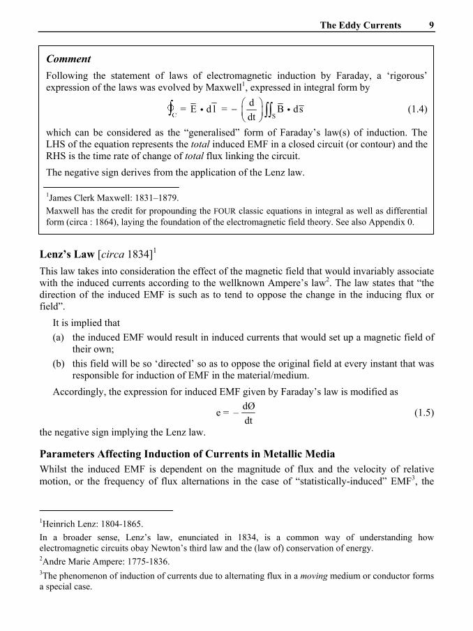
Comment Following the statement of laws of electromagnetic induction by Faraday, a ‘rigorous’ expression of the laws was evolved by Maxwell1, expressed in integral form by

= E d li =

S

d B ds dt

⎛ ⎞− ⎜ ⎟⎝ ⎠ ∫∫ i (1.4)

which can be considered as the “generalised” form of Faraday’s law(s) of induction. The LHS of the equation represents the total induced EMF in a closed circuit (or contour) and the RHS is the time rate of change of total flux linking the circuit. The negative sign derives from the application of the Lenz law.

1James Clerk Maxwell: 1831–1879. Maxwell has the credit for propounding the FOUR classic equations in integral as well as differential form (circa : 1864), laying the foundation of the electromagnetic field theory. See also Appendix 0.

Lenz’s Law [circa 1834]1 This law takes into consideration the effect of the magnetic field that would invariably associate with the induced currents according to the wellknown Ampere’s law2. The law states that “the direction of the induced EMF is such as to tend to oppose the change in the inducing flux or field”. It is implied that

(a) the induced EMF would result in induced currents that would set up a magnetic field of their own;

(b) this field will be so ‘directed’ so as to oppose the original field at every instant that was responsible for induction of EMF in the material/medium.

Accordingly, the expression for induced EMF given by Faraday’s law is modified as

e = dØ–dt

(1.5)

the negative sign implying the Lenz law.

Parameters Affecting Induction of Currents in Metallic Media Whilst the induced EMF is dependent on the magnitude of flux and the velocity of relative motion, or the frequency of flux alternations in the case of “statistically-induced” EMF3, the

1Heinrich Lenz: 1804-1865. In a broader sense, Lenz’s law, enunciated in 1834, is a common way of understanding how electromagnetic circuits obay Newton’s third law and the (law of) conservation of energy. 2Andre Marie Ampere: 1775-1836. 3The phenomenon of induction of currents due to alternating flux in a moving medium or conductor forms a special case.


induced currents would depend on the resistivity of the medium. When the net flux, considering the magnetic effect of the induced currents (as per the Lenz’s law) is also taken into account, which may be pronounced for ferrous media, the inductive effect of the paths of currents, too, restricts the currents’ flow.

As mentioned earlier, the distribution of the currents across the cross-section (in case of a conductor) or over the surface (in case of plane strips etc.), would depend on the manner in which the flux interacts with the medium and whether the latter is non-magnetic (e.g., copper or aluminium) or magnetic such as iron or steel.

In general, the physical parameters that directly determine the distribution of eddy current in the media are

(a) the electrical conductivity, σ (S/m); (b) the frequency of the alternating excitation, or rather the angular frequency, ω (= 2πf, f

being the frequency in Hz), rad/s; (c) the permeability, µ (= µ0µr, μ0 being the permeability of free space and µr the relative

permeability) corresponding to the given strength of the (AC) magnetising field at the particular instant1.

SKIN EFFECT When a conducting region, for example a round conductor of diameter D and area of cross-section A, is excited by an alternating field produced by, say, a surrounding excitation coil or winding, the induced currents in the conductor2 are NOT distributed uniformly, unlike a direct current, but “crowd” towards the surface as shown in Fig.1.6, with practically ‘no’ current flowing through the centre, depending on the diameter of the conductor. This tendency of the time-varying or alternating current to crowd, or squeeze, towards the surface or outer layer is called “skin effect” and plays an important role in the electromagnetic behaviour of the material under varying circumstances.

The effect can be ascribed to the inductive property of the currents such that the inductance of the central parts of the conductor exceeds that of the region near the surface or outer layer(s). The (inductive) reactance of the central part is therefore greater with minimal current flow and, consequently, the currents being forced towards the outer layers.

1Clearly for non-magnetic media, µr = 1 and has its own significance in the current distribution. 2Or indeed if the conductor is carrying an alternating current.

Fig.1.6: AC and DC flow in a conductor

The Eddy Currents 11

A more illustrative explanation of the phenomenon can be provided by considering the conductor of Fig.1.6, carrying an alternating current I (A). Assume the conductor to be made up of an infinite number of very small ‘filaments’, arranged parallel to the conductor axis, each carrying a small fraction of the given current equal to I/N, N being the number of filaments and the current flow in each filament being uniform. Then the flux density at a radius (or distance from the centre), r (m), within the conductor will be

( )rB = 0 2I r ,

2 aμ

π 1r a≤ (1.6)

where a is the radius of the conductor, itself assumed to be non-magnetic.

The variation of flux density at any radius as well as the total flux is given in Fig.1.7. It is seen that the flux surrounding the filaments central to the conductor is greater than that near the surface. Thus, the central filaments have greater inductance (and hence greater reactance at the given excitation frequency) and lesser current flow than the outer layers.

Two consequences of this uneven distribution of current across the conductor sections are

(i) the current flow is not restricted by its (DC) resistance alone; and

(ii) the effective area of cross-section for the current flow is relatively less, such that the ‘resistance’ itself is different from that for the flow of direct current.

Thus, in terms of any filament, let R be its resistance and L the inductance per unit length. Then its impedance will be

Z = ( )2 2 2R L+ ω (1.7)

where ω is the angular frequency (= 2πf). At low frequencies (even the power frequency), the term ω2L2 may be small compared to R2 so that the impedance can simply be equal to R and current in the conductor being given by

I = VR

(1.8)

where V is the applied voltage across the conductor. The opposite would be the case at high frequencies when ω2L2 >> R2 and the current confined to outer layer(s) or “skin” of the conductor; hence the name of the phenomenon.

1See, for example, William D. Stevenson, Jr: Elements of Power System Analysis (book), McGraw-Hill Book Co., Inc., New York, Chapter 2, p 22.

Fig.1.7: Flux density and total flux in a round conductor due

to alternating current


Skin Effect in Rectangular Cross-sections In a conductor of rectangular cross-section excited by an alternating magnetic field as in Fig.1.5, the eddy currents across the section will still form closed loops, but will crowd towards outer surfaces owing to the skin effect, leaving the ‘central’ part with practically no current flowing through it as depicted in Fig.1.8.

Skin Effect in Conducting Plates When the alternating field impinges a conducting plate at right angles to its surface, produced, for example, by a winding enclosing a soft iron core as shown in Fig.1.9, the closed paths or circuit of induced current will be largely confined to its surface. Depending on the nature of the material, the concentration and magnitude of the currents will, once again, be near to the surface or outer layer, gradually decreasing along the depth. In some cases, this may constitute a ‘desirable’ feature of induced currents, concentrating near the surface of the medium, the parameters being appropriately chosen to suit the required applications. [See Chapter II].

SKIN DEPTH A term closely associated with skin effect is “skin depth” or “depth of penetration” of the induced current in a perpendicular direction to their circuital flow; for example along “d” in Fig.1.9. In a given conducting material, magnetic or non-magnetic, the phenomenon of current penetration depends on

(a) the electrical conductivity, and (b) permeability of the material

and, from the point of alternating excitation, on (c) the frequency of the magnetising field1

1Here, it is assumed that the magnetic field resulting in induced currents is time-varying of any waveform and frequency and not owing to relative, spatial motion of the field and the medium.

Fig.1.9: Skin effect in a conducting plate

Fig.1.8: Skin effect in rectangular conductors


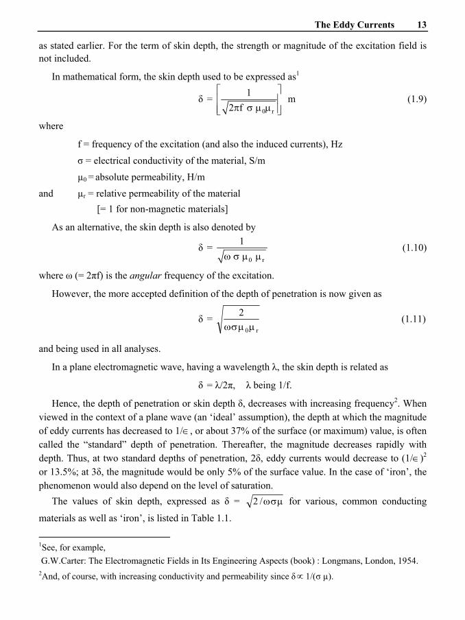
as stated earlier. For the term of skin depth, the strength or magnitude of the excitation field is not included.

In mathematical form, the skin depth used to be expressed as1

δ = 0 r

1 m2 f

⎡ ⎤⎢ ⎥

π σ μ μ⎢ ⎥⎣ ⎦ (1.9)

where

f = frequency of the excitation (and also the induced currents), Hz

σ = electrical conductivity of the material, S/m µ0 = absolute permeability, H/m and µr = relative permeability of the material [= 1 for non-magnetic materials]

As an alternative, the skin depth is also denoted by

δ = 0 r

1 ω σ μ μ

(1.10)

where ω (= 2πf) is the angular frequency of the excitation.

However, the more accepted definition of the depth of penetration is now given as

δ = r0

2μμσω

(1.11)

and being used in all analyses.

In a plane electromagnetic wave, having a wavelength λ, the skin depth is related as

δ = λ/2π, λ being 1/f.

Hence, the depth of penetration or skin depth δ, decreases with increasing frequency2. When viewed in the context of a plane wave (an ‘ideal’ assumption), the depth at which the magnitude of eddy currents has decreased to 1/∈, or about 37% of the surface (or maximum) value, is often called the “standard” depth of penetration. Thereafter, the magnitude decreases rapidly with depth. Thus, at two standard depths of penetration, 2δ, eddy currents would decrease to (1/∈)2 or 13.5%; at 3δ, the magnitude would be only 5% of the surface value. In the case of ‘iron’, the phenomenon would also depend on the level of saturation. The values of skin depth, expressed as δ = μσω/2 for various, common conducting

materials as well as ‘iron’, is listed in Table 1.1.

1See, for example, G.W.Carter: The Electromagnetic Fields in Its Engineering Aspects (book) : Longmans, London, 1954. 2And, of course, with increasing conductivity and permeability since δ∝ 1/(σ µ).


Table 1.1: Skin depth in various metals at different frequencies

Medium/conductor σ (S/m) µr Skin depth, mm

frequency, Hz 50 500 104 106 aluminium 35 × 106 1.0 12.03 3.87 0.85 0.085 copper 58 × 106 1.0 9.3 2.9 0.66 0.066 silver 62 × 106 1.0 9.05 2.82 0.64 0.064 “iron” (say, mild steel)

10 × 106 500.0 (assumed)

0.98 0.32 0.07 0.007

Thus, as a case in practice, if aluminium or copper1 is used as conductor material for carrying current a ‘thickness’ of only 8.5/6.6 mm is effectively utilised for AC at 50 Hz (or power frequency). Also, even though copper is a better conductor than aluminium, its effectiveness (in terms of skin depth) in the distribution of current across the conductor cross-section is less than that of aluminium. The skin depth of “iron” presents a special case, revealing a much lower degree of penetration, dependent on the given/chosen value of its relative permeability, arbitrarily assumed to be 500 in the above calculations. As the saturation sets in, again a function of the strength of magnetising field, the skin depth will vary appreciably. Under intense saturation condition, µr 5 (say), the skin depth maybe comparable to aluminium or copper ( 7 mm, at f = 50 Hz and µr = 5.0) and has its significance in some applications. The (acute) dependence of skin depth on frequency of (AC) excitation is also indicated by relevant figures in Table 1.1, showing rapid decrease of the depth, even for aluminium, as the frequency approaches radio-waves range (i.e., MHz). Clearly, the current penetration in unsaturated iron with high value of permeability is practically zero at radio frequencies.

Comment Skin Depth and Conductors for AC Transmission Lines The property of aluminium conductors carrying AC through the entire cross-section is effectively utilised in the design and use of special conductors for transmission of huge quantity of power, extending to hundreds of megawatt, through AC HV or EHV transmission lines, over long to very long distances. Typically, such conductors comprise strands of aluminium wires, each about 4 to 5 mm in diameter (such that the entire cross-section is used up to conduct the current). The strands are arranged spirally with alternate layers being in opposite directions to prevent un-winding and to make the outer radius of one layer coincide with the inner radius of the next. Stranding results in the ‘overall’ conductors to be flexible, even for large overall cross-section, and provide convenience during commissioning of the line. Clearly, the number of strands depends on the total current per conductor (for each phase), corresponding to the power being transmitted. To impart mechanical strength, such conductors are provided with a steel wire of appropriate diameter at the centre; the wire itself carrying no current. Accordingly, such conductors are known as ACSR: Aluminium Conductor, Steel Reinforced, and nowadays universally employed in power transmission lines.

1The most commonly used metals.


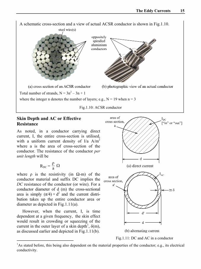
A schematic cross-section and a view of actual ACSR conductor is shown in Fig.1.10.

Total number of strands, N = 3n2 – 3n + 1 where the integer n denotes the number of layers; e.g., N = 19 when n = 3

Fig.1.10: ACSR conductor

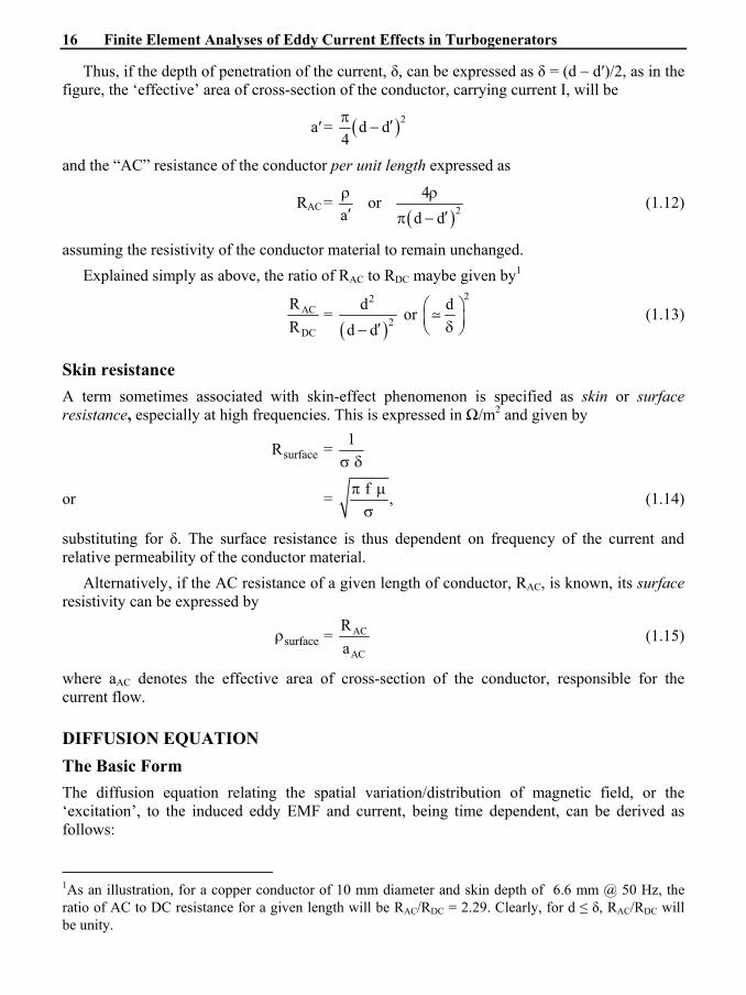
Skin Depth and AC or Effective Resistance As noted, in a conductor carrying direct current, I, the entire cross-section is utilised, with a uniform current density of I/a A/m2 where a is the area of cross-section of the conductor. The resistance of the conductor per unit length will be

RDC = aρΩ

where ρ is the resistivity (in Ω-m) of the conductor material and suffix DC implies the DC resistance of the conductor (or wire). For a conductor diameter of d (m) the cross-sectional area is simply (π/4) × d2 and the current distri-bution takes up the entire conductor area or diameter as depicted in Fig.1.11(a). However, when the current, I, is time dependent at a given frequency, the skin effect would result in crowding or squeezing of the current in the outer layer of a skin depth1, δ(m), as discussed earlier and depicted in Fig.1.11(b).

1As stated before, this being also dependent on the material properties of the conductor; e.g., its electrical conductivity.

Fig.1.11: DC and AC in a conductor


Thus, if the depth of penetration of the current, δ, can be expressed as δ = (d – d′)/2, as in the figure, the ‘effective’ area of cross-section of the conductor, carrying current I, will be

a′ = ( )2d d4π ′−

and the “AC” resistance of the conductor per unit length expressed as

RAC = aρ′ or

( )24

d dρ

′π − (1.12)

assuming the resistivity of the conductor material to remain unchanged. Explained simply as above, the ratio of RAC to RDC maybe given by1

AC

DC

RR

= ( )

2

2d

d d′− or

2d⎛ ⎞⎜ ⎟δ⎝ ⎠

(1.13)

Skin resistance A term sometimes associated with skin-effect phenomenon is specified as skin or surface resistance, especially at high frequencies. This is expressed in Ω/m2 and given by

surfaceR = 1 σ δ

or = f ,π μσ

(1.14)

substituting for δ. The surface resistance is thus dependent on frequency of the current and relative permeability of the conductor material. Alternatively, if the AC resistance of a given length of conductor, RAC, is known, its surface resistivity can be expressed by

surfaceρ = AC

AC

Ra

(1.15)

where aAC denotes the effective area of cross-section of the conductor, responsible for the current flow.

DIFFUSION EQUATION The Basic Form The diffusion equation relating the spatial variation/distribution of magnetic field, or the ‘excitation’, to the induced eddy EMF and current, being time dependent, can be derived as follows:

1As an illustration, for a copper conductor of 10 mm diameter and skin depth of 6.6 mm @ 50 Hz, the ratio of AC to DC resistance for a given length will be RAC/RDC = 2.29. Clearly, for d ≤ δ, RAC/RDC will be unity.


The differential form of Maxwell’s equation, relating magnetic field intensity, H, to the induced current density, J, in a linear conducting medium can be written

curl H = ∇ H = J (1.16) disregarding the displacement current density, D Taking curl of both sides of eqn.(1.16)

∇ (∇ )H = ∇ J (1.17)

Using the well-known vector calculus identity, this equation can be written

( ) 2 H H∇ ∇ −∇i = ∇ J (1.18)

Now H∇ i for a linear region with μr = constant, is zero by Gauss’s1 law for magnetism – or from Maxwell’s second equation – following B∇ i = 0, H being B .μ

∴ 2– H∇ = ∇ J (1.19)

Assuming the region to have constant, uniform/homogenous electrical conductivity, σ, the RHS can be expressed by J = E,σ where E denotes the electric field intensity.

∴ 2– H∇ = σ ∇ E (1.20)

Now from the third Maxwell’s equation

∇ E = Bt

∂−

∂ (1.21)

∴ substituting

2 H∇ = 2

B t

⎛ ⎞∂σ ⎜ ⎟∂⎝ ⎠

2 (1.22)

and is known as the diffusion equation for a linear, homogenous region, medium or material with constant relative permeability and electrical conductivity3. By definition, in general, B = ( )0 H Mμ + (1.23)

M being the intensity of magnetisation; μ0 is the absolute permeability. The above equation can then be written

2 H∇ = 0H M t t

⎛ ⎞∂ ∂μ σ +⎜ ⎟∂ ∂⎝ ⎠

(1.24)

1Carl Friedrich Gauss: 1777-1855. 2The equation is three-dimensional, with components of H being x yH , H , and zH , and B as

x, y, zB B B in Cartesian coordinates. Also, a general time variation of B is implied. 3These, in general, may vary, even in three perpendicular directions.


Equation in Terms of Magnetic Vector Potential Dealing with conducting media or regions, ferrous or non-ferrous (e.g., copper or aluminium), where the displacement current can be disregarded being negligible, the field equations of interest can be written in Maxwell’s differential equations form as

curl E = ∇ E = B–t

∂∂

(1.25)

or = – 0 rH ,t

⎛ ⎞∂μ μ ⎜ ⎟∂⎝ ⎠

(1.26)

B being equal to 0 rH,μ μ and is either constant for a ‘linear’ material or, more generally, a function of

H, i.e., ( )f H⎡ ⎤⎣ ⎦

curl H = ∇ H = J (1.27)

and div B = B∇ i = 0 (1.28)

with the usual notation.

Further, in a conducting region or a conductor, the electric field strength/intensity, E, is related to the current density1, J, by “Ohm’s2 law” J = Eσ (1.29)

where σ denotes electrical conductivity of the given medium.

An additional constraint on the current density, J, may be imposed owing to the law of conservation of charge which, in the absence of ‘free’ electric charge, yields

div J = J∇ i = 0 (1.30)

to be interpreted as the field equivalent of Kirchhoff’s3 current law. Taking curl of eqn.(1.27),

∇ ∇ H = ∇ Eσ (1.31)

or ( ) 2 H H∇ ∇ − ∇i = σ ∇ E + ( )∇σ E (1.32)

Expressing eqn.(1.28) in terms of H and expanding

B∇ i = ( ) H∇ μi = 0 [μ = 0μ rμ ]

or = ( ) H H μ ∇ + ∇μi = 0

1As discussed later, the current density can take the form of source or induced current(s) in a time-varying field. 2Georg Simon Ohm: 1789-1854. 3Gustav Kirchhoff: 1824-1887.


from which

H∇ i = 1 H⎛ ⎞− ∇μ⎜ ⎟μ⎝ ⎠

Using eqn.(1.24), eqn.(1.32) takes the form

2 H∇ = – σ ∇ ( )E – ∇ σ E

= ( )0 rH 1 1 H t

⎡ ⎤⎛ ⎞ ⎛ ⎞∂ ⎛ ⎞σ μ μ −∇ ∇μ − ∇ σ⎢ ⎥⎜ ⎟ ⎜ ⎟ ⎜ ⎟∂ μ σ⎝ ⎠⎝ ⎠⎝ ⎠ ⎣ ⎦i ∇ H (1.33)

which, inside a linear magnetic or nonmagnetic material of constant permeability, reduces to

2 H∇ = 0 rH t

∂σ μ μ

∂ (1.34)

since both ∇μ and ∇σ will be zero.

Considering all the components, eqn.(1.34) in the Cartesian coordinates system can be expressed as

2 2 2

x x x2 2 2

H H Hx y z

∂ ∂ ∂+ +

∂ ∂ ∂ = xH

t∂

σ μ∂

2 2 2

y y y2 2 2

H H Hx y z

∂ ∂ ∂+ +

∂ ∂ ∂ = yH

t

∂σ μ

∂ (1.35)

2 2 2

z z z2 2 2

H H Hx y z

∂ ∂ ∂+ +

∂ ∂ ∂ = zH

t∂

σ μ∂

in which μ is given by 0 r .μ μ

The above expanded forms are helpful when considering specific eddy-current problems or applications, with given approximations and assumptions.

Now as a direct consequence of eqn.(1.28), the magnetic flux density, B, can be expressed as the curl of a vector, say A, invariably known as “magnetic vector potential”1. Hence

B = ∇ A (1.36)

and A∇ i = 0

Taking curl of both sides of eqn.(1.36),

∇ ∇ A = ∇ B

1It is, however, clear that the vector, A, is NOT uniquely defined since to it can be added another vector, say Q (such that the ‘new’ vector is A Q),+ without altering the relation B∇ i = 0.


or ( ) 2 A A∇ ∇ −∇i = ∇ Hμ

= μ ∇ H + ( )∇ μ H

Since A∇ i = 0 by definition; for a linear medium with ∇μ = 0,

2 A∇ = − μ∇ H

or 2 A∇ = J− μ , using eqn.(1.27). (1.37)

Equation (1.37) represents the (desired) diffusion equation in terms of A.

The other forms By substituting Eσ for J, eqn.(1.37) can be written

2 A∇ = E− μ σ (1.38)

or = 0 r E− μ μ σ

Now from eqn.(1.24),

∇ E = Bt

⎛ ⎞∂−⎜ ⎟∂⎝ ⎠

= t∂

−∂ (∇ )A

= − ∇ At

⎛ ⎞∂⎜ ⎟∂⎝ ⎠

or ∇ AEt

⎛ ⎞∂+⎜ ⎟∂⎝ ⎠

= 0

which, after integration, yields

E = A Øt

∂− − ∇

∂ (1.39)

where Ø is a scalar potential. Substituting for E from eqn.(1.39) into eqn.(1.38) results

2 A∇ = A Øt

⎛ ⎞∂μ σ +∇⎜ ⎟∂⎝ ⎠

(1.40)

representing yet another form of diffusion equation in A 1. Any of the forms can, of course, be expanded in either Cartesian or cylindrical coordinates by employing appropriate expansion of the Laplacian2 operator, ∇2. 1It will be seen that this form is generally applicable in finite element analyses involving induced (or eddy) currents where the time variation of A in the given form and accounting for the scalar potential, Ø, leads to a given spatial solution of A . 2Pierre-Simon Laplace: 1749-1827.


Poynting’s Theorem This theorem due to Poynting1 is essentially an expression of the law of conservation of energy applied to electromagnetic fields. This is of relevance to the study and analyses involving eddy currents since the latter manifest as “ohmic” loss in many cases and hence result in (electrical) power or energy loss2. Disregarding the displacement current(s) once again being inconsequential in (linear) metallic media and at low or power frequency, the mathematical statement of the theorem is

(E )H ni ds +

VBH dvt

⎛ ⎞∂⎜ ⎟∂⎝ ⎠

∫ i = –V

J dvE ∫ i (1.41)

where the volume V is enclosed by the surface S and n denotes the unit vector normal to the surface, being directed outwards at the given point as illustrated in Fig.1.12.

In general, the integral on the RHS of eqn.(1.41), not considering the negative sign, represents the loss of electric power in the volume, being the volume integral of the (volumetric) current density and electric field intensity. If the current density, and hence the current, is purely conduction current, then, by Ohm’s law [eqn.(1.29)], the quantity represented by the integral is simply the ohmic loss within V. In this case, the Poynting’s theorem would reduce to,

2V V

1 BJ dv H dvt

⎛ ⎞∂⎛ ⎞ + ⎜ ⎟⎜ ⎟σ ∂⎝ ⎠ ⎝ ⎠∫ ∫ i = – (E H i n ds (1.42)

rearranging the terms. Eqn.(1.42) can be interpreted as “the sum of the ohmic loss, and ‘power absorbed by the magnetic field’ in V is equal to the net inflow of power”. In this context, the Poynting vector is defined as the vector product

S = E H (1.43)

universally denoted by S, and can be regarded, owing to its form in eqn.(1.41), as the (instantaneous) “density of power flow” at a point.

1John Henry Poynting: 1852-1914.

2This can be considerable in various AC equipment and devices such as generators, transformers and transmission line conductors where special means and practices are employed to minimise the loss of power/energy.

Fig.1.12: Surface and volume for Poynting theorem


Poynting Vector for Sinusoidally Time-varying Fields Often the Poynting vector is associated with the power or energy flow in electromagnetic fields involving sinusoidally time-varying quantities. In such cases, the vectors themselves are represented as phasors (or generally as complexers) and the Poynting vector takes the form

S = 12 (E )*H

being the time-average density of power flow; *H representing the complex conjugate of H, related to H by

H = Re H∈jωt = 12

[ H∈jωt + *H ∈–jωt] (1.44)

in which ω is the angular frequency of the sinusoidally time-varying field [ H in the present case].

Comment A Case of Application of Poynting’s Theorem It is of interest to observe the flow of power along the conductors of a transmission line when viewed from the perspective of Poynting’s theorem and the associated fields. Refer to Fig.1.13 which shows a section of one of the transmission line conductors, carrying a current I at a potential V with respect to adjacent conductor or the ground.

Fig.1.13: Poynting vector and power flow in a transmission line

As indicated in Fig.1.13(b), the E field due to V is directed radially outward, there being no E field inside the conductor. Likewise, the H field due to current I (flowing “in”) is of the form shown, surrounding the conductor. Then, the Poynting vector, S at any point is the cross product of E and H, is non-zero outside the conductor, and directed inward, that is, in the ‘direction’ of the current. This shows that the flow of power (or energy) through the conductors at any time occurs outside the conductors as an interaction of E and H fields, the conductors themselves acting only as a ‘guide’ or medium.


SOME CASES OF SKIN EFFECT IN PRACTICE

Skin Effect in a ‘Long’, Thin Rectangular Sheet or Conductor

The section of a long (in theory ‘infinite’) rectangular conductor, placed symmetrically, in Cartesian coordinates is shown in Fig.1.14.

Fig.1.14: Skin effect in a long, thin rectangular conductor

To interpret the thin sheet, it is assumed that

2h >> 2b

Thus, with negligible error, in terms of the magnetic and electric field intensities, H = xH and E = zE Let the sheet material has electrical conductivity σ (S/m) and permeability μ [= 0μ rμ H/m] and both H and E are sinusoidally time varying.

Then, as derived earlier,

2x

2Hx

∂∂

i

=

12xk Hi

1

and

2z

2E

x∂∂

i

= 2

zk Ei

where k2 = j ω σ μ here, j ω deriving from ∂/∂t of sinusoidally-varying quantities.

1Note that, with the assumption of sinusoidal time variations, the quantities Hx and Ez are complex variables in time domain, denoted by xH

i and zE

iwith a dot above.

(1.45)

(1.46)


Solving eqns.(1.46)

xHi

= 1Hi∈kx + 2H

i∈–kx

and zEi

= 1Ei∈kx + 2E

i∈–kx

The constants 1H ,i

, . . . , 2Ei

are easily derived from the known boundary conditions. Also, it is evident from Fig.1.14, by the reasoning of symmetry, that

( )H x+i

= ( )H x− − yielding

1Hi

= 2– Hi

= 0H 2i

(1.48) and similarly

( )E x+i

= ( )E x−i

giving

1Ei

= 2Ei

= 0E 2i

(1.49)

where H0 and E0 denote the integration constants. Then eqns.(1.47) can be written

xHi

= 0H sinh kxi

and zEi

= 0E cosh kxi

From Ohm’s law, J = Eσ and therefore, the current density is

zJi

= 0E cosh kxσi

(1.51) To determine the integration constant E0, the expression for the total current I can be used in the form of the integral

I = b

b2 h

+

−∫ zJ dxi

= 4hk

⎛ ⎞⎜ ⎟⎝ ⎠

σ 0Ei

sinh kb (1.52)

from which it follows that

zEi

= k I cosh kx 4h sinh kbσ

(1.53)

To determine the integration constant 0H ,i

use is made of the line integral

H d li = I (Ampere’s law) (1.54) which in the present case is given by

( ) ( )x b x – b2 h H 2 h H= =+i i

= I (1.55)

and this, using eqn.(1.49), would yield

0Hi

= I4 h sinh kb

(1.56)

(1.47)

(1.50)


and the equation for magnetic field, H,i

would be of the form

xHi

= I sinh kx 4 h sinh kb

(1.57)

To obtain ohmic power loss Using eqns.(1.51) and (1.53), the current density variation is given by

Ji = k I cosh kx

4 h sinh kb (1.58)

The power loss may then be determined either by the use of Poynting vector or simply by the volume integral

P = 2v

1 |J | dvσ ∫

i (1.59)

Now the “modulus” value of the current density is given by the product

2| J |i

= J × *J (1.60)

Using eqns.(1.58) and (1.60), the current modulus | J |i

is obtained using the expression

| J |i

= ( ) ( )( ) ( )

cosh 2x a cos 2x a2 I4 h a cosh 2b a cos 2b a

+−

(1.61)

where a is the depth of penetration given by

a = 1 f π σ μ

[also denoted by δ]

Substituting for | J |i

in the integral of eqn.(1.59), the power loss per unit length, the field vectors being invariant in z direction, is given by

P = b 2b

2 h |J | dx+

−σ ∫i

or P = 2I

4 a h σ

( ) ( )( ) ( )

sinh 2b a sin 2b a W m

cosh 2b a cos 2b a+−

(1.62)

It is seen that as 2b, or the sheet thickness, approaches zero, the power loss will be zero, too.

Skin Effect or Alternating Current Flow in a ‘Long’ Circular Wire1 The flow of alternating or time-varying current in a circular wire (or a very “thin” cylindrical conductor) exhibits the already discussed skin effect, forcing the current towards the outer layer(s); this can be much pronounced at higher frequencies.

1See also Appendix I for an alternative approach.

Fig.1.15: A long circular wire carrying alternating current


Consider a (“infinitely”) long wire of radius r(m) such that its length >> r

so that the analysis can be assumed to be two-dimensional, carrying a current I(A) in axial direction. See Fig.1.15. Clearly, the magnetic field, H, has only tangential component and the ‘induced’ current (density), J , is axially directed.

From the first Maxwell’s equation J = ∇ H , in cylindrical coordinates,

J = zJ = H Hr r

∂+

∂ = r rH H

r r∂

+∂

(1.63)

Also, from the equation ∇ E = B ,t

∂−∂

introducing Ohm’s law J = E,σ

Jr

∂∂

= H t

∂σ μ

∂ (1.64)

assuming constant permeability which for a non-magnetic wire material such as copper or aluminium is μ = [ ]0 r 1 .μ μ =

or zJr

∂∂

= 1rj Hω σ μ 1 (1.65)

= 2rj k H (1.65a)

when the magnetic field is assumed to be quasi-stationary, varying sinusoidally with time so that ∂/∂t = jω; also k2 = ω σ μ.

Then, from eqns.(1.63) and (1.65),

2

22

d J 1 dJ j k Jr drdr

+ − = *0 (1.66)

dropping the suffix z from J terms and using normal, not partial, derivatives.

Eqn.(1.66) is Bessel2 differential equation in J. The solution of the equation for 0 ≤ r ≤ R, where R denotes the wire radius, is seen to be J = C J0 (j3/2 k r) (1.67)

Here, J0 (j3/2 kr) is known as modified Bessel function of the first kind and ‘index’ zero. The integration constant, C, is obtained by using the surface integral of current density, equating it to total current I.

1See footnote on page 19. *From eqn.(1.65a), ( )2

r zH 1 jk J r .= ∂ ∂

Or, differentiating, ∂Hr/∂r = (1/jk2) ∂2Jz/∂r2. Substituting these in eqn.(1.63) and rearranging yields eqn.(1.66) 2Friedrich Wilhelm Bessel: 1784-1813.


Thus

I =sJ ds∫ = ( )R 3 2

00

2 C r J j k r drπ ∫

= ( )3 213 2

2 C R J j k Rj kπ (1.68)

whence

C = ( )

3 2

3 21

j k I2 R J j k Rπ

(1.69)

Substituting for C in eqn.(1.67)

J = ( )( )

3 2 3 20

3 21

j k I J j k r

2 R J j k Rπ (1.70)

at any radius r. Now by substituting the expression for J from eqn.(1.70) in eqn.(1.65) and differentiating, the magnetic field within the conductor (r ≤ R) is given by

H = 21 J

rj k∂∂

or = I2 Rπ

( )( )

3 21

3 21

J j k r

J j k R (1.71)

It is customary to express Bessel functions with the complex argument z = (j3/2 x) as Kelvin functions such that

Jn (j3/2 x) = nber x + n j bei x

= ( )nM x ∈jθn(x) (1.72)

in which both the modulus as well as the argument are functions of the independent variable x. Then J (above) can be written

J = 3 2

0 0

1 1

ber r + j bei rj kI 2 R ber R + j bei Rπ

(1.73)

From the knowledge of J in complex form, the power loss in the wire/conductor can be obtained from

P = 12

⎛ ⎞⎜ ⎟σ⎝ ⎠ V

J∫ × *J dv (1.74)

where *J represents the complex conjugate of J.

or, in the present case (of ‘infinite’ wire length), simply

P = 12σ

R 2

0 0J

π

∫ ∫ × *J r dθ dr (1.75)

per unit length.


Current Distribution and Power Loss in a Cylinder of Finite Length1

Assumptions

The analysis is based on the following assumptions:

• Even though the cylinder is of finite length, the power density is uniform along the length

• The ‘end effects’ are disregarded

• The analysis can thus be two-dimensional, in r, θ plane, the field quantities being invariant along the axial length; this also implies that the length/diameter ratio of the cylinder is very large

• If the cylinder is of magnetic material, its permeability is constant, given by the AC magnetisation curve at the given excitation

• The cylinder is ‘excited’ by an alternating current, to be identified as “source” current, the mmf pulsating at the given frequency and sinusoidally spaced along the circumference

• Accordingly, both the magnetic vector potential, A, and induced current density, J, in the cylinder are only axially directed.

Then, the partial differential equation applicable in this case is the diffusion equation

2A∇ = Akt

∂′∂

(1.76)

in magnetic vector potential, A, where k′ is a constant, depending on the various properties of the cylinder material.

Solution in cylindrical coordinates Eqn.(1.76) can be expressed in cylindrical coordinates in two dimensions as follows

2 2

2 2 21 A 1 A 1 A

r rr r⎧ ⎫∂ ∂ ∂⎪ ⎪+ +⎨ ⎬

μ ∂∂ ∂θ⎪ ⎪⎩ ⎭ = Ak

t∂′∂

(1.77)

suiting the geometry of the medium. The cylinder and the coordinate system in this case are depicted in Fig.1.16.

When the source currents, and hence the magnetic vector potential and induced currents, are sinusoidally time-varying, eqn.(1.77) can be written

1See also Appendix II.

Fig.1.16: Solid cylinder of finite length and

cylindrical coordinates system


2 2

2 2 2A 1 A 1 A

r rr r∂ ∂ ∂

+ +∂∂ ∂θ

i i i

= 2jk Ai

(1.78)

where k2 = ω σ μ

and in which A = zA = Ai

is expressed in complex notation.

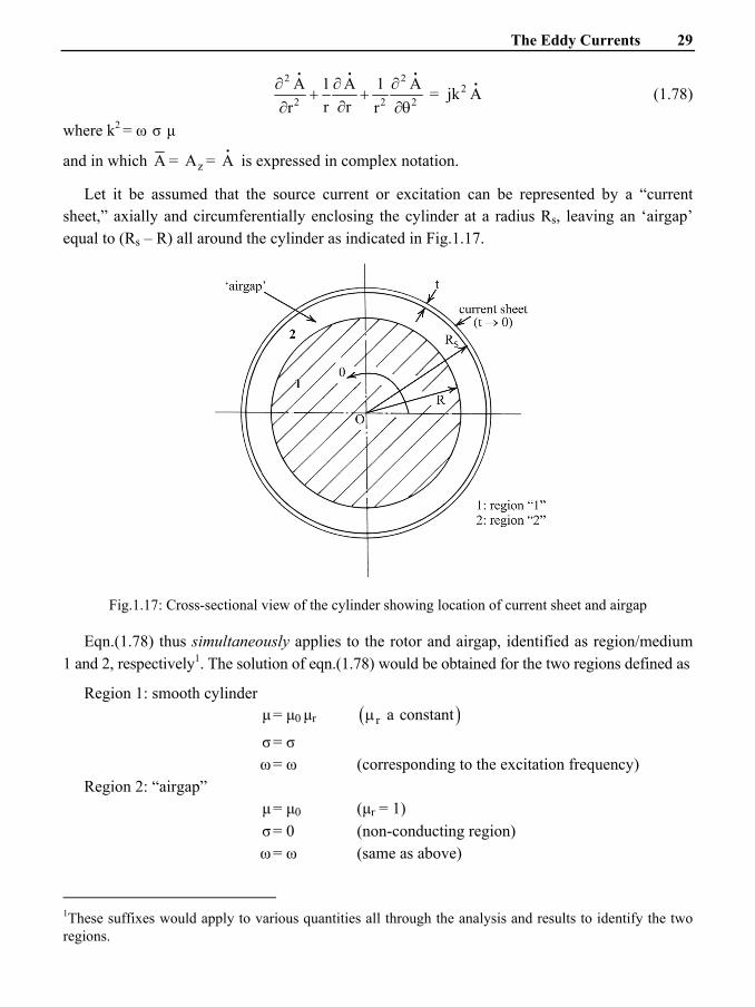
Let it be assumed that the source current or excitation can be represented by a “current sheet,” axially and circumferentially enclosing the cylinder at a radius Rs, leaving an ‘airgap’ equal to (Rs – R) all around the cylinder as indicated in Fig.1.17.

Fig.1.17: Cross-sectional view of the cylinder showing location of current sheet and airgap

Eqn.(1.78) thus simultaneously applies to the rotor and airgap, identified as region/medium 1 and 2, respectively1. The solution of eqn.(1.78) would be obtained for the two regions defined as

Region 1: smooth cylinder μ = μ0 μr ( )r a constantμ

σ = σ ω = ω (corresponding to the excitation frequency) Region 2: “airgap” μ = μ0 (μr = 1) σ = 0 (non-conducting region) ω = ω (same as above)

1These suffixes would apply to various quantities all through the analysis and results to identify the two regions.


The eqn.(1.78) can thus be written for the two regions as

Region 1: Ai

= 1Ai

2 21 1 1

2 2 2A 1 A 1 A

r rr r∂ ∂ ∂

+ +∂∂ ∂θ

i i i

= 21jk Ai

(1.79)

Region 2: Ai

= 2Ai

2 22 2 2

2 2 2A 1 A 1 A

r rr r∂ ∂ ∂

+ +∂∂ ∂θ

i i i

= 0 (1.80)

The solutions of eqns.(1.79) and (1.80) are given in Appendix II from where 1Ai

and 2Ai

are obtained as

1Ai

= ( ) ( )1 n nnn

C ber kr j bei kr cos n⎡ + ⎤ θ⎣ ⎦∑i

(1.81)

in terms of Bessel/Kelvin1 functions of the first kind and order n, and

2Ai

= n n2 3n nC r C r cos n−⎡ ⎤

+ θ⎢ ⎥⎣ ⎦

i i (1.82)

where 1 2 3n n nC , C , Ci i i

are complex constants (for the given radius and n representing the mmf harmonic order), fully evaluated in Appendix II, using the following boundary conditions:

1. the tangential component of H at the inner surface of the current sheet is equal to the surface current density, or

2 r RsH θ =

= J J(θ) (1.83)

2. on the cylinder/airgap interface boundary, the radial components of flux density and tangential components of magnetising force are continuous, or

1r r RB

= = 2r r R

B=

and 1 r R

H θ = = 2 r R

H θ =

Expressions for Magnetic Field Components and Power Loss in the Cylinder

When the distribution of magnetic vector potential, A ,i

in the two regions is known by solving

eqns.(1.79) and (1.80), the expressions for magnetic field components, Bi

and H;i

the current

density, J;i

and power dissipation in the cylinder can be deduced using

1Sir William Thomson-Lord Kelvin: 1824-1907.

(1.84)


B = ∇ A

E = At

∂−

∂

J = Eσ

and P = v

*1 J J2

×σ∫ dv

Since A has only one component, in z-direction, B will have only “r” and “θ” components, each a complex quantity. Thus

1rHi

= 11 1r r

1 1 A , B Hr∂

= μμ ∂θ

ii i

1H θi

= 11 1

1 A , B Hr θ θ

⎛ ⎞∂⎜ ⎟− = μ⎜ ⎟μ ∂⎜ ⎟

⎝ ⎠

ii i

[μ = μ0 μr] and similarly,

2rHi

= 22 2r r

1 1 A , B Hr∂

= μμ ∂θ

ii i

2H θi

= 22 2

1 A , B Hr θ θ

⎛ ⎞∂⎜ ⎟− = μ⎜ ⎟μ ∂⎜ ⎟

⎝ ⎠

ii i

[μ = μ0]

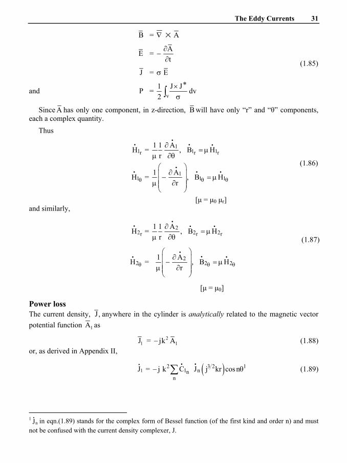
Power loss The current density, J, anywhere in the cylinder is analytically related to the magnetic vector potential function 1A as

1J = 21jk A− (1.88)

or, as derived in Appendix II,

1Ji

= ( )2 3 2 11 nn

nj k C J j kr cos n− θ∑

i i 1 (1.89)

1

nJi in eqn.(1.89) stands for the complex form of Bessel function (of the first kind and order n) and must

not be confused with the current density complexer, J.

(1.85)

(1.86)

(1.87)


Knowing, 1Ji

, the expression for power loss, using eqn.(1.85), is given by

P = 31 L R k

2 2×

σ 2

1nCi K′ (1. 90)

as derived by a special treatment in Appendix II and where

K′ = ( ) ( ) ( ) n n nber kR ber kR bei kR′ ′−

( ) ( ) ( ) n n nbei kR ber kR bei kR′ ′+ + (1.91)

in terms of Kelvin functions.

The Eddy Currents - BSP Books

Documents

Transcript of The Eddy Currents - BSP Books