Eur. Phys. J. A (2020) 56:234https://doi.org/10.1140/epja/s10050-020-00230-9

Review

Nuclear currents in chiral effective field theory

Hermann Krebsa

Faculty of Physics and Astronomy, Institute for Theoretical Physics II, Ruhr-Universität Bochum, 44780 Bochum, Germany

Received: 11 August 2020 / Accepted: 19 August 2020 / Published online: 17 September 2020© The Author(s) 2020Communicated by Ulf Meissner

Abstract In this article, we review the status of the cal-culation of nuclear currents within chiral effective field the-ory. After formal discussion of the unitary transformationtechnique and its application to nuclear currents we give allavailable expressions for vector, axial-vector currents. Vec-tor and axial-vector currents are discussed up to order Qwith leading-order contribution starting at order Q−3. Pseu-doscalar and scalar currents will be discussed up to orderQ0 with leading-order contribution starting at order Q−4.This is a complete set of expressions in next-to-next-to-next-to-leading-order (N3LO) analysis for nuclear scalar, pseu-doscalar, vector and axial-vector current operators. Differ-ences between vector and axial-vector currents calculatedvia transfer-matrix inversion and unitary transformation tech-niques are discussed. The importance of a consistent regu-larization is an additional point which is emphasized: lack ofa consistent regularization of axial-vector current operatorsis shown to lead to a violation of the chiral symmetry in thechiral limit at order Q. For this reason a hybrid approach atorder Q, discussed in various publications, is non-applicable.To respect the chiral symmetry the same regularization pro-cedure needs to be used in the construction of nuclear forcesand current operators. Although full expressions of consis-tently regularized current operators are not yet available, theisoscalar part of the electromagnetic charge operator up toorder Q has a very simple form and can be easily regularizedin a consistent way. As an application, we review our recenthigh accuracy calculation of the deuteron charge form factorwith a quantified error estimate.

1 Introduction

The internal structure of nucleons and nuclei can be studiedby probing them with electromagnetic, weak, or even scalar

a e-mail: hermann.krebs@rub.de (corresponding author)

probes. Scalar probes play an important role in beyond thestandard model searches of dark matter. The interactions ofhadrons with the external probes are well approximated byone photon, W±, Z0. In this case, the full scattering ampli-tude factorizes in a leptonic and a hadronic part. In case ofthe electroweak interaction, the amplitude can be written asa multiplication of leptonic and hadronic four-current opera-tors. Leptonic four-current can be well approximated by per-turbative calculations within the standard model. Hadronicfour-current is less known. Electroweak nuclear currents havebeen extensively studied in the last century within boson-exchange (pions and heavier mesons) and soliton models,see [1,2] for recent and [3,4] for earlier reviews on this topic.Electromagnetic nuclear currents have been reviewed in [5–8]. One of the simplest approximations of the nuclear currentoperator is the impulse approximation (IA) where only onenucleon in a nucleus is probed by an external source andthe other nucleons act as spectators. The IA can be expectedto work well at higher energies. However, this approxima-tion is not satisfactory in the low-energy sector. Riska andBrown showed in their seminal paper [9] on radiative cap-ture of a thermal neutron on a proton, n + p → γ + d,that 10% discrepancy between the IA prediction and exper-iment can be explained by taking into account the leadingpion exchange electromagnetic current between two nucle-ons which was calculated by Villars [10] and took addi-tionally Δ(1232) resonance and ω → π + γ channel into account [11]. This was a start for the development ofmore sophisticated meson exchange currents where heav-ier mesons and nucleon resonances have been taken intoaccount. The currents have been studied both in relativis-tic and non-relativistic formalisms. Relativistic approach ismore complicated than a non-relativistic one and is reviewede.g. in [12,13], see also [14] for relativistic Hamiltonianapproach. In a non-relativistic formalism one usually per-forms a Foldy-Wouthousen unitary transformation [16] andeliminates in this way antinucleon contributions. In practi-

123

234 Page 2 of 55 Eur. Phys. J. A (2020) 56 :234

cal calculations, relativistic corrections are then treated interms of one-over-nucleon-mass expansion. Based on thestudies of Poincare algebra [17,18] one can give a sys-tematic one-over-nucleon-mass expansion of wave functionsand currents [19–21]. One can even block-diagonalize thefull Poincare algebra simultaneously reducing in this way,quantum field theoretical problem to quantum mechanicalone [22,23].1 In this way one can either keep everythingrelativistic or perform a large nucleon mass expansion ofblock-diagonalized operators. Through the phenomenolog-ical studies of the nuclear currents of the last century, onecould gain very important insights into a general constructionof nuclear currents. The interrelation between nuclear forcesand currents was clearly emphasized to keep gauge sym-metry exact [24]. Gauging technique of nuclear forces weredeveloped to derive consistent nuclear currents out of nuclearforces which respect explicitly the gauge symmetry [25,26].Off-shell and energy-dependence of the nuclear forces andcurrents had been extensively studied. Block-diagonalizationtechniques were developed to construct energy-independentnuclear forces [28,29]. Extension of these techniques, in par-ticular unitary transformation technique, to a construction ofnuclear currents had been presented in [32]. The advantage ofthe procedure presented in [32] is a systematic constructionof the nuclear currents if perturbation theory would work.Within this procedure, a vector current has been studied upto one-loop level in a meson exchange model [33] which isof comparable complexity as the state of the art calculationsof nuclear currents in chiral effective field theory.

Already in the early studies of the nuclear current oper-ators, the prominent role of the chiral symmetry (symmetryof QCD if the quark masses are set to zero) in the nuclearforces and currents was well appreciated [27]. Basically inall realistic models the longest range interactions are gov-erned by one-pion-exchange. For this reason, the chiral sym-metry was respected in lowest order approximation in thelow energy-momentum expansion. How to further system-atically improve phenomenological models and in particulartheir connection to QCD was rather unclear. A groundbreak-ing idea that made systematically improvable calculations ofnuclear forces and currents possible came with the birth ofthe chiral perturbation theory [34,35]. Gasser and Leutwylershowed in [34] that perturbative expansion in small momentaand masses of pions divided by the chiral symmetry break-ing scale Λχ can be systematically performed beyond a tree-level approximation [35]. To organize the infinite numberof possible interactions they used naive dimensional analy-sis (power counting scheme) which was proposed by Wein-berg [35]. The price which one has to pay is the appearance

1 This statement was proven by Glöckle and Müller in [22] only for arestrictive model. The proof for a general field theory was given onlyrecently [23].

of more and more complicated Lagrangians with unknowncoefficients, so-called low energy constants (LEC), if higherprecision is required. The procedure in [34] allows one toapproximate Green functions of QCD in the pionic sectorby chiral perturbation theory in a systematically improvableway [36]. Degrees of freedom in chiral perturbation theoryare pointlike pions which gain their structure at higher ordersin the chiral expansion (loop effects). Only a few years laterchiral perturbation theory was formulated in the presenceof matter field allowing to extend the formalism to nucleondegrees of freedom [37]. Nucleon states appeared in [37] asinitial and final states which are on-shell. Strictly speaking,the formalism does not allow to make any statement aboutoff-shell dynamics of the nucleons with a clear connectionto QCD. However, within QCD calculated matrix elementswith on-shell nucleons in the initial and final states can beapproximated in a systematically improvable way by chi-ral perturbation theory. One technical difficulty which ariseswith the description of nucleons within chiral perturbationtheory is the appearance of the nucleon mass which is a hardscale. As a consequence nucleon mass divided by chiral sym-metry breaking scale is not small but of the order one. Naiveapplication of dimensional regularization in loop diagramswould generate also terms proportional to positive powers ofnucleon mass and would destroy in this way a power count-ing. There are two solutions to this problem: the first one is toperform a field redefinition and eliminate nucleon mass fromthe nucleon propagator on the path integral level reducingthe theory to a non-relativistic approach. Poincaré invari-ance is restored order by order in the form of a systematiclarge nucleon mass expansion. The method is called heavy-baryon approach [38,39] and was successfully applied to var-ious scattering observables in the single-nucleon sector [40].Another method, called infrared regularization, respects theLorentz-invariance of the theory resuming the whole largenucleon mass expansion without violation of power count-ing [41]. In this formulation, one introduces nonphysical cutsfar away from the applicability region of the theory. Never-theless, in practical calculations, these cuts might have longtails such that it is advantageous not to have them. Anotherformulation of the relativistic theory without violation of thepower counting scheme can be realized by modification of thesubtraction scheme. In this modified scheme all power count-ing violating terms which are caused by hard nucleon massscale are absorbed into available LECs. The method is calledextended-on-mass-renormalization-scheme [42,43]. Appli-cations of relativistic and non-relativistic chiral perturbationtheory methods in the single-nucleon sector are reviewedin [44].

Extension of chiral perturbation theory to two- and more-nucleon sector was pioneered by Weinberg [45–47]. Thedifficulty in the two- and more-nucleon sectors is the exis-tence of bound states which makes the perturbative approach

123

Eur. Phys. J. A (2020) 56 :234 Page 3 of 55 234

impossible. As a way out of this Weinberg suggested usingchiral perturbation theory for the calculation of an effec-tive potential, which is called nuclear force. Observables likenuclear spectra can be extracted out of the non-perturbativenumerical solution of the Schrödinger equation with chiralnuclear forces as input. The effective potential was origi-nally defined as a set of time-ordered diagrams without two-nucleon or more-nucleon intermediate states. The absenceof these states makes a perturbative approach applicable.This idea was followed by several groups. Already one yearafter original publication [46] nuclear forces have been stud-ied up to next-to-leading-order (NLO) in chiral expansionby [48]. Soon after this publication next-to-next-to-leading-order (NNLO) corrections have been calculated in [49–51].At this order, one has to take two-pion-exchange correctionsinto account. For two-nucleon operators, they appear as oneloop corrections and for three-nucleon forces as tree-leveldiagrams. Time-ordered perturbation theory (TOPT) givesa nice graphical interpretation of the forces but introduceda drawback of energy-dependence in nuclear forces. Thismakes it difficult to apply them in a few- and many-body sim-ulations. This drawback, however, was cured with the appli-cation of unitary transformation technique for constructionof nuclear forces [52,53] and lead to properly normalizedenergy-independent nuclear forces. Next-to-next-to-next-to-leading-order (N3LO) corrections to two-nucleon forces havebeen calculated more than a decade ago [56–59]. Numeri-cal studies of these contributions, including fits of variousshort-range LECs which appear at this order, have been per-formed by Bonn–Bochum [60] and Idaho group [61]. We callthese forces as first-generation nuclear forces in further dis-cussion. At the same order, there are corrections to leadingthree-nucleon forces which have been calculated in [62,63].At N3LO also four-nucleon forces start to contribute. Theiranalytical expressions can be found in [68,69]. Density-dependent interactions which are needed for applications innuclear matter studies have been derived from the N3LOthree-nucleon forces in [64,65] and from the N3LO four-nucleon forces in [66], see [67] for a review on this direction.A first numerical estimate of 4He expectation values of four-nucleon forces has been performed in [70]. Numerical imple-mentations of N3LO three- and four-nucleon forces in a few-nucleon sector are non-trivial and still under investigation.Only exploratory studies have been presented in [71–73] andvarious perturbative applications in many-body sector havebeen considered in [74–77]. In these studies, however, one didnot pay any attention to consistency issues of regularizationbetween the two-, three- and four-nucleon forces. Nowadays,we know that a mismatch of dimensional and cut-off regular-izations leads to a violation of the chiral symmetry at a one-loop level in three-nucleon forces which is N3LO, the same istrue for the axial vector currents [78]. So a more careful inves-tigation is needed which is work in progress. Construction

and application of nuclear forces in chiral EFT are reviewedin several comprehensive review articles, see e.g. [79–83].Three-nucleon forces within chiral EFT have been reviewedin [84,85]. By now two-nucleon forces have been calculatedup to next-to-next-to-next-to-next-to-leading-order (N4LO)for the two-nucleon forces [86–90]. Even partial N5LOcontributions have been considered [91]. First applicationsof these second-generation chiral two-nucleon forces canbe found in [92–96]. N4LO corrections to three-nucleonforces have been considered only partly [97,98]. Longest andintermediate-range contributions have been calculated. Var-ious short-range interactions, however, are still under con-struction. Their numerical implementations are under con-struction like in the case of N3LO three-nucleon forces.

In parallel to chiral EFT activities where numerical cal-culations are performed within a finite cut-off range, therewas activity on non-perturbative renormalization of the the-ory for arbitrary values of cut-offs. A pioneering worktowards this direction was published by Kaplan, Savage andWise (KSW) [99,100]. Based on unnaturally large nucleon-nucleon scattering length the authors suggested using a dif-ferent power counting and to reorganize a resummationof the effective potential. In their power counting pionphysics and higher-order short-range interactions are treatedperturbatively. Only the leading-order short-range interac-tions are resumed. Although this approach leads to a non-perturbatively renormalizable theory it showed a poor con-vergence in description of 3S1 −3 D1 channel in nucleon-nucleon scattering [101], see also [102] for recent discussion.In the same framework, electromagnetic form factors of thedeuteron [103] and radiative capture n + p → d + γ wereanalyzed up to next-to-leading-order. KSW power countingis also used in a pionless EFT where pions are treated as heavydegrees of freedom and are integrated out, see [104] and ref-erences therein. The expansion is performed around the uni-tary limit where two-nucleon scattering length diverges. Weare not going to discuss in this review all important develop-ments in the pionless EFT. A comprehensive review on thistopic can be found in [105].

Soon after Weinberg’s seminal papers on nuclear forces[45,46] Park et al. presented the first study of nuclear elec-troweak currents based on chiral EFT [106,107] up to N3LO2

in chiral expansion. However, these first calculations wereincomplete: only irreducible one-loop diagrams were con-sidered, fourth-order pion Lagrangian contributions were nottaken into account, in the case of vector current considera-

2 Note that there is no contribution at the order Q−2 for vector- andaxial-vector current operators. For this reason, order Q−1 contributionsto vector- and axial-vector currents are denoted here as NLO. This con-vention is similar to nuclear forces where order Q0 and Q2 contributionsare denoted as leading-order (LO) and NLO, respectively. One advan-tage of this convention is that axial-vector current at NNLO depends onthe same LECs as the three-nucleon force at NNLO.

123

234 Page 4 of 55 Eur. Phys. J. A (2020) 56 :234

tions of two-pion-exchange diagrams were restricted to mag-netic moment operator. The calculated vector currents leadto an excellent description of the total cross section in radia-tive neutron-proton capture at thermal energy in the hybridcalculation with Argonne v18 nuclear force [107,111]. Theyalso successfully calculated proton-proton fusion rate [112]showing that at N3LO meson-exchange currents make a 4%-effect on proton-proton fusion rate compared to the lead-ing single-particle Gamow–Teller matrix element. Polar-ized neutron-proton capture within N3LO currents was pre-sented later in [113] where the authors included also a short-range current contribution which was ignored in [107,111].Deuteron electromagnetic form factors have been studiedin [108–110]. Magnetic moment and radiative capture ofthermal neutrons for three-nucleon observables had beenstudied in [114]. After fitting short-range current to the mag-netic moment of the deuteron the cut-off dependence of theresults was significantly reduced. Application of the currentsto the solar hep process followed where the authors calcu-lated S-factor with an accuracy smaller than 20% [135,136].Application to muon capture on deuteron can be foundin [137,138]. Although the absorption of the muon by thedeuteron leads to the energetically higher region, the part ofthe capture rate where two neutrons carry higher energy isknown to be small such that the dominant contribution comesfrom the energy region where two outgoing neutrons carrylow energy such that the formalism is still applicable. Alsocontributions of meson-exchange currents to triton β-decaywere studied in [139] where the authors tried to extract thelow energy constant D which governs chiral three-nucleonforce at NNLO. Development of the second-generation ofchiral EFT currents started with the work [108,140,141],where also reducible-like diagrams had been taken intoaccount. These diagrams show up when one defines aneffective potential as a transition amplitude with subtractediterated parts. In this way, one gets an energy-independentnuclear force which is much easier to deal with in calcu-lations of three- and more-nucleon observables. In [141](TOPT currents) the authors also considered chiral nuclearforces at NLO level in order to derive consistent chiral forcesand currents using only chiral EFT and leaving in this way ahybrid approach. In parallel to these activities chiral nuclearvector currents have been derived by using unitary transfor-mation technique [142,143] (UT currents)where the sameoff-shell scheme had been used as in [60]. Various applica-tions of the second-generation currents followed: Deuteronelectromagnetic form factors have been studied with UT cur-rents in [144]. Application to 2H and 3He photodisintegrationwith UT currents has been studied in [145]. TOPT currentshave been applied to thermal neutron captures on deuteronand 3He in [115]. To solve the three- and four-body prob-lem the authors used hyperspherical-harmonics technique,see e.g. [116] for a review. Electromagnetic form factors

of deuteron and 3H and 3He and deuteron photo(electro)-disintegration have been studied in [117,118]. Electromag-netic moments and transitions have been studied for nucleiwith A ≤ 9 by using quantum Monte Carlo (QMC) formal-ism in [119,120]. The second-generation axial-vector currenthas been presented in [125] within TOPT and in [23] withinUT methods. Application of the TOPT current to tritium β-decay has been discussed in [126] and [134]. Inclusive neu-trino scattering off the deuteron has been analyzed in [127]where the authors find that the predicted cross-sections areconsistently larger by a couple of percents than those givenin phenomenological analysis of Nakamura et al. [128,129].They also found a very tiny cut-off dependence of the crosssections. QMC calculation of weak transitions for A = 6−10have been presented in [130] where the authors calculatedβ-decays of 6He and 10C and electron capture in 7Be. Theyfound an excellent agreement with experimental data for theelectron captures in 7Be and an overestimate of the 6He and10C data by ∼ 2% and ∼ 10%, respectively. In the latter case,a phenomenological AV18+IL7 wave function has been used.Preliminary results presented in [130], however, indicate thatonce chiral EFT wave functions [131–133] are used the dis-crepancy for 10C decreases from 10 to 4%. In more recentQMC studies of weak transitions in A ≤ 10 nuclei [121] theauthors find in most cases an agreement with experimentaldata. As input they used N3LO axial-vector currents and chi-ral EFT wave functions [131–133]. Two-body currents con-tribute at the 2–3% level with exception of 8Li, 8B, and 8Heβ-decays. In the latter cases, the contribution of the impulseapproximation of the Gamow-Teller transition operator (LOapproximation) is suppressed. Two-body currents provide a20–30% correction which is, however, insufficient to achievethe agreement with experimental data. Extensive β-decaystudies from light-, medium-mass nuclei to 100Sn have beenpresented in [122]. The authors used interactions and currentsfrom chiral EFT [123,124] in combination with no-core shellmodel, valence-space in-medium similarity renormalizationgroup, and coupled-cluster approaches to cover the wholelight- and medium-mass nuclei sectors. They found an overallgood description of experimental data for light nuclei. Sim-ilar to QMC studies, they found for A ≤ 7 nuclei that two-body current contributions to the Gamow-Teller operator arerelatively small. They also found a substantial enhancementof 8He Gamow–Teller matrix elements due to two-body cur-rents. For medium-mass nuclei the authors found a remark-ably good agreement of Gamow–Teller matrix elements. Theinclusion of the two-body currents and three-nucleon forceswas essential for the description of the data in the medium-mass nuclei sector.

The purpose of this work is to review the construction ofnuclear currents within chiral EFT. Electroweak, as well aspseudoscalar and scalar two-nucleon current operators, willbe discussed up to one-loop (two-pion-exchange) approxi-

123

Eur. Phys. J. A (2020) 56 :234 Page 5 of 55 234

mation. In the main part of this manuscript, we will con-centrate on the unitary transformation technique. Gauge andchiral symmetries as well as four-vector relations will be dis-cussed. Another purpose of this work is to quantify the dif-ferences between the unitary transformation technique usedin the derivation of all currents by our group and the currentsderived by time-ordered perturbation theory in combinationwith subtraction technique by JLab-Pisa group. In the lastpart of this review, we will concentrate on the symmetry pre-serving regularization. We will show that keeping the chiralsymmetry at one-loop level will require a consistent regu-larization of nuclear forces and currents which is still workin progress. In all available calculations, sofar dimensionalregularization has been used in the construction of the cur-rent. In the practical calculations of observable, the currentoperators are usually multiplied with a cut-off regulator. Wewill show that this mismatch of the regularizations leads tothe chiral symmetry violation at one-loop order. To cure thisit is necessary to calculate both nuclear forces and currentswith the same regulator which respects gauge and the chiralsymmetry by construction.

We start in Sect. 2 with the presentation of the unitarytransformation technique for nuclear forces. Extension of thistechnique to nuclear currents will be discussed in Sect. 3.In Sect. 4 we will discuss consistency checks like a four-vector relation or continuity equations. Those have to besatisfied with any effective current operators. Section 5 isdevoted to current operators within chiral EFT where welist all expressions for vector, axial-vector, pseudoscalar, andscalar current operators which are obtained within a uni-tary transformation technique up to N3LO. In Sect. 6 wecompare our results with those obtained by JLab-Pisa groupvia using time-ordered perturbation theory in a combina-tion with a transfer-matrix inversion technique. In Sect. 7we discuss a path towards construction of consistently regu-larized nuclear forces and currents. We will demonstrate thata naive use of the dimensional regularization for currents incombination with a cutoff regularization of all operators inthe Schrödinger or Lippmann–Schwinger equations leads toa violation of the chiral symmetry at N3LO. For this rea-son at this level of precision, we have to use a consistentregularization with the same symmetry-preserving regulatorin nuclear forces and currents. In Sect. 8 we will discuss adeuteron charge operator which is calculated within a con-sistent and symmetry-preserving higher derivative regulator.A high precision determination of the deuteron charge formfactor allows for very precise extraction of the neutron radius.Lengthy expressions for two-pion exchange vector and scalarcurrents as well as technical details about folded-diagramtechnique, transfer-matrix with time-dependent interactions,and a derivation of the continuity equations are given in theAppendices.

2 Block diagonalization of the Hamilton operator

The CHPT Hamiltonian up to a given order in chiral expan-sion has a rather simple form but operates on the full Fock-space which includes all possible pion-nucleon states. Non-perturbative calculations of the amplitude with its inputrequires the quantum field theoretical methods which arevery complicated. In order to reduce the complexity of thecalculation it is advantageous to decompose the full Fockspace F into a model space and a rest space. In our case themodel space M will be generated by states which includeonly nucleons. All other states like the state with one or morepions or delta resonance belong to the rest space RF = M ⊕ R. (1)

Let us denote by η and λ projector operators which project Fto M and R, respectively. In the absence of external sourcesthere is no energy-momentum flow into the system. Transla-tion invariance guarantees energy conservation. For this rea-son, after switching off pseudoscalar, vector and axial vectorsources, the Hamilton operator becomes time independentand we can start with the stationary Schrödinger equation

H |ψ〉 = E |ψ〉. (2)

In the first step we look for a unitary transformation whichbrings the Hamilton operator H into a block diagonal formsuch that the stationary Schrödinger equation is restricted tomodel space

ηU †HUη|φ〉 = Eη|φ〉, (3)

where

|φ〉 = U †|ψ〉, (4)

and due to block - diagonalization we have

ηU †HUλ = λU †HUη = 0. (5)

A unitary transformation which satisfies Eq. (5) can be con-structed via an ansatz of Okubo [28]

ηUη = (η + A†A

)−1/2, ηUλ = −A†(1 + AA†)−1/2

,

λUη = A(1 + A†A)−1/2, λUλ = (

λ + AA†)−1/2, (6)

where the operator A satisfies

A = λAη, (7)

and a nonlinear decoupling equation

λ(H − [

A, H] − AH A

)η = 0. (8)

Equation (8) can be solved within chiral perturbation the-ory [52,53]. The effective Hamiltonian is given by

Heff = U †HU (9)

123

234 Page 6 of 55 Eur. Phys. J. A (2020) 56 :234

It is important to note that the unitary transformation U ofEq. (6) is not unique. Any additional transformation of theη-space for example will not affect decoupling conditionsof Eq. (5). This degree of freedom can be used in order toachieve renormalizability of the effective potential. Renor-malizability of Heff means that it becomes finite after per-forming dimensional regularization with beta functions takenfrom the pion and one-nucleon sector which are specifiedin [54,55,182]. Explicit construction of the operator U isreviewed in [83]. Recent calculations of nuclear forces areperformed up to N4LO in the chiral expansion which cor-responds to the full two-loop calculation for NN- and fullone-loop calculation for 3N-operators.

3 Nuclear current operator

In order to construct a nuclear current we start with the chiralperturbation theory Hamiltonian in the presence of externalsources, see Appendix A, and define the effective Hamilto-nian in a similar way via

Heff [s, p, a, v] = U †H [s, p, a, v]U, (10)

where s, p, a and v denote scalar, pseudoscalar, axial-vectorand vector sources, respectively. Here we use the same uni-tary transformationU which leads to a block-diagonal effec-tive Hamiltonian in the absence of external pseudoscalar,axial-vector and vector sources. Scalar source is set to thelight quark mass matrix. Note that the effective Hamiltonianof Eq. (10) is not block-diagonal such that in general

ηHeff [s, p, a, v]λ �= 0 �= λHeff [s, p, a, v]η. (11)

Only the strong part of the Hamiltonian is block-diagonal:

ηHeff [mq , 0, 0, 0]λ = λHeff [mq , 0, 0, 0]η = 0. (12)

There is, however, no reason for block-diagonalization ofHeff [s, p, a, v] since we only want to consider expectationvalues of the current operator and are not interested in its non-perturbative iterations. We can derive a current operator outof the effective Hamiltonian in the presence of the externalsources by

JX = δ

δXHeff [s, p, a, v]

∣∣∣s=mq ,p=a=v=0

, (13)

where X stays for s, p, a or v depending on which kindof nuclear current we are interested in. With Heff fromEq. (10), however, we will get a singular current whichis non-renormalizable. In order to work with renormaliz-able current we need to apply further unitary transformationon the effective Hamiltonian which depends explicitly onexternal sources. Due to its explicit dependence on externalsources this additional unitary transformation becomes time

dependent. In order to understand how Heff changes undertime-dependent unitary transformation U (t) consider a statein the Schrödinger picture which satisfies a time-dependentSchrödinger equation

i∂

∂t|φ(t)〉 = Heff [s, p, a, v]|φ(t)〉. (14)

The state |φ(t)〉 contains all information of the quantum sys-tem in the presence of external sources. We can rewrite thisequation by multiplying left hand side and right hand side byU (t)† and inserting a unity operator we get

i∂

∂t|φ′(t)〉 = H ′

eff [s, p, a, v]|φ′(t)〉, (15)

where

|φ′(t)〉 = U (t)†|φ(t)〉 (16)

and

H ′eff [s, s, p, p, a, a, v, v] = U (t)†Heff [s, p, a, v]U (t)

+(i

∂

∂tU †(t)

)U (t). (17)

The renormalizable current operator can be generated out ofH ′

eff . The momentum space currents are defined

JX (k) = δ

δ X(k)H ′

eff , (18)

where H ′eff is taken at x0 = 0 and s = mq , s = p = p =

a = a = v = v = 0. X stays for s, p, a or v in dependencewhich current we are considering and

X(k) =∫

d4x

(2π)4 X (x)ei k·x . (19)

Note, that due to time derivative term in Eq. (17), the cur-rent JX (k) becomes energy-transfer dependent. The explicitform of the unitary transformationsU andU (t) can be foundin [23].

The energy-transfer dependent current of Eq. (18) has aspecific general structure. To see this, let us parametrize theunitary transformations from Eq. (17) by

U (t) = exp (i U(t)) , (20)

where the hermitian operator U has a form

U(t) =∫

d3x[vcμ(x)Vμ,c(x) + acμ(x)Aμ,c(x)

+pc(x)Pc(x) + sc(x)Sc(x)], (21)

where we use Einstein-convention for the space-time andisospin-indices. The momentum-space form of this operatoris given by

123

Eur. Phys. J. A (2020) 56 :234 Page 7 of 55 234

U(t) =∫

d4 p∫

d3x

(2π)3 e−i p·x[vcμ(p)Vμ,c(x)

+acμ(p)Aμ,c(x) + pc(p)Pc(x) + sc(p)Sc(x)]

=∫

d4 p e−i p0t[vcμ(p)Vμ,c(−p) + acμ(p)Aμ,c(−p)

+ pc(p)Pc(−p) + sc(p)Sc(−p)]. (22)

For the current operator of Eq. (18) we get

JX (k) = δ

δ X(k)Heff [s, p, a, v]

+i[Heff [mq , 0, 0, 0], δ

δ X(k)U(0)

] − ∂

∂tU(t)

∣∣∣∣t=0

= δ

δ X(k)Heff [s, p, a, v]

+i[Heff [mq , 0, 0, 0], X (−k)

] − ik0 X (−k), (23)

where X stays for S, P, A or V dependent on which currentwe consider, and all sources are set to zero after the functionalderivative is taken. Eq. (23) shows a general form of theenergy-transfer dependent current. In the first line of Eq. (23)we see a current operator

δ

δ X(k)Heff [s, p, a, v] (24)

which denotes the current with all phases of the time-dependent transformations put to zero. The part proportionalto the phases of the additional time-dependent transforma-tions is in the second line of Eq. (23). We see that the energy-transfer dependent part of the current is always accompa-nied with the commutator of the same structure with thenuclear force. An expectation value of the the second lineof Eq. (23) vanishes on-shell when k0 = E f − Ei whereE f and Ei are final and initial eigenenergies of the nuclearforce Heff [mq , 0, 0, 0], respectively. This result is certainlyexpected since unitary transformations can not affect observ-ables.

4 Consistency checks

There are various consistency checks which the nuclear vec-tor and axial-vector current have to satisfy, in general. Theserelations are rooted in various symmetries of the currents.

4.1 Four-vector relation

Vector and axial-vector currents are four-vectors and thussatisfy

e−ie·Kθ J Hμ (x)eie·Kθ = Λ(θ) ν

μ J Hν (Λ(θ)−1x), (25)

where J Hμ is a (axial) vector current in Heisenberg picture,K

is a boost generator, e is a boost direction, θ is a boost angleand Λ(θ) is a 4×4 boost matrix. After a block-diagonalizingunitary transformation this equation turns to

e−ie·Keffθ J Heffμ (x)eie·Keffθ = Λ(θ) ν

μ J Heffν (Λ(θ)−1x), (26)

where

Heff = U †HU,

Keff = U †KU, (27)

and

J Heffμ (x) = ei Heff x0U † Jμ(x)Ue−i Heff x0 . (28)

In order to keep the notation short we denote from now onthe effective current U † Jμ(x)U in the Schrödinger pictureby Jμ(x) such that Eq. (28) turns in this notation to

J Heffμ (x) = ei Heff x0 Jμ(x)e−i Heff x0 . (29)

Note that the effective boost operator Keff has a block-diagonal form like the effective Hamiltonian Heff . The rea-son is that the whole Poincaré algebra get’s a block-diagonalform after the application of unitary transformationU . A per-turbative proof of this statement to all orders can be foundin [22] for a special model and in [23] for an arbitrary localfield theory.

Expanding Eq. (26) in θ and comparing the coefficientswe get

− i[e · Keff , J

Heffμ (x)

]=J Heff ,⊥

μ (x)−x⊥α ∂α

x JHeffμ (x), (30)

where we used

Λ(θ)x = x + θx⊥ + O(θ2), (31)

and

x⊥ = (e · x, e x0), (32)

where e is a unit vector which is a boost direction. In the nextstep, we use the Poincaré algebra relation to get

e−i Heff x0Keffei Heff x0 = Keff − x0P, (33)

where P denotes the momentum operator. Using Eq. (33) wecan rewrite Eq. (30) into a well known relation [20]

− i[e · Keff , Jμ(x)

]= J⊥

μ (x) − ie · x[Heff , Jμ(x)], (34)

where we used the relation3

[ie · P, Jμ(x)

]= −e · ∇x Jμ(x). (35)

Now we transform Eq. (34) into momentum space and get

− i[e · Keff , Jμ(k)

]= J⊥

μ (k) − e · ∇k[Heff , Jμ(k)

], (36)

3 For x = 0 e.g. this relation can be found in Eqs. (93a) and (93b) ofthe seminal work of Friar [21], see also [19] for more general case.

123

234 Page 8 of 55 Eur. Phys. J. A (2020) 56 :234

where

Jμ(k) =∫

d3x ei k·x Jμ(x). (37)

At this stage the effective current operator Jμ(k) does notdepend on energy-transfer k0 since sofar we did not applyany time-dependent unitary transformation. As we are inter-ested in a more general current operator we apply now thesetransformations and get

Jμ(k) → Jμ(k) + i k0Yμ(k) − i[Heff , Yμ(k)

], (38)

where Yμ(k) is some local hermitian operator. Our goal isto derive a consistency relation for the operator Jμ(k) whichshould be a generalization of Eq. (36). The only informationabout an operator Yμ(k) which we will use is its localityproperty[P, Yμ(k)

] = −k Yμ(k). (39)

In particular, we do not require the operator Yμ(k) to be afour-vector. In order to derive the relation we rewrite thecommutator[Keff ,

[Heff , Yμ(k)

]] = [Heff ,

[Keff , Yμ(k)

]]

+[[Keff , Heff

], Yμ(k)

]]. (40)

Using Poincaré algebra relation[Keff , Heff

] = −i P, (41)

we get[Keff ,

[Heff , Yμ(k)

]] = [Heff ,

[Keff , Yμ(k)

]]

+i kYμ(k). (42)

Using this result in combination with Eq. (36) we get

− i[e · Keff , Jμ(k)

]= J⊥

μ (k) − e · ∇k

[Heff , Jμ(k)

]

− e · k ∂

∂k0Jμ(k) + i

[Heff , Xμ(k)

]− ik0 Xμ(k), (43)

where a hermitian operator Xμ is defined by

Xμ(k) = Y⊥μ (k) + i

[e · (

Keff + i Heff∇k), Yμ(k)

]. (44)

Note, Jμ(k) is linear in k0, so we have

Yμ(k) = −i∂

∂k0Jμ(k). (45)

For this reason, we can rewrite the Xμ(k) operator in termsof Jμ(k).

Equation (43) is a final consistency relation which buildson a four-vector property of the (axial) vector current. Asomewhat different derivation of this result can be foundin [23] where, however, we did not specify the form of theoperator Xμ(k). In this respect, Eq. (43) with the additionalEq. (44) includes more information than Eq. (2.78) of [23].

Equation (43) relates the charge and current operators witheach other. In particular it allows to extract a charge opera-tor out of the current operator. To see this we multiply theEq. (43) by (0,−e) and get

J0(k) +[Heff ,

∂

∂k0J0(k)

]− k0

∂

∂k0J0(k)

= −i

[Z ,

(1 − k0

∂

∂k0

)e · J(k)

]+ e · k ∂

∂k0e · J(k)

−i

[Heff ,

[Z ,

∂

∂k0e · J(k)]

], (46)

where

Z = e · (Keff + i Heff∇k

). (47)

Since the sum of the second and third term on the left handside of Eq. (46) is unobservable,

〈α|([

Heff ,∂

∂k0J0(k)

]− k0

∂

∂k0J0(k)

)|β〉

= (Eα − Eβ − k0)〈α| ∂

∂k0J0(k)|β〉 = 0, (48)

Equation (46) determines the charge operator (modulo unob-servable off-shell effects) once the current operator is known.So for practical calculations one can always use the right handside of Eq. (46) as an energy transfer independent chargeoperator. This operator, however, can not be used to test thecontinuity equation since in that case the off-shell informa-tion of the charge operator is essential, see next paragraphfor explanation. It is interesting that the boost transforma-tion constrains the charge operator in such a way that onecan express it either by longitudinal current, for the choicee = k/|k|, or by transverse current for the choice e = k⊥,or by linear combination of them for other choices of boostdirection.

4.2 Continuity equation

Chiral effective field theory is by construction invariant underchiral SU(2)L × SU(2)R as well as U (1)V transformations.As a consequence this leads to various Ward – identities foramplitudes and continuity equations for current operators.Continuity equation for the currents follows directly fromthe requirement that the Hamilton operator in the presenceof external sources is unitary equivalent to the Hamiltonianin the presence of transformed external sources. This meansthat there exists a (time-dependent) unitary transformationU(t) such that

H ′eff [s′, s′, p′, p′, a′, a′, v′, v′] =

(i

∂

∂tU(t)†

)U(t)

+U(t)†H ′eff [s, s, p, p, a, a, v, v]U(t). (49)

123

Eur. Phys. J. A (2020) 56 :234 Page 9 of 55 234

Here, the primed external sources denote the transformedsources. Considering infinitesimal chiral or U (1)V transfor-mations, expanding both sides of Eq. (49) up to the first orderin transformation angles, and comparing the coefficients infront of transformation angles we get the continuity equation.For the vector current, we get

CV,A(k, 0) + [Heff ,

∂

∂k0CV,A(k, k0)

] = 0, (50)

where for the electromagnetic vector current, the quantity CVis defined via

CV (k) = [Heff , V0(k)

] − k · V(k), (51)

and for the axial vector current, CA is

CA(k) = [Heff , A

a0(k)

] − k · Aa(k) + imq Pa(k). (52)

Here we denote vector, axial vector and pseudoscalar currentsin momentum space by Vμ(k), Aa

μ(k) and Pa(k), respec-tively. In the derivation of the continuity equation (50), weused the fact that the energy-transfer dependence of the cur-rent is at most linear. For more general energy-transfer depen-dence the continuity equation gets more complicated formwith increasing number of nested commutators if the powerof energy-transfer dependence increases. There is, however,a way to give a general continuity equation for currentswithout specification of their energy-transfer dependence.In Appendix B we prove the following general continuityequations: for the vector current one gets

exp

(

Heff

−→∂

∂k0

)

kμVμ(k) exp

(

−Heff

←−∂

∂k0

) ∣∣∣∣k0=0

= 0,

(53)

and for the axial-vector current

exp

(

Heff

−→∂

∂k0

) [kμ Aμ(k) + i mq P(k)

]

× exp

(

−Heff

←−∂

∂k0

) ∣∣∣∣k0=0

= 0. (54)

Between exponential operators in Eqs. (53) and (54), wefind structures which should vanish in the classical limit asa consequence of the continuity equation. k0-derivatives inthe exponentials generate an increasing number of nestedcommutators with the effective Hamiltonian. If we sandwichcontinuity equations (53) and (54) between initial and finaleigenstates of the full Hamiltonian

Heff |i〉 = Ei |i〉, Heff | f 〉 = E f |i〉, (55)

we get the classical continuity equations

kμVμ(k)|k0=E f −Ei = 0,

kμ Aμ(k) + i mq P(k)|k0=E f −Ei = 0. (56)

For derivation of Eq. (56) we used the relation for energy-shift operator

exp

(

E f

−→∂

∂k0

)

f (k0) = f (k0 + E f ),

f (k0) exp

(

−Ei

←−∂

∂k0

)

= f (k0 − E f ), (57)

which are valid for any infinitely differentiable function f .So one can interpret the continuity equations (53) and (54)as an energy-independent form of classical continuity equa-tion (56). The energies are replaced by corresponding effec-tive Hamiltonians by using energy-shift operator.

5 Nuclear currents in chiral EFT

In this section, we summarize all expressions of the nuclearcurrents up to order Q in chiral expansion. Q denotesmomenta and masses which are much smaller than the chi-ral symmetry breaking scale. We skip here the discussion oftheir construction. As an example, we discuss here Feynmandiagrams which contribute to the two-nucleon vector cur-rent at leading order Q−1. All other details about Feynmandiagrams and specification of unitary phases can be foundin [23,142,143,166,171].

5.1 Power counting

To organize chiral EFT calculations of nuclear current oper-ators we follow Weinberg’s analysis [45,46]. A Feynmandiagram contributing to the current operator counts as Qν .To derive the expression for the chiral dimension ν, we con-sider a generic Feynman diagram which is proportional tothe integral written symbolically as4

δ(4)(p)C∫

(d4q)L1

(q2)Ip

1

q In0

∏

i

(qdi )Vi , (58)

where L is the number of loops, Ip and In are number ofinternal pion and nucleon lines, respectively. di is the numberof derivatives or pion mass insertions in the vertex “i ′′, Videnotes how many times the vertex “i ′′ appears in a givendiagram, and C denotes the number of connected pieces inthe diagram. From Eq. (58) we read off the index ν:2019

4 This expression is valid for irreducible Feynman diagrams. Nuclearforces and currents are derived within the Hamiltonian approach whereone has to deal with time-ordered structures. Propagators are given inform of energy denominators, one has to take into account phase spacefactors, and loop integrals are three-dimensional. However, dimensionalcounting in the Hamiltonian approach leads to the same expression forν as if one would deal with an irreducible Feynman diagram in a four-dimensional formalism [45,46].

123

234 Page 10 of 55 Eur. Phys. J. A (2020) 56 :234

ν = 4 − 4C + 4L − 2Ip − In +∑

i

Vi di . (59)

The couplings of external sources are not taken into accountin Eq. (59). We treat them as small but count them separately.They are also not taken into account in di . For example,di = 0 for the leading-order photon-nucleon coupling. Usingthe identities∑

i

Vi ni = 2In + En (60)

∑

i

Vi pi = 2Ip + Ep, (61)

where ni and pi denotes the number of nucleon and pionfields in the vertex “i”, respectively. En and Ep denote thenumber of external nucleon and pion lines, respectively. Awell known topological identity which connects the numberof loops with the number of internal lines is given by

L = C + Ip + In −∑

i

Vi . (62)

Using Eqs. (60), (61) and (62) we get

ν = 4 − 3

2En − Ep +

∑

i

Vi κi , (63)

where κi is given by

κi = di + 3

2ni + pi − 4. (64)

We are not interested here in the pion production, so thenumber of external pions Ep = 0. The number of nucleonsis always conserved and we denote it by

N = 2En . (65)

The expression for the chiral dimension is then given by

ν = 4 − 3N +∑

i

Vi κi . (66)

As was pointed out in [68], Eq. (66) is inconvenient sinceit depends on the total number of nucleons N . For example,one-pion exchange diagram in the two-nucleon system hasthe chiral order ν = 0 since N = 2, κ1 = 1 and V1 = 2. Inthe presence of a third nucleon which acts as a spectator, it haschiral order ν = −3 according to Eq. (66) since N = 3. Theorigin of this discrepancy lies in the different normalizationof two- and three-nucleon states:

2N : 〈p1 p2|p′1 p

′2〉 = δ(3)(p′

1 − p1)δ(3)(p′

2 − p2),

3N : 〈p1 p2 p3|p′1 p

′2 p

′3〉

= δ(3)(p′1 − p1)δ

(3)(p′2 − p2)δ

(3)(p′3 − p3). (67)

One can circumvent this if one assigns a chiral dimensionto the transition operator rather than to its matrix elementin N -nucleon system. In this case, we have to modify theexpression for ν by adding 3N to Eq. (66), accounting in

this way for the normalization of the N -nucleon system. Theexpression for ν becomes independent of N but gives ν = 6for one-pion-exchange. As was proposed in [68], we adjustthe final expression for ν by subtracting from it 6 to getν = 0 for one-pion-exchange, which is a convention. Thefinal expression for the chiral dimension of the transitionoperator becomes

ν = −2 +∑

i

Vi κi . (68)

Similar to [149], we can also express the chiral dimensionν in terms of the inverse mass dimension of the couplingconstant at a vertex “i”

κi = di + 3

2ni + pi + si − 4, (69)

where si is the number of external sources which for thecurrent operators can be only 0 or 1. Consistent with [149],we get

ν = −3 +∑

i

Viκi . (70)

for the current operator and

ν = −2 +∑

i

Viκi . (71)

for the nuclear force.For the counting of the nucleon mass m, we adopt a two-

nucleon power counting where 1/m-contributions count astwo powers of Q [46]

Q

m∼ Q2

Λ2χ

. (72)

Here Λχ ∼ 700 MeV and m are the chiral symmetry break-ing scale and the nucleon mass, respectively.

5.2 Vector current up to order Q

5.2.1 Single-nucleon current

We start our discussion with electromagnetic vector cur-rent. Leading contribution to the vector current starts at theorder Q−3. At this order there is only a contribution to thesingle-nucleon charge operator. It is well known that chiralexpansion of the single-nucleon currents does not convergewell [5,176,177]. For moderate virtualities Q2 ∼ 0.3 GeV2,an explicit inclusion of ρ-meson is essential. For this reasonthe usual practice is to parametrize single-nucleon vector cur-rent by e.g. Sachs form factors and use their phenomenolog-ical form extracted from experimental data in practical cal-culations [199–203]. The general form of the single-nucleon

123

Eur. Phys. J. A (2020) 56 :234 Page 11 of 55 234

current can be characterized by its non-relativistic one-over-nucleon-mass expansion given symbolically by

V 01N = V 0

1N:static + V 01N:1/m + V 0

1N:1/m2 ,

V 1N = V 1N:static + V 1N:1/m + V 1N:1/m2 + V 1N:off−shell.

(73)

In terms of Sachs form factors, the non-relativistic charge isparametrized by

V 01N:static = eGE (Q2),

V 01N:1/m = i e

2m2 k · (k1 × σ )GM (Q2),

V 01N:1/m2 = − e

8m2

[Q2 + 2 i k · (k1 × σ )

]GE (Q2), (74)

and the non-relativistic current is given by

V 1N:static = − i e

2mk × σ GM (Q2),

V 1N:1/m = e

mk1 GE (Q2),

V 1N:1/m2 = e

16m3

[i k × σ (2k 2

1 + Q2) + 2 i k × k1 k1 · σ

+2k1(i k · (k1 × σ ) + Q2) − 2 k k · k1

+6 i k1 × σ k · k1

]GM (Q2), (75)

where k is a photon momentum, k1 = (p ′ +p)/2, and p′(p)

are outgoing (incoming) momenta of the single–nucleoncurrent operator. Virtuality in our kinematics is given byQ2 = k2. Note, that the form factors GE (Q2) and GM (Q2)

in Eqs. (74) and (75) are operators in isospin space. Theproton and neutron electromagnetic form factors can beextracted out of them by projecting these to the correspond-ing state.

As already briefly explained in Sect. 3 (see [149] for morecomprehensive discussion) we apply unitary transformationson the Hamilton operator which explicitly depends on anexternal source and thus on time. These unitary transforma-tions generate off-shell contributions to the longitudinal com-ponent of the current which depend on energy transfer k0 andadditional relativistic 1/m corrections. This contribution canalso be parametrized by Sachs form factors via

V 1N:off−shell = k(k0 − k · k1

m

)e

Q2

[(GE (Q2) − GE (0)

)

+ i

2m2 k · (k1 × σ )(GM (Q2) − GM (0)

)].

(76)

5.2.2 Two-nucleon vector current

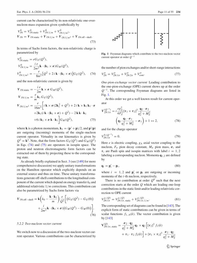
We switch now to a discussion of the two-nucleon vector cur-rent operator. Various contributions can be characterized by

Fig. 1 Feynman diagrams which contribute to the two-nucleon vectorcurrent operator at order Q−1

the number of pion exchanges and/or short-range interactions

Vμ2N = Vμ

2N:1π + Vμ2N:2π + Vμ

cont. (77)

One-pion-exchange vector current Leading contribution tothe one-pion-exchange (OPE) current shows up at the orderQ−1. The corresponding Feynman diagrams are listed inFig. 1.

At this order we get a well known result for current oper-ator

V (Q−1)2N:1π = i

eg2A

4F2π

[τ 1 × τ 2]3 q2 · σ 2

q22 + M2

π(q1

q1 · σ 1

q21 + M2

π

− σ 1

)+ 1 ↔ 2, (78)

and for the charge operator

V 0,(Q−1)2N:1π = 0. (79)

Here e is electric coupling, gA axial vector coupling to thenucleon, Fπ pion decay constant, Mπ pion mass, σ i andτ i are Pauli spin and isospin matrices with label i = 1, 2labeling a corresponding nucleon. Momenta q1,2 are definedby

qi = p′i − pi , (80)

where i = 1, 2 and p′i or pi are outgoing or incoming

momenta of the i-th nucleon, respectively.There is no contribution at order Q0 such that the next

correction starts at the order Q which are leading one-loopcontributions in the static limit and/or leading relativistic cor-rection to OPE current

Vμ,(Q)2N:1π = Vμ,(Q)

2N:1π, static + Vμ,(Q)2N:1π,1/m . (81)

The corresponding set of diagrams can be found in [143]. Theexplicit form of static contributions can be given in terms ofscalar functions f1...6(k). The vector contribution is givenby [143]

V(Q)2N:1π, static = σ 2 · q2

q22 + M2

π

q1 × q2

[[τ 2]3 f1(k)

+ τ 1 · τ 2 f2(k)]

+ [τ 1 × τ 2]3 σ 2 · q2

q22 + M2

π

123

234 Page 12 of 55 Eur. Phys. J. A (2020) 56 :234

×{k

[q2 × σ 1

]f3(k) + k × [

q1 × σ 1]f4(k)

+σ 1 · q1

(kk2 − q1

q21 + M2

π

)

f5(k)

+[

σ 1 · q1

q21 + M2

π

q1 − σ 1

]f6(k)

}+1 ↔ 2,

(82)

where the scalar functions fi (k) are given by

f1 (k) = 2iegAF2

π

d8, f2 (k) = 2iegAF2

π

d9,

f3 (k) = −iegA

64F4ππ2

[g3A (2L(k) − 1) + 32F2

ππ2d21

],

f4 (k) = −iegA

4F2π

d22,

f5 (k) = −ieg2A

384F4ππ2

[2(4M2

π + k2)L(k)

− +(

6 l6 − 5

3

)k28M2

π

],

f6 (k) = −iegAF2

π

M2π d18. (83)

Here di are low-energy constants (LEC) from the order Q3

pion-nucleon Lagrangian [183]. l6 is a LEC from Q4 pion-Lagrangian [37]. Their values can be fixed from pion-nucleonscattering and pion-photo- or electroproduction. The chargecontribution is given by

V 0,(Q)2N:1π, static = σ 2 · q2

q22 + M2

π

[τ 2]3[σ 1 · k q2 · k f7(k)

+σ 1 · q2 f8(k)

]+1 ↔ 2, (84)

where

f7(k) = eg4A

64F4ππ

[A(k) + Mπ − 4M2

π A(k)

k2

],

f8(k) = eg4A

64F4ππ

[(4M2

π + k2)A(k) − Mπ

]. (85)

The loop function L(k) and A(k) are defined

L(k) = 1

2

√k2 + 4M2

π

klog

(√k2 + 4M2

π + k√k2 + 4M2

π − k

)

,

A(k) = 1

2karctan

(k

2Mπ

). (86)

Relativistic corrections for the vector operator vanish

V(Q)1π :1/m = 0. (87)

Relativistic corrections for the charge operator are

V 0,(Q)2N:1π,1/m = eg2

A

16F2πm

1

q22 + M2

π

{(1 − 2β9)

× ([τ ]32 + τ 1 · τ 2

)σ 1 · kσ 2 · q2 − i(1 + 2β9) [τ 1 × τ 2]3

×[σ 1 · k1σ 2 · q2 − σ 2 · k2σ 1 · q2 − 2

σ 1 · q1

q21 + M2

π

σ 2 · q2

×q1 · k1

]}+ eg2

A

16F2πm

σ 1 · q2 σ 2 · q2

(q22 + M2

π )2

[(2β8 − 1)

×([τ 2]3 + τ1 · τ 2)q2 · k + i [τ 1 × τ 2]3 ((2β8 − 1

)q2 · k1

− (2β8 + 1

)q2 · k2

)] + 1 ↔ 2. (88)

Here β8 and β9 are phases from unitary transformationswhich are not fixed. The same phases show up in nuclearforces. Usually they are fixed by requirement of minimalnon-locality of the OPE NN potential.

Two-pion-exchange vector current Contributions to two-pion-exchange (TPE) vector current start to show up at orderQ. They are parameter-free. The corresponding diagrams canbe found in [142]. Due to the coupling of the vector sourceto two pions there appear loop functions which depend onthree momenta k,q1 and q2 which are momentum transferof the vector source, momentum transfer of the first and sec-ond nucleons, respectively. This leads to a somewhat lengthyexpression which have been derived in [142] and are listedin Appendix D for completeness:

Short-range vector current The first contribution to short-range two-nucleon current shows up at the order Q. Thediagrams with short-range interactions at this order can befound in [143]. There are two contributions [143]

Vμ,(Q)2N: cont = Vμ,(Q)

2N:cont,tree + Vμ,(Q)2N:cont,loop. (89)

The current contribution coming from tree-diagrams is givenby

V(Q)2N:cont,tree = e

i

16[τ 1 × τ 2]3

[(C2 + 3C4 + C7) q1

− (−C2 + C4 + C7) (σ 1 · σ 2) q1 + C7 (σ 2 · q1 σ 1

+ σ 1 · q1 σ 2)

]− e

C5 i

16[τ 1]3 [

(σ 1 + σ 2) × q1]

+ieL1 [τ 1]3 [(σ 1 − σ 2) × k]

+ieL2[(σ 1 + σ 2) × q1

]. (90)

As can be seen from Eq. (90) there are Ci LECs which alsocontribute to the two-nucleon potential and appear here dueto the minimal coupling, and there are two additional con-stants L1,2 which describe entirely electromagnetic effects.Charge short-range contribution from tree diagrams at orderQ vanishes

123

Eur. Phys. J. A (2020) 56 :234 Page 13 of 55 234

V 0,(Q)2N:cont,tree = 0. (91)

There are also contributions from one-loop diagrams whichinclude one leading-order two-nucleon contact interactionand two-pion propagators. They only contribute to chargeoperator5

V 0,(Q)2N:cont,loop = CT [τ 1]3 [σ 1 · k σ 2 · k f9(k)

+ σ 1 · σ 2 f10(k)] , (92)

where

f9(k) = eg2A

16F2ππ

(A(k) + Mπ − 4M2

π A(k)

k2

),

f10(k) = eg2A

16F2ππ

(Mπ − (4M2

π + 3k2) A(k))

. (93)

Corresponding contributions to the current operator vanish

V(Q)cont:loop = 0. (94)

5.2.3 Three-nucleon vector current

At the order Q there are first contributions to three-nucleonvector current [149]. There are no contributions to the vectoroperator

V(Q)3N = 0. (95)

Contributions to the charge operator can be parametrized inthe form

V 0,(Q)3N =

[(q1 + q2) · σ 3

(q1 + q2)2 + M2π

+ q3 · σ 3

q23 + M2

π

]

×(v3N:long + v3N:short

) + 5 permutations. (96)

where the long- and short-range contributions are given by

v3N:long = e

16F4π

q1 · σ 1

q21 + M2

π

[(τ 1 · τ 3[τ 2]3 − τ 2 · τ 3[τ 1]3)

×(

− 2g4A

q21 + q1 · q2

(q1 + q2)2 + M2π

+ g2A

)

−i[τ 1 × τ 3]32g4A

q21 + q1 · q2

(q1 + q2)2 + M2π

], (97)

v3N:short = −[τ 1 × τ 3]3 e g2ACT

2F2π

(q1 + q2) · (σ 1 × σ 2)

(q1 + q2)2 + M2π

.

(98)

Due to the approximate spin-isospin SU(4) Wigner symme-try [150], CT appears to be small such that we do not expectlarge contributions from short-range part of the three-nucleonvector current.

5 Different conventions are being used in the literature for the leading-order two-nucleon contact interactions ∝ CS,T . To match the conven-tion of Refs. [88–90], the factors of 32F2

π in Eq. (5.7) of [143] shouldbe replaced by 16F2

π .

5.3 Axial vector current up to order Q

The weak sector of nuclear physics can be probed by a nuclearaxial-vector current. We give here its expressions up to orderQ in chiral expansion.

5.3.1 Single-nucleon axial vector current

The leading-order contribution to an axial vector currentshows up at order Q−3 where axial-vector source couplesdirectly to a single-nucleon or to a pion, which itself propa-gates and couples to a single-nucleon generating in this waya pion-pole term. It is convenient to parametrize the single-nucleon current by the axial and pseudoscalar form factors.Up to the order Q the parametrization is given by

Aμ,a1N = Aμ,a

1N:on−shell + Aμ,a1N:off−shell. (99)

The charge operator is parametrized by

A0,a1N:on−shell = [τ ]a

2

[− k1 · σ

mGA(t) + k · k1

m

(k · σ

4m2

−k · σ (k2 + 4k21) + 4k · k1k1 · σ

32m4

)

×GP (t)

],

A0,a1N:off−shell = 0. (100)

The current operator is parametrized by

Aa1N:on−shell = [τ ]a

2

[(− σ + 1

8m2

(4 σ k2

1 − 4 k1 k1 · σ

+2 i k × k1 + k k · σ))

GA(t)

+k(k · σ

4m2 − 1

32m4

(k · σ k2

+4 k · σ k21 + 4 k1 · σ k · k1

))GP (t)

],

Aa1N:off−shell = k

(k0 − k · k1

m

) [τ ]a16m3

[− (1 + 2β9)

×k1 · σ GP (t) + (1 + 2β8)k · k1k · σ G ′P (t)

],

(101)

Chiral EFT results are given by chiral expansion of the axialand pseudoscalar form factors. Corresponding expressionsare worked out in [23]. To make this review self-consistentwe will briefly discuss them here.

The well-known leading-order result for the axial chargeand current operators have the form

A0,a (Q−3)1N: static = 0,

Aa (Q−3)1N:static = −gA

2[τ i ]a

(σ i − k k · σ i

k2 + M2π

). (102)

123

234 Page 14 of 55 Eur. Phys. J. A (2020) 56 :234

There are only vanishing contributions at order Q−2. At orderQ−1, we encounter three kinds of corrections. First, there areterms emerging from the time-dependence of unitary trans-formations which have the form

A0,a (Q−1)

1N:UT′ = gA2

k0

k2 + M2π

k · σ i [τ i ]a, (103)

Aa (Q−1)

1N:UT′ = 0. (104)

and contribute to Aμ,a1N:off−shell. Secondly, at order Q−1 there

are static limit contributions to Aμ,a1N:on−shell which are given

by

A0,a (Q−1)1N:static = 0,

Aa (Q−1)1N:static = 1

2d22

(σ i k

2 − k k · σ i

)[τ i ]a

−d18M2π [τ i ]a k k · σ i

k2 + M2π

. (105)

Finally, there are leading relativistic 1/m-corrections whichin our counting scheme start contributing at order Q−1 toAμ,a

1N:on−shell and read

A0,a (Q−1)1N:1/m = − gA

2m[τ i ]a σ i · ki , (106)

Aa (Q−1)1N:1/m = 0, (107)

where

k = pi′ − pi , ki = pi′ + pi2

. (108)

There are no corrections to the 1N charge and current opera-tors at the order Q0. Finally, there are various contributionsat order Q. The off-shell contributions coming from time-dependent unitary transformations give different contribu-tions. One of them is coming from relativistic correctionswhich are proportional to k0/m and are given by

A0,a (Q)

1N:1/m,UT′ = 0,

Aa (Q)

1N:1/m,UT′ = −gAk0

8m

kk2 + M2

π

[τ i ]a(

2(1 + 2 β9)σ i · ki

−(1 + 2 β8)k · σ ip′ 2i − p2

i

k2 + M2π

). (109)

They explicitly depend on unitary phases β8 and β9. Notethat these are the same unitary phases that influence a non-locality degree of relativistic 1/m2 corrections of the one-pion-exchange nuclear force. For the static part which is pro-portional to k0, we get nonvanishing contributions

A0,a (Q)

1N:static,UT′ = −k0[τ i ]a

2k · σ i

[d22 + 2d18M2

π

k2 + M2π

],

Aa (Q)

1N:static,UT′ = 0. (110)

The second class of order-Q contributions involves relativis-tic 1/m2-corrections:

A0,a (Q)

1N: 1/m2 = 0,

Aa (Q)

1N:1/m2 = gA16m2 [τ i ]a

(k k · σ i (1 − 2β8)

(p′ 2i − p2

i )2

(k2 + M2π )2

−2k(p′ 2

i + p2i )k · σ i − 2β9(p′ 2

i − p2i )ki · σ i

k2 + M2π

+2 i [k × ki ] + k k · σ i − 4 ki ki · σ i

+σ i

(2(p′ 2

i + p2i ) − k2

)). (111)

These are a linear combination of on-shell and off-shell con-tributions. The third kind of order-Q contributions emergesfrom relativistic 1/m-corrections to the leading one-loopterms which contributes to Aμ,a

1N:on−shell:

A0,a (Q)1N: 1/m = d22ki · σ i [τ i ]a k2

2m, (112)

Aa (Q)1N:1/m = 0. (113)

Finally, static two-loop contributions to the on-shell currentare given by

A0,a (Q)1N:static = 0,

Aa (Q)1N: static = −1

2[τ i ]aσ i

(− f A0 M2

πk2 + f A1 k4

+G(Q4)A (−k2)

)+ 1

8k k · σ i [τ i ]a

(− 4 f A0 M2

π

− f P1 k2 + G(Q2)P (−k2)

). (114)

Here we perform the chiral expansion of the axial form factorwhich can be found e.g. in [151,152], see also [153,154]for results obtained within Lorentz-invariant formulations.Rewritten in our notation, the chiral expansion of the axialform factor is given by

GA(t) = gA + (d22 + f A0 M2π )t + f A1 t2 + G(Q4)

A (t)

+O(Q5), (115)

where f Ai are LECs of dimension GeV−4 and

G(Q4)A (t) = t3

π

∫ ∞

9M2π

Im G(Q4)A (t ′ )

t ′ 3(t ′ − t − iε)dt ′, (116)

with the imaginary part calculated utilizing the Cutkoskyrules [151]

Im G(Q4)A (t) = gA

192π3F4π

∫

z2<1dω1dω2

[6g2

A(√t ω1 − M2

π )

×( l2l1

+ z)arccos(−z)√

1 − z2

123

Eur. Phys. J. A (2020) 56 :234 Page 15 of 55 234

+2g2A

(M2

π − √t ω1 − ω2

1

)+ M2

π − √t ω1

+2ω21

], (117)

where

ωi =√l2i + M2

π with i = 1, 2, and

z = l1 · l2 = ω1ω2 − √t(ω1 + ω2) + 1

2 (t + M2π )

l1l2. (118)

Here and in what follows, li ≡ |li |, while li ≡ li/ li . Thepseudoscalar form-factor up to order Q4 is given by [159]

GP (t) = 4mgπN Fπ

M2π − t

− 2

3gAm

2〈r2A〉 + m2 f P1 t

+m2G(Q2)P (t) + O(Q3), (119)

where f Pi denotes the corresponding linear combinations of

the LECs of dimension GeV−4 from L(5)πN and

G(Q2)P (t) = t2

π

∫ ∞

9M2π

Im G(Q2)P (t ′ )

t ′ 2(t ′ − t − iε)dt ′, (120)

with the imaginary part calculated using the Cutkoskyrules [159]

Im G(Q2)P (t) = Im G(1)

P (t) + Im G(2)P (t) (121)

and

Im G(1)P (t) = gA

8π3F4π

∫

z2<1dω1dω2

[1

18− M4

π

12(t − M2π )2

+4ω21 − M2

π

6t+ ω2

1(3M2π − t)

(t − M2π )2

+2M2πω1ω2z

t (t − M2π )

l2l1

],

Im G(2)P (t) = g3

A

8π3F4π t

∫

z2<1dω1dω2

[(M2

π − √tω1)

×(z + l2

l1

)arccos(−z)√

1 − z2+ l21

3+ t

9

+ M2π

t − M2π

(7

8

√t − ω1 − ω2

)(2ω1z

l2l1

+√t +

((t + M2

π )(4ω1 − √t) − 4

√tω1ω2

)

× arccos(−z)

2l1l2√

1 − z2

)]. (122)

It is important to note that the induced pseudoscalar formfactor is related to the induced pseudoscalar coupling con-stant

gP = Mμ

2mGP (t = −0.88M2

μ), (123)

which is measured in muon capture experiment [155]. Fortheoretical determination of gP by using chiral Ward iden-tities of QCD we refer to a groundbreaking work [156], seealso [157,158].

In practical calculations, alternatively to the chiral expan-sion of the axial and pseudoscalar form factors, one can taketheir empirical parametrization [157]. This is in particularreasonable if we would like to consider electroweak probesof nuclei without being affected by the convergence issue ofthe chiral expansion of electroweak single-nucleon currents.

5.3.2 Two-nucleon axial vector current

We now switch to a discussion of the two-nucleon axial vectorcurrent operator. Various contributions can be characterizedby the number of pion exchanges and/or short-range interac-tions

Aμ,a2N = Aμ,a

2N: 1π + Aμ,a2N: 2π + Aμ,a

2N: cont. (124)

One-pion-exchange axial vector current Leading contribu-tion to the one-pion-exchange (OPE) current shows upat the order Q−1. At this order we get a well knownresult [137,160,161]

A0,a (Q−1)2N: 1π = − igAq1 · σ 1[τ 1 × τ 2]a

4F2π

(q2

1 + M2π

) + 1 ↔ 2 , (125)

Aa (Q−1)2N: 1π = 0. (126)

At the order Q0 there are only contributions to the vectoroperator

Aa (Q0)2N: 1π = gA

2F2π

σ 1 · q1

q21 + M2

π

{[τ 1]a

[− 4c1M

2π

kk2 + M2

π

+2c3

(q1 − k k · q1

k2 + M2π

)]+ c4[τ 1 × τ 2]a

(q1 × σ 2

−k k · q1 × σ 2

k2 + M2π

)− κv

4m[τ 1 × τ 2]ak × σ 2

}

+1 ↔ 2, (127)

where ci denote the LECs from L(2)πN and κv is the isovector

anomalous magnetic moment of the nucleon.At the order Q there are leading one-loop contributions in

the static limit and/or leading relativistic correction to OPEcurrent

Aμ,a(Q)2N:1π = Aμ,a(Q)

2N:1π, static + Aμ,a(Q)2N:1π,1/m + Aμ,a(Q)

2N:1π,UT′ . (128)

The explicit form of static contributions can be given in termsof scalar functions h1...8(q2). The vector contribution is givenby

Aa (Q)2N:1π,static = 4F2

π

gA

q1 · σ 1

q21 + M2

π

{[τ 1 × τ 2]a

×([q1 × σ 2] h1(q2) + [q2 × σ 2] h2(q2)

)

123

234 Page 16 of 55 Eur. Phys. J. A (2020) 56 :234

+[τ 1]a(q1 − q2

)h3(q2)

}+ 4F2

π

gA

q1 · σ 1 k

(k2 + M2π )(q2

1 + M2π )

×{[τ 1]ah4(q2) + [τ 1 × τ 2]aq1 · [q2 × σ 2]h5(q2)

}

+ 1 ↔ 2, (129)

and the charge contribution is given by

A0,a (Q)2N: 1π,static = i

4F2π

gA

q1 · σ 1

q21 + M2

π

{[τ 1 × τ 2]a

(h6(q2)

+k2h7(q2)) + [τ 1]a q1 · [q2 × σ 2] h8(q2)

}+ 1 ↔ 2,

(130)

where the scalar functions hi (q2) are given by

h1(q2) = − g6AMπ

128πF6π

,

h2(q2) = g4AMπ

256πF6π

+ g4A A(q2)

(4M2

π + q22

)

256πF6π

,

h3(q2) = g4A

(g2A + 1

)Mπ

128πF6π

+ g4A A(q2)

(2M2

π + q22

)

128πF6π

,

h4(q2) = g4A

256πF6π

(A(q2)

(2M4

π + 5M2πq

22 + 2q4

2

)

+(

4g2A + 1

)M3

π + 2(g2A + 1

)Mπq

22

),

h5(q2) = − g4A

256πF6π

(A(q2)

(4M2

π + q22

)

+(

2g2A + 1

)Mπ

),

h6(q2) = g2A

(3(64 + 128g2

A

)M2

π + 8(19g2

A + 5)q2

2

)

36864π2F6π

− g2A

768π2F6π

L(q2)( (

8g2A + 4

)M2

π

+(

5g2A + 1

)q2

2

) + d18gAM2π

8F4π

− d5g2AM

2π

2F4π

−g2A(2d2 + d6)

(M2

π + q22

)

16F4π

,

h7(q2) = g2A(2d2 − d6)

16F4π

,

h8(q2) = −g2A(d15 − 2d23)

8F4π

. (131)

Here di are low-energy constants (LEC) from Q3 pion-nucleon Lagrangian. Their values can be fixed from pion-nucleon scattering and axial-pion-production.

The relativistic corrections for the charge operator vanish

A0,a (Q)2N: 1π, 1/m = 0, (132)

and for the current operator are given by

Aa (Q)2N: 1π, 1/m = gA

16F2πm

{i[τ 1 × τ 2]a

×[

1

(q21 + M2

π )2

(B1 − k k · B1

k2 + M2π

)

+ 1

q21 + M2

π

(B2

(k2 + M2π )2 + B3

k2 + M2π

+ B4

)]

+[τ 1]a[

1

(q21 + M2

π )2

(B5 − k k · B5

k2 + M2π

)

+ 1

q21 + M2

π

(B6

(k2 + M2π )2 + B7

k2 + M2π

+ B8

)]}

+1 ↔ 2, (133)

where the vector-valued quantities Bi depend on variousmomenta and the Pauli spin matrices and are given by

B1 = g2Aq1 · σ 1[−2(1 + 2β8)q1 k1 · q1

−(1 − 2β8)(2q1 k2 · q1 − i q1 × σ 2 k · q1],B2 = (1 − 2β8)g

2Ak k · q1q1 · σ 1[2k · k2 − ik · q1 × σ 2],

B3 = 2k[

− g2A((1 + 2β9)k · q1k1 · σ 1

+(1 − 2β9)q1 · σ 1(k · k2 + k2 · q1))

+q1 · σ 1(k · k2 + i k · q1 × σ 2 − k1 · q1 + k2 · q1)],

B4 = g2A[2(1 + 2β9)q1k1 · σ 1

+(1 − 2β9)q1 · σ 1(2k2 − ik × σ 2)]−2q1 · σ 1(iq1 × σ 2 − ik × σ 2 + 2k2),

B5 = g2Aq1 · σ 1

[(1 − 2β8)(q1 k · q1 − 2i q1 × σ 2k2 · q1)

−2i(1 + 2β8)q1 × σ 2 k1 · q1

],

B6 = −(1 − 2β8)g2Ak q1 · σ 1[(k · q1)

2

−2i k · k2k · q1 × σ 2],B7 = g2

Ak[(1 − 2β9)q1 · σ 1(−2i(k · k2 × σ 2

+k2 · q1 × σ 2) + k2 + q21 )

−2i(1 + 2β9)k1 · σ 1k · q1 × σ 2

],

B8 = −g2A[(1 − 2β9)q1 · σ 1(k − 2i k2 × σ 2)

−2i(1 + 2β9)q1 × σ 2 k1 · σ 1]. (134)

Finally, there are also energy-transfer dependent contribu-tions to OPE axial vector current at order Q which are givenby

A0,a (Q)

2N: 1π,UT′ = 0 , (135)

123

Eur. Phys. J. A (2020) 56 :234 Page 17 of 55 234

Aa (Q)

2N: 1π,UT′ = −igA

8F2π

k0 k q1 · σ 1

(k2 + M2π )(q2

1 + M2π )

×(

[τ 1 × τ 2]a(

1 − 2g2Ak · q1

k2 + M2π

)− 2g2

A[τ 1]ak · [q1 × σ 2]k2 + M2

π

)

+1 ↔ 2. (136)

It is important to note that it is not enough to know the currentsat vanishing energy-transfer k0 = 0. As will be demonstratedlater the knowledge of the slope in energy-transfer k0 is essen-tial for checking the continuity equations. All expressionsproportional to the energy-transfer k0 are off-shell effectswhich disappear in the calculation of on-shell observables.Energy-transfer contributions are always accompanied by thecommutator with the effective Hamiltonian. On-shell a linearcombination of k0-term and the commutator with the effec-tive Hamiltonian

k0X − [Heff , X

](137)

vanishes. Here X denotes some operator. More on this willbe discussed in Sect. 5.6.

Two-pion-exchange axial vector current Contributions tothe two-pion-exchange axial vector current start to show upat order Q. These contributions are parameter-free. The finalresults for the two-pion exchange operators read

Aa (Q)2N: 2π = 2F2

π

gA

kk2 + M2

π

{[τ 1]a

(− q1 · σ 2 q1 · k g1(q1)

+q1 · σ 2 g2(q1) − k · σ 2 g3(q1))

+[τ 2]a(

− q1 · σ 1 q1 · k g4(q1) − k · σ 1 g5(q1)

−q1 · σ 2 q1 · k g6(q1) + q1 · σ 2 g7(q1)

+k · σ 2 q1 · k g8(q1) − k · σ 2 g9(q1))

+[τ 1 × τ 2]a(

− q1 · [σ 1 × σ 2]q1 · k g10(q1)

+q1 · [σ 1 × σ 2] g11(q1)

−q1 · σ 2 q1 · [q2 × σ 1] g12(q1))}

+2F2π

gA

{q1

([τ 2]a q1 · σ 1 g13(q1)

+[τ 1]a q1 · σ 2 g14(q1))

− [τ 1]a σ 2 g15(q1)

−[τ 2]a σ 2 g16(q1) − [τ 2]a σ 1 g17(q1)

}

+1 ↔ 2, (138)

A0,a (Q)2N: 2π = i

2F2π

gA

{[τ 1 × τ 2]aq1 · σ 2 g18(q1)

+[τ 2]aq1 · [σ 1 × σ 2]g19(q1)

}+ 1 ↔ 2, (139)

where the scalar functions gi (q1) are defined as

g1(q1) = g4A A(q1)

((8g2

A − 4)M2

π + (g2A + 1

)q2

1

)

256πF6πq

21

−g4AMπ

((8g2

A − 4)M2

π + (3g2

A − 1)q2

1

)

256πF6πq

21

(4M2

π + q21

) ,

g2(q1) = g4A A(q1)

(2M2

π + q21

)

128πF6π

+ g4AMπ

128πF6π

,

g3(q1) = −g4A A(q1)

((8g2

A − 4)M2

π + (3g2

A − 1)q2

1

)

256πF6π

−(3g2

A − 1)g4AMπ

256πF6π

,

g4(q1) = −g6A A(q1)

128πF6π

,

g5(q1) = −q21 g4(q1),

g6(q1) = g8(q1) = g10(q1) = g12(q1) = 0,

g7(q1) = g4A A(q1)

(2M2

π + q21

)

128πF6π

+(2g2

A + 1)g4AMπ

128πF6π

,

g9(q1) = g6AMπ

64πF6π

,

g11(q1) = −g4A A(q1)

(4M2

π + q21

)

512πF6π

− g4AMπ

512πF6π

,

g13(q1) = −g6A A(q1)

128πF6π

,

g14(q1) = g4A A(q1)

((8g2

A − 4)M2

π + (g2A + 1

)q2

1

)

256πF6πq

21

+g4AMπ

((4 − 8g2

A

)M2

π + (1 − 3g2

A

)q2

1

)

256πF6πq

21

(4M2

π + q21

) ,

g15(q1) = g4A A(q1)

((8g2

A − 4)M2

π + (3g2

A − 1)q2

1

)

256πF6π

+(3g2

A − 1)g4AMπ

256πF6π

,

g16(q1) = g4A A(q1)

(2M2

π + q21

)

64πF6π

+ g4AMπ

64πF6π

,

g17(q1) = −g6Aq

21 A(q1)

128πF6π

,

g18(q1) = g2AL(q1)

((4 − 8g2

A

)M2

π + (1 − 3g2

A

)q2

1

)

128π2F6π

(4M2

π + q21

) ,

g19(q1) = g4AL(q1)

32π2F6π

. (140)

Short-range axial vector current The first contribution toshort-range two-nucleon current shows up at the order Q0.

123

234 Page 18 of 55 Eur. Phys. J. A (2020) 56 :234

A0,a (Q0)2N: cont = 0,

Aa (Q0)2N: cont = −1

4D [τ 1]a

(σ 1 − k σ 1 · k

k2 + M2π

)+ 1 ↔ 2,

(141)

where D denote the LEC from L(1)πNN . At the order Q we

decompose the short-range current in three different compo-nents

Aμ,a,(Q)2N:cont = Aμ,a,(Q)

2N:cont, static + Aμ,a,(Q)2N:cont ,1/m + Aμ,a,(Q)

2N:cont, UT′ .

Static contributions are given by

Aa (Q)2N: cont, static = 0, (142)

A0,a (Q)2N: cont, static = i z1[τ 1 × τ 2]a σ 1 · q2

+i z2[τ 1 × τ 2]a σ 1 · q1 + i z3[τ 1]a q2 · σ 1 × σ 2

+z4([τ 1]a − [τ 2]a)(σ 1 − σ 2) · k1 + 1 ↔ 2, (143)

where LECs zi are unknown coefficients and have to be fittedto experimental data. Relativistic corrections are given by

Aa (Q)2N: cont, 1/m = − gA

4m

kk2 + M2

π

[τ 1]a{(1 − 2β9)

(CSq2 · σ 1

+CT (q2 · σ 2 + 2i k1 · σ 1 × σ 2))

− 1 − 2β8

k2 + M2π

(CSk · q2k · σ 1 + CT (k · q2k · σ 2

+2i k · k1k · σ 1 × σ 2))}

+ 1 ↔ 2. (144)

Finally, the energy-transfer dependent contributions aregiven by

A0,a (Q)

2N: cont, UT′ = 0,

Aa (Q)

2N: cont, UT′ = −i k0kgACTk · σ 1[τ 1 × τ 2]a

(k2 + M2

π

)2 + 1 ↔ 2.

(145)

5.3.3 Three-nucleon axial vector current

At the order Q there are first contributions to three-nucleonaxial vector current. We decompose it into long and short-range contributions

Aμ,a (Q)3N = Aμ,a (Q)

3N: π + Aμ,a (Q)3N: cont (146)

We start with the long-range part. There are no charge con-tributions such that

A0,a (Q)3N: π = 0. (147)

Current contributions are given by

Aa (Q)3N:π = −2F2

π

gA

8∑

i=1

Cai + 5 permutations, (148)

where spin-isospin dependent vector structures, which includeup to four pion propagators are given by

Ca1 = g6

A

16F6π

q2 · σ 2

[[τ 2]a

[q3((q2 · q3 + q2

2 )(τ 1 · τ 3

−σ 1 · σ 3) + q2 · σ 1(q2 · σ 3 + q3 · σ 3))

−q2(q3 · σ 1(q2 · σ 3 + q3 · σ 3) − (q2 · q3 + q23 )σ 1 · σ 3

−(q2 · q3 + q22 )τ 1 · τ 3) − σ 3((q2 · q3 + q2

3 )q2 · σ 1

−(q2 · q3 + q22 )q3 · σ 1)

]− [τ 2 × τ 3]a (q2 × σ 1

+q3 × σ 1)(q2 · q3 + q22 ) − (q2 + q3)

×([τ 1 × τ 2]aq2 · q3 × σ 3 + [τ 3]aτ 1 · τ 2(q2 · q3 + q22 ))

]

× 1

[q22 + M2

π ][(q1 − k)2 + M2π ]2

,

Ca2 = g4

A

32F6π

1

[q22 + M2

π ][(q1 − k)2 + M2π ]

×q2 · σ 2[[τ 2 × τ 3]a(k × σ 1 − q1 × σ 1)

+(k − q1)([τ 3]aτ 1 · τ 2 − [τ 2]aτ 1 · τ 3)],

Ca3 = g4

A

32F6π

1

[q21 + M2

π ][q22 + M2

π ][q23 + M2

π ]×(k − 2q3)[τ 3]aτ 1 · τ 2q1 · σ 1q2 · σ 2

×(k · σ 3 − 2q1 · σ 3),

Ca4 = g4

A

32F6π

σ 1q2 · σ 2q3 · σ 3([τ 1]aτ 2 · τ 3 − [τ 3]aτ 1 · τ 2)

[q22 + M2

π ][q23 + M2

π ] ,

Ca5 = g6

A

16F6π

k q1 · σ 1

[k2 + M2π ][q2

1 + M2π ][(q1 + q2)2 + M2

π ]2

×[

− [τ 1]aq1 · q2 × σ 2(k · q1 × σ 3 + k · q2 × σ 3)

− [τ 1 × τ 3]a q1 · q2 × σ 2(k · q1 + k · q2)

+ [τ 1 × τ 2]a (q1 · q2 + q21 )(k · q1 × σ 3

+k · q2 × σ 3) − (τ 2 · τ 3[τ 1]a − τ 1 · τ 3[τ 2]a

)

×(q1 · q2 + q21 )(k · q1 + k · q2)

],

Ca6 = − g4

A

32F6π

k q1 · σ 1

[k2 + M2π ][q2

1 + M2π ][(q1 + q2)2 + M2

π ]×

[(k · q1 × σ 3 + k · q2 × σ 3) [τ 1 × τ 2]a

−(k · q1 + k · q2 + q1 · q2 + q21 )

× (τ 2 · τ 3[τ 1]a − τ 1 · τ 3[τ 2]a

)

−q1 · q2 × σ 2 [τ 1 × τ 3]a],

Ca7 = − g4

A

32F6π

k q1 · σ 1q2 · σ 2q3 · σ 3τ 1 · τ 2[τ 3]a

× (M2

π + 2q1 · q2 + q21 + q2

2

)

× 1

[k2 + M2π ][q2

1 + M2π ][q2

2 + M2π ][q2

3 + M2π ] ,

Ca8 = − g4

A

64F6π

k q2 · σ 2q3 · σ 3

[k2 + M2π ][q2

2 + M2π ][q2

3 + M2π ]

123

Eur. Phys. J. A (2020) 56 :234 Page 19 of 55 234

× (τ 2 · τ 3[τ 1]a(q2 · σ 1 + q3 · σ 1)

− 2τ 1 · τ 2[τ 3]a(q1 · σ 1 + q2 · σ 1)). (149)

The short-range contributions to the charge operator vanish

A0,a (Q)3N: cont = 0, (150)

and the short-range vector contributions are given by

Aa (Q)3N: cont = −2F2

π

gA

3∑

i=1

Dai + 5 permutations, (151)

with

Da1 = −g4

ACT

4F4π

[(k − q1)[τ 1 × τ 3]a(k · σ 2 × σ 3

−q1 · σ 2 × σ 3) − ([τ 2]a − [τ 3]a)((k − q1)σ 1 · σ 2

×(k · σ 3 − q1 · σ 3) + σ 3((k · σ 1 − q1 · σ 1)

×(k · σ 2 − q1 · σ 2) + (2k · q1 − k2 − q21 )σ 1 · σ 2))

]

× 1

[(q1 − k)2 + M2π ]2 ,

Da2 = g4

ACT

4F4π

k[k2 + M2

π ][(q1 + q3)2 + M2π ]2 (q1 · σ 1 × σ 3

+q3 · σ 1 × σ 3)([τ 3]ak · q2 × σ 2 + [τ 2 × τ 3]a (k2

− k · q2)) ,

Da3 = −g2

ACT

8F4π

k[k2 + M2

π ][(q1 + q3)2 + M2π ] (q1 · σ 1 × σ 3

+q3 · σ 1 × σ 3) [τ 2 × τ 3]a . (152)

Due to the smallness of CT , these contributions areexpected to be small.

5.4 Pseudoscalar current up to order Q0

Approximate chiral symmetry leads to relations betweenpseudoscalar current and axial-vector current. In the follow-ing, we list all expressions for pseudoscalar current up toorder Q0.

5.4.1 Single-nucleon pseudoscalar current

Single-nucleon pseudoscalar current can be parametrized bypseudoscalar form factors and their derivatives via

i mq Pa1N = i mq P

a1N:on−shell + i mq P

a1N:off−shell, (153)

where

i mq Pa1N:on−shell = [τ i ]a

2

(GA(t) + t

4m2 GP (t)

)

×(k · σ

(1 − 4 k2

1 + k2

8m2

)− k · k1 k1 · σ

2m2 + O(1/m3)

),

i mq Pa1N:off−shell = −M2

π

k2 k · Aa1N:off−shell. (154)

Chiral EFT results for pseudoscalar current are given by chi-ral expansion of the axial and pseudoscalar form factors. Cor-responding expressions are worked out in [23]. Here we willbriefly discuss them.

The single-nucleon pseudoscalar current starts to con-tribute at the order Q−4 and is given by

Pa (Q−4)1N: static = i

M2πgA

2mq[τ i ]a k · σ i

k2 + M2π

= −i1

mqk · Aa (Q−3)

1N: static, (155)

with Aa (Q−3)1N: static given in Eq. (102). At the order Q−3, there

are only vanishing contributions. At order Q−2 there are onlystatic limit contributions which are given by

Pa (Q−2)1N: static = i

M2π d18

mqk2[τ i ]a k · σ i

k2 + M2π

= −i1

mqk · Aa (Q−1)

1N: static, (156)

with Aa (Q−1)1N: static given in Eq. (105). There are no contributions

to the single-nucleon pseudoscalar current at order Q−1.Finally, there are various corrections at order Q0: There arerelativistic corrections that depend on the energy transfer.Their explicit form is given by

Pa (Q0)

1N: 1/m,UT′ = iM2

π

mqk2 k · Aa (Q)

1N: 1/m,UT′ , (157)

with Aa (Q)

1N: 1/m,UT′ given in Eq. (109). The second kind of

the order-Q0 contributions is given by relativistic 1/m2 -corrections.

Pa (Q0)

1N: 1/m2 = iM2

πgA16mqm2 [τ i ]a

(k · σ i (1 − 2β8)

(p′ 2i − p2

i )2

(k2 + M2π )2

−2(p′ 2

i + p2i )k · σ i − 2β9(p′ 2

i − p2i )ki · σ i

k2 + M2π

).

(158)

Notice that this expression is related to the pion-pole termsin the corresponding axial current operator Aa (Q)

1N: 1/m2 whoseexpression is given in Eq. (111), via

Pa (Q0)

1N: 1/m2 = iM2

π

mqk2 k · Aa (Q)

1N: 1/m2

∣∣∣∣pion−pole terms

. (159)

The third kind of order-Q0 contributions are coming fromstatic two-loop contributions and is given by

123

234 Page 20 of 55 Eur. Phys. J. A (2020) 56 :234

Pa (Q0)1N: static = i

1

8mqk · σ i [τ i ]a

(4 G(Q4)

A (−k2)

−k2 G(Q2)P (−k2)

). (160)

where G(Q4)A (t) and G(Q2)

P (t) are defined in Eqs. (116) and(120), respectively.

Alternatively to the chiral expansion of the axial andpseudoscalar form factors, one can take their empiricalparametrization in practical calculations.

5.4.2 Two-nucleon pseudoscalar current

Similar to axial vector current we can characterize two-nucleon pseudoscalar current by the number of the pionexchanges and/or short-range interactions

Pa2N = Pa

2N: 1π + Pa2N: 2π + Pa

2N: cont. (161)

First contributions start to show up at order Q−1. At thisorder, there are only OPE and contact contributions which canbe expressed by the longitudinal part of axial-vector currentvia

i mq Pa,(Q−1)2N: 1π = k · Aa,(Q0)

2N: 1π , (162)

i mq Pa,(Q−1)2N: cont = k · Aa,(Q0)

2N: cont, (163)

where Aa,(Q0)2N: 1π and Aa,(Q0)

2N: cont are defined in Eqs. (127) and(141), respectively.

One-pion-exchange pseudoscalar current At the order Q0

leading one-loop static contributions and relativistic 1/m cor-rections start to show up.

Pa (Q0)2N: 1π = Pa (Q0)

2N: 1π,static + Pa (Q0)2N: 1π,1/m + Pa (Q0)

2N: 1π,UT′ . (164)

The corresponding static expressions are

i mq Pa (Q0)2N: 1π,static = −4 M2

π F2π

gA

q1 · σ 1

q21 + M2

π

{[τ 1]a

[hP

1 (q2)

+ h4(q2)

k2 + M2π

]+ [τ 1 × τ 2]aq1 · [q2 × σ 2] h5(q2)

k2 + M2π

}

+1 ↔ 2, (165)

where the scalar functions h4(q2) and h5(q2) are defined inEq. (131), while hP

1 (q2) is given by

hP1 (q2) = g4

A

256πF6π

((1 − 2g2

A)Mπ + (2M2π + q2

2 )A(q2)).

(166)

The relativistic 1/m corrections are

i mq Pa (Q0)2N: 1π, 1/m = − gAM2

π

16F2π m

{i[τ 1 × τ 2]a

×[

− B1 · k(q2

1 + M2π )2(k2 + M2

π )+ 1

q21 + M2

π

(B2 · k

k2(k2 + M2π )2

+ B3 · kk2(k2 + M2

π )

)]+ [τ 1]a

[− B5 · k

(q21 + M2

π )2(k2 + M2π )

+ 1

q21 + M2

π

(B6 · k

k2(k2 + M2π )2 + B7 · k

k2(k2 + M2π )

)]}

+1 ↔ 2, (167)

where the vector quantities Bi are defined in Eq. (134).Finally, the energy-transfer dependent contributions are

i mq Pa (Q0)

2N: 1π,UT′ = −M2π

k2 k · Aa (Q)

2N: 1π,UT′ , (168)

where Aa (Q)

2N: 1π,UT′ is given in Eq. (136).

Two-pion-exchange pseudoscalar current Two-pion-ex-change contributions can be expressed in terms of the longi-tudinal component of the axial vector current. The expressionis given by

i mq Pa (Q0)2N: 2π = −M2

π

k2 k · Aa (Q)2N: 2π

∣∣∣∣g13=g14=g15=g16=g17=0

,

(169)

with the scalar functions g1(q1), . . . , g12(q1) being definedin Eq. (140).

Short-range pseudoscalar current The first contribution toshort-range two-nucleon current shows up at the order Q−1

and is given in Eq. (163). At order Q0 we characterize short-range contributions via

Pa,(Q0)2N: cont = Pa,(Q0)

2N: cont,static + Pa,(Q0)2N: cont,1/m + Pa,(Q0)

2N: cont,UT′ .

(170)

The static contributions at the order Q0 vanish

Pa,(Q0)2N: cont,static = 0. (171)

The relativistic corrections are given by

i mq Pa,(Q0)2N: cont,1/m = −M2

π

k2 k · Aa (Q)2N: cont, 1/m, (172)

where Aa (Q)2N: cont, 1/m is specified in Eq. (144). Finally, the

energy-transfer-dependent contributions are given by

i mq Pa (Q0)

2N: cont, UT′ = −M2π

k2 k · Aa (Q)

2N: cont, UT′ , (173)

where Aa (Q)

2N: cont, UT′ is specified in Eq. (145).

5.4.3 Three-nucleon pseudoscalar current

At the order Q0 there are first contributions to the three-nucleon pseudoscalar current. Similar to the axial-vector cur-

123

Eur. Phys. J. A (2020) 56 :234 Page 21 of 55 234

rent we decompose the current into the long and the short-range contributions

Pa (Q0)3N = Pa (Q0)

3N: π + Pa (Q)3N: cont. (174)

The long-range contributions are given by

Pa (Q0)3N: π = −i

2 F2π M

2π

gAmq

8∑

i=5

Cai · kk2 + 5 permutations, (175)

where Cai are defined in Eq. (149). Short-range contributions

are given by

Pa (Q)3N: cont = −i

2 F2π M

2π

gAmq

3∑

i=2

Dai · kk2 + 5 permutations,

(176)

with Dai defined in Eq. (152).

5.5 Scalar current up to the order Q

Nuclear scalar current is important for the dark mattersearches. A scenario that dark matter is realized by weaklyinteracting massive particles (WIMPs) can be tested vianuclear recoil produced by the scattering of WIMPs offatomic nuclei (see [162] and the references therein). If WIMP,denoted by χ , is a spin-1/2 particle and interacts with quarksand gluons via [165,166]

Lχ = 1

Λ3

∑

q

[CSSq χχmqqq + CPS

q χ iγ5χmqqq

+CSPq χχmqqiγ5q + CPP

q χ iγ5χmqqiγ5q

]

+ 1

Λ2

∑

q

[CVVq χγ μχ qγμq + CAV

q χγ μγ5χ qγμq

+CVAq χγ μχ qγμγ5q + CAA

q χγ μγ5χ qγμγ5q

],

(177)

where Λ is a beyond standard model scale and various Wil-son coefficients Cq are dimensionless. Indices S, P, V andA stay for scalar, pseudoscalar, vector and axial-vector quan-tum numbers, respectively. q-field is a quark field and mq isa quark mass. Eq. (177) can be considered as a starting pointfor chiral EFT analysis where one needs to study scalar-,pseudoscalar-, vector- and axial-vector currents within chi-ral EFT. While vector- and axial-vector currents have beenextensively studied within standard model, scalar-current inchiral EFT appears first in beyond standard model physicsand is much less known. Pioneering work towards this direc-tion was the leading-order calculation of the scalar currentby Cirigliano et al. [164] and Hoferichter et al. [166], seealso [167–170]. Recently we derived leading one-loop cor-rections to these results [171]. Although the information

about short-range physics at this order needs to be fixed thesecalculations give long-range contributions in a parameter-free way. In the following all contributions to scalar currentup to order Q0.

5.5.1 Single-nucleon scalar current

Scalar current on a single-nucleon can be parametrized by ascalar form factor which in principle can be calculated withinchiral perturbation theory. Due to the lack in convergence [41,151] one prefers to use dispersion relation techniques whereππ scattering channel dominates t-dependence of the scalarform factor [163].

5.5.2 Two-nucleon scalar current

Two- and three-nucleon scalar current will be formulatedhere within chiral EFT. In the following, we characterize atwo-nucleon scalar current by the range of interaction

S2N = S2N: 1π + S2N: 2π + S2N: cont. (178)

One-pion-exchange scalar current First contributions to theone-pion-exchange current show up at the order Q−2 and aregiven by

mqS(Q−2)2N: 1π = −g2

AM2π

4F2π

q1 · σ 1q2 · σ 2τ 1 · τ 2(M2

π + q21

) (M2

π + q22

) . (179)

Next correction shows up first at the order Q0. The result isgiven by

mqS(Q0)2N: 1π, = q1 · σ 1

q21 + M2

π

[q2 · σ 2

(o1(k)

q22 + M2

π

+ o2(k)

)

+k · σ 2

(o3(k) + q2

2o4(k)

)]+ 1 ↔ 2, (180)

where the scalar functions oi (k) are given by

o1(k) = gAM2π

128π2F4π

[64π2d18F

2π M

2π + gAk

2l4

−gAL(k)(

2k2 + M2π

)+ gA

(k2 + M2

π

) ],

o2(k) = gAM2π

64π2F4π

[32π2F2

π

(2d16 − d18

) − gAl4

−4g3AL(k)

(k2 + 3M2

π

)

k2 + 4M2π

],

o3(k) = − gAM2π

128π2F4πk

2

[128π2d16F

2πk

2 + g3A

(−k2 + M2

π

)

+2gAk2 − 4gAL(k)

k2 + 4M2π

((2g2

A + 1)k4

+(

5g2A + 4

)k2M2

π + g2AM

4π

) ],

123

234 Page 22 of 55 Eur. Phys. J. A (2020) 56 :234

o4(k) = − g4AM

2π

128π2F4πk

2

k2 + 4M2π (1 − L(k))

k2 + 4M2π

. (181)

The relativistic corrections and the energy-transfer depen-dent contributions to one-pion-exchange at the order Q0 van-ish.

Two-pion-exchange scalar current Two-pion-exchangecurrent shows up first at order Q0. Due to the appearance

of three-point functions the results are lengthy. Their explicitform can be found in [171] and, for completeness, is givenin Appendix E.

Short-range scalar current Short-range two-nucleon currentstarts to contribute at order Q0. The relevant LECs come from

L(0)NN = −CS

2(N †N )2 + 2CT N

†SμNN †SμN ,

L(2)NN = −DS

8〈χ+〉(N †N )2 + DT

2〈χ+〉N †SμNN †SμN ,

(182)

where N is the heavy-baryon notation for the nucleon fieldwith velocity vμ, Sμ = −γ5[γμ, γν]vν/4 is the covariantspin-operator, χ+ = 2B

(u†(s + i p)u† + u(s − i p)u

), B,

CS,T and DS,T are LECs. 〈. . . 〉 denotes the trace in the flavorspace. All the non-vanishing diagrams which contribute atorder Q0 are listed in [171]. After the renormalization of theshort-range LECs we got

mqS(Q0)2N: cont = σ 1 · σ 2s1(k) + k · σ 1k · σ 2s2(k) + s3(k),

(183)

with the scalar function si (k) defined by

s1(k) = − M2π

8π2F2πmq

[2g2

ACT − 4π2 DT F2π

+g2ACT L(k)

(3k2 + 4M2

π

)

k2 + 4M2π

],

s2(k) = 3g2ACT M2

π

8π2F2πk

2mq

k2 − 4M2π (L(k) − 1)

k2 + 4M2π

,

s3(k) = M2π

16π2F2πmq

[g2ACT + 8π2 DS F

2π

−2g2ACT L(k)

(3k2 + 8M2

π

)

k2 + 4M2π

]. (184)

The renormalized, scale-independent LECs DS , DT arerelated to the bare ones DS , DT according to

Di = Di + βNNi

F4 λ + βNNi

16π2F4 ln

(Mπ

μ

), (185)

with the corresponding β-functions given by

βNNS = 1

2

(1 + 6g2

A − 15g4A + 24F2g2

ACT

),

βNNT = 1

4

(1 + 6g2

A − 15g4A + 48F2g2

ACT

), (186)

and the quantity λ defined as

λ = μd−4

16π2

(1

d − 4+ 1

2

(γE − ln 4π − 1

)), (187)

where γE = −�′(1) � 0.577 is the Euler constant, d thenumber of space-time dimensions andμ is the scale of dimen-sional regularization.

Notice that the LECs CS , CT , DS and DT also con-tribute to the 2N potential. The experimental data on nucleon-nucleon scattering, however, do not allow one to disentanglethe Mπ -dependence of the contact interactions and only con-strain the linear combinations of the LECs [172]

CS = CS + M2π DS, CT = CT + M2

π DT . (188)

The LECs DS and DT can, in principle, be determined oncereliable lattice QCD results for two-nucleon observables suchas e.g. the 3S1 and 1S0 scattering lengths at unphysical (butnot too large) quark masses are available, see Refs. [173]and references therein for a discussion of the current statusof research along this line.

5.5.3 Relativistic corrections

There are only vanishing 1/m-corrections and the energy-transfer dependent contributions at the order Q0.

5.5.4 Three-nucleon scalar current

At the order Q0 there are no three-nucleon current contri-butions. Nonvanishing contributions start to show up first atorder Q.

Scalar current at vanishingmomentum transfer At the van-ishing momentum transfer, one can relate the scalar currentto a quark mass derivative of the nuclear forces. On the mass-shell one gets

〈 f |S(0)|i〉 =⟨f

∣∣∣∣∂Heff

∂mq

∣∣∣∣i

⟩, (189)

where the states |i〉 and | f 〉 are the eigenstates of the Hamil-tonian Heff . The on-shell condition requires that the corre-sponding eigenenergies Ei and E f are equal. For eigenstates|�〉 corresponding to a discrete energy E ,

Heff |�〉 = E |�〉, (190)

the Feynman-Hellmann theorem allows one to interpret thescalar form factor at zero momentum transfer in terms of theeigenenergy slope in the quark mass:

〈�|mqS(0)|�〉 = mq∂E(mq)

∂mq. (191)

123

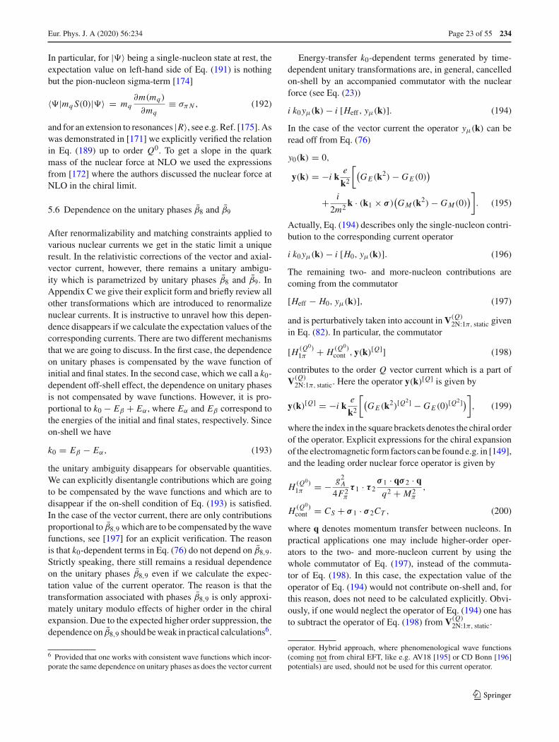
Eur. Phys. J. A (2020) 56 :234 Page 23 of 55 234

In particular, for |�〉 being a single-nucleon state at rest, theexpectation value on left-hand side of Eq. (191) is nothingbut the pion-nucleon sigma-term [174]

〈�|mqS(0)|�〉 = mq∂m(mq)

∂mq≡ σπN , (192)

and for an extension to resonances |R〉, see e.g. Ref. [175]. Aswas demonstrated in [171] we explicitly verified the relationin Eq. (189) up to order Q0. To get a slope in the quarkmass of the nuclear force at NLO we used the expressionsfrom [172] where the authors discussed the nuclear force atNLO in the chiral limit.

5.6 Dependence on the unitary phases β8 and β9

After renormalizability and matching constraints applied tovarious nuclear currents we get in the static limit a uniqueresult. In the relativistic corrections of the vector and axial-vector current, however, there remains a unitary ambigu-ity which is parametrized by unitary phases β8 and β9. InAppendix C we give their explicit form and briefly review allother transformations which are introduced to renormalizenuclear currents. It is instructive to unravel how this depen-dence disappears if we calculate the expectation values of thecorresponding currents. There are two different mechanismsthat we are going to discuss. In the first case, the dependenceon unitary phases is compensated by the wave function ofinitial and final states. In the second case, which we call a k0-dependent off-shell effect, the dependence on unitary phasesis not compensated by wave functions. However, it is pro-portional to k0 − Eβ + Eα , where Eα and Eβ correspond tothe energies of the initial and final states, respectively. Sinceon-shell we have

k0 = Eβ − Eα, (193)

the unitary ambiguity disappears for observable quantities.We can explicitly disentangle contributions which are goingto be compensated by the wave functions and which are todisappear if the on-shell condition of Eq. (193) is satisfied.In the case of the vector current, there are only contributionsproportional to β8,9 which are to be compensated by the wavefunctions, see [197] for an explicit verification. The reasonis that k0-dependent terms in Eq. (76) do not depend on β8,9.Strictly speaking, there still remains a residual dependenceon the unitary phases β8,9 even if we calculate the expec-tation value of the current operator. The reason is that thetransformation associated with phases β8,9 is only approxi-mately unitary modulo effects of higher order in the chiralexpansion. Due to the expected higher order suppression, thedependence on β8,9 should be weak in practical calculations6.

6 Provided that one works with consistent wave functions which incor-porate the same dependence on unitary phases as does the vector current

Energy-transfer k0-dependent terms generated by time-dependent unitary transformations are, in general, cancelledon-shell by an accompanied commutator with the nuclearforce (see Eq. (23))

i k0yμ(k) − i [Heff , yμ(k)]. (194)

In the case of the vector current the operator yμ(k) can beread off from Eq. (76)

y0(k) = 0,

y(k) = −i ke

k2

[(GE (k2) − GE (0)

)

+ i

2m2 k · (k1 × σ )(GM (k2) − GM (0)

)]. (195)

Actually, Eq. (194) describes only the single-nucleon contri-bution to the corresponding current operator

i k0yμ(k) − i [H0, yμ(k)]. (196)

The remaining two- and more-nucleon contributions arecoming from the commutator

[Heff − H0, yμ(k)], (197)

and is perturbatively taken into account in V(Q)2N:1π, static given

in Eq. (82). In particular, the commutator

[H (Q0)1π + H (Q0)

cont , y(k)[Q]] (198)

contributes to the order Q vector current which is a part ofV(Q)

2N:1π, static. Here the operator y(k)[Q] is given by

y(k)[Q] = −i ke

k2

[(GE (k2)[Q2] − GE (0)[Q2])

], (199)

where the index in the square brackets denotes the chiral orderof the operator. Explicit expressions for the chiral expansionof the electromagnetic form factors can be found e.g. in [149],and the leading order nuclear force operator is given by

H (Q0)1π = − g2

A

4F2π

τ 1 · τ 2σ 1 · qσ 2 · qq2 + M2

π

,

H (Q0)cont = CS + σ 1 · σ 2CT , (200)

where q denotes momentum transfer between nucleons. Inpractical applications one may include higher-order oper-ators to the two- and more-nucleon current by using thewhole commutator of Eq. (197), instead of the commuta-tor of Eq. (198). In this case, the expectation value of theoperator of Eq. (194) would not contribute on-shell and, forthis reason, does not need to be calculated explicitly. Obvi-ously, if one would neglect the operator of Eq. (194) one hasto subtract the operator of Eq. (198) from V(Q)

2N:1π, static.

operator. Hybrid approach, where phenomenological wave functions(coming not from chiral EFT, like e.g. AV18 [195] or CD Bonn [196]potentials) are used, should not be used for this current operator.

123

234 Page 24 of 55 Eur. Phys. J. A (2020) 56 :234

Similar to the vector current, we can write an axial vectorversion of Eq. (194) which is given by

i k0zaμ(k) − i [Heff , z

aμ(k)], (201)

where

za0(k) = 0,

za(k) = i k[τ ]a16m3

((1 + 2β9)k1 · σGP (−k2)

−(1 + 2β8)k · k1k · σG ′P (−k2)

). (202)

Replacing Heff by H0 in Eq. (201) we reproduce the off-shell part of Eq. (101). The leading two-nucleon contribu-

tion of Eq. (201) is given by the commutator −i[H (Q0)

eff −H0, zμ(k)

]which depends on the unitary phases β8,9. Its

explicit form is given by

Aa2N: 1π, off−shell = −i

[H (Q0)

1π , z(k)]

= kg2A

64F2πm

3

× 1

q21 + M2

π

[[τ 1 × τ 2]a

(− 2(1 + 2β9)k2 · q1q1 · σ 1

×GP (−k2) + (1 + 2β8)k · q1(2k · k2 − i k · (q1 × σ 2))

×q1 · σ 1G′P (−k2)

)+ [τ 1]a

(− (1 + 2β9)(2k2 · (q1 × σ 2)

+i q21)q1 · σ 1GP (−k2) + (1 + 2β8)(i (k · q1)

2

+2k · k2k · (q1 × σ 2))q1 · σ 1G

′P (−k2)

]+ 1 ↔ 2 . (203)

In addition, at order Q, one also needs to take into accountthe relativistic corrections to the OPE 2N current that are notassociated with the terms in Eq. (201) and have the form

δAa (Q)2N: 1π, 1/m = gA

16F2πm

{i[τ 1 × τ 2]a

×[

1

(q21 + M2

π )2

(B1 − k k · B1

k2 + M2π

)

+ 1

q21 + M2

π

(δB2

(k2 + M2π )2 + δB3

k2 + M2π

+ B4

)]

+[τ 1]a[

1

(q21 + M2

π )2

(B5 − k k · B5

k2 + M2π

)

+ 1

q21 + M2

π

(δB6

(k2 + M2π )2 + δB7

k2 + M2π

+ B8

)]}

+ 1 ↔ 2 , (204)

where B1,B4,B5 and B8 are defined in Eq. (134), and

δB2 = −2g2A k σ 1 · q1k · q1

(i k · (q1 × σ 2) − 2 k · k2

),

δB3 = −2 k(g2A(1 + 2β9)k · q1k1 · σ 1 + σ 1 · q1

×( − i k · (q1 × σ 2) + (g2A(1 − 2β9) − 1

)k · k2

+k1 · q1 + (2g2A − 1)k2 · q1

)),

δB6 = −2g2A k σ 1 · q1

( − 2 i k · (q1 × σ 2)k · k2

+(k · q1)2),

δB7 = −g2Ak

(2 i (1 + 2β9)k1 · σ 1k · (q1 × σ 2)

+q1 · σ 1(2 i (1 − 2β9)k · (k2 × σ 2)

+4 i k2 · (q1 × σ 2) − (1 − 2β9)k2 − 2q21

)). (205)

Note that

Aa (Q)2N: 1π, 1/m = Aa

2N: 1π, off−shell + δAa (Q)2N: 1π, 1/m

+O(Q2). (206)

In the same way, we can decompose the relativistic correc-tions involving the contact interactions:

Aa2N: cont, off−shell = −i

[H (Q0)

cont , z(k)]

= −k[τ 1]a16m3

×(

− (1 + 2β9)(2 i CTk1 · (σ 1 × σ 2) + CSq2 · σ 1

+CTq2 · σ 2)GP (−k2) + (1 + 2β8)

(k · q2(CSk · σ 1

+CTk · σ 2) + 2 i CT k · k1k · (σ 1 × σ 2))G ′

P (−k2)

)

+1 ↔ 2. (207)

The remaining relativistic corrections to short-range 2N cur-rent at order Q are given by

δAa (Q)2N: cont, 1/m = −k

gA2m

[τ 1]ak2 + M2

(2 i CTk1 · (σ 1 × σ 2)

+CSq2 · σ 1 + CTq2 · σ 2 − 1

k2 + M2

(k · q2(CSk · σ 1

+CTk · σ 2) + 2 i CTk · k1k · (σ 1 × σ 2)))

+1 ↔ 2. (208)

As in the case of the one-pion-exchange contributions, wehave

Aa (Q)2N: cont, 1/m = Aa

2N: cont, off−shell + δAa (Q)2N: cont, 1/m

+O(Q2). (209)

The unitary ambiguity in the operator

Aa1N:off−shell + Aa

2N: off−shell (210)

is proportional to k0 − Eβ + Eα which vanishes on-shell.Therefore, β8,9-dependence in this operators vanishes onlyonce k0 = Eβ − Eα . On the other hand, the unitary β8,9-

ambiguity in δAa (Q)2N: 1π, 1/m is compensated by the same uni-

tary ambiguity of the initial and final state wave functions.

123

Eur. Phys. J. A (2020) 56 :234 Page 25 of 55 234

Table 1 Chiral expansion of thenuclear electromagnetic currentoperator up to N3LO. LO, NLO,NNLO and N3LO refer to chiralorders Q−3, Q−1, Q0 and Q,respectively. The single-nucleoncontributions are given inEqs. (2.7) and (2.16) of [149]

Order Single-nucleon Two-nucleon Three-nucleon

LO – – –

NLO V 1N: static V 2N: 1π , Eq. (78) –

+V 1N: 1/m

NNLO V 1N: static – –

N3LO V 1N: static V 2N: 1π , Eq. (82) –

+V 1N: 1/m +V 2N: 2π , Eq. (299)

+V 1N: off−shell +V 2N: cont, Eq. (89)

Table 2 Chiral expansion of thenuclear electromagnetic chargeoperator up to N3LO. LO, NLO,NNLO and N3LO refer to chiralorders Q−3, Q−1, Q0 and Q,respectively. The single-nucleoncontributions are given inEq. (2.6) of [149]

Order Single-nucleon Two-nucleon Three-nucleon

LO V01N:static – –

NLO V01N:static, – –

NNLO V01N:static – –

N3LO V01N: static V0

2N: 1π , Eq. (84) V03N: π , Eqs. (96), (97)

+V01N:1/m +V0

2N: 2π , Eq. (300) +V03N: cont, Eqs. (96), (98)

+V01N:1/m2 +V0

2N: cont, Eq. (89)

+V02N: 1π, 1/m , Eq. (88)

Table 3 Chiral expansion of thenuclear axial current operator upto N3LO. LO, NLO, NNLO andN3LO refer to chiral ordersQ−3, Q−1, Q0 and Q,respectively

Order Single-nucleon Two-nucleon Three-nucleon

LO A1N:static, Eq. (102) – –

NLO A1N:static, Eq. (105) – –

NNLO — A2N:1π , Eq. (127) –

+A2N:cont, Eq. (141)

N3LO A1N:static,Eq. (114) A2N:1π , Eq. (129) A3N:π , Eq. (148)

+A1N:1/m,UT′ , Eq. (109) +A2N:1π,UT′ , Eq. (136) +A3N:cont, Eq. (151)

+A1N:1/m2 , Eq. (111) +A2N: 1π, 1/m , Eq. (133)

+A2N: 2π , Eq. (138)

+A2N:cont, UT′ , Eq. (145)

+A2N:cont, 1/m, Eq. (144)

Table 4 Chiral expansion of thenuclear axial charge operator upto N3LO. LO, NLO, NNLO andN3LO refer to chiral ordersQ−3, Q−1, Q0 and Q,respectively

Order Single-nucleon Two-nucleon Three-nucleon

LO – – –

NLO A01N: UT′ , Eq. (103) A0

2N: 1π , Eq. (125) –

+A01N: 1/m , Eq. (106)

NNLO – – –

N3LO A01N: static, UT′ , Eq. (110) A0

2N: 1π , Eq. (130) –

+A01N: 1/m , Eq. (112) +A0

2N: 2π , Eq. (139)

+A02N: cont, Eq. (143)

5.7 Summary on current operators in chiral EFT

Let us now summarize the status of calculations of currentoperators in chiral EFT. In Tables 1, 2, 3, 4, 5 and 6 allpossible contributions up to N3LO are summarized for vector,

axial vector, pseudoscalar and scalar operators. Note that thenucleon mass m is counted as

p

m∼ p2

Λ2b

, (211)

123

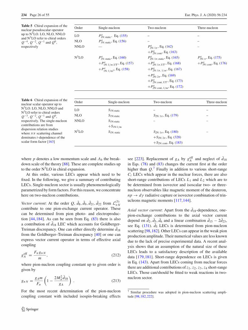
234 Page 26 of 55 Eur. Phys. J. A (2020) 56 :234

Table 5 Chiral expansion of thenuclear pseudoscalar operatorup to N3LO. LO, NLO, NNLOand N3LO refer to chiral ordersQ−4, Q−2, Q−1 and Q0,respectively

Order Single-nucleon Two-nucleon Three-nucleon

LO Pa1N: static, Eq. (155) – –

NLO Pa1N: static, Eq. (156) – –

NNLO — Pa2N: 1π , Eq. (162) –

+Pa2N: cont, Eq. (163)

N3LO Pa1N: static, Eq. (160) Pa

2N: 1π,static, Eq. (165) Pa3N: π , Eq. (175)

+Pa1N: 1/m,UT′ , Eq. (157) +Pa

2N: 1π,UT′ , Eq. (168) +Pa3N: cont, Eq. (176)

+Pa1N: 1/m2 , Eq. (158) +Pa

2N: 1π, 1/m , Eq. (167)

+Pa2N: 2π , Eq. (169)

+Pa2N: cont, UT′ , Eq. (173)

+Pa2N: cont, 1/m, Eq. (172)

Table 6 Chiral expansion of thenuclear scalar operator up toN3LO. LO, NLO, NNLO andN3LO refer to chiral ordersQ−3, Q−2, Q−1 and Q0,respectively. The single-nucleoncontributions are fromdispersion relation studieswhere ππ scattering channeldominates t-dependence of thescalar form factor [163]

Order Single-nucleon Two-nucleon Three-nucleon

LO S1N:static – –

NLO S1N:static S2N: 1π , Eq. (179) –

NNLO S1N:static – –

+S1N:1/m

N3LO S1N: static S2N: 1π , Eq. (180) –

+S2N: 2π , Eq. (328)

+S2N: cont, Eq. (183)

where p denotes a low momentum scale and Λb the break-down scale of the theory [88]. These are complete studies upto the order N3LO in chiral expansion.

At this order, various LECs appear which need to befixed. In the following, we give a summary of contributingLECs. Single-nucleon sector is usually phenomenologicallyparametrized by form factors. For this reason, we concentratehere on two-nucleon contributions.

Vector current: At the order Q, d8, d9, d21, d22 from L(3)πN

contribute to one pion-exchange current operator. Thesecan be determined from pion photo- and electroproduc-tion [44,184]. As can be seen from Eq. (83) there is alsoa contribution of d18 LEC which accounts for Goldberger-Treiman discrepancy. One can either directly determine d18

from the Goldberger–Treiman discrepancy [40] or one canexpress vector current operator in terms of effective axialcoupling

geffA = FπgπN

m, (212)

where pion-nucleon coupling constant up to given order isgiven by

gπN = gAm

Fπ

(1 − 2M2

π d18

gA

). (213)

For the most recent determination of the pion-nucleoncoupling constant with included isospin-breaking effects

see [223]. Replacement of gA by geffA and neglect of d18

in Eqs. (78) and (83) changes the current first at the orderhigher than Q.7 Finally in addition to various short-rangeCi LECs which appear in the nuclear forces, there are alsoshort-range contributions of LECs L1 and L2 which are tobe determined from isovector and isoscalar two- or three-nucleon observables like magnetic moment of the deuteron,np → dγ radiative capture or isovector combination of trin-ucleons magnetic moments [117,144].

Axial vector current: Apart from the d18-dependence, one-pion-exchange contributions to the axial vector currentdepend on d2, d5, d6 and a linear combination d15 − 2d23,see Eq. (131). d5 LECs is determined from pion-nucleonscattering [98,182]. Other LECs can appear in the weak pionproduction amplitude. Their numerical values are less knowndue to the lack of precise experimental data. A recent anal-ysis shows that an assumption of the natural size of theseLECs leads to a satisfactory description of the availabledata [179,181]. Short-range dependence on LECs is givenin Eq. (143). Apart from LECs coming from nuclear forcesthere are additional contributions of z1, z2, z3, z4 short-rangeLECs. Those can/should be fitted to weak reactions in two-nucleon sector.

7 Similar procedure was adopted in pion-nucleon scattering ampli-tude [98,182,222].

123

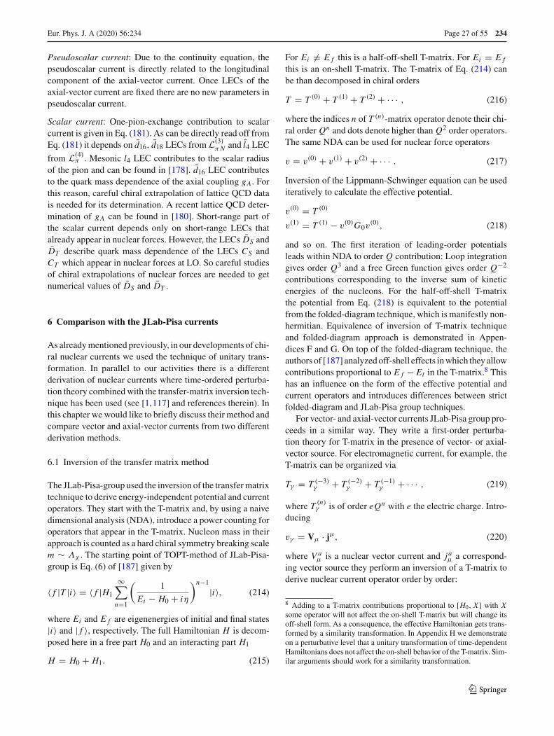
Eur. Phys. J. A (2020) 56 :234 Page 27 of 55 234

Pseudoscalar current: Due to the continuity equation, thepseudoscalar current is directly related to the longitudinalcomponent of the axial-vector current. Once LECs of theaxial-vector current are fixed there are no new parameters inpseudoscalar current.

Scalar current: One-pion-exchange contribution to scalarcurrent is given in Eq. (181). As can be directly read off fromEq. (181) it depends on d16, d18 LECs from L(3)

πN and l4 LEC

from L(4)π . Mesonic l4 LEC contributes to the scalar radius

of the pion and can be found in [178]. d16 LEC contributesto the quark mass dependence of the axial coupling gA. Forthis reason, careful chiral extrapolation of lattice QCD datais needed for its determination. A recent lattice QCD deter-mination of gA can be found in [180]. Short-range part ofthe scalar current depends only on short-range LECs thatalready appear in nuclear forces. However, the LECs DS andDT describe quark mass dependence of the LECs CS andCT which appear in nuclear forces at LO. So careful studiesof chiral extrapolations of nuclear forces are needed to getnumerical values of DS and DT .

6 Comparison with the JLab-Pisa currents

As already mentioned previously, in our developments of chi-ral nuclear currents we used the technique of unitary trans-formation. In parallel to our activities there is a differentderivation of nuclear currents where time-ordered perturba-tion theory combined with the transfer-matrix inversion tech-nique has been used (see [1,117] and references therein). Inthis chapter we would like to briefly discuss their method andcompare vector and axial-vector currents from two differentderivation methods.

6.1 Inversion of the transfer matrix method

The JLab-Pisa-group used the inversion of the transfer matrixtechnique to derive energy-independent potential and currentoperators. They start with the T-matrix and, by using a naivedimensional analysis (NDA), introduce a power counting foroperators that appear in the T-matrix. Nucleon mass in theirapproach is counted as a hard chiral symmetry breaking scalem ∼ Λχ . The starting point of TOPT-method of JLab-Pisa-group is Eq. (6) of [187] given by

〈 f |T |i〉 = 〈 f |H1

∞∑

n=1

(1

Ei − H0 + iη

)n−1

|i〉, (214)

where Ei and E f are eigenenergies of initial and final states|i〉 and | f 〉, respectively. The full Hamiltonian H is decom-posed here in a free part H0 and an interacting part H1

H = H0 + H1. (215)

For Ei �= E f this is a half-off-shell T-matrix. For Ei = E f

this is an on-shell T-matrix. The T-matrix of Eq. (214) canbe than decomposed in chiral orders

T = T (0) + T (1) + T (2) + · · · , (216)

where the indices n of T (n)-matrix operator denote their chi-ral order Qn and dots denote higher than Q2 order operators.The same NDA can be used for nuclear force operators

v = v(0) + v(1) + v(2) + · · · . (217)

Inversion of the Lippmann-Schwinger equation can be usediteratively to calculate the effective potential.

v(0) = T (0)

v(1) = T (1) − v(0)G0v(0), (218)

and so on. The first iteration of leading-order potentialsleads within NDA to order Q contribution: Loop integrationgives order Q3 and a free Green function gives order Q−2

contributions corresponding to the inverse sum of kineticenergies of the nucleons. For the half-off-shell T-matrixthe potential from Eq. (218) is equivalent to the potentialfrom the folded-diagram technique, which is manifestly non-hermitian. Equivalence of inversion of T-matrix techniqueand folded-diagram approach is demonstrated in Appen-dices F and G. On top of the folded-diagram technique, theauthors of [187] analyzed off-shell effects in which they allowcontributions proportional to E f − Ei in the T-matrix.8 Thishas an influence on the form of the effective potential andcurrent operators and introduces differences between strictfolded-diagram and JLab-Pisa group techniques.

For vector- and axial-vector currents JLab-Pisa group pro-ceeds in a similar way. They write a first-order perturba-tion theory for T-matrix in the presence of vector- or axial-vector source. For electromagnetic current, for example, theT-matrix can be organized via

Tγ = T (−3)γ + T (−2)

γ + T (−1)γ + · · · , (219)

where T (n)γ is of order eQn with e the electric charge. Intro-

ducing

vγ = Vμ · jμ, (220)

where V aμ is a nuclear vector current and jaμ a correspond-

ing vector source they perform an inversion of a T-matrix toderive nuclear current operator order by order:

8 Adding to a T-matrix contributions proportional to [H0, X ] with Xsome operator will not affect the on-shell T-matrix but will change itsoff-shell form. As a consequence, the effective Hamiltonian gets trans-formed by a similarity transformation. In Appendix H we demonstrateon a perturbative level that a unitary transformation of time-dependentHamiltonians does not affect the on-shell behavior of the T-matrix. Sim-ilar arguments should work for a similarity transformation.

123

234 Page 28 of 55 Eur. Phys. J. A (2020) 56 :234

v−3γ = T (−3)

γ

v−2γ = T (−2)

γ −[v(−3)γ G0v

(0) + v(0)G0v(−3)γ

]. (221)

In the following, we will discuss the differences betweenJLab-Pisa and Bochum–Bonn–Currents. The differences inthe two methods appear first at the order Q.

6.2 Difference in the vector current at order Q

At order Q, we decompose the current in the number of pion-exchange via Eq. (77).

6.2.1 One-pion-exchange contributions to the vectorcurrent

We start with the static OPE contributions. OPE contributionsof the JLab-Pisa group have been presented in [141] wherethey give only unrenormalized results. Even relaxing con-straints on beta functions of di -LECs from L(3)

πN Lagrangianwe are unable to renormalize their Eqs. (3.30) − (3.42).In a later publication [117] JLab-Pisa group decided toparametrize the OPE in terms of form factors, see Eqs.(2.22)–(2.25) of [117]. Since they use this form in all theirnumerical calculations, we compare if our results are compat-ible with their parametrization. Replacing the form factor byunity (which does not affect order-Q results) we consider thedifference between our results and that of JLab-Pisa group

δV (Q),μ2N:1π,static = V (Q),μ

2N:1π,static − V JLab−Pisa(Q),μ2N:1π,static . (222)

The OPE contributions can be written in the form of Eq. (82)for current and Eq. (84) for charge contributions, respectively.For this reason, it is enough to give the difference in termsof scalar functions

δ fi (k) = fi (k) − f JLab−Pisai (k), i = 1, . . . , 8, (223)

where the functions fi (k) are defined in Eqs. (83) and (85).f JLab−Pisai (k) are extracted out of Eq. (2.22) and (2.24)

of [117]. The difference is given by

δ f1(k) = δ f2(k) = 0,

δ f3(k) = −ie

64π2F4π

(g4A(2L(k) − 1) + (4πFπ )2gAd22

),

δ f4(k) = −iegA4F2

π

d22, δ f6(k) = − iegAM2π

F2π

d18,

δ f5(k) = − ieg2A

1152π2F4π

(− 24M2

π + k2(−5 + 288π2l6)

+6(k2 + 4M2π )L(k)

). (224)

Note, that Piarulli et al. [117] discuss only tree-level con-tributions to OPE and make a phenomenological extension

of these results. They multiply the tree-diagram results pro-portional to di ’s with Gγ NΔ(k)/μγ NΔ and with Gγ Nρ(k)form factors which are set here to unity. All other terms ofthese form factors contribute to orders higher than Q. In con-trast to the statement of Piarulli et al. [117], the differenceδV(Q)

2N:1π,static contributes to the magnetic moment operatorμ = −(i/2)∇k × V|k=0. The difference for the magneticmoment operator is given by

δμ = −(i/2)∇k × δV(Q)|k=0 = eg4A

64π2F4π

[τ 1 × τ 2]3

q21 + M2

π

×(

[q1 × σ 2]q1 · σ 1 − [q1 × σ 1]q1 · σ 2

). (225)

This difference, however, comes from δ f3(k) and can beabsorbed into d21 if one makes a shift

d21 → d21 + g3A

32π2F2π

. (226)

Charge operator contributions have also been discussed byJLab-Pisa group. Since they do not mention any static con-tributions to OPE charge at order Q we conclude that

f JLab−Pisa7 (k) = f JLab−Pisa

8 (k) = 0, (227)

in clear disagreement to our results of Eq. (85).At the same order Q there are also relativistic corrections

to OPE charge and current operators. Both groups give van-ishing results for relativistic corrections9 for current opera-tors such that there is no disagreement on the current levelfor relativistic corrections. Relativistic corrections to chargecontributions agree only if one fixes unitary phases to

β8 = ν

2, β9 = −1

2, (228)

which means that they are unitary equivalent. Parameters β8

and β9 are directly related to unitary phase parameters μ

and ν introduced by Friar [21,185,186] to describe an off-shell dependence of relativistic 1/m2 corrections to OPE NNpotential:

μ = 4β9 + 1, ν = 2β8. (229)

These parameters are usually set to

β8 = 1

4, β9 = −1

4, (230)

to achieve a minimal non-locality form of OPE NN poten-tial [89]. From Eq. (228) we conclude that the charge operator

9 Piarulli et al. discuss 1/m2 and 1/m3 corrections to OPE currentoperator. Although they do not vanish they contribute to higher ordersin the power counting adopted by our group.

123

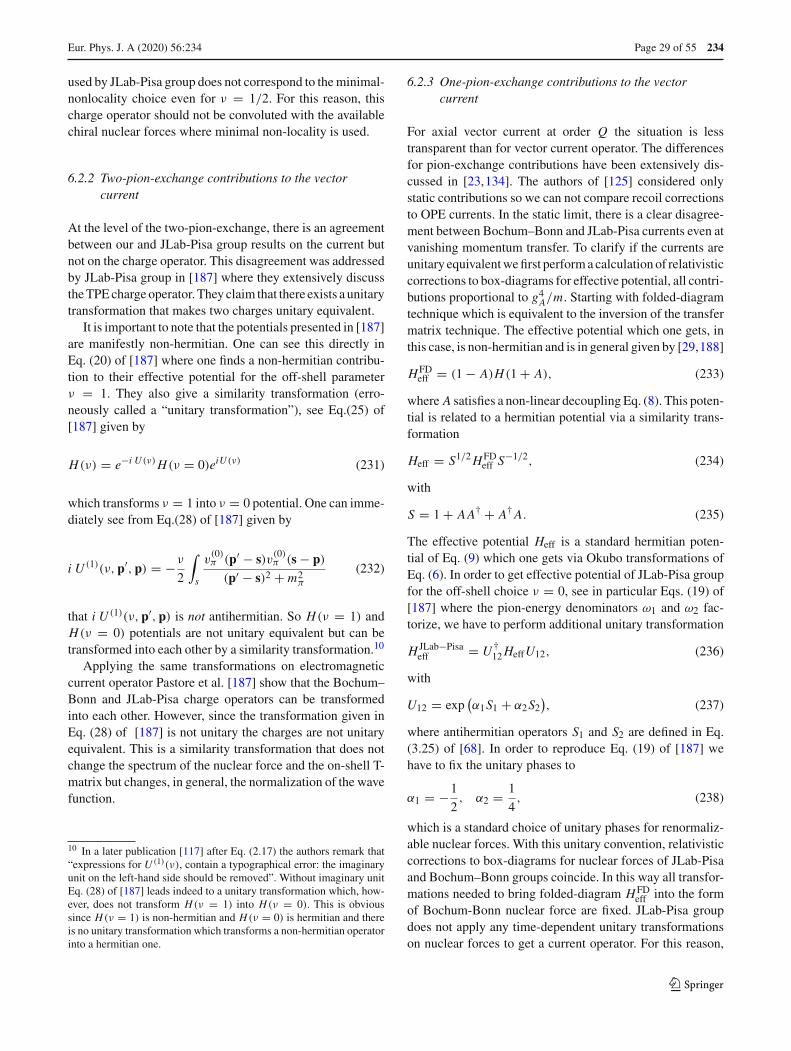
Eur. Phys. J. A (2020) 56 :234 Page 29 of 55 234

used by JLab-Pisa group does not correspond to the minimal-nonlocality choice even for ν = 1/2. For this reason, thischarge operator should not be convoluted with the availablechiral nuclear forces where minimal non-locality is used.

6.2.2 Two-pion-exchange contributions to the vectorcurrent

At the level of the two-pion-exchange, there is an agreementbetween our and JLab-Pisa group results on the current butnot on the charge operator. This disagreement was addressedby JLab-Pisa group in [187] where they extensively discussthe TPE charge operator. They claim that there exists a unitarytransformation that makes two charges unitary equivalent.

It is important to note that the potentials presented in [187]are manifestly non-hermitian. One can see this directly inEq. (20) of [187] where one finds a non-hermitian contribu-tion to their effective potential for the off-shell parameterν = 1. They also give a similarity transformation (erro-neously called a “unitary transformation”), see Eq.(25) of[187] given by

H(ν) = e−i U (ν)H(ν = 0)eiU (ν) (231)

which transforms ν = 1 into ν = 0 potential. One can imme-diately see from Eq.(28) of [187] given by

i U (1)(ν,p′,p) = −ν

2

∫

s

v(0)π (p′ − s)v(0)

π (s − p)

(p′ − s)2 + m2π

(232)

that i U (1)(ν,p′,p) is not antihermitian. So H(ν = 1) andH(ν = 0) potentials are not unitary equivalent but can betransformed into each other by a similarity transformation.10

Applying the same transformations on electromagneticcurrent operator Pastore et al. [187] show that the Bochum–Bonn and JLab-Pisa charge operators can be transformedinto each other. However, since the transformation given inEq. (28) of [187] is not unitary the charges are not unitaryequivalent. This is a similarity transformation that does notchange the spectrum of the nuclear force and the on-shell T-matrix but changes, in general, the normalization of the wavefunction.

10 In a later publication [117] after Eq. (2.17) the authors remark that“expressions for U (1)(ν), contain a typographical error: the imaginaryunit on the left-hand side should be removed”. Without imaginary unitEq. (28) of [187] leads indeed to a unitary transformation which, how-ever, does not transform H(ν = 1) into H(ν = 0). This is obvioussince H(ν = 1) is non-hermitian and H(ν = 0) is hermitian and thereis no unitary transformation which transforms a non-hermitian operatorinto a hermitian one.

6.2.3 One-pion-exchange contributions to the vectorcurrent

For axial vector current at order Q the situation is lesstransparent than for vector current operator. The differencesfor pion-exchange contributions have been extensively dis-cussed in [23,134]. The authors of [125] considered onlystatic contributions so we can not compare recoil correctionsto OPE currents. In the static limit, there is a clear disagree-ment between Bochum–Bonn and JLab-Pisa currents even atvanishing momentum transfer. To clarify if the currents areunitary equivalent we first perform a calculation of relativisticcorrections to box-diagrams for effective potential, all contri-butions proportional to g4

A/m. Starting with folded-diagramtechnique which is equivalent to the inversion of the transfermatrix technique. The effective potential which one gets, inthis case, is non-hermitian and is in general given by [29,188]

HFDeff = (1 − A)H(1 + A), (233)

where A satisfies a non-linear decoupling Eq. (8). This poten-tial is related to a hermitian potential via a similarity trans-formation

Heff = S1/2HFDeff S

−1/2, (234)

with

S = 1 + AA† + A†A. (235)

The effective potential Heff is a standard hermitian poten-tial of Eq. (9) which one gets via Okubo transformations ofEq. (6). In order to get effective potential of JLab-Pisa groupfor the off-shell choice ν = 0, see in particular Eqs. (19) of[187] where the pion-energy denominators ω1 and ω2 fac-torize, we have to perform additional unitary transformation

H JLab−Pisaeff = U †

12HeffU12, (236)

with

U12 = exp(α1S1 + α2S2

), (237)

where antihermitian operators S1 and S2 are defined in Eq.(3.25) of [68]. In order to reproduce Eq. (19) of [187] wehave to fix the unitary phases to

α1 = −1

2, α2 = 1

4, (238)

which is a standard choice of unitary phases for renormaliz-able nuclear forces. With this unitary convention, relativisticcorrections to box-diagrams for nuclear forces of JLab-Pisaand Bochum–Bonn groups coincide. In this way all transfor-mations needed to bring folded-diagram HFD

eff into the formof Bochum-Bonn nuclear force are fixed. JLab-Pisa groupdoes not apply any time-dependent unitary transformationson nuclear forces to get a current operator. For this reason,

123

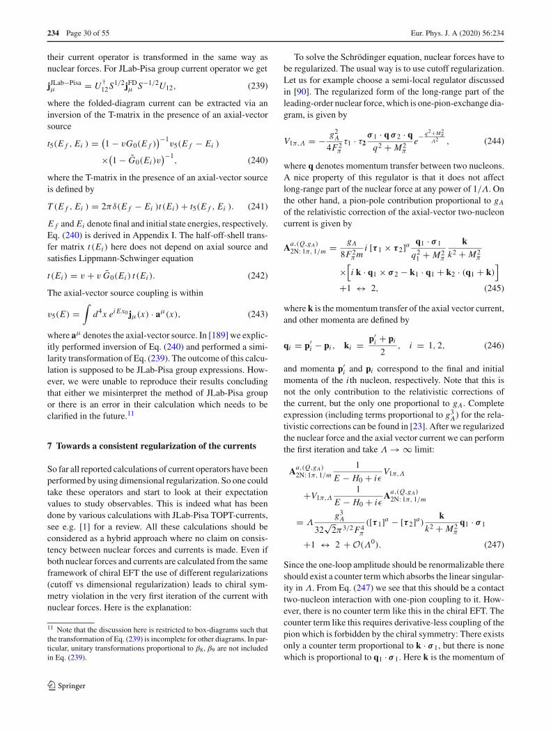
234 Page 30 of 55 Eur. Phys. J. A (2020) 56 :234

their current operator is transformed in the same way asnuclear forces. For JLab-Pisa group current operator we get

jJLab−Pisaμ = U †

12S1/2jFD

μ S−1/2U12, (239)

where the folded-diagram current can be extracted via aninversion of the T-matrix in the presence of an axial-vectorsource

t5(E f , Ei ) = (1 − vG0(E f )

)−1v5(E f − Ei )

×(1 − G0(Ei )v

)−1, (240)

where the T-matrix in the presence of an axial-vector sourceis defined by

T (E f , Ei ) = 2πδ(E f − Ei )t (Ei ) + t5(E f , Ei ). (241)

E f and Ei denote final and initial state energies, respectively.Eq. (240) is derived in Appendix I. The half-off-shell trans-fer matrix t (Ei ) here does not depend on axial source andsatisfies Lippmann-Schwinger equation

t (Ei ) = v + v G0(Ei ) t (Ei ). (242)

The axial-vector source coupling is within

v5(E) =∫

d4x ei Ex0 jμ(x) · aμ(x), (243)

where aμ denotes the axial-vector source. In [189] we explic-itly performed inversion of Eq. (240) and performed a simi-larity transformation of Eq. (239). The outcome of this calcu-lation is supposed to be JLab-Pisa group expressions. How-ever, we were unable to reproduce their results concludingthat either we misinterpret the method of JLab-Pisa groupor there is an error in their calculation which needs to beclarified in the future.11

7 Towards a consistent regularization of the currents

So far all reported calculations of current operators have beenperformed by using dimensional regularization. So one couldtake these operators and start to look at their expectationvalues to study observables. This is indeed what has beendone by various calculations with JLab-Pisa TOPT-currents,see e.g. [1] for a review. All these calculations should beconsidered as a hybrid approach where no claim on consis-tency between nuclear forces and currents is made. Even ifboth nuclear forces and currents are calculated from the sameframework of chiral EFT the use of different regularizations(cutoff vs dimensional regularization) leads to chiral sym-metry violation in the very first iteration of the current withnuclear forces. Here is the explanation:

11 Note that the discussion here is restricted to box-diagrams such thatthe transformation of Eq. (239) is incomplete for other diagrams. In par-ticular, unitary transformations proportional to β8, β9 are not includedin Eq. (239).

To solve the Schrödinger equation, nuclear forces have tobe regularized. The usual way is to use cutoff regularization.Let us for example choose a semi-local regulator discussedin [90]. The regularized form of the long-range part of theleading-order nuclear force, which is one-pion-exchange dia-gram, is given by

V1π,Λ = − g2A

4F2π

τ1 · τ2σ 1 · q σ 2 · qq2 + M2

π

e− q2+M2π

Λ2 , (244)

where q denotes momentum transfer between two nucleons.A nice property of this regulator is that it does not affectlong-range part of the nuclear force at any power of 1/Λ. Onthe other hand, a pion-pole contribution proportional to gAof the relativistic correction of the axial-vector two-nucleoncurrent is given by

Aa,(Q,gA)2N: 1π, 1/m = gA

8F2πm

i [τ 1 × τ 2]a q1 · σ 1

q21 + M2

π

kk2 + M2

π

×[i k · q1 × σ 2 − k1 · q1 + k2 · (q1 + k)

]

+1 ↔ 2, (245)

where k is the momentum transfer of the axial vector current,and other momenta are defined by

qi = p′i − pi , ki = p′

i + pi2

, i = 1, 2, (246)

and momenta p′i and pi correspond to the final and initial

momenta of the i th nucleon, respectively. Note that this isnot the only contribution to the relativistic corrections ofthe current, but the only one proportional to gA. Completeexpression (including terms proportional to g3

A) for the rela-tivistic corrections can be found in [23]. After we regularizedthe nuclear force and the axial vector current we can performthe first iteration and take Λ → ∞ limit:

Aa,(Q,gA)2N: 1π, 1/m

1

E − H0 + iεV1π,Λ

+V1π,Λ

1

E − H0 + iεAa,(Q,gA)

2N: 1π, 1/m

= Λg3A

32√

2π3/2F4π

([τ 1]a − [τ 2]a) kk2 + M2

π

q1 · σ 1

+1 ↔ 2 + O(Λ0). (247)

Since the one-loop amplitude should be renormalizable thereshould exist a counter term which absorbs the linear singular-ity in Λ. From Eq. (247) we see that this should be a contacttwo-nucleon interaction with one-pion coupling to it. How-ever, there is no counter term like this in the chiral EFT. Thecounter term like this requires derivative-less coupling of thepion which is forbidden by the chiral symmetry: There existsonly a counter term proportional to k · σ 1, but there is nonewhich is proportional to q1 · σ 1. Here k is the momentum of

123

Eur. Phys. J. A (2020) 56 :234 Page 31 of 55 234

the pion coupling to the two-nucleon interaction.12 If thereis no counter term that absorbs the linear cutoff singularitythere should be some cancelation in the amplitude with otherterms. Indeed the same singularity but with the opposite signwe would get for the static limit of the axial vector current ofthe order Q if we would calculate the current by using cutoffregularization. Axial vector current at the order Q, however,is calculated by using dimensional regularization and is finite.It also remains finite if we just multiply the current with anycutoff regulator we want. So at the level of the amplitude,the mismatch between cutoff and dimensional regularizationused in the construction of operators leads to a violation ofthe chiral symmetry at the one-loop level which, however, isthe order of accuracy of our calculations. So we see that it isdangerous to multiply the current operators calculated withindimensional regularization by some cutoff regulator and cal-culate the expectation values of this. With similar argumentsone can show that dimensionally regularized three-nucleonforces at the level of N3LO, which were published in [62,63],can not be used in combination with the cutoff regularizedtwo-nucleon forces at the same order [79]. The mismatchbetween dimensional and cutoff regularization will lead alsoin this case to a violation of the chiral symmetry at the oneloop level.

To respect the chiral symmetry we need to calculate bothnuclear forces and currents with the same regulator. On topof it the regulator which we choose should be symmetry pre-serving. One possibility to construct a regulator, which man-ifestly respects the chiral symmetry was proposed more thanfour decades ago by Slavnov [190], where he introduced ahigher derivative regularization in a study of the non-linearsigma model. Recently, the first applications of this techniqueto the chiral EFT have been discussed in the literature [191,192]. A basic idea of Slavnov is to change the propagator of apion field on the Lagrangian level. Since pion fields are orga-nized in U -fields which are elements of SU(2) group and allderivatives in the Lagrangian appear as covariant derivativesto maintain gauge and chiral symmetry, the modified chiralLagrangian should be expressed in terms of covariant deriva-tives of U -fields. In this way the gauge- and chiral symmetryare maintained by construction. For our purpose, we changethe static pion propagator by a regularized one

1

q2 + M2π

→ e− q2+M2π

Λ2

q2 + M2π

. (248)

The choice of this regulator is consistent with the semilo-cal regulator used in nuclear forces where pion propagator isregularized via Eq. (248) and contact interactions via a non-

12 At higher orders one can construct derivative-less pion-four-nucleoninteractions by multiplying low energy constants with M2

π . They arecoming from the explicit chiral symmetry breaking by finite quark mass.However, at the order Q we can not construct a counter term like this.

local Gaussian regulator. The challenge is to construct themodified chiral Lagrangian in terms of covariant derivativesand chiral U -fields which leads to modified pion propagatorof Eq. (248), modified contact interactions and to regular-ized forces and currents. Construction of consistent nuclearforces and currents within the higher derivative approach is awork in progress. However, the first results for the deuteroncharge in this consistent approach are already available [197]and will be briefly discussed in the next section.

8 Two-nucleon charge operator

As already mentioned in Sect. 7, at the moment we can nottake expectation values of the current operators at the orderQ without violation of the chiral symmetry at the same orderof accuracy. This happens due to the mismatch of dimen-sional and cutoff regularizations of nuclear forces and cur-rents. Inconsistency between regularization of forces and cur-rents leads in some cases to strong cut-off dependence inthe observables, see [145] for discussion of photodisintegra-tion on 2H and 3He calculated with order Q vector current.In many cases, however, the inconsistent (hybrid) approachgives a satisfactory description of the data. In the last decade,there are various application of hybrid approach with JLab-PIsa TOPT current operators, see [1] for a recent review and[118,121,193,194] and references therein for the most recentactivities in this field. We are not going to report here on thehybrid approach activities but rather concentrate on the con-sistent calculation of the deuteron charge form factor [197].

8.1 Deuteron charge

Deuteron form factors have been extensively studied withinEFT in pion-full and pion-less approaches, see [12,13,198]for reviews. To perform a consistent calculation of deuteronform factors, we need to construct a regularized NN potentialand electromagnetic current operator with the same off-shellproperties. Up to order Q the expressions for unregularizedcurrent have been discussed in Sect. 5.2. At the order Qmeson-exchange contributions to the deuteron charge formfactor are given by just relativistic corrections to the one-pion-exchange charge operator, Eq. (88). Such a simplifica-tion for the charge operator appears since the deuteron isan isoscalar. All complicated one-loop terms proportionalto [τ 1]3 and [τ 1]3 do not contribute to expectation valuesafter convolution with the deuteron wave function. The onlynon-vanishing order Q pion-exchange contribution to thedeuteron charge operator is given by

V 0,(Q)2N:1π,1/m = − 3eg2

A

16F2πm

[1 − 2β9

q22 + M2

π

σ 1 · kσ 2 · q2

+ 2β8 − 1

(q22 + M2

π )2σ 1 · q2 σ 2 · q2q2 · k

]+ 1 ↔ 2. (249)

123

234 Page 32 of 55 Eur. Phys. J. A (2020) 56 :234

For the single-nucleon charge operator, we use Eq. (74)where the charge operator is expressed in terms of electro-magnetic form factors. Due to poor convergence of chiralexpansion for electromagnetic form factors we used theirphenomenological parametrization. For the calculation of thedeuteron charge form factor we used a global analysis of theexperimental data of Refs. [199,200]. To estimate a system-atic error we also used dispersive analyses of Refs. [201–203]. In derivation of Eq. (249) we applied unitary trans-formations of nuclear forces on the leading-order single-nucleon charge operator. Since we work now with the formfactor parametrization of the single-nucleon contribution weapply the same transformation on the electric form factor andreplace Eq. (249) by

V 0,(Q)2N:1π,1/m = − 3eg2

A

16F2πm

[1 − 2β9

q22 + M2

π

σ 1 · kσ 2 · q2

+ 2β8 − 1

(q22 + M2

π )2σ 1 · q2 σ 2 · q2q2 · k

]GS

E (k2) + 1 ↔ 2,

(250)

where GSE (k2) is the isoscalar part of the electric form factor

GSE (k2) = Gp

E (k2) + GnE (k2), (251)

and GpE (k2) and Gn

E (k2) are electric form factors of protonand neutron, respectively. To regularize Eq. (250) we have totake the same regulator which was used in the construction ofnuclear forces. This requires to make following replacementsin Eq. (250) for pion-exchange propagators

1

q22 + M2

π

→ e− q22+M2

π

Λ2

q22 + M2

π

,

1

[q22 + M2

π ]2→

(1 + q2

2 + M2π

Λ2

)e− q2

2+M2π

Λ2

[q22 + M2

π ]2. (252)

Note the dependence of the deuteron charge operator inEq. (250) on unitary phases β8 and β9. The same unitaryphases appear in relativistic 1/m2-corrections to one-pion-exchange in nuclear force. They are usually chosen as

β8 = 1

4, β9 = −1

4, (253)

to maintain a minimal non-locality of the nuclear force. How-ever, they might be chosen differently, and any calculatedobservable should only weakly depend on them in a consis-tent calculation.13 To test the consistency of our calculationwe generated two versions of nuclear forces, the non-minimal

13 If unitary transformations with the phases β8 and β9 would be imple-mented in an exact way without any approximation the observableswould be independent on them.

coupling choice of Eq. (253) and

β8 = β9 = 1

2, (254)

for which the deuteron pion-exchange charge contributiondisappears. Both versions lead to the same results for thedeuteron charge form factor. It is important to note that reg-ularization prescription in Eq. (252) works only due to thesimple structure of the charge operator in Eq. (250). For thecurrent operator or even for the charge operator for isovectorobservables the regularization of the current operator needsmore effort and can be worked out within higher derivativeregularization. This is still a work in progress.

At the order Q there are no short-range contribution todeuteron charge form factor, as can be directly followed fromEq. (92). The first short-range contributions show up at theorder Q2 and can be parametrized by three parameters mul-tiplied with isoscalar electric form factor

V 02N:cont = 2eGS

E(k2)

(A k2 + B k2(σ 1 · σ 2)

+C k · σ 1k · σ 2

), (255)

where A, B, and C are low-energy constants (LECs) [5].Although these are Q2-order effects, they catch the short-range off-shell dependence of N4LO nuclear forces. This isa direct consequence of the fact that contributions in Eq. (255)can be generated with unitary transformations acting on thesingle-nucleon charge density. The same unitary transfor-mations acting on the kinetic energy term produce off-shellshort-range contributions to nuclear force at N4LO. Not allthree LECs contribute independently in the deuteron chargeform factor. Only a linear combination A+ B+C/3 appearsas a free parameter that we fitted to the deuteron charge formfactor data. We regularize these charge contributions in thesame non-local way as was done in N4LO nuclear force [90]

V 0,reg2N:cont = 2eGS

E(k2)

×[(A + B (σ 1 · σ 2))F1

(p1 − p2

2,p′

1 − p′2

2,k

)

+CF2

(p1 − p2

2,p′

1 − p′2

2,k

) ], (256)

where the functions F1 and F2 are defined as

Fi (p,p′,k) := Ei

(p − k

2,p′

)+ Ei

(p + k

2,p′

)

+Ei

(p′ − k

2,p

)+ Ei

(p′ + k

2,p

),

(257)

123

Eur. Phys. J. A (2020) 56 :234 Page 33 of 55 234

E1(p,p′) :=

(p2 − p′2) e− p2+p′2

Λ2 ,

E2(p,p′) := [

(σ 1 · p)(σ 2 · p) − (σ 1 · p′)(σ 2 · p′)]

×e− p2+p′2Λ2 . (258)

In order to give a theoretical error quantification due totruncation of chiral expansion one can use the algorithm pro-posed in [88]. Namely, one can estimate the truncation errorδ(X)(i) of an observable X at i-th order of the chiral expan-sion, with i = 0, 2, 3, . . . . If Q denotes the chiral expansionparameter, the expressions for truncation errors are

δ(X)(0) ≥ max(Q2|X (0)| , |X (i≥0) − X ( j≥0)|

),

δ(X)(2) = max(Q3|X (0)| , Q|ΔX (2)| , |X (i≥2) − X ( j≥2)|

),

δ(X)(i) = max(Qi+1|X (0)| , Qi−1|ΔX (2)| , Qi−2|ΔX (3)|

)

for i ≥ 3 . (259)

In the above formulas X (i) is a prediction for the observableX at i th order, ΔX (2) ≡ X (2) − X (0) and ΔX (i) ≡ X (i) −X (i−1) for i ≥ 3. The algorithm of Eq. (259) is very simple.However, it does not give a statistical interpretation of theerror estimate. An interesting algorithm based on Bayesianapproach was developed in [204–206]. Based on these studieswe employed a Bayesian model specified in [207] to give atheoretical truncation error estimate of the deuteron chargeform factor.

Deuteron charge form factor based on the consistently reg-ularized charge operator, defined in Eqs. (250), (252), (256)is shown in Fig. 2 for cutoff Λ = 500 MeV. A fit to the dataup to Q = 4 fm−1 was performed to fix a linear combina-tion of LECs A + B + C/3. It was verified that the cutoffvariation in the range of Λ = 400 · · · 500 MeV leads to theresults which are lying well within the truncation error band.Out of the calculated deuteron charge form factor one canextract the structure radius of the deuteron

rstr = 1.9731+0.0013−0.0018 fm, (260)

Individual contributions to the uncertainties are given inTable 7. This structure radius was calculated with theminimal-nonlocality choice of Eq. (253) of unitary phasesβ8 and β9. We repeated the calculation of the structure radiuswith the choice of Eq. (254) for which the deuteron contri-butions of long-range charge operator vanish. The result forthe structure radius for this choice agreed with the one inEq. (260) which confirms that off-shell ambiguities do notaffect the final result. With this finding, we were able to makea prediction for neutron root-mean-square (RMS) radius. Thestructure radius of the deuteron can be expressed as the RMSradius of the deuteron minus individual nucleon contributionsand minus relativistic correction (Foldy–Darwin term):

r2str = r2

d − r2p − r2

n − 3

4m2p, (261)

Fig. 2 Deuteron charge form factor from the best fit to data up to Q = 4fm−1 evaluated for the cutoff Λ = 500 MeV (solid blue lines). Bandbetween dashed (blue) lines corresponds to a 1σ error in the determi-nation of the short-range contribution to the charge density operator atN4LO. Light-shaded (orange dotted) band corresponds to the estimatederror (68% degree of belief) from truncation of the chiral expansion atN4LO. Open violet circles, green triangles and blue squares are exper-imental data from Refs. [208–210], respectively. Black solid circlescorrespond to the parameterization of the deuteron form factors fromRef. [12,211] which is not used in the fit and shown just for compari-son. The rescaled charge form factor of the deuteron, GC(Q)scaled, asdefined in Ref. [12], is shown on a linear scale

where rd , rp and rn are deuteron, proton and neutron RMScharge radii, respectively. mp denotes here a proton mass.

The extraction of the deuteron-proton RMS charge radiidifference can be made from the hydrogen-deuterium 1S–2S isotope shift measurements [214] accompanied with anaccurate QED analysis up to three-photon exchange accu-racy. According to [214] the deuteron-proton RMS chargeradii difference is given by

r2d − r2

p = 3.82070(31)fm2. (262)

See also [215] for an earlier determination. This relation leadsimmediately to a very precise prediction of the neutron rmsradius

r2n = −0.106+0.007−0.005 fm2. (263)

which is 1.7σ smaller than the one given by the PDG [216].It is important to note that our results for neutron radiusrely on chiral nuclear forces fitted to the Granada-2013database [217]. Isospin breaking effect analysis in the nuclearforce was done along with the treatment of Nijmegensgroup [218]. Isospin-breaking in one-pion-exchange due todifferent pion masses Mπ0 and Mπ± as well as charge depen-dence of the short-range interactions in the 1S0 wave wasexplicitly taken into account. These are the dominant isospin-

123

234 Page 34 of 55 Eur. Phys. J. A (2020) 56 :234

Table 7 Deuteron structure radius squared predicted at N4LO in χEFT(1st column) and the individual contributions to its uncertainty: from thetruncation of the chiral expansion (2nd), the statistical error in the short-range charge density operator extracted from GC(Q2) (3rd), the errorsfrom the statistical uncertainty in πN LECs from the Roy–Steiner anal-ysis of Ref. [212,213] propagated through the variation in the deuteron

wave functions (4th), the errors from the statistical uncertainty in 2NLECs from the analysis of the 2N observables of Ref. [90] (5th), theerror from the choice of the maximal energy in the fit (6th) as wellas the total uncertainty evaluated using the sum of these numbers inquadrature (7th). All numbers are given in fm2

r2str Truncation ρcont

2N πN LECs 2N LECs Q range Total

3.8933 ±0.0032 ±0.0037 ±0.0004 +0.0010−0.0047 ±0.0017 +0.0053−0.0070

breaking effects that are needed for a correct descriptionof the phase-shifts. For calculation of scattering observ-ables in the two-nucleon system, the isospin-breaking dueto long-range electromagnetic interaction have been con-sidered. Improved Coulomb potential [219], the magnetic-moment interaction [220] as well as the vacuum-polarizationpotential [221] were taken into account [79]. There are, how-ever, further corrections that are systematically worked outwithin chiral EFT. Expressions for the leading and sub-leading isospin-breaking two-pion-exchange-potential andirreducible pion-photon exchange contributions are alreadyavailable. Also charge-dependence of the pion-nucleon cou-pling constant needs to be accounted for in a systematic treat-ment within chiral EFT. Chiral nuclear force which takesinto account these isospin-breaking effects was presentedin [223]. It will be interesting to repeat the calculation of thedeuteron charge form factor by using the new chiral nuclearforce [223] and extract in this way the value for neutron RMSradius.

9 Summary

As reviewed in this article, chiral EFT provides a power-ful framework for the description of nuclear forces and cur-rents in a systematically improvable way. Nuclear forces con-structed up to N4LO achieved already a tremendous precisionsuch that they describe two-nucleon data with χ2 ∼ 1 andcan be considered as a partial wave analysis [90]. Nuclearvector and axial-vector current operators have been workedout up to order Q with the leading-order starting at Q−3.They have been calculated by using the T-matrix inversiontechnique by JLab-Pisa group and the unitary transformationtechnique by Bochum–Bonn group. Pseudoscalar (scalar)current operators have been worked out up to order Q0 withthe leading-order starting at Q−4 (Q−3). They have beencalculated within the unitary transformation technique byBochum–Bonn group. To get a renormalizable current ourgroup used time-dependent unitary transformations whichexplicitly depend on external sources. This leads to energy-transfer dependent currents with the modified continuityequations for vector and axial-vector currents. The behav-

ior of four-vectors under the Lorentz transformation furtherconstrains the currents. Expressions for vector as well asfor axial-vector currents derived by JLab-Pisa and Bochum–Bonn group differ at order Q. It was shown that for the vec-tor current, two-pion-exchange operators can be transformedinto each other by a similarity transformation. For the axial-vector current the situation is more confusing. We recalcu-lated box-diagram contributions to the axial vector current,which are proportional to g5

A, by using the T-matrix inver-sion technique. At the level of Fock-space we came to theconclusion that these currents should be unitary equivalentto Bochum–Bonn current. However, we could not reproducethe final results of JLab-Pisa group. This issue should beclarified in the future.

In most available calculations of nuclear currents, dimen-sional regularization has been used to regularize loop dia-grams. Additional regularization of the current operator is,however, required when it is sandwiched between wave func-tions for calculation of observables. Nuclear wave func-tions themselves are calculated from the solution of theSchrödinger equation with an input of nuclear force wherecutoff regularization was used. A naive procedure to multiplythe current operators with some cutoff function does not workat order Q. In the case of axial-vector current we have explic-itly shown that this procedure leads to violation of the chiralsymmetry. This happens due to different divergent pieces indimensional and cutoff regularization. A completely pertur-bative one-loop calculation of two-nucleon axial-vector cur-rent observable does not exist in this case in an infinite cutofflimit. To renormalize the theory one has to include derivative-less pion-two-nucleon vertices. Chiral symmetry constraint,however, does not allow the existence of such a vertex. Thisshows that regularization artifacts in such a procedure are notunder control. This happens just due to different regulariza-tions used in the calculation of currents (dimensional regular-ization) and in the iteration procedure (cutoff regularization).If one would use the same regularization in the calculationof forces and current operators this problem would not arise.We conclude that to achieve order-Q precision, the currentoperators have to be calculated with the same cutoff regular-ization which was used in nuclear forces. On top of this, achosen cutoff regularization should preserve the chiral sym-

123

Eur. Phys. J. A (2020) 56 :234 Page 35 of 55 234

metry. A higher derivative regularization approach, wherecutoff regularization is introduced on the Lagrangian levelwith all derivative operators being covariant, seems to be apromising tool to achieve this goal. Calculation of nuclearcurrent operators within this procedure is in progress.

Concerning numerical studies with nuclear current oper-ators, we restricted our discussion only to consistently reg-ularized current operators. It is important to mention thatdeuteron form factors and many other observables for thevector and axial-vector current have been extensively dis-cussed in the literature within a hybrid approach, see Sect. 1for references. We claim, however, that at the order Q theconsistency issue becomes essential and should be carefullyinvestigated.

As the first application of a consistently regularized elec-tromagnetic charge operator, we discussed the deuteroncharge form factor. Although consistently regularized cur-rent operators are not yet available, it is already possible toget a consistently regularized electromagnetic charge opera-tor for isoscalar observables like deuteron charge form factor.The reason is that the meson-exchange charge operator at theorder Q has a very simple form. Only relativistic 1/m – cor-rections to the leading one-pion-exchange charge operatorsurvive at this order. A consistent regularization of this oper-ator is very simple and was discussed in Sect. 8.1. On top of aparameter-free long-range charge operator, there is one short-range operator that we fitted to the deuteron charge form fac-tor. The constructed charge operator inherits automaticallyunitary ambiguities of the nuclear force. Thus, a nontrivialtest of the consistency is a test if the deuteron form factor isindependent of the chosen unitary ambiguity in nuclear forcesand currents. This consistency check was performed and wewere able to describe the deuteron form factor with a quan-tified truncation error analysis. The Bayesian approach wasused to give a statistical interpretation of truncation errors.It was demonstrated that working with consistently regu-larized forces and currents allows for very precise extrac-tion of the RMS radius of the neutron out of the deuteronradius. At this level of precision isospin-breaking effects innuclear forces play a significant role. So far they have beentaken into account only partly, in the same way as was donein most phenomenological potentials. Chiral EFT, however,allows for more precise treatment. In particular, contribu-tions of the leading and subleading isospin-breaking two-pion-exchange-potential, irreducible pion-photon exchangeand charge-dependence of pion-nucleon coupling constantneeds to be accounted for in a systematic treatment withinchiral EFT. The construction of this force is by now finished.So it will be very interesting to repeat the calculation of thedeuteron form factor with the consistently regularized cur-rent operator and the state of the art chiral nuclear force. Thisis work in progress.

Acknowledgements I would like to express my thanks to my collabo-rators Evgeny Epelbaum and Ulf-G. Meißner as well as Arseniy Filin,Vadim Baru, Patrick Reinert and Daniel Möller for sharing their insighton the discussed topics. This work is supported by DFG (CRC110,“Symmetries and the Emergence of Structure in QCD”).

Funding Open access funding provided by Projekt DEAL.

Data Availability Statement This manuscript has no associated dataor the data will not be deposited. [Authors’ comment: The datasetsgenerated during and/or analysed during the current study are availablefrom the corresponding author on reasonable request.]

Open Access This article is licensed under a Creative Commons Attri-bution 4.0 International License, which permits use, sharing, adaptation,distribution and reproduction in any medium or format, as long as yougive appropriate credit to the original author(s) and the source, pro-vide a link to the Creative Commons licence, and indicate if changeswere made. The images or other third party material in this articleare included in the article’s Creative Commons licence, unless indi-cated otherwise in a credit line to the material. If material is notincluded in the article’s Creative Commons licence and your intendeduse is not permitted by statutory regulation or exceeds the permit-ted use, you will need to obtain permission directly from the copy-right holder. To view a copy of this licence, visit http://creativecommons.org/licenses/by/4.0/.

Appendix A: External sources in chiral EFT

In this appendix, we briefly review the role of external sourcesin chiral perturbation theory. External sources played anessential role in the original formulation of chiral pertur-bation theory by Gasser and Leutwyler [34]. They allowfor a systematic inclusion of chiral symmetry breakingeffects, they provide a tool for generating all possible Ward-identities, and they can be used to define nuclear currentoperators. Let us briefly follow the discussion of [34] fortwo-flavour case. We start with QCD Lagrangian in the chi-ral limit where up and down quark masses are set to zero,

L0QCD =

∑

quark flavors

qiγ μ

(∂μ + ig

λa

2Ga

μ

)q

−1

4Ga

μνGaμν, (264)

with the gluon-fields Gaμ and

Gaμν = ∂μG

aν − ∂νG

aμ − g f abcGb

μGcν (265)

the corresponding field strength tensor. λa are 3×3 hermitiantraceless Gell-Mann matrices in color space, which satisfythe relations

Tr (λaλb) = 2δab, (266)[λa

2,λb

2

]= i f abc

λc

2, (267)

with f abc the totally antisymmetric SU(3) structure con-stants. It is easy to show that L0

QCD is invariant under the

123

234 Page 36 of 55 Eur. Phys. J. A (2020) 56 :234

global chiral SU(2)L ×SU(2)R transformation which can bedecomposed in vector and axial transformations. The invari-ance of L0

QCD under vector transformation is equivalent toisospin-symmetry. The invariance under axial transforma-tion is not shared by the ground state. So the axial symmetryof QCD is spontaneously broken. As a consequence thereexist three (number of broken generators) massless Gold-stone bosons which one identifies with pions. Due to theirGoldstone boson nature, the interaction between pions van-ishes if their four-momenta vanish. This gives us an expan-sion parameter in low energy sector given by low momenta ofpions divided by chiral symmetry breaking scale Λχ . In real-ity, quark masses are not equal to zero but are much smallerthan Λχ . A massive version of QCD violates chiral sym-metry. However, since the quark masses are small one canuse perturbation theory for the systematic inclusion of chiralsymmetry breaking effects. Additional to quark-gluon inter-action, quarks also interact with photons andW±, Z0 bosons.A convenient method for the description of these interac-tions and incorporation of quark masses is the introductionof axial-vector, vector, pseudoscalar, and scalar sources. Oneextends massless QCD to

LQCD = L0QCD + qγ μ(vμ + γ5aμ)q − q(s − iγ5 p)q,

(268)

where the external fields vμ(x), aμ(x), s(x), p(x) are hermi-tian, color-neutral matrices in flavor space. The quark massmatrix is included in s(x). If we require that the externalfields transform under a local chiral transformation as

v′μ + a′

μ = R(vμ + aμ)R† + i R∂μR†,

v′μ − a′

μ = L(vμ − aμ)L† + i L∂μL†,

s′ + i p′ = R(s + i p)L†, (269)

then LQCD is invariant under a local chiral transformation,and the generating functional

exp(i Z [v, a, s, p]) =∫

[dG][dq][dq] exp

(i∫

d4xLQCD

)

is invariant under the transformation given in Eq. (269):

Z [v′, a′, s′, p′] = Z [v, a, s, p]. (270)

Equation (270) can be used as a master equation for gener-ating all possible Ward identities of QCD. In the absence ofanomalies, the Ward identities are equivalent to the statementthat the generating functional is invariant under the gaugetransformation of the external fields [36]. In order that theGreen functions of the effective field theory obey the Ward-Identities of QCD it is sufficient to construct an effectivegenerating functional in the presence of the same externalfields such that it is invariant under the same gauge transfor-

mation:

Zeff [v′, a′, s′, p′] = Zeff [v, a, s, p]. (271)

The generating functional Zeff is built out of the point-likepion and nucleon degrees of freedom. A path-integral formof the effective generating functional is given by

exp(i Zeff [v, a, s, p]) =∫

[dN ][d N ][dU ] exp

(i∫

d4xLeff

),

where N and U denote nucleon and pion fields, respectively.U field is parametrized in form of a unitary matrix withdetU = 1. The effective Lagrangian Leff in Zeff is the mostgeneral Lagrangian compatible with Eq. (271). To achievethis, one replaces the usual derivative of pion fields by thecovariant one:

∂μU → ∇μU = ∂μU − i(vμ + aμ)U + iU (vμ − aμ).

(272)

Under local chiral transformations the above term transformsas

∇μU → R(∇μU )L†. (273)

The scalar and pseudoscalar external fields can be embodiedin the field

χ = 2B(s + i p), (274)

where the constant B is related to the non vanishing quarkcondensate by

〈0|uu|0〉 = 〈0|dd|0〉 = −F2π B + O(mu,md). (275)

The lowest order contribution toLeff with only pionic degreesof freedom which is invariant under a local chiral transfor-mation is then given by

L(2)ππ = F2

π

4Tr

(∇μU (∇μU )† + χU † +Uχ†

). (276)

The only requirement for the pion fieldU is that it has to be aunitary matrix with detU = 1. Their explicit parametrizationaffects only off-shell objects but does not affect observables.We see that the introduction of external sources can be usedas a tool for the systematic construction of chiral perturba-tion theory where explicit chiral symmetry breaking (dueto the non-vanishing quark mass) as well as electro-weakcouplings are taken into account. In the same framework, itis natural to use external sources to derive nuclear currentswhere nuclei are probed by photon or W±, Z0 exchange.For this purpose, one can derive effective Hamiltonian out ofthe effective Lagrangian. The effective Hamiltonian whichwe get in this way depends on external sources and is time-dependent. Explicit expressions for the effective Hamiltoniancan be found in [23,125,142]. Nuclear currents are derivedout of the quantized effective Hamiltonian by taking func-tional derivatives in external sources.

123

Eur. Phys. J. A (2020) 56 :234 Page 37 of 55 234

Appendix B: Continuity equation

Here we derive a continuity equation which is a direct con-sequence of chiral or U(1)V symmetry. The effective Hamil-tonian in the presence of external sources can be written inthe form

Heff [s, p, a, v] = Heff +∫

d3x[S(x) fs

(i

∂

∂t

)(s(x) − mq)

+P(x) f p

(i

∂

∂t

)· p(x) + Aμ(x) fa

(i

∂

∂t

)· aμ(x)

+Vμ(x) fv

(i

∂

∂t

)· vμ(x)

]+ O(source2), (277)

where “source” denotes one of the sources s, p, a or v. Thesources depend on a four-vector x = (t, x). Note that weallow here a dependence of the Hamiltonian not only onthe sources but also on arbitrary many time-derivatives ofthe sources which we denote by functions fs, f p, fa , andfv . Under an infinitesimal local chiral transformation, thesources transform via

vμ → v′μ = vμ + vμ × εV + aμ × εA + ∂μεV ,

aμ → a′μ = aμ + aμ × εV + vμ × εA + ∂μεA,

s0 → s′0 = s0 − p · εA,

s → s′ = s + s × εV − p0εA,

i p0 → i p′0 = i(p0 + s · εA),

i p → i p′ = i( p + p × εV + s0 εA). (278)

Due to the chiral symmetry, there exists a unitary transfor-mation U (t) such that

Heff [s′, p′, a′, v′] = U (t)†Heff [s, p, a, v]U (t)

+(i

∂

∂tU (t)†

)U (t). (279)

We make an ansatz

U (t) = exp

(i∫

d3x[Rv(x, i∂/∂t) · εV (x, t)

+Ra(x, i∂/∂t) · εA(x, t)])

(280)

We concentrate now on the vector part and set εA = 0. Thederivation of the continuity equation for the axial-vector fol-lows the same path. Keeping only linear terms in εV and set-ting all sources to zero, besides s0 which is set to s0 = mq ,we get

∫d3x

[Vμ(x) fv

(i

∂

∂t

)∂μ + i

[Rv(x, i∂/∂t), Heff

]

−Rv(x, i∂/∂t)∂

∂t

]· εV (x, t) = 0, (281)

for arbitrary εV (x, t). We can solve this equation perturba-tively in i ∂/∂t writing

Rv(x, i∂/∂t) =∞∑

n=0

Rvn(x)

(i

∂

∂t

)n

,

fv (i∂/∂t) =∞∑

n=0

f nv

(i

∂

∂t

)n

. (282)

With this ansatz we can rewrite Eq. (281) into a series ofequations∫

d3x[

− i V 0(x) f n−1v − ∂ jV j (x) f nv + i

[Rvn(x), Heff

]

+i Rvn−1(x)

]·(i

∂

∂t

)n

εV (x, t) = 0, (283)

with f −1v = Rv−1(x) = 0. Eq. (283) gives a recursive def-

inition of Rvn−1(x) operator. The vector current operator in

momentum space is given by

Vμ(k, k0) =∫

d4xVμ(x) fv

(i

∂

∂t

)exp(−i k · x)

= Vμ(k) fv (k0) . (284)

Rewritten in momentum space Eq. (283) is given by

1

n!∂n

∂kn0

∣∣∣∣k0=0

kμVμ(k) +[Heff , R

v

n(k)]

− Rv

n−1(k) = 0,

One can also write this in a following form

kμVμ(k)|k0=0 +[Heff , R

v

1(k)]

= 0,

Rv

1(k) = ∂

∂k0

∣∣∣∣k0=0

kμVμ(k) +[Heff , R

v

2(k)],

Rv

2(k) = 1

2!∂2

∂k20

∣∣∣∣k0=0

kμVμ(k) +[Heff , R

v

3(k)],

and so on. So altogether we get

∞∑

n=0

1

n![Heff ,

∂n

∂kn0

∣∣∣∣k0=0

kμVμ(k)]

n= 0, (285)

where we used a definition of n-th commutator[A, B

]n = [

A,[A, B

]n−1

], and

[A, B]0 = B. (286)

Using the Baker–Campbell–Hausdorff formula

exp(A)B exp(−A) =∞∑

n=0

1

n! [A, B]n, (287)

we can write the continuity equation (285) in a more compactform

exp

(

Heff

−→∂

∂k0

)

kμVμ(k) exp

(

−Heff

←−∂

∂k0

) ∣∣∣∣k0=0

= 0.

(288)

123

234 Page 38 of 55 Eur. Phys. J. A (2020) 56 :234

In a similar way one can derive the continuity equation forthe axial-vector current

exp

(

Heff

−→∂

∂k0

) [kμ Aμ(k) + i mq P(k)

]

× exp

(

−Heff

←−∂

∂k0

) ∣∣∣∣k0=0

= 0. (289)

Note that without exponential operators Eqs. (288) and (289)reduce to the on-shell continuity equations. So the exponen-tial operators in Eqs. (288) and (289) seem to switch on theon-shell condition. In order to prove that this is indeed thecase we put Eqs. (288) between initial and final states whichare the eigenstates of the nuclear force

Heff |i〉 = Ei |i〉, Heff | f 〉 = E f | f 〉. (290)

Using Eq. (290) we get

exp

(

E f

−→∂

∂k0

)

〈 f |kμVμ(k)|i〉 exp

(

−Ei

←−∂

∂k0

) ∣∣∣∣k0=0

= 0

(291)

Since the exponential operators in Eq. (291) are just the trans-lation operators with the property

exp

(

E f

−→∂

∂k0

)

F(k0) = F(k0 + E f ), (292)

for any smooth function F(k0). Applying exponential oper-ators from the left and right hand sides we get

exp

(

E f

−→∂

∂k0

)

F(k0) exp

(

−Ei

←−∂

∂k0

) ∣∣∣∣k0=0

= F(k0 + E f − Ei )

∣∣∣∣k0=0

= F(k0)

∣∣∣∣k0=E f −Ei

. (293)

Applying this result to the continuity equation for the vectorcurrent we get

〈 f |kμVμ(k)|i〉∣∣∣∣k0=E f −Ei

= 0. (294)

But the condition on the left-hand side of Eq. (294) is justthe on-shell condition. So we see that the exponential oper-ators in Eqs. (288) and (289) do just switch on the on-shellcondition. Note that for the energy-transfer independent cur-rents Eqs. (288) and (289) reduce to the ordinary continuityequations[Heff , V 0(k)

]= k · V (k),

[Heff , A0(k)

]= k · A(k) − i mq P(k), (295)

For the linear dependence on the energy-transfer Eqs. (288)and (289) reduce to Eq. (50). For the quadratic and the higher-order dependence on the energy-transfer Eqs. (288) and (289)

produce an increasing number of commutators which, how-ever, is always finite, as long as the currents are polynomialsof the energy transfer.

Appendix C: Unitary transformations

In this appendix we review all unitary transformations whichare needed for derivation of renormalizable nuclear forcesand currents. As already explained in Sect. 3, the unitarytransformations which bring nuclear Hamiltonian into ablock-diagonal renormalizable form are time-independent.The renormalizability of the chiral nuclear force constrainsstrongly the choice of the unitary phases and leaves only twophases β8 and β9 unfixed. These unitary transformations canbe parametrized via

Uη = exp

(6∑

i=1

αi Si

)

, (296)

where Si are antihermitian operators. Their explicit form aswell as the values of the phases αi can be found in [68]. Thesetransformations act on η-space only, and are applied to theeffective Hamiltonian on top of Okubo transformations ofEq. (6). Uη are needed to make nuclear forces renormaliz-able.

Additionally to these transformations there are further twotime-independent transformations which contribute to rela-tivistic corrections:

Uη,1/m = exp(β8S8 + β9S9

), (297)

where antihermitian operators S8 and S9 are given by [143,149]

S8 = ηH (2)20 ηH (1)

21λ1

E3π

H (1)21 − h.c.,

S9 = ηH (3)21

λ1

E2π

H (1)21 − h.c.. (298)

The operators H (κ)ab refer to the vertices in the effective chiral

Hamiltonian with a nucleon and b pion fields. κ denotes theinverse mass dimension of the coupling constant in the givenvertex, see Eq. (69). The operators H (κ)

ab refer to the 1/m-correction of the corresponding vertices. The phases β8 andβ9 are known to be responsible for the degree of non-localityof the relativistic 1/m2-correction to the one-pion exchange.Minimal nonlocality is achieved for the values in Eq. (253).

There are various time-dependent unitary transformationswhich depend on external sources. Those are extensively dis-cussed in [143,149] for vector currents and in [23] for axial-vector and pseudoscalar currents. Most of the phases of theseunitary transformations are either fixed by renormalizabilityand matching to nuclear forces requirements or they do notaffect the final expressions of the current operators.

123

Eur. Phys. J. A (2020) 56 :234 Page 39 of 55 234

Appendix D: Vector current: two-pion-exchange

In this appendix, we give two-pion-exchange contributionsto the vector current operator. Due to the coupling of thescalar source to two pions there appear loop functions whichdepend on three momenta k,q1 and q2 which are momen-tum transfer of the vector source, momentum transfer of thefirst and second nucleons, respectively. This leads to lengthyexpressions which have been derived in [142] and are listedhere for completeness:

J =5∑

i=1

24∑

j=1

f ji (q1,q2) TiO j , (299)

J 0 =5∑

i=1

8∑

j=1

f j Si (q1,q2) Ti O

Sj , (300)

where f ji ≡ f j

i (q1,q2) are scalar functions and the spin-momentum operators Oi and OS

i are given by

O1 = q1 + q2,

O2 = q1 − q2,

O3 = [q1 × σ 2

] + [q2 × σ 1

],

O4 = [q1 × σ 2

] − [q2 × σ 1

],

O5 = [q1 × σ 1

] + [q2 × σ 2

],

O6 = [q1 × σ 1

] − [q2 × σ 2

],

O7 = q1(q1 · [

q2 × σ 2]) + q2

(q1 · [

q2 × σ 1])

,

O8 = q1(q1 · [

q2 × σ 2]) − q2

(q1 · [

q2 × σ 1])

,

O9 = q2(q1 · [

q2 × σ 2]) + q1

(q1 · [

q2 × σ 1])

,

O10 = q2(q1 · [

q2 × σ 2]) − q1

(q1 · [

q2 × σ 1])

,

O11 = (q1 + q2) (σ 1 · σ 2) ,

O12 = (q1 − q2) (σ 1 · σ 2) ,

O13 = q1 (q1 · σ 1) (q1 · σ 2) + q2 (q2 · σ 1) (q2 · σ 2) ,

O14 = q1 (q1 · σ 1) (q1 · σ 2) − q2 (q2 · σ 1) (q2 · σ 2) ,

O15 = (q1 + q2) (q2 · σ 1) (q1 · σ 2) ,

O16 = (q1 − q2) (q2 · σ 1) (q1 · σ 2) ,

O17 = (q1 + q2) (q1 · σ 1) (q2 · σ 2) ,

O18 = (q1 − q2) (q1 · σ 1) (q2 · σ 2) ,

O19 = σ 1 (q1 · σ 2) + σ 2 (q2 · σ 1) ,

O20 = σ 1 (q1 · σ 2) − σ 2 (q2 · σ 1) ,

O21 = σ 1 (q2 · σ 2) + σ 2 (q1 · σ 1) ,

O22 = σ 1 (q2 · σ 2) − σ 2 (q1 · σ 1) ,

O23 = q1 (q2 · σ 1) (q2 · σ 2) + q2 (q1 · σ 1) (q1 · σ 2) ,

O24 = q1 (q2 · σ 1) (q2 · σ 2) − q2 (q1 · σ 1) (q1 · σ 2) , (301)

and

OS1 = 1,

OS2 = q1 · [q2 × σ 2] + q1 · [q2 × σ 1] ,

OS3 = q1 · [q2 × σ 2] − q1 · [q2 × σ 1] ,

OS4 = σ 1 · σ 2 ,

OS5 = (q1 · σ 2) (q2 · σ 1) ,

OS6 = (q1 · σ 1) (q2 · σ 2) ,

OS7 = (q2 · σ 1) (q2 · σ 2) + (q1 · σ 1) (q1 · σ 2) ,

OS8 = (q2 · σ 1) (q2 · σ 2) − (q1 · σ 1) (q1 · σ 2) . (302)

As a basis for the isospin operators we choose

T1 = [τ 1]3 + [τ 2]3,

T2 = [τ 1]3 − [τ 2]3,

T3 = [τ 1 × τ 2]3 ,

T4 = τ 1 · τ 2 ,

T5 = 1. (303)

The nonvanishing long-range contributions to the scalar func-tions f j

i ≡ f ji (q1,q2) are given by

f 13 = ieg2

AL(q1)

128π2F4π

[g2A(8M2

π + 3q21 )

4M2π + q2

1

− 1

]

+ eπ

F4π

[g4AM

4π I

(d+2)(2,1,2) + 4πg4

AM2πq

21 I

(d+4)(2,2,2)

−8πg4AM

2πq1 I

(d+4)(3,1,2)(q1 − q2z) − 96π2g4

Aq31q2z I

(d+6)(4,1,2)

+32π2g4Aq

21q2 I

(d+6)(3,2,2)(q1z + q2z

2 + q2)

−2πg4Aq1 I

(d+4)(2,1,2)(q1 + 2q2z) − 2(g2

A − 1)g2AM

2π

×I (d+2)(2,1,0) − 4π(g2

A − 1)g2Aq

21 I

(d+4)(2,2,0)

+8π(g2A − 1)g2

Aq1 I(d+4)(3,1,0)(q1 − q2z)

−2π(g2A − 1)2 I (d+4)

red (2,1,0)

]− (1 ↔ 2), (304)

f 23 = ieg2

A(g2A + 1)

256π2F4π

+ ieg2AL(q1)

128π2F4π

[g2A(8M2

π + 3q21 )

4M2π + q2

1

− 1

]

+ e

8F4π

[−64π2g4

Aq1 I(d+4)(3,1,2)(M

2π (q1 − q2z) + q2

1q2z)

+16π2g4Aq1 I

(d+4)(2,2,2)(q1q

22 (z2 + 1)

−2M2π (q1 − q2z)) − 2πg4

A I(d+2)(1,1,2)(2M

2π + q1q2z)

+ 8πg4AM

2π I

(d+2)(2,1,2)(M

2π + q1(q2z − q1))

−768π3g4Aq

31q2z I

(d+6)(4,1,2) − 256π3g4

Aq21q2 I

(d+6)(3,2,2)

×(q1z − q2(z2 + 1)) + 16π2g4

Aq1 I(d+4)(2,1,2)(q1 − 2q2z)

+2π(g4A − 1)I (d+2)

red (1,1,0) − 8π(g2A − 1)g2

A I(d+2)(2,1,0)

×(2M2π + q1(q2z − q1)) + 32π2(g2

A − 1)g2Aq1 I

(d+4)(2,2,0)

×(q1 − q2z) + 64π2(g2A − 1)g2

Aq1 I(d+4)(3,1,0)(q1 − q2z)

−16π2(g2A − 1)2 I (d+4)

red (2,1,0) + g4AM

4π I

(4)(1,1,2)

−2(g2A − 1)g2

AM2π I

(4)(1,1,0)

]+ (1 ↔ 2), (305)

123

234 Page 40 of 55 Eur. Phys. J. A (2020) 56 :234

f 31 = ieg2

A(g2A + 1)

256π2F4π

+ ieg2AL(q1)

128π2F4π

×[g2A(8M2

π + 3q21 )

4M2π + q2

1

− 1

]+ (1 ↔ 2), (306)

f 41 = ieg2

AL(q1)

128π2F4π

[g2A(8M2

π + 3q21 )

4M2π + q2

1

− 1

]− (1 ↔ 2), (307)

f 51 = − ieg4

A

128π2F4π

+ ieg4AL(k)

32π2F4π

− ieg4AL(q1)

64π2F4π

+ eg2Aπ

2F4π

×[g2A(−M2

π )I (d+2)(1,1,2) + 4πg2

Aq1 I(d+4)(2,1,2)(q1 − q2z)

+(g2A − 1)I (d+2)

red (1,1,0)

]+ (1 ↔ 2), (308)

f 61 = − ieg4

AL(q1)

64π2F4π

− 2eg4Aπ2

F4π

I (d+4)(2,1,2)q1(q1 + q2z)

−(1 ↔ 2), (309)

f 71 = eg2

Aπ

2F4π

[8πg2

A(q21 − 2M2

π )I (d+4)(3,1,2) − g2

AM2π I

(d+2)(2,1,2)

+192π2g2Aq

21 I

(d+6)(4,1,2) − 64π2g2

Aq1q2z I(d+6)(3,2,2)

+8πg2A I

(d+4)(2,1,2) + (g2

A − 1)I (d+2)(2,1,0)

+16π(g2A − 1)I (d+4)

(3,1,0)

]− (1 ↔ 2), (310)

f 81 = ieg4

A

32π2F4πk

2 − ieg4AL(k)

32π2F4πk

2 + eg2Aπ

4F4π

×[

16πg2A(q2

1 − 2M2π )I (d+4)

(3,1,2) − 2g2AM

2π I

(d+2)(2,1,2)

+384π2g2Aq

21 I

(d+6)(4,1,2) − 8πg2

Aq1q2z I(d+4)(2,2,2)

−128π2g2Aq1q2z I

(d+6)(3,2,2) + g2

A I(d+2)(1,1,2) + 16πg2

A I(d+4)(2,1,2)

+2(g2A − 1)I (d+2)

(2,1,0) + 32π(g2A − 1)I (d+4)

(3,1,0)

]+ (1 ↔ 2),

(311)

f 91 = eg2

Aπ

2F4π

[g2AM

2π I

(d+2)(2,1,2) − 8πg2

Aq21 I

(d+4)(3,1,2)

−64π2g2Aq1 I

(d+6)(3,2,2)(q1 + q2z) + 4πg2

A I(d+4)(2,1,2)

+(1 − g2A)I (d+2)

(2,1,0)

]− (1 ↔ 2), (312)

f 101 = ieg4

A

32π2F4πk

2 − ieg4AL(k)

32π2F4πk

2 − eg2Aπ

4F4π

×[−8πg2

A I(d+4)(2,2,2)(2M

2π + q1q2z) − 2g2

AM2π I

(d+2)(2,1,2)

+16πg2Aq

21 I

(d+4)(3,1,2) + 128π2g2

Aq1 I(d+6)(3,2,2)(q1 − q2z)

+g2A I

(d+2)(1,1,2) + 8πg2

A I(d+4)(2,1,2) + 2(g2

A − 1)I (d+2)(2,1,0)

+16π(g2A − 1)I (d+4)

(2,2,0)

]+ (1 ↔ 2). (313)

These two-pion exchange contributions have been calculatedby using dimensional regularization. In addition, there are

nonvanishing functions f j2 given by

f 32 = f 4

1 , f 42 = f 3

1 , f 52 = − f 6

1 , f 62 = − f 5

1 ,

f 72 = f 8

1 , f 82 = f 7

1 , f 92 = f 10

1 , f 102 = f 9

1 . (314)

In the above equations, z ≡ q1 · q2, qi ≡ |qi| and the loopfunctions L(q) and A(q) are defined by

L (q) = 1

2

s

qln

(s + q

s − q

), with s =

√q2 + 4M2

π ,

A (q) = 1

2qarctan

(q

2Mπ

). (315)

Further, the functions I correspond to the three-point func-tions via

I (d)(ν1,ν2,ν3)

≡ I (d; 0, 1; q1, ν1;−q2, ν2; 0, ν3) (316)

with the notation for the momenta

qi = (0,qi ) (317)

and a scalar one-loop three-point function in d space-timedimensions defined by

I (d; p1, ν1; p2, ν2; p3, ν3; p4, ν4) = μ4−d∫

dd�

(2π)d

1

[(� + p1)2 − M2

π ]ν1 [(� + p2)2 − M2π ]ν2 [(� + p3)2 − M2

π ]ν3 [v · (� + p4)]ν4.

(318)

Note that in this definition higher power of covariant andheavy-baryon propagators are allowed. Here, all propagatorsare understood to have an infinitesimal positive imaginarypart. Notice that here and in what follows, we will only needthe functions I for four-momenta with vanishing zeroth com-ponent. We further emphasize that all functions I (d+n)

(ν1,ν2,ν3)

which enter the above equations except I (d+2)(1,1,0), I

(d+4)(2,1,0) and

I (d+4)(1,2,0) are finite in dimensional regularization in the limitd → 4. For these functions, we define reduced functions bysubtracting the poles in four dimensions

I (d+2)red (1,1,0) = I (d+2)

(1,1,0) − i

4πL(μ) − i

128π3 ln

(M2

π

μ2

),

I (d+4)red (2,1,0) = I (d+4)

(2,1,0) + i

48π2 L(μ) + i

1536π4 ln

(M2

π

μ2

),

I (d+4)red (1,2,0) = I (d+4)

(1,2,0) + i

48π2 L(μ) + i

1536π4 ln

(M2

π

μ2

),

(319)

where

L(μ) = μd−4

16π2

[1

d − 4+ 1

2(γE − 1 − ln (4π))

]. (320)

Here, μ is the scale introduced in dimensional regularizationand γE = −�′(1) � 0.577. Finally, for scalar functions

123

Eur. Phys. J. A (2020) 56 :234 Page 41 of 55 234

contributing to the charge density we obtain the followingexpressions:

f 2S3 = eg4

A A(k)

64πF4π

+ iπ2eg4A

F4π

[−2M2

π I(d+4)(2,1,3) + 16πq2

1 I(d+6)(3,1,3)

−8πq1q2z I(d+6)(2,2,3) + I (d+4)

(1,1,3)

]+ (1 ↔ 2), (321)

f 3S3 = 2iπ2eg4

A

F4π

[8πq2

1 I(d+6)(3,1,3) − M2

π I(d+4)(2,1,3)

]− (1 ↔ 2), (322)

f 1S1 = eg4

AMπ (12M4π + 7M2

πq21 + q2

1q22 )

64πF4π (4M2

π + q21 )(4M2

π + q22 )

−eg4A A(k)(2M2

π + q21 )

16πF4π

+ eg4A A(q1)(2M2

π + q21 )

32πF4π

+ ieg4Aπ

F4π

[M4

π (−I (d+2)(1,1,3)) + 8πM2

πq1 I(d+4)(2,1,3)(q1 − q2z)

+64π2q31q2z I

(d+6)(3,1,3) − 16π2q2

1q22 (z2 + 1)I (d+6)

(2,2,3)

+2πq1q2z I(d+4)(1,1,3)

]+ (1 ↔ 2), (323)

f 4S1 = −eg4

Aq21 A(q1)

64πF4π

− 2ieg4Aπ2

F4π

[8πq2

1q22 (z2 − 1)I (d+6)

(2,2,3)

−q1q2z I(d+4)(1,1,3)

]+ (1 ↔ 2), (324)

f 5S1 = 2ieg4

Aπ2

F4π

[8πq1q2z I

(d+6)(2,2,3) − I (d+4)

(1,1,3)

]+ (1 ↔ 2), (325)

f 6S1 = 16iπ3eg4

A

F4π

q1q2z I(d+6)(2,2,3) + (1 ↔ 2),

f 7S1 = eg4

A A(q1)

128πF4π

− 16iπ3eg4A

F4π

q21 I

(d+6)(2,2,3) + (1 ↔ 2),

f 8S1 = −eg4

A A(q1)

128πF4π

− 16iπ3eg4A

F4π

q21 I

(d+6)(2,2,3) − (1 ↔ 2),

f 1S2 = eg4

AM3πq

21

64πF4π (4M2

π + q21 )(4M2

π + q22 )

(326)

+eg2A(g2

A − 1)A(q1)(2M2π + q2

1 )

32πF4π

− (1 ↔ 2),

f 7S2 = −eg4

A A(q1)

128πF4π

− (1 ↔ 2),

f 8S2 = eg4

A A(q1)

128πF4π

+ (1 ↔ 2). (327)

Note that we use here an overcomplete basis for three-pointfunctions in d + x space-time dimensions. One could reducethem and express everything through just one three-pointfunction. In this case, however, we would produce a lot ofunphysical singularities which would cancel in the final resultbut would make expressions more lengthy.

Appendix E: Scalar current: two-pion-exchange

In this appendix, we give two-pion-exchange contributionsto the scalar current operator. Due to the coupling of thescalar source to two pions there appear loop functions which

depend on the three momenta k,q1 and q2 which denotethe momentum transfer of the scalar source, the momentumtransfer of the first and the second nucleons, respectively.This leads to lengthy expressions which have been derivedin [171] and are listed here for completeness:

S(Q0)2N: 2π = τ 1 · τ 2

(q1 · σ 1k · σ 2t1 + t2

)

+q1 · σ 1q2 · σ 2t3 + q2 · σ 1q1 · σ 2t4

+q1 · σ 1q1 · σ 2t5 + σ 1 · σ 2t6 + 1 ↔ 2, (328)

The scalar functions ti are expressed in terms of the two andthree-point functions. The notation for the three-point func-tion is

I (d : p1, ν1; p2, ν2; p3, ν3; 0, ν4)

=∫

ddl

(2π)d

3∏

j=1

1

[(l + p j )2 − M2π + iε]ν j

1

[v · l + iε]ν4.

(329)

For our purpose we need only

I (4 : 0, 1; q1, 1; k, 1; 0, 0)

= i

16π2

∫ 1

0dt

∫ t

0dy

1

C

1

(y − y1)(y − y2), (330)

with

y1 = D

2C+

√D2 + 4AC

4C2 , y2 = D

2C−

√D2 + 4AC

4C2 ,

and A = M2 + q21 (1 − t)t , B = −2q1 · q2, C = q2

2 andD = 2q1 ·q2 +q2

2 + t B. For k = 0, the three-point functionreduces to a two-point function

I (4 : 0, 1; q1, 1; k, 1; 0, 0)∣∣k=0 = − i

8π2

L(q1)

4M2π + q2

1

.

(331)

Deploying Eq. (331) in the following expression for ti we getthe scalar current at the vanishing momentum transfer k = 0.

mq S(Q0)2N:2π

∣∣k=0 = M2

π

64π2F4π

(4M2

π + q21

)[

L(q1)

4M2π + q2

1

×(

6g4A

(4M2

π + q21

) (q2

1 σ 1 · σ 2 − q1 · σ 1q1 · σ 2)

+(16M4

π

(−8g4A + 4g2

A + 1) + 8M2

πq21

(−10g4A + 5g2

A + 1)

+q41

(−11g4A + 6g2

A + 1) )

τ 1 · τ 2

)

− 1

2

(4M2

π

(15g4

A − 2g2A + 1

) + q21

(1 − 2g2

A + 17g4A

) )

×τ 1 · τ 2

]. (332)

Using the expressions from [172] one can evaluate the slopeof the nuclear forces in respect to the quark mass. Combiningthese with expressions for the scalar current at k = 0, it isstraightforward to show the validity of Eq. (189), see [171]for more details. The final expressions for ti are given by

123

234 Page 42 of 55 Eur. Phys. J. A (2020) 56 :234

mqt1 = g4AM

2π

128π2F4πk

2 − g4AM

4π L(k)

32π2F4πk

2(k2 + 4M2

π

) ,

mqt2 = −(g2A − 1

)M2

π

8F4π

( (g2A − 1

)k2q2

1q22

4((q1 · q2)2 − q2

1q22

) +(

3g2A + 1

)M2

π + 2g2Aq

21

)

i I (4; 0, 1; q1, 1; k, 1; 0, 0)

− M2π L(q1)

256π2F4π

((q1 · q2)2 − q2

1q22

)

(

− g4A(

4M2π + q2

1

) (q2

1q22

(k2 + 4M2

π

) − 4M2π (q1 · q2)2

)(

2k8(

8M4π + 3M2

πq21

)

− k6(M4

π

(52q2

1 + 64q22

)+ M2

π

(19q4

1 + 36q21q

22

)+ 4q4

1q22

)+ k4

(M4

π

(60q4

1 + 52q21q

22 + 96q4

2

)

+ M2π

(21q6

1 + 35q41q

22 + 64q2

1q42

)+ 5q4

1q22

(q2

1 + 2q22

))

+k2Q2−(M4

π

(−28q4

1 + 12q21q

22 + 64q4

2

)+ M2

π

(−9q6

1 + 5q41q

22 + 44q2

1q42

)

+q41q

22

(q2

1 + 8q22

))+ Q6−

(4M4

π

(q2

1 − 4q22

)+ M2

π

(q4

1 − 10q21q

22

)− 2q4

1q22

) )

− 2g2A

(k4 − k2

(q2

1 + 2q22

)− q2

2 Q2−)

+ q21

(k2 − Q2−

))− M2

π L(k)

512π2F4π

((q1 · q2)2 − q2

1q22

)

×(

− g4A(

k2 + 4M2π

) (q2

1q22

(k2 + 4M2

π

) − 4M2π (q1 · q2)2

)(

5k10M2π + k8

(20M4

π − 46M2πq

21 − 7q2

1q22

)

+2k6q21

(−92M4

π + M2π

(37q2

1 + q22

)+ 15q2

1q22

)+ 2k4

(52M4

πq22

(q2

1 + 3q22

)+ M2

π

(83q4

1q22 − 23q6

1

)

−8q61q

22 + 8q4

1q42

)− 4k2M2

πq41 Q

2−(

58M2π − q2

1 + 27q22

)+ 4M2

πq41 Q

2−(

16M2π

(q2

1 − 3q22

)

+ q41 − 2q2

1q22

)− + − +

)+ 8g2

A

(2q2

1q22 + q2

2q1 · q2 − (q1 · q2)2)

− 2k2q1 · q2

)−

(g2A + 1

)2M2

π

128π2F4π

,

mqt3 = 3i g4A I (4; 0, 1; q1, 1; k, 1; 0, 0)M2

π (q1 · q2)2

8F4π

(q2

1q22 − (q1 · q2)2

) + 3g4AM

2πq

21q

22

(k2 + Q2−

)L(q1)q1 · q2

64π2F4π

(q2

1q22 − (q1 · q2)2

) (q2

1q22

(k2 + 4M2

π

) − 4M2π (q1 · q2)2

)

+3g4AM

2π L(k)

64π2F4π

(1

k2 + 4M2π

− q21q

22

(k4 − Q4−

)

4(q2

1q22 − (q1 · q2)2

) (q2

1q22

(k2 + 4M2

π

) − 4M2π (q1 · q2)2

)

)

,

mqt4 = mqt3 + 3i g4A I (4; 0, 1; q1, 1; k, 1; 0, 0)M2

π (q21q

22 − (q1 · q2)

2)

8F4π

(q2

1q22 − (q1 · q2)2

) ,

mqt5 = 3g4AM

2πq

22 L(k)

(−k6M2π + k4

(3M2

π Q2+ + 2q2

1q22

) − 3k2M2π Q

4− + M2π Q

4−Q2+)

64π2F4π

(k2 + 4M2

π

) (q2

1q22 − (q1 · q2)2

) (q2

1q22

(k2 + 4M2

π

) − 4M2π (q1 · q2)2

)

− 3g4AM

2πq

21q

42

(k2 − Q2−

)L(q2)

64π2F4π

(q2

1q22 − (q1 · q2)2

) (q2

1q22

(k2 + 4M2

π

) − 4M2π (q1 · q2)2

)

−3i g4A I (4; 0, 1; q1, 1; k, 1; 0, 0)M2

πq22q1 · q2

4F4π

(q2

1q22 − (q1 · q2)2

)

− 3g4AM

2πq

21q

42

(k2 + Q2−

)L(q1)

64π2F4π

(q2

1q22 − (q1 · q2)2

) (q2

1q22

(k2 + 4M2

π

) − 4M2π (q1 · q2)2

) ,

mqt6 = −3g4AM

2π L(k)

(−k6M2π + k4

(3M2

π Q2+ + 2q2

1q22

) − 3k2M2π Q

4− + M2π Q

4−Q2+)

128π2F4π

(k2 + 4M2

π

) (q2

1q22

(k2 + 4M2

π

) − 4M2π (q1 · q2)2

)

+ 3g4AM

2πq

21q

22

(k2 + Q2−

)L(q1)

64π2F4π

(q2

1q22

(k2 + 4M2

π

) − 4M2π (q1 · q2)2

) , (333)

where Q2± ≡ q21 ± q2

2 .

123

Eur. Phys. J. A (2020) 56 :234 Page 43 of 55 234

Appendix F: Folded-diagram technique I

An energy-independent potential can be easily derived withina Releigh–Schrödinger perturbation theory. We will fol-low the arguments of [29]. The starting point is a time-independent Schrödinger equation

H |�〉 = E |�〉. (334)

We project Eq. (334) to model and rest spaces and get(E − H0

)η|�〉 = ηVη|�〉 + ηVλ|�〉,

(E − H0

)λ|�〉 = λVη|�〉 + λVλ|�〉. (335)

Eliminating λ|�〉 from Eq. (335) we get(E − H0

)η|�〉 = Q(E)η|�〉, (336)

with an energy-dependent potential also called a Q-boxdefined by

Q(E) = ηVη + ηVλ1

E − H0 − λVλλVη. (337)

For scattering observables we get

|�+〉 = |φ〉 + 1

E − H0 + iεV |�+〉

= |φ〉 + 1

E − H0 + iεT (E)|φ〉 (338)

with

(H − E)|�+〉 = 0 and (H0 − E)|φ〉 = 0. (339)

For the initial state from the model space |φ〉 = η|φ〉 weproject Eq. (338) to the model space and get

η|�+〉 =(

1 − 1

E − H0 + iεQ(E)

)−1

η|φ〉

=(

1 + 1

E − H0 + iεηT (E)η

)η|φ〉. (340)

From Eq. (340) we get the T-matrix

ηT (E)η = (E − H0 + iε)

[(1 − 1

E − H0 + iεQ(E)

)−1

− 1

]

= Q(E) + Q(E)1

E − H0 − Q(E) + iεQ(E). (341)

To define an energy-independent potential we introduce aMøller operator � which is defined by

|�〉 = �η|�〉, (342)

with the requirement

� = �η. (343)

So this operator reproduces the original state out of projectedstate.14 By projecting Eq. (342) to the model space one imme-diately gets

η� = η. (344)

One applies now the operator � to the original Schrödingerequation and gets(E − H0

)�η|�〉 = V |�〉, (345)

(E − �H0

)η|�〉 = �ηV |�〉, (346)

where H0 denotes a free Hamiltonian. In order to getEq. (346) one first projects the original Schrödinger equa-tion Eq. (334) to the model space and applies on the resultingequation the operator�. Subtracting Eq. (346) from Eq. (345)we get[�, H0

]η|�〉 = (

V − �ηV)|�〉

= (V − �ηV

)�η|�〉 (347)

In this way we get a non-linear equation for the �-operator[�, H0

] − V� + �V� = 0. (348)

We can rewrite this equation into an equation for an operatorA defined by

� = η + A, (349)

with A = λAη. The last relation follows from Eqs. (343)and (344). From Eq. (348) we get

λ(H + [

H, A] − AV A

)η = 0. (350)

The effective energy-independent potential is defined by

R = ηV�η. (351)

If one projects the Schrödinger equation to the model spaceone immediately gets(H0 + ηV�

)η|�〉 = (

H0 + R)η|�〉 = Eη|�〉 (352)

For the initial state from the model space |φ〉 = η|φ〉 weproject Eq. (338) to the model space and get

η|�+〉 =(

1 − 1

E − H0 + iεR

)−1

η|φ〉

=(

1 + 1

E − H0 + iεηT (E)η

)η|φ〉. (353)

For the projected transfer matrix we get in this way

ηT (E)η = (E − H0 + iε)

[(1 − 1

E − H0 + iεR

)−1

− 1

]

= R + R1

E − H0 − R + iεR. (354)

14 This is only true in the restricted energy range which should be belowthe pion-production threshold.

123

234 Page 44 of 55 Eur. Phys. J. A (2020) 56 :234

Note that Eqs. (354) and (341) describe the same T-matrix.The right-hand sides of these equations are identical evenhalf-off-shell. Energy independent potential can be easilydescribed in the form of Q-boxes by using Eq. (350). Todo this we multiply the energy-independent potential R withan initial state from model space |i〉 = η|i〉 and get

R|i〉 = ηVη|i〉 + ηV Aη|i〉 (355)

Rewriting the decoupling equation Eq. (350) into

λ(V + H A − AH0 − AR

)η = 0 (356)

and applying it to the model state |α〉 we get

A|α〉 = 1

Eα − λHλ

(λVη − AR

)|α〉, (357)

with H0|α〉 = Eα|α〉. After multiplication of Eq. (357) withηV from the left we get

R|α〉 = Q(Eα)|α〉 − ηV1

Eα − λHλA|β〉〈β|R|α〉. (358)

Here we use Einstein-convention where we sum over doubleappearing states (in this case |β〉〈β|). Eqs. (357) and (358)provide an iterative solution for energy-independent poten-tial. Applying e.g. Eq. (357) to Eq. (358) we can eliminate A-dependence and get iterative non-linear solution for R givenby

R|α〉 = Q(Eα)|α〉 + Q1(Eα, Eβ)|β〉〈β|R|α〉+ηV

1

Eα − λHλ

1

Eβ − λHλA|γ 〉〈γ |R|β〉〈β|R|α〉.

= Q(Eα)|α〉 +∞∑

n=1

Qn(Eα, Eβ1 , . . . , Eβn )

×〈βn|R|βn−1〉〈βn−1|R|βn−2〉 . . . 〈β1|R|α〉, (359)

where higher Q-boxes are defined by

Qn(E1, . . . , En+1) = (−1)nηVn+1∏

j=1

1

E j − λHλVη . (360)

Up to three Q-boxes we get

R|α〉 = Q(Eα)|α〉 + Q1(Eα, Eβ)|β〉〈β|R|α〉+Q2(Eα, Eβ1 , Eβ2 )|β2〉〈β2|R|β1〉〈β1|R|α〉

= Q(Eα)|α〉 + Q1(Eα, Eβ)|β〉〈β|Q(Eα)|α〉+Q1(Eα, Eβ)|β〉〈β|Q1(Eα, Eγ )|γ 〉〈γ |Q(Eα)|α〉+Q2(Eα, Eβ1 , Eβ2 )|β2〉〈β2|Q(Eβ1)|β1〉〈β1|Q(Eα)|α〉.

(361)

One can get the same result (but derived in a more cumber-some way) with the folded-diagram technique via inversionof half-off-shell T-matrix, see Appendix G for derivation. Forapplication of Q-box formalism within chiral EFT see [188].

Note that the potential R is manifestly non-hermitian.Nevertheless, the half-off-shell T-matrix is exactly repro-duced by iterations of the R potential. If one prefers to workwith the hermitian potential, what is usually the case, onecan derive them by applying the unitary transformation tech-nique. Unitary transformations do not affect the spectrumof the Hamiltonian and under some assumptions lead to thesame scattering matrix [30,31], see also [15] for a perturba-tive proof. The perturbative proof of this statement is simpleand we show this here on the level of the T-matrix. We startwith the half off-shell T-matrix element and rewrite it into ashorter form

〈 f |T (Ei )|i〉 =⟨f |

(V + V

1

E − H + iεV

)|i⟩

=⟨f |

(H − E f + (

H − E f) 1

Ei − H + iε

(H − Ei

))|i⟩

=⟨f |(H − E f

) iε

Ei − H + iε|i⟩

= (Ei − E f

)⟨f | iε

Ei − H + iε|i⟩. (362)

The T-matrix from the transformed Hamiltonian U †HU ,where U is a unitary transformation is given by⟨f |TU (Ei )|i〉 = (

Ei − E f)〈 f |U † iε

Ei − H + iεU |i

⟩

= (Ei − E f

)⟨f |U †

(1 − 1

Ei − H0 + iεV

)−1

× iε

Ei − H0 + iεU |i

⟩

= (Ei − E f

)⟨f |U † iε

Ei − H0 + iεU |i

⟩

+(Ei − E f

)⟨f |U † 1

Ei − H0 + iεV

×(

1 − 1

Ei − H0 + iεV

)−1 iε

Ei − H0 + iεU |i

⟩

(363)

We require now for the unitary transformation U = 1 + δUto fulfill

H0δU |i〉 �= Ei |i〉 H0δU |i〉 �= E f | f 〉. (364)

This is a reasonable assumption if δU is at least of the firstorder in the interaction V . It is easy to see that the first termof Eq. (363) does not contribute to the on-shell T-matrix,

(Ei − E f

)〈 f |U † iε

Ei − H0 + iεU |i〉

= (Ei − E f

)(〈 f |U †|i〉 + 〈 f |U † iε

Ei − H0 + iεδU |i〉

)

123

Eur. Phys. J. A (2020) 56 :234 Page 45 of 55 234

= (Ei − E f

)[〈 f |U †|i〉 + 〈 f |δU † iε

Ei − H0 + iεδU |i〉

]

+iε〈 f |δU |i〉. (365)

since the term in the rectangular bracket of Eq. (365) is byassumption non-singular at Ei = E f . To see what remainsfrom the second term in Eq. (363) on the energy-shell wenote that

iε

Ei − H0 + iεU |i〉 = |i〉 + iε

Ei − H0 + iεδU |i〉 (366)

The contribution of the second term of Eq. (366) to the matrixelement in Eq. (363) is non-singular at Ei = E f since it hitsat least once the interaction V from the left. So due to iε infront of it this term vanishes. On the other hand

(Ei − E f

)〈 f |U † 1

Ei − H0 + iεV = −〈 f |V

+(Ei − E f

)〈 f |δU † 1

Ei − H0 + iεV . (367)

Only the first term in Eq. (367) survives on the mass-shellsuch that we get the T-matrix equivalence

〈 f |TU (Ei )|i〉 = 〈 f |T (Ei )|i〉 + O(Ei − E f ). (368)

A more elegant proof where the authors use the Møller oper-ator can be found in [15].

Appendix G: Folded-diagram technique II

In this appendix, we would like to discuss the folded-diagramtechnique introduced by Kuo et al. in the shell-model calcula-tions, see [147] for comprehensive introduction. In particular,we show here the transfer matrix equivalence formulation ofthis technique presented in [148]. We start with Lippmann-Schwinger equation for half-off-shell T-matrix given by

T (Ei ) = V + V G+(Ei )T (Ei ), (369)

where Ei denotes the energy of initial state and the free Greenfunction and its Fourier transform are defined by

G+(t) = −i θ(t)e−i (H0−i ε)t ,

G+(Ei ) =∫

dt ei Ei tG+(t) = 1

Ei − H0 + i ε. (370)

We can rewrite the transfer-matrix into

T (Ei ) = Q(Ei ) + Q(Ei )Gη+(Ei )T (Ei ), (371)

where Q is an energy-dependent potential which satisfies

Q(Ei ) = V + ηV Gλ+(Ei )Q(Ei ), (372)

and

Gη+(E) = G+(E)η, Gλ+(E) = G+(E)λ. (373)

This result can be directly derived by rewriting Eq. (369) via[1 − V Gλ+(Ei )

]T (Ei ) = V + V Gη

+(Ei )T (Ei ). (374)

Multiplying both sides of Eq. (374) with[1 − V Gλ+(Ei )

]−1

we get Eq. (371) with energy-dependent potential given by

Q(Ei ) = [1 − V Gλ+(Ei )

]−1V . (375)

Using Eq. (370) we can rewrite the effective potential into

Q(Ei ) = [1 − Vλ(Ei − H0)

−1]−1V

= (Ei − H0 − Vλ + Vλ)1

Ei − H0 − VλV

= V + V1

Ei − λHλV . (376)

We project Eq. (371) to the model space and get

ηT (Ei )η = Qη(Ei ) + Qη(Ei )Gη+(Ei )ηT (Ei )η, (377)

with

Qη(Ei ) = ηQ(Ei )η. (378)

From now on we will work only with the model projectedpotential Qη(Ei ) rather than with full Q(Ei ). To abbreviatethe notation we make a replacement in the notation Qη → Qusing from now on

Q(Ei ) = ηVη + ηV1

Ei − λHλVη. (379)

The effective potential Q(Ei ) is energy-dependent and isdifficult to deal with in practical calculation with A > 2. Forthis reason, we can define an energy-independent potentialby using the folded-diagram technique. For this purpose, wedefine higher Q-boxes by

Qn(E1, . . . , En+1) =n+1∑

k=1

Ck(E1, . . . , En+1)Q(Ek), (380)

with

Ck(E1, . . . , En+1) =k−1∏

i=1

1

Ek − Ei

n+1∏

j=k+1

1

Ek − E j. (381)

The higher Q-boxed can be rewritten into a simpler form ofEq. (360) by using the partial fraction decomposition

n+1∑

k=1

Ck(E1, . . . , En+1)1

Ek − λHλ= (−1)n

n+1∏

k=1

1

Ek − λHλ,

(382)

as well as

n+1∑

k=1

Ck(E1, . . . , En+1) = 0. (383)

123

234 Page 46 of 55 Eur. Phys. J. A (2020) 56 :234

To define a folded-diagram we follow [148] and applythe T-matrix equivalence approach. We start with the firstiteration of the energy-dependent potential and replace theenergy Ei in the Q-box by the energy of the state on whichthe Q-box operates. To compensate this change we need toadd to the changed expression a folded-diagram

〈 f |Q(Ei )Gη+(Ei )Q(Ei )|i〉

=∑

α

〈 f |Q(Eα)|α〉〈α|Gη+(Ei )Q(Ei )|i〉 − 〈 f |Q′

∫Q|i 〉.

(384)

Equation (384) defines a folded-diagram by a differencebetween the original and the modified iterations. Havingdefined a folded-diagram we can express it in terms of thehigher Q-boxes:

⟨f |Q′

∫Q|i

⟩=

∑

α

〈 f |(Q(Eα) − Q(Ei ))|α〉

×〈α|Gη+(Ei )Q(Ei )|i 〉

=∑

α

〈 f |(Q(Eα) − Q(Ei ))|α〉

Ei − Eα

〈α|Q(Ei )|i 〉

= −∑

α

〈 f |Q1(Ei , Eα)|α〉〈α|Q(Ei )|i〉, (385)

where in the last step we used the definition of the higherQ-boxes given in Eqs. (380) and (381). As a direct conse-quence of Eq. (360) there are no pure nucleon cuts in a folded-diagram. If we would define an effective energy-independentpotential by

〈α|Veff |β〉 =⟨α|Q(Eβ)|β

⟩−

⟨α|Q′

∫Q|β

⟩, (386)

the sum of the zeroth and the first iteration of this potentialwould reproduce the original result for the T-matrix (up to thetwo Q-boxes approximation). This idea can be generalized toany number of iteration. Let us demonstrate this for two iter-ations. We define a twice-folded-diagram 〈 f |Q′∫ Q

∫Q|i〉

by

⟨f |Q(Ei )G

η+(Ei )Q(Ei )G

η+(Ei )Q(Ei )|i

⟩

=∑

α,β

⟨f |Q(Eα)|α

⟩⟨α|Gη

+(Ei )Q(Eβ)|β⟩〈β|Gη

+(Ei )Q(Ei )|i〉

−∑

β

⟨f |Q′

∫Q|β

⟩⟨β|Gη

+(Ei )Q(Ei )|i⟩

−∑

α,β

⟨f |Q(Eα)|α〉〈α|Gη

+(Ei )|β⟩⟨

β|Q′∫

Q|i⟩

+⟨f |Q′

∫Q

∫Q|i

⟩

=∑

α,β

⟨f |Q(Eα)|α

⟩⟨α|Q(Eβ)|β

⟩

Ei − Eα

〈β|Q(Ei )|i〉Ei − Eβ

+∑

α,β

⟨f |Q1(Eβ, Eα)|α

⟩⟨α|Q(Eβ)|β

⟩ 〈β|Q(Ei )|i⟩

Ei − Eβ

+∑

α,β

⟨f |Q(Eα)|α

⟩

Ei − Eα

⟨α|Q1(Ei , Eβ)|β

⟩⟨β|Q(Ei )|i

⟩

+〈 f |Q′∫

Q∫

Q|i〉. (387)

For twice-folded-diagram we get

〈 f |Q′∫

Q∫

Q|i〉 =∑

α,β

[ 〈 f |Q(Ei )|α〉Ei − Eα

〈α|Q(Ei )|β〉Ei − Eβ

−〈 f |Q(Eα)|α〉Ei − Eα

〈α|Q(Eβ)|β〉Ei − Eβ

− 〈 f |Q1(Eβ, Eα)|α〉

×〈α|Q(Eβ)|β〉Ei − Eβ

− 〈 f |Q(Eα)|α〉Ei − Eα

〈α|Q1(Ei , Eβ)|β〉]

×〈β|Q(Ei )|i〉=

∑

α,β

[( 〈 f |Q(Ei )|α〉Ei − Eα

− 〈 f |Q(Eα)|α〉Ei − Eα

−〈 f |Q1(Eβ, Eα)|α〉) 〈α|Q(Eβ)|β〉

Ei − Eβ

+ 〈 f |Q1(Ei , Eα)|α〉

×〈α|Q1(Ei , Eβ)|β〉]〈β|Q(Ei )|i〉

=∑

α,β

[( 〈 f |Q(Ei )|α〉(Ei − Eα)(Ei − Eβ)

+ 〈 f |Q(Eβ)|α〉(Eβ − Ei )(Eβ − Eα)

+ 〈 f |Q(Eα)|α〉(Eα − Ei )(Eα − Eβ)

)〈α|Q(Eβ)|β〉

+〈 f |Q1(Ei , Eα)|α〉〈α|Q1(Ei , Eβ)|β〉]〈β|Q(Ei )|i〉

=∑

α,β

[〈 f |Q2(Ei , Eα, Eβ)|α〉〈α|Q(Eβ)|β〉

+〈 f |Q1(Ei , Eα)|α〉〈α|Q1(Ei , Eβ)|β〉]〈β|Q(Ei )|i〉.

(388)

For the effective potential we get

〈α|Veff |β〉 =⟨α|Q(Eβ)|β〉 −

⟨α|Q′

∫Q|β

⟩

+⟨f |Q′

∫Q

∫Q |i〉. (389)

To reproduce higher number of iterations one should includemore and more foldings into the effective potential. Up to thethree Q-boxes one gets

123

Eur. Phys. J. A (2020) 56 :234 Page 47 of 55 234

〈α|Veff |β〉 = 〈α|Q(Eβ)|β〉+〈α|Q1(Eβ, Eγ )|γ 〉〈γ |Q(Eβ)|β〉+〈α|Q2(Eβ, Eδ, Eγ )|γ 〉〈γ |Q(Eδ)|δ〉〈δ|Q(Eβ)|β〉+〈α|Q1(Eβ, Eγ )|γ 〉〈γ |Q1(Eβ, Eδ)|δ〉〈δ|Q(Eβ)|β〉.

(390)

¿From three and a higher number of iterations one can derivein a similar way further corrections to the energy-independentpotential.

Appendix H: Unitary equivalence of the S-matrix

in this appendix we want to clarify under which condi-tion the scattering matrix for original and transformed time-dependent interactions remains the same? Assume that wehave a time-dependent Hamiltonian H(t) = H0 + V (t) anda state |�(t)〉 which satisfies the Schrödinger equation

i∂

∂t|�(t)〉 = H(t)|�(t)〉. (391)

Here H0 denotes a free Hamiltonian.15 Let |i(t)〉 and | f (t)〉be stationary eigenstates of the free Hamiltonian

i∂

∂t|α(t)〉 = H0|α(t)〉, α = i, f, (392)

which can be written in the form

|i(t)〉 = e−i Ei t |i〉, | f (t)〉 = e−i E f t |i〉 (393)

Let U (t) = 1 + δU (t) be a time-dependent unitary trans-formation with existing Fourier transform for δU (t). Thismeans, in particular, that δU (t) decreases fast enough withincreasing |t |. Then a transformed state

|�U (t)〉 = U †(t)|�(t)〉 (394)

satisfies the Schrödinger equation

i∂

∂t|�U (t)〉 = HU (t)|�U (t)〉, (395)

with

HU (t) = U †(t)H(t)U (t) + i U †(t)U (t), (396)

where dot on top of the letter denotes a time-derivative

U † = ∂

∂tU †(t). (397)

We show now that the scattering matrices for both Hamilto-nians H(t) and HU (t) are the same. To give the scatteringmatrix in terms of Hamiltonians and keep notation short wechange the notation for a free Green-function (compared to

15 It could be also any time-independent Hamiltonian which e.g. canhave bound states as eigenstates. In our case this will be kinetic energyof nucleons and pions.

Appendix G, see Eq. (370)) which we denote now byG(+)0 (t).

The free Green-function satisfies(i

∂

∂t− H0

)G(+)

0 (t) = δ(t). (398)

The formal solution of this equation is given by

G(+)0 (t) = −i θ(t)e−i H0t , (399)

where θ(t) is a step function

θ(t > 0) = 1, θ(t < 0) = 0. (400)

The state |�(+)(t)〉 which satisfies

|�(+)(t)〉 = |i(t)〉 +∫ ∞

−∞dt ′G(+)

0 (t − t ′)V (t ′ )|�(+)(t ′ )〉,(401)

satisfies also the original Schrödinger equation (391). Theiε-prescription chosen in Eq. (399) is chosen to make theintegrand of Eq. (401) vanish for t ′ approaching minus infin-ity. The step function in Eq. (401) causes the state |�(+)(t)〉for t → −∞ to become a free incoming asymptotic state

|�(+)(−∞)〉 = |i(−∞)〉. (402)

The scattering matrix for the Hamiltonian H(t) is givenby [146]

〈 f |S|i〉 = 〈 f |i〉 − i 〈 f |T |i〉, (403)

where the on-shell T-matrix is defined by

〈 f |T |i〉 = limt→∞ i

∫ ∞

−∞dt ′〈 f (t)|G(+)

0 (t − t ′ )V (t ′ )|�(+)(t ′ )〉.(404)

Note that in this formulation energy-conservation delta func-tion is not yet extracted out of the T-matrix. A full Green-function is defined via a differential equation

(i

∂

∂t− H(t)

)G(+)(t, t ′ ) = δ(t − t ′ ),

G(+)(t, t ′ )(

− i←−∂

∂t ′− H(t ′ )

)= δ(t − t ′ ). (405)

which is equivalent to an iterative solution of the integralequation

G(+)(t, t ′ ) = G(+)0 (t − t ′)

+∫

dt1G(+)0 (t − t1)V (t1)G

(+)(t1, t′ ). (406)

Indeed applying i∂/∂t − H(t) on both sides of Eq. (406) weget(i

∂

∂t− H(t)

)G(+)(t, t ′ ) = δ(t − t ′ ) − V (t)G(+)

0 (t − t ′ )

+∫

dt1

(i

∂

∂t− H(t)

)G(+)

0 (t − t1)V (t1)G(+)(t1, t

′ )

123

234 Page 48 of 55 Eur. Phys. J. A (2020) 56 :234

= δ(t − t ′ ) + V (t)

(G(+)(t, t ′ ) − G(+)

0 (t − t ′ )

−∫

dt1G(+)0 (t − t1)V (t1)G

(+)(t1, t′ )

)

= δ(t − t ′ ). (407)

If we know the full Green function we know the solution ofthe Schrödinger equation

|�(+)(t)〉 = |i(t)〉 +∫ ∞

−∞dt ′G(+)(t, t ′)V (t ′ )|i(t ′ )〉,

(408)

Using Eq. (408) and

〈 f (t)|G(+)0 (t − t ′ ) = 〈 f (t ′)| (409)

we can rewrite the on-shell T-matrix to

〈 f |T |i〉 = i∫ ∞

−∞dt1〈 f (t1)|V (t1)|i(t1)〉

+ i∫ ∞

−∞dt1dt2〈 f (t1)|V (t1)G

(+)(t1, t2)V (t2)|i(t2)〉.(410)

We write now the step function as

θ(t) = limε→0+

∫dω

2π i

eiωt

ω − iε. (411)

0+ means here that ε > 0 condition is valid during thelimiting procedure. We let from now on ε > 0 and take thelimit at the end of the calculation. This will slightly modifythe differential equation for a Green function. To see thisconsider the derivative of the step function at ε > 0

∂

∂tθ(t) =

∫dω

2π iiω − iε + iε

ω − iεeiωt

= δ(t) − εθ(t). (412)

In the case of a free Green function, this leads to(i

∂

∂t− H0 + iε

)G(+)

0 (t) = δ(t). (413)

For the full Green function, we get a similar relation(i

∂

∂t− H(t) + iε

)G(+)(t, t ′) = δ(t − t ′). (414)

We can explicitly see this if we apply the operator i∂/∂t −H(t) + iε to Eq. (406)(i

∂

∂t− H(t) + iε

)G(+)(t, t ′) = δ(t − t ′)

+V (t)

(G(+)(t, t ′ ) − G(+)

0 (t − t ′ )

−∫

dt1G(+)0 (t − t1)V (t1)G

(+)(t1, t′ )

)

= δ(t − t ′ ). (415)

We use now V (t) = H(t) − H0 and rewrite∫

dt2G(+)(t1, t2)V (t2)|i(t2)〉

=∫

dt2G(+)(t1, t2)

(H(t2) − H0

)|i(t2)〉

=∫

dt2G(+)(t1, t2)

(H(t2) − i

∂

∂t2

)|i(t2)〉

=∫

dt2G(+)(t1, t2)

(H(t2) + i

←−∂

∂t2− iε + iε

)|i(t2)〉

= −∫

dt2δ(t1 − t2)|i(t2)〉 + iε∫

dt2G(+)(t1, t2)|i(t2)〉

= −|i(t1)〉 + iε∫

dt2G(+)(t1, t2)|i(t2)〉. (416)

Using Eq. (416) we can rewrite T-matrix of Eq. (410) into

〈 f |T |i〉 = i∫ ∞

−∞dt1dt2〈 f (t1)|V (t1)iεG

(+)(t1, t2)|i(t2)〉.(417)

With the same steps as in Eq. (416) we get∫

dt1〈 f (t1)|V (t1)G(+)(t1, t2)

= −〈 f (t2)| + iε∫

dt1〈 f (t1)|G(+)(t1, t2). (418)

Using Eq. (418) we can rewrite the T-matrix into

〈 f |T |i〉 = ε

∫ ∞

−∞dt1〈 f (t1)|i(t1)〉

−iε2∫ ∞

−∞dt1dt2〈 f (t1)|G(+)(t1, t2)|i(t2)〉

= −iε2∫ ∞

−∞dt1dt2〈 f (t1)|G(+)(t1, t2)|i(t2)〉.

(419)

In the last step of Eq. (419) we used the fact that

ε

∫ ∞

−∞dt1〈 f (t1)|i(t1)〉 = ε2πδ(E f − Ei )〈 f |i〉, (420)

which vanishes in the limit ε → 0+. Now we introduce unityoperators on the left and the right-hand side of the Greenfunction in Eq. (419) and get

〈 f |T |i〉 = −iε2∫ ∞

−∞dt1dt2〈 f (t1)|U (t1)

×U †(t1)G(+)(t1, t2)U (t2)U

†(t2)|i(t2)〉. (421)

We denote the transformed Green function by

G(+)U (t, t ′ ) = U †(t)G(+)(t, t ′ )U (t ′ ), (422)

123

Eur. Phys. J. A (2020) 56 :234 Page 49 of 55 234

which satisfies(i

∂

∂t− HU (t)

)G(+)

U (t, t ′ ) = δ(t − t ′ ),

G(+)U (t, t ′ )

(− i

←−∂

∂t ′− HU (t ′ )

)= δ(t − t ′ ). (423)

Equation (423) follows directly from multiplying Eq. (407)with U †(t) and U (t ′) from left and right, respectively. Dueto Eq. (423) we also have

G(+)U (t, t ′ ) = G(+)

0 (t − t ′)

+∫

dt1G(+)0 (t − t1)V

U (t1)G(+)U (t1, t

′ ) = G(+)0 (t − t ′)

+∫

dt1G(+)U (t, t1)V

U (t1)G(+)0 (t1 − t ′ ), (424)

where

VU (t) = HU (t) − H0. (425)

We see that the difference between G(+) and G(+)U is in the

Hamiltonian. G(+) and G(+)U are full Green-functions with

Hamiltonians H(t) and HU (t), respectively. The original T-matrix expressed in terms of G(+)

U is given by

〈 f |T |i〉 = −iε2∫ ∞

−∞dt1dt2〈 f (t1)|U (t1)G

(+)U (t1, t2)

×U †(t2)|i(t2)〉. (426)

On the other hand the T-matrix with the transformed Hamil-tonian HU is given by

〈 f |TU |i〉 = −iε2∫ ∞

−∞dt1dt2〈 f (t1)|G(+)

U (t1, t2)|i(t2)〉.(427)

We want to show that in the limit ε → 0+ the two T-matricesare equal:

limε→0+〈 f |T |i〉 = lim

ε→0+〈 f |TU |i〉, (428)

if the unitary transformation satisfies

limε→0+ ε

∫dt2G

(+)0 (t1 − t2)δU

†(t2)|i(t2)〉 = 0,

limε→0+ ε

∫dt1〈 f (t1)|δU (t1)G

(+)0 (t1 − t2) = 0. (429)

To do this we use Eq. (424) to rewrite the T-matrix into

〈 f |T |i〉 = −iε2∫ ∞

−∞dt1dt2〈 f (t1)|U (t1)

[G(+)

0 (t1 − t2)

+∫

dt3G(+)0 (t1 − t3)V

U (t3)G(+)0 (t3 − t2)

+∫

dt3dt4G(+)0 (t1 − t3)V

U (t3)G(+)U (t3, t4)V

U (t4)

×G(+)0 (t4 − t2)

]U†(t2)|i(t2)〉. (430)

A time integration over the time t2 gives∫

dt2G(+)0 (t1, t2)|i(t2)〉 =

∫dt2θ(t1 − t2)

×e−i(H0−iε)(t1−t2)e−i Ei t2 |i〉 = |i〉e−i Ei t1

×∫ t1

−∞dt2e

−ε(t1−t2) = |i(t1)〉1

ε, (431)

Similarly, for the integration over t1 we get∫

dt1〈 f (t1)|G(+)0 (t1 − t2) = 〈 f (t1)|1

ε. (432)

Due to condition in Eq. (429) all contributions proportionalto δU (t) do not generate poles in small ε and for this reasonvanish in the limit ε → 0+.16

Appendix I: Transfer matrix with time-dependent inter-action

In this appendix we derive a transfer matrix for time-dependent interaction. We start with the Schrödinger equa-tion(i

∂

∂t− H0

)|�(t)〉 = V (t)|�(t)〉. (433)

To keep the notation short we again change the notation fora free retarded Green function which satisfies(i

∂

∂t− H0

)G+(t − t ′ ) = δ(t − t ′) (434)

with a constraint

G+(t − t ′ ) = 0, for t < t ′ . (435)

The solution is given by

G+(t − t ′ ) = −i θ(t − t ′ )e−i (H0−i ε) (t−t ′). (436)

The solution of the Schröding equation can be written as

|�+(t)〉 = |φ(t)〉 +∫ ∞

−∞dt ′ G+(t − t ′ )V (t ′ )|�+(t ′ )〉,

(437)

with the state |φ(t)〉 satisfying a free Schrödinger equation(i

∂

∂t− H0

)|φ(t)〉 = 0. (438)

16 More elegant proof for time-independent unitary transformations canbe found in [15]. Note that we did not consider here nonperturbativeeffects but concentrated only on perturbation theory. More rigorousproof for time-independent unitary transformations can be found in [31].

123

234 Page 50 of 55 Eur. Phys. J. A (2020) 56 :234

We take now a Fourier transform of Eq. (437) by multiplyingboth sides by ei Et and integrating over time:

|�+(E)〉 = |φ(E)〉+

∫ ∞

−∞dt dt ′ ei EtG+(t − t ′ )V (t ′)|�+(t ′ )〉. (439)

For the Fourier transform we use

|�+(E)〉 =∫ ∞

−∞dt ei Et |�+(t)〉,

|φ(E)〉 =∫ ∞

−∞dt ei Et |φ(t)〉. (440)

To simplify Eq. (439) we Fourier-transform the free Green-function G+

G+(E) =∫ ∞

−∞dt ei EtG+(t) = −i

∫ ∞

0dt ei(E−H0+i ε)t

= 1

E − H0 + i ε. (441)

The backward Fourier transformations are given by

G+(t) =∫

dE

2πe−i Et G+(E),

|�+(t)〉 =∫

dE

2πe−i Et |�+(E)〉. (442)

Using Eq. (442) we can rewrite Eq. (439) into

|�+(E)〉 = |φ(E)〉+G+(E)

∫dE ′

2πV (E − E ′ )|�+(E ′)〉 (443)

= |φ(E)〉 + G+(E)

∫dE ′

2πT (E, E ′)|φ(E ′)〉.

(444)

Equation (444) defines the transition matrix in the presenceof an external source. It satisfies an integral equation

T (E, E ′) = V (E − E ′)

+∫

dE ′′

2πV (E − E ′′ )G+(E ′′ )T (E ′′, E ′ ).

(445)

which is also equivalent to

T (E, E ′) = V (E − E ′)

+∫

dE ′′

2πT (E, E ′′ )G+(E ′′ )V (E ′′ − E ′).

(446)

Rewriting Eq. (446) into

V (E − E ′ ) =∫

dE ′′

2πT (E, E ′′ )

(2πδ(E ′′ − E ′ )

−G+(E ′′)V (E ′′ − E ′ ))

, (447)

and replacing V (E − E ′ ) in Eq. (443) by the left-hand sideof Eq. (447) we get

|�+(E)〉 = |φ(E)〉 + G+(E)

∫dE ′

2π

∫dE ′′

2πT (E, E ′′)

×(

2πδ(E ′′ − E ′ ) − G+(E ′′)V (E ′′ − E ′ ))

|�+(E ′ )〉.

Using

|φ(E ′′ )〉 =∫

dE ′

2π

(2πδ(E ′′ − E ′ )

−G+(E ′′ )V (E ′′ − E ′))

|�+(E ′ )〉, (448)

we indeed get Eq. (444).We decompose now the interaction into the time-dependentand the time-independent parts

V (E − E ′ ) = 2πδ(E − E ′ )v + v5(E − E ′), (449)

where v denotes the time-independent nuclear force and v5

an axial vector source dependent interaction which vanisheswhen the axial-vector source is switched off. Similarly, wecan decompose the transition matrix

T (E, E ′ ) = 2πδ(E − E ′ )t (E) + t5(E, E ′). (450)

The off-shell transfer matrix t (E) satisfies the Lippmann–Schwinger equation

t (E) = v + v G+(E) t (E). (451)

t5 transfer matrix satisfies

t5(E, E ′ ) = v5(E − E ′ ) + vG+(E)t5(E, E ′)+v5(E − E ′ )G+(E ′)t (E ′)

+∫

dE ′′

2πv5(E − E ′′)G+(E ′′)t5(E ′′, E ′).

(452)

The last term contributes only to the processes with at leasttwo external sources, so we neglect this term here. If we onlyconcentrate on one external source coupling we get(1 − vG+(E)

)t5(E, E ′ ) = v5(E − E ′ )

×(1 + G+(E ′)t (E ′)

) = v5(E − E ′ )

×(1 + G+(E ′)v

(1 − G+(E ′)v

)−1) = v5(E − E ′ )

×(

1 − G+(E ′)v + G+(E ′)v)(

1 − G+(E ′)v)−1

= v5(E − E ′ )(1 − G+(E ′)v

)−1 (453)

So we get

t5(E, E ′ ) = (1 − vG+(E)

)−1v5(E − E ′ )

(1 − G+(E ′)v

)−1.

(454)

123

Eur. Phys. J. A (2020) 56 :234 Page 51 of 55 234

We see that all energies which appear on the left-hand side ofv5 are the final state energies and all energies which appearon the right-hand side of v5 are the initial state energies.

References

1. D.O. Riska, R. Schiavilla, Int. J. Mod. Phys. E 26(01n02),1740022 (2017). https://doi.org/10.1142/S0218301317400225.arXiv:1603.01253 [nucl-th]

2. K. Kubodera, M. Rho, https://doi.org/10.1142/9789814329880_0010. arXiv:1011.4919 [nucl-th]

3. J. Carlson, R. Schiavilla, Rev. Mod. Phys. 70, 743 (1998). https://doi.org/10.1103/RevModPhys.70.743

4. D.O. Riska, Phys. Rep. 181, 207 (1989). https://doi.org/10.1016/0370-1573(89)90129-4

5. D.R. Phillips, Ann. Rev. Nucl. Part. Sci. 66, 421–447 (2016).https://doi.org/10.1146/annurev-nucl-102014-022321

6. S. Bacca, S. Pastore, J. Phys. G 41(12), 123002 (2014). https://doi.org/10.1088/0954-3899/41/12/123002. arXiv:1407.3490 [nucl-th]

7. J. Golak, R. Skibinski, H. Witala, W. Glockle, A. Nogga, H.Kamada, Phys. Rep. 415, 89 (2005). https://doi.org/10.1016/j.physrep.2005.04.005. arXiv:nucl-th/0505072

8. H. Arenhovel, Prog. Part. Nucl. Phys. 34, 137–146 (1995). https://doi.org/10.1016/0146-6410(95)00011-7

9. D.O. Riska, G.E. Brown, Phys. Lett. 38B, 193 (1972). https://doi.org/10.1016/0370-2693(72)90376-0

10. F. Villars, Helv. Phys. Acta 20, 476 (1947). https://doi.org/10.5169/seals-111814

11. M. Chemtob, M. Rho, Nucl. Phys. A. 163, 1 (1971). Erra-tum: [Nucl. Phys. A 212, 628 (1973)]. https://doi.org/10.1016/0375-9474(73)90834-8. https://doi.org/10.1016/0375-9474(71)90520-3

12. L.E. Marcucci et al., J. Phys. G 43, 023002 (2016). https://doi.org/10.1088/0954-3899/43/2/023002. arXiv:1504.05063 [nucl-th]

13. M. Garcon, J.W. Van Orden, Adv. Nucl. Phys. 26,293 (2001). https://doi.org/10.1007/0-306-47915-X_4.arXiv:nucl-th/0102049

14. W.N. Polyzou, Y. Huang, C. Elster, W. Glockle, J. Golak,R. Skibinski, H. Witala, H. Kamada, Few Body Syst.49, 129 (2011). https://doi.org/10.1007/s00601-010-0149-x.arXiv:1008.5215 [math-ph]

15. E. Epelbaum, W. Gloeckle, A. Kruger, U.-G. Meißner,Nucl. Phys. A. 645, 413 (1999). https://doi.org/10.1016/S0375-9474(98)00585-5. arXiv:nucl-th/9809084

16. L.L. Foldy, S.A. Wouthuysen, Phys. Rev. 78, 29 (1950). https://doi.org/10.1103/PhysRev.78.29

17. R.A. Krajcik, L.L. Foldy, Phys. Rev. D 10, 1777 (1974). https://doi.org/10.1103/PhysRevD.10.1777

18. J.L. Friar, Phys. Rev. C 12, 695 (1975). https://doi.org/10.1103/PhysRevC.12.695

19. F.E. Close, H. Osborn, Phys. Rev. D 2, 2127 (1970). https://doi.org/10.1103/PhysRevD.2.2127

20. F. Coester, A. Ostebee, Phys. Rev. C 11, 1836 (1975). https://doi.org/10.1103/PhysRevC.11.1836

21. J.L. Friar, Ann. Phys. 104, 380 (1977). https://doi.org/10.1016/0003-4916(77)90337-2

22. W. Gloeckle, L. Muller, Phys. Rev. C 23, 1183 (1981). https://doi.org/10.1103/PhysRevC.23.1183

23. H. Krebs, E. Epelbaum, U.-G. Meißner, Ann. Phys. 378,317 (2017). https://doi.org/10.1016/j.aop.2017.01.021.arXiv:1610.03569 [nucl-th]

24. A.J.F. Siegert, Phys. Rev. 52, 787 (1937). https://doi.org/10.1103/PhysRev.52.787

25. R.G. Sachs, Phys. Rev. 74, 433 (1948). https://doi.org/10.1103/PhysRev.74.433

26. E.M. Nyman, Nucl. Phys. B 1, 535 (1967). https://doi.org/10.1016/0550-3213(67)90089-2

27. M. Rho, G.E. Brown, Comments Nucl. Part. Phys. 10, 201 (1981)28. S. Okubo, Prog. Theor. Phys. 12, 603 (1954). https://doi.org/10.

1143/PTP.12.60329. K. Suzuki, R. Okamoto, Prog. Theor. Phys. 70, 439 (1983). https://

doi.org/10.1143/PTP.70.43930. W.N. Polyzou, W. Glckle, Three-body interactions and on-shell

equivalent two-body interactions. Few-Body Syst. 9, 97 (1990).https://doi.org/10.1007/BF01091701

31. W.N. Polyzou, Phys. Rev. C 82, 014002 (2010). https://doi.org/10.1103/PhysRevC.82.014002. arXiv:1001.4523 [math-ph]

32. M. Gari, H. Hyuga, Z. Phys. A 277, 291 (1976). https://doi.org/10.1007/BF01415604

33. U.-G. Meißner, M. Gari, Phys. Lett. 125B, 364 (1983). https://doi.org/10.1016/0370-2693(83)91303-5

34. J. Gasser, H. Leutwyler, Ann. Phys. 158, 142 (1984). https://doi.org/10.1016/0003-4916(84)90242-2

35. S. Weinberg, Phys. A 96(1–2), 327–340 (1979). https://doi.org/10.1016/0378-4371(79)90223-1

36. H. Leutwyler, Ann. Phys. 235, 165 (1994). https://doi.org/10.1006/aphy.1994.1094. arXiv:hep-ph/9311274

37. J. Gasser, M.E. Sainio, A. Svarc, Nucl. Phys. B 307, 779 (1988).https://doi.org/10.1016/0550-3213(88)90108-3

38. E.E. Jenkins, A.V. Manohar, Phys. Lett. B 255, 558 (1991). https://doi.org/10.1016/0370-2693(91)90266-S

39. V. Bernard, N. Kaiser, J. Kambor, U.-G. Meißner, Nucl. Phys. B388, 315 (1992). https://doi.org/10.1016/0550-3213(92)90615-I

40. V. Bernard, N. Kaiser, U.-G. Meißner, Int. J. Mod. Phys.E 4, 193 (1995). https://doi.org/10.1142/S0218301395000092.arXiv:hep-ph/9501384

41. T. Becher, H. Leutwyler, Eur. Phys. J. C 9, 643 (1999). https://doi.org/10.1007/PL00021673. arXiv:hep-ph/9901384

42. J. Gegelia, G. Japaridze, Phys. Rev. D 60, 114038 (1999). https://doi.org/10.1103/PhysRevD.60.114038. arXiv:hep-ph/9908377

43. T. Fuchs, J. Gegelia, G. Japaridze, S. Scherer, Phys. Rev.D. 68, 056005 (2003). https://doi.org/10.1103/PhysRevD.68.056005. arXiv:hep-ph/0302117

44. V. Bernard, Prog. Part. Nucl. Phys. 60, 82 (2008). https://doi.org/10.1016/j.ppnp.2007.07.001. arXiv:0706.0312 [hep-ph]

45. S. Weinberg, Phys. Lett. B 251, 288 (1990). https://doi.org/10.1016/0370-2693(90)90938-3

46. S. Weinberg, Nucl. Phys. B363, 3 (1991). https://doi.org/10.1016/0550-3213(91)90231-L

47. S. Weinberg, Phys. Lett. B 295, 114 (1992). https://doi.org/10.1016/0370-2693(92)90099-P. arXiv:hep-ph/9209257

48. C. Ordonez, U. van Kolck, Phys. Lett. B 291, 459 (1992). https://doi.org/10.1016/0370-2693(92)91404-W

49. C. Ordonez, L. Ray, U. van Kolck, Phys. Rev. Lett. 72, 1982(1994). https://doi.org/10.1103/PhysRevLett.72.1982

50. U. van Kolck, Phys. Rev. C 49, 2932 (1994). https://doi.org/10.1103/PhysRevC.49.2932

51. E. Epelbaum, A. Nogga, W. Gloeckle, H. Kamada, U.-G. Meißner,H. Witala, Phys. Rev. C 66, 064001 (2002). https://doi.org/10.1103/PhysRevC.66.064001. arXiv:nucl-th/0208023

52. E. Epelbaum, W. Gloeckle, U.-G. Meißner, Nucl. Phys. A 637,107 (1998). https://doi.org/10.1016/S0375-9474(98)00220-6.arXiv:nucl-th/9801064

53. E. Epelbaum, W. Gloeckle, U.-G. Meißner, Nucl. Phys. A. 671,295 (2000). https://doi.org/10.1016/S0375-9474(99)00821-0.arXiv:nucl-th/9910064

123

234 Page 52 of 55 Eur. Phys. J. A (2020) 56 :234

54. J. Gasser, M.A. Ivanov, E. Lipartia, M. Mojzis, A. Ruset-sky, Eur. Phys. J. C. 26, 13 (2002). https://doi.org/10.1007/s10052-002-1013-z. arXiv:hep-ph/0206068

55. G. Ecker, M. Mojzis, Phys. Lett. B. 365, 312–318 (1996). https://doi.org/10.1016/0370-2693(95)01275-3. arXiv:hep-ph/9508204

56. N. Kaiser, Phys. Rev. C 65, 017001 (2002). https://doi.org/10.1103/PhysRevC.65.017001. arXiv:nucl-th/0109071

57. N. Kaiser, Phys. Rev. C. 64, 057001 (2001). https://doi.org/10.1103/PhysRevC.64.057001. arXiv:nucl-th/0107064

58. N. Kaiser, Phys. Rev. C 62, 024001 (2000). https://doi.org/10.1103/PhysRevC.62.024001. arXiv:nucl-th/9912054

59. N. Kaiser, Phys. Rev. C 61, 014003 (2000). https://doi.org/10.1103/PhysRevC.61.014003. arXiv:nucl-th/9910044

60. E. Epelbaum, W. Glockle, U.-G. Meißner, Nucl. Phys. A747, 362 (2005). https://doi.org/10.1016/j.nuclphysa.2004.09.107. arXiv:nucl-th/0405048

61. D.R. Entem, R. Machleidt, Phys. Rev. C 68, 041001(2003). https://doi.org/10.1103/PhysRevC.68.041001.arXiv:nucl-th/0304018

62. V. Bernard, E. Epelbaum, H. Krebs, U.-G. Meißner, Phys.Rev. C 77, 064004 (2008). https://doi.org/10.1103/PhysRevC.77.064004. arXiv:0712.1967 [nucl-th]

63. V. Bernard, E. Epelbaum, H. Krebs, U.-G. Meißner, Phys.Rev. C 84, 054001 (2011). https://doi.org/10.1103/PhysRevC.84.054001. arXiv:1108.3816 [nucl-th]

64. N. Kaiser, B. Singh, arXiv:1903.03183 [nucl-th]65. N. Kaiser, V. Niessner, Phys. Rev. C 98(5), 054002 (2018). https://

doi.org/10.1103/PhysRevC.98.054002. arXiv:1810.09412 [nucl-th]

66. N. Kaiser, R. Milkus, Eur. Phys. J. A 52(1), 4 (2016). https://doi.org/10.1140/epja/i2016-16004-7. arXiv:1508.07323 [nucl-th]

67. J.W. Holt, N. Kaiser, W. Weise, Prog. Part. Nucl. Phys.73, 35 (2013). https://doi.org/10.1016/j.ppnp.2013.08.001.arXiv:1304.6350 [nucl-th]

68. E. Epelbaum, Eur. Phys. J. A 34, 197 (2007). https://doi.org/10.1140/epja/i2007-10496-0. arXiv:0710.4250 [nucl-th]

69. E. Epelbaum, Phys. Lett. B 639, 456 (2006). https://doi.org/10.1016/j.physletb.2006.06.046. arXiv:nucl-th/0511025

70. D. Rozpedzik, J. Golak, R. Skibinski, H. Witala, W. Glockle, E.Epelbaum, A. Nogga, H. Kamada, Acta Phys. Polon. B 37, 2889(2006). arXiv:nucl-th/0606017

71. T. Hther, K. Vobig, K. Hebeler, R. Machleidt, R. Roth,arXiv:1911.04955 [nucl-th]

72. J. Golak et al., Eur. Phys. J. A 50, 177 (2014). https://doi.org/10.1140/epja/i2014-14177-7. arXiv:1410.0756 [nucl-th]

73. R. Skibinski et al., Phys. Rev. C 84, 054005 (2011). https://doi.org/10.1103/PhysRevC.84.054005. arXiv:1107.5163 [nucl-th]

74. C. Drischler, K. Hebeler, A. Schwenk, Phys. Rev. Lett.122(4), 042501 (2019). https://doi.org/10.1103/PhysRevLett.122.042501. arXiv:1710.08220 [nucl-th]

75. C. Drischler, T. Krger, K. Hebeler, A. Schwenk, Phys. Rev.C 95(2), 024302 (2017). https://doi.org/10.1103/PhysRevC.95.024302. arXiv:1610.05213 [nucl-th]

76. C. Drischler, A. Carbone, K. Hebeler, A. Schwenk, Phys. Rev.C 94(5), 054307 (2016). https://doi.org/10.1103/PhysRevC.94.054307. arXiv:1608.05615 [nucl-th]

77. K. Hebeler, J.D. Holt, J. Menendez, A. Schwenk, Ann.Rev. Nucl. Part. Sci. 65, 457 (2015). https://doi.org/10.1146/annurev-nucl-102313-025446. arXiv:1508.06893 [nucl-th]

78. H. Krebs, Proceeding of Science, Chiral Dynamics (2018)79. E. Epelbaum, H. Krebs, P. Reinert, arXiv:1911.11875 [nucl-th]80. R. Machleidt, D.R. Entem, Phys. Rep. 503, 1 (2011). https://doi.

org/10.1016/j.physrep.2011.02.001. arXiv:1105.2919 [nucl-th]81. E. Epelbaum, U.-G. Meißner, Ann. Rev. Nucl. Part. Sci. 62, 159

(2012). https://doi.org/10.1146/annurev-nucl-102010-130056.arXiv:1201.2136 [nucl-th]

82. E. Epelbaum, H.W. Hammer, U.-G. Meißner, Rev. Mod. Phys.81, 1773 (2009). https://doi.org/10.1103/RevModPhys.81.1773.arXiv:0811.1338 [nucl-th]

83. E. Epelbaum, Prog. Part. Nucl. Phys. 57, 654 (2006). https://doi.org/10.1016/j.ppnp.2005.09.002. arXiv:nucl-th/0509032

84. N. Kalantar-Nayestanaki, E. Epelbaum, J.G. Messchendorp, A.Nogga, Rep. Prog. Phys. 75, 016301 (2012). https://doi.org/10.1088/0034-4885/75/1/016301. arXiv:1108.1227 [nucl-th]

85. H.W. Hammer, A. Nogga, A. Schwenk, Rev. Mod. Phys.85, 197 (2013). https://doi.org/10.1103/RevModPhys.85.197.arXiv:1210.4273 [nucl-th]

86. D.R. Entem, N. Kaiser, R. Machleidt, Y. Nosyk, Phys. Rev.C 91(1), 014002 (2015). https://doi.org/10.1103/PhysRevC.91.014002. arXiv:1411.5335 [nucl-th]

87. D.R. Entem, R. Machleidt, Y. Nosyk, Phys. Rev. C 96(2),024004 (2017). https://doi.org/10.1103/PhysRevC.96.024004.arXiv:1703.05454 [nucl-th]

88. E. Epelbaum, H. Krebs, U.-G. Meißner, Phys. Rev. Lett.115(12), 122301 (2015). https://doi.org/10.1103/PhysRevLett.115.122301. arXiv:1412.4623 [nucl-th]

89. E. Epelbaum, H. Krebs, U.-G. Meißner, Eur. Phys. J. A51(5), 53 (2015). https://doi.org/10.1140/epja/i2015-15053-8.arXiv:1412.0142 [nucl-th]

90. P. Reinert, H. Krebs, E. Epelbaum, Eur. Phys. J. A54(5), 86 (2018). https://doi.org/10.1140/epja/i2018-12516-4.arXiv:1711.08821 [nucl-th]

91. D.R. Entem, N. Kaiser, R. Machleidt, Y. Nosyk, Phys. Rev.C 92(6), 064001 (2015). https://doi.org/10.1103/PhysRevC.92.064001. arXiv:1505.03562 [nucl-th]

92. Y. Volkotrub, J. Golak, R. Skibinski, K. Topolnicki, H. Witala,E. Epelbaum, H. Krebs, P. Reinert, arXiv:2003.06175 [nucl-th]

93. H. Witala, J. Golak, R. Skibinski, K. Topolnicki, E. Epel-baum, K. Hebeler, H. Kamada, H. Krebs, U.G. Meißner, A.Nogga, Few Body Syst. 60(1), 19 (2019). https://doi.org/10.1007/s00601-019-1485-0

94. E. Epelbaum et al. [LENPIC Collaboration], Phys. Rev. C 99(2),024313 (2019). https://doi.org/10.1103/PhysRevC.99.024313.arXiv:1807.02848 [nucl-th]

95. S. Binder et al. [LENPIC Collaboration], Phys. Rev. C 98(1),014002 (2018). https://doi.org/10.1103/PhysRevC.98.014002.arXiv:1802.08584 [nucl-th]

96. S. Binder et al. [LENPIC Collaboration], Phys. Rev. C 93(4),044002 (2016). https://doi.org/10.1103/PhysRevC.93.044002.arXiv:1505.07218 [nucl-th]

97. H. Krebs, A. Gasparyan, E. Epelbaum, Phys. Rev. C 87(5),054007 (2013). https://doi.org/10.1103/PhysRevC.87.054007.arXiv:1302.2872 [nucl-th]

98. H. Krebs, A. Gasparyan, E. Epelbaum, Phys. Rev. C 85,054006 (2012). https://doi.org/10.1103/PhysRevC.85.054006.arXiv:1203.0067 [nucl-th]

99. D.B. Kaplan, M.J. Savage, M.B. Wise, Nucl. Phys. B 534,329 (1998). https://doi.org/10.1016/S0550-3213(98)00440-4.arXiv:nucl-th/9802075

100. D.B. Kaplan, M.J. Savage, M.B. Wise, Phys. Lett. B 424,390 (1998). https://doi.org/10.1016/S0370-2693(98)00210-X.arXiv:nucl-th/9801034

101. S. Fleming, T. Mehen, I.W. Stewart, Nucl. Phys. A 677,313 (2000). https://doi.org/10.1016/S0375-9474(00)00221-9.arXiv:nucl-th/9911001

102. D.B. Kaplan, arXiv:1905.07485 [nucl-th]103. D.B. Kaplan, M.J. Savage, M.B. Wise, Phys. Rev. C

59, 617 (1999). https://doi.org/10.1103/PhysRevC.59.617.arXiv:nucl-th/9804032

104. U. van Kolck, Nucl. Phys. A 645, 273 (1999). https://doi.org/10.1016/S0375-9474(98)00612-5. arXiv:nucl-th/9808007

123

Eur. Phys. J. A (2020) 56 :234 Page 53 of 55 234

105. H.-W. Hammer, S. Knig, U. van Kolck, arXiv:1906.12122 [nucl-th]

106. T.S. Park, D.P. Min, M. Rho, Phys. Rep. 233, 341(1993). https://doi.org/10.1016/0370-1573(93)90099-Y.arXiv:hep-ph/9301295

107. T.S. Park, D.P. Min, M. Rho, Nucl. Phys. A 596, 515(1996). https://doi.org/10.1016/0375-9474(95)00406-8.arXiv:nucl-th/9505017

108. M. Walzl, U.-G. Meißner, Phys. Lett. B 513, 37 (2001). https://doi.org/10.1016/S0370-2693(01)00727-4. arXiv:nucl-th/0103020

109. D.R. Phillips, Phys. Lett. B 567, 12 (2003). https://doi.org/10.1016/S0370-2693(03)00867-0. arXiv:nucl-th/0304046

110. D.R. Phillips, J. Phys. G 34, 365 (2007). https://doi.org/10.1088/0954-3899/34/2/015. arXiv:nucl-th/0608036

111. T.S. Park, D.P. Min, M. Rho, Phys. Rev. Lett. 74, 4153(1995). https://doi.org/10.1103/PhysRevLett.74.4153.arXiv:nucl-th/9412025

112. T.S. Park, K. Kubodera, D.P. Min, M. Rho, Astrophys. J. 507, 443(1998). https://doi.org/10.1086/306331. arXiv:astro-ph/9804144

113. T.S. Park, K. Kubodera, D.P. Min, M. Rho, Phys. Lett. B 472,232 (2000). https://doi.org/10.1016/S0370-2693(99)01438-0.arXiv:nucl-th/9906005

114. Y.H. Song, R. Lazauskas, T.S. Park, Phys. Rev. C 79,064002 (2009). https://doi.org/10.1103/PhysRevC.79.064002.arXiv:0812.3834 [nucl-th]

115. L. Girlanda, A. Kievsky, L.E. Marcucci, S. Pastore, R. Schiavilla,M. Viviani, Phys. Rev. Lett. 105, 232502 (2010). https://doi.org/10.1103/PhysRevLett.105.232502. arXiv:1008.0356 [nucl-th]

116. A. Kievsky, S. Rosati, M. Viviani, L.E. Marcucci, L. Girlanda, J.Phys. G 35, 063101 (2008). https://doi.org/10.1088/0954-3899/35/6/063101. arXiv:0805.4688 [nucl-th]

117. M. Piarulli, L. Girlanda, L.E. Marcucci, S. Pastore, R. Schiavilla,M. Viviani, Phys. Rev. C 87(1), 014006 (2013). https://doi.org/10.1103/PhysRevC.87.014006. arXiv:1212.1105 [nucl-th]

118. R. Schiavilla et al., Phys. Rev. C 99(3), 034005 (2019). https://doi.org/10.1103/PhysRevC.99.034005. arXiv:1809.10180 [nucl-th]

119. S. Pastore, S.C. Pieper, R. Schiavilla, R.B. Wiringa, Phys. Rev.C 87(3), 035503 (2013). https://doi.org/10.1103/PhysRevC.87.035503. arXiv:1212.3375 [nucl-th]

120. S. Pastore, R.B. Wiringa, S.C. Pieper, R. Schiavilla, Phys. Rev.C 90(2), 024321 (2014). https://doi.org/10.1103/PhysRevC.90.024321. arXiv:1406.2343 [nucl-th]

121. G.B. King, L. Andreoli, S. Pastore, M. Piarulli, R. Schiavilla,R.B. Wiringa, J. Carlson, S. Gandolfi, arXiv:2004.05263 [nucl-th]

122. P. Gysbers, G. Hagen, J.D. Holt, G.R. Jansen, T.D. Morris, P.Navrtil, T. Papenbrock, S. Quaglioni, A. Schwenk, S.R. Stroberg,K.A. Wendt, Nat. Phys. 15(5), 428–431 (2019). https://doi.org/10.1038/s41567-019-0450-7. arXiv:1903.00047 [nucl-th]

123. K. Hebeler, S.K. Bogner, R.J. Furnstahl, A. Nogga, A. Schwenk,Phys. Rev. C 83, 031301 (2011). https://doi.org/10.1103/PhysRevC.83.031301. arXiv:1012.3381 [nucl-th]

124. A. Ekström, G.R. Jansen, K.A. Wendt, G. Hagen, T. Papenbrock,B.D. Carlsson, C. Forssén, M. Hjorth-Jensen, P. Navrátil, W.Nazarewicz, Phys. Rev. C 91(5), 051301 (2015). https://doi.org/10.1103/PhysRevC.91.051301. arXiv:1502.04682 [nucl-th]

125. A. Baroni, L. Girlanda, S. Pastore, R. Schiavilla, M. Viviani,Phys. Rev. C 93(1), 015501 (2016). Erratum: [Phys. Rev. C93(4), 049902 (2016)]. Erratum: [Phys. Rev. C 95(5), 059901(2017)]. https://doi.org/10.1103/PhysRevC.93.049902. https://doi.org/10.1103/PhysRevC.93.015501. https://doi.org/10.1103/PhysRevC.95.059901. arXiv:1509.07039 [nucl-th]

126. A. Baroni, L. Girlanda, A. Kievsky, L.E. Marcucci, R. Schi-avilla, M. Viviani, Phys. Rev. C 94(2), 024003 (2016). Erra-tum: [Phys. Rev. C 95(5), 059902 (2017)]. https://doi.org/10.

1103/PhysRevC.94.024003. https://doi.org/10.1103/PhysRevC.95.059902. arXiv:1605.01620 [nucl-th]

127. A. Baroni, R. Schiavilla, Phys. Rev. C 96(1), 014002(2017). https://doi.org/10.1103/PhysRevC.96.014002.arXiv:1704.02002 [nucl-th]

128. S. Nakamura, T. Sato, S. Ando, T.S. Park, F. Myhrer, V.P. Gudkov,K. Kubodera, Nucl. Phys. A 707, 561 (2002). https://doi.org/10.1016/S0375-9474(02)00993-4. arXiv:nucl-th/0201062

129. G. Shen, L.E. Marcucci, J. Carlson, S. Gandolfi, R. Schiav-illa, Phys. Rev. C 86, 035503 (2012). https://doi.org/10.1103/PhysRevC.86.035503. arXiv:1205.4337 [nucl-th]

130. S. Pastore, A. Baroni, J. Carlson, S. Gandolfi, S.C. Pieper, R. Schi-avilla, R.B. Wiringa, Phys. Rev. C 97(2), 022501 (2018). https://doi.org/10.1103/PhysRevC.97.022501. arXiv:1709.03592 [nucl-th]

131. M. Piarulli et al., Phys. Rev. Lett. 120(5), 052503 (2018). https://doi.org/10.1103/PhysRevLett.120.052503. arXiv:1707.02883[nucl-th]

132. M. Piarulli, L. Girlanda, R. Schiavilla, RNavarro Prez, J .E.Amaro, E Ruiz Arriola, Phys. Rev. C. 91(2), 024003 (2015).https://doi.org/10.1103/PhysRevC.91.024003. arXiv:1412.6446[nucl-th]

133. M. Piarulli et al., Phys. Rev. C 94(5), 054007 (2016). https://doi.org/10.1103/PhysRevC.94.054007. arXiv:1606.06335 [nucl-th]

134. A. Baroni et al., Phys. Rev. C 98(4), 044003 (2018). https://doi.org/10.1103/PhysRevC.98.044003. arXiv:1806.10245 [nucl-th]

135. T.S. Park et al., arXiv:nucl-th/0107012136. T.S. Park et al., Phys. Rev. C 67, 055206 (2003). https://doi.org/

10.1103/PhysRevC.67.055206. arXiv:nucl-th/0208055137. S. Ando, T.S. Park, K. Kubodera, F. Myhrer, Phys. Lett. B 533,

25 (2002). https://doi.org/10.1016/S0370-2693(02)01619-2.arXiv:nucl-th/0109053

138. J. Adam Jr., M. Tater, E. Truhlik, E. Epelbaum, R. Machleidt, P.Ricci, Phys. Lett. B 709, 93–100 (2012). https://doi.org/10.1016/j.physletb.2012.01.065. arXiv:1110.3183 [nucl-th]

139. D. Gazit, S. Quaglioni, P. Navratil, Phys. Rev. Lett. 103, 102502(2009). Erratum: [Phys. Rev. Lett.122(2), 029901 (2019)]. https://doi.org/10.1103/PhysRevLett.103.102502. https://doi.org/10.1103/PhysRevLett.122.029901. arXiv:0812.4444 [nucl-th]

140. S. Pastore, R. Schiavilla, J.L. Goity, Phys. Rev. C 78,064002 (2008). https://doi.org/10.1103/PhysRevC.78.064002.arXiv:0810.1941 [nucl-th]

141. S. Pastore, L. Girlanda, R. Schiavilla, M. Viviani, R.B.Wiringa, Phys. Rev. C80, 034004 (2009). https://doi.org/10.1103/PhysRevC.80.034004. arXiv:0906.1800 [nucl-th]

142. S. Kolling, E. Epelbaum, H. Krebs, U.-G. Meißner, Phys.Rev. C 80, 045502 (2009). https://doi.org/10.1103/PhysRevC.80.045502. arXiv:0907.3437 [nucl-th]

143. S. Kolling, E. Epelbaum, H. Krebs, U.-G. Meißner, Phys.Rev. C 84, 054008 (2011). https://doi.org/10.1103/PhysRevC.84.054008. arXiv:1107.0602 [nucl-th]

144. S. Kolling, E. Epelbaum, D.R. Phillips, Phys. Rev. C 86,047001 (2012). https://doi.org/10.1103/PhysRevC.86.047001.arXiv:1209.0837 [nucl-th]

145. D. Rozpedzik, J. Golak, S. Kolling, E. Epelbaum, R. Skibinski,H. Witala, H. Krebs, Phys. Rev. C 83, 064004 (2011). https://doi.org/10.1103/PhysRevC.83.064004. arXiv:1103.4062 [nucl-th]

146. J.D. Bjorken, S.D. Drell, Relativistic Quantum Mechanics(McGraw-Hill Book Company, New York, 1964)

147. T.T.S. Kuo, E. Osnes,LectureNotes in Physics, vol. 364 (Springer,Berlin, 1990), p. 1. https://doi.org/10.1007/3-540-53023-1_1

148. T.T.S. Kuo, J.W. Holt, E. Osnes, Phys. Scr. 91(3), 033009(2016). https://doi.org/10.1088/0031-8949/91/3/033009.arXiv:1510.04432 [nucl-th]

123

234 Page 54 of 55 Eur. Phys. J. A (2020) 56 :234

149. H. Krebs, E. Epelbaum, U.-G. Meißner, Few Body Syst.60(2), 31 (2019). https://doi.org/10.1007/s00601-019-1500-5.arXiv:1902.06839 [nucl-th]

150. T. Mehen, I.W. Stewart, M.B. Wise, Phys. Rev. Lett. 83,931–934 (1999). https://doi.org/10.1103/PhysRevLett.83.931.arXiv:hep-ph/9902370

151. V. Bernard, N. Kaiser, U.-G. Meißner, Nucl. Phys. A 611, 429(1996). arXiv:hep-ph/9607428

152. H.W. Fearing, R. Lewis, N. Mobed, S. Scherer, Phys. Rev. D 56,1783 (1997). arXiv:hep-ph/9702394

153. V. Bernard, N. Kaiser, T.S.H. Lee, U.-G. Meißner, Phys. Rep. 246,315 (1994). arXiv:hep-ph/9310329

154. M.R. Schindler, T. Fuchs, J. Gegelia, S. Scherer, Phys. Rev. C 75,025202 (2007). arXiv:nucl-th/0611083

155. V.A. Andreev et al. [MuCap], Phys. Rev. Lett 110(1), 012504(2013). https://doi.org/10.1103/PhysRevLett.110.012504.arXiv:1210.6545 [nucl-ex]

156. V. Bernard, N. Kaiser, U.-G. Meißner, Phys. Rev. D 50,6899–6901 (1994). https://doi.org/10.1103/PhysRevD.50.6899.arXiv:hep-ph/9403351

157. V. Bernard, L. Elouadrhiri, U.-G. Meißner, J. Phys. G 28,R1–R35 (2002). https://doi.org/10.1088/0954-3899/28/1/201.arXiv:hep-ph/0107088

158. S. Pastore, F. Myhrer, K. Kubodera, Int. J. Mod. Phys. E 23(08),1430010 (2014). https://doi.org/10.1142/S0218301314300100.arXiv:1405.1358 [nucl-th]

159. N. Kaiser, Phys. Rev. C 67, 027002 (2003).arXiv:nucl-th/0301034

160. K. Kubodera, J. Delorme, M. Rho, Phys. Rev. Lett. 40, 755 (1978).https://doi.org/10.1103/PhysRevLett.40.755

161. D.O. Riska, Phys. Rep. 242, 345 (1994). https://doi.org/10.1016/0370-1573(94)90168-6

162. M. Hoferichter, P. Klos, J. Menndez, A. Schwenk,arXiv:1903.11075 [hep-ph]

163. M. Hoferichter, C. Ditsche, B. Kubis, U.-G. Meißner,JHEP 06, 063 (2012). https://doi.org/10.1007/JHEP06(2012)063.arXiv:1204.6251 [hep-ph]

164. V. Cirigliano, M.L. Graesser, G. Ovanesyan, JHEP 1210,025 (2012). https://doi.org/10.1007/JHEP10(2012)025.arXiv:1205.2695 [hep-ph]

165. J. Goodman, M. Ibe, A. Rajaraman, W. Shepherd, T. Tait,H.B. Yu, Phys. Rev. D82, 116010 (2010). https://doi.org/10.1103/PhysRevD.82.116010. arXiv:1008.1783 [hep-ph]

166. M. Hoferichter, P. Klos, A. Schwenk, Phys. Lett. B746, 410 (2015). https://doi.org/10.1016/j.physletb.2015.05.041.arXiv:1503.04811 [hep-ph]

167. M. Hoferichter, P. Klos, J. Menéndez, A. Schwenk, Phys. Rev. D94(6), 063505 (2016). arXiv:1605.08043 [hep-ph]

168. F. Bishara, J. Brod, B. Grinstein, J. Zupan, JCAP 1702, 009 (2017).arXiv:1611.00368 [hep-ph]

169. C. Körber, A. Nogga, J. de Vries, Phys. Rev. C 96(3), 035805(2017). arXiv:1704.01150 [hep-ph]

170. M. Hoferichter, P. Klos, J. Menéndez, A. Schwenk, Phys. Rev. D99(5), 055031 (2019). arXiv:1812.05617 [hep-ph]

171. H. Krebs, E. Epelbaum, U.-G. Meißner, arXiv:2005.07433 [nucl-th]

172. E. Epelbaum, U.-G. Meißner, W. Glöckle, Nucl.Phys. A 714, 535–574 (2003). https://doi.org/10.1016/S0375-9474(02)01393-3. arXiv:nucl-th/0207089 [nucl-th]

173. T.A. Lähde, U.-G. Meißner, E. Epelbaum, Eur. Phys. J. A 56(3),89 (2020). https://doi.org/10.1140/epja/s10050-020-00093-0.arXiv:1906.00607 [nucl-th]

174. J. Ruiz de Elvira, M. Hoferichter, B. Kubis, U.-G. Meißner,J. Phys. G 45(2), 024001 (2018). https://doi.org/10.1088/1361-6471/aa9422. arXiv:1706.01465 [hep-ph]

175. J. Ruiz de Elvira, U.-G. Meißner, A. Rusetsky, G. Schierholz,Eur. Phys. J. C 77(10), 659 (2017). https://doi.org/10.1140/epjc/s10052-017-5237-3. arXiv:1706.09015 [hep-lat]

176. B. Kubis, U.-G. Meißner, Nucl. Phys. A 679, 698(2001). https://doi.org/10.1016/S0375-9474(00)00378-X.arXiv:hep-ph/0007056

177. M.R. Schindler, J. Gegelia, S. Scherer, Eur. Phys. J. A26, 1-5 (2005). https://doi.org/10.1140/epja/i2005-10145-8.arXiv:nucl-th/0509005

178. J. Bijnens, G. Ecker, Ann. Rev. Nucl. Part. Sci. 64, 149(2014). https://doi.org/10.1146/annurev-nucl-102313-025528.arXiv:1405.6488 [hep-ph]

179. D.L. Yao, L. Alvarez-Ruso, A.N. Hiller Blin, M.J. Vicente Vacas,Phys. Rev. D 98(7), 076004 (2018). https://doi.org/10.1103/PhysRevD.98.076004. arXiv:1806.09364 [hep-ph]

180. C.C. Chang et al., Nature 558(7708), 91 (2018). https://doi.org/10.1038/s41586-018-0161-8. arXiv:1805.12130 [hep-lat]

181. D.L. Yao, L. Alvarez-Ruso, M.J. Vicente Vacas, Phys. Lett. B794, 109 (2019). https://doi.org/10.1016/j.physletb.2019.05.036.arXiv:1901.00773 [hep-ph]

182. N. Fettes, U.-G. Meißner, S. Steininger, Nucl. Phys. A 640,199 (1998). https://doi.org/10.1016/S0375-9474(98)00452-7.arXiv:hep-ph/9803266

183. N. Fettes, U.-G. Meißner, M. Mojzis, S. Steininger, Ann. Phys.283, 273–302 (2000). https://doi.org/10.1006/aphy.2000.6059.arXiv:hep-ph/0001308

184. G.H. Guerrero Navarro, M.J. Vicente Vacas, A.N.H. Blin,D.L. Yao, Phys. Rev. D 100(9), 094021 (2019). https://doi.org/10.1103/PhysRevD.100.094021. arXiv:1908.00890 [hep-ph]

185. J.L. Friar, Phys. Rev. C 60, 034002 (1999). https://doi.org/10.1103/PhysRevC.60.034002. arXiv:nucl-th/9901082

186. J.L. Friar, Phys. Rev. C 22, 796 (1980). https://doi.org/10.1103/PhysRevC.22.796

187. S. Pastore, L. Girlanda, R. Schiavilla, M. Viviani, Phys. Rev.C 84, 024001 (2011). https://doi.org/10.1103/PhysRevC.84.024001. arXiv:1106.4539 [nucl-th]

188. H. Krebs, V. Bernard, U.-G. Meißner, Ann. Phys. 316,160 (2005). https://doi.org/10.1016/j.aop.2004.09.007.arXiv:nucl-th/0407078

189. H. Krebs, E. Epelbaum, U.-G. Meißner, Phys. Rev. C 101(5),055502 (2020). https://doi.org/10.1103/PhysRevC.101.055502.arXiv:2001.03904 [nucl-th]

190. A.A. Slavnov, Nucl. Phys. B 31, 301 (1971). https://doi.org/10.1016/0550-3213(71)90234-3

191. D. Djukanovic, M.R. Schindler, J. Gegelia, S. Scherer, Phys.Rev. D 72, 045002 (2005). https://doi.org/10.1103/PhysRevD.72.045002. arXiv:hep-ph/0407170

192. B. Long, Y. Mei, Phys. Rev. C 93(4), 044003 (2016). https://doi.org/10.1103/PhysRevC.93.044003. arXiv:1605.02153 [nucl-th]

193. A. Lovato, N. Rocco, R. Schiavilla, arXiv:1903.08078 [nucl-th]194. A. Lovato, S. Gandolfi, J. Carlson, E. Lusk, S.C. Pieper, R. Schiav-

illa, Phys. Rev. C 97(2), 022502 (2018). https://doi.org/10.1103/PhysRevC.97.022502. arXiv:1711.02047 [nucl-th]

195. R.B. Wiringa, V.G.J. Stoks, R. Schiavilla, Phys. Rev.C 51, 38 (1995). https://doi.org/10.1103/PhysRevC.51.38.arXiv:nucl-th/9408016

196. R. Machleidt, Phys. Rev. C 63, 024001 (2001). https://doi.org/10.1103/PhysRevC.63.024001. arXiv:nucl-th/0006014

197. A.A. Filin, V. Baru, E. Epelbaum, H. Krebs, D. Mler, P. Reinert,arXiv:1911.04877 [nucl-th]

198. R.A. Gilman, F. Gross, J. Phys. G 28, R37 (2002). https://doi.org/10.1088/0954-3899/28/4/201. arXiv:nucl-th/0111015

199. Z. Ye, J. Arrington, R.J. Hill, G. Lee, Phys. Lett. B777, 8 (2018). https://doi.org/10.1016/j.physletb.2017.11.023.arXiv:1707.09063 [nucl-ex]

123

Eur. Phys. J. A (2020) 56 :234 Page 55 of 55 234

200. Z. Ye, An analysis of the nucleon EM FFs completely analogousto that in Ref. [198] is carried out using the input for the protoncharge radius from CODATA-2018, private communication

201. M.A. Belushkin, H.-W. Hammer, U.-G. Meißner, Phys. Rev.C 75, 035202 (2007). https://doi.org/10.1103/PhysRevC.75.035202. arXiv:hep-ph/0608337

202. I.T. Lorenz, H.-W. Hammer, U.-G. Meißner, Eur. Phys. J.A 48, 151 (2012). https://doi.org/10.1140/epja/i2012-12151-1.arXiv:1205.6628 [hep-ph]

203. I.T. Lorenz, U.-G. Meißner, H.-W. Hammer, Y.-B. Dong, Phys.Rev. D 91(1), 014023 (2015). https://doi.org/10.1103/PhysRevD.91.014023. arXiv:1411.1704 [hep-ph]

204. R.J. Furnstahl, N. Klco, D.R. Phillips, S. Wesolowski, Phys. Rev.C 92(2), 024005 (2015). https://doi.org/10.1103/PhysRevC.92.024005. arXiv:1506.01343 [nucl-th]

205. J.A. Melendez, S. Wesolowski, R.J. Furnstahl, Phys. Rev.C 96(2), 024003 (2017). https://doi.org/10.1103/PhysRevC.96.024003. arXiv:1704.03308 [nucl-th]

206. J.A. Melendez, R.J. Furnstahl, D.R. Phillips, M.T. Pratola,S. Wesolowski, Phys. Rev. C 100(4), 044001 (2019). https://doi.org/10.1103/PhysRevC.100.044001. arXiv:1904.10581 [nucl-th]

207. E. Epelbaum et al., arXiv:1907.03608 [nucl-th]208. D.M. Nikolenko et al., Phys. Rev. Lett. 90, 072501 (2003). https://

doi.org/10.1103/PhysRevLett.90.072501209. D. Abbott et al. [JLAB t20 Collaboration], Eur. Phys.

J. A 7, 421 (2000). https://doi.org/10.1007/PL00013629.arXiv:nucl-ex/0002003

210. D. Abbott et al. [JLAB t(20) Collaboration], Phys. Rev. Lett.84, 5053 (2000). https://doi.org/10.1103/PhysRevLett.84.5053.arXiv:nucl-ex/0001006

211. I. Sick, private communication212. M. Hoferichter, J. Ruiz de Elvira, B. Kubis, U.-G. Meißner,

Phys. Rev. Lett. 115(19), 192301 (2015). https://doi.org/10.1103/PhysRevLett.115.192301. arXiv:1507.07552 [nucl-th]

213. M. Hoferichter, J. Ruiz de Elvira, B. Kubis, U.-G. Meißner, Phys.Rep. 625, 1 (2016). https://doi.org/10.1016/j.physrep.2016.02.002. arXiv:1510.06039 [hep-ph]

214. K. Pachucki, V. Patk, V.A. Yerokhin, Phys. Rev. A. 97(6),062511 (2018). https://doi.org/10.1103/PhysRevA.97.062511.arXiv:1803.10313 [physics.atom-ph]

215. U.D. Jentschura et al., Phys. Rev. A 83, 042505 (2011)216. M. Tanabashi et al. [Particle Data Group], Phys. Rev. D 98(3),

030001 (2018). https://doi.org/10.1103/PhysRevD.98.030001217. R. Navarro Prez, J.E. Amaro, E. Ruiz Arriola, Phys. Rev. C

88(6), 064002 (2013). Erratum: [Phys. Rev. C 91(2), 029901(2015)]. https://doi.org/10.1103/PhysRevC.88.064002. https://doi.org/10.1103/PhysRevC.91.029901. arXiv:1310.2536 [nucl-th]

218. V.G.J. Stoks, R.A.M. Klomp, M.C.M. Rentmeester, J.J. de Swart,Phys. Rev. C 48, 792 (1993). https://doi.org/10.1103/PhysRevC.48.792

219. G.J.M. Austen, J.J. de Swart, Phys. Rev. Lett. 50, 2039 (1983).https://doi.org/10.1103/PhysRevLett.50.2039

220. V.G.J. Stoks, J.J. De Swart, Phys. Rev. C 42, 1235 (1990). https://doi.org/10.1103/PhysRevC.42.1235

221. L. Durand, Phys. Rev. 108, 1597 (1957). https://doi.org/10.1103/PhysRev.108.1597

222. D. Siemens, J. Ruiz de Elvira, E. Epelbaum, M. Hoferichter,H. Krebs, B. Kubis, U.-G. Meißner, Phys. Lett. B 770,27–34 (2017). https://doi.org/10.1016/j.physletb.2017.04.039.arXiv:1610.08978 [nucl-th]

223. P. Reinert, H. Krebs, E. Epelbaum, arXiv:2006.15360 [nucl-th]

Hermann Krebs is a theoreti-cal nuclear physicist. He receiveda doctoral degree from the Uni-versity of Bonn, Germany in2003 and worked as a researchassociate at ForschungszentrumJülich and University of Bonnuntil 2010. He has been work-ing on developments of nuclearforces and currents within chiraleffective field theory. From 2010he is a research associate (staffmember since 2013) at Ruhr-University Bochum, Germany.

123