AIAA 2015-2589

AIAA Aviation

June 22-26, 2015, Dallas, TX

33rd AIAA Applied Aerodynamics Conference

Delayed Detached Eddy Simulation of Projectile

Flows

Jiaye Gan ∗, Ge-Cheng Zha†

Dept. of Mechanical and Aerospace Engineering

University of Miami

Coral Gables, Florida 33124

E-mail: gzha@miami.edu

Abstract

This paper conducts Delayed-Detached Eddy Simulation (DDES) of a guided projectile base flows.The inviscid fluxes are evaluated by the 5th order weighted essentially non-oscillatory (WENO) schemewith the low diffusion E-CUSP approximate Riemann solver and the viscous fluxes are calculated bysecond order central differencing. Time marching is performed with the second-order dual time steppingscheme and implicit unfactored Gauss-Seidel line iteration method in order to achieve high convergencerate. The accuracy of the DDES is validated with the force and moment experimental data. The DDESpredicts the time averaged drag more accurately than the URANS and RANS. The primary difference ofthe drag prediction between the DDES and URANS is the pressure drag prediction in the base region.The DDES is demonstrated to be superior to the URANS for the projectile flow prediction due to moreaccurate base large vortex structures and pressure simulation.

1 Introduction

Accurate prediction of force and moment of projectiles is very challenge since Reynolds-averaged Navier-Strokes (RANS) equations cannot predict vortical base flows accurately. The weakness of RANS motivatesthe large eddy simulation(LES), which directly resolves large eddy structures and models the small eddiesthat are more isotropic. LES requires significant more computational time than RANS. The excessive CPUrequirement, particularly in the near-wall regions, leads to the development of hybrid models to combinethe best aspects of RANS and LES methodologies. An example of a hybrid technique is the detached-eddy simulation (DES) approach[1]. This model attempts to treat the near-wall regions in a RANS-likemanner, and treat the rest of the flow in an LES-like manner. DES appears to be a suitable compromisebetween the physical models of turbulence and CPU efficiency. However, with the spread of successfulDES applications [2, 3, 4], a defect of the first generation DES model(DES97) was also exposed. DES maybehave unfavorably in the regions of thick boundary layers and shallow separation regions due to the gridspacing dependence[5]. Delayed detached-eddy simulation (DDES) by Spalart[5] is an improved versionof the original DES97 model to overcome the Model Stress Depletion(MSD) problem. In the frameworkof DDES, a blending function similar to the one used by Menter and Kuntz [6] for the SST model isintroduced. It limits the DES length scale to ensure the transition of RANS to LES be independent ofgrid spacing. The DDES model has demonstrated excellent agreement with experiment and a significantimprovement over the DES97 for the tested cases presented by previous studies[5, 7].

∗ Graduate Student, AIAA Member† Professor, AIAA Associate Fellow

Copyright c©2015 by all the authors of this article. Published by the American Institute of Aeronautics and Astronautics, Inc., with permission.

1

Many efforts have been made to simulate the aerodynamic force and moment of projectiles with variousdegree of success. Weinacht et al[8] use the Parabolic Navier-Stokes(PNS) method to calculate pitchdamping from a coning motion for bodies of revolution at supersonic velocities. The predicted pitch-damping force and moment coefficients have excellent agreement with the experiment. However, thefriction force along streamwise direction and bases drag can not be predicted accurately with PNS method.DeSpiri et al [9] predict the aerodynamic coefficients of a spinned projectile in the subsonic and transonicflow regimes with detached eddy simulation. The highest deviation of the predicted roll damping is about15% from the experiment. Sahu et al[10] used coupled CFD/rigid body dynamics (RBD) techniquesto compute the aerodynamic forces and moments of the finned projectile. It was shown that the flighttrajectory can be calculated fiarly well with the coupled method.

The objective of this paper is two folds: 1)perform advanced DDES of projectile flow to accuratelypredict the aerodynamic moments and forces; 2)Investigate and understand the flow physics to guide highperformance projectile design.

2 Numerical Methodology

The DDES of Spalart[5] is employed with the recently developed low diffusion E-CUSP scheme[11] andthe 5th order WENO scheme for the inviscid fluxes and 2nd order central differencing scheme for viscousterms. An implicit unfactored Gauss-Seidel line iteration is used to achieve high convergence rate. Thehigh-scalability numerical technique is applied to save wall clock time[12].

Governing Equations. The governing equations for the flow field computation are the spatially fil-tered 3D time accurate compressible Navier-Stokes equations in generalized coordinates(ξ, η, ζ) and can beexpressed as the following conservative form:

∂Q∂t + ∂E

∂ξ + ∂F∂η + ∂G

∂ζ = 1Re

(

∂Ev

∂ξ + ∂Fv

∂η + ∂Gv

∂ζ

)

+ S (1)

where Re is the Reynolds number. Delayed detached eddy simulation( DDES ) turbulence model introducedby Sparlat et al.[5] is used to close the system of equations. The equations are nondimenisonalized basedon the blade chord length L∞, upstream characteristic density ρ∞ and velocity U∞.

The conservative variable vector Q, the inviscid flux vectors E, F, G, the viscous fluxes Ev, Fv, Gv andthe source term vector S are expressed as

Q =1

J

ρρuρvρwρeρνt

,E =

ρUρuU + lxpρvU + ly pρwU + lz p

(ρe + p) U − ltpρνtU

(2)

F =

ρVρuV + mxpρvV + my pρwV + mz p

(ρe + p) V − mtpρνtV

(3)

2

G =

ρWρuW + nxpρvW + nypρwW + nzp

(ρe + p) W − ntpρνtW

(4)

Ev =

0lk τxk

lk τyk

lk τzk

lk (uiτki − qk)ρσ (ν + νt) (l • ∇νt)

(5)

Fv =

0mk τuxk

mkτyk

mk τuzk

mk (uiτki − qk)ρσ (ν + νt) (m • ∇νt)

(6)

Gv =

0nkτxk

nk τyk

nkτzk

nk (uiτki − qk)ρσ (ν + νt) (n • ∇νt)

(7)

S =1

J

00000Sν

(8)

where ρ is the density, p is the static pressure, and e is the total energy per unit mass. The over bardenotes a regular filtered variable, and the tilde is used to denote the Favre filtered variable. U , V and Ware the contravariant velocities in ξ, η, ζ directions, and defined as follows.

U = lt + l •V = lt + lxu + ly v + lzw (9)

V = mt + m • V = mt + mxu + myv + mzw (10)

W = nt + n • V = nt + nxu + nyv + nzw (11)

where lt, mt and nt are the components of the interface contravariant velocity of the control volume in ξ,η and ζ directions respectively. l, m and n denote the normal vectors located at the centers of ξ, η andζ interfaces of the control volume with their magnitudes equal to the surface areas and pointing to thedirections of increasing ξ, η and ζ. J is the Jacobian of the transformation. The source term Sν in eq. (8),

3

is given bySν = ρCb1 (1 − ft2) Sνt

+ 1

Re

[

−ρ(

Cw1fw −Cb1

κ2 ft2

) (

νt

d

)2

+ ρσCb2 (∇νt)

2−

1σ (ν + νt)∇νt • ∇ρ

]

+Re[

ρft1 (∆q)2]

(12)

where

νt = νfv1 χ =ν

ν(13)

fv1 =χ3

χ3 + c3v1

fv2 = 1 −χ

1 + χfv1

(14)

ft1 = Ct1gtexp

[

−Ct2ω2

t

∆U2

(

d2 + g2t d

2t

)

]

(15)

ft2 = Ct3exp(

−Ct4χ2)

fw = g(1 + c6

w3

g6 + c6w3

)1/6 (16)

g = r + cw2(r6− r) gt = min

(

0.1,∆q

ωt∆xt

)

(17)

S = S +ν

k2d2fv2 (18)

r =ν

Sk2d2(19)

where, ωt is the wall vorticity at the wall boundary layer trip location, d is the distance to the closest wall,dt is the distance of the field point to the trip location, ∆q is the difference of the velocities between thefield point and the trip location, ∆xt is the grid spacing along the wall at the trip location. The valuesof the coefficients are: cb1 = 0.1355, cb2 = 0.622, σ = 2

3, cw1 = cb1

k2 + (1 + cb2)/σ, cw2 = 0.3, cw3 = 2, k =0.41, cv1 = 7.1, ct1 = 1.0, ct2 = 2.0, ct3 = 1.1, ct4 = 2.0.

The shear stress τik and total heat flux qk in Cartesian coordinates is given by

τik = (µ + µt)

[

(

∂ui

∂xk+

∂uk

∂xi

)

−2

3δik

∂uj

∂xj

]

(20)

qk = −

(

µ

P r+

µt

Prt

)

∂T

∂xk(21)

where µ is from Sutherland’s law, and µt is determined by the S-A model. Coefficients in Eq.(8) given byreference[13] are used. The above equations are in the tensor form, where the subscripts i, k represents thecoordinates x, y, z and the Einstein summation convention is used. Eq.(20) and (21) are transformed tothe generalized coordinate system in computation.

To overcome grid induced separation problem, the DDES model by Sparlat et al.[5] switches the subgridscale formulation in S-A model as follows

d = d − fdmax(0, d − CDES∆) (22)

wherefd = 1 − tanh([8rd]

3) (23)

4

rd =νt + ν

(Ui,jUi,j)0.5k2d2(24)

where ∆ is the largest spacing of the grid cell in all the directions. Within the boundary layer close towalls, d = d, and away from the boundary layer, d = d− fdmax(0, d − CDES∆) is most of the cases. Thismechanism enables DDES to behave as a RANS model in the near-wall region, and the LES away fromthe walls. This modification in d reduces the grey transition area between RANS and LES. The coefficientCDES = 0.65 is used as set in the homogeneous turbulence[14]. The Prt may take the value of 0.9 withinthe boundary layer for RANS mode and 0.5 for LES mode away from the wall surface.

The equation of state as a constitutive equation relating density to pressure and temperature is definedas:

ρe =p

(γ − 1)+

1

2ρ(u2 + v2 + w2) (25)

where γ is the ratio of specific heats. For simplicity, all the bar and tilde in above equations will be droppedin the rest of this paper.

Time Marching Scheme. The time dependent governing equation (1) is solved with the dual timestepping method suggested by Jameson[15]. A pseudo temporal term ∂Q

∂τ is added to the governing Eq.(1). This term vanishes at the end of each physical time step, and has no influence on the accuracy ofthe solution. An implicit pseudo time marching scheme using Gauss-Seidel line relaxation is employedto achieve high convergence rate instead of using the explicit scheme. The physical temporal term isdiscretized implicitly using a three point, backward differencing as the following:

∂Q

∂t=

3Qn+1− 4Qn + Qn−1

2∆t(26)

where n − 1, n and n + 1 are three sequential time levels, which have a time interval of ∆t. The first-order Euler scheme is used to discretize the pseudo temporal term. The semi-discretized equations of thegoverning equations are given as the following:

[

(

1∆τ + 1.5

∆t

)

I −

(

∂R∂Q

)n+1,m]

δQn+1,m+1

= Rn+1,m−

3Qn+1,m−4Qn+Qn−1

2∆t

(27)

where the ∆τ is the pseudo time step, and R means the net flux going through the control volume, givenby

R = 1V

∫

s [(Ev − E) + (Fv − F) + (Gv − G)] · ds (28)

where V is the volume of the control volume and s is the control volume surface area vector.

Approximate Riemann Solver. An accurate Riemann solver is necessary to calculate the interfacefluxes with shock discontinuities. The Low Diffusion E-CUSP (LDE) Scheme suggested by Zha et al [11] isused to evaluate the inviscid fluxes with the 5th order WENO scheme[16]. The variables are extrapolatedto the cell interface as left(L) and right(R) values using the values on neighboring cells, then the inviscidfluxes are reconstructed based on these extrapolated variables. The basic idea of the LDE scheme is tosplit the inviscid flux into the convective flux Ec and the pressure flux Ep. With an extra equation fromthe S-A model for DDES, the splitting using the LDE scheme is basically the same as the original schemefor the Euler equation. This is an advantage over the Roe scheme[17], for which the eigenvectors need tobe derived when any extra equation is added to the governing equations. In [18], the LDE scheme is shownto be more efficient than the Roe scheme when the S-A one equation turbulence model is coupled.

5

The 5th Order WENO Scheme. The interface flux, Ei+ 12

= E(QL, QR), is evaluated by determining

the conservative variables QL and QR using fifth-order WENO scheme[16]. For example,

(QL)i+ 12

= ω0q0 + ω1q1 + ω2q2 (29)

whereq0 = 1

3Qi−2 −

76Qi−1 + 11

6Qi

q1 = −16Qi−1 + 5

6Qi + 1

3Qi+1

q2 = 13Qi + 5

6Qi+1 −

16Qi+2

(30)

ωk =αk

α0 + . . . + αr−1

(31)

αk = Ck

ǫ+ISk, k = 0, . . . , r − 1

C0 = 0.1, C1 = 0.6, C2 = 0.3

IS0 = 1312

(Qi−2 − 2Qi−1 + Qi)2 +

14(Qi−2 − 4Qi−1 + 3Qi)

2

IS1 = 1312

(Qi−1 − 2Qi + Qi+1)2 + 1

4(Qi−1 − Qi+1)

2

IS2 = 1312

(Qi − 2Qi+1 + Qi+2)2 +

14(3Qi − 4Qi+1 + Qi+2)

2

(32)

where, ǫ is originally introduced to avoid the denominator becoming zero and is supposed to be a verysmall number. In [16], it is observed that ISk will oscillate if ǫ is too small and also shift the weights awayfrom the optimal values in the smooth region. The higher the ǫ values, the closer the weights approach theoptimal values, Ck, which will give the symmetric evaluation of the interface flux with minimum numericaldissipation. When there are shocks in the flow field, ǫ can not be too large to maintain the sensitivity toshocks. In [16], ǫ = 10−2 is recommended for the transonic flow with shock waves. In this paper, sincethere is no shock in the flow, the ǫ = 0.3 is used.

3 Mesh and boundary condition

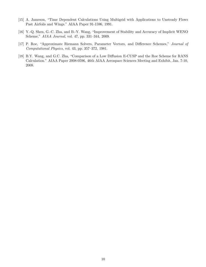
The projectile calculated in this paper is an cone-cylinder-finned configuration as shown in Fig. 1. Thelength of the projectile model is 12.5in and the diameter is 1.25in. The cone nose is 3.5 in long and theafter-body length is 9 in. Four fins are located at the end of the projectile. Each fin has the dimension of1.25in in long, 1.25in in height and 1in in thickness. The Mach number is 0.752 and Reynolds number is400000.

The computational mesh for the projectile model is in a O-type shape as shown in Fig. 2. Two differentdomain sizes of computational model are tested for considering the effect of the far-field boundary on theresults. One model is 3 times body length away from the model in all the three directions. The other meshhas a bigger domain, which uses a large domain mesh surrounding a smaller mesh domain. The final sizeof the computational domain is about 40 times of the body length of the projectile in all the directions. Toavoid singular point at the tip of the nose, a small tip ”O-type” block is created. Fig. 2 shows a 3-D viewof the full projectile mesh. The total number of grid points of the small computational domain is about7 million with 184 blocks. The mesh size of the large domain is about 14 million with 328 blocks. Fig. 3shows an expanded view of the grid in the small mesh. The first wall grid point spacing is at Y+ value ofabout 1.0 for both the meshes. The growth rate of the grids away from the solid wall is 1.25.

The total pressure, total temperature and flow angle are specified at computational domain inlet as theboundary conditions. The static pressure at the outlet is specified to determine the freestream Mach num-ber. In the computation, the free stream flow is kept horizontal. For a flow with an angle of attack(AoA),the mesh is rotated to create the AoA as demonstrated in Fig. 3.

6

4 Results and Discussion

The simulations are performed with parallel computing with about 40,000-50,000 cells in each mesh block.The calculations took about 10 hours to converge for steady simulation and 168 hours for the unsteadyDDES calculation. The unsteady calculation reaches the stable solution at about 250 characteristic time.The solution residuals are reduced at least 2 orders of magnitude within each physical time step andthe aerodynamic coefficients vary less than 0.1% over the last 100 time steps. The aerodynamic forcecoefficients are the determining factor in convergence.

To accurately predict wall friction, the mesh near the solid surface is refined. However, the quality of themesh may decrease due to the high aspect ratio as the number of grid points is increased in the boundarylayer. To have a suitable mesh density with acceptable CPU time and numerical accuracy, three differentgrid distributions are tested for grid convergence. The first mesh(Mesh1) is to make sure y+=1 on everysolid wall surface, including the leading edge, the tip surfaces of the fins and solid surface at the leadingedge of the nose. The second one(Mesh2) is to keep the same grid distribution as mesh1, except neglectingthe effect of small walls, including the surfaces at the leading edge and the tips of the fins, and the surfaceat the leading edge of the nose. Coarse grid distribution are used on those small wall surfaces and wallfunction boundary conditions are employed for Mesh2. To study the effect of y+ on the forces calculation,a third computational mesh (Mesh3) with y+ value equal to 6 is tested. All cases are run at AoA=0◦ withRANS model. The Mach number using in the grid convergence test is 0.677. The computed axial forceswith different meshes are presented in Table 1. We can see that the predicted force and moment fromMesh1 and Mesh2 are almost the same and closer to experiment data than that of Mesh3. The computedy+ of Mesh2 and Mesh3 at wall surface are shown in Fig. 4. It can be seen that y+=1.0 around thecylinder body are achieved in Mesh2. Therefore, Mesh2 is used in the unsteady DDES simulation.

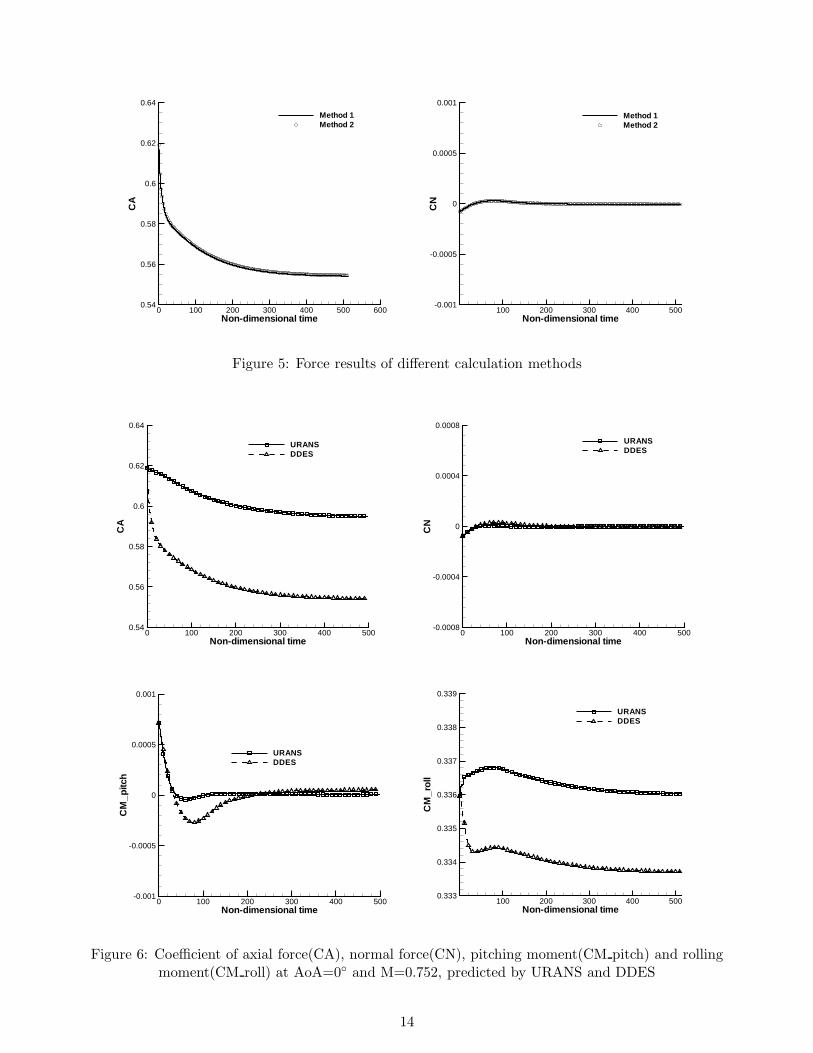
To reduce the uncertainty in the drag prediction, two different ways of wall shear stress calculation aredeveloped. Method 1 is based on the velocity gradient near the wall, in which the tangential velocityand the distance of the first cell center away from the wall are calculated. The other method (Method 2)extracts the shear stress directly from the viscous term of the Navier-Stokes equations. The results areshown in 5. It is shown that both results are in excellent agreement.

The time history of CA, CN, CM pitching and CM roll at AoA=0◦ and M=0.752 are shown in Fig. 6.The results of DDES method are compared with those of URANS. Both simulations are started from thesame RANS results. The predicted drag of DDES agree better with the experiment than the URANS. Thedifference of the drag prediction by DDES and URANS in the subsonic regime indicates that the unsteadywake flow impacts the upstream side forces. The roll moment from the URANS follows the same trendsas that of DDES.

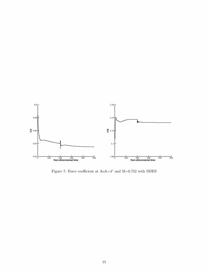
The DDES force and moment convergence history of CA, CN, CM pitching and CM roll at AoA=4◦

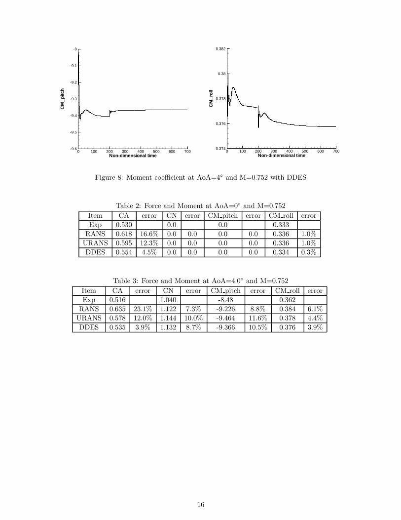
and M=0.752 are shown in Fig. 7 and Fig. 8. The URANS is used for the first 2000 time steps and thecalculation is switched to DDES. Fig. 8 shows that there are discontinuities in the convergence historieswhen the calculation is switched from URANS to DDES.

The results of RANS, URANS and DDES at AoA=0◦ and M=0.752 are summarized in Table 2. Fromthe table, DDES significantly reduce the axial force prediction error to about 4.5%, URANS has an errorof 12.3%, and RANS has an error of 16.6%. DDES is demonstrated to have the best accuracy among thethree methods. The URANS gives more accurate results than the steady state RANS because the vortexvortex shedding in the wake region is unsteady. All three methods have excellent agreement in predictingthe rolling moment. The predicted normal force and pitching moment are close to zero at AoA=0◦ as theexperiment since the geometry is mostly axi-symmetric except the fins that generate circumferential force.

The comparisons of different methods at AoA=4◦ and M=0.752 are shown in Table 3. The axial forcepredicted by DDES has an error of 3.9% compared with the experiment, significantly more accurate thanthat predicted by URANS with an error of 12%. For the nomal forces, the URANS and DDES have thedeviation about 10.0% and 8.7% respectively. The DDES is again more accurate than the URANS even

7

though the deviation is greater than the axial force.

Table 4 and Table 5 present the the breakdowns of the normal and axial forces of each componentincluding the projectile main body, the base surface, and the fins. In the table, CLp is the lift contributedby pressure, CLv is the lift contributed by viscous shear stress lift, CDp is the drag contributed by pressureand CDv is the drag contributed by the viscous shear stresses. The predicted friction drags are almost thesame between the URANS and DDES for both the case of at AoA=0◦ or AoA=4◦. The reason is thatwithin the wall boundary layer, URANS is also used by DDES. For the predicted pressure drag, URANSand DDES are quite different. At AoA=0◦, CDp predicted by URANS is about 10% greater than that ofDDES. At AoA=4◦, it is about 9.5% larger. The pressure value at the base redicted by DDES is about 4%greater than that of URANS, which results in a smaller overall drag since the predicted drag of the mainbody are about the same. Drag contribution of the fin is about 36% of the total drag at AoA=0◦ and isincreased to 41% at AoA=4◦. The pressure drag predicted by DDES is smaller than that of URANS.

Fig. 9 shows the Mach contours obtained by URANS and DDES at AoA=0◦ and M=0.752 at the mid-plane. Both plots show similar flow structures over the projectile. The vortex shedding at the trailing edgeof the projectile is captured as shown in Fig. 10. The flow field at AoA=4◦ has similar flow structure asthe case at AoA=0◦. Fig. 11 shows the velocity vector field behind the fins. It shows the fin tip vorticesdue to the lift that creates the the roll moment and cause the body to spin with magnus effect. Fig.12illustrates instantaneous entropy contours, which indicates that the wake region suffers high loss due tothe base flow. Fig 13 is the Mach number contour in the wake region for both the AoA=0◦ and 4◦. Thewakes of the fins merge with the wake of the base surface.

Fig.14 shows the instantaneous static pressure contour predicted by DDES at M=0.752. The base areahas very low pressure that contributes to the base drag. Fig. 15 shows the surface pressure contours andthe surface pressure distributions of the mid plane on the lower and upper side. At AoA=0◦, the pressureis symmetric with no lift. The pressure decreases rapidly from leading edge to the cone-cylinder transitionpoint due to the converging area, and then increase rapidly after that due to fast area expansion. At AoA=4◦, the pressure variation trend along the body is similar to that at AoA= 0◦, but the pressures on theupper and lower side is largely different due to generating the lift. The fin surface pressure coefficientspredicted by DDES at AoA=0◦ and 4◦ are shown in Fig.16 and Fig.17, respectively. At AoA=0◦, the finsdo not generate lift and the pressure distributions on the 4 fins are the same. At AoA=4◦, the fin surfacepressure are not symmetric due to the lift generation.

5 Conclusions

High order accuracy numerical algorithm is utilized to predict the force and moment of a guided projectilewith DDES model. The DDES demonstrates its excellent ability to accurately simulate the vortical baseflow. The predicted drag coefficients for the projectile by the DDES shows a good agreement with theexperiment. For an ARDEC Projectile at M=0.752, AoA=0◦ and 4◦, the DDES significantly reduces theaxial force prediction error to about 4%, whereas the URANS has an error of 12%, and the RANS has anerror of 16% to 23%. The primary difference of the drag prediction between the DDES and URANS is thepressure drag prediction in the base region. The DDES is demonstrated to be superior to the URANS forthe projectile flow prediction due to more accurate base large vortex structures and pressure simulation.

8

6 Acknowledgment

The simulation is conducted at the high performance super-computing center of Oak Ridge NationalLab, Army supercomputer center, and the center for computational sciences at the University of Miami.

References

[1] P.R. Spalart, W.H. Jou, M. Strelets, and S.R. Allmaras, “Comments on the Feasibility of LES forWings, and on a Hybrid RANS/LES Approach.” Advances in DNS/LES, 1st AFOSR Int. Conf. onDNS/LES, Greyden Press, Columbus, H., Aug. 4-8, 1997.

[2] B.Y. Wang, and G.C. Zha, “ Detached Eddy Simulations of a Circular Cylinder Using a Low Diffu-sion E-CUSP and High-Order WENO Scheme.” AIAA Paper 2008-3855, AIAA 38th Fluid DynamicsConference, Seattle, Washington, June 23-26, 2008.

[3] S. Kapadia, and S. Roy, “Detached Eddy Simulation of Turbine Blade Cooling.” AIAA Paper 2003-3632, the 36th Thermophysics Conference, Orlando, Florida, 23 - 26 June 2003.

[4] P. Spalart, “Young-Person’s Guide to Detached-Eddy Simulation Grids.” NASA/CR-2001-211032,2001.

[5] P.R. Spalart, S. Deck, M. Shur, and K.D. Squires, “A New Version of Detached-Eddy Simulation,Resistant to Ambiguous Grid Densities,” Theoritical and Computational Fluid Dynamics, vol. 20,pp. 181–195, 2006.

[6] F.R. Menter, and M. Kuntz, “Adaptation of Eddy-Viscosity Turbulence Models to Unsteady SeparatedFlow Behind Vehilces, The Aerodynamics of Heavy Vehicles: Trucks, Buses and Trains, Edited by

McCallen, R. Browand, F. and Ross, J. ,” Springer, Berlin Heidelberg New York, 2004, 2-6 Dec.2002.

[7] Im, H.-S., and Zha, G.-C., “Delayed Detached Eddy Simulation of Airfoil Stall Flows Using High-OrderSchemes,” Journal of Fluids Engineering, vol. 136, 2014.

[8] P. Weinacht, W. B. Sturek, and L. B. Schiff, “Navier-Stokes Predictions of Pitch-Damping for Axisym-metric Shell Using Steady Coning Motion,” Journal of Spacecraft and Rockets, vol. 34, pp. 753–761,2013.

[9] J. DeSpirito and K. R. Heavy, “CFD Computations of Magnus Moment and Roll Damping Momentof Spinning projectile.” AIAA Atmospheric Flight Mechanics Conference and Exhibit, August 16 -19, 2004.

[10] J. Sahu and K. R. Heavy, “Parallel CFD Computations of Projectile Aerodynamics with a FlowControl Mechanism,” Computers Fluids, 2013.

[11] G.C. Zha, Y.Q. Shen, and B.Y. Wang, “An Improved Low Diffusion E-CUSP Upwind Scheme,” 2011.

[12] B.-Y. Wang, and G.-C. Zha, “A General Sub-Domain Boundary Mapping Procedure For StructuredGrid CFD Parallel Computation,” AIAA Journal of Aerospace Computing, Information, and Com-

munication, vol. 5, pp. 425–447, 2008.

[13] P.R. Spalart, and S.R. Allmaras, “A One-equation Turbulence Model for Aerodynamic Flows.” AIAA-92-0439, 1992.

[14] M. Shur, P.R. Spalart, M. Strelets, and A. Travin, “Detached-Eddy Simulation of an Airfoil at HighAngle of Attack”, 4th Int. Symp. Eng. Turb. Modelling and Measurements, Corsica.” May 24-26, 1999.

9

[15] A. Jameson, “Time Dependent Calculations Using Multigrid with Applications to Unsteady FlowsPast Airfoils and Wings.” AIAA Paper 91-1596, 1991.

[16] Y.-Q. Shen, G.-C. Zha, and B.-Y. Wang, “Improvement of Stability and Accuracy of Implicit WENOScheme,” AIAA Journal, vol. 47, pp. 331–344, 2009.

[17] P. Roe, “Approximate Riemann Solvers, Parameter Vectors, and Difference Schemes,” Journal of

Computational Physics, vol. 43, pp. 357–372, 1981.

[18] B.Y. Wang, and G.C. Zha, “Comparison of a Low Diffusion E-CUSP and the Roe Scheme for RANSCalculation.” AIAA Paper 2008-0596, 46th AIAA Aerospace Sciences Meeting and Exhibit, Jan. 7-10,2008.

10

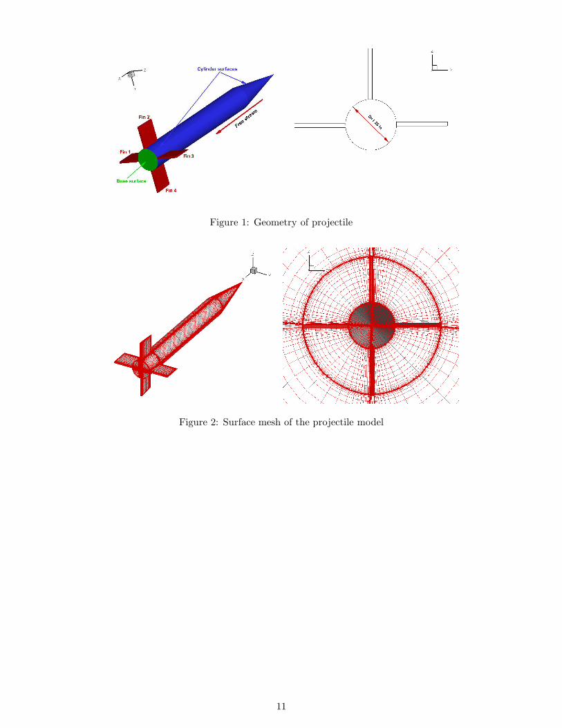
Figure 1: Geometry of projectile

Figure 2: Surface mesh of the projectile model

11

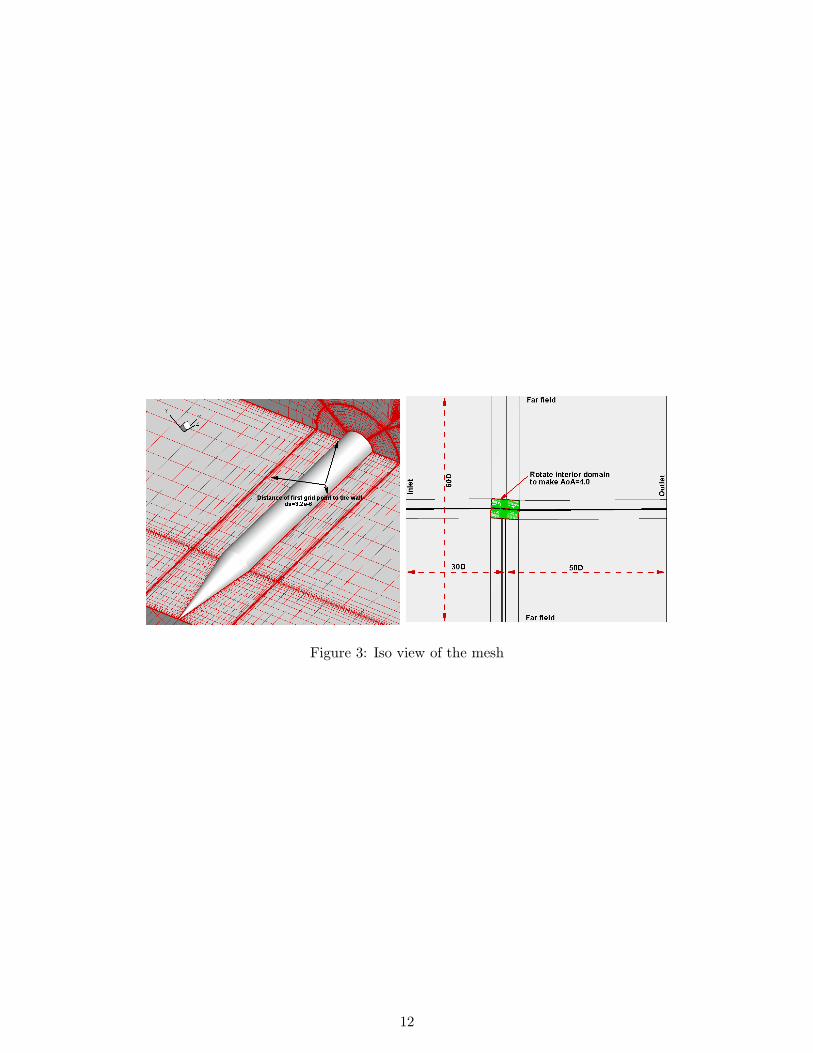
Figure 3: Iso view of the mesh

12

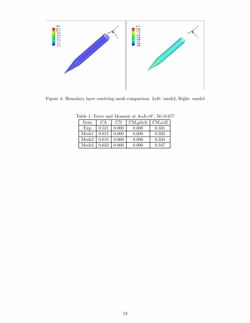
Figure 4: Boundary layer resolving mesh comparison. Left: mesh2, Right: mesh3

Table 1: Force and Moment at AoA=0◦, M=0.677

Item CA CN CM pitch CM roll

Exp 0.521 0.000 0.000 0.331

Mesh1 0.615 0.000 0.000 0.334

Mesh2 0.618 0.000 0.000 0.334

Mesh3 0.632 0.000 0.000 0.347

13

Non-dimensional time

CA

0 100 200 300 400 500 6000.54

0.56

0.58

0.6

0.62

0.64

Method 1Method 2

Non-dimensional time

CN

100 200 300 400 500-0.001

-0.0005

0

0.0005

0.001

Method 1Method 2

Figure 5: Force results of different calculation methods

Non-dimensional time

CA

0 100 200 300 400 5000.54

0.56

0.58

0.6

0.62

0.64

URANSDDES

Non-dimensional time

CN

0 100 200 300 400 500-0.0008

-0.0004

0

0.0004

0.0008

URANSDDES

Non-dimensional time

CM

_pi

tch

0 100 200 300 400 500-0.001

-0.0005

0

0.0005

0.001

URANSDDES

Non-dimensional time

CM

_rol

l

100 200 300 400 5000.333

0.334

0.335

0.336

0.337

0.338

0.339

URANSDDES

Figure 6: Coefficient of axial force(CA), normal force(CN), pitching moment(CM pitch) and rollingmoment(CM roll) at AoA=0◦ and M=0.752, predicted by URANS and DDES

14

Non-dimensional time

CA

0 100 200 300 400 5000.52

0.54

0.56

0.58

0.6

Non-dimensional time

CN

0 100 200 300 400 5001.08

1.1

1.12

1.14

1.16

Figure 7: Force coefficient at AoA=4◦ and M=0.752 with DDES

15

Non-dimensional time

CM

_pi

tch

0 100 200 300 400 500 600 700-9.6

-9.5

-9.4

-9.3

-9.2

-9.1

-9

Non-dimensional time

CM

_rol

l

0 100 200 300 400 500 600 7000.374

0.376

0.378

0.38

0.382

Figure 8: Moment coefficient at AoA=4◦ and M=0.752 with DDES

Table 2: Force and Moment at AoA=0◦ and M=0.752

Item CA error CN error CM pitch error CM roll error

Exp 0.530 0.0 0.0 0.333

RANS 0.618 16.6% 0.0 0.0 0.0 0.0 0.336 1.0%

URANS 0.595 12.3% 0.0 0.0 0.0 0.0 0.336 1.0%

DDES 0.554 4.5% 0.0 0.0 0.0 0.0 0.334 0.3%

Table 3: Force and Moment at AoA=4.0◦ and M=0.752

Item CA error CN error CM pitch error CM roll error

Exp 0.516 1.040 -8.48 0.362

RANS 0.635 23.1% 1.122 7.3% -9.226 8.8% 0.384 6.1%

URANS 0.578 12.0% 1.144 10.0% -9.464 11.6% 0.378 4.4%

DDES 0.535 3.9% 1.132 8.7% -9.366 10.5% 0.376 3.9%

16

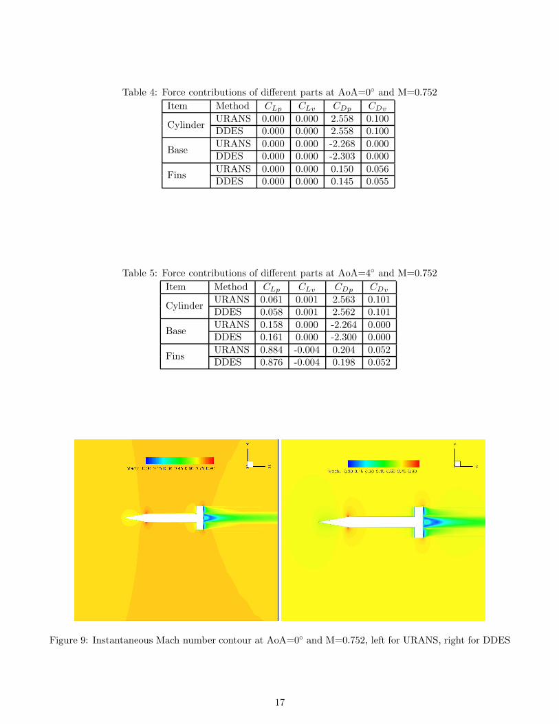
Table 4: Force contributions of different parts at AoA=0◦ and M=0.752

Item Method CLp CLv CDp CDv

CylinderURANS 0.000 0.000 2.558 0.100DDES 0.000 0.000 2.558 0.100

BaseURANS 0.000 0.000 -2.268 0.000DDES 0.000 0.000 -2.303 0.000

FinsURANS 0.000 0.000 0.150 0.056DDES 0.000 0.000 0.145 0.055

Table 5: Force contributions of different parts at AoA=4◦ and M=0.752

Item Method CLp CLv CDp CDv

CylinderURANS 0.061 0.001 2.563 0.101DDES 0.058 0.001 2.562 0.101

BaseURANS 0.158 0.000 -2.264 0.000DDES 0.161 0.000 -2.300 0.000

FinsURANS 0.884 -0.004 0.204 0.052DDES 0.876 -0.004 0.198 0.052

Figure 9: Instantaneous Mach number contour at AoA=0◦ and M=0.752, left for URANS, right for DDES

17

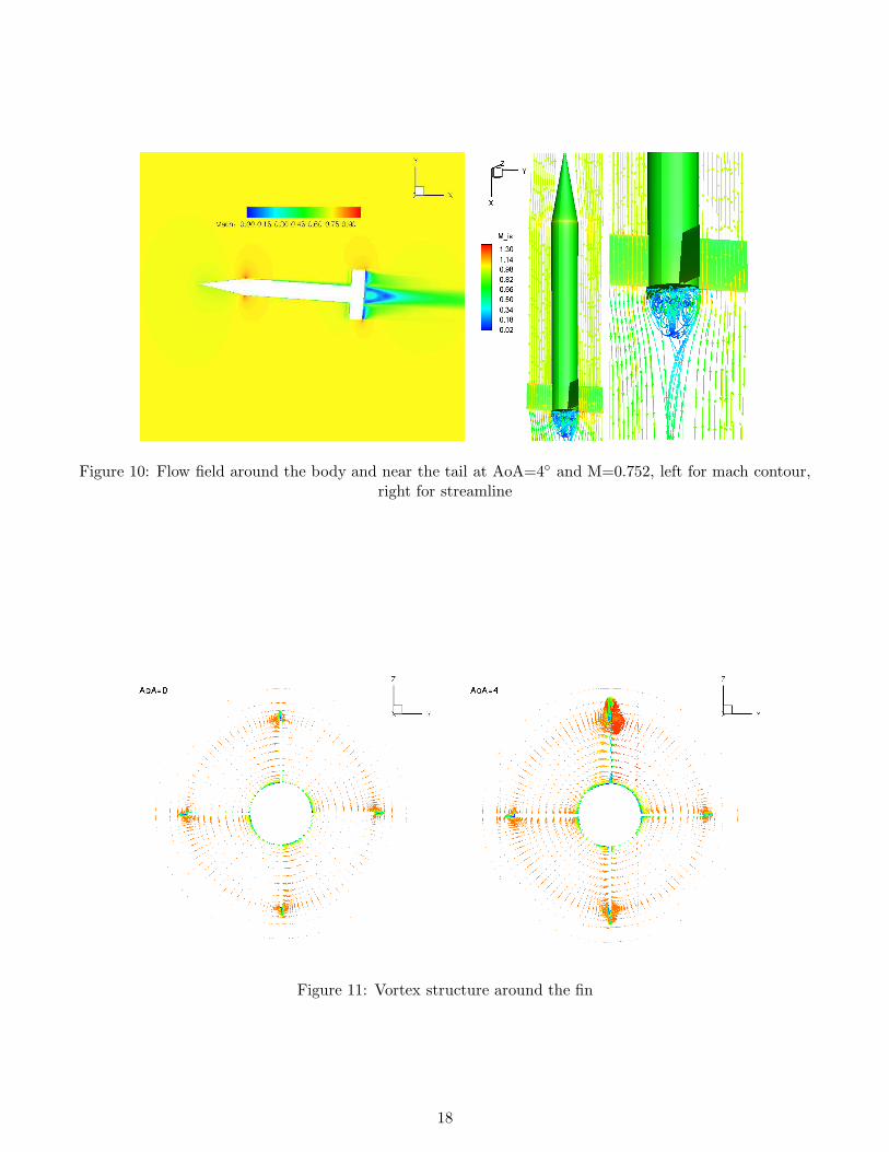
Figure 10: Flow field around the body and near the tail at AoA=4◦ and M=0.752, left for mach contour,right for streamline

Figure 11: Vortex structure around the fin

18

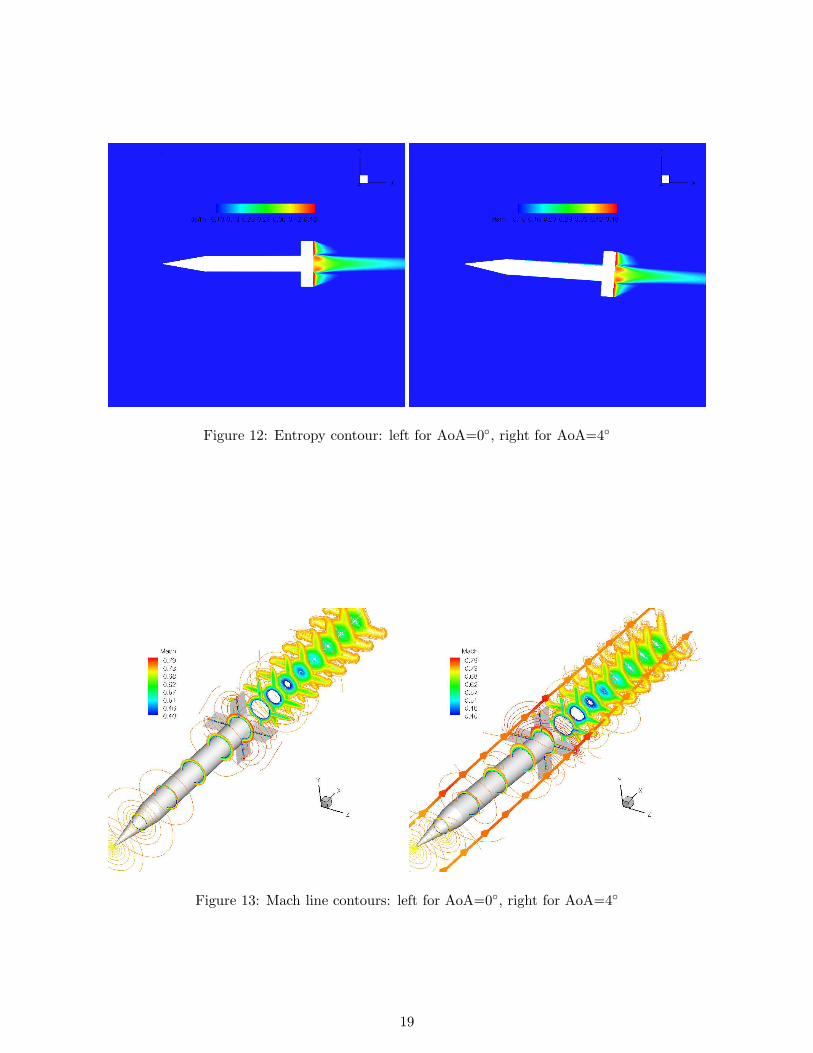
Figure 12: Entropy contour: left for AoA=0◦, right for AoA=4◦

Figure 13: Mach line contours: left for AoA=0◦, right for AoA=4◦

19

Figure 14: Static pressure contour: left for AoA=0◦, right for AoA=4◦

Figure 15: Computed Surface Pressure: left for AoA=0◦, right for AoA=4◦

20

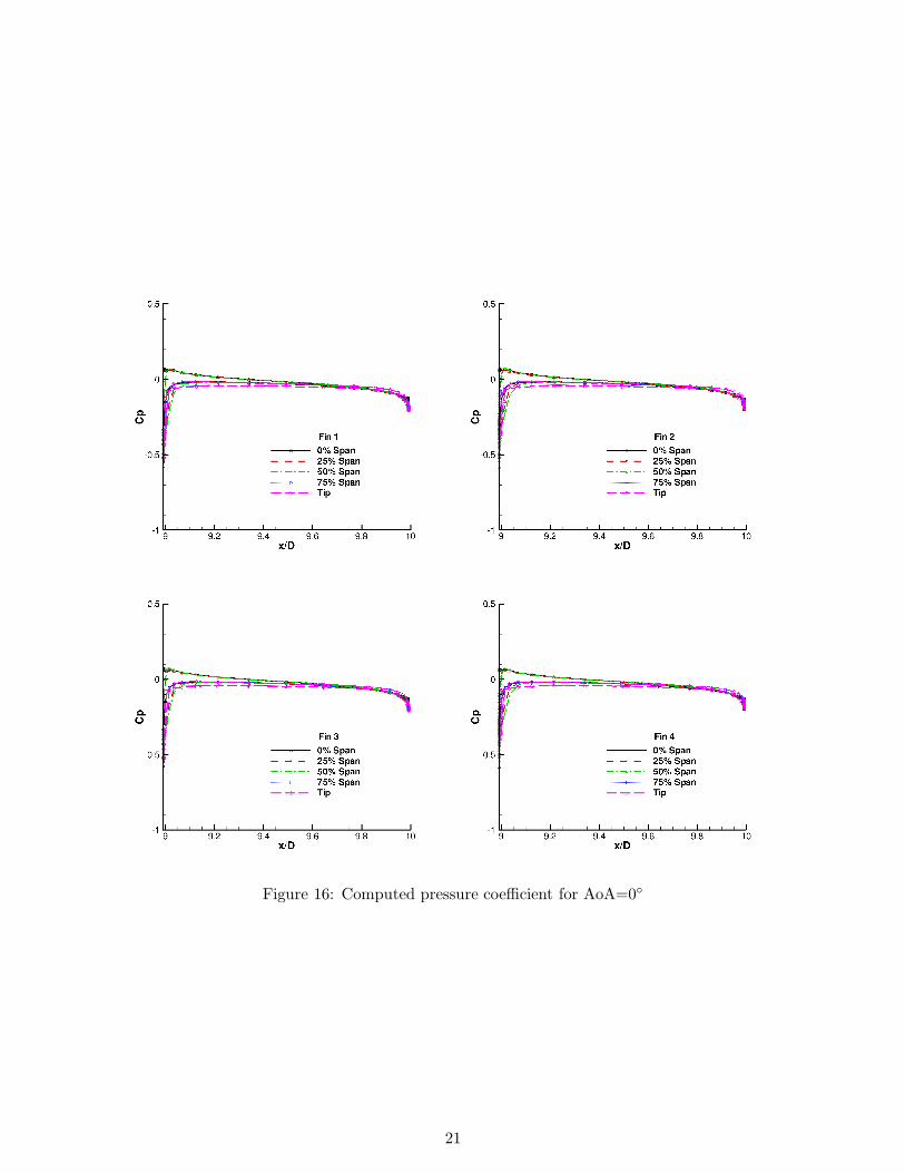
Figure 16: Computed pressure coefficient for AoA=0◦

21

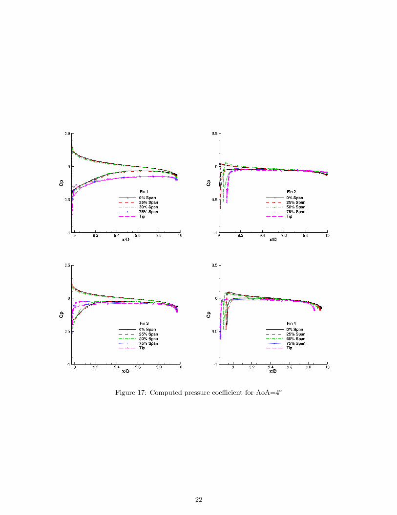
Figure 17: Computed pressure coefficient for AoA=4◦

22