aerospace

Article

Non-Propellant Eddy Current Brake and Traction in SpaceUsing Magnetic Pulses

Yi Zhang †, Qiang Shen †, Liqiang Hou † and Shufan Wu *

Citation: Zhang, Y.; Shen, Q.; Hou,

L.; Wu, S. Non-Propellant Eddy

Current Brake and Traction in Space

Using Magnetic Pulses. Aerospace

2021, 8, 24. https://doi.org/10.3390/

aerospace8020024

Academic Editor: George Z.H. Zhu

Received: 8 December 2020

Accepted: 18 January 2021

Published: 20 January 2021

Publisher’s Note: MDPI stays neutral

with regard to jurisdictional claims in

published maps and institutional affil-

iations.

Copyright: © 2021 by the authors.

Licensee MDPI, Basel, Switzerland.

This article is an open access article

distributed under the terms and

conditions of the Creative Commons

Attribution (CC BY) license (https://

creativecommons.org/licenses/by/

4.0/).

School of Aeronautics and Astronautics, Shanghai Jiao Tong University, No. 800, Dongchuan Road,Minhang District, Shanghai 200240, China; zhang_yi_951112@sjtu.edu.cn (Y.Z.); qiangshen@sjtu.edu.cn (Q.S.);hlq@sjtu.edu.cn (L.H.)* Correspondence: shufan.wu@sjtu.edu.cn; Tel.: +86-34208597† These authors contributed equally to this work.

Abstract: The safety of on-orbit satellites is threatened by space debris with large residual angularvelocity and the space debris removal is becoming more challenging than before. This paper exploresthe non-contact despinning and traction problem of high-speed rotating targets and proposes aneddy current brake and traction technology for space targets without any propellant consumption.The principle of the conventional eddy current brake is analyzed in this article and the conceptof eddy current brake and traction without propellant is put forward for the first time. Secondly,according to the key technical requirements, a brand-new structure of a satellite generating artificialmagnetic field is designed accordingly. Then the control mechanism of eddy current brake andtraction without propellant is analyzed qualitatively by simplifying the model and conditions. Then,the magnetic pulse control method is proposed and analyzed quantitatively. Finally, the feasibility ofthe technology is verified by the numerical simulation method. According to the simulation results,the eddy current brake and traction technology based on magnetic pulses can make the angularspeed of target decrease linearly without propellant during the process. This technology has hugeadvantages compared with conventional eddy current brake technology in terms of efficiency andreduced propellant consumption.

Keywords: eddy current; debris removal; electromagnetic traction; despinning

1. Introduction

With the development of aerospace technology, human activities in space are becomingmore frequent. The space debris left by human beings in space, especially in the Earth’sorbit, is increasing at a tremendous rate because of the rapid deployment of large scale lowearth orbit constellations, such as the plan of more than 20,000 satellites proposed by twodozen companies [1]. Space debris mainly consists of abandoned satellites, rocket finalstage devices and collision debris [2]. According to the results of computer simulation,even if we were to stop all space activities and comply with the 25-year removal guidelines,the amount of space debris will continue to grow, and the density of space debris willincrease as well due to random collisions. This transitive phenomenon is called the “Kesslerphenomenon” [3]. Actively removing orbital debris is the only feasible solution to controlthe spread of debris in the future.

Unlike satellites that operate stably in orbit, the motion state of space debris is irregularand it is likely that there is a large residual angular momentum due to passivation, collision,environmental torque, etc. Existing contact debris despinning technologies such as flexiblebrush [4,5], mechanical pulse [6], space manipulator technology or deceleration brushdespinning technology relying on manipulators [7] require a relatively static situationbetween the service satellite and the target. This requires extremely high accuracy inmodeling and control and is prone to collision risks. For irregular targets that rotate at highspeed, there is no way to make safe contact. However, the more researched space rope

Aerospace 2021, 8, 24. https://doi.org/10.3390/aerospace8020024 https://www.mdpi.com/journal/aerospace

Aerospace 2021, 8, 24 2 of 16

net method [8] also has unsafe factors such as excessive force at the moment of contact.Non-contact despinning technology is a hot topic that has emerged in recent years. Itsapplication methods include the compressed gas method [9], ion beam method [10,11],electrostatic force method [12] and laser ablation method [13,14] and other new conceptsand methods. Electricity, magnetism or jet-flow are usually adopted to generate despinningtorque. Since there is no direct contact, the magnitude of the despinning torque is usuallysmall, at the level of mN·m. Therefore, the target has little impact on the service satelliteand robotic arm during the process of despinning and the time required is usually atthe level of hundreds of hours. During this period, the position and attitude accuracyrequirements are low, and the effective working distance has a large range of variation. Inorder to overcome the shortcomings of the existing contact and non-contact despinningtechnologies, it is necessary to seek a more effective non-contact despinning method.

Electromagnetic eddy current despinning is a method of despinning based on theelectromagnetic eddy current damping effect. It is a non-contact depinning method thatuses the damping moment generated by the rotating conductor to cut the magnetic lineof induction in an artificial magnetic field. This torque is also called the eddy currenttorque. The earliest systematic study of eddy current torque came from NASA’s studyon the rotation characteristics of a near-Earth satellite in the Earth’s magnetic field in1965 [15]. It was the first work to put forward the inherent characteristics of conductors-theconcept of electromagnetic tensor, and give the eddy current torque expression. Due tothe weak geomagnetic effect, the ultimate research goal was to explore the long-termeffect of the average eddy current induced by the geomagnetism on the satellite. Later,researchers mostly carried out research and experiments on the basis of this theoreticalmodel. The concept of eddy current despinning was formally proposed in the 1980s.Scientists conducted more in-depth research on the eddy current torque generated byrotating magnets induced by artificial electromagnetic fields. In 1995, the American scientistKadaba [16] conducted an engineering feasibility study on eddy current despinning forspacecrft, and proposed an electromagnetic eddy current despinning scheme based onhigh-temperature superconducting coils.

In the past decade, the need for space debris removal has become increasingly urgent,and new concepts including electromagnetic eddy current despinning methods have onceagain become research hotspots. Sugai studied an electromagnetic brake system based ona robotic arm [17], using a smart robotic arm to carry electromagnetic brake pads closeto the target surface for damping braking, which is similar to the method of the robotarm decelerating brush proposed by the Japan Aerospace Agency in 2006 [7]. In 2019,Xie et al. designed new permanent magnet array brake pads and dual manipulator structureand established dynamic model further verifying the effectiveness of this approach [18].However, the distance between the eddy current brake and the target is limited to a verysmall range in above method, which cannot really solve the collision safety problem ofcontact despinning. In 2015, Ortiz Gómez et al. at the University of Southampton usedAriane H10 final stage despinning as an application scenario, focusing on explaining themechanism of eddy current depinning [19,20]. and they constructed a standardized eddycurrent force and eddy current torque model. In 2019, Liu et al. conducted dynamicmodeling for eddy current brake in three-dimensional environment on the basis of existingresearches, and designed nonlinear sliding model controller, which further verified thefeasibility of eddy current despinning technology [21]. However, the existing eddy currentdespinning technology still relies on the thrust device of the service satellite to maintainthe relative position, which often lasts as long as several days. Moreover, the efficiencydepends on the target speed. When the target speed drops, the despinning efficiency willbe significantly reduced. The above problems greatly limit the application process of eddycurrent despinning technology. In order to break through the bottleneck of the applicationof eddy current despinning technology, this paper develop a non-propellant eddy currentdespinning and traction technology based on magnetic pulses. Compared with [19–21],

Aerospace 2021, 8, 24 3 of 16

the proposed method makes the despinning process get rid of the propellant limitation,and enables the target speed to decrease steadily.

This article is outlined as follows. In the second section, the article introduces thetechnical details of the non-propellant eddy current brake and traction technology basedon magnetic pulse, including basic theory (Section 2.1), device design (Section 2.2), analysismethod (Section 2.3) And control strategy (Section 2.4). In the third section, the simulationresults of this technology are shown. The effectiveness and superiority of the technologyproposed in this paper are proved from three aspects of control strategy (Section 3.1),efficiency (Section 3.2) and traction control effect (Section 3.3).

2. Non-Propellant Eddy Current Brake and Traction Using Magnetic Pulse

In this section, non-propellant eddy current brake and traction technology based onmagnetic pulse is introduced in detail. Firstly, the origin of the concept of non-propellanteddy current brake is explained. Secondly, according to the key technical details, an overallplan to realize the technology is designed and the model is simplified in order to analyzethe technical principles. Finally, a unique magnetic pulse control method is proposed.

2.1. Basic Theory

Natalia Ortiz Gómez et al. analyzed the mechanism of eddy current despinning indetail in [19,20], and studied the traction problem under the conventional mode. Accordingto the derivation results in the literature, the object rotating in a fixed magnetic field canbe damped by the eddy current torque T. The eddy current torque calculation equation isshown as follows:

T =(

µe f f M(w× BGt))× BGt (1)

where, w is the relative rotation angular velocity vector between the target and servingsatellite, M is the electromagnetic tensor of the target, which is the inherent electromagneticproperty of the conductor target, determined by the material and structure of the conductor.The target selected in this paper is a metal spherical shell, and its electromagnetic tensor is:

M = 2πσtR4t etE/3 (2)

where, M is the third-order diagonal matrix, E third-order unit matrix, σt is the conductivityof the target conductive material, Rt is the radius of the spherical shell, et is the thickness ofthe spherical shell. µeff is the effective factor of non-uniform magnetic field, used to correctthe eddy current torque error caused by non-uniform magnetic field.

The object rotating in a fixed magnetic field is also affected by the eddy current forceF, so that the angular momentum conservation of the system can be satisfied. The eddycurrent force calculation equation is shown as follows:

F = µe f f MΛGt(w× BGt) (3)

where, ΛGt represents the Jacobian matrix of the magnetic field, the matrix equation isshown as follows:

ΛGt =3µ0

4πr4

m//

−2 0 00 1 00 0 1

+ m⊥

0 1 01 0 00 0 0

(4)

where, m is the magnetic moment of the coil, µ0 is permeability of vacuum, r is the distancebetween target and service satellite.

2.2. Device Design

This section first analyzes the principle of the conventional eddy current despinningmethod. Then, in order to further improve the efficiency and reduce propellant consump-

Aerospace 2021, 8, 24 4 of 16

tion, we proposed the concept of eddy current despinning and traction based on a variablemagnetic field. Finally, a new device was designed according to the requirements.

The conventional eddy current despinning mode is shown in Figure 1. The servicesatellite applies a constant magnetic field to the target, so that the target is subject to eddycurrent damping torque. Eddy current forces are generated at the same time, satisfyingthe angular momentum conservation. However, the eddy current force generated bythe coupling of the target angular velocity and the applied magnetic field is regardedas a non-linear interference and needs to be offset by the attitude orbit controller of theservice satellite.

Aerospace 2021, 8, x FOR PEER REVIEW 4 of 17

where, m is the magnetic moment of the coil, μ0 is permeability of vacuum, r is the distance between target and service satellite.

2.2. Device Design This section first analyzes the principle of the conventional eddy current despinning

method. Then, in order to further improve the efficiency and reduce propellant consump-tion, we proposed the concept of eddy current despinning and traction based on a variable magnetic field. Finally, a new device was designed according to the requirements.

The conventional eddy current despinning mode is shown in Figure 1. The service satellite applies a constant magnetic field to the target, so that the target is subject to eddy current damping torque. Eddy current forces are generated at the same time, satisfying the angular momentum conservation. However, the eddy current force generated by the coupling of the target angular velocity and the applied magnetic field is regarded as a non-linear interference and needs to be offset by the attitude orbit controller of the service satellite.

Figure 1. Schematic diagram of conventional mode.

According to Equation (3), the eddy current force is mainly controlled by the relative angular velocity and magnetic field strength. The relative angular velocity is essentially the angular velocity of the target relative to the static magnetic field. When the magnetic field is variable, the relative angular velocity is determined by the angular velocity of the target and the angular velocity of the magnetic field. As long as the hardware conditions permit, the variable magnetic field is able to dominate the direction and magnitude of the target eddy current force, achieving arbitrary control of the target.

Figure 2 shows our newly designed despinning device. According to the concept of eddy current brake using variable magnetic field, the despinning device needs to be equipped with at least three non-coplanar magnetic field generators to meet the needs of generating arbitrary magnetic fields. In order to make the distance between the satellite and the target adjustable, the despinning device needs to have a telescopic structure. Due to the application of superconducting technology, light and heat shielding needs to be designed for the magnetic generators, thereby reducing the power consumption of the satellite. In addition, the storage, transportation and launch of satellites need to meet ac-tual conditions, and the despinning device should also have a foldable design. It can main-tain the folded state during the storage, transportation and launch stages, enhancing the structural strength.

Figure 1. Schematic diagram of conventional mode.

According to Equation (3), the eddy current force is mainly controlled by the relativeangular velocity and magnetic field strength. The relative angular velocity is essentiallythe angular velocity of the target relative to the static magnetic field. When the magneticfield is variable, the relative angular velocity is determined by the angular velocity of thetarget and the angular velocity of the magnetic field. As long as the hardware conditionspermit, the variable magnetic field is able to dominate the direction and magnitude of thetarget eddy current force, achieving arbitrary control of the target.

Figure 2 shows our newly designed despinning device. According to the conceptof eddy current brake using variable magnetic field, the despinning device needs to beequipped with at least three non-coplanar magnetic field generators to meet the needs ofgenerating arbitrary magnetic fields. In order to make the distance between the satelliteand the target adjustable, the despinning device needs to have a telescopic structure. Dueto the application of superconducting technology, light and heat shielding needs to bedesigned for the magnetic generators, thereby reducing the power consumption of thesatellite. In addition, the storage, transportation and launch of satellites need to meetactual conditions, and the despinning device should also have a foldable design. It canmaintain the folded state during the storage, transportation and launch stages, enhancingthe structural strength.

Aerospace 2021, 8, x FOR PEER REVIEW 5 of 17

Figure 2. Diagram of service star structure.

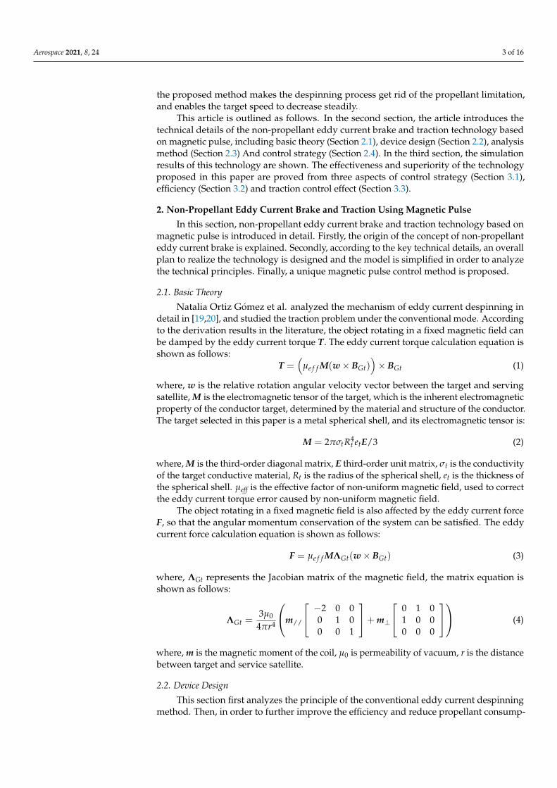
The electromagnetic coil structure in the Figure 2 is able to generate any magnetic field at the target. The coil realizes the adjustment of the working range and the storage function through the adjustable telescopic rod. The triangular column structure in the pic-ture can be retracted into the satellite star. The rotation nodes on the cylinder work with the slide rails together so that the coil structure can also be incorporated into the satellite star during launch. Figure 3 shows the fully folded service star structure.

Figure 3. Diagram of service satellite folding state.

In addition, the coil structure should also be specially treated as shown in Figure 4 so as to better shield the light and heat interference.

Figure 4. Diagram of the shielding structure.

Located in the center of the connecting rod in the Figure 4 is the superconducting cable and the coolant channel. The wire is gray, and the coolant path and loop are green and blue respectively. The black part of the primary connecting rod is the supporting

Figure 2. Diagram of service star structure.

Aerospace 2021, 8, 24 5 of 16

The electromagnetic coil structure in the Figure 2 is able to generate any magnetic fieldat the target. The coil realizes the adjustment of the working range and the storage functionthrough the adjustable telescopic rod. The triangular column structure in the picture canbe retracted into the satellite star. The rotation nodes on the cylinder work with the sliderails together so that the coil structure can also be incorporated into the satellite star duringlaunch. Figure 3 shows the fully folded service star structure.

Aerospace 2021, 8, x FOR PEER REVIEW 5 of 17

Figure 2. Diagram of service star structure.

The electromagnetic coil structure in the Figure 2 is able to generate any magnetic field at the target. The coil realizes the adjustment of the working range and the storage function through the adjustable telescopic rod. The triangular column structure in the pic-ture can be retracted into the satellite star. The rotation nodes on the cylinder work with the slide rails together so that the coil structure can also be incorporated into the satellite star during launch. Figure 3 shows the fully folded service star structure.

Figure 3. Diagram of service satellite folding state.

In addition, the coil structure should also be specially treated as shown in Figure 4 so as to better shield the light and heat interference.

Figure 4. Diagram of the shielding structure.

Located in the center of the connecting rod in the Figure 4 is the superconducting cable and the coolant channel. The wire is gray, and the coolant path and loop are green and blue respectively. The black part of the primary connecting rod is the supporting

Figure 3. Diagram of service satellite folding state.

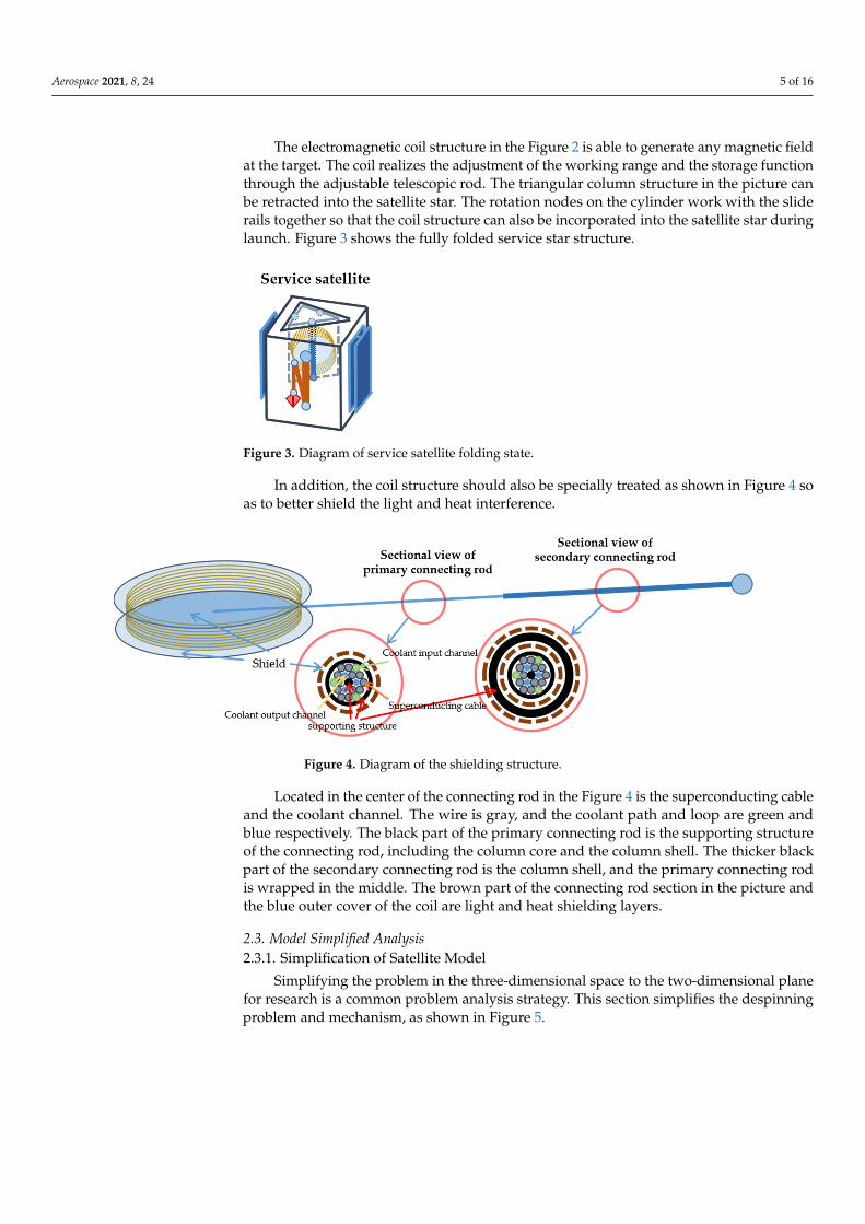
In addition, the coil structure should also be specially treated as shown in Figure 4 soas to better shield the light and heat interference.

Aerospace 2021, 8, x FOR PEER REVIEW 5 of 17

Figure 2. Diagram of service star structure.

The electromagnetic coil structure in the Figure 2 is able to generate any magnetic field at the target. The coil realizes the adjustment of the working range and the storage function through the adjustable telescopic rod. The triangular column structure in the pic-ture can be retracted into the satellite star. The rotation nodes on the cylinder work with the slide rails together so that the coil structure can also be incorporated into the satellite star during launch. Figure 3 shows the fully folded service star structure.

Figure 3. Diagram of service satellite folding state.

In addition, the coil structure should also be specially treated as shown in Figure 4 so as to better shield the light and heat interference.

Figure 4. Diagram of the shielding structure.

Located in the center of the connecting rod in the Figure 4 is the superconducting cable and the coolant channel. The wire is gray, and the coolant path and loop are green and blue respectively. The black part of the primary connecting rod is the supporting

Figure 4. Diagram of the shielding structure.

Located in the center of the connecting rod in the Figure 4 is the superconducting cableand the coolant channel. The wire is gray, and the coolant path and loop are green andblue respectively. The black part of the primary connecting rod is the supporting structureof the connecting rod, including the column core and the column shell. The thicker blackpart of the secondary connecting rod is the column shell, and the primary connecting rodis wrapped in the middle. The brown part of the connecting rod section in the picture andthe blue outer cover of the coil are light and heat shielding layers.

2.3. Model Simplified Analysis2.3.1. Simplification of Satellite Model

Simplifying the problem in the three-dimensional space to the two-dimensional planefor research is a common problem analysis strategy. This section simplifies the despinningproblem and mechanism, as shown in Figure 5.

Aerospace 2021, 8, 24 6 of 16

Aerospace 2021, 8, x FOR PEER REVIEW 6 of 17

structure of the connecting rod, including the column core and the column shell. The thicker black part of the secondary connecting rod is the column shell, and the primary connecting rod is wrapped in the middle. The brown part of the connecting rod section in the picture and the blue outer cover of the coil are light and heat shielding layers.

2.3. Model Simplified Analysis 2.3.1. Simplification of Satellite Model

Simplifying the problem in the three-dimensional space to the two-dimensional plane for research is a common problem analysis strategy. This section simplifies the despinning problem and mechanism, as shown in Figure 5.

Figure 5. Simplified model.

The service satellite has two connecting rods and magnetic field generators placed perpendicular to each other, which can generate a magnetic field of any size and direction in the xOy plane at the target. The target rotation axis is always parallel to the z-axis di-rection. According to Equation (3), it can be seen that the eddy current force on the target is in the xOy plane. When the eddy current force F is given, it is not difficult to find from Figure 6 that the magnetic field needs to rotate in a specific direction at a specific angular velocity to meet the control requirements according to Equation (3). The magnetic field at this time is a variable periodic function, and the period is ΔTi.

Figure 6. Diagram of instantaneous eddy current force.

Figure 5. Simplified model.

The service satellite has two connecting rods and magnetic field generators placedperpendicular to each other, which can generate a magnetic field of any size and directionin the xOy plane at the target. The target rotation axis is always parallel to the z-axisdirection. According to Equation (3), it can be seen that the eddy current force on the targetis in the xOy plane. When the eddy current force F is given, it is not difficult to find fromFigure 6 that the magnetic field needs to rotate in a specific direction at a specific angularvelocity to meet the control requirements according to Equation (3). The magnetic field atthis time is a variable periodic function, and the period is ∆Ti.

Aerospace 2021, 8, x FOR PEER REVIEW 6 of 17

structure of the connecting rod, including the column core and the column shell. The thicker black part of the secondary connecting rod is the column shell, and the primary connecting rod is wrapped in the middle. The brown part of the connecting rod section in the picture and the blue outer cover of the coil are light and heat shielding layers.

2.3. Model Simplified Analysis 2.3.1. Simplification of Satellite Model

Simplifying the problem in the three-dimensional space to the two-dimensional plane for research is a common problem analysis strategy. This section simplifies the despinning problem and mechanism, as shown in Figure 5.

Figure 5. Simplified model.

The service satellite has two connecting rods and magnetic field generators placed perpendicular to each other, which can generate a magnetic field of any size and direction in the xOy plane at the target. The target rotation axis is always parallel to the z-axis di-rection. According to Equation (3), it can be seen that the eddy current force on the target is in the xOy plane. When the eddy current force F is given, it is not difficult to find from Figure 6 that the magnetic field needs to rotate in a specific direction at a specific angular velocity to meet the control requirements according to Equation (3). The magnetic field at this time is a variable periodic function, and the period is ΔTi.

Figure 6. Diagram of instantaneous eddy current force. Figure 6. Diagram of instantaneous eddy current force.

The magnetic field components in each direction have the following mathematical expressions:

Bix = Bi(θ) cos(wBi t

)i = 1, 2, 3 · · ·

Biy = Bi(θ) sin(wBi t

)i = 1, 2, 3 · · · (5)

where:

Bi(θ) =

Bi θ = θ00 θ 6= θ0

(6)

2.3.2. Simplification of Superconducting Coil Loop

The last section gives the expression form of the ideal magnetic field, and the period∆Ti under ideal conditions can be infinitely small. In reality, charging and discharging of

Aerospace 2021, 8, 24 7 of 16

the inductance is limited because of the inductive reactance of the magnetic field gener-ators. The expression of the ideal magnetic field in Equation (5) needs to be corrected toEquation (7):

Bix = Bi(θ) cos(wBi t

)i = 1, 2, 3 · · ·

Biy = Bi(θ) sin(wBi t

)i = 1, 2, 3 · · · (7)

where:

Bi(θ) =

Bi |θ − θ0| ≤ kτwBi0 |θ − θ0| > kτwBi

(8)

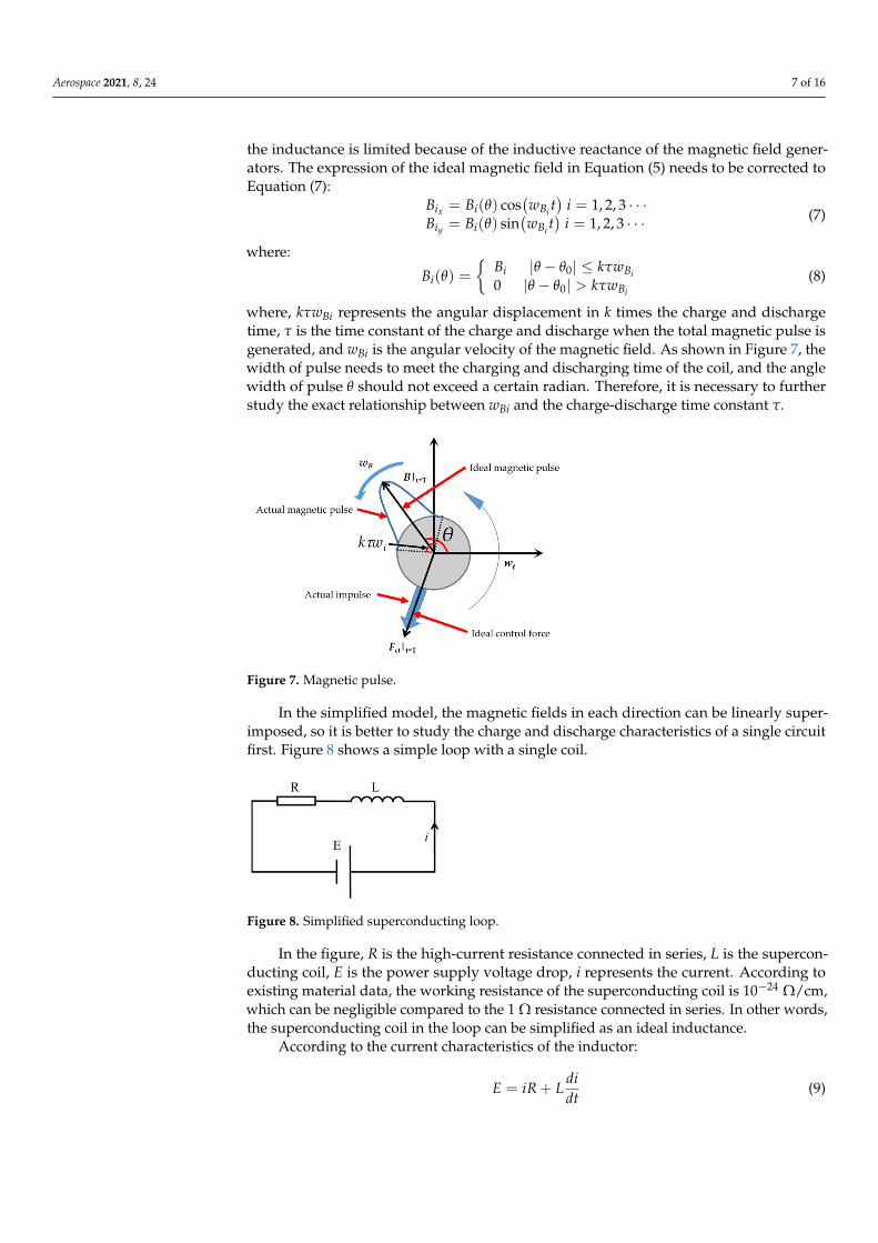
where, kτwBi represents the angular displacement in k times the charge and dischargetime, τ is the time constant of the charge and discharge when the total magnetic pulse isgenerated, and wBi is the angular velocity of the magnetic field. As shown in Figure 7, thewidth of pulse needs to meet the charging and discharging time of the coil, and the anglewidth of pulse θ should not exceed a certain radian. Therefore, it is necessary to furtherstudy the exact relationship between wBi and the charge-discharge time constant τ.

Aerospace 2021, 8, x FOR PEER REVIEW 7 of 17

The magnetic field components in each direction have the following mathematical expressions:

( ) ( )( ) ( )

3,2,1sin3,2,1cos

==

==

itwBB

itwBB

iy

ix

Bii

Bii

θθ

(5)

where:

( )

≠=

=0

0

0 θθθθ

θ ii

BB (6)

2.3.2. Simplification of Superconducting Coil Loop The last section gives the expression form of the ideal magnetic field, and the period

ΔTi under ideal conditions can be infinitely small. In reality, charging and discharging of the inductance is limited because of the inductive reactance of the magnetic field genera-tors. The expression of the ideal magnetic field in Equation (5) needs to be corrected to Equation (7):

( ) ( )( ) ( )

3,2,1sin3,2,1cos

==

==

itwBBitwBB

iy

ix

Bii

Bii

θθ

(7)

where:

( )

>−≤−

=i

i

B

Bii wk

wkBB

τθθτθθ

θ0

0

0 (8)

where, kτwBi represents the angular displacement in k times the charge and discharge time, τ is the time constant of the charge and discharge when the total magnetic pulse is gener-ated, and wBi is the angular velocity of the magnetic field. As shown in Figure 7, the width of pulse needs to meet the charging and discharging time of the coil, and the angle width of pulse θ should not exceed a certain radian. Therefore, it is necessary to further study the exact relationship between wBi and the charge-discharge time constant τ.

Figure 7. Magnetic pulse.

In the simplified model, the magnetic fields in each direction can be linearly super-imposed, so it is better to study the charge and discharge characteristics of a single circuit first. Figure 8 shows a simple loop with a single coil.

Figure 7. Magnetic pulse.

In the simplified model, the magnetic fields in each direction can be linearly super-imposed, so it is better to study the charge and discharge characteristics of a single circuitfirst. Figure 8 shows a simple loop with a single coil.

Aerospace 2021, 8, x FOR PEER REVIEW 8 of 17

Figure 8. Simplified superconducting loop.

In the figure, R is the high-current resistance connected in series, L is the supercon-ducting coil, E is the power supply voltage drop, i represents the current. According to existing material data, the working resistance of the superconducting coil is 10−24 Ω/cm, which can be negligible compared to the 1 Ω resistance connected in series. In other words, the superconducting coil in the loop can be simplified as an ideal inductance.

According to the current characteristics of the inductor:

dtdiLiRE += (9)

Solving Equation (9), we can get:

zyxnieeREti n

tt

n

nn

nn ,,)0()1()( =+−=−−

ττ (10)

zyxnRL

n

nn ,,==τ (11)

where, the coil inductance Ln can be approximated by the following equation:

zyxnlSNkLn ,,

20 == μ

(12)

where, k is the Nagaoka coefficient, S is the cross-sectional area of the coil, N is the number of turns, and l is the length of the coil.

Here we take the x-axis as an example to study the charging and discharging process of the magnetic pulse so as to draw conclusions about ΔTi and τ. First, the derivative of Equation (1) in Equation (8) is obtained as follows:

( )twwBBiix BBii sin−= (13)

so:

[ ]

ΔΔ

−=−∈i

i

i

iBiBii T

BT

BwBwBBiix

ππ 2,2, (14)

Then we take the derivative of the current equation in the x direction in Equation (10):

( ) ( ) tLR

x eRiEL

ti−

⋅−= )0(1 (15)

where, E is the power supply voltage, and can be changed freely in range [−Em, Em]. Be-cause of

xi xB i∝ , there is the following equation relationship:

xBi iCBx

= (16)

Figure 8. Simplified superconducting loop.

In the figure, R is the high-current resistance connected in series, L is the supercon-ducting coil, E is the power supply voltage drop, i represents the current. According toexisting material data, the working resistance of the superconducting coil is 10−24 Ω/cm,which can be negligible compared to the 1 Ω resistance connected in series. In other words,the superconducting coil in the loop can be simplified as an ideal inductance.

According to the current characteristics of the inductor:

E = iR + Ldidt

(9)

Aerospace 2021, 8, 24 8 of 16

Solving Equation (9), we can get:

in(t) =En

Rn(1− e−

tτn ) + e−

tτn in(0) n = x, y, z (10)

τn =Ln

Rnn = x, y, z (11)

where, the coil inductance Ln can be approximated by the following equation:

Ln =kµ0SN2

ln = x, y, z (12)

where, k is the Nagaoka coefficient, S is the cross-sectional area of the coil, N is the numberof turns, and l is the length of the coil.

Here we take the x-axis as an example to study the charging and discharging processof the magnetic pulse so as to draw conclusions about ∆Ti and τ. First, the derivative ofEquation (1) in Equation (8) is obtained as follows:

.Bix = −BiwBi sin

(wBi t

)(13)

so:.Bix ∈

[−BiwBi , BiwBi

]=

[−2Biπ

∆Ti,

2Biπ

∆Ti

](14)

Then we take the derivative of the current equation in the x direction in Equation (10):

.ix(t) =

1L(E− i(0)R) · e−

RL t (15)

where, E is the power supply voltage, and can be changed freely in range [−Em, Em].Because of Bix ∝ ix, there is the following equation relationship:

Bix = CBix (16)

where, CB is the constant coefficient. It’s necessary to make the actual magnetic field tokeep up with ideal magnetic field, the following inequality can be obtained:

min(

CB.ix

)≤ −BiwBi

max(

CB.ix

)≥ BiwBi

(17)

Namely:−CB(Em + imaxR)

L ≤ −BiwBiCB(Em − imaxR)

L ≥ BiwBi

(18)

With further simplification:

∆Ti ≥2πBiL

CB(Em − iminR)(19)

Equation (19) gives the limiting condition of the control period ∆Ti. The charge anddischarge time constant of the total magnetic pulse is set as follows:

τ = max[τx, τy, τz

](20)

In the process of selecting magnetic pulse parameters, the angular velocity wBi of themagnetic field needs to meet the constraints of Equation (19). The charging and dischargingtime constant τ of the total magnetic pulse satisfies Equation (20). The k in Equation (8) can

Aerospace 2021, 8, 24 9 of 16

be adjusted according to the pulse width, so that the angular displacement of the magneticfield vector Bi in a period meets the control requirements of traction.

2.4. Control Method Design2.4.1. Control Strategy

The core of the magnetic pulse control technology is the variable pulse magneticfield described in Section 2.3.1. In order to obtain the control signal used to resolve theelectromagnetic pulse, the system introduces Equation (21), called the reference dynamicEquation [20], achieving reference state rref, as shown in Figure 9.

Aerospace 2021, 8, x FOR PEER REVIEW 9 of 17

where, CB is the constant coefficient. It’s necessary to make the actual magnetic field to keep up with ideal magnetic field, the following inequality can be obtained:

( )( )

i

i

BixB

BixB

wBiC

wBiC

≥

−≤

max

min (17)

Namely:

( )

( )i

i

BimB

BimB

wBRiEC

wBRiEC

≥

−≤+−

L

Lmax

max

- (18)

With further simplification:

( )RiECLBT

mB

ii

min

2−

≥Δ π (19)

Equation (19) gives the limiting condition of the control period ΔTi. The charge and discharge time constant of the total magnetic pulse is set as follows:

[ ]zyx ττττ ,,max= (20)

In the process of selecting magnetic pulse parameters, the angular velocity wBi of the magnetic field needs to meet the constraints of Equation (19). The charging and discharg-ing time constant τ of the total magnetic pulse satisfies Equation (20). The k in Equation (8) can be adjusted according to the pulse width, so that the angular displace-ment of the magnetic field vector Bi in a period meets the control requirements of traction.

2.4. Control Method Design 2.4.1. Control Strategy

The core of the magnetic pulse control technology is the variable pulse magnetic field described in Section 2.3.1. In order to obtain the control signal used to resolve the electro-magnetic pulse, the system introduces Equation (21), called the reference dynamic Equa-tion [20], achieving reference state rref, as shown in Figure 9.

Figure 9. Magnetic pulse control loop. Figure 9. Magnetic pulse control loop.

The reference state is used to generate the reference control signal Fref, which formsan open-loop control system. In order to suppress the divergence of the system, the stateoutput r of the dynamic Equation is differentiated from the reference state rref and theresult is introduced into control signals, forming a feedback control loop. The referencecontrol signal Fref and the feedback control signal Ffb together form a continuous signalfor magnetic pulse calculation. The original control signal is a continuous and needs to bediscretized. Different from the conventional discretization method, we propose a methodbased on momentum, which is introduced in detail in Section 2.4.2:

..rre f = −

µ

R3

[I− 3 R

R ·RT

R

]rre f +

mt ·mcmt+mc

Fct..R = − µ

R3 R(21)

In addition, after the system converges, the eddy current control force is greatlyreduced, and the eddy current torque will also decrease simultaneously, which reduces thedespinning efficiency. In order to avoid the reduction of the efficiency, the eddy currenttorque enhancement module is specially introduced and designed. By imposing periodicdisturbance on the state of the observer, the eddy current torque is always maintained atan effective value, which can be verified later:

rRe f = rre f + A · sin(w · t) (22)

where, A represents the interference amplitude, and w represents the angular velocity ofthe sinusoidal interference signal.

Aerospace 2021, 8, 24 10 of 16

2.4.2. Discretization Method of Continuous Control Signal

As shown in Figure 6, due to the uniqueness of the eddy current force form, con-ventional control ideas cannot be used directly here. It is not difficult to find that theinstantaneous eddy current force has a certain periodic nature. The eddy current force at acertain moment can be regarded as a pulse in a variable period ∆Ti, where ∆Ti = 2π/wi.Since the target sways slightly near the predetermined position in the actual control process,there is no harm using the impulse within a variable period ∆Ti to characterize the controleffect of the object. In order to facilitate the derivation and expression of the control force,it is stipulated that the calculation range of the impulse received by the target is a circle.that is, the time for a magnetic field to scan the target is ∆Ti, and the total impulse receivedby the target during this period is calculated.

The curve of impulse, reduced impulse and equivalent impulse with respect to positionafter unfolding the target circle in the unit of circumference is shown in Figure 10. Theleft side of the picture is the actual demonstration diagram, and the right side is theschematic diagram of the circle expansion. The curve in the first coordinate system showsthe distribution of impulse within ∆Ti of the applied control force at different positionsin the unit of circle. The curve in the second coordinate system represents the impulsedistribution curve at the position where the remaining impulse is positive after the impulsein the opposite direction is offset. The curve in the third coordinate system represents theequivalent impulse of the vector sum of the impulses in ∆Ti, and the impulse pulse widthis determined according to the coil inductance model parameters in Section 2.3.2.

Aerospace 2021, 8, x FOR PEER REVIEW 11 of 17

Figure 10. Diagram of impulse model.

It should be noted that the concept of equivalent impulse in ΔTi is based on the as-sumption that ΔTi is small enough and the target displacement within the variable period is small.

2.4.3. Solution of Magnetic Pulse Signal The first step of magnetic pulse control is to find the control force at any time, and

then through the discretization, the relative angular velocity w and the central magnetic field BGt can be inversely solved by Equation (3). As shown in Figure 11, the result of the inverse solution is not unique. Therefore, the solution rules need to be appointed.

Figure 11. Diagram of inverse solution result.

In the two-dimensional plane model, the magnetic angular velocity required in Re-sult 1 is much smaller than that in Result 2. A larger magnetic angular velocity may in-crease the difficulty of controlling the magnetic field generator. In addition, the eddy cur-rent torque in result 1 is opposite to the target speed, which plays a role of braking. The eddy current torque in result 2 is in the same direction as the target speed, which acceler-ates the target’s rotation speed. Therefore, when solving Equation (3), it is necessary to make the applied magnetic field speed as small as possible and the eddy current torque

Figure 10. Diagram of impulse model.

It should be noted that the concept of equivalent impulse in ∆Ti is based on theassumption that ∆Ti is small enough and the target displacement within the variableperiod is small.

2.4.3. Solution of Magnetic Pulse Signal

The first step of magnetic pulse control is to find the control force at any time, andthen through the discretization, the relative angular velocity w and the central magneticfield BGt can be inversely solved by Equation (3). As shown in Figure 11, the result of theinverse solution is not unique. Therefore, the solution rules need to be appointed.

Aerospace 2021, 8, 24 11 of 16

Aerospace 2021, 8, x FOR PEER REVIEW 11 of 17

Figure 10. Diagram of impulse model.

It should be noted that the concept of equivalent impulse in ΔTi is based on the as-sumption that ΔTi is small enough and the target displacement within the variable period is small.

2.4.3. Solution of Magnetic Pulse Signal The first step of magnetic pulse control is to find the control force at any time, and

then through the discretization, the relative angular velocity w and the central magnetic field BGt can be inversely solved by Equation (3). As shown in Figure 11, the result of the inverse solution is not unique. Therefore, the solution rules need to be appointed.

Figure 11. Diagram of inverse solution result.

In the two-dimensional plane model, the magnetic angular velocity required in Re-sult 1 is much smaller than that in Result 2. A larger magnetic angular velocity may in-crease the difficulty of controlling the magnetic field generator. In addition, the eddy cur-rent torque in result 1 is opposite to the target speed, which plays a role of braking. The eddy current torque in result 2 is in the same direction as the target speed, which acceler-ates the target’s rotation speed. Therefore, when solving Equation (3), it is necessary to make the applied magnetic field speed as small as possible and the eddy current torque

Figure 11. Diagram of inverse solution result.

In the two-dimensional plane model, the magnetic angular velocity required in Result1 is much smaller than that in Result 2. A larger magnetic angular velocity may increasethe difficulty of controlling the magnetic field generator. In addition, the eddy currenttorque in result 1 is opposite to the target speed, which plays a role of braking. The eddycurrent torque in result 2 is in the same direction as the target speed, which accelerates thetarget’s rotation speed. Therefore, when solving Equation (3), it is necessary to make theapplied magnetic field speed as small as possible and the eddy current torque along theopposite direction of the target angular velocity as much as possible, which must be takenas the criterion.

3. Numerical Study3.1. Accuracy Verification of Discretization Method

The role of the momentum model is to ensure the stability of the system during thediscretization of the continuous control signal. The discrete process without the eddycurrent torque enhancement module is shown in Figures 12 and 13. When the continuouscontrol signal is input, the total impulse of the input signal is calculated in units of cycles.

Aerospace 2021, 8, x FOR PEER REVIEW 12 of 17

along the opposite direction of the target angular velocity as much as possible, which must

be taken as the criterion.

3. Numerical Study

3.1. Accuracy Verification of Discretization Method

The role of the momentum model is to ensure the stability of the system during the

discretization of the continuous control signal. The discrete process without the eddy cur-

rent torque enhancement module is shown in Figures 12 and 13. When the continuous

control signal is input, the total impulse of the input signal is calculated in units of cycles.

Figure 12. Periodic total impulse curve.

Figure 13. Pulse control curve.

Applying the continuous control signal to the model, as shown in Figure 14, the con-

trol effect does not change significantly compared with the above discrete control. There-

fore, when ΔTi is small, the momentum-based discrete method proposed in the article

does not affect the control performance of the system.

Figure 12. Periodic total impulse curve.

Aerospace 2021, 8, 24 12 of 16

Aerospace 2021, 8, x FOR PEER REVIEW 12 of 17

along the opposite direction of the target angular velocity as much as possible, which must

be taken as the criterion.

3. Numerical Study

3.1. Accuracy Verification of Discretization Method

The role of the momentum model is to ensure the stability of the system during the

discretization of the continuous control signal. The discrete process without the eddy cur-

rent torque enhancement module is shown in Figures 12 and 13. When the continuous

control signal is input, the total impulse of the input signal is calculated in units of cycles.

Figure 12. Periodic total impulse curve.

Figure 13. Pulse control curve.

Applying the continuous control signal to the model, as shown in Figure 14, the con-

trol effect does not change significantly compared with the above discrete control. There-

fore, when ΔTi is small, the momentum-based discrete method proposed in the article

does not affect the control performance of the system.

Figure 13. Pulse control curve.

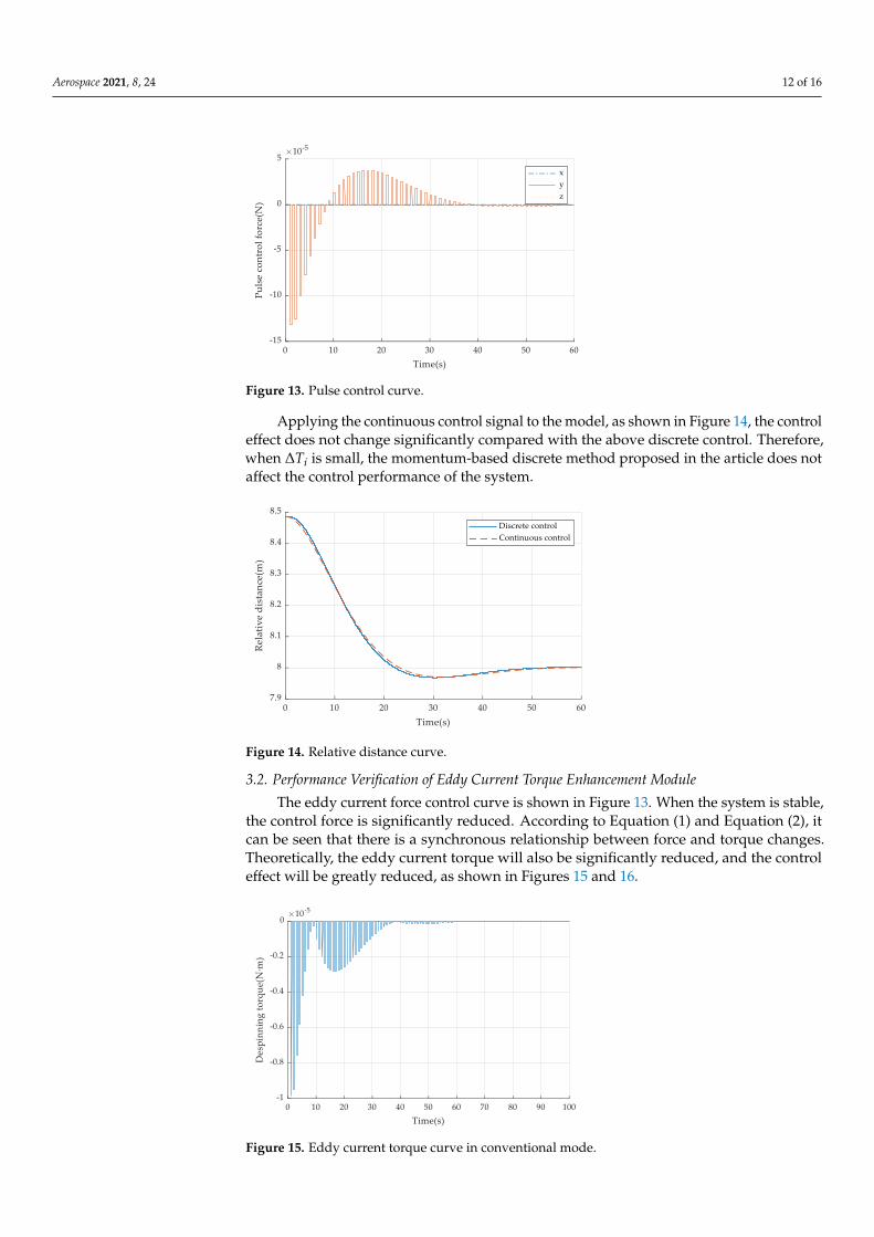
Applying the continuous control signal to the model, as shown in Figure 14, the controleffect does not change significantly compared with the above discrete control. Therefore,when ∆Ti is small, the momentum-based discrete method proposed in the article does notaffect the control performance of the system.

Aerospace 2021, 8, x FOR PEER REVIEW 13 of 17

Figure 14. Relative distance curve.

3.2. Performance Verification of Eddy Current Torque Enhancement Module

The eddy current force control curve is shown in Figure 13. When the system is stable,

the control force is significantly reduced. According to Equation (1) and Equation (2), it

can be seen that there is a synchronous relationship between force and torque changes.

Theoretically, the eddy current torque will also be significantly reduced, and the control

effect will be greatly reduced, as shown in Figures 15 and 16.

Figure 15. Eddy current torque curve in conventional mode.

Figure 16. Target speed curve in conventional mode.

Figure 14. Relative distance curve.

3.2. Performance Verification of Eddy Current Torque Enhancement Module

The eddy current force control curve is shown in Figure 13. When the system is stable,the control force is significantly reduced. According to Equation (1) and Equation (2), itcan be seen that there is a synchronous relationship between force and torque changes.Theoretically, the eddy current torque will also be significantly reduced, and the controleffect will be greatly reduced, as shown in Figures 15 and 16.

Aerospace 2021, 8, x FOR PEER REVIEW 13 of 17

Figure 14. Relative distance curve.

3.2. Performance Verification of Eddy Current Torque Enhancement Module

The eddy current force control curve is shown in Figure 13. When the system is stable,

the control force is significantly reduced. According to Equation (1) and Equation (2), it

can be seen that there is a synchronous relationship between force and torque changes.

Theoretically, the eddy current torque will also be significantly reduced, and the control

effect will be greatly reduced, as shown in Figures 15 and 16.

Figure 15. Eddy current torque curve in conventional mode.

Figure 16. Target speed curve in conventional mode.

Figure 15. Eddy current torque curve in conventional mode.

Aerospace 2021, 8, 24 13 of 16

Aerospace 2021, 8, x FOR PEER REVIEW 13 of 17

Figure 14. Relative distance curve.

3.2. Performance Verification of Eddy Current Torque Enhancement Module

The eddy current force control curve is shown in Figure 13. When the system is stable,

the control force is significantly reduced. According to Equation (1) and Equation (2), it

can be seen that there is a synchronous relationship between force and torque changes.

Theoretically, the eddy current torque will also be significantly reduced, and the control

effect will be greatly reduced, as shown in Figures 15 and 16.

Figure 15. Eddy current torque curve in conventional mode.

Figure 16. Target speed curve in conventional mode. Figure 16. Target speed curve in conventional mode.

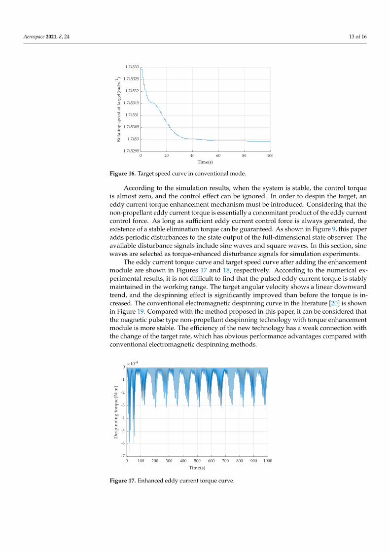
According to the simulation results, when the system is stable, the control torqueis almost zero, and the control effect can be ignored. In order to despin the target, aneddy current torque enhancement mechanism must be introduced. Considering that thenon-propellant eddy current torque is essentially a concomitant product of the eddy currentcontrol force. As long as sufficient eddy current control force is always generated, theexistence of a stable elimination torque can be guaranteed. As shown in Figure 9, this paperadds periodic disturbances to the state output of the full-dimensional state observer. Theavailable disturbance signals include sine waves and square waves. In this section, sinewaves are selected as torque-enhanced disturbance signals for simulation experiments.

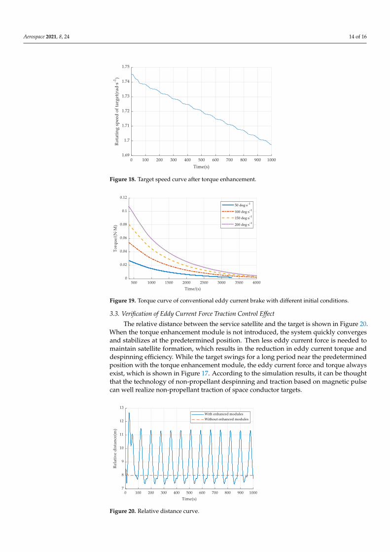
The eddy current torque curve and target speed curve after adding the enhancementmodule are shown in Figures 17 and 18, respectively. According to the numerical ex-perimental results, it is not difficult to find that the pulsed eddy current torque is stablymaintained in the working range. The target angular velocity shows a linear downwardtrend, and the despinning effect is significantly improved than before the torque is in-creased. The conventional electromagnetic despinning curve in the literature [20] is shownin Figure 19. Compared with the method proposed in this paper, it can be considered thatthe magnetic pulse type non-propellant despinning technology with torque enhancementmodule is more stable. The efficiency of the new technology has a weak connection withthe change of the target rate, which has obvious performance advantages compared withconventional electromagnetic despinning methods.

Aerospace 2021, 8, x FOR PEER REVIEW 14 of 17

According to the simulation results, when the system is stable, the control torque is

almost zero, and the control effect can be ignored. In order to despin the target, an eddy

current torque enhancement mechanism must be introduced. Considering that the non-

propellant eddy current torque is essentially a concomitant product of the eddy current

control force. As long as sufficient eddy current control force is always generated, the ex-

istence of a stable elimination torque can be guaranteed. As shown in Figure 9, this paper

adds periodic disturbances to the state output of the full-dimensional state observer. The

available disturbance signals include sine waves and square waves. In this section, sine

waves are selected as torque-enhanced disturbance signals for simulation experiments.

The eddy current torque curve and target speed curve after adding the enhancement

module are shown in Figures 17 and 18, respectively. According to the numerical exper-

imental results, it is not difficult to find that the pulsed eddy current torque is stably main-

tained in the working range. The target angular velocity shows a linear downward trend,

and the despinning effect is significantly improved than before the torque is increased.

The conventional electromagnetic despinning curve in the literature [20] is shown in Fig-

ure 19. Compared with the method proposed in this paper, it can be considered that the

magnetic pulse type non-propellant despinning technology with torque enhancement

module is more stable. The efficiency of the new technology has a weak connection with

the change of the target rate, which has obvious performance advantages compared with

conventional electromagnetic despinning methods.

Figure 17. Enhanced eddy current torque curve.

Figure 18. Target speed curve after torque enhancement.

Figure 17. Enhanced eddy current torque curve.

Aerospace 2021, 8, 24 14 of 16

Aerospace 2021, 8, x FOR PEER REVIEW 14 of 17

According to the simulation results, when the system is stable, the control torque is

almost zero, and the control effect can be ignored. In order to despin the target, an eddy

current torque enhancement mechanism must be introduced. Considering that the non-

propellant eddy current torque is essentially a concomitant product of the eddy current

control force. As long as sufficient eddy current control force is always generated, the ex-

istence of a stable elimination torque can be guaranteed. As shown in Figure 9, this paper

adds periodic disturbances to the state output of the full-dimensional state observer. The

available disturbance signals include sine waves and square waves. In this section, sine

waves are selected as torque-enhanced disturbance signals for simulation experiments.

The eddy current torque curve and target speed curve after adding the enhancement

module are shown in Figures 17 and 18, respectively. According to the numerical exper-

imental results, it is not difficult to find that the pulsed eddy current torque is stably main-

tained in the working range. The target angular velocity shows a linear downward trend,

and the despinning effect is significantly improved than before the torque is increased.

The conventional electromagnetic despinning curve in the literature [20] is shown in Fig-

ure 19. Compared with the method proposed in this paper, it can be considered that the

magnetic pulse type non-propellant despinning technology with torque enhancement

module is more stable. The efficiency of the new technology has a weak connection with

the change of the target rate, which has obvious performance advantages compared with

conventional electromagnetic despinning methods.

Figure 17. Enhanced eddy current torque curve.

Figure 18. Target speed curve after torque enhancement. Figure 18. Target speed curve after torque enhancement.

Aerospace 2021, 8, x FOR PEER REVIEW 15 of 17

Figure 19. Torque curve of conventional eddy current brake with different initial conditions.

3.3. Verification of Eddy Current Force Traction Control Effect

The relative distance between the service satellite and the target is shown in Figure

20. When the torque enhancement module is not introduced, the system quickly con-

verges and stabilizes at the predetermined position. Then less eddy current force is

needed to maintain satellite formation, which results in the reduction in eddy current

torque and despinning efficiency. While the target swings for a long period near the pre-

determined position with the torque enhancement module, the eddy current force and

torque always exist, which is shown in Figure 17. According to the simulation results, it

can be thought that the technology of non-propellant despinning and traction based on

magnetic pulse can well realize non-propellant traction of space conductor targets.

Figure 20. Relative distance curve.

4. Conclusions

This paper studies the despinning method of the space rotating target, proposes a method

of despinning and traction based on magnetic pulse without propellant, and designs a

new despinning device. In order to realize the proposed despinning and traction method,

a discretization method of control signal based on momentum model is studied in this

paper. This method grasps the relatively static characteristics of the formation between

the active and passive sides and discretizes the continuous control signal by calculating

the total impulse of the eddy current force in a small period. Then, the simplified induct-

ance model is used to derive the magnetic pulse in the two-dimensional simplified model,

obtaining constraints on key parameters such as the electromagnetic pulse period ΔTi. In

addition, an eddy current torque enhancement module that uses periodic interference sig-

nals is designed so as to solve the problem of the despinning torque disappearing in the

steady state of the system.

Figure 19. Torque curve of conventional eddy current brake with different initial conditions.

3.3. Verification of Eddy Current Force Traction Control Effect

The relative distance between the service satellite and the target is shown in Figure 20.When the torque enhancement module is not introduced, the system quickly convergesand stabilizes at the predetermined position. Then less eddy current force is needed tomaintain satellite formation, which results in the reduction in eddy current torque anddespinning efficiency. While the target swings for a long period near the predeterminedposition with the torque enhancement module, the eddy current force and torque alwaysexist, which is shown in Figure 17. According to the simulation results, it can be thoughtthat the technology of non-propellant despinning and traction based on magnetic pulsecan well realize non-propellant traction of space conductor targets.

Aerospace 2021, 8, x FOR PEER REVIEW 15 of 17

Figure 19. Torque curve of conventional eddy current brake with different initial conditions.

3.3. Verification of Eddy Current Force Traction Control Effect

The relative distance between the service satellite and the target is shown in Figure

20. When the torque enhancement module is not introduced, the system quickly con-

verges and stabilizes at the predetermined position. Then less eddy current force is

needed to maintain satellite formation, which results in the reduction in eddy current

torque and despinning efficiency. While the target swings for a long period near the pre-

determined position with the torque enhancement module, the eddy current force and

torque always exist, which is shown in Figure 17. According to the simulation results, it

can be thought that the technology of non-propellant despinning and traction based on

magnetic pulse can well realize non-propellant traction of space conductor targets.

Figure 20. Relative distance curve.

4. Conclusions

This paper studies the despinning method of the space rotating target, proposes a method

of despinning and traction based on magnetic pulse without propellant, and designs a

new despinning device. In order to realize the proposed despinning and traction method,

a discretization method of control signal based on momentum model is studied in this

paper. This method grasps the relatively static characteristics of the formation between

the active and passive sides and discretizes the continuous control signal by calculating

the total impulse of the eddy current force in a small period. Then, the simplified induct-

ance model is used to derive the magnetic pulse in the two-dimensional simplified model,

obtaining constraints on key parameters such as the electromagnetic pulse period ΔTi. In

addition, an eddy current torque enhancement module that uses periodic interference sig-

nals is designed so as to solve the problem of the despinning torque disappearing in the

steady state of the system.

Figure 20. Relative distance curve.

Aerospace 2021, 8, 24 15 of 16

4. Conclusions

This paper studies the despinning method of the space rotating target, proposes amethod of despinning and traction based on magnetic pulse without propellant, anddesigns a new despinning device. In order to realize the proposed despinning and tractionmethod, a discretization method of control signal based on momentum model is studied inthis paper. This method grasps the relatively static characteristics of the formation betweenthe active and passive sides and discretizes the continuous control signal by calculating thetotal impulse of the eddy current force in a small period. Then, the simplified inductancemodel is used to derive the magnetic pulse in the two-dimensional simplified model,obtaining constraints on key parameters such as the electromagnetic pulse period ∆Ti.In addition, an eddy current torque enhancement module that uses periodic interferencesignals is designed so as to solve the problem of the despinning torque disappearing in thesteady state of the system.

According to the simulation results, the discretization method based on momentummodel proposed in this paper doesn’t affect the control stability of the system under thelimitation of electromagnetic pulse parameters. By comparing the changes of the targetangular velocity before and after the introduction of the eddy current torque enhancementmodule, it is not difficult to find that the eddy current torque enhancement module in-troduced in this paper really solve the problem of the torque disappearing in the steadystate. What’s more, the efficiency of the conventional eddy current despinning methoddecrease with the decrease of the target speed, and it is necessary to consume propellant fora long time to maintain the formation. The eddy current despinning and traction methodbased on magnetic pulse does not need propellant, and the efficiency is not affected by thetarget state. Compared with conventional methods, the method proposed in this paper hascertain advantages. Apart from the field of despinning, this technology can also be appliedto the field of passive traction of space targets, etc. The theoretical research and numericalexperimental data in this paper can provide an effective reference for the development ofrelated fields.

Author Contributions: Conceptualization, Y.Z.; Investigation, Y.Z.; Methodology, Y.Z.; Projectadministration, Q.S., S.W. and L.H.; Writing—review and editing, Q.S., S.W. All authors have readand agreed to the published version of the manuscript.

Funding: This research was supported partially by National Natural Science Foundation of Chinaunder Grant U20B2056, Natural Science Foundation of Shanghai under Grant 20ZR1427000, ShanghaiSailing Program under Grant 20YF1421600.

Informed Consent Statement: Informed consent was obtained from all subjects involved in the study.

Acknowledgments: The author would like to thank the reviewers and the editors for their valuablecomments and constructive suggestions that helped to improve the paper significantly.

Conflicts of Interest: The authors declare no conflict of interest.

References1. Muelhaupt, T.J.; Sorge, M.E.; Morin, J.; Wilson, R.S. Space traffic management in the new space era. J. Space Saf. Eng. 2019, 6,

80–87. [CrossRef]2. Sgobba, T.; Rongier, I. Space Safety is No Accident: The 7th IAASS Conference; Springer: Berlin/Heidelberg, Germany, 2015.3. Kessler, D.J.; Johnson, N.L.; Liou, J.C.; Matney, M. The kessler syndrome: Implications to future space operations. Adv. Astronaut.

Sci. 2010, 137, 2010.4. Cheng, W.; Li, Z.; He, Y. Modeling and Analysis of Contact Detumbling by Using Flexible Brush. In Proceedings of the 2019 IEEE

International Conference on Unmanned Systems (ICUS), Beijing, China, 17–19 October 2019; pp. 95–102.5. Cheng, W.; Li, Z.; He, Y. Strategy and Control for Robotic Detumbling of Space Debris by Using Flexible Brush. In Proceedings of

the 2019 3rd International Conference on Robotics and Automation Sciences (ICRAS), Wuhan, China, 1–3 June 2019; pp. 41–47.6. Liu, Y.Q.; Yu, Z.W.; Liu, X.F. Active detumbling technology for high dynamic non-cooperative space targets. Multibody Syst. Dyn.

2019, 47, 21–41. [CrossRef]7. Kawamoto, S.; Makida, T.; Sasaki, F. Precise numerical simulations of electro dynamic tethers for an active debris removal system.

Acta Astronaut. 2006, 59, 139–148. [CrossRef]

Aerospace 2021, 8, 24 16 of 16

8. Zhang, F.; Huang, P.F. Inertia parameter estimation for an noncooperative target captured by a space tethered system. J. Astronaut.2015, 36, 630–639.

9. Peters, T.V.; Olmos, D.E. COBRA contactless detumbling. Ceas Space J. 2016, 8, 143–165. [CrossRef]10. Kitamura, S. Large space debris reorbiter using ion beam irradiation. In Proceedings of the 61st International Astronautical

Congress, Prague, Czech Republic, 27 September–1 October 2010.11. Bombardelli, C.; Pelaez, J. Ion beam shepherd for contactless space debris removal. J. Guid. Control Dyn. 2011, 34, 916–920.

[CrossRef]12. Bennett, T.; Schaub, H. Touchless Electrostatic Three-dimensional Detumbling of Large Axi-symmetric Debris. J. Astronaut. Sci.

2015, 152, 233–253. [CrossRef]13. Gibbings, A.; Vasile, M.; Hopkins, J.M. Experimental Characterization of the Thrust Induced by Laser Ablation onto an Asteroid.

Mmw Fortschr. Der Med. 2013, 153, 28–30.14. Soulard, R.; Quinn, M.N.; Tajima, T. ICAN: A novel laser architecture for space debris removal. Acta Astronaut. 2014, 105, 192–200.

[CrossRef]15. Smith, G.L. Effects of Magnetically Induced Eddy-Current Torques on Spin Motions of an Earth Satellite; NASA: Washington, DC,

USA, 1965.16. Kadaba, P.K.; Naishadham, K. Feasibility of noncontacting electromagnetic despinning of a satellite by inducing eddy currents in

its skin. I. Analytical considerations. IEEE Trans. On Magn. 2002, 31, 2471–2477. [CrossRef]17. Sugai, F.; Abiko, S.; Tsujita, T. Development of an eddy current brake system for detumbling malfunctioning satellites. In

Proceedings of the IEEE/SICE International Symposium on System Integration, Fukuoka, Japan, 16–18 December 2012.18. Xie, Z.; Gong, P.; Liang, M. Using Permanent Magnetic Array Device to Detumble and Despin Defunct Spacecraft. In IOP

Conference Series: Materials Science and Engineering; IOP Publishing: Bristol, UK, 2019; Volume 631, p. 032039.19. Gomez, N.O.; Walker, S.J.I. Eddy currents applied to de-tumbling of space debris: Analysis and validation of approximate

proposed methods. Acta Astronaut. 2015, 114, 34–53. [CrossRef]20. Gomez, N.O.; Walker, S.J.I.; Jankovic, M. Control analysis for a contactless de-tumbling method based on eddy currents: Problem

definition and approximate proposed solutions. In Proceedings of the Aiaa Scitech Forum & Exposition, San Diego, CA, USA,4–8 January 2016.

21. Liu, X.; Huang, P.; Zhao, Y. Dynamics and Control for Eddy Braking a Space Tumbling target. In Proceedings of the 2019 IEEE9th Annual International Conference on CYBER Technology in Automation, Control, and Intelligent Systems (CYBER), Suzhou,China, 29 July–2 August 2019; pp. 1102–1106.