Proceedings of CHT-08 ICHMT International Symposium on Advances in Computational Heat Transfer

May 11-16, 2008, Marrakech, Morocco

CHT-08-407

REFINED EDDY VISCOSITY SCHEMES AND LARGE EDDY SIMULATIONS

FOR ASCENDING MIXED CONVECTION FLOWS

Amir Keshmiri*, Yacine Addad, Mark A. Cotton, Dominique R. Laurence and Flavien Billard School of Mechanical, Aerospace and Civil Engineering (MACE),

The University of Manchester, Manchester M60 1QD, U.K. *Corresponding author: E-mail: a.keshmiri@postgrad.manchester.ac.uk Tel: +44 (0) 161 275 4401

ABSTRACT The present work is concerned with the modelling of ascending turbulent (‘mixed convection’) flow in a vertical heated pipe. All fluid properties are assumed to be constant and buoyancy is accounted for within the Boussinesq approximation. Four Eddy Viscosity Models (EVMs) are examined against experimental measurements and the direct numerical simulation data of You et al. [2003]. The EVMs embody distinct physical refinements with respect to the parent high-Reynolds-number k-ε model. Large Eddy Simulations (LES) employing the classical Smagorinsky sub-grid-scale model are also presented. Three different CFD codes have been employed in the study: ‘CONVERT’, ‘Code_Saturne’, and ‘STAR-CD’, which are respectively in-house, industrial, and commercial packages. In relation to forced convection Nusselt number and local friction coefficient, discrepancies are identified between ‘reference’ data sources, namely earlier DNS and experimental results and the present LES computations. The Launder-Sharma closure [Launder and Sharma, 1974] is in the closest agreement with DNS results for levels of heat transfer impairment in ascending mixed convection flow, although again there is a lack of consensus between reference sources.

1) INTRODUCTION

1.1) General Background Convective heat transfer is traditionally divided into the regimes of ‘forced’ convection (where motion is in response to an externally-applied pressure difference) and ‘free’ convection (where motion is due to density variations within the fluid). However, both mechanisms may operate simultaneously; where there is a buoyancy-modified forced flow, the heat transfer regime is termed ‘mixed’ convection. In the case of turbulent mixed convection in vertical flow passages, wholesale modifications may occur to the turbulence structure. The effects on heat transfer performance are complex, and forced and free convection influences do not combine in a simple additive manner.

An important engineering application where mixed convection flows may occur relates to post-trip decay heat removal in nuclear reactor cores. The principal focus of the present study is on ascending turbulent mixed convection flows and the work is therefore relevant to the UK fleet of gas-cooled ‘Magnox’ and ‘Advanced Gas-cooled Reactors’ (AGRs) in which an upwards-flowing carbon dioxide coolant is employed. It is noted that in proposed ‘Generation IV’ Very High Temperature Reactor (VHTR) designs the coolant is a descending flow of helium.

Experimental data for turbulent mixed convection flows have, for the main, been obtained using air as the working fluid. In addition, however, studies employing water have been reported (see below).

NOMENCLATURE

Bo Buoyancy parameter, )/( .. 8042534 rPeRGr108×

fc Local friction coefficient

pc Specific heat coefficient at constant pressure

sC Smagorinsky model constant

μC Constant in Eddy-Viscosity Models D Pipe diameter

ig Acceleration due to gravity Gr Grashof number, )/( 24 qgD λνβ k Turbulent kinetic energy, 2uu ii / L Length scale Nu Nusselt number, )(/ bw TTDq −λ p Pressure

kP Rate of shear-production of k rP Prandtl number, λμ /pc

q Wall heat flux +q Heat loading parameter, )/( bpbbb TcUq ρ

r Radial coordinate R Pipe radius, 2/D Re Reynolds number, ν/DU b

teR Turbulent Reynolds number, )ε~ν/(k 2 S Strain parameter, Eq. (13)

ijS Mean strain rate tensor, ijji xUxU ∂∂+∂∂ //

S~ Non-dimensional strain rate, )SS(2/1~/k ijijε t Time T Temperature

tT Turbulence timescale

θju Turbulent heat flux tensor

τU Friction velocity, 21w

/)/( ρτ

ii uU , Mean, fluctuating velocity components in Cartesian tensors

jiuu Reynolds stress tensor yx, Streamwise and wall-normal coordinates +y Dimensionless distance from the wall,

ν/Uy τ Greek Symbols: α Blending parameter, Eq. (18) β Coefficient of volumetric expansion

ijδ Kronecker delta Δ LES filter width ε Rate of dissipation of k ε~ Modified dissipation rate, 2

i21 xk2 )/( / ∂∂− νε

λ Thermal conductivity μ Dynamic viscosity

tμ Turbulent viscosity, or LES sub-grid viscosity

ν Kinematic viscosity, ρμ / ρ Density

tσ Turbulent Prandtl number

wτ Wall shear stress

ijΩ Mean vorticity tensor, ijji xUxU ∂∂−∂∂ //

Ω~ Non-dimensional vorticity, )(2/1~/k ijijΩΩε Subscripts: b Bulk t Turbulent w Wall Superscripts: _

Time-average Additional symbols are defined in the text.

In the present work computations are undertaken for an air flow (Pr = 0.71) that ascends along a uniformly-heated vertical pipe. The general flow configuration is illustrated in Fig. 1. In ascending turbulent mixed convection flows heat transfer rates, quantified in terms of Nusselt number, may be either impaired or enhanced with respect to the corresponding forced convection flow at the same Reynolds and Prandtl numbers. The impaired condition occurs at low-to-moderate levels of buoyancy influence, while enhancement is found at very high levels of buoyancy influence. By contrast, heat transfer is always enhanced in descending flow. The monograph of Petukhov and Polyakov [1988] and the review papers of Jackson et al. [1989] and Jackson [2006] provide extended discussions of heat transfer performance under mixed convection conditions.

Figure 1. Schematic diagram of ascending mixed convection flow

A dimensionless group known as the ‘buoyancy parameter’, Bo, is widely used to characterize the extent of buoyancy influence. The buoyancy parameter was developed in the semi-empirical analysis of Hall and Jackson [1969] and is written here in the form quoted by Jackson et al. [1989]:

8.0425.34

PrReGr108Bo ×= (1)

Variable property effects other than those associated with buoyancy become significant where the temperature variations in a flow are large. An appropriate dimensionless measure of axial and radial temperature variations is provided by the ‘heat loading parameter’, +q :

bpbbb TcU

qqρ

=+ (2)

1.2) Review of Previous Work Experimental studies of ascending mixed convection air flows include the works of Steiner [1971], Carr et al. [1973], Polyakov and Shindin [1988], Vilemas et al. [1992] and Shehata and McEligot [1998]. Results for water flows are reported by Parlatan et al. [1996]. In recent years the body of experimental data on turbulent mixed convection existing in the literature has been complemented by the appearance of Direct Numerical Simulation (DNS) results. One of the earliest studies on this kind was undertaken by Kasagi and Nishimura [1997] who carried out a simulation of mixed convection between two vertical parallel plates maintained at different uniform temperatures. A focus of the present study is the recent DNS work of You et al. [2003] who conducted a study of turbulent mixed convection in a vertical uniformly-heated pipe for constant property conditions; buoyancy was accounted for using the Boussinesq approximation. You et al. restricted their attention to conditions of hydrodynamically and thermally fully-developed flow. Adoption of the Boussinesq approximation framework is attractive from the viewpoint of turbulence model/computer code validation because it permits an examination of buoyancy effects in isolation from other variable property phenomena (thus q+, Eq. (2) above, is not a relevant parameter of the simulations).

Turbulence model computations of mixed convection flows have been reported by Walklate [1976], Abdelmeguid and Spalding [1979], Tanaka et al. [1987], Cotton and Jackson [1990], Yu [1991], Mikielewicz [1994], Kirwin [1995] and Kim et al. [2006]. All those authors used various forms of two-equation closure and a finding to emerge from the studies taken together was that the ‘low-Reynolds-number’ model of Launder and Sharma [1974] was generally superior to the other

variants examined. Cotton et al. [2001] compared the Launder-Sharma scheme against the three-equation closure of Cotton and Ismael [1998]; the present work includes a further examination of the Launder-Sharma and Cotton-Ismael models. Researchers in the field have also evaluated other strategies: for example, Richards et al. [2004] and Kim et al. [2006] report some success in applying the ‘ fv2 − ’ model of Durbin [1991] to turbulent mixed convection flows.

In addition to studying the Launder-Sharma and Cotton-Ismael eddy viscosity models, the present work examines a revised form of the fv2 − scheme (the ‘Manchester fv2 − ’ model) and the non-linear formulation of Craft, Launder and Suga [1996] (termed the ‘Suga model’ below). New Large Eddy Simulations are also reported.

2) COMPUTATIONAL STRATEGIES

2.1) Introduction In the engineering computation of steady turbulent flows the instantaneous equations of motion and energy are first averaged over time. This process of ‘Reynolds-averaging’ gives rise to unknown Reynolds stresses and turbulent heat fluxes in the governing equations of the mean flow. It is the role of a turbulence model to achieve closure of the averaged equation set. The mean flow equations are quoted in Section 2.2 below, while various turbulence models are presented in Section 2.3. Large Eddy Simulations, in which the instantaneous equations are ‘filtered’ (as opposed to averaged), are introduced in Section 2.4. In Section 2.5 there is a discussion of the computational codes employed in the present study.

2.2) Mean Flow Equations The mean flow equations are written in the Boussinesq approximation. Adopting Cartesian tensor notation, the equations read as follows:

Continuity: 0xU

j

j =∂∂

(3)

Momentum: [ ])()( 0ij

it

ji

i TT1gxU

xxp

DtDU

−−+⎟⎟⎠

⎞⎜⎜⎝

⎛

∂∂

+∂∂

+∂∂

−= βρμμρ (4)

flowascendingin]0,0,g[gwhere i −= (5)

Energy: ⎥⎥⎦

⎤

⎢⎢⎣

⎡

∂∂

⎟⎟⎠

⎞⎜⎜⎝

⎛+

∂∂

=jt

t

j xT

rPxDtDT

σμμρ (6)

2.3) Eddy Viscosity Turbulence Models The turbulence models examined in the present work may be considered ‘refined’ in the sense all have some distinct modification with respect to the parent high-Reynolds-number formulation of Launder and Spalding [1974]. The four models to be evaluated in Section 3 below are as follows:

2.3.1) The Launder and Sharma Model - ‘LS Model’ The scale-determining variables most widely selected in two-equation EVMs are the turbulent kinetic energy, k, and ε , the rate of viscous dissipation of k. Within this framework, quantification of the local turbulence level may be made in terms of a turbulent Reynolds number of the form εν ~/2

t keR = (where ε~ is a modified dissipation variable to which the wall boundary condition ε~ = 0 is applied); departures from ‘universality’ are parameterized as functions of Ret. The first ‘low-Reynolds-number’ ε−k turbulence model was proposed by Jones and Launder [1972]; here a re-optimization of that scheme due to Launder and

Sharma [1974] is adopted as a benchmark against which more recent strategies are assessed. Despite the early appearance of the LS closure, it remains one of the more conceptually advanced, and accurate, of a large group of two-equation model variants (Patel et al., 1985; Cotton and Kirwin, 1995).

Eddy viscosity in the LS model is obtained as:

ερμ μμ~/kfC 2

t = (7)

where

( )( )[ ]2t 50/Re1/4.3expf +−=μ (8)

Within the LS model k and ε~ are determined from the following transport equations:

( )

⎥⎥

⎦

⎤

⎢⎢

⎣

⎡

⎟⎟⎠

⎞⎜⎜⎝

⎛

∂∂

+−⎥⎥⎦

⎤

⎢⎢⎣

⎡

∂∂

⎟⎟⎠

⎞⎜⎜⎝

⎛+

∂∂

+=2

j

2/1

jk

t

jk x

k2~xk

xP

DtkD νερ

σμμρρ

(9)

εεεε

εερε

σμμερερ E

k

~fC

x

~

xP

k

~C

Dt

~D 2

2j

t

jk1 +−

⎥⎥⎦

⎤

⎢⎢⎣

⎡

∂∂

⎟⎟⎠

⎞⎜⎜⎝

⎛+

∂∂

+= (10)

where j

ijik x

UuuP∂∂

−= .

Note that direct buoyant production terms are omitted from the transport equations, these having been found not to be influential in mixed convection flows, see for example Cotton and Jackson [1990].

The constants appearing in the model are quoted in Table 1 below, while the functions fε and Eε are given in Table 4.

Table 1. Constants appearing in the LS Model μC kσ εσ 1Cε 2Cε

0.09 1.0 1.3 1.44 1.92

2.3.2) The Cotton and Ismael Model – ‘CI Model’ Cotton and Ismael [1998] argued that a fundamental weakness exists in the stress/rate-of-strain relationship of high-Reynolds-number EVMs. Thus, for example, one might consider the constitutive equation of the ‘standard’ ε−k model [Launder and Spalding, 1974]: under the influence of simple shear, the structural ratio

kuv /− as determined by this model varies linearly with the group y/U)ε/k( ∂∂ :

( ) y/U/kCk/uv ∂∂=− εμ (11) where μC is a constant. The expression above represents the ratio of the large-scale turbulence timescale ( ε/k ) to the mean strain timescale, (∂U/∂y)-1. Alternatively, it may be considered as total strain (t.∂U/∂y) truncated on

the turbulence timescale. In a preliminary step Cotton and Ismael advanced a generalization of the above relationship based upon dimensional analysis. Hence, quite simply, the structural ratio is now expressed as: ( )[ ]y/U/kfk/uv ∂∂=− ε (12)

where f is a function to be determined.

The second stage of the development is based upon the proposals of Townsend [1970] and Maxey [1982] and consists of the introduction of an additional transport equation for a ‘strain parameter’, S:

( )εσν

ε ~/~ kS

xS

xxU

xUk

21

DtDS

jS

t

j

2

i

j

j

i −⎟⎟⎠

⎞⎜⎜⎝

⎛

∂∂

∂∂

+⎟⎟⎠

⎞⎜⎜⎝

⎛

∂∂

+∂∂

= (13)

where ε has now been replaced by ε~ (cf. the LS model, above). Under equilibrium conditions, S takes the value ( )[ ]2yUk ∂∂ /~/ ε ; where the flow is a non-equilibrium state, Eq. (13) mimics some aspects of Rapid Distortion Theory (RDT), see for example Hunt and Carruthers [1990]. Eddy viscosity in the CI model is obtained as:

( ) ερμ μμ~/kSf)eR(fC 2

Stt = (14)

where

[ ]50/eRexp3.01)eR(f tt −−=μ (15)

( ) ( )[ ]{ }3S S0015.0S135.0exp55.01

S165.0188.2Sf +−−×

+= (16)

Note that, in contrast to EVMs in which damping effects are attributed wholly to viscous effects, Eq. (15) rapidly asymptotes to unity. The k-equation of the CI model is identical to that of the LS scheme, while the ε -equation differs only in the value assigned to σε and the prescription of the functions fε and Eε (Tables 2 and 4).

Table 2. Constants appearing in the CI Model μC kσ εσ Sσ 1Cε 2Cε

0.09 1.0 1.21 6.0 1.44 1.92

2.3.3) The Craft, Launder and Suga Non-Linear Model – ‘Suga Model’ In a research effort that proceeded in parallel with the development of the CI model, Craft et al. [1996] developed a two-equation model in which quadratic and cubic mean strain and vorticity terms were introduced into the constitutive equation. (A subsequent refinement of the approach included a third transport equation for A2, the second invariant of the stress anisotropy tensor.)

The transport equations for k and ε in the Suga model take the generic forms of Eqs. (9) and (10); model constants and functions are given in Tables 3 and 4. It is noted that the strain field of the present mixed convection flows approximates simple shear and that the non-linear terms of the Suga model are consequently close to zero. The model does, however, depart significantly from the standard ε−k closure because of the specification of μC which has a parameterization akin to the

( )Sfs damping function of the CI model. An additional source term in the Suga model ε -equation which is generally referred to as the ‘Yap correction’ [Craft et al., 1996] has been omitted in the present work. It is the case, however, that the term is only of importance in flows where the turbulence length scale exceeds equilibrium values, while in heat-transfer-impaired ascending mixed convection flows the length scale generally lies below the equilibrium distribution.

Table 3. Constants appearing in the Suga NLEVM

1c 2c 3c 4c 5c 6c 7c

-0.1 0.1 0.26 -10 2cμ 0 -5 2cμ 5 2cμ

Table 4. Functions appearing in the LS, CI and Suga Models Variable LS model CI model Suga Model

μC 09.0C =μ 09.0C =μ

( ) ( ) ⎟⎟⎠⎞

⎜⎜⎝

⎛⎥⎦

⎤⎢⎣

⎡

Ω−−

−×Ω+

=)~,~max(.exp

.exp)~,~max(.

.. S750

3601S3501

30C 51μ

where )SS(2/1~/kS~ ijijε= )(2/1~/k~

ijijΩΩ=Ω ε

μf

⎥⎥⎥⎥

⎦

⎤

⎢⎢⎢⎢

⎣

⎡

⎟⎠⎞

⎜⎝⎛ +

−= 2

t

50Re1

4.3expfμ

⎥⎦⎤

⎢⎣⎡−−=

50Reexp3.01f t

μ

Additional damping function:

( )

{ })]..(exp[...

3

S

S00150S13505501S16501

882Sf

+−−×+

= ])400/(Re)90/(Reexp[1f 2

t2/1

t −−−=μ

εf ( )2tReexp3.01f −−=ε 1f =ε

( )2tReexp3.01f −−=ε

jiuu ⎟⎟⎠

⎞⎜⎜⎝

⎛

∂

∂+

∂∂

−=i

j

j

itijji x

UxU2k

32uu νδ

⎟⎟⎠

⎞⎜⎜⎝

⎛

∂

∂+

∂∂

−=i

j

j

itijji x

UxU2k

32uu νδ

( )

( )

( )

( )

( )

( )

klklij2

2

t7klklij2

2

t6

ijnlmnlmmjlmilmjlmil2

2

t5

kllikjljki2

2

t4

ijklkljkikt3

kijkkjikt2

ijklkljkikt1

ijtijji

S~kcSSS~

kc

S3/2SS~kc

SSS~kc

3/1~kc

SS~kc

SS3/1SS~kc

Sk3/2uu

ΩΩ++

ΩΩ−ΩΩ+ΩΩ+

Ω+Ω+

ΩΩ−ΩΩ+

Ω+Ω+

−+

−=

εν

εν

δε

ν

εν

δε

ν

εν

δε

ν

νδ

where ijjiij xUxUS ∂∂+∂∂= //

ijjiij xUxU ∂∂−∂∂=Ω //

tν εν μμ~/2

t kfC= ( ) εν μμ~/2

St kSffC= εν μμ~/2

t kfC=

εE 2

kj

i2

t

xxU

2E ⎟⎟⎠

⎞⎜⎜⎝

⎛

∂∂∂

=ρμ

με

2

kj

i2

t

xxU

90E ⎟⎟⎠

⎞⎜⎜⎝

⎛

∂∂∂

=ρμ

με . 2

kj

i22

t

xxUkS

00220E ⎟⎟⎠

⎞⎜⎜⎝

⎛

∂∂∂

=εμ

ε ~

~. for 250Ret <

2.3.4) The Manchester v2-f Model The paths leading to the advancement of the Manchester fv2 − model are described in some detail in a companion paper by the authors and their colleagues (Keshmiri et al. [2008]). In terms of the chronology of the model type development, it is sufficient here to note that that the original fv2 − scheme was proposed by Durbin [1991]; refinements were subsequently advanced by Lien and Durbin [1996], Hanjalić et al. [2004] and Laurence et al. [2004]. The revised forms all sought to improve the ‘code friendliness’ of the fv2 − approach, the original model having suffered from numerical problems associated with the ‘stiffness’ of the

equation set. Nonetheless, problems remained, and in particular the variants were apt to be unstable in near-wall regions.

In an attempt to alleviate further the numerical difficulties of fv2 − methodologies, the present formulation adopts the ‘elliptic blending’ approach of Manceau [2005] whereby a new equation is introduced for a ‘blending parameter’, α (Eq. (18), below). In full, the equation set reads as follows:

t2

t TvC ρμ μ= (17)

where v is the wall-normal fluctuating velocity and Tt is the large-scale turbulence timescale limited on the Kolmogorov scale, ( )ε/νC,ε/kxmaT Tt = . α is determined as:

1L 22 −=−∇ αα (18)

where ( )4/13η

2/3L )ε/ν(C,ε/kxmaCL = .

The blending parameter controls the weighting between near-wall sub-model (Eq. (19), below) and homogeneous sub-model (Eq. (20)) that appear in the ϕ -equation (where k/v2=ϕ , Eq. (21)):

ϕεk

fwall −= (19)

)32)(1PCC(

T1f k

21t

mho −−+−= ϕε

(20)

⎥⎥⎦

⎤

⎢⎢⎣

⎡

∂∂

⎟⎟⎠

⎞⎜⎜⎝

⎛+

∂∂

+∂∂

∂∂

⎟⎟⎠

⎞⎜⎜⎝

⎛+−−+=

j

t

jjjk

tkwall

3mho

3

xxxxk

k2

kPf)1(f

DtD ϕ

σμμϕ

σμϕραρραρϕ

ϕ

(21)

The wall boundary condition applied to Eq. (18) is α = 0, an aspect of the current proposal that has a significant effect in reducing the stiffness of the equation set. The k-equation is identical to the standard form (e.g. Launder and Sharma [1974], while the dissipation rate equation is only slightly modified:

⎥⎥⎦

⎤

⎢⎢⎣

⎡

∂∂

⎟⎟⎠

⎞⎜⎜⎝

⎛+

∂∂

+−

=j

t

jt

2k1

xxTCPC

DtD ε

σμμερρε

ε

εε (22)

The functions and constants appearing in the Manchester fv2 − model are listed in Table 5.

Table 5. Specification of the Manchester fv2 − model

1Cε 2Cε 1C 2C kσ εσ ϕσ ηC μC LC TC

( )( )ϕα /1104.0144.1 3−+ 1.83 1.7 1.2 1.0 1.22 1.0 90 0.22 0.22 6.0

2.4) Large Eddy Simulations (LES) The final set of computations undertaken in the course of the present study consists of a series of Large Eddy Simulations. The classical Smagorinsky/Lilly model is employed and the model constant, Cs, is set to 0.047. The sub-grid filter width, Δ is notionally defined as twice the cube root of local cell volume. The Sub-Grid-Scale (SGS) expression for eddy viscosity may be written as:

( ) SC 2st Δ= ρμ (23)

Where S , the resolved strain rate is defined as 2/1

ijij SS21

⎟⎠⎞

⎜⎝⎛ . To account for near-wall effects the

definition of the sub-grid filter width is modified to read as (Lilly [1966]):

),ymin( Δ=Δ κ (24)

where κ = 0.42 and y is the distance from the nearest wall. Turbulent Prandtl number used to determine sub-grid thermal conductivity is set to 0.9. Details of the physical aspects of the SGS models are discussed by Addad [2005].

Periodic boundary conditions are applied in the axial direction and the domain is made sufficiently long in this direction (30R) to avoid the introduction of any unphysical spatial correlations.

In view of the well-known deficiencies of the classical SGS model by comparison with the dynamic approach, a fine mesh has been used for the present LES runs: the resolution at the wall is Δr+ ≈ 1.0, RΔφ+ ≈ 6.3, and Δz+ = 18.0. Using this mesh the maximum value of the ratio of SGS-to-molecular viscosity was found to be less than 0.1, confirming that the computations are well-resolved and minimizing dependence on the details of the SGS formulation (the maximum occurs in the forced convection case which has the highest turbulence levels).

The simulated real time required for the flow to reach a steady state before meaningful statistics can be gathered varies from case to case. The attainment of a statistically steady state was determined by examining the mean square fluctuating radial and azimuthal velocities at various monitoring locations in the flow domain. Typically, 4 through-domain passes were needed for a forced convection case, while 8-10 were needed for laminarized mixed convection cases because of the larger structures present in these flows. Convergence of the statistics was in turn evaluated by recording the variation of wall shear stress and heat transfer coefficient; checks were also made on the radial symmetry of the Reynolds stress profiles.

LES runs have been generated for seven values of the buoyancy parameter, four of these values corresponding directly to the cases of You et al. [2003].

2.5) Computational Codes

2.5.1) CONVERT Computations using the first three turbulence models described in Section 2.3 (the LS, CI, and Suga models) have been performed using an in-house code, known as ‘CONVERT’ (for Convection in Vertical Tubes). The code is written in the ‘thin shear’ (or ‘boundary layer’ approximations. CONVERT was originally developed by Cotton [1987] and later extended by Yu [1991], Mikielewicz [1994], Kirwin [1995] and Keshmiri [work in progress], amongst others.

The differential equations to be solved are first formally integrated over a control volume and then discretized in accordance with the finite volume/finite difference ‘PASSABLE’ scheme of

Leschziner [1982]. The thin shear equations are of parabolic form and therefore the program is able to ‘march’ in the streamwise direction. CONVERT differs from PASSABLE principally in that the overall mass continuity constraint is satisfied using the ‘exact’ method of Raithby and Schneider [1979].

The radial mesh consists of 100 control volumes and a double expansion technique is employed to ensure good resolution of the near-wall flow (the wall-adjacent node is typically located at +y = 0.5 and half the nodes are located between the wall and +y ≈ 60). Small steps (of 0.001R) are taken in the axial direction and at-station iteration is applied to ensure a converged solution before the computation is advanced to the next location downstream.

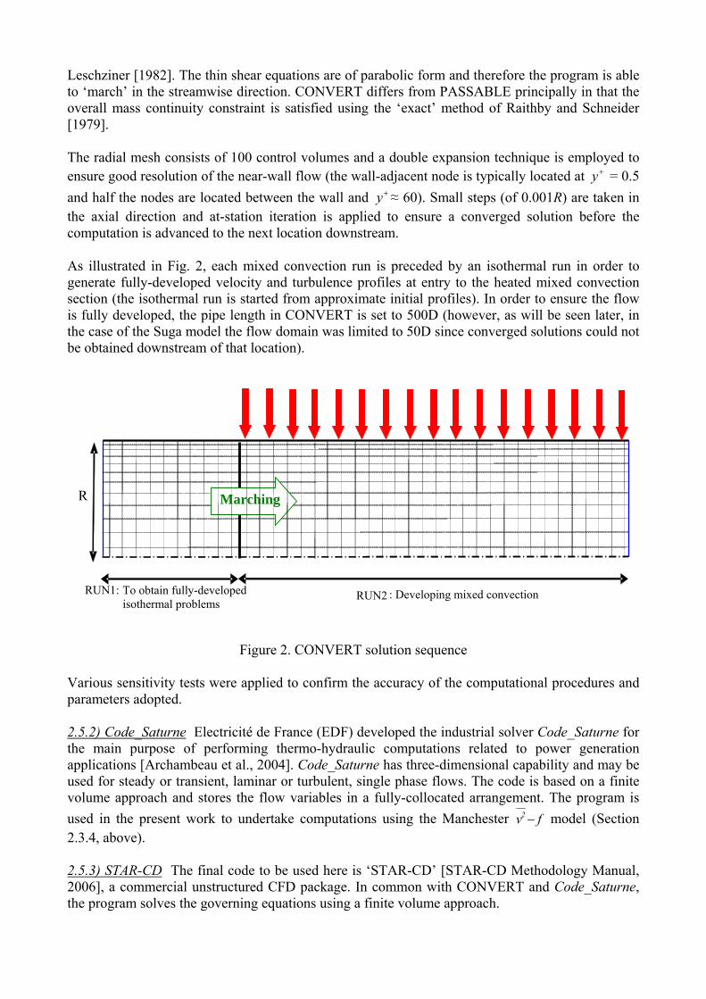
As illustrated in Fig. 2, each mixed convection run is preceded by an isothermal run in order to generate fully-developed velocity and turbulence profiles at entry to the heated mixed convection section (the isothermal run is started from approximate initial profiles). In order to ensure the flow is fully developed, the pipe length in CONVERT is set to 500D (however, as will be seen later, in the case of the Suga model the flow domain was limited to 50D since converged solutions could not be obtained downstream of that location).

Figure 2. CONVERT solution sequence

Various sensitivity tests were applied to confirm the accuracy of the computational procedures and parameters adopted.

2.5.2) Code_Saturne Electricité de France (EDF) developed the industrial solver Code_Saturne for the main purpose of performing thermo-hydraulic computations related to power generation applications [Archambeau et al., 2004]. Code_Saturne has three-dimensional capability and may be used for steady or transient, laminar or turbulent, single phase flows. The code is based on a finite volume approach and stores the flow variables in a fully-collocated arrangement. The program is used in the present work to undertake computations using the Manchester fv2 − model (Section 2.3.4, above). 2.5.3) STAR-CD The final code to be used here is ‘STAR-CD’ [STAR-CD Methodology Manual, 2006], a commercial unstructured CFD package. In common with CONVERT and Code_Saturne, the program solves the governing equations using a finite volume approach.

RUN1: To obtain fully-developed isothermal problems

RUN2 : Developing mixed convection

R Marching

STAR-CD is employed here to perform the LES calculations described in Section 2.4. The domain is made long in the axial direction (30R) in order to avoid the introduction of unphysical space correlations. The grid resolution at the wall is +Δr = 1.0, +ΔφR ≈ 6.3, and +Δz ≈ 18.0. (For comparison, the resolution of the DNS grid used by You et al. [2003] was +Δr ≈ 0.2, +ΔφR ≈ 8.8 and +Δz ≈ 10.5.)

3) RESULTS AND DISCUSSION

Results are presented in two main sections: in the first of these, there is an evaluation of model hydrodynamic and thermal performance in forced and mixed convection. The section includes an examination of mixed convection impairment or enhancement of Nusselt number and local friction coefficient with respect to forced convection values. Fully-developed Nu/Nu0 and cf /cf0 are plotted against the buoyancy parameter, Bo (Eq. (1)) and the present EVM and LES computations are compared against several sets of experimental data and the DNS results of You et al. [2003].

In the second section, mean flow and turbulence profiles are presented and comparison is again made with the DNS data of You et al.

3.1) Thermal-Hydraulic Performance in Forced and Mixed Convection

3.1.1) Forced convection To obtain an initial assessment of turbulence model accuracy, calculations were made for forced convection conditions. Reynolds number and Prandtl number are set to 5300 and 0.71. Values of fully-developed Nusselt number and friction coefficient are shown in Table 6 and Fig. 3. The first entry in Table 6 represents the DNS data of You et al; this is followed by results for the four EVMs and the LES run. The final row relates to the experiments of Polyakov and Shindin [1988] and is discussed further below. The third and fifth columns of Table 6 show percentage differences in Nu0 and cf0 with respect to the DNS values.

In the hydrodynamic comparisons, it is seen that the CI model and LES values of cf0 are in closest agreement with the DNS data. However, all the formulations, apart from the LS scheme, return what might be considered acceptably accurate values for cf0. It is worthy of note that the DNS result is itself well within 1% of the friction coefficient obtained from the Blasius equation, viz.

325.00f 1026.9Re079.0c −− ×== .

Turning to examine heat transfer coefficients, the value of Nu0 returned by the Suga model lies closest to the DNS data; all formulations, with the possible exception of the LES computations, are in reasonable agreement with the direct simulation data. Comparison of the DNS value of Nusselt number with a modified form of the Dittus-Boelter equation [Kays and Leung, 1963],

7.17PrRe022.0Nu 5.08.00 == , reveals the DNS value of Nu0 to be approximately 3% higher than

the correlation (the LS model is within 2% of this latter value). It should, however, be noted that Kays and Leung report comparisons with data only for Re ≥ 104. Finally it is recorded that the experimental measurements of Polyakov and Shindin [1988]* yield a value of Nu0 that is 7% above the DNS result, but within 3% of the current LES computations. Such discrepancies between the DNS figure and other possible ‘reference’ values of Nu0 is naturally a cause for concern. This concern relates directly to the preceding comparisons of forced convection Nusselt number; it also extends to the evaluation of turbulence model computations of mixed convection heat transfer levels where there might be expected to be similar discrepancies within the reference database.

* Polyakov and Shindin’s experiments were conducted at Re = 5100. The value of Nu0 = 19.6 appearing in Table 6 has been obtained by scaling the present authors’ determination of Nu0 = 19.0 by a factor of (5300/5100)0.8.

Table 6. Results for fully-developed forced convection Models/Codes 0Nu % difference 0fc % difference

DNS of You et al. [2003] 18.3 - 9.28E-03 -

Launder & Sharma (CONVERT) 17.4 -4.9 8.52E-03 -8.2

Cotton & Ismael (CONVERT) 18.9 +3.3 9.17E-03 -1.2

Suga NLEVM (CONVERT) 18.3 0.0 8.93E-03 -3.8

Manchester fv2 − (Code_Saturne) 18.6 +1.6 8.95E-03 -3.6

LES (STAR-CD) 20.1 +9.8 9.39E-03 +1.2

Expt. of Polyakov & Shindin [1988] 19.6 +7.1 - -

0

5

10

15

20

25

DN

S o

f Y

ou

et

al (

2003

)

Lau

nd

er &

Sh

arm

a(C

ON

VE

RT

)

Co

tto

n &

Ism

ael

(CO

NV

ER

T)

Su

ga

NL

EV

M(C

ON

VE

RT

)

Man

ches

ter-

v2f

(Co

de_

Sat

urn

e)

LE

S (

ST

AR

-CD

)

cf x

100

0 -

Nu

Nusselt number

Friction coefficient

Figure 3. Results for fully-developed forced convection

3.1.2) Mixed convection The DNS data of You et al. [2003] were generated for Reynolds and Prandtl numbers of Re = 5300 and Pr = 0.71; buoyancy influence was varied by altering the Grashof number. Four simulations are reported by You et al. and these are detailed in Table 7 (Case A represents the case of pure forced convection considered above). Figures 4 and 5, which show respectively Nu/Nu0 and cf /cf0 vs. Bo, include the DNS results for Cases B-D.

Table 7. DNS cases of You et al. [2003] Case Bo Thermal-Hydraulic Regime

A 0 Forced convection B 0.13 Early-onset mixed convection

C 0.18 Laminarization

D 0.50 Recovery

Expt. of Polyakov & Shindin [1988]

Also represented in Fig. 4 are the data of Steiner [1971], Carr et al. [1973] and Parlatan et al. [1996]. While these data were obtained for values of Re, Pr, and Gr different from those of You et al., all are cast in terms of Bo. A factor affecting the experimental data, but not accounted for in the DNS of You et al., or the present simulations, relates to variable property (principally viscosity) influences.

Fig. 4 is completed by the Nu/Nu0 vs. Bo distributions computed using the various turbulence models and LES of the present study. (Following You et al., Re and Pr were unchanged from the forced convection tests.) Where available, all sets of data and the current authors’ computations are normalized using the corresponding Nu0 value of that particular test case. (Note, however, that some of the physical experiments represented in Fig. 4 did not report a forced convection Nusselt number and therefore an established heat transfer correlation is employed to normalize the Nusselt number.)

The most striking picture to emerge from Fig. 4 is the abrupt and dramatic reduction in heat transfer levels occurring at around 0.15 < Bo < 0.25. DNS Case C (Bo = 0.18) is representative of this laminarized state in which heat transfer levels are only approximate 4/10ths of those found in forced convection under otherwise identical conditions.

0.2

0.4

0.6

0.8

1.0

1.2

1.4

1.6

0.01 0.1 1 10Bo

Nu

/Nu

0

Launder & Sharma Model (CONVERT)Cotton & Ismael Model (CONVERT)Suga Model (CONVERT)Manchester v2f Model (Code_Saturne)Large Eddy SimulationDNS - You et al (2003)Data of Steiner (1971)Data of Carr et al (1973)Data of Parlatan et al (1996)

Figure 4. Nusselt number impairment and enhancement

The formulation in closest agreement with the three DNS data points is the LS model. Another model that performs well is the Manchester fv2 − scheme, although this scheme is not as close to the DNS point at the lowest level of buoyancy influence (Case B; Bo = 0.13). The Large Eddy Simulations indicate that large-scale heat transfer impairment occurs at a lower value of Bo, and

interestingly these results, at least at lower levels of buoyancy influence, are in good agreement with the water data of Parlatan et al. [1996]. The CI model returns an unduly late onset of impairment. The Suga model shows a considerable delay in the onset of heat transfer impairment and also significantly under-predicts the extent of impairment (these results are for x/D = 50 because, for cases with relatively high Bo, converged solutions could not be obtained at locations further downstream). Examining the experimental data for the ‘Recovery’ region, a general observation might be made that there is considerable scatter in the measurements, a feature that may be due in part to variable property effects.

Figure 5 shows normalized local friction coefficient plotted against the buoyancy parameter. Of the turbulence models considered, the Manchester fv2 − scheme is in closest agreement with the three DNS points of You et al. [2003] and the data of Carr et al. [1973]. The LS, CI and Suga models indicate little or no reduction in mixed convection cf below the cf0 level (in the case of the LS model this is in part related to its under-prediction of cf0, Table 6). The Large Eddy Simulations show an early onset of cf-reduction (compare with Fig. 4 for Nu/Nu0); it is also seen that the LES computations return the lowest values of cf /cf0 found in the present study. Note that there is again considerable scatter in the experimental measurements, especially for higher Bo.

0.5

1.0

1.5

2.0

2.5

3.0

0.01 0.1 1 10Bo

cf/c

f 0

Launder & Sharma Model (CONVERT)Cotton & Ismael Model (CONVERT)Suga Model (CONVERT)Manchester v2f Model (Code_Saturne)Large Eddy SimulationDNS - You et al (2003)Data of Carr et al (1973)Data of Polyakov & Shindin (1988)Data of Parlatan et al (1996)

Figure 5. Local friction coefficient impairment and enhancement

3.2) Flow Profiles Computed profiles of velocity, temperature, and Reynolds shear stress are next compared against the DNS data of You et al. [2003]. Unfortunately DNS results for turbulent kinetic energy were not reported by You et al.

Considering first the forced convection case (Case A of Table 7), Fig. 6 shows that all four EVMs and the LES computations resolve the mean flow DNS profiles with reasonable accuracy (Figs. 6(a) and (b)). The situation is different in regard to the Reynolds shear stress profiles of Fig. 6(c): the present LES computations are in excellent agreement with the DNS. The CI model only slightly under-predicts the data, while the Suga model profile lies somewhat further below the DNS distribution. Clearly the Manchester fv2 − and LS models are in significantly worse agreement with the numerical simulations.

(a) (b)

(c)

Figure 6. Flow profiles for Case A (‘Forced convection’)

At the moderate buoyancy influence of Fig. 7 there is no appreciable distortion of the velocity and temperature profiles. There is some suggestion in the Reynolds stress profiles of Fig. 7(c) that the CI model and LES computations fail to detect the initial onset of mixed convection influences.

(a) (b)

(c)

Figure 7. Flow profiles for Case B (‘Early-onset mixed convection’)

The situation changes radically in Fig. 8 which clearly indicates the ‘catastrophic’ onset of large-scale mixed convection influences. The LES computations and the LS and fv2 − models capture the ‘M’-shaped distortion of the velocity profile (Fig. 8(a)). (Similar M-shapes are also characteristic of velocity profiles in ascending laminar mixed convection flows.) By contrast, the CI and Suga models continue to return velocity profiles that are essentially unchanged from the forced convection distributions. The same grouping of the models is evident in the temperature profiles of

Fig. 8(b). Turbulence collapse is evident in the DNS profile of Fig. 8(c). The LES computations are in closest agreement with the data, while the LS and fv2 − models return broadly the correct behaviour. (Note, however, that the LS model indicates a complete laminarization of the flow up to y+ ≈ 40-50.) While the CI and Suga models show some reduction in turbulence levels by comparison with the forced convection case of Fig. 6, the effects they indicate are only modest. This delay in the turbulence response of the two models is directly related to the late onset of heat transfer impairment seen in Fig. 4.

(a) (b)

(c)

Figure 8. Flow profiles for Case C (‘Laminarization’)

The final set of profiles is shown in Fig. 9. This case (Bo = 0.50) corresponds to the ‘Recovery’ regime, where heat transfer levels increase above the maximum impairment value (Fig. 4). All

models correctly predict M-shape velocity profiles and the appropriate distortion of the temperature profiles. While no scheme could be said accurately to resolve the DNS Reynolds shear stress profile of Fig. 9(c), the LES computations and fv2 − and CI models capture the general trends of the data.

(a) (b)

(c)

Figure 9. Flow profiles for Case D (‘Recovery’)

4) CONCLUDING REMARKS

Four eddy-viscosity turbulence models and new Large Eddy Simulations have been compared against the forced and mixed convection DNS data of You et al. [2003]. The turbulence models, which all embody different modifications of the parent form, are those of Launder and Sharma [‘LS’, 1974], Cotton and Ismael [‘CI’, 1998], Craft, Launder and Suga [‘Suga’, 1996] and the

‘Manchester fv2 − ’ scheme (details of which are given by Keshmiri et al. [2008]). The classical Smagorinsky/Lilly Sub-Grid-Scale model is adopted for the LES computations.

In relation to forced convection, the CI model and LES results are closest to the DNS figure for local friction coefficient, whereas the Suga model is in best agreement with the DNS value of Nusselt number. It is noted that discrepancies exist between what might be expected to be reliable ‘reference’ sources for forced convection number, namely the DNS and LES results and the experimental data of Polyakov and Shindin [1988]. All formulations are able to resolve the DNS profiles of mean velocity and temperature. However, in examining Reynolds shear stress profiles only the CI model and the Large Eddy Simulations (and to a lesser extend the Suga model) are acceptably close to the direct simulations.

The LS model best captures the DNS-computed impairment of heat transfer level in ascending mixed convection flows; the fv2 − scheme also performs well. By contrast, the CI model indicates that impairment occurs at higher values of a ‘buoyancy parameter’, Bo, while the Large Eddy Simulations show an earlier onset of heat transfer impairment. The Suga model under-predicts the extent of impairment. DNS flow and turbulence profiles at the maximum impairment condition, where the flow is largely laminarized, are resolved most accurately by the LES computations and the fv2 − and LS models. It should be noted, however, that no single scheme could be said to be in excellent agreement with the DNS data.

ACKNOWLEDGEMENTS

This work was carried out as part of the ‘Towards a Sustainable Energy Economy’ (TSEC) programme ‘Keeping the Nuclear Option Open’ (KNOO) and as such we are grateful to the UK Engineering and Physical Sciences Research Council for funding under grant EP/C549465/1.

REFERENCES

Abdelmeguid, A. M. and Spalding, D. B. [1979], Turbulent Flow and Heat Transfer in Pipes with Buoyancy Effects, J. Fluid Mech., Vol. 94, pp. 383-400.

Addad, Y., [2005], Large Eddy Simulations of Bluff Body, Mixed and Natural Convection Turbulent Flows with Unstructured FV Codes, PhD thesis, Department of Mechanical, Aerospace and Manufacturing Engineering, UMIST (now University of Manchester).

Archambeau, F., Mechitoua, N. and Sakiz, M. [2004], A Finite Volume Method for the Computation of Turbulent Incompressible Flows – Industrial Applications, Int. J. Finite Volumes, Vol. 1

Carr, A.D., Connor, M.A. and Buhr, H.O. [1973], Velocity, Temperature and Turbulence Measurements in Air for Pipe Flow with Combined Free and Forced Convection, Trans. ASME C, J. Heat Transfer, Vol. 95, pp. 445-452.

Cotton, M.A. [1987], Theoretical Studies of Mixed Convection in Vertical Tubes, PhD thesis, University of Manchester, UK.

Cotton, M.A. and Jackson, J.D. [1990], Vertical Tube Air Flows in the Turbulent Mixed Convection Regime calculated using a Low-Reynolds-Number ε−k Model, Int. J. Heat Mass Transfer, Vol. 33, pp. 275-286.

Cotton, M.A. and Kirwin, P.J. [1995], A variant of the Low-Reynolds-Number Two-Equation Turbulence Model Applied to Variable Property Mixed Convection Flows, Int. J. Heat Fluid Flow, Vol. 16, pp. 486-492.

Cotton, M.A. and Ismael, J.O. [1998], A Strain Parameter Turbulence Model and its Application to Homogeneous and Thin Shear Flows, Int. J. Heat Fluid Flow, Vol. 19, pp. 326-337.

Cotton, M.A., Ismael, J.O. and Kirwin, P.J [2001], Computations of Post-Trip Reactor Core Thermal Hydraulics using a Strain Parameter Turbulence Model, Nuclear Eng. and Design, Vol. 208, pp. 51-66.

Craft, T.J., Launder, B.E. and Suga, K. [1996], Development and Application of a Cubic Eddy-Viscosity Model of Turbulence, Int. J. Heat Fluid Flow, Vol. 17, pp. 108-115.

Durbin, P. A. [1991], Near-wall Turbulence Closure Modelling without Damping Functions, Theoret. Comput. Fluid Dyamics, Vol. 3, pp. 1-13.

Hall, W.B. and Jackson, J.D. [1969], Laminarization of a Turbulent Pipe Flow by Buoyancy Forces, ASME Paper 69-HT-55.

Hanjalić, K., Popovac, M. and Hadziabdic, M. [2004], A Robust Near-Wall Elliptic-Relaxation Eddy-Viscosity Turbulence Model for CFD, Int. J. Heat and Fluid Flow, Vol. 24, pp. 1047-1051.

Hunt, J.C.R. and Carruthers, D.J. [1990], Rapid Distortion Theory and the ‘Problems’ of Turbulence, J. Fluid Mech., Vol. 212, pp. 497-532.

Jackson, J.D., Cotton, M.A. and Axcell, B. P. [1989], Studies of Mixed Convection in Vertical Tubes, Int. J. Heat Fluid Flow, Vol. 10, pp. 2-15.

Jackson, J.D. [2006], Studies of Buoyancy-Influenced Turbulent Flow and Heat Transfer in Vertical Passages, Keynote lecture, 13th Int. Heat Transfer Conference, ‘IHTC13’, Sydney, Australia, 13-18 August 2006.

Jones, W.P. and Launder, B.E. [1972], The Prediction of Laminarization with a Two-Equation Model of Turbulence, Int. J. Heat Mass Transfer, Vol. 15, pp. 301-314.

Kasagi, N. and Nishimura, M. [1997], Direct Numerical Simulation of Combined Forced and Natural Turbulent Convection in a Vertical Plane Channel, Int. J. Heat Fluid Flow, Vol. 18, pp. 88-99.

Kays, W.M. and Leung, E.Y., [1963], Heat Transfer in Annular Passages - Hydrodynamically Developed Turbulent Flow with Arbitrarily Prescribed Heat Flux, Int. J. Heat Mass Transfer, Vol. 6, pp. 537-557.

Keshmiri, A., Cotton, M.A., Addad, Y., Rolfo, S. and Billard, F. [2008], RANS and LES Investigations of Vertical Flows in the Fuel Passages of Gas-Cooled Nuclear Reactors, To appear in Proc. 16th ASME Int. Conf. on Nuclear Engineering, ‘ICONE16’, Orlando, Florida, USA, 11th-15th May 2008.

Kim, W.S., Jackson, J.D. and He, S. [2006], Computational Investigation into Buoyancy-Aided Turbulent Flow and Heat Transfer to Air in a Vertical Tube, Turbulence, Heat and Mass Transfer, Vol. 5, (Hanjalić, K., Nagano, Y. and Jakirlić, S. (Editors))

Kirwin, P.J. [1995], Investigation and Development of Two-Equation Turbulence Closures with reference to Mixed Convection in Vertical Pipes, PhD thesis, University of Manchester, UK.

Launder, B.E. and Sharma, B.I. [1974], Application of the Energy Dissipation Model of Turbulence to the Calculation of Flow near a Spinning Disc, Lett. Heat Mass Transfer, Vol. 1, pp. 131-138.

Launder, B.E. and Spalding, D.B. [1974], The Numerical Computation of Turbulent Flows, Comp. Meth. Appl. Mech. Eng., Vol. 3, pp. 269-289.

Laurence, D.R., Uribe, J.C. and Utyuzhnikov, S.V. [2004], A Robust Formulation of the fv2 − Model, Flow, Turbulence and Combustion, Vol. 73, pp. 169-185.

Leschziner, M.A. [1982], An Introduction and Guide to the Computer Code PASSABLE, Report, Mech. Eng. Dept., UMIST, Manchester, UK.

Lien, F.S. and Durbin, P.A. [1996], Non Linear k-ε−v2 Modeling with application to High Lift, NASA Ames/Stanford University Center for Turbulence Research, Proc. Summer School Program, pp. 5-25.

Lilly, D.K., [1966], On the Application of the Eddy Viscosity Concept in the Inertial Sub-range of Turbulence, NCAR manuscript No.123, National Center for Atmospheric Research, Boulder, CO, USA.

Manceau, R. [2005], An Improved Version of the Elliptic Blending Model. Application to Non-Rotating and Rotating Channel Flows, in Proc. 4th Symp. Turb. Shear Flow Phenomena, J.A.C. Humphrey et al., eds., Williamsburg, Virginia, USA, pp. 259-264.

Maxey, M.R. [1982], Distortion of Turbulence in Flows with Parallel Streamlines, J. Fluid Mech., Vol. 124, pp. 261-282.

Mikielewicz, D.P. [1994], Comparative Studies of Turbulence Models under Conditions of Mixed Convection with Variable Properties in Heated Vertical Tubes, PhD thesis, University of Manchester, UK.

Parlatan, Y., Todreas, N.E. and Driscoll, M.J. [1996], Buoyancy and Property Variation Effects in Turbulent Mixed Convection of Water in Vertical Tubes, ASME J. Heat Transfer, Vol. 118, pp. 381-387.

Patel, V.C., Rodi, W. and Scheuerer, G. [1985], Turbulence Models for Near-Wall and Low Reynolds Number Flows: A Review, AIAA J., Vol. 23, pp. 1308-1319.

Petukhov, B.S. and Polyakov, A.F. [1988], Heat Transfer in Turbulent Mixed Convection, B.E. Launder (ed.), Hemisphere, Bristol, PA, USA.

Polyakov, A.F. and Shindin, S.A. [1988], Development of Turbulent Heat Transfer over the Length of Vertical Tubes in the presence of Mixed Air Convection, Int. J. Heat Mass Transfer, Vol. 31, pp. 987-992.

Raithby, G.D. and Schneider, G.E. [1979], Numerical Solution of Problems in Incompressible Fluid Flow: Treatment of the Velocity–Pressure Coupling, Numer. Heat Transfer, Vol. 2, pp. 417–440.

Richards, A.H., Spall, R.E. and McEligot, D.M. [2004], An Assessment of Turbulence Models for Strongly-Heated Internal Gas Flows, Proc. 15th IASTED int. Conf., Modeling and Simulation, Marina Del Rey, California, USA.

Shehata, A.M. and McEligot, D.M. [1998], Mean Turbulence Structure in the Viscous Layer of Strongly-Heated Internal Gas Flows-Measurements, Int. J. Heat Mass Transfer, Vol. 41, pp. 4297–4313.

STAR-CD [2006], Methodology Manual (Version 4.02), Computational Dynamics Limited, CD-Adapco.

Steiner, A. [1971], On the Reverse Transition of a Turbulent Flow under the Action of Buoyancy Forces, J. Fluid Mech., Vol. 47, pp. 503-512.

Tanaka, H., Maruyama, S. and Hatano, S. [1987], Combined Forced and Natural Convection Heat Transfer for Upward Flow in a Uniformly Heated Vertical Pipe, Int. J. Heat Mass Transfer, Vol. 30, pp. 165-174.

Townsend, A.A. [1970], Entrainment and the Structure of Turbulent Flow, J. Fluid Mech., Vol. 41, pp. 13-46.

Vilemas, J.V., Polkas, P.S. and Kaupas, V.E. [1992], Local Heat Transfer in a Vertical Gas-Cooled Tube with Turbulent Mixed Convection and different Heat Fluxes, Int. J. Heat Mass Transfer, Vol. 35, pp. 2421-2428.

Walklate, P.J. [1976], A Comparative Study of Theoretical Models of Turbulence for the Numerical Prediction of Boundary Layer Flows, PhD thesis, University of Manchester Institute of Science and Technology (UMIST), UK.

You, J., Yoo, J.Y. and Choi. H. [2003], Direct Numerical Simulation of Heated Vertical Air Flows in Fully Developed Turbulent Mixed Convection, Int. J. Heat Mass Transfer, Vol. 46, pp. 1613-1627.

Yu, L.S.L. [1991], A Computational Study of Turbulent Mixed Convection in Vertical Tubes, PhD thesis, University of Manchester, UK.