Refined procedure of evaluating experimental single-molecule force spectroscopy data

Alexander Fuhrmann,* Dario Anselmetti, and Robert Ros*,†

Experimental Biophysics, Physics Department, Bielefeld University, 33615 Bielefeld, Germany

Sebastian Getfert and Peter ReimannCondensed Matter Theory, Physics Department, Bielefeld University, 33615 Bielefeld, Germany

�Received 13 August 2007; revised manuscript received 9 November 2007; published 13 March 2008�

Dynamic force spectroscopy is a well-established tool to study molecular recognition in a wide range ofbinding affinities on the single-molecule level. The theoretical interpretation of these data is still very chal-lenging and the models describe the experimental data only partly. In this paper we reconsider the basicassumptions of the models on the basis of an experimental data set and propose an approach of analyzing andquantitatively evaluating dynamic force spectroscopy data on single ligand-receptor complexes. We present ourprocedure to process and analyze the force-distance curves, to detect the rupture events in an automatedmanner, and to calculate quantitative parameters for a biophysical characterization of the investigatedinteraction.

DOI: 10.1103/PhysRevE.77.031912 PACS number�s�: 82.37.Rs, 87.15.�v, 82.37.Np

I. INTRODUCTION

Dynamic force spectroscopy is widely used to investigatemolecular recognition on the single-molecule level �e.g., re-viewed in �1��. From these experiments, quantitative data interms of energy landscape parameters and kinetic constantsof the interaction can be obtained �2�. The technique can beapplied to a remarkable range of interactions; from the bind-ing of complex biological molecules like antibodies �3–6�,proteoglycans �7,8�, cytochromes �9�, chaperones �10�, selec-tines �11�, protein-DNA interactions �12–14� to small bioor-ganic or organic compounds like peptides �15� and supramo-lecular systems �16–18�. The binding affinities of the probedcomplexes can differ by several orders of magnitude. Forexample, the seminal early force spectroscopy works onstreptavidin/avidin-biotin interactions �19,20� yield a disso-ciation constant KD in the range of 10−15 M, whereas forweak calixarene-ion complexes one finds a KD of 10−5 M�18�.

Ligand-receptor interactions are mainly probed by dy-namic force spectroscopy based on atomic force microscopy�AFM�, but also alternative techniques like the biomembraneforce probe �2,21� or optical tweezers �22� are available. Atypical experimental setup is sketched in Fig. 1. One bindingpartner is connected to the force transducer �i.e., the tip of asoft AFM cantilever� and the other is bound to a surface. Theligand, the receptor-molecules, or both, are usually linked viapolymeric tethers to the tip and to the surface, respectively�3,5,12,15,23�. In order to obtain force-distance curves, theAFM tip or the surface is cycled up and down while mea-suring the force acting on the cantilever. From these forcecurves rupture or unbinding forces are analyzed for variouspulling velocities.

The interpretation and theoretical modeling of these ex-periments is challenging, as shown in various publications

�24–27�. Starting with the original works of Bell �28� andEvans and Ritchie �29�, almost all theoretical models rely onthe assumption of a well-defined force-extension character-istic of all the involved elastic components of the experimen-tal setup, which is independent of the velocity at which thepulling force increases and in particular does not changeupon many repetitions of the same experiment. Since disper-sive linker lengths, nonorthogonal pulling geometries, orpartly mis- or unfolded binding partners can contribute tosystemic spreads in force-extension characteristics, the mainpurpose of our present paper is a careful reconsideration ofthe above-mentioned basic assumption by analyzing theforce-extension curves of specific protein-DNA interactionsin the field of prokaryotic transcriptional regulation �30�. Ad-

*Present address: Department of Physics, Arizona State Univer-sity, Tempe, AZ 85287, USA

†robert.ros@asu.edu

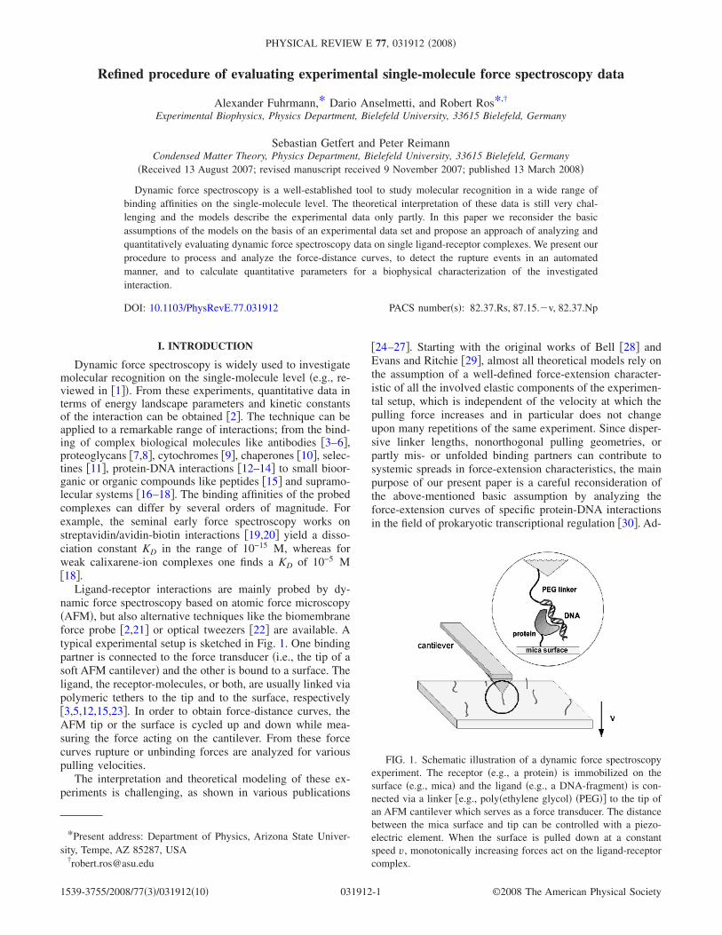
FIG. 1. Schematic illustration of a dynamic force spectroscopyexperiment. The receptor �e.g., a protein� is immobilized on thesurface �e.g., mica� and the ligand �e.g., a DNA-fragment� is con-nected via a linker �e.g., poly�ethylene glycol� �PEG�� to the tip ofan AFM cantilever which serves as a force transducer. The distancebetween the mica surface and tip can be controlled with a piezo-electric element. When the surface is pulled down at a constantspeed v, monotonically increasing forces act on the ligand-receptorcomplex.

PHYSICAL REVIEW E 77, 031912 �2008�

1539-3755/2008/77�3�/031912�10� ©2008 The American Physical Society031912-1

ditionally, we present our procedure to process and analyzethe force-distance curves, to detect the rupture events in anautomated manner, and to calculate quantitative parametersfor a biophysical characterization of the investigated interac-tion. This results in a data analysis technique for dynamicforce spectroscopy on single ligand-receptor complexes.

II. THEORETICAL BACKGROUND

In this section we briefly summarize the main theoreticalframework relevant for our subsequent discussions. Nearlyall theoretical models for bond rupture are based on theseminal works of Bell, Evans, and Ritchie �28,29�. Withinthis approach, a forced bond rupture is viewed as a thermallyactivated decay of a single slow reaction coordinate over apotential barrier.

Let f�t� denote the force that acts on the bond at time t.Since it is increasing much slower than all relevant molecu-lar relaxation processes, the reaction kinetics can be verywell approximated by

n�t� = − k„f�t�…n�t� , �1�

where n�t� denotes the survival probability of the bond up totime t and k�f� the dissociation rate at an arbitrary but fixedforce f .

A further key assumption is that the instantaneous forcef�t� depends solely on the total instantaneous extension s=s�t� of all elastic components of the complex �cantilever,linker, receptor, and ligand�. In other words, there exists acommon function F�s� �later referred to as the master curve�such that

f�t� = F„s�t�… �2�

for all the pulling experiments under consideration, indepen-dently of any further details �pulling speed, linker properties,etc.� of the single repetitions of the experiment.

Finally, we restrict ourselves to the usual case that thesurface is retracted at constant velocity v, i.e.,

s�t� = vt , �3�

and without loss of generality we choose the time offset suchthat t=0 when pulling starts. Hence it can be assumed thatf�t� is a continuous and monotonically increasing function oftime. Then Eq. �1� can be expressed in terms of the forcewith formal solution

n�f� = nv�f� = exp�−1

v�

fmin

f

df�k�f��

F�„F−1�f��…� �4�

for f � fmin, where fmin denotes the threshold value of theforce below which the measurement is dominated by randomfluctuations and artifacts so that rupture events cannot bedetected in this regime �see Sec. III A�. The subscript v re-fers to the velocity dependence of the survival probability.

In order to extract any useful and interesting quantitativeinformation from the measurement, further assumptionsabout the force dependence of the dissociation rate k�f� haveto be made. A quite common approximation going back toBell �28� is

k�f� = k0 exp� x�f

kBT� , �5�

with k0 the dissociation rate in the absence of an externalforce, x� the distance between potential well and barrier, andkBT the thermal energy. In the following we refer to themodel relying on Eqs. �1�–�5� as the standard or Bell model.Generalizations of this approximation have recently attractedconsiderable interest �31–33�.

As can be seen from Eq. �4�, specifying the force depen-dence of the rate k�f� alone is not sufficient for analyzing thedata: Also the full force-extension characteristic F�s� includ-ing the threshold value fmin is required. It should be re-marked that there exist a number of different models describ-ing the mechanical response of idealized polymeric chains interms of microscopic parameters like contour and Kuhnlength �e.g., the freely jointed chain or the wormlike chainmodel, as reviewed, e.g., in �34��. Since the total elastic en-tity is composed of cantilever, linkers, and ligand-receptormolecules, no simple realistic model exists to describe therelevant force-extension curve F�s�. In the following wetherefore just assume that an appropriate approximation forF�s� is available from experimental data.

Given the survival probability nv�f�, the probability den-sity to observe a rupture event is

p��f ��� ,v,F, fmin� = −d

dfnv�f� , �6�

where the notation in terms of a conditional probabilityp��f �¯� refers to the fact that this density is also conditionedon the model parameters �� �e.g., in the Bell model ��= �x� ,k0��, the pulling velocity v, the full force-extensioncurve, and the force offset fmin. Under the above discussedassumption that F�s� in Eq. �2� is the same function in allrupture measurements, a direct consequence of Eq. �4� is that−v ln(nv�f�) is independent of the pulling velocity �35�. For alarge number of experimental data sets this has been demon-strated not to be the case �26�. In particular the distributionsof measured rupture forces are much broader than those pre-dicted by the standard model. A possible explanation for thisdiscrepancy is given in �27�, consisting of a heterogeneousbond model such that Eqs. �1�–�5� are still valid except thatdue to uncontrollable variations of the molecular complex orof the local environment of the bond, the parameter x� isitself subjected to random variations. Sampling this param-eter from a Gaussian distribution with mean x� and variance�x

2 results in a good agreement with the analyzed data sets.The heterogeneous bond model thus involves the three pa-rameters �� = �x� ,�x ,k0�. Note that the standard model is aspecial case of the heterogeneous bond model correspondingto �x=0, while the qualitative and quantitative differencesbetween the two models become more and more pronouncedwith increasing variance �x.

III. DATA ANALYSIS

A dynamic force spectroscopy experiment consists typi-cally of thousands of force-distance curves. This requires a

FUHRMANN et al. PHYSICAL REVIEW E 77, 031912 �2008�

031912-2

stable procedure to detect and process extended data sets. Wedeveloped MATLAB �Mathworks� based routines for theanalysis of force-distance curves, which automatically detect,categorize, and quantify rupture events. In the following sec-tions we motivate and develop step by step this procedure ofprocessing and evaluating experimental single-moleculeforce spectroscopy data.

A. Raw data analysis

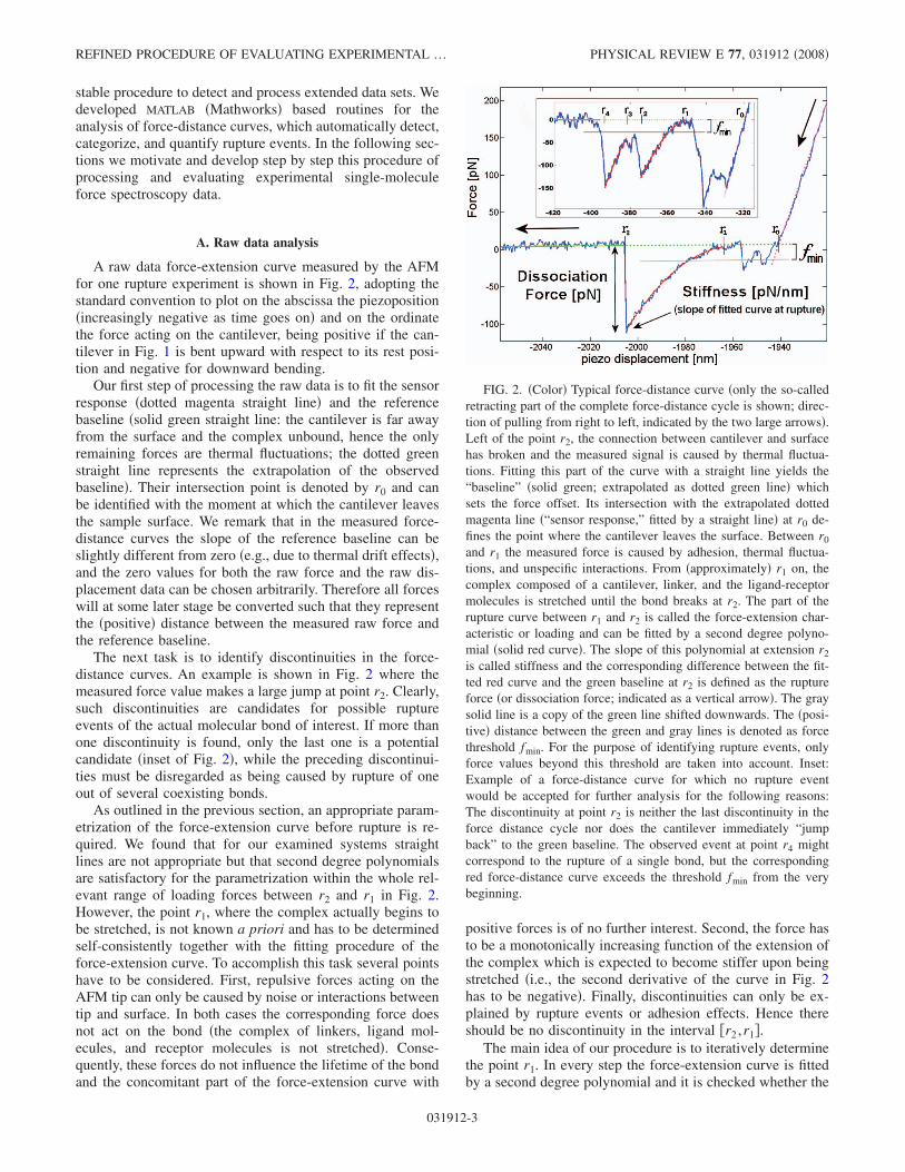
A raw data force-extension curve measured by the AFMfor one rupture experiment is shown in Fig. 2, adopting thestandard convention to plot on the abscissa the piezoposition�increasingly negative as time goes on� and on the ordinatethe force acting on the cantilever, being positive if the can-tilever in Fig. 1 is bent upward with respect to its rest posi-tion and negative for downward bending.

Our first step of processing the raw data is to fit the sensorresponse �dotted magenta straight line� and the referencebaseline �solid green straight line: the cantilever is far awayfrom the surface and the complex unbound, hence the onlyremaining forces are thermal fluctuations; the dotted greenstraight line represents the extrapolation of the observedbaseline�. Their intersection point is denoted by r0 and canbe identified with the moment at which the cantilever leavesthe sample surface. We remark that in the measured force-distance curves the slope of the reference baseline can beslightly different from zero �e.g., due to thermal drift effects�,and the zero values for both the raw force and the raw dis-placement data can be chosen arbitrarily. Therefore all forceswill at some later stage be converted such that they representthe �positive� distance between the measured raw force andthe reference baseline.

The next task is to identify discontinuities in the force-distance curves. An example is shown in Fig. 2 where themeasured force value makes a large jump at point r2. Clearly,such discontinuities are candidates for possible ruptureevents of the actual molecular bond of interest. If more thanone discontinuity is found, only the last one is a potentialcandidate �inset of Fig. 2�, while the preceding discontinui-ties must be disregarded as being caused by rupture of oneout of several coexisting bonds.

As outlined in the previous section, an appropriate param-etrization of the force-extension curve before rupture is re-quired. We found that for our examined systems straightlines are not appropriate but that second degree polynomialsare satisfactory for the parametrization within the whole rel-evant range of loading forces between r2 and r1 in Fig. 2.However, the point r1, where the complex actually begins tobe stretched, is not known a priori and has to be determinedself-consistently together with the fitting procedure of theforce-extension curve. To accomplish this task several pointshave to be considered. First, repulsive forces acting on theAFM tip can only be caused by noise or interactions betweentip and surface. In both cases the corresponding force doesnot act on the bond �the complex of linkers, ligand mol-ecules, and receptor molecules is not stretched�. Conse-quently, these forces do not influence the lifetime of the bondand the concomitant part of the force-extension curve with

positive forces is of no further interest. Second, the force hasto be a monotonically increasing function of the extension ofthe complex which is expected to become stiffer upon beingstretched �i.e., the second derivative of the curve in Fig. 2has to be negative�. Finally, discontinuities can only be ex-plained by rupture events or adhesion effects. Hence thereshould be no discontinuity in the interval �r2 ,r1�.

The main idea of our procedure is to iteratively determinethe point r1. In every step the force-extension curve is fittedby a second degree polynomial and it is checked whether the

FIG. 2. �Color� Typical force-distance curve �only the so-calledretracting part of the complete force-distance cycle is shown; direc-tion of pulling from right to left, indicated by the two large arrows�.Left of the point r2, the connection between cantilever and surfacehas broken and the measured signal is caused by thermal fluctua-tions. Fitting this part of the curve with a straight line yields the“baseline” �solid green; extrapolated as dotted green line� whichsets the force offset. Its intersection with the extrapolated dottedmagenta line �“sensor response,” fitted by a straight line� at r0 de-fines the point where the cantilever leaves the surface. Between r0

and r1 the measured force is caused by adhesion, thermal fluctua-tions, and unspecific interactions. From �approximately� r1 on, thecomplex composed of a cantilever, linker, and the ligand-receptormolecules is stretched until the bond breaks at r2. The part of therupture curve between r1 and r2 is called the force-extension char-acteristic or loading and can be fitted by a second degree polyno-mial �solid red curve�. The slope of this polynomial at extension r2

is called stiffness and the corresponding difference between the fit-ted red curve and the green baseline at r2 is defined as the ruptureforce �or dissociation force; indicated as a vertical arrow�. The graysolid line is a copy of the green line shifted downwards. The �posi-tive� distance between the green and gray lines is denoted as forcethreshold fmin. For the purpose of identifying rupture events, onlyforce values beyond this threshold are taken into account. Inset:Example of a force-distance curve for which no rupture eventwould be accepted for further analysis for the following reasons:The discontinuity at point r2 is neither the last discontinuity in theforce distance cycle nor does the cantilever immediately “jumpback” to the green baseline. The observed event at point r4 mightcorrespond to the rupture of a single bond, but the correspondingred force-distance curve exceeds the threshold fmin from the verybeginning.

REFINED PROCEDURE OF EVALUATING EXPERIMENTAL … PHYSICAL REVIEW E 77, 031912 �2008�

031912-3

above-mentioned points are satisfied. In detail, our algorithmworks as follows: �i� r1 is chosen only slightly larger than r2;�ii� a second degree polynomial is fitted to the raw data in theinterval �r2 ,r1�; and �iii� it is checked whether the fitted poly-nomial meets one of the following conditions within the in-terval �r2 ,r1�: �a� it crosses the reference baseline; �b� it ex-hibits a maximum; �c� it has the “wrong” curvature ascompared to the red line in Fig. 2, i.e., its second derivativeis positive; and �d� another discontinuity has been detected inthis interval. If none of the conditions are fulfilled, r1 isincreased by a small value �r and steps �ii� and �iii� arerepeated. Otherwise, r1 is decreased by �r and the resultingfinal r1 value is defined as the position where the complexbegins to be stretched. The corresponding final polynomialfit is chosen for the parametrization of the force-extensioncurve and the rupture force f i is defined as the differencebetween this fit and the reference baseline at r2 �see Fig. 2�.In this way noise effects that especially dominate the mea-surement in the low-force regime can be reduced to a mini-mum. In practice, we found that an additional discontinuity�condition �d�� in fact always implies a maximum �condition�b�� of the fitted polynomial.

The force value at the beginning of the fit �at r=r1� is the�force� offset for this single rupture curve. Most fits do notreach the zero force baseline for basically two reasons. First,due to a limited resolution of the apparatus and unspecificinteractions between tip and surface, we cannot measure ar-bitrarily small forces. Second, as discussed above we onlyuse the last rupture event in each force-distance cycle. How-ever, in case that there are multiple rupture events in thecycle, it is likely that the cantilever does not “jump back” tothe baseline after the second to last bond has ruptured �seeinset of Fig. 2�. We therefore introduce a threshold parallel tothe baseline but at a distance fmin below it �see also Fig. 2�.Note that by convention fmin is always positive like the rup-ture force. For a quantitative evaluation of the experiment itis required �see Eqs. �4� and �6�� that the bond has beenformed at forces lower than this threshold value fmin and thatall rupture events with rupture forces larger than this thresh-old value can be detected, i.e., fmin must in particular belarger than the thermal fluctuations. That means we only ac-cept rupture events with the properties that the polynomial fitcrosses the threshold between r2 and r1 before jumping backto the baseline at r2. Consequently, when choosing fmin toosmall a lot of rupture events will not be accepted because thecorresponding force value at the beginning of the pulling �atr=r1� is already larger than the threshold force. On the otherhand, when choosing fmin too large also a lot of ruptureevents will not be accepted because the rupture force issmaller than fmin. Hence we usually choose this value suchthat as many rupture events as possible can be used for theevaluation of the experiment. In our experiment we foundthat noise effects increase with the pulling velocity. There-fore we generally admit that the offset fmin still depends onthe pulling velocity, i.e., fmin= fmin�v�.

Other technical problems, when automatically processingthe force-distance curves, are caused by adhesion effects.Near the sample surface, adhesion forces act on the cantile-ver which can cause a signal in the force-extension curve �cf.Fig. 2 left of point r0�. Most successful single-molecule force

spectroscopy experiments use polymeric linkers of a definedlength to connect the binding partners to the tip and thesurface, respectively. This allows limiting the forced ruptureevents of interest to a distinct distance window �37�. Hencewe use the distance from r0 to r1 as another selection crite-rion and exclude rupture events with small �r1−r0� from fur-ther analysis.

B. Construction of the force-extension master curve

One of the basic theoretical assumptions �see Sec. II� is awell-defined force-extension characteristic which, in particu-lar, is independent of the pulling velocity and does notchange upon repeating the experiment many times. In thissection we show that this assumption does often not apply tothe experimental reality and present a numerical scheme toremedy this discrepancy.

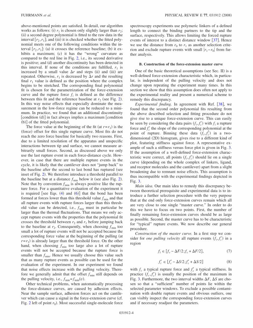
Experimental finding. In agreement with Ref. �38�, wefound that the second order polynomial fits resulting fromthe above described selection and fitting procedure do notgive rise to a unique force-extension curve. This can easilybe seen by considering the data pairs �f i , f i�� with f i a ruptureforce and f i� the slope of the corresponding polynomial at thepoint of rupture. Binning these data �f i , f i�� in a two-dimensional �2D� histogram, gives rise to a different kind ofplot, featuring stiffness against force. A representative ex-ample of such a stiffness versus force plot is given in Fig. 3.If the assumption of a well-defined force-extension charac-teristic were correct, all points �f i , f i�� should lie on a singlecurve �depending on the whole complex of linkers, ligand,and receptor molecules and the cantilever� apart from a slightbroadening due to remnant noise effects. This assumption isthus incompatible with the experimental findings depicted inFig. 3.

Main idea. Our main idea to remedy this discrepancy be-tween theoretical prerequisite and experimental data is to in-troduce a further selection procedure with the very purposethat at the end only force-extension curves remain which allare very close to one single “master curve.” In order to dothis we have to focus on two points. First, the number offinally remaining force-extension curves should be as largeas possible. Second, the master curve has to be characteristicfor “typical” rupture events. We now describe our generalprocedure.

Construction of the master curve. In a first step we con-sider for one pulling velocity all rupture events �f i , f i�� in aregion

f i � �fc − �F/2; fc + �F/2� , �7�

f i� � �fc� − �S/2; fc� + �S/2� �8�

with fc a typical rupture force and fc� a typical stiffness. Inpractice �fc , fc�� is usually the position of the maximum inFig. 3. Furthermore, the two interval widths �F, �S are cho-sen so that a “sufficient” number of points lie within theselected parameter windows. To exclude a possible contami-nation with double rupture events and obvious outliers, onecan visibly inspect the corresponding force-extension curvesand if necessary readjust the parameters.

FUHRMANN et al. PHYSICAL REVIEW E 77, 031912 �2008�

031912-4

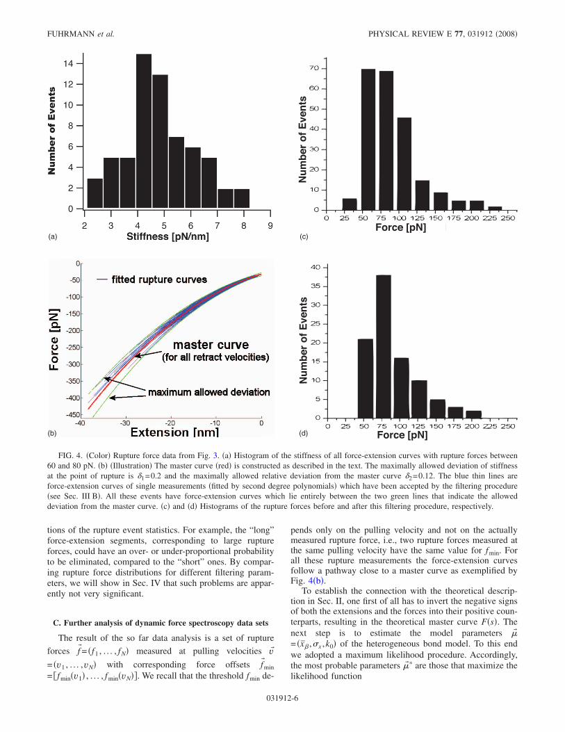
After applying the above selection procedure, the remain-ing force-extension curves are automatically aligned byproperly transforming abscissa and ordinate in Fig. 2 as fol-lows: In a first step, the data are transformed such that thegreen reference baseline in Fig. 2 falls on top of the zeroforce line. Then the abscissa is shifted such that every ad-justed force-extension curve crosses the gray threshold lineat the same position r=0, see Fig. 4�b�. Finally, this data setis used for a second degree polynomial fit, henceforth calledthe �force-extension� master curve and exemplified by thered line in Fig. 4�b�.

Selection procedure. In a second step all force-extensioncurves for all pulling velocities are compared with this mas-ter curve. The decision of which curves are accepted for thefurther analysis is controlled by two parameters ��1 ,�2�. Thefirst of them sets the maximum relative deviation of the slopeat the rupture point from the slope of the master curve at thispoint. The second defines an interval around the mastercurve, limiting the maximum relative deviation from themaster curve as indicated by the green lines in Fig. 4�b�.Only force-extension curves lying entirely in this intervalwill be accepted.

In the previous section we have described the necessity tointroduce a threshold force fmin and to use only rupture

events for the evaluation where the bond has formed belowthis force, but with rupture force f i� fmin. However, it seemsdesirable that the master curve should also correctly describethe part of the force-extension curve for lower forces. Hencefor the construction of the master curve, i.e., for choosing thesubset of rupture forces out of which the master curve isconstructed, a lower threshold force fmin� fmin should beused sooner than later for the quantitative evaluation of theexperiment.

It should be noted that the parameters ��1 ,�2� control howsimilar the force-extension curves of the accepted ruptureevents are. Ideally, one would wish to choose both as smallas possible. However, the smaller they are, the lower is thenumber of accepted rupture events and, hence, the worse thestatistic. Therefore one has to make a compromise betweenthese two points. In contrast to the choice of ��1 ,�2� thechoice of the interval widths �F and �S in Eqs. �7� and �8�is rather uncritical as they only determine the number ofevents used to construct the master curve. The detailed dis-cussion of the explicit choice of the “filtering parameters” fora particular experiment will be given in Sec. IV.

A subtle point arising with the above selection of force-extension curves regards the question whether such a “filter-ing procedure” is not introducing certain hidden modifica-

FIG. 3. �Color� Rupture force data for protein-DNA interaction previously studied in �30� are plotted against the slope of the force-extension curve at the point of rupture r2 �stiffness� in a 2D histogram �red, high frequency, blue, low frequency�. At a pulling velocity ofv=5000 nm /s, 2317 rupture curves have been measured. After the automated analysis �see Sec. III A� with threshold force fmin=42 pN,259 specific rupture events have been identified. The white solid line corresponds to the master curve which has been constructed out of theforce-extension curves at the maximum of the stiffness against force plot. The cumulated distributions of the rupture force and of the stiffnessare shown above and to the left of the 2D histogram. Inset: Illustration of raw data force-extension curves of the rupture events with �f i , f i��falling into the marked region of the 2D histogram.

REFINED PROCEDURE OF EVALUATING EXPERIMENTAL … PHYSICAL REVIEW E 77, 031912 �2008�

031912-5

tions of the rupture event statistics. For example, the “long”force-extension segments, corresponding to large ruptureforces, could have an over- or under-proportional probabilityto be eliminated, compared to the “short” ones. By compar-ing rupture force distributions for different filtering param-eters, we will show in Sec. IV that such problems are appar-ently not very significant.

C. Further analysis of dynamic force spectroscopy data sets

The result of the so far data analysis is a set of rupture

forces f�= �f1 , . . . , fN� measured at pulling velocities v�

= �v1 , . . . ,vN� with corresponding force offsets f�min

= �fmin�v1� , . . . , fmin�vN��. We recall that the threshold fmin de-

pends only on the pulling velocity and not on the actuallymeasured rupture force, i.e., two rupture forces measured atthe same pulling velocity have the same value for fmin. Forall these rupture measurements the force-extension curvesfollow a pathway close to a master curve as exemplified byFig. 4�b�.

To establish the connection with the theoretical descrip-tion in Sec. II, one first of all has to invert the negative signsof both the extensions and the forces into their positive coun-terparts, resulting in the theoretical master curve F�s�. Thenext step is to estimate the model parameters ��= �x� ,�x ,k0� of the heterogeneous bond model. To this endwe adopted a maximum likelihood procedure. Accordingly,the most probable parameters �� � are those that maximize thelikelihood function

(a)

(b)

(c)

(d)

FIG. 4. �Color� Rupture force data from Fig. 3. �a� Histogram of the stiffness of all force-extension curves with rupture forces between60 and 80 pN. �b� �Illustration� The master curve �red� is constructed as described in the text. The maximally allowed deviation of stiffnessat the point of rupture is �1=0.2 and the maximally allowed relative deviation from the master curve �2=0.12. The blue thin lines areforce-extension curves of single measurements �fitted by second degree polynomials� which have been accepted by the filtering procedure�see Sec. III B�. All these events have force-extension curves which lie entirely between the two green lines that indicate the alloweddeviation from the master curve. �c� and �d� Histograms of the rupture forces before and after this filtering procedure, respectively.

FUHRMANN et al. PHYSICAL REVIEW E 77, 031912 �2008�

031912-6

L��� � = i=1

N

p„�f i��� ,vi,F, fmin�vi�… . �9�

In doing so, it has been taken for granted that all force-extension curves follow exactly the master curve. This seemsjustified in view of the selection procedure described in thepreceding section such that the actual deviations of the re-maining force-extension curves from the master curve arevery small. For a more detailed discussion of the adoptedmaximum likelihood procedure we refer to �36�. Here, weonly point out that for estimating the parameters, no binningof the rupture forces to histograms is needed. The histogramsare only used to compare the fitted distribution with the ex-perimentally measured one. A further advantage is that esti-mates for the statistical error are easily obtained. The mostprobable parameters �� � are found by maximizing the likeli-hood function numerically. For practical purposes we haveused =ln�k0� as a fit parameter. Using k0 itself would resultin the same estimate k0

� for the parameter but the correspond-ing error interval is not symmetrically around the most prob-able value. For the data presented in this work a commercialalgorithm from the NAG �National Algorithms Group� li-brary has been used for the maximization.

D. Software integration

The entire above described procedure for dynamic forcespectroscopy data analysis is developed in MATLAB �Math-works� and C programming language. Most functions of theprogram can be handled via a graphical user interface �GUI�enabling one to do a data analysis with a scan rate of about200 force distance curves per minute with a standard PC.This force spectroscopy software can analyze both the dataformat of our homebuilt force spectroscopy instruments �12�and the data provided by the commercial MFP-3D �AsylumResearch, USA�.

IV. RESULTS AND DISCUSSION

In order to test and illustrate our data analysis method, theraw data originally published in �30� have been taken. Theexperiment conducted involved specific protein-DNA inter-actions relevant for prokaryotic transcriptional regulation.These interactions are mediated by small signaling molecules�N-acyl homoserine lactones, AHL�, which are able to stimu-late the protein-DNA binding by docking onto the proteins.In this particular experiment, the DNA target sequence islocated on a 285 bp long DNA fragment, which is immobi-lized on the tip via an approximately 35 nm long poly�eth-ylene glycol�-linker, see also Fig. 1. The proteins are immo-bilized on mica surfaces via short linker molecules andstimulated by the AHL N-decanoyl-DL-homoserine lactone�C10-HL�.

Each force-extension curve could be well-approximatedby a second degree polynomial �for a particular example seeFig. 2�, but no universal force-distance curve, neither for aspecific pulling velocity, nor for the entire data set could befound, in disagreement with the theoretical model. Qualita-tively this can be seen in Fig. 3, where the plot shows a

broad single maximum with a significant number of outliers.To quantify this finding, we choose the subset of force-extension curves corresponding to rupture forces between 60and 80 pN. For this subset, Fig. 4�a� shows the histogram ofthe slope �stiffness� of the fitted polynomials at the point ofrupture. It has a pronounced maximum at 4.5 pN/nm but alsoa dispersion which cannot be neglected. Possible explana-tions are a dispersion of linker length �25� or that in somecases not single but multiple bonds are stretched. In the lattercase, the corresponding complex is stiffer. Another possiblereason is that the angle between the stretched complex andthe surface normal is in most cases not zero �37�. As differentangles yield different force-extension curves, variations ofthe pulling geometry might also explain our findings.

To account for the problem that no universal force-extension curve exists, a master curve can be constructed andonly rupture events with a force-extension characteristicclose to this curve are accepted for further analysis. For theconstruction of the master curve a subset of rupture events ischosen and a second degree polynomial is fitted to the cor-responding force-extension curves. A fully objective criterionwhich subset should be chosen for this construction does notexist. However, as discussed in Sec. III B the master curveshould be characteristic for typical rupture events. Thereforewe have used the rupture curves corresponding to the peak ofthe 2D histogram in Fig. 3. The corresponding pulling veloc-ity is v=5000 nm /s being the highest pulling velocity usedin �30�. The reason for considering just the largest v is sim-ply that the rupture force increases with the pulling velocity.Hence the constructed master curve should be more appro-priate for describing the force-extension characteristic in thehigh force regime than the corresponding curve constructedfrom rupture curves sampled at lower pulling velocities.Analogously, for an appropriate parametrization of the force-extension characteristic in the low-force regime it is desir-able that the force-extension curves used to construct themaster curve start well below the threshold force fmin whichhad to be introduced for a quantitative evaluation of the ex-periment �see Sec. III B�. We have, thus, temporarily used a

lower threshold fmin for this construction than later in thequantitative evaluation. In particular a threshold of 10 pNresults in a very low number of force curves �10–20� whichare then used for the construction. The red line in Fig. 4�b�shows the constructed master curve together with the force-extension curves of various single measurements which areused for a quantitative evaluation of the experiment. Allthese rupture curves lie within a preset level of deviation.Thus all rupture events that are used for further analysis haveapproximately the same force-extension pathway. Since it isvery unlikely that a multiple and a single bond have the sameforce-extension curve, it follows that a contamination of therupture force data by multiple-rupture events is reduced to aminimum. In order to examine whether the constructed mas-ter curve strongly depends on the selected subset of ruptureforces, we have varied the selected area in the 2D histogram.As long as this area is near the peak, the constructed mastercurves were always similar. We have also compared the re-sulting master curve with constructed master curves fromother pulling velocities, but no systematic deviations couldbe found.

REFINED PROCEDURE OF EVALUATING EXPERIMENTAL … PHYSICAL REVIEW E 77, 031912 �2008�

031912-7

In a next step, we have applied the filtering procedure fordifferent choices of the tolerance levels ��1 ,�2�. Our generalobservation is that with decreasing tolerance levels the widthof the histogram of rupture forces initially decreases slightly.From a certain point on, however, the width is constant andthe only effect of further lowering ��1 ,�2� is that the numberof accepted rupture events gets smaller. For the particularchoice ��1=0.2,�2=0.12� the result of this filtering proce-dure is shown in Figs. 4�c� and 4�d� where the histograms ofrupture forces before and after the filtering procedure arepresented for one particular pulling velocity. Within their in-trinsic statistical uncertainties, these histograms differ fromeach other only slightly. The same was found for all otherpulling velocities and analyzed data sets. Even going tosmaller tolerance levels ��1 ,�2� does not change this finding,implying that the distribution of rupture forces does not criti-cally depend on details of the force-extension characteristic.Moreover, it follows that the filtering procedure itself doesnot introduce significant artifacts into the rupture force sta-tistics.

Having ensured that the theoretical assumption of aunique force-extension characteristic is met at least for theconsidered subset of data, we can now check whether anymodel relying on Eqs. �1�–�3� is compatible to the experi-mental data. Given Nv rupture forces f i, i=1, . . . ,Nv, mea-sured at a pulling velocity v, the survival probability of thebond can be approximated as nv�f�=Nv

−1i=1Nv �f i− f� with

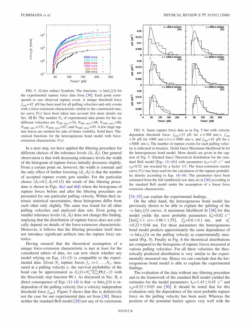
the Heaviside step function �·�. As discussed in Sec. II, adirect consequence of Eqs. �1�–�4� is that −v ln(nv�f�) is in-dependent of the pulling velocity �for a velocity independentthreshold force fmin�. Figure 5 shows that this is definitivelynot the case for our experimental data set from �30�. Henceneither the standard Bell model �29� nor any of its extensions

�31–33� can explain the experimental findings.On the other hand, the heterogeneous bond model has

previously shown to be able to explain the splitting of the−v ln(nv�f�) curves. A maximum likelihood fit �36� for thismodel yields the most probable parameters k0

�=0.02 s−1

�ln�k0��1 s�=−3.86�1.55�, x�

� =0.6�0.1 nm, and �x�

=0.23�0.04 nm. For these parameters the heterogeneousbond model predicts approximately the same dependence of−v ln(nv�f�) on the pulling velocity as experimentally mea-sured �Fig. 5�. Finally in Fig. 6 the theoretical distributionsare compared to the histograms of rupture forces measured atvarious pulling velocities. For all these velocities the theo-retically predicted distribution is very similar to the experi-mentally measured one. Hence we can conclude that the het-erogeneous bond model is able to explain the experimentalfindings.

The evaluation of the data without any filtering procedureand in the framework of the standard Bell model yielded theestimates for the model parameters: k0=1.43�0.45 s−1 andx�=0.52�0.03 nm �30�. It should be noted that for thisevaluation only the dependence of the most probable ruptureforce on the pulling velocity has been used. Whereas theposition of the potential barrier agrees very well with the

101

102

103

104

50 100 150 200 250

-vln

n v(f

)[n

m/s

]

Force f [pN]

5000 nm/s3000 nm/s2000 nm/s1000 nm/s500 nm/s200 nm/s

FIG. 5. �Color online� Symbols: The functions −v ln(nv�f�) forthe experimental rupture force data from �30�. Each point corre-sponds to one observed rupture event. A unique threshold forcefmin=42 pN has been used for all pulling velocities and only eventswith a force-extension characteristic similar to the constructed mas-ter curve F�s� have been taken into account �for more details seeSec. III B�. The number Nv of experimental data points for the sixdifferent velocities are N200 nm/s=54, N500 nm/s=48, N1000 nm/s=80,N2000 nm/s=151, N3000 nm/s=87, and N5000 nm/s=95. A few large rup-ture forces are omitted for sake of better visibility. Solid lines: The-oretical functions for the heterogeneous bond model with force-extension characteristic F�s�.

0.02

0.015

0.01

0.005

0

p(f)

[pN

-1]

v = 200.0 nm/sec

0.02

0.015

0.01

0.005

0

p(f)

[pN

-1]

v = 200.0 nm/sec[64]

0.02

0.015

0.01

0.005

0

p(f)

[pN

-1]

v = 200.0 nm/sec[64]

v = 500.0 nm/secv = 500.0 nm/sec[56]

v = 500.0 nm/sec[56]

0.02

0.015

0.01

0.005

0

p(f)

[pN

-1]

v = 1000.0 nm/sec

0.02

0.015

0.01

0.005

0

p(f)

[pN

-1]

v = 1000.0 nm/sec[82]

0.02

0.015

0.01

0.005

0

p(f)

[pN

-1]

v = 1000.0 nm/sec[82]

v = 2000.0 nm/secv = 2000.0 nm/sec[160]

v = 2000.0 nm/sec[160]

0.02

0.015

0.01

0.005

0200150100500

p(f)

[pN

-1]

Force f [pN]

v = 3000.0 nm/sec

0.02

0.015

0.01

0.005

0200150100500

p(f)

[pN

-1]

Force f [pN]

v = 3000.0 nm/sec[92]

0.02

0.015

0.01

0.005

0200150100500

p(f)

[pN

-1]

Force f [pN]

v = 3000.0 nm/sec[92]

200150100500

Force f [pN]

v = 5000.0 nm/sec

200150100500

Force f [pN]

v = 5000.0 nm/sec[95]

200150100500

Force f [pN]

v = 5000.0 nm/sec[95]

FIG. 6. Same rupture force data as in Fig. 5 but with velocitydependent threshold force: fmin=32 pN for v 500 nm /s, fmin

=38 pN for 1000 nm /s v 3000 nm /s, and fmin=42 pN for v=5000 nm /s. The number of rupture events for each pulling veloc-ity is indicated in brackets. �Solid lines� Maximum likelihood fit forthe heterogeneous bond model. More details are given in the cap-tion of Fig. 5. �Dashed lines� Theoretical distribution for the stan-dard Bell model �Eqs. �1�–�6�� with parameters k0=1.43 s−1 andx�=0.52 nm rescaled by a factor 1/3. The force-extension mastercurve F�s� has been used for the calculation of the rupture probabil-ity density according to Eqs. �4�–�6�. The parameters have beenestimated from the full �unfiltered� raw data set in �30� according tothe standard Bell model under the assumption of a linear forceextension characteristic.

FUHRMANN et al. PHYSICAL REVIEW E 77, 031912 �2008�

031912-8

mean position of the barrier estimated above, the dissociationrate is two orders of magnitude larger. This clearly demon-strates the importance of consistent data analysis standardsfor extracting quantitative and comprehensive molecular datain a robust and independent manner. Assuming that the Bellmodel with these parameters is true, the distribution of rup-ture forces for the force-extension master curve and givenforce offsets can be calculated via Eqs. �4�–�6�. Figure 6shows clearly that these “expected” distributions explain theexperimental findings only unsatisfactorily for all pulling ve-locities in agreement with our above conclusions.

V. SUMMARY AND CONCLUSIONS

In this paper we have described a data analysis method inthe field of dynamic force spectroscopy on single ligand-receptor pairs. This method allows the careful processing andanalysis of the force-distance characteristic in an automatedmanner. We have paid particular attention to guarantee thatthe assumptions made for the theoretical interpretation andevaluation of the experiment are really satisfied.

A common basic assumption in the context of theoreti-cally interpreting and quantitatively evaluating single-molecule force spectroscopy experiments is that the force-extension characteristic of the considered molecular complex�including ligand, receptor, linkers, AFM, etc.� is always thesame, i.e., it does not change from one pulling experiment tothe next and does not depend on the pulling velocity. Herewe have demonstrated by means of data from a representa-tive experiment that this assumption is in fact not satisfied. Inthe absence of previously existing careful examinations ofthis assumption, we must conclude that similar discrepanciesbetween theoretical models and experimental reality may bequite common and may require reconsideration of the experi-mental data and the hence deduced quantitative conclusions.

In a next step, we have put forward a selection procedureof rupture events such that this initial discrepancy betweentheory and experiment is remedied by construction. Yet, wefound that this amendment is not sufficient to overcome yetanother recently discovered inconsistency between experi-mental data and the common theoretical assumption that for

any given instantaneous pulling force, the chemical bond be-tween ligand and receptor always dissociates according to aunique instantaneous decay rate, independent of the pullingvelocity or any other system property apart from the instan-taneous pulling force.

A third often adopted assumption which is disproved byour present work is that the force-extension characteristic canbe satisfactorily approximated by a linear behavior. Ideally,one would instead use a simple realistic model to describethe force-extension curve. Unfortunately, no such model ex-ists which incorporates all components of the entire elasticentity composed of cantilever, linker, receptor, and ligandmolecules. Realizing, however, that the parametrization ofthe curve is only an intermediate step in the evaluation, anyfunction which satisfactorily describes the force-extensioncharacteristic over the full range of pulling forces may beused. In our experiment second degree polynomials weresufficient. For other experiments more complicated functionsmay be necessary or for these systems physical models mayexist �e.g., the freely jointed chain �FJC� or a worm-likechain �WLJ� model� where the model parameters provideinteresting information about the system. To generalize ourclassification scheme to these cases only little modificationsin the algorithm described in Sec. III A are necessary.

By using an extension of the usually applied model toevaluate single-molecule pulling experiments we were ableto consistently explain the experimental findings from therepresentative experiment. In doing so the rate constant ofdissociation, the distance between the potential minimumand the barrier, as well as the variations of this distance canbe determined in a quantitative manner.

Finally, we like to point out that our method for process-ing and analyzing the force-distance characteristic has thepotential to detect and analyze different subpopulations ofthe force-extension characteristic separately, which couldgive insights into different modes of binding between thereceptor and the respective ligand.

ACKNOWLEDGMENT

This work was supported by SFB 613 from the DeutscheForschungsgemeinschaft.

�1� J. Zlatanova, S. M. Lindsay, and S. H. Leuba, Prog. Biophys.Mol. Biol. 74, 37 �2000�.

�2� R. Merkel et al., Nature �London� 397, 50 �1999�.�3� P. Hinterdorfer et al., Proc. Natl. Acad. Sci. U.S.A. 93, 3477

�1996�.�4� U. Dammer et al., Biophys. J. 70, 2437 �1996�.�5� R. Ros et al., Proc. Natl. Acad. Sci. U.S.A. 95, 7402 �1998�.�6� F. Schwesinger et al., Proc. Natl. Acad. Sci. U.S.A. 97, 9972

�2000�.�7� U. Dammer et al., Science 267, 1173 �1995�.�8� S. Garcia-Manyes et al., J. Biol. Chem. 281, 5992 �2006�.�9� B. Bonanni et al., Biophys. J. 89, 2783 �2005�.

�10� A. Vinckier et al., Biophys. J. 74, 3256 �1998�.

�11� J. Fritz, A. G. Katopodis, F. Kolbinger, and D. Anselmetti,Proc. Natl. Acad. Sci. U.S.A. 95, 12283 �1998�.

�12� F. W. Bartels et al., J. Struct. Biol. 143, 145 �2003�.�13� F. Kühner et al., Biophys. J. 87, 2683 �2004�.�14� B. Baumgarth et al., Microbiology 151, 259 �2005�.�15� R. Eckel et al., Angew. Chem. Int. Ed. 44, 3921 �2005�.�16� S. Zapotoczny et al., Langmuir 18, 6988 �2002�.�17� T. Auletta et al., J. Am. Chem. Soc. 126, 1577 �2004�.�18� R. Eckel et al., Angew. Chem. Int. Ed. 44, 484 �2005�.�19� E. L. Florin, V. T. Moy, and H. E. Gaub, Science 264, 415

�1994�.�20� G. U. Lee, D. A. Kidwell, and R. J. Colton, Langmuir 10, 354

�1994�.

REFINED PROCEDURE OF EVALUATING EXPERIMENTAL … PHYSICAL REVIEW E 77, 031912 �2008�

031912-9

�21� E. Evans, K. Ritchie, and R. Merkel, Biophys. J. 68, 2580�1995�.

�22� R. I. Litvinov, H. Shuman, J. S. Bennett, and J. W. Weisel,Proc. Natl. Acad. Sci. U.S.A. 99, 7426 �2002�.

�23� P. Hinterdorfer et al., Single Mol. 1, 99 �2000�.�24� W. Baumgartner, P. Hinterdorfer, and H. Schindler, Ultrami-

croscopy 82, 85 �2000�.�25� C. Friedsam, A. K. Wehle, F. Kühner, and H. E. Gaub, J.

Phys.: Condens. Matter 15, S1709 �2003�.�26� M. Raible et al., J. Biotechnol. 112, 13 �2004�.�27� M. Raible et al., Biophys. J. 90, 3851 �2006�.�28� G. I. Bell, Science 200, 618 �1978�.�29� E. Evans and K. Ritchie, Biophys. J. 72, 1541 �1997�.

�30� F. W. Bartels et al., Biophys. J. 92, 4391 �2007�.�31� O. K. Dudko, A. E. Filippov, J. Klafter, and M. Urbakh, Proc.

Natl. Acad. Sci. U.S.A. 100, 11378 �2003�.�32� G. Hummer and A. Szabo, Biophys. J. 85, 5 �2003�.�33� O. K. Dudko, G. Hummer, and A. Szabo, Phys. Rev. Lett. 96,

108101 �2006�.�34� R. Merkel, Phys. Rep. 346, 343 �2001�.�35� M. Evstigneev and P. Reimann, Phys. Rev. E 68, 045103

�2003�.�36� S. Getfert and P. Reimann, Phys. Rev. E 76, 052901 �2007�.�37� T. V. Ratto et al., Biophys. J. 86, 2430 �2004�.�38� E. Thormann, P. L. Hansen, A. C. Simonsen, and O. G. Mou-

ritsen, Colloids Surf., B 53, 149 �2006�.

FUHRMANN et al. PHYSICAL REVIEW E 77, 031912 �2008�

031912-10