Eddy characteristics in the eastern South Pacific

HAL Id: hal-00123739https://hal.archives-ouvertes.fr/hal-00123739

Submitted on 11 Jun 2014

HAL is a multi-disciplinary open accessarchive for the deposit and dissemination of sci-entific research documents, whether they are pub-lished or not. The documents may come fromteaching and research institutions in France orabroad, or from public or private research centers.

L’archive ouverte pluridisciplinaire HAL, estdestinée au dépôt et à la diffusion de documentsscientifiques de niveau recherche, publiés ou non,émanant des établissements d’enseignement et derecherche français ou étrangers, des laboratoirespublics ou privés.

Eddy characteristics in the eastern South PacificAlexis Chaigneau, Oscar Pizarro

To cite this version:Alexis Chaigneau, Oscar Pizarro. Eddy characteristics in the eastern South Pacific. Journal of Geo-physical Research, American Geophysical Union, 2005, 110, pp.C06005, 12. �10.1029/2004JC002815�.�hal-00123739�

https://hal.archives-ouvertes.fr/hal-00123739

https://hal.archives-ouvertes.fr

Eddy characteristics in the eastern South Pacific

Alexis ChaigneauCentro de Investigacion Oceanografica en el Pacıfıco Sur-Oriental/Programa Regional de Oceanografıa Fısica y Clima,Universidad de Concepcion, Concepcion, Chile

Oscar PizarroDepartamento de Geofısica/Centro de Investigacion Oceanografica en el Pacıfico Sur-Oriental/Programa Regional deOceanografıa Fısica y Clima, Universidad de Concepcion, Concepcion, Chile

Received 19 November 2004; revised 28 February 2005; accepted 17 March 2005; published 18 June 2005.

[1] The main eddy characteristics (length scales, rotation period, swirl and translationvelocities) are determined in the eastern South Pacific region (10�–35�S and 70�–100�W)based on surface drifter measurements, satellite altimetry, and hydrographic data fromthe WOCE-P19 section. The ‘‘Chile-Peru Current eddies’’ have a typical diameter of orderof 30 km, smaller than the typical Rossby radii observed in the region. They areprincipally formed near the South American coast and propagate seaward with atranslation velocity varying from 3 cm s�1 in the southern part of the study domain to6 cm s�1 north of 15�S. Long-lived anticyclonic eddies propagate northwestward with amean angle of around 333�T, whereas cyclonic vortices propagate westward, consistentwith the vortices propagation theory on a b plane. The radial distribution of the swirlvelocity shows that the Chile-Peru Current eddies have a maximum diameter of order200 km with a swirl velocity of around 14 cm s�1 and a rotation period of 50 days.Hydrographic data reveal a vertical extent down to around 2000 m for energetic eddies.No significant difference is observed between the tangential velocities of cyclonic andanticyclonic eddies. Geostrophic balance can be considered for large radii, whereasageostrophic dynamics may play an important role near the eddy centers.

Citation: Chaigneau, A., and O. Pizarro (2005), Eddy characteristics in the eastern South Pacific, J. Geophys. Res., 110, C06005,

doi:10.1029/2004JC002815.

1. Introduction

[2] During the last two decades, Lagrangian observationshave been extensively used to study ocean surface charac-teristics from large-scale circulation to high-frequency tidaland inertial properties. However, these studies are princi-pally limited to the Atlantic ocean [e.g., Brugge, 1995;Martins et al., 2002] and the North Pacific [e.g., Poulainand Niiler, 1989; Swenson and Niiler, 1996], while there isa lack of knowledge on the surface ocean dynamics of theeastern South Pacific. Recently, Chaigneau and Pizarro[2005], have analyzed the large-scale circulation and turbu-lent flow characteristics of the study region (10�–35�S and70�–100�W), based on 25 years of surface drifter measure-ments. This area includes the eastward South Pacific Cur-rent (SPC) south of 30�S which is part of the northeasternextension of the West Wind Drift [Strub et al., 1998], thenorthward Chile-Peru Current (CPC) east of 82�W and theSouth Equatorial Current (SEC) flowing westward north of25�S. The region is also known for the presence of a strongupwelling front, observed during summer and spring alongthe coast, separating relatively cold and fresh coastal water

from warmer and saltier offshore water [Blanco et al.,2001].[3] Superimposed on this large-scale circulation, the

mesoscale turbulent flow shows typical Lagrangian timeand length scales of around 3–6 days and 30–40 kmrespectively, with an elongation in the zonal direction[Chaigneau and Pizarro, 2005]. These length scalesincrease equatorward, proportionally to the Rossby radius,as observed from drifter measurements in the whole Pacificbasin [Zhurbas and Oh, 2003, 2004] and from altimetrydata [Stammer, 1997, 1998; Chaigneau and Pizarro, 2004].Energetic mesoscale eddies have been observed in theregion from both hydrographic data [Blanco et al., 2001]and satellite measurements [Hormazabal et al., 2004]. Theyhave a clear signature on the eddy kinetic energy (EKE)calculated from altimeter measurements [Hormazabal et al.,2004] and satellite tracked drifters [Chaigneau and Pizarro,2005], with enhanced levels of EKE near the coast and inthe southwestern part of the study domain. Mesoscaleeddies play an important role in the ocean heat andfreshwater transports [Wunsch, 1999; Jayne and Marotzke,2002; Zhurbas and Oh, 2003, 2004]. Near the coast of thestudy region, Chaigneau and Pizarro [2005] have shownthat in the surface layer, the lateral diffusion induced by theturbulent flow provides heat and salt to the coastal waters,

JOURNAL OF GEOPHYSICAL RESEARCH, VOL. 110, C06005, doi:10.1029/2004JC002815, 2005

Copyright 2005 by the American Geophysical Union.0148-0227/05/2004JC002815

C06005 1 of 12

Correction published 19 August 2005

and counterbalances totally the advective fluxes of thelarge-scale currents which transport relatively cold and freshwater from the south. However, the eddy characteristics inthe eastern South Pacific have not been well documented.For example, what are their rotation periods? What are thecorresponding diameters and swirl speeds? Do the cyclonicand anticyclonic eddies exhibit distinct characteristics? Inorder to validate numerical simulations of oceanic meso-scale features, it is important to have a good description ofthe eddy characteristics. This study will focus on themesoscale characteristics of the eastern South Pacific basedon satellite tracked drifter measurements, altimetry obser-vations, and in situ hydrographic data.[4] The paper is organized as follows. In section 2 we

describe the data sets and the methods used to identify andcharacterize eddies. The horizontal characteristics and im-portant eddy statistics are describe in section 3. In section 4,we study a particular cold core cyclonic eddy observedduring a high-resolution hydrographic section. Finally, adiscussion on the main results is given in section 5.

2. Data Sets and Methods

[5] The combination of different data sets, which providedistinct but complementary information, is necessary todescribe eddy characteristics. For example, satellite tracked

drifters are useful to describe horizontal mesoscale featuresof several km and days. In contrast, altimetry measurementshave typical resolutions of several tens km and weeks with aregular spatiotemporal coverage. Finally, hydrographic dataare necessary to provide information on the eddy verticalstructure.[6] The surface satellite tracked drifter data set spans

the period 1979–2003 and is part of the Global DrifterProgram/Surface Velocity Program. In the study region atotal of 476 different drifters were followed (Figure 1a).They were equipped with a holey sock drogue centered at15 m depth in order to reduce surface drag induced by bothwind and waves. The Atlantic Oceanographic and Meteo-rological Laboratory (AOML), Miami, received the drifterpositions from Doppler measurements from ServiceARGOS. These positions, irregularly distributed in time,were therefore quality controlled and interpolated to uni-form 6 hour intervals using an optimum interpolationprocedure [Hansen and Poulain, 1996]. Velocity compo-nents are calculated by a centered difference scheme at each6 hour interval. Most of the drifters also provide surfacetemperature measurements, but due to the heterogeneity ofthe surface water in the study region, and the influence ofthe seasonal cycle on the surface temperature changes, wewill not use these data. To remove high-frequency tidal andinertial wave energy and to avoid aliasing the energy into

Figure 1. (a) Daily positions of the 476 surface drifters crossing the study region (70�–100�W and10�–35�S) over the 1979–2003 period. The black line corresponds to the track of the WOCE-P19section, whereas the black point is the geographic location of the sea level anomalies (SLA) shown inFigure 1c. (b) Mean rotary density spectrum obtained with the 160 drifter trajectories longer than 120 days.(c) Time series of the original SLA (thin line) and the filtered SLA (bold shaded line). (d) Spectrum of theoriginal SLA (thin line) and the filtered SLA (bold shaded line).

C06005 CHAIGNEAU AND PIZARRO: CHILE-PERU CURRENT EDDY CHARACTERISTICS

2 of 12

C06005

the low-frequency motions, these drifter data were dailyaveraged [Swenson and Niiler, 1996; Martins et al., 2002].The maximum amount of data were observed during the1990s, corresponding to the World Ocean Circulation Ex-periment (WOCE) period, and all seasons of the year wereequally sampled. Figure 1a shows the spatial distribution ofthe daily data. There is higher resolution in the southwestand in the north of the study domain (10�–35�S and 70�–100�W), whereas the region near the coast is poorlysampled.[7] Each trajectory was visually examined to extract all

closed loops ascribed to the presence of vortex-like eddies.As a result, 1290 mesoscale current loops were obtainedassociated with eddies or vortices having a closed circula-tion; 35% of the total correspond to a cyclonic rotation and65% to anticyclones. These complete vortices, which cer-tainly correspond to the most energetic structures, aremostly observed in the southwest part of the domain (notshown) where the number of data is enhanced (Figure 1a).[8] Figure 1b shows the mean rotary spectrum obtained

with the 160 drifter trajectories longer than 120 days. Itconfirms that anticyclonic rotation dominates cyclonic ro-tation in all the frequency bands. Furthermore, the differ-ence between cyclonic and anticyclonic spectrum energiesis increased for displacement periods of 3–5 days (�8–13 cycles per month) corresponding to the shorter loops andtypical Lagrangian timescales of the turbulent flow in theregion [Chaigneau and Pizarro, 2005]. For lower frequen-cies, the large-scale circulation also indicates anticyclonicrotation enhanced by the large-scale gyre bounded by theeastward SPC south of 30�S, the equatorward CPC east of82�S and the SEC flowing westward north of �25�S[Chaigneau and Pizarro, 2005]. The following drifterresults and statistics are thus based on the 1290 closedloops. For each complete loop, the rotation period, the meanposition, diameter and tangential or swirl velocity weredetermined. The swirl velocity Vq is obtained by Vq = L/T,where L is the perimeter and T the rotation period of theloop. The apparent radius R is approximated by L/2p. Thistechnique has been also used for example in the NorthAtlantic by van Aken [2002] and Martins et al. [2002], inthe North Pacific ocean by Rabinovich et al. [2002] andTakematsu et al. [1999], or by Lupton et al. [1998] tocharacterize subsurface hydrothermal plume in the easternNorth Pacific.[9] Owing to the relatively high spatiotemporal coverage,

satellite altimetry provides an excellent opportunity to studymesoscale structures. However, to obtain better resolution, itis necessary to merge multisatellite altimeter data sets [LeTraon et al., 1995, 1998; Ducet et al., 2000]. Here, we usethe gridded product of TOPEX/Poseidon (T/P), ERS-1/2,and Jason-1 sea level anomalies (SLA) provided byArchiving Validation and Interpretation of Satellite Datain Oceanography (AVISO). This data set spans the Novem-ber 1992–March 2002 period with weekly SLA distributedon a 1/3�Mercator grid. Sea level anomalies are relative to a7 year mean calculated over the 1993–1999 period, and thespatial resolution varies between 30 km and 35 km in ourstudy region. The mapping method used to process the dataand reduced the errors are described in detail by Ducet et al.[2000]. The merged data set of T/P and ERS provides morehomogeneous and reduced mapping errors than either

individual data set, yielding more realistic sea level andgeostrophic current than the T/P data alone [Ducet et al.,2000]. As the resolution of the gridded data is of order of30–35 km in the region, and the SLA variations at 50 kmwavelength have their energy reduced by 50% [Ducet et al.,2000], this data set can be used to study eddies havingdiameters larger than 70 km, corresponding to the typicalRossby radius for the region [Chelton et al., 1998].Considering the geostrophic balance, residual sea surfacevelocity components were calculated from the SLA, usingthe geostrophic relation

U 0g ¼

g

f

@ SLAð Þ

@y

V 0g ¼ �

g

f

@ SLAð Þ

@x;

where g is the acceleration due to gravity, f is the Coriolisparameter, and @x and @y are the eastward and northwarddistances.[10] Because we intend to identify only mesoscale eddies,

the SLA maps were filtered to remove the low-frequencySLA variability associated, for example, with the El NinoSouthern Oscillation events or with the seasonal cycle of thesteric expansion/contraction. For each weekly map, weremoved the mean SLA of the region, and we detrendedthe obtained data in both the zonal and the meridionaldirections. Figure 1c shows the original and the filteredSLA time series at the arbitrary chosen 11�S and 83�Wposition (black circle on Figure 1a). The large SLA ofaround 20 cm during the El Nino event of 1997–1998 andthe seasonal SLA of �5 to �10 cm encountered each yearin spring (September–October) disappear in the filteredtime series. Figure 1d shows the spatially average spectrumsof both the original and the filtered SLA series. It confirmsthat the interannual and annual energies are strongly re-duced with this filtering method, but for the higher frequen-cies, relevant for this study, the form of the spectrum isunchanged. For commodity reason, hereinafter, SLA willdenote the filtered SLA product.[11] To identify eddies automatically, we used a criterion

based on the SLA closed contours. The mean filtered SLAstandard deviation is on average around 3 cm in the studyregion, varying from around 1.5 cm at 10�S to �5 cm nearthe coast (not shown). For this reason, we adopt the ±6 cmcontour line in SLA as the edge of an eddy (around twicethe mean standard deviation). Other relevant techniques ofeddy identification can be found in the literature [e.g., Isern-Fontanet et al., 2003; Morrow et al., 2004], but manystudies are based on SLA contour criteria. For example,Fang and Morrow [2003] and Morrow et al. [2004] used a10 cm SLA to track eddies in the Indian and Southernoceans respectively; Wang et al. [2003] used a 7.5 cmcriteria in the China Sea whereas a 5 cm contour has beenused for the study of the Subtropical Countercurrent eddies[Hwang et al., 2004]. For this study, we consider that all the±6 cm SLA closed contours determine the edge of an eddy.This choice, which is close to the 2–3 cm noise floor ofaltimetry [Le Traon and Ogor, 1998; Le Traon et al., 1998],


3 of 12

C06005

eliminates the less energetic vortices. Center and apparentradius R were determined for each cyclonic (�6 cm) oranticyclonic eddy (+6 cm). Owing to the resolution of thealtimetry gridded data, we does not retain eddies having adiameter lower than 70 km. The swirl velocity Vq of eachdetected eddy is obtained by averaging the geostrophicvelocities (

ffiffiffiffiffiffiffiffiffiffiffiffiffiffiffiffiffiffiffi

U 02g þ V 02

g

q

) on the corresponding ±6 cm SLAcontour. The rotation period of the eddy is then given by T =2pR/Vq . Finally, we determine the eddy translation velocityVT considering the distance between two consecutivepositions of the eddy center.[12] Satellite tracked drifters and merged altimetry mea-

surements are well suited to mesoscale studies but are limitedto the horizontal description. Complementary information onthe vertical eddy structure can be obtained, however, from insitu data. For this goal, the last section of the paper will focuson a particular cold cyclonic eddy observed from the high-resolution WOCE P19 hydrographic section. This sectionwas occupied in February–April 1993, principally fromsouthern Chile to Guatemala along a nominal longitude of88�W from 35�S to 20�S. Further north, it deflected eastwardto 85.5�W (Figure 1a, black line). Between 35�S and 10�S atotal of 54 deep conductivity-temperature-depth (CTD) sta-

tions were occupied by R/V Knorr, with spacing less than50 km. The ship was also equipped with an AcousticDoppler Current Profiler (ADCP), measuring velocity com-ponents from 30 m to around 450 m depth. The processingof the data, the vertical water properties, and the importantfeatures in the property distribution associated with thelarge-scale circulation can be found in the work of Tsuchiyaand Talley [1998]. Here, we will concentrate on a cold andfresh mesoscale structure observed around 19�S and havinga clear signature on the altimetry measurements.

3. Horizontal Eddy Characteristics and Statistics

3.1. Eddy Formation and Propagation

[13] Figure 2 shows examples of both cyclonic(Figures 2a–2c) and anticyclonic eddies (Figures 2d–2f)extracted from the daily drifter data. They are also clearlyassociated with mesoscale structures captured by altimetrymeasurements. Positive sea level anomalies are associatedwith anticyclonic eddies. Apparent loop diameters can varyfrom several kilometers (Figures 2b and 2d) to more than150 km (Figure 2e), and the associated period of rotationvaries from several days to more than one month. Some

Figure 2. Examples of (a–c) cyclonic and (d–f) anticyclonic eddies identified from drifter data (blackdots) and from sea level anomaly measurements (shading). The SLA are in centimeters. See color versionof this figure at back of this issue.


4 of 12

C06005

eddies are more or less stationary but in general movingeddies are observed. Drifters can be ‘‘trapped’’ into an eddyobserved by altimetry and moved with it for several weeks.During this mean advection, the drifting buoy showsdifferent loops of the same rotation sense. Figure 2 alsosuggests that while the consecutive cyclonic loops arecentered progressively westward or slightly south of duewestward (Figures 2b–2c), the centers of consecutiveanticyclonic loops move somewhat north of due westward(Figures 2e–2f). This is confirmed by the tracking of ‘‘long-lived’’ eddies, followed formore than3months fromaltimetry(Figure 3). Figure 3 shows that both cyclonic and anticy-clonic eddies are principally generated near the coast whereeddy kinetic energy (EKE) exhibits higher levels [Chaigneauand Pizarro, 2005]. The enhanced level of EKE and theformation of eddies near the coast, may be due to severalprocesses, such as the interaction of the PCC system with thecoastline, the strong upwelling front, or the intraseasonal andseasonal variability of the coastal flow [Pizarro et al., 2002].Furthermore, the intensification of the poleward subsurfacePeru-Chile Undercurrent by the downwelling phase Kelvinwaves can also destabilize the near surface coastal circula-tion [Shaffer et al., 1997; Zamudio et al., 2001] generatingeddies. Eddies formed near the Chile-Peru Current tend topropagate either southwestward for the cyclonic vortices(Figure 3a) or northwestward (Figure 3b) for anticycloniceddies. The inset Figure 3b shows the mean propagationdirections for both the cyclones and anticyclones. It confirmsthat cyclonic eddies (solid line) move preferentially west-ward/southwestward with a mean angle of around +0.4�from the westward direction (positive for anticlockwise). Incontrast, anticylonic eddies (dashed line) propagate towardthe northwest with a mean angle of �12.6�. This divergencein the warm and cold eddy pathways is linked to the b effect[Cushman-Roisin, 1994]: due to the rotation of the eddy, thesurrounding water is advected to different latitude and so to adifferent planetary vorticity f. By conservation of potential

vorticity, it induces a change in relative vorticity on bothflanks of the vortex. This b effect leads to a westwarddisplacement for all eddies, but also to a poleward displace-ment of the cyclonic eddies, and an equatorward displace-ment of the anticyclonic vortices. This argument has beenrecently verified in the southeast Indian (Leeuwin Currenteddies), in the southeast Atlantic (Agulhas eddies) and inthe northeast Pacific oceans (Californian Current eddies)[Morrow et al., 2004]. Here, we show that this propagationpattern is also observed in the eastern South Pacific region,for the Chile-Peru Current eddies. Figure 3c indicates thatthe translation velocity of the short and long-lived eddiesincreases equatorward from typical values of about 3 cm s�1

south of 30�S to around 6 cm s�1 north of 15�S. Thisnorthward increase of the translation velocity is consistentwith the meridional changes of eddy motions on a b plane[Cushman-Roisin, 1994]. No significant difference was ob-served between the translation velocity speed of cyclonic andanticyclonic eddies. Furthermore, in contrast to the highernumber of anticyclonic vortices identified from drifter data,Figure 3 indicates that there is 148 cyclonic and 90 anticy-clonic long-lived eddies identified from the 10 years (1992–2002) of altimetry measurements. In general, long-lived anti-cyclonic eddies decay below the 6 cm level within 1000 kmofthe coast. Note, that Morrow et al. [2004] found that in thenortheast Pacific, warm Californian Current eddies have alonger lifespan than their cyclonic counterparts, but theirresults were influenced by the strong El Nino event of 1997–1998 which was not filtered out from their altimetry data.

3.2. Eddy Characteristics

[14] The number of observed loops from drifters andaltimetry provides a unique opportunity to characterize boththe cyclonic and anticylonic eddies in terms of period ofrotation, swirl speed, apparent radius, and translation ve-locity. Figure 4 shows the cumulative functions of eacheddy characteristic. The vortices observed from drifter data

Figure 3. Propagation pathways for (a) cyclonic and (b) anticyclonic eddies tracked with altimetry datafor more than 3 months. The inset in Figure 3b shows the mean propagation direction of the cyclonic(solid line) and anticyclonic (dashed line) eddies. (c) Mean translation velocity of the eddies as functionof latitude.


5 of 12

C06005

and from altimetry show distinct rotation periods andassociated radii: 90% of the 1290 eddies observed fromdrifter measurements have a rotation period lower than 25–30 days (Figure 4a) and a radius lower than around 40 km(Figure 4b); in contrast, 90% of the eddies observed fromaltimetry have a rotation period lower than 50–60 days anda radius in the range 35–75 km. The drifter measurementsare thus important to characterize the small-scale loopsunresolved by satellite data, whereas altimetry providesinformation on the larger scales. Ninety percent of thedetected eddies have a swirl velocity lower than 15–17 cm s�1 (Figure 4c) and a translation velocity lower than7 cm s�1 (Figure 4d).[15] In order to study the radial evolution from the

eddy center of the rotation period and tangential velocity,

Figure 5 shows the ensemble averages T and Vq in differentradius bins. Figure 5a shows that the rotation periodincreases outward quasi linearly for radii smaller than100 km. For distance larger than 100 km from the eddycenter, the time of rotation increases more strongly.Figure 5b shows that the tangential velocity increasesrapidly over the first 20 km to a maximum of 14–15 cms�1 at radii larger than 50 km. For radii larger than 100–120 km the swirl velocity estimated from altimetry slightlydecreases (Figure 5b), associated with a change in theincreasing rate of the rotation period (Figure 5a), andasymptotes to a 10–11 cm s�1 value. There is a goodagreement between the drifter and altimeter results, but thetangential velocities obtained from drifter data are slightlyhigher. This can be linked to the neglected ageostrophic part

Figure 4. Cumulative functions of the eddy properties identified from drifter (thin lines) and altimeterdata (bold lines): (a) rotation period, (b) radius, (c) tangential velocity, and (d) translation velocity. The10–90% region is shaded.


6 of 12

C06005

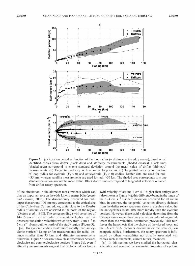
of the circulation in the altimeter measurements which canplay an important role on the eddy kinetic energy [Chaigneauand Pizarro, 2005]. The discontinuity observed for radiilarger than around 100 kmmay correspond to the critical sizeof the Chile-Peru Current eddies, quite close to the Rossbyradius of around 95 km observed in the north of the region[Chelton et al., 1998]. The corresponding swirl velocities of14–15 cm s�1 are an order of magnitude higher than theobserved translation velocities which vary from 3 cm s�1 to7 cm s�1 from south to north of the study region (Figure 3).[16] Do cyclonic eddies rotate more rapidly than anticy-

clonic vortices? Using drifter measurements for radial dis-tance smaller than 35 km, and altimetry measurementsotherwise, Figure 5c does not show clear differences betweenclockwise and counterclockwise vortices (Figure 5c), even ifaltimetry measurements suggest that cyclonic eddies have a

swirl velocity of around 2 cm s�1 higher than anticyclones(also shown in Figure 4c), this difference being in the range ofthe 3–4 cm s�1 standard deviation observed for all radiusbins. In contrast, the tangential velocities directly deducedfrom the drifter rotary spectrum, show in absolute value, thatthe anticyclones rotate 30% more rapidly than the cyclonicvortices. However, these swirl velocities determine from the63 trajectories longer than one year are an order of magnitudelower than the velocities determined previously. This rein-forces the hypothesis that the choice of the closed loops andthe ±6 cm SLA contours discriminates the smaller, lessenergetic eddies. Furthermore, the rotary spectrum is influ-enced by others variabilities not directly associated witheddies such as filaments, current bursts, meanders.[17] In this section we have studied the horizontal char-

acteristics and some of the kinematic properties of cyclonic

Figure 5. (a) Rotation period as function of the loop radius (= distance to the eddy center), based on allidentified eddies from drifter (black dots) and altimetry measurements (shaded crosses). Black lines(shaded area) correspond to ± one standard deviation around the mean value of drifter (altimetry)measurements. (b) Tangential velocity as function of loop radius. (c) Tangential velocity as functionof loop radius for cyclonic (Vq < 0) and anticyclonic (Vq > 0) eddies. Drifter data are used for radii<35 km, whereas satellite measurements are used for radii >35 km. The shaded area corresponds to ± onestandard deviation around the mean value. Black dotted lines correspond to tangential velocities obtainedfrom drifter rotary spectrum.


7 of 12

C06005

and anticyclonic eddies in the eastern South Pacific. In orderto describe the vertical structure of the Chile-Peru Currenteddies, the next section deals with a case study of a coldcore eddy observed during the P19 WOCE section.

4. Vertical Eddy Characteristics: A Case Study ofa Cold Core Eddy

[18] Figure 6a shows the vertical distribution, in the first500 m of the water column, of the potential density obtained

from temperature and salinity CTD profile data during theP19 WOCE section between 35�S and 10�S. The propertiesof the different water masses and the effect of the large-scalecirculation on the vertical tracer distributions are describedin details in Tsuchiya and Talley [1998]. A particularmesoscale structure centered at around 19�S was sampledbetween the 18 and the 21 March 1993 (Figure 6a). Theuplift of ispopycnal levels at this latitude indicates thecyclonic nature of the eddy. The influence of this coldcyclonic eddy is visible down to 2000 m with a temperature

Figure 6. (a) Vertical distribution, over the first 500 m, of the potential density s0 along the WOCE-P19section. (b) Temperature (blue), salinity (green), and density (red) averaged between 150 m and 500 mand detrended meridionally. (c) Dynamic height relative to 3000 m (detrended meridionally, blue), TP/ERS altimetry interpolated at the time and location of the WOCE-P19 measurements (red), and velocityfrom the ADCP data averaged between 30 m and 450 m (green). (d) Vertical distribution, over the first400 m, of the zonal velocity from the ADCP measurements. Black arrows indicate the cold core eddycenter position. See color version of this figure at back of this issue.


8 of 12

C06005

anomaly at this depth of around �0.1�C (not shown). In theabsence of any other vertical hydrographic measurements ofcold core eddy in the study region, we consider this depth(2000 m), as a typical vertical extension of the eastern SouthPacific or Chile-Peru Current eddies. Figure 6b presents thetemperature, salinity and density averaged over the 150–500 m layer and detrended meridionally. The cyclonic eddycentered at 19�S has a lower temperature of around 1�–

1.5�C and a lower salinity of around 0.1–0.15 compared tothe surrounding water. This is associated with higherdensities of around 0.1 kg m�3. These anomalies canincrease locally to more than �2.5�C in temperature and�0.4 in salinity. The northern and southern limits of theeddy are around 18�S and 20�S respectively correspondingto a radius approximately of 100–120 km. The surface datado not show important anomalies at 19�S (not shown). This

Figure 7. Time series of the SLA (in centimeters) between October 1992 and August 1993. Thevertical solid line corresponds to the WOCE-P19 section. Drifter D1 (D2) track is shown by a black(white) line. The bold lines correspond to the drifter positions at the times of the SLA maps ±14 days.The white crosses correspond to the cold core eddy position. See color version of this figure at back ofthis issue.


9 of 12

C06005

suggests that the eddy was formed far away from theWOCE section, and during its displacement toward thehydrographic section its surface properties were modifiedby air-sea exchanges (heat flux and evaporation/precipita-tion). As the air-sea interactions modify mainly the mixedlayer properties at the scales considered here, below 150–500 m depth (and down to 2000 m) the eddy core mayconserve the water properties of its formation region.[19] Figure 6c (blue line) shows the dynamic height

relative to 3000 m, calculated from in situ measurementsand detrended meridionally. It compares quite well with thealtimetry measurements interpolated along the WOCE sec-tion (red line). All along the section, the correlation is of80% with 2 cm of rms difference; considering only the 15�–25�S latitude band, the correlation increases to 96% with1.1 cm of rms difference. The cold core cyclonic eddycentered at 19�S exhibits a maximum sea level anomaly ofaround �10 cm. Near its centre, the velocity, correspondingto the ADCP measurements averaged between 30 m and450 m, is of order of 2 cm s�1 (Figure 6c). This velocityincreases toward the edges of the eddy to reach a maximumof 11.8 cm s�1 on the southern flank and 13.3 cm s�1 on thenorthern flank. The zonal velocity component (Figure 6d) isin agreement with the SLA slopes: south of the eddy centre,a negative meridional SLA gradient is associated with anegative (westward) zonal velocity, whereas north of theeddy core, the zonal velocity reverses eastward. As the eddyis well captured by SLA satellite measurements, we cantrace it back in time to determine its formation region.Unfortunately, the satellite measurements began only the14 October 1992, and we can follow the eddy only fromthis date. In beginning November 1992 the eddy waslocated at around 20.5�S and 81�W (Figure 7) and a second,weaker cyclonic centre is visible at around 19�S and 82�W.In December the two cyclonic eddies started to mergetogether. During the following months, this large �10 cmSLA centre propagated to the west and crossed the WOCEsection from February to the end of March 1993, at the time

of the in situ measurements. From April, the cold core eddylost its intensity and its SLA progressively reduced, but wecan still track it visually until October 1993. On the basis ofthe �6 cm SLA contour, the apparent eddy radius at thetime of the WOCE measurements is 102 km, in agreementwith the estimated 100–120 km from in situ data (Figure 6).It confirms that the ±6 cm SLA contour is a robust criterionin the study region for the eddy edge identification. FromFigure 5c, a cyclonic eddy of around 100 km wide mayhave a swirl velocity of around 12–13 cm s�1 in agreementwith the velocity estimated from ADCP data (Figure 6c).[20] Figure 7 also shows that two different drifters have

sampled this cold eddy. The first one (D1) was deployed ataround 15�S and 80�W on 3 November 1992. It first flowsNorth on the western flank of a cyclonic eddy (Figure 7b)before moving eastward and southward by different con-secutive anticyclonic/cyclonic eddies. On 6 February 1993it is trapped by the cold cyclonic eddy centered at 19�S androtates at its edge during around 50 days. On the basis ofthese 50 days of daily displacements we estimate anindependent eddy swirl velocity of 13.4 cm s�1 with astandard deviation of 6.2 cm s�1. The second drifter (D2)where launched from the R/V Knorr at 19.1�S and 87.5�Wthe 20 March 1993. D2 is trapped in the eddy until mid-July1993 but we only use its first 30 days of navigation tocalculate the swirl velocity of the cold core cyclone. Weestimate Vq = 12.2 cm s�1 with a reduced standard deviationof 3.8 cm s�1, in good agreement with both the velocityestimated from ADCP data and the calculations of theradial statistics given in the previous section. Finally,Figure 8 presents the longitude-time diagram of the SLAaveraged meridionally on the 19�–21�S latitude band, forthe October 1992–December 1993 period. Again, we seethat the interesting cyclonic eddywas followed from80�WinOctober 1992 to around 94�W in September 1993 withmaximum amplitude of�8 to�10 cm until April–May 1993after the crossing of the WOCE section. This eddy has thustraversed about 1500 km in an 11months period, correspond-

Figure 8. Longitude-time diagram of SLA averaged between 19� and 21�S. The white asterisks showsthe moment when the WOCE-P19 stations between 19� and 21�S were occupied. See color version ofthis figure at back of this issue.


10 of 12

C06005

ing to a translation velocity of around 5.2 cm s�1, quite closeto the mean VT observed at this latitude (Figure 3c).

5. Discussion and Conclusion

[21] On the basis of satellite tracked drifter measure-ments, altimetry data, and in situ hydrographic section, thisstudy has characterized the mesoscale structures and theirpropagation in the eastern South Pacific. We have high-lighted the complementarities of these data sets: drifter datapermit to study structures with radii smaller than 35 km thatthe multisatellite merged product does not resolve, whereasSLA measurements allow us to track eddies in time, andspace hydrographic data are useful to have a vertical visionof the eddy cores.[22] About 2/3 of the vortices identified from drifter data

are anticyclonic, whereas 2/3 of the long-lived eddiestracked from altimetry measurements are cyclonic. Owingto its resolution and the applied optimum interpolation, thealtimetry mapped data imposes certain space and time-scales. It misses a large part of the small-scale vorticesand any ageostrophic convergence. In contrast, drifters arebiased toward regions of convergent flow associated withanticyclones, higher velocities, and may give a biasedrepresentation of the entire eddy field (Figure 2). Thus openquestions still remain such as, what part of the flow thealtimetry signal represents? How the biased drifter move-ments can impact on our statistics? The higher number ofdrifter anticyclonic loops is due to the buoys trapping intoconvergent flow, or is it due to a cascade of the large-scaleanticyclonic vorticity toward mesoscale motion? Furtherinvestigation, including high-resolution numerical simula-tions, is needed to respond to these questions. Even if thealtimetry and drifter data measure different scales (Figure 4),the horizontal eddy size observed from altimetry data is inagreement with what observed in the interior ocean fromhydrographic CTD measurements (Figure 6c). The smallerscales shown by the drifter loops may be influenced byageostrophic components, more energetic near the surface.[23] The majority of the long-lived eddies are formed

near the coast in the Chile-Peru Current system where theEKE is higher [Chaigneau and Pizarro, 2005; Hormazabalet al., 2004]. Then, they migrate westward in the directionof warmer and saltier offshore water, with a translationvelocity of 3 cm s�1 south of 30�S to more than 6 cm s�1

north of 15�S. The higher number of cold cyclonic long-lived eddies can impact on the biology and biogeochemistryof the open ocean ecosystems [Siegel et al., 1999]. Forma-tion of cyclonic eddies in the coastal upwelling regionuplifts nutrient-rich, isopycnal surfaces into the euphoticzone, where those nutrients are rapidly utilized by phyto-plankton. In contrast, the downwelling associated withanticyclones pushes nutrient-depleted waters into theaphotic zone, where there is no ecosystem response[McGillicuddy et al., 1998]. Thus the westward migrationof the cyclonic eddies can influence the upper oceanbiogeochemistry of the oligotrophic interior ocean. Further-more, due to the b effect the meridional component of thetranslation velocity depends on the eddy rotation sense: coldcyclonic eddies migrate slightly poleward, whereas warmanticyclones propagate slightly equatorward. This diver-gence of the eddy pathways, which has been also observed

in others eastern boundary regions [Morrow et al., 2004],may have important repercussions on tracer budgets, lead-ing for example to a net equatorward heat transport. Finally,as the warm anticyclonic eddies move equatorward, they aresubject in the southern hemisphere to a higher planetaryvorticity; in order to maintain their absolute vorticity, theirrelative vorticity may decrease. Effectively, the relativevorticity of the anticyclonic ‘‘long-lived’’ eddies identifiedin Figure 3 decreases in average from 3.5 � 10�6 s�1 to lessthan 1 � 10�6 s�1 after 80 weeks of displacements (notshown). The associated standard deviation is around10�6 s�1. In contrast, the relative vorticity of the cycloniclong-lived eddies does not show important variation due thequasi westward motion of these cold cores.[24] The critical extensions of the Chile-Peru Current

eddies have appeared to be of order of 200 km laterally(radius of 100 km) and around 2000 m vertically. Thislarge-scale eddies have in average a swirl velocity of around14 cm s�1 and a rotation period of around 50 days. Thistangentialvelocity issmaller than the20cms�1observed in theNorth Atlantic [van Aken, 2002] and than the 40–50 cm s�1

of the more energetic Kuroshio region [Rabinovich et al.,2002]. The mean radius of the loops observed from driftermeasurements is around 10 km (Figure 4b). If we considerthat the drifters are on average statistically evenly distributedon the eddy of radius R, the probability density p(r,q) offinding the drifter at a radius r and direction q relative to thecentre of the eddy is constant and equal to

p r; qð Þ ¼1

Z

R

0

Z

2p

0

rdrdq

¼1

pR2:

The mean distance R1, or the expectation

E rð Þ ¼

Z

R

0

Z

2p

0

r2p r; qð Þdrdq;

of the drifter from the eddy centre is then given by R1 = 2R/3.A mean loop diameter of 20 km is thus associated with aneddy diameter of around 30 km, which corresponds to thetypical mean diameter of the mesoscale Chile-Peru Currenteddies. This order of magnitude is lower than the 30–95 km Rossby radii of deformation observed in the studyregion [Chelton et al., 1998]. A typical eddy diameter of30 km is also consistent with the Lagrangian length scalesof 30–40 km observed in the domain [Chaigneau andPizarro, 2005], but may depend of the considered latitude,since the Lagrangian length scales increase equatorwardwith the Rossby radius [Zhurbas and Oh, 2003, 2004].[25] The swirl velocity structure of typical large eddy has

been reconstructed from all the identified eddies. The radialdistribution of the swirl velocity (Vq as function of r) ineddies (Figure 5b) allows us to compare the relative andplanetary vorticities (x and f respectively) using the relation[Pingree and Le Cann, 1992; van Aken, 2002]

x

f

�

�

�

�

�

�

�

�

¼1

f

�

�

�

�

�

�

�

�

@ rVqð Þ

r@r

�

�

�

�

�

�

�

�

:


11 of 12

C06005

At the critical radius of 100 km, the relative vorticity x isabout 1% of f, suggesting that edges of large eddies are ingeostrophic balance. The consideration of the geostrophicrelationship to determine the swirl velocity at the eddyedges from altimetry measurements, appears then tobe appropriate for large eddy diameters. The vorticity rate(jx/f j) of the eddies, increases when r decreases: at a radiusof 10 km it is around 0.1 and around 0.4 near the centre. Arelative vorticity of about 0.4 times the planetary vorticitysuggests that eddy cores are ageostrophic. Although thelarge-scale eddies may be considered in geostrophicbalance, ageostrophic dynamics and centrifugal effectsmay play an important role for the growth and decay ofthe mesoscale cores.[26] Finally, these results could serve as a benchmark for

interpreting and documenting the mesoscale activity inregional numerical models of the eastern South Pacific withregards to the choice of an appropriate spatial resolution. Inthat sense, this study may provide useful metrics for thevalidation of these high-resolution models along with helpin developing strategies of future drifter deployments andcruise measurements.

[27] Acknowledgments. The drifter data were provided by theNational Oceanic and Atmospheric Administration (NOAA). The authorsthank Rosemary Morrow and Boris Dewitte for their helpful comments.A.C. was supported by ECOS-SUD and Fundacion Andes grant D-13615.This work was also supported by the Chilean National Research Council(FONDAP-COPAS).

ReferencesBlanco, J. L., A. C. Thomas, M.-E. Carr, and P. T. Strub (2001), Seasonalclimatology of hydrographic conditions in the upwelling region off north-ern Chile, J. Geophys. Res., 106, 11,451–11,467.

Brugge, B. (1995), Near-surface mean circulation and kinetic energy in thecentral North Atlantic from drifter data, J. Geophys. Res., 100, 20,543–20,554.

Chaigneau, A., and O. Pizarro (2004), Eddy characteristics and tracer trans-ports from TP/ERS altimetry, in a region offshore Chile, Proc. PORSEC,68, 102–107.

Chaigneau, A., and O. Pizarro (2005), Mean surface circulation and meso-scale turbulent flow characteristics in the eastern South Pacific fromsatellite tracked drifters, J. Geophys. Res., 110, C05014, doi:10.1029/2004JC002628.

Chelton, D. B., R. A. deSzoeke, M. G. Schlax, K. El Naggar, andN. Siwertz (1998), Geographical variability of the first-baroclinic Rossbyradius of deformation, J. Phys. Oceanogr., 28, 433–460.

Cushman-Roisin, B. (1994), Introduction to Geophysical Dynamics, 320pp., Prentice-Hall, Upper Saddle River, N. J.

Ducet, N., P. Y. Le Traon, and G. Reverdin (2000), Global high-resolutionmapping of ocean circulation from TOPEX/Poseidon and ERS-1 and -2,J. Geophys. Res., 105, 19,477–19,498.

Fang, F., and R. Morrow (2003), Evolution, movement and decay of warm-core Leeuwin Current eddies, Deep Sea Res., Part II, 50, 2245–2261.

Hansen, D. V., and P.-M. Poulain (1996), Quality control and interpolationsof WOCE-TOGA drifter data, J. Atmos. Oceanic Technol., 13, 900–909.

Hormazabal, S., G. Shaffer, and O. Leth (2004), Coastal transition zone offChile, J. Geophys. Res., 109, C01021, doi:10.1029/2003JC001956.

Hwang, C., C.-R. Wu, and R. Kao (2004), TOPEX/Poseidon observationsof mesoscale eddies over the Subtropical Countercurrent: Kinematic char-acteristics of an anticyclonic eddy and a cyclonic eddy, J. Geophys. Res.,109, C08013, doi:10.1029/2003JC002026.

Isern-Fontanet, J., E. Garcia-Ladona, and J. Font (2003), Identification ofmarine eddies from altimeter maps, J. Atmos. Oceanic Technol., 20, 772–778.

Jayne, S. R., and J. Marotzke (2002), The oceanic eddy heat transport,J. Phys. Oceanogr., 32, 3328–3345.

Le Traon, P.-Y., and F. Ogor (1998), ERS-1/2 orbit improvement usingTOPEX/Poseidon: The 2 cm challenge, J. Geophys. Res., 103, 8045–8057.

Le Traon, P.-Y., P. Gaspar, F. Ogor, and J. Dorandeu (1995), Satellites workin tandem to improve accuracy of data, Eos Trans. AGU, 76, 385–389.

Le Traon, P.-Y., F. Nadal, and N. Ducet (1998), An improved mappingmethod of multi-satellite altimeter data, J. Atmos. Oceanic Technol.,15, 522–534.

Lupton, J. E., E. T. Baker, N. Garfield, G. J. Massoth, R. A. Feely, J. P.Cowen, R. R. Greene, and T. A. Rago (1998), Tracking the evolution of ahydrothermal event plume with a RAFOS neutrally buoyant drifter,Science, 280, 1052–1055.

Martins, C. S., M. Hamann, and A. F. G. Fiuza (2002), Surface circulationin the eastern North Atlantic, from drifters and altimetry, J. Geophys.Res., 107(C12), 3217, doi:10.1029/2000JC000345.

McGillicuddy, D. J., Jr., A. R. Robinson, D. A. Siegel, H. W. Jannasch,R. Johnson, T. D. Dickey, J. McNeil, A. F. Michaels, and A. H. Knap(1998), Influence of mesoscale eddies on new production in the SargassoSea, Nature, 394, 263–266.

Morrow, R., F. Birol, D. Griffin, and J. Sudre (2004), Divergent pathwaysof cyclonic and anti-cyclonic ocean eddies, Geophys. Res. Lett., 31,L24311, doi:10.1029/2004GL020974.

Pingree, R. D., and B. Le Cann (1992), Three anti-cyclonic Slope WaterOceanic eDDIES (SWODDIES) in the Southern Bay of Biscay, Deep SeaRes., Part A, 39, 1147–1175.

Pizarro, O., G. Shaffer, B. Dewitte, and M. Ramos (2002), Dynamics ofseasonal and interanual variability of the Peru-Chile Undercuurent, Geo-phys. Res. Lett., 29(12), 1581, doi:10.1029/2002GL014790.

Poulain, P.-M., and P. P. Niiler (1989), Statistical analysis of the surfacecirculation in the California Current system using satellite-tracked drif-ters, J. Phys. Oceanogr., 19, 1588–1603.

Rabinovich, A. B., R. E. Thomson, and S. J. Bograd (2002), Drifterobservations of anticyclonic eddies near Bussol Strait, the Kuril islands,J. Oceanogr., 58, 661–671.

Shaffer, G., O. Pizarro, L. Djurfeldt, S. Salinas, and J. Rutlant (1997),Circulation and low frequency variability near the Chile coast:Remotely-forced fluctuations during the 1991–1992 El Nino, J. Phys.Oceanogr., 27, 217–235.

Siegel, D. A., D. J. McGillicuddy Jr., and E. A. Fields (1999), Mesoscaleeddies, satellite altimetry, and new production in the Sargasso sea,J. Geophys. Res., 104, 13,359–13,379.

Stammer, D. (1997), Global characteristics of ocean variability estimatedfrom regional TOPEX/Poseidon altimeter measurements, J. Phys.Oceanogr., 27, 1743–1769.

Stammer, D. (1998), On eddy characteristics, eddy transports, and meanflow properties, J. Phys. Oceanogr., 28, 727–739.

Strub, P. T., J. M. Mesias, V. Montecino, J. Rutllant, and S. Salinas (1998),Coastal ocean circulation off western South America, in The Sea, vol. 11,edited by A. R. Robinson and K. H. Brink, pp. 273–313, John Wiley,Hoboken, N. J.

Swenson, M. S., and P. P. Niiler (1996), Statistical analysis of the surfacecirculation of the California Current, J. Geophys. Res., 101, 22,631–22,645.

Takematsu, M., A. G. Ostrovskii, and Z. Nagano (1999), Observations ofeddies in the Japan Basin interior, J. Oceanogr., 55, 237–246.

Tsuchiya, M., and L. D. Talley (1998), A Pacific hydrographic section at88�W:Water property distribution, J. Geophys. Res., 103, 12,899–12,918.

van Aken, H. M. (2002), Surface currents in the Bay of Biscay as observedwith drifters between 1995 and 1999, Deep Sea Res., Part I, 49, 1071–1086.

Wang, G., J. Su, and P. C. Chu (2003), Mesoscale eddies in the South ChinaSea observed with altimeter data, Geophys. Res. Lett., 30(21), 2121,doi:10.1029/2003GL018532.

Wunsch, C. (1999), Where do ocean eddy heat fluxes matter?, J. Geophys.Res., 104, 13,235–13,249.

Zamudio, L., A. P. Leonardi, S. D. Meyers, and J. J. O’Bryen (2001),ENSO and eddies on the southwest coast of Mexico, Geophys. Res. Lett.,28, 13–16.

Zhurbas, V., and I. S. Oh (2003), Lateral diffusivity and Lagrangian scalesin the Pacific Ocean as derived from drifter data, J. Geophys. Res.,108(C5), 3141, doi:10.1029/2002JC001596.

Zhurbas, V., and I. S. Oh (2004), Drifter-derived maps of lateral diffusivityin the Pacific and Atlantic Oceans in relation to surface circulationpatterns, J. Geophys. Res., 109, C05015, doi:10.1029/2003JC002241.

��

A. Chaigneau, Centro de Investigacion Oceanografica en el Pacıfico Sur-Oriental/Programa Regional de Oceanografıa Fısıca y Clima, Cabina 7,Universidad de Concepcion, Concepcion 3, Chile. ([email protected])O. Pizarro, Departamento de Geofısica/Centro de Investigacıon Oceano-

grafica en el Pacıfico Sur-Oriental/Programa Regional de OceangrafıaFısica y Clima, Cabina 7, Universidad de Concepcion, Concepcion 3,Chile. ([email protected])


12 of 12

C06005

4 of 12

Figure 2. Examples of (a–c) cyclonic and (d–f) anticyclonic eddies identified from drifter data (blackdots) and from sea level anomaly measurements (shading). The SLA are in centimeters.

C06005 CHAIGNEAU AND PIZARRO: CHILE-PERU CURRENT EDDY CHARACTERISTICS C06005

8 of 12

Figure 6. (a) Vertical distribution, over the first 500 m, of the potential density s0 along the WOCE-P19section. (b) Temperature (blue), salinity (green), and density (red) averaged between 150 m and 500 mand detrended meridionally. (c) Dynamic height relative to 3000 m (detrended meridionally, blue), TP/ERS altimetry interpolated at the time and location of the WOCE-P19 measurements (red), and velocityfrom the ADCP data averaged between 30 m and 450 m (green). (d) Vertical distribution, over the first400 m, of the zonal velocity from the ADCP measurements. Black arrows indicate the cold core eddycenter position.


9 of 12

Figure 7. Time series of the SLA (in centimeters) between October 1992 and August 1993. Thevertical solid line corresponds to the WOCE-P19 section. Drifter D1 (D2) track is shown by a black(white) line. The bold lines correspond to the drifter positions at the times of the SLA maps ±14 days.The white crosses correspond to the cold core eddy position.


10 of 12

Figure 8. Longitude-time diagram of SLA averaged between 19� and 21�S. The white asterisks showsthe moment when the WOCE-P19 stations between 19� and 21�S were occupied.


Eddy characteristics in the eastern South Pacific

Documents

Transcript of Eddy characteristics in the eastern South Pacific