�����������������

Citation: Liu, T.; He, Y.; Zhai, X.; Liu,

X. Diagnostics of Coherent Eddy

Transport in the South China Sea

Based on Satellite Observations.

Remote Sens. 2022, 14, 1690.

https://doi.org/10.3390/rs14071690

Academic Editors: Guoqi Han,

Changming Dong, Chunyan Li and

Jingsong Yang

Received: 3 February 2022

Accepted: 25 March 2022

Published: 31 March 2022

Publisher’s Note: MDPI stays neutral

with regard to jurisdictional claims in

published maps and institutional affil-

iations.

Copyright: © 2022 by the authors.

Licensee MDPI, Basel, Switzerland.

This article is an open access article

distributed under the terms and

conditions of the Creative Commons

Attribution (CC BY) license (https://

creativecommons.org/licenses/by/

4.0/).

remote sensing

Article

Diagnostics of Coherent Eddy Transport in the South China SeaBased on Satellite ObservationsTongya Liu 1 , Yinghui He 2,* , Xiaoming Zhai 3 and Xiaohui Liu 1,4

1 State Key Laboratory of Satellite Ocean Environment Dynamics, Second Institute of Oceanography,Ministry of Natural Resources, Hangzhou 310000, China; liutongya@sio.org.cn (T.L.); xh_liu@sio.org.cn (X.L.)

2 State Key Laboratory of Tropical Oceanography, South China Sea Institute of Oceanology,Chinese Academy of Sciences, Guangzhou 510000, China

3 School of Environmental Sciences, University of East Anglia, Norwich NR4 7TJ, UK; xiaoming.zhai@uea.ac.uk4 Southern Marine Science and Engineering Guangdong Laboratory (Zhuhai), Zhuhai 519000, China* Correspondence: heyinghui@scsio.ac.cn

Abstract: The large discrepancy between Eulerian and Lagrangian work motivates us to examinethe leakage of Eulerian eddies and quantify the contribution of coherent eddy transport in the SouthChina Sea (SCS). In this study, Lagrangian particles with a resolution of 1/32◦ are advected by surfacegeostrophic currents derived from satellite observations spanning 23 years, and two types of methodsare employed to identify sea surface height (SSH) eddies and Lagrangian coherent structures. SSHeddies are proven to be highly leaky during their lifetimes, with more than 80% of the original waterleaking out of the eddy interior. As a result of zonal and meridional eddy propagation, the leakedwater exhibits a spatial pattern of asymmetry relative to the eddy center. The degree of eddy leakageis found to be independent of several eddy parameters including the nonlinearity parameter U/c,which has been commonly used to assess eddy coherency. Finally, the Lagrangian coherent structuresin the SCS are diagnosed and the associated coherent eddy diffusivity is calculated. It is found thatcoherent eddies contribute to less than 5% of the total eddy material transport in both zonal andmeridional directions. These findings suggest that previous studies based on the Eulerian frameworksignificantly overestimate the contribution of coherent eddy transport in the SCS.

Keywords: mesoscale eddies; coherent transport; eddy leakage; Lagrangian methods; South China Sea

1. Introduction

As rotating structures with horizontal scales of ~100 km, mesoscale eddies are ubiq-uitous in the global oceans. They often last several weeks to months, storing a significantproportion of the ocean’s kinetic energy [1–3]. These eddies trap, transport, and stir oceanictracers such as heat, salt, and nutrients, thus having crucial impacts on ocean circulations,biochemical processes, and the global climate system [4–6].

As the largest semi-closed marginal sea in the northwest Pacific, the South ChinaSea (SCS) has an active current system with multiscale processes that are primarily at-tributed to the seasonally reversing monsoon, complex bottom topography, and Kuroshiointrusion [7,8]. These dynamical conditions facilitate the generation of instabilities, whichtransform the SCS into a “zoo” of mesoscale eddies. Previous investigations have reportedstatistical features of eddy properties [9,10] and estimates of eddy material transport [11,12]in the SCS using both observations and numerical simulations. However, the strength ofcoherent eddy transport remains unclear due to different eddy definitions used in previousstudies, which motivates us to revisit this issue.

The coherent structure is characterized by that the interior water mass is enclosed by amaterial barrier (boundary) and transported for a distance without volume exchange withthe ambient flows [13]. Because of their ability to trap and transport materials, mesoscaleeddies are typically treated as coherent structures when the nonlinearity parameter U/c

Remote Sens. 2022, 14, 1690. https://doi.org/10.3390/rs14071690 https://www.mdpi.com/journal/remotesensing

Remote Sens. 2022, 14, 1690 2 of 18

(with U the azimuthal eddy velocity and c the translation speed) is greater than 1 [3]. On aglobal scale, Dong et al. [14] used a velocity-based method to identify and track eddies andthen combined them with Argo profiles to calculate the heat and salt content trapped byeddies, concluding that “eddy heat and salt transports are primarily attributed to individualeddy movements”. Zhang et al. [15] defined eddies using the potential vorticity contourand estimated the eddy-induced zonal mass transport to be approximately 30–40 Sv, whichis surprisingly large and comparable to that of the large-scale ocean circulation. Bothof these appealing studies emphasize the importance of coherent material transport viamesoscale eddies.

Numerous studies have been conducted in the last two decades to investigate thespatiotemporal distributions, surface and vertical structures, evolution features, and gener-ation mechanisms of eddies in the SCS [8–10,16–19]. Coherent eddy transport has also beenhighlighted as estimated by eddy size and propagation speed (following Dong et al. [14]and Zhang et al. [15]). For example, Zhang et al. [20] captured two deep-reaching anticy-clonic eddies via a full-water column mooring system and observed the simultaneous orlagging enhancement of suspended sediment concentration with eddy temperature andvelocity signals. They estimated that the net near-bottom sediment transport by thesetwo eddies might be in the millions of tons. Statistically, Wang et al. [21] suggested thatheat, salt, and volume transports induced by mesoscale eddies around the Luzon Straitinto the SCS are around 3× 10−5 PW, 4× 103 kg/s, and 0.3 Sv, respectively. Accordingto Zhang et al. [22], transport by shedding anticyclonic eddies from the Kuroshio reaches0.24–0.38 Sv, accounting for 6.8–10.8% of the upper-layer Luzon Strait transport. He et al. [10]composited the three-dimensional structure of mesoscale eddies in the SCS based on aneddy dataset and Argo profiles, and pointed out that the westward water transport byeddies reaches 1.4 Sv, accounting for nearly 30% of the annual flux in the Luzon Strait.Considering four types of eddies around the Luzon Strait, Yang et al. [23] updated thecoherent heat, salt, and volume transports to 8.78× 10−4 PW, 7.88× 104 kg/s, and 0.77 Sv,respectively, highlighting the important role of eddies in water exchange in the SCS. Itis worth noting that all these previous studies of eddy coherent transport in the SCS fallwithin the Eulerian framework, that is, they use the Eulerian method to determine theeddy boundary.

General eddy identification methods can be classified into two categories: Eulerianand Lagrangian. The key idea behind Eulerian methods is to track the eddy center andboundary from the snapshots at neighboring times. Typically, the eddy boundary is definedby the closed contour of a physical feature such as sea surface height (SSH) [3], potentialvorticity [15], Okubo–Weiss parameter [24,25], velocity streamlines [26], etc. Some Eule-rian methods (especially the SSH method) have been widely used because of their simpleprocedure. However, they have critical defects in defining coherent structures [13]. Thefundamental problem is that the Eulerian eddy boundary does not represent a materialbarrier, which means that fluid initially inside of the Eulerian eddy boundary can cross thisboundary and exchange with the fluid outside at later times [27]. Lagrangian methods,unlike Eulerian methods, which are based on instantaneous flow features, examine waterparcel trajectories over a finite-time interval to assess the skeleton of coherent structures.Many techniques such as finite-time Lyapunov exponents [28], finite-scale Lyapunov expo-nent [29], and Lagrangian-averaged vorticity deviation (LAVD) [30] have been developed toidentify the Lagrangian coherent structures, but they are seldomly employed to investigateeddy features in the SCS.

Several recent publications based on the Lagrangian framework have demonstratedthat the use of Eulerian methods significantly overestimates the strength of coherent eddytransport. For example, Beron-Vera et al. [31] and Wang et al. [32] showed that the coherentmaterial transport by Agulhas rings is quite limited and its contribution to the total eddyflux is significantly less than previous Eulerian estimates. Abernathey and Haller [27]used the LAVD method [30] to identify coherent eddies in the eastern Pacific and foundthat transport by coherent eddies contributes to less than 1% of the net meridional eddy

Remote Sens. 2022, 14, 1690 3 of 18

transport. Using an idealized model simulation, Liu et al. [33] examined the leakage ofEulerian eddies defined by closed SSH contours during their lifespans, and found that morethan 50% of the initial water leaks from the eddy interior into the background flow. Thesestudies indicate that, although Eulerian eddies can temporarily trap and transport material,the incoherent motions in a turbulent flow such as swirling, stirring, and filamentationcause these eddies to lose coherence rapidly and these incoherent motions may be thedominant mechanism for eddy transport [13,27].

Based on satellite measurements, this study aims to estimate the contribution ofcoherent eddies to material transport in the SCS, updating some traditional views of eddy-induced transport in this region. First, we systematically examine the leakage of Eulerianeddies in their lifetimes by employing Lagrangian particles, which to our knowledge,has not yet been attempted in the SCS. Second, we investigate the relationship betweeneddy properties and the degree of eddy leakage, especially focusing on the nonlinearityparameter proposed by Chelton et al. [3]. Third, we evaluate the relative contribution ofmaterial transport by coherent eddies to the full turbulent transport and discuss the rolesof incoherent motions.

The rest of the paper is organized as follows. In Section 2, we describe the dataset aswell as the Eulerian and Lagrangian eddy identification techniques used in this study. InSections 3.1 and 3.2, we examine the leakage of SCS eddies defined by the Eulerian method.In Section 3.3, we investigate the relationship between several eddy parameters and eddyleakiness. The relative contributions of coherent eddies and incoherent motions to materialtransport are presented in Section 3.4. We end the paper with discussions and conclusionsin Section 4.

2. Data and Methods

This study is based on the satellite altimetry dataset produced by SSALTO/DUACSand distributed by AVISO (http://www.aviso.altimetry.fr/duacs/, accessed on 8 August2021). In this dataset, the daily sea level anomaly (SLA) is objectively interpolated toa 1/4◦ latitude–longitude grid by merging along-track measurements from the severalaltimeter missions. This product also provides the absolute dynamic topography η and thesurface geostrophic velocity field Vg derived via k̂× Vg = −g/ f∇η, where f is the Coriolisparameter, k̂ is the vertical unit vector, and g is the gravitational acceleration. We use theAVISO SLA to identify Eulerian eddies and use the precomputed geostrophic velocities toadvect the Lagrangian particles. The time period from January 1993 to December 2015 isconsidered in this study.

The Lagrangian particle, as proposed by Liu et al. [33], is an effective tool for inves-tigating the coherence of the Eulerian eddy. Numerical advection of millions of virtualLagrangian particles in the eastern Pacific has been conducted based on satellite obser-vations [27]. In a related work, we extend this application to the global ocean in orderto produce a coherent eddy dataset. From 1993 to 2015, the Lagrangian particles with aresolution of 1/32◦ are initialized on the global ocean surface on the first day of everymonth. The AVISO two-dimensional geostrophic velocities are then used to propel themforward for 180 days until the next initialization. The Lagrangian trajectory equationdXdt = V is solved using the MITgcm [34] in offline mode, where X = (x, y) is the particle

position vector and V = (u, v) is the velocity vector. The original AVISO velocity fields arelinearly interpolated to a 1/10◦ latitude–longitude grid to resolve fine-scale filaments inthe flow field. The positions of all particles as well as the relative vorticity are calculatedevery day for Lagrangian eddy identification and related analysis. In this study, only theregion around the SCS (Figure 1A) is considered. Figure 2A shows the initial latitude ofLagrangian particles released on 1 January 2006 (randomly selected), and Figure 2B showsthe meridional displacement of particles after 180 days, the pattern of which suggests a keyrole of eddies in transporting and redistributing particles in the SCS. It should be notedthat the small correction to the AVISO geostrophic velocity field is conducted in order tominimize the divergence caused by variations of the Coriolis parameter with latitude and

Remote Sens. 2022, 14, 1690 4 of 18

to perform no-normal-flow boundary conditions at the coastlines [35]. Additionally, eddiesin regions shallower than 200 m are excluded in this study.

Remote Sens. 2022, 14, x 4 of 20

Lagrangian particles released on 1 January 2006 (randomly selected), and Figure 2B shows the meridional displacement of particles after 180 days, the pattern of which suggests a key role of eddies in transporting and redistributing particles in the SCS. It should be noted that the small correction to the AVISO geostrophic velocity field is conducted in order to minimize the divergence caused by variations of the Coriolis parameter with lat-itude and to perform no-normal-flow boundary conditions at the coastlines [35]. Addi-tionally, eddies in regions shallower than 200 m are excluded in this study.

Figure 1. Climatological (A) surface geostrophic currents (black vectors) and their speed (colors); (B) surface eddy kinetic energy (colors) in the SCS. The black contour in (B) indicates the 200 m isobath.

Following [33], two types of methods, Eulerian and Lagrangian, are applied to iden-tify coherent eddies. The boundary of Eulerian eddies is defined as the outermost closed contour of SLA (SSH eddies hereafter), a method most commonly utilized for eddy iden-tification. The algorithm adopted here is described in He et al. [36,37], which is similar to those used in Chelton et al. [3] and Faghmous et al. [38], but is modified to effectively reduce bogus eddies (e.g., filaments or irregular eddies). The definition of Lagrangian ed-dies is based on a diagnostic of coherent structures proposed by Haller et al. [30]. Over a finite-time interval, all fluid parcels along a coherent eddy boundary should have the same angular speed, which is analogous to rigid-body rotation. This physical essence con-verts defining the coherent eddy boundary to identify the outermost closed outlines of the LAVD, a quantity reflecting the averaged rotation magnitude of each Lagrangian particle over the period. In a two-dimensional flow field, LAVD is expressed as 𝐿𝐴𝑉𝐷 (𝑥 , 𝑦 ) = 1𝑡 − 𝑡 |𝜁′ 𝑥(𝑥 , 𝑦 , 𝑡), 𝑦(𝑥 , 𝑦 , 𝑡), 𝑡 |𝑑𝑡 (1)

where (𝑡 , 𝑡 ) signifies a finite-time interval, (𝑥, 𝑦) denotes the position of the particle in-itially released on (𝑥 , 𝑦 ), and 𝜁′ denotes the relative vorticity deviation from the spatial average. A larger LAVD value means that the particle rotates faster, with the local maxi-mum corresponding to the eddy center and the eddy boundary being the outermost closed LAVD curve. Recent publications [27,33,39] have effectively employed the LAVD technique to identify the rotationally coherent Lagrangian vortex (RCLV, also called the Lagrangian eddy). The particle position and LAVD fields are outputted every 10 days for the following visualization.

Figure 1. Climatological (A) surface geostrophic currents (black vectors) and their speed (colors);(B) surface eddy kinetic energy (colors) in the SCS. The black contour in (B) indicates the 200 m isobath.

Remote Sens. 2022, 14, x 5 of 20

Figure 2. (A) The initial latitude of Lagrangian particles released around the SCS on 1 January 2006. (B) The meridional displacement (in degree) of these particles after 180 days. (C) A 30-day LAVD field.

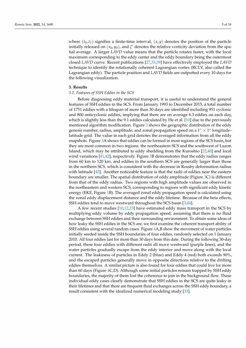
3. Results 3.1. Features of SSH Eddies in the SCS

Before diagnosing eddy material transport, it is useful to understand the general fea-tures of SSH eddies in the SCS. From January 1993 to December 2015, a total number of 1751 eddies with a lifespan of more than 30 days are identified including 951 cyclonic and 800 anticyclonic eddies, implying that there are on average 6.3 eddies on each day, which is slightly less than the 9.1 eddies calculated by He et al. [10] due to the previously men-tioned algorithm modification. Figure 3 shows the geographic distribution of the eddy genesis number, radius, amplitude, and zonal propagation speed on a 1° × 1° longitude–latitude grid. The value in each grid denotes the averaged information from all the eddy snapshots. Figure 3A shows that eddies can be formed in most regions of the SCS basin, but they are most common in two regions: the northeastern SCS and the southwest of Luzon Island, which may be attributed to eddy shedding from the Kuroshio [22,40] and local wind variations [41,42], respectively. Figure 3B demonstrates that the eddy radius ranges from 60 km to 120 km, and eddies in the southern SCS are generally larger than those in the northern SCS, which is consistent with the decrease in Rossby deformation radius with latitude [43]. Another noticeable feature is that the radii of eddies near the eastern boundary are smaller. The spatial distribution of eddy amplitude (Figure 3C) is different from that of the eddy radius. Two regions with high amplitude values are ob-served in the northeastern and western SCS, corresponding to regions with significant eddy kinetic energy (EKE, Figure 1B). The averaged zonal eddy propagation speed is cal-culated using the zonal eddy displacement distance and the eddy lifetime. Because of the beta effects, SSH eddies tend to move westward throughout the SCS basin [3,44].

Figure 2. (A) The initial latitude of Lagrangian particles released around the SCS on 1 January 2006.(B) The meridional displacement (in degree) of these particles after 180 days. (C) A 30-day LAVD field.

Following [33], two types of methods, Eulerian and Lagrangian, are applied to identifycoherent eddies. The boundary of Eulerian eddies is defined as the outermost closedcontour of SLA (SSH eddies hereafter), a method most commonly utilized for eddy iden-tification. The algorithm adopted here is described in He et al. [36,37], which is similarto those used in Chelton et al. [3] and Faghmous et al. [38], but is modified to effectivelyreduce bogus eddies (e.g., filaments or irregular eddies). The definition of Lagrangianeddies is based on a diagnostic of coherent structures proposed by Haller et al. [30]. Over afinite-time interval, all fluid parcels along a coherent eddy boundary should have the sameangular speed, which is analogous to rigid-body rotation. This physical essence convertsdefining the coherent eddy boundary to identify the outermost closed outlines of the LAVD,a quantity reflecting the averaged rotation magnitude of each Lagrangian particle over theperiod. In a two-dimensional flow field, LAVD is expressed as

LAVDt1t0(x0, y0) =

1t1 − t0

∫ t1

t0

∣∣ζ ′[x(x0, y0, t), y(x0, y0, t), t]∣∣dt (1)

Remote Sens. 2022, 14, 1690 5 of 18

where (t0, t1) signifies a finite-time interval, (x, y) denotes the position of the particleinitially released on (x0, y0), and ζ ′ denotes the relative vorticity deviation from the spa-tial average. A larger LAVD value means that the particle rotates faster, with the localmaximum corresponding to the eddy center and the eddy boundary being the outermostclosed LAVD curve. Recent publications [27,33,39] have effectively employed the LAVDtechnique to identify the rotationally coherent Lagrangian vortex (RCLV, also called theLagrangian eddy). The particle position and LAVD fields are outputted every 10 days forthe following visualization.

3. Results3.1. Features of SSH Eddies in the SCS

Before diagnosing eddy material transport, it is useful to understand the generalfeatures of SSH eddies in the SCS. From January 1993 to December 2015, a total numberof 1751 eddies with a lifespan of more than 30 days are identified including 951 cyclonicand 800 anticyclonic eddies, implying that there are on average 6.3 eddies on each day,which is slightly less than the 9.1 eddies calculated by He et al. [10] due to the previouslymentioned algorithm modification. Figure 3 shows the geographic distribution of the eddygenesis number, radius, amplitude, and zonal propagation speed on a 1◦ × 1◦ longitude–latitude grid. The value in each grid denotes the averaged information from all the eddysnapshots. Figure 3A shows that eddies can be formed in most regions of the SCS basin, butthey are most common in two regions: the northeastern SCS and the southwest of LuzonIsland, which may be attributed to eddy shedding from the Kuroshio [22,40] and localwind variations [41,42], respectively. Figure 3B demonstrates that the eddy radius rangesfrom 60 km to 120 km, and eddies in the southern SCS are generally larger than thosein the northern SCS, which is consistent with the decrease in Rossby deformation radiuswith latitude [43]. Another noticeable feature is that the radii of eddies near the easternboundary are smaller. The spatial distribution of eddy amplitude (Figure 3C) is differentfrom that of the eddy radius. Two regions with high amplitude values are observed inthe northeastern and western SCS, corresponding to regions with significant eddy kineticenergy (EKE, Figure 1B). The averaged zonal eddy propagation speed is calculated usingthe zonal eddy displacement distance and the eddy lifetime. Because of the beta effects,SSH eddies tend to move westward throughout the SCS basin [3,44].

A few recent studies [10,12,23] have estimated eddy mass transport in the SCS bymultiplying eddy volume by eddy propagation speed, assuming that there is no fluidexchange between SSH eddies and their surrounding environment. To obtain some ideas ofhow leaky the SSH eddies in the SCS are, we first examine the coherent transport ability ofSSH eddies using several random cases. Figure 4A,B show the movement of water particlesinitially seeded inside the SSH boundaries of four eddies, randomly selected on 1 January2010. All four eddies last for more than 30 days from this date. During the following 30-dayperiod, these four eddies with different radii all move westward (purple lines), and thewater particles gradually escape from the eddy interior and move along with the localcurrent. The leakiness of particles in Eddy 2 (blue) and Eddy 4 (red) both exceeds 90%,and the escaped particles generally move in opposite directions relative to the driftingeddies themselves. A similar picture is also found for four eddies that could live for morethan 60 days (Figure 4C,D). Although some initial particles remain trapped by SSH eddyboundaries, the majority of them lost the coherence to join in the background flow. Theseindividual eddy cases clearly demonstrate that SSH eddies in the SCS are quite leaky intheir lifetimes and that there are frequent fluid exchanges across the SSH eddy boundary, aresult consistent with the idealized numerical modeling study [33].

Remote Sens. 2022, 14, 1690 6 of 18Remote Sens. 2022, 14, x 6 of 20

Figure 3. Geographic distributions of the eddy (A) genesis number, (B) radius, (C) amplitude, and (D) zonal propagation speed on a 1° × 1° longitude–latitude grid in the SCS from January 1993 to 2015. The black contour in each panel denotes the 200 m isobath.

A few recent studies [10,12,23] have estimated eddy mass transport in the SCS by multiplying eddy volume by eddy propagation speed, assuming that there is no fluid ex-change between SSH eddies and their surrounding environment. To obtain some ideas of how leaky the SSH eddies in the SCS are, we first examine the coherent transport ability of SSH eddies using several random cases. Figure 4A,B show the movement of water par-ticles initially seeded inside the SSH boundaries of four eddies, randomly selected on 1 January 2010. All four eddies last for more than 30 days from this date. During the follow-ing 30-day period, these four eddies with different radii all move westward (purple lines), and the water particles gradually escape from the eddy interior and move along with the local current. The leakiness of particles in Eddy 2 (blue) and Eddy 4 (red) both exceeds 90%, and the escaped particles generally move in opposite directions relative to the drift-ing eddies themselves. A similar picture is also found for four eddies that could live for more than 60 days (Figure 4C,D). Although some initial particles remain trapped by SSH eddy boundaries, the majority of them lost the coherence to join in the background flow. These individual eddy cases clearly demonstrate that SSH eddies in the SCS are quite leaky in their lifetimes and that there are frequent fluid exchanges across the SSH eddy boundary, a result consistent with the idealized numerical modeling study [33].

Figure 3. Geographic distributions of the eddy (A) genesis number, (B) radius, (C) amplitude, and(D) zonal propagation speed on a 1◦ × 1◦ longitude–latitude grid in the SCS from January 1993 to2015. The black contour in each panel denotes the 200 m isobath.

3.2. Statistical Analysis of SSH Eddy Leakage

To investigate the degree and spatial pattern of the SSH eddy leakage in the SCS, wecarry out a statistical analysis of all the identified SSH eddies. First, eddy particle locations(x, y) on the longitude–latitude coordinate are converted onto an eddy-centric coordinate(X, Y) normalized by eddy radius R and center (xc, yc),

(X, Y) =(x, y)− (xc, yc)

R. (2)

The new location (X, Y) maintains the relative distance between the eddy centerand the particle. Figure 5A,B shows the particle locations (green dots) in the normalizedcoordinates for a randomly-selected anticyclonic eddy on 1 May 1993 when particles areseeded inside its SSH boundary, and particle locations a month later on to 31 May. Forthis anticyclonic eddy, more than 90% of the initial particles have crossed the eddy SSHboundary after only 30 days, and the majority of the initial particles are not even locatedwithin four times the eddy radius (4R). If we further build a 0.2R× 0.2R grid, the proportionof original eddy water in each grid Q can be calculated by Q = n/Ntotal , where n and Ntotalindicate the particle number in a single grid and the total particle number for each eddy,respectively. Since the total number of particles is conserved, the sum of Q is always 1.Figure 5C shows that at the initial time, the values of Q in the eddy interior are close to 1%.It should be noted that this specific value Q is determined by the grid resolution (0.2R);it is the subsequent variation and spatial distribution of Q in the eddy lifespan that is ofinterest here. Figure 5D shows that after 30 days, the number of grids containing the initialeddy water becomes quite limited within 1R, and the value of Q decreases by nearly oneorder of magnitude. In addition, some of the leaked initial particles are advected to the eastside of the eddy center.

Remote Sens. 2022, 14, 1690 7 of 18Remote Sens. 2022, 14, x 7 of 20

Figure 4. The initial (left panels) and final (right panels) particle locations of randomly selected ed-dies that live for longer than (A,B) 30 and (C,D) 60 days. Colored contours are eddy boundaries defined by SSH contours. Colored dots represent the initial particles inside the eddy boundaries. Purple lines indicate eddy center trajectories.

3.2. Statistical Analysis of SSH Eddy Leakage To investigate the degree and spatial pattern of the SSH eddy leakage in the SCS, we

carry out a statistical analysis of all the identified SSH eddies. First, eddy particle locations (𝑥, 𝑦) on the longitude–latitude coordinate are converted onto an eddy-centric coordinate (𝑋, 𝑌) normalized by eddy radius 𝑅 and center (𝑥 , 𝑦 ), (𝑋, 𝑌) = ( , ) ( , ). (2)

The new location (𝑋, 𝑌) maintains the relative distance between the eddy center and the particle. Figure 5A,B shows the particle locations (green dots) in the normalized coor-dinates for a randomly-selected anticyclonic eddy on 1 May 1993 when particles are seeded inside its SSH boundary, and particle locations a month later on to 31 May. For this anticyclonic eddy, more than 90% of the initial particles have crossed the eddy SSH boundary after only 30 days, and the majority of the initial particles are not even located within four times the eddy radius (4R). If we further build a 0.2𝑅 × 0.2𝑅 grid, the pro-portion of original eddy water in each grid 𝑄 can be calculated by 𝑄 = 𝑛/𝑁 , where 𝑛 and 𝑁 indicate the particle number in a single grid and the total particle number for each eddy, respectively. Since the total number of particles is conserved, the sum of 𝑄 is always 1. Figure 5C shows that at the initial time, the values of 𝑄 in the eddy interior are close to 1%. It should be noted that this specific value 𝑄 is determined by the grid

Figure 4. The initial (left panels) and final (right panels) particle locations of randomly selectededdies that live for longer than (A,B) 30 and (C,D) 60 days. Colored contours are eddy boundariesdefined by SSH contours. Colored dots represent the initial particles inside the eddy boundaries.Purple lines indicate eddy center trajectories.

Remote Sens. 2022, 14, x 8 of 20

resolution (0.2𝑅); it is the subsequent variation and spatial distribution of 𝑄 in the eddy lifespan that is of interest here. Figure 5D shows that after 30 days, the number of grids containing the initial eddy water becomes quite limited within 1R, and the value of 𝑄 decreases by nearly one order of magnitude. In addition, some of the leaked initial parti-cles are advected to the east side of the eddy center.

Figure 5. (A,B) Particle locations (green dots) and (C,D) distributions of 𝑄 in the normalized coor-dinate for a randomly-selected anticyclonic eddy at the initial and final times. Red contours repre-sent SSH eddy boundaries. The eddy trajectory in the lifespan is denoted by the yellow dashed lines. 𝑄 is a measure of the proportion of initial eddy particles in each 0.2𝑅 × 0.2𝑅 grid.

An advantage of the Eulerian identification method is that SSH eddies can be identi-fied at any instantaneous time that the SLA data is available. For the Lagrangian identifi-cation method, due to the enormous amount of outputs from the LAVD calculations, La-grangian particles with a resolution of 1/32° are only initialized on the first day of every month from January 1993 to December 2015, which means that the realistic initial date of SSH eddies may not match the date of Lagrangian particle release. In order to examine the leakage of SSH eddies using Lagrangian particles, we must first verify that the initial SSH eddy is fully covered by particles. For an SSH eddy, the first following release day is considered as its initial time and it will be used for the statistical analysis if it can survive for more than 20 days. The final time is determined from the last output day (a frequency of 10 days) during its lifespan. For example, the anticyclonic eddy in Figure 5 is generated on 18April 1993 and its duration is 47 days. The time interval from 1 May 1993 to 31 May 1993 is chosen to execute the related analysis. Despite the fact that this scheme might dis-card a small fraction of the eddy lifespan, it is an effective method for diagnosing the eddy leakage [33].

Figure 6 depicts the statistical distributions of 𝑄 in the normalized coordinates for all eddies at the initial and final times, based on the method described above. It is shown that the averaged values of 𝑄 within 1R are close to 1% at the initial time. Due to the fact that the shape of an SSH eddy is not always a perfect circle, some particles at the initial time are located outside of the 1R circle in the normalized coordinate, however, their 𝑄 values are substantially smaller than those in the eddy interior. With the rapid escape of particles

Figure 5. (A,B) Particle locations (green dots) and (C,D) distributions of Q in the normalized coordi-nate for a randomly-selected anticyclonic eddy at the initial and final times. Red contours representSSH eddy boundaries. The eddy trajectory in the lifespan is denoted by the yellow dashed lines. Q isa measure of the proportion of initial eddy particles in each 0.2R× 0.2R grid.

Remote Sens. 2022, 14, 1690 8 of 18

An advantage of the Eulerian identification method is that SSH eddies can be identifiedat any instantaneous time that the SLA data is available. For the Lagrangian identificationmethod, due to the enormous amount of outputs from the LAVD calculations, Lagrangianparticles with a resolution of 1/32◦ are only initialized on the first day of every month fromJanuary 1993 to December 2015, which means that the realistic initial date of SSH eddiesmay not match the date of Lagrangian particle release. In order to examine the leakage ofSSH eddies using Lagrangian particles, we must first verify that the initial SSH eddy isfully covered by particles. For an SSH eddy, the first following release day is consideredas its initial time and it will be used for the statistical analysis if it can survive for morethan 20 days. The final time is determined from the last output day (a frequency of 10 days)during its lifespan. For example, the anticyclonic eddy in Figure 5 is generated on 18April1993 and its duration is 47 days. The time interval from 1 May 1993 to 31 May 1993 is chosento execute the related analysis. Despite the fact that this scheme might discard a smallfraction of the eddy lifespan, it is an effective method for diagnosing the eddy leakage [33].

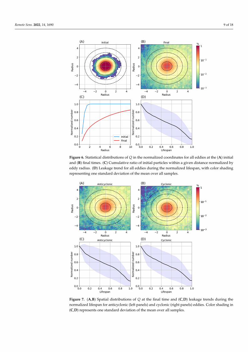
Figure 6 depicts the statistical distributions of Q in the normalized coordinates forall eddies at the initial and final times, based on the method described above. It is shownthat the averaged values of Q within 1R are close to 1% at the initial time. Due to the factthat the shape of an SSH eddy is not always a perfect circle, some particles at the initialtime are located outside of the 1R circle in the normalized coordinate, however, their Qvalues are substantially smaller than those in the eddy interior. With the rapid escape ofparticles from SSH eddies, the values of Q within 1R significantly decrease, and the leakedwater moves along with the local currents. An intriguing aspect of the Q value distributionis that there are more particles on the east side of the eddy than that on the west side atthe final time due to the fact that most eddies propagate westward (Figure 3). This alsoindicates that particles leaked from SSH eddies are not carried coherently westward bythe eddies and as a result, they show up on the east half of the eddy-centric coordinate.Figure 6C shows that all the particles a located within 2R from the eddy centers. At thefinal time, more than 60% of the particles are located outside of 2R, and only about 20% ofthe particles remain within the normalized eddy interior (1R).

Since the time intervals used in the above analysis may not always cover the wholelifespan of SSH eddies, here, we normalize these time intervals relative to the full lengthof eddy lifespan. For example, for the random eddy shown in Figure 5, the selected timeinterval corresponds to the normalized stage from 0.28 to 0.91. Figure 6D shows the averageleakage trend for all eddies over the normalized lifespan. The initially trapped water bySSH eddies leaks at a nearly linear rate, with only less than 20% remaining inside theSSH boundary at the final time. The strong leakage could be explained by the Reynoldstransport theorem [45]. When the velocity of the eddy boundary (SSH contour) does notalways coincide with the fluid velocity in a two-dimensional eddy system, there will beactive material flux across the boundary [33].

Having described the statistics of all eddies, we now present the differences betweenanticyclonic and cyclonic eddies. Figure 7 shows the spatial distributions of Q at the finaltime and leakage trends as a function of the normalized lifespan for the two types ofeddies. In addition to the aforementioned zonal asymmetry of Q distribution, there isalso an obvious meridional asymmetry of Q for anticyclonic and cyclonic eddies. Highervalues of Q are found on the north side of anticyclonic eddies, and the opposite is true forcyclonic eddies. This result is likely due to the fact that anticyclonic (cyclonic) eddies tend topropagate equatorward (poleward) in the Northern Hemisphere [3], thereby leaving leakedparticles behind on the north (south) side of the eddies. The numerical simulation [46]of eddy evolution and propagation corroborates these findings. Other than that, the twotypes of eddies have similar leakage trends, including both leakage degree (more than 80%)and rate. Our results suggest that, although the spatial distributions of leaked water aresomewhat different between anticyclonic and cyclonic eddies, a common feature for allSSH eddies in the SCS is that they are highly leaky during their lifespans.

Remote Sens. 2022, 14, 1690 9 of 18

Remote Sens. 2022, 14, x 9 of 20

from SSH eddies, the values of 𝑄 within 1R significantly decrease, and the leaked water moves along with the local currents. An intriguing aspect of the 𝑄 value distribution is that there are more particles on the east side of the eddy than that on the west side at the final time due to the fact that most eddies propagate westward (Figure 3). This also indi-cates that particles leaked from SSH eddies are not carried coherently westward by the eddies and as a result, they show up on the east half of the eddy-centric coordinate. Figure 6C shows that all the particles a located within 2R from the eddy centers. At the final time, more than 60% of the particles are located outside of 2R, and only about 20% of the parti-cles remain within the normalized eddy interior (1R).

Since the time intervals used in the above analysis may not always cover the whole lifespan of SSH eddies, here, we normalize these time intervals relative to the full length of eddy lifespan. For example, for the random eddy shown in Figure 5, the selected time interval corresponds to the normalized stage from 0.28 to 0.91. Figure 6D shows the aver-age leakage trend for all eddies over the normalized lifespan. The initially trapped water by SSH eddies leaks at a nearly linear rate, with only less than 20% remaining inside the SSH boundary at the final time. The strong leakage could be explained by the Reynolds transport theorem [45]. When the velocity of the eddy boundary (SSH contour) does not always coincide with the fluid velocity in a two-dimensional eddy system, there will be active material flux across the boundary [33].

Figure 6. Statistical distributions of 𝑄 in the normalized coordinates for all eddies at the (A) initial and (B) final times. (C) Cumulative ratio of initial particles within a given distance normalized by eddy radius. (D) Leakage trend for all eddies during the normalized lifespan, with color shading representing one standard deviation of the mean over all samples.

Having described the statistics of all eddies, we now present the differences between anticyclonic and cyclonic eddies. Figure 7 shows the spatial distributions of 𝑄 at the final time and leakage trends as a function of the normalized lifespan for the two types of ed-dies. In addition to the aforementioned zonal asymmetry of 𝑄 distribution, there is also an obvious meridional asymmetry of 𝑄 for anticyclonic and cyclonic eddies. Higher

Figure 6. Statistical distributions of Q in the normalized coordinates for all eddies at the (A) initialand (B) final times. (C) Cumulative ratio of initial particles within a given distance normalized byeddy radius. (D) Leakage trend for all eddies during the normalized lifespan, with color shadingrepresenting one standard deviation of the mean over all samples.

Remote Sens. 2022, 14, x 10 of 20

values of 𝑄 are found on the north side of anticyclonic eddies, and the opposite is true for cyclonic eddies. This result is likely due to the fact that anticyclonic (cyclonic) eddies tend to propagate equatorward (poleward) in the Northern Hemisphere [3], thereby leav-ing leaked particles behind on the north (south) side of the eddies. The numerical simula-tion [46] of eddy evolution and propagation corroborates these findings. Other than that, the two types of eddies have similar leakage trends, including both leakage degree (more than 80%) and rate. Our results suggest that, although the spatial distributions of leaked water are somewhat different between anticyclonic and cyclonic eddies, a common fea-ture for all SSH eddies in the SCS is that they are highly leaky during their lifespans.

Figure 7. (A,B) Spatial distributions of 𝑄 at the final time and (C,D) leakage trends during the normalized lifespan for anticyclonic (left panels) and cyclonic (right panels) eddies. Color shading in (C) and (D) represents one standard deviation of the mean over all samples.

3.3. Dependence of Leakiness on Eddy Parameters Eddies are often characterized by a number of parameters including amplitude (the

absolute value of SSH difference between the eddy center and the boundary), radius, rel-ative vorticity, kinetic energy, and so on. Does the degree of eddy leakage depend on any of these eddy parameters? To investigate this issue, six representative eddy parameters are selected.

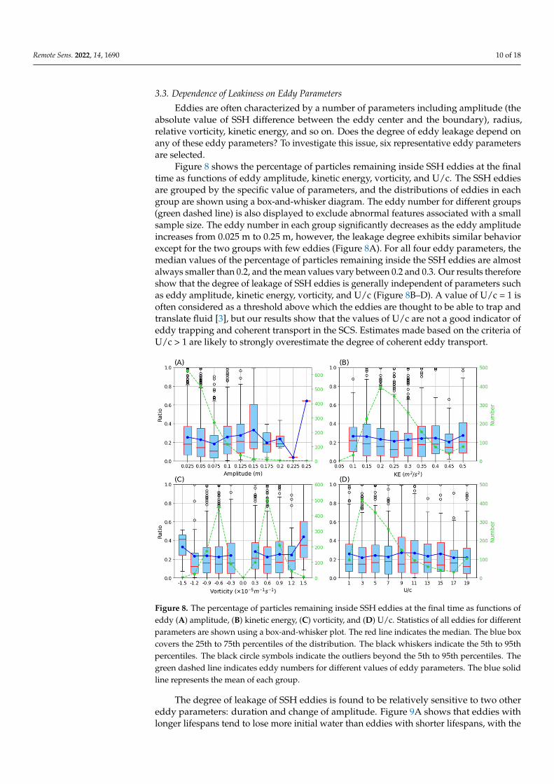
Figure 8 shows the percentage of particles remaining inside SSH eddies at the final time as functions of eddy amplitude, kinetic energy, vorticity, and U/c. The SSH eddies are grouped by the specific value of parameters, and the distributions of eddies in each group are shown using a box-and-whisker diagram. The eddy number for different groups (green dashed line) is also displayed to exclude abnormal features associated with a small sample size. The eddy number in each group significantly decreases as the eddy amplitude increases from 0.025 m to 0.25 m, however, the leakage degree exhibits similar behavior except for the two groups with few eddies (Figure 8A). For all four eddy param-eters, the median values of the percentage of particles remaining inside the SSH eddies are almost always smaller than 0.2, and the mean values vary between 0.2 and 0.3. Our

Figure 7. (A,B) Spatial distributions of Q at the final time and (C,D) leakage trends during thenormalized lifespan for anticyclonic (left panels) and cyclonic (right panels) eddies. Color shading in(C,D) represents one standard deviation of the mean over all samples.

Remote Sens. 2022, 14, 1690 10 of 18

3.3. Dependence of Leakiness on Eddy Parameters

Eddies are often characterized by a number of parameters including amplitude (theabsolute value of SSH difference between the eddy center and the boundary), radius,relative vorticity, kinetic energy, and so on. Does the degree of eddy leakage depend onany of these eddy parameters? To investigate this issue, six representative eddy parametersare selected.

Figure 8 shows the percentage of particles remaining inside SSH eddies at the finaltime as functions of eddy amplitude, kinetic energy, vorticity, and U/c. The SSH eddiesare grouped by the specific value of parameters, and the distributions of eddies in eachgroup are shown using a box-and-whisker diagram. The eddy number for different groups(green dashed line) is also displayed to exclude abnormal features associated with a smallsample size. The eddy number in each group significantly decreases as the eddy amplitudeincreases from 0.025 m to 0.25 m, however, the leakage degree exhibits similar behaviorexcept for the two groups with few eddies (Figure 8A). For all four eddy parameters, themedian values of the percentage of particles remaining inside the SSH eddies are almostalways smaller than 0.2, and the mean values vary between 0.2 and 0.3. Our results thereforeshow that the degree of leakage of SSH eddies is generally independent of parameters suchas eddy amplitude, kinetic energy, vorticity, and U/c (Figure 8B–D). A value of U/c = 1 isoften considered as a threshold above which the eddies are thought to be able to trap andtranslate fluid [3], but our results show that the values of U/c are not a good indicator ofeddy trapping and coherent transport in the SCS. Estimates made based on the criteria ofU/c > 1 are likely to strongly overestimate the degree of coherent eddy transport.

Remote Sens. 2022, 14, x 11 of 20

results therefore show that the degree of leakage of SSH eddies is generally independent of parameters such as eddy amplitude, kinetic energy, vorticity, and U/c (Figure 8B–D). A value of U/c = 1 is often considered as a threshold above which the eddies are thought to be able to trap and translate fluid [3], but our results show that the values of U/c are not a good indicator of eddy trapping and coherent transport in the SCS. Estimates made based on the criteria of U/c > 1 are likely to strongly overestimate the degree of coherent eddy transport.

Figure 8. The percentage of particles remaining inside SSH eddies at the final time as functions of eddy (A) amplitude, (B) kinetic energy, (C) vorticity, and (D) U/c. Statistics of all eddies for different parameters are shown using a box-and-whisker plot. The red line indicates the median. The blue box covers the 25th to 75th percentiles of the distribution. The black whiskers indicate the 5th to 95th percentiles. The black circle symbols indicate the outliers beyond the 5th to 95th percentiles. The green dashed line indicates eddy numbers for different values of eddy parameters. The blue solid line represents the mean of each group.

The degree of leakage of SSH eddies is found to be relatively sensitive to two other eddy parameters: duration and change of amplitude. Figure 9A shows that eddies with longer lifespans tend to lose more initial water than eddies with shorter lifespans, with the leakage ratio reaching more than 90% for eddies surviving longer than 180 days, indi-cating that it is difficult to maintain a coherent structure for eddies traveling a long dis-tance. The change in eddy amplitude over a time interval is of interest here because it is a measure of the stage of eddy evolution. Positive (negative) values represent the growing (decaying) state of eddies, which generally corresponds to an increase (decrease) in eddy radius [33]. For two eddies of the same size at the initial time, the leakage degree of the growing eddy may be smaller than that of the decaying eddy because the boundary of a growing eddy is likely to expand over time, making it more likely to contain the particles. This potentially explains why in Figure 9B, the percentage of particles remaining inside SSH eddies increases with increasing amplitude change. The dependence of eddy trap-ping efficiency on stages of eddy growth/decay is worth further investigation, but is left for a future study.

Figure 8. The percentage of particles remaining inside SSH eddies at the final time as functions ofeddy (A) amplitude, (B) kinetic energy, (C) vorticity, and (D) U/c. Statistics of all eddies for differentparameters are shown using a box-and-whisker plot. The red line indicates the median. The blue boxcovers the 25th to 75th percentiles of the distribution. The black whiskers indicate the 5th to 95thpercentiles. The black circle symbols indicate the outliers beyond the 5th to 95th percentiles. Thegreen dashed line indicates eddy numbers for different values of eddy parameters. The blue solidline represents the mean of each group.

The degree of leakage of SSH eddies is found to be relatively sensitive to two othereddy parameters: duration and change of amplitude. Figure 9A shows that eddies withlonger lifespans tend to lose more initial water than eddies with shorter lifespans, with the

Remote Sens. 2022, 14, 1690 11 of 18

leakage ratio reaching more than 90% for eddies surviving longer than 180 days, indicatingthat it is difficult to maintain a coherent structure for eddies traveling a long distance. Thechange in eddy amplitude over a time interval is of interest here because it is a measure ofthe stage of eddy evolution. Positive (negative) values represent the growing (decaying)state of eddies, which generally corresponds to an increase (decrease) in eddy radius [33].For two eddies of the same size at the initial time, the leakage degree of the growingeddy may be smaller than that of the decaying eddy because the boundary of a growingeddy is likely to expand over time, making it more likely to contain the particles. Thispotentially explains why in Figure 9B, the percentage of particles remaining inside SSHeddies increases with increasing amplitude change. The dependence of eddy trappingefficiency on stages of eddy growth/decay is worth further investigation, but is left for afuture study.

Remote Sens. 2022, 14, x 12 of 20

Figure 9. As in Figure 8, but for (A) eddy duration and (B) change of amplitude.

3.4. Coherent and Incoherent Contributions to Total Eddy Transport Having demonstrated that SSH eddies identified by the Eulerian method are far from

coherent structures, we now turn to detecting actual coherent eddies based on the Lagran-gian framework and examine the role of these eddies in material transport.

Figure 10 shows the initial and final locations of 30-day RCLVs generated on 1 Sep-tember 2010 as well as 60-day RCLVs generated on 1 April 2006. An obvious feature is that the majority of RCLVs are initially placed around the local extremum of the SLA, but their size is much smaller than the outermost closed SLA contour, which has also been noticed by previous studies [27,33]. In August 2012, 15 coherent eddies are identified in the SCS, and they are able to maintain a coherent structure without significant leakage. Filamentary structures develop for several eddies because we use a relatively moderate parameter [47] in the eddy detection to avoid underestimating the number of coherent structures (see Appendix A). Despite this, only two 60-day coherent eddies are found in the whole SCS basin in this randomly selected time period, which means that the long-lived coherent eddies are relatively rare in the SCS.

Figure 10. Initial (red dots) and final (blue dots) locations for (A) 30-day and (B) 60-day RCLVs in two random time intervals. The purple line indicates the eddy trajectory. The black contours repre-sent the SLA on the initial date with an interval of 2 cm.

From January 1993 to December 2015, there are 3239 30-day RCLVs and 516 60-day RCLVs identified in the SCS. Figure 11A shows the time series for the eddy number per month. The number of 30-day RCLVs typically ranges between 7 and 18 per month with-out any discernible seasonal or interannual signals. Since the number of 60-day RCLVs is

Figure 9. As in Figure 8, but for (A) eddy duration and (B) change of amplitude.

3.4. Coherent and Incoherent Contributions to Total Eddy Transport

Having demonstrated that SSH eddies identified by the Eulerian method are farfrom coherent structures, we now turn to detecting actual coherent eddies based on theLagrangian framework and examine the role of these eddies in material transport.

Figure 10 shows the initial and final locations of 30-day RCLVs generated on 1 Septem-ber 2010 as well as 60-day RCLVs generated on 1 April 2006. An obvious feature is thatthe majority of RCLVs are initially placed around the local extremum of the SLA, but theirsize is much smaller than the outermost closed SLA contour, which has also been noticedby previous studies [27,33]. In August 2012, 15 coherent eddies are identified in the SCS,and they are able to maintain a coherent structure without significant leakage. Filamentarystructures develop for several eddies because we use a relatively moderate parameter [47]in the eddy detection to avoid underestimating the number of coherent structures (seeAppendix A). Despite this, only two 60-day coherent eddies are found in the whole SCSbasin in this randomly selected time period, which means that the long-lived coherenteddies are relatively rare in the SCS.

From January 1993 to December 2015, there are 3239 30-day RCLVs and 516 60-dayRCLVs identified in the SCS. Figure 11A shows the time series for the eddy number permonth. The number of 30-day RCLVs typically ranges between 7 and 18 per month withoutany discernible seasonal or interannual signals. Since the number of 60-day RCLVs istypically less than 5 per month, we do not attempt to use an even longer detection period inthis study. Although the identified SSH eddies (1751) are less than the Lagrangian eddies,SSH eddies have longer lifespans. We counte the total snapshot number of SSH eddiesin each month and divide the number by 30, and then compare the value (green line inFigure 11A) with the number of 30-day RCLVs. It is observed that the number of SSHeddies calculated in this way also ranges between 7 and 18, indicating that the probability ofoccurrence for the two types of eddies is similar. However, they differ significantly in termsof eddy radius (Figure 11B). The radius of SSH eddies decreases with increasing latitude(from 5◦N to 20◦N) from 95 km to 77 km, with an average radius of 80.69 km. For 30-day

Remote Sens. 2022, 14, 1690 12 of 18

and 60-day RCLVs, the radius does not vary significantly with latitude. The average radiusof 30-day and 60-day RCLVs is 44.75 km and 44.68 km, respectively, approximately half ofthe size of SSH eddies. Previous numerical results [33] support the ratio observed here.

Remote Sens. 2022, 14, x 12 of 20

Figure 9. As in Figure 8, but for (A) eddy duration and (B) change of amplitude.

3.4. Coherent and Incoherent Contributions to Total Eddy Transport Having demonstrated that SSH eddies identified by the Eulerian method are far from

coherent structures, we now turn to detecting actual coherent eddies based on the Lagran-gian framework and examine the role of these eddies in material transport.

Figure 10 shows the initial and final locations of 30-day RCLVs generated on 1 Sep-tember 2010 as well as 60-day RCLVs generated on 1 April 2006. An obvious feature is that the majority of RCLVs are initially placed around the local extremum of the SLA, but their size is much smaller than the outermost closed SLA contour, which has also been noticed by previous studies [27,33]. In August 2012, 15 coherent eddies are identified in the SCS, and they are able to maintain a coherent structure without significant leakage. Filamentary structures develop for several eddies because we use a relatively moderate parameter [47] in the eddy detection to avoid underestimating the number of coherent structures (see Appendix A). Despite this, only two 60-day coherent eddies are found in the whole SCS basin in this randomly selected time period, which means that the long-lived coherent eddies are relatively rare in the SCS.

Figure 10. Initial (red dots) and final (blue dots) locations for (A) 30-day and (B) 60-day RCLVs in two random time intervals. The purple line indicates the eddy trajectory. The black contours repre-sent the SLA on the initial date with an interval of 2 cm.

From January 1993 to December 2015, there are 3239 30-day RCLVs and 516 60-day RCLVs identified in the SCS. Figure 11A shows the time series for the eddy number per month. The number of 30-day RCLVs typically ranges between 7 and 18 per month with-out any discernible seasonal or interannual signals. Since the number of 60-day RCLVs is

Figure 10. Initial (red dots) and final (blue dots) locations for (A) 30-day and (B) 60-day RCLVs in tworandom time intervals. The purple line indicates the eddy trajectory. The black contours representthe SLA on the initial date with an interval of 2 cm.

Remote Sens. 2022, 14, x 13 of 20

typically less than 5 per month, we do not attempt to use an even longer detection period in this study. Although the identified SSH eddies (1751) are less than the Lagrangian ed-dies, SSH eddies have longer lifespans. We counte the total snapshot number of SSH ed-dies in each month and divide the number by 30, and then compare the value (green line in Figure 11A) with the number of 30-day RCLVs. It is observed that the number of SSH eddies calculated in this way also ranges between 7 and 18, indicating that the probability of occurrence for the two types of eddies is similar. However, they differ significantly in terms of eddy radius (Figure 11B). The radius of SSH eddies decreases with increasing latitude (from 5°N to 20°N) from 95 km to 77 km, with an average radius of 80.69 km. For 30-day and 60-day RCLVs, the radius does not vary significantly with latitude. The aver-age radius of 30-day and 60-day RCLVs is 44.75 km and 44.68 km, respectively, approxi-mately half of the size of SSH eddies. Previous numerical results [33] support the ratio observed here.

Figure 11. (A) Numbers of 30-day (red line) and 60-day (blue line) RCLVs per month from 1993 to 2015, with the total snapshot number of SSH eddies per month (divided by 30) as shown by the green line. (B) The radii of RCLVs and SSH eddies as a function of latitude. The error bar represents one standard deviation of the mean over all samples in a 1.5° bin.

The absolute diffusivity is often used as a means to represent the fundamental prop-erties of a turbulent flow [27,48,49]. The meridional component of the absolute diffusivity is defined as 𝐾 = (𝑦 − 𝑦 ) , (3)

Figure 11. (A) Numbers of 30-day (red line) and 60-day (blue line) RCLVs per month from 1993 to2015, with the total snapshot number of SSH eddies per month (divided by 30) as shown by the greenline. (B) The radii of RCLVs and SSH eddies as a function of latitude. The error bar represents onestandard deviation of the mean over all samples in a 1.5◦ bin.

The absolute diffusivity is often used as a means to represent the fundamental proper-ties of a turbulent flow [27,48,49]. The meridional component of the absolute diffusivity isdefined as

Kabs =12

∂

∂t(y− y0)

2, (3)

Remote Sens. 2022, 14, 1690 13 of 18

where y is the meridional position of a particle initially released at y0. The absolutediffusivity measures the growth rate of the absolute dispersion of all particles advectedby the full flow field. In this study, we mainly focus on the eddy component of the fullmaterial transport, which can be measured by the relative diffusivity Krel after removingthe effects of the mean flow in the Lagrangian frame [27,50],

Krel =12

∂

∂t(y− y)2, (4)

where y is the averaged position of all particles released at y0. In this study, the ensembleconsists of all particles originating in the same month over 23 years. We calculate Krel for12 months and then take an average in order to remove the effects of the seasonal basin-scalecirculation in the SCS [7,8]. In addition, the material transport by eddies can be dividedinto two types: coherent (trapping) transport and incoherent (stirring) transport [27,51].Since we know the behaviors of all Lagrangian particles, the contribution of coherent eddytransport to the total eddy flux can be estimated by introducing a masking function todetermine whether particles are coherently trapped by eddies or not [27]. The coherentrelative diffusivity is then defined as

KCSrel =

12

∂

∂tm(y− y)2, (5)

where m is the masking function, which is 1 inside each Lagrangian eddy and 0 outside.We now calculate the absolute diffusivity, relative diffusivity, and coherent relative

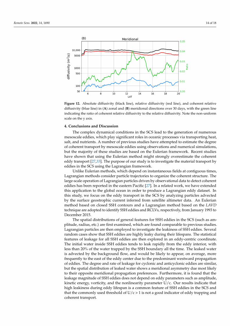
diffusivity in zonal and meridional directions over a 30-day period (Figure 12). It shouldbe noted that only 30-day RCLVs are considered in the calculation of coherent relativediffusivity. The value of Kabs is close to 10,000 m2/s in both directions, and the value of Krelis between 5000 and 7000 m2/s. The difference between them indicates the contribution ofthe mean flow to the dispersion of Lagrangian particles. The zonal KCS

rel has a magnitudeof about 200 m2/s, which is slightly higher than the meridional component due to thestronger zonal propagation of eddies. The most striking result here is that the magnitudeof KCS

rel is much smaller than Kabs and Krel . The fraction of coherent eddy transport to thetotal eddy transport can be quantified via the ratio of KCS

rel to Krel (green line in Figure 12),which never exceeds 5% in both zonal and meridional directions. This small contributionof coherent eddy structures to the total eddy transport suggests that material transport byeddies in the SCS is primarily caused by incoherent motions (such as filamentation outsidethe eddy core), which is broadly consistent with the results in [27,32]. The emphasis here ison representing the comparison of coherent and incoherent motions in the SCS in order toupdate the traditional perception of the importance of coherent eddy transport.

Remote Sens. 2022, 14, x 15 of 20

Figure 12. Absolute diffusivity (black line), relative diffusivity (red line), and coherent relative dif-fusivity (blue line) in (A) zonal and (B) meridional directions over 30 days, with the green line indi-cating the ratio of coherent relative diffusivity to the relative diffusivity. Note the non-uniform scale on the y axis.

4. Conclusions and Discussion The complex dynamical conditions in the SCS lead to the generation of numerous

mesoscale eddies, which play significant roles in oceanic processes via transporting heat, salt, and nutrients. A number of previous studies have attempted to estimate the degree of coherent transport by mesoscale eddies using observations and numerical simulations, but the majority of these studies are based on the Eulerian framework. Recent studies have shown that using the Eulerian method might strongly overestimate the coherent eddy transport [27,33]. The purpose of our study is to investigate the material transport by ed-dies in the SCS using the Lagrangian framework.

Unlike Eulerian methods, which depend on instantaneous fields at contiguous times, Lagrangian methods consider particle trajectories to organize the coherent structure. The large-scale operation of Lagrangian particles driven by observational data to detect coher-ent eddies has been reported in the eastern Pacific [27]. In a related work, we have ex-tended this application to the global ocean in order to produce a Lagrangian eddy dataset. In this study, we focus on the eddy transport in the SCS by analyzing particles advected by the surface geostrophic current inferred from satellite altimeter data. An Eulerian method based on closed SSH contours and a Lagrangian method based on the LAVD tech-nique are adopted to identify SSH eddies and RCLVs, respectively, from January 1993 to December 2015.

Figure 12. Cont.

Remote Sens. 2022, 14, 1690 14 of 18

Remote Sens. 2022, 14, x 15 of 20

Figure 12. Absolute diffusivity (black line), relative diffusivity (red line), and coherent relative dif-fusivity (blue line) in (A) zonal and (B) meridional directions over 30 days, with the green line indi-cating the ratio of coherent relative diffusivity to the relative diffusivity. Note the non-uniform scale on the y axis.

4. Conclusions and Discussion The complex dynamical conditions in the SCS lead to the generation of numerous

mesoscale eddies, which play significant roles in oceanic processes via transporting heat, salt, and nutrients. A number of previous studies have attempted to estimate the degree of coherent transport by mesoscale eddies using observations and numerical simulations, but the majority of these studies are based on the Eulerian framework. Recent studies have shown that using the Eulerian method might strongly overestimate the coherent eddy transport [27,33]. The purpose of our study is to investigate the material transport by ed-dies in the SCS using the Lagrangian framework.

Unlike Eulerian methods, which depend on instantaneous fields at contiguous times, Lagrangian methods consider particle trajectories to organize the coherent structure. The large-scale operation of Lagrangian particles driven by observational data to detect coher-ent eddies has been reported in the eastern Pacific [27]. In a related work, we have ex-tended this application to the global ocean in order to produce a Lagrangian eddy dataset. In this study, we focus on the eddy transport in the SCS by analyzing particles advected by the surface geostrophic current inferred from satellite altimeter data. An Eulerian method based on closed SSH contours and a Lagrangian method based on the LAVD tech-nique are adopted to identify SSH eddies and RCLVs, respectively, from January 1993 to December 2015.

Figure 12. Absolute diffusivity (black line), relative diffusivity (red line), and coherent relativediffusivity (blue line) in (A) zonal and (B) meridional directions over 30 days, with the green lineindicating the ratio of coherent relative diffusivity to the relative diffusivity. Note the non-uniformscale on the y axis.

4. Conclusions and Discussion

The complex dynamical conditions in the SCS lead to the generation of numerousmesoscale eddies, which play significant roles in oceanic processes via transporting heat,salt, and nutrients. A number of previous studies have attempted to estimate the degreeof coherent transport by mesoscale eddies using observations and numerical simulations,but the majority of these studies are based on the Eulerian framework. Recent studieshave shown that using the Eulerian method might strongly overestimate the coherenteddy transport [27,33]. The purpose of our study is to investigate the material transport byeddies in the SCS using the Lagrangian framework.

Unlike Eulerian methods, which depend on instantaneous fields at contiguous times,Lagrangian methods consider particle trajectories to organize the coherent structure. Thelarge-scale operation of Lagrangian particles driven by observational data to detect coherenteddies has been reported in the eastern Pacific [27]. In a related work, we have extendedthis application to the global ocean in order to produce a Lagrangian eddy dataset. Inthis study, we focus on the eddy transport in the SCS by analyzing particles advectedby the surface geostrophic current inferred from satellite altimeter data. An Eulerianmethod based on closed SSH contours and a Lagrangian method based on the LAVDtechnique are adopted to identify SSH eddies and RCLVs, respectively, from January 1993 toDecember 2015.

The spatial distributions of general features for SSH eddies in the SCS (such as am-plitude, radius, etc.) are first examined, which are found comparable to previous studies.Lagrangian particles are then employed to investigate the leakiness of SSH eddies. Severalrandom cases show that SSH eddies are highly leaky during their lifespans. The statisticalfeatures of leakage for all SSH eddies are then explored in an eddy-centric coordinate.The initial water inside SSH eddies tends to leak rapidly from the eddy interior, withless than 20% of the water trapped by the SSH boundary all the time. The leaked wateris advected by the background flow, and would be likely to appear, on average, morefrequently to the east of the eddy center due to the predominant westward propagationof eddies. The degree and rate of leakage for cyclonic and anticyclonic eddies are similar,but the spatial distribution of leaked water shows a meridional asymmetry due most likelyto their opposite meridional propagation preferences. Furthermore, it is found that theleakage magnitude of SSH eddies does not depend on eddy parameters such as amplitude,kinetic energy, vorticity, and the nonlinearity parameter U/c. Our results indicate thathigh leakiness during eddy lifespan is a common feature of SSH eddies in the SCS andthat the commonly used threshold of U/c > 1 is not a good indicator of eddy trapping andcoherent transport.

Remote Sens. 2022, 14, 1690 15 of 18

The detected RCLVs are compared to SSH eddies in terms of eddy number and radius.From 1993 to 2015, there are approximately 7 to 18 30-day RCLVs every month, with amuch lower number of 60-day RCLVs. Though the frequency of occurrence is similar forthe two types of eddies, RCLVs are typically smaller in size than SSH eddies, with a ratioof radius of roughly 0.5. Several types of diffusivities are then calculated to quantify thecontribution of the coherent eddy transport to the total eddy flux. Our key finding is thatKcs

rel , standing for the diffusive transport induced by coherent eddies, accounts for lessthan 5% of Krel , the diffusive transport induced by the full eddying flow in both zonaland meridional directions. This indicates that the transport by coherent eddies provides anegligible contribution to the net eddy material transport in the SCS.

What may cause substantial leakage of SSH eddies in the SCS? The idealized numericalexperiment of an isolated eddy [46] shows that most of the tracer originally inside of theeddy remains trapped by the SSH boundary after 675 days, which indicates that the SSHeddy is close to bea coherent structure and conforms to the conventional understanding.However, the statistical leakage of SSH eddies in an idealized ocean basin driven by con-stant wind forcing can reach about 50% after 30 days [33]. The primary difference betweenthe above two numerical experiments is that the isolated eddy moves in a tranquil basin,whereas the latter involves a turbulent ocean. This suggests that the background flowcan exert a large influence on the coherency of Eulerian eddies. The intricate multi-scaleprocesses in the SCS such as the large-scale seasonal circulation, eddy–eddy interactions,Kuroshio intrusion, internal waves, and sub-mesoscale processes may be factors that leadto stronger leakage (80% in our calculation) than that found in the idealized model exper-iments. Recent observations have shown that the level of turbulent mixing is elevatedin the periphery of mesoscale eddies [52], also providing reasonable evidence that thenonlinear effects may reduce the degree of coherent transport. Another factor that poten-tially causes high eddy leakage in the SCS is its complex topography including numerousislands and seamounts. Numerical simulations have shown that when encountering anisland/seamount, the eddy behavior changes dramatically [53]. Physical processes andfactors that influence eddy trapping efficiency is worth further investigation, and we planto conduct a suite of numerical experiments in a future study to explore this issue.

In this study, the Lagrangian particles are advected by two-dimensional surfacegeostrophic currents derived from satellite altimeter data. As such, the effect of verticalmotion on eddy coherent transport is not considered here. Due to the lack of observationsof three-dimensional flow fields under the surface, research on the effect of vertical motionson eddy material transport will inevitably rely on numerical model simulations. Despitethis caveat, the implications from this study are clear: Eulerian eddies are not coherentstructures and are highly leaky, and therefore, previous studies based on Eulerian methodsare likely to significantly overestimate coherent eddy transport in the SCS. Since coherenteddy transport only makes a small contribution to the total eddy transport in the SCS, moreattention is required to understand material transport by incoherent motions in the future.

Author Contributions: Conceptualization, T.L. and Y.H.; Methodology, T.L., Y.H. and X.Z.; Software,T.L.; Validation, T.L.; Formal analysis, T.L.; Investigation, T.L.; Resources, T.L.; Data curation, T.L.;Writing—original draft preparation, T.L. and Y.H.; Writing—review and editing, T.L., Y.H., X.Z. andX.L.; Visualization, T.L.; Supervision, T.L.; Project administration, T.L.; Funding acquisition, T.L., Y.H.and X.L. All authors have read and agreed to the published version of the manuscript.

Funding: This research is funded by the National Natural Science Foundation of China (42106008,41730535, 42176009), the China Postdoctoral Science Foundation (2020M681968), the Zhejiang Provin-cial Natural Science Foundation (LY21D060001), the Youth Innovation Promotion Association CAS(2019336), and the Natural Science Foundation of Guangdong Province (2021A1515012538).

Institutional Review Board Statement: Not applicable.

Informed Consent Statement: Not applicable.

Remote Sens. 2022, 14, 1690 16 of 18

Data Availability Statement: The only dataset in this study is the satellite altimetry product byAVISO, which can be found at http://www.aviso.altimetry.fr/duacs (accessed on 8 August 2021).The script used for calculating and plotting is available at https://github.com/liutongya/SCS_Eddy(accessed on 2 February 2022).

Acknowledgments: We thank to four anonymous reviewers for their helpful comments. All analysisin this study is conducted on the cloud-based platform Pangeo (https://pangeo.io/, accessed on 2February 2022).

Conflicts of Interest: The authors declare no conflict of interest.

Appendix A

The Lagrangian eddy boundary is defined as a closed curve of the LAVD field. Convex-ity deficiency (CD) is introduced by Haller et al. [30] to search the outermost closed curveencircling the eddy center. CD measures how strongly the boundary curve departs from aconvex curve. The closer CD is to zero, the closer the eddy boundary is to a convex curve.The sensitivity analysis by Tarshish et al. [47] has shown that CD < 0.1 is a representativevalue for identifying moderately coherent eddies, which is also adopted by Liu et al. [33].Figure A1 shows the boundaries and locations of detected Lagrangian eddies based onthree CD values in a random time interval. For CD < 0.01, only 6 RCLVs are identified andthe size is quite small, which means that this condition is too strict to find coherent eddies.In contrast, the condition of CD < 0.5 is too loose to define coherent eddies because most ofthese structures are highly leaky. For CD < 0.1, although the filamentary structure developsfor several eddies, the identified eddies could well maintain the coherency, which suggeststhat the estimate of coherent eddy transport based on this parameter is reasonable.

Remote Sens. 2022, 14, x 18 of 20

Figure A1. LAVD fields (colors) and 30-day Lagrangian eddy boundaries (red lines) for (A) CD < 0.01, (B) CD < 0.1, and (C) CD < 0.5 in a random time interval. Initial (red dots) and final (blue dots) locations for (D) CD < 0.01, (E) CD < 0.1, and (F) CD < 0.5.

References 1. Wunsch, C.; Ferrari, R. Vertical mixing, energy, and the general circulation of the oceans. Annu. Rev. Fluid Mech. 2004, 36, 281–314. 2. Fu, L.-L.; Chelton, D.; Le Traon, P.-Y.; Morrow, R. Eddy Dynamics From Satellite Altimetry. Oceanography 2010, 23, 14–25.

https://doi.org/10.5670/oceanog.2010.02. 3. Chelton, D.B.; Schlax, M.G.; Samelson, R.M. Global observations of nonlinear mesoscale eddies. Prog. Oceanogr. 2011, 91, 167–216. 4. Jayne, S.R.; Marotzke, J. The dynamics of ocean heat transport variability. Rev. Geophys. 2001, 39, 385–411.

https://doi.org/10.1029/2000rg000084. 5. Thompson, A.F.; Heywood, K.; Schmidtko, S.; Stewart, A. Eddy transport as a key component of the Antarctic overturning

circulation. Nat. Geosci. 2014, 7, 879–884. https://doi.org/10.1038/ngeo2289. 6. Busecke, J.J.M.; Abernathey, R.P. Ocean mesoscale mixing linked to climate variability. Sci. Adv. 2019, 5, eaav5014.

https://doi.org/10.1126/sciadv.aav5014. 7. Liu, Q.; Kaneko, A.; Jilan, S. Recent progress in studies of the South China Sea circulation. J. Oceanogr. 2008, 64, 753–762.

https://doi.org/10.1007/s10872-008-0063-8. 8. Zheng, Q.; Hu, J.; Ho, C.-R.; Xie, L. Advances in Research of Regional Oceanography of the South China Sea: Overview; World Scientific

Publishing Company: Singapore, 2020; pp. 1–18. https://doi.org/10.1142/9789811206917_0001. 9. Chen, G.; Hou, Y.; Chu, X. Mesoscale eddies in the South China Sea: Mean properties, spatiotemporal variability, and impact

on thermohaline structure. J. Geophys. Res. Ocean. 2011, 116, 711–720. https://doi.org/10.1029/2010jc006716. 10. He, Q.; Zhan, H.; Cai, S.; He, Y.; Huang, G.; Zhan, W. A New Assessment of Mesoscale Eddies in the South China Sea: Surface

Features, Three-Dimensional Structures, and Thermohaline Transports. J. Geophys. Res. Ocean. 2018, 123, 4906–4929. https://doi.org/10.1029/2018jc014054.

11. Liu, Y.; Dong, C.; Liu, X.; Dong, J. Antisymmetry of oceanic eddies across the Kuroshio over a shelfbreak. Sci. Rep. 2017, 7, 6761. 12. Ding, R.; Xuan, J.; Zhang, T.; Zhou, L.; Zhou, F.; Meng, Q.; Kang, I.-S. Eddy-induced Heat Transport in the South China Sea. J.

Phys. Oceanogr. 2021, 51, 2329–2349. https://doi.org/10.1175/jpo-d-20-0206.1. 13. Haller, G. Lagrangian coherent structures. Annu. Rev. Fluid Mech. 2015, 47, 137–162. 14. Dong, C.; McWilliams, J.C.; Liu, Y.; Chen, D. Global heat and salt transports by eddy movement. Nat. Commun. 2014, 5, 3294.

https://doi.org/10.1038/ncomms4294. 15. Zhang, Z.; Wang, W.; Qiu, B. Oceanic mass transport by mesoscale eddies. Science 2014, 345, 322–324. https://doi.org/10.1126/sci-

ence.1252418.

Figure A1. LAVD fields (colors) and 30-day Lagrangian eddy boundaries (red lines) for (A) CD < 0.01,(B) CD < 0.1, and (C) CD < 0.5 in a random time interval. Initial (red dots) and final (blue dots)locations for (D) CD < 0.01, (E) CD < 0.1, and (F) CD < 0.5.

Remote Sens. 2022, 14, 1690 17 of 18

References1. Wunsch, C.; Ferrari, R. Vertical mixing, energy, and the general circulation of the oceans. Annu. Rev. Fluid Mech. 2004, 36, 281–314.

[CrossRef]2. Fu, L.-L.; Chelton, D.; Le Traon, P.-Y.; Morrow, R. Eddy Dynamics From Satellite Altimetry. Oceanography 2010, 23, 14–25.

[CrossRef]3. Chelton, D.B.; Schlax, M.G.; Samelson, R.M. Global observations of nonlinear mesoscale eddies. Prog. Oceanogr. 2011, 91, 167–216.

[CrossRef]4. Jayne, S.R.; Marotzke, J. The dynamics of ocean heat transport variability. Rev. Geophys. 2001, 39, 385–411. [CrossRef]5. Thompson, A.F.; Heywood, K.; Schmidtko, S.; Stewart, A. Eddy transport as a key component of the Antarctic overturning

circulation. Nat. Geosci. 2014, 7, 879–884. [CrossRef]6. Busecke, J.J.M.; Abernathey, R.P. Ocean mesoscale mixing linked to climate variability. Sci. Adv. 2019, 5, eaav5014. [CrossRef]7. Liu, Q.; Kaneko, A.; Jilan, S. Recent progress in studies of the South China Sea circulation. J. Oceanogr. 2008, 64, 753–762.

[CrossRef]8. Zheng, Q.; Hu, J.; Ho, C.-R.; Xie, L. Advances in Research of Regional Oceanography of the South China Sea: Overview; World Scientific

Publishing Company: Singapore, 2020; pp. 1–18. [CrossRef]9. Chen, G.; Hou, Y.; Chu, X. Mesoscale eddies in the South China Sea: Mean properties, spatiotemporal variability, and impact on

thermohaline structure. J. Geophys. Res. Ocean. 2011, 116, 711–720. [CrossRef]10. He, Q.; Zhan, H.; Cai, S.; He, Y.; Huang, G.; Zhan, W. A New Assessment of Mesoscale Eddies in the South China Sea: Surface

Features, Three-Dimensional Structures, and Thermohaline Transports. J. Geophys. Res. Ocean. 2018, 123, 4906–4929. [CrossRef]11. Liu, Y.; Dong, C.; Liu, X.; Dong, J. Antisymmetry of oceanic eddies across the Kuroshio over a shelfbreak. Sci. Rep. 2017, 7, 6761.

[CrossRef]12. Ding, R.; Xuan, J.; Zhang, T.; Zhou, L.; Zhou, F.; Meng, Q.; Kang, I.-S. Eddy-induced Heat Transport in the South China Sea. J.

Phys. Oceanogr. 2021, 51, 2329–2349. [CrossRef]13. Haller, G. Lagrangian coherent structures. Annu. Rev. Fluid Mech. 2015, 47, 137–162. [CrossRef]14. Dong, C.; McWilliams, J.C.; Liu, Y.; Chen, D. Global heat and salt transports by eddy movement. Nat. Commun. 2014, 5, 3294.

[CrossRef] [PubMed]15. Zhang, Z.; Wang, W.; Qiu, B. Oceanic mass transport by mesoscale eddies. Science 2014, 345, 322–324. [CrossRef] [PubMed]16. Wang, G.; Su, J.; Chu, P. Mesoscale eddies in the South China Sea observed with altimeter data. Geophys. Res. Lett. 2003, 30.

[CrossRef]17. Xiu, P.; Chai, F.; Shi, L.; Xue, H.; Chao, Y. A census of eddy activities in the South China Sea during 1993–2007. J. Geophys. Res.

Ocean. 2010, 115. [CrossRef]18. Hu, J.; Gan, J.; Sun, Z.; Zhu, J.; Dai, M. Observed three-dimensional structure of a cold eddy in the southwestern South China Sea.

J. Geophys. Res. Ocean. 2011, 116. [CrossRef]19. Lin, X.; Dong, C.; Chen, D.; Liu, Y.; Yang, J.; Zou, B.; Guan, Y. Three-dimensional properties of mesoscale eddies in the South

China Sea based on eddy-resolving model output. Deep Sea Res. Part I: Oceanogr. Res. Pap. 2015, 99, 46–64. [CrossRef]20. Zhang, Y.; Liu, Z.; Zhao, Y.; Wang, W.; Li, J.; Xu, J. Mesoscale eddies transport deep-sea sediments. Sci. Rep. 2014, 4, 5937.

[CrossRef]21. Wang, X.; Li, W.; Qi, Y.; Han, G. Heat, salt and volume transports by eddies in the vicinity of the Luzon Strait. Deep Sea Res. Part I

Oceanogr. Res. Pap. 2011, 61, 21–33. [CrossRef]22. Zhang, Z.; Zhao, W.; Qiu, B.; Tian, J. Anticyclonic Eddy Sheddings from Kuroshio Loop and the Accompanying Cyclonic Eddy in

the Northeastern South China Sea. J. Phys. Oceanogr. 2017, 47, 1243–1259. [CrossRef]23. Yang, Y.; Zeng, L.; Wang, Q. How Much Heat and Salt Are Transported Into the South China Sea by Mesoscale Eddies? Earth’s

Futur. 2021, 9, e2020EF001857. [CrossRef]24. Okubo, A. Horizontal dispersion of floatable particles in the vicinity of velocity singularities such as convergences. Deep Sea Res.

Oceanogr. Abstr. 1970, 17, 445–454. [CrossRef]25. Weiss, J. The dynamics of enstrophy transfer in two-dimensional hydrodynamics. Phys. D Nonlinear Phenom. 1991, 48, 273–294.

[CrossRef]26. Nencioli, F.; Dong, C.; Dickey, T.; Washburn, L.; McWilliams, J.C. A Vector Geometry–Based Eddy Detection Algorithm and

Its Application to a High-Resolution Numerical Model Product and High-Frequency Radar Surface Velocities in the SouthernCalifornia Bight. J. Atmos. Ocean. Technol. 2010, 27, 564–579. [CrossRef]

27. Abernathey, R.; Haller, G. Transport by Lagrangian Vortices in the Eastern Pacific. J. Phys. Oceanogr. 2018, 48, 667–685. [CrossRef]28. Shadden, S.C.; Lekien, F.; Marsden, J.E. Definition and properties of Lagrangian coherent structures from finite-time Lyapunov

exponents in two-dimensional aperiodic flows. Phys. D Nonlinear Phenom. 2005, 212, 271–304. [CrossRef]29. D’Ovidio, F.; Isern-Fontanet, J.; López, C.; Hernández-García, E.; García-Ladona, E. Comparison between Eulerian diagnostics

and finite-size Lyapunov exponents computed from altimetry in the Algerian basin. Deep Sea Res. Part I Oceanogr. Res. Pap. 2009,56, 15–31. [CrossRef]

30. Haller, G.; Hadjighasem, A.; Farazmand, M.; Huhn, F. Defining coherent vortices objectively from the vorticity. J. Fluid Mech.2016, 795, 136–173. [CrossRef]

31. Haller, G.; Beron-Vera, F.J. Coherent Lagrangian vortices: The black holes of turbulence. J. Fluid Mech. 2013, 731. [CrossRef]

Remote Sens. 2022, 14, 1690 18 of 18

32. Wang, Y.; Olascoaga, M.J.; Beron-Vera, F.J. Coherent water transport across the South Atlantic. Geophys. Res. Lett. 2015,42, 4072–4079. [CrossRef]

33. Liu, T.; Abernathey, R.; Sinha, A.; Chen, D. Quantifying Eulerian Eddy Leakiness in an Idealized Model. J. Geophys. Res. Ocean.2019, 124, 8869–8886. [CrossRef]

34. Adcroft, A.; Campin, J.M.; Doddridge, S.D.; Evangelinos, C.; Ferreira, D.; Follows, M.; Scott, J. MITgcm documentation. ReleaseCheckp. 2018, 19, 67a-12-gbf23121.

35. Abernathey, R.P.; Marshall, J. Global surface eddy diffusivities derived from satellite altimetry. J. Geophys. Res. Ocean. 2013,118, 901–916. [CrossRef]

36. He, Y.; Xie, J.; Cai, S. Interannual variability of winter eddy patterns in the eastern South China Sea. Geophys. Res. Lett. 2016,43, 5185–5193. [CrossRef]

37. He, Y.; Feng, M.; Xie, J.; He, Q.; Liu, J.; Xu, J.; Chen, Z.; Zhang, Y.; Cai, S. Revisit the Vertical Structure of the Eddies andEddy-Induced Transport in the Leeuwin Current System. J. Geophys. Res. Ocean. 2021, 126, e2020JC016556. [CrossRef]

38. Faghmous, J.H.; Frenger, I.; Yao, Y.; Warmka, R.; Lindell, A.; Kumar, V. A daily global mesoscale ocean eddy dataset from satellitealtimetry. Sci. Data 2015, 2, 150028. [CrossRef]

39. Zhang, W.; Wolfe, C.L.P.; Abernathey, R. Role of Surface-Layer Coherent Eddies in Potential Vorticity Transport in Quasi-geostrophic Turbulence Driven by Eastward Shear. Fluids 2019, 5, 2. [CrossRef]

40. Nan, F.; Xue, H.; Chai, F.; Shi, L.; Shi, M.; Guo, P. Identification of different types of Kuroshio intrusion into the South China Sea.Ocean Dyn. 2011, 61, 1291–1304. [CrossRef]

41. Wang, G.; Chen, D.; Su, J. Winter Eddy Genesis in the Eastern South China Sea due to Orographic Wind Jets. J. Phys. Oceanogr.2008, 38, 726–732. [CrossRef]

42. Cheng, X.; Xie, S.-P.; Du, Y.; Wang, J.; Chen, X.; Wang, J. Interannual-to-decadal variability and trends of sea level in the SouthChina Sea. Clim. Dyn. 2015, 46, 3113–3126. [CrossRef]

43. Chelton, D.B.; DeSzoeke, R.A.; Schlax, M.G.; El Naggar, K.; Siwertz, N. Geographical variability of the first baro-clinic Rossbyradius of deformation. J. Phys. Oceanogr. 1998, 28, 433–460. [CrossRef]

44. Huang, R.; Xie, L.; Zheng, Q.; Li, M.; Bai, P.; Tan, K. Statistical analysis of mesoscale eddy propagation velocity in the South ChinaSea deep basin. Acta Oceanol. Sin. 2020, 39, 91–102. [CrossRef]

45. Reynolds, O. The Sub-Mechanics of the Universe; University Press: Cambridge, UK, 1903; Volume 3.46. Early, J.J.; Samelson, R.M.; Chelton, D.B. The Evolution and Propagation of Quasigeostrophic Ocean Eddies. J. Phys. Oceanogr.

2011, 41, 1535–1555. [CrossRef]47. Tarshish, N.; Abernathey, R.; Zhang, C.; Dufour, C.O.; Frenger, I.; Griffies, S. Identifying Lagrangian coherent vortices in a

mesoscale ocean model. Ocean Model. 2018, 130, 15–28. [CrossRef]48. LaCasce, J. Statistics from Lagrangian observations. Prog. Oceanogr. 2008, 77, 1–29. [CrossRef]49. Klocker, A.; Ferrari, R.; LaCasce, J.H. Estimating Suppression of Eddy Mixing by Mean Flows. J. Phys. Oceanogr. 2012,

42, 1566–1576. [CrossRef]50. Bennett, A.F. Relative Dispersion: Local and Nonlocal Dynamics. J. Atmos. Sci. 1984, 41, 1881–1886. [CrossRef]51. Frenger, I.; Münnich, M.; Gruber, N.; Knutti, R. Southern Ocean eddy phenomenology. J. Geophys. Res. Ocean. 2015, 120, 7413–7449.

[CrossRef]52. Yang, Q.; Zhao, W.; Liang, X.; Dong, J.; Tian, J. Elevated Mixing in the Periphery of Mesoscale Eddies in the South China Sea. J.

Phys. Oceanogr. 2017, 47, 895–907. [CrossRef]53. Yang, S.; Xing, J.; Chen, D.; Chen, S. A modelling study of eddy-splitting by an island/seamount. Ocean Sci. 2017, 13, 837–849.

[CrossRef]