
VISUAL FIELD DIGEST - : Haag-Streit Diagnostics
305
-0.8 2.1 4.1 6.7 2.6 0.4 0.4 0.6 0.7 1.0
-
Upload
khangminh22 -
Category
Documents
-
view
0 -
download
0
Transcript of VISUAL FIELD DIGEST - : Haag-Streit Diagnostics

VISUAL FIELD DIGEST
Illustrated by Philip Earnhart
Lyne Racette, Monika Fischer, Hans Bebie, Gábor Holló, Chris A. Johnson, Chota Matsumoto
A guide to perimetry and the Octopus perimeter
-0.8
2.14.1
6.72.60.4
0.4
0.60.7
1.0
6th edition
VISUAL FIELD DIGESTA guide to perimetry and the Octopus perimeter
6th edition
Lyne Racette, Monika Fischer, Hans Bebie,
Gábor Holló, Chris A. Johnson, Chota Matsumoto
Illustrated by Philip Earnhart

Editor:Haag-Streit AG, Köniz, Switzerland
6 Edition, published 2016
Layout, cover design & illustrations by Philip Earnhart
ISBN 978-3-033-05854-5
Copyright © 2016 HAAG-STREIT AGHaag-Streit AG allows the use of this publication for personal or academic use under the conditions that (i) it is used without commercial purpose and (ii) the content is reproduced exactly as the original by mentioning Haag-Streit AG, Switzerland as the owner of the copyright.
Non-academic, non-personal or commercial users might only use this publication in whole or in part after a written authorization by the copyright holder.
Trademark statement“Haag-Streit”, “900” and “Octopus” are either registered trademarks or trademarks of Haag-Streit Holding AG.
The following are either registered trademarks or trademarks of Carl Zeiss Meditec: “Guided Progression Analysis”, “GPA”, “Humphrey”, “HFA”, “SITA”, “SITA Fast”, “SITA Standard”, “Visual Field Index”, and “VFI”.

III
AUTHORS & CONTRIBUTORS
AUTHORS LYNE RACETTE, PhDAssistant ProfessorEugene and Marilyn Glick Eye Institute, Department of OphthalmologyIndiana University School of MedicineIndianapolis, USA
MONIKA FISCHER, MScMarket Manager PerimetryHaag-Streit AGKöniz, SWITZERLAND
HANS BEBIE, PhDProfessor EmeritusInstitute for Theoretical PhysicsUniversity of BernBern, SWITZERLAND
GÁBOR HOLLÓ, MD, PhD, DScProfessor of OphthalmologyDirector of Glaucoma and Perimetry UnitDepartment of OphthalmologySemmelweis UniversityBudapest, HUNGARY
CHRIS A. JOHNSON, PhD, DScProfessor of OphthalmologyDirector of Visual Field Reading CenterUniversity of IowaIowa City, USA
CHOTA MATSUMOTO, MD, PhDProfessor of OphthalmologyDepartment of Ophthalmology, Kindai University Faculty of MedicineOsaka-Sayama, JAPAN
CONTRIBUTORS
JONATHAN MYERS, MDCo-Director of Glaucoma ServiceWills Eye HospitalPhiladelphia, USA
RAMANARASIAH RANGARAJ, MDConsultant Surgeon & Head of the Department of OphthalmologyPremier Eye Care And Surgical CenterChennai, INDIA
FIONA ROWE, PhDProfessor of Orthoptics Orthoptics and Health Services ResearchInstitute of Psychology, Health and SocietyUniversity of LiverpoolLiverpool, UNITED KINGDOM
SONOKO TAKADA MD, PhDAdjunct Assistant ProfessorDepartment of OphthalmologyKindai University Faculty of MedicineOsaka-Sayama, JAPAN
ILLUSTRATOR
PHILIP EARNHARTArt, Communication & Designearnhart.chBiel, SWITZERLAND


Preface V
PREFACE
Since the publication of the 5th edition of the Visual Field Digest in 2004, clinicians’ expectations regarding visual ield testing and analysis have signi icantly increased.
In today’s busy and fast-paced clinics, maximizing the trade-off between accuracy of results, test duration and the effort required from both the patient and the examiner is more important than ever before.
While the basic testing principles used in perimetry today have remained largely unchanged since the intro-duction of the manual Goldmann perimeter in 1946, Octopus perimeters have pioneered numerous import-ant changes in perimetry. The development of the irst automated perimeter, the Octopus 201, by Fankhauser, Spahr and Jenni in 1974, opened the door for automated perimetric testing as we know it today. Further, semi- automation in kinetic perimetry, irst introduced for the Octopus perimeter nearly 20 years ago, has facilitated kinetic testing.
Since then, knowledge on how to best select, perform and interpret perimetric tests in clinical practice has increased considerably. Normative databases, global indices such as Mean Defect, the Defect Curve and many other useful tools for analyzing the measured sensitivity thresholds have been irst introduced on Octopus perime-ters, before becoming worldwide standards in visual ield interpretation.
Since the last edition of this book 12 years ago, several advances in perimetric testing with Octopus perimeters have been achieved. EyeSuite Progression Analysis has been developed and is a powerful tool for assessing pro-gression. In addition, both Cluster Analysis and Polar Analysis are helpful features for establishing a relationship between functional and structural results. This new edition of the Visual Field Digest provides in-depth information
about these recent advancements and retains the com-prehensiveness of past editions.
Furthermore, this 6th edition puts a stronger emphasis on the challenges and possible pitfalls associated with visual ield testing in clinical practice and provides guid-ance on how to overcome them. While this edition builds on the previous versions, its format has been updated with the intention of making visual ield testing accessible to everyone, including clinicians, residents, researchers, examiners, students and those without previous knowl-edge of perimetry. Much effort has been invested in creating instructive igures to support the key points of the text.
We wish to thank Philip Earnhart for creating the igures and graphics that beautifully illustrate this book and Koo-sha Ramezani for proofreading the inal version. Further-more, this project would not have been possible without the unfailing support of Haag-Streit AG, for which we are grateful. Finally, we should like to thank our contributors for providing us with the clinical cases used throughout the book to illustrate various aspects of perimetry and for sharing their knowledge with us.
We hope that this book on perimetry in general, and on the Octopus perimeter in particular, is not only compre-hensive, but also enjoyable to read for anybody inter-ested in visual ield testing. We are convinced that the information shared in the pages ahead will be useful to clinicians and ultimately to their patients, whose sight we care deeply about. We wish you an enriching and pleasant reading experience.
Lyne Racette, Monika Fischer, Hans Bebie, Gábor Holló, Chris A. Johnson, Chota Matsumoto September 2016
Table of contentsVI
TABLE OF CONTENTS
1. INTRODUCTION 1 WHY READ THIS BOOK 1 WHO SHOULD READ THIS BOOK 1 HOW TO READ THIS BOOK 2 CONTENT AT A GLANCE 3
2. WHAT IS PERIMETRY 7 INTRODUCTION 7 Perimetry – A standard test in ophthalmology 7 THE NORMAL VISUAL FIELD 8
Spatial extent of the visual ield 8 Sensitivity to light in the visual ield 9 The hill of vision – A visualization of visual function 10 MEASURING SENSITIVITY TO LIGHT ACROSS THE VISUAL FIELD 11
Perimetry allows quanti ication of abnormal sensitivity to light 11 The perimetric test 12 DISPLAY OF SENSITIVITY THRESHOLDS 14
The decibel scale used in Perimetry 14 Graphic display of sensitivity thresholds 16 CHALLENGES IN VISUAL FIELD TESTING AND INTERPRETATION 17
Perimetric testing has low resolution 17 Normal sensitivities depend on age and test location 18 Perimetry has objective and subjective components 20 Normal luctuation depends on test locations and disease severity 20 Clinical standard for visual function testing 22
3. HOW TO PERFORM PERIMETRY YOU CAN TRUST 25 INTRODUCTION 25
Perimetry – A subjective test 25 Perimetry – Need for a team approach 26 The important role of the doctor 26 The important role of the visual ield examiner 27 HOW TO PERFORM VISUAL FIELD TESTING 28
Setting up the perimeter 28 Placing an adequate trial lens 29 Instructing the patient 29 Setting up and positioning the patient 31 Monitoring the patient during the examination 35

Table of contents VII
COMMON PITFALLS TO AVOID 37
Inconsistent patient behavior 37 Mistakes in the set-up procedure 40 External obstructions blocking stimuli from reaching the retina 43 Clinical relevance of untrustworthy visual ields 45
4. KEY EXAMINATION PARAMETERS 47 FIXED EXAMINATION PARAMETERS 47 PATIENT-SPECIFIC EXAMINATION PARAMETERS 48 Type of perimetry: Static or kinetic perimetry 48 Stimulus type: Standard or non-conventional 51 Test pattern 54 Test strategy 56
5. SELECTING A TEST PATTERN 59 INTRODUCTION 59 TEST PATTERNS FOR GLAUCOMA 60
Typical visual ield defects in glaucoma 60 Standard test pattern in glaucoma care 62 Alternative test patterns for the central 30° 64 Further test patterns for glaucoma 65 TEST PATTERNS FOR NEUROLOGICAL VISUAL FIELD LOSS 67
Typical visual ield defects in neuro-ophthalmic conditions 67 Thorough assessment of neurological visual ield defects 69 TEST PATTERNS FOR RETINOPATHIES 70
Typical visual ield defects in retinopathies 70 Test patterns for the macula 71 Test patterns for the full ield 72 TEST PATTERNS FOR VISUAL ABILITY TESTING 74
Test patterns for visual ability to drive 74 Test patterns for blepharoptosis 76 Test patterns for visual impairment 78
6. SELECTING A TEST STRATEGY 81 INTRODUCTION 81 QUANTITATIVE STRATEGIES 82 Normal strategy 83 Dynamic strategy 85 Low-vision strategy 86 Tendency-Oriented-Perimetry (TOP) strategy 87 QUALITATIVE STRATEGIES 90
1-Level Test strategy (two-zone strategy) 91 Screening strategy 92 2-Level Test strategy (three-zone strategy) 94 RECOMMENDATIONS ON KEY EXAMINATION PARAMETERS 96

Table of contentsVIII
7. OVERVIEW OF VISUAL FIELD REPRESENTATIONS 99 INTRODUCTION 99 RELATIONSHIP AMONG OCTOPUS VISUAL FIELD REPRESENTATIONS 99 REPRESENTATIONS DISPLAYING SENSITIVITY THRESHOLDS 101
Values 101 Grayscale of Values 102 REPRESENTATIONS BASED ON COMPARISON WITH NORMAL 103
Comparison 103 Grayscale of Comparison 105 Probabilities 107 Defect Curve 109 Cluster Analysis 110 Polar Analysis 113 REPRESENTATIONS BASED ON COMPARISON WITH NORMAL, CORRECTED FOR DIFFUSE DEFECT 115 Corrected Comparison 115 Corrected Probabilities 117 Corrected Cluster analysis 118 GLOBAL INDICES 118 Mean Sensitivity (MS) 119 Mean Defect (MD) 119 Square root of Loss Variance (sLV) 120 Corrected square root of Loss Variance (CsLV) 121 Diffuse Defect (DD) 121 Local Defect (LD) 122 RELIABILITY INDICES 123 False Positive (FP) answers 123 False Negative (FN) answers 124 Reliability Factor (RF) 124 Short-term Fluctuation (SF) 124
8. CLINICAL INTERPRETATION OF A VISUAL FIELD 127 INTRODUCTION 127 STEP-BY-STEP INTERPRETATION OF A VISUAL FIELD 134
Overview of step-by-step work low 134 Step 1 – Con irm patient and examination parameters 135 Step 2 – Determine whether the visual ield can be trusted 136 Step 3 – Identify diffuse visual ield defects 140 Step 4 – Distinguish between normal and abnormal visual ields 145 Step 5 – Assess shape and depth of defect 149 Step 6 – Assess cluster defects in glaucoma 152 Step 7 – Where to look for a structural defects 155 Step 8 – Assess severity 159

Table of contents IX
9. INTERPRETATION OF VISUAL FIELD PROGRESSION 165 INTRODUCTION 165 ASSESSMENT OF GLOBAL VISUAL FIELD CHANGE 168
Change of Mean Defect (MD) as a measure of global change 168 Trend analysis for the visualization of change 168 Using probabilities to distinguish between stable and changing visual ield series 171 MD Trend Analysis 174 Interpretation of MD Trend Analysis 176 Selection of adequate visual ields for analysis 176 DISTINCTION BETWEEN LOCAL AND DIFFUSE CHANGE 178
Importance of distinction between local and diffuse change 178 Use of Diffuse Defect index (DD) to identify diffuse change 179 Use of Local Defect index (LD) to identify local change 180 Use of square root of Loss Variance (sLV) to identify local change 180 Clinical interpretation of 4 Global Trend Analyses 181 CLUSTER TREND AND CORRECTED CLUSTER TREND ANALYSIS 183
Importance of assessing cluster progression in glaucoma 183 Cluster Trend and Corrected Cluster Trend Analysis 183 POLAR TREND ANALYSIS 187
Importance of establishing a relationship between structural and functional progression 187 Use of polar trend analysis to assist in the detection of glaucomatous structural progression 187
10. NON-CONVENTIONAL PERIMETRY 193 INTRODUCTION 193 FUNCTION-SPECIFIC PERIMETRY 194
Rational for using function-speci ic perimetry 194 Use of function-speci ic perimetry in clinical practice 195 Pulsar Perimetry 196 Flicker Perimetry 198 Short Wavelength Automated Perimetry (SWAP) 200 STIMULUS V FOR PATIENTS WITH LOW VISION 201
11. KINETIC PERIMETRY 205 WHAT IS KINETIC PERIMETRY 205
Limitations of static perimetry 205 Description of kinetic perimetry 207 WHY PERFORM KINETIC PERIMETRY 210
Bene its of kinetic perimetry 210 Limitations of kinetic perimetry 212 HOW TO PERFORM KINETIC PERIMETRY 214
The Goldmann perimeter: Kinetic visual ield testing 214 Key decisions in kinetic perimetry 215 Stimulus types 216 General testing methodologies 218 Step-by-Step example of kinetic perimetry 227 Automation of kinetic perimetry 230

Table of contentsX
12. TRANSITIONING TO A DIFFERENT PERIMETER MODEL 235 INTRODUCTION 235 GENERAL ASPECTS OF TRANSITIONING 236
Measured sensitivity thresholds cannot be compared across different perimeter models 236 Device-speci ic normative databases allow comparison of sensitivity losses between devices 237 Import of existing data to ensure continuity 239 Managing patient-related luctuation 243 SPECIFIC ASPECTS RELATED TO TRANSITIONING FROM THE HUMPHREY FIELD ANALYZER 243
Selection of test parameters 243 Interpretation of a single visual ield 244 Interpretation of visual ield progression 250
13. CLINICAL CASES 255 INTRODUCTION 255 GLAUCOMA – SINGLE FIELD 257 GLAUCOMA – TREND 266 NEUROLOGICAL DISEASES 272 RETINAL DISEASES 280
INDEX 285


1
CHAPTER 1INTRODUCTION
WHY READ THIS BOOK
WHO SHOULD READ THIS BOOK
The irst Visual Field Digest was published in 1983 and has been used as a guide to perimetry and the Octopus perimeter by thousands of Octopus users ever since. This 6th edition is a completely revised version of the 5th edition published in 2004. Not only does it contain updates on features developed since the last edition was
This book has been written for any current or future eye care professionals who perform or interpret visual ield examinations as part of their diagnostic routine.
This group not only includes clinicians in optometry and ophthalmology, but also visual ield examiners who administer perimetric tests to patients.
A wide range of users will ind useful information in this book. It has been created for students with limited knowledge in perimetry and therefore explains funda-mentals in perimetry in an easy to understand manner. In addition, it has been composed for experienced eye
published (e.g., Global Trend Analysis, Cluster Trend Analysis and Polar Trend Analysis), this edition places a stronger emphasis on the clinical application of perim-etry compared to previous editions. All key concepts are illustrated to facilitate understanding. This allows any reader to easily and quickly grasp the key information.
care professionals and provides many practical tips and tricks to get even more out of their perimetric testing. And last, it has been written for researchers and expert users of perimetry who are interested in the scienti ic background of perimetry and the Octopus perimeter.
While this book provides in-depth information about the design and use of the Octopus perimeters, it is also very useful reading for users of other perimeter brands, as the fundamental concepts of perimetry are compara-ble among perimeter brands and are illustrated in this book in an easy to understand way.

2 Chapter 1 | Introduction
51Key examination parameters | Patient-specific examination parameters
--
---
es, refer to BOX 4B
ADVANTAGES
WHAT IT IS BEST AT DETECTING
COMMON USES
STATIC
Fully automated
Macular diseases
Visual ability testing
KINETIC
Remaining vision in advanced diseases
STANDARD WHITE-ON-WHITE PERIMETRY
STIMULUS TYPE: STANDARD OR NON-CONVENTIONAL
COMPARISON BETWEEN STATIC AND KINETIC PERIMETRY TABLE 4-1
52 Key examination parameters | Patient-specific examination parameters
FIGURE 4-3 Stimuli of function-specific perimetry from left to right: Short Wavelength Automated Perimetry (SWAP), Flicker
Perimetry and Pulsar Perimetry.
SWAP PulsarFlicker
ON
Time 1
OFF
Time 2
V
IV
III
II
I
1.7°
0.8°
0.43°
0.2°
0.1°
20
BLIND SPOT
-FIG 4-3
-
FUNCTION-SPECIFIC PERIMETRY
FUNCTION-SPECIFIC PERIMETRY
GOLDMANN SIZES I TO V
-
-
The Goldmann stimuli I to V are presented in relation
to the size of the physiological blind spot.
BOX 4B
TABLEProvides a quick
overview andcontrasts differentconcepts/methods
TEXTFull presentation
of a topic
BOXProvides expert
knowledge
FIGUREIllustrates keyinformation in
an easy tounderstand way
HOW TO READ THIS BOOK
To cater to the needs of readers with different experi-ence levels as well as different learning styles, this book can be read in several ways.
For students and inexperienced users in perimetry, this book is structured in a way that, when read from begin-ning to end, it allows the content to be followed with minimal prior knowledge. For this reason, the book starts with fundamentals of perimetry such as, what the test does, how to administer the test and how to choose test parameters, before moving on to visual ield inter-pretation and special topics like kinetic perimetry or function-speci ic perimetry. To tie the learning to real clinical situations, this book concludes with a case pre-sentation section.
For more experienced users, individual chapters or sec-tions in this book can also be read individually, as each chapter is structured in a way that it is self-explanatory, or if not, a clear reference to another chapter is given.
To find and understand key information quickly, all essential concepts are graphically illustrated to support a quick understanding of the concept. With more than 200 graphics available in this book, it is thus possible to grasp key information just by looking at the graphics and reading the captions.
If several choices or methods are compared, overview tables are provided for quick comparison between them. Sometimes, in-depth background information
KEY ELEMENTS USED IN THIS BOOK
FIGURE 1-1 To accommodate the preferences of different readers, different structural elements are used in the Visual Field
Digest. To highlight key information, there are Figures and Tables; to provide a full overview of a topic, there is full text; and to
provide in-depth expert knowledge, there are Boxes.

3Content at a glance
CONTENT AT A GLANCE
In this section, a brief overview of the content of each chapter is presented.
is of interest to some readers, but not crucial for good clinical practice. Such information is provided in a light blue box and can be read for interest but does not inter-
fere with the low of the book. The elements described above are shown in FIG 1-1.
CHAPTER 2 – WHAT IS PERIMETRY?
CHAPTER 4 – KEY EXAMINATION PARAMETERS
CHAPTER 3 – HOW TO PERFORM PERIMETRY YOU CAN TRUST
Chapter 2 provides essential information on perimetry as a technology which is valid for any perimeter brand. It shows how and why visual ield testing is performed,
Chapter 4 focuses on ixed examination parameters and the key patient-speci ic parameters a clinician needs to decide about. Key questions to be answered regard-ing patient-speci ic test parameters are the following: 1) Static or kinetic perimetry? 2) Which stimulus type? 3) Which test pattern? 4) Which strategy?
Chapter 3 focuses on information relevant to visual ield technicians and those people instructing them. It stresses the importance of the visual ield technician in obtaining trustworthy visual ield results and explains the essential steps of visual ield testing. In a second part, common pit-
provides a general introduction on how the data is dis-played, and highlights common challenges associated with visual ield testing.
The idea is to provide an introduction to what these pa-rameters are and how to make appropriate testing deci-sions. The key parameters will be described in depth in subsequent chapters.
falls in perimetry such as learning effects, fatigue effects, set-up errors and artifacts are presented, along with the procedures for avoiding these problems. How to detect whether a visual ield is trustworthy is later presented in Chapter 8.
4 Chapter 1 | Introduction
CHAPTER 6 – SELECTING A TEST STRATEGY
CHAPTER 7 – OVERVIEW OF VISUAL FIELD REPRESENTATIONS
CHAPTER 8 – CLINICAL INTERPRETATION OF A VISUAL FIELD
CHAPTER 9 – INTERPRETATION OF VISUAL FIELD PROGRESSION
Chapter 6 presents all available test strategies on Octo-pus perimeters and shows that there is always a trade-off between test duration and accuracy in order to guide the
Chapter 7 introduces all visual ield representations avail-able on Octopus perimeters and shows their respective relationships. Further, each representation is explained in detail, including a clear de inition of all the symbols used
Chapter 8 is a key chapter in this book, guiding clinicians through visual ield interpretation in an easy to follow work low. It starts by showing 6 visual ield examples and their respective representations across all stages of disease to provide a graphical reference on what visual ield results look like in a given situation. The same cases
are also provided as a poster that can be removed from the book as a reference in daily clinical practice.
Chapter 9 focuses on the use of EyeSuite Progression Analysis to assess visual ield progression. It explains the fundamentals of the trend analysis approach used to
clinician in selecting one of the various quantitative or qualitative test strategies.
in each representation and further information about the design of the representation. For clinicians, this chapter can serve as a glossary.
Further, this chapter highlights those representations most useful in answering speci ic clinical questions, and shows how to interpret these representations in clinical practice. Clinical examples are frequently provided to illustrate the bene its of each respective representation in a certain clinical situation.
determine whether a visual ield series is stable or not. Further, it shows the bene its and interpretation of the various trend representations, including Global Trend
CHAPTER 5 – SELECTING A TEST PATTERN
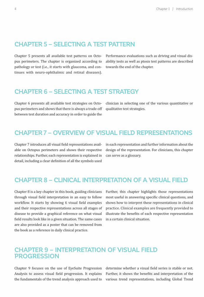
Chapter 5 presents all available test patterns on Octo-pus perimeters. The chapter is organized according to pathology or test (i.e., it starts with glaucoma, and con-tinues with neuro-ophthalmic and retinal diseases).
Performance evaluations such as driving and visual dis-ability tests as well as ptosis test patterns are described towards the end of the chapter.

5Content at a glance
CHAPTER 10 – NON-CONVENTIONAL PERIMETRY
CHAPTER 13 – CLINICAL CASES
CHAPTER 11 – KINETIC PERIMETRY
CHAPTER 12 – TRANSITIONING TO A DIFFERENT PERIMETER MODEL
Chapter 10 focuses on other stimulus types besides the standard Goldmann size III used in perimetry. The chap-ter starts with function-speci ic perimetry designed for early glaucoma detection and provides background in-
To support the interpretation of visual ield results in clinical practice, 23 clinical cases are presented, show-ing typical visual ields of patients with glaucoma, neu-ro-ophthalmic disease and retinal disease. All these cases
Chapter 11 focuses on kinetic perimetry. Similar to the static perimetry chapter, the basic examination parame-ters and when to choose each one are discussed. Gener-al approaches on how to perform kinetic perimetry are
Chapter 12 focuses on speci ic challenges associated with transitioning from one perimeter model to another. It focuses both on the transition to a different Octopus model, as well as the transition from a Humphrey to an Octopus model. It highlights the importance of normative databases for minimizing the differences between pe-
formation about Pulsar, SWAP and Flicker perimetry. The chapter then concludes with the bene its of using a larger stimulus V for low-vision patients.
contain key patient information, as well as visual ield results and other relevant diagnostic results such as IOP, fundus images, OCT scans and MRIs.
presented and illustrated in a real clinical case. Towards the end, the bene its of different levels of automation are also discussed.
rimeter models and shows the impact of patient-related luctuation. To support a smooth transition from an HFA
perimeter to an Octopus perimeter, guidance in relation to known HFA perimeter terminologies is provided on the selection of test parameters as well as the interpreta-tion of the perimetric result.
Analysis, Cluster Trend Analysis and Polar Trend Analy-sis, which not only allow it to be determined whether a visual ield series is progressing and at which rate, but also whether progression is diffuse or local, the area of
the visual ield in which progression is occurring and, in case of glaucoma, where to look for a spatial relationship with structural results.

6

7
CHAPTER 2WHAT IS PERIMETRY?
INTRODUCTION
PERIMETRY – A STANDARD TEST IN OPHTHALMOLOGY
Perimetry is a standard method used in ophthalmol-ogy and optometry to assess a patient’s visual ield. It provides a measure of the patient’s visual function throughout their ield of vision. The devices used to per-form this evaluation are called perimeters. Perimetry is performed for several reasons: 1) detection of pathol-ogies; 2) evaluation of disease status; 3) follow-up of pathologies over time to determine progression or dis-ease stability; 4) determination of ef icacy of treatment and 5) visual ability testing.
Any pathology along the visual pathway usually results in a loss of visual function. Perimetry can identify de-viations from normal, and consequently the associated pathologies. Perimetry is most commonly used to diag-
nose glaucoma, but it is also often used to assess visu-al loss resulting from retinal diseases, as well as optic nerve, chiasmal or post-chiasmal damage due to trauma, stroke, compression and tumors.
Additionally, perimetry is used regularly for visual ability testing. Its most common use is to test a person’s visual ability to drive. Furthermore, it is used to provide a quantitative measure of visual function in order to de-termine eligibility for a pension for visual impairment, and also to assess the bene its of ptosis surgery.
In sum, perimetry is a universally available diagnostic method to assess a patient’s visual ield or visual function.
8
TE
MP
OR
AL
(rig
ht
eye
)
NA
SA
L
(rig
ht
eye
)SUPERIOR
INFERIOR
SUPERIOR
TEMPORAL
(right eye)
NASAL
(right eye)
INFERIOR
Fixation
Fixation
TE
MP
OR
AL
(rig
ht
eye
)
TE
MP
OR
AL
(left
eye
)
SUPERIOR
TEMPORAL
(right eye)
TEMPORAL
(left eye)
INFERIOR
SUPERIOR
INFERIOR
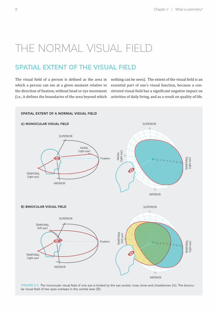
FIGURE 2-1 The monocular visual fi eld of one eye is limited by the eye socket, nose, brow and cheekbones (A). The binocu-
lar visual fi eld of two eyes overlaps in the central area (B).
Chapter 2 | What is perimetry?
SPATIAL EXTENT OF A NORMAL VISUAL FIELD
A) MONOCULAR VISUAL FIELD
B) BINOCULAR VISUAL FIELD
THE NORMAL VISUAL FIELD
SPATIAL EXTENT OF THE VISUAL FIELD
The visual ield of a person is de ined as the area in which a person can see at a given moment relative to the direction of ixation, without head or eye movement (i.e., it de ines the boundaries of the area beyond which
nothing can be seen). The extent of the visual ield is an essential part of one’s visual function, because a con-stricted visual ield has a signi icant negative impact on activities of daily living, and as a result on quality of life.

9
Sensitivity
to light
Light
intensity
Dim lightHigh
Bright lightLow
The normal visual fi eld
SENSITIVITY TO LIGHT
SENSITIVITY TO LIGHT IN THE VISUAL FIELD
The area in which a person can see (extent of the visual ield) does not suf ice to describe a person’s vision. It is
also important to have a measure of sensitivity to light.But what is a person’s sensitivity to light? One can imagine a room in which 100 people are present. The room is dim, with an adjustable light bulb at its lowest
level hanging from the ceiling. In that room, only a few people can see. As the light intensity of the bulb is in-creased, an increasing number of people will be able to see in the room. The people who could see even the very dim light bulb have a very high sensitivity to light, while the others have a lower sensitivity to light (FIG 2-2).
In people with normal vision, the visual ield is binoc-ular (FIG 2-1B). This means that it contains input from both eyes, with integration and mapping of information from the two eyes, allowing for stereo acuity and depth perception. Visual information in the central 60 degrees of the visual ield is processed by both eyes.
The visual ield of one eye is called the monocular visual ield (FIG 2-1A). Its spatial extent in people with normal
vision is limited by the facial anatomy of the person, with the eye socket, nose, brow and cheekbones, which outlines the limits of the visual ield. On average, the monocular visual ield extends from 60° nasally to ap-proximately 90° or more temporally, and from approxi-mately 60° superiorly to 70° inferiorly.
FIGURE 2-2 This fi gure illustrates the inverse relationship between light intensity and sensitivity to light. A person who can
perceive a very dim light has a very high sensitivity to light, while a person who can only perceive very bright lights has low
sensitivity to light.

10
FIGURE 2-3 The hill of vision is a three-dimensional representation of the visual fi eld, with the x- and y-axes showing the
spatial extent of the visual fi eld using radial coordinates, and the z-axis showing sensitivity to light. Its name stems from the
fact that normal sensitivity to light is higher at the center than in the periphery, so that normal vision in this representation
resembles a hill.
Chapter 2 | What is perimetry?
90˚80˚
70˚
SUPERIOR
TE
MP
OR
AL
NA
SA
L
INFERIOR
Blind SpotFixation
Sensitivity
to light
THE HILL OF VISION – A VISUALIZATION OF VISUAL FUNCTION
Sensitivity to light is not uniform across the spatial ex-tent of the visual ield and depends on location within the visual ield. For normal eyes and in typical daytime illumination, sensitivity is highest in the central area of the visual ield and decreases gradually towards the pe-riphery. To visualize this, sensitivities across the visual ield can be drawn as a three-dimensional graph, with
HILL OF VISION
the x- and y-axes representing the visual ield locations and the z-axis representing the sensitivity to light. Since this representation resembles a hill, it is commonly re-ferred to as the hill of vision, which is a visualization of a person’s visual function. Areas within the hill of vision represent areas of seeing, and areas outside the hill of vi-sion represent areas of non-seeing (FIG 2-3).

11Measuring sensitivity to light across the visual fi eld
Normal Hill of Vision
Pathological Hill of Vision
Sensitivity
to light
PERIMETRY ALLOWS QUANTIFICATION OF ABNORMAL SENSITIVITY TO LIGHT
Deviations from the normal hill of vision provide valu-able clues regarding visual ield loss and the underlying pathologies. The pattern and shape of visual loss can be identi ied by investigating deviations from the normal hill of vision. Differences in the visual ield between the two eyes can also be identi ied by inspecting deviations from the normal hill of vision. These deviations from normal
PERIMETRY ALLOWS DETECTION OF ABNORMAL SENSITIVITY TO LIGHT
can be either constrictions of the boundaries of the visual ield, or depressions of sensitivity. Such depressions can
be present throughout the visual ield (widespread low-ering of sensitivity), or localized in speci ic areas of the visual ield (scotomas). It is thus desirable to quantify a patient’s hill of vision with high accuracy and to identify its deviation from a normal hill of vision (FIG 2-4).
MEASURING SENSITIVITY TO LIGHT ACROSS THE VISUAL FIELD
FIGURE 2-4 Pathologies affecting sensitivity to light result in an altered hill of vision for the patient. The deviation from the
normal hill of vision provides valuable information regarding the nature and severity of the pathology.

12 Chapter 2 | What is perimetry?
DimStimulus
No
No
No
Yes
Yes
Yes
Yes
BrightStimulus
Stimulus
Do you seethe stimulus?
Fixation
SE
NS
ITIV
ITY
TH
RE
SH
OLD
= Seen
= Not seen
THE PERIMETRIC TEST
Perimetry accurately quanti ies a patient’s sensitivity to light throughout the visual ield in a systematic, highly standardized manner. To assess the visual ield, a hemi-spheric cupola is typically used to project small light stimuli across the entire area of the visual ield. These stimuli, and the uniform background onto which the stimuli are projected, are highly standardized in terms of shape, size, color, light intensity and duration, to ensure high reproducibility. The most commonly used test con-ditions project a round, white stimulus on a background, which is also white, but dimmer than the stimulus. The luminance (i.e., the re lected light intensity) of the stim-ulus can be altered from very low to very high. More detailed information on key examination parameters is provided in Chapter 4.
To perform a perimetric test, patients are asked to sit in front of the cupola with their head stabilized, to ix-ate onto a target in the center, and to indicate seeing a
stimulus anywhere in their visual ield by pressing a re-sponse button. Conceptually and to simplify things, one can imagine that at the irst location the luminance of the stimulus is increased from the “off” position to the dimmest level of an adjustable light bulb. If the patient cannot see the stimulus when it is off or very dim, anoth-er stimulus is shown later, at a higher level of light inten-sity. Once the stimulus reaches a certain light intensity, the patient can see it and presses the button. It should be noted that the stimulus is always turned off before the next stimulus is presented.
This minimum light intensity that can be seen de ines the patient’s sensitivity to light (i.e., the threshold between non-seeing and seeing) (FIG 2-5). Due to this evaluation method, in perimetry the word threshold is often used, instead of sensitivity to light. For ease of understanding, “sensitivity threshold” is the term used throughout this book.
SENSITIVITY THRESHOLDS
FIGURE 2-5 The sensitivity threshold between seeing and non-seeing for stimuli of different intensity presented against a
fi xed background illumination at a given location in the visual fi eld provides one data point on the hill of vision.

13Measuring sensitivity to light across the visual fi eld
Stimulus
Sensitivity thresholdof first location
Do you seethe stimulus?
Fixation
Sensitivity
threshold
Sensitivity thresholdsat all tested locations
Stimulus
Fixation
Do you see here?
Do you see there?
Sensitivity
threshold
Sensitivity thresholdsat all tested locationsStimulus
Fixation
Do you see here?
Do you see there?
Sensitivity
threshold
The sensitivity threshold at the irst test location provides the irst data point to characterize the hill of vision (FIG
2-6A). To determine the patient’s hill of vision, the afore-mentioned procedure is then repeated at many locations
across the visual field (FIG 2-6B). By connecting the sensitivity thresholds at all tested locations, a patient’s hill of vision can be drawn (FIG 2-6C).
DRAWING THE HILL OF VISION FROM THE SENSITIVITY THRESHOLDS
FIGURE 2-6 The hill of vision can be drawn from the individually determined sensitivity thresholds at each location.
A) SENSITIVITY THRESHOLD OF FIRST LOCATION
B) SENSITIVITY THRESHOLDS AT DIFFERENT LOCATIONS
C) SENSITIVITY THRESHOLDS AT ALL TESTED LOCATIONS

14 Chapter 2 | What is perimetry?
While the process used to determine sensitivity thresh-olds is easy to understand, it would be much too time-con-suming to test each location of the hill of vision in this manner. Therefore, more ef icient strategies are used in
perimetry and they will be discussed in depth in Chapters 4, 5 and 6. Additionally, the order of stimulus presentation is randomized throughout the visual ield, to avoid patients becoming accustomed to a certain presentation pattern.
THE DECIBEL SCALE USED IN PERIMETRY
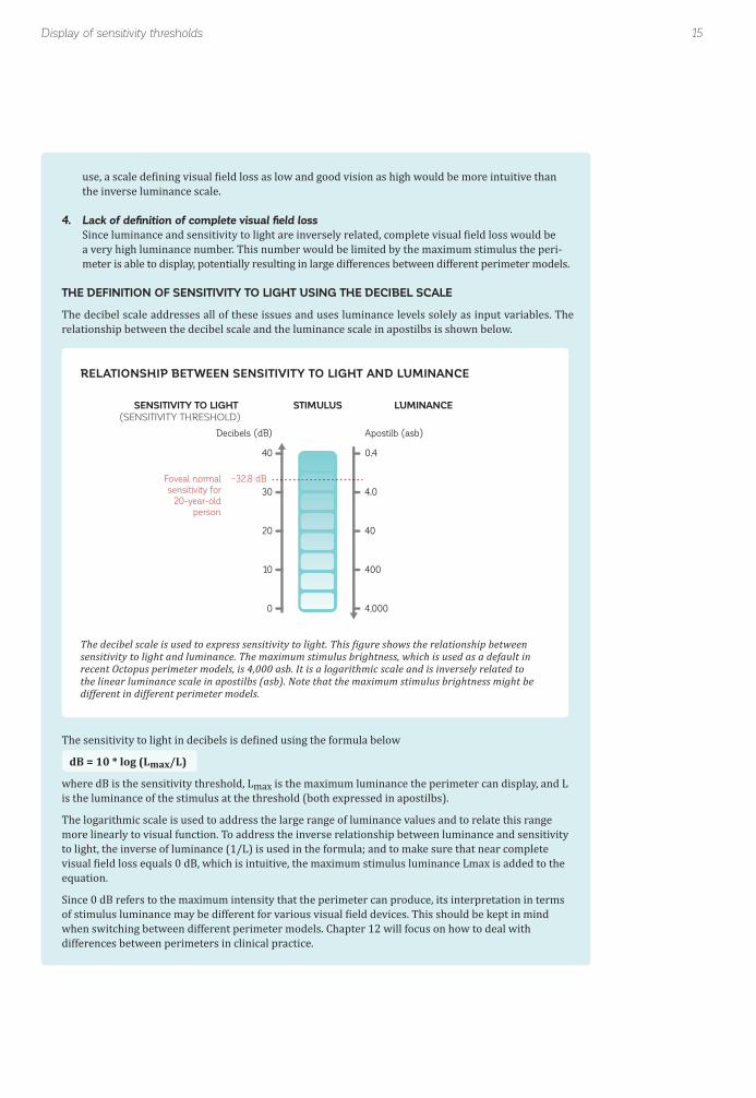
In clinical practice, visual ield information needs to be easy to interpret and should directly correspond to the clinical situation. For that purpose, perimetry employs the decibel scale, with its unit of measurement being the decibel (dB). The decibel range depends on perim-eter type and typically ranges from 0 dB to approxi-mately 32 dB in the fovea. A sensitivity threshold of 0 dB means that a patient is not able to see the most intense
perimetric stimulus that the device can display, whereas values close to 32 dB represent normal foveal vision for a 20-year-old person. While the decibel scale is intuitive to understand and use in clinical practice, the underlying considerations and formulas are less intuitive and of lim-ited relevance for clinical practice. For those interested, they are explained in BOX 2A.
DISPLAY OF SENSITIVITYTHRESHOLDS
THE RATIONALE FOR THE USE OF THE DECIBEL SCALE
The intensity of the light that is re lected on the perimetric surface is called luminance and can be measured objectively with a light meter. It is expressed in candelas per meter squared (cd/m ) or in the older unit, the apostilb (asb), with 1 cd/m corresponding to 3.14 asb. The measurement indicates light lux per unit area.
In theory, sensitivity thresholds could be expressed in luminance units. While this would be correct, it would be impractical in clinical practice for the following reasons:
1. Large number of discrete luminance levels The human eye can adjust to a large range of luminance levels over at least 3-4 orders of magnitude (e.g., from almost 0 asb to 10,000 asb in normal daytime lighting conditions). This would make certain threshold values very large and impractical to display.
2. The relationship between visual function and luminance is not linear Visual function is not linear with regard to the light intensity levels. For example, while an increase of 90 asb is likely to be noticed when luminance is increased from 10 to 100 asb, this same absolute increase in luminance (90 asb) would hardly be noticeable when luminance is increased from 1,000 to 1,090 asb.
3. Inverse relationship between luminance and sensitivity to light There is an inverse relationship between stimulus luminance and a patient’s sensitivity to light. A patient with high sensitivity to light only needs a stimulus with low luminance to be able to see it, while a patient with low sensitivity to light needs a stimulus with high luminance. For clinical
BOX 2A
15Display of sensitivity thresholds
SENSITIVITY TO LIGHT (SENSITIVITY THRESHOLD)
LUMINANCESTIMULUS
40
~32.8 dBFoveal normal
sensitivity for
20-year-old
person
30
20
10
0
Apostilb (asb)Decibels (dB)
0.4
4.0
40
400
4,000
use, a scale de ining visual ield loss as low and good vision as high would be more intuitive than the inverse luminance scale.
4. Lack of defi nition of complete visual fi eld loss Since luminance and sensitivity to light are inversely related, complete visual ield loss would be a very high luminance number. This number would be limited by the maximum stimulus the peri- meter is able to display, potentially resulting in large differences between different perimeter models.
THE DEFINITION OF SENSITIVITY TO LIGHT USING THE DECIBEL SCALE
The decibel scale addresses all of these issues and uses luminance levels solely as input variables. The relationship between the decibel scale and the luminance scale in apostilbs is shown below.
The sensitivity to light in decibels is de ined using the formula below
dB = 10 * log (Lmax/L)
where dB is the sensitivity threshold, Lmax is the maximum luminance the perimeter can display, and L is the luminance of the stimulus at the threshold (both expressed in apostilbs).
The logarithmic scale is used to address the large range of luminance values and to relate this range more linearly to visual function. To address the inverse relationship between luminance and sensitivity to light, the inverse of luminance (1/L) is used in the formula; and to make sure that near complete visual ield loss equals 0 dB, which is intuitive, the maximum stimulus luminance Lmax is added to the equation.
Since 0 dB refers to the maximum intensity that the perimeter can produce, its interpretation in terms of stimulus luminance may be different for various visual ield devices. This should be kept in mind when switching between different perimeter models. Chapter 12 will focus on how to deal with differences between perimeters in clinical practice.
RELATIONSHIP BETWEEN SENSITIVITY TO LIGHT AND LUMINANCE
The decibel scale is used to express sensitivity to light. This igure shows the relationship between sensitivity to light and luminance. The maximum stimulus brightness, which is used as a default in recent Octopus perimeter models, is 4,000 asb. It is a logarithmic scale and is inversely related to the linear luminance scale in apostilbs (asb). Note that the maximum stimulus brightness might be different in different perimeter models.

16 Chapter 2 | What is perimetry?
GRAPHIC DISPLAY OF SENSITIVITY THRESHOLDS
The three-dimensional hill of vision contains large amounts of information. It may therefore be challenging to appropriately display all aspects of a patient’s visual
function from the three-dimensional representation. Cartographers face similar challenges when displaying three-dimensional mountains or hills, and have used
10 30 40 50 60 70 80 90
0m
600m 1200m
2400m
3000m
Numerical altitude map Numerical sensitivity threshold map
Color altitude map Color sensitivity threshold map
Altitude lines map Sensitivity threshold lines map
Values
Grayscale of Values
Kinetic Perimetry
3D map 3D map
0m
0m
0m
0m0m
30 dB30 dB
20 dB
20 dB
20 dB
20 dB
10 dB
10 dB
10 dB
10 dB
10 dB
10 dB
10 dB
600m
600m600m
600m
1200m
1200m
1200m
1200m
1800m
2400m
1800m
1800m
1800m
1800m
2400m3000m
1800m
2400m
2400m3000m3600m
2727
27
28
2527
28
27
25
26
28
2729
30
2829
31
30
28
26
27
2629
29
21 2931
29
31
31
31
30
333131
30
30
323128
26
332928
MOUNTAIN – Geographical display HILL OF VISION – Perimetric display OCTOPUS REPRESENTATIONS
No 3D map availableon Octopus perimeters
GRAPHIC DISPLAY OF SENSITIVITY THRESHOLDS
FIGURE 2-7 As in cartography, there are different ways to display the three-dimensional hill of vision in two dimensions.
Sampled altitude levels can be displayed numerically, a color code can be used to represent different altitude levels, or altitude
lines can show the different altitude levels.

17
90
270
0180
90
270
0180
Ideal Practical Ideal Practical
Challenges in visual fi eld testing and interpretation
two-dimensional maps as a solution. Similar display strategies are used to display the hill of vision in two dimensions.
As in geographical maps (FIG 2-7), the various sensitivity thresholds can be displayed numerically (i.e., by sam-pling certain altitudes to give a feel for the overall shape of the hill or mountain). Color codes for different altitude levels are also often presented on geographical maps. Last but not least, lines of the same altitude level can
provide a good representation of a hill on a map. For perimetry, these lines of equal altitude are referred to as isopters (lines of equal sensitivity).
It should be noted that whichever display form is used, there is always some information lost. All three versions are used to display perimetric results, as each emphasizes different clinical information. For more details of the various representations, see Chapters 7, 8, and 11.
PERIMETRIC TESTING HAS LOW RESOLUTION
So far, this book has presented perimetry as a very accu-rate way of continuously showing the stimuli of increasing intensity for the patient. It has also been assumed that thresholding is performed at all locations across the visual ield.
From a practical point of view, however, it is nearly impossible to test each location within the visual ield (spatial resolution) using each possible light intensity (luminance resolution). This would take too long to be useful in a clinical setting. Therefore, referring back to
CHALLENGES IN VISUAL FIELD TESTING AND INTERPRETATION
IDEAL VERSUS PRACTICAL PERIMETRIC TESTING
SPATIAL RESOLUTION RESOLUTION OF SENSITIVITY THRESHOLDS
FIGURE 2-8 Ideally, the hill of vision would be drawn from an infi nite number of test locations and from a continuously
changing stimulus luminance. In reality, the time constraints do not allow for this kind of testing, and only sampling at some
locations and some luminance levels is possible.

18
20-year-old
Sensitivity
threshold
85-year-old
Chapter 2 | What is perimetry?
the example of the light bulb in a room, the dimmer only has a set number of discrete levels, such as high, medi-um and low, and there are only a few bulbs to illuminate the room (FIG 2-8).
For perimetry, this means that stimuli are presented at a ixed number of key locations and that only a limited num-
ber of light intensity levels are presented. This approach introduces inaccuracies in the perimetric test. In order to still be able to receive the information necessary for good clinical decision-making, a number of elaborate process-es are used in perimetry. This maximizes clinical infor-mation and offers a good trade-off between testing time and accuracy. These are described in Chapters 4, 5 and 6.
NORMAL SENSITIVITIES DEPEND ON AGE AND TEST LOCATION
As already illustrated in the section about the hill of vision, normal sensitivity thresholds depend on the test location and are higher at the center than in the pe-riphery. In addition, the normal hill of vision is affected by age. Normal sensitivity to light in decibels decreases approximately linearly with increasing age, beginning at the age of 20.1-3 Thus, the hill of vision of a 20-year-old is typically higher than the hill of vision of an 85-year-old person (FIG 2-9).
For these reasons, sensitivity thresholds are challenging to interpret directly in the clinic, because the representations of normal and abnormal values depend on testing- and patient-speci ic factors. For correct clinical assessment of sensitivity thresholds, a clinician would have to keep normal reference values in mind for all age groups and test locations, in order to correctly interpret the results. That would be a challenging task.
HILL OF VISION IS AGE- AND LOCATION-DEPENDENT
FIGURE 2-9 The normal hill of vision shows the highest sensitivity thresholds at the center, with decreasing sensitivity thresh-
olds towards the periphery. Similarly, there is also a decrease in sensitivity thresholds with increasing age at all test locations.
19
Sensitivity
threshold
Measured Valuesof a 20-year-old
Comparison
Normative Valuesof 20-year-olds
NORMATIVE VALUES (MEASURED) VALUES COMPARISON (TO NORMAL)Normal sensitivity threshold Measured sensitivity threshold Sensitivity loss
- =
Challenges in visual fi eld testing and interpretation
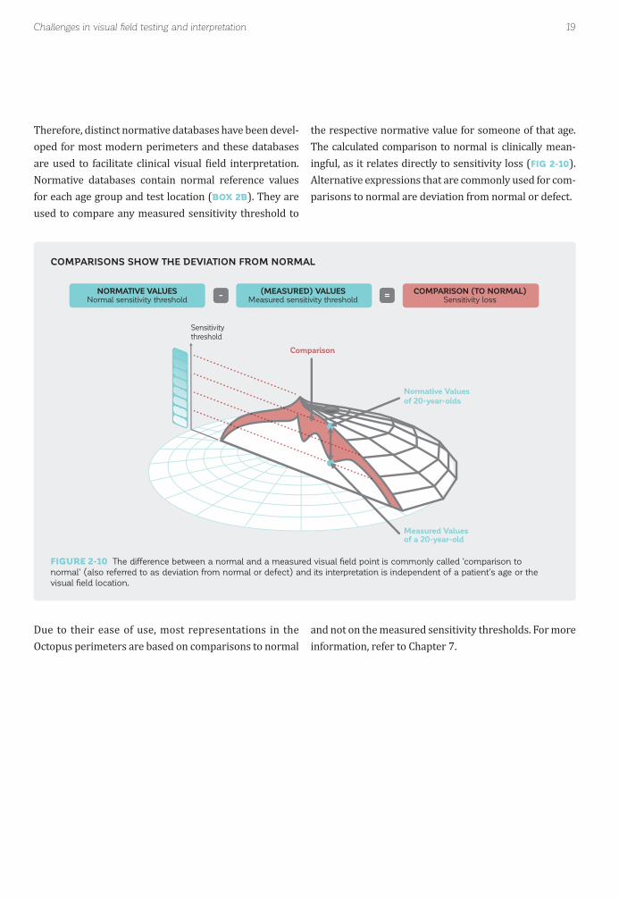
Therefore, distinct normative databases have been devel-oped for most modern perimeters and these databases are used to facilitate clinical visual ield interpretation. Normative databases contain normal reference values for each age group and test location (BOX 2B). They are used to compare any measured sensitivity threshold to
Due to their ease of use, most representations in the Octopus perimeters are based on comparisons to normal
the respective normative value for someone of that age. The calculated comparison to normal is clinically mean-ingful, as it relates directly to sensitivity loss (FIG 2-10). Alternative expressions that are commonly used for com-parisons to normal are deviation from normal or defect.
and not on the measured sensitivity thresholds. For more information, refer to Chapter 7.
COMPARISONS SHOW THE DEVIATION FROM NORMAL
FIGURE 2-10 The difference between a normal and a measured visual fi eld point is commonly called ‘comparison to
normal’ (also referred to as deviation from normal or defect) and its interpretation is independent of a patient’s age or the
visual fi eld location.

20 Chapter 2 | What is perimetry?
NORMATIVE DATABASES IN OCTOPUS PERIMETERS
DESIGN OF A NORMATIVE DATABASE
By de inition, the normative database of a perimeter consists of a pool of visual ield data from people with normal vision in all age groups. The challenge associated with generating this pool is to ensure that these normal visual ields are truly normal and that there are suf icient visual ields to account for individual differences.
The standards to be ful illed for a perimetric normative database are described exhaustively in the ISO norm «Ophthalmic instruments - Perimeters (ISO 12866:1999/Amd1:2008); Amendment A1, Appendix C». All normative databases of Octopus perimeters comply fully with these standards. The typical process to comply with the standards is to perform a clinical study that includes a thorough eye examination and repeated visual ield testing.
DISTINCT NORMATIVE DATABASES FOR DIFFERENT DEVICES AND EXAMINATION PARAMETERS
Since particular perimeter models vary in design and might use different examination parameters, a stimulus of the same light intensity may be perceived differently on various perimeter models. Therefore, there are distinct normative databases for different perimeter types and settings.
PERIMETRY HAS OBJECTIVE AND SUBJECTIVE COMPONENTS
NORMAL FLUCTUATION DEPENDS ON TEST LOCATIONS AND DISEASE SEVERITY
In the interest of simplicity, perimetry has been treated as a purely objective procedure, with exact measurements and distinct sensitivity thresholds at each test location. This is true for the equipment and the test conditions. However, there is a subjective element to perimetry, due to the subjectivity of the patients undergoing the test. As a result, there is always a certain amount of normal luctuation both among different normal individuals, as
well as between different measurements of the same individual over a short period of time. The accuracy of the test results is highly dependent on several factors, including the cooperation of the patients, their cognitive and physical abilities, and their decision criteria.4-6 If the
A further complication in visual ield interpretation is the fact that normal luctuation is not uniformly distributed across the visual ield (FIG 2-11). Instead, normal luctua-
patient does not understand the test, does not pay atten-tion or does not focus continuously on the central target, then the results of the test will be dif icult to interpret. Additionally, some patients may be very conservative in their judgements, requiring a more intense stimulus for detection, while other patients may be liberal and accept a less intense stimulus for detection. The most important person to maximize the performance of the patients is the visual ield examiner (e.g., a perimetrist or technician). Chapter 3 focuses on potential sources of unreliable and thereby highly luctuating visual ields and provides prac-tical guidance on how to minimize these factors.
tion is smaller at the center of the visual ield than in the periphery and is also smaller in areas of good vision than in areas of poor vision.1,7
BOX 2B

21Challenges in visual fi eld testing and interpretation
Average Hill of Vision
Normal fluctuation
Sensitivity
threshold
Abnormal
THE FREQUENCY-OF-SEEING (FOS) CURVE
Due to luctuation, distinct sensitivity thresholds at a given test location cannot be measured precisely. In reality, the same patient always shows slightly varying responses in repetitive testing. In other words, the likelihood of seeing or not seeing a stimulus is probabilistic.
As the luminance (i.e., the light intensity of the stimulus) increases, there is a gradual increase from “unseen” to “seen” responses, so that the probability that a patient will perceive a stimulus changes gradually from 0% to 100%. Because of this, sensitivity thresholds are de ined as the stimulus luminance that is perceived with a probability of 50%.
To get a measure of luctuation, one can show a stimulus of a certain luminance to a patient many times at a given test location and determine how often the patient is able to see it. The probability of perceiving a stimulus can be mapped in a graph as a function of stimulus luminance. When doing this for many dif-ferent luminance levels, one can generate a frequency-of-seeing (FOS) curve, which describes the prob-ability that a patient will perceive a target as a function of stimulus luminance. This is a useful tool to illustrate the variability associated with the determination of thresholds.⁸ In areas of normal sensitivity, the FOS curve is typically steep, indicating that there is less variability. In other words, the patient has a high probability of seeing stimuli that are slightly more intense than the luminance at the threshold, and also a high probability of not seeing stimuli that are slightly less intense than those at the threshold. This is illustrated on the left side of the igure by the steep shape of the FOS curve.
In areas where defects are present, the FOS curve is typically shallow, indicating that there is greater variability. In other words, there is a gradual change in the probability of detecting stimuli that are higher and lower than the luminance at threshold. This is illustrated on the right side of the igure by the shallow shape of the FOS curve.
These two factors must be kept in mind when making clinical decisions based on visual ield results. To objectively
measure luctuation around a sensitivity threshold, the frequency-of-seeing (FOS) curve may be used (BOX 2C).
NORMAL FLUCTUATION IN PERIMETRY
FIGURE 2-11 Since perimetry contains a subjective, patient-related component, there is always normal fl uctuation. Its magnitude
depends on both the test location and disease severity.
BOX 2C

22 Chapter 2 | What is perimetry?
Fluctuation Fluctuation
Normalsensitivitythreshold
Pro
ba
bili
ty o
f se
ein
g th
e s
tim
ulu
s
0%
Dim stimulus Bright stimulus
50%
100%
Abnormalsensitivitythreshold
FREQUENCY-OF-SEEING (FOS) CURVE
The frequency-of-seeing curve provides the scienti ic de inition of a light sensitivity threshold while taking luctuation into account. It shows the probability of a patient perceiving a certain stimulus luminance. The light sensitivity threshold is de ined as the stimulus luminance that the patient can see 50% of the time. Fluctuation is quanti ied as the range of luminance at which the probability of seeing the stimulus is 0% to the luminance at which the probability of seeing the stimulus is 100%.
CLINICAL STANDARD FOR VISUAL FUNCTION TESTING
Even though perimetry has low resolution and contains subjective, patient-related components resulting in normal luctuation, perimetric testing is useful to assess visual ields in clinical practice. It remains highly important be-
cause visual ield function is most directly related to a patient’s quality of life and ability to perform activities of
daily living, which are the most important factors for the patient. Additionally, slowly progressing diseases such as glaucoma can be followed accurately through all stages of the disease. Perimetry is therefore an indispensable tool for every glaucoma specialist.

23References
REFERENCES1. Zulauf M. Normal visual ields measured with Octopus Program G1. I. Differential light sensitivity at individual test locations. Graefes Arch Clin Exp Ophthalmol. 1994;232:509-515.2. Zulauf M, LeBlanc RP, Flammer J. Normal visual ields measured with Octopus-Program G1. II. Global visual ield indices. Graefes Arch Clin Exp Ophthalmol. 1994;232:516-522.3. Haas A, Flammer J, Schneider U. In luence of age on the visual ields of normal subjects. Am J Ophthalmol. 1986;101: 199-203.4. Flammer J, Drance SM, Fankhauser F, Augustiny L. Differential light threshold in automated static perimetry. Factors in luencing short-term luctuation. Arch Ophthalmol. 1984;102:876-879.5. Flammer J, Niesel P. Reproducibility of perimetric study results. Klin Monbl Augenheilkd. 1984;184:374-376.6. Stewart WC, Hunt HH. Threshold variation in automated perimetry. Surv Ophthalmol. 1993;37:353-361.7. Wall M, Woodward KR, Doyle CK, Artes PH. Repeatability of automated perimetry: a comparison between standard automated perimetry with stimulus size III and V, matrix, and motion perimetry. Invest Ophthalmol Vis Sci. 2009;50: 974-979.8. Chauhan BC, Tompkins JD, LeBlanc RP, McCormick TA. Characteristics of frequency-of-seeing curves in normal subjects, patients with suspected glaucoma, and patients with glaucoma. Invest Ophthalmol Vis Sci. 1993;34:3534-3540.

24

25
CHAPTER 3HOW TO PERFORM PERIMETRY YOU CAN TRUST
INTRODUCTION
PERIMETRY – A SUBJECTIVE TEST
Perimetry is an elaborate test that depends, to a great extent, on subjective factors such as the patient’s cooper-ation and comfort, as well as on using the correct patient information and set-up. Due to this subjective compo-nent, untrustworthy visual ield tests are common. The extent of untrustworthy results largely depends on how well perimetry is performed in clinical practice and has been reported to range from 3% to 29% of all visual ield tests performed.¹-⁵
In view of the relatively high occurrence of untrust-worthy visual ields, it is extremely important to make sure that the time invested in perimetry is well spent, because poorly performed perimetric tests have hardly any diagnostic value. It therefore pays to take the time and care necessary to obtain trustworthy results by fol-lowing certain rules to avoid the most common pitfalls.

26
Provide clear in
stru
ctio
ns
focus on perimetry
Co
llabo
rate
with the tes
ting
procedure
Provide enco
ura
gem
en
t
Allow necessary time to
Be m
otivate
d to p
erfo
rm th
e test
throughout th
e te
st
imp
ort
ance
of pe
rimetry
Provide recognition and appreciation
Provide su
perv
isio
n
Provide adequate training
Ask q
uest
ions
about
PA
TIE
NT
DOCTOREXAMINER
Em
ph
asiz
e t
he im
port
ance
of t
he test
Ask q
uestio
ns
Accuracy in entering data
Express need
for a
bre
ak
Make notes about patient performance
Perform perimetric test well
FIGURE 3-1 In perimetry, it is essential that doctors, examiners and patients have a positive attitude towards perimetry and that
each member of the team contributes to achieving optimum results.
Chapter 3 | How to perform perimetry you can trust
PERIMETRY – NEED FOR A TEAM APPROACH
THE IMPORTANT ROLE OF THE DOCTOR
Three key players are involved in perimetry: the patient, the examiner and the eye doctor. All three should work collaboratively to obtain optimal perimetric test results.
Patients who understand why perimetry is needed and its importance to their eye care are likely to be more moti-vated to undergo a perimetric test. Due to the relationship
FIG 3-1 shows how each member of the team can contrib-ute. When this approach is successfully implemented, perimetry can be performed in a positive atmosphere.
and trust they establish with their patients, doctors are in the best position to convey the importance of perimetry to their patients.
THE DOCTOR-PATIENT RELATIONSHIP
PERIMETRY REQUIRES A TEAM APPROACH

27Introduction
THE IMPORTANT ROLE OF THE VISUAL FIELD EXAMINER
The visual ield examiner is in a unique position to have an impact on the quality of the perimetric results in two ways. Not only are examiners responsible for correctly
Eye doctors should also clearly convey the importance of perimetry to the visual ield examiners who work with them in the clinic. For example, the doctor is responsible for ensuring that the visual ield examiners understand the importance of trustworthy perimetric results to the clinical decision-making process. The visual ield examin-ers should know that the doctor has a genuine interest in building their perimetric knowledge and skills. Towards
The visual ield examiner is responsible for entering the correct patient information in the perimeter. This is crucial because this information has a direct impact on whether the results of the test can be trusted. Diligence
A crucial role of the visual ield examiner is to ensure that the patients perform perimetry to the very best of their capacity each time they take a test. To give their best performance, patients need to be comfortably positioned at the perimeter, they need to know what is expected of them, and they need to understand how to perform the test. A competent examiner will ensure that the patient is not only correctly positioned, but also comfortable. Similarly, a good examiner will convey what is expected of the patient and will give clear instructions on how to perform the test. The examiner can also provide brief rest periods by pausing the test if this will be helpful to the
setting up the perimeter, they also directly oversee the patient during the test.
this goal, the doctor must provide training and give feed-back to the examiners. It is also crucial for the doctor to have reasonable expectations in terms of the time required to perform trustworthy perimetric tests. Doctors should arrange for their visual ield examiners to be able to dedi-cate time exclusively to performing perimetric tests. This means that they should be free of other tasks that might reduce the examiner’s focus on the patient.
in performing this aspect of perimetry can significantly reduce the number of untrustworthy tests and inter-pretation errors. The examiner is also responsible for ensuring that an adequate refractive lens is used.
patient. Additionally, the patient should be encouraged to communicate to the examiner any dif iculties or prob-lems encountered, and when a brief rest period would be bene icial.
There is more, however, to the role of a visual ield exam-iner. Outstanding examiners will have taken perimetric tests themselves and will understand how the patient feels during the test. This compassionate approach will go a long way in ensuring patient cooperation and will allow the examiner to give genuine encouragement to the patient when needed during the test.
THE DOCTOR-EXAMINER RELATIONSHIP
ROLE IN CORRECTLY SETTING UP THE PERIMETER
THE EXAMINER-PATIENT RELATIONSHIP

28
Noise
Light Heat
Cold
FIGURE 3-2 A perimeter should be set up in a distraction-free, dimly-lit environment.
Chapter 3 | How to perform perimetry you can trust
HOW TO PERFORMVISUAL FIELD TESTING
SETTING UP THE PERIMETER
Perimetry should be performed in a distraction-free environment, to enable the patient to concentrate on the perimetric test (FIG 3-2). The room should be quiet, with no activity distracting the patient, and should be at a comfortable room temperature. The cupola should be kept clean and free of dust and particles. Additionally, the room should be dimly lit, to prevent stray light from in-luencing the perimetric result. A dimly-lit environment
is essential when a cupola perimeter, such as the Octopus 900 is used, but is also helpful for non-cupola perimeters.
Ideally, perimetry should be performed in a room dedi-cated solely to this purpose. However, if the layout of the clinical practice does not offer a stand-alone perimetry
PERIMETER SET UP
room, opaque curtains around the perimeter and earmuffs offer a cost-effective alternative.
The perimeter is automatically calibrated each time it is turned on. It is important for the calibration to take place in the same lighting conditions as those used during peri-metric testing. Calibration can take up to two minutes and should be performed prior to testing patients. Thus, the perimeter should be turned on prior to the patient visit.
Ideally, patient data (date of birth, refraction, etc.) are entered before the patient enters the room. If an electronic medical record system is in use, it will automatically pop-ulate the information to the perimeter.

29
30°
180° 0°
150° 30°
120° 60°
90°
FIGURE 3-3 Placement of a cylindrical lens for a patient with a cylindrical correction of 30°, seen from the examiner’s perspective.
How to perform visual fi eld testing
PLACEMENT OF CYLINDRICAL TRIAL LENSES
INSTRUCTING THE PATIENT
PLACING AN ADEQUATE TRIAL LENS
Due to the subjective components involved in perimetry, careful patient instruction is fundamental to achieving trustworthy results. Patients will be able to cooperate more effectively and produce more consistent results if they understand what is expected of them and why the test is being performed.
The visual ield examiner should therefore take the time to explain the aim of the test, what the patient should ex-pect to see, and what the patient is expected to do (FIG
3-4). It can be helpful for examiners to take a perimetry test themselves, in order to gain a better understanding of what patients are experiencing.
It is fundamental to ensure that the patients know that they are not expected to see all stimuli and that some-times no stimuli are presented. This will help to reduce some of the potential anxiety experienced by patients, who should also know that they can pause the test if they experience fatigue or have questions.
The trial lens calculator is helpful in determining the adequate spherical and cylindrical trial lenses, based on the patient’s current refraction and age. It is vital to en-sure that the patient’s refractive data is up-to-date and it is best practice to determine this prior to each test. The correct trial lens should be put into the trial lens holder prior to seating the patient. Trial lenses with a narrow metal rim should be used, to prevent the rim of the trial lens from blocking the patient’s ield of view. If more
than one trial lens is used, the spherical correction should be placed closest to the patient’s eye. Special attention should be given to the orientation of cylindrical lenses, which should be oriented in the angle of the astigmatism
(FIG 3-3).
To con irm that adequate refraction is used, the examiner should position the patient and ask whether the ixation target is clearly visible.

30
1. Perimetry tests your central and peripheral vision.
2. Be relatively still once positioned.
3. Always look straight ahead at the fixation target.
Do not look around the bowl for stimuli.
4. Press the response button whenever you see the stimulus.
a. The stimulus is a flash of light.
b. Only one stimulus is presented at a time.
c. The stimulus might appear anywhere.
d. Some stimuli are very bright, some are very dim,
and sometimes no stimulus is presented.
e. You are not expected to see all stimuli.
f. Do not worry about making mistakes.
5. Blink regularly to avoid discomfort.
a. Don’t worry about missing a point, the device does not
measure while you blink.
6. If you feel uncomfortable or are getting tired
a. Close your eye for a moment, the test will automatically stop.
b. The test will resume once you open your eye.
7. If you have a question
a. Keep the response button pressed; this will pause the test.
FIGURE 3-4 Proper instructions to the patient are essential for the patient to understand their task and consequently to
perform perimetry well. The sequence of instructions listed in this Figure can be used.
Chapter 3 | How to perform perimetry you can trust
STEP-BY-STEP PATIENT INSTRUCTIONS

31
FIGURE 3-5 An eye patch should cover the eye that is not being tested. It should be positioned so as to not obstruct the
patient’s vision in the tested eye.
INCORRECTCord obstructs view of test eye
How to perform visual fi eld testing
CORRECT EYE PATCH POSITION
CORRECT PATIENT POSITION
EYE-PATCH POSITION
SETTING UP AND POSITIONING THE PATIENT
Trustworthy and accurate perimetric results are more likely to be obtained when the patient is comfortable during the test. It is also important to ensure that the pa-
CORRECTUnobstructed view of test eye
Before fully positioning the patient, the eye not being test-ed should be covered with an eye patch that allows the patient to blink freely (FIG 3-5). If the eye patch is main-tained in place with a cord, it is important to ensure that the cord does not obstruct the patient’s ield of view
The patient should be seated in a comfortable position that can be easily maintained throughout the test. A height-adjustable chair with a backrest and, if available, armrests should therefore be used. The perimeter should be placed on a height-adjustable table to ensure that the
tient is correctly positioned and that the non-tested eye is covered. The optimum ways to ensure patient comfort and correct alignment will be discussed in this section.
for the tested eye. If an adhesive eye patch is used, it is important to make sure that it adheres well all around the eye. All eye patches should be translucent, to avoid adaptation to the dark by the untested eye, which would alter the results of subsequent testing of that eye.⁶
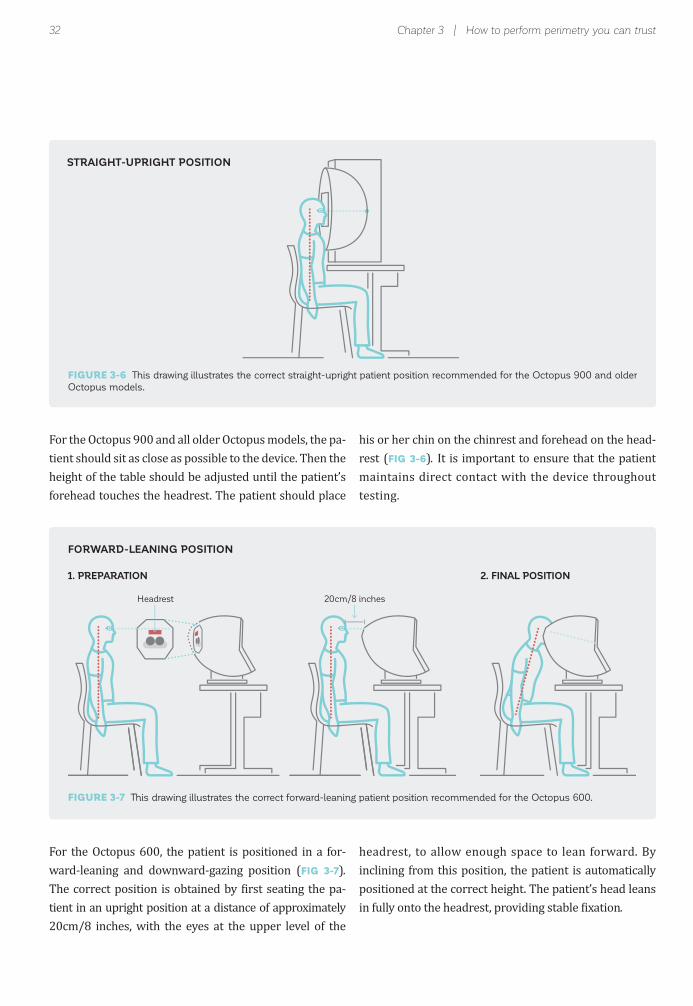
patient is comfortable. Different Octopus models offer different types of positioning: the Octopus 900 offers a straight-upright patient position and the Octopus 600 offers a forward-leaning position.
32
FIGURE 3-6 This drawing illustrates the correct straight-upright patient position recommended for the Octopus 900 and older
Octopus models.
Headrest 20cm/8 inches
STRAIGHT-UPRIGHT POSITION
Chapter 3 | How to perform perimetry you can trust
FORWARD-LEANING POSITION
For the Octopus 900 and all older Octopus models, the pa-tient should sit as close as possible to the device. Then the height of the table should be adjusted until the patient’s forehead touches the headrest. The patient should place
For the Octopus 600, the patient is positioned in a for-ward-leaning and downward-gazing position (FIG 3-7).
The correct position is obtained by irst seating the pa-tient in an upright position at a distance of approximately 20cm/8 inches, with the eyes at the upper level of the
headrest, to allow enough space to lean forward. By inclining from this position, the patient is automatically positioned at the correct height. The patient’s head leans in fully onto the headrest, providing stable ixation.
FIGURE 3-7 This drawing illustrates the correct forward-leaning patient position recommended for the Octopus 600.
1. PREPARATION 2. FINAL POSITION
his or her chin on the chinrest and forehead on the head-rest (FIG 3-6). It is important to ensure that the patient maintains direct contact with the device throughout testing.

33
FIGURE 3-8 The left-hand panel shows an eye in the video monitor that is correctly positioned, with the cross-hair target locat-
ed within the boundaries of the pupil. The right-hand panel shows an eye that is incorrectly positioned, with the cross-hair target
located outside the boundaries of the pupil.
FIGURE 3-9 The patient’s eye should be positioned in the center of the trial lens and as close as possible without touching it.
CORRECTCentral pupil position
CORRECTCentral pupil position
CORRECTTrial lens close to eye
INCORRECT Off-center pupil position
INCORRECTOff-center pupil position
INCORRECTTrial lens too far away
How to perform visual fi eld testing
CORRECT EYE POSITION
CORRECT PUPIL POSITION
CORRECT TRIAL LENS POSITION
Once the patient is correctly positioned in the device, it is important to ensure that the eye is also correctly po-sitioned. Overall, the eye should be well-aligned with the ixation target and should be relatively close to the trial
It is important for the patient’s eye to be as close as pos-sible to the trial lens, in order to avoid the typical “ring” defect (i.e., trial lens rim artifact) that occurs when the
The Octopus perimeters provide a video monitor so that the examiner can see the patient’s eye. When the patient looks straight at the ixation target, the pupil should be aligned with the cross-hair target provided on the video
lens. However, the lens should not touch the eyelashes, allowing the patient to blink freely and avoiding the lens being smeared with make-up.
patient is positioned too far away from the trial lens (FIG
3-9). The eyelashes should not touch the lens, however.
monitor. The patient is correctly positioned when the cross-hair target is within the boundaries of the pupil (FIG 3-8). The position of the pupil can be adjusted by changing the position of the chinrest.

34 Chapter 3 | How to perform perimetry you can trust
10°
CORRECT FIXATION
FIXATION TARGETS
When a visual ield test assesses both the central and the peripheral visual ields, it will be necessary to remove the trial lens for the part of the test that covers the periphery,
It is essential for patients to maintain steady ixation throughout the test. The Octopus perimeters offer three different ixation targets (FIG 3-10) to promote steady ix-ation in as many patients as possible. Most patients will be able to maintain ixation using the standard cross mark ixation target. If patients have dif iculty under-standing where to look when the cross mark ixation target is used, the central point ixation target can be used, provided that the test pattern does not test the central point. For this reason, the central point ixation
in order to avoid trial lens rim artifacts. Also, visual itness to drive is assessed binocularly (both eyes open). In this case, no trial lens should be used.
target is not recommended for the G, M, N and D patterns (see Chapter 5) and for any pattern where the foveal threshold function is turned on.
Finally, some patients with severe visual ield loss in the macula region may not be able to see the standard cross mark ixation target. In these patients, the use of the larger ring target is recommended, to provide an estimate of the location of the ixation target.
FIGURE 3-10 Octopus perimeters offer 3 different fi xation targets. The cross mark target is the default target. The central
point target can be used in test patterns that do not test the central point. The ring target is recommended for patients with
fi xation issues due to severe visual fi eld loss in the macula.
10°
CENTRAL POINTAlternative
(do not use on test patterns with central locations)
RINGFor patients with severevisual fi eld loss in the
macula
CROSS MARKStandard

35How to perform visual fi eld testing
USE OF FIXATION CONTROL
MONITORING THE PATIENT DURING THE EXAMINATION
To ensure good patient cooperation and trustworthy results, it is essential to monitor patients throughout the examination and not leave them unattended and unmon-itored. During the test, it is helpful to encourage patients by telling them that they are doing well and by letting them know how much of the test they have already com-pleted. This will help them to remain attentive and may re-duce anxieties that might negatively in luence the results.
Particular attention should be paid during the irst min-ute of the test, to ensure that patients have understood what they are expected to do during the test. If a patient shows an unusual response (e.g., no response at all, a re-
Loss of ixation is a primary reason for unreliable visual ield results. Therefore, all current Octopus devices have
a built-in Fixation Control for static testing that can track the patient’s pupil at all times and prevent ixation errors. With Fixation Control, the test is stopped automatically if the patient loses ixation (due to blinking, searching for stimuli or head movements) and automatically restarted once proper ixation is regained. Missed stimuli are au-tomatically repeated later during the test. If ixation loss occurs for more than just a few seconds, a warning message will alert the examiner to properly reposition and reinstruct the patient.
Fixation Control consists of several separate control mechanisms, as outlined in FIG 3-11, which can be turned on and off. It is recommended to keep each of the Fixation
sponse even if there is no stimulus, or unsteady ixation), the test should be interrupted and the patient should be reinstructed. If the results seem compromised, it is rec-ommended to start a new test and discard the compro-mised one. It is important to note, however, that patients with impaired vision often do not respond due to their condition and not because they answer unreliably.
If a patient shows inconsistent behavior, the examiner should make a note of this on the examination ile, to com-municate this information to the clinician. The knowledge that the test has reduced reliability may in luence the interpretation of the test.
Control mechanisms active. However, since some patients might not be able to maintain steady ixation for patholog-ical reasons (i.e., reduced central vision, unsteady pupil or nystagmus), individual mechanisms within Fixation Con-trol can be turned off individually, to make patient testing possible. If it is necessary to turn off some mechanisms, careful patient monitoring is key and it is good practice to make a note in the patient ile about the patient’s ability to maintain ixation. The clinician should then interpret the results in the light of this information and should consider that the test might have reduced reliability.
FIG 3-11 provides more information about the different control mechanisms of Octopus Fixation Control. Note that the con iguration depends on the Octopus model.

36 Chapter 3 | How to perform perimetry you can trust
BLINK CONTROL
FIXATION CONTROL PREVENTS FIXATION LOSSES
PUPIL POSITION CONTROL
DART CONTROL
AUTOMATED EYE TRACKING (AET)
CONTACT CONTROL
RUNNING
RUNNING
RUNNING
RUNNING
RUNNING
PAUSED
PAUSED
PAUSED
ADJUSTING POSITION
PAUSED
Prevents fi xation loss due to blinking.
• Detects eye closure due to blinking or falling asleep
• Testing occurs only if the patient’s eye is open
• Allows the patient to blink normally
• Prevents dry eyes
• Increases patient comfort
• Ensures that no stimuli are missed due to blinking
Prevents fi xation losses due to incorrect pupil position.
• Detects off-centered pupils due to incorrect fi xation or head
movement
• Testing occurs only if the pupil is correctly centered
• Ensures correct gaze direction
Prevents fi xation loss due to rapid eye movement.
• Detects rapid eye movement when the patient is searching
for stimuli
• Testing occurs only if the pupil is steadily fi xating
• Ensures correct gaze direction
Automatically adjusts the patient’s eye position.
• Moves the headrest and chinrest to keep the eye in the center
of the trial lens
• Maintains optimum position even if the patient is moving
around slightly
• Reduces trial lens rim artifacts due to off-centered eye
position
Prevents loss of contact with the perimeter.
• Detects contact with the headrest or chinrest
• Testing occurs only if the head is in contact with the device
• Ensures that the head remains close enough to the device to
minimize lens rim artifact
FIGURE 3-11 Fixation control prevents fi xation losses by automatically pausing the test during blinks, loss of contact with
the device, off-centered pupils and rapid eye movements. The test is automatically restarted once optimum conditions are
achieved. Further, Automated Eye Tracking automatically centers the pupil. Note that not all mechanisms are available on the
different Octopus perimeter models.

37Common pitfalls to avoid
INCONSISTENT PATIENT BEHAVIOR
COMMON PITFALLS TO AVOID
There are many factors that can lead to visual ield tests that cannot be trusted. By paying attention to and man-aging these factors, a well-trained examiner will have a substantial positive in luence on the quality of the visual ield results and on the subsequent clinical decisions.
Therefore, this section is dedicated to the most common pitfalls in perimetry and provides guidance on how to avoid them.
Patient behavior (i.e., lack of patient cooperation), errors
in the set-up procedure, and external obstructions block-ing the stimuli from reaching the retina, are all commonly occurring sources of untrustworthy visual ield results. Many of these pitfalls can be avoided by paying close at-tention to the set-up procedure, by observing the patient carefully during testing, and by making adjustments or repeating instructions if necessary, which is the focus of this section. Chapters 7 and 8 provide information on how to detect visual ield results that cannot be trusted after the test is completed.
LEARNING OR PRACTICE EFFECT
When taking their irst tests, patients often do not fully understand the nature of the test and hesitate to press the button when seeing faint stimuli near the sensitivity threshold. This translates into visual ield results that are worse than the patient’s true visual ield, as illustrated in
FIG 3-12. In subsequent testing, the patients then perform better and their visual ield results resemble their true
visual function more closely.
While learning and practice effects most often occur for patients taking their irst visual ield examination, they can also occur when switching from one perimeter to another, due to small differences in the design (see Chapter 12).
EXAMPLE OF A LEARNING EFFECT
FIGURE 3-12 Example of a patient with normal vision with a strong learning or practice effect from the fi rst to third visual
fi eld tests. The fourth and fi fth tests represent the true visual fi eld of the patient.
1st Test 2nd Test 3rd Test 4th Test 5th Test
LEARNING EFFECT NO LEARNING EFFECT

38 Chapter 3 | How to perform perimetry you can trust
While learning or practice effects cannot always be prevented, their frequency can be reduced by careful pa-tient instruction and observation. Running a practice test prior to real testing is a good procedure if time allows. Careful observation during the irst minute of the test is
also helpful. If a patient does not understand the task of performing perimetry, the patient will often be hesitant during the irst part of the test, or will not press the re-sponse button at all. If this is observed, it is recommended to interrupt the test and reinstruct the patient.
FATIGUE EFFECT
Visual ield tests require alertness and attention. When patients become tired, their attention level may decrease and their answers may become less consistent, resulting in a visual ield that is worse than the patient’s true visual ield (FIG 3-13).⁷-¹¹
To reduce fatigue effects for patients who have dif iculty concentrating for long periods of time, it may be appro-priate to use tests that are shorter in duration, despite the associated loss of accuracy. This may generate more meaningful visual ield results by reducing the unreliabil-ity due to the fatigue effect. Individual differences exist in how quickly patients experience fatigue, and this should be considered when selecting a test.
To further reduce fatigue effects, patients should be ad-
vised to blink regularly to avoid dry eyes and discomfort, given that Fixation Control is active. Arti icial tear drops prior to the test may also reduce fatigue effects due to dry eyes. Additionally, patients should be encouraged to take brief rests, by closing their eyes to relax, if they feel that they are getting tired. Usually, this adds only a few seconds to the test duration, but signi icantly improves the reliability of the results. Furthermore, using a beep-ing sound upon each stimulus presentation may help the patients to concentrate better on the test. BOX 3A pro-vides more information about the advantages and disad-vantages of this option.
Sometimes fatigue is noticeable as drooping eyelids. In such cases, it is best to actively interrupt the test for a while and to allow the patient to rest before continuing testing.
INFLUENCE OF FATIGUE EFFECT ON VISUAL FIELD
FIGURE 3-13 Example of a patient tested on the same day and eye within 15 minutes. Note the signifi cant worsening of the
visual fi eld in the second test, due to fatigue.
NO FATIGUE EFFECT9:30 am
FATIGUE EFFECT9:45 am

39Common pitfalls to avoid
BOX 3A
LOSS OF FIXATION
If a patient does not consistently ixate on the central tar-get, the test will lose its reference point and it will not be possible to identify the location of abnormal visual ield points (FIG 3-14). This is called ixation loss and is one of the most common sources of unreliable ields.¹² It occurs especially if the patient is insecure about his or her per-formance and starts looking around, searching for stimuli. To avoid ixation losses, it is therefore crucial to explain carefully to the patient that it is perfectly normal not to be able to see all of the stimuli.
The Octopus Fixation Control should be enabled when-ever possible, to avoid unreliable visual ields due to ixa-tion losses. It should only be turned to a lower setting or completely turned off if a patient is not able to maintain steady ixation, for pathological reasons (i.e., reduced central vision, unsteady pupil or nystagmus). Direct ob-servation of the patient’s ixation behavior early in the test can also be helpful in this regard.
INFLUENCE OF LOSS OF FIXATION ON VISUAL FIELD
FIGURE 3-14 If there is a loss of fi xation, visual fi eld defects will not be in their exact location, but will either be shifted
together with the fi xation or masked. In the above example, loss of fi xation took place during the entire test. In practice, loss of
fi xation is typically brief, resulting in more random defect patterns.
Do you see?
CORRECT FIXATIONReal defect is detected
FixationTarget& PatientFixation
LOSS OF FIXATIONReal defect is missed and/or artifactual defect is identified
Do you see?
FixationTarget
PatientFixation
Loss of Fixation
ADVANTAGES AND DISADVANTAGES OF USING SOUNDS UPON STIMULUSPRESENTATION
A beeping sound upon stimulus presentation may be helpful for some patients, to maintain their atten-tion during the perimetric test, because it provides them with a steady rhythm to follow. Additionally, it provides reassurance to the patient that the test is running and everything is working normally.
However, the beeping sound may also encourage patients to press the response button even though they cannot see a stimulus. This may increase false answers, resulting in unreliable visual ields. In addition, if more than one perimeter is in a room, the beeping sound of neighboring machines may be distracting.
By default, it is thus recommended to turn the beeping sound off and to only use it for selected patients that have dif iculties with maintaining concentration throughout the test.

40 Chapter 3 | How to perform perimetry you can trust
MISTAKES IN THE SET-UP PROCEDURE
LACK OF PATIENT ATTENTION
ACCURATE ENTRY OF PATIENT INFORMATION
TRIGGER-HAPPY PATIENTS
INADEQUATE CORRECTION OF REFRACTIVE ERROR
Visual field tests require the patient’s full attention. Distractions such as noise can negatively in luence the patient’s test performance. In addition, some patients experience anxiety when performing visual ield tests, due to fear that they are not performing well, or anxiety about the outcome.
Patient data, such as date of birth and refraction, need to be entered in the perimeter. It is important to ensure that this information is accurate. For example, if the wrong date of birth is entered, most representations of the visual ield test will be inaccurate, because each set of
Some patients, consciously or unconsciously, want to positively in luence the result of the visual ield test (e.g., if their ability to drive is at stake, or if they fear a bad diag-nosis). These patients may be trigger-happy, pressing the response button even if they do not see a stimulus. False positive trials where no stimuli are presented are used to detect trigger-happy patients (for more details, see Chapter 7). It is important to watch for false positive
Inadequate correction of refractive error can lead to a blurring of the stimulus. If the patient does not have a sharp image of the stimulus, the visual ield results will be worse than the patient’s true visual ield. Additionally, a lens with too much plus power can lead to an arti icially enlarged visual ield, while a lens with too much minus power will have the opposite effect.
The irst source of error is that the patient has been in-correctly refracted, or that the examiner uses the wrong
Soothing and encouraging words from the visual ield technician can strongly reduce these anxieties and in-crease the reliability of the results. Distractions should also be reduced to a minimum. If the clinic layout does not offer a stand-alone perimetry room, light-dimming curtains around the perimeter and ear muffs can offer a cost-effective alternative.
measured sensitivities is compared to the data for an average normal person of the same age, rather than an average normal person who is younger or older. FIG 3-15
illustrates the in luence of incorrect patient age on the patient’s visual ield.
answers carefully during the examination. If a patient responds to more than one false positive stimulus during the test, it will be helpful to interrupt the test immediately and reinstruct the patient, in order to avoid an unreliable result. Note that a beeping sound upon stimulus presen-tation may encourage trigger-happy patients to press the response button and it is thus recommended not to use this, except in speci ic situations.
refraction for a patient. To avoid this, it is recommended to check the refraction on the same day as the perimetric test. Even if the patient’s refraction has been checked previously, it is possible that it may have changed since then, especially among older patients.
The second source of error is the incorrect choice of trial lens. It is important to consult the user manual for the respective perimeter, as the choice of trial lens depends on the perimeter model. The paragraphs below describe

41Common pitfalls to avoid
BOX 3B
CORRECT AGE58 years
INCORRECT AGEToo old: 88 years
INCORRECT AGEToo young: 18 years
INFLUENCE OF INCORRECT PATIENT AGE ON VISUAL FIELD RESULTS
A B C
FIGURE 3-15 If the date of birth of a 58-year-old patient (A) is incorrectly entered, so that the patient’s age is 88 in the
perimeter, the results will be artifi cially good (B). If the same patient is entered as an 18-year-old patient, the results will be
artifi cially bad (C).
the choice of trial lens for the current Octopus models 900 and 600.
Patients need their far-distance correction for relaxed vision. Depending on age, an added near-distance correc-tion for presbyopia is also needed, because perimeters test at near distances. It is important to use the adequate correction for presbyopia proposed by the perimeter’s manufacturer, and not the patient’s reading glass pre-scription. Special attention should be given to noting the sign (plus or minus) of the correction. If a minus lens is employed when a plus lens should have been used, the patient’s vision may become blurry.
To save time and avoid mistakes, it is recommended to al-ways use the built-in trial lens calculator to determine the required refractive lens. The trial lens calculator always uses the patient’s actual best far-distance correction. It then automatically calculates the necessary age-dependent near-distance correction. It determines and recommends the trial lens with the lowest possible power, in order to minimize the risk of artifacts. BOX 3B presents the under-lying assumptions of the trial lens calculator.
It is best practice to ask each patient prior to starting the test whether they can see the ixation target sharply and, if necessary, adjust the refraction so as to avoid inadequate correction of the refractive error.
RATIONALE USED IN THE DESIGN OF THE TRIAL LENS CALCULATOR
DETERMINATION OF APPROPRIATE SPHERICAL LENS
The current Octopus perimeter models 600 and 900 present stimuli at a distance of 30 cm (11.8 inches) from the eye. This corresponds to an approximate refraction of + 3.25 diopters (D), as calculated using the following formula:
Power (D) = 1/stimulus distance (m) = 1/0.3 = 3.33
To enable the patient to focus at this distance, the patient’s far-distance refraction values are needed. Depending on the patient’s refraction, different scenarios occur:

42 Chapter 3 | How to perform perimetry you can trust
Normal sighted patients:
Young emmetropic patients can accommodate at 30cm, so they do not need an additional trial lens. With increasing age, patients gradually lose their ability to accommodate their eyes (i.e., to change their lens power) to objects presented at near distances. To facilitate near optical correction, additional diop-ters (D) of refractive power are needed depending of the age of the patient (see table below).
Hyperopic and presbyopic patients:
Hyperopic patient may have dif iculty to focus at 30 cm. For these patients, a trial lens is needed, corre-sponding to their refraction (R). As with emmetropic patients who are older, additional diopters (D) are needed to support their near optical correction (presbyopia) (see table below).
Myopic patients:
Near sighted patients of up to -3 D do not necessarily need corrective lenses, as they can focus at 30 cm. Patients with strong myopia (greater than -3 D) will have dif iculty focusing at 30 cm and need additional correction. For refractive values above -3 D, add 3.25 D to the refractive value (e.g., for R = -4 D; use a -0.75 D lens). As for presbyopic and emmetropic patients, with increasing age, near optical correction is more dif icult and additional diopters are needed.
Corrections in the cupola perimeter of Octopus 900
Cupola perimeters allow for full- ield peripheral testing that extends beyond the range of a trial lens. Therefore, all lenses and the lens holder must be removable to allow for peripheral testing. No trial lens should be used for testing beyond 30° eccentricity. The Octopus 900 has a built-in trial lens calculator to determine which trial lens should be used. The following look-up table shows the outputs of the Octopus trial lens calculator.
Correction in the central fi eld perimeter of the Octopus 600
In order to simplify the clinical work low, the Octopus 600 perimeter has a built-in +3.25 D lens that covers the central 30° of the visual ield. All patients, irrespective of age, therefore receive the maximum correction for presbyopia. Only their actual refraction (R) is needed. If younger patients are over-cor-rected, they are able to compensate by relaxing their lens without negative effect on their visual ield.
DETERMINATION OF APPROPRIATE CYLINDER LENS
Cylinder Correction (Octopus 900)
A cylinder correction can be discarded when the prescription is 0.25 D or less, because it does not alter the result of the visual ield test. For cylinders from 0.5 to 1 D, the spherical equivalent is used and added to the spherical lens needed for each patient. The spherical equivalent is calculated using the following formula:
Spherical equivalent = ½ * cylinder correction
This formula is an approximation that adequately corrects for small cylinders, but does not suf iciently correct for cylinders larger than 1 D. For cylinders larger than 1 D, a cylindrical correction is needed. Remember to get the cylinder axis oriented to the proper angle on the lens holder. (For the special case of the Octopus 600 refer to the user manual).
Age
< 30
30 – 39
40 – 44
45 – 49
50 – 54
55 -59
>= 60
Hyperopic
R > 0 D
R
R + 1.0 D
R + 1.5 D
R + 2.0 D
R + 2.5 D
R + 3.0 D
R + 3.25 D
Emmetropic
R = 0 D
No lens
+1
+1.5
+2.0
+2.5
+3.0
+3.25
R = -0.5 D
No lens
+0.5
+1.0
+1.5
+2.0
+2.5
+2.75
R = -1 D
No lens
No lens
+0.5
+1.0
+1.5
+2.0
+2.25
R = -1.5 D
No lens
No lens
No lens
+0.5
+1.0
+1.5
+1.75
R = -2 D
No lens
No lens
No lens
No lens
+0.5
+1.0
+1.25
R = -2.5 D
No lens
No lens
No lens
No lens
No lens
+0.5
+0.75
R = -3 D
No lens
No lens
No lens
No lens
No lens
No lens
No lens
R < -3 D
R + 3.25
R + 3.25
R + 3.25
R + 3.25
R + 3.25
R + 3.25
R + 3.25
Myopic

43Common pitfalls to avoid
NO ARTIFACT LENS RIM ARTIFACT
EXTERNAL OBSTRUCTIONS BLOCKING STIMULI FROM REACHING THE RETINA
LENS RIM ARTIFACTS
If the edge of the trial lens blocks the patient’s view (FIG
3-16), the visual ield results will be adversely affected and will show absolute defects at the edges. To avoid trial lens rim artifacts, the patient should be positioned
so that the eye is as close as possible to the trial lens with-out touching it, and aligned in the center of the trial lens holder. The Octopus 900 provides a measurement func-tion to warn if the lens is too far from the eye.
INFLUENCE OF LENS RIM ARTIFACTS ON VISUAL FIELD RESULTS
FIGURE 3-16 If the patient is correctly positioned close to the trial lens (A), rim artifacts do not appear within 30° of the fi eld
of view. If the patient is too far away from the trial lens (B), the edge of the visual fi eld shows the rim of the lens.
FACIAL STRUCTURE OF THE PATIENT
It is important to observe the physiognomy (facial struc-ture) of the patient. A prominent nose, a heavy brow or long eyelashes can alter the ield of view, leading to misinter-pretation of the visual ield results. If there is a prominent facial structure, it is recommended to turn or tilt the patient’s head to the side slightly, without losing ixation.
Droopy lids (ptosis) and droopy lid skin (dermatochalasis) might also obstruct the patients’ upper ield of view (FIG
3-17). To avoid artifacts caused by ptosis, tape can be used to lift the eyelid. Care should be taken to leave enough freedom to allow blinking.
DIRTY CONTACT LENS
Since very high corrections can lead to peripheral dis-tortions, it is advisable for a patient with very high cor-rections to wear contact lenses. Patients with moderate myopia may also leave their contact lenses in. If contact
lenses are used, they must be inspected before the test. Dirty contact lenses reduce the amount of light entering the eye, resulting in a diffuse defect. This will also appear in the Defect Curve as a downward shift of the entire curve.
A) B)

44 Chapter 3 | How to perform perimetry you can trust
PUPIL SIZE
The amount of light entering the eye is controlled by the diameter of the pupil. As a rule, the pupil must have a diameter of at least 3 mm for the results of the test to be trustworthy. Small pupils decrease the amount of incident light on the retina and result in a uniform de-pression of the visual ield (FIG 3-18).¹³,¹⁴ Increasing diffraction around the margin of the pupil may also be
observed. These artifacts may simulate glaucomatous visual ield defects. To avoid this, patients with a pupil size of less than 3 mm, as measured in a dimly-lit room, may be dilated before the perimetric examination. Highly arti icially dilated pupils may, however, occasionally lead to mild peripheral visual ield distortions.
INFLUENCE OF FACIAL STRUCTURE ON VISUAL FIELD
INFLUENCE OF SMALL PUPIL SIZE ON VISUAL FIELD
FIGURE 3-17 Ptosis (droopy lid) results in external superior obstruction of the visual fi eld that is not related to any pathology
of the eye (A). Patients with severe ptosis or dermatochalasis should therefore be tested with the lid taped up (B), in order to
assess the visual fi eld without the effect of ptosis, as seen in the example below.
FIGURE 3-18 If a patient’s pupil is too small, the overall sensitivity to light will be reduced, resulting in a visual fi eld with diffuse
defect.
SMALL PUPIL SIZE NORMAL PUPIL SIZE
Light Source
A) PTOSIS
B) PTOSIS WITH LID TAPED UP

45References
Obtaining reliable results is important in order to interpret the visual ields correctly. Unreliable visual ields unfor-tunately occur relatively frequently in clinical practice. In more controlled conditions such as the large Ocular Hy-pertension Treatment Study (OHTS), ixation losses were the most frequently observed cause of unreliable visual ields, accounting for 70% of all unreliable visual ields.²
REFERENCES
CLINICAL RELEVANCE OF UNTRUSTWORTHY VISUAL FIELDS
1. Bickler-Bluth M, Trick GL, Kolker AE, Cooper DG. Assessing the utility of reliability indices for automated visual ields. Testing ocular hypertensives. Ophthalmology. 1989;96:616-619.2. Johnson CA, Keltner JL, Cello KE, et al. Baseline visual ield characteristics in the ocular hypertension treatment study. Ophthalmology. 2002;109:432-437.3. Johnson CA, Nelson-Quigg JM. A prospective three-year study of response properties of normal subjects and patients during automated perimetry. Ophthalmology. 1993;100:269-274.4. Katz J, Sommer A. Reliability indexes of automated perimetric tests. Arch Ophthalmol. 1988;106:1252-1254.5. Katz J, Sommer A, Witt K. Reliability of visual ield results over repeated testing. Ophthalmology. 1991;98:70-75.6. Fuhr PS, Hershner TA, Daum KM. Ganzfeld blankout occurs in bowl perimetry and is eliminated by translucent occlusion. Arch Ophthalmol. 1990;108:983-988.7. Gonzalez de la Rosa M, Pareja A. In luence of the "fatigue effect" on the mean deviation measurement in perimetry. Eur J Ophthalmol. 1997;7:29-34.8. Hudson C, Wild JM, O'Neill EC. Fatigue effects during a single session of automated static threshold perimetry. Invest Ophthalmol Vis Sci. 1994;35:268-280.9. Johnson CA, Adams CW, Lewis RA. Fatigue effects in automated perimetry. Appl Opt. 1988;27:1030-1037.10. Marra G, Flammer J. The learning and fatigue effect in automated perimetry. Graefes Arch Clin Exp Ophthalmol. 1991;229:501-504.11. Wild JM, Searle AE, Dengler-Harles M, O'Neill EC. Long-term follow-up of baseline learning and fatigue effects in the automated perimetry of glaucoma and ocular hypertensive patients. Acta Ophthalmol (Copenh). 1991;69:210-216.12. Keltner JL, Johnson CA, Cello KE, et al. Classi ication of visual ield abnormalities in the ocular hypertension treatment study. Arch Ophthalmol. 2003;121:643-650.13. Lindenmuth KA, Skuta GL, Rabbani R, Musch DC. Effects of pupillary constriction on automated perimetry in normal eyes. Ophthalmology. 1989;96:1298-1301.14. Wood JM, Wild JM, Bullimore MA, Gilmartin B. Factors affecting the normal perimetric pro ile derived by automated static threshold LED perimetry. I. Pupil size. Ophthalmic Physiol Opt. 1988;8:26-31.
The second most frequent cause of unreliable visual ields was false positive errors, which accounted for 18% of all unreliable visual ields.² Of all the visual ield hemi ields included in the OHTS, 0.4% had rim artifacts,¹² while superior and inferior depressions due to facial features accounted for only 0.2% of all hemi ields. In less controlled conditions, these numbers may be signi icantly higher.

46
47
CHAPTER 4KEY EXAMINATION PARAMETERS
FIXED EXAMINATION PARAMETERS
Perimetric testing must be as standardized as possible, in order to allow comparisons over time and across different eye care providing of ices. Therefore, many examination parameters are ixed by the perimeter used and are not specifically selected by the user of the perimeter. These ixed parameters typically include background color and luminance, maximum stimulus luminance and stimulus duration.
Different perimeter models use different ixed settings. Therefore, when switching from one device to another, it is important to consider their in luence on the perimetric
results. Chapter 12 provides an overview of the most common differences between devices and provides prac-tical advice on how to successfully master the transition.
For the sake of completeness, a summary of the most es-sential ixed examination parameters of current Octopus perimeters and the rationales behind them is provided in BOX 4A. Note that the settings presented below apply to Standard Automated Perimetry. In special situations, other ixed examination parameters are chosen. They are discussed in the respective chapters.
FIXED EXAMINATION PARAMETERS
BACKGROUND INTENSITY AND COLOR
Background luminance (i.e., the re lected light intensity of the background) determines the contrast between the stimulus presented and the background, and thus has a considerable in luence on stimulus perception. To achieve comparable test results, it must be kept constant.
The ideal background luminance of a perimeter should not be too bright, in order to allow display of very dim stimuli for a large dynamic testing range. Neither should it be too dark, to avoid time-consum-ing dark adaptation of the eye. It should stimulate selected cell types.
The standard background luminance of current Octopus models consists of white light with a lumi-nance of 31.4 asb, which equals 10 cd/m . This luminance level is at the low end of photopic vision (i.e., the visual system used in normal daylight conditions) and does not require time for dark adaptation, but still provides a high dynamic testing range. White light is used because it is detected by all cell types in the retina and is therefore non-selective.
MAXIMUM STIMULUS LUMINANCE
As seen in Chapter 2, the maximum stimulus luminance (i.e., the maximum stimulus intensity) of a perimeter de ines the luminance associated with 0 dB on the decibel scale. It is also part of the formula to calculate a decibel value from the stimulus luminance. If the maximum stimulus luminance were to change, then the whole decibel scale would shift, so it must be kept constant for comparable results to be achieved.
In order to offer a large dynamic testing range from normal to impaired vision, the maximum stimu-lus intensity value should be as high as possible. However, when the maximum stimulus intensity is
BOX 4A
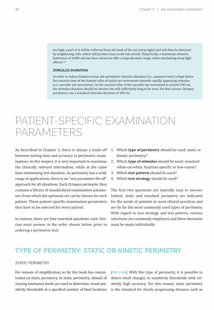
48 Chapter 4 | Key examination parameters
TYPE OF PERIMETRY: STATIC OR KINETIC PERIMETRY
For reasons of simpli ication, so far this book has concen-trated on static perimetry. In static perimetry, stimuli of varying luminance levels are used to determine visual sen-sitivity thresholds at a speci ied number of ixed locations
(FIG 4-1A). With this type of perimetry, it is possible to detect small changes in sensitivity thresholds with rel-atively high accuracy. For this reason, static perimetry is the standard for slowly progressing diseases such as
STATIC PERIMETRY
too high, a part of it will be re lected from the back of the eye (stray light) and will then be detected by neighboring cells, which will produce inaccurate test results. Empirically, a maximum stimulus luminance of 4,000 asb has been shown to offer a large dynamic range, while minimizing stray light effects. ,
STIMULUS DURATION
In order to reduce ixation losses, the perimetric stimulus duration (i.e., exposure time) is kept below the reaction time of the human re lex of quick eye movements towards rapidly appearing stimulus (i.e., saccadic eye movement). As the reaction time of the saccadic eye movement is around 200 ms, the stimulus duration should be shorter, but still suf iciently long to be seen. For that reason, Octopus perimeters use a standard stimulus duration of 100 ms.
PATIENT-SPECIFIC EXAMINATIONPARAMETERS
As described in Chapter 2, there is always a trade-off between testing time and accuracy in perimetric exam-inations. In this respect, it is very important to maximize the clinically relevant information, while at the same time minimizing test duration. As perimetry has a wide range of applications, there is no “one parameter its all” approach for all situations. Each Octopus perimeter thus contains a library of standardized examination parame-ters from which the optimum set can be chosen for each patient. These patient-speci ic examination parameters thus have to be selected for every patient.
In essence, there are four essential questions each clini-cian must answer, in the order shown below, prior to ordering a perimetric test:
1. Which type of perimetry should be used: static or kinetic perimetry?2. Which type of stimulus should be used: standard white-on-white, function-speci ic or low-vision?3. Which test pattern should be used?4. Which test strategy should be used?
The irst two questions are typically easy to answer. Indeed, static and standard perimetry are indicated for the needs of patients in most clinical practices and are by far the most commonly used types of perimetry. With regard to test strategy and test pattern, various selections are commonly employed, and these decisions must be made individually.

49Patient-specifi c examination parameters
DimStimulus
No
No
No
Yes
Yes
Yes
Yes
BrightStimulus
Stimulus
Do you seethe stimulus?
Fixation
= Seen
= Not seen
SE
NS
ITIV
ITY
TH
RE
SH
OLD
135
225
150
210
165
195
180
Vector(Stimulus trajectory)
Patientresponse
Do you seethe stimulus?
Fixation
Yes
Yes
Yes
No
No
= Seen
= Not seen
FIGURE 4-1 Both static and kinetic perimetry are designed to provide visual sensitivity thresholds that allow mapping the hill
of vision of a patient. In static perimetry (A), stimuli of differing light intensity are shown at given locations, to determine the
sensitivity threshold at those positions. In kinetic perimetry (B), a stimulus of a given light intensity is moved along the visual
fi eld (non-seeing to seeing), to determine the location of that sensitivity threshold.
Kinetic perimetry was the irst quantitative method of performing visual ield testing and is an alternative to static perimetry. In kinetic perimetry, moving stim-uli of pre-determined light intensities are moved from
non-seeing to seeing areas. The patient response then de ines the visual ield location of the speci ic light sen-sitivity threshold (FIG 4-1B).
KINETIC PERIMETRY
STATIC AND KINETIC PERIMETRY TESTING METHODS
A) STATIC PERIMETRY
B) KINETIC PERIMETRY
glaucoma. Since it is fully automated, it is also easy to use in clinical practice.
As the majority of visual ield tests are performed for glaucoma, static perimetry is the most commonly used type of perimetry today.

50
FIGURE 4-2 In static perimetry, each sensitivity threshold is displayed independently, either as a color or as a numerical map
(not shown here). In kinetic perimetry, areas of equal sensitivity thresholds form an isopter that provides similar information to
static perimetry about the shape of defects. Local areas of depression inside an isopter are called scotomas.
10 3020 40 50 60 70 80 90
STATIC KINETIC
SEEING NON-SEEING
SEEING NON-SEEING
Isopter
Scotoma(here blind spot)
Scotoma(here blind spot)
Chapter 4 | Key examination parameters
DISPLAY OF STATIC AND KINETIC VISUAL FIELDS
Since the patient can report seeing the stimulus at any location along the trajectory of the stimuli, kinetic perime-try provides high spatial resolution and fast testing over a large area. It is therefore bene icial for diseases affecting the periphery and sharp-edged defects and is frequent-ly used to evaluate neurological diseases and peripheral retinal diseases. As moving stimuli are easier to see than non-moving ones in the periphery, kinetic perimetry is also often used for children and for patients with cog-nitive impairment or severe visual ield loss. However,
kinetic perimetry is currently not fully automated, making it more challenging in everyday use.
As the majority of visual ield tests are performed to as-sess glaucoma and due to the ease of use of automation, static perimetry is by far the most commonly used type of perimetry today. For that reason, all of the following paragraphs and chapters focus on static perimetry, while kinetic perimetry will be discussed in depth in Chapter 11. The key differences between static and kinetic perimetry are summarized in TABLE 4-1.
After repeating this process for a speci ic stimulus size and intensity across the entire visual ield, the visual sen-sitivity thresholds can be connected to form an isopter (line of equal sensitivity). An isopter marks the boundary between seeing and non-seeing around the hill of vision
for a given stimulus size and intensity and is similar to an altitude line on a geographical map. Local regions of reduced sensitivity inside the isopter are identi ied in the same way and are called scotomas. FIG 4-2 shows how static and kinetic perimetry results are displayed.
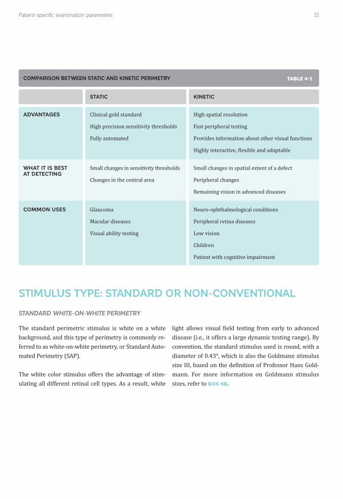
51Patient-specifi c examination parameters
The standard perimetric stimulus is white on a white background, and this type of perimetry is commonly re-ferred to as white-on-white perimetry, or Standard Auto-mated Perimetry (SAP).
The white color stimulus offers the advantage of stim-ulating all different retinal cell types. As a result, white
light allows visual ield testing from early to advanced disease (i.e., it offers a large dynamic testing range). By convention, the standard stimulus used is round, with a diameter of 0.43°, which is also the Goldmann stimulus size III, based on the de inition of Professor Hans Gold-mann. For more information on Goldmann stimulus sizes, refer to BOX 4B.
ADVANTAGES
WHAT IT IS BEST AT DETECTING
COMMON USES
STATIC
Clinical gold standard
High precision sensitivity thresholds
Fully automated
Small changes in sensitivity thresholds
Changes in the central area
Glaucoma
Macular diseases
Visual ability testing
KINETIC
High spatial resolution
Fast peripheral testing
Provides information about other visual functions
Highly interactive, lexible and adaptable
Small changes in spatial extent of a defect
Peripheral changes
Remaining vision in advanced diseases
Neuro-ophthalmological conditions
Peripheral retina diseases
Low vision
Children
Patient with cognitive impairment
STANDARD WHITE-ON-WHITE PERIMETRY
STIMULUS TYPE: STANDARD OR NON-CONVENTIONAL
COMPARISON BETWEEN STATIC AND KINETIC PERIMETRY TABLE 4-1

52 Chapter 4 | Key examination parameters
FIGURE 4-3 Stimuli used in function-specifi c perimetry from left to right: Short Wavelength Automated Perimetry (SWAP),
Flicker Perimetry and Pulsar Perimetry.
SWAP PulsarFlicker
ON
Time 1
OFF
Time 2
V
IV
III
II
I
1.7°
0.8°
0.43°
0.2°
0.1°
20
BLIND SPOT
Function-speci ic perimetry uses different stimulus types to stimulate different visual functions (e.g., motion, or color vision), but they all have the same purpose: measuring a subset of the visual system individually, to get more sensitive responses for early disease detection. Different Octopus perimeter models offer different func-tion-speci ic stimuli (FIG 4-3): a blue stimulus on a yellow
background (Short-Wavelength Automated Perimetry, or SWAP); a white lickering stimulus on a white back-ground (Flicker Perimetry); or a pulsating stimulus with concentric rings changing in both spatial resolution and contrast (Pulsar Perimetry). They are described in more detail in Chapter 10.
FUNCTION-SPECIFIC PERIMETRY
FUNCTION-SPECIFIC PERIMETRY
GOLDMANN SIZES I TO V
The size conventions used today to describe a perimetric stimulus are derived from the work of Professor Hans Goldmann, who developed the Goldmann perimeter in 1946. He de ined standard sizes for perimetric stimuli, and the Goldmann sizes I to V are still widely used. Each step corresponds to a change in diameter by a factor of 2 and in area by a factor of 4. Size III is several times smaller than the physiological blind spot and was considered to be an accurate measurement size.
The Goldmann stimulus sizes I to V are presented in
relation to the size of the physiological blind spot.
BOX 4B
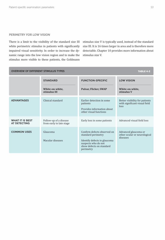
53Patient-specifi c examination parameters
There is a limit to the visibility of the standard size III white perimetric stimulus in patients with signi icantly impaired visual sensitivity. In order to increase the dy-namic range into the low vision region and to make the stimulus more visible to these patients, the Goldmann
stimulus size V is typically used, instead of the standard size III. It is 16 times larger in area and is therefore more detectable. Chapter 10 provides more information about stimulus size V.
PERIMETRY FOR LOW VISION
ADVANTAGES
WHAT IT IS BEST AT DETECTING
COMMON USES
STANDARD
White-on-white,stimulus III
Clinical standard
Follow-up of a disease from early to late stage
Glaucoma
Macular diseases
FUNCTION-SPECIFIC
Pulsar, Flicker, SWAP
Earlier detection in some patients
Provides information about other visual functions
Early loss in some patients
Con irm defects observed on standard perimetry
Identify defects in glaucoma suspects who do not show defects on standard perimetry
LOW VISION
White-on-white,stimulus V
Better visibility for patients with signi icant visual ield loss
Advanced visual ield loss
Advanced glaucoma or other ocular or neurological diseases
OVERVIEW OF DIFFERENT STIMULUS TYPES TABLE 4-2

54 Chapter 4 | Key examination parameters
FIGURE 4-4 Covering the entire visual fi eld with high resolution within a reasonable test duration is not possible. Either the fi eld
is only roughly covered, or the test duration is unacceptable, as shown in this example with three different test patterns.
10º SPACING~190 size III targets
6º SPACING~550 size III targets
2º SPACING~4800 size III targets
90
270
0180
90
270
0180
90
270
0180
In clinical practice, patients can sometimes become tired quickly during perimetric testing, which signi icantly limits the number of test locations that can be reliably tested. - A reasonably dense grid of test locations, cov-ering the entire visual ield with 2° degree spacing, would require around 4,800 size III stimuli, and a grid with 6° degree spacing would require approximately 550 test
In order to maximize perimetric information and mini-mize test duration, a test pattern should be chosen with a high density of test locations in the area of high inter-est and a low density of test locations in areas of low interest (FIG 4-5). For that reason, Octopus perimeters
locations. A very rough grid with 10° degree spacing be-tween the stimuli would require approximately 190 test locations, but would be highly inaccurate, as there would be only 5 test points in the central 10° of vision, which is an important area for visual functions such as reading and identifying objects (FIG 4-4).
offer a large library of testing patterns for common perimetric applications.
The most commonly used test patterns available on the Octopus perimeter and the rationale for which to select are described in depth in Chapter 5.
TEST PATTERN
ILLUSTRATION OF THE LOW SPATIAL RESOLUTION OF PERIMETRIC TESTING

55Patient-specifi c examination parameters
FIGURE 4-5 Examples of test patterns for various clinical perimetric applications are presented. Each pattern maximizes the
relevant information for that clinical situation, while minimizing the test duration by only evaluating the most relevant areas. (A)
The G-pattern for glaucoma tests within 30° at locations that follow the retinal nerve fi bre bundle patterns. (B) The M-pattern for
the macula tests within the central 10°. (C) The Esterman tests binocularly for visual fi tness to drive (120° horizontally and 60°
vertically). (D) The Ptosis test pattern only evaluates the upper hemifi eld along common eyelid locations.
G-PATTERN(Glaucoma)
M-PATTERN(Macula)
ESTERMAN(Visual driving ability)
PTOSIS
10 30 40 50 60 70 80 90
90
270
0180
10 30 40 50 60 70 80 90
90
270
0180 10 30 40 50 60 70 80 90
90
270
0180
10 30 40 50 60 70 80 90
90
270
0180
EXAMPLES OF DIFFERENT TEST PATTERNS
A)
C)
B)
D)
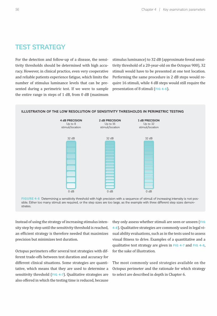
56
4 dB PRECISIONUp to 8
stimuli/location
2 dB PRECISIONUp to 16
stimuli/location
1 dB PRECISIONUp to 32
stimuli/location
32 dB 32 dB 32 dB
0 dB 0 dB 0 dB
Chapter 4 | Key examination parameters
For the detection and follow-up of a disease, the sensi-tivity thresholds should be determined with high accu-racy. However, in clinical practice, even very cooperative and reliable patients experience fatigue, which limits the number of stimulus luminance levels that can be pre-sented during a perimetric test. If we were to sample the entire range in steps of 1 dB, from 0 dB (maximum
Instead of using the strategy of increasing stimulus inten-sity step by step until the sensitivity threshold is reached, an ef icient strategy is therefore needed that maximizes precision but minimizes test duration.
Octopus perimeters offer several test strategies with dif-ferent trade-offs between test duration and accuracy for different clinical situations. Some strategies are quanti-tative, which means that they are used to determine a sensitivity threshold (FIG 4-7). Qualitative strategies are also offered in which the testing time is reduced, because
stimulus luminance) to 32 dB (approximate foveal sensi-tivity threshold of a 20-year-old on the Octopus 900), 32 stimuli would have to be presented at one test location. Performing the same procedure in 2 dB steps would re-quire 16 stimuli, while 4 dB steps would still require the presentation of 8 stimuli (FIG 4-6).
they only assess whether stimuli are seen or unseen (FIG
4-8). Qualitative strategies are commonly used in legal vi-sual ability evaluations, such as in the tests used to assess visual itness to drive. Examples of a quantitative and a qualitative test strategy are given in FIG 4-7 and FIG 4-8, for the sake of illustration.
The most commonly used strategies available on the Octopus perimeter and the rationale for which strategy to select are described in depth in Chapter 6.
TEST STRATEGY
ILLUSTRATION OF THE LOW RESOLUTION OF SENSITIVITY THRESHOLDS IN PERIMETRIC TESTING
FIGURE 4-6 Determining a sensitivity threshold with high precision with a sequence of stimuli of increasing intensity is not pos-
sible. Either too many stimuli are required, or the step sizes are too large, as the example with three different step sizes demon-
strates.
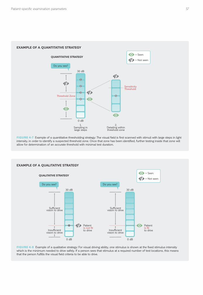
57
Threshold Zone
SensitivityThreshold
Do you see?
QUANTITATIVE STRATEGY
1.Sampling inlarge steps
2.Detailing withinthreshold zone
30 dB
0 dB
1
2
3
4
5
= Seen
= Not seen
Patientis not fitto drive
Do you see?
30 dB
0 dB
Sufficientvision to drive
Insufficientvision to drive
QUALITATIVE STRATEGY
Patientis fitto drive
Sufficientvision to drive
Insufficientvision to drive
Do you see?
30 dB
0 dB
= Seen
= Not seen
Patient-specifi c examination parameters
EXAMPLE OF A QUANTITATIVE STRATEGY
EXAMPLE OF A QUALITATIVE STRATEGY
FIGURE 4-7 Example of a quantitative thresholding strategy: The visual fi eld is fi rst scanned with stimuli with large steps in light
intensity, in order to identify a suspected threshold zone. Once that zone has been identifi ed, further testing inside that zone will
allow for determination of an accurate threshold with minimal test duration.
FIGURE 4-8 Example of a qualitative strategy: For visual driving ability, one stimulus is shown at the fi xed stimulus intensity
which is the minimum needed to drive safely. If a person sees that stimulus at a required number of test locations, this means
that the person fulfi lls the visual fi eld criteria to be able to drive.

58 Chapter 4 | Key examination parameters
REFERENCES1. Fankhauser F, Haeberlin H. Dynamic range and stray light. An estimate of the falsifying effects of stray light in perimetry. Doc Ophthalmol. 1980;50:143-167.2. Anderson RS, Redmond T, McDowell DR, Breslin KM, Zlatkova MB. The robustness of various forms of perimetry to different levels of induced intraocular stray light. Invest Ophthalmol Vis Sci. 2009;50:4022-4028.3. Johnson CA, Adams CW, Lewis RA. Fatigue effects in automated perimetry. Appl Opt. 1988;27:1030-1037.4. Wild JM, Searle AE, Dengler-Harles M, O’Neill EC. Long-term follow-up of baseline learning and fatigue effects in the automated perimetry of glaucoma and ocular hypertensive patients. Acta Ophthalmol (Copenh). 1991;69:210-216.5. Hudson C, Wild JM, O’Neill EC. Fatigue effects during a single session of automated static threshold perimetry. Invest Ophthalmol Vis Sci. 1994;35:268-280.6. Gonzalez de la Rosa M, Pareja A. In luence of the “fatigue effect” on the mean deviation measurement in perimetry. Eur J Ophthalmol. 1997;7:29-34.
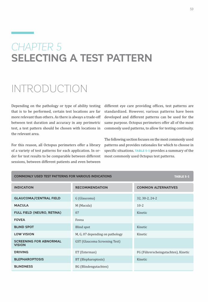
59
CHAPTER 5SELECTING A TEST PATTERN
INTRODUCTION
Depending on the pathology or type of ability testing that is to be performed, certain test locations are far more relevant than others. As there is always a trade-off between test duration and accuracy in any perimetric test, a test pattern should be chosen with locations in the relevant area.
For this reason, all Octopus perimeters offer a library of a variety of test patterns for each application. In or-der for test results to be comparable between different sessions, between different patients and even between
different eye care providing of ices, test patterns are standardized. However, various patterns have been developed and different patterns can be used for the same purpose. Octopus perimeters offer all of the most commonly used patterns, to allow for testing continuity.
The following section focuses on the most commonly used patterns and provides rationales for which to choose in speci ic situations. TABLE 5-1 provides a summary of the most commonly used Octopus test patterns.
INDICATION
GLAUCOMA/CENTRAL FIELD
MACULA
FULL FIELD (NEURO, RETINA)
FOVEA
BLIND SPOT
LOW VISION
SCREENING FOR ABNORMAL VISION
DRIVING
BLEPHAROPTOSIS
BLINDNESS
RECOMMENDATION
G (Glaucoma)
M (Macula)
07
Fovea
Blind spot
M, G, 07 depending on pathology
GST (Glaucoma Screening Test)
ET (Esterman)
BT (Blepharoptosis)
BG (Blindengutachten)
COMMON ALTERNATIVES
32, 30-2, 24-2
10-2
Kinetic
Kinetic
Kinetic
FG (Führerscheingutachten), Kinetic
Kinetic
COMMONLY USED TEST PATTERNS FOR VARIOUS INDICATIONS TABLE 5-1

60 Chapter 5 | Selecting a test pattern
TYPICAL VISUAL FIELD DEFECTS IN GLAUCOMA
Glaucoma is a disease resulting in the degeneration of retinal nerve iber bundles in the eye. Since the largest proportion of retinal nerve ibers is located within the central 30°,¹-⁴ most early to moderate glaucoma visual ield loss occurs within the central 30°. Typical defect
patterns follow the distribution of the retinal nerve iber bundles and there is a clear separation along the superi-or and inferior hemi ields at the horizontal meridian. The typical patterns of visual ield loss due to glaucoma are partial arcuate, paracentral, nasal step, arcuate, temporal wedge and altitudinal defects (FIG 5-1).⁵
Since glaucomatous visual ield defects typically occur within the central visual ield, the best trade-off between test duration and accuracy is achieved by using a central
30° test pattern, which has become the standard for visual ield testing in glaucoma today. Conversely, the periphery
is rarely affected in isolation in glaucoma,⁶ so that peripheral testing is less common in cases of glaucoma for diagnostic reasons and, if used at all, is aimed to assess a patient’s quality of life.
In very advanced glaucoma, the visual field usually constricts to a macular visual ield⁷ and testing outside the macula does not provide any further diagnostic information. Therefore, it is common to switch to a 10° macular test pattern in advanced glaucoma, in order to track residual vision in that area with higher resolution⁷,⁸ for the same test duration.
TEST PATTERNS FOR GLAUCOMA

FIGURE 5-1 The typical visual fi eld defects in glaucoma are the partial arcuate, paracentral, nasal step, diffuse, arcuate,
temporal wedge, altitudinal and constricted in advanced glaucoma (ordered according to frequency of occurrence). All
manifest themselves within the central 30° visual fi eld, so that central 30° testing in glaucoma care is standard.
61Test patterns for glaucoma
PARTIAL ARCUATE
DIFFUSE
ALTITUDINAL
PARACENTRAL
ARCUATE
CONSTRICTED(Double arcuate)
NASAL STEP
TEMPORAL WEDGE
TYPICAL VISUAL FIELD DEFECTS IN GLAUCOMA

FIGURE 5-2 The distribution of the test locations in the G pattern follows the retinal nerve fi ber bundles.
62 Chapter 5 | Selecting a test pattern
The standard perimetric stimulus is white, and is pre-sented on a white background. This type of perimetry is commonly referred to as white-on-white perimetry, or Standard Automated Perimetry (SAP).
The white color stimulus offers the advantage of stim-ulating all different retinal cell types. As a result, white
light allows visual ield testing from early to advanced disease (i.e., it offers a large dynamic testing range). By convention, the standard stimulus used is round, with a diameter of 0.43°, which is also the Goldmann stimulus, size III, based on the de inition by Professor Hans Gold-mann. For more information on Goldmann stimulus sizes, refer to BOX 4B.
STANDARD TEST PATTERN IN GLAUCOMA CARE
G PATTERN
The G pattern was designed to serve as a multi-purpose test and offers an excellent trade-off between test dura-tion and accuracy.⁹-¹¹ There are 59 different locations within the central 30° of the visual ield and they are distributed in a pattern that facilitates not only the de-
tection of visual loss associated with glaucoma, but also neuro-ophthalmological and macular diseases.
To maximize the detection of glaucomatous visual loss, the test locations are distributed along the retinal nerve iber bundles, where visual loss is most likely to occur (FIG 5-2).
THE G PATTERN FOR GLAUCOMA
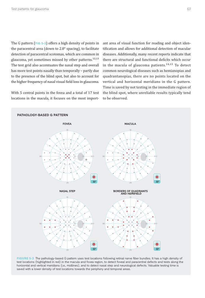
FIGURE 5-3 The pathology-based G pattern uses test locations following retinal nerve fi ber bundles. It has a high density of
test locations (highlighted in red) in the macula and fovea region, to detect foveal and paracentral defects and tests along the
horizontal and vertical meridians (i.e., midlines), and to detect nasal step and neurological defects. Valuable testing time is
saved with a lower density of test locations towards the periphery and temporal areas.
63Test patterns for glaucoma
10 30
90
270
0180 20
30°
10 30
90
270
0180 20
10 30
90
270
0180 2010 30
90
270
0180 20
30°
30° 30°
FOVEA MACULA
NASAL STEP BORDERS OF QUADRANTS AND HEMIFIELD
The G pattern (FIG 5-3) offers a high density of points in the paracentral area (down to 2.8° spacing), to facilitate detection of paracentral scotomas, which are common in glaucoma, yet sometimes missed by other patterns.¹²,¹³ The test grid also accentuates the nasal step and overall has more test points nasally than temporally – partly due to the presence of the blind spot, but also to account for the higher frequency of nasal visual ield loss in glaucoma.
With 5 central points in the fovea and a total of 17 test locations in the macula, it focuses on the most import-
ant area of visual function for reading and object iden-ti ication and allows for additional detection of macular diseases. Additionally, many recent reports indicate that there are structural and functional de icits which occur in the macula of glaucoma patients.¹⁴,¹⁵ To detect common neurological diseases such as hemianopias and quadrantanopias, there are no points located on the vertical and horizontal meridians in the G pattern. Time is saved by not testing in the immediate region of the blind spot, where unreliable results typically tend to be observed.
PATHOLOGY-BASED G PATTERN

64
10 30
90
270
0180 20 10 30
90
270
0180 20 10 30
90
270
0180 20
30° 30° 30°
3274 test locations
30-276 test locations
24-254 test locations
Chapter 5 | Selecting a test pattern
ALTERNATIVE TEST PATTERNS FOR THE CENTRAL 30°
32/30-2 AND 24-2 PATTERNS
The 32, 30-2 and 24-2 patterns (FIG 5-4) are similar to the G pattern in that they cover the central visual ield and respect the vertical and horizontal meridians. In con-trast however, they are not optimized for speci ic pathol-ogies. Instead, all test locations are equidistant from each other and separated by 6°.
Historically, the 32 pattern¹⁶ was initially used in the irst series of Octopus perimeters in 1977, while the 30-2
pattern was among the irst central patterns used on the Humphrey Field Analyzer. These patterns are nearly identical to each other. The sole difference is that the 30-2 pattern has 2 extra test locations in the blind spot, which are omitted in the 32 pattern. With their 74 or 76 test locations respectively, the 32/30-2 patterns take
longer to complete than the G pattern without providing considerably more meaningful clinical information.
The 24-2 pattern is based on the 30-2 pattern, but the most peripheral ring of test locations is removed, except for the two nasal points. With only 54 test points, the test duration of the 24-2 pattern is as short as that of the G pattern, but the test pattern is not optimized for typical pathologies.
Since it is optimized for pathology and quicker, the G pattern is recommended for new patients. However, the 32/30-2 and 24-2 patterns are recommended when a large set of existing data taken from one of these patterns is available for a patient, and the eye care provider wish-es to have continuity in the testing procedure.
FIGURE 5-4 The 30-2 pattern is similar to the 32 pattern, but has 2 additional test locations in the blind spot area. The 24-2
pattern is an abbreviated version of the 30-2 pattern, with most peripheral locations excluded, except for the nasal step region.
CENTRAL 30° TEST PATTERNS

65
30°
30°
G M
12°
12°
Test patterns for glaucoma
FURTHER TEST PATTERNS FOR GLAUCOMA
MACULA TESTING PATTERNS FOR ADVANCED GLAUCOMA
KINETIC PERIMETRY FOR ADVANCED GLAUCOMA
PERIPHERAL TEST PATTERNS TO ASSESS QUALITY OF LIFE
In advanced glaucoma, the visual ield is typically con-stricted to the macular area. In these situations, testing the full 30° will not offer a good trade-off between test duration and the clinical information received, because more than 65% of the locations will be in known areas of non-seeing (FIG 5-5). To further maximize useful clinical
Since static testing is challenging for patients with advanced glaucoma,¹⁷-¹⁹ kinetic perimetry is a good
Even though the periphery is rarely affected in isolation in glaucoma,²⁰-²² there may still be a need to assess the peripheral vision, in order to evaluate the patient’s over-all quality of life.
In these situations, the G-Periphery pattern (FIG 5-6) is a very time-effective peripheral screening pattern, with only 14 test locations in the periphery, and is intended to
information, it is common to switch to testing patterns that solely evaluate the area of the macula.⁷,⁸
For further information on macula patterns, please see the section on the macula testing patterns M or 10-2.
alternative to static testing in such cases. For more infor-mation, please see Chapter 11 on kinetic perimetry.
be an add-on to the standard G pattern. The G-Periphery pattern places strong emphasis on the nasal step area, as this is the most relevant peripheral location in glau-coma.²⁰,²³
For an in-depth and ef icient assessment of the periph-ery in low-vision patients, the use of kinetic perimetry should be considered.
FIGURE 5-5 In advanced glaucoma with a severely constricted visual fi eld, the focus of visual fi eld testing is on the remaining
vision in the macula. In these situations, a macula pattern like the M pattern provides more clinically relevant information than
a central pattern such as the G pattern.
MACULA PATTERN FOR ADVANCED GLAUCOMA

66 Chapter 5 | Selecting a test pattern
10 30
90
270
0180 20
30°
10 30 40 50 60 70 80 90
90
270
0180
G-PERIPHERY14 test locations
G-SCREENING28 test locations
90°
ABBREVIATED G PATTERN FOR SCREENING
In some instances, a screening visual ield test is a con-venient procedure for every patient, to make sure that visual ield loss is not missed as part of a routine eye examination.
For screening of a presumed healthy population, the G-Screening (GS) pattern offers a good trade-off between
test duration and accuracy. It is an abbreviated version of the G pattern with only 28 test locations (FIG 5-6). The locations have been chosen on the basis of their ability to predict glaucoma and other commonly occurring eye dis-eases, such as macula defects and quadrantanopias and hemianopias. The G-Screening (GS) pattern is available exclusively with the screening strategy.
FIGURE 5-6 The G-Periphery pattern is an add-on to the G pattern, to quickly screen the periphery and dominantly the
peripheral nasal step in glaucoma. The G-Screening pattern is used for routine screening of dominantly healthy patients.
ADDITIONAL TESTING PATTERNS FOR GLAUCOMA
67Testing patterns for neurological visual fi eld loss
TYPICAL VISUAL FIELD DEFECTS IN NEURO-OPHTHALMIC CONDITIONS
Neurological conditions lead to a large variety of typical visual ield defect patterns which are very speci ic, de-pending on the location at which the visual pathways are affected (FIG 5-7).²⁴ Lesions of the optic disc and optic nerve lead to unilateral (i.e., only affecting one eye) visual ield defects. Common optic nerve and nerve head diseas-
es include disc edema, optic neuropathies, optic neuritis, compressive lesions such as those caused by idiopathic intracranial hypertension, and a number of congenital abnormalities, such as optic nerve head drusen. Typical visual ield defect patterns appear in the central 30° and include foveal and macular defects, enlarged blind spots, or patterns similar to those occurring in glaucoma. However, de icits in the far peripheral visual ield beyond 30° also frequently occur.
Chiasmal lesions resulting from diseases such as pitu-itary adenomas and related lesions typically result in bitemporal (i.e., left and right eye defects are mirrored) hemianopias, which progress from the superior to the in-ferior hemi ield, but always respect the vertical midline. Damage can be more pronounced in one eye than the other. Postchiasmal lesions typically lead to homony-mous (i.e., left and right eye defects are on same side of
vision) visual ield defects, with congruity (similarity in location, size and magnitude of the de icit) between the two eyes being most common further back in the visual pathways at or near the occipital lobe. Large lesions re-sult in complete hemianopias, although quadrantanopias and wedge-like defects are also common. While large lesions also affect the central visual ield, small lesions may not extend to the central 30°. It should also be noted that a complete homonymous hemianopia only indicates that the de icit is post-chiasmal and that all visual path-way ibers leading back to the occipital lobe have been damaged.
To cover all of the aforementioned visual ield defects, the full visual ield needs to be thoroughly tested, with a high density of test locations in the macula, the blind spot and the central ield. Therefore, thorough neurological visual ield tests are time-consuming. If the type of disease is
identi ied, then the focus of testing can be in the area af-fected by the disease, in order to reduce the test duration.
To maximize perimetric information and minimize test duration, kinetic perimetry should also be considered.
TEST PATTERNS FOR NEUROLOGICAL VISUAL FIELD LOSS

68 Chapter 5 | Selecting a test pattern
LEFT TEMPORAL FIELD RIGHT TEMPORAL FIELD
Visual field of the right eye (OD)
Caecocentral scotoma
Nerve fiber bundle defect
Central scotoma
Heteronymous (bitemporal) hemianopia
Heteronymous(bitemporal) quadrantanopia
Homonymous hemianopia
Superior homonymousquadrantanopiaTemporal lobe lesion
Inferior homonymousquadrantanopiaParietal lobe lesion
Homonymous hemianopiaOccipital lobe lesion
Visual field of the left eye (OS)
Optic disc (blind spot)
Retina
Optic chiasm
Optic tract
Lateral geniculatebody
Optic radiations(temporal lobe)
Optic radiations(parietal lobe)
Occipital lobeVisual cortex
NASAL FIELD
60°
60° 30° 90°
Optic nerve damage Chiasmal deficit Postchiasmal deficit
1
2
3
4
4
5
6
7
8
12
3
45
6
7
8
TYPICAL VISUAL FIELD DEFECTS IN NEUROLOGICAL DISEASES
FIGURE 5-7 Typical visual fi eld defects in diseases are unilateral if the optic nerve is damaged, heteronymous (the two eyes are
mirror images) around the chiasm and homonymous (the two eyes show non-mirror symmetry) beyond the chiasm. Both hemi-
anopias (vertical hemisphere defect) and quadrantanopias (quadrant defects) are typical neurological visual fi eld defects.

69Testing patterns for neurological visual fi eld loss
10 30
90
270
0180 20
30°
N-BLIND SPOT54 test locations
90°
10 30 40 50 60 70 80 90
90
270
0180
N-FOVEA21 test locations
N-FULL FIELD71 test locations
10°
10
90
270
0180
THOROUGH ASSESSMENT OF NEUROLOGICAL VISUAL FIELD DEFECTS
N PATTERN
The N pattern is speci ically designed for neuro-ophthal-mic diseases. Given the wide variety of defect patterns, it consists of several components that can be combined independently. The N pattern includes a full ield, fovea and blind spot testing pattern (FIG 5-8).
The N-Full Field pattern is designed to test the full visual ield. It is useful to detect any kind of neurological dis-
ease. It extends from 40° nasally to 67° temporally and 40° vertically. With its 54 test locations in the central vi-sual ield and an additional 17 locations in the peripheral visual ield, it offers an excellent trade-off between test duration and accuracy in the detection of central and early peripheral neurological defects.
The N-Fovea pattern is designed to detect foveal defects,
such as nerve compressions, with high accuracy and should be used when this kind of pathology is suspected. With its 21 test locations extending from 0 to 3°, it pro-vides a rapid assessment of the important foveal region and can also be useful for other indications in which the fovea is affected.
The N-Blind Spot pattern is designed to detect the bound-aries of the blind spot with adequate accuracy to check for blind spot enlargements. It covers the area around the blind spot from 9 to 19° horizontally, and 9.5° superiorly to 19° inferiorly in 2.5° steps. To account for tilted discs, extra points are added at the superior, temporal corner and the inferior nasal corner. With its 54 test locations, it takes a relatively long time to complete, while spatial resolution is limited to 2.5°.
FIGURE 5-8 The N pattern for neuro-ophthalmic disease consists of three testing patterns: a full fi eld pattern, a fovea pattern
and a pattern to test the blind spot.
DIFFERENT PATTERNS FOR NEURO-OPHTHALMOLOGY
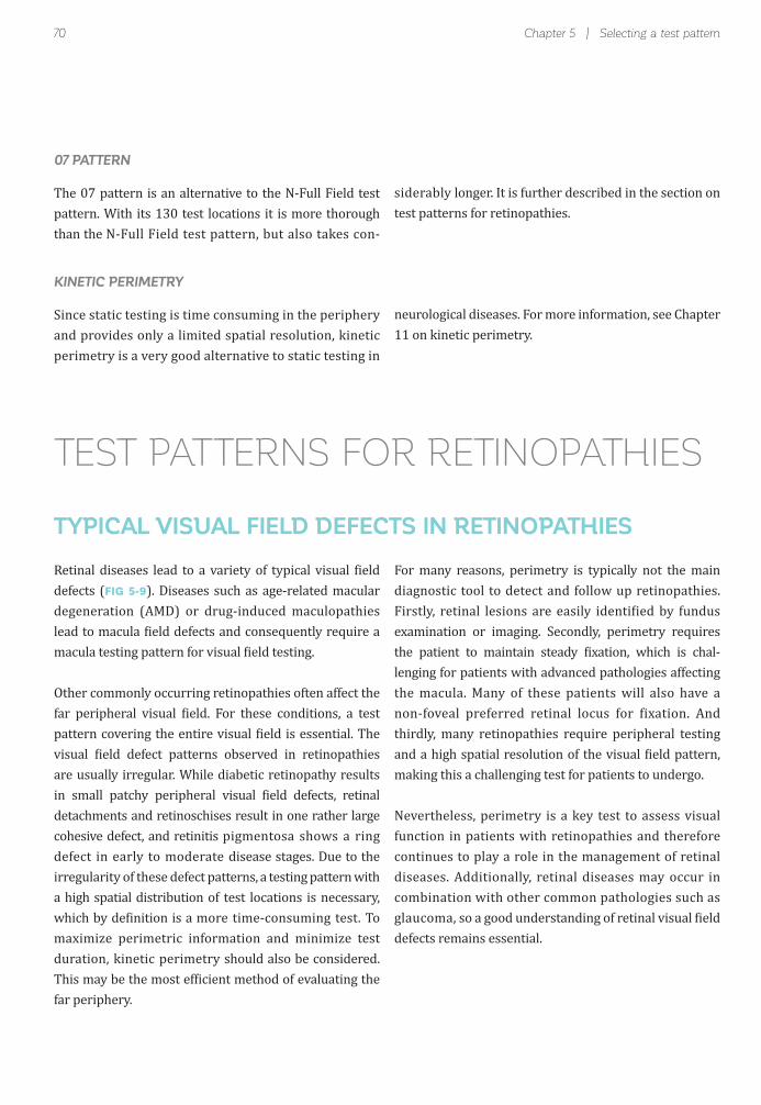
70 Chapter 5 | Selecting a test pattern
07 PATTERN
KINETIC PERIMETRY
The 07 pattern is an alternative to the N-Full Field test pattern. With its 130 test locations it is more thorough than the N-Full Field test pattern, but also takes con-
Since static testing is time consuming in the periphery and provides only a limited spatial resolution, kinetic perimetry is a very good alternative to static testing in
siderably longer. It is further described in the section on test patterns for retinopathies.
neurological diseases. For more information, see Chapter 11 on kinetic perimetry.
TYPICAL VISUAL FIELD DEFECTS IN RETINOPATHIES
Retinal diseases lead to a variety of typical visual ield defects (FIG 5-9). Diseases such as age-related macular degeneration (AMD) or drug-induced maculopathies lead to macula ield defects and consequently require a macula testing pattern for visual ield testing.
Other commonly occurring retinopathies often affect the far peripheral visual ield. For these conditions, a test pattern covering the entire visual ield is essential. The visual ield defect patterns observed in retinopathies are usually irregular. While diabetic retinopathy results in small patchy peripheral visual ield defects, retinal detachments and retinoschises result in one rather large cohesive defect, and retinitis pigmentosa shows a ring defect in early to moderate disease stages. Due to the irregularity of these defect patterns, a testing pattern with a high spatial distribution of test locations is necessary, which by de inition is a more time-consuming test. To maximize perimetric information and minimize test duration, kinetic perimetry should also be considered. This may be the most ef icient method of evaluating the far periphery.
For many reasons, perimetry is typically not the main diagnostic tool to detect and follow up retinopathies. Firstly, retinal lesions are easily identi ied by fundus examination or imaging. Secondly, perimetry requires the patient to maintain steady ixation, which is chal-lenging for patients with advanced pathologies affecting the macula. Many of these patients will also have a non-foveal preferred retinal locus for fixation. And thirdly, many retinopathies require peripheral testing and a high spatial resolution of the visual ield pattern, making this a challenging test for patients to undergo.
Nevertheless, perimetry is a key test to assess visual function in patients with retinopathies and therefore continues to play a role in the management of retinal diseases. Additionally, retinal diseases may occur in combination with other common pathologies such as glaucoma, so a good understanding of retinal visual ield defects remains essential.
TEST PATTERNS FOR RETINOPATHIES

71Testing patterns for retinopathies
AMD DRUG-INDUCED MACULOPATHY
DIABETIC RETINOPATHY RETINITIS PIGMENTOSA
90°
10°
MA
CU
LA
FULL
FIE
LD
M PATTERN
The M pattern is the recommended pattern for macula visual ield evaluation.²⁵ With its 45 equally spaced test locations, with 1° spacing in the fovea (central 4°), it of-fers the highest density of test locations in the most es-sential area for visual function.²⁵ The remaining 36 of the 81 test locations in total are radially arranged outside the fovea (FIG 5-10).
The M pattern is most commonly used for the testing of drug-induced maculopathies, to follow up advanced-stage glaucoma patients, and for visual function testing in patients with AMD or other macular dysfunction.
FIGURE 5-9 Typical visual fi eld defects in retinal diseases either affect the macula (e.g., AMD, drug-induced maculopathies)
or are characterized by patchy, irregular loss affecting the full visual fi eld (e.g., diabetic retinopathy, retinitis pigmentosa).
TYPICAL VISUAL FIELD DEFECTS IN RETINAL DISEASES
TEST PATTERNS FOR THE MACULA

72 Chapter 5 | Selecting a test pattern
M81 test locations
10°
10
90
270
0180
10-276 test locations
10°
10
90
270
0180
10-2 PATTERN
07 PATTERN
The 10-2 pattern is the alternative to the M pattern, but is not physiology-based (i.e., there is no emphasis on the fovea). Instead, all 76 test locations are equidistant, being separated from each other by 2° (FIG 5-10). Its test dura-tion is comparable to the M pattern.
The 07 pattern is the recommended static testing pattern to identify the patchy peripheral visual ield loss associ-ated with a variety of retinal diseases, such as diabetic retinopathy, retinoschisis, retinal detachment and retinitis pigmentosa.
It has 130 test locations, extending from 70° temporally to 55° nasally, arranged radially with 15° spacing²⁶ (FIG 5-11).
The 10-2 grid is identical to that used on the Humphrey Field Analyzer, thereby allowing for continuity when tran-sitioning from the Humphrey to the Octopus perimeter.
It provides reasonably high spatial resolution to be able to identify larger retinal lesions with a test duration that is acceptable for most patients. Nevertheless, the test duration using a quantitative strategy is long, so that a qualitative test strategy offers a good trade-off between test duration and accuracy (more details on quanti-tative and qualitative tests are provided in Chapter 6).
FIGURE 5-10 Both the M pattern and the 10-2 pattern are designed to exclusively test the macula. While the M pattern is
physiology-based, with a high density of test locations in the fovea, the test locations are equidistant in the 10-2 pattern.
MACULA TEST PATTERNS
TEST PATTERNS FOR THE FULL FIELD
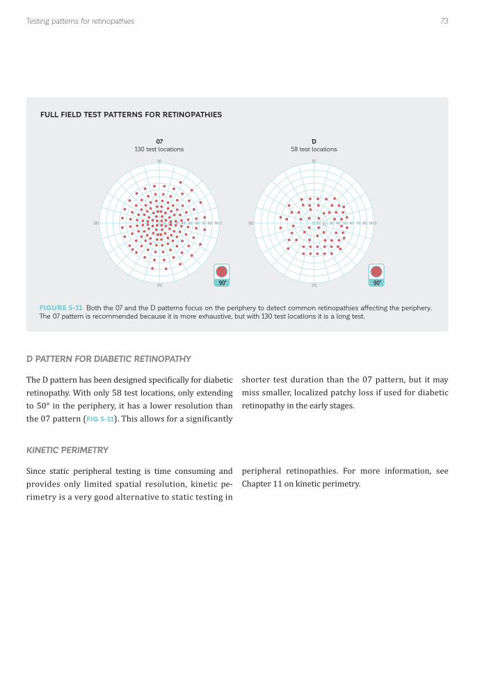
73Testing patterns for retinopathies
90°
07130 test locations
10 30 40 50 60 70 80 90
90
270
0180
90°
D58 test locations
10 30 40 50 60 70 80 90
90
270
0180
D PATTERN FOR DIABETIC RETINOPATHY
KINETIC PERIMETRY
The D pattern has been designed speci ically for diabetic retinopathy. With only 58 test locations, only extending to 50° in the periphery, it has a lower resolution than the 07 pattern (FIG 5-11). This allows for a signi icantly
Since static peripheral testing is time consuming and provides only limited spatial resolution, kinetic pe-rimetry is a very good alternative to static testing in
shorter test duration than the 07 pattern, but it may miss smaller, localized patchy loss if used for diabetic retinopathy in the early stages.
peripheral retinopathies. For more information, see Chapter 11 on kinetic perimetry.
FIGURE 5-11 Both the 07 and the D patterns focus on the periphery to detect common retinopathies affecting the periphery.
The 07 pattern is recommended because it is more exhaustive, but with 130 test locations it is a long test.
FULL FIELD TEST PATTERNS FOR RETINOPATHIES

74 Chapter 5 | Selecting a test pattern
ESTERMAN TEST
The Esterman test was developed by Ben Esterman²⁷ and has become an accepted standard visual ield test for driving ability that is available in most modern perimeters. While this test must be used in countries that require it by law, it is also commonly used in countries in which there are broader statutory requirements.
The Esterman test contains 120 test points. It horizon-tally spans 160°, and vertically from 30° superior to 60° inferior (FIG 5-12). It is typically a binocular test since driving is undertaken binocularly, but a monocular version is also available.
TEST PATTERNS FOR VISUAL ABILITY TO DRIVE
TEST PATTERNS FOR VISUALABILITY TESTING
Visual ability testing is often performed in a legal con-text, for example to assess a person’s visual ability to drive, eligibility for a pension or presence of visual disability. Therefore, highly standardized visual ield tests are prescribed by local law and must be adhered to strictly. While certain legislation sets very specific
Safe driving requires a large horizontal ield of view, to be able to notice other cars coming from the side, and a fairly intact central ield of view, to be able to notice obsta-cles ahead. As driving is performed with both eyes open, the binocular ield of view is relevant for safe driving.
requirements and de ines test conditions in great detail, other legislation sets broader requirements. It is there-fore essential to be familiar with the statutory require-ments in one’s own country and to choose a testing pattern that adheres to these regulations.
By law, in many countries visual ability to drive tests are mandatory to obtain and maintain a driver's license. While the precise requirements differ according to local legislation, often a visual ield test is required. While the legislation in some countries is rather vague, in other countries a speci ic test is requested.
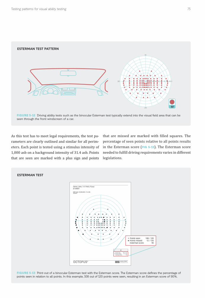
75Testing patterns for visual ability testing
90°
10 30 40 50 60 70 80 90
90
270
0180
80°
Demo, John, 1/1/1945 (71yrs)ID 00001
Points seen: 108 / 120Points missed: 12 / 120Esterman score: 90
Both eyes / 05/05/2015 / 16:.3:05Symbols
Points seen: 108 / 120Points missed: 12 / 120Esterman score: 90
OCTOPUS®
As this test has to meet legal requirements, the test pa-rameters are clearly outlined and similar for all perim-eters. Each point is tested using a stimulus intensity of 1,000 asb on a background intensity of 31.4 asb. Points that are seen are marked with a plus sign and points
that are missed are marked with illed squares. The percentage of seen points relative to all points results in the Esterman score (FIG 5-13). The Esterman score needed to ful ill driving requirements varies in different legislations.
FIGURE 5-12 Driving ability tests such as the binocular Esterman test typically extend into the visual fi eld area that can be
seen through the front windscreen of a car.
FIGURE 5-13 Print-out of a binocular Esterman test with the Esterman score. The Esterman score defi nes the percentage of
points seen in relation to all points. In this example, 108 out of 120 points were seen, resulting in an Esterman score of 90%.
ESTERMAN TEST PATTERN
ESTERMAN TEST

76 Chapter 5 | Selecting a test pattern
90°
10 30 40 50 60 70 80 90
90
270
0180
ADDITIONAL DRIVING ABILITY TESTS
BT PATTERN FOR BLEPHAROPTOSIS
Octopus perimeters also offer the German driving ability test FG (Führerscheingutachten). Additional driving ability test patterns can be created using the custom test function.
The BT pattern is designed speci ically for blepharoptosis testing and covers the area of the lid lines in the superior
Some legislations also accept driving ability tests per-formed with kinetic perimetry. For more information on kinetic perimetry, see Chapter 11.
ield (FIG 5-14). As there is no vision underneath the lid line, qualitative testing (seen, not seen) is suf icient.
FIGURE 5-14 The BT pattern for blepharoptosis testing covers the area of the potential lid line.
BLEPHAROPTOSIS TEST PATTERN
TEST PATTERNS FOR BLEPHAROPTOSIS
Visual ield testing for blepharoptosis is performed in order to objectively quantify the in luence of ptosis on visual function. If it is signi icant, many insurance com-panies accept blepharoplasty as a medically required surgery, instead of a cosmetic surgery, and will cover the cost. The acceptance criteria are not standardized and local legislation, as well as the respective insurance company, should be consulted.
To objectively assess the potential bene its of blepha-roplasty for visual function, the affected eye is typically tested twice: once under normal conditions, and once with the lid taped up to mimic visual function after sur-gery (FIG 5-15). The difference in the superior visual ield between the taped and non-taped eye is then used
to determine the bene its of blepharoplasty.

77Testing patterns for visual ability testing
90°
Demo, John, 1/1/1945 (71yrs)
Points seen: 21 / 87Points missed: 66 / 87Score [%]: 24
Right eye (OD) / 03/21/2014 / 11:36:24Symbols
OCTOPUS®
90°
Demo, John, 1/1/1945 (71yrs)
Points seen: 64 / 87Points missed: 23 / 87Score [%]: 74
Right eye (OD) / 03/21/2014 / 16:53:12Symbols
OCTOPUS®
KINETIC PERIMETRY
Since static peripheral testing is time-consuming, kinetic perimetry is a more time-ef icient method to perform
visual ield testing in blepharoptosis. For more informa-tion, see Chapter 11 on kinetic perimetry.
FIGURE 5-15 Visual fi eld testing for blepharoptosis is typically performed twice. Once under normal conditions and once with
the lid taped up to mimic post-surgery condition. The difference between the two visual fi eld tests determines the potential
benefi ts of blepharoplasty for visual function.
VISUAL FIELD TESTING FOR BLEPHAROPTOSIS

78 Chapter 5 | Selecting a test pattern
90°
10 30 40 50 60 70 80 90
90
270
0180
BG PATTERN
The German examination to assess legal blindness, BG (Blindengutachten) tests at 55 locations extending radi-ally out to 55° (FIG 5-16). This test was designed based
on legal requirements in Germany, but can also be useful in other countries in which the legislation is less speci ic.
FIGURE 5-16 The BG test pattern for visual impairment has 55 test locations and scans the entire visual fi eld up to 55°.
BG
TEST PATTERN FOR VISUAL IMPAIRMENT
In many countries, there is a pension system to support visually impaired people. In order to determine a per-son’s eligibility for such a pension, an objective visual function test is required that is related to a patient’s
quality of life. Typically, test patterns for visual impair-ment exhaustively test the central visual function and also extend into the periphery.
79References
REFERENCES1. Popovic Z, Sjöstrand J. Resolution, separation of retinal ganglion cells, and cortical magni ication in humans. Vision Res. 2001;41:1313-1319.2. Curcio CA, Allen KA. Topography of ganglion cells in human retina. J Comp Neurol. 1990;300:5-25.3. Stone J, Johnston E. The topography of primate retina: a study of the human, bushbaby, and new- and old-world monkeys. J Comp Neurol. 1981;196:205-223.4. Rovamo J, Virsu V. An estimation and application of the human cortical magni ication factor. Exp Brain Res. 1979;37: 495-510.5. Keltner JL, Johnson CA, Cello KE, et al. Classi ication of visual ield abnormalities in the ocular hypertension treatment study. Arch Ophthalmol. 2003;121:643-650.6. Harrington DO, Drake MV. The Visual Fields: Text and Atlas of Clinical Perimetry. St. Louis: CV Mosby; 1990.7. Weber J, Schultze T, Ulrich H. The visual ield in advanced glaucoma. Int Ophthalmol. 1989;13:47-50.8. Rao HL, Begum VU, Khadka D, Mandal AK, Senthil S, Garudadri CS. Comparing glaucoma progression on 24-2 and 10-2 visual ield examinations. PLoS One. 2015;10: e0127233.9. Sugimoto K, Schötzau A, Bergamin O, Zulauf M. Optimizing distribution and number of test locations in perimetry. Graefes Arch Clin Exp Ophthalmol. 1998;236:103-108.10. Messmer C, Flammer J. Octopus program G1X. Ophthalmologica. 1991;203:184-188.11. Flammer AJ, Jenni A, Bebie H. Keller B. The Octopus glaucoma G1 program. Glaucoma. 1987;9:67-72.12. Hood DC, Nguyen M, Ehrlich AC, et al. A test of a model of glaucomatous damage of the macula with high-density perimetry: Implications for the locations of visual ield test points. Transl Vis Sci Technol. 2014;3:5.13. Ehrlich AC, Raza AS, Ritch R, Hood DC. Modifying the conventional visual ield test pattern to improve the detection of early glaucomatous defects in the central 10°. Transl Vis Sci Technol. 2014;3:6.14. Asaoka R. Mapping glaucoma patients' 30-2 and 10-2 visual ields reveals clusters of test points damaged in the 10-2 grid that are not sampled in the sparse 30-2 grid. PLoS One. 2014;9:e98525.15. Asaoka R, Russell RA, Malik R, Crabb DP, Garway-Heath DF. A novel distribution of visual ield test points to improve the correlation between structure-function measurements. Invest Ophthalmol Vis Sci. 2012;53:8396-8404.16. Gloor B, Gloor E. Detectability of glaucomatous visual ield defects with the Octopus automatic perimeter. A comparison between program G-1 and programs 31 and 32 and their combinations. Klin Monbl Augenheilkd. 1986;188:33-38.17. Nowomiejska K, Wrobel-Dudzinska D, Ksiazek K, et al. Semi-automated kinetic perimetry provides additional information to static automated perimetry in the assessment of the remaining visual ield in end-stage glaucoma. Ophthalmic Physiol Opt. 2015;35:147-154.18. Nevalainen J, Paetzold J, Krapp E, Vonthein R, Johnson CA, Schiefer U. The use of semi-automated kinetic perimetry (SKP) to monitor advanced glaucomatous visual ield loss. Graefes Arch Clin Exp Ophthalmol. 2008;246:1331-1339.19. Scheuerle AF, Schiefer U, Rohrschneider K. Functional diagnostic options for advanced and end stage glaucoma. Ophthalmologe. 2012;109:337-344.20. Caprioli J, Spaeth GL. Static threshold examination of the peripheral nasal visual ield in glaucoma. Arch Ophthalmol. 1985;103:1150-1154.21. Drance SM, Susanna R, Fairclough M. Early defects in the visual ield in glaucoma (author's transl). Klin Monbl Augenheilkd. 1978;173:519-523.22. Schulzer M, Mikelberg FS, Drance SM. A study of the value of the central and peripheral isoptres in assessing visual ield progression in the presence of paracentral scotoma measurements. Br J Ophthalmol. 1987;71:422-427.23. Stewart WC, Shields MB. The peripheral visual ield in glaucoma: reevaluation in the age of automated perimetry. Surv Ophthalmol. 1991;36:59-69.24. Rowe F. Visual ields via the visual pathway. Second ed. Boca Raton, FL: CRC Press, Taylor & Francis Group; 2016.25. Kaiser HJ, Flammer J, Bucher PJ, De Natale R, Stümp ig D, Hendrickson P. High-resolution perimetry of the central visual ield. Ophthalmologica. 1994;208:10-14.26. Graf M, Meienberg O. Octopus perimetry in neuro-ophthalmologic diseases. A contribution to the problem of optimal program choice based on 427 cases. Klin Monbl Augenheilkd. 1991;198:530-537.27. Esterman B. Functional scoring of the binocular ield. Ophthalmology. 1982;89:1226-1234.

80

81
CHAPTER 6SELECTING A TEST STRATEGY
INTRODUCTION
As illustrated in Chapter 4, determining sensitivity thresholds by assessing all levels of stimulus intensity (e.g., stimulus luminance) is not practical because of the time it would require. Several strategies have therefore been developed to minimize test duration while maxi-mizing clinically relevant information. Some strategies are quantitative, providing a good estimate of the local sensitivity thresholds, while others are qualitative and can only determine whether a stimulus of a given inten-sity is seen or not.
The optimal strategy for a given test situation depends on a number of factors. The patient’s ability to reliably complete the test is a crucial factor. A test that is designed to be very accurate can lead to inaccurate perimetric re-sults if the patient is only able to perform reliably during a portion of the test. In such situations, a potentially less
accurate but shorter test may yield more useful visual ield results.
Another important factor is the reason for which the test is being performed. For example, in order to detect and follow pathologies such as glaucoma, it is important to be able to detect small changes in sensitivity thresh-olds with high accuracy. To achieve this, an accurate quantitative strategy is needed. On the other hand, areas with no clinically meaningful information such as the blind spot or the area under the lid in ptosis test-ing can be identi ied equally well with a qualitative test that simply determines whether stimuli are seen or not seen. Qualitative test strategies are also often suf icient in legal performance ability tests to assess, for example, whether someone ful ills the visual ield requirements to drive. TABLE 6-1 summarizes the differences between qualitative and quantitative testing strategies.

82 Chapter 6 | Selecting a test strategy
Quantitative sensitivity threshold strategies are used to obtain sensitivity thresholds at various locations within the visual ield. They are commonly used to detect and follow pathological visual ield defects. One exception is the detection and follow-up of pathologies that result in sharp absolute defects such as blind spot enlargements, which can be equally well detected with a qualitative strategy.
Two types of quantitative sensitivity threshold strategies are available. In the irst type, there is a systematic sampling of the entire range of light intensities in large steps, with further detailing within the expected sensitivity threshold zone using smaller steps. This approach is designed to
Finally, it is also important to consider patient comfort. Tests of short duration are easier to perform and may motivate patients to come regularly for follow-up testing.
offer higher accuracy, but it also has longer test duration.
In the second type of quantitative sensitivity threshold strategy, predetermined estimates (e.g., educated guesses) are made about the sensitivity thresholds at each location based on information obtained from other neighboring visual ield locations. Systematic sampling at each lo-cation is not performed. This approach is used in the Tendency-Oriented Perimetry (TOP) strategy, a shorter test with reduced accuracy in some situations.
The characteristics of these strategies are summarized in TABLE 6-2 and are further detailed in the next paragraphs.
All quantitative and qualitative test strategies available on the Octopus perimeters are described in more detail in the following sections.
QUANTITATIVE STRATEGIES
ADVANTAGES
WHAT IT IS BEST AT DETECTING
COMMON USES
QUANTITATIVE STRATEGIES (THRESHOLDING)
Quanti ication of sensitivity thresholds and visual ield lossesHigher accuracy
Small changes in sensitivity
Ocular and neurologic pathologies
All pathologies(e.g., glaucoma, age-related maculardegeneration)
QUALITATIVE STRATEGIES (SCREENING)
Faster compared to most quantitative strategies
Normal versus abnormal visionCompliance with legally required visual ield criteria(e.g., ability to drive)
Absolute defects
Visual ability tests (e.g., driving, legal blindness, ptosis)
Pathologies with predominantly absolute defects(e.g., blind spot enlargement, certain neuro-ophthalmological and retinal pathologies)
Screening of eyes for abnormality
CHARACTERISTICS OF QUANTITATIVE AND QUALITATIVE STRATEGIES TABLE 6-1

83Quantitative sensitivity threshold strategies
NORMAL STRATEGY
The normal strategy was the irst quantitative testing strategy built into Octopus perimeters. It provides the determination of sensitivity thresholds with an accura-cy of about 1 dB.¹,² This strategy takes approximately 10 to 12 minutes per eye for the G pattern.³ Due to its rel-atively long test duration and the availability of quicker tests, this strategy is no longer recommended for stan-dard testing. The long test duration can lead to fatigue, and many patients show signi icantly reduced reliability in spite of the higher accuracy of this strategy. It is still available, however, and can be useful in clinical research
projects or used to detect early and shallow defects in younger patients who have the endurance necessary to perform reliably on longer tests.
The normal strategy uses a 4-2-1 dB sampling procedure to determine sensitivity thresholds. In this sampling pro-cedure, stimuli are irst presented in 4 dB steps to ind the threshold zone. Further detailing occurs in 2 dB steps and the sensitivity threshold is determined as the average between the last seen and not seen stimuli.
TEST DURATION*
WHAT IT IS BEST AT DETECTING
BEST SUITED FOR
COMMON USES
METHODOLOGY
ACCURACY IN dB
TOP
2-4 minutes
Contiguous defects (central 30°)
Patients struggling with fatigueBusy practices
Glaucoma Macula
Spatial relationship among sensitivity thresholds of neighboring zones
n/a
DYNAMIC
6-8 minutes
Contiguous defectsIsolated defectsPeripheral defectsMild sensitivity threshold changes
Patients with mild changes in sensitivity thresholdsPatients with good cooperation and attention
GlaucomaMaculaPeriphery (Neuro, Retina)
Sampling with increasing step size (2 – 10 dB)
From ± 1 dB (normal vision) to ±5 dB (Low vision)
LOW VISION
6-8 minutes
Contiguous defectsIsolated defectsPeripheral defectsSensitivity thresholds with low sensitivity
Low vision patients
Low vision
Sampling with 4 dB step sizeStart at 0 dB sensitivity
± 2 dB
NORMAL
10-12 minutes
Contiguous defectsIsolated defectsPeripheral defectsMild sensitivity threshold changes
Patients with excellent cooperation, attention and minimal fatigue
Clinical research
Sampling with 4-2-1 dB step size
± 1 dB
CHARACTERISTICS OF THE TOP, DYNAMIC, LOW VISION AND NORMAL STRATEGIES TABLE 6-2
*Test duration estimates are provided for the 30° G pattern with 59 test locations.

FIGURE 6-1 An example of the procedure used in the normal strategy is presented. The 4-2-1 bracketing procedure of the
normal strategy proceeds by fi rst presenting stimuli in 4 dB steps (stimuli 1 to 4) to fi nd the threshold zone, then further details
in 2 dB steps (stimuli 5 and 6), and fi nally determines the sensitivity threshold as the average between the last seen and not
seen stimuli.
84
Threshold Zone
Threshold19 dB
Do you see?
1. Sampling in4 dB steps
2. Detailing with 2 dBstep in threshold zone
32 dB
28 dB
24 dB
20 dB
16 dB
12 dB
8 dB
4 dB
0 dB
20 dB
16 dB
18 dB
1
2
3
4
5
6
= Seen
= Not seen
Chapter 6 | Selecting a test strategy
Because the widely used dynamic strategy is a variation of the normal strategy, understanding the details of the
normal strategy, outlined in BOX 6A, is helpful for grasp-ing the dynamic strategy.
NORMAL STRATEGY
THE DETAILS OF THE NORMAL STRATEGY
The normal strategy initially tests one anchor point location in each of the four quadrants to determine sensitivity thresholds at one position in each quadrant. Using this information as an initial stimulus for neighboring locations, it then uses a 4-2-1 dB sampling procedure. This sampling procedure is also referred to as bracketing, and is performed using the staircase procedure in which two response reversals ( irst from “not seen” to “seen” and then from “seen” to “not seen”) are required. For example, the test begins by presenting a stimulus at an intensity that corresponds to a given sensitivity threshold (e.g., 28 dB). If this stimulus is not seen, the next stimuli are presented in decreasing 4 dB steps, until the stimulus is seen (e.g., 16 dB; FIG 6-1). At this point, the procedure switches to a second crossing of the threshold, but now in steps of 2 dB. The initial stimulus of that sequence is presented at 18 dB. If it is "seen", the following stimuli are presented in increasing 2 dB steps until "not seen" (second response reversal); however, if the 18 dB stimulus is "not seen", the following stimuli are presented in descend-ing 2 dB steps until "seen". In both cases, the sensitivity threshold is calculated as the mean of the last “seen” and “not seen” stimuli (FIG 6-1). It is expressed in dB with an uncertainty of approximately ±1 dB.
Except for the anchor points, the level of the initial stimulus is determined from the results already ob-tained at neighboring test locations, in order to further reduce test duration. It is important to note that even though information from neighboring test locations is used, each sensitivity threshold is deter-mined independently of the neighboring sensitivity thresholds with the sampling procedure described above. Typically, the procedure requires about 4 - 5 stimuli per test location.
It is possible for the patient’s sensitivity threshold to be above the level of the initial stimulus. This occurs when the irst stimulus presented is seen. In this situation, the next stimulus is presented in increasing 4 dB steps until "not seen". The rules for the second crossing of the threshold remain the same.
BOX 6A
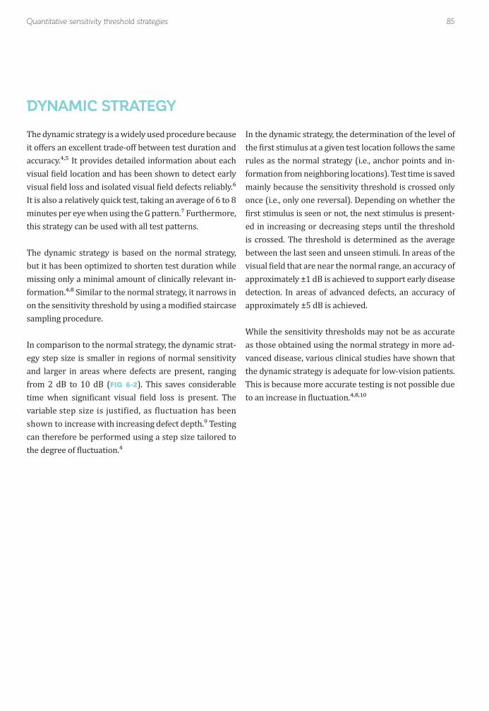
85Quantitative sensitivity threshold strategies
The dynamic strategy is a widely used procedure because it offers an excellent trade-off between test duration and accuracy.⁴,⁵ It provides detailed information about each visual ield location and has been shown to detect early visual ield loss and isolated visual ield defects reliably.⁶ It is also a relatively quick test, taking an average of 6 to 8 minutes per eye when using the G pattern.⁷ Furthermore, this strategy can be used with all test patterns.
The dynamic strategy is based on the normal strategy, but it has been optimized to shorten test duration while missing only a minimal amount of clinically relevant in-formation.⁴,⁸ Similar to the normal strategy, it narrows in on the sensitivity threshold by using a modi ied staircase sampling procedure.
In comparison to the normal strategy, the dynamic strat-egy step size is smaller in regions of normal sensitivity and larger in areas where defects are present, ranging from 2 dB to 10 dB (FIG 6-2). This saves considerable time when signi icant visual ield loss is present. The variable step size is justified, as fluctuation has been shown to increase with increasing defect depth.⁹ Testing can therefore be performed using a step size tailored to the degree of luctuation.⁴
In the dynamic strategy, the determination of the level of the irst stimulus at a given test location follows the same rules as the normal strategy (i.e., anchor points and in-formation from neighboring locations). Test time is saved mainly because the sensitivity threshold is crossed only once (i.e., only one reversal). Depending on whether the irst stimulus is seen or not, the next stimulus is present-
ed in increasing or decreasing steps until the threshold is crossed. The threshold is determined as the average between the last seen and unseen stimuli. In areas of the visual ield that are near the normal range, an accuracy of approximately ±1 dB is achieved to support early disease detection. In areas of advanced defects, an accuracy of approximately ±5 dB is achieved.
While the sensitivity thresholds may not be as accurate as those obtained using the normal strategy in more ad-vanced disease, various clinical studies have shown that the dynamic strategy is adequate for low-vision patients. This is because more accurate testing is not possible due to an increase in luctuation.⁴,⁸,¹⁰
DYNAMIC STRATEGY

FIGURE 6-2 An example of the procedure used in the dynamic strategy is presented. The dynamic strategy samples with
increasing step size (from 2 to 10 dB from normal sensitivity threshold) after the fi rst stimulus is not seen until a stimulus is
seen without any further detailing. As a result, the accuracy is between ±1 and ±5 dB, depending on the step size.
86 Chapter 6 | Selecting a test strategy
Threshold14.5 dB
Threshold Zone
Do you see?
Sampling withincreasing step size
32 dB
28 dB
24 dB
20 dB
16 dB
12 dB
8 dB
4 dB
0 dB
1
2
3
4
= Seen
= Not seen
DYNAMIC STRATEGY
The low-vision (LV) strategy is useful for assessing pa-tients with end-stage diseases, when only limited visual ield function remains. It employs a methodology similar
to the normal strategy, but only performs one threshold crossing (4-2 bracketing), which reduces test duration. While an accuracy of only approximately ±2 dB can be achieved, this is justi ied by the large luctuation in areas of low vision.⁹ In addition, the low-vision strat-egy starts testing at a sensitivity threshold of 0 dB (FIG
6-3). This means that the initial stimulus used is at the maximum stimulus intensity because of the inverse re-lationship between light intensity and sensitivity thresh-old, as outlined in FIG 2-2. This approach further reduces test duration when a visual ield contains a large number of locations with absolute defects. For such situations, testing with the dynamic or normal strategy would take
longer because more stimuli would be presented in lo-cations where there is no sensitivity.
Besides saving test time, the low-vision strategy is also more patient-friendly for low-vision patients, because starting the test with the maximum stimulus intensity increases the likelihood that the initial stimulus will be seen. This allows patients to feel con ident about their performance in the initial stage of the test.
In order to extend the dynamic testing range into the low-vision area and also to make the target easier to see for low-vision patients, the low-vision strategy is typically used in combination with a stimulus size V that is pre-sented for 200 ms (see Chapter 10 for more information on stimulus size V for low-vision patients).
LOW-VISION STRATEGY

FIGURE 6-3 The low-vision strategy is optimized for low-vision patients and is a variation of the normal strategy. Signifi cant
test time is saved by crossing the threshold only once. Patient confi dence is also increased by starting at a sensitivity threshold
of 0 dB, the maximum stimulus intensity available on the device.
87Quantitative sensitivity threshold strategies
Threshold Zone
Do you see?
Sampling in4 dB steps
32 dB
28 dB
24 dB
20 dB
16 dB
12 dB
8 dB
4 dB
0 dB
Threshold6 dB
1
3
2
= Seen
= Not seen
LOW-VISION STRATEGY
The Tendency-Oriented Perimetry (TOP) strategy is a widely used and fast procedure. It takes only two to four minutes per eye for a complete sensitivity thresh-old examination with the G pattern.³,¹¹-¹³ Because of its short duration, it is especially recommended for patients unable to maintain concentration for long periods, such as the neurologically impaired or children.¹⁴ For these patients, fatigue or lack of concentration in a longer test would lead to unreliable results.¹⁵,¹⁶ The TOP strategy is also useful as a practical routine method for testing and following patients of all age groups, especially in busy practices.¹⁶
The TOP strategy takes advantage of the fact that sensi-tivity thresholds at each location of the visual ield are
related to the sensitivity thresholds at nearby locations (i.e., there is a spatial correlation among adjacent test lo-cations). During the test, answers at any given location are taken into account to adjust the expected sensitivity thresholds at neighboring locations. The test starts by presenting stimuli at 50% of normal sensitivity thresh-olds at a quarter of the test locations. If the stimulus at a certain location is missed, the stimuli at immediately adjacent locations are presented at lower sensitivity thresholds. However, if the stimulus is seen, the initial stimuli at neighboring locations are presented at higher sensitivity thresholds. This procedure is repeated for all test locations with answers from neighboring test loca-tions leading to an adaptation of all test locations. See BOX 6B for more details.
TENDENCY-ORIENTED PERIMETRY (TOP) STRATEGY

88 Chapter 6 | Selecting a test strategy
TOP STRATEGY – STEP-BY-STEP PROCEDUREBOX 6B
STEP 0• Baseline: normal
sensitivities at each
test location
• Test pattern divided into
4 sub-test patterns
STEP 1A• Submatrix 1 = ½ of
normal sensitivity
• Stimulus presentation
on 1st sub-test pattern
STEP 1B• Seen: Add ¼ of
normal sensitivity
• Not seen: Substract ¼
of normal sensitivity
STEP 1CCalculate responses for
sub-test patterns 2-4
from average of
neighboring locations
by interpolation
STEP 2A• Submatrix 2 = Submatrix 1
+ Response Matrix 1
• Stimulus presentation on
2nd sub-test pattern
STEP 2B• Seen: Add 3/16 of
normal sensitivity
• Not seen: Substract 3/16
of normal sensitivity
STEP 2CCalculate responses for
sub-test patterns 1, 3, 4
from average of
neighboring locations
by interpolation
29 30 31 31 31
30 31 31 32 32
30 32 32 33 33
30 32 32 33 33
30 31 32 32 32
27 28 28 28
28 29 29 29 29 28
29 30 31 31 31 31 30 30
29 30 31 31 32 32 32 31 30 30
29 30 32 32 33 33 32 BS 31 30
30 30 32 32 33 33 32 BS 31 30
30 30 31 32 32 32 32 31 30 30
28 30 31 31 31 31 30 30
28 29 30 30 30 29
29 29 29 29
15 15 16 16 16
15 16 16 16 16
15 16 16 17 17
15 16 16 17 17
15 16 16 16 16
Submatrix 1
7 8 8 0 -8
8 8 8 0 -8
8 8 8 0 -8
8 8 8 4 0
8 8 8 8 8
Response Matrix 1
22 23 24 16 8
23 24 24 16 8
23 24 24 17 9
23 24 24 21 17
23 24 24 24 24
Submatrix 2
NormalSensitivity Threshold
Response Matrix 2
5 5 3 0 -3
5 6 6 6 0
6 6 6 6 0
6 6 6 6 0
6 6 6 6 3
STEP 3A• Submatrix 3 = Submatrix 2
+ Response Matrix 2
• Stimulus presentation on
3rd sub-test pattern
STEP 3B• Seen: Add 2/16 of
normal sensitivity
• Not seen: Substract 2/16
of normal sensitivity
STEP 3CCalculate responses for
sub-test patterns 1, 2, 4
from average of
neighboring locations
by interpolation
27 28 27 16 5
28 30 30 22 8
29 30 30 23 9
29 30 30 27 17
29 30 30 30 27
Submatrix 3
2 0 0 -2 -4
4 4 4 0 -4
4 4 4 2 0
4 4 4 4 4
4 4 4 4 4
Response Matrix 3

89Quantitative sensitivity threshold strategies
STEP 5• Sensitivity threshold =
Submatrix 4 + Response
Matrix 4
STEP 4A• Submatrix 4 = Submatrix 3
+ Response Matrix 3
• Stimulus presentation on
4th sub-test pattern
STEP 4B• Seen: Add 1/16 of
normal sensitivity
• Not seen: Substract 1/16
of normal sensitivity
STEP 4CCalculate responses for
sub-test patterns 1 – 3
from average of
neighboring locations
by interpolation
29 28 27 14 1
32 34 34 22 4
33 34 34 25 9
33 34 34 31 21
33 34 34 34 31
Submatrix 4
-2 -2 -2 -2 -2
-2 -2 -1 0 0
-2 -2 0 2 2
-2 -2 0 2 2
-2 -2 0 2 2
Response Matrix 4
27 26 25 12 0
30 32 33 22 4
31 32 34 27 11
31 32 34 33 23
31 32 34 36 33
Sensitivity Threshold
14 3 0 0
22 16 3 0 0 0
26 25 23 11 0 0 0 2
28 29 30 31 21 4 0 0 4 7
29 30 31 34 26 10 4 BS 5 7
29 30 31 34 33 22 16 BS 13 13
29 30 30 33 35 32 29 26 24 21
29 29 31 32 32 32 3 30
28 28 29 29 29 28
27 28 28 28
Because the initial stimuli are presented at a lower sensi-tivity threshold – and thus higher light intensity (see FIG
2-2 for the inverse relationship between light intensity and sensitivity threshold) – in the TOP strategy than in the dynamic or normal strategies, the likelihood of see-ing most of the initial stimuli is increased. This allows patients to feel con ident about their performance for the initial stage of the test, resulting in a shorter patient learning curve, increased reliability for the initial exam-inations, and possibly greater motivation for patients to return for follow up testing.
While the advantages of the TOP strategy, in terms of reduction of test duration and fatigue effects, can lead to
increased accuracy,¹⁵ this strategy also has some short-comings related to accuracy. The TOP strategy can reliably detect large contiguous scotomas such as those present in glaucoma.¹³,¹⁶,¹⁷ However, it smoothes the edges of the scotomas¹⁸ (FIG 6-4) and is less sensitive to small, localized defects compared to a systematic sampling pro-cedure such as the dynamic strategy.⁶,¹¹,¹² These factors should be kept in mind when making clinical decisions.
In addition, the TOP strategy requires a reasonably dense test grid to justify the assumption that there is a spatial correlation between the test points. Therefore, it is only available for the central 30° patterns G, 32, 30-2 and 24-2 and the macula test patterns M and 10-2.

90 Chapter 6 | Selecting a test strategy
SPATIAL RESOLUTION OF NORMAL, DYNAMIC AND TOP STRATEGY
FIGURE 6-4 When choosing a test strategy, there is a trade-off between test duration and accuracy as the example above illus-
trates. The same patient was tested with the G pattern and the normal (left), dynamic (center) and TOP (right) strategies. Note
that while all strategies allow the identifi cation of a double arcuate defect, the visual fi eld measured with the TOP strategy shows
the defect as shallower with smoother edges, but it also saves considerable test time.
DYNAMIC6-8 minutes
NORMAL10-12 minutes
TOP2-4 minutes
9
12
6
3
12
6
9 3 9
12
6
3
Qualitative strategies are useful and time-ef icient when the quanti ication of a patient’s sensitivity threshold is not necessary. These strategies are used for visual ield performance ability testing including driving,¹⁹ legal blindness and ptosis examinations. They are also some-times used for pathologies that result in absolute defects. For example, qualitative strategies can be used to assess the vision of patients with neurological conditions that result in hemianopia, quadrantanopia²⁰ and blind spot enlargements. Furthermore, they can also be useful in
assessing the vision of patients with certain retinal pa-thologies. Finally, they can be used to quickly screen patients with assumed normal vision.
The answers obtained with these strategies are always qualitative (e.g., seen/not seen or normal visual ield/abnormal visual ield). Octopus perimeters offer several qualitative strategies for different purposes, as described below.
QUALITATIVE STRATEGIES

91Qualitative strategies
FIGURE 6-5 Three examples of visual fi eld tests performed with a 1LT strategy. For absolute defects such as the lid margin
in blepharoptosis testing (left) or blind spot testing (center), the 1LT strategy provides suffi cient information to delineate the
boundaries. In the Esterman test (right), it is used to determine the percentage of test locations missed and provides informa-
tion about a patient’s ability to drive.
EXAMPLES OF THE USE OF THE 1-LEVEL TEST STRATEGY IN DIFFERENT SITUATIONS
30°
BLEPHAROPTOSIS BLIND SPOT BINOCULAR ESTERMAN
90°
10 30 40 50 60 70 80 90
90
270
0180
90
270
0180
90°
10 30 40 50 60 70 80 90
90
270
0180
With the 1LT strategy, only one stimulus is presented at each test location at the predetermined intensity level of 6 dB below the normal sensitivity threshold. The pa-tient either sees or misses these stimuli (FIG 6-6). The visual ield is consequently divided into two zones, seen (represented by a “+” sign) and not seen (represented by a “ ”symbol). As a result, this strategy is sometimes referred to as a two-zone strategy. Clinically, visual ield
locations with the “+” sign can be interpreted as normal and those with the “ ”symbol as abnormal.
Note that typically more than one abnormal visual ield location showing a disease-speci ic pattern is required to classify a visual ield as abnormal. For more detailed information on the distinction between normal and ab-normal visual ields, see FIG 7-9, 7-10, 8-14 and 8-15..
The 1-Level Test (1LT) is a fast test strategy most com-monly used for legal performance ability tests to assess whether someone ful ills the minimal visual ield criteria to drive or to perform other daily tasks. In addition, it is
used to assess absolute visual ield defects such as blind spot enlargements or the lid margin in blepharoptosis testing (FIG 6-5).
1-LEVEL TEST STRATEGY (TWO-ZONE STRATEGY)

92 Chapter 6 | Selecting a test strategy
1-LEVEL TEST STRATEGY
FIGURE 6-6 With the 1LT strategy, the visual fi eld is divided into areas of likely normal and abnormal visual fi eld locations.
Stimuluspresented at6dB below
normalsensitivitythreshold
0 dB
Normal
Abnormal
Do you see?
0 dB
Abnormalvisual field location
Normalvisual field location
= Seen
= Not seen
The screening strategy is used to quickly distinguish be-tween people with normal and abnormal visual ields. It is a very fast strategy and patients with normal visual ields can typically complete it within one minute. It is
designed to be used with the G-Screening (GS) pattern.
The screening strategy is useful and time-effective when routine visual ield testing is performed on every patient to identify pathologies that would otherwise be missed
with a routine eye examination. In that context, the screening strategy together with the GS pattern offers a very good trade-off between testing time and accuracy by being fast while at the same time allowing the identi-ication of patients with abnormal visual ields. If a visual ield abnormality is detected during routine screening,
further quantitative testing is recommended to assess the extent and depth of visual ield loss (FIG 6-7).
SCREENING STRATEGY

93Qualitative strategies
EXAMPLE OF THE USE OF THE SCREENING STRATEGY
EXAMPLE OF THE USE OF THE SCREENING STRATEGY
FIGURE 6-7 The routine testing with the screening strategy and the short G-Screening pattern allows the identifi cation of poten-
tially unnoticed visual fi eld defects with minimal test duration. This can identify patients who require a more detailed evaluation.
In the case presented above, a patient with early glaucoma was detected during routine screening, and consequent quantitative
visual fi eld testing confi rmed the existence of the previously unnoticed partial arcuate defect.
FIGURE 6-8 The screening strategy distinguishes between normal and abnormal visual fi elds by presenting a stimulus at an
intensity that people with normal visual fi elds would see 95% of the time.
SCREENING TESTScreening strategy
G-Screening pattern
QUANTITATIVE TESTDynamic strategy
G pattern
9
12
6
3 9
12
6
3
+ +
+
+
+
+
++
+
+ +
+++
+
+ +
++
+
+
+
+
+
+
Normal
Abnormal
Normalvisual field location
Normalvisual field location
0 dB
Do you see?
Stimulusintensity
that peoplewith normalvisual fields
see 95%of time
0 dB 0 dB
Abnormalvisual field location
= Seen
= Not seen
The screening strategy is a modi ied version of the 1-Level Test strategy (FIG 6-8). The irst stimulus at each location is presented at the intensity that an average subject with a normal visual ield would see 95% of the time. If the point is seen, the location is designated as normal. If it is not seen however, the same point is repeated twice to con irm suspected abnormalities and to avoid false nega-tive errors, which are common in patients inexperienced
with visual ield testing. If the patient sees the stimulus on any of these repetitions, the location is designated as normal (represented by a “+” sign), otherwise it is re-corded as abnormal (represented by a “ ” sign). Because unseen points are tested three times, the likelihood of obtaining false negative errors is reduced. This approach results in better speci icity for the screening test.²¹

94 Chapter 6 | Selecting a test strategy
The 2-Level Test (2LT) strategy is similar to the 1LT, but presents stimuli at two sensitivity thresholds. It conse-quently divides the visual ield into three zones and is thus also referred to as a three-zone strategy.
The 2LT strategy is commonly used as an alternative to the quantitative dynamic strategy to assess the full visual ield in pathologies that result in hemianopia, quadran-
tanopia or certain retinal conditions such as diabetic retinopathies, retinal detachments and retinoschisis. Because these pathologies affect a signi icant portion of the visual ield and often contain a meaningful number of absolute defects, quantitative testing with a reasonably dense test pattern can be too time-consuming and conse-quently lead to unreliable results in some patients due to
fatigue. In such situations, the 2LT strategy offers a good trade-off between test duration and accuracy, often with only minimum loss of clinical information (FIG 6-9).
The 2LT strategy provides only a rough indication of the status of the visual ield. It is designed to distinguish between areas of normal visual ield, areas with relative defects (i.e., with reduced sensitivity thresholds) and areas with absolute defects (i.e., with a sensitivity thresh-old of 0dB, where the maximum stimulus intensity of the perimeter cannot be seen). This information is often clinically suf icient to identify diseases whose diagnosis is based on the shape of the defect rather than on small changes in sensitivity.
2-LEVEL TEST STRATEGY (THREE-ZONE STRATEGY)
QUALITATIVE TEST WITH 2LT STRATEGY VS QUANTITATIVE TEST
FIGURE 6-9 The qualitative 2LT strategy allows distinction of areas of normal vision and relative and absolute defects with
minimal test duration (left) and provides valuable information about the shape of defects. Quantifi cation of the same test pattern
with the dynamic strategy reveals the same pattern as well as detailed information about the sensitivity thresholds, but at the
expense of a longer test (right). In this example, because the visual fi eld shows an absolute defect, the amount of information
provided by the 2LT strategy is comparable to the more detailed information provided by the quantitative dynamic strategy.
QUANTITATIVE TESTDynamic strategy
07 pattern
QUALITATIVE TEST2 LT strategy07 pattern
+
+
+
++
+ +
+ ++
++
+ ++ +
++++
++
+ + +
+
+++
+ + +
+ +
+
++
+ +
++ +
++
++
+
+
+
+ +
++
+
+
+ +
++
+
+
+
+
+
+ +
+ +
++
+++
++
+ +
+
12
6
9 3
12
6
9 3
++
+

95Qualitative strategies
The 2LT strategy starts with the presentation of a stim-ulus 4dB below the normal sensitivity threshold at each location. When this stimulus is seen, it is designated as normal (represented by a “+” sign). When this stimulus is not seen, a second stimulus is presented at a sensitivity threshold of 0 dB, which corresponds to the maximum stimulus intensity that the perimeter can present (FIG
6-10). If this is seen, the location is marked as having a relative defect (represented by a “ ” sign) and if it is not
seen, it is marked as having an absolute defect (repre-sented by a “ ” sign).
Note that typically more than one abnormal visual ield location showing a disease-speci ic pattern is required to classify a visual ield as abnormal. For more detailed information on the distinction between normal and ab-normal visual ields, see FIG 7-9, 7-10, 8-14 and 8-15.
2-LEVEL TEST STRATEGY
FIGURE 6-10 With the 2LT strategy, the visual fi eld is divided into areas of normal visual fi eld results, relative defects and
absolute defects.
Stimuluspresented at4dB below
normalsensitivitythreshold
0 dB 0 dB 0 dB
Normal visualfield location
Relativedefect
Absolutedefect
Normal
Relative defect
Absolute defect
Do you see?
= Seen
= Not seen

96 Chapter 6 | Selecting a test strategy
There is always a trade-off between test duration and accuracy, but depending on the pathology or visual abil-ity test performed, certain test parameter combinations offer better trade-offs than others. TABLE 6-3 presents
This does not mean that these settings are the best for each visual ield test; an expert user may prefer other combinations for certain situations. Therefore, Octopus perimeters offer the lexibility to customize examination parameters. However, there are two exceptions: 1) because the TOP strategy requires test locations to be relatively
recommended combinations of test patterns and strat-egies for a variety of visual ield testing situations that maximize clinical information and minimize test duration.
close to each other, it can only be used with the suf icient-ly dense central 30° and macula test patterns; 2) legally prescribed ability tests such as the Esterman test are offered only with their standardized settings to ensure that the legal requirements are met.
RECOMMENDATIONS ON KEY EXAMINATION PARAMETERS
GLAUCOMA/CENTRAL FIELD
MACULA
FULL FIELD (NEURO, RETINA)
FOVEA
BLIND SPOT
LOW VISION
SCREENING FORABNORMAL VISION
DRIVING
BLEPHAROPTOSIS
BLINDNESS
TEST PATTERN
G, 32, 30-2, 24-2
M, 10-2
07
Fovea
Blind spot
M, G, 07 depending on pathology
G-Screening
Esterman
German Legal Driving (Führerscheingutachten FG)
BT
BG
RECOMMENDED STRATEGIES
Dynamic or TOP
Dynamic or TOP
Dynamic or 2LT
Dynamic
1LT
Low Vision
Screening
Fixed parameters(1LT, stimulus duration 500 ms)
Fixed parameters(2LT, stimulus duration 200ms)
1LT
Fixed parameters(1LT, stimulus duration 500ms)
RECOMMENDED TEST PATTERN AND STRATEGY COMBINATIONS TABLE 6-3

97References
REFERENCES1. Bebie H, Fankhauser F, Spahr J. Static perimetry: strategies. Acta Ophthalmol (Copenh). 1976; 54:325-38.2. Spahr J. Optimization of the presentation pattern in automated static perimetry. Vision Res. 1975;15:1275-1281.3. Gonzáles de la Rosa M, Morales J, Dannheim F, et al. Multicenter evaluation of tendency-oriented perimetry (TOP) using the G1 grid. Eur J Ophthalmol. 2003;13:32-41.4. Weber J, Klimaschka T. Test time and ef iciency of the dynamic strategy in glaucoma perimetry. Ger J Ophthalmol. 1995;4:25-31.5. Weber J. A new strategy for automated static perimetry. Fortschr Ophthalmol. 1990;87:37-40.6. Maeda H, Nakaura M, Negi A. New perimetric threshold test algorithm with dynamic strategy and tendency oriented perimetry (TOP) in glaucomatous eyes. Eye (Lond). 2000;14:747-751.7. Zein WM, Bashshur ZF, Jaafar RF, Noureddin BN. The distribution of visual ield defects per quadrant in standard automated perimetry as compared to frequency doubling technology perimetry. Int Ophthalmol. 2010;30:683-689.8. Zulauf M, Fehlmann P, Flammer J. Perimetry with normal Octopus technique and Weber 'dynamic' technique. Initial results with reference to reproducibility of measurements in glaucoma patients. Ophthalmologe. 1996;93:420-427.9. Wall M, Woodward KR, Doyle CK, Artes PH. Repeatability of automated perimetry: a comparison between standard automated perimetry with stimulus size III and V, matrix, and motion perimetry. Invest Ophthalmol Vis Sci. 2009;50:974-979.10. Gardiner SK, Swanson WH, Goren D, Mansberger SL, Demirel S. Assessment of the reliability of standard automated perimetry in regions of glaucomatous damage. Ophthalmology. 2014:121:1359-1369.11. King AJ, Taguri A, Wadood AC, Azuara-Blanco A. Comparison of two fast strategies, SITA Fast and TOP, for the assessment of visual ields in glaucoma patients. Graefes Arch Clin Exp Ophthalmol. 2002;240:481-487.12. Morales J, Weitzman ML, Gonzáles de la Rosa M. Comparison between Tendency-Oriented Perimetry (TOP) and octopus threshold perimetry. Ophthalmology. 2000;107:134-142.13. Wadood AC, Azuara-Blanco A, Aspinall P, Taguri A, King AJ. Sensitivity and speci icity of frequency-doubling technology, tendency-oriented perimetry, and Humphrey Swedish interactive threshold algorithm-fast perimetry in a glaucoma practice. Am J Ophthalmol. 2002;133:327-332.14. Morales J, Brown SM. The feasibility of short automated static perimetry in children. Ophthalmology. 2001;108:157-162.15. Gonzalez-Hernandez M, Morales J, Azuara-Blanco A, Sanchez JG, de la Rosa MG. Comparison of diagnostic ability between a fast strategy, tendency-oriented perimetry, and the standard bracketing strategy. Ophthalmologica. 2005;219:373-378.16. Scherrer M, Fleischhauer JC, Helbig H, Johann Auf der Heide K, Sutter FK. Comparison of tendency-oriented perimetry and dynamic strategy in octopus perimetry as a screening tool in a clinical setting: a prospective study. Klin Monbl Augenheilkd. 2007;224:252-254.17. Pierre-Filho Pde T, Schimiti RB, de Vasconcellos JP, Costa VP. Sensitivity and speci icity of frequency-doubling technology, tendency-oriented perimetry, SITA Standard and SITA Fast perimetry in perimetrically inexperienced individuals. Acta Ophthalmol Scand. 2006;84:345-350.18. Anderson AJ. Spatial resolution of the tendency-oriented perimetry algorithm. Invest Ophthalmol Vis Sci. 2003;44: 1962-1968.19. Esterman B. Functional scoring of the binocular ield. Ophthalmology. 1982;89:1226-1234.20. Siatkowski RM, Lam BL, Anderson DR, Feuer WJ, Halikman AM. Automated suprathreshold static perimetry screening for detecting neuro-ophthalmologic disease. Ophthalmology. 1996;103:907-917.21. Turpin A, Myers JS, McKendrick AM. Development of visual ield screening procedures: a case study of the Octopus perimeter. Transl Vis Sci Technol. 2016; doi: 10.1167/tvst.5.3.3.

98

99
CHAPTER 7OVERVIEW OF VISUAL FIELDREPRESENTATIONS
INTRODUCTION
RELATIONSHIP AMONG OCTOPUSVISUAL FIELD REPRESENTATIONS
Perimetry determines sensitivity thresholds through-out the visual ield. However, it can be challenging to correctly interpret the raw data in clinical practice be-cause 1) normal sensitivity thresholds vary with age and eccentricity of test location; 2) visual ield testing contains a subjective component due to the patient de-cision processes, which contributes to luctuation; 3) both visual ield location and disease severity in luence fluctuation; and 4) in some patients, more than one disease may be present. For more information on these points, see Chapter 2.
Most visual ield representations on Octopus perimeters are based on the following three key representations: 1) Values (the sensitivity thresholds); 2) Comparison (the comparison of the sensitivity thresholds with age-matched normative data); and 3) Corrected Comparison (the comparison of the sensitivity thresholds with age-matched normative data, with a correction that eliminates
For these reasons, Octopus perimeters offer several re-presentations that are based on the measured sensitivity thresholds, but highlight speci ic aspects of the visual ield, in order to support clinical decision-making. In
this chapter, a systematic presentation of all visual ield representations and indices is offered, with their de ini-tions, design and relationships. While a detailed under-standing of these characteristics is not necessary for correct clinical interpretation, some readers will ind this information useful. The clinical meaning and inter-pretation of these same visual ield representations are subsequently discussed in a clinical step-by-step work-low in Chapter 8, which also includes several examples.
the in luence of diffuse or widespread defects). FIG 7-1 provides an overview of these relationships.
In addition, Octopus perimeters determine several indi-cators of visual ield reliability, to assess whether a visual ield test is trustworthy or not. These are presented at
the end of this chapter.

FIGURE 7-1 All visual fi eld representations are based on the measured sensitivity thresholds (i.e., Values) and are mostly
compared to age-matched normative data (top), resulting in representations that show sensitivity loss (center). Some
representations also only display local sensitivity loss (bottom) because they are additionally corrected to eliminate the
infl uence of diffuse or widespread defects.
100 Chapter 7 | Overview of visual fi eld representations
7
+ +5
+
++
5
10
10
22
1221
10
5 17++
15 13
67
30
+
+
6 6
8
10
57 31
+8
+ 5
58
13 22
+8
22 16
+5
11 +
++
25
7
9 8
+8
1 59
5%
95%
-5
0
5
10
15
20
25
9.1
11.315.8
24.99.7
4.42.7
3.55.8
8.3
102030[dB]
S
IN T
+
+ ++
+
++
+
5
+
16
715
5
+ 12++
10 8
++
24
+
+
+ +
+
5
++ 26
++
+ +
++
8 17
++
16 10
++
6 +
++
20
+
+ +
++
3.7
5.910.4
19.54.3
++
++
2.9
24
29 2928
28
2528
26
18
22
7
1611
19
28 163031
12 14
2323
1
30
25
23 21
19
18
3024 1
2824
23 21
2322
15 5
2521
9 15
2927
18 25
2627
1
19
17 17
2421
31 31
3131
28
28
33 333333
27 27
2930
28
29
27 26
2628
32 32
3332
28
28
27
27
29 29
3030
26 25
2829
29 29
3131
31
3135
26 26
2830
28 27
2929
31 323232
31 31
3232
Normative Values
(Measured )Values
Comparison Grayscale (Comparison)
Grayscale (Values)
Defect Curve
Diffuse Defect
DD
Probabilities Cluster Analysis
Polar Analysis
Corrected Comparison Corrected Probabilities Corrected Cluster Analysis
MD(Mean Defect)
sLV(square root
of Loss Variance)DD
(Diffuse Defect)LD
(Local Defect)
Defe
ct (
dB
)
Rank
MS(Mean Sensitivity)
=
-
-
SENSITIVITY THRESHOLDS
SENSITIVITY LOSS
= LOCAL SENSITIVITY LOSS
RELATIONSHIP AMONG DIFFERENT VISUAL FIELD REPRESENTATIONS
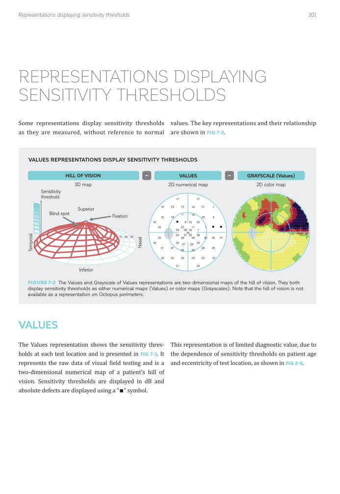
FIGURE 7-2 The Values and Grayscale of Values representations are two-dimensional maps of the hill of vision. They both
display sensitivity thresholds as either numerical maps (Values) or color maps (Grayscales). Note that the hill of vision is not
available as a representation on Octopus perimeters.
101
Superior
HILL OF VISION
3D map
GRAYSCALE (Values)
2D color map
VALUES
2D numerical map
Tem
po
ral
Nasal
Inferior
Blind spotFixation
24
29 2928
28
2528
26
18
22
7
1611
19
28 163031
12 14
2323
1
30
25
23 21
19
18
3024 1
2824
23 21
2322
15 5
2521
9 15
2927
18 25
2627
1
19
17 17
2421
90˚80˚70˚
Sensitivity
threshold
~~
Representations displaying sensitivity thresholds
VALUES REPRESENTATIONS DISPLAY SENSITIVITY THRESHOLDS
REPRESENTATIONS DISPLAYINGSENSITIVITY THRESHOLDS
Some representations display sensitivity thresholds as they are measured, without reference to normal
values. The key representations and their relationship are shown in FIG 7-2.
The Values representation shows the sensitivity thres-holds at each test location and is presented in FIG 7-3. It represents the raw data of visual ield testing and is a two-dimensional numerical map of a patient’s hill of vision. Sensitivity thresholds are displayed in dB and absolute defects are displayed using a “ ” symbol.
This representation is of limited diagnostic value, due to the dependence of sensitivity thresholds on patient age and eccentricity of test location, as shown in FIG 2-9.
VALUES
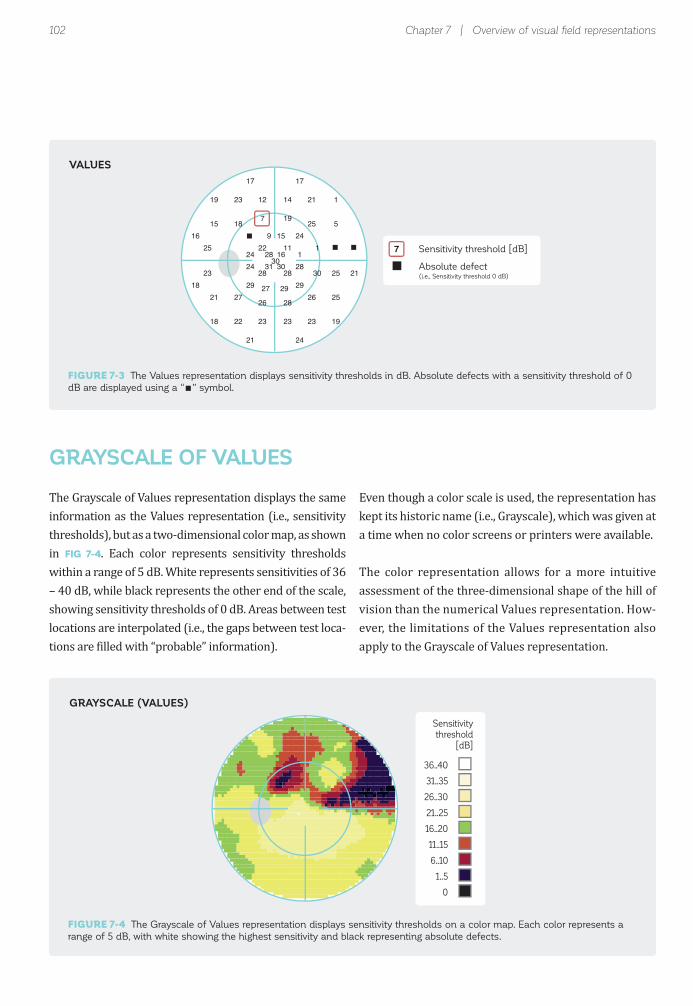
102 Chapter 7 | Overview of visual fi eld representations
Sensitivity threshold [dB]7
Absolute defect(i.e., Sensitivity threshold 0 dB)
24
29 2928
28
2528
26
18
22
7
1611
19
28 163031
12 14
2323
1
30
25
23 21
19
18
3024 1
2824
23 21
2322
15 5
2521
9 15
2927
18 25
2627
1
19
17 17
2421
Sensitivity
threshold
[dB]
36..40
31..35
26..30
21..25
16..20
11..15
6..10
1..5
0
The Grayscale of Values representation displays the same information as the Values representation (i.e., sensitivity thresholds), but as a two-dimensional color map, as shown in FIG 7-4. Each color represents sensitivity thresholds within a range of 5 dB. White represents sensitivities of 36 – 40 dB, while black represents the other end of the scale, showing sensitivity thresholds of 0 dB. Areas between test locations are interpolated (i.e., the gaps between test loca-tions are illed with “probable” information).
Even though a color scale is used, the representation has kept its historic name (i.e., Grayscale), which was given at a time when no color screens or printers were available.
The color representation allows for a more intuitive assessment of the three-dimensional shape of the hill of vision than the numerical Values representation. How-ever, the limitations of the Values representation also apply to the Grayscale of Values representation.
GRAYSCALE OF VALUES
VALUES
GRAYSCALE (VALUES)
FIGURE 7-3 The Values representation displays sensitivity thresholds in dB. Absolute defects with a sensitivity threshold of 0
dB are displayed using a “ ” symbol.
FIGURE 7-4 The Grayscale of Values representation displays sensitivity thresholds on a color map. Each color represents a
range of 5 dB, with white showing the highest sensitivity and black representing absolute defects.

103Representations based on comparison with normal
24
29 2928
28
2528
26
18
22
7
1611
19
28 163031
12 14
2323
1
30
25
23 21
19
18
3024 1
2824
23 21
2322
15 5
2521
9 15
2927
18 25
2627
1
19
17 17
2421
7
+ +5
+
++
5
10
10
22
1221
5 17++
15 13
67
30
+
+
6 6
8
10
57 31
+8
+ 5
58
13 22
+8
22 16
+5
11 +
++
25
7
9 8
+8
31 31
3131
28
28
33 333333
27 27
2930
28
29
27 26
2628
32 32
3332
28
28
27
27
29 29
3030
26 25
2829
29 29
3131
31
3135
26 26
2830
28 27
2929
31 323232
31 31
3232
Sensitivity
threshold
NORMATIVE VALUESNormal sensitivity threshold
- =
(MEASURED) VALUESMeasured sensitivity threshold
COMPARISON (TO NORMAL)Sensitivity loss
Measured Valuesof a 20-year-old
Comparison
Normative Valuesof 20-year-olds
1029
The Comparison representation allows direct assessment of the shape and magnitude of disease-related change in sensitivity. In contrast to the Values representation, its in-terpretation is independent of the age and eccentricity of
test locations. For that reason, it is the most widely used in clinical practice, and most visual ield representations are based on it.
COMPARISON
COMPARISON REPRESENTATION DISPLAYS DEVIATIONS FROM THE NORMAL VISUAL FIELD
REPRESENTATIONS BASED ON COMPARISON WITH NORMAL
FIGURE 7-5 The Comparison representation calculates the deviation of the measured Values (sensitivity thresholds) from
the Values of an average normal person of the same age (normal sensitivity threshold at each location obtained from a
normative database).

104
Sensitivity loss < 5 dB
Sensitivity loss [dB]22
Absolute defect(i.e., Sensitivity threshold 0 dB)
7
+ +5
+
++
5
10
10
22
1221
10
5 17++
15 13
67
30
+
+
6 6
8
10
57 31
+8
+ 5
58
13 22
+8
22 16
+5
11 +
++
25
7
9 8
+8
+
Chapter 7 | Overview of visual fi eld representations
The Comparison representation is de ined as the individ-ual deviation from the average normal visual ield (stem-ming from the normative database) of the respective age group. The difference in the normative Value minus the measured Value at each test location is also termed sen-sitivity loss, loss value or defect value. This principle is shown in FIG 7-5. More information on normative Values is given in BOX 2B.
Deviations from a normative visual ield are displayed for each location in dB. While the Comparisons are calculated at all visual ield locations, their numerical values are not necessarily presented at all locations, as shown in FIG 7-6.
Deviations smaller than 5 dB in magnitude are displayed with “+” symbols, because as a rule of thumb, they can be considered to be approximately within the normal range of luctuation within the central 30 degrees of the visual ield. Consequently, these small numerical values are not
meaningful for the interpretation of the visual ield. Test locations with a sensitivity threshold of 0 dB have reached the loor of perimetric testing and are marked with a “ ” symbol.
Similar representations in non-Octopus devices are alter-natively called defect map, total deviation (see TABLE 12-5) or deviation from normal.
FIGURE 7-6 The Comparison representation allows for a direct assessment of the magnitude and location of a patient’s
sensitivity loss in dB. A deviation from a normal sensitivity threshold smaller than 5 dB is marked with a “+” symbol, and an
absolute defect with a sensitivity threshold of 0 dB is displayed with a “ ” symbol.
COMPARISON

105
Sensitivity loss [% of normal]0..1011..2223..3435..4647..5859..7071..8283..9495..100
Representations based on comparison with normal
The Grayscale of Comparison is used clinically to intui-tively assess the magnitude and shape of sensitivity loss. It is also useful for patient education because it is easy to understand.
It is a color map in which the areas between test locations are interpolated (i.e., the gaps in between test locations are illed with “probable” information) (FIG 7-7). Since it
There is an inverse relationship between the sensitivity thresholds displayed in the Grayscale of Values and the sensitivity loss displayed in the Grayscale of Comparison. In other words, a high sensitivity threshold means that there is a small, or no loss of sensitivity (i.e., virtually no difference from normal). To facilitate the interpretation of
is based on the Comparison representation, it is indepen-dent of both patient age and eccentricity of test locations.A color scale is used to display sensitivity loss in % in rela-tion to a normal visual ield, with different colors used for different levels of change in sensitivity. For example, a 0% to 10% change in sensitivity is displayed in white, 47% to 58% sensitivity loss is shown in green, and 95% to 100% change in sensitivity is displayed in black.
the Grayscales, similar colors are used to display close to normal visual ields or fully defective visual ields. Since the Values scale is absolute, showing ranges in dB, and the Comparison scale is relative, showing visual ield loss in percent, the patterns show marginal differences. FIG 7-8 demonstrates this relationship.
GRAYSCALE OF COMPARISON
FIGURE 7-7 The Grayscale of Comparison representation is a color map showing sensitivity loss in relation to a normal visual
fi eld. It allows for assessment of the depth and shape of sensitivity loss and is also useful for patient education.
GRAYSCALE (COMPARISON)

106
GRAYSCALE (Values) GRAYSCALE (Comparison)
(MEASURED) VALUES COMPARISON (TO NORMAL)
24
29 2928
28
2528
26
18
22
7
1611
19
28 163031
12 14
2323
1
30
25
23 21
19
18
3024 1
2824
23 21
2322
15 5
2521
9 15
2927
18 25
2627
1
19
17 17
2421
5
+ ++
+
++
+
9
8
21
1120
9
+ 16++
14 12
55
20
+
+
5 5
7
9
+6 30
+6
+ +
+6
12 21
+7
20 14
++
10 +
++
24
6
7 7
+6
Low sensitivity
loss [0 dB]
Low sensitivity
threshold 0 [dB]
High sensitivity
loss [dB]
High sensitivity
threshold [dB]
Sensitivity loss
[% of normal]
Sensitivity
threshold
[dB]
0..10
11..22
23..34
35..46
47..58
59..70
71..82
83..94
95..100
36..40
31..35
26..30
21..25
16..20
11..15
6..10
1..5
0
Chapter 7 | Overview of visual fi eld representations
It should be noted that the Grayscale of Comparison pro-vides more clinically meaningful information than the Grayscale of Values because it is not affected by patient age or the eccentricity of test location, and thus shows a patient’s visual ield loss. When comparing Grayscales of Values for younger and older controls, the Grayscales of the older person are likely to show more loss, because normal age effects are not taken into account. The
Grayscale of Values also shows more severe loss in the peripheral area compared to the central area, due to the effect of eccentricity. The Grayscale of Comparison adjusts for age and eccentricity. For clinical purposes, it is therefore recommended to always use the Grayscale of Comparison, which is part of the standard printouts of Octopus perimeters.
FIGURE 7-8 There is an inverse relationship between the Grayscale of Values and the Grayscale of Comparison represen-
tations. Yet because an inverse color scale is used, the graphics appear similar, thereby facilitating interpretation (light colors
indicate normal areas and darker colors indicate areas with defects). As the Grayscale of Values is an absolute scale (dB) and
the Grayscale of Comparison is a relative scale (percent of normal), the shapes and depths are comparable, but not identical.
INVERSE RELATIONSHIP BETWEEN VALUES AND COMPARISON REPRESENTATIONS

107
ADVANCEDGLAUCOMA
Person A
MODERATEGLAUCOMA
Person B
EARLYGLAUCOMA
Person C
GLAUCOMASUSPECTPerson D
Numberof people
Highsensitivityloss
Nosensitivity
loss
P > 5%
0 dB(Average
normal value)
5%2%
1%0.5%
P <
5%
P <
2%
P <
1%P < 0.5%
NORMALPerson E
Representations based on comparison with normal
The Probabilities representation is used clinically to dis-tinguish between normal and abnormal visual ield loca-tions. This representation is needed because normal luc-tuation is not uniformly distributed across the visual ield; instead, it is smaller in the center and larger towards the peripheral visual ield. It is therefore not possible to use the same numerical cut-off point (e.g., 6 dB sensitivity loss, representing an abnormal visual ield location) for all visual ield locations.
The Probabilities representation uses symbols that are associated with the statistical distribution of normative
data. More precisely, they show the probability that a given sensitivity threshold would be obtained at the respective location for a person of the same age as the patient with a normal visual ield.
For example, a person with a normal visual ield has a high probability of having little to no sensitivity losses. But there is also a small probability that a person with a nor-mal visual ield would obtain some sensitivity loss. FIG 7-9 illustrates this and also displays examples of patient visual ields in relation to normal visual ields.
PROBABILITIES
FIGURE 7-9 The distribution displayed in blue indicates the range of possible sensitivity losses at a specifi c test location
and the probability of these being obtained for a person with a normal visual fi eld. It ranges from no sensitivity loss (right) to
high sensitivity loss (left), with an average normal value of 0 dB. While it is highly unlikely that a person with a normal visual
fi eld would obtain a sensitivity loss at a specifi c test location similar to those seen on the left of the P < 0.5% mark, a small
proportion (0.5%) of the test locations of normal subjects do give these results. The top part of the fi gure illustrates the results
typically obtained for patients at different stages of the disease, at a majority of test locations. Note that for easier readability
the distribution is not drawn to scale.
DISTRIBUTION OF SENSITIVITY THRESHOLDS OF THE NORMAL POPULATION

108
P > 5%P < 5%P < 2%P < 1%P < 0.5%
Probability that a personwith a normal visual field
shows this result
Chapter 7 | Overview of visual fi eld representations
It should be noted that caution is essential in the clinical interpretation of the Probabilities representation. This is due to the fact that a small number of isolated test loca-tions at a level of signi icance of P < 5% is likely to show up, even in normal visual ields. For example. in a G pattern, which has 59 test locations, by de inition a P value of P < 5% should occur in 1 out of 20 locations (i.e., on average
The Probabilities representation shows the probability (P) that a normal population shows a given sensitivity loss. When the sensitivity loss is high, the likelihood that it comes from a person with a normal visual ield is low. From a clinical perspective, one could assume that it is more likely that the sensitivity loss comes from the pa-tient population.
Increasingly darker symbols are used to show the de-creasing probability that a person with a normal visual ield would show a given sensitivity loss at a certain test
location (FIG 7-10):
(P > 5%): there is a high probability that a person with a normal visual ield would show this sensitivity loss.
for 3 locations). The same is true for a level of signi icance of P < 2%, which by de inition occurs in 1 out of 50 test locations (i.e., on average for one location in the G pattern). A level of signi icance of P < 0.5% is even expected to occur in one out of three normal visual ields. More information on how to clinically interpret the Probabilities representa-tion is given in FIG 8-15.
(P < 5%): there is a smaller than 5% (and larger than 2%) chance that a person with a normal visual ield would show this sensitivity loss.
(P < 2%): there is a smaller than 2% (and larger than 1%) chance that a person with a normal visual ield would show this sensitivity loss.
(P < 1%): there is a smaller than 1% (and larger than 0.5%) chance that a person with a normal visual ield would show this sensitivity loss.
(P < 0.5%): there is a smaller than 0.5% chance that a person with a normal visual ield would show this sen-sitivity loss.
FIGURE 7-10 The various symbols on the Probabilities representation show the likelihood that a given sensitivity loss would
be obtained for a person with normal vision. For example, the black square (P < 0.5%) indicates that while it is possible that a
person with normal vision could obtain that defect value, the probability of this occurring is very small (less than 0.5%).
PROBABILITIES

109
COMPARISON (TO NORMAL)
7
+ +5
+
++
5
10
10
22
1221
10
5 17++
15 13
67
30
+
+
6 6
8
10
57 31
+8
+ 5
58
13 22
+8
22 16
+5
11 +
++
25
7
9 8
+8
1 59
5%
95%
-5
0
5
10
15
20
25
Average normalDefect Curve
Normal band of Defect Curve
Defect Curve
X-axis:Ranks
Y-axis:Defectsin dB
+
7
13
22
DESIGN OF THE DEFECT CURVE
The Defect Curve is based on the Comparison representation (i.e., the sensitivity loss in comparison to the normal visual ield). The Comparisons are irst ranked according to their magnitude, from the small-est to the largest defect. The Defect Curve is drawn by plotting the defects (y-axis) as a function of their rank (x-axis). To give an example, the 28th smallest defect in the igure below is about 7 dB. The y-axis ranges from -5 to 25 dB. It must be noted that negative values indicate that there was no defect com-pared to normal and that the sensitivity is higher than the average normal value. This typically happens randomly at a few locations in every normal visual ield, and therefore the average normal visual ield shows negative values in the irst ranks.
This procedure generates the Defect Curve, which by de inition always starts from the top left and moves to the bottom right. Note that spatial information is lost. The average normal Defect Curve is displayed to serve as a reference, lanked by upper and lower limits that show the area in which 90% of normal Defect Curves lie.
BOX 7A
Representations based on comparison with normal
The Defect Curve (also called Bebie Curve¹) is a graphical representation that alerts the clinician to the presence of diffuse defects. It provides a summary of the visual ield
The interpretation of the Defect Curve is straightforward. Parallel downward shifts of the Defect Curve represent diffuse defects; a drop on the right-hand side of the curve represents local defects and Defect Curves within the normal band are considered to be normal. In many
and makes it possible to distinguish between local and diffuse defects at a glance. For more information on its design, see BOX 7A.
instances, a combination of diffuse (or widespread) loss and local visual ield loss is present. FIG 7-11 shows these four main situations, while more examples are provided in FIG 8-10.
DEFECT CURVE
The Defect Curve is a representation that ranks individual defects according to their size from left to right. Normal visual ields have a Defect Curve within the normal band, while the Defect Curve in abnormal visual ields lies outside the normal band.
DEFECT CURVE

110
DIFFUSE DEFECT
Parallel downward shift of
Defect Curve
1 59
5%
95%
-5
0
5
10
15
20
25
LOCAL DEFECT
Drop of Defect Curve
on the right
1 59
5%
95%
-5
0
5
10
15
20
25
LOCAL & DIFFUSE DEFECT
Parallel downward shift on
the left and drop on the right
1 59
5%
95%
-5
0
5
10
15
20
25
NORMAL
Defect Curve within normal
band
1 59
5%
95%
-5
0
5
10
15
20
25
Defe
ct (
dB
)
Rank
Defe
ct (
dB
)
Rank
Defe
ct (
dB
)
Rank
Defe
ct (
dB
)
Rank
9.1
11.315.8
24.99.7
4.42.7
3.55.8
8.3
COMPARISON
7
+ +5
+
++
5
10
10
22
1221
10
5 17++
15 13
67
30
+
+
6 6
8
10
57 31
+8
+ 5
58
13 22
+8
22 16
+5
11 +
++
25
7
9 8
+8
CLUSTER ANALYSIS
Chapter 7 | Overview of visual fi eld representations
Cluster Analysis has been designed specifically for glaucoma and is very sensitive to detection of subtle glaucomatous defects. It capitalizes on the fact that typical glaucomatous defects consist of a cluster of adjacent de-fective visual ield locations that correspond to the path followed by the retinal nerve iber bundles in the retina.²
For Cluster Analysis, visual ield locations corresponding to the same retinal nerve iber layer (RNFL) bundle are grouped and used to calculate a mean cluster defect (Clus-ter MD). In total, the visual ield is divided into ten clusters, as shown in FIG 7-12.
CLUSTER ANALYSIS
FIGURE 7-11 The Defect Curve is helpful to distinguish intuitively between diffuse and local sensitivity loss. The four main
situations: normal, diffuse defect, local defect, and local plus diffuse defect, are shown here.
FIGURE 7-12 The Cluster Analysis displays 10 visual fi eld clusters that spatially correlate with retinal nerve fi ber bundles. In
each Cluster, the average sensitivity loss is calculated and presented as a Cluster Mean Defect (MD). In this example, the
superior paracentral cluster is highlighted in red and its corresponding sensitivity losses are written in red font.
DEFECT CURVE
CLUSTER ANALYSIS DISPLAYS TEN CLUSTER MEAN DEFECTS
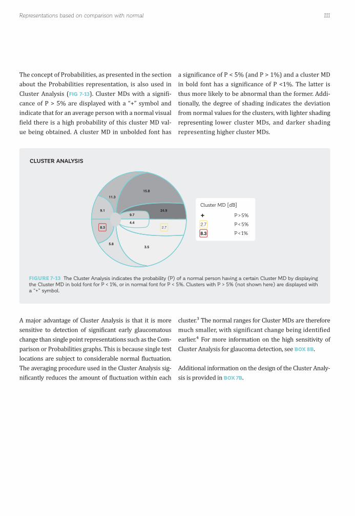
111
P > 5%
P < 5%2.78.3 P < 1%
+9.1
11.315.8
24.99.7
4.42.7
3.55.8
8.3
Cluster MD [dB]
Representations based on comparison with normal
A major advantage of Cluster Analysis is that it is more sensitive to detection of signi icant early glaucomatous change than single point representations such as the Com-parison or Probabilities graphs. This is because single test locations are subject to considerable normal luctuation. The averaging procedure used in the Cluster Analysis sig-ni icantly reduces the amount of luctuation within each
The concept of Probabilities, as presented in the section about the Probabilities representation, is also used in Cluster Analysis (FIG 7-13). Cluster MDs with a signi i-cance of P > 5% are displayed with a “+” symbol and indicate that for an average person with a normal visual ield there is a high probability of this cluster MD val-
ue being obtained. A cluster MD in unbolded font has
cluster.³ The normal ranges for Cluster MDs are therefore much smaller, with signi icant change being identi ied earlier.⁴ For more information on the high sensitivity of Cluster Analysis for glaucoma detection, see BOX 8B.
Additional information on the design of the Cluster Analy-sis is provided in BOX 7B.
a signi icance of P < 5% (and P > 1%) and a cluster MD in bold font has a signi icance of P <1%. The latter is thus more likely to be abnormal than the former. Addi-tionally, the degree of shading indicates the deviation from normal values for the clusters, with lighter shading representing lower cluster MDs, and darker shading representing higher cluster MDs.
FIGURE 7-13 The Cluster Analysis indicates the probability (P) of a normal person having a certain Cluster MD by displaying
the Cluster MD in bold font for P < 1%, or in normal font for P < 5%. Clusters with P > 5% (not shown here) are displayed with
a “+” symbol.
CLUSTER ANALYSIS
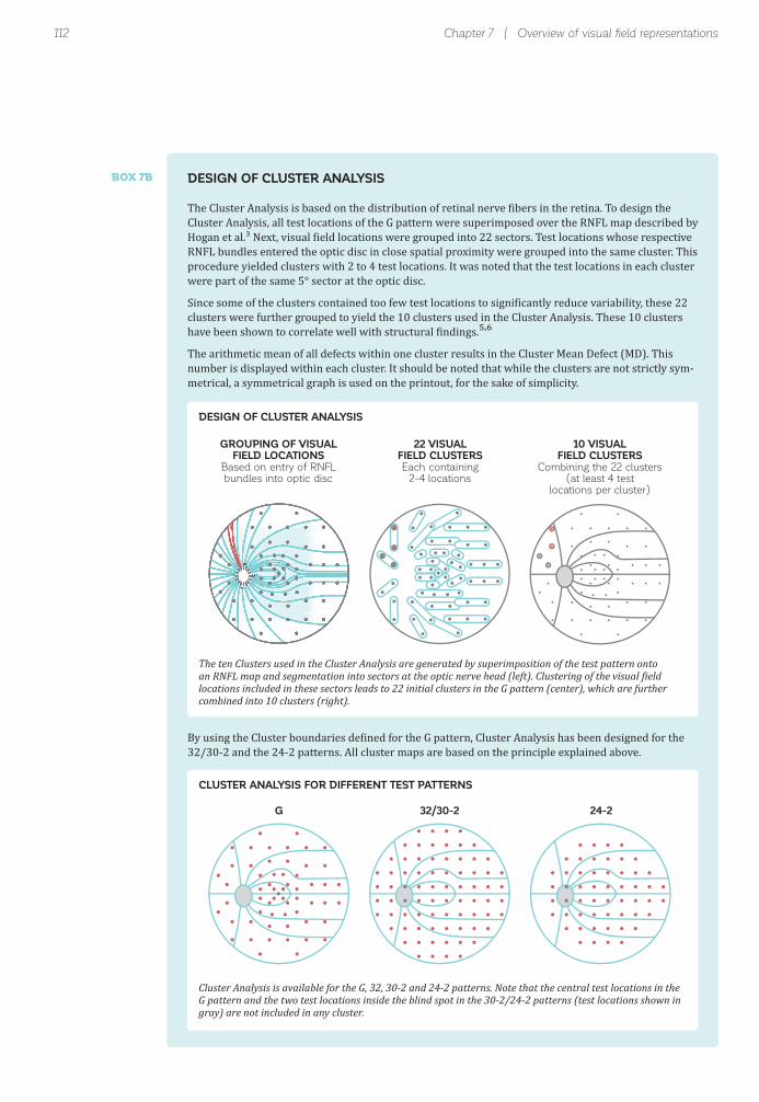
112
GROUPING OF VISUALFIELD LOCATIONS
Based on entry of RNFLbundles into optic disc
22 VISUALFIELD CLUSTERSEach containing
2-4 locations
10 VISUALFIELD CLUSTERS
Combining the 22 clusters(at least 4 test
locations per cluster)
270
90
0 180
G 32/30-2 24-2
BOX 7B
DESIGN OF CLUSTER ANALYSIS
CLUSTER ANALYSIS FOR DIFFERENT TEST PATTERNS
Chapter 7 | Overview of visual fi eld representations
DESIGN OF CLUSTER ANALYSIS
The Cluster Analysis is based on the distribution of retinal nerve ibers in the retina. To design the Cluster Analysis, all test locations of the G pattern were superimposed over the RNFL map described by Hogan et al.³ Next, visual ield locations were grouped into 22 sectors. Test locations whose respective RNFL bundles entered the optic disc in close spatial proximity were grouped into the same cluster. This procedure yielded clusters with 2 to 4 test locations. It was noted that the test locations in each cluster were part of the same 5° sector at the optic disc.
Since some of the clusters contained too few test locations to signi icantly reduce variability, these 22 clusters were further grouped to yield the 10 clusters used in the Cluster Analysis. These 10 clusters have been shown to correlate well with structural indings.⁵,⁶
The arithmetic mean of all defects within one cluster results in the Cluster Mean Defect (MD). This number is displayed within each cluster. It should be noted that while the clusters are not strictly sym-metrical, a symmetrical graph is used on the printout, for the sake of simplicity.
By using the Cluster boundaries de ined for the G pattern, Cluster Analysis has been designed for the 32/30-2 and the 24-2 patterns. All cluster maps are based on the principle explained above.
The ten Clusters used in the Cluster Analysis are generated by superimposition of the test pattern onto an RNFL map and segmentation into sectors at the optic nerve head (left). Clustering of the visual ield locations included in these sectors leads to 22 initial clusters in the G pattern (center), which are further combined into 10 clusters (right).
Cluster Analysis is available for the G, 32, 30-2 and 24-2 patterns. Note that the central test locations in the G pattern and the two test locations inside the blind spot in the 30-2/24-2 patterns (test locations shown in gray) are not included in any cluster.

113Representations based on comparison with normal
As with the interpretation of the Probabilities represen-tations, however, some caution is essential in the clinical interpretation of the Cluster Analysis representation. This is due to the fact that one cluster defect at a signif-icance of p < 5% is likely to show up in one out of two normal visual ields (1 out of 10 clusters at P < 5% occurs
in 50% of normal visual ields), and one cluster at p < 1 % in one out of 10 normal visual ields (1 out of 10 clusters at P < 1% occurs in 10% of normal visual ields). A signif-icant cluster defect is thus far more clinically meaningful if it is spatially correlated with another signi icant cluster defect, or if it correlates with a structural defect.
POLAR ANALYSISThe Polar Analysis has been designed speci ically for glaucoma.⁷ It provides information about where struc-tural defects are to be expected at the optic disc, by dis-playing visual ield results using structural coordinates. It is based on the known relationship between structure and function and capitalizes on the fact that each visual ield location corresponds to a speci ic retinal nerve iber bundle in the retina (i.e., a superior visual ield
location corresponds to an inferior retinal location and a nasal visual ield location corresponds to a temporal retinal location).² For more information on the rela-tionship between structure and function, see BOX 8C.
Similar to the Cluster Analysis, the Polar Analysis is based on a superimposition of the test pattern onto Hogan’s² RNFL map (FIG 7-14). Since the superior visual ield corresponds to the inferior retina, the visual ield
is irst lipped across the horizontal axis.
Once the visual ield has been lipped across the hor-izontal axis, each sensitivity loss obtained from the Comparison representation is mapped onto the nerve iber that corresponds to it. The nerve iber projects to
the optic disc and enters at a speci ic angle around the optic disc. The angle of entry of each nerve iber is de-termined and used to place each test location as a radial bar on the Polar Analysis representation. The length of the bar shows the sensitivity loss in dB from the Com-parison representation. Note that if two or more test locations map onto the nerve ibers that enter at the same angle, the values of the corresponding test point locations are averaged. To facilitate interpretation, a gray band ranging from +4 dB to -4 dB provides a rough indication of a normal range. The definitions of the Polar Analysis are shown in FIG 7-15.

114 Chapter 7 | Overview of visual fi eld representations
S
I
NT
VISUAL FIELD ORIENTATION
STRUCTURAL ORIENTATION
7
+ +5
+
++
5
10
10
22
1221
10
5 17++
15 13
67
30
+
+
6 6
8
10
57 31
+8
+ 5
58
13 22
+8
22 16
+5
11 +
++
25
7
9 8
+8
T TNTT TTNN 102030[dB]
S
IN T
COMPARISON
1. Locate nerve fiberentry site at optic disc
2. Define nerve fiberentry angle at optic disc
3. Draw polar bar at previouslydetermined location
(Length corresponds to defect size)
4. Repeat for all test locations
270
90
0 180
270
90
0 180
105°
FIGURE 7-14 The Polar Analysis orients visual fi eld results (top) like a structural result (bottom), fl ipping the results across
the horizontal meridian. It projects a sensitivity loss from the Comparison chart (e.g., 13 dB, highlighted in red, top) along the
corresponding retinal nerve fi bers on the retina to the optic disc (red circle, bottom left). At the nerve fi ber entry site a red
bar is drawn at the angle at which the nerve fi ber enters the optic disc (here 105°, bottom middle), with the length of the bar
corresponding to the magnitude of the sensitivity loss (i.e., 13 dB, bottom right). By repeating this procedure for all visual fi eld
locations, the Polar Analysis is drawn (all red bars, bottom right). (S: Superior; I: Inferior; N: Nasal; T: Temporal)
DESIGN OF THE POLAR ANALYSIS

FIGURE 7-15 The Polar Analysis displays sensitivity losses from the Comparison chart as a projection onto the optic disc, to
allow for easy correlation with structural results. The length of the bars indicates the sensitivity loss in dB.
115Representations based on comparison with normal, corrected for diffuse defects
Defect [dB]
Normal range
SINT
Superior
Inferior
Nasal
Temporal
• Length of bar indicates defect size [dB]
• Position along the optic disc represents
the entry angle of RNFL fibers associated
to each test location
102030[dB]
S
IN T
The Polar Analysis is a very useful tool to link structural and functional results because it allows direct side-by-side comparison of the structural and functional results, as can be seen in FIG 8-24. It has been shown to correlate
well with structural results⁸ and usefully assists the identi ication of the spatially corresponding structural (RNFL) defects.
POLAR ANALYSIS
It is useful to analyze localized visual ield defects inde-pendently of diffuse defects, which in many cases are caused by cataract. To do so, the Comparison, Probabilities and Cluster Analysis representations are all available in a corrected version. This corrected version removes diffuse or widespread defects and displays only localized visual ield loss. All “corrected” representations are based on the
Corrected Comparison representation.
The correction applied to the Corrected Comparison is based on the DD global index, which represents the magnitude of diffuse defect. The DD is subtracted from the sensitivity losses displayed in the Comparison representation. The DD is explained in detail in the section on global indices. FIG 7-16 illustrates how the corrected representations are calculated.
CORRECTED COMPARISON
REPRESENTATIONS BASED ON COMPARISON WITH NORMAL, CORRECTED FOR DIFFUSE DEFECTS

FIGURE 7-16 The Corrected Comparison representation is calculated by subtracting the magnitude of the diffuse defect ex-
pressed in the DD index from each sensitivity loss in the Comparison representation. It allows for the assessment of localized
visual fi eld loss without the infl uence of diffuse defects and is the basis for the calculation of both the Corrected Probabilities
and the Corrected Cluster Analysis.
116 Chapter 7 | Overview of visual fi eld representations
7
+ +5
+
++
5
10
10
22
1221
10
5 17++
15 13
67
30
+
+
6 6
8
10
57 31
+8
+ 5
58
13 22
+8
22 16
+5
11 +
++
25
7
9 8
+8
9.1
11.315.8
24.99.7
4.42.7
3.55.8
8.3
+
+ ++
+
++
+
5
+
16
715
5
+ 12++
10 8
++
24
+
+
+ +
+
5
++ 26
++
+ +
++
8 17
++
16 10
++
6 +
++
20
+
+ +
++
3.7
5.910.4
19.54.3
++
++
2.9
COMPARISON PROBABILITIES CLUSTER ANALYSIS
CORRECTED COMPARISON CORRECTED PROBABILITIES CORRECTED CLUSTER ANALYSIS
-
=
DD = 4.5 dB
10
5
CORRECTED COMPARISON AND ITS RELATIONHIP WITH OTHER CORRECTED REPRESENTATIONS

117Representations based on comparison with normal, corrected for diffuse defects
+
+ ++
+
++
+
5
+
16
715
5
+ 12++
10 8
++
24
+
+
+ +
+
5
++ 26
++
+ +
++
8 17
++
16 10
++
6 +
++
20
+
+ +
++
Local sensitivity loss < 5 dB
Local sensitivity loss [dB]16
Absolute defect(i.e., Sensitivity threshold 0 dB)
+
P > 5%P < 5%P < 2%P < 1%P < 0.5%
Probability that a personwith a normal visual field
shows this result
The Corrected Comparison representation is similar to the Comparison representation and uses the same
symbols to show local sensitivity loss (FIG 7-17).
CORRECTED COMPARISON
CORRECTED PROBABILITIES
The Corrected Probabilities representation is very similar to the Probabilities representation and shows the proba-bility that a person with a normal visual ield shows this
corrected sensitivity loss at various signi icance levels, as shown in FIG 7-18.
CORRECTED PROBABILITIES
FIGURE 7-17 The Corrected Comparison representation shows the magnitude of local sensitivity loss once the diffuse defect
is removed. It uses the same defi nitions as the Comparison representation.
FIGURE 7-18 Similar to the Probabilities representation, the Corrected Probabilities representation shows the likelihood that
an average person with a normal visual fi eld would have a given sensitivity loss, but is based on the Corrected Comparison
representation that only displays local visual fi eld loss.

118
P > 5%
P < 5%2.95.9 P < 1%
+3.7
5.910.4
19.54.3
+
2.9+
+
+
Corrected Cluster MD [dB]
Chapter 7 | Overview of visual fi eld representations
CORRECTED CLUSTER ANALYSIS
The Corrected Cluster Analysis is very similar to the Cluster Analysis, but is based on the Corrected Com-parison. It shows the probability that a person with a
normal visual ield shows this corrected Cluster Mean Defect in dB at various signi icance levels, as shown in FIG 7-19.
CORRECTED CLUSTER ANALYSIS
FIGURE 7-19 Similar to the Cluster Analysis, the Corrected Cluster Analysis indicates the probability (P) of an average normal
person having a certain Cluster MD, but is based on the Corrected Comparison representation that only displays local visual
fi eld loss.
Global indices are useful numerical summaries of the entire visual ield, or of an aspect of the visual ield.⁹ They 1) provide a summary of the status of the visual ield, 2) are useful to objectively assess and classify the severity of visual ield loss and 3) are helpful in the assessment of
change over time. Some indices summarize the entire visual ield, while others focus solely on a part of the visual ield. They are presented in detail in the section below. The
formula used to calculate each global index is shown in TABLE 7-1.
GLOBAL INDICES

119Global indices
The Mean Sensitivity (MS) is the arithmetic mean of the sensitivity thresholds displayed in the Values rep-resentation. It represents the average height of the hill of vision with respect to the locations that are tested, and thus a patient’s average sensitivity to light. MS is
The Mean Defect (MD) is the arithmetic mean of the sen-sitivity loss displayed in the Comparison representation. It represents the average visual ield loss of a patient derived from the locations that are tested and is thus
based on the Values and its diagnostic value is therefore limited by the same factors that affect the Values (e.g., it is dependent on patient age and on the spatial distribu-tion of the test locations).
often used to assess visual ield severity.⁹ It is a key index used in the progression analysis available on Octopus perimeters to identify the presence of progression (see Chapter 9).
MEAN SENSITIVITY (MS)
MEAN DEFECT (MD)
FORMULA VARIABLES
N: Total number of test locations
xi: Sensitivity threshold at test location i, or mean of two repeated measurements xi1, xi2 at test location i
ni: Normal value at test location i
di: Sensitivity loss at test location i
ME: Mean Error
GLOBAL INDICES AVAILABLE FOR OCTOPUS PERIMETERS TABLE 7-1
INDEX
MEAN SENSITIVITY(MS)
MEAN DEFECT (MD)
SQUARE ROOT OF LOSS VARIANCE (sLV)
CORRECTED SQUARE ROOT OF LOSS VARIANCE (CsLV)

120
MD6.5 dB
MD6.3 dB
sLV8.5 dBsLV
2.5 dB
6 6
59
+
6
7 766
11 10
68
+
8
5 5
57
5 7
66
+
5
+
5
11 +
515
9 9
55
8 10
610
7
67
8 5
58
+ +
59
5 +79
7 7
+7
2326
+ +
22
+
13155 6
66
+ +
+
+
+8
+ +
1821
+ +
+
+
19
+
1013
+ +
+8
+ +
1017
+ +
22
+12
85
+ +
+15
+ +
1721+ +
1921
+ +
DIFFUSE DEFECT LOCAL DEFECT
78
10
15
11 11
10 10
9 9 9 9 9
8 8 8 87 7777
65 5 5 5 5 5 5 5 5 5 5 5 5
66 6 66 66 6 6 67 7 7 7 8 8 8
6
+ ++
++
++ +++
+++++
++++ ++++ +++ +
+++++ +
+
6 655
10 1011
12 1315 15
17 17
19 1918
2121 212222
2623
COMPARISON COMPARISON
MD 6.3 dBsLV 2.5 dB
MD 6.5 dBsLV 8.5 dB
Chapter 7 | Overview of visual fi eld representations
SQUARE ROOT OF LOSS VARIANCE (sLV)
The square root of Loss Variance (sLV) represents the standard deviation of the individual defects at all visualield locations and provides a measure of variability
across the visual ield.⁹ This index is useful because the Mean Defect (MD) does not provide any information about whether visual ield loss is uniformly distributed
(i.e., diffuse) or localized at some locations. The sLV index thus further summarizes the characteristics of a visual ield. The sLV index is large in inhomogeneous visual ields (localized defects) and small in homoge-neous visual ields (diffuse defects), as shown in FIG 7-20.
SQUARE ROOT OF LOSS VARIANCE (sLV)
FIGURE 7-20 The sLV provides a measure of the inhomogeneity of a visual fi eld. This is illustrated in this fi gure, which shows
a homogeneous visual fi eld with diffuse defect (left) and a heterogeneous visual fi eld with localized defect (right). If the visual
fi eld is homogeneous, the sensitivity losses at specifi c test locations (shown on the y-axis in the bottom part of the fi gure) do
not deviate strongly from MD, and sLV is small (left). If the visual fi eld is heterogeneous, some locations deviate strongly from
MD, and therefore sLV is large (right). Note that sLV is the standard deviation of the local defects and thus does not span the
full range of determined sensitivity losses.

121Global indices
95%
5%
-5
1 5912 16
0
5
10
15
20
25
Average normalDefect Curve
X-axis:Ranks
Y-axis:Defects in dB
Diffuse Defect
DEFINITION OF DIFFUSE DEFECT (DD)
As shown in the section about the Defect Curve, diffuse defects result in a parallel downward shift of the Defect Curve. The magnitude of that shift is measured by assessing the distance between the Defect Curve and the average normal Defect Curve at a representative location along the curve. This generates the index DD.
As the Defect Curve may not be fully parallel with the average normal Defect Curve, it is essential to measure at a location that represents diffuse visual ield loss. DD is calculated from the 20th to the 27th percentile of the ranks. For the G pattern, which includes 59 test locations, this translates into the range from the 12th to the 16th rank from the left. This area is neither too close from the left to be meaningfully affected by random abnormally high sensitivity responses, nor too close to the right to be meaningfully affected by local defects. To be less in luenced by variability, an average of the deviations of the respective ranks from the median Defect Curve is used.
BOX 7C
The Corrected square root of Loss Variance (CsLV) is similar to the sLV, with an added correction factor to account for the variability of patient responses that occurs during a perimetric test. It is a useful index to distin-guish between a truly heterogeneous visual ield and a visual ield that is heterogeneous due to Short-term Fluctuation.⁹
The reliability index used for CsLV is Short-term Fluc-tuation (SF), which is explained in detail in the section about reliability indices. Note that CsLV is only displayed if SF is actively determined during the visual ield test by repeated testing at all test locations.
CORRECTED SQUARE ROOT OF LOSS VARIANCE (CsLV)
DIFFUSE DEFECT (DD)
In the Defect Curve, all individual defects are ranked from 1 to the total number of test locations (e.g., the 59 locations of the G pattern are shown here). The DD is calculated from the magnitude of the downward shift of the Defect Curve at the ranks from the 20th to the 27th percentile (for the G pattern, ranks 12 to 16).
DIFFUSE DEFECT (DD)

122 Chapter 7 | Overview of visual fi eld representations
5%
95%
-5
1 59
0
5
10
15
20
25
Average normalDefect Curve
X-axis:Ranks
Y-axis:Defects in dB
Diffuse Defect
Local Defect
DEFINITION OF LOCAL DEFECT (LD)
Any point on the Defect Curve outside normal limits represents an abnormal visual ield point. Shifting down the average normal Defect Curve by the amount of the diffuse defect DD yields a curve represent-ing the diffuse defect. Any further deviation of the individual Defect Curve downwards indicates local defects. The local defect index LD is de ined as the average of these deviations measured between the 14th and 59th ranks for the G pattern. In more general terms and also applicable to other test patterns, the LD index is de ined as the average of these deviations measured between the 23rd percentile of ranks and the last rank.
BOX 7D
The index LD allows quantification of the mean local defect in dB and is also derived from the Defect Curve, as explained in BOX 7D. It is used in the progression analysis
The index DD allows quanti ication of diffuse defect in dB and is derived from the Defect Curve, as explained in BOX 7C. It is mainly used to calculate the Corrected Com-parison representation, which is discussed in the previous
available on Octopus perimeters to identify the presence of local progression.
section of this chapter. It is also used in the progression analysis available on Octopus perimeters to identify the presence of diffuse progression (see Chapter 9).
LOCAL DEFECT (LD)
The LD index represents the magnitude of the average local defect and is derived from the Defect Curve. It is calculated from the deviation between the Diffuse Defect and the Defect Curve, as indicated by the red area.
LOCAL DEFECT (LD)
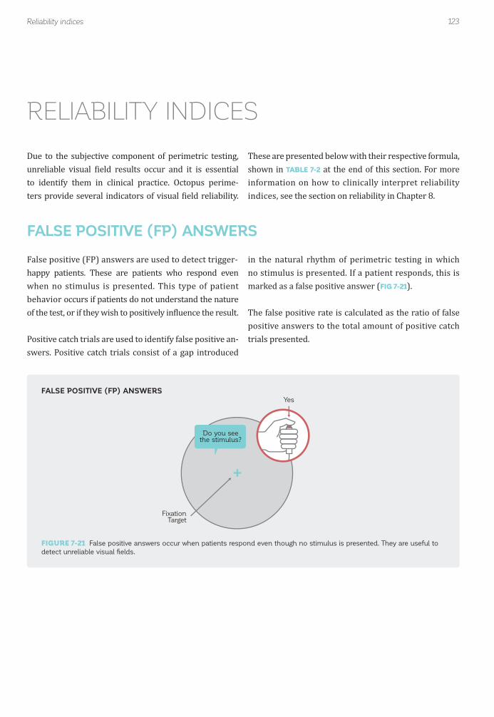
123Reliability indices
Do you seethe stimulus?
Yes
FixationTarget
False positive (FP) answers are used to detect trigger-happy patients. These are patients who respond even when no stimulus is presented. This type of patient behavior occurs if patients do not understand the nature of the test, or if they wish to positively in luence the result.
Positive catch trials are used to identify false positive an-swers. Positive catch trials consist of a gap introduced
in the natural rhythm of perimetric testing in which no stimulus is presented. If a patient responds, this is marked as a false positive answer (FIG 7-21).
The false positive rate is calculated as the ratio of false positive answers to the total amount of positive catch trials presented.
FALSE POSITIVE (FP) ANSWERS
Due to the subjective component of perimetric testing, unreliable visual ield results occur and it is essential to identify them in clinical practice. Octopus perime-ters provide several indicators of visual ield reliability.
These are presented below with their respective formula, shown in TABLE 7-2 at the end of this section. For more information on how to clinically interpret reliability indices, see the section on reliability in Chapter 8.
RELIABILITY INDICES
FALSE POSITIVE (FP) ANSWERS
FIGURE 7-21 False positive answers occur when patients respond even though no stimulus is presented. They are useful to
detect unreliable visual fi elds.

124 Chapter 7 | Overview of visual fi eld representations
Yes
Do you seethe stimulus?
FixationTarget
Do you seethe stimulus?
No
FixationTarget
False negative answers are used to detect fatigue, loss of attention and potential ixation loss during perimetric testing.
Negative catch trials are used to identify false negative answers. Negative catch trials consist of stimuli that are presented at a higher intensity than the patient has previously seen. Patients who perform the test reliably
The Reliability Factor (RF) summarizes the false positive and false negative answers. RF is calculated as the ratio of
The Short-term Fluctuation (SF) index provides a measure of the variability of patient responses that occurs during a perimetric test.⁹ In order to determine SF, the sensitivity thresholds are measured again at the end of the test, and
should be able to see these bright stimuli, and when they are missed, this is marked as a false negative answer (FIG 7-22).
The false negative rate is calculated as the ratio of false negative answers to the total amount of negative catch trials presented.
both false positive and false negative answers to the sum of positive and negative catch trials presented.
the deviations between the irst and second sensitivity thresholds are determined. SF is de ined as the standard deviation of the distribution of the results of repeated measurements of the same threshold.¹⁰
FALSE NEGATIVE (FN) ANSWERS
RELIABILITY FACTOR (RF)
SHORT-TERM FLUCTUATION (SF)
FALSE NEGATIVE (FN) ANSWERS
FIGURE 7-22 False negative answers occur when patients do not respond to a stimulus of higher intensity (right) than a
stimulus they had previously seen at that location (left). A high false negative response rate can indicate an unreliable fi eld
and may be an indicator of fatigue.

125Reliability indices
FORMULA VARIABLES
nf+ : Number of false positive answers
ntot+ : Total number of positive catch trials presented
nf- : Number of false negative answers
ntot- : Total number of negative catch trials presented
xi1 : Sensitivity threshold at test location i determined in 1st of two repeated measurements
xi2 : Sensitivity threshold at test location i determined in 2nd of two repeated measurements
N : Total number of test locations
RELIABILITY INDICES AVAILABLE ON OCTOPUS PERIMETERS TABLE 7-2
INDEX
FALSE POSITIVE (FP) ANSWERS [%]
FALSE NEGATIVE (FN) ANSWERS [%]
RELIABILITY FACTOR (RF) [%]
SHORT-TERM FLUCTUATION (SF)

126 Chapter 7 | Overview of visual fi eld representations
REFERENCES1. Bebie H, Flammer J, Bebie T. The cumulative defect curve: separation of local and diffuse components of visual ield damage. Graefes Arch Clin Exp Ophthalmol. 1989;227:9-12.2. Hogan MJ, Alvarado JA, Weddel JE. Histology of the human eye: an atlas and textbook. Philadelphia: WB Saunders; 1971.3. Mandava S, Zulauf M, Zeyen T, Caprioli J. An evaluation of clusters in the glaucomatous visual ield. Am J Ophthalmol. 1993;116:684-691.4. Naghizadeh F, Holló G. Detection of early glaucomatous progression with octopus cluster trend analysis. J Glaucoma. 2014;23:269-275.5. Holló G. Comparison of structure-function relationship between corresponding retinal nerve ibre layer thickness and Octopus visual ield cluster defect values determined by normal and tendency-oriented strategies. Br J Ophthalmol. 2016; doi: 10.1136/bjophthalmol-2015-307759.6. Naghizadeh F, Garas A, Vargha P, Holló G. Structure-function relationship between the Octopus perimeter cluster mean sensitivity and sector retinal nerve iber layer thickness measured with the RTVue optical coherence tomography and scanning laser polarimetry. J Glaucoma. 2014;23:11-18.7. Buerki E. Update Octopus Perimetrie 1. Teil: Die Polardarstellung der Gesichtsfelddaten. Ophta. 2006;7:9-12.8. Holló G, Naghizadeh F. Evaluation of Octopus Polar Trend Analysis for detection of glaucomatous progression. Eur J Ophthalmol. 2014;24:862-868.9. Flammer J. The concept of visual ield indices. Graefes Arch Clin Exp Ophthalmol. 1986;224:389-392.10. Bebie H, Fankhauser F, Spahr J. Static perimetry: accuracy and luctuations. Acta Ophthalmol (Copenh). 1976;54:339-348.
127
CHAPTER 8CLINICAL INTERPRETATIONOF A VISUAL FIELD
INTRODUCTION
Octopus perimeters offer a variety of visual ield repre-sentations that are based on the raw data (i.e., the sen-sitivity thresholds). Each of them focuses on different clinically relevant aspects of visual ield interpretation, to facilitate clinical decision-making. While there is often overlap in the information provided by the different rep-resentations, there is typically one representation that is best suited to provide information about a certain clinical aspect of a visual ield.
This chapter provides a systematic approach on how to interpret visual ields in a clinically meaningful way and highlights particular representations to answer speci ic clinical questions. To illustrate how the various repre-sentations can be used in clinical situations, this chapter starts by presenting six typical visual ields at different stages of disease severity (FIG 8-1). The examples include
a normal and a borderline visual ield, as well as visual ields with localized loss, diffuse loss, and both local and
diffuse loss, and a visual ield with advanced loss. These examples provide an excellent starting point to become familiar with the various representations and their be-havior in standard clinical situations and are referenced throughout the book. A removable poster of these exam-ples is also included in the back cover of this book.
Thereafter, this chapter presents the various representa-tions in a step-by-step work low. Because this chapter focuses on how to interpret visual fields for clinical purposes, only an introduction to the de initions, design and relationships between the representations is present-ed. Detailed information about each representation is provided in Chapter 7 and should be consulted as required.
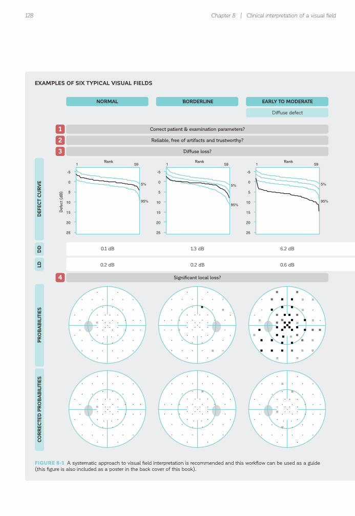
128 Chapter 8 | Clinical interpretation of a visual fi eld
1 59
5%
95%
-5
0
5
10
15
20
25
1 59
5%
95%
-5
0
5
10
15
20
25
1 59
5%
95%
-5
0
5
10
15
20
25
NORMAL
1 Correct patient & examination parameters?
2 Reliable, free of artifacts and trustworthy?
3 Diffuse loss?
Defe
ct
(dB
)
Rank Rank Rank
4 Significant local loss?
BORDERLINE EARLY TO MODERATE
Diffuse defect
DE
FEC
T C
UR
VE
PR
OB
AB
ILIT
IES
CO
RR
EC
TED
PR
OB
AB
ILIT
IES
DD
LD
1.3 dB
0.2 dB
0.1 dB 6.2 dB
0.2 dB 0.6 dB
EXAMPLES OF SIX TYPICAL VISUAL FIELDS
FIGURE 8-1 A systematic approach to visual fi eld interpretation is recommended and this workfl ow can be used as a guide
(this fi gure is also included as a poster in the back cover of this book).

129Introduction
1 59
5%
95%
-5
0
5
10
15
20
25
1 59
5%
95%
-5
0
5
10
15
20
25
1 59
5%
95%
-5
0
5
10
15
20
25
1Correct patient & examination parameters?
2Reliable, free of artifacts and trustworthy?
Rank RankRank
3Diffuse loss?
4Significant local loss?
Local defect
DE
FEC
T C
UR
VE
PR
OB
AB
ILITIES
CO
RR
EC
TED
PR
OB
AB
ILITIES
DD
LD
Local & diffuse defect
EARLY TO MODERATE ADVANCED
1.3 dB 5.9 dB 19.3 dB
7.0 dB 6.1 dB 4.7 dB

130 Chapter 8 | Clinical interpretation of a visual fi eld
+ +
++
+
+
+ +++
+ +
++
+
+
+ +
++
+ +
++
+
+
+
+
+ +
++
+ +
++
+ +
++
+
++
+ +
++
+ +
++
+ +++
+ +
++
++
+ +
+
+
+++ +
++
+ +
+
+
++
+ +
++
+ +
+
+
+
+
++
+ +
++
+ +
8+
+ +
+
++
+5
+ 6
7+
+ +
+++ +
++
+ +
6 6
59
+
6
7 766
11 10
68
+
8
5 5
57
5 7
66
+
5
+
5
11 +
515
9 9
55
8 10
610
7
67
8 5
58
+ +
59
5 +79
7 7
+7
+ +
++
+
+
+ +++
+ +
++
+
+
+ +
++
+ +
++
+
+
+
+
+ +
++
+ +
++
+ +
++
+
++
+ +
++
+ +
++
+ +++
+ +
++
++
+ +
+
+
+++ +
++
+ +
+
+
++
+ +
++
+ +
+
+
+
+
++
+ +
++
+ +
7+
+ +
+
++
++
+ +
5+
+ +
+++ +
++
+ +
+ +
++
+
+
+ +++
5 +
++
+
+
+ +
++
+ +
++
+
+
+
+
5 +
+8
+ +
++
+ +
++
+
++
+ +
++
+ +
++
+ +++
+ +
++
NORMAL
5 Assess shape & depth of defect.
BORDERLINE EARLY TO MODERATE
Diffuse defect
GR
AY
SC
ALE
(C
OM
PA
RIS
ON
)C
OM
PA
RIS
ON
CO
RR
EC
TED
CO
MP
AR
ISO
N
EXAMPLES OF SIX TYPICAL VISUAL FIELDS (CONTINUED)

131Introduction
2326
+ +
22
+
13155 6
66
+ +
+
+
+8
+ +
1821
+ +
+
+
19
+
1013
+ +
+8
+ +
1017
+ +
22
+12
85
+ +
+15
+ +
1721+ +
1921
+ +
2125
+ +
20
+
1214+ 5
+5
+ +
+
+
+6
+ +
1620
+ +
+
+
17
+
911
+ +
+7
+ +
916
+ +
21
+10
7+
+ +
+14
+ +
1520+ +
1820
+ +
26 27
2712
8 91122
24 9 18
1019
19
24
20
22
9
25
24
14 171517
15 17
2219
6 7
8+
+ +++
5 + +
++
+
5
+
+
+
6
5
+ +++
+ +
++
9 12
55
25
5
10 115+
22
98
+
6
+
58
14 13
++
+
5
21
+
6 23
125
19
+12
17 17
77
24
75
14
109
+
57
10 12++
12 12
++
+ 6
++
19
+
+ 5++
16
++
+
+
+
++
8 7
++
+
+
15
+
+ 17
6+
13
+6
11 12
++
18
++
8
++
+
++
+ 6++
7 6
++
5Assess shape & depth of defect.
Local defect
GR
AY
SC
ALE
(CO
MP
AR
ISO
N)
CO
MP
AR
ISO
NC
OR
RE
CTE
D C
OM
PA
RIS
ON
Local & diffuse defect
EARLY TO MODERATE ADVANCED

132 Chapter 8 | Clinical interpretation of a visual fi eld
102030[dB]
S
IN T
+
++
++
++
++
+
+
++
+2.0
++
++
+
+
++
+2.0
++
++
+
10 20 30[dB]
S
IT N
3.4
+2.5
++
++
++
+
2.1
++
++
++
++
+
102030[dB]
S
IN T
+
8.56.0
5.16.1
6.66.1
6.46.9
7.2
+
2.3+
++
++
++
+
+
2.3+
++
++
++
+
6 For glaucoma: Significant cluster defects?
CLU
STE
R A
NA
LYS
ISM
DsL
V
NORMAL BORDERLINE EARLY TO MODERATE
Diffuse defect
CO
RR
EC
TED
CLU
STE
R A
NA
LYS
IS
7 For glaucoma: Where to look for structural defects.
8 Severity?
PO
LA
R A
NA
LYS
IS
1.5 dB 1.9 dB 2.5 dB
-0.2 dB 1.0 dB 6.3 dB
EXAMPLES OF SIX TYPICAL VISUAL FIELDS (CONTINUED)

133Introduction
10 20 30[dB]
S
IT N
+
6.617.4
20.715.5
3.0+
++
+
+
5.3
1.7+
++
+
+
16.1
19.414.2
1.7+
++
+
102030[dB]
S
IN T
+
19.217.1
17.011.1
3.24.2
7.87.5
6.4
+
13.311.2
11.15.2
+++
+
++
1.91.6
+
102030[dB]
S
IN T
22.5
23.726.1
20.610.1
17.020.3
25.424.4
25.8
3.2
4.46.8
1.3+
+1.0
6.15.1
6.5
3.2
4.46.8
1.3+
+1.0
6.15.1
6.5
6For glaucoma: Significant cluster defects?
CLU
STE
R A
NA
LYS
ISM
DsLV
Local defect
CO
RR
EC
TED
CLU
STE
R A
NA
LYS
IS
7For glaucoma: Where to look for structural defects.
8Severity?
PO
LA
R A
NA
LYS
IS
Local & diffuse defect
EARLY TO MODERATE ADVANCED
8.3 dB 7.2 dB 5.6 dB
6.5 dB 10.1 dB 21.7 dB

FIGURE 8-2 A systematic approach to visual fi eld interpretation is recommended and this workfl ow can be used as a guide.
134 Chapter 8 | Clinical interpretation of a visual fi eld
Patient name & age
Refraction
Pattern/strategy
False positives
False negatives
Repetitions
Duration
Defect Curve
DD, LD
Probabilities
Corrected Probabilities
Grayscale (Comparison)
Comparison
Corrected Comparison
Cluster Analysis
Corrected Cluster Analysis
Polar Analysis
MD, sLV
Correct patient & examination parameters?
Yes
Yes
Yes No
Yes
Yes Yes
Yes
Yes
No
No
No
No
No
No
Diffuse loss? Caused bypathology?
Reliable, free ofartifacts & trustworthy?
Retest if clinicallyrelevant
Potentially unreliable,retest if clinically relevant
Normal visual field OR
Diffuse defect only
Consider non-glaucomatous field defects
Consider non-glaucomatous field defects
Consider non-glaucomatous field defects
Consider glaucoma
Yes Consider glaucoma
Consider pathologyleading to diffuse defect
Borderline or significant local loss?
Assess shape & depth of defect.Typical for glaucoma?
Glaucoma only: Significant cluster defects?
Glaucoma only:Where to look for structural defects.
Is there a relationship?
Severity?
1
2
3
4
5
6
7
8
VISUAL FIELD INTERPRETATION WORKFLOW
STEP-BY-STEP INTERPRETATIONOF A VISUAL FIELD
OVERVIEW OF STEP-BY-STEP WORKFLOW

135Step-by-step interpretation of a visual fi eld
Correct patient & examination parameters?1
This chapter provides a systematic step-by-step approach on how to interpret visual ields in a clinically meaningful way and highlights particular representations to answer speci ic clinical questions. This suggested sequence has been validated by many experts and can serve as an
Octopus perimeters display key patient and examination parameters for all visual ields (FIG 8-4). Special attention should be paid to patient age and refraction. If these are incorrect, this can lead to non-pathological diffuse visual ield loss. The following parameters are displayed:
excellent starting point to interpret visual ield results. Different sequences may, however, be equally valid or even more adequate in speci ic cases and should be used accordingly. An overview of that work low is presented in FIG 8-2.
• Patient’s name and identi ication number• Patient’s date of birth and age• Tested eye• Date and time of examination• Test pattern and strategy• Stimulus type• Maximum stimulus intensity and background luminance• Refraction entered or trial lens used • Pupil size
STEP 1 – CONFIRM PATIENT AND EXAMINATION PARAMETERS
STEP 1 – CONFIRM PATIENT AND EXAMINATION PARAMETERS
IMPORTANCE OF CONFIRMING PATIENT AND EXAMINATION PARAMETERS
It is essential to con irm that the correct information is used for each test, in order to make accurate clinical decisions.
FIGURE 8-3 Before interpreting visual fi eld results, it is important to confi rm that the correct patient data has been entered
and that the correct examination parameters have been used during the test.

STEP 2 - DETERMINE WHETHER THE VISUAL FIELD CAN BE TRUSTED
IMPORTANCE OF ASSESSING WHETHER THE VISUAL FIELD CAN BE TRUSTED
Due to the subjective, patient-related component of perimetric testing, unreliable visual field tests, tests with artifacts or tests that cannot be trusted for other
reasons can occur frequently, must be identi ied and should not be clinically interpreted.
136
Defe
ct
(dB
)
Rank
EyeSuite™ Static perimetry, V3.5.0OCTOPUS 101
Demo, John, 1/5/1942 (63yrs)
Left eye (OS) / 01/24/2005 / 16:25:23Seven-in-One
Comment:
NV: T21 V2.1
Good fixation
Pupil [mm]: 5.6 IOP [mmHg]:Refraction S/C/A: VA [m]:Catch trials: 1/18 (6%) +, 1/18 (6%) -
-3.5 / 1.25 / 35RF: 5.5
Parameters: 4 / 1000 asb III 100 ms Duration: 15:32Programs: G Standard White/White / Normal Questions / repetitions: 356 / 23 MS [dB]: 19.7
MD [< 2.0 dB]: 9.9sLV [< 2.5 dB]: 8.1
30°
[%]
Grayscale (CO) Values [dB]
24
29 2928
28
2528
26
18
22
7
1611
19
28 163031
12 14
2323
1
30
25
23 21
19
18
3024 1
2824
23 21
2322
15 5
2521
9 15
2927
18 25
2627
1
19
17 17
2421
MS [dB]11.316.8
24.1 25.9
Comparison [dB]
7
+ +5
+
++
5
10
10
22
1221
10
5 17++
15 13
67
30
+
+
6 6
8
10
57 31
+8
+ 5
58
13 22
+8
22 16
+5
11 +
++
25
7
9 8
+8
Corrected comparisons [dB]
+
+ ++
+
++
+
5
+
16
715
5
+ 12++
10 8
++
24
+
+
+ +
+
5
++ 26
++
+ +
++
8 17
++
16 10
++
6 +
++
20
+
+ +
++
Defect curve1 59
5%
95%
-5
0
5
10
15
20
25
Diffuse defect [dB]: 5.4
Probabilities Corrected probabilities
[%]
P > 5P < 5P < 2P < 1P < 0,5
OCTOPUS®
MD [dB]17.612.2
6.1 3.9
0..1011..2223..3435..4647..5859..7071..8283..9495..100
Comment:
NV: T21 V2.1
Good fixation
Pupil [mm]: 5.6 IOP [mmHg]:Refraction S/C/A: VA [m]:Catch trials: 1/18 (6%) +, 1/18 (6%) -
-3.5 / 1.25 / 35RF: 5.5
Parameters: 4 / 1000 asb III 100 ms Duration: 15:32Programs: G Standard White/White / Normal Questions / repetitions: 356 / 23
Demo, John, 1/5/1942 (63yrs)
Left eye (OS) / 01/24/2005 / 16:25:23
Reliable, free of artifacts & trustworthy?2
Chapter 8 | Clinical interpretation of a visual fi eld
Visual ield results that cannot be trusted may occur for a number of reasons, as shown in Chapter 3. They can be caused by inconsistent patient behavior resulting from fatigue, learning effects, distraction, lack of understand-
ing of the task to perform, or a desire to in luence the results. Untrustworthy tests can also occur following set-up errors, for example when incorrect test parameters or inadequate refraction are used, or when the incorrect
OVERVIEW OF PATIENT AND EXAMINATION PARAMETERS
STEP 2 – ASSESS WHETHER THE VISUAL FIELD CAN BE TRUSTED
FIGURE 8-5 Before interpreting visual fi eld results, it is important to confi rm that the visual fi eld can be trusted. Visual fi elds
that are not reliable, contain artifacts or cannot be trusted for other reasons should be retested if this is clinically relevant.
FIGURE 8-4 All patient and examination parameters are displayed for every perimetric result.

137
Reliable normal
Less reliable normal
Normal who experiences difficulties with perimetry
Normal with learning effects (tests 1 to 3)
Normal with artifactual defects (here: lens rim artifact on 1st, 2nd and 4th test)
1st Test 2nd Test 3rd Test 4th Test 5th Test
Step-by-step interpretation of a visual fi eld
UNTRUSTWORTHY VISUAL FIELD TESTS CAN SHOW SIGNIFICANT DEFECTS
FIGURE 8-6 The examples above show several visual fi eld series from different individuals with clinically confi rmed normal
visual fi elds and no pathology. Note that while some individuals perform perimetric testing consistently, some show improve-
ment over time due to learning effects, and some perform variably from one examination to the next. This results in untrust-
worthy visual fi eld results, which may be misinterpreted.

FIGURE 8-7 The example above shows the impact of a high rate of false positive answers on the visual fi eld. The fi eld on the
left is unreliable because the patient responded in the absence of a stimulus. As a result, the visual fi eld appears better than
the true visual fi eld of the patient, which is shown on the right.
138
1st Test 2nd Test
HIGH FALSE POSITIVESReal defect is missed
NO FALSE POSITIVESReal defect is visible
Chapter 8 | Clinical interpretation of a visual fi eld
date of birth is entered. In addition, artifacts stemming from incorrect positioning of the patient, droopy eye-lid or incorrectly centered correction lenses can also lead to untrustworthy results. While a well-trained and observant visual ield examiner can signi icantly reduce the amount of untrustworthy visual ields in a clinical practice, some patients are simply unable to perform perimetric testing consistently.
FIGURE 8-6 shows the impact of unreliable visual ield tests, inconsistent patient behavior and set-up errors on
the visual ield results of several individuals with clinically con irmed normal visual ields and no pathology.
Since visual ields that cannot be trusted may not repre-sent the true status of a patient’s visual ield, they may be clinically meaningless. It is thus essential to identify them as a irst step in visual ield interpretation. The reliabili-ty indicators provided by Octopus perimeters, as well as further indicators of whether a visual ield can be trusted, should be used. These are presented in this section.
IMPACT OF FALSE POSITIVE ANSWERS ON VISUAL FIELD RESULT
FALSE POSITIVE AND FALSE NEGATIVE ANSWERS
Octopus perimeters offer several indicators to detect unreliable visual ields (see TABLE 7-2 for the de initions of each of these indicators). The two most important indicators of unreliability are the false positive (see FIG
7-21) and false negative answers (see FIG 7-22).
False positive answers occur when the patient presses the response button when no stimulus is presented. Patients who respond in the absence of a stimulus are referred to as trigger-happy, and may have visual ield results that are better than their true visual ield sta-tus, as shown in FIG 8-7. When the false positive an-swer rate exceeds 10 to 15%,¹ the results should be
interpreted with caution and the test should ideally be repeated if it is essential for clinical decision-making. In most clinical studies however, false positive rates of up to 20 to 33% are accepted.²-⁶
Note that if only a few positive catch trials are present-ed (e.g., the default setting of the G TOP test contains only six positive catch trials), one accidentally missed positive catch trial has a great impact on the false pos-itive rate. In this situation, more lenient acceptance criteria may be appropriate.

139
1st Test 2nd Test
HIGH FALSE NEGATIVESDefect is deeper
NO FALSE NEGATIVESReal defect shape & depth
Step-by-step interpretation of a visual fi eld
False negative answers occur when patients do not re-spond to stimuli that they should be able to see. Patients who do not respond to stimuli they should be able to see may experience fatigue or a loss of attention, and may have results that are worse than their true visual ield status, as shown in FIG 8-8. For most patients, clinical studies often exclude results with false negative rates above 20 or 30%.⁴ In patients with severe vision loss, however, false negative errors are not a meaningful indicator of reliability because there is a large increase
in luctuation with increasing visual ield loss. This can result in false negative rates above 50%, even though the visual ield test is performed without any subjective mis-takes.⁷ False negative answers should thus be interpreted with care in more advanced vision loss.
Note that if only a few negative catch trials are presented, more lenient acceptance criteria may be appropriate, as explained in the section on false positive answers.
FIGURE 8-8 The example above shows the impact of a high rate of false negative answers on the visual fi eld. The fi eld on the
left is unreliable because the patient did not respond to stimuli that should have been seen. As a result, the visual fi eld appears
worse than the true status of the patient’s visual fi eld, which is shown on the right.
IMPACT OF FALSE NEGATIVE ANSWERS ON VISUAL FIELD RESULT
CONSISTENCY OF RESULTS WITH FURTHER DIAGNOSTIC TESTS
Any drastic inconsistency in the location of a visual ield defect in repeated testing can suggest that some of the visual ield tests may not be trusted. This is because pathologies lead to characteristic visual ield defect patterns in speci ic locations. While these defects may deepen, expand or in some instances also improve over time, they are usually consistently located at the same position in repeated visual ield testing. If defect pat-terns shift to different locations on repeated testing, as can be seen in some of the examples shown in FIGURE
8-6, this is typically a sign of an untrustworthy visual ield test. Therefore it is good clinical practice to base
a clinical decision on two to three visual ield tests, in order to con irm or discard an initially observed visual
ield defect.⁸ These visual ield tests can be used in the future to evaluate progression or stability.
Furthermore, if a visual ield defect corresponds to the results of another diagnostic test, this strongly supports the decision that the visual ield result can be trusted. For example, if a patient shows a visual ield defect characteristic of glaucoma and shows a related RNFL thinning or rim thinning at the related optic disc loca-tion, as well as high IOP, it will be highly likely that the patient has glaucoma and that the visual ield result is thus trustworthy. The results of visual ield tests should therefore always be interpreted in light of the full clinical pro ile.

140
Diffuse loss?3
Chapter 8 | Clinical interpretation of a visual fi eld
OTHER INDICATORS TO DETERMINE WHETHER VISUAL FIELD TESTS CAN BE TRUSTED
In addition to the false positive and false negative answers, other indicators are also useful to determine whether visual ield test results can be trusted. One of the most powerful indicators remains the visual ield examiner’s direct observation of the patient during the test. Examiners should note their observations in the pa-tient’s chart.
In addition, besides the false positive answers, the Defect Curve can also be helpful to identify trigger-happy patient behavior. See FIG 8-10 for more information on how to
detect trigger-happy behavior using the Defect Curve.
Test duration can be a further indicator of whether visual ield results can be trusted. Abnormally long test durations can indicate that a patient is struggling with the task of performing perimetry.
Finally, if a patient can sustain prolonged testing, one can also retest the determined visual sensitivity thresholds to determine Short-term Fluctuation (SF), a further index de ined in TABLE 7-2.
STEP 3 – IDENTIFY DIFFUSE VISUAL FIELD DEFECTS
NEED FOR THE DETECTION OF DIFFUSE DEFECTS
It is helpful to be alerted to the presence of diffuse defects early in the process of visual ield interpretation, because although they are commonly caused by pathology (e.g.,
Diffuse defects are present when most visual ield locations show defects of approximately the same magnitude (i.e., there is no apparent visual ield loss pattern). Conversely, a visual ield with a local defect is characterized by a speci ic defect pattern in which certain visual ield points are affected more than others. Diffuse loss can also occur in the presence of a local
cataracts, glaucoma, retinal and neurological diseases), they may also indicate the presence of untrustworthy visual ield results.
defect. The etiology of diffuse and local visual ield defects is presented in TABLE 8-1.
In clinical decision-making it is essential to clarify the cause of diffuse defects. If pathology can be ruled out, the visual ield should be treated as potentially untrust-worthy and should be retaken, if clinically relevant.
STEP 3 – IDENTIFY DIFFUSE VISUAL FIELD LOSS
FIGURE 8-9 Diffuse visual fi eld loss should ideally be identifi ed early on, as it can be a sign of both a pathology leading to
diffuse defects or an untrustworthy visual fi eld.

141Step-by-step interpretation of a visual fi eld
DEFECT CURVE
The Defect Curve is a graphical representation that pro-vides a summary of the visual ield and distinguishes between local and diffuse defects.⁹ In clinical practice it is very helpful in alerting the clinician to the presence of diffuse defects that may be missed by looking at other
It is important to note that when advanced visual ield loss is present (e.g., MD > 20 dB), most visual ield locations are affected. As a result, diffuse loss is always present.
representations, and also provides other clinically valu-able information, as shown in FIG 8-10. For more details of the design and de initions of the Defect Curve, see BOX 7A.
To quickly identify the presence of diffuse defects, the Defect Curve is useful.
DIFFUSE(WIDESPREAD) DEFECT
LOCAL DEFECT
EXAMPLES OF PATHOLOGIES
• Lens opacity (e.g., cataract)• Cornea opacity (e.g., Fuchs dystrophy)• Dense vitreous opacity• Any advanced pathology resulting in severe visual ield loss (e.g., advanced glaucoma)
• Glaucoma• Age-related macular degeneration• Hemianopia• Quadrantanopia• Vitreous opacity
EXAMPLES OF UNTRUSTWORTHY RESULTS
• Incorrect refraction• Incorrect patient age• Small pupil size• Learning effect• Distraction• Fixation loss• Fatigue
• Lens rim artifact• Lid artifact
THE ETIOLOGY OF DIFFUSE AND LOCAL VISUAL FIELD DEFECTS TABLE 8-1
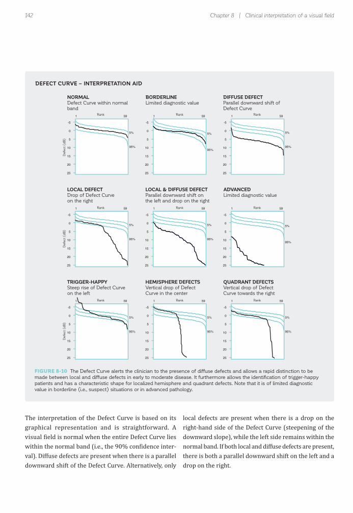
142
DIFFUSE DEFECT
Parallel downward shift of
Defect Curve
1 59
5%
95%
-5
0
5
10
15
20
25
LOCAL DEFECT
Drop of Defect Curve
on the right
1 59
5%
95%
-5
0
5
10
15
20
25
LOCAL & DIFFUSE DEFECT
Parallel downward shift on
the left and drop on the right
1 59
5%
95%
-5
0
5
10
15
20
25
NORMAL
Defect Curve within normal
band
1 59
5%
95%
-5
0
5
10
15
20
25
BORDERLINE
Limited diagnostic value
1 59
5%
95%
-5
0
5
10
15
20
25
ADVANCED
Limited diagnostic value
1 59
5%
95%
-5
0
5
10
15
20
25
TRIGGER-HAPPY
Steep rise of Defect Curve
on the left
1 59
5%
95%
-5
0
5
10
15
20
25
HEMISPHERE DEFECTS
Vertical drop of Defect
Curve in the center
1 59
5%
95%
-5
0
5
10
15
20
25
QUADRANT DEFECTS
Vertical drop of Defect
Curve towards the right
1 59
5%
95%
-5
0
5
10
15
20
25
Defe
ct
(dB
)D
efe
ct
(dB
)D
efe
ct
(dB
)
Rank RankRank
Rank RankRank
Rank RankRank
Chapter 8 | Clinical interpretation of a visual fi eld
The interpretation of the Defect Curve is based on its graphical representation and is straightforward. A visual ield is normal when the entire Defect Curve lies within the normal band (i.e., the 90% con idence inter-val). Diffuse defects are present when there is a parallel downward shift of the Defect Curve. Alternatively, only
local defects are present when there is a drop on the right-hand side of the Defect Curve (steepening of the downward slope), while the left side remains within the normal band. If both local and diffuse defects are present, there is both a parallel downward shift on the left and a drop on the right.
DEFECT CURVE – INTERPRETATION AID
FIGURE 8-10 The Defect Curve alerts the clinician to the presence of diffuse defects and allows a rapid distinction to be
made between local and diffuse defects in early to moderate disease. It furthermore allows the identifi cation of trigger-happy
patients and has a characteristic shape for localized hemisphere and quadrant defects. Note that it is of limited diagnostic
value in borderline (i.e., suspect) situations or in advanced pathology.

143
DIFFUSE DEFECTS OF VARIOUS MAGNITUDE
LOCAL DEFECT
Gra
yscale
(C
om
pariso
n)
Defe
ct
Cu
rve
1 59
5%
95%
-5
0
5
10
15
20
25
1 59
5%
95%
-5
0
5
10
15
20
25
1 59
5%
95%
-5
0
5
10
15
20
25
1 59
5%
95%
-5
0
5
10
15
20
25
1 59
5%
95%
-5
0
5
10
15
20
25
1st Test
Defe
ct
(dB
)
Rank Rank Rank RankRank
2nd Test 3rd Test 4th Test 5th Test
Step-by-step interpretation of a visual fi eld
CORRECTING FOR DIFFUSE DEFECTS
Local and diffuse defects may occur together, for exam-ple in glaucoma patients who also have cataracts. In such cases, the diffuse defects may mask localized defects. It is therefore desirable to distinguish between the local and diffuse visual ield components, in order to analyze the local visual ield loss independently. To achieve this, Octopus perimeters offer corrected representations, in
While the Defect Curve is very helpful and straightfor-ward to interpret in early to moderate disease, it has lim-ited clinical usefulness in suspect situations or advanced disease. In suspect situations, all visual ield points typi-
which the unspeci ic, diffuse defect is removed, as shown in FIG 7-16.
The corrected representations provide very helpful clinical information to determine whether there is local loss when diffuse loss is also present, as illustrated in
FIG 8-12.
cally remain within the normal band. In severe pathology, most visual ield points are affected to some extent and absolute defects are not drawn on the Defect Curve. As a result, the Defect Curve lies in the lower left-hand corner.
EXAMPLE OF THE CLINICAL USEFULNESS OF THE DEFECT CURVE
FIGURE 8-11 This example shows a series of fi ve visual fi eld tests of a patient with glaucoma with a local superior nasal de-
fect that deepens from the 1st to the 5th test. In addition, visual fi elds 2 to 5 show diffuse defects of various magnitudes. The
diffuse defect is most pronounced on the 3rd test, as can be seen from the large parallel downward shift of the Defect Curve.
An inspection of the Defect Curve thus immediately alerts the clinician to the presence of the fl uctuating diffuse defect. In
this example, the near-absence of diffuse defect on the 4th and 5th test indicates that the diffuse loss observed on the 3rd
test was due to fl uctuation and not pathology.
The Defect Curve can also identify trigger-happy re-sponse behavior, which results in a steep slope above the normal band on the left. Hemisphere and quadrant defects, on the other hand, usually show a characteristic
nearly vertical drop at a given location along the curve. FIG 8-11 illustrates the usefulness of the Defect Curve in a clinical situation.
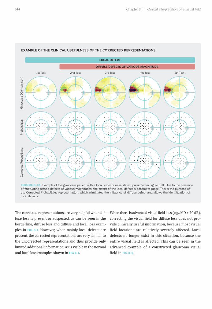
144
DIFFUSE DEFECTS OF VARIOUS MAGNITUDE
LOCAL DEFECT
Gra
yscale
(C
om
pariso
n)
Pro
bab
ilitie
sC
orr
ecte
d P
robab
ilitie
s
1st Test 2nd Test 3rd Test 4th Test 5th Test
Chapter 8 | Clinical interpretation of a visual fi eld
The corrected representations are very helpful when dif-fuse loss is present or suspected, as can be seen in the borderline, diffuse loss and diffuse and local loss exam-ples in FIG 8-1. However, when mainly local defects are present, the corrected representations are very similar to the uncorrected representations and thus provide only limited additional information, as is visible in the normal and local loss examples shown in FIG 8-1.
When there is advanced visual ield loss (e.g., MD > 20 dB), correcting the visual ield for diffuse loss does not pro-vide clinically useful information, because most visual ield locations are relatively severely affected. Local
defects no longer exist in this situation, because the entire visual ield is affected. This can be seen in the advanced example of a constricted glaucoma visual ield in FIG 8-1.
EXAMPLE OF THE CLINICAL USEFULNESS OF THE CORRECTED REPRESENTATIONS
FIGURE 8-12 Example of the glaucoma patient with a local superior nasal defect presented in Figure 8-11. Due to the presence
of fl uctuating diffuse defects of various magnitudes, the extent of the local defect is diffi cult to judge. This is the purpose of
the Corrected Probabilities representation, which eliminates the infl uence of diffuse defect and allows the identifi cation of
local defects.

145
Borderline or significant local loss?4
Step-by-step interpretation of a visual fi eld
PROBABILITIES AND CORRECTED PROBABILITIES
The Probabilities and Corrected Probabilities repre-sentations serve the purpose of distinguishing between normal and abnormal visual ields. They show the prob-ability (P) that a person of the same age with an average normal visual ield (or one with a visual ield corrected for diffuse loss in the case of the Corrected Probabilities representation) has a certain visual field result at a
Distinguishing between normal and abnormal visual ields is challenging because 1) there is luctuation in healthy eyes, 2) this luctuation is not uniformly distributed across the visual ield, as shown in FIG 2-11, and 3) subtle visu-al ield defects, as they occur in early glaucoma, are often
In view of the challenges mentioned above, there is a need for representations that allow for the distinction between normal and abnormal visual ield locations. This is the purpose of the Probabilities and Corrected Probabilities representations, which employ statistical analysis to distinguish between normal and abnormal visual ields. These representations are especially useful in borderline situations or to detect subtle visual ield change in which
given test location. Increasingly darker symbols are used to show the decreasing probability that a given visual ield result would be obtained for a person with an aver-
age normal visual ield (FIG 8-14). For more details on the de initions used in the Probabilities representations, see FIG 7-9, 7-10 and 7-18.
smaller than normal luctuation. In sum, the challenge is to detect faint signals within noise. For example, there are borderline ields which may remain stable and normal, while others, although appearing the same, have already undergone the irst steps towards pathology.
the direct assessment of the visual ield sensitivity thresh-olds can be very challenging.
It is thus worth looking at these representations prior to performing an in-depth analysis of the visual field in order to 1) avoid spending unnecessary time on analysis of a normal visual ield and 2) avoid confusion between normal luctuation and truly abnormal visual ields.
STEP 4 – DISTINGUISH BETWEEN NORMAL AND ABNORMAL VISUAL FIELDS
NEED TO DISTINGUISH BETWEEN NORMAL AND ABNORMAL VISUAL FIELDS
STEP 4 – DISTINGUISH BETWEEN NORMAL AND ABNORMAL VISUAL FIELDS
FIGURE 8-13 Before analyzing a visual fi eld in detail, statistical analysis is used to assess whether a visual fi eld is within nor-
mal limits, or is abnormal. The Probabilities and Corrected Probabilities are used to achieve this essential step, which results
from the normal fl uctuation present in perimetry.

146
Probability that a person with a normal visual fieldshows this result
Correctedfor diffuse
defect
Likely normal location
Potentially abnormal location
Highly likely abnormal location
P > 5%
P < 5%
P < 2%
P < 1%
P < 0.5%
PROBABILITIES CORRECTED PROBABILITIES DEFINITION INTERPRETATION
Chapter 8 | Clinical interpretation of a visual fi eld
The clinical interpretation of the Probabilities repre-sentation is straightforward in that it is easy to see the pattern of visual ield loss marked by dark symbols. However, there are some factors to be aware of in clinical decision-making. Firstly, there are no criteria allowing for an unambiguous distinction between normal and abnormal visual ields. Secondly, it is common to have a few random test locations that show a P value lower than 5% in normal visual ields. For further details concerning these points, see FIG 7-9 and 7-10.
Due to these factors, the Probabilities representation must be clinically interpreted with care. Depending on the pathology, different clinical guidelines are available to de ine visual ield abnormality and severity.¹⁰,¹¹ To
determine a visual ield as abnormal, these guidelines typically require the presence of one or more clusters of abnormal visual ield locations that are consistent with the expected visual ield loss pattern of a disease. This is because it is highly unlikely that such clusters would form in normal visual ields. If, however, the distribution of a few likely abnormal test locations is random and does not correspond with a disease pattern, this can often be attributed to normal luctuation. FIG 8-15 illustrates how to clinically interpret the Probabilities plots of several visual ields with potential early glaucomatous visual ield loss, in which the magnitude of visual ield loss, as
illustrated in the Grayscale of Comparison representa-tion, is similar.
PROBABILITIES AND CORRECTED PROBABILITIES – INTERPRETATION AID
FIGURE 8-14 The various symbols on the Probabilities representations show the likelihood that a person with a normal
visual fi eld would show a given sensitivity loss. For example, the black square (P < 0.5) indicates that while it is possible that
a person with an average normal visual fi eld could obtain that defect value, the probability of this occurring is very small.
Note that the Corrected Probabilities representation shows the same information, but is adjusted to remove diffuse visual fi eld
defects and is based on the Corrected Comparison representation.

147
Number of locations atP < 5% 2P < 2% 2P < 1% 1
Random distribution of likely abnormal locations
Likely normal
Number of locations atp < 5% 2
Two adjacent likely abnormal test locations, no cluster
Likely normal
Number of locations atp < 5% 2P < 2% 1P < 1% 1P < 0.5% 2
Five likely abnormal locationsclustered in an inferior partial arcuate defect pattern
One likely abnormal locationat random position
Likely abnormalInvestigate further
Number of locations atp < 5% 7P < 2% 3P < 0.5% 1
Six likely abnormal locationsclustered in a superior partialarcuate defect pattern
Three likely abnormal locationsclustered in an inferior,paracentral defect pattern
Likely abnormalInvestigate further
GRAYSCALE (Comparison) PROBABILITIES DESCRIPTION INTERPRETATION
Step-by-step interpretation of a visual fi eld
CLINICAL INTERPRETATION OF PROBABILITIES IN BORDERLINE SITUATIONS
FIGURE 8-15 The visual fi eld results obtained from four potential early glaucoma cases are presented. They are challenging
to interpret by simply looking at the relative sensitivity loss, which is marked with yellow in the Grayscale of Comparison repre-
sentation. In the two examples at the top, the few randomly distributed test locations with a probability smaller than 5% also
occur frequently in normal visual fi elds. The absence of clusters of likely abnormal visual fi eld locations suggests that these
two examples can be interpreted as likely normal. In the two examples at the bottom, the few test locations with a probability
smaller than 5% are organized in clusters and may be interpreted as likely abnormal.
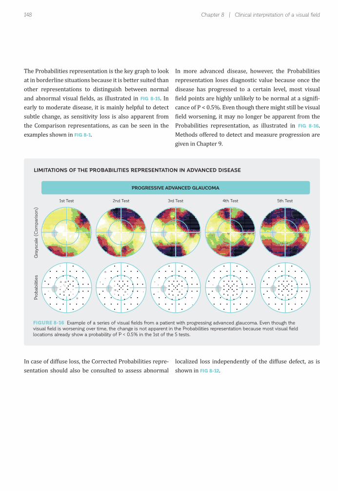
148
PROGRESSIVE ADVANCED GLAUCOMA
Gra
yscale
(C
om
pariso
n)
Pro
bab
ilitie
s
1st Test 2nd Test 3rd Test 4th Test 5th Test
Chapter 8 | Clinical interpretation of a visual fi eld
The Probabilities representation is the key graph to look at in borderline situations because it is better suited than other representations to distinguish between normal and abnormal visual ields, as illustrated in FIG 8-15. In early to moderate disease, it is mainly helpful to detect subtle change, as sensitivity loss is also apparent from the Comparison representations, as can be seen in the examples shown in FIG 8-1.
In case of diffuse loss, the Corrected Probabilities repre-sentation should also be consulted to assess abnormal
In more advanced disease, however, the Probabilities representation loses diagnostic value because once the disease has progressed to a certain level, most visual ield points are highly unlikely to be normal at a signi i-
cance of P < 0.5%. Even though there might still be visual ield worsening, it may no longer be apparent from the
Probabilities representation, as illustrated in FIG 8-16. Methods offered to detect and measure progression are given in Chapter 9.
localized loss independently of the diffuse defect, as is shown in FIG 8-12.
LIMITATIONS OF THE PROBABILITIES REPRESENTATION IN ADVANCED DISEASE
FIGURE 8-16 Example of a series of visual fi elds from a patient with progressing advanced glaucoma. Even though the
visual fi eld is worsening over time, the change is not apparent in the Probabilities representation because most visual fi eld
locations already show a probability of P < 0.5% in the 1st of the 5 tests.

149
Assess shape & depth of defect.Typical for glaucoma?
5
Step-by-step interpretation of a visual fi eld
Once it has been determined that a visual ield is trust-worthy and abnormal, the shape of the defect area and the depth of the defect should be assessed. Since different pathologies show different disease patterns, these char-acteristics are helpful to determine the possible cause and
The Comparison representations are key in that they provide a thorough analysis of both the depth and shape of defects, thus providing information about the possible causes of the visual ield loss. They do so by comparing the measured sensitivity thresholds to a normal visual ield, as shown in FIG 7-5.
severity of the visual ield defect, and to indicate potential further diagnostic tests. Typical visual ield defects for glaucoma, neuro-ophthalmic and retinal diseases are presented in FIG 5-1, 5-7 and 5-9.
Three representations are available. The Grayscale of Comparison is a color map of a patient’s visual ield loss. The Comparison and Corrected Comparison repre-sentations show the same information using numerical maps. An overview of how to clinically interpret them is provided in FIG 8-18. For further details, see FIG 7-6,
7-7 and 7-17.
STEP 5 – ASSESS SHAPE AND DEPTH OF DEFECT
NEED FOR ASSESSING SHAPE AND DEPTH OF DEFECT
GRAYSCALE OF COMPARISON, COMPARISON AND CORRECTED COMPARISON
STEP 5 – ASSESS SHAPE AND DEPTH OF DEFECT
FIGURE 8-17 The shape and depth of a defect provide valuable clues to identify and characterize pathology. They can be
analyzed from a graphical (Grayscale of Comparison) or numerical (Comparison and Corrected Comparison) map.

150
Sensitivity loss [% of normal]
Normal
Visual field loss(the darker the worse)
Correctedfor diffuse
defect
Normal
Visual field loss(the larger the worse)
Maximum visual field loss
Sensitivity loss < 5 dB
Sensitivity loss [dB]22
Absolute defect(i.e., Sensitivity threshold 0 dB)
+
0..10
11..2223..3435..4647..5859..7071..8283..9495..100
7
+ +5
+
++
510
10
2212
21
10
5 17++
15 13
67
30
+
+
6 6
8
10
57 31+8
+ 5
58
13 22
+8
2216
+5
11 +
++
25
7
9 8
+8
+
+ ++
+
++
+5
+
167
15
5
+ 12++
10 8
++
24
+
+
+ +
+
5
++ 26++
+ +
++
8 17
++
1610
++
6 +
++
20
+
+ +
++
GRAYSCALE (Comparison) DEFINITION INTERPRETATION
COMPARISON CORRECTED COMPARISON DEFINITION INTERPRETATION
Chapter 8 | Clinical interpretation of a visual fi eld
The Grayscale of Comparison representation is ideally suited to assess defect shapes and to gain a quick irst impression of a patient’s overall visual ield loss. Since it is intuitive to understand, it is also very useful for patient education.
Since it is based on the Comparison representation, which eliminates the effect of patient age and eccentric-
ity of test locations (see FIG 2-9 for more information), it represents a patient’s true sensitivity loss. However, caution is essential when interpreting the precise boundaries of the Grayscale of Comparison representa-tion, as its high spatial resolution might give the impres-sion that the detailed boundaries of a defect are known, which is not true, as explained in BOX 8A.
GRAYSCALE OF COMPARISON, COMPARISON AND CORRECTED COMPARISON – INTERPRETATION AID
FIGURE 8-18 The Grayscale of Comparison is a color map that is especially useful to determine the shape of the sensitivity
loss, whereas the Comparison and Corrected Comparison representations are numerical maps showing sensitivity loss in dB.
The Corrected Comparison representation shows localized loss only. All representations are key to identifying possible causes
of disease.

151
Sensitivity loss [% of normal]0..1011..2223..3435..4647..5859..7071..8283..9495..100
OCTOPUS GRAPHICGaps between test points
are interpolated
REALISTIC GRAPHICPoor spatial resolution
in most perimetric tests
Step-by-step interpretation of a visual fi eld
Conversely, both the Comparison and Corrected Com-parison representations are better suited to assess precise defect depth than the Grayscale of Comparison representation, because they show visual ield loss in 1 dB steps. Even small sensitivity loss can be seen in these representations. While the Comparison represen-tation shows the actual local visual ield loss (deviation of measured sensitivity threshold from normal), the Corrected Comparison representation shows localized visual ield loss only, as explained in FIG 7-16 and 7-17.
The Comparison representations should be looked at in all clinical situations, as the shape and depth of defect are key information sources in any clinical situation, from early to advanced disease, as shown in the examples in FIGURE 8-1. An exception may be borderline visual ields in which defect depth is small and thereby challenging to distinguish from normal luctuation. In those situations, the Probabilities representations are better suited to identify the shape and depth of a potential defect.
GRAYSCALE OF COMPARISON IS AN INTERPOLATED COLOR MAP
It is essential to be aware that the Grayscale of Comparison is an interpolated visual fi eld map,
where gaps between visual fi eld points are fi lled by interpolation (left). Its true spatial resolution is
much poorer, as illustrated in the panel on the right.
BOUNDARIES OF GRAYSCALE OF COMPARISON CAN BE MISLEADING
It is important to remember that in perimetric testing only a discrete number of locations are tested, as illustrated in FIG 4-4. As a result, there are large gaps between test points for which no information is available. These gaps are illed with interpolated (i.e., probable or likely) information in the Grayscale of Comparison representation. The boundaries of a visual ield defect shown in the Grayscale of Compari-son representation are thus only estimated and may not re lect the exact boundaries. The resolution of a test is only as good as that of the test pattern. This is important to remember when interpreting Grayscale of Comparison maps, to avoid incorrect interpretation of a slightly changing defect pattern.
BOX 8A

152
Glaucoma only: Significant cluster defects?
6
Chapter 8 | Clinical interpretation of a visual fi eld
Typical glaucomatous defects (just like other neurolog-ical defects caused by localized retinal nerve iber dam-age) consist of a cluster of adjacent defective visual ield locations (FIG 5-1) that correspond to the path followed by
Many glaucomatous visual ield changes, however, are smaller than the normal range of luctuation and are not marked as abnormal. In those cases, the Probabilities rep-resentation may not be sensitive enough to detect very subtle glaucomatous visual ield loss. In addition, it is time consuming, subjective and not suf iciently sensitive
The Cluster Analysis and the Corrected Cluster Analysis have been designed speci ically for glaucoma and are very sensitive to detect subtle glaucomatous visual ield defects. In Cluster Analysis, visual ield locations corre-sponding to the same retinal nerve iber layer (RNFL) bundle are grouped in 10 visual ield clusters and used to calculate the respective average Cluster Mean Defects (Cluster MDs).
the retinal nerve iber bundles in the retina. Thus, in the assessment of glaucomatous visual ield defects, one is looking for a cluster of affected visual ield locations both in the Probabilities and Comparison representations.
and speci ic to analyze individual test locations to identify clusters of visual ield defects.
Therefore, further representations are offered to facilitate the interpretation of localized glaucomatous visual ield loss. The Cluster Analysis and the Corrected Cluster Anal-ysis were developed for this purpose.
Similar to the Probabilities representation, they show the probability (P) that a person with a normal visual ield (or one with a visual ield corrected for diffuse loss
in the case of the Corrected Cluster Analysis) would have a given Cluster value. They thus provide clinical information as to whether a visual ield cluster is likely to be normal or not. This is summarized in FIG 8-20. For further details of the design and the de initions of both Cluster and Corrected Cluster Analysis, see FIG 7-12, 7-13 and 7-19, and BOX 7B.
STEP 6 - ASSESS CLUSTER DEFECTS IN GLAUCOMA
NEED TO ASSESS CLUSTER DEFECTS IN GLAUCOMA
CLUSTER ANALYSIS AND CORRECTED CLUSTER ANALYSIS
STEP 6 – ASSESS CLUSTER DEFECTS IN GLAUCOMA
FIGURE 8-19 Assessment of visual fi eld defects in clusters is helpful for the detection of subtle glaucomatous changes. This
is the purpose of the Cluster and Corrected Cluster Analysis.
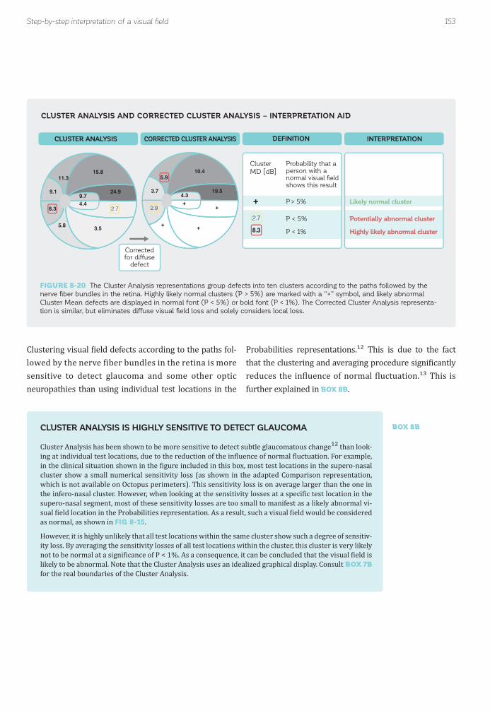
153
Probability that a person with a normal visual fieldshows this result
Correctedfor diffuse
defect
Likely normal cluster
Potentially abnormal cluster
Highly likely abnormal cluster
P > 5%
P < 5%
P < 1%
2.78.3
+9.1
11.315.8
24.99.74.4
2.7
3.55.8
8.3
3.7
5.910.4
19.54.3
+
2.9+
+
+
Cluster
MD [dB]
CLUSTER ANALYSIS CORRECTED CLUSTER ANALYSIS DEFINITION INTERPRETATION
Step-by-step interpretation of a visual fi eld
Clustering visual ield defects according to the paths fol-lowed by the nerve fiber bundles in the retina is more sensitive to detect glaucoma and some other optic neuropathies than using individual test locations in the
Probabilities representations.¹² This is due to the fact that the clustering and averaging procedure signi icantly reduces the in luence of normal luctuation.¹³ This is further explained in BOX 8B.
CLUSTER ANALYSIS AND CORRECTED CLUSTER ANALYSIS – INTERPRETATION AID
FIGURE 8-20 The Cluster Analysis representations group defects into ten clusters according to the paths followed by the
nerve fi ber bundles in the retina. Highly likely normal clusters (P > 5%) are marked with a “+” symbol, and likely abnormal
Cluster Mean defects are displayed in normal font (P < 5%) or bold font (P < 1%). The Corrected Cluster Analysis representa-
tion is similar, but eliminates diffuse visual fi eld loss and solely considers local loss.
CLUSTER ANALYSIS IS HIGHLY SENSITIVE TO DETECT GLAUCOMA
Cluster Analysis has been shown to be more sensitive to detect subtle glaucomatous change¹² than look-ing at individual test locations, due to the reduction of the in luence of normal luctuation. For example, in the clinical situation shown in the igure included in this box, most test locations in the supero-nasal cluster show a small numerical sensitivity loss (as shown in the adapted Comparison representation, which is not available on Octopus perimeters). This sensitivity loss is on average larger than the one in the infero-nasal cluster. However, when looking at the sensitivity losses at a speci ic test location in the supero-nasal segment, most of these sensitivity losses are too small to manifest as a likely abnormal vi-sual ield location in the Probabilities representation. As a result, such a visual ield would be considered as normal, as shown in FIG 8-15.
However, it is highly unlikely that all test locations within the same cluster show such a degree of sensitiv-ity loss. By averaging the sensitivity losses of all test locations within the cluster, this cluster is very likely not to be normal at a signi icance of P < 1%. As a consequence, it can be concluded that the visual ield is likely to be abnormal. Note that the Cluster Analysis uses an idealized graphical display. Consult BOX 7B for the real boundaries of the Cluster Analysis.
BOX 8B

154
+
+2.3
+++
+
+
+
+
GRAYSCALE (Comparison) PROBABILITIESTwo superior paracentral locations at p < 5%
CLUSTER ANALYSISSupero-nasal cluster at p < 1%
VISUAL FIELD ORIENTATION
3.2
++
+
+
+
+
+
+
+
2 1
211
1
3
3
1
30
20
1
13
3 101
2 3
00
1
1
0
1
1
1
3
0
20 204
4 3
23
2 0
02
2 2
21
6 2
12
5
0
3 1
42
SENSITIVITY LOSS(Adapted Comparison representation)
PROBABILITIES CLUSTER ANALYSIS
Chapter 8 | Clinical interpretation of a visual fi eld
Besides being more sensitive than the Probabilities rep-resentation to detect early glaucomatous visual ield loss (FIG 8-21), the Cluster Analysis is also easier to read and avoids having to spend time identifying and counting
potentially abnormal locations to detect clusters of ab-normal visual ield locations. This makes the Cluster Analysis a fast and useful tool in clinical practice.
ILLUSTRATION OF THE HIGH SENSITIVITY OF CLUSTER ANALYSIS TO DETECT GLAUCOMA
FIGURE 8-21 Example of a borderline visual fi eld. By just looking at the Grayscale of Comparison (left) and Probabilities
(middle) representations, one may interpret this visual fi eld as likely to be normal, as there is no pattern of contiguous ab-
normal locations. However, examination of the Cluster Analysis (right) shows a small, but signifi cant superior arcuate defect
pattern, which calls for further investigation.
ILLUSTRATION OF THE CLINICAL USEFULNESS OF CLUSTER ANALYSIS
This example highlights the high sensitivity of Cluster Analysis for the detection of subtle glau-
comatous visual fi eld defects. When looking at the sensitivity loss of the individual test locations
(left) in the superior arcuate cluster (red shading), only one location is marked as abnormal in
the Probabilities representation (center). However, most locations are slightly, but not signifi cantly
elevated, which results in a signifi cantly abnormal (P < 1 %) Cluster MD in the Cluster Analysis.

155
Glaucoma only:Where to look for structural defects.
Is there a relationship?
7
Step-by-step interpretation of a visual fi eld
As with the interpretation of the Probabilities represen-tations, some caution is essential in the clinical interpre-tation of the Cluster representation. This is because one random cluster showing a P value smaller than 5% is expected to occur frequently, also in normal visual ields.
Thus, clinicians can be more con ident that a cluster at P < 5 % is truly abnormal when a contiguous cluster is also abnormal, or when there is a spatially corresponding structural defect.
When an eye is investigated for glaucoma, both functional alterations and structural damage (neuroretinal rim tissue loss; decrease of retinal nerve iber layer thickness, RNFLT) should be considered.
In clinical practice, spatially corresponding structural and visual ield alterations are necessary to detect glaucoma and to separate glaucoma from other diseases. This is par-
Glaucomatous structural damage occurs at the optic disc and results in a degeneration of the nerve ibers that con-nect the damaged disc location to the retina. Perimetric testing presents stimuli at various retinal locations along the defective layer and is able to identify the defect.
ticularly dif icult in eyes with early stages of the disease. A mild alteration in the visual ield has more clinical value for decision-making if a spatially corresponding structur-al alteration is also detected, and vice versa. However, it is not quite straightforward to understand the geometric relation between the usual presentation of the visual ield (perimetry) and the structural results (i.e., fundus
photography or optical coherence tomography OCT).
While there is a correspondence between the structural and functional defect locations, the reference coordinates are different. Different conventions are therefore used to display structural and functional results. See BOX 8C for more information on the spatial relationship between structural and functional results.
STEP 7– WHERE TO LOOK FOR STRUCTURAL DEFECTS
NEED TO IDENTIFY RELATIONSHIP BETWEEN FUNCTIONAL AND STRUCTURAL DAMAGE IN GLAUCOMA
STEP 7 – WHERE TO LOOK FOR STRUCTURAL DEFECTS
FIGURE 8-22 Knowing where to look for structural defects to identify a spatial relationship between structural and functional
results is helpful for the detection of subtle glaucomatous changes. This is the purpose of the Polar Analysis.

156
I
13dB
TN
S
I
NT
II
13d13dBBB111313313d13dd13d3d3dB3dBB3dBdBdBBB
TTNN
VISUAL FIELD ORIENTATION STRUCTURAL ORIENTATION
7
+ +5
+
++
5
10
10
22
1221
10
5 17++
15 13
67
30
+
+
6 6
8
10
57 31
+8
+ 5
58
13 22
+8
22 16
+5
11 +
++
25
7
9 8
+8
COMPARISON RETINA WITH OPTIC DISC
270
90
0 180
Chapter 8 | Clinical interpretation of a visual fi eld
SPATIAL RELATIONSHIP BETWEEN VISUAL FIELDS AND STRUCTURAL RESULTS
Structural damage and visual fi eld results are fl ipped across the horizontal midline (i.e., a superior
visual fi eld defect corresponds to an inferior structural defect at the corresponding location at
the optic disc). Note that even though structural and functional results are also fl ipped across
the vertical midline, the defects are displayed on the same side because of the different viewing
directions of the patient (visual fi eld) and the observing clinician (structure).
Due to the different coordinates used to display structural and functional results it is useful to have an analysis tool that facilitates inding the relationship between structural
and functional representations in an intuitive way, to save valuable time. This is the purpose of the Polar Analysis.
ANATOMICAL RELATIONSHIP BETWEEN STRUCTURAL AND FUNCTIONAL RESULTS
Glaucomatous structural damage can be observed at the level of the optic disc and results in a degen-eration of the nerve ibers that connect from the damaged disc location to the retina. As a result, light entering the retina anywhere along the defective nerve iber bundle cannot be processed and this results in visual ield defect at the respective retinal location.
Furthermore, while visual ield results are oriented like a real-world image associated with post-process-ing in the brain, the real world image is lipped both horizontally and vertically when passing through the lens and entering the retina, and thus the structural and visual ield results are also lipped horizontally and vertically. This means that a superior visual defect is produced by inferior optic nerve head damage and a nasal visual ield defect is produced by temporal optic nerve head damage.
In addition, while visual ields are oriented from a patient’s view, structural results are oriented from a doctor’s view, looking onto a patient’s retina. Due to these different viewpoints, the graphical represen-tations of structural and functional results appear like mirror images lipped at the horizontal axis, as is illustrated in the graphic below.
BOX 8C

157
Location of potential structural damage on optic disc
Short bar
Long bar
Normal location
Abnormal location
Defect [dB]
Normal range
SINT
Superior
Inferior
Nasal
Temporal
• Length of bar indicates defect size [dB]
• Position along the optic disc represents the entry
angle of RNFL fibers associated to each test location
(Within gray normal range)
102030[dB]
S
IN T
POLAR ANALYSIS DEFINITION INTERPRETATION
Step-by-step interpretation of a visual fi eld
The Polar Analysis representation is designed to facili-tate the identi ication of the spatial relationship between structural and functional results by mapping visual ield defects onto the optic disc in the same orientation as a structural result. This allows intuitive side-by-side comparison between structural and functional results.
Clinical use of the Polar Analysis is straightforward. After placing it next to a structural result taken during the same time period, a clinician should look for locations in the Polar Analysis with a cluster of red bars that are outside of normal range. This allows clinicians to see the signi icantly deviating visual ield test locations that may correspond to structural regions of the optic nerve head rim where
The Polar Analysis displays individual visual ield defects as red bars along the perimeter of the optic disc. The lo-cation of the bar indicates the corresponding structural area, and the length of the bar shows the amount of sen-sitivity loss in dB, with longer bars indicating greater magnitude of defect, as shown in FIG 8-23. For more infor-mation on the design of the Polar Analysis, see FIG 7-14.
losses have occurred. Using this graphical representation, the visual ield results can be related to structural results, thereby making detailed and accurate comparison of damaged segments much easier (see FIG 8-24 for an ex-ample). The results of the Polar Analysis have been shown to correlate well with structural OCT results.¹⁴
POLAR ANALYSIS
POLAR ANALYSIS - INTERPRETATION AID
FIGURE 8-23 The Polar Analysis maps functional results onto the optic disc, to appear like a structural result. This assists in
assessing the spatial relationship between visual fi eld defects and possibly associated structural defects.

158
S
INT
+
+2.3
+++
+
+
+
+
102030[dB]
GRAYSCALE (Comparison) PROBABILITIESTwo superior paracentral locations at p < 5%
CLUSTER ANALYSISSupero-nasal cluster at p < 1%
POLAR ANALYSISSubtle visual field loss
at 7 o’clock position
FUNDUS IMAGESplinter hemorrhage and subtle RNFL loss
at 7 o’clock position
OCT MACULA MAPRetinal ganglion cell loss
at 7 o’clock position
STRUCTURAL ORIENTATION
VISUAL FIELD ORIENTATION
Chapter 8 | Clinical interpretation of a visual fi eld
ILLUSTRATION OF THE CLINICAL USEFULNESS OF THE POLAR ANALYSIS
FIGURE 8-24 Patient with suspected very early glaucoma. While the Probabilities representation is not sensitive enough to
show signifi cant visual fi eld loss, the Cluster Analysis shows that the supero-nasal cluster is likely abnormal at P < 1%. The
Polar Analysis shows a potential defect at the 7 o’clock position of the optic disc, where a very subtle disc hemorrhage is also
found in the fundus photo (darker area within the blue circle). The Macula map picks up the loss of retinal ganglion cells at a
comparable location. Due to the spatial relationship between the subtle defect in the visual fi eld (Polar Analysis) and structur-
al measurements (Fundus Image and Macula Map), glaucoma is confi rmed.

159
Severity?8
Step-by-step interpretation of a visual fi eld
A key element prior to clinical decision-making is to as-sess the severity of visual ield loss in an objective manner, in order to decide on an adequate clinical intervention. This is challenging to perform from the representations discussed so far because there is a wide variety of visual ield defect patterns and depths.
The Mean Defect (MD) provides a summary of the over-all severity of visual ield loss, which is useful to assess overall disease severity and essential to judge disease progression.¹⁵ If a visual ield defect worsens, indepen-dent of whether it is a local or a diffuse defect, MD will worsen too. As a general interpretation rule, it can thus be said that the higher the MD, the greater the visual ield damage.
As its name suggests, the MD is a mathematical repre-sentation of the average of the individual visual ield
It is desirable to have summarizing quantitative measures (i.e., global indices) that allow for a characterization of a visual ield in a few words. Summarizing global indices¹⁵
are needed for visual ield severity staging systems, but they are also very useful when patients are referred, and they also ind use in clinical studies or guidelines. An overview of the design and de initions of available global indices is provided in TABLE 7-1.
defects of all test locations, expressed in decibels. Its calculation formula is shown in TABLE 7-1 and its clinical relevance is illustrated in FIG 8-26.
The MD is an essential index used in both the Brusini and Hodapp-Parrish-Anderson glaucoma staging sys-tems.¹⁰, ¹¹, ¹⁶, ¹⁷ In the Hodapp-Parrish-Anderson system, early visual ield defects are characterized by an MD of up to 6 dB, moderate visual ield defects are character-ized by an MD ranging from 6 to 12 dB, and severe visual ield defects have an MD worse than 12 dB.
STEP 8 – ASSESS SEVERITY
NEED TO ASSESS SEVERITY OF VISUAL FIELD LOSS
MEAN DEFECT (MD)
STEP 8 – ASSESS VISUAL FIELD SEVERITY
FIGURE 8-25 Global indices provide useful information to quickly characterize a visual fi eld and to assess disease severity.

160
-0.2 dB 1 dB 6.3 dB 6.5 dB 10.1 dB 21.7 dBMD
NORMAL SUSPECT
Diffuse defect Local defect Local & diffuse defect
EARLY TO MODERATE ADVANCED
Chapter 8 | Clinical interpretation of a visual fi eld
ILLUSTRATION OF THE USEFULNESS OF MD
FIGURE 8-26 The Mean Defect (MD) summarizes the severity of visual fi eld loss in one number, for comparison with other
patients and to quickly communicate the severity of visual fi eld loss. The examples above show different visual fi elds with
increasingly severe visual fi eld loss.
In clinical practice, local and diffuse defects typically have very different causes, as shown in TABLE 8-1, and therefore require different clinical management. How-ever, the global index MD does not distinguish between them, because it is based on an average visual field defect. For example, two visual ields with similar MD (FIG 8-27) can look completely different, depending on whether there is diffuse or local loss.
It is thus useful to use an additional global index to distinguish between local and diffuse loss. This is the purpose of the square root of Loss Variance (sLV) which provides a measure of variability of local loss across all test locations. The formula used to calculate it is shown in TABLE 7-1. Note that sLV is merely the standard deviation of the local defect values.
Clinical interpretation is straightforward. If sLV is small, a visual ield is homogeneous (i.e., all defects have ap-proximately the same size), suggesting that the visual ield is normal, or that the deterioration is predom-
inantly diffuse, or that the visual ield has advanced, severe visual ield loss. However, if sLV is larger, then the visual ield is heterogeneous, which means that the individual defects vary substantially. The larger the sLV, the greater the variability among the different defects. It is noteworthy to mention that in early to advanced glaucoma, sLV becomes increasingly higher; but in very advanced glaucoma, sLV is low, since in this stage most visual ield locations are very severely damaged and the defect pattern is therefore diffuse.
SQUARE ROOT OF LOSS VARIANCE (sLV)

161
6 6
59
+
67 7
66
11 10
68
+
8
5 5
57
5 7
66
+
5
+
5
11 +
515
9 9
55
8 10
610
7
67
8 5
58
+ +
59
5 +79
7 7
+7
2326
+ +
22
+1315
5 6
66
+ +
+
+
+8
+ +
1821
+ +
+
+
19
+
1013
+ +
+8
+ +
1017
+ +
22
+12
85
+ +
+15
+ +
1721+ +
1921
+ +
MD6.5 dB
MD6.3 dB
sLV8.5 dBsLV
2.5 dB
78
10
15
11 11
10 10
9 9 9 9 98 8 8 8
7 77776
5 5 5 5 5 5 5 5 5 5 5 5 566 6 66 66 66 6
7 7 7 7 8 8 86
+ ++
++
++ ++++
++++
++++ ++++ +++ +
+++++ +
+
6 655
10 1011
12 1315 15
17 17
19 1918
2121 212222
2623
DIFFUSE DEFECT LOCAL DEFECT
COMPARISON COMPARISON
MD 6.3 dBsLV 2.5 dB
MD 6.5 dBsLV 8.5 dB
Step-by-step interpretation of a visual fi eld
ILLUSTRATION OF THE USEFULNESS OF sLV
FIGURE 8-27 Visual fi elds with either diffuse defects (left) or local defects (right) appear fundamentally different, but can
have similar MD values, as this example illustrates. The square root of Loss Variance (sLV) is then useful to distinguish
between the two situations, as sLV is smaller in the case of homogeneous or diffuse visual fi eld defects and larger in the case
of heterogeneous or local visual fi eld defects. In short, sLV is a measure of how much the defects at different test locations
differ from the mean defect, as illustrated in the graphic at the bottom.

162 Chapter 8 | Clinical interpretation of a visual fi eld
sLV is an essential index used in the Brusini Glaucoma Staging System¹¹,¹⁶,¹⁷ in combination with MD to divide visual field loss into 5 stages, and is also commonly
used to judge local disease progression in glaucoma. For more information on how to judge disease progression, see Chapter 9.

163References
REFERENCES1. Lee M, Zulauf M, Caprioli J. The in luence of patient reliability on visual ield outcome. Am J Ophthalmol. 1994; 117:756-761.2. Advanced Glaucoma Intervention Study. 2. Visual ield test scoring and reliability. Ophthalmology. 1994;101:1445-1455.3. Gillespie BW, Musch DC, Guire KE, et al. The collaborative initial glaucoma treatment study: baseline visual ield and test-retest variability. Invest Ophthalmol Vis Sci. 2003;44:2613-2620.4. Johnson CA, Keltner JL, Cello KE, et al. Baseline visual ield characteristics in the ocular hypertension treatment study. Ophthalmology. 2002;109:432-437.5. Keltner JL, Johnson CA, Cello KE, Wall M, NORDIC Idiopathic Intracranial Hypertension Study Group. Baseline visual ield indings in the Idiopathic Intracranial Hypertension Treatment Trial (IIHTT). Invest Ophthalmol Vis Sci. 2014;55: 3200-3207.6. Miglior S, Zeyen T, Pfeiffer N, et al. The European glaucoma prevention study design and baseline description of the participants. Ophthalmology. 2002;109:1612-1621.7. Bengtsson B, Heijl A. False-negative responses in glaucoma perimetry: indicators of patient performance or test reliability? Invest Ophthalmol Vis Sci. 2000;41:2201-2204.8. European Glaucoma Society. Terminology and Guidelines for Glaucoma. 4th ed. Savona: PubliComm; 2014.9. Bebie H, Flammer J, Bebie T. The cumulative defect curve: separation of local and diffuse components of visual ield damage. Graefe's Arch Clin Exp Ophthalmol. 1989;227:9-12.10. Hodapp E, Parrish RK, Anderson DR. Clinical decisions in glaucoma. 1st ed. St. Louis: Mosby; 1993.11. Susanna R Jr., Vessani RM. Staging glaucoma patient: why and how? Open Ophthalmol J. 2009;3:59-64.12. Naghizadeh F, Holló G. Detection of early glaucomatous progression with octopus cluster trend analysis. J Glaucoma. 2014;23:269-275.13. Mandava S, Zulauf M, Zeyen T, Caprioli J. An evaluation of clusters in the glaucomatous visual ield. Am J Ophthalmol. 1993;116:684-691.14. Holló G, Naghizadeh F. Evaluation of Octopus Polar Trend Analysis for detection of glaucomatous progression. Eur J Ophthalmol. 2014;24:862-868.15. Flammer J. The concept of visual ield indices. Graefe's Arch Clin Exp Ophthalmol. 1986;224:389-392.16. Koçak I, Zulauf M, Hendrickson P, Stümp ig D. Evaluation of the Brusini glaucoma staging system for follow-up in glaucoma. Eur J Ophthalmol. 1997;7:345-350.17. Koçak I, Zulauf M, Bergamin O. Evaluation of the Brusini glaucoma staging system for typing and staging of perimetric results. Ophthalmologica. 1998;212:221-227.

164

165
CHAPTER 9INTERPRETATION OF VISUALFIELD PROGRESSION
INTRODUCTION
Vision-related quality of life is severely diminished both when diffuse deterioration within the central 30-degrees of the visual ield (increase of MD) reaches a critical level and when localized progression prevents the per-formance of normal daily activities (e.g., due to severe progression of a localized inferior paracentral scotoma). In clinical practice, it is essential to detect progression and to measure its speed (i.e., rate of progression expressed as change per year in dB) as early as possible to make decisions about potential interventions before signi icant visual ield loss develops.
Because progression in diseases such as glaucoma is typically slow, the magnitude of luctuation can be larger than the annual rate of progression. Identifying disease progression from a series of visual ields is therefore a challenging and time-consuming task in clinical prac-tice (FIG 9-1). As a result, expert agreement is moderate at best (45% to 65%).¹-⁵ Statistical progression analy-ses greatly support the assessment of progression that is needed for clinical decision-making. The use of pro-gression software options was shown to improve expert agreement,¹-⁵ but to also reduce overall visual field analysis time.⁴

166 Chapter 9 | Interpretation of visual fi eld progression
Stable?
Or progressing?Glaucoma Patient 1
Glaucoma Patient 2
Glaucoma Patient 3
1st Test 2nd Test 3rd Test 4th Test 5th Test 6th Test
CHALLENGES ASSOCIATED WITH ASSESSING VISUAL FIELD PROGRESSION
FIGURE 9-1 Determination of whether visual fi elds are stable over time or whether they are progressing can be challenging,
especially when the change is small and there is considerable fl uctuation. This is illustrated with the visual fi eld series of three
different patients.
The EyeSuite Progression Analysis function of the Octo-pus perimeters has been designed to assess visual ield progression in an effective and ef icient way. It includes the following three types of progression analysis: Global Trend Analysis (GTA), (Corrected) Cluster Trend Analy-sis (CTA and CCTA), and Polar Trend Analysis (PTA) are shown in FIG 9-2.
The Global Progression Analysis measures and statisti-cally classi ies long-term change in the global indices, namely Mean Defect (MD), Diffuse Defect (DD), Local Defect (LD) and square Root of Loss Variance (sLV). It not only assesses whether a series of visual ields is stable or shows significant change, but also provides information about the rate of change in dB/year and on the local, diffuse or combined nature of progression.
The Cluster Trend Analysis and Polar Trend Analysis have been speci ically designed to detect subtle glau-comatous change. The Cluster Trend Analysis assesses cluster-specific progression within ten nerve fiber bundle regions separately, which is particularly useful in glaucoma in which localized (cluster) progression and stability occur at different locations independently from each other in the same eye. Furthermore, the Polar Trend Analysis facilitates the detection of spatially cor-responding structural and visual ield changes.
The different types of progression analyses make a statement about whether a visual ield series is stable or not and also show the location of progression. How-ever, it is also important to know the shape, location and depth of a defect. For example, a deep defect approaching
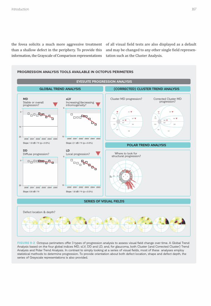
167Introduction
-0.8
2.14.1
2.60.4
6.7
0.4
0.60.7
1.0
0
15
2000 2001 2002 2003 2004 200525
MDStable or overallprogression?
Slope: 1.9 dB / Yr (p < 0.5%)
0
2000 2001 2002 2003 2004 200515
sLVIncreasing/decreasinginhomogeneity?
Slope: 2.1 dB / Yr (p < 0.5%)
0
2000 2001 2002 2003 2004 200525
DDDiffuse progression?
Defect location & depth?
Slope: 0.6 dB / Yr
0
2000 2001 2002 2003 2004 200515
LDLocal progression? Where to look for
structural progression?
Cluster MD progression?
-1.4
1.53.5
2.0-0.2
6.0
-0.2
-0.10.0
-0.3
Corrected Cluster MDprogression?
Slope: 1.8 dB / Yr (p < 0.5%)
102030[dB]
S
IN T
GLOBAL TREND ANALYSIS (CORRECTED) CLUSTER TREND ANALYSIS
POLAR TREND ANALYSIS
EYESUITE PROGRESSION ANALYSIS
SERIES OF VISUAL FIELDS
PROGRESSION ANALYSIS TOOLS AVAILABLE IN OCTOPUS PERIMETERS
FIGURE 9-2 Octopus perimeters offer 3 types of progression analysis to assess visual fi eld change over time. A Global Trend
Analysis based on the four global indices MD, sLV, DD and LD, and, for glaucoma, both Cluster (and Corrected Cluster) Trend
Analysis and Polar Trend Analysis. In contrast to simply looking at a series of visual fi elds, most of these analyses employ
statistical methods to determine progression. To provide orientation about both defect location, shape and defect depth, the
series of Grayscale representations is also provided.
the fovea solicits a much more aggressive treatment than a shallow defect in the periphery. To provide this information, the Grayscale of Comparison representations
of all visual ield tests are also displayed as a default and may be changed to any other single ield represen-tation such as the Cluster Analysis.

168 Chapter 9 | Interpretation of visual fi eld progression
ASSESSMENT OF GLOBALVISUAL FIELD CHANGE
CHANGE OF MEAN DEFECT (MD) AS A MEASURE OF GLOBAL CHANGE
TREND ANALYSIS FOR THE VISUALIZATION OF CHANGE
To judge whether a current treatment strategy is effec-tive as well as to make a clinical decision about future interventions, it is essential to know whether, overall, a visual ield series is stable, worsening or improving. This can be achieved by analyzing the change of the global in-dex Mean Defect (MD) over time.
The global index MD summarizes the sensitivity loss over
The simplest way to assess MD change is to plot the MD of each visual ield test in a two-dimensional graph. The MD is plotted on the y-axis and test date is plotted on the x-axis. This allows graphical assessment of visual ield change over time as shown in FIG 9-3. Because an in-creasing MD represents visual ield worsening, it is most intuitive to use a scale showing the smallest MD at the top and the largest at the bottom.
the area of the visual ield that was tested. It is the aver-age of all individual sensitivity losses and is expressed in dB. Consequently, if any visual ield location worsens or improves, MD will also change accordingly, even though the change may be small. This makes MD a good index to track overall visual ield change. For more information on the de inition of the index MD see TABLE 7-1, and for more information on its clinical interpretation see FIG 8-26.
If there is no luctuation and the change in MD over time is suf iciently large, it is simple to graphically determine whether a series of visual ields is stable, worsening or improving by drawing a trend line. Intuitively, the trend line corresponds to the line that provides the best linear it for all the MD points. If this line is lat, then the visual ield series is stable, if it is sloping upwards, then the
series is improving and if it is sloping downwards, then the series is worsening (FIG 9-4).

169Assessment of global visual fi eld change
Test date [years]
MD
[d
B]
0
5
10
15
20
2002 2003 2004 2005
25
Test date
MD [dB]
10/2002
0.9
01/2003
2.2
06/2003
1.7
12/2003
4.5
06/2004
3.3
01/2005
6.0
MD
[d
B]
MD
[d
B]
MD
[d
B]
0
5
10
15
20
2002 2003 2004 200525
0
5
10
15
20
2002 2003 2004 200525
0
5
10
15
20
2002 2003 2004 200525
STABLE WORSENING IMPROVING
TREND ANALYSIS FOR DISPLAYING OVERALL CHANGE
GRAPHICAL INTERPRETATION OF A TREND LINE
FIGURE 9-3 A simple way to assess visual fi eld change over time is to draw a two-dimensional graph with the test date of
each visual fi eld test on the x-axis and the corresponding MD on the y-axis. By drawing a trend line that provides the best
linear fi t for the individual MD points (red line), it is easy to see that this visual fi eld series is worsening (downward slope).
FIGURE 9-4 If visual fi eld change is suffi ciently large, just looking at the red trend line allows one to intuitively assess whether
a visual fi eld series is stable (fl at line, left) worsening (downward sloping line, middle) or improving (upward sloping line, right)
over time.

FIGURE 9-5 To determine the rate of overall visual fi eld change, the best-fi t line is drawn through the MD data points in the
Global Trend Analysis. Once this trend line is drawn, the actual data points can be discounted and the rate of change can be
determined using the slope of the trend line. The rate of change is automatically expressed in dB per year. In this example, the
slope or rate of change is 1.9 dB/year.
170
Test date [years]
MD
[d
B]
Slope1.9 dB/year
0
5
10
15
20
2002 2003 2004 2005
25
1.9 dB
1 year
Chapter 9 | Interpretation of visual fi eld progression
This approach is referred to as trend analysis and is used for all representations that are part of the EyeSuite Pro-gression Analysis. To best it the trend line to the mea-sured MD values, linear regression analysis with the ordinary least squares it is used. For more details on this approach as well as key characteristics of trend analysis, refer to BOX 9A.
The steepness of the line is referred to as the slope and is used to assess the rate of change in MD over time. The rate of change is expressed in dB per year and is derived by determining the amount of change in MD (y-axis) that occurs over the selected period of time (x-axis). In FIG
9-5, the rate of change for MD is 1.9 dB/year.
SLOPE OF TREND ANALYSIS PROVIDES RATE OF CHANGE

171Assessment of global visual fi eld change
USING PROBABILITIES TO DISTINGUISH BETWEEN STABLE AND CHANGING VISUAL FIELD SERIES
A key challenge in the assessment of visual ield progres-sion is the distinction between a series of visual ields that is truly changing and one that is stable but shows luctuation. This challenge is greater in cases in which
the magnitude of the change is small and the amount of luctuation is large, which is a common situation when
assessing glaucomatous progression.
In clinical practice, the trend line alone is not suf icient to distinguish between stable and changing visual ields. This is because most visual ield series will show at least a small trend upwards or downwards. The challenge is to determine whether this trend is signi icantly different from a lat line (i.e., one with a slope of zero).
To distinguish between a stable and a truly changing se-ries of visual ields, a t-test is used. The t-test is a statis-tical test of hypothesis that allows the determination of whether two sets of data are signi icantly different from each other. For trend analysis, the t-test is applied to the observed slope to determine whether it is signi icantly different from a slope of zero (e.g., lat line showing no change over time, which represents the typical situation of a stable visual ield series). The concept of probability is then used to determine the probability (P) that a stable visual ield series with an assumed slope of zero would show a given slope (see BOX 9A). Its interpretation is similar to the P values used in the Probabilities plot (see FIG 7-9 and 7-10). If there is a low probability that a stable visual ield series would look like the series in question, then that series is unlikely to be stable and consequently it is likely that the visual ield series is changing.
To facilitate interpretation, the EyeSuite Progression Analysis uses red downward arrows to show signi icant worsening and green upward arrows to show signi icant improvement at two probability levels and also marks loor effects using the following symbols:
Worsening at P < 5%: this visual ield series shows overall worsening. There is a smaller than 5% (and larg-er than 1%) chance that a stable visual ield series would look like the series in question, which means there is a high likelihood that the visual ield series is worsening.
Worsening at P < 1%: this visual ield series shows overall worsening. There is a smaller than 1% chance that a stable visual ield series would look like the series in question, which means there is very high likelihood that the visual ield series is worsening.
Improvement at P < 5%: this visual ield series shows overall improvement. There is a smaller than 5% (and larger than 1%) chance that a stable visual ield series would look like the series in question, which means there is a high chance that the visual ield series is improving.
Improvement at P < 1%: this visual ield series shows overall improvement. There is a smaller than 1% chance that a stable visual ield series would look like the series in question, which means there is a very high chance that the visual ield series is improving.
Floor effect: There is more than 20 dB sensitivity loss in the visual ield series and no signi icant change, which means that the determination of progression or stability is not possible due to the advancement of the disease.
If there is no symbol, then there is a probability of P > 5% that a stable visual ield series would look like the series in question or in other words that the data do not show change at the levels mentioned above. This either means that the visual ield is stable, or that the data available are not suf icient to capture change. This is often the case when only a few visual ield tests are available and pro-gression is slow or when luctuation is large as explained in BOX 9A.
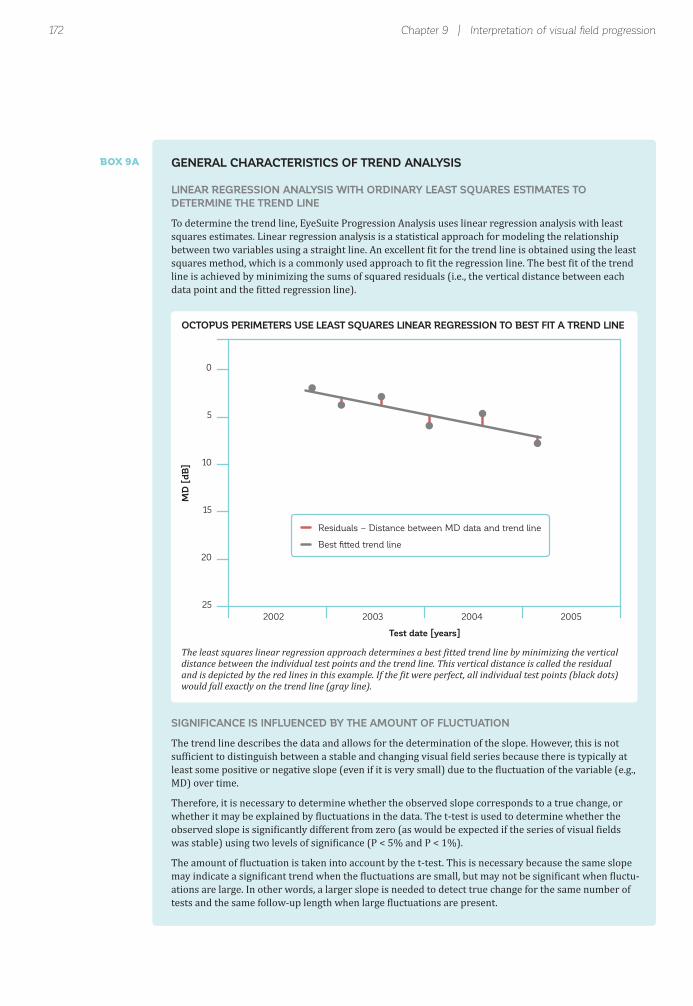
172 Chapter 9 | Interpretation of visual fi eld progression
Test date [years]
MD
[d
B]
Residuals – Distance between MD data and trend line
Best fitted trend line
0
5
10
15
20
2002 2003 2004 2005
25
SIGNIFICANCE IS INFLUENCED BY THE AMOUNT OF FLUCTUATION
The trend line describes the data and allows for the determination of the slope. However, this is not suf icient to distinguish between a stable and changing visual ield series because there is typically at least some positive or negative slope (even if it is very small) due to the luctuation of the variable (e.g., MD) over time.
Therefore, it is necessary to determine whether the observed slope corresponds to a true change, or whether it may be explained by luctuations in the data. The t-test is used to determine whether the observed slope is signi icantly different from zero (as would be expected if the series of visual ields was stable) using two levels of signi icance (P < 5% and P < 1%).
The amount of luctuation is taken into account by the t-test. This is necessary because the same slope may indicate a signi icant trend when the luctuations are small, but may not be signi icant when luctu-ations are large. In other words, a larger slope is needed to detect true change for the same number of tests and the same follow-up length when large luctuations are present.
BOX 9A GENERAL CHARACTERISTICS OF TREND ANALYSIS
LINEAR REGRESSION ANALYSIS WITH ORDINARY LEAST SQUARES ESTIMATES TO DETERMINE THE TREND LINE
To determine the trend line, EyeSuite Progression Analysis uses linear regression analysis with least squares estimates. Linear regression analysis is a statistical approach for modeling the relationship between two variables using a straight line. An excellent it for the trend line is obtained using the least squares method, which is a commonly used approach to it the regression line. The best it of the trend line is achieved by minimizing the sums of squared residuals (i.e., the vertical distance between each data point and the itted regression line).
OCTOPUS PERIMETERS USE LEAST SQUARES LINEAR REGRESSION TO BEST FIT A TREND LINE
The least squares linear regression approach determines a best itted trend line by minimizing the vertical distance between the individual test points and the trend line. This vertical distance is called the residual and is depicted by the red lines in this example. If the it were perfect, all individual test points (black dots) would fall exactly on the trend line (gray line).

173Assessment of global visual fi eld change
No symbol indicating change
Slope 0.9 dB/year
Outliers in 3rd & 4th test
NO PROGRESSION
Large slope
Considerable fluctuation
Stable series
Considerable fluctuation may prevent a change to be declared significant
Significant worsening at P < 5%
Slope 0.6 dB/year
Test data close to trend line
WORSENING
Smaller slope
Consistent results
Progressing series
Slope0.9 dB/year
Slope0.6 dB/year
0
15
2010 2011 2012
2010 2011 2012
25
MD Mean defect
0
15
25
MD Mean defect
TREND ANALYSIS DESCRIPTION INTERPRETATION
Outliers
SIGNIFICANCE IS INFLUENCED BY THE NUMBER OF VISUAL FIELD TESTS
The number of visual ield examinations (n) included in a trend analysis is important because it in lu-ences the outcome of the t-test. The EyeSuite Progression Analysis can be performed with a minimum of three visual ield tests. However, if there are only three or four visual ield tests included in the analysis, the slope must be quite steep to be able to separate true change from luctuations. On the other hand, if there are many visual ield tests included, even a visual ield series with a shallow slope can identify signi icant change. For typical progressing visual ields, trends will not become signi icant before ive or six examinations are included in the analysis. Guidelines on glaucoma treatment⁶ typical-ly recommend a minimum of 6 visual ields in the irst two years to reliably detect glaucomatous visual ield progression. However, if luctuation is large and the slope is small, an even larger number of visual ield tests are required to detect progression.⁷,⁸
ILLUSTRATION OF THE INFLUENCE OF FLUCTUATION ON SIGNIFICANCE
In this igure, the visual ield series from two different patients are shown over a comparable time period with approximately the same amount of test data. In the example on top, luctuation is large because the 3rd and 4th test are outliers. As a result, even the relatively large slope (0.9 dB/year) is insuf icient to indicate signi icant change and the series appears to be stable (no symbol). More visual ield tests may be needed to identify whether the series is truly stable or progressing. However, when there is less luctuation in the visual ield data (bottom), even a small slope (0.6 dB/year) suf ices to detect signi icant change (red downward arrow) and the series is con irmed as progressing.

174
No symbol indicating change
Slope 0.9 dB/year
Outliers in 3rd & 4th test
6 Visual field tests
NO PROGRESSION
Large slope
Considerable fluctuation
Series declared stable because of fluctuation
More test data is needed
Significant worsening at P < 1%
Slope 0.7 dB/year
Test data close to trend line
10 Visual field tests
WORSENING
Overall consistent results
Progressing seriesSufficient number of tests
Tests 1-6
All tests
Outliers
6 Tests
10 Tests
0
15
2010 2011 2012 2013
Slope 0.9 dB/year
Slope 0.7 dB/year
201425
MD Mean defect
0
15
2010 2011 2012 2013 201425
MD Mean defect
Defect location & depth?
TREND ANALYSIS DESCRIPTION
SERIES OF VISUAL FIELDS
INTERPRETATION
Chapter 9 | Interpretation of visual fi eld progression
THE INFLUENCE OF THE NUMBER OF VISUAL FIELD TESTS ON SIGNIFICANCE
The number of visual ield tests signi icantly in luences whether a visual ield series is considered stable or not. More visual ields are required when the slope is shallow or when luctuation is large. In this example, due to luctuation in tests 3 and 4, the visual ield series doesn’t show signi icant change after the initial 6 tests (top) even though the slope of 0.9 dB/year is relatively large. Change is only detected by the trend analysis upon inclusion of more tests (bottom).
MD TREND ANALYSIS
Interpretation of MD Trend Analysis in clinical practice is a fast and straightforward process (if adequate visual ields are selected, which is described in more detail later in this chapter). The decision about whether a visual ield series is stable, signi icantly worsening or signi icantly
improving can be made solely by looking at the red down-ward (signi icant worsening) or the green upward (sig-ni icant improvement) arrows displayed. To assess rate of change, the slope is numerically displayed as change in dB/year at the bottom of the graph (FIG 9-6).

FIGURE 9-6 MD Trend Analysis allows for a quick identifi cation of worsening (red downward arrow) or improvement (green
upward arrow) of a visual fi eld series. In addition, it displays the rate of change (slope in dB/year) and shows the trend graphic
including slope and individual test points to graphically assess severity of visual fi eld loss, rate of progression, test interval,
amount of fl uctuation and number of tests included in the analysis.
175Assessment of global visual fi eld change
Worsening at P < 5%
Worsening at P < 1%
Improvement at P < 5%
Improvement at P < 1%
Floor effect (MD > 20 dB,
no significant progression)
MD trend line
Slope [dB/year]
MD of visual field test
(taken at specific date)
Normal range of MD
MD of 15 dB
No symbol P > 5%
Probability of stable visual field series
showing this result
Stable
Likely worsening
Highly likely worsening
Likely improving
Highly likely improving
Maximum loss(No further measurement of progression possible)
MD change in dB/year
Seriously impaired visual field
2000 2001 2002 2003 2004 2005
Slope: 1.9 dB/year
0
15
25
15
1.9 dB/year
MD TREND DEFINITION INTERPRETATION
Y-axisMD [dB]
Magnitude ofvisual field loss
X-axisTime (years)
While the detailed graphical presentation of the trend line and the test data is not necessary for deciding about the presence and rate of MD change, it provides valuable infor-mation. It allows for a quick assessment of disease severity as well as rate of disease progression. The lower the level of the curve, the more the disease has progressed and the steeper the curve, the more rapid the change.
The graph also allows for a quick determination of the frequency of the visual ield tests performed. In addition, it allows one to see at a glance if there is a signi icant out-lier, which calls for more careful evaluation to make sure that this visual ield is reliable and whether it should be included in the analysis. For more information, consult the next section in this chapter on adequate selection of visual ield tests.
Visual ields included in the analysis are marked in a different color which supports the visual ield selection process. Lastly, different symbols are used for each pe-rimeter model to draw attention to a possible perimeter model-related bias. This can for example occur when a patient is tested for the irst time on a new perimeter model and shows a strong learning effect. For more information on transitioning from one perimeter model to another, please refer to Chapter 12.
Further orientation is provided by a gray band at the top which indicates the normal range of MD (i.e., the 95% con idence interval) and a red line at 15 dB which rep-resents seriously impaired visual ields. The graph stops at 25 dB because in many countries, an MD of 20 to 25 dB is considered legal blindness.
MD TREND ANALYSIS - INTERPRETATION AID

176 Chapter 9 | Interpretation of visual fi eld progression
INTERPRETATION OF MD TREND ANALYSIS
SELECTION OF ADEQUATE VISUAL FIELDS FOR ANALYSIS
MD Trend Analysis provides information about the pres-ence and rate of progression as well as the magnitude of the sensitivity loss (i.e., magnitude of MD) of a patient. However, this data is not suf icient to make a clinical decision as these factors have a very different meaning depending on their relation to each other as well as the patient’s age and life expectancy.
For example, an MD of 3 dB in a patient progressing at a rate of 0.4 dB/year has a very different meaning in a 50-year-old patient compared to an 80-year-old patient. Assuming a life expectancy of 90 years for both patients and projecting the current slope linearly into the future,
at the end of their respective lifespan, the 80-year-old pa-tient would have an MD of 7 dB whereas the 50-year-old patient would have an MD of 19 dB. However, if this same 80-year-old patient showed a progression rate of 2 dB per year, at age 90 this patient would have an MD of 23 dB, which represents near total visual ield loss.
It therefore goes without saying that these factors as well as a patient’s lifestyle, adherence to and persistence with medications, other clinical issues and the practitioner’s overall clinical assessment have to be taken into account to make a clinical decision.
A trend analysis is only clinically meaningful if adequate visual ields are selected for analysis. To facilitate the selection process, the EyeSuite Progression Analysis allows examiners to choose the visual ields to be in-cluded in the analysis with a simple click. Visual ields
It is important that only trustworthy visual ields, re-liable and free of artifacts, be included in the analysis. Untrustworthy visual fields increase the amount of
included in the progression analysis should be reliable, be part of a relevant time period, and be tested using the same test parameters. Each of these requirements is described in this section.
luctuation in a visual ield series and may change the outcome of visual field trend analysis as illustrated in FIG 9-7.
IMPORTANCE OF SELECTING ADEQUATE VISUAL FIELD TESTS FOR ANALYSIS
EXCLUSION OF UNTRUSTWORTHY VISUAL FIELD TESTS

FIGURE 9-7 Visual fi eld tests that are not trustworthy can signifi cantly alter the trend analysis result as the example above
illustrates. In this example, the fi rst test is not trustworthy due to a ptosis lid artifact and tests fi ve and six are unreliable due to
high false positive rates. If all seven visual fi eld tests are included in the analysis, the series seems to be improving (top), if the
lid artifact is excluded (middle), the series appears to be stable and if all three untrustworthy visual fi elds are excluded from
analysis, a signifi cant visual fi eld worsening becomes apparent (bottom).
177Assessment of global visual fi eld change
Filled green upward arrow
(Improvement at P < 1%)
Slope – 0.6 dB/year
Unreliable visual fields included
IMPROVING
Considerable fluctuation
Filled red downward arrow
(Worsening at P < 1%)
Slope 0.9 dB/year
1st test with ptosis artifact and
5th & 6th test with high false positive
rates excluded
WORSENING
Consistent results
No symbol
Slope 0.0 dB/year
1st test with ptosis artifact excluded
STABLE
Considerable fluctuation
Artifact
0
15
2010 2011 2012 2013
Slope -0.6 dB/year
201425
MD Mean defect
Artifact
0
15
2010 2011 2012 2013
Slope 0.9 dB/year
201425
MD Mean defect
Artifact
0
15
2010 2011 2012 2013
Slope 0.0 dB/year
201425
MD Mean defect
Defect location & depth?
SERIES OF VISUAL FIELDS
TREND ANALYSIS DESCRIPTION INTERPRETATION
High falsepositives
High falsepositives
High falsepositives
Ptosis
Falsepositives:
71%
Falsepositives:
57%
IMPORTANCE OF EXCLUSION OF UNTRUSTWORTHY VISUAL FIELD TESTS

178 Chapter 9 | Interpretation of visual fi eld progression
When choosing a time period for visual ield progression analysis, it is important to keep in mind that changes in treatment as well as surgical interventions can signi i-cantly change both visual ield severity and progression rates. For example, a patient with both cataract and glaucoma typically shows a significant improvement of the MD after cataract surgery. This improvement makes it challenging to assess glaucomatous progres-sion rates after surgery, if pre-surgery visual ield data are included in the progression analysis. In those cases only post-surgery data should be analyzed.
All visual ields included in a given progression analysis must have the same test parameters in order to obtain meaningful information about visual ield progression. Therefore, the EyeSuite Progression Analysis offers the trend calculations only on visual ields tests that have been done with the same test pattern and stimulus and background characteristics. However, although ideally
Another example is the situation in which a switch to more aggressive glaucoma treatment is made. This switch can change the rate of progression. In that situ-ation, it would be much harder to detect the change in rate if pre-treatment data are included. However, it should be noted that the impact of the switch in treatment on rate of progression may only be assessed once a suf icient number of visual ield tests become available after the switch. Thus the new rate cannot be assessed immedi-ately following the change in treatment.
only one type of test strategy is used, the EyeSuite Pro-gression Analysis allows inclusion of visual ield results obtained using different quantitative testing strategies. The rationale for this is that even though the levels of accuracy between the TOP and the other strategies slightly differ, these effects are minimized at the level of the global indices.⁹,¹⁰
ADEQUATE TIME PERIOD FOR ANALYSIS
COMPARABLE TEST PARAMETERS
DISTINCTION BETWEEN LOCAL AND DIFFUSE CHANGE
When both local and diffuse defects are present, it is not only desirable to know whether there is change but also whether the detected change is local or diffuse. This is important because local and diffuse change can be caused by different clinical situations that may call for different types of intervention (see TABLE 8-1 on the etiology of local and diffuse loss). Because MD is affected
by both local and diffuse change, it is impossible to deter-mine the nature of the change by looking at MD alone.
For example, a patient may have both a local defect due to glaucoma and a diffuse defect due to a cataract. If the MD is worsening in this patient, it is essential for a clinician to know whether the cataract, the glaucoma or
IMPORTANCE OF DISTINCTION BETWEEN LOCAL ANDDIFFUSE CHANGE

FIGURE 9-8 This fi gure illustrates the typical behavior of the four Global Trend Analyses in potentially worsening visual fi eld
series from early to moderate disease. A quick visual inspection of the four global indices provides a straightforward assess-
ment of whether a visual fi eld series is worsening (MD worsening) and of whether the change is caused by diffuse worsening
(MD and DD worsening), local worsening (MD, LD, and sLV worsening) or both diffuse and local worsening (MD, DD, LD and
sLV worsening). Note that in more advanced disease (e.g., MD > 20 dB), with most visual fi eld locations showing some degree
of sensitivity loss, MD and also DD shows worsening while LD and sLV show improvement.
179Distinction between local and diffuse change
Stable
Diffuse progression
Local progression
Diffuse & local progression
MD sLV DD LD
TYPICAL BEHAVIOR OF GLOBAL TREND ANALYSES FROM EARLY TO MODERATE DISEASE
To determine whether there is diffuse visual field change independent from the presence or absence of local change, Octopus perimeters use the global index DD. This index represents the magnitude of the diffuse defect and is calculated from the Defect Curve. For more information on its design and de inition see BOX 7C.
The DD Trend Analysis uses comparable de initions as the MD Trend Analysis but displays DD values on the y-axis instead of MD values and thus allows assessment
of diffuse change. No symbol is displayed if there is no diffuse change, signi icant diffuse worsening is indicated by red downward arrows and significant diffuse im-provement is shown by green upward arrows, similarly to that described for the MD slope.
Four typical situations (stable, local progression, diffuse progression, local and diffuse progression) and the respective behavior of the DD Trend Analysis are shown in FIG 9-8.
USE OF DIFFUSE DEFECT (DD) INDEX TO IDENTIFY DIFFUSE CHANGE
both are worsening. Examples of the presence of both local and diffuse change are presented in FIG 9-9.
In addition, the distinction between local and diffuse change is not only helpful in the presence of both a local and diffuse pathology, it is also very useful in all situa-
tions in which MD is not suf iciently sensitive to detect subtle local changes. This can for example be the case if there is subtle local glaucomatous change, but the visual ield series also shows increased diffuse luctuation.
An example of this is given in FIG 9-10.

180 Chapter 9 | Interpretation of visual fi eld progression
While the combined evaluation of the DD and LD Trend Analysis is suf icient to distinguish between local and diffuse change, some users are more familiar with the square root of Loss Variance(sLV) index. Octopus perim-eters therefore also provide a trend graphic of the index sLV as an alternative to using the DD and LD Trend Anal-ysis. This allows clinicians to choose the analysis they prefer to assess progression.
The sLV global index provides a measure for the inho-mogeneity of the visual ield. If a visual ield is normal, shows a diffuse defect or shows severe pathology (e.g., MD > 20 dB), it is very homogenous and sLV is low. On the other hand, if a visual ield shows one or more local defects, it is more inhomogenous and sLV is larger. sLV therefore increases if a local defect is increasing, and it remains stable if a diffuse defect is increasing. While this provides comparable information in a situation in which there is only local or only diffuse change, it becomes
challenging to understand the visual ield change in case of simultaneous local and diffuse change. For more information on the design and de inition of sLV see FIG
7-20 and TABLE 7-1. For more information on its clinical interpretation, see FIG 8-27.
The sLV Trend Analysis uses comparable de initions as the MD Trend Analysis but displays sLV values on the y-axis instead of MD values and thus allows distinction between homogenous and inhomogenous change. No symbol is displayed if there is no change; increasing inhomogeneity is indicated by red downward arrows and increasing homogeneity is shown by green upward arrows, similarly to that described for the MD Trend Analysis.
The typical behavior of the sLV Trend Analysis in pro-gressing from early to moderate disease (e.g., worsening glaucoma) is shown in FIG 9-8.
USE OF SQUARE ROOT OF LOSS VARIANCE (sLV) TO IDENTIFY LOCAL CHANGE
To determine whether there is local visual ield change independent from the presence or absence of diffuse change, Octopus perimeters use the global index LD. This index represents the magnitude of the local defect and is calculated from the Defect Curve. For more infor-mation on its design and de inition see BOX 7D.
The LD Trend Analysis uses comparable de initions as the MD Trend Analysis but displays LD values on the y-axis instead of MD values and thus allows assessment
of localized change. No symbol is displayed if there is no local change, red downward arrows indicate signi i-cant local worsening and signi icant local improvement is shown by green upward arrows, similarly to that de-scribed for the MD slope.
The typical behavior of the LD Trend Analysis in pro-gressing from early to moderate disease (e.g., worsening glaucoma) is shown in FIG 9-8.
USE OF LOCAL DEFECT (LD) INDEX TO IDENTIFY LOCAL CHANGE

FIGURE 9-9 This fi gure illustrates the usefulness of looking at the four global indices in combination. In this example, a
patient has both confi rmed glaucoma and cataract. While the visual fi eld shows overall signifi cant worsening (MD worsening
at p < 0.5% ), the MD Trend Analysis does not show which disease is progressing. An analysis of the Diffuse (DD) and Local
(LD) Trend Analyses shows both signifi cant local and diffuse progression, suggesting that both glaucoma and the cataract are
progressing.
181Distinction between local and diffuse change
MD Worsening
DD Diffuse
worsening
sLV Stable
LD Local
worsening
Fast (1.5 dB/year) worseningof visual field series
Both local and diffuse worsening
Progression of cataract and glaucoma
0
15
2010 2011 2012 2013 2014 2010 2011 2012 2013 2014
2010 2011 2012 2013 2014 2010 2011 2012 2013 2014
25
MDStable or overallprogression?
Slope: 1.5 dB / Yr (p < 0.5%)
0
15
sLVIncreasing/decreasinginhomogeneity?
Slope: 0.2 dB / Yr
0
25
DDDiffuse progression?
Defect location & depth?
Slope 1.2 dB / Yr (p < 0.5%)
0
15
LDLocal progression?
Slope: 0.6 dB / Yr (p < 0.5%)
DESCRIPTION INTERPRETATIONGLOBAL TREND ANALYSIS
SERIES OF VISUAL FIELDS
CASE EXAMPLE 1: PATIENT WITH BOTH PROGRESSING CATARACT AND GLAUCOMA
In clinical practice it is helpful to jointly consider the information from the four indices presented in the Global Trend Analysis. It is useful to assess the symbols marking signi icant change irst to get a quick overview
of a patient’s series of visual ields. Further analysis of the individual graphs can then be performed given the clinical situation. Two clinical examples are shown in FIG 9-9 and 9-10.
CLINICAL INTERPRETATION OF GLOBAL TREND ANALYSES

FIGURE 9-10 This glaucoma patient shows a marked nasal step and some diffuse visual fi eld loss in visual fi elds 3 and 4
in the series of Grayscale (Comparison) representation. Looking solely at MD change, the visual fi eld series appears to be
stable (no symbol). Nevertheless, the MD Trend Analysis also shows an outlier on the 3rd test, which is also present in the DD
Trend Analysis suggesting this is caused by diffuse fl uctuation. Assessment of the DD Trend Analysis (no change), sLV Trend
Analysis (signifi cant worsening at P < 1%) and LD Trend Analysis (signifi cant worsening at P < 5%) reveals no diffuse change
but signifi cant local change. In conclusion, in this situation MD is too affected by diffuse fl uctuation to show the signifi cant but
local worsening of the nasal step defect. Thus, the additional assessment of local and diffuse change in this situation is more
sensitive in detecting subtle local change than the assessment of only the MD Trend Analysis.
182 Chapter 9 | Interpretation of visual fi eld progression
MD Stable
DD Stable
sLV Increasing
inhomogeneity
LD Local
worsening
Clinically confirmed
pathology: glaucoma
Slow (0.3 dB/year) local worsening of visual field series
Some fluctuation
Slow local glaucomaprogression
0
15
15
2010 2011 2012 2013 2014 2010 2011 2012 2013 2014
2010 2011 2012 2013 2014 2010 2011 2012 2013 2014
25
MDStable or overallprogression?
Slope: 0.4 dB / Yr
0
15
sLVIncreasing/decreasinginhomogeneity?
Slope: 0.5 dB / Yr (p < 0.5%)
0
25
DDDiffuse progression?
Defect location & depth?
Slope: 0.1 dB / Yr
0
15
LDLocal progression?
Slope: 0.3 dB / Yr (p < 2%)
DESCRIPTION INTERPRETATIONGLOBAL TREND ANALYSIS
SERIES OF VISUAL FIELDS
CASE EXAMPLE 2: SUBTLE LOCAL GLAUCOMATOUS CHANGE AND MAINLY DIFFUSE FLUCTUATION

183Cluster Trend and Corrected Cluster Trend Analysis
Typical glaucomatous defects caused by localized retinal nerve iber damage, as well as some visual ield defects caused by optic nerve damage, consist of a cluster of adjacent defective visual ield locations (FIG 5-1) that correspond to the path followed by the retinal nerve iber bundles in the retina (see step 5 in Chapter 8). Localized visual ield progression therefore typically occurs in a cluster of visual ield locations.
However, if localized glaucomatous progression is small and there is additional luctuation, the global index MD may not be sensitive enough to detect that subtle clus-ter change because MD is an average of the sensitivity loss of the whole visual ield. While in some instances looking at local change using the LD or sLV indices can lead to the detection of such change, spatial information about where the change occurs is missing.
Cluster Trend Analysis (CTA) is a trend analysis based on the single ield Cluster Analysis whose design and de initions have already been explained in FIG 7-12 and 7-13 and BOX 7B and whose clinical interpretation and usefulness have already been shown in FIG 8-20 and 8-21 and BOX 8B. The Corrected Cluster Trend Analysis (CCTA) is very similar to CTA, but is based on the Correct-ed Cluster Analysis (see FIG 7-19) which eliminates the in luence of diffuse defect.
For example, to determine whether there is a corre-sponding structural change in glaucoma to con irm a suspected glaucomatous change, it is helpful to know in which area of the visual ield the change is happening. In addition, in a constricted glaucomatous visual ield with many visual ield locations showing absolute defects (i.e., sensitivity thresholds of 0 dB), progression in the re-maining central visual ield of a patient is of key impor-tance for quality of life but may not be apparent from the MD Trend Analysis, due to its relative insensitivity in detecting localized change.
It is thus helpful to assess Cluster MD progression in addition to the global indices to detect subtle localized visual field change in glaucoma as well as to receive additional spatial information about where the change is happening. This is the purpose of both the Cluster and Corrected Cluster Trend Analysis.
Both types of Cluster Trend Analysis employ the same statistical analysis also used in the global MD Trend Analysis and use comparable symbols to indicate sig-ni icance of change. However, instead of looking for signi icant MD change over time, they are looking for signi icant Cluster or Corrected Cluster Mean Defect (MD) change over time.
CLUSTER AND CORRECTED CLUSTER TREND ANALYSIS
CLUSTER TREND AND CORRECTED CLUSTER TREND ANALYSIS
IMPORTANCE OF ASSESSING CLUSTER PROGRESSION IN GLAUCOMA

FIGURE 9-11 The Cluster Trend representations display 10 visual fi eld clusters that spatially correlate with retinal nerve fi ber
bundles. In each cluster, a Cluster MD change in dB/year is indicated. Signifi cant Cluster MD worsening is marked with a red
downward arrow, whereas signifi cant Cluster MD improvement is marked with green upward arrows. Stable clusters do not
have a symbol and clusters which show a fl oor effect are marked with a black symbol.
184 Chapter 9 | Interpretation of visual fi eld progression
Worsening at P < 5%
Worsening at P < 1%
Improvement at P < 5%
Improvement at P < 1%
Floor effect
(Cluster MD > 20 dB,
no significant progression)
Cluster MD Slope
[dB/year]
Corrected Cluster
MD Slope [dB/year]
No symbol P > 5%
Probability of stable visual field series
showing this result
Stable
Likely worsening cluster
Highly likely worsening cluster
Likely improving cluster
Highly likely improving cluster
Maximum cluster loss(No further measurement of progression possible
in this cluster)
Cluster MD change in dB/year
Corrected Cluster MD changein dB/year
-0.8
2.14.1
2.60.4
6.7
0.4
0.60.7
1.0
-1.4
1.53.5
2.0-0.2
6.0
-0.2
-0.10.0
-0.3
6.7
6.0
CLUSTER TREND
CORRECTED CLUSTER TREND
DEFINITION INTERPRETATION
CLUSTER TREND AND CORRECTED CLUSTER TREND – INTERPRETATION AID
CTA and CCTA also use the red downward arrows and green upward arrows to show signi icant cluster wors-ening or improvement. However, the graphical display is different from the MD Trend Analysis. The individual Cluster MDs are not shown in a two-dimensional trend graph. Instead, both the Cluster MD change in dB/year and a symbol indicating the signi icance of this change are displayed in each of the 10 clusters as shown in FIG 9-11.
Similar to the interpretation of Cluster Analysis, some caution is essential in the clinical interpretation of CTA and CCTA. This is because one random cluster showing a P value smaller than 5% is expected to occur even in sta-ble visual ields. Thus, a signi icant cluster defect is much
more clinically meaningful if it is spatially correlated with another meaningful cluster defect or if it correlates with a signi icant structural change.
Similar to Cluster Analysis (see BOX 8B), CTA has been shown to be highly sensitive in detecting subtle, early glaucomatous change and has been shown to be more sensitive in detecting change than MD Trend Analysis and local event analysis¹¹ (not available as a statisti-cal tool in the EyeSuite Progression Analysis).
These indings can be explained with the same rationale used to explain why Cluster Analysis is highly sensitive in detecting early glaucomatous defects. Because glauco-matous change is mostly local, the averaging used to de-

FIGURE 9-12 The usefulness of Cluster Trend Analysis (CTA) in a case which shows a considerable amount of fl uctuation
is visible in the data. This visual fi eld series of a glaucoma patient appears to be stable (no symbol indicating change) on
the global index MD, but shows local worsening on the LD index. Using CTA, signifi cant worsening (red downward arrow) is
apparent in the superior paracentral, superior and infero-temporal clusters indicating clear local worsening. In this situation,
CTA is more sensitive in detecting progression than MD and provides additional information about the location of progression
compared to the LD index.
185Cluster Trend and Corrected Cluster Trend Analysis
0
15
15
2011 2012 2013 2014 2011 2012 2013 2014
2011 2012 2013 2014 2011 2012 2013 2014
25
MDStable or overallprogression?
CLUSTER TRENDCluster MD progression?
Slope: 0.5 dB / Yr
0
15
sLVIncreasing/decreasinginhomogeneity?
Slope: 0.3 dB / Yr
0
25
DDDiffuse progression?
Defect location & depth?
Slope: 0.0 dB / Yr
0
15
LDLocal progression?
Slope: 0.6 dB / Yr (p < 0.5%)
0.0
0.51.6
1.4-0.6
0.6
0.5
-0.7-0.1
1.9
GLOBAL TREND ANALYSIS CLUSTER TREND ANALYSIS
EYESUITE PROGRESSION ANALYSIS
SERIES OF VISUAL FIELDS
Significant superiorparacentral, superiorand infero-temporal
progression
ILLUSTRATION OF THE USEFULNESS OF CLUSTER TREND ANALYSIS
rive the MD global index reduces the chances of detecting early localized change (FIG 9-12 and 9-13). On the other
hand, single point event analysis is too in luenced by luctuation to detect signi icant change early.

FIGURE 9-13 This example presents the visual fi elds of a glaucoma patient with a severe superior altitudinal defect and no
remaining sensitivity in most of the upper visual fi eld (fl oor effect, no further progression can be detected). All four global
indices are stable with no symbol indicating change. However, using the Cluster Trend Analysis, signifi cant localized worsening
(red downward arrow) is apparent in the inferior cluster. In such advanced situations, Cluster Trend Analysis can assist in the
detection of progression in areas with remaining sensitivity, which is important for the management of the patient.
186 Chapter 9 | Interpretation of visual fi eld progression
15
0
0
15
20112010 2012 2013 2014 20112010 2012 2013 2014
20112010 2012 2013 2014 20112010 2012 2013 2014
25
MDStable or overallprogression?
CLUSTER TRENDCluster MD progression?
Slope: 0.2 dB / Yr
0
15
sLVIncreasing/decreasinginhomogeneity?
Slope: 0.0 dB / Yr
25
DDDiffuse progression?
Defect location & depth?
Slope: 0.0 dB / Yr
0
15
LDLocal progression?
Slope: 0.2 dB / Yr
0.9
0.1-0.1
-0.6-0.3
0.7
-0.6
0.21.6
0.1
GLOBAL TREND ANALYSIS CLUSTER TREND ANALYSIS
EYESUITE PROGRESSION ANALYSIS
SERIES OF VISUAL FIELDS
Floor effect
Significant inferiorprogression
ILLUSTRATION OF THE USEFULNESS OF CLUSTER TREND ANALYSIS IN ADVANCED DISEASE

187Polar Trend Analysis
In eyes with early glaucomatous damage or only subtle progression, detection of pathological changes is chal-lenging. Therefore, it is often useful to consider both functional and structural change (i.e., neuroretinal rim tissue loss; decrease of retinal nerve fiber layer thickness.
Polar Trend Analysis is based on Polar Analysis, whose design and de initions have already been shown in FIG
7-14 and 7-15 and whose clinical interpretation and use-fulness have been presented in FIG 8-23 and 8-24.
It graphically represents change at each visual ield test location where the corresponding retinal nerve fiber
Because visual ield damage is often detected in a repre-sentation of a retinal location while structural damage is evident at the optic disc, there is a need to use a repre-sentation that links the structural to the functional visual ield progression. This is the purpose of Polar Trend
Analysis.
bundles arrive at the margin of the disc. It does so by employing the same trend analysis approach also used in the global MD Trend Analysis (see FIG 9-3 and 9-5 and BOX 9A), but applies it to sensitivity loss at each test lo-cation (pointwise trend analysis). For more information on the design of Polar Trend Analysis, refer to BOX 9B.
IMPORTANCE OF ESTABLISHING A RELATIONSHIP BETWEEN STRUCTURAL AND FUNCTIONAL PROGRESSION
USE OF POLAR TREND ANALYSIS TO ASSIST IN THE DETECTION OF GLAUCOMATOUS STRUCTURAL PROGRESSION
POLAR TREND ANALYSIS
BOX 9BTHE DESIGN OF POLAR TREND ANALYSIS
Polar Trend Analysis performs pointwise trend analysis on sensitivity loss data to determine the trend line but not the signi icance of the slope for each visual ield location individually. This is illustrated in the graphic in this box, which uses the example of one superior nasal test location circled in red in the Grayscale representation.
However, the graphical display of Polar Trend Analysis is fundamentally different from the other representations discussed previously. Instead of using the slope to determine a rate of change, the trend line is used to determine a best itted sensitivity loss for the irst (blue point in the graphic in this box) and the last (yellow point) of the visual ield tests. It should be noted that these two data points are based on the trend line at the respective test dates, not on the individual visual ield test result at a given test date.
These two itted sensitivity loss values are then marked in the same Polar grid also used for Polar Analysis and connected by a straight line at the position where the corresponding nerve iber bundles of the test location arrive at the margin of the disc. If there is worsening between that irst and last itted sensitivity loss, then the bar is drawn in red, while it is drawn in green if there is improvement.

188 Chapter 9 | Interpretation of visual fi eld progression
Sen
siti
vity
loss
at
on
e t
est
loca
tio
n (
dB
)
Test date (years)
Best fitted firstsensitivity loss
0
15
2002 2003 2004 200525
102030[dB]
S
IN T
SENSITIVITY LOSSAT ONE TEST LOCATION
POLAR TREND ANALYSISAT ONE TEST LOCATION
SERIES OF VISUAL FIELDS
Best fitted lastsensitivity loss
Progression (worsening) is represented by a red bar, the length of which corresponds to the best- itted change in the sensitivity loss in dB. Improvement is similarly represented using a green bar. Though the quantity of
change is not given numerically, the approximate change of each defect can be identi ied on the graph in dB. A gray band in the center indicates approximate normal ranges for those bars (FIG 9-14).
THE DESIGN OF POLAR TREND ANALYSIS
Polar Trend Analysis performs point-wise trend analysis to determine the trend line at each visual ield location. The individual sensitivity losses from one test location over time, shown as red circles in the series of visual ields (bottom) are used to determine the trend line of the sensitivity losses at that test location (top left). The trend line, and not on the actual test data (gray squares), is used to determine the initial (blue) and last sensitivity loss (yellow). These sensitivity losses are used as the start and end location of the progression bar in the Polar Trend Analysis (top right). Overall worsening is illustrated with a red bar (shown in this example), and overall improvement is illustrated with a green bar (not shown in this example). The length of the bar indicates the magnitude of change.

FIGURE 9-14 Polar Trend Analysis representation projects local progression per test location onto the optic disc to allow for
easy linking with structural results. Red bars indicate worsening while green bars indicate improvement. The starting and end
location point (i.e. the length) of each bar is based on the loss indicated by the local trend line between the fi rst and the last
examination.
189Polar Trend Analysis
Sensitivity loss [dB]
• Length of bar indicates total change from first to last selected test
Sensitivity gain [dB]
• Length of bar indicates total change from first to last selected test
Normal range
Indication of change at each test
location projected onto optic disc
Worsening location• Short bar – small worsening• Long bar – large worsening
Improving location• Short bar – small improvement• Long bar – large improvement
102030[dB]
S
IN T
POLAR TREND DEFINITION INTERPRETATION
Clinical interpretation of Polar Trend Analysis is straight-forward and based solely on the graphical representation. The longer the bar, the more absolute change has occurred during the time period of interest and the further away the bar is located from the center, the more damage was already present at a given test location at the time of the irst test.
If there are many red bars indicating worsening clus-tered at one optic disc location, this indicates a visual ield worsening at that position. One can determine
whether a corresponding structural change at that same position is present. Defect progression on the Polar Trend Analysis report can be considered as a warning message for localized visual ield progression, which may draw the clinicians’ attention to the spatially corresponding
potential structural progression. However, it is import-ant to note, no rates of progression or signi icance of progression are provided by Polar Trend Analysis. For an exact evaluation of these parameters, one can refer to Cluster Trend and Corrected Cluster Trend Analyses. It is important to remember that those representations are oriented as visual ields and not as structural data. This means that related defects will be positioned at the location lipped vertically across the horizontal midline.
Polar Trend Analysis has been shown to correlate well with structural progression data¹² and is therefore a very useful and quick tool for assistance with the combined evaluation of both structural and functional progres-sion. A clinical case is illustrated in FIG 9-15.
POLAR TREND ANALYSIS – INTERPRETATION AID

FIGURE 9-15 This glaucoma patient shows signifi cant local visual fi eld worsening (MD, LD and sLV worsening at P < 1%)
over a period of 5 years starting from the superior paracentral and superior nasal step areas and expanding to the inferior
paracentral area, while deepening at the original defect locations (signifi cant corrected cluster worsening in these areas). Polar
Trend Analysis displays strong supero- and infero-temporal worsening. Looking at the change on the OCT retinal nerve fi ber
layer thickness between 2008 and 2013 (supero-and infero-temporal structural progression), there is a clear spatial relationship
between structural and functional change, thus confi rming that these changes stem from glaucoma.
190 Chapter 9 | Interpretation of visual fi eld progression
2008 2013
102030[dB]
S
IN T
0.4
2.52.6
1.70.7
-0.5
0.2
-0.00.0
-0.1
2008 2013
GLOBAL TREND ANALYSIS CORRECTED CLUSTERTREND ANALYSIS
POLAR TRENDANALYSIS
SERIES OF VISUAL FIELDS
OCT
0
15
201325
MD Mean defect
Slope: 1.0 dB / Yr (p < 0.5%)
0
201325
DD Diffuse defect
Slope: 0.2 dB / Yr
0
15
sLV Loss variance
Slope: 0.4 dB / Yr (p < 0.5%)
0
2013
2013
15
LD Local defect
Slope: 1.1 dB / Yr (p < 0.5%)
MD change1.0 dB/year
Fast superior& paracentralprogression
Significant furtherRNFLT decreaseinferotemporally
and superotemporally
ILLUSTRATION OF THE USEFULNESS OF POLAR TREND ANALYSIS

191References
REFERENCES1. Tanna AP, Bandi JR, Budenz DL, et al. Interobserver agreement and intraobserver reproducibility of the subjective determination of glaucomatous visual ield progression. Ophthalmology. 2011;118:60-65.2. Tanna AP, Budenz DL, Bandi J, et al. Glaucoma Progression Analysis software compared with expert consensus opinion in the detection of visual ield progression in glaucoma. Ophthalmology. 2012;119:468-473.3. Viswanathan AC, Crabb DP, McNaught AI, et al. Interobserver agreement on visual ield progression in glaucoma: a comparison of methods. Br J Ophthalmol. 2003;87:726-730.4. Lin AP, Katz LJ, Spaeth GL, et al. Agreement of visual ield interpretation among glaucoma specialists and comprehensive ophthalmologists: comparison of time and methods. Br J Ophthalmol. 2011;95:828-831.5. Iester M, Capris E, De Feo F, et al. Agreement to detect glaucomatous visual ield progression by using three different methods: a multicentre study. Br J Ophthalmol. 2011;95:1276-1283.6. European Glaucoma Society. Terminology and Guidelines for Glaucoma. 4th ed. Savona: PubliComm; 2014.7. Taketani Y, Murata H, Fujino Y, Mayama C, Asaoka R. How Many Visual Fields Are Required to Precisely Predict Future Test Results in Glaucoma Patients When Using Different Trend Analyses? Invest Ophthalmol Vis Sci. 2015;56:4076-4082.8. Chauhan BC, Garway-Heath DF, Goñi FJ, et al. Practical recommendations for measuring rates of visual ield change in glaucoma. Br J Ophthalmol. 2008;92:569-573.9. Anderson AJ. Spatial resolution of the tendency-oriented perimetry algorithm. Invest Ophthalmol Vis Sci. 2003;44: 1962-1968.10. Maeda H, Nakaura M, Negi A. New perimetric threshold test algorithm with dynamic strategy and tendency oriented perimetry (TOP) in glaucomatous eyes. Eye (Lond). 2000;14:747-751.11. Naghizadeh F, Holló G. Detection of early glaucomatous progression with octopus cluster trend analysis. J Glaucoma. 2014;23:269-275.12. Holló G, Naghizadeh F. Evaluation of Octopus Polar Trend Analysis for detection of glaucomatous progression. Eur J Ophthalmol. 2014;24:862-868.

192

193
CHAPTER 10NON-CONVENTIONAL PERIMETRY
INTRODUCTION
Static Standard Automated Perimetry (SAP, alternative-ly called white-on-white perimetry), which uses a white Goldmann size III stimulus presented on a white back-ground, is by far the most commonly used type of peri-metric test today. It is the standard of care to detect and follow glaucoma. The white stimulus stimulates nearly all types of retinal ganglion cells and as a result the test has a large dynamic range. Nevertheless, it would be desirable to have a more sensitive test than SAP for early detection of irreversible vision loss in diseases such as glaucoma.
Furthermore, the following shortcomings are associat-ed with SAP using a size III stimulus: 1) there is large
variability in patient responses in areas of significant vision impairment or low vision and 2) there is a marked loor effect in areas of signi icant vision impairment or
low vision.
Other forms of perimetry have been developed to allow for earlier detection and to overcome the shortcomings of SAP. Non-conventional perimetry includes function-speci ic perimetric tests that use stimuli which target speci ic pathways and visual functions (e.g., licker) and also white-on-white perimetry performed with the larger size V stimulus, which provides a useful alternative for testing in areas of vision impairment or low vision.

FIGURE 10-1 Function-specifi c perimetry has been developed to reduce the redundancy within the visual system with the
goal of detecting visual fi eld loss earlier. The idea is based on the hypothesis that white light universally stimulates nearly all
retinal ganglion cell types. The loss of a few retinal cells should therefore be easily compensated by the remaining cells, as the
example with the SAP stimulus (top) illustrates. The white stimulus stimulates many retinal cells and even when several are
dysfunctional, the white stimulus (white circle) is still seen. In function-specifi c perimetry, only one cell type is predominantly
stimulated. In the example with the Pulsar stimulus (bottom), there is no remaining functional magnocellular cell that can be
stimulated by the Pulsar stimulus. As a result, the stimulus is not seen.
194 Chapter 10 | Non-conventional perimetry
SAP
Parvocellular
Koniocellular
Magnocellular
STIMULUS TYPE OF RETINALGANGLION CELLS
Magnocellular
Pulsar
NORMAL EARLY PATHOLOGY
FUNCTION-SPECIFIC PERIMETRY
RATIONALE FOR USING FUNCTION-SPECIFIC PERIMETRY
Different Octopus perimeter models offer different types of function-speci ic stimuli. Pulsar perimetry uses a lick-ering stimulus with concentric rings changing in both spatial resolution and contrast that resembles a bullseye. Flicker perimetry uses a white lickering stimulus present-ed on a white background. Short-Wavelength Automated Perimetry (SWAP - alternatively called blue-on-yellow perimetry) uses a blue (short wavelength) stimulus pre-sented on a yellow background. Similar to SAP, all these tests are based on functional decline due to retinal ganglion cell loss in glaucoma.
While the stimuli used in SWAP, Flicker perimetry and Pulsar perimetry differ substantially from each other, the same rationale was used to develop them. These tests are designed to overcome the redundancy of the visual sys-tem by selectively stimulating a subset of retinal cells and as a result get a more sensitive response to early changes (FIG 10-1). This rationale is based on the hypothesis that different types of retinal ganglion cells process different visual functions, but nearly all retinal ganglion cells can detect the white stimulus used in SAP. While some cells are adversely affected by pathology such as glaucoma,
ILLUSTRATION OF THE RATIONALE BEHIND FUNCTION-SPECIFIC PERIMETRY

195Function-specifi c perimetry
USE OF FUNCTION-SPECIFIC PERIMETRY IN CLINICAL PRACTICE
While many studies have reported that function-spe-ci ic perimetry detects glaucomatous vision loss earlier than SAP,¹,² other studies have found no such effect.³,⁴ As a result, experts have not yet reached a consensus on whether function-specific perimetry provides added value in comparison to SAP.
When making a decision about whether or not to use function-speci ic perimetry, it is essential to keep in mind that the quantitative results cannot be directly compared with white-on-white perimetry. While SAP is the recom-mended standard, one may choose either SAP or one of the function-speci ic perimetry tests as a default test for disease detection. If time allows, one might choose to perform an additional test, particularly in situations of uncertainty (i.e., to con irm suspected but uncon irmed visual ield loss as shown in the example in FIG 10-2).
other neighboring cells may still detect the SAP stimulus. This presumably makes the SAP test less sensitive to early visual ield loss. To give a simple analogy, it is as though one person out of the 20 who promised to help you move calls in sick on moving day. The other 19 helpers can effectively carry on the task and the impact of the one missing person is not felt too strongly.
In contrast, function-specific perimetry targets only a subset of retinal ganglion cells. It is assumed that if a few cells in this subset are adversely affected by
While there are distinct normative databases for each function-speci ic stimulus as well as for SAP, it is es-sential to consider that function-speci ic perimetry has a smaller dynamic range than SAP. Therefore, while normal subjects may show comparable responses on all tests, patients with more advanced disease are likely to show visual ield defects that appear more severe on function-speci ic pe rimetry due to the smaller dynamic range.
Consequently, function-speci ic perimetry cannot be used through all disease stages. If there is advanced disease, one should use SAP. If function-speci ic perime-try is chosen as a default for disease detection, switching to SAP is recommended for follow-up at some point. In order to avoid a lack of historic reference data, it may be best to switch to SAP early in the follow-up process.
pathology such as glaucoma, there are a smaller number of cells that are able to detect the function-speci ic stim-ulus, making the test more sensitive to early visual ield loss. Using the previous analogy, this would translate into having one person out of only two cancel on moving day. There is only one person to help with the move and the task becomes much more dif icult.
The function-speci ic stimuli currently available have all been developed for early glaucoma detection, but have also been used for other diseases.

FIGURE 10-2 The same patient with an early glaucomatous defect is tested twice, once with the SAP test (top) and once
with the function-specifi c Pulsar stimulus (bottom). While SAP does not show a statistically signifi cant defect in this patient,
there is a clear defect visible when using function-specifi c Pulsar perimetry. Note that the locations with p < 5% for SAP are
within the area in which the defect is present for function-specifi c perimetry.
196 Chapter 10 | Non-conventional perimetry
GRAYSCALE (CO) COMPARISON PROBABILITIES
7+
+ +
+
+
97
+ +
11
10
7+
+ +
5+
+ +
8
10
+
+
11+
+ +
77
+ +
++
+ +
117
+ +
+
++
6+
+ +
7+
+ 7+ +
5+8+
+ 5
++
+ +
+
+
+++ +
++
+ +
+
+
++
+ +
++
+ +
+
+
+
+
++
+ +
++
+ +
+8
+ +
+
++
7+
+ +
++
+ 7
+++ +
++
+ +
SA
PFU
NC
TIO
N-S
PE
CIF
IC P
ER
IME
TRY
EXAMPLE OF SAP AND FUNCTION-SPECIFIC PERIMETRY IN THE SAME EYE
PULSAR PERIMETRY
The Pulsar stimulus is a function-speci ic stimulus that tests both licker sensitivity and contrast sensitivity. It has been developed speci ically for early glaucoma de-tection and has been shown to be both sensitive and speci ic in the detection of early glaucoma.¹,² It is a very patient-friendly perimetric test.
The stimulus used in Pulsar perimetry consists of a ring pattern with a diameter of 5° of visual angle, which is more than 10 times larger in radius and 100 times larger in area than the white size III stimulus used in SAP. The Pulsar stimulus consists of phase and counter-phase im-ages. This means that light rings on the phase image are displayed as dark rings on the counter-phase image. The
two images alternate at a frequency of 10 Hz over 500 ms. If licker sensitivity is reduced, the visual system cannot detect the change between the phase and counter-phase images. As a result, the phase and counter-phase images are perceived as a single image. Because the average intensity of the rings of the phase and counter-phase images are equal to the mean intensity of the back-ground, the Pulsar stimulus blends with the background and is not visible anymore (FIG 10-3). However, if licker-sensitivity is not affected, the visual system distinguishes between the phase and counter-phase images and the Pulsar stimulus is perceived like a pulsating ring pattern, similar to the ripple pattern generated if a water drop enters a smooth water surface.¹

FIGURE 10-3 The Pulsar stimulus consists of a fl ickering phase and counter-phase image. If the function of the fl icker-sen-
sitive cells is intact, the stimulus can be seen (bottom left). If it is decreased, then the phase and counter-phase images are
perceived as one image that equals the background and is invisible (bottom right).
FIGURE 10-4 Pulsar perimetry allows the determination of sensitivity thresholds by showing stimuli of both increasing spatial
resolution (sr) and contrast (c). Sensitivity thresholds are expressed in src.
197Function-specifi c perimetry
PHASE COUNTER-PHASE
DISEASEDflicker-sensitive cells
HEALTHYflicker-sensitive cells
Seen Not seen
LESS VISIBLE MORE VISIBLE
CO
NT
RA
ST
SP
ATI
AL
RE
SO
LUTI
ON
DESIGN OF THE PULSAR STIMULUS
SENSITIVITY THRESHOLDS WITH PULSAR PERIMETRY
The Pulsar test uses a very patient-friendly stimulus. It is easy to instruct the patients on how to perform the test (seen or not seen) and patients have more con idence about seeing the stimulus both because of its large size and perceived motion. As a result, Pulsar perimetry has low test-retest variability and a minimal learning effect.⁵,⁶ These features make it very suitable for screening purposes.
In addition, sensitivity thresholds can also be deter-mined. Pulsar perimetry employs its own unit scale, the src scale, consisting of 36 distinct steps, with increased spatial resolution (sr) and contrast (c) with each step (FIG 10-4). The results of this threshold test are then displayed as any SAP result and all the visual ield repre-sentations presented in Chapters 7-9 are available. Pulsar perimetry uses all representations available for SAP.

FIGURE 10-5 Flicker perimetry uses a fl ickering white stimulus (size III) of 4,000 asb on a white background that fl ickers at
different temporal frequencies. The frequency is expressed in Hertz, a unit that defi nes how many times the stimulus is fl ickering
per second. In the example above, the stimulus has a frequency of 4 Hz.
198 Chapter 10 | Non-conventional perimetry
Flickering
4,000 asb
t
Stimulus
Fixation
Time (t) = 1 s
Frequency = 4 stimuli/s = 4 Hz
ON
Time 1
OFF
Time 2
Do you see thestimulus flicker?
Flicker perimetry is similar to Pulsar perimetry in that it stimulates licker sensitive cells and has been created for early glaucoma detection. However, the stimulus design is fundamentally different from that of Pulsar perimetry. Flicker perimetry determines the critical fusion fre-quency (CFF), or in other words, the frequency at which the licker appears to fuse into continuous steady light. In this test, a white stimulus of Goldmann size III with a stimulus intensity of 4,000 asb (i.e., the most intense
Flicker perimetry was shown to be both sensitive and speci ic in the detection of early glaucoma.⁷-⁹ One of its major additional advantages is that sensitivity thresholds
stimulus that the perimeter can display) lickers over a period of 1 second and the patient is instructed to press the response button only when the stimulus seems to licker (FIG 10-5). The licker frequency ranges from
very fast (approximately 50 cycles per second) to slow (i.e., 1-5 cycles per second). The CFF represents the sen-sitivity threshold of Flicker perimetry (FIG 10-6) and is expressed in Hertz (Hz).
are minimally in luenced by media opacities stemming from pathologies such as cataracts or refractive errors, for example.⁹,¹⁰
FLICKER PERIMETRY
DESIGN OF THE FLICKER STIMULUS

HOW TO PERFORM RELIABLE FLICKER PERIMETRY
Most points highlighted in Chapter 3 on how to run a reliable visual ield test also apply to licker perimetry. However, there are some speci ic points to which particular attention should be given.
First, patient instructions need to be slightly adapted and should include a description of a lickering stimulus. An example referring to old television sets or to a candle in the wind might prove helpful. It might also be useful to describe that the test examines one’s ability to recognize when lights go on and off when they are switched rapidly. It also needs to be stressed that all stimuli are visible for a full second, but that the patient should only respond when a lickering motion is perceived and not upon the mere presence of a stimulus. It might be worth starting with a practice test to make sure that the patient understands the task.
It is also recommended that the examiner pays very close attention to ixation losses, because patients are more likely to search for stimuli in licker perimetry than in other forms of perimetry because of its inherent challenges.
199Function-specifi c perimetry
LESS VISIBLE
High frequency
t t t
Low frequency
MORE VISIBLE
FRE
QU
EN
CY
(HZ
)
Flicker perimetry is more demanding of patients com-pared to Pulsar perimetry, because they must pay atten-tion to both the presence of a stimulus and whether it is lickering or not. Thus, careful patient instruction and observation are even more essential in licker perimetry than in other perimetry forms. Its use is therefore recom-
mended only for patients who perform very well on perimetry. In these patients, it is a useful perimetric test.
BOX 10A provides practical guidance on how to best perform licker perimetry.
SENSITIVITY THRESHOLDS WITH FLICKER PERIMETRY
FIGURE 10-6 In fl icker perimetry, stimuli fl icker from high frequencies (50Hz, fl icker is more diffi cult to see) to low frequencies
(1-5 Hz, fl icker is easier to see) to determine the Critical Fusion Frequency (i.e., the frequency in Hertz (Hz) at which a fl icker-
ing stimulus appears to fuse into continuous steady light). The CFF defi nes the sensitivity threshold at a given location.
BOX 10A

200 Chapter 10 | Non-conventional perimetry
LESS VISIBLE MORE VISIBLE
STI
MU
LUS
LUM
INA
NC
E
Short Wavelength Automated Perimetry (SWAP) is com-monly referred to as blue-on-yellow perimetry, because it displays a large blue (short wavelength) stimulus of Goldmann size V on a bright yellow background with a luminance of 315 asb (100 cd/m²).¹¹ The patient is asked to respond whenever a blue stimulus is visible.
SWAP is designed to elicit a response from the blue sen-sitive pathway (S-cones for “short” wavelength cones and the koniocellular cells in the lateral geniculate body that
Like other types of function-specific perimetry, SWAP has also been shown to be useful for early glaucoma detection.¹²,¹³ Unlike licker perimetry, it is in luenced by media opacities and blur.¹⁴
The task of performing SWAP is easy to understand for the patients (seen or unseen). Nevertheless, this test is challenging for patients because the intensity of the yellow background makes it dif icult to perceive the blue stimuli. This results in increased test-retest variability.¹⁵,¹⁶ In
receive input from blue-sensitive retinal ganglion cells) while the intense yellow background is used to suppress (i.e., adapt or fatigue) the relative sensitivity of both the green (M-cones for “middle” wavelength cones) and the red cones (L-cones for “long” wavelength cones). Sensitivity thresholds are determined by increasing the luminance (i.e., light intensity) of the blue stimuli from less visible to more visible and are expressed in dB (FIG 10-7). Never-theless, the numerical dB values are not directly compa-rable to those obtained with SAP.
addition, the patient’s eye needs to adapt to the very in-tense background for several minutes before starting the test in order to avoid false results. This light adaptation is time-consuming and makes SWAP an overall longer test to perform than SAP.
However, given a patient who is able to perform the test reliably, SWAP is a useful perimetric test. BOX 10B provides practical guidance on how to best administer a SWAP test.
SHORT WAVELENGTH AUTOMATED PERIMETRY (SWAP)
DESIGN OF SHORT WAVELENGTH AUTOMATED PERIMETRY (SWAP)
FIGURE 10-7 SWAP allows the determination of sensitivity thresholds by showing blue stimuli of increasing light intensity on
an intense yellow background. Sensitivity thresholds are expressed in dB but are not directly comparable to results from SAP.

201Stimulus V for patients with low vision
III 0.43° V 1.7°
GOLDMANN STIMULUS SIZE III VS V FOR LOW VISION
FIGURE 10-8 The Goldmann stimulus size V used for patients with severe vision loss is 16 times larger in area than the stan-
dard Goldmann size III. Both are displayed with the same intensities on the same white background, but due to its greater size,
the size V stimulus is more visible for low-vision patients than the size III.
HOW TO ADMINISTER A RELIABLE SWAP TEST
Most points highlighted in Chapter 3 on how to run a reliable visual ield test also apply to SWAP perimetry, However, particular attention needs to be given to some speci ic points.
For SWAP, allow the patient’s eye to adapt to the very in tense background for several minutes before starting the test in order to avoid untrustworthy results. Patients should be instructed to press the response button when they see a blue light presented anywhere in the bowl. The examiner should let the patient know that the color of the stimulus may appear to be slightly different from blue, as some patients report seeing the stimulus as bluish or purplish.
SWAP is a more challenging test to perform than SAP. The examiner should closely monitor the patients as they are taking the test, to identify any need to rest. Particular attention should also be paid to reliability indices to ensure that patients are performing the test to the best of their ability. It is often helpful to provide a brief demonstration test to familiarize the patient with the test procedure.
BOX 10B
STIMULUS V FOR PATIENTS WITH LOW VISION
There is a limit to the visibility of the standard size III white perimetric stimulus in patients with signi icantly impaired sensitivity. This is because there are no longer enough intact cells to elicit a response to a stimulus even though the patient has some vision remaining (FIG 10-9). In order to overcome this loor effect and to increase the
Because the larger stimulus V reaches more intact cells, it can elicit a response when the smaller stimulus III no
dynamic range in regions of poor vision, the Goldmann stimulus V can be used. When this stimulus, which is 16 times larger in area than the size III stimulus (FIG 10-8), is displayed for a longer period of time (i.e., 200 ms), it provides a useful alternative perimetric stimulus for patients with severe visual ield loss.
longer can,¹⁷ as illustrated in the example shown in FIGURE 10-9.

202 Chapter 10 | Non-conventional perimetry
STIMULUS
Parvocellular Koniocellular Magnocellular
Receptive retinalganglion cells
SAP stimulus III
SAP stimulus V
0.43°
1.7°
NORMAL ADVANCED PATHOLOGY
ILLUSTRATION OF THE PRINCIPLE OF USING STIMULUS V FOR LOW VISION PATIENTS
FIGURE 10-9 The standard Goldmann size III white stimulus is too small to reach suffi cient cells to elicit a response in this
example (top). The larger Goldmann stimulus size V can still trigger cells, offering an increased dynamic testing range for
patients with severe vision loss.
In addition to the increased dynamic range, the larger and thus more visible stimulus size V has also been shown to have signi icantly lower test-retest variability compared to stimulus size III.¹⁸-²⁰ This is thought to be due to a larger stimulus being easier to see, which is essential in low-vision patients who struggle much more with perimetric testing than patients with normal visual ields.
Besides using stimulus size V for low-vision patients, use of the low-vision strategy, which starts with the most
intense stimulus available (as illustrated in FIG 6-3), is also recommended. This approach saves valuable testing time and is easier for patients to complete. For more informa-tion on the low-vision strategy, see Chapter 6.
Because stimulus sizes III and V are not directly compa-rable, switching to stimulus V is only recommended for patients for whom testing with stimulus III no longer renders useful clinical results, either due to the loor effect or the large variability of stimulus III.

203References
REFERENCES1. Gonzalez de la Rosa M, Gonzalez-Hernandez M. Pulsar perimetry. A review and new results. Ophthalmologe. 2013;110:107-115.2. Zeppieri M, Brusini P, Parisi L, Johnson CA, Sampaolesi R, Salvetat ML. Pulsar perimetry in the diagnosis of early glaucoma. Am J Ophthalmol. 2010;149:102-112.3. van der Schoot J, Reus NJ, Colen TP, Lemij HG. The ability of short-wavelength automated perimetry to predict conversion to glaucoma. Ophthalmology. 2010;117:30-34.4. Sample PA, Medeiros FA, Racette L, et al. Identifying glaucomatous vision loss with visual-function-speci ic perimetry in the diagnostic innovations in glaucoma study. Invest Ophthalmol Vis Sci. 2006;47:3381-3389.5. Gonzalez-Hernandez M, de la Rosa MG, de la Vega RR, Hernandez-Vidal A. Long-term luctuation of standard automatic perimetry, pulsar perimetry and frequency-doubling technology in early glaucoma diagnosis. Ophthalmic Res. 2007;39:338-343.6. Salvetat ML, Zeppieri M, Parisi L, Johnson CA, Sampaolesi R, Brusini P. Learning effect and test-retest variability of pulsar perimetry. J Glaucoma. 2013;22:230-237.7. Matsumoto C, Takada S, Okuyama S, Arimura E, Hashimoto S, Shimomura Y. Automated licker perimetry in glaucoma using Octopus 311: a comparative study with the Humphrey Matrix. Acta Ophthalmol Scand. 2006;84:210-215.8. Nomoto H, Matsumoto C, Takada S, et al. Detectability of glaucomatous changes using SAP, FDT, licker perimetry, and OCT. J Glaucoma. 2009;18:165-171.9. Rota-Bartelink A. The diagnostic value of automated licker threshold perimetry. Curr Opin Ophthalmol. 1999;10: 135-139.10. Lachenmayr BJ, Gleissner M. Flicker perimetry resists retinal image degradation. Invest Ophthalmol Vis Sci. 1992;33:3539-3542.11. Sample PA, Johnson CA, Haegerstrom-Portnoy G, Adams AJ. Optimum parameters for short-wavelength automated perimetry. J Glaucoma. 1996;5:375-383.12. Horn FK, Brenning A, Jünemann AG, Lausen B. Glaucoma detection with frequency doubling perimetry and short- wavelength perimetry. J Glaucoma. 2007;16:363-371.13. Johnson CA, Brandt JD, Khong AM, Adams AJ. Short-wavelength automated perimetry in low-, medium-, and high- risk ocular hypertensive eyes. Initial baseline results. Arch Ophthalmol. 1995;113:70-76.14. Delgado MF, Nguyen NT, Cox TA, et al. Automated perimetry: a report by the American Academy of Ophthalmology. Ophthalmology. 2002;109:2362-2374.15. Mojon DS, Zulauf M. Normal values of short-wavelength automated perimetry. Ophthalmologica. 2003;217:260-264.16. Kwon YH, Park HJ, Jap A, Ugurlu S, Caprioli J. Test-retest variability of blue-on-yellow perimetry is greater than white-on- white perimetry in normal subjects. Am J Ophthalmol. 1998;126:29-36.17. Wall M, Woodward KR, Doyle CK, Zamba G. The effective dynamic ranges of standard automated perimetry sizes III and V and motion and matrix perimetry. Arch Ophthalmol. 2010;128:570-576.18. Wall M, Doyle CK, Eden T, Zamba KD, Johnson CA. Size threshold perimetry performs as well as conventional automated perimetry with stimulus sizes III, V, and VI for glaucomatous loss. Invest Ophthalmol Vis Sci. 2013;54:3975-3983.19. Wall M, Doyle CK, Zamba KD, Artes P, Johnson CA. The repeatability of mean defect with size III and size V standard automated perimetry. Invest Ophthalmol Vis Sci. 2013;54:1345-1351.20. Wall M, Woodward KR, Doyle CK, Artes PH. Repeatability of automated perimetry: a comparison between standard automated perimetry with stimulus size III and V, matrix, and motion perimetry. Invest Ophthalmol Vis Sci. 2009;50:974-979.

204

FIGURE 11-1 Static perimetry has relatively low spatial resolution as demonstrated in this example in which the blind spot
is tested. Using a 30-2 pattern with 6°spacing, only one or two locations are tested within the blind spot, providing no details
about its size. Using a customized test pattern with 2°spacing provides higher, but not optimal resolution, while increasing test
duration. Kinetic perimetry in this situation provides much higher spatial resolution with similar or lower test duration.
205
STATIC, 6° SPACING(30-2)
STATIC, 2° SPACING KINETIC
10 2010 20 10 20
CHAPTER 11KINETIC PERIMETRY
WHAT IS KINETIC PERIMETRY?
Static perimetry is currently the most commonly used type of perimetry. With static perimetry, sensitivity thresholds are determined at a speci ied number of test locations. These thresholds are then compared to the sensitivity thresholds of normal controls of the same age as the patient. Small changes in sensitivity can be detected with high accuracy. Because this is essential for detecting glaucoma and monitoring its progression, static perimetry is well suited for glaucoma care and management.
The major drawback of static perimetry is that the most common static test patterns have low spatial resolution. Because testing the entire visual ield with a densely spaced test grid would be very time-consuming, only a representative sampling of potential visual ield locations is tested. As a result, static perimetry provides very lim-ited information about small-sized scotomas such as the blind spot, as shown in FIG 11-1. Additionally, de ining the boundaries of scotomas can also be compromised by the low spatial resolution of static perimetry.
LOW SPATIAL RESOLUTION
LOW SPATIAL RESOLUTION WITH STATIC PERIMETRY
LIMITATIONS OF STATIC PERIMETRY

FIGURE 11-2 Peripheral testing with static perimetry is time-consuming under both quantitative and qualitative strategies, as
this example of a postchiasmal lesion resulting in hemianopia with macular sparing demonstrates. Note that a kinetic test can
be up to three times faster than a quantitative static test.
206 Chapter 11 | Kinetic perimetry
10 3020 40 50 60 70 80 90
STATIC Quantitative dynamic
strategy
07 pattern
STATIC Qualitative 2LT
strategy
07 pattern
KINETIC
+
+
+
++
+
+
+ ++
+
+
++
++
+
+
+
+
++
+
+
+
+
+
+
+
++
+ +
+
+
++
+
+
+ +
+
+
+
+
+
+
+
+
+ +
+
+
+
+
+ +
+
+
++
++
+
12
6
9 9 93
12
6
3
12
6
3
Static perimetric testing is typically limited to the central 30° visual ield because this is the most crucial area of visual function and the region in which most early and moderate glaucomatous scotomas occur. When static perimetry is performed in the periphery, it is often used in a qualitative way such as in legal documentation or vi-sual disability tests (e.g., visual ield driving examinations,
FIG 5-13) or with widely spaced test grids such as in the G-Periphery pattern (FIG 5-6) for glaucoma to save test time. More detailed full threshold tests like the 07 pat-tern (FIG 5-11) require considerable test time and are too long for some patients to complete reliably. In addition, their accuracy is still limited due to the large extent of the peripheral visual ield as illustrated in FIG 11-2.
SLOW PERIPHERAL TESTING
SLOW PERIPHERAL TESTING WITH STATIC PERIMETRY

207What is kinetic perimetry
With kinetic perimetry, sensitivity thresholds are deter-mined by moving stimuli of various sizes and light inten-sities from a region of non-seeing to a region of seeing. The trajectory of the stimulus is called a vector.
As in static perimetry, the patient is asked to press the response button once the stimulus is seen. The speci ic
When a suf iciently large number of vectors are tested throughout the visual ield with the same stimulus, the response points of each vector can be connected to form a boundary of equal sensitivity. This boundary is called an isopter and is comparable to the contour line on a topographical map. If a person has normal vision, then all points inside the isopter are areas of seeing and all points outside the isopter are areas of non-seeing for a given
visual ield location at which that response occurs has a sensitivity threshold equal to the speci ic light intensity used along the vector. The process continues so that all regions of the visual ield are evaluated with this light intensity and stimulus size. This procedure is then repeat-ed with stimuli of different intensities and size so that a map of visual ield sensitivity can be generated (FIG 11-3).
light intensity. In pathological situations this does not always apply because within the isopters there may be smaller areas of non-seeing (scotomas) that will be dis-cussed in the next section. Several isopters can be drawn by varying the size and intensity of the stimuli from more visible (larger and more intense) to less visible (smaller and dimmer) targets.
MOVING STIMULI ALONG VECTORS
ISOPTERS
DESCRIPTION OF KINETIC PERIMETRY
Kinetic perimetry is an alternative method to static perimetry. Its major advantages are that it provides high-er spatial resolution, is faster for peripheral testing and involves greater interaction between the examiner and the patient. It has the same goal as static perimetry, in
that it is used to map a patient’s hill of vision in order to identify regions of normal and abnormal sensitivity to light. However, the procedure used to achieve this goal is fundamentally different.
Not all locations within a given isopter are areas of seeing. There may also be areas of non-seeing (i.e., scotomas).Using the analogy of the hill, these areas of non-seeing are like lakes or local depressions on the hill of vision, which are not identi iable using the procedure described above. Instead, static points of the same intensity as the outer isopter already drawn have to be evaluated at differ-ent locations inside the isopter to locate scotomas. These
evaluations are called spot checks. Once located, radi-al vectors can be drawn moving again from the area of non-seeing (here the location of the center of the scoto-ma) towards an area of seeing (i.e., outwards). Using this approach and combining all isopters and scotomas, the hill of vision can be drawn as illustrated in FIG 11-4.
SCOTOMAS

FIGURE 11-3 In kinetic perimetry, sensitivity thresholds are determined by moving a stimulus of fi xed intensity and size along
a vector from an area of non-seeing to an area of seeing (top). In a normal visual fi eld, the area of non-seeing to seeing is
typically in the direction from the periphery towards fi xation. The hill of vision can be drawn by connecting several thresholds
of equal sensitivity (middle) thus forming an isopter and by drawing several isopters (bottom). An isopter can be thought of as
a contour line of the hill of vision.
208
Sensitivity
threshold
Threshold along first vector
Do you seethe stimulus?
Fixation
Isopter(Thresholds of one stimulus type)
Fixation
Do you seethe stimulus?
Fixation
Hill of vision(Thresholds of several stimulus types)
Vector(Stimulus trajectory)
Patientresponse
Patientresponses
Patientresponses
Vector(Stimulus trajectory)
Vector(Stimulus trajectory)
Do you seethe stimulus?
Fixation
Sensitivity
threshold
Sensitivity
threshold
Chapter 11 | Kinetic perimetry
KINETIC TESTING METHODOLOGY

FIGURE 11-4 Static points (spot checks) are used to identify areas of local depression. Once identifi ed, radial vectors
originating from the location of the local depression allow drawing the isopter representing the boundary of the local
depression. The hill of vision can be drawn by connecting several thresholds of equal sensitivity thus forming an isopter and
by drawing several isopters.
209
Sensitivity
threshold
Static points inside isopter(Identification of areas of local depression)
Do you seethe stimulus?
Fixation
Isopter of local depression(Identification of boundaries of local depression)
Fixation
Do you seethe stimulus?
Fixation
Hill of vision(Thresholds of several stimulus types
including local depressions)
Static points
Patientresponses
Patientresponses
Patientresponses
Vector (Stimulus trajectory)
Vector(Stimulus trajectory)
Do you seethe stimulus?
Fixation
Sensitivity
threshold
Sensitivity
threshold
= Seen
= Not seen
= Seen
= Not seen
What is kinetic perimetry
IDENTIFICATION OF LOCAL SCOTOMAS WITH KINETIC PERIMETRY

FIGURE 11-5 Kinetic results are displayed similarly to a topographical map. Lines of equal stimulus intensity and size are
called isopters and are used to display the hill of vision in a two-dimensional map, similar to contour lines on a topographical
map. Localized areas of non-seeing, such as that shown by the fi lled light blue circle, represent scotomas or areas of non-
seeing for that target.
210 Chapter 11 | Kinetic perimetry
Fixation
Fixation
Isopter 1
Isopter 2
Isopter 3
Isopter 4
Sensitivity
threshold
Kinetic results are displayed as a topographical map. Similar to contour lines on a topographical map, isopters are used to display the hill of vision with its outline, its crevices, ridges and even local depressions as shown in FIG 11-5. In this manner the three-dimensional hill of vision can be represented in a two-dimensional drawing.
The procedure used to create the topographical map of
the hill of vision largely depends on its expected shape (i.e., the pattern of a speci ic pathology). In addition to the outline of the hill of vision, crevices, ridges and lo-cal depressions have to be identi ied individually, and the slope of sensitivity transitions should be noted. Because of this, kinetic perimetry today is not fully automated and requires an interaction between the examiner and the patient.
THE HILL OF VISION AS A TOPOGRAPHICAL MAP
HILL OF VISION AS A TOPOGRAPHICAL MAP
WHY PERFORM KINETIC PERIMETRY?
In contrast to static perimetry, in which thresholds are carefully determined at a number of pre-determined locations (assessing a wide range of light intensities to determine thresholds at each location), kinetic perimetry searches for the location at which a given light intensity
will be at threshold (scanning through a large area and identifying a speci ic location). This leads to a number of very distinct advantages of kinetic perimetry over static perimetry.
BENEFITS OF KINETIC PERIMETRY

FIGURE 11-6 A patient with a ring scotoma due to retinitis pigmentosa tested both with static (left) and kinetic (right)
perimetry. Note that kinetic perimetry provides a much higher spatial resolution that allows detection of even small defects.
Static perimetry, in contrast, provides much less information during equal testing time.
211Why perform kinetic perimetry?
10 3020 40 50 60 70 80 90
STATICDynamic strategy
07 patternKINETIC12
6
9 3
12
6
9 3
Kinetic perimetry is better at de ining the pattern and shape of visual ield loss than static perimetry, as illus-trated in FIG 11-6. Because the patient can report seeing the stimulus at any location along the entire trajectory of a vector, many possible response locations can be mapped with a small number of vectors and the sequence of kinetic scanning can be different for each eye rather than using the same test pattern for all tests. This is especially bene icial if one is interested in identifying sharp-edged scotomas or steep isopter boundaries such as the de icits
Kinetic perimetry is a very ef icient method of evaluat-ing the periphery (beyond 30 degrees of eccentricity), because a large area can be covered in a relatively short time due to the moving stimuli,³ as shown in FIG 11-6.
Several neurological and retinal diseases affect the pe-ripheral visual ield earlier or more signi icantly than the
present in quadrantanopia and hemianopia¹ or a con-stricted visual ield in end-stage glaucoma.² It is also very bene icial if small scotomas need to be mapped reliably, such as the blind spot or a scotoma due to a retinal hem-orrhage.
However, while stimulus intensities may be varied, typ-ically only a small number of light intensities are used, making it challenging to detect small threshold changes throughout the hill of vision.
central visual field; thus kinetic perimetry has many advantages for these conditions.¹,²,⁴-⁶
Driving ability testing, legal blindness examinations or pto-sis testing³,⁷ also require peripheral visual ield evaluation. Thus, in some countries (e.g., Germany), kinetic perimetry is a legally accepted method to perform these tests.
HIGH SPATIAL RESOLUTION
FAST PERIPHERAL TESTING
STATIC VERSUS KINETIC PERIMETRY

212 Chapter 11 | Kinetic perimetry
Kinetic perimetry is highly lexible and interactive, and hence can be adjusted to the reliability and capabilities of the patient. Additionally, a moving stimulus is easier to see than a non-moving stimulus.⁸ Because of these
There is no consensus or standard method of conducting kinetic perimetry, making it more challenging to com-pare results from one clinical center with the indings from another than it is with static perimetry. And even
Even though kinetic perimetry is highly versatile, one of its drawbacks is that it cannot be fully automated for all clinical situations, as the shape and height of an indi-vidual hill of vision depends on pathology. Thus, kinetic perimetry requires much more interaction between the examiner and patient than static perimetry.
Conceptually, the difference between static and kinetic perimetry is similar to the difference between checkers and chess. Static perimetry uses a pattern of visual ield locations (placed along either a Cartesian coordinate grid or a polar coordinate system) that are ixed for each test, and uses the same strategy to determine the sensitivity threshold for an increment of light on the uniform back-ground. It is similar to checkers in that the procedure is essentially the same for each eye tested, which limits the amount of information one can obtain. Kinetic perimetry,
factors, kinetic perimetry is often used for low vision patients⁴,⁵ or patients who experience challenges in performing perimetry, including children.⁹
within one clinical center, the quality and ef iciency of kinetic perimetry can vary considerably from one exam-iner to the next.
on the other hand, is a heuristic procedure that is highly interactive between the patient and the examiner. Every stimulus manipulation by the examiner affects how the patient will respond, and these responses will in turn in-luence the next maneuver of the examiner. In this sense,
kinetic perimetry is similar to chess in that it incorpo-rates a lexible and adaptive strategy.
Being able to correctly map all possible clinical situations requires great skill. Depending on prior knowledge, it may take a training period of three months or more for the examiner to become fully familiar and comfortable with the test procedure in any situation. In this view, it is a very challenging procedure to implement on an auto-mated device. With a skilled and experienced examiner, however, it is possible to obtain the highest quality infor-mation concerning the peripheral visual ield.
EASIER FOR PATIENTS
VARIABILITY AMONG EXAMINERS
REQUIRES HIGH SKILL OF THE EXAMINER
LIMITATIONS OF KINETIC PERIMETRY

213Why perform kinetic perimetry?
While kinetic perimetry is better at identifying the pat-terns and shapes of visual loss compared to static perime-try, small sensitivity changes²,⁶ and widespread or diffuse
loss are more dif icult to identify with kinetic perimetry.A direct comparison between static and kinetic perimetry is provided in TABLE 11-1.
CHALLENGING IDENTIFICATION OF SMALL SENSITIVITY CHANGES AND DIFFUSE LOSS
LOCATIONS
AUTOMATION
SPATIAL RESOLUTION
ACCURACY OF VISUAL SENSITIVITY THRESHOLDS
WHAT IT IS BEST AT DETECTING
COMMON USES
STATIC
Fixed number of pre-determined locations
Fully automated
Low
Higher
Small changes in sensitivity
Changes in central 30°
Glaucoma
Macular diseases
Visual ability testing
KINETIC
Individually adjustable moving targets
Semiautomated, needs involvement of examiner
High
Lower
Small changes in spatial extent(e.g., sharp-edged scotomas)
Changes in periphery
Remaining vision in advanced disease
Defects in children
Neuro-ophthalmological conditions
Peripheral retinal diseases
Low vision
Children
COMPARISON BETWEEN STATIC AND KINETIC PERIMETRY TABLE 11-1

FIGURE 11-7 The Octopus perimeters (right) retain all the characteristics of the manual Goldmann perimeter (left).
214 Chapter 11 | Kinetic perimetry
HOW TO PERFORM KINETIC PERIMETRY
Quantitative kinetic perimetry was developed in 1946 by Hans Goldmann and Haag-Streit¹⁰ and was the stan-dard of visual ield testing prior to the invention of the irst automated perimeter, the Octopus 201, in 1974.¹¹,¹²
To allow for continuity, the Octopus kinetic perimeter retains all the characteristics of the manual Goldmann perimeter including the same lexible and adaptive prop-erties. It has been shown to be fully comparable to a manual Goldmann perimeter.¹³-¹⁶ In addition, it provides standardized test conditions and semiautomation of ki-netic perimetry to optimize clinical work low and increase consistency of results among examiners and centers.
Because of the lexible and adaptive properties of kinet-ic perimetry, the manual Goldmann perimeter (FIG 11-7) is still widely used and remains the reference for kinetic perimetry today.
TABLE 11-2 summarizes the major differences and similar-ities between Octopus and Goldmann kinetic perimetries.
It is helpful to keep the legacy of manual Goldmann perimetry in mind because many de initions and uses stem from the time when the Goldmann perimeter was invented, and they are easier to understand when one is familiar with the manual Goldmann perimeter.
THE GOLDMANN PERIMETER: KINETIC VISUAL FIELD TESTING
THE GOLDMANN PERIMETER AND ITS SUCCESSOR, THE OCTOPUS 900

215How to perform kinetic perimetry
METHODOLOGY
DESIGN
STIMULUS TYPES
STIMULUS SPEED
VECTOR TYPES
INDIVIDUALIZATION & AUTOMATION
ADDITIONAL FEATURES
OCTOPUS KINETIC PERIMETRY
Computer controlled stimulus presentation
Goldmann bowl (radius = 30cm) Background illumination 31.4 asb (10 cd/m²)
Goldmann sizes I to VIntensities 1a to 4e
Fixed (1 – 10°/s)Manually guided
Guided vectorFree-hand vectorStatic points
Full individualizationAutomation with added individualizationFull automation
Reaction time compensationNormal isopter ranges
GOLDMANN KINETIC PERIMETRY
Manual stimulus presentation
Goldmann bowl (radius = 30cm)Background illumination 31.4 asb (10 cd/m²)
Goldmann sizes 0 to VIntensities 1a to 4e
Manually guided
StraightCurvilinearStatic points
Full individualization
COMPARISON BETWEEN OCTOPUS KINETIC PERIMETRY AND GOLDMANN KINETIC PERIMETRY
TABLE 11-2
As with static perimetry, a number of key questions need to be asked before starting a kinetic test and the answers will largely determine the results that one is able to achieve. These questions are similar to those asked for static perimetry, but are answered differently. These questions are:
• Which stimulus type should be used? • Which stimulus size? • Which stimulus intensity? • Which stimulus speed? • Which testing methodology should be used? • What is the trajectory of the vector? • Can some of the testing be automated?
KEY DECISIONS IN KINETIC PERIMETRY

FIGURE 11-8 By using stimuli of different size and intensity, the hill of vision of a person with normal vision can be drawn.
The III4e stimulus is larger and more intense and leads to a larger isopter than the smaller and dimmer I1e stimulus.
216 Chapter 11 | Kinetic perimetry
10 30 40 50 60 70 80 90
90105120 75 60
270255240 285 300
45135
315225
30150
330210
15165
345195
0180I1e
I2eI4e
III4e
V4e
Similarly to the questions asked in static perimetry, the irst question about stimulus type in kinetic perimetry
has no clearly right or wrong answer. One can de ine standard testing methodologies for certain situations and follow them through for each patient.
In order to scan a patient’s entire hill of vision, one needs more and less visible stimuli to be able to identify different
isopters and scotomas. Stimuli can be made more visible by changing the stimulus size or intensity or by varying both together. For a normal visual ield, the most visible stimuli lead to the largest isopters and the least visible stimuli lead to the smallest isopters. In FIG 11-8, common stimuli are shown that allow a thorough assessment of the full visual ield.
STIMULUS TYPES
NORMAL ISOPTERS FOR DIFFERENT STIMULUS TYPES
Octopus kinetic perimetry uses ive distinct stimulus siz-es, Goldmann I to V, with Goldmann I being the smallest and each subsequent size being four times larger in area than the previous one as shown in TABLE 11-3. The sizes and naming scheme stem from the convention used by the manual Goldmann perimeter and were kept exactly the same to provide direct continuity.
While there is no standardized procedure for kinetic perimetry, and stimulus selection depends on the exam-iner and the patient, Goldmann sizes I to V at the highest intensity are commonly used to test the far and inter-mediate peripheral visual ield. Goldmann sizes I and II combined with lower intensities are then used for the highly sensitive central area because the isopters of the
larger stimuli III to V are detected outside of the central visual ield in people with normal vision. Goldmann size I is also often used to map small or shallow scotomas that require high spatial resolution (e.g., the blind spot). Although size 0 is available on the Goldmann perimeter, it has not been included on the Octopus perimeter. This is because the size 0 stimulus is dif icult to perceive through the optics of the eye, which can lead to unre-liable and artefactual test results. The size O stimulus also has a limited dynamic range.
Goldmann V is the largest and most visible stimulus and is often used for low vision patients who cannot see smaller stimuli.
STIMULUS SIZE

217How to perform kinetic perimetry
1.7°
0.8°
0.43°
0.2°
0.1°
1a: Darkest stimulus19 dB
a b c d e a b c d e a b c d e a b c
1 2 3 4
d e
4e: Brightest stimulus0 dB
STIMULUS INTENSITIES IN KINETIC PERIMETRY
Stimulus intensities in Octopus kinetic perimetry range from 1a to 4e, with 1a being the dimmest and 4e being the brightest. A total of 20 distinct stimulus intensities are available, as shown in FIG 11-9. The naming convention
for stimulus intensity stems from the manual Goldmann perimeter (Box 11A). Because this scale is the accepted standard in kinetic perimetry, it is also incorporated into Octopus kinetic perimetry.
STIMULUS INTENSITY
AREA [MM2]
64
16
4
1
0.25
SIZE
V
IV
III
II
I
DIAMETER RECOMMENDED FOR
Low vision (end stage disease)Far periphery (determination of anatomical visual ield borders)
PeripheryStandard for static testing
Peripheral and central testingSmall area and high resolution (e.g., blind spot, small or shallow scotomas)
GOLDMANN STIMULUS SIZES I TO V TABLE 11-3
FIGURE 11-9 The intensities of the Goldmann stimuli used in kinetic perimetry are presented in 1 dB steps from the darkest
1a to the brightest 4e intensity.
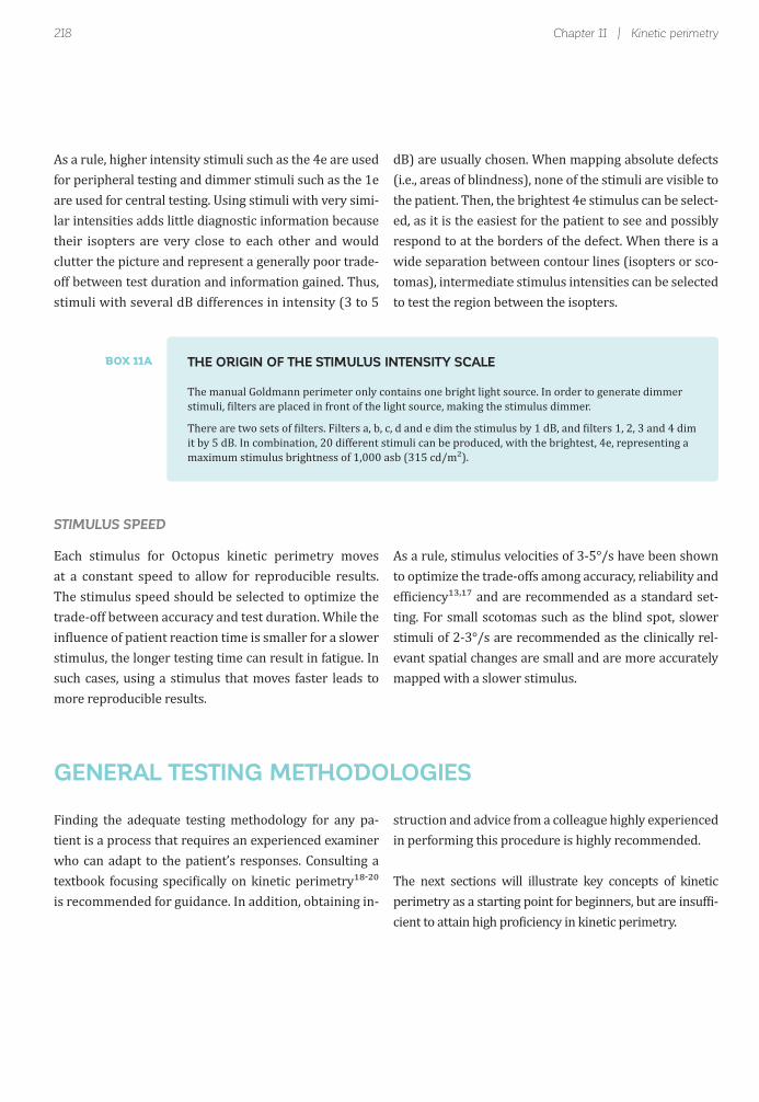
218 Chapter 11 | Kinetic perimetry
As a rule, higher intensity stimuli such as the 4e are used for peripheral testing and dimmer stimuli such as the 1e are used for central testing. Using stimuli with very simi-lar intensities adds little diagnostic information because their isopters are very close to each other and would clutter the picture and represent a generally poor trade-off between test duration and information gained. Thus, stimuli with several dB differences in intensity (3 to 5
dB) are usually chosen. When mapping absolute defects (i.e., areas of blindness), none of the stimuli are visible to the patient. Then, the brightest 4e stimulus can be select-ed, as it is the easiest for the patient to see and possibly respond to at the borders of the defect. When there is a wide separation between contour lines (isopters or sco-tomas), intermediate stimulus intensities can be selected to test the region between the isopters.
THE ORIGIN OF THE STIMULUS INTENSITY SCALE
The manual Goldmann perimeter only contains one bright light source. In order to generate dimmer stimuli, ilters are placed in front of the light source, making the stimulus dimmer.
There are two sets of ilters. Filters a, b, c, d and e dim the stimulus by 1 dB, and ilters 1, 2, 3 and 4 dim it by 5 dB. In combination, 20 different stimuli can be produced, with the brightest, 4e, representing a maximum stimulus brightness of 1,000 asb (315 cd/m²).
BOX 11A
Each stimulus for Octopus kinetic perimetry moves at a constant speed to allow for reproducible results. The stimulus speed should be selected to optimize the trade-off between accuracy and test duration. While the in luence of patient reaction time is smaller for a slower stimulus, the longer testing time can result in fatigue. In such cases, using a stimulus that moves faster leads to more reproducible results.
As a rule, stimulus velocities of 3-5°/s have been shown to optimize the trade-offs among accuracy, reliability and ef iciency¹³,¹⁷ and are recommended as a standard set-ting. For small scotomas such as the blind spot, slower stimuli of 2-3°/s are recommended as the clinically rel-evant spatial changes are small and are more accurately mapped with a slower stimulus.
STIMULUS SPEED
Finding the adequate testing methodology for any pa-tient is a process that requires an experienced examiner who can adapt to the patient’s responses. Consulting a textbook focusing speci ically on kinetic perimetry¹⁸-²⁰ is recommended for guidance. In addition, obtaining in-
struction and advice from a colleague highly experienced in performing this procedure is highly recommended.
The next sections will illustrate key concepts of kinetic perimetry as a starting point for beginners, but are insuf i-cient to attain high pro iciency in kinetic perimetry.
GENERAL TESTING METHODOLOGIES

FIGURE 11-10 The normal isopters provide guidance on where to start a vector of a given intensity. They also serve as a
guide in judging whether an isopter is normal. The dark red band represents 25–75% of healthy normals; the outer light red
band represents 5–95% of healthy normals of the same age. Note that the isopters are not round, but egg-shaped. They
extend farthest in the inferior temporal visual fi eld and least in the superior nasal visual fi eld.
219How to perform kinetic perimetry
10 30 40 50 60 70 80 90
90105120 75 60
270255240 285 300
45135
315225
30150
330210
15165
345195
0180 9090
270 285 300
315
30
3
15
45
00
270 285 300
315
330
1
345
0
25 – 75% 5 – 95%
For each stimulus size and intensity, Octopus kinetic pe-rimetry automatically provides the age-matched normal isopter location as a reference. The inner dark central band represents 25–75% of age-matched normals; the outer light band denotes 5–95% of age-matched healthy normals, as shown in FIG 11-10.
These zones support at-a-glance identi ication of devia-tions from normal and are especially helpful in interpret-ing central visual ield defects and generalized diffuse or widespread loss. As the hill of vision is rather lat from the mid-periphery to the macula, those isopter locations are signi icantly in luenced by age and only comparison
to age-matched normative data will allow correct in-terpretation of the results. As the hill of vision is rather steep towards the far periphery, large age-related sen-sitivity changes have only a small in luence on isopter location.²⁰-²²
In practical terms, the normal isopter location provides guidance on where to start placing vectors. Placing vec-tors far outside of a normal isopter would only waste time, as the patient cannot see the stimuli in these areas. Conversely, starting too near the anticipated location of detection can make the patient unprepared to respond and can produce untrustworthy results.
IDENTIFICATION OF NORMAL ISOPTER LOCATION AND SHAPE
NORMAL ISOPTERS

FIGURE 11-11 Superior-nasal quadrantanopia identifi ed with radial vectors along meridians. Note that the vectors along the
horizontal and vertical midlines are placed parallel to them to allow for better detection of the boundaries of the visual loss in
that quadrant. There are no responses in the superior nasal quadrant of this right eye, indicating the quadrantanopia.
220 Chapter 11 | Kinetic perimetry
10 30 40 50 60 70 80 90
90105120 75 60
270255240 285 300
45135
315225
30150
330210
15165
345195
0180 10 30 40 50 60 70 80 90
90105120 75 60
270255240 285 300
45135
315225
30150
330210
15165
345195
0180
As with any contour or topographic map, the hill of vision may have crevices or depressions, which represent relative or absolute scotomas. As shown in FIG 11-11, these defects may not be identi ied with standard vectors moving from the periphery to the center. This is where custom-ized individual assessment is needed. The examiner has to identify where there is a lack of normal response,
which either manifests as inconsistent with adjacent vec-tors or outside of the expected normal sensitivity, which requires further investigation.
Conceptually, the process is always the same. When alerted to a potential abnormal isopter shape, the operator should estimate where the isopter is likely to be. To verify
DETAILING THE BOUNDARIES OF AN ISOPTER
MAPPING THE OUTLINE OF THE HILL OF VISION
The overall outline of the hill of vision provides valuable information about a patient’s visual ield because devi-ations from normal isopter shapes indicate abnormal visual fields. Thus, mapping the outline of the hill of vision is usually the irst step in kinetic perimetric testing. To map the outline of the hill of vision, stimuli are moved from the peripheral end of the normal band towards the center ( ixation) along a given radial meridian. By repeating this procedure with different stimulus types, the outline of the hill of vision can be drawn in detail, as shown in FIG 11-11.
This procedure is a fast and easy way to identify quadran-tanopia and hemianopia, as the isopter will dip in the
affected area of the visual ield. As a general rule, stimuli should not move directly along the horizontal or vertical meridians, because inconsistent results will be obtained. This is because the boundaries of quadrantanopia and hemianopia are typically positioned along the horizon-tal and vertical meridians and a stimulus moving along these meridians cannot map them clearly. Glaucomatous de icits along the nasal horizontal meridian (e.g,. nasal steps and arcuate scotomas) represent another example where the stimulus should not be moved along the hor-izontal meridian. Thus, for these conditions, the radial vectors are best placed with an offset of a few degrees and possibly parallel to the horizontal and vertical meridians.
MAPPING THE OUTLINE OF THE HILL OF VISION

221How to perform kinetic perimetry
10 30 40 50 60 70 80 90
90105120 75 60
270255240 285 300
45135
315225
30150
330210
15165
345195
0180 10 30 40 50 60 70 80 90
90105120 75 60
270255240 285 300
45135
315225
30150
330210
15165
345195
0180
DETAILING THE BOUNDARIES OF AN ISOPTER
While the procedure shown in FIG 11-12 allows identi i-cation of the outline of the hill of vision, it usually misses isolated absolute defects or local depressions located in-side of an isopter or between isopters. In keeping with the analogy of a hill, isolated defects can be thought of as lakes or depressions of different shapes and depths. In order to identify these defects, spot-checking inside the hill of vision must be performed. Spot-checking quickly examines locations between isopters using static points of the same size and intensity as the outer isopter, to ind
possible areas of sensitivity loss (areas of non-seeing or scotomas). This allows for quick identi ication of scoto-mas as shown in FIG 11-13.
If areas of defects are identi ied, their boundaries can be mapped by moving radial stimuli from inside of the de-fects from the center towards its edges. This procedure can be repeated with stimuli of different visibility to de ine the slope and depth of the defect.
IDENTIFICATION OF ISOLATED SCOTOMAS
that this isopter is correct, additional vectors are drawn perpendicular to the anticipated boundary of the isopter, as shown in FIG 11-12. The perpendicular vectors optimize the likelihood that the hill of vision will be met “head-on”, which will reduce variability and provide more clinically meaningful information. Before initiating this process, it is important to recheck the abnormal isopter shape
to confirm that it is outside of the normal expected responses.
If the patient response is as expected on the imagined isopter, the isopter shape is con irmed and can be drawn. If not, the procedure has to be repeated, taking into account the new information until the isopter location is con irmed.
FIGURE 11-12 Procedure for detailing the boundaries of abnormal isopters on a superior-nasal quadrantanopia. The lack
of normal responses allows the examiner to estimate the location of the isopter (dotted gray line), and then test using
perpendicular vectors (bold red) crossing that line to confi rm the shape of the true isopter.
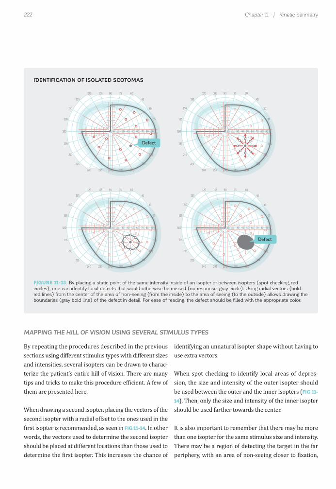
FIGURE 11-13 By placing a static point of the same intensity inside of an isopter or between isopters (spot checking, red
circles), one can identify local defects that would otherwise be missed (no response, gray circle). Using radial vectors (bold
red lines) from the center of the area of non-seeing (from the inside) to the area of seeing (to the outside) allows drawing the
boundaries (gray bold line) of the defect in detail. For ease of reading, the defect should be fi lled with the appropriate color.
222 Chapter 11 | Kinetic perimetry
10 30 40 50 60 70 80 90
90105120 75 60
270255240 285 300
45135
315225
30150
330210
15165
345195
018010 30 40 50 60 70 80 90
90105120 75 60
270255240 285 300
45135
315225
30150
330210
15165
345195
0180
Defect
10 30 40 50 60 70 80 90
90105120 75 60
270255240 285 300
45135
315225
30150
330210
15165
345195
0180 10 30 40 50 60 70 80 90
90105120 75 60
270255240 285 300
45135
315225
30150
330210
15165
345195
0180
Defect
By repeating the procedures described in the previous sections using different stimulus types with different sizes and intensities, several isopters can be drawn to charac-terize the patient’s entire hill of vision. There are many tips and tricks to make this procedure ef icient. A few of them are presented here.
When drawing a second isopter, placing the vectors of the second isopter with a radial offset to the ones used in the irst isopter is recommended, as seen in FIG 11-14. In other
words, the vectors used to determine the second isopter should be placed at different locations than those used to determine the irst isopter. This increases the chance of
identifying an unnatural isopter shape without having to use extra vectors.
When spot checking to identify local areas of depres-sion, the size and intensity of the outer isopter should be used between the outer and the inner isopters (FIG 11-
14). Then, only the size and intensity of the inner isopter should be used farther towards the center.
It is also important to remember that there may be more than one isopter for the same stimulus size and intensity. There may be a region of detecting the target in the far periphery, with an area of non-seeing closer to ixation,
MAPPING THE HILL OF VISION USING SEVERAL STIMULUS TYPES
IDENTIFICATION OF ISOLATED SCOTOMAS

223How to perform kinetic perimetry
10 30 40 50 60 70 80 90
90105120 75 60
270255240 285 300
45135
315225
30150
330210
15165
345195
0180
III4e
I2e
10 30 40 50 60 70 80 90
90105120 75 60
270255240 285 300
45135
315225
30150
330210
15165
345195
0180 10 30 40 50 60 70 80 90
90105120 75 60
270255240 285 300
45135
315225
30150
330210
15165
345195
0180
III4e
I2e
10 30 40 50 60 70 80 90
90105120 75 60
270255240 285 300
45135
315225
30150
330210
15165
345195
0180
III4e
I2e
PLACEMENT OF VECTORS AND STATIC POINTS USING DIFFERENT STIMULUS TYPES
DISTINCTION BETWEEN ABSOLUTE AND RELATIVE SCOTOMAS
Local scotomas can be absolute defects with sharp-edged boundaries such as the blind spot or relative defects with a gentle slope on the edge of the defect as in glaucoma. To distinguish between the two, more than one stimulus is needed to characterize a local scotoma as can be seen in
FIG 11-15. For easy interpretation, these local depressions are typically illed with color to indicate that the corre-sponding stimulus cannot be seen within that visual ield area.
followed by a second area that can detect the target. This can occur in some cases of retinal disease, moderate to advanced glaucoma, and neurologic disorders affecting
the visual pathways. Because of this, it is important to make good use of spot checking and evaluate the entire visual ield.
FIGURE 11-14 Vectors of different stimulus sizes and intensities are best placed with an offset to increase the chance of
identifi cation of abnormal isopter shapes. When placing static points between two isopters, always use the intensity of the
more visible outer isopter.
FIGURE 11-15 More than one isopter is needed to distinguish between absolute and relative scotomas. This example shows a
nasal step for a glaucoma patient.

224 Chapter 11 | Kinetic perimetry
10 30 40 50 60 70 80 90
90105120 75 60
270255240 285 300
45135
315225
30150
330210
15165
345195
0180 10 30 40 50 60 70 80 90
90105120 75 60
270255240 285 300
45135
315225
30150
330210
15165
345195
0180
LOW SHORT-TERM FLUCTUATIONThe two gray dots on each vector
are close to each other
HIGH SHORT-TERM FLUCTUATIONThe two gray dots on each vector
are far from each other
Like static visual ield testing, kinetic perimetry has a patient-related subjective component and the reliability of the results largely depends on good patient coopera-tion and minimizing variability due to learning or fatigue effects.²¹,²³,²⁴ Therefore, it is also essential to check for patient reliability in kinetic perimetry. While static pe-rimetry uses global indices such as false positive and false negative catch trials and short-term luctuation, kinetic perimetry employs other methodologies to test for similar reliability indicators.
To assess short-term luctuation, it is worth duplicating
In legal driving and blindness examinations performed with kinetic perimetry, it is worth checking for false an-swers to identify patients who may simulate responses or a lack of response (functional changes or visual mea-sures that are non-physiologic and non-pathologic). This can produce visual ield results that are either better or worse than the actual visual ield sensitivity pro ile. As in static perimetry, it is possible to check for both false
certain vectors to check for consistency of responses, as shown in FIG 11-16. To do this, two vectors should be placed as close together as possible (or repeated) and then compared for consistency. If the responses are reliable, the two patient responses should be very close together, as shown in the igure below to the left which means there is low test-retest variability. If they are sep-arated, as in the example below to the right, it indicates an unreliable result with high test-retest variability. This procedure provides a good indicator for the quality of the results. Similarly, spot checking can be repeated at various locations to assess response consistency.
positive and false negative answers even though the pro-cedure is different. Checking for false positive answers can be easily done by presenting stimuli outside of the normal isopter area (FIG 11-17). By de inition, the patient is not supposed to see these stimuli. If there are many positive responses, this is a strong indicator of a patient who is malingering.
CHECKING FOR VISUAL FIELD RELIABILITY
CHECKING FOR SHORT-TERM FLUCTUATION
FIGURE 11-16 By repeating some vectors, short-term fl uctuation and thus test-retest variability can be assessed. If the
responses are close together (left), it indicates good patient cooperation, good repeatability and high reliability. If the responses
largely differ (right), it indicates an unreliable visual fi eld.

225How to perform kinetic perimetry
10 30 40 50 60 70 80 90
90105120 75 60
270255240 285 300
45135
315225
30150
330210
15165
345195
018010 30 40 50 60 70 80 90
90105120 75 60
270255240 285 300
45135
315225
30150
330210
15165
345195
0180
NO FALSE POSITIVESNo response to stimulioutside normal isopter
FALSE POSITIVES3 responses to stimulioutside normal isopter
10 30 40 50 60 70 80 90
90105120 75 60
270255240 285 300
45135
315225
30150
330210
15165
345195
0180 10 30 40 50 60 70 80 90
90105120 75 60
270255240 285 300
45135
315225
30150
330210
15165
345195
0180
NO FALSE NEGATIVESImmediate response to larger or more intense
stimulus at a location previously seen
FALSE NEGATIVESRandom response to larger or more intense
stimulus at a location previously seen
Smaller or lessintense stimulus
Larger or moreintense stimulus
Smaller or lessintense stimulus
Larger or moreintense stimulus
To detect false negative answers one places a more intense or larger stimulus at a location where the stimulus was previously detected. This stimulus should be easy for
the patient to observe (FIG 11-18). Failure to see a more intense or larger stimulus than the one that was detected at threshold is considered to be a false negative response.
CHECKING FOR FALSE POSITIVES
CHECKING FOR FALSE NEGATIVES
FIGURE 11-17 Checking for false positive responses can be done by placing vectors or static points outside of a normal
isopter. If a patient responds, then these are false positives, as the patient cannot see them.
FIGURE 11-18 Checking for false negative responses can be done by placing larger or more intense vectors or static points at
a location where a smaller or less intense stimulus was previously detected. If a patient does not respond, then these are false
negatives, as the patient should be able to see them.

226 Chapter 11 | Kinetic perimetry
Reaction time(RT) vector
Standard vector
Patient sees Patient responds
Standard vector withRT compensation
523 ms0 ms
Patient reaction time in luences the size of an isopter as the patient’s response is produced some time after the stimulus is actually seen.²¹,²²,²⁵ This also adds signi icant variability to the test procedure.²³ If a patient’s re-sponses were always instantaneous, outlines of the hill of vision would be larger and isolated defects would be smaller than they appear on the printout. This makes the interpretation of results challenging, especially in pa-tients with long or inconsistent reaction times.
For a precise measurement of patient reaction time, us-ing the average reaction time obtained from two or three different vectors for each stimulus type is recommended,
For this reason, Octopus kinetic perimetry offers the possibility of adjusting for patient reaction time by mea-suring its magnitude in the patient’s intact visual ield and applying a reaction time correction for it, as illus-trated in FIG 11-19. In order to do so, the examiner should choose a reaction time vector of the same stimulus type as the isopter and place it into the patient’s seeing area. The patient should be able to see the stimulus immediately as it is presented. Thus, the time between stimulus pre-sentation and when the patient presses the response button represents the patient’s reaction time.
placing the reaction time vectors close to the correspond-ing isopter. FIG 11-20 provides an example of the clinical usefulness of reaction time compensation.
PATIENT REACTION TIME COMPENSATION
PATIENT REACTION TIME COMPENSATION
FIGURE 11-19 There is always a lag between the moment the patient sees a stimulus and the moment a patient presses the
response button. This constitutes the patient’s reaction time. By placing reaction time (RT) vectors into the patient’s seeing
area, one can account for this lag.

227How to perform kinetic perimetry
10 30 40 50 60 70 80 10 30 40 50 60 70 80
REACTION-TIME compensation
turned OFF
REACTION-TIMEcompensation
turned ON
Reaction time vectors
10 30 40 50 60 70 80 90
90105120 75 60
270255240 285 300
45135
315225
30150
330210
15165
345195
0180 10 30 40 50 60 70 80 90
90105120 75 60
270255240 285 300
45135
315225
30150
330210
15165
345195
0180
1. Mapping outline of hill of visionI4e, 5°/s
2. Detailing boundaries of isopterI4e, 5°/s
EXAMPLE OF THE CLINICAL USEFULNESS OF REACTION TIME COMPENSATION
STEP-BY-STEP EXAMPLE OF A KINETIC TEST WITH SEVERAL ISOPTERS (STEPS 1-2)
FIGURE 11-20 Without reaction time compensation, local depressions look uncharacteristically large (left). By using reaction
time vectors (bold red, double arrows) to determine the patient’s reaction time and by turning reaction time compensation on
(right), the patient’s adjusted defect size is revealed.
FIGURE 11-21 This example above shows a full kinetic perimetric test of a quadrantanopia with 4 isopters (shown here in
blue, red, gray and green), static points and reaction time compensation. Checks for consistent results and false positives are
not shown in this example.
A real-life example of a complete kinetic test as performed in clinical practices is provided in FIGURE 11-21.
STEP-BY-STEP EXAMPLE OF KINETIC PERIMETRY
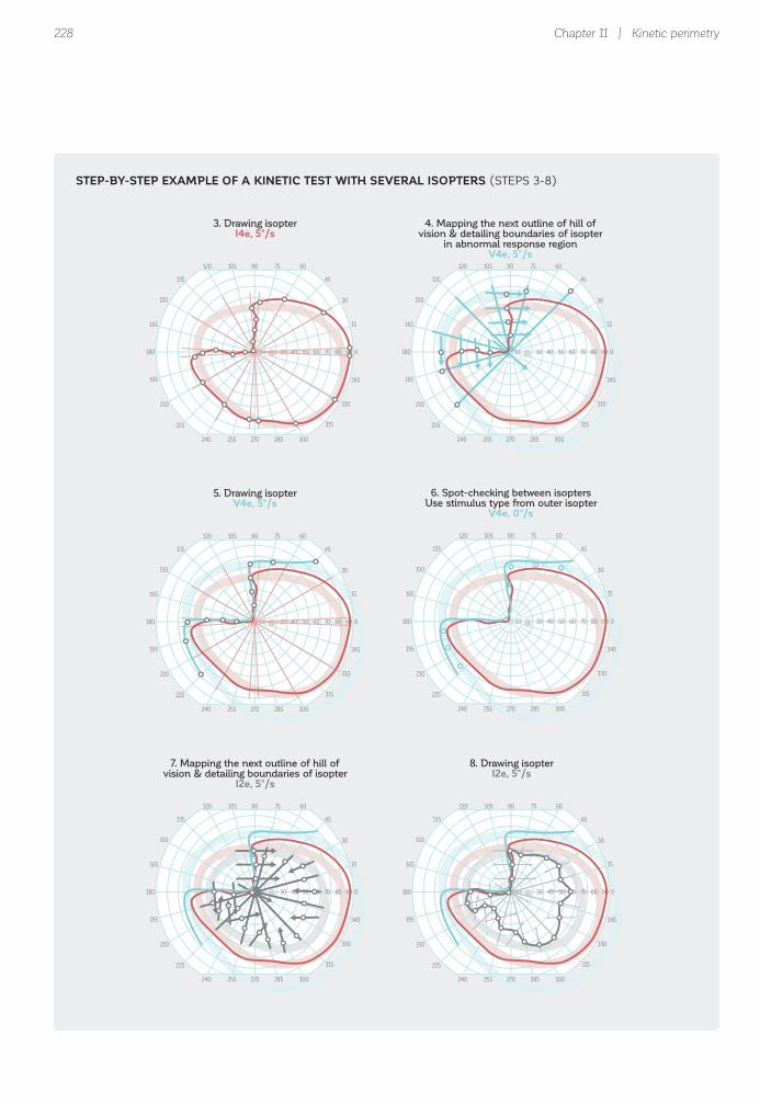
228 Chapter 11 | Kinetic perimetry
10 30 40 50 60 70 80 90
90105120 75 60
270255240 285 300
45135
315225
30150
330210
15165
345195
0180 10 30 40 50 60 70 80 90
90105120 75 60
270255240 285 300
45135
315225
30150
330210
15165
345195
0180
3. Drawing isopterI4e, 5°/s
4. Mapping the next outline of hill ofvision & detailing boundaries of isopter
in abnormal response regionV4e, 5°/s
10 30 40 50 60 70 80 90
90105120 75 60
270255240 285 300
45135
315225
30150
330210
15165
345195
0180
7. Mapping the next outline of hill ofvision & detailing boundaries of isopter
I2e, 5°/s
10 30 40 50 60 70 80 90
90105120 75 60
270255240 285 300
45135
315225
30150
330210
15165
345195
0180
8. Drawing isopterI2e, 5°/s
10 30 40 50 60 70 80 90
90105120 75 60
270255240 285 300
45135
315225
30150
330210
15165
345195
0180
5. Drawing isopterV4e, 5°/s
10 30 40 50 60 70 80 90
90105120 75 60
270255240 285 300
45135
315225
30150
330210
15165
345195
0180
6. Spot-checking between isoptersUse stimulus type from outer isopter
V4e, 0°/s
STEP-BY-STEP EXAMPLE OF A KINETIC TEST WITH SEVERAL ISOPTERS (STEPS 3-8)

229How to perform kinetic perimetry
10 30 40 50 60 70 80 90
90105120 75 60
270255240 285 300
45135
315225
30150
330210
15165
345195
018010 30 40 50 60 70 80 90
90105120 75 60
270255240 285 300
45135
315225
30150
330210
15165
345195
0180
9. Spot-checking between isoptersUse stimulus type from outer isopter
I4e, 0°/s
10. Mapping the next outline of hill of vision & detailing boundaries & drawing isopter
I1e, 2°/s
10 30 40 50 60 70 80 90
90105120 75 60
270255240 285 300
45135
315225
30150
330210
15165
345195
0180
11. Spot-checking between isoptersUse stimulus type from outer isopter
I2e, 0°/s, I1e, 0°/s
10 30 40 50 60 70 80 90
90105120 75 60
270255240 285 300
45135
315225
30150
330210
15165
345195
0180 10 30 40 50 60 70 80 90
90105120 75 60
270255240 285 300
45135
315225
30150
330210
15165
345195
0180
13. Draw reaction time vectorsin visible area
RT vectors, same intensity, sizeand speed as respective standard vector
14. Reaction-time compensationRT on
10 30 40 50 60 70 80 90
90105120 75 60
270255240 285 300
45135
315225
30150
330210
15165
345195
0180
12. Mapping of isolated defect(blind spot)
I4e, 2°/s
STEP-BY-STEP EXAMPLE OF A KINETIC TEST WITH SEVERAL ISOPTERS (STEPS 9-14)

230 Chapter 11 | Kinetic perimetry
10 30 40 50 60 70 80 90
90105120 75 60
270255240 285 300
45135
315225
30150
330210
15165
345195
0180 10 30 40 50 60 70 80 90
90105120 75 60
270255240 285 300
45135
315225
30150
330210
15165
345195
0180 0500 000
Untaped
PTOSIS TEMPLATEFull automation possible
PTOSIS TESTTest performed twice
with taped and untaped lid
Taped
In manual kinetic perimetry, the operator draws each vector individually for each patient. This procedure, which is used on manual Goldmann perimeters, is fully implemented on the Octopus perimeters. Therefore, a Goldmann manual perimetric test can be performed on the Octopus perimeter. The example presented above illustrates the lexibility of manual kinetic perimetry.
Manual kinetic perimetry is still widely used today be-cause it allows full lexibility to adapt to any patient sit-
While kinetic perimetry testing often needs to be individ-ualized, there are certain indications where the expected
uation. A drawback of manual kinetic perimetry is the lack of consensus for a standard way to conduct it. As a result, there is limited comparability between the results obtained from different examiners and clinics. Another drawback is that manual kinetic perimetry requires intensive training and there is a certain operator bias. Simpler procedures are therefore desirable for more consistent and effective clinical work lows.
responses are already known. An example is visual ield testing for ptosis, as illustrated in FIG 11-22.
MANUAL KINETIC PERIMETRY – FULL FLEXIBILITY
AUTOMATED KINETIC PERIMETRY– STANDARDIZATION
AUTOMATION OF KINETIC PERIMETRY
EXAMPLE OF FULLY AUTOMATED KINETIC PERIMETRY TO TEST FOR PTOSIS
FIGURE 11-22 In ptosis testing, one is trying to identify the exact position of the lid, which always curves upwards from
the nasal to temporal side. Therefore, a standardized testing procedure of a few vertical vectors is all that is needed and a
very visible and adequately fast III4e to V4e at 3–5°/s is a good stimulus choice. This procedure can be fully automated and
performed both on taped and untaped lids.

231How to perform kinetic perimetry
10 30 40 50 60 70 80 90
90105120 75 60
270255240 285 300
45135
315225
30150
330210
15165
345195
018010 30 40 50 60 70 80 90
90105120 75 60
270255240 285 300
45135
315225
30150
330210
15165
345195
0180
GENERAL ASSESSMENT PITUITARY ADENOMA
10 30 40 50 60 70 80 90
90105120 75 60
270255240 285 300
45135
315225
30150
330210
15165
345195
0180 10 30 40 50 60 70 80 90
90105120 75 60
270255240 285 300
45135
315225
30150
330210
15165
345195
0180
HEMIANOPIA BLIND SPOT
Semiautomated kinetic perimetry offers the bene its of both automated and manual kinetic perimetry with much less of their respective shortcomings, and is a part of Octo-pus kinetic perimetry.
In semiautomated kinetic perimetry, the examination is started using a given prede ined template in an automated
For any such indication with a clearly known defect pat-tern, Octopus kinetic perimetry allows storage of fully automated templates that can, once programmed, be run in the same way as Standard Automated Perimetry by simply pressing the start button. Only the isopters remain to be drawn manually.
mode. In contrast to automated kinetic perimetry, vec-tors can be individually added, but responses can also be repeated or deleted if the examiner deems it necessary. Because of the full lexibility offered by semiautomated kinetic perimetry, it can provide results that are as pre-cise as manual kinetic perimetry while greatly improving the standardization within a clinic, as all examiners use
Full automation not only standardizes kinetic testing and makes it much more comparable across examiners and clinics, it also makes the procedure as easy to learn and perform as static perimetry. As there is currently no con-sensus on how a certain indication should be tested, each clinic can de ine the automated templates according to its current testing methodologies.
SEMIAUTOMATED KINETIC PERIMETRY – STANDARDIZATION AND FULL FLEXIBILITY
EXAMPLE OF CUSTOMIZED TEMPLATES FOR NEURO-OPHTHALMIC CONDITIONS
FIGURE 11-23 Kinetic templates allow testing standardization, as the same methodology is always used. Full fl exibility of adap-
tation to a patient’s specifi c situation is also enabled. Above are four examples of templates regularly used in a neuro-ophthalmic
clinic.²⁴-²⁶ For simplicity, only one stimulus type is displayed, but templates with more than one stimulus type are also possible.

232 Chapter 11 | Kinetic perimetry
the same underlying technique and only make adapta-tions if the patient requires it. This greatly improves consistency amongexaminers and facilitates clinical result interpretation.
Many different templates can be created for the most
commonly occurring indications, based on each clinic’s needs. FIG 11-23 shows a number of templates that can be used in a neuro-ophthalmic clinic. These templates are not considered the only possible templates for such condi-tions, but rather examples of performing effective kinetic perimetry in these situations.

233References
REFERENCES1. Rowe FJ, Noonan C, Manuel M. Comparison of octopus semi-automated kinetic perimetry and humphrey peripheral static perimetry in neuro-ophthalmic cases. ISRN Ophthalmol. 2013;doi: 10.1155/2013/753202.2. Scheuerle AF, Schiefer U, Rohrschneider K. Functional diagnostic options for advanced and end stage glaucoma. Ophthalmologe. 2012;109: 337-344.3. Alniemi ST, Pang NK, Woog JJ, Bradley EA. Comparison of automated and manual perimetry in patients with blepharoptosis. Ophthal Plast Reconstr Surg. 2013;29:361-363.4. Nowomiejska K, Brzozowska A, Koss MJ, et al. Quanti ication of the visual ield loss in retinitis pigmentosa using semi- automated kinetic perimetry. Curr Eye Res. 2016;doi: 10.3109/02713683.2015.1079328.5. Nowomiejska K, Wrobel-Dudzinska D, Ksiazek K, et al. Semi-automated kinetic perimetry provides additional information to static automated perimetry in the assessment of the remaining visual ield in end-stage glaucoma. Ophthalmic Physiol Opt. 2015;35:147-154.6. Agarwal HC, Gulati V, Sihota R. Visual ield assessment in glaucoma: comparative evaluation of manual kinetic Goldmann perimetry and automated static perimetry. Indian J Ophthalmol. 2000;48:301-306.7. Riemann CD, Hanson S, Foster JA. A comparison of manual kinetic and automated static perimetry in obtaining ptosis ields. Arch Ophthalmol. 2000;118:65-69.8. Nevalainen J, Paetzold J, Krapp E, Vonthein R, Johnson CA, Schiefer U. The use of semi-automated kinetic perimetry (SKP) to monitor advanced glaucomatous visual ield loss. Graefes Arch Clin Exp Ophthalmol. 2008;246:1331-1339.9. Patel DE, Cumberland PM, Walters BC, Russell-Eggitt I, Rahi JS, OPTIC study group. Study of Optimal Perimetric Testing in Children (OPTIC): Feasibility, Reliability and Repeatability of Perimetry in Children. PLoS One. 2015; doi: 10.1371/ journal.pone.0130895.10. Haag-Streit AG, (Hrsg.). 1858 - 2008: 150 Jahre Haag-Streit/150 Years of Haag-Streit. Bern: Stämp li Publikationen AG; 2008. 11. Johnson CA, Wall M, Thompson HS. A history of perimetry and visual ield testing. Optom Vis Sci. 2011;88:E8-15.12. Fankhauser F. Remembrance of Hans Goldmann, 1899-1991. Surv Ophthalmol. 1992;37:137-142.13. Rowe FJ, Rowlands A. Comparison of diagnostic accuracy between Octopus 900 and Goldmann kinetic visual ields. Biomed Res Int. 2014;doi: 10.1155/2014/214829.14. Nowomiejska K, Vonthein R, Paetzold J, Zagorski Z, Kardon R, Schiefer U. Comparison between semiautomated kinetic perimetry and conventional Goldmann manual kinetic perimetry in advanced visual ield loss. Ophthalmology. 2005;112:1343-1354.15. Ramirez AM, Chaya CJ, Gordon LK, Giaconi JA. A comparison of semiautomated versus manual Goldmann kinetic perimetry in patients with visually signi icant glaucoma. J Glaucoma. 2008;17:111-117.16. Rowe FJ, Hanif S. Uniocular and binocular ields of rotation measures: Octopus versus Goldmann. Graefes Arch Clini Exp Ophthalmol. 2011;249:909-919.17. Johnson CA, Keltner JL. Optimal rates of movement for kinetic perimetry. Arch Ophthalmol. 1987;105:73-75.18. Anderson DR. Testing the ield of vision. St.Louis: CV Mosby; 1982.19. Anderson DR. Perimetry - With and without automation. 2nd ed. St.Louis: CV Mosby; 1987.20. Walsh TJ. Visual Fields: Examination and interpretation. 3rd ed. American Academy of Ophthalmology Monograph Series; Oxford University Press; 2010.21. Nowomiejska K, Brzozowska A, Zarnowski T, Rejdak R, Weleber RG, Schiefer U. Variability in isopter position and fatigue during semi-automated kinetic perimetry. Ophthalmologica. 2012;227:166-172.22. Grobbel J, Dietzsch J, Johnson CA, et al. Normal values for the full visual ield, corrected for age- and reaction time, using semiautomated kinetic testing on the Octopus 900 perimeter. Transl Vis Sci Technol. 2016;5:doi:10.1167/tvst.5.2.5.23. Hirasawa K, Shoji N. Learning effect and repeatability of automated kinetic perimetry in healthy participants. Curr Eye Res. 2014;39:928-937.24. Rowe FJ, Sarkies NJ. Assessment of visual function in idiopathic intracranial hypertension: a prospective study. Eye (Lond). 1998;12:111-118.25. Rowe FJ, Cheyne CP, García-Fiñana M, et al. Detection of visual ield loss in pituitary disease: Peripheral kinetic versus central static. Neuro-Ophthalmology. 2015;39:116-124.26. Rowe FJ, Wright D, Brand D, et al. A prospective pro ile of visual ield loss following stroke: prevalence, type, rehabilitation, and outcome. Biomed Res Int. 2013; doi: 10.1155/2013/719096.

234

235
CHAPTER 12TRANSITIONING TO A DIFFERENT PERIMETER MODEL
INTRODUCTIONAt the end of the life span of a perimeter or in order to bene it from technologies only available on a different perimeter model or brand, transitioning to a new perimeter with distinct characteristics may be necessary. Due to differences in the design and test parameters between perimeter models, the measured sensitivity thresholds are not directly comparable. As a result, the variability introduced by a transition must be acknowledged and addressed.
Octopus perimeters offer several features that make it possible to transition smoothly between perimeter models, regardless of whether the transition is from one Octopus model to another Octopus model or from a Humphrey Field Analyzer (HFA) to any Octopus model. These features minimize, to a large extent, the impact of the different parameters used in the various perimeter models and are systematically presented in this chapter.
An explanation of why different sensitivity thresholds
are obtained on different perimeter models is irst pre-sented. Then, this chapter highlights that while sensi-tivity thresholds are not directly comparable between different models, sensitivity losses (i.e., deviations from normal sensitivity thresholds) are comparable to a large extent because of the use of device-speci ic normative databases. This chapter also provides practical guidance on how to minimize patient-related luctuation that may arise during the transition and subside as patients become familiar with the new device.
In addition, when transitioning from an HFA to an Octopus perimeter, it is important to recognize that each perimeter uses its own, sometimes proprietary, test parameters and result displays. As a result, the transition may appear challenging. Practical recommendations for the selection of test patterns and strategies are presented to facilitate the transition. Furthermore, information is provided on how to interpret the perimetric result after the transition from an HFA to an Octopus perimeter.

236 Chapter 12 | Transitioning to a different perimeter model
GENERAL ASPECTS OF TRANSITIONING
Since different perimeter models vary in design and sometimes use different test parameters, patients may perceive perimetric stimuli differently. As a result, the measured sensitivity thresholds can vary¹ and measured
sensitivity thresholds cannot be directly compared. BOX
12A presents an overview of major causes of variability between different Octopus perimeter models as well as the HFA perimeter and Octopus perimeter models.
MEASURED SENSITIVITY THRESHOLDS CANNOT BE COMPARED ACROSS DIFFERENT PERIMETER MODELS
MAJOR DIFFERENCES BETWEEN VARIOUS OCTOPUS PERIMETER MODELS
Since the various Octopus perimeter models vary in design and sometimes use different test parameters, measured sensitivity thresholds also vary.¹
Firstly, design differences can lead to a different perception of perimetric stimuli. For example, there are two fundamentally different designs used in recent Octopus perimeter models. Cupola perimeters (e.g., Octopus 101 and 900) allow for testing of the full ield (e.g., 90° radius) and use a moving projector to present the perimetric stimuli onto the whitish surface of a cupola. On the other hand, screen-based perimeters (e.g., Octopus 600) allow for testing of the central ield only (e.g., 30° radius) and generate the stimulus on a computer display. Because of the different stimulus presentation technologies used, patients may perceive stimuli differently.
In addition, the full ield cupola perimeters are open and thus need to operate under dim room lighting conditions to avoid stray light in luencing the result, whereas screen-based perimeters are closed, not in luenced by stray light and thus can be operated under daylight conditions. Further, while the mechanical projector of the cupola perimeters makes some noise upon stimulus presentation, screen-based perimeters are silent during stimulus presentations. As a result, even if completely identical test conditions are used (i.e., same stimulus size, same stimulus luminance and same background luminance), patients may respond differently. They can be in luenced by these differences and, as a result, determined sensitivity thresholds may vary.
Secondly, different test parameters may also lead to different perimetric results. For this reason, all recent Octopus models (e.g., Octopus 900, Octopus 600, Octopus 300 and Octopus 123) use the same ixed test parameters, which are described in Box 4A. An exception is the Octopus 101, which uses
a background luminance of 4 asb (instead of 31.4 asb), operating under mesopic illumination (i.e., midway between daylight and night vision) instead of photopic illumination (i.e., daylight vision), which may in luence the perception of the perimetric stimulus. To reduce this bias when transitioning from an Octopus 101 to an Octopus 900, the Octopus 900 can be optionally operated using a background luminance of 4 asb.
MAJOR DIFFERENCES BETWEEN THE HFA PERIMETER AND OCTOPUS PERIMETER MODELS
As already explained in the section above, design differences between the HFA perimeter (which is a cupola perimeter) and other Octopus perimeter models may lead to different perception of perimetric stimuli even if the same test conditions were used.
However, the HFA perimeter and the various Octopus perimeter models also use different ixed test parameters. The most marked difference between the determined sensitivity thresholds of an HFA perimeter and recent Octopus perimeter models (e.g., Octopus 900, 600, 300 and 123) stems from the different maximum stimulus luminances used (4,000 asb in Octopus perimeters compared to 10,000
BOX 12A

237General aspects of transitioning
Whenever an Octopus perimeter model is developed, data are collected from people with healthy eyes and of different ages on that model in order to develop a nor-mative database for it (see BOX 2B for more detail on normative databases). As a result, each Octopus model has its respective normative database. Furthermore, all Octopus models contain the normative databases of all other models in order to allow for smooth transitions between models. When transitioning from one Octopus model to another, the existing data of one device can be imported into the other device and the data compared to the appropriate normative database. For example, when the visual ield tests taken on a given Octopus model (e.g.,
HFA perimeters use an HFA-speci ic normative database to calculate the sensitivity losses presented in the Total Deviation representation, while each Octopus model uses its own normative database. As a result, the use of these device-speci ic normative databases largely elimi-nates any model-related bias between perimetric results when looking at sensitivity losses. For example, while the
an Octopus 300) are imported into another model (e.g., Octopus 900), the user can be sure that the imported sen-sitivity thresholds are compared with the Octopus 300 device-speci ic normative database to calculate the sen-sitivity losses.
Using device-speci ic normative databases largely elimi-nates device-speci ic differences in sensitivity losses. As a result, sensitivity losses and all related representations, with the exception of the Values and Grayscale (Values), are largely comparable across perimeter models as shown in FIG 12-1.
measured sensitivity thresholds of an HFA II and an Octopus 900 show an offset of 4 dB as explained in BOX
12A, the respective normative databases show the same offset, and as a result the sensitivity losses are comparable. This means that all representations with the exception of the Values and Grayscale (Values) representations are comparable.
SENSITIVITY LOSSES CAN BE COMPARED BETWEEN DIFFERENT OCTOPUS PERIMETER MODELS
SENSITIVITY LOSSES CAN BE COMPARED BETWEEN HFA PERIMETERS AND DIFFERENT OCTOPUS
PERIMETER MODELS
DEVICE-SPECIFIC NORMATIVE DATABASES ALLOW COMPARISON OF SENSITIVITY LOSSES BETWEEN DEVICES
asb in HFA perimeters). This difference leads to an offset of 4 dB in the default decibel scale used to display sensitivity thresholds. This is due to the fact that both instruments take the maximum stimulus luminance as the origin of their dB scale (0 dB), as explained in BOX 2A. A stimulus of 1,000 asb intensity therefore corresponds to a sensitivity threshold of 10 dB on an HFA II perimeter and to 6 dB on an Octopus 900 perimeter.

FIGURE 12-1 This example illustrates the benefi ts of using device-specifi c normative databases (i.e., an individual normative
database for each device). In this example, sensitivity thresholds of a patient with retinal detachment were determined on
an Octopus 900, Octopus 600 and on an HFA II perimeter on the same day (left). These sensitivity thresholds cannot
be compared to each other due to the different characteristics of the three perimeter models. However, because distinct
normative databases are used for the Octopus 900, Octopus 600 and the HFA II perimeter (middle), the sensitivity losses are
comparable. Sensitivity losses are calculated as the deviation of the measured sensitivity thresholds of each model from its
respective normative database and are the basis of most visual fi eld representations such as the Corrected Probabilities
or Pattern Deviation Probability Map shown in this fi gure. Note that comparability applies to all representations with the
exception of the Values and Grayscale (Values) representations.
18 23 23 19
18 24 28 17
19 23 21 1 13
3
6 20
13 23 17
17 18 29 19 18
13 24 28 23 9
20 8 2 0
3
16 20 19
19 24 24 19 19
16 21 27 11
18 18 5
5
19 23 21 19
17 20 26 22 16
18 20 22 11 5
15 2
16 18
17 22 23 21
20 24 26 18
23 26 21 1 0
4
5 18
10 20 14
16 25 25 24 23
18 26 27 22 1
23 8 2
3
16 21 21
21 20 21 21 17
23 23 29 6
23 18 5
5
19 22 22 20
18 23 25 23 16
21 26 22 11
15 2
14 17
OC
TOP
US
90
0O
CTO
PU
S 6
00
HFA
II
MEASURED SENSITIVITY THRESHOLDS
NOT COMPARABLE
NOT COMPARABLE
COMPARABLE
COMPARABLE
NORMATIVE VALUES SENSITIVITY LOSSES
Values Normative Database Corrected Probabilities
Values Normative Database Corrected Probabilities
Threshold Values Normative Database Pattern Deviation Probability Map
238 Chapter 12 | Transitioning to a different perimeter model
SENSITIVITIY LOSSES BETWEEN DIFFERENT DEVICES ARE LARGELY COMPARABLE
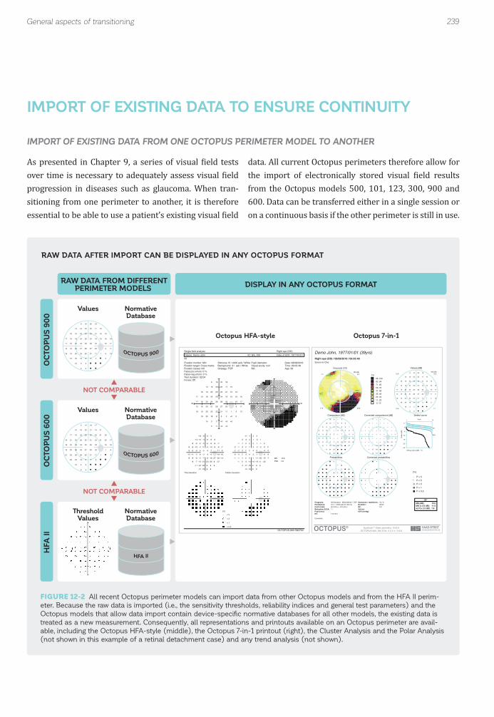
FIGURE 12-2 All recent Octopus perimeter models can import data from other Octopus models and from the HFA II perim-
eter. Because the raw data is imported (i.e., the sensitivity thresholds, reliability indices and general test parameters) and the
Octopus models that allow data import contain device-specifi c normative databases for all other models, the existing data is
treated as a new measurement. Consequently, all representations and printouts available on an Octopus perimeter are avail-
able, including the Octopus HFA-style (middle), the Octopus 7-in-1 printout (right), the Cluster Analysis and the Polar Analysis
(not shown in this example of a retinal detachment case) and any trend analysis (not shown).
18 23 23 19
18 24 28 17
19 23 21 1 13
3
6 20
13 23 17
17 18 29 19 18
13 24 28 23 9
20 8 2 0
3
16 20 19
19 24 24 19 19
16 21 27 11
18 18 5
5
19 23 21 19
17 20 26 22 16
18 20 22 11 5
15 2
16 18
17 22 23 21
20 24 26 18
23 26 21 1 0
4
5 18
10 20 14
16 25 25 24 23
18 26 27 22 1
23 8 2
3
16 21 21
21 20 21 21 17
23 23 29 6
23 18 5
5
19 22 22 20
18 23 25 23 16
21 26 22 11
15 2
14 17
OC
TOP
US
90
0O
CTO
PU
S 6
00
HFA
II
RAW DATA FROM DIFFERENTPERIMETER MODELS
NOT COMPARABLE
NOT COMPARABLE
DISPLAY IN ANY OCTOPUS FORMAT
Single field analysisName: Demo John ID: GS_103 Date of birth: 1977/01/01
Right eye (OD)
OCTOPUS 900 SN3704
32Fixation monitor: MinFixation target: Cross marksFixation losses: 0/0False pos errors: 0 %False neg errors: 0 %Test duration: 02:04Fovea: Off
Stimulus: III / 4000 asb / WhiteBackground: 31 asb / WhiteStrategy: TOP
Pupil diameter: Visual acuity: nullRX:
Date: 08/08/2016Time: 09:05:48Age: 39
18 23 23 19
18 24 28 17
19 23 21 1 13
3 <0 <0
6 20
13 23 17
17 18 29 19 18
13 24 28 23 9
20 8 2 0
3 <0
16 20 19
19 24 24 19 19
16 21 27 11
18 18 5 <0
5 <0
19 23 21 19
17 20 26 22 16
18 20 22 11 5
15 2 <0
16 18
30
<0 <0
<0
<0
<0
<0
30
-8 -5 -5 -8
-9 -5 -3 -9
-8 -5 -8 -27 -14
-24
-18 -4-12 -3 -9
-9 -10 0 -10 -9
-13 -5 -3 -6 -18
-7 -21 -26 -27
-23
-10 -6 -6
-8 -4 -5 -9 -7
-11 -9 -4 -16
-8 -10 -23
-21
-8 -5 -6 -7
-9 -9 -5 -7 -11
-8 -8 -7 -18 -22
-11 -25
-8 -5
-1 3 2 -1
-2 2 4 -2
-1 2 -1 -20 -7
-17
-11 3-5 4 -2
-2 -3 7 -3 -2
-6 2 4 1 -11
0 -14 -19 -20
-16
-3 1 1
-1 3 2 -2 0
-4 -2 3 -9
-1 -3 -16
-14
-1 2 1 0
-2 -2 2 0 -4
-1 -1 0 -11 -15
-4 -18
-1 2
Total deviation Pattern deviation
MD -10.6 PSD 7.8
[%]< 5
< 2
< 1
< 0.5 EyeSuite™ Static perimetry, V3.5.0OCTOPUS 900, SN 3704, V 2.3.1 / 3.6.0
Demo John, 1977/01/01 (39yrs)Right eye (OD) / 08/08/2016 / 09:05:48Seven-in-One
Comment:
NV: T12 V2.1Pupil [mm]: IOP [mmHg]:Refraction S/C/A: VA [m]:Catch trials: 0/4 (0%) +, 0/4 (0%) - RF: 0.0Parameters: 31.4 / 4000 asb III 100 ms Duration: 02:04Programs: 32 Standard White/White / TOP Questions / repetitions: 74 / 0 MS [dB]: 15.5
MD [< 2.0 dB]: 11.6sLV [< 2.5 dB]: 7.8
30°
[%]95..10083..9471..8259..7047..5835..4623..3411..22 0..10
Grayscale (CO)MD [dB]
6.97.5
11.8 20.6
Values [dB]
18 23 23 19
18 24 28 17
19 23 21 1 13
3
6 20
13 23 17
17 18 29 19 18
13 24 28 23 9
20 8 2 0
3
16 20 19
19 24 24 19 19
16 21 27 11
18 18 5
5
19 23 21 19
17 20 26 22 16
18 20 22 11 5
15 2
16 18 MS [dB]19.819.4
15.6 7.1
Comparison [dB]
8 5 5 8
9 5 + 9
8 5 8 27 14
24
18 +
12 + 9
9 10 + 10 9
13 5 + 6 18
7 21 26 27
23
10 6 6
8 + 5 9 7
11 9 + 16
8 10 23
21
8 5 6 7
9 9 5 7 11
8 8 7 18 22
11 25
8 5
Corrected comparisons [dB]
+ + + +
+ + + +
+ + + 20 7
17
11 +
5 + +
+ + + + +
6 + + + 11
+ 14 19 20
16
+ + +
+ + + + +
+ + + 9
+ + 16
14
+ + + +
+ + + + +
+ + + 11 15
+ 18
+ +
Defect curve
Probabilities Corrected probabilities
[%]
P > 5P < 5P < 2P < 1P < 0,5
OCTOPUS®
Diffuse defect [dB]: 7.0
Rank
Def
ect (
dB)
471
5%
95%
-5
0
5
10
15
20
25
Values
Octopus HFA-style Octopus 7-in-1
NormativeDatabase
Values NormativeDatabase
ThresholdValues
NormativeDatabase
239General aspects of transitioning
RAW DATA AFTER IMPORT CAN BE DISPLAYED IN ANY OCTOPUS FORMAT
As presented in Chapter 9, a series of visual ield tests over time is necessary to adequately assess visual ield progression in diseases such as glaucoma. When tran-sitioning from one perimeter to another, it is therefore essential to be able to use a patient’s existing visual ield
data. All current Octopus perimeters therefore allow for the import of electronically stored visual ield results from the Octopus models 500, 101, 123, 300, 900 and 600. Data can be transferred either in a single session or on a continuous basis if the other perimeter is still in use.
IMPORT OF EXISTING DATA FROM ONE OCTOPUS PERIMETER MODEL TO ANOTHER
IMPORT OF EXISTING DATA TO ENSURE CONTINUITY

240 Chapter 12 | Transitioning to a different perimeter model
To ensure a seamless transition, Octopus perimeters import the measured sensitivity thresholds, reliability indices and general test parameters, including infor-mation as to which perimeter model the data is coming from. The imported measured sensitivity thresholds are then compared to the relevant normative database as described in the previous section (e.g., if importing existing data from an Octopus 300 into an Octopus 900, the measured sensitivity thresholds are compared to the Octopus 300 normative database). Because all Octo-pus representations are calculated from the measured sensitivity thresholds (SEE FIG 7-1), by comparing them to device-speci ic normative databases, the new device
To ensure that existing data collected on an HFA can be used after a transition to an Octopus perimeter, all recent Octopus perimeter models allow import of elec-tronically stored data from an HFA II. This includes the sensitivity thresholds, general test parameters, perim-eter model from which the data stems (HFA II), as well as reliability indices. To largely eliminate the in luence of any device-related differences at the level of sensitivity losses, each Octopus perimeter also contains a normative database for the HFA II perimeter. The sensitivity losses (i.e., Total Deviation on the HFA-style printout and the Comparisons on the Octopus-style printout) of the HFA data are then calculated from the imported sensitivity
can treat the existing data like any new measurement and display it in exactly the same format as shown in FIG 12-2. Potential differences in de initions of represen-tations and indices used are thus eliminated and pro-gression of visual ield data can be assessed as shown in FIG 12-3. In addition, this approach offers the advantage that data taken years ago can be viewed with the latest analysis tools (e.g., Cluster Trend Analysis).
For full transparency, the device from which a mea-surement stems is clearly marked on each visual ield test and assigned a distinct symbol in the global trend analysis.
thresholds and the HFA normative database, thus largely eliminating device-speci ic differences. Because raw data (i.e., sensitivity thresholds) are imported, the Octopus perimeter can treat the existing data like any new mea-surement and display it in exactly the same format as shown in FIG 12-2.
To assess visual ield progression, it is important to be able to use the existing HFA data imported into an Octo-pus perimeter and the new measurements in the same trend analysis. This is possible as long as comparable test parameters (i.e., same stimulus type, same test pattern) are used. FIG 12-4 provides an example.
IMPORT OF EXISTING DATA FROM AN HFA TO AN OCTOPUS PERIMETER

FIGURE 12-3 All Octopus perimeters allow import of existing patient data to ensure data continuity. The measured sensitivity
thresholds are imported and compared to the appropriate device-specifi c normative database. The data can then be displayed
in any Octopus format. In the example above, a glaucoma patient with an inferior arcuate defect has been tested on an
Octopus 123 perimeter (unfi lled triangle) from 2006 to 2009 using Standard Automated Perimetry (SAP) with a G test pattern.
In 2010, the clinic transitioned to an Octopus 300 (fi lled triangle) and continued testing the patient with the same test
parameters. The data of both devices can be used in the same Global Trend Analysis to monitor progression. Note that this
patient shows typical levels of fl uctuation both before and after the transition.
201420132012201120102009200820072006
O’123
O’300
25
15
0
Octopus 300
Octopus 123
MD Mean defect
MD TREND ANALYSIS
SERIES OF VISUAL FIELDS
OCTOPUS 300OCTOPUS 123
241General aspects of transitioning
OCTOPUS PERIMETERS CAN JOINTLY DISPLAY DATA FROM ANY OCTOPUS PERIMETER IN A TREND ANALYSIS

FIGURE 12-4 In this example, a glaucoma patient with a superior arcuate defect has been tested on an HFA II perimeter from
2006 to 2009 using SAP with a 24-2 test pattern. In 2010, the clinic transitioned to an Octopus 900 and continued testing
the patient with the same test parameters. The HFA II data can be imported into the Octopus 900 perimeter and the data of
both devices can be used in the same Global Trend Analysis because of the device-specifi c normative databases used by the
Octopus perimeters.
201420132012201120102009200820072006
O’900
HFA II
25
15
0
Octopus 900HFA II
MD Mean defect
SERIES OF VISUAL FIELDS
OCTOPUS 900HFA II
242 Chapter 12 | Transitioning to a different perimeter model
OCTOPUS PERIMETERS CAN JOINTLY DISPLAY HFA AND OCTOPUS DATA IN A TREND ANALYSIS

243Specifi c aspects related to transitioning from the Humphrey Field Analyzer
As described in the sections above, Octopus perimeters offer several features that minimize the impact of the transition between different perimeter models. Never-theless, one may still observe differences in some but not all patients after switching devices.
This can be explained in part by the fact that patient-related luctuation is always present in perimetry and should
therefore also be expected during the transition from one perimeter to another. During the transition, patient-related luctuation can be associated with the transition itself or it may be independent of it. Chapter 3 provides many practical tips on how to minimize patient-related luctuation. The transition between perimeter models
itself may increase the amount of patient-related luc-tuation in some but not all patients. Because the design and working conditions of different perimeter models vary, some patients may show learning effects during the initial tests on the new device (for more information on learning effects, see FIG 3-12). To minimize the impact of
learning effects, it is thus good practice for technicians to take some examinations with the new device themselves and to make sure to include noticeable differences in the patient instructions. Furthermore, running a practice test with a patient on a new device is also helpful.
In addition to learning effects, some patients may show personal preferences for one perimeter model over the other. For example, while cupola perimeters such as the Octopus 900 or the HFA II need to be operated under dim room light conditions, closed 30° perimeters like the Octopus 600 or 300 may also be operated at daylight levels. Different ambient light conditions may in luence the patient’s performance during the perimetric test, with dim light conditions enhancing concentration in some, while making others sleepy and less alert. While personal preferences cannot be eliminated, typically the impact on the visual ield test results is within expected levels of luctuation.
MANAGING PATIENT-RELATED FLUCTUATION
SPECIFIC ASPECTS RELATEDTO TRANSITIONING FROM THE HUMPHREY FIELD ANALYZER
As shown in FIGURES 12-1 and 12-4, visual ield tests tak-en on either the HFA or the Octopus perimeter result in comparable test results that can be used equally well for clinical decision-making.²-⁴ However, because both perimeter brands use their own test patterns and strate-gies to perform visual ield testing, one may not intuitively know which ones to choose on an Octopus perimeter after a transition from an HFA perimeter.
TABLE 12-1 provides an overview of the most common choices of Octopus test patterns and strategies following a transition from an HFA perimeter. More detailed infor-mation on all available Octopus test patterns is presented in Chapter 5 and more details on the available test strate-gies are presented in Chapter 6.
SELECTION OF TEST PARAMETERS

244 Chapter 12 | Transitioning to a different perimeter model
30°(Glaucoma/General)
10°(Macula, constricted fi eld,
hydroxy-chloroquine retinopathy)
FULL FIELD (Threshold)
FULL FIELD (Screening)
DRIVING ABILITY
HFA
24-2, 30-2
24-2, 30-2
10-2
10-2
60-4
81FF, 120FF, 135 FF
Esterman test
TEST PATTERN
OCTOPUS
24-2, 30-2, G
24-2, 30-2, G
10-2, M
10-2, M
07
07
Esterman test
HFA
SITA Fast
SITA Standard
SITA Fast
SITA Standard
SITA Standard
3-zone
TEST STRATEGY
OCTOPUS
TOP
Dynamic
TOP
Dynamic
Dynamic
2LT
COMMON CHOICES OF TEST PATTERNS AND STRATEGIES IN HFA AND OCTOPUS PERIMETERS
TABLE 12-1
While EyeSuite Progression Analysis (see Chapter 9) can be performed on tests that use different test strategies, it requires the same test pattern and the same overall test conditions to be used for all tests included in the visu-al ield series. If progression analyses are needed when transitioning from an HFA perimeter to an Octopus perim-eter, it is thus best to select the same test pattern used
in the patient’s existing visual ield tests. For this reason, Octopus perimeters provide the most commonly used HFA test patterns, namely the 24-2, 30-2 (FIG 5-4) and 10-2 (FIG 5-10). If any other HFA pattern not available on an Octopus perimeter is needed, it is possible to create that test pattern using the Custom Test function available on some Octopus models.
Both Octopus and HFA perimeters have developed their own brand-speci ic visual ield representations. While the underlying reasoning and de initions are comparable, they have different names, a different graphical style and the formulas used in their calculation can vary.⁵,⁶
To facilitate the transition from an HFA to an Octopus perimeter with minimal training in visual ield interpre-tation, all Octopus perimeters offer an HFA mode. In this mode, an HFA-style printout is available in which the single ield representations and indices are named and calculated based on the de initions used in the original HFA printout. FIG 12-2 shows that any visual ield test taken or
imported on an Octopus perimeter can be displayed using both the Octopus-style as well as the HFA-style printout.
HFA and corresponding Octopus representations are very similar. Once the Octopus-speci ic terminology of each representation becomes familiar, those familiar with the HFA terminology can easily interpret the results. FIG
12-5 presents a side-by-side comparison of all available HFA and Octopus representations and also highlights differences relevant for clinical interpretation. Guidance on how to transition from the Glaucoma Hemi ield Test (GHT) to the Defect Curve is provided in BOX 12B.
INTERPRETATION OF A SINGLE VISUAL FIELD

FIGURE 12-5 Side-by-side comparison of the HFA Single Field Analysis and the Octopus 7-in-1 printout of the same visual
fi eld test that was taken on an HFA II perimeter and then imported into an Octopus perimeter. Many representations in the
two printouts are based on the same principles, but use different names. It should be noted that while differences between the
results of the two perimeters are present, they are typically very small and do not alter the clinical interpretation of the case.
Small differences in the defi nitions used between the perimeters are highlighted in the comment column.
245Specifi c aspects related to transitioning from the Humphrey Field Analyzer
14
17 20
15 21 22
5 22 20 22
8 9 16 29
15 13 15 12 30
27
20 18
24 23 27
26 25 27 28
27 30 29 27
31 31 28 28 26
29
30 31 30 29
29 30 29 26
30 30 28 28
29 29 28
26 28
28
26 23 27 28 28
19 23 28 28
21 24 28 29
23 24 25
25 21
17
6 +
10 5 5
21 6 9 7
18 19 14 +
12 16 16 20 +
+
+ 6
+ + +
+ + + +
+ + + +
+ + + +
+
+ + + +
+ + + +
+ + + +
+ + +
+ +
+
+ 6 + + 5
7 6 + +
7 5 + +
5 5 +
+ 6
CORRESPONDINGOCTOPUS REPRESENTATION
HFA REPRESENTATION
THRESHOLD VALUES VALUES
GRAYSCALE GRAYSCALE (COMPARISON)
TOTAL DEVIATIONNUMERICAL MAP
COMPARISON
COMMENTS
Both perimeters display the
measured sensitivity thresholds.
Octopus perimeters display absolute
defects (i.e., sensitivity thresholds 0
dB) with a “@” sign (see FIG 7-2 and
7-3).
Both perimeters use an interpolated
graphical map to assess magnitude
and shape of defects.
The HFA Grayscale is based on
sensitivity thresholds (Threshold
Values) in dB, thus it is influenced
by both patient-age and eccentricity
of test location.
The Octopus Grayscale (Comparison)
is based on sensitivity loss in %,
thus its interpretation is independent
of patient-age and eccentricity of test
locations (see FIG 7-7 and 8-18).
Both perimeters display sensitivity
loss (i.e., deviation from age-corrected
normal values), but they use opposite
signs.
Octopus perimeters display sensitivity
loss < 5 dB with a “+” sign (see FIG
7-6 and 8-18).
SIMILARITIES AND DIFFERENCES BETWEEN HFA AND CORRESPONDING OCTOPUS REPRESENTATIONS
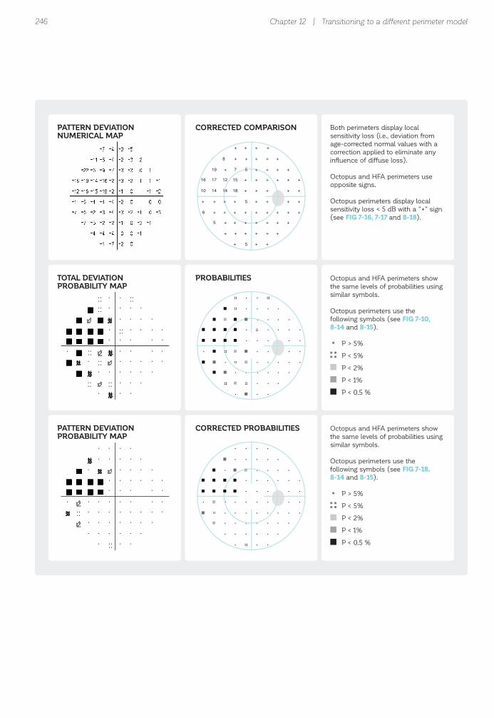
246
15
+ +
8 + +
19 + 7 5
16 17 12 +
10 14 14 18 +
+
+ +
+ + +
+ + + +
+ + + +
+ + + +
+
+ + + +
+ + + +
+ + + +
+ + +
+ +
+
+ + + + 5
6 + + +
5 + + +
+ + +
+ 5
PATTERN DEVIATIONNUMERICAL MAP
CORRECTED COMPARISON
TOTAL DEVIATIONPROBABILITY MAP
PROBABILITIES
PATTERN DEVIATIONPROBABILITY MAP
CORRECTED PROBABILITIES
Both perimeters display local
sensitivity loss (i.e., deviation from
age-corrected normal values with a
correction applied to eliminate any
influence of diffuse loss).
Octopus and HFA perimeters use
opposite signs.
Octopus perimeters display local
sensitivity loss < 5 dB with a “+” sign
(see FIG 7-16, 7-17 and 8-18).
Octopus and HFA perimeters show
the same levels of probabilities using
similar symbols.
Octopus perimeters use the
following symbols (see FIG 7-10,
8-14 and 8-15).
P > 5%
P < 5%
P < 2%
P < 1%
P < 0.5 %
Octopus and HFA perimeters show
the same levels of probabilities using
similar symbols.
Octopus perimeters use the
following symbols (see FIG 7-18,
8-14 and 8-15).
P > 5%
P < 5%
P < 2%
P < 1%
P < 0.5 %
Chapter 12 | Transitioning to a different perimeter model
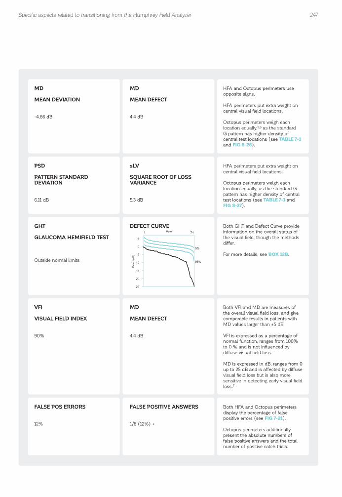
247
MD
MEAN DEVIATION
-4.66 dB
MD
MEAN DEFECT
4.4 dB
PSD
PATTERN STANDARDDEVIATION
6.11 dB
sLV
SQUARE ROOT OF LOSSVARIANCE
5.3 dB
GHT
GLAUCOMA HEMIFIELD TEST
Outside normal limits
DEFECT CURVE
HFA and Octopus perimeters use
opposite signs.
HFA perimeters put extra weight on
central visual field locations.
Octopus perimeters weigh each
location equally,5,6 as the standard
G pattern has higher density of
central test locations (see TABLE 7-1
and FIG 8-26).
HFA perimeters put extra weight on
central visual field locations.
Octopus perimeters weigh each
location equally, as the standard G
pattern has higher density of central
test locations (see TABLE 7-1 and
FIG 8-27).
VFI
VISUAL FIELD INDEX
90%
MD
MEAN DEFECT
4.4 dB
FALSE POS ERRORS
12%
FALSE POSITIVE ANSWERS
1/8 (12%) +
Both VFI and MD are measures of
the overall visual field loss, and give
comparable results in patients with
MD values larger than ±5 dB.
VFI is expressed as a percentage of
normal function, ranges from 100%
to 0 % and is not influenced by
diffuse visual field loss.
MD is expressed in dB, ranges from 0
up to 25 dB and is affected by diffuse
visual field loss but is also more
sensitive in detecting early visual field
loss.7
Both HFA and Octopus perimeters
display the percentage of false
positive errors (see FIG 7-21).
Octopus perimeters additionally
present the absolute numbers of
false positive answers and the total
number of positive catch trials.
Both GHT and Defect Curve provide
information on the overall status of
the visual field, though the methods
differ.
For more details, see BOX 12B.
471
5%
95%
-5
0
5
10
15
20
25
Rank
Def
ect (
dB)
Specifi c aspects related to transitioning from the Humphrey Field Analyzer

RELATIONSHIP BETWEEN THE GLAUCOMA HEMIFIELD TEST (GHT) AND THE DEFECT CURVE
The Glaucoma Hemi ield Test (GHT) is an intuitive text-based index that provides information about the overall status of the visual ield and classi ies the visual ield results as “Within normal limits”, “Border-line”, “Outside normal limits”, “General reduction of sensitivity” and “Abnormally high sensitivity”. Its design is based on the asymmetry of sensitivity thresholds for the superior and inferior arcuate nerve iber bundle regions. It therefore determines statistically signi icant differences between two corre-
sponding visual ield clusters divided by the horizontal midline.
In Octopus perimeters, the Defect Curve is used to determine overall visual ield status. And while it is based on different principles, it provides similar information about whether visual ields are normal or whether local or diffuse defects are present. The table below summarizes some rules of thumb on how to read the Defect Curve to obtain information that is comparable to the GHT. For more details on the Defect Curve, refer to FIG 7-11 and 8-10.
BOX 12B
248
FALSE NEG ERRORS
12%
FALSE NEGATIVE ANSWERS
1/8 (12%) -
FIXATION LOSSES
0/12
NOT AVAILABLE
GAZE TRACKER NOT AVAILABLE
Both HFA and Octopus perimeters
display the percentage of false
negative errors (see FIG 7-22).
Octopus perimeters additionally
present the absolute numbers of
false negative answers and the total
number of negative catch trials.
HFA perimeters use the Heijl-Krakau
method to determine the percentage
of fixation losses.
Octopus perimeters prevent fixation
losses by using Fixation Control, in
which the test is interrupted when
adequate fixation is not maintained
(see FIG 3-11).
HFA perimeters record eye
movements using the gaze tracker.
Octopus perimeters prevent fixation
losses by using Fixation Control, in
which the test is interrupted when
adequate fixation is not maintained
(see FIG 3-11).
Chapter 12 | Transitioning to a different perimeter model

249
591
5%
95%
-5
0
5
10
15
20
25
521
5%
95%
-5
0
5
10
15
20
25
591
5%
95%
-5
0
5
10
15
20
25
591
5%
95%
-5
0
5
10
15
20
25
591
5%
95%
-5
0
5
10
15
20
25
DEFECT CURVEGHT DEFECT CURVEINTERPRETATION
Rank
Def
ect (
dB)
Rank
Def
ect (
dB)
Rank
Def
ect (
dB)
Rank
Def
ect (
dB)
Rank
Def
ect (
dB)
WITHIN NORMAL LIMITS NORMAL
Defect Curve within normal
band
BORDERLINE BORDERLINE
Defect Curve along/slightly
below normal band
OR
Defect Curve within normal
band, but with characteristic
drop on the right (not shown)
OUTSIDE NORMAL LIMITS LOCAL DEFECT
Drop of Defect Curve on
the right
GENERAL REDUCTIONOF SENSITIVITY
DIFFUSE DEFECT
Parallel downward shift of
Defect Curve
ABNORMALLY HIGHSENSITIVITY
TRIGGER-HAPPY
Steep rise of Defect Curve
on the left
Specifi c aspects related to transitioning from the Humphrey Field Analyzer

FIGURE 12-6 Side-by-side comparison of the HFA and the Octopus progression analyses of the same visual fi eld series
that was taken on an HFA II perimeter and then imported into an Octopus perimeter. Some analyses identify similar aspects
of progression, such as whether there is progression and where localized progression occurs, but use a different approach.
Further, the Octopus perimeter offers analyses for identifying diffuse progression and providing guidance on where to look for
structural progression. Differences in the methods used between the perimeters are presented in the comment column.
250
0
15
201525
MD Mean defect100%
VFI
AGE74 84 94
80%
60%
40%
20%
0%
Slope: 0.5 dB / Yr (p<0.5%)
Rate of progression: -2.6 ± 1.8%(95% confidence)Slope significant at P < 5%
OCTOPUS REPRESENTATIONHFA REPRESENTATION
OV
ER
ALL
PR
OG
RE
SS
ION
GUIDED PROGRESSIONANALYSIS (GPA)
EYESUITE PROGRESSIONANALYSIS
GPA TREND ANALYSIS MD TREND ANALYSIS
COMMENTS
GPA uses both trend analysis
and point-wise event analysis,
which requires two reliable
baseline tests.
EyeSuite Progression
Analysis uses trend analysis.
Both perimeters use trend
analysis to determine signi-
ficance and rate of change.
HFA uses the Visual Field
Index (VFI), which typically
ranges from 100% to 0%.
Significant change is shown
in text.
Octopus uses the Mean
Defect (MD), which typically
ranges from 0 to 25 dB.
Significant worsening is
shown with red downward
arrows (see FIG 9-6).
Chapter 12 | Transitioning to a different perimeter model
Both HFA and Octopus perimeters offer methods for assessing visual field progression. FIG 12-6 presents a side-by-side comparison of all available HFA and Octopus progression analyses and also highlights differences relevant for clinical interpretation. For more detailed information on EyeSuite Progression Analysis, refer to Chapter 9.
To judge whether a visual ield series is stable or pro-gressing, both HFA and Octopus perimeters use a trend analysis approach and determine both signi icance of
change and the rate of change. In addition, both HFA and Octopus perimeters provide tools to determine whether there is local progression beyond what is ap-parent in the MD trend analysis and where the change happens. The Octopus also offers a method for identify-ing diffuse progression independently. Furthermore, to facilitate the combined evaluation of structural and functional progression in glaucoma, Octopus perimeters offer a trend procedure, the Polar Trend Analysis, which facilitates inding a relationship between structural and functional losses.
INTERPRETATION OF VISUAL FIELD PROGRESSION
OVERVIEW OF PROGRESSION TOOLS AVAILABLE ON HFA AND OCTOPUS PERIMETERS

251
0.2
0.80.8
1.00.10.1
0.2
0.70.2
0.2
0
201515
LD Local defect
Deviation from Baseline
Slope: 0.5 dB / Yr (p<0.5%)
Progression Analysis
LOC
AL
PR
OG
RE
SS
ION
GPA EVENT ANALYSIS (CORRECTED) CLUSTERTREND ANALYSIS
LD TREND ANALYSIS
HFA uses point-wise event
analysis to assess local
progression and requires two
trustworthy baseline tests.
GPA Alert displays likelihood
of progression as text.
Octopus uses trend analysis
to determine significance
and rate of change of the
variables (see FIG 9-8)
• (Corrected) Cluster MD
(average defects of 10
clusters following RNFL
distribution on the retina,
see FIG 9-11)
• LD (Local Defect, see
BOX 7D)
• sLV (Octopus equivalent
of PSD, see FIG 8-27)
Trend analysis is relatively
robust to outliers.
Furthermore, individual
visual fields can be easily
excluded from the trend
analysis in the Octopus
perimeter by simply clicking
on a given test.
LOC
AL
PR
OG
RE
SS
ION
0
20155
sLV Loss variance
Slope: 0.4 dB / Yr (p<5%)
POSSIBLE PROGRESSION
LOC
AL
PR
OG
RE
SS
ION
sLV TREND ANALYSIS
Specifi c aspects related to transitioning from the Humphrey Field Analyzer

252
0
201525
DD Diffuse defect
Slope: 0.1 dB / Yr
102030[dB]
S
IN T
DIF
FUS
E P
RO
GR
ES
SIO
N
NOT AVAILABLE DD TREND ANALYSIS Octopus uses trend analysis
to determine significance
and rate of change of the
variable DD (Diffuse Defect,
see BOX 7C).
WH
ER
E T
O L
OO
K F
OR
ST
RU
CT
UR
AL
PR
OG
RE
SS
ION
NOT AVAILABLE POLAR TREND ANALYSIS Octopus uses Polar Trend
Analysis to show point-wise
progression per visual field
location projected onto the
optic disc as guidance on
where to look for structural
progression (see FIG 9-14).
Chapter 12 | Transitioning to a different perimeter model

253References
REFERENCES1. Anderson DR, Feuer WJ, Alward WL, Skuta GL. Threshold equivalence between perimeters. Am J Ophthalmol. 1989;107:493-505.2. King AJ, Taguri A, Wadood AC, Azuara-Blanco A. Comparison of two fast strategies, SITA Fast and TOP, for the assessment of visual ields in glaucoma patients. Graefes Arch Clin Exp Ophthalmol. 2002;240:481-487.3. Pierre-Filho Pde T, Schimiti RB, de Vasconcellos JP, Costa VP. Sensitivity and speci icity of frequency-doubling technology, tendency-oriented perimetry, SITA Standard and SITA Fast perimetry in perimetrically inexperienced individuals. Acta Ophthalmol Scand. 2006;84:345-350.4. Wadood AC, Azuara-Blanco A, Aspinall P, Taguri A, King AJ. Sensitivity and speci icity of frequency-doubling technology, tendency-oriented perimetry, and Humphrey Swedish interactive threshold algorithm-fast perimetry in a glaucoma practice. Am J Ophthalmol. 2002;133:327-332.5. Funkhouser A, Fankhauser F. The effects of weighting the "mean defect" visual ield index according to threshold variability in the central and midperipheral visual ield. Graefes Arch Clin Exp Ophthalmol. 1991;229:228-231.6. Funkhouser AT, Fankhauser F. A comparison of the mean defect and mean deviation indices within the central 28 degrees of the glaucomatous visual ield. Jpn J Ophthalmol. 1990;34:414-420.7. Artes PH, O'Leary N, Hutchison DM, et al. Properties of the statpac visual ield index. Invest Ophthalmol Vis Sci. 2011;52:4030-4038.

254

255
CHAPTER 13CLINICAL CASES
INTRODUCTION
The previous chapters of this book have systematically presented various aspects of visual field testing and interpretation. To conclude, visual ield interpretation is now put into a clinical context. In this chapter, 23 clin-ical cases are presented that show visual ields or visual ield series of patients with glaucoma, neuro-ophthal-
mic disorder and retinal disease. The selected cases are model cases. They present typical defect patterns of the disease rather than unusual cases and are reliable, free of artifacts and can be fully trusted.
To link visual ield interpretation to the clinical situation, the visual ield results are presented in addition to other
relevant clinical information. Background information on the patient’s history as well as other diagnostic results such as visual acuity, IOP, fundus images, OCT scans and MRIs which are relevant for clinical decision making, are shown. In all examples, visual acuity is expressed in dec-imal units for uniformity, but the Octopus allows users to select different units when performing the test. In each case, key diagnostic indings leading to disease diagnosis are presented and summarized.
An overview of all available cases is presented on the next page.

256 Chapter 13 | Clinical cases
GLAUCOMA – SINGLE FIELD1. Very early stage glaucoma (normal tension glaucoma)2. Early stage glaucoma (normal tension glaucoma)3. Early stage glaucoma (primary open-angle glaucoma)4. Early stage glaucoma (with cataract)5. Early stage glaucoma (normal tension glaucoma)6. Early stage glaucoma (primary open-angle glaucoma)7. Moderate glaucoma (normal tension glaucoma)8. Moderate glaucoma (primary open-angle glaucoma)9. Late stage glaucoma (normal tension glaucoma)
GLAUCOMA – TREND10. Early to moderate glaucoma (normal tension glaucoma)11. Early to moderate glaucoma (primary open-angle glaucoma)12. Early to moderate glaucoma (primary open-angle glaucoma)13. Early to moderate glaucoma (normal tension glaucoma)14. Early to moderate glaucoma (primary open-angle glaucoma)15. End-stage glaucoma (exfolitative glaucoma)
NEUROLOGICAL DISEASES16. Cerebral infarction (bilateral)17. Leber hereditary optic neuropathy (bilateral)18. Bilateral optic neuritis (multiple sclerosis)19. Tuberculum sellae meningioma (bilateral)
RETINAL DISEASES20. Age-related macular degeneration21. Branch central retinal artery occlusion22. Macular hole23. Branch central retinal vein occlusion

257
OCTOPUS 101
Demo Jane, 1947/01/01 (57yrs)Right eye (OD) / 2004/11/18 / 12:01:27Seven-in-One
Classification:Comment:
:]gHmm[ POI:]mm[ lipuPRefraction S/C/A: -3.25// VA: 1.0Catch trials: 0/26 (0%) +, 1/26 (4%) - RF: 1.9Parameters: 4 / 1000 asb III 100 ms Duration: 16:41Programs: 32 Standard White/White / Normal Questions / repetitions: 520 / 0 30°
MS [dB]: 28.0MD [< 2.0 dB]: -1.5sLV [< 2.5 dB]: 1.8CsLV [dB]: 1.5SF [dB]: 1.6
95%..100%83%...94%71%...82%59%...70%47%...58%35%...46%23%...34%11%...22% 0%...10%
Grayscale (CO)
-1.9-1.6
3.1-1.1-
Values
2929
29 30
33
26
29
26
30
31
27
28
22
28
26
30
26
28
28
31
28 28
28 28 28 29
29
28
28 31 31 30
29 28
25 23
30 29
6292
21 30 32 27
26 26 31 29
9282
27 27
28 27
28 27 27 29
30 30 31 29
8262
9282
29 29 29 31
27 28 29 28
27.927.4
8.829.72
Comparison
++
+ +
+
+
+
+
+
+
+
+
+
+
+
+
+
+
+
+
+ +
+ + + +
+
+
+ + + +
+ +
+ +
+ +
++
+ + + +
+ + + +
++
+ +
+ +
+ + + +
+ + + +
++
++
+ + + +
+ + + +
Corrected comparisons
++
+ +
+
+
+
+
+
+
+
+
+
+
+
+
+
+
+
+
+ +
+ + + +
+
+
+ + + +
+ +
+ +
+ +
++
5 + + +
+ 5 + +
++
+ +
+ +
+ + + +
+ + + +
++
++
+ + + +
+ + + +
Defect curve
Diffuse defect [dB]: -1.1
471
5%
95%
-5
0
5
10
15
20
25
Probabilities Corrected probabilities
P > 5P < 5P < 2P < 1P < 0,5
OCTOPUS®
Rank
Def
ect (
dB)
All testlocationsat P > 5%
Defect Curvein normal
range
Glaucoma | Single fi eld
• 57-year-old female, no family history • Patient reported decreased visual acuity in both eyes and discomfort in left eye
• 15 mmHg/ 1.2 – 5.25 (sph)
• C/D = 0.9 • Rim thinning at 6 to 11 o'clock position • Optic disc hemorrhage and narrow slit-like RNFL defect at 11 o'clock position • Temporal alpha zone and beta zone peripapillary chorioretinal atrophy (PPA)
• No visual ield loss• Fundus indings show changes indicative of very early glaucoma including neuroretinal rim loss, optic disc hemorrhage, and RNFL loss
PATIENT
IOP/VA corr
FUNDUS
VERY EARLY STAGE GLAUCOMA (NORMAL TENSION GLAUCOMA)1

258
Rank
Def
ect (
dB)
OCTOPUS 101
Demo Jane, 1942/01/01 (53yrs)Left eye (OS) / 1996/06/21 / 14:24:40Seven-in-One
Classification:Comment: NTG
Pupil [mm]: 5.3 IOP [mmHg]: 12Refraction S/C/A: // VA: 1.2Catch trials: 0/24 (0%) +, 1/24 (4%) - RF: 2.0Parameters: 4 / 1000 asb III 100 ms Duration: 16:49Programs: G Standard White/White / Normal Questions / repetitions: 481 / 1 30°
MS [dB]: 25.9MD [< 2.0 dB]: 1.6sLV [< 2.5 dB]: 4.2CsLV [dB]: 3.9SF [dB]: 1.7
95%..100%83%...94%71%...82%59%...70%47%...58%35%...46%23%...34%11%...22% 0%...10%
Grayscale (CO)
6.90.7
9.0-3.0-
Values
2425
30 30
16
27
17
33
27
28
26
26
28
30
30
27
32 23
3334
21 24
2828
24
31
28
29
10
25
23
27
3432 17
3230
4242
2727
1282
2728
27 23
3231
8172
3125
14
23
23 21
2727
20.026.2
6.825.82
Comparison
5+
+ +
14
+
10
+
+
+
+
+
+
+
+
+
+ 9++
+ +
++
5
+
+
+
15
+
+
+
++ 13
++
+ +
++
++
++
+ 6
++
+ 9
++
11
+
+ +
++
Corrected comparisons
5+
+ +
14
+
10
+
+
+
+
+
+
+
+
+
+ 9++
+ +
++
5
+
+
+
15
+
+
+
++ 13
++
+ +
++
++
++
+ 6
++
+ 9
++
10
+
+ +
++
Defect curve
Probabilities Corrected probabilities
P > 5P < 5P < 2P < 1P < 0,5
Diffuse defect [dB]: -1.1
471
5%
95%
-5
0
5
10
15
20
25
OCTOPUS®
Cluster ofabnormal locations
with P < 0.5 %
Chapter 13 | Clinical cases
• Mild superior nasal step and mild superior paracentral scotoma• Spatial relationship between visual ield loss and both rim thinning and RNFL loss in fundus photo
• 53-year-old female, no family history• Optic nerve cupping observed during unrelated emergency eye surgery
• 12 mmHg/ 1.2 + 0.25 (sph)
• C/D = 0.8• Rim thinning and RNFL loss at 5 to 6 o'clock position
PATIENT
IOP/VA corr
FUNDUS
2 EARLY STAGE GLAUCOMA (NORMAL TENSION GLAUCOMA)

259
Demo Jane, 1958/01/01 (56yrs)Right eye (OD) / 2015/01/09 / 01:31:08Four-in-One
Comment:
NV: T31 V1.0Pupil [mm]: 3.0 IOP [mmHg]:Refraction S/C/A: VA [m]:Catch trials: 0/4 (0%) +, 0/4 (0%) - RF: 0.0Parameters: 31.4 / 4000 asb III 100 ms Duration: 02:18Programs: G Standard White/White / TOP Questions / repetitions: 72 / 0 MS [dB]: 26.4
MD [< 2.0 dB]: 0.9sLV [< 2.5 dB]: 4.5
30°
Grayscale (CO)
MD [dB]2.52.2
-1.0 -0.5
Cluster analysis [dB]
+
+3.1
5.47.4
++
++
+
Defect curve Polar analysis
10 20 30[dB]
S
IT N
OCTOPUS®
Diffuse defect [dB]: 2.3
591
5%
95%
-5
0
5
10
15
20
25
Rank
Def
ect (
dB)
Structural damagesuggested at 7 to 8
o'clock position
Nasal step,superior arcuate
and superiorparacentral defect
Local defect(glaucoma)
GC thinninginferortemporally
RNFL lossinferortemporally
Glaucoma | Single fi eld
• Nasal step, superior arcuate and superior paracentral defect apparent in Cluster Analysis• Spatial relationship between visual ield loss (Polar Analysis suggests structural damage at 7 to 8 o'clock position) and inferotemporal structural loss (fundus photo, RNFL & GC thickness map)
• 56-year-old female, her brother has POAG• Patient visited clinic to rule out glaucoma because of her family history
• 24 mmHg /1.0 - 3.25 (sph)
• Inferior RNFL defects
• RNFL and ganglion cell loss inferotemporally at 7 to 8 o’clock position
PATIENT
IOP/VA corr
FUNDUS
OCT
3 EARLY STAGE GLAUCOMA (PRIMARY OPEN-ANGLE GLAUCOMA)
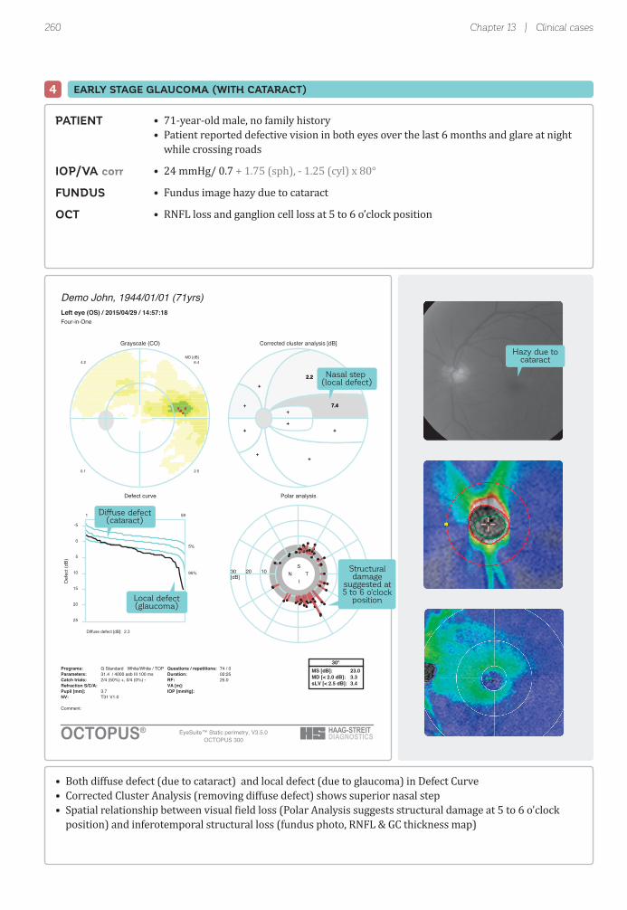
260
Demo John, 1944/01/01 (71yrs)Left eye (OS) / 2015/04/29 / 14:57:18Four-in-One
Comment:
NV: T31 V1.0Pupil [mm]: 3.7 IOP [mmHg]:Refraction S/C/A: VA [m]:Catch trials: 2/4 (50%) +, 0/4 (0%) - RF: 25.0Parameters: 31.4 / 4000 asb III 100 ms Duration: 02:25Programs: G Standard White/White / TOP Questions / repetitions: 74 / 0 MS [dB]: 23.0
MD [< 2.0 dB]: 3.3sLV [< 2.5 dB]: 3.4
30°
Grayscale (CO)
MD [dB]6.44.2
0.1 2.5
Corrected cluster analysis [dB]
+
+2.2
7.4+
++
++
+
+
+2.2
7.4+
++
++
+
Defect curve Polar analysis
102030[dB]
S
IN T
OCTOPUS®
Diffuse defect [dB]: 2.3
591
5%
95%
-5
0
5
10
15
20
25
EyeSuite™ Static perimetry, V3.5.0OCTOPUS 300
Rank
Def
ect (
dB)
Nasal step (local defect)
Diffuse defect(cataract)
Structuraldamage
suggested at5 to 6 o'clock
positionLocal defect(glaucoma)
Hazy due tocataract
Chapter 13 | Clinical cases
• 71-year-old male, no family history• Patient reported defective vision in both eyes over the last 6 months and glare at night while crossing roads
• 24 mmHg/ 0.7 + 1.75 (sph), - 1.25 (cyl) x 80°
• Fundus image hazy due to cataract
• RNFL loss and ganglion cell loss at 5 to 6 o’clock position
• Both diffuse defect (due to cataract) and local defect (due to glaucoma) in Defect Curve• Corrected Cluster Analysis (removing diffuse defect) shows superior nasal step• Spatial relationship between visual ield loss (Polar Analysis suggests structural damage at 5 to 6 o'clock position) and inferotemporal structural loss (fundus photo, RNFL & GC thickness map)
PATIENT
IOP/VA corr
FUNDUS
OCT
EARLY STAGE GLAUCOMA (WITH CATARACT)4

261
Rank
Def
ect (
dB)
Defect curve
OCTOPUS 101
Demo Jane, 1944/01/01 (58yrs)Left eye (OS) / 2003/03/14 / 16:43:49Seven-in-One
Classification:Comment: Gla
Pupil [mm]: 5.0 IOP [mmHg]: 13Refraction S/C/A: +0.5/-0.75/80 VA: 1.2Catch trials: 3/23 (13%) +, 0/23 (0%) - RF: 6.5Parameters: 4 / 1000 asb III 100 ms Duration: 15:23Programs: G Standard White/White / Normal Questions / repetitions: 459 / 0 30°
MS [dB]: 25.0MD [< 2.0 dB]: 2.2sLV [< 2.5 dB]: 5.8CsLV [dB]: 5.5SF [dB]: 2.8
95%..100%83%...94%71%...82%59%...70%47%...58%35%...46%23%...34%11%...22% 0%...10%
Grayscale (CO)
3.46.9
5.0-7.0-
Values
28
29 29
32
30
29
15
27
26
36
29
28
21
27
27
27 24
3331
22 23
2728
21
30
24
29
18
26
21
26
3221 31
3131
4212
2426
3252
2627
23
3032
4232
2827
23
23
20 21
2626
23.219.8
0.826.82
Comparison
+
+ +
+
+
+
15
+
+
+
+
+
8
+
+
+ 7++
+ +
++
7
+
+
+
7
+
+
+
+8 +
++
+ +
++
++
++
5
++
+ +
++
+
+
+ +
++
Corrected comparisons
+
+ +
+
+
+
14
+
+
+
+
+
8
+
+
+ 7++
+ +
++
7
+
+
+
6
+
+
+
+8 +
++
+ +
++
++
++
5
++
+ +
++
+
+
+ +
++
Probabilities Corrected probabilities
P > 5P < 5P < 2P < 1P < 0,5
OCTOPUS®
Diffuse defect [dB]: -1.1
471
5%
95%
-5
0
5
10
15
20
25
Absolute defect(sensitivity threshold 0 dB)
Glaucoma | Single fi eld
• 58-year-old female, father had glaucoma• Optic nerve cupping detected during routine medical visit
• 16 mmHg/ 1.2 – 1.0 (sph), - 0.75 (cyl) x 80°
• C/D = 0.9• Rim thinning and wide RNFL loss at 5 to 6 o'clock position
• Dense paracentral scotoma• Spatial relationship between visual ield loss and both rim thinning and RNFL loss in fundus photo
PATIENT
IOP/VA corr
FUNDUS
EARLY STAGE GLAUCOMA (NORMAL TENSION GLAUCOMA)5

262
Rank
Def
ect (
dB)
OCTOPUS 101
Demo John, 1951/01/01 (55yrs)Left eye (OS) / 2007/05/11 / 10:02:54Seven-in-One
Classification:Comment:
Pupil [mm]: 6.7 IOP [mmHg]:Refraction S/C/A: -2.75/-1.0/180 VA: 1.0Catch trials: 0/22 (0%) +, 0/23 (0%) - RF: 0.0Parameters: 4 / 1000 asb III 100 ms Duration: 13:43Programs: G Standard White/White / Normal Questions / repetitions: 447 / 0 30°
MS [dB]: 24.2MD [< 2.0 dB]: 3.3sLV [< 2.5 dB]: 8.7CsLV [dB]: 8.6SF [dB]: 1.5
95%..100%83%...94%71%...82%59%...70%47%...58%35%...46%23%...34%11%...22% 0%...10%
Grayscale (CO)
15.11.2
4.1-0.2-
Values
921
31 30
31
31
29
32
31
30
31
17
27
10
18
533 32
3133
25 23
3030
3
30
28
30
4
29
27
29
3430 3
3131
9162
2431
692
2729
23 3
3031
612
2830
15
28
24 23
2930
11.725.6
0.921.03
Comparison
207
+ +
+
+
+
+
+
+
+
10
+
20
10
22+ +
++
+ +
++
26
+
+
+
21
+
+
+
++ 27
++
+ 5
++
91+
++
6 26
++
6 21
++
9
+
+ +
++
Corrected comparisons
218
+ +
+
+
+
+
+
+
+
10
+
21
10
22+ +
++
+ +
++
26
+
+
+
22
+
+
+
++ 28
++
+ 6
++
02+
++
7 26
++
7 22
++
10
+
+ +
++
Defect curve
Probabilities Corrected probabilities
P > 5P < 5P < 2P < 1P < 0,5
OCTOPUS®
Diffuse defect [dB]: -1.1
471
5%
95%
-5
0
5
10
15
20
25
Very reliable test
Local defect
Chapter 13 | Clinical cases
• Visual ield shows superior arcuate defect• Spatial relationship between visual ield loss and rim thinning in fundus photo indicative of glaucoma
• 55-year-old male, no family history• Patient reported decreased visual acuity and blurred vision
• 23 mmHg/ 1.2 – 4.25 (sph), - 1.0 (cyl) x 180°
• C/D = 0.8• Small disc• Rim thinning at 5 to 6 o'clock position
PATIENT
IOP/VA corr
FUNDUS
6 EARLY STAGE GLAUCOMA (PRIMARY OPEN-ANGLE GLAUCOMA)

263
Rank
Def
ect (
dB)
Demo Jane, 1947/01/01 (57yrs)Left eye (OS) / 2004/11/18 / 12:25:31Seven-in-One
Classification:Comment:
Pupil [mm]: 5.8 IOP [mmHg]:Refraction S/C/A: -3.25// VA: 1.0Catch trials: 0/32 (0%) +, 2/33 (6%) - RF: 3.0Parameters: 4 / 1000 asb III 100 ms Duration: 21:13Programs: 32 Standard White/White / Normal Questions / repetitions: 642 / 0 30°
MS [dB]: 18.4MD [< 2.0 dB]: 8.2sLV [< 2.5 dB]: 10.9CsLV [dB]: 11.0SF [dB]: 2.2
95%..100%83%...94%71%...82%59%...70%47%...58%35%...46%23%...34%11%...22% 0%...10%
Grayscale (CO)
14.11.9
5.416.1
Values
616
11
24
27
28
32
23
13
2
29
31
28
28
27
32
1
17
26
2227
11222527
4
141827
2729
2017
2025
328
412428
262728
27
328
2627
15232529
227
928
28
172429
26222926
11.724.1
3.219.52
Comparison
2211
18
+
+
+
+
+
13
22
+
+
+
+
+
+
24
10
+
++
135++
24
1110+
++
+6
6+
23+
21295+
+++
+
24+
++
9+++
26+
18+
+
126+
+5++
Corrected comparisons
2211
17
+
+
+
+
+
12
22
+
+
+
+
+
+
23
9
+
++
135++
24
1010+
++
+5
6+
22+
2028++
+++
+
24+
++
8+++
26+
17+
+
115+
++++
Defect curve
Probabilities Corrected probabilities
P > 5P < 5P < 2P < 1P < 0,5
OCTOPUS 101OCTOPUS®
Diffuse defect [dB]: -1.1
471
5%
95%
-5
0
5
10
15
20
25
Large sLV showssevere local defect
Glaucoma | Single fi eld
• 57-year-old female, no family history• Patient reported decreased visual acuity in both eyes and discomfort in left eye
• 16 mmHg/ 1.0 – 5.5 (sph)
• C/D = 0.95• Rim thinning at 12 to 6 o'clock position• Vein angulation and bayoneting at 12 and 6 o'clock position
• Dense partial double arcuate visual ield defect• Spatial relationship between visual ield loss and both rim thinning and vein bending in fundus photo
PATIENT
IOP/VA corr
FUNDUS
MODERATE GLAUCOMA (NORMAL TENSION GLAUCOMA)7

264
Rank
Def
ect (
dB)
Demo Jane, 1954/01/01 (52yrs)Right eye (OD) / 2007/02/06 / 09:27:13Seven-in-One
Classification:Comment:
:]gHmm[ POI:]mm[ lipuP 13Refraction S/C/A: -3.0/-0.25/180 VA: 1.2Catch trials: 0/22 (0%) +, 5/23 (22%) - RF: 11.1Parameters: 4 / 1000 asb III 100 ms Duration: 14:18Programs: G Standard White/White / Normal Questions / repetitions: 448 / 4 30°
MS [dB]: 17.2MD [< 2.0 dB]: 10.4sLV [< 2.5 dB]: 10.4CsLV [dB]: 10.3SF [dB]: 2.1
95%..100%83%...94%71%...82%59%...70%47%...58%35%...46%23%...34%11%...22% 0%...10%
Grayscale (CO)
8.723.9
8.09.7
Values
15
21 31
29
26
25
29
25
14
21
24
12
337
29 33
911
26 27
16
28
297
15
27
27306
28 31
21
6222
23
629
1211
24 27
241
8281
11
5
25 24
18.43.1
5.720.02
Comparison
13
8 +
+
+
+
+
+
14
6
+
16
+24+ +
1615
+ +
13
+
+19
10
+
6+24
+ +
5
+ +
+
+81
1718
6 +
+27
11 +
13
19
+ +
Corrected comparisons
10
5 +
+
+
+
+
+
11
+
+
13
+21+ +
1312
+ +
11
+
+16
7
+
++21
+ +
+
+ +
+
+51
1415
+ +
+24
8 +
10
16
+ +
Defect curve
Probabilities Corrected probabilities
P > 5P < 5P < 2P < 1P < 0,5
OCTOPUS 101OCTOPUS®
Diffuse defect [dB]: -1.1
471
5%
95%
-5
0
5
10
15
20
25
Absolute defects(sensitivity threshold 0 dB)
Chapter 13 | Clinical cases
• Dense visual ield loss in superior nasal quadrant with many locations showing absolute defects and little remaining sensitivity near ixation corresponding with RNFL loss at 6 to 8 o’clock position• Mild sensitivity loss on lower nasal ield relating to RNFL loss at 11 o’clock position
• 52-year-old female, no family history• Patient diagnosed with glaucoma during medical check-up
• 20 mmHg/ 1.2 – 4.0 (sph), - 0.25 (cyl) x 180°
• C/D = 0.9• Rim thinning at 6 to 8 o'clock position and notching at 11 o’clock position• Large RNFL loss at 6 to 8 o'clock position and small RNFL loss at 11 o’clock position• Angulation of lower vein and undermining due to optic disc cupping• Temporal alpha zone and beta zone peripapillary chorioretinal atrophy (PPA)
PATIENT
IOP/VA corr
FUNDUS
8 MODERATE GLAUCOMA (PRIMARY OPEN-ANGLE GLAUCOMA)
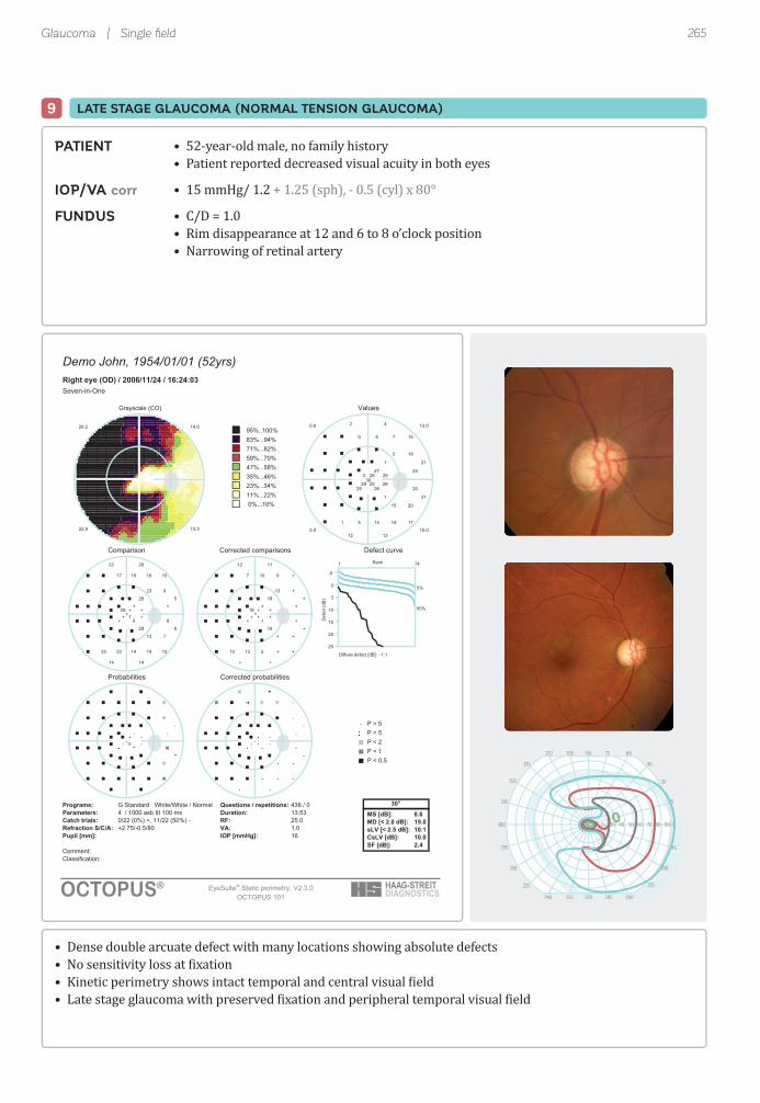
265
Rank
Def
ect (
dB)
Demo John, 1954/01/01 (52yrs)Right eye (OD) / 2006/11/24 / 16:24:03Seven-in-One
Classification:Comment:
:]gHmm[ POI:]mm[ lipuP 16Refraction S/C/A: +2.75/-0.5/80 VA: 1.0Catch trials: 0/22 (0%) +, 11/22 (50%) - RF: 25.0Parameters: 4 / 1000 asb III 100 ms Duration: 13:53Programs: G Standard White/White / Normal Questions / repetitions: 438 / 0 30°
MS [dB]: 8.6MD [< 2.0 dB]: 19.0sLV [< 2.5 dB]: 10.1CsLV [dB]: 10.0SF [dB]: 2.4
95%..100%83%...94%71%...82%59%...70%47%...58%35%...46%23%...34%11%...22% 0%...10%
Grayscale (CO)
14.026.2
3.319.22
Values
1
1
26
21
27
21
28
283
29 25
69
5 14
24
20
15
17
3029
28
7
411
18
20
5
15
42
12 13
13.00.8
0.510.5
Comparison
28
29
5
6
+
5
+
+29+ 7
1917
22 14
+
8
10
10
+++
19
25 14
9
7
23
13
2022
14 14
Corrected comparisons
18
19
+
+
+
+
+
+19+ +
107
13 5
+
+
+
+
+++
9
15 +
+
+
13
+
1112
+ +
Defect curve
Probabilities Corrected probabilities
P > 5P < 5P < 2P < 1P < 0,5
OCTOPUS 101OCTOPUS®
Diffuse defect [dB]: -1.1
471
5%
95%
-5
0
5
10
15
20
25
10 30 40 50 60 70 80 90
90105120 75 60
270255240 285 300
45135
315225
30150
330210
15165
345195
0180
Glaucoma | Single fi eld
• 52-year-old male, no family history• Patient reported decreased visual acuity in both eyes
• 15 mmHg/ 1.2 + 1.25 (sph), - 0.5 (cyl) x 80°
• C/D = 1.0• Rim disappearance at 12 and 6 to 8 o’clock position• Narrowing of retinal artery
• Dense double arcuate defect with many locations showing absolute defects• No sensitivity loss at ixation• Kinetic perimetry shows intact temporal and central visual ield• Late stage glaucoma with preserved ixation and peripheral temporal visual ield
PATIENT
IOP/VA corr
FUNDUS
LATE STAGE GLAUCOMA (NORMAL TENSION GLAUCOMA)9
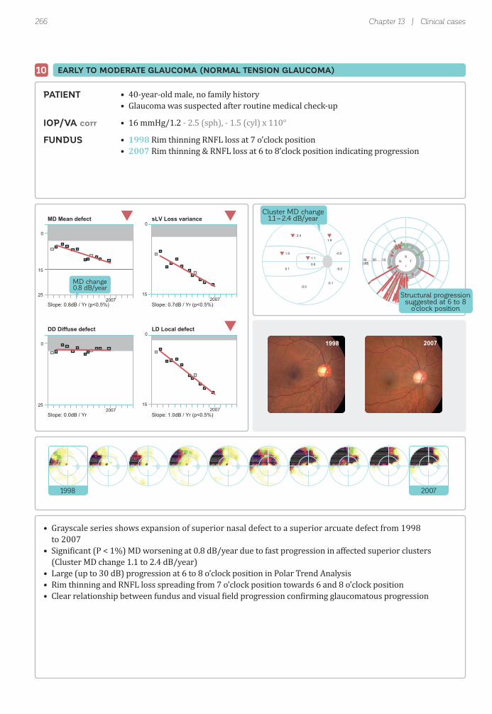
266 Chapter 13 | Clinical cases
0
15
25
MD Mean defect
Slope: 0.8dB / Yr (p<0.5%)
0
15
sLV Loss variance
Slope: 0.7dB / Yr (p<0.5%)
0
25
DD Diffuse defect
Slope: 0.0dB / Yr
0
2007 2007
2007 200715
LD Local defect
Slope: 1.0dB / Yr (p<0.5%)
MD change0.8 dB/year
1998 2007
-0.0
1.92.4
1.10.0
1.9
0.1
-0.0-0.1
-0.2
102030[dB]
S
IN T
Structural progressionsuggested at 6 to 8
o'clock position
Cluster MD change1.1 – 2.4 dB/year
1998 2007
• 40-year-old male, no family history• Glaucoma was suspected after routine medical check-up
• 16 mmHg/1.2 - 2.5 (sph), - 1.5 (cyl) x 110°
• 1998 Rim thinning RNFL loss at 7 o’clock position• 2007 Rim thinning & RNFL loss at 6 to 8’clock position indicating progression
• Grayscale series shows expansion of superior nasal defect to a superior arcuate defect from 1998 to 2007• Signi icant (P < 1%) MD worsening at 0.8 dB/year due to fast progression in affected superior clusters (Cluster MD change 1.1 to 2.4 dB/year)• Large (up to 30 dB) progression at 6 to 8 o’clock position in Polar Trend Analysis• Rim thinning and RNFL loss spreading from 7 o’clock position towards 6 and 8 o’clock position• Clear relationship between fundus and visual ield progression con irming glaucomatous progression
PATIENT
IOP/VA corr
FUNDUS
EARLY TO MODERATE GLAUCOMA (NORMAL TENSION GLAUCOMA)10

267Glaucoma | Trend
0
15
2001 200825
MD Mean defect
Slope: 0.4dB / Yr (p<0.5%)
0
2001 2008
2001 2008 2001 2008
15
sLV Loss variance
Slope: 0.8dB / Yr (p<0.5%)
0
25
DD Diffuse defect
Slope: -0.2dB / Yr
0
15
LD Local defect
Slope: 0.8dB / Yr (p<0.5%)
MD change0.4 dB/year
2001 2008
0.3
1.11.8
1.9-0.2
2.1
-0.3
0.1-0.4
0.5
102030[dB]
S
IN T
Structural progressionsuggested at 6 to 8
o'clock position
2001 2008
Large progression at 6 to 8 o’clock position
• 68-year-old female, no family history• High IOP identi ied during visit initiated due to eye pain
• 22 mmHg/1.5 + 0.75 (sph), - 0.25 (cyl) x 10°
• 2001 Mild, slit-like RNFL loss at 7 o’clock position. No rim thinning or notching.• 2008 RNFL loss & additional rim thinning with undermining at 6 to 8 o’clock position indicating progression; laser scar at 1 to 3 o’clock position due to treated BRVO, which developed in 2002 during follow up
• Grayscale series shows expansion of superior nasal defect to a superior arcuate defect from 2001 to 2008 and mild inferotemporal sensitivity loss due to BRVO • Signi icant (P < 1%) but slow MD worsening at 0.4 dB/year due to fast progression in affected superior clusters (Cluster MD change 1.1 to 2.1 dB/year)• Large (up to 30 dB) progression at 6 to 8 o’clock position in Polar Trend Analysis• Rim thinning and RNFL loss spreading from 7 o’clock position towards 6 and 8 o'clock position• Clear relationship between fundus and visual ield progression con irming glaucomatous progression
PATIENT
IOP/VA corr
FUNDUS
11 EARLY TO MODERATE GLAUCOMA (PRIMARY OPEN-ANGLE GLAUCOMA)

268 Chapter 13 | Clinical cases
0
15
2002 2008
2002 2008
2002 2008
2002 2008
25
MD Mean defect
Slope: 0.5dB / Yr (p<0.5%)
0
15
sLV Loss variance
Slope: 0.1dB / Yr
0
25
DD Diffuse defect
Slope: 0.2dB / Yr
0
15
LD Local defect
Slope: 0.5dB / Yr (p<0.5%)
2002 2008
102030[dB]
S
IN T
0.2
0.61.1
0.10.1
2.5
0.2
-0.40.0
0.0
Structural progressionsuggested at
5 o'clock position
Floor effect(near absolute sensitivity loss)
2002 2008
Large progression at 5 o’clock position
• 53-year-old male, no family history• High IOP identi ied during visit related to eye pain
• 25 mmHg/1.2 - 0.75 (sph), - 1.0 (cyl) x 90°
• 2002 Rim thinning at 1 to 2 o’clock position. Rim notching at 5 o’clock position. RNFL loss at same positions. Optic disc hemorrhage at 6 o’clock position.• 2008 Rim thinning from 1 to 6 o’clock position
• Grayscale series shows expansion of inferior arcuate defect to superior nasal side from 2002 to 2008 • Signi icant (P < 1%) but slow MD worsening at 0.5 dB/year due to fast progression in affected superior clusters (Cluster MD change up to 2.5 dB/year)• Large (~28 dB) progression at 5 o’clock position in Polar Trend Analysis• Rim thinning and RNFL loss spreading from 1 to 2 o'clock position towards 6 o'clock position• Clear relationship between fundus and visual ield progression con irming glaucomatous progression
PATIENT
IOP/VA corr
FUNDUS
EARLY TO MODERATE GLAUCOMA (PRIMARY OPEN-ANGLE GLAUCOMA)12

269Glaucoma | Trend
0
15
2001 2002 2003 200425
MD Mean defect
Slope: 1.2dB / Yr (p<0.5%)
0
2001 2002 2003 200415
sLV Loss variance
Slope: 0.8dB / Yr (p<0.5%)
0
2001 2002 2003 200425
DD Diffuse defect
Slope: 0.5dB / Yr
0
2001 2002 2003 200415
LD Local defect
Slope: 1.0dB / Yr (p<0.5%)
2001 2004
102030[dB]
S
IN T
0.8
0.81.1
5.43.3
0.8
0.4
0.60.6
0.5
Very fast progressionin central visual
field clustersLarge progression suggestedat inferior temporal optic disc
2001 2004
• 51-year-old male, no family history• Patient reported a blind spot in visual ield of left eye during reading and a visual ield defect temporally near ixation upon ixation of distant objects
• 15 mmHg/1.0 – 6.0 (sph), - 1.25 (cyl) x 160°
• 2001 Small disc. RNFL loss (including papillomacular nerve iber) from 2 to 5 o’clock position. Temporal alpha zone and beta zone peripapillary chorioretinal atrophy (PPA).• 2004 Challenging to identify changes because of small disc and severe myopia
• Grayscale series shows expansion of superior paracentral defect towards ixation from 2001 to 2004• Signi icant (P < 1%) and fast MD worsening at 1.2 dB/year due to very fast progression in affected central clusters (Cluster MD change 3.3 and 5.4 dB/year)• Challenging to asses structural changes, but large (up to 30 dB) progression at 5 o’clock position in Polar Trend Analysis corresponding with RNFL loss in fundus image suggests glaucomatous progression• Relationship between fundus and visual ield progression con irming glaucomatous progression
PATIENT
IOP/VA corr
FUNDUS
13 EARLY TO MODERATE GLAUCOMA (NORMAL TENSION GLAUCOMA)

270 Chapter 13 | Clinical cases
0
15
201325
MD Mean defect
Slope: 1.0dB / Yr (p<0.5%)
0
201325
DD Diffuse defect
Slope: 0.2dB / Yr
0
15
sLV Loss variance
Slope: 0.4dB / Yr (p<0.5%)
0
2013
2013
15
LD Local defect
Slope: 1.1dB / Yr (p<0.5%)
MD change1.0 dB/year
Significantlocal
progression
No diffuseprogression
2008 2013
102030[dB]
S
IN T
0.4
2.52.6
1.70.7
-0.5
0.2
-0.00.0
-0.1
Fast superiorparacentralprogression
2008 2013
• 74-year-old female• Patient showed advanced disc damage at presentation Suboptimal IOP control under topical medication, but patient refused surgery
• 16-22 mmHg (28 mmHg pre-treatment)/1.0
• 2008 Pathologically low peripapillary RNFLT in inferotemporal sectors • 2013 Statistically signi icant further RNFLT decrease both infero- and superotemporally
• 2008 Advanced disc damage (C/D=0.95)
• Grayscale series shows progression of superior arcuate and both superior and inferior paracentral defects from 2008 to 2013• Local progression apparent from signi icant (P < 1%) sLV increase and LD worsening due to very fast progression in superior arcuate and superior and inferior paracentral clusters (Cluster MD change up to 2.6dB/year)• Up to 30 dB progression at infero- and superotemporal test locations in Polar Trend Analysis spatially related to further RNFLT loss between 2008 and 2013• Relationship between OCT and visual ield progression con irming glaucomatous progression
PATIENT
IOP/VA uncorr
OCT
FUNDUS
EARLY TO MODERATE GLAUCOMA (PRIMARY OPEN-ANGLE GLAUCOMA)14

271Glaucoma | Trend
0
15
201335
MD Mean defect
Slope: 0,1dB / Yr
0
201315
sLV Loss variance
Slope: -0,2dB / Yr (p<10%)
0
201325
DD Diffuse defect
Slope: -0,0dB / Yr
0
201315
LD Local defect
Slope: 0,0dB / Yr
Floor effect(DDc > 20 dB, no progression)
Floor effect(MD > 20 dB, no progression)
2008 2013
-0.0
0.0-0.0
1.42.5
-0.0
-0.9
0.0-0.0
-0.0
102030[dB]
S
IN T
Fast superiorand inferiorparacentralprogression
2008 2013
• 79-year-old female • Patient presented with end-stage glaucoma, iltration surgery was performed with no further medication during follow up• Patient reported only minimal central visual ield worsening during follow-up
• 08 - 14 mmHg (43mmHg pre-treatment)/1.0 + 1.0 (sph)
• 2008 Severe peripapillary RNFLT loss• 2013 No change in the average peripapillary RNFLT
• 2008 C/D=0.99
• Grayscale series shows very dense visual ield loss with little remaining sensitivity in macula• MD appears stable, but cannot be interpreted for progression because of loor effect (exceeding perimeter’s measurement range)• Signi icant (P < 1%) superior and inferior paracentral progression (Cluster MD change 1.4 and 2.5 dB/year)• 12 to 25 dB progression at 8 to 10 o’clock position (papillomacular bundle) in Polar Trend Analysis not apparent in OCT results due to the loor effect of OCT in end-stage glaucoma• Polar and Cluster Trend Analysis indicate late-stage glaucomatous progression
PATIENT
IOP/VA corr
OCT
FUNDUS
15 END-STAGE GLAUCOMA (EXFOLITATIVE GLAUCOMA)

272
Rank
Def
ect (
dB)
Demo John, 1933/01/01 (65yrs)Left eye (OS) / 1999/07/12 / 11:36:23Seven-in-One
Classification:Comment:
Pupil [mm]: 6.4 IOP [mmHg]: 14Refraction S/C/A: +0.75/-1.5/90 VA: 0.4Catch trials: 0/20 (0%) +, 4/21 (19%) - RF: 9.7Parameters: 4 / 1000 asb III 100 ms Duration: 15:54Programs: G Standard White/White / Normal Questions / repetitions: 409 / 2 30°
MS [dB]: 18.3MD [< 2.0 dB]: 8.4sLV [< 2.5 dB]: 12.4CsLV [dB]: 12.5SF [dB]: 1.5
95%..100%83%...94%71%...82%59%...70%47%...58%35%...46%23%...34%11%...22% 0%...10%
Grayscale (CO)
25.7-0.1
9.70.1-
Values
24
31 27
28
26
27
31
29
29
21
30
1
29 1
224
26
2830
18
27
30
24
27
2330
130
27
2828
25
2627
28 5
3029
26
2727
1
24
24
2629
0.426.3
0.914.82
Comparison
+
+ +
+
+
+
+
+
+
9
+
26
+ 30297
+
++
11
+
+
+
+
9+
28+
+
++
+
++
+ 23
++
+
++
23
+
+
++
Corrected comparisons
+
+ +
+
+
+
+
+
+
9
+
26
+ 30297
+
++
10
+
+
+
+
9+
28+
+
++
+
++
+ 23
++
+
++
23
+
+
++
Defect curve
Probabilities Corrected probabilities
P > 5P < 5P < 2P < 1P < 0,5
OCTOPUS 101OCTOPUS®
Diffuse defect [dB]: -1.1
471
5%
95%
-5
0
5
10
15
20
25
Sensitivity lossat fixation
Vertical dropcharacteristic forquadrantanopia
Chapter 13 | Clinical cases
• 65-year-old male, no family history• Patient experienced occipital headache and optic agnosia of name, letters, etc.• Diagnosed with cerebral infarction in left temporal lobe• Previous central serous chorioretinopathy in left eye
PATIENT
CEREBRAL INFARCTION (BILATERAL)16

273
Demo John, 1933/01/01 (65yrs)Right eye (OD) / 1999/07/12 / 11:00:42Seven-in-One
Classification:Comment:
Pupil [mm]: 6.0 IOP [mmHg]: 14Refraction S/C/A: +0.5/-2.0/90 VA: 1.0Catch trials: 0/21 (0%) +, 6/22 (27%) - RF: 13.9Parameters: 4 / 1000 asb III 100 ms Duration: 16:01Programs: G Standard White/White / Normal Questions / repetitions: 424 / 0 30°
MS [dB]: 19.9MD [< 2.0 dB]: 6.8sLV [< 2.5 dB]: 11.3CsLV [dB]: 11.3SF [dB]: 2.0
95%..100%83%...94%71%...82%59%...70%47%...58%35%...46%23%...34%11%...22% 0%...10%
Grayscale (CO)
24.1-0.1
1.64.1-
Values
28
30 24
26
29
29
28
24
27
21
28
13
1
3
130
31 20
24
28 25
27
29 18
27
28
25
2928
29
23
8282
25
4292
2528
30 27
27
5282
26
27
25
28 25
2.026.3
4.123.82
Comparison
+
+ 5
+
+
+
+
+
+
9
+
13
26
22
30++ 11
+
+ +
+
+ 9
+
+
+
+++
+
+ +
+
++
++
+ +
+
+ +
+
+
+
+ +
Corrected comparisons
+
+ 5
+
+
+
+
+
+
9
+
13
25
22
29++ 11
+
+ +
+
+ 9
+
+
+
+++
+
+ +
+
++
++
+ +
+
+ +
+
+
+
+ +
Defect curve
Probabilities Corrected probabilities
P > 5P < 5P < 2P < 1P < 0,5
OCTOPUS 101OCTOPUS®
Diffuse defect [dB]: -1.1
471
5%
95%
-5
0
5
10
15
20
25
Rank
Def
ect (
dB)
Neuro | Single fi eld
• OD 19 mmHg/ 1.0 + 0.5 (sph), - 2.0 (cyl) x 100°; OS 20 mmHg/ 0.4 - 1.5 (cyl) x 90°
• No abnormality
IOP/VA corr
FUNDUS
• Superior homonymous quadrantanopia sparing ixation on right side of vertical meridian due to cerebral infarction in left temporal lobe• Signi icant sensitivity loss at ixation in left eye due to previous central serous chorioretinopathy with decrease in visual acuity (0.4)

274
Demo John, 1973/01/01 (31yrs)Left eye (OS) / 2004/10/21 / 12:51:41Seven-in-One
Classification:Comment:
Pupil [mm]: 6.0 IOP [mmHg]:Refraction S/C/A: // VA:Catch trials: 0/29 (0%) +, 4/30 (13%) - RF: 6.7Parameters: 4 / 1000 asb III 100 ms Duration: 19:20Programs: 32 Standard White/White / Normal Questions / repetitions: 585 / 0 30°
MS [dB]: 14.2MD [< 2.0 dB]: 14.0sLV [< 2.5 dB]: 9.2CsLV [dB]: 9.2SF [dB]: 1.9
95%..100%83%...94%71%...82%59%...70%47%...58%35%...46%23%...34%11%...22% 0%...10%
Grayscale (CO)
18.78.5
5.028.7
Values
226
28
19
22
23
20
17
9
16
3
16
22
22
19
12
24
2015
14102218
10202021
1824
1221
1721
1512322
42222
27
521
2321
1371421
1132224
124
22
21125
15222419
8.819.3
0.84.12
Comparison
28+
+
13
6
6
8
7
19
9
29
9
6
6
13
16
+
611
1219610
1710108
105
167
107
113176
2397
+
249
57
1219136
281785
275
7
29205
117510
Corrected comparisons
20+
+
5
+
+
+
+
11
+
21
+
+
+
5
9
+
++
+11++
9+++
++
8+
++
+23++
15++
+
16+
++
5125+
209++
19+
+
2113+
++++
Defect curve
Probabilities Corrected probabilities
P > 5P < 5P < 2P < 1P < 0,5
OCTOPUS 101OCTOPUS®
Diffuse defect [dB]: -1.1
471
5%
95%
-5
0
5
10
15
20
25
Rank
Def
ect (
dB)
10 30 40 50 60 70 80 90
90105120 75 60
270255240 285 300
45135
315225
30150
330210
15165
345195
0180
V4e
I4e
I3e
I3a
Chapter 13 | Clinical cases
• 31-year-old male, no family history• Patient reported decreased visual acuity in right eye • Patient diagnosed with central serous chorioretinopathy and retinal hemorrhage• After referral, patient diagnosed with optic neuropathy based on MRI indings• Patient diagnosed with Leber hereditary optic neuropathy based on maternal mitochondrial DNA test
PATIENT
LEBER HEREDITARY OPTIC NEUROPATHY (BILATERAL)17

275
Rank
Def
ect (
dB)
Demo John, 1973/01/01 (31yrs)Right eye (OD) / 2004/10/21 / 13:17:49Seven-in-One
Classification:Comment:
Pupil [mm]: 6.2 IOP [mmHg]:Refraction S/C/A: // VA:Catch trials: 0/29 (0%) +, 3/29 (10%) - RF: 5.1Parameters: 4 / 1000 asb III 100 ms Duration: 18:29Programs: 32 Standard White/White / Normal Questions / repetitions: 572 / 0 30°
MS [dB]: 20.0MD [< 2.0 dB]: 8.2sLV [< 2.5 dB]: 7.6CsLV [dB]: 7.5SF [dB]: 1.8
95%..100%83%...94%71%...82%59%...70%47%...58%35%...46%23%...34%11%...22% 0%...10%
Grayscale (CO)
12.64.7
2.016.5
Values
2426
23 24
22
22
25
24
23
24
21
20
19
19
20
4
7
23
23
24
24 24
22 26 22 21
25
25
23 23 21 25
25 23
18 20
24 23
142
22 22 15
23 24 19
8132
24 23
25 25
22 23 25 18
24 23 22
23
122
22 20 22 24
21 23 22 24
15.222.7
1.919.22
Comparison
5+
8 6
11
+
+
+
+
+
+
12
6
9
8
28
25
5
6
+
+ +
+ + 6 7
5
6
+ 7 9 +
+ 6
7 5
+ 5
72+
+ 10 13
+ 7 10
115
5 7
+ +
+ + + 9
5 7 8
5
826
7 11 9 6
5 6 7 5
Corrected comparisons
++
+ +
6
+
+
+
+
+
+
7
+
+
+
22
20
+
+
+
+ +
+ + + +
+
+
+ + + +
+ +
+ +
+ +
22+
+ + 8
+ + 5
6+
+ +
+ +
+ + + +
+ + +
+
32+
+ 5 + +
+ + + +
Defect curve
Probabilities Corrected probabilities
P > 5P < 5P < 2P < 1P < 0,5
OCTOPUS 101OCTOPUS®
Diffuse defect [dB]: -1.1
471
5%
95%
-5
0
5
10
15
20
25
10 30 40 50 60 70 80 90
90105120 75 60
270255240 285 300
45135
315225
30150
330210
15165
345195
0180
V4e
I4e
I3e
I3c
I2e
Neuro | Single fi eld
• OD 10 mmHg/ 10 cm, inger counting; OS 10 mmHg/ 30 cm, hand motion
• Pale optic discs in both eyes
• OD 32 Hz; OS 42 Hz
• Dense sensitivity loss in center of both eyes• Additional inferior nasal visual ield loss from 20 to 50°• Asymmetrical visual ield defect, central and peripheral scotomas more severe in left eye
IOP/VA corr
FUNDUS
CENTRAL CFF

276
Rank
Def
ect (
dB)
Demo Jane, 1975/01/01 (25yrs)Left eye (OS) / 2001/11/30 / 14:19:18Seven-in-One
Classification:Comment:
Pupil [mm]: 6.3 IOP [mmHg]: 11Refraction S/C/A: +0.25/-0.5/80 VA: 1.0Catch trials: 0/31 (0%) +, 1/32 (3%) - RF: 1.5Parameters: 4 / 1000 asb III 100 ms Duration: 20:51Programs: 32 Standard White/White / Normal Questions / repetitions: 627 / 2 30°
MS [dB]: 22.0MD [< 2.0 dB]: 6.6sLV [< 2.5 dB]: 4.4CsLV [dB]: 3.9SF [dB]: 2.6
95%..100%83%...94%71%...82%59%...70%47%...58%35%...46%23%...34%11%...22% 0%...10%
Grayscale (CO)
4.16.7
1.48.11
Values
2523
14 26
19
25
23
29
22
24
26
26
28
22
24
22
9
22
18
20
2621
23252518
25
28
24271815
2618
1613
2422
2322
22272420
22271224
2420
2624
2418
24222316
25282323
2520
2426
25261314
25252021
23.821.4
8.428.71
Comparison
67
17 5
6
+
+
+
+
+
+
7
5
5
5
5
24
7
12
9
+6
+++10
5
+
++1214
+11
912
+7
56
5578
65205
59
+7
+10
+5+11
++86
+9
5+
551917
++108
Corrected comparisons
++
12 +
+
+
+
+
+
+
+
+
+
+
+
+
18
+
7
+
++
+++5
+
+
++79
+6
+7
++
++
++++
++15+
++
++
+5
+++6
++++
++
++
++1411
++5+
Defect curve
Probabilities Corrected probabilities
P > 5P < 5P < 2P < 1P < 0,5
OCTOPUS 101OCTOPUS®
Diffuse defect [dB]: -1.1
471
5%
95%
-5
0
5
10
15
20
25
10 30 40 50 60 70 80 90
90105120 75 60
270255240 285 300
45135
315225
30150
330210
15165
345195
0180
V4e
I4e
I3e
I3b
I2e
I2b
I1e
Chapter 13 | Clinical cases
• 25-year-old female, no family history• Patient reported dif iculty in seeing for two weeks
PATIENT
BILATERAL OPTIC NEURITIS (MULTIPLE SCLEROSIS)18

277
Rank
Def
ect (
dB)
Demo Jane, 1975/01/01 (25yrs)Right eye (OD) / 2001/11/30 / 14:45:35Seven-in-One
Classification:Comment:
:]gHmm[ POI:]mm[ lipuP 13Refraction S/C/A: +0.25/-1.0/85 VA: 0.7Catch trials: 0/28 (0%) +, 2/29 (7%) - RF: 3.5Parameters: 4 / 1000 asb III 100 ms Duration: 19:38Programs: 32 Standard White/White / Normal Questions / repetitions: 568 / 4 30°
MS [dB]: 24.7MD [< 2.0 dB]: 3.9sLV [< 2.5 dB]: 4.7CsLV [dB]: 4.5SF [dB]: 1.9
95%..100%83%...94%71%...82%59%...70%47%...58%35%...46%23%...34%11%...22% 0%...10%
Grayscale (CO)
2.02.1
3.86.3
Values
3028
27 20
25
25
26
28
26
27
26
29
19
26
27
26
26
28
23
23
27 26
26 26 23 27
28
27
24 26 7 23
29 20
16 24
25 26
6262
25 30 27 28
27 30 26 29
7272
25 15
24 21
22 24 23 27
27 29 29 29
7272
9282
27 15 18 15
25 26 19 20
26.225.8
3.123.52
Comparison
++
+ 11
+
+
+
5
+
+
+
+
14
+
+
+
7
+
7
6
+ +
+ + 6 +
+
+
+ 5 23 6
+ 9
9 +
+ +
++
+ + + +
+ + 6 +
++
+ 16
+ 7
+ + + +
+ + + +
++
++
+ 16 14 16
+ + 11 9
Corrected comparisons
++
+ 9
+
+
+
+
+
+
+
+
12
+
+
+
+
+
5
+
+ +
+ + + +
+
+
+ + 21 +
+ 7
7 +
+ +
++
+ + + +
+ + + +
++
+ 13
+ 5
+ + + +
+ + + +
++
++
+ 14 12 13
+ + 9 7
Defect curve
Probabilities Corrected probabilities
P > 5P < 5P < 2P < 1P < 0,5
OCTOPUS 101OCTOPUS®
Diffuse defect [dB]: -1.1
471
5%
95%
-5
0
5
10
15
20
25
10 30 40 50 60 70 80 90
90105120 75 60
270255240 285 300
45135
315225
30150
330210
15165
345195
0180
V4e
I4e
I3e
I3b
I2e
I2b
I1e
I1a
Intact peripheralvisual field
Neuro | Single fi eld
• OD 13 mmHg/ 0.7 + 0.25 (sph), - 1.0 (cyl) x 85° OS 11mmHg/ 1.0 + 0.25 (sph), - 0.5 (cyl) x 80°
• No abnormality
• OD 34 Hz; OS 44 Hz
• Demyelinated plaque at optic chiasm
• Sensitivity loss on lower temporal side of vertical meridian in both eyes (i.e., mild bitemporal hemianopia) • MRI shows demyelinated plaque , thus bitemporal hemianopia is attributed to multiple sclerosis at optic chiasm
IOP/VA corr
FUNDUS
CFF
MRI

278
Rank
Def
ect (
dB)
Demo John, 1941/01/01 (64yrs)Left eye (OS) / 2005/10/12 / 12:52:19Seven-in-One
Classification:Comment:
Pupil [mm]: 5.7 IOP [mmHg]: 15Refraction S/C/A: +1.0/-1.0/100 VA: 1.0Catch trials: 0/21 (0%) +, 7/21 (33%) - RF: 16.6Parameters: 4 / 1000 asb III 100 ms Duration: 16:34Programs: 32 Standard White/White / Normal Questions / repetitions: 415 / 0 30°
MS [dB]: 13.0MD [< 2.0 dB]: 13.1sLV [< 2.5 dB]: 12.4CsLV [dB]: 12.4SF [dB]: 1.4
95%..100%83%...94%71%...82%59%...70%47%...58%35%...46%23%...34%11%...22% 0%...10%
Grayscale (CO)
1.624.7
9.05.62
Values
25
27
30
25
24
23
18
24
22
30
2
23
21222
27
29
25271
24
18
24
23
2530
2627
25
25
22
1924151
2527
28
27
2728
21269
23.70.9
4.526.0
Comparison
+
+
+
+
+
+
+
+
+
+
24
+
+524
+
+
++27
+
5
+
+
++
++
+
+
+
++1024
++
+
+
++
++18
Corrected comparisons
+
+
+
+
+
+
+
+
+
+
22
+
++22
+
+
++25
+
+
+
+
++
++
+
+
+
++721
++
+
+
++
++16
Defect curve
Probabilities Corrected probabilities
P > 5P < 5P < 2P < 1P < 0,5
OCTOPUS 101OCTOPUS®
Diffuse defect [dB]: -1.1
471
5%
95%
-5
0
5
10
15
20
25
Absolute defectstopping at
vertical midline
10 30 40 50 60 70 80 90
90105120 75 60
270255240 285 300
45135
315225
30150
330210
15165
345195
0180
V4e
I4e
I3e
I2e
I1e
Chapter 13 | Clinical cases
• 64-year-old male, no family history• Patient reported dif iculty in reading books and newspaper
PATIENT
TUBERCULUM SELLAE MENINGIOMA (BILATERAL)19

279
Rank
Def
ect (
dB)
Demo John, 1941/01/01 (64yrs)Right eye (OD) / 2005/10/12 / 13:14:55Seven-in-One
Classification:Comment:
Pupil [mm]: 6.0 IOP [mmHg]: 13Refraction S/C/A: +0.5// VA: 0.15Catch trials: 0/18 (0%) +, 8/19 (42%) - RF: 21.6Parameters: 4 / 1000 asb III 100 ms Duration: 15:20Programs: 32 Standard White/White / Normal Questions / repetitions: 363 / 0 30°
MS [dB]: 4.3MD [< 2.0 dB]: 21.8sLV [< 2.5 dB]: 7.8CsLV [dB]: 7.7SF [dB]: 2.1
95%..100%83%...94%71%...82%59%...70%47%...58%35%...46%23%...34%11%...22% 0%...10%
Grayscale (CO)
25.625.3
1.728.9
Values
24
24
20
15
4
2
23
18 19
13
16 26
19
18
7
14
18 22
8 12
0.00.1
0.06.61
Comparison
5
7
+
11
20
28
6
7 9
13
9 +
7
9
19
12
9 7
16 15
Corrected comparisons
+
+
+
+
+
9
+
+ +
+
+ +
+
+
+
+
+ +
+ +
Probabilities Corrected probabilities
P > 5P < 5P < 2P < 1P < 0,5
OCTOPUS 101OCTOPUS®
Diffuse defect [dB]: -1.1
471
5%
95%
-5
0
5
10
15
20
25
10 30 40 50 60 70 80 90
90105120 75 60
270255240 285 300
45135
315225
30150
330210
15165
345195
0180
V4e
I4e
I3e
I2e
I1e
Neuro | Single fi eld
• OD 12 mmHg/0.15 – 2.0 (sph) OS 13 mmHg/1.2 – 1.5 (sph), - 1.0 (cyl) x 100°
• Pale optic disc with slight cupping• Slight bending of blood vessels
• OD 25 Hz; OS 40 Hz
• Meningioma in tuberculum sellae
• Complete sensitivity loss (heterononymous hemianopia) temporally of vertical meridian• Additional absolute defect in superior nasal quadrant of right eye
IOP/VA corr
FUNDUS
CFF
MRI
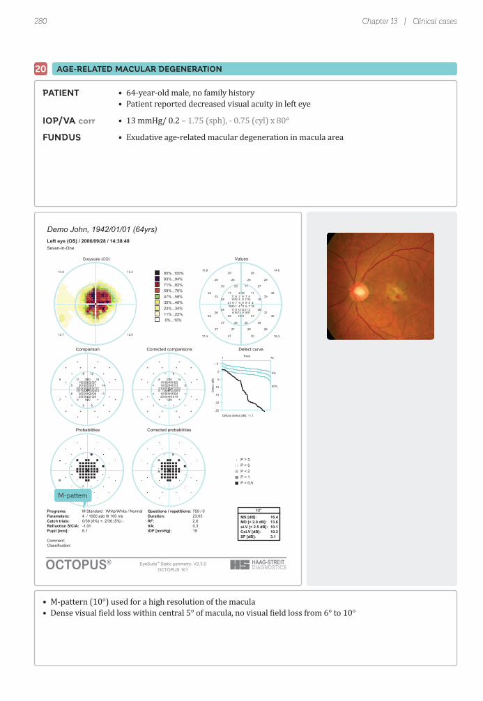
280
Rank
Def
ect (
dB)
Demo John, 1942/01/01 (64yrs)Left eye (OS) / 2006/09/28 / 14:38:48Seven-in-One
Classification:Comment:
Pupil [mm]: 6.1 IOP [mmHg]: 19Refraction S/C/A: -1.0// VA: 0.3Catch trials: 0/38 (0%) +, 2/38 (5%) - RF: 2.6Parameters: 4 / 1000 asb III 100 ms Duration: 23:03Programs: M Standard White/White / Normal Questions / repetitions: 759 / 0 12°
MS [dB]: 16.4MD [< 2.0 dB]: 13.6sLV [< 2.5 dB]: 10.1CsLV [dB]: 10.2SF [dB]: 3.1
95%..100%83%...94%71%...82%59%...70%47%...58%35%...46%23%...34%11%...22% 0%...10%
Greyscale (CO)
15.213.8
0.217.21
Values
411
6 11
212
962118711
119
109
1159
4209
1313
278
149410467 7 6118
31213111816
11
2829
27172330
3023
1625
2624
3022
29252427
3027
29252828
11172525
31262725
28282727
14.615.8
3.814.71
Comparison
2719
25 20
2919
232510132421
2122
2022
202723
281122
1918
282323
17232720272525 25 263013
281919201315
20
++
+126+
+6
145
56
+7
+56+
++
++++
1912++
+++5
++++
Corrected comparisons
2215
20 15
2415
1820592017
1618
1618
152219
24718
1413
231918
13182316222120 21 22268
24151516910
16
++
+8++
++
9+
++
++
++++
++
++++
158++
++++
++++
Defect curve
Probabilities Corrected probabilities
P > 5P < 5P < 2P < 1P < 0,5
OCTOPUS 101OCTOPUS®
Diffuse defect [dB]: -1.1
471
5%
95%
-5
0
5
10
15
20
25
M-pattern
Chapter 13 | Clinical cases
• 64-year-old male, no family history• Patient reported decreased visual acuity in left eye
• 13 mmHg/ 0.2 – 1.75 (sph), - 0.75 (cyl) x 80°
• Exudative age-related macular degeneration in macula area
• M-pattern (10°) used for a high resolution of the macula• Dense visual ield loss within central 5° of macula, no visual ield loss from 6° to 10°
PATIENT
IOP/VA corr
FUNDUS
AGE-RELATED MACULAR DEGENERATION20
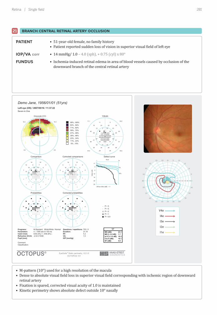
281
Demo Jane, 1956/01/01 (51yrs)Left eye (OS) / 2007/05/16 / 11:37:22Seven-in-One
Classification:Comment:
:]gHmm[ POI:]mm[ lipuPRefraction S/C/A: -2.5/-0.75/80 VA: 1.0Catch trials: 0/35 (0%) +, 3/36 (8%) - RF: 4.2Parameters: 4 / 1000 asb III 100 ms Duration: 21:19Programs: M Standard White/White / Normal Questions / repetitions: 703 / 0 12°
MS [dB]: 23.1MD [< 2.0 dB]: 7.7sLV [< 2.5 dB]: 10.3CsLV [dB]: 10.1SF [dB]: 4.0
95%..100%83%...94%71%...82%59%...70%47%...58%35%...46%23%...34%11%...22% 0%...10%
Greyscale (CO)
10.319.3
8.05.0
Values
131
33 32
333331
2933
31293332
30
916278
1
253029
422932815
283225 33 25292632313331
323332
611
2320212
2322
297
3027
3126
30323132
2929
18222319
202520
31313132
28293030
20.211.1
2.034.03
Comparison
1830
+ +
+++
++
++++
+
2317524
30
7++
2729++2416
++8 + 8+5++++
+++
2218
6102818
77
+24
++
++
++++
++
117610
11510
++++
++++
Corrected comparisons
1729
+ +
+++
++
++++
+
2215+22
29
5++
2628++2315
++6 + 7++++++
+++
2116
592716
56
+22
++
++
++++
++
96+9
9+9
++++
++++
Defect curve
Probabilities Corrected probabilities
P > 5P < 5P < 2P < 1P < 0,5
OCTOPUS 101OCTOPUS®
Diffuse defect [dB]: -1.1
471
5%
95%
-5
0
5
10
15
20
25
Rank
Def
ect (
dB)
10 30 40 50 60 70 80 90
90105120 75 60
270255240 285 300
45135
315225
30150
330210
15165
345195
0180
V4e
I4e
I3e
I2e
I1e
Retina | Single fi eld
• M-pattern (10°) used for a high resolution of the macula• Dense to absolute visual ield loss in superior visual ield corresponding with ischemic region of downward retinal artery• Fixation is spared, corrected visual acuity of 1.0 is maintained• Kinetic perimetry shows absolute defect outside 10° nasally
• 51-year-old female, no family history• Patient reported sudden loss of vision in superior visual ield of left eye
• 14 mmHg/ 1.0 – 4.0 (sph), + 0.75 (cyl) x 80°
• Ischemia-induced retinal edema in area of blood vessels caused by occlusion of the downward branch of the central retinal artery
PATIENT
IOP/VA corr
FUNDUS
21 BRANCH CENTRAL RETINAL ARTERY OCCLUSION

282
Rank
Def
ect (
dB)
Demo Jane, 1939/01/01 (67yrs)Right eye (OD) / 2006/07/31 / 13:23:40Seven-in-One
Classification:Comment:
:]gHmm[ POI:]mm[ lipuP 14Refraction S/C/A: +1.0/-2.5/80 VA: 0.2Catch trials: 1/30 (3%) +, 2/31 (6%) - RF: 4.9Parameters: 4 / 1000 asb III 100 ms Duration: 18:13Programs: M Standard White/White / Normal Questions / repetitions: 611 / 0 12°
MS [dB]: 25.5MD [< 2.0 dB]: 4.3sLV [< 2.5 dB]: 3.8CsLV [dB]: 3.6SF [dB]: 1.9
95%..100%83%...94%71%...82%59%...70%47%...58%35%...46%23%...34%11%...22% 0%...10%
Greyscale (CO)
4.34.0
6.46.3
Values
2728
25 27
2526
2627 17
18 2425
2325
2824 2127
25
2324
20 2226
2525 25
25 2420 2530 24 251623 18 28
26 2423 2626 27
28
22 25
27 27 27 26
7262
9292
8292
6282
28 30 29 28
28 25
22 28 27 27
29 270392
828230 30
28 28 27 26
25.125.6
3.524.62
Comparison
++
5 +
55
5+ 15
14 76
85
+ 7 115
6
77
12 9 5
55 5
6 711 5+ 7 7169 13 +
5 7 9 55 +
+
5 +
+ + + +
++
++
++
++
+ + + +
+ +
6 + + +
+ +++
+++ +
+ + + +
Corrected comparisons
++
+ +
++
++ 13
12 5+
6+
+ 5 8+
+
55
9 6 +
++ +
+ 5 8 ++ 5 +146 11 +
+ 5 6 ++ +
+
+ +
+ + + +
++
++
++
++
+ + + +
+ +
+ + + +
+ +++
+++ +
+ + + +
Defect curve
Probabilities Corrected probabilities
P > 5P < 5P < 2P < 1P < 0,5
OCTOPUS 101OCTOPUS®
Diffuse defect [dB]: -1.1
471
5%
95%
-5
0
5
10
15
20
25
M-pattern
Signficantfoveal defectat P < 0.5%
Chapter 13 | Clinical cases
• 67-year-old female, no family history• Patient reported distorted vision in right eye
• 12 mmHg/ 0.2 – 1.5 (sph), - 2.5 (cyl) x 80°
• Macular hole with luid cuff in surrounding region
• M-pattern (10°) used for a high resolution of the macula• Signi icant visual ield loss in the central fovea leading to decreased visual acuity (0.2) due to macular hole
PATIENT
IOP/VA corr
FUNDUS
MACULAR HOLE22

283
Rank
Def
ect (
dB)
Demo John, 1928/01/01 (76yrs)Left eye (OS) / 2004/03/24 / 15:44:51Seven-in-One
Classification:Comment:
Pupil [mm]: 7.2 IOP [mmHg]:Refraction S/C/A: +7.0/-2.0/170 VA: 0.2Catch trials: 1/24 (4%) +, 0/24 (0%) - RF: 2.0Parameters: 4 / 1000 asb III 100 ms Duration: 16:31Programs: G Standard White/White / Normal Questions / repetitions: 474 / 1 30°
MS [dB]: 19.1MD [< 2.0 dB]: 6.9sLV [< 2.5 dB]: 4.1CsLV [dB]: 4.0SF [dB]: 2.1
95%..100%83%...94%71%...82%59%...70%47%...58%35%...46%23%...34%11%...22% 0%...10%
Greyscale (CO)
8.78.7
8.41.5
Values
1814
24 23
24
22
10
11
14
21
24
21
20
19
14
1811 16
2422
12 18
2022
20
24
20
22
15
18
18
20
1724 25
2420
5181
2422
6132
2223
14 15
2323
2112
2422
17
22
16 16
2222
16.716.7
4.126.12
Comparison
1013
+ 5
5
5
16
17
11
+
5
7
5
10
12
718 14
68
12 6
65
7
+
5
+
8
6
5
5
14+ +
58
6 8
++
8+
++
14 12
55
5 13
++
6
+
7 6
++
Corrected comparisons
+7
+ +
+
+
11
12
6
+
+
+
+
+
7
+13 9
++
6 +
++
+
+
+
+
+
+
+
+
9+ +
++
+ +
++
++
++
8 7
++
+ 8
++
+
+
+ +
++
Defect curve
Probabilities Corrected probabilities
P > 5P < 5P < 2P < 1P < 0,5
OCTOPUS 101OCTOPUS®
Diffuse defect [dB]: -1.1
471
5%
95%
-5
0
5
10
15
20
25
Very reliable test
Diffuse &local defect
Retina | Single fi eld
• Sensitivity loss in superior visual ield corresponding with inferior retinal hemorrhage• Diffuse visual ield defect associated with poor visual acuity (0.2)• Signi icant local visual ield loss in superior paracentral area due to macular edema
• 76-year-old male, no family history• Patient reported decreased visual acuity in left eye, blurred and double vision
• 10 mmHg/ 0.2 + 3.75 (sph), - 2.0 (cyl) x 170°
• Retinal hemorrhage and soft exudate along RNFL in lower retinal arcade
PATIENT
IOP/VA corr
FUNDUS
23 BRANCH CENTRAL RETINAL VEIN OCCLUSION

284

Index 285
INDEX
07 pattern 70, 72-7310-2 pattern 72, 2441-level test (1 LT) 91-9224-2 pattern 64, 2442-level test (2 LT) 94-9532/30-2 pattern 64, 244
Aability testing 74-78abnormal visual ield 11, 19, 145-148absolute defect 101-102, 261age-related macular degeneration (AMD) 70-71, 280altitudinal defect 60-61apostilb (asb) 14-15arcuate defect 60-61, 259, 265-268, 270artifactual visual ields, see untrustworthy visual ieldasb, see apostilb automated kinetic perimetry 230-231
Bbackground 47background luminance 47, 200, 236baseline tests 250-251beeping sound 39binocular visual ield 8-9blepharoptosis, see ptosis blind spot 69, 90-91, 205blue-on-yellow perimetry, see SWAP
Ccaecocentral defect 68candela per m2 (cd/m2) 14-15cataract 140-141, 181, 260catch trials 123-124cd/m2, see candela per m2 central defect 68, 70-71, 280, 282chiasmal defect, see heteronymous defect Cluster Analysis 110-113, 152-155cluster defect 146-147, 152-155, 183Cluster Trend Analysis (CTA) 166-167, 183-186Comparison 103-106, 149-151
constricted visual ield 60-61, 65, 148, 271Corrected Cluster Analysis 116, 118, 143-144, 152-155Corrected Cluster Trend Analysis (CCTA) 166-167, 183-186Corrected Comparison 115-117, 143-144, 149-151Corrected Probabilities 116-117, 143-148Corrected square root of Loss Variance (CsLV) 119, 121critical fusion frequency (CFF) 198-199cupola perimeter 214-215, 236, 243
DD pattern 73data import 239-242dB, see decibel DD (diffuse defect) 115-118, 121-122, 179, 181-182DD Trend Analysis 166-167, 179, 181-182decibel (dB) 14-15Defect Curve 109-110, 141-143defect, see sensitivity loss deviation from normal, see sensitivity loss diabetic retinopathy 70-71, 73diffuse defect 60-61, 100, 115-118, 140-144, 178-182disability testing 78driving license test 74-76drug-induced maculopathy 70-71dynamic range 195, 201-202dynamic strategy 83, 85-86
EEsterman test 74-75examination parameters ixed 47-48 patient-speci ic 48-57exfolitative glaucoma 271eye patch 31EyeSuite Progression Analysis 166-190

Index286
Ffalse negative answers 124-125, 138-139, 225, 248false positive answers 45, 123, 125, 138-139, 177, 224-225, 247fatigue effect 38ixation 34-36ixation loss 35, 39, 45, 248ixation targets 34ixed examination parameters 47-48licker perimetry 52-53, 198-199loor effect 171, 175, 184, 195, 201-201,268, 271luctuation 20-22, 136-140, 172-173, 243
frequency-of-seeing curve 21-22function-speci ic perimetry 52-53, 193-196
GG pattern 39, 62-63, 65gaze tracker 248glaucoma advanced stage 65, 148, 265, 271 altitudinal defect 60-61 arcuate defect 60-61, 259, 265-268, 270 constricted visual ield 60-61, 65, 148, 271 diffuse defect 60-61 early stage 153-154, 158, 257-262, 266-270 exfoliative 271 moderate stage 263-264, 266-270 nasal step 60-61, 143-144, 258, 260, 266-267 normal tension 257-258, 261, 263, 267, 269 paracentral defect 60-61, 258-259, 261, 269-270 partial arcuate defect 60-61, 262-263 primary open-angle 259, 262, 264-266, 268, 270 progression 181-182, 185-186, 190, 266-271 temporal wedge defect 60-61 test patterns 62-66 typical defects 60-61Glaucoma Hemi ield Test (GHT) 247-249global indices 118-122Global Trend Analysis (GTA) 166-167Goldmann perimeter 214-215 stimulus intensities 217-218 stimulus size 52, 216-217GPA, see Guided Progression Analysis G-Periphery pattern 65-66
Grayscale of Comparison 105-106, 149-151 of Values 102, 106, 245G-Screening pattern 66, 92-93Guided Progression Analysis (GPA) 250-252
HHeijl-Krakau blind spot monitoring 248hemianopia 67-68, 206, 231, 278Hertz (Hz) 198-199heteronymous defect 67-68, 278-279HFA, see Humphrey Field Analyzerhill of vision 10-11, 13, 16, 18-19, 207-210homonymous defect 67-68, 272-273Humphrey Field Analyzer 235-252hydroxychloroquine, see drug-induced maculopathy
Iintensity, see luminanceisopter 207-210, 219-223
Kkinetic perimetry 48-51, 205-232
LLD (local defect) 122, 180-182LD Trend Analysis 166-167, 180-182learning effect 37-38, 243lens rim artifact 43, 45lens, see trial lens lid artifact, see also ptosis 43-44, 77, 177linear regression analysis 172local defect 100, 115-118, 140-143, 178-182local sensitivity loss, see local defect low vision 53, 65, 86-87, 148, 265, 201-202, 212, 271low vision strategy 83, 86-87luminance background 47, 200, 236 general 14-15, 47-48 maximum stimulus intensity 47-48, 236-237 stimulus intensity 14-15, 47-48, 217-218
MM pattern 65, 71-72, 280, 282macular hole 282

Index 287
manual kinetic perimetry 230maximum stimulus luminance 47-48, 236-237MD Trend Analysis 166-167, 174-176, 178-179Mean Defect (MD) 119, 159-160, 168, 174-176, 178-179Mean Deviation (MD) 247Mean Sensitivity (MS) 119monocular visual ield 8-9
NN pattern 69nasal step 60-61, 143-144, 258, 260, 266-267nerve iber bundle defect 68neurological disease caecocentral defect 68 central defect 68 disk edema 67 hemianopia 67-68, 206, 231, 278 heteronymous defect 67-68, 278-279 homonymous defect 67-68, 272-273 idiopathic intercranial hypertension (IIH) 67 nerve iber bundle defect 60-61, 68 optic nerve head drusen 67 optic neuritis 67, 276-277 optic neuropathy 67, 274-275 quadrantanopia 67-68, 227-229, 272-273, 279 stroke 67, 272-273 test patterns 67-70 tumor 67, 231, 278-279 typical defects 67-68normal strategy 83-84normal tension glaucoma 257-258, 261, 263, 267, 269normal visual ield 8-10, 18-22, 145-148normative data base 18-20, 237-238normative values 18-20, 237-238
Ooptic neuritis 67, 276-277optic neuropathy 67, 274-275
Pparacentral defect 60-61, 258-259, 261, 269-270partial arcuate defect 60-61, 262-263patient data date of birth 28, 40, 135-136 refraction 28, 40-42, 135-136
patient instructions 29-30, 199, 201patient monitoring 35-36patient positioning 31-34patient-speci ic examination parameters 48-57Pattern Deviation 245-246Pattern Standard Deviation (PSD) 247pattern, see test patternperimeter cupola perimeter 214-215, 236, 243 screen-based perimeter 236, 243 set-up 28perimeter set-up eye patch 31 patient 31-34 pupil 33 trial lens 33-34perimetrist, see visual ield examinerPerimetry 7point-wise event analysis 250-251point-wise trend analysis 187-188Polar Analysis 113-115, 155-158Polar Trend Analysis (PTA) 166-167, 187-190Post chiasmal defect, see homonymous defectprimary open-angle glaucoma 259, 262, 264-266, 268, 270Probabilities 107-108, 145-148progression 165-190 selection of visual ields 176-178ptosis 43-44, 76-77, 177, 230pulsar perimetry 52-53, 196-197pupil 33, 44
Qquadrantanopia 67-68, 227-229, 272-273, 279qualitative strategy 56-57, 81-82, 90-95quantitative strategy 56-57, 81-90
Rrate of progression 170, 174-176reaction time compensation 226-227refractive error 28, 40-42, 135-136Reliability Factor (RF) 124-125reliability indices 123-125retinal disease age-related macular degeneration (AMD) 70-71, 280
Index288
branch central retinal artery occlusion 281 branch central retinal vein occlusion 283 diabetic retinopathy 70-71, 73 drug-induced maculopathy 70-71 macular hole 282 retinitis pigmentosa (RP) 70-71, 211 test patterns 70-73 typical defects 70-71retinal nerve iber layer (RNFL) 60, 62, 155-156, 187retinitis pigmentosa (RP) 70-71, 211RNFL, see retinal nerve iber layer
SSAP (Standard Automated Perimetry) 51-53, 193-196scotoma 207-209, 221-223screen-based perimeter 236, 243screening 62, 92-93, 244semi-automated kinetic perimetry 231-232sensitivity loss 18-19, 100, 103-106sensitivity threshold 12-17, 100-102, 236-237sensitivity to light 9, 11-14sensitivity, see sensitivity thresholdsetting up perimeter 28set-up errors 28, 40, 135-136Short-term Fluctuation (SF) 124-125, 140, 224-225Short-Wavelength Automated Perimetry, see SWAP 52-53, 200-201signi icance of change 171-174SITA fast 244SITA standard 244slope 170, 174-176sLV Trend Analysis 166-167, 180-182spot checking 207, 209square root of Loss Variance (sLV) 119-120, 160-162src 197Standard Automated Perimetry, see SAPstatic perimetry 12-14, 48-51, 205-206stimulus exposure time 48stimulus luminance 14-15, 47-48, 217-218stimulus speed 218stimulus type 51-53 licker 52-53, 198-199 function-speci ic 52-53, 193-196 Goldmann sizes 52, 217 low vision 53, 201-202 pulsar 52-53, 196-197
SAP (standard automated perimetry) 51-53, 193-196 SWAP (Short-Wavelength Automated Perimetry) 52-53, 200-201strategy 56-57, 81-82, 96 1-level test (1 LT) 91-92 2-level test (2 LT) 94-95 dynamic 83, 85-86 low vision 83, 86-87 normal 83-84 qualitative 56-57, 81-82, 90-95 quantitative 56-57, 81-90 screening 92-93 Tendency-Oriented Perimetry (TOP) 83, 87-90stroke 67, 272-273structure-function relationship 155-156, 187, 258-271subjectivity 20-21, 25, 243suprathreshold test, see qualitative strategySWAP 52-53, 200-201
Ttechnician, see visual ield examinertemporal wedge defect 60-61Tendency-Oriented Perimetry (TOP) 83, 87-90test duration 140test parameters, see examination parameters test pattern 54-55, 59 07 70, 72-73 10-2 72, 244 24-2 64, 244 32/30-2 64, 244 60-4 244 BG (blindness) 78 BT (Blepharoptosis) 76-77 D 73 Esterman 74-75 G (glaucoma) 39, 62-63, 65 G-Periphery 65-66 G-Screening 66, 92-93 M (macula) 65, 71-72, 280, 282 N 69three-zone strategy, see 2-level testthreshold test, see quantitative strategyThreshold Values 245threshold, see sensitivity threshold

Index 289
Total Deviation 245-246trend analysis 168-174 in luence of luctuation 172-173 in luence of number of tests 173-174 linear regression analysis 172 ordinary least square it 172 point-wise 187-188 rate of progression 170, 174-176 selection of visual ields 176-178 signi icance of change 171-174 slope 170, 174-176 trend line 168-170 t-test 170-171trial lens 29, 33-34, 41-42trial lens calculator 41-42trigger-happy 40, 138, 142-143t-test 170-171tumor 67, 231, 278-279two-zone strategy, see 1-level test
Uunreliable visual ields, see untrustworthy visual ielduntrustworthy visual ield 136-140 false negative answers 124-125, 138-139, 225, 248 false positive answers 45, 123, 125, 138-139, 177, 224-225, 247 fatigue 38 ixation loss 35, 39, 45, 248 incorrect patient age 40-41 lack of attention 40 learning 37-38, 243 lens rim artifact 43, 45 lid artifact 43-44, 77, 177 pupil size 44 refractive error 40-42 set-up errors 28, 40, 135-136 trigger-happy 40, 138, 142-143
VValues 101-102vector 207-209, 219-223visual ield abnormal 11, 19, 145-148 age-dependency 18-19 binocular 8-9, 74
central 18, 60-64, 67 eccentricity 18-19 interpretation 127-162 monocular 8-9 normal 8-10, 18-22, 145-148 peripheral 18, 65, 67, 69, 72-73, 206, 211, 213 progression 165-190 spatial extent 8-9 spatial resolution 17-18, 54visual ield examiner 27Visual Field Index (VFI) 247, 250visual function 22visual impairment 78
Wwhite-on-white perimetry, see SAP widespread defect, see diffuse defect


HAAG-STREIT Holding AGwww.haag-streit-holding.com
HAAG-STREIT AG, Diagnosticswww.haag-streit.com
HAAG-STREIT AG, Verkauf Schweizwww.haag-streit.ch
HAAG-STREIT Deutschland GmbHwww.haag-streit.de
HAAG-STREIT Far Eastwww.haag-streit-fareast.com
HAAG-STREIT Medtech AGwww.haag-streit-medtech.com
HAAG-STREIT Surgical GmbHwww.haag-streit-surgical.com
HAAG-STREIT UKwww.haag-streit-uk.com
HAAG-STREIT USAwww.haag-streit-usa.com
Asetronics AGwww.asetronics.ch
HAAG-STREIT AGGartenstadtstrasse 103098 KoenizSwitzerlandPhone +41 31 978 01 11Fax +41 31 978 02 [email protected]
MEMBERS OF HAAG-STREIT GROUP
CLEMENT CLARKE Ltd.www.clement-clarke.com
ComLab AGwww.comlab.ch
HS DOMS GmbHwww.hs-doms.com
IPRO GmbHwww.ipro.de
John Weiss Ltd.www.johnweiss.com
Möller-Wedel GmbH & Co KGwww.haag-streit-surgical.com
Möller-Wedel Optical GmbHwww.moeller-wedel-optical.com
OptoMedical Technologies GmbHwww.haag-streit-surgical.com
Reliance Medical Inc.www.haag-streit-usa.com
SPECTROS AGwww.spectros.ch