Generated using version 3.0 of the official AMS LATEX template

Estimating suppression of eddy mixing by mean flows1

Andreas Klocker ∗ , Raffaele Ferrari

Massachusetts Institute of Technology, Cambridge, Massachusetts, USA2

Joseph H. LaCasce

Department of Geosciences, University of Oslo, Norway3

∗Corresponding author address: Andreas Klocker, Massachusetts Institute of Technology, 77 Mas-

sachusetts Avenue, 54-1622, Cambridge, MA 02139.

E-mail: aklocker@mit.edu

1

ABSTRACT4

Particle and tracer-based estimates of lateral diffusivities are used to estimate the sup-5

pression of eddy mixing across strong currents. Particles and tracers are advected using6

a velocity field derived from sea surface height measurements from the South Pacific, in a7

region west of Drake Passage. This velocity field has been used in a companion paper to8

show that both particle and tracer-based estimates of eddy diffusivities are equivalent, de-9

spite recent claims to the contrary. These estimates of eddy diffusivities are here analyzed to10

show (1) that the degree of suppression of mixing across the strong Antarctic Circumpolar11

Current is correctly predicted by mixing length theory modified to include eddy propagation12

along the mean flow, and (2) that the suppression can be inferred from particle trajectories13

by studying the structure of the autocorrelation function of the particle velocities beyond14

the first zero crossing. These results are then used to discuss how to compute lateral and15

vertical variations in eddy diffusivities using floats and drifters in the real ocean.16

1. Introduction17

Eddy transport across mean currents is a central element in many phenomena, such as in18

the poleward movement of warm waters in the Southern Ocean and the lateral spreading of19

nutrient-rich waters in upwelling zones. Understanding this transport, and parameterizing it20

in coarse resolution climate models, is of great interest at present (e.g. Toole and McDougall21

2001).22

Often the eddies responsible for transport derive from the instability of a mean current,23

such as the Antarctic Circumpolar Current (ACC) in the Southern Ocean or the California24

1

Current over the western slope of North America. This suggests that eddy transport is25

greatest near the mean current itself, as eddy mixing scales with eddy kinetic energy (Prandtl26

1925). However, there is a growing body of evidence suggesting that the mean flow also27

suppresses mixing (e.g. Nakamura 1996; Bower et al. 1985; Marshall et al. 2006; Abernathey28

et al. 2010; Ferrari and Nikurashin 2010). Thus assessing cross-jet transport involves finding29

the balance between the enhancement of mixing by instability and the suppression imposed30

by the mean.31

The present study seeks to improve this understanding by considering mixing in a the-32

oretical model and by measuring mixing with a realistic velocity field. The work builds on33

the study of Ferrari and Nikurashin (2010), extending the theoretical work to particles and34

by addressing mixing at depth in addition to that at the surface. It also follows a companion35

paper, Klocker et al. (2011), in which tracer- and particle-based diffusivities were compared.36

The present focus is on the Southern Ocean. We show that mixing is suppressed across37

the core of the ACC, i.e. from the surface down to 1500 m. Mixing is greater to the north38

of the ACC and below it. As suggested by the theoretical model, the suppression of the39

diffusivity is associated with the drift of eddies with respect to the mean flow. This in turn40

is manifested in a negative lobe in the particle autocorrelation function. Accurate diffusivity41

estimates thus require that this lobe be taken into account.42

The paper is organized as follows. The theoretical model is derived in Section 2. Then the43

velocity field, derived from fields in the Southern Ocean, is discussed in Section 3. Tracer-44

derived diffusivities are examined in Section 4a and compared directly to the theoretical45

model. Particle-based estimates are examined further in Section 4b, and recommendations46

are made for observational studies. The work concludes with Section 5.47

2

2. Theory48

To illustrate the suppression of mixing across a jet, we follow Ferrari and Nikurashin49

(2010) and represent eddy mixing as a stochastically forced wave equation. Ferrari and50

Nikurashin (2010) found that such a model, when used to advect a passive tracer, success-51

fully reproduces the meridional variation of the eddy diffusivity deduced using Nakamura’s52

technique (1996) applied to surface geostrophic velocities. Here we examine the particle-53

based (Lagrangian) diffusivities derived using a similar stochastic flow.54

We represent the ocean as an equivalent-barotropic fluid, governed by the quasi-geostrophic

potential vorticity (QGPV) equation:

∂tq + U∂xq + (∂yQ)∂xψ + J(ψ, q) = 0, (1)

where J the Jacobian operator, ψ is the geostrophic streamfunction representing the wave

motions and

q = ∇2ψ − Fψ (2)

is the associated potential vorticity (Pedlosky 1987). In the latter, ∇2ψ and Fψ represent55

the relative and stretching vorticities, respectively; F = 1/λ2 is the inverse square of the56

deformation radius. The waves are imbedded in a mean zonal flow U and a large-scale PV57

gradient ∂yQ = β+FU , where β is the planetary gradient of PV and the FU is the contribu-58

tion by the mean flow shear (in an equivalent-barotropic model U is the difference between59

the flow in the active layer and the quiescent abyss, so it is a proxy for the vertical shear).60

Curvature terms associated with the bending of the mean flow are neglected, consistent with61

the assumption that the mean flow varies on scales much larger than the waves.62

3

We express the streamfunction in terms of its Fourier transform:

ψ(x, y, t) =∑

k

∑

l

a(t)eikx+ily (3)

The amplitude, a, is then governed by:

d

dta+ ikcwa = N (4)

where N is a nonlinear function, proportional to the transform of the advective term and

where:

cw = U + c, c = − ∂yQ

κ2 + F(5)

with κ2 = k2 + l2 the square of the total wavenumber. c is the free phase speed of the63

baroclinic Rossby wave and cw is the Doppler shifted Rossby wave speed that would be64

measured with a Hovmoller diagram of the streamfunction. Thus (4) governs the evolution65

of Rossby waves forced by eddy interactions, represented by N (deriving, for example, from66

baroclinic instability).67

Analytical solutions to (4) can be obtained if one replacesN with a fluctuation-dissipation

stochastic forcing term, as this effectively linearizes the PV equation. There is an extensive

literature on such models (e.g. Farrell and Ioannou 1993; Flierl and McGillicuddy 2002;

DelSole 2004) wherein these representations are described. The particular form we will use

is:

N = −2U√γκ

r(t)eikx+ily − γaeikx+ily . (6)

The fluctuations are generated by a white noise random process r(t), with zero mean and an

autocorrelation 〈r(t)r∗(t′)〉 = δ(t − t′) (where 〈 · 〉 denotes the expected value and the star

is the complex conjugate). The amplitude of the forcing is determined by the constant U .

4

The dissipation is represented as a linear damping term acting on the potential vorticity (a

choice of simplicity rather than realism). Thus the evolution equation for the streamfunction

amplitude, a, is:

d

dta + ikcwa+ γa = −2U√γ

κr(t) (7)

The solution to (7) is:

a(t) =2U√γκ

∫

∞

0

r(t− τ)e−γτ−ikcwτ dτ, (8)

The form of the RHS is chosen to omit the initial condition, which is irrelevant in what

follows. Given this, the kinetic energy of the eddy field is:

EKE ≡ 1

2

(

|∂xψ|2 + |∂yψ|2)

= U2 , (9)

where the bars indicate a spatial average over the lateral domain. The result explains our68

choice of amplitude in (6).69

With the eddy streamfunction, we can derive relations for the motion of particles advected

by the field. As our focus is on mixing across the zonal mean current, we will concentrate

on meridional displacements. Following Taylor (1921), we can define a diffusivity in the

meridional direction:

K1y(x, y, t) =1

2

d

dt〈η2〉 =

∫ t

0

R(t′, t) dt′, (10)

where the integrand in the last term,

R(t− t′) ≡< vL(t; x, y, t)vL(t′; x, y, t) > , (11)

is the autocorrelation of the meridional Lagrangian velocity. Here vL(t′; x, y, t) is the velocity70

at time t′ of a particle that passes through (x, y) at time t. As the eddy field produced by the71

5

stochastic model is stationary, the autocorrelation only depends on the difference between72

t′ and t and we can accordingly replace the vL(t; x, y, t) with vL(0; x, y, 0) without loss of73

generality. Furthermore, as the eddy field is homogeneous, we can replace the ensemble74

average with an integral over space and the autocorrelation becomes independent of position.75

For small amplitude eddies, particles simply drift zonally at the speed U and one can

easily compute the Lagrangian velocity from the Eulerian one,

vL (t′; x, y, 0) = v (x− Ut′, y, t′) . (12)

While this relationship is valid only if one ignores, at leading order, the particle motions

induced by the eddies, the resulting autocorrelation appears to hold for finite amplitude

eddies as well, as noted hereafter. Armed with this relationship, the transformed Lagrangian

meridional velocity for the stochastically-driven flow is:

vL(t′; x, y, 0) =

∂ψ

∂x

∣

∣

∣

∣

(x−Ut′,y,t′)

= ika(t′)eik(x−Ut′)+ily (13)

with the amplitude, a, given in (8). As v is complex, we calculate the autocorrelation thus:

Rvv(t′) =

1

2< v∗(x− Ut′, y, t′)v(x, y, 0) + v(x− Ut′, y, t′)v∗(x, y, 0) > . (14)

Substituting in the full expression for v, we obtain:

Rvv =2k2U2γ

κ2

[∫

∞

0

dτ ′∫

∞

0

dτ r(t′ − τ ′)r(t− τ)e−γ(τ+τ ′)+ik(cw−U)(τ−τ ′) + c.c.

]

(15)

where c.c. is the complex conjugate of the preceding double integral. Using the fact that:

r(t′ − τ ′)r(t− τ) = δ(t′ − τ ′ − t + τ) (16)

Eq.(15) reduces to:

Rvv(t′) =

2k2 U2

κ2e−γt′ cos [k(cw − U)t′] (17)

6

The autocorrelation decays exponentially in time, with a time scale proportional to γ−1, the76

inverse of the linear damping coefficient. At the same time R oscillates, with a frequency of77

k(cw − U) = kc. This is a consequence of the wave-like nature of the solution.78

The meridional diffusivity is the integral of the autocorrelation. It is straightforward to

show that this has a long-time asymptote of:

limt→∞K1y =2k2

κ2γ U2

γ2 + k2(cw − U)2. (18)

Thus the character of the autocorrelation and the size of the diffusivity depend on cw−U = c.79

If c = 0, the diffusivity is proportional to the EKE times the eddy decorrelation timescale80

γ−1. This is what one would conclude from the mixing length theory (Prandtl 1925). With81

a non-zero c, the autocorrelation oscillates with lag and the diffusivity is suppressed.82

The phase speed c is proportional to the mean PV gradient, ∂yQ = β + FU . Thus c is83

likely large in jets where the surface PV gradient is large, while it is smaller and possibly84

zero on the flanks of jets where the surface PV gradient is weak. Critical layers where c = 085

can only arise at the lateral flanks of jets in the equivalent barotropic mode, but they arise86

also in the vertical in the real ocean if the mean flow decays with depth. The Rossby wave87

speed of the equivalent barotropic model must be interpreted as the surface phase speed88

c = cw−U(z = 0). In the real ocean, mean currents tend to decay in the vertical and critical89

layers develop also in the vertical where cw −U(z) = 0. Ferrari and Nikurashin (2010) show90

that Eq. (18) holds also for vertically varying flows, if one substitutes the depth dependent91

eddy kinetic energy U(z)2 in the numerator and the depth dependent vertical velocity U(z)92

in the denominator, while cw = U(z = 0)+c remains the surface Doppler shifted wave speed.93

Hence more generally the suppression of K1y vanishes also in the vertical at critical layers94

7

where cw = U(z). Such levels are the steering levels of baroclinic instability and must exist95

if the jet is to be baroclinically unstable (e.g. Pedlosky 1987). Thus one expects large cw−U96

in the upper core of jets and strong suppression of mixing. On the lateral and vertical flanks97

cw − U is instead weaker and mixing is not suppressed.98

In regions where the mean flow is weak, the mean PV gradient is just β and c is the99

slow (westward) phase speed of the baroclinic Rossby wave and there is little suppression of100

mixing.101

If we define K01y to be the eddy diffusivity for eddies with c = 0, then Eq. (18) can be

written as,

K1y =K0

1y

1 + k2(cw − U)2/γ2. (19)

This shows that the reduction in K is proportional to the ratio of the decorrelation timescale102

γ−1 over the advection timescale 1/k(cw − U) = 1/kc.103

Interestingly, one arrives at the same result if one considers a passive tracer (Ferrari and

Nikurashin 2010). Assuming a mean zonal flow and a mean meridional gradient for the

tracer, Γ, this is:

∂C

∂t+ U

∂C

∂x+ J(ψ,C) + Γv = 0 (20)

where ψ is the eddy streamfunction obtained above. The solution is obtained by calculating104

the correlation between C and the meridional velocity and then dividing the result by the105

mean gradient, Γ. The result is the same as the particle-based estimate in Eq. (18) and106

is equivalent to that obtained by Ferrari and Nikurashin (2010) (their Eq. (12)1). The107

1Eq. (18) corrects an inconsequential factor of 2 that did not appear in Eq. (12) of Ferrari and Nikurashin

(2010).

8

only difference is that cw − U in their model is the intrinsic phase speed of Eady waves108

propagating on the mean temperature gradient, because they use a surface quasi-geostrophic109

model instead of an equivalent barotropic model. Thus the present diffusivity is recovered110

if the Eady wave is replaced with a baroclinic Rossby wave. The tracer-based solution is111

obtained by assuming the tracer has the same structure as the eddy field, so that the Jacobian112

of ψ and C vanishes. This is equivalent to our linearization of the Lagrangian velocity in113

terms of the mean Eulerian flow.114

Green (1970) also derives a similar expression for the eddy diffusivity for potential vor-115

ticity in horizontally homogeneous, baroclinically unstable flow based on the fastest growing116

linear normal mode. We review the argument and discuss the connection to the present117

model in the Appendix.118

Thus the tracer- and particle-derived diffusivities agree. Such agreement was found in119

the numerical experiments of Klocker et al. (2011). It is also implicit in the results of120

Shuckburgh and Haynes (2003), who compared probability density functions (PDFs) for121

tracers and particles using a kinematic model.122

One can also compare the present approach with previous studies using stochastic models123

for particle advection. In particular, the “first order stochastic model with spin” examined by124

Veneziani et al. (2004) yields an autocorrelation function which is the product of a decaying125

exponential and an oscillatory function. In this model, the stochastic forcing is applied126

directly to the particle velocity, and the oscillatory behavior comes from a rotational term127

coupling the velocities in the x and y directions. Veneziani et al. (2004) determined the128

rotational frequency by studying the motion of looping float trajectories in the Gulf Stream129

region.130

9

The two approaches are complimentary. However, the philosophy is slightly different. In131

the stochastic model, the random forcing is applied directly to the particles, and the “spin”132

is imposed to reproduce the looping trajectories produced by ocean drifters and floats. The133

approach is purely kinematic. In the present model, the stochastic forcing represents the134

action of eddies in the potential vorticity equation. The particles are simply advected by the135

flow. This clarifies the physical basis for the looping motion of the particles and shows that136

the suppression of eddy diffusivities in the ocean is the result of eddy propagation.137

3. The velocity field138

To study the modulation of eddy mixing across a mean current, we construct a velocity139

field representative of the ACC using the geostrophic streamfunction as measured from140

altimeters. This is the same velocity field used in a companion paper (Klocker et al. 2011)141

- we will provide a summary here, but the reader is referred to Klocker et al. (2011) for a142

more detailed description.143

The sea level anomaly maps come from the combined processing of Ocean Topography144

Experiment (TOPEX) and European Remote Sensing Satellite-1 and 2 (ERS-1 and ERS-2)145

altimetry data, and the mean streamlines are computed using the zonal mean of the sum146

of the mean geoid and the 3-year time-mean sea-surface height from altimetry. The sea147

level data has a temporal resolution of 10 days and a spatial resolution of 1/4o longitude ×148

1/4o latitude. We then use the geostrophic relation to derive geostrophic velocities at the149

ocean surface and interpolate the velocities onto a 1/10o grid to advect tracers and floats.150

We construct two different velocity fields - an ‘eddy’ velocity field in which we only use sea151

10

surface height anomalies to calculate geostrophic velocities and a ‘full’ velocity field in which152

we add the zonal average of the zonal mean flow (ignoring the weak meridional mean flow).153

We focus on a region upstream of Drake Passage between 103o-78oW and 30o-66oS -154

the same region studied by the ongoing Diapycnal and Isopycnal Mixing Experiment in the155

Southern Ocean (DIMES). To calculate horizontal velocities below the surface we assume156

an equivalent-barotopic structure of the ACC as suggested by Killworth and Hughes (2002);157

that is, we scale the surface geostrophic velocity by a structure function µ(z). This struc-158

ture function is calculated from the output of the Southern Ocean State Estimate (SOSE;159

Mazloff et al. (2010)), an eddy-permitting general circulation model of the Southern Ocean160

constrained to observations in a least-squares sense. Using the surface geostrophic veloc-161

ity field and the structure function, we construct a three-dimensional map of geostrophic162

velocities.163

The advection of tracers and floats is purely horizontal, i.e. vertical velocities are ne-164

glected. A correction to the surface velocity field is imposed to eliminate the weak lateral165

convergences associated with upwelling and downwelling (see Marshall et al. (2006) for more166

details). This adjustment is small and hardly affects our estimates of eddy diffusivities. In167

addition, we impose no-normal flow conditions at the north-south boundaries and periodic168

conditions at the east-west boundaries.169

11

4. Suppression of eddy diffusivity across the Antarctic170

Circumpolar Current171

The equivalent-barotropic velocity field based on altimetric measurements and a state

estimate is now used to advect numerical floats and tracers. The tracer distributions are

used to calculate effective diffusivity as defined by Nakamura (1996),

Ke =κ

L20(y)

∂∂A

∫

|∇C|2dA(

∂C∂A

)2 (21)

where C is a tracer contour encircling the area A, κ is the numerical diffusivity used to

advect the tracer and L0(y) is the zonal extent of the domain at the latitude y (technically

the equivalent latitude as defined in Shuckburgh and Haynes (2003)). The float trajectories

are used to calculate the meridional single-particle diffusivity K1y as defined in Taylor (1921)

and Davis (1991),

K1y =1

2

d

dt〈(y(t)− y0)

2〉 (22)

where y(t) is the latitude of a particle released at y0 at t = 0, and 〈·〉 is the average over all172

particles released at y0.173

We only consider cross-ACC diffusivities, because Nakamura’s approach is not well suited174

to compute along-current diffusivities. In the Pacific sector considered, the ACC flow from175

the east is along latitude lines and hence the analysis is in terms of meridional diffusivities.176

Klocker et al. (2011) show that Ke and K1y are indistinguishable from each other if177

one uses a sufficient number of floats. Here we consider both estimates to illustrate how178

suppression of mixing across strong currents affects tracer and float statistics.179

12

a. Tracer-based estimates180

The results from the stochastic model suggest that the latitudinal variations in eddy181

diffusivity are best interpreted as a competition between the enhancement of mixing by182

eddy stirring and suppression by mean flow advection. We test this hypothesis by running183

two sets of calculations. In the first set, the tracer is advected by the full velocity field. In184

the second set, the tracer is advected by the eddy velocity only, i.e. by the full velocity185

minus the zonal mean ACC flow.186

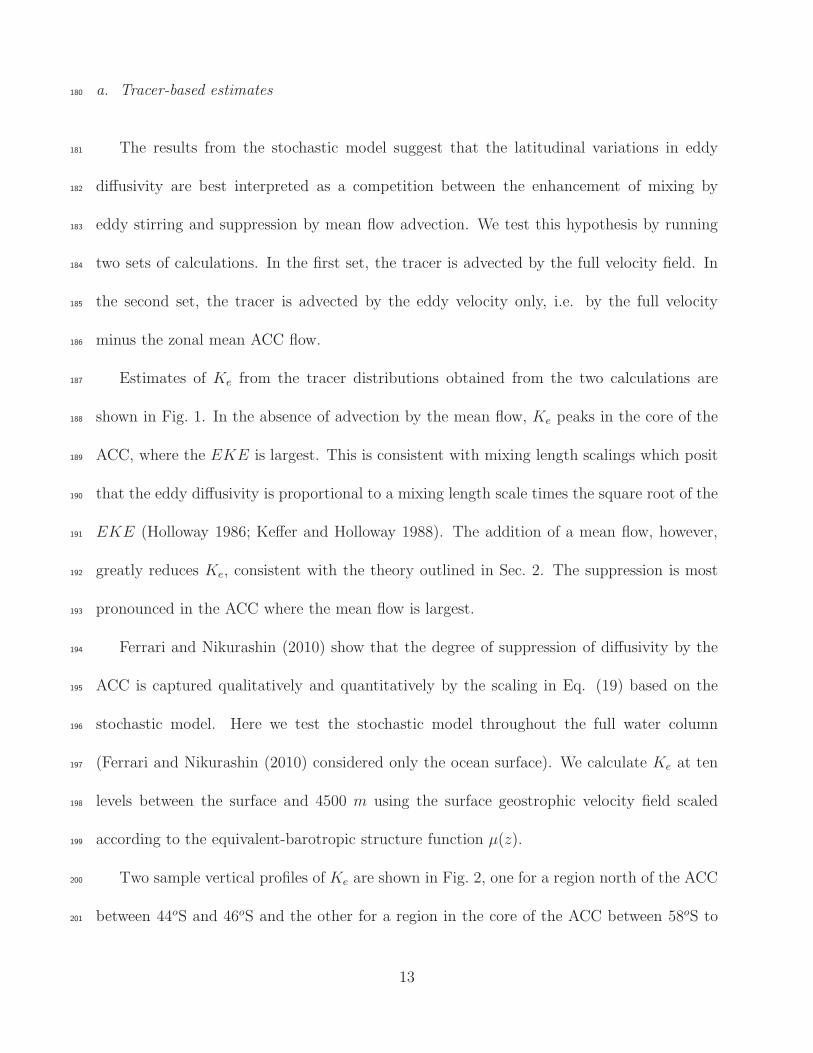
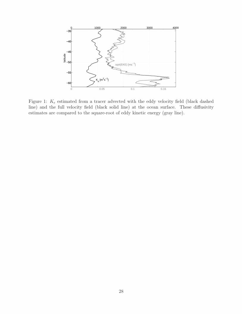
Estimates of Ke from the tracer distributions obtained from the two calculations are187

shown in Fig. 1. In the absence of advection by the mean flow, Ke peaks in the core of the188

ACC, where the EKE is largest. This is consistent with mixing length scalings which posit189

that the eddy diffusivity is proportional to a mixing length scale times the square root of the190

EKE (Holloway 1986; Keffer and Holloway 1988). The addition of a mean flow, however,191

greatly reduces Ke, consistent with the theory outlined in Sec. 2. The suppression is most192

pronounced in the ACC where the mean flow is largest.193

Ferrari and Nikurashin (2010) show that the degree of suppression of diffusivity by the194

ACC is captured qualitatively and quantitatively by the scaling in Eq. (19) based on the195

stochastic model. Here we test the stochastic model throughout the full water column196

(Ferrari and Nikurashin (2010) considered only the ocean surface). We calculate Ke at ten197

levels between the surface and 4500 m using the surface geostrophic velocity field scaled198

according to the equivalent-barotropic structure function µ(z).199

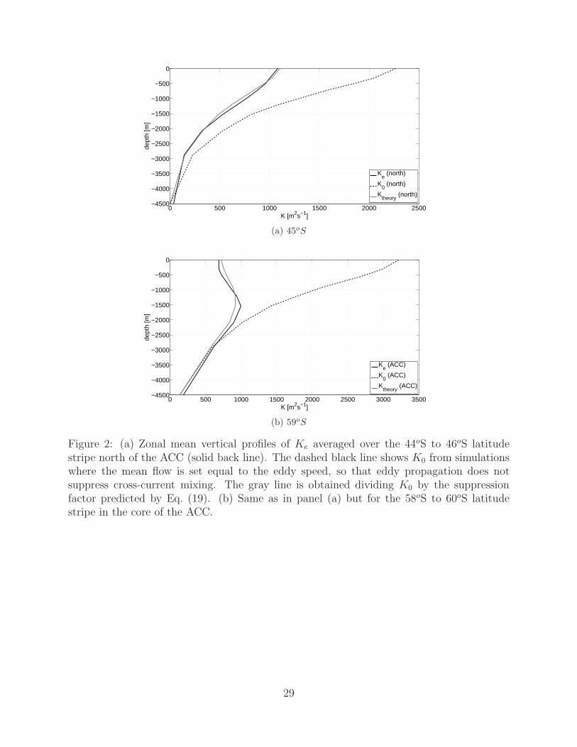
Two sample vertical profiles of Ke are shown in Fig. 2, one for a region north of the ACC200

between 44oS and 46oS and the other for a region in the core of the ACC between 58oS to201

13

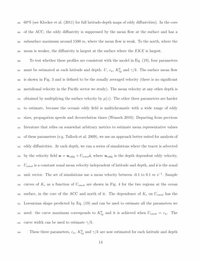
60oS (see Klocker et al. (2011) for full latitude-depth maps of eddy diffusivities). In the core202

of the ACC, the eddy diffusivity is suppressed by the mean flow at the surface and has a203

subsurface maximum around 1500 m, where the mean flow is weak. To the north, where the204

mean is weaker, the diffusivity is largest at the surface where the EKE is largest.205

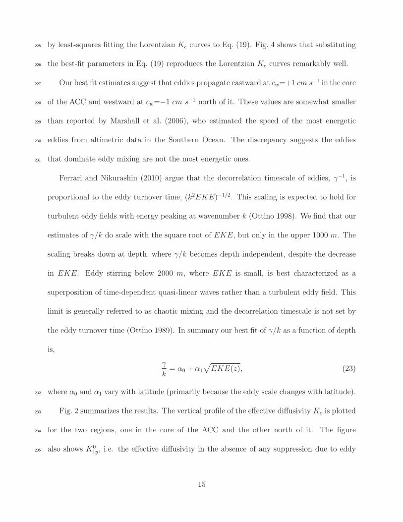
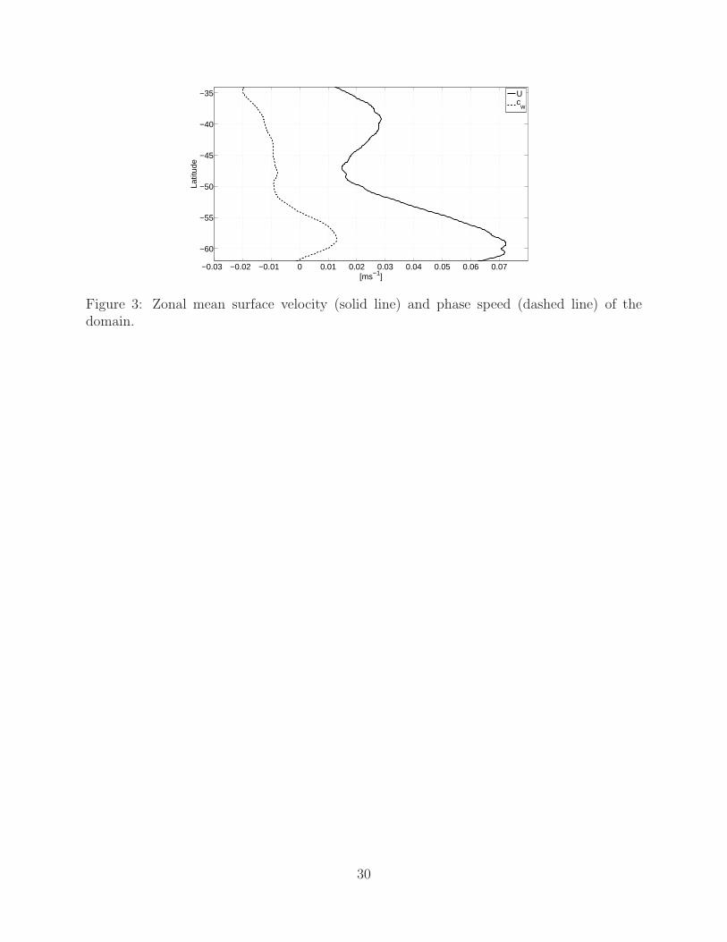
To test whether these profiles are consistent with the model in Eq. (19), four parameters206

must be estimated at each latitude and depth: U , cw, K01y and γ/k. The surface mean flow207

is shown in Fig. 3 and is defined to be the zonally averaged velocity (there is no significant208

meridional velocity in the Pacific sector we study). The mean velocity at any other depth is209

obtained by multiplying the surface velocity by µ(z). The other three parameters are harder210

to estimate, because the oceanic eddy field is multichromatic with a wide range of eddy211

sizes, propagation speeds and decorrelation times (Wunsch 2010). Departing from previous212

literature that relies on somewhat arbitrary metrics to estimate mean representative values213

of these parameters (e.g. Tulloch et al. 2009), we use an approach better suited for analysis of214

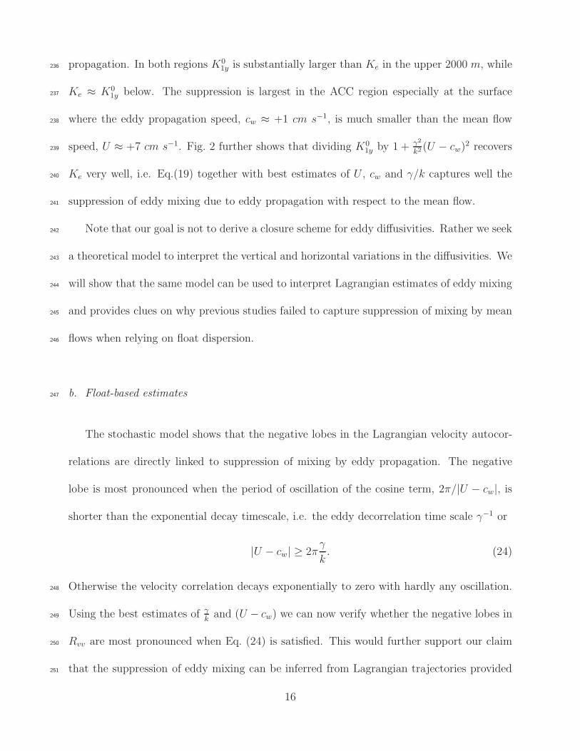
eddy diffusivities. At each depth, we run a series of simulations where the tracer is advected215

by the velocity field u = ueddy + Uconsti, where ueddy is the depth dependent eddy velocity,216

Uconst is a constant zonal mean velocity independent of latitude and depth, and i is the zonal217

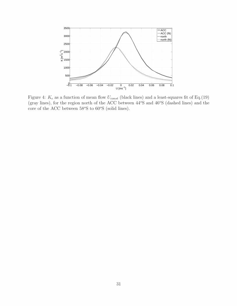
unit vector. The set of simulations use a mean velocity between -0.1 to 0.1 m s−1. Sample218

curves of Ke as a function of Uconst are shown in Fig. 4 for the two regions at the ocean219

surface, in the core of the ACC and north of it. The dependence of Ke on Uconst has the220

Lorentzian shape predicted by Eq. (19) and can be used to estimate all the parameters we221

need: the curve maximum corresponds to K01y and it is achieved when Uconst = cw. The222

curve width can be used to estimate γ/k.223

These three parameters, cw, K01y and γ/k are now estimated for each latitude and depth224

14

by least-squares fitting the Lorentzian Ke curves to Eq. (19). Fig. 4 shows that substituting225

the best-fit parameters in Eq. (19) reproduces the Lorentzian Ke curves remarkably well.226

Our best fit estimates suggest that eddies propagate eastward at cw=+1 cm s−1 in the core227

of the ACC and westward at cw=−1 cm s−1 north of it. These values are somewhat smaller228

than reported by Marshall et al. (2006), who estimated the speed of the most energetic229

eddies from altimetric data in the Southern Ocean. The discrepancy suggests the eddies230

that dominate eddy mixing are not the most energetic ones.231

Ferrari and Nikurashin (2010) argue that the decorrelation timescale of eddies, γ−1, is

proportional to the eddy turnover time, (k2EKE)−1/2. This scaling is expected to hold for

turbulent eddy fields with energy peaking at wavenumber k (Ottino 1998). We find that our

estimates of γ/k do scale with the square root of EKE, but only in the upper 1000 m. The

scaling breaks down at depth, where γ/k becomes depth independent, despite the decrease

in EKE. Eddy stirring below 2000 m, where EKE is small, is best characterized as a

superposition of time-dependent quasi-linear waves rather than a turbulent eddy field. This

limit is generally referred to as chaotic mixing and the decorrelation timescale is not set by

the eddy turnover time (Ottino 1989). In summary our best fit of γ/k as a function of depth

is,

γ

k= α0 + α1

√

EKE(z), (23)

where α0 and α1 vary with latitude (primarily because the eddy scale changes with latitude).232

Fig. 2 summarizes the results. The vertical profile of the effective diffusivity Ke is plotted233

for the two regions, one in the core of the ACC and the other north of it. The figure234

also shows K01y, i.e. the effective diffusivity in the absence of any suppression due to eddy235

15

propagation. In both regions K01y is substantially larger than Ke in the upper 2000 m, while236

Ke ≈ K01y below. The suppression is largest in the ACC region especially at the surface237

where the eddy propagation speed, cw ≈ +1 cm s−1, is much smaller than the mean flow238

speed, U ≈ +7 cm s−1. Fig. 2 further shows that dividing K01y by 1 + γ2

k2(U − cw)

2 recovers239

Ke very well, i.e. Eq.(19) together with best estimates of U , cw and γ/k captures well the240

suppression of eddy mixing due to eddy propagation with respect to the mean flow.241

Note that our goal is not to derive a closure scheme for eddy diffusivities. Rather we seek242

a theoretical model to interpret the vertical and horizontal variations in the diffusivities. We243

will show that the same model can be used to interpret Lagrangian estimates of eddy mixing244

and provides clues on why previous studies failed to capture suppression of mixing by mean245

flows when relying on float dispersion.246

b. Float-based estimates247

The stochastic model shows that the negative lobes in the Lagrangian velocity autocor-

relations are directly linked to suppression of mixing by eddy propagation. The negative

lobe is most pronounced when the period of oscillation of the cosine term, 2π/|U − cw|, is

shorter than the exponential decay timescale, i.e. the eddy decorrelation time scale γ−1 or

|U − cw| ≥ 2πγ

k. (24)

Otherwise the velocity correlation decays exponentially to zero with hardly any oscillation.248

Using the best estimates of γkand (U − cw) we can now verify whether the negative lobes in249

Rvv are most pronounced when Eq. (24) is satisfied. This would further support our claim250

that the suppression of eddy mixing can be inferred from Lagrangian trajectories provided251

16

that the number of trajectories is large enough to accurately compute the negative lobes in252

Rvv.253

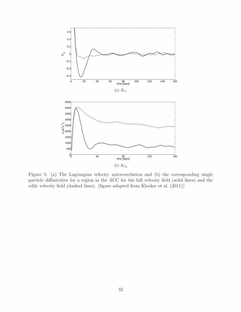
In Sec. 3 we estimated that in the ACC (bin centered at 59oS) γ/k ≃ 0.03 m s−1 and254

|U − cw| ≃ 0.06 m s−1, whereas to the north (bin centered at 45oS) γ/k ≃ 0.03 m s−1 and255

|U − cw| ≃ 0.03 m s−1. Hence |U − cw| > γ/k in the ACC, leading to a large negative lobe in256

Rvv. North of the ACC, |U − cw| ≃ γ/k and the negative lobe is less pronounced. The width257

of the negative lobes of the Lagrangian autocorrelation function scales as π/k|U − cw| as per258

Eq. (17). In the ACC latitude band eddies have scales of approximately 100 km, and hence259

k ≈ 2π/100 km−1. This gives a negative lobe of 20 days, a value consistent with the width of260

the negative lobe of Rvv in Fig. 5a (solid line). For comparison, Fig. 5a (dashed line) shows261

Rvv computed from trajectories advected by the eddy velocity field only (i.e. no mean); the262

negative lobe is much less pronounced since in these simulations for which |cw| < γ/k. The263

single-particle diffusivities corresponding to these Lagrangian velocity autocorrelations are264

shown in Fig. 5b.265

The stochastic model derived in Sec. 2 suggests that particle- and tracer-derived estimates266

of diffusivity are equivalent. Consistently, Klocker et al. (2011) showed similar agreement267

everywhere in the Southern Ocean sector considered here. However, other studies using tra-268

jectories from real drifters and floats deployed in the Southern Ocean (e.g. Sallee et al. 2008)269

obtain diffusivities larger than those reported here. The present results, and those of Klocker270

et al. (2011), suggest that the discrepancy lies with computation of the autocorrelation. As271

the uncertainty in the autocorrelation increases with lag, it is common practice to fit an272

exponential function (e.g. Garraffo et al. 2001; Sallee et al. 2008) or to integrate Rvv only up273

to the first zero crossing (e.g. Freeland et al. 1975; Poulain and Niiler 1989). In both cases,274

17

the negative lobe in Rvv is ignored and the diffusivity thereby overestimated.275

5. Summary and discussion276

We computed lateral eddy diffusivities using tracers and floats advected by a proxy veloc-277

ity field to study the suppression of eddy mixing by eddy propagation along mean flows. We278

focussed on a region in the Southern Ocean, upstream of Drake Passage, which is the region279

of a large field experiment, the Diapycnal and Isopycnal Mixing Experiment in the Southern280

Ocean (DIMES). The main goal of DIMES is to quantify both isopycnal and diapycnal dif-281

fusivities in the Southern Ocean. In a companion paper (Klocker et al. 2011) we have shown282

that eddy diffusivities calculated using tracer and particle-based approaches are equivalent.283

In this manuscript, we used these lateral and vertical profiles of eddy diffusivities to study284

(1) what suppresses eddy mixing across mean flows and (2) to identify what statistics from285

float observations are robust markers of mixing suppression. The latter point is especially286

relevant to DIMES, since a primary aim is to estimate eddy diffusivities and their variations287

from the release of neutrally buoyant floats.288

We addressed point (1) using mixing length arguments together with the eddy diffusivities289

calculated from the proxy velocity field. Traditional mixing length arguments assume that290

eddy diffusivity is proportional to the eddy kinetic energy times a mixing length (e.g. Prandtl291

1925). In the oceanographic literature, it is often assumed that the mixing length scales with292

the eddy size (e.g. Holloway 1986), but Ferrari and Nikurashin (2010) found that propagating293

eddies reduce the mixing length and thereby play a crucial role in determining the variations294

in eddy diffusivity across the ocean. We extended the model here to study Lagrangian295

18

estimates of diffusivity. We find, in particular, that the latter is identical to the tracer-based296

estimate, confirming the numerical results of Klocker et al. (2011).297

In Klocker et al. (2011) we found that eddy diffusivities are smaller than 1000 m2 s−1298

in the core of the ACC from the surface down to 1500 m, but are larger than 1000 m2 s−1299

at depth and on the lateral flanks. Ferrari and Nikurashin (2010) interpret this pattern as300

evidence that mixing is suppressed in the core of the ACC where eddies propagate slower301

than the mean current: eddies propagate eastward at a few cm s−1, while the mean current302

flows at O(10 cm s−1). On the flanks of the ACC and at depth the mean current speed is303

weaker and comparable to the eddy speed. These are the critical layers where there is no304

suppression of mixing.305

To test the suppression of mixing by eddy propagation along mean flows, we ran a306

series of experiments with an eddy-only velocity field (i.e. the geostrophic velocity field307

calculated from sea surface height anomalies) and then added a constant zonal mean velocity308

independent of depth and latitude. By changing the mean velocity, we changed the relative309

speed between the eddies and the mean flow. We found that the eddy diffusivities computed310

for different mean flows followed closely the scaling law derived in Ferrari and Nikurashin311

(2010). That is, the spatial variations in eddy diffusivities estimated by Klocker et al. (2011)312

can be explained by mixing length arguments, if the drift of the eddies with respect to the313

mean flow is taken into account.314

Next we focussed on how to estimate the suppression of mixing using observations.315

Presently the only feasible approach to sample eddy diffusivities in the global ocean is by316

releasing drifters and floats (tracer release experiments are also an option, but are too costly317

to be done in more than a handful of locations). Previous analyses of drifter trajectories318

19

from the Southern Ocean (e.g. Sallee et al. 2008; Griesel et al. 2010) failed to show such319

mixing suppression across the mean flows.320

As seen in Klocker et al. (2011) and with the present stochastic model, the Lagrangian321

velocity autocorrelation is comprised of an exponentially decaying part and an oscillatory322

part; the latter depends on the phase speed of the eddies relative to the mean flow. If eddies323

and mean flow propagate at different speeds, the oscillatory part produces a negative lobe in324

the autocorrelation; this disappears when the eddies and mean flow propagate at the same325

speed. The negative lobe leads to a suppression of mixing, because it contributes negatively326

to the integral of the autocorrelation, which is the diffusivity. In order to properly sample327

these negative lobes in the ACC, one must resolve time lags of order a month. Many previous328

observational estimates truncated the calculation at much shorter time lags of order one week329

and thereby missed the suppression.330

In any case, it is difficult to obtain accurate estimates of eddy diffusivities from float331

statistics alone (see Klocker et al. (2011) for a more detailed discussion on necessary float332

statistics). Rather one needs to combine float trajectories with additional information,333

such as the release of tracer patches, satellite-derived geostrophic velocities together with334

equivalent-barotropic scaling arguments, or high-resolution numerical models.335

Acknowledgments.336

This work was done as part of the Diapycnal and Isopycnal Mixing Experiment in the337

Southern Ocean (DIMES). We wish to acknowledge the generous support of NSF through338

award OCE-0825376 (RF and AK). We also wish to thank all the DIMES principal investi-339

20

gators for many useful discussions and suggestions.340

21

APPENDIX341

Green (1970) proposed a theory for PV fluxes in a horizontally homogeneous, baroclini-

cally unstable flow based on the fastest growing linear normal mode. This idea was further

developed as a full eddy parameterization scheme by Killworth (1997). The upshot of linear

theory is that mixing by the most unstable mode in the quasi-geostrophic approximation

generates a diffusivity given by,

Klinear =k−1

κ2ciEKE

c2i + (U − cr)2, (A1)

where ci and cr are the imaginary and real speeds of the most unstable baroclinic mode. If one342

assumes that eddies decorrelate on a timescale proportional to their growth rate, ci ∼ k−1γ,343

and propagate at the speed of the most unstable mode, cr = cw, then one recovers Eq. (18).344

Hence Green’s theory can be viewed as a special example of a general class of mixing models345

that account both for the finite eddy decorrelation time and for the eddy propagation speed.346

22

347

REFERENCES348

Abernathey, R., J. Marshall, M. Mazloff, and E. Shuckburgh, 2010: Critical layer enhance-349

ment of mesoscale eddy stirring in the Southern Ocean. Journal of Physical Oceanography,350

40, 170–184.351

Bower, A. S., H. T. Rossby, and J. L. Lillibridge, 1985: The Gulf Stream - barrier or blender?352

Journal of Physical Oceanography, 15, 24–32.353

Davis, R., 1991: Observing the general circulation with floats. Deep-Sea Research, 38A,354

S531–S571.355

DelSole, T., 2004: Stochastic models of quasigeostrophic turbulence. Surveys in Geophysics,356

25, 107–149.357

Farrell, R. and P. J. Ioannou, 1993: Stochastic dynamics of baroclinic waves. Journal of358

Atmospheric Sciences, 50, 4044–4057.359

Ferrari, R. and M. Nikurashin, 2010: Suppression of eddy diffusivity across jets in the360

Southern Ocean. Journal of Physical Oceanography, 40, 1501–1519.361

Flierl, G. R. and D. J. McGillicuddy, 2002: Mesoscale and sub-mesoscale physical-biological362

interactions. The Sea: Ideas and Observations on Progress in the Study of the Seas, Vol.363

12, A. R. Robinson, J. J. McCarthy, and B. Rothschild, Eds., John Wiley & Sons, 113–185.364

23

Freeland, H., P. Rhines, and T. Rossby, 1975: Statistical observations of the trajectories of365

neutrally buoyant floats in the North Atlantic. Journal of Marine Research, 33, 383–404.366

Garraffo, Z., A. Mariano, A. Griffa, and C. Veneziani, 2001: Lagrangian data in a high-367

resolution numerical simulation of the North Atlantic. I. comparison with in-situ drifter368

data. Journal of Marine Systems, 29, 157–176.369

Green, J. S. A., 1970: Transfer properties of the large-scale eddies and the general circulation370

of the atmosphere. Quart. J. Roy. Meteor. Soc., 96, 157–185.371

Griesel, A., S. T. Gille, J. Sprintall, L. McClean, J, H. LaCasce, J, and M. E. Maltrud, 2010:372

Isopycnal diffusivities in the Antarctic Circumpolar Current inferred from Lagrangian373

floats in an eddying model. Journal of Marine Research, 66, 441–463.374

Holloway, G., 1986: Estimation of oceanic eddy transports from satellite altimetry. Nature,375

323, 243–244.376

Keffer, T. and G. Holloway, 1988: Estimating Southern Ocean eddy flux of heat and salt377

from satellite altimetry. Nature, 332, 624–626.378

Killworth, P. D., 1997: On the parameterization of eddy transfer. Part I: Theory. Journal of379

Marine Research, 55, 1171–1197.380

Killworth, P. D. and C. W. Hughes, 2002: The Antarctic Circumpolar Current as a free381

equivalent-barotropic jet. Journal of Marine Research, 60, 19–45.382

Klocker, A., R. Ferrari, J. H. LaCasce, and S. T. Merrifield, 2011: Reconciling float-based383

and tracer-based estimates of eddy diffusivities, Journal of Marine Research, submitted.384

24

Marshall, J., E. Shuckburgh, J. H., and C. Hill, 2006: Estimates and implications of surface385

eddy diffusivity in the Southern Ocean derived from tracer transport. Journal of Physical386

Oceanography, 36, 1806–1821.387

Mazloff, M. R., P. Heimbach, and C. Wunsch, 2010: An eddy-permitting Southern Ocean388

state estimate. Journal of Physical Oceanography, 40, 880–899.389

Nakamura, N., 1996: Two-dimensional mixing, edge formation, and permeability diagnosed390

in area coordinates. Journal of Atmospheric Science, 53, 1524–1537.391

Ottino, J. M., 1989: The Kinematics of Mixing: Stretching, Chaos, and Transport. Cam-392

bridge University Press.393

Ottino, J. M., 1998: Lectures on Geophysical Fluid Dynamics. Oxford University Press.394

Pedlosky, J., 1987: Geophysical Fluid Dynamics. Springer.395

Poulain, P.-M. and P. P. Niiler, 1989: Statistical analysis of the surface circulation in the Cal-396

ifornia Current system using satellite-tracked drifters. Journal of Physical Oceanography,397

19, 1588–1603.398

Prandtl, L., 1925: Bericht uber Untersuchungen zur ausgebildeten Turbulenz. Z. Angew.399

Math. Mech., 5, 136–139.400

Sallee, J. B., K. Speer, R. Morrow, and R. Lumpkin, 2008: An estimate of Lagrangian401

eddy statistics and diffusion in the mixed layer of the Southern Ocean. Journal of Marine402

Research, 66, 441–463.403

25

Shuckburgh, E. and P. Haynes, 2003: Diagnosing transport and mixing using a tracer-based404

coordinate system. Physics of Fluids, 15, doi:10.1063/1.1610 471.405

Taylor, G. I., 1921: Diffusion by continuous movements. Proc. London Math. Soc., 20, 196–406

211.407

Toole, J. M. and T. J. McDougall, 2001: Mixing and stirring in the ocean interior. Ocean408

circulation and climate: observing and modelling the global ocean, G. Siedler, J. Church,409

and J. Gould, Eds., Academic Press, San Diego, 337–356.410

Tulloch, R., J. Marshall, and K. S. Smith, 2009: Interpretation of the propagation of surface411

altimetric observations in terms of planetary waves and geostrophic turbulence. Journal412

of Geophysical Research, 114, C02 005, doi:10.1029/2008JC005 055.413

Veneziani, M., A. Griffa, A. M. Reynolds, and A. J. Mariano, 2004: Oceanic turbulence and414

stochastic models from subsurface Lagrangian data for the North-West Atlantic Ocean.415

Journal of Physical Oceanography, 34, 1884–1906.416

Wunsch, C., 2010: Toward a midlatitude ocean frequency-wavenumber spectral density and417

trend determination. Journal of Physical Oceanography, 40, 2264–2281.418

26

List of Figures419

1 Ke estimated from a tracer advected with the eddy velocity field (black dashed420

line) and the full velocity field (black solid line) at the ocean surface. These421

diffusivity estimates are compared to the square-root of eddy kinetic energy422

(gray line). 28423

2 (a) Zonal mean vertical profiles of Ke averaged over the 44oS to 46oS latitude424

stripe north of the ACC (solid back line). The dashed black line shows K0425

from simulations where the mean flow is set equal to the eddy speed, so that426

eddy propagation does not suppress cross-current mixing. The gray line is427

obtained dividing K0 by the suppression factor predicted by Eq. (19). (b)428

Same as in panel (a) but for the 58oS to 60oS latitude stripe in the core of the429

ACC. 29430

3 Zonal mean surface velocity (solid line) and phase speed (dashed line) of the431

domain. 30432

4 Ke as a function of mean flow Uconst (black lines) and a least-squares fit of433

Eq.(19) (gray lines), for the region north of the ACC between 44oS and 46oS434

(dashed lines) and the core of the ACC between 58oS to 60oS (solid lines). 31435

5 (a) The Lagrangian velocity autocorrelation and (b) the corresponding single436

particle diffusivities for a region in the ACC for the full velocity field (solid437

lines) and the eddy velocity field (dashed lines). (figure adapted from Klocker438

et al. (2011)) 32439

27

−60

−55

−50

−45

−40

−35

0 0.05 0.1 0.15

latit

ude

sqrt(EKE) [ms−1]

−60

−55

−50

−45

−40

−350 1000 2000 3000 4000

Ke [m2s−1]

Figure 1: Ke estimated from a tracer advected with the eddy velocity field (black dashedline) and the full velocity field (black solid line) at the ocean surface. These diffusivityestimates are compared to the square-root of eddy kinetic energy (gray line).

28

0 500 1000 1500 2000 2500−4500

−4000

−3500

−3000

−2500

−2000

−1500

−1000

−500

0

K [m2s−1]

dept

h [m

]

Ke (north)

K0 (north)

Ktheory

(north)

(a) 45oS

0 500 1000 1500 2000 2500 3000 3500−4500

−4000

−3500

−3000

−2500

−2000

−1500

−1000

−500

0

K [m2s−1]

dept

h [m

]

Ke (ACC)

K0 (ACC)

Ktheory

(ACC)

(b) 59oS

Figure 2: (a) Zonal mean vertical profiles of Ke averaged over the 44oS to 46oS latitudestripe north of the ACC (solid back line). The dashed black line shows K0 from simulationswhere the mean flow is set equal to the eddy speed, so that eddy propagation does notsuppress cross-current mixing. The gray line is obtained dividing K0 by the suppressionfactor predicted by Eq. (19). (b) Same as in panel (a) but for the 58oS to 60oS latitudestripe in the core of the ACC.

29

−0.03 −0.02 −0.01 0 0.01 0.02 0.03 0.04 0.05 0.06 0.07

−60

−55

−50

−45

−40

−35

[ms−1]

Latit

ude

Uc

w

Figure 3: Zonal mean surface velocity (solid line) and phase speed (dashed line) of thedomain.

30

−0.1 −0.08 −0.06 −0.04 −0.02 0 0.02 0.04 0.06 0.08 0.10

500

1000

1500

2000

2500

3000

3500

U [ms−1]

K [m

2 s−1 ]

ACCACC (fit)northnorth (fit)

Figure 4: Ke as a function of mean flow Uconst (black lines) and a least-squares fit of Eq.(19)(gray lines), for the region north of the ACC between 44oS and 46oS (dashed lines) and thecore of the ACC between 58oS to 60oS (solid lines).

31

0 20 40 60 80 100 120 140 160

−0.3

−0.2

−0.1

0

0.1

0.2

0.3

time [days]

Rvv

(a) Rvv

0

500

1000

1500

2000

2500

3000

3500

4000

4500

0 40 80 120 160

K [m

2 s−1 ]

time [days]

(b) K1y

Figure 5: (a) The Lagrangian velocity autocorrelation and (b) the corresponding singleparticle diffusivities for a region in the ACC for the full velocity field (solid lines) and theeddy velocity field (dashed lines). (figure adapted from Klocker et al. (2011))

32