Journalof TurbulenceVolume6, No. 31,2005

The ensemblemeanlimit of the one-dimensionalturb ulencemodeland application to residualstressclosure

in finite volume large-eddysimulation

RANDALL J.MCDERMOTT∗†∗∗, ALAN R. KERSTEIN‡, RODNEY C. SCHMIDT§andPHILIP J.SMITH†

†TheUniversityof Utah,SaltLakeCity, UT 84112,USA‡SandiaNationalLaboratories,Livermore,CA 94551,USA

§SandiaNationalLaboratories,Albuquerque,NM 87185,USA

In orderto gaininsightinto theone-dimensionalturbulence(ODT) modelof Kerstein[1] asit pertainsto residualstressclosurein large-eddysimulation(LES),wedevelopensemblemeanclosure(EMC),analgebraicstressclosurebasedonthemappingsandtimescalephysicsemployedin ODT. To allowanalyticdeterminationof thestresstheODT modelis simplified,conceptually, suchthateddyeventsactupona velocity field linearizedby the local resolvedscalestrain.EMC canaccountfor viscouseffects, addressingthe laminar flow finite eddy viscosity problemwithout implementationof thedynamicprocedure[2]. Thealgebraicform of themodellendsitself to analysis[3] andweareabletoderive atheoreticalvaluefor theeddyrateconstant.Thisvalueis aboundontherateconstantfor fullODT subgridclosureandyieldsgoodresultsin LESof decayingisotropicturbulencewith EMC.

1. Intr oduction

Large-eddysimulation(LES) is a powerful and increasinglyimportant tool for modelingturbulentflow. However, thefidelity, costandrobustnessof availablesubgridclosuremodelsremainsignificantbarriersto itsgreaterapplication.Sagaut[4] providesanexcellentsurvey ofthewiderangeof modelsthathavebeenproposed.Recently, averydifferentturbulencemod-eling approach,called‘one-dimensionalturbulence’(ODT), hasbeen developedby Kersteinetal. [1, 5] andappliedto arangeof problemsamenableto analysiswhereturbulence-inducedvariationsaregeometricallysimple.Although thesetwo approachesarefundamentallydif-ferent,it hasbeenrecognized(see,for example[6]) thatODT is a closuremodelcandidatefor LES.Schmidtet al. [7] usedODT to resolve thewall shearstressin a channelflow LES.Also, Schmidtet al. [8] andMcDermott[9] have developedmethodsfor usingODT astheLES bulk flow residualstressclosure.Additionally, the‘linear-eddymodel’ (LEM) [10, 11],thepredecessorof ODT, hasmaturedandgainedpopularityfor modelingturbulent reactingflows [12–14].

The ‘workhorse’closuremodelfor LES hasbeentheSmagorinsky eddyviscositymodel[15] anddynamicvariationsthereof[2, 16]. In this paperwe introducethe ‘ensemblemeanclosure’ (EMC) model which establishesa link betweenODT and the more conventional

∗Correspondingauthor. Email: randy@crsim.utah.edu∗∗Currentaddress:CornellUniversity, Ithaca,NY 14853,USA. Email: rjm75@cornell.edu

Journalof TurbulenceISSN:1468-5248(onlineonly) c© 2005Taylor& Francis

http://www.tandf.co.uk/journalsDOI: 10.1080/14685240500293894

Downloaded By: [University Of Utah] At: 18:38 15 May 2009

2 R.J. McDermottet al.

eddyviscositymethods.ODT closurefor LES requiresa lengthscaleparameter(the max-imum ODT eddy size), analogousto (but not the sameas) the Smagorinsky filter width,and a rate constant,analogousto the Smagorinsky constant.As with the Smagorinskymodel,for a given rateof residualenergy production(i.e. the rateat which energy is trans-ferred betweenresolved and unresolved scales)the rate constantand length scaleare in-verselyproportionalto oneanotherandcombineto form somethinglike aturbulentmixinglength.

ThoughSmagorinsky andODT areboth basedon mixing length theory, ODT is a con-siderablymorecomplex modelthatcapturescontributionsfrom a spectrumof lengthscales.In fact, ODT is really more of a modeling framework than a uniquemodel.The buildingblocks of this framework are: a one-dimensionalmapping,an eddy time scaledistribu-tion and a one-dimensionalEulerianevolution equation.Thereexist a myriad of choicesto fill eachof theseblocks. As such, and in no small part due to the stochasticsam-pling procedure,theoreticalanalysisof ODT is challenging.EMC was born of a desiretobetterunderstandODT and to provide a theoreticalbasisfor the empirically determinedrateconstantfor coupledLES/ODT isotropic turbulencesimulations.The resultingmodelhasa validity of its own and,following ODT, accountsfor viscouseffects,addressingthelaminar-flow finiteeddyviscosityproblemwhichplaguestheconstantcoefficientSmagorinskymodel.

2. EMC formulation

2.1 Overview

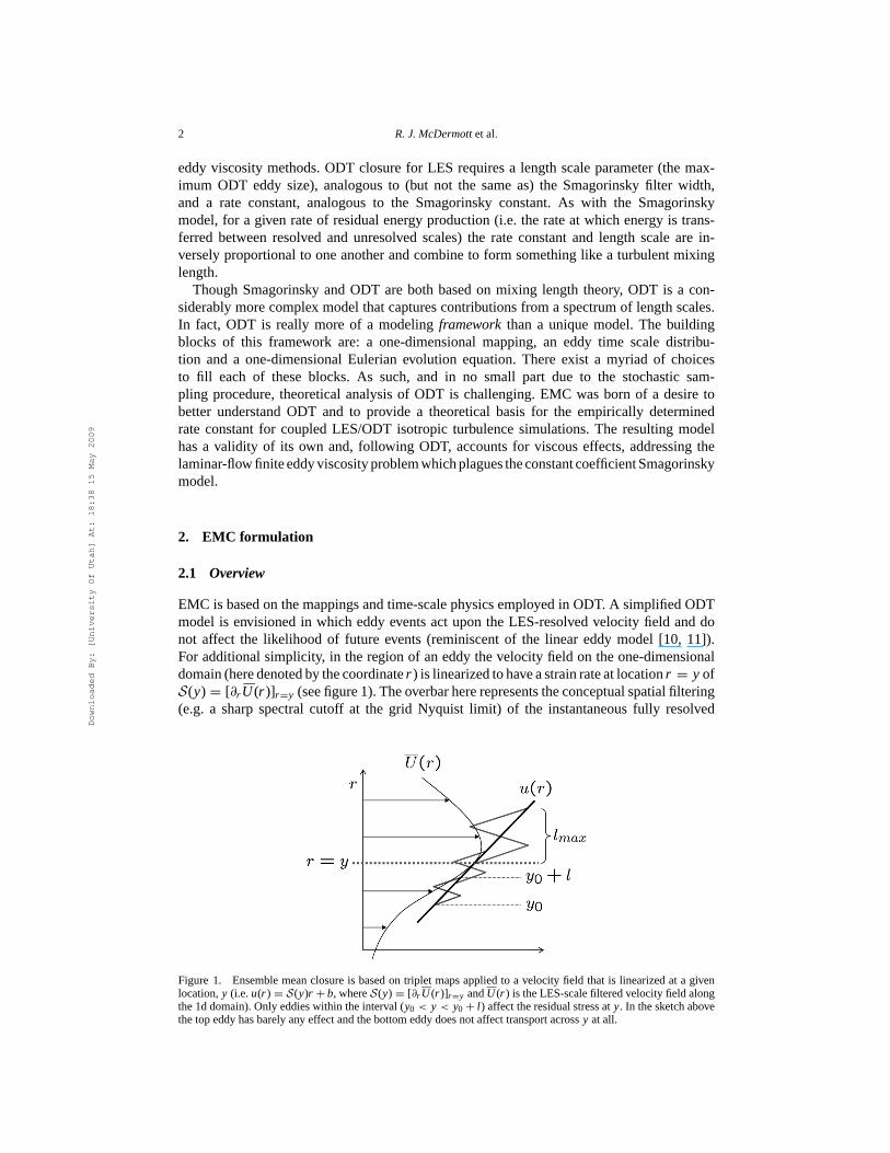
EMC is basedon themappingsandtime-scalephysicsemployedin ODT. A simplifiedODTmodel is envisionedin which eddyeventsact uponthe LES-resolved velocity field anddonot affect the likelihood of future events(reminiscentof the linear eddy model [10, 11]).For additionalsimplicity, in theregion of aneddythevelocity field on theone-dimensionaldomain(heredenotedbythecoordinater ) islinearizedtohave astrainrateatlocationr = y ofS(y) = [∂r U (r )]r =y (seefigure1).Theoverbarhererepresentstheconceptualspatialfiltering(e.g. a sharpspectralcutoff at the grid Nyquist limit) of the instantaneousfully resolved

Figure 1. Ensemblemeanclosureis basedon triplet mapsappliedto a velocity field that is linearizedat a givenlocation,y (i.e.u(r ) = S(y)r + b, whereS(y) = [∂r U (r )]r =y andU (r ) is theLES-scalefilteredvelocityfield alongthe1ddomain).Only eddieswithin theinterval (y0 < y < y0 + l ) affect theresidualstressat y. In thesketchabovethetopeddyhasbarelyany effectandthebottomeddydoesnotaffect transportacrossy atall.

Downloaded By: [University Of Utah] At: 18:38 15 May 2009

Residualstressclosure in finitevolumeLES 3

velocity field which resultsin the‘LES-resolved’ velocity field, U (r ). Eddyeventsactuponthelinearfield,

u(r ) = S(y)r + b, (1)

whereb is a constantthatdropsout in thederivationsto follow. This linearity simplificationallowsfor relatively simpleanalyticaltreatmentof themappingfunction(describedin section2.2). Finally, stressesarebasedon ensembleaveragedmomentumtransportby ODT eddyevents,ratherthantheusualstochasticeddysampling.Theresultingmodelis comparabletoconventionalLESclosuressuchastheconstantcoefficientSmagorinsky model[15].

The form of the ensembleclosure(which is independentof the linearization)is given,following Kerstein[17], by accountingfor all eddyeventswhich canaffect a givenlocation,y, on an ODT line. First, we find theamountof momentumdisplacedacrossy for aneddyparameterizedby its starting location, y0, and length scale,l . The amountof momentumdisplaced,ψ(y; y0, l ), is thenmultipliedby theeventratedensityof theeddy, givenby 1/(l 2τ ),whereτ is theeddytimescale(in general,τ = τ (U (r ), l ), but wewill suppressthefunctionaldependenceuntil specificrelationshipsaredeveloped).With this, the form of the residualstressis

R(y) =∫ lmax

lmin

∫ y

y−l

ψ(y; y0, l )

l 2τdy0dl . (2)

The integrationlimits reflecttherangeof y0 andl spacewhich canpossiblyaffect y. Com-pletionof themodelrequiresspecificationof ψ andτ .

As a point of clarification,we shouldmentionthat so far the model(2) is written to ac-countfor subgridtransportfor onecomponentalongonedirectiononly. Thetensorialnatureof the stressbecomesevident whenwe considermultiple componentsandmultiple direc-tions.BeingbasedonODT, EMC is mostnaturallyinterpretedasamodelfor theunresolvedadvectivestressesacrosscontrolsurfacesin afinite volumeformulation.Applicationto three-dimensionalfinite volumeclosureis describedin section4. We will adopttheconventioninthis paperthat,unlessotherwisespecified,τ R

ij ≡ Ui U j − U i U j will denotethedefinitionoftheresidualstresstensor(in thenotationof Pope[18]) andRij will denotethemodelfor τ R

ij .In theEMC modelther coordinatebecomesalignedwith the x j directionandthe location,y, indicatesthe locationof the flux surfacefor which we arecomputingthe stress(i.e. theunresolved flux of component-i ). Thus, Ri (x j = y), which we will write assimply Ri (y),providesthemacroscopiccontrolvolumeanalogof themicroscopicRij stresstensor.

In whatfollowswewill firstestablishtheformof themomentumdisplacementfunctionandtimescalefor thesimplestversionof ODT (one-componentODT [5], hereafterreferredto as‘vanilla ODT’). Thenwe will evaluatetheintegral (2). We will find closesimilarity betweentheresultingalgebraicmodelandtheSmagorinsky model[15] for theturbulentstress.Wethenconsiderthethree-componentvectorformulationof ODT [1] (hereafter‘vectorODT’). Thisversioncontainsa ‘pressurescrambling’modelwhich redistributesenergy amongvelocitycomponentsaftera triplet map(seesection2.3).Next, we addcomplexity to thetime scale,first by consideringanenergy-basedtimescaleandthenby consideringtheReynoldsnumberdependence.Theone-dimensionalanalogof Lilly’ sanalysis[3] is thenusedto obtainavaluefor therateconstant.In section4.5weshow resultsusingEMC in LESof decayingisotropicturbulence.And, finally, wedescribeanextensionof EMC to passivescalarsubgridtransportin section5.

Downloaded By: [University Of Utah] At: 18:38 15 May 2009

4 R.J. McDermottet al.

2.2 EMC basedon one-componentODT

It is usefulto startwith vanillaODT becausethesalientfeaturesof thissimpleanalysisextendto themorecomplex versions.In vanilla ODT momentumdisplacementis governedonly bythe triplet map(i.e. no pressurescrambling)andthe time scaleis basedon the local strainrate.Similarly, in thissectiontheEMC timescale,τ , isbasedonthe resolvedstrainalongtheone-dimensionaldomain,

1

τ= Ce|S(y)|, (3)

whereCe is theeddyrateconstantand|S(y)| is themagnitudeof thestrain.

2.2.1 Triplet map momentumdisplacement. Thetriplet map(seefigure2) mapsafield,u(r ), to u( f (r )), where

f (r ) = y0 +

3(r − y0) for y0 ≤ r ≤ y0 + 13l

2l − 3(r − y0) for y0 + 13l ≤ r ≤ y0 + 2

3l

3(r − y0) − 2l for y0 + 23l ≤ r ≤ y0 + l

r − y0 otherwise.

(4)

Themomentumdriven acrossapoint, y, by an eddy(y0, l ) in thepositivedirectionis thengiven by

ψ(y; y0, l ) =∫ y0+l

y[u( f (r )) − u(r )]dr. (5)

Figure 2. A triplet mapof the linearfield, u(r ), to u( f (r )), with y0 = 0.1 andl = 0.8. Sincepositionis given ontheordinate,thismappingrepresentsanegative transportof momentumin theverticaldirection.

Downloaded By: [University Of Utah] At: 18:38 15 May 2009

Residualstressclosure in finitevolumeLES 5

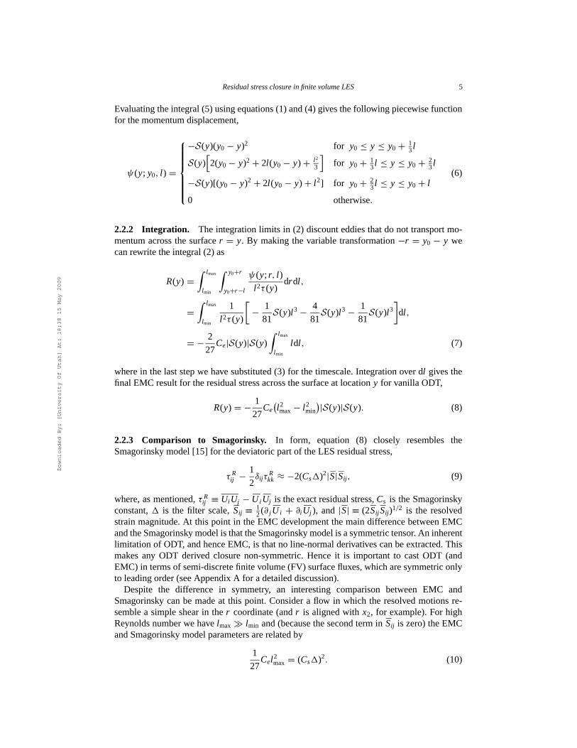
Evaluatingtheintegral (5) usingequations(1) and(4) gives thefollowing piecewisefunctionfor themomentumdisplacement,

ψ(y; y0, l ) =

−S(y)(y0 − y)2 for y0 ≤ y ≤ y0 + 13l

S(y)[2(y0 − y)2 + 2l (y0 − y) + l 2

3

]for y0 + 1

3l ≤ y ≤ y0 + 23l

−S(y)[(y0 − y)2 + 2l (y0 − y) + l 2] for y0 + 23l ≤ y ≤ y0 + l

0 otherwise.

(6)

2.2.2 Integration. Theintegrationlimits in (2) discounteddiesthatdo not transportmo-mentumacrossthe surfacer = y. By makingthe variabletransformation−r = y0 − y wecanrewrite theintegral (2) as

R(y) =∫ lmax

lmin

∫ y0+r

y0+r −l

ψ(y; r, l )

l 2τ (y)dr dl ,

=∫ lmax

lmin

1

l 2τ (y)

[−

1

81S(y)l 3 −

4

81S(y)l 3 −

1

81S(y)l 3

]dl ,

= −2

27Ce|S(y)|S(y)

∫ lmax

lmin

ldl , (7)

wherein thelaststepwe have substituted(3) for thetimescale.Integrationover dl gives thefinal EMC resultfor theresidualstressacrossthesurfaceat locationy for vanillaODT,

R(y) = −1

27Ce

(l 2max − l 2

min

)|S(y)|S(y). (8)

2.2.3 Comparison to Smagorinsky. In form, equation (8) closely resemblestheSmagorinsky model[15] for thedeviatoricpartof theLESresidualstress,

τ Rij −

1

2δijτ

Rkk ≈ −2(Cs�)2|S|Sij , (9)

where,asmentioned,τ Rij ≡ Ui Uj − U i Uj is theexactresidualstress,Cs is theSmagorinsky

constant,� is the filter scale,Sij ≡ 12(∂ j U i + ∂i Uj ), and |S| ≡ (2Sij Sij )1/2 is the resolved

strainmagnitude.At this point in theEMC developmentthemaindifferencebetweenEMCandtheSmagorinsky modelis thattheSmagorinsky modelis asymmetrictensor. An inherentlimitation of ODT, andhenceEMC, is thatno line-normalderivatives canbeextracted.Thismakes any ODT derived closurenon-symmetric.Henceit is important to castODT (andEMC) in termsof semi-discretefinite volume(FV) surfacefluxes,whicharesymmetriconlyto leadingorder(seeAppendixA for adetaileddiscussion).

Despite the difference in symmetry, an interesting comparisonbetween EMC andSmagorinsky canbe madeat this point. Considera flow in which the resolved motionsre-semblea simpleshearin the r coordinate(andr is alignedwith x2, for example).For highReynoldsnumberwe have lmax ≫ lmin and(becausethesecondtermin Sij is zero)theEMCandSmagorinsky modelparametersarerelatedby

1

27Cel

2max = (Cs�)2. (10)

Downloaded By: [University Of Utah] At: 18:38 15 May 2009

6 R.J. McDermottet al.

If lmax is setequalto the filter width andthe rateconstant,Ce, is set to unity, we find thatC2

s = 1/27, or Cs ≈ 0.19, in closeagreementwith thetheoreticalvalue oftheSmagorinskyconstantfrom Lilly’ s analysis[3] (Cs ≈ 0.17 for a sharpspectralfilter). In otherwords,ifsimplifying assumptionsare appliedto ODT which bring it more closely in line with theassumptionsmadeby the Smagorinsky model (i.e. resolved strain is the driving force forenergy dissipation),the geometryof the triplet mapnaturallyproducesa reasonablemodelconstant.

2.3 EMC basedon vectorODT

The vector formulation of ODT [1] carriesall threevelocity components,ui = [u, v, w],on a given line as a function of r . As an example,considerthe ODT line alignedwiththe x2 directionof an Eulerianreferenceframe in figure 3. For LES closure(section4.1)we will similarly defineODT domainsalignedwith the x1 and x3 coordinates.The tripletmap rearrangesfluid elementswhich carry the scalarcomponentsu, v and w. The vec-tor ODT model also accountsfor ‘return to isotropy’ by conservatively redistributing thecomponentenergiesafter a mappingevent. This redistribution procedureis henceforthre-ferredto asthe‘pressure-scrambling’model(see[1] for adetaileddiscussion).In thissectionwe begin addinglevels of complexity to EMC by accountingfor the pressurescramblingmodel.

2.3.1 Kernel-basedmomentumdisplacement. In vectorODT thefinal velocity field in-volvesadditionof akernelfunction,ci K (r ), wherethekernelisdefinedtobeK (r ) = r − f (r )andci is a componentspecificamplitude,yet to bespecified.Notethat

∫ ∞−∞ K (r )dr = 0 and

sothekerneldoesnot changethemomentumof anODT domain(i.e. thekernelis not a mo-mentumsourceor sink).Themomentumdriven acrossaspecificpoint,y, however, is affectedby thekernel:

ψi (y; y0, l ) =∫ y0+l

y[ui ( f (r )) + ci K (r ) − ui (r )]dr. (11)

Due to the linear velocity profile and kernel definition, it can be shown that themomentum displacementfunction (with kernel based redistribution included) can be

Figure 3. Conceptualvelocityfieldsin thevectorformulation,in thiscasewith r alignedwith thex2 coordinate.Thecomponent2 velocity fields,U2(r ) andu2(r ), aredefinedanalogously. Thebold solid linesdepict thelinearizationsthatdetermineS1 andS3 at r = y.

Downloaded By: [University Of Utah] At: 18:38 15 May 2009

Residualstressclosure in finitevolumeLES 7

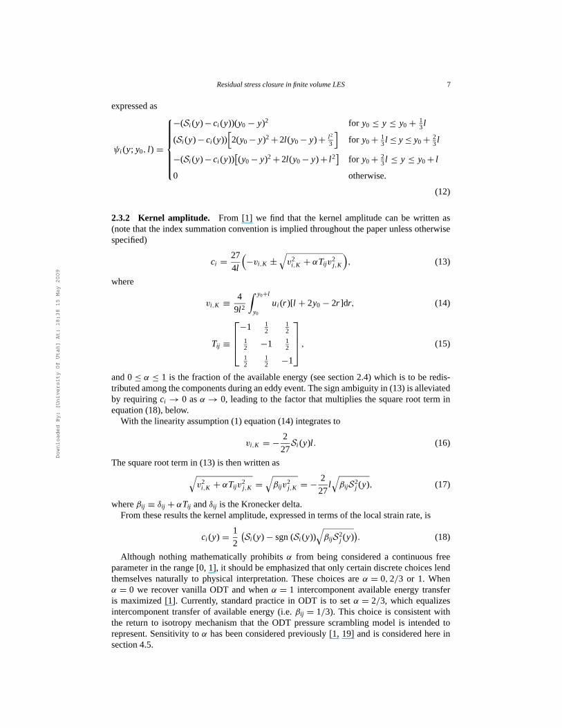
expressedas

ψi (y; y0, l ) =

−(Si (y) − ci (y))(y0 − y)2 for y0 ≤ y ≤ y0 + 13l

(Si (y) − ci (y))[2(y0 − y)2 + 2l (y0 − y) + l 2

3

]for y0 + 1

3l ≤ y ≤ y0 + 23l

−(Si (y) − ci (y))[(y0 − y)2 + 2l (y0 − y) + l 2

]for y0 + 2

3l ≤ y ≤ y0 + l

0 otherwise.

(12)

2.3.2 Kernel amplitude. From [1] we find that the kernel amplitudecan be written as(notethat theindex summationconventionis implied throughoutthepaperunlessotherwisespecified)

ci =27

4l

(−vi,K ±

√v2

i,K + αTijv2j,K

), (13)

where

vi,K ≡4

9l 2

∫ y0+l

y0

ui (r )[l + 2y0 − 2r ]dr, (14)

Tij ≡

−1 12

12

12 −1 1

2

12

12 −1

, (15)

and0 ≤ α ≤ 1 is the fractionof theavailableenergy (seesection2.4) which is to be redis-tributedamongthecomponentsduringaneddyevent.Thesignambiguityin (13) is alleviatedby requiringci → 0 as α → 0, leadingto the factorthat multiplies the squareroot term inequation(18),below.

With thelinearityassumption(1) equation(14) integratesto

vi,K = −2

27Si (y)l . (16)

Thesquareroot termin (13) is thenwrittenas√

v2i,K + αTijv

2j,K =

√βijv

2j,K = −

2

27l√

βijS2j (y), (17)

whereβij ≡ δij + αTij andδij is theKroneckerdelta.Fromtheseresultsthekernelamplitude,expressedin termsof thelocal strainrate,is

ci (y) =1

2

(Si (y) − sgn(Si (y))

√βijS

2j (y)

). (18)

Although nothing mathematicallyprohibits α from being considereda continuousfreeparameterin therange[0, 1], it shouldbeemphasizedthatonly certaindiscretechoiceslendthemselves naturally to physical interpretation.Thesechoicesare α = 0, 2/3 or 1. Whenα = 0 we recover vanilla ODT and whenα = 1 intercomponentavailableenergy transferis maximized[1]. Currently, standardpracticein ODT is to setα = 2/3, which equalizesintercomponenttransferof availableenergy (i.e. βij = 1/3). This choiceis consistentwiththe return to isotropy mechanismthat the ODT pressurescramblingmodel is intendedtorepresent.Sensitivity to α hasbeenconsideredpreviously [1, 19] andis consideredhereinsection4.5.

Downloaded By: [University Of Utah] At: 18:38 15 May 2009

8 R.J. McDermottet al.

2.3.3 Integration. At this stagein thedevelopmentof themodelwe wish to addonly thecomplexity of energy redistribution.So,in thissectionwewill retaintheassumptionthattheeddytime scalevariesinverselywith strainrate.Thedifferencebetweenthis andthemodelin section2.2 is thatherewe needto accountfor all componentsin thestrainratedefinition.Thetimescalewill, therefore,begiven by

1

τ= Ce|S(y)|, (19)

where

|S(y)| ≡√∑

j

S2j (y). (20)

Using(18)weobtainthefollowing relationship,which is neededin (12),

Si (y) − ci (y) =1

2Si (y) +

1

2sgn(Si (y))

√βijS

2j (y). (21)

Theimportantthingtonoteisthattheinclusionof ci (y) did notintroduceany new dependencieson y0 or l . Hence,the integrationof (2) follows easilyfrom section2.2.TheresultingEMCmodel,which includespressurescramblingeffects,is given by

Ri (y) = −1

27Ce

(l 2max − l 2

min

)|S(y)|

[1

2Si (y) +

1

2sgn(Si (y))

√βijS

2j (y)

]. (22)

2.4 Energy-basedtimescale

In this sectionwe examineanalternatedefinitionof theeddytime scalewhich is usedin themorerecentODT formulations[1, 20]. Fromthelengthandtimescaleswehave availablewecandimensionallyconstructanenergy, E, as

E ∼ ρ0ll 2

τ 2, (23)

whereρ0 is aconstantdensity(massperunit length).Wecanthendefinethetimescaleas

1

τ= Ce

√E

ρ0l 3. (24)

Themodelingquestionbecomes:whatshouldweusefor theenergy?KersteinandWunsch[21] have suggestedusingthe total availableenergy, definedby (26), below. This ideawasoriginally introducedin thecontext of single-componentODT by WunschandKerstein[20].The definition of availableenergy is motivated asfollows. The energy changefor a givencomponent,i , duringaneddyeventis given by

�Ei =1

2ρ0

∫ y0+l

y0

[(ui ( f (r )) + ci K (r ))2 − ui (r )2]dr. (25)

Notethatthis formulageneratesa function,�Ei (ci ), which is quadraticin ci . Also notethatfor ci = 0 we have �Ei = 0, sincethe triplet map is measurepreserving.In figure 4 weplot the energy changefunction againstthe kernelamplitudefor a linear field of slopeSi .Anotherconsequenceof thelinearitysimplificationis thatif ci = Si thereis nocomponentimomentumtransfer, asper(12),andhencenoenergychange.Thisisalsoconfirmedin figure4.Thesecondzerocrossingcorrespondsto ci = Si .

Downloaded By: [University Of Utah] At: 18:38 15 May 2009

Residualstressclosure in finitevolumeLES 9

Figure 4. Componentenergy change(equation25)asa functionof kernelamplitude.Noticethezerocrossingsfordifferentstrainrates.

Fromtheplot we canseethat it is possibleto addaninfinite amountof energy to a givencomponent.Theamountof energy whichcanbesubtracted, however, isbounded,andis equalto theminimaof thecurvesin figure4. It canbeshown [1, 9] thatthisenergy is given by

−�Ei |max ≡ Qi =27

8ρ0lv

2i,K , (26)

wherevi,K is given by (14).With linearity (16) this reducesto

Qi =1

54ρ0l

3S2i (y). (27)

Due to the restriction∑

i �Ei = 0, the amountof energy available for redistribution isboundedby,

∑i Qi . On theadviceof KersteinandWunsch[21], we chooseE =

∑i Qi as

thebasisfor theeddytimescale.From(24)we thenhave

1

τ= Ce

√∑i Qi

ρ0l 3,

=Ce√54

|S(y)|. (28)

Again,no new lengthscaledependencieshave beenintroducedandsotheEMC modelisgiven by

Ri (y) = −1

27

Ce√54

(l 2max − l 2

min

)|S(y)|

[1

2Si (y) +

1

2sgn(Si (y))

√βijS

2j (y)

]. (29)

Note the subtledifferencebetween(29) and (22). The factor of 1/√

54 shows up as aconsequenceof thechoicefor the time scale.This is thesortof insightwe areseekingwithregardto full ODT closure(see,for example[8]).

Downloaded By: [University Of Utah] At: 18:38 15 May 2009

10 R.J. McDermottet al.

2.5 Reynoldsnumberdependence

In realviscousflow an instabilitymustbeabletoovercomethemolecularforcesof viscosityinorderto propagate.Therefore,it doesnotmakephysicalor computationalsenseto implementeddieswhichhave lifetimesshorterthantheviscoustimescale.Weimposethisconstraintonthemodelby requiringtheavailableenergy of aneddyto belargerthansomethreshold,elsetheeddyis rejected.This is doneby makingthefollowing simplechangeto theenergy scale[1],

E ∼∑

j

Q j − Eν, (30)

whereEν is aviscousenergy scalegiven by

Eν = Z2ρ0ν2

l. (31)

Heretheconstantof proportionalityis takento be Z2, becausethisallows Z to beinterpretedasacritical Reynoldsnumberfor eddyturnover in ODT.

Inserting(30) into (24)andinvokingthelinearityassumptionfor theavailableenergy (27),theformulafor thetimescalebecomes

1

τ= Ce

√√√√ 1

54

∑

j

S2j (y) − Z2

ν2

l 4, (32)

andτ now dependson l . Sincethe time scaledoesnot dependon y0, the form of thestressclosurecanbewrittenas(seeAppendixB for details)

Ri (y) =∫ lmax

lmin

1

τ

∫ y

y−l

ψi (y; y0, l )

l 2dy0dl ,

= −1

27CeF(Si (y), lmax, lmin, Z, ν)

[1

2Si (y) +

1

2sgn(Si (y))

√βijS

2j (y)

], (33)

where

F(Si (y), lmax, lmin, Z, ν) =√

1

54

∑

j

S2j (y)l 4

max− (Zν)2 −√

1

54

∑

j

S2j (y)l 4

min − (Zν)2

+ Zν

[sin−1

(Zν√

154

∑j S

2j (y)l 4

max

)

− sin−1

(Zν√

154

∑j S

2j (y)l 4

min

)]. (34)

HerenoticethatF takesontherolepreviouslyplayedby (l 2max− l 2

min)|S(y)|/√

54andshouldhave identicalbehavior in thelimit ν → 0. Indeedthis is thecase.For ν = 0, equations(33)and(34) togetherreduceto (29).This limit is alsoconfirmedby theasymptotein figure5.

The following restrictionsapply: Of course,lmax > lmin. But also,for a real solutionwemusthave

1

54

∑

j

S2j (y)l 4

min − (Zν)2 ≥ 0. (35)

Downloaded By: [University Of Utah] At: 18:38 15 May 2009

Residualstressclosure in finitevolumeLES 11

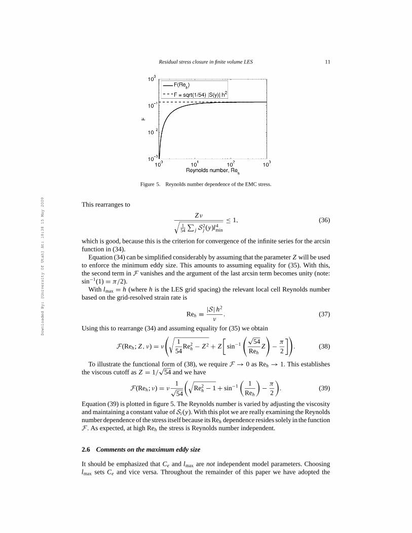
Figure 5. Reynoldsnumberdependenceof theEMC stress.

This rearrangesto

Zν√154

∑j S

2j (y)l 4

min

≤ 1, (36)

which is good,becausethis is thecriterionfor convergenceof theinfinite seriesfor thearcsinfunctionin (34).

Equation(34)canbesimplifiedconsiderablybyassumingthattheparameterZ will beusedto enforcethe minimum eddysize.This amountsto assumingequality for (35). With this,thesecondtermin F vanishesandtheargumentof thelastarcsintermbecomesunity (note:sin−1(1) = π/2).

With lmax = h (whereh is theLES grid spacing)therelevant local cell Reynoldsnumberbasedon thegrid-resolvedstrainrateis

Reh ≡|S| h2

ν. (37)

Usingthis to rearrange(34)andassumingequalityfor (35)weobtain

F(Reh; Z, ν) = ν

(√1

54Re2

h − Z2 + Z

[sin−1

(√54

RehZ

)−

π

2

]). (38)

To illustratethefunctionalform of (38),we requireF → 0 as Reh → 1. This establishestheviscouscutoff as Z = 1/

√54andwehave

F(Reh; ν) = ν1

√54

(√Re2

h − 1 + sin−1

(1

Reh

)−

π

2

). (39)

Equation(39) is plottedin figure5. TheReynoldsnumberis variedby adjustingtheviscosityandmaintainingaconstantvalue ofSi (y). With thisplotwearereallyexaminingtheReynoldsnumberdependenceof thestressitselfbecauseitsReh dependenceresidessolelyin thefunctionF . As expected,athighReh thestressis Reynoldsnumberindependent.

2.6 Commentson themaximumeddysize

It shouldbe emphasizedthat Ce and lmax arenot independentmodelparameters.Choosinglmax setsCe and vice versa.Throughoutthe remainderof this paperwe have adoptedthe

Downloaded By: [University Of Utah] At: 18:38 15 May 2009

12 R.J. McDermottet al.

conventionlmax = h for EMC becauseit is convenientfor analysis.Thoughit is temptingtodraw comparisons,lmax is not a ‘filter width’ in theclassicalLES sensein thatvarying lmax

doesnot affect the definition of the local strain.As we will seein section3, whatever onechoosesfor lmax in EMC thereis arateconstant,Ce, thatwill yield thecorrectrateof residualenergyproduction(Pr ). Thesameis truefor full ODTclosure.With ODT, however, for agivenPr therateconstantwill be lower becauseODT sampleseddyeventsfrom aninstantaneoustimescaledistribution,causingoneeddyto cascadeinto several(moreon this in section3.2).UnlikeEMC,with ODT wearealsoconcernedwith thequalityof thesubgridstatistics,whichdependonPr and Ce. For a given Pr , if Ce is settoo high in ODT thenenergy will pile upin the high wavenumbersubgridODT field (for a given molecularviscosityhigherstrainswill berequiredto dissipateenergy at thecorrectrate).Theoppositeis trueif Ce is too low.Therefore,for ODT Ce shouldbedeterminedby matchinghigh wavenumberstatisticsfor agivenPr . Themaximumeddysizemustfollow to matchPr . Thereis evidence[8, 9] thattheoptimummaximumeddy-sizefor ODT subgridclosureis approximately3h.

3. Theoretical determination of the eddy rate constant

A limitationof stand-aloneODTis theneedtoempiricallytunemodelparametersfor differentflows.In principle,mergingODT with LESshouldhelpalleviatethisproblemsinceLEScanaccountfor threedimensionalityandcomplex boundaryconditions.Aspreviouslymentioned,it is difficult to applyLilly’ s analysis[3] for determiningthe rateconstantdirectly to ODT.Here,instead,we applyLilly’ s analysisto EMC, which,dueto therecursive natureof ODTmappings,establishesanupperboundontheODT rateconstant.As shown in section4.5,thetheoreticalconstantworksreasonablywell for LESwith ensemblemeanclosure.

3.1 Lilly’ s analysisin onedimension

Lilly’ s analysisassumesisotropy andequilibrium(i.e. thattheproductionof residualkineticenergy equalsthe moleculardissipationrate) to determinea value for the modelconstant.First,wemustestablishaone-dimensionalkineticenergy equation.Westartwith thefilteredmomentumequationsin differentialform,

∂U i

∂t+

∂(U i U j )

∂x j= −

∂ P

∂xi+ ν

∂2U i

∂x j ∂x j−

∂τ Rij

∂x j, (40)

wheretheoverbarrepresentsaprojectionof thevelocityfield ontothefinite dimensionalLESspace(e.g.asharpspectralcutoff at thegrid Nyquistlimit). Multiplying thisequationby U i ,anddefiningE f ≡ 1

2U i U i , we have thetransportequationfor thefilteredkineticenergy, leftin termsof velocitygradients,

∂E f

∂t+

∂(E f U j )

∂x j+

∂

∂x j

(U j P − ν

∂E f

∂x j+ U i τ

Rij

)= −ε f − Pr , (41)

wherethefilteredviscouspseudo-dissipationis heredefinedas

ε f ≡ ν∂U i

∂x j

∂U i

∂x j, (42)

Downloaded By: [University Of Utah] At: 18:38 15 May 2009

Residualstressclosure in finitevolumeLES 13

andtheproductionof residualkineticenergy is

Pr ≡ −τ Rij

∂U i

∂x j. (43)

If (41) is averagedover ahomogeneousregionof space,suchthatthetransporttermsvanish,andif theflow isisotropic,wemaywrite [9, 18] (nosummationover y throughoutthissection)

⟨∂E f

∂t

⟩= −3ν

⟨∂U i

∂y

∂U i

∂y

⟩+ 3

⟨τ R

iy

∂U i

∂y

⟩. (44)

We maynow proceedwith theanalysis.Themeanfilteredpseudo-dissipationis given by(for asharpspectralfilter)

〈ε f 〉 = 3ν

⟨∂U i

∂y

∂U i

∂y︸ ︷︷ ︸∑

i S2i (y)

⟩= 2ν

∫ π/�

0κ2E(κ)dκ. (45)

InsertingtheKolmogorov spectrum,E(κ) = CK ε2/3κ−5/3 (see,for example,[18]), andinte-gratingweget

3

⟨ ∑

j

S2j (y)

⟩= 3

⟨|S(y)|2

⟩= 2CK ε2/3

[3

4

(π

�

)4/3], (46)

or(

4

3

)3/2( 3

2CK

)3/2(�

π

)2⟨|S(y)|3

⟩∗ = ε, (47)

where� is the filter width, ε is the moleculardissipationrate and CK is Kolmogorov’suniversalconstant.Theasteriskon theaverageof thecubeof thestrainmagnitudeindicatesthatwe have assumedtheexponentandaveragecommute.UsingDNS,MeneveauandLund[22] establishedtheerrorin thisassumptionto beon theorderof 20%.

Assumingequilibriumandsubstitutingourmodelinto theanalysis(i.e.usingτ Riy = Ri (y)),

wehave

−3

⟨Ri (y)

∂U i

∂y

⟩= ε. (48)

Let usnow plug in theEMC modelfrom (29) with α = 0. We startherebecausethephysi-cally preferredmodelvalue ofα = 2/3 requiresanadditionalspeculativeassumptionfor thisanalysiswhichwewill seebelow. Using(47) for ε, (48)becomes

−3

⟨[−

1

27

Ce√54

(l 2max− l 2

min

)|S(y)|Si (y)

]∂U i

∂y

⟩=

(4

3

)3/2( 3

2CK

)3/2(�

π

)2⟨|S(y)|3

⟩, (49)

We let lmin = 0 andusetheempiricallydeterminedvalueCK ≈ 1.5 (see,for example,[18]).Noting∂yU i = Si (y) andSi (y)Si (y) = |S(y)|2, for lmax = � theeddyrateconstantis

Ce = 9

(4

3.0

)3/2( 1

π

)2√54 ≈ 1.4

√54. (50)

Letusalsoanalyzethecasewhereα = 2/3,equipartitionof availableenergy in thepressurescramblingmodel.Using(29) for Ri (y), takinglmax ≫ lmin, andrecallingβij = 1/3, wemay

Downloaded By: [University Of Utah] At: 18:38 15 May 2009

14 R.J. McDermottet al.

write (48) as

1

9

Ce√54

l 2max

⟨|S(y)|

[1

2Si (y)Si (y)︸ ︷︷ ︸

|S(y)|2

+1

2sgn(Si (y))Si (y)︸ ︷︷ ︸

‖Si (y)‖L1

1√

3|S(y)|

]⟩= ε. (51)

Thesecondtermin thebracketcontainstheL1 normof thestrainvector. Notethatourcurrentdefinitionof thestrainmagnitude,|S(y)|, is theL2 normof thestrainvector. To proceedwiththeanalysiswemustmake an assumptionabouthow thesenormsarerelated.If all thestrainsareroughlyequalin magnitudethenwehavetherelation,‖Si (y)‖L1 ≈

√3 |S(y)|. Whenthisis

substitutedinto (51)therateconstantfrom (50) is unchanged.As wewill seein latersections,however, resultsobtainedusingEMC in LESareslightly dependentonthechoiceof α, so thisassumptionseemsratherpoor. Analternativeis toassumethattwocomponentsof thestrainaredominant(andequal),mimickinga local vortex [42]. This resultsin ‖S j (y)‖L1 ≈

√2 |S(y)|.

Usingthis in (51)gives(

1

2+

1√

6

)

︸ ︷︷ ︸≈0.91

1

9

Ce√54

l 2max

⟨|S(y)|3

⟩= ε. (52)

Therateconstantis, therefore,increasedto

Ce ≈1.4

0.91

√54 ≈ 1.5

√54, (53)

which is consistentwith thetrendin figure6 (section4.5).

3.2 Remarkson the rateconstantfor full ODT closure

Full ODT naturallyexhibitscascadedynamics.Dueto thecascadeprocessandtheparticularmappingchosen(i.e.thetripletmap)weexpecttherateconstantfor full ODTclosuretobelessthanthat for EMC by roughlya factorof 3 (e.g.with lmax = h, Ce ≈ 1.4

3

√54). Preliminary

resultswith ODT supportthis assertion[8, 9]. The specificfactor, 3, resultsbecauseonceaneddymappingtakesplacein ODT thelocal straintriples(dueto thetriplet map),makinganothereddy(1/3thesizeorsmaller)threetimesmorelikelytooccur.Smallereddies,however,

Figure 6. A zoom-inneartheNyquistlimit of thethree-dimensionalenergyspectrain decayingisotropicturbulenceof the Kang et al. datawith variouschoicesof α andCe = 1.4

√54 and Z = 0.14. The solid lines representthe

experimentaldata,respectively, from topto bottom,atx/M = 20(initial condition),x/M = 30andx/M = 48.Thex/M = 40datais omittedfor clarity.

Downloaded By: [University Of Utah] At: 18:38 15 May 2009

Residualstressclosure in finitevolumeLES 15

donotaffecttransportasmuchaslargereddies.Theeffectivetransportdecreasesgeometricallyasthelengthscaledecreases.Therefore,accountingfor thefirstrecursivemappingeventshouldbetheleadingordercorrectionto thetheoreticalEMC rateconstantwhenappliedto ODT.

It ispossibletoconfirmthisassertionbyperformingLilly’ sanalysiswith astand-aloneODTmodelusedto closethestressin (48),thusproviding atheoreticallink betweenCe andlmax forfull ODTclosure(weleavethisfor futurework).Toimaginehow thiswouldworkfirstconsiderthatit isnotarequirementthatthestressbedeterminedalgebraically. With EMC,for example,wecouldhavestochasticallyimplementedmappingeventsbasedonthelinearfield.For EMCtheeventdistributionis uniform.Eachtimeaneddywassampledwewouldfirst computeandstoretheresultingstressandthenre-linearizethefield. Theensembleaverageof thestresseswouldyield thesameresultasthealgebraicanalysis.Wecanperformthesametypeof stochas-tic simulationwith ODT, thesimpledifferencebeingthatwe would not re-linearizethefieldandthereforeaccountfor stressesinducedby thevaryingtimescaledistribution(i.e.recursivemappings).

Regardingthecascade,it shouldbeappreciatedthatthegeometricincreasein frequenciesandthepropertiesof thetriplet maparewhatallow ODT to producea−5/3energy spectrum[5]. No suchphysicalmechanismis presentin EMC. Like other eddy viscosity closures,the EMC model only indirectly representsthe energy cascadethroughthe assumptionofequilibrium(i.e. productionequalsdissipation).

4. Ensemblemeanclosure in finite volumeLES

In this sectionwe apply theEMC model,sofar derived for multiple componentsin a singledirection,to subgridclosurein a three-dimensionalfinite volumeLES.We first describetheLES formulation and numericalmethodsemployed. We then presentresultsfor decayingisotropicturbulence,examiningsensitivity to thepressurescramblingmodelandestablishinganempiricalvaluefor theviscouscutoff. Wethencomparestatisticalmeasuresof the resolvedfield with high Re wind tunnel data [23] including structurefunction probability density,hyper-flatnessfactors,residualenergy productionandtheprobabilitydensityfunction(PDF)of theresidualstress.

4.1 Finite volumegoverning equations

Theformulationpresentedhereis similar to Schumann[24] andis chosento make useof acombinationof thefinitevolume(FV) andsemi-discreteapproachesfor thenumericalsolutionof scalarconservationlaws.Bothmethodsreceiveconsiderableattentionin Lomaxetal. [25]andVerstappenandVeldman[26]. Theintegral form of thegoverningequationsfor massandmomentumconservationof anincompressiblefluid are,respectively,

∮

SU j n j dS = 0 (54)

and

d

dt

∫

VUi dV = −

∫

S(Ui U j + Pδij + τij )n j dS, (55)

whereP is thehydrodynamicpressure,τij = −ν(∂ j Ui + ∂i U j ) is theviscousstressandν isthekinematicviscosity. A principaladvantageof theFV methodis thatdiscreteconservationof solutionvariablesis obtaineda priori . Caremustbe taken, however, to ensurediscreteconservationof kinetic energy (see,for example,[26–28]).Thoughthemethodis suitedforirregularandunstructuredgrids,hereweconsideronlysimplecubiccontrolvolumes(CVs)of

Downloaded By: [University Of Utah] At: 18:38 15 May 2009

16 R.J. McDermottet al.

sideh. Thus,theCV volumeis V = h3 andthesurfaceareaof agivenCV facek is Sk = h2.We definea surfacefiltered field, φ

( j )(x), to be the averagevalue of the scalar, φ(x), on a

two-dimensionalplanarsurfacenormalto thex j direction.Thatis, we applytwo orthogonaltophatfilterstothescalarfield.For example,thex1 surface-filteredfieldfor athree-dimensionaldomainis

φ(1)

(x) ≡1

h2

∫ x3+h/2

x3−h/2

∫ x2+h/2

x2−h/2φ(x′)dx′

2dx′3. (56)

The ‘volume-filtered’or ‘cell-average’field is then given by applying a one-dimensionaltophatfilter to thesurface-filteredfield (in thedirectionnormalto thesurface):

φ(x) ≡1

h3

∫ x3+h/2

x3−h/2

∫ x2+h/2

x2−h/2

∫ x1+h/2

x1−h/2φ(x′)dx′

1dx′2dx′

3

=1

h3

∫

V(x)φdV =

1

h

∫ x j +h/2

x j −h/2φ

( j )(x′)dx′

j ⊥Sj. (57)

Thenetresultis whatPope[18] refersto asan‘anisotropicboxfilter’ andis referenceframedependent,aninherentcharacteristicof thefinite volumeapproachwhichis toleratedbecauseof thepracticaladvantagesof themethod.

Toobtainthefinitevolumediscretizationwesamplethefilteredfieldsfromadiscretespace.For example,φ(x) → φ(i, j, k). By inserting(56) and(57) into (55) we endup with theFVmomentumequation:

dUi

dt= −

Sk

Vnk j

(Ui U j

(k) + P(k)

δij + τ(k)ij

), (58)

wherenk j is a matrix of unit normal vectorsfor eachfacek. The summationconventionapplies(exceptfor superscripts,whichareusedheresimply to referenceaparticularsurface)andhenceSk

V nk j = h2

h3 nk j = 1hnk j is thefinite volume‘divergence’operator. For a cubicCV

alignedwith acartesianreferenceframethismatrix is simply

nk j =

1 0 0

−1 0 0

0 1 0

0 −1 0

0 0 1

0 0 −1

. (59)

In this notationthe numberof rows in nk j equalsthe numberof facesof the CV and thenumberof columnsequalsthedimensionof thedomain(e.g.3columnsfor athree-dimensionalproblem).Eachrow storestheunit normalvectorfor thatface.Sk is a row vector(i.e.a1× 6matrix) of CV faceareas,all equalto h2 in this case.This notationis alsoconvenientforunstructuredgridswith irregularCV shapes.

4.2 FV LES formulation

Equation(58) is obviously just a redefinitionof termsin the integral momentumequationbut highlightsthe fact that the FV approachemploys two differentfilters. The challengeofa numericalmethodis to approximatethe surfaceintegralsbasedon cell-average(volume-filtered) data.In LES we have the additionaldifficulty that the underlyingcontinuousdata

Downloaded By: [University Of Utah] At: 18:38 15 May 2009

Residualstressclosure in finitevolumeLES 17

arenot guaranteedto besmoothin any sense.In this paperwe introducea decompositionofthe advective stressinto ‘numerical’ and‘residual’ components.The residualstressis thusdefinedby the differencebetweenthe exact surface-filteredflux (e.g.the surfacefilter (56)appliedto aDNS-likefield) andthenumericalapproximationusedfor theadvectiveflux. Weareleft with thefollowing FV LESequations:

dUi

dt= −

Sk

Vnk j

(U

x j

i Uxi

j + P(k)

δij + τ(k)ij + τ

R,(k)ij

), (60)

where

τR,(k)ij ≡ Ui U j

(k) − Ux j

i Uxi

j . (61)

Note thedistinctionbetweenthenumericaladvective flux definedby, for example,an inter-polant(notethat it is alsocommonto invoke anENO reconstruction[29, 30]), heredenotedby anoverbarwith superscriptxi , andtheflux definedby applicationof asurfacefilter to theDNS-likevelocityfield,heredenotedby anoverbarwith superscipt(k). Thefirst termin (61),thesurface-filteredterm,is theapplicationof (56)to thedyadicUi U j onsurfacek. Thesecondtermdependsonthenumericalmethodandfor ourcalculationsis given by(66) in section4.4wherewe have followed the notationof Morinishi et al. [28]. The point to be madeis thateventhough(60) alreadycontainsreferenceto thenumericalprocedureto beemployedit isstill anexactrepresentationof theCV momentumbalance.

4.3 Physicalinterpretationof residualstressclosure

Following [31] theresidualstress(61) canbedecomposedinto a Leonardstress(Lij ), crossstresses(Cij ), andaReynoldsstress(Rij ):

τR,(k)ij = U

x j

i Uxi

j

(k)− U

x j

i Uxi

j︸ ︷︷ ︸Lij

+Ux j

i U ′j

(k) + U ′i U

xi

j

(k)

︸ ︷︷ ︸Cij

+U ′i U

′j

(k)

︸ ︷︷ ︸Rij

, (62)

whereU ′j ≡ U j − U

xi

j . The numericaladvective term is constanton a faceandso in thisformulationtheLeonardtermis identicallyzero.Thecrossstressessurvive, however, becausethevelocity fluctuationis definedby the interpolant,not thesurfacefilter. Notice that if we

haddefinedthefluctuationasU ′j ≡ U j − U

(k)j wewouldhave aReynoldsdecompositionand

thecrosstermswouldvanishasin Schumann’s formulation[24]. Wehavechosentheformerdecompositionbecauseof its consistency with thephysicalpictureof ODT.

In principle,atripletmaprepresentssubgridadvectionalongtheODTlinedirection.Thatis,an‘eddyevent’ isamodelforU ′

j (takingtheconventionconsistentwith thedivergenceoperatorthatcomponenti is beingadvectedin the j direction).Sincefull ODT carriesthescalarsUi

on a givenline thenthemappingeventsphysicallyrepresenta modelfor theReynoldsstressandthefirst termof thecrossstress.(A discussiononcapturingtheeffectsof thesecondcrossstressin the full ODT approachis beyond the scopeof this paper. The interestedreaderisreferredto McDermott[9] andSchmidtet al. [8]. Thephysicalpicturein EMC is somewhatdifferent.Hereeddyeventsmaponly theU

x j

i field. Therefore,EMC is reallybestthoughtofasamodelfor thefirst termof thecrossstress,which, likeEMC, is notsymmetric(recallthediscussionin section2.2.3).In thepresentcase,however, we assumeEMC to accountfor allof theresidualenergy production,understandingthat it shouldbepossibleto combineEMCwith othermodelsto produceabetterphysicalpictureof thesubgridtransport,in thespirit ofthe‘mixedmodel’ of Bardinaetal. [32], for example).

Downloaded By: [University Of Utah] At: 18:38 15 May 2009

18 R.J. McDermottet al.

4.4 Numericalmethod

In thesemi-discreteapproachonefirst approximatesthesurface-filteredfluxesusingthecellaveragesat a giventime, t . Oneis thenleft with thetaskof solvinga coupledsetof ordinarydifferentialequationsin time.Our codeusesa uniform meshwith thestaggeredgrid storagearrangementof Harlow andWelch [33](equivalentlyseeMorinishi etal. [28]) andthethird-orderRunge-Kutta(RK3) time integrationschemeof ShuandOsher[34]. Following SureshandHuynh[35], we first describethetime advancementfor a singleforwardEulerstepandthenextendthis to theRK3 scheme.

After Chorin[36], continuity(54) is integratedwith (60) asfollows: Let Wni representthe

discreteLESstateat time, tn. Wedesireanexplicit updateof thefollowing form,

Wn+1i = Wn

i + �t

[F

(Wn

i

)−

δϕ

δxi

], (63)

where�t = tn+1 − tn, Wn+1i is divergencefree (discretely),F(·) is the explicit advection-

diffusion-subgridoperator(yetto bedefined)andϕ is thescalarusedto enforcethecontinuityconstraint.(Wehavemadethesechangesin notationfromtheLESformulationin theprevioussectionin orderto avoid theconfusionoftenrelatedto explicit filtering.TheLESstateis nevertruly definedby anexplicit filtering step.Onenever filters a DNS field, U , to obtainU , forexample.Rather, the LES stateis definedby the numericalprocedure.)In the notationofMorinishi et al. [28] thesecond-orderdifference(in thex1 direction,for example)is definedby

δφ

δx1

∣∣∣∣x1,x2,x3

≡φ(x1 + h/2, x2, x3) − φ(x1 − h/2, x2, x3)

h. (64)

Thespatialdiscretizationoperator, F(Wi ), is decomposedas

F(Wi ) = −δ

δx j

[W

x j

i Wxi

j + ν

(δWi

δx j+

δWj

δxi

)+ Rij

], (65)

wherethetermson theright-handsideof (65) are,respectively, theadvective, diffusive andsubgridforces.For theadvective operatorwe employ thekinetic energy preservingsecond-orderstaggeredgrid schemeof Harlow andWelch[33]. Hereweemploy Morinishi’snotation[28] for theHarlow andWelchscheme.Theinterpolationoperatorusedin (65) is definedasfollows.Thesecond-orderinterpolation(in thex1 direction,for example)is

φx1|x1,x2,x3 ≡

φ(x1 + h/2, x2, x3) + φ(x1 − h/2, x2, x3)

2. (66)

We take Rij to representa model for the residualstress(61). One can envision severaloptionsfor implementationof theEMC modelon staggeredgrids.Thereaderis referredtoAppendixC for detailsof thespecificmethodemployedhere.

Sincethe correct‘pressure’field, ϕ(x), neededto make the LES statedivergencefree isunknown, we first computea velocity field updatebasedon a guessfor the pressurefield.Settingtheguessfor thepressurefield to zerogives thepredictorstep,

W∗i = Wn

i + �t[F

(Wn

i

)]. (67)

Subtracting(67) from (63)yieldsthesocalledpressureprojection,

Wn+1i = W∗

i − �tδϕ

δxi. (68)

Downloaded By: [University Of Utah] At: 18:38 15 May 2009

Residualstressclosure in finitevolumeLES 19

Takingthediscretedivergenceof (68)andsettingδi Wn+1i = 0resultsin thePoissonequation

for thepressure,

δ

δxi

δϕ

δxi=

1

�t

δW∗i

δxi, (69)

which is solvedfor ϕ, andtheresultusedin (68). Fromhereon we refer to combinedsteps(69)and(68), in thatorder, as theprojectionoperator, P(·). For example,Wn+1

i = P(W∗i ), is

theprojectionof W∗i , from (67),ontoadivergencefreespace.

With theprojectionestablished,theRK3schemecanbewrittenasfollows.Let W(0)i = Wn

i .Then,proceedingfrom left to right, top to bottom:

W∗(1)i = W(0)

i + �t F(W(0)

i

), W(1)

i = P(W∗(1)

i

),

W∗(2)i = 3

4W(0)i + 1

4�t F(W(1)

i

), W(2)

i = P(W∗(2)

i

),

W∗(3)i = 1

3W(0)i + 2

3�t F(W(2)

i

), W(3)

i = P(W∗(3)

i

),

(70)

and Wn+1i = W(3)

i . As a practicalnote, it is importantthat the sequenceof averagingandprojectionbekeptasthey arein (70) to avoid accumulationof numericalmassdivergenceinthesystem.

4.5 Resultsfor decayingisotropicturbulence

WestarttheEMC validationby comparingresultsto theactivegrid highRewind-tunneldataof Kangetal. [23]. Weuseauniformmeshspacing,h = L/N, where,following Kangetal.[23], L = 5.12 m and N = 64. Hence,h = 0.08 m, correspondingto the filter scale�4 intheKangdata.All simulationswererun with anadvectionlimiting CFL of �t‖W‖∞

h = 0.25,which is quiteconservative for theRK3 time integrationscheme.Thenon-dimensionaltimesfor thedatapointsare:x/M = 20(initial condition),30,40and48(notethatx is thedistancedownstreamof theactivegrid andM is thedistancebetweenrotationshaftsof theactivegrid;see[23] for moredetails).Thesecorrespondto dimensionaltimesof: t = 0, 0.15, 0.30 and0.42s in oursimulations.

Theinitial conditionfor thevelocityfieldwasgeneratedbythefollowingprocedure.Fouriermodeswith randomphasesweresuperimposedto matchtheinitial spectrumof thedata.Thisfield was thenallowed to evolve for a shortperiod(2–3 time steps)during which time theenergywoulddecayandcoherentturbulentstructurewoulddevelop.Energywastheninjectedbackinto theFouriermodessuchthatthespectrumof theinitial conditionagainmatchedthespectrumof theinitial data.Thisprocesswasrepeatedseveraltimesuntil thecoherentstructuresstabilized.The initial field was thenfiltered with a spectralcutoff at the grid Nyquist limit(π/h).

Wefirst testedthesensitivity of EMC to thechoiceof pressurescramblingmodel.WeusedthetheoreticallydeterminedrateconstantCe = 1.4

√54(basedonlmax = h) andviscouscutoff

Z = 1/√

54 ≈ 0.14.In section3 it isshown thattheuncertaintyassociatedwith thecommu-tativity assumptionin (47) is greaterthanthe α sensitivity of the theoreticalrateconstant.Additionally, it isshown thatincreasingα decreasesthedecayrate.Thiswasdemonstratedinfigure6. Dueto assumptionsin Lilly’ sanalysis(e.g.commutationof theaveragingoperationandtheshapeof thefilter) thetheoreticalrateconstantfor agivenα leadsto imperfectresultsin practice(noticethattheα = 0 caseis toodissipative).Figure7,however, demonstratesthatLilly’ s analysisworks well for quantifyingtheeffectsof α on thedecayrate.Herethetheo-retically linkedvaluesfor Ce andα areusedandverysimilar resultsareachieved.This lendssupportto theassumptionthattwo componentsof thestraindominatelocally (seesection3).

Downloaded By: [University Of Utah] At: 18:38 15 May 2009

20 R.J. McDermottet al.

Figure 7. A zoom-inneartheNyquistlimit of thethree-dimensionalenergy spectrafor theKangetal. data.BasedonLilly’ sanalysis(section3) with theassumptionthattwo componentsof thestrainvectoraredominantandequal,thetwoCe/α combinationsshownhereshouldyield thesameresults.Notethattherateconstantin thelegendhasbeennormalizedby

√54.Thesolid linesrepresenttheexperimentaldata,respectively, from top to bottom,at x/M = 20

(initial condition),x/M = 30andx/M = 48.Thex/M = 40datais omittedfor clarity.

Basedon figure 6 the standardODT value ofα = 2/3 (i.e. equipartitionof energy in thepressurescramblingmodel)seemsto yield thebestresultswhenusedwith Ce = 1.4

√54(see

alsofigure8). Wewill seefurtherevidencesupportingthechoiceα = 2/3 in section5.With thesebaselineparametersestablished(i.e.Ce = 1.4

√54andα = 2/3),wenext tested

themodelagainstthelow Re data ofComte-BellotandCorrsin(CBC) [37]. Viscouseffectsare importantin this dataset for a well-resolved LES, testingthe model’s Re dependence.Following de Bruyn Kops [38], we useda periodic box of side L = 9 × 2π centimeters(≈0.566m) andν = 1.5×10−5 m2/sfor thekinematicviscosity. Thenon-dimensionaltimesfor thisdatasetarex/M = 42(initial condition),98and171.Thesecorrespondtodimensionaltimesof t = 0.00,0.28 and0.66 s in our simulations.In figure9 theLES three-dimensionalenergy spectraarecomparedto theCBCdatafor two valuesof theviscouscutoff. Theinitialguessof Z = 1/

√54 ≈ 0.14allows themodelto dissipateenergy tooquickly, indicatingthe

modelisnotturningitselfoff in laminarflow regions.Theviscouscutoff wastunedto Z = 3.0

Figure 8. Three-dimensionalenergyspectrafor theKangdatawith Ce = 1.4√

54,α = 2/3andZ = 0.14.Thesolidlinesrepresenttheexperimentaldata,respectively, from top to bottom,at x/M = 20 (initial condition),x/M = 30,x/M = 40andx/M = 48.

Downloaded By: [University Of Utah] At: 18:38 15 May 2009

Residualstressclosure in finitevolumeLES 21

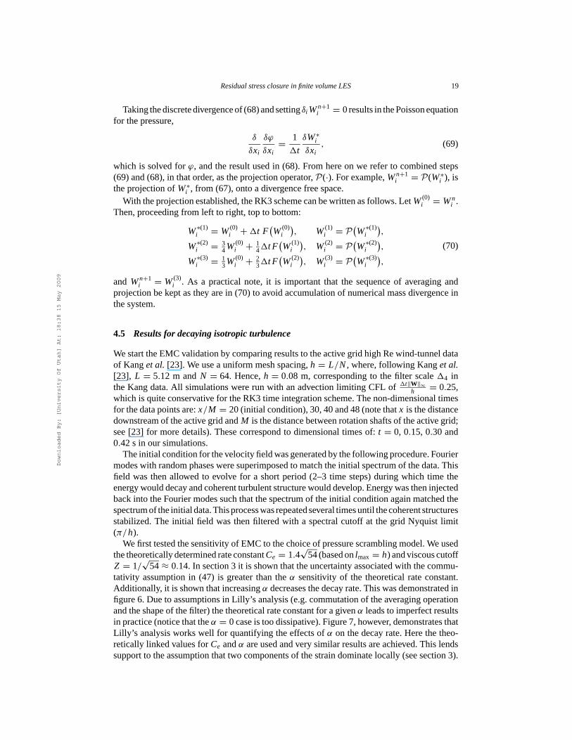
Figure 9. Three-dimensionalenergy spectrafor the CBC datacomparingvaluesof the viscouscutoff, Z (note:1/

√54 ≈ 0.14)with Ce = 1.4

√54andα = 2/3.Thesolidlinesrepresenttheexperimentaldata,from topto bottom,

at x/M = 42 (initial condition),x/M = 98andx/M = 171.

to matchtheCBCdata.In figure10wehavereruntheKangetal. datawith thenew valuefortheviscouscutoff. As shouldbe thecase,at high Reynoldsnumbertheviscouscutoff doesnotaffect theresultsandthespectrafor thetwo differentcutoff valuesareidentical.

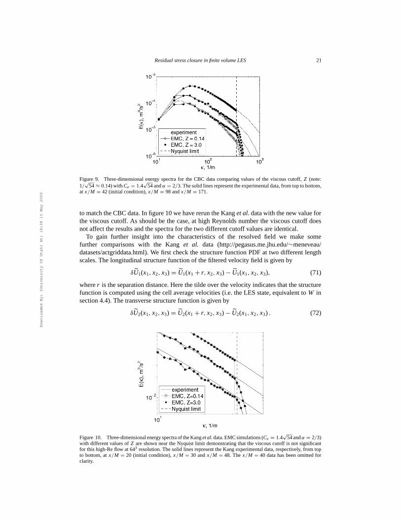
To gain further insight into the characteristicsof the resolved field we make somefurther comparisonswith the Kang et al. data (http://pegasus.me.jhu.edu/∼meneveau/datasets/actgriddata.html).We first checkthestructurefunctionPDFat two differentlengthscales.Thelongitudinalstructurefunctionof thefilteredvelocity field is given by

δU1(x1, x2, x3) = U1(x1 + r, x2, x3) − U1(x1, x2, x3), (71)

wherer is theseparationdistance.Herethetilde over thevelocity indicatesthatthestructurefunctionis computedusingthecell averagevelocities(i.e. theLES state,equivalentto W insection4.4).Thetransversestructurefunctionis given by

δU2(x1, x2, x3) = U2(x1 + r, x2, x3) − U2(x1, x2, x3) . (72)

Figure 10. Three-dimensionalenergyspectraof theKangetal. data.EMCsimulations(Ce = 1.4√

54andα = 2/3)with differentvaluesof Z areshown neartheNyquist limit demonstratingthat theviscouscutoff is not significantfor this high-Reflow at 643 resolution.Thesolid linesrepresenttheKangexperimentaldata,respectively, from topto bottom,at x/M = 20 (initial condition),x/M = 30 andx/M = 48. The x/M = 40 datahasbeenomittedforclarity.

Downloaded By: [University Of Utah] At: 18:38 15 May 2009

22 R.J. McDermottet al.

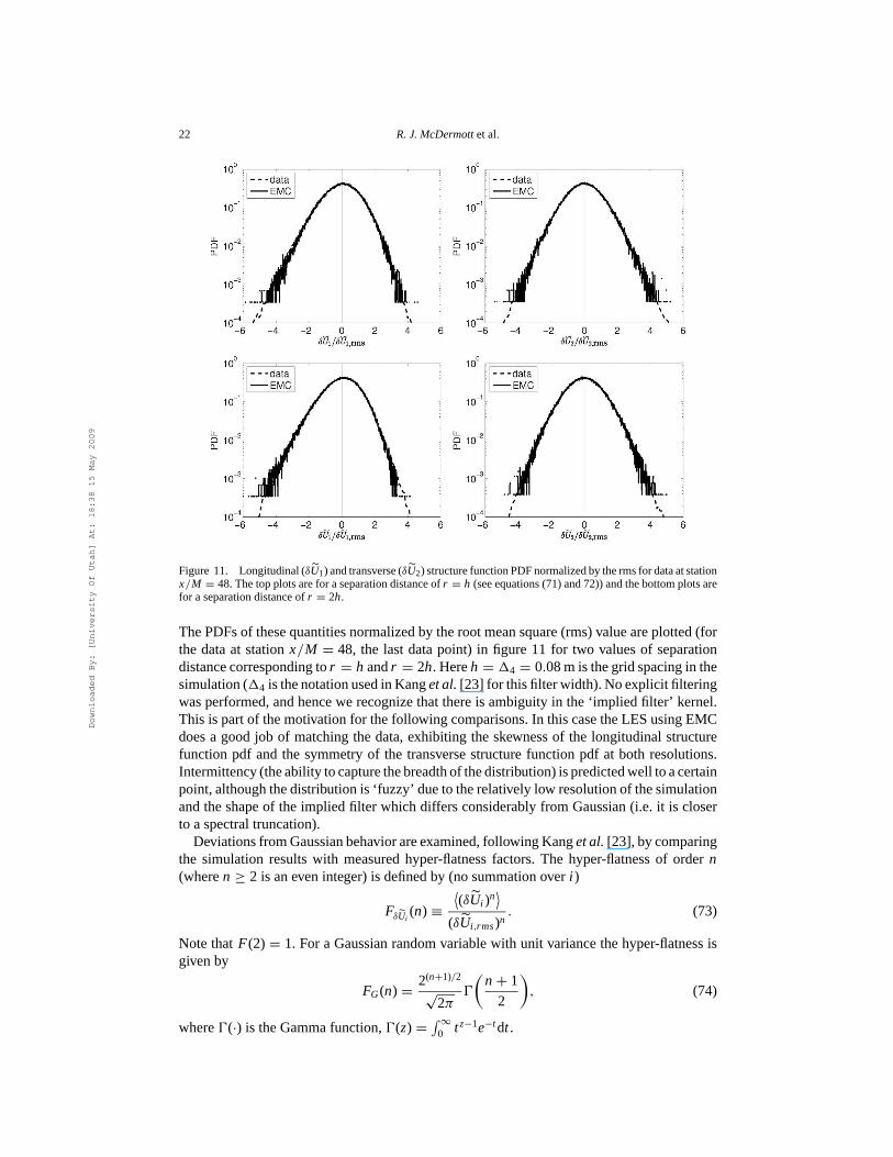
Figure 11. Longitudinal(δU1) andtransverse(δU2) structurefunctionPDFnormalizedby thermsfor dataatstationx/M = 48.Thetopplotsarefor aseparationdistanceof r = h (seeequations(71)and72))andthebottomplotsarefor aseparationdistanceof r = 2h.

ThePDFsof thesequantitiesnormalizedby therootmeansquare(rms)valueareplotted(forthe dataat stationx/M = 48, the last datapoint) in figure 11 for two valuesof separationdistancecorrespondingto r = h andr = 2h. Hereh = �4 = 0.08m isthegrid spacingin thesimulation(�4 is thenotationusedin Kangetal. [23] for thisfilter width).Noexplicit filteringwas performed,andhencewe recognizethatthereis ambiguityin the‘implied filter’ kernel.This is partof themotivationfor thefollowing comparisons.In thiscasetheLESusingEMCdoesa goodjob of matchingthe data,exhibiting the skewnessof the longitudinalstructurefunction pdf andthe symmetryof the transversestructurefunction pdf at both resolutions.Intermittency (theability tocapturethebreadthof thedistribution)ispredictedwell toacertainpoint,althoughthedistributionis ‘fuzzy’ dueto therelatively low resolutionof thesimulationandtheshapeof theimplied filter which differsconsiderablyfrom Gaussian(i.e. it is closerto aspectraltruncation).

DeviationsfromGaussianbehavior areexamined,followingKangetal. [23], bycomparingthe simulationresultswith measuredhyper-flatnessfactors.The hyper-flatnessof order n(wheren ≥ 2 is an even integer)is definedby (nosummationover i )

FδUi(n) ≡

⟨(δUi )n

⟩

(δUi,rms)n. (73)

Notethat F(2) = 1. For a Gaussianrandomvariablewith unit variancethehyper-flatnessisgiven by

FG(n) =2(n+1)/2

√2π

Ŵ

(n + 1

2

), (74)

whereŴ(·) is theGammafunction,Ŵ(z) =∫ ∞

0 tz−1e−tdt .

Downloaded By: [University Of Utah] At: 18:38 15 May 2009

Residualstressclosure in finitevolumeLES 23

Figure 12. Comparisonof theskewnesscoefficientwith increasingcorrelationdistancefor theconstant-coefficientSmagorinky model(CSM) thedynamicSmagorinsky model(DSM) andensemblemeanclosure(EMC).

The top two plots of figure 12 show resultsfor the longitudinal (i = 1) and transverse(i = 2) hyper-flatnessat variousorders.Data are shown for two separationscalesbut thesimulationresultsarepresentedonly at r = h. The factorsfor a Gaussianvariablearealsopresentedfor reference.Somewhat interestingly, the simulationmatchesvery well with thetransversefactorsat r = 2�4 (recall h = �4). This is presumablyanotherconsequenceofthe implied filter kernelandseemsmoreor lessfortuitous.This trendcontinues,however,whenexaminingthe8thorderhyper-flatnessfactors(thetwo lowerplotsin figure12)andtheskewnesscoefficientsin figure13.Theskewnesscoefficient is given by

S =⟨(δU1)3

⟩⟨(δU1)2

⟩3/2 . (75)

In theseplotswealsoshow comparisonsfor theconstantcoefficientSmagorinsky model[15]andthedynamicSmagorinsky model[2]. All threemodelsexhibit similarbehavior, matchingthe overall trendsquite well, but the simulationresultsseemto be off by roughly onefilterwidth.Weattributethisdiscrepancy moreto thenumericalprocedure(i.e.poorgrid resolutionfor the given filter width) than to the residualstressmodel. Given that most engineeringcalculationsareperformedwithout explicit filtering it is prudentto examineandunderstandthe limitation of model performanceunder theseconditions.The skewness,in particular,seemsto bestronglyaffectedby thenumericsat thescaler = h. At largerscales,however,thesimulationsrecover theskewnesstrendsquitewell.

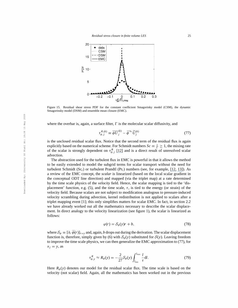
For referencewe alsopresentthe PDFsof the productionof residualkinetic energy andtheτ R

12 componentof theresidualstress(computedfor thenorthucell face).Theseresultsaregiven in figures14 and15, respectively. Theconlusionsaresimilar to thosefoundby Kang

Downloaded By: [University Of Utah] At: 18:38 15 May 2009

24 R.J. McDermottet al.

Figure 13. Comparisonof theskewnesscoefficientwith increasingcorrelationdistancefor theconstantcoefficientSmagorinky model(CSM), thedynamicSmagorinsky model(DSM) andensemblemeanclosure(EMC).

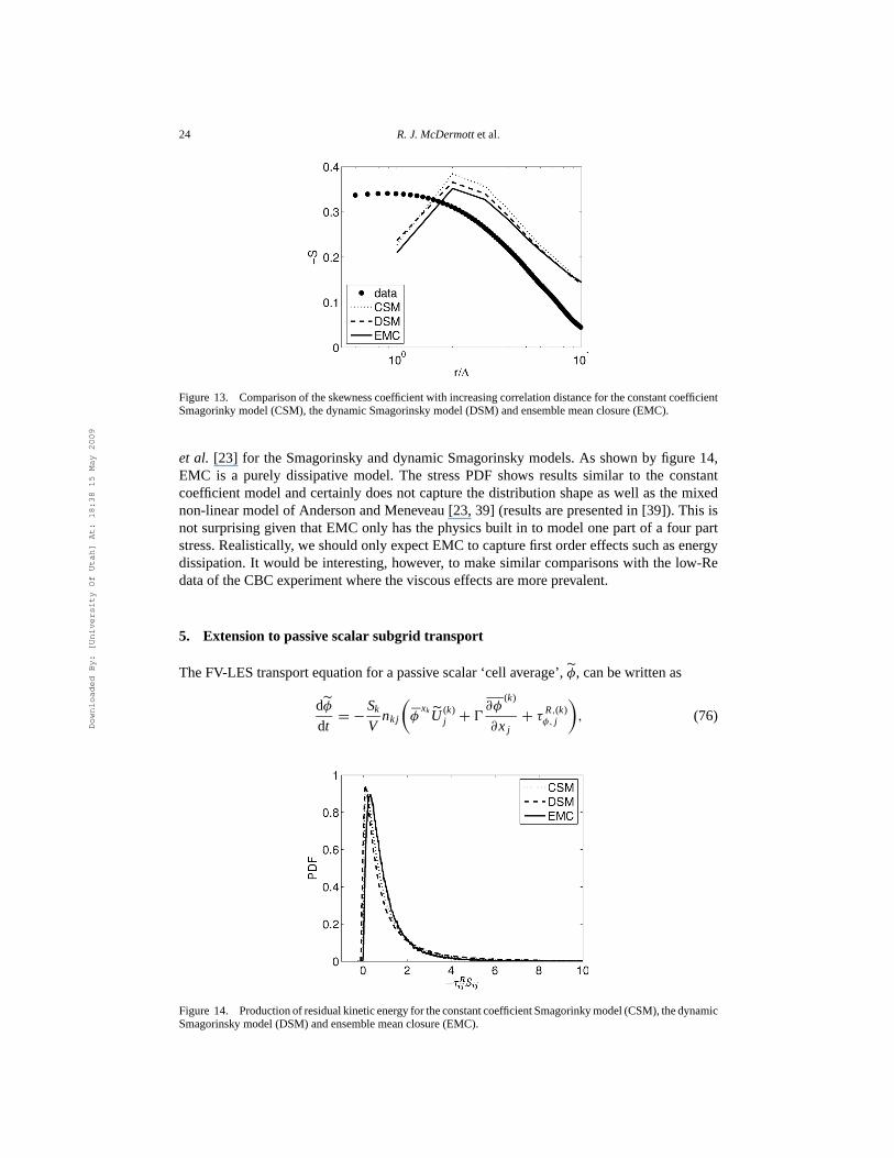
et al. [23] for the Smagorinsky anddynamicSmagorinsky models.As shown by figure 14,EMC is a purely dissipative model.The stressPDF shows resultssimilar to the constantcoefficient modelandcertainlydoesnot capturethedistribution shapeaswell asthemixednon-linearmodelof AndersonandMeneveau[23, 39] (resultsarepresentedin [39]). This isnot surprisinggiven thatEMC only hasthephysicsbuilt in to modelonepartof a four partstress.Realistically, we shouldonly expectEMC to capturefirst ordereffectssuchasenergydissipation.It would be interesting,however, to make similar comparisonswith the low-Redata oftheCBC experimentwheretheviscouseffectsaremoreprevalent.

5. Extensionto passivescalar subgrid transport

TheFV-LES transportequationfor apassivescalar‘cell average’,φ, canbewrittenas

dφ

dt= −

Sk

Vnk j

(φ

xkU (k)j + Ŵ

∂φ(k)

∂x j+ τ

R,(k)φ, j

), (76)

Figure 14. Productionof residualkineticenergy for theconstantcoefficientSmagorinky model(CSM),thedynamicSmagorinsky model(DSM) andensemblemeanclosure(EMC).

Downloaded By: [University Of Utah] At: 18:38 15 May 2009

Residualstressclosure in finitevolumeLES 25

Figure 15. Residual shear stressPDF for the constantcoefficient Smagorinky model (CSM), the dynamicSmagorinsky model(DSM) andensemblemeanclosure(EMC).

wheretheoverbaris, again,asurfacefilter, Ŵ is themolecularscalardiffusivity, and

τR,(k)φ, j ≡ φU

(k)j − φ

xk U (k)j (77)

is theunclosedresidualscalarflux. Notice that thesecondtermof theresidualflux is againexplicitly basedonthenumericalscheme.For SchmidtnumbersSc≡ ν

Ŵ≥ 1, themixing rate

of the scalaris stronglydependenton τ Rφ, j [12] and is a direct result of unresolved scalar

advection.Theabstractionusedfor theturbulentflux in EMC is powerful in thatit allows themethod

to be easilyextendedto model the subgridtermsfor scalartransportwithout the needforturbulent Schmidt(Sct ) or turbulent Prandtl(Prt ) numbers(see,for example,[12, 13]). Asa review of theEMC concept,thescalar is linearized(basedon the local scalargradientinthe conceptualODT line direction)andmapped(via the triplet map)at a ratedeterminedby the time scalephysicsof thevelocityfield. Hence,thescalarmappingis tied to the ‘dis-placement’function, e.g. (5), and the time scale,τ , is tied to the energy (or strain)of thevelocity field. Becausescalarsarenot subjectto modificationanalogousto pressure-inducedvelocity scramblingduring advection,kernel redistribution is not appliedto scalarsafter atriplet mappingevent [1]; this only simplifiesmattersfor scalarEMC. In fact,in section2.2we have alreadyworked out all the mathematicsnecessaryto describethe scalardisplace-ment.In directanalogyto thevelocity linearization(seefigure1), thescalaris linearizedasfollows:

ϕ(r ) = Sφ(y)r + b, (78)

whereSφ ≡ [∂r φ(r )]r =y and,again,bdropsoutduringthederivation.Thescalardisplacementfunctionis, therefore,simply given by (6) with Sφ(y) substitutedfor S(y). Leaving freedomto improvethetimescalephysics,wecanthengeneralizetheEMC approximationto (77),forx j = y, as

τ Rφ,y ≈ Rφ(y) = −

2

27Sφ(y)

∫ lmax

lmin

l

τdl . (79)

Here Rφ(y) denotesour model for the residualscalarflux. The time scaleis basedon thevelocity (not scalar)field. Again, all the mathematicshasbeenworked out in the previous

Downloaded By: [University Of Utah] At: 18:38 15 May 2009

26 R.J. McDermottet al.

sections.Thus,for vanilla scalarEMC wehave

Rφ(y) = −1

27Ce

(l 2max − l 2

min

)|S(y)| Sφ(y). (80)

Notethat|S(y)| = [∂U (r )]r =y. For anenergy-basedtimescalewehave

Rφ(y) = −1

27

Ce√54

(l 2max − l 2

min

)|S(y)|Sφ(y). (81)

And for aReynoldsnumber-dependenttimescalewehave

Rφ(y) = −1

27CeF(Reh; Z, ν)Sφ(y), (82)

whereF is given by (38).Themodels(80)–(82)donotmakeuseof aturbulentSchmidtnumber. However, bycompar-

ing thescalarmodelwith themomentummodelwecandeduceanimplied turbulentSchmidtnumberfor EMC andwe find thatSct is dependenton thechoiceof α. Considera canonicalscalarflow problemin which a meanscalargradientanda homogeneoussheararealigned.That is, Sφ = S1 andS2 = S3 = 0. To mostclearly seethe affect of α with regard to theimplied turbulentSchmidtnumber, assumetheflow is at high Re(i.e. lmax ≫ lmin). We maythenuseequations(29)and(81) in ouranalysis.With thescalarandvelocitystrainsequalwecandeterminetheturbulentSchmidtnumberby (divide(29)by (81)for thespecificconditionsof thestatedcanonicalproblem)

Sct =1

2+

1

2

√β11. (83)

Therefore,recallingβij = δij +αTij (seesection2.3.2),for α = 0 we have Sct = 1,for α = 2/3we have Sct ≈ 0.79, andfor α = 1 we have Sct = 1/2. Hence,thevalueα = 2/3, which isphysicallypreferablebasedonequipartitionof energy, putstheturbulentSchmidtnumberveryneartheacceptedengineeringconstantvalue of0.7[12, 13].In reality, theturbulentSchmidtandPrandtlnumbersarenot constant,however. They vary in spaceandtime. Experimentalevidence(see,for example,[40]) suggeststhat the valuesrangefrom 0.7 to 0.9. EMC is acomputationallycheapmethodfor accountingfor the local variation.Note that Sct = 0.79(for α = 2/3) is specificto the conditionsof the canonicalproblem.The implied turbulentSchmidtnumberfor EMC wouldvaryspatiallyandtemporallywithin a realflow simulation.It shouldbenotedthat thehigh Reversionof themodelwas usedheresimply for clarity intheexample.TheRe-dependentversionfor scalarEMC (82) will alsoexhibit local variationin theturbulentSchmidtnumberandthemodelwill turn off in regionsof theflow wherethevelocity field is resolved.

6. Conclusions

Ensemblemeanclosureis anidealizationof ODT andallowstheoreticaldeterminationof therateconstantusingLilly’ s method[3]. Thetheoreticalvalue,Ce = 1.4

√54,workedwell for

thesuiteof validationtestspresentedhere(with thecaveatthattheconstantwasderived basedonα = 0 andwesubsequentlyfoundα = 2/3 to yield slightly betterresults).Thisrepresentsa significantimprovementin our understandingof ODT (ultimately our modelof interest).Thefactors1/27and1/

√54,for example,werepreviouslyburiedin empiricaltuning.Dueto

recursivemappingandthegeometryof thetripletmap,therateconstantfor thefull ODTmodelshouldbe lower by roughly a factorof 3. PreliminaryODT resultssupportthis hypothesis

Downloaded By: [University Of Utah] At: 18:38 15 May 2009

Residualstressclosure in finitevolumeLES 27

[8, 9]. Additionally, acomputationalmethodfor directevaluationof theODT rateconstantisidentifiedthatis analogousto thealgebraicmethodappliedto EMC.

EMC is a viable LES closurein its own right. The Reynoldsnumber-dependentversionincludesa viscouscutoff parameterwhich representsthe critical cell Reynoldsnumberforan eddyturnover andaddressesthe problemof finite eddyviscositywithout usingthe dy-namicprocedure.The low Re wind tunneldata ofComte-BellotandCorrsin[37] was usedto empirically determinethe cutoff value (Z ≈ 3.0). Good resultsareobtainedfor decay-ing isotropic turbulencesimulationsat two Taylor scaleReynoldsnumbersdiffering by anorderof magnitude.No explicit filtering stepwas requiredin thesecases,makingtheover-all approachattractive for engineeringcalculations.It hasbeenshown that the EMC con-ceptcanbe extendedin a straightforward way to modelthe residualadvective transportofscalarsin LES, providing a consistentlink betweensubgridmomentumand scalartrans-port without the needfor a priori specificationof turbulent SchmidtandPrandtlnumbers.Moreover, EMC yieldsa theoreticalpredictionof thesequantitiesthatagreeswith empiricalestimates.

The utility of EMC extendsbeyond LES closure.Many problemsin engineering,mete-orology andastrophysicsreachReynoldsnumberswhereeven resolvingODT down to thedissipativescalesis tooexpensive. EMC is theprimecandidatefor subgridclosureof ODT inthiscase.Schmidtetal. [8] usedEMC asthesubgridclosurefor ODT, which in turnwas thesubgridclosurefor anLESof decayingisotropicturbulence,showingproofof conceptof whatis truly a multiscalemodelingapproach.Theefficacy of this strategy hasbeendemonstratedby ageophysicalflow application[21].

Furtherwork is requiredto determinetheimplicationsof thepresenttheoreticalframeworkwith regardto thefull ODT model.In full ODT anoptimalvaluefor lmax will exist. Variationof lmax is directly offsetby variationin Ce, throughLilly’ s analysis(i.e. lmax andCe arenotindependentparameters)andsoin EMC thespecificvalue ofthelengthscaleis unimportant;how onecomputesthe local strain is really what determinesthe filter width. In full ODT,however, stochasticbackscatterandsubgridstatisticscanbemodeledandthespecificCe–lmax

combinationcanaffect theresultssignificantly.

Acknowledgements

Fundingfor thiswork wasprovidedthroughaDepartmentof Energy ComputationalScienceGraduateFellowship(DE-FG02-97ER25308).This work was partially supportedby theUSDepartmentof Energy, Office of Basic Energy Sciences,Division of ChemicalSciences,Geosciences,andBiosciences.SandiaNationalLaboratoriesis a multi-programlaboratoryoperatedby SandiaCorporation,a LockheedMartin Company, for the US DepartmentofEnergy undercontractDE-AC04-94-AL85000.Wewouldliketo especiallythankTom Smithfor his isotropicturbulenceinitializationcode,StevedeBruynKopsfor insightfuldiscussionsregardinginitializationandChrisKennedyfor helpwith hishighorderinterpolants.

Appendix A. Finite volumeflux symmetry

Herewe clarify what is meantby ‘symmetry’ of thefinite volumesurfacefluxes,show thatthey aresymmetricto secondorderin spaceandgive asimpleflow exampleto show thatthesefluxesarenot identicallysymmetricin general.

Theresidualstressonasurfaceof acontrolvolume(CV) is definedas

τ Rij ≡ Ui U j − U i U j . (84)

Downloaded By: [University Of Utah] At: 18:38 15 May 2009

28 R.J. McDermottet al.

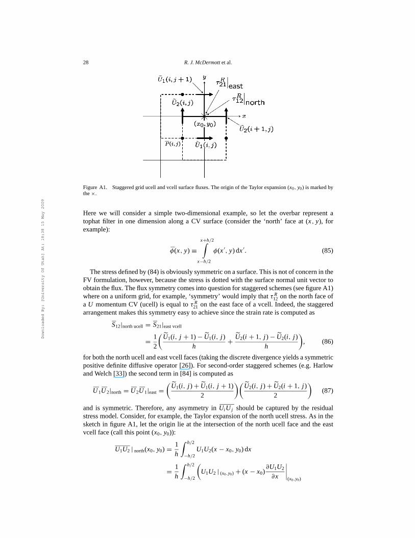
Figure A1. Staggeredgrid ucell andvcell surfacefluxes.Theorigin of theTaylor expansion(x0, y0) is markedbythe×.

Here we will considera simple two-dimensionalexample,so let the overbar representatophatfilter in one dimensionalong a CV surface(considerthe ‘north’ faceat (x, y), forexample):

φ(x, y) ≡x+h/2∫

x−h/2

φ(x′, y) dx′. (85)

Thestressdefinedby (84)is obviouslysymmetriconasurface.Thisis notof concernin theFV formulation,however, becausethestressis dottedwith thesurfacenormalunit vectortoobtaintheflux. Theflux symmetrycomesinto questionfor staggeredschemes(seefigureA1)whereon a uniform grid, for example,‘symmetry’ would imply thatτ R

12 on thenorthfaceofa U momentumCV (ucell) is equalto τ R

21 on theeastfaceof a vcell. Indeed,thestaggeredarrangementmakesthis symmetryeasyto achievesincethestrainrateis computedas

S12|northucell = S21|eastvcell

=1

2

(U1(i, j + 1) − U1(i, j )

h+

U2(i + 1, j ) − U2(i, j )

h

), (86)

for boththenorthucellandeastvcell faces(takingthediscretedivergenceyieldsasymmetricpositive definitediffusive operator[26]). For second-orderstaggeredschemes(e.g.HarlowandWelch[33]) thesecondtermin [84] is computedas

U1U2|north = U2U1|east=(

U1(i, j ) + U1(i, j + 1)

2

)(U2(i, j ) + U2(i + 1, j )

2

)(87)

and is symmetric.Therefore,any asymmetryin Ui U j shouldbe capturedby the residualstressmodel.Consider, for example,theTaylor expansionof thenorthucell stress.As in thesketchin figure A1, let the origin lie at the intersectionof the north ucell faceandthe eastvcell face(call thispoint (x0, y0)):

U1U2 | north(x0, y0) =1

h

∫ h/2

−h/2U1U2(x − x0, y0) dx

=1

h

∫ h/2

−h/2

(U1U2 | (x0,y0) + (x − x0)

∂U1U2

∂x

∣∣∣∣(x0,y0)

Downloaded By: [University Of Utah] At: 18:38 15 May 2009

Residualstressclosure in finitevolumeLES 29

+(x − x0)2

2

∂2U1U2

∂x2

∣∣∣∣(x0,y0)

+ · · ·)

dx

= U1U2 | (x0,y0) +h2

24

∂2U1U2

∂x2

∣∣∣∣(x0,y0)

+ · · · (88)

Similarly, theeastvcell advectiveflux is

U2U1|east(x0, y0) = U2U1|(x0,y0) +h2

24

∂2U2U1

∂y2

∣∣∣∣(x0,y0)

+ · · · (89)

Subtracting(89) from (88) yieldstheasymmetryin thesurfacefluxes,which is secondorderfor theuniformgrid case(all termsevaluatedat (x0, y0)):

U1U2 | north − U2U1 | east=h2

24

[∂2U1U2

∂x2−

∂2U2U1

∂y2

]+ · · · (90)

As asimpleexampleillustratingthat(90) is not zeroin generalconsidertheflow field

U1(x, y) = ax + by,

U2(x, y) = cx − ay, (91)

wherea, b andc areconstants.This field obeys continuity ∂xU1 + ∂yU2 = a − a = 0, butuponsubstitutioninto (90)yields

U1U2 | north − U2U1 | east=h2

12[a(b + c)] + · · · (92)

If b = c the flow is irrotational (ωz = ∂yU1 − ∂xU2 = b − c) but the fluxes are still notidenticallysymmetric.

Appendix B. Derivation of Reynoldsnumber-dependentclosure

Herewe go throughthederivationof (33).Usingthekernel-basedmomentumdisplacement(section2.3.1)wecanwrite

Ri (y) =∫ lmax

lmin

1

τ

∫ y

y−l

ψi (y; y0, l )

l 2dy0 dl ,

= −2

27

(1

2Si (y) +

1

2sgn(Si (y))

√βijS

2j (y)

)

︸ ︷︷ ︸A

∫ lmax

lmin

l

τdl ,

= ACe

∫ lmax

lmin

l

(1

54

∑

j

S2j (y) −

Z2ν2

l 4

)1/2

dl . (93)

At thispointwemake thefollowing changeof variables.Let

Ri (y) = ACe

∫ lmax

lmin

l√

a2 − x2 dl , (94)

where

a2 =1

54

∑

j

S2j (y) and x2 =

Z2ν2

l 4. (95)

Downloaded By: [University Of Utah] At: 18:38 15 May 2009

30 R.J. McDermottet al.

Hence,

l = (Zν)12 x− 1

2 and dl = −1

2(Zν)

12 x− 3

2 dx . (96)

Substitutingthesechangesinto (94)yields

Ri (y) = ACe

∫ xmax

xmin

l︷ ︸︸ ︷[(Zν)

12 x− 1

2 ]√

a2 − x2

dl︷ ︸︸ ︷[−

1

2(Zν)

12 x− 3

2 dx

],

= ACe

(−

1

2

)Zν

∫ xmax

xmin

√a2 − x2

x2dx . (97)

Thelimits of integrationarexmin = Zν/ l 2min andxmax = Zν/ l 2

max.Fromintegral tableswefind that

∫ √a2 − x2

x2dx = − sin−1

(x

a

)−

√a2 − x2

x+ C. (98)

Hence,

Ri (y) = ACe

(−

1

2

)Zν

[− sin−1

(x

a

)−

√a2 − x2

x

]Zν/ l 2max

Zν/ l 2min

,

= ACe

(−

1

2

)Zν

sin−1

(Zν

al2min

)+

√a2 −

(Zν

l 2min

)2

Zν

l 2min

− sin−1

(Zν

al2max

)−

√a2 −

(Zνl 2max

)2

Zνl 2max

,

= −1

2ACe

[√a2l 4

min − (Zν)2 −√

a2l 4max − (Zν)2

+ Zν

(sin−1

(Zν

al2min

)− sin−1

(Zν

al2max

))], (99)

recovering(33)and(34).

Appendix C. Numerical implementation details for EMC

Here we detail the numerical implementationfor EMC with a staggeredgrid arrange-ment. Perhapsthe most clear and conciseway to describethis implementationis to fol-low a two-dimensionalexample.The sameideasareeasilyextendedto threedimensions.This particular implementationwas chosento maintain consistency with full ODT clo-sure for LES [8, 9] where the ODT lattice lines intersectat the pressurecell (pcell)center.

To avoid confusionrelatedto componentindexing andgrid indexing we will use[U, V ]insteadof [U1,U2] to representthevelocitycomponents.Herekeepin mindthattheindex pair

Downloaded By: [University Of Utah] At: 18:38 15 May 2009

Residualstressclosure in finitevolumeLES 31

Figure C1. Staggeredgrid arrangementfor computingEMC stresses.The smalldotted(notdashed)linescrossingat thepcell centerrepresentanODT lattice.

(i , j ) representsa computationalstoragelocation,not a discretespatiallocation.FigureC1shows the staggeredgrid layout. The solid dotsrepresentthe pcell center. The right arrowrepresentsthestoragelocationandcenterof au momentumcell (ucell) andtheuparrow isav momentumcell center(vcell).

Thefirst stepin computingthestressis to interpolatetheucell andvcell velocitiesto thepcell location.ThesearestoredasUp andVp. Weusethe10th-orderinterpolationof Kennedy[41]. We use(33) astheEMC modelwith (38) employed for F . Evaluatingthestressfor agiven directionreducesto evaluatingthevelocitygradientvectorfor thatdirection.

C.1 Diagonal components

Thediagonalcomponentsof thestressarecomputedandstoredat thepcell center. Herewewill needthefull velocitygradienttensor.

∂xU | pcell ≈U (i, j ) − U (i − 1, j )

h,

∂xV | pcell ≈Vp(i + 1, j ) − Vp(i − 1, j )

2h,

∂yU | pcell ≈Up(i, j + 1) − Up(i, j − 1)

2h,

∂yV | pcell ≈V(i, j ) − V(i, j − 1)

h. (100)

C.2 Off-diagonal components

WestoreR21 at theucell locationfor easyaveragingover thevcell eastandwestfaces:

∂xU | ucell ≈Up(i + 1, j ) − Up(i, j )

h,

Downloaded By: [University Of Utah] At: 18:38 15 May 2009

32 R.J. McDermottet al.

∂xV | ucell ≈Vp(i + 1, j ) − Vp(i, j )

h. (101)

WestoreR12 at thevcell locationfor easyaveragingover theucell northandsouthfaces:

∂yU | vcell ≈Up(i, j + 1) − Up(i, j )

h,

∂yV | vcell ≈Vp(i, j + 1) − Vp(i, j )

h. (102)

C.3 Computingthestressdivergence

The averageof the diagonalcomponentsis subtractedand the deviatoric part usedin thecomputation(hereq, r, s arecomponentindices),

Rdqr = Rqr − δqr Rss . (103)

For theucell the R11 stressis locatedon theeastandwestfacesof a ucell CV. Thenorthandsouthfacestressesrequireaveraging.Referringto (65),thediscreteapproximationto thesubgridforceis given by (k is acomponentindex andsummationis implied)

δR1k

δxk(i, j ) =

Rd11(i + 1, j ) − Rd

11(i, j )

h+

Rd12(i, j ) − Rd

12(i, j − 1)

h, (104)

where

Rd12(i, j ) =

Rd12(i, j ) + Rd

12(i + 1, j )

2. (105)

Similarly, for thevcell wehave

δR2k

δxk(i, j ) =

Rd22(i, j + 1) − Rd

22(i, j )

h+

Rd21(i, j ) − Rd

21(i − 1, j )

h, (106)

where

Rd21(i, j ) =

Rd21(i, j ) + Rd

21(i, j + 1)

2. (107)

References

[1] Kerstein,A.R.,Ashurst,W.T.,Wunsch,S.andNilsen,V.,2001,One-dimensionalturbulence:vectorformulationandapplicationto freeshearflows.Journalof Fluid Mechanics, 447, 85–109.

[2] Germano,M., Piomelli, U., Moin, P. andCabot,W., 1991,A dynamicsubgrid-scaleeddyviscositymodel.Physicsof FluidsA, 3, 1760–1765.

[3] Lilly , D.K., 1967,Therepresentationof small-scaleturbulencein numericalsimulationexperiments.In Pro-ceedingsof the IBM ScientificComputingSymposiumon EnvironmentalSciences(Yorktown Heights,NewYork: IBM).

[4] PierreSagaut.,2001,LargeEddySimulationfor IncompressibleFlows(Berlin: Springer).[5] Kerstein,A.R.,1999,One-dimensionalturbulence:modelformulationandapplicationto homogeneousturbu-

lence,shearflows,andbuoyantstratifiedflows.Journalof Fluid Mechanics, 392, 277–334.[6] Pope,S.B., 2004,Ten questionsconcerningthe large-eddysimulationof turbulent flows. New Journal of

Physics, 6.[7] Schmidt,R.C., Kerstein,A.R., Wunsch,S. and Nilsen, V., 2003, Near-wall LES closurebasedon one-

dimensionalturbulencemodeling.Journalof ComputationalPhysics, 186, 317–355.[8] Schmidt,R.C., McDermott,R. andKerstein,A., 2005,ODTLES: A Model for 3D Turbulent Flow Based

onOne-dimensionalTurbulenceModelingConcepts,Report2005–0206(Albuquerque,New Mexico: SandiaNationalLaboratories).

[9] McDermott,R.J.,2005,Towardone-dimensionalturbulencesubgridclosurefor large-eddysimulation.PhDthesis,Universityof Utah.

Downloaded By: [University Of Utah] At: 18:38 15 May 2009

Residualstressclosure in finitevolumeLES 33

[10] Kerstein,A.R., 1988,A linear-eddymodelof turbulentscalartransportandmixing. CombustionScienceandTechnology, 60, 391–421.

[11] Kerstein,A.R., 1991,Linear-eddymodellingof turbulent transport.Part 6. Microstructureof diffusive scalarmixing fields.Journalof Fluid Mechanics, 231, 361–394.

[12] Fox. R.O., 2003,ComputationalModelsfor Turbulent ReactingFlows (Cambridge:CambridgeUniversityPress).

[13] NorbertPeters,2000,TurbulentCombustion(Cambridge:CambridgeUniversityPress).[14] Sankaran,V., Porumbel,I. andMenon,S.,2003,Large-eddysimulationof single-cupgas-turbinecombustor

flows. In 39thAIAAJoint PropulsionConference:AIAA2003-5083.[15] Smagorinsky, J.,1963,Generalcirculationexperimentswith theprimitiveequations.MonthlyWeatherReview,

91, 99–106.[16] Moin, P.,Squires,K., Cabot,W. andLee,S.,1991,A dynamicsubgrid-scalemodelfor compressibleturbulence

andscalartransport.Physicsof FluidsA, 3, 2746–2757.[17] Kerstein,A.R., 2003,Nonlocalfirst-orderclosurebasedonODT. Unpublished.[18] Pope,S.B.,2000,TurbulentFlows(Cambridge:CambridgeUniversityPress).[19] Ashurst,W.T. andKerstein,A.R., 2005,One-dimensionalturbulence:variable-densityformulationandappli-

cationto mixing layers.Physicsof Fluids, 17, 025107-1–025107-26.[20] Wunsch,S. andKerstein,A., 2001,A model for layer formation in stablystratifiedturbulence.Physicsof

Fluids, 13, 703–712.[21] Kerstein,A.R. andWunsch,S., In press,Simulationof a stablystratifiedatmosphericboundarylayer using

one-dimensionalturbulence.BoundaryLayerMeteorology.[22] Meneveau,C. andLund,T.S.,1997,ThedynamicSmagorinsky modelandscale-dependentcoefficientsin the

viscousrangeof turbulence.Physicsof Fluids, 9, 3932–3934.[23] Kang,H.S.,Chester, S. andMeneveau,C., 2003,Decayingturbulencein an active-grid-generatedflow and

comparisonswith large-eddysimulation.Journalof Fluid Mechanics, 480, 129–160.[24] Schumann,U., 1975,Subgridscalemodelfor finite differencesimulationof turbulentflows in planechannels

andannuli.Journalof ComputationalPhysics, 18, 376–404.[25] Lomax,H., Pulliam,T.H. andZingg, D.W., 2001,Fundamentalsof ComputationalFluid Dynamics(Berlin:

Springer).[26] R.W.Verstappen,C.P. andA.Veldman,E.P., 2003,Symmetry-preservingdiscretizationof turbulentflow. Jour-

nal of ComputationalPhysics, 187, 343–368.[27] Ham,F.E., Lien, F.S.andStrong,A.B., 2002,A fully conservative second-orderfinite differenceschemefor

incompressibleflow onnon-uniformgrids.Journalof ComputationalPhysics, 177, 117–133.[28] Morinishi, Y., Lund, T.S.,Vasilyev, O.V. andMoin, P., 1998,Fully conservative high orderfinite difference

schemesfor incompressibleflow. Journalof ComputationalPhysics, 143, 90–124.[29] Harten,A., 1989,ENOschemeswith subcellresolution.Journalof ComputationalPhysics, 83, 148–184.[30] Shu, C.W., 1997, Essentiallynon-oscillatoryand weightedessentiallynon-oscillatoryschemesfor hyper-

bolic conservation laws. NASA/CR-97-206253ICASE ReportNo. 97-65.Availableonline at: http://www.icase.edu./library/reports/rdp/97/97-65RDP.refer.html

[31] Leonard,A., 1974,Energy cascadein largeeddysimulationof turbulentfluid flow. Advancesin Geophysics,18A, 237–248.

[32] Bardina,J.,Ferziger, J.H.andReynolds,W.C.,1980,Improvedsubgrid-scalemodelsfor large-eddysimulation.AIAA, 980–1357.AmericanInstituteof AeronauticsandAstronautics,FluidandPlasmaDynamicsConference,13th,Snowmass,Colo.,July14–16,1980.

[33] Harlow, F.H. andWelch,J.E.,1965,Numericalcalculationof time-dependentviscousincompressibleflow offluid with a freesurface.Physicsof Fluids, 8, 2182–2189.

[34] Shu, C.W. and Osher, S., 1988, Efficient implementationof essentiallynon-oscillatoryshock-capturingschemes.Journalof ComputationalPhysics, 77, 439–471.

[35] Suresh,A. andHuynh,H.T.,1997,Accuratemonotonicity-preservingschemeswith Runge-Kuttatimestepping.Journalof ComputationalPhysics, 136, 83–99.

[36] Chorin,A.J. andMarsden,J.E.,1990,A MathematicalIntroductionto Fluid Mechanics, 3rd Edn(New York:Springer).

[37] Comte-Bellot,G. andCorrsin,S., 1971,SimpleEulariantime correlationof full- andnarrow-bandvelocitysignalsin grid-generated,‘isotropic’ turbulence.Journalof Fluid Mechanics, 48, 273–337.

[38] deBruyn Kops.S.M., 1999,Numericalsimulationof non-premixed turbulentcombustion.PhDthesis,Uni-versityof Washington.

[39] Anderson,R. andMeneveau,C., 1999,Effectsof the similarity model in finite-differenceLES of isotropicturbulenceusingaLagrangiandynamicmixedmodel.Flow TurbulenceandCombustion, 62, 201–225.

[40] Chang,K. andCowen,A., 2002,TurbulentPrandtlnumberin neutrallybuoyant turbulent roundjet. Journalof EngineeringMechanics, 128, 1082–1087.

[41] Kennedy, C.A. and Carpenter, M.H., 1994, Several new numericalmethodsfor compressibleshear-layersimulations.AppliedNumericalMathematics, 14, 397–433.

[42] Misra, A. andPullin, D., 1997,A vortex-basedsubgridstressmodel for large-eddysimulation.PhysicsofFluids, 9, 2443–2454.

Downloaded By: [University Of Utah] At: 18:38 15 May 2009