A Ionescu LAP Mixing monograph

Foreword

The interaction between mathematics and biology can be divided in three classes. The first

one implies applying some known mathematical techniques to some biological problems. Such

applications are influencing the mathematics only when the biological context requires the refining

of these techniques – this is of course a slow process. The second class contains the cases where the

mathematical techniques are not adequate, so there are necessary new techniques to be developed,

in an appropriate working context. Finally, the third class contains the situations when new

biological trends could require new qualitative or analytical thinking. In these cases there is

necessary to create new mathematical zones for a good approach of these biological problems.

Thus, the development of new biological technologies and the faster collecting and processing of

data would imply both using the actual mathematics and creating new ones.

It is worthy of note the important influence of other domains. The theory of dynamic

systems and partial derivatives equations are domains where the biological problems brought

serious results. In theoretic fluid mechanics, the dominant trend was the understanding of large

Reynold numbers fluids and incompressible fluids. Recently, the molecular biology stimulated the

advance in topological and low dimensions analysis.

The present work is an interdisciplinary one, approaching a very actual interest area, namely

the qualitative analysis of excitable media. By approaching this question from the systems’ theory

standpoint, a great step is made on fulfilling a realist requirement – namely the interdisciplinary

approach necessity. There are a lot of examples for showing the call of passing from local, “hand-

made” approaches to larger, “industrial” ones, for the problems which the science often encounters.

Having not the claim to be “the science of sciences”, the systems’ theory answered in a good

manner to this call.

The basic target of this work is part of a larger one: the study of the oscillators’, structural

stability, especially for the biological oscillator. The structural stability is understood in the

Andronov’s sense, namely is taken into account the topological structure change for a dynamical

system when its structure is changed. There is pointed out on the parallelism between the structural

stability concept and the mixing concept, in Ottino’s sense. The experimental results matched the

numerical simulations, in a space-time panel with random distributed events. The statistical cases

carefully collected are very important for further studies on the way of far from equilibrium models.

Table of contents

1. Introduction. Recent trends in biomathematics 3

2. Biological rhythms. The simplest biological oscillators and their stimulation 9

2.1. Daily rhythms 9

2.2 Rhythms in cell populations 11

2.3. Biochemical oscillators 13

2.4. Neural oscillators 15

2.5. Oscillators’ stimulation 19

3. Mixing and turbulence in excitable media 28

3.1. Flow kinematics. Length and surface deformations 28

3.2. Kinematics of deformations 34

3.3. The analysis of mixing efficiency for 2D and 3D excitable media 37

3.4 Concluding remarks 54

Appendix 58

References 61

2

1. INTRODUCTION. RECENT TRENDS IN BIOMATHEMATICS

During the time, the application of mathematics in biology had an important influence on

developing the new branches of mathematics. If the mathematical theories have a long life –

hundreds, maybe thousands years, the most biological knowledge are recent and the biological

theories have a rapid evolution. However, the interaction between mathematics and biology

produced the issue of new mathematical fields.

The interaction between mathematics and biology can be divided in three classes. First one

implies applying some actual mathematical techniques in some biological problems. Applications

like these influence mathematics only when the biological context requires the refinement of these

techniques, and this is obviously a slow process. The second case contains the cases where the

mathematical techniques are not adequate, and therefore it is necessary the improvement of them, in

a new context. Finally, the third class contains the situations where new biological currents could

require new qualitative or analytical thinking manners. In these cases it is necessary to construct

new mathematical areas for approaching these new biological problems. The fast development of

new biological technologies, on one hand, and the fast acquiring of data, on the other hand, will

imply to handle the classical mathematics, but also to develop new mathematics.

Going back into the history, it can be seen that the applications of mathematics in biology is

not new. The botanist Robert Brown discovered the Brownian movement from the study of the

pollen grains in water. Nowadays, this movement is central in probabilities theory. Also, the

catastrophe theory is a mathematical branch which can allow important extends by biological

approaches. Rene Thom [75] brought a large interest in singularities bifurcations of dynamical

systems theory, the modelling tools producing amazing applications. And, lat but not least, the

statistics origins are closely related to biology.

It must be also noticed another domain when consistent influence, namely the theory of

dynamic systems and partial differential equations. There, the biological problems brought fruitful

results. In theoretic fluid mechanics, the basic developing trend was to understand the flows of great

Reynolds number and incompressible flows. Biology justified a great number of results in fluids

viscosity [62].

3

Statistics and Stochastic Processes

Statistics is the most applied mathematical branch in biology, its position showing the actual

intellectual and scientific development in 20th century: “From the chances doctrine to the

probabilities theory, from the least squares to regression analysis, the statistic progresses registered

until 1900 are as influent as those associated with the name of Darwin and Newton [69].

Let us remember the most important influences. Porter (1986) assessed that “the modern

field of mathematical statistics derived from biometry is not just fortuitous. The quantitative study

of the biological heritage and of the evolution offered a context for the statistical thinking. The

quantitative genetics remains a good example for a scientific area whose theoretical base is

completely constructed from statistical concepts. The great stimulus of modern statistics comes

from the correlation method invented by Galton, and assembled firstly not numerically, but like a

statistical low of heredity”.

The problems of genetics and evolution theory have a great influence both on probabilities

and statistics. Galton and Watson constructed the so-called “branch processes” theory, in response

to the problem of extending human family names. Yule, a Galton’s student, developed the random

process named also “the Yule’s process”, answering to some generic problems [85]. Later Mc

Kendrick [43] developed himself a nonlinear process theory of growing and death responding to the

epidemiology theory.

The influence of biology in statistics and probabilities theory was also very powerful this

century. The famous work of Feller on stochastic processes laid back on Volterra’s competition

theory and then continued by answering some population genetics’ problems [19,44].

There are few recent and future challenges for statistics and probabilities, which are inspired

from molecular biology, genetics and molecular evolution and which would require new theories

and techniques. An example of such a challenge is the study of the DNA sequence data in order to

reconstruct the genetic trees, analyzing complex genetic features and studying other problems. As

long as data sequences are collected, new patterns issue and new exploratory analysis theories are

required in order to verify the patterns’ consistency. Comparing two DNA (or protein) sequences

for finding similarities (aligned sequences) required new algorithms. The comparisons could answer

both to evolution and functional problems. Are these sequences part of a common ancient

sequence? Are they dedicated to similar functions? An important deal was to calculate the

probability of a large overlapping region for two DNA sequences, where there is involved a

dependence level as result of overlapping region. There were established strong limiting laws,

producing, with a given error, rates of the longest overlapping areas between different sequences, as

long as the sequence length increases. A special distributional behaviour was obtained by Chein-

4

Stein method of approximate by a Poisson random variable. These distributional results are now

used as basis for statistics tests.

In this field must also be noticed as relevant appliances, the calculus with Markov chains

and with probabilities on direct graphs, the maximum probable estimation for multinomial with

strongly non-smooth parameter spaces.

Another mathematical research area stimulated by biology is the probabilistic theory of

discrete and dynamics structures. If this research type began in the last three decades, the significant

results are now issuing. Significant developments in this area are including random graphs and

random directed graphs, systems of interacting particles, stochastic automatic cells, products of

random matrix and nonlinear dynamic systems with random coefficients. For example, Erdos and

Renyi [16] created a field of random graphs in order to model some seemingly random connexions

in neural networks. They also discovered few “phase transitions” examples in neural activity.

The achievements of computational methods made a revolution in the measurements

techniques, producing an amount of biological data and simultaneously a requirement of improving

the analyzing quantitative methods. The interface between experiment, mathematics and calculus is

pointed out at each stage of the scientific research. A biological investigation concludes almost

always with a proposal for a certain class of mathematical models. These models could go into the

molecular process (although this is not experimentally observable) and suggest new experiments.

For example, the numbering processes were developed for studying patterns of nervous impulses

interactions from different neurons (Brillinger [11], Tuckwell [78]). Markov processes were

extensively used for analyzing the data of membranes chains, studying the kinetic behaviour of

ionic chains and also understanding the surviving potential of human cell, and the risk of ionization

radiations on the DNA (Neyman and Puri [54];Yang and Swenberg [84]). A special feature of these

studies is that both the transition mechanisms and the states’ space have to be interpolated from

data. In fact, the analysis of singular data chains by markovian models produced new evaluations of

some neural parameters which are different from those of the classical Hodgkin-Huxley model [2].

The stochastic character of the measurements produced new developments in stochastic

differentiation and integration. Also, the neuro-biology has influenced a lot the development of this

area.

5

The dynamic systems theory

This theory was also much stimulated by biology. For example, the iterations of a nonlinear

function described by a simple population model, records the dynamics of an isolated population

with discrete generations, and consequently the influences which are modelling the population

number by the population size exclusively. In concrete terms, it is supposed that the size of the

population at (n+1) th generation is a (given) non-linear function of the size of the population at n th

generation. These types of models were introduced in the populations study much time ago. Isolated

studies on the functions’ iterations appeared at the beginning of 20-th century. Between them there

must be noticed those of Julia [42] and Fatou [17], then Sarkovskii [64] and Myrberg, which

brought a richer mathematical structure. However, only at the beginning of 70’s it was recorded a

great appreciation on the beauty and depth of the mathematic phenomena involved in these

problems. It is not sure if this iterations theory should finish without the influences of populations’

biology, but for sure the reasons from this domain were a part of the historical events chain which

led to important mathematical discoveries.

The study of the simple populations’ models is a classical example of mutual interaction

between mathematics and biology, with important results and benefits for both. The jointed efforts

of mathematicians, physicists and biologists formed a positive results network which realized a

new, sophisticated level. Their investigations clearly showed the existence of some universal

bifurcation sequences in the iterations of one-dimensional applications. Libchaber has shown the

striking matching of Feigenbaum’s discoveries concerning the period doubling in flow convection

experiments. These studies were basic for much mathematical achievements. Thus, Lanford

extended the Feigenbaum’s works using numeric analysis and gave a strong computational proof.

The study of interval applications was extended to circle applications. This study of circle

applications was used by Glass, Winfree & others [80] in order to describe the phase responses of

biological oscillators, especially in cardiology. The studies on interval applications constituted also

the start point for the works on Henon application, a two-dimensional application which is a

prototype of chaotic application.

The mathematics described above can be evaluated both from the impact on mathematics

itself, and for its significance in the real world. The topic is of very large interest. There is exhibited

a rich structure using a consistent mathematical objects set. Extending a little, there can be assessed

that all one-dimensional applications families have the same dynamic behaviour. Understanding this

analytical and geometrical truth is still a challenge and also an important research area with

amazing interactions in “complex dynamics world” and cvasi-conform applications. On the other

hand, the above mathematical theory contains basic mechanisms necessary for realizing a chaotic

behaviour in physical systems and for universal bifurcations patterns which systems that seem to

6

have no initial connection each other, exhibits. Within mathematics, this events sequence had a

great success, and the interest on biological models was an important stimulus for mathematicians.

But the impact of the mathematics on the biological sciences is still continuing. Close by the studies

implying one-dimensional applications iterations, there issued a lot of common points of biological

sciences and dynamic systems theory. Is quite rare when there can be measured all the parameters

values of a dynamic system associated to a biological phenomena; in fact the models themselves

represent the behaviour of some aggregated situations. That’s why there is desired to have a

classification of possible dynamic behaviours proceeding from models. This problem stays like an

important common problem of mathematics and biology. For example, recent a great interest

exhibits the dynamics of biological neurons networks and also the dynamics of coupled oscillators

systems. In both of situations there are searched explanations for the details of the dynamic

behaviour and understanding how the community behaviour issues from coupling the individual

elements. As the number of elements grows, there is necessary a combination of singular

perturbations methods, continuum methods and dynamics systems theory.

Nonlinear Partial Differential Equations and Functional Equations

These equations were applied custumal in physical sciences. There are a lot of examples

pointing out the impact of biological ideas on mathematical research in this area.

The demographic methods were applied from centuries to the stud of human and non human

populations. These methods, which constitute the basis both for the population projections and for

understanding the consequences of life historical phenomena, had a strong impact on the

mathematical theory. An important imagine of the demographic impact is given by the ergodic

theorems history. The renewing equation – a convolution integral equation which was the first

dynamic model for an age – dependent population, has its roots in the work of Euler, Bortkiewicz

and Lotka [63].

Sharpe and Lotka [66] motivated that the solutions of their renewing equation can be

represented in a Fourier type development. The mathematic reason was accepted only when Feller

[18] gave a rigorous proof for the asymptotic behaviour in similar conditions. Establishing the

conditions when the renewing equation admits a Fourier type solution is nowadays still an open

problem.

The further demographic models of McKendrick [51] and Gurtin and MacCamy [29] and

the epidemic models of Kermack and McKendrick [43] and Hoppensteadt [34] produced important

mathematical challenges in the functional equations domain. The strong interactions between

biology, ecology, demography and epidemics are a continuous source of mathematical problems

related to the existence, uniqueness and characterization of nonlinear functional equations’

7

solutions. And it must be assessed that these problems will be a fruitful area of mathematical

research.

The diffusion theory, describing the behaviour of molecules and particles populations with a

random movement, exhibits a field which is usually common to chemistry or physics. However, the

mathematics of nonlinear diffusion equations received a lot from biology. The interest of R.A.

Fisher [20] in the problem of diffusing the advanced genes in a population has stimulated the

preoccupations on an equation which mixes in the multiplicity diffusion with a nonlinear simple

(logistic) growing term. This feature was also concerned in by Kolmogorov and others, which

proved the existence of a stable travelling wave with its fixed velocity representing the advancing

wave of the advanced gene. This simple nonlinear reaction-diffusion equation was also studied like

a model for a spatial dispersion of a population.

The reaction –diffusion equations were investigated by Turing [76] for understanding the

pattern formation and the morphogenesis, two basic problems of development biology. The context

that non-uniform distributions of chemical substances should guide the cells differentiation

preceded Turing almost a half century, but it was not clear how “pre-patterns’ like that could

appear. Turing proved that the simple molecular diffusion, connected with appropriate bimolecular

interactions, could spontaneously produce this kind of pre-patterns, as a spatial uniform solution of

some coupled parabolic equations are bifurcating in a non-uniform state when some parameters are

varied.

Following the way opened by Turing and Fisher, the study of nonlinear reaction –diffusion

equations undergone a strong mathematical development. The study of travelling and stationary

waves’ solutions and also the study of bifurcations and dynamic behaviour of such equations

produced new and advanced mathematical techniques. Two and three dimensional geometry has

recent come into focus, including “target- patterns”, spirals, the roll waves geometry, etc. The

connections with the chemical reaction of Zhabotinskii [52], with cardiac physiology pathologies

and with non-uniform areal distributions of organisms in space brought new and consistent reasons

in this domain interest.

Although the equations and mathematical knowledge from demography and epidemiology

has already found their applications, there is a strong need for new mathematical branches to give

rise important and biologically based questions. An example is the interface between social

dynamics and biology where there are already constructed models describing the so-called “social

mixing” and its role in the diseases issue. These models could influence the practical statistics of

population health. Since the current techniques are still at the beginnings, it is expected that the

efforts give rise to new mathematical branches.

8

2. BIOLOGICAL RHYTHMS. THE SIMPLEST BIOLOGICAL OSCILLATORS AND

THEIR STIMULATION

Although the existence of biological rhythms is confirmed from ancient, the existence of

biological oscillators was relatively recent accepted. A basic feature of biological rhythms is that

their behaviour is due to external periodic effects (such as the daily periodic changes of the light

and darkness). Nowadays there are widespread the regards to “biological clocks”.

The most interesting oscillators are the “long-period oscillators”, generally with 24 hours

period. They generate a special interest, for the following reasons:

a) they are extremely important in biological functions;

b) their universality: except bacteria and the simplest organisms, all the living organisms have

such rhythms;

c) the biological mechanism responsible for these rhythms is still not elucidated;

d) the large time scale used allows realizing experiments for detailed study of different rhythms

dynamic properties.

2.1. Daily rhythms

Recent results assess the existence of endogenous oscillators in living systems. In particular,

it seems that daily cycles of biological phenomena are governed by such oscillators rather than

their own day/night interchanging. A reason for that is the organisms kept in carefully

controlled media, with constant light and temperature intensity, exhibited a periodicity in their

behaviour. Generally, the period is not of 24 hours, it varies between 22 and 26 hours. For an

individual the period remains generally (but not always) unchanged in time.

Fig.1. Daily rhythm outline

12 24 0 A B C D . . .

1 2 3 4 5 . . .

9

The behaviour of an individual can be handled in order to follow periodic changes of light and/or

temperature intensity – this is named in custom terms stimulation, or synchronisation. This is

possible only if the extern cycle period is closed to the intern period or to submultiples of it. An

interesting example is that of the kitchen beetle motion activity, the results are shown in Fig.2.

28

1

48

24h

Fig.2. Outline of a kitchen beetle motion activity

The connection between stimulus and behaviour is of great importance when studying the

biological oscillators, since the perturbations can be due both to changes in light and temperature,

and chemical factors.

It must be outlined that none of the above experiments properties is surprising for a clock

which has as basic function controlling the organism behaviour relative to environment.

If the organism behaviour is directly controlled by its environment, it must necessary appear some

delays between the light changing and – let’s say – the environment changing. Moreover, the

organism shall be more sensitive to random perturbations.

On the other hand, having an interior clock, synchronised with the external behaviour allows

the organism to better respond to daily environment changes. For example, most of people are

waking up in the morning by rote (and this is the interior clock) or by the alarm clock, therefore an

internal clock allows establishing a prediction control. The skill of predict certain events is an

important advantage for an individual and in this sense it comes to be natural that such a “clock”

exists in each individual studied until our days, from man and mammiferous going back on the

10

biological scale to insects and even unicellular organisms. This controller is named “daily clock”

and comes from the Latin expression “circa-diem” (approximately a day). This consists in fact of

two mutual coupled oscillators. In normal conditions, they are synchronised and behave as a single

oscillator. On the other hand, it is obviously that any organism can contain more than one

independent clock, each of which controlling a different function. This is the situation for man and

superior animals, unlike the unicellular organisms where there appears the opposite phenomena

(one clock is controlling few different functions).

2.2 Rhythms in cells populations

Relative to the stimulus, there exist four rhythm types.

1) Division and growing rhythms

A cells population which proliferates by division generally satisfies the following equation:

(1) ,)()( dttNtRdN ⋅=

where:

- dN is the changing in the cells number , from t to )(tN tt Δ+ ;

- R(t) is the cellular division rate; if .)( 0 constRtR == , then , that means

the population will have a logarithmic growing;

teNtN R ⋅⋅= 0)0()(

- the generation time – the time when the population doubles its number – is given by the

formula

(2) 2ln0

1⋅=

RgT

The cells cultures which satisfy the relation (2) are named logarithmic cultures. In certain

conditions, there exists the possibility to obtain synchronic cultures, with in most of time. 0)( =tR

Below is presented Fig.3. it must be observed that between t1 and t2 we have .)( consttN = ,

and between t2 and t3 is recorded a step changing. Also, if gTtt ≤− 13 , then 2)()(

1

3 =tNtN

. If the hills

R(t) are equally distanced, but smaller than Tg, then the corresponding steps will be negatively

correlated. This behaviour was observed in the cells culture of Euglena Gracilis.

11

N, R

t t1

t2

t3

N(t)

Fig.3. Rhythm cycle in “Euglena Gracilis”

Thus, the rhythm can be induced by light or temperature cycles, or by singular pulsations. The

rhythm still persists in constant light and temperature conditions, and can be stimulated by various

photo-periodic regimes. We can speak here about linear self-sustained oscillator.

2) Photo-tactile rhythms

In this class are included the algae, which respond to the light by swimming toward them.

This fact is very convenient for experimental measurements. For example: a lighting bar is pointed

toward the cells culture and the photo-tactile response is measured by the darkness degree.

t

Mob i l i t y

Fig.4. Time step race recording

The above figure shows a typical time step race recording, by interrupting the light with light

pulsations. The rhythm will be defined by the maxims hull. In the specific literature there are

defined few daily photo-tactile rhythms [149].

12

3) Biochemical rhythms

It can be measured the velocity with which various chemical reactions happen in various day

moments. In a number of moments, these velocities have a daily periodicity. This happens, for

example, when monoacids incorporating velocity in Euglena Gracilis, or in photo-synthetic

capacity of Gonyaulax Polyedra.

4) Rhythms related to luminosity

Here there can be considered, again, the algae, as many algae species exhibit daily rhythms.

These rhythms are strongly related to their various luminosity aspects. Recently it was proved that

there exists at least one species whose rhythm behaves like a single, “master” clock controls the

other and especially the cellular division, the photo-synthetic and luminescent ability. This does not

remain true for other species, which could have daily cycles of activity and disoperation with a

period different from its own temperature cycle.

The study of daily rhythms (or other rhythms) in micro-organisms is more adequate for

facilitate the understanding the “clocks” nature, than the study in superior organized species: as

long as the organism is simpler, the probability that the output of daily regulator is kept from

intermediate systems is smaller. Also, is easier to study the effect of chemical factors on the clock:

in a superior organism is possible to be never attained the basic regularisation level, because of the

complex metabolic system implied there.

2.3. Biochemical oscillators

The study of the chemical kinetics shows that it is really possible to have sustained

oscillations in the concentration of a chemical substance. Such an oscillator can serve as clock in

daily rhythms of cells populations. Prigogine and his collaborators have extensively studied this

problem in thermodynamics and described systems which can exhibit oscillations both in time and

space. Paintings for these oscillations were realized at cellular level by experiments, and

Zhabotinskii studied oscillations in inorganic media. Also, there were described various forms of

enzyme – catalysed reactions, which exhibit oscillations.

Particularly, there were studied DPNH (di -phosphor –pyridine nucleotide) oscillations, in

barm cells. This substance has a lot of properties which allow fast measurements with high accuracy

concentration, both in unbroken cells and in extracts.

Figure 5 below shows these oscillations.

13

DPNH

← 10 min → 347-390mm

Fig.5. DPNH oscillations

The waves in these oscillations can have a lot of forms, like in the below figures.

t

Fig.6

t

DPNH

Fig.7

These forms can be observed only in the cells without extract, and in intact cells there are observed

only sinusoidal wave forms. However, this fact does not indicate a basic difference in oscillation

mechanism in the two cases. The wave form handling is realized by adding different substances to

extracts. An intact cellular membrane is blocking any addition type and the handling is not possible.

Adding chemical substances and particularly, DPA (5-diphosphat adenosine) can promptly

produce important phase modifications (displacements) of oscillation. Moreover, the displacement

size and direction depend on the point where there were made the PDA addition.

Obviously, the derivative of DPNH concentration with respect to time has a discontinuity in the

point of PDA addition. That means either PDA concentration appears explicitly in the expression of

14

the associated dynamic system, or that on variable has a concentration which can be modified by

PDA at a greater rate than the rate of the other reactions implied in the oscillation. In such a case,

the reaction dynamics between PDA and the substance X can be ignored and further the X

concentration can be expressed as a simple function of that PDA, and the PDA concentration should

explicitly appear in the state equation.

2.4. Neural oscillators

There exist few examples of intensive periodic activity of various animals’ nervous system.

The study of neural membranes dynamics’ models, as well as direct observations, show that a

neuron can maintain an intensive activity at a constant rate for long time periods. This can be

considered as the simplest model of neural oscillator.

Let us show, in what follows, some basic models for locusts and marine organisms.

a) The control of locusts flying system

There is shown that “firing” patterns of the neurons which control the wings movie of this

insect are not depending on the prio- receptor feedback mechanisms. Also, there is no direct

correspondence between its pulsations and the pulsations produced by CNS (Central Nervous

System). The last ones seem to control only the global frequency and the oscillations level and are

responsible for passing from a level to another – for example from that of figure 8 a to figure 8 b

and reverse.

Fig.8 a Fig.8 b

An important conclusion was the existence of a neural oscillators group which are generating the

oscillating models. The oscillations frequency is controlled by external inputs, on that group, or, on

other CNS parts, or by various sensors.

15

b) Cellular firing patterns at marine organisms

Fig.8 c

The above figure shows the pattern of a cell of abdominal ganglia of Aplysia. A special

feature of this neuron is that the time intervals distribution between pulsations has a parabolic form

and therefore this cell has a so-called “parabolic firing”. Moreover, there were noticed some

additional properties. These oscillations can be basically described in terms of nervous membrane

dynamics. Between the mathematical studies and models, the Hodgkin- Huxley equations are

distinguished. Some features of macroscopic behaviour can be deduced from the simplified

equations, this being a usual practice.

A simple dynamic model of a neuron can be expressed by the following form:

(3) .,0 RpifEpdtdp

T ≤=+⋅

If , a pulsation is emitted and p is instantaneous fixed at 0; p corresponds – in a coarse

language – to membrane potential, R to the excitation level, and E is a non-polarising agent. This

formalism is very close to many mathematical and electronic models described in literature. If

,

Rp =

.constE = RE > , then the model is “firing” at a constant rate with the interval T given by

(4) .1ln0 ⎟⎠⎞

⎜⎝⎛ −⋅−=

ERTT

It must be noticed that, despite the negative sign, . If 00 >T RE >> , it can be used a power series

development for log and it is found

(5) .0 ERTT ⋅=

Let us suppose that E is a time-periodic function, like in the figure below:

t1 t2 t33 t4

Fig.9

16

If there is used a linear approximation for E, the equation (3) can be written as;

(6)

⎪⎪⎪

⎩

⎪⎪⎪

⎨

⎧

<<−⋅−−⋅−=+⋅

<<=+⋅

<<−⋅+⋅=+⋅

,4,3),(1)3(10

32,0

2,1),(110

tntttnttEtntEmEpdtdpT

tttmEpdtdpT

tntttnttEntEpdtdpT

with in all cases. The first equation has the following solution: 0)( =ntp

(7) )(1

0exp1)011()( nttE

Tntt

tEntEtp −⋅+⎥⎥⎦

⎤

⎢⎢⎣

⎡⎟⎟⎠

⎞⎜⎜⎝

⎛ −−−⋅⋅−⋅=

When , tRp = n+1 cannot be found explicitly, except the series development of the exponential. If

there is defined

(8) ntntnT −+= 1

there is obtained

(9) ntERT

nT⋅⋅

=10

Then for the middle part we have

(10) ⎟⎟⎠

⎞⎜⎜⎝

⎛−⋅−=

mERTnT 1ln0

and for the last one

(11) .)3(1

0tntEmE

RTnT

−⋅−⋅

=

It must be noticed that, although the graph of Tn with respect to n is not an exact parabola, it seems

to be like – this is also seen from relations (5) , (9) and (10). A more special graph would require

special calculus near t1 and t4:

t

Peaks number

17Fig.10

Thus, it can be assessed that a “parabolic firing” is characteristic for a sinusoidal variation in the

depolarisation input.

There are few experiments with different linear oscillators’ types which reveal that,

changing the parameters that result from an amplitude increasing, involves a frequency decreasing.

Thus, this wave is out of type. Moreover, the peaks’ form suggests that they can be considered as

output of a reduced filter driven by pulsations which represent the neuron output. In this context,

there exists the possibility that oscillator consists by a loop of units, one going out from the other,

like below:

Fig.11

The common feature of these models types is that the oscillations resulting periods are determined

by synaptic delays and therefore they cannot be longer than the size order of these delays. In the

case of the locusts flying system – for example, or other high frequency neural oscillators’ system,

there is no problem since the distance between the peaks are smaller than 100 msec.

On the other hand, the biochemical processes can produce longer period oscillators and, if

they are used as depolarisation tools, then neural oscillations of similar periods can be generated.

However, in these cases, the nervous system has the role of an oscillations convertor rather than a

generator. Therefore, it is not convenient to search for the daily clock controller or for other long

period oscillations of moving activities, in interactions between the nervous system units.

18

2.5. Oscillators’ stimulation

When a linear oscillating system is governed by a periodic external input, its answer

contains both frequency components. However, in this case, if the extern frequency is close to the

oscillator characteristic frequency, there is possible to get an answer to the extern frequency only.

This is the so-called stimulation or synchronisation phenomena. It has a basic importance in

studying the biological oscillators, because it allows the environment adaption. Thus, a rhythm with

a 24.7h free period can be synchronized at 24h when it is exposed at the natural day-night

succession.

With some simplification, let us suppose we have a one freedom degree oscillator described

by the equation:

(12) ).1cos(2

0,2

2tEx

dtdxxf

dt

xd⋅⋅=⋅+⎟

⎠⎞

⎜⎝⎛+ ωω

Two different cases are distinguished:

i) 0≡f , then we have a linear system with the solution of the form:

(13) ,21

20

)0cos()0sin()(ωω

ωω−

+⋅⋅+⋅⋅=EtBtAtx

with A and B constants depending on ω0.

ii) 0≠f , then there exists a set of values pairs of amplitude E and the frequencies absolute

difference: 10 ωωω =Δ − , so that the system output contains only the frequency ω1.

Δω

E Synchronization Region

Fig.12

But what happens if the values of E and ∆ω are under the line but close to it?

Generally, there exist few answers, characterized both of the presence of 0ω and 1ω . In the case

0=Δω and E very small, the oscillator’s phase is not influenced by the input. Finally, if 1ω is close

to an entire multiple of 0ω , then there is possible to have an sub-harmonic stimulation at the

corresponding fraction of 1ω .

19

Concerning the biological oscillators, their study revealed the fact that they can be

stimulated by periodic changes in their environment, and also that the stimulation limits are

dependent by some factors, like the input amplitude. There is an interesting correspondence relation

between the oscillators’ properties derived by their abstract mathematical analysis and experimental

observations. The analysis results can be applied to the biological rhythms behaviour when they

undergo a gradual changing in their environment [60].

Stimulation by pulsations

Let us present in what follows the effect of pulsations sequences, understood as stimulation

factors.

Suppose that a T free period oscillator undergoes some stimuli in a sequence form S, at

certain T1 time units. Furthermore, suppose not only that S duration is smaller than T1 duration, but

also that in this time interval the system state goes back sufficiently close to the limit cycle for

justifying the use of the phase curve for the next appearance of S. therefore, the following analysis

can be realized [60]: the equation

(14) [ ] Tpfpq mod)(+=

can be used for expressing the phase qn of the system just after acting with the n th stimulus:

(15) [ ] Tnpfnpnq mod)(+=

The pn+1 th phase, just before acting with the n+1-th stimulus, will be given by

(16) [ ] TTnpfnpnp mod1)(1 ++=+

Of course, a necessary condition for stimulation is

(17) npnp =+1

This can be done in two cases:

(18) .,1)(

01)(ZkTkTnpf

Tnpf∈⋅=+

=+

20

The first relation (18) involves a resuming of the oscillation, rather than stimulation. The second

relation (18) involves a harmonic stimulation if k=1, or supra-harmonic stimulation if k > 1.

Let A be the maxim phase curve phase increasing for S and D the maxim phase delay. If f(p)

is the phase displacement produced by S when it is applied in a point p, the we have:

(19)

(20)

)(min

)(max

pfp

D

pfp

A

=

=

Let pA and pD be the locations where these extreme appear. Then the first equation (18) can be

solved with respect to T1 in order to give maxim and minim values for stimulation:

(21) DTkT +⋅=max1

(22) ATkT −⋅=min1

Then the harmonic stimulation domain will be defined by

(23) DTTAT +≤≤− 1

and the supra-harmonic domain, by:

(24) DTkTATk +⋅≤≤−⋅ 1

The above equation gives necessary but not sufficient conditions. It must be established the

condition to have a stable stimulation, that is the difference equation (16) to have a stable solution

(25) *1 pnpnp ==+

A well-known result from the difference equations shows that, if the absolute value of the right-side

derivative calculated in the solution is less than one, than the solution is stable, that means

(26) [ ] *in1mod1)(

ppdp

TTpfpd=<

++

21

or

(27) *ppdp

pdf=<+ in1

)(1

The above relation is equivalent with

(28) *ppdp

pdf=<<− in0)(2

This constrain implies to modify the stimulation limits by defining A and D as maxim phase

displacements only in the region where there the equation (28) is satisfied, namely

(29) )(max pfRp

A∈

=′

R is the interval where 0)(2 <<− pf , and

(30) )(min pfRp

D∈

=′

with R the same interval.

Then the stable stimulation domain will be defined by 1,1 ≥′+⋅≤≤′−⋅ kDTkTATk .

It must be noticed that this terminology can also be used for studying the case where there are

recorded two appearances of S during one period.

The oscillations’ stimulation by light and temperature cycles

This stimulation type is maybe the most popular experiment type realized by the specialists.

At the beginnings, the results of such a work were used to establish the endogenous nature of

biological clock. From analytical standpoint, the synchronisation is obtained at variations of

temperature and light cycles with periods close to 24h. Also, the rhythm phase can be modified by

cycles with 24h exactly period. The quantitative features of synchronisation and especially the

dependence of synchronisation limits on the input amplitude can be illustrated. This dependence has

a quite “academic” importance for the animals which are living in an arctic environment, where the

light changes in 24h are very small. They carried a slow light variation in a 24h interval. The

synchronisation in this case means to “adjust” the phase to the input activity and to a 24 period (and

this happens in the context when the free period is generally different of 24h).

22

The figure below shows the stimulus form which consists in a sinusoidal variation with a

flatted minimum. The “photo-fraction” term refers to that period part where the light intensity is

above the minimum.

Imin Imax

24h

Photo-fraction

Fig.13

There were studied 30 individuals from some nocturnal and three diurnal Rosaria species. It was

concluded that the important parameters which control the stimulation are the rate between the

intensities, Imax and Imin and the photo-fraction length. Another parameter (less important) is the

illumination middle level. The bellow table collects the results in terms of synchronisation percents

of the experiment. It is noticed that when the synchronisation is slower, two cases issue: the

oscillations become free, or the oscillations loose any rhythmic output. From the table is easy to see

that over a threshold value there is more possible to get a stimulation, and for values like

, the trend is to slow the stimulation. Figure 14 shows this, too. III <minmax /

Table 1

Temperature

variation

(0C)

Defined

stimulation

(%)

Possible

stimulation

(%)

Possible free

Oscillation

(%)

19.2-26.9 95 - -

18.5-22.1 75 13 12

19.4-21 75 13 12

18.8-19.7 33 13 7

23

100 80 60 40 20 0

%

10 100 1000

Imax/Imin

II

I

Fig.14

The effect of light pulsations on daily rhythms can be illustrated with the insect Drosophila

pseudoobscura. The study of its fruits eclosiune rhythm revealed a phase curve for 15 min light

pulsations (fig.15).

24

10 5 5 10

2 4 6 8 10 12 14 16 18 20

Delay

Advance

Fig.15

A special experiments class imply the use of a short pulsations pair or a longer light pulsation

followed by a darkness period. In this case a certain particular phase (the end of the non-sensitive

zone) would be equal to 12h approximately. Sudden transitions form delays to advances appear

around 18h and thus the stimulation is possible for shorter darkness periods. This is shown in figure

16 below, which describes the experimental results.

24

12

24

Pn+2 Pn

12 6 18 24

A

B

Fig.16

If the oscillator’s characteristic frequency is close to an entire sub-multiple of the in put frequency,

there is possible to have stimulation at that sub-multiple. This is the so-called phenomena of sub-

harmonic stimulation or frequency reduction.

Let us consider first the case when the input is a short duration pulsations sequence. If T1 is

the time between two successive pulsations, we have the following relation for pn+1 phase at the

moment of n+1-th pulsation:

(31) [ ] Tnnn Tpfpp mod11 )( ++=+

The stimulation for the m-th sub-harmonic will exist if

∑

−+

=+ +=⋅++=

1

11)(mn

ninnmn TpTmpfpp

if the condition is fulfilled. ∑−+

==⋅+

1

11)(mn

niTTmpf

a) If , then the sum of the phase displacements is zero. But this is a condition easy

to fulfill in the daily thythms. During the most time of the daily cycle, and the rest si

equally divided between positive and negative values. The stimulation will be stable if

TTm =⋅ 1

0)( =pf

( ) 1)(1

1<′+∏

=

m

iipf

25

b) If , then the sum of phase displacements will be equal with their difference.

The stimulation limits will be established in this case like in the classical case of extern commands

stimulation.

TTm ≠⋅ 1

Let us consider the case of sub-harmonic stimulation of weak non-linear oscillators. This

context is widespread in the literature [49]. Let us consider the following particular system:

(32) ZtExxfxx ∈⋅⋅+

•⋅=+ ωωμ ,)sin(),(

The characteristic frequency of the autonomous system is supposed equal to 1. The sub-harmonic

stimulation will appear if the non-autonomous system has a periodic solution of period 1. The

analysis of the system is facilitated if there is introduced a transformation:

)sin(1 2 tExz ⋅⋅−

−= ωω

and then make the coordinates change

⎪⎪⎩

⎪⎪⎨

⎧

⋅−⋅=

⋅+⋅=

tztdtdzv

tztdtduu

cossin

sincos

So, the original equation becomes

⎪⎪⎩

⎪⎪⎨

⎧

⋅⋅=

⋅⋅=

ttvudtdv

ttvudtdu

sin),,(

cos),,(

ψμ

ψμ

where

⎟⎠⎞

⎜⎝⎛ ⋅⋅

−⋅

+⋅+⋅⋅⋅−

+⋅−⋅= )cos(1

sincos),sin(1

cossin),,( 22 tEtvtutEtvtuftvu ωω

ωωω

ψ

We can assume that the solution of the equation (32) is of the form:

)sin(1

cos),(sin),()( 2 tEttvttutx ⋅⋅−

+⋅−⋅= ωω

μμ

26

Furthermore, the expression of u and v can be determined by asymptotic techniques. In particular

case it can be proved that a necessary condition for u and v to be periodic with the period 1 is to

exist the constants a and b, so that

∫∫⋅⋅

=⋅=⋅xx

dtttbadtttba2

0

2

0

0sin),,(,0cos),,( ψψ

The above conditions are sufficient for the existence of sub-harmonic stimulation, but don’t stand

up for its stability, for this being necessary a special study.

Generally, concluding the sub-harmonic stimulation depends not only on E and ω values,

but also on oscillator’s initial conditions. These problems were studied in detail, especially for

oscillators with linear amortization and non-linear recursion terms, like below:

(33) )sin()(2 tExgxx ⋅⋅=+′⋅⋅+ ωμ

The possible determined sub-harmonic oscillation order depends strongly on the form of g(x). For

example, if

331)( xcxcxg ⋅+⋅=

there is possible only a sub-harmonic of order 3. For

531)( xcxcxg ⋅+⋅=

there are possible order 3 and order 5 harmonics.

A partial explanation of these results can be possible using linearization techniques for

equations like (33). These techniques are based on balancing the coefficients of trigonometric

functions: x(t) is presented as a sum of expressions with )sin( t⋅α and )cos( t⋅α , α being an entire

sub-multiple of ω. The superior order sub-harmonics could result only when g(x) is close to a great

power of x.

The sub-harmonic stimulation phenomenon was observed in some experiments implying

diurnal rhythms [60]. The results indicated the stimulation until the 6-th sub-harmonic. This fact

implies a strongly non-liner system (stimulated by external commands) and solving it implies often

nonlinear analysis techniques.

27

3. MIXING AND TURBULENCE IN EXCITABLE MEDIA

3.1. Flow kinematics. Length and surface deformations

Although the turbulence is often associated with fluid dynamics, it is in fact a basic feature

for most systems with few or infinity freedom degrees. For the moment it can be defined as chaotic

behavior of the systems with few freedom degrees and which are far from the thermodynamic

equilibrium. In this area two important zones are distinguished:

- The theory of transition from laminar smooth motions to irregular motions, characteristic

to turbulence;

- Characteristic studies of completely developed turbulent systems.

In hydrodynamics, the transition problem lays back to the end of last century, at the

pioneering works of Osborne Reynolds and Lord Rayleigh. Since the beginnings, there was pointed

out the fruitful investigation method of considering the linear stability of basic laminar flow until

infinitesimal turbulences. Nonlinearity can act in the sense of stabilizing the flow and therefore the

primary state is replaced with another stable motion which is considered secondary flow. This one

can be further replaced with a tertiary stable flow, and so on. It is in fact about a bifurcations

sequence, and Couette- Taylor flow is maybe the most widespread example in this sense.

The situation becomes hard to approach if the non-linearity is acting in the sense of

increasing the rate of growing the unstable linear modes. Although it was anticipated that the flows

can be stable according to the linear theory, in experiments it was concluded that they are unstable.

It must be noticed that Reynolds himself understood this possibility, and suggested that for the

transition from laminar to turbulence for a pipe flow, “the condition must be of instability at certain

size perturbations and stability at smaller perturbations”. The issue of transition in flows such

Poiseuille flow until Reynolds numbers under the critical value, must be due to instabilities at finite

amplitude perturbations. For these flows there was nothing relevant found concerning the eventual

secondary stable motions, moreover it seems that turbulence issue directly from primary flow, at a

fixed Reynolds number. These strong turbulence problems are quite difficult to approach and this

gives evidence that still is to be added more substance to the original Reynolds’ suggestion, after

one hundred years of stability studies.

The physical idea of flow is represented by the punctual application

28

(34) x = Φt(X), with X=Φt=0(X)

It is said that X is applied in x in a time t.

In continuum mechanics the relation (34) is named motion and generally is supposed to be

invertible and differentiable. In dynamic systems terms, it is said that (34) describes an

transformation

(35) Φt(X) → x

which is a Ck class dipheomorphism (that means one-to one application, and its inverse is k times

differentiable). Also, the transformation (34) must satisfy the relation

(36) ⎟⎟

⎠

⎞

⎜⎜

⎝

⎛=∞⟨⟨

jXix

JJ∂∂

det,0 , or ( )( )xtDJ Φ= det

where D denotes the derivation operation with respect to the reference configuration, in this case

with X. If the jacobian J is unitary, it is said we have an isochoric flow.

The relation (36) implies two particles, X1 and X2 which occupy the same position x at a given

moment, or a particle which splits in two parts. That means, non-topological motions like break up

or disintegration are not allowed. [77].

In dynamic systems terms, the dipheomorphisms set like (34) for all the particles X

belonging to a volume V0 constitute a flow. That means, it is about a one-parameter

dipheomorphisms set which is represented by

(36) ( ) XtXtx Φ=Φ=

where X is the particles set belonging to V0 (V0=X and Vt=x). Thus, it is said (fig.17) that V0

is applied in Vt at the time t:

(37) Vt=ΦtV0

or, that the material line L0 is applied in the material line Lt at the time t:

(38) Lt=ΦtL0

29

L0 Фt(X)

motion

Xx

V0

Vt

Фt(X)

Lt

Fig.17a Fig.17b

Figure 17 above present the two states: the reference state (a) and the present state (b), at a

deformation of lines and volumes by a flow x=Φt(X).

There is defined the velocity of X particle by the following relation:

(39) ( ) ( )tvxt

t ,XXΦ

v =∂

∂≡

The acceleration a, is defined by

(40) ( ) ( )tXaxt

Xta ,2

2=

∂

Φ∂≡

30

Any function G (scalar, vectorial, tensorial) can be approached in two ways: G(X, t) – the

Lagrangian or material approach, when describing a particular particle fluid motion, and G(x,t) –

the Eulerian or spatial approach, when describing the property of X particle which happens to be in

x spatial location at the time t.

Thus, v(X,t) is the lagrangian velocity and v(x,t) is the eulerian velocity. In the most classical fluid

mechanics problems it suffices to obtain the spatial description. The material (lagrangian) derivative

is defined by

(41) xtG

DtDG

∂∂

=

and represents the change of the property G in time as the particle X is moving in time. The

standard derivative with respect to time is

(42) xtG

tG

∂∂

=∂∂

and represents the change at a fixed position x. The relation between the above formulas is found by

the chain rule

(43) GvtG

DtDG

∇⋅+∂∂

=

There are few ways of observing a flow. Below are some of them.

a) The orbit (trajectory) of a particle

Given the Eulerian vectorial field v=v(x, t), the trajectory of X particle is given by the

solution of the following Cauchy problem:

(44) dx/dt=v(x, t),

x=X at t=0

Physically, it corresponds to a photographic exposure in a long time of a lightened fluid particle.

The solution x=Φt(X) of the above equation, well-known from differential equations theory, is

unique and continuous with respect to initial conditions if v(x) has a Lipschitz constant, K>0. In

these conditions, the trajectories behave following the relation:

31

(45) ( ) 0,exp ⟩⋅⋅−≤− KtK2X1X2x1x

b) Streamlines

These lines correspond to the solution of the equations system

(46) dx/ds=v(x, t)

where the time t is taken into account as constant and s is a parameter – that means there exist a

“picture” of the vectorial field v at the time t. Physically, the streamlines can be made like by

considering a collection of fluid particles and taking two successive pictures at the times t and t+∆t.

Rejoining the displacements there is obtained v in the neighbourhood of x. The streamlines are

tangential at the instantaneous velocity in each point, excepting the points where v=0.

c) Streak lines

The position at the moment t of the streak line which passes the point x’ is the curve formed

by all the particles X which passed by x’ in the interval 0<t’<t. Physically, this corresponds to a

curve produce by a non-diffusive tracer injected in the position x’, that is, the particles X of the

tracer are moving according to x=Φt(X).

In the following let us present an example of 2D dimensional linear flow, widespread in the

literature. This model is a broad representation of an isochoric 2D linear flow [57]. The

mathematical model is the following:

(47)

0.,11,

12

21

⟩⟨⟨−

⎪⎪⎩

⎪⎪⎨

⎧

⋅⋅=

⋅=GK

xGKdt

dx

xGdt

dx

Associating the initial condition

(48) ( ) ( ) ( ) ( ) 20202;10101 XtxxXtxx ======

With the notation [55] KG ⋅=.γ , there are obtained the trajectories of the above system of the

following form:

32

(49)

( ) ( )⎪⎪⎪

⎩

⎪⎪⎪

⎨

⎧

⎟⎟

⎠

⎞

⎜⎜

⎝

⎛⋅−⋅⋅−⋅+

⎟⎟

⎠

⎞

⎜⎜

⎝

⎛⋅⋅+⋅⋅=

⎟⎟

⎠

⎞

⎜⎜

⎝

⎛⋅−⋅⎟⎟

⎠

⎞⎜⎜⎝

⎛−⋅−

⎟⎟

⎠

⎞

⎜⎜

⎝

⎛⋅⋅⎟⎟

⎠

⎞⎜⎜⎝

⎛⋅+⋅=

tXKXtXXKx

tXK

XtX

KXx

.exp122

1.exp212

12

.exp1

221.

exp21

121

1

γγ

γγ

It can be shown [55] that the stream lines of the above model satisfy the relation . ,

and this is corresponding to some ellipses with the axes rate

21

22 constxKx =⋅−

2/11⎟⎟⎠

⎞⎜⎜⎝

⎛

K if K is negative, and to some

hyperbolas with the angle 2/1

1arctan ⎟⎟⎠

⎞⎜⎜⎝

⎛=

Kβ between the extension axis and x2, if K is positive. The

figure below exhibits few portraits of 2D isochoric velocities.

Fig.18 a) b) c)

33

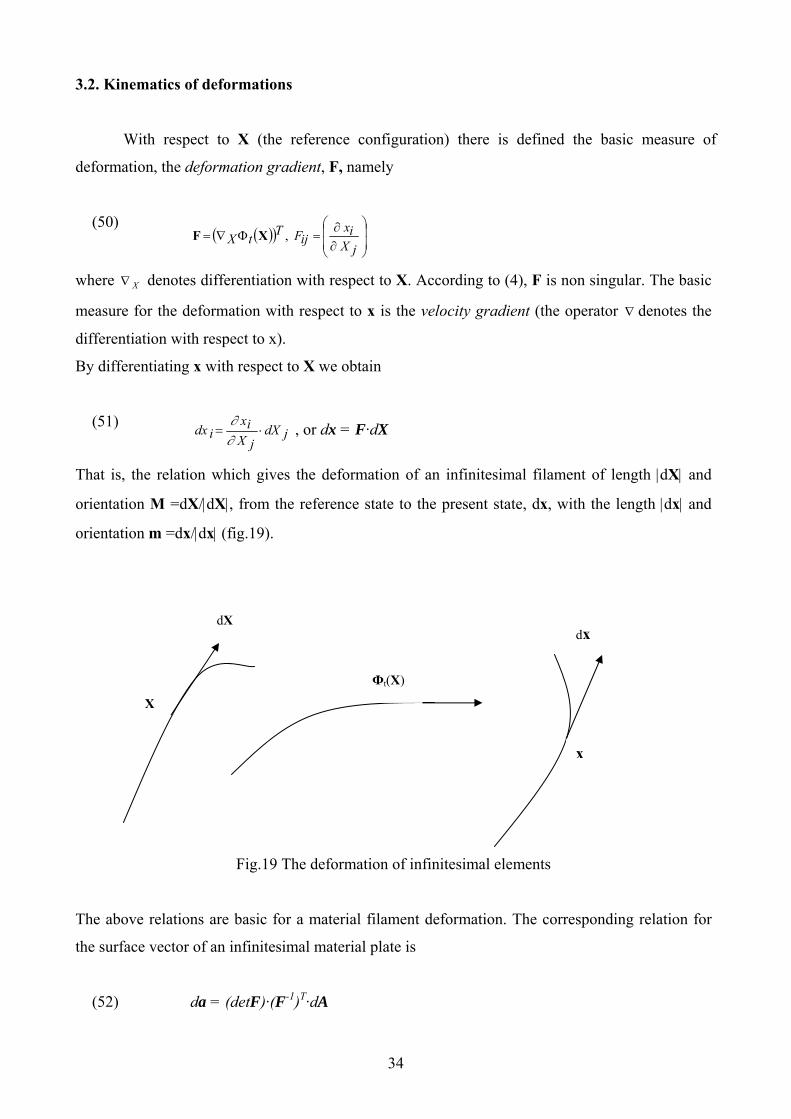
3.2. Kinematics of deformations

With respect to X (the reference configuration) there is defined the basic measure of

deformation, the deformation gradient, F, namely

(50) ( )( )

⎟⎟

⎠

⎞

⎜⎜

⎝

⎛

∂∂

=Φ∇=jX

ixijFT

tX ,XF

where denotes differentiation with respect to X. According to (4), F is non singular. The basic

measure for the deformation with respect to x is the velocity gradient (the operator denotes the

differentiation with respect to x).

X∇

∇

By differentiating x with respect to X we obtain

(51) jdX

jXix

idx ⋅=∂∂ , or dx = F·dX

That is, the relation which gives the deformation of an infinitesimal filament of length |dX| and

orientation M =dX/|dX|, from the reference state to the present state, dx, with the length |dx| and

orientation m =dx/|dx| (fig.19).

X

dX

Фt(X)

x

dx

Fig.19 The deformation of infinitesimal elements

The above relations are basic for a material filament deformation. The corresponding relation for

the surface vector of an infinitesimal material plate is

(52) da = (detF)·(F-1)T·dA

34

In this case, the surface in the present configuration is da = ⎜da⎜and the orientation n =da/⎜da⎜, and

in the reference (initial) configuration the surface is dA=⎜dA⎜ and the orientation N =dA/⎜dA⎜.

After defining the basic deformation of a material filament and the corresponding relation for

the area of an infinitesimal material surface, we can define the basic deformation measures: the

length deformation λ and surface deformation η, with the relations:

(53) ( ) ( )2/1

:1det,2/1: ⎟⎠⎞⎜

⎝⎛ −⋅== NNCMMC Fηλ

with C (=FT·F) the Cauchy-Green deformation tensor, and the vectors M,N - the orientation

versors in length and surface respectively, defined by:

(54) AAN

XXM

dd

dd

== ,

Very often, in practice is used the scalar form of (53), namely:

(55) ( ) jNiMijCFjNiMijC ⋅⋅−⋅=⋅⋅= 1det2,2 ηλ

with ΣMi2 = 1, ΣNj

2 = 1

The deformation tensor F and the associated tensors C, C-1, etc form the fundamental

quantities for the analysis of deformation of infinitesimal elements. In most cases the flow

( )Xtx Φ= is unknown and has to be obtained by integration from the Eulerian velocity field. If this

can be done analytically, then F can be obtained by differentiation of the flow with respect to the

material coordinates X. The flows of interest belong to two classes: i) flows with a special form of

and ii) flows with a special form of F. The second class is what we are interested for, as it

contains the so-called Constant Stretch History Motion – CSHM. Also, here is an important subset,

that of limous-metric flows, the so-called Steady Curvilinear Flows – SCF.

v∇

In the above context, the mixing concept implies stretching and folding of material elements

[55,59]. Thus, if a material filament dX and an area element dA are fixed in an initial random

position P, the specific length and surface deformations are given by the equations:

(56) D(lnλ)/Dt = D:mm, D(lnη)/Dt = ∇v-D:nn

35

where D is the deformation tensor, obtained by decomposing the velocity gradient in its symmetric

and non-symmetric part, namely:

ΩD +=∇v

( )

( ) )(,2

)(

,2

icnonsymmetrtensorspinalthe

symetric

tensorndeformatiothe

T

T

vvΩ

vvD

∇−∇=

∇+∇=

(57)

and m and n are given by the relation

(58) m= dx/⎜dx⎜, n = da/⎜da⎜

We say that the flow x=Φt(X) has a good mixing if the mean values D(lnλ)/Dt and

D(lnη)/Dt are not decreasing to zero, for any initial position P and any initial orientations M and N.

It must be noticed that it is not very exact to compare the flows based on the deformation values

D(lnλ)/Dt and D(lnη)/Dt, since these values depend obviously on time units. Therefore it is

searched for a quantification of the deformation process efficiency, in order to have a comparison

basis with respect to the availability for mixing of various flows.

It must be noticed that the specific deformations are bounded and so the deformation

efficiency can be naturally quantified. Thus, there is defined the deformation efficiency in length,

eλ= eλ (X,M,t) of the material element dX, like

(59) ( )( )

1:

/ln2/1 ≤=

DDDtDe λ

λ

and similarly, the deformation efficiency in surface, , eη= eη (X,N,t) of the area element dA: in the

case of an isochoric flow (the jacobian equal 1), we have:

36

(60) ( )( )

1:

/ln2/1 ≤=

DDDtDe η

η

There can be also defined the asymptotic efficiencies, namely:

( )tMXet

e ,,lim λλ∞→

=∞

( )tNXet

e ,,lim ηη∞→

=∞

(61)

3.3. The analysis of mixing efficiency for 2D and 3D excitable media

In this section there is exhibited the analysis of the length and surface deformations

efficiency for a mathematical 3-dimensional model associated to a vortexation phenomena. The

biological material used is the aquatic algae Spirulina Platensis.

The mathematical study was done in association with the experiments realized in a special

vortexation tube, closed at one end. Locally, there is produced a high intensity annular vorticity

zone, which is acting like a tornado. The small scale at which the turbulence issues allows retaining

the solid particles, mixing the textile fibbers or breaking up the multi-cellular filaments of aquatic

algae.

The special vortex tube used for achieving the breaking up of Spirulina Platensis filaments

is a modified version at low pressure of a Ranque-Hilsch tube [71]. Completely closing an end of

the tube, there is obtained in this region a high intensity swirl. The flow in the tube is generally like

a swirl, with a rate tangential velocity / axial velocity maxim near the closed end, where is also

created the annular vortex structure.

The approaching aerodynamic circuit is made from: a pressure source, the box of tangential

inputs, the diffusion zone, the tube where there is produced the swirl with additional pollutants

inputs, and the closing end with a rotating end.

It must be noticed that this torrential flow are concentrating and intensifying the vorticity, in

contrast with the usual cyclone-type flow or other flows generators. If in the installation is

introduced a pollutant, there issues a turbulent mixing in the annular vorticity zone. The spatial and

temporal scales revealed the existence of different domains, starting with laboratory ones and until

dissipative domains or others - corresponding to fine –structure wave numbers.

37

Thus, the applications area is very large, including collecting, aggregating, separating and

fragmenting the various pollutants.

From physical standpoint [72], the vortex produced in the installation implies four

mechanisms:

- Convection (scalar transport), due to streamlines which are directed towards the ending

lid near the tube walls, with the pressure source near the tube centre line;

- Turbulent diffusion due to the pressure and velocity variation;

- Stratification effects due to pressure and temperature gradients;

- Turbulent mixing due to the velocity concentration in annular structures.

The convection keeps in the transport and deposit of the powder pollutant when the graining

diameter is greater than 5μm. However, the graining spectra domain under 5μm undergoes a

turbulent diffusion and stratification effects which are generally out of control. For revealing the

local concentration of the streamlines 2D simplified models were tested. The multiphase 3D flows

simulation is still in study.

The turbulent mixing in multiphase flow reveals the following experiment components:

- The topological limit of the multiphase flow when the pollutant enters in the aggregation

stare or remains fragmented, in the host fluid;

- The rheological behaviour of non-Newtonian compositions, under macroscopic effects

of the air velocity.

The installation was realized in two versions: a small scale vortex tube (10-20mm diameter) and a

large scale one (100-300mm). They correspond generally at two particles processing classes,

although in most cases the classes can be superposed.

The first category refers to collecting and separating various powders, from gaseous

emissions to ceramic powders. The parameters which must be taken into account are the graining

spectra, the atmosphere nature and concentration. The vorticity concentration can be used for

processing the deposit of different particles in powder or cement form by an adequate closing lid.

The second category contains the processing on small scale, including deformation and

breaking up mechanisms for various particles in a host fluid. It is studied the vorticity concentration

near the closing lid.

Such an experiment is described in what follows [37]. With the installation described above,

it was processed the aquatic algae Spirulina Platensis in the host fluid water.

From the taxonomy standpoint, this algae belongs to Spirulina Platensis, “Cyanophita” class and

“Oscilatoriaceae” family. This is a filamentous bacterium characterized by spiral sequences of

trichomi cells. The filaments are contorted in a regular spiral with more than 1-2 rounds, generally

38

compressed at the transversal walls of the cells. The length of a filamentous sequence is between

50 and 500μm, and the width between 3 and 8μm.

After the processing, the long chains of cellular filaments were fragmented, producing

isolated cell units or – sometimes – there was recorded the breaking up of some cellular

membranes (with less than 100 Angstrom thickness). The initial and final observations (after the

vortexation) are exhibited in figure 20 below. It was used the non-dimensional parameter3D

Qta

⋅=τ ,

where t represents the time (in seconds), Q the installation debit (m3/sec) and D the diameter (m3).

As it can be seen from the picture, the fragmentation degree starts to increase as τa grows. There

can also be observed the algae form before and after the fragmentation.

Following the opinion of the specialists in cellular biology, this new technological method

of processing the flows is more efficient than the classical centrifugation method.

Fig.20 The fragmentation degree variation of Spirulina Platensis

Three specific applications were performed as fluid waste management:

the agglomeration of short fibers (aerodynamic spinning);

the retention of particles under 5µm without any material filter;

the breakout of cell membranes of the phytoplankton from polluted waters and the providing of a

cell content solution with important bio-stimulating features.

39

The mathematical modeling and analytically testing of the above experiment confirmed the

experimental study. Concerning the phenomenon scale, there were taken into account medium

helicoidally streamlines with approximating 10μm width. There were not gone further to

molecular level. Also, it is important to notice that for this moment of the analytical testing of the

model there were not studied the influence of strictly biological parameters (such as pH, the

temperature, the humidity, etc).

The complex multiphase flow necessarily implies a theoretical approach for discovering the

ways of optimization, developing and control of the installation. Numeric simulation of 3D

multiphase flows is currently in study. In the mathematical framework, the flow complexity

implies following three stages:

modeling the global swirling streamlines;

local modeling of the concentrated vorticity structure;

introducing the elements of chaotic turbulence.

The mathematical model associated to the vortex phenomena is, in the first stage, the 3D

version of the widespread isochoric two-dimensional flow [55]:

(62)

⎪⎩

⎪⎨

⎧

⟩⟨⟨−⋅⋅=

⋅=

0,11,1.2

2.1

GKxGKx

xGx

namely the following model is in study:

(63)

.,11,.3

1.2

2.1

constcK

cx

xGKx

xGx

=⟨⟨−

⎪⎪⎪

⎩

⎪⎪⎪

⎨

⎧

=

⋅⋅=

⋅=

where for the third component, the “z-axis” it was taken the rotation velocity, with a constant

value, c. Attaching to this system the initial condition

(64) ( ) ( ) ( ) 303,202,101 XxXxXx ===

leads to the solution of the Cauchy problem (63)-(64) of the following form:

40

(65)

( ) ( )

⎪⎪⎪⎪⎪⎪

⎩

⎪⎪⎪⎪⎪⎪

⎨

⎧

+⋅=

⎟⎟

⎠

⎞

⎜⎜

⎝

⎛⋅−⋅⋅−⋅+

⎟⎟

⎠

⎞

⎜⎜

⎝

⎛⋅⋅+⋅⋅=

⎟⎟

⎠

⎞

⎜⎜

⎝

⎛⋅−⋅⎟⎟

⎠

⎞⎜⎜⎝

⎛−⋅−

⎟⎟

⎠

⎞

⎜⎜

⎝

⎛⋅⋅⎟⎟

⎠

⎞⎜⎜⎝

⎛⋅+⋅=

33

.exp122

1.exp212

12

.exp12

21.

exp21

121

1

Xtcx

tXKXtXXKx

tXK

XtXK

Xx

γγ

γγ

with the notation KG ⋅=.γ , the same as in section 3.1.

From physically standpoint, (65) reveals the xi state of the system at the t moment, with respect to

Xj state (i,j =1,2,3). From the experimental standpoint, it concerns the state of the aquatic algae

after the vortexation, according to the experiment.

We are interested to analyze the stability of the model (63)-(64), in fact to analyze the

length and surface deformations of algae filaments in certain vortexation conditions. In this order,

the tensor F and FT have to be calculated. The matrix F is in this case,

F

xX

xX

xX

xX

xX

xX

xX

xX

xX

=

⎡

⎣

⎢⎢⎢⎢⎢⎢⎢

⎤

⎦

⎥⎥⎥⎥⎥⎥⎥

∂∂

∂∂

∂∂

∂∂

∂∂

∂∂

∂∂

∂∂

∂∂

1

1

1

2

1

3

2

1

2

2

2

3

3

1

3

2

3

3

that means:

(66)

⎥⎥⎥⎥⎥⎥⎥⎥⎥

⎦

⎤

⎢⎢⎢⎢⎢⎢⎢⎢⎢

⎣

⎡

⎟⎟

⎠

⎞

⎜⎜

⎝

⎛⋅−⋅+

⎟⎟

⎠

⎞

⎜⎜

⎝

⎛⋅⋅

⎟⎟

⎠

⎞

⎜⎜

⎝

⎛⋅−⋅−

⎟⎟

⎠

⎞

⎜⎜

⎝

⎛⋅⋅

⎟⎟

⎠

⎞

⎜⎜

⎝

⎛⋅−⋅

⋅−

⎟⎟

⎠

⎞

⎜⎜

⎝

⎛⋅⋅

⋅⎟⎟

⎠

⎞

⎜⎜

⎝

⎛⋅−⋅+

⎟⎟

⎠

⎞

⎜⎜

⎝

⎛⋅⋅

=

100

0.

exp21.

exp21.

exp2

.exp

2

0.

exp2

1.exp

21.

exp21.

exp21

tttKtK

tK

tK

tt

F γγγγ

γγγγ

The transposed matrix FT follows immediately, with the form:

41

(67)

⎥⎥⎥⎥⎥⎥⎥⎥⎥

⎦

⎤

⎢⎢⎢⎢⎢⎢⎢⎢⎢

⎣

⎡

⎟⎟

⎠

⎞

⎜⎜

⎝

⎛⋅−⋅+

⎟⎟

⎠

⎞

⎜⎜

⎝

⎛⋅⋅

⎟⎟

⎠

⎞

⎜⎜

⎝

⎛⋅−⋅

⋅−

⎟⎟

⎠

⎞

⎜⎜

⎝

⎛⋅⋅

⋅

⎟⎟

⎠

⎞

⎜⎜

⎝

⎛⋅−⋅−

⎟⎟

⎠

⎞

⎜⎜

⎝

⎛⋅⋅

⎟⎟

⎠

⎞

⎜⎜

⎝

⎛⋅−⋅+

⎟⎟

⎠

⎞

⎜⎜

⎝

⎛⋅⋅

=

100

0.

exp21.

exp21.

exp2

1.exp

21

0.

exp2

.exp

2

.exp

21.

exp21

tttK

tK

tKtKtt

TF γγγγ

γγγγ

Furthermore, for the Cauchy-Green deformation tensor C=FTF the calculus leads to:

(68)

⎥⎥⎥⎥⎥⎥⎥⎥⎥⎥⎥⎥⎥⎥⎥⎥⎥⎥⎥⎥⎥⎥⎥⎥⎥⎥⎥⎥⎥

⎦

⎤

⎢⎢⎢⎢⎢⎢⎢⎢⎢⎢⎢⎢⎢⎢⎢⎢⎢⎢⎢⎢⎢⎢⎢⎢⎢⎢⎢⎢⎢

⎣

⎡

⎟⎟

⎠

⎞

⎜⎜

⎝

⎛

⎟⎟

⎠

⎞

⎜⎜

⎝

⎛⋅−+

⎟⎟

⎠

⎞

⎜⎜

⎝

⎛⋅

+

⎟⎟⎟⎟⎟⎟

⎠

⎞

⎜⎜⎜⎜⎜⎜

⎝

⎛

⎟⎟

⎠

⎞

⎜⎜

⎝

⎛⋅−

⋅−⎟⎟

⎠

⎞

⎜⎜

⎝

⎛⋅

⎥⎥⎥⎥⎥⎥

⎦

⎤

⎢⎢⎢⎢⎢⎢

⎣

⎡

−

⎟⎟⎟⎟⎟⎟

⎠

⎞

⎜⎜⎜⎜⎜⎜

⎝

⎛

⎟⎟

⎠

⎞

⎜⎜

⎝

⎛⋅⋅−

−⎟⎟

⎠

⎞

⎜⎜

⎝

⎛⋅⋅

⋅+

⎥⎥⎥⎥⎥⎥

⎦

⎤

⎢⎢⎢⎢⎢⎢

⎣

⎡

−

⎟⎟⎟⎟⎟⎟

⎠

⎞

⎜⎜⎜⎜⎜⎜

⎝

⎛

⎟⎟

⎠

⎞

⎜⎜

⎝

⎛⋅⋅−

−⎟⎟

⎠

⎞

⎜⎜

⎝

⎛⋅⋅

⋅+

⎟⎟

⎠

⎞

⎜⎜

⎝

⎛

⎟⎟

⎠

⎞

⎜⎜

⎝

⎛⋅−−

⎟⎟

⎠

⎞

⎜⎜

⎝

⎛⋅

+⎟⎟

⎠

⎞

⎜⎜

⎝

⎛

⎟⎟

⎠

⎞

⎜⎜

⎝

⎛⋅−+

⎟⎟

⎠

⎞

⎜⎜

⎝

⎛⋅

=

100

0

2.exp

21.

exp21

2

.exp

21.

exp2

1

1.

2exp

.2exp

21

21

01.

2exp

.2exp

21

21

2.exp

2

.exp

2

2.exp

21.

exp21

tt

t

Kt

K

t

t

KK

t

t

KK

tKtK

tt

C

γγ

γ

γ

γ

γ

γ

γ

γγ

γγ

The matrix C-1 will have a similar expression, having in addition some expressions of K [37].

After this stage of calculus, some useful remarks have to be noticed:

• The determinant det F is the same, both in 2D and in 3D; also, the transposed FT is

the same in 2D and in 3D;

• Det C has the same value both in 2D and in 3D, based on the above observation;

also, C is a symmetric matrix, in both cases, and this fact facilitates the further

calculus for the length and surface deformations.

With these elements there is possible the calculus of length and surface deformations, λ2, and η2

respectively. For λ2, taking into account the definition (55) and that C is symmetric, there is

obtained

42

(69)

2312

2

2.exp

21.

exp21

2.exp

21.

exp2

1

211.

2exp.

2exp211

21

2.exp

2

.exp

2

2.exp

21.

exp212

MMtttK

tK

MMttKK

MtKtKtt

⋅+⋅⎥⎥⎥

⎦

⎤

⎢⎢⎢

⎣

⎡

⎟⎟

⎠

⎞

⎜⎜

⎝

⎛

⎟⎟

⎠

⎞

⎜⎜

⎝

⎛⋅−+

⎟⎟

⎠

⎞

⎜⎜

⎝

⎛⋅+⎟

⎟

⎠

⎞

⎜⎜

⎝

⎛

⎟⎟

⎠

⎞

⎜⎜

⎝

⎛⋅−−

⎟⎟

⎠

⎞

⎜⎜

⎝

⎛⋅

+⋅⋅⎥⎥

⎦

⎤

⎢⎢

⎣

⎡−⎟

⎟

⎠

⎞

⎜⎜

⎝

⎛

⎟⎟

⎠

⎞

⎜⎜

⎝

⎛⋅−−

⎟⎟

⎠

⎞

⎜⎜

⎝

⎛⋅

+

+⋅⎥⎥⎥

⎦

⎤

⎢⎢⎢

⎣

⎡

⎟⎟

⎠

⎞

⎜⎜

⎝

⎛

⎟⎟

⎠

⎞

⎜⎜

⎝

⎛⋅−−

⎟⎟

⎠

⎞

⎜⎜

⎝

⎛⋅+⎟

⎟

⎠

⎞

⎜⎜

⎝

⎛

⎟⎟

⎠

⎞

⎜⎜

⎝

⎛⋅−+

⎟⎟

⎠

⎞

⎜⎜

⎝

⎛⋅=

γγγγ

γγ

γγγγλ

It must be noticed that the deformations have quite large expressions. Taking into account that det

F=1, there is obtained for η2 the relation:

(70) ( )

( )

( ) ( ) 2321

.2exp

.2exp

.4exp

.4exp

41

2

21

22

21

.2exp

.2exp

6417

.4exp

.4exp

det12

NNN

tt

tt

KK

NN

KB

tt

ttKA

C

+⋅⋅

⎥⎥⎥⎥⎥⎥

⎦

⎤

⎢⎢⎢⎢⎢⎢

⎣

⎡

⎟⎟

⎠

⎞

⎜⎜

⎝

⎛

⎟⎟

⎠

⎞

⎜⎜

⎝

⎛⋅−−

⎟⎟

⎠

⎞

⎜⎜

⎝

⎛⋅

−⎟⎟

⎠

⎞

⎜⎜

⎝

⎛

⎟⎟

⎠

⎞

⎜⎜

⎝

⎛⋅−+

⎟⎟

⎠

⎞

⎜⎜

⎝

⎛⋅

⋅+

−⎟⎠⎞⎜

⎝⎛ +⋅

⎥⎥⎥⎥⎥⎥⎥⎥⎥⎥⎥⎥⎥⎥

⎦

⎤

⎢⎢⎢⎢⎢⎢⎢⎢⎢⎢⎢⎢⎢⎢

⎣

⎡

−⎟⎟

⎠

⎞

⎜⎜

⎝

⎛

⎟⎟

⎠

⎞

⎜⎜

⎝

⎛⋅−+

⎟⎟

⎠

⎞

⎜⎜

⎝

⎛⋅

+⎟⎟⎟⎟

⎠

⎞

⎜⎜⎜⎜

⎝

⎛

⎟⎟

⎠

⎞

⎜⎜

⎝

⎛⋅−+

⎟⎟

⎠

⎞

⎜⎜

⎝

⎛⋅

⋅

⋅=

γγ

γγ

γγ

γγ

η

where A(K) and B(K) are forms of K [37]:

( ) ( )

KKKKB

KKKKA

2561651216,

2561617216 +−

=++

=

For establishing the relationship of efficiencies, the following identities were used, in order to

facilitate the calculus:

(71) ( )

2

2

21ln

λ

λλ td

d

tdd

⋅= , ( )2

2

21ln

η

ηη td

d

tdd

⋅=

43

In this context, after deriving with respect to time the quantities corresponding to the

versors , the following form is obtained for e21,23,2

2,21 MMMMM λ:

(72)

⎟⎟⎟⎟

⎠

⎞

⎜⎜⎜⎜

⎝

⎛

+⋅⋅−

+⋅⋅+

−⋅−

+⎟⎟

⎠

⎞

⎜⎜

⎝

⎛⋅⋅−⋅

⎥⎥⎥⎥

⎦

⎤

⎢⎢⎢⎢

⎣

⎡

⋅⋅+

+⋅⋅

+−⋅

+

+⎟⎟

⎠

⎞

⎜⎜

⎝

⎛⋅⋅⋅

⎥⎥⎥⎥

⎦

⎤

⎢⎢⎢⎢

⎣

⎡

⋅⋅+

+⋅⋅⋅

++⋅

+

⎟⎟

⎠

⎞

⎜⎜

⎝

⎛⋅⋅−⋅

⎥⎥⎥⎥

⎦

⎤

⎢⎢⎢⎢

⎣

⎡

⋅⎟⎠⎞

⎜⎝⎛ +−

⋅⋅+

+⋅⎟⎠⎞

⎜⎝⎛ +−

+⎟⎟

⎠

⎞

⎜⎜

⎝

⎛⋅⋅⋅

⎥⎥⎥⎥

⎦

⎤

⎢⎢⎢⎢

⎣

⎡

⋅⎟⎠⎞

⎜⎝⎛ +

+⋅⋅+

+⋅⎟⎠⎞

⎜⎝⎛ +

⋅=

23

222

1

2112

121

.2exp

224

1

21212

141

.2exp

224

1

21212

141

.2exp

22

11

2112

141

.2exp

22

11

2112

141

2

.

MMK

K

MMKKMK

tM

KK

MMKKMK

tM

KK

MMKKMK

tM

K

MMKKMK

tM

K

MMKKMK

e

γ

γ

γ

γ

γλ

Similar calculus is made for eη, but its form is more complex. It is given by the following relation

(73):

44

(73) ( )

( )( )

( ) ( )

( )

( )

( )

( ) ( ) 232

2121

21

.2exp

.2exp

.4exp

.4exp

41

22

21

.2exp

.2exp

6417.

4exp.

4exp

21

2

211222

21.4exp

2

214

23.2exp

23.

2exp12

2

21.4exp

423.

2exp21.

2exp162

22

21

.4exp

6417

.4exp12

3217.

4exp.

4exp

423.

2exp21.

2exp162

det

.

NKKNN

ttttNN

KB

ttttKA

NN

KK

KK

Kt

KK

KKt

Kt

K

KKt

KKt

Kt

K

NN

tK

tK

tt

KKt

Kt

KKA

Ce

++

⋅

⋅

⎥⎥⎥⎥⎥

⎦

⎤

⎢⎢⎢⎢⎢

⎣

⎡+⎟

⎟

⎠

⎞

⎜⎜

⎝

⎛

⎟⎟

⎠

⎞

⎜⎜

⎝

⎛⋅−−

⎟⎟

⎠

⎞

⎜⎜

⎝

⎛⋅−⎟

⎟

⎠

⎞

⎜⎜

⎝

⎛

⎟⎟

⎠

⎞

⎜⎜

⎝

⎛⋅−+

⎟⎟

⎠

⎞

⎜⎜

⎝

⎛⋅

−⎟⎠⎞⎜

⎝⎛ +

⋅

⎥⎥⎥⎥

⎦

⎤

⎢⎢⎢⎢

⎣

⎡−⎟

⎟

⎠

⎞

⎜⎜

⎝

⎛

⎟⎟

⎠

⎞

⎜⎜

⎝

⎛⋅−+

⎟⎟

⎠

⎞

⎜⎜

⎝

⎛⋅+⎟

⎟

⎠

⎞

⎜⎜

⎝

⎛

⎟⎟

⎠

⎞

⎜⎜

⎝

⎛⋅−+

⎟⎟

⎠

⎞

⎜⎜

⎝

⎛⋅⋅

⋅

⋅

⎥⎥⎥⎥⎥⎥⎥⎥⎥⎥⎥⎥⎥⎥⎥

⎦

⎤

⎢⎢⎢⎢⎢⎢⎢⎢⎢⎢⎢⎢⎢⎢⎢

⎣

⎡

+⎟⎠⎞

⎜⎝⎛ +−

++

⎟⎟

⎠

⎞

⎜⎜

⎝

⎛⋅−

⋅

⎟⎟⎟⎟⎟⎟

⎠

⎞

⎜⎜⎜⎜⎜⎜

⎝

⎛

+−−

⎟⎟

⎠

⎞

⎜⎜

⎝

⎛⋅−

⋅+⎟⎟

⎠

⎞

⎜⎜

⎝

⎛⋅⎟

⎠⎞

⎜⎝⎛ −−

−⎟⎟

⎠

⎞

⎜⎜

⎝

⎛ +⎟⎟

⎠

⎞

⎜⎜

⎝

⎛⋅−

⋅⎟⎟

⎠

⎞

⎜⎜

⎝

⎛ −+

⎟⎟

⎠

⎞

⎜⎜

⎝

⎛⋅−−

⎟⎟

⎠

⎞

⎜⎜

⎝

⎛⋅⎟

⎠⎞

⎜⎝⎛ +

+⎟⎠⎞⎜

⎝⎛ +

⋅

⎥⎥⎥⎥⎥⎥⎥⎥⎥⎥⎥

⎦

⎤

⎢⎢⎢⎢⎢⎢⎢⎢⎢⎢⎢

⎣

⎡

⎟⎟

⎠

⎞

⎜⎜

⎝

⎛⋅−

+⎟⎟

⎠

⎞

⎜⎜

⎝

⎛⋅⎟

⎠⎞

⎜⎝⎛ +−⎟

⎟

⎠

⎞

⎜⎜

⎝

⎛

⎟⎟

⎠

⎞

⎜⎜

⎝

⎛⋅−−

⎟⎟

⎠

⎞

⎜⎜

⎝

⎛⋅

⋅⎟⎟

⎠

⎞

⎜⎜

⎝

⎛ −+

⎟⎟

⎠

⎞

⎜⎜

⎝

⎛⋅−−

⎟⎟

⎠

⎞

⎜⎜

⎝

⎛⋅⎟

⎠⎞

⎜⎝⎛ +⋅

⋅=

γγγγ

γγγγ

γ

γ

γ

γ

γγ

γ

γγγ

γγ

γη

The above mathematical framework allows the analysis of the efficiency of length and surface

deformation process for the biological material which undergoes the vortexation process. As

described above, in relations (59) and (60), the averaging factor (D:D)1/2 offers an adequate

quantification of the length and surface deformation efficiencies. The deformation tensor D has in

our 3D case, the following form:

(74)

⎥⎥⎥

⎦

⎤

⎢⎢⎢

⎣

⎡

⋅+++⋅+++⋅

⋅=

zwzvywzuxwywzvyvyuxvxwzuxvyuxu

D2

22

21

Since the target is the study of the efficiencies eλ and eη at successive moments, the analysis is a

discrete one, which aims testing the special events that could appear at various, random, values of

the versors Mi, Nj. Therefore, the factor (D:D)1/2, which in concrete cases has numerical values, has

not an important significance in the numeric analysis.

45

With the numeric soft MAPLE11, the analysis has two parts. Firstly, the following Cauchy

problems are solved:

( ) ( )( ) ( ) 00,0

00,0==

==

xtexte

ηλ

using a discrete numeric calculus procedure [32,35]. The output of the procedure is a listing of the

form . In the second part there are realized discrete time plots, in 25 time units,

following the listings obtained in the first part. The plots represent in fact the image of the length

and surface deformations, in the established scale time.

( )( ) 25..0,, =iitxit

Very few irrational value sets were chosen for the length, respectively surface versors,

taking into account the versor condition:

. ∑ ∑ == 1,1 jNiM

Also, for the parameter K there were chosen few values, let us notice the most important of them:

8.0,5.0,2.0 === KKK ,

the symmetric values relative to the origin leading to the same results. For the parameter the

values are a little different for the two deformations..

γ.

The studied cases are in fact represented by the events associated to different values of

length and surface orientation versors: ( )3,2,1 MMM and ( )3,2,1 NNN for length and surface

respectively. The events were very few, about 60. Their statistical interpretation is synthesized in

Appendix1, including also the two-dimensional case.

The graphical events are illustrating the analysis of the deformations for Spirulina Platensis,

in 25 time units’ vortexation. The studied flow is a special flow, and is needed for it in order to get

a filaments’ break up. According to the first section, the algae filaments represent Lagrange

markers. The special spiral form of the algae gives the answer to the computational context that the

surface deformation eη is significant, since it brings more cases of filaments’ break up. It was

called rare event the event of very sudden breaking up of the algae filaments, this corresponding

from mathematical standpoint to the break out of the program (because of impossibility of

maintaining the required accuracy). Thus, a very important fact happened: the mathematical

simulations matched the experimental analysis.

46

In what follows there is exhibited the graphical / computational analysis of the surface

deformation of the tested (3D case), with some comparative situations of 2D case. The cases are

labeled on the figures.

Fig.22 The precedent case with

K=0.2, =0.01 .

2 γ⋅

Fig.21 The case ( ) ⎟⎟⎠

⎞⎜⎜⎝

⎛−= 0,

21,

21

3,2,1 NNN

K=0.2, =0.008 .

2 γ⋅


K=0.2, =.

2 γ⋅ 2


⎞⎜⎜⎝

⎛−= 0,

32,

31

3,2,1 NNN

K=0.2, =0.008 .

2 γ⋅

47

Fig.25 The precedent case with Fig.26 The precedent case with

K=0.8, =.

2 γ⋅ 2 K=0.2, =.

2 γ⋅ 3

Fig.27 The precedent case with Fig.28 The case ( ) ⎟

⎟⎠

⎞⎜⎜⎝

⎛= 0,

23,

21

3,2,1 NNN

K=0.2, =0.008 .

2 γ⋅

K=0.8, =.

2 γ⋅ 3

48

Fig.29 The precedent case with Fig.30 The case ( ) ⎟

⎟⎠

⎞⎜⎜⎝

⎛= 0,

23,

21

3,2,1 NNN

K=0.2, =.

2 γ⋅ 3

K=0.2, =.

2 γ⋅ 2


K=0.2, =0.008 .

2 γ⋅


K=0.2, =0.8 .

2 γ⋅

49


K=0.2, =0.01 .

2 γ⋅


⎞⎜⎜⎝

⎛= 0,

52,

51

3,2,1 NNN

K=0.2, =0.008 .

2 γ⋅


K=0.2, =.

2 γ⋅ 3 K=0.2, =.

2 γ⋅ 2

50


K=0.2, =0.8 .

2 γ⋅


K=0.2, =0.01 .

2 γ⋅


K=0.8 =.

2 γ⋅ 3 K=0.8, =.

2 γ⋅ 2

51


K=0.8 =.

2 γ⋅ 3


⎞⎜⎜⎝

⎛= 0,

23,

21

3,2,1 NNN

K=0.8, =.

2 γ⋅ 2

For comparison, some significant pictures for 2D surface deformation follow. The cases are also

labeled.

Fig.43 The case ( ) ( 0,12,1 =NN ) Fig.44 The precedent case with

K=0.2 =0.002 .

2 γ⋅K=0.2, =0.008 .

2 γ⋅

52


K=0.5 =.

2 γ⋅ 2 K=0.5, =0.008 .

2 γ⋅


K=0.8 =.

2 γ⋅ 2 K=0.2, =.

2 γ⋅ 2

53

Fig.49 The case ( ) ( 0,12,1 −=NN ) Fig.50 The precedent case with

K=0.8 =0.002 .

2 γ⋅K=0.8, =0.008 .

2 γ⋅

3.4 Concluding remarks

The central target presented here is the mathematical modeling of breaking up of Spirulina

Platensis filaments which are in a turbulent flow process. It is obviously that the breaking up is due

to alternating loadings that the filament undergoes, in a space-time with random events, available

to the break phenomena. The modeling had the following basic stages:

• Associating known streamlines to the medium flow (that means helical flow in a

cylinder);

• Determining the linear and surface deformations from continuum fluid mechanics;

• Associating a sequence of random values to the (vectorial) length and surface

orientations.

It is easy to see that the calculus has a quite large complexity; therefore the results must be

statistically interpreted. Analyzing the above pictures, as well as the synthetic table in appendix, we

observe that there exist some cases when the phenomenon is almost linear, or is much closed to the

picture 20. But, here are also cases in which there appear deformations followed by folding, or

there issue sudden breaking up of spirulina filaments. In fact, there are four types of processes:

54

1) Processes with relative linear behavior – in this case are figures 21,22, 33, 43, 44, 47,

49

2) Linear-negative processes – corresponding to the figures 23-27, 34-38. They correspond

to alternate tasks of stretching and folding of filaments and are the most

3) Mixing phenomena where there issue smaller or larger deviations or strong

discontinuities; here are figures 31, 35, 46, 48 and concern the situations when some

pieces are suddenly coming off from the whole filament, followed by the restarting of

vortexation for the rest of algae;

4) Rare events – these correspond to the turbulent mixing and represent the sudden break

up of spirulina filaments; they can be found in the figures 29, 30, 32, 39-42 and 50.

Thus there were obtained alternate loadings which justify the breaking of the filaments.

From the statistical situation of the appendix1 and also of the pictures an important fact is

concluding, that the mixing, and especially the turbulent mixing, is introduced at irrational values

– such as 5,3,2 for parameter and length and surface versors. This fact must be not so

surprising, taking into account that

.2 γ⋅

5,3,2 represent themselves random values.

A second important remark is that the turbulence appears, in most of cases, at small values

of time units – and this was also regained in the experimental standpoint. There were not specified

the scale for the time units, such a manner being in agreement with the start point of the analysis,

namely the expression of the parameter τa: depending on the context, we can deal with seconds,

minutes, hours or even more. This is also true for 2D case. Moreover, there were tested some

situations for larger versor values, for example 13,11,7 and there were not recorded significant

special behaviors unlike the above mentioned.

From mathematical (analytical) standpoint, eλ and eη are decreasing with time, but there

were searched for the beginning of the process and for the rare events, and that’s why only 25 time

units were taken into account at the simulations. In fact, there is observed that in situations like that

of figure 47, from a certain moment there is no fragmentation. Thus, the validity of the model is

confirmed by two aspects:

• the statistic increment in time of the breaking cases, according to the experiments;

• the relative singularity of the events which could produce the breaking, fact which is

confirmed by the quite long duration of the experiments which led to the filaments

break up; in very rare cases, the cellular membrane could be broken, and the cellular

content collected.

55

There was also tested a more complicated version of the 3D model, obtained by perturbing

one of right hand members of the system with a logistic term. Although the complexity of the

calculus was important, there were not recorded significant results comparing with the initial ones.

[37]

Crossing over from 2D to 3D case, it is easy to deduce the requirement of a special analysis

of the influence of parameters on the behavior of this complex mixing flow. This would be

achieved by the spectral analysis. Together with this aspect it must be also noticed the enlarging of

the time scale. In fact, the parameters influence on the model is a quite rich interdisciplinary area,

with very few analytic and numeric appliances. It suffices to notice the diverse tools that

MAPLE11 offers for the users, and the wide scale of their applications [6,7,10,14].

It is obvious that the testing of more and more values / parameters sets remains basic. If for 3D

case, 60 statistical cases suffice for proving the special events favorable for breaking up of the

biological filaments, it is expected an acceptance testing of the consistency with the

interdisciplinary area. Thus, the issues of repetitive phenomena, both in 2D and 3D case, give rises

to achieve some appliances of chaotic dynamical systems, whose numeric models would give new

research directions on the behavior in excitable media. This would be a next aim.

Now, if we go back a little in the history and take a look, we see that the history of mixing

evolved in interesting cycles: namely, that since the years ’48, three basic stages were clearly

identified in the study of the mixing:

- The entrainment stage – for these, the large scale flow structure need to be correctly

described;

- The subsequent stirring process (responsible for the interfacial surface generation

between the mixing species) – for these there is necessary a correct defined intermediate

range of scales;

- The dynamic process – at the smallest scales – this must be captured to describe the

molecular mixing process itself.

With the above recent studies, with the powerful appliances of computational fluid dynamics, it is

important to notice that for the recent models, a little perturbation has a consistent influence on the

model, going into a far from equilibrium model. If there is annexed the irrationality of the length /

surface versors values (an appliance used since the beginning of the mixing study), a globally panel

is obtained, with random distributed events. This space-time context consolidates the basic

statement that the turbulent mixing flows must be approached as chaotic systems. This is in fact

regaining the idea of a system / model high sensitive to initial conditions. In this context, amazing

ways and new keys are opening in modeling, and we name here only spectral analysis and Smale’s

56

horseshoe application. These would be of a huge help in understanding these special models and

phenomena and constructing a coherent and consistent theory on mixing models as far from

equilibrium models.

57

APPENDIX

1. Versor

label

2. Versor

value

3. K 4. 2* γ. 5. t 6. Remarks

0.2 0.001

0.008

3.0

linear

linear

linear

0.5 0.008

3.0

linear

linear

(1,0)

0.8 0.008

3.0

linear

linear

2D

(M1,M2)

(-1,1) 0.2 0.008

0.001

10

linear

an abrupt

increasing

0.2

0.008

2

6

2..4

strong

discontinuity

strong

discontinuity

2D (1,0)

(N1,N2)

0.5 0.008 2 strong

discontinuity

19 the points come

near

2

0.8 0.008 linear

12,13 maxim,

discontinuity

2

rare event 0.2 0.008

3.0

7

linear

(-1,1)

0.5 0.008 linear

3.0 linear

0.8 0.008 linear

0.2 0.008

3.0

linear

linear

3D 12

12

0, ,⎛⎝⎜

⎞⎠⎟

(M1,M2,M3)

0.5 0.008 linear


58

3.0 linear

rare event 2

0.2 0.008 linear

3.0

√2

linear

rare event

13

23

0, ,−⎛

⎝⎜

⎞

⎠⎟

0.5 0.008 linear

3.0 linear


linear 3.0

0.2 0.008 linear 12

32

0, ,⎛

⎝⎜

⎞

⎠⎟

3.0 linear

rare event √2

rare event √3

0.5 0.008 linear

3.0 linear

0.8 0.008 linear

3.0 linear

0.2 0.008

0.01

8

7

abrupt

increasing

rare event

(N1,N2,N3) 12

12

0, ,−⎛⎝⎜

⎞⎠⎟

0.5 0.008 linear

3.0 linear

0.2 0.008 linear

3.0 linear 13

23

0, ,−⎛

⎝⎜

⎞

⎠⎟

0.5 0.008 linear

3.0 linear

0.2 0.008 20 the points came

near 12

32

0, ,⎛

⎝⎜

⎞

⎠⎟

0.01 20 the same case

0.08 8 maxim

rare event 0.8 8

rare event 5 √2

rare event 4 √3

59

0.2 0.008 linear

0.01 9 the points came

near

15

25

0, ,⎛⎝⎜

⎞⎠⎟

0.5 0.008 linear

3.0 linear

0.8 0.008 linear

60

REFERENCES

[1] Abraham, R. & J. Marsden. Foundations of mechanics. Benjamin. New York. 1978

[2] Aldrich, R.W., D.P. Corey, & C.F. Stevens. A reinterpretation of

mammalian sodium channel gating based on single channel recording. Nature 306:436-441. 1983

[3] Akcakaya, H.R., Population cycles of mammals: evidence of a ratio-dependent predation

hypothesis. Ecological Monographs 62, 119-142. 1992

[4] Akcakaya, H.R., L.R. Ginzburg, D. Slice & L.B. Slobodkin, The theory of population

dynamics: II:Physiological delays. Bulletin of Mathematical Biology 50, 503-515. 1988

[5] Ascher, U., Mattheij, R., Russell, R. Numerical Solution of Boundary Value Problems for

Ordinary Differential Equations. SIAM Classics in Applied Mathematics 13 (1995)

[6] Ascher, U., Petzold, L. Computer Methods for Ordinary Differential Equations and

Differential-Algebraic Equations. SIAM, Philadelphia, 1998

[7] Bailey, P.B, Shampine, L.F., Waltman, P.E. Nonlinear Two Point Boundary Value Problems.

Academic Press, New York, 1968

[8] Ball, F.G. & M.S.P. Samson. Temporal clustering of ion channel openings incorporating time

interval omission. IMA J. Math. Appl. Med. & Biol. 4:333-361.1987

[9] Bollobás, B. Random Graphs. Academic Press, London, Orlando. 1985

[10] Boyce, W.E., DiPrima, R.C. Elementary Differential Equations and Boundary Value

Problems. John Wiley & Sons, New York, 1997

[11] Brillinger, D. R. Some statistical methods for random process data from seismology and

neurophysiology. Ann. Statist. 16(1):1-54, 1988

[12] Carrier, G. F. Pearson, C. E. Partial Differential Equations: Theory and Technique (2ed).

Academic Press, 1988

[13] J.R.Cash, The Integration of stiff IVP in ODE using modified extended BDF, Computers and

Mathematics with Applications, 9, 645-657 (1983)

[14] E.S. Cheb-Terrab, K. von Bulow. A Computational Approach for the Analytical Solving of

Partial Differential Equations. Computer Physics Communications 90 (1995): 102-116

[15] Chow, S.-N., K. Lu. Invariant manifolds for flows in Banach spaces. J, Diff. Eqns. 74, 285-

317. 1988

[16] Erdos, P., A. Renyi. On the evolution of random graphs. Publ. Math. Inst., Hungar. Acad. Sci.

5:17-61. 1960

[17] Fatou, M.P. Sur les équations fonctionelles. Bull. Soc. Math. France 47:161-271, 1920

[18] Feller, W. On the integral equation of renewal theory. Ann. Math. Stat. 12:243-267. 1941

61

[19] Feller, W. Diffusion processes in genetics. pp. 227-246 In Proc. 2nd Berkeley Symp. Math.

Stat. Probab. Univ. of California Press, Berkeley. 1951

[20] Fisher, R.A. The wave of advance of advantageous genes. Ann. Eugen. (London) 7:355-369.

1937

[21] Fox, P.T., J.S. Perlmutter, M.E. Raichle. Stereotactic localization for positron emission

tomography. J. Cereb. Blood Flow Metab. 5 Suppl. 1:S611-S612. 1985

[22] Fox, P.T., J.S. Perlmutter, M.E. Raichle. Stereotactic localization for positron emission

tomography. J. Cereb. Blood Flow Metab. 5 Suppl. 1:S611-S612. 1985

[23] Fredkin, D.R., J.A. Rice. On aggregated Markov chains. J. Appl. Probab. 23:208-214. 1986

[24] Galton, F., H.W. Watson. On the probability of extinction of families. J. R. Anthropol. Inst.

4:138-144. 1974

[25] Gear, C.W. Numerical Initial Value Problems in Ordinary Differential Equations. Prentice-

Hall, 1971

Georgescu, A. Asymptotic approximations. Technical Press, Bucarest 1989 [26]

[27] Geman, S., D.E. McClure. Bayesian image analysis: an application to single photon emission

tomography. pp. 12-18 In Proc. of the Amer. Statistical Assoc. Statistical Computing Section. 1985

[28] Godeanu, M., D. Stanca, I. Stanescu. Technological transfer of Spirulina Platensis culture in

termomineral water from IRATOS Arad. International Workshop on cost efficient methods and

Techniques for technology transfer services TTCAM 99 (9-11). Constanta 1999

[29] Gurtin, M.E., R.C. MacCamy. Non-linear age-dependent population dynamics. Archive of

Rational Mechanics and Analysis 54:281-300. 1974

[30] Hale, J.K. Critical cases for neutral functional differential equations. J. Diff. Eqns 10, 59-82.

1970

[31] Hartman, P. Ordinary differential equations. P. Hartman. 1973

[32] Hindmarsh, Alan C., Stepleman, R.S., (eds.) Odepack, a Systemized Collection of ODE

Solvers. North-Holland, Amsterdam, 1983

[33] Hirsch, M., C. Pugh, M. Schub. Invariant manifolds. Springer Lecture Notes In Math. Vol.

583. Springer-Verlag. Berlin & New York. 1977

[34] Hoppensteadt, F. An age-dependent epidemic model. J. Franklin Inst. 297:325-333. 1974

[35] Hubbard J.H., West, B.H. Differential Equations: A Dynamical Systems Approach Part I, One

Dimensional Equations. Springer, New York, 1990

[36] Hull, T.E., Enright, W.H., Fellen, B.M., Sedgwick, A.E. Comparing Numerical Methods for

Ordinary Differential Equations. SIAM J. Numer. Anal., 9 (1972) 603-637

62

[37] Ionescu, A. The structural stability of biological oscillators. Analytical contributions. Ph.D.

Thesis, Polytechnic University of Bucarest. Bucarest 2002

[38] Ionescu, A. & Georgescu, A.. Existence of a center manifold for a biological model. (277-

285). Proceedings of the Conference on Applied and Industrial Mathematics. Bucarest. 1996

[39] Iooss, G. Bifurcations of maps and applications. Math. Studies 36. Elsevier-North-Holland.

Amsterdam. 1979

[40] Jagers, P.. Branching Processes with Biological Applications. Wiley, New York. 1975

[41] Johnstone, I.M., B.W. Silverman. Speed of emission in positron emission tomography and

related inverse problems. Ann. Statist. 18:251-280. 1990

[42] Julia, C.. Memoire sur l'iteration des fonctions rationelles. J. Math. Pures Appl. 4:47-245.

1918

[43] Kermack, W.O., A.G. McKendrick. Contributions to the mathematical theory of epidemics.

Proc. R. Soc. Lond. Ser A 115:700-721. 1927

[44] Kolmogorov, A.M.. The transition of branching processes into diffusion processes and

associated problems of genetics. Teor. Veroyatn. i Primen. 4:233-236. 1959

[45] Kirchgassner, K.. Wave solutions of reversible systems and applications. J. Diff. Eqns. 45,

113-127. 1982

[46] MacArthur, R.H. & J.H. Connell. The biology of populations. John Wiley, New York, USA.

1966

[47] Markus, L. The Behavior of the Solutions of a Differential System near a Periodic Solution.

Ann. Math. 73, No 2. 1960

[48] Markus, L. Structurally Stable Differential Systems. Ann. Math. 73, No 1. 1961

[49] Mielke, A. A reduction principle for nonautonomous systems in infinite dimensional spaces. J.

Diff. Eqns. 65, 68-88. 1986

[50] Milne, R. K., G.F. Yeo, B.W. Madsen, R.O. Edenson. Estimation of single channel kinetic

parameters from data subject to limited time resolution. Biophys. J. 55:673-676. 1989

[51] McKendrick, A.G.. Application of mathematics to medical problems. Proc. Edinburgh Math.

Soc. 44:98-130. 1926

[52] Murray, J.D.. Mathematical Biology. Biomathematics 19. Springer-Verlag, Berlin. 1989

[53] Murray, J.D., G.F. Oster.. Cell traction models for generating pattern and form in

morphogenesis. J. Math. Biol. 19:265-279. 1984

[54] Neyman, J., P.S. Puri. A hypothetical stochastic mechanism of radiation effects in single cells.

Proc. R. Soc. Lond. 213:139-160. 1981

63

[55] Ottino, J.M. The kinematics of mixing: stretching, chaos and transport. Cambridge University

Press. 1989

[56] Ottino, J.M., W.E. Ranz, C.W. Macosko. A lamellar model for analysis of liquid - liquid

mixing. Chem. Eng. Sci. 34, 877-890. 1979

[57] Ottino, J.M., W.E. Ranz, C.W. Macosko. A framework for the mechanical mixing of fluids.

AlChE J. 27, 565-577. 1981

[58] Ottino, J.M., & C.W. Macosko. An efficiency parameter for batch mixing of viscous fluids.

Chem. Eng. Sci.35, 1454-1457. 1980

[59] Ottino, J.M., C.W. Leong, H. Rising, P.D. Swanson. Morphological structures produced by

mixing in chaotic flows. Nature 333, 419-425. 1988

[60] Pavlidis, T. Biological Oscillators: Their mathematical Analysis. Academic Press, New York

& London. 1973

[61] Pavlidis, T. Populations of Interacting Oscillators and Circadian Rhythms. J. Theor. Biol. 22,

418-436. 1969

[62] Purcell, E.M.. Life at low Reynolds number. Am. J. Physics. 45(1):3-11. 1977

[63] Samuelson, P.A.. Resolving a historical confusion in population analysis. Hum. Biol. 48:559-

580. 1976

[64] Sarkovskii, A.N. 1964. Coexistence of cycles of a continuous map of a line into itself. Ukr.

Mat. Zh. 16:61-71. 1964

[65] Shampine, L.F., Corless, R.M. Initial Value Problems for ODEs in Problem Solving

Environments. J. Comp. Appl. Math, vol. 125(1-2) ,31-40 (2000)

Sharpe, F.R., A.J. Lotka. A problem in age-distribution. Philos. Mag. Ser. 6, 21:243-267. 1911 [66]

[67] Shepp, L.A., B.F. Logan. The Fourier reconstruction of a head section. IEEE Trans. Nucl.

Sci. NS-21:21-43. 1974

[68] Smale, S. Stability and genericity in dynamical systems. Lecture Notes in Mathematics, vol.

180. 1970. Springer-Verlag

[69] Stigler, S.M. The History of Statistics. The Measurement of Uncertainty Before 1900. Belknap

Press of Harvard University Press, Cambridge, MA. 1986

[70] Strikwerda, J. C. Finite Difference Schemes and Partial Differential Equations. Wadsworth

and Brooks/Cole, 1989

[71] Savulescu, St.N. A special vortex tube for particle processing flows. Rev. Roum. Sci. Techn. -

Mec. Appl., Tome 43, No 5 (611-615). 1998

[72] Savulescu, St.N. Applications of multiple flows in a vortex tube closed at one end. Internal

Reports, CCTE, IEA. Bucarest. (1996-1998)

64

[73] Savulescu, St.N. Mathematical researches in modern theory of limit layer. Academic Press,

Bucarest Romania, 1981

[74] Scarpellini, B. Center manifolds of infinite dimensions. Preprint 1989

[75] Thom, R. Structural Stability and Morphogenesis. W.A. Benjamin, Reading, MA. 1975

[76] Turing, A.M. The chemical basis of morphogenesis. Philos. Trans. R. Soc. Lond. B 237:37-72.

1952

[77] Truesdell, C.A. & R. Toupin. The classical field theories (226-793). In: Handbbuch der

Physik III/I, S. Flugge ed., Springer-Verlag. Berlin. 1960

[78] Tuckwell, H. Stochastic processes in the neurosciences. CBMS-NSF Regional Conference ser.

N.56, Society for Industrial and Applied Mathematics, Philadephia, PA. 1988.

[79] Wolpert, L. Positional information and the spatial pattern of cellular differentiation. J. Theor.

Biol. 25:1-47. 1969

[80] Winfree, A.T.. Stable particle-like solutions to the nonlinear wave equations of three-

dimensional excitable media. SIAM Rev. 32:1-53. 1990

[81] Zadeh, L.A. Fuzzy sets. Information and control. 1965

[82] Zakharov, V.V.. Kolmogorov spectra in the theory of weak turbulence (3-36). In: “Basic

Plasma Physics”, M.N. Rosenbluth & R.Z. Sagdev (eds), vol 2. North Holland, Amsterdam. 1984

[83] Zakharov, V.V., S.L. Musher. Kolmogorov spectrum in the system of nonlinear oscillators.

Doklady Akad. Nauk SSSR 209, 1063-1065. 1973

[84] Yang, G.L. and C.E. Swenberg. Stochastic modeling of dose-response for single cells in

radiation experiments. Math. Scientist 16:46-65. 1991

[85] Yule, G.U. A mathematical theory of evolution based upon the conclusions of Dr J.C. Willis,

FRS. Philos. Trans. R. Soc. Lond. B 213:21-87. 1924

65

A Ionescu LAP Mixing monograph

Documents

Transcript of A Ionescu LAP Mixing monograph