Large-eddy simulation of the turbulent mixing layer

J. Fluid Mech. (1997), vol. 339, pp. 357–390. Printed in the United Kingdom

c© 1997 Cambridge University Press

357

Large-eddy simulation of the turbulentmixing layer

By B E R T V R E M A N, B E R N A R D G E U R T SAND H A N S K U E R T E N

Department of Applied Mathematics, University of Twente, PO Box 217, 7500 AE Enschede,The Netherlands

e-mail: [email protected]

(Received 23 November 1995 and in revised form 23 January 1997)

Six subgrid models for the turbulent stress tensor are tested by conducting large-eddysimulations (LES) of the weakly compressible temporal mixing layer: the Smagorin-sky, similarity, gradient, dynamic eddy-viscosity, dynamic mixed and dynamic Clarkmodels. The last three models are variations of the first three models using thedynamic approach. Two sets of simulations are performed in order to assess thequality of the six models. The LES results corresponding to the first set are comparedwith filtered results obtained from a direct numerical simulation (DNS). It appearsthat the dynamic models lead to more accurate results than the non-dynamic modelstested. An adequate mechanism to dissipate energy from resolved to subgrid scalesis essential. The dynamic models have this property, but the Smagorinsky model istoo dissipative during transition, whereas the similarity and gradient models are notsufficiently dissipative for the smallest resolved scales. In this set of simulations, atmoderate Reynolds number, the dynamic mixed and Clark models are found to beslightly more accurate than the dynamic eddy-viscosity model. The second set of LESconcerns the mixing layer at a considerably higher Reynolds number and in a largercomputational domain. An accurate DNS for this mixing layer can currently not beperformed, thus in this case the LES are tested by investigating whether they resem-ble a self-similar turbulent flow. It is found that the dynamic models generate betterresults than the non-dynamic models. The closest approximation to a self-similarstate was obtained using the dynamic eddy-viscosity model.

1. IntroductionLarge-eddy simulation (LES) is an important technique to simulate turbulent flows.

In LES the large-scale motions in the flow are solved, whereas the effect of the small-scale motions is modelled by a so-called subgrid model (Rogallo & Moin 1984).LES requires less computational effort or can simulate flows at higher Reynoldsnumbers than direct numerical simulation (DNS), which attempts to solve all scalespresent in the turbulent flow. The turbulent stress tensor τij is the most importantsubgrid term in LES. Much effort has been put into the development of good subgridmodels for this tensor (Moin & Jimenez 1993) and, consequently, a large number ofsubgrid models exist. The purpose of this paper is to perform a comparative studyof LES using various subgrid models. We do not focus on numerical methods, butsystematically investigate and compare the characteristic behaviour of a number ofsubgrid models in actual LES of a free shear flow.

358 B. Vreman, B. Geurts and H. Kuerten

The flow simulated is the three-dimensional temporal compressible mixing layer.Direct numerical simulations of the turbulent mixing layer at various Mach num-bers have been reported in literature. We mention the incompressible simulationsby Comte, Lesieur & Lamballais (1992) and Rogers & Moser (1993) and the highlycompressible simulations at convective Mach numbers 0.8 and 1.2 (Luo & Sand-ham 1994 and Vreman, Sandham & Luo 1996c, respectively). The mixing layer inthis paper is simulated at a low convective Mach number of 0.2. At this Machnumber the physical characteristics of the flow are similar to those of the incom-pressible flow (Sandham & Reynolds 1991). Furthermore, the subgrid modellingin LES of this flow can be regarded as incompressible. This implies that the tur-bulent stress tensor is the only subgrid term which needs to be modelled (Vreman1995).

In this paper we test the following subgrid models for the turbulent stress tensor:the Smagorinsky model (Smagorinsky 1963), the similarity model (Bardina, Ferziger& Reynolds 1984; Liu, Meneveau & Katz 1994a), the gradient model (Clark, Ferziger& Reynolds 1979; Liu et al. 1994a), the dynamic eddy-viscosity model (Germano1992), the dynamic mixed model (Zang, Street & Koseff 1993; Vreman, Geurts &Kuerten 1994b) and the dynamic Clark model (Vreman, Geurts & Kuerten 1996b).Among these models are important representatives of the available subgrid models.Three models employ the dynamic procedure (Germano 1992) in order to adjust thevalue of the model coefficient to the local turbulence. We have restricted this studyto models which do not require the solution of an additional differential equation(Ghosal et al. 1995).

Two sets of LES are conducted to test these subgrid-models. The tests are so-called a posteriori tests, to be distinguished from a priori tests in which no LES areperformed (Meneveau 1994; Vreman, Geurts & Kuerten 1995). The LES results inthe first set are compared with filtered DNS results. The Reynolds number in thiscase (specified in §3.1) is low, which is required to perform an accurate DNS withthe present computer capacity. The simulations in the second set are performedat a higher Reynolds number and in a larger computational domain than in thefirst set. These results are not compared with DNS data (DNS for this flow wouldrequire too much computational effort), but are judged with respect to the degree ofself-similarity.

Although the flow considered in this paper is not physically realizable due to theperiodic boundary condition in the streamwise direction, it displays many charac-teristic features of turbulence, like the energy cascade and inertial subrange, whichare main elements to be captured in subgrid modelling. A detailed quantitativecomparison between model predictions and experimental findings is not possibledue to the temporal framework of the simulation. However, a qualitative com-parison of the dominant mechanisms can be made. Based on the present studywe arrive at the identification and explanation of shortcomings of subgrid models,which provides a basis for future modelling of more complex, spatially evolving,flows.

The paper is organized as follows. The mathematical formulation, specifyinggoverning equations, numerical approach and subgrid models, is found in §2. Thecomparison of LES results with filtered DNS data is subject of §3. In §4 resultsfrom the second set of simulations are presented. Section 5 summarizes the con-clusions. In the Appendix the effective filter width of the filter resulting from twoconsecutively applied top-hat filters is estimated, which is needed in the dynamicprocedure.

Large-eddy simulation of the turbulent mixing layer 359

2. Mathematical formulation

In the first subsection we will describe the configuration of the mixing layer, thefiltered Navier–Stokes equations and the numerical discretization. The subgrid modelswill be formulated in the second subsection.

2.1. Governing equations

The temporal mixing layers simulated contain two streams with equal and oppositefree-stream speed U, which is used as reference velocity. Other reference values arehalf the initial vorticity thickness (LR) and the free-stream values for the density(ρR), temperature (TR) and viscosity (µR). The free-stream Mach number M (also theconvective Mach number in this case) equals 0.2. The mixing layers are solved in acubic domain [0, L]× [− 1

2L, 1

2L]× [0, L], where the streamwise, normal and spanwise

directions are denoted by x1, x2 and x3 respectively. Periodic boundary conditionsare imposed in the stream- and spanwise directions, whereas the boundaries in thenormal direction are free-slip walls. The non-dimensionalized initial mean velocityprofile is given by u1 = tanh(x2), whereas the initial temperature profile is obtainedfrom the Crocco–Busemann law (Ragab & Wu 1989) and the initial mean pressuredistribution is uniform. In order to initiate turbulence, either a random or aneigenfunction perturbation is superimposed on the mean profile.

The mixing layer is simulated in a compressible framework, because the workreported here is part of a research project on compressible flow. The interestingcompressibility effects in this flow are discussed elsewhere (Vreman et al. 1996c).

The partial differential equations which govern a compressible flow are the Navier–Stokes equations, representing conservation of mass, momentum and energy. In DNSthese equations are directly solved, but in the LES approach these equations arefiltered in order to reduce the number of scales to be solved. The filter operationextracts the large-scale part f from a flow variable f. In this paper we employ thetop-hat filter (Vreman, Geurts & Kuerten 1994a) with filter width ∆, representingthe size of the smallest eddies resolved in LES. For compressible flows, Favre (1983)introduced a related filter operation, f = ρf/ρ, where ρ denotes the fluid density.

The filtered Navier–Stokes equations can be written in the following form (Vreman1995):

∂tρ+ ∂j(ρuj) = 0, (2.1)

∂t(ρui) + ∂j(ρuiuj) + ∂ip− ∂jσij = −∂j(ρτij) + Ri, (2.2)

∂te+ ∂j((e+ p)uj)− ∂j(σij ui) + ∂jqj = Re, (2.3)

where t represents time and the symbols ∂t and ∂j denote the partial differentialoperators ∂/∂t and ∂/∂xj respectively. Furthermore, the summation convention forrepeated indices is used.

Concerning the flow variables, the Favre-filtered velocity vector is denoted by u,while ρ is the filtered density and p the filtered pressure; e is the total energy densityof the filtered variables e = p/(γ−1)+ 1

2ρuiui. The filtered temperature T is related to

the filtered density and pressure by the ideal gas law, ρT = γM2p in non-dimensionalform. The ratio of the specific heats CV and CP is denoted by γ and is given the value1.4.

The viscous stress tensor based on filtered variables is defined as σij = (µ/Re)Sij .

The viscosity µ(= µ(T )) is calculated from Sutherland’s law for air, Re is the Reynolds


number based on the reference values introduced above, and

Sij = ∂jui + ∂iuj − 23δij∂kuk, (2.4)

is the strain rate based on the Favre-filtered velocity, where δij is the Kronecker delta.The symbol q in the energy equation represents the heat flux vector proportional tothe gradient of the filtered temperature, where the Prandtl number equals 1.

In this description the left-hand sides of (2.1)–(2.3) are the Navier–Stokes equationsexpressed in the filtered variables ρ, uj and p. The right-hand sides of the filteredequations are the so-called subgrid terms. The most important subgrid-term occursin the momentum equation (2.2) and contains the turbulent stress tensor, defined as

τij = uiuj − uiuj . (2.5)

The subgrid term Ri, resulting from the nonlinearity in the viscous stress tensor, andthe subgrid terms in the energy equation (2.3), denoted by Re, can be neglected forthis flow and this Mach number (Vreman 1995).

The Navier–Stokes equations (in DNS) and filtered Navier–Stokes equations (inLES) are discretized using central differences on a non-staggered uniform grid withgrid spacing h. The time integration is explicit and is performed with a compact-storage second-order accurate four-stage Runge–Kutta method (Vreman 1995). Theconvective terms (including pressure) are discretized with a robust fourth-ordermethod, which approximates e.g. ∂1f as (Vreman, Geurts & Kuerten 1996a)

(∂1f)i,j,k ≈ (−si+2,j,k + 8si+1,j,k − 8si−1,j,k + si−2,j,k)/(12h1) (2.6)

with si,j,k = (−gi,j−2,k + 4gi,j−1,k + 10gi,j,k + 4gi,j+1,k − gi,j+2,k)/16,

with gi,j,k = (−fi,j,k−2 + 4fi,j,k−1 + 10fi,j,k + 4fi,j,k+1 − fi,j,k+2)/16.

The viscous terms contain second-order derivatives and are calculated with second-order accuracy. The viscous stress tensor, the turbulent stress tensor in LES and theheat flux are calculated in centres of cells. In centre (i+ 1

2, j + 1

2, k + 1

2) the derivative

∂1f is approximated as

(∂1f)i+

12,j+

12,k+

12

≈ (si+1,j+

12,k+

12

− si,j+

12,k+

12

)/h (2.7)

with si,j+

12,k+

12

= (fi,j,k + fi,j+1,k + fi,j,k+1 + fi,j+1,k+1)/4.

The divergences of the viscous stress tensor and heat flux are subsequently calculatedwith the same discretization rule applied to control volumes centred around vertices(i, j, k).

It is important that the dissipation caused by the numerical scheme is small. Forthis reason Blaisdell, Mansour & Reynolds (1993) recast the convective terms in thecompressible momentum equation in the skew-symmetric form (see Gresho 1991 foran overview of the existing forms for incompressible flow). A central scheme appliedto the skew-symmetric form is ‘kinetic energy-conserving’, i.e. the total kinetic energyis conserved apart from viscous and compressibility effects, but loses the conservationof momentum. Although this scheme prevents a ‘blow up’ of kinetic energy, it doesnot guarantee that other possible instabilities in a compressible solver will not occur(e.g. locally negative temperature) (see §4). Our scheme discretizes the convectiveterms in their standard divergence form and, consequently, mass, momentum andtotal energy (kinetic plus internal energy) are conserved. We will verify that thenumerical dissipation of the scheme is small, albeit not zero (see §3.2.2). For thesame reason we do not use any explicit artificial dissipation. If the spatial resolution


Model for τij Curve

M0 0 (no model) solidM1 Smagorinsky ∗M2 similarity ×M3 gradient +M4 dynamic eddy viscosity dashedM5 dynamic mixed dottedM6 dynamic Clark dashed-dotted

Table 1. Subgrid models for the turbulent stress tensor.

is sufficient, the dissipation provided by the viscous and subgrid terms makes thenumerical method stable.

The filter width ∆ in LES is set equal to 2h, indicating that a minimum of twogrid points is taken to represent the smallest eddies resolved in LES. Compared to∆ = h, LES results obtained with ∆ = 2h are less sensitive to discretization errors. Inseveral studies it was found that ∆ = 2h leads to more accurate results than ∆ = h(Kwak, Reynolds & Ferziger 1975; Vreman et al. 1996a) and in some cases even∆/h > 2 seems necessary (Lund, Kaltenback & Akselvdl 1995). A larger ∆/h ratioleads to smaller discretization errors, but on the other hand the ∆/h ratio is requiredto be as small as possible in order to retain a maximum amount of information inthe resolved scales. An explicit use of the filter is only made in some of the subgridmodels and in filtering the DNS data.

2.2. Subgrid models

In total six models for the turbulent stress tensor τij as it appears in the subgrid termin the momentum equation will be investigated in this paper. For transparency wepresent the incompressible formulations in which ρ = 1. In this case the Favre filterreduces to the ‘bar’ filter and the turbulent stress tensor is written as

τij = uiuj − uiuj . (2.8)

The compressible formulations of the subgrid models are given in Vreman (1995).The names of the models for τij with their abbreviations used here are listed in

table 1. We consider three non-dynamic subgrid models (M1–3) and three dynamicsubgrid models (M4–6). The first three models form the basis of the latter three. M4is the dynamic version of the Smagorinsky model (M1), whereas in M5 the similaritymodel (M2) and in M6 the gradient model (M3) are supplemented with a dynamiceddy viscosity. The abbreviation M0 corresponds to the case in which τij is simplyomitted. In this case the LES is in fact a DNS on the coarse LES grid starting fromfiltered initial conditions. The case M0 is included in order to provide a point ofreference for the other subgrid models.

2.2.1. The Smagorinsky model

The first model is the well-known Smagorinsky model (M1) (Smagorinsky 1963;Rogallo & Moin 1984), given by

τ(1)ij = −C2

S∆2|S |Sij with |S |2 = 1

2S

2

ij . (2.9)

Several values have been proposed for the Smagorinsky constant CS : e.g. 0.2 inisotropic turbulence (Deardorff 1971) and 0.1 in turbulent channel flow (Deardorff


1970). With the use of power laws for the shape of the energy spectrum, Schumann(1991) suggests CS = 0.17. In this paper we use the latter value 0.17 and discuss theeffect of adopting a lower value in §4. The Smagorinsky model is often too dissipativein laminar regions with mean shear (Germano et al. 1991) and the correlation withthe actual turbulent stress tensor is usually quite low (about 0.3 in several flows). Thesimilarity and gradient model, described below, are less dissipative in laminar regimesand correlate much better with the actual turbulent stress (0.6 to 0.9 in several flows(Liu et al. 1994a; Vreman et al. 1995)).

2.2.2. The similarity model

The similarity model (M2), formulated by Bardina et al. (1984) and revisited byLiu et al. (1994a), is not of the eddy-viscosity type. It is based on the assumption thatthe velocities at different levels give rise to turbulent stresses with similar structures.More specifically, the definition of τij in terms of the unfiltered variables ui is appliedto the filtered variables ui:

τ(2)ij = uiuj − uiuj . (2.10)

In contrast to eddy-viscosity models, this model has a mechanism to representbackscatter of energy from subgrid to resolved scales.

2.2.3. The gradient model

The gradient model (M3) expresses τij as an inner product of velocity gradients(Clark et al. 1979; Liu et al. 1994a):

τ(3)ij = 1

12∆2(∂kui)(∂kuj). (2.11)

This model is equal to the lowest-order term in ∆ after substituting the followingTaylor expansions into the similarity model (2.10):

uiuj = uiuj + 124∆2∂kk(uiuj) + O(∆4), (2.12)

ui = ui + 124∆2∂kkui + O(∆4). (2.13)

To obtain the gradient model we expanded the similarity model and not the realturbulent stress τij itself. An expansion of τij itself involves Taylor series expansions ofthe rapidly fluctuating unfiltered velocity field (Rogallo & Moin 1984). An expansionof the similarity model is more appropriate since it involves Taylor series expansionsof filtered quantities only, which are varying much more smoothly over a length oforder ∆ than unfiltered quantities. A reason to consider the gradient model is itshigher efficiency in actual simulations when compared to the similarity model. Noextra filterings are needed and the derivatives of the velocity can be reused in thecalculation of the viscous stresses.

Simulations with the pure gradient model (2.11) appear to be unstable (Vreman,Geurts & Kuerten 1996b). Clark et al. (1979) added the Smagorinsky model, butthe resulting model inherits the excessive dissipation of the Smagorinsky model.We follow another approach, suggested by Liu et al. (1994a) and supply the gradientmodel with a ‘limiter’ to prevent energy backscatter. In this procedure the subgridmodel is prescribed by cτ

(3)ij , i.e. the gradient model multiplied with a function c.

The function c equals one if τ(3)ij ∂jui 6 0 and zero otherwise. This substitution ensures

that the subgrid model dissipates energy from resolved to subgrid scales.


2.2.4. The dynamic eddy-viscosity model

The excessive dissipation of the Smagorinsky model in laminar regimes is overcomeif the model constant is replaced by a coefficient which is dynamically obtained anddepends on the local structure of the flow. Such a dynamic eddy-viscosity model(M4), which has been proposed by Germano (1992), has successfully been applied toa number of flows (Moin & Jimenez 1993). This model adopts Smagorinsky’s eddy-viscosity formulation, but the square of the Smagorinsky constant CS is replaced bya coefficient Cd:

τ(4)ij = −Cd∆2|S |Sij . (2.14)

The coefficient Cd is dynamically adjusted to the local structure of the flow using thefollowing procedure. First, apart from the basic filter level (F-level), denoted by thebar filter, Germano introduced a test filter (at the G-level), which is denoted by a hat( . ) and corresponds to a filter width 2∆. The consecutive application of these twofilters, resulting in e.g. ui, defines a filter on the ‘FG-level’ with which a filter width κ∆can be associated. For top-hat filters, adopted in this work, the optimum value for κequals

√5 (see the Appendix). Next we consider Germano’s identity, which reads

Tij − τij = Lij . (2.15)

The right-hand side of (2.15) can explicitly be calculated from the variables on theF-level:

Lij = uiuj − uiuj , (2.16)

The terms on the left-hand side of the Germano identity are the turbulent stress onthe FG-level,

Tij = uiuj − uiuj , (2.17)

and the turbulent stress on the F-level filtered with the test filter, respectively. Theterms on the left-hand side cannot be calculated from the variables on the F-level.

The subgrid model (equation (2.14)) is substituted into the Germano identity, whichmeans that expressions for Tij and τij are obtained by formulating the subgrid modelin FG-filtered quantities and F-filtered quantities, respectively. This yields

CdMij = Lij , (2.18)

with

Mij = −(κ∆)2|S |S ij + ∆2 |S |Sij . (2.19)

Since equation (2.18) represents a system of equations for the single unknown Cd, aleast-squares approach (Lilly 1992) is followed to calculate the model coefficient,

Cd =〈MijLij〉〈MijMij〉

. (2.20)

In order to prevent numerical instability caused by negative values of Cd, the nu-merator and denominator in equation (2.20) are averaged over the homogeneousdirections, which is expressed by the symbol 〈.〉. Furthermore, the model coefficientCd is artificially set to zero at locations where the right-hand side of (2.20) has negativevalues. One assumption of the formulation above is that variations of Cd on the scaleof the test filter are small. An alternative formulation which does not require thisassumption has been proposed by Piomelli & Liu (1994). Some LES in this paperhave been repeated using this formulation, but no significant differences were found.


2.2.5. The dynamic mixed model

The relatively accurate representation of the turbulent stress by the similaritymodel and a proper dissipation provided by the dynamic eddy-viscosity concept arecombined in the dynamic mixed model (Zang et al. 1993; Vreman et al. 1994b).The dynamic mixed model (M5) employs the sum of the similarity and Smagorinskyeddy-viscosity model as base model:

ρτ(5)ij = ρτ

(2)ij − Cd∆2|S |Sij . (2.21)

The dynamic model coefficient Cd is obtained by substitution of this model into theGermano identity, which yields

Hij + CdMij = Lij , (2.22)

where the tensors Lij and Mij are defined by equations (2.16) and (2.19) and thetensor Hij is defined as

Hij =uiuj −

uiuj − (uiuj − uiuj). (2.23)

By analogy with the formulation of the dynamic eddy-viscosity model, the dynamicmodel coefficient is obtained with the least-squares approach:

Cd =〈Mij(Lij −Hij)〉〈MijMij〉

, (2.24)

which completes the formulation of the dynamic mixed model.

2.2.6. The dynamic Clark model

Finally, we consider the dynamic Clark model (M6) (Vreman et al. 1996b), whichemploys the Clark model as base model:

τ(6)ij = τ

(3)ij − Cd∆2|S |Sij . (2.25)

The formulation is similar to the formulation of M5, the only difference beingthe ‘gradient’ part M3, which replaces the similarity part M2 of the model M5.Substitution of the dynamic Clark model into the Germano identity yields equation(2.22) for Cd. In this case the tensor Hij expresses the difference of the gradient modelon the FG-level and the F-level:

Hij = 112

(κ∆k)2∂kui∂kuj − 1

12∆2k∂kui∂kuj . (2.26)

The dynamic model coefficient Cd is obtained from the right-hand side of expression(2.24). Unlike the gradient model M3, the model M6 does not require a limiter forstability purposes. Model M6 requires less computational effort than the dynamicmixed model, in the same way that M3 is cheaper than M2.

3. Agreement with filtered DNS dataIn this section the performance of the six subgrid models is tested in actual LES

and the results are compared with filtered DNS results.

3.1. Description of DNS and LES

We simulate the three-dimensional temporal mixing layer described in §2.1. Thelength L of the domain is set equal to four times the wavelength of the most unstablemode according to linear stability theory, thus allowing two subsequent pairings of


spanwise rollers. The initial condition is formed by the mean profiles superimposedwith two- and three-dimensional perturbation modes obtained from linear stabilitytheory (Sandham & Reynolds 1991). A single mode is denoted with (α, β), whereα is the streamwise and β the spanwise wavenumber. The two-dimensional modesare (4,0), (2,0) and (1,0), where (4,0) is the most unstable mode with wavelengthequal to L/4. The subharmonic modes (2,0) and (1,0) initiate vortex pairings. Three-dimensionality is introduced by adding the oblique mode disturbances (4,4), (4,−4),(2,2), (2,−2), (1,1) and (1,−1). Furthermore, random phase shifts in the obliquemodes remove the symmetry in the initial conditions. Following Moser & Rogers(1993) the amplitude of the disturbances is large (0.05 for the two-dimensional and0.15 for the three-dimensional modes).

The Reynolds number Re based on upper-stream velocity and half the initialvorticity thickness equals 50. It is sufficiently high to allow a mixing transition tosmall scales as observed in the incompressible simulations by Comte et al. (1992) andMoser & Rogers (1993). On the other hand it is sufficiently low to enable an accurateDNS that resolves all relevant turbulent scales on the computational mesh.

The DNS is conducted on a uniform grid with 1923 cells. The accuracy of thissimulation is found satisfactory. In particular the linear growth rates of the dominantinstability modes are captured within 1%. Furthermore, very similar results areobtained from a simulation using a coarser grid with 1283 cells (as shown in Vreman1995). The time step of the explicit four-stage method equals 0.022, which is requiredfor stability purposes. It is much smaller than needed for an accurate temporalevolution of the smallest scales.

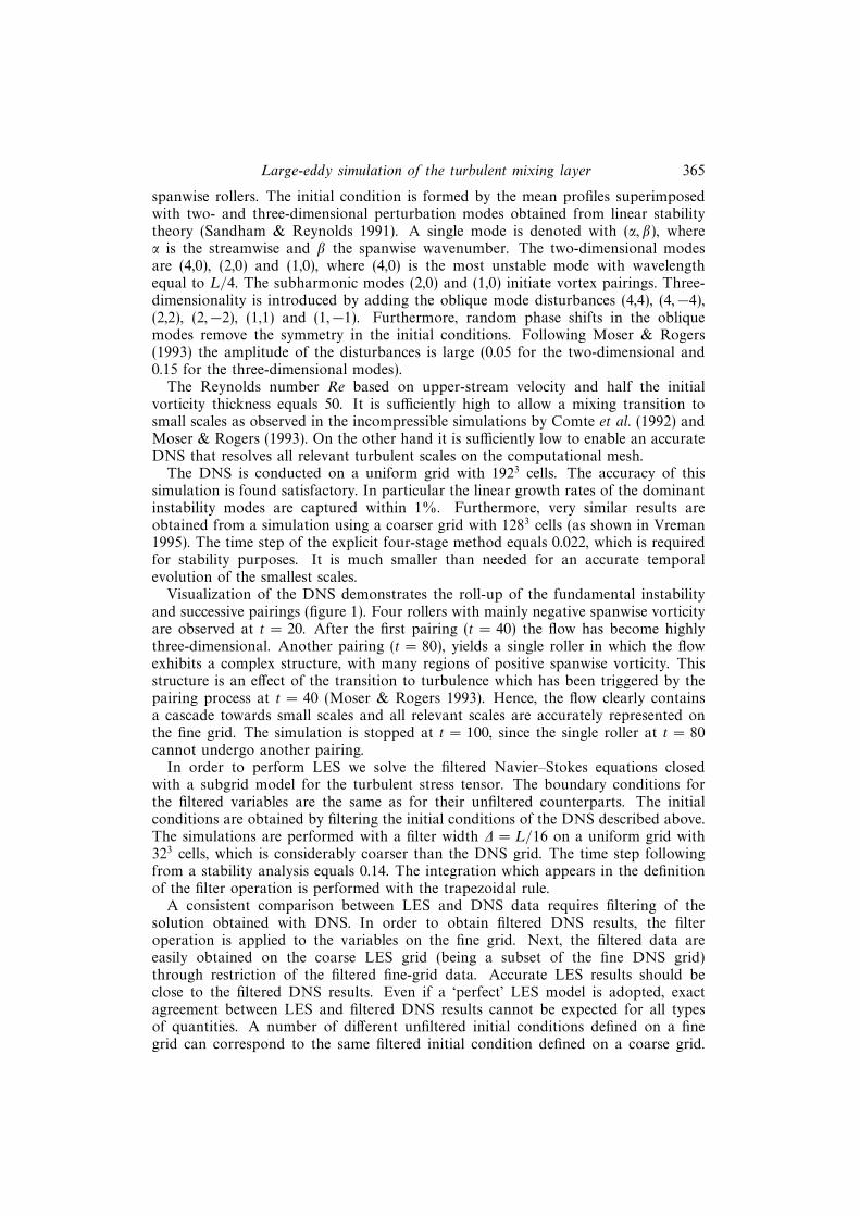
Visualization of the DNS demonstrates the roll-up of the fundamental instabilityand successive pairings (figure 1). Four rollers with mainly negative spanwise vorticityare observed at t = 20. After the first pairing (t = 40) the flow has become highlythree-dimensional. Another pairing (t = 80), yields a single roller in which the flowexhibits a complex structure, with many regions of positive spanwise vorticity. Thisstructure is an effect of the transition to turbulence which has been triggered by thepairing process at t = 40 (Moser & Rogers 1993). Hence, the flow clearly containsa cascade towards small scales and all relevant scales are accurately represented onthe fine grid. The simulation is stopped at t = 100, since the single roller at t = 80cannot undergo another pairing.

In order to perform LES we solve the filtered Navier–Stokes equations closedwith a subgrid model for the turbulent stress tensor. The boundary conditions forthe filtered variables are the same as for their unfiltered counterparts. The initialconditions are obtained by filtering the initial conditions of the DNS described above.The simulations are performed with a filter width ∆ = L/16 on a uniform grid with323 cells, which is considerably coarser than the DNS grid. The time step followingfrom a stability analysis equals 0.14. The integration which appears in the definitionof the filter operation is performed with the trapezoidal rule.

A consistent comparison between LES and DNS data requires filtering of thesolution obtained with DNS. In order to obtain filtered DNS results, the filteroperation is applied to the variables on the fine grid. Next, the filtered data areeasily obtained on the coarse LES grid (being a subset of the fine DNS grid)through restriction of the filtered fine-grid data. Accurate LES results should beclose to the filtered DNS results. Even if a ‘perfect’ LES model is adopted, exactagreement between LES and filtered DNS results cannot be expected for all typesof quantities. A number of different unfiltered initial conditions defined on a finegrid can correspond to the same filtered initial condition defined on a coarse grid.


20

10

0

–10

–20

0 10 20 30 40 50x1

x2

(a)

0 10 20 30 40 50x1

(b)

20

10

0

–10

–20

0 10 20 30 40 50x1

x2

(c)

Figure 1. Contours of spanwise vorticity from DNS for the plane x3 = 0.75L at (a) t = 20, (b)t = 40 and (c) t = 80. Solid and dotted contours indicate negative and positive vorticity respectively.The contour increment is 0.1.

In general the DNS starting from these unfiltered initial conditions will not lead toexactly the same filtered DNS results. The agreement between LES and filtered DNSresults for averaged quantities is likely to be higher than for instantaneous quantities.Hence, good quantitative agreement between accurate LES and filtered DNS results isdemanded for averaged quantities and global features, rather than for instantaneousquantities, such as the evolution of the velocity at a specific location.

LES are performed using the six subgrid models for τij formulated in § 2.2.The performance of a specific subgrid model is considered to be bad if the errors(deviations from the filtered DNS) are comparable to or larger than the errorscorresponding to M0 (no subgrid model). In such a case the incorporation of thesubgrid model does not make sense. For most quantities the discrepancy between thecoarse-grid simulation without a subgrid model and the filtered DNS is quite large,


illustrating that there is something to improve upon; the contribution of a subgridmodel should be significant.

3.2. Comparison of results

Various quantities obtained from LES with M0–6 are shown and compared with thefiltered DNS data. We consider several aspects of the kinetic energy in detail: theevolution of total kinetic energy, turbulent and molecular dissipation, backscatterand Fourier energy spectra. The turbulent stress tensor accounts for the transfer ofkinetic energy from resolved to subgrid scales. Some of the selected models adoptthe eddy-viscosity hypothesis in order to approximate the energy transfer to subgridscales. In contrast to these models, non-eddy-viscosity models (e.g. similarity) canhave mechanisms to produce backscatter of energy from subgrid to resolved scales.For these models the amount of backscatter will be calculated. Furthermore, as alocal quantity the spanwise vorticity in a representative plane serves to monitor thelocal qualitative performance of the six models. We also investigate the evolution ofthe momentum thickness and various averaged statistics, e.g. Reynolds-stress profiles.In this way a number of essentially different quantities (mean, local, plane averaged)are included in the a posteriori tests in order to assess the quality of the models.

3.2.1. Total kinetic energy

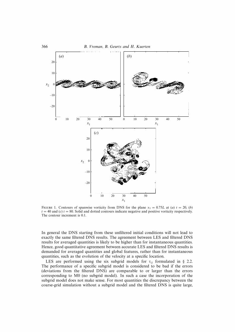
A comparison of the subgrid models with respect to the evolution of the totalkinetic energy, based on filtered variables,

E =

∫Ω

12ρuiuidx, (3.1)

is given in figure 2. First we discuss the Smagorinsky model M1, which gives evenworse predictions than M0. The total kinetic energy E for M1 is observed to exhibita characteristic behaviour: in the transitional regime of the simulation the dissipationof energy is far too large, while it is far too low afterwards. M1 gives such an excessivedissipation in the transitional regime that the transition to turbulence is hindered.The excessive dissipation caused by this model has also been observed by Piomelliet al. (1990a) in their study of turbulent channel flow. The other models (M2–6) arenot too dissipative in the transitional regime. The M3 case gives no improvementover M0, but M2 and M4–6 do improve the results. In contrast to M3, no limiteris required to stabilize M2. Comparison of the curves of M2 and M0 in figure 2shows that the similarity model M2 dissipates approximately the correct amount ofenergy. As will be shown below, the simulation with M2 does not provide sufficientdissipation for small scales, although the total dissipation is reasonably well predicted.The results for M4, the dynamic eddy-viscosity model by Germano et al., illustratethat the dynamic adjustment of the model coefficient meets the major shortcomingof Smagorinsky’s model, namely the excessive dissipation in the transitional regime.Indeed the results are much better than those of M1. The dynamic mixed modelM5 and the dynamic Clark model M6 both accurately predict the evolution of E.Within the group of models considered, M5 most closely approaches the filtered DNSresults.


10.0

9.5

9.0

8.0

7.5

0 20 40 60 80 100

Tota

l kin

etic

ene

rgy

8.5

(×104)

7.0

Time

Figure 2. Comparison of the total kinetic energy E obtained from the filtered DNS () and fromLES using M0–6 (see table 1 for symbols).

3.2.2. Turbulent and molecular dissipation

The decay of the total kinetic energy, E, is described by the following partialdifferential equation:

∂tE =

∫Ω

(Pd − εµ − εsgs)dx, (3.2)

where

Pd = p∂kuk, (3.3)

εµ = µSij∂j ui, (3.4)

εsgs = −ρτij∂j ui. (3.5)

In our case the contribution of the pressure dilatation Pd can be neglected, since theflow is almost incompressible. The molecular dissipation, εµ, is always positive due

to the equality Sij∂j ui = 12S2ij . The subgrid dissipation, εsgs, represents the amount

of energy transferred from resolved to subgrid scales, which is positive if an eddy-viscosity model is adopted for τij . For non-eddy-viscosity models, however, this termcan be positive or negative, referring to forward or backscatter of subgrid-scale kineticenergy respectively. Backscatter produced by subgrid-models is sometimes hard tocontrol within a simulation and can lead to numerical instability. From the modelswe consider, the gradient model (M3), as formulated in equation (2.11), leads toinstabilities if the backscatter is not prevented with the use of a limiter (§2.2.3).

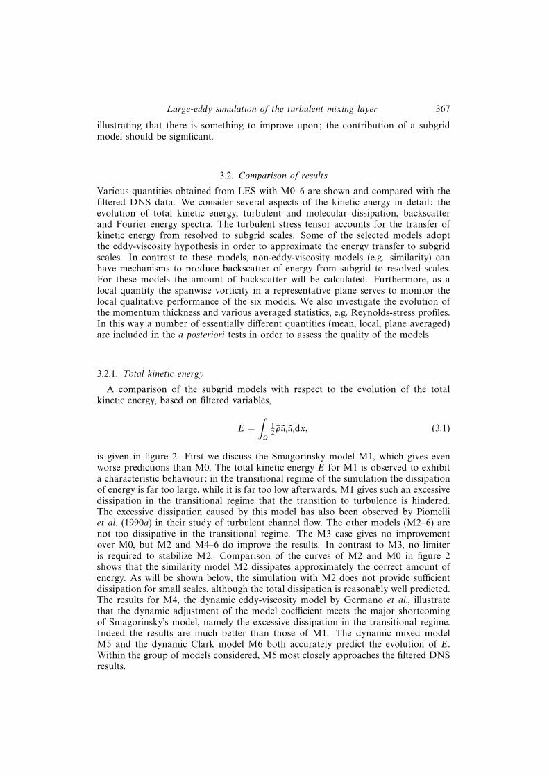
Thus, the decay of total kinetic energy is caused by both subgrid-scale and moleculardissipation. The subgrid-scale dissipation and molecular dissipation integrated overthe domain are shown in figure 3. Simulation M0 is not found in figure 3(a): it hasno subgrid-scale dissipation, since no subgrid-model is adopted. Figure 3(a) clearlyreveals the excessive dissipation of M1 in the transitional regime. For the othermodels the subgrid-scale dissipation is initially small, whereas it grows when the flowundergoes the transition to turbulence. Furthermore, M2 (without limiter) and M3(with limiter) are observed to dissipate energy, although these models do not employ


400

300

100

0 20 40 60 80 100

Sub

grid

dis

sipa

tion

200

Time

(a)300

100

0 20 40 60 80 100

Mol

ecul

ar d

issi

pati

on

200

Time

(b)250

150

50

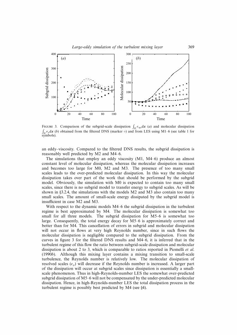
Figure 3. Comparison of the subgrid-scale dissipation∫Ωεsgsdx (a) and molecular dissipation∫

Ωεµdx (b) obtained from the filtered DNS (marker ) and from LES using M1–6 (see table 1 for

symbols).

an eddy–viscosity. Compared to the filtered DNS results, the subgrid dissipation isreasonably well predicted by M2 and M4–6.

The simulations that employ an eddy viscosity (M1, M4–6) produce an almostconstant level of molecular dissipation, whereas the molecular dissipation increasesand becomes too large for M0, M2 and M3. The presence of too many smallscales leads to the over-predicted molecular dissipation. In this way the moleculardissipation takes over part of the work that should be performed by the subgridmodel. Obviously, the simulation with M0 is expected to contain too many smallscales, since there is no subgrid model to transfer energy to subgrid scales. As will beshown in §3.2.4, the simulations with the models M2 and M3 also contain too manysmall scales. The amount of small-scale energy dissipated by the subgrid model isinsufficient in case M2 and M3.

With respect to the dynamic models M4–6 the subgrid dissipation in the turbulentregime is best approximated by M4. The molecular dissipation is somewhat toosmall for all three models. The subgrid dissipation for M5–6 is somewhat toolarge. Consequently, the total energy decay for M5–6 is approximately correct andbetter than for M4. This cancellation of errors in subgrid and molecular dissipationwill not occur in flows at very high Reynolds number, since in such flows themolecular dissipation is negligible compared to the subgrid dissipation. From thecurves in figure 3 for the filtered DNS results and M4–6, it is inferred that in theturbulent regime of this flow the ratio between subgrid-scale dissipation and moleculardissipation is about 2 to 3, which is comparable to ratios reported in Piomelli et al.(1990b). Although this mixing layer contains a mixing transition to small-scaleturbulence, the Reynolds number is relatively low. The molecular dissipation ofresolved scales (εµ) will decrease if the Reynolds number is increased. A larger partof the dissipation will occur at subgrid scales since dissipation is essentially a small-scale phenomenon. Thus in high-Reynolds-number LES the somewhat over-predictedsubgrid dissipation of M5–6 will not be compensated by the under-predicted moleculardissipation. Hence, in high-Reynolds-number LES the total dissipation process in theturbulent regime is possibly best predicted by M4 (see §4).


0

–20

–400 20 40 60 80 100

Bac

ksca

tter

–30

Time

–10

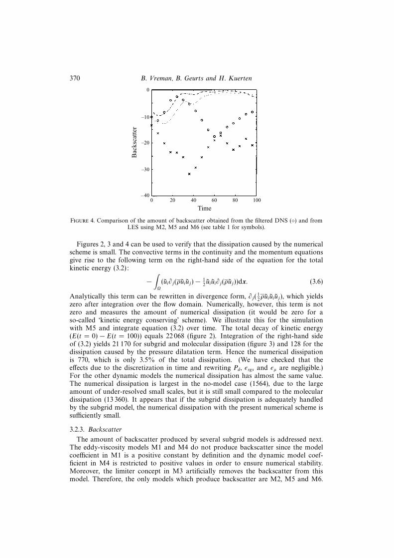
Figure 4. Comparison of the amount of backscatter obtained from the filtered DNS () and fromLES using M2, M5 and M6 (see table 1 for symbols).

Figures 2, 3 and 4 can be used to verify that the dissipation caused by the numericalscheme is small. The convective terms in the continuity and the momentum equationsgive rise to the following term on the right-hand side of the equation for the totalkinetic energy (3.2):

−∫Ω

(ui∂j(ρuiuj)− 12uiui∂j(ρuj))dx. (3.6)

Analytically this term can be rewritten in divergence form, ∂j(12ρuiuiuj), which yields

zero after integration over the flow domain. Numerically, however, this term is notzero and measures the amount of numerical dissipation (it would be zero for aso-called ‘kinetic energy conserving’ scheme). We illustrate this for the simulationwith M5 and integrate equation (3.2) over time. The total decay of kinetic energy(E(t = 0) − E(t = 100)) equals 22 068 (figure 2). Integration of the right-hand sideof (3.2) yields 21 170 for subgrid and molecular dissipation (figure 3) and 128 for thedissipation caused by the pressure dilatation term. Hence the numerical dissipationis 770, which is only 3.5% of the total dissipation. (We have checked that theeffects due to the discretization in time and rewriting Pd, εsgs and εµ are negligible.)For the other dynamic models the numerical dissipation has almost the same value.The numerical dissipation is largest in the no-model case (1564), due to the largeamount of under-resolved small scales, but it is still small compared to the moleculardissipation (13 360). It appears that if the subgrid dissipation is adequately handledby the subgrid model, the numerical dissipation with the present numerical scheme issufficiently small.

3.2.3. Backscatter

The amount of backscatter produced by several subgrid models is addressed next.The eddy-viscosity models M1 and M4 do not produce backscatter since the modelcoefficient in M1 is a positive constant by definition and the dynamic model coef-ficient in M4 is restricted to positive values in order to ensure numerical stability.Moreover, the limiter concept in M3 artificially removes the backscatter from thismodel. Therefore, the only models which produce backscatter are M2, M5 and M6.


For these models the total amount of backscatter, defined as∫Ω

min(εsgs, 0)dx, (3.7)

is plotted in figure 4. Since M5–6 incorporate an eddy-viscosity, these models produceless backscatter than M2. The amount of backscatter for M5–6 is relatively low in theturbulent regime, where the eddy-viscosity part of the model is more important thanin the transitional regime. A comparison with the filtered DNS results shows that M2produces too much backscatter, whereas M5–6 do not produce enough backscatter.Except in the early stages of the simulation, the amount of backscatter is only asmall fraction of the forward scatter (about 10% for the filtered DNS results). Apriori tests of transitional and turbulent channel flow show comparable back- andforward scatter for the spectral cut-off filter, but smaller back- than forward scatterfor the top-hat and Gaussian filters (Piomelli et al. 1990b). Here a posteriori tests ofthe mixing layer demonstrate that in the filtered DNS on a coarse grid and in actualLES with the top-hat filter the structure of the turbulent flow is such that the amountof backscatter is relatively small. In a recent study on dynamic LES of isotropicturbulence, taking backscatter into account did not significantly influence the resultseither (Carati, Ghosal & Moin 1995).

Others decompose the subgrid dissipation εsgs into a mean and a fluctuating part(Jimenez-Hartel 1994; Horiuti 1995) and find that the amount of backscatter in thefluctuating part is relatively large. In this subsection we focused on the importanceof backscatter relative to the full dissipation of energy to subgrid scales.

3.2.4. Magnitude of turbulent stress

In this subsection we turn to the prediction of the separate components of theturbulent stress. We restrict the presentation to the τ12 component, but similarconclusions hold for the other components as well.

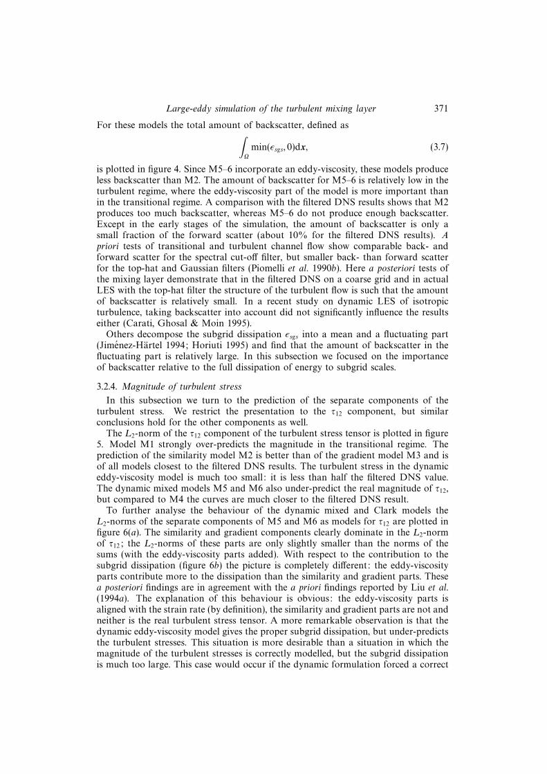
The L2-norm of the τ12 component of the turbulent stress tensor is plotted in figure5. Model M1 strongly over-predicts the magnitude in the transitional regime. Theprediction of the similarity model M2 is better than of the gradient model M3 and isof all models closest to the filtered DNS results. The turbulent stress in the dynamiceddy-viscosity model is much too small: it is less than half the filtered DNS value.The dynamic mixed models M5 and M6 also under-predict the real magnitude of τ12,but compared to M4 the curves are much closer to the filtered DNS result.

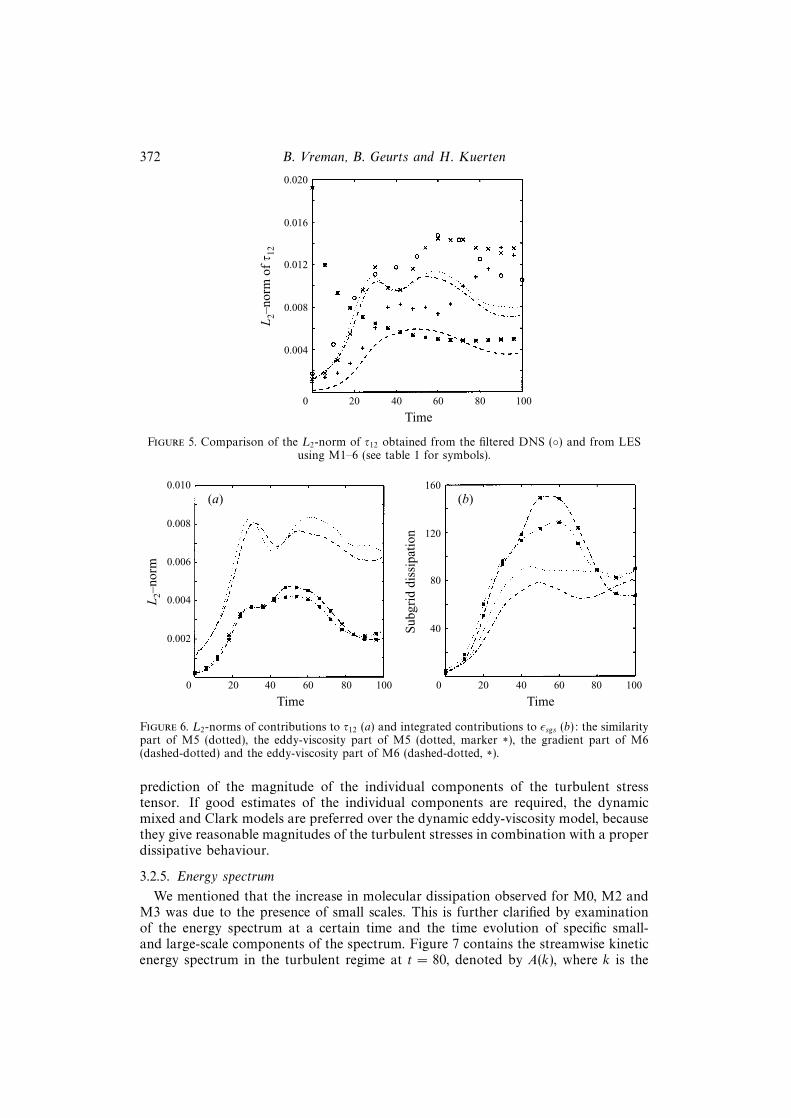
To further analyse the behaviour of the dynamic mixed and Clark models theL2-norms of the separate components of M5 and M6 as models for τ12 are plotted infigure 6(a). The similarity and gradient components clearly dominate in the L2-normof τ12; the L2-norms of these parts are only slightly smaller than the norms of thesums (with the eddy-viscosity parts added). With respect to the contribution to thesubgrid dissipation (figure 6b) the picture is completely different: the eddy-viscosityparts contribute more to the dissipation than the similarity and gradient parts. Thesea posteriori findings are in agreement with the a priori findings reported by Liu et al.(1994a). The explanation of this behaviour is obvious: the eddy-viscosity parts isaligned with the strain rate (by definition), the similarity and gradient parts are not andneither is the real turbulent stress tensor. A more remarkable observation is that thedynamic eddy-viscosity model gives the proper subgrid dissipation, but under-predictsthe turbulent stresses. This situation is more desirable than a situation in which themagnitude of the turbulent stresses is correctly modelled, but the subgrid dissipationis much too large. This case would occur if the dynamic formulation forced a correct


0.020

0.012

0 20 40 60 80 100

L2–

norm

of τ 1

2

0.008

Time

0.016

0.004

Figure 5. Comparison of the L2-norm of τ12 obtained from the filtered DNS () and from LESusing M1–6 (see table 1 for symbols).

0.010

0.008

0.004

0 20 40 60 80 100

L2–

norm

0.006

Time

(a)160

0 20 40 60 80 100

Sub

grid

dis

sipa

tion

Time

(b)

120

80

400.002

Figure 6. L2-norms of contributions to τ12 (a) and integrated contributions to εsgs (b): the similaritypart of M5 (dotted), the eddy-viscosity part of M5 (dotted, marker ∗), the gradient part of M6(dashed-dotted) and the eddy-viscosity part of M6 (dashed-dotted, ∗).

prediction of the magnitude of the individual components of the turbulent stresstensor. If good estimates of the individual components are required, the dynamicmixed and Clark models are preferred over the dynamic eddy-viscosity model, becausethey give reasonable magnitudes of the turbulent stresses in combination with a properdissipative behaviour.

3.2.5. Energy spectrum

We mentioned that the increase in molecular dissipation observed for M0, M2 andM3 was due to the presence of small scales. This is further clarified by examinationof the energy spectrum at a certain time and the time evolution of specific small-and large-scale components of the spectrum. Figure 7 contains the streamwise kineticenergy spectrum in the turbulent regime at t = 80, denoted by A(k), where k is the


100

101

A(k)

k

10–2

10–4

10–6

10–8

100

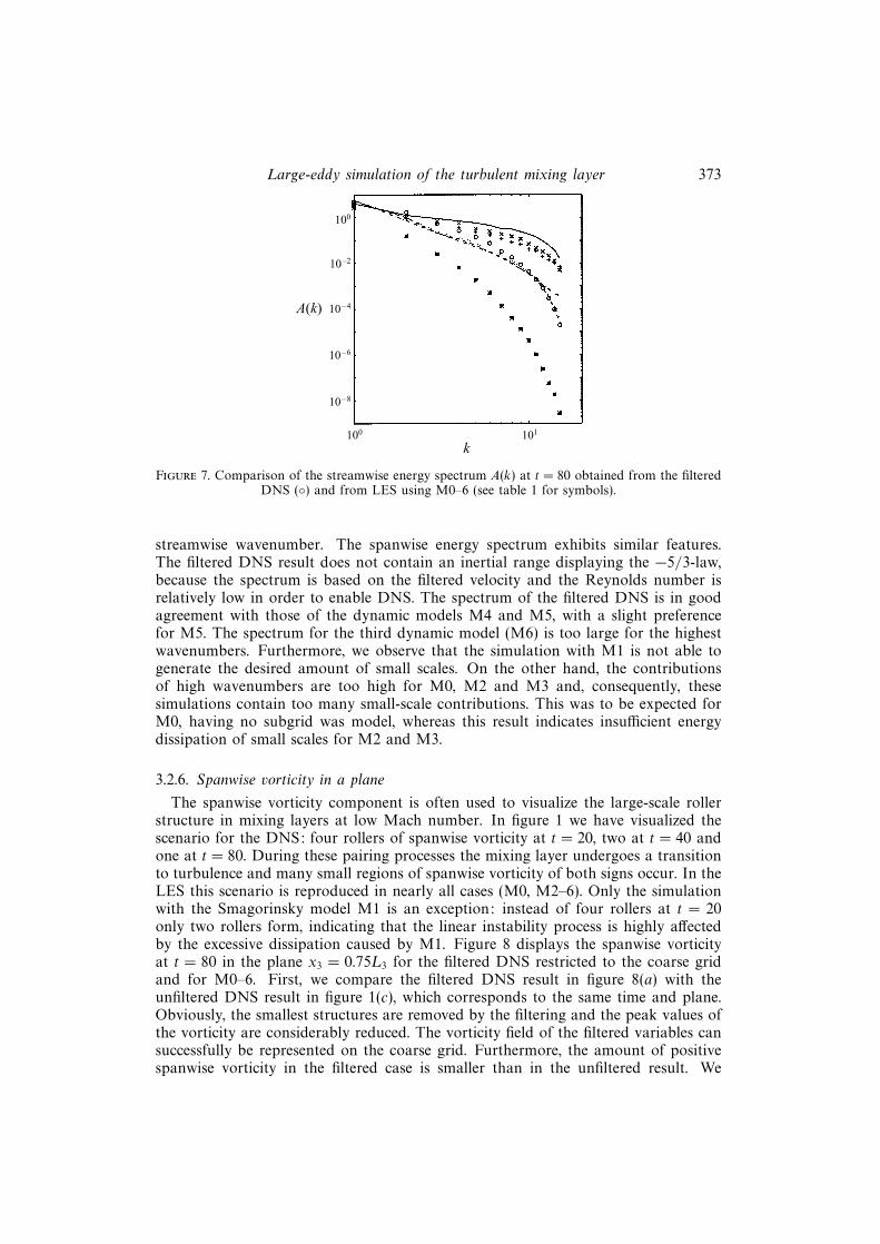
Figure 7. Comparison of the streamwise energy spectrum A(k) at t = 80 obtained from the filteredDNS () and from LES using M0–6 (see table 1 for symbols).

streamwise wavenumber. The spanwise energy spectrum exhibits similar features.The filtered DNS result does not contain an inertial range displaying the −5/3-law,because the spectrum is based on the filtered velocity and the Reynolds number isrelatively low in order to enable DNS. The spectrum of the filtered DNS is in goodagreement with those of the dynamic models M4 and M5, with a slight preferencefor M5. The spectrum for the third dynamic model (M6) is too large for the highestwavenumbers. Furthermore, we observe that the simulation with M1 is not able togenerate the desired amount of small scales. On the other hand, the contributionsof high wavenumbers are too high for M0, M2 and M3 and, consequently, thesesimulations contain too many small-scale contributions. This was to be expected forM0, having no subgrid was model, whereas this result indicates insufficient energydissipation of small scales for M2 and M3.

3.2.6. Spanwise vorticity in a plane

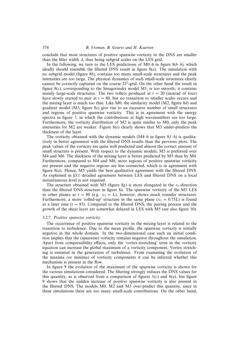
The spanwise vorticity component is often used to visualize the large-scale rollerstructure in mixing layers at low Mach number. In figure 1 we have visualized thescenario for the DNS: four rollers of spanwise vorticity at t = 20, two at t = 40 andone at t = 80. During these pairing processes the mixing layer undergoes a transitionto turbulence and many small regions of spanwise vorticity of both signs occur. In theLES this scenario is reproduced in nearly all cases (M0, M2–6). Only the simulationwith the Smagorinsky model M1 is an exception: instead of four rollers at t = 20only two rollers form, indicating that the linear instability process is highly affectedby the excessive dissipation caused by M1. Figure 8 displays the spanwise vorticityat t = 80 in the plane x3 = 0.75L3 for the filtered DNS restricted to the coarse gridand for M0–6. First, we compare the filtered DNS result in figure 8(a) with theunfiltered DNS result in figure 1(c), which corresponds to the same time and plane.Obviously, the smallest structures are removed by the filtering and the peak values ofthe vorticity are considerably reduced. The vorticity field of the filtered variables cansuccessfully be represented on the coarse grid. Furthermore, the amount of positivespanwise vorticity in the filtered case is smaller than in the unfiltered result. We


conclude that most structures of positive spanwise vorticity in the DNS are smallerthan the filter width ∆, thus being subgrid scales on the LES grid.

In the following, we turn to the LES predictions of M0–6 in figure 8(b–h), whichideally should resemble the filtered DNS result in figure 8(a). The simulation withno subgrid model (figure 8b), contains too many small-scale structures and the peakintensities are too large. The physical dynamics of such small-scale structures clearlycannot be correctly captured on the coarse 323-grid. On the other hand the result infigure 8(c), corresponding to the Smagorinsky model M1, is too smooth; it containsmainly large-scale structures. The two rollers produced at t = 20 (instead of four)have slowly started to pair at t = 80, but no transition to smaller scales occurs andthe mixing layer is much too thin. Like M0, the similarity model (M2, figure 8d) andgradient model (M3, figure 8e) give rise to an excessive number of small structuresand regions of positive spanwise vorticity. This is in agreement with the energyspectra in figure 7, in which the contributions at high wavenumbers are too large.Furthermore, the vorticity distribution of M2 is quite similar to M0, only the peakintensities for M2 are weaker. Figure 8(e) clearly shows that M3 under-predicts thethickness of the layer.

The vorticity obtained with the dynamic models (M4–6 in figure 8f–h) is qualita-tively in better agreement with the filtered DNS results than the previous plots. Thepeak values of the vorticity are quite well predicted and almost the correct amount ofsmall structure is present. With respect to the dynamic models, M5 is preferred overM4 and M6. The thickness of the mixing layer is better predicted by M5 than by M4.Furthermore, compared to M4 and M6, more regions of positive spanwise vorticityare present and the negative regions are less connected, which is in agreement withfigure 8(a). Hence, M5 yields the best qualitative agreement with the filtered DNS.As explained in §3.1 detailed agreement between LES and filtered DNS on a localinstantaneous level is not required.

The structure obtained with M5 (figure 8g) is more elongated in the x1-directionthan the filtered DNS structure in figure 8a. The spanwise vorticity of the M5 LESin other planes at t = 80 (e.g. x3 = L), however, shows much rounder structures.Furthermore, a more ‘rolled-up’ structure in the same plane (x3 = 0.75L) is foundat a later time (t = 85). Compared to the filtered DNS, the pairing process and thegrowth of the shear layer are somewhat delayed in LES with M5 (see also figure 10).

3.2.7. Positive spanwise vorticity

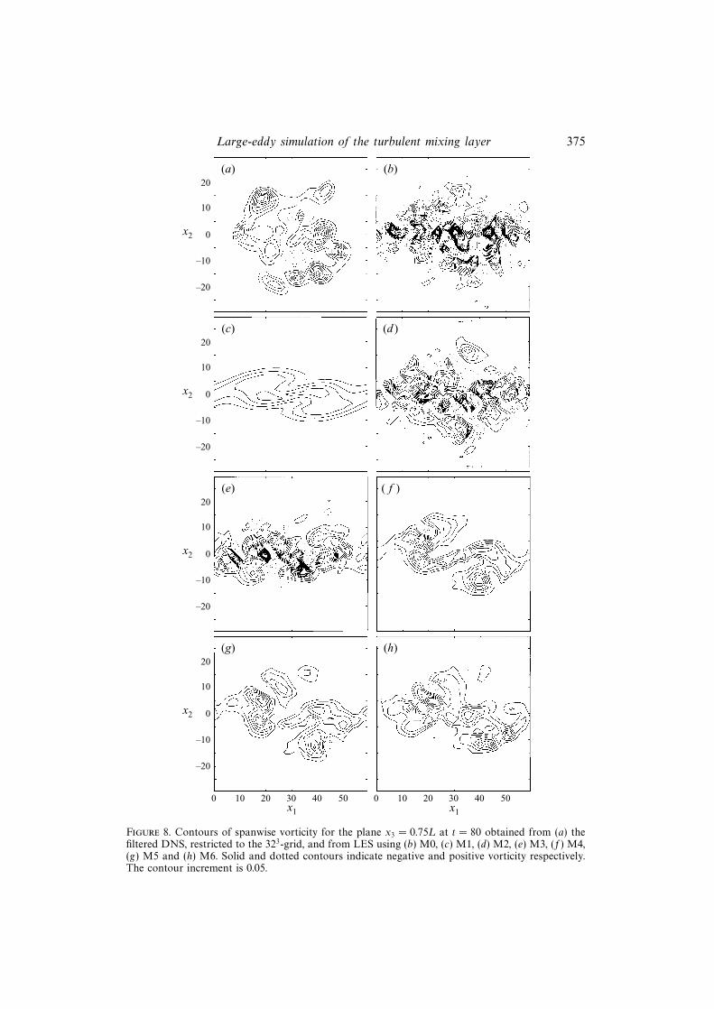
The occurrence of positive spanwise vorticity in the mixing layer is related to thetransition to turbulence. Due to the mean profile, the spanwise vorticity is initiallynegative in the whole domain. In the two-dimensional case such an initial condi-tion implies that the (spanwise) vorticity remains negative throughout the simulation.Apart from compressibility effects, only the ‘vortex-stretching’ term in the vorticityequation can increase the global maximum of a vorticity component. Vortex stretch-ing is essential in the generation of turbulence. From examining the evolution ofthe maxima (or minima) of vorticity components it can be inferred whether thismechanism is present in the flow.

In figure 9 the evolution of the maximum of the spanwise vorticity is shown forthe various simulations considered. The filtering strongly reduces the DNS values forthis quantity, as is observed from a comparison of figures 1(c) and 8(a), but figure9 shows that the sudden increase of positive spanwise vorticity is also present inthe filtered DNS. The models M0, M2 and M3 over-predict this quantity, since inthese simulations there are too many small-scale contributions. On the other hand,


x2

–20

0

–10

0

10

20

10 20 30 40 50x1

(g)

0 10 20 30 40 50x1

(h)

x2

–20

–10

0

10

20

(e) ( f )

x2

–20

–10

0

10

20

(c) (d )

x2

–20

–10

0

10

20

(a) (b)

Figure 8. Contours of spanwise vorticity for the plane x3 = 0.75L at t = 80 obtained from (a) thefiltered DNS, restricted to the 323-grid, and from LES using (b) M0, (c) M1, (d) M2, (e) M3, (f) M4,(g) M5 and (h) M6. Solid and dotted contours indicate negative and positive vorticity respectively.The contour increment is 0.05.


Max

imum

spa

nwis

e vo

rtic

ity

0.2

0

0.4

0.6

0.8

20 40 60Time

80 100

1.0

Figure 9. Comparison of the spatial maximum of positive spanwise vorticity as a function of timeobtained from the filtered DNS () and from LES using M0–6 (see table 1 for symbols).

in the simulation with M1 no positive spanwise vorticity is generated for a longtime, corresponding to the absence of strong vortex stretching. This result againillustrates that the Smagorinsky model hinders the transition to turbulence. Thedynamic models M4 and M5 both give predictions which are relatively close to thefiltered DNS results, whereas the increase of positive spanwise vorticity starts tooearly for M6.

3.2.8. Momentum thickness

From figure 8 we have already observed that the thickness of the mixing layerdepends on the subgrid model. This dependence is further clarified in figure 10, inwhich the evolution of the momentum thickness, based on filtered variables,

δ = 14

∫ L/2

−L/2〈ρ〉(

1− 〈ρu1〉〈ρ〉

)(〈ρu1〉〈ρ〉 + 1

)dx2, (3.8)

is shown. The operator 〈.〉 represents an averaging over the homogeneous directionsx1 and x3. Since the definition of the momentum thickness employs the mean velocityprofile, tests for the momentum thickness quantify the spreading of the mean velocityprofile. Figure 9 displays a short period of laminar growth (until t = 20), followed bya period in which the mixing layer grows considerably faster, visualizing the increasedmixing caused by turbulence.

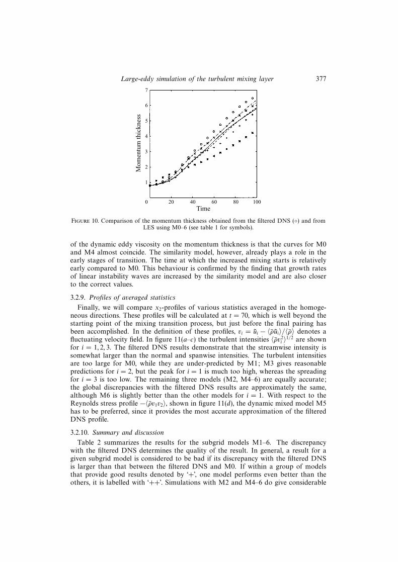
The models M1 and M3 lead to worse predictions for the momentum thicknessthan M0, indicating that with respect to this quantity LES without a subgrid modelis preferred over adopting M1 or M3. The slow growth of the momentum thicknessfor M1 further establishes the observation that this model hinders the transitionto turbulence. The results for M4 are quite similar to M0, whereas the modelsM2, M5 and M6 clearly yield improvement over M0 and are relatively close to thefiltered DNS result. It is remarkable that the evolution of the momentum thickness isalmost identical for M2 and M5. This indicates that for the momentum thickness theimprovement over M0 is mainly due to the similarity model, since the eddy viscositypart of M5 does not seem to affect this quantity. Other evidence for the small effect


Mom

entu

m th

ickn

ess

3

0

4

5

6

20 40 60Time

80 100

7

2

1

Figure 10. Comparison of the momentum thickness obtained from the filtered DNS () and fromLES using M0–6 (see table 1 for symbols).

of the dynamic eddy viscosity on the momentum thickness is that the curves for M0and M4 almost coincide. The similarity model, however, already plays a role in theearly stages of transition. The time at which the increased mixing starts is relativelyearly compared to M0. This behaviour is confirmed by the finding that growth ratesof linear instability waves are increased by the similarity model and are also closerto the correct values.

3.2.9. Profiles of averaged statistics

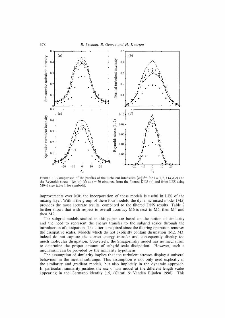
Finally, we will compare x2-profiles of various statistics averaged in the homoge-neous directions. These profiles will be calculated at t = 70, which is well beyond thestarting point of the mixing transition process, but just before the final pairing hasbeen accomplished. In the definition of these profiles, vi = ui − 〈ρui〉/〈ρ〉 denotes afluctuating velocity field. In figure 11(a–c) the turbulent intensities 〈ρv2

i 〉1/2 are shownfor i = 1, 2, 3. The filtered DNS results demonstrate that the streamwise intensity issomewhat larger than the normal and spanwise intensities. The turbulent intensitiesare too large for M0, while they are under-predicted by M1; M3 gives reasonablepredictions for i = 2, but the peak for i = 1 is much too high, whereas the spreadingfor i = 3 is too low. The remaining three models (M2, M4–6) are equally accurate;the global discrepancies with the filtered DNS results are approximately the same,although M6 is slightly better than the other models for i = 1. With respect to theReynolds stress profile −〈ρv1v2〉, shown in figure 11(d), the dynamic mixed model M5has to be preferred, since it provides the most accurate approximation of the filteredDNS profile.

3.2.10. Summary and discussion

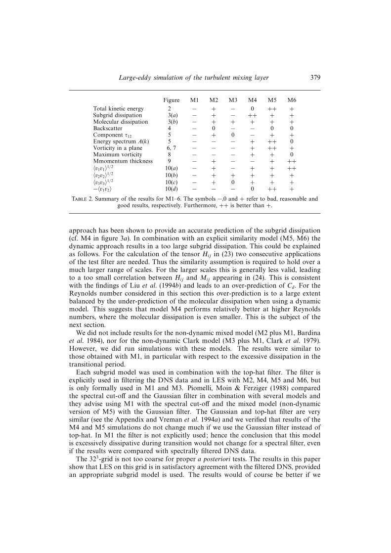
Table 2 summarizes the results for the subgrid models M1–6. The discrepancywith the filtered DNS determines the quality of the result. In general, a result for agiven subgrid model is considered to be bad if its discrepancy with the filtered DNSis larger than that between the filtered DNS and M0. If within a group of modelsthat provide good results denoted by ‘+’, one model performs even better than theothers, it is labelled with ‘++’. Simulations with M2 and M4–6 do give considerable

378 B. Vreman, B. Geurts and H. KuertenS

panw

ise

turb

ulen

t int

ensi

ty

0

0.2

0.3

0.4

–20 –10 0x2

10 20

0.5

0.1

(c)–R

eyno

lds

stre

ss (

1, 2

)

0

0.04

0.06

0.08

–20 –10 0x2

10 20

0.10

0.02

(d )

Str

eam

wis

e tu

rbul

ent i

nten

sity

0

0.2

0.3

0.4

0.5

0.1

(a)

Nor

mal

turb

ulen

t int

ensi

ty

0

0.2

0.3

0.4

0.5

0.1

(b)

Figure 11. Comparison of the profiles of the turbulent intensities 〈ρv2i 〉1/2 for i = 1, 2, 3 (a, b, c) and

the Reynolds stress −〈ρv1v2〉 (d) at t = 70 obtained from the filtered DNS (o) and from LES usingM0–6 (see table 1 for symbols).

improvements over M0; the incorporation of these models is useful in LES of themixing layer. Within the group of these four models, the dynamic mixed model (M5)provides the most accurate results, compared to the filtered DNS results. Table 2further shows that with respect to overall accuracy M6 is next to M5, then M4 andthen M2.

The subgrid models studied in this paper are based on the notion of similarityand the need to represent the energy transfer to the subgrid scales through theintroduction of dissipation. The latter is required since the filtering operation removesthe dissipative scales. Models which do not explicitly contain dissipation (M2, M3)indeed do not capture the correct energy transfer and consequently display toomuch molecular dissipation. Conversely, the Smagorinsky model has no mechanismto determine the proper amount of subgrid-scale dissipation. However, such amechanism can be provided by the similarity hypothesis.

The assumption of similarity implies that the turbulent stresses display a univeralbehaviour in the inertial subrange. This assumption is not only used explicitly inthe similarity and gradient models, but also implicitly in the dynamic approach.In particular, similarity justifies the use of one model at the different length scalesappearing in the Germano identity (15) (Carati & Vanden Eijnden 1996). This


Figure M1 M2 M3 M4 M5 M6

Total kinetic energy 2 − + − 0 ++ +Subgrid dissipation 3(a) − + − ++ + +Molecular dissipation 3(b) − + + + + +Backscatter 4 − 0 − − 0 0Component τ12 5 − + 0 − + +Energy spectrum A(k) 5 − − − + ++ 0Vorticity in a plane 6, 7 − − − + ++ +Maximum vorticity 8 − − − + + 0Mmomentum thickness 9 − + − − + ++〈v1v1〉1/2 10(a) − + − + + ++〈v2v2〉1/2 10(b) − + + + + +〈v3v3〉1/2 10(c) − + 0 + + +−〈v1v2〉 10(d) − − − 0 ++ +

Table 2. Summary of the results for M1–6. The symbols −,0 and + refer to bad, reasonable andgood results, respectively. Furthermore, ++ is better than +.

approach has been shown to provide an accurate prediction of the subgrid dissipation(cf. M4 in figure 3a). In combination with an explicit similarity model (M5, M6) thedynamic approach results in a too large subgrid dissipation. This could be explainedas follows. For the calculation of the tensor Hij in (23) two consecutive applicationsof the test filter are needed. Thus the similarity assumption is required to hold over amuch larger range of scales. For the larger scales this is generally less valid, leadingto a too small correlation between Hij and Mij appearing in (24). This is consistentwith the findings of Liu et al. (1994b) and leads to an over-prediction of Cd. For theReynolds number considered in this section this over-prediction is to a large extentbalanced by the under-prediction of the molecular dissipation when using a dynamicmodel. This suggests that model M4 performs relatively better at higher Reynoldsnumbers, where the molecular dissipation is even smaller. This is the subject of thenext section.

We did not include results for the non-dynamic mixed model (M2 plus M1, Bardinaet al. 1984), nor for the non-dynamic Clark model (M3 plus M1, Clark et al. 1979).However, we did run simulations with these models. The results were similar tothose obtained with M1, in particular with respect to the excessive dissipation in thetransitional period.

Each subgrid model was used in combination with the top-hat filter. The filter isexplicitly used in filtering the DNS data and in LES with M2, M4, M5 and M6, butis only formally used in M1 and M3. Piomelli, Moin & Ferziger (1988) comparedthe spectral cut-off and the Gaussian filter in combination with several models andthey advise using M1 with the spectral cut-off and the mixed model (non-dynamicversion of M5) with the Gaussian filter. The Gaussian and top-hat filter are verysimilar (see the Appendix and Vreman et al. 1994a) and we verified that results of theM4 and M5 simulations do not change much if we use the Gaussian filter instead oftop-hat. In M1 the filter is not explicitly used; hence the conclusion that this modelis excessively dissipative during transition would not change for a spectral filter, evenif the results were compared with spectrally filtered DNS data.

The 323-grid is not too coarse for proper a posteriori tests. The results in this papershow that LES on this grid is in satisfactory agreement with the filtered DNS, providedan appropriate subgrid model is used. The results would of course be better if we


increased the resolution to 643, but then even the coarse-grid DNS (M0) would givereasonable results and the subgrid dissipation would not be larger than the moleculardissipation. Using the 323-grid, however, the subgrid dissipation is about three timeshigher than the molecular dissipation (figure 3), indicating that a subgrid model isneeded, since the largest part of the dissipation is caused by the small subgrid eddies.On the other hand the 323 grid is sufficiently fine to discern the largest eddies, namelythe four spanwise rollers, subsequently pairing to two, and finally to one roller. Theresolution of 32 uniformly spaced points in the normal direction on a uniform gridis not too small for the representation of the mean profile, which can be concludedfrom the following arguments. Firstly, we have repeated the full comparison on aLES grid of 32 × 64 × 32 points and this set of simulations confirmed the findingsin this section. Secondly, it has to be noticed that according to the definition of theinitial conditions in LES, filtered mean profiles are used, which are smoother thanthe original mean profiles. The instability resulting from this profile is essentially thesame as in the filtered DNS, since for all models considered (except for M1) LESon the 323-grid was observed to reproduce the four-roller structure that results fromthe primary instability. Furthermore, the flow structure in the turbulent regime (e.g.figures 1c, 8) suggests the choice of equal grid sizes in all three directions.

4. Self-similarityIn this section we perform LES of the temporal mixing layer at a higher Reynolds

number and in a larger domain using the subgrid models M0–6. Although thesimulation described in §3 contained a transition to small scales, the size of thedomain allowed two successive pairings only and the Reynolds number was relativelylow (50) in order to enable DNS. Compared to DNS, LES should be able to simulateflows in a larger domain and at higher Reynolds number at the same computationalcost.

The temporal mixing layer in this section is simulated at Re = 500, based on thereference values defined in §2.1. The calculation is performed on a grid with 1203 cellsand the computational domain is large, L = 120. This size is equal to eight timesthe wavelength of the fundamental linear instability. Hence, the flow allows threesuccessive pairings before it saturates. Uniform noise is used to perturb the initialmean flow (amplitude 0.05 and multiplied with e−x

22/4), in contrast to §3.1 where an

eigenfunction perturbation was used. The LES employ the top-hat filter with thebasic filter width equal to twice the grid spacing.

At this Reynolds number there are no DNS results to compare with, but we canverify whether the flow is self-similar. A temporal mixing layer is self-similar if thedevelopment of the shear layer thickness is linear in time and profiles of normalizedstatistical quantities at different times coincide. The common opinion is that turbulentmixing layers display self-similar behaviour, provided the Reynolds number is highand the computational domain is large and the simulation is performed sufficientlyfar in time (Rogers & Moser 1994; Vreman et al. 1996c). Experimental work supportsthe notion of similarity (Brown & Roshko 1974; Campagne, Pao & Wynanski 1976;Bell & Mehta 1990). The specific self-similar state, however, is not unique but dependson the initial forcing (Dimotakis & Brown 1976).

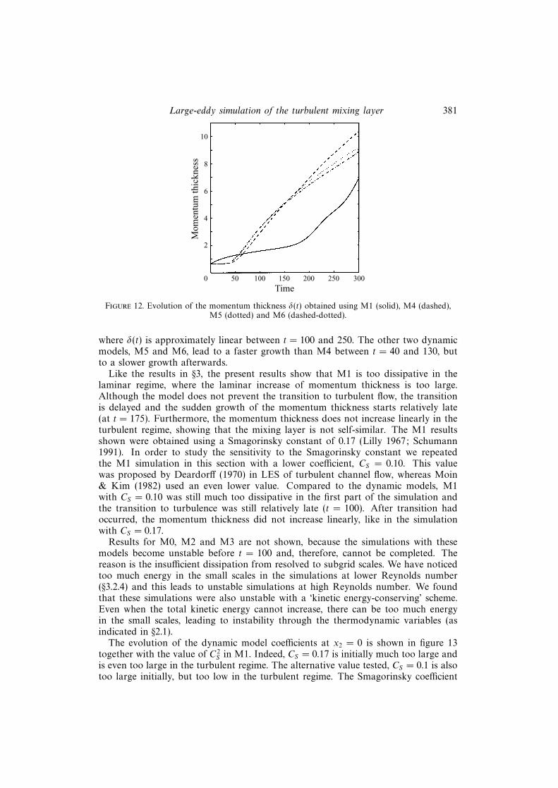
The evolution of the momentum thickness is shown in figure 12 for the subgrid-models M1 and M4–6. None of the simulations is fully self-similar, since in eachcase the momentum thickness curve is not perfectly straight in the turbulent regime.The most self-similar case is obtained with the dynamic eddy-viscosity model M4,


Mom

entu

m th

ickn

ess

0

4

6

8

50 100 150

Time250 300

10

2

200

Figure 12. Evolution of the momentum thickness δ(t) obtained using M1 (solid), M4 (dashed),M5 (dotted) and M6 (dashed-dotted).

where δ(t) is approximately linear between t = 100 and 250. The other two dynamicmodels, M5 and M6, lead to a faster growth than M4 between t = 40 and 130, butto a slower growth afterwards.

Like the results in §3, the present results show that M1 is too dissipative in thelaminar regime, where the laminar increase of momentum thickness is too large.Although the model does not prevent the transition to turbulent flow, the transitionis delayed and the sudden growth of the momentum thickness starts relatively late(at t = 175). Furthermore, the momentum thickness does not increase linearly in theturbulent regime, showing that the mixing layer is not self-similar. The M1 resultsshown were obtained using a Smagorinsky constant of 0.17 (Lilly 1967; Schumann1991). In order to study the sensitivity to the Smagorinsky constant we repeatedthe M1 simulation in this section with a lower coefficient, CS = 0.10. This valuewas proposed by Deardorff (1970) in LES of turbulent channel flow, whereas Moin& Kim (1982) used an even lower value. Compared to the dynamic models, M1with CS = 0.10 was still much too dissipative in the first part of the simulation andthe transition to turbulence was still relatively late (t = 100). After transition hadoccurred, the momentum thickness did not increase linearly, like in the simulationwith CS = 0.17.

Results for M0, M2 and M3 are not shown, because the simulations with thesemodels become unstable before t = 100 and, therefore, cannot be completed. Thereason is the insufficient dissipation from resolved to subgrid scales. We have noticedtoo much energy in the small scales in the simulations at lower Reynolds number(§3.2.4) and this leads to unstable simulations at high Reynolds number. We foundthat these simulations were also unstable with a ‘kinetic energy-conserving’ scheme.Even when the total kinetic energy cannot increase, there can be too much energyin the small scales, leading to instability through the thermodynamic variables (asindicated in §2.1).

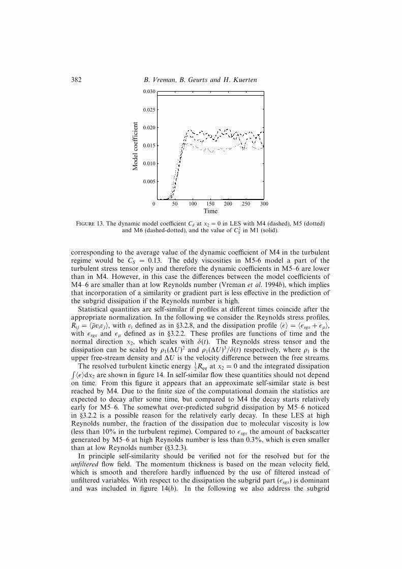
The evolution of the dynamic model coefficients at x2 = 0 is shown in figure 13together with the value of C2

S in M1. Indeed, CS = 0.17 is initially much too large andis even too large in the turbulent regime. The alternative value tested, CS = 0.1 is alsotoo large initially, but too low in the turbulent regime. The Smagorinsky coefficient


Mod

el c

oeff

icie

nt

0

0.015

0.020

0.025

50 100 150

Time250 300

0.030

0.010

200

0.005

Figure 13. The dynamic model coefficient Cd at x2 = 0 in LES with M4 (dashed), M5 (dotted)and M6 (dashed-dotted), and the value of C2

S in M1 (solid).

corresponding to the average value of the dynamic coefficient of M4 in the turbulentregime would be CS = 0.13. The eddy viscosities in M5-6 model a part of theturbulent stress tensor only and therefore the dynamic coefficients in M5–6 are lowerthan in M4. However, in this case the differences between the model coefficients ofM4–6 are smaller than at low Reynolds number (Vreman et al. 1994b), which impliesthat incorporation of a similarity or gradient part is less effective in the prediction ofthe subgrid dissipation if the Reynolds number is high.

Statistical quantities are self-similar if profiles at different times coincide after theappropriate normalization. In the following we consider the Reynolds stress profiles,Rij = 〈ρvivj〉, with vi defined as in §3.2.8, and the dissipation profile 〈ε〉 = 〈εsgs + εµ〉,with εsgs and εµ defined as in §3.2.2. These profiles are functions of time and thenormal direction x2, which scales with δ(t). The Reynolds stress tensor and thedissipation can be scaled by ρ1(∆U)2 and ρ1(∆U)3/δ(t) respectively, where ρ1 is theupper free-stream density and ∆U is the velocity difference between the free streams.

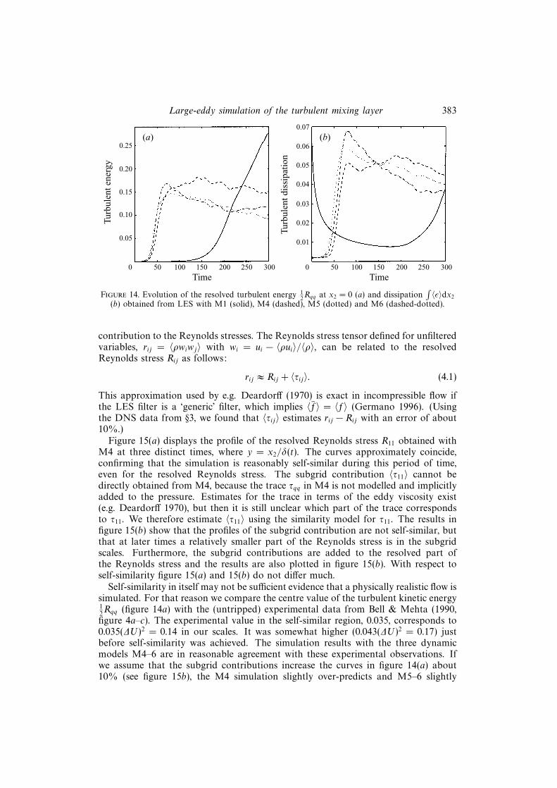
The resolved turbulent kinetic energy 12Rqq at x2 = 0 and the integrated dissipation∫

〈ε〉dx2 are shown in figure 14. In self-similar flow these quantities should not dependon time. From this figure it appears that an approximate self-similar state is bestreached by M4. Due to the finite size of the computational domain the statistics areexpected to decay after some time, but compared to M4 the decay starts relativelyearly for M5–6. The somewhat over-predicted subgrid dissipation by M5–6 noticedin §3.2.2 is a possible reason for the relatively early decay. In these LES at highReynolds number, the fraction of the dissipation due to molecular viscosity is low(less than 10% in the turbulent regime). Compared to εsgs the amount of backscattergenerated by M5–6 at high Reynolds number is less than 0.3%, which is even smallerthan at low Reynolds number (§3.2.3).

In principle self-similarity should be verified not for the resolved but for theunfiltered flow field. The momentum thickness is based on the mean velocity field,which is smooth and therefore hardly influenced by the use of filtered instead ofunfiltered variables. With respect to the dissipation the subgrid part (εsgs) is dominantand was included in figure 14(b). In the following we also address the subgrid

Large-eddy simulation of the turbulent mixing layer 383Tu

rbul

ent e

nerg

y

0

0.15

0.20

0.25

50 100 150

Time250 300

0.10

200

0.05

(a)

Turb

ulen

t dis

sipa

tion

0

0.05

0.06

0.07

50 100 150

Time250 300

0.04

200

0.03

(b)

0.02

0.01

Figure 14. Evolution of the resolved turbulent energy 12Rqq at x2 = 0 (a) and dissipation

∫〈ε〉dx2

(b) obtained from LES with M1 (solid), M4 (dashed), M5 (dotted) and M6 (dashed-dotted).

contribution to the Reynolds stresses. The Reynolds stress tensor defined for unfilteredvariables, rij = 〈ρwiwj〉 with wi = ui − 〈ρui〉/〈ρ〉, can be related to the resolvedReynolds stress Rij as follows:

rij ≈ Rij + 〈τij〉. (4.1)

This approximation used by e.g. Deardorff (1970) is exact in incompressible flow ifthe LES filter is a ‘generic’ filter, which implies 〈f〉 = 〈f〉 (Germano 1996). (Usingthe DNS data from §3, we found that 〈τij〉 estimates rij − Rij with an error of about10%.)

Figure 15(a) displays the profile of the resolved Reynolds stress R11 obtained withM4 at three distinct times, where y = x2/δ(t). The curves approximately coincide,confirming that the simulation is reasonably self-similar during this period of time,even for the resolved Reynolds stress. The subgrid contribution 〈τ11〉 cannot bedirectly obtained from M4, because the trace τqq in M4 is not modelled and implicitlyadded to the pressure. Estimates for the trace in terms of the eddy viscosity exist(e.g. Deardorff 1970), but then it is still unclear which part of the trace correspondsto τ11. We therefore estimate 〈τ11〉 using the similarity model for τ11. The results infigure 15(b) show that the profiles of the subgrid contribution are not self-similar, butthat at later times a relatively smaller part of the Reynolds stress is in the subgridscales. Furthermore, the subgrid contributions are added to the resolved part ofthe Reynolds stress and the results are also plotted in figure 15(b). With respect toself-similarity figure 15(a) and 15(b) do not differ much.

Self-similarity in itself may not be sufficient evidence that a physically realistic flow issimulated. For that reason we compare the centre value of the turbulent kinetic energy12Rqq (figure 14a) with the (untripped) experimental data from Bell & Mehta (1990,

figure 4a–c). The experimental value in the self-similar region, 0.035, corresponds to0.035(∆U)2 = 0.14 in our scales. It was somewhat higher (0.043(∆U)2 = 0.17) justbefore self-similarity was achieved. The simulation results with the three dynamicmodels M4–6 are in reasonable agreement with these experimental observations. Ifwe assume that the subgrid contributions increase the curves in figure 14(a) about10% (see figure 15b), the M4 simulation slightly over-predicts and M5–6 slightly

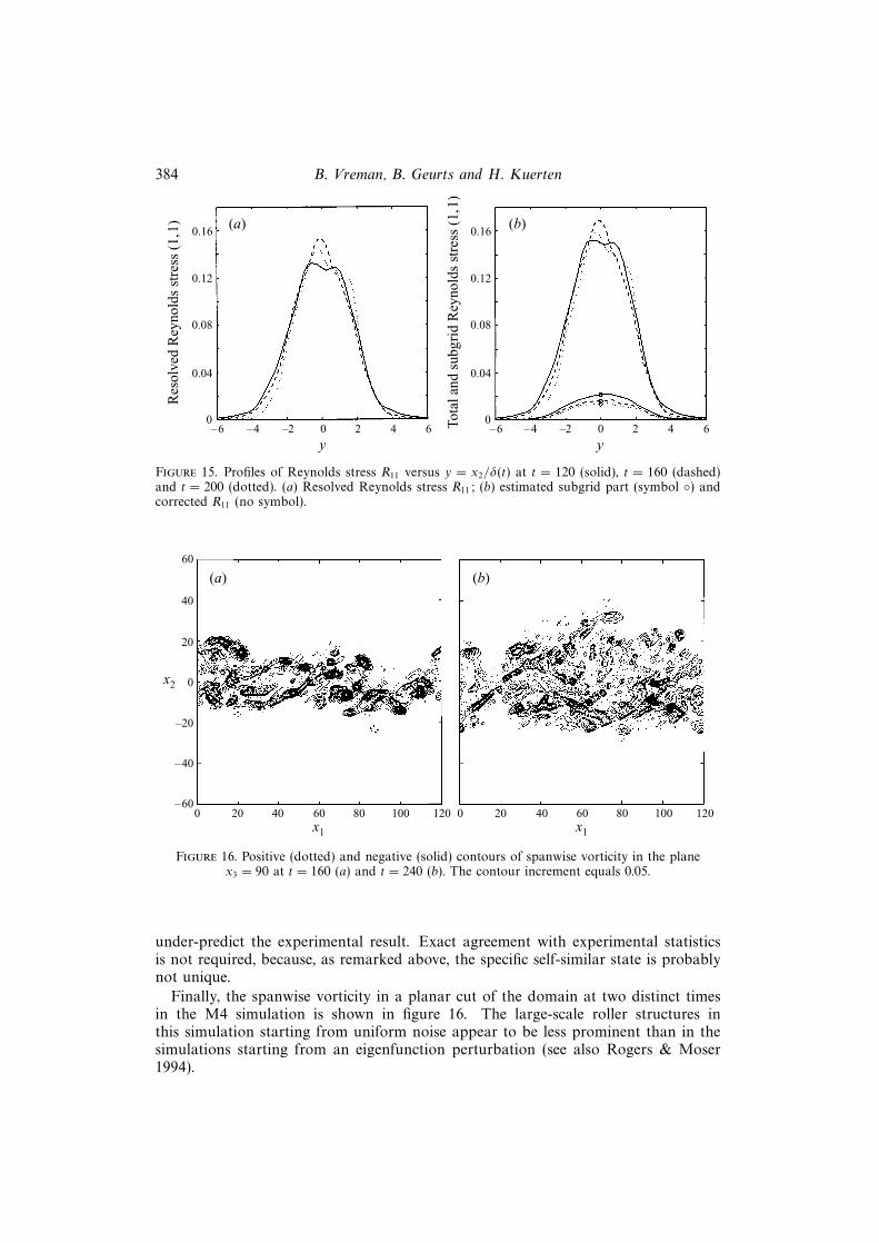
384 B. Vreman, B. Geurts and H. KuertenR

esol

ved

Rey

nold

s st

ress

(1,

1)

0

0.08

0.12

0.16

–6 –4 –2

y2 40

0.04

(a)

6 Tota

l and

sub

grid

Rey

nold

s st

ress

(1,

1)

0

0.08

0.12

0.16

–6 –4 –2

y2 40

0.04

(b)

6

Figure 15. Profiles of Reynolds stress R11 versus y = x2/δ(t) at t = 120 (solid), t = 160 (dashed)and t = 200 (dotted). (a) Resolved Reynolds stress R11; (b) estimated subgrid part (symbol ) andcorrected R11 (no symbol).

20

40

60

0 20 40x1

8060

–20

(a)

120

0

–40

–60100

x2

0 20 40x1

8060

(b)

120100

Figure 16. Positive (dotted) and negative (solid) contours of spanwise vorticity in the planex3 = 90 at t = 160 (a) and t = 240 (b). The contour increment equals 0.05.

under-predict the experimental result. Exact agreement with experimental statisticsis not required, because, as remarked above, the specific self-similar state is probablynot unique.

Finally, the spanwise vorticity in a planar cut of the domain at two distinct timesin the M4 simulation is shown in figure 16. The large-scale roller structures inthis simulation starting from uniform noise appear to be less prominent than in thesimulations starting from an eigenfunction perturbation (see also Rogers & Moser1994).


5. Conclusions

In this paper we have presented a posteriori tests of LES of the temporal mixinglayer using six subgrid models: Smagorinsky (M1), similarity (M2), gradient (M3),dynamic eddy viscosity (M4), dynamic mixed (M5) and dynamic Clark (M6). Thefirst three subgrid models form the basis for the latter three dynamic models. Two setsof simulations have been performed, at low and high Reynolds number respectively.The LES in the first set have been compared with DNS data, whereas in the analysisof the second set of simulations we focused on other aspects, such as self-similarity.The conclusions drawn from the first set of simulations are presented first.

In the first set of simulations the quality of a model is determined by the discrepancyof its results with the filtered DNS results. Furthermore, in order to determine whetherthe inclusion of the subgrid model is useful, comparisons with a coarse-grid simulationwithout any subgrid model (M0) have been performed. A summary of the resultsis found in table 2. When the models are arranged with respect to the overallaccuracy of their results, the following sequence is obtained: M5, M6, M4, M2, M3,M1. The results of the latter two models are in general worse than the M0 results;incorporation of these subgrid-models in LES of the mixing layer is not useful. Theother models in general give better results than M0. The overall results indicate thatthe dynamic mixed model displayed the best performance when compared to filteredDNS results. The dynamic mixed model was also observed to yield the most accurateresults in comparative tests of subgrid models in LES of a driven cavity (Zang et al.1993) and a rotating boundary layer (Wu & Squires 1995).

The Smagorinsky model was found to be excessively dissipative in the transitionalregime. Comparison with the filtered DNS demonstrated that M1 strongly influencesthe linear evolution of disturbances, since the four-roller structure is not reproduced.Furthermore, M1 hindered the transition to turbulence. No positive spanwise vorticitywas generated, the sudden growth of the momentum thickness did not occur andturbulent intensities and Reynolds stress profiles were under-predicted.

Although from the a priori point of view M2 and M3 are very similar and bothprovide highly accurate representations of the turbulent stress tensor (Vreman etal. 1995) they behave very differently in actual simulations: M2 yields reasonableresults, whereas M3 leads to instabilities if no limiter is used. However, even with theincorporation of a limiter, M3 produces too many small scales and leads to inaccurateresults for integral quantities and e.g. the streamwise turbulent intensity. In order tostabilize the gradient model, the inclusion of a dynamic eddy viscosity as in M6 ispreferred over a limiter (M3), since the first case leads to more accurate results.

Examination of the energy spectra demonstrates that only the models which containa dynamic eddy viscosity (M4–6) provide the correct amount of small scales. Dueto insufficient dissipation of small scales by the subgrid model, the flow simulatedwith M0, M2 and M3 contains too many small structures. This gives rise to a highermolecular dissipation, which supplements the insufficient small-scale dissipation ofthe model. Although the dissipation for small scales is insufficient, the total energydissipation provided by M2 was observed to be reasonable, since too much energywas subtracted from the large scales. It is remarkable that the dynamic eddy-viscosity model M4 provides satisfactory results, although it severely under-predictsthe magnitude of the individual turbulent stress components. An adequate dissipativebehaviour appears to be more important than a good prediction of the individualturbulent stresses. A suitable mechanism for this dissipation is provided by thesimilarity assumption used in the dynamic approach.


The models M2 and M5–6 have mechanisms to mimic the backscatter of energyfrom subgrid scales to resolved scales, but do not accurately predict it. However,actual LES of the mixing layer seems to require only a small amount of backscatter.The same is observed from the filtered DNS results, in which the backscatter is about10% of the subgrid dissipation. Hence, a poor representation of the backscatter bythe subgrid models is not too much of a problem.

In this paper we have presented a posteriori tests. In a priori tests the six modelscorrelate with the real turbulent stress as follows: the correlation is high for M2 andM3, somewhat lower for M5 and M6 and very low for the eddy-viscosity models M1and M4 (e.g. Liu et al. 1994a; Vreman et al. 1995). Meneveau (1994) remarks that apriori testing is often too pessimistic, i.e. a low correlation does not necessarily lead topoor results, which is confirmed by our results obtained with M4. However, a prioritesting can also be much too optimistic, since a high correlation does not necessarilylead to good results as our results for M2 and M3 show.

The second set of LES with M0–6 concern a mixing layer at a much higherReynolds number in a larger computational domain (§4). No DNS results areavailable to compare with, since the Reynolds number is too high to accuratelyresolve all scales with the present supercomputers.

Since the amount of subgrid dissipation obviously depends on the value of theSmagorinsky constant CS , the dissipative behaviour of the Smagorinsky model couldbe better using a lower value for CS . Therefore, in this case we also used the lowerCS = 0.10 in the simulation with M1. The model was still too dissipative in thelaminar regime; the transition occurred, but too late, and in the turbulent regime themodel was not sufficiently dissipative. Hence, a varying model coefficient that attainsthe appropriate value in transitional and turbulent regimes is required. The dynamicmodels meet this requirement.

The simulations with M0, M2 and M3 become unstable in the turbulent regime.M0 has no subgrid dissipation and the dissipation of M2 and M3 is insufficient toprevent an excessive amount of small scales.

The three dynamic models M4–6 adequately suppress the generation of smallscales, but there are differences between the results of the three simulations. Withinthis group of models the dynamic eddy-viscosity model yields the most self-similarturbulent statistics.

Despite the large improvements originating from the dynamic approach, the re-sults presented in this paper still show considerable discrepancies in several flowquantities, such as the profiles of the turbulent intensities and the momentum thick-ness. Additional improvement of subgrid modelling may be guided by the presentresults.

The results in this paper apply to the mixing layer at low Mach number. Details ofthe comparison may be valid only for this case, but the global features are expectedto be more generally applicable. Examples of such global features are: the excessivedissipation of the Smagorinsky model, the insufficient dissipation of small scales bythe similarity and gradient models, the relatively adequate subgrid-dissipation bythe dynamic models and the under-predicted magnitude of the individual turbulentstress components by the dynamic eddy-viscosity model. In order to substantiatethis, we are at present studying more complex flows, which are physically realizableand admit a quantitative comparison with experimental results. Examples of suchflows are the spatial mixing layer and (separated) boundary layer flow. Also, theformulation of the LES approach to transonic compressible flows is subject ofstudy.


The time for the computations was provided by the Stichting Nationale Comput-erfaciliteiten (National Computing Facilities Foundation, NCF), which is financiallysupported by the Nederlandse Organisatie van Wetenschappelijk Onderzoek (Nether-lands Organization for Scientific Research, NWO). The authors thank the referees fortheir comments.

AppendixThe dynamic procedure requires formulations of the subgrid model at the F-level

and the FG-level. The F-level is associated with the filter width ∆, the G-level with thefilter width 2∆ and the FG-level with the filter width κ∆. The value of κ equals 2 forthe spectral cut-off filter (Germano et al. 1991) and

√5 for Gaussian filters (Germano

1992). For spectral cut-off and Gaussian filters, κ can be determined exactly, since theconsecutive application of two of these filters yields a filter function of the same type.However, the consecutive application of two top-hat filters does not yield a top-hatfilter and the value of κ should not be 2 (as used for instance by Zang et al. 1993).In this Appendix we argue that in conjunction with top-hat filters the optimum valueof κ equals

√5.

We denote the original filter function by Ga with filter width a = ∆ and the test-filter function by Gb with filter width b > a. The filter function corresponding to theconsecutive application of these two filters is denoted by H and satisfies the followingformula:

H(y) =

∫Ω

Gb(y − z)Ga(z)dz. (A 1)

If Ga and Gb are spectral filters, H is a spectral filter as well with filter width b,whereas if Ga and Gb are Gaussian filters, H is a Gaussian filter with filter width(a2 + b2)1/2. However, the consecutive application of two top-hat filters is not atop-hat filter; the filter function H has a trapezoidal shape. In LES employing thedynamical procedure with top-hat filters, the filter width of H is usually assumed tobe the same as the filter width of Gb (Zang et al. 1993). However, this approximationcannot be correct, because the H-filter will certainly render smoother signals than theGb-filter, so the filter width associated with H should be larger than b. We proceedto show how an appropriate value for the filter width of H can be found. Sincethe three-dimensional filter function is usually a product of three one-dimensionalfilter functions, the analysis can be performed in one dimension. Suppose that H isthe trapezoidal filter function resulting from the consecutive application of two one-dimensional top-hat filter functions Ga and Gb with b > a. This yields the followingexpression:

H(y) =

(1/ab)(y + 1

2(b+ a)) if − 1

2(b+ a) < y < − 1

2(b− a),

(1/b) if − 12(b− a) 6 y 6 1

2(b− a),

−(1/ab)(y − 12(b+ a)) if 1

2(b− a) < y < 1

2(b+ a),

0 if |y| > 12(b+ a) .

(A 2)

We next find an optimal approximation of H by a top-hat filter function Gc, given by

Gc(y) =

1/c if − 1

2c < y < 1

2c,

0 if |y| > 12c .

(A 3)


For this purpose we minimize the L2-norm of the error, which is a function of c:

δ(c) = ‖Gc −H‖. (A 4)

The choice of the L2-norm has the advantage that the error is also minimum inspectral space, due to Parseval’s theorem. The minimum value of c will certainlysatisfy b − a 6 c 6 b + a. In this range the square of the error equals (after somecalculation)

(δ(c))2 =1

b− a

3b2+b+ a

ab+

1

c

(a

2b+

b

2a

)+

c

2ab. (A 5)

Minimisation of the error requires

d

dc(δ(c))2 = 0, (A 6)

which finally yields

c = (a2 + b2)1/2. (A 7)

It is remarkable that this relation, which represents an optimal approximation fortop-hat filters, is identical to the exact relation for Gaussian filters. Furthermoreit appears that when equation (A 7) is satisfied for top-hat filters, not only is δ(c)minimum, but also the second moments of Gc and H are equal:∫ c/2

c/2

y2Gc(y)dy =

∫ (b+a)/2

−(b+a)/2

y2H(y)dy. (A 8)

Usually the ratio between the filter width of the test and the original filter is equal to2 (b = 2a), in which case equation (A 7) gives c =

√5a, which corresponds to κ =

√5.

REFERENCES

Bardina, J., Ferziger, J. H. & Reynolds, W. C. 1984 Improved turbulence models based onLES of homogeneous incompressible turbulent flows. Rep. TF-19. Department of MechanicalEngineering, Stanford.

Bell, J. H. & Mehta, R. D. 1990 Development of a two-stream mixing layer from tripped anduntripped boundary layers. AIAA J. 28, 2034–2042.

Blaisdell, G. A., Mansour, N. N. & Reynolds, W. C. 1993 Compressibility effects on the growthand structure of homogeneous turbulent shear flow. J. Fluid Mech. 256, 443–485.

Brown, G. L. & Roshko, A. 1974 On density effects and large structure in turbulent mixing layers.J. Fluid Mech. 64, 775–816.

Campagne, F. H., Pao, Y. H. & Wygnanski, I. J. 1976 On the two dimensional mixing region. J.Fluid Mech. 74, 209–250.

Carati, D., Ghosal, S. & Moin, P. 1995 On the representation of backscatter in dynamic localizationmodels. Phys. Fluids 7, 606–616.

Carati, D. & Vanden Eijnden, E. 1996 On the self-similarity assumption in dynamic models forlarge eddy simulations. Phys. Fluids (submitted).

Clark, R. A., Ferziger, J. H. & Reynolds, W. C. 1979 Evaluation of subgrid-scale models usingan accurately simulated turbulent flow. J. Fluid Mech. 91, 1–16.

Comte, P., Lesieur, M. & Lamballais, E. 1992 Large and small-scale stirring of vorticity and apassive scalar in a 3D temporal mixing layer. Phys. Fluids A 4, 2761.

Deardorff, J. W. 1970 A numerical study of three-dimensional turbulent channel flow at largeReynolds numbers. J. Fluid Mech. 41, 453–480.

Deardorff, J. W. 1971 On the magnitude of the subgrid scale eddy viscosity coefficient. J. Comput.Phys. 7, 120–133.

Dimotakis, P. E. & Brown, G. L. 1976 The mixing layer at high Reynolds number: large-structuredynamics and entrainment. J. Fluid Mech. 78, 535–560.


Favre, A. 1983 Turbulence: space-time statistical properties and behavior in supersonic flows. Phys.Fluids 26, 2851–2863.

Germano, M., Piomelli, U., Moin, P. & Cabot, W. H. 1991 A dynamic subgrid-scale eddy viscositymodel. Phys. Fluids A 3, 1760–1765.

Germano, M. 1992 Turbulence: the filtering approach. J. Fluid Mech. 238, 325–336.

Germano, M. 1996 A statistical formulation of the dynamic model. Phys. Fluids 8, 565–571.

Ghosal, S., Lund, T. S., Moin, P. & Akselvoll, K. 1995 A dynamic localization model forlarge-eddy simulation of turbulent flows. J. Fluid Mech. 286, 229–255.

Gresho, P. 1991 Incompressible fluid dynamics: some fundamental formulation issues. Ann. Rev.Fluid Mech. 23, 343–370.

Horiuti, K. 1995 Backward cascade of subgrid-scale kinetic energy in wall bounded and free turbu-lent flows. In Proc. Turbulent Shear Flows 10, The Pennsylvania State University, pp. 20.13-18.

Jimenez-Hartel, C. J. 1994 Analyse und Modellierung der Feinstruktur im wandnahen Bere-ich turbulenter Scherstromungen. Forschungsbericht 94-22. Institut fur Stromungs- mechanik,Gottingen.

Kwak, D., Reynolds, W. C. & Ferziger, J. H. 1975 Three-dimensional time dependent computationof turbulent flow. Report TF-5. Stanford University.

Lilly, D. K. 1967 The representation of small-scale turbulence in numerical simulation experiments.In Proc. IBM Scientific Computing Symp. on Environmental Sciences. IBM Form no. 320-1951,195-210.

Lilly, D. K. 1992 A proposed modification of the Germano subgrid-scale closure method. Phys.Fluids A 4, 633–635.

Liu, S., Meneveau, C. & Katz, J. 1994a On the properties of similarity subgrid-scale models asdeduced from measurements in a turbulent jet. J. Fluid Mech. 275, 83–119.

Liu, S., Meneveau, C. & Katz, J. 1994b Experimental study of similarity subgrid-scale models ofturbulence in the far-field of a jet. In Direct and Large-Eddy Simulation I, pp. 37–48. Kluwer.

Lund, T. S., Kaltenbach, H. J. & Akselvoll, K. 1995 On the behavior of centered finite differenceschemes for large eddy simulation. In Proc. Sixth Intl Symp. on Computational Fluid Dynamics.Lake Tahoe, NV, 4–8 September 1995.

Luo, K. H. & Sandham, N. D. 1994 On the formation of small scales in a compressible mixinglayer. In Direct and Large-Eddy Simulation I, pp. 335–346. Kluwer.

Meneveau, C. 1994 Statistics of turbulence subgrid-scale stresses: Necessary conditions and exper-imental tests. Phys. Fluids 6, 815–833.

Moin, P. & Jimenez, J. 1993 Large Eddy Simulation of complex turbulent flows. AIAA 24th FluidDyn. Conf. Orlando.

Moin, P. & Kim, P. 1982 Numerical investigation of turbulent channel flow. J. Fluid Mech. 118,341–377.

Moser, R. D. & Rogers, M. 1993 The three-dimensional evolution of a plane mixing layer: pairingand transition to turbulence. J. Fluid Mech. 247, 275–320.

Piomelli, U., Moin, P. & Ferziger, J. H. 1988 Model consistency in large eddy simulation ofturbulent channel flows. Phys. Fluids 31, 1884–1891.

Piomelli, U., Zang, T. A., Speziale, C. G. & Hussaini, M. Y. 1990a On the large-eddy simulationof transitional wall-bounded flows. Phys. Fluids A, 2, 257–265.

Piomelli, U., Cabot, W. H., Moin, P. & Lee, S. 1990b Subgrid-scale backscatter in transitional andturbulent flows. CTR Proc. Summer Program 1990, pp. 19–30.

Piomelli, U. & Liu, J. 1994 Large-Eddy Simulation of rotating channel flows using a localizeddynamic model. Application of Direct and Large Eddy Simulation to Transition and Turbulence,AGARD Conf. Proc. 551, pp. 3.1–9.

Ragab, S. A. & Wu, J. L. 1989 Linear instabilities in two-dimensional compressible mixing layers.Phys. Fluids A, 1, 957–966.

Rogallo, R. S. & Moin, P. 1984 Numerical simulation of turbulent flows. Ann. Rev. Fluid Mech.16, 99–137.

Rogers, M. M. & Moser, R. D. 1994 Direct simulation of a self-similar turbulent mixing layer.Phys. Fluids 6, 903–924.

Sandham, N. D. & Reynolds, W. C. 1991 Three-dimensional simulations of large eddies in thecompressible mixing layer. J. Fluid Mech. 224, 133–158.

Schumann, U. 1991 Direct and large eddy simulation of turbulence - summary of the state-of-the-


art 1991. Lecture Series 1991–02: Introduction to the Modeling of Turbulence. Von KarmanInstitute, Brussels.

Smagorinsky, J. 1963. General circulation experiments with the primitive equations. Mon. WeatherRev. 91, 99–164.

Vreman, A. W. 1995. Direct and Large-Eddy Simulation of the compressible turbulent mixing layer.PhD Dissertation, University of Twente.

Vreman, B., Geurts, B. & Kuerten, H. 1994a Realizability conditions for the turbulent stresstensor in large eddy simulation. J. Fluid Mech. 278, 351–362.

Vreman, B., Geurts, B. & Kuerten, H. 1994b On the formulation of the dynamic mixed subgrid-scale model. Phys. Fluids 6, 4057–4059.

Vreman, B., Geurts, B. & Kuerten, H. 1995 A priori tests of Large Eddy Simulation of thecompressible plane mixing layer. J. Engng Maths 29, 299–327.

Vreman, B., Geurts, B. & Kuerten, H. 1996a Comparison of numerical schemes in Large EddySimulation of the temporal mixing layer. Intl J. Numer. Meth. Fluids 22, 297–311.

Vreman, B., Geurts, B. & Kuerten, H. 1996b Large eddy simulation of the temporal mixing layerusing the Clark model. Theor. Comput. Fluid Dyn. 8, 309–324.

Vreman, A. W., Sandham, N. D. & Luo, K. H. 1996c Compressible mixing layer growth rate andturbulence characteristics. J. Fluid Mech. 320, 235–258.

Wu, X., & Squires, K. D. 1995 Large-eddy simulation of a canonical three-dimensional boundarylayer. In Proc. Turbulent Shear Flows 10, The Pennsylvania State University, pp. 8.19-24.

Zang, Y., Street, R. L. & Koseff, J. R. 1993 A dynamic mixed subgrid-scale model and itsapplication to turbulent recirculating flows. Phys. Fluids A 5, 3186–3196.

Large-eddy simulation of the turbulent mixing layer

Documents

Transcript of Large-eddy simulation of the turbulent mixing layer