3344 VOLUME 16J O U R N A L O F C L I M A T E

q 2003 American Meteorological Society

Ocean Heat Uptake in Transient Climate Change: Mechanisms and Uncertainty due toSubgrid-Scale Eddy Mixing

BOYIN HUANG, PETER H. STONE, AND ANDREI P. SOKOLOV

Joint Program on the Science and Policy of Global Change, Massachusetts Institute of Technology, Cambridge, Massachusetts

IGOR V. KAMENKOVICH

Department of Atmospheric Sciences, University of Washington, Seattle, Washington

(Manuscript received 30 January 2003, in final form 20 April 2003)

ABSTRACT

The ocean heat uptake (OHU) is studied using the Massachusetts Institute of Technology (MIT) ocean generalcirculation model (OGCM) with idealized ocean geometry. The OGCM is coupled with a statistical–dynamicatmospheric model. The simulation of OHU in the coupled model is consistent with other coupled ocean–atmosphere GCMs in a transient climate change when CO2 concentration increases by 1% yr21. The globalaverage surface air temperature increases by 1.78C at the time of CO2 concentration doubling (year 70). Theocean temperature increases by about 1.08C near the surface, 0.18C at 1000 m in the Pacific, and 0.38C in theAtlantic. The maximum overturning circulation (MOTC) in the Atlantic at 1350 m decreases by about 4.5 Sv(1 Sv [ 106 m3 s21). The center of MOTC drifts upward about 300 m, and therefore a large OTC anomaly (14Sv) is found at 2700 m. The MOTC recovers gradually, but the OTC anomaly at 2700 m does not seem torecover after CO2 concentration is kept constant during 400-yr simulation period.

The diagnosis of heat flux convergence anomaly indicates that the warming in the lower latitudes of theAtlantic is associated with large-scale advection. But, the warming in the higher latitudes is associated with theheat brought down from the surface by convection and eddy mixing. In global average, the treatments ofconvection and eddy mixing are the two main factors affecting the OHU.

The uncertainty of OHU due to subgrid-scale eddy mixing is studied. In the MIT OGCM this mixing is acombination of Gent–McWilliams bolus advection and Redi isopycnal diffusion (GMR), with a single diffusivitybeing used to calculate the isopycnal and thickness diffusion. Experiments are carried out with values of thediffusivity of 500, 1000, and 2000 m2 s21. The total OHU is insensitive to these changes. The insensitivity ismainly due to the changes in the vertical heat flux by GMR mixing being compensated by changes in the othervertical heat flux components.

In the Atlantic when the diffusivity is reduced from 1000 to 500 m2 s21, the surface warming can penetratedeeper. Therefore, the warming decreases by about 0.158C above 2000 m but increases by about 0.158C below2500 m. Similarly, when the diffusivity is increased from 1000 to 2000 m2 s21, the surface warming becomesshallower; the warming increases by about 0.28C above 1000 m but decreases by about 0.28C below 1000 m.These changes in the vertical distribution of the OHU also contribute to the insensitivity of the total OHU tochanges in the GMR mixing. The analysis of heat flux convergence indicates that the difference of OHU seemsto be associated with the MOTC circulation.

1. Introduction

The ocean regulates global climate change becauseof its large heat capacity. In a global warming scenario,the rate of ocean heat uptake (OHU) is a critical factoraffecting the global climate change. Observations in-dicate a warming in the World Ocean in the past decades(Levitus et al. 2000). The warming appears to be as-sociated with the increase of greenhouse gas concen-trations according to the simulations of Levitus et al.

Corresponding author address: Dr. Boyin Huang, The Center forResearch on the Changing Earth System, 10211 Wincopin Circle,Suite 240, Columbia, MD 21044.E-mail: bhuang@wind.mit.edu

(2001) and Barnett et al. (2001). However, the OHU insimulations may depend strongly on how models are setup and how subgrid-scale mixing is parameterized. Forexample, the vertical diffusivity may have a wide rangebetween 0.1 and 1 3 1024 m2 s21 (Zhang et al. 2001;Ledwell et al. 2000; Jenkins 1991; Nakamura and Cao2000). The isopycnal diffusivity may range from 500to 2000 m2 s21 (Ku and Luo 1994; Hirst and Cai 1994;Jenkins 1991; Ledwell et al. 1998; Thiele 1986). There-fore, different magnitudes of simulated OHU may di-rectly result in large differences in the projection of thefuture climate (Houghton et al. 2001). As indicated inthe study of Huang et al. (2003a), the ocean’s equilib-rium heat content appears to be sensitive to the isopycnal

15 OCTOBER 2003 3345H U A N G E T A L .

FIG. 1. Idealized topography of oceans.

and diapycnal diffusivities of temperature based on sim-ulations with an adjoint ocean general circulation model(OGCM). The further study of Huang et al. (2003b)indicated that the OHU is largely associated with thereduction of upward heat flux due to eddy mixing. Thisraises the question of whether OHU is sensitive to thestrength of the eddy mixing.

Using an OGCM coupled with a statistical–dynamicatmospheric model, we look at how OHU in a transientclimate change depends on the strength of the eddymixing. The coupled model is briefly described in sec-tion 2, followed by the transient response of climate insection 3. The mechanisms of OHU are diagnosed insection 4. The uncertainty of OHU due to different eddydiffusivities is analyzed in section 5. Section 6 is thesummary.

2. Model

We use the Massachusetts Institute of Technology(MIT) OGCM (Marshall et al. 1997) coupled with atwo-dimensional (meridional and height) statistical dy-namical atmospheric model (Sokolov and Stone 1998;Kamenkovich et al. 2002, hereafter KSS). The oceanbasin is set with an idealized Pacific, Atlantic, andSouthern Ocean with flat bottom topography except atthe Drake Passage where a sill of 1600 m is added (Fig.1). The horizontal resolution is 48 3 48 except near theeastern and western boundaries where a finer resolutionof 18 in longitude is used so that the boundary currentscan be simulated more realistically. The vertical reso-lution is 15 levels with the thickness ranging from 50m near the surface to 550 m at the bottom of 4500 m.The time step of the OGCM is 30 min for momentumequations and 8 h for tracer equations. The sea ice isnot included in our OGCM, but the ocean temperatureis limited above 228C.

The resolution of the atmospheric model is 7.88 latitudefrom 908S to 908N, and nine levels in the vertical fromsurface to 10 hPa. The time step is 20 min. The atmo-sphere and ocean are coupled in a time interval of 8 h,

with each model being forced by climatological boundaryconditions plus anomalies generated by the other model.The ocean forces the atmosphere through the impositionof anomalies in zonal averaged sea surface temperature(SST), and the atmospheric model calculates the anom-alies in the zonal averages of surface heat and freshwaterfluxes, and their partial derivatives with respect to theSST. The calculated anomalous fluxes are redistributedzonally before forcing the ocean model:

]FaF 5 F 1 (SST 2 SST ), (1)o a ]SST

where Fo and Fa are the anomalous fluxes into the oceanand from the atmosphere, respectively. is zonallySSTaveraged SST. The sea ice is calculated using a two-layer thermodynamic sea ice model. The anomaly ofzonal wind stress calculated by the atmospheric modeldirectly forces the ocean without zonal redistribution(see KSS for more detail).

Small-scale vertical diffusion of temperature and sa-linity are parameterized with a constant diffusion co-efficient of 0.5 3 1024 m2 s21, and is treated implicitly.The convection adjustment is parameterized by an in-stantaneous (within one time step) mixing of the tem-perature and salinity between two adjacent unstable lay-ers (Cox and Bryan 1984). Mesoscale eddies are pa-rameterized in the MIT OGCM by the Gent–Mc-Williams (1990) thickness diffusion or bolus advectionof tracers, in combination with the Redi (1982) diffusionalong isopycnal surfaces. The thickness and isopycnaldiffusivities are set equal, and have a uniform value of1000 m2 s21 in the standard version of the model.

The Redi isopycnal diffusion is formulated as

]t; = · K M =t, (2)Redir]t

where Kr is the diffusivity along isopycnal surface,

1 0 S x

M 5 0 1 S , (3) Redi y 2S S |S| x y

]zS 5 2 , (4)x 1 2]x

r

]zS 5 2 , (5)y 1 2]y

r

2 2 2|S| 5 S 1 S , (6)x y

and t is a tracer. The Gent–McWilliams thickness dif-fusion (bolus advection) is formulated as

]t; 2= · v*t 5 = · K M =t, (7)GMGM]t

where KGM is the coefficient of thickness diffusivity, and

3346 VOLUME 16J O U R N A L O F C L I M A T E

FIG. 2. Anomaly of net surface heat flux (W m22, positive down-ward) between PTB and CTR runs in the (a) Pacific and (b) Atlantic.The anomaly is averaged zonally and from year 61 to 80, except forMIT and KSS, which is an annual average of year 70.

FIG. 3. Temporal evolution of global average SAT (8C) in PTB andCTR runs.

0 0 2S x

M 5 0 0 2S . (8) GM y S S 0 x y

Assume Kr 5 KGM [ KI. Now the Redi diffusion andthe Gent–McWilliams thickness diffusion can be com-bined simply as

1 0 0

K M 1 K M 5 K 0 1 0 , (9) Redi GMr GM I 22S 2S |S| x y

and are referred to as GMR mixing hereafter.The coupled model is spun up for 2000 yr with the

initial condition for the ocean taken from an ocean-aloneintegration of 5000-yr duration. The simulation is thenseparated into a control (CTR) run and a perturbation(PTB) run. The CO2 concentration is set to 332 ppm inCTR, but increases at 1% yr21 for 75 yr and is keptconstant for 400 yr in PTB, which can be thought of asa global warming scenario.

The evolution of our coupled ocean–atmosphere sys-tem is comparable with other atmosphere–ocean GCMs

(AOGCMs). For example, as shown in Fig. 2, our sim-ulation (indicated as MIT) shows that the zonally andannually averaged anomaly of surface heat flux at thetime of CO2 doubling (year 70) is about 7 W m22 inthe Southern Ocean south of 508S, and 20 W m22 inthe North Atlantic north of 508N. The heat flux anomalyin our simulation is consistent with the simulation ofKSS. KSS used the Geophysical Fluid Dynamics Lab-oratory (GFDL) OGCM with the same ocean configu-ration as ours, and coupled it with the same statistical–dynamical atmospheric model. Our simulation is alsoconsistent with the simulations of fully coupledAOGCMs from the Climate Model IntercomparisonProject-2 (CMIP-2). That project used the same scenarioas ours, with CO2 increasing 1% yr21. The changes ina number of the CMIP models’ surface heat flux av-eraged zonally are shown in Fig. 2. The models includedare the Bureau of Meteorology Research Centre model(BMRC1; Power et al. 1993), European Centre Ham-burg Large Scale Geotrophic OGCM (ECHAM3-LSG;Voss et al. 1998), the Geophysical Fluid Dynamics Lab-oratory model (GFDLpR15pa; Manabe et al. 1991), theGoddard Institute for Space Studies model (GISS-Rus-sell; Russell et al. 1995), the Institute of AtmosphericPhysics Laboratory for Atmospheric Sciences and Geo-physical Fluid Dynamics model (IAP-LASG1; Zhang etal. 2000), the National Center for Atmospheric ResearchClimate System Model (NCAR-CSM; Boville and Gent1998), and the Met Office-Hadley Centre second-gen-eration coupled GCM (UKMO-HadCM2; Johns et al.1997).

3. Transient response

As indicated in Fig. 2, our model can simulate theheat forcing from the atmosphere such as otherAOGCMs, but how about the transient response of theocean to the atmospheric warming due to the increasesof CO2 concentration? Figure 3 shows the evolution of

15 OCTOBER 2003 3347H U A N G E T A L .

TABLE 1. Anomalies of global averaged SAT (8C) and AtlanticMOTC (Sv) between PTB and CTR runs at the time of CO2 con-centration doubling (year 70).

Models DSAT (8C) DMOTC (Sv)

MITKSSBMRC1ECHAM3-LSGGFDLpR15paGISS-RussellIAP-LSAG1NCAR-CSMUKMO-HadCM2

1.71.61.41.32.21.41.71.41.7

4.54.5N/A553216.5

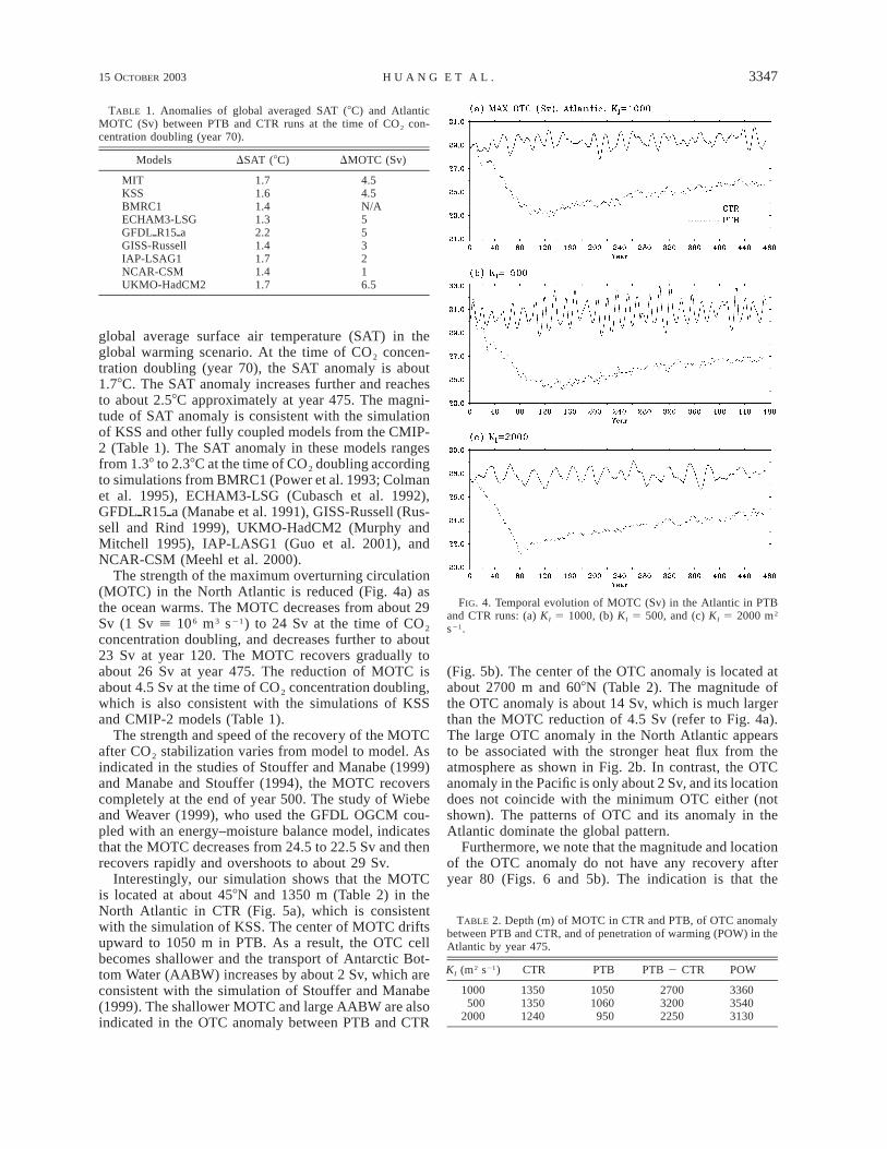
FIG. 4. Temporal evolution of MOTC (Sv) in the Atlantic in PTBand CTR runs: (a) KI 5 1000, (b) KI 5 500, and (c) KI 5 2000 m2

s21.

TABLE 2. Depth (m) of MOTC in CTR and PTB, of OTC anomalybetween PTB and CTR, and of penetration of warming (POW) in theAtlantic by year 475.

KI (m2 s21) CTR PTB PTB 2 CTR POW

1000500

2000

135013501240

10501060950

270032002250

336035403130

global average surface air temperature (SAT) in theglobal warming scenario. At the time of CO2 concen-tration doubling (year 70), the SAT anomaly is about1.78C. The SAT anomaly increases further and reachesto about 2.58C approximately at year 475. The magni-tude of SAT anomaly is consistent with the simulationof KSS and other fully coupled models from the CMIP-2 (Table 1). The SAT anomaly in these models rangesfrom 1.38 to 2.38C at the time of CO2 doubling accordingto simulations from BMRC1 (Power et al. 1993; Colmanet al. 1995), ECHAM3-LSG (Cubasch et al. 1992),GFDLpR15pa (Manabe et al. 1991), GISS-Russell (Rus-sell and Rind 1999), UKMO-HadCM2 (Murphy andMitchell 1995), IAP-LASG1 (Guo et al. 2001), andNCAR-CSM (Meehl et al. 2000).

The strength of the maximum overturning circulation(MOTC) in the North Atlantic is reduced (Fig. 4a) asthe ocean warms. The MOTC decreases from about 29Sv (1 Sv [ 106 m3 s21) to 24 Sv at the time of CO2

concentration doubling, and decreases further to about23 Sv at year 120. The MOTC recovers gradually toabout 26 Sv at year 475. The reduction of MOTC isabout 4.5 Sv at the time of CO2 concentration doubling,which is also consistent with the simulations of KSSand CMIP-2 models (Table 1).

The strength and speed of the recovery of the MOTCafter CO2 stabilization varies from model to model. Asindicated in the studies of Stouffer and Manabe (1999)and Manabe and Stouffer (1994), the MOTC recoverscompletely at the end of year 500. The study of Wiebeand Weaver (1999), who used the GFDL OGCM cou-pled with an energy–moisture balance model, indicatesthat the MOTC decreases from 24.5 to 22.5 Sv and thenrecovers rapidly and overshoots to about 29 Sv.

Interestingly, our simulation shows that the MOTCis located at about 458N and 1350 m (Table 2) in theNorth Atlantic in CTR (Fig. 5a), which is consistentwith the simulation of KSS. The center of MOTC driftsupward to 1050 m in PTB. As a result, the OTC cellbecomes shallower and the transport of Antarctic Bot-tom Water (AABW) increases by about 2 Sv, which areconsistent with the simulation of Stouffer and Manabe(1999). The shallower MOTC and large AABW are alsoindicated in the OTC anomaly between PTB and CTR

(Fig. 5b). The center of the OTC anomaly is located atabout 2700 m and 608N (Table 2). The magnitude ofthe OTC anomaly is about 14 Sv, which is much largerthan the MOTC reduction of 4.5 Sv (refer to Fig. 4a).The large OTC anomaly in the North Atlantic appearsto be associated with the stronger heat flux from theatmosphere as shown in Fig. 2b. In contrast, the OTCanomaly in the Pacific is only about 2 Sv, and its locationdoes not coincide with the minimum OTC either (notshown). The patterns of OTC and its anomaly in theAtlantic dominate the global pattern.

Furthermore, we note that the magnitude and locationof the OTC anomaly do not have any recovery afteryear 80 (Figs. 6 and 5b). The indication is that the

3348 VOLUME 16J O U R N A L O F C L I M A T E

FIG. 5. OTC in (a) global, (c) Pacific, and (e) Atlantic in CTR run, and (b), (d), (f ) its anomaly between PTB and CTR runs, respectively.It is averaged from year 66 to 75. The contour intervals (CIs) are 3 Sv in (a), (c), and (e), but 2 Sv in (b), (d), and (f ). Solid (dotted)contours indicate sinking in the north (south).

MOTC in the North Atlantic may at least partly recoverwhen CO2 concentration is kept constant after doubling,but its effect on the deep circulation below 3000 m doesnot disappear.

In the meantime, the ocean temperature increasesgradually as the atmospheric heat flux into the oceanincreases. By year 70, the ocean temperature increasesby about 18C near the surface, and 0.18C at 1000 m in

15 OCTOBER 2003 3349H U A N G E T A L .

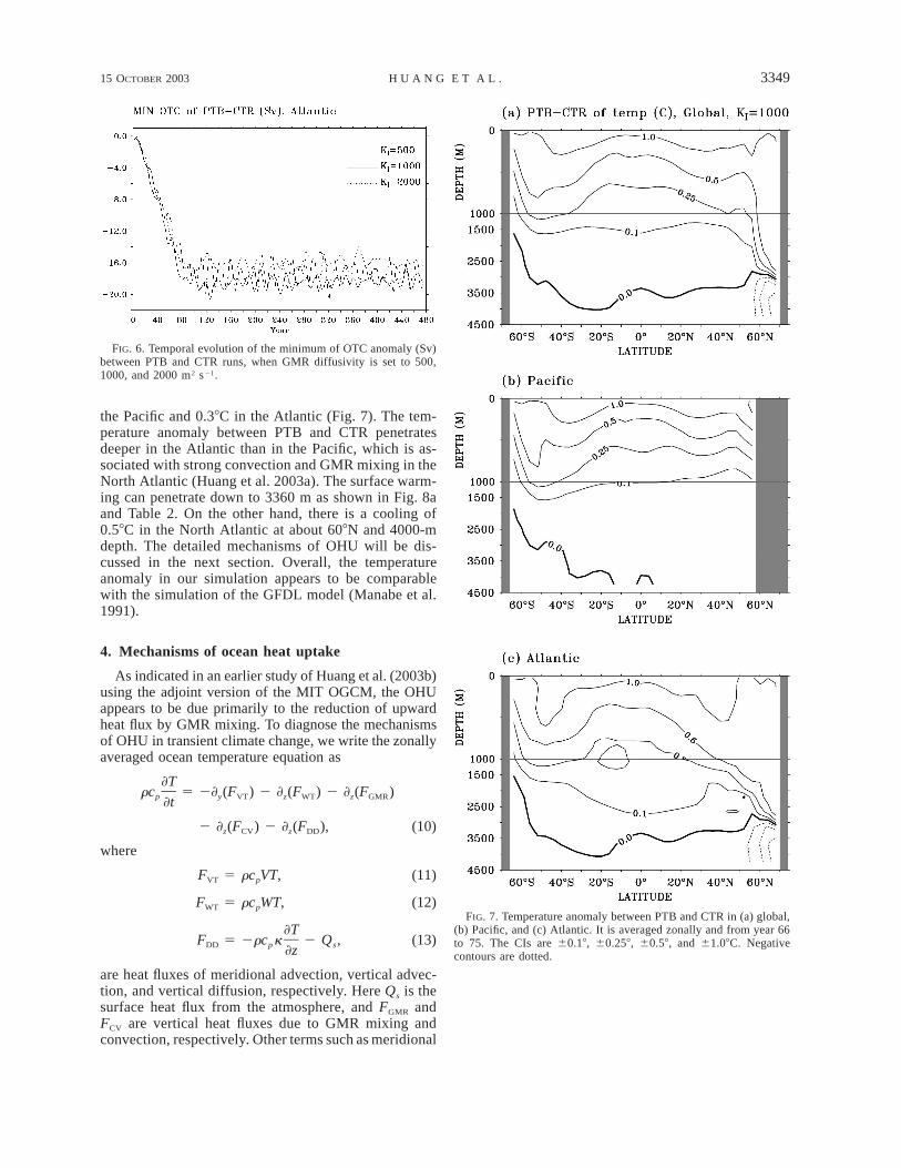
FIG. 6. Temporal evolution of the minimum of OTC anomaly (Sv)between PTB and CTR runs, when GMR diffusivity is set to 500,1000, and 2000 m2 s21.

FIG. 7. Temperature anomaly between PTB and CTR in (a) global,(b) Pacific, and (c) Atlantic. It is averaged zonally and from year 66to 75. The CIs are 60.18, 60.258, 60.58, and 61.08C. Negativecontours are dotted.

the Pacific and 0.38C in the Atlantic (Fig. 7). The tem-perature anomaly between PTB and CTR penetratesdeeper in the Atlantic than in the Pacific, which is as-sociated with strong convection and GMR mixing in theNorth Atlantic (Huang et al. 2003a). The surface warm-ing can penetrate down to 3360 m as shown in Fig. 8aand Table 2. On the other hand, there is a cooling of0.58C in the North Atlantic at about 608N and 4000-mdepth. The detailed mechanisms of OHU will be dis-cussed in the next section. Overall, the temperatureanomaly in our simulation appears to be comparablewith the simulation of the GFDL model (Manabe et al.1991).

4. Mechanisms of ocean heat uptake

As indicated in an earlier study of Huang et al. (2003b)using the adjoint version of the MIT OGCM, the OHUappears to be due primarily to the reduction of upwardheat flux by GMR mixing. To diagnose the mechanismsof OHU in transient climate change, we write the zonallyaveraged ocean temperature equation as

]Trc 5 2] (F ) 2 ] (F ) 2 ] (F )p y VT z WT z GMR]t

2 ] (F ) 2 ] (F ), (10)z CV z DD

where

F 5 rc VT, (11)VT p

F 5 rc WT, (12)WT p

]TF 5 2rc k 2 Q , (13)DD p s]z

are heat fluxes of meridional advection, vertical advec-tion, and vertical diffusion, respectively. Here Qs is thesurface heat flux from the atmosphere, and FGMR andFCV are vertical heat fluxes due to GMR mixing andconvection, respectively. Other terms such as meridional

3350 VOLUME 16J O U R N A L O F C L I M A T E

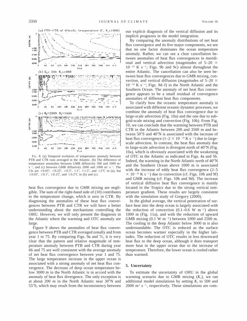
FIG. 8. (a) Temporal evolution of temperature anomaly betweenPTB and CTR runs averaged in the Atlantic. (b) The difference oftemperature anomalies between GMR diffusivity 500 and 1000 m2

s21, and (c) between GMR diffusivity 2000 and 1000 m2 s21. TheCIs are 60.058, 60.258, 60.58, 618, 61.58, and 628C in (a), but60.058, 60.18, 60.158, and 60.28C in (b) and (c).

heat flux convergence due to GMR mixing are negli-gible. The sum of the right-hand side of (10) contributesto the temperature change, which is zero in CTR. Bydiagnosing the anomalies of these heat flux conver-gences between PTB and CTR we will have a betterunderstanding about the mechanisms controlling theOHU. However, we will only present the diagnosis inthe Atlantic where the warming and OTC anomaly arelarge.

Figure 9 shows the anomalies of heat flux conver-gence between PTB and CTR averaged zonally and fromyear 1 to 75. By comparing Figs. 9a and 7c, it is veryclear that the pattern and relative magnitude of tem-perature anomaly between PTB and CTR during year66 and 75 are well consistent with the average anomalyof net heat flux convergence between year 1 and 75.The large temperature increase in the upper ocean isassociated with a strong anomaly of net heat flux con-vergence. The decrease of deep ocean temperature be-low 3000 m in the North Atlantic is in accord with theanomaly of heat flux divergence. The only exception isat about 200 m in the North Atlantic near 308N and558S, which may result from the inconsistency between

our explicit diagnosis of the vertical diffusion and itsimplicit prognosis in the model integration.

By comparing the anomaly distributions of net heatflux convergence and its five major components, we seethat no one factor dominates the ocean temperatureanomaly. Rather, we can see a clear cancellation be-tween anomalies of heat flux convergences in meridi-onal and vertical advection (magnitudes of 5–20 310210 K s21; Figs. 9b and 9c) almost throughout theentire Atlantic. The cancellation can also be seen be-tween heat flux convergences due to GMR mixing, con-vection, and vertical diffusion (magnitudes of 5–20 310210 K s21; Figs. 9d–f) in the North Atlantic and theSouthern Ocean. The anomaly of net heat flux conver-gence appears to be a small residual of convergenceanomalies of different heat flux components.

To clarify how the oceanic temperature anomaly isassociated with different oceanic dynamic processes, wecombine the anomaly of heat flux convergence due tolarge-scale advection (Fig. 10a) and the one due to sub-grid-scale mixing and convection (Fig. 10b). From Fig.10, we can conclude that the warming between PTB andCTR in the Atlantic between 200 and 3500 m and be-tween 508S and 408N is associated with the increase ofheat flux convergence (1–2 3 10210 K s21) due to large-scale advection. In contrast, the heat flux anomaly dueto large-scale advection is divergent north of 408N (Fig.10a), which is obviously associated with the weakeningof OTC in the Atlantic as indicated in Figs. 4a and 5b.Indeed, the warming in the North Atlantic north of 408Nand the Southern Ocean above 1000 m is associatedwith the increase of eddy heat flux convergence (2–53 10210 K s21) due to convection (cf. Figs. 10b and 9f)and GMR mixing (cf. Figs. 10b and 9d). The increaseof vertical diffusive heat flux convergence is mainlylocated in the Tropics due to the strong vertical tem-perature gradient. These results are largely consistentwith the simulation study of Gregory (2000).

In the global average, the vertical penetration of sur-face heat into the deep ocean is largely associated withthe reduction of convection (0.1–0.6 W m22) above1000 m (Fig. 11a), and with the reduction of upwardGMR mixing (0.1 W m22) between 1000 and 2500 m.The cooling in the deep Atlantic below 3000 m is alsounderstandable. The OTC is reduced as the surfaceocean becomes warmer especially in the higher lati-tudes. The reduction of OTC results in less downwardheat flux to the deep ocean, although it does transportmore heat in the upper ocean due to the increase oftemperature. Therefore, the lower ocean is cooled ratherthan warmed.

5. Uncertainty

To estimate the uncertainty of OHU in the globalwarming scenario due to GMR mixing (KI), we ranadditional model simulations by setting KI to 500 and2000 m2 s21, respectively. These simulations are com-

15 OCTOBER 2003 3351H U A N G E T A L .

FIG. 9. Anomaly of heat flux convergence between PTB and CTR runs: (a) net, (b) meridional advection, (c) vertical advection, (d) GMRmixing, (e) vertical diffusion, and (f ) convection. It is averaged zonally in the Atlantic and from year 1 to 75. The CIs are 60.5, 61, 62,and 65 3 10210 K s21 in (a), but 65, 610, and 620 3 10210 K s21 in (b)–(f ). Positive (negative) indicates convergence (divergence).

pared with the standard run in which KI is set to 1000m2 s21. The range of KI from 500 to 2000 m2 s21 maybe reasonable based on observations at different oceaniclocations and of eddies at different spatial scales (Ku

and Luo 1994; Hirst and Cai 1994; Jenkins 1991; Led-well et al. 1998; Thiele 1986).

We want to remind readers that the OHU is definedas the difference of ocean temperature or heat capacity

3352 VOLUME 16J O U R N A L O F C L I M A T E

FIG. 10. Combined anomaly of heat flux convergence between PTBand CTR runs. (a) Meridional and vertical advection, and (b) GMRmixing, vertical diffusion, and convection. It is averaged zonally inthe Atlantic and from year 1 to 75. The CIs are 61, 62, 65, and610 3 10210 K s21.

FIG. 11. Anomaly of global vertical heat flux (W m22, positivedownward) between PTB and CTR runs. It is averaged globally andfrom year 1 to 75. (a) KI 5 1000, (b) KI 5 500, and (c) KI 5 2000m2 s21.

TABLE 3. Total OHU (31024 J) in different basins by year 475.

KI (m2 s21) Global Pacific Atlantic

1000500

2000

3.913.903.77

2.242.202.19

1.671.701.58

between the PTB and CTR runs when CO2 concentra-tion is changed. That is to say, the difference amongCTR runs using three different KI is excluded. Our sim-ulations of CTR runs indicate (not shown) that the oceantemperature increases by about 1.28C between 100 and1500 m, and about 0.58C below 2000 m when KI de-creases from 1000 to 500 m2 s21. Likewise, the oceantemperature decreases by about 1.28C between 100 and1500 m, and about 0.38C below 2000 m when KI in-creases from 1000 to 2000 m2 s21. Corresponding withthe ocean temperature change, the MOTC of CTR runsin the Atlantic increases by about 4 Sv when KI de-creases from 1000 to 500 m2 s21, but decreases by about2 Sv when KI increases from 1000 to 2000 m2 s21 (Figs.5a,c, and 5e). The reason is that when KI decreases(increases), the convection have to be stronger (weaker)to balance the vertical heat flux due to vertical advectionand diffusion (Huang et al. 2003a). The stronger (weak-er) convection enhances (weakens) the MOTC, whicheventually increases (decreases) the ocean temperature.

Similar to the reasons for analyzing OHU mecha-nisms in the Atlantic, we will only discuss the uncer-tainty of ocean heat uptake due to KI in the Atlantic.The changes in the Pacific are similar but with smallermagnitude and slightly different vertical distribution.

a. Temporal evolution

First, we find that the evolution of MOTC in the NorthAtlantic for KI of 500 and 2000 m2 s21 follows almostthe same trajectory as for KI of 1000 m2 s21 (Figs. 4a–c). In all three cases, the OTC anomaly below 3000 mpersists after year 100 (Fig. 6). The difference of min-imum OTC anomaly between PTB and CTR when KI

is set to 2000 m2 s21 is about 2 Sv larger than that whenKI is set to 1000 m2 s21. However, we should note thatthe depth of these minimum OTC anomalies is differentas indicated in Figs. 5d,f, and Table 2.

The total OHU is very insensitive to the changes inthe eddy mixing, as shown in Table 3. This is primarily

15 OCTOBER 2003 3353H U A N G E T A L .

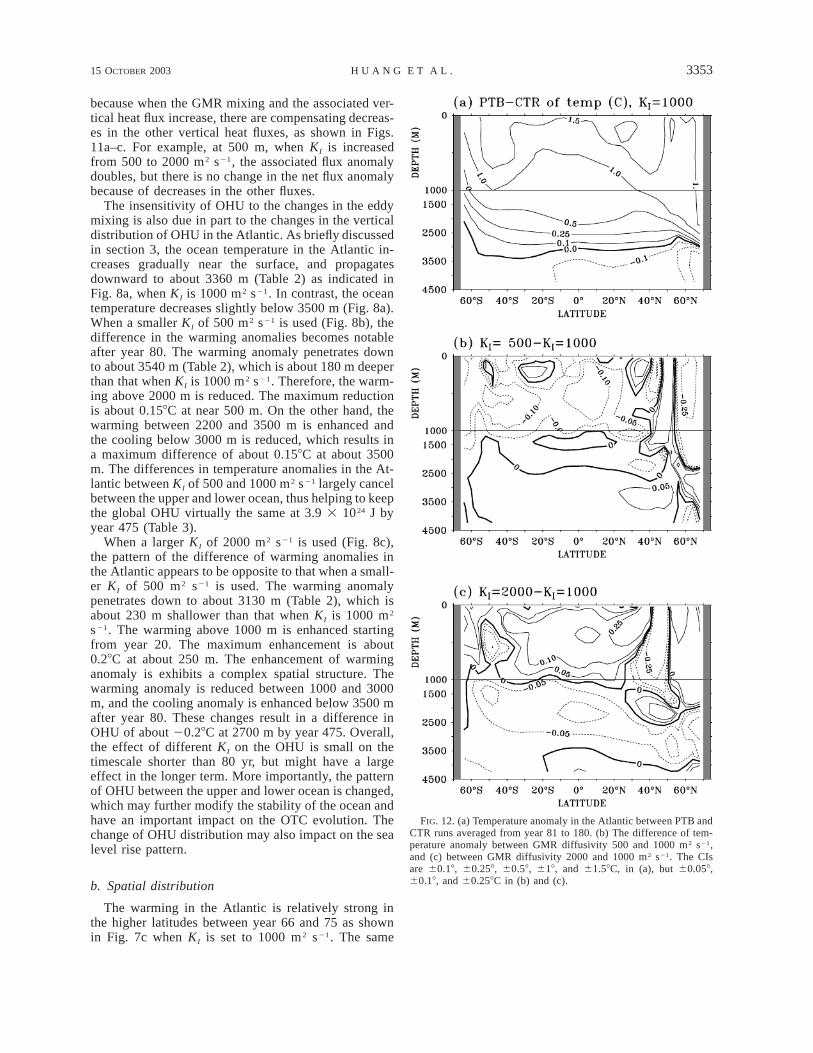
FIG. 12. (a) Temperature anomaly in the Atlantic between PTB andCTR runs averaged from year 81 to 180. (b) The difference of tem-perature anomaly between GMR diffusivity 500 and 1000 m2 s21,and (c) between GMR diffusivity 2000 and 1000 m2 s21. The CIsare 60.18, 60.258, 60.58, 618, and 61.58C, in (a), but 60.058,60.18, and 60.258C in (b) and (c).

because when the GMR mixing and the associated ver-tical heat flux increase, there are compensating decreas-es in the other vertical heat fluxes, as shown in Figs.11a–c. For example, at 500 m, when KI is increasedfrom 500 to 2000 m2 s21, the associated flux anomalydoubles, but there is no change in the net flux anomalybecause of decreases in the other fluxes.

The insensitivity of OHU to the changes in the eddymixing is also due in part to the changes in the verticaldistribution of OHU in the Atlantic. As briefly discussedin section 3, the ocean temperature in the Atlantic in-creases gradually near the surface, and propagatesdownward to about 3360 m (Table 2) as indicated inFig. 8a, when KI is 1000 m2 s21. In contrast, the oceantemperature decreases slightly below 3500 m (Fig. 8a).When a smaller KI of 500 m2 s21 is used (Fig. 8b), thedifference in the warming anomalies becomes notableafter year 80. The warming anomaly penetrates downto about 3540 m (Table 2), which is about 180 m deeperthan that when KI is 1000 m2 s21. Therefore, the warm-ing above 2000 m is reduced. The maximum reductionis about 0.158C at near 500 m. On the other hand, thewarming between 2200 and 3500 m is enhanced andthe cooling below 3000 m is reduced, which results ina maximum difference of about 0.158C at about 3500m. The differences in temperature anomalies in the At-lantic between KI of 500 and 1000 m2 s21 largely cancelbetween the upper and lower ocean, thus helping to keepthe global OHU virtually the same at 3.9 3 1024 J byyear 475 (Table 3).

When a larger KI of 2000 m2 s21 is used (Fig. 8c),the pattern of the difference of warming anomalies inthe Atlantic appears to be opposite to that when a small-er KI of 500 m2 s21 is used. The warming anomalypenetrates down to about 3130 m (Table 2), which isabout 230 m shallower than that when KI is 1000 m2

s21. The warming above 1000 m is enhanced startingfrom year 20. The maximum enhancement is about0.28C at about 250 m. The enhancement of warminganomaly is exhibits a complex spatial structure. Thewarming anomaly is reduced between 1000 and 3000m, and the cooling anomaly is enhanced below 3500 mafter year 80. These changes result in a difference inOHU of about 20.28C at 2700 m by year 475. Overall,the effect of different KI on the OHU is small on thetimescale shorter than 80 yr, but might have a largeeffect in the longer term. More importantly, the patternof OHU between the upper and lower ocean is changed,which may further modify the stability of the ocean andhave an important impact on the OTC evolution. Thechange of OHU distribution may also impact on the sealevel rise pattern.

b. Spatial distribution

The warming in the Atlantic is relatively strong inthe higher latitudes between year 66 and 75 as shownin Fig. 7c when KI is set to 1000 m2 s21. The same

3354 VOLUME 16J O U R N A L O F C L I M A T E

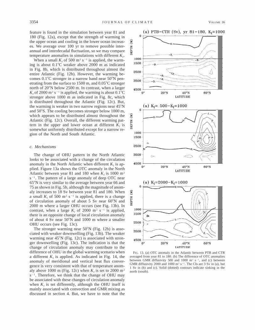
FIG. 13. (a) OTC anomaly in the Atlantic between PTB and CTRaveraged from year 81 to 180. (b) The difference of OTC anomaliesbetween GMR diffusivity 500 and 1000 m2 s21, and (c) betweenGMR diffusivity 2000 and 1000 m2 s21. The CIs are 3 Sv in (a), but1 Sv in (b) and (c). Solid (dotted) contours indicate sinking in thenorth (south).

feature is found in the simulation between year 81 and180 (Fig. 12a), except that the strength of warming inthe upper ocean and cooling in the lower ocean increas-es. We average over 100 yr to remove possible inter-annual and interdecadal fluctuation, so we may comparetemperature anomalies in simulations with different KI.

When a small KI of 500 m2 s21 is applied, the warm-ing is about 0.18C weaker above 2000 m as indicatedin Fig. 8b, which is distributed throughout almost theentire Atlantic (Fig. 12b). However, the warming be-comes 0.18C stronger in a narrow band near 508N pen-etrating from the surface to 1500 m, and 0.058C strongernorth of 208N below 2500 m. In contrast, when a largerKI of 2000 m2 s21 is applied, the warming is about 0.18Cstronger above 1000 m as indicated in Fig. 8c, whichis distributed throughout the Atlantic (Fig. 12c). But,the warming is weaker in two narrow regions near 458Nand 508S. The cooling becomes stronger below 1000 m,which appears to be distributed almost throughout theAtlantic (Fig. 12c). Overall, the different warming pat-tern in the upper and lower ocean at different KI issomewhat uniformly distributed except for a narrow re-gion of the North and South Atlantic.

c. Mechanisms

The change of OHU pattern in the North Atlanticlooks to be associated with a change of the circulationanomaly in the North Atlantic when different KI is ap-plied. Figure 13a shows the OTC anomaly in the NorthAtlantic between year 81 and 180 when KI is 1000 m2

s21. The pattern of a large anomaly of deep OTC near658N is very similar to the average between year 66 and75 as shown in Fig. 5b, although the magnitude of anom-aly increases to 18 Sv between year 81 and 180. Whena small KI of 500 m2 s21 is applied, there is a changeof circulation anomaly of about 5 Sv near 608N and2000 m where a larger OHU occurs (see Fig. 13b). Incontrast, when a large KI of 2000 m2 s21 is applied,there is an opposite change of local circulation anomalyof about 4 Sv near 508N and 1000 m where a smallerOHU occurs (see Fig. 13c).

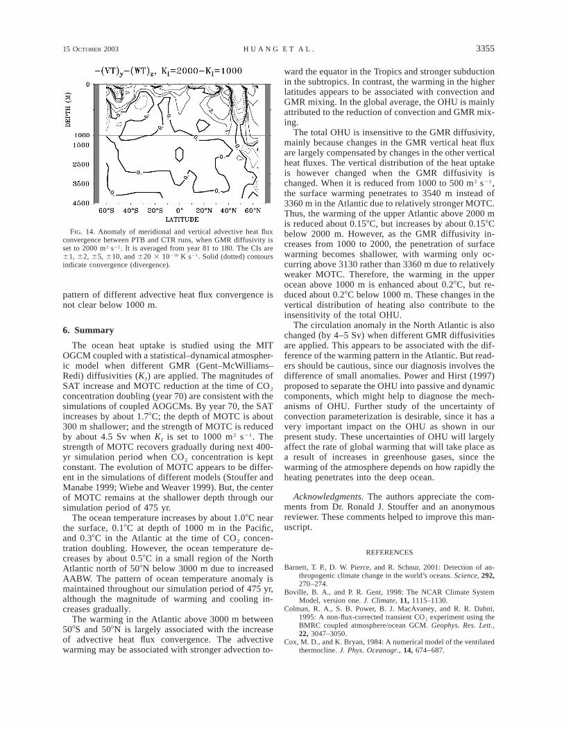
The stronger warming near 508N (Fig. 12b) is asso-ciated with weaker downwelling (Fig. 13b). The weakerwarming near 458N (Fig. 12c) is associated with stron-ger downwelling (Fig. 13c). The indication is that thechange of circulation anomaly may contribute to thedifference of OHU in the global warming scenario whena different KI is applied. As indicated in Fig. 14, theanomaly of meridional and vertical heat flux conver-gence is very consistent with that of temperature anom-aly above 1000 m (Fig. 12c) when KI is set to 2000 m2

s21. Therefore, we think that the change of OHU maybe associated with these changes of circulation anomalywhen KI is set differently, although the OHU itself ismainly associated with convection and GMR mixing asdiscussed in section 4. But, we have to note that the

15 OCTOBER 2003 3355H U A N G E T A L .

FIG. 14. Anomaly of meridional and vertical advective heat fluxconvergence between PTB and CTR runs, when GMR diffusivity isset to 2000 m2 s21. It is averaged from year 81 to 180. The CIs are61, 62, 65, 610, and 620 3 10210 K s21. Solid (dotted) contoursindicate convergence (divergence).

pattern of different advective heat flux convergence isnot clear below 1000 m.

6. Summary

The ocean heat uptake is studied using the MITOGCM coupled with a statistical–dynamical atmospher-ic model when different GMR (Gent–McWilliams–Redi) diffusivities (KI) are applied. The magnitudes ofSAT increase and MOTC reduction at the time of CO2

concentration doubling (year 70) are consistent with thesimulations of coupled AOGCMs. By year 70, the SATincreases by about 1.78C; the depth of MOTC is about300 m shallower; and the strength of MOTC is reducedby about 4.5 Sv when KI is set to 1000 m2 s21. Thestrength of MOTC recovers gradually during next 400-yr simulation period when CO2 concentration is keptconstant. The evolution of MOTC appears to be differ-ent in the simulations of different models (Stouffer andManabe 1999; Wiebe and Weaver 1999). But, the centerof MOTC remains at the shallower depth through oursimulation period of 475 yr.

The ocean temperature increases by about 1.08C nearthe surface, 0.18C at depth of 1000 m in the Pacific,and 0.38C in the Atlantic at the time of CO2 concen-tration doubling. However, the ocean temperature de-creases by about 0.58C in a small region of the NorthAtlantic north of 508N below 3000 m due to increasedAABW. The pattern of ocean temperature anomaly ismaintained throughout our simulation period of 475 yr,although the magnitude of warming and cooling in-creases gradually.

The warming in the Atlantic above 3000 m between508S and 508N is largely associated with the increaseof advective heat flux convergence. The advectivewarming may be associated with stronger advection to-

ward the equator in the Tropics and stronger subductionin the subtropics. In contrast, the warming in the higherlatitudes appears to be associated with convection andGMR mixing. In the global average, the OHU is mainlyattributed to the reduction of convection and GMR mix-ing.

The total OHU is insensitive to the GMR diffusivity,mainly because changes in the GMR vertical heat fluxare largely compensated by changes in the other verticalheat fluxes. The vertical distribution of the heat uptakeis however changed when the GMR diffusivity ischanged. When it is reduced from 1000 to 500 m2 s21,the surface warming penetrates to 3540 m instead of3360 m in the Atlantic due to relatively stronger MOTC.Thus, the warming of the upper Atlantic above 2000 mis reduced about 0.158C, but increases by about 0.158Cbelow 2000 m. However, as the GMR diffusivity in-creases from 1000 to 2000, the penetration of surfacewarming becomes shallower, with warming only oc-curring above 3130 rather than 3360 m due to relativelyweaker MOTC. Therefore, the warming in the upperocean above 1000 m is enhanced about 0.28C, but re-duced about 0.28C below 1000 m. These changes in thevertical distribution of heating also contribute to theinsensitivity of the total OHU.

The circulation anomaly in the North Atlantic is alsochanged (by 4–5 Sv) when different GMR diffusivitiesare applied. This appears to be associated with the dif-ference of the warming pattern in the Atlantic. But read-ers should be cautious, since our diagnosis involves thedifference of small anomalies. Power and Hirst (1997)proposed to separate the OHU into passive and dynamiccomponents, which might help to diagnose the mech-anisms of OHU. Further study of the uncertainty ofconvection parameterization is desirable, since it has avery important impact on the OHU as shown in ourpresent study. These uncertainties of OHU will largelyaffect the rate of global warming that will take place asa result of increases in greenhouse gases, since thewarming of the atmosphere depends on how rapidly theheating penetrates into the deep ocean.

Acknowledgments. The authors appreciate the com-ments from Dr. Ronald J. Stouffer and an anonymousreviewer. These comments helped to improve this man-uscript.

REFERENCES

Barnett, T. P., D. W. Pierce, and R. Schnur, 2001: Detection of an-thropogenic climate change in the world’s oceans. Science, 292,270–274.

Boville, B. A., and P. R. Gent, 1998: The NCAR Climate SystemModel, version one. J. Climate, 11, 1115–1130.

Colman, R. A., S. B. Power, B. J. MacAvaney, and R. R. Dahni,1995: A non-flux-corrected transient CO2 experiment using theBMRC coupled atmosphere/ocean GCM. Geophys. Res. Lett.,22, 3047–3050.

Cox, M. D., and K. Bryan, 1984: A numerical model of the ventilatedthermocline. J. Phys. Oceanogr., 14, 674–687.

3356 VOLUME 16J O U R N A L O F C L I M A T E

Cubasch, U., K. Hasselmann, H. Hock, E. Maier-Reimer, U. Miko-lajewicz, B. D. Santer, and R. Sausen, 1992: Time-dependentgreenhouse warming computations with a coupled ocean–at-mosphere model. Climate Dyn., 8, 55–69.

Gent, P. R., and J. C. McWilliams, 1990: Isopycnal mixing in oceancirculation models. J. Phys. Oceanogr., 20, 150–155.

Gregory, J. M., 2000: Vertical heat transports in the ocean and theireffect on time-dependent climate change. Climate Dyn., 16, 501–515.

Guo, Y., Y. Yu, X. Liu, and X. Zhang, 2001: Simulation of climatechange induced by CO2 increasing for East Asia with IAP/LASGGOALS model. Adv. Atmos. Sci., 18, 53–66.

Hirst, A., and W. Cai, 1994: Sensitivity of a World Ocean GCM tochanges in subsurface mixing parameterization. J. Phys. Ocean-ogr., 24, 1256–1279.

Houghton, J. T., Y. Ding, D. J. Griggs, M. Noguer, P. J. van derLinden, and D. Xiaosu, Eds., 2001: Climate Change 2001: TheScientific Basis. Cambridge University Press, 944 pp.

Huang, B., P. H. Stone, and C. Hill, 2003a: Sensitivities of deep-ocean heat uptake and heat content to surface fluxes and subgrid-scale parameters in an OGCM with idealized geometry. J. Geo-phys. Res., 108, 3015, doi:10.1029/2001JC001218.

——, ——, A. P. Sokolov, and I. V. Kamenkovich, 2003b: The deep-ocean heat uptake in transient climate change. J. Climate, 16,1352–1363.

Jenkins, W. J., 1991: Determination of isopycnal diffusivity in theSargasso Sea. J. Phys. Oceanogr., 21, 1058–1061.

Johns, T. C., R. E. Carnell, J. F. Crossley, J. M. Gregory, J. F. B.Mitchell, C. A. Senior, S. F. B. Tett, and R. A. Wood, 1997: Thesecond Hadley Centre coupled ocean–atmosphere GCM: Modeldescription, spinup and validation. Climate Dyn., 13, 103–134.

Kamenkovich, I. V., A. P. Sokolov, and P. H. Stone, 2002: An efficientclimate model with a 3D ocean and statistical-dynamical at-mosphere. Climate Dyn., 19, 585–598.

Ku, T. L., and S. Luo, 1994: New appraisal of Radium 226 as a large-scale oceanic mixing tracer. J. Geophys. Res., 99, 10 255–10 273.

Ledwell, J. R., A. J. Watson, and C. S. Law, 1998: Mixing of a tracerin the pycnocline. J. Geophys. Res., 103, 21 499–21 529.

——, E. T. Montgomery, K. L. Polzin, L. C. St. Laurent, R. W.Schmitt, and J. M. Toole, 2000: Evidence for enhanced mixingover rough topography in the abyssal ocean. Nature, 403, 179–182.

Levitus, S., J. I. Antonov, T. P. Boyer, and C. Stephens, 2000: Warm-ing of the world ocean. Science, 287, 2225–2229.

——, ——, J. Wang, T. L. Delworth, K. W. Dixon, and A. J. Broccoli,2001: Anthropogenic warming of earth’s climate system. Sci-ence, 292, 267–270.

Manabe, S., and R. J. Stouffer, 1994: Multiple century response ofa coupled ocean–atmosphere model to an increase of atmosphericcarbon dioxide. J. Climate, 7, 5–23.

——, ——, M. J. Spelman, and K. Bryan, 1991: Transient responses

of a coupled ocean–atmosphere model to gradual changes ofatmospheric CO2. Part I: Annual mean response. J. Climate, 4,785–818.

Marshall, J., A. Adcroft, C. Hill, L. Perelman, and C. Heisey, 1997:A finite volume, incompressible Navier stokes model for studiesof the ocean on parallel computers. J. Geophys. Res., 102, 5753–5766.

Meehl, G. A., W. D. Collins, B. A. Boville, J. T. Kiehl, T. M. L.Wigley, and J. M. Arblaster, 2000: Response of the NCAR cli-mate system model to increased CO2 and the role of physicalprocesses. J. Climate, 13, 1879–1898.

Murphy, J. M., and J. F. B. Mitchell, 1995: Transient response of theHadley Centre coupled ocean–atmosphere model to increasingcarbon dioxide. Part II: Spatial and temporal structure of re-sponse. J. Climate, 8, 57–80.

Nakamura, M., and Y. Cao, 2000: On the eddy isopycnal thicknessdiffusivity of the Gent–McWilliams subgrid mixing parameter-ization. J. Climate, 13, 502–510.

Power, S. B., and A. C. Hirst, 1997: Eddy parameterization and oce-anic response to idealized global warming. Climate Dyn., 13,417–428.

——, R. A. Colman, B. J. McAvaney, R. R. Dahni, A. M. Moore,and N. R. Smith, 1993: The BMRC Coupled atmosphere/ocean/sea-ice model. BMRC Research-Rep. 37, Bureau of MeteorologyResearch Centre, Melbourne, Australia, 58 pp.

Redi, M. H., 1982: Oceanic isopycnal mixing by coordinate rotation.J. Phys. Oceanogr., 12, 1154–1158.

Russell, G. L., and D. Rind, 1999: Response to CO2 transient increasein GISS coupled models: Regional coolings in a warming cli-mate. J. Climate, 12, 531–539.

——, J. R. Miller, and D. Rind, 1995: A coupled atmosphere–oceanmodel for transient climate change studies. Atmos.–Ocean, 33,683–730.

Sokolov, A. P., and P. H. Stone, 1998: A flexible climate model foruse in integrated assessments. Climate Dyn., 14, 291–303.

Stouffer, R. J., and S. Manabe, 1999: Response of a coupled ocean–atmosphere model to increasing atmospheric carbon dioxide:Sensitivity to the rate of increase. J. Climate, 12, 2224–2236.

Thiele, G., 1986: Baroclinic flow and transient-tracer fields in theCanary–Cape Verde Basin. J. Phys. Oceanogr., 16, 814–826.

Voss, R., R. Sausen, and U. Cubasch, 1998: Periodically synchro-nously coupled integrations with the atmosphere–ocean generalcirculation model ECHAM3/LSG. Climate Dyn., 14, 249–266.

Wiebe, E. C., and A. J. Weaver, 1999: On the sensitivity of globalwarming experiments to the parameterisation of sub-grid scaleocean mixing. Climate Dyn., 15, 875–893.

Zhang, H. M., M. D. Prater, and T. Rossby, 2001: Isopycnal Lagrang-ian statistics from North Atlantic Current RAFOS float obser-vations. J. Geophys. Res., 106, 13 817–13 836.

Zhang, X.-H., G.-Y. Shi, H. Liu, and Y.-Q. Yu, Eds.,2000: IAP GlobalAtmosphere–Land System Model. Science Press, 259 pp.