Combustion and Flame 146 (2006) 635–648www.elsevier.com/locate/combustflame

Modeling subgrid scale mixture fraction variance in LES ofevaporating spray

Cécile Pera 1, Julien Réveillon, Luc Vervisch ∗, Pascale Domingo

LMFN, UMR-CNRS-6614-CORIA, INSA and Université de Rouen, Campus du Madrillet, Avenue de l’Université, BP 8,76801 Saint-Etienne-du-Rouvray, France

Received 29 August 2005; received in revised form 16 June 2006; accepted 3 July 2006

Available online 4 August 2006

Abstract

Simulations of a dilute spray evaporating in spatially decaying homogeneous turbulence are performed. AnEulerian description of the flow is adopted, while the behavior of the discrete liquid phase is captured usingLagrangian modeling. Time and length scales of the continuous carrier phase are fully simulated and by varyingthe properties of the modeled spray, a database of spray carrier phase direct numerical simulation (CP-DNS) isobtained. The CP-DNS is then filtered on a coarse grid to conduct a priori tests of subgrid scale (SGS) closures.The objective is to provide methods for approximating the level of SGS mixture fraction variance in large eddysimulation (LES) of fuel spray turbulent combustion. Direct estimation of the variance from the scales resolvedin LES is first discussed. Then, the solving of a balance equation to get the variance is addressed, with closuresfor the scalar dissipation rate and the correlation between vapor source and mixture fraction. From the results, aprocedure to couple spray evaporation with SGS turbulent combustion modeling emerges.© 2006 Published by Elsevier Inc. on behalf of The Combustion Institute.

Keywords: Large eddy simulation; Direct numerical simulation; Spray; Nonpremixed flames

1. Introduction

Many combustion systems operate with liquid fuelinjection, such as gas turbines, diesel engines, indus-trial furnaces, and liquid-fueled rocket engines. Nu-merous physical phenomena interact in those com-bustion chambers, beginning with the breakup of liq-uid sheets, followed by atomization and droplet dis-persion [1] along with its impact on turbulence [2], toend with the strongly coupled evaporation and com-

* Corresponding author.E-mail address: vervisch@coria.fr (L. Vervisch).

1 Present address: IFP, TAE 1 & 4 av. du Bois-Préau,92852 Rueil-Malmaison Cedex, France.

0010-2180/$ – see front matter © 2006 Published by Elsevier Inc.doi:10.1016/j.combustflame.2006.07.003

bustion processes [3–8]. Spray turbulent combustionis unsteady by nature and this may be accounted forin numerical modeling using large eddy simulation(LES), associated to a subgrid scale (SGS) descrip-tion of phenomena unresolved by the grid. A varietyof SGS closures for initially nonpremixed reactantsmake use of mixture fraction [9–12]. This scalar in-forms on the degree of mixing between fuel and oxi-dizer. The SGS mixture fraction variance brings moreinformation on the amplitude of unresolved fluctua-tions in the mixing between the reactants [9,13–21].It is intended in this paper to determine a procedureto estimate this SGS variance in the context of evapo-rating sprays.

Simulations of low-Reynolds-number spatially de-caying grid turbulence carrying an evaporating dilute

on behalf of The Combustion Institute.

636 C. Pera et al. / Combustion and Flame 146 (2006) 635–648

spray are first conducted. The carrier flow is fully re-solved; the discrete spray phase is, however, modeledfrom a Lagrangian approach for dilute spray, resultingin a carrier phase direct numerical simulation (CP-DNS). Those simulations are not full DNS of theproblem, because the liquid phase and the smallestscales of the vapor field around droplets are not re-solved. Nevertheless, for a given distribution of theobtained Eulerian turbulent vapor field, various cor-relations between filtered Eulerian quantities can beprobed and compared to their estimates from SGSmodels. The main properties of the spray (Stokesnumber and characteristic evaporation time) are var-ied to construct a set of simulations. The dilute sprayis initially monodisperse, but the two-way couplingbetween the flow and the droplets rapidly leads toan evaporating polydisperse spray. The mixture frac-tion is defined from the resulting fuel concentrationfield and its Eulerian distribution is filtered to performa priori studies on the mass-weighted SGS mixturefraction variance.

Scale similarity hypotheses are common in SGSmodeling; it is thus assumed that the unknown SGSfluctuations are proportional to fluctuations that canbe measured between the LES filter and a wider testfilter. This direct estimation of SGS mixture frac-tion variance was used previously for gaseous fuelcombustion [13]. An equilibrium hypothesis betweenproduction and dissipation of variance was also com-bined with a dynamic procedure to determine themodeling parameters of the SGS variance [9]. An-other alternative to get the mixture fraction varianceconsists of solving an additional balance equation.These approaches are evaluated from CP-DNS.

The CP-DNS numerical procedure is presented inthe next section; then the scale similarity and equilib-rium assumptions are discussed for mixture fractionvariance in the case of spray evaporation. In the subse-quent section, the introduction of a balance equationfor the variance is detailed and the modeling of itsvarious unclosed terms is discussed.

2. Evaporating spray model problem andnumerical procedure

The simulations operate with dilute spray. In a liq-uid fuel combustion chamber [22], this would corre-spond to an idealized regime where all the dropletshave been atomized with no liquid sheet remain-ing; breakup and coalescence phenomena are thusavoided. Every droplet is assumed to be unaware ofthe existence of the others, either in its motion orevaporation. However, a two-way coupling is used be-tween the droplets and the continuous phase; in this

description, droplets are seen from the Eulerian fieldsas simple point sources of mass and momentum.

2.1. Model problem and numerics

A spatially decaying grid turbulence is simulated,in a flow configuration similar to the one studiedin [23]. The DNS package developed by Guichardet al. [24] is used. The three-dimensional computa-tional domain is divided into two parts; in a bufferzone, grid turbulence laden with droplets is gener-ated, and it is used as inlet conditions for the maincomputational domain, where the turbulence spatiallydecays and droplets evaporate (Fig. 1). The turbu-lence is generated in the buffer zone by solving thethree-dimensional form of the Navier–Stokes equa-tions with a spectral method [25] that is associatedwith a forcing scheme to sustain velocity fluctuations;details may be found in [24]. In the spectral solver, theLagrangian solution of the discrete phase is one-waycoupled with momentum; the droplets are dispersedby velocity fluctuations but are not allowed to evap-orate. An accurate solution of grid turbulence ladenwith droplets is thus obtained. This solution is pre-scribed at each instant in time as the inlet condition ofa finite difference Navier–Stokes solver of freely spa-tially decaying turbulence, where droplets are allowedto evaporate with two-way coupling. Four solvers arethus simultaneously running (Fig. 1): (1) an Eulerianforced turbulence spectral solution with (2) a La-grangian solver, where droplets are in equilibriumwith the flow, followed by (3) an Eulerian finite dif-ference solver associated with (4) a two-way coupledLagrangian solution of spray. Droplets only evaporatein the second part of the flow, namely when turbu-lence spatially decays.

The time integration of the governing equations isdone with a third-order explicit Runge–Kutta schemewith minimal data storage [26]. The detailed set ofsolved equations, all the expressions for spray quan-tities, and coupling between continuous and discretephases are from usual spray modeling [3]. The bal-ance equations and expressions used for the controlparameters of evaporation and DNS have been pub-lished recently [8,18,27] and are not repeated here.2

The sixth-order PADE scheme [28] is used to approx-imate spatial derivatives on a uniform Cartesian meshin the second part of the flow (Fig. 1). Nonreflect-ing inlet and outlet are prescribed in the streamwisedirection from modified [24] Navier–Stokes charac-teristics boundary conditions (NSCBC) [29], while

2 In Eq. (17) of [8], the last term in the brackets shouldappear with a minus sign; the same applies to Eq. (3.23) of[27]. In Eq. (5) of [8] one should read 1/tkv instead of tkv .

C. Pera et al. / Combustion and Flame 146 (2006) 635–648 637

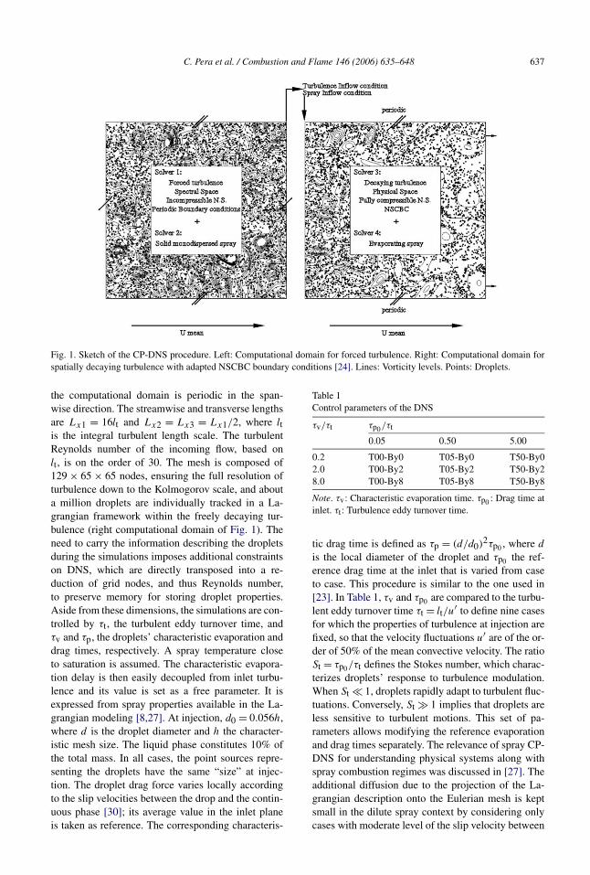
Fig. 1. Sketch of the CP-DNS procedure. Left: Computational domain for forced turbulence. Right: Computational domain forspatially decaying turbulence with adapted NSCBC boundary conditions [24]. Lines: Vorticity levels. Points: Droplets.

the computational domain is periodic in the span-wise direction. The streamwise and transverse lengthsare Lx1 = 16lt and Lx2 = Lx3 = Lx1/2, where ltis the integral turbulent length scale. The turbulentReynolds number of the incoming flow, based onlt, is on the order of 30. The mesh is composed of129 × 65 × 65 nodes, ensuring the full resolution ofturbulence down to the Kolmogorov scale, and abouta million droplets are individually tracked in a La-grangian framework within the freely decaying tur-bulence (right computational domain of Fig. 1). Theneed to carry the information describing the dropletsduring the simulations imposes additional constraintson DNS, which are directly transposed into a re-duction of grid nodes, and thus Reynolds number,to preserve memory for storing droplet properties.Aside from these dimensions, the simulations are con-trolled by τt, the turbulent eddy turnover time, andτv and τp, the droplets’ characteristic evaporation anddrag times, respectively. A spray temperature closeto saturation is assumed. The characteristic evapora-tion delay is then easily decoupled from inlet turbu-lence and its value is set as a free parameter. It isexpressed from spray properties available in the La-grangian modeling [8,27]. At injection, d0 = 0.056h,where d is the droplet diameter and h the character-istic mesh size. The liquid phase constitutes 10% ofthe total mass. In all cases, the point sources repre-senting the droplets have the same “size” at injec-tion. The droplet drag force varies locally accordingto the slip velocities between the drop and the contin-uous phase [30]; its average value in the inlet planeis taken as reference. The corresponding characteris-

Table 1Control parameters of the DNS

τv/τt τp0/τt

0.05 0.50 5.00

0.2 T00-By0 T05-By0 T50-By02.0 T00-By2 T05-By2 T50-By28.0 T00-By8 T05-By8 T50-By8

Note. τv: Characteristic evaporation time. τp0 : Drag time atinlet. τt: Turbulence eddy turnover time.

tic drag time is defined as τp = (d/d0)2τp0 , where d

is the local diameter of the droplet and τp0 the ref-erence drag time at the inlet that is varied from caseto case. This procedure is similar to the one used in[23]. In Table 1, τv and τp0 are compared to the turbu-lent eddy turnover time τt = lt/u

′ to define nine casesfor which the properties of turbulence at injection arefixed, so that the velocity fluctuations u′ are of the or-der of 50% of the mean convective velocity. The ratioSt = τp0/τt defines the Stokes number, which charac-terizes droplets’ response to turbulence modulation.When St � 1, droplets rapidly adapt to turbulent fluc-tuations. Conversely, St � 1 implies that droplets areless sensitive to turbulent motions. This set of pa-rameters allows modifying the reference evaporationand drag times separately. The relevance of spray CP-DNS for understanding physical systems along withspray combustion regimes was discussed in [27]. Theadditional diffusion due to the projection of the La-grangian description onto the Eulerian mesh is keptsmall in the dilute spray context by considering onlycases with moderate level of the slip velocity between

638 C. Pera et al. / Combustion and Flame 146 (2006) 635–648

Fig. 2. (a) Vorticity (isolines) and droplets (dots) in stream-wise planes. (b) Mixture fraction (isolines) and droplets(dots) in spanwise planes.

the discrete and continuous phases. Typically, this slipvelocity stays below 10% of the mean flow velocityin the presented cases. It is important to note that thesimulations performed here are strongly restricted todilute spray. Such spray regime may be observed inaeronautical or rocket engines at a given stage of thecombustion process [31]. Extrapolating the reportedresults to other spray regimes may not be straightfor-ward. Figs. 2 and 3 show snapshots of the mixturefraction field with droplet positions.

2.2. DNS a priori filtering

DNS fields are probed so that all spatial fluctu-ations smaller than a length � are damped using afiltering operation, or local volume averaging. LESfiltering is expressed as

(1)Z(x, t) =+∞∫

−∞Z(x′, t)G�(x − x′)dx′,

where G�(x −x′) is a normalized Gaussian filter [32,33] applied to the scalar field Z. As is usually donein variable density flows, a mass-weighted filteringZ = ρZ/ρ is introduced. SGS modeling including adynamic formulation is developed; thereby a test fil-ter of characteristic size � = 2� is also introducedto perform filtering of the LES field. The reference

filter size is five times larger than the uniform DNSmesh, � = 5h. The choice of those filters was madeso that they are within the decay range of the energeticspectrum of the present low-Reynolds-number spa-tially decaying turbulence. They would be located inthe inertial range when the modeling is applied to realcombustion systems featuring much larger Reynoldsnumbers. Quantities are averaged over the x2–x3 ho-mogeneous and transverse planes (Fig. 2) to providestreamwise (x1) distributions of filtered quantities atevery instant in time of the simulations:

(2)

⟨Z(x1, t)

⟩ = 1

Lx2Lx3

×Lx2∫

x2=0

Lx3∫x3=0

Z(x1, x2, x3, t)dx2 dx3.

All the plots are presented in dimensionless unitsbased on lt, the integral length scale, and τt = lt/u

′,a measure of the eddy turnover time in the inlet plane.

3. SGS mixture fraction variance

The mixture fraction Z = YF/YF,0 is defined fromthe fuel mass fraction. The normalizing value YF,0 isset to unity, and Z takes values between zero and Ys,the fuel mass fraction at saturation. The balance equa-tion for the mixture fraction may be written

(3)∂ρZ

∂t+ ∇ · (ρuZ) = ∇ · (ρD∇Z) + ρW ,

where ρW is the Eulerian source of vapor obtainedfrom projection of the Lagrangian solution onto theDNS Cartesian mesh [8,27]. Usual notations are oth-erwise adopted for Eq. (3) [10]. After assuming thatthe diffusive coefficient D is constant, the equationfor the filtered mixture fraction may be written

(4)

∂ρZ

∂t+ ∇ · (ρuZ) = −∇ · τZ

+ ∇ · (ρD∇Z) + ρ ˜W,

where τZ = (ρuZ − ρuZ) denotes the SGS turbu-lent flux. More information on the statistical behav-ior of the mixture fraction is needed in many turbu-lent combustion closures, for instance, to presume itsSGS probability density function. The SGS mixturefraction variance is then used in those circumstances[13,15]. It is defined as the unresolved part of the en-ergy of the Z field:

(5)Zv = ZZ − ZZ.

In those simulations of evaporating sprays, Z variesbetween zero and its level at saturation that depends

C. Pera et al. / Combustion and Flame 146 (2006) 635–648 639

Fig. 3. Streamwise (left) and spanwise (right) distributions for case T05-By8. (a) Vorticity. (b) Filtered mixture fraction. (c) SGSvariance. (d) Droplets. The black line indicates the position of the corresponding spanwise x1 = 4lt (respectively streamwisex3 = 4lt) plane (lengths in the graphs are 10lt).

on the flow properties. Various options are availableto calibrate Zv. In the presented results, Zv is nor-malized by the square of Z0, the mass fraction of fuelthat is observed when all the liquid is evaporated andfully mixed with ambient air,

(6)Z0 = QmF

QmF + QmO

,

where Qmi denotes the mass flow rate of fuel (i = F)or oxidizer (i = O) in the inlet plane. Fig. 4 showsstreamwise profiles of 〈Zv〉. Short evaporation delaysare characterized by a rapid increase of SGS fluctu-ations followed by a decay that is similar to the onethat would be found in frozen flow mixing. This isobserved for the cases T00-By0 (circle in Fig. 4) andT00-By2 (square); for a normalized streamwise po-sition larger than 6, the response of the variance issimilar in both cases and features a quasi-exponentialdecay representative of inert mixing. A larger evapo-ration delay (T00-By8, Diamond) leads to an increase

of variance till the first half of the computational do-main, which is followed by a slow decay. Increasingthe drag characteristic time (case T05-By8, Triangleand T50-BY8, Plus) provides much smaller levels of〈Zv〉 that are maintained till the flow outlet. There,an equilibrium between production and dissipation ofvariance is almost established.

Those distributions are representative of a continu-ous interaction between sources of Zv and relaxationby turbulent micromixing. To allow for an analysis ofthe impact of evaporation on the variance, only thecases where spray evaporation persists far enough inthe computational domain are discussed in the follow-ing (i.e., the cases of Table 1 where τv/τt = 2.0 and8.0).

To seek out the phenomena controlling Zv, its bal-ance equation may be derived from Eqs. (3) and (4),together with the continuity equation ∂ρ/∂t + ∇ ·(ρu) = ρW . After some manipulations, an equationfor Z2 is first obtained,

640 C. Pera et al. / Combustion and Flame 146 (2006) 635–648

Fig. 4. Streamwise distribution of the SGS normalized mixture fraction variance. (Z0 defined by Eq. (6).) Circle: Case T00-By0.Square: T00-By2. Diamond: T00-By8. Triangle: T05-By8. Plus: T50-By8 (Table 1).

∂ρZ2

∂t+ ∇ · (ρuZ2

) = −∇ · τZ2 + ∇ · (ρD∇Z2)(7)− 2ρχZ + 2ρZW − ρ ˜Z2W ,

where τZ2 = (ρuZ2 − ρuZ2) and ρχZ = ρD|∇Z|2is the scalar dissipation rate. Similarly, an equation forσ = ZZ may be written

∂ρσ

∂t+ ∇ · (ρuσ ) = −∇ · (2ZτZ) + ∇ · (ρD∇σ )

(8)+ 2τZ · ∇Z − 2ρD|∇Z|2 − ρσ ˜W + 2ρZ ˜W.

From Eqs. (7) and (8), the balance equation for Zv =Z2 − σ reads

∂ρZv

∂t+ ∇ · (ρuZv) = −∇ · τZv + ∇ · (ρD∇Zv)

− 2τZ · ∇Z − 2sχZ + 2ρ(ZW − Z ˜W )

(9)− ρ(˜Z2W − σ ˜W )

with τZv = (τZ2 −2ZτZ) and where the scalar dissi-pation rate has been decomposed into its resolved andSGS (sχZ ) parts:

(10)ρχZ = ρD|∇Z|2 = ρD|∇Z|2 + sχZ .

Those balance equations are controlled by SGS turbu-lent fluxes, resolved molecular diffusion, productionand dissipation rates, and vapor sources. To visualizethe amplitude of those terms, Fig. 5 shows for twocases the streamwise evolution of the SGS scalar dis-sipation rate sχZ and of the spray sources organizedas in Eq. (9):

(11)ρ ˜W+ = 2ρ(ZW − Z ˜W )

and

(12)ρ ˜W− = −ρ(˜Z2W − σ ˜W )

.

The sources behave so that ρ ˜W− � ρ ˜W+, while2sχZ competes with ρ ˜W+. The modeling of Zv isnow discussed.

3.1. Scale similarity assumption

Assuming that the behavior of SGS energy is self-similar over the turbulent scales, Cook and Riley [13]have proposed to write the SGS variance as

(13)Zv = ZZ − ZZ = Csv

[ρZZ

ρ− ρZ

ρ

ρZ

ρ

],

where Csv is a scale similarity constant to be deter-

mined.Because of the underlying hypothesis, it is ex-

pected that the scale-similarity assumption can onlybe formulated for a well-developed scalar spectrumand when scalar fluctuations follow an inertial be-havior. Nonetheless, Eq. (13) has been successfullyapplied to various flows and much literature has beendevoted to its accuracy and to the proper determina-tion of Cs

v [13,15–17,34,35]. It was found that Csv

depends on many parameters, as for instance, the am-plitude of resolution of the large eddies lt/�, the filterratio �/�, and the turbulent Reynolds number. In thecase of an evaporating spray, Z is not a passive scalarand the scale similarity assumption may also be ex-pected to fail because of fuel sources.

For fixed values of lt/� and �/�, and assum-ing that the two-way coupling does not impact on lt,

C. Pera et al. / Combustion and Flame 146 (2006) 635–648 641

(a) (b)

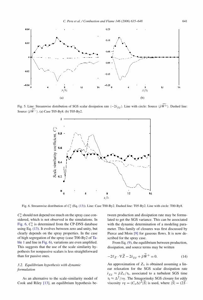
Fig. 5. Line: Streamwise distribution of SGS scalar dissipation rate 〈−2sχZ〉. Line with circle: Source 〈ρ ˜W+〉. Dashed line:

Source 〈ρ ˜W−〉. (a) Case T05-By8. (b) T05-By2.

Fig. 6. Streamwise distribution of Csv (Eq. (13)). Line: Case T00-By2. Dashed line: T05-By2. Line with circle: T00-By8.

Csv should not depend too much on the spray case con-

sidered, which is not observed in the simulations. InFig. 6, Cs

v is determined from the CP-DNS databaseusing Eq. (13). It evolves between zero and unity, butclearly depends on the spray properties. In the caseof high segregation of the spray (case T00-By2 of Ta-ble 1 and line in Fig. 6), variations are even amplified.This suggests that the use of the scale similarity hy-pothesis for nonpassive scalars is less straightforwardthan for passive ones.

3.2. Equilibrium hypothesis with dynamicformulation

As an alternative to the scale-similarity model ofCook and Riley [13], an equilibrium hypothesis be-

tween production and dissipation rate may be formu-lated to get the SGS variance. This can be associatedwith the dynamic determination of a modeling para-meter. This family of closures was first discussed byPierce and Moin [9] for gaseous flows. It is now de-scribed for the spray case.

From Eq. (9), the equilibrium between production,dissipation, and source terms may be written

(14)−2τZ · ∇Z − 2sχZ + ρ ˜W+ = 0.

An approximation of Zv is obtained assuming a lin-ear relaxation for the SGS scalar dissipation ratesχZ ≈ ρZv/τt, associated to a turbulent SGS timeτt ≈ �2/νT. The Smagorinsky SGS closure for eddyviscosity νT = (Cs�)2|S| is used, where |S| = (2S ·

642 C. Pera et al. / Combustion and Flame 146 (2006) 635–648

S)1/2 is the magnitude of the large-scale strain ratetensor S = (1/2)(∇u + ∇T u). Cs is the Smagorinskyconstant which is determined dynamically [36,37].With this eddy dissipation closure, the SGS turbu-lent flux becomes τZ = −ρ(νT/ScT)∇Z and the pro-duction term reads −2τZ · ∇Z = 2ρ(νT/ScT)|∇Z|2,where ScT is a turbulent Schmidt number to be de-termined. Introducing those modeling assumptions inEq. (14), Zv may be written

ρZv = ρ(ZZ − ZZ)

(15)= Cev

(ρ�2|∇Z|2 + ρ ˜W+

C2s |S|

),

where Cev is a modeling parameter to be determined

dynamically. Cev incorporates various SGS effects re-

lated to nonuniform turbulent Schmidt number andother unresolved phenomena. The determination ofCe

v from a dynamic procedure applied to Eq. (15) hasbeen attempted from the CP-DNS without much suc-cess in the prediction of Zv. The best results wereobtained using a dual-step dynamic formulation in-volving two parameters, Ce∗

v and Ce∗∗v .

Without spray evaporation, the SGS variance esti-mated from Eq. (14) reads

(16)ρZv = ρ(ZZ − ZZ) = Ce∗v ρ�2|∇Z|2,

where Ce∗v is a parameter related to SGS frozen-flow

mixing only. Starting from Eq. (16), it is proposed tokeep the frozen flow mixing parameter Ce∗

v when ascalar source exists, but to combine it with a new pa-rameter, leading to the approximation

ρZv = ρ(ZZ − ZZ)

(17)= Ce∗∗v

(Ce∗

v ρ�2|∇Z|2 + ρ ˜W+C2

s |S|)

.

A dynamic procedure is applied successively toEqs. (16) and (17) to estimate the values of Ce∗

vand Ce∗∗

v . The main lines of the dynamic procedureby Germano [36] are now discussed as organized inPierce [38]. Filtering Eq. (16) at the level � brings

(18)ρZZ − ρZZ = Ce∗v ρ�2|∇Z|2.

The equilibrium hypothesis is also assumed valid atthe test filter level with the same value of Ce∗

v ; thus,

ρZZ − ρρZ

ρ

ρZ

ρ= ρZZ − ρ ˇZ ˇZ

(19)= Ce∗v ρ�2∣∣∇ ˇZ∣∣2,

where ˇa = ρa/ρ denotes Favre (mass weighted) fil-tering at the test level. Combining Eqs. (18) and (19)leads to

(20)Lv = Ce∗v Mv,

where Lv is a Leonard type term that is computablefrom the resolved large eddy field,

(21)Lv = ρZZ − ρ ˇZ ˇZ,

and the corresponding modeled term reads

(22)Mv = ρ�2∣∣∇ ˇZ∣∣2 − ρ�2|∇Z|2.

The coefficient Ce∗v may be obtained from Eq. (20)

and various techniques have been discussed to cal-culate SGS model parameters in homogeneous andnonhomogeneous flows [37,39]. Because of the sim-ple flow geometry of the CP-DNS, here it is deducedfrom

(23)Ce∗v = 〈LvMv〉

〈MvMv〉 ,

where the angle brackets indicate averaging over di-rections of flow homogeneity (Eq. (2)). Once Ce∗

vis known, a similar dynamic procedure is applied toEq. (17) to get the Ce∗∗

v parameter.The approximation given by Eq. (17) is com-

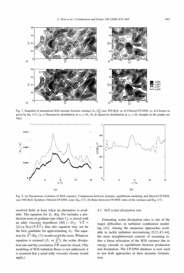
pared with filtered CP-DNS in Fig. 7 for the caseT05-By8. The spatial variations and the topologyof Zv are well captured by this dynamic formu-lation, suggesting that the model reproduces thestructure of the variance field. However, the stream-wise distribution of 〈Zv〉 indicates that the exactlevel of SGS fluctuations is not obtained (Fig. 8a);the same tendency is observed in other cases (notdisplayed). The ratio between the exact variancefrom CP-DNS and Eq. (17) is shown in Fig. 8bfor that streamwise distribution; it evolves between0.5 and 0.8. Therefore, even in this oversimplifiedhomogeneous flow, the determination of the vari-ous modeling parameters is not trivial when a masssource term is acting, and the solving of a balanceequation may be necessary to correctly approxi-mate Zv.

4. A modeled balance equation for SGS mixturefraction variance

Two options exist to get SGS variance from abalance equation. The equation for the variance, Zv(Eq. (9)), or the equation for the square of the sig-nal, Z2 (Eq. (7)), can be solved. The choice of theproper formalism depends on constraints associatedwith the case under study. One major guideline iseasily identified that is related to the LES grid. InLES of combustion systems, the grid cannot be highlyrefined at every location, and local lack of resolu-tion may lead to various problems with scalar fields.For instance, it can be of practical interest to avoidsource terms that are fully driven by gradients of the

C. Pera et al. / Combustion and Flame 146 (2006) 635–648 643

Fig. 7. Snapshot of normalized SGS mixture fraction variance Zv/Z20 case T05-By8. (a, b) Filtered CP-DNS. (c, d) Closure as

given by Eq. (17). (a, c) Streamwise distribution at x3 = 4lt . (b, d) Spanwise distribution at x1 = 4lt (lengths in the graphs are10lt).

(a) (b)

Fig. 8. (a) Streamwise evolution of SGS variance. Comparison between dynamic equilibrium modeling and filtered CP-DNS,case T05-By8. Symbols: Filtered CP-DNS. Line: Eq. (17). (b) Ratio between CP-DNS value of the variance and Eq. (17).

resolved field, at least when an alternative is avail-able. The equation for Zv (Eq. (9)) includes a pro-duction term of gradient type when τZ is closed withan eddy viscosity hypothesis [40] (−2τZ · ∇Z ≈2ρ(νT/ScT)|∇Z|2); thus this equation may not bethe best candidate for approximating Zv. The equa-tion for Z2 (Eq. (7)) would avoid this term. Whateverequation is retained (Zv or Z2), the scalar dissipa-

tion rate and the correlation ZW must be closed. (Themodeling of SGS turbulent fluxes is not addressed; itis assumed that a usual eddy viscosity closure wouldapply.)

4.1. SGS scalar dissipation rate

Estimating scalar dissipation rates is one of themajor difficulties in turbulent combustion model-ing [41]. Among the numerous approaches avail-able to tackle turbulent micromixing [9,21,42–44],the most straightforward consists of assuming ei-ther a linear relaxation of the SGS variance due toenergy cascade or equilibrium between productionand dissipation. The CP-DNS database is now usedto test both approaches in their dynamic formula-tion.

644 C. Pera et al. / Combustion and Flame 146 (2006) 635–648

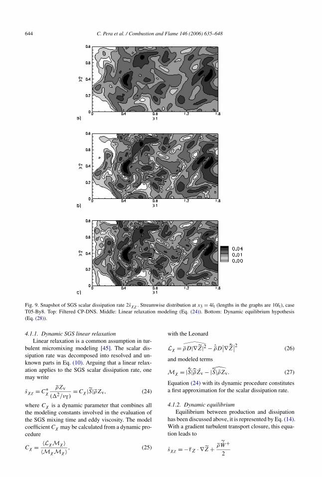
Fig. 9. Snapshot of SGS scalar dissipation rate 2sχZ. Streamwise distribution at x3 = 4lt (lengths in the graphs are 10lt), case

T05-By8. Top: Filtered CP-DNS. Middle: Linear relaxation modeling (Eq. (24)). Bottom: Dynamic equilibrium hypothesis(Eq. (28)).

4.1.1. Dynamic SGS linear relaxationLinear relaxation is a common assumption in tur-

bulent micromixing modeling [45]. The scalar dis-sipation rate was decomposed into resolved and un-known parts in Eq. (10). Arguing that a linear relax-ation applies to the SGS scalar dissipation rate, onemay write

(24)sχZ = C∗χ

ρZv

(�2/νT)= Cχ |S|ρZv,

where Cχ is a dynamic parameter that combines allthe modeling constants involved in the evaluation ofthe SGS mixing time and eddy viscosity. The modelcoefficient Cχ may be calculated from a dynamic pro-cedure

(25)Cχ = 〈LχMχ 〉〈M M 〉 ,

χ χ

with the Leonard

(26)Lχ = ρD|∇Z|2 − ρD∣∣∇ ˇZ∣∣2

and modeled terms

(27)Mχ = ˇ|S |ρZv − |S|ρZv.

Equation (24) with its dynamic procedure constitutesa first approximation for the scalar dissipation rate.

4.1.2. Dynamic equilibriumEquilibrium between production and dissipation

has been discussed above, it is represented by Eq. (14).With a gradient turbulent transport closure, this equa-tion leads to

sχZ = −τZ · ∇Z + ρ ˜W+

2

C. Pera et al. / Combustion and Flame 146 (2006) 635–648 645

(a) (b)

(c) (d)

Fig. 10. Streamwise distribution of SGS scalar dissipation rate 〈sχZ〉. Circle: Filtered CP-DNS. Line: Dynamic linear relaxation

(Eq. (24)). Long dashed line: Dynamic equilibrium (Eq. (28)). (a) Case T00-By8. (b) Case T50-By8. (c) Case T05-By8. (d) CaseT05-By2.

(28)= ρ(νT/ScT)|∇Z|2 + ρ ˜W+2

,

where ρ ˜W− is still neglected according to Fig. 5. Thescalar SGS diffusion coefficient DT = νT/ScT maybe written

(29)DT = CZ�2|S|.The knowledge of this quantity is necessary to solvefor the filtered mixture fraction field and the parame-ter CZ is obtained from the relations

(30)CZ = 〈LM〉〈MM〉

with

(31)L = − ρuZ + ρ ˇu ˇZand

(32)M = ρ�2 ˇ|S|∇ ˇZ − ρ�2|S|∇Z.

The prediction capabilities of linear relaxation andequilibrium assumptions are evaluated in Figs. 9and 10. Keeping the evaporation time the same, butincreasing the drag time of the droplets, leads to aslight decrease of the SGS scalar dissipation rate(Figs. 10a and 10b). For a moderate drag, reducingthe evaporation time is followed by a vigorous in-crease of sχZ that is localized in the early part of theflow. When the scalar dissipation rate is concerned,the quality of the agreement between CP-DNS andthe various models varies a lot depending on the caseunder study, and it is difficult to really push forwardone expression from the results. Both provide the cor-rect topology of the SGS dissipation rate distribution(Fig. 9), and an interesting approximation of its am-plitude is obtained (Fig. 10). The linear relaxationmay, however, be preferred when a balance equationfor Z2 is to be solved, because it avoids the introduc-tion of a sink term that is proportional to the gradient

646 C. Pera et al. / Combustion and Flame 146 (2006) 635–648

(a) (b)

(c) (d)

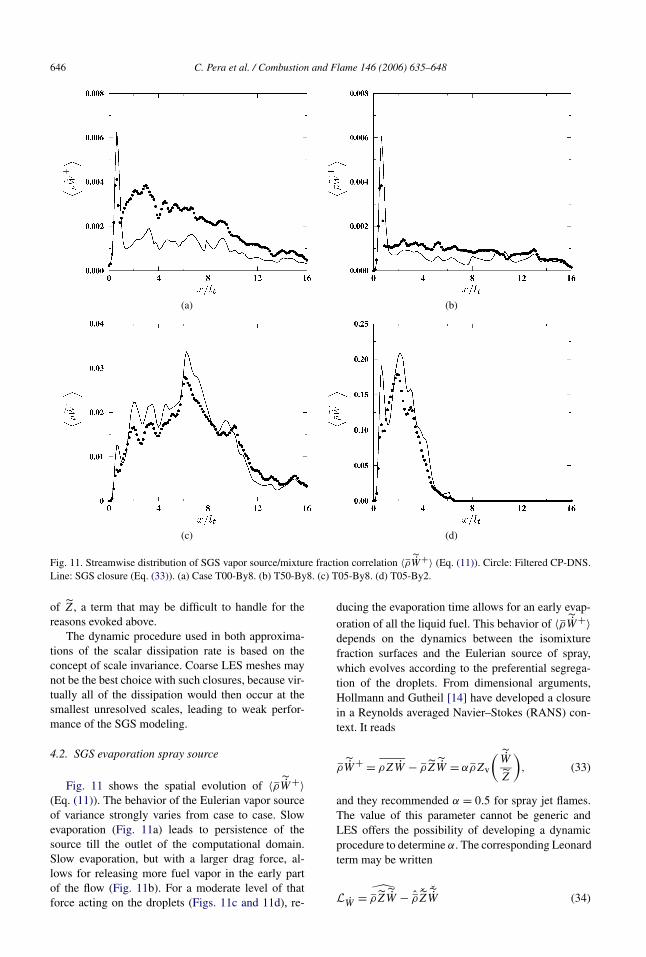
Fig. 11. Streamwise distribution of SGS vapor source/mixture fraction correlation 〈ρ ˜W+〉 (Eq. (11)). Circle: Filtered CP-DNS.Line: SGS closure (Eq. (33)). (a) Case T00-By8. (b) T50-By8. (c) T05-By8. (d) T05-By2.

of Z, a term that may be difficult to handle for thereasons evoked above.

The dynamic procedure used in both approxima-tions of the scalar dissipation rate is based on theconcept of scale invariance. Coarse LES meshes maynot be the best choice with such closures, because vir-tually all of the dissipation would then occur at thesmallest unresolved scales, leading to weak perfor-mance of the SGS modeling.

4.2. SGS evaporation spray source

Fig. 11 shows the spatial evolution of 〈ρ ˜W+〉(Eq. (11)). The behavior of the Eulerian vapor sourceof variance strongly varies from case to case. Slowevaporation (Fig. 11a) leads to persistence of thesource till the outlet of the computational domain.Slow evaporation, but with a larger drag force, al-lows for releasing more fuel vapor in the early partof the flow (Fig. 11b). For a moderate level of thatforce acting on the droplets (Figs. 11c and 11d), re-

ducing the evaporation time allows for an early evap-

oration of all the liquid fuel. This behavior of 〈ρ ˜W+〉depends on the dynamics between the isomixturefraction surfaces and the Eulerian source of spray,which evolves according to the preferential segrega-tion of the droplets. From dimensional arguments,Hollmann and Gutheil [14] have developed a closurein a Reynolds averaged Navier–Stokes (RANS) con-text. It reads

(33)ρ ˜W+ = ρZW − ρZ ˜W = αρZv

( ˜WZ

),

and they recommended α = 0.5 for spray jet flames.The value of this parameter cannot be generic andLES offers the possibility of developing a dynamicprocedure to determine α. The corresponding Leonardterm may be written

(34)LW =

ρZ ˜W − ρ ˇZ ˇW

C. Pera et al. / Combustion and Flame 146 (2006) 635–648 647

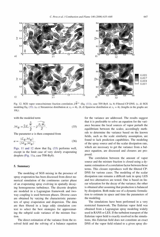
Fig. 12. SGS vapor source/mixture fraction correlation ρ ˜W+ (Eq. (11)), case T05-By8. (a, b) Filtered CP-DNS. (c, d) SGSmodeling Eq. (33). (a, c) Streamwise distribution at x3 = 4lt . (b, d) Spanwise distribution at x1 = 4lt (lengths in the graphs are10lt).

with the modeled term

(35)MW = ρZv

ˇW

ˇZ−

ρZv

˜Wv

Z.

The parameter α is then computed from

(36)α = 〈LWMW 〉〈MWMW 〉 .

Figs. 11 and 12 show that Eq. (33) performs well,except in the limit case of very slowly evaporatingdroplets (Fig. 11a, case T00-By8).

5. Summary

The modeling of SGS mixing in the presence ofspray evaporation has been discussed from direct nu-merical simulation of the continuous carrier phaseof an evaporating spray evolving in spatially decay-ing homogeneous turbulence. The discrete dropletsare modeled in a Lagrangian framework and two-way coupling is used between phases. Diverse casesare obtained by varying the characteristic parame-ters of spray evaporation and dispersion. The dataare then filtered in a large eddy simulation con-text to select the best strategies for approximat-ing the subgrid scale variance of the mixture frac-tion.

The direct estimation of the variance from the re-solved field and the solving of a balance equation

for the variance are addressed. The results suggestthat it is preferable to solve an equation for the vari-ance because the local sources of vapor perturb theequilibrium between the scales; accordingly meth-ods to determine the variance based on the knownfields, such as the scale similarity assumption, arefound to lack prediction capabilities. The modelingof the spray source and of the scalar dissipation rate,which are necessary to get the variance from a bal-ance equation, are discussed and closures are pro-posed.

The correlation between the amount of vaporsource and the mixture fraction is closed using a dy-namic estimation of a correlation factor between thoseterms. This closure reproduces well the filtered CP-DNS for various cases. The modeling of the scalardissipation rate remains a difficult task in spray LESand two alternatives are tested. One is based on lin-ear relaxation for the decay of the variance; the otheris obtained after assuming that production is balancedby dissipation. Both make use of a dynamic formula-tion to estimate in space and time the parameters ofthe modeling.

The simulations have been performed in a veryrestricted framework. The Eulerian vapor field wasobtained from a Lagrangian spray modeling widelyused in RANS or LES. If the turbulent transport of theEulerian vapor field is exactly resolved in the simula-tions, this Eulerian field does not constitute an exactDNS of the vapor field related to a given spray dis-

648 C. Pera et al. / Combustion and Flame 146 (2006) 635–648

tribution. This would require a full description of theliquid phase and of its interface with the gaseous one.Consequently, some effects directly related to the sub-tle dispersion of droplets over the Eulerian grid cannotbe addressed carefully and it is difficult to conclude,at this stage, on their exact effects on the SGS mixturefraction variance.

Acknowledgments

The authors acknowledge the support from IDRIS-CNRS (Institut de Developpement et de Ressourcesen Informatique Scientifique) where computationswere performed. Support was also provided by theproject “Modelling of UnSteady Combustion in Low-Emission Systems” (MUSCLES) under EC ContractG4RD-CT-2001-00644. The authors are grateful toDr. A.P. Wandel and Professor E. Mastorakos forpointing out typos in the CP-DNS spray balance equa-tions of previously published papers.

References

[1] K. Squires, J. Eaton, J. Fluid Mech. 226 (1991) 1–35.[2] M. Boivin, O. Simonin, K. Squires, J. Fluid Mech. 375

(1998) 235–263.[3] G. Faeth, Prog. Energy Combust. Sci. 9 (1983) 1–76.[4] F. Mashayek, Int. J. Heat Mass Transfer 41 (17) (1998)

2601–2617.[5] F. Lacas, X. Calimez, Proc. Combust. Inst. 28 (2000)

943–951.[6] F. Demoulin, R. Borghi, Combust. Sci. Technol. 158

(2000) 249–271.[7] Y. Wang, C.J. Rutland, Proc. Combust. Inst. 30 (2005)

893–900.[8] P. Domingo, L. Vervisch, J. Réveillon, Combust.

Flame 140 (3) (2005) 172–195.[9] C. Pierce, P. Moin, Phys. Fluids 10 (12) (1998) 3041–

3044.[10] N. Peters, Turbulent Combustion, Cambridge Univ.

Press, Cambridge, UK, 2000.[11] T. Poinsot, D. Veynante, Theoretical and Numerical

Combustion, Edwards, Philadelphia, 2001.[12] P.A. McMurtry, S. Menon, A.E. Kerstein, Energy Fu-

els 7 (1993) 817–826.[13] A. Cook, J. Riley, Phys. Fluids 6 (8) (1994) 2868–2870.[14] C. Hollmann, E. Gutheil, Proc. Combust. Inst. 26

(1996) 1731–1738.[15] A. Cook, J.J. Riley, G. Kosàly, Combust. Flame 109

(1997) 332–341.[16] J. Jimiénez, A. Liñàn, M. Rogers, F. Higuera, J. Fluid

Mech. 349 (1997) 149–171.[17] P. DesJardin, S. Frankel, Phys. Fluids 10 (9) (1998)

2298–2314.

[18] J. Réveillon, L. Vervisch, Combust. Flame 121 (2000)75–90.

[19] N. Smith, C. Cha, H. Pitsch, J. Oefelein, in: CTR Proc.,2000, pp. 207–218.

[20] R. Miller, J. Bellan, Phys. Fluids 12 (3) (2000) 650–671.

[21] C. Jiménez, F. Ducros, B. Cueno, B. Cédat, Phys. Flu-ids 13 (6) (2001) 1748–1754.

[22] H.H. Chiu, H.Y. Kim, E.J. Croke, Proc. Combust.Inst. 19 (1982).

[23] J. Réveillon, C. Pera, M. Massot, R. Knikker, J. Turbu-lence 1 (2004) 1–27.

[24] L. Guichard, J. Réveillon, R. Hauguel, Flow Turbu-lence Combust. 73 (2) (2005) 95–116.

[25] C. Canuto, M.Y. Hussaini, A. Quarteroni, T.A. Zang,Spectral Methods in Fluid Dynamics, Springer-Verlag,Berlin/New York, 1988.

[26] A.A. Wray, Minimal Storage Time-AdvancementSchemes for Spectral Methods, Technical report, Cen-ter for Turbulence Research, Stanford University, 1990.

[27] J. Réveillon, L. Vervisch, J. Fluid Mech. 537 (2005)317–347.

[28] S.K. Lele, J. Comput. Phys. 103 (1992) 16–42.[29] T. Poinsot, S.K. Lele, J. Comput. Phys. 1 (101) (1992)

104–129.[30] G.M. Faeth, Prog. Energy Combust. Sci. 13 (1987)

293–345.[31] R. Borghi, in: Combustion and Turbulence in Two-

Phase Flows, Lecture Series 1996-02, Von Karman In-stitute for Fluid Dynamics, 1996.

[32] J.H. Ferziger, in: Large Eddy Simulation of ComplexEngineering and Geophysical Flows, Cambridge Univ.Press, Cambridge, UK, 1993, pp. 37–54.

[33] C. Meneveau, J. Katz, Annu. Rev. Fluid Mech. 32(2000) 1–32.

[34] J. Réveillon, L. Vervisch, Phys. Fluids 8 (1996) 2248–2250.

[35] A. Cook, Phys. Fluids 9 (5) (1997) 1485–1487.[36] M. Germano, J. Fluid Mech. 238 (1992) 325–336.[37] C. Meneveau, T.S. Lund, W. Cabot, J. Fluid Mech. 319

(1996) 353–386.[38] C. Pierce, Progress Variable Approach for Large Eddy

Simulation of Turbulent Combustion, Ph.D. thesis,Stanford University, 2001.

[39] S. Ghosal, T.S. Lund, P. Moin, K. Akselvoll, J. FluidMech. 286 (1995) 229.

[40] J. Smagorinsky, Mon. Weather Rev. 61 (1963) 99–164.[41] D. Veynante, L. Vervisch, Prog. Energy Combust.

Sci. 28 (2002) 193–266.[42] S. Girimaji, Y. Zhou, Phys. Fluids 8 (5) (1995) 1224–

1236.[43] A. Cook, W. Bushe, Phys. Fluids 11 (3) (1999) 746–

748.[44] F. di Mare, W.P. Jones, K.R. Menzies, Combust.

Flame 137 (3) (2004) 278–294.[45] R.O. Fox, Computational Models for Turbulent React-

ing Flows, Cambridge Univ. Press, Cambridge, UK,2003.