Estimation of the Conditional Variance-Covariance Matrix of Returns using the Intraday Range

Richard D.F. Harris University of Exeter

Fatih Yilmaz

Bank of America

Paper Number: 07/11

October 2007

Abstract There has recently been renewed interest in the intraday range (defined as the difference between the intraday high and low prices) as a measure of local volatility. Recent studies have shown that estimates of volatility based on the range are significantly more efficient than estimates based on the daily close-to-close return, are relatively robust to market microstructure noise, and are approximately log-normally distributed. However, little attention has so far been paid to forecasting volatility using the daily range. This is partly because there exists no multivariate analogue of the range and so its use is limited to the univariate case. In this paper, we propose a simple estimator of the multivariate conditional variance-covariance matrix of returns that combines both the return-based and range-based measures of volatility. The new estimator offers a significant improvement over the equivalent return-based estimator, both statistically and economically. Keywords: Conditional variance-covariance matrix of returns; Exponentially weighted moving average (EWMA); Intraday range. Address for correspondence: Professor Richard D. F. Harris, Xfi Centre for Finance and Investment, University of Exeter, Exeter EX4 4PU, UK. Tel: +44 (0) 1392 263215, Fax: +44 (0) 1392 263242 Email: R.D.F.Harris@exeter.ac.uk.

2

1. Introduction

There has been much recent interest in estimating the integrated (or local) volatility of

short-horizon financial asset returns. Although estimators based on the squares and

cross-products of daily returns are, in the absence of a drift, unbiased, they are very

inaccurate because the noise that they contain dominates any signal about unobserved

volatility. More recently, the development of the realized volatility literature has

provided a rigorous framework for estimating integrated volatility on the basis of

intraday returns. Under very general assumptions, the sum of squared intraday returns

converges to the unobserved integrated volatility as the intraday interval goes to zero

(see, for example, Andersen et al, 2001; Barndorff-Nielson and Shephard, 2002). In

practice, however, the implementation of the realized volatility approach is limited by

microstructure effects that induce an upward bias in estimated volatility that increases

as the measurement interval becomes smaller (see, for example, Bandi and Russell,

2003).

More recently, the intraday range (defined as the difference between intraday high and

low prices) has experienced renewed interest as an estimator of integrated volatility.

Building on the earlier results of Parkinson (1980), Garman and Class (1980) and

others, Alizadeh et al., (2002) show that, in addition to being significantly more

efficient than the squared daily return, the daily range is much less affected by market

microstructure noise than realized volatility, and that the log range is approximately

normally distributed, thus greatly facilitating maximum likelihood estimation of

stochastic volatility models. A significant practical advantage of the intraday range is

that in contrast with intraday data (which is required for computation of realized

volatility), the range is readily available for almost all financial assets over extended

periods of time.1 However, a significant shortcoming of the range-based estimator is

that no multivariate analogue of the intraday range exists, and so while it is

straightforward to estimate the variances of individual assets, it is not generally

possible to estimate their covariance.2 This is problematic because the application of

1 For example, Datastream records the intraday range for most securities, including equities, currencies and commodities, going back to about 1985. 2 Christensen and Podolskij (2005) and Martens and van Dijk (2007) combine the range-based and realized volatility estimators to yield the ‘realized range’, which is

3

finance theory tends to rely as much on the covariance between assets as it does on

their individual variances. For example, mean-variance optimisation, asset pricing,

hedging, portfolio value-at-risk and the pricing of options that depend on more than

one asset all depend on the variance-covariance matrix of returns. As a solution to this

problem, Brandt and Diebold (2006) note that the covariance of two assets can be

imputed from the variance of a portfolio of the two assets, and that, in certain

circumstances, the daily range for the latter is readily available. In currency markets,

for example, triangular arbitrage implies that cross-rates are equal to the difference

between individual exchange rates, and so these can be used to impute their

covariance. However, such triangular arbitrage relationships are unique to the foreign

exchange market. In the bond market, one could argue (as Brandt and Diebold (2006)

do) that an analogous arbitrage relationship exists in the form of the expectations

hypothesis, and that this could be used to impute the covariance between bonds of

different maturities. However, there is now overwhelming evidence that the

expectations hypothesis does not hold, and so this is unlikely to provide a viable

solution.3 In the equity market, no such triangular arbitrage relationship exists, even in

theory. Thus, in spite of its obvious merits, the range-based estimator is thus far

limited to estimation of individual variances.

A number of studies have considered the use of the daily range in forecasting the

variance of returns. Brandt and Jones (2006) formulate a model that is analogous to

Nelson’s (1991) EGARCH model, but uses the square root of the intraday range in

place of the absolute return. Similarly, Chou (2005) develops a conditional

autoregressive range (CARR) estimator that is analogous to the conditional duration

model of Engle and Russell (1998) (see also and Chou and Wang, 2005). Both studies

find that the range-based GARCH estimators offer a significant improvement over

their return-based counterparts. However, as with estimation of integrated volatility,

the use of the range in the estimation of conditional volatility has necessarily been

limited to the univariate case.

the sum of the range-based estimator of volatility over intraday intervals. The realized range can be used to estimate covariances. See also Brunetti and Lildholt (2002). However, all of these approaches require intraday data. Moreover, since they measure the range over intraday intervals, they can only be applied to highly traded securities. 3 For evidence on the rejection of the expectations hypothesis, see, for example, Bekaert, Hodrick and Marshall (1997).

4

This paper develops a multivariate conditional variance-covariance estimator that

combines the range-based and return-based approaches. In particular, the new

estimator uses a range-based exponentially weighted moving average (EWMA)

specification (that is similar in form to the CARR estimator of Chou, 2005) to

estimate the variances of individual assets, and a more standard return-based EWMA

specification to estimate the time-varying conditional correlation between assets. The

conditional covariance between individual assets is then estimated as the product of

the (range-based) conditional standard deviations of the individual assets and the

(return-based) conditional correlation coefficient between them. Like the standard

return-based EWMA model, the range-based EWMA model generates estimates of the

conditional variance-covariance matrix that are positive semi-definite under very

general assumptions about the data generating process for returns, and is easily

implemented in a spreadsheet package such as Excel.

To investigate the performance of the multivariate range-based EWMA estimator, we

generate estimates of the conditional variance-covariance matrix of returns for the

USD/GBP, USD/EUR and USD/JPY exchange rates over the period 01/01/2003 to

31/12/2006. As a benchmark, we use the realized variance-covariance matrix based on

30-minute returns. We compare the performance of the range-based EWMA

estimators with the corresponding return-based EWMA estimator using a number of

statistical forecast criteria, and by evaluating their use in estimating the minimum

variance hedge ratio for three-cross hedged currency portfolios. Using the RiskMetrics

decay factor of 0.94, the range-based estimator offers a significant improvement over

the return-based estimator in terms of forecast accuracy, bias and efficiency, and

yields significantly superior hedging performance. A further feature of the range-

based estimator, is that its statistical and economic performance is much less sensitive

to the choice of decay factor, enhancing its reliability in practice where the ‘true’

decay factor for a given sample of data is unknown.4

4 The decay factor of the EWMA model can of course be estimated, for example by specifying a conditional distribution and using maximum likelihood. However, the efficacy of such an approach is predicated on the assumption that the decay factor is stable over time, which is unlikely to be the case in practice.

5

The outline of the remainder of the paper is as follows. The following section

provides the analytical framework for volatility, and describes the return-based and

range-based EWMA conditional volatility models. Section 3 describes the data used

for the analysis of the EWMA models and the criteria against which the models are

evaluated. Section 4 presents the empirical results and undertakes a sensitivity

analysis. Section 5 concludes and offers some suggestions for future research.

2. Theoretical background

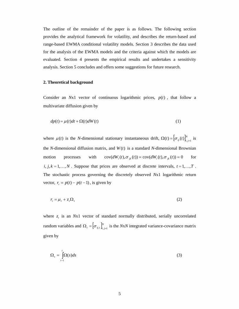
Consider an Nx1 vector of continuous logarithmic prices, )(tp , that follow a

multivariate diffusion given by

)()()()( tdWtdtttdp Ω+= µ (1)

where )(tµ is the N-dimensional stationary instantaneous drift, [ ]Njiij tt

1,)()(

==Ω σ is

the N-dimensional diffusion matrix, and )(tW is a standard N-dimensional Brownian

motion processes with 0))(),(cov())(),(cov( == ttdWttdW jkijki σσ for

Nkji ,,1,, K= . Suppose that prices are observed at discrete intervals, Tt ,,1K= .

The stochastic process governing the discretely observed Nx1 logarithmic return

vector, )1()( −−= tptprt , is given by

tttt zr Ω+= µ (2)

where tz is an Nx1 vector of standard normally distributed, serially uncorrelated

random variables and [ ]Njitijt 1,, =

=Ω σ is the NxN integrated variance-covariance matrix

given by

∫−

Ω=Ωt

tt dss

1

)( (3)

6

(See, for example, Andersen, Bollerslev and Diebold, 2003). The integrated variance-

covariance matrix given by (3) is unobservable. However, an estimate of tΩ is given

by

∑=

+−+−=Ωq

ssqtsqt

qRVt rr

/1

1

'11

)( (4)

Under very general conditions, )(qRVtΩ converges uniformly in probability to tΩ as

0→q (see Andersen, Bollerslev and Diebold, 2003). With the growing availability of

intra-day data on security prices, increasingly precise estimates of integrated volatility

can be obtained using finer measures of )(qRVtΩ . However, the accuracy of such an

approach is limited by the fact that market microstructure effects distort the

measurement of returns at high frequencies in such a way that measured returns no

longer satisfy the regularity conditions that are required for the consistency properties

of realised volatility. In particular, microstructure effects induce an upward bias in

estimated volatility that increases as the measurement interval becomes smaller (see,

for example, Ait-Sahalia, Mykland and Zhang, 2005; Zhang, Mykland and Ait-

Sahalia; 2003; Bandi and Russell, 2003). Consequently, some researchers have

proposed estimation of integrated volatility by sampling returns at non-negligible time

intervals. Generally, the empirical evidence suggests that intervals between five and

30 minutes are effective for the estimation of integrated volatility (Andersen,

Bollerslev, Diebold, and Labys, 2001, 2003; Barndorff-Nielsen and Shephard, 2002,

2004b).

An alternative estimator of the diagonal elements of the integrated variance-

covariance matrix is based on the intraday range, which is defined as the difference

between the log intraday high price and the log intraday low price. Specifically, the

range-based estimator of the integrated variance of tir , is given by

2,,, )(

2ln41 L

tiHti

Rangetii pp −=σ , Ni ,,1K= (5)

7

where Htip , and L

tip , are the intraday maximum and minimum of tip , , respectively.

Parkinson (1980) shows that if )(tpi follows the Brownian Motion process given by

(1), the MSE of Rangetii,σ (with respect to the true integrated variance, tii,σ ) is about five

times smaller than the MSE of )1(,

RVtiiσ . In practice, since prices are only observed at

discrete intervals, the sample range under-estimates the true range of the continuous

price. However, in liquid markets where there may be 1000 or more trades each day,

this bias becomes negligible. Alizadeh, Brandt and Diebold (2002) show that the

range-based estimator given by (5) is relatively robust to market microstructure noise,

and, unlike the squared return, is approximately log normally distributed, which

greatly improves the estimation efficiency of stochastic volatility models using

maximum likelihood. A significant shortcoming of the range-based estimator,

however, is that there is no multivariate analogue of the intraday range, and so it is not

possible to directly estimate the off-diagonal elements of the variance-covariance

matrix. Brandt and Diebold (2006) note that if we have the daily range of a portfolio

of the two assets, we can impute the range-based estimate of the covariance between

from the range-based estimate of the variance of the portfolio. However, while in the

foreign exchange market, such two-asset portfolios are observed in the form of cross-

exchange rates that are determined through triangular arbitrage, in other markets such

triangular arbitrage relationships either do not exist in theory (such as in the stock

market), or exist in theory but not in practice (such as the expectations hypothesis in

the bond market).

Applications in finance typically require an estimate of the conditional variance-

covariance matrix of returns, which is given by

[ ]1|ˆ−ΛΩ=Ω ttt E (6)

where [ ].E is the mathematical expectation operator and tΛ is the time-t information

set. A number of approaches to estimating the conditional variance-covariance matrix

have been proposed, including rolling window estimation of the sample variance-

covariance matrix, exponentially weighted moving average (EWMA) models,

multivariate GARCH models, multivariate stochastic volatility models and dynamic

8

models of the realized variance-covariance matrix. 5 A number of authors have

employed the range-based estimator for forecasting the diagonal elements of the

variance-covariance matrix. For example, Brandt and Jones (2006) formulate a model

that is analogous to the EGARCH model of Nelson’s (1991), but uses the square root

of the intraday range in place of the absolute return. Similarly, Chou (2005) develops

a conditional autoregressive range (CARR) estimator that is analogous to the

conditional duration model of Engle and Russell (1998), and is essentially a GARCH

model specified in terms of the range (see also and Chou and Wang, 2005). Both

studies find that the range-based GARCH estimators offer an improvement over their

return-based counterparts. However, since no multivariate counterpart of the intraday

range exists, the use of the range in forecasting volatility is necessarily limited to the

univariate case.

Here we propose a simple estimator of the variance-covariance matrix of returns that

combines the range-based and return-based approaches, and which offers significant

advantages over the purely return-based approach. The estimator is based on the

multivariate EWMA model of the conditional variance-covariance matrix, which is

given by

)1(

1,0)1(

1,0)1(

, )1(ˆˆ RVtij

RVtij

RVtij −− −+= σλσλσ , Nji ,,1, K= (7)

where 0λ is the single decay factor. The mean return is assumed to be zero, which is a

common assumption practice when dealing with short horizon returns (see, for

example, Figlewski, 1997; Hull and White, 1998). The multivariate EWMA model is

a special case of the diagonal vech multivariate GARCH model of Engle and Kroner

(1995), and corresponds to an integrated diagonal vech model with no constant vector.

The multivariate EWMA model, popularised by its use in the RiskMetrics VaR

software of JP Morgan (see JP Morgan, 1994), is perhaps the most widely used

conditional volatility model among practitioners, who often eschew more

sophisticated models in favour of their simpler counterparts. The popularity of the

5 For a recent review of multivariate GARCH models, see Bauwens et al. (2006). For a review of multivariate stochastic volatility models, see Harvey, Ruiz and Shephard (1994).

9

EWMA model is due partly to the simplicity of its implementation, and partly

because, in spite of its simplicity, it typically outperforms more sophisticated

conditional volatility models (see, for example, Boudoukh, Richardson and Whitelaw,

1997; Alexander and Leigh, 1997; Brooks and Chong, 2001). In contrast with the

more general diagonal vech model that nests it, imposing the restriction that the decay

factor is identical for all conditional variances and covariance ensures that the

resulting conditional variance-covariance matrix, tΩ , is positive semi-definite. The

decay factor, 0λ , is typically set to 0.94, estimated by JP Morgan as the average value

of the decay factor that minimises the mean square error of daily out-of-sample

conditional volatility forecasts for a wide range of assets. The success of the

multivariate EWMA model stems from the fact that while the true data generating

process for conditional volatility is not actually integrated, it is close to being

integrated and so the cost of the restrictions imposed by the EWMA model is low

relative to the benefits that arise from its parsimonious specification.

The range-based estimator of the conditional variance-covariance matrix that we

propose is given by

⎪⎩

⎪⎨⎧

≠=−+

= −−

jiji

Rangetjj

Rangetii

RVtij

Rangetii

RangetiiRange

tij for )ˆˆ(ˆfor )1(ˆ

ˆ 5.0,,

)1(,

1,11,1, σσρ

σλσλσ , Nji ,,1, K= (8)

where

5.0)1(

,)1(

,,)1(

,)1(

, )ˆˆ(ˆˆ −= RVtjj

RVtiitij

RVtij

RVtij σσσρ Nji ,,1, K= (9)

)1(

1,2)1(

1,2)1(

, )1(ˆˆ RVtij

RVtij

RVtij −− −+= σλσλσ , Nji ,,1, K= (10)

The conditional variance equation is a univariate EWMA model for the range-based

variance, with a single decay factor, 1λ , and can be thought of as a special case of the

CARR model of Chou (2005). As with the returns-based EWMA model, the

restrictions imposed by the range-based model are almost certainly counterfactual.

However, the extent to which this outweighs any potential gain from the parsimony of

10

the model is an empirical matter, which we explore in the following section. The

conditional covariance is specified as the product of the range-based conditional

standard deviations and the returns-based conditional correlation coefficient. The

formulation of the covariance equation in this way is motivated by the fact that while )1(

,RV

tijσ is an inherently noisy estimate of tij ,σ (and hence )1(,ˆ RVtijσ will be an inherently

noisy measure of the true conditional covariance, tij ,σ ), a proportion of this noise

cancels in the estimation of the conditional correlation coefficient because the

elements of the variance-covariance matrix share a common trend (see, for example,

Andersen et al., 2005). Our expectation, therefore, is that the range-based EWMA

model should provide more accurate forecasts of the integrated variance-covariance

matrix than the return-based model. Note also that since the range-based conditional

covariance is simply the product of the return-based EWMA correlation coefficient,

with a single decay factor, 2λ , and the range-based standard deviations, the range-

based variance-covariance matrix will be positive semi-definite by construction. The

model described here can also be thought of as a special case of the Dynamic

Conditional Correlation model of Engle and Shephard (2001) and Engle (2002), with

range-based EWMA estimation of the conditional variances and return-based EWMA

estimation of the dynamic correlation.

3. Data and methodology

We use the return-based EWMA model and the range-based EWMA model to

estimate the conditional variance-covariance matrix of the daily log returns for the

USD/GBP, USD/EUR and USD/JPY exchange rates. We implement both models

using the commonly used RiskMetrics decay factor of 0.94, but also explore the

sensitivity of the performance of each model with respect to the decay factor. We

evaluate the conditional volatility estimates using both statistical and economic

measures. In this section, we describe the data that we use in the empirical tests and

the evaluation criteria.

11

3.1 Data

We estimate the conditional variance-covariance matrix of daily log returns for the

USD/GBP, USD/EUR and USD/JPY exchange rates. As a benchmark, we use the

estimated realized variance-covariance matrix based on 30-minute returns. The use of

30-minute returns should be of a sufficiently high frequency to provide an accurate

estimate of the true, integrated variance-covariance matrix, but of a sufficiently low

frequency to avoid the impact of microstructure effects. Intraday data for the period

02 January 2001 to 29 December 2006 were provided by Bank of America. The

market operates around the clock, and so there are a total of 48 30-minute

observations each day, or 75,072 observations in total for each series. The dataset

reports the 30-minute exchange rate and the intraday high and low exchange rates for

each currency. The data contained three outliers that were clearly the result of data

entry errors, and so the values for these observations were linearly interpolated from

their adjacent values.

The full sample is divided into an initialisation period, from 02 January 2001 to 02

December 2002 (500 observations) and a forecast period from 03 December 2002 to

29 December 2006 (1,064 observations). The initialisation period is used to remove

any dependency of the EWMA models on the initial variance or covariance, which is

set to an estimate of the conditional variance or covariance over the initialisation

period. Realized variances and covariances were computed using (4), and range-based

variances computed using (5). The half-hour exchange rates were used to calculate

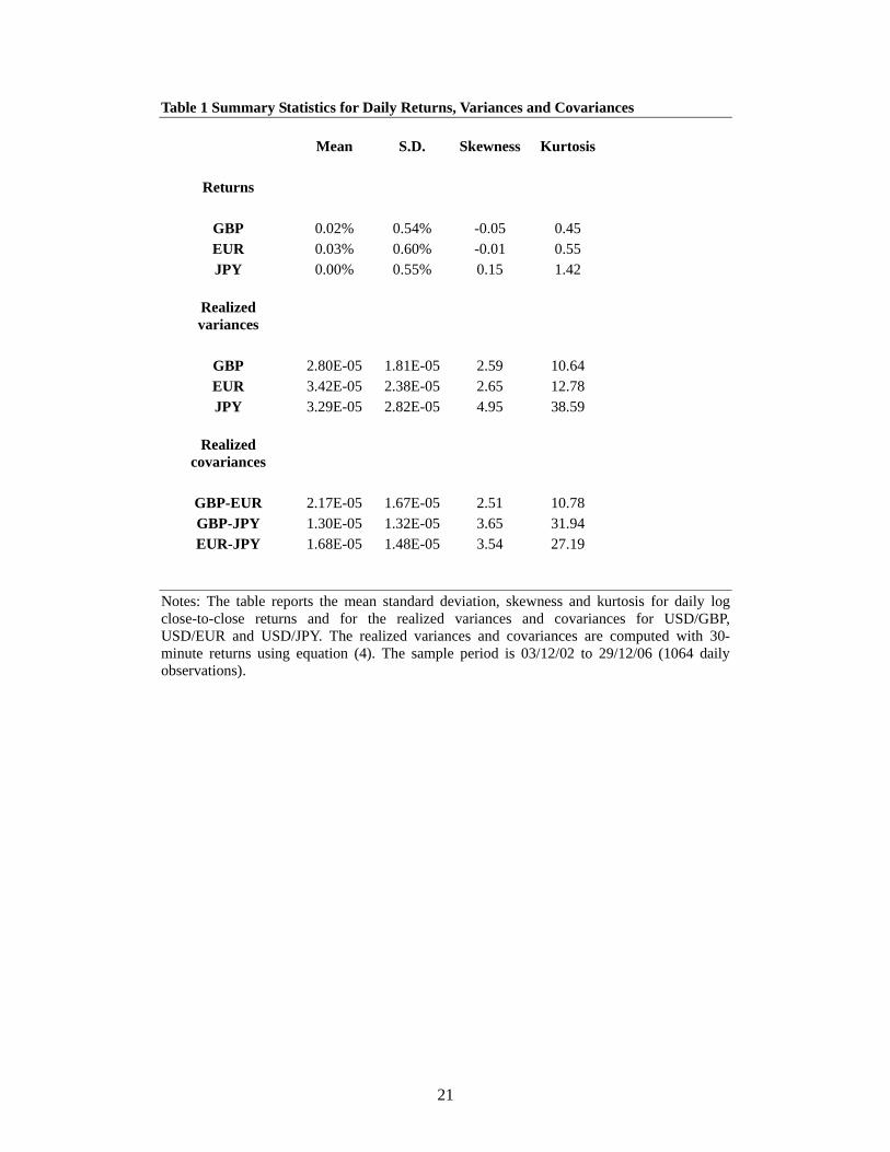
daily log returns, using the 12.00am price. Table 1 reports summary statistics for the

daily returns and the realized and variances and covariances over the forecast period.

[Table 1]

3.2 Forecast evaluation

In order to evaluate the forecasting performance of the return-based and range-based

conditional volatility models, two approaches are used. The first considers the

statistical performance of the volatility forecasts, using realized volatility as the

12

benchmark. For each of the conditional volatility models, ),)1(

,, ˆ,ˆˆ Rangetij

RVtijtij σσσ = , we

employ the following measures:

(1) Root mean square error (RMSE)

∑=

−=T

ttij

RVtijT

RMSE1

2,

)48(, )ˆ(1 σσ (11)

(2) Mean absolute error (MAE)

∑=

−=T

ttij

RVtijT

MAE1

,)48(

, ˆ1 σσ (12)

(3) Mincer-Zarnowitz regression

tijtijijijRV

tij ,,)48(

, ˆ εσβασ ++= (13)

(4) Encompassing regression

tijRange

tijijRV

tijijijRV

tij ,,)1(

,)48(

, ˆˆ εσγσβασ +++= (14)

The RMSE and MAE measure the accuracy of the forecasts from each model. The

Mincer-Zarnowitz regression measures the bias and efficiency of the forecasts from

each model. In particular, if the model is unbiased, we should not be able to reject the

null hypothesis tijijijH ,1 )1(: σβα −= , where tij ,σ is the unconditional variance or

covariance. If the model is (weakly) efficient then we should not be able to reject the

null hypothesis 1,0:2 == ijijH βα . We test both of these hypotheses for each model,

for each element of the variance-covariance matrix, for each pair of currencies. The

R-squared coefficient from the Mincer-Zarnowitz regression reveals the explanatory

power of the model’s forecasts, independently of any bias or inefficiency. Finally, the

encompassing regression tests whether the forecasts of one model contains any

13

incremental information over the forecasts of the other model. In particular, we can

separately test the null hypotheses 0:3 =ijH β and 0:4 =ijH γ .

The second way in which we evaluate the forecasting performance of the different

conditional volatility models is to use the estimated conditional variance-covariance

matrix to construct a forecast of the daily minimum-variance hedge ratio between

each pair of currencies, and then evaluate the performance of the resulting hedged

portfolios. In particular, on each day t, for each of the three pairs of currencies, we

construct the conditional minimum-variance hedge ratio given by

tjj

tijtijh

,

,, ˆ

ˆˆσσ

= (15)

We then construct a hedge portfolio whose log return is given by

tjtijtitp rhrr ,,,,ˆ−= (16)

We calculate the percentage reduction of the hedged portfolio variance with respect to

the variance of the unhedged currency

)var()var()var(

,

.,

ti

titp

rrr −

(17)

4. Results

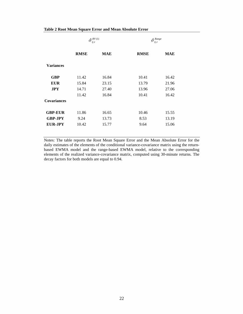
Table 2 reports the RMSE and MAE for the return-based EWMA model and the

range-based EWMA model over the forecast period, using the realized variance-

covariance matrix as the benchmark. The single decay factor for the return-based

EWMA model, 0λ , and the two decay factors for the range-based EWMA model, 1λ

and 2λ , are all set to the RiskMetrics value of 0.94. In all cases, the range-based

EWMA model outperforms the return-based EWMA model in terms of forecast

accuracy. In some cases, the differences are substantial. For example, for the

14

conditional variance of USD/EUR, the RMSE of the range-based model is about 13

percent lower than that of the return-based model. Generally, the difference in RMSE

is greater than the difference in MAE, suggesting that the range-based model is less

sensitive to outlying errors in the conditional variance-covariance matrix. Also, the

improved performance of the range-based model applies equally to both the variances

of the three exchange rates return series and the covariances between them. For the

conditional variances, these results are comparable with those of Chou (2005) and

Brandt and Jones (2006).

[Table 2]

The estimation results of the Mincer-Zarnowitz regression given by (13) are reported

in Table 3, together with the p-values for the tests of the hypotheses H1 (unbiasedness)

and H2 (efficiency). For all elements of the conditional variance-covariance matrix

except the variance of USD/JPY, the return-based model is unbiased. However, the

unbiasedness hypothesis H1 can be rejected for the range-based model at the five

percent significance level in three of the six cases. This is almost certainly because the

return-based EWMA model is unbiased by construction since it is a weighted sum of

squared (or the cross-product of) returns, the expectation of which is equal to the

unconditional variance (or covariance).6 In contrast, the intra-day range is a biased

estimator of the integrated variance when prices are discrete. Nevertheless, from Table

1 it is evident that the higher degree of bias of the range-based model does not

translate into lower accuracy. In all cases, the estimated slope coefficient is less than

unity, and for all cases, we can reject the efficiency hypothesis H2, implying that the

forecasts from both models are weakly inefficient, with high forecasts tending to be

too high, and low forecasts too low. In particular, they are too dispersed. However, the

range-based model is clearly much more efficient than the return-based model, with

an estimated slope coefficient that is closer to unity in all cases. The range-based

model has greater explanatory power in five of the six cases, and in some cases, the

difference is substantial.

[Table 3] 6 In this respect, the apparent bias for the variance of USD/JPY is likely to be suprious.

15

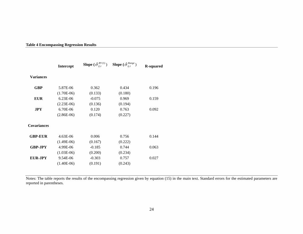
Table 4 reports the estimation results of the encompassing regression given by (14). In

all but one case, we cannot reject the hypothesis H3 that the range-based model

encompasses the return-based model, and in no case can we reject the hypothesis H4

that the return-based model encompasses the range-based model. In particular, except

for the conditional variance of USD/GBP, the estimated slope coefficient for the

return-based model is not significantly different from zero. In contrast, the estimated

slope coefficient for the range-based model is not significantly different from unity in

five of the six cases. Thus, it would appear that the range-based EWMA model

dominates the return-based EWMA model in terms of accuracy, efficiency and

information content.

[Table 4]

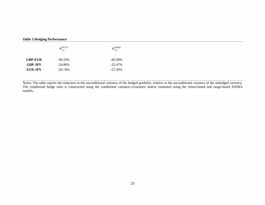
The hedging performance of the two models is reported in Table 5. Here, again, the

range-based model dominates the return-based model, offering a greater reduction in

hedged portfolio variance for all three currency pairs.

[Table 5]

Sensitivity Analysis

The results presented up to this point have all been based on an implementation of

both the return-based EWMA model and the range-based EWMA model using the

RiskMetrics decay factor of 0.94. As noted above, the RiskMetrics decay factor is

based on an average optimal decay factor for a large number of assets and so it is

unlikely that the value of 0.94 is the optimal value for either model in any particular

setting. Here we undertake a limited sensitivity analysis of the performance of each

model to the decay factor. For the return-based EWMA model, there is a single decay

factor that controls the dynamic equations both for the conditional variances and the

conditional covariance. We analyse the performance of the return-based model for

values of the decay factor between 0.900 and 0.995. For the range-based model, there

are two separate decay factors: one for the conditional variance equations, and one for

the conditional covariance equations. We analyse the performance of the range-based

16

model in relation to each of these decay factors separately, varying them from 0.900

to 0.995. For the sake of brevity, we report results only for the root mean square error

of the conditional variance-covariance matrix for one of the three currency pairs,

namely USD/GBP and USD/EUR. However, similar conclusions are drawn from the

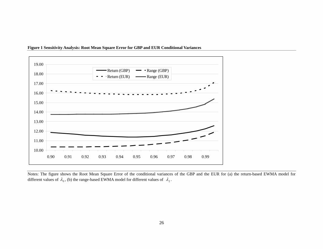
other evaluation criteria and for the other currency pairs. 7 Figure 1 shows the

sensitivity of the conditional variances of USD/GBP and USD/EUR to changes in the

decay factor for the two models. For both models, and for both currencies, increasing

the decay factor leads to a deterioration in model accuracy. For the return-based

EWMA model, the optimal decay factor in terms of RMSE is 0.945 for USD/GBP and

0.950 for the USD/EUR, both very close to the RiskMetrics value of 0.94. For the

range-based model, the performance improves as the decay factor is reduced, and the

optimal decay factor for both currencies is lower than 0.9.8 However, a notable feature

of the range-based model is that it is less sensitive to the choice of decay factor, with

very little difference observed between 0.90 and 0.96. In contrast, the performance of

the return-based model worsens as the decay factor falls, especially for USD/GBP.

[Figure 1]

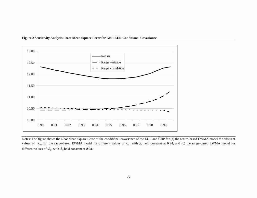
Figure 2 reports the sensitivity analysis for the conditional covariance of USD/GBP

and USD/EUR. In particular, for the return-based model, it reports the RMSE for

values of 0λ between 0.900 and 0.995. For the range-based model, two sensitivity

analyses are reported. The first varies the decay factor that controls the correlation

coefficient, 2λ , while holding 1λ constant at the RiskMetrics value of 0.94. The

second varies the decay factor that controls the conditional variance equations, 1λ ,

while holding 2λ constant. Perhaps the most striking feature of the range-based

conditional covariance is its insensitivity to the decay factor for the correlation

coefficient, 2λ . Although there is some deterioration in the RMSE as 2λ falls, the

difference in RMSE between 900.02 =λ and 995.02 =λ is negligible. The optimal

value of 2λ in terms of RMSE is about 0.997, although for the other currency pairs

7 The results of the sensitivity analysis for the remaining evaluation criteria and for all three currencies are available from the authors. 8 The optimal value of 1λ is 0.885 for USD/GBP and 0.880 for USD/EUR.

17

(not reported), it was somewhat lower. Varying 1λ , but holding 2λ fixed at 0.94

reduces the performance of the range-based model as 1λ rises above about 0.96, but it

is again relatively insensitive to the choice of decay factor as 1λ falls. In contrast, the

return-based model is sensitive to both a lower and higher decay factor, with the

optimal value of 0λ being 0.95, again very close to the RiskMetrics value of 0.94.

5. Conclusion

Estimates of integrated variance based on the intraday range offer substantial

efficiency improvements over those based on the squared return. However, since no

multivariate analogue of the intraday range exists, it can not be directly used to

estimate the integrated covariance of returns. While partial solutions to this problem

have been suggested, their use is limited to cases where triangular arbitrage

relationships exists that allow the covariance of returns to be imputed from the

variance of a two-asset portfolio. Except for the foreign exchange market, this

approach is unlikely to be useful in practice. In this paper, we have introduced a

simple yet effective model for estimating both the variances and covariances of

returns that exploits both the return-based and range-based estimates of integrated

volatility. The range-based model is more accurate than the return-based model,

contains more information about integrated volatility, and generates better

performance when applied to the economic problem of conditional minimum-variance

hedging. Moreover, the performance of the range-based model is less sensitive to the

choice of parameter values, enhancing its reliability in practice where the true values

of the parameters are unknown and subject to instability.

The range-based EWMA model that we propose could be extended in several

directions. Firstly, it can be thought of as a special case of the dynamic conditional

correlation model of Engle and Shephard (2001) and Engle (2002). In particular, the

conditional variance equations are specified in terms of range-based measures of

volatility, while the dynamic correlation coefficient is based on the EWMA return

model. It would be natural to investigate whether a more general formulation of the

model (in particular in a GARCH-type framework) offers any improvement in model

performance.

18

It would also be useful to investigate the performance of the range-based EWMA

model in other markets, such as equities, bonds and commodities, and over a longer

sample period. While accurate assessment of statistical performance necessitates the

use of intraday data to construct a benchmark measure of the integrated variance-

covariance matrix, it would nevertheless be interesting to evaluate the models against

purely economic criteria, such as hedging performance, the accuracy of value at risk

forecasts, or in terms of portfolio efficiency in a mean-variance optimisation context.

19

References Aït-Sahalia, Y., P.A. Mykland, and L. Zhang, 2005, “How often to sample a continuous-time process in the presence of market microstructure noise”. Review of Financial Studies, Vol 18, 2, 351-416. Alexander, C. and C. Leigh, 1997, “On the Covariance Matrices Used in Value at Risk Models”, Journal of Derivatives 4, 50-62. Alizadeh, S., M. Brandt and F. Diebold, 2002, “Range-based estimation of stochastic volatility models,” Journal of Finance 57, 1047–92. Andersen, T., T. Bollerslev and F. Diebold, 2005, “Parametric and Nonparametric Volatility Measurement”, Handbook of Financial Econometrics, forthcoming. Andersen, T.G, T. Bollerslev, F. Diebold and J. Wu, 2006, “Realized Beta: Persistence and Predictability” in T. Fomby and D. Terrell (eds.) Advances in Econometrics: Econometric Analysis of Economic and Financial Time Series in Honor of R.F. Engle and C.W.J. Granger , Volume B, 1-40. Bandi F, Russell J. 2003, “Microstructure Noise, Realized Volatility, and Optimal Sampling”, Working Paper. University of Chicago. Graduate School of Business. Barndorff-Nielsen, O.E, and N. Shephard, 2002, “Estimating quadratic variation using realised variance”, Journal of Applied Econometrics 17, 457–477. Barndorff-Nielsson, O., and N. Shephard, 2001, “Econometric Analysis of Realised Volatility and its Use in Estimating Stochastic Volatility Models”, Manuscript, University of Oxford. Bauwens, L., S. Laurent and J. Rombouts, 2006, “Multivariate GARCH Models: A Survey”, Journal of Applied Econometrics 21, 79-109. Bekaert, G., R. Hodrick and D. Marshall, 1997, “On Biases in Tests of the expectations Hypothesis of the Term Structure of Interest Rates,” Journal of Financial Economics 44, 309-348. Boudoukh, J., M. Richardson and R. Whitelaw, 1997, “Investigation of a Class of Volatility Estimators”, Journal of Derivatives 24, 470-486. Brandt, M., and F. Diebold, 2006, “A No-Arbitrage Approach to Range-Based Estimation of Return Covariances and Correlations,” Journal of Business 79, 61–74. Brandt, M., and C. Jones, 2006, “Volatility Forecasting with Range-Based EGARCH Models,” Journal of Business and Economic Statistics 79, 61–74. Brooks, C. and J. Chong, 2001, “The Cross-Currency Hedging Performance of Implied versus Statistical Volatility Models”, Journal of Futures Markets, Vol. 21(11), 1043–1069. Brunetti, C., and P. Lildolt, 2002, “Return-based and range-based (co)variance estimation, with an application to foreign exchange markets,” Unpublished paper. Christensen, K., and M. Podolskij, 2005, “Realized Range-Based Estimation of Integrated Variance,” Unpublished paper, Aarhus School of Business.

20

Chou, R., 2005, “Forecasting Financial Volatilities with Extreme Values: The Conditional Autoregressive Range (CARR) Model”, Journal of Money, Credit and Banking 37, 561-582. Chou, R., and D. Wang, 2005, “Estimating and Forecasting Volatility of the Stock Indices Using Conditional Autoregressive Range (CARR) Model”, Working Paper, Ming Chuan University. Engle, R., 2002, “Dynamic Conditional Correlation: A simple Class of Multivariate Generalized Autoregressive Conditional Heteroskedasticity Models”, Journal of Business and Economic Statistics, 20, 339-350. Engle, R., and K. Kroner, 1995, “Multivariate Simultaneous Generalised ARCH”, Econometric Theory 11, 122–50. Engle, R., and J. Russell, 1998, “Autoregressive Conditional Duration: A New Model for Irregular Spaced Transaction Data”, Econometrica 66, 1127-1162. Engle, F., and K. Sheppard, K., 2001, “Theoretical and Empirical Properties of Dynamic Conditional Correlation Multivariate GARCH”, NBER Working Paper 8554. Figlewski, S., 1997, “Forecasting Volatility”, Financial Markets, Institutions and Instruments Vol. 6, No. 1. Garman, M., and M. Klass, 1980, “On the estimation of price volatility from historical data,” Journal of Business 53, 67–78. Harvey, A., E. Ruiz and N. Shephard, 1994, “Multivariate Stochastic Variance Models”, Review of Economic Studies 61, 247-264. Hull, J., and A. White, 1998, “Incorporating Volatility Updating into the Historical Simulation Method for Value-at-Risk”, Journal of Risk 1, 5-19. JP Morgan, 1996, RiskMetricsTM Technical Document, 4th Edition, New York. Martens, M., and D. van Dijk, 2007, “Measuring Volatility with the Realized Range”, Journal of Econometrics 138, 181-207. Nelson, D., 1991, “Conditional Heteroskedasticity in Asset Returns: A New Approach”, Econometrica 59, 347-370. Parkinson, M., 1980, “The extreme value method for estimating the variance of the rate of return,” Journal of Business 53, 61–65. Zhang, L., Y. Aït-Sahalia, P.A. Mykland, 2005, “A tale of two time scales: Determining integrated volatility with noisy high-frequency data”, Journal of the American Statistical Association, 100 1394-1411.

21

Table 1 Summary Statistics for Daily Returns, Variances and Covariances

Mean S.D. Skewness Kurtosis

Returns

GBP 0.02% 0.54% -0.05 0.45 EUR 0.03% 0.60% -0.01 0.55 JPY 0.00% 0.55% 0.15 1.42

Realized variances

GBP 2.80E-05 1.81E-05 2.59 10.64 EUR 3.42E-05 2.38E-05 2.65 12.78 JPY 3.29E-05 2.82E-05 4.95 38.59

Realized

covariances

GBP-EUR 2.17E-05 1.67E-05 2.51 10.78 GBP-JPY 1.30E-05 1.32E-05 3.65 31.94 EUR-JPY 1.68E-05 1.48E-05 3.54 27.19

Notes: The table reports the mean standard deviation, skewness and kurtosis for daily log close-to-close returns and for the realized variances and covariances for USD/GBP, USD/EUR and USD/JPY. The realized variances and covariances are computed with 30-minute returns using equation (4). The sample period is 03/12/02 to 29/12/06 (1064 daily observations).

22

Table 2 Root Mean Square Error and Mean Absolute Error

)1(

,ˆ RVtijσ

Rangetij ,σ

RMSE MAE RMSE MAE

Variances

GBP 11.42 16.84 10.41 16.42 EUR 15.84 23.15 13.79 21.96 JPY 14.71 27.40 13.96 27.06

11.42 16.84 10.41 16.42 Covariances

GBP-EUR 11.86 16.65 10.46 15.55 GBP-JPY 9.24 13.73 8.53 13.19 EUR-JPY 10.42 15.77 9.64 15.06

Notes: The table reports the Root Mean Square Error and the Mean Absolute Error for the daily estimates of the elements of the conditional variance-covariance matrix using the return-based EWMA model and the range-based EWMA model, relative to the corresponding elements of the realized variance-covariance matrix, computed using 30-minute returns. The decay factors for both models are equal to 0.94.

Table 3 Mincer-Zarnowitz Regression Results

)1(

,ˆ RVtijσ

Rangetij ,σ

Intercept Slope R-squared H1 H2 Intercept Slope R-squared H1 H2

Variances

GBP 8.38E-06 0.667 0.191 0.240 0.000 4.23E-06 0.899 0.190 0.497 0.002 (1.34E-06) (0.042) (1.59E-06) (0.057)

EUR 1.35E-05 0.567 0.140 0.787 0.000 6.72E-06 0.866 0.159 0.000 0.000 (1.72E-06) (0.043) (2.05E-06) (0.061)

JPY 1.28E-05 0.659 0.083 0.002 0.000 6.10E-06 0.907 0.092 0.405 0.000 (2.22E-06) (0.067) (2.72E-06) (0.088)

Covariances

GBP-EUR 7.68E-06 0.554 0.134 0.691 0.000 4.61E-06 0.763 0.144 0.040 0.000 (1.19E-06) (0.043) (1.37E-06) (0.057)

GBP-JPY 6.30E-06 0.427 0.054 0.252 0.000 5.14E-06 0.536 0.062 0.005 0.000 (9.46E-07) (0.055) (1.02E-06) (0.064)

EUR-JPY 1.20E-05 0.264 0.019 0.407 0.000 1.02E-05 0.390 0.025 0.755 0.000 (1.17E-06) (0.059) (1.34E-06) (0.075)

Notes: The table reports the results of the Mincer-Zarnowitz regression given by equation (15) in the main text. The table also reports the p-values for the tests of the hypotheses tijijijH ,1 )1(: σβα −= and 1,0:2 == ijijH βα . Standard errors for the estimated parameters are reported in parentheses.

24

Table 4 Encompassing Regression Results

Intercept Slope ( )1(,ˆ RVtijσ ) Slope ( Range

tij ,σ ) R-squared

Variances

GBP 5.87E-06 0.362 0.434 0.196 (1.70E-06) (0.133) (0.180)

EUR 6.23E-06 -0.075 0.969 0.159 (2.23E-06) (0.136) (0.194)

JPY 6.70E-06 0.120 0.763 0.092 (2.86E-06) (0.174) (0.227)

Covariances

GBP-EUR 4.63E-06 0.006 0.756 0.144 (1.49E-06) (0.167) (0.222)

GBP-JPY 4.99E-06 -0.185 0.744 0.063 (1.03E-06) (0.200) (0.234)

EUR-JPY 9.54E-06 -0.303 0.757 0.027 (1.40E-06) (0.191) (0.243)

Notes: The table reports the results of the encompassing regression given by equation (15) in the main text. Standard errors for the estimated parameters are reported in parentheses.

25

Table 5 Hedging Performance

)1(

,ˆ RVtijσ

Rangetij ,σ

GBP-EUR -60.20% -60.58% GBP-JPY -24.80% -25.47% EUR-JPY -26.74% -27.50%

Notes: The table reports the reduction in the unconditional variance of the hedged portfolio, relative to the unconditional variance of the unhedged currency. The conditional hedge ratio is constructed using the conditional variance-covariance matrix estimated using the return-based and range-based EWMA models..

26

Figure 1 Sensitivity Analysis: Root Mean Square Error for GBP and EUR Conditional Variances

10.00

11.00

12.00

13.00

14.00

15.00

16.00

17.00

18.00

19.00

0.90 0.91 0.92 0.93 0.94 0.95 0.96 0.97 0.98 0.99

Return (GBP) Range (GBP)Return (EUR) Range (EUR)

Notes: The figure shows the Root Mean Square Error of the conditional variances of the GBP and the EUR for (a) the return-based EWMA model for different values of 0λ , (b) the range-based EWMA model for different values of 2λ .

27

Figure 2 Sensitivity Analysis: Root Mean Square Error for GBP-EUR Conditional Covariance

10.00

10.50

11.00

11.50

12.00

12.50

13.00

0.90 0.91 0.92 0.93 0.94 0.95 0.96 0.97 0.98 0.99

Return

Range variance

Range correlation

Notes: The figure shows the Root Mean Square Error of the conditional covariance of the EUR and GBP for (a) the return-based EWMA model for different values of 0λ , (b) the range-based EWMA model for different values of 2λ , with 1λ held constant at 0.94, and (c) the range-based EWMA model for different values of 1λ , with 2λ held constant at 0.94.