How Much of Interviewer Variance Is Really Nonresponse Error Variance?

University of Nebraska - LincolnDigitalCommons@University of Nebraska - Lincoln

Sociology Department, Faculty Publications Sociology, Department of

1-1-2010

How Much of Interviewer Variance Is ReallyNonresponse Error Variance?Brady T. WestUniversity of Michigan, Ann Arbor, [email protected]

Kristen OlsonUniversity of Nebraska - Lincoln, [email protected]

Follow this and additional works at: http://digitalcommons.unl.edu/sociologyfacpubPart of the Sociology Commons

This Article is brought to you for free and open access by the Sociology, Department of at DigitalCommons@University of Nebraska - Lincoln. It hasbeen accepted for inclusion in Sociology Department, Faculty Publications by an authorized administrator of DigitalCommons@University ofNebraska - Lincoln.

West, Brady T. and Olson, Kristen, "How Much of Interviewer Variance Is Really Nonresponse Error Variance?" (2010). SociologyDepartment, Faculty Publications. Paper 144.http://digitalcommons.unl.edu/sociologyfacpub/144

http://digitalcommons.unl.edu?utm_source=digitalcommons.unl.edu%2Fsociologyfacpub%2F144&utm_medium=PDF&utm_campaign=PDFCoverPages

http://digitalcommons.unl.edu/sociologyfacpub?utm_source=digitalcommons.unl.edu%2Fsociologyfacpub%2F144&utm_medium=PDF&utm_campaign=PDFCoverPages

http://digitalcommons.unl.edu/sociology?utm_source=digitalcommons.unl.edu%2Fsociologyfacpub%2F144&utm_medium=PDF&utm_campaign=PDFCoverPages

http://digitalcommons.unl.edu/sociologyfacpub?utm_source=digitalcommons.unl.edu%2Fsociologyfacpub%2F144&utm_medium=PDF&utm_campaign=PDFCoverPages

http://network.bepress.com/hgg/discipline/416?utm_source=digitalcommons.unl.edu%2Fsociologyfacpub%2F144&utm_medium=PDF&utm_campaign=PDFCoverPages

http://digitalcommons.unl.edu/sociologyfacpub/144?utm_source=digitalcommons.unl.edu%2Fsociologyfacpub%2F144&utm_medium=PDF&utm_campaign=PDFCoverPages

1004

Published in Public Opinion Quarterly 74:5 (2010), pp. 1004–1026; doi: 10.1093/poq/nfq061 Copyright © 2011 Brady T. West and Kristen Olson. Published by Oxford University Press on behalf of the American Association for Public Opinion Research. Used by permission.

How Much of Interviewer Variance Is Really Nonresponse Error Variance?

Brady T. West and Kristen Olson

Corresponding author — Brady T. West, Michigan Program in Survey Methodology, P.O. Box 1248, 426 Thompson Street, Ann Arbor, MI 48106, USA;

email [email protected]

AbstractKish’s (1962) classical intra-interviewer correlation (ρint) provides survey researchers with an estimate of the effect of interviewers on variation in measurements of a survey variable of interest. This correlation is an un-desirable product of the data collection process that can arise when an-swers from respondents interviewed by the same interviewer are more similar to each other than answers from other respondents, decreasing the precision of survey estimates. Estimation of this parameter, however, uses only respondent data. The potential contribution of variance in non-response errors between interviewers to the estimation of ρint has been largely ignored. Responses within interviewers may appear correlated because the interviewers successfully obtain cooperation from different pools of respondents, not because of systematic response deviations. This study takes a first step in filling this gap in the literature on interviewer effects by analyzing a unique survey data set, collected using computer-assisted telephone interviewing (CATI) from a sample of divorce records. This data set, which includes both true values and reported values for re-spondents and a CATI sample assignment that approximates interpen-

Brady T. West is a PhD candidate in the Michigan Program in Survey Methodology (MPSM), University of Michigan, Ann Arbor, Michigan, USA. Kristen Olson is an Assistant Professor in the Survey Research and Methodology Program and the Department of Sociol-ogy, University of Nebraska–Lincoln, Lincoln, Nebraska, USA. The authors express sincere thanks to Paul Biemer, Bob Groves, Mick Couper, Frauke Kreuter, Jim Lepkowski, and four anonymous reviewers for helpful comments and guidance on earlier drafts, and to Vaughn Call for providing access to these data. The U.S. National Science Foundation generously provided support [SES-0620228 to K.O.]. The Wisconsin Divorce Study was supported by the National Institute of Child Health and Human Development, the National Institutes of Health [HD-31035 and HD32180–03 to Vaughn Call and Larry Bumpass]. The study was designed and carried out at the Center for Demography and Ecology at the University of Wisconsin–Madison and Brigham Young University under the direction of Vaughn Call and Larry Bumpass.

h o w muc h i n te r v i e w er v ar i an c e i s n o n r es p o n s e e r r o r v ar i an c e? 1005

etrated assignment of subsamples to interviewers, enables the decom-position of interviewer variance in means of respondent reports into nonresponse error variance and measurement error variance across in-terviewers. We show that in cases where there is substantial interviewer variance in reported values, the interviewer variance may arise from non-response error variance across interviewers.

Introduction

Survey research organizations conducting interviewer-administered sur-veys often find that estimates of key population parameters tend to vary across interviewers. Ideally, all interviewers working a random subset of the entire sample obtain a 100 percent response rate, and sampling variance is the only source of variance in measurements between interviewers. Empir-ical evidence, however, is to the contrary in both telephone and interpene-trated face-to-face surveys (Davis and Scott 1995; Schnell and Kreuter 2005): Respondents interviewed by the same person tend to provide more similar responses for some survey questions than respondents interviewed by differ-ent persons (e.g., Groves and Magilavy 1986; Hansen, Hurwitz, and Bershad 1960; O’Muircheartaigh and Campanelli 1998).

One possible source of this between-interviewer variance is correlated de-viations of responses from true values within each interviewer (e.g., Biemer and Stokes 1991; Biemer and Trewin 1997; Groves 2004, Chapter 8; Han-sen, Hurwitz, and Bershad 1960). Various hypotheses have been proposed in the literature concerning the source of these correlations, including the complexity of the survey question (e.g., Collins and Butcher 1982), interac-tions between the interviewer and the respondents (e.g., Mangione, Fowler, and Louis 1992), or an inability to disentangle geographic effects from inter-viewer effects without interpenetrated designs (O’Muircheartaigh and Cam-panelli 1998). In this article, we provide empirical support for an alternative hypothesis, motivated by consistent findings of between-interviewer vari-ance in response rates (Campanelli and O’Muircheartaigh 1999; Durrant et al. 2010; O’Muircheartaigh and Campanelli 1999; Pickery and Loosveldt 2002; Singer and Frankel 1982). We find that intra-interviewer correlations among respondents on some items arise from variable nonresponse errors across in-terviewers, rather than correlated response deviations. Surprisingly, to our knowledge, this study is the first to formally examine this hypothesis.

Between-interviewer variance is a well-documented source of instability in survey estimates, decreasing data quality (Groves 2004, 364). The multi-plicative “interviewer effect” on the variance of an estimated mean is simi-lar to a design effect due to cluster sampling. This multiplicative effect on the variance is written as 1 + (m‾ – 1)ρint , where m‾ represents the average sample workload for an interviewer and ρint represents an item-specific intra-inter-viewer correlation (Kish 1962). When responses to a particular question are

w e st & o l s o n i n p ubl i c op i ni o n qu a r ter l y 74 (2010)1006

more similar for respondents interviewed by the same interviewer than for re-spondents interviewed by different interviewers, ρint can become high, ranging up to 1 (in theory). When responses to a particular question for respondents in-terviewed by the same interviewer are equivalent to responses obtained from a simple random sample of the total respondent pool, ρint approaches 0. Low in-tra-interviewer correlations, however, can substantially affect the precision of an estimated mean. For example, assuming 30 respondents per interviewer, a value of 0.01 for ρint would result in a 29-percent increase in the variance—or a 13.6 percent increase in the standard error—of an estimated mean, increasing confidence interval width and reducing effective sample sizes.

In practice, empirical estimates of ρint generally vary from small (0.01) to much larger (0.12 or above). Groves and Magilavy (1986) report that roughly 80 percent of all ρint estimates fall below 0.02; unfortunately, much of the pub-lished literature fails to report how many of these estimates represent signifi-cant (i.e., non-zero) variability across interviewers. Estimates of ρint tend to be larger in face-to-face surveys than in telephone surveys (Groves and Magi-lavy 1986) and are generally on par with or larger than the effects of clusters in area probability sample designs (Davis and Scott 1995; O’Muircheartaigh and Campanelli 1998; Schnell and Kreuter 2005). Many estimates of ρint are larger than 0.02 for factual survey items; estimates of ρint for attitudinal items tend to be similar to those for factual items (e.g., Groves and Magilavy 1986; Kish 1962; Mangione, Fowler, and Louis 1992). Estimates of ρint rang-ing from 0.03 to 0.12 have been reported for factual survey items, includ-ing age (Kish 1962, face-to-face), ethnicity (Fellegi 1964, face-to-face), present employment (Groves and Kahn 1979, telephone), existence of health condi-tions (Mangione, Fowler, and Louis 1992, face-to-face), recent doctor visits (Groves and Magilavy 1986, telephone), and car buying and type of school last attended full-time (Collins and Butcher 1982, face-to-face). Surprisingly, O’Muircheartaigh and Campanelli (1998) report significant intra-interviewer correlations for a series of self-completion items in a face-to-face survey.

One possible hypothesis for these unexpected findings is that nonresponse error variance occurs between interviewers. We define nonresponse error vari-ance in this context as the variance across interviewers of the nonresponse bi-ases specific to each interviewer’s subsample of cases when he or she achieves less than 100 percent response rates. Under this hypothesis, correlations among respondents interviewed by the same person arise because of differential non-response errors across interviewers (i.e., interviewers successfully recruit and interview different types of people), not because interviewers introduce corre-lations in responses to the survey questions (i.e., systematic measurement er-rors that differ across interviewers). Although suggested previously, especially in the case of telephone surveys (Groves and Fultz 1985, 45; Stokes and Yeh 1988, 358), this hypothesis has not been formally evaluated.

Variation across interviewers in response, contact, and cooperation rates has been clearly documented (Hox and de Leeuw 2002; Link 2006; Morton-


Williams 1993; O’Muircheartaigh and Campanelli 1999; Snijkers, Hox, and de Leeuw 1999; Wiggins, Longford, and O’Muircheartaigh 1992). Empirical ex-aminations of the variable effects of interviewers on nonresponse focus on the association between survey participation rates and fixed characteristics of the interviewers (Groves and Couper 1998), their attitudes (Durrant et al. 2010; Hox and de Leeuw 2002), doorstep behaviors (Campanelli, Sturgis, and Purdon 1997; Morton-Williams 1993), and vocal characteristics (Groves et al. 2008; Oksenberg and Cannell 1988). Yet whether interviewers vary in the types of respondents that they recruit has received little research attention, due largely to a lack of information about nonrespondents and the absence of record values for all sample units.

Expanded statistical models for the joint effects of nonresponse and corre-lated measurement errors on the variance of survey estimates have been pos-ited (Biemer 1980; Groves and Magilavy 1984; Lessler and Kalsbeek 1992; Platek and Gray 1983), although estimation of ρint in practice typically uses only respondent data. For example, Platek and Gray express an unadjusted es-timate of a population total based on respondent reports on a variable x as a function of a participation indicator Rj (where Rj = 1 when sample person j par-ticipates and Rj = 0 when person j is a nonrespondent), the individual’s true value on the survey variable Yj, and their individual response deviation, ej: x̂ = N ∑n Rj(Yj + ej). n j=1

Platek and Gray show that in the absence of any type of weighting or im-putation method to compensate for nonresponse (which they refer to as the “zero substitution” method), the variance of this unadjusted linear statistic can be decomposed into five terms: sampling variance, uncorrelated mea-surement error variance (i.e., simple response variance), correlated measure-ment error variance, uncorrelated nonresponse error variance, and correlated nonresponse error variance.

We present their general derivation of this variance below (Platek and Gray 1983, 287, 316), using the notation pij for the response propensity of per-son j assigned to interviewer i, σij for the standard deviation of the response deviations for person j assigned to interviewer i, Bij for a person’s average re-sponse deviation, r2ijj’ for the correlation of the response deviations for two sampled persons j and j’ assigned to interviewer i, and r1ijj’ for the correlation of the participation indicators R for persons j and j’ assigned to interviewer i. To emphasize the nesting of sample persons within interviewers, we use A for the total number of interviewers in the population, and M for the fixed subsample size assigned to each interviewer:

V(x̂ ) = Sampling Variance + Simple Measurement Error (ME) Variance + Correlated Measurement Error (ME) Variance (Equation PG) + Simple Nonresponse Error (NE) Variance + Correlated Nonresponse Error (NE) Variance


where

Sampling Variance

Simple ME Variance

Correlated ME Variance

Simple NE Variance and

Correlated NE Variance

This daunting expression shows that under the normal situation of less than 100 percent response rates, the correlated measurement error variance component of a linear statistic contains correlations arising from (1) correla-tions among response deviations between two respondents; and (2) correla-tions among the participation indicators between two different units. Corre-lated nonresponse error variance in the last term of the equation arises from correlations among indicators for survey participation, Rij and Rij’, between two different units assigned to the same interviewer.

Applying these models to the estimation of nonresponse and measurement error variance due to the interviewer is complicated. Platek and Gray argue that interviewers are one potential source for these correlations, but interview-ers are not explicitly accounted for in the model. Further, few of these models have been applied to nonsimulated survey data or non-imputed data. In fact, Platek and Gray illustrate their formulas by assuming values for many of the terms rather than estimating them, including the correlations among response deviations and among participation indicators. Our review of the literature found that none of the past work in this area has developed separate estima-tors for the correlated components of measurement error variance and nonre-


sponse error variance for unadjusted estimators (although some work has been done using imputed data). Further, no work has extended these results to ex-plicitly account for the role of interviewers in introducing correlated measure-ment errors and correlated response indicators, despite several examples of in-terviewers introducing correlations of both forms in the literature.

Despite these complications, the models that have been proposed for the joint effects of correlated nonresponse and measurement errors on sur-vey estimates are particularly useful in that they elucidate characteristics of the data that are needed for estimating these components. First, each inter-viewer employed for the survey should be assigned a completely random in-terpenetrated subsample of the full sample selected for the survey (Mahala-nobis 1946). Second, important survey variables must be available for both respondents and nonrespondents (perhaps on the original sampling frame) and measured without error. Third, these important survey variables should be asked in identical form in the survey questionnaire to minimize any sys-tematic response biases. We consider a survey data set having these unique properties in this study.

In this article, we present an initial descriptive examination of the vari-ance in these two critical error sources among interviewers, in hopes of mo-tivating future analytical development. We analyze a unique survey data set that enables estimation of correlated interviewer variance due to measure-ment error and nonresponse error. The data arise from a survey adminis-tered to a sample drawn from a frame of records containing items that are also asked in the survey. Sample cases are assigned to interviewers based on an interpenetrated sample design. Knowledge of true values on survey vari-ables for the respondents and nonrespondents permits calculation of nonre-sponse error variance due to interviewers. We use these data to show that re-spondent means may vary between interviewers not because of correlated response deviations within interviewers, but because interviewers success-fully obtain participation from different pools of respondents.

Data and Methods

Data: The survey data used here were collected by the University of Wis-consin–Madison as part of the Wisconsin Divorce Study (WDS). The WDS se-lected a simple random sample of 733 divorce certificates from a frame of certif-icates in 1989 and 1993 from four counties in Wisconsin. The sampled divorce certificates included official information that was also collected in the survey. The present study considers data collected from 355 respondents (AAPOR RR1 = 71.0 percent) by 31 trained interviewers1 using computer-assisted telephone interviewing (CATI), meaning that interviewer effects will likely be attenuated in this analysis relative to a face-to-face survey (Groves and Magilavy 1986).

1. Additional interviewer-level information, such as interviewing experience, is not available.


The divorce date on each certificate was recorded by an official body; other information on the frame (e.g., marriage date, birth dates) was reported by at least one member of the divorcing couple (not indicated in the records) and therefore could be more susceptible to measurement error. For purposes of this study, we assume that the frame data are essentially error-free. The ques-tionnaire itself collected measures on six variables that will be analyzed in this study with respect to the frame records: length of marriage in months (divorce date minus marriage date), time since divorce in months (interview date mi-nus divorce date), time since marriage in months (interview date minus mar-riage date), number of marriages up to and including the divorce, age at mar-riage (marriage date minus birth date), and age at divorce (divorce date minus birth date). We note that five of these six variables are functions of dates col-lected in the survey, which is common in survey practice. The WDS question wording for these variables was “How many times have you been married?”; “In what month and year did your marriage begin?”; “In what month and year did you get divorced?”; and “What is your date of birth?”

The call records in the WDS were kept using paper-and-pencil cover sheets for each sample case, and the call-record data were entered using double entry. Illegible interviewer handwriting resulted in limited amounts of item-missing data in the call records. The interviewer also recorded his or her initials at each call. In some instances, subjective decisions about the interviewer identification codes associated with each call had to be made (e.g., an interviewer recorded two initials for one call and then three initials for another call). Interviewer ini-tials in the electronic data file that were deemed by the authors to correspond to the same person were combined. All analyses in this study were performed before and after this combining operation; no substantive differences in the results were found. Important variables from the call records for the present study include the initials of the interviewer making the call attempt, the num-ber of call attempts to a particular sample case, the time of the call attempt, the day of the week of the call attempt, and the call outcome.

Assigning sampled cases to interviewers: Ideally, for purposes of esti-mating nonresponse error variance among interviewers, each interviewer in the WDS would have had a fixed random subsample of cases to work and never made call attempts to cases being worked by other interviewers (e.g., Singer and Frankel 1982). In practice, however, any CATI survey involves frequent changes in the interviewer who works the sampled case. As a result, how to assign cases to interviewers for estimating components of variance due to nonresponse error is a nontrivial decision.

In this study, we assumed that interviewers working a particular shift (e.g., weekdays, 9–5 p.m.) were assigned random subsamples of all sampled per-sons called during that shift. This assumption of interpenetration within shifts was empirically tested for each survey variable of interest (discussed below). Assigning interviewers to discrete shifts is difficult in CATI surveys because the work of interviewers often extends across multiple calling shifts. We con-


ducted all of our analyses conditional on a calling shift; that is, we estimated variance between interviewers within a shift. Because persons with different characteristics are likely to be contacted at different times of the day (e.g., em-ployed persons are more likely to be contacted during evening hours; Groves and Couper 1998), not accounting for the shift of work could confound nonre-sponse error with true differences in sampled persons across shifts.

Assigning shifts: We included only telephone calls with a recorded in-terviewer making the call and a time and day of call recorded in the data set, leaving 5,267 calls for analysis (94.9 percent of all 5,548 recorded calls). The time and day of each call were combined into a single shift variable denot-ing three time slots: weekday day, or Monday through Friday before 5 p.m. (Shift 1); weekday evening after 5 p.m. (Shift 2); and weekend calls on Satur-day and Sunday (Shift 3). Stokes and Yeh (1988) also used this collapsing of shifts to analyze interviewer variance in a telephone survey.2 Overall, 44.1 percent of the calls made in the WDS were made during the weekday eve-ning shift, 29.1 percent during the weekend shift, and 26.8 percent during the weekday day shift. About 90 percent of the interviewers made at least one call during each of the three shifts. Only seven of the 31 interviewers made at least 90 percent of their calls during one of the three shifts, indicating shift crossing similar to that found by Stokes and Yeh (1988, 368).

Assigning nonrespondents to interviewers: Multiple interviewers worked cases in multiple shifts, leading to difficulty in assigning a single in-terviewer and shift to each case for analysis. For all 355 interviewed cases, the interviewer who conducted the interview was assigned to each respon-dent, as was the corresponding shift during which the interview was con-ducted. For nonresponding cases, decisions about how to assign interviewers and shifts were more complicated.

Sample cases that had no call attempts with an interviewer ID recorded in the call records were deleted from the data set. This resulted in the de-letion of 54 sample cases with call records but item-missing data on inter-viewer IDs, while 679 sample cases were retained (of which 355 responded). The remaining 324 sample cases consisted of both refusals and noncontacts. If a sample case was contacted at some point but refused to cooperate, it was assigned to the first interviewer receiving a refusal from that case. If there were no prior explicit refusals for a contacted case, the nonrespondent case was assigned to the last interviewer making contact. The WDS documenta-tion states that prior refusals were assigned to interviewers trained in refusal conversion, but no particular guidelines were followed for cases that had not been previously contacted (Mitchell 2004). Therefore, if calls were made to a

2. The present study also considered three alternative shifts: Monday through Friday before 5 p.m., Sunday through Thursday after 5 p.m., and Friday or Saturday after 5 p.m./week-ends before 5 p.m. The results from this analysis were qualitatively the same, so we pres-ent results from only the first shift assignment.


sample case but contact was never established, the nonrespondent was as-signed to the last interviewer making a call, assumed to be randomly selected from all interviewers working a shift.3

Increasing response rates of 41.1 percent, 54.2 percent, and 59.8 per-cent were found across the three shifts under the nonresponse assignment method described above (Table 1). Cooperation rates across the three shifts among contacted cases were fairly stable (75.3 percent, 73.1 percent, and 75.4 percent, respectively). Consistent with previous work examining op-timal calling periods (Brick et al. 2007; Groves and Couper 1998; Hu et al. 2009; Weeks, Kulka, and Pierson 1987), this finding suggests that interview-ers had a more difficult time making contact during the week, especially before 5:00 p.m.

The number of interviewers who worked each shift ranged from 19 to 24 (table 1). These numbers limit the power of analyses to detect statistically sig-nificant variation between interviewers. Substantial variability in assigned workloads (respondents and nonrespondents) across interviewers within a shift is also evident. Mean workloads range from 8.2 sampled cases (Shift 1) to 14.4 sampled cases (Shift 2), and workload standard deviations range from 8.9 (Shift 3) to 15.0 (Shift 2).

Analytic Approach: The traditional interviewer variance model for a survey variable Y in interviewer-administered surveys with 100 percent re-sponse rates expresses an individual response as xij = Y‾ + bi + eij , where xij

Table 1. Descriptive Statistics for Interviewer Workloads and Response Rates, by Shift

Shift 1: Shift 2: Shift 3: Weekday day Weekday evening Weekend Total

# Cases Attempted 163 345 169 677**# Respondents 67 187 101 355Response Rate (%) 41.1% 54.2% 59.8% 52.4%# of Interviewers 20 24 19 30Mean Interviewer 8.2 14.4 8.9 10.7Workload (SD) (12.0) (15.0) (8.9) (12.6)

SD = Standard Deviation.** 2 cases did not have a final shift recorded in the call records.

3. Assignment of noncontacts to the last interviewer attempting a call attempt may be con-sidered arbitrary. An alternative method of assigning noncontacts was also considered. In this method, an interviewer making at least one call to a case that had not been con-tacted was selected at random from all of the interviewers making calls to this case and assigned to it. The primary findings in this study did not vary when using this alterna-tive method of assigning noncontacts to interviewers, suggesting that interviewers mak-ing the final calls to noncontacted cases were randomly selected from all interviewers. Additional methods of assigning noncontacts were not considered.


is respondent j’s report collected by interviewer i, Y‾ is the population mean of the true values, bi is the deviation in the respondent’s report due to inter-viewer i, and eij is a random measurement error term. The variance of a sam-ple mean can then be written (approximately) in terms of the sampling vari-ance, the variance due to interviewers, and random error variance (Biemer and Stokes 1991; U.S. Bureau of the Census 1985, 228; Kish 1962):

(1)

In equation (1), n is the sample size, σY2 represents the element variance of

the true values of Y, σb2 is the correlated component of variance due to inter-

viewers, σe2 is random error variance, m‾ represents the average interviewer

workload, and ρY represents the intra-interviewer correlation of variable Y, with ρY = σb

2/(σY2 + σb

2 + σe2). Thus, estimates with larger correlated compo-

nents of variance in responses due to interviewers (σb2) have larger intra-in-

terviewer correlations (ρY). Estimators of ρY have been proposed in the litera-ture based on analysis of variance methods (U.S. Bureau of the Census 1985; Kish 1962) and multilevel modeling methods (e.g., O’Muircheartaigh and Campanelli 1998). These estimators assume 100 percent response rates and focus exclusively on measurement error.

Our analytic approach considered a descriptive method for decomposing interviewer variance in respondent reports into estimates of nonresponse er-ror variance and measurement error variance. We then explored the ratio of nonresponse error variance to total interviewer variance. Let yij be the true value of survey variable Y for sample unit j assigned to interviewer i, and let xij be the reported value for Y for that sample unit if the unit responds to the survey. Assuming interpenetrated assignment of subsamples to interviewers, the expectation of the mean of respondent reports x‾i for interviewer i is

E(x‾i|i) = Y‾ + BiasNR,i + BiasME,i = Y‾ + (y‾R,i – y‾i ) + (x‾i – y‾R,i) (2)

That is, the expected value of the respondent mean for interviewer i is the sum of (1) the population mean of the true values, Y‾; (2) the difference be-tween the mean of the true values for all respondents interviewed by inter-viewer i, y‾R,i, and the mean of the true values for all units assigned to inter-viewer i, y‾i (nonresponse bias); and (3) the difference between the mean of the reported values for all respondents interviewed by interviewer i, x‾i, and y‾R,i (measurement error bias).

Assuming interpenetration and negligible covariance between the two bias terms,4 the variance of the expectation in (2) is defined by the sum of two variance components: Var (BiasNR,i) and Var (BiasME, i). We sought un-

4. We computed the correlations (r) of these two bias sources for interviewers within each shift. The correlations ranged from −0.05 to 0.32. None were significant (p < 0.05), provid-ing empirical support for the assumption.


biased estimates of these variance components and the ratio of the nonre-sponse error variance (the first component) to the total interviewer-related variance (the sum of the two components). Estimation of these variance com-ponents using closed-form estimators is possible for very simple design and response scenarios (e.g., equal assignment sizes and response rates across in-terviewers) typically not experienced in practice. Given the unequal assign-ment sizes and respondent counts for each interviewer in the WDS, we es-timated these components for each variable within each calling shift using three distinct steps.

Estimation Step 1. First, we estimated the variance among interviewers in the means of the true values for all sample cases assigned to each inter-viewer. Assuming interpenetrated assignment of cases to interviewers, this variance component should be negligible, as all interviewers should have a full sample mean of true values equal, on average, to the population mean. We estimated this component using a one-way random effects model, as-suming that the interviewers were a random subsample from a larger hypo-thetical population of interviewers:

yij = Y‾ + bi + eij. (3)

In this notation, yij is the true value of variable Y for sample unit j as-signed to interviewer i, bi is the random deviation of interviewer i’s assign-ment mean from the population mean of the true values, Y‾ , and eij is a nor-mally distributed random error with mean 0 and constant variance (the element variance within each assignment). We estimated the variance of the bi, or Var(bi) = σ 2

int, full, using restricted maximum likelihood (REML) estima-tion to obtain an unbiased estimate of this variance component given un-equal interviewer workloads (Patterson and Thompson 1971).

Significance tests for variance components are more complicated than those for means and proportions. A large body of statistical research has been dedicated to appropriate methods for testing the significance of vari-ance components in models including random effects (Zhang and Lin 2008). We tested a null hypothesis that the interviewer variance component is equal to zero, H0 : σ 2

int, full = 0, versus the alternative that assignment means vary across interviewers, HA : σ 2

int, full > 0. One test of this hypothesis is the Wald test, where the REML estimate of the variance component is divided by its asymptotic standard error.5 Although intuitively simple, this test behaves poorly due to the complicated distribution of the test statistic under the null hypothesis, among other reasons (Berkhof and Snijders 2001). A likelihood

5. Bates (2009), the developer of the nlme and lme4 packages for fitting mixed-effects mod-els in R, advises against reporting standard errors for estimated variance components when the distributions of the estimators are not symmetric. This applies for REML esti-mators of variance components. We follow this recommendation.


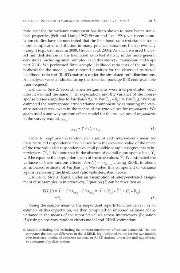
ratio test6 for the variance component has been shown to have better statis-tical properties (Self and Liang 1987; Stram and Lee 1994), yet recent simu-lation studies have demonstrated that the likelihood ratio test statistic has a more complicated distribution in many practical situations than previously thought (e.g., Crainiceanu 2008; Greven et al. 2008). As such, we used the ex-act null distribution of the likelihood ratio test statistic under more general conditions (including small samples, as in this study) (Crainiceanu and Rup-pert 2004). We performed finite-sample likelihood ratio tests of the null hy-pothesis for the models, and reported p-values for the observed restricted likelihood ratio test (RLRT) statistics under the simulated null distributions. All analyses were conducted using the statistical package R (R code available upon request).

Estimation Step 2. Second, when assignments were interpenetrated, each interviewer had the same y‾i in expectation, and the variance of the nonre-sponse biases simplifies to Var(BiasNR,i) = Var(y‾R,i – y‾i ) = Var(y‾R,i). We thus estimated the nonresponse error variance component by estimating the vari-ance across interviewers in the means of the true values for respondents. We again used a one-way random effects model for the true values of respondents to the survey request, yR,ij :

yR,ij = Y‾ + b′i + e′ij (4)

Here, b′i captures the random deviation of each interviewer’s mean for their recruited respondents’ true values from the expected value of the mean of the true values for respondents over all possible sample assignments to in-terviewers (Y‾R ). We note that in the absence of overall nonresponse bias, Y‾R will be equal to the population mean of the true values, Y‾ . We estimated the variance of these random effects, Var(b′i ) = σ 2

int,resp , using REML to obtain an unbiased estimate of Var(BiasNR,i). We tested this component of variance against zero using the likelihood ratio tests described above.

Estimation Step 3. Third, under an assumption of interpenetrated assign-ment of subsamples to interviewers, Equation (2) can be rewritten as

E(x‾i|i) = Y‾ + BiasNR,i + BiasME,i = Y‾ + (y‾R,i – Y‾ ) + (x‾i – y‾R,i)

= x‾i (5)

Using the sample mean of the respondent reports for interviewer i as an estimate of this expectation, we then computed an unbiased estimate of the variance in the means of the reported values across interviewers (Equation (5)) using a one-way random effects model and REML estimation:

6. Models including and excluding the random interviewer effects are estimated. The test compares the positive difference in the -2 REML log-likelihood values for the two models (the restricted likelihood ratio test statistic, or RLRT statistic, under the null hypothesis) to a mixture of χ2 distributions.


xij = X‾ R + b′′i + e′′ij (6)

This is the interviewer variance model that is often estimated in prac-tice using respondent data only. The variance of the random interviewer de-viations (b′′i) around the expected value of the mean of the respondent re-ports over all possible sample assignments to interviewers ( X‾ R), or Var(b′′i) = σ 2

int,resp,obs, captures both measurement error variance and nonresponse error variance introduced by the interviewers, and is thus the “total variance” due to interviewers. We tested this variance component for significance using ap-propriate finite-sample likelihood ratio tests. We then subtracted the esti-mate of the nonresponse error variance from Estimation Step 2 to get an es-timate of the measurement error variance across interviewers. The estimated proportion of variance introduced by interviewers due to nonresponse error variance was then computed as

σ̂ 2int,resp – σ̂ 2

int,full

σ̂ 2int,resp,obs – σ̂ 2

int,full (7)

Evidence of successful interpenetration from Estimation Step 1 implies that σ 2

int,full = 0 (i.e., interviewer-level means of true values for their full as-signments do not vary). We subtracted estimates of σ 2

int,full from the numera-tor and denominator to remove components of variance that were not due to the interviewer from this calculation.

Results

For each of the three WDS calling shifts, Table 2 displays the sample size, number of interviewers, and number of responding cases. The number of responding cases varies slightly over items due to differential item non-

Table 2. Total Counts of Interviewers, Sampled Cases, and Item Respondents, by Shift

Shift 1: Shift 2: Shift 3: Weekday Weekday Weekend day evening

Number of Interviewers Total 20 24 19 Responding Cases Only 17 23 17Number of Sampled Persons Frame Total 163 345 169 Item Respondents Minimum 53 161 87 Maximum 67 187 101


response. We have limited power to detect variance among interviewers within each shift, given the small counts of interviewers and the small num-ber of cases assigned to each interviewer.

Table 3 presents estimates of the three variance components of interest and the estimated proportion of the interviewer variance due to nonresponse error variance across interviewers for each WDS variable in each shift. We first consider the assumption of interpenetrated assignment of subsamples of active sample cases to interviewers within each calling shift. Estimates of the variance in means of true values for cases assigned to each interviewer are provided in column 3. We find little evidence against assumptions of inter-penetration within each shift, as very little variance occurs among interview-ers in the means of the assigned subsamples. Although there is low power to detect significant differences, the magnitude of the estimated variance term σ 2

int,full is very small for almost all of the variable/shift combinations. In three cases (age at divorce in Shift 1, months since marriage in Shift 2, and months since divorce in Shift 2), there is evidence of marginal variance among inter-viewers in assignment means, suggesting that the assumption of interpene-trated assignment did not appear to hold for all variables in all shifts.

Next, we examine interviewer variance due to nonresponse error and measurement error. We find two variable/shift combinations presenting evi-dence of significant interviewer variance in the means of respondent reports, despite evidence of successful interpenetration: age at marriage in Shift 2 (weekday evening), and age at divorce in Shift 2. For age at marriage in Shift 2, we see negligible variance among interviewers in the means of true val-ues for responding cases, suggesting negligible nonresponse error variance. There is significant (p < 0.01) variance among interviewers in the means of reported values for respondents, which suggests that the majority of the in-terviewer variance arises from measurement error variance. This is consis-tent with the long-standing hypothesis that interviewer variance arises due to correlations among response deviations for respondents interviewed by the same interviewer.

For age at divorce in Shift 2, we see evidence of significant (p = 0.05) vari-ance between interviewers in the means of true values for respondents alone. Thus, different interviewers successfully recruited respondents having differ-ent ages at divorce. The estimate of the interviewer variance in means of re-ported values for respondents was only slightly higher and remained signif-icant (p = 0.03), suggesting little added variance from measurement error variance among the interviewers. Overall, an estimated 80.6 percent of the vari-ance added by interviewers in this case was due to nonresponse error variance.

In several cases, the estimates of nonresponse error variance or the to-tal interviewer variance are extremely close to zero, preventing reliable es-timation of the proportion of interviewer variance due to nonresponse error variance. For the remaining eight variable/shift combinations where the esti-mated proportion of interviewer variance due to nonresponse error variance

w e st & o l s o n i n p ubl i c op i ni o n qu a r ter l y 74 (2010)1018Ta

ble

3. E

stim

ates

of I

nter

view

er V

aria

nce

Com

pone

nts

for

Each

WD

S va

riab

le in

Eac

h W

DS

Shift

, and

Est

imat

ed P

ropo

rtio

ns o

f Int

ervi

ewer

Va

rian

ce D

ue t

o N

onre

spon

se E

rror

Var

ianc

e ac

ross

Inte

rvie

wer

s

Est

’d P

ropo

rtio

n of

E

st’d

Var

ianc

e

Es

t’d V

aria

nce

Est

’d V

aria

nce

In

terv

iew

er V

aria

nce

due

in

Tru

e Va

lues

in T

rue

Valu

es

in R

epor

ted

Valu

es

to N

R E

rror

Var

ianc

e:W

DS

of S

ubsa

mpl

es:

R

LRT

of R

esp.

:

R

LRT

of R

esp.

:

RLR

T

σ̂2 int,r

esp –

σ̂2 in

t,ful

l

Vari

able

Sh

ift

σ̂

2 int,f

ull

St

atis

tic

σ̂2 in

t,res

p

St

atis

tic

σ̂

2 int,r

esp,

obs

Sta

tistic

σ̂2 in

t,res

p,ob

s – σ̂

2 int,f

ull

Age

at

1 0.

55

0.38

1.

73

0.31

2.

58

0.55

0.

583

Mar

riag

e 2

0.55

0.

52

0.00

0.

00

3.66

7.

26**

* 0.

000

3

0.00

0.

00

0.00

0.

00

0.00

0.

00

N/A

Age

at

1 4.

44

2.06

* 1.

79

0.02

1.

38

0.01

N

/AD

ivor

ce

2 0.

74

0.46

3.

57

2.27

**

4.25

3.

18**

0.

806

3

0.00

0.

00

3.05

0.

30

4.07

0.

50

0.74

9

Mon

ths

Sinc

e 1

0.00

0.

00

0.00

0.

00

570.

50

0.28

0.

000

Mar

riag

e 2

234.

05

1.74

* 28

7.07

1.

09

277.

38

0.50

N

/A

3 0.

00

0.00

0.

00

0.00

0.

00

0.00

N

/A

Mon

ths

Sinc

e 1

0.00

0.

00

0.00

0.

00

0.00

0.

00

N/A

Div

orce

2

12.0

7 2.

36**

17

.51

0.65

35

.18

0.73

0.

235

3

0.00

0.

00

27.8

2 0.

48

33.0

9 0.

39

0.84

1

Leng

th o

f 1

0.00

0.

00

0.00

0.

00

0.00

0.

00

N/A

Mar

riag

e 2

134.

76

0.77

16

8.00

0.

43

204.

17

0.51

0.

479

3

38.2

8 0.

02

0.00

0.

00

0.00

0.

00

N/A

Cont

inue

d


Tabl

e 3.

Con

tinue

d

Est’d

Pro

port

ion

of

Est

’d V

aria

nce

Est’d

Var

ianc

e

E

st’d

Var

ianc

e

Inte

rvie

wer

Var

ianc

e du

e

in T

rue

Valu

es

in

Tru

e Va

lues

in

Rep

orte

d Va

lues

to

NR

Err

or V

aria

nce:

WD

S

of

Sub

sam

ples

:

RLR

T

o

f Res

p.:

RLR

T

of

Res

p.:

R

LRT

σ̂2 in

t,res

p – σ̂

2 int,f

ull

Vari

able

Sh

ift

σ̂

2 int,f

ull

St

atis

tic

σ̂2 in

t,res

p

St

atis

tic

σ̂

2 int,r

esp,

obs

Sta

tistic

σ̂2 in

t,res

p,ob

s – σ̂

2 int,f

ull

Num

ber

of

1 0.

00

0.00

0.

02

1.48

* 0.

00

0.00

N

/AM

arri

ages

2

< 0.

01

0.98

<

0.00

1 0.

00

0.00

7 1.

06

0.00

0

3 <

0.01

0.

02

< 0.

01

0.34

0.

01

0.44

0.

749

* p

≤ 0.

10 ;

** p

≤ 0

.05

; ***

p ≤

0.0

1

The

p-v

alue

for

the

rest

rict

ed li

kelih

ood

ratio

tes

t (R

LRT

) st

atis

tic is

bas

ed o

n th

e fin

ite s

ampl

e di

stri

butio

n of

the

RLR

T s

tatis

tic u

nder

the

nul

l hy

poth

esis

tha

t th

e va

rian

ce c

ompo

nent

is e

qual

to

0 (C

rain

icea

nu a

nd R

uppe

rt 2

004)

and

is c

ompu

ted

usin

g 10

,000

sim

ulat

ions

from

the

nul

l di

stri

butio

n.

N/A

: The

est

imat

ed p

ropo

rtio

n of

inte

rvie

wer

var

ianc

e du

e to

non

resp

onse

err

or v

aria

nce

amon

g in

terv

iew

ers

coul

d no

t be

com

pute

d, f

or

one

of t

wo

reas

ons:

(1)

the

inte

rvie

wer

var

ianc

e co

mpo

nent

s w

ere

cons

iste

ntly

est

imat

ed t

o be

ext

rem

ely

smal

l (ve

ry c

lose

to

0); o

r (2

) th

e es

timat

ed n

onre

spon

se e

rror

var

ianc

e w

as g

reat

er t

han

the

tota

l int

ervi

ewer

var

ianc

e ba

sed

on r

espo

nden

t da

ta. T

his

may

hav

e oc

curr

ed if

re

spon

dent

rep

orts

att

enua

ted

the

exis

ting

nonr

espo

nse

erro

r va

rian

ce, r

athe

r th

an a

ddin

g to

it, o

r if

a no

n-ze

ro c

orre

latio

n be

twee

n th

e bi

as

com

pone

nts

exis

ted

(ran

ging

from

–0.

05 t

o 0.

32 in

thi

s st

udy)

. Add

ition

al r

esea

rch

into

the

se u

nusu

al fi

ndin

gs is

nee

ded.


could be computed, four of the estimated proportions were greater than 50 percent, which suggests that more variance was being introduced by nonre-sponse error than by measurement error. However, the tests of significance for the total interviewer variance in these eight cases all fail to reject the null hypothesis of no interviewer variance in the means of respondent reports. This could be a function of the limited power that we had to detect inter-viewer variance in these shifts. We include these results to motivate studies with more power to examine the mix of nonresponse error variance and mea-surement error variance in total interviewer variance.

Figure 1 compares the distributions of interviewer-specific nonresponse errors and measurement errors for age of marriage and age of divorce in Shift 2. In each shift, the nonresponse error is computed for each interviewer i as (y‾R,i – y‾i ), and the measurement error for each interviewer is computed as the mean response deviation. The errors for the interviewers are weighted by their assigned subsample sizes in the box plot.

The nonresponse error variance among interviewers is much larger than the measurement error variance for the age at divorce variable (in Shift 2). For the age at marriage variable in Shift 2, the increased measurement error variance appears to be driven partially by a single unusual interviewer who collected extreme values on the age at marriage measures. Even after exclud-

Figure 1. Box Plots Showing Nonresponse Error Variance and Measurement Error Variance among Interviewers for the Two Variable/Shift Combinations with Evidence of Significant Interviewer Variance Based on Respondent Data, with Interviewers Weighted by Their Assigned Subsample Sizes in Each Shift.


ing this extreme interviewer, the variance of the means of the respondent re-ports across interviewers was still significant (p < 0.01), suggesting that mea-surement error variance was the primary source of the interviewer variance for this variable in this shift.

Given these results, we revisit the variance of an estimated sample to-tal presented by Platek and Gray (equation PG). We note that in the case of no measurement error (i.e., Bij = 0 for all respondents), the correlated nonre-sponse error variance term can be re-expressed as the covariance of true val-ues within interviewers for different respondents:

In a one-way random effects model, the variance of the random interviewer effects is equivalent to the marginal covariance of two values within the same interviewer (see West, Welch, and Galecki 2007, Appendix B); we estimate this component in Table 3 (σ̂ 2

int,resp). In the absence of measurement error, the contribution of interviewers to the total variance is thus defined by σ̂ 2

int,resp. Allowing for measurement error in the respondent reports, r2ijj,σijσij′ in equa-tion PG is the between-interviewer variance in the mean response deviations. We can re-express this term as the covariance of response deviations from two respondents interviewed by the same interviewer. To approximate this covariance, we can compute σ̂ 2

int,resp,obs – σ̂ 2int,resp in Table 3, assuming negligi-

ble covariance between bias terms. We also used the WDS data to estimate the intra-interviewer correlations in

response indicators and response deviations for these two variables measured in Shift 2.7 For age at divorce, these estimates were 0.175 and 0.041, respec-tively, while for age at marriage, these estimates were 0.176 and 0.043. Platek and Gray, citing an absence of empirical information in the literature on these correlations of response indicators and response deviations between different sample persons, used 0.05 as an average correlation when illustrating how to calculate the variance (equation PG) under different design scenarios. In those examples, Platek and Gray (1983, 301) found that the proportion of total vari-ance due to nonsampling variance ranged from 0.31 to 0.44, and stated that when the two average correlations were fixed to 0.05, “the bulk of the nonsam-pling variances are due to the errors among individual units rather than pairs of units…” (304). As reported here and in other studies of interviewer variance in response rates (e.g., O’Muircheartaigh and Campanelli 1999), the intra-in-terviewer correlation in response indicators is much higher than speculated by Platek and Gray. We deduce then that the contributions of correlated measure-ment error and nonresponse error variance to overall nonsampling variance will be larger than suggested by Platek and Gray.

7. These intra-interviewer correlations were estimated using PROC GLIMMIX (fitting a one-way random effects logit model to the response indicators) and PROC MIXED (fitting a one-way random effects model to the continuous response deviations) in SAS (Version 9.2). Detailed code for these computations is available from the authors upon request.


Discussion

This study has shown that “large” estimates of ρint previously observed in studies of interviewer variance may result from significant nonresponse error variance across interviewers in addition to measurement error variance. We used a unique survey data set with record values available for respondents and nonrespondents to conduct a descriptive examination of the relative con-tributions of nonresponse error variance and measurement error variance. We focused on variables presenting evidence of significant interviewer variance in respondent reports, despite successful interpenetrated assignment of cases to interviewers within calling shifts. We found evidence that interviewer-related variance on some key survey items may be due to nonresponse error variance, that is, differences in respondent characteristics across interviewers, rather than measurement difficulties. We also found that measurement error variance is the primary source of interviewer variance for some estimates.

One of the survey items on which we found significant interviewer vari-ance—the age of the respondent at divorce—was created from the sampled person’s divorce date and birth date. This suggests that different interview-ers may successfully recruit respondents of different ages, despite successful interpenetration of sample pools based on age. When analyzing interviewer variance in the ages of the respondents according to the divorce records, there was weak evidence (estimated variance component = 1.68, RLRT sta-tistic = 0.59, p = 0.19) of variance among second-shift interviewers in the mean ages of respondents. Notably, the shift of interview was taken into ac-count during these analyses, so the results are not due to different interview-ers working different hours. Interviewers may be more successful at recruit-ing respondents around the same age as themselves, consistent with liking theory (Durrant et al. 2010). Alternatively, certain interviewers may be more proficient with particular age groups (e.g., talking slowly for the elderly), re-gardless of the interviewers’ age. Why different interviewers recruited re-spondents of different ages is not knowable from these data, unfortunately; interviewer characteristics such as age or experience level were not available. In general, more work is needed to assess whether certain types of survey items are more or less susceptible to nonresponse error variance or measure-ment error variance among interviewers.

This study considered one method of assigning nonrespondents to CATI interviewers, which is a difficult problem in general. Importantly, there was little evidence of differential assignment of cases to interviewers prior to the survey interviews; only after the interview occurred did notable differences across interviewers occur in the survey reports. In addition, the study re-sults did not change when the interviewer was randomly assigned from all of the interviewers who had ever called a case that had not been contacted. The sensitivity of these results to alternative methods should be examined in future research. The findings from this study would also be strengthened by replication. In an ideal study, a large number of interviewers would be


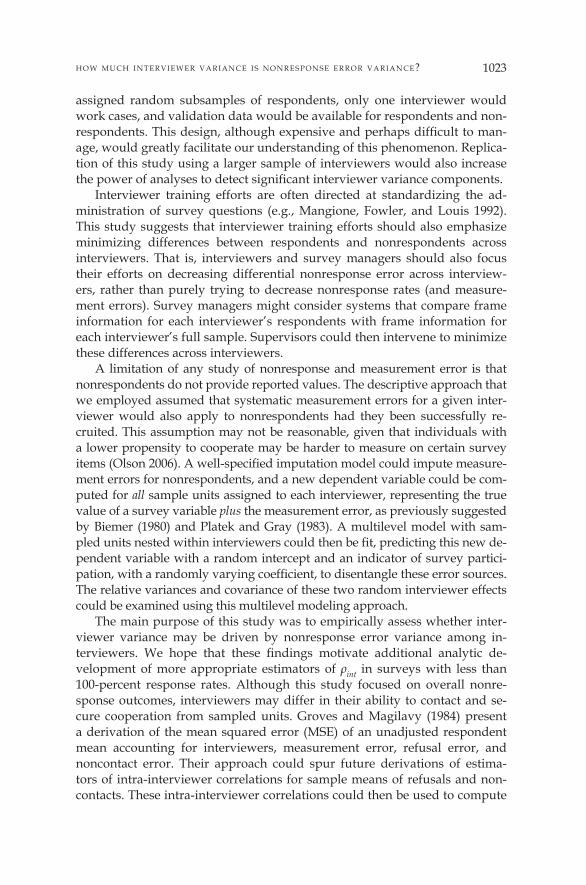
assigned random subsamples of respondents, only one interviewer would work cases, and validation data would be available for respondents and non-respondents. This design, although expensive and perhaps difficult to man-age, would greatly facilitate our understanding of this phenomenon. Replica-tion of this study using a larger sample of interviewers would also increase the power of analyses to detect significant interviewer variance components.

Interviewer training efforts are often directed at standardizing the ad-ministration of survey questions (e.g., Mangione, Fowler, and Louis 1992). This study suggests that interviewer training efforts should also emphasize minimizing differences between respondents and nonrespondents across interviewers. That is, interviewers and survey managers should also focus their efforts on decreasing differential nonresponse error across interview-ers, rather than purely trying to decrease nonresponse rates (and measure-ment errors). Survey managers might consider systems that compare frame information for each interviewer’s respondents with frame information for each interviewer’s full sample. Supervisors could then intervene to minimize these differences across interviewers.

A limitation of any study of nonresponse and measurement error is that nonrespondents do not provide reported values. The descriptive approach that we employed assumed that systematic measurement errors for a given inter-viewer would also apply to nonrespondents had they been successfully re-cruited. This assumption may not be reasonable, given that individuals with a lower propensity to cooperate may be harder to measure on certain survey items (Olson 2006). A well-specified imputation model could impute measure-ment errors for nonrespondents, and a new dependent variable could be com-puted for all sample units assigned to each interviewer, representing the true value of a survey variable plus the measurement error, as previously suggested by Biemer (1980) and Platek and Gray (1983). A multilevel model with sam-pled units nested within interviewers could then be fit, predicting this new de-pendent variable with a random intercept and an indicator of survey partici-pation, with a randomly varying coefficient, to disentangle these error sources. The relative variances and covariance of these two random interviewer effects could be examined using this multilevel modeling approach.

The main purpose of this study was to empirically assess whether inter-viewer variance may be driven by nonresponse error variance among in-terviewers. We hope that these findings motivate additional analytic de-velopment of more appropriate estimators of ρint in surveys with less than 100-percent response rates. Although this study focused on overall nonre-sponse outcomes, interviewers may differ in their ability to contact and se-cure cooperation from sampled units. Groves and Magilavy (1984) present a derivation of the mean squared error (MSE) of an unadjusted respondent mean accounting for interviewers, measurement error, refusal error, and noncontact error. Their approach could spur future derivations of estima-tors of intra-interviewer correlations for sample means of refusals and non-contacts. These intra-interviewer correlations could then be used to compute


multiplicative interviewer effects on more specific variance components of the MSE, indicating where resources should be targeted for minimizing ef-fects of interviewer variance. Future methodological studies of interviewer variance should continue to consider multiple error sources that interviewers might affect based on a total survey error framework.

References

Bates, Douglas. 2009. ‘‘Assessing the Precision of Estimates of Variance Compo-nents.’’ Presentation at the Max Planck Institute for Ornithology, Seewiesen, Austria, July 21, 2009. See http://lme4.r-forge.r-project.org/slides/2009-07-21-Seewiesen/4PrecisionD.pdf

Berkhof, Johannes, and Tom A. B. Snijders. 2001. ‘‘Variance Component Testing in Multilevel Models.’’ Journal of Educational and Behavioral Statistics 26(2):133–52.

Biemer, Paul P. 1980. ‘‘A Survey Error Model Which Includes Edit and Imputation Error.’’ Proceedings of the American Statistical Association, Section on Survey Research Methods 616–21.

Biemer, Paul P., and S. Lynne Stokes. 1991. ‘‘Approaches to the Modeling of Measure-ment Error.’’ In Measurement Errors in Surveys, eds. P. P. Biemer, R. M. Groves, L. Lyberg, N. A. Mathiowetz, and S. Sudman, 487–516. New York: Wiley.

Biemer, Paul P., and Dennis Trewin. 1997. ‘‘A Review of Measurement Error Effects on the Analysis of Survey Data.’’ In Survey Measurement and Process Quality, eds. L. Lyberg, P. P. Biemer, M. Collins, E. D. de Leeuw, C. Dippo, N. Schwarz, and D. Trewin, 603–32. New York: Wiley-Interscience.

Brick, J. Michael, Pat D. Brick, Sarah Dipko, Stanley Presser, Clyde Tucker, and Yang-yang Yuan. 2007. ‘‘Cell Phone Survey Feasibility in the U.S.: Sampling and Calling Cell Numbers versus Landline Numbers.’’ Public Opinion Quarterly 71:23–39.

Campanelli, Pamela, and Colm O’Muircheartaigh. 1999. ‘‘Interviewers, Interviewer Continuity, and Panel Survey Nonresponse.’’ Journal of Official Statistics 2(3):303–14.

Campanelli, Pamela, Patrick Sturgis, and Susan Purdon. 1997. Can You Hear Me Knock-ing: An Investigation into the Impact of Interviewers on Survey Response Rates. London: SCPR.

Collins, Martin, and Bob Butcher. 1982. ‘‘Interviewer and Clustering Effects in an Atti-tude Survey.’’ Journal of the Market Research Society 25:39–58.

Crainiceanu, Ciprian M. 2008. ‘‘Likelihood Ratio Testing for Zero Variance Compo-nents in Linear Mixed Models.’’ In Random Effect and Latent Variable Model Selection, ed. D.B. Dunson, Springer Lecture Notes in Statistics, 192.

Crainiceanu, Ciprian M., and David Ruppert. 2004. ‘‘Likelihood Ratio Tests in Linear Mixed Models with One Variance Component.’’ Journal of the Royal Statistical Soci-ety, Series B 66:165–85.

Davis, Peter, and Alastair Scott. 1995. ‘‘The Effect of Interviewer Variance on Domain Comparisons.’’ Survey Methodology 21(2):99–106.

Durrant, Gabriele B., Robert M. Groves, Laura Staetsky, and Fiona Steele. 2010. ‘‘Ef-fects of Interviewer Attitudes and Behaviors on Refusal in Household Surveys.’’ Public Opinion Quarterly 74(1):1–36.

Fellegi, Ivan P. 1964. ‘‘Response Variance and Its Estimation.’’ Journal of the American Statistical Association 59:1016–41.


Greven, Sonja, Ciprian M. Crainiceanu, Helmut Kuchenhoff, and Annette Peters. 2008. ‘‘Restricted Likelihood Ratio Testing for Zero Variance Components in Linear Mixed Models.’’ Journal of Computational and Graphical Statistics 17(4):870–91.

Groves, Robert M. 2004. ‘‘Chapter 8: The Interviewer as a Source of Survey Mea-surement Error.’’ In Survey Errors and Survey Costs, 2nd ed. New York: Wiley-Interscience.

Groves, Robert M., and Mick P. Couper. 1998. Nonresponse in Household Interview Sur-veys. New York: Wiley.

Groves, Robert M., and Nancy H. Fultz. 1985. ‘‘Gender Effects among Telephone In-terviewers in a Survey of Economic Attitudes.’’ Sociological Methods and Research 14(1):31–52.

Groves, Robert M., and Robert L. Kahn. 1979. Surveys by Telephone. New York: Aca-demic Press.

Groves, Robert M., and Lou J. Magilavy. 1984. ‘‘An Experimental Measurement of To-tal Survey Error.’’ Proceedings of the Joint Statistical Meetings of the American Statisti-cal Association, Section on Survey Research Methods 698–703.

————. 1986. ‘‘Measuring and Explaining Interviewer Effects in Centralized Telephone Surveys.’’ Public Opinion Quarterly 50(2):251–66.

Groves, Robert M., Barbara C. O’Hare, Dottye Gould-Smith, Jose Benki, and Patty Ma-her. 2008. ‘‘Telephone Interviewer Voice Characteristics and the Survey Partici-pation Decision.’’ In Advances in Telephone Survey Methodology, eds. J. Lepkowski, C. Tucker, M. Brick, E. de Leeuw, L. Japec, and P.J. Lavrakas, 385–40. New York: Wiley.

Hansen, Morris H., N. WilliamHurwitz, and Max A. Bershad. 1960. ‘‘Measurement Er-rors in Censuses and Surveys.’’ Bulletin of the International Statistical Institute, 32nd Session 38(Part 2): 359–74.

Hox, Joop J., and Edith D. de Leeuw. 2002. ‘‘The Influence of Interviewers’ Attitude and Behavior on Household Survey Nonresponse: An International Comparison.’’ In Survey Nonresponse, eds. R. M. Groves, D. A. Dillman, J. L. Eltinge, and R.J.A. Lit-tle, 103–20. New York: Wiley.

Hu, S. Sean, Lina Balluz, William Garvin, andMohamed Qayad. 2009. ’’Optimizing Call Time of Day in an RDD Survey.’’ Poster presented at the 2009 Joint Statistical Meetings (Activity 284, Poster 33).

Kish, Leslie. 1962. ‘‘Studies of Interviewer Variance for Attitudinal Variables.’’ Journal of the American Statistical Association 57:92–115.

Lessler, Judith T., and William D. Kalsbeek. 1992. Nonsampling Errors in Surveys. New York: Wiley-Interscience.

Link, Michael W. 2006. ‘‘Predicting the Persistence and Performance of Newly Re-cruited Telephone Interviewers.’’ Field Methods 18(3):305–20.

Mahalanobis, Prasanta C. 1946. ‘‘Recent Experiments in Statistical Sampling in the In-dian Statistical Institute.’’ Journal of the Royal Statistical Society 109:325–78.

Mangione, Thomas W., Floyd J. Fowler, and Thomas A. Louis. 1992. ‘‘Question Char-acteristics and Interviewer Effects.’’ Journal of Official Statistics 8(3):293–307.

Mitchell, Colter. 2004. ‘‘Wisconsin Divorce Study.’’ Unpublished documentation pre-pared for second author.

Morton-Williams, Jean. 1993. Interviewer Approaches. Aldershot, UK: Dartmouth Pub-lishing Company Limited.

Oksenberg, Lois, and Charles F. Cannell. 1988. ‘‘Effects of Interviewer Vocal Charac-teristics on Nonresponse.’’ In Telephone Survey Methodology, eds. R.M. Groves, P.P.


Biemer, L. E. Lyberg, J.T. Massey, W.L. Nicholls II., and J. Waksberg, 257–69. New York: Wiley.

Olson, Kristen. 2006. ‘‘Survey Participation, Nonresponse Bias, Measurement Error Bias, and Total Bias.’’ Public Opinion Quarterly 70(5):737–58.

O’Muircheartaigh, Colm, and Pamela Campanelli. 1999. ‘‘A Multilevel Exploration of the Role of Interviewers in Survey Non-response.’’ Journal of the Royal Statistical So-ciety, Series A 162(Part 3):437–46.

————. 1998. ‘‘The Relative Impact of Interviewer Effects and Sample Design Effects on Survey Precision.’’ Journal of the Royal Statistical Society, Series A 161(1):63–77.

Patterson, H. Desmond, and Robin Thompson. 1971. ‘‘Recovery of Inter-block Infor-mation When Block Sizes Are Unequal.’’ Biometrika 58:545–54.

Pickery, Jan, and Geert Loosveldt. 2002. ‘‘A Multilevel Multinomial Analysis of Inter-viewer Effects on Various Components of Unit Nonresponse.’’ Quality and Quan-tity 36:427–37.

Platek, Richard, and Gerald B. Gray. 1983. ‘‘Imputation Methodology.’’ In Incomplete Data in Sample Surveys, eds. W.G. Madow, I. Olkin, and D.B. Rubin, 255–94. New York: Academic Press.

Schnell, Rainer, and Frauke Kreuter. 2005. ‘‘Separating Interviewer and Sampling-point Effects.’’ Journal of Official Statistics 21(3):389–410.

Self, Steven G., and Kung-Yee Liang. 1987. ‘‘Asymptotic Properties of Maximum Like-lihood Estimators and Likelihood Ratio Tests under Nonstandard Conditions.’’ Journal of the American Statistical Association 82:605.

Singer, Eleanor, and Martin R. Frankel. 1982. ‘‘Informed Consent Procedures in Tele-phone Interviews.’’ American Sociological Review 47(3):416–26.

Snijkers, Ger, Joop J. Hox, and Edith D. de Leeuw. 1999. ‘‘Interviewers’ Tactics for Fighting Survey Nonresponse.’’ Journal of Official Statistics 15:185–98.

Stokes, S. Lynne, and Ming-Yih Yeh. 1988. ‘‘Searching for Causes of Interviewer Ef-fects in Telephone Surveys.’’ In Telephone Survey Methodology, eds. R. M. Groves, Paul P. Biemer, Lars E. Lyberg, James T. Massey, William L. Nicholls II, and Joseph Waksberg, 357–73. New York: John Wiley and Sons.

Stram, Daniel O., and Jae Won Lee. 1994. ‘‘Variance Components Testing in the Longi-tudinal Mixed-effects Model (Corr: 95V51, p. 1196).’’ Biometrics 50:1171.

U.S. Bureau of the Census. 1985. Evaluating Censuses of Population and Housing, ST-DISP-TR-5. Washington, DC: U.S. Government Printing Office.

Weeks, Michael F., Richard A. Kulka, and Stephanie A. Pierson. 1987. ‘‘Optimal Call Scheduling for a Telephone Survey.’’ Public Opinion Quarterly 51:540–49.

West, Brady T., Kathleen B. Welch, and Andrzej T. Galecki. 2007. Linear Mixed Mod-els: A Practical Guide Using Statistical Software. Boca Raton, FL: Chapman and Hall/CRC Press.

Wiggins, Richard D., Nicholas T. Longford, and Colm A. O’Muircheartaigh. 1992. ‘‘A Variance Components Approach to Interviewer Effects.’’ In Survey and Statistical Computing, eds. A. Westlake, R. Banks, C. Payne, and T. Orchard, 243–54. Amster-dam: North-Holland.

Zhang, Daowen, and Xihong Lin. 2008. ‘‘Variance Component Testing in Generalized Linear Mixed Models for Longitudinal/Clustered Data and Other Related Topics.’’ In Random Effect and Latent Variable Model Selection, eds. D. B. Dunson, Springer Lecture Notes in Statistics, 192.

How Much of Interviewer Variance Is Really Nonresponse Error Variance?

Documents

Transcript of How Much of Interviewer Variance Is Really Nonresponse Error Variance?