Variance measurements - Practical use - Statistics

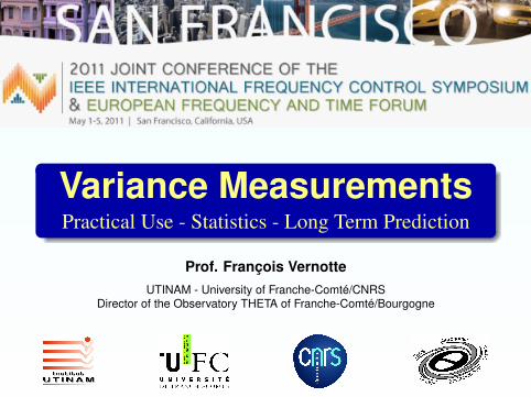
Variance MeasurementsPractical Use - Statistics - Long Term Prediction

Prof. François VernotteUTINAM - University of Franche-Comté/CNRS

Director of the Observatory THETA of Franche-Comté/Bourgogne

IntroductionPractical use of the Allan variance

Statistics of the Allan variance and the Allan deviationPrediction of very long term time stability

Outline

1 Introduction

2 Practical use of the Allan variance

3 Statistics of the Allan variance and the Allan deviation

4 Prediction of very long term time stability

F. Vernotte Variance measurements 2



Notations in the time domainNotations in the frequency domainNoise model

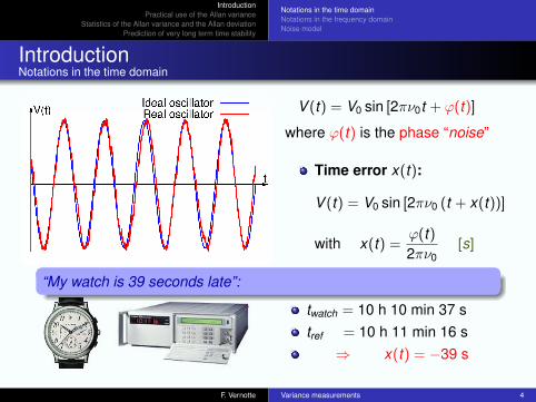
IntroductionNotations in the time domain

V (t) = V0 sin [2πν0t + ϕ(t)]

where ϕ(t) is the phase “noise”

Time error x(t):

V (t) = V0 sin [2πν0 (t + x(t))]

with x(t) =ϕ(t)2πν0

[s]

“My watch is 39 seconds late”:

twatch = 10 h 10 min 37 stref = 10 h 11 min 16 s

⇒ x(t) = −39 s





Frequency noise

V (t) = V0sin [2πν0t + ϕ(t)]

Instantaneous frequency ν(t):

V (t) = V0 sin [2πν(t)]

with ν(t) =1

2πd [2πν0t + ϕ(t)]

dt= ν0 +

12π

dϕ(t)dt

[Hz]

Frequency noise ∆ν(t):

∆ν(t) =1

2πdϕ(t)

dt[Hz]

Frequency deviation y(t):

y(t) =∆ν(t)ν0

=1

2πν0

dϕ(t)dt

[dimensionless]





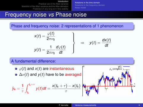
Frequency noise vs Phase noise

Phase and frequency noise: 2 representations of 1 phenomenon

x(t) =ϕ(t)2πν0

y(t) =1

2πν0

dϕ(t)dt

⇒ y(t) =dx(t)

dt

A fundamental difference:

ϕ(t) and x(t) are instantaneous∆ν(t) and y(t) have to be averaged

yk =1τ

∫ tk+τ

tky(t)dt =

x(tk + τ)− x(tk )

τ





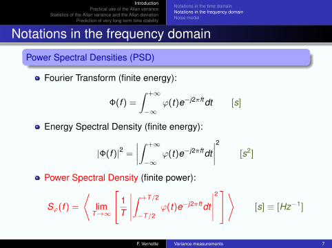
Notations in the frequency domain

Power Spectral Densities (PSD)

Fourier Transform (finite energy):

Φ(f ) =

∫ +∞

−∞ϕ(t)e−j2πftdt [s]

Energy Spectral Density (finite energy):

|Φ(f )|2 =

∣∣∣∣∫ +∞

−∞ϕ(t)e−j2πftdt

∣∣∣∣2 [s2]

Power Spectral Density (finite power):

Sϕ(f ) =

⟨lim

T→∞

1T

∣∣∣∣∣∫ +T/2

−T/2ϕ(t)e−j2πftdt

∣∣∣∣∣2⟩ [s] ≡ [Hz−1]





Relationships between PSD

Time error PSD: Sx (f )

x(t) =ϕ(t)2πν0

⇒ Sx (f ) =1

4π2ν20

Sϕ(f )

Dimension: [s3] ≡ [Hz−3]

Frequency deviation PSD: Sy (f )

y(t) =1

2πν0

dϕ(t)dt

⇒ Sy (f ) =f 2

ν20

Sϕ(f )

y(t) =dx(t)

dt⇒ Sy (f ) = 4π2f 2Sx (f )

Dimension: [s] ≡ [Hz−1]





Noise model

The power law noise model

Sy (f ) =+2∑

α=−2

hαfα α integer

Sy (f ) Sϕ(f ) Noise type Originh−2f−2 b−4f−4 Random Walk Freq. Mod. Environmenth−1f−1 b−3f−3 Flicker F.M. Resonator

h0 b−2f−2 White F.M. Thermal noiseh1f b−1f−1 Flicker Phase Mod. Electronic noiseh2f 2 b0 White P.M. External white noise





White FM vs Random Walk FM

White FM

RandomWalk FM




A statistical estimator as well as a spectral analysis toolPractical calculation of the Allan varianceAllan variance versus Allan deviation

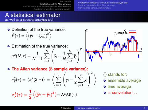
A statistical estimatoras well as a spectral analysis tool

Definition of the true variance:I2(τ) =

⟨(yk − 〈yk 〉)2

⟩Estimation of the true variance:

σ2(N, τ) =1

N − 1

N∑i=1

yi −1N

N∑j=1

yj

2

The Allan variance (2-sample variance):

σ2y (τ) =

⟨σ2(2, τ)

⟩=

⟨2∑

i=1

yi −12

2∑j=1

yj

2⟩

σ2y (τ ) =

12

⟨(y2 − y1)2

⟩= AVAR(τ)

⟨⟩stands for:ensemble averagetime average≡ convolution. . .





A spectral analysis toolas well as a statistical estimator

Convolution in the time domain. . .

σ2y (τ) =

⟨[∫ +∞

−∞y(t)hy (tk − t)dt

]2⟩

with

hy (t) =

−1√2τ

if −τ ≥ t < 0

hy (t) =+1√2τ

if 0 ≥ t < τ

hy (t) = 0 else

. . . filtering in the frequency domain

σ2y (τ) =

∫ ∞0

Sy (f ) |Hy (f )|2 df

with |Hy (f )|2 = |FT [hy (t)]|2 = 2sin4(πτ f )

(πτ f )2





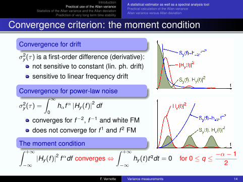
Convergence criterion: the moment condition

Convergence for drift

σ2y (τ) is a first-order difference (derivative):

not sensitive to constant (lin. ph. drift)sensitive to linear frequency drift

Convergence for power-law noise

σ2y (τ) =

∫ ∞0

hαfα |Hy (f )|2 df

converges for f−2, f−1 and white FMdoes not converge for f 1 and f 2 FM

The moment condition∫ +∞

−∞|Hy (f )|2 fαdf converges⇔

∫ +∞

−∞hy (t)tqdt = 0 for 0 ≤ q ≤ −α− 1

2





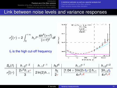
Link between noise levels and variance responses

σ2y (τ) = 2

∫ +∞

0hαfα

sin4(πτ f )

(πτ f )2 df

fh is the high cut-off frequency

Sy (f ) h−2f−2 h−1f−1 h0f 0 h+1f+1 h+2f+2

σ2y (τ)

2π2h−2τ

32 ln(2)h−1

h0

2τ[1.04 + 3 ln(2πfhτ)] h+1

4π2τ23h+2fh4π2τ2





Practical calculation of the Allan varianceCalculation from time error samples

Calculation from frequency deviation

σ2y (τ) =

12

⟨(y2 − y1)2

⟩=⟨

[y(t) ∗ hy (t)]2⟩

σ2y (τ) =

∫ ∞0

Sy (f ) |Hy (f )|2 df

Calculation from time error samples

σ2y (τ) =

∫ ∞0

Sx (f ) |j2πfHy (f )|2 df

=⟨

[x(t) ∗ hx (t)]2⟩

with hx (t) =dhy (t)

dt

σ2y (τ) =

12

⟨(y2 − y1)2

⟩=

12τ

⟨[x(t + τ)− 2x(t) + x(t − τ)]2

⟩F. Vernotte Variance measurements 16




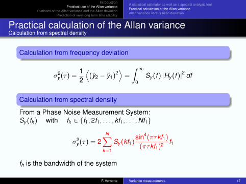
Practical calculation of the Allan varianceCalculation from spectral density

Calculation from frequency deviation

σ2y (τ) =

12

⟨(y2 − y1)2

⟩=

∫ ∞0

Sy (f ) |Hy (f )|2 df

Calculation from spectral density

From a Phase Noise Measurement System:Sy (fk ) with fk ∈ {f1,2f1, . . . , kf1, . . . ,Nf1}

σ2y (τ) = 2

N∑k=1

Sy (kf1)sin4(πτkf1)

(πτkf1)2 f1

fh is the bandwidth of the system





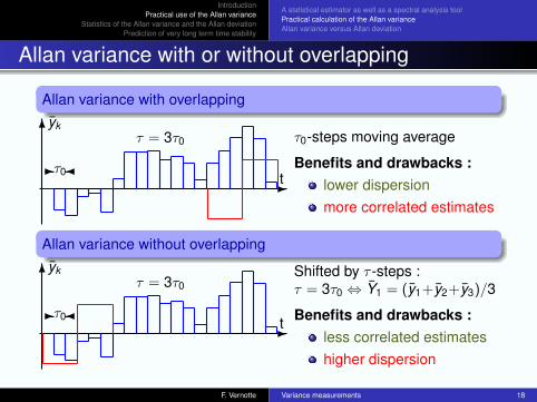
Allan variance with or without overlapping

Allan variance with overlapping

t-

yk6τ = 3τ0

- �τ0

τ0-steps moving average

Benefits and drawbacks :lower dispersionmore correlated estimates

Allan variance without overlapping

t-

yk6τ = 3τ0

- �τ0

Shifted by τ -steps :τ = 3τ0 ⇔ Y1 = (y1+y2+y3)/3

Benefits and drawbacks :less correlated estimateshigher dispersion





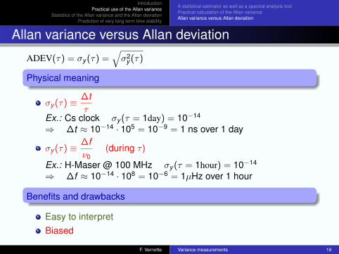
Allan variance versus Allan deviation

ADEV(τ) = σy (τ) =√σ2

y (τ)

Physical meaning

σy (τ) ≡ ∆tτ

Ex.: Cs clock σy (τ = 1day) = 10−14

⇒ ∆t ≈ 10−14 · 105 = 10−9 = 1 ns over 1 day

σy (τ) ≡ ∆fν0

(during τ )

Ex.: H-Maser @ 100 MHz σy (τ = 1hour) = 10−14

⇒ ∆f ≈ 10−14 · 108 = 10−6 = 1µHz over 1 hour

Benefits and drawbacks

Easy to interpretBiased




Chi-square and Equivalent Degrees of FreedomConfidence interval over the Allan variance/deviation measuresParameter estimationIncreasing the number of edf: the Total variance

Chi-squared and Rayleigh distribution

Allan variance: σ2y (τ) =

12

⟨(y2 − y1)2

⟩Estimate: σ2

y (τ) =1

2N

N∑i=1

(y2 − y1)2

y2 − y1: Gaussian centered values

(y2 − y1)2: χ21 distribution

12N

N∑i=1

(y2 − y1)2: χ2N distribution

Allan deviation: σy (τ) =

√12

⟨(y2 − y1)2

⟩Estimate: σy (τ) =

√√√√ 12N

N∑i=1

(y2 − y1)2 ⇒ χN distributed (Rayleigh)

N is the number of Equivalent Degrees of Freedom (EDF)F. Vernotte Variance measurements 21




Reminder of the Equivalent Degrees of Freedom

Meaning of the EDF

Mean(χ2ν) = ν and Variance(χ2

ν) = 2νThe EDF ν contains the information about the dispersion of therandom variable χ2

ν

Estimation of the EDF

σ2y (τ) =

12N

N∑i=1

(y2 − y1)2 ⇒ χ2N if {y1, y2, . . .} uncorrelated!

False:for low frequency noises (flicker and random walk FM)with overlapping variances

Algorithm for estimating the EDF:C. Greenhall and W. Riley, 2003, “Uncertainty of StabilityVariances Based on Finite Differences” (35th PTTI).Used in Stable 32 as well as in SigmaTheta.





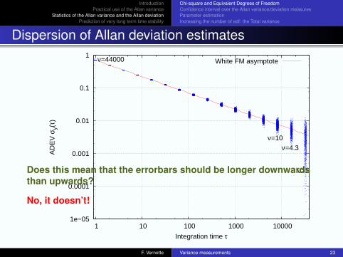
Dispersion of Allan deviation estimates

1e−05

0.0001

0.001

0.01

0.1

1

1 10 100 1000 10000

AD

EV

σy(

τ)

Integration time τ

ν=1

ν=4.3ν=10

ν=44000 White FM asymptote

Does this mean that the errorbars should be longer downwardsthan upwards?

No, it doesn’t!





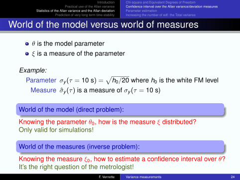
World of the model versus world of measures

θ is the model parameterξ is a measure of the parameter

Example:Parameter σy (τ = 10 s) =

√h0/20 where h0 is the white FM level

Measure σy (τ) is a measure of σy (τ = 10 s)

World of the model (direct problem):

Knowing the parameter θ0, how is the measure ξ distributed?Only valid for simulations!

World of the measures (inverse problem):

Knowing the measure ξ0, how to estimate a confidence interval over θ?It’s the right question of the metrologist!





Model parameter and measure for a χ2 distribution

0.0001

0.001

0.01

0.1

1

10

100

1000

10000

0.1 1 10 100 1000

Mea

sure

ξ

Parameter θ

0.9521.05

Let us fix the measure to ξ0 = 1± 5 %. . .





Model parameter values for a measure ξ0 ≈ 1Theoretical results versus 20,000 simulations

0.94

0.96

0.98

1

1.02

1.04

1.06

0.1 1 10 100 1000

Mea

sure

ξ

Parameter θ

2.5 % 2.5 %95 %

0.521 6.28

<θ> = 1.77

e<ln(θ)> = 1.33

The errorbars should be shorter downward than upward!





Study of a χ distribution with 2 degrees of freedomDirect problem

Probability density function: p(χ) = χe−χ2/2

The pdf is normalized:∫ ∞

0p(χ)dχ = 1

Mathematical expectation: µ =

∫ ∞0

χ · p(χ)dχ =

√π

2

Cumulative distribution function: P(χ) =

∫ χ

0p(y)dy = 1− e−χ

2/2

Inverse cdf: P−1(α) =√−2 ln(1− α)





Confidence Interval of a χ2 random variable

{. . . χi . . .} is a set of realizations of the random variable χP−1(0.025) ≈ 0.22502⇒ χi < 0.22502 with 2.5% confidence

P−1(0.975) ≈ 2.7162⇒ χi < 2.7162 with 97.5% confidence

Confidence Interval:E(χ) ≈ 1.25330.22502 < χi < 2.7162 with 95% confidence

General case of a random variable x = k · χ

Estimation of the scale factor: k =E(x)E(χ)

≈ < x >µ

⇒ 0.22502 · k < xi < 2.7162 · k with 95% confidence





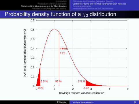
Probability density function of a χ2 distribution

0

0.1

0.2

0.3

0.4

0.5

0.6

0.7

0 1 2 3 4 5

PD

F o

f a R

ayle

igh

dist

ribut

ion

with

ν=

2

Rayleigh random variable realization

mean

1.25

2.5 %

0.23

2.5 %

2.72

95 %





Conditionnal probabilitiesReduced variable (I)

Let us consider the standard χ22 variable: χ2

2 = X 21 + X 2

2where X1 and X2 are 2 Gaussian centered standard randomvariables

⇒ E(χ22) = 2 ⇒ E

(12χ2

2

)= 1.

We assume that σ2y (τ) = ξ2 is χ2

2 distributed and is an unbiasedestimator of the parameter σ2

y (τ) = θ2:

E(ξ2

θ2

)= 1.

We can then define the reduced variable χ22 as:

χ22 = 2

ξ

θ.





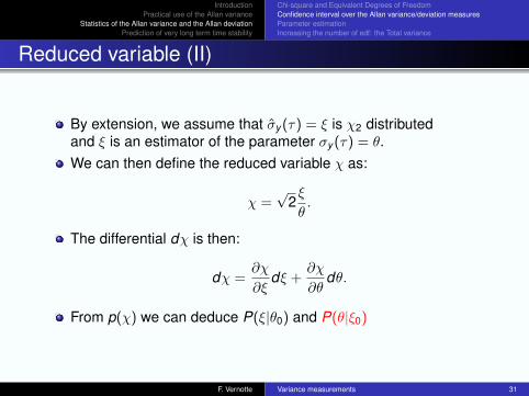
Reduced variable (II)

By extension, we assume that σy (τ) = ξ is χ2 distributedand ξ is an estimator of the parameter σy (τ) = θ.We can then define the reduced variable χ as:

χ =√

2ξ

θ.

The differential dχ is then:

dχ =∂χ

∂ξdξ +

∂χ

∂θdθ.

From p(χ) we can deduce P(ξ|θ0) and P(θ|ξ0)





Parameter estimation from a single measureUsual frequentist reasonning

We assume that the measure ξ represents the estimate σy (τ) and theparameter θ stands for the real unknown value σy (τ).

Reduced variable: χ =√

2ξ/θLow bound: B2.5% ≈ 0.22502High bound: B97.5% ≈ 2.716295 % confidence interval: 0.22502 <

√2ξ/θ < 2.7162

Frequentist reversal:√

2ξ0

2.7162< θ <

√2ξ0

0.22502@ 95 %

⇒ 0.52066 · ξ0 < θ < 6.2847 · ξ0 with 95 % confidence.

We obtain directly the same result from P(θ|ξ0) (as well as from theBayesian method with a total lack of knowledge prior).





Generalization to a χν distribution

Reduced variable: χ =√νξ

θ

pdf: p(χ) =21−ν/2χν−1e−χ

2/2

Γ(ν/2)

Mathematical expectation: µν =√

2Γ(ν+1

2

)Γ(ν2 )

cdf: P(χ) = Γ

(ν

2,χ2

2

)





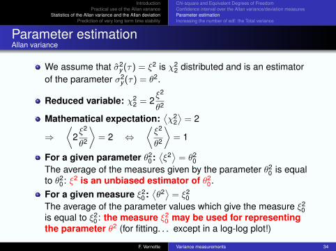
Parameter estimationAllan variance

We assume that σ2y (τ) = ξ2 is χ2

2 distributed and is an estimatorof the parameter σ2

y (τ) = θ2.

Reduced variable: χ22 = 2

ξ2

θ2

Mathematical expectation:⟨χ2

2

⟩= 2

⇒⟨

2ξ2

θ2

⟩= 2 ⇔

⟨ξ2

θ2

⟩= 1

For a given parameter θ20:⟨ξ2⟩

= θ20

The average of the measures given by the parameter θ20 is equal

to θ20: ξ2 is an unbiased estimator of θ2

0.For a given measure ξ2

0:⟨θ2⟩

= ξ20

The average of the parameter values which give the measure ξ20

is equal to ξ20 : the measure ξ2

0 may be used for representingthe parameter θ2 (for fitting. . . except in a log-log plot!)





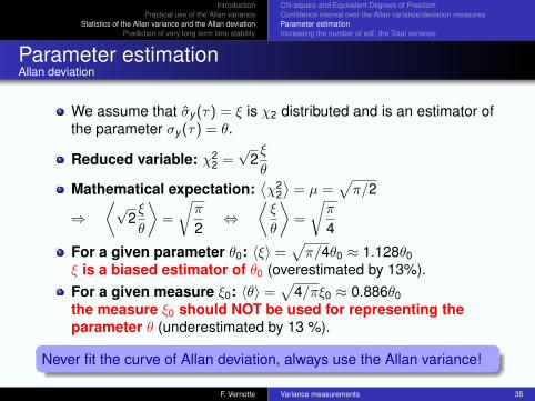
Parameter estimationAllan deviation

We assume that σy (τ) = ξ is χ2 distributed and is an estimator ofthe parameter σy (τ) = θ.

Reduced variable: χ22 =√

2ξ

θ

Mathematical expectation:⟨χ2

2

⟩= µ =

√π/2

⇒⟨√

2ξ

θ

⟩=

√π

2⇔

⟨ξ

θ

⟩=

√π

4

For a given parameter θ0: 〈ξ〉 =√π/4θ0 ≈ 1.128θ0

ξ is a biased estimator of θ0 (overestimated by 13%).For a given measure ξ0: 〈θ〉 =

√4/πξ0 ≈ 0.886θ0

the measure ξ0 should NOT be used for representing theparameter θ (underestimated by 13 %).

Never fit the curve of Allan deviation, always use the Allan variance!





Increasing the number of edf: the Total variance

The longer the time du-ration, the larger theuncertainty.

What about very longterm stability ?

In order to improve estimates for very long term, D. Howe developed:Total variance: UFFC-47(5), 1102-1110 (2000)

Theo: Metrologia 43, S322-S331 (2006)




Fitting curve over variance measurementEstimation of the noise levels from the fitting curveExtrapolation to very long term time stability

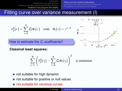
Fitting curve over variance measurement (I)

σ2y (τ) =

4∑i=0

Ci Φi (τ) with Φi (τ) = τ i−2

How to estimate the Ci coefficients?

Classical least squares:

N∑j=1

(σ2

y (τj )−4∑

i=0

Ci Φi (τj )

)2

is minimum

not suitable for high dynamicnot suitable for positive or null valuesnot suitable for variance curves





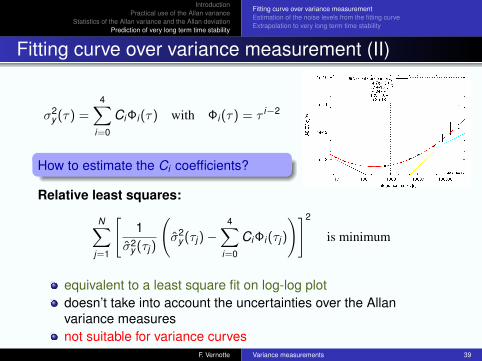
Fitting curve over variance measurement (II)

σ2y (τ) =

4∑i=0



Relative least squares:

N∑j=1

[1

σ2y (τj )

(σ2

y (τj )−4∑

i=0

Ci Φi (τj )

)]2

is minimum

equivalent to a least square fit on log-log plotdoesn’t take into account the uncertainties over the Allanvariance measuresnot suitable for variance curves





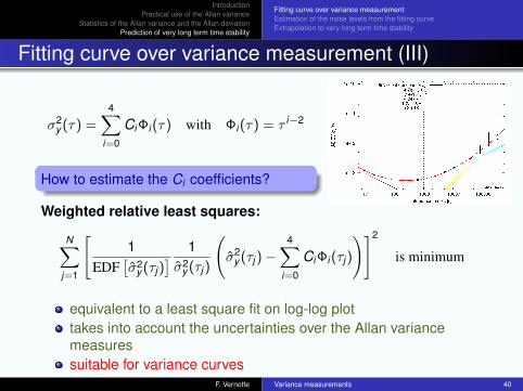
Fitting curve over variance measurement (III)

σ2y (τ) =

4∑i=0



Weighted relative least squares:

N∑j=1

[1

EDF[σ2

y (τj )] 1σ2

y (τj )

(σ2

y (τj )−4∑

i=0

Ci Φi (τj )

)]2

is minimum

equivalent to a least square fit on log-log plottakes into account the uncertainties over the Allan variancemeasuressuitable for variance curves





Estimation of the noise levels from the fitting curve

σ2y (τ) =

4∑i=0


C0τ−2 White or Flicker PM: h+2 =

4π2C0

3fhor h+1 ≈ 4π2C0

C1τ−1 White FM: h0 = 2C1

C2τ0 Flicker FM: h−1 =

C2

2 ln(2)

C3τ Random Walk FM: h−2 =3C3

2π2

C4τ2 Linear frequency drift: D1 =

√2C4

Uncertainties ∆hα ? See Vernotte et al., IM-42(2), 342-350 (1993)





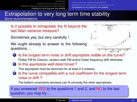
Extrapolation to very long term time stabilitySome recommendations

Is it possible to extrapolate the fit beyond thelast Allan variance measure?

Sometimes yes, but very carefully !

We ought already to answer to the followingquestions. . .

1 Is the longest term noise or drift asymptote visible on the curve?Flicker FM for Cesium, random walk FM and/or linear frequency drift otherwise

2 Is this asymptote well determined ?This asymptote must be dominant for at least 2-3 octaves

3 Is the curve compatible with a null coefficient for the longest termnoise or drift ?The bottom uncertainty domains can fit correctly the other asymptotes

If you answered YES to the questions 1 and 2, and NO to the lastquestion, you may try. . .


Variance measurements - Practical use - Statistics

Documents

Transcript of Variance measurements - Practical use - Statistics