arX

iv:1

109.

5587

v1 [

mat

h.ST

] 2

6 Se

p 20

11Submitted to the Statistical Science

High-dimensional regressionwith unknown varianceChristophe Giraud, Sylvie Huet and Nicolas Verzelen

Ecole Polytechnique and Institut National de Recherche en Agronomie

AbstractWe review recent results for high-dimensional sparse linear re-gression in the practical case of unknown variance. Different sparsitysettings are covered, including coordinate-sparsity, group-sparsity andvariation-sparsity. The emphasize is put on non-asymptotic analysesand feasible procedures. In addition, a small numerical study comparesthe practical performance of three schemes for tuning the Lasso esti-mator and some references are collected for some more general models,including multivariate regression and nonparametric regression.

AMS 2000 subject classifications: 62J05, 62J07, 62G08, 62H12.Key words and phrases: linear regression, high-dimension, unknownvariance.

1. INTRODUCTION

In the present paper, we mainly focus on the linear regression model

Y = Xβ0 + ε ,(1)

where Y is a n-dimensional response vector, X is a fixed n × p design matrix,and the vector ε is made of n i.i.d Gaussian random variables with N (0, σ2)distribution. In the sequel, X(i) stands for the i-th row of X. Our interest is onthe high-dimensional setting, where the dimension p of the unknown parameterβ0 is large, possibly larger than n.

The analysis of the high-dimensional linear regression model has attracteda lot of attention in the last decade. Nevertheless, there is a longstanding gapbetween the theory where the variance σ2 is generally assumed to be known andthe practice where it is often unknown. The present paper is mainly devotedto review recent results on linear regression in high-dimensional settings withunknown variance σ2. A few additional results for multivariate regression andthe nonparametric regression model

(2) Yi = f(X(i)) + εi, i = 1, . . . , n ,

will also be mentioned.

CMAP, UMR CNRS 7641, Ecole Polytechnique, Route de Saclay, 91128Palaiseau Cedex, FRANCE. (e-mail: christophe.giraud@polytechnique.edu)UR341 MIA, INRA, F-78350 Jouy-en-Josas, FRANCE (e-mail:sylvie.huet@jouy.inra.fr) UMR729 MISTEA, INRA, F-34060 Montpellier,FRANCE Montpellier (e-mail: nicolas.verzelen@supagro.inra.fr)

1

2 GIRAUD, HUET AND VERZELEN

1.1 Sparsity assumptions

In a high-dimensional linear regression model, accurate estimation is unfeasibleunless it relies on some special properties of the parameter β0. The most commonassumption on β0 is that it is sparse in some sense. We will consider in this paperthe three following classical sparsity assumptions.

Coordinate-sparsity. Most of the coordinates of β0 are assumed to be zero (orapproximately zero). This is the most common acceptation for sparsity in linearregression.

Structured-sparsity. The pattern of zero(s) of the coordinates of β0 is assumedto have an a priori known structure. For instance, in group-sparsity [69], thecovariates are clustered intoM groups and when the coefficient β0,i correspondingto the covariate Xi (the i-th column of X) is non-zero, then it is likely that allthe coefficients β0,j with variables Xj in the same cluster as Xi are non-zero.

Variation-sparsity. The p− 1-dimensional vector βV0 of variation of β0 is defined

by βV0,j = β0,j+1 − β0,j . Sparsity in variation means that most of the components

of βV0 are equal to zero (or approximately zero). When p = n and X = In,

variation-sparse linear regression corresponds to signal segmentation.

1.2 Statistical objectives

In the linear regression model, there are roughly two kinds of estimation objec-tives. In the prediction problem, the goal is to estimateXβ0, whereas in the inverseproblem it is to estimate β0. When the vector β0 is sparse, a related objective isto estimate the support of β0 (model identification problem) which is the set ofthe indices j corresponding to the non zero coefficients β0,j . Inverse problems andprediction problems are not equivalent in general. When the Gram matrix XX

∗

is poorly conditioned, the former problems can be much more difficult than thelatter. Since there are only a few results on inverse problems with unknown vari-ance, we will focus on the prediction problem, the support estimation problembeing shortly discussed in the course of the paper.

In the sequel, Eβ0[.] stands for the expectation with respect to Y ∼ N (Xβ0, σ

2In)and ‖.‖2 is the euclidean norm. The prediction objective amounts to build esti-mators β so that the risk

(3) R[β;β0] := Eβ0[‖X(β − β0)‖22]

is as small as possible.

1.3 Approaches

Most procedures that handle high dimensional linear models [20, 23, 53, 62,63, 70, 72, 74] rely on tuning parameters, whose optimal value depends on σ.For example, Bickel et al. [15] state that under some assumptions on X, thetuning parameter λ of the Lasso should be chosen of the order of σ

√2 log(p).

As a consequence, all these procedures cannot be directly applied when σ2 isunknown.

A straightforward approach is to replace σ2 by an estimate of the variancein the optimal value of the tuning parameter(s). Nevertheless, the variance σ2 isdifficult to estimate in high-dimensional settings, so a plug-in of the variance does

REGRESSION WITH UNKNOWN VARIANCE 3

not necessarily yield good results. There are basically two approaches to build onthis amount of work on high dimensional estimation with known variance.

1. Ad-hoc estimation. There has been some recent work [14, 58, 61] to modifyprocedures like the Lasso in such a way that the tuning parameter doesnot depend anymore on σ2 (see Section 4.2). The challenge is to find asmart modification of the procedure, so that the resulting estimator β is

computationally feasible and with a risk R[β;β0

]as small as possible.

2. Estimator selection. Given a collection (βλ)λ∈Λ of estimators, the objectiveof estimator selection is to pick an index λ such that the risk of β

λis as

small as possible; ideally as small as the risk R[βλ∗ ;β0] of the so-calledoracle estimator

(4) βλ∗ := argmin{βλ, λ∈Λ}

R[βλ;β0

].

Efficient estimator selection procedures can then be applied to tune theaforementioned estimation methods [20, 23, 53, 62, 63, 70, 72, 74]. Amongthe most famous methods for estimator selection, we mention V -fold cross-validation (Geisser [29]), AIC (Akaike [1]) and BIC (Schwartz [54]) criteria.

The objective of this survey is to describe state-of-the-art procedures for high-dimensional linear regression with unknown variance. We will review both au-tomatic tuning methods and ad-hoc methods. There are some procedures thatwe will let aside. For example, Baraud [9] provides a versatile estimator selectionscheme, but the procedure is computationally intractable in large dimensions. Lin-ear or convex aggregation of estimators are also valuable alternatives to estimatorselection when the goal is to perform estimation, but only a few theoretical workshave addressed the aggregation problem when the variance is unknown [32, 30].For these reasons, we will not review these approaches in the sequel.

1.4 Why care on non-asymptotic analyses ?

AIC [1], BIC [54] and V -fold Cross-Validation [29] are probably the most popu-lar criteria for estimator selection. The use of these criteria relies on some classicalasymptotic optimality results. These results focus on the setting where the collec-tion of estimators (βλ)λ∈Λ and the dimension p are fixed and consider the limitbehavior of the criteria when the sample size n goes to infinity. For example,under some suitable conditions, Shibata [57], Li [44] and Shao [56] prove that therisk of the estimator selected by AIC or V -fold CV (with V = Vn → ∞) is asymp-totically equivalent to the oracle risk R[βλ∗ ;β0]. Similarly, Nishii [50] shows thatthe BIC criterion is consistent for model selection.

All these asymptotic results can lead to misleading conclusion in modern sta-tistical settings where the sample size remains small and the parameters dimen-sion becomes large. For instance it is proved in [10, Sect.3.3.2] and illustratedin [10, Sect.6.2] that BIC (and thus AIC) can strongly overfit and should not beused for p larger than n. Additional examples are provided in the appendix. Anon-asymptotic analysis takes into account all the characteristics of the selectionproblem (sample size n, parameter dimension p, number of models per dimen-sion, etc). It treats n and p as they are and it avoids to miss important features

4 GIRAUD, HUET AND VERZELEN

hidden in asymptotic limits. For these reasons, we will restrict in this review onnon-asymptotic results.

1.5 Organization of the paper

In Section 2, we investigate how the ignorance of the variance affects the min-imax risk bounds. In Section 3, some ”generic” estimators selection schemes arepresented. The coordinate-sparse setting is addressed Section 4 : some theoreticalresults are collected and a small numerical experiment compares different Lasso-based procedures. The group-sparse and variation-sparse settings are reviewed inSection 5 and 6, and Section 7 is devoted to some more general models such asmultivariate regression or nonparametric regression.

In the sequel, C, C1,. . . refer to numerical constants, while ‖β‖0 stands for thenumber of non zero components of β and |J | for the cardinality of a set J .

2. THEORETICAL LIMITS

The goal of this section is to address the intrinsic difficulty of a coordinate-sparse linear regression problem. We will answer the following questions: Whichrange of p can we reasonably consider? When the variance is unknown, can wehope to do as well as when the variance is known?

2.1 Minimax adaptation

A classical way to assess the performance of an estimator β is to measure itsmaximal risk over a class B ⊂ R

p. This is the minimax point of view. As weare interested in coordinate-sparsity for β0, we will consider the sets B[k, p] ofvectors that contain at most k non zero coordinates for some k > 0.

Given an estimator β, the maximal prediction risk of β over B[k, p] for a fixeddesign X and a variance σ2 is defined by supβ0∈B[k,p]R[β;β0]/σ

2 where the riskfunction R[., β0] is defined by (3). Taking the infimum of the maximal risk overall possible estimators β, we obtain the minimax risk

(5) R[k,X] = infβ

supβ0∈B[k,p]

R[β;β0]

σ2.

Minimax bounds are convenient results to assess the range of problems that arestatistically feasible and the optimality of particular procedures. Below, we saythat an estimator β is ”minimax” over B[k, p] if its maximal prediction risk isclose to the minimax risk.

In practice, the number of non-zero coordinates of β0 is unknown. The factthat an estimator β is minimax over B[k, p] for some specific k > 0 does notimply that β estimates well vectors β0 that are less sparse. A good estimationprocedure β should not require the knowledge of the sparsity k of β0 and shouldperform as well as if this sparsity were known. An estimator β that nearly achievesthe minimax risk over B[k, p] for a range of k is said to be adaptive to thesparsity. Similarly, an estimator β is adaptive to the variance σ2, if it does notrequire the knowledge of σ2 and nearly achieves the minimax risk for all σ2 > 0.When possible, the main challenge is to build adaptive procedures. For somestatistical problems, adaptation is in fact impossible and there is an unavoidableloss when the variance or the sparsity parameter is unknown. In such situations,it is interesting to quantify this loss.

REGRESSION WITH UNKNOWN VARIANCE 5

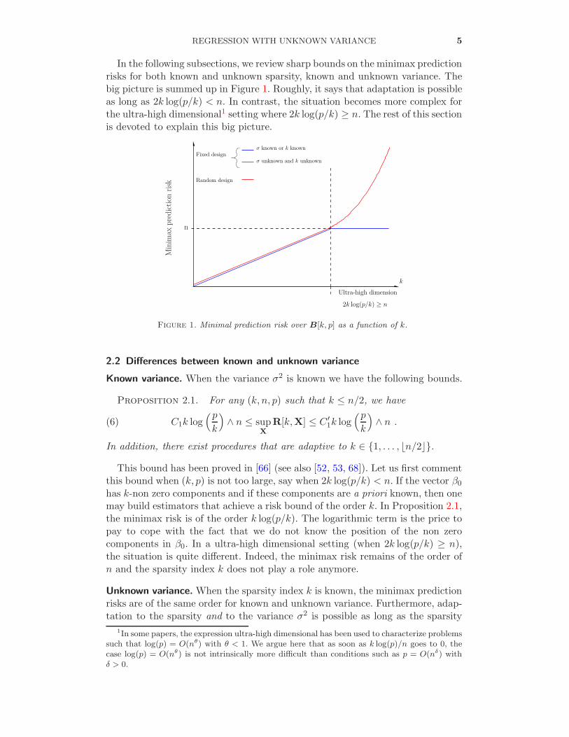
In the following subsections, we review sharp bounds on the minimax predictionrisks for both known and unknown sparsity, known and unknown variance. Thebig picture is summed up in Figure 1. Roughly, it says that adaptation is possibleas long as 2k log(p/k) < n. In contrast, the situation becomes more complex forthe ultra-high dimensional1 setting where 2k log(p/k) ≥ n. The rest of this sectionis devoted to explain this big picture.

Fixed design

Random design

Ultra-high dimension

k

σ known or k known

σ unknown and k unknown

2k log(p/k) ≥ n

Minim

axpredictionrisk

n

Figure 1. Minimal prediction risk over B[k, p] as a function of k.

2.2 Differences between known and unknown variance

Known variance. When the variance σ2 is known we have the following bounds.

Proposition 2.1. For any (k, n, p) such that k ≤ n/2, we have

(6) C1k log(pk

)∧ n ≤ sup

X

R[k,X] ≤ C ′1k log

(pk

)∧ n .

In addition, there exist procedures that are adaptive to k ∈ {1, . . . , ⌊n/2⌋}.

This bound has been proved in [66] (see also [52, 53, 68]). Let us first commentthis bound when (k, p) is not too large, say when 2k log(p/k) < n. If the vector β0has k-non zero components and if these components are a priori known, then onemay build estimators that achieve a risk bound of the order k. In Proposition 2.1,the minimax risk is of the order k log(p/k). The logarithmic term is the price topay to cope with the fact that we do not know the position of the non zerocomponents in β0. In a ultra-high dimensional setting (when 2k log(p/k) ≥ n),the situation is quite different. Indeed, the minimax risk remains of the order ofn and the sparsity index k does not play a role anymore.

Unknown variance. When the sparsity index k is known, the minimax predictionrisks are of the same order for known and unknown variance. Furthermore, adap-tation to the sparsity and to the variance σ2 is possible as long as the sparsity

1In some papers, the expression ultra-high dimensional has been used to characterize problemssuch that log(p) = O(nθ) with θ < 1. We argue here that as soon as k log(p)/n goes to 0, thecase log(p) = O(nθ) is not intrinsically more difficult than conditions such as p = O(nδ) withδ > 0.

6 GIRAUD, HUET AND VERZELEN

index k satisfies 2k log(p/k) ≤ n, see [66]. The situation is different in a ultra-highdimensional setting as shown in the next proposition (from [66]).

Proposition 2.2. Consider any p ≥ n ≥ C and k ≤ p1/3 ∧ n/2 such thatk log(p/k) ≥ C ′n. There exists a design X of size n×p such that for any estimatorβ, we have either

supσ2>0

R[β; 0p]

σ2> C1n , or

supβ0∈B[k,p] , σ2>0

R[β;β0]

σ2> C2k log

(pk

)exp

[C3

k

nlog

(pk

)].

As a consequence, any estimator β that does not rely on σ2 has to pay at leastone of these two prices:

1. The estimator β does not use the sparsity of the true parameter β0 and itsrisk for estimating X0p is of the same order as the minimax risk over Rn.

2. For any 1 ≤ k ≤ p1/3, the risk of β fulfills

supσ>0

supβ0∈B[k,p]

R[β;β0]

σ2≥ Ck log (p) exp

[Ck

nlog (p)

].

It follows that the maximal risk of β is blowing up in an ultra-high dimen-sional setting (red curve in Figure 1), while the minimax risk is stuck ton (blue curve in Figure 1). We conclude that adaptation to the sparsity isimpossible when the variance is unknown.

2.3 Aspects of ultra-high dimensionality

The previous results have illustrated the existence of a phase transition whenk and p are very large (2k log(p/k) ≥ n) : the prediction problem with unknownvariance and unknown sparsity becomes extremely difficult in ultra-high dimen-sional settings. Similar phenomenons occur for some other statistical problems,including the prediction problem with random design, the inverse problem (esti-mation of β0), the variable selection problem (estimation of the support of β0),the dimension reduction problem, etc [66, 67, 41]. This kind of phase transitionhas been observed in a wide range of random geometry problems [26], suggestingsome universality of this limitation.

Finally, where lie the limits of accurate high-dimensional sparse estimation?In practice, the sparsity index k is not known, but given (n, p) we can computek∗ := max{k : 2k log(p/k) ≥ n}. As a rule of thumb, one may interpret that theproblem is still reasonably difficult as long as k ≤ k∗. This gives a simple rule ofthumb to know what we can hope from a given regression problem. For example,setting p = 5000 and n = 50 leads to k∗ = 3, implying that the prediction problembecomes extremely difficult when there are more than 4 relevant covariates (seethe simulations in [66]).

2.4 What should we expect from a good estimation procedure?

Let us consider an estimator β that does not depend on σ2. In the sequel, wewill say that β achieves an optimal risk bound (with respect to the sparsity) if

(7) R[β;β0] ≤ C1‖β0‖0 log(p)σ2 ,

REGRESSION WITH UNKNOWN VARIANCE 7

for any σ > 0 and any vector β0 ∈ Rp such that ‖β0‖0 log(p) ≤ C2n. Such

risk bounds prove that the estimator is approximately (up to a possible log(k)factor) minimax adaptive to the unknown variance and the unknown sparsity innon ultra-high dimensional setting. Fast procedures such as those presented inSection 4.2 achieve this kind of bounds under some restrictive assumptions onthe design matrix X.

For some procedure, (7) can be improved into a bound of the form

(8) R[β;β0] ≤ C1 infk≤Cn/ log p

{inf

β, ‖β‖0=k‖X(β − β0)‖22 + k log(p)σ2

}.

This kind of bound makes clear a trade-off between a bias and a variance term.For instance, when β0 contains many components that are nearly equal to zero,the bound (8) can be much smaller than (7).

3. SOME GENERIC SELECTION SCHEMES

Among the selection schemes not requiring the knowledge of the variance σ2,some are very specific to a particular algorithm, while some others are moregeneric. We describe in this section three versatile selection principles and referto the examples for the more specific schemes.

3.1 Cross-Validation procedures

The cross-validation schemes are nearly universal in the sense that they can beimplemented in most statistical frameworks and for most estimation procedures.The principle of the cross-validation schemes is to split the data into a training setand a validation set : the estimators are built on the training set and the validationset is used for estimating their prediction risk. This training / validation splittingis eventually repeated several times. The most popular cross-validation schemesare :

• Hold-out [49, 24] which is based on a single split of the data for trainingand validation.

• V -fold CV [29]. The data is split into V subsamples. Each subsample is suc-cessively removed for validation, the remaining data being used for training.

• Leave-one-out [59] which corresponds to n-fold CV.• Leave-p-out (also called delete-p-CV ) [55] where every possible subset of

cardinality p of the data is removed for validation, the remaining data beingused for training.

We refer to Arlot and Celisse [6] for a review of the cross-validation schemes andtheir theoretical properties.

3.2 Penalized empirical loss

Penalized empirical loss criteria form another class of versatile selection schemes,yet less universal than CV procedures. The principle is to select among a family(βλ)λ∈Λ of estimators by minimizing a criterion of the generic form

(9) Crit(λ) = LX(Y, βλ) + pen(λ),

where LX(Y, βλ) is a measure of the distance between Y and Xβλ, and pen is afunction from Λ to R

+. The penalty function sometimes depends on data.

8 GIRAUD, HUET AND VERZELEN

Penalized log-likelihood. The most famous criteria of the form (9) are AIC

and BIC. They have been designed to select among estimators βλ obtained bymaximizing the likelihood of (β, σ) with the constraint that β lies on a linearspace Sλ (called model). In the Gaussian case, these estimators are given byXβλ = ΠSλ

Y , where ΠSλdenotes the orthogonal projector onto the model Sλ.

For AIC and BIC, the function LX corresponds to twice the negative log-likelihoodLX(Y, βλ) = n log(‖Y − Xβλ‖22) and the penalties are pen(λ) = 2dim(Sλ) andpen(λ) = dim(Sλ) log(n) respectively. We recall that these two criteria can per-form very poorly in a high-dimensional setting.

In the same setting, Baraud et al. [10] propose alternative penalties builtfrom a non-asymptotic perspective. The resulting criterion can handle the high-dimensional setting where p is possibly larger than n and the risk of the selectionprocedure is controlled in terms of the risk R[βλ∗ ;β0] of the oracle (4), see The-orem 2 in [10].

Plug-in criteria.Many other penalized-empirical-loss criteria have been developedin the last decades. Several selection criteria [12, 16] have been designed from anon-asymptotic point of view to handle the case where the variance is known.These criteria usually involve the residual least-square LX(Y, βλ) = ‖Y −Xβλ‖22and a penalty pen(λ) depending on the variance σ2. A common practice is thento plug in the penalty an estimate σ2 of the variance in place of the variance. Forlinear regression, when the design matrix X has a rank less than n, a classicalchoice for σ2 is

σ2 =‖Y −ΠXY ‖22n− rank(X)

,

with ΠX the orthogonal projector onto the range of X. This estimator σ2 has thenice feature to be independent of ΠXY on which usually rely the estimators βλ.Nevertheless, the variance of σ2 is of order σ2/ (n− rank(X)) which is small onlywhen the sample size n is quite large in front of the rank of X. This situation isunfortunately not likely to happen in a high-dimensional setting where p can belarger than n.

3.3 Approximation versus complexity penalization : LinSelect

The criterion proposed by Baraud et al. [10] can handle high-dimensional set-tings but it suffers from two rigidities. First, it can only handle fixed collectionsof models (Sλ)λ∈Λ. In some situations, the size of Λ is huge (e.g. for completevariable selection) and the estimation procedure can then be computationallyintractable. In this case, we may want to work with a subcollection of models(Sλ)λ∈Λ, where Λ ⊂ Λ may depend on data. For example, for complete variable

selection, the subset Λ could be generated by efficient algorithms like LARS [27].The second rigidity of the procedure of Baraud et al. [10] is that it can only handleconstrained-maximum-likelihood estimators. This procedure then does not helpfor selecting among arbitrary estimators such as the Lasso or Elastic-Net.

These two rigidities have been addressed recently by Baraud et al. [11]. Theypropose a selection procedure, LinSelect, which can handle both data-dependentcollections of models and arbitrary estimators βλ. The procedure is based on acollection S of linear spaces which gives a collection of possible ”approximative”supports for the estimators (Xβλ)λ∈Λ. A measure of complexity on S is providedby a weight function ∆ : S → R

+ . We refer to Sections 4.1 and 5 for examples of

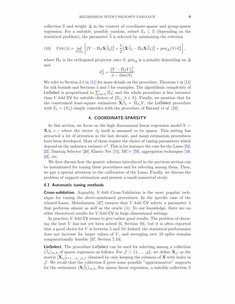
REGRESSION WITH UNKNOWN VARIANCE 9

collection S and weight ∆ in the context of coordinate-sparse and group-sparseregression. For a suitable, possibly random, subset Sλ ⊂ S (depending on thestatistical problem), the parameter λ is selected by minimizing the criterion

(10) Crit(λ) = infS∈Sλ

[‖Y −ΠSXβλ‖22 +

1

2‖Xβλ −ΠSXβλ‖22 + pen∆(S) σ

2S

],

where ΠS is the orthogonal projector onto S, pen∆ is a penalty depending on ∆and

σ2S =

‖Y −ΠSY ‖22n− dim(S)

.

We refer to Section 2.1 in [11] for more details on the procedure, Theorem 1 in [11]for risk bounds and Sections 4 and 5 for examples. The algorithmic complexity ofLinSelect is proportional to

∑λ∈Λ |Sλ| and the whole procedure is less intensive

than V -fold CV for suitable choices of {Sλ, λ ∈ Λ}. Finally, we mention that forthe constrained least-square estimators Xβλ = ΠSλ

Y , the LinSelect procedurewith Sλ = {Sλ} simply coincides with the procedure of Baraud et al. [10].

4. COORDINATE-SPARSITY

In this section, we focus on the high dimensional linear regression model Y =Xβ0 + ε where the vector β0 itself is assumed to be sparse. This setting hasattracted a lot of attention in the last decade, and many estimation procedureshave been developed. Most of them require the choice of tuning parameters whichdepend on the unknown variance σ2. This is for instance the case for the Lasso [62,22], Dantzig Selector [20], Elastic Net [74], MC+ [70], aggregation techniques [19,23], etc.

We first discuss how the generic schemes introduced in the previous section canbe instantiated for tuning these procedures and for selecting among them. Then,we pay a special attention to the calibration of the Lasso. Finally, we discuss theproblem of support estimation and present a small numerical study.

4.1 Automatic tuning methods

Cross-validation. Arguably, V -fold Cross-Validation is the most popular tech-nique for tuning the above-mentioned procedures. In the specific case of therelaxed-Lasso, Meinshausen [47] ensures that V -fold CV selects a parameter λthat performs almost as well as the oracle (4). To our knowledge, there are noother theoretical results for V -fold CV in large dimensional settings.

In practice, V -fold CV seems to give rather good results. The problem of choos-ing the best V has not yet been solved [6, Section 10], but it is often reportedthat a good choice for V is between 5 and 10. Indeed, the statistical performancedoes not increase for larger values of V , and averaging over 10 splits remainscomputationally feasible [37, Section 7.10].

LinSelect. The procedure LinSelect can be used for selecting among a collection(βλ)λ∈Λ of sparse regressors as follows. For J ⊂ {1, . . . , p}, we define XJ as thematrix [Xij ]i=1,...,n, j∈J obtained by only keeping the columns of X with index inJ . We recall that the collection S gives some possible ”approximative” supportsfor the estimators (Xβλ)λ∈Λ. For sparse linear regression, a suitable collection S

10 GIRAUD, HUET AND VERZELEN

and measure of complexity ∆ are

S ={S = range(XJ ), J ⊂ {1, . . . , p} , |J | ≤ n/(3 log p)

}

and ∆(S) = log

(p

dim(S)

).

Let us introduce the spaces Sλ = range(X

supp(βλ)

)and the subcollection of S

S ={Sλ, λ ∈ Λ

}, where Λ =

{λ ∈ Λ : Sλ ∈ S

}.

The following proposition gives a risk bound when selecting λ with LinSelect withSλ = S for all λ ∈ Λ and the above choice of ∆.

Proposition 4.1 (Theorem 1 in [11]). There exists a constant C > 1 suchthat for any minimizer λ of the Criterion (10), we have

R[βλ;β0

]≤ C E

[infλ∈Λ

{‖Xβλ −Xβ0‖22 + ‖βλ‖0 log(p)σ2

}].(11)

The bound (11) cannot be formulated in the form (8) due to the random natureof the set Λ. Nevertheless, a bound similar to (7) can be deduced from (11) whenthe estimators βλ fulfill Xβλ = ΠSλ

Y , see Corollary 4 in [11].

4.2 Lasso-type estimation under unknown variance

The Lasso is certainly one of the most popular methods for variable selectionin a high-dimensional setting. Given λ > 0, the Lasso estimator βL

λ is defined by

βLλ := argminβ∈Rp ‖Y −Xβ‖22+λ‖β‖1. A sensible choice of λmust be homogeneous

with the square-root of the variance σ2. As explained above, when the variance σ2

is unknown, one may apply V -fold CV or LinSelect to select λ. Some alternativeapproaches have also been developed for tuning the Lasso. Their common ideais to modify the ℓ1 criterion so that the tuning parameter becomes pivotal withrespect to σ2. This means that the method remains valid for any σ > 0 andthat the choice of the tuning parameter does not depend on σ. For the sakeof simplicity, we assume throughout this subsection that the columns of X arenormalized to one.

ℓ1-penalized log-likelihood. In low-dimensional regression, it is classical to con-sider a penalized log-likelihood criterion instead of a penalized least-square crite-rion to handle the unknown variance. Following this principle, Stadler et al. [58]propose to minimize the ℓ1-penalized log-likelihood criterion

βLLλ , σLL

λ := argminβ∈Rp,σ′>0

[n log(σ′) +

‖Y −Xβ‖222σ′2

+ λ‖β‖1σ′

].(12)

By reparametrizing (β, σ), Stadler et al. [58] obtain a convex criterion that canbe efficiently minimized. Interestingly, the penalty level λ is pivotal with respectto σ. Under suitable conditions on the design matrix X, Sun and Zhang [60] showthat the choice λ = C

√2 log p, with C > 1 yields optimal risk bounds in the sense

of (7).

REGRESSION WITH UNKNOWN VARIANCE 11

Scaled Lasso. Alternatively, Antoniadis [3] suggests to minimize a penalized Hu-ber’s loss [39, page 179]

βSLλ , σSL

λ := argminβ∈Rp,σ′>0

[nσ′ +

‖Y −Xβ‖222σ′

+ λ‖β‖1]

.(13)

This convex criterion can be minimized with roughly the same computationalcomplexity as a Lars-Lasso path [27]. Furthermore, Sun and Zhang [61] statesharp oracle inequalities for this estimator with λ = C

√2 log(p), with C > 1.

Their empirical results suggest that the criterion (13) provides slightly betterresults than the ℓ1-penalized log-likelihood.

Square-root Lasso. Belloni et al. [14] propose to replace the residual sum ofsquares in the Lasso criterion by its square-root

βSR = argminβ∈Rp

[√‖Y −Xβ‖22 +

λ√n‖β‖1

].

Interestingly, the penalty level λ is again pivotal. For λ = C√2 log(p) with C > 1,

the square-root Lasso estimator also achieves optimal risk bounds under suitableassumptions on the design X.

Bayesian Lasso. The Bayesian paradigm allows to put prior distributions on thevariance σ2 and the tuning parameter λ, as in the Bayesian Lasso [51]. Bayesianprocedures straightforwardly handle the case of unknown variance, but no fre-quentist analysis of these procedures are yet available.

4.3 Support estimation and inverse problem

Until now, we only discussed estimation methods that perform well in pre-diction. Little is known when the objective is to infer β0 or its support underunknown variance.

Inverse problem. The scaled Lasso [61] and the square root Lasso [14] are provedto achieve near optimal risk bound for the inverse problems under suitable as-sumptions on the design X.

Support estimation. Up to our knowledge, there are no non-asymptotic results onsupport estimation for the aforementioned procedures in the unknown variancesetting. Nevertheless, some related results and heuristics have been developpedfor the cross-validation scheme. If the tuning parameter λ is chosen to minimizethe prediction error (that is take λ = λ∗ as defined in (4)), the Lasso is notconsistent for support estimation [43, 48]. One idea to overcome this problem, isto choose the parameter λ that minimizes the risk of the so-called Gauss-Lassoestimator βGL

λ which is the least square estimator over the support of the Lasso

estimator βLλ

(14) βGLλ := argmin

β∈Rp:supp(β)⊂supp(βLλ)

‖Y −Xβ‖22 .

When the objective is support estimation, we advise to apply LinSelect or theV -fold CV scheme to the Gauss-Lasso estimators instead of the Lasso estimators.Similar remarks also apply for the Dantzig Selector [20].

12 GIRAUD, HUET AND VERZELEN

4.4 Numerical Experiments

We present two numerical experiments to illustrate the behavior of some of theabove mentioned procedures for high-dimensional sparse linear regression. Thefirst one concerns the problem of tuning the parameter λ of the Lasso algorithmfor estimating Xβ0. The procedures will be compared on the basis of the pre-diction risk. The second one concerns the problem of support estimation withLasso-type estimators. We will focus on the false discovery rates (FDR) and theproportion of true discoveries (Power).

Simulation design. The simulation design is the same as the one described inSections 6.1, and 8.2 of [11], except that we restrict to the case n = p = 100.Therefore, 165 examples are simulated. They are inspired by examples foundin [62, 74, 73, 38] and cover a large variety of situations. The simulation werecarried out with R (www.r-project.org), using the library elasticnet.

Experiment 1 : tuning the Lasso for prediction.

In the first experiment, we compare 10-fold CV [29], LinSelect [11] and the scaled-Lasso [61] (with λ =

√2 log(p) ) for tuning the Lasso. For each tuning proce-

dure ℓ ∈ {10-fold CV, LinSelect, scaled-Lasso}, we focus on the prediction risk

R[βLλℓ

;β0

]of the selected Lasso estimator βL

λℓ

.

For each simulated example e = 1, . . . , 165, we estimate on the basis of 400runs

• the risk of the oracle (4) : Re = R[βλ∗ ;β0

],

• the risk when selecting λ with procedure ℓ : Rℓ,e = R[βλℓ

;β0

].

The comparison between the procedures is based on the comparison of themeans, standard deviations and quantiles of the risk ratios Rℓ,e/Re computedover all the simulated examples e = 1, . . . , 165. The results are displayed in Ta-ble 1.

quantilesprocedure mean std-err 0% 50% 75% 90% 95%

Lasso V -fold CV 1.19 0.09 1.07 1.16 1.27 1.33 1.36Lasso LinSelect 1.19 0.58 1.02 1.05 1.09 1.11 2.24

Scaled Lasso 5.77 7.35 1.30 2.75 5.85 13 21Table 1

For each procedure ℓ, mean, standard-error and quantiles of the ratios{Rℓ,e/Re, e = 1, . . . , 165}.

For 10-fold CV and LinSelect, the risk ratios are close to one. For 90% of theexamples, the risk of the Lasso-LinSelect is smaller than the risk of the Lasso-CV,but there are a few examples where the risk of the Lasso-LinSelect is significantlylarger than the risk of the Lasso-CV. For the scaled-lasso procedure, the risk ratiosare clearly larger than for the two others. An inspection of the results reveals thatthe scaled-Lasso selects estimators with supports of small size. This feature canbe interpreted as follows. Due to the bias of the Lasso-estimator, the residualvariance tends to over-estimate the variance, leading the scaled-lasso to choose alarge λ. Consequently the risk is high. We illustrate this phenomenon in Table 2,

where we consider apart easy examples with ratio R[βλ∗ ;β0

]/nσ2 smaller than

REGRESSION WITH UNKNOWN VARIANCE 13

0.1 and difficult examples with ratio R[βλ∗ ;β0

]/nσ2 greater than 0.8. The bias

of the Lasso estimator is small for easy examples, whereas it is large for difficultexamples. The difference of behavior between the scaled-Lasso and the two otherprocedures is significant.

easy examples difficult examples

mean risk ratio ‖βL

λℓ

‖0 mean risk ratio ‖βL

λℓ

‖0

Oracle 1 (11) 1 (43)Lasso V -fold CV 1.35 (13) 1.12 (45)Lasso LinSelect 1.06 (11) 1.71 (40)

Scaled Lasso 1.89 (8) 15 (3.5)Table 2

Mean risk ratio Rℓ,e/Re for each selection procedure ℓ on easy and difficult examples. In

parentheses : ‖βL

λℓ

‖0. The first line gives the same values for the oracle βLλ⋆

Experiment 2 : variable selection with Gauss-Lasso and scaled-Lasso.

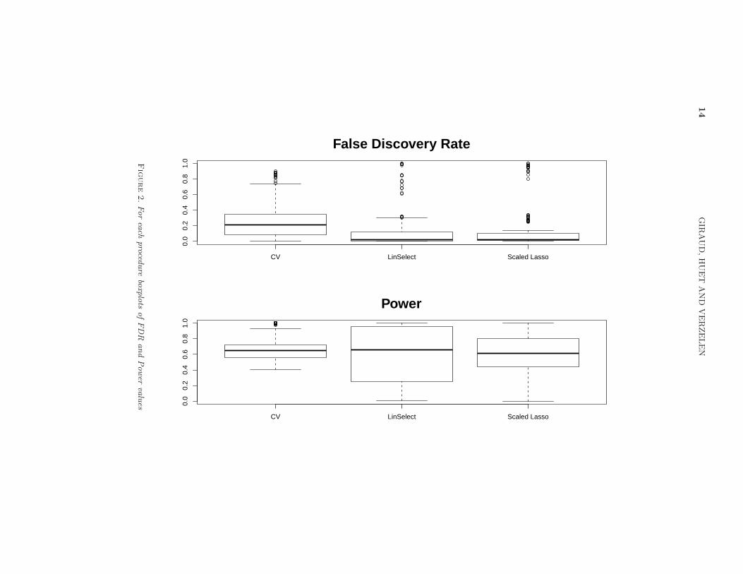
We consider now the problem of support estimation, sometimes referred as theproblem of variable selection. We implement three procedures. The Gauss-Lassoprocedure tuned by either 10-fold CV or LinSelect and the scaled-Lasso. Thesupport of β0 is estimated by the support of the selected estimator.

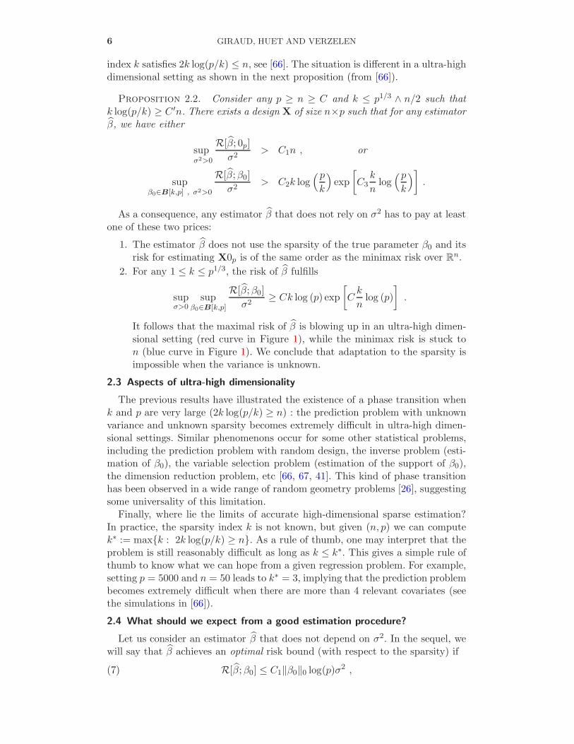
For each simulated example, the FDR and the Power are estimated on thebasis of 400 runs. The results are given on Figure 2. It appears that the Gauss-Lasso CV procedure gives greater values of the FDR than the two others. TheGauss-Lasso LinSelect and the scaled-Lasso behave similarly for the FDR, butthe values of the power are more variable for the LinSelect procedure.

5. GROUP-SPARSITY

In the previous section, we have made no prior assumptions on the form of β0.In some applications, there are some known structures between the covariates. Asan example, we treat the now classical case of group sparsity. The covariates areassumed to be clustered intoM groups and when the coefficient β0,i correspondingto the covariate Xi is non-zero then it is likely that all the coefficients β0,j withvariables Xj in the same group as Xi are non-zero. We refer to the introductionof Bach [8] for practical examples of this so-called group-sparsity assumption.Let G1, . . . , GM form a given partition of {1, . . . , p}. For λ = (λ1, . . . , λM ), thegroup-Lasso estimator βλ is defined as the minimizer of the convex optimizationcriterion

(15) ‖Y −Xβ‖22 +M∑

k=1

λk‖βGk‖2,

where βGk = (βj)j∈Gk. The Criterion (15) promotes solutions where all the co-

ordinates of βGk are either zero or non-zero, leading to group selection [69].Under some assumptions on X, Lounici et al. [45] provides a suitable choice ofλ = (λ1, . . . , λM ) that leads to near optimal prediction bounds. As expected, thischoice of λ = (λ1, . . . , λM ) is proportionnal to σ.

As for the Lasso, V -fold CV is widely used in practice to tune the penaltyparameter λ = (λ1, . . . , λM ). To our knowledge, there is not yet any extension

14

GIR

AUD,HUET

AND

VERZELEN

CV LinSelect Scaled Lasso

0.0

0.2

0.4

0.6

0.8

1.0

False Discovery Rate

CV LinSelect Scaled Lasso

0.0

0.2

0.4

0.6

0.8

1.0

Power

Figure2.Foreach

proced

ure

boxplots

ofFDR

andPower

values

REGRESSION WITH UNKNOWN VARIANCE 15

of the procedures described in Section 4.2 to the group Lasso. An alternative tocross-validation is to use LinSelect.

Tuning the group-Lasso with LinSelect. For any K ⊂ {1, . . . ,M}, we define thesubmatrix X(K) of X by only keeping the columns of X with index in

⋃k∈KGk.

The collection S and the function ∆ are given by

S =

{range(X(K)) : K ⊂ {1, . . . ,M} and 2|K| log(M) ∨

∑

k∈K

|Gk| ≤ n/2

}

and ∆(range(X(K))) = |K| log(M). For a given Λ ⊂ RM+ , similarly to Section 4.1,

we define Kλ ={k : ‖βGk

λ ‖2 6= 0}and Sλ = S for all λ ∈ Λ, where

S ={range(X

(Kλ)), λ ∈ Λ

}, with Λ =

{λ ∈ Λ, range(X

(Kλ)) ∈ S

}.

Theorem 1 in [11] provides the following risk bound.

Proposition 5.1. Let λ be any minimizer of the Criterion (10) with theabove choice of Sλ and ∆. Then, there exists a constant C > 1 such that

(16) R[βλ;β0

]≤ C E

[infλ∈Λ

{‖Xβλ −Xβ0‖22 +

(‖βλ‖0 ∨ |Kλ| log(M)

)σ2

}].

In the case where each group Gk is a singleton, we have M = p and we recoverthe result of Proposition 4.1 when we assume that λ1 = λ2 = . . . = λM . When thecardinality of each Gk is larger than log(M), we have ‖βλ‖0 ≥ |Kλ| log(M) withprobability one, so the final estimator nearly achieves the best trade off between‖Xβλ −Xβ0‖22 and ‖βλ‖0σ2 for λ ∈ Λ.

Let us compare Proposition 5.1 with the bounds of Lounici et al. [45] in thespecific case of multitask learning with M tasks that is n = Mn0 and p = Mp0.Suppose that only m groups out of M correspond to non-zero vector βGk

0 . Undersuitable assumptions on the design X, it is proved in [45] that the group Lassoestimator βλ with a well-chosen tuning parameter λ∗(σ) satisfies

‖Xβλ∗(σ) −Xβ0‖22 ≤ C [mp0 ∨ k log(M)] σ2 ,

and that ‖βλ∗(σ)‖0 ≤ Cmp0 with large probability. It follows that with largeprobability

infλ∈Λ

{‖Xβλ −Xβ0‖22 +

(‖βλ‖0 ∨ |Kλ| log(M)

)σ2

}≤ C [mp0 ∨m log(M)] σ2 ,

suggesting that βλsatisfies the same kind of bounds as βλ∗(σ) without requiring

the knowledge of σ.

6. VARIATION-SPARSITY

We focus in this section to the variation-sparse regression. We recall that thevector βV ∈ R

p−1 of the variations of β has for coordinates βVj = βj+1 − βj and

that the variation-sparse setting corresponds to the setting where the vector ofvariations βV

0 is coordinate-sparse. In the following, we restrict to the case where

16 GIRAUD, HUET AND VERZELEN

n = p and X is the identity matrix. In this case, the problem of variation-sparseregression coincides with the problem of segmentation of the mean of the vectorY = β0 + ε.

For any subset I ⊂ {1, . . . , n− 1}, we define SI ={β ∈ R

n : supp(βV ) ⊂ I}

and βI = ΠSIY . For any integer q ∈ {0, . . . , n− 1}, we define also the ”best”

subset of size q byIq = argmin

|I|=q‖Y − βI‖22.

Though the number of subsets I ⊂ {1, . . . , n− 1} of cardinality q is of ordernq+1, this minimization can be performed using dynamic programming with acomplexity of order n2 [35]. To select I = Iq with q in {0, . . . , n − 1}, any of thegeneric selection schemes of Section 3 can be applied. Below, we instantiate theseschemes and present some alternatives.

6.1 Penalized empirical loss

When the variance σ2 is known, penalized log-likelihood model selection amountsto select a subset I which minimizes a criterion of the form ‖Y −βI‖22+pen(Card(I)).This is equivalent to select I = Iq with q minimizing

(17) Crit(q) = ‖Y − βIq‖22 + pen(q).

Following the work of Birge and Massart [16], Lebarbier [42] considers thepenalty

pen(q) = (q + 1) (c1 log(n/(q + 1)) + c2) σ2

and determines the constants c1 = 2, c2 = 5 by extensive numerical experiments.With this choice of the penalty, the procedure satisfies a bound of the form

(18) R[βI, β0

]≤ C inf

I⊂{1,...,n−1}

{‖βI − β0‖22 + (1 + |I|) log(n/(1 + |I|))σ2

}.

When σ2 is unknown, several approaches have been proposed.

Plug-in estimator. The idea is to replace σ2 in pen(q) by an estimator of the

variance such as σ2 =∑n/2

i=1(Y2i−Y2i−1)2/n, or one of the estimators proposed by

Hall and al. [36]. No theoretical results are proved in a non-asymptotic framework.

Estimating the variance by the residual least-squares. Baraud et al. [10] Section5.4.2 propose to select q by minimizing a penalized log-likelihood criterion. Thiscriterion can be written in the form Crit(q) = ‖Y − βIq‖

22(1 + Kpen(q)), with

K > 1 and the penalty pen(q) solving

E[(U − pen(q)V )+

]=

1

(q + 1)(n−1

q

) ,

where (.)+ = max(., 0), and U , V are two independent χ2 variables with respec-tively q + 2 and n − q − 2 degrees of freedom. The resulting estimator β

I, with

I = Iq, satisfies a non asymptotic risk bound similar to (18) for all K > 1. Thechoice K = 1.1 is suggested for the practice.

REGRESSION WITH UNKNOWN VARIANCE 17

Slope heuristic. Lebarbier [42] implements the slope heuristic introduced by Birgeand Massart [17] for handling the unknown variance σ2. The method consistsin calibrating the penalty directly, without estimating σ2. It is based on thefollowing principle. First, there exists a so-called minimal penalty penmin(q) suchthat choosing pen(q) = Kpenmin(q) in (17) with K < 1 can lead to a strongoverfitting, whereas for K > 1 the bound (18) is met. Second, it can be shownthat there exists a dimension jump around the minimal penalty, allowing toestimate penmin(q) from the data. The slope heuristic then proposes to selectq by minimizing the criterion Crit(q) = ‖Y − β

Iq‖22 + 2 penmin(q). Arlot and

Massart [7] provide a non asymptotic risk bound for this procedure. Their resultsare proved in a general regression model with heteroscedatic and non gaussianerrors, but with a constraint on the number of models per dimension which is notmet for the family of models (SI)I⊂{1,...,n−1}. Nevertheless, the authors indicatehow to generalize their results for the problem of signal segmentation.

Finally, for practical issues, different procedures for estimating the minimalpenalty are compared and implemented in Baudry et al. [13].

6.2 CV procedure

In a recent paper, Arlot and Celisse [5] consider the problem of signal segmen-tation using cross-validation. Their results apply in the heteroscedastic case. Theyconsider several CV-methods, the leave-one-out, leave-p-out and V -fold CV for es-timating the quadratic loss. They propose two cross-validation schemes. The first

one, denoted Procedure 5, aims to estimate directly E

[‖β0 − β

Iq‖22], while the

second one, denoted Procedure 6, relies on two steps where the cross-validation isused first for choosing the best partition of dimension q, then the best dimensionq. They show that the leave-p-out CV method can be implemented with a com-plexity of order n2, and they give a control of the expected CV risk. The use ofCV leads to some restrictions on the subsets I that compete for estimating β0.This problem is discussed in [5], Section 3 of the supplemental material.

6.3 Alternative for very high-dimensional settings

When n is very large, the dynamic programming optimization can become com-putationally too intensive. An attractive alternative is based on the fused Lassoproposed by Tibshirani et al. [63]. The estimator βTV

λ is defined by minimizingthe convex criterion

‖Y − β‖22 + λn−1∑

j=1

|βj+1 − βj |,

where the total-variation norm∑

j |βj+1 − βj | promotes solutions which are

variation-sparse. The family (βTVλ )λ≥0 can be computed very efficiently with the

LARS-algorithm, see Vert and Bleakley [64]. A sensible choice of the parameterλ must be proportional to σ. When the variance σ2 is unknown, the parameterλ can be selected either by V -fold CV or by LinSelect (see Section 5.1 in [11] fordetails).

18 GIRAUD, HUET AND VERZELEN

7. EXTENSIONS

7.1 Gaussian design and graphical models

Assume that the design X is now random and that the n rows X(i) are in-

dependent observations of a Gaussian vector with mean 0p and unknown co-variance matrix Σ. This setting is mainly motivated by applications in com-pressed sensing [25] and in Gaussian graphical modeling. Indeed, Meinshausenand Buhlmann [48] have proved that it is possible to estimate the graph of aGaussian graphical model by studying linear regression with Gaussian designand unknown variance. If we work conditionally on the observed X design, thenall the results and methodologies described in this survey still apply. Nevertheless,these prediction results do not really take into account the fact that the design israndom. In this setting, it is more natural to consider the integrated predictionrisk E

[‖Σ1/2(β − β0)‖22

]rather than the risk (3). Some procedures [31, 65] have

been proved to achieve optimal risk bounds with respect to this risk but theyare computationally intractable in a high dimensional setting. In the context ofGaussian graphical modeling, the procedure GGMSelect [34] is designed to selectamong any collection of graph estimators and it is proved to achieve near optimalrisk bounds in terms of the integrated prediction risk.

7.2 Non Gaussian noise

A few results do not require that the noise ε follows a Gaussian distribu-tion. The Lasso-type procedures such as the Scaled Lasso [61] or the square-rootLasso [14] do not require the normality of the noise and extend to other distri-butions. In practice, it seems that cross-validation procedures still work well forother distributions of the noise.

7.3 Multivariate regression

Multivariate regression deals with T simultaneous linear regression models yk =Xβk + εk, k = 1, . . . , T . Stacking the yk’s in a n × T matrix Y , we obtain themodel Y = XB+E, where B is a p×T matrix with columns given by βk and Eis a n×T matrix with i.i.d. entries. The classical structural assumptions on B areeither that most rows of B are identically zero, or the rank of B is small. The firstcase is a simple case of group sparsity and can be handled by the group-lasso asin Section 5. The second case, first considered by Anderson [2] and Izenman [40],is much more non-linear. Writing ‖.‖F for the Frobenius (or Hilbert-Schmidt)norm, the problem of selecting among the estimators

Br = argminB:rank(B)≤r

‖Y −XB‖2F , r ∈ {1, . . . ,min(T, rank(X))}

has been investigated recently from a non-asymptotic point of view by Buneaet al. [18] and Giraud [33]. To handle the case of unknown variance, Bunea etal. [18] propose to plug an estimate of the variance in their selection criterion(which works when rank(X) < n), whereas Giraud [33] introduces a penalizedlog-likelihood criterion independent of the variance. Both papers provide oraclerisk bounds for the resulting estimators showing rate-minimax adaptation.

7.4 Nonparametric regression

In the nonparametric regression model (2), classical estimation procedures in-clude local-polynomial estimators, kernel estimators, basis-projection estimators,

REGRESSION WITH UNKNOWN VARIANCE 19

k-nearest neighbors etc. All these procedures depend on one (or several) tuningparameter(s), whose optimal value(s) scales with the variance σ2. V -fold CV iswidely used in practice for choosing these parameters, but little is known on itstheoretical performance.

The class of linear estimators (including spline smoothing, Nadaraya estima-tors, k-nearest neighbors, low-pass filters, kernel ridge regression, etc) has at-tracted some attention in the last years. Some papers have investigated the tuningof some specific family of estimators. For example, Cao and Golubev [21] providesa tuning procedure for spline smoothing and Zhang [71] analyses in depth kernelridge regression. Recently, two papers have focused on the tuning of arbitrarylinear estimators when the variance σ2 is unknown. Arlot and Bach [4] generalizethe slope heuristic to symmetric linear estimators with spectrum in [0, 1] andprove an oracle bound for the resulting estimator. Baraud et al. [11] Section 4shows that LinSelect can be used for selecting among a (almost) completely ar-bitrary collection of linear estimators (possibly non-symmetric and/or singular).Corollary 2 in [11] provides an oracle bound for the selected estimator under themild assumption that the effective dimension of the linear estimators is not largerthan a fraction of n. This assumption can be viewed as a ”sparsity assumption”suitable for linear estimators.

REFERENCES

[1] Akaike, H. (1973). Information theory and an extension of the maximum likelihoodprinciple. In Second International Symposium on Information Theory (Tsahkadsor, 1971).Akademiai Kiado, Budapest, 267–281. MR0483125 (58 #3144)

[2] Anderson, T. W. (1951). Estimating linear restrictions on regression coefficients for mul-tivariate normal distributions. Ann. Math. Statistics 22, 327–351. MR0042664 (13,144f)

[3] Antoniadis, A. (2010). Comments on: ℓ1-penalization for mixture regression mod-els [mr2677722]. TEST 19, 2, 257–258. http://dx.doi.org/10.1007/s11749-010-0198-y.MR2677723

[4] Arlot, S. and Bach, F. (2009). Data-driven calibration of linear estimators with minimalpenalties. In Advances in Neural Information Processing Systems 22, Y. Bengio, D. Schuur-mans, J. Lafferty, C. K. I. Williams, and A. Culotta, Eds. 46–54.

[5] Arlot, S. and Celisse, A. (2010a). Segmentation of the mean of het-eroscedastic data viacross-validation. Stat. Comput., 1–20. 10.1007/s11222-010-9196-x,http://dx.doi.org/10.1007/s11222-010-9196-x.

[6] Arlot, S. and Celisse, A. (2010b). A survey of cross-validation procedures for model se-lection. Stat. Surv. 4, 40–79. http://dx.doi.org/10.1214/09-SS054. MR2602303 (2011g:62111)

[7] Arlot, S. and Massart, P. (2010). Data-driven calibration of penalties for least-squaresregression. J. Mach. Learn. Res. 10, 245–279.

[8] Bach, F. (2008). Consistency of the group lasso and multiple kernel learning. J. Mach.Learn. Res. 9, 1179–1225. MR2417268 (2010a:68132)

[9] Baraud, Y. (2010). Estimator selection with respect to hellinger-type risks. ProbabilityTheory and Related Fields, 1–49. http://dx.doi.org/10.1007/s00440-010-0302-y.

[10] Baraud, Y., Giraud, C., and Huet, S. (2009). Gaussian model selection with an un-known variance. Ann. Statist. 37, 2, 630–672.

[11] Baraud, Y., Giraud, C., and Huet, S. (2010). Estimator selection in the gaussiansetting. arXiv:1007.2096v2.

[12] Barron, A., Birge, L., and Massart, P. (1999). Risk bounds for modelselection via penalization. Probab. Theory Related Fields 113, 3, 301–413.http://dx.doi.org/10.1007/s004400050210. MR1679028 (2000k:62049)

[13] Baudry, J.-P., Maugis, C., and Michel, B. (2010). Slope heuristics: Overview andimplementation. http://hal.archives-ouvertes.fr/hal-00461639/fr/.

20 GIRAUD, HUET AND VERZELEN

[14] Belloni, A., Chernozhukov, V., and Wang, L. (2010). Square-root lasso: Pivotalrecovery of sparse signals via conic programming. http://arxiv.org/pdf/1009.5689v2.

[15] Bickel, P., Ritov, Y., and Tsybakov, A. (2009). Simultaneous analysis of lasso andDantzig selector. Ann. Statist. 37, 4, 1705–1732. http://dx.doi.org/10.1214/08-AOS620.MRMR2533469

[16] Birge, L. and Massart, P. (2001). Gaussian model selection. J. Eur. Math. Soc.(JEMS) 3, 3, 203–268. MRMR1848946 (2002i:62072)

[17] Birge, L. and Massart, P. (2007). Minimal penalties for Gaussian model selection.Probab. Theory Related Fields 138, 1-2, 33–73. http://dx.doi.org/10.1007/s00440-006-0011-8. MRMR2288064 (2008g:62070)

[18] Bunea, F., She, Y., and Wegkamp, M. H. (2011). Optimal selection of reduced rankestimators of high-dimensional matrices. Ann. Stat. 39, 2, 1282–1309.

[19] Bunea, F., Tsybakov, A., and Wegkamp, M. (2007). Aggregation for Gaussian regres-sion. Ann. Statist. 35, 4, 1674–1697. MRMR2351101

[20] Candes, E. J. and Tao, T. (2007). The Dantzig selector: statistical estimation when p ismuch larger than n. Ann. Statist. 35, 6, 2313–2351. MRMR2382644

[21] Cao, Y. and Golubev, Y. (2006). On oracle inequalities related to smoothing splines.Math. Methods Statist. 15, 4, 398–414 (2007). MR2301659 (2008i:62039)

[22] Chen, S., Donoho, D., and Saunders, M. (1998). Atomic decomposition by basis pur-suit. SIAM J. Sci. Comput. 20, 1, 33–61. http://dx.doi.org/10.1137/S1064827596304010.MR1639094 (99h:94013)

[23] Dalalyan, A. and Tsybakov, A. (2008). Aggregation by exponential weighting, sharporacle inequalities and sparsity. Machine Learning 72, 1-2, 39– 61.

[24] Devroye, L. P. and Wagner, T. J. (1979). The L1 convergence of kernel density esti-mates. Ann. Statist. 7, 5, 1136–1139. MR536515 (80k:62054)

[25] Donoho, D. (2006). Compressed sensing. IEEE Trans. Inform. Theory 52, 4, 1289–1306.http://dx.doi.org/10.1109/TIT.2006.871582. MR2241189 (2007e:94013)

[26] Donoho, D. and Tanner, J. (2009). Observed universality of phase transitions in high-dimensional geometry, with implications for modern data analysis and signal processing.Philos. Trans. R. Soc. Lond. Ser. A Math. Phys. Eng. Sci. 367, 1906, 4273–4293. With elec-tronic supplementary materials available online, http://dx.doi.org/10.1098/rsta.2009.0152.MR2546388 (2010k:62407)

[27] Efron, B., Hastie, T., Johnstone, I., and Tibshirani, R. (2004). Least angle re-gression. Ann. Statist. 32, 2, 407–499. With discussion, and a rejoinder by the authors.MRMR2060166 (2005d:62116)

[28] Fan, J. and Li, R. (2001). Variable selection via nonconcave penalized like-lihood and its oracle properties. J. Amer. Statist. Assoc. 96, 456, 1348–1360.http://dx.doi.org/10.1198/016214501753382273. MR1946581 (2003k:62160)

[29] Geisser, S. (1975). The predictive sample reuse method with applications. J. Amer.Statist. Assoc. 70, 320–328.

[30] Gerchinovitz, S. (2011). Sparsity regret bounds for individual sequences in online linearregression. Arxiv:1101.1057.

[31] Giraud, C. (2008a). Estimation of Gaussian graphs by model selection. Electron. J.Stat. 2, 542–563.

[32] Giraud, C. (2008b). Mixing least-squares estimators when the variance isunknown. Bernoulli 14, 4, 1089–1107. http://dx.doi.org/10.3150/08-BEJ135.MR2543587 (2010k:62274)

[33] Giraud, C. (2011). Low rank multivariate regression. Electron. J. Stat. (to appear).http://arxiv.org/abs/1009.5165.

[34] Giraud, C., Huet, S., and Verzelen, N. (2009). Graph selection with ggmselect.arXiv:0907.0619.

[35] Guthery, S. B. (1974). A transformation theorem for one-dimensional F -expansions. J.Number Theory 6, 201–210. MR0342484 (49 #7230)

[36] Hall, P., Kay, J. W., and Titterington, D. M. (1990). Asymptotically optimaldifference-based estimation of variance in nonparametric regression. Biometrika 77, 3, 521–528. http://dx.doi.org/10.1093/biomet/77.3.521. MR1087842 (92d:62042)

REGRESSION WITH UNKNOWN VARIANCE 21

[37] Hastie, T.,Tibshirani, R., and Friedman, J. (2009). The elements of statistical learning,Second ed. Springer Series in Statistics. Springer, New York. Data mining, inference, andprediction, http://dx.doi.org/10.1007/978-0-387-84858-7. MR2722294

[38] Huang, J., Ma, S., and Zhang, C.-H. (2008). Adaptive Lasso for sparse high-dimensionalregression models. Statist. Sinica 18, 4, 1603–1618. MR2469326 (2010a:62214)

[39] Huber, P. (1981). Robust statistics. John Wiley & Sons Inc., New York. Wiley Series inProbability and Mathematical Statistics. MR606374 (82i:62057)

[40] Izenman, A. J. (1975). Reduced-rank regression for the multivariate linear model. J.Multivariate Anal. 5, 248–264. MR0373179 (51 #9381)

[41] Ji, P. and Jin, J. (2010). Ups delivers optimal phase diagram in high dimensional variableselection. http://arxiv.org/abs/1010.5028.

[42] Lebarbier, E. (2005). Detecting multiple change-points in the mean of gaussian processby model selection. Signal Processing 85, 717–736.

[43] Leng, C., Lin, Y., and Wahba, G. (2006). A note on the lasso and related procedures inmodel selection. Statist. Sinica 16, 4, 1273–1284. MR2327490

[44] Li, K.-C. (1987). Asymptotic optimality for Cp, CL, cross-validation andgeneralized cross-validation: discrete index set. Ann. Statist. 15, 3, 958–975.http://dx.doi.org/10.1214/aos/1176350486. MR902239 (89c:62112)

[45] Lounici, K., Pontil, M., Tsybakov, A., and van de Geer, S. (2010). Oracle inequalitiesand optimal inference under group sparsity. Arxiv:1007.1771v3.

[46] Mallows, C. L. (1973). Some comments on cp. Technometrics 15, 661–675.

[47] Meinshausen, N. (2007). Relaxed Lasso. Comput. Statist. Data Anal. 52, 1, 374–393.http://dx.doi.org/10.1016/j.csda.2006.12.019. MR2409990

[48] Meinshausen, N. and Buhlmann, P. (2006). High-dimensional graphs and variable se-lection with the lasso. Ann. Statist. 34, 3, 1436–1462. MRMR2278363 (2008b:62044)

[49] Mosteller, F. and Tukey, J. (1968). Data analysis, including statistics. In Handbookof Social Psychology, Vol. 2, G. Lindsey and E. Aronson, Eds. Addison-wesley.

[50] Nishii, R. (1984). Asymptotic properties of criteria for selection of variables in multi-ple regression. Ann. Statist. 12, 2, 758–765. http://dx.doi.org/10.1214/aos/1176346522.MR740928 (86f:62109)

[51] Park, T. and Casella, G. (2008). The Bayesian lasso. J. Amer. Statist. Assoc. 103, 482,681–686. http://dx.doi.org/10.1198/016214508000000337. MR2524001

[52] Raskutti, G., Wainwright, M., and Yu, B. (2009). Minimax rates of estimations forhigh-dimensional regression over lq balls. Tech. rep., UC Berkeley.

[53] Rigollet, P. and Tsybakov, A. (2010). Exponential screening and optimal rates ofsparse estimation. http://arxiv.org/pdf/1003.2654.

[54] Schwarz, G. (1978). Estimating the dimension of a model. Ann. Statist. 6, 2, 461–464.MR0468014 (57 #7855)

[55] Shao, J. (1993). Linear model selection by cross-validation. J. Amer. Statist. As-soc. 88, 422, 486–494. MR1224373 (94k:62107)

[56] Shao, J. (1997). An asymptotic theory for linear model selection. Statist. Sinica 7, 2,221–264. With comments and a rejoinder by the author. MR1466682 (99m:62104)

[57] Shibata, R. (1981). An optimal selection of regression variables. Biometrika 68, 1, 45–54.http://dx.doi.org/10.1093/biomet/68.1.45. MR614940 (84a:62103a)

[58] Stadler, N., Buhlmann, P., and van de Geer, S. (2010). ℓ1-penalization for mix-ture regression models. TEST 19, 2, 209–256. http://dx.doi.org/10.1007/s11749-010-0197-z.MR2677722

[59] Stone, M. (1974). Cross-validatory choice and assessment of statistical predictions. J.Roy. Statist. Soc. Ser. B 36, 111–147. With discussion by G. A. Barnard, A. C. Atkinson, L.K. Chan, A. P. Dawid, F. Downton, J. Dickey, A. G. Baker, O. Barndorff-Nielsen, D. R. Cox,S. Giesser, D. Hinkley, R. R. Hocking, and A. S. Young, and with a reply by the authors.MR0356377 (50 #8847)

[60] Sun, T. and Zhang, C.-H. (2010). Comments on: ℓ1-penalization for mixture regressionmodels [mr2677722]. TEST 19, 2, 270–275. http://dx.doi.org/10.1007/s11749-010-0201-7.MR2677726

[61] Sun, T. and Zhang, C.-H. (2011). Scaled sparse linear regression. arXiv:1104.4595.

22 GIRAUD, HUET AND VERZELEN

[62] Tibshirani, R. (1996). Regression shrinkage and selection via the lasso. J. Roy. Statist.Soc. Ser. B 58, 1, 267–288. MR1379242 (96j:62134)

[63] Tibshirani, R., Saunders, M., Rosset, S., Zhu, J., and Knight, K. (2005). Sparsityand smoothness via the fused lasso. J. R. Stat. Soc. Ser. B Stat. Methodol. 67, 1, 91–108.http://dx.doi.org/10.1111/j.1467-9868.2005.00490.x. MR2136641

[64] Vert, J.-P. and Bleakley, K. (2010). Fast detection of multiple change-points sharedby many signals using group lars. In Advances in Neural Information Processing Systems 23,J. Lafferty, C. K. I. Williams, J. Shawe-Taylor, R. Zemel, and A. Culotta, Eds. 2343–2351.

[65] Verzelen, N. (2010a). High-dimensional gaussian model selection on a gaussian design.Ann. Inst. H. Poincare Probab. Statist. 46, 2, 480–524.

[66] Verzelen, N. (2010b). Minimax risks for sparse regressions: Ultra-high-dimensional phe-nomenons. arXiv:1008.0526.

[67] Wainwright, M. (2009). Information-theoretic limits on sparsity recovery in thehigh-dimensional and noisy setting. IEEE Trans. Inform. Theory 55, 12, 5728–5741.http://dx.doi.org/10.1109/TIT.2009.2032816. MRMR2597190

[68] Ye, F. and Zhang, C.-H. (2010). Rate minimaxity of the Lasso and Dantzig selector forthe ℓq loss in ℓr balls. J. Mach. Learn. Res. 11, 3519–3540. MR2756192

[69] Yuan, M. and Lin, Y. (2006). Model selection and estimation in regressionwith grouped variables. J. R. Stat. Soc. Ser. B Stat. Methodol. 68, 1, 49–67.http://dx.doi.org/10.1111/j.1467-9868.2005.00532.x. MR2212574

[70] Zhang, C.-H. (2010). Nearly unbiased variable selection under minimax con-cave penalty. Ann. Statist. 38, 2, 894–942. http://dx.doi.org/10.1214/09-AOS729.MR2604701 (2011d:62211)

[71] Zhang, T. (2005). Learning bounds for kernel regression using effective data dimen-sionality. Neural Comput. 17, 9, 2077–2098. http://dx.doi.org/10.1162/0899766054323008.MR2175849 (2006d:62062)

[72] Zhang, T. (2011). Adaptive Forward-Backward Greedy Algorithm for Learning SparseRepresentations. IEEE Trans. Inform. Theory 57, 7, 4689–4708.

[73] Zou, H. (2006). The adaptive lasso and its oracle properties. J. Amer. Statist. As-soc. 101, 476, 1418–1429. MRMR2279469 (2008d:62024)

[74] Zou, H. and Hastie, T. (2005). Regularization and variable selection via the elastic net.J. R. Stat. Soc. Ser. B Stat. Methodol. 67, 2, 301–320. MRMR2137327

APPENDIX A: A NOTE ON BIC TYPE CRITERIA

The BIC criterion has been initially introduced [54] to select an estimatoramong a collection of constrained maximum likelihood estimators. Nevertheless,modified versions of this criterion are often used for tuning more general esti-mation procedures. The purpose of this appendix is to illustrate why we adviseagainst this approach in a high dimensional setting.

Definition A.1. A Modified BIC criterion. Suppose we are given a col-lection (βλ)λ∈Λ of estimators depending on a tuning parameter λ ∈ Λ. For anyλ ∈ Λ, we consider σ2

λ = ‖Y −Xβλ‖22/n, and define the modified BIC

(19) λ ∈ argminλ∈Λ

{−2Ln(βλ, σλ) + log(n)‖βλ‖0

},

where Ln is the log-likelihood and Λ ={λ ∈ Λ : ‖βλ‖0 ≤ n/2

}.

Sometimes, the log(n) term is replaced by log(p). Replacing Λ by Λ allows toavoid trivial estimators. First, we would like to emphasize that there is no theo-retical warranty that the selected estimator does not overfit in a high dimensional

REGRESSION WITH UNKNOWN VARIANCE 23

setting. In practice, using this criterion often leads to overfitting. Let us illustratethis with a simple experiment.

Setting. We consider the model

(20) Yi = β0,i + εi, i = 1, . . . , n ,

with ε ∼ N (0, σ2In) so that p = n and X = In. Here, we fix n = 10000, σ = 1and β0 = 0n.

Methods. We apply the modified BIC criterion to tune the Lasso [62], SCAD [28]and the hard thresholding estimator. The hard thresholding estimator βHT

λ is

defined for any λ > 0 by [βHTλ ]i = Yi1|Yi|≥λ. Given λ > 0 and a > 2, the

SCAD estimator βSCADλ,a is defined as the minimizer of the penalized criterion

‖Y −Xβ‖22 +∑n

i=1 pλ(|βi|) , where for x > 0,

p′λ(x) = λ1x≤λ + (aλ− x)+1x>λ/(a− 1) .

For the sake of simplicity we fix a = 3. We note βL;BIC, βSCAD;BICa , and βHT ;BIC

for the Lasso, hard thresholding, and SCAD estimators selected by the modifiedBIC criterion.

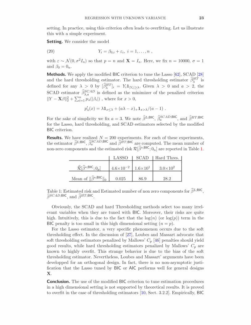
Results. We have realized N = 200 experiments. For each of these experiments,the estimator βL;BIC, βSCAD,BIC

a and βHT ;BIC are computed. The mean number ofnon-zero components and the estimated risk R[β∗;BIC; 0n] are reported in Table 1.

LASSO SCAD Hard Thres.

R[β∗;BIC; 0p] 4.6×10−2 1.6×101 3.0×102

Mean of ‖β∗;BIC‖0 0.025 86.9 28.2

Table 1: Estimated risk and Estimated number of non zero components for βL;BIC,βSCAD;BIC, and βHT ;BIC.

Obviously, the SCAD and hard Thresholding methods select too many irrel-evant variables when they are tuned with BIC. Moreover, their risks are quitehigh. Intuitively, this is due to the fact that the log(n) (or log(p)) term in theBIC penalty is too small in this high dimensional setting (n = p).

For the Lasso estimator, a very specific phenomenon occurs due to the softthresholding effect. In the discussion of [27], Loubes and Massart advocate thatsoft thresholding estimators penalized by Mallows’ Cp [46] penalties should yieldgood results, while hard thresholding estimators penalized by Mallows’ Cp areknown to highly overfit. This strange behavior is due to the bias of the softthresholding estimator. Nevertheless, Loubes and Massart’ arguments have beendevelopped for an orthogonal design. In fact, there is no non-asymptotic justi-fication that the Lasso tuned by BIC or AIC performs well for general designsX.

Conclusion. The use of the modified BIC criterion to tune estimation proceduresin a high dimensional setting is not supported by theoretical results. It is provedto overfit in the case of thresholding estimators [10, Sect. 3.2.2]. Empirically, BIC

24 GIRAUD, HUET AND VERZELEN

seems to overfit except for the Lasso. We advise the practitionner to avoid BIC

(and AIC) when p is at least of the same order as n. For instance, LinSelect issupported by non-asymptotic arguments and by empirical results [11] in contrastto BIC.