arX

iv:1

411.

6428

v1 [

mat

h.ST

] 2

4 N

ov 2

014

An extended Generalised Variance,

with Applications

Luc Pronzato∗, Henry P. Wynn†and Anatoly A. Zhigljavsky‡

CNRS, London School of Economics and Cardiff University

January 26, 2015

Abstract

We consider a measure ψk of dispersion which extends the notion of Wilk’sgeneralised variance, or entropy, for a d-dimensional distribution, and is basedon the mean squared volume of simplices of dimension k ≤ d formed byk + 1 independent copies. We show how ψk can be expressed in terms ofthe eigenvalues of the covariance matrix of the distribution, also when a n-point sample is used for its estimation, and prove its concavity when raisedat a suitable power. Some properties of entropy-maximising distributions arederived, including a necessary and sufficient condition for optimality. Finally,we show how this measure of dispersion can be used for the design of optimalexperiments, with equivalence to A and D-optimal design for k = 1 and k = drespectively. Simple illustrative examples are presented.

MSC: Primary 94A17; secondary 62K05keyword: dispersion, generalised variance, ,quadratic entropy, ,maximum-entropy

measure, design of experiments, optimal design

1 Introduction

The idea of dispersion is fundamental to statistics and with different terminology,such as potential, entropy, information and capacity, stretches over a wide area. Thevariance and standard deviation are the most prevalent for a univariate distribution,and Wilks generalised variance is the term usually reserved for the determinant ofthe covariance matrix, V , of a multivariate distribution. Many other measuresof dispersion have been introduced and a rich area comprises those that are order-preserving with respect to a dispersion ordering; see [21, 12, 5]. These are sometimesreferred to as measures of peakness and peakness ordering, and are related to thelarge literature on dispersion measures which grew out of the Gini coefficient, usedto measure income inequality [4] and diversity in biology, see [15], which we willdiscuss briefly below.

In the definitions there are typically two kinds of dispersion, those measuringsome kind of mean distance, or squared distance, from a central value, such asin the usual definition of variance, and those based on the expected distance, orsquared distance, between two independent copies from the same distribution, such

∗pronzato@i3s.unice.fr, Laboratoire I3S, UMR 7172, UNS/CNRS, 2000 route des Lucioles,Les Algorithmes, bat. Euclide B, 06900 Sophia Antipolis, France

†H.Wynn@lse.ac.uk, London School of Economics, Houghton Street, London, WC2A 2AE, UK‡ZhigljavskyAA@cf.ac.uk, School of Mathematics, Cardiff University, Senghennydd Road,

Cardiff, CF24 4YH, UK

1

as the Gini coefficient. It is this second type that will concern us here and we willgeneralise the idea in several ways by replacing distance by volumes of simplicesformed by k independent copies and by transforming the distance, both inside theexpectation and outside.

The area of optimal experimental design is another which has provided a rangeof dispersion measures. Good designs, it is suggested, are those whose parameterestimates have low dispersion. Typically, this means that the design measure, thespread of the observation sites, maximises a measure of dispersion and we shallstudy this problem.

We think of a dispersion measure as a functional directly on the distribution.The basic functional is an integral, such as a moment. The property we shallstress for such functionals most is concavity: that a functional does not decreaseunder mixing of the distributions. A fundamental theorem in Bayesian learning isthat we expect concave functionals to decrease through taking of observations, seeSection 2.2 below.

Our central result (Section 3) is an identity for the mean squared volume of sim-plices of dimension k, formed by k+1 independent copies, in terms of the eigenvaluesof the covariance matrices or equivalently in terms of sums of the determinants ofk-marginal covariance matrices. Second, we note that after an appropriate (exte-rior) power transformation the functional becomes concave. We can thus (i) deriveproperties of measures that maximise this functional (Section 4.1), (ii) use thisfunctional to measure the dispersion of parameter estimates in regression problems,and hence design optimal experiments which minimise this measure of dispersion(Section 4.2).

2 Dispersion measures

2.1 Concave and homogeneous functionals

Let X be a compact subset of Rd, M be the set of all probability measures on theBorel subsets of X and φ : M −→ R

+ be a functional defined on M . We will beinterested in the functionals φ(·) that are (see Appendix for precise definitions)

(a) shift-invariant,

(b) positively homogeneous of a given degree q, and

(c) concave: φ[(1 − α)µ1 + αµ2] ≥ (1 − α)φ(µ1) + αφ(µ2) for any α ∈ (0, 1) andany two measures µ1, µ2 in M .

For d = 1, a common example of a functional satisfying the above properties,with q = 2 in (b), is the variance

σ2(µ) = E(2)µ − E2

µ =1

2

∫ ∫(x1 − x2)

2 µ(dx1)µ(dx2) ,

where Eµ = Eµ(x) =∫xµ(dx) and E

(2)µ =

∫x2 µ(dx). Concavity follows from

linearity of E(2)µ , that is, E

(2)(1−α)µ1+αµ2

= (1−α)E(2)µ1 +αE

(2)µ2 , and Jensen’s inequality

which implies E2(1−α)µ1+αµ2

≤ (1− α)E2µ1

+ αE2µ2.

Any moment of µ ∈ M is a homogeneous functional of a suitable degree. How-ever, the variance is the only moment which satisfies (a) and (c). Indeed, theshift-invariance implies that the moment should be central, but the variance is theonly concave functional among the central moments, see Appendix. In this sense,one of the aims of this paper is a generalisation of the concept of variance.

2

In the general case d ≥ 1, the double variance 2σ2(µ) generalises to

φ(µ) =

∫ ∫‖x1−x2‖2 µ(dx1)µ(dx2) = 2

∫‖x−Eµ‖2 µ(dx) = 2 trace(Vµ) , (2.1)

where ‖·‖ is the L2-norm in Rd and Vµ is the covariance matrix of µ. This functional,like the variance, satisfies the conditions (a)-(c) with q = 2.

The functional (2.1) is the double integral of the squared distance between tworandom points distributed according to the measure µ. Our main interest will beconcentrated around the general class of functionals defined by

φ(µ) = φ[k],δ,τ (µ) =

(∫. . .

∫Vδk (x1, . . . , xk+1)µ(dx1) . . . µ(dxk+1)

)τ, k ≥ 2

(2.2)for some δ and τ in R+, where Vk(x1, . . . , xk+1) is the volume of the k-dimensionalsimplex (its area when k = 2) formed by the k + 1 vertices x1, . . . , xk+1 in Rd,with k = d as a special case. Property (a) for the functionals (2.2) is then astraightforward consequence of the shift-invariance of Vk, and positive homogeneityof degree q = k δτ directly follows from the positive homogeneity of Vk with degreek. Concavity will be proved to hold for δ = 2 and τ ≤ 1/k in Section 3. There,we show that this case can be considered as a natural extension of (2.1) (whichcorresponds to k = 1), with φ[k],2,τ (µ) being expressed as a function of Vµ, thecovariance matrix of µ. The concavity for k = τ = 1 and all 0 < δ ≤ 2, followsfrom the Schoenberg theory, which will be discussed briefly below. The functionals(2.2) with δ = 2 and τ > 0, 1 ≤ k ≤ d, can be used to define a family of criteria foroptimal experimental design, concave for τ ≤ 1/k, for which an equivalence theoremcan be formulated.

2.2 Quadratic entropy and learning

In a series of papers [15, 16, 17] C.R. Rao and co-workers have introduced a quadraticentropy which is a generalised version of the k = 2 functional of this section butwith a general kernel K(x1, x2) in R

d:

QR =

∫ ∫K(x1, x2)µ(dx1)µ(dx2) . (2.3)

For the discrete version

QR =

N∑

i=1

N∑

j=1

K(xi, xj) pi pj,

Rao and co-workers developed a version of the Analysis of Variance (ANOVA),which they called Anaysis of Quadratic Entropy (ANOQE). The Gini coefficient,also used in the continuous and discrete form is a special case with d = 1 andK(x1, x2) = |x1 − x2|.

As pointed in [17, Chap. 3], a necessary and sufficient condition for the functionalQR to be concave is ∫ ∫

K(x1, x2)ν(dx1)ν(dx2) ≤ 0 (2.4)

for all measures ν with∫ν(dx) = 0. The discrete version of this is

N∑

i=1

N∑

j=1

K(xi, xj) qi qj ≤ 0

3

for any choice of real numbers q1, . . . , qN such that∑N

i=1 qi = 0. Schoenberg [19]solves the general problem of finding for what class of functions B(·) on ‖x1 − x2‖2does the kernel K(x1, x2) = B

(‖x1 − x2‖2

)satisfy (2.4). The solution is that B

must be a so-called Bernstein function, see [18]. We do not develop these ideashere, but note that B(λ) = λα is a Bernstein function for all 0 < α ≤ 1. This is thereason that, above, we can claim concavity for k = 1 and all 0 < δ ≤ 2 in (2.2).

Hainy et al [6] discuss the link to embedding and review some basic results relatedto Bayesian learning. One asks what is the class of functionals ψ on a distributionµ(θ) of a parameter in the Bayesian statistical learning such that for all µ(θ) andall sampling distributions π(x|θ) one expects to learn, in the preposterior sense:ψ(µ(θ)) ≤ Eνψ(π(θ|X)), with X ∼ ν. The condition is that ψ is convex, a resultwhich has a history but is usually attributed to De Groot [2]. This learning isenough to justify calling such a functional a generalised information functional, ora general learning functional. Shannon information falls in this class, and earlierversions of the result were for Shannon information. It follows that wherever, inthis paper, we have a concave functional then its negative is a learning functional.

3 Functionals based on squared volume

In the rest of the paper we focus our attention on the functional

µ ∈ M −→ ψk(µ) = φ[k],2,1(µ) = Eµ{V 2k (x1, . . . , xk+1)} ,

which corresponds to the mean squared volume of simplices of dimension k formedby k + 1 independent samples from µ. For instance,

ψ2(µ) =

∫ ∫ ∫V

22 (x1, x2, x3)µ(dx1)µ(dx2)µ(dx3) , (3.1)

with V2(x1, x2, x3) the area of the triangle formed by the three points with coordi-nates x1, x2 and x3 in Rd, d ≥ 2. Functionals φ[k],δ,τ (µ) for δ 6= 2 will be consideredelsewhere, including the case of negative δ and τ in connection with space-fillingdesign for computer experiments.

Theorem 3.1 of Section 3.1 indicates how ψk(µ) can be expressed as a functionof Vµ, the covariance matrix of µ, and shows that φ[k],2,1/k(·) satisfies properties(a), (b) and (c) of Section 2.1. The special case of k = d was known to Wilks[25, 26] in his introduction of generalised variance, see also [24]. The connectionwith U-statistics is exploited in Section 3.2, where an unbiased minimum-varianceestimator of ψk(µ) based on a sample x1, . . . , xn is expressed in terms of the empir-ical covariance matrix of the sample.

3.1 Expected squared k-simplex volume

Theorem 3.1. Let the xi be i.i.d. with the probability measure µ ∈ M . Then, forany k ∈ {1, . . . , d}, we have

ψk(µ) =k + 1

k!

∑

i1<i2<···<ik

det[{Vµ}(i1,...,ik)×(i1,...,ik)] (3.2)

=k + 1

k!

∑

i1<i2<···<ik

λi1 [Vµ]× · · · × λik [Vµ] , (3.3)

where λi[Vµ] is the i-th eigenvalue of the covariance matrix Vµ and all ij belong

to {1, . . . , d}. Moreover, the functional ψ1/kk (·) is shift-invariant, homogeneous of

degree 2 and concave on M .

4

The proof uses the following two lemmas.

Lemma 3.1. Let the k + 1 vectors x1, . . . , xk+1 of Rk be i.i.d. with the probabilitymeasure µ, k ≥ 2. For i = 1, . . . , k + 1, denote zi = (x⊤i 1)⊤. Then

Eµ

{det

[k+1∑

i=1

ziz⊤i

]}= (k + 1)! det[Vµ] .

Proof. We have

Eµ

{det

[k+1∑

i=1

ziz⊤i

]}= (k + 1)! det

[Eµ(x1x

⊤1 ) Eµ

E⊤µ 1

]= (k + 1)! det[Vµ] ,

see for instance [13, Theorem 1].

Lemma 3.2. The matrix functional µ 7→ Vµ is Loewner-concave on M , in thesense that, for any µ1, µ2 in M and any α ∈ (0, 1),

V(1−α)µ1+αµ2� (1− α)Vµ1

+ αVµ2, (3.4)

where A � B means that A−B is nonnegative definite.

Proof. Take any vector z of the same dimension as x. Then z⊤Vµz = varµ(z⊤x),

which is a concave functional of µ, see Section 2.1. This implies that z⊤V(1−α)µ1+αµ2z =

var(1−α)µ1+αµ2(z⊤x) ≥ (1−α)varµ1

(z⊤x)+αvarµ2(z⊤x) = (1−α)z⊤Vµ1

z+αz⊤Vµ2z,

for any µ1, µ2 in M and any α ∈ (0, 1) (see Section 2.1 for the concavity of varµ).Since z is arbitrary, this implies (3.4).

Proof of Theorem 3.1. When k = 1, the results follow from ψ1(µ) = 2 trace(Vµ),see (2.1). Using Binet-Cauchy formula, see, e.g., [3, vol. 1, p. 9], we obtain

V2k (x1, . . . , xk+1) =

1

(k!)2det

(x2 − x1)⊤

(x3 − x1)⊤

...(xk+1 − x1)

⊤

[(x2 − x1) (x3 − x1) · · · (xk+1 − x1)]

=1

(k!)2

∑

i1<i2<···<ik

det2

{x2 − x1}i1 · · · {xk+1 − x1}i1...

......

{x2 − x1}ik · · · {xk+1 − x1}ik

=1

(k!)2

∑

i1<i2<···<ik

det2

{x1}i1 · · · {xk+1}i1...

......

{x1}ik · · · {xk+1}ik1 · · · 1

,

where {x}i denotes the i-th component of vector x. Also, for all i1 < i2 < · · · < ik,

det2

{x1}i1 · · · {xk+1}i1...

......

{x1}ik · · · {xk+1}ik1 · · · 1

= det

k+1∑

j=1

zjz⊤j

where we have denoted by zj the k+1-dimensional vector with components {xj}iℓ , ℓ =1, . . . , k, and 1. When the xi are i.i.d. with the probability measure µ, usingLemma 3.1 we obtain (3.2), (3.3). Therefore

ψk(µ) = Ψk[Vµ] =k + 1

k!Ek{λ1[Vµ], . . . , λd[Vµ]} , (3.5)

5

with Ek{λ1[Vµ], . . . , λd[Vµ]} the elementary symmetric function of degree k of the deigenvalues of Vµ, see, e.g., [11, p. 10]. Note that

Ek[Vµ] = Ek{λ1[Vµ], . . . , λd[Vµ]} = (−1)kad−k ,

with ad−k the coefficient of the monomial of degree d − k of the characteristicpolynomial of Vµ; see, e.g., [11, p. 21]. We have in particular E1[Vµ] = trace[Vµ]

and Ed[V µ)] = det[Vµ]. The shift-invariance and homogeneity of degree 2 of ψ1/kk (·)

follow from the shift-invariance and positive homogeneity of Vk with degree k. Con-

cavity of Ψ1/kk (·) follows from [11, p. 116] (take p = k in eq. (10), with E0 = 1).

From [9], the Ψ1/kk (·) are also Loewner-increasing, so that from Lemma 3.2, for any

µ1, µ2 in M and any α ∈ (0, 1),

ψ1/kk [(1− α)µ1 + αµ2] = Ψ

1/kk {V(1−α)µ1+αµ2

}≥ Ψ

1/kk [(1 − α)Vµ1

+ αVµ2]

≥ (1− α)Ψ1/kk [Vµ1

] + αΨ1/kk [Vµ2

]

= (1− α)ψ1/kk (µ1) + αψ

1/kk (µ2) .

The functionals µ −→ φ[k],2,τ (µ) = ψτk (µ) are thus concave for 0 < τ ≤ 1/k,with τ = 1/k yielding positive homogeneity of degree 2. The functional ψ1(µ)is a quadratic entropy QR, see (2.3), ψd(µ) is proportional to Wilks generalised

variance, and ψ1/22 (µ), see (3.1), and ψ

1/33 (µ) can be respectively considered as

particular versions of cubic and quartic entropies.From the well-known expression of the coefficients of the characteristic polyno-

mial of a matrix V , we have

Ψk(V ) =k + 1

k!Ek(V ) (3.6)

=k + 1

(k!)2det

trace(V ) k − 1 0 · · ·trace(V 2) trace(V ) k − 2 · · ·

· · · · · · · · · · · ·trace(V k−1) trace(V k−2) · · · 1trace(V k) trace(V k−1) · · · trace(V )

,

see, e.g., [10, p. 28], and the Ek(V ) satisfy the recurrence relations (Newton identi-ties):

Ek(V ) =1

k

k∑

i=1

(−1)i−1 Ek−i(V ) E1(V i) , (3.7)

see, e.g., [3, Vol. 1, p. 88] and [9]. Particular forms of ψk(·) are

k = 1 : ψ1(µ) = 2 trace(Vµ) ,

k = 2 : ψ2(µ) =3

4[trace2(Vµ)− trace(V 2

µ )] ,

k = 3 : ψ3(µ) =1

9[trace3(Vµ)− 3 trace(V 2

µ )trace(Vµ) + 2 trace(V 3µ )] ,

k = d : ψd(µ) =d+ 1

d!det(Vµ) .

6

3.2 The empirical version and unbiased estimates

Let x1, . . . , xn be a sample of n vectors of Rd, i.i.d. with the measure µ. Thissample can be used to obtain an empirical estimate (ψ1)n of ψk(µ), through theconsideration of the

(nk+1

)k-dimensional simplices that can be constructed with the

xi. Below we show how a much simpler (and still unbiased) estimation of ψk(µ) canbe obtained through the empirical variance-covariance matrix of the sample. Seealso [25, 26].

Denote

xn =1

n

n∑

i=1

xi ,

Vn =1

n− 1

n∑

i=1

(xi − xn)(xi − xn)⊤ =

1

n(n− 1)

∑

i<j

(xi − xj)(xi − xj)⊤ ,

respectively the empirical mean and variance-covariance matrix of x1. Note thatboth are unbiased. We thus have

(ψ1)n =2

n(n− 1)

∑

i<j

‖xi − xj‖2 = 2 trace[Vn] = Ψ1(Vn) = ψ1(µn) ,

with µn the empirical measure of the sample, and the estimator (ψ1)n is unbiased.More generally, for k ≥ 1 we have the following.

Theorem 3.2. For x1, . . . , xn a sample of n vectors of Rd, i.i.d. with the measureµ, and for any k ∈ {1, . . . , d}, the quantity

(ψk)n =(n− k − 1)!(n− 1)k

(n− 1)!Ψk(Vn) =

(n− k − 1)!(n− 1)k

(n− 1)!ψk(µn) , (3.8)

forms an unbiased estimator of ψk(µ) and has minimum variance among all unbi-ased estimators.

Proof. Denote

(ψk)n =

(n

k + 1

)−1 ∑

j1<j2<···<jk+1

V2k (xj1 , . . . , xjk+1

) . (3.9)

It forms a U-statistics for the estimation of ψk(µ) and is thus unbiased and hasminimum variance, see, e.g., [20, Chap. 5]. We only need to show that it can bewritten as (3.8).

We can write

(ψk)n =

(n

k + 1

)−1

×∑

j1<j2<···<jk+1

1

(k!)2

∑

i1<i2<···<ik

det2

{xj1}i1 · · · {xjk+1}i1

......

...{xj1}ik · · · {xjk+1

}ik1 · · · 1

,

=

(n

k + 1

)−11

(k!)2

∑

i1<i2<···<ik

det

n∑

j=1

{zj}i1,...,ik{zj}⊤i1,...,ik

,

7

where we have used Binet-Cauchy formula and where {zj}i1,...,ik denotes the k + 1dimensional vector with components {xj}iℓ , ℓ = 1, . . . , k, and 1. This gives

(ψk)n =

(n

k + 1

)−1nk+1

(k!)2

∑

i1<i2<···<ik

det

1

n

n∑

j=1

{zj}i1,...,ik{zj}⊤i1,...,ik

,

=

(n

k + 1

)−1nk+1

(k!)2

×∑

i1<i2<···<ik

det

[(1/n){∑n

j=1 xjx⊤j }(i1,...,ik)×(i1,...,ik) {xn}i1,...,ik

{xn}⊤i1,...,ik 1

],

=

(n

k + 1

)−1nk+1

(k!)2

∑

i1<i2<···<ik

det

[n− 1

n{Vn}(i1,...,ik)×(i1,...,ik)

],

and thus (3.8).

Using the notation of Theorem 3.1, since Ek(V ) = (−1)kad−k(V ), with ad−k(V )the coefficient of the monomial of degree d − k of the characteristic polynomial ofV , for a nonsingular V we obtain

Ek(V ) = det(V ) Ed−k(V −1) , (3.10)

see also [9, Eq. 4.2]. Therefore, we also have

(ψd−k)n =(n− d+ k − 1)!(n− 1)d−k

(n− 1)!

(d− k + 1)k!

(k + 1)(d− k)!det(Vn)Ψk(V

−1n ) , (3.11)

which forms an unbiased and minimum-variance estimator of ψd−k(µ). Note thatthe estimation of ψk(µ) is much simpler through (3.8) or (3.11) than using the directconstruction (3.9).

One may notice that ψ1(µn) is clearly unbiased due to the linearity of Ψ1(·), butit is remarkable that ψk(µn) becomes unbiased after a suitable scaling, see (3.8).

Since Ψk(·) is highly nonlinear for k > 1, this property would not hold if Vn werereplaced by another unbiased estimator of Vµ.

The value of (ψk)n only depend on Vn, with E{(ψk)n} = ψk(Vµ), but its variance

depends on the distribution itself. From [20, Lemma A, p. 183], the variance of (ψk)nsatisfies

var[(ψk)n] =(k + 1)2

nω +O(n−2) ,

where ω = var[h(x)], with h(x) = E{V 2k (x1, x2, . . . , xk+1)|x1 = x}. Obviously,

E[h(x)] = ψk(µ) and calculations similar to those in the proof of Theorem 3.1 give

ω =1

(k!)2

∑

I,J

det[{Vµ}I×I ] det[{Vµ}J×J ] (3.12)

×[E{(Eµ − x)⊤I {Vµ}−1

I×I(Eµ − x)I(Eµ − x)⊤J {Vµ}−1J×J(Eµ − x)J

}− k2

],

where I and J respectively denote two sets of indices i1 < i2 < · · · ik and j1 < j2 <· · · jk in {1, . . . , k + 1}, the summation being over all possible such sets. Simplifi-cations occur in some particular cases. For instance, when µ is a normal measure,then

ω =2

(k!)2

∑

I,J

det[{Vµ}I×I ] det[{Vµ}J×J ]

× trace[{Vµ}−1

J×J{Vµ}J×I{Vµ}−1I×I{Vµ}I×J

].

8

If, moreover, Vµ is the diagonal matrix diag{λ1, . . . , λd}, then

ω =2

(k!)2

∑

I,J

β(I, J)∏

I

λi∏

J

λj ,

with β(I, J) denoting the number of coincident indices between I and J (i.e., thesize of I ∩J). When µ is such that the components of x are i.d.d. with variance σ2,then Vµ = σ2Id, with Id the d-dimensional identity matrix, and

E{(Eµ − x)⊤I {Vµ}−1

I×I(Eµ − x)I(Eµ − x)⊤J {Vµ}−1J×J(Eµ − x)J

}=

E

(∑

i∈I

z2i

)∑

j∈J

z2j

,

where the zi = {x−Eµ}i/σ are i.i.d. with mean 0 and variance 1. We then obtain

ω =σ4k

(k!)2(E{z4i } − 1)βd,k ,

where

βd,k =∑

I,J

β(I, J) =

k∑

i=1

i

(d

i

)(d− i

k − i

)(d− i− (k − i)

k − i

)

=(d− k + 1)2

d

(d

k − 1

)2

.

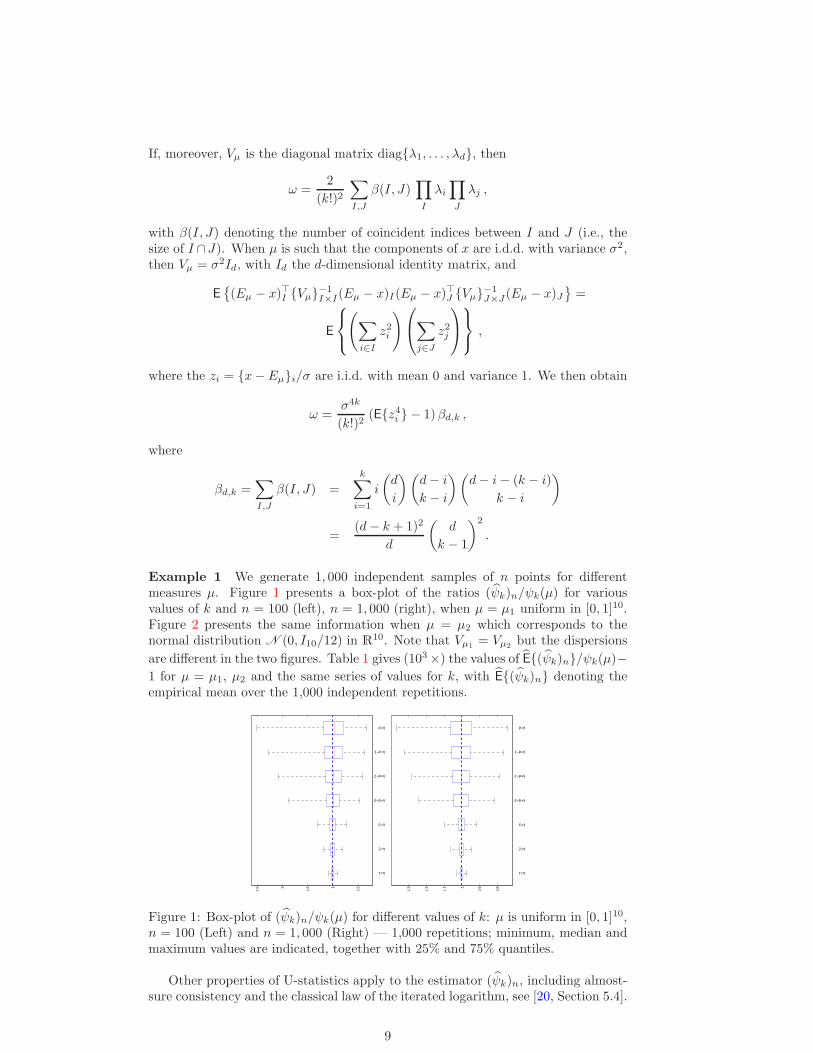
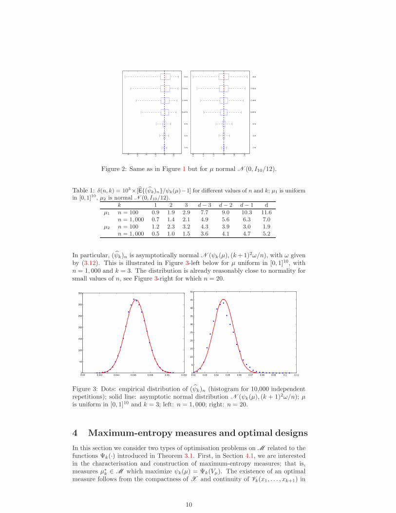
Example 1 We generate 1, 000 independent samples of n points for differentmeasures µ. Figure 1 presents a box-plot of the ratios (ψk)n/ψk(µ) for variousvalues of k and n = 100 (left), n = 1, 000 (right), when µ = µ1 uniform in [0, 1]10.Figure 2 presents the same information when µ = µ2 which corresponds to thenormal distribution N (0, I10/12) in R

10. Note that Vµ1= Vµ2

but the dispersions

are different in the two figures. Table 1 gives (103×) the values of E{(ψk)n}/ψk(µ)−1 for µ = µ1, µ2 and the same series of values for k, with E{(ψk)n} denoting theempirical mean over the 1,000 independent repetitions.

0.51

1.52

2.5

k=1

k=2

k=3

k=d−3

k=d−2

k=d−1

k=d

0.8

0.91

1.1

1.2

1.3

k=1

k=2

k=3

k=d−3

k=d−2

k=d−1

k=d

Figure 1: Box-plot of (ψk)n/ψk(µ) for different values of k: µ is uniform in [0, 1]10,n = 100 (Left) and n = 1, 000 (Right) — 1,000 repetitions; minimum, median andmaximum values are indicated, together with 25% and 75% quantiles.

Other properties of U-statistics apply to the estimator (ψk)n, including almost-sure consistency and the classical law of the iterated logarithm, see [20, Section 5.4].

9

0.51

1.52

2.53

k=1

k=2

k=3

k=d−3

k=d−2

k=d−1

k=d

0.6

0.81

1.2

1.4

1.6

k=1

k=2

k=3

k=d−3

k=d−2

k=d−1

k=d

Figure 2: Same as in Figure 1 but for µ normal N (0, I10/12).

Table 1: δ(n, k) = 103× [E{(ψk)n}/ψk(µ)−1] for different values of n and k; µ1 is uniformin [0, 1]10, µ2 is normal N (0, I10/12).

k 1 2 3 d− 3 d− 2 d− 1 d

µ1 n = 100 0.9 1.9 2.9 7.7 9.0 10.3 11.6n = 1, 000 0.7 1.4 2.1 4.9 5.6 6.3 7.0

µ2 n = 100 1.2 2.3 3.2 4.3 3.9 3.0 1.9n = 1, 000 0.5 1.0 1.5 3.6 4.1 4.7 5.2

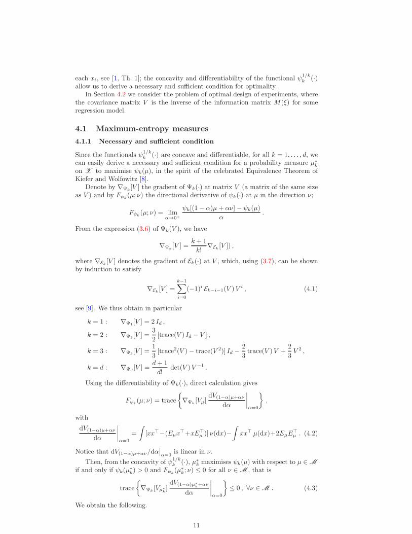
In particular, (ψk)n is asymptotically normal N (ψk(µ), (k+1)2ω/n), with ω givenby (3.12). This is illustrated in Figure 3-left below for µ uniform in [0, 1]10, withn = 1, 000 and k = 3. The distribution is already reasonably close to normality forsmall values of n, see Figure 3-right for which n = 20.

0.04 0.042 0.044 0.046 0.048 0.05 0.0520

50

100

150

200

250

300

350

0.02 0.03 0.04 0.05 0.06 0.07 0.08 0.09 0.1 0.110

5

10

15

20

25

30

35

40

45

50

Figure 3: Dots: empirical distribution of (ψk)n (histogram for 10,000 independentrepetitions); solid line: asymptotic normal distribution N (ψk(µ), (k + 1)2ω/n); µis uniform in [0, 1]10 and k = 3; left: n = 1, 000; right: n = 20.

4 Maximum-entropy measures and optimal designs

In this section we consider two types of optimisation problems on M related to thefunctions Ψk(·) introduced in Theorem 3.1. First, in Section 4.1, we are interestedin the characterisation and construction of maximum-entropy measures; that is,measures µ∗

k ∈ M which maximize ψk(µ) = Ψk(Vµ). The existence of an optimalmeasure follows from the compactness of X and continuity of Vk(x1, . . . , xk+1) in

10

each xi, see [1, Th. 1]; the concavity and differentiability of the functional ψ1/kk (·)

allow us to derive a necessary and sufficient condition for optimality.In Section 4.2 we consider the problem of optimal design of experiments, where

the covariance matrix V is the inverse of the information matrix M(ξ) for someregression model.

4.1 Maximum-entropy measures

4.1.1 Necessary and sufficient condition

Since the functionals ψ1/kk (·) are concave and differentiable, for all k = 1, . . . , d, we

can easily derive a necessary and sufficient condition for a probability measure µ∗k

on X to maximise ψk(µ), in the spirit of the celebrated Equivalence Theorem ofKiefer and Wolfowitz [8].

Denote by ∇Ψk[V ] the gradient of Ψk(·) at matrix V (a matrix of the same size

as V ) and by Fψk(µ; ν) the directional derivative of ψk(·) at µ in the direction ν;

Fψk(µ; ν) = lim

α→0+

ψk[(1− α)µ + αν]− ψk(µ)

α.

From the expression (3.6) of Ψk(V ), we have

∇Ψk[V ] =

k + 1

k!∇Ek

[V ]) ,

where ∇Ek[V ] denotes the gradient of Ek(·) at V , which, using (3.7), can be shown

by induction to satisfy

∇Ek[V ] =

k−1∑

i=0

(−1)i Ek−i−1(V )V i , (4.1)

see [9]. We thus obtain in particular

k = 1 : ∇Ψ1[V ] = 2 Id ,

k = 2 : ∇Ψ2[V ] =

3

2[trace(V ) Id − V ] ,

k = 3 : ∇Ψ3[V ] =

1

3[trace2(V )− trace(V 2)] Id −

2

3trace(V )V +

2

3V 2 ,

k = d : ∇Ψd[V ] =

d+ 1

d!det(V )V −1 .

Using the differentiability of Ψk(·), direct calculation gives

Fψk(µ; ν) = trace

{∇Ψk

[Vµ]dV(1−α)µ+αν

dα

∣∣∣∣α=0

},

with

dV(1−α)µ+αν

dα

∣∣∣∣α=0

=

∫[xx⊤−(Eµx

⊤+xE⊤µ )] ν(dx)−

∫xx⊤ µ(dx)+2EµE

⊤µ . (4.2)

Notice that dV(1−α)µ+αν/dα∣∣α=0

is linear in ν.

Then, from the concavity of ψ1/kk (·), µ∗

k maximises ψk(µ) with respect to µ ∈ M

if and only if ψk(µ∗k) > 0 and Fψk

(µ∗k; ν) ≤ 0 for all ν ∈ M , that is

trace

{∇Ψk

[Vµ∗

k]dV(1−α)µ∗

k+αν

dα

∣∣∣∣α=0

}≤ 0 , ∀ν ∈ M . (4.3)

We obtain the following.

11

Theorem 4.1. The probability measure µ∗k such that ψk(µ

∗k) > 0 is ψk-optimal,

that is, maximises ψk(µ) with respect to µ ∈ M , k ∈ {1, . . . , d}, if and only if

maxx∈X

(x − Eµ∗

k)⊤

∇Ψk[Vµ∗

k]

Ψk(Vµ∗

k)(x− Eµ∗

k) ≤ k . (4.4)

Moreover,

(x− Eµ∗

k)⊤

∇Ψk[Vµ∗

k]

Ψk(Vµ∗

k)(x− Eµ∗

k) = k (4.5)

for all x in the support of µ∗k.

Proof. First note that the Newton equations (3.7) and the recurrence (4.1) for∇Ek[·]

imply that trace(V∇Ψk[V ]) = kΨk(V ) for all k = 1, . . . , d.

The condition (4.4) is sufficient. Indeed, suppose that µ∗k such that ψk(µ

∗k) > 0

satisfies (4.4). We obtain

∫(x − Eµ∗

k)⊤∇Ψk

[Vµ∗

k](x− Eµ∗

k) ν(dx) ≤ trace

{Vµ∗

k∇Ψk

[Vµ∗

k]}

for any ν ∈ M , which gives (4.3) when we use (4.2). The condition is also necessarysince (4.3) must be true in particular for δx, the delta measure at any x ∈ X , whichgives (4.4). The property (4.5) on the support of µ∗

k follows from the observationthat

∫(x− Eµ∗

k)⊤∇Ψk

[Vµ∗

k](x− Eµ∗

k)µ∗

k(dx) = trace{Vµ∗

k∇Ψk

[Vµ∗

k]}.

Note that for k < d, the covariance matrix Vµ∗

kof a ψk-optimal measure µ∗

k

is not necessarily unique and may be singular; see, e.g., Example 1 below. Also,ψk(µ) > 0 implies that ψk−1(µ) > 0, k = 2, . . . , d.

Remark 4.1. As a natural extension of the concept of potential in case of order-two interactions (k = 1), we call Pk,µ(x) = ψk(µ, . . . , µ, δx) the potential of µ at x,where

ψk(µ1, . . . , µk+1) =

∫. . .

∫V

2k (x1, . . . , xk+1)µ1(dx1) . . . µk+1(dxk+1) .

This yields Fψk(µ; ν) = (k + 1) [ψk(µ, . . . , µ, ν) − ψk(µ)], where µ appears k times

in ψk(µ, . . . , µ, ν). Therefore, Theorem 4.4 states that µ∗k is ψk-optimal if and

only if ψk(µ∗k, . . . , µ

∗k, ν) ≤ ψk(µ

∗k) for any ν ∈ M , or equivalently Pk,µ∗

k(x) ≤

ψk(µ∗k) for all x ∈ X .

Remark 4.2. Consider Kiefer’s Φp-class of orthogonally invariant criteria andtheir associated functional ϕp(·), defined by

ϕp(µ) = Φp(Vµ) =

λmax(Vµ) for p = ∞ ,

{ 1d trace(V

pµ )}1/d for p 6= 0,±∞ ,

det1/d(Vµ) for p = 0 ,λmin(Vµ) for p = −∞ ,

where Vµ is a d × d matrix; see, e.g., [14, Chap. 6]. From a result in [7], if ameasure µp optimal for some ϕp(·) with p ∈ (−∞, 1] is such that Vµp

is proportionalto the identity matrix Id, then µp is simultaneously optimal for all orthogonallyinvariant criteria. A measure µp having this property is therefore ψk-optimal for

all k = 1, . . . , d. Notice that ψ1(·) and ψ1/dd (·) respectively coincide with ϕ1(·) and

ϕ0(·) (up to a multiplicative scalar).

12

Remark 4.3. Using (3.10), when V is nonsingular we obtain the property

Ψk(V ) =(k + 1)(d− k)!

(d− k + 1)k!det(V )Ψd−k(V

−1)

which implies that maximising Ψk(V ) is equivalent to maximising log det(V ) +logΨd−k(V

−1). Therefore, Theorem 4.4 can be reformulated as: µ∗k maximises

ψk(µ) if and only if

maxx∈X

(x− Eµ∗

k)⊤

[V −1µ∗

k− V −1

µ∗

k

∇Ψd−k[V −1µ∗

k]

Ψd−k(V−1µ∗

k)V −1µ∗

k

](x− Eµ∗

k) ≤ d− k ,

with equality for x in the support of µ∗k. When k is large (and d− k is small), one

may thus check the optimality of µ∗k without using the complicated expressions of

Ψk(V ) and ∇Ψk[V ].

4.1.2 A duality property

The characterisation of maximum-entropy measures can also be approached fromthe point of view of duality theory.

When k = 1, the determination of a ψ1-optimal measure µ∗1 is equivalent to the

dual problem of constructing the minimum-volume ball B∗d containing X . If this

ball has radius ρ, then ψ1(µ∗1) = 2ρ2, and the support points of µ∗

1 are the pointsof contact between X and B∗

d ; see [1, Th. 6]. Moreover, there exists an optimalmeasure with no more than d+ 1 points.

The determination of an optimal measure µ∗d is also dual to a simple geometrical

problem: it corresponds to the determination of the minimum-volume ellipsoid E ∗d

containing X . This is equivalent to a D-optimal design problem in Rd+1 for theestimation of β = (β0, β

⊤1 )⊤, β1 ∈ Rd, in the linear regression model with intercept

β0 + β⊤1 x, x ∈ X , see [23]. Indeed, denote

Wµ =

∫

X

(1 x⊤)⊤(1 x⊤)µ(dx) .

Then E ∗d+1 = {z ∈ R

d+1 : z⊤W−1µ∗

dz ≤ d + 1}, with µ∗

d maximising det(Wµ), is

the minimum-volume ellipsoid centered at the origin and containing the set {z ∈Rd+1 : z = (1 x⊤)⊤, x ∈ X }. Moreover, E ∗

d corresponds to the intersectionbetween E ∗

d+1 and the hyperplane {z}1 = 1; see, e.g., [22]. This gives ψd(µ∗d) =

(d+1)/d! det(Wµ∗

d). The support points of µ∗

d are the points of contact between X

and E ∗d , there exists an optimal measure with no more than d(d + 3)/2 + 1 points,

see [23].The property below generalises this duality property to any k ∈ {1, . . . , d}.

Theorem 4.2.

maxµ∈M

Ψ1/kk (Vµ) = min

M,c: X ⊂E (M,c)

1

φ∞k (M),

where E (M, c) denotes the ellipsoid E (M, c) = {x ∈ Rd : (x − c)⊤M(x − c) ≤ 1}and φ∞k (M) is the polar function

φ∞k (M) = infV�0: trace(MV )=1

1

Ψ1/kk (V )

. (4.6)

The proof is given in Appendix. The polar function φ∞k (·) possesses the prop-erties of what is called an information function in [14, Chap. 5]; in particular, itis concave on the set of symmetric non-negative definite matrices. This dualityproperty has the following consequence.

13

Corollary 4.1. The determination of a covariance matrix V ∗k that maximises

Ψk(Vµ) with respect to µ ∈ M is equivalent to the determination of an ellipsoidE (M∗

k , c∗k) containing X , minimum in the sense that M∗

k maximizes φ∞k (M). Thepoints of contact between E (M∗

k , c∗k) and X form the support of µ∗

k.

For any V � 0, denote by M∗(V ) the matrix

M∗(V ) =∇Ψk

[V ]

kΨk(V )]=

1

k∇log Ψk

[V ] . (4.7)

Note that M∗(V ) � 0, see [14, Lemma 7.5], and that

trace[VM∗(V )] = 1 ,

see the proof of Theorem 4.4. The matrix V � 0 maximises Ψk(V ) under theconstraint trace(MV ) = 1 for some M � 0 if and only if V [M∗(V ) − M ] = 0.Therefore, ifM is such that there exists V∗ = V∗(M) � 0 such thatM =M∗[V∗(M)],

then φ∞k (M) = Ψ−1/kk [V∗(M)]. When k < d, the existence of such a V∗ is not

ensured for all M � 0, but happens when M =M∗k which maximises φ∞k (M) under

the constraint X ∈ E (M, c). Moreover, in that case there exists a µ∗k ∈ M such

that M∗k =M∗(Vµ∗

k), and this µ∗

k maximises ψk(µ) with respect to µ ∈ M .Consider in particular the case k = 1. Then, M∗(V ) = Id/trace(V ) and

φ∞1 (M) = λmin(M)/2. The matrix M∗k of the optimal ellipsoid E (M∗

k , c∗k) is pro-

portional to the identity matrix and E (M∗k , c

∗k) is the ball of minimum-volume that

encloses X .When k = 2 and Id � (d − 1)M/trace(M), direct calculations show that

φ∞2 (M) = Ψ−1/22 [V∗(M)], with

V∗(M) = [Id trace(M)/(d− 1)−M ] [trace2(M)/(d− 1)− trace(M2)]−1 ;

the optimal ellipsoid is then such that trace2(M)/(d−1)− trace(M2) is maximised.

4.1.3 Examples

Example 2 Take X = [0, 1]d, d ≥ 1 and denote by vi, i = 1, . . . , 2d the 2d vertices

of X . Consider µ∗ = (1/2d)∑2d

i=1 δvi , with δv the Dirac delta measure at v. Then,Vµ∗ = Id/4 and one can easily check that µ∗ is ψ1-optimal. Indeed, Eµ∗ = 1d/2,with 1d the d-dimensional vector of ones, and maxx∈X (x−1d/2)

⊤(2 Id)(x−1d/2) =d/2 = trace{Vµ∗∇Ψ1

[Vµ∗ ]}. From Remark 4.2, the measure µ∗ is ψk-optimal for allk = 1, . . . , d.

Note that the two-point measure µ∗1 = (1/2)[δ0 + δ1d

] is such that Vµ∗

1=

(1d 1⊤d )/4 and ψ1(µ

∗1) = d/2 = ψ1(µ

∗), and is therefore ψ1-optimal too. It isnot ψk-optimal for k > 1, since ψk(µ

∗1) = 0, k > 1.

Example 3 TakeX = Bd(0, ρ), the closed ball ofRd centered at the origin 0 withradius ρ. Let µ0 be the uniform measure on the sphere Sd(0, ρ) (the boundary ofBd(0, ρ)). Then, Vµ0

is proportional to the identity matrix Id, and trace[Vµ0] = ρ2

implies that Vµ0= ρ2Id/d. Take k = d. We have Eµ0

= 0 and

maxx∈X

(x− Eµ0)⊤∇Ψd

[Vµ0](x− Eµ0

) =(d+ 1)ρ2d

dd−1d!= trace{Vµ0

∇Ψd[Vµ0

]} ,

so that µ0 is ψd-optimal from (4.4).Let µd be the measure that allocates mass 1/(d + 1) at each vertex of a d

regular simplex having its d+ 1 vertices on Sd(0, ρ), with squared volume ρ2d(d+

14

1)d+1/[dd(d!)2]. We also have Vµd= ρ2Id/d, so that µd is ψd-optimal too. In view

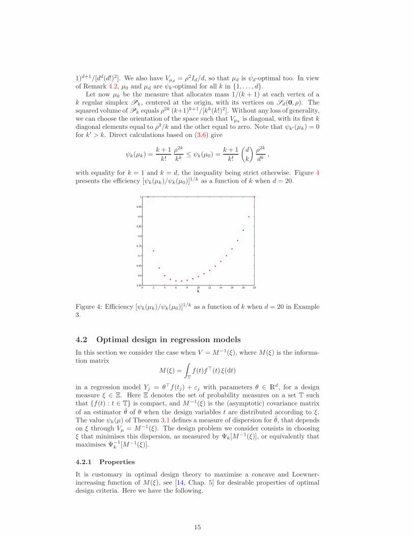
of Remark 4.2, µ0 and µd are ψk-optimal for all k in {1, . . . , d}.Let now µk be the measure that allocates mass 1/(k + 1) at each vertex of a

k regular simplex Pk, centered at the origin, with its vertices on Sd(0, ρ). Thesquared volume of Pk equals ρ

2k (k+1)k+1/[kk(k!)2]. Without any loss of generality,we can choose the orientation of the space such that Vµk

is diagonal, with its first kdiagonal elements equal to ρ2/k and the other equal to zero. Note that ψk′(µk) = 0for k′ > k. Direct calculations based on (3.6) give

ψk(µk) =k + 1

k!

ρ2k

kk≤ ψk(µ0) =

k + 1

k!

(d

k

)ρ2k

dk,

with equality for k = 1 and k = d, the inequality being strict otherwise. Figure 4presents the efficiency [ψk(µk)/ψk(µ0)]

1/k as a function of k when d = 20.

0 2 4 6 8 10 12 14 16 18 200.55

0.6

0.65

0.7

0.75

0.8

0.85

0.9

0.95

1

k

Figure 4: Efficiency [ψk(µk)/ψk(µ0)]1/k as a function of k when d = 20 in Example

3.

4.2 Optimal design in regression models

In this section we consider the case when V =M−1(ξ), where M(ξ) is the informa-tion matrix

M(ξ) =

∫

T

f(t)f⊤(t) ξ(dt)

in a regression model Yj = θ⊤f(tj) + εj with parameters θ ∈ Rd, for a design

measure ξ ∈ Ξ. Here Ξ denotes the set of probability measures on a set T suchthat {f(t) : t ∈ T} is compact, and M−1(ξ) is the (asymptotic) covariance matrix

of an estimator θ of θ when the design variables t are distributed according to ξ.The value ψk(µ) of Theorem 3.1 defines a measure of dispersion for θ, that dependson ξ through Vµ = M−1(ξ). The design problem we consider consists in choosingξ that minimises this dispersion, as measured by Ψk[M

−1(ξ)], or equivalently thatmaximises Ψ−1

k [M−1(ξ)].

4.2.1 Properties

It is customary in optimal design theory to maximise a concave and Loewner-increasing function of M(ξ), see [14, Chap. 5] for desirable properties of optimaldesign criteria. Here we have the following.

15

Theorem 4.3. The functions M −→ Ψ−1/kk (M−1), k = 1, . . . , d, are Loewner-

increasing, concave and differentiable on the set M+ of d × d symmetric positive-definite matrices. The functions Ψk(·) are also orthogonally invariant.

Proof. The property (3.10) yields

Ψ−1/kk (M−1) =

(k + 1

k!

)−1/kdet1/k(M)

E1/kd−k(M)

(4.8)

which is a concave function of M , see Eq. (10) of [11, p. 116]. Since Ψk(·) is

Loewner-increasing, see [9], the functionM −→ Ψ−1/kk (M−1) is Loewner-increasing

too. Its orthogonal invariance follows from the fact that it is defined in terms ofthe eigenvalues of M .

Note that Theorems 3.1 and 4.3 imply that the functions M −→ − logΨk(M)and M −→ logΨk(M

−1) are convex for all k = 1, . . . , d, a question which was leftopen in [9].

As a consequence of Theorem 4.3, we can derive a necessary and sufficient con-

dition for a design measure ξ∗k to maximise Ψ−1/kk [M−1(ξ)] with respect to ξ ∈ Ξ,

for k = 1, . . . , d.

Theorem 4.4. The design measure ξ∗k such that M(ξ∗k) ∈ M+ maximises ψk(ξ) =

Ψ−1/kk [M−1(ξ)] with respect to ξ ∈ Ξ if and only if

maxt∈T

f⊤(t)M−1(ξ∗k)∇Ψk

[M−1(ξ∗k)]

Ψk[M−1(ξ∗k)]M−1(ξ∗k)f(t) ≤ k (4.9)

or, equivalently,

maxt∈T

{f⊤(t)M−1(ξ∗k)f(t)− f⊤(t)

∇Ψd−k[M(ξ∗k)]

Ψd−k[M(ξ∗k)]f(t)

}≤ d− k . (4.10)

Moreover, there is equality in (4.9) and (4.10) for all t in the support of ξ∗k .

Proof. From (4.8), the maximisation of ψk(ξ) is equivalent to the maximisation ofφk(ξ) = log det[M(ξ)]−log Ψd−k[M(ξ)]. The proof is similar to that of Theorem 4.4and is based on the following expressions for the directional derivatives of these twofunctionals at ξ in the direction ν ∈ Ξ,

Fψk(ξ; ν) = trace

(1

kM−1(ξ)

∇Ψk[M−1(ξ)]

Ψk[M−1(ξ)]M−1(ξ) [M(ν) −M(ξ)]

)

and

Fφk(ξ; ν) = trace

({M−1(ξ)− ∇Ψd−k

[M(ξ)]

Ψd−k[M(ξ)]

}[M(ν)−M(ξ)]

),

and on the property trace{M∇Ψj[M ]} = jΨj(M).

In particular, consider the following special cases for k (note that Ψ0(M) =E0(M) = 1 for any M).

k = d : ψd(ξ) = log det[M(ξ)] ,

k = d− 1 : ψd−1(ξ) = log det[M(ξ)]− log trace[M(ξ)]− log 2 ,

k = d− 2 : ψd−2(ξ) = log det[M(ξ)]

− log{trace2[M(ξ)]− trace[M2(ξ)]

}− log(3/4) .

16

The necessary and sufficient condition (4.10) then takes the following form:

k = d : maxt∈T

f⊤(t)M−1(ξ∗k)f(t) ≤ d ,

k = d− 1 : maxt∈T

{f⊤(t)M−1(ξ∗k)f(t)−

f⊤(t)f(t)

trace[M(ξ∗k)]

}≤ d− 1 ,

k = d− 2 : maxt∈T

{f⊤(t)M−1(ξ∗k)f(t)

−2trace[M(ξ∗k)]f

⊤(t)f(t)− f⊤(t)M(ξ∗k)f(t)

trace2[M(ξ∗k)]− trace[M2(ξ∗k)]

}≤ d− 2 .

Also, for k = 1 condition (4.9) gives

maxt∈T

f⊤(t)M−2(ξ∗1 )

trace[M−1(ξ∗1 )]f(t) ≤ 1

(which corresponds to A-optimal design), and for k = 2

maxt∈T

trace[M−1(ξ∗2 )]f⊤(t)M−2(ξ∗2)f(t)− f⊤(t)M−3(ξ∗2 )f(t)

trace2[M−1(ξ∗2)]− trace[M−2(ξ∗2)]≤ 1 .

Finally, note that a duality theorem, in the spirit of Theorem 4.2, can be for-

mulated for the maximisation of Ψ−1/kk [M−1(ξ)]; see [14, Th. 7.12] for the general

form a such duality properties in optimal experimental design.

4.2.2 Examples

Example 4 For the linear regression model on θ0 + θ1 x on [−1, 1], the optimaldesign for ψk(·) with k = d = 2 or k = 1 is

ξ∗k =

{−1 11/2 1/2

},

where the first line corresponds to support points and the second indicates theirrespective weights.

Example 5 For linear regression with the quadratic polynomial model θ0+ θ1 t+θ2 t

2 on [−1, 1], the optimal designs for ψk(·) have the form

ξ∗k =

{−1 0 1wk 1− 2wk wk

},

with w3 = 1/3, w2 = (√33−1)/16 ≃ 0.2965352 and w1 = 1/4. Define the efficiency

Effk(ξ) of a design ξ as

Effk(ξ) =ψk(ξ)

ψk(ξ∗k).

Table 2 gives the efficiencies Effk(ξ∗j ) for j, k = 1, . . . , d = 3. The design ξ∗2 , op-

timal for ψ2(·), appears to make a good compromise between A-optimality (whichcorresponds to ψ1(·)) and D-optimality (which corresponds to ψ3(·)).

Example 6 For linear regression with the cubic polynomial model θ0 + θ1 t +θ2 t

2 + θ3 t3 on [−1, 1], the optimal designs for ψk(·) have the form

ξ∗k =

{−1 −zk zk 1wk 1/2− wk 1/2− wk wk

},

17

Table 2: Efficiencies Effk(ξ∗j ) for j, k = 1, . . . , d in Example 5.

Eff1 Eff2 Eff3

ξ∗1 1 0.9770 0.9449ξ∗2 0.9654 1 0.9886ξ∗3 0.8889 0.9848 1

Table 3: Efficiencies Effk(ξ∗j ) for j, k = 1, . . . , d in Example 6.

Eff1 Eff2 Eff3 Eff4

ξ∗1 1 0.9785 0.9478 0.9166ξ∗2 0.9694 1 0.9804 0.9499ξ∗3 0.9180 0.9753 1 0.9897ξ∗4 0.8527 0.9213 0.9872 1

where

z4 = 1/√5 ≃ 0.4472136 , w4 = 0.25 ,

z3 ≃ 0.4350486 , w3 ≃ 0.2149859 ,z2 ≃ 0.4240013 , w2 ≃ 0.1730987 ,

z1 =√3√7− 6/3 ≃ 0.4639509 , w1 = (4 −

√7)/9 ≃ 0.1504721 ,

with z3 satisfying the equation 2z6 − 3z5 − 45z4 + 6z3 − 4z2 − 15z + 3 = 0 and

w3 =5 z6 + 5 z4 + 5 z2 + 1−

√z12 + 2 z10 + 3 z8 + 60 z6 + 59 z4 + 58 z2 + 73

12(z6 + z4 + z2 − 3),

with z = z3. For k = d− 2 = 2, the numbers z2 and w2 are too difficult to expressanalytically. Table 3 gives the efficiencies Effk(ξ

∗j ) for j, k = 1, . . . , d. Here again

the design ξ∗2 appears to make a good compromise: it maximises the minimumefficiency mink Efff (·) among the designs considered.

Appendix

Shift-invariance and positive homogeneity Denote by M the set of proba-bility measures defined on the Borel subsets of X , a compact subset of Rd. For anyµ ∈ M , any θ ∈ Rd and any λ ∈ R+, respectively denote by T−θ[µ] and Hλ−1 [µ]the measures defined by:

for any µ-measurable A ⊆ X , T−θ[µ](A + θ) = µ(A ) , Hλ−1 [µ](λA ) = µ(A ) ,

where A + θ = {x + θ : x ∈ A } and λA = {λx : x ∈ A }. The shift-invarianceof φ(·) then means that φ(T−θ[µ]) = φ(µ) for any µ ∈ M and any θ ∈ Rd, positivehomogeneity of degree q means that φ(Hλ−1 [µ]) = λq φ(µ) for any µ ∈ M and anyλ ∈ R+.

The variance is the only concave central moment For q 6= 2, the q-th centralmoment ∆q(µ) =

∫‖x − Eµ‖q µ(dx) is shift-invariant and homogeneous of degree

q, but it is not concave on M (X ). Indeed, consider for instance the two-pointprobability measures

µ1 =

{0 11/2 1/2

}and µ2 =

{0 101w 1− w

},

where the first line denotes the support points and the second one their respectiveweights. Then, for

w = 1− 1

404

201q−1 − 202q + 405

201q−1 − 101q + 102

18

one has ∂2∆q[(1 − α)µ1 + αµ2]/∂α2∣∣α=0

≥ 0 for all q ≥ 1.84, the equality beingobtained at q = 2 only. Counterexamples are easily constructed for values of qsmaller than 1.84.

Proof of Theorem 4.2

(i) The fact that maxµ∈M Ψ1/kk (Vµ) ≥ minM,c: X ⊂E (M,c) 1/φ

∞k (M) is a consequence

of Theorem 4.4. Indeed, the measure µ∗k maximises Ψ

1/kk (Vµ) if and only if

(x− Eµ∗

k)⊤M∗(Vµ∗

k)(x− Eµ∗

k) ≤ 1 for all x in X . (4.11)

Denote M∗k = M∗(Vµ∗

k), c∗k = Eµ∗

k, and consider the Lagrangian L(V, α;M) for

the maximisation of (1/k) logΨk(V ) with respect to V � 0 under the constrainttrace(MV ) = 1: L(V, α;M) = (1/k) logΨk(V )− α[trace(MV )− 1] . We have

∂L(V, 1;M∗k )

∂V

∣∣∣∣V=Vµ∗

k

=M∗k −M∗

k = 0

and trace(M∗kVµ∗

k) = 1, with Vµ∗

k� 0. Therefore, Vµ∗

kmaximises Ψk(V ) under the

constraint trace(M∗kV ) = 1, and, moreover, X ⊂ E (M∗

k , c∗k) from (4.11). This

implies

Ψ1/kk (Vµ∗

k) = max

V�0: trace(M∗

kV )=1

Ψ1/kk (V )

≥ minM,c: X ⊂E (M,c)

maxV�0: trace(MV )=1

Ψ1/kk (V ) = min

M,c: X ⊂E (M,c)

1

φ∞k (M).

(ii) We prove now that minM,c: X ⊂E (M,c) 1/φ∞k (M) ≥ maxµ∈M Ψ

1/kk (Vµ). Note

that we do not have an explicit form for φ∞k (M) and that the infimum in (4.6) canbe attained at a singular V , not necessarily unique, so that we cannot differentiateφ∞k (M). Also note that compared to the developments in [14, Chap. 7], here weconsider covariance matrices instead of moment matrices.

Consider the maximisation of logφ∞k (M) with respect to M and c such thatX ⊂ E (M, c), with Lagrangian

L(M, c, β) = logφ∞k (M) +∑

x∈X

βx[1− (x− c)⊤M(x− c)] , βx ≥ 0 for all x in X .

For the sake of simplicity we consider here X to be finite, but β may denote any pos-itive measure on X otherwise. Denote the optimum by T ∗ = maxM,c: X ⊂E (M,c) logφ

∞k (M) .

It satisfies T ∗ = maxM,cminβ≥0 L(M, c, β) ≤ minβ≥0 maxM,c L(M, c, β), and maxM,c L(M, c, β)is attained for any c such that Mc =M

∑x∈X

βx x/(∑

x∈Xβx), that is, in partic-

ular for

c∗ =

∑x∈X

βx x∑x∈X

βx,

and for M∗ such that 0 ∈ ∂ML(M, c∗, β)∣∣M=M∗

, the subdifferential of L(M, c∗, β)with respect to M at M∗. This condition can be written as

∑

x∈X

βx (x− c∗)(x− c∗)⊤ = V ∈ ∂ logφ∞k (M)∣∣M=M∗

,

with ∂ logφ∞k (M) the subdifferential of logφ∞k (M),

∂ log φ∞k (M) = {V � 0 : Ψ1/kk (V )φ∞k (M) = trace(MV ) = 1} ,

19

see [14, Th. 7.9]. Since trace(MV ) = 1 for all V ∈ ∂ logφ∞k (M), trace(M∗V ) = 1

and thus∑

x∈Xβx (x − c∗)⊤M∗(x − c∗) = 1 . Also, Ψ

1/kk (V ) = 1/φ∞k (M∗), which

gives

L(M∗, c∗, β) = − logΨ1/kk

[∑

x∈X

βx (x− c∗)(x − c∗)⊤

]+∑

x∈X

βx − 1 .

We obtain finally

minβ≥0

L(M∗, c∗, β)

= minγ>0, α≥0

{− logΨ

1/kk

[∑

x∈X

αx (x− c∗)(x − c∗)⊤

]+ γ − log(γ)− 1

},

= minα≥0

− logΨ1/kk

[∑

x∈X

αx (x − c∗)(x− c∗)⊤

]= − logΨ

1/kk (V ∗

k ) ,

where we have denoted γ =∑

x∈Xβx and αx = βx/γ for all x. Therefore T ∗ ≤

− logΨ1/kk (V ∗

k ), that is, log[minM,c: X ⊂E (M,c) 1/φ

∞k (M)

]≥ log Ψ

1/kk (V ∗

k ).

References

[1] G. Bjorck. Distributions of positive mass, which maximize a certain generalizedenergy integral. Arkiv for Matematik, 3(21):255–269, 1956.

[2] M.H. DeGroot and M.M. Rao. Bayes estimation with convex loss. Ann. Math.Statist., 34(3):839–846, 1963.

[3] F.R. Gantmacher. Theorie des Matrices. Dunod, Paris, 1966.

[4] C. Gini. Measurement of inequality of incomes. Economic J., 31(121):124–126,1921.

[5] A. Giovagnoli and H.P. Wynn. Multivariate dispersion orderings. Stat. & Prob.Lett., 22(4):325–332, 1995.

[6] M. Hainy, W.G. Muller, and H.P. Wynn. Learning functions and approximatebayesian computation design: ABCD. Entropy, 16(8):4353–4374, 2014.

[7] R. Harman. Lower bounds on efficiency ratios based on φp-optimal designs. InA. Di Bucchianico, H. Lauter, and H.P. Wynn, editors, mODa’7 – Advancesin Model–Oriented Design and Analysis, Proceedings of the 7th Int. Workshop,Heeze (Netherlands), pages 89–96, Heidelberg, 2004. Physica Verlag.

[8] J. Kiefer and J. Wolfowitz. The equivalence of two extremum problems. Canad.J. Math., 12:363–366, 1960.

[9] J. Lopez-Fidalgo and J.M. Rodrıguez-Dıaz. Characteristic polynomial criteriain optimal experimental design. In A.C. Atkinson, L. Pronzato, and H.P.Wynn, editors, Advances in Model–Oriented Data Analysis and ExperimentalDesign, Proceedings of MODA’5, Marseilles, June 22–26, 1998, pages 31–38.Physica Verlag, Heidelberg, 1998.

[10] I.G. Macdonald. Symmetric functions and Hall polynomials. Oxford UniversityPress, Oxford, 1995. [2nd ed.].

20

[11] M. Marcus and H. Minc. A Survey of Matrix Theory and Matrix Inequalities.Dover, New York, 1964.

[12] H. Oja. Descriptive statistics for multivariate distributions. Stat. & Prob. Lett.,1(6):327–332, 1983.

[13] L. Pronzato. On a property of the expected value of a determinant. Stat. &Prob. Lett., 39:161–165, 1998.

[14] F. Pukelsheim. Optimal Experimental Design. Wiley, New York, 1993.

[15] C.R. Rao. Diversity and dissimilarity coefficients: a unified approach. Theoret.Popn Biol., 21(1):24–43, 1982.

[16] C.R. Rao. Diversity: Its measurement, decomposition, apportionment andanalysis. Sankhya: Indian J. Statist., Series A, 44(1):1–22, 1982.

[17] C.R. Rao. Convexity properties of entropy functions and analysis of diversity.In Inequalities in Statistics and Probability, volume 5, pages 68–77. LectureNotes-Monograph Series, IMS, Hayward, CA, 1984.

[18] R.L. Schilling, R. Song, and Z. Vondracek. Bernstein Functions: Theory andApplications. de Gruyter, Berlin/Boston, 2012.

[19] I.J. Schoenberg. Metric spaces and positive definite functions. Trans. Amer.Math. Soc., 44(3):522–536, 1938.

[20] R.J. Serfling. Approximation Theorems of Mathematical Statistics. Wiley, NewYork, 1980.

[21] M. Shaked. Dispersive ordering of distributions. J. Appl. Prob., pages 310–320,1982.

[22] N.Z. Shor and O.A. Berezovski. New algorithms for constructing optimal cir-cumscribed and inscribed ellipsoids. Optim. Meth. Soft., 1:283–299, 1992.

[23] D.M. Titterington. Optimal design: some geometrical espects of D-optimality.Biometrika, 62(2):313–320, 1975.

[24] H.R. van der Vaart. A note on Wilks’ internal scatter. Ann. Math. Statist.,36(4):1308–1312, 1965.

[25] S.S. Wilks. Certain generalizations in the analysis of variance. Biometrika,24:471–494, 1932.

[26] S.S. Wilks. Multidimensional statistical scatter. In I. Olkin, S.G. Ghurye,W. Hoeffding, W.G. Madow, and H.B. Mann, editors, Contributions to Prob-ability and Statistics: Essays in Honor of Harold Hotelling, pages 486–503.Stanford University Press, Stanford, 1960.

21