Generalized multirate analysis of variance

SEPTEMBER 2003 IEEE SIGNAL PROCESSING MAGAZINE 391053-5888/03/$17.00©2003IEEE

Generalized multivariate analysis ofvariance (GMANOVA) [1]-[9]and related reduced-rank regres-sion [10]-[15] are general statisti-

ca l models that comprise vers ions ofregression, canonical correlation, and profileanalyses as well as analysis of variance(ANOVA) and covariance in univariate andmultivariate settings. It is a powerful and, yet,not very well-known tool. In this article, we de-velop a unified framework for explaining, ana-lyzing, and extending signal processingmethods based on GMANOVA. We show theapplicability of this framework to a number ofdetection and estimation problems in signalprocessing and communications and providenew and simple ways to derive numerous exist-ing algorithms for� synchronization and space-time channel andnoise estimation in [16]-[33]� space-time symbol detection in [23] and[30]-[38]� blind and semiblind channel equalization, es-timation, and signal separation in [39]-[44]� source location using parametric signal mod-els in [17], [23], [28], [31], and [45]-[51]� radar target estimation and detection in[45]-[50] and [52]-[55]� spectral analysis [56], [57] and nuclear mag-netic resonance (NMR) spectroscopy [58].

Many of the above methods were originallyderived “from scratch,” without knowledge oftheir close relationship with the GMANOVAmodel. We explicitly show this relationship andpresent new insights and guidelines for general-izing these methods. We also acknowledge thepioneering works of Brillinger (on frequencywavenumber analysis; see [59]) and Kelly andForsythe (on radar detection; see [53]) who ©DIGITAL VISION, LTD.

first applied GMANOVA to signal processing problems.Note that special cases of GMANOVA have also been ap-plied to time-delay estimation for proximity acoustic sen-sors [60], synthetic aperture radar (SAR) [61], [62],inverse SAR (ISAR) of maneuvering targets [63], andhyperspectral image data analysis [64]-[66]; for applica-tions of related reduced-rank regression methods to sys-tem identification, see [67] and references therein. Ourresults could inspire applications of the general frame-work of GMANOVA to new problems in signal process-ing. We will present such an application to flaw detectionin nondestructive evaluation (NDE) of materials. Apromising area for future growth is image processing, asis shown in [61]-[66].

Problem Formulation and Main Results

Historical BackgroundThe GMANOVA model was first formulated by Potthoffand Roy [1], who were interested in fitting the followingpatterned-mean problem:E[ ]Y = AX�, where Y is a datamatrix whose columns are independent random vectorswith common covariance matrix Σ, A, and � are knownmatrices, and X is a matrix of unknown regression coeffi-cients. In [1], this model was applied to fitting growthpatterns of groups of individuals, hence also the namegrowth-curve model [1]-[8]. (Other common statisticalapplications are: clinical trials of pharmaceutical drugs,agronomical investigations, and business surveys; see[6]-[9] for illustrative examples.) In [2], Khatri com-puted maximum likelihood (ML) estimates of X and Σunder the multivariate normal model for Y . Khatri’s re-sults are closely related to the concomitant-variablemethod, independently developed by Rao [3], [4]. In[68], it was shown that the estimates of the regression co-efficients and corresponding generalized likelihood ratiotests developed in [2] are robust when the errors are notnormal.

In the following, we describe the measurement modeland state the main results and important special cases.

Measurement ModelWe now present the general measurement model that willbe examined in this article. Let y( )t be an m ×1 complexdata vector (snapshot) received at time t and assume thatwe have collected N snapshots. (Note that in image pro-cessing applications, y( )t are independent sets of pixel ob-servations, indexed by t that generally does notcorrespond to time.) Consider the following model forthe received snapshots:

y A X e( ) ( ) ( , ) ( ), , ,t t t t N= + =� � � 1 K , (1)

where the signal is described by� an m r× matrix A( ) ( )� m r≥� d ×1 vectors � �( , ), , ,t t N=1 K

� an r d× matrix X of unknown regression coefficients.Here, � and � are parameter vectors (unknown in gen-eral) and e( )t is temporally white and circularly symmetriczero-mean complex Gaussian noise vector with unknownpositive definite spatial covariance Σ, i.e.,

[ ]E e e( ) ( ) , , { , , , }t t NHtτ δ ττ= ∈−Σ 12 K . (2)

In sensor array processing applications, � is usually a vec-tor of spatial parameters describing source locations, and

( )A � is the array response (steering) matrix. The vector �usually consists of temporal parameters. More details onthe choices of � in various applications will be given later.Also, δ t denotes the Kronecker delta symbol and “ H ” theHermitian (conjugate) transpose. Our goal is to presentmethods for� estimating the unknown signal and noise parametersX , �, �, and Σ� detecting the presence of signal (e.g., in radar)� demodulating the received signal (communications).

Main ResultsWe present the basic results of this article. Details of theirderivation are relegated to the Appendix. First, define thefollowing matrices:

[ ]Y = ⋅⋅⋅y y( ) ( )1 N , (3a)

[ ]� � � � � �( ) ( , ) ( , ) ,= ⋅⋅⋅1 N (3b)

$ ( / )R yyHN= ⋅1 YY , (3c)

$ ( / ) ( ) ( )R��

� � � �= ⋅1 N H , (3d)

( ) ( )$ $ /R R y

H

yHNφ = = ⋅φ 1 Y� � , (3e)

( )[ ]$ $ $ $ $

( / ) ( )

|S R R R R

I

y yy y yH

NH HN

φ φ φφ−

φ= −

= ⋅ −1 Y Y� � � (3f)

[ ]$ ( ) ( ) $ ( ) ( )|T A A S A AAH

yH= φ

−−

� � � �1 ,(3g)

where I m denotes the identity matrix of size m,�( ) ( )B B B B B= −H H the projection matrix onto the col-umn space of a matrix B, and “ − ” a generalized inverse ofa matrix, respectively. (A generalized inverse of a matrix A

is defined as any matrix A− such that AA A A

− = ; see, e.g.,[5, ch. 1.6] and [69, ch. 9].) Note that� $R yy is the sample correlation matrix of the received datay( )t� $Rφφ is the sample correlation matrix of � �( , )t

40 IEEE SIGNAL PROCESSING MAGAZINE SEPTEMBER 2003

� $R yφ is the sample cross-correlation matrix between y( )tand � �( , )t� $

|S y φ is the sample correlation matrix of the receiveddata projected onto the space orthogonal to the row spaceof � �( ).Here, $

|S y φ , $Rφφ , and $R yφ are functions of �, and $TA is afunction of � and �. To simplify the notation, we omitthese dependencies throughout this article. Assumingthat

[ ]N m≥ +rank � �( ) , (4)

$|S y φ will be a positive definite matrix (with probability

one), and the maximum likelihood (ML) estimates of X

and Σ for known � and � are (see the Appendix)

[ ]$ ( , ) ( ) $ ( ) ( ) $ $ $| |X A S A A S R R

I

� � � � �=

+ −

φ−

−

φ−

φ φφ−H

yH

y y

r

1 1

[ ][ ]

A A

A I

( ) ( )

( ) ( ) ( ) ,

� �

� � � � �

−

−+ −

Ξ

Ξ

1

2H

d (5a)

( )$( , ) $ $ $

$ $ $ $ $

| |Σ � � = + −

⋅ −

φ φ−

φ φφ−

φ

S I T S

R R R I T S

y m A y

y yH

m A

1

( )y

H

| ,φ−1

(5b)

where Ξ1 and Ξ2 are arbitrary matrices (of appropriate di-mensions). Here, I A Ar − −( ) ( )� � is a matrix whose col-umns span the space orthogonal to the column space ofA( )� H and [ ( ) ( ) ]I d

H− −� � � � is a matrix whosecolumns span the space orthogonal to the column spaceof � �( ). Therefore, premultiplying (5a) by A( )� andpostmultiplying by � �( ) reduces the second and thirdterms in (5a) to zero, implying that the estimate of themean A X( ) $ ( , ) ( )� � � � � is unique (and is equal to (A.17)in the Appendix).

For unknown � and �, their ML estimates $� and $� canbe obtained by maximizing the concentrated likelihoodfunction (see the Appendix):

GLR( , )| $ |

| $ $ $ $ $ $ ||

� � =− φ φ φφ

−φ

−

R

R T S R Ryy

yy A y y yH1

R,

(6)

where ||⋅ denotes the determinant. (Concentrated likeli-hood function is also known as the profile likelihood; see[70, ch. 7.2.4.] for its definition and properties) Here,the ML estimates of X and Σ follow by substituting � and� in (5a) and (5b) with $� and $�. In [31], we also computeclosed-form Cramér-Rao bound expressions for� and �.

DetectionExpression (6) is written in the form of a generalized like-lihood ratio (GLR) test statistic for testingH0 :X = 0 ver-susH1 :X ≠ 0(i.e., detecting the presence of signal) for thecase of known � and �. (See, e.g., [4, p. 418], [71], and[74, ch. 6.4.2.] for the definition of the generalized likeli-hood ratio test.) The GLR test computes the ratio of like-lihood functions under the two hypotheses, withunknown parameters (X and Σ under H1 and Σ underH0 ) replaced by their ML estimates; see also the Appen-dix. If � and � are unknown, the GLR test comparesmax GLR GLRθ , ( , ) ($, $ )

�� = with a threshold. Since (6)

is concentrated with respect to the ML estimates of thenuisance parameters (Σ in this case), it is also the maxi-mized relative likelihood, as defined in [72]. Under H0and assuming known � and �, 1 / ( , )GLR � � is distributedas complex Wilks’ lambda; see [53] and [73]. SinceWilks’ lambda distribution does not depend on the un-known parameters (Σ in this case), we can compute athreshold (with which the above test statistic should becompared) that maintains a constant probability of falsealarm. Such a detector is referred to as a constant falsealarm rate (CFAR) detector; see, e.g., [74].

GLR as a Function of A⊥ ( )�

In some applications, it may be convenient to express theabove GLR test statistic in terms of a matrix A⊥ ( )� whosecolumns span the space orthogonal to the column spaceof A( )� [see(7) at the bottom of the page], which followsby applying Lemma 2 from the Appendix, with S S= φ

$|y

and A A⊥ ⊥= ( )� , to (6). For example, if A( )� is aVandermonde matrix, we can easily construct a corre-sponding A⊥ ( )� and apply polynomial-rooting basedideas to estimate �; see e.g., [75] and [76].

GLR for Full-Rank A( )�

If A( )� has full rank r, the second term in (5a) becomeszero, and (6) simplifies to

GLR( , )| ( ) $ ( )|

| ( ) $ ( )||

� ��

� �= φ

−

−

A S A

A R A

Hy

Hyy

1

1,

(8)

see [31, App. A]. (In sensor array processing applica-tions, (8) can be viewed as the ratio of the Capon spec-tral estimate in the direction � using the data Y , and theCapon spectral estimate in the direction � using theprojection of the data onto the space orthogonal to therow space of � �( ). In other words, it is the overallpower arriving from the direction �, normalized by thepower of the noise only, arriving from the same direc-

tion � [59].) We will use(8) shortly to derive thereduced-rank regressionequations in (14) and thecorresponding GLR ex-pression in (13).

SEPTEMBER 2003 IEEE SIGNAL PROCESSING MAGAZINE 41

[ ]GLR( , )

| $ |

| $ $ ( ) ( ) $ ( )| | |

� ��

=+φ φ ⊥ ⊥ φ ⊥

−

R

S S A A S A A

yy

y yH

y ⊥ φ φφ−

φ( ) $ $ $ |� Hy y

HR RR (7)

GLR for Full-rank A( )� and � �( )If, in addition to A( )� , � �( ) has full rank (equal to d),then both the second and third terms in (5a) are zero,$ ( , )X � � is unique, and another interesting expression for

GLR( , )� � follows (see [31]):

GLR( , )| $ $ ( ) $ |

| $ ( )||

� ��

�=

−φφ φ φ

φ

R R R

SyH

y

y

W,

(9)

where

[ ]W( ) $ $ ( ) ( ) $ ( ) ( ) $� � � � �= −− − −−

−R R A A R A A Ryy yyH

yyH

yy1 1 1

11

(10a)

$ ( ) $ $ $ $|S R R R Rφ φφ φ

−φ= −y y

Hyy y� 1 . (10b)

Assuming d =1,� �( ) becomes a 1× N vector, $ $R ry yφ φ=reduces to an m ×1vector, and $ $R φφ φφ= r to a scalar. Then,(9) simplifies to

[ ]GLR( , )

$ $ ( ) ( ) $ ( ) ( ) $

� �

� � � �

=

+φ

− −−

11 1

1r R A A R A A Ry

H Hyy

Hyy yy y

yH

yy yr

−φ

φφ φ−

φ−

1

1

$

$ $ $ $.

r

r R r (11)

Special cases of the above expression have been used fortarget parameter estimation with radar arrays [48]-[50]and target detection in hyperspectral images [64], [65],which will be discussed in the Applications Section (Ra-dar Array Processing).

Reduced-Rank RegressionConsider a nonparametric model for the matrix A A( )� = ,i.e., assume that it is completely unknown having full rankr d m≤ min( , ). To solve this problem, it is useful to performeigenvalue decomposition of the following matrix:

$ $ $ $ $ $ $ $/ /R R R R U Uyy y yH

yyH−

φ φφ−

φ− =1 2 1 2 2

R � , (12)

where $ { $ ( ), $ ( ), , $ ( )}�2 2 2 21 2= diag λ λ λK m and$ ( ) $ ( ) $ ( )λ λ λ1 2 0≥ ≥ ≥ ≥L m . [Here, R 1 2/ denotes aHermitian square root of a Hermitian matrix R, andR R− −=1 2 1 2 1/ /( ) .] Again, for notational simplicity weomit the dependence of the above quantities on �. Notethat $ ( )λ k are the sample canonical correlations betweeny( )t and � �( , )t ; see, e.g., [11]. Note that (8) with un-structured A A( )� = can be interpreted as a multivariate

Rayleigh quotient and is easily maximized with respect toA, yielding

GLR low rank ( )$ ( )

� =−=

∏ 1

1 21 λ kk

r

.(13)

For details of the proof, see the derivation in [31, App.B]. The above result is also closely related to the Poincaréseparation theorem [4, pp. 64-65], which addresses theproblem of maximizing the multivariate Rayleigh quo-tient. Interestingly, log GLR low rank[ ( )]� is a measure ofthe (estimated) mutual information between y( )t and� �( , )t ; see [77, sec. 9.2]. Using the results of [31, App.B.], the ML estimates of H AX= and Σ follow:

$ ( ) $ $ $ $ ( ) $ ( ) $ $ $/ /H R U U R Ryy yylow rank � = = −AX r r Hy

1 2 1 2φ R

[ ]φφ−

−+ ⋅ −Ξ Φ ΦI d ( ) ( ) ,� � (14a)

$( ) $ $ $ ( ) $ ( ) $ ( ) $/ /Σ Λ� = −R R U U Ryy yyyyHr r r1 2 2 1 2 , (14b)

where Ξ is an arbitrary matrix (of appropriate dimen-sions), $ ( ) { $ ( ), $ ( ), , $ ( )}�2 2 2 21 2r r= diag λ λ λK , and $ ( )U r isthe matrix containing the first r columns of $U. If � �( )hasfull rank, the second term in (14a) disappears, and (14a)and (14b) reduce to the complex versions of the re-duced-rank regression and noise covariance estimates in[10]-[14].

Canonical Correlation Analysisand Reduced-Rank RegressionConsider the problem depicted in Figure 1: we wish tofind the r m× and r d× matrices B and W that minimizethe sample (estimated) geometric mean-square error ofBy W( ) ( , )t t− � � , or, equivalently, maximize its inverse:

lN H

( , , )|( / ) ( ) ( ) |

,

( ) ( ),

��

� �

B W

BY W

=⋅ ⋅

= −

11 E E

Ewhere Φ (15)

subject to the normalizing constraint

BR B I$ ,yyH

r= (16)

which prevents the trivial solution (in which B and Wequal zero), and decorrelates the rows of the filtered datamatrix BY . The optimal B and W for the above problemare (see [42]):

$( ) $ ( ) $ /B U R yy� = −r H 1 2 , (17a)

$ ( ) $( ) $ $W B R� �= φ φφ−

y R (17b)

and


� 1. Canonical correlation analysis based on GMANOVA.

( )l � � � �, $( ), $ ( ) ( )B W =GLR low rank (18)

is exactly the GLR expression for reduced-rank regressionin (13). (Interestingly, a stronger result holds: the optimalB and W in (17) simultaneously minimize all theeigenvalues of the sample mean-square error matrixE E( ) ( ) /� �⋅ H N subject to (16); see [42].) Note that theelements of $( ) ( )B y� t and $ ( ) ( , )W � � �t are the estimatedcanonical variates of y( )t and � �( , )t (see, e.g., [11] and[42]). The above results can be used to derive blind adap-tive signal extraction algorithms in [40]; see the Applica-tions section (Wireless Communications).

MANOVAMultivariate analysis of variance (MANOVA) is an im-portant special case of GMANOVA where A I( )� ≡ m , andhence the coefficient matrix becomes H X= . Then, themeasurement model (1) simplifies to

y H e( ) ( , ) ( ), , ,t t t t N= + =� � 1 K . (19)

The MANOVA model dates back to the first half of the20th century and is a standard part of modern textbookson multivariate statistical analysis; see, e.g., [4]-[7], [9],[11], [78]. The GLR in (8) and ML estimates of H X=and Σ simplify to [using (5) or (14)]

GLR( )| $ |

| $ ||

� =φ

R

Syy

y

,(20a)

[ ]$ ( ) $ $ ( ) ( )H R I� � � � �= + ⋅ −φ φφ− −

y dR Ξ , (20b)

$( ) $|Σ � = φS y , (20c)

where, as before, Ξ is an arbitrary matrix of appropriatedimensions. The above GLR can be used for noncoherentdetection of space-time codes, as will be discussed in theApplications section (Wireless Communications). Its re-cursive implementation was derived in [31]. Interest-ingly, if � �( )has full rank (equal to d) and d m< , it can beshown that the concentrated likelihood function in (20a)increases by iterating between the following two steps.

Step 1: Fix � and compute � � �= $ ( ) using

[ ]$ ( ) $ ( ) $ $ ( ) $ ( ) $� � � � �= ⋅−−

−H R H H R YHyy

Hyy

11

1

(21)

[where $ ( ) $ $H R R� = φ−φφy

1 ].

Step 2: Fix � and find � that minimizes

[ ] [ ]� � � � � �− ⋅ −( ) ( ) H .(22)

The derivation of this result is based on identity (18); see[42]. The above iteration will be used in the followingdiscussion to develop blind equalization (DW-ILSP andLSCMA) algorithms; see the Applications section (Wire-less Communications). An alternative way to maximize(20a) is by using the cyclic ML approach in [37, sec.III-D]; see also [42, sec. V].

In the following, we review several important signalprocessing applications of GMANOVA and MANOVAmodels.

ApplicationsWe discuss the applications of GMANOVA to radar arrayprocessing, spectral analysis, and wireless communica-tions. We also derive a multivariate energy detector andoutline how it can be applied to NDE flaw detection incorrelated interference.

Radar Array Processing

Kelly’s Detector and ExtensionsAssume that an n-element radar array receives P pulse re-turns, where each pulse provides N range-gate samples.After collecting spatio-temporal data from the tth rangegate into a vector y( )t (of size m nP= ), we search for thepresence of targets in one range gate at a time. Withoutloss of generality, let t =1 be under test. Then, this radararray detection problem can be formulated within theGMANOVA framework in (1) with

[ ]� �( ) , , , ,= 10 0 0K of size 1× N, (23)

� X x= , an r ×1 vector of target amplitudes� A( )� , an m r× spatiotemporal steering matrix of thetargets� �, a vector of target parameters, e.g., directions of ar-rival (DOAs) and Doppler shifts; see [52] and [79].We wish to test H0 :x =0 (targets absent) versus H1 :x ≠0(targets present). The unknown noise covariance Σ ac-counts for broadband noise, clutter, and jamming. To beable to estimate Σ, we need noise-only snapshotsy y y( ), ( ), , ( )2 3 K N , where N m≥ +1; see (4). In [52],Kelly derived the GLR test for the above problem assum-ing one target (r =1). It was originally derived fromscratch, but Kelly and Forsythe recognized its close rela-tionship with GMANOVA in [53].

We now show how celebrated Kelly’s detector and itsextensions follow from the GMANOVA framework. Col-lecting all noise-only snapshots into one matrix

[ ]Z y y y= ⋅⋅⋅( ) ( ) ( )2 3 N , (24)

and substituting (23)-(24) into (3), we obtain

N yH$

|S ZZφ = ,(25a)


N y$ ( )R yφ = 1 ,

(25b)

N $R φφ =1.(25c)

After substituting (25) into (6), using the determinantformula| |I ab b a+ = +H H1 (see, e.g., [69, cor. 18.1.3 atp. 416]) and applying the monotonic transformation1 1− / ( )GLR � , we have (26), found at the bottom of thepage, which is a multivariate extension (for r >1) of theKelly’s detector.

The above detector can be further generalized to si-multaneously testing multiple (d) snapshots. Withoutloss of generality, choose the first d snapshots to be undertest: Y y yT = ⋅⋅⋅[ ( ) ( )]1 d . This problem easily fits theGMANOVA framework in (1) with

[ ]Y Y Z= T , , (27a)

[ ]Z y y y= + + ⋅⋅⋅( ) ( ) ( )d d N1 2 , (27b)

[ ]� �( ) ,= I d 0 , (27c)

where N m d≥ + ; see (4). Substituting (27) into (6)yields

( )

( )

GLR T T

T

( )

( )

( )

�

�

�

= − +

⋅

⋅

⋅

− −

−

I I Y ZZ Y

Y ZZ A

A

d dH

H

H

H

1 1

1

( )

( )

H H

H H

ZZ A

A ZZ Y

− −

− −

⋅

1

1 1

( )

( )

�

� T

which is a multivariate extension (for r >1 ) of Wang andCai’s detector in [54]. Indeed, for one target (r =1) wehave A a( ) ( )� �= , and the above expression simplifies to(28) at the bottom of the page, which is exactly the detec-tor in [54], originally derived “from scratch.”

Range, Velocity, and Direction EstimationRadar array estimation algorithms in [47]-[49] can alsobe cast into the GMANOVA framework. Equation (1)with

A a( ) ( )� �= , (29a)

X = x, (29b)

[ ]� �( , ) ( ) ( ) , , ,t s t j t t N= − ⋅ − =τ ω τexp D 1 K (29c)

can be used to model the signal reflected from a singlepoint target and received by an m-element radar array.Here, y( )t contains the array measurements at time t, a( )θis the array response to a planewave reflected from the tar-get,� is the vector of DOA parameters (e.g., azimuth andelevation), x is the (scalar) complex amplitude of the re-ceived target signal, s t( ) is the transmitted waveform, τ isthe time delay (proportional to the target’s range), andω D is the Doppler shift (proportional to the target’s radialvelocity). Then � = [ , ]τ ω D

T and

[ ]{ }$ $ ( ) ( ) ( )R r yy yt

N

Nt s t j tφ φ

=

∗= = − ⋅ −∑1

1

τ ω τexp D ,(30a)

$ $ | ( )|R φφ φφ=

= = −∑rN

s tt

N11

2τ ,(30b)

where “∗” denotes complex conjugation. Assuming thatthe entire signal s t( )− τ is included in the observation in-terval t N=12, , ,K and for integer delay τ, $rφφ in (30b)simplifies to the signal energy (which is independent of�) and $ryφ in (30a) can be computed using the Parseval’sidentity:

$ ( ) ( , )r yy Ndφ −

∗= ∫1

2πω ω ω

π

π

DTFT DTFTφ � ,(31)

where

y yDTFT exp( ) ( ) ( )ω ω= −=∑t

N

t j t1

,(32a)


( ) ( )GLR

GLRWang Cai

T T T

& ( )( )

( )�

�

�= − =

+− −

1 11 1

a ZZ Y I Y ZZ YH Hd

HH ( )( )

− −

−

1 1

1

Y ZZ a

a ZZ a

TH H

H H

( )

( ) ( )

�

� � (28)

( ) ( )GLR

GLRKelly

-1

( )( )

( ) ( ) ( ) ( )�

�

� � �= − =

−

1 1 11

y ZZ A A ZZ AHH H H ( )( )

+

−

A ZZ y

y ZZ y

H -

H

( ) ( )

( ) ( )

� H

H

1

-1

1

1 1 1 (26)

s s t j tt

N

DTFT exp( ) ( ) ( )ω ω= −=

∑1

,(32b)

( )φDTFT DTFT D exp( , ) ( )ω ω ω ωτ� = − ⋅ −s j . (32c)

Note that yDTFT ( )ω and φDTFT ( , )ω � are the discrete-timeFourier transforms (DTFTs) of y( )t and φ( , )t � . Substitut-ing (30) into (11), we obtain the concentrated likelihoodfunction

GLR( , )|$ $ ( )|

( ) $ ( ) $� �

�

� �= +

⋅ −φ

−

−

φφ

11 2

1

r R a

a R a

Hyy

yy

y

H r( )$ $ $r R ryH

yy yφ φ

−1,

(33)which needs to be maximized to obtain the ML estimatesof � and �; see also [49]. A similar expression was usedfor target detection in hyperspectral images; see [65, eq.(3-6)].

If we are interested in estimating η(range and velocity)only, we can apply the MANOVA model. Then, substitut-ing A I( )� = m and (29c) into (11) yieldsGLR( ) $ / ($ $ $ $ )� = −φφ φφ φ

−φr r y

Hyy yr R r1 . After the monotonic

transformation 1 1− / ( )GLR � , we obtain a simpler formof the GLR:

GLR′ = φ−

φ

φφ

( )$ $ $

$�

r R rHy yy y

r

1

,(34)

see also [49] and [64], where it was applied to target de-tection in hyperspectral images. To maximize (33) and(34) with respect to noninteger delays τ, we can use (31)to compute $ryφ ; see also [74, sec. 7.5].

If s t( )≡1 and τ ≡0, then $rφφ =1 and $ryφ in (30a) be-comes proportional to the DTFT of y( )t , evaluated atω D .This scenario, analyzed extensively in [48], implies thatmatched filtering has been performed beforehand [i.e.,the snapshot y( )t corresponds to the matched-filtered re-turn from the tth pulse] and the DOA and Doppler shiftare estimated using the filtered data. Under this model,(33)-(34) reduce to [48, eqs. (16) and (32)], and (11) tothe concentrated likelihood function for low-angle targetestimation in [50, eq. (32)].

Spectral AnalysisConsider estimating the parameters of a single complexsinusoid from a noisy discrete-time complex data se-quence y t( ). Using common spectral estimation method-ology, construct N data snapshots as follows:

[ ]y( ) ( ), ( ), , ( ) , , , ,t y t y t y t m t NT= + + − =1 1 12K K ,

(35)and choose� � �= = ω (angular frequency of the sinusoid)� A a( ) ( ) [ , ( ), , ( ( ) )]� = = −ω ω ω1 1exp expj j m TK� � �( ) ( ) [ ( ), ( ), , ( )]= =ϕ ω ω ω ωT j j jNexp exp exp2 K .

Then the concentrated likelihood for estimatingω simpli-fies to (33) with $rφφ =1, a a( ) ( )� = ω , and

$ $ ( ) ( / ) ( )r r yy y Nφ φ= = ⋅ω ω1 DTFT , (36)

see also (32a).

Amplitude and Phase Estimation of a Sinusoid (APES)Substituting the above model into (5a) yields theGMANOVA estimate of the complex amplitude X = xfor given ω:

$( ) ( ) $ ( )x Hyω ω ω= ⋅ φh rAPES , (37)

where

hS a

a S aAPES ( )

$ ( )

( ) $ ( )|

|

ωω

ω ω= φ

−

φ−

y

Hy

1

1

(38)

is exactly the (forward) amplitude and phase estimationof a sinusoid (APES) filter proposed in [56] and [57].(An extension to forward-backward APES is straightfor-ward; see [56].) It was derived “from scratch” in [56] us-ing the ML-based approach. An alternative,nonparametric derivation of APES was presented in [57].Note that $ $ $ ( ) $ ( )|S R r ry yy y y

Hφ φ φ= − ω ω and its inverse can

be efficiently computed using the matrix inversionlemma; see [56, eq. (23)].

APES for Damped SinusoidsA 2-D APES filter for damped sinusoids in [58] followsfrom the GMANOVA framework by choosing (35),a( ) [ , ( ), , {( ) ( )}]� = − + − + −1 1exp expβ ω β ωj j m TK , andφ( , ) {( ) }, , ,t j t t N� = − + =exp β ω 1 K , where� �= = [ , ]ω β T and β >0 is the damping factor. In [58],this filter was applied to NMR spectroscopy.

An extension of APES for chirp signals was derived in[63] and applied to ISAR imaging of maneuveringtargets.

Estimating Frequencies of Multiple SinusoidsSimultaneous estimation of the frequencies of multiple si-nusoids can be easily cast into the GMANOVA frame-work: choose


We develop a unified frameworkfor explaining, analyzing, andextending signal processingmethods based on thegeneralized multivariate analysisof variance.

[ ]� �= = ω ω ω1 2, , ,K rT

(39a)

[ ]A a a a( ) ( ) ( ) ( )� = ⋅⋅⋅ω ω ω1 2 r , (39b)

( ) ( ) ( )[ ]� � � �( ) ( )= = ⋅⋅⋅ϕ ω ϕ ω ϕ ω1 2 r

T, (39c)

where r is the number of sinusoids, and estimate the un-known frequencies ω ω ω1 2, , ,K r by maximizing theGLR express ions in (6)-(9). Here$ ( / ) [ ( ), ( ), , ( )].R y y yy rNφ = ⋅1 1 2DTFT DTFT DTFTω ω ωK

Wireless CommunicationsIn wireless communications, the simple MANOVA mea-surement model (19) is by far the most predominantlyused, although it is not referred to as such. Here, H isknown as the channel response matrix. The MANOVA es-timates of H and the noise covariance matrix Σ [given in(20b)-(20c)] and the GLR in (20a) have been utilized innumerous recent algorithms for channel and noise esti-mation [17], [27], [32], [33], synchronization [18],[19], [20], [21], [25], [26], and symbol detection [23],[31]-[38]. (In most of the above references, theMANOVA equations and corresponding GLR were de-rived from scratch, see [17]-[21], [25], [26], [33],[35]-[37].) Special cases of the more complexGMANOVA and reduced-rank models have also been ap-plied to channel estimation and synchronization; see[16], [22]-[24], [28]-[31]. For example, the re-duced-rank regression results in (14) have been applied tolow-rank channel estimation in [22], [23], and[29]-[31]. The temporal parameter vector � typicallycontains� i) unknown time delays or Doppler shifts, or both (inchannel estimation for wireless communications and ra-dar target estimation)� ii) unknown frequencies (spectral analysis)� iii) unknown symbols (blind equalization andnoncoherent detection)� iv) unknown phases of the received signal (con-stant-modulus blind equalization).

The vector � can be estimated by maximizing theGLR( )� functions in (13) and (20a) under the re-duced-rank and MANOVA models, respectively. Below,we discuss applications of these models to noncoherentspace-time detection and blind and semiblind channelequalization and estimation.

Noncoherent Space-Time DetectionWe derive methods for noncoherent space-time detectionin spatially correlated noise with unknown covariance.

We use the MANOVA model in (19) to describe aflat-fading multi-input, multi-output (MIMO) wirelesschannel with antenna arrays employed at both ends of thewireless link. Here

� y( )t is an m ×1measurement vector received by the re-ceiver array at time t� � �( , )t is the d ×1 vector of symbols transmitted by anarray of d antennas and received by the receiver array attime t.The matrix � �( ) contains one or more space-timecodewords to be detected. Assume that the transmittedspace-time codewords are uniquely described by �. Then,the MANOVA-based GLR demodulation scheme con-sists of finding � that maximizes GLR( )� in (20a):

( )[ ]

$ max| $ |

| $ |

m ( )

|

ηη

η

GLR arg

arg in

=

= −

φ

R

S

Y I Y

yy

y

NH H� � �

(40)

which is exactly the GLR detector proposed and analyzedin [23], [31], and [34]-[37]. The above detector can beviewed as a multivariate extension (accounting for multi-ple receive antennas and spatially correlated noise) of themultiuser detector in [80]. For a single-input, single-out-put (SISO) scenario with m d= =1, it further reduces tothe standard noncoherent detector in, e.g., [81, sec.5.4)]. The logarithm of the GLR expression in (20a) and(40) can be approximated as

( ) ( )

( )

ln| $ |

| $ |ln ( )

( )

|

R

SI Y

Y

yy

y

NH H

H

φ

= − −

≈

� � � �

� � � �tr ( )[ ]H ,(41)

which is the subspace-invariant detector in [38] and canbe viewed as a multivariate extension of (34). Here, theequality follows by using the determinant formula| | | |I AB I BA+ = + (see, e.g., [69, cor. 18.1.2, p. 416]) andthe approximate expression is obtained by keeping onlythe first term in the Taylor-series expansion:

( ) ( )( ) ( )[ ]

( ) ( )[ ]

− −

=

+

+

ln ( )

( )

( )

I Y

Y

Y

NH H

H H

H H

� � � �

� � � �

� � � �

tr

tr12

2L.

(42)

Blind EqualizationWe utilize the proposed GMANOVA framework to de-rive algorithms for blind channel equalization and signalseparation in [39]-[41].

Iterative Least Squares with Projection (ILSP) andLeast-Squares Constant Modulus Algorithm (LSCMA)We derive ILSP [41] and LSCMA [39] algorithms usingthe iteration (21)-(22). First, we specialize theMANOVA model in (19) to the single-input, multi-out-


put (SIMO) flat-fading scenario, i.e., assuming that d =1.Define the vector of (unknown) received symbols:

[ ]� � �( ) ( ), ( ), , ( )= =T s s s N1 2 K . (43)

Then

$ $ ( / ) ( ) ( )R r yy yt

N

N t s tφ φ=

∗= = ⋅∑11 (44a)

$ $ ( / ) | ( )|R φφ φφ=

= = ⋅∑r N s tt

N

1 2

1

,(44b)

and the concentrated likelihood is given in (34). Hence,we need to find the most likely symbol sequence (43) thatmaximizes (34). To accomplish this task, apply the itera-tion (21)-(22) with (43)-(44):

Step 1: Fix � and compute

ω ω( ) $ ( , )$

$ $ $$ $ ( ),t t t

tyH

yy y

yH= = ⋅φφ

φ−

φ

φ�r

r R rr R y-

1 yy1

=12, , , ,K N (45)

[where $ryφ and rφφ are defined in (44)].Step 2: Fix ω( ), , , ,t t N=12 K , and minimize

| ( ) ( )|t

N

t s t=∑ −

1

2ω(46)

with respect to �.Based on the finite-alphabet property of the received

symbols, Step 2 reduces to project ing eachω( ), , , ,t t N=12 K onto finite alphabet. In this case, theabove iteration is identical to the decoupled weighted it-erative least squares with projection algorithm in(DW-ILSP) [41]. To resolve phase ambiguity, a smallnumber of known (training) symbols is typically embed-ded in the transmission scheme (see [41]); the above al-gorithm can be easily modified to utilize the training data.

If the transmitted symbols belong to a con-stant-modulus constellation, we can model the receivedsignal as follows:

[ ]Φ( ) ( ( )), ( ( )), , ( ( ))� = exp exp expj j j Nϑ ϑ ϑ1 2 K , (47a)

� = [ ( ), ( ), , ( )]ϑ ϑ ϑ1 2 K N T , (47b)

$ ( / ) ( ) ( ( ))r yyt

N

N t j tφ=

= ⋅ −∑11

exp ϑ ,(47c)

$rφφ =1, (47d)

where ϑ( ), , , ,t t N=12 K are the unknown phases. In thiscase, iteration (21)-(22) simplifies to the following.

Step 1: Fix � = [ ( ), ( ), , ( )]ϑ ϑ ϑ1 2 K N T and compute

ω ω( ) $ ( , )$ $ $

$ $ ( ),

,

t t t

tyH

yy y

yH

yy= = ⋅

=φ

−φ

φ−�

1

1

1

1

r R rr R y

2, , ,K N(48)

[where $ryφ is defined in (47c)].Step 2: Fixω( ), , , ,t t N=12 K , and update �as follows:

$ [ ( ), ( ), , ( )]� = ∠ ∠ ∠ω ω ω1 2 K N T . (49)

The above algorithm is identical to the least-squaresconstant modulus algorithm (LSCMA) in [39].

The DW-ILSP and LSCMA algorithms were origi-nally derived using approaches very different from theML-based methodology presented here; see [41] and[39]. Note that our approach provides a framework forextending these algorithms to the MIMO scenario, basedon the iteration (21)-(22).

Spectral Self-Coherence Restoral (SCORE) AlgorithmsConsider the problem of “matching” the receiver arraymeasurements y( )t with frequency-shifted (by a constantα) and possibly conjugated replicas of y( )t :

� � � �( , ) ( ) ( ) ( , ) ( ) ( )t t j t t t j t= = ∗y yexp or exp2 2πα πα ,(50)

see [40, eq. (31)]. We now adopt the reduced-rank ca-nonical correlation model with r =1, i.e., we wish to mini-mize the sample mean-square error of

By W b y w( ) ( , ) ( ) ( , )t t t tH H− = −� � � � , (51)

subject to b R bHyy

$ ; see (16). Then, the optimal $b and $ware

$ $ $ ( )/b R U= −yy

1 2 1(52a)

$ $ $ ( ) $ $ $/W w U R R= = −φ φφ

−H Hyy y1 1 2

R ,(52b)

see (17). [Note that (50) together with (4) implies thatboth $R yy and $R φφ are positive definite with probabilityone. However, due to generality, we present expressions(52) that allow for singular $R φφ , which may be useful inother applications.] The above solutions satisfy

$ ( ) $ $ $ $ $ $λ2 1 ⋅ = φ φφ−

φR b R R R bHyy y y ,

(53a)

$ ( ) $ $ $ $ $ $λ2 11 ⋅ =φφ φ−

φR w R R R wyH

yy y ,(53b)

which are exactly the cross-SCORE eigenequations in[40, eqs. (35) and (36)].


Semiblind Channel and Noise EstimationUsing the EM AlgorithmConsider a SIMO flat-fading channel described by thefollowing equation:

y h e( ) ( ) ( ), , , ,t s t t t N= ⋅ + =12 K , (54)

where� h is an unknown m ×1 channel response vector� s t t N( ), , , ,=12 K are the unknown symbols receivedby the array.The above equation is a special case of the MANOVAmodel (19) with d =1; this model has also been used toderive the DW-ILSP algorithm. However, unlike theDW-ILSP approach which treats the unknown symbolss t( ) as deterministic parameters, we model them as inde-pendent, identically distributed (i.i.d.) random variablesthat take values from an M-ary constant-modulus con-stellation { , , , }s s s M1 2 K with equal probability; the con-stant-modulus assumption implies that| | , , , ,s n Mn = =1 12 K . (These assumptions can be relaxed,resulting in more cumbersome computations.) As dis-cussed before, to allow unique estimation of the channel h(i.e., to resolve the phase ambiguity), we also assume thata small number (N T ) of training symbols

s NT T( ), , , ,τ τ =12 K (55)

is embedded in the transmission scheme. Denote the cor-responding snapshots received by the array asyT T( ), , , ,τ τ =12 K N . Then, the measurement model(54) holds for the training symbols as well, with y( )t ands t( ) replaced by yT ( )τ and sT ( )τ , respectively.

In [43] and [44], we treat the unknown symbols as theunobserved (or missing) data and combine the MANOVAmodel with the expectation-maximization (EM) algo-rithm to estimate the channel h and spatial noisecovariance Σ. We now sketch the main ideas of this ap-proach. We first computed the joint distribution of y( )t ,s t( ) (for t N=12, , ,K ), and yT ( )τ (for τ =12, , ,K N T ),which is also known as the complete-data likelihood func-tion. Using this joint distribution, we then obtained com-plete-data sufficient statistics for estimating h and Σ:

$ ( ) ( ) ( ) ( )r y yyt

N N

N Nt s t sφ

=

∗

=

∗=+

+

∑ ∑1

1 1TT T

T

τ

τ τ ,(56a)

$ ( ) ( ) ( ) ( )R y y y yyyt

NH

NH

N Nt t=

++

= =∑ ∑1

1 1TT T

T

τ

τ τ(56b)

and observed that the complete-data likelihood belongsto the exponential family of distributions, i.e., its loga-rithm is a linear function of the above natural sufficientstatistics (see e.g., [82] for the definition and properties ofthe exponential family). If the complete-data likelihoodbelongs to the exponential family and if N N m+ ≥ +T 1[see (4)], the EM algorithm is easily derived as follows.� The expectation (E) step is reduced to computing con-ditional expectations of the complete-data sufficient sta-tistics [in (56)] given the observed data y( ), , ,t t N=1 Kand yT T T( ), ( ), , ,τ τ τs N=1 K .� The maximization (M) step is reduced to finding theexpressions for the complete-data ML estimates of theunknown parameters h and Σ and replacing the com-plete-data natural sufficient statistics (56) that occur inthese expressions with their conditional expectationscomputed in the E step.In our problem, the complete-data ML estimates of handΣ follow as a special case (for d =1) of the MANOVAequations in (20b) and (20c):

$ ( ) ( ) ( ) ( )h y y=+

+

=

∗

=

∗∑ ∑11 1N N

t s t st

N N

TT T

T

τ

τ τ ,(57a)

$ $ $ $Σ = −R hhyyH , (57b)

where we used the constant-modulus property of thetransmitted symbols. Following the above procedure, wederive the EM algorithm for estimating h and Σ:

Step 1:

h

yy

( )

* ( )

( )[ { ( ) ( )

k

t

Nnn

M H k

N N

ts t

+

=

=−

=+

⋅ ∑ ∑

1

1

1

1

2

T

exp Re Σ 1

112

h

y h

y

( )

( ) ( )

}]

[ { ( ) ( ) }]

kn

l

M H k kl

s

t sexp Re

T

=−∑

+

Σ

τ

τ τ=

∗∑

1

N

sT

T( ) ( ) ,(58a)

Step 2:

( )Σ ( )( ) ( )

( )

( )

( )k

yyyy

k k Hyy

k+ − −

− + + −

+= +

−1 1 1

1 1 1 1

11R

R h h R

h Hyy

kR h− +1 1( ).

(58b)

Note that (58a) and (58b) each incorporate both E andM steps. To avoid matrix inversion, we applied the matrixinversion lemma (see, e.g., [69, cor. 18.2.10, p. 424]) to


The MANOVA model dates backto the first half of the 20thcentury and is a standard part ofmodern textbooks onmultivariate statistical analysis.

directly compute the estimates of Σ −1 ; see (58b). We nowutilize the above channel estimates to detect the unknowntransmitted symbols s t( ) (see [43] and [44]):

$( ) max { ( ) (( ) { , , , }

( )s t t s ts t s s s

Hyy

M

= ⋅∈

− ∞arg Re1 2

1

Ky R h )}, (59)

where h( )∞ is the ML estimate of h obtained from the EMiteration (58a)-(58b).

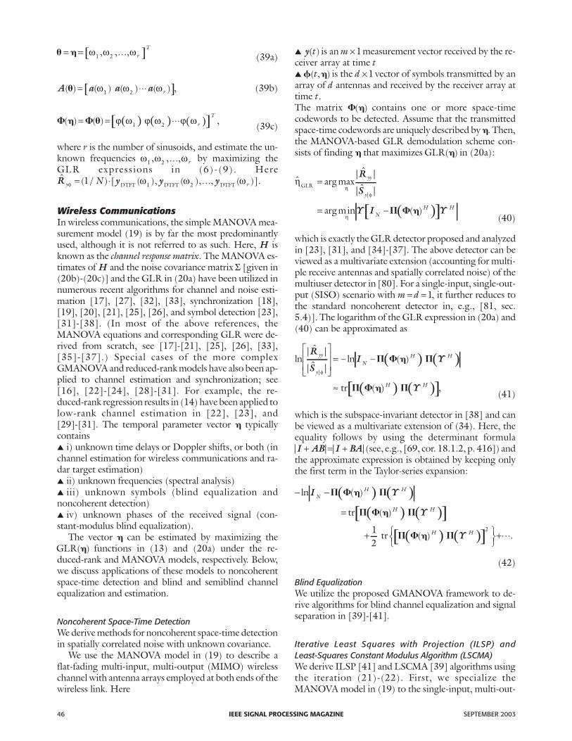
In Figure 2, we compare symbol error rates of the de-tector (59) and the DW-ILSP detec-tor in (45)-(46). We consider anarray of m =5 receiver antennas. Thetransmitted symbols were generatedfrom an uncoded QPSK modulatedconstellation (i.e., M = 4) with nor-mal ized energy. We added athree-symbol training sequence( )N T =3 , which was utilized to ob-tain initial estimates of the channelcoefficients. (For further details ofthe simulation scenario, see [44].)The symbol error rates averaged overrandom channel realizations areshown as functions of the bit sig-nal-to-noise ratio (SNR) per receiverantenna for block lengths N =50,100, and 150. An intuitive explana-tion for the better performance of theEM-based detector is that the EM al-gorithm exploits additional informa-tion provided by the distribution ofthe unknown symbols. Note also thatthe number of real parameters in therandom-symbol measurement modelequals m m2 2+ , and, therefore, is in-dependent of N. This is in contrastwith DW-ILSP and other determin-istic ML methods (e.g., [37], [42],and [83]) where the number ofparameters grows with N.

Other Applications

Multivariate Weighted Energy DetectorConsider the problem of detectingthe presence of a signal in a data ma-trix under test YT of size m d× , wherenoise-only data matrix Z of sizem N d× −( ) is avai lable, andN m d≥ + . If we do not have any ad-ditional information about the natureof the signal to be detected, we canchoose a nonparametric model for thesignal mean:

E T[ ]Y X= . (60)

Using the definitions in (27) and A I( )� = m , we simplify(8) to the following GLR test statistic:

GLR T T=+| |

| |Y Y ZZ

ZZ

H H

H(61)

for testingH0 :X =0 versusH1 :X ≠0. The above statisticcan be viewed as a multivariate extension of the classicalenergy detector; indeed, for m =1, it simplifies to the en-


� 2. Symbol error rates of the EM-based and DW-ILSP detectors as functions of the SNRper receiver antenna.

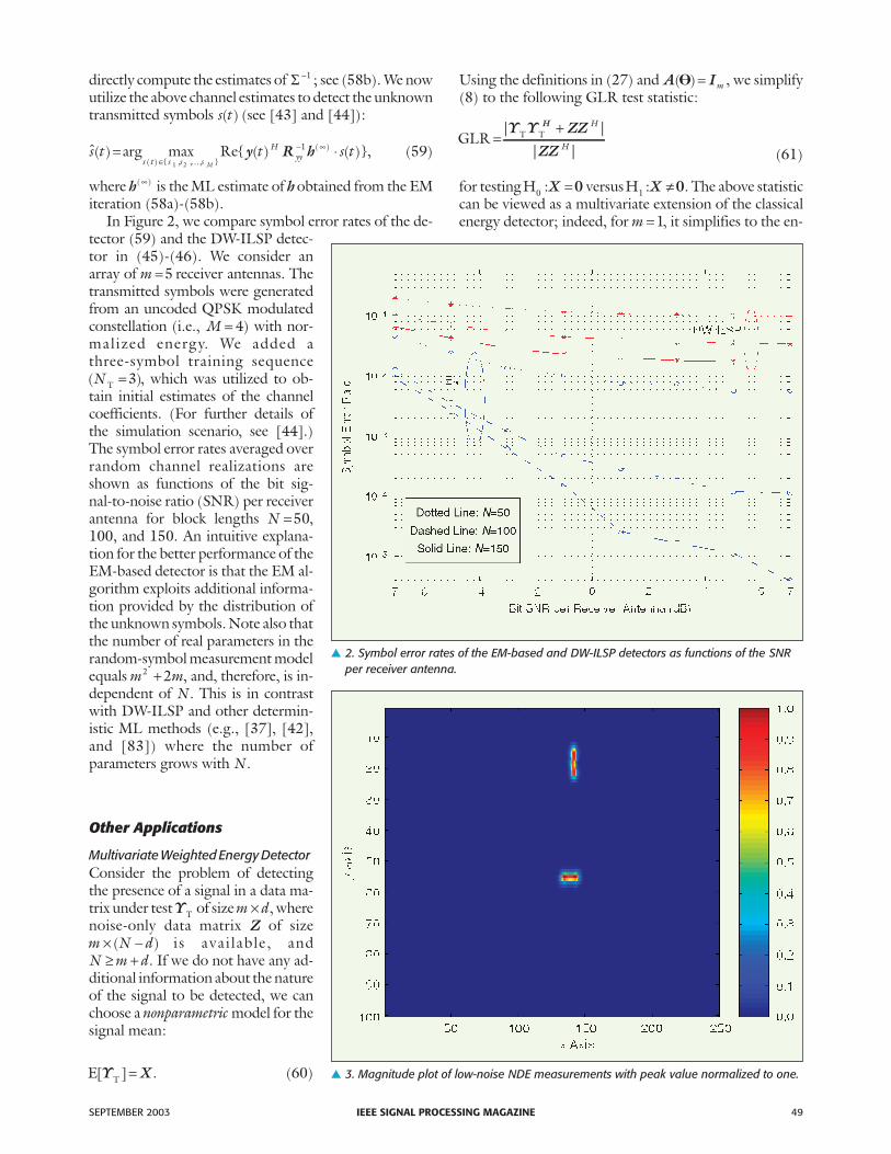
� 3. Magnitude plot of low-noise NDE measurements with peak value normalized to one.


ergy detector in, e.g., [74, ch. 7.3.]. Expression (61) sim-plifies also when the presence of a signal is tested in onesnapshot at a time (i.e., d =1 and hence Y yT T= ):

GLR T T= + −1 1y yH HZZ( ) . (62)

which is the weighted energy detector in [62, eq. (37)]and [66, eq. (20)].

Flaw Detection for Nondestructive Evaluation of Materials:We now apply the above test to NDE flaw detection incorrelated noise; see also [85]. In NDE, correlated noiseis typically caused by� backscattered “clutter” in ultrasonic NDE array sys-tems (similar to the clutter in radar) [84]� random liftoff variations between measurement loca-tions in eddy-current systems [86]. (Liftoff is the distancebetween the probe and the testpiece surface.)

A key aim of eddy-current NDE is toquantify flaws in conductors usingchanges of the probe impedance due todefects; see [86]. Figure 3 shows amagnitude plot of low-noise experi-mental eddy-current impedance mea-surements in a sample containing tworealistic flaws, where each pixel corre-sponds to a measurement location.The data was collected by scanning thetestpiece surface columnwise (parallelto the y axis). To model liftoff varia-tions, we added complex Gaussiannoise, correlated along y direction (i.e.,between rows) and uncorrelated alongx direction (i.e., independent col-umns). Figure 4 shows a magnitudeplot of noisy measurements. We used aregion R of the image to generate thenoise-only data matrix Z. A windowYT of size m d× = ×10 10 was sweptacross the noisy image, as depicted inFigure 4. For each location of the win-dow, we computed the (logarithms of)� the proposed GLR test statistic in(61)� the classical energy detector forwhite noise

tr T T( )Y Y H , (63)

which is simply the sum of squaredmagnitudes of all measurementswithin the window YT ; see Figure 5.Clearly, the proposed detector whichaccounts for noise correlation out-performs the classical detector, whichbreaks down in this scenario.

Concluding RemarksWe reviewed GMANOVA and its ap-plications to numerous problems insignal processing and communica-tions. We presented a unified frame-work for developing GMANOVA-based methods and showed thatmany existing algorithms readily fol-low as its special cases. More impor-

� 4. Magnitude plot of noisy NDE measurements.

� 5. Logarithms of (a) the proposed GLR test statistic in (61) and (b) classical energy de-tector for uncorrelated noise in (63).

tantly, insights gained from this framework allowgeneralizations of many of these methods. A novel appli-cation to flaw detection for nondestructive evaluation ofmaterials was proposed. We hope that our results wouldlead to successful applications of this powerful tool tonew and exciting signal processing problems.

AcknowledgmentThis work was supported by the NSF Industry-UniversityCooperative Research Program, Center for Nondestruc-tive Evaluation, Iowa State University, the Air Force Officeof Scientific Research under Grants F49620-00-1-0083and F49620-02-1-0339, the National Science Foundationunder Grant CCR-0105334, and the Office of Naval Re-search under Grant N00014-01-1-0681.

Aleksandar Dogand(zic received the Dipl. Ing. degree(summa cum laude) in electrical engineering from theUniversity of Belgrade, Yugoslavia, in 1995, and the M.S.and Ph.D. degrees in electrical engineering and computerscience from the University of Illinois at Chicago (UIC) in1997 and 2001, respectively. In August 2001, he joined theDepartment of Electrical and Computer Engineering,Iowa State University, Ames, as an Assistant Professor. Hisresearch interests are in statistical signal processing and itsapplications to wireless communications, nondestructiveevaluation of materials, radar, and biomedicine. He re-ceived UIC’s 2001 Outstanding Thesis Award in the Divi-sion of Engineering, Mathematics, and Physical Sciences.

Arye Nehorai received the Ph.D. degree from StanfordUniversity. From 1985 to 1995 he was a faculty memberat Yale University. In 1995 he joined the University of Illi-nois at Chicago as a Full Professor where he was laternamed University Scholar. He is vice president-Publica-tions of the IEEE Signal Processing Society and was edi-tor-in-chief of IEEE Transactions on Signal Processing. Heserved as chair of the IEEE Signal Processing SocietyTechnical Committee on Sensor Array and MultichannelProcessing and was corecipient of the 1989 IEEE SPS Se-nior Award for Best Paper. He was elected DistinguishedLecturer of the IEEE Signal Processing Society from2004 to 2005. He has been Fellow of the IEEE since1994 and of the Royal Statistical Society since 1996.

References[1] R.F. Potthoff and S.N. Roy, “A generalized multivariate analysis of vari-

ance model useful especially for growth curve problems,” Biometrika, vol.51, no. 3/4, pp. 313-326, 1964.

[2] C.G. Khatri, “A note on a MANOVA model applied to problems ingrowth curve,” Ann. Inst. Statist. Math., vol. 18, pp. 75-86, 1966.

[3] C.R. Rao, “The theory of least squares when the parameters are stochasticand its application to the analysis of growth curves,” Biometrika, vol. 52,no. 3/4, pp. 447-458, 1965.

[4] C.R. Rao, Linear Statistical Inference and Its Applications, 2nd ed. NewYork: Wiley, 1973.

[5] M.S. Srivastava and C.G. Khatri, An Introduction to Multivariate Statistics.New York: North-Holland, 1979.

[6] M.S. Srivastava and E.M. Carter, An Introduction to Applied MultivariateStatistics. New York, North-Holland, 1983.

[7] G.A.F. Seber, Multivariate Observations. New York: Wiley, 1984.

[8] A.M. Kshirsagar and W.B. Smith, Growth Curves. New York: MarcelDekker, 1995.

[9] E.F. Vonesh and V.M. Chinchilli, Linear and Nonlinear Models for the Anal-ysis of Repeated Measurements. New York: Marcel Dekker, 1997.

[10] T.W. Anderson, “Estimating linear restrictions on regression coefficientsfor multivariate normal distributions,” Ann. Math. Statist., vol. 22, no. 3,pp. 327-351, Sept. 1951.

[11] T.W. Anderson, An Introduction to Multivariate Statistical Analysis, 2nded. New York: Wiley, 1984.

[12] P.M. Robinson, “Identification, estimation and large-sample theory for re-gressions containing unobservable variables,” Int. Econ. Rev., vol. 15, no. 3,pp. 680-692, Oct. 1974.

[13] M.K.-S. Tso, “Reduced-rank regression and canonical analysis,” J. R. Stat.Soc., Ser. B, vol. 43, no. 2, pp. 183-189, 1981.

[14] P. Stoica and M. Viberg, “Maximum likelihood parameter and rank esti-mation in reduced-rank multivariate linear regressions,” IEEE Trans. SignalProcessing, vol. 44, pp. 3069-3078, Dec. 1996.

[15] G. Reinsel and R. Velu, “Reduced-rank growth curve models,” J. Stat.Planning and Inference, vol. 114, no. 1/2, pp. 107-129, June 1, 2003.

[16] D.M. Dlugos and R.A. Scholtz, “Acquisition of spread spectrum signalsby an adaptive array,” IEEE Trans. Acoust., Speech, Signal Processing, vol. 37,pp. 1253-1270, Aug. 1989.

[17] M. Cedervall and A. Paulraj, “Joint channel and space-time parameter esti-mation,” in Proc. 30th Asilomar Conf. Signals, Syst. Comput., Pacific Grove,CA, Nov. 1996, pp. 375-379.

[18] D. Zheng, J. Li, S.L. Miller, and E.G. Ström, “An efficient code-timingestimator for DS-CDMA signals,” IEEE Trans. Signal Processing, vol. 45,pp. 82-89, Jan. 1997.

[19] Z.-S. Liu, J. Li, and S. Miller, “An efficient code-timing estimator for re-ceiver diversity DS-CDMA systems,” IEEE Trans. Commun., vol. 46, pp.826-835, June 1998.

[20] A. Jakobsson, A.L. Swindlehurst, D. Astély, and C. Tidestav, “A blind fre-quency domain method for DS-CDMA synchronization using antenna ar-rays,” in Proc. 32nd Asilomar Conf. Signals, Syst. Comput., Pacific Grove, CA,Nov. 1998, pp. 1848-1852.

[21] D. Astély, A. Jakobsson, and A.L. Swindlehurst, “Burst synchronizationon unknown frequency selective channels with co-channel interference us-ing an antenna array,” in Proc. 49th Veh. Technol. Conf., Houston, TX, May1999, pp. 2363-2367.

[22] E. Lindskog and C. Tidestav, “Reduced rank channel estimation,” in Proc.49th Veh. Technol. Conf., Houston, TX, May 1999, pp. 1126-1130.

[23] A. Dogand(zic′ and A. Nehorai, “Space-time fading channel estimation inunknown spatially correlated noise,” in Proc. 37th Annu. Allerton Conf.Commun., Control, Computing, Monticello, IL, Sept. 1999, pp. 948-957.

[24] E.G. Ström and F. Malmsten, “A maximum likelihood approach for esti-mating DS-CDMA multipath fading channels,” IEEE J. Select. AreasCommun., vol. 18, pp. 132-140, Jan. 2000.

[25] G. Seco, A.L. Swindlehurst, and D. Astély, “Exploiting antenna arrays forsynchronization,” in Signal Processing Advances in Communications: Trendsin Single- and Multi-User Systems, vol. 2, G.B. Giannakis Y. Hua, P.Stoica,and L. Tong, Eds. Englewood Cliffs, NJ: Prentice-Hall, 2001, ch. 10, pp.403-430.


[26] G. Seco, J.A. Fernández-Rubio, and A.L. Swindlehurst, “Code-timingsynchronization in DS-CDMA systems using space-time diversity,” SignalProcess., vol. 81 , no. 8, pp. 1581-1602, Aug. 2001.

[27] C. Sengupta, J.R. Cavallaro, and B. Aazhang, “On multipath channel esti-mation for CDMA systems using multiple sensors,” IEEE Trans. Commun.,vol. 49, pp. 543-553, Mar. 2001.

[28] K. Wang and H. Ge, “Joint space-time channel parameter estimation forDS-CDMA system in multipath Rayleigh fading channels,” Electron. Lett.,vol. 37 , no. 7, pp. 458-460, Mar. 2001.

[29] M. Nicoli, O. Simeone, and U. Spagnolini, “Multislot estimation offast-varying space-time communication channels,” IEEE Trans. Signal Pro-cessing, vol. 51, pp. 1184-1195, May 2003.

[30] U. Spagnolini, “Adaptive rank-one receiver for GSM/DCS systems,” IEEETrans. Veh. Technol., vol. 48, pp. 1264-1271, Sept. 2002.

[31] A. aDogand(zic′ and A. Nehorai, “Space-time fading channel estimationand symbol detection in unknown spatially correlated noise,” IEEE Trans.Signal Processing, vol. 50, pp. 457-474, Mar. 2002.

[32] L. Li, H. Li, and Y.-D. Yao, “Channel estimation and interference sup-pression in frequency-selective fading channels,” Electron. Lett., vol. 38, no.8, pp. 383-385, Apr. 2002.

[33] L. Li, H. Li, and Y.-D. Yao, “Channel estimation and interference sup-pression for space-time coded systems in frequency-selective fading chan-nels,” Wireless Commun. Mob. Comput., vol. 2, no. 7, pp. 751-761, Nov.2002.

[34] K.W. Forsythe, D.W. Bliss, and C.M. Keller, “Multichannel adaptivebeamforming and interference mitigation in multiuser CDMA systems,” inProc. 33rd Asilomar Conf. Signals, Syst. Comput., Pacific Grove, CA, Oct.1999, pp. 506-510.

[35] E.G. Larsson, J. Liu, and J. Li, “Demodulation of space-time codes in thepresence of interference,” Electron. Lett., vol. 37, pp. 697-698, May 2001.

[36] E.G. Larsson, P. Stoica, and J. Li, “On maximum-likelihood detectionand decoding for space-time coding systems,” IEEE Trans. Signal Processing,vol. 50, pp. 937-944, Apr. 2002.

[37] E.G. Larsson, P. Stoica, and J. Li, “Orthogonal space-time block codes:Maximum likelihood detection for unknown channels and unstructured in-terferences,” IEEE Trans. Signal Processing, vol. 51, pp. 362-372, Feb.2003.

[38] K.W. Forsythe, “Performance of space-time codes over a flat-fading chan-nel using a subspace-invariant detector,” in Proc. 36th Asilomar Conf. Sig-nals, Syst. Comput., Pacific Grove, CA, Nov. 2002, pp. 750-755.

[39] B.G. Agee, “The least-squares CMA: A new technique for rapid correctionof constant modulus signals,” in Proc. Int. Conf. Acoust., Speech, Signal Pro-cessing, Tokyo, Japan, Apr. 1986, pp. 953-956.

[40] B.G. Agee, S.V. Schell, and W.A. Gardner, “Spectral self-coherencerestoral: A new approach to blind adaptive signal extraction using antennaarrays” Proc. IEEE, vol. 78, pp. 753-767, Apr. 1990.

[41] A. Ranheim, “A decoupled approach to adaptive signal separation usingan antenna array,” IEEE Trans. Veh. Technol., vol. 48, pp. 676-682, May1999.

[42] A. Dogand(zic′ and A. Nehorai, “Finite-length MIMO adaptive equaliza-tion using canonical correlation analysis,” IEEE Trans. Signal Processing, vol.50, pp. 984-989, Apr. 2002.

[43] A. Dogand(zic′, W. Mo, and Z. Wang, “Maximum likelihood semi-blindchannel and noise estimation using the EM algorithm,” in Proc. 37th Annu.Conf. Inform. Sci. Syst., Baltimore, MD, Mar. 2003, pp. WA3.1-WA3.6.

[44] A. Dogand(zic′, W. Mo, and Z. Wang, “Semi-blind channel and noise esti-mation using the EM algorithm,” IEEE Trans. Signal Processing, to be pub-lished.

[45] M. Viberg, B. Ottersten, and O. Erikmats, “A comparison of model-baseddetection and adaptive sidelobe cancelling for radar array processing,” inProc. Nordic Antenna Symp., Eskilstuna, Sweden, May 1994.

[46] J. Li, B. Halder, P. Stoica, and M. Viberg, “Computationally efficient an-gle estimation for signals with known waveforms,” IEEE Trans. Signal Pro-cessing, vol. 43, pp. 2154-2163, Sept. 1995.

[47] M. Viberg, P. Stoica, and B. Ottersten, “Maximum likelihood array pro-cessing in spatially correlated noise fields using parameterized signals,”IEEE Trans. Signal Processing, vol. 45, pp. 996-1004, Apr. 1997.

[48] A.L. Swindlehurst and P. Stoica, “Maximum likelihood methods in radararray signal processing,” Proc. IEEE, vol. 86, pp. 421-441, Feb. 1998.

[49] A. Dogand(zic′ and A. Nehorai, “Estimating range, velocity, and directionwith a radar array,” in Proc. Int. Conf. Acoust., Speech, Signal Processing,Phoenix, AZ, Mar. 1999, pp. 2773-2776.

[50] K. Boman and P. Stoica, “Low angle estimation: Models, methods, andbounds,” Dig. Signal Process., vol. 11, no. 1, pp. 35-79, Jan. 2001.

[51] A. Dogand(zic′ and A. Nehorai, “Estimating evoked dipole responses in un-known spatially correlated noise with EEG/MEG arrays,” IEEE Trans. Sig-nal Processing, vol. 48, pp. 13-25, Jan. 2000.

[52] E.J. Kelly, “An adaptive detection algorithm,” IEEE Trans. Aerosp. Elec-tron. Syst., vol. 22, pp. 115-127, Mar. 1986.

[53] E.J. Kelly and K.M. Forsythe, “Adaptive detection and parameter estima-tion for multidimensional signal models,” Lincoln Lab., Mass. Inst.Technol., Lexington, MA, Tech. Rep. 848, Apr. 1989.

[54] H. Wang and L. Cai, “On adaptive multiband signal detection with GLRalgorithm,” IEEE Trans. Aerosp. Electron. Syst., vol. 27, pp. 225-233, Mar.1991.

[55] K.A. Burgess and B.D. Van Veen, “Subspace-based adaptive generalizedlikelihood ratio detection,” IEEE Trans. Signal Processing, vol. 44, pp.912-927, Apr. 1996.

[56] J. Li and P. Stoica, “An adaptive filtering approach to spectral estimationand SAR imaging,” IEEE Trans. Signal Processing, vol. 44, pp. 1469-1484,June 1996.

[57] P. Stoica, H. Li, and J. Li, “A new derivation of the APES filter,” IEEESignal Processing Lett., vol. 6, pp. pp. 205-206, Aug. 1999.

[58] P. Stoica and T. Sundin, “Nonparametric NMR spectroscopy,” J. Magn.Reson., vol. 152, no. 1, pp. 57-69, Sept. 2001.

[59] D.R. Brillinger, “A maximum likelihood approach to frequency-wavenumber analysis,” IEEE Trans. Acoust., Speech, Signal Processing, vol. 33, pp.1076-1085, Oct. 1985.

[60] X. Li,E.G. Larsson, M. Sheplak, and J. Li, “Phase-shift-based time-delayestimators for proximity acoustic sensors,” IEEE J. Oceanic Eng., vol. 27,pp. 47-56, Jan. 2002.

[61] H.S. Kim and A.O. Hero, “Comparison of GLR and invariant detectorsunder structured clutter covariance,” IEEE Trans. Image Processing, vol. 10,pp. 1509-1520, Oct. 2001.

[62] L.M. Novak and M.C. Burl, “Optimal speckle reduction in polarimetricSAR imagery,” IEEE Trans. Aerosp. Electron. Syst., vol. 26, pp. 293-305,Mar. 1990.

[63] G. Wang, X.-G. Xia, and V.C. Chen, “Adaptive filtering approach to chirpestimation and inverse synthetic aperture radar imaging of maneuvering tar-gets,” Opt. Eng., vol. 42, no. 1, pp. 190-199, Jan. 2003.

[64] I.S. Reed and X. Yu, “Adaptive multiple-band CFAR detection of an opti-cal pattern with unknown spectral distribution,” IEEE Trans. Acoust.,Speech, Signal Processing, vol. 38, pp. 1760-1770, Oct. 1990.

[65] X. Yu, I.S. Reed, and A.D. Stocker, “Comparative analysis of adaptivemultispectral detectors,” IEEE Trans. Signal Processing, vol. 41, pp.2639-2656, Aug. 1993.


[66] D. Manolakis and G. Shaw, “Detection algorithms for hyperspectral imag-ing applications,” IEEE Signal Processing Mag., vol. 19, pp. 29-43, Jan. 2002.

[67] B.C. Juricek, D.E. Seborg, and W.E. Larimore, “Identification ofmultivariable, linear, dynamic models: Comparing regression and subspacetechniques,” Ind. Eng. Chem. Res., vol. 41, no. 9, pp. 2185-2203, 2002.

[68] C.G. Khatri, “Robustness study for a linear growth model,” J.Multivariate Analysis, vol. 24, no. 1, pp. 66-87, 1989.

[69] D.A. Harville, Matrix Algebra From a Statistician’s Perspective. New York:Springer-Verlag, 1997.

[70] P. McCullagh and J.A. Nelder, Generalized Linear Models, 2nd ed. Lon-don, U.K.: Chapman & Hall, 1989.

[71] H.L. Van Trees, Detection, Estimation and Modulation Theory. New York:Wiley, 1968, pt. I.

[72] J.D. Kalbfleisch and D.A. Sprott, “Application of likelihood methods tomodels involving large numbers of parameters,” J. R. Stat. Soc., Ser. B, vol.32, no. 2, pp. 175-208, 1970.

[73] C.G. Khatri, “Classical statistical analysis based on a certain multivariatecomplex Gaussian distribution,” Ann. Math. Stat., vol. 36, no. 1, pp.98-114, Feb. 1965.

[74] S.M. Kay, Fundamentals of Statistical Signal Processing: Detection Theory.Englewood Cliffs, NJ: Prentice Hall, 1998, pt. II.

[75] Y. Bresler and A. Macovski, “Exact maximum likelihood parameter esti-mation of superimposed exponential signals in noise,” IEEE Trans. Acoust.,Speech, Signal Processing, vol. ASSP-34, pp. 1081-1089, Oct. 1986.

[76] H. Krim and M. Viberg, “Two decades of array signal processing re-search—The parametric approach,” IEEE Signal Processing Mag., vol. 13,pp. 67-94, July 1996.

[77] M.S. Pinsker, Information and Information Stability of Random Variablesand Processes. San Francisco, CA: Holden-Day, 1964.

[78] R.J. Muirhead, Aspects of Multivariate Statistical Theory. New York: Wiley,1982.

[79] J. Ward, E.J. Baranoski, and R.A. Gabel, “Adaptive processing for air-borne surveillance radar,” in Proc. 30th Asilomar Conf. Signals, Syst. Comput.,Pacific Grove, CA, Nov. 1996, pp. 566-571.

[80] E. Visotsky and U. Madhow, “Noncoherent multiuser detection forCDMA systems with nonlinear modulation: A non-Bayesian approach,”IEEE Trans. Inform. Theory, vol. 47, pp. 1352-1367, May 2001.

[81] J.G. Proakis, Digital Communications, 4th ed. New York: McGraw-Hill,2000.

[82] P.J. Bickel and K.A. Doksum, Mathematical Statistics: Basic Ideas and Se-lected Topics, 2nd ed. Upper Saddle River, NJ: Prentice-Hall, 2000.

[83] N. Seshadri, “Joint data and channel estimation using blind trellis searchtechniques,” IEEE Trans. Commun., vol. 42, pp. 1000-1011, Feb.-Apr. 1994.

[84] R.B. Thompson and T.A. Gray, “Use of ultrasonic models in the designand validation of new NDE techniques,” Phil. Trans. R. Soc. Lond., A, vol.320, no. 1554, pp. 329-340, 1986.

[85] A. Dogand(zic′ and N. Eua-Anant, “Flaw detection in correlated noise,” inProc. Annu. Rev. Progress Quantitative Nondestructive Evaluation, Green Bay,WI, July 2003.

[86] B.A. Auld and J.C. Moulder, “Review of advances in quantitative eddycurrent nondestructive evaluation,” J. Nondestructive Eval., vol. 18, no. 1,pp. 3-36, Mar. 1999.

AppendixWe derive the ML estimates of X and Σ in (5) and theGLR expression in (6). To derive (5), we follow an ap-

proach similar to that of Srivastava and Khatri [5]. (Foran alternative, conditional approach to solving this prob-lem, see e.g., [2], [8], and [9].) Then, we compute theGLR in (6) by substituting the estimates of Σ (underH0 :X =0) and X and Σ [under H1 :X ≠0; see (5)] intothe likelihood ratio. Note that our concentrated likeli-hood function in (6) is simpler than the one that followsfrom [5, th. 1.10.3].

For completeness, we first state the following two lem-mas from [5], which will be used in the derivation. Theyare also of general interest to the signal processing audi-ence. (Special cases of both lemmas have been widelyused in signal processing literature.)

Lemma 1Let S be an m m× positive definite matrix. Then, fora b> >0 0, ,

[ ]| | exp ( ) | / | exp( )Σ Σ− − −− ≤ −b ba a b mbtr 1 S S (A.1)

for all m m× positive definite matricesΣ. Equality holds ifand only if Σ = a bS / .

Lemma 2Let S:m m× be a positive definite matrix, and A:m r×and A⊥ ×:m s be two matrices such thatrank rank( ) ( )A A⊥ = −m and A AH

⊥ =0. Then

( )S S A A S A A S A A SA AH H− − − − −⊥ ⊥ ⊥

−

⊥− =1 1 1 1( )H H

(A.2)is a positive semidefinite matrix of rank m − rank( )A .

Under the measurement model in (1) and (2), the like-lihood function is

L N( , , , ) | |

exp [ ( ) ( )] [ ( )

X

Y A X Y A X

� �

� � � � �

Σ Σ

Σ

=

⋅ − − ⋅ −

−

−

π

tr 1{ }( )( )] .� H

(A.3)Applying Lemma 1 to (A.3), with b N= and a =1, we ob-tain

L L N( , , , ) ( , , ,( / ) [ ( ) ( )]

[ ( ) (

X X Y A X

Y A X

� � � � � � �

� � �

Σ ≤ ⋅ −

⋅ −

1

)] )| ( / ) [ ( ) ( )]

[ ( ) ( )] | exp(

H

H N

N= ⋅ ⋅ −

⋅ − ⋅−

π 1 Y A X

Y A X

� � �

� � � −mN), (A.4)

where the equality holds if and only if

Σ = ⋅ − ⋅ −( / ) [ ( ) ( )] [ ( ) ( )]1 N HY A X Y A X� � � � � � .(A.5)

Clearly, the above expression is the ML estimate of thenoise covariance Σ for given θ, ,� and X , and (A.4) is thelikelihood function, concentrated with respect to this esti-mate. Observe that, in the absence of signal (i.e., X =0),the ML estimate of the noise covariance is simply $R yy and(A.4) becomes


| |L mNyy yy

N( , , , $ ) $ exp( )0 � � R R= ⋅ −

−π .

(A.6)

Computing the ratio between the concentrated likeli-hood functions (A.4) and (A.6) and then raising it to thepower 1/ N yields the following GLR test statistic:

GLR( , , )

| $ |

|( / ) [ ( ) ( )] [ ( ) ( )

X

R

Y A X Y A X

� �

� � � � � �=

⋅ − ⋅ −yy

N1 ] |,

H(A.7)

for testing H0 :X =0 versus H1 :X X= . To be able tocompute the above expression, we require that[ ( ) ( )] [ ( ) ( )]Y A X Y A X− ⋅ −� � � � � � H is positive defi-nite for every X , �, and �.

We now maximize (A.7) with respect to the regressioncoefficient matrix X . Let

[ ]$ ( ) ( ) ( ) $ $H Y RLS = =−

φ φφ−� � � � �H H

yΦ R (A.8)

denote a least-squares (LS) estimate of the coefficient ma-trix H [≡ A X( )� ] in the MANOVA model (19). To sim-plify the notation, we omit the dependence of $H LS on �.Expression (3f) can be written in terms of $H LS as

[ ][ ]$ ( / ) $ ( ) $ ( )|S Y H Y Hy

HNφ = ⋅ − ⋅ −1 LS LS� � � � . (A.9)

Then, the decomposition

[ ( ) ( )] [ ( ) ( )] [ $ ( )]

[ $

Y A X Y A X Y H

Y H

− ⋅ − = −

⋅ −

� � � � � � � �

�

HLS

LS ( )] [ $ ( ) ] ( ) ( )

[ $ ( ) ]

� � � � � �

�

H H

H

+ − ⋅

⋅ −

H A X

H A XLS

LS (A.10)

is obtained by completing the squares and using basicproperties of generalized inverses; see [5, th. 1.10.3]. Asdiscussed before, we require that the left-hand side of theabove expression is positive definite for every X , imply-ing that $

|S y φ must also be positive definite (considerX =0). To ensure positive definiteness of $

|S y φ (with prob-ability one), we impose condition (4), which follows us-ing arguments similar to those in [78, th. 3.1.4]. Now wecan write

( / ) [ ( ) ( )] [ ( ) ( )]

$|

1 N H

y m

⋅ − ⋅ −

= ⋅ +

Y A X Y A X

S I

� � � � � �

φ [ ][ ]

$ $ ( ) $

$ ( )

$

|

|

S H A X R

H A X

S Id

y

H

y

φ φφ

φ

− ⋅ − ⋅

⋅ −

= ⋅

1LS

LS

�

�

[ ][ ]

+ ⋅ − ⋅

⋅ −

−$ $ ( ) $

$ ( ) ,

|R H A X S

H A X

φφ φLS

LS

�

�

H

y1

(A.11)

where we used the definitions in (3) and the determinantformula| | | |I AB I BA+ = + . Also

[ ] [ ]$ ( ) $ $ ( )

( ) $

|

|

H A X S H A X X

A S

LS LS− ⋅ ⋅ − = +

⋅

−

−

� � �

�

H

yH

Hy

φ

φ

δ1

1 A X,( )� ⋅δ (A.12)

where

[ ]� = ⋅ − ⋅− − −$ $ $ $ $ $| | |H S S T S HLS A LS

Hy y yφ φ φ

1 1 1 ,(A.13a)

[ ]δX A S A A S H X= −φ−

−

φ−( ) $ ( ) ( ) $ $

| |� � �Hy

Hy

1 1LS .

(A.13b)To derive (A.12), we have used (3g) and the identity

[ ]A S T A S A A S A

A

( ) $ $ ( ) $ ( ) ( ) $ ( )| | |� � � � �Hy

Hy

Hyφ φ φ

− − −−

=1 1 1A

( ) ( ) ,� �H H= A (A.14)

see [69, th. 14.12.11(5).]. By Lemma 2, � is positivesemidefinite, and hence

� � � �� = + ⋅IN ( / ) ( ) ( )1 N H (A.15)

is positive definite. Thus, substituting (A.12) into (A.11)yields

|( / ) [ ( ) ( )] [ ( ) ( )] |

| $ || |||

1 N H

y

⋅ − ⋅ −

= ⋅ ⋅φ

Y A X Y A X

S

� � � � � �

� I

X A S A X

N +

⋅ ⋅

−

φ− −

�

� � � � � � �

1 2

1 1 21

/

|/( / ) ( ) ( ) $ ( ) ( )N H H H

yδ δ |.

(A.16)Clearly, (A.16) is minimized with respect to δX( a n d hence X) i f and only i f� � � � � �( ) ( ) $ ( ) ( )|

H H Hyδ δX A S A Xφ− =1 0, or, equivalently,

A X( ) ( )� � �δ =0, or

( )A X T S Y( ) ( ) $ $ ( )|� � � � � �= φ−

A yH1 .

(A.17)

Therefore,

GLR GLR( , , ) ( , )| $ |

| $ || |

| $ |

| $

|

|

XR

S

R

S

� � � ��

≤ =⋅

=

φ

φ

yy

y

yy

y + −φφ φ−

φφ$ $ $ $ $ $ $ $ |

,|H R H T S H R HLS LS A LS LS

Hy

H1

(A.18)which is equal to (6), the ML estimates of X in (5a) fol-low from (A.17), and the ML estimate of Σ in (5b) fol-lows by substituting (A.17) into (A.5).


Generalized multirate analysis of variance

Documents

Transcript of Generalized multirate analysis of variance