General Synthesis Procedures for FIR Lossless Transfer Matrices, for Perfect-Reconstruction...

IEEE TRANSACTIONS ON ACOUSTICS, SPEECH, AND SIGNAL PROCESSING, VOL. 36, NO. IO, OCTOBER 1988 1561

General Synthesis Procedures for FIR Lossless Transfer Matrices, for Perfect-Reconstruction

Multirate Filter Bank Applications ZINNUR DOGANATA, STUDENT MEMBER, IEEE, P. P. VAIDYANATHAN, SENIOR MEMBER, IEEE,

AND TRUONG Q. NGUYEN, STUDENT MEMBER, IEEE

Abstract-A recently reported procedure for the design of M-chan- ne1 perfect-reconstruction quadrature mirror filter banks uses the concept of “lossless alias-component matrices.” The synthesis of such QMF banks centers around the generation of a lossless M X M FIR transfer matrix E ( z ) . Recent results for such generation have been somewhat ad hoc, Le., not sufficiently general. In this paper, a general procedure is outlined for the generation of such transfer matrices E ( z ) . The procedure is based on a cascaded-lattice structure, derived from a state-space viewpoint. The structure is such that it generates only M X M lossless FIR transfer matrices (regardless of parameter values), and conversely, any M X M lossless FIR transfer matrix can he obtained by a suitable choice of parameters. These parameters turn out to be angles Ok, and the structure is such that the number of angles is minimal. A design example is presented to demonstrate the main results.

I. INTRODUCTION UADRATURE mirror filter (QMF) banks and their applications have received considerable attention in

the last few years [1]-[4]. Fig. 1 shows an M-channel, maximally decimated quadrature mirror filter bank where Hk (z) and Fk ( z ) are the analysis and synthesis filters, respectively. It is well known [7] that the reconstructed signal 2(n) suffers from aliasing, amplitude, and phase dis- tortions. It has been shown in a number of recent references [6], [12], [14], [16]-[18] that all these distor- tions can be cancelled by appropriate choices of the filters Hk (z ) and Fk (z ) resulting in a “perfect-reconstruction system,” i.e., a system satisfyingj(n) = c x ( n - no) for some c and no.

In [ 161, a procedure was outlined for the design of such perfect-reconstruction systems for arbitrary M , based on the concept of lossless, alias-component (AC) matrices. Subsequently, a special two-channel case was studied in greater detail [17]. The purpose of this paper, in relation to our earlier work [ 161, [ 171, is to outline a completely general procedure for forcing the AC matrix to be lossless. The design procedure is a generalization of the methods in Section VI of [16] (which were somewhat ad hoc)

Q

Manuscript received October 1, 1987; revised April 4, 1988. This work was supported in part by the National Science Foundation under Grant DCI 8552579; by the matching funds provided by Pacific Bell and General Elec- tric Co.; by Caltech’s Programs in Advanced Technology Grant sponsored by Aerojet General, General Motors, GTE, and TRW; and by the National Science Foundation under Grant MIP 8604456.

The authors are with the Department of Electrical Engineering, 116-81, California Institute of Technology, Pasadena, CA 91 125.

IEEE Log Number 8822830.

and is general in the sense that every QMF bank with FIR analysis and synthesis filters, which has a lossless AC matrix, is covered. An algorithm for the optimization of the analysis filters is developed, which guarantees that the search is automatically conducted over the set of all filters with lossless AC matrices. Some portions of these results have appeared in a recent conference proceedings [ 181.

The following notations are used in the paper. Super- script T stands for matrix (or vector) transposition, whereas superscript dagger ( t ) stands for transposition followed by complex conjugation. Boldface italic letters indicate matrices and vectors. The row and column in- dexes of matrices and vectors begin with “zero.” The ( i , j ) t h entries of matrices U and uk,1 are denoted by Ui,j and U!;;, respectively. Superscript asterisk ( *) stands for complex conjugation, while subscript asterisk denotes conjugation of coefficients of a function or a matrix. The tilde accent on a matrix F ( z ) is defined such that, P(z) = F;(z-’) and for matrices with real coefficients, P (z ) = FT(z- ’ ) . Thus, on the unit circle, P ( z ) = F t ( z ) . Fi- nally, a P x M matrix R will be called unitary if R t R =

An alternate representation for the analysis filter bank ZM.

is possible [3], [15], [16] if we write M- 1

Hk(z) = c Z-‘Ek,l(ZM), 0 5 k I M - 1. ( l a ) l = O

In a similar manner, the synthesis filters can be expressed as

M - 1

F&) = c z- (M-l - l )R l,k(ZM), 0 5 k I M - 1. l = O

( 1b) Defining theM X Mrnatrices E ( z ) = [Ek,, ( z ) ] andR(z ) = [Rl,k(z)], 0 I k , 1 5 M - 1, we can redraw Fig. 1 as in Fig. 2. Equations (la) and ( lb) can now be rewritten in matrix form as

[Hob) H1(z) * H , - 1 ( z ) I T

= ~ ( z ~ ) [ 1 z- l * * Z - ( M - l ) ~ T , (2a)

0096-3518/88/1000-1561$01.00 O 1988 IEEE

1562 IEEE TRANSACTIONS ON ACOUSTICS, SPEECH, AND SIGNAL PROCESSING, VOL. 36, NO. IO, OCTOBER 1988

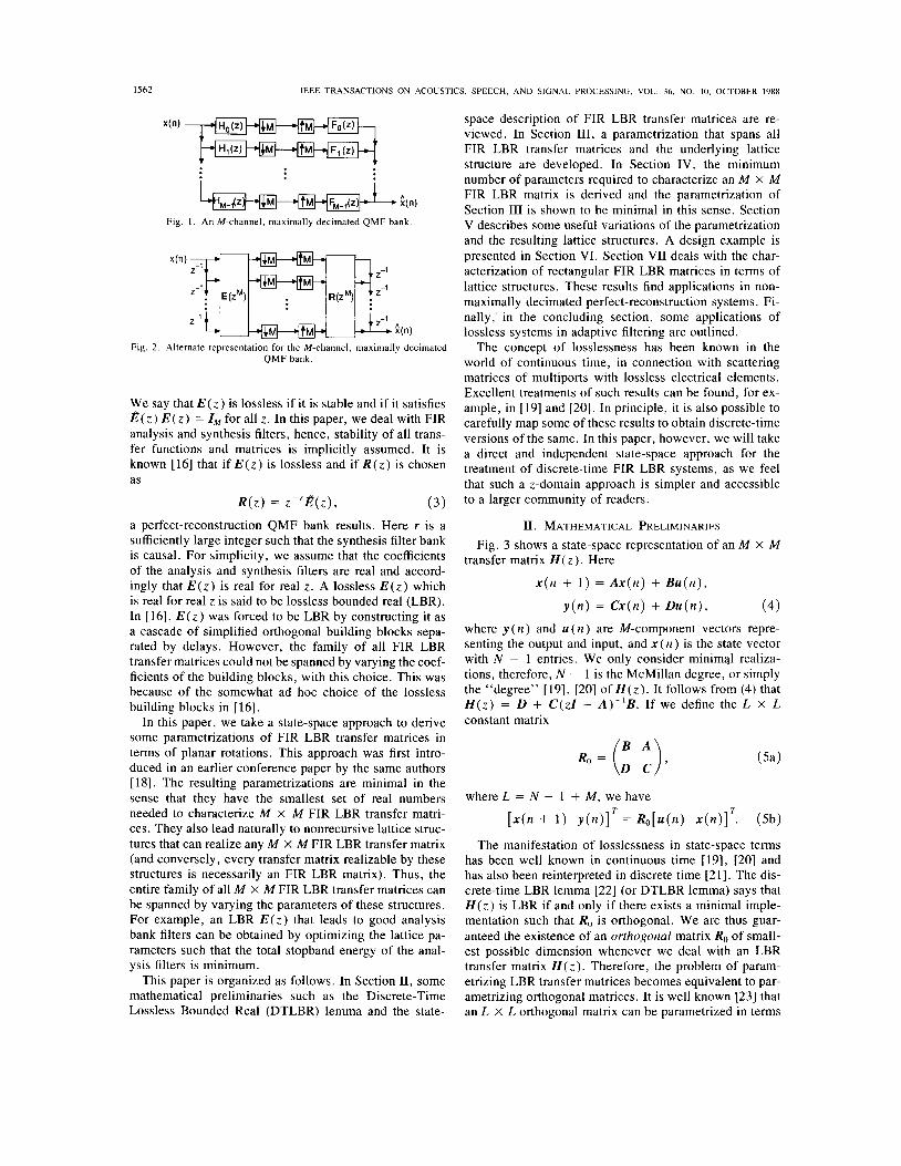
Fig. 1. An M-channel, maximally decimated QMF bank

Fig. 2 . Alternate representation for the M-channel, maximally decimated QMF bank.

We say that E ( z ) is lossless if it is stable and if it satisfies E ( z ) E ( z ) = I,,,, for all z . In this paper, we deal with FIR analysis and synthesis filters, hence, stability of all transfer functions and matrices is implicitly assumed. It is known [16] that if E ( z ) is lossless and if R ( z ) is chosen as

R ( z ) = z - T ( z ) , ( 3 ) a perfect-reconstruction QMF bank results. Here r is a sufficiently large integer such that the synthesis filter bank is causal. For simplicity, we assume that the coefficients of the analysis and synthesis filters are real and accordingly that E ( z ) is real for real z . A lossless E ( z ) which is real for real z is said to be lossless bounded real (LBR). In [16], E ( z ) was forced to be LBR by constructing it as a cascade of simplified orthogonal building blocks sepa- rated by delays. However, the family of all FIR LBR transfer matrices could not be spanned by varying the coefficients of the building blocks, with this choice. This was because of the somewhat ad hoc choice of the lossless building blocks in [ 161.

In this paper, we take a state-space approach to derive some parametrizations of FIR LBR transfer matrices in terms of planar rotations. This approach was first intro- duced in an earlier conference paper by the same authors [ 181. The resulting parametrizations are minimal in the sense that they have the smallest set of real numbers needed to characterize M X M FIR LBR transfer matrices. They also lead naturally to nonrecursive lattice structures that can realize any M X M FIR LBR transfer matrix (and conversely, every transfer matrix realizable by these structures is necessarily an FIR LBR matrix). Thus, the entire family of all M X M FIR LBR transfer matrices can be spanned by varying the parameters of these structures. For example, an LBR E ( z ) that leads to good analysis bank filters can be obtained by optimizing the lattice parameters such that the total stopband energy of the analysis filters is minimum.

This paper is organized as follows. In Section 11, some mathematical preliminaries such as the Discrete-Time Lossless Bounded Real (DTLBR) lemma and the state-

space description of FIR LBR transfer matrices are re- viewed. In Section 111, a parametrization that spans all FIR LBR transfer matrices and the underlying lattice structure are developed. In Section IV, the minimum number of parameters required to characterize an M X M FIR LBR matrix is derived and the parametrization of Section I11 is shown to be minimal in this sense. Section V describes some useful variations of the parametrization and the resulting lattice structures. A design example is presented in Section VI. Section VI1 deals with the char- acterization of rectangular FIR LBR matrices in terms of lattice structures. These results find applications in nonmaximally decimated perfect-reconstruction systems. Fi- nally; in the concluding section, some applications of lossless systems in adaptive filtering are outlined.

The concept of losslessness has been known in the world of continuous time, in connection with scattering matrices of multiports with lossless electrical elements. Excellent treatments of such results can be found, for example, in [19] and [20]. In principle, it is also possible to carefully map some of these results to obtain discrete-time versions of the same. In this paper, however, we will take a direct and independent state-space approach for the treatment of discrete-time FIR LBR systems, as we feel that such a z-domain approach is simpler and accessible to a larger community of readers.

11. MATHEMATICAL PRELIMINARIES Fig. 3 shows a state-space representation of an M X M

transfer matrix H ( z ) . Here

x ( n + 1 ) = A x ( n ) + B u ( n ) ,

y ( n ) = C x ( n ) + D u ( n ) , (4) where y ( n ) and u ( n ) are M-component vectors representing the output and input, and x ( n ) is the state vector with N - 1 entries. We only consider minimal realiza- tions, therefore, N - 1 is the McMillan degree, or simply the “degree” 1191, 1201 of H ( z ) . It follows from (4) that H ( z ) = D + C(zZ - A ) - ’ B . If we define the L x L constant matrix

B A

R o = ( D C ) ’

where L = N - 1 + M, we have

[ I ( . + 1 ) Y ( 4 1 T = R O [ W x ( 4 1 T . (33)

The manifestation of losslessness in state-space terms has been well known in continuous time 1191, [20] and has also been reinterpreted in discrete time [2 11. The discrete-time LBR lemma [22] (or DTLBR lemma) says that H ( z ) is LBR if and only if there exists a minimal implementation such that Ro is orthogonal. We are thus guar- anteed the existence of an orthogonal matrix Ro of smallest possible dimension whenever we deal with an LBR transfer matrix H ( z ) . Therefore, the problem of param- etrizing LBR transfer matrices becomes equivalent to par- ametrizing orthogonal matrices. It is well known [23] that an L x L orthogonal matrix can be parametrized in terms

DOGANATA el 01 . : SYNTHESIS PROCEDURES FOR FIR LOSSLESS TRANSFER MATRICES 1563

0

1

- - N - 2

N - 1

L - 1

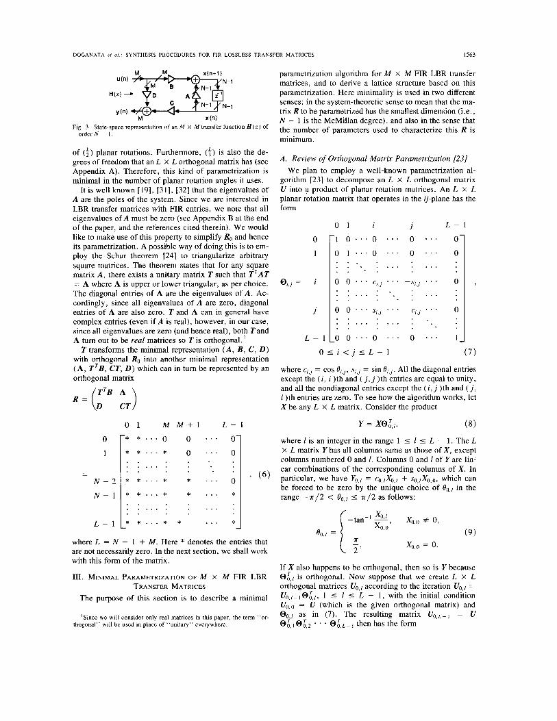
Fig. 3. State-space representation of an M X M transfer function H ( z ) of order N - 1 .

- 0 0 * * * 0- * * . . .

0 * * . . . * 0 . . . . . . . . . . .

* 2 (6) . .

0 * * . . . * * . . . * * . . . * * . . . * . . . . . . . . . . . . . . . * * . . . * * . . . * - -

of (4) planar rotations. Furthermore, (4) is also the degrees of freedom that an L X L orthogonal matrix has (see Appendix A). Therefore, this kind of parametrization is minimal in the number of planar rotation angles it uses.

It is well known 1191, [31], 1321 that the eigenvalues of A are the poles of the system. Since we are interested in LBR transfer matrices with FIR entries, we note that all eigenvalues of A must be zero (see Appendix B at the end of the paper, and the references cited therein). We would like to make use of this property to simplify Ro and hence its parametrization. A possible way of doing this is to employ the Schur theorem [24] to triangularize arbitrary square matrices. The theorem states that for any square matrix A , there exists a unitary matrix T such that TtAT = A where A is upper or lower triangular, as per choice. The diagonal entries of A are the eigenvalues of A . Ac- cordingly, since all eigenvalues of A are zero, diagonal entries of A are also zero. T and A can in general have complex entries (even if A is real), however, in our case, since all eigenvalues are zero (and hence real), both T and A turn out to be real matrices so T i s orthogonal.’

T transforms the minimal representation ( A , B, C, D ) with orthogonal Ro into another minimal representation ( A , T T B , CT, D ) which can in turn be represented by an orthogonal matrix

TTB A

R = ( D C T )

111. MINIMAL PARAMETRIZATION OF M x M FIR LBR TRANSFER MATRICES

The purpose of this section is to describe a minimal

‘Since we will consider only real matrices in this paper, the term “orthogonal” will be used in place of “unitary” everywhere.

parametrization algorithm for M x M FIR LBR transfer matrices, and to derive a lattice structure based on this parametrization. Here minimality is used in two different senses: in the system-theoretic sense to mean that the matrix R to be parametrized has the smallest dimension (i.e., N - 1 is the McMillan degree), and also in the sense that the number of parameters used to characterize this R is minimum.

A. Review of Orthogonal Matrix Parametrization [23] We plan to employ a well-known parametrization al-

gorithm 1231 to decompose an L X L orthogonal matrix U into a product of planar rotation matrices. An L X L planar rotation matrix that operates in the 0-plane has the form

0

1

Q j = i

j

L - 1

1 0 . . . 0 . . . 0 0 . . . 0 1 * * * 0 * 0 0 . . . . . . . . . . . . . . . . . . .

0 1 1 j L - 1

. . . . . .

. . . . . . . . . . . . . 0 0 . . . 0 . . .

. . . . 0 . . .

Ci, j

1 0 . . .

0 1 i < j < L - l ( 7 )

where ci,j = cos O i J , si,j = sin O i , j . All the diagonal entries except the (i, i )th and ( j, j )th entries are equal to unity, and all the nondiagonal entries except the ( i , j )th and ( j, i )th entries are zero. To see how the algorithm works, let X be any L X L matrix. Consider the product

Y = XO&, ( 8 )

where I is an integer in the range 1 I I I L - 1. The L X L matrix Y has all columns same as those of X, except columns numbered 0 and I. Columns 0 and I of Yare linear combinations of the corresponding columns of X. In particular, we have Yo,/ = co,,&,, + so,lXo,o, which can be forced to be zero by the unique choice of Bo,/ in the range - n / 2 < eo./ I a / 2 as follows:

If X also happens to be orthogonal, then so is Y because O& is orthogonal. Now suppose that we create L X L orthogonal matrices Uo,/ according to the iteration Uo,/ = U o , / - l O ~ , ~ , 1 5 1 5 L - 1 , with the initial condition Uo,o = U (which is the given orthogonal matrix) and Oo I as in (7). The resulting matrix Uo,L- l = U

* - Ol ,L- l then has the form


U 0 , L - I = (" O ). b U1,I

where U , , ] is ( L - 1) X ( L - 1 ) orthogonal. Because of the orthogonality of Uo,L- we have a = f 1 and b = 0. By adding 7~ to if necessary, we can always take a = 1. We have thus forced the first row (and column) to be all zeros (but one entry). We can now proceed to the second step which is to repeat the above process with UI, so as to obtain

where U2,2 is ( L - 2 ) x ( L - 2 ) orthogonal and Bo,/ are ( L - 1) X ( L - 1 ) planar rotation matrices. If we define B T = ai,, * * @i,L-2, we can summarize the first two steps as follows:

which shows that the second step does not affect the entries of the 0th row, created during the first step.

Proceeding in this manner, we eventually obtain

The determinant of e,,, is 1 as seen from (7). The last diagonal entry on the right-hand side of (13) is 1 or - 1 depending on whether det U is 1 or - 1, respectively. We assume det U = 1 for simplicity hereafter (the det U = - 1 case can be handled similarly). This leads to the factorization

u = [ @ L - 2 , L - l ] * * [ @ l , L - I * * @ 1 , 2 ]

* [@O,L-1 * * @ 0 , 2 @ 0 , l l (14) which can be represented by means of a signal flow graph (lattice structure) as in Fig. 4(a), with building blocks as in Fig. 4(b). Each criss-cross in Fig. 4(b) (and other fig- ures of this paper) has the form shown in Fig. 4(c) which is a planar rotation. The (4) angles Bi,j thus completely characterize U which therefore has (4) degrees of freedom (also see Appendix A in this context).

B. Parametrization of M X M FIR LBR Transfer Matrices

In this subsection, we will apply the parametrization algorithm described in Section 111-A to the orthogonal matrix R as defined by (6). We will then use this parametrization to derive a lattice structure capable of realizing only (and all ) M X M FIR LBR transfer matrices.

Let us consider again the construction of Y from X as

2

L- 1

L-2 L- 1 ...

: j . I ....

sin ei

coseii

(C) Fig. 4. (a) Signal flow graph representation for the parametrization of

Section 111-A. (b) Internal details of T1. (c) Internal details for the criss- crosses.

in (8), where eo,[ is chosen as in (9) so as to ensure that Yo,/ = 0. IfXo,[ is already zero, then eo,[ = 0 is the obvious choice, hence, we have Y = X. Now, the factorization of (13) is obtained by means of the recursion

vk,[ = V k , [ - l @ l / , k < 15 L - 1, (15)

for 0 I k I L - 2 , and with the initialization Vo,o = U . From Section 111-A, we know that @kT,[ has the form

= (" O ) 0 BT '

where B is an ( L - k ) x ( L - k ) planar rotation operator of the form (7). If the ( k , 1 )th entry of v k , / - happens to be zero, then = 1 L - k and Vk,[ = vk,[-l. This shows, by an obvious inductive reasoning, that if the matrix U has the form (6) (i.e., certain entries I!Jk,[ are zero as indicated), then so do the matrices v k , [ . Accordingly, the form (6) forces the angles ek, [ to be restricted such that

'

eo,,+, = =. . . - - = o - - = = o -

O N - 2 , L - I = 0, (17)

where N = L - M + 1. More compactly, e k , / = 0, 0 I k I N - 2, M + k I 1 I L - 1. Thus, out of the ( 5 ) angles appearing on the right-hand side of (14), (:) angles

DOCANATA et a / . : SYNTHESIS PROCEDURES FOR FIR LOSSLESS TRANSFER MATRICES 1565

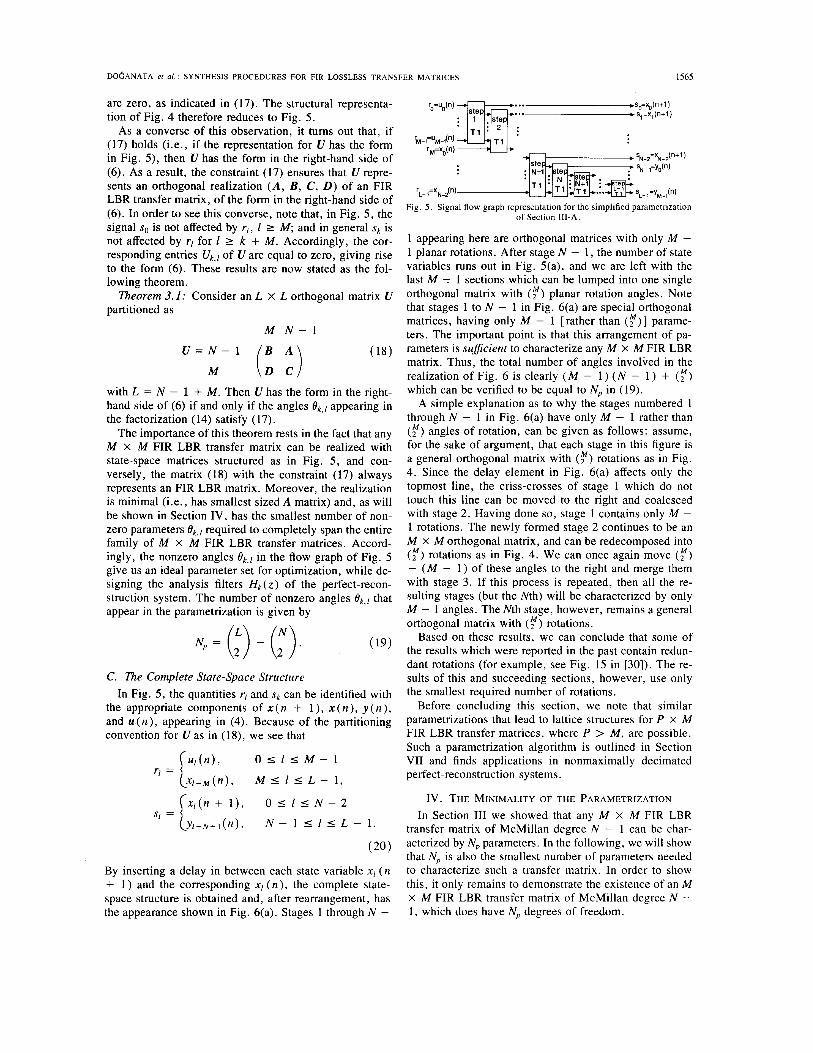
are zero, as indicated in (17). The structural representation of Fig. 4 therefore reduces to Fig. 5 .

As a converse of this observation, it turns out that, if (17) holds (Le., if the representation for U has the form in Fig. 5 ) , then U has the form in the right-hand side of (6). As a result, the constraint (17) ensures that U represents an orthogonal realization ( A , B, C, D ) of an FIR LBR transfer matrix, of the form in the right-hand side of (6). In order to see this converse, note that, in Fig. 5, the signal so is not affected by r l , I I M; and in general sk is not affected by ri for 1 2 k + M. Accordingly, the corresponding entries uk,[ of U are equal to zero, giving rise to the form (6). These results are now stated as the following theorem.

Theorem 3.Z: Consider an L X L orthogonal matrix U partitioned as

M N - 1

(18) U = N - l M ix 3

with L = N - 1 + M. Then U has the form in the right- hand side of (6) if and only if the angles & [ appearing in the factorization (14) satisfy (17).

The importance of this theorem rests in the fact that any M X M FIR LBR transfer matrix can be realized with state-space matrices structured as in Fig. 5, and conversely, the matrix (18) with the constraint (17) always represents an FIR LBR matrix. Moreover, the realization is minimal (i.e., has smallest sized A matrix) and, as will be shown in Section IV, has the smallest number of nonzero parameters f?k,[ required to completely span the entire family of M X M FIR LBR transfer matrices. Accord- ingly, the nonzero angles t$[ in the flow graph of Fig. 5 give us an ideal parameter set for optimization, while designing the analysis filters Hk ( z ) of the perfect-reconstruction system. The number of nonzero angles O k , i that appear in the parametrization is given by

NP = ( 4 ) - (;). C. The Complete State-Space Structure

In Fig. 5 , the quantities r/ and sk can be identified with the appropriate components of x ( n + 1 ), x ( n ), y ( n ), and u ( n ) , appearing in (4). Because of the partitioning convention for U as in (1 8), we see that

ui (4 2 O I I I M - 1 ri = [

x / - M ( n ) ,

x / ( n + l ) ,

M I I I L - 1 ,

0 I 1 I N - 2

N - 1 I 1 I L - 1 .

(20)

By inserting a delay in between each state variable x1 ( n + 1) and the corresponding xi ( n ) , the complete state- space structure is obtained and, after rearrangement, has the appearance shown in Fig. 6(a). Stages 1 through N -

Fig. 5 . Signal flow graph representation for the simplified parametrization of Section 111-A.

1 appearing here are orthogonal matrices with only M - 1 planar rotations. After stage N - 1 , the number of state variables runs out in Fig. 5(a), and we are left with the last M 7 1 sections which can be lumped into one single orthogonal matrix with (f) planar rotation angles. Note that stages 1 to N - 1 in Fig. 6(a) are special orthogonal matrices, having only M - 1 [rather than (f)] parameters. The important point is that this arrangement of parameters is suficient to characterize any M x M FIR LBR matrix. Thus, the total number of angles involved in the realization of Fig. 6 is clearly ( M - 1) ( N - 1) + (f) which can be verified to be equal to Np in (19).

A simple explanation as to why the stages numbered 1 through N - 1 in Fig. 6(a) have only M - 1 rather than ( y ) angles of rotation, can be given as follows: assume, for the sake of argument, that each stage in this figure is a general orthogonal matrix with (f) rotations as in Fig. 4 . Since the delay element in Fig. 6(a) affects only the topmost line, the criss-crosses of stage 1 which do not touch this line can be moved to the right and coalesced with stage 2. Having done so, stage 1 contains only M - 1 rotations. The newly formed stage 2 continues to be an M X M orthogonal matrix, and can be redecomposed into (f) rotations as in Fig. 4. We can once again move (f) - ( M - 1) of these angles to the right and merge them with stage 3 . If this process is repeated, then all the resulting stages (but the Nth) will be characterized by only M - 1 angles. The Nth stage, however, remains a general orthogonal matrix with (f) rotations.

Based on these results, we can conclude that some of the results which were reported in the past contain redun- dant rotations (for example, see Fig. 15 in [30]). The results of this and succeeding sections, however, use only the smallest required number of rotations.

Before concluding this section, we note that similar parametrizations that lead to lattice structures for P X M FIR LBR transfer matrices, where P > M , are possible. Such a parametrization algorithm is outlined in Section VI1 and finds applications in nonmaximally decimated perfect-reconstruction systems.

IV. THE MINIMALITY OF THE PARAMETRIZATION In Section I11 we showed that any M x M FIR LBR

transfer matrix of McMillan degree N - 1 can be characterized by N,, parameters. In the following, we will show that Np is also the smallest number of parameters needed to characterize such a transfer matrix. In order to show this, it only remains to demonstrate the existence of an M x M FIR LBR transfer matrix of McMillan degree N - 1, which does have Np degrees of freedom.


..............................................................

I . a . -D ...

...

I .

a . . .

,. ............................................................ !

4 T 2 C

(b) Fig. 6. (a) The FIR lattice structure of Section 111. (b) Internal details of

T2.

First consider an M X 1 FIR LBR vector h O ( z ) where

h,T(z) = [ H o ( z ) HI(Z) * - 4 9 - d z > I . (21) The LBR property is equivalent to the power complemen- tary property, i.e.,

which can be rewritten by analytical continuation as

i.e., h;(z-l)h,(z) = 1. Assumethatho(z) hastheform h O ( z ) = .E::; h ( k ) z P k , with h ( 0 ) # 0 and h ( N - 1 ) # 0 to avoid trivialities. The condition (22b) implies that Hk(z), 0 I k I M - 2 can be arbitrary causal FIR functions of order N - 1 (subject to the inequality constraints C k = O I Hk(ejW)l2 I 1 forallw)andthatHM-I(z)should be chosen to satisfy the equality constraint (22b). Since the left-hand side of (22b) is a symmetric polynomial of degree 2 ( N - 1 ), the number of distinct equality constraints is equal to N , which is equal to the number of coefficients in H M - I ( z ) . The total number of degrees of freedom left over in an M x 1 FIR LBR vector is therefore N ( M - 1) .

An FIR lattice structure with precisely N ( M - 1 ) parameters (angles of rotation) to realize an arbitrary M x 1 FIR LBR vector is presented in [25], and has the overall appearance in Fig. 7. Here, each of the N - 1 rectangular boxes is a special orthogonal matrix with only M - 1 rotations [Fig. 7(b)], and the real numbers pk, 0 I k I M - 1 are such that .E;=-: p i = 1. From here it is clear that we can express hO ( z ) as

M - 2

. I

. , . I

, . I . I . 3::: W

W

... ! ....................... ..................,

4 T 3

(b) Fig. 7 . (a) An FIR lossless lattice structure. (b) Internal details of T3

FIR LBR. Now consider an M X M orthogonal matrix V whose leftmost column is vO

V = [vo vl - * * v ~ - ~ ] , V T V = I . (24)

If we next define the M X M transfer matrix

H ( z ) L2 S ( z ) [VO U ] * Y M - 1 1 , ( 2 5 ) whose 0th column is clearly h O ( z ) , then H ( z ) is LBR (since S ( z ) is LBR and Vis orthogonal). Let us now count the number of freedoms that we could exercise in the construction of H ( z ) .

Since an orthogonal matrix has ( f ) degrees of freedom, and since no is already fixed, we are left with ( y ) - ( M - 1 ) degrees of freedom in constructing V (see Section 111-A and Appendix A). The total number of degrees of freedom that we can exercise in the construction of h O ( z ) and V is therefore N ( M - 1 ) + (f) - ( M - 1 ) which indeed simplifies to Np in (19).

This argument shows that at least Np degrees of freedom are required to characterize an arbitrary M X M FIR LBR matrix of McMillan degree N - 1. Combining this with the fact that Np parameters are sufficient to construct such LBR matrices, we conclude that Np is the number of free parameters necessary and sufficient to span the entire family of M X M FIR LBR matrices.

v . OTHER PARAMETRIZATION ALGORITHMS AND LATTICE STRUCTURES

The lattice structure presented in Section 111-C has two problems. First, the stages are interconnected in a rather complicated manner. Second, the criss-crosses do not always interconnect neighboring links. If one intends to directly implement this structure in hardware (VLSI), then these are undesirable features.

We will show in this section that the first problem can be eliminated simply by rearranging the rows of R , and the second problem by allowing only planar rotation matrices that operate in neighboring planes in the parametrization algorithm.

D O ~ A N A T A et d.: SYNTHESIS PROCEDURES FOR FIR LOSSLESS TRANSFER MATRICES I561

... I . I . I .

t

...

t

4 T 4 t

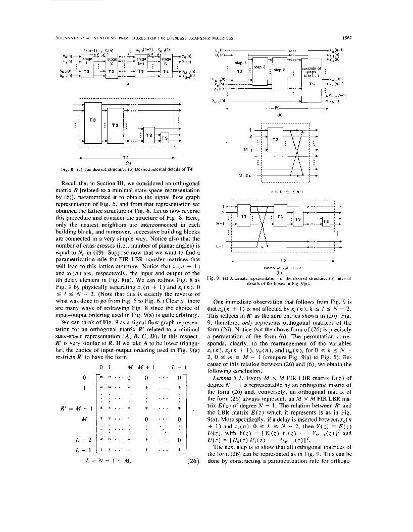
(b) Fig. 8. (a) The desired structure. (b) Desired internal details of T4.

Recall that in Section 111, we considered an orthogonal matrix R [related to a minimal state-space representation by (6)], parametrized it to obtain the signal flow graph representation of Fig. 5 , and from that representation we obtained the lattice structure of Fig. 6. Let us now reverse this procedure and consider the structure of Fig. 8. Here, only the nearest neighbors are interconnected in each building block, and moreover, successive building blocks are connected in a very simple way. Notice also that the number of criss-crosses (Le., number of planar angles) is equal to Np in (19). Suppose now that we want to find a parametrization rule for FIR LBR transfer matrices that will lead to this lattice structure. Notice that xI ( n + 1 ) and xI ( n ) are, respectively, the input and output of the lth delay element in Fig. 8(a). We can redraw Fig. 8 as Fig. 9 by physically separating x1 ( n + 1 ) and x1 ( n ) , 0 I I I N - 2. (Note that this is exactly the reverse of what was done to go from Fig. 5 to Fig. 6 . ) Clearly, there are many ways of redrawing Fig. 8 since the choice of input-output ordering used in Fig. 9(a) is quite arbitrary.

We can think of Fig. 9 as a signal flow graph representation for an orthogonal matrix R' related to a minimal state-space representation (A , B , C, D ) . In this respect, R' is very similar to R . If we take A to be lower triangular, the choice of input-output ordering used in Fig. 9(a) restricts R' to have the form

0 1 M M + 1 L - 1

3

. . .

* . . . *

L = N - l + M . (26)

q M-2+i 1

I\ . , . , . I . . , . I .

I \ I ; \

.... L - 1 ; *... -*

t T5

Cascade of steps N IO L-1

(b) Fig. 9 . (a) Alternate representation for the desired structure. (b) Internal

details of the boxes in Fig. 9(a).

One immediate observation that follows from Fig. 9 is that x k ( n + 1 ) is not affected by xI ( n ) , k I 1 I N - 2. This reflects in R' as the zero entries shown in (26). Fig. 9 , therefore, only represents orthogonal matrices of the form (26). Notice that the above form of (26) is precisely a permutation of the form (6) . The permutation corre- sponds, clearly, to the rearrangement of the variables x k ( n ) , x k ( n + l ) , y , (n ) , and u,(n), for 0 I k I N - 2, 0 I m I M - 1 (compare Fig. 9(a) to Fig. 5) . Be- cause of this relation between (26) and (6), we obtain the following conclusion.

Lemma 5.1: Every M X M FIR LBR matrix E ( z ) of degree N - 1 is representable by an orthogonal matrix of the form (26) and, conversely, an orthogonal matrix of the form (26) always represents an M x M FIR LBR matrix E ( z ) of degree N - l . The relation between R' and the LBR matrix E ( z ) which it represents is as in Fig. 9(a). More specifically, if a delay is inserted between xk ( n + 1 ) andxk(n ) , 0 I k I N - 2, then Y ( z ) = E ( z ) U ( z ) , with Y ( z ) = [ Y o ( z ) Y , ( z ) * * YM-l(z)lr and

The next step is to show that all orthogonal matrices of the form (26) can be represented as in Fig. 9. This can be done by constructing a parametrization rule for orthogo-

U ( z ) = [ U o ( z ) U , ( z > . * * u M - l ( z ) l T .

1568 IEEE TRANSACTIONS ON ACOUSTICS, SPbECH, AND SIGNAL PROCESSING, VOL. 36, NO. IO, OCTOBER 1988

nal matrices that will always yield a representation as in Fig. 9 when applied to matrices of the form (26). Such an algorithm is described in Appendix C.

Now, since Fig. 9 is obtained by a rearrangement of the "desired structure" shown in Fig. 8, we conclude, with the help of Lemma 5.1, the following.

Lemma 5.2: Any M X M FIR LBR matrix of degree N - 1 can be realized as in Fig. 8(a) with building blocks as in Fig. 8(b), with each criss-cross representing a planar rotation. Conversely, Fig. 8 always represents an M x M FIR LBR matrix.

Before concluding this section, we note that the possi- bilities for other lattice structures are several. Consider, for example, R arranged as in (6) with a lower triangular choice of A and the parametrization algorithm governed by the recursion

urn,[ = urn,[- I@:- I , k y

= Urn,L-rn- l , 0 I m I L - 2,

I ~ l I L - l - r n , k = L - l ,

(27) where are determined such that Ul;$ = 0. If we let Uo,o = R, we have the structure of Fig. 10. Note that this structure has nearest neighbor link interconnections only.

As a slightly different example, consider R as

with an upper triangular A. The application of the parametrization algorithm governed by

urn,/ = @L,kUrn,[- l ,

Urn+l ,o = Urn,L-rn- l , 0 I m I L - 2,

1 1 1 1 L - l - m , k = L - I ,

(29) where are determined such that Uzt;fi = 0, yields the structure of Fig. 11. Note that this structure has a special first stage with ( y ) planar rotations rather than a special last stage. Detailed derivations of the structures are omitted for brevity. In any case, the structure of Fig. 8 seems to be the most attractive one from an implementation viewpoint.

VI. A DESIGN EXAMPLE In this section, we shall consider a 5-band perfect-re-

construction QMF bank, with lossless E ( z ) . Our aim is to optimize the angles O k , [ so as to minimize the sum of the stopband energies of Hk ( z ) . We shall impose a constraint on the analysis-bank structure such that the 5 filters Hk ( z ) satisfy the following pairwise symmetry property:

H k ( z ) = H 4 - k ( - ~ ) , 0 I k 5 2. (30)

This condition implies that the magnitude response I H k ( e'") 1 is the image of 1 e'") 1 with respect to a /2 . Such a constraint reduces the number of parameters

4 T 7 e

(b) Fig. 1 1 . (a) An alternate FIR lattice structure. (b) Internal details of T6

and T I .

(angles) in the optimization program by a factor of 2 , thereby reducing the design time enormously.

Consider the structure of Fig. 12 where E' ( 2 ) is a 5 x 5 lossless matrix, r ( z ) is a diagonal matrix of the form

and R is an orthogonal matrix of a specific form men- tioned in [28]. This form is

a b c cos 8 sin 8

sin 8 -cos 8

a c -cos 8 -sin8

( 3 2 4

DOGANATA er a / . : SYNTHESIS PROCEDURES FOR FIR LOSSLESS TRANSFER MATRICES 1569

Ho (Z) H 1 (Z)

H 2 ( z ) H, (4 H, (4

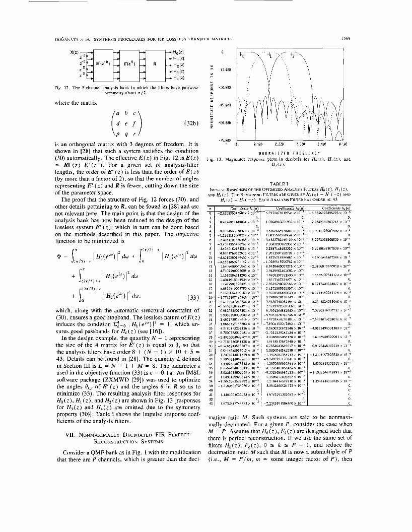
Fig. 12. The 5-channel analysis bank in which the filters have painvise symmetry about ~ / 2 .

where the matrix

is an orthogonal matrix with 3 degrees of freedom. It is shown in [28] that such a system satisfies the condition (30) automatically. The effective E(z) in Fig. 12 is E(z) = RT(z) E' (z2). For a given set of analysis-filter lengths, the order of E' ( z ) is less than the order of E(z) (by more than a factor of 2), so that the number of angles representing E' ( z ) and R is fewer, cutting down the size of the parameter space.

The proof that the structure of Fig. 12 forces (30), and other details pertaining to R, can be found in [28] and are not relevant here. The main point is that the design of the analysis bank has now been reduced to the design of the lossless system E' ( z ) , which in turn can be done based on the methods described in this paper. The objective function to be minimized is

(33)

which, along with the automatic structural constraint of (30), ensures a good stopband. The lossless nature of E ( z ) induces the condition 1 H k ( e J " ) l 2 = 1, which ensures good passbands for Hk (z) (see [ 161).

In the design example, the quantity N - 1 representing the size of the A matrix for E' (z) is equal to 3, so that the analysis filters have order 8 + ( N - 1 ) x 10 + 5 = 43. Details can be found in [28]. The quantity L defined in Section I11 is L = N - 1 + M = 8. The parameter E

used in the objective function (33) is E = 0.1 ?r. An IMSL software package (ZXMWD [29]) was used to optimize the angles ek,l of E' ( 2 ) and the angles 8 in R so as to minimize (33). The resulting analysis filter responses for Ho(z), H, (z), and H2(z) are shown in Fig. 13 [responses for H3(z) and H4(z) are omitted due to the symmetry property (30)]. Table I shows the impulse response coefficients of the analysis filters.

VII. NONMAXIMALLY DECIMATED FIR PERFECT- RECONSTRUCTION SYSTEMS

Consider a QMF bank as in Fig. 1 with the modification that there are P channels, which is greater than the deci-

0 .

-15 I 000

-30.000

-45 I 000

-60 .000

-75.000

I I

0. 0.100 0.200 0.300 0.400 0.500

N O R l i R L I Z E O F R E Q U E N C Y Fig. 13. Magnitude response plots in decibels for Hn(z), H,(z), and

H>(z).

TABLE I IMPULSE RESPONSES OF THE OPTIMIZED ANALYSIS FILTERS &(Z), Hi (Z) ,

AND H2 (z). THE REMAINING FILTERS ARE GIVEN BY H3 ( Z ) = Hi ( - Z ) A N D H4(z) = Ho( -z). EACH ANALYSIS FILTER HAS ORDER 5 43

- - n 0 1 2 3 4 5 6 7 8 9 10 11 12 13 14 15 16 17 18 19 20 21 22 23 24 25 26 27 28 29 30 31 32 33 34 35 36 37 38 39 40 41 42 43

-

-

Coefficients h,(n) -2.4835360125087 x

0.

0. -3.7034566338920 x lo-' -1.1245182366259 x lo-' -2.2361121450286 x lo-' -3.4764353486761 x lo-' -4.4759159183384 x lo-' -4.8561769832515 x lo-' -4.4015380139465 x lo-' -3.1834850261147 X lo-' -1.5407699099947 x lo-'

4.7107590068008 x 1.1389954711266 x lo-' 1.49416121949'24 x lo-' 1.1977991392325 x lo-' 5.6522819058759 x lo-'

-7.1555054490160 x -4.7745497795845 x lo-' -5.5712037910736 x lo-' -3.5768510479471 x lo-' -6.6525355077401 x l o r 3

9.9939390002089 x 1.4657730336919 x lo-' 1.0884757133802 x lo-' 4.2187173262136 x l o r 3 8.7290788035681 x

-2.4319063992967 x -2.7169726951436 x -6.5465233588287 x -6.0414958963013 x

1.2474044871629 x 3.8952448682281 x 1.4492595073735 x 8.6559484816013 x 8.6226618002995 x lo-'

-1.6493439929514 x lo-' -1.2647395522992 x -1.9162408723980 x lo-'

0. -1.1401061636328 x lo-'

0. 1.6722647743373 x lo-'

6.9528912143064 x

Coefficients h,(n) 5.7278475612794 X IO-'

0. -1.0764916551265 X lo-'

0. 2.8752558978040 x IO-' 1.0825561580492 X lo-'

-5.4383762140129 X IO-' -7.9639280769991 x IO-' -5.1487148482336 x lo r3

7.2671997796727 x lo-' 1.8328214990681 x lo-'

-1.0288013756762 x lo-' -6.0780449007278 x lo-'

1.9439861463095 x lo-' 3.6918497231530 X lo-' 1.6317387334877 X lo-'

-2.9532698026966 x lo-' -5.4272565360597 x lo-' -3.2210505485030 x lo-'

1.2918828138243 x lo-' 3.8370748052164 x lo-' 2.9719022018506 x lo-' 6.3954104882840 X lo-'

-8.6951626023338 x lo-' -1.0718954226404 X lo-' -7.6004132917402 X lo-' -3.8406926872346 x lo-' -3.7512229381334 x l o r 3

2.0386865966176 x lo-' 1.8165512657849 x lo-' 6.2654643849857 x 3.0099548542930 x l o r 3

-1.1938502254712 X -2.2497732170841 X -1,3870390939344 X

-3.7737403058425 x l o r 4 -8.2524688987315 x lo r5

7.1906572891807 x lo-' 1.2104410519710 x 8.3542496021572 X

0. 4.9705293322685 x lo-'

0. -7.2905851904860 X lo-'

Coefficients hz(n) -6.8556822325223 x lo-'

0. 2.0842992761747 x IO-'

0. -3.9041326907409 x lo-'

0. 5.2972968100559 x lo-'

0. -5.4338887407838 x lo-'

0. 4.1301954587344 x lo-'

0. -2.0766076876058 x lo-'

0. 1.8582407343124 x lo-'

0. 6.5217429524827 x IO-'

0. -6.7744452252176 x lo-'

0. 2.2943524515046 x lo-'

0. 7.0926516303202 x IOK3

0. -7.5333676224076 x l o r 3

0. -3.9818493531489 x l o r 3

0. 1.8745939322991 x l o r 3

0. 6.9123448305219 x lo-'

0. -1.3171097826729 x lo-"

0. -1.5302445152613 x l o r 4

0. -9,1044984419491 x lo-'

0.

0. 0. 0 . 0. 0 .

1.3354135358735 x

mation ratio M . Such systems are said to be nonmaximally decimated. For a given P , consider the case when M = P. Assume that Hk(z), Fk(z) are designed such that there is perfect reconstruction. If we use the same set of filters Hk(z), Fk(z), 0 5 k I P - 1, and reduce the decimation ratio M such that M is now a submultiple of P (Le., M = P / m , m = some integer factor of P ) , then

1570 IEEE TRANSACTIONS ON ACOUSTICS, SPEECH, AND SIGNAL PROCESSING, VOL. 36, NO. IO; OCTOBER 1988

2-1 2-1 +++ h

Fig. 14 A redrawing of Fig. 2.

f ( n ) is not altered by this choice of M except for a scale factor. This can be verified by referring to the alias-can- cellation equations [ 16, eqn. (1 b)] and replacing W with W"', which yields a subset of the set of equations for P = M . In this section, we will consider the more general case where M < P and M is not necessarily a submultiple of P .

The applications of nonmaximally decimated structures are not very clear at this time. Such systems may be of interest in short-time spectral analysis [26], and even in certain new types of subband coding [27]. Regardless of the possible applications, the main purpose of this section, however, is to show how a perfect-reconstruction QMF bank can be designed by a simple extension of the ideas presented earlier in this paper and in [16].

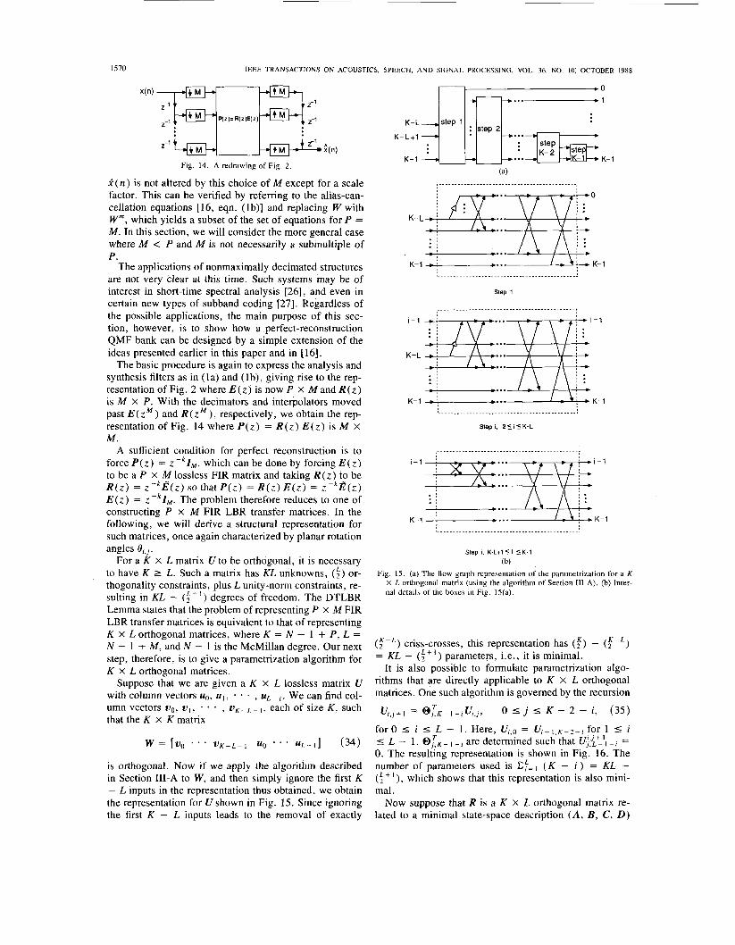
The basic procedure is again to express the analysis and synthesis filters as in (la) and (lb), giving rise to the representation of Fig. 2 where E(z) is now P X Mand R(z) is M X P . With the decimators and interpolators moved past E ( z ) and R ( z ) , respectively, we obtain the representation of Fig. 14 where P(z) = R ( z ) E ( z ) is M X M .

A sufficient condition for perfect reconstruction is to force P(z) = zPkZM, which can be done by forcing E ( z ) to be a P x M lossless FIR matrix and taking R ( z ) to be R ( z ) = z-~B(z) so that P ( z ) = R ( z ) E ( z ) = Z - ~ ~ ( Z ) E( z ) = z -kZM. The problem therefore reduces to one of constructing P x M FIR LBR transfer matrices. In the following, we will derive a structural representation for such matrices, once again characterized by planar rotation angles e,,,.

For a K x L matrix U to be orthogonal, it is necessary to have K 1 L. Such a matrix has KL unknowns, (k) orthogonality constraints, plus L unity-norm constraints, resulting in KL - (5") degrees of freedom. The DTLBR Lemma states that the problem of representing P X M FIR LBR transfer matrices is equivalent to that of representing K X L orthogonal matrices, where K = N - 1 + P , L = N - 1 + M , and N - 1 is the McMillan degree. Our next step, therefore, is to give a parametrization algorithm for K X L orthogonal matrices.

Suppose that we are given a K X L lossless matrix U with column vectors uo, IC,, a . - , uL- I . We can find column vectors vo, v I , - , v ~ - ~ - I , each of size K , such that the K x K matrix

w = [VO " * VK-L-1 " ' U L - l ] (34)

is orthogonal. Now if we apply the algorithm described in Section 111-A to W, and then simply ignore the first K - L inputs in the representation thus obtained, we obtain the representation for U shown in Fig. 15. Since ignoring the first K - L inputs leads to the removal of exactly

(a) , _ . _ _ _ _ _ _ _ _ _ _ _ _ _ _ _ _ _ _ _ _ _ _ _ _ _ _ _ _ _ _ _ _ _ _ _ _ _ - - - - -

i - 1

K- L

- 1

Step i, K-L+15 i S K - 1

(b) Fig. 15. (a) The flow graph representation of the parametrization for a K

x L orthogonal matrix (using the algorithm of Section 111-A). (b) Inter- nal details of the boxes in Fig. 15(a).

(f -") criss-crosses, this representation has ( t ) - ( f - L )

= KL - ( ; + I ) parameters, i.e., it is minimal. It is also possible to formulate parametrization algo-

rithms that are directly applicable to K X L orthogonal matrices. One such algorithm is governed by the recursion

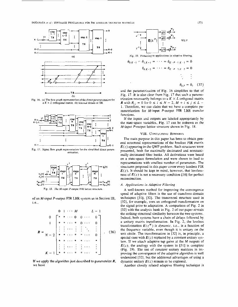
f o r 0 5 i I L - 1. Here, Uf,o = U , - I , K - 2 - f for 1 5 i I: L - 1. I are determined such that Uf:ILf_ll = 0. The resulting representation is shown in Fig. 16. The number of parameters used is Cf-_- I ( K - i ) = KL - ( ; ' I ) , which shows that this representation is also minimal.

Now suppose that R is a K X L orthogonal matrix related to a minimal state-space description ( A , B , C, D )

D O ~ A N A T A et a / . : SYNTHESIS PROCEDURES FOR FIR LOSSLESS TRANSFER MATRICES 1571

.......................................................,

.........................................................

4 T 8 (b)

Fig. 16. (a) The flow graph representation of the direct parametrization for a K X L orthogonal matrix. (b) Internal details of TS.

...- 0 ...- 1 K-L .. .-D 2

K-L+l L ,

.... .... ....

K-1 .... C.. K-1

Fig. 17. Signal flow graph representation for the simplified direct parametrization.

Fig. 18. The M-input P-output FIR lattice'structure

of an M-input P-output FIR LBR system as in Section 111, i.e.,

0 1 * . - M L - 1 . . . . . . . . . . . . . .

0 0 * * *

. . . . . . . . . . . . . * . . (36) N - 2 . . . . . . . . . .

. . . .

. . K - 1 . . . . . . . . . . .

If we apply the algorithm just described to parametrize R, we have

Fig. 19. Pertaining to applications in adaptive filtering.

0O.P = 0, (37)

and the parametrization of Fig. 16 simplifies to that of Fig. 17. It is also clear from Fig. 17 that such a parametrization necessarily belongs to a K X L orthgonal matrix Rwith Ri,j = 0 f o r 0 I i I N - 2, M + i 5 j 5 L - 1. Therefore, we can claim that we have a complete parametrization for M-input P-output FIR LBR transfer functions.

If the inputs and outputs are labeled appropriately by the state-space variables, Fig. 17 can be redrawn as the M-input P-output lattice structure shown in Fig. 18.

VIII. CONCLUDING REMARKS The main purpose in this paper has been to obtain gen-

eral structural representations of the lossless FIR matrix E ( z ) appearing in the QMF problem. Such structures were presented, both for maximally decimated and nonmaximally decimated filter banks. All derivations were based on a state-space formulation and were shown to lead to representations with smallest number of parameters. The structures proposed in this paper cover every lossless FIR E ( z ) . It should be kept in mind, however, that losslessness of E ( z ) is not a necessary condition [16] for perfect reconstruction.

A. Applications in Adaptive Filtering A well-known method for improving the convergence

speed of adaptive filters is the use of transform-domain techniques [3 13, [32]. The transversal structure used in [32], for example, uses an orthogonal transformation on the signal prior to adaptation. A comparison of Fig. 2 in [32] with the analysis bank in Fig. 2 of our paper reveals the striking structural similarity between the two systems. Indeed, both systems have a chain of delays followed by a unitary matrix transformation. In Fig. 2, the lossless transformation E ( z M ) is dynamic, i.e., is a function of the frequency variable, even though it is unitary on the unit circle. The transformation in [32] is, in principle, a special case with E ( z ) replaced by a constant unitary system. If we attach adaptive tap gains at the M outputs of E ( z ) , the analogy with the system in [31] is complete (Fig. 19). The use of constant unitary matrices in improving the convergence of the adaptive algorithm is well understood [32], but the additional advantages of using a dynamic unitary E ( z ) remain to be explored.

Another closely related adaptive filtering technique is


the subband adaptation technique proposed in [33] and [35]. Here the signal is split into subbands by use of an analysis bank, and the subband signals are used for adaptation. Notice again that if the unitary matrix in [32] is taken to be the DFT matrix, the system is identical to the subband adaptation scheme with analysis filters Hk ( z ) that are uniformly shifted versions of a prototype H,( z ) = ET=-: z - k . The analysis filters used in [33] are essentially the frequency sampling type of filters [34]. The use of a general lossless E ( z ) in place of such constant unitary matrices clearly permits the benefits of unitary transfor- mations to be combined with the advantage of having sharper cutoff$ilters with higher attenuation. One advantage of splitting a signal into subbands before adaptation is that the spectral dynamic range in each subband is typ- ically smaller than the corresponding dynamic range for the entire signal, resulting in a small eigenvalue spread of the covariance matrices and, hence, faster adaptation [31],

APPENDIX A

1321.

Let U = [uouI . . * uL - 1 ] be an L X L orthogonal matrix. The column vectors of U must satisfy

u;ul = u;u2 = * = u;uL-I = 0

U T U 2 = * * * = UTUL-I = 0

It is easy to see that the (k) orthogonality constraints of (Al) and the L normalization constraints of (A2) are all independent. On the other hand, U has L2 unknown entries. Hence, an L x L orthogonal matrix has a total of L2 - [ L + ( i ) ] = (4) degrees of freedom. The parametrization of Section 111-A, which uses (4) angles, is therefore minimal.

APPENDIX B STATE-SPACE DESCRIPTIONS F O R P X r FIR SYSTEMS

h ( n ) z P n be any causal p X r FIR system, so that h ( n ) are constant p X r matrices. Fig. 20 shows a direct-form realization of H ( z ) . Let the outputs of the delay elements in Fig. 20 be denoted x k ( n ) , 0 I k I J - 2. Each xk( n ) is an r-component vector. Defin- ingx(n) = [ x ; ( n ) x T ( n ) * e - ~ ; - ~ ( n ) ] ~ , wecanobtain a state-space description as in (4) with

Let H ( z ) =

0 0 0 * - - 0 0

. . . . . . . . 0 0 0 . . * z, 0

c = (h (1 ) h ( 2 ) * * * h ( J - l ) ) , D = h ( O ) ,

Fig. 20. Direct form realization of H ( z ) = EiZA h ( n ) z-".

s o t h a t A i s ( J - l ) r x ( J - l ) r , B i s ( J - l ) r X r , C i s p X ( J - l ) r , a n d D i s p X r.

Since A is lower-triangular with all diagonal entries equal to zero, all its eigenvalues are zero [24]. The above implementation is, however, not necessarily minimal, Le., the number of delays (or equivalently, the size of A; see Fig. 3) is not the smallest. It is well known that an implementation is minimal if it is both controllable and observable [36]. There exist well-known techniques for obtaining a minimal implementation from an arbitrary nonminimal implementation (see Theorems 5-16, 5-17, and 5-18 in [36]). It can further be shown that the eigenvalues of the A-matrix of such a minimal system form a subset of the eigenvalues of the matrix A for the original nonminimal realization.

As a conclusion, given any p X r FIR system, it is possible to obtain a minimal realization with all eigenvalues of A equal to zero. Since any two minimal reali- zations of a particular transfer matrix are related by a similarity transformation (Theorem 5-20 in [36]), they have the same set of eigenvalues. As a result, every minimal implementation of an FIR transfer matrix is such that all the eigenvalues of the A-matrix are zero. These results are also obtainable from the fact that the poles of the entries of H ( z ) (being also the eigenvalues of the A-matrix in any minimal realization of H ( z ) , [37, pp. 40 and 361) are all located at z = 0.

APPENDIX C A PARAMETRIZATION ALGORITHM FOR ORTHOGONAL

MATRICES

The purpose of the algorithm to be described here is to give a constructive proof that all orthogonal matrices of the form (26) can be represented as in Fig. 9.

Let us consider an arbitrary orthogonal matrix U . In the first step, we define

u,,, = U o , l - l @ : - l , k , 1 I f I L - 1, k = L - 1

(C1) with U0,, = U . @:-I,k are determined such that U:' = 0. This step yields an intermediate orthogonal matrix Uo,L-l as in (10) with (Y = 1 and b = 0.

In the next step, instead of operating on the next row, we proceed to the Mth row and define

uk4.1 = uM,L- 1 @;- I , k ,

1 I 1 I L - M - 1, k = L - 1,

uM.O = uO,L- 1 , ( C2a 1

DOeANATA et ai . : SYNTHESIS PROCEDURES FOR FIR LOSSLESS TRANSFER MATRICES 1573

where we define

are determined such that U Z i = 0. Next,

UM.1 = U M J - 10:- l , k ,

L - M I 1 I L - 3, k = L - 1 - 1 .

(C2b) Here again Finally, we write

are determined such that U:; = 0.

and determine OY,, such that U Z f - ’ = 0. This step is aimed at creating zero entries along the Mth row, thereby forcing a 1 at the ( M , M)th position. While doing so, previously created zeros are preserved since this step does not have rotations involving the 0th plane. At the end of this step, we have

0 1 M L - 1

0

1

UA4.L-2 =

M

L - 1

1 0 * . * 0 0 0 - * . 0 0 . . . . . 0 . . . . . . . . . . . . . . . . . . . . . . . . . . . 0 . . . . . 0 . . . . . 0 0 * * * 0 1 0 - * . 0 0 . . . . . 0 . . . . . . . . . . . . . . . . . . . . . . . . . . . . 0 * . . . * 0 * . . . *

For the next N - 2 steps, we repeat this procedure for rows M + 1 through L - 1. Recursions related to the ( M + i )th row, 1 I i I N - 2, can be obtained simply by substituting M + i for M in (C2a), (C2b), and (C2c). As we proceed, previously created zeros are not disturbed since while dealing with thejth row, M + 1 I j 5 L - 1 , we do not use rotations involving planes 0 and M through j - 1. At the end of the Nth step, we have

- U L - I , M - I -

‘ 1 0 - * * 0 0 0 . . - 0‘ . . . * 0 0 * . * 0 0 *

. . . . . . . . . . . . . . . . . . . . . . 0 * . . . * 0 0 . . . 0

0 0 * . . 0 1 0 * * - 0

0 0 . . . 0 0 1 . . . 0 . . . . . . . . . . . . . . . . . .

, o 0 - - * 0 0 0 - . . 1-

......................................

Step i, 2 5 1 CN-l

(b) Fig. 21. (a) Signal flow graph representation of the new factorization of

U. (b) Some internal details of Fig. 20(a).

We now parametrize the ( M - I ) x (M - I ) nontri- vial orthogonal block V that appears in (C4) using the algorithm of Section 111-A, by ( y - ) planar rotations. Since these rotations involve planes 1 through M - 1 only, previously created zeros are not altered. The complete parametrization is shown in Fig. 2 1 .

It can easily be verified now that if we parametrize an orthogonal matrix of the form (26) using this algorithm, we obtain the representation of Fig. 9.

ACKNOWLEDGMENT

We gratefully acknowledge the encouraging remarks from Prof. B. D. Anderson, of the Australian National University, on the contents of this paper.

REFERENCES

[ I ] A. Croisier, D. Esteban, and C. Galand, “Perfect channel splitting by use of interpolationldecimation/tree decomposition techniques, ” presented at the Int. Conf. Inform. Sci. Syst., Patras, Greece, 1976.

[2] D. Esteban and C. Galand, “Application of quadrature mirror filters to split-band voice coding schemes,” in Proc. IEEE Inr. Con$ Acoust., Speech, Signal Processing, Hartford, CT, May 1977, pp. 19 1- 195.

[3] R. E. Crochiere and L. R. Rabiner, Multirate Digital Signal Pro- cessing. Englewood Cliffs, NJ: Prentice-Hall, 1983.

[4] V. K. Jain and R. E. Crochiere, “Quadrature mirror filter design in the time domain,” IEEE Trans. Acoust., Speech, Signal Processing, vol. ASSP-32, pp. 353-361, Apr. 1984.

[5] C. R. Galand and H. J . Nussbaumer, “New quadrature mirror filter structures,” IEEE Trans. ACOUSI. , Speech, Signal Processing, vol. ASSP-32, pp. 522-531, June 1984.

[6] M. J . T. Smith and T. P. Barnwell, 111, “A procedure for designing exact reconstruction filter banks for tree structured subband coders,” in Proc. IEEE Conf. ACOUSI. , Speech, Signal Processing, San Diego, CA, Mar. 1984, pp. 27.1.1-27.1.4.

[7] -, “A unifying framework for analysis/synthesis systems based on maximally decimated filter banks,” in Proc. IEEE In?. Conf. Acousr., Speech, Signal Processing, Tampa, FL, Mar. 1985, pp. 521-524.

[SI H. J . Nussbaumer, “Pseudo-QMF filter bank,” IBM Tech. Disc. Bull., vol. 24, no. 6 , pp. 3081-3087, Nov. 1981.

[9] P. L. Chu, “Quadrature mirror filter design for an arbitrary number of equal bandwidth channels,” IEEE Trans. Acoust., Speech, Signal Processing, vol. ASSP-33, pp. 203-218, Feb. 1985.


[IO] J. H. Rothweiler, “Polyphase quadrature filters-A new subband coding technique,” in Proc. I983 IEEE Int. Con5 Acoust., Speech, Signal Processing, Boston, MA, Mar. 1983, pp. 1280-1283.

[ I I] K. Swaminathan and P. P. Vaidyanathan, “Theory and design of uni- form DFT, parallel quadrature mirror filter banks,” IEEE Trans. Cir- cuits Syst., vol. CAS-33, pp. 1170-1191, Dec. 1986.

[ 121 M. Vetterli, “Splitting a signal into subsampled channels allowing perfect reconstruction,” in Proc. IASTED Con5 Appl. Signal Pro- cessing Digital Filtering, Paris, France, June 1985.

[ 131 M. Vetterli, ‘‘Filter banks allowing for perfect reconstruction,” Sig- nal Processing, vol. 10, no. 3, pp. 219-244, Apr. 1986.

[ 141 F. Mintzer, “Filters for distortion-free two-band multirate filter banks,” IEEE Trans. Acousr., Speech, Signal Processing, vol. ASSP- 33, pp. 626-630, June 1985.

[15] M. G. Bellanger, G. Bonnerot, and M. Coudreuse, “Digital filtering by polyphase network: Application to sample-rate alteration and filter banks,” IEEE Trans. Acoust., Speech, Signal Processing, vol. ASSP- 24, pp. 109-114, Apr. 1976.

[16] P. P. Vaidyanathan, “Theory and design of M-channel maximally decimated quadrature mirror filters with arbitrary M, having the perfect-reconstruction property,” IEEE Trans. Acousr., Speech, Signal Processing, vol. ASSP-35, pp. 476-492, Apr. 1987.

[I71 P. P. Vaidyanathan and P.-Q. Hoang, “Lattice structures for optimal design and robust implementation of two-channel perfect-reconstruction QMF banks,” IEEE Trans. Acoust., Speech, Signal Processing, vol. 36, pp. 81-94, Jan. 1988.

[I81 P. P. Vaidyanathan, Z. Doganata, and T. Q. Nguyen, “More results on the perfect reconstruction problem in M-band parallel QMF banks,” in Proc. IEEE Int. Symp. Circuits Syst., Philadelphia, PA, May 1987, pp. 847-850.

1191 B. D. 0. Anderson and S. Vongpanitlerd, Network Analysis and Syn- thesis.

1201 V. Belevitch, Classical Network Synthesis. San Francisco, CA: Holden-Day, 1968.

[21] L. Hitz and B. D. 0. Anderson, “Discrete positive-real functions and their application to system stability,” Proc. IEE, pp. 153-155, Jan. 1969.

[22] P. P. Vaidyanathan, “The discrete-time bounded-real lemma,’’ IEEE Trans. Circuits Sysr., vol. CAS-32, pp. 918-924, Sept. 1985.

[23] F. D. Murnaghan, The Unitary and Rotation Groups. Washington, DC: Spartan Books, 1962.

[24] J. Franklin, Marrix Theory. Englewood Cliffs, NJ: Prentice-Hall, 1968.

[25] P. P. Vaidyanathan, “Passive cascaded-lattice structures for low-sen- sitivity FIR filter design, with applications to filter banks,” IEEE Trans. Circuits Sysr., vol. CAS-33, pp. 1045-1064, Nov. 1986.

[26] M. R. Portnoff, “Time-frequency representation of digital signals and systems based on short-time Fourier analysis,” IEEE Trans. Acoust., Speech, Signal Processing, vol. ASSP-28, pp. 55-69, Feb. 1980.

Englewood Cliffs, NJ: Prentice-Hall, 1973.

M. J . T. Smith, private conversation. T. Q. Nguyen and P. P. Vaidyanathan, “Maximally decimated perfect-reconstruction FIR filter banks with pairwise mirror-image analysis (and synthesis) frequency responses,” IEEE Trans. Acoust., Speech, Signal Processing, vol. 36, pp. 693-706, May 1988. The IMSL library, A set of Fortran subroutines for mathematics and statistics. P. P. Vaidyanathan, “Quadrature mirror filter banks, M-band exten- sions and perfect-reconstruction techniques,” IEEE ASSP Mag., vol.

B. Widrow, Adaptive Signal Processing. Englewood Cliffs, NJ: Prentice-Hall, 1985. S. S. Narayan, A. M. Peterson, and M. J . Narasimha, “Transform domain LMS algorithm,” IEEE Trans. Acoust., Speech, Signal Pro- cessing, vol. ASSP-31, pp. 609-615, June 1983. R. P. Bitmead and B. D. 0. Anderson, “Adaptive frequency sampling filters,” IEEE Trans. Circuits Syst . , vol. CAS-28, pp. 524- 534, June 1981. A. V. Oppenheim and R. W. Schafer, Digiral Signal Processing. Englewood Cliffs, NJ: Prentice-Hall, 1975. A. Gilloire and M. Vetterli, “Adaptive filtering in subbands,” in Proc. IEEE Int. Con5 Acoust., Speech, Signal Processing, Apr. 1988. C.-T. Chen, Linear System Theory and Design. New York: Holt, Rinehart and Winston, 1979. L. B. Jackson, Digilal Fillers and Signal Processing. Norwell, MA: Kluwer Academic Publishers, 1986.

4, pp. 4-20, July 1987.

Zinnur Doganata (S’86) was born in Ankara, Turkey, on October 29, 1959. She received the B.S. and M.S. degrees in electrical engineering from the Middle East Technical University, An- kara, in 1981 and 1984, respectively.

During the period 1981-1984, she worked part time for the Military Electronic Industries of Tur- key. Presently she is pursuing the Ph.D. degree in electrical engineering at the California Institute of Technology, Pasadena. Her main research in- terests are in digital signal processing and lossless systems.

P. P. Vaidyanathan (S’80-M183-SM’88), for a photograph and biography, see p. 94 of the January 1988 issue of this TRANSACTIONS.

Truong Q. Nguyen (S’86), for a photograph and biography, see p. 706 of the May 1988 issue of this TRANSACTIONS.

General Synthesis Procedures for FIR Lossless Transfer Matrices, for Perfect-Reconstruction...

Documents

Transcript of General Synthesis Procedures for FIR Lossless Transfer Matrices, for Perfect-Reconstruction...