applied sciences

Article

A Fast Method of Visually Lossless Compression ofDental Images

Sergey Krivenko 1,*, Vladimir Lukin 1, Olha Krylova 2, Liudmyla Kryvenko 2 and Karen Egiazarian 3

Citation: Krivenko, S.; Lukin, V.;

Krylova, O.; Kryvenko, L.; Egiazarian,

K. A Fast Method of Visually Lossless

Compression of Dental Images. Appl.

Sci. 2021, 11, 135. https://dx.doi.org/

10.3390/app11010135

Received: 10 November 2020

Accepted: 22 December 2020

Published: 25 December 2020

Publisher’s Note: MDPI stays neu-

tral with regard to jurisdictional claims

in published maps and institutional

affiliations.

Copyright: © 2020 by the authors. Li-

censee MDPI, Basel, Switzerland. This

article is an open access article distributed

under the terms and conditions of the

Creative Commons Attribution (CC BY)

license (https://creativecommons.org/

licenses/by/4.0/).

1 Department of Information and Communication Technologies, National Aerospace University,Chkalova Str. 17, 61070 Kharkiv, Ukraine; v.lukin@khai.edu

2 Department of Therapeutic Dentistry & Department of Pediatric Dentistry and Implantology,Kharkiv National Medical University, 4 Nauky Avenue, 61022 Kharkiv, Ukraine; krylovaol@ukr.net (O.K.);ls.kryvenko@knmu.edu.ua (L.K.)

3 Computational Imaging Group, Tampere University, 33720 Tampere, Finland; karen.eguiazarian@tuni.fi* Correspondence: s.kryvevnko@khai.edu

Abstract: A noniterative approach to the problem of visually lossless compression of dental images isproposed for an image coder based on the discrete cosine transform (DCT) and partition scheme opti-mization. This approach considers the following peculiarities of the problem. It is necessary to carryout lossy compression of dental images to achieve large compression ratios (CRs). Since dental imagesare viewed and analyzed by specialists, it is important to preserve useful diagnostic informationpreventing appearance of any visible artifacts due to lossy compression. At last, dental images maycontain noise having complex statistical and spectral properties. In this paper, we have analyzed andutilized dependences of three quality metrics (Peak signal-to-noise ratio, PSNR; eak Signal-to-NoiseRatio using Human Visual System and Masking (PSNR-HVS-M); and feature similarity, FSIM) on thequantization step (QS), which controls a compression ratio for the so-called advanced DCT coder(ADCTC). The threshold values of distortion visibility for these metrics have been considered. Finally,the recent results on detectable changes in noise intensity have been incorporated in the QS setting.A visual comparison of original and compressed images allows to conclude that the introduceddistortions are practically undetectable for the proposed approach; meanwhile, the provided CR lieswithin the interval.

Keywords: dental image; visually lossless compression; fast processing

1. Introduction

Image processing has found numerous applications in multimedia and smart educa-tion [1–3], remote sensing and non-destructive control [4–6], etc. It is widely used in variousmedical applications [7–9]. Medical images acquired by different types of devices are ap-plied in diagnostics and control in numerous branches of medicine. One of them is indentistry [10,11], for which imaging systems and acquired images have specific peculiarities.

The most modern imaging systems produce dental images of large size [12,13].This causes a problem for their storage if the number of daily or monthly acquired images isvery large [14], and in image transmission via communication channels in telemedicine [15].Therefore, it is desirable to use image compression to reduce data size for storing, handlingand transmitting content [14–17]. There are two types of image compression algorithms—lossless and lossy compression [18,19]. It has been well understood [19,20] that lossless(reversible) compression provides a small compression ratio (CR) that often does not meetthe requirements of the storage and/or transmission of medical data; and the use of lossycompression can be, in general, acceptable in practice but only under specific conditions.The main condition is that distortions introduced by a lossy compression should not reducea diagnostic value of an image (i.e., distortions should be “invisible” and/or no artifacts

Appl. Sci. 2021, 11, 135. https://dx.doi.org/10.3390/app11010135 https://www.mdpi.com/journal/applsci

Appl. Sci. 2021, 11, 135 2 of 14

should be introduced due to compression). Other conditions relate to the computation effi-ciency and security. Compression and decompression should be fast; sometimes standardcoders have to be used [20], whilst the use of non-standard coders can provide an extrasecurity of compressed data.

The main problem in the modern lossy compression is to provide a reasonable trade-off between CR (in bitrate, bits per pixel—bpp) and image quality (characterized by ametric’s value). With an application to medical images (e.g., dental images), this problemcan be solved in different ways:

(1) Setting a recommended or maximal CR for the considered type of images [19–22] fora given compression method. This practically guarantees invisibility of distortionsbut makes it impossible to adapt to image/noise properties and thus increase CRwhen it is possible;

(2) Controlling a quality of an image subject to compression and reaching a possiblelimit [20]. In this case, there are two bottlenecks. One is that an adequate metricshould be chosen, and the corresponding distortion invisibility threshold must beknown in advance. The standard peak signal-to-noise ratio (PSNR) is known to benot always a reliable metric from a human visual system point of view, a choiceof other visual quality metrics can be a question alongside threshold selection [23].Thus, a compression can become iterative for finding a proper parameter that controlscompression (PCC), for example, quality factor for JPEG, bitrate for JPEG2000 orSet partitioning in hierarchical trees (SPIHT), quantization step (QS) for discretecosine transform (DCT)-based coders [24–27], etc. Another bottleneck is that sucha compression might need extensive computational and time expenses, which isundesirable. Thus, fast procedures for providing invisibility of distortions and highCR are needed.

Medical images, in general, and dental images, in particular, can be corrupted by anoise [28–30], which can be seen well in the visualized data. Noise properties depend onmany factors and, in general, are not purely additive and white [29–31]. Moreover, a lossyimage compression had several peculiarities discovered in [32,33] and was consideredlater in the literature [34,35]. A main peculiarity is a specific noise filtering effect thatappears due to a lossy compression. This effect is mostly positive but only if low contrastinformative details are not removed or considerably smeared. Thus, noise properties in thecase of compressing noisy images must be considered in the coder’s PCC setting.

Considering all the aforementioned features of the considered problem of lossy com-pression of dental images avoiding an appearance of visible artifacts (without losingdiagnostically important information), we analyze a possibility of applying an advancedDCT coder (ADCT) codec (ADCTC) [36] within the fast and effective procedure. The inter-est in ADCTC is explained by the following factors: (a) This compression technique allowsadapting to the image content and; thus, providing better performance characteristics thanJPEG, JPEG2000, SPIHT and other coders [24]; (b) since this compression method is notstandardized, a certain degree of security (privacy) of compressed data can be ensured.The goal of this paper is to find such a PCC value for ADCTC that guarantees invisibilityof introduced distortions and fast compression due to the absence of iterations.

The rest of the paper is organized as follows. Section 2 gives some assumptions onimage/noise properties of dental images. In Section 3, the basic dependences of three im-age quality metrics—PSNR, Peak Signal-to-Noise Ratio using Human Visual System andMasking (PSNR-HVS-M) and feature similarity (FSIM)—on compression ratio (CR) for AD-CTC, JPEG2000 and SPIHT are given. Section 4 investigates threshold values of distortioninvisibility for ADCTC and JPEG2000 image coders. A verification of selected quantizationsteps for image coders on real clinical data is provided in Section 5. Finally, conclusions aregiven in Section 6.

Appl. Sci. 2021, 11, 135 3 of 14

2. Some Assumptions on Image/Noise Properties

The dental images acquired by the modern imaging systems are large in size, at leastone megapixel data [12,13,31]. In particular, this relates to the images acquired by thesystem Morita, panoramic X-ray (Veraviewepocs 3D R100 J) [37]. Such images usuallyhave a square (in general, rectangular) shape where the ratio of dimensions depends onimaging system and on its operation mode. Meanwhile, one may need to compress animage fragment in a region of interest that can be square or rectangular and of differentcontext. Examples of such fragments are given in Figure 1.

Appl. Sci. 2021, 11, x FOR PEER REVIEW 3 of 14

tion invisibility for ADCTC and JPEG2000 image coders. A verification of selected quan-tization steps for image coders on real clinical data is provided in Section 5. Finally, con-clusions are given in Section 6.

2. Some Assumptions on Image/Noise Properties The dental images acquired by the modern imaging systems are large in size, at least

one megapixel data [12,13,31]. In particular, this relates to the images acquired by the sys-tem Morita, panoramic X-ray (Veraviewepocs 3D R100 J) [37]. Such images usually have a square (in general, rectangular) shape where the ratio of dimensions depends on imag-ing system and on its operation mode. Meanwhile, one may need to compress an image fragment in a region of interest that can be square or rectangular and of different context. Examples of such fragments are given in Figure 1.

(a) (b)

(c) (d)

Figure 1. The 512 × 512 pixel fragments of different context (a,b) and scatterplot of local variance estimates (c) for homogeneous regions ((d), gray color) of the fragment in (a).

There is a noise present in dental images, as one can see from these fragments, that might partly mask important diagnostic information. This noise arises due to a limited time of imaging the object, and properties of noise are complex [29,31,38]. In the simplest case, one can model noise in dental images as Poisson-like signal dependent [29]. How-ever, more detailed analysis shows that it is, in general, signal dependent but has more complex nature. It has a signal-independent (SI) component and a signal-dependent (SD) component, variance of which can be proportional to a signal intensity [31]. For example, a variance can be expressed as σ = σ ∙ I + k ∙ I + σ (Model 3), where I is a true in-tensity value of an ij-th image pixel (i = 1, N, j = 1,M, N and M denote vertical and hori-

Figure 1. The 512 × 512 pixel fragments of different context (a,b) and scatterplot of local varianceestimates (c) for homogeneous regions ((d), gray color) of the fragment in (a).

There is a noise present in dental images, as one can see from these fragments,that might partly mask important diagnostic information. This noise arises due to alimited time of imaging the object, and properties of noise are complex [29,31,38]. In thesimplest case, one can model noise in dental images as Poisson-like signal dependent [29].However, more detailed analysis shows that it is, in general, signal dependent but has morecomplex nature. It has a signal-independent (SI) component and a signal-dependent (SD)component, variance of which can be proportional to a signal intensity [31]. For example,a variance can be expressed as σ2 = σ2

µ·I2ij + k·Iij + σ2

a (Model 3), where Iij is a true inten-sity value of an ij-th image pixel (i = 1, N, j = 1, M, N and M denote vertical and horizontalimage sizes, respectively); σ2

µ is an estimate of multiplicative noise relative variance; σ2a is

an estimate of additive noise variance; k is a quasi-Poisson noise parameter. Experimentsin [31] show that the simple models σ2 = σ2

µ·I2ij + σ2

a (Model 1) and σ2 = k·Iij + σ2a

(Model 2) often fit real data better than the complex general model given above.

Appl. Sci. 2021, 11, 135 4 of 14

Experiments carried out with Morita system show that an equivalent noise variancefor a most general model depends on both image and noise properties and is approximatelyequal to

σ2eq = σ2

a + σ2µ

N

∑i=1

M

∑j=1

I2ij/NM + k

N

∑i=1

M

∑j=1

Iij/NM (1)

Figure 1c presents the scatterplot of local variance estimates on local mean estimatesfor the fragment in Figure 1a. These estimates have been obtained only in locally passive(quasi-homogeneous) blocks of this fragment—the corresponding map of block locationsis given in Figure 1d, the curves for all three models are fitted (Figure 1c) and it is seenthat Models 1 and 3 provide almost the same approximations that are considerably betterthan for Model 2 (it is not a problem to determine the best fit, see [31] for more details).The determined parameters for Model 1 for the fragment in Figure 1c are the following:σ2µ = 0.0020, σ2

a = 2.27 and equivalent variance is, respectively, equal to 15.7. Similaroperations give σ2

eq = 80.7 for the fragment in Figure 1b (σ2µ = 0.0043, σ2

a = 37.49).Note that the noise characteristics for Morita system dental images have been analyzed

for two modes of its operation. For one mode, σ2eq varies in the range 5–20 for images

of low mean intensity (Figure 1a) and in the range 50–70 for images with a high meanintensity. For another mode, σ2

eq is about 30 for images of low mean intensity and it isin the range 60–200 for images with low and high mean intensity (see the fragment inFigure 1b). In all cases, noise is seen well in the visualized data.

A detailed analysis carried out in [31] has also shown that a noise is spatially correlatedwhere spectral properties depend on imaging mode, and there can be clipping artifacts.Note that all aforementioned properties and effects are partly explained by a specific nonlineartransformation carried out in imaging devices with the purpose of better visualization.

3. Basic Dependences

We use ADCTC codec in this paper (more information on this coder can be found athttps://ponomarenko.info/adct.htm). The main peculiarity of this coder is that it employspartition schemes (i.e., a variable size DCT is carried out in image blocks). In addition, cod-ing of numbers of significant bits, context modeling and coding of signs of DCT coefficientsare applied. Figure 2 gives an illustration of ADCTC partition schemes. The maximal blocksize is 64× 64 pixels, the minimal size is 8× 8 pixels, and all blocks have rectangular shapewith sides equal to the power of two. A larger block is divided into two smaller ones basedon the entropy analysis (e.g., when the block contains heterogeneous parts). The ADCTChas the following peculiarities:

(1) Fast DCT algorithms can be used in the coder;(2) Coding of partition scheme is fast, and the obtained partition scheme occupies con-

siderably less space than the coded quantized DCT coefficients;(3) A specific adaptation to the image content takes place and this results in better

compression. Note that the partition scheme also depends on QS (partition schemesin Figure 2 are shown for two values of QS).

Appl. Sci. 2021, 11, 135 5 of 14Appl. Sci. 2021, 11, x FOR PEER REVIEW 5 of 14

(a) (b)

Figure 2. The 512 × 512 pixel fragment with two partition schemes obtained for quantization step (QS) = 3 (a) and QS = 13 (b).

ADCTC outperforms many compression techniques, even including those proposed recently [24]. The corresponding comparisons have been made earlier using standard op-tical test images. Here we show that this is also valid for dental images.

Recall that a quantization step serves for ADCTC, as PCC and larger QS leads to a larger CR and, simultaneously, increases the level of introduced distortions (which means worse compressed image quality). The performance of a compression technique is usually compared using rate/distortion curves for a set of test images in terms of an image quality metric characterizing decompressed image quality. Most often researchers have used two metrics—mean square error (MSE) of introduced distortions and peak signal-to-noise ra-tio (PSNR) strictly related to it. During the last decade, unconventional visual quality met-rics have been widely used. One such image quality metric is PSNR-HVS-M, which is a generalization of PSNR: PSNR − HVS −M = 10log (2)

where MSE is a specific MSE determined in the DCT domain using two important features of HVS: (a) The fact that distortions in low spatial frequencies can be more easily detected visually than distortions in high spatial frequencies; (b) the masking effect (i.e., ability of textures, edges and details to mask distortions). MSE for an entire image is calculated as a mean of local estimates MSE n), n = 1,… , N, where n is a block index and N denotes the total number of analyzed blocks of size 8 × 8 pixels. Local values of MSE n) are calculated in the DCT domain using weights that use the JPEG quan-tization table, which is based on the contrast sensitivity function. In addition, an existence of the masking effect is verified for every block and employed in the calculation of MSE n). More details can be found in http://ponomarenko.info/psnrhvsm.htm.

Note that both PSNR and PSNR-HVS-M are expressed in dB (Formula (2) relates to 8-bit representation of images). Smaller values of both metrics, in general, correspond to worse quality. PSNR at the level of 36 dB and PSNR-HVS-M around 41 dB can be consid-ered as empirically found thresholds of distortion invisibility [23].

Dependences of PSNR and PSNR-HVS-M on CR for the fragments in Figure 1 are presented in Figure 3 for ADCTC, JPEG2000 and SPIHT [25]. Analysis of these curves shows the following: (1) ADCTC provides sufficiently better results than both JPEG2000 and SPIHT: Larger

PSNR and PSNR-HVS-M values for CR in the range of interest for both test images;

Figure 2. The 512 × 512 pixel fragment with two partition schemes obtained for quantization step(QS) = 3 (a) and QS = 13 (b).

ADCTC outperforms many compression techniques, even including those proposedrecently [24]. The corresponding comparisons have been made earlier using standardoptical test images. Here we show that this is also valid for dental images.

Recall that a quantization step serves for ADCTC, as PCC and larger QS leads to alarger CR and, simultaneously, increases the level of introduced distortions (which meansworse compressed image quality). The performance of a compression technique is usuallycompared using rate/distortion curves for a set of test images in terms of an image qualitymetric characterizing decompressed image quality. Most often researchers have usedtwo metrics—mean square error (MSE) of introduced distortions and peak signal-to-noiseratio (PSNR) strictly related to it. During the last decade, unconventional visual qualitymetrics have been widely used. One such image quality metric is PSNR-HVS-M, which isa generalization of PSNR:

PSNR−HVS−M = 10 log10

(2552

MSEHVS−M

)(2)

where MSEHVS−M is a specific MSE determined in the DCT domain using two importantfeatures of HVS: (a) The fact that distortions in low spatial frequencies can be more eas-ily detected visually than distortions in high spatial frequencies; (b) the masking effect(i.e., ability of textures, edges and details to mask distortions). MSEHVS−M for an entireimage is calculated as a mean of local estimates MSEHVS−M(n), n = 1, . . . , N, where nis a block index and N denotes the total number of analyzed blocks of size 8 × 8 pixels.Local values of MSEHVS−M(n) are calculated in the DCT domain using weights that usethe JPEG quantization table, which is based on the contrast sensitivity function. In addition,an existence of the masking effect is verified for every block and employed in the calculationof MSEHVS−M(n). More details can be found in http://ponomarenko.info/psnrhvsm.htm.

Note that both PSNR and PSNR-HVS-M are expressed in dB (Formula (2) relates to8-bit representation of images). Smaller values of both metrics, in general, correspondto worse quality. PSNR at the level of 36 dB and PSNR-HVS-M around 41 dB can beconsidered as empirically found thresholds of distortion invisibility [23].

Dependences of PSNR and PSNR-HVS-M on CR for the fragments in Figure 1 arepresented in Figure 3 for ADCTC, JPEG2000 and SPIHT [25]. Analysis of these curvesshows the following:

(1) ADCTC provides sufficiently better results than both JPEG2000 and SPIHT: LargerPSNR and PSNR-HVS-M values for CR in the range of interest for both test images;

Appl. Sci. 2021, 11, 135 6 of 14

(2) These dependences can be treated in another way—a larger CR is provided for a givenquality (fixed values of PSNR or PSNR-HVS-M); the benefit in CR can reach 20%.

Appl. Sci. 2021, 11, x FOR PEER REVIEW 6 of 14

(2) These dependences can be treated in another way—a larger CR is provided for a given quality (fixed values of PSNR or PSNR-HVS-M); the benefit in CR can reach 20%.

(a)

(b)

(c)

Figure 3. Cont.

Appl. Sci. 2021, 11, 135 7 of 14Appl. Sci. 2021, 11, x FOR PEER REVIEW 7 of 14

(d)

Figure 3. Dependences of Peak signal-to-noise ratio (PSNR) (a,b) and Peak Signal-to-Noise Ratio using Human Visual System and Masking (PSNR-HVS-M) (c,d) on compression ratio (CR) for complex structure (a,c) and simple structure (b,d) images.

One can argue that ADCTC uses DCT and the metric PSNR-HVS-M also employs DCT. Due to this, a comparison of ADCTC with JPEG2000 and SPIHT coders, both based on wavelets, in terms of PSNR-HVS-M might not seem fair. Because of this, we also car-ried out a similar analysis using the feature similarity (FSIM) index [39], which is a low-level feature-based image quality assessment metric. The basic principle of FSIM is that human vision perceives images based on their salient low-level features. Two types of features are employed, the phase congruency and the gradient magnitude. The phase con-gruency is used to weight the contribution of each point to the similarity of distorted and reference images. FSIM values vary from 0 to 1, where the latter one corresponds to the perfect quality.

The dependences are given in Figure 4 and their analysis confirms that the perfor-mance of ADCTC is superior according to the metric FSIM as well.

(a)

Figure 3. Dependences of Peak signal-to-noise ratio (PSNR) (a,b) and Peak Signal-to-Noise Ratiousing Human Visual System and Masking (PSNR-HVS-M) (c,d) on compression ratio (CR) forcomplex structure (a,c) and simple structure (b,d) images.

One can argue that ADCTC uses DCT and the metric PSNR-HVS-M also employs DCT.Due to this, a comparison of ADCTC with JPEG2000 and SPIHT coders, both based onwavelets, in terms of PSNR-HVS-M might not seem fair. Because of this, we also carriedout a similar analysis using the feature similarity (FSIM) index [39], which is a low-levelfeature-based image quality assessment metric. The basic principle of FSIM is that humanvision perceives images based on their salient low-level features. Two types of features areemployed, the phase congruency and the gradient magnitude. The phase congruency is usedto weight the contribution of each point to the similarity of distorted and reference images.FSIM values vary from 0 to 1, where the latter one corresponds to the perfect quality.

The dependences are given in Figure 4 and their analysis confirms that the perfor-mance of ADCTC is superior according to the metric FSIM as well.

Appl. Sci. 2021, 11, x FOR PEER REVIEW 7 of 14

(d)

Figure 3. Dependences of Peak signal-to-noise ratio (PSNR) (a,b) and Peak Signal-to-Noise Ratio using Human Visual System and Masking (PSNR-HVS-M) (c,d) on compression ratio (CR) for complex structure (a,c) and simple structure (b,d) images.

One can argue that ADCTC uses DCT and the metric PSNR-HVS-M also employs DCT. Due to this, a comparison of ADCTC with JPEG2000 and SPIHT coders, both based on wavelets, in terms of PSNR-HVS-M might not seem fair. Because of this, we also car-ried out a similar analysis using the feature similarity (FSIM) index [39], which is a low-level feature-based image quality assessment metric. The basic principle of FSIM is that human vision perceives images based on their salient low-level features. Two types of features are employed, the phase congruency and the gradient magnitude. The phase con-gruency is used to weight the contribution of each point to the similarity of distorted and reference images. FSIM values vary from 0 to 1, where the latter one corresponds to the perfect quality.

The dependences are given in Figure 4 and their analysis confirms that the perfor-mance of ADCTC is superior according to the metric FSIM as well.

(a)

Figure 4. Cont.

Appl. Sci. 2021, 11, 135 8 of 14Appl. Sci. 2021, 11, x FOR PEER REVIEW 8 of 14

(b)

Figure 4. Dependences of A Feature Similarity Index (FSIM) on compression ratio (CR) for simple structure (a) and complex structure (b) image fragments.

As it was mentioned above, larger QS values correspond to larger compression ratios. To demonstrate this, we show the plots obtained for integer values of QS varying in the limits from 1 to 40 for twenty 512 × 512 image fragments of different complexity (Figure 5a). All dependences (CR on QS for a given image fragment) are monotonous. Meanwhile, for a given QS, CR values vary in the wide limits depending on image fragment context. For example, for QS = 10, CR varies from 6 to 22, whilst, for QS = 20, CR varies from 12 to 78. That is, CR can differ by one order or even more.

PSNR decreases monotonously if QS increases (Figure 4b). If QS ≤ 5, PSNR values for the same QS are almost the same for all fragments. Meanwhile, for larger QS, PSNR values for the same QS can vary a lot. For example, for QS = 20, PSNR values are in the limit of 34 to 40 dB (i.e., they vary in wide limits).

(a)

(b)

Figure 4. Dependences of A Feature Similarity Index (FSIM) on compression ratio (CR) for simplestructure (a) and complex structure (b) image fragments.

As it was mentioned above, larger QS values correspond to larger compression ratios.To demonstrate this, we show the plots obtained for integer values of QS varying in thelimits from 1 to 40 for twenty 512× 512 image fragments of different complexity (Figure 5a).All dependences (CR on QS for a given image fragment) are monotonous. Meanwhile,for a given QS, CR values vary in the wide limits depending on image fragment context.For example, for QS = 10, CR varies from 6 to 22, whilst, for QS = 20, CR varies from12 to 78. That is, CR can differ by one order or even more.

Appl. Sci. 2021, 11, x FOR PEER REVIEW 8 of 14

(b)

Figure 4. Dependences of A Feature Similarity Index (FSIM) on compression ratio (CR) for simple structure (a) and complex structure (b) image fragments.

As it was mentioned above, larger QS values correspond to larger compression ratios. To demonstrate this, we show the plots obtained for integer values of QS varying in the limits from 1 to 40 for twenty 512 × 512 image fragments of different complexity (Figure 5a). All dependences (CR on QS for a given image fragment) are monotonous. Meanwhile, for a given QS, CR values vary in the wide limits depending on image fragment context. For example, for QS = 10, CR varies from 6 to 22, whilst, for QS = 20, CR varies from 12 to 78. That is, CR can differ by one order or even more.

PSNR decreases monotonously if QS increases (Figure 4b). If QS ≤ 5, PSNR values for the same QS are almost the same for all fragments. Meanwhile, for larger QS, PSNR values for the same QS can vary a lot. For example, for QS = 20, PSNR values are in the limit of 34 to 40 dB (i.e., they vary in wide limits).

(a)

(b)

Figure 5. Dependences of compression ratio (CR) (a) and Peak signal-to-noise ratio (PSNR) (b) onquantization step (QS) for many image fragments for ADCTC.

Appl. Sci. 2021, 11, 135 9 of 14

PSNR decreases monotonously if QS increases (Figure 4b). If QS ≤ 5, PSNR values forthe same QS are almost the same for all fragments. Meanwhile, for larger QS, PSNR valuesfor the same QS can vary a lot. For example, for QS = 20, PSNR values are in the limit of34 to 40 dB (i.e., they vary in wide limits).

This means that setting a given QS leads to a wide variation of CR and PSNR if QSis large. In other words, by setting some QS it is not easy to provide a desired quality ofcompressed images, at least, according to the metric PSNR and for large QS. For example,QS = 20 leads to invisibility of distortions for some images and their visibility for otherimages (note that, according to [23], distortions are, with high probability, invisible ifPSNR > 36 dB).

4. Invisibility Threshold and Compression

There are several approaches to visually lossless compression of images. For the caseof noise-free or near noise-free images, one of the main approaches is presented in [40],according to which:

(1) One must choose an adequate metric that characterizes well a visual quality;(2) In addition, a distortion invisibility threshold for the chosen metric must be a priori

known or determined;(3) Finally, a way to provide this threshold value for the chosen metric at image compres-

sion stage must be found and the corresponding algorithm needs to be fast enough.

Since there are numerous visual quality metrics [41], it is difficult to choose the bestamong them. Meanwhile, for the grayscale images considered here, we decided to analyzetwo visual quality metrics mentioned above—PSNR-HVS-M and FSIM, for the followingreasons. These metrics have rank correlations with mean opinion scores for many imagedatabases [23,41] among the largest for the known metrics. For these metrics, there existsthreshold values of distortion invisibility [23]. These metrics are based on DCT and wavelets;thus, if the conclusions drawn from the analysis of these metrics are in a good agreement,then one can be confident that these conclusions are correct with a high probability.

What concerns the visibility thresholds are: Experimental data presented in the pa-per [23] show that distortions are practically invisible when the PSNR-HVS-M value isabove 41 dB or FSIM > 0.99. One additional condition is that distortions shall be “uniformly”distributed across a compressed image.

Finally, efficient noniterative methods to provide a desired visual quality of com-pressed images have been proposed recently [31,42]. This is important for ADCTC, since itis computationally more demanding than JPEG due to a partition scheme optimizationand use of DCTs of different sizes. Note that by “fast method” with application to ADCTC,we mean an efficient noniterative compression method.

Let us consider the dependences of PSNR-HVS-M and FSIM on QS. They are presentedfor image fragments in Figure 6. As one can see from this figure, curve points are placedcompactly. It is practically guaranteed that PSNR-HVS-M > 40 dB and FSIM > 0.99 ifQS ≤ 12. The exceptions are image fragments with very simple structure. This can besupported also by other results. In [31] it was found that MSEHVS−M = 0.02896·QS1.976.This expression was obtained for a different coder, but it is also approximately valid forADCTC. Then one has QSdes ≈ MSEHVS−Mdes/0.02896)1/2, where MSEHVS−Mdes is thedesired MSEHVS−M (for PSNR-HVS-M about 41 dB it corresponds to 5) one gets QSdes ≈ 13.

Appl. Sci. 2021, 11, 135 10 of 14Appl. Sci. 2021, 11, x FOR PEER REVIEW 10 of 14

(a)

(b)

Figure 6. Dependences of PSNR-HVS-M (a) and FSIM (b) on QS for image fragments.

We have already discussed a noise filtering effect if a lossy compression is applied to a noisy image. Recent study shows that people practically do not detect changes in a noise level if these changes are one order smaller than the level of an original noise [43] (i.e., in our case, if the introduced losses have to be by one order smaller than noise σ in origi-nal images). Then, for σ value around 50, one needs to provide PSNR at the level of 40 dB. This happens if QS is around 11 (see data in Figure 5b). Thus, we can generally set QS to 12. In the next Section, we verify this conclusion for image fragments. But first, let us compare the performance of the proposed method to other approaches.

Coder efficiency can be analyzed and compared in many ways. In our case, we would like a lossy compression method to guarantee a lossy compression with invisible distor-tions in one iteration (i.e., to be fast) and with high values of CR. ADCTC with a selected QS = 12 was applied to the set of dental image fragments. Then, mean PSNR-HVS-M (PHVSMmean) and root mean square (RMSEPHVSM) of its deviation were determined. Simi-larly, mean CR (CRmean) and root mean square (RMSECR) were calculated: PHVSMmean = 42.5 dB, RMSEPHVSM = 1.42 (PSNR-HVS-M values varied from 40.5 to 45.6 dB (i.e., it was practically guaranteed that introduced distortions are invisible), CRmean = 12.82, RMSECR = 5.57 (CR varied from 7.5 to 20.6 depending on image complexity).

For a fair comparison, we set such a CR for JPEG2000 that PHVSMmean = 42.5 dB. This CR occurred to be equal to 6.5 (i.e., considerably smaller than CRmean = 12.82). For JPEG2000, RMSEPHVSM = 1.76 (PSNR-HVS-M values varied from 40.5 to 46.9 dB), that is, a method based on JPEG2000 with the fixed CR or bitrate produces smaller CR and worse accuracy in providing the desired visual quality characterized by PSNR-HVS-M. Note, that the accuracy for JPEG2000 can be still improved if the iterative compression proce-dure is applied; however, the same can be done also for ADCTC.

5. Verification of Selected QS

Figure 6. Dependences of PSNR-HVS-M (a) and FSIM (b) on QS for image fragments.

We have already discussed a noise filtering effect if a lossy compression is appliedto a noisy image. Recent study shows that people practically do not detect changes in anoise level if these changes are one order smaller than the level of an original noise [43](i.e., in our case, if the introduced losses have to be by one order smaller than noise σ2

eq inoriginal images). Then, for σ2

eq value around 50, one needs to provide PSNR at the level of40 dB. This happens if QS is around 11 (see data in Figure 5b). Thus, we can generally setQS to 12. In the next Section, we verify this conclusion for image fragments. But first, let uscompare the performance of the proposed method to other approaches.

Coder efficiency can be analyzed and compared in many ways. In our case, we wouldlike a lossy compression method to guarantee a lossy compression with invisible distortionsin one iteration (i.e., to be fast) and with high values of CR. ADCTC with a selected QS = 12was applied to the set of dental image fragments. Then, mean PSNR-HVS-M (PHVSMmean)and root mean square (RMSEPHVSM) of its deviation were determined. Similarly, mean CR(CRmean) and root mean square (RMSECR) were calculated: PHVSMmean = 42.5 dB,RMSEPHVSM = 1.42 (PSNR-HVS-M values varied from 40.5 to 45.6 dB (i.e., it was practi-cally guaranteed that introduced distortions are invisible), CRmean = 12.82, RMSECR = 5.57(CR varied from 7.5 to 20.6 depending on image complexity).

For a fair comparison, we set such a CR for JPEG2000 that PHVSMmean = 42.5 dB.This CR occurred to be equal to 6.5 (i.e., considerably smaller than CRmean = 12.82).For JPEG2000, RMSEPHVSM = 1.76 (PSNR-HVS-M values varied from 40.5 to 46.9 dB),that is, a method based on JPEG2000 with the fixed CR or bitrate produces smaller CR andworse accuracy in providing the desired visual quality characterized by PSNR-HVS-M.Note, that the accuracy for JPEG2000 can be still improved if the iterative compressionprocedure is applied; however, the same can be done also for ADCTC.

Appl. Sci. 2021, 11, 135 11 of 14

5. Verification of Selected QS

A clinical part of the work was performed at the University Dental Center, KharkivNational Medical University, Pediatric Dentistry and Implantology Department. All proce-dures managed in the dental office were performed according to the protocols for providingdental care to the population in Ukraine. The standard procedure included interviewing apatient (if a child, with a parent), clinical examination with standard equipment and indica-tion of X-ray examination (panoramic X-ray, lateral cephalography, if needed). The decisionof X-ray type was made by a dental specialist—orthodontist or pedodontist, or both ofthem. The X-ray was necessary for the statement of a correct diagnose and for making anadequate treatment planning.

After the clinical examination, a patient visited the diagnostic X-ray laboratory, wherehe/she performed X-ray examination (The Veraview X800, Morita, Japan) according to theindication list. Totally, 140 X-ray images were taken for testing, including 95 panoramicX-ray and 45 lateral cephalography data. All these images were used as the necessary step oftreatment planning. The main purpose of X-ray diagnostics was to detect dental pathology,such as dental caries, periodontal diseases, impacted wisdom teeth and as an assessment forthe placement of dental implant, orthodontic pre- and post-operative assessment of occlusion,temporomandibular joint dysfunctions and other possible dental pathology.

The results of X-ray examination are usually sent to a dentist by e-mail. The imageidentification, such as the name and sex, do not accompany the radiograph to protectpatient’s privacy. The file format of the radiographs is usually JPG or DICOM and they aresent by email as an attachment.

To ensure an efficient evaluation, dental specialists who have been working at theUniversity Dental Center for three years or more, evaluated the clinical images. Be-fore starting this study, seven dental specialists (orthodontists and pedodontists) weretrained to evaluate X-ray images, and the objective criteria for the qualitative evalu-ation of the images were discussed. All dental specialists (evaluators) classified theoverall quality of X-ray images into the following grades: 1. Optimal for diagnosis,2. adequate for diagnosis, 3. poor but diagnosable, and 4. unrecognizable, not enoughfor diagnosis (the classification was based on the Clinical Image Quality EvaluationChart, https://www.researchgate.net/publication/232257582_Clinical_image_quality_evaluation_for_panoramic_radiography_in_Korean_dental_clinics). The monitors thatwere used by evaluators were the following: (1) Monitor of laptop ASUS (15.6′, 1920 × 1080,Full HD, IPS), (2) monitor of IPhone XR, (3) monitor of IPad.

After receiving X-ray images, the doctors evaluated images visually using computermonitor or smartphone, using maximum zooming of images. The first stage of evaluation—dental specialists analyzed images anonymously, without information about the type ofimage—“original” or “compressed”, according to a set qualification criteria. The sec-ond stage was the detailed analysis of the known compressed and original images andevaluation according to the qualification criteria.

At the first stage of anonymous image evaluation, according to this classification,89 images were deemed “optimal for obtaining diagnosis”, 38 were “adequate for diagno-sis”, 13 were “poor but diagnosable”, no images were “unrecognizable”. At the secondstep, after comparing “original” and “compressed” images, the same result was obtained.According to the grades of evaluation, all the images were referred to the same groups.

Visually, in most cases, no differences were detected (see an example in Figure 7). Even inthe cases when minor changes were detected (less than 3% of all cases), they were not relatedto degradation of any useful diagnostic information or artifacts (some noise suppressionhas been noticed). Thus, the obtained results showed no differences that should influencediagnose statement, and compressed images were qualified the same as the original accordingto the Clinical Image Quality Evaluation Chart and dental specialists’ evaluation.

Appl. Sci. 2021, 11, 135 12 of 14Appl. Sci. 2021, 11, x FOR PEER REVIEW 12 of 14

(a)

(b)

Figure 7. A fragment of dental image before (a) and after (b) compression with the recommended QS, CR = 13.5.

If original images have representation with more than 8 bits, the recommended QS can be calculated as D/20, where D is the dynamic range of data representation. Note that the provided CR were by about one order larger than CR for lossless compression (ZIP provides CR varying in the range from 1.5 to 2.1).

6. Conclusions The problem of efficient noniterative visually lossless compression of dental images

was considered. It was shown that this problem can be solved by applying ADCTC with the proposed setting of QS. After setting QS, no extra iterations for the compression scheme were needed and invisibility of the introduced distortions was practically guar-anteed. This was validated according to the objective visual quality metrics that highly correlate with MOS, confirmed by visual examples and experiments carried out by the group of dentists. No introduced artifacts and/or losses of diagnostically valuable infor-mation were detected. Meanwhile, high values of CR (from 7.5 to 20.6 depending on im-age context) were provided.

Figure 7. A fragment of dental image before (a) and after (b) compression with the recommendedQS, CR = 13.5.

If original images have representation with more than 8 bits, the recommended QScan be calculated as D/20, where D is the dynamic range of data representation. Note thatthe provided CR were by about one order larger than CR for lossless compression (ZIPprovides CR varying in the range from 1.5 to 2.1).

6. Conclusions

The problem of efficient noniterative visually lossless compression of dental images wasconsidered. It was shown that this problem can be solved by applying ADCTC with theproposed setting of QS. After setting QS, no extra iterations for the compression scheme wereneeded and invisibility of the introduced distortions was practically guaranteed. This wasvalidated according to the objective visual quality metrics that highly correlate with MOS,confirmed by visual examples and experiments carried out by the group of dentists. No intro-duced artifacts and/or losses of diagnostically valuable information were detected. Mean-while, high values of CR (from 7.5 to 20.6 depending on image context) were provided.

In the future, we plan to consider other coders for this study.

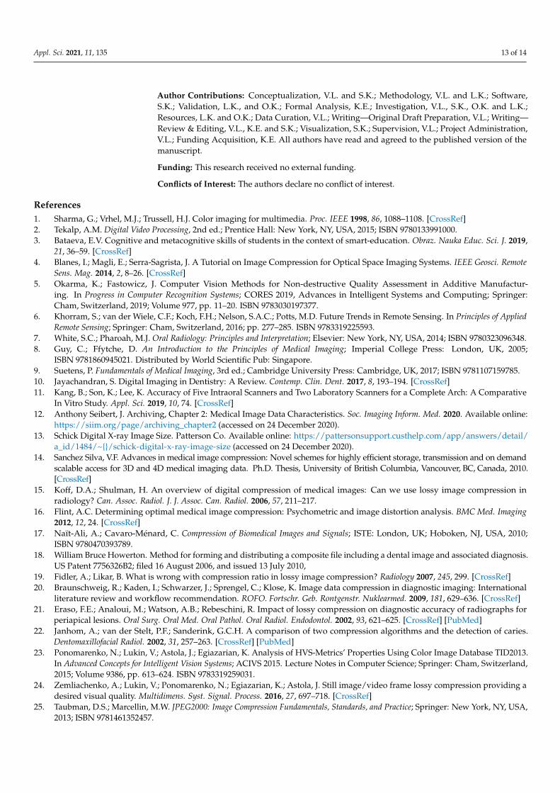
Appl. Sci. 2021, 11, 135 13 of 14

Author Contributions: Conceptualization, V.L. and S.K.; Methodology, V.L. and L.K.; Software,S.K.; Validation, L.K., and O.K.; Formal Analysis, K.E.; Investigation, V.L., S.K., O.K. and L.K.;Resources, L.K. and O.K.; Data Curation, V.L.; Writing—Original Draft Preparation, V.L.; Writing—Review & Editing, V.L., K.E. and S.K.; Visualization, S.K.; Supervision, V.L.; Project Administration,V.L.; Funding Acquisition, K.E. All authors have read and agreed to the published version of themanuscript.

Funding: This research received no external funding.

Conflicts of Interest: The authors declare no conflict of interest.

References1. Sharma, G.; Vrhel, M.J.; Trussell, H.J. Color imaging for multimedia. Proc. IEEE 1998, 86, 1088–1108. [CrossRef]2. Tekalp, A.M. Digital Video Processing, 2nd ed.; Prentice Hall: New York, NY, USA, 2015; ISBN 9780133991000.3. Bataeva, E.V. Cognitive and metacognitive skills of students in the context of smart-education. Obraz. Nauka Educ. Sci. J. 2019,

21, 36–59. [CrossRef]4. Blanes, I.; Magli, E.; Serra-Sagrista, J. A Tutorial on Image Compression for Optical Space Imaging Systems. IEEE Geosci. Remote

Sens. Mag. 2014, 2, 8–26. [CrossRef]5. Okarma, K.; Fastowicz, J. Computer Vision Methods for Non-destructive Quality Assessment in Additive Manufactur-

ing. In Progress in Computer Recognition Systems; CORES 2019, Advances in Intelligent Systems and Computing; Springer:Cham, Switzerland, 2019; Volume 977, pp. 11–20. ISBN 9783030197377.

6. Khorram, S.; van der Wiele, C.F.; Koch, F.H.; Nelson, S.A.C.; Potts, M.D. Future Trends in Remote Sensing. In Principles of AppliedRemote Sensing; Springer: Cham, Switzerland, 2016; pp. 277–285. ISBN 9783319225593.

7. White, S.C.; Pharoah, M.J. Oral Radiology: Principles and Interpretation; Elsevier: New York, NY, USA, 2014; ISBN 9780323096348.8. Guy, C.; Ffytche, D. An Introduction to the Principles of Medical Imaging; Imperial College Press: London, UK, 2005;

ISBN 9781860945021. Distributed by World Scientific Pub: Singapore.9. Suetens, P. Fundamentals of Medical Imaging, 3rd ed.; Cambridge University Press: Cambridge, UK, 2017; ISBN 9781107159785.10. Jayachandran, S. Digital Imaging in Dentistry: A Review. Contemp. Clin. Dent. 2017, 8, 193–194. [CrossRef]11. Kang, B.; Son, K.; Lee, K. Accuracy of Five Intraoral Scanners and Two Laboratory Scanners for a Complete Arch: A Comparative

In Vitro Study. Appl. Sci. 2019, 10, 74. [CrossRef]12. Anthony Seibert, J. Archiving, Chapter 2: Medical Image Data Characteristics. Soc. Imaging Inform. Med. 2020. Available online:

https://siim.org/page/archiving_chapter2 (accessed on 24 December 2020).13. Schick Digital X-ray Image Size. Patterson Co. Available online: https://pattersonsupport.custhelp.com/app/answers/detail/

a_id/1484/~/schick-digital-x-ray-image-size (accessed on 24 December 2020).14. Sanchez Silva, V.F. Advances in medical image compression: Novel schemes for highly efficient storage, transmission and on demand

scalable access for 3D and 4D medical imaging data. Ph.D. Thesis, University of British Columbia, Vancouver, BC, Canada, 2010.[CrossRef]

15. Koff, D.A.; Shulman, H. An overview of digital compression of medical images: Can we use lossy image compression inradiology? Can. Assoc. Radiol. J. J. Assoc. Can. Radiol. 2006, 57, 211–217.

16. Flint, A.C. Determining optimal medical image compression: Psychometric and image distortion analysis. BMC Med. Imaging2012, 12, 24. [CrossRef]

17. Naït-Ali, A.; Cavaro-Ménard, C. Compression of Biomedical Images and Signals; ISTE: London, UK; Hoboken, NJ, USA, 2010;ISBN 9780470393789.

18. William Bruce Howerton. Method for forming and distributing a composite file including a dental image and associated diagnosis.US Patent 7756326B2; filed 16 August 2006, and issued 13 July 2010,

19. Fidler, A.; Likar, B. What is wrong with compression ratio in lossy image compression? Radiology 2007, 245, 299. [CrossRef]20. Braunschweig, R.; Kaden, I.; Schwarzer, J.; Sprengel, C.; Klose, K. Image data compression in diagnostic imaging: International

literature review and workflow recommendation. ROFO. Fortschr. Geb. Rontgenstr. Nuklearmed. 2009, 181, 629–636. [CrossRef]21. Eraso, F.E.; Analoui, M.; Watson, A.B.; Rebeschini, R. Impact of lossy compression on diagnostic accuracy of radiographs for

periapical lesions. Oral Surg. Oral Med. Oral Pathol. Oral Radiol. Endodontol. 2002, 93, 621–625. [CrossRef] [PubMed]22. Janhom, A.; van der Stelt, P.F.; Sanderink, G.C.H. A comparison of two compression algorithms and the detection of caries.

Dentomaxillofacial Radiol. 2002, 31, 257–263. [CrossRef] [PubMed]23. Ponomarenko, N.; Lukin, V.; Astola, J.; Egiazarian, K. Analysis of HVS-Metrics’ Properties Using Color Image Database TID2013.

In Advanced Concepts for Intelligent Vision Systems; ACIVS 2015. Lecture Notes in Computer Science; Springer: Cham, Switzerland,2015; Volume 9386, pp. 613–624. ISBN 9783319259031.

24. Zemliachenko, A.; Lukin, V.; Ponomarenko, N.; Egiazarian, K.; Astola, J. Still image/video frame lossy compression providing adesired visual quality. Multidimens. Syst. Signal. Process. 2016, 27, 697–718. [CrossRef]

25. Taubman, D.S.; Marcellin, M.W. JPEG2000: Image Compression Fundamentals, Standards, and Practice; Springer: New York, NY, USA,2013; ISBN 9781461352457.

Appl. Sci. 2021, 11, 135 14 of 14

26. Ponomarenko, N.; Lukin, V.; Egiazarian, K.; Astola, J. DCT Based High Quality Image Compression. In Image Analysis; Kalviainen,H., Parkkinen, J., Kaarna, A., Eds.; Lecture Notes in Computer Science; Springer: Berlin/Heidelberg, Germany, 2005; Volume 3540,pp. 1177–1185. ISBN 9783540263203.

27. Krivenko, S.S.; Krylova, O.; Bataeva, E.; Lukin, V.V. Smart Lossy Compression of Images Based on Distortion Prediction.Telecommun. Radio Eng. 2018, 77, 1535–1554. [CrossRef]

28. Hiremath, P.S.; Akkasaligar, P.T.; Badiger, S. Speckle Noise Reduction in Medical Ultrasound Images. In Advancements andBreakthroughs in Ultrasound Imaging; Gunarathne, G.P.P., Ed.; InTech: London, UK, 2013; ISBN 9789535111597.

29. Flynn, M.J.; Hames, S.M.; Wilderman, S.J.; Ciarelli, J.J. Quantum noise in digital X-ray image detectors with optically coupledscintillators. IEEE Trans. Nucl. Sci. 1996, 43, 2320–2325. [CrossRef]

30. Aja-Fern, S.; Trist, A. A Review on Statistical Noise Models for Magnetic Resonance Imaging 1. Available online: /paper/A-review-on-statistical-noise-models-for-Magnetic-1-Aja-Fern-Trist/b67c196652a722aa713c1619610b09b52e2cb9bf (accessed on22 October 2020).

31. Abramova, V.; Krivenko, S.; Lukin, V.; Krylova, O. Analysis of Noise Properties in Dental Images. In Proceedings of the 2020 IEEE40th International Conference on Electronics and Nanotechnology (ELNANO), Kyiv, Ukraine, 22–24 April 2020; pp. 511–515.

32. Al-Shaykh, O.K.; Mersereau, R.M. Lossy compression of noisy images. IEEE Trans. Image Proc. 1998, 7, 1641–1652. [CrossRef]33. Odegard, J.E.; Guo, H.; Burrus, C.S.; Baraniuk, R.G. Joint Compression and Speckle Reduction of SAR Images using Embedded

Zerotree Models. In Workshop on Image and Multidimensional Digital Signal Processing; IDFL: Belize city, Belize, 1996; pp. 80–81.34. Ponomarenko, N.; Krivenko, S.; Lukin, V.; Egiazarian, K.; Astola, J.T. Lossy Compression of Noisy Images Based on Visual

Quality: A Comprehensive Study. EURASIP J. Adv. Signal. Process. 2010, 2010, 976436. [CrossRef]35. Chang, S.G.; Yu, B.; Vetterli, M. Adaptive wavelet thresholding for image denoising and compression. IEEE Trans. Image Proc.

2000, 9, 1532–1546. [CrossRef]36. Ponomarenko, N.N.; Egiazarian, K.O.; Lukin, V.V.; Astola, J.T. High-Quality DCT-Based Image Compression Using Partition

Schemes. IEEE Signal. Proc. Lett. 2007, 14, 105–108. [CrossRef]37. Diagnostic and Imaging Equipment|MORITA. Available online: https://www.jmoritaeurope.de/en/products/diagnostic-and-

imaging-equipment-overview/ (accessed on 19 October 2020).38. Huda, W.; Abrahams, R.B. Radiographic Techniques, Contrast, and Noise in X-Ray Imaging. Am. J. Roentgenol. 2015,

204, W126–W131. [CrossRef]39. Lin, Z.; Lei, Z.; Xuanqin, M.; Zhang, D. FSIM: A Feature Similarity Index for Image Quality Assessment. IEEE Trans. Image Process.

2011, 20, 2378–2386. [CrossRef]40. Krivenko, S.; Lukin, V.; Krylova, O.; Shutko, V. Visually Lossless Compression of Retina Images. In Proceedings of the 2018 IEEE

38th International Conference on Electronics and Nanotechnology (ELNANO), Kiev, Ukraine, 22–24 April 2018; pp. 255–260.41. Lin, W.; Jay Kuo, C.-C. Perceptual visual quality metrics: A survey. J. Vis. Commun. Image Represent. 2011, 22, 297–312. [CrossRef]42. Li, F.; Krivenko, S.; Lukin, V. A Two-step Procedure for Image Lossy Compression by ADCTC With a Desired Quality. In Proceed-

ings of the 2020 IEEE 11th International Conference on Dependable Systems, Services and Technologies (DESSERT), Kiev, Ukraine,22–24 April 2020; pp. 307–312.

43. Ponomarenko, M.; Ieremeiev, O.; Lukin, V.; Egiazarian, K. An expandable image database for evaluation of full-reference imagevisual quality metrics. Electron. Imaging 2020, 2020, 137-1–137-6. [CrossRef]