IEEE TRANSACTIONS ON WIRELESS COMMUNICATIONS 1

Adaptive Lossless Entropy Compressors for TinyIoT Devices

Massimo Vecchio, Member, IEEE, Raffaele Giaffreda and Francesco Marcelloni, Member, IEEE.

Abstract—Internet of Things (IoT) devices are typically pow-ered by small batteries with a limited capacity. Thus, savingpower as much as possible becomes crucial to extend theirlifetime and therefore to allow their use in real applicationdomains. Since radio communication is in general the main causeof power consumption, one of the most used approaches to saveenergy is to limit the transmission/reception of data, for instance,by means of data compression. However, the IoT devices are alsocharacterized by limited computational resources which imposethe development of specifically designed algorithms. To this aim,we propose to endow the lossless compression algorithm (LEC),previously proposed by us in the context of wireless sensornetworks, with two simple adaptation schemes relying on thenovel concept of appropriately rotating the prefix-free tables.We tested the proposed schemes on several datasets collectedin several real sensor network deployments by monitoring fourdifferent environmental phenomena, namely, air and surfacetemperatures, solar radiation and relative humidity. We showthat the adaptation schemes can achieve significant compressionefficiencies in all the datasets. Further, we compare such resultswith the ones obtained by LEC and, by means of a non-parametric multiple statistical test, we show that the performanceimprovements introduced by the adaptation schemes are statis-tically significant.

Index Terms—Internet of Things (IoT), lossless compression,wireless sensor networks, power efficiency.

I. INTRODUCTION

MODERN society yearns for moving towards an always-connected paradigm, so as to finally fill in the gap

between the physical and the digital worlds. Indeed, networks(both wired and wireless) are (almost) everywhere, openstandards (e.g., WiMAX, IPv6 and 6LoWPAN) are defined androlled out, while several technologies beneath the umbrella of“Future Internet” are already being researched and developed[1]. In this context, the “Internet of Things” (IoT) representsone of the visions that just captured the interest of academiaand industry at the time of its coinage (according to Ashton,K., “Internet of Things” started its life since the presentationhe made at Procter&Gamble in 1999) and more and moremomentum has gained in terms of development efforts inrecent years.

The original IoT vision encloses a framework where objects(i.e., things) can be uniquely identified and whose virtual rep-resentations can be accessed and controlled using an Internet-like structure [2]. Undoubtedly, the recent advances in micro-electronics and communications, which are deeply impacting

M. Vecchio and R. Giaffreda are with CREATE-NET, Trento, Italy. e-mail:{name.surname@create-net.org}.

F. Marcelloni is with the Dipartimento di Ingegneria dell’Informazione ofthe University of Pisa, Italy. e-mail: f.marcelloni@iet.unipi.it.

Manuscript received: 01-Jun-2013; Revised version Submitted Date(s): 25-Sep-2013; Accepted Date: 12-Nov-2013

on the costs, sizes and power requirements of the IoT mainenabling technologies (e.g., RFIDs, sensors, actuators) havepushed such embryonic vision towards a more establishedreality. Nowadays, several disparate IoT applications permeatethrough practically all areas of every-day life of individuals,enterprises, and society as a whole; IoT already extends acrossindustries, including intelligent environmental monitoring, in-telligent building, homes, and cities, smart transportation, andsmart health care [3], [4]. It is not a coincidence that aprediction from Forrester Research [5] has revealed that globalIoT revenues will be thirty times those of the Internet, makingit the next trillion-level communication industry linking overa hundred billion devices by 2020 [6].

Despite the plethora of application domains and the spe-cific features each single application might require, a listof common modules characterizing all IoT solutions can besummarized as (see [7]):

• a module for interaction with local IoT devices (e.g.,embedded in mobile phones or located in the immediateproximity of the user and reachable through short rangewireless interfaces);

• a module for local analysis and processing of observa-tions acquired by IoT devices;

• a module for interaction with remote IoT devices, directlyover the Internet or, more likely, through a proxy;

• a module for application-specific data analysis and pro-cessing;

• a module for integration of IoT-generated informationinto the business processes of an enterprise;

• a (web or mobile) user interface for visual representationof measurements in a given context (e.g., maps) andinteraction with the user.

Due to the ever increasing amount of different IoT devicesused in diverse application domains, wireless networks arelargely growing in number and density. Though several IoTdevices will be still connected to the energy grid all the time,the great majority of them will have to rely on their ownlimited energy resources or energy harvesting throughout theirlifetime. Thus, slim and lightweight implementations at alllayers (i.e., from the communication to the application layers)still represent key-features for effective and more robust IoTapplications. Further, considering the exponentially growingscale of IoT deployments, the heterogeneity of the involveddevices and the continuously changing scenarios and real-time requirements (operational conditions), flexible design atboth network and device levels represents also a desirable andalmost unavoidable property.

In this landscape, wireless sensor networks (WSNs) play

IEEE TRANSACTIONS ON WIRELESS COMMUNICATIONS 2

one of the most important roles in enabling the IoT paradigm.Further, the benefits of connecting both WSNs and other IoTdevices go beyond the simplistic remote access capability,since heterogeneous information systems may be able tocollaborate and provide common services [8]. Examples ofsuch services include, for instance, the possibility of pushingdata produced by wireless sensor nodes directly to the cloudor social platforms [9], [10]. In particular, Libelium companyalready commercializes wireless sensor nodes able to sendcollected sensor data (directly, or through a special nodeworking as an Internet gateway) to Twitter and Wordpress[9], while the Cosm platform (formerly Pachube) is an on-line database service allowing developers to connect sensor-derived data to the Web and to build their own applicationsbased on that data [10].

By deeply analyzing the breeding ground of existent IoTservices and components we realized that, except for theCosm platform that adopts a general-purpose gzip compressionscheme for compressing the sensed data stream before sendingit, to the best of our knowledge a lightweight and adaptivecompression scheme suitable for the IoT sensing devices isnot available in the literature yet. Since the main cause ofenergy consumption in IoT devices is generally representedby the communication unit, it still makes sense for thesedevices to reduce the amount of information to be transmittedby means of compression techniques [11]. Moreover, someIoT devices may be featured by even more reduced hardwarecapabilities (i.e., memory and microprocessor) than currentlyavailable wireless sensor nodes. Thus, special attention shouldbe paid when designing software solutions suitable for suchdevices, in terms of memory occupation and computationaleffort requirements. In the framework of WSNs, the LosslessEntropy Compression (LEC) algorithm, we introduced in[11], [12], has proven to be very effective in compressingenvironmental data and also very efficient in terms of powerconsumption [13].

Nevertheless, in the most general IoT framework, a com-pression algorithm should be able to react to highly variableoperational conditions. Thus, we believe that the LEC algo-rithm can be improved by adding some mechanism for makingit adaptive. To this aim, we endow LEC with two simpleadaptation schemes, which allow it to cope with variable op-erational conditions, though preserving its original simplicity.We tested the proposed schemes on several datasets collectedin several real sensor network deployments. We show thatthe adaptation schemes can achieve significant compressionefficiencies in all the datasets. Further, by means of a non-parametric multiple statistical test we present that the twoschemes outperform in terms of compression efficiency LEC,while there exists no statistical difference between them.

The paper is organized as follows. Sec. II reviews the LECalgorithm and some of its variants proposed in the recentliterature. In Sec. III we introduce the two adaptation schemes.Sec. IV discusses the implementation of the LEC algorithmand of the adaptation schemes. The experimental analysis isgiven in Sec. V. Finally, we draw some conclusions in Sec. VI.

II. RELATED WORKS

In this section, we first describe the LEC algorithm and thenwe discuss some of the variants which have been proposed inthe literature to make it adaptive.

A. The LEC algorithm

The main idea of the LEC algorithm relies on dividingthe alphabet of numbers into groups whose sizes increaseexponentially. Indeed, like in Golomb and Elias codings [14],[15], a LEC codeword is a hybrid of unary and binary codes,where the unary code (a variable-length code) specifies thegroup and the binary code (a fixed-length code) represents theindex within the group. The main difference between LECand its precursors is that groups are entropy coded rather thanunary coded. For more details on the LEC algorithm and itssimilarities and peculiarities with respect to Golomb and Eliascodings, the interested reader can refer to [11].

In the sensing unit of a sensor node, each measurementmi acquired by a sensor is converted by an ADC to a binaryrepresentation ri on R bits, where R is the resolution of theADC i.e., the number 2R of discrete values the ADC canproduce over the range of analogue values. For each newacquisition ri, LEC computes the difference di = ri − ri−1,which is input to an entropy encoder (to compute d1 it isconventionally assumed that r0 = 0). The entropy encoderperforms compression losslessly by encoding differences dimore compactly based on their statistical characteristics. Inparticular, each non-zero di value is represented as a bitsequence bsi composed of two parts si|ai, where si codifiesthe number ni of bits needed to represent di (i.e., the groupdi belongs to) and ai is the representation of di (i.e., theindex position in the group). When di is equal to 0, thecorresponding group (i.e., group 0) has size equal to 1 andtherefore there is no need to codify the index position in thegroup: it follows that ai is not represented.

Formally, ni is computed as

ni =

{0 if di = 0

blog2 (|di|)c+ 1 otherwise.(1)

It follows that at most ni is equal to R. Thus, in order toencode ni a prefix-free table S of R + 1 entries has to bespecified. In principle, S should depend on the distributionof the differences di: more frequent differences should beassociated with shorter codes si. Since LEC was introducedwith the main aim of compressing environmental signals,which vary slowly and therefore are characterised by havingthe most frequent differences di close to 0, we adopted theprefix-free table shown in Table I.

The ai part of the bit sequence bsi is a variable-lengthinteger code generated as follows:

ai =

not needed if di = 0

〈di〉Lniif di > 0

〈di − 1〉Lniotherwise,

(2)

where the operator 〈x〉Ly (resp., 〈x〉Hy ) indicates the y low-order(resp., high-order) bits of the two’s complement representation

IEEE TRANSACTIONS ON WIRELESS COMMUNICATIONS 3

TABLE IDEFAULT LEC PREFIX-FREE TABLE.

ni si di0 00 01 010 −1,+12 011 −3,−2,+2,+33 100 −7, . . . ,−4,+4, . . . ,+74 101 −15, . . . ,−8,+8, . . . ,+155 110 −31, . . . ,−16,+16, . . . ,+316 1110 −63, . . . ,−32,+32, . . . ,+637 11110 −127, . . . ,−64,+64, . . . ,+1278 111110 −255, . . . ,−128,+128, . . . ,+2559 1111110 −511, . . . ,−256,+256, . . . ,+51110 11111110 −1023, . . . ,−512,+512, . . . ,+102311 111111110 −2047, . . . ,−1024,+1024, . . . ,+204712 1111111110 −4095, . . . ,−2048,+2048, . . . ,+409513 11111111110 −8191, . . . ,−4096,+4096, . . . ,+819114 111111111110 −16383, . . . ,−8192,+8192, . . . ,+16383

of the argument x. The procedure used to generate ai guar-antees that all possible values have different codes. Once bsiis generated, it is appended to the bitstream which forms thecompressed version of the sequence of measurements mi.

Since its first appearance, the LEC algorithm has capturedthe attention of several researchers who have proposed dif-ferent modifications of its original scheme to the aim ofimproving its performances. The most interesting LEC variantswill be reviewed in the next section. As discussed in [16], LEChas also been implemented in hardware on a small, low costand low power Complex Programmable Logic Device (CPLD)from the Xilinx CoolRunner-II family [17]. Then, the authorshave connected the programmed CPLD to an MDA100 sensornode of the Crossbow family [18] to quantify the energy savingintroduced by delegating the compression of environmentaldata samples collected by the sensors on board the MDA100platform to the CPLD. In particular, they have shown that,by off-loading the compression task to the CPLD, the overallenergy consumption of a WSN framework could be halvedwith respect to not compressing the samples, thus confirmingboth the effectiveness and the simplicity of the LEC algorithm.

B. LEC variantsSome researchers have tried to improve the LEC algorithm

by mitigating its main drawback, that is, the lack of adaptive-ness. To better review the most interesting LEC variants, inthe following discussion we will refer to the block diagramof the most general LEC-based compression scheme shown inFig. 1. Here, the prediction block PRED, exploiting one ormore previous samples, generates the predicted value ri of thecurrent sample ri with respect to which the general differencedi = ri− ri is computed; the encoder block ENC compressesdi by exploiting a prefix-free table Si; the adaptation blockADAPT is responsible for adapting the prefix-free table to thesignal to be compressed. In the original LEC scheme, PREDis implemented as a simple delay block (i.e., the predictedsample ri coincides with the previous sample ri−1), ENC isresponsible for producing the bsi values as described by eq. (1)and eq. (2), and ADAPT is omitted (i.e., the adaptation blockis not implemented by LEC). It follows that S1 is the defaultprefix-free table shown in Table I and it remains unchangedduring the overall compression task (i.e., Si = S1 ∀i).

PRED

ENC

ADAPT

ri

ri

di bsi

S1

Si

+

−

Fig. 1. Block diagram of the most general LEC-based compression scheme.

A simple modification of the LEC algorithm was discussedin [19], where the authors proposed to substitute the delayblock used in the prediction block PRED of LEC with amore sophisticated median predictor block. The ENC andADAPT blocks are unchanged with respect to the LECscheme. More in detail, this variant of LEC exploits thethree previous samples ri−3, ri−2 and ri−1 for estimatinga prediction value ri that allows reducing the magnitude ofdi. Thus, di can be represented more compactly. Then, theencoder adds a 2-bits-long pre-code before each compressedsample to inform the decoder on the actual prediction valueused to compress it. We have implemented the variant of LECand have proved it on the same datasets used in the paperthat introduced the original version of LEC [11]. We haveobtained 51.02% and 44.95% average compression ratios forthe variant against 62.27% and 56.20% for the original LECon the temperature and relative humidity datasets, respectively.Thus, we can conclude that the compression performancesobtained by this variant are actually worse than the onesachieved by the original LEC on real environmental datasets.

Another LEC variant was discussed in [20], where theauthors proposed to endow the original LEC algorithm withthree different prefix-free tables to better fit the statistics ofthe different signals to be compressed. Unlike LEC, whichcompresses each sample on the fly, this variant first collectsa sequence of samples; then, it computes all the differencesbetween consecutive samples in the sequence and compressesthese differences by using all the three prefix-free tables;finally, it appends the smallest compressed sequence to thecompressed bitstream, together with a pre-code that identifiesthe specific table used to compress the sequence (this pre-code is needed by the decoder to unambiguously recover thecompressed block). Referring to Fig. 1, we note that thisvariant implements the ADAPT block as a 3-way switchwhich activates the best table among the prefix-free tablesafter having tested all of them over the sequence of samplesto be compressed. In [20], the authors show that this variantoutperforms LEC (on average, the compression ratio of thevariant is 2-3% higher than the original LEC). On the otherhand, this variant requires to store a sequence of samplesand three prefix-free tables rather than only one as in theoriginal LEC. Further, it needs to repeat for each samplethree times the execution of most of the instructions of theoriginal LEC. Thus, this variant trades a light improvementin the compression performances for the light memory load,the intrinsic on-the-fly elaboration and the low computationalcomplexity of the original LEC.

Another LEC variant was discussed in [21], where the

IEEE TRANSACTIONS ON WIRELESS COMMUNICATIONS 4

authors have proposed to use the Dynamic Huffman Com-pression (DHC) scheme [22] to adaptively compress groupsni. Hence, like in LEC, each Huffman codeword uniquelyrepresents a group ni of input symbols rather than only onesymbol as in the original DHC. Unlike in LEC, which employsthe static prefix-free Table I, however, this variant exploits theoriginal Vitter’s implementation and management of the tree-structure [23] to codify more frequent groups of symbols withshorter codewords. On the one hand, exploiting the powerfulVitter’s implementation to manage the prefix-free table offersa higher degree of adaptiveness, which can be particularlyuseful when compressing large and high-variable signals. Onthe other hand, the management of the tree-structure canbe computationally intensive and not suitable for the sensornodes, as observed in [13].

III. THE PROPOSED ADAPTIVE COMPRESSION SCHEMES

Sec. II-A has highlighted how LEC strongly relies on theassumption of knowing the statistics of the signals to becompressed. In particular, its default prefix-free table (Table I)maximally exploits the assumption that the probabilities ofthe input symbols to the encoder (i.e., the differences oftwo consecutive samples) are inversely proportional to theirabsolute values. It follows that, when such assumption does nothold or scarcely holds, it is likely that LEC will not optimally1

compress the input signal. In [11] we discussed the possibilityof performing a preliminary study on the specific phenomenonto monitor/compress, so as to off–line identify the optimalprefix-free table. However, we were conscious that this best-effort practice was just a viable workaround for small andhomogeneous scenarios, while adaptive mechanisms wouldhave been always preferable.

In this paper we propose two tiny adaptation mechanismsthat can be embedded in the LEC approach without affectingits original simplicity. Indeed, in order to effectively enablelossless compression in tiny sensor nodes, the compression al-gorithm cannot be complex, as the benefits of reducing the useof the radio transceiver on-board the node could be vanishedby an intense use of the processing unit [24]. The proposed twomechanisms implement the adaptation by rotating the prefix-free table depending on two different conditions. To makethe rotation effective, however, the table has to be accuratelydefined. In this section, we first introduce how the rotationcan be managed. Then, we propose a heuristic approach toadequately generate the prefix-table. Finally, we explain howthe rotation is applied in the two mechanisms to adapt theprefix-table to the actual samples to be compressed.

A. Managing rotation of the prefix-free tables

We handle the prefix-free table as a circular buffer. Tothis aim, we introduce a simple data structure S denotedprefix-free rotation table, consisting of a static table S, wherethe set of T prefix-free codes s[0], . . . , s[T − 1] are actuallystored, and an integer vector e of size T , whose elements are

1in the entropy meaning i.e., compressing the most probable symbols usingthe shortest codewords.

initially set to the corresponding position in the vector (i.e.,e[0] = 0, . . . , e[T − 1] = T − 1). Two basic operations can beperformed on S, namely access the k-th entry (i.e., s[k]) androtate all the elements by h steps. The first operation simplycorresponds to the indirection S[e[k]]. The second operation isimplemented by applying (e[k]−h) modulo T to all e[k] (i.e.,∀k ∈ [0, . . . , T − 1] , e[k] = |e[k]− h|T , where |·|T denotesmodulo T ). Since we access the codes in table S by theindirection S[e[k]], the rotation of the elements of e allowsus to efficiently simulate the rotation of the prefix-free tableS without changing its elements. Note that only elementaryinstructions on integer operands are executed in both theoperations. Further, we have only introduced an additionalinteger vector of size T with respect to LEC. In Sec. IV wewill describe an even more efficient implementation of therotation prefix-free table, which actually does not need vectore to manage the access and the rotation.

Although in principle the initialization of the static table Scan be left to the user, in the following we propose a simpleheuristic methodology to initialize it in the specific contextof adaptive compression of environmental data. Specifically,the goal is to build an effective S (in terms of compressionperformances of the algorithms that will rely on it) startingfrom a set of T prefix-free codes. To avoid unnecessaryoverloading of notation, we assume that the input prefix-freecodes are sorted in ascending order of lengths and relabel themas s0, . . . , sT−1, such that len(sk) ≤ len(sk+1) ∀k and len(x)is a function returning the number of bits of x. The proposedheuristic methodology initializes the first entry of S to s0 andthen adopts the following iterative procedure to initialize theremaining T − 1 entries: the second entry of S is set to s1,the last to s2, the third to s3, the second-to-last to s4, and soon. More formally:

s[k] =

s0 if k = 0

s2k−1 if 0 < k < dT/2esT−1 if k = dT/2es2(T−k) if dT/2e < k < T.

(3)

The proposed heuristic initialization of S guarantees thatinitially the shortest input prefix-free code will be assigned tothe first entry of the table (recalling that it is a rotation table,we will refer to the shortest prefix-free code as the center ofthe table) while the length of the prefix-free codes assignedto the remaining entries increases with the increase of theirdistances from the center. The advantages of such property willbe clear in the next section. As an example of generation of atable S, let us assume to use the prefix-free codes of the defaultLEC table (hence, the input prefix-free codes are the si entriesshown in Table I and T = 15). The resulting rotation table isshown in Table II, where the center of the table is marked inbold (we recall that at the beginning s[k] = S[e[k]] = s[k]).

B. Enabling adaptiveness by prefix-free table rotations basedon conditions

The adaptation mechanisms proposed in this paper employthe prefix-free rotation table S to efficiently encode groups ni

IEEE TRANSACTIONS ON WIRELESS COMMUNICATIONS 5

TABLE IIROTATION TABLE USING THE PREFIX-FREE CODES OF THE DEFAULT LECTABLE AS INPUT FOR THE INITIALIZATION: THE CENTER OF THE TABLE IS

MARKED IN BOLD.

ni si di0 00 01 010 −1,+12 100 −3,−2,+2,+33 110 −7, . . . ,−4,+4, . . . ,+74 11110 −15, . . . ,−8,+8, . . . ,+155 1111110 −31, . . . ,−16,+16, . . . ,+316 111111110 −63, . . . ,−32,+32, . . . ,+637 11111111110 −127, . . . ,−64,+64, . . . ,+1278 111111111110 −255, . . . ,−128,+128, . . . ,+2559 1111111110 −511, . . . ,−256,+256, . . . ,+51110 11111110 −1023, . . . ,−512,+512, . . . ,+102311 111110 −2047, . . . ,−1024,+1024, . . . ,+204712 1110 −4095, . . . ,−2048,+2048, . . . ,+409513 101 −8191, . . . ,−4096,+4096, . . . ,+819114 011 −16383, . . . ,−8192,+8192, . . . ,+16383

of input differences di. Adaptiveness is performed by appro-priately rotating all the elements by h steps upon verificationof specific conditions or, more formally:

Si+1 =

{Si.rotate(h) if C = TRUE

Si otherwise.(4)

When a sample ri is input to the compressor, the LEC’sencoding block is used to produce the corresponding bit se-quence bsi, after computing the input difference di = ri−ri−1.Unlike LEC, which adopts the prefix-free table shown inTable I for encoding each sample ri, the adaptive schemesuse the prefix-free rotation table Si, which is updated at eachsample. In particular, Si is used to codify the group ni towhich di belongs to and thus generate the si part of bsi;then eq. (2) is applied to generate ai. Once bsi has beencomputed, the adaptation block evaluates condition C: if thecondition is true, (i) a rotation of h = (ni − c) modulo Tsteps is performed to produce Si+1 and (ii) c is updated asc = ni; otherwise, Si+1 = Si. We observe that the effect ofthe rotation is to encode group ni with the shortest prefix-code(i.e., s[c]) from the next sample, while all the other elementsare rotated consequently, so as to maintain the rigidity of thedata structure.

Although different conditions C can be defined to designa plethora of adaptation blocks, in this paper we adopt twosimple conditions, denoted C1 and C2 in the following, forrespectively implementing a greedy adaptation and an adapta-tion based on use frequency. Hence, we introduce two differentadaptation blocks, namely GA-LEC and FA-LEC, which differfrom each other only for the specific condition to verify (C1for GA-LEC and C2 for FA-LEC). Both the blocks employan integer c, which acts as an index of the prefix-free rotationtable constantly pointing to its center (hence, at the beginningc = 0). C1 is implemented as a naive short-circuit, hence C1is always verified in GA-LEC. Though conceptually simple,this choice has a rational justification. Indeed, if ri representsthe first sample of a sequence characterized by differencesbetween consecutive samples in the range of group ni (or inranges of groups close to group ni), GA-LEC will be able to

optimize the output bit sequence in terms of number of bitsfrom the next sample ri+1. On the other hand, if ri is due onlyto a sample quite different from the average, the adaptationmechanism will bring back the prefix-free rotation table tothe previous configuration just at the subsequent sample ri+1.In the latter case, only sample ri+1 is possibly coded witha larger number of bits than the one generated by using theprevious table used for encoding ri.

Condition C2 is more sophisticated than C1 and, conse-quently, also more complex to support. Indeed, it requiresan integer vector f of length T , whose components areinitialized to 0. After processing each ri and producing thecorresponding bsi, the element of f in position ni (as usual,ni represents the group which ri belongs to), is increased by1, i.e., f [ni] = f [ni] + 1. Condition C2 tests if f [ni] ≥ f [c].Thus, the basic idea of FA-LEC is to rotate Si only when thecurrent most frequent group changes from c to ni.

In the following, we give a practical example of applicationof both the adaptation blocks. Without loss of generality, let usassume that Si corresponds to the one shown in Table II. Letus suppose that the input symbol to the encoder is di = 31,which belongs to group ni = 5, and c = 0. Then, accordingto Table II, group ni = 5 is entropy coded as 1111110, whilethe index position of the symbol in the group is mapped to11111. Thus, bsi = 1111110|11111 is generated as output. Sofar, except for the different prefix-free codes used to representni, LEC and the proposed adaptive variants perform the sameactions. Indeed, the adaptation mechanisms act at this moment.

As regards GA-LEC, the condition is always verified; hencec is set to 5 and the prefix-free table is rotated of h = 5steps. As regards FA-LEC, f [5] is increased by 1 and the sameactions as for GA-LEC are performed only if condition f [5] ≥f [c] is verified. The rotated table of h = 5 steps is shown inTable III and, according to it, if the subsequent difference di+1

still belongs to group 5, then the si+1 part of bsi+1 will becoded as 00 rather than 110 of the standard LEC. Also, if thisdifference belongs to groups greater than 5, but close enoughto it (i.e., groups 6, 7, 8), the corresponding si+1 part wouldbe 3 bits long, thus saving 1, 2 and 3 bits respectively, withrespect to LEC. On the other hand, if di+1 is 0, it would becoded using 8 bits, rather than 2 bits of the standard LEC(recall that, in this case, ai+1 is not needed).

Independently of the conditions used in the adaptationblocks, the rotations are consistently applied to the overallprefix-free table, thus affecting the representation of all groups.In particular, also groups that are close to (resp., far from)the center of the rotation table will be represented by short(resp., large) prefix-codes. Thus, similar to LEC, GA-LECand FA-LEC are still able to efficiently compress those signalswhose distributions of the differences of consecutive samplesresemble bell-shaped curves with rather pronounced peakvalues. The advantage with respect to the standard LEC is thatthey well perform also when the peak of the bell is displacedwith respect to zero. On the other hand, the flatter the bellof the input distribution will be, the less the payoff of theproposed adaptation blocks will be. Indeed, as highlighted inthe example, if the next difference di+1 is 0, it would becompressed using 8 bits.

IEEE TRANSACTIONS ON WIRELESS COMMUNICATIONS 6

TABLE IIIPREFIX-FREE ROTATION TABLE II, AFTER APPLYING A ROTATION OF

h = 5 STEPS.

ni si di0 11111110 01 111110 −1,+12 1110 −3,−2,+2,+33 101 −7, . . . ,−4,+4, . . . ,+74 011 −15, . . . ,−8,+8, . . . ,+155 00 −31, . . . ,−16,+16, . . . ,+316 010 −63, . . . ,−32,+32, . . . ,+637 100 −127, . . . ,−64,+64, . . . ,+1278 110 −255, . . . ,−128,+128, . . . ,+2559 11110 −511, . . . ,−256,+256, . . . ,+51110 1111110 −1023, . . . ,−512,+512, . . . ,+102311 111111110 −2047, . . . ,−1024,+1024, . . . ,+204712 11111111110 −4095, . . . ,−2048,+2048, . . . ,+409513 111111111110 −8191, . . . ,−4096,+4096, . . . ,+819114 1111111110 −16383, . . . ,−8192,+8192, . . . ,+16383

To limit the effects of not efficiently encoding those inputdifferences belonging to groups far from the center of therotation table, we can adopt two rotation sub-tables in place ofthe rotation table of size T . The two sub-tables, named SL andSH , are responsible for encoding groups 0, . . . , dT/2e−1, anddT/2e , . . . , T − 1, respectively. Let s0, . . . , sT−1 be the inputprefix-free codes sorted in ascending order of lengths. Sub-tables SL and SH are initialized by applying eq. (3) to, respec-tively, the dT/2e shortest prefix-codes (i.e., s0, . . . , sdT/2e−1)and the remaining prefix-codes (i.e., sdT/2e, . . . , sT−1). Whena sample ri is input to the compressor, the group ni which thedifference di = ri− ri−1 belongs to, determines the sub-tableto be used (if ni ∈ [0, . . . , dT/2e − 1], then SL will be used,otherwise SH ). The sub-tables are handled independently ofeach other: obviously, only the table with the group ni willbe rotated, if the condition C is satisfied. in the following, wedenote the versions of GA-LEC and FA-LEC, which adoptthe two rotation tables in place of only one, as GAS-LEC andFAS-LEC, respectively.

Referring to the numerical example discussed above, let usassume that the input symbol to the encoder is di = 31,which belongs to group ni = 5, and cL = 0 and cH = 0,where cL and cH are the two integer indexes pointing to thecenters of SL and SH , respectively. Then, only sub-table SLis involved in the compression process. If the condition weare considering is verified, the sub-table is rotated by h = 5steps. Table IV shows the two sub-tables after the rotation. Ifthe subsequent difference di+1 still belongs to group ni = 5,then the si+1 part of bsi+1 will be coded as 00 rather than110 of the standard LEC. Moreover, by using the two rotationsub-tables, if di+1 is 0, it would be coded using 3 bits ratherthan the 8 bits utilized when adopting a unique rotation table.

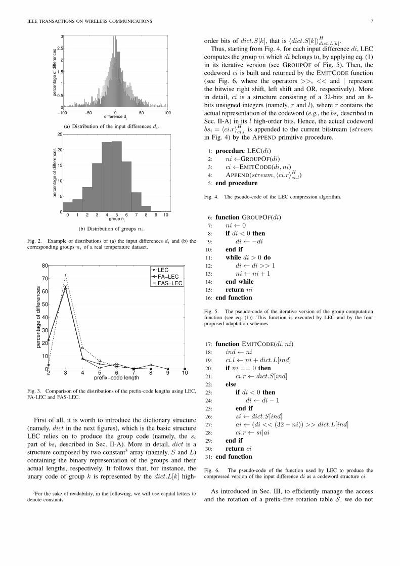
To highlight the advantage of using two rotation sub-tables for compressing environmental data, Fig. 2 shows,as an example, the distribution of the input differences andthe corresponding group distribution of a real temperaturedataset2. As expected the distribution of the input differencesresembles a bell-shaped curve centered around di = 0 (around

2source: air temperature dataset collected by node 9 of the Sensorscope’sPDG deployment [25].

TABLE IVTHE TWO SUB-TABLES AFTER A ROTATION OF h = 5 STEPS. NOTICE THAT

ONLY THE SL SUB-TABLE HAS BEEN AFFECTED BY THE ROTATION.

ni si di0 110 01 11110 −1,+12 1110 −3,−2,+2,+33 101 −7, . . . ,−4,+4, . . . ,+74 011 −15, . . . ,−8,+8, . . . ,+155 00 −31, . . . ,−16,+16, . . . ,+316 010 −63, . . . ,−32,+32, . . . ,+637 100 −127, . . . ,−64,+64, . . . ,+127

8 111110 −255, . . . ,−128,+128, . . . ,+2559 1111110 −511, . . . ,−256,+256, . . . ,+51110 111111110 −1023, . . . ,−512,+512, . . . ,+102311 11111111110 −2047, . . . ,−1024,+1024, . . . ,+204712 111111111110 −4095, . . . ,−2048,+2048, . . . ,+409513 1111111110 −8191, . . . ,−4096,+4096, . . . ,+819114 11111110 −16383, . . . ,−8192,+8192, . . . ,+16383

the 3% of the input differences are 0 and they will be encodedby LEC using the shortest prefix-free code). On the otherhand, the most frequent group is ni = 5. Further, significantcomponents of groups ni = 0, . . . , 8 make the distributionof the groups rather flat. Thus, there exists a non-negligibleprobability that, for instance, after a sample in group 5, thesubsequent sample is in group 0. As we have already pointedout, in the case of a unique rotation table, when it is centeredon group 5, subsequent input differences equal to 0 will beencoded using 8 bits; in the case of two rotation sub-tables,only 3 bits are necessary.Finally, Fig. 3 shows a comparisonof the distributions of the prefix-code lengths using LEC, FA-LEC and FAS-LEC. It can be observed that both the versionswere able to increase the percentage of input differencesencoded by using the shortest prefix-free code up to 22%.Since the adaptive schemes use shorter prefix-free codes fora larger percentage of samples, they both improve LEC. Thedifference between the two adaptation versions is revealed byobserving the right tails of the corresponding distributions ofthe prefix-free lengths. Indeed, around the 3% of the inputdifferences were encoded using 8 bits by the version with theunique rotation table, while the version with two rotation sub-tables has never needed to resort to large prefix-free codes.In Sec. V, we will observe how this apparently not significantdifference will slightly affect the compression performances ofthe corresponding algorithms. Finally, in the next section wewill see that the implementation of the adaptive block based ontwo sub-tables is minimally different with respect to the onebased on a unique table, and that both of them need only somebasic extra logic with respect to the original LEC algorithm.

IV. IMPLEMENTATION

In this section we will analyze in detail the implementationof the adaptive schemes. We will start by showing the detailedimplementation of the LEC algorithm, by means of pseudo-codes. Then, we will highlight the portions of the LEC codewhich have to be changed in order to implement the fourproposed adaptation schemes. We aim to make evident howthe difference between the LEC algorithm and its adaptiveversions is limited to very few instructions.

IEEE TRANSACTIONS ON WIRELESS COMMUNICATIONS 7

−100 −50 0 50 100

0

0.5

1

1.5

2

2.5

3

difference di

perc

enta

ge o

f diffe

rences

(a) Distribution of the input differences di.

0 1 2 3 4 5 6 7 8 9 100

5

10

15

20

25

group ni

perc

enta

ge o

f diffe

rences

(b) Distribution of groups ni.

Fig. 2. Example of distributions of (a) the input differences di and (b) thecorresponding groups ni of a real temperature dataset.

2 3 4 5 6 7 8 9 100

10

20

30

40

50

60

70

80

prefix−code length

perc

enta

ge o

f diffe

rences

LEC

FA−LEC

FAS−LEC

Fig. 3. Comparison of the distributions of the prefix-code lengths using LEC,FA-LEC and FAS-LEC.

First of all, it is worth to introduce the dictionary structure(namely, dict in the next figures), which is the basic structureLEC relies on to produce the group code (namely, the sipart of bsi described in Sec. II-A). More in detail, dict is astructure composed by two constant3 array (namely, S and L)containing the binary representation of the groups and theiractual lengths, respectively. It follows that, for instance, theunary code of group k is represented by the dict.L[k] high-

3For the sake of readability, in the following, we will use capital letters todenote constants.

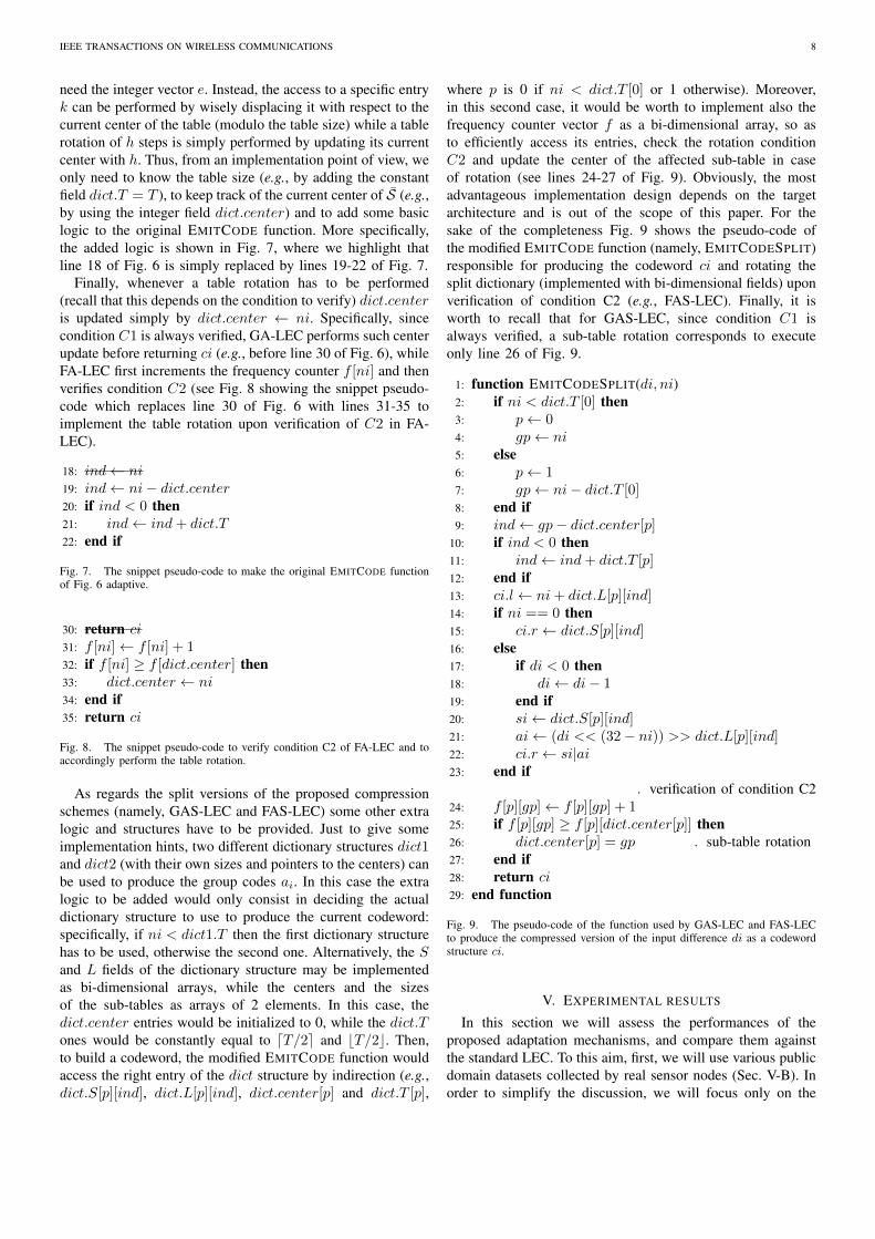
order bits of dict.S[k], that is 〈dict.S[k]〉Hdict.L[k].Thus, starting from Fig. 4, for each input difference di, LEC

computes the group ni which di belongs to, by applying eq. (1)in its iterative version (see GROUPOF of Fig. 5). Then, thecodeword ci is built and returned by the EMITCODE function(see Fig. 6, where the operators >>, << and | representthe bitwise right shift, left shift and OR, respectively). Morein detail, ci is a structure consisting of a 32-bits and an 8-bits unsigned integers (namely, r and l), where r contains theactual representation of the codeword (e.g., the bsi described inSec. II-A) in its l high-order bits. Hence, the actual codewordbsi = 〈ci.r〉Hci.l is appended to the current bitstream (streamin Fig. 4) by the APPEND primitive procedure.

1: procedure LEC(di)2: ni←GROUPOF(di)3: ci←EMITCODE(di, ni)4: APPEND(stream, 〈ci.r〉Hci.l)5: end procedure

Fig. 4. The pseudo-code of the LEC compression algorithm.

6: function GROUPOF(di)7: ni← 08: if di < 0 then9: di← −di

10: end if11: while di > 0 do12: di← di >> 113: ni← ni+ 114: end while15: return ni16: end function

Fig. 5. The pseudo-code of the iterative version of the group computationfunction (see eq. (1)). This function is executed by LEC and by the fourproposed adaptation schemes.

17: function EMITCODE(di, ni)18: ind← ni19: ci.l← ni+ dict.L[ind]20: if ni == 0 then21: ci.r ← dict.S[ind]22: else23: if di < 0 then24: di← di− 125: end if26: si← dict.S[ind]27: ai← (di << (32− ni)) >> dict.L[ind]28: ci.r ← si|ai29: end if30: return ci31: end function

Fig. 6. The pseudo-code of the function used by LEC to produce thecompressed version of the input difference di as a codeword structure ci.

As introduced in Sec. III, to efficiently manage the accessand the rotation of a prefix-free rotation table S, we do not

IEEE TRANSACTIONS ON WIRELESS COMMUNICATIONS 8

need the integer vector e. Instead, the access to a specific entryk can be performed by wisely displacing it with respect to thecurrent center of the table (modulo the table size) while a tablerotation of h steps is simply performed by updating its currentcenter with h. Thus, from an implementation point of view, weonly need to know the table size (e.g., by adding the constantfield dict.T = T ), to keep track of the current center of S (e.g.,by using the integer field dict.center) and to add some basiclogic to the original EMITCODE function. More specifically,the added logic is shown in Fig. 7, where we highlight thatline 18 of Fig. 6 is simply replaced by lines 19-22 of Fig. 7.

Finally, whenever a table rotation has to be performed(recall that this depends on the condition to verify) dict.centeris updated simply by dict.center ← ni. Specifically, sincecondition C1 is always verified, GA-LEC performs such centerupdate before returning ci (e.g., before line 30 of Fig. 6), whileFA-LEC first increments the frequency counter f [ni] and thenverifies condition C2 (see Fig. 8 showing the snippet pseudo-code which replaces line 30 of Fig. 6 with lines 31-35 toimplement the table rotation upon verification of C2 in FA-LEC).

18: ind← ni19: ind← ni− dict.center20: if ind < 0 then21: ind← ind+ dict.T22: end if

Fig. 7. The snippet pseudo-code to make the original EMITCODE functionof Fig. 6 adaptive.

30: return ci31: f [ni]← f [ni] + 132: if f [ni] ≥ f [dict.center] then33: dict.center ← ni34: end if35: return ci

Fig. 8. The snippet pseudo-code to verify condition C2 of FA-LEC and toaccordingly perform the table rotation.

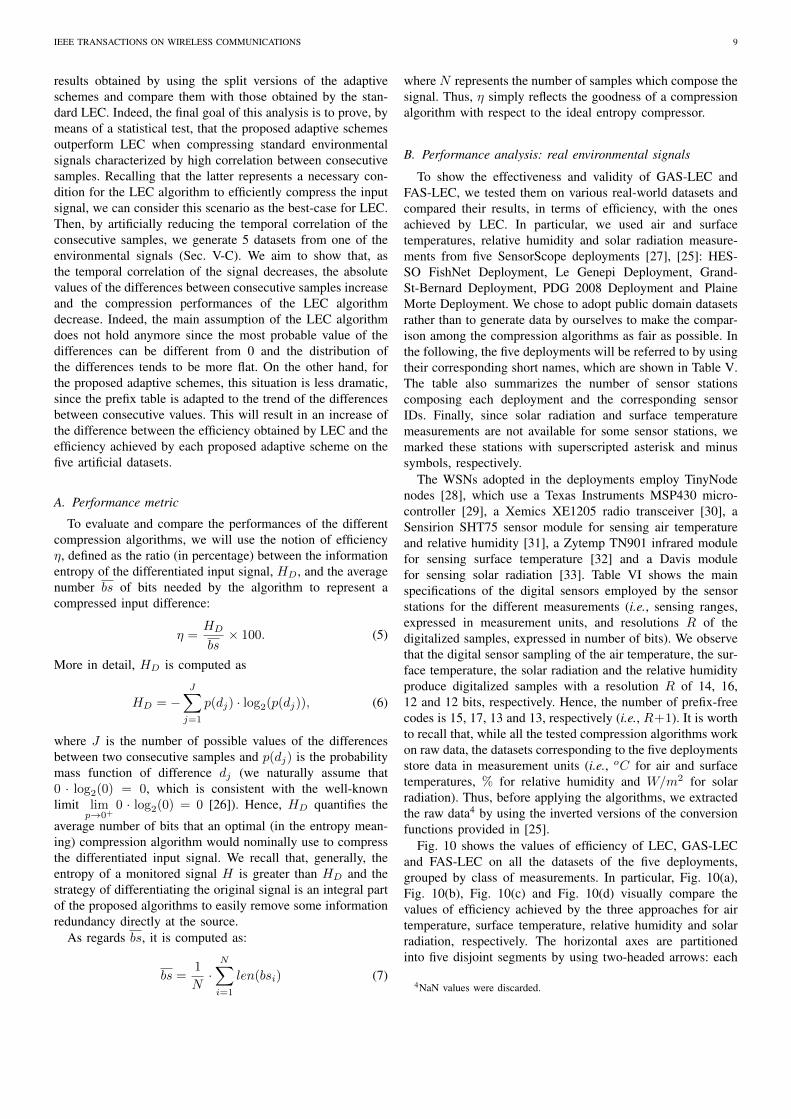
As regards the split versions of the proposed compressionschemes (namely, GAS-LEC and FAS-LEC) some other extralogic and structures have to be provided. Just to give someimplementation hints, two different dictionary structures dict1and dict2 (with their own sizes and pointers to the centers) canbe used to produce the group codes ai. In this case the extralogic to be added would only consist in deciding the actualdictionary structure to use to produce the current codeword:specifically, if ni < dict1.T then the first dictionary structurehas to be used, otherwise the second one. Alternatively, the Sand L fields of the dictionary structure may be implementedas bi-dimensional arrays, while the centers and the sizesof the sub-tables as arrays of 2 elements. In this case, thedict.center entries would be initialized to 0, while the dict.Tones would be constantly equal to dT/2e and bT/2c. Then,to build a codeword, the modified EMITCODE function wouldaccess the right entry of the dict structure by indirection (e.g.,dict.S[p][ind], dict.L[p][ind], dict.center[p] and dict.T [p],

where p is 0 if ni < dict.T [0] or 1 otherwise). Moreover,in this second case, it would be worth to implement also thefrequency counter vector f as a bi-dimensional array, so asto efficiently access its entries, check the rotation conditionC2 and update the center of the affected sub-table in caseof rotation (see lines 24-27 of Fig. 9). Obviously, the mostadvantageous implementation design depends on the targetarchitecture and is out of the scope of this paper. For thesake of the completeness Fig. 9 shows the pseudo-code ofthe modified EMITCODE function (namely, EMITCODESPLIT)responsible for producing the codeword ci and rotating thesplit dictionary (implemented with bi-dimensional fields) uponverification of condition C2 (e.g., FAS-LEC). Finally, it isworth to recall that for GAS-LEC, since condition C1 isalways verified, a sub-table rotation corresponds to executeonly line 26 of Fig. 9.

1: function EMITCODESPLIT(di, ni)2: if ni < dict.T [0] then3: p← 04: gp← ni5: else6: p← 17: gp← ni− dict.T [0]8: end if9: ind← gp− dict.center[p]

10: if ind < 0 then11: ind← ind+ dict.T [p]12: end if13: ci.l← ni+ dict.L[p][ind]14: if ni == 0 then15: ci.r ← dict.S[p][ind]16: else17: if di < 0 then18: di← di− 119: end if20: si← dict.S[p][ind]21: ai← (di << (32− ni)) >> dict.L[p][ind]22: ci.r ← si|ai23: end if

. verification of condition C224: f [p][gp]← f [p][gp] + 125: if f [p][gp] ≥ f [p][dict.center[p]] then26: dict.center[p] = gp . sub-table rotation27: end if28: return ci29: end function

Fig. 9. The pseudo-code of the function used by GAS-LEC and FAS-LECto produce the compressed version of the input difference di as a codewordstructure ci.

V. EXPERIMENTAL RESULTS

In this section we will assess the performances of theproposed adaptation mechanisms, and compare them againstthe standard LEC. To this aim, first, we will use various publicdomain datasets collected by real sensor nodes (Sec. V-B). Inorder to simplify the discussion, we will focus only on the

IEEE TRANSACTIONS ON WIRELESS COMMUNICATIONS 9

results obtained by using the split versions of the adaptiveschemes and compare them with those obtained by the stan-dard LEC. Indeed, the final goal of this analysis is to prove, bymeans of a statistical test, that the proposed adaptive schemesoutperform LEC when compressing standard environmentalsignals characterized by high correlation between consecutivesamples. Recalling that the latter represents a necessary con-dition for the LEC algorithm to efficiently compress the inputsignal, we can consider this scenario as the best-case for LEC.Then, by artificially reducing the temporal correlation of theconsecutive samples, we generate 5 datasets from one of theenvironmental signals (Sec. V-C). We aim to show that, asthe temporal correlation of the signal decreases, the absolutevalues of the differences between consecutive samples increaseand the compression performances of the LEC algorithmdecrease. Indeed, the main assumption of the LEC algorithmdoes not hold anymore since the most probable value of thedifferences can be different from 0 and the distribution ofthe differences tends to be more flat. On the other hand, forthe proposed adaptive schemes, this situation is less dramatic,since the prefix table is adapted to the trend of the differencesbetween consecutive values. This will result in an increase ofthe difference between the efficiency obtained by LEC and theefficiency achieved by each proposed adaptive scheme on thefive artificial datasets.

A. Performance metric

To evaluate and compare the performances of the differentcompression algorithms, we will use the notion of efficiencyη, defined as the ratio (in percentage) between the informationentropy of the differentiated input signal, HD, and the averagenumber bs of bits needed by the algorithm to represent acompressed input difference:

η =HD

bs× 100. (5)

More in detail, HD is computed as

HD = −J∑

j=1

p(dj) · log2(p(dj)), (6)

where J is the number of possible values of the differencesbetween two consecutive samples and p(dj) is the probabilitymass function of difference dj (we naturally assume that0 · log2(0) = 0, which is consistent with the well-knownlimit lim

p→0+0 · log2(0) = 0 [26]). Hence, HD quantifies the

average number of bits that an optimal (in the entropy mean-ing) compression algorithm would nominally use to compressthe differentiated input signal. We recall that, generally, theentropy of a monitored signal H is greater than HD and thestrategy of differentiating the original signal is an integral partof the proposed algorithms to easily remove some informationredundancy directly at the source.

As regards bs, it is computed as:

bs =1

N·

N∑

i=1

len(bsi) (7)

where N represents the number of samples which compose thesignal. Thus, η simply reflects the goodness of a compressionalgorithm with respect to the ideal entropy compressor.

B. Performance analysis: real environmental signals

To show the effectiveness and validity of GAS-LEC andFAS-LEC, we tested them on various real-world datasets andcompared their results, in terms of efficiency, with the onesachieved by LEC. In particular, we used air and surfacetemperatures, relative humidity and solar radiation measure-ments from five SensorScope deployments [27], [25]: HES-SO FishNet Deployment, Le Genepi Deployment, Grand-St-Bernard Deployment, PDG 2008 Deployment and PlaineMorte Deployment. We chose to adopt public domain datasetsrather than to generate data by ourselves to make the compar-ison among the compression algorithms as fair as possible. Inthe following, the five deployments will be referred to by usingtheir corresponding short names, which are shown in Table V.The table also summarizes the number of sensor stationscomposing each deployment and the corresponding sensorIDs. Finally, since solar radiation and surface temperaturemeasurements are not available for some sensor stations, wemarked these stations with superscripted asterisk and minussymbols, respectively.

The WSNs adopted in the deployments employ TinyNodenodes [28], which use a Texas Instruments MSP430 micro-controller [29], a Xemics XE1205 radio transceiver [30], aSensirion SHT75 sensor module for sensing air temperatureand relative humidity [31], a Zytemp TN901 infrared modulefor sensing surface temperature [32] and a Davis modulefor sensing solar radiation [33]. Table VI shows the mainspecifications of the digital sensors employed by the sensorstations for the different measurements (i.e., sensing ranges,expressed in measurement units, and resolutions R of thedigitalized samples, expressed in number of bits). We observethat the digital sensor sampling of the air temperature, the sur-face temperature, the solar radiation and the relative humidityproduce digitalized samples with a resolution R of 14, 16,12 and 12 bits, respectively. Hence, the number of prefix-freecodes is 15, 17, 13 and 13, respectively (i.e., R+1). It is worthto recall that, while all the tested compression algorithms workon raw data, the datasets corresponding to the five deploymentsstore data in measurement units (i.e., oC for air and surfacetemperatures, % for relative humidity and W/m2 for solarradiation). Thus, before applying the algorithms, we extractedthe raw data4 by using the inverted versions of the conversionfunctions provided in [25].

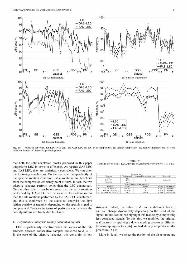
Fig. 10 shows the values of efficiency of LEC, GAS-LECand FAS-LEC on all the datasets of the five deployments,grouped by class of measurements. In particular, Fig. 10(a),Fig. 10(b), Fig. 10(c) and Fig. 10(d) visually compare thevalues of efficiency achieved by the three approaches for airtemperature, surface temperature, relative humidity and solarradiation, respectively. The horizontal axes are partitionedinto five disjoint segments by using two-headed arrows: each

4NaN values were discarded.

IEEE TRANSACTIONS ON WIRELESS COMMUNICATIONS 10

TABLE VTHE FIVE SENSORSCOPE DEPLOYMENTS: SUPERSCRIPTED ASTERISK AND MINUS SYMBOLS IDENTIFY THOSE STATIONS FOR WHICH SOLAR RADIATION

AND SURFACE TEMPERATURE MEASUREMENTS ARE NOT AVAILABLE, RESPECTIVELY.

Deployment name Short name No. stations IDs

HES-SO FishNet FN 6 101, 102, 103, 104∗, 105∗, 106∗.

Le Genepi GE 16 2, 3, 4, 6, 7∗, 8, 10∗, 11∗, 12∗,13∗, 15∗, 16∗, 17, 18∗, 19∗, 20∗.

Grand-St-Bernard GSB 232, 3, 4, 5, 6∗, 7∗, 8∗, 9∗, 10∗,11∗, 12∗, 13∗, 14∗, 15∗, 17∗,18∗, 19∗, 20∗, 25, 28, 29, 31, 32.

PDG 2008 PDG 10 1, 3, 4, 5, 7, 9−, 10, 15, 16, 18.

Plaine Morte PM 13 2∗, 6∗, 20, 38∗, 58, 74, 78,83, 90, 91∗, 101, 102, 110∗.

TABLE VIMAIN SPECIFICATIONS OF THE DIGITAL SENSORS EMPLOYED BY A TINYNODE NODE FOR COLLECTING DIFFERENT TYPES OF ENVIRONMENTAL

MEASURES.

measurement type sensor module sensing range [measurement units] resolution R [bits]Air temperature Sensirion SHT75 [31] [−20, 60]oC 14Surface temperature Zytemp TN901 [32] [−33, 220]oC 16Air relative humidity Sensirion SHT75 [31] [0, 100]% 12Solar radiation Davis Solar Radiation [33] [0, 1800]W/m2 12

segment represents a different deployment, specified by thecorresponding short name.

By analyzing Fig. 10, we can appreciate how the adaptationblocks exploited by GAS-LEC and FAS-LEC allow improvingthe values of efficiency with respect to LEC. Fig. 11 showsthe boxplot diagram of the efficiency obtained by the three al-gorithms on the four different types of data. For each boxplot,the lowest and the largest efficiency values are represented aswhiskers, the lower and upper quartiles are shown with a box,the median is represented by a line, the mean value by a blackcircle and efficiency values that may be considered outliersare possibly marked with asterisks [34]. To ease a quantitativecomparison, Table VII shows the values of the medians ofthe efficiency distributions obtained by the tested algorithmson the four different types of data. Although the datasetsof this experiment represent real environmental signals withrather high correlations between consecutive samples (the idealsituation for the LEC algorithm), we can observe that both theadaptive schemes outperform the LEC compression algorithm.

TABLE VIIVALUES OF THE MEDIANS OF THE EFFICIENCY DISTRIBUTIONS OBTAINEDBY LEC, FAS-LEC AND GAS-LEC ON THE AIR TEMPERATURE, SURFACE

TEMPERATURE, RELATIVE HUMIDITY AND SOLAR RADIATION DATASETSOF SENSORSCOPE DEPLOYMENTS.

LEC GAS-LEC FAS-LECAir temperature 92.33 95.78 95.22Surface temperature 87.57 88.57 89.78Relative humidity 90.84 93.62 93.76Solar radiation 94.82 97.17 95.14

To verify this impression, we perform a statistical analysis.For each of the three approaches, we merge all the efficiencyvalues achieved on all the datasets by the approach, thusobtaining three distributions. Then, we apply the Friedmantest in order to compute a ranking among such distributions[35], and the Iman and Davenport test [36] to evaluate whetherthere exist statistically relevant differences among them. If

there exists a statistical difference, we apply a post-hoc pro-cedure, namely the pairwise Holm test [37]. This test allowsdetecting effective statistical differences between the pairs ofdistributions.

Air temp. Surf. temp. Rel. hum. Sol. rad.75

80

85

90

95

100

effic

iency %

LECGAS−LECFAS−LEC

Fig. 11. Boxplots of the values of efficiency obtained by LEC, FAS-LECand GAS-LEC on the four different types of datasets.

Table VIII shows the results of the non-parametric statisticaltests: for each algorithm, we show the Friedman rank and theIman and Davenport p–value. If the p–value is lower thanthe level of significance α (in the experiments α = 0.05),we can reject the null hypothesis and affirm that there existstatistical differences between the multiple distributions as-sociated with each approach. Otherwise, no statistical differ-ence exists among the distributions and therefore the threedistributions are statistically equivalent. We observe that theIman and Davenport’s statistical hypothesis of equivalence isrejected and so statistical differences among the distributionsare detected. Thus, we have to apply the pairwise Holm post-hoc procedure. We realize that the statistical hypothesis ofequivalence is rejected both between LEC and GAS-LEC,and between LEC and FAS-LEC, while cannot be rejectedbetween GAS-LEC and FAS-LEC. Thus, we can conclude

IEEE TRANSACTIONS ON WIRELESS COMMUNICATIONS 11

84

86

88

90

92

94

96

98

100

dataset

eff

icie

ncy %

LECGAS−LECFAS−LEC

FN GE GSB PDG PM

(a) Air temperature.

75

80

85

90

95

100

dataset

eff

icie

ncy %

LECGAS−LECFAS−LEC

FN GE GSB PDG PM

(b) Surface temperature.

82

84

86

88

90

92

94

96

98

100

dataset

eff

icie

ncy %

LECGAS−LECFAS−LEC

FN GE GSB PDG PM

(c) Relative humidity.

82

84

86

88

90

92

94

96

98

100

dataset

eff

icie

ncy %

LECGAS−LECFAS−LEC

FN GE GSB PDG PM

(d) Solar radiation.

Fig. 10. Values of efficiency for LEC, FAS-LEC and GAS-LEC on the (a) air temperature, (b) surface temperature, (c) relative humidity and (d) solarradiation datasets of SensorScope deployments.

that both the split adaptation blocks proposed in this paperoutperform LEC in terms of efficiency. As regards GAS-LECand FAS-LEC, they are statistically equivalent. We can drawthe following conclusions. On the one side, independently ofthe specific rotation condition, table rotations are beneficialfrom the compression efficiency point of view. In fact, the twoadaptive schemes perform better than the LEC counterpart.On the other side, it can be observed that the early rotationsperformed by GAS-LEC can be more or less advantageousthan the late rotations performed by the FAS-LEC counterpart,and this is confirmed by the statistical analysis: the light(either positive or negative, depending on the specific signal tocompress) differences in terms of performances between thetwo algorithms are likely due to chance.

C. Performance analysis: weakly correlated signals

LEC is particularly effective when the values of the dif-ferences between consecutive samples are close to d = 0.In the case of the adaptive schemes, this constraint is less

TABLE VIIIRESULTS OF THE NON-PARAMETRIC STATISTICAL TESTS WITH α = 0.05.

Friedman testAlgorithm Friedman rank Iman and Davenport p-value Hypothesis

LEC 2.89120 RejectedFAS-LEC 1.4770

GAS-LEC 1.6318Pairwise Holm post-hoc procedure

i Algorithm z-value p-value alpha/i Hypothesis3 LEC vs. FAS-LEC 15.4597 0 0.0167 Rejected2 LEC vs. GAS-LEC 13.7674 0 0.0250 Rejected1 FAS-LEC vs. GAS-LEC 1.6923 0.0905 0.0500 Not rejected

stringent. Indeed, the value of d can be different from 0and can change dynamically depending on the trend of thesignal. In this section, we highlight this feature by compressingless correlated signals. To this aim, we modified the originalreal datasets by applying a downsampling process at different(downsampling) factors [26]. We had already adopted a similarprocedure in [38].

More in detail, we select the portion of the air temperature

IEEE TRANSACTIONS ON WIRELESS COMMUNICATIONS 12

signal sampled at node 1 of the PDG deployment during thetime interval between 16 and 20 April 2008, for a total of5 monitoring days5. Then, such signal is downsampled by 2,3, 4 and 5 to obtain four different versions of the originaldataset sampled every 4, 6, 8 and 10 minutes, respectively.Finally, a variable downsampling procedure is applied to thesame signal to obtain a version of the original signal, sampledat variable frequency. Specifically, the portion of the signalcorresponding to the first day is kept as-is. The portions ofthe signal corresponding to the second, third, fourth and fifthdays are downsampled by 2 (1 sample each 4 minutes), 3 (1sample each 6 minutes), 4 (1 sample each 8 minutes), and 5(1 sample each 10 minutes), respectively. The five signals arethen compressed using all the proposed adaptive schemes andthe original LEC algorithm.

The aim of this experiment is to evaluate the benefits of theproposed adaptation schemes when compressing environmen-tal signals whose temporal correlation between consecutivesamples is less prominent (and not even constant for thevariable downsampled signal). Further, it is worth to observethat the constant downsampled signals realistically modelthose situations in which different sensor devices are deployedin the same zone to monitor the same environmental phe-nomenon, but at different sampling rates. Finally, the variabledownsampled signal models the specific monitoring situationin which a node starts to collect samples at full samplingrate and then progressively decreases the rate as its battery isrunning low, so as to prolong the whole monitoring applicationlifetime. It is evident that, in all such circumstances, the optionof optimally (and manually) designing different prefix-freetables for the different devices/phenomena/sampling frequen-cies is not viable, while the proposed adaptive mechanismshelp reducing the effects of not-optimally compressing thecorresponding signals.

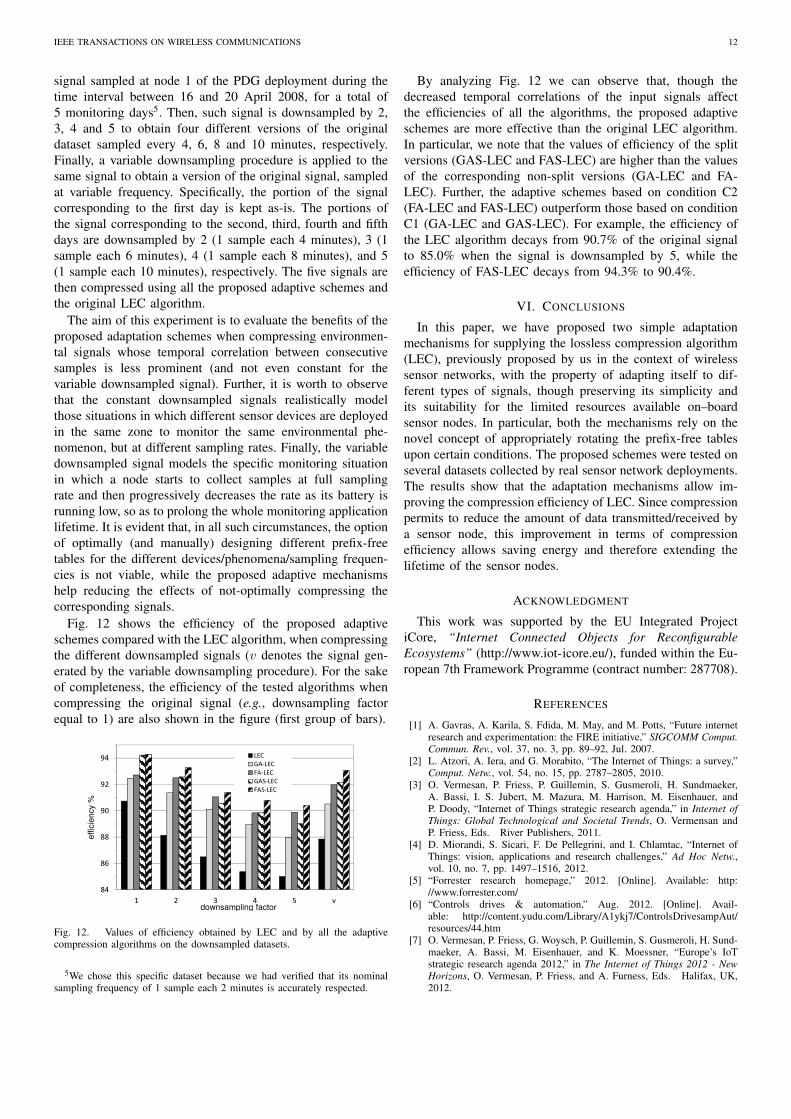
Fig. 12 shows the efficiency of the proposed adaptiveschemes compared with the LEC algorithm, when compressingthe different downsampled signals (v denotes the signal gen-erated by the variable downsampling procedure). For the sakeof completeness, the efficiency of the tested algorithms whencompressing the original signal (e.g., downsampling factorequal to 1) are also shown in the figure (first group of bars).

��

��

��

��

effic

ien

cy %

���

������

������

�������

�������

��

��

� � � �

downsampling factor

Fig. 12. Values of efficiency obtained by LEC and by all the adaptivecompression algorithms on the downsampled datasets.

5We chose this specific dataset because we had verified that its nominalsampling frequency of 1 sample each 2 minutes is accurately respected.

By analyzing Fig. 12 we can observe that, though thedecreased temporal correlations of the input signals affectthe efficiencies of all the algorithms, the proposed adaptiveschemes are more effective than the original LEC algorithm.In particular, we note that the values of efficiency of the splitversions (GAS-LEC and FAS-LEC) are higher than the valuesof the corresponding non-split versions (GA-LEC and FA-LEC). Further, the adaptive schemes based on condition C2(FA-LEC and FAS-LEC) outperform those based on conditionC1 (GA-LEC and GAS-LEC). For example, the efficiency ofthe LEC algorithm decays from 90.7% of the original signalto 85.0% when the signal is downsampled by 5, while theefficiency of FAS-LEC decays from 94.3% to 90.4%.

VI. CONCLUSIONS

In this paper, we have proposed two simple adaptationmechanisms for supplying the lossless compression algorithm(LEC), previously proposed by us in the context of wirelesssensor networks, with the property of adapting itself to dif-ferent types of signals, though preserving its simplicity andits suitability for the limited resources available on–boardsensor nodes. In particular, both the mechanisms rely on thenovel concept of appropriately rotating the prefix-free tablesupon certain conditions. The proposed schemes were tested onseveral datasets collected by real sensor network deployments.The results show that the adaptation mechanisms allow im-proving the compression efficiency of LEC. Since compressionpermits to reduce the amount of data transmitted/received bya sensor node, this improvement in terms of compressionefficiency allows saving energy and therefore extending thelifetime of the sensor nodes.

ACKNOWLEDGMENT

This work was supported by the EU Integrated ProjectiCore, “Internet Connected Objects for ReconfigurableEcosystems” (http://www.iot-icore.eu/), funded within the Eu-ropean 7th Framework Programme (contract number: 287708).

REFERENCES

[1] A. Gavras, A. Karila, S. Fdida, M. May, and M. Potts, “Future internetresearch and experimentation: the FIRE initiative,” SIGCOMM Comput.Commun. Rev., vol. 37, no. 3, pp. 89–92, Jul. 2007.

[2] L. Atzori, A. Iera, and G. Morabito, “The Internet of Things: a survey,”Comput. Netw., vol. 54, no. 15, pp. 2787–2805, 2010.

[3] O. Vermesan, P. Friess, P. Guillemin, S. Gusmeroli, H. Sundmaeker,A. Bassi, I. S. Jubert, M. Mazura, M. Harrison, M. Eisenhauer, andP. Doody, “Internet of Things strategic research agenda,” in Internet ofThings: Global Technological and Societal Trends, O. Vermensan andP. Friess, Eds. River Publishers, 2011.

[4] D. Miorandi, S. Sicari, F. De Pellegrini, and I. Chlamtac, “Internet ofThings: vision, applications and research challenges,” Ad Hoc Netw.,vol. 10, no. 7, pp. 1497–1516, 2012.

[5] “Forrester research homepage,” 2012. [Online]. Available: http://www.forrester.com/

[6] “Controls drives & automation,” Aug. 2012. [Online]. Avail-able: http://content.yudu.com/Library/A1ykj7/ControlsDrivesampAut/resources/44.htm

[7] O. Vermesan, P. Friess, G. Woysch, P. Guillemin, S. Gusmeroli, H. Sund-maeker, A. Bassi, M. Eisenhauer, and K. Moessner, “Europe’s IoTstrategic research agenda 2012,” in The Internet of Things 2012 - NewHorizons, O. Vermesan, P. Friess, and A. Furness, Eds. Halifax, UK,2012.

IEEE TRANSACTIONS ON WIRELESS COMMUNICATIONS 13

[8] C. Alcaraz, P. Najera, J. Lopez, and R. Roman, “Wireless sensor net-works and the Internet of Things: do we need a complete integration?”in Proc. of the 1st International Workshop on the Security of the Internetof Things, 2010.

[9] (2013) Libelium homepage. [Online]. Available: http://www.libelium.com/

[10] (2013) Cosm homepage. [Online]. Available: http://cosm.com/[11] F. Marcelloni and M. Vecchio, “An efficient lossless compression algo-

rithm for tiny nodes of monitoring wireless sensor networks,” Comput.J., vol. 52, no. 8, pp. 969–987, 2009.

[12] F. Marcelloni and M. Vecchio, “A simple algorithm for data compressionin wireless sensor networks,” IEEE Commun. Lett., vol. 12, no. 6, pp.411–413, Jun. 2008.

[13] T. Srisooksai, K. Keamarungsi, P. Lamsrichan, and K. Araki, “Practicaldata compression in wireless sensor networks: a survey,” J. Netw.Comput. Appl., vol. 35, no. 1, pp. 37–59, 2012.

[14] S. W. Golomb, “Run-length encodings,” IEEE Trans. Inf. Theory,vol. 12, pp. 399–401, September 1966.

[15] P. Elias, “Universal codeword sets and representations of the integers,”IEEE Trans. Inf. Theory, vol. 21, no. 2, pp. 194–203, Mar 1975.

[16] G. Chrysos and I. Papaefstathiou, “Heavily reducing WSNs’ energyconsumption by employing hardware-based compression,” in Ad-Hoc,Mobile and Wireless Networks, ser. Lect. Notes Comput. Sc., P. Ruizand J. Garcia-Luna-Aceves, Eds. Springer Berlin Heidelberg, 2009,vol. 5793, pp. 312–326.

[17] (2013) Xilinx homepage. [Online]. Available: http://www.xilinx.com/[18] (2013) Crossbow Technology homepage. [Online]. Available: http:

//bullseye.xbow.com:81/[19] A. K. Maurya, D. Singh, and A. K. Sarje, “Median predictor based

data compression algorithm for wireless sensor network,” InternationalJournal of Smart Sensors and Ad Hoc Networks, vol. 1, no. 1, pp. 62–65,2011.

[20] J. G. Kolo, S. A. Shanmugam, D. W. G. Lim, L. M. Ang, and K. P.Seng, “An adaptive lossless data compression scheme for wireless sensornetworks,” Journal of Sensors, 2012.

[21] C. Tharini and P. V. Ranjan, “Design of modified adaptive Huffmandata compression algorithm for wireless sensor network,” Journal ofComputer Science, vol. 5, no. 6, pp. 466–460, 2009.

[22] J. S. Vitter, “Design and analysis of dynamic Huffman codes,” J. ACM,vol. 34, no. 4, pp. 825–845, Oct. 1987.

[23] J. S. Vitter, “Algorithm 673: dynamic Huffman coding,” ACM Trans.Math. Softw., vol. 15, no. 2, pp. 158–167, Jun. 1989.

[24] K. C. Barr and K. Asanovic, “Energy-aware lossless data compression,”ACM Trans. Comput. Syst., vol. 24, no. 3, pp. 250–291, Aug. 2006.

[25] (2013) Sensorscope homepage. [Online]. Available: http://lcav.epfl.ch/sensorscope-en/

[26] D. Salomon, Data compression: the complete reference, 4th ed. London,UK: Springer-Verlag, 2007.

[27] F. Ingelrest, G. Barrenetxea, G. Schaefer, M. Vetterli, O. Couach,and M. Parlange, “Sensorscope: application-specific sensor network forenvironmental monitoring,” ACM Trans. Sen. Netw., vol. 6, no. 2, pp.17:1–17:32, Mar. 2010.

[28] H. D. Ferriere, L. Fabre, R. Meier, and P. Metrailler, “TinyNode: acomprehensive platform for wireless sensor network applications,” inProc. of the 5th international conference on Information processing insensor networks (IPSN’06), 2006, pp. 358–365.

[29] (2013) Texas Instruments homepage. [Online]. Available: http://www.ti.com/

[30] (2013) Xemics homepage. [Online]. Available: http://www.xemics.com/[31] (2013) Sensirion homepage. [Online]. Available: http://www.sensirion.

com/[32] (2013) Zytemp homepage. [Online]. Available: http://www.zytemp.com/[33] (2013) Davis homepage. [Online]. Available: http://www.davisnet.com/[34] J. W. Tukey, Exploratory Data Analysis. Addison-Wesley, 1977.[35] M. Friedman, “The use of ranks to avoid the assumption of normality

implicit in the analysis of variance,” J. Amer. Statist. Assoc., vol. 32, no.200, pp. 675–701, 1937.

[36] R. L. Iman and J. H. Davenport, “Approximations of the critical regionof the Friedman statistic,” Commun. Stat. A-Theor., vol. 9, pp. 571–595,1980.

[37] S. Holm, “A simple sequentially rejective multiple test procedure,”Scand. J. Stat., vol. 6, no. 2, pp. 65–70, 1979.

[38] F. Marcelloni and M. Vecchio, “Enabling compression in tiny wirelesssensor nodes,” in Wireless Sensor Networks, S. Tarannum, Ed. InTech,2011, ch. 12, pp. 257–276.

Massimo Vecchio received the Laurea degree inComputer Engineering (Magna cum Laude) from theUniversity of Pisa and the Ph.D. degree in ComputerScience and Engineering (with Doctor Europaeusmention) from IMT Lucca Institute for AdvancedStudies in 2005 and 2009, respectively. His researchbackground is on computational and artificial intel-ligence techniques, such as metaheuristics for globaloptimization and fuzzy logic. During his Ph.D. de-gree, however, his research interests moved towardspower-efficient engineering and application designs

for pervasive systems and devices. From October 2008 to March 2010 heworked as simulation engineer at INRIA-Saclay (France). Then, he joined theSignal Processing in Communications group at the University of Vigo (Spain)as a post-doctoral researcher, until September 2012. Recently he moved backto Italy to work as senior researcher at CREATE-NET, mainly in the fieldof Internet of Things devices and resources virtualization. Besides, currentMassimo’s research interests include metaheuristic and stochastic methodsfor wireless sensor nodes self-localization, node mobility for efficient datacollection and power-aware consensus techniques. He is author of one bookmonograph and co-author of two book chapters, 10 journal papers and variousconference papers.

Raffaele Giaffreda graduated at Politecnico Torino(Italy, 1995) and also holds an MSc in TelecomEngineering from University College of London(UK, 2001). He has a wide technology backgroundin the telecommunications domain, spanning fromoptical backhaul networks to wireless access oneswith research emphasis on dynamic resource us-age optimisation, information retrieval and contextawareness. He worked in the research departmentsof Telecom Italia (1994-1995, self-healing opticalcommunication rings), British Telecom (1998-2008,

information retrieval systems, context-aware networks and service deliveryplatforms) and is currently the head of the research group smaRt IOT(RIOT) at CREATE-NET, focusing on cognitive Internet of Things andassociated proof-of-concept implementation and related applications. He hasbeen involved in many international collaborative projects and is currentlythe coordinator of the EU FP7 Internet of Things project iCore (www.iot-icore.eu). He has more than 30 co-authored publications in internationaljournals, conferences and workshops.

Francesco Marcelloni received the Laurea degreein Electronics Engineering and the Ph.D. degree inComputer Engineering from the University of Pisain 1991 and 1996, respectively. He is currently anassociate professor at the University of Pisa. He hasco-founded the Computational Intelligence Groupat the Department of Information Engineering ofthe University of Pisa in 2002. Further, he is thefounder and head of the Competence Centre onMObile Value Added Services (MOVAS). His mainresearch interests include multi-objective evolution-

ary algorithms, genetic fuzzy systems, fuzzy clustering algorithms, patternrecognition, signal analysis, neural networks, mobile information systems, anddata compression and aggregation in wireless sensor networks. He has co-edited three volumes, four journal special issues, and is (co-)author of a bookand of more than 180 papers in international journals, books and conferenceproceedings. He has been TPC co-chair of the 9th International Conferenceon Intelligent Systems Design and Applications (ISDA’09) and ISDA’11, TPCchair of the 8th IEEE International workshop on Sensor Networks and Systemsfor Pervasive Computing, general co-chair of ISDA’10, and co-organizer ofseveral workshops and special sessions in international conferences. Currently,he serves as associate editor of Information Sciences (Elsevier) and SoftComputing (Springer) and is on the editorial board of other four internationaljournals.