Copyright 2006 Society of Photo-Optical Instrumentation Engineers. This paper was published in The Journal of Electronic Imaging and is made available as an electronic reprint (preprint) with permission of SPIE. One print or electronic copy may be made for personal use only. Systematic or multiple reproduction, distribution to multiple locations via electronic or other means, duplication of any material in this paper for a fee or for commercial purposes, or modification of the content of the paper are prohibited. 

Journal of Electronic Imaging 15(2), 023014 (Apr–Jun 2006)

Lossless compression of color palette images withone-dimensional techniques

Ziya ArnavutSUNY Fredonia

Department of Computer ScienceFredonia, New York, 14063

E-mail: ziya.arnavut@fredonia.edu

Ferat SahinRochester Institute of Technology

Department of Electrical Engineering

Rochester, New York, 14623

Abstract. Palette images are widely used on the World Wide Web(WWW) and in game-cartridge applications. Many images used onthe WWW are stored and transmitted after they are compressedlosslessly with the standard graphics interchange format (GIF), orportable network graphics (PNG). Well-known 2-D compressionschemes, such as JPEG-LS and JPEG-2000, fail to yield bettercompression than GIF or PNG due to the fact that the pixel valuesrepresent indices that point to color values in a look-up table. Toimprove the compression performance of JPEG-LS and JPEG-2000techniques, several researchers have proposed various reindexingalgorithms. We investigate various compression techniques for colorpalette images. We propose a new technique comprised of a trav-eling salesman problem (TSP)-based reindexing scheme, Burrows-Wheeler transformation, and inversion ranks. We show that the pro-posed technique yields better compression gain on average than allthe other 1-D compressors and the reindexing schemes that utilizeJPEG-LS or JPEG-2000. © 2006 SPIE and IS&T.�DOI: 10.1117/1.2194517�

1 IntroductionImage compression usually operates on one or more inten-sity planes of digitized images. For computer graphics im-ages, frequently each color is mapped to an index from alook-up table and the indices of the pixels are then com-pressed, usually losslessly. The size of the look-up table ismuch smaller than that of the color intensity space. Hence,this “color palette” approach can generally achieve a bettercompression ratio for images with limited color.

Highly compressed palletized images are used in manyapplications. For example, palletized images are widelyused on the World Wide Web �WWW�. Many images usedon the WWW are stored and transmitted as graphics inter-change format �GIF� files, which use Lempel-Ziv compres-sion. Lempel-Ziv compression treats the data as a 1-D se-quence of index values. The portable network graphics�PNG� format was designed to replace the GIF format.PNG is an improvement over GIF and, fortunately, unlike

Paper 05088R received May 17, 2005; revised manuscript received Aug.30, 2005; accepted for publication Oct. 31, 2005; published online Apr. 18,2006.

1017-9909/2006/15�2�/023014/11/$22.00 © 2006 SPIE and IS&T.

Journal of Electronic Imaging 023014-

GIF, it is also patent-free. An image stored as a losslessPNG file can be 5 to 25% smaller than the GIF file of thesame image.

Since palette images are widely used in WWW applica-tions, many techniques have been investigated to improvecompression performance of palette images.1 Severalresearchers1–6 have investigated reindexing color maps toimprove the compression gain of predictive techniques,such as JPEG-LS and JPEG-2000. Memon andVenkateswaran3 treated the problem as a general smooth-ness maximization problem. Zeng et al. suggested anindex-difference-based reindexing method.4 Batatiato etal.6 and Spira and Malah5 suggested color reindexing meth-ods based on the approximate solution to a traveling sales-man problem �TSP�. Pinho and Neves have given an im-proved version of Zeng’s algorithm.2 Other researchershave also investigated color-palette-based reorderingtechniques.1 According to the survey paper of Pinho andNeves,1 Memon’s and Venkateswaran’s reindexing schemeyields the best compression gain when JPEG-LS or JPEG-2000 is used.

Ausbeck7 introduced the piecewise-constant �PWC� im-age model, which is a two-pass object-based model.Boundaries between constant color pieces and domain col-ors are determined in the first and second passes, respec-tively. The PWC image model was shown to yield the bestcompression on palette images that have more than 32colors.8 Recently, Forchammer and Salinas8 developed a2-D version of prediction by partial matching �PPM�. Thecoder developed by Forchammer and Salinas yields bettercompression gains on images that have less than 32 colors;of course, it is slower than PWC since the technique isbased on PPM.

The block-sorting compression �also known as BW94,Burrows-Wheeler compression� technique introduced byBurrows and Wheeler9 had a great impact in the data com-pression area. Since the name Burrows-Wheeler compres-sion �BWC� is more widely used in the literature, we use ithere. Compression gains of BWC on text or image data are

better than with Ziv-Lempel techniques, with comparable

Apr–Jun 2006/Vol. 15(2)1

Arnavut and Sahin: Lossless compression of color palette images¼

speed,9–11 while its compression performance is close tothat of context-based methods, such as PPM. The schemeof the Burrows-Wheeler coder is presented in Fig. 1. Thefirst step performs the alphabetical �lexical� sorting trans-formation, which is widely called the Burrows-Wheelertransformation �BWT�. The second step is the move-to-front �MTF� coding12 �transformation�. The MTF codingoriginally was introduced by Bentley et al.12 and was inde-pendently discovered by Elias13 �called recency ranking byElias�. The last stage utilizes a statistical coder, such as theHuffman or arithmetic coder.

An MTF coder starts with an identity permutation of thesize of the alphabet used in the underlying data source. Forexample, when an MTF coder is implemented forcharacter-based data, the identity permutation is con-structed from the set of �0, . . . ,255�. Whenever a new char-acter or symbol is received from the underlying data string,the coder outputs the index of the symbol. In addition, ifthe symbol is not at the front of the list, the coder adjuststhe permutation �list� by simply moving the symbol to thefront of the existing permutation. In essence, a new permu-tation is generated for each symbol in the data string.

The first block-sorting-based 1-D scheme for compres-sion of color-mapped images was investigated in Ref. 14,where the author introduced the linear order transformation�LOT�. Later, in Ref. 15, it was shown that while the MTFcoder may be required to obtain better compression gainswhen the underlying data stream is text, it may not be nec-essary for some image data. In particular, the authorsshowed that by transforming image data with the BWT andutilizing a hierarchical arithmetic coder,16 about 8% morecompression can be attained over the well-known block-sorting coder bzip2. Most recently, our studies have shownthat when inversion ranks17 are used after a block-sortingtransformation, such as BWT, followed by a structuredarithmetic coder, compression gains improve 14% with re-spect to bzip2. However, as reported in Ref. 14, the LOT’sforward transformation is much faster than the BWT’s,while the reverse transformations of both techniques re-quire almost the same amount of time. Furthermore, LOTrequires less memory than BWT. When the data string ele-ments are 8 bit, such as ASCII characters, LOT requires256 additional integer indices �pointers�. Yet, for the sameASCII data, BWT requires 4n integer indices �pointers�,where n is the size of the data string.

This paper is organized as follows. In Sec. 2, we exposethe reader to the BWT and the LOT. Section 3 briefly ex-plains inversion ranks. Section 4 describes a TSP-based re-indexing algorithm. In Sec. 5, we present our experimentalresults and compare them to the well-known techniquessuch as bzip2, GIF, PNG, and other compression techniquesthat utilize reindexing schemes for reordering palette col-ors. Section 6 discusses the effect of transformations for

Fig. 1 Burrows-Wheeler coder.

image data. Finally, in Sec. 7, we conclude our discussion.

Journal of Electronic Imaging 023014-

2 Block-Sorting TransformationsLet A be an ordered alphabet of size m, and let s= �s1 ,s2 . . .sn� be a string of size n from the alphabet A.Starting with the original string s we construct the matrix,

S =�s1 s2 ¯ sn−1 sn

s2 s3 ¯ sn s1

�sn−1 sn ¯ sn−3 sn−2

sn s1 ¯ sn−2 sn−1

,

where the successive rows of S are consecutive cyclic left-shifts of the sequence s= �s1 ,s2 . . .sn�. A different matrix His formed by sorting the rows of S lexically,

H =�h1

1 h21

¯ hn−11 hn

1

h12 h2

2¯ hn−1

2 hn2

�h1

n−1 h2n−1

¯ hn−1n−1 hn

n−1

h1n h2

n¯ hn−1

n hnn .

Let � indicate the lexicographic order relationship betweenany two strings. Then, the rows of H are in the form of

H1 � H2 � ¯ � Hn,

where Hi denotes the i’th row of H, 1� i�n. Let Hi,k bethe k’th symbol in Hi, 1�k�n. We define column k ofmatrix H by the array

Ck�1, . . . ,n� = �H1,kH2,k ¯ Hn,k� ,

and write Ck for Ck�1, . . . ,n�. Let I �1� I�n� be the indexpointing the row I in H �HI�, which corresponds to theoriginal string s. When the forward BWT is applied to astring s it yields a pair, namely the index I and the lastcolumn Cn of H. The reverse of BWT, given I and Cn,retrieves the original string HI=s. For example, string s= �c a c a b�, after constructing the matrix S and by lexi-cally sorting its rows we obtain the following matrix

H =�a b c a c

a c a b c

b c a c a

c a b c a

c a c a b .

The original string appears in row 5. Hence, the sendersends the index 5, which corresponds to the row index ofthe original string s in H, as well as the last column �C5

= �c c a a b�� to the receiver. The receiver, on obtaining C5,can construct C1 by sorting the elements of C5. Once C1and C5 are both constructed, the receiver obtains the per-mutation �= �3 4 5 1 2�, which maps C5 to C1. Applying �to each Ci �1� i�3� yields the successive columns of thematrix H, that is C2, C3, and C4. Since the receiver knowsthe original index of s in H, the receiver can recover the

string s.

Apr–Jun 2006/Vol. 15(2)2

Arnavut and Sahin: Lossless compression of color palette images¼

The block-sorting transformation just described is calledBWT. The group-theoretical18 and the combinatorialproperties19,20 of the BWT have been studied extensively.Among others, an efficient implementation of the BWT isgiven in Refs. 9, 11, and 21–23.

A simpler block transformation, LOT, is first introducedin Ref. 14. Later in Ref. 19, it is delineated to the BWT andshown that the data transformed by either transformation isin the inverse set of each other. Here, we briefly describethe LOT transformation.

The linearly ordered matrix S̄ of a string s is formed asthe follows:

1. Starting with s= �s1s2 . . .sn�, form an n�n matrixS by cyclically left-shifting the successive rows.

2. Sort the rows of S in ascending order with respectto the first element of each row in S. The rows of

S̄ are formed by scanning s from left to right. Foreach v�A, determine the positions j1 , j2 , . . . , j fv

,where v=si for some i, 1� i�n, and fv is thenumber �frequency� of v’s in s.

For each occurrence of v, cyclically left shift the string s�jk−1� positions �1�k� fv�. Let C̄k represent the column k

in S̄ and C̄i,k represent the i’th element from top to bottom

in column C̄k. The resulting linearly ordered matrix S̄ con-

sists of the sorted values of s in its first column, C̄1. An

obvious observation about the linearly ordered matrix S̄ isthe following: For any given two pairs from the first two

columns of S̄, �C̄i,1 , C̄i,2� and �C̄k,1 , C̄k,2�, with the condition

C̄i,1= C̄k,2, then the pair �C̄i,1 , C̄i,2� appears earlier than the

pair �C̄k,1 , C̄k,2� in S̄ �scanning from top to bottom� if and

only if the pair �C̄i,1 , C̄i,2� appears earlier in s �scanningfrom left to right�. Obviously, the linear ordering induces aparticular order on the pairs of the elements. We can re-

cover s if we know C̄2 and the row index of s in S̄. Given

C̄2 and the row index of s in C̄2, one can construct s by

obtaining the frequencies of the elements in C̄2 using thecount sort24 in one pass. For example, let s= �c a c a b� and

suppose s occurs at position 5 in S̄, and the second column

is C̄2= �c b c a a�. Then C̄1= �a a b c c�; hence the matrix

of the first two columns C̄1 and C̄2 of S̄ is

�C̄1,C̄2� = a a b c c

c b c a a�T

,

where T denotes the transpose of the matrix. Accessing the

fifth position of the preceding matrix, �C̄1 , C̄2�, we acquire

the first two elements of s, �C̄5,1 , C̄5,2�= �c a�. By markingthe fifth entry we eliminate it from further consideration

�from the preceding matrix �C̄1 , C̄2��. To find the rest of the

elements of C̄2, we determine what follows C̄5,2=a in s.

Thus, we scan C̄1 from top to bottom and determine thefirst unused �unmarked� entry that has a value a. This is the

third element of s. In our example, this is the first entry

Journal of Electronic Imaging 023014-

where C̄1,1= C̄5,2=a. Hence, C̄1,2=c should follow C̄5,2=a

in C̄2. We then eliminate consideration of the first entry

from the matrix �C̄1 , C̄2�. Since C̄1,2=c is determined, theprocess is repeated to get the fourth element of s. Again, we

scan C̄1 to determine the position of the first unused entry

that contains C̄1,2=c. By finding the first unused entry that

contains the value c at position four in C̄1, we discover that

the fourth element of s is C̄4,2=a. This entry is eliminatedfrom further consideration. Finally, to find the fifth elementof s, we scan to find the first unused entry that has value a

in C̄1. Since the first entry that has a value a is used previ-

ously, the second entry is considered, C̄2,1=a. Therefore,

the last element of s is C̄2,1=b, and s= �c b c a a�.The LOT just described has context length one, while

the BWT has10 context length n. One can generalize theblock-sorting transformations to have context length m,where 2�m�n. Schindler21 used this fact in the imple-mentation of his szip compression program, where he usescontext level 12. Schindler’s work was explained morethroughly by Yokoo.20 For the discussion of different con-textual block-sorting algorithms, interested readers can re-fer to Refs. 20 and 21.

3 Inversion RanksAll the variants of the block sorting compressor �e.g.,bzip2, szip� utilize the MTF coder on the data stream, trans-formed with Burrows-Wheeler, before actually sending thedata stream to an encoder such as the arithmetic or Huff-man encoder.

Recently, we have shown that better compression thanGIF, PNG, and bzip2 can be obtained when inversion ranksare used in the second step of a block-sorting based coder.17

To keep this paper concise, we only briefly describe inver-sion ranks. For further information, interested readers canconsult Refs. 19, 25, and 26.

Definition 3.1. Let M,be a multiset permutation of ele-ments from an underlying set S= �1,2 , . . . ,k�. Let � denotecatenation of data strings. We define the inversion rank vec-tor D=Dk for M as follows:

1. D0= � .2. For 1� i�k, Di=Di−1�Ti with Ti

= �x1 ,x2 , . . . ,xfi , where

i. x1 is the position of the first occurrence of i in M.ii. And for j�1, xj is the number of elements y in

M, y� i occurring between the �j−1�’st and j’thoccurrence of i in M.

For example, for the multiset permutation M= �1,1 ,2 ,3 ,1 ,2 ,4 ,3 ,4 ,2 ,4�, we have S= �1,2 ,3 ,4�. Ini-tially D0= � . For i=1�S, we have D1=D0�T1, whereT1= �1,0 ,2 , so D1= �1,0 ,2 . For i=2�S, D2=D1�T2,where T2= �3,1 ,3 . Therefore, D2= �1,0 ,2 ,3 ,1 ,3 . For i=3�S, D3=D2�T3, where T3= �4,1 , so D3

= �1,0 ,2 ,3 ,1 ,3 ,4 ,1 . For i=4�S, D4=D3�T4, whereT4= �7,0 ,0 . Hence, D=D4= �1,0 ,2 ,3 ,1 ,3 ,4 ,1 ,7 ,0 ,0 .

To recover the original multiset permutation M from D,

Apr–Jun 2006/Vol. 15(2)3

Arnavut and Sahin: Lossless compression of color palette images¼

we need the knowledge of the multiset described by thefrequency vector F= �f1 , f2 , . . . , fk�. We initially let M= �−,−, . . . ,−� where �M � = �D � =�i=1

k f i. From the definition ofinversion ranks, D is built recursively as Di=Di−1�Ti,where Ti= �x1 ,x2 , . . . ,xfi

and x1 represents the position ofthe first occurrence of i in M and each xj , j�1, representsthe number of elements greater than i, which occur betweenthe �j−1�’st and j’th occurrences of i in M. Hence, we canrecover the elements of M by first inserting i in locationM�x1� and for j=2, . . . , f i inserting i in the �xj +1�’st empty�dash� position in M from the last inserted i.

For example, for the preceding multiset permutation M,F= �3,3 ,2 ,3 . The receiver, on receiving vectors S, F andD, can reconstruct the multiset permutation M as follows.The receiver first creates a vector M of size �i=1

4 f i=11.From the ordered F, the receiver determines S and that thefirst element of M is 1 and there are three 1s in the multisetM. The receiver then knows that, the first three entries in Dare the locations related to 1 and in the first pass, the re-ceiver inserts 1s in their location in M correctly. Since thefirst entry in D is 1, it follows that the location of the firstelement in D is at position 1, hence M= �1,− ,− ,− ,− ,− ,− ,− ,− ,− ,−�. The second entry in D is 0. This means that,there is no element that is greater than 1, between the firstand second occurrences of 1. Hence, the receiver inserts thesecond 1 in the first blank position next to the first 1, soM= �1,1 ,− ,− ,− ,− ,− ,− ,− ,− ,−�. The third entry in D is a2. This means that, there are two elements greater than 1,between the second and third 1s. Hence, the third 1 shouldbe placed in the third empty position after the second 1.Therefore, M= �1,1 ,− ,− ,1 ,− ,− ,− ,− ,− ,−�. Again, from Sand F, the receiver knows that there are three 2s in M.Accessing the fourth position in D it learns the location ofthe first 2 in M, should occur in position 3. Hence, M= �1,1 ,2 ,− ,1 ,− ,− ,− ,− ,− ,−�.

The receiver then proceeds to insert the second 2 into M.From D, the receiver determines that between the first 2and second 2, there is one element that is greater than 2. So,starting from the location of the first 2 in M, the receiverskips one blank and inserts the second 2 into the secondblank position. Similarly, for the third 2 the receiver deter-mines from D that between the second and third 2s, thereare three elements that are greater than 2. Therefore, thereceiver inserts the third 2 into the fourth blank position,after the second 2. Hence, M= �1,1 ,2 ,− ,1 ,2 ,− ,− ,− ,2 ,−�.Continuing the above procedure, the receiver can fully re-construct M.

4 Ordering of Color IndicesThere are several reindexing techniques in the literature1

that aim to improve the compression performance of pre-dictive techniques, such as JPEG-LS and JPEG-2000.Some of these reindexing methods utilize approaches basedon the TSP to reduce prediction errors.

A recent example of such a technique is given byBattiato et al.6 They propose an approximate solution toTSP and showed that their technique is faster than otherreindexing techniques. They built a TSP model to minimizethe sum of the differences between the values of neighbor-

ing pixels in a given image.

Journal of Electronic Imaging 023014-

We explore the possible benefit from reindexing the col-ors in an image before we apply the BWT and later inver-sion method �B+INV�. However, we note that the knownreindexing techniques are not designed to optimize thecompression performance of B+INV. Thus, we stronglybelieve that finding an optimal reindexing method to im-prove the compression gain of B+INV is an open problemthat requires further investigation.

In this paper, we use a TSP-based reindexing algorithmsimilar to the one presented in Ref. 6. Let us assume thatwe have an image of size n�m with N colors �color indi-ces� and by raster scanning the image, the pixel sequencep1 , p2 , . . . , pn�m is generated. Let S�ci ,cj� denote the num-ber of times the pair of colors �ci ,cj� has been seen over thepixel sequence p1 , p2 , . . . pn�m, and let W= �wij� be an N�N matrix representing the edge weights between the col-ors. The edge weights are calculated based on the numberof occurence of the color pairs. For example, the edgeweights between color ci and color cj is calculated as

�wij = wji = S�ci,cj� + S�cj,ci� if i � j

wij = 0 if i = j ,� �1�

where i , j=1, . . . ,N.By calculating edge weights between the colors, we gen-

erate the weight matrix W:

W = �w11 . . . w1N

. . . . . . . . .

wN1 . . . wNN . �2�

After calculating the weight matrix, we apply the cross-entropy �CE�-based TSP algorithm27 to find a closed paththat covers all the colors. The TSP algorithm is set to maxi-mize the sum of the edge weights in the closed path tocover edges with higher weights. According to Ref. 6, asimple Hamiltonian path in a graph of maximum weightgives an optimal reindexing scheme for differential losslesscompression techniques. To achieve this maximization weset the CE-based TSP algorithm to maximize the followingcost function:

J = �i=1

N

�j=1

N

S�ci,cj�uij , �3�

where uij =1 when ci and cj are adjacent colors in theclosed path, and uij =0 otherwise.

Maximizing the sum of the edge weights in a closedpath yields a smaller entropy since the colors that appearfrequently together will be relabeled with new values suchthat the difference between those colors will be smaller. Forexample, in a pixel sequence if colors ci and cj appeartogether the most, then the edge weight between them willbe the largest. Thus, this edge will be part of the closedpath formed by the TSP algorithm. When colors ci and cjare relabeled based on the closed path, they will be labeledwith consecutive values.

To relabel the color indices, we must determine wherethe labeling should start. Since we are trying to label thecolors that appear together frequently in the sequence close

to each other, we must determine the colors that appear

Apr–Jun 2006/Vol. 15(2)4

Arnavut and Sahin: Lossless compression of color palette images¼

together the least number of times and label them far fromeach other. After we find the closed path that maximizes thesum of the weights, we remove the edge with the minimumweight. Let us assume that the minimum weighted edge isbetween the colors ci and cj. Then, we create a path from cito cj by removing the edge between these colors. Finally,we start relabeling by labeling cj as zero and continue re-labeling until ci is reached. Since the closed path has theedges with higher weights, after the relabeling, the sum ofdifferences between the relabeled colors will be reduceddramatically.

We give an example to clarify the algorithm just de-scribed. Let us consider an image with four colors and thefollowing pixel sequence

33221211123300100220011200333011.

Based on the sequence, the numbers of occurences of thecolor pairs are as shown in Table 1, and for the sequencejust given, the following weight matrix is calculated usingEq. �1�:

W =�0 4 3 3

4 0 5 0

3 5 0 2

3 0 2 0 .

Figure 2 shows the colors and the corresponding weights.Since the TSP algorithm is trying to maximize the sum ofthe weights, the resulting close path is 0 to 1 to 2 to 3 to 0.The sum of the weights for this route is 14. The edge with

Table 1 Occurrences of color pairs.

ci 0 1 0 2 0 3 1 2 1 3 2 3

cj 1 0 2 0 3 0 2 1 3 1 3 2

S�ci ,cj� 3 1 1 2 1 2 3 2 0 0 1 1

Fig. 2 Example for traveling salesman algorithm utilized in this

paper.

Journal of Electronic Imaging 023014-

minimum weight is the edge between colors 2 and 3. Thus,we create a path from color 3 to color 2 as 3 to 0 to 1 to 2by removing this edge. Then, we start relabeling from color2, we obtain the relabeling, as shown in Fig. 2. Thus, color0 is relabeled with 2, color 1 is re-relabeled with 1, color 2is re-relabeled with 0, and finally color 3 is relabeled with3. After the relabeling the sequence becomes

33001011103322122002211022333211.

Then, the sum of the differences between the relabeled col-ors becomes 24. The sum of differences between the colorsin the original sequence was 26.

5 Experimental ResultsThis section presents experimental results and provides dis-cussion on the performance of various techniques. All thetest images utilized in our work were obtained from the ftpsite, ftp://ftp.ieeta.pt/~ap/images and previously were usedas test images in Ref. 1. Three of the test images are shownin Figs. 3–5. All of the test images are converted from PPMformat to GIF, PNG, and BMP �bitmap� formats using theversion 1.2.3 of the Gimp program. We notice that the BMPformatted, or GIF compressed images generated by theGimp program are slightly different in size than the onesthat may be obtained using the Unix utility function “ppm-togif” or some other software, such as “xv”. This may bebecause each program may encode the header informationdifferently. Thus, for some of the test images the bits perpixel �bpp� values for GIF compression scheme reported inRef. 2 or some other papers may vary slightly from ourresults presented in this paper.

Table 2 presents the experimental results of differentcompression techniques on the set of test images. Columnslabeled L+X and B+X present the results of the algorithms

Fig. 3 “Sunset” image in gray.

Fig. 4 “Gate” image in gray.

Apr–Jun 2006/Vol. 15(2)5

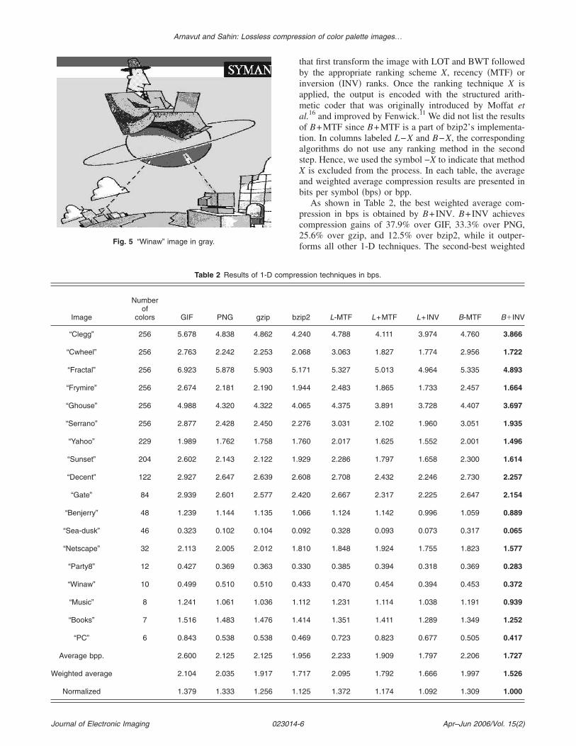
Fig. 5 “Winaw” image in gray.

Arnavut and Sahin: Lossless compression of color palette images¼

Journal of Electronic Imaging 023014-

that first transform the image with LOT and BWT followedby the appropriate ranking scheme X, recency �MTF� orinversion �INV� ranks. Once the ranking technique X isapplied, the output is encoded with the structured arith-metic coder that was originally introduced by Moffat etal.16 and improved by Fenwick.11 We did not list the resultsof B+MTF since B+MTF is a part of bzip2’s implementa-tion. In columns labeled L−X and B−X, the correspondingalgorithms do not use any ranking method in the secondstep. Hence, we used the symbol −X to indicate that methodX is excluded from the process. In each table, the averageand weighted average compression results are presented inbits per symbol �bps� or bpp.

As shown in Table 2, the best weighted average com-pression in bps is obtained by B+INV. B+INV achievescompression gains of 37.9% over GIF, 33.3% over PNG,25.6% over gzip, and 12.5% over bzip2, while it outper-forms all other 1-D techniques. The second-best weighted

ssion techniques in bps.

ip2 L-MTF L+MTF L+INV B-MTF B�INV

40 4.788 4.111 3.974 4.760 3.866

68 3.063 1.827 1.774 2.956 1.722

71 5.327 5.013 4.964 5.335 4.893

44 2.483 1.865 1.733 2.457 1.664

65 4.375 3.891 3.728 4.407 3.697

76 3.031 2.102 1.960 3.051 1.935

60 2.017 1.625 1.552 2.001 1.496

29 2.286 1.797 1.658 2.300 1.614

08 2.708 2.432 2.246 2.730 2.257

20 2.667 2.317 2.225 2.647 2.154

66 1.124 1.142 0.996 1.059 0.889

92 0.328 0.093 0.073 0.317 0.065

10 1.848 1.924 1.755 1.823 1.577

30 0.385 0.394 0.318 0.369 0.283

33 0.470 0.454 0.394 0.453 0.372

12 1.231 1.114 1.038 1.191 0.939

14 1.351 1.411 1.289 1.349 1.252

69 0.723 0.823 0.677 0.505 0.417

56 2.233 1.909 1.797 2.206 1.727

17 2.095 1.792 1.666 1.997 1.526

25 1.372 1.174 1.092 1.309 1.000

Table 2 Results of 1-D compre

Image

Numberof

colors GIF PNG gzip bz

“Clegg” 256 5.678 4.838 4.862 4.2

“Cwheel” 256 2.763 2.242 2.253 2.0

“Fractal” 256 6.923 5.878 5.903 5.1

“Frymire” 256 2.674 2.181 2.190 1.9

“Ghouse” 256 4.988 4.320 4.322 4.0

“Serrano” 256 2.877 2.428 2.450 2.2

“Yahoo” 229 1.989 1.762 1.758 1.7

“Sunset” 204 2.602 2.143 2.122 1.9

“Decent” 122 2.927 2.647 2.639 2.6

“Gate” 84 2.939 2.601 2.577 2.4

“Benjerry” 48 1.239 1.144 1.135 1.0

“Sea-dusk” 46 0.323 0.102 0.104 0.0

“Netscape” 32 2.113 2.005 2.012 1.8

“Party8” 12 0.427 0.369 0.363 0.3

“Winaw” 10 0.499 0.510 0.510 0.4

“Music” 8 1.241 1.061 1.036 1.1

“Books” 7 1.516 1.483 1.476 1.4

“PC” 6 0.843 0.538 0.538 0.4

Average bpp. 2.600 2.125 2.125 1.9

Weighted average 2.104 2.035 1.917 1.7

Normalized 1.379 1.333 1.256 1.1

Apr–Jun 2006/Vol. 15(2)6

Arnavut and Sahin: Lossless compression of color palette images¼

average compression result is achieved by L+INV. Thecompression performance of the L+INV technique is ap-proximately 9% worse than B+INV. However, as men-tioned earlier, L+INV is much faster than B+INV sinceLOT is a context-level one transformation as opposed tocontext level n and uses less memory than the BWT trans-formation.

The third-best weighted average compression result isobtained by bzip2. This well-known coder is composed ofthe BWT and MTF transformations in addition to a modi-fied Huffman coder. The fourth-best weighted averagecompression is achieved by L+MTF. Note that all thetransformation-based techniques yield better compressionresults, in terms of weighted average bit per symbol, thanGIF and PNG, with the exception of the L−MTF tech-nique. Apparently, L−MTF and the B−MTF perform com-parably. Although B−MTF yields approximately 1.2% bet-ter compression than L−MTF in terms of weighted averagebps, L−MTF performs better than B−MTF for most of theimages that have a high number of colors. As we can see inFigs. 6 and 7, both transformations yield similar output asexpected. Although in images, the neighboring pixel valuesare highly correlated, it is hard to find similar long patternsin different regions of an image. For images with fewercolors this may not be true. Thus, B−MTF performsslightly better than L−MTF on images that have fewer col-ors.

Unlike the results presented in Table 2, where the resultswere presented in bps, the results in Table 3 are presentedin bpp so that we can have a fair comparison with theresults presented in Ref. 1. Table 3 shows the results ofreindexing schemes. The results presented under the col-

Fig. 6 Segment of BWTed “Gate” image.

umns titled Memon, Zeng, mZeng, and Battiato are taken

Journal of Electronic Imaging 023014-

from Table 1 of the recently published survey paper ofPinho and Neves.1 In Table 3, under the column titled T+B+INV, we present the results of the B+INV technique,which is combined with our TSP-based reindexing scheme.In the proposed column, we present the results of our newtechnique. Our new technique is simply a combination ofT+B+INV and B+INV. When the number of colors in animage is less than 32, the TSP-based reindexing schemehelps B+INV to yield better compression gains. Our algo-rithm uses the B+INV technique for images that have morethan 31 colors and for images that have less than 32 colorsit uses the T+B+INV technique. This improves our com-pression gain close to 1% for the 18 test images used inTable 3.

From the compression results shown in Table 3, it isclear that our proposed technique yields the best compres-sion gain in terms of weighted average bpp. Our proposedscheme achieves 73.0% better compression gain over Bat-tiato’s technique, while it yields 46.5% better compressiongain over Memon’s technique, which is the best methodamong the reindexing schemes presented in Ref. 1.

In Table 4, we present the compression results of imageswith and without dithering for the test sets of “Natural1”and “Natural2.” These test images were also obtained fromthe same ftp site mentioned earlier. They are color quan-tized. Also, in each set there are those different groups ofimages, namely, those with 256, 128, and 64 colors, bothwith and without dithering. In each color group �with andwithout dithering�, there are 23 images in Natural1, whilethere are 12 images in Natural2. Our proposed techniqueyields 15.1 to 16.5% better compression gains on averagefor images without dithering, and 18.0 to 26.0% for images

Fig. 7 Segment of LOTed “Gate” image.

with dithering.

Apr–Jun 2006/Vol. 15(2)7

Arnavut and Sahin: Lossless compression of color palette images¼

It is clear that our proposed algorithm yields slightlybetter compression gain over B+INV, as expected. The re-indexing algorithm aims to minimize the sum of differencesbetween the values of the neighboring pixels. This minimi-zation does not boost the performance of B+INV becauseB+INV does not depend on the differences between thevalues of the neighboring pixels. If a reindexing algorithmis specially modeled for the B+INV technique, the resultsmight be improved. At this time, we are not aware of anypreprocessing technique that can help inversion ranks toincrease compression gain. This requires further investiga-tion and should be material for future research.

6 Effect of TransformationsIt is well known that neighboring pixel values in an imageare highly correlated. Most often, in a given gray-coloredimage, the difference between the values of two neighbor-

Table 3 Compression results of rein

Image

Numberof

colors Memon Zheng

“Clegg” 256 5.22 5.863

“Cwheel” 256 2.724 3.058

“Fractal” 256 5.763 6.193

“Frymire” 256 3.259 3.619

“Ghouse” 256 4.229 4.841

“Serrano” 256 3.001 3.393

“Yahoo” 229 1.743 1.798

“Sunset” 204 2.407 2.570

“Decent” 122 2.817 2.943

“Gate” 84 2.548 2.587

“Benjerry” 48 1.133 1.154

“Sea_dusk” 46 0.197 0.189

“Netscape” 32 1.745 1.791

“Party8” 12 0.321 0.318

“Winaw” 10 0.450 0.450

“Music” 8 1.051 1.060

“Books” 7 1.453 1.469

“PC” 6 0.748 0.743

Average 2.267 2.447

Weighted average 2.243 2.452

Normalized 1.465 1.601

ing pixels will not exceed ±10. Of course, this is not true

Journal of Electronic Imaging 023014-

when neighboring pixel values are in different regions oredges. In general, if a pixel’s neighbor is on an edge, theabsolute difference of neighboring pixel values may bequite high ��30�.

The forward BWT sorts the lexical sequences in increas-ing order. When an image is BWT transformed, frequently,pixel values tend to group together “nicely,” except forsome peaks that may occur due to edges. Figures 6 and 7display the output of 3000 elements of the BWTed andLOTed gate image, respectively. These 3000 elements aretaken from the same exact coordinates of BWTed andLOTed gate image data. Notice the similarities betweenFigs. 6 and 7. In both figures, most of the values occurbetween 30 and 45. However, it appears that similar valuestend to group together in Fig. 6 better than in Fig. 7.

Contrary to the nature of image data, in text data, fre-quently, the values between neighboring characters may

techniques and our method in bpp.

mZheng Battiato T+B+INV Proposed

5.456 6.075 3.971 3.881

2.878 3.374 1.729 1.726

5.828 7.234 4.935 4.913

3.376 3.946 1.692 1.668

4.541 5.418 3.715 3.705

3.273 3.779 1.963 1.948

1.789 2.008 1.565 1.550

2.307 2.647 1.626 1.619

2.854 3.531 2.290 2.276

2.566 3.116 2.175 2.167

1.137 1.186 0.909 0.900

0.189 0.189 0.069 0.065

1.752 1.907 1.592 1.582

0.318 0.319 0.284 0.284

0.450 0.464 0.376 0.376

1.051 1.071 0.961 0.961

1.469 1.453 1.282 1.282

0.745 0.743 0.417 0.417

2.332 2.692 1.753 1.740

2.333 2.65 1.546 1.532

1.521 1.730 1.009 1.000

dexing

differ significantly. For any given sentence, we have spaces

Apr–Jun 2006/Vol. 15(2)8

Arnavut and Sahin: Lossless compression of color palette images¼

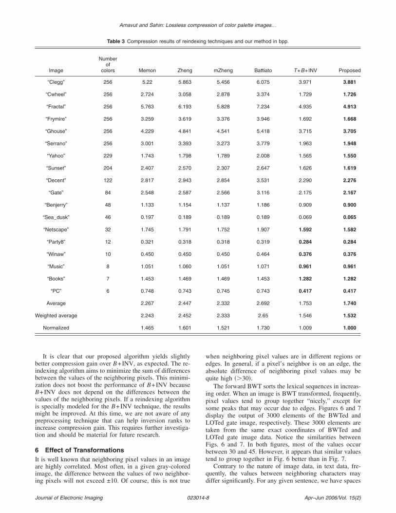
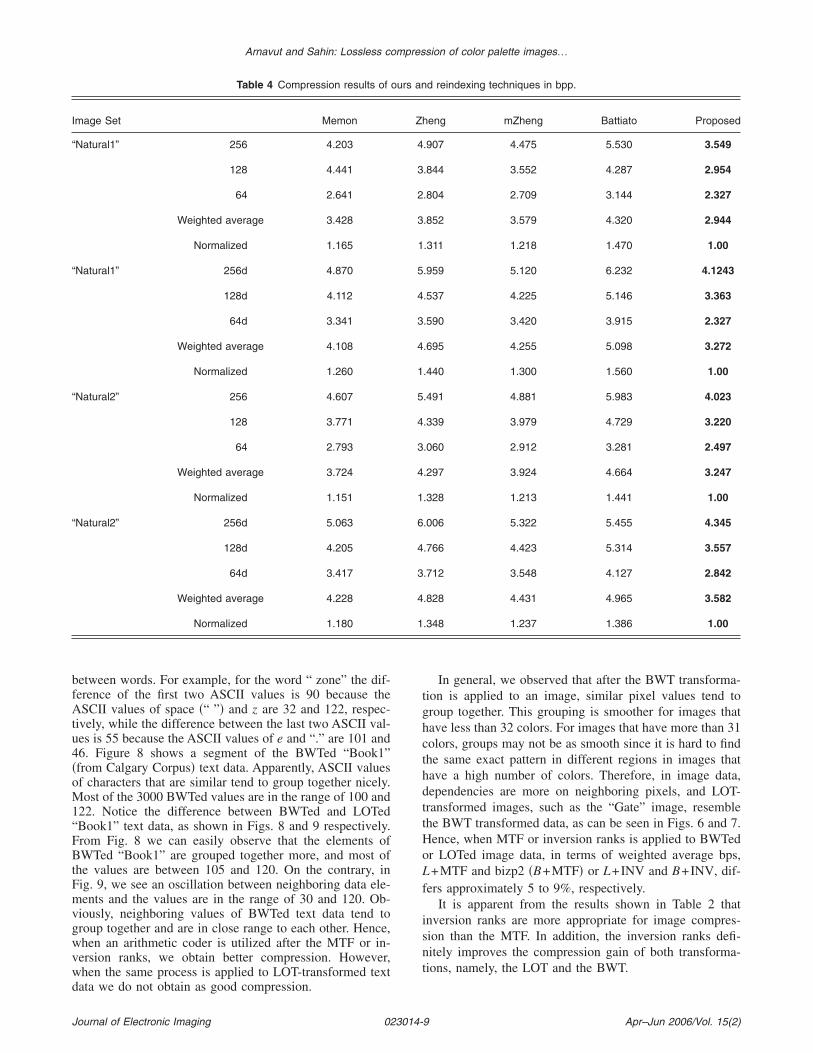
between words. For example, for the word “ zone” the dif-ference of the first two ASCII values is 90 because theASCII values of space �“ ”� and z are 32 and 122, respec-tively, while the difference between the last two ASCII val-ues is 55 because the ASCII values of e and “.” are 101 and46. Figure 8 shows a segment of the BWTed “Book1”�from Calgary Corpus� text data. Apparently, ASCII valuesof characters that are similar tend to group together nicely.Most of the 3000 BWTed values are in the range of 100 and122. Notice the difference between BWTed and LOTed“Book1” text data, as shown in Figs. 8 and 9 respectively.From Fig. 8 we can easily observe that the elements ofBWTed “Book1” are grouped together more, and most ofthe values are between 105 and 120. On the contrary, inFig. 9, we see an oscillation between neighboring data ele-ments and the values are in the range of 30 and 120. Ob-viously, neighboring values of BWTed text data tend togroup together and are in close range to each other. Hence,when an arithmetic coder is utilized after the MTF or in-version ranks, we obtain better compression. However,when the same process is applied to LOT-transformed text

Table 4 Compression results of o

Image Set Memon

“Natural1” 256 4.203

128 4.441

64 2.641

Weighted average 3.428

Normalized 1.165

“Natural1” 256d 4.870

128d 4.112

64d 3.341

Weighted average 4.108

Normalized 1.260

“Natural2” 256 4.607

128 3.771

64 2.793

Weighted average 3.724

Normalized 1.151

“Natural2” 256d 5.063

128d 4.205

64d 3.417

Weighted average 4.228

Normalized 1.180

data we do not obtain as good compression.

Journal of Electronic Imaging 023014-

In general, we observed that after the BWT transforma-tion is applied to an image, similar pixel values tend togroup together. This grouping is smoother for images thathave less than 32 colors. For images that have more than 31colors, groups may not be as smooth since it is hard to findthe same exact pattern in different regions in images thathave a high number of colors. Therefore, in image data,dependencies are more on neighboring pixels, and LOT-transformed images, such as the “Gate” image, resemblethe BWT transformed data, as can be seen in Figs. 6 and 7.Hence, when MTF or inversion ranks is applied to BWTedor LOTed image data, in terms of weighted average bps,L+MTF and bizp2 �B+MTF� or L+INV and B+INV, dif-fers approximately 5 to 9%, respectively.

It is apparent from the results shown in Table 2 thatinversion ranks are more appropriate for image compres-sion than the MTF. In addition, the inversion ranks defi-nitely improves the compression gain of both transforma-tions, namely, the LOT and the BWT.

d reindexing techniques in bpp.

heng mZheng Battiato Proposed

.907 4.475 5.530 3.549

.844 3.552 4.287 2.954

.804 2.709 3.144 2.327

.852 3.579 4.320 2.944

.311 1.218 1.470 1.00

.959 5.120 6.232 4.1243

.537 4.225 5.146 3.363

.590 3.420 3.915 2.327

.695 4.255 5.098 3.272

.440 1.300 1.560 1.00

.491 4.881 5.983 4.023

.339 3.979 4.729 3.220

.060 2.912 3.281 2.497

.297 3.924 4.664 3.247

.328 1.213 1.441 1.00

.006 5.322 5.455 4.345

.766 4.423 5.314 3.557

.712 3.548 4.127 2.842

.828 4.431 4.965 3.582

.348 1.237 1.386 1.00

urs an

Z

4

3

2

3

1

5

4

3

4

1

5

4

3

4

1

6

4

3

4

1

Apr–Jun 2006/Vol. 15(2)9

Arnavut and Sahin: Lossless compression of color palette images¼

7 ConclusionAll variants of the block sorting coder �e.g., bzip2, szip�first transform a given data stream with the BWT and then

Fig. 8 Segment of BWTed “Book1” text data.

Fig. 9 Segment of LOTed “Book1” text data.

Journal of Electronic Imaging 023014-1

utilize the MTF transformation before coding the resultingdata stream with an arithmetic or Huffman coder.

In this paper, we investigated, various 1-D compressiontechniques for color palette images. We showed that amongthe 1-D techniques, blocks-sorting-based compressors thatutilize inversion ranks in the second step yield better com-pression than all the other 1-D compressors. Moreover, ourproposed technique provides compression gains in terms ofweighted average bps over the set of test images on theorder of 38.9% over GIF, 33.3% over PNG, and 12.5% overbzip2.

We also showed that for various sets of test images ourproposed reindexing-based scheme yields results superiorto the best reindexing scheme, namely, that of Memon andVenkateswaran. Our technique achieves 46.5% better com-pression on average on synthetic images, while it yields15.1 to 16.5% better compression for various nonsynthetic,natural images, and 18.0 to 26.0% for the corresponding setof dithered images.

AcknowledgmentsWe would like to thank Dr. Joseph Straight for his valuablecomments and suggestions, Dr. Armando J. Pinho for sup-plying the test images and answering our several questions,Dr. Thomas Taimre for letting us modifying his code toimplement our TSP-based reindexing algorithm, Dr. Wen-jun Zeng for supplying us another set of images, and to theunknown referees for their valuable suggestions to improvethe quality of this work.

References1. A. J. Pinho and A. J. R. Neves, “Survey on palette reordering meth-

ods,” IEEE Trans. Image Process. 13�11�, 1411–1417 �2004�.2. A. J. Pinho and A. J. R. Neves, “A note on Zeng’s technique for color

reindexing of palette-based images,” IEEE Signal Process. Lett.11�2�, 232–235 �2004�.

3. N. D. Memon and A. Venkateswaran, “On ordering color maps forlossless predictive coding,” IEEE Trans. Image Process. 5�11�, 1522–1527 �1996�.

4. W. Zeng, J. Li, and S. Lei, “An efficient color reindexing scheme forpalette-based compression,” in Proc. IEEE Int. Conf. on Image Pro-cessing �ICIP-2000�, Vol. 3, pp. 476–479 �2000�.

5. A. Spira and D. Malah, “Improved lossless compression of color-mapped images by an approximate solution of the traveling salesmanproblem,” in Proc. Acoustics, Speech, and Signal Processing �IC-ASSP ’01�, Vol. 3, pp. 1797–1800 �2001�.

6. S. Battiato, G. Gallo, G. Impoco, and F. Stanco, “An efficient rein-dexing, algorithm for color-mapped images,” IEEE Trans. ImageProcess. 13�11�, 1419–1423 �2004�.

7. P. J. Ausbeck Jr., “The piecewise-constant image model,” in Proc.IEEE on Lossless Data Compression: Special Issue, pp. 1779–1789�2000�.

8. S. Forchhammer and M. J. Salinas, “Progressive coding of paletteimages and digital maps,” in Proc. Data Compression Conf., DCC-2002, pp. 362–371 �2002�.

9. M. Burrows and D. J. Wheeler, “A block-sorting lossless data com-pression algorithm,” SRC Research Report 124 �1994� �ftp site: gate-keeper.dec.com, /pub/DEC/SRC/research-reports/SRC-124.ps.Z�.

10. J. G. Cleary, W. J. Teahan, and I. H. Witten, “Unbounded lengthcontexts for PPM,” in Proc. Data Compression Conf., DCC-95, pp.52–61 �1995�.

11. P. Fenwick, “The Burrows-Wheeler transform for block sorting textcompression: principles and improvements,” Comput. J. 39�9�, 731–740 �1996�.

12. J. L. Bentley, D. D. Sleator, R. E. Tarjan, and V. K. Wei, “A locallyadaptive data compression scheme,” Commun. ACM 29�29�, 320–330�1986�.

13. P. Elias, “Interval and recency Rank source coding: two on-line adap-tive variable-length schemes,” IEEE Trans. Inf. Theory IT-33�1�,3–10 �1987�.

14. Z. Arnavut, “Lossless compression of pseudo-color images,” Opt.Eng. 38�6�, 1001–1005 �1999�.

15. Z. Arnavut and H. Otu, “Lossless compression of color-mapped im-

ages with Burrows-Wheeler transformation,” in Proc. Signal Process-

Apr–Jun 2006/Vol. 15(2)0

Arnavut and Sahin: Lossless compression of color palette images¼

ing Conf., IASTED, pp. 185–189 �2001�.16. A. Moffat, R. Neal, and I. H. Witten, “Arithmetic coding revisited,”

in Proc. Data Compression Conf., DCC-95, pp. 202–211 �1995�.17. Z. Arnavut and F. Sahin, “Inversion ranks for lossless compression of

palette images,” in Proc. IEEE Electro/Information TechnologyConf., CDROM �2005�.

18. Z. Arnavut and S. S. Magliveras, “Lexical permutation sorting algo-rithm,” Comput. J. 40�5�, 292–295 �1997�.

19. Z. Arnavut and M. Arnavut, “Investigation of block sorting transfor-mations,” J. Comput. Math. 2�1�, 46–57 �2004�.

20. H. Yokoo, “Notes on block-sorting data compression,” Electron.Commun. Jpn. 82�6�, 18–25 �1999�.

21. M. Schindler, “A fast block sorting algorithm for lossless data com-pression,” in Proc. Data Compression Conf., DCC-97, p. 469 �1997�.

22. N. J. Larsson, “The context trees of block sorting compression,” inProc. Data Compression Conf., DCC-98, pp. 189–198 �1998�.

23. J. Seward, “The Bzip2 program,” vers. 0.1pl2, http://www.muraroa.demon.co.uk �1997�.

24. T. H. Cormen, C. E. Leiserson, and R. L. Riverst, Introduction toAlgorithms, McGraw-Hill, New York �1986�.

25. Z. Arnavut, “Inversion coder,” Comput. J. 47�1�, 46–57 �2004�.26. R. Sedgewick, “Permutation generation methods: a review,” ACM

Comput. Surv. 9�2�, 137–164 �1977�.27. P.-T. De Boer, D. P. Kroese, S. Mannor, and R. Y. Rubinstein, “A

tutorial on the gross-entropy method,” Ann. Operat. Res. 134�1�,19–67 �2005�.

Ziya Arnavut received his BSc degree inapplied mathematics from Ege University,Turkey, in 1983, his MSc degree from theUniversity of Miami in 1987, and his PhDdegrees in computer science from the Uni-versity of Nebraska, Lincoln, in 1995. Dur-ing 1996 and 1997, he was a researchanalyst with the Remote Sensing Lab, atthe University of Nebraska, Omaha. SinceAugust 1997, he has been with the StateUniversity of New York �SUNY�, Fredonia,

where he is an associate professor in the Computer Science Depart-ment. His research interests are data compression, algorithms, im-age processing, and remote sensing. He is a member of the IEEEComputer Society.

Journal of Electronic Imaging 023014-1

Ferat Sahin received his BSc degree inelectronics and communications engineer-ing from Istanbul Technical University, Tur-key, in 1992 and his MSc and PhD degreesin electrical engineering from Virginia Poly-technic Institute and State University in1997 and 2000, respectively. His MSc the-sis concerned a radial basis function net-works solution to a real-time color imageclassification problem. During his PhDstudy, he performed research in biological

decision-theoretic intelligent agent design and its application to mo-bile robots in the context of distributed multiagent systems. In Sep-tember 2000, he became an assistant professor with the RochesterInstitute of Technology. His interests are biologically inspired algo-rithms, decision theory, Bayesian networks, artificial immune sys-tems, microactuators, microelectro mechanical systems �MEMs�,autonomous robots, intelligent control, and nonlinear control. He is amember of the IEEE Systems, Man, and Cybernetics Society, Ro-botics and Automation Society, and the American Association forEngineering Education �ASEE�. He was the student activities chairfor the IEEE SMC society from 2001 to 2003 and he is currently thesecretary.

Apr–Jun 2006/Vol. 15(2)1