chapter 5 using fir to improve cusum charts for monitoring
99
-
Upload
khangminh22 -
Category
Documents
-
view
1 -
download
0
Transcript of chapter 5 using fir to improve cusum charts for monitoring


iii
© Sanusi Ridwan Adeyemi
2016

iv
To my parents

v
ACKNOWLEDGMENTS
All praise and adoration to almighty Allah for giving me the opportunity to be a Muslim,
and to complete my master’s degree program successfully.
My candid appreciation goes to my parents for their prayers and support. May Almighty
Allah give me the ability to take good care of them.
My undiluted appreciation also goes to my supervisor; Dr. Muhammad Riaz, for his
belief in me; my co-supervisors; Dr. Samuh Munjed and Dr. Nasir Abbas; and my other
lectures, especially Dr. Saddam Akbar Abbasi, Dr. Mohammad H. Omar and Dr. Mu'azu
Ramat Abujiya, for their moral and educational advice.
I cannot forget my academic father, Professor Emanuel B. Lucas, no word in the
dictionary could be used to appreciate him. Thank you for your support and advice so far.
To my siblings, family members, friends and everybody that have supported me in one
way or the other, I say “Jazakumullahu khairan”. Finally, my affectionate gratitude goes
to my best friend; Bose, for her patience, love and care, despite the distance between us.
May almighty Allah guide us to the right path.
vi
TABLE OF CONTENTS
ACKNOWLEDGMENTS ............................................................................................................. V
LIST OF TABLES ..................................................................................................................... VIII
LIST OF FIGURES ....................................................................................................................... X
LIST OF ABBREVIATIONS ...................................................................................................... XI
ABSTRACT ................................................................................................................................ XII
XIII ............................................................................................................................... ملخص الرسالة
CHAPTER 1 INTRODUCTION ................................................................................................. 1
1.1 CUSUM CONTROL CHART ................................................................................................................ 2
CHAPTER 2 LITERATURE REVIEW ..................................................................................... 4
2.1 OBJECTIVES OF THE STUDY ............................................................................................................. 7
CHAPTER 3 .................................................................................................................................. 8
Efficient CUSUM-Type Control Charts for Monitoring the Process Mean Using Auxiliary Information...... 8
3.1 INTRODUCTION ............................................................................................................................... 9
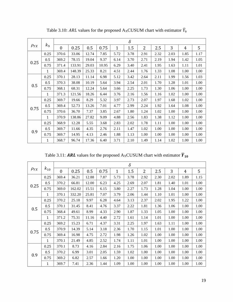
3.2 THE CLASSICAL CUSUM CONTROL CHART ...................................................................................... 11
3.3 THE PROPOSED AXCUSUM CONTROL CHART ................................................................................. 12
3.4 COMPARISONS .............................................................................................................................. 21
3.5 ILLUSTRATIVE EXAMPLE ................................................................................................................ 23
3.6 SUMMARY AND CONCLUSIONS ..................................................................................................... 25
CHAPTER 4 ................................................................................................................................ 27
Combined Shewhart CUSUM Charts using Auxiliary Variable ................................................................. 27
4.1 INTRODUCTION ............................................................................................................................. 28
vii
4.2 LOCATION ESTIMATORS AND THEIR PROPERTIES .......................................................................... 31
4.3 GENERAL STRUCTURE OF THE PROPOSED CHARTS ........................................................................ 35
4.3.1 SPECIAL CASES .......................................................................................................................... 37
4.4 PERFORMANCE MEASURES ........................................................................................................... 37
4.5 COMPARISONS WITH EXISTING CHARTS ....................................................................................... 51
4.5.1 CSCM i charts 10,,3,2 i vs. Classical CSC chart CSCM1 ................................ 51
4.5.2 CSCM i charts 10,,3,2 i vs. CUSUM charts based on Median, Mid-range, Hodges-
Lehman (HL), and Trimean (TM) estimators under unconterminated Normal distribution. .................... 52
4.6 ILLUSTRATIVE EXAMPLE ................................................................................................................ 54
4.7 CONCLUSIONS AND RECOMMENDATIONS .................................................................................... 57
CHAPTER 5 USING FIR TO IMPROVE CUSUM CHARTS FOR MONITORING
PROCESS DISPERSION ........................................................................................................... 58
5.1 INTRODUCTION ............................................................................................................................. 59
5.2 THE PROPOSED CHARTS ................................................................................................................ 61
5.2.1 CUSUM chart for monitoring process mean .............................................................................. 61
5.2.2 CUSUM chart for monitoring process dispersion ...................................................................... 62
5.2.3 FAST INITIAL RESPONSE (FIR) .................................................................................................... 66
5.3 PERFORMANCE EVALUATION AND COMPARISON ........................................................................ 66
5.4 SUMMARY AND CONCLUSION ...................................................................................................... 77
CHAPTER 6 SUMMARY AND CONCLUSION ..................................................................... 78
REFERENCES............................................................................................................................. 80
VITAE .......................................................................................................................................... 85
viii
LIST OF TABLES
Table 3.1 : Definition and properties of some estimators for estimating population
mean ................................................................................................................ 13
Table 3.2: Design parameters (𝑘𝑝, ℎ𝑝) of the proposed AXCUSUM for 𝐴𝑅𝐿0 ≅ 370 ... 15
Table 3.3: 𝐴𝑅𝐿 values for the proposed AXCUSUM chart with estimator 𝑌2 ................. 15
Table 3.4: 𝐴𝑅𝐿 values for the proposed AXCUSUM chart with estimator 𝑌3 ................. 16
Table 3.5: 𝐴𝑅𝐿 values for the proposed AXCUSUM chart with estimator 𝑌4 ................. 16
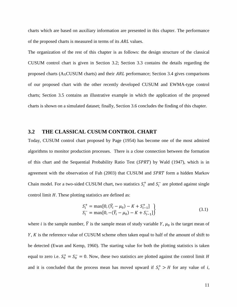
Table 3.6: 𝐴𝑅𝐿 values for the proposed AXCUSUM chart with estimator 𝑌5 ................. 17
Table 3.7: 𝐴𝑅𝐿 values for the proposed AXCUSUM chart with estimator 𝑌6 ................. 17
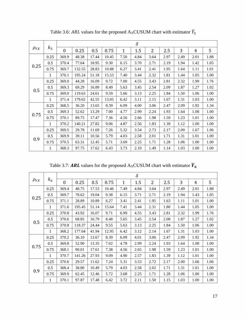
Table 3.8: 𝐴𝑅𝐿 values for the proposed AXCUSUM chart with estimator 𝑌7 ................. 18
Table 3.9: 𝐴𝑅𝐿 values for the proposed AXCUSUM chart with estimator 𝑌8 ................. 18
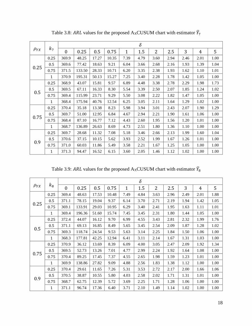
Table 3.10: 𝐴𝑅𝐿 values for the proposed AXCUSUM chart with estimator 𝑌9 ............... 19
Table 3.11: 𝐴𝑅𝐿 values for the proposed AXCUSUM chart with estimator 𝑌10 ............. 19
Table 3.12: Performance comparison of classical EWMA, classical CUSUM and
AXCUSUM charts with fixed 𝐴𝑅𝐿0 = 370 .................................................. 22
Table 4.1 : ARL values of the proposed charts with 25.0XA and k = 0.25 ........... 39
Table 4.2: ARL values of the proposed charts with 25.0XA and k = 0.5 ............ 40
Table 4.3: ARL values of the proposed charts with 75.0XA and k = 0.25 ......... 41
Table 4.4: ARL Values of the proposed charts with 75.0XA and k = 0.5 .................. 42
Table 4.5: SDRL values for the proposed charts with 25.0XA and k = 0.25 ............. 43
Table 4.6: SDRL Values for the proposed charts with 25.0XA and k = 0.5 ............ 44
Table 4.7: SDRL Values for the proposed charts with 75.0XA and k = 0.25 ........ 45

ix
Table 4.8: SDRL Values for the proposed charts with 75.0XA and k = 0.5 ............. 46
Table 4.9: Some selected proposed charts versus existing CUSUM charts based
on different estimators (Median, Mid-range, Hodges-Lehmann [HL]
and Trimean [TM]), when k = 0.25. ………………………………………….53
Table 4.10: Some selected proposed charts versus existing CUSUM charts based
on different estimators (Median, Mid-range, Hodges-Lehmann [HL]
and Trimean [TM]), when k = 0.5. …………………………………………..54
Table 5.1: SDRL and Quantile points of the proposed charts for upward shifts in 𝝈 at
ARL0 = 200. ..................................................................................................... 68
Table 5.2: SDRL and Quantile points of the proposed charts for downward shifts in
𝝈 at ARL0 = 200. .............................................................................................. 69
Table 5.3: EQL, RARL and PCI of the proposed charts. ................................................. 70
Table 5.4 : ARL comparison of dispersion charts for positive shift in process standard
deviation. ......................................................................................................... 71
Table 5.5: ARL comparison of dispersion charts for negative shift in process standard
deviation. .......................................................................................................... 72
x
LIST OF FIGURES
Figure 3.1: Graphical display of the classical CUSUM, A2CUSUM, A4CUSUM and
A10CUSUM charts for dataset 1 .................................................................... 25
Figure 3.2: Graphical display of the classical CUSUM, A2CUSUM, A4CUSUM and
A10CUSUM charts for dataset 2 .................................................................... 26
Figure 4.1: ARL curve of the proposed charts with XA = 0.25, k = 0.25 and
ARL0 = 370. .................................................................................................. 47
Figure 4.2: ARL curve of the proposed charts with XA = 0.25, k = 0.50 and
ARL0 = 370. .................................................................................................. 48
Figure 4.3: ARL curve of the proposed charts with XA = 0.75, k = 0.25 and
ARL0 = 370. .................................................................................................. 49
Figure 4.4: ARL curve of the proposed charts with XA = 0.75, k = 0.50 and
ARL0 = 370. .................................................................................................. 50
Figure 4.5: Graphical display of the CSCM i 2,1i charts. ......................................... 55
Figure 4.6. Graphical display of the CSCM i 5,4i charts. ....................................... 56
Figure 5.1: ARL curves of the proposed charts and some existing charts for positive shift
in standard deviation. ................................................................................... 73
Figure 5.2: ARL curves of the proposed charts and some existing charts for negative
shift in standard deviation. ........................................................................... 74

xi
LIST OF ABBREVIATIONS
ARL : Average Run Length
ARL0 : The ARL value when there is no shift in a process
ARL1 : The ARL value when there is a shift in a process
CL : Center Line
CUSUM : Cumulative Sum
EWMA : Exponentially Weighted Moving Average
FAR : False Alarm Rate
FIR : Fast Initial Response
LCL : Lower Control Limit
UCL : Upper Control Limit
xii
ABSTRACT
Full Name : [SANUSI Ridwan Adeyemi]
Thesis Title : [NEW EFFICIENT CUSUM CONTROL CHARTS]
Major Field : [Applied Statistics]
Date of Degree : [April, 2016]
Statistical quality control deals with monitoring of the production/manufacturing
processes and control chart is one of its major tools. It is vastly applied in industry to
keep the process variability under control. One of the most popular categories of control
charts is CUSUM chart which is based on utilizing the information on cumulative sum
pattern to detect small shifts. This thesis proposes new efficient CUSUM charts which are
based on the utilization of auxiliary information to monitor the location parameter of a
study variable. Furthermore, to increase the sensitivity of the proposed charts in detecting
moderate to large shifts, the proposed charts are extended to Combined Shewhart
CUSUM charts. CUSUM chart for monitoring dispersion parameter is also improved by
applying the Fast Initial Response. The average run length performance of the proposed
charts is evaluated in terms of shifts in study variable and compared with some recently
designed control structures meant for the same purposes. The comparisons revealed that
the proposed charts perform really well relative to the other charts under discussion. At
last, real life industrial examples are provided to describe the application procedure of the
proposed charts.

xiii
ملخص الرسالة
أدييمي رضوان ،سانوسي :االسم الكامل
الجديدة واألكثر فعالية CUSUMخرائط المراقبة :عنوان الرسالة
إحصاء تطبيقي التخصص:
2016نيسان، :تاريخ الدرجة العلمية
التصنيع، وخريطة المراقبة هي إحدى أدواتها. يتم تطبيق /يتعامل الضبط االحصائي للجودة مع مراقبة عمليات اإلنتاج
خريطة المراقبة الى حد كبير في الصناعة للحفاظ على تبيان العمليات بالمنتج ضمن المواصفات المطلوبة. إن
CUSUM هي واحدة من أهم أصناف خرائط المراقبة وهي مبنية على استخدام المعلومات عن ماهية أو نمط الجمع
جديدة وأكثر فعالية مبنية على CUSUMللكشف عن االزاحات الصغيرة. في هذه الرسالة نقترح طريقة التراكمي
استخدام معلومات مساعدة للتحكم بمعلمة الموقع الخاصة بالمتغير قيد الدراسة. إضافة الى أن هذه الطريقة المقترحة
Shewhartطة المقترحة تم توسعتها الى خرائط لها القدرة في الكشف عن اإلزاحات المتوسطة الى الكبيرة، الخري
CUSUM المركبة. كذلك في هذه الرسالة تم إجراء تحسين على خريطةCUSUM للتحكم بمعلمة التشتت من
للخريطة المقترحة من ARL. تم حساب متوسط طول المدى FIRخالل تطبيق ما يسمى باالستجابة األولية السريعة
ر قيد الدراسة وتم مقارنتها مع تصاميم أخرى حديثة مماثلة. أظهرت المقارنات بأن أداء خالل معلمة االزاحة للمتغي
الخريطة المقترحة أفضل من الخرائط األخرى التي شملتها الرسالة. وأخيرا، تم عرض أمثلة واقعية من القطاع
الصناعي وذلك كتطبيق على الطريقة الجديدة المقترحة في هذه الرسالة.
1
1 CHAPTER 1
INTRODUCTION
Control chart is a statistical chart to observe process quality, it is one of the seven tool kits
(Pareto diagram, Cause and effect diagram, Flowcharts, Control chart, Histogram, Scatter
diagram and Check sheet) of statistical process control (Montgomery, 2009). Two core types of
control chart exist depending on the number of process features or variable to be examined; the
univariate control chart and the multivariate control charts. The former is a graphical
representation that summarizes one quality characteristic, while the latter describes the
characteristics of two or more variable of interest.
Univariate control chart shows the value of the variable of interest over time or against sample
number. In addition, three lines exist in a chart; the lower control limit (LCL), the center line
(CL) and the upper control limit (UCL). The CL indicates the average value of the in-control
process, while the UCL and the LCL give boundaries around the CL for declaring that a process
is in-control. These control limits are carefully chosen to ensure that all the study observations
are within these boundaries as far as the process remains in-control.
Control charts are used for observing different shifts in a process, these shifts can be a transient
shift (memoryless structure) or a persistent shift (memory structure). Shewhart (1924) introduced
the Shewhart control chart for detecting transient shifts. This chart monitors sudden shift by
using information from the most recent examined samples, consequently, it is not effective in
monitoring minute shifts in a process. However, small shifts can be monitored by the memory-
2
type control charts, which are the EWMA chart, developed by Roberts (1959), and the CUSUM
control chart, proposed by Page (1954). The Exponentially Weighted Moving Average
(EWMA), allot larger weight to the most current data points for detecting small shifts in a
process. Also, the CUSUM chart is based on geometric moving average. It detects smaller shifts
efficiently by using information from a very long sequence of samples.
In this thesis, CUSUM control chart is considered extensively by proposing new CUSUM charts
that are more efficient in detecting smaller to moderate shifts, than the ones in the literature. The
efficiency is mainly compared using the average run length (ARL) approach. The proposed
charts are compared with existing charts of the same purpose. Efficient estimators used in the
field of sampling techniques are used for the construction of the proposed CUSUM charts. The
proposed charts detect shifts in location parameter or dispersion parameter in a process, and
various statistical properties of the charts are examined.
1.1 CUSUM CONTROL CHART
The CUSUM control chart is used in detecting small shift in a variable (X) of a process, it is a
cumulative deviation from the target value 0 . It is calculated by two statistics which are the
10,0max ttt CKXC (1.1)
10,0max ittt CKXC (1.2)
upper CUSUM tC and the lower CUSUM tC , where t is the observation number and
000 CC though they can also be set to other values (Headstart values) for fast initial
3
response (FIR) CUSUM (Hawkins and Olwell, 1998). Both
tC and
tC are plotted against
control limits (H). K is the reference value, and it is taken to be half of the shift (𝛿) to be
detected, scaled in standard deviation (𝜎) unit, under the assumption that the study variable X is
normally distributed. The lower the value of K , the more sensitive the CUSUM control chart is
to small shifts. tX represents the tth observation for a single sample size (n = 1). For a subgroup (
1n ), tX is replaced with the mean of the subgroup in each observation.

4
2 CHAPTER 2
LITERATURE REVIEW
In the field of engineering, statistical process control (SPC) is recurrently connected to the use of
charting methods for identifying changes in variability or mean of a process. Its activities include
Pareto analysis, the experimental design and multivariable analysis, design of sampling and
inspection schemes. Base on design structure, we can group control charts into two different
aspects; the memoryless control chart (Shewhart-type) and memory control charts. The
frequently used memory control charts are the Cumulative Sum (CUSUM) control charts and the
Exponentially Weighted Moving Average (EWMA) control chart proposed by Page (1954) and
Roberts (1959) respectively. Unlike the Shewhart-type charts that ignores the past information,
the CUSUM and the EWMA charts make use of the past information and the current information
to give a better performance in detecting small shifts and moderate shifts. The structure of the
CUSUM charts and their average run length(ARL) performance for various choices of parameters
are well explained in Hawkins and Olwell (1998). When fundamental distribution of a process is
not normal or unlikely to be normal, nonparametric control charts will be good. Considering
small shifts in scatter outliers, Midi and Shabbak (2011) proposed robust EWMA and CUSUM
for early detection of the shift in multivariate case. Li et al. (2010) introduced two nonparametric
equivalents of the CUSUM and EWMA control charts for detecting shifts in the location
parameter of a process, based on the Wilcoxon rank-sum test. The application of robust control
chart in CUSUM for detecting shifts in location and dispersion of a process simultaneously was
considered by Reynolds and Stoumbos (2010).
5
Some authors also consider the use of auxiliary variable to increase the efficiency of the study
variate, which we also consider in this thesis work. When assessing a control chart’s plotting
statistic(s), Riaz (2008a) popularized the notion of using auxiliary information. He suggested a
control chart which uses a regression-type estimator as the plotting statistic to monitor the
process’s variability, and showed the supremacy of his chart over the famous Shewhart-type
control charts for the same drive. Aiming on small shifts and moderate shifts in the location
parameter of a process, Abbas et al. (2014) proposed an EWMA-type control chart which uses
one auxiliary variable. The mean in the structure of the proposed chart is estimated using the
regression estimation method. It was established that the chart outperformed its univariate and
bivariate counterparts. Furthermore, Riaz (2008b) proposed a regression-type estimator to
monitor the location of a process. He not only showed the superiority of his proposal over the
Shewhart’s X -chart, but also over the regression charts and the cause-selecting charts.
Due to the advancement in technology and industrial processes, there is need to enhance the
sensitivity of CUSUM charts to large shifts. This is done by combining the CUSUM chart with
the Shewhart chart, to detects small to large shifts effectively at the same time. Westgard et al.
(1977) applied this concept to improve quality control in clinical chemistry. The combination of
Shewhart chart and CUSUM chart was observed by Lucas (1982) after which some scholars
improved the chart by proposing more efficient charts. Combined Shewhart-CUSUM (hereafter
called “CSC”) for location parameter can be optimized over the entire mean shift range by
adding an extra parameter (w) known as the exponential of the sample mean shift, to the
structure of the CSC. This will improve its performance and it will not increase the difficulty
level of understanding and implementing the chart (Wu et al., 2008). The CSC, which has a wide
range of application, attracts the attention of Environmentalists, and it is the only quality control

6
chart directly recommended by the United States Environment Protection Agency for intra-well
monitoring. It has been consistently applied to waste disposal facilities for detection monitoring
programs (Gibbons, 1999). Abujiya et al. (2013) replaced the traditional simple random
sampling in the plotting statistic of the CSC chart with ranked set sampling.
Control charts monitor the location and (or) dispersion parameter(s) of a process. The location
parameter monitoring and its modification is mostly available in the literature, but little work has
been done on dispersion monitoring. In detecting shift in process dispersion, CUSUM was
applied to subgroup range by Page (1954). Tuprah and Ncube (1987) later compared this
procedure with another procedure that was based on sample standard deviation. Using ARL
approach, they found that the procedure based on the sample standard deviation detects shift
from the target value faster, given that the process variables are normally distributed.
Furthermore, one-sided and two-sided CUSUM structures based on logarithmic transformation
of process variance was proposed by Chang & Gan (1995) for monitoring shift in process
variance, and they also enhanced the performance of the schemes by introducing the Fast Initial
Response (FIR) feature. The FIR was first proposed by Roberts (1959) and later improved by
Steiner (1999) to reduce the time-varying limits of the first few sample observations. The FIR
feature improves the performance of CUSUM chart if there is shift in a process at start-up
(Hawkins and Olwell, 1998). The performance of this feature was later improved by using a
power transformation with respect to time t (Haq, 2013).

7
2.1 OBJECTIVES OF THE STUDY
We summarize the main objectives to be achieved in this study:
1. To improve CUSUM control chart that monitor location parameter.
2. To improve CUSUM control chart that monitor dispersion parameter.
3. To extend the proposed charts to combined Shewhart-CUSUM chart.
4. To compare the proposed charts with their counterparts using average run length and some
other performance measures.
5. Apply this study to numerous real life dataset.
8
3 CHAPTER 3
Efficient CUSUM-Type Control Charts for Monitoring the Process Mean
Using Auxiliary Information
Statistical quality control deals with monitoring of the production/manufacturing processes and
control chart is one of its major tools. It is vastly applied in industry to keep the process
variability under control. One of the most popular categories of control charts is CUSUM chart
which is based on utilizing the information on cumulative sum pattern. This article proposes a
new two-sided CUSUM charts which are based on the utilization of auxiliary information. The
𝐴𝑅𝐿 performance of the proposed charts is evaluated in terms of shifts in study variable and
compared with some recently designed control structures meant for the same purposes. The
comparisons revealed that the proposed charts perform really well relative to the other charts
under discussion. At last, a real life industrial example is provided to describe the application
procedure of the proposal.
9
3.1 INTRODUCTION
The output of all the manufacturing processes always includes some amount of variation in it;
e.g. in the process of filling two bottles with cooking oil, the amount of oil filled in any of the
two bottles will not be exactly the same, and in the process of making tube light rods, the
diameter or length of any two rods will not be the same, etc. This inherent part of process is
known as common (uncontrollable) cause variation. The variations outside this common cause
pattern are called special (controllable) cause variations. These variations are usually large in
magnitude, controllable in nature and due to many inescapable causes. Statistical Quality Control
(𝑆𝑄𝐶) includes some tools that can be used to discriminate between common and special cause
variations. There are seven most commonly referred tools (Montgomery, 2009) and these tools
are jointly known as 𝑆𝑄𝐶 tool-kit. The most important and the most powerful tool of this kit is
the control chart which is the graphical display of a quality characteristic plotted against three
lines named as Upper Control Limit (𝑈𝐶𝐿), Center Line (𝐶𝐿) and Lower Control Limit (𝐿𝐶𝐿).
The two control limits (i.e. 𝑈𝐶𝐿 and 𝐿𝐶𝐿) are basically the parameters of a control chart which
are selected in such a way that there is a very small probability, generally referred as False Alarm
Rate (𝐹𝐴𝑅) in quality control literature and denoted by (𝛼)) of the in-control data points falling
outside these limits.
Control charts are further classified as Shewhart, CUSUM and EWMA-type control charts. The
structure of Shewhart-type control charts proposed by Shewhart (1924) is made such that they
utilize just the present information and hence, they ignore all the past information which results
in less efficiency of these charts for detecting shifts (alterations in a process) that are of smaller
magnitude. This drawback of Shewhart-type control charts leads to the proposal of Cumulative
Sum (CUSUM) control charts (Page, 1954) and Exponentially Weighted Moving Average
(EWMA) control charts (Roberts, 1959). The formation of these control charts is based on
10
utilizing the past information along with the present to improve the performance of control charts
for detecting small amount of shifts. The two most commonly named performance measures for
control charts are power and average run length (𝐴𝑅𝐿). Power of a control chart is defined as the
probability of detecting a shift whereas 𝐴𝑅𝐿 is defined as average number of samples required to
detect a shift. 𝐴𝑅𝐿0 and 𝐴𝑅𝐿1 are the representations of in-control and out-of-control chart 𝐴𝑅𝐿𝑠
respectively, for a control chart. The 𝐴𝑅𝐿𝑠 for the Shewhart-type charts ( like �̅�, 𝑅, 𝑆 and 𝑆2)
can be obtained by taking the reciprocal of power, as the assumptions of having a geometric run
falseishypothesisnullhypothesisnullrejectPPowerARL
|
11
length variable are fulfilled for these charts. For CUSUM and EWMA-type control chart, the
𝐴𝑅𝐿 values are obtained through averaging the exact run length distribution, as the assumption
of geometric run length variable does not hold for these charts.
Auxiliary information is the extra information accessible apart from the information from the
sample, at the estimation stage. Ratio, product and regression-type estimators are the most
commonly quoted fashions of the exploitation of auxiliary information at the time of estimation
(Fuller, 2011). The design of these estimators are structured such that they make use of the
sample information and the auxiliary information, hence, they are more efficient than the
traditional ones. There is a long history of the use of auxiliary information in the field of survey
sampling but Riaz (2008a) popularized the concept of using it at estimation stage in 𝑆𝑄𝐶. Riaz
(2008a) and Riaz (2008b) proposed the auxiliary based control charts for monitoring the process
variability and location respectively where both of these charts are based on regression-type
estimators. Furthermore, Riaz and Does (2009) suggested another variability chart based on a
ratio-type estimator and showed the dominance of their proposed chart over the one based on
regression-type estimator. Following the work of all these authors, several CUSUM-type control
11
charts which are based on auxiliary information are presented in this chapter. The performance
of the proposed charts is measured in terms of its 𝐴𝑅𝐿 values.
The organization of the rest of this chapter is as follows: the design structure of the classical
CUSUM control chart is given in Section 3.2; Section 3.3 contains the details regarding the
proposed charts (AXCUSUM charts) and their 𝐴𝑅𝐿 performance; Section 3.4 gives comparisons
of our proposed chart with the other recently developed CUSUM and EWMA-type control
charts; Section 3.5 contains an illustrative example in which the application of the proposed
charts is shown on a simulated dataset; finally, Section 3.6 concludes the finding of this chapter.
3.2 THE CLASSICAL CUSUM CONTROL CHART
Today, CUSUM control chart proposed by Page (1954) has become one of the most admired
algorithms to monitor production processes. There is a close connection between the formation
of this chart and the Sequential Probability Ratio Test (𝑆𝑃𝑅𝑇) by Wald (1947), which is in
agreement with the observation of Fuh (2003) that CUSUM and 𝑆𝑃𝑅𝑇 form a hidden Markov
Chain model. For a two-sided CUSUM chart, two statistics 𝑆𝑖+ and 𝑆𝑖
− are plotted against single
control limit 𝐻. These plotting statistics are defined as:
𝑆𝑖
+ = max[0, (�̅�𝑖 − 𝜇0) − 𝐾 + 𝑆𝑖−1+ ]
𝑆𝑖− = max[0, −(�̅�𝑖 − 𝜇0) − 𝐾 + 𝑆𝑖−1
− ]} (3.1)
where 𝑖 is the sample number, �̅� is the sample mean of study variable 𝑌, 𝜇0 is the target mean of
𝑌, 𝐾 is the reference value of CUSUM scheme often taken equal to half of the amount of shift to
be detected (Ewan and Kemp, 1960). The starting value for both the plotting statistics is taken
equal to zero i.e. 𝑆0+ = 𝑆0
− = 0. Now, these two statistics are plotted against the control limit 𝐻
and it is concluded that the process mean has moved upward if 𝑆𝑖+ > 𝐻 for any value of 𝑖,

12
whereas the process mean is said to be shifted downward if 𝑆𝑖− > 𝐻 for any value of 𝑖. The
CUSUM chart is defined by two parameters i.e. 𝐾 and 𝐻 which are to be chosen very carefully
because, the 𝐴𝑅𝐿 performance of the CUSUM chart is very sensitive to these parameters
(Montgomery, 2009). These two parameters are used in the standardized manner (Montgomery,
2009) given as:
𝐾 = 𝑘 × √Var(�̅�), and 𝐻 = ℎ × √Var(�̅�) (3.2)
where √Var(�̅�) =𝜎𝑌
√𝑛⁄ and 𝜎𝑌 is the standard deviation of 𝑌. In the next section, we provide
the details regarding the proposed chart, for which we have used the version of the CUSUM
given in (3.1).
3.3 THE PROPOSED AXCUSUM CONTROL CHART
Suppose (𝑦𝑖1, 𝑥𝑖1), (𝑦𝑖2, 𝑥𝑖2), (𝑦𝑖3, 𝑥𝑖3), . .. (where 𝑖 = 1,2, …) represent a sequence of paired
observations taken for a quality characteristic 𝑌 (which is the study variable) and is also
correlated with the auxiliary variable 𝑋. Each pair (𝑌𝑖𝑗 , 𝑋𝑖𝑗) for 𝑗 = 1,2,3, … , 𝑛 is assumed to
follow bivariate normal distribution with mean vector 𝜇 and variance-covariance matrix Σ given
as:
𝜇 = (𝜇0 + 𝛿𝜎𝑌
𝜇𝑋), 𝛴 = (
𝜎𝑌2 Cov(𝑌, 𝑋)
Cov(𝑋, 𝑌) 𝜎𝑋2 ) (3.3)
where 𝜇0 is the in-control mean of study variable 𝑌 and 𝜇𝑋 are the known mean of auxiliary
variable 𝑋. 𝜎𝑌2 and 𝜎𝑋
2 are the population variances of 𝑌 and 𝑋, respectively, and are assumed to
be known. Cov(𝑌, 𝑋) = Cov(𝑋, 𝑌) is the covariance between the study variable 𝑌 and the
auxiliary variable 𝑋. 𝛿 represents the amount of shift introduced in the study variable 𝑌 in 𝜎𝑌

13
units i.e. 𝛿 =|𝜇1−𝜇0|
𝜎𝑌, where 𝜇1 represents the out-of-control mean of 𝑌. Now based on (3.3),
there are several estimators in the literature for estimating the population mean (Srivastava
(1967), Singh and Tailor (2003), Kadilar and Cingi (2004) and Cochran (1977)). Some of them
(along with their expected value and mean square error) are given in Table 3.1.
Table 3.1 : Definition and properties of some estimators for estimating population mean
Estimators (�̅�𝑝, 𝑝 = 1,2, … ,10) 𝐸(�̅�𝑝) 𝑀𝑆𝐸(�̅�𝑝)
�̅�1 =∑ 𝑌𝑗
𝑛𝑗=1
𝑛 𝜇0
𝜎𝑌2
𝑛
�̅�2 = �̅� + 𝑏𝑌𝑋(𝜇𝑋 − �̅�) 𝜇0 − Cov(�̅�, 𝑏𝑌𝑋) 𝜎𝑌
2
𝑛(1 − 𝜌𝑌𝑋
2 )
�̅�3 = �̅� (𝜇𝑋
�̅�) 𝜇0 +
𝜇𝑌(𝐶𝑋2 − 𝜌𝑌𝑋𝐶𝑌𝐶𝑋)
𝑛
𝜇𝑌2(𝐶𝑌
2 + 𝐶𝑋2 − 2𝜌𝑌𝑋𝐶𝑌𝐶𝑋)
𝑛
�̅�4 = �̅� (𝜇𝑋 + 𝜌𝑌𝑋
�̅� + 𝜌𝑌𝑋
) 𝜇0 +𝜇𝑌𝑔(𝑔𝐶𝑋
2 − 𝜌𝑌𝑋𝐶𝑌𝐶𝑋)
𝑛
𝜇𝑌2(𝐶𝑌
2 + 𝑔2𝐶𝑋2 − 2𝑔𝜌𝑌𝑋𝐶𝑌𝐶𝑋)
𝑛
�̅�5 = [�̅� + 𝑏𝑌𝑋(𝜇𝑋 − �̅�)] (𝜇𝑋
�̅�) 𝜇0 +
𝜇𝑋𝐶𝑋2
𝑛
𝜇𝑋2 [𝐶𝑋
2 + 𝐶𝑌2(1 − 𝜌𝑌𝑋
2 )]
𝑛
�̅�6 = [�̅� + 𝑏𝑌𝑋(𝜇𝑋 − �̅�)] (𝜇𝑋 + 𝐶𝑋
�̅� + 𝐶𝑋
) 𝜇0 +𝜇𝑋𝐶𝑋
2
𝑛(
𝜇𝑋
𝜇𝑋 + 𝐶𝑋)
2
𝜇𝑋
2 [(𝜇𝑋
𝜇𝑋 + 𝐶𝑋)
2𝐶𝑋
2 + 𝐶𝑌2(1 − 𝜌𝑌𝑋
2 )]
𝑛
�̅�7 = [�̅� + 𝑏𝑌𝑋(𝜇𝑋 − �̅�)] (𝜇𝑋 + 𝛽2(𝑋)
�̅� + 𝛽2(𝑋)
) 𝜇0 +𝜇𝑋𝐶𝑋
2
𝑛(
𝜇𝑋
𝜇𝑋 + 𝛽2(𝑋))
2
𝜇𝑋
2 [(𝜇𝑋
𝜇𝑋 + 𝛽2(𝑋))
2
𝐶𝑋2 + 𝐶𝑌
2(1 − 𝜌𝑌𝑋2 )]
𝑛
�̅�8 = [�̅� + 𝑏𝑌𝑋(𝜇𝑋 − �̅�)] (𝜇𝑋𝛽2(𝑋) + 𝐶𝑋
�̅�𝛽2(𝑋) + 𝐶𝑋
) 𝜇0 +𝜇𝑋𝐶𝑋
2
𝑛(
𝜇𝑋𝛽2(𝑋)
𝜇𝑋𝛽2(𝑋) + 𝐶𝑋)
2
𝜇𝑋
2 [(𝜇𝑋𝛽2(𝑋)
𝜇𝑋𝛽2(𝑋) + 𝐶𝑋)
2
𝐶𝑋2 + 𝐶𝑌
2(1 − 𝜌𝑌𝑋2 )]
𝑛
�̅�9 = [�̅� + 𝑏𝑌𝑋(𝜇𝑋 − �̅�)] (𝜇𝑋𝐶𝑋 + 𝛽2(𝑋)
�̅�𝐶𝑋 + 𝛽2(𝑋)
) 𝜇0 +𝜇𝑋𝐶𝑋
2
𝑛(
𝜇𝑋𝐶𝑋
𝜇𝑋𝐶𝑋 + 𝛽2(𝑋))
2
𝜇𝑋
2 [(𝜇𝑋𝐶𝑋
𝜇𝑋𝐶𝑋 + 𝛽2(𝑋))
2
𝐶𝑋2 + 𝐶𝑌
2(1 − 𝜌𝑌𝑋2 )]
𝑛
�̅�10 = �̅� (𝜇𝑋
�̅�)
𝛼
𝜇0 +
𝜇𝑌 (𝛼(𝛼 − 1)
2𝐶𝑋
2 − 𝛼𝜌𝑌𝑋𝐶𝑌𝐶𝑋)
𝑛
𝜇𝑌2(𝐶𝑌
2 + 𝛼2𝐶𝑋2 − 2𝛼𝜌𝑌𝑋𝐶𝑌𝐶𝑋)
𝑛

14
Some of the quantities in Table 3.1 are defined as: 𝑏𝑌𝑋 =𝑠𝑌𝑋
𝑠𝑋2 is the sample regression coefficient
where 𝑠𝑌𝑋 =1
𝑛−1∑ (𝑌𝑗 − �̅�)(𝑋𝑗 − �̅�)𝑛
𝑗=1 and 𝑠𝑋2=
1
𝑛−1∑ (𝑋𝑗 − �̅�)
2𝑛𝑗=1 ; 𝛽𝑌𝑋 =
𝜎𝑌𝑋
𝜎𝑋2 is the population
regression coefficient; 𝜌𝑌𝑋 is the population correlation coefficient between the variables 𝑋 and
𝑌; 𝐶𝑌 =𝜎𝑌
𝜇𝑌 and 𝐶𝑋 =
𝜎𝑋
𝜇𝑋 are the population coefficient of variation for variables 𝑌 and 𝑋,
respectively; 𝑔 =𝜇𝑋
𝜇𝑋+𝜌𝑌𝑋; 𝛽2(𝑋) is the population coefficient of kurtosis for variable 𝑋; the
optimal value for 𝛼 (that minimizes the mean square error) 𝛼 = −𝜌𝑌𝑋𝐶𝑌
𝐶𝑋.
In this section, we have utilized the efficiency of the estimators in Table 3.1 to design a
CUSUM-type structure and tried to study the effect of these efficient estimators on the 𝐴𝑅𝐿
performance of CUSUM chart. Now the plotting statistics of the proposed chart (which is based
on the estimators given in Table 1) is given as:
𝑇𝑖+ = max [0, (�̅�𝑝,𝑖 − 𝐸(�̅�𝑝)) − 𝐾𝑝 + 𝑇𝑖−1
+ ]
𝑇𝑖− = max [0, − (�̅�𝑝,𝑖 − 𝐸(�̅�𝑝)) − 𝐾𝑝 + 𝑇𝑖−1
− ]} (3.4)
Initial values for the statistics given in (3.4) are taken equal to zero i.e. 𝑇0+ = 𝑇0
− = 0. The
decision rule for the proposed chart is given as: the statistics 𝑇𝑖+ and 𝑇𝑖
− are plotted against the
control limit 𝐻𝑝. For any value of 𝑖, if the value of 𝑇𝑖+ exceeds the value of 𝐻𝑝 then the process
mean is declared to be shifted upward and if the value of 𝑇𝑖− exceeds the value of 𝐻𝑝 then the
process mean is said to be moved downward. 𝐾𝑝 and 𝐻𝑝 are defined as:
𝐾𝑝 = 𝑘𝑝 × √𝑀𝑆𝐸(�̅�𝑝) and 𝐻𝑝 = ℎ𝑝 × √𝑀𝑆𝐸(�̅�𝑝) (3.5)
where 𝑘𝑝 and ℎ𝑝 are the design parameters of the proposed AXCUSUM chart. The values of 𝑘𝑝
and ℎ𝑝 need to be selected very carefully because the 𝐴𝑅𝐿 properties of the proposed chart
mainly depend on these two constants (along with the value of 𝜌𝑌𝑋). For some selected values of

15
Table 3.2: Design parameters (𝒌𝒑, 𝒉𝒑) of the proposed AXCUSUM for 𝑨𝑹𝑳𝟎 ≅ 𝟑𝟕𝟎
𝜌𝑌𝑋 Estimator
�̅�1 �̅�2 �̅�3 �̅�4 �̅�5 �̅�6 �̅�7 �̅�8 �̅�9 �̅�10
0.25
(0.25,8.008) (0.25,8.082) (0.25,8.018) (0.25,8.048) (0.25,8.048) (0.25,8.094) (0.25,8.085) (0.25,8.083) (0.25,8.040) (0.25,8.091)
(0.50,4.774) (0.50,5.099) (0.50,4.787) (0.50,4.782) (0.50,4.782) (0.50,5.088) (0.50,5.101) (0.50,5.088) (0.50,5.059) (0.50,5.100)
(0.75,3.339) (0.75,3.860) (0.75,3.340) (0.75,3.348) (0.75,3.348) (0.75,3.860) (0.75,3.850) (0.75,3.863) (0.75,3.831) (0.75,3.864)
(1.00,2.516) (1.00,3.180) (1.00,2.512) (1.00,2.522) (1.00,2.522) (1.00,3.177) (1.00,3.169) (1.00,3.175) (1.00,3.150) (1.00,3.194)
0.50
(0.25,8.008) (0.25,8.083) (0.25,8.000) (0.25,8.004) (0.25,8.004) (0.25,8.078) (0.25,8.083) (0.25,8.078) (0.25,8.084) (0.25,8.135)
(0.50,4.774) (0.50,5.060) (0.50,4.775) (0.50,4.762) (0.50,4.762) (0.50,5.070) (0.50,5.084) (0.50,5.066) (0.50,5.086) (0.50,5.138)
(0.75,3.339) (0.75,3.860) (0.75,3.329) (0.75,3.330) (0.75,3.330) (0.75,3.838) (0.75,3.836) (0.75,3.834) (0.75,3.840) (0.75,3.894)
(1.00,2.516) (1.00,3.180) (1.00,2.508) (1.00,2.499) (1.00,2.499) (1.00,3.146) (1.00,3.145) (1.00,3.145) (1.00,3.145) (1.00,3.217)
0.75
(0.25,8.008) (0.25,8.084) (0.25,8.014) (0.25,7.995) (0.25,7.995) (0.25,8.075) (0.25,8.050) (0.25,8.067) (0.25,8.072) (0.25,8.108)
(0.50,4.774) (0.50,5.065) (0.50,4.775) (0.50,4.760) (0.50,4.760) (0.50,5.045) (0.50,5.040) (0.50,5.039) (0.50,5.043) (0.50,5.108)
(0.75,3.339) (0.75,3.845) (0.75,3.342) (0.75,3.332) (0.75,3.332) (0.75,3.780) (0.75,3.772) (0.75,3.772) (0.75,3.773) (0.75,3.885)
(1.00,2.516) (1.00,3.168) (1.00,2.513) (1.00,2.506) (1.00,2.506) (1.00,3.070) (1.00,3.070) (1.00,3.069) (1.00,3.066) (1.00,3.210)
0.90
(0.25,8.008) (0.25,8.030) (0.25,8.010) (0.25,7.984) (0.25,7.984) (0.25,8.049) (0.25,8.041) (0.25,8.041) (0.25,8.035) (0.25,8.043)
(0.50,4.774) (0.50,5.066) (0.50,4.768) (0.50,4.744) (0.50,4.744) (0.50,4.936) (0.50,4.946) (0.50,4.942) (0.50,4.939) (0.50,5.100)
(0.75,3.339) (0.75,3.840) (0.75,3.338) (0.75,3.320) (0.75,3.320) (0.75,3.630) (0.75,3.636) (0.75,3.640) (0.75,3.626) (0.75,3.882)
(1.00,2.516) (1.00,3.163) (1.00,2.512) (1.00,2.500) (1.00,2.500) (1.00,2.890) (1.00,2.900) (1.00,2.901) (1.00,2.880) (1.00,3.192)
Table 3.3: 𝐴𝑅𝐿 values for the proposed AXCUSUM chart with estimator �̅�2
𝜌𝑌𝑋 𝑘2 𝛿
0 0.25 0.5 0.75 1 1.5 2 2.5 3 4 5
0.25
0.25 371.8 31.91 12.36 7.65 5.58 3.70 2.85 2.26 2.02 1.80 1.12
0.5 370.9 28.56 8.88 4.95 3.46 2.25 1.76 1.35 1.08 1.00 1.00
0.75 370.7 82.32 14.79 6.47 4.12 2.46 1.87 1.46 1.13 1.00 1.00
1 370.6 141.90 23.53 7.72 4.33 2.37 1.71 1.28 1.06 1.00 1.00
0.5
0.25 371.2 26.95 10.77 6.76 4.96 3.33 2.56 2.07 1.98 1.46 1.01
0.5 369.7 35.61 9.66 5.40 3.80 2.46 1.97 1.62 1.21 1.00 1.00
0.75 369.3 64.13 11.55 5.37 3.52 2.19 1.68 1.24 1.04 1.00 1.00
1 369.4 115.40 16.82 6.08 3.59 2.08 1.49 1.12 1.02 1.00 1.00
0.75
0.25 371.4 18.39 7.84 5.06 3.78 2.60 2.03 1.93 1.51 1.01 1.00
0.5 369.3 20.58 6.52 3.90 2.83 1.99 1.52 1.08 1.01 1.00 1.00
0.75 369.9 32.70 6.79 3.61 2.53 1.71 1.16 1.01 1.00 1.00 1.00
1 367.6 60.24 8.26 3.70 2.45 1.53 1.08 1.01 1.00 1.00 1.00
0.9
0.25 372.2 10.81 4.98 3.34 2.56 1.98 1.47 1.02 1.00 1.00 1.00
0.5 369.5 9.79 3.83 2.48 1.98 1.22 1.01 1.00 1.00 1.00 1.00
0.75 370.7 11.67 3.55 2.21 1.69 1.04 1.00 1.00 1.00 1.00 1.00
1 370.1 17.16 3.63 2.10 1.50 1.02 1.00 1.00 1.00 1.00 1.00

16
Table 3.4: 𝐴𝑅𝐿 values for the proposed AXCUSUM chart with estimator �̅�3
𝜌𝑌𝑋 𝑘3 𝛿
0 0.25 0.5 0.75 1 1.5 2 2.5 3 4 5
0.25
0.25 369.4 32.96 12.76 7.90 5.75 3.80 2.91 2.34 2.04 1.83 1.20
0.5 370.1 42.25 11.52 6.24 4.31 2.73 2.09 1.77 1.43 1.02 1.00
0.75 367.3 59.42 13.09 6.04 3.84 2.30 1.71 1.32 1.09 1.00 1.00
1 368.5 80.22 16.72 6.55 3.78 2.08 1.47 1.15 1.02 1.00 1.00
0.5
0.25 370.3 24.52 9.97 6.30 4.66 3.14 2.38 2.03 1.94 1.25 1.00
0.5 369.8 28.41 8.39 4.78 3.40 2.24 1.80 1.38 1.08 1.00 1.00
0.75 368.8 38.85 8.71 4.37 2.93 1.87 1.35 1.07 1.00 1.00 1.00
1 371.8 53.81 10.30 4.40 2.75 1.63 1.17 1.02 1.00 1.00 1.00
0.75
0.25 371.7 15.33 6.72 4.38 3.32 2.25 1.97 1.64 1.11 1.00 1.00
0.5 369.5 14.67 5.16 3.18 2.37 1.71 1.15 1.00 1.00 1.00 1.00
0.75 369.1 17.88 4.77 2.72 1.98 1.26 1.01 1.00 1.00 1.00 1.00
1 369.1 23.85 4.91 2.52 1.74 1.11 1.00 1.00 1.00 1.00 1.00
0.9
0.25 368.9 8.76 4.16 2.84 2.15 1.77 1.04 1.00 1.00 1.00 1.00
0.5 368.8 7.09 3.00 2.05 1.60 1.01 1.00 1.00 1.00 1.00 1.00
0.75 370.3 7.06 2.56 1.66 1.18 1.00 1.00 1.00 1.00 1.00 1.00
1 371.3 8.02 2.35 1.42 1.07 1.00 1.00 1.00 1.00 1.00 1.00
Table 3.5: 𝑨𝑹𝑳 values for the proposed AXCUSUM chart with estimator �̅�𝟒
𝜌𝑌𝑋 𝑘4 𝛿
0 0.25 0.5 0.75 1 1.5 2 2.5 3 4 5
0.25
0.25 368.9 32.99 12.76 7.90 5.76 3.81 2.91 2.34 2.04 1.83 1.20
0.5 370.1 41.79 11.47 6.23 4.30 2.72 2.09 1.76 1.42 1.02 1.00
0.75 369.2 59.38 13.13 6.03 3.84 2.31 1.71 1.32 1.08 1.00 1.00
1 369.7 80.63 16.73 6.54 3.78 2.09 1.47 1.15 1.03 1.00 1.00
0.5
0.25 370.7 24.47 9.98 6.29 4.64 3.14 2.38 2.02 1.94 1.25 1.00
0.5 371.6 28.20 8.32 4.76 3.38 2.24 1.80 1.37 1.08 1.00 1.00
0.75 369.6 38.83 8.70 4.34 2.92 1.86 1.35 1.07 1.00 1.00 1.00
1 368.6 53.29 10.26 4.38 2.73 1.62 1.17 1.02 1.00 1.00 1.00
0.75
0.25 370.7 15.21 6.70 4.37 3.30 2.24 1.97 1.62 1.11 1.00 1.00
0.5 369.4 14.64 5.13 3.16 2.36 1.70 1.14 1.00 1.00 1.00 1.00
0.75 368.3 17.90 4.75 2.71 1.98 1.25 1.01 1.00 1.00 1.00 1.00
1 368.9 23.96 4.88 2.51 1.73 1.11 1.00 1.00 1.00 1.00 1.00
0.9
0.25 369.7 8.71 4.13 2.83 2.14 1.77 1.04 1.00 1.00 1.00 1.00
0.5 370.6 7.03 2.98 2.04 1.59 1.01 1.00 1.00 1.00 1.00 1.00
0.75 370.3 7.03 2.54 1.65 1.18 1.00 1.00 1.00 1.00 1.00 1.00
1 368.6 7.94 2.34 1.42 1.07 1.00 1.00 1.00 1.00 1.00 1.00
17
Table 3.6: 𝐴𝑅𝐿 values for the proposed AXCUSUM chart with estimator �̅�5
𝜌𝑌𝑋 𝑘5 𝛿
0 0.25 0.5 0.75 1 1.5 2 2.5 3 4 5
0.25
0.25 369.9 48.38 17.44 10.45 7.50 4.84 3.64 2.97 2.49 2.01 1.88
0.5 370.4 77.64 18.95 9.30 6.15 3.70 2.71 2.19 1.94 1.42 1.05
0.75 369.7 132.55 28.83 10.88 6.27 3.41 2.41 1.95 1.64 1.11 1.01
1 370.1 195.24 51.18 15.53 7.40 3.44 2.32 1.81 1.44 1.05 1.00
0.5
0.25 369.0 44.28 16.09 9.72 7.00 4.55 3.43 2.81 2.32 1.99 1.76
0.5 369.3 69.29 16.89 8.49 5.63 3.45 2.54 2.09 1.87 1.27 1.02
0.75 369.0 119.63 24.61 9.59 5.66 3.13 2.25 1.84 1.50 1.06 1.00
1 371.4 179.62 42.55 13.05 6.42 3.11 2.15 1.67 1.31 1.03 1.00
0.75
0.25 368.5 36.20 13.65 8.39 6.09 4.00 3.06 2.47 2.09 1.92 1.34
0.5 369.3 52.62 13.29 7.00 4.77 2.99 2.24 1.93 1.64 1.08 1.00
0.75 370.1 89.75 17.47 7.36 4.56 2.66 1.98 1.59 1.23 1.01 1.00
1 370.2 140.21 27.82 9.06 4.87 2.56 1.83 1.39 1.12 1.00 1.00
0.9
0.25 369.5 29.78 11.69 7.26 5.32 3.54 2.73 2.17 2.00 1.67 1.06
0.5 369.9 39.11 10.56 5.79 4.03 2.58 2.01 1.71 1.31 1.01 1.00
0.75 370.5 63.31 12.45 5.71 3.69 2.25 1.71 1.28 1.06 1.00 1.00
1 368.3 97.75 17.62 6.43 3.73 2.10 1.49 1.14 1.03 1.00 1.00
Table 3.7: 𝑨𝑹𝑳 values for the proposed AXCUSUM chart with estimator �̅�𝟔
𝜌𝑌𝑋 𝑘6 𝛿
0 0.25 0.5 0.75 1 1.5 2 2.5 3 4 5
0.25
0.25 369.4 48.75 17.53 10.46 7.49 4.84 3.64 2.97 2.49 2.01 1.88
0.5 369.7 78.62 19.04 9.38 6.15 3.71 2.71 2.19 1.94 1.43 1.05
0.75 371.1 28.89 10.89 6.27 3.41 2.41 1.95 1.63 1.11 1.01 1.00
1 371.6 195.45 51.14 15.64 7.41 3.44 2.31 1.80 1.44 1.05 1.00
0.5
0.25 370.8 43.92 16.07 9.71 6.99 4.55 3.43 2.81 2.32 1.99 1.76
0.5 370.6 68.85 16.79 8.48 5.65 3.45 2.54 2.08 1.87 1.27 1.02
0.75 370.8 118.37 24.44 9.55 5.63 3.13 2.25 1.84 1.50 1.06 1.00
1 368.2 177.64 41.94 12.95 6.42 3.12 2.14 1.67 1.31 1.03 1.00
0.75
0.25 370.2 36.10 13.67 8.39 6.09 4.01 3.06 2.47 2.09 1.92 1.34
0.5 369.8 52.90 13.35 7.02 4.78 2.99 2.24 1.93 1.64 1.08 1.00
0.75 368.1 90.01 17.61 7.38 4.56 2.65 1.98 1.59 1.23 1.01 1.00
1 370.7 141.26 27.93 9.09 4.90 2.57 1.83 1.39 1.12 1.01 1.00
0.9
0.25 370.6 29.57 11.62 7.24 5.31 3.53 2.72 2.17 2.00 1.66 1.06
0.5 368.4 38.80 10.49 5.79 4.03 2.58 2.02 1.71 1.31 1.01 1.00
0.75 369.9 62.45 12.46 5.72 3.68 2.25 1.71 1.28 1.06 1.00 1.00
1 370.1 97.87 17.48 6.42 3.72 2.11 1.50 1.15 1.03 1.00 1.00
18
Table 3.8: 𝐴𝑅𝐿 values for the proposed AXCUSUM chart with estimator �̅�7
𝜌𝑌𝑋 𝑘7 𝛿
0 0.25 0.5 0.75 1 1.5 2 2.5 3 4 5
0.25
0.25 369.9 48.25 17.27 10.35 7.39 4.79 3.60 2.94 2.46 2.01 1.00
0.5 369.6 77.42 18.63 9.21 6.04 3.66 2.68 2.16 1.93 1.39 1.04
0.75 371.5 133.50 28.33 10.71 6.20 3.35 2.38 1.93 1.62 1.10 1.01
1 370.9 195.31 50.13 15.27 7.25 3.40 2.28 1.78 1.42 1.05 1.00
0.5
0.25 368.9 43.07 15.81 9.57 6.89 4.48 3.38 2.78 2.29 1.98 1.73
0.5 369.5 67.11 16.33 8.30 5.54 3.39 2.50 2.07 1.85 1.24 1.02
0.75 369.4 115.99 23.71 9.29 5.50 3.08 2.22 1.82 1.47 1.05 1.00
1 368.4 175.94 40.76 12.54 6.25 3.05 2.11 1.64 1.29 1.02 1.00
0.75
0.25 370.4 35.18 13.38 8.23 5.98 3.94 3.01 2.43 2.07 1.90 1.29
0.5 369.7 51.00 12.95 6.84 4.67 2.94 2.21 1.90 1.61 1.06 1.00
0.75 368.4 87.10 16.77 7.12 4.43 2.60 1.95 1.56 1.20 1.01 1.00
1 368.7 136.89 26.63 8.69 4.73 2.51 1.80 1.36 1.10 1.00 1.00
0.9
0.25 369.7 28.68 11.32 7.08 5.18 3.46 2.66 2.13 1.99 1.60 1.04
0.5 370.6 37.15 10.15 5.62 3.93 2.52 1.99 1.67 1.26 1.01 1.00
0.75 371.0 60.03 11.86 5.49 3.58 2.21 1.67 1.25 1.05 1.00 1.00
1 371.3 94.47 16.52 6.15 3.60 2.05 1.46 1.12 1.02 1.00 1.00
Table 3.9: 𝐴𝑅𝐿 values for the proposed AXCUSUM chart with estimator �̅�8
𝜌𝑌𝑋 𝑘8 𝛿
0 0.25 0.5 0.75 1 1.5 2 2.5 3 4 5
0.25
0.25 369.4 48.63 17.53 10.48 7.49 4.84 3.63 2.96 2.49 2.01 1.88
0.5 371.1 78.15 19.04 9.37 6.14 3.70 2.71 2.19 1.94 1.42 1.05
0.75 369.1 133.91 29.03 10.95 6.29 3.40 2.41 1.95 1.63 1.11 1.01
1 369.4 196.36 51.60 15.74 7.45 3.45 2.31 1.80 1.44 1.05 1.00
0.5
0.25 372.4 44.07 16.12 9.70 6.99 4.55 3.43 2.81 2.32 1.99 1.76
0.5 371.1 69.13 16.85 8.49 5.65 3.45 2.54 2.09 1.87 1.28 1.02
0.75 369.3 118.74 24.54 9.53 5.63 3.14 2.25 1.84 1.50 1.06 1.00
1 368.3 177.81 42.25 12.94 6.41 3.11 2.14 1.67 1.31 1.03 1.00
0.75
0.25 370.9 36.12 13.69 8.39 6.09 4.00 3.05 2.47 2.09 1.92 1.34
0.5 369.5 52.73 13.26 7.01 4.77 2.99 2.24 1.92 1.64 1.08 1.00
0.75 370.4 89.25 17.45 7.37 4.55 2.65 1.98 1.59 1.23 1.01 1.00
1 369.9 138.86 27.82 9.09 4.88 2.56 1.83 1.38 1.12 1.00 1.00
0.9
0.25 370.4 29.61 11.65 7.26 5.31 3.53 2.72 2.17 2.00 1.66 1.06
0.5 370.5 38.87 10.55 5.80 4.03 2.58 2.02 1.71 1.31 1.01 1.00
0.75 368.7 62.75 12.39 5.72 3.69 2.25 1.71 1.28 1.06 1.00 1.00
1 371.1 96.74 17.36 6.40 3.71 2.10 1.49 1.14 1.02 1.00 1.00
19
Table 3.10: 𝐴𝑅𝐿 values for the proposed AXCUSUM chart with estimator �̅�9
𝜌𝑌𝑋 𝑘9 𝛿
0 0.25 0.5 0.75 1 1.5 2 2.5 3 4 5
0.25
0.25 370.6 33.06 12.74 7.85 5.72 3.78 2.91 2.32 2.03 1.85 1.17
0.5 369.2 78.15 19.04 9.37 6.14 3.70 2.71 2.19 1.94 1.42 1.05
0.75 371.4 133.91 29.03 10.95 6.29 3.40 2.41 1.95 1.63 1.11 1.01
1 369.4 148.39 25.33 8.21 4.51 2.44 1.76 1.33 1.08 1.00 1.00
0.5
0.25 370.1 28.13 11.14 6.98 5.12 3.42 2.64 2.11 1.99 1.56 1.03
0.5 370.3 38.08 10.19 5.64 3.94 2.54 2.01 1.70 1.28 1.01 1.00
0.75 368.1 68.31 12.24 5.64 3.66 2.25 1.73 1.30 1.06 1.00 1.00
1 371.3 121.56 18.26 6.44 3.76 2.16 1.56 1.16 1.02 1.00 1.00
0.75
0.25 369.7 19.66 8.29 5.32 3.97 2.73 2.07 1.97 1.68 1.02 1.00
0.5 369.4 52.73 13.26 7.01 4.77 2.99 2.24 1.92 1.64 1.08 1.00
0.75 370.6 36.70 7.37 3.85 2.67 1.80 1.24 1.02 1.00 1.00 1.00
1 370.9 138.86 27.82 9.09 4.88 2.56 1.83 1.38 1.12 1.00 1.00
0.9
0.25 368.9 12.28 5.55 3.68 2.83 2.02 1.78 1.11 1.00 1.00 1.00
0.5 369.7 11.66 4.35 2.76 2.11 1.47 1.02 1.00 1.00 1.00 1.00
0.75 369.7 14.95 4.13 2.46 1.88 1.13 1.00 1.00 1.00 1.00 1.00
1 368.7 96.74 17.36 6.40 3.71 2.10 1.49 1.14 1.02 1.00 1.00
Table 3.11: 𝑨𝑹𝑳 values for the proposed AXCUSUM chart with estimator �̅�𝟏𝟎
𝜌𝑌𝑋 𝑘10 𝛿
0 0.25 0.5 0.75 1 1.5 2 2.5 3 4 5
0.25
0.25 369.4 36.21 12.88 7.87 5.73 3.78 2.92 2.30 2.02 1.89 1.15
0.5 370.2 66.81 12.00 6.23 4.25 2.69 2.07 1.81 1.40 1.01 1.00
0.75 369.0 162.02 15.51 6.15 3.80 2.27 1.73 1.28 1.04 1.00 1.00
1 370.1 332.20 25.81 7.07 3.79 2.06 1.44 1.10 1.01 1.00 1.00
0.5
0.25 370.2 25.18 9.97 6.28 4.64 3.13 2.37 2.02 1.95 1.22 1.00
0.5 370.1 31.45 8.41 4.76 3.37 2.22 1.81 1.36 1.06 1.00 1.00
0.75 368.4 49.61 8.99 4.33 2.90 1.87 1.33 1.05 1.00 1.00 1.00
1 371.2 75.31 11.16 4.40 2.72 1.61 1.14 1.01 1.00 1.00 1.00
0.75
0.25 369.2 15.23 6.71 4.37 3.31 2.25 1.97 1.63 1.11 1.00 1.00
0.5 370.9 14.39 5.14 3.18 2.36 1.70 1.15 1.01 1.00 1.00 1.00
0.75 369.4 16.98 4.75 2.72 1.98 1.26 1.02 1.00 1.00 1.00 1.00
1 370.1 21.49 4.85 2.52 1.74 1.11 1.01 1.00 1.00 1.00 1.00
0.9
0.25 370.1 8.73 4.16 2.84 2.16 1.75 1.06 1.00 1.00 1.00 1.00
0.5 370.2 6.99 3.01 2.05 1.59 1.02 1.00 1.00 1.00 1.00 1.00
0.75 369.2 6.82 2.57 1.66 1.20 1.00 1.00 1.00 1.00 1.00 1.00
1 369.7 7.41 2.36 1.44 1.09 1.00 1.00 1.00 1.00 1.00 1.00
20
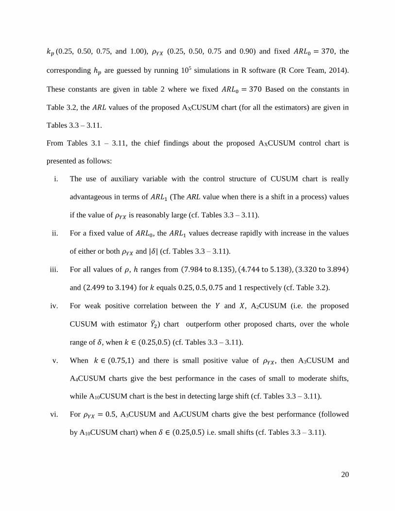
𝑘𝑝 (0.25, 0.50, 0.75, and 1.00), 𝜌𝑌𝑋 (0.25, 0.50, 0.75 and 0.90) and fixed 𝐴𝑅𝐿0 = 370, the
corresponding ℎ𝑝 are guessed by running 105 simulations in R software (R Core Team, 2014).
These constants are given in table 2 where we fixed 𝐴𝑅𝐿0 = 370 Based on the constants in
Table 3.2, the 𝐴𝑅𝐿 values of the proposed AXCUSUM chart (for all the estimators) are given in
Tables 3.3 – 3.11.
From Tables 3.1 – 3.11, the chief findings about the proposed AXCUSUM control chart is
presented as follows:
i. The use of auxiliary variable with the control structure of CUSUM chart is really
advantageous in terms of 𝐴𝑅𝐿1 (The ARL value when there is a shift in a process) values
if the value of 𝜌𝑌𝑋 is reasonably large (cf. Tables 3.3 – 3.11).
ii. For a fixed value of 𝐴𝑅𝐿0, the 𝐴𝑅𝐿1 values decrease rapidly with increase in the values
of either or both 𝜌𝑌𝑋 and |𝛿| (cf. Tables 3.3 – 3.11).
iii. For all values of 𝜌, ℎ ranges from (7.984 to 8.135), (4.744 to 5.138), (3.320 to 3.894)
and (2.499 to 3.194) for 𝑘 equals 0.25, 0.5, 0.75 and 1 respectively (cf. Table 3.2).
iv. For weak positive correlation between the 𝑌 and 𝑋, A2CUSUM (i.e. the proposed
CUSUM with estimator �̅�2) chart outperform other proposed charts, over the whole
range of 𝛿, when 𝑘 ∈ (0.25,0.5) (cf. Tables 3.3 – 3.11).
v. When 𝑘 ∈ (0.75,1) and there is small positive value of 𝜌𝑌𝑋, then A3CUSUM and
A4CUSUM charts give the best performance in the cases of small to moderate shifts,
while A10CUSUM chart is the best in detecting large shift (cf. Tables 3.3 – 3.11).
vi. For 𝜌𝑌𝑋 = 0.5, A3CUSUM and A4CUSUM charts give the best performance (followed
by A10CUSUM chart) when 𝛿 ∈ (0.25,0.5) i.e. small shifts (cf. Tables 3.3 – 3.11).
21
vii. For 𝜌𝑌𝑋 = 0.5, A4CUSUM and A10CUSUM charts give the best performance (followed
by A3CUSUM chart) when 𝛿 ∈ (0.75,5) i.e. moderate and large shifts (cf. Tables 3.3 –
3.11).
viii. For 𝜌𝑌𝑋 = 0.75, A3CUSUM and A4CUSUM charts precede A10CUSUM chart in
outperforming other proposed charts in detecting small shift (cf. Tables 3.3 – 3.11).
ix. For a strong positive correlation 𝜌𝑌𝑋 ≥ 0.75, A3CUSUM, A4CUSUM and A10CUSUM
charts are the best preceded by A2CUSUM chart, in detecting moderate to large shift (i.e.
𝛿 ≥ 0.75) (cf. Tables 3.3 – 3.11).
3.4 COMPARISONS
Generally, 𝐴𝑅𝐿 is used to compare the performance of two charts. Wu et al. (2009) highlighted
some of the drawbacks of 𝐴𝑅𝐿 as it gives the performance of a control chart for a specific shift
size. Hence, they recommended some measures which evaluate the performance of a control
chart over a range of 𝛿 values. These measures are named as extra quadratic loss (𝐸𝑄𝐿) and ratio
of average run lengths (𝑅𝐴𝑅𝐿) which are defined as:
𝐸𝑄𝐿 =1
𝛿max−𝛿min∫ 𝛿2𝐴𝑅𝐿(𝛿)𝑑𝛿
𝛿max
𝛿min (3.6)
𝑅𝐴𝑅𝐿 =1
𝛿max−𝛿min∫
𝐴𝑅𝐿(𝛿)
𝐴𝑅𝐿benchmark(𝛿)𝑑𝛿
𝛿max
𝛿min (3.7)
Another performance measure named as performance comparison index (𝑃𝐶𝐼) given by Ou et al.
(2012) is defined as:
𝑃𝐶𝐼 =𝐸𝑄𝐿
𝐸𝑄𝐿benchmark (3.8)
where 𝐴𝑅𝐿benchmark and 𝐸𝑄𝐿benchmark are evaluated for the benchmark chart (taken as the best
chart in this section).
22
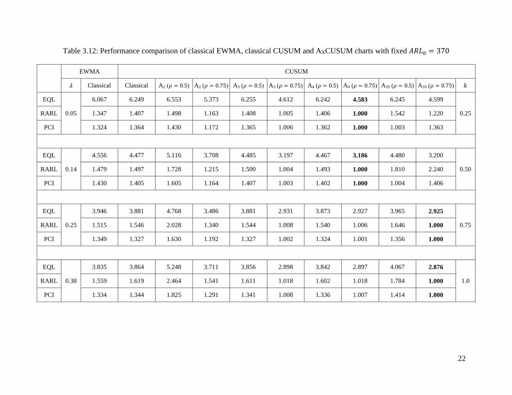
Table 3.12: Performance comparison of classical EWMA, classical CUSUM and AXCUSUM charts with fixed 𝐴𝑅𝐿0 = 370
EWMA CUSUM
𝜆 Classical Classical A2 (𝜌 = 0.5) A2 (𝜌 = 0.75) A3 (𝜌 = 0.5) A3 (𝜌 = 0.75) A4 (𝜌 = 0.5) A4 (𝜌 = 0.75) A10 (𝜌 = 0.5) A10 (𝜌 = 0.75) 𝑘
EQL
0.05
6.067 6.249 6.553 5.373 6.255 4.612 6.242 4.583 6.245 4.599
0.25 RARL 1.347 1.407 1.498 1.163 1.408 1.005 1.406 1.000 1.542 1.220
PCI 1.324 1.364 1.430 1.172 1.365 1.006 1.362 1.000 1.003 1.363
EQL
0.14
4.556 4.477 5.116 3.708 4.485 3.197 4.467 3.186 4.480 3.200
0.50 RARL 1.479 1.497 1.728 1.215 1.500 1.004 1.493 1.000 1.810 2.240
PCI 1.430 1.405 1.605 1.164 1.407 1.003 1.402 1.000 1.004 1.406
EQL
0.25
3.946 3.881 4.768 3.486 3.881 2.931 3.873 2.927 3.965 2.925
0.75 RARL 1.515 1.546 2.028 1.340 1.544 1.008 1.540 1.006 1.646 1.000
PCI 1.349 1.327 1.630 1.192 1.327 1.002 1.324 1.001 1.356 1.000
EQL
0.38
3.835 3.864 5.248 3.711 3.856 2.898 3.842 2.897 4.067 2.876
1.0 RARL 1.559 1.619 2.464 1.541 1.611 1.018 1.602 1.018 1.784 1.000
PCI 1.334 1.344 1.825 1.291 1.341 1.008 1.336 1.007 1.414 1.000
23
In this current study, we have used the sensitivity parameter of CUSUM chart 𝑘 =
0.25, 0.5, 0.75 and 1 which are the optimal choices for detecting a shift of size 𝛿 =
0.5, 1, 1.5 and 2, respectively. For the same values of 𝛿, we have found the optimal
choices for the sensitivity parameter (𝜆) of EWMA chart to be 𝜆 = 0.05, 0.14, 0.25 and
0.38 for 𝛿 = 0.5, 1, 1.5 and 2, respectively, using the technique of Crowder (1989).
Finally, the comparisons of all the charts under discussion in the form of 𝐸𝑄𝐿, 𝑅𝐴𝑅𝐿 and
𝑃𝐶𝐼 are provided in Table 3.12 where the in-control 𝐴𝑅𝐿 for all the charts is fixed at
370. In Table 3.12, smaller value of 𝐸𝑄𝐿 shows a better performance of a chart, and the
best chart in every situations is taken as the benchmark chart, indicated by bold value.
The best charts in Table 3.12 are A4CUSUM for 𝑘=0.25,0.5 and A10CUSUM for
𝑘=0.75,1. Similarly, the value of 𝑅𝐴𝑅𝐿 (or 𝑃𝐶𝐼) greater than 1 means that the benchmark
chart has a superior overall performance and vice versa. It can be clearly seen from Table
3.12 that AXCUSUM is outperforming the classical EWMA and the classical CUSUM
charts.
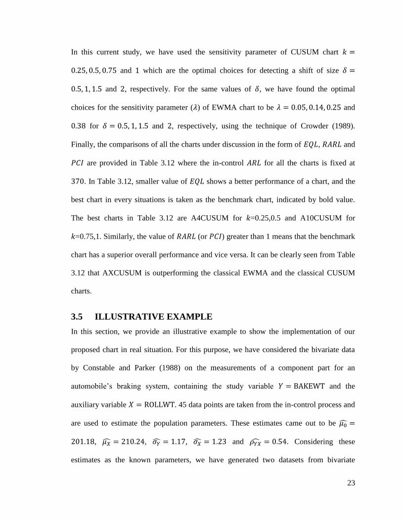
3.5 ILLUSTRATIVE EXAMPLE
In this section, we provide an illustrative example to show the implementation of our
proposed chart in real situation. For this purpose, we have considered the bivariate data
by Constable and Parker (1988) on the measurements of a component part for an
automobile’s braking system, containing the study variable 𝑌 = BAKEWT and the
auxiliary variable 𝑋 = ROLLWT. 45 data points are taken from the in-control process and
are used to estimate the population parameters. These estimates came out to be 𝜇0̂ =
201.18, 𝜇�̂� = 210.24, 𝜎�̂� = 1.17, 𝜎�̂� = 1.23 and 𝜌𝑌�̂� = 0.54. Considering these
estimates as the known parameters, we have generated two datasets from bivariate
24
normal distribution. Dataset 1 with 𝜇1 = 201.7, 𝜇𝑋 = 210.24, 𝜎𝑌 = 1.17, 𝜎𝑋 = 1.23 and
𝜌𝑌𝑋 = 0.54 contains 15 paired observations which refer to an out-of-control situation
with 𝛿 =(𝜇1−𝜇0)
𝜎𝑌
√𝑛⁄
=(201.7−201.18)
1.17√1
⁄≅ 1. Similarly, Dataset 2 with 𝜇1 = 200.6, 𝜇𝑋 =
210.24, 𝜎𝑌 = 1.17, 𝜎𝑋 = 1.23 and 𝜌𝑌𝑋 = 0.54 contains 15 paired observations which
refer to an out-of-control situation with negative shift i.e. 𝛿 =(𝜇1−𝜇0)
𝜎𝑌
√𝑛⁄
=(200.6−201.18)
1.17√1
⁄≅
−1.1. The inspiration of generating dataset in such manner is taken from Singh and
Mangat, (1996, pp. 221).
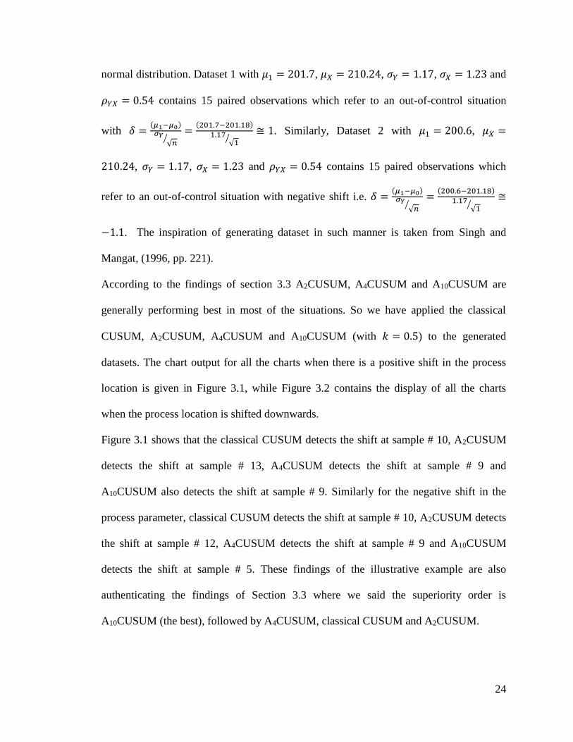
According to the findings of section 3.3 A2CUSUM, A4CUSUM and A10CUSUM are
generally performing best in most of the situations. So we have applied the classical
CUSUM, A2CUSUM, A4CUSUM and A10CUSUM (with 𝑘 = 0.5) to the generated
datasets. The chart output for all the charts when there is a positive shift in the process
location is given in Figure 3.1, while Figure 3.2 contains the display of all the charts
when the process location is shifted downwards.
Figure 3.1 shows that the classical CUSUM detects the shift at sample # 10, A2CUSUM
detects the shift at sample # 13, A4CUSUM detects the shift at sample # 9 and
A10CUSUM also detects the shift at sample # 9. Similarly for the negative shift in the
process parameter, classical CUSUM detects the shift at sample # 10, A2CUSUM detects
the shift at sample # 12, A4CUSUM detects the shift at sample # 9 and A10CUSUM
detects the shift at sample # 5. These findings of the illustrative example are also
authenticating the findings of Section 3.3 where we said the superiority order is
A10CUSUM (the best), followed by A4CUSUM, classical CUSUM and A2CUSUM.

25
Figure 3.1: Graphical display of the classical CUSUM, A2CUSUM, A4CUSUM and
A10CUSUM charts for dataset 1
3.6 SUMMARY AND CONCLUSIONS
Quality of manufactured products and services are always important for the management
department of a firm or industry. 𝑆𝑄𝐶 provides some suitable tools to monitor and
improve the quality of products by reducing the undesirable variation in their output.
Control chart is the most important tool of 𝑆𝑄𝐶 which is further categorized into
Shewhart, CUSUM and EWMA-type control charts. Shewhart-type control charts are
0
0.5
1
1.5
2
2.5
3
3.5
4
1 2 3 4 5 6 7 8 9 10 11 12 13 14 15
Sta
ndar
diz
ed m
ean
/ C
um
ula
tiv
e su
m
Sample Number
C+ (1) H (1) C+ (2) H (2) C+ (4) H (4) C+ (10) H (10)

26
Figure 3.2: Graphical display of the classical CUSUM, A2CUSUM, A4CUSUM and
A10CUSUM charts for dataset 2
built to detect large shifts in the process while CUSUM and EWMA-type control charts
are designed to give better performance against small and moderate shifts. This chapter
proposes a new two-sided CUSUM-type control chart named as AXCUSUM control chart
for monitoring the mean of a process. The proposed chart is based on the information of
auxiliary variable and different estimators are used to exploit the auxiliary information.
The study revealed that the proposed chart is generalized form of the classical CUSUM
chart and its performance is also better than the classical CUSUM and the classical
EWMA charts.
-5
-4.5
-4
-3.5
-3
-2.5
-2
-1.5
-1
-0.5
0
1 2 3 4 5 6 7 8 9 10 11 12 13 14 15
Sta
ndar
diz
ed m
ean
/ C
um
ula
tiv
e su
m
Sample Number
C- (1) -H (1) C- (2) -H (2) C- (4) -H (4) C- (10) -H (10)

27
4 CHAPTER 4
Combined Shewhart CUSUM Charts using Auxiliary Variable
Control chart is an important tool for monitoring disturbances in a statistical process, and
it is richly applied in the industrial sector, the health sector, the agricultural sector, among
others. The Shewhart chart and the cumulative sum (CUSUM) chart are traditionally used
for detecting large shifts and small shifts, respectively, while the Combined Shewhart
CUSUM (CSC) monitors both small and large shifts. Using auxiliary information, we
propose new CSC (MiCSC) charts with more efficient estimators (the Regression-type
estimator, the Ratio estimator, the Singh and Tailor estimator, the power ratio-type
estimator, and the Kadilar and Cingi estimators) for estimating the location parameter.
We compare the charts using average run length, standard deviation run length and extra
quadratic loss, with other existing charts of the same purpose, and found out that some of
the MiCSC charts outperform their counterparts. At last, a real-life industrial example is
provided.
28
4.1 INTRODUCTION
The most widely known quality control chart, Shewhart chart, was proposed by
(Shewhart, 1924). It detects shifts in a production process by signaling when a process
goes beyond some particular threshold limits known as control limits. Shewhart chart
makes use of the information when the process goes out of the control limits and ignores
the information when the process is within the control limits, i.e. in-control. Due to this
fact, the chart is sensitive for detecting large shifts (or disturbance) in a process. Roberts
(1959) and Page (1954) proposed Exponentially Weighted Moving Average (EWMA)
chart and Cumulative Sum (CUSUM) chart, respectively, which make use of the
information when the process gets out of control and even when the process is in-control,
hence, these charts are sensitive to small and moderate shifts in a process. Other
modifications of these charts have been proposed to increase their efficiency in terms of
time, cost, and simplicity of usage and expression.
The plotting statistic of CUSUM chart assumes normality. What if the plotting statistic is
not normally distributed or its normality is altered? Nazir et al., (2013) answered these
questions by suggesting some charts which are not normally distributed or their normality
has been altered. They aimed at finding charts that perform practically well under normal,
contaminated normal, non-normal, and special cause contaminated parent cases. Based
on mean, median, Hodge-Lehman, midrange and trimean statistics, they proposed
different CUSUM charts for phase II monitoring of location parameter and computed
their performance measure using the average run length (ARL) approach. Abujiya et al.
(2015) suggested the use of well-structured sampling techniques such as the double
ranked set sampling, the median-double ranked set sampling, and the double-median
29
ranked set sampling, to significantly improve the performance of the CUSUM chart,
without inflating the false alarm rate. They compared their proposed charts with some
existing charts and found out that their charts perform better.
Due to the advancement in technology and industrial processes, emphasis has been made
on the implementation of CUSUM chart to existing Levey-Jennings or Shewhart control
charts to improve their performance. These can be done manually using control charts or
in a computerized quality control systems. Westgard et al. (1977) applied this concept to
improve quality control in clinical chemistry. The combination of Shewhart chart and
CUSUM chart was observed by Lucas (1982), after which some scholars improved the
chart by proposing more efficient charts. Combined Shewhart-CUSUM (hereafter called
“CSC”) for location parameter can be optimized over the entire mean shift range by
adding an extra parameter (w) known as the exponential of the sample mean shift, to the
structure of the CSC. This will improve its performance and it will not increase the
difficulty level of understanding and implementing the chart (Wu et al., 2008). The CSC,
which has a wide range of application, attracts the attention of Environmentalists, and it
is the only quality control chart directly recommended by the United States Environment
Protection Agency for intra-well monitoring. It has been consistently applied to waste
disposal facilities for detection monitoring programs (Gibbons, 1999). Abujiya et al.
(2013) replaced the traditional simple random sampling in the plotting statistic of the
CSC, with ranked set sampling.
The control statistics of the classical Shewhart, CUSUM, and CSC charts for monitoring
location parameter are based on the usual unbiased simple mean estimator
30
n
i ixnx1
1 for estimating the population mean. However, in the field of sample
survey, different scholars have suggested many estimators other than the simple mean in
terms of their mean square error (MSE). Some of these estimators requires the use of
auxiliary variable(s) which are cheap, easy and affordable to get, and also, with known
population parameters (Cochran, 1953). According to Cochran (1953), the correlation
between the study variable and the auxiliary variable will serves as an advantage to
increase the precision of estimation. Sukhatme & Sukhatme (1970) proposed regression
estimator for estimating the mean, while power ratio-type estimator and modified ratio-
type estimator were suggested by Srivastava (1967) and Ahmad et al. (2014) respectively.
Interested reader can see H. P. Singh & Tailor (2003), Kadilar & Cingi (2004), Kadilar &
Cingi (2006a), Kadilar & Cingi (2006b), Gupta & Shabbir (2008) and Adebola et al.
(2015) for different forms of a transformed ratio estimator.
G. Zhang (1992) suggested the cause-selecting control chart, while Riaz (2008b)
popularised the use of auxiliary information at the estimation stage, for monitoring
dispersion parameter. He concluded that the chart is better than the R chart, the S chart
and the S2 chart. Furthermore, Riaz (2008a) suggested similar chart for location
parameter estimation, which was also superior to the Shewhart chart, the regression chart
and the cause-selecting control chart. Assuming stability of parameters, Ahmad et al.
(2014) proposed new Shewhart charts based on auxiliary information for non-cascading
processes. The charts monitor a dispersion parameter in an efficient way. The superiority
of the charts over competing charts was shown using the ARL, relative average run
length (RARL) and extra quadratic loss (EQL) under t and normal distributed process
environment. Similar work was also done for location parameter monitoring, and it was
31
found out that there is an improvement in the detection ability of Shewhart chart base on
the level of correlation between the concerned variables (Riaz, 2015).
Since most of the estimators are more efficient than the simple mean estimator based on
simple random sample, their introduction to the plotting statistic(s) of the Shewhart chart,
the CUSUM chart, and the CSC chart would results to efficient control charts. Hence,
this study aims at optimizing the CSC chart by introducing some efficient estimators to
its plotting statistics. These estimators use auxiliary information in the sampling stage.
This is helpful whenever there is no information about the population of the variable of
interest, but there is information about a closely related variable(s) which is cheap and
affordable to get.
The rest of this article is organized as follows: Location estimators and their properties
are explained in the next section; The general structure of the proposed charts is
explained in Section 4.3; Section 4 explains the performance measures for evaluating the
proposed charts and compares the proposed charts with their existing counterparts;
Section 4.5 gives an illustrative example; and finally, conclusions and recommendations
are given in Section 4.6.
4.2 LOCATION ESTIMATORS AND THEIR PROPERTIES
We assume that a process has a quality characteristic of interest X and an auxiliary
quality characteristic A . Let the population parameters of X and A , respectively, be
represented as X and A for the means; 2
X and 2
A for the variances; XC XX
and AC AA for the coefficient of variations; X2 and
A2 for the coefficient of
32
kurtoses; XA for the covariance between X and A ; and
XA for the correlation
coefficient. Let the sample statistics of X and A , respectively, be represented as x and
a for the means; 2
xs and 2
as for the variances; xc and ac for the coefficient of
variations; xas for the covariance; and xar for the correlation coefficient. Let ix and
ii ax , be univariate and bivariate sample respectively, where ni ,,2,1 and n
sample size. From the sample statistics, we have nxxn
i i
1, naa
n
i i
1,
11
22 nxxs
n
i ix, 1
1
22 naas
n
i ia, xsc xx , asc aa and
axxaxa sssr . Based on this introduction, some efficient estimators with one auxiliary
variable for estimating the mean of a quality process characteristic, assuming sampling
with replacement, are presented with their respective bias (B) and MSE.
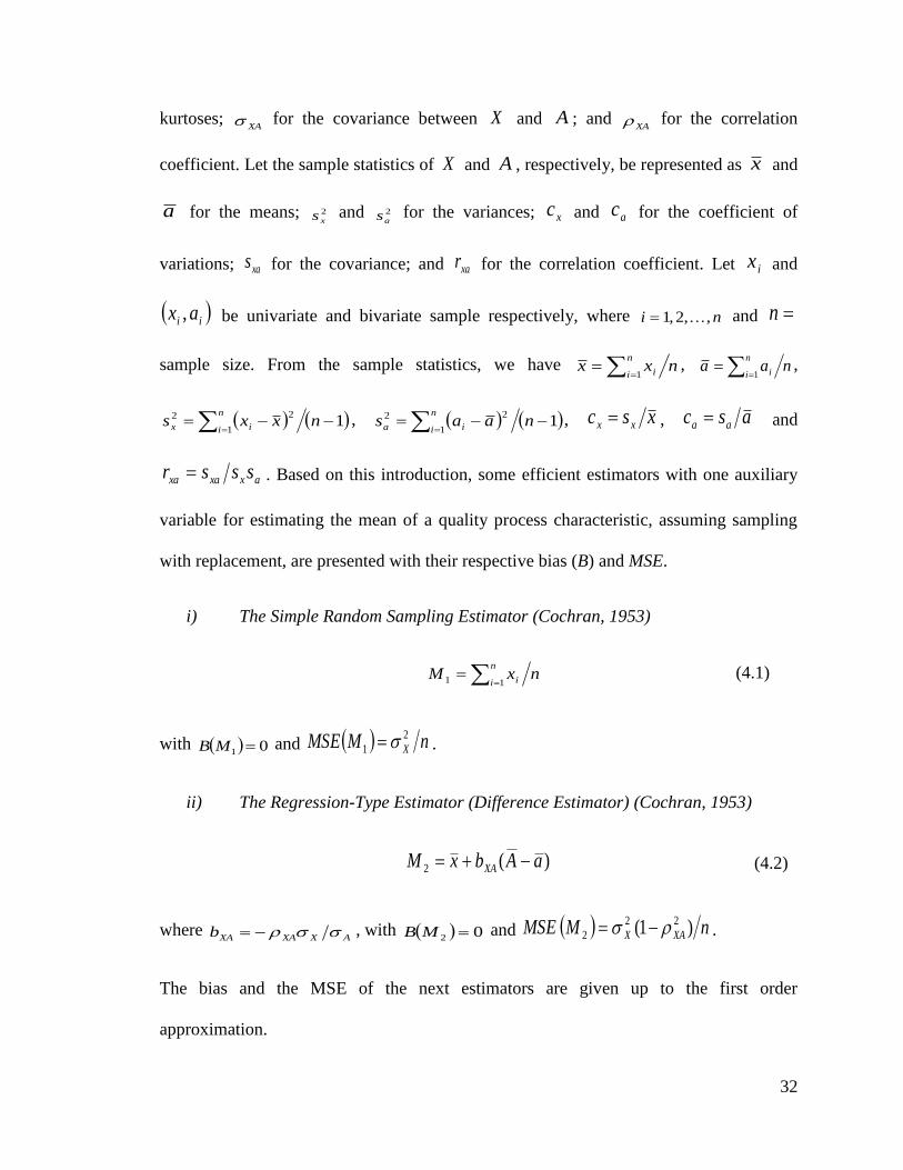
i) The Simple Random Sampling Estimator (Cochran, 1953)
nxMn
i i
11 (4.1)
with 01 MB and nMMSE X
2
1 .
ii) The Regression-Type Estimator (Difference Estimator) (Cochran, 1953)
)(2 aAbxM XA (4.2)
where AXXAXAb , with 02 MB and nMMSE XAX )1( 22
2 .
The bias and the MSE of the next estimators are given up to the first order
approximation.

33
iii) The Ratio Estimator (Cochran, 1953)
aAxM 3 (4.3)
with AXXAA CCCXMB 2
3 )( and AXXAAX CCCCXMMSE 2)( 222
3
iv) The Singh and Tailor Estimator (H. P. Singh & Tailor, 2003)
XA
XA
a
AxM
4
(4.4)
with nCCgCgXMB AXXAA 2
4 )( and
nCCgCgCXMMSE AXXAAX 2)( 2222
4 , where XAAAg .
v) The Power Ratio-Type Estimator (Srivastava, 1967)
)/(5 aAxM (4.5)
where AXXA CC , with AXXAA CCCnXMB 2
5 21 and
)21( 2222
5 AXXAXAX CCCCnMMSE .
vi) The Kadilar and Cingi Estimator’s Series 1 (Kadilar & Cingi, 2004)
aAaAbxM XA 6 (4.6)
with nCXMB A
2
6 and nCCXMMSE XAXA
2222
6 1
vii) The Kadilar and Cingi Estimator’s Series 2 (Kadilar & Cingi, 2004)
34
A
A
XACa
CAaAbxM
7 (4.7)
with 22
7 AA CAACnXMB and
22222
7 1 XAXAA CCCAAnXMMSE .
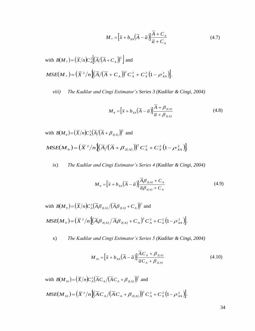
viii) The Kadilar and Cingi Estimator’s Series 3 (Kadilar & Cingi, 2004)
A
A
XAa
AaAbxM
2
2
8
(4.8)
with 22
2
8 AA AACnXMB and
2222
2
2
8 1 XAXAA CCAAnXMMSE .
ix) The Kadilar and Cingi Estimator’s Series 4 (Kadilar & Cingi, 2004)
AA
AA
XACa
CAaAbxM
2
2
9
(4.9)
with 222
2
9 AAAA CAACnXMB and
2222
22
2
9 1 XAXAAAA CCCAAnXMMSE .
x) The Kadilar and Cingi Estimator’s Series 5 (Kadilar & Cingi, 2004)
AA
AA
XACa
CAaAbxM
2
2
10
(4.10)
with 22
2
10 AAAA CACACnXMB and
2222
2
2
10 1 XAXAAAA CCCACAnXMMSE .

35
4.3 GENERAL STRUCTURE OF THE PROPOSED CHARTS
The CSC is a combination of the Shewhart chart and the CUSUM chart, where the
Shewhart chart is responsible for early detection of a large shift while the CUSUM chart
detects small to moderate shifts in a quality control process. The addition of Shewhart
chart limits to CUSUM chart will improve the performance of CUSUM in detecting a
large shift, which is an advantage over ordinary CUSUM chart, though there will be
payoff in the CUSUM structure, as well as in the Shewhart structure, by widening the
control limits of the two charts. According to Henning et al. (2015), the CSC is the
probabilistic combination of two charts to form a new one by adjusting their control
limits, and taking the sensitivity of false alarm rates to the new scheme into
consideration. This has large scope of application {Westgard et al. (1977), Lucas (1982),
Wu et al. (2008), Montgomery (2009), Abujiya et al. (2013) and Henning et al. (2015)}.
Like the CUSUM chart, the CSC chart is not difficult to construct and use (Lucas, 1982).
In this study, a bivariate setup from a normal distribution such that
XAAXAXNAX ,,,,~, 22
2 is assumed in proposing some improved CSC control
charts, using the location estimators 10,,3,2, iM i . Let ii MMtit MZ , be the
standardized transformation of the estimators 10,,3,2, iM i , for the n-subgroup tht
sample, where iM MBXi
and iM MMSEi2 . Hence, the general control
charting structure of the proposed charts is presented. The CUSUM’s plotting statistics
are given as
0);,0max(
0);,0max(
01
01
CCkZC
CCkZC
ttt
ttt (4.11)
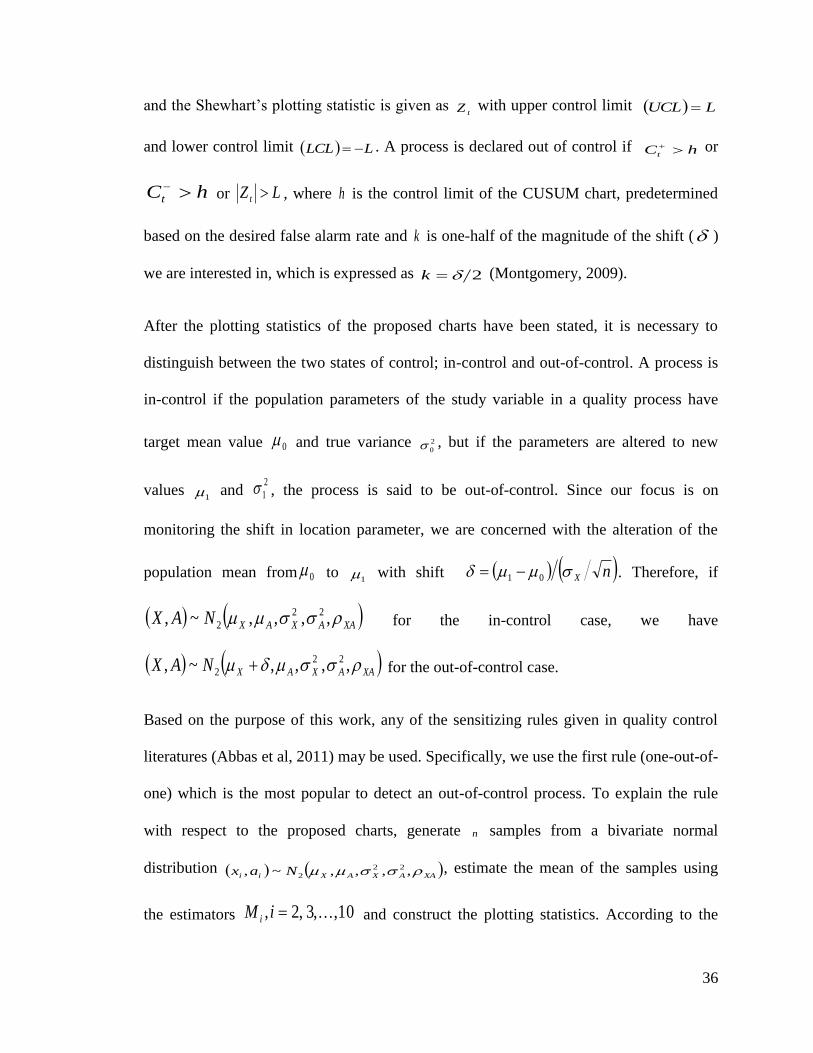
36
and the Shewhart’s plotting statistic is given as tZ with upper control limit LUCL
and lower control limit LLCL . A process is declared out of control if hCt or
hCt or LZ t , where h is the control limit of the CUSUM chart, predetermined
based on the desired false alarm rate and k is one-half of the magnitude of the shift ( )
we are interested in, which is expressed as 2k (Montgomery, 2009).
After the plotting statistics of the proposed charts have been stated, it is necessary to
distinguish between the two states of control; in-control and out-of-control. A process is
in-control if the population parameters of the study variable in a quality process have
target mean value 0 and true variance 2
0 , but if the parameters are altered to new
values 1 and
2
1 , the process is said to be out-of-control. Since our focus is on
monitoring the shift in location parameter, we are concerned with the alteration of the
population mean from 0 to 1 with shift nX 01 . Therefore, if
XAAXAXNAX ,,,,~, 22
2 for the in-control case, we have
XAAXAXNAX ,,,,~, 22
2 for the out-of-control case.
Based on the purpose of this work, any of the sensitizing rules given in quality control
literatures (Abbas et al, 2011) may be used. Specifically, we use the first rule (one-out-of-
one) which is the most popular to detect an out-of-control process. To explain the rule
with respect to the proposed charts, generate n samples from a bivariate normal
distribution XAAXAXii Nax ,,,,~, 22
2, estimate the mean of the samples using
the estimators 10,,3,2, iM i and construct the plotting statistics. According to the

37
first rule, once the plotting statistics fall outside the process control limits, the process is
declared as out-of-control, to indicate a shift in the location parameter of the variable of
interest.
4.3.1 SPECIAL CASES
Let 10,,3,2,1, iCSCM i represents the proposed chart.
i. It is worthy of note that CSCM1 chart is the classical CSC chart.
ii. If h approaches infinity, we have the Shewhart chart.
iii. If L approaches infinity, we have the CUSUM chart.
4.4 PERFORMANCE MEASURES
In this section, following the works of some authors {Zhang et al. (2012); Riaz, (2015)},
performance of the CSCM i charts 10,,3,2 i using the ARL and the standard
deviation run length (SDRL) for each shift is done. In addition, evaluation of the
overall precision of the charts over the entire shift is carried out using extra quadratic loss
(EQL) in order to make an accurate and reliable conclusion about the relative
effectiveness of the CSCM i charts 10,,3,2 i . Below is a brief description of these
measures.
ARL is the average number of points (samples) plotted until a point indicates an out-of-
control signal (Montgomery, 2009). It is a popular measure for measuring the
effectiveness of a control chart. ARL can be categorized into ARL0 and ARL1. ARL0 is
the ARL value when a process is stable i.e. in an in-control state ( 0 ) while ARL1 is

38
the ARL value when a process is unstable i.e. in an out-of-control state ( 0 ). It is
expected that ARL0 has a large value while ARL1 has a small value (Ahmad et al., 2014).
This idea is often used to measure the effectiveness of a chart and to compare the
performance of different charting structures. Interested reader should see Jamali et al.
(2006), Riaz & Does (2008), Cox (2010), Abbasi et al. (2012), Busaba et al. (2012) and
the references therein.
On the other hand, SDRL is the standard deviation of points (samples) plotted until a
point indicates an out-of-control signal. It is also used to compare different charts and
examine their response to shift in parameter(s). The smaller the SDRL, the better the
performance of a control chart (Abujiya et al., 2015). There is also EQL, which is the
weighted average ARL over all shifts considered in a control process. It measures the
effectiveness of a chart over all range of shifts, unlike ARL that deals with a specific
shift. In the work of Wu et al. (2008), Wu et al. (2009), Ou et al. (2012) and Abujiya et
al. (2015), EQL and its other forms were used to measure the effectiveness of control
charts over a range of process shifts. The mathematical expression of EQL is given as
max
min
2
minmax
1
dARLEQL (4.12)
where min and max are the minimum and maximum values of the shifts considered in
a process; and ARL is the ARL at a particular shift . The EQL values are
computed with numerical integration approach. A particular CSC chart could have
different combinations of h and L, and the combination with the lowest EQL will give the
optimum choice of h and L.
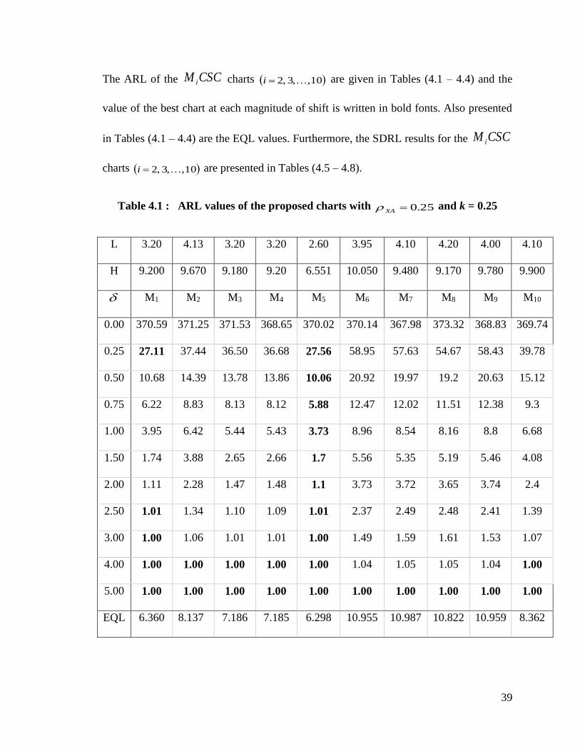
39
The ARL of the CSCM i charts 10,,3,2 i are given in Tables (4.1 – 4.4) and the
value of the best chart at each magnitude of shift is written in bold fonts. Also presented
in Tables (4.1 – 4.4) are the EQL values. Furthermore, the SDRL results for the CSCM i
charts 10,,3,2 i are presented in Tables (4.5 – 4.8).
Table 4.1 : ARL values of the proposed charts with 25.0XA and k = 0.25
L 3.20 4.13 3.20 3.20 2.60 3.95 4.10 4.20 4.00 4.10
H 9.200 9.670 9.180 9.20 6.551 10.050 9.480 9.170 9.780 9.900
M1 M2 M3 M4 M5 M6 M7 M8 M9 M10
0.00 370.59 371.25 371.53 368.65 370.02 370.14 367.98 373.32 368.83 369.74
0.25 27.11 37.44 36.50 36.68 27.56 58.95 57.63 54.67 58.43 39.78
0.50 10.68 14.39 13.78 13.86 10.06 20.92 19.97 19.2 20.63 15.12
0.75 6.22 8.83 8.13 8.12 5.88 12.47 12.02 11.51 12.38 9.3
1.00 3.95 6.42 5.44 5.43 3.73 8.96 8.54 8.16 8.8 6.68
1.50 1.74 3.88 2.65 2.66 1.7 5.56 5.35 5.19 5.46 4.08
2.00 1.11 2.28 1.47 1.48 1.1 3.73 3.72 3.65 3.74 2.4
2.50 1.01 1.34 1.10 1.09 1.01 2.37 2.49 2.48 2.41 1.39
3.00 1.00 1.06 1.01 1.01 1.00 1.49 1.59 1.61 1.53 1.07
4.00 1.00 1.00 1.00 1.00 1.00 1.04 1.05 1.05 1.04 1.00
5.00 1.00 1.00 1.00 1.00 1.00 1.00 1.00 1.00 1.00 1.00
EQL 6.360 8.137 7.186 7.185 6.298 10.955 10.987 10.822 10.959 8.362

40
Table 4.2: ARL values of the proposed charts with 25.0XA and k = 0.5
L 3.20 4.20 3.25 3.20 2.70 4.40 4.20 4.40 4.30 4.30
h 9.200 4.060 5.247 5.40 3.463 5.330 5.558 5.354 5.360 5.510
M1 M2 M3 M4 M5 M6 M7 M8 M9 M10
0.00 371.01 371.28 368.43 371.18 368.74 368.48 371.84 366.72 368.76 369.76
0.25 31.31 52.33 46.49 47.83 35.75 82.74 89.22 83.19 85.51 53.55
0.50 8.90 12.66 12.17 12.47 8.62 19.87 20.73 19.72 19.98 13.06
0.75 4.91 6.87 6.52 6.52 4.54 9.73 10.14 9.77 9.84 6.98
1.00 3.21 4.71 4.33 4.35 3.02 6.37 6.62 6.29 6.46 4.76
1.50 1.65 2.9 2.37 2.32 1.64 3.82 3.95 3.79 3.85 2.93
2.00 1.11 1.92 1.47 1.45 1.11 2.74 2.81 2.72 2.76 1.99
2.50 1.01 1.31 1.1 1.09 1.01 2.07 2.04 2.05 2.05 1.39
3.00 1.00 1.07 1.01 1.01 1.00 1.59 1.49 1.54 1.54 1.10
4.00 1.00 1.00 1.00 1.00 1.00 1.08 1.05 1.07 1.07 1.00
5.00 1.00 1.00 1.00 1.00 1.00 1.01 1.00 1.00 1.01 1.00
EQL 6.190 7.562 6.962 6.950 6.183 9.865 9.911 9.776 9.853 7.703

41
Table 4.3: ARL values of the proposed charts with 75.0XA and k = 0.25
L 3.200 4.000 3.150 3.100 4.300 3.625 4.000 4.000 3.9.00 4.200
H 5.350 10.100 9.692 10.000 11.370 4.620 9.183 9.258 9.640 9.500
M1 M2 M3 M4 M5 M6 M7 M8 M9 M10
0.00 370.59 367.75 370.81 373.083 368.91 372.01 367.96 369.31 367.73 368.35
0.25 27.11 22.57 15.75 17.72 20.84 22.17 40.86 40.02 43.26 22.72
0.50 10.68 9.47 5.27 6.96 9.03 8.28 15.20 14.97 15.91 9.50
0.75 6.22 5.94 2.94 3.46 5.66 5.07 9.35 9.22 9.65 6.01
1.00 3.95 4.04 1.87 1.84 3.71 3.72 6.69 6.61 6.9 4.29
1.50 1.74 1.71 1.08 1.05 1.47 2.40 4.11 4.03 4.15 2.08
2.00 1.11 1.06 1.00 1.00 1.03 1.62 2.50 2.42 2.46 1.14
2.50 1.01 1.00 1.00 1.00 1.00 1.15 1.50 1.44 1.42 1.01
3.00 1.00 1.00 1.00 1.00 1.00 1.01 1.12 1.10 1.10 1.00
4.00 1.00 1.00 1.00 1.00 1.00 1.00 1.00 1.00 1.00 1.00
5.00 1.00 1.00 1.00 1.00 1.00 1.00 1.00 1.00 1.00 1.00
EQL 6.360 6.260 5.554 5.628 6.113 6.639 8.534 8.402 8.528 6.425

42
Table 4.4: ARL Values of the proposed charts with 75.0XA and k = 0.5
L 3.20 4.15 3.20 3.15 4.30 4.00 4.00 4.20 4.00 4.20
H 5.350 4.06 5.355 5.490 6.700 5.507 5.497 5.300 5.577 5.680
M1 M2 M3 M4 M5 M6 M7 M8 M9 M10
0.00 371.01 370.25 368.66 371.36 370.64 370.31 371.63 367.64 369.27 369.08
0.25 31.31 22.85 16.06 16.35 20.62 60.13 59.59 54.91 60.47 25.09
0.50 8.90 7.05 5.32 5.35 6.87 14.18 14.43 13.55 14.6 7.59
0.75 4.91 4.15 2.92 2.92 4.09 7.55 7.50 7.12 7.57 4.45
1.00 3.21 2.96 1.83 1.8 2.84 5.08 5.09 4.86 5.12 3.16
1.50 1.65 1.62 1.06 1.06 1.41 3.09 3.1 2.99 3.12 1.75
2.00 1.11 1.08 1.00 1.00 1.03 2.06 2.07 2.05 2.07 1.12
2.50 1.01 1.01 1.00 1.00 1.00 1.39 1.39 1.43 1.40 1.01
3.00 1.00 1.00 1.00 1.00 1.00 1.11 1.11 1.13 1.11 1.00
4.00 1.00 1.00 1.00 1.00 1.00 1.00 1.00 1.00 1.00 1.00
5.00 1.00 1.00 1.00 1.00 1.00 1.00 1.00 1.00 1.00 1.00
EQL 6.190 5.998 5.549 5.548 5.883 7.921 7.922 7.834 7.955 6.116

43
Table 4.5: SDRL values for the proposed charts with 25.0XA and k = 0.25
L 3.20 4.13 3.20 3.20 2.60 3.95 4.10 4.20 4.00 4.10
H 9.200 9.670 9.180 9.20 6.551 10.050 9.480 9.170 9.780 9.900
M1 M2 M3 M4 M5 M6 M7 M8 M9 M10
0.00 358.20 360.25 352.77 356.51 364.25 364.09 357.81 363.34 363.31 356.60
0.25 14.66 13.46 10.90 22.77 16.46 40.47 39.61 37.87 40.06 23.47
0.50 4.32 5.17 3.99 5.90 4.17 9.10 8.89 8.30 9.08 5.59
0.75 2.66 3.46 2.96 3.29 2.46 4.31 4.10 3.91 4.19 2.76
1.00 2.07 2.08 1.68 2.46 1.88 2.73 2.56 2.46 2.63 1.81
1.50 1.04 0.97 0.85 1.61 0.97 1.70 1.53 1.40 1.65 1.38
2.00 0.35 0.39 0.34 0.81 0.34 1.48 1.33 1.22 1.41 1.22
2.50 0.09 0.20 0.17 0.31 0.09 1.27 1.20 1.14 1.24 0.68
3.00 0.00 0.08 0.00 0.11 0.01 0.79 0.82 0.81 0.8.0 0.27
4.00 0.00 0.00 0.00 0.00 0.00 0.2 0.23 0.23 0.20 0.04
5.00 0.00 0.00 0.00 0.00 0.00 0.05 0.06 0.06 0.05 0.02

44
Table 4.6: SDRL Values for the proposed charts with 25.0XA and k = 0.5
L 3.20 4.20 3.25 3.20 2.70 4.40 4.20 4.40 4.30 4.30
H 9.200 4.060 5.247 5.400 3.463 5.330 5.558 5.354 5.360 5.510
M1 M2 M3 M4 M5 M6 M7 M8 M9 M10
0.00 358.20 368.03 370.10 361.17 363.61 367.80 368.31 366.08 360.52 365.63
0.25 14.66 44.53 39.87 40.86 30.24 75.98 80.33 75.94 76.79 45.85
0.50 4.32 6.55 7.04 7.13 4.87 13.04 13.60 12.82 12.95 6.99
0.75 2.66 2.65 2.99 3.04 2.03 4.74 4.78 4.67 4.77 2.78
1.00 2.07 1.54 1.85 1.90 1.28 2.49 2.57 2.42 2.54 1.57
1.50 1.04 0.88 1.15 1.16 0.75 1.18 1.22 1.14 1.18 0.86
2.00 0.35 0.75 0.71 0.71 0.33 0.82 0.87 0.79 0.83 0.72
2.50 0.09 0.51 0.33 0.31 0.1 0.68 0.77 0.69 0.71 0.53
3.00 0.00 0.26 0.11 0.11 0.02 0.58 0.60 0.57 0.59 0.30
4.00 0.00 0.04 0.00 0.00 0.01 0.27 0.23 0.25 0.25 0.06
5.00 0.00 0.01 0.00 0.00 0.01 0.08 0.07 0.06 0.08 0.03

45
Table 4.7: SDRL Values for the proposed charts with 75.0XA and k = 0.25
L 3.2 4 3.15 3.1 4.3 3.625 4 4 3.9 4.2
H 5.35 10.1 9.692 10 11.37 4.62 9.183 9.258 9.64 9.5
M1 M2 M3 M4 M5 M6 M7 M8 M9 M10
0.00 367.01 365.04 363.77 364.27 368.51 359.04 364.22 363.1 354.66 362.83
0.25 24.22 17.61 10.03 8.2 8.53 13.61 25.46 24.62 26.79 10.27
0.50 4.61 3.14 2.3 3.16 2.57 3.14 6.06 5.9 6.37 2.87
0.75 2.15 1.5 1.33 2.06 1.67 1.5 2.98 2.92 3.12 1.58
1.00 1.46 0.95 0.93 1.15 1.53 0.95 1.97 1.94 2.13 1.27
1.50 0.84 0.67 0.28 0.23 0.78 0.67 1.4 1.4 1.53 1.06
2.00 0.35 0.56 0.04 0.03 0.17 0.56 1.22 1.2 1.27 0.39
2.50 0.09 0.36 0.01 0 0.04 0.36 0.76 0.72 0.71 0.11
3.00 0.02 0.12 0 0 0.01 0.12 0.36 0.32 0.32 0.04
4.00 0 0 0 0 0.01 0 0.07 0.05 0.05 0.02
5.00 0 0 0 0 0 0 0.01 0.01 0.01 0.01
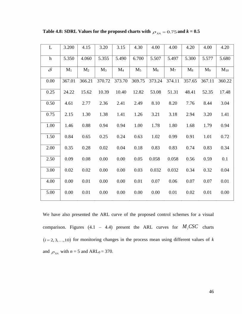
46
Table 4.8: SDRL Values for the proposed charts with 75.0XA and k = 0.5
L 3.200 4.15 3.20 3.15 4.30 4.00 4.00 4.20 4.00 4.20
h 5.350 4.060 5.355 5.490 6.700 5.507 5.497 5.300 5.577 5.680
M1 M2 M3 M4 M5 M6 M7 M8 M9 M10
0.00 367.01 366.21 370.72 373.70 369.75 373.24 374.11 357.65 367.11 360.22
0.25 24.22 15.62 10.39 10.40 12.82 53.08 51.31 48.41 52.35 17.48
0.50 4.61 2.77 2.36 2.41 2.49 8.10 8.20 7.76 8.44 3.04
0.75 2.15 1.30 1.38 1.41 1.26 3.21 3.18 2.94 3.20 1.41
1.00 1.46 0.88 0.94 0.94 1.00 1.78 1.80 1.68 1.79 0.94
1.50 0.84 0.65 0.25 0.24 0.63 1.02 0.99 0.91 1.01 0.72
2.00 0.35 0.28 0.02 0.04 0.18 0.83 0.83 0.74 0.83 0.34
2.50 0.09 0.08 0.00 0.00 0.05 0.058 0.058 0.56 0.59 0.1
3.00 0.02 0.02 0.00 0.00 0.03 0.032 0.032 0.34 0.32 0.04
4.00 0.00 0.01 0.00 0.00 0.01 0.07 0.06 0.07 0.07 0.01
5.00 0.00 0.01 0.00 0.00 0.00 0.00 0.01 0.02 0.01 0.00
We have also presented the ARL curve of the proposed control schemes for a visual
comparison. Figures (4.1 – 4.4) present the ARL curves for CSCM i charts
10,,3,2 i for monitoring changes in the process mean using different values of k
and XA with n = 5 and ARL0 = 370.
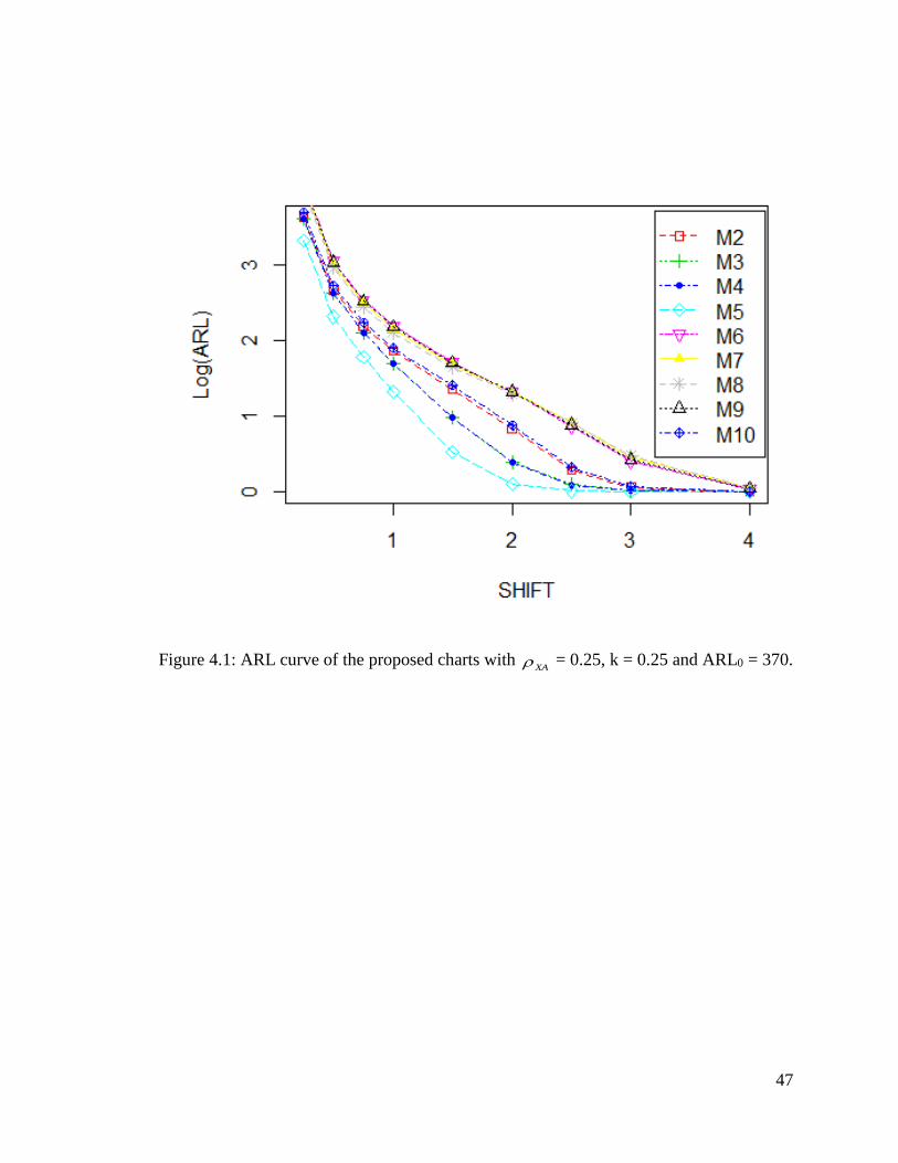
47
Figure 4.1: ARL curve of the proposed charts with XA = 0.25, k = 0.25 and ARL0 = 370.

48
Figure 4.2: ARL curve of the proposed charts with XA = 0.25, k = 0.50 and ARL0 = 370.

49
Figure 4.3: ARL curve of the proposed charts with XA = 0.75, k = 0.25 and ARL0 =
370.

50
Figure 4.4: ARL curve of the proposed charts with XA = 0.75, k = 0.50 and ARL0 = 370.
Based on the results in Tables (4.1 – 4.8) and Figures (4.1 – 4.4), we summarize our
major findings from the proposed charts as follow:
I. The proposed CSCM 5 chart has smaller ARL values than all other charts when
25.0XA for all values of k. This means that the chart is able to detect all
magnitudes of the shift faster than other proposed charts when there is a weak
positive correlation between the study variable and the auxiliary variable. A point
equally supported by the SDRL (cf. Table 4.6). On the overall performance in

51
terms of EQL, the proposed CSCM 5 still dominates all other charts (Tables 4.1 -
4.2, Figures 4.1 – 4.2).
II. For 75.0XA , the proposed CSCM 3 chart and CSCM 4
chart have smaller
ARL values than all other charts when 2 for all values of k. This means that
the charts are able to detect small to moderate shifts faster than other proposed
charts when there is a strong positive correlation between the study variable and
the auxiliary variable. On the overall performance in terms of EQL, the proposed
CSCM 3 and CSCM 4
still dominate all other charts (Tables 4.3 – 4.4, Figures
4.3 – 4.4).
III. Almost all the charts have good performance in detecting large shifts, over all
values of k (Tables 4.1 – 4.4, Figures 4.1 – 4.4).
IV. The proposed charts are ARL unbiased for all the different values of XA and ,
i.e., ARL0 is always greater than ARL1 for any choice of δ (Tables 4.1 – 4.8).
V. For 0 , there is no significant difference between the ARL and the SDRL of
the proposed charts. In addition, the ARL and SDRL values approach 1 and 0,
respectively, as shift increases (Tables 4.1 – 4.8).
4.5 COMPARISONS WITH EXISTING CHARTS
4.5.1 CSCM i charts 10,,3,2 i vs. Classical CSC chart CSCM1
Most of the proposed charts outperform the classical CSC chart except for few cases of
detecting small and large shifts when there is weak positive correlation between the study
variable and the auxiliary variable. For example, in Tables 4.1 – 4.2, CSCM1 chart shows
52
the best performance for shift of 0.25, while CSCM 5 chart (closely followed by
CSCM1 chart) shows the best performance for other values of shifts. This implies that
our proposed charts will perform better than the classical CSC when there is a high value
of XA , irrespective of the value of k This is evident from the low values of ARL1 and
EQL of the proposed charts (Tables 4.1 – 4.4).
4.5.2 CSCM i charts 10,,3,2 i vs. CUSUM charts based on Median, Mid-
range, Hodges-Lehman (HL), and Trimean (TM) estimators under
unconterminated Normal distribution.
Nazir et al., (2013) proposed robust CUSUM charts that are effective in detecting small
shifts when the parameters of the underlying normal distribution of a process are
contaminated. Assuming no contamination in the parameters of the normal distribution of
a process, most of our proposed charts outperform their charts in detecting all magnitudes
of shift, over all values of k. Specifically, CSCM 5 chart (when 25.0XA ), CSCM 3
chart (when 75.0XA ) and CSCM 4chart (when 75.0XA ) perform better than
their proposed charts, and this is evident from the low ARL1 values of CSCM 3 chart,
CSCM 4chart and CSCM 5 chart (cf. Tables 4.9 – 4.10).
*

53
Table 4.9: Some selected proposed charts versus existing CUSUM charts based on
different estimators (Median, Mid-range, Hodges-Lehmann [HL] and Trimean [TM]),
when k = 0.25.
L 3.15 3.10 2.60
h 9.692 10.000 6.551 8.030 8.030 8.030 8.030
M3(rho=.75) M4(rho=.75) M5(rho=.25) Median Mid-range HL TM
0.00 370.81 373.08 370.02 372.50 370.75 373.12 373.93
0.25 15.75 17.72 27.56 31.59 29.82 25.83 27.59
0.50 5.27 6.96 10.06 12.38 11.68 10.44 10.92
0.75 2.94 3.46 5.88 7.70 7.31 6.55 6.90
1.00 1.87 1.84 3.73 5.60 5.35 4.81 5.07
1.50 1.08 1.05 1.70 3.73 3.55 3.25 3.39
2.00 1.00 1.00 1.10 2.85 2.73 2.48 2.60
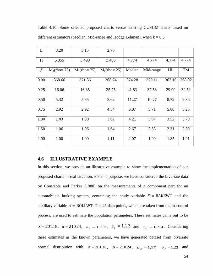
54
Table 4.10: Some selected proposed charts versus existing CUSUM charts based on
different estimators (Median, Mid-range and Hodge Lehman), when k = 0.5.
L 3.20 3.15 2.70
H 5.355 5.490 3.463 4.774 4.774 4.774 4.774
M3(rho=.75) M4(rho=.75) M5(rho=.25) Median Mid-range HL TM
0.00 368.66 371.36 368.74 374.28 370.11 367.10 368.02
0.25 16.06 16.35 35.75 41.83 37.53 29.99 32.52
0.50 5.32 5.35 8.62 11.27 10.27 8.79 9.36
0.75 2.92 2.92 4.54 6.07 5.71 5.00 5.25
1.00 1.83 1.80 3.02 4.21 3.97 3.52 3.70
1.50 1.06 1.06 1.64 2.67 2.53 2.31 2.39
2.00 1.00 1.00 1.11 2.07 1.99 1.85 1.91
4.6 ILLUSTRATIVE EXAMPLE
In this section, we provide an illustrative example to show the implementation of our
proposed charts in real situation. For this purpose, we have considered the bivariate data
by Constable and Parker (1988) on the measurements of a component part for an
automobile’s braking system, containing the study variable 𝑋 = BAKEWT and the
auxiliary variable 𝐴 = ROLLWT. The 45 data points, which are taken from the in-control
process, are used to estimate the population parameters. These estimates came out to be
18.201x , 24.210a , 17.1xs , 23.1as and 54.0xar . Considering
these estimates as the known parameters, we have generated dataset from bivariate
normal distribution with 18.201X , 24.210A , 17.1X , 23.1A and
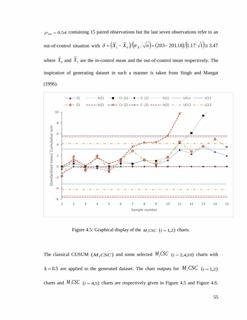
55
54.0XA containing 15 paired observations but the last seven observations refer to an
out-of-control situation with 47.3117.118.20120301 nXX X
where 0X and 1X are the in-control mean and the out-of-control mean respectively. The
inspiration of generating dataset in such a manner is taken from Singh and Mangat
(1996).
Figure 4.5: Graphical display of the CSCM i 2,1i charts.
The classical CUSUM CSCM1 and some selected CSCM i 10,4,2i charts with
5.0k are applied to the generated dataset. The chart outputs for CSCM i 2,1i
charts and CSCM i 5,4i charts are respectively given in Figure 4.5 and Figure 4.6.
-6
-4
-2
0
2
4
6
8
10
1 2 3 4 5 6 7 8 9 10 11 12 13 14 15
Stan
dar
diz
ed m
ean
/ C
um
ula
tive
su
m
Sample number
Z1 h(1) C+ (1) C- (1) -h(1) UCL1 LCL1
Z2 h(2) C+ (2) C- (2) -h(2) UCL2 LCL2
56
They are splited into two figures to aid visually. The CSCM i 5,4,2,1i charts signal a
shift in the process when either of the Shewhart or CUSUM detects a shift. In accordance
with our findings, the proposed charts show their superiority. CSCM1 detects the shift
at sample #12 (cf Figure 4.5), CSCM 2 detects the shift earlier at sample #10 (cf Figure
4.5) while CSCM 4 and CSCM 5
detect the shift at sample #11 (cf Figure 4.6).
Figure 4.6. Graphical display of the CSCM i 5,4i charts.
-6
-4
-2
0
2
4
6
8
10
1 2 3 4 5 6 7 8 9 10 11 12 13 14 15
Stan
dar
diz
ed m
ean
/ C
um
ula
tive
su
m
Sample number
Z4 h (4) C+ (4) C- (4) -h(4) UCL4 LCL4
Z5 h(5) C+ (5) C- (5) -h(5) UCL5 LCL5

57
4.7 CONCLUSIONS AND RECOMMENDATIONS
Shewhart chart is traditionally used for detecting large shifts, while CUSUM chart is used
for detecting small shifts. CSC chart was proposed to monitor small and large shifts
simultaneously. We study the effect of introducing some efficient estimators to CSC
chart, and observed that some of the proposed charts with the following estimators; the
Ratio estimator, the Singh and Tailor estimator, and the Power ratio-type estimator give a
better performance than the classical CSC chart and some existing CUSUM charts, in
detecting small, moderate and large shifts.
We hereby recommend that if there is a weak positive correlation between a study
variable and an auxiliary variable, CSCM 5 chart (with the Power ratio-type estimator)
should be preferred, while CSCM 3 chart (with the Ratio estimator) or CSCM 4 chart
(with the Singh and Tailor estimator) should be preferred over their counterparts in
detecting small, moderate and large shifts.
58
CHAPTER 5
USING FIR TO IMPROVE CUSUM CHARTS FOR
MONITORING PROCESS DISPERSION
Statistical process control deals with monitoring process to detect disturbances in the
process. These disturbances may be from the process mean or variance. In this study, we
propose some charts that are efficient for detecting early shifts in dispersion parameter,
by applying the First Initial Response feature. Performance measures such as average run
length, standard deviation run length, extra quadratic length, relative average run length
and performance comparison index are used to compare the proposed charts with their
existing counterparts including the Shewhart R, the Shewhart S chart, the Shewhart S
chart with warning lines, the CUSUM of the range R, CUSUM of the standard deviation
S, the EWMA of 2ln S , the CUSUM of 2ln S , the CUSUMP , the CUSUM and
the CUSUMCP . The proposed charts do not only detect early shifts in process
dispersion faster, but also have better overall performance than their existing
counterparts.
59
5.1 INTRODUCTION
Statistical process control (SPC) is a collection of useful tools for detecting alteration in a
process. It has wide application in the industrial field, the medical field, and other fields
where variation is being monitored. The variation may be a natural cause variation or a
special cause variation. The natural cause variation is always small, random, tolerable,
acceptable, harmless, uncontrollable and unassignable. A process with this type of
variation is sad to be in-control. Inversely, special cause variation has properties that are
direct opposite of the natural cause variation, hence, a process with this kind of variation
is said to be out-of-control. SPC has seven major tools namely Histogram, Cause-and-
effect diagram, Pareto Chart, Check Sheets, Defect concentration diagram, Scatter plot
and Control chart (Montgomery, 2007). Control chart is the most useful, the most
effective and the most commonly used tool among the other tools. There are generally
accepted rules on how control charts are to be used in companies, unlike in the past when
there is no universally acceptable rules on the usage of control charts. Some of the
universally acceptable international regulatory standards being used, due to the rapid rate
of business exchange between different countries, are ISO 7870-4:2011, ISO 7870-
3:2012, ISO 7870-2:2013, ASTM E2587:2012, ASTM D6299:2013, ISO 7870-1:2014,
ISO 7870-5:2014 and ISO 7870-6:2014.
Control charts monitor the location and (or) dispersion parameter(s) of a process. The
location parameter monitoring and its modification is mostly available in the literature,
but little work has been done on dispersion monitoring. There are two good reasons to
monitor dispersion parameter; increase in process variance above the required level may
imply increase in the number of defective unit in a process; and decrease in process

60
variance below the required level may imply that process units are closer to their target
value, leading to high process capability (Acosta-Mejia et al. 1999). The control charts
for location and dispersion monitoring can be broadly divided into two; the memory
control chart and the memoryless control chart, which are respectively good for early
detection of small and large shifts. The Shewhart chart proposed by Shewhart (1931) is
the traditional memoryless control chart, while the traditional memory control charts are
the Cumulative Sum (CUSUM) chart and the Exponential Moving Average (EWMA)
chart proposed by Page (1954) and Roberts (1959) respectively. CUSUM and EWMA get
memory from past information. Many authors have studied their structures and also
suggested several modifications to improve their structures for monitoring process mean,
but less attention has been given to the monitoring of process variance.
In detecting shift in process dispersion, CUSUM was applied to subgroup range by Page
(1954). Tuprah and Ncube (1987) later compared this procedure with another procedure
that was based on sample standard deviation. Using average run length (ARL) approach,
they found that the procedure based on the sample standard deviation detects shift from
the target value faster, given that the process variables are normally distributed.
Furthermore, EWMA structure based on subgroup range was suggested by Ng (1988),
while natural logarithmic transformation of subgroup variance was introduced to a one-
sided EWMA structure to monitor process standard deviation (Crowder and Hamilton,
1992). Similarly, one-sided and two-sided CUSUM structures based on logarithmic
transformation of process variance was proposed by Chang & Gan (1995) for monitoring
shift in process variance, and they also enhanced the performance of the schemes by
introducing Fast Initial Response (FIR). The FIR feature was first proposed by Roberts
61
(1959) and later improved by Steiner (1999) to reduce the time-varying limits of the first
few sample observations. The FIR feature improves the performance of CUSUM chart if
there is shift in a process at start-up (Hawkins and Olwell, 1998). The performance of this
feature was later improved by using a power transformation with respect to time t (Haq,
2013).
This chapter focuses on using the FIR feature to improve the work of Acosta-Mejia et al.
(1999), where they monitor increase and decrease in the variance of a normal process
using CUSUM structures based on the chi-squared CUSUM transformation, the
inverse normal transformation CUSUMP , and the CUSUM structure derived from the
likelihood ratio test for the change point of a normal process CUSUMCP .
The rest of this chapter is organized as follows; the general structure of the proposed
charts, and the FIR feature are explained in Section 5.2; Section 5.3 contains the
performance evaluations and comparisons; and finally, summary and conclusions are
given in Section 5.4.
5.2 THE PROPOSED CHARTS
5.2.1 CUSUM chart for monitoring process mean
CUSUM chart for monitoring process mean is good for early detection of small shift in a
process. It has different structures, one of them is the standardized two-sided CUSUM
structure. Let iX be the thi mean of sample observation of size n from a normal

62
distribution with mean 0 and standard deviation 0 , and nXZ ii 00 , then
the standardized two-sided CUSUM is given as
12
11
,0max
,0max
iii
iii
CkZC
CkZC (5.1)
where 0,
ii CC , 0
ii CC and 21 kk is the upper (lower) reference value. Mostly,
kkk 21 . nk 021 is taken to be half of the mean shift to be detected, scaled
in standard deviation unit. The plotting statistics
iC and
iC are respectively plotted
against the control limits 1h and 2h . The process detects an upward shift when either of
the plotting statistics plot outside its respective control limit. In most cases, hhh 21 ,
that is, the control limits for the plotting statistics may be the same.
5.2.2 CUSUM chart for monitoring process dispersion
Let 2
00 ,~ NX i be the thi observation of the study variable in a process. Suppose
there is a disturbance in the variance of the process, the distribution of iX becomes
2
0
2
0 ,~ NX i , where represents a shift in standard deviation . 1 implies no
shift, 1 implies positive shift while 1 implies negative shift. We now show that
an out-of-control ARL when 1 can be calculated directly from the in-control ARL.
Let
2
0
0 ,0~
N
XT i
i
(5.2)
1,0~0
0 NXT
Z ii
i
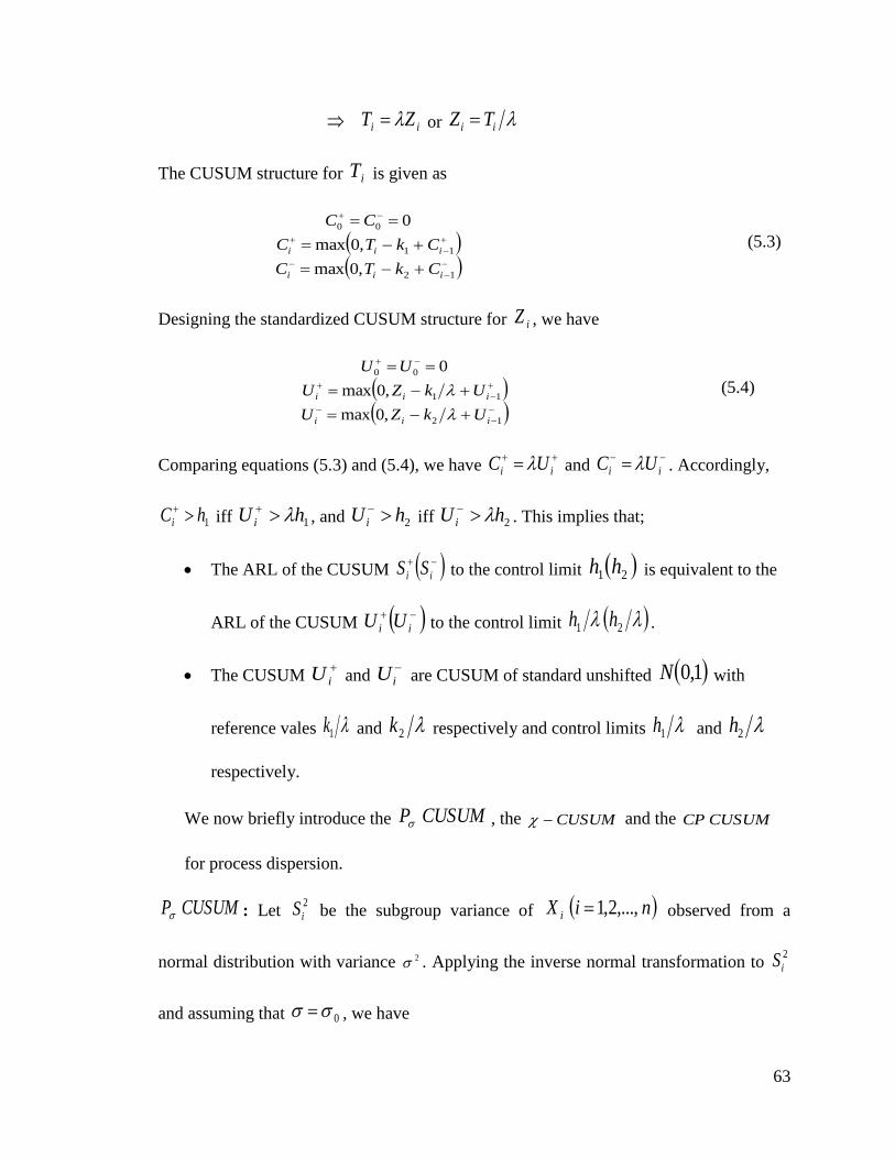
63
ii ZT or ii TZ
The CUSUM structure for iT is given as
12
11
00
,0max
,0max
0
iii
iii
CkTC
CkTC
CC
(5.3)
Designing the standardized CUSUM structure for iZ , we have
12
11
00
,0max
,0max
0
iii
iii
UkZU
UkZU
UU
(5.4)
Comparing equations (5.3) and (5.4), we have ii UC and
ii UC . Accordingly,
1hCi iff 1hU i
, and 2hU i iff 2hU i
. This implies that;
The ARL of the CUSUM
ii SS to the control limit 21 hh is equivalent to the
ARL of the CUSUM
ii UU to the control limit 21 hh .
The CUSUM
iU and
iU are CUSUM of standard unshifted 1,0N with
reference vales 1k and 2k respectively and control limits 1h and 2h
respectively.
We now briefly introduce the CUSUMP , the CUSUM and the CUSUMCP
for process dispersion.
CUSUMP : Let 2
iS be the subgroup variance of niX i ,...,2,1 observed from a
normal distribution with variance 2 . Applying the inverse normal transformation to 2
iS
and assuming that 0 , we have

64
2
0
2
21 11
i
i
SnFP
n
where 1,0~ NP , is the cumulative distribution from a standard normal
distribution and 2
1nF is the cumulative distribution from a chi-squared distribution
with 1n degree of freedom. Monitoring the mean of iP is equivalent to monitoring
the variance of iX . As a result, we could replace iZ by iP in equation (5.1) to monitor
process variance. The reference values 1k and
2k , and the control limits 1h and
2h that
fix a particular ARL could be guessed by a search method or by simulation.
CUSUM : Wilson & Hilferty (1931) proved that 3 2 nn is approximately
nnN 92,921 . For ,Niid , when 0 we have
1,0
19
2
19
212
02 3
1
N
n
niSi
.
Monitoring the mean of i
is equivalent to monitoring the variance of iX . Hence,
replacing iZ by i
in equation (1) gives the CUSUM . 1h and
2h that fix a
particular ARL could be guessed by a search method or by simulation. To determine 1k
and 2k , let 01 for upward shift and 02 for downward shift be the process
standard deviation to be monitored, then
101 ||2
1 ii EEk

65
19
2
19
2112
0212
1 31
nn
and
202 ||2
1 ii EEk
19
2
19
212
021
12
1 31
nn .
CUSUMCP : This is derived from the likelihood ratio test for the change point of a
normal process variance to monitor process dispersion. The CUSUMCP structure is
given as
12
2
11
2
00
,0max
,0max
0
iii
iii
CnkZC
CnkZC
CC
where
n
m imi ZZ1
22 . 00 imim XZ represents the mth standardized observation
in subgroup i . The reference values are defined as
2
22
1
11
11
ln;
11
ln
kk
where 011 and 022 are the relative increase and decrease in process
standard deviation.
The CUSUMP , the CUSUM and the CUSUMCP were shown by Acosta-Mejia et
al. (1999) to detect shifts in process variance quickly. If there is an out-of-control point at
the start of a process, it could be detected at the earliest time by introducing a head start
to CUSUM structure.
66
5.2.3 FAST INITIAL RESPONSE (FIR)
FIR CUSUM feature is designed by given a process a head start. Head start enables the
CUSUM structure to start off at a point other than the usual zero-point. The CUSUM
structure works by accumulating small shift until the shift is large enough to be noticed.
The FIR feature would enable a CUSUM chart to give signal as early as possible if there
is a shift at the start of a process, hence, reducing the time to signal. To maintain the same
in-control 0ARLARL of a CUSUM chart, the h value of the corresponding FIR
CUSUM must be increased by small amount. Ironically, the out-of-control 1ARLARL of
the FIR CUSUM would be lesser than that of its corresponding CUSUM chart. In the
work of Lucas & Crosier (1982), the 1ARL of FIR CUSUM is 30% to 40% shorter than
the corresponding 1ARL of CUSUM chart, in monitoring location parameter. Using their
recommended head start, we make 20 hC in our CUSUM schemes, and we focus on
one-sided FIR CUSUM scheme.
5.3 PERFORMANCE EVALUATION AND COMPARISON
In the work of Abujiya et al. (2015), performance measures such as ARL, standard
deviation run length (SDRL), extra quadratic length (EQL), relative average run length
(RARL) and performance comparison index (PCI) were used in determining and
explaining the efficiency of their proposed chart. In the same manner, we consider the
same approach in this section.
ARL: is the average number of samples observed until the first out-of-control signal
(false alarm) is detected in a process. ARL0 represents the ARL when there is no shift in a
process parameter (dispersion parameter in our case) while ARL1 represents the ARL

67
when there is shift in a process parameter (dispersion parameter in our case). It is
desirable to have high value of ARL0 but low value of ARL1 to efficiently monitor
process parameter(s) (Riaz et al. 2014).
SDRL: is the standard deviation of the number of samples observed until a false alarm is
detected in a process. It is often used to evaluate the performance measure of a chart, and
the ability of the chart to respond to shift in its parameter (Abbasi et al. 2012). The chart
with a better performance have a smaller SDRL.
QUANTILE: The 0.05, 0.25, 0.50, 0.75 and 0.95 quantiles (denoted as q5, q25, q50, q75
and q95) are estimated to determine the pattern of the run length distribution of an in-
control process.
EQL: gives the efficiency of a chart over the entire shifts considered in a process. The
chart with the lowest EQL is said to be the most efficient chart. It is calculated using
numerical computation, with the formula;
max
min
2
maxmin
1
dARLEQL .
RARL: gives the overall effectiveness of a chart with respect to a benchmark (bmk)
chart. A benchmark chart is usually the best chart (with the lowest EQL) or the chart been
compared with. It uses ARL values to determine how close a chart is to the benchmark
chart. RARL equals to one for the benchmark chart, and greater than one for the inferior
chart (to the benchmark chart) (Zhao et al. 2005).
max
minmaxmin
1
d
ARL
ARLRARL
bmk
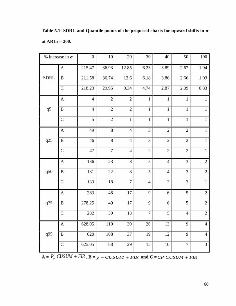
68
Table 5.1: SDRL and Quantile points of the proposed charts for upward shifts in 𝝈
at ARL0 = 200.
% increase in 𝝈 0 10 20 30 40 50 100
SDRL
A 215.47 36.93 12.85 6.23 3.89 2.67 1.04
B 211.58 36.74 12.6 6.18 3.86 2.66 1.03
C 218.23 29.95 9.34 4.74 2.87 2.09 0.83
q5
A 4 2 2 1 1 1 1
B 4 2 2 1 1 1 1
C 5 2 1 1 1 1 1
q25
A 49 8 4 3 2 2 1
B 46 8 4 3 2 2 1
C 47 7 4 2 2 2 1
q50
A 136 23 8 5 4 3 2
B 131 22 8 5 4 3 2
C 133 18 7 4 3 3 1
q75
A 283 48 17 9 6 5 2
B 278.25 49 17 9 6 5 2
C 282 39 13 7 5 4 2
q95
A 628.05 110 39 20 13 9 4
B 620 108 37 19 12 9 4
C 625.05 88 29 15 10 7 3
A = FIRCUSUMP , B = FIRCUSUM and C = FIRCUSUMCP
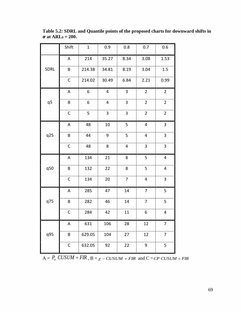
69
Table 5.2: SDRL and Quantile points of the proposed charts for downward shifts in
𝝈 at ARL0 = 200.
Shift 1 0.9 0.8 0.7 0.6
SDRL
A 214 35.27 8.34 3.08 1.53
B 214.38 34.81 8.19 3.04 1.5
C 214.02 30.49 6.84 2.21 0.99
q5
A 6 4 3 2 2
B 6 4 3 2 2
C 5 3 3 2 2
q25
A 48 10 5 4 3
B 44 9 5 4 3
C 48 8 4 3 3
q50
A 134 21 8 5 4
B 132 22 8 5 4
C 134 20 7 4 3
q75
A 285 47 14 7 5
B 282 46 14 7 5
C 284 42 11 6 4
q95
A 631 106 28 12 7
B 629.05 104 27 12 7
C 632.05 92 22 9 5
A = FIRCUSUMP , B = FIRCUSUM and C = FIRCUSUMCP

70
PCI: is the ratio of the EQL of a chart to the EQL of a benchmark chart under the same
condition. The best chart (benchmark chart) has PCI = 1, while the worst chart, as
compared to the benchmark chart, has the highest value of PCI (Ou et al., 2012).
bmkEQL
EQLPCI
Table 5.3: EQL, RARL and PCI of the proposed charts.
Upward shift in 𝝈 Downward shift in 𝝈
A B C A B C
EQL 28.62225 28.22307 25.29412 28.24351 28.06285 26.76816
RARL 1.208851 1.198675 1 1.180846 1.168157 1
PCI 1.131577 1.115796 1 1.055116 1.048367 1
A = FIRCUSUMP , B = FIRCUSUM and C = FIRCUSUMCP
Based on the result presented in Tables 5.1 – 5.5 and Figures 5.1 – 5.2, the basic findings
are summarized as follows;
I. For 0 , there is no significant difference between the ARL and the SDRL of
the proposed charts (Tables 5.1, 5.2, 5.4 and 5.5).
II. For 0 , the ARL and the SDRL of the proposed charts decrease rapidly
(Tables 5.1, 5.2, 5.4 and 5.5).
III. The FIR feature does not only improve the charts ability to detect out-of-control
signal at process start-up, but also improve the detection ability of the charts for
any shift in process standard deviation. (Tables 5.4 – 5.5 and Figures 5.1 – 5.2).
IV. The quantile points show that the run length distribution of the proposed charts
are positively skewed (Tables 5.1 – 5.2).
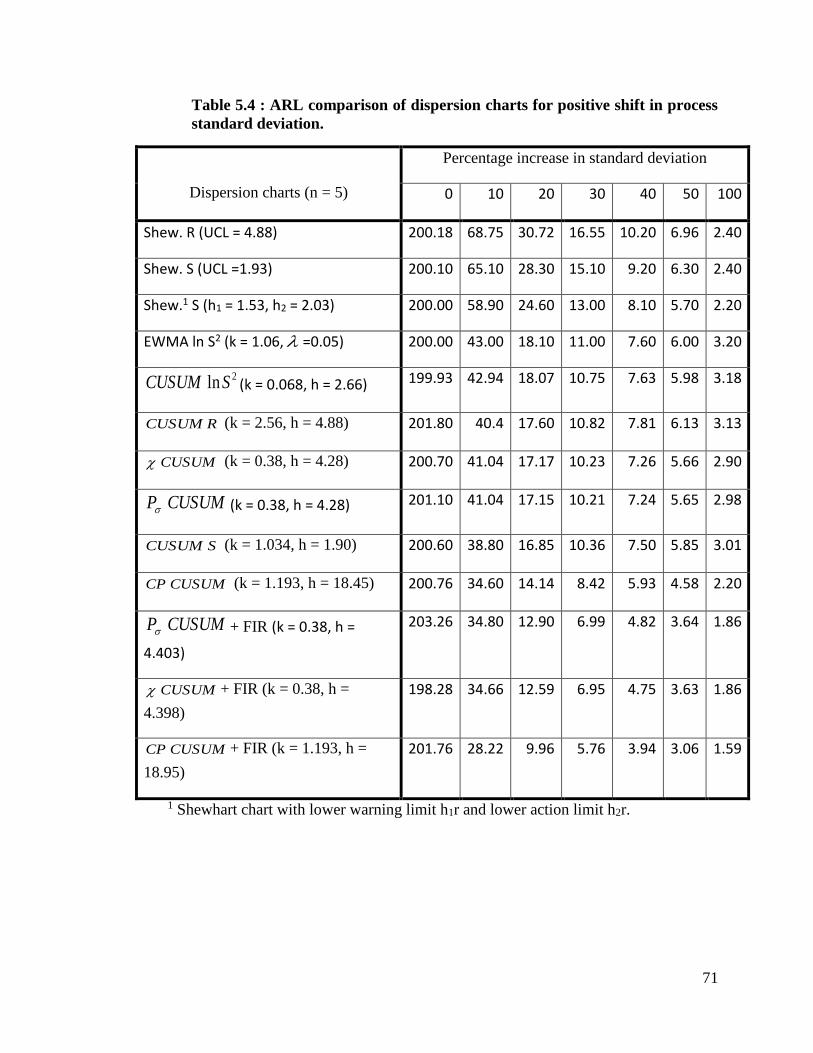
71
Table 5.4 : ARL comparison of dispersion charts for positive shift in process
standard deviation.
Dispersion charts (n = 5)
Percentage increase in standard deviation
0 10 20 30 40 50 100
Shew. R (UCL = 4.88) 200.18 68.75 30.72 16.55 10.20 6.96 2.40
Shew. S (UCL =1.93) 200.10 65.10 28.30 15.10 9.20 6.30 2.40
Shew.1 S (h1 = 1.53, h2 = 2.03) 200.00 58.90 24.60 13.00 8.10 5.70 2.20
EWMA ln S2 (k = 1.06, =0.05) 200.00 43.00 18.10 11.00 7.60 6.00 3.20
2ln SCUSUM (k = 0.068, h = 2.66) 199.93 42.94 18.07 10.75 7.63 5.98 3.18
RCUSUM (k = 2.56, h = 4.88) 201.80 40.4 17.60 10.82 7.81 6.13 3.13
CUSUM (k = 0.38, h = 4.28) 200.70 41.04 17.17 10.23 7.26 5.66 2.90
CUSUMP (k = 0.38, h = 4.28) 201.10 41.04 17.15 10.21 7.24 5.65 2.98
SCUSUM (k = 1.034, h = 1.90) 200.60 38.80 16.85 10.36 7.50 5.85 3.01
CUSUMCP (k = 1.193, h = 18.45) 200.76 34.60 14.14 8.42 5.93 4.58 2.20
CUSUMP + FIR (k = 0.38, h =
4.403)
203.26 34.80 12.90 6.99 4.82 3.64 1.86
CUSUM + FIR (k = 0.38, h =
4.398)
198.28 34.66 12.59 6.95 4.75 3.63 1.86
CUSUMCP + FIR (k = 1.193, h =
18.95)
201.76 28.22 9.96 5.76 3.94 3.06 1.59
1 Shewhart chart with lower warning limit h1r and lower action limit h2r.
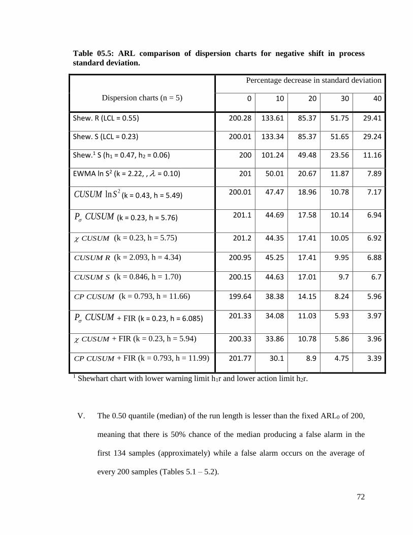
72
Table 05.5: ARL comparison of dispersion charts for negative shift in process
standard deviation.
Dispersion charts (n = 5)
Percentage decrease in standard deviation
0 10 20 30 40
Shew. R (LCL = 0.55) 200.28 133.61 85.37 51.75 29.41
Shew. S (LCL = 0.23) 200.01 133.34 85.37 51.65 29.24
Shew.1 S (h1 = 0.47, h2 = 0.06) 200 101.24 49.48 23.56 11.16
EWMA ln S2 (k = 2.22, , = 0.10) 201 50.01 20.67 11.87 7.89
2ln SCUSUM (k = 0.43, h = 5.49) 200.01 47.47 18.96 10.78 7.17
CUSUMP (k = 0.23, h = 5.76) 201.1 44.69 17.58 10.14 6.94
CUSUM (k = 0.23, h = 5.75) 201.2 44.35 17.41 10.05 6.92
RCUSUM (k = 2.093, h = 4.34) 200.95 45.25 17.41 9.95 6.88
SCUSUM (k = 0.846, h = 1.70) 200.15 44.63 17.01 9.7 6.7
CUSUMCP (k = 0.793, h = 11.66) 199.64 38.38 14.15 8.24 5.96
CUSUMP + FIR (k = 0.23, h = 6.085) 201.33 34.08 11.03 5.93 3.97
CUSUM + FIR (k = 0.23, h = 5.94) 200.33 33.86 10.78 5.86 3.96
CUSUMCP + FIR (k = 0.793, h = 11.99) 201.77 30.1 8.9 4.75 3.39
1 Shewhart chart with lower warning limit h1r and lower action limit h2r.
V. The 0.50 quantile (median) of the run length is lesser than the fixed ARL0 of 200,
meaning that there is 50% chance of the median producing a false alarm in the
first 134 samples (approximately) while a false alarm occurs on the average of
every 200 samples (Tables 5.1 – 5.2).
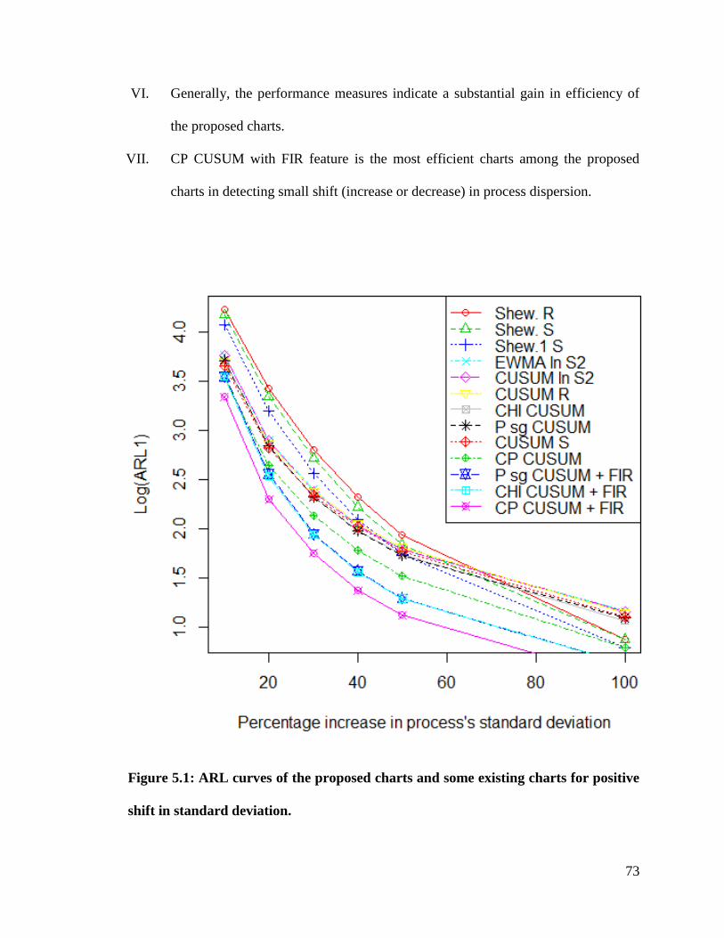
73
VI. Generally, the performance measures indicate a substantial gain in efficiency of
the proposed charts.
VII. CP CUSUM with FIR feature is the most efficient charts among the proposed
charts in detecting small shift (increase or decrease) in process dispersion.
Figure 5.1: ARL curves of the proposed charts and some existing charts for positive
shift in standard deviation.
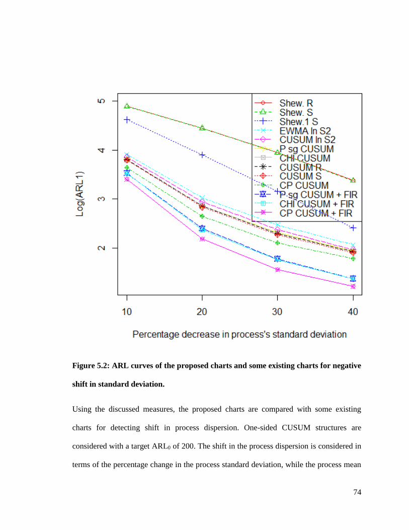
74
Figure 5.2: ARL curves of the proposed charts and some existing charts for negative
shift in standard deviation.
Using the discussed measures, the proposed charts are compared with some existing
charts for detecting shift in process dispersion. One-sided CUSUM structures are
considered with a target ARL0 of 200. The shift in the process dispersion is considered in
terms of the percentage change in the process standard deviation, while the process mean

75
is assumed stable. The existing charts taken into consideration are ; the Shewhart R, the
Shewhart S chart, the Page's (1963) Shewhart S chart with warning lines, the CUSUM of
the range R, CUSUM of the standard deviation S, the EWMA of 2ln S (Crowder &
Hamilton, 1992), the CUSUM of 2ln S (Chang & Gan, 1995), and the CUSUMP , the
CUSUM and the CUSUMCP of Acosta-Mejia et al. (1999).
The reference values (k) and the plotting statistics of the charts considered are
standardized to be independent of any value of 0 . In the CUSUM S chart, we have
110,0max iii CkSC
where 21 0141 ck , for the upper one-sided plotting statistic. Similarly, the
upper one-sided plotting statistic of the CUSUM of R chart is given as
110,0max iii CkRC
where 21 0121 dk .
Table 5.4 (and Figure 5.1) presents the ARL comparison of the charts in detecting 20%
increase in process standard deviation, with subgroup of size 5. The charts are arranged in
ascending order of their respective performance. Supplementing the Shewhart S chart
with warning line gives a better performance than the Shewhart S chart and the Shewhart
R chart. EWMA 2ln S chart gives a better performance than the Shewhart’s charts in
detecting increase in process’s standard deviation, but it is outperformed by the CUSUM
2ln S chart. However, the CUSUM R, the CUSUM , the CUSUMP , the CUSUM
S and the CP CUSUM all outperformed the CUSUM 2ln S chart, but perform worse
76
than the CUSUMP with FIR, the CUSUM with FIR and the CP CUSUM with
FIR.
Table 5.5 (and Figure 5.2) gives the ARL performance of the charts in detecting 20%
decrease in process standard deviation, with fixed ARL0 200 and subgroup of size 5. The
one-sided plotting statistic of the CUSUM S chart in detecting decrease in process
standard deviation is given as
10,0max iii CRkC
while the one-sided plotting statistic of the CUSUM R chart for detecting decrease in
process standard deviation is given as
10,0max iii CSkC .
The CUSUM R gains advantage over the CUSUM and the CUSUMP in detecting
decrease in (unlike when detecting increase in ). The CUSUMP , the
CUSUM , the CUSUM R and the CUSUM S are comparable and show better
performance than the Shewhart’s charts, the EWMA 2ln S chart and the CUSUM 2ln S
chart, but perform worse than the CP CUSUM, the CUSUMP with FIR, the
CUSUM with FIR and the CP CUSUM with FIR. Consistently, the charts with FIR
features give the best performance, with CP CUSUM + FIR having the overall best
performance.
77
5.4 SUMMARY AND CONCLUSION
Control chart is one of the tools of quality control to monitor production process, and to
distinguish between assignable causes and chance causes of variation. The variation may
be due to change in location parameter and/or dispersion parameter of a process. Few
works has been done on monitoring dispersion parameter of a process. The work of
Acosta-Mejia et al. (1999) was improved to efficiently detect shift in dispersion
parameter at start-up by applying the First Initial Response proposed by Lucas and
Crosier (1982). The proposed charts do not only detect shifts in process dispersion faster,
but also have better overall performance than their charts and some other existing charts
for monitoring process dispersion. Performance measures such as ARL, SDRL, quantile,
EQL, RQRL and PCI are used for comparison.

78
CHAPTER 6
SUMMARY AND CONCLUSION
A new two-sided CUSUM charts which are based on the utilization of auxiliary
information are proposed. The 𝐴𝑅𝐿 performance of the proposed charts is evaluated in
terms of shifts in study variable and compared with some recently designed control
structures meant for the same purposes. The comparisons revealed that the proposed
charts perform really well relative to the other charts under discussion, and a real life
industrial example is provided to describe the application procedure of the proposal.
Furthermore, the Shewhart chart and the cumulative sum (CUSUM) chart are
traditionally used for detecting large shifts and small shifts respectively, while the
Combined Shewhart CUSUM (CSC) monitors small shifts and large shifts
simultaneously. Using auxiliary information, new CSC (MiCSC, i = 2, 3, …, 10) charts
with more efficient estimators (the Regression-type estimator, the Ratio estimator, the
Singh and Tailor estimator, the power ratio-type estimator and the Kadilar and Cingi
estimators) for estimating location parameters are proposed. The charts are compared
using Average Run Length (ARL), Standard Deviation Run Length (SDRL) and Extra
Quadratic Loss (EQL), with other existing charts of the same purpose, and it is shown
that some of the MiCSC charts outperform their counterparts. A real-life industrial
example is provided to show the efficiency and the application of the proposed charts.
In addition, it is known that statistical process control deals with monitoring process to
detect disturbance in the process. The disturbance may be from the process mean or
variance. We assume that the process mean is stable and propose some charts that are
efficient for detecting early shifts in dispersion parameter, by applying the First Initial

79
Response (FIR) feature. Performance measures such as average run length (ARL),
standard deviation run length (SDRL), extra quadratic length (EQL), relative average run
length (RARL) and performance comparison index (PCI) are used to compare the
proposed charts with their existing counterparts including the Shewhart R, the Shewhart
S chart, the Shewhart S chart with warning lines, the CUSUM of the range R, CUSUM of
the standard deviation S, the EWMA of 2ln S , the CUSUM of 2ln S , the CUSUMP ,
the CUSUM and the CUSUMCP . The proposed charts do not only detect early
shifts in process dispersion faster, but also have better overall performance than their
existing counterparts.
80
References
Abbas, N., Riaz, M., & Does, R. J. M. M. (2011). Enhancing the performance of EWMA
charts. Quality and Reliability Engineering International, 27(6), 821–833.
Abbas, N., Riaz, M., & Does, R. J. M. M. (2014). An EWMA-Type Control Chart for
Monitoring the Process Mean Using Auxiliary Information. Communications in
Statistics - Theory and Methods, 43(16), 3485–3498.
doi:10.1080/03610926.2012.700368
Abbasi, S. A., Riaz, M., & Miller, A. (2012). Enhancing the performance of CUSUM
scale chart. Computers & Industrial Engineering, 63(2), 400–409.
Abujiya, M. R., Lee, M. H., & Riaz, M. (2015). Increasing the Sensitivity of Cumulative
Sum Charts for Location. Quality and Reliability Engineering International, 31(6),
1035–1051. doi:10.1002/qre.1661
Abujiya, M. R., Riaz, M., & Lee, M. H. (2013). Improving the Performance of Combined
Shewhart–Cumulative Sum Control Charts. Quality and Reliability Engineering
International, 29(8), 1193–1206.
Acosta-Mejia, C. a., Pignatiello, J. J., & Venkateshwara Rao, B. (1999). A comparison of
control charting procedures for monitoring process dispersion. IIE Transactions,
31(6), 569–579. doi:10.1080/07408179908969859
Adebola, F. B., Adegoke, N. A., & Sanusi, R. A. (2015). A Class of Regression Estimator
with Cum-Dual Ratio Estimator as Intercept. International Journal of Probability
and Statistics, 4(2), 42–50.
Ahmad, S., Abbasi, S. A., Riaz, M., & Abbas, N. (2014). On efficient use of auxiliary
information for control charting in SPC. Computers and Industrial Engineering,
67(1), 173–184. doi:10.1016/j.cie.2013.11.004
Ahmad, S., Riaz, M., Abbasi, S. A., & Lin, Z. (2014). On efficient median control
charting. Journal of the Chinese Institute of Engineers, 37(3), 358–375.
Busaba, J., Sukparungsee, S., Areepong, Y., & Mititelu, G. (2012). Analysis of average
run length for CUSUM procedure with negative exponential data. Chiang Mai
Journal of Science, 39(2), 222–230.
Chang, T. C., & Gan, F. F. (1995). Cumulative sum control chart for monitoring process
variance. Scholarbank.nus.edu.sg.
Cochran, W. G. (1953). Sampling techniques.
Constable, C. G., & Parker, R. L. (1988). Statistics of the geomagnetic secular variation
for the past 5 m.y. Journal of Geophysical Research, 93(B10), 11569.
doi:10.1029/JB093iB10p11569

81
Cox, M. A. A. (2010). Average run lengths of control charts for monitoring observations
from a Burr distribution. The Journal of Risk Finance, 11(5), 508–514.
Crowder, S. V. (1989). Design of exponentially weighted moving average schemes.
Journal of Quality Technology, 21(3), 155–162.
Crowder, S. V, & Hamilton, M. D. (1992). An {EWMA} for monitoring a process
standard deviation. Journal of Quality Technology, 24(1), 12–21. Retrieved from
http://cat.inist.fr/?aModele=afficheN&cpsidt=5111232
Ewan, W. D., & Kemp, K. W. (1960). Sampling inspection of continuous processes with
no autocorrelation between successive results. Biometrika, 47(3/4), 363–380.
Fuh, C.-D. (2003). SPRT and CUSUM in hidden Markov models. Annals of Statistics,
942–977.
Fuller, W. A. (2011). Sampling statistics (Vol. 560). John Wiley & Sons.
Gibbons, R. D. (1999). Use of Combined Shewhart‐CUSUM Control Charts for Ground
Water Monitoring Applications. Wiley Online Library, 37(5), 682–691.
Gupta, S., & Shabbir, J. (2008). On improvement in estimating the population mean in
simple random sampling. Journal of Applied Statistics, 35(5), 559–566.
doi:10.1080/02664760701835839
Haq, A. (2013). A new hybrid exponentially weighted moving average control chart for
monitoring process mean. Quality and Reliability Engineering International, 29(7),
1015–1025.
Hawkins, D. M., & Olwell, D. H. (1998). Cumulative sum charts and charting for quality
improvement. Springer Science & Business Media.
Henning, E., Samohyl, R. W., Walter, O. M. F. C., & Konrath, A. C. (2015). Performance
of a Combined Cusum-Shewhart Chart for Binomial Data for Large Shifts in the
Process Mean. Int. Journal of Engineering Research and Application, 5(8), 235–
243.
Jamali, A. S., Jinlin, L., & Durad, M. H. (2006). Average run length performance of
Shewhart control charts with interpretation rules. In Industrial Informatics, 2006
IEEE International Conference on (pp. 1329–1333). IEEE.
Kadilar, C., & Cingi, H. (2004). Ratio estimators in simple random sampling, 151, 893–
902. doi:10.1016/S0096-3003(03)00803-8
Kadilar, C., & Cingi, H. (2006a). Improvement in estimating the population mean in
simple random sampling. Applied Mathematics Letters, 19(1), 75–79.
Kadilar, C., & Cingi, H. (2006b). New ratio estimators using correlation coefficient. Inter
Stat, 4(March), 1–11.
Li, S.-Y., Tang, L.-C., & Ng, S.-H. (2010). Nonparametric CUSUM and EWMA control
82
charts for detecting mean shifts. Journal of Quality Technology, 42(2), 209.
Lucas, J. M. (1982). Combined Shewhart-CUSUM quality control schemes. Journal of
Quality Technology, 14(2).
Lucas, J. M., & Crosier, R. B. (1982). Fast initial response for CUSUM quality-control
schemes: give your CUSUM a head start. Technometrics, 24(3), 199–205.
Midi, H., & Shabbak, A. (2011). Robust multivariate control charts to detect small shifts
in mean. Mathematical Problems in Engineering, 2011.
Montgomery, D. (2009). Introduction to statistical quality control. John Wiley & Sons
Inc. doi:10.1002/1521-3773(20010316)40:6<9823::AID-ANIE9823>3.3.CO;2-C
Montgomery, D. C. (2007). Introduction to statistical quality control. John Wiley &
Sons.
Nazir, H. Z., Riaz, M., Does, R. J. M. M., & Abbas, N. (2013). Robust CUSUM Control
Charting. Quality Engineering, 25(3), 211–224. doi:10.1080/08982112.2013.769057
Ng, C. H. (1988). Development and evaluation of control charts using Exponentially
Weighted Moving Averages. Oklahoma State University.
Ou, Y., Wu, Z., & Tsung, F. (2012). A comparison study of effectiveness and robustness
of control charts for monitoring process mean. International Journal of Production
Economics, 135(1), 479–490.
Page, E. S. (1954). Continuous inspection schemes. Biometrika, 100–115.
Page, E. S. (1963). Controlling the standard deviation by CUSUMS and warning lines.
Technometrics, 5(3), 307–315.
R Core Team (2014). R: A language and environment for statistical computing. R Found
ation for Statistical Computing, Vienna, Austria. URL http://www.R-project.org/.
Reynolds, M. R., & Stoumbos, Z. G. (2010). Robust CUSUM charts for monitoring the
process mean and variance. Quality and Reliability Engineering International,
26(5), 453–473.
Riaz, M. (2008a). Monitoring process mean level using auxiliary information. Statistica
Neerlandica, 62(4), 458–481.
Riaz, M. (2008b). Monitoring process variability using auxiliary information.
Computational Statistics, 23(2), 253–276.
Riaz, M. (2015). Control charting and survey sampling techniques in process monitoring.
Journal of the Chinese Institute of Engineers, 38(3), 342–354.
Riaz, M., Abbasi, S. A., Ahmad, S., & Zaman, B. (2014). On efficient phase II process
monitoring charts. The International Journal of Advanced Manufacturing
83
Technology, 70(9-12), 2263–2274.
Riaz, M., & Does, R. J. M. M. (2008). An alternative to the bivariate control chart for
process dispersion. Quality Engineering, 21(1), 63–71.
Riaz, M., & Does, R. J. M. M. (2009). A process variability control chart. Computational
Statistics, 24(2), 345–368.
Roberts, S. W. (1959). Control chart tests based on geometric moving averages.
Technometrics, 1(3), 239–250. doi:10.1080/00401706.1959.10489860
Shewharrt, W. A. (1931). Economic Control of Quality of Manufactured Products. New
York: Macmillan.
Shewhart, W. A. (1924). Some applications of statistical methods to the analysis of
physical and engineering data. Bell System Technical Journal, 3(1), 43–87.
Singh, H. P., & Tailor, R. (2003). Use of known correlation coefficient in estimating the
finite population mean. Statistics in Transition, 6(4), 555–560.
Singh, R., & Mangat, N. S. (1996). Elements of Survey Sampling (Vol. 15).
doi:10.1007/978-94-017-1404-4
Srivastava, S. K. (1967). An estimator using auxiliary information in sample surveys.
Calcutta Statistical Association Bulletin, 16(62-63), 121–132.
Steiner, S. H. (1999). Exponentially weighted moving average control charts with time
varying control limits and fast initial response. Journal of Quality Technology,
31(0), 1.
Sukhatme, P. V, & Sukhatme, B. V. (1970). Sampling theory of surveys with
applications. London:[sn].
Tuprah, K., & Ncube, M. (1987). A comparison of dispersion quality control charts.
Sequential Analysis, 6(2), 155–163.
Wald, A. (1973). Sequential analysis. Courier Corporation.
Westgard, J. O., Groth, T., Aronsson, T., & de Verdier, C. H. (1977). Combined
Shewhart-CUSUM control chart for improved quality control in clinical chemistry.
Clinical Chemistry, 23(10), 1881–7. Retrieved from
http://www.ncbi.nlm.nih.gov/pubmed/902415
Wilson, E. B., & Hilferty, M. M. (1931). The distribution of chi-square. Proceedings of
the National Academy of Sciences, 17(12), 684–688.
Wu, Z., Jiao, J., Yang, M., Liu, Y., & Wang, Z. (2009). An enhanced adaptive CUSUM
control chart. IIE Transactions, 41(7), 642–653.
Wu, Z., Yang, M., Jiang, W., & Khoo, M. B. C. (2008). Optimization designs of the
combined Shewhart-CUSUM control charts. Computational Statistics and Data
84
Analysis, 53(2), 496–506. doi:10.1016/j.csda.2008.08.032
Zhang, C. W., Xie, M., & Jin, T. (2012). An improved self-starting cumulative count of
conforming chart for monitoring high-quality processes under group inspection.
International Journal of Production Research, 50(March 2015), 7026–7043.
doi:10.1080/00207543.2011.649305
Zhang, G. (1992). Cause-selecting Control Chart and Diagnosis: Theory and Practise.
aarhus School of Business.
Zhao, Y., Tsung, F., & Wang, Z. (2005). Dual CUSUM control schemes for detecting a
range of mean shifts. IIE Transactions, 37(11), 1047–1057.
doi:10.1080/07408170500232321

85
Vitae
Name :SANUSI, Ridwan Adeyemi
Nationality :Nigerian
Date of Birth :7/17/1989
Email :[email protected]
Address :A216, Ifelodun street, Ajagba, Wakajaye, Iyana-Church,
Iwo-Road, Ibadan, Nigeria
Academic Background :Click here to enter text.
EDUCATION
2014 – 2016 King Fahd University of Petroleum and Minerals, Department of
Mathematics, Dhahran, Saudi Arabia. M.Sc. in Statistics [CGPA: 3.929/4.000]
2008 – 2012 University of Ibadan, Department of Mathematics & Statistics,
Ibadan, Nigeria. B.Sc. (Hons) in Statistics [First Class]
2007 – 2009 University of Ibadan, Department of Mathematics & Statistics,
Ibadan, Nigeria. Professional Diploma in Statistics [Credit]
PEER-REVIEWED ARTICLES
Ridwan A. Sanusi, Muhammad Riaz, Nasir Abbas and Mu'azu Ramat Abujiya.
‘Using FIR to improve CUSUM charts for monitoring process dispersion’. (Under
preparation).
Ridwan A. Sanusi, Mu'azu Ramat Abujiya, Muhammad Riaz and Nasir Abbas.
‘Combined Shewhart CUSUM Charts using Auxiliary Variable’. Quality and
Reliability Engineering International (Under review).
Ridwan A. Sanusi, Muhammad Riaz and Nasir Abbas ‘An Efficient CUSUM-
Type Control Chart for Monitoring the Process Mean Using Auxiliary
Information’. Quality Technology and Qualitative Management (Under review).
86
Sanusi, RA, Adebola, FB, Adegoke, NA. (2016). "Cases of Road Traffic
Accident in Nigeria: A Time Series Approach." Mediterranean Journal of Social
Sciences 7.2 S1 (2016): 542.
Adebola, FB, Sanusi, RA, Adegoke, NA. (2015). ‘Consequences of road traffic
accident in Nigeria: Time series approach.’ International Journal of Computer
Applications Technology and Research, 4 (4), pp. 262-273.
Adebola, FB, Adegoke, NA, Sanusi, RA. (2015). ‘A Class of Regression
Estimator with Cum-Dual Ratio Estimator as Intercept.’ International Journal of
Probability and Statistics, 4(2), pp. 42-50. doi: 10.5923/j.ijps.20150402.02.
CONFERENCE ARTICLE
Sanusi, RA, Riaz, M, Adegoke, NA. (2016). ‘A New EWMA-Type Control Chart
for Monitoring Location Parameter Using Auxiliary Information In The Form of
Ratio Estimator’. UAE MATH DAY 2016, New York University, Abu Dhabi, UAE.