CUMIN charts

Metrika (2009) 70:111–130DOI 10.1007/s00184-008-0184-5

CUMIN charts

Willem Albers · Wilbert C. M. Kallenberg

Received: 2 July 2007 / Published online: 26 March 2008© The Author(s) 2008

Abstract Classical control charts are very sensitive to deviations from normality.In this respect, nonparametric charts form an attractive alternative. However, theseoften require considerably more Phase I observations than are available in practice.This latter problem can be solved by introducing grouping during Phase II. Then eachgroup minimum is compared to a suitable upper limit (in the two-sided case also eachgroup maximum to a lower limit). In the present paper it is demonstrated that suchMIN charts allow further improvement by adopting a sequential approach. Once anew observation fails to exceed the upper limit, its group is aborted and a new onestarts right away. The resulting CUMIN chart is easy to understand and implement.Moreover, this chart is truly nonparametric and has good detection properties. Forexample, like the CUSUM chart, it is markedly better than a Shewhart X -chart, unlessthe shift is really large.

Keywords Statistical process control · Phase II control limits · Order statistics ·CUSUM-chart

1 Introduction and motivation

By now it is well-known that standard control charts for controlling the mean of aproduction process, such as the Shewhart or CUSUM chart (see, e.g., 954;Lorden 1971), are highly sensitive to deviations from normality (see, e.g., Chan et al.1988; Pappanastos and Adams 1996; Hawkins and Olwell 1998, p. 75, Albers andKallenberg 2004, 2005b). Let us take the Shewhart X -chart for individual observations

W. Albers (B) · W. C. M. KallenbergDepartment of Applied Mathematics, University of Twente,P.O. Box 217, 7500 AE Enschede, The Netherlandse-mail: [email protected]

123

112 W. Albers, W. C. M. Kallenberg

(which we shall denote by IND) as a starting point. Here an out-of-control (OoC) signalimmediately occurs once an incoming observation falls above an upper limit UL orbelow a lower limit L L . While the process is in-control (I C), the false alarm rate (FAR)should equal some small p, like p = 1/1, 000 or 1/500. Even if we assume that theobservations come from a normal distribution, typically its parameters are unknown.An initial sample of size n (the so-called Phase I observations) is then needed alreadyto estimate these parameters and subsequently the UL and L L . Conditional on then Phase I observations, the FAR of the corresponding estimated chart now also is arandom variable (rv) Pn , and this Pn shows considerable variation around the intendedp. In fact, quite large values of n are required before this stochastic error (SE) becomesnegligible. Just see Albers and Kallenberg (AK for short) (2005a), which provides arecent non-technical review of the results available, as well as additional references.

However, if normality fails, we actually estimate the wrong control limits and Pn isnot even consistent for p anymore. In addition to the SE, we thus have a nonvanishingmodel error (ME). A first remedy is to consider wider parametric families, i.e., tobetter adapt the distribution used to the data at hand by supplying (and estimating)more than just two parameters. In this way, this ME can often be reduced substantially,be it at the cost of a somewhat further increase of the SE (see, e.g., Albers et al. 2004).The natural endpoint in this respect is a fully nonparametric approach: see, e.g., Bakirand Reynolds (1979), Bakir (2006), Chakraborti et al. (2001, 2004), Qiu and Hawkins(2001), and Qiu and Hawkins (2003), as well as Albers and Kallenberg (2004). In thelatter paper the control limits are simply based on empirical quantiles, i.e., appropriateorder statistics, of the initial sample. In this way, the ME is indeed removed completely,but the price will typically be a huge SE, unless n is very large. By way of example,consider a customary value like n = 100 and then realize the difficulty of subsequentlyestimating the upper and lower 1/1, 000-quantiles in a nonparametric way. Hence, aseach type of chart has its own potential drawback, a sensible overall approach thus isto adopt a data driven method (see Albers et al. 2006): let the data decide whether itis safe to stick to a normality based chart, or, if not, whether estimating an additionalparameter offers a satisfactory solution. If neither is the case, a nonparametric approachis called for, which will be fine if n is sufficiently large.

Consequently, what does remain is the need for a satisfactory nonparametric pro-cedure for ordinary n. This problem has subsequently been successfully addressed byAlbers and Kallenberg (2006, 2008). The idea is to group the observations during themonitoring phase. Hence the decision to give a signal is no longer based on a singleincoming observation, but instead on a group of size m, with m > 1 (with m = 1we are back in the boundary case IND). The question which choice is best, is morecomplicated than it might seem at first sight, even if we restrict attention (as is quitecustomary) to OoC behavior characterized by a shift d. In fact, it is twofold: (i) what mshould we take, and (ii) which group statistic? Consequently, this problem is dealt withfirst in Albers and Kallenberg (2006) for the case of known, not necessarily normal,underlying distributions. Afterwards, the estimation aspects—which form the verymotivation to consider grouping at all—are the topic of Albers and Kallenberg (2008).

Because of its optimality under normality, the obvious group statistic is the average,or equivalently, the sum. The corresponding chart is nothing but a Shewhart X -chartchart, which we will denote by SUM (or occasionally by SU M(m)) here. It is easily

123

CUMIN charts 113

verified that the optimal value of m decreases in d. In fact, for larger d, SU M(1) =I N D is best, but for a wide range of d-values of practical interest, a choice of mbetween say 2 and 5 will provide better performance. Incidentally, this is in line withthe observed superiority of CUSUM over IND for d not too large; we will comeback to this point in Sect. 3. However, we should realize that all of the foregoingassumes normality; once this assumption is abandoned, SUM is no longer optimal.Even worse, it is also difficult to adapt it to the nonparametric case. Approximationsbased on the central limit theorem are simply not at all reliable, as m is small and we aredealing with the tails. Moreover, a direct approach (see Albers and Kallenberg 2005b)leads to interesting theoretical insights into the tail behavior of empirical distributionfunctions for convolutions, but does not help much as far as practical implementationis concerned: the estimation still requires an n which is typically too large.

Consequently, there remains a definite need to consider alternative choices for thegroup statistic. Now a very good idea turns out to be using the minimum of the mobservations in the group in connection with some upper limit (and thus the groupmaximum with a lower limit). The corresponding chart we have called MIN (see Albersand Kallenberg 2006). Just like SUM, it beats IND, unless d becomes quite large. Ofcourse, under normality it is (somewhat) less powerful than SUM, but outside thenormal model, the roles can easily be reversed. Hence, even for known distributions,MIN is a serious competitor for SUM. However, as soon as we drop this artificialassumption, the attractiveness of MIN becomes fully apparent. For, as we just argued,in this nonparametric setting SUM can easily lead to a large ME if we continue toassume normality, while its nonparametric adaptation is no success. On the otherhand, the nonparametric version of IND is simple, but has a huge SE unless n is verylarge. In fact, this was what prompted us to consider grouping.

Hence with both SUM and IND we run into trouble. However, MIN has a straight-forward nonparametric adaptation, and hence M E = 0, just like the nonparametricIND. Moreover, unlike IND, it turns out to have an SE which is quite well-behavedand comparable to that of the normal SUM chart. The intuitive explanation is actuallyquite simple: application of MIN requires estimation of much less extreme quantilesthan IND or SUM. Take e.g., m = 3, then the upper 1/10-quantile is exceeded by agroup minimum with probability (1/10)3 = 1/1, 000, which is the same small valueas before. But estimating an upper 1/10-quantile on the basis of a sample of sizen = 100 is quite feasible, i.e., leads to a very reasonable SE. Hence (only) for MIN,both ME and SE are under control! As a consequence, the conclusion from Albers andKallenberg (2008) is quite positive towards this new chart: it is easy to understandand to implement, it is truly nonparametric and its power of detection is comparableto that of the standard, normality based, charts using sums.

After this favorable conclusion, the question arises whether there is room for furtherimprovement. Specifically, having mentioned the CUSUM chart before, and havingremarked that for not too large shifts this chart is superior compared to IND, the ideasuggests itself that a cumulative or sequential version of MIN might serve this purpose.In the present paper we shall demonstrate that this is indeed the case. Not surprisingly,we will call the corresponding proposal a CUMIN chart. In Sect. 2 we will introducethese charts in a systematic manner, taking once more the case of a known underlyingdistribution as our starting point (cf. Albers and Kallenberg 2006). The focus will

123


be on demonstrating that CUMIN remains quite easy to understand and implement.Section 3 is devoted to studying the performance during OoC and comparing it to thatof its competitors. In Sect. 4 the artificial assumption of known underlying distributionis abandoned and it is shown how the estimated version of the chart is obtained.

2 Definition and basic properties of CUMIN

Let X be a random variable (rv) with a continuous distribution function (df) F . Asannounced, we shall begin by assuming that F is known. Hence for now, there is noPhase I sample: we start immediately with the monitoring phase for the incomingX1, X2, . . .. For ease of presentation, we shall mainly concentrate on the one-sidedcase; only occasionally we shall consider the two-sided case, which can be treatedin a completely similar fashion. (Merely keep in mind to switch from (CU)MIN to(CU)MAX at the lower control limit.) First consider IND, the individual case withm = 1. Hence for given p, we need UL such that P(X > U L) = p during IC. For any

df H we write H = 1 − H and H−1 and H−1

for the respective inverse functions,

and thus U L = F−1(1 − p) = F−1

(p).Next we move on to the grouped case, where m > 1 and consider for the first group

T = T (m) = min (X1, . . . , Xm) (2.1)

as our control statistic for the upper MIN chart. (Here and in what follows we add‘(m)’ to the quantities we define when needed to avoid confusion, but often we usethe abbreviated notation.) As in this case P(T > U L) = F(U L)m during IC, itfollows that a fair comparison to IND is obtained by choosing U L = U L(m) =F

−1((mp)1/m), leading to F AR = P(T > U L) = mp. To see this, note that in this

way the average run length (ARL) will be m/F AR = 1/p, which thus agrees with the

ARL of IND based on U L = F−1

(p). During OoC, we consider a shift d > 0, i.e.,the Xi will have df F(x − d). Thus we immediately have that in this case we obtainfor the ARL of MIN that

ARL M (m, d) = m

P(T > U L)= m

{F(U L − d)}m= m

{F(F−1

((mp)1/m) − d)}m.

(2.2)

Clearly, ARL M (m, 0) = 1/p again. Moreover, by looking at ARL M (1, d) −ARL M (m, d) and/or ARL M (m, d)/ARL M (1, d), we can compare the performanceof MIN to that of IND. As demonstrated in Albers and Kallenberg (2006), the conclu-sion is that MIN is better than IND for a wide range of d values of practical interest.Only for large d, IND is best.

Note that the above holds for arbitrary F , and not just for the normal case. Forthe sake of comparison, we shall now also briefly consider the SUM chart (i.e., theShewhart X -chart). However, here normality is more or less required: for general F ,we wind up with rather intractable convolutions. So let � denote the standard normaldf and suppose that F(x) = �((x − µ)/σ). Actually, since we are in the case of

123

CUMIN charts 115

known F , we can take µ = 0 and σ = 1 without loss of generality, and thus F = �.In the case of SUM, we replace T in (2.1) by the standardized SUM of the first groupX1, . . . , Xm :

T = T (m) = m−1/2m∑

i=1

Xi = m1/2 X . (2.3)

Clearly, T then has df � as well and thus the choice U L = �−1

(mp) will producethe desired ARL = 1/p for F = �. It is also straightforward that under �(x − d)

ARL S(m, d) = m

�(�−1

(mp) − m1/2d). (2.4)

Again under F = �, studying ARL SS(1, d)−ARL S(m, d) and/or ARL SS(m, d)/

ARL S(1, d) makes sense for comparing the performance of SUM and IND. Oncemore the resulting picture is that IND is preferable only for rather large d (seeAlbers and Kallenberg 2006 for details). Likewise ARL M (m, d) − ARL S(m, d)

and/or ARL S(m, d)/ARL M (m, d) can be studied in order to compare SUM and MIN(cf. Albers and Kallenberg 2006 again).

In the above we have introduced and described IND, MIN and SUM. Now we are ina position to move on to the cumulative or sequential approach. As announced in theIntroduction, the idea is actually quite simple. Just look at the MIN chart for some givenm. Then each time a complete group of size m is assembled, its minimum value T

from (2.1) is computed and this T is subsequently compared to U L = F−1

((mp)1/m).But of course, as soon as an observation occurs within such a group which falls belowthis UL, it makes no sense to complete that group and we could as well stop rightaway. The next observation will then be the first of a new attempt. This idea leads tothe following definition of a sequential MIN procedure:

“Give an alarm at the 1st time m consecutive observations all exceed some UL”

(2.5)

In other words, this CUMIN chart is an accelerated version of MIN: before the finalsuccessful attempt to get m consecutive Xi > U L , the failed ones are broken of assoon as possible, rather than letting these all reach length m as well.

The proposal in (2.5) is inspired by the representation of CUSUM which can befound, e.g., in Page (1954) and Lorden (1971). The alternative form of CUSUM from,e.g., Lucas (1982) leads to an alternative for (2.5) as well. Let I (A) be the indicatorfunction of the set A and set S0 = 0. Consider Si = I ({Xi > U L})(1 + Si−1), i =1, 2, . . . , and give an alarm as soon as Sk ≥ m for some k.

Next we shall investigate the properties of CUMIN. In (2.5) we have deliberately

been a bit vague (’some UL’). Indeed, the UL for CUMIN, say F−1

( p), will have to be

different from F−1

((mp)1/m), the UL of MIN. As CUMIN reacts more quickly thanMIN, it is evident that its UL will have to be somewhat larger, i.e., p < (mp)1/m willhold. To find this p exactly, a bit more effort is required. First let us introduce somenotation. By ’Y is G(θ)’ we will mean that the rv Y has a geometric distribution with

123


parameter θ , and thus that P(Y = k) = θ(1 − θ)k−1, for k = 1, 2, . . .. Moreover, by’Z is Gm(θ)’ we will mean that the rv Z has an m-truncated geometric distributionwith parameter θ , which is defined through P(Z = k) = P(Y = k|Y ≤ m), k =1, . . . , m, where Y is G(θ). Clearly, G∞ = G again. Finally, let RL denote the runlength of a chart (and thus E(RL) = ARL). Then we have the following result.

Lemma 2.1 For the CUMIN chart defined in (2.5), with U L = F−1

( p), the runlength is distributed as

RL = m +V −1∑

i=1

Bi , (2.6)

where V, B1, B2, . . . , are independent rv’s and moreover V is G( pm) and the Bi areGm(1 − p). Consequently,

E(RL) = 1 − pm

(1 − p) pm= 1

1 − p

(1

pm− 1

),

var(RL) = 1 − pm

{(1 − p) pm}2

{1 + pm{ p − 2m(1 − p)}

1 − pm

}. (2.7)

Before proving Lemma 2.1 we present the following general result on m-truncateddistributions.

Lemma 2.2 Let B∗1 , B∗

2 , . . . , be independent and identically distributed (iid) rv’s withP(B∗

1 > m) > 0 and df H. Let V = min{k : B∗k > m}. Then, conditional on V = v,

the rv’s B∗1 , . . . , B∗

v−1 are iid with df Hm given by

Hm(b) = H(b)

H(m)f or b ≤ m and Hm(b) = 1 f or b > m.

Moreover, there exist rv’s B1, B2, . . . , such that V, B1, B2, . . . , are independent, Bi

has df Hm and for each function g the rv’s g(B∗1 , . . . , B∗

V −1) and g(B1, . . . , BV −1)

(with g equal to some constant if V = 1) have the same distribution.

Proof By definition of V , the event {V = v} = {B∗1 ≤ m, . . . , B∗

v−1 ≤ m, B∗v > m}.

Hence, we obtain for b1, . . . , bv−1 ≤ m, using the independence of B∗1 , B∗

2 , . . . ,

P(B∗1 ≤ b1, . . . , B∗

v−1 ≤ bv−1|V = v) = P(B∗1 ≤ b1, . . . , B∗

v−1 ≤ bv−1, B∗v > m)

P(B∗1 ≤ m, . . . , B∗

v−1 ≤ m, B∗v > m)

= �v−1i=1

{P(B∗

i ≤ bi )

P(B∗i ≤ m)

}= �v−1

i=1 Hm(bi )

and the first result easily follows. Define rv’s B1, B2, . . . , such that V, B1, B2, . . . ,

are independent and Bi has df Hm . Note that Hm , the conditional df of B∗1 , . . . , B∗

v−1

123

CUMIN charts 117

given V = v, does not depend on v, and hence the Bi can be defined as above. Nowwe have for any x

P(g(B∗1 , . . . , B∗

V −1) ≤ x) =∞∑

v=1

P(g(B∗1 , . . . , B∗

v−1) ≤ x |V = v)P(V = v)

=∞∑

v=1

P(g(B1, . . . , Bv−1) ≤ x)P(V = v)

=∞∑

v=1

P(g(B1, . . . , Bv−1) ≤ x, V = v)

= P(g(B1, . . . , BV −1) ≤ x).

��Proof of Lemma 2.1. Consider two forms of blocks of experiments for the sequenceX1, X2, . . .. The first one is related to the MIN chart and consists of fixed blocks ofsize m : W1 = (X1, . . . , Xm), W2 = (Xm+1, . . . , X2m), . . .. Obviously, W1, W2, . . .

are iid. The second one concerns the CUMIN chart. The first block now ends withthe first Xi ≤ U L . This gives W1. The second block starts with the next X andends with the second Xi ≤ U L . This produces W2, and so on. Again, W1, W2, . . .

are iid. In both situations the experiment Wi is called successful if at least m X ’sin Wi satisfy Xi > U L . Hence the probability of success in experiment Wi equalsθ = pm in either situation. Let V be the waiting time till the first successful experimentWi , then V is indeed G( pm). For the MIN chart we simply have RL = mV andE(RL) = m/ pm shows that in that case choosing p = (mp)1/m indeed producesE(RL) = ARL = 1/p.

For the second situation define B∗i as the length of the vector Wi . Since W1, W2, . . . ,

are iid, the rv’s B∗1 , B∗

2 , . . . , are also iid. Furthermore, the experiment Wi is successfulif B∗

i > m and hence V = min{k : B∗k > m}. In view of (2.5) we have that

RL = m + ∑V −1i=1 B∗

i . The first part of Lemma 2.1 now follows by application of

Lemma 2.2 with g(B1, . . . , BV −1) = m + ∑V −1i=1 Bi , noting that B∗

i is the first timethat we get X ≤ U L and thus B∗

i is G(1 − p).To obtain the moments in (2.7), let Y be G(θ) and Z be Gm(θ). For r = 1, 2, . . . ,

we observe that the memoryless property of the geometric distribution produces E(Y +m)r = ∑∞

k=1(k + m)r P(Y = k + m|Y > m) = ∑∞k=m+1 kr P(Y = k)/P(Y > m) =

{EY r − E Zr P(Y ≤ m)}/P(Y > m) and thus E Zr = {EY r − E(Y + m)r P(Y >

m)}/P(Y ≤ m). For r = 1 this gives E Z = EY − m P(Y > m)/P(Y ≤ m) =1/θ − m(1 − θ)m/{1 − (1 − θ)m}. Hence E(RL) = m + E(V − 1)E B = m +(1/ pm −1){1/(1− p)−m pm/(1− pm)} and the first result in (2.7) follows. Moreover,applying the result above for r = 2 as well leads to var(Z) = var(Y ) − m2 P(Y >

m)/{P(Y ≤ m)}2 = (1− θ)/θ2 −m2(1− θ)m/{1− (1− θ)m}2. It remains to use thatvar(RL) = (E B)2var(V ) + var(B)(EV − 1) in order to obtain the second resultin (2.7). ��

123


Remark 2.1 E(RL) can also be obtained by applying renewal theory (see, e.g., Ross1996). Instead of (2.6), use the representation RL = m − CV + ∑V

i=1 Ci , where theCi are simply G(1 − p). As ECV = m + 1/(1 − p), while Wald’s equation givesE(

∑Vi=1 Ci ) = EV EC1 = 1/{ pm(1 − p)}, the first line in (2.7) again follows. ��

From (2.7) it follows that ARL = 1/p will result if p is chosen such that

(1 − p) pm

1 − pm= p, (2.8)

As p is very small, pm will be of the order p, and hence as a first approximationwe have pm ≈ p/(1 − p1/m), i.e.,

p ≈(

p

1 − p1/m

)1/m

. (2.9)

This already is quite accurate; if desired, (2.9) can be replaced by p ≈ {p/(1 −[p/(1 − p1/m)]}1/m)}1/m , which is very precise. Note that the interpretation of (2.9)is still rather simple: the failed sequences of fixed length m for MIN are replaced bysequences of expected length approximately 1/(1 − p) for CUMIN. Hence the totalexpected length changes from m/ pm to about 1/{(1 − p) pm} and thus the formersolution (mp)1/m becomes (2.9). Indeed, 1/(1 − p1/m) is considerably smaller thanm : for p = 0.001, e.g., 1.11 for m = 3 and 1.46 for m = 6.

Next we note that the fact that pm is of order p implies in view of (2.7) thatvar(RL) ≈ 1/{(1− p) pm}2. This leading term is essentially due to (E B)2var(V ); thesecond part var(B)(EV −1) of var(RL) just gives a lower order contribution. In otherwords, the RL of CUMIN behaves to first order as V/(1− p) (cf. the RL of MIN whichexactly equals mV ). Moreover, if p satisfies (2.8), it follows that var(RL) ≈ 1/p2.Hence the simple conclusion is that the RL of the CUMIN chart from Lemma 2.1with p selected such that (2.8) holds, behaves like a G( pm)/(1 − p) rv. By way ofillustration, we give:

Example 2.1 For p = 0.001 and m = 3 we obtain that p = 0.103677 and pm =0.001114. The approximation from (2.9) leads to p = 0.103574 and pm = 0.001111,which produces 0.000997 rather than p = 0.001 in (2.8). The refinement below(2.9) gives p = 0.103712 and pm = 0.001116, which gives 0.001001 in (2.8). (Wehave dragged along more digits than would be useful in practice, just to show thedifferences.) Roughly speaking, the RL behaves like 10/9 times a G(1/900)rv.

If we choose instead m = 6, the results become p = 0.338708 and pm = 0.001510.The approximation from (2.9) then leads to p = 0.336911 and pm = 0.001462, whichproduces 0.000971 rather than p = 0.001 in (2.8). The refinement below (2.9) leadsto p = 0.338640 and pm = 0.001508, and 0.000999 as the result of (2.8). Here RLis roughly 3/2 times a G(3/2000) rv. ��We summarize the previous discussion with the following formal result.

123

CUMIN charts 119

Lemma 2.3 Let p be defined by (2.8) and let V be G( pm). Then, for p → 0,

E(RL) = E

(V

1 − p

)− 1

1 − p= E

(V

1 − p

)(1 + O(p)) , (2.10)

var(RL)=var

(V

1 − p

) {1 + pm p − 2m(1 − p)

1 − pm

}= var

(V

1 − p

)(1 + O(p)) .

(2.11)

Proof Let h(x) = (1 − x)xm/(1 − xm), then h( p) = p. For any ε we obtain thatlim p→0h(p1/m(1 + ε))/p = (1 + ε)m and hence

p = p1/m(1 + o(1)) (2.12)

as p → 0. As V is G( pm), it follows that E(V/(1 − p) equals

1

pm(1 − p)= 1 − pm

pm(1 − p)+ 1

1 − p= E(RL) + 1

1 − p= 1

p+ O(1)

as p → 0 and thus (2.10) holds. Likewise, the definition of V implies that var(V/(1− p)) = (1− pm)/{(1− p) pm}2. Now (2.11) follows from (2.7) by noting thatpm{ p − 2m(1 − p)/(1 − pm} = pm{−2m + O( p)} = O(p). ��

3 Out-of-control behavior

In this section we shall study the OoC behavior of CUMIN and compare it to that of itscompetitors. For MIN and SUM, the ARL during OoC has already been given in (2.2)and (2.4), respectively. Lemma 2.1 continues to hold in the OoC case if we replace p

by F(F−1

( p) − d). In view of (2.7) we now obtain for CUMIN that

ARLC M (m, d) ={

1

(F(F−1

( p) − d))m− 1

}1

F(F−1

( p) − d), (3.1)

where p = p(m) is the solution of (2.8), as given approximately by (2.9). Hencewe have ARLC M (m, 0) = 1/p again for all F (just like MIN, cf. (2.2)), and not justfor F = � (like SUM, cf. (2.4)).

Note that we have made only explicit in (3.1) the dependence of the ARL on m andd. To achieve full generality, we should of course write ARLC M (p, m, d, F). However,to avoid an unnecessarily lengthy exposition, we shall not pursue the dependence onp and F in detail. For p the reason is quite simple: it really suffices to concentrateon a single representative value, like the case p = 0.001 from our examples. Thevalues used in practice will be of a similar order of magnitude and it can be verifiedthat for such values the conclusions about the behavior of the function from (3.1) willbe qualitatively the same. As concerns F , the situation is a bit more complicated. Inprinciple, it would be quite interesting to see how (3.1) behaves for a variety of F’s.

123


However, as most of the competitors (IND, SUM, CUSUM) are only valid under thesingle option F = �, there is little to compare to outside normality. For that reasononly, we will restrict attention to F = � for our CUMIN as well. Hence, as indicatedin (3.1), in what follows we concentrate on m and d.

The first question of interest (cf. Sect. 1) is of course: what m should we take? Asmentioned, the answer depends on d: the larger d, the smaller m should be. To be a bitmore specific, for really large d, like d = 3, it is best to simply let m = 1, i.e., to useIND. For values in an interval around the typical choice d = 1 (cf. e.g., Ryan 1989,p.107), a simple rule of thumb for the optimal value of m is:

mopt ≈ 17

1 + 2d2 . (3.2)

As d increases from 1/2 to 3/2 in steps of 1/4, the rule in (3.2) indeed produces thecorresponding correct values of mopt : 11, 8, 6, 4 and 3. For values of d even smallerthan 1/2, the optimal value of m rises sharply. However, the function in (3.1) thenremains quite flat over a wide range of m-values, so there seems to be no need toconsider m larger than 10. All in all, a simple advice for use in practice could be:

• Use m = 1, i.e., IND, only if the supposed d is really large (d ≈ 3).• In all other cases, considerable improvement w.r.t. IND is possible.• If d is supposed to be moderately large (≈ 3/2 or 2), m = 3 is suitable. (3.3)

• For somewhat smaller d (≈ 1), m = 6 seems fine.• For really small d (1/2 or below), m = 10 should do.

Do remember that this advice is tuned at p = 0.001 and F = �. For differentp we might get slightly different results; for (quite) different F in principle (quite)different behavior could be advisable. However, if a specific interest arises for a givenF , a suitable analog of (3.2) can easily be found through (3.1) along the same lines.

It should be stressed that the resulting picture about the relation between d and m isby no means typical for CUMIN. In fact, expressions (2.2) and (2.4) lead to completelysimilar results for MIN and SUM, respectively. From (2.2) we obtain as an analog to(3.2) for MIN that mopt ≈ 1, 000/(75+80d2) for 1/2 ≤ d ≤ 3/2, while (2.4) producesmopt ≈ 40/(1 + 4d2) for SUM and these values of d, e.g., for d = 1, mopt = 6 forMIN and mopt = 8 for SUM. Hence, as already stated before, both SUM and MIN alsobeat IND for smaller values of d. In fact, detailed information on the relation betweenIND, SUM and MIN was already presented in AK (2006). Here we just present a singlebut representative example.

Example 3.1 From Albers and Kallenberg (2006) we quote that for p = 0.001 andF = �, at d = 1 the ARL of the individual chart equals 54.6. Suppose we haddecided to use m = 3, then this result is improved with 26.7 by taking MIN, yieldingARL = 27.9; the further improvement when using SUM is much less: 8.5, givingARL = 19.4. (That the overall winner here is SUM is of course by virtue of thechoice F = �; outside normality, MIN can be the winner; see Albers and Kallenberg(2006) for examples.) If we now in addition suppose that we did not simply use m = 3,but in fact had guessed correctly and selected mopt in either case, the picture is modified

123

CUMIN charts 121

MARL (6,d) - ARL (6,d)

CMM

ARL (6,d) / ARL (6,d)CM

00.5 1 1.5 2 0 0.5 1 1.5 2

5

10

15

20

d

1

1.02

1.04

1.06

1.08

1.1

1.12

1.14

d

Fig. 1 Comparison of CUMIN to MIN

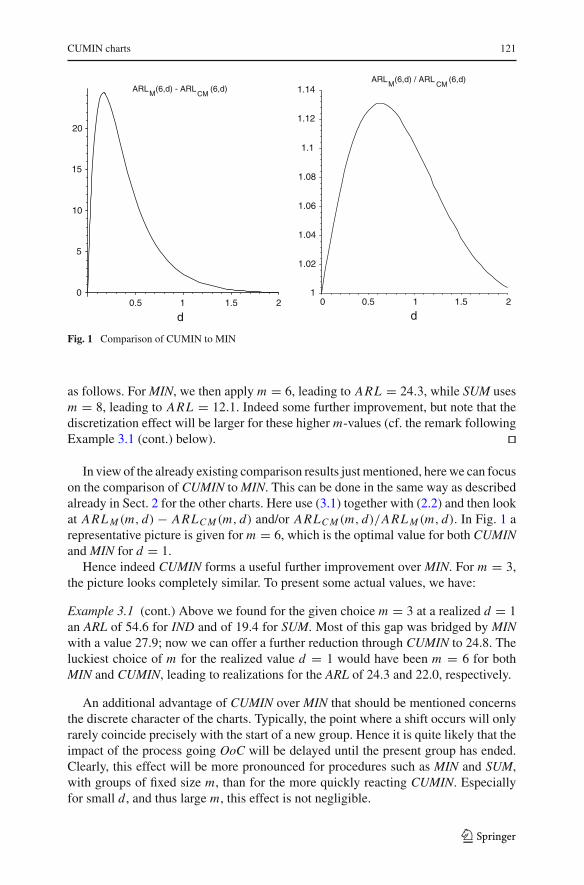
as follows. For MIN, we then apply m = 6, leading to ARL = 24.3, while SUM usesm = 8, leading to ARL = 12.1. Indeed some further improvement, but note that thediscretization effect will be larger for these higher m-values (cf. the remark followingExample 3.1 (cont.) below). ��

In view of the already existing comparison results just mentioned, here we can focuson the comparison of CUMIN to MIN. This can be done in the same way as describedalready in Sect. 2 for the other charts. Here use (3.1) together with (2.2) and then lookat ARL M (m, d) − ARLC M (m, d) and/or ARLC M (m, d)/ARL M (m, d). In Fig. 1 arepresentative picture is given for m = 6, which is the optimal value for both CUMINand MIN for d = 1.

Hence indeed CUMIN forms a useful further improvement over MIN. For m = 3,the picture looks completely similar. To present some actual values, we have:

Example 3.1 (cont.) Above we found for the given choice m = 3 at a realized d = 1an ARL of 54.6 for IND and of 19.4 for SUM. Most of this gap was bridged by MINwith a value 27.9; now we can offer a further reduction through CUMIN to 24.8. Theluckiest choice of m for the realized value d = 1 would have been m = 6 for bothMIN and CUMIN, leading to realizations for the ARL of 24.3 and 22.0, respectively.

An additional advantage of CUMIN over MIN that should be mentioned concernsthe discrete character of the charts. Typically, the point where a shift occurs will onlyrarely coincide precisely with the start of a new group. Hence it is quite likely that theimpact of the process going OoC will be delayed until the present group has ended.Clearly, this effect will be more pronounced for procedures such as MIN and SUM,with groups of fixed size m, than for the more quickly reacting CUMIN. Especiallyfor small d, and thus large m, this effect is not negligible.

123


To complete the picture, it remains to add some comparison to CUSUM as well.However, let us first point out some confusion which might arise here, due to the factthat the notion of grouped data is used in various ways. Quite often, data used forcontrol charting occur already in subgroups of sizes, e.g., 3, 4 or 5. The correspondingsubgroup averages are then used and a Shewhart X -chart is applied, rather than aShewhart X -chart for individual observations. This sounds as if, in our terminology,SUM is used instead of IND. However, this does not necessarily have to be the case.Consider, e.g., Ryan (1989), Sect. 5.3, where the CUSUM procedure is compared tothe Shewhart X -chart. An example involving subgroups of size 4 is used and it isrightfully concluded that, e.g., for d = 1 the CUSUM chart really is much better. Thequestion; however, is: much better than what? The point is that in this example theshift d is given in units of σX and not of σX . Hence, in our terminology, the Xi are usedas individual observations again, and the comparison is between CUSUM and IND,and not between CUSUM and SUM. If the appropriate Xi in their turn are collectedinto groups according to our setup, the gap in performance would be much smaller.To illustrate this qualitative explanation, we have the following example.

Example 3.2 Ryan (1989) gives in Table 5.6 an ARL of 10.4 for the CUSUM chartwith d = 1 (k = 0.5) and h = 5. In comparison, he mentions that the X -chart scoresthe much larger 43.96. Indeed, this latter value is the ARL of IND for d = 1 andp = 0.00135 = �(3), used in the customary ‘3σ ’-chart. As according to Table 5.6the two-sided CUSUM chart in question has ARL = 465 during I C , the appropriatep to use would be 1/930. In that case IND even requires an ARL = 51.8 for d = 1.However, suppose we would have used SUM with m = 8 (which is mopt for d = 1 andthe present value p = 1/930 as well). Then it follows from (2.4) that the correspondingARL is merely 11.9, which indeed is much closer to CUSUM’s 10.4 than IND’s 51.8.Admittedly, this result looks extremely nice because we (more or less) took mopt inSUM. But take, e.g., d = 1/2 instead of d = 1, then the ARL’s rise for CUSUM to 38.0and for IND to 196. In this situation, m = 8 is not at all optimal anymore for SUM.Nevertheless, the SU M(8) chart has ARL = 48.0 for d = 1/2, which still largelybridges the gap between 196 and 38.0.

Hence the resulting picture is as follows. For a wide range of d values, an (oftensubstantial) improvement over IND is offered by MIN. This chart in its turn is furtherimproved by its sequential analogue CUMIN, both directly (cf. Fig. 1) and because ofthe discrete character of the charts. For the sum-based procedures the situation actuallyis completely analogous. First IND is substantially improved by SUM, which in its turnis further improved by CUSUM. When focusing on the case F = �, sum-based chartsare obviously better than min-based ones. But always bear in mind that this superiorityrests on this normality assumption, which is often quite questionable, especially in thetails. If normality fails, both SUM and CUSUM run into trouble. For known F = �,they are awkward to handle, whereas for the min-based charts � plays no special roleat all (cf. (2.2) and (3.1)). And when F is unknown, SUM and CUSUM (cf. Hawkinsand Olwell 1998, p.75) may lead to a considerable ME. In case of IND, see, e.g., Table 1on p. 173 of Albers et al. (2004). Various nonnormal distributions are considered here,such as the normal power family, based on |Z |1+γ sign(Z), with Z standard normaland γ > −1. For γ = 1/2, and p = 0.001, we have ME = 5.6p, while for γ = 1

123

CUMIN charts 123

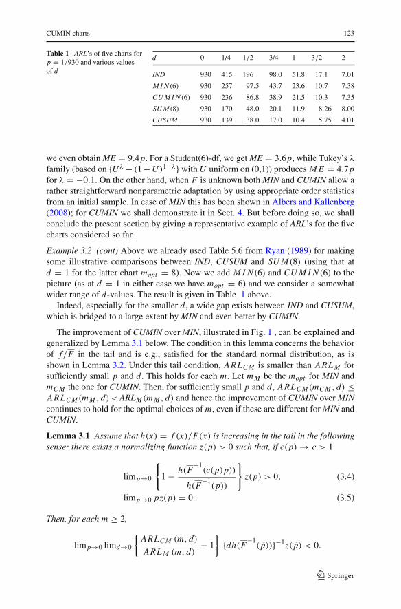
Table 1 ARL’s of five charts forp = 1/930 and various valuesof d

d 0 1/4 1/2 3/4 1 3/2 2

IND 930 415 196 98.0 51.8 17.1 7.01

M I N (6) 930 257 97.5 43.7 23.6 10.7 7.38

CU M I N (6) 930 236 86.8 38.9 21.5 10.3 7.35

SU M(8) 930 170 48.0 20.1 11.9 8.26 8.00

CUSUM 930 139 38.0 17.0 10.4 5.75 4.01

we even obtain ME = 9.4p. For a Student(6)-df, we get ME = 3.6p, while Tukey’s λ

family (based on {Uλ − (1 − U )1−λ} with U uniform on (0,1)) produces M E = 4.7pfor λ = −0.1. On the other hand, when F is unknown both MIN and CUMIN allow arather straightforward nonparametric adaptation by using appropriate order statisticsfrom an initial sample. In case of MIN this has been shown in Albers and Kallenberg(2008); for CUMIN we shall demonstrate it in Sect. 4. But before doing so, we shallconclude the present section by giving a representative example of ARL’s for the fivecharts considered so far.

Example 3.2 (cont) Above we already used Table 5.6 from Ryan (1989) for makingsome illustrative comparisons between IND, CUSUM and SU M(8) (using that atd = 1 for the latter chart mopt = 8). Now we add M I N (6) and CU M I N (6) to thepicture (as at d = 1 in either case we have mopt = 6) and we consider a somewhatwider range of d-values. The result is given in Table 1 above.

Indeed, especially for the smaller d, a wide gap exists between IND and CUSUM,which is bridged to a large extent by MIN and even better by CUMIN.

The improvement of CUMIN over MIN, illustrated in Fig. 1 , can be explained andgeneralized by Lemma 3.1 below. The condition in this lemma concerns the behaviorof f/F in the tail and is e.g., satisfied for the standard normal distribution, as isshown in Lemma 3.2. Under this tail condition, ARLC M is smaller than ARL M forsufficiently small p and d. This holds for each m. Let mM be the mopt for MIN andmC M the one for CUMIN. Then, for sufficiently small p and d, ARLC M (mC M , d) ≤ARLC M (m M , d)< ARLM (m M , d) and hence the improvement of CUMIN over MINcontinues to hold for the optimal choices of m, even if these are different for MIN andCUMIN.

Lemma 3.1 Assume that h(x) = f (x)/F(x) is increasing in the tail in the followingsense: there exists a normalizing function z(p) > 0 such that, if c(p) → c > 1

lim p→0

{1 − h(F

−1(c(p)p))

h(F−1

(p))

}z(p) > 0, (3.4)

lim p→0 pz(p) = 0. (3.5)

Then, for each m ≥ 2,

lim p→0 limd→0

{ARLC M (m, d)

ARL M (m, d)− 1

}{dh(F

−1( p))}−1z( p) < 0.

123


Proof Taylor expansion of ARLC M (m, d), given in (3.1), and application ofARLC M (m, 0) = (1 − p)−1( p−m − 1), cf. (2.7), yields as d → 0

ARLC M (m, d) = ARLC M (m, 0) − mdh(F−1

( p))

(1 − p) pm+ d

(1

pm− 1

)ph(F

−1( p))

(1 − p)2

+ O(d2) = ARLC M (m, 0){1 − mdk( p) + O(d2)},

where k( p) = h(F−1

( p))[1 + pm/(1 − pm) − p/((1 − p)m)]. By Taylor expansionof ARL M (m, d), as given in (2.2), we get

ARL M (m, d) = ARL M (m, 0) − m2d F(F−1

((mp)1/m))−m−1 f (F−1

((mp)1/m)) + O(d2)

= ARL(m, 0){1 − mdh(F−1

((mp)1/m)) + O(d2)}

as d → 0. Since ARLC M (m, 0) = ARL M (m, 0) = p−1, we obtain

ARLC M (m, d)

ARL M (m, d)= 1 − mdk( p)

1 − mdh(F−1

((mp)1/m))+ O(d2)}

= 1 − md{k( p) − h(F−1

((mp)1/m))} + O(d2)}

as d → 0. Hence we get

limd→0

{ARLC M (m, d)

ARL M (m, d)− 1

}d−1 = −m{k( p) − h(F

−1((mp)1/m))}. (3.6)

Define c( p) = (mp)1/m p−1. (Note that p can be considered as a function of p andvice versa.) In view of (2.12) we have that lim p→0 c( p) = m1/m > 1. According tothe condition on h there exists a function z with z( p) > 0 such that

lim p→0

{1 − h(F

−1((mp)1/m))

h(F−1

( p))

}z( p) > 0

and lim p→0 pz( p) = 0. Together with (3.6) and the definition of k( p) we obtain

lim p→0 limd→0

{ARLC M (m, d)

ARL M (m, d)− 1

}{dh(F

−1( p))}−1z( p)

= lim p→0 − mz( p)

{1 + pm

1 − pm− p

(1 − p)m− h(F

−1((mp)1/m))

h(F−1

( p))

}

= lim p→0 − mz( p)

{1 − h(F

−1((mp)1/m))

h(F−1

( p))

}< 0

as was to be proved. ��We check the conditions on h in case where F = �.

123

CUMIN charts 125

Lemma 3.2 For the standard normal distribution h(x) = ϕ(x)/�(x) is increasingin the sense of (3.4) and (3.5).

Proof The behavior of � in the tail is given by the following expansion for largequantiles:

�−1

(q) = (2|logq|)1/2[1 − k1(q) + o(|logq|−1)],

as q → 0, where k1(q) = (2|logq|)−1{log(2|logq|) + log(2π)}/2.Furthermore use that h(x) = x[1 + x−2{1 + o(1)}] as x → ∞. Let c(p) → c > 1

as p → 0. Then we obtain, as p → 0, that h(�−1

(c(p)p))/h(�−1

(p)) equals

�−1

(c(p)p)

�−1

(p)

{1 + [�−1

(c(p)p)]−2(1 + o(1))

1 + [�−1(p)]−2(1 + o(1))

}

= k0(p)

{1 − k1(c(p)p) + o(|logp|−1)

1 − k1(p) + o(|logp|−1)

}k2(p)(1 + o(1)),

in which k0(p) = {|log(c(p)p)|/|logp|}1/2 and k2(p) = {1+(2|log(c(p)p)|)−1}{1+(2|logp|)−1}. For the various ki we have the following results:

k0(p) ={−logc(p) + |logp|

|logp|}1/2

= 1 − 1

2

logc

|logp| + o(|logp|−1),

1 − k1(c(p)p))

1 − k1(p))= [1 − k1(c(p)p))][1 + k1(p)] + o(|logp|−1) = 1 + o(|logp|−1),

k2(p) = 1 + o(|logp|−1),

and thus, as p → 0,

h(�−1

(c(p)p))

h(�−1

(p))= 1 − 1

2

(logc

|logp|)

+ o(|logp|−1).

Now define z(p) = |logp|, then the limit in (3.4) equals (logc)/2. As c > 1, this isindeed positive. Moreover, (3.5) holds as well. ��

4 The nonparametric chart

In Sects. 2 and 3 we have worked under the assumption of known F . This was very use-ful in order to demonstrate the properties and performance of CUMIN and to compareit to its various competitors. However, by now we should drop this artificial assump-tion again and return to our main case of interest. There the normality assumption isnot to be trusted, especially in the tail area we are dealing with, and a nonparametricapproach is desired. Hence a Phase I sample X1, . . . , Xn is needed again and will beused to obtain an estimated U L (and, for the two-sided case, an estimated L L).

123


Assume that F is continuous and let Fn(x) = n−1#{Xi ≤ x} be the empirical dfand F−1

n the corresponding quantile function, i.e., F−1n (t) = inf{x |Fn(x) ≥ t}. Then it

follows that F−1n (t) equals X(i) for (i −1)/n < t ≤ i/n, where X(1) < · · · < X(n) are

the order statistics corresponding to X1, . . . , Xn . Hence, letting F−1n (t) = F−1

n (1−t),we get for the nonparametric IND that a signal occurs if for a single new observationY we have

Y > U L, with U L = F−1n (p) = X(n−r), (4.1)

where r = [np], with [y] the largest integer ≤ y. Note that for p = 0.001 this r willremain 0, and thus U L will equal the maximum of the Phase I sample, until n is atleast 1,000. Details on this chart, as well as suitably corrected versions, can be foundin Albers and Kallenberg (2004). For the grouped case, after Phase I, we have a newgroup of observations Y1, . . . , Ym and consider T = min(Y1, . . . , Ym) for MIN (cf.(2.1)). In analogy to (4.1), the estimation step for the nonparametric version of MINleads to

T > U L, with U L = F−1n ((mp)1/m) = X(n−r), (4.2)

with this time r = [n(mp)1/m]. For p = 0.001, m = 3 and n = 100, we e.g., obtainr = 14 and we are dealing with X(86), which is much less extreme than the samplemaximum X(100). Details and corrected versions for this chart are given in Albers andKallenberg (2008).

In view of (4.1) and (4.2), it is clear how to obtain a nonparametric adaptation of

CUMIN. In Sect. 2 , we replaced F−1

((mp)1/m) by F−1

( p) and thus (2.5) will nowbecome:

“Give an alarm at the 1st time m consecutive

observations all exceed F−1n ( p) = X(n−r)”, (4.3)

with r = [n p] here, in which p is defined through (2.8) as a function of p and m (seealso (2.9)). For p = 0.001, m = 3 and n = 100 we find r = 10 (see Example 2.1)and thus X(90), which again is much less extreme than X(100).

Using stochastic limits in (4.1)–(4.3) means that the fixed ARL’s from the case ofknown F now have become stochastic. From (2.2) together with (4.2), we immediatelyget for MIN that, conditional on X1, . . . , Xn ,

ARL M (m, d) = m

{F(F−1n ((mp)1/m) − d)}m

. (4.4)

Let U(1) < · · · < U(n) denote order statistics for a sample of size n from theuniform df on (0,1), then it readily follows from (4.4) that during I C

ARL M (m, 0) ∼= m

{U(r+1)}m, (4.5)

with ‘∼=’ denoting ‘distributed as’ and r = [n(mp)1/m]. Hence indeed MIN and IND(which is the case m = 1 in (4.4) and (4.5)) are truly nonparametric. Moreover,

123

CUMIN charts 127

{U(r+1)}m →P mp as n → ∞ and thus ARL M (m, 0) →P 1/p: there is no ME andthe SE tends to 0. However, as mentioned in the Introduction, this convergence is quiteslow and for m = 1 the SE of the corresponding IND is huge, unless n is very large.The explanation is that the relevant quantity of course is the relative error

WM = ARL M (m, 0)(1p

) − 1 ∼= mp

{U(r+1)}m− 1, (4.6)

which for m = 1 indeed shows a very high variability. As is demonstrated in Albersand Kallenberg (2008), using m > 1, i.e., a real MIN chart, dramatically reduces thisvariability. In fact, from m = 3 on, the resulting SE is roughly the same as that of theShewhart X -chart.

For CUMIN we obtain along the same lines through (3.1) and (4.3) that

ARLC M (m, d) ={

1

(F(F−1n ( p) − d))m

− 1

}1

F(F−1n ( p) − d)

, (4.7)

and thus that during IC

ARLC M (m, 0) ∼={

1

{U(r+1)}m− 1

}1

(1 − U(r+1)), (4.8)

where r = [n p], with p as in (2.8). Obviously, about the relative error WC M =ARLC M (m, 0)/(1/p) − 1, completely similar remarks can be made as about WM

from (4.6). Hence, just like MIN, CUMIN has no ME and a SE which is as well-behaved as that of a Shewhart X -chart for m ≥ 3.

This actually already concludes the discussion of the simple basic proposal (4.3)for the nonparametric version of CUMIN. However, the following should be noted.The fact that for m ≥ 3 the SE is no longer huge but comparable to that of an ordinaryShewhart X -chart, is gratifying of course. But on the other hand, such an SE is stillnot negligible. In fact, at the very beginning of the paper we remarked that quite largevalues of n are required before this will be the case, even for the most standard typesof charts. Hence it remains worthwhile to derive corrections to bring such stochasticcharacter under control. This has e.g., been done for both normal and nonparametricIND, as well as for nonparametric MIN (see Albers and Kallenberg 2005a, 2004, 2008,respectively). Here we shall address this point for CUMIN as well. However, to avoidrepetition, we shall not go into full detail about all possible types of corrections. Forthat purpose we refer to the papers just mentioned.

The idea behind the desire for corrections is easily made clear by means of anexample. For our typical value p = 0.001, during I C the intended ARLC M = 1/p =1, 000. However, the estimation step results in the stochastic version given by (4.8),rather than in a fixed value such as 1,000. On the average, the result from (4.8) will beclose to this target value 1,000, but its actual realizations for given outcomes x1, . . . , xn

may fluctuate quite a bit around this value. The larger the SE, the larger this variationwill be. To some extent, such variation is acceptable, but it should only rarely exceed

123


certain bounds, e.g., a value below 800 should occur in at most 20% of the cases.Hence what we in fact want is a bound on an exceedance probability like:

P

(ARLC M (m, 0) <

1

{p(1 + ε)})

≤ α, (4.9)

for given small, positive ε and α. In the motivating example, ε = 0.25 and α = 0.2.Note that (4.9) can also be expressed as P(WC M < −ε) ≤ α, with ε = ε/(1+ε) ≈ ε.

First we shall give expressions for the exceedance probability in (4.9) for theuncorrected version of the chart.

Lemma 4.1 Let h(x) = (1 − x)xm/(1 − xm) and pε = h−1(p(1 + ε)) (and thusp0 = p = h−1(p)). Let B(n, p∗, j) stand for the cumulative binomial probabilityP(Z ≤ k) with Z bin(n, p∗). Then

P

(ARLC M (m, 0) <

1

p(1 + ε)

)= B(n, pε, r) →

�

((r + 1/2 − n pε)

{n pε(1 − pε)}1/2

)≈ �

(− ε

m

{n p

1 − p

}1/2)

, (4.10)

where the first step is exact, the second holds for n → ∞ and the last one moreoveris meant for ε small.

Proof From (4.8) it is immediate that ARLC M (m, 0) = 1/h(U(r+1)) and thus that theprobability in (4.9) equals P(h(U(r+1)) > p(1 + ε)) = P(U(r+1) > pε). Now thereis a well-known relation between beta and binomial distributions: P(U(i) > p) =B(n, p, i −1) and thus the first result in (4.10) follows. The second step is nothing butthe usual normal approximation for the binomial distribution. As r = [n p], we have r+1/2 ≈ n p, while pε ≈ p(1+ε)1/m and therefore r+1/2−n pε ≈ n p{1−(1+ε)1/m} ≈−εn p/m. ��

The result from (4.10) readily serves to illustrate the point that the SE is not negli-gible and corrections are desirable.

Example 4.1 Once more let p = 0.001, m = 3 and n = 100 and, just as above, chooseε = 0.25. From Example 2.1 we have that p = 0.1037 and thus r = 10; likewise weobtain that p0.25 = h−1(0.00125) = 0.1120. Hence the exact exceedance probabilityin this case equals B(100, 0.1120, 10) = 0.428, whereas the two approximations from(4.10) produce 0.412 and 0.388, respectively. Consequently, in about 40% of the casesthe ARL will produce a value below 800, which percentage is well above the valueα = 0.2 used above. ��

A corrected version can be given in exactly the same way as for MIN in Albersand Kallenberg (2008). In order to satisfy (4.9), essentially X(n−r) in (4.3) is replacedby a slightly more extreme order statistic X(n+k−r), for some nonnegative integer k.To be more precise, equality in (4.9) can be achieved by randomizing between twosuch shifted order statistics. Let V be independent of (X1, . . . , Xn, Y1, . . .), with

123

CUMIN charts 129

P(V = 1) = 1 − P(V = 0) = λ. Then replace X(n−r) in (4.3) by

U L(k, λ) = (1 − V )X(n+k+1−r) + V X(n+k−r). (4.11)

Let b(n, p∗, j) stand for the binomial probability P(Z = j), with Z bin(n, p∗), then:

Lemma 4.2 Equality in (4.9) will result by selecting k and λ in (4.11) such that

B(n, pε, r − k − 1) ≤ α < B(n, pε, r − k), λ = (α − B(n, pε, r − k − 1))

b(n, pε, r − k).

(4.12)

Moreover, for large n, approximately k = [ki ] and 1 − λ = ki − [ki ], i = 1, 2, where

k1 = uα{n pε(1 − pε)}1/2 + {r + 1/2 − n pε} ≈ k2 = uα{n p(1 − p}1/2 − εn p

m,

(4.13)

with k2 meant for ε small. Equivalently, k2 ≈ uα{r(1 − r/n)}1/2 − εr/m.

Proof In view of (4.11), in combination with (4.9) and (4.10), it is immediate thatP(ARLC M (m, 0) < 1/{p(1 + ε)}) = {(1 − λ)P(U(r−k) > pε) + λP(U(r−k+1) >

pε)} = {(1 − λ)B(n, pε, r − k − 1) + λB(n, pε, r − k)} = B(n, pε, r − k − 1) +λb(n, pε, r − k), from which (4.12) follows. Arguing as in Lemma 4.1, we have thatB(n, pε, r − k) → �((r − k + 1/2 − n pε)/{n pε(1 − pε)}1/2). Equating this to thedesired boundary value �(−uα) = α gives (4.13) for k1. The result for k2 followslikewise. ��Example 4.1 (cont.) Again p = 0.001, n = 100 and m = 3, leading to r = 10, andε = 0.25. We obtain for B(100, 0.1120, 10 − j) the outcomes 0.428, 0.305 and 0.199for j = 0, 1 and 2 respectively. Hence if X(90) is replaced by X(92), the percentageof ARL’s below 800 is indeed reduced to less than 20. Equality in (4.9) for α = 0.2results according to (4.12) by letting k = 1 and λ = 0.01, i.e., by using X(91) ratherthan X(92) in 1% of the cases. The approximations from (4.13) produce k1 = 1.95 andk2 = 1.69, respectively. Hence indeed k = 1 in either case, while λ = 0.05 and 0.31,respectively. ��

Open Access This article is distributed under the terms of the Creative Commons Attribution Noncom-mercial License which permits any noncommercial use, distribution, and reproduction in any medium,provided the original author(s) and source are credited.

References

Albers W, Kallenberg WCM (2004) Empirical nonparametric control charts: estimation effects and correc-tions. J Appl Stat 31:345–360

Albers W, Kallenberg WCM (2005a) New corrections for old control charts. Qual Eng 17:467–473

123


Albers W, Kallenberg WCM (2005b) Tail behavior of the empirical distribution function of convolutions.Math Methods Stat 14:133–162

Albers W, Kallenberg WCM (2006) Alternative Shewhart-type charts for grouped observations. MetronLXIV(3):357–375

Albers W, Kallenberg WCM (2008) Minimum control charts. J Stat Plan Inference 138:539–551Albers W, Kallenberg WCM, Nurdiati S (2004) Parametric control charts. J Stat Plan Inference 124:

159–184Albers W, Kallenberg WCM, Nurdiati S (2006) Data driven choice of control charts. J Stat Plan Inference

136:909–941Bakir ST, Reynolds MR Jr (1979) A nonparametric procedure for process control based on within-group

ranking. Technometrics 21:175–183Bakir ST (2006) Distribution-free quality control charts based on signed-rank-like statistics. Commun Stat

Theory Methods 35:743–757Chakraborti S,van der Laan P, Bakir ST (2001) Nonparametric control charts: an overview and some results.

J Qual Technol 33:304–315Chakraborti S,van der Laan P,van de Wiel MA (2004) A class of distribution-free control charts. J Royal

Stat Soc Ser C 53:443–462Chan LK, Hapuarachchi KP, Macpherson BD (1988) Robustness of X and R charts. IEEE Trans Reliability

37:117–123Hawkins DM, Olwell DH (1998) Cumulative SUM Charts and charting for quality improvement. Springer,

New YorkLorden G (1971) Procedures for reacting to a change in distribution. Ann Math Stat 42:1897–1908Lucas JM (1982) Combined Shewhart-CUSUM quality control schemes. J Qual Technol 14:51–59Page ES (1954) Continuous inspection themes. Biometrika 41:100–115Pappanastos EA, Adams BM (1996) Alternative designs of the Hodges–Lehmann control chart. J Qual

Technol 28:213–223Qiu P, Hawkins D (2001) A rank based multivariate CUSUM procedure. Technometrics 43:120–132Qiu P, Hawkins D (2003) A nonparametrice multivariate cumulative sum procedure for detecting shifts in

all directions. J Royal Statist Soc, Ser d 52:151–164Ross SM (1996) Some results for renewal processes, 2nd edn. Wiley, New YorkRyan TP (1989) Statistical methods for quality improvement. Wiley, New York

123

CUMIN charts

Documents

Transcript of CUMIN charts