Citation: Tang, W.; Chen, Y. Variance

and Semi-Variances of Regular

Interval Type-2 Fuzzy Variables.

Symmetry 2022, 14, 278. https://

doi.org/10.3390/sym14020278

Academic Editor: José Carlos

R. Alcantud

Received: 4 January 2022

Accepted: 25 January 2022

Published: 29 January 2022

Publisher’s Note: MDPI stays neutral

with regard to jurisdictional claims in

published maps and institutional affil-

iations.

Copyright: © 2022 by the authors.

Licensee MDPI, Basel, Switzerland.

This article is an open access article

distributed under the terms and

conditions of the Creative Commons

Attribution (CC BY) license (https://

creativecommons.org/licenses/by/

4.0/).

symmetryS S

Article

Variance and Semi-Variances of Regular Interval Type-2Fuzzy VariablesWenjing Tang and Yitao Chen *

School of Management, Shanghai University, Shanghai 200444, China; stacy_0911@shu.edu.cn* Correspondence: yitaochen@shu.edu.cn; Tel.: +86-21-6613-4414-805

Abstract: In this paper, we define the variance and semi-variances of regular interval type-2 fuzzyvariables (RIT2-FVs) as well as derive a calculation formula of them based on the credibility dis-tribution. Following the relationship between the variance and the semi-variances of the regularsymmetric triangular interval type-2 fuzzy variables (RSTIT2-FVs), a special type of interval type-2fuzzy variable is discovered and proved. Furthermore, for applying the two measures, we propose theoperational law for the variance and semi-variances of the linear function of mutually independentRSTIT2-FVs. Some numerical examples are illustrated. The consequences of examples prove that theformulas we proposed can be effectively applied to the calculation of the variance of RSTIT2-FVs.The results indicate that they play a great role in the application of variance of type-2 fuzzy sets invarious fields.

Keywords: interval type-2 fuzzy variable; variance; semi-variance; operational law

1. Introduction

As an important numerical characteristic, measuring the deviation of the data fromthe expected value, variance is widely used in mathematics, finance, medicine, sportingevents and many other fields. The variance of fuzzy variables is a significant tool forthe quantitative study of the ambiguity of practical problems. In this case, some domainscholars introduced the variances into the fuzzy set theory. Zadeh [1] introduced the fuzzysets theory in 1965; it has a wide range of applications in plenty of academic research andpractical situations. Dubois and Prade [2] gave a definition of the membership togetherwith the function of the LR-type fuzzy variable in 1983. In 2002, Liu [3] gave a function fortype-1 fuzzy sets (T1-FSs) about its credibility distribution. In 2003, Robert and Peter [4]gave a definition of the crisp weighted possibilistic mean value and proposed varianceand covariance of fuzzy numbers at the same time. Wu [5] proposed the variance offuzzy data, introduced it into the traditional analysis of variance and applied it to solvingoptimization problems in 2007. Tsao [6] calculated the variance of the fuzzy numbers bythe revised algorithms and illustrated the calculation process and its application by anexample of portfolio selection in 2010. Gong et al. [7] introduced the magnitude possibilisticvariance of the LR-type fuzzy variable and investigate the relationship between the interval-valued possibilistic mean and variance in 2016. In 2019, Gu [8] defined and discussed thedefinitions of the variance bounds and semi-variances of the fuzzy interval, presenting fourrather elementary formulas about the upper bounds and lower bounds on the varianceand upper and lower semi-variances, respectively. In 2020, Zhang and Sun [9] gave a newdefinition of the possible mean and variance of the generalized trapezoidal intuitionisticfuzzy number (GTIFN) and proved the characteristics of the possible mean and variance ofGTIFN. In addition, many scholars have applied their research on fuzzy set theory and thevariance of fuzzy numbers into other practical problems as well. For example, the GARCHmodeling and option pricing problem, portfolio selection problem, the class allocationproblem, and the multiple attribute group decision-making problem [10–13].

Symmetry 2022, 14, 278. https://doi.org/10.3390/sym14020278 https://www.mdpi.com/journal/symmetry

Symmetry 2022, 14, 278 2 of 20

The study for the variance of T1-FS has been initially refined, and due to the charac-teristics of membership function of T1-FS, the degree of describing fuzziness of practicalproblems is still limited. In 1975 Zadel [14] proposed the type-2 fuzzy sets (T2-FSs) forthe first time. On the basis of T1-FS, the membership function of T1-FS is also uncertain,which greatly increases the ability to describe the uncertainty of fuzzy events. Currently,T2-FSs are widely used in plenty of practical issues, such as the background modeling ofstatic camera issue, the wireless sensor network lifetime analysis issue, the project portfolioselection issue, R&D project evaluation, the modeling of qualitative distances issue, the as-sessment of project issues and the aircraft type selection issue [15–20]. In the course ofresearching practical issues in these fields, the variance of T2-FSs is a reliable tool for solvingthese problems. In this context, scholars began to study T2-FSs and its variance. The mainresearch status presented was summarized in Table 1. Wu and Mendel [21], based on theT1-FSs theory, proposed the concepts of the center point, cardinality, ambiguity, variance,and skewness of T2-FSs, and the formula of variance for general T2-FSs is defined in 2007.Zhai [22] provided a definition for centroid, skewness, cardinality, variance and fuzzinessof interval T2-FS in 2010. In 2016, Wei [23] introduced the definition of the expected valueand variance for the T2-FS and combined them to express the three-dimensional uncer-tainty of T2-FS, which can reduce the information distortion that traditional defuzzificationmethods will lead to. In 2017, Gong and Yang [24] introduced the concepts and someproperties of magnitude mean value and variance of interval type-2 trapezoidal fuzzynumbers (IT2 TrFNs). Wu [25] proposed a Constrained Representation Theorem (CRT),and also computed five constrained uncertainty measures for well-shaped IT2 FSs in 2018.Tolga [26] studied the T2-FSs variance of the subnormal Trapezoidal and applied it to theactual medical system with the view of the real options analysis in 2020.

Although there have been several scholars focusing their eyes on the variance of T2-FSbefore, the results of variance calculations they proposed are fuzzy intervals or sets ratherthan a specific value, and limited to a specific type of fuzzy set and cannot be widelyused. Few of these researchers have studied the operational laws of variance, which areoften involved in the solution of practical problems. The calculations proposed in thesestudies are far from adequate in the context of complex practical problems. For calcu-lating more efficiently, the variance of T2-FSs of this paper is studied according to thedefinition of variance.

Therefore, this paper is a continuation of the study of the concept of variance in fuzzyset theory and an in-depth discussion of the above work. In this paper, we define theformulas for the variance and semi-variances based on their credibility distributions andinvestigate the relationships between them by providing the relevant equations. Then,based on the theory proposed by Li and Cai [27] the operational law of the varianceand semi-variances for the linear functions of mutually independent regular symmetrictriangular interval type-2 fuzzy variables are deduced and some numerical examples areintroduced. The results of numerical experiments prove that formulas for calculating thevariance and semi-variance in this paper can give a specific value of RSTIT2-FVs and are tooeasy to follow. Meanwhile, it can be widely used in the variance calculation of T2-FS ratherthan a particular type of fuzzy set. Furthermore, the successful realization of variancecalculation is a great contribution to the application for variance. As a metric, the varianceof T2-FS is applied in many practical fields and helps us to make variance analysis for fuzzyevents, and enables us to handle fuzzy data properly.

Symmetry 2022, 14, 278 3 of 20

Table 1. The literature review for the variance and semi-variance of Interval Type-2 Fuzzy Set.

Type-1 Fuzzy Set Type-2 Fuzzy Set

Literature Formula Literature Formula

Robert and Peter

(2003)Var f (A) =

∫ 10

(a2(γ)−a1(γ)

2

)2f (γ)dγ

Wu and Mendel

(2007)

vA(Ae) =∑N

i=2[xi − c(A)

]2µAe(xi)

∑Ni=1 µAe(xi)

VA ≡⋃∀Ae vA(Ae) = [min∀Ae vA(Ae), max∀Ae vA(Ae)]

Gong et al.

(2016)Var(A) = 1

2

∫ 10 (a+ + a2(γ)− a− − a1(γ))

2γdγWei et al. (2016) Var[A] =

∫[µ(x)−m(E(A))]2 ∗ µ′(µ(x))dx∫

µ′(µ(x)) ∗ d(µ(x))

/x

Wu et al. (2018) VCA=[min∀Ae vA

(ACN

e), max∀Ae vA

(ACN

e)]

Gu et al.

(2019)

Sv+[$] =

E[($− e)2], if $ > e

0, if $ ≤ e

Gong et al.

(2017)

Var(A) = 12

(12

∫ hU

0 α(

AU2 (α) + aU

3 − AU1 (α)− aU

2)2dα+

12

∫ hL

0 α(

AL2 (α) + aL

3 − AL1 (α)− aL

2)2dα

)Tolga (2020) σ2(A) = 1

2

∫ H20 γ(o2(γ)− o1(γ))

2dγ

Zhang

(2019)

var(

x1 A1 + x2 A2

)= x2

1 var(

A1

)+ x2

2 var(

A2

)+2|x1x2| cov

(A1, A2

)This paper

V[S] =∫ +∞

0

[1−ΦS(ε +

√x) + ΦS(ε−

√x)]dx

Sv+[S] =∫ +∞

0

[1−ΦS(ε +

√x)]dx

Sv−[S] =∫ +∞

0 ΦS(ε−√

x)dx

Symmetry 2022, 14, 278 4 of 20

The remainder of this paper is structured as follows. Some fundamental concepts ofT1-FSs and T2-FSs are recalled in Section 2. Then, we give a formula for calculating thevariance of RIT2-FVs in Section 3. Based on the credibility distribution, the calculationformulas of the semi-variance is proposed in Section 4, together with the relationshipbetween variance and semi-variance. In Section 5, we discuss the operational law ofvariance and semi-variance for the linear combination of RSTIT2-FVs and give a numericalexample to apply it. In the end, the conclusions are drawn in Section 6.

2. Preliminaries

To measure the variance and semi-variance of RIT2-FSs and RSTIT2-FSs, some funda-mental concepts about IT2-FSs and RSTIT2-FSs will be stated in the following.

2.1. Interval Type-2 Fuzzy Sets

Definition 1. (Zadeh [14]) X is the universe of x. µA(x) is a crisp membership function whoserange is the subset of nonnegative real numbers with finite supremum. Then a T1-FS A can bedefined as

A =∫

x∈X

µA(x)x

.

Definition 2. (Liu [28]) Considering that Ω stands for a universal set, Υ(Ω) symbolizes the powerset of Ω, Pos represents the possibility measure .Given that R symbolizes a real number set, thetriplet (Ω, Υ(Ω), Pos) is called a possibility space, thereupon the function ζ: (Ω, Υ(Ω), Pos)→ Rrepresentsis called a type-1 fuzzy variable (T1-FV).

Definition 3. (Liu [28]) The definition of the credibility distribution for a T1-FV ζ is proposed as:

Φζ(x) = Crζ ≤ x = 12

(supζ≤xµζ(x) + 1− supζ>xµζ(x)

),

where µζ(x) is the membership function of ζ.

Definition 4. (Dubois and Prade [29]) A T1-FV ζ is regarded as an LR-type FV when there existfunctions satisfying:

µζ(x) =

LS(

h− xα

), x ∈ (−∞, h]

RS(

x− hβ

), x ∈ [h,+∞),

where the right-side and left-side shape function RS and LS are functions mapping from R to theinterval [0, 1], complying with RS(1) = LS(1) = 0 and RS(0) = LS(0) = 1, and the scalers β andα(β, α > 0) are called the right and left spreads of ζ.

Definition 5. (Zhou et al. [30]) Suppose that f (x1, x2, · · · , xm) is regarded as a strictly monotonefunction, then it is strictly increasing towards x1, x2, · · · , xk and strictly decreasing towardsxk+1, xk+2, · · · , xn, that is, when xi ≤ yi for i = 1, 2, · · · , m and xi ≥ yi for i = k + 1, · · · , m

f (x1, · · · , xk, xk+1, · · · , xm) ≤ f (y1, · · · , yk, yk+1, · · · , ym),

and when xi < yi for i = 1, 2, · · · , k and xi > yi for i = k + 1, · · · , m

f (x1, · · · , xk, xk+1, · · · , xm) < f (y1, · · · , yk, yk+1, · · · , ym).

Symmetry 2022, 14, 278 5 of 20

Definition 6. (Zhou et al. [30]) Suppose that ζ is an LR-type FV with a continuous and strictlyincreasing credibility distribution Φζ , and Φζ conforms to 0 < Φ(ζ) < 1, limx→+∞ Φ(x) = 0,then ζ is called a regular LR-FV.

Definition 7. (Mendel and John [31]) A T2-FS, denoted as Z and symbolized by a membershipfunction µZ(x, u), can be expressed as:

Z =∫

x∈X

∫u∈Jx

µZ(x, u)(x, u)

,

where X stands for the universe of x, u ∈ Jx ⊆ [0, 1] is the primary membership function of x, µZ(x, u)is the secondary membership function of u, and

∫ ∫represents the aggregation of all admissible x and u.

In order to provide a proper literal depiction of all the support sets for the secondarymembership function of type-2 fuzzy set and better describe its characteristics, Mendel andJohn [31] proposed the footprint of uncertainty (FOU) to represent the information whichthe three-dimensional space of T2-FS maps to the planar dimension.

Definition 8. (Mendel and John [31]) Given that a T2-FS Z with the primary membership functionof x , u ∈ Jx ⊆ [0, 1], x ∈ X, the union of all Jx is formulated as the FOU of Z, that is,

FOU(Z) =⋃

x∈XJx.

The lower and upper membership function (LMF and UMF) of Z represent the lower boundand upper bound of the FOU, respectively.

Definition 9. (Mendel and John [31]) An IT2-FS Z can be regarded as a specific T2-FS withµZ(x, u) = 1, ∀(x, u), which can be formulated by:

Z =∫

x∈X

∫u∈Jx

1/(x, u) =∫

x∈X

[∫u∈Jx

1/u]

/x.

The secondary membership function, in Definition 9, of an IT2-FV is identical to 1,such that the uncertainty—that is, the information which the third dimension of the IT2-FV describes—of the membership function can be omitted. Therefore, the IT2-FV can beexpressed by the deterministic FOU or its upper and lower membership functions.

2.2. The Membership Function of the RSTIT2-FV

Definition 10. (Li and Cai [27]) An IT2-FV Z is regarded as RSTIT2-FV if its UMF and LMFare described as:

UMF =

1lU

x− c− lUlU

, x ∈ [c− lU , c)

− 1lU

x +c + lU

lU, x ∈ [c, c + lU ]

0, otherwise,

(1)

and

LMF =

1lL

x− c− lLlL

, x ∈ [c− lL, c)

− 1lL

x +c + lL

lL, x ∈ [c, c + lL]

0, otherwise.

(2)

Symmetry 2022, 14, 278 6 of 20

Z can be denoted as:(

c− lU c c + lUc− lL c c + lL

), where the peak of the UMF and LMF are equal

to 1 when x reaches c, and lU > lL.

Example 1. An RSTIT2-FV A =(

2 6 104 6 8

)is visualized in Figure 1.

Figure 1. The three dimensional graph of an RSTIT2-FV A.

Afterwards, Li and Cai [27] defined the medium of an RSTIT2-FV by means of theUMF and LMF to avoid the uncertainty of the membership functions in an uncertain andconvoluted context. Then according to the membership function of the medium, theyderived the credibility distribution of an RSTIT2-FV.

Definition 11. (Li and Cai [27]) Given that Z is an RSTIT2-FV, ζ is a T1-FV. If their membershipfunctions conform to:

µζ(x) =12

UMF +12

LMF,

then ζ is called the medium of Z, and µζ(x) can be calculated by:

µζ(x) =

12

(1lU

x− c− lUlU

), x ∈ [c− lU , c− lL)

12

(1lU

x− c− lUlU

)+

12

(1lL

x− c− lLlL

), x ∈ [c− lL, c)

12

(− 1

lUx +

c + lUlU

)+

12

(− 1

lLx +

c + lLlL

), x ∈ [c, c + lL)

12

(− 1

lUx +

c + lUlU

), x ∈ [c + lL, c + lU ]

0, otherwise.

(3)

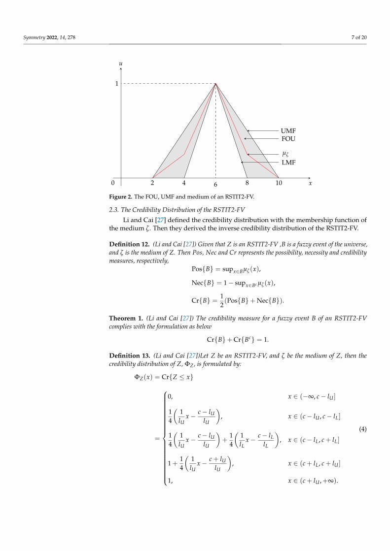
Example 2. For the RSTIT2-FV in Example 1, the membership function of its medium ζ1 isdepicted as the red line in Figure 2.

Symmetry 2022, 14, 278 7 of 20

0 x

u

2 4 8 106

1

µζ

UMF

LMF

FOU

Figure 2. The FOU, UMF and medium of an RSTIT2-FV.

2.3. The Credibility Distribution of the RSTIT2-FV

Li and Cai [27] defined the credibility distribution with the membership function ofthe medium ζ. Then they derived the inverse credibility distribution of the RSTIT2-FV.

Definition 12. (Li and Cai [27]) Given that Z is an RSTIT2-FV ,B is a fuzzy event of the universe,and ζ is the medium of Z. Then Pos, Nec and Cr represents the possibility, necessity and credibilitymeasures, respectively,

PosB = supx∈Bµζ(x),

NecB = 1− supx∈Bc µζ(x),

CrB = 12(PosB+ NecB).

Theorem 1. (Li and Cai [27]) The credibility measure for a fuzzy event B of an RSTIT2-FVcomplies with the formulation as below

CrB+ CrBc = 1.

Definition 13. (Li and Cai [27])Let Z be an RSTIT2-FV, and ζ be the medium of Z, then thecredibility distribution of Z, ΦZ, is formulated by:

ΦZ(x) = CrZ ≤ x

=

0, x ∈ (−∞, c− lU ]

14

(1lU

x− c− lUlU

), x ∈ (c− lU , c− lL]

14

(1lU

x− c− lUlU

)+

14

(1lL

x− c− lLlL

), x ∈ (c− lL, c + lL]

1 +14

(1lU

x− c + lUlU

), x ∈ (c + lL, c + lU ]

1, x ∈ (c + lU ,+∞).

(4)

Symmetry 2022, 14, 278 8 of 20

The inverse credibility distribution of Z, Φ−1Z , is:

Φ−1Z (α) =

4lUα + c− lU , α ∈[

0,lU − lL

4lU

)4lU lLα− 2lU lL

lU + lL+ c, α ∈

[lU − lL

4lU, 1− lU − lL

4lU

)

4lUα + c− 3lU , α ∈[

1− lU − lL4lU

, 1]

.

(5)

Theorem 2. (Li and Cai [27]) Suppose that there are RSTIT2-FVs Zi which are mutually indepen-dent, and ζi are the mediums of Zi respectively, i = 1, 2, . . . , m, when f (x1, . . . , xk, xk+1, . . . , xm)is strictly increasing towards xi, i = 1, 2, . . ., k, and strictly decreasing towards xi, i = k + 1, k +2, . . . , m, then the inverse credibility distribution of

Z = f (Z1, · · · , Zk, Zk+1, · · · , Zm)

is formulated as

Φ−1Z (α) = f

(Φ−1

Z1(α), · · · , Φ−1

Zk(α), Φ−1

Zk+1(1− α), · · · , Φ−1

Zm(1− α)

). (6)

2.4. The Expected Value, Variance and Semi-Variances of the Fuzzy Variable

Definition 14. (Liu [32]) Suppose that Z is a fuzzy variable and its expected value is ε, then itsvariance can be formulated as:

V[Z] = E[(Z− ε)2

]. (7)

Definition 15. (Liu [28]) Suppose that Z is a fuzzy variable, then the expected value of Z can beformulated as:

E[Z] =∫ +∞

0CrZ ≥ xdx−

∫ 0

−∞CrZ ≤ xdx. (8)

Theorem 3. (Liu [33]) Given that Z is an fuzzy variable, then its expected value can be reformed to:

E[Z] =∫ 1

0Φ−1

Z (α)dα. (9)

Specifically, for an RSTIT2-FV, Li and Cai [27] has proved that its expected value isidentical to the center value, that is, E[Z] = ε.

Theorem 4. (Li and Cai [27]) Given that Z =(

c− lU c c + lUc− lL c c + lL

)is an RSTIT2-FV with the

center value c and the inverse credibility distribution Φ−1Z (α), then its expected value is identical to

c, that is,

E[Z] =∫ 1

0Φ−1

Z (α)dα = c. (10)

Theorem 5. (Li and Cai [27]) Suppose that Z is an RSTIT2-FV and k is a constant, then

E[kZ] = kE[Z]. (11)

Definition 16. (Gu et al. [8]) Suppose that Z is a fuzzy variable and its expected value is ε, thenthe upside semi-variance of Z can be formulated as:

Symmetry 2022, 14, 278 9 of 20

Sv+[Z] = E[((Z− ε)+

)2], (12)

where

(Z− ε)+ =

Z− ε, if Z > ε

0, if Z ≤ ε.

Definition 17. (Huang [34]) Suppose that Z is a fuzzy variable and its expected value is ε, thenthe downside semi-variance of Z can be formulated as:

Sv−[Z] = E[((Z− ε)−

)2], (13)

where

(Z− ε)− =

0, if Z > ε

Z− ε, if Z ≤ ε.

In the following sections, the variance and semi-variances for the RIT2-FV as well asthe covariance and operational law for the RSTIT2-FV will be defined.

3. The Variance of the RIT2-FV

We will provide the calculation formula for the variance of an RIT2-FV via the credi-bility distribution in this section, which can be derived by Definitions 14 and 15.

Definition 18. Let Z be an RIT2-FV and its expected value is ε, then its variance is formulated as:

V[Z] = E[(Z− ε)2

]. (14)

Definition 19. Let Z be an RIT2-FV, then the expected value of Z can be formulated as:

E[Z] =∫ +∞

0CrZ ≥ xdx−

∫ 0

−∞CrZ ≤ xdx. (15)

Theorem 6. Given that Z is an RIT2-FV. Then ΦZ(x) is the credibility distribution of Z and ε isthe expected value of Z. Its variance can be calculated by:

V[Z] =∫ +∞

0

[1−ΦZ(ε +

√x) + ΦZ(ε−

√x)]dx. (16)

Proof. On the basis of Definitions 18 and 19, we derive:

V[Z] = E[(Z− ε)2

]=∫ +∞

0Cr(Z− ε)2 ≥ x

dx−

∫ 0

−∞Cr(Z− ε)2 ≤ x

dx

=∫ +∞

0CrZ ≥

√x + ε ∪ Z ≤ ε−

√x

=∫ +∞

0

[1−ΦZ(ε +

√x) + ΦZ(ε−

√x)]dx.

Thus, Equation (16) is naturally obtained.

Symmetry 2022, 14, 278 10 of 20

Remark 1. For an RSTIT2-FV Z=(

c− lU c c + lUc− lL c c + lL

), the formula for calculating its variance

can be simplified as:

V[Z] =∫ +∞

0

[1−ΦZ(ε +

√x) + ΦZ(ε−

√x)]dx

=∫ l2

L

0

(1−√

x4lU−√

x4lL− 1

2+

12−√

x4lU−√

x4lL

)dx

+∫ l2

U

l2L

[1− 1− 1

4

(√x

lU− 1)+

14

(1−√

xlU

)]dx

=16

(l2L + l2

U

).

(17)

Example 3. For two RSTIT2-FVs A =(

2 6 104 6 8

)and B =

(2 5 83 5 7

), we can easily obtain

their variances by Equation (17) as:

V[A] =16

(22 + 42

)=

103

, V[B] =16

(22 + 32

)=

136

.

Theorem 7. Given that Z is an RIT2-FV. Then ΦZ(x) is the credibility distribution of Z and ε isthe expected value of Z. Its variance can be calculated by:

V[Z] =∫ 1

0

[Φ−1

Z (α)− ε]dx, (18)

where Φ−1Z (α) is the inverse credibility distribution of Z.

Proof. Following from Theorem 6, the part of∫ +∞

0

[1−ΦZ(ε +

√x)]dx of Equation (16)

can be transformed to:

∫ +∞

0

[1−ΦZ(ε +

√x)]dx =

∫ 1

ΦZ(ε)(1− α)d

[Φ−1

Z (α)− ε]2

=∫ 1

ΦZ(ε)

[Φ−1

Z (α)− ε]dα

by replacing ΦZ(ε +√

x) with α. Similarly, the part of∫ +∞

0 Φs(ε−√

x)dx can be trans-formed to:

∫ +∞

0ΦZ(ε−

√x)dx =

∫ 0

ΦZ(ε)αd[ε−Φ−1

Z (α)]2

=∫ ΦZ(ε)

0

[Φ−1

Z (α)− ε]dα

by replacing Φs(ε−√

x) with α. Hence, we obtain:

V[Z] =∫ +∞

0

[1−ΦZ(ε +

√x) + ΦZ(ε−

√x)]dx

=∫ 1

ΦZ(ε)

[Φ−1

Z (α)− ε]dα +

∫ ΦZ(ε)

0

[Φ−1

Z (α)− ε]dα

=∫ 1

0

[Φ−1

Z (α)− ε]dx.

Symmetry 2022, 14, 278 11 of 20

4. The Semi-Variances of an RIT2-FV

In the previous section, we have derived the calculation formula for the variance ofthe RIT2-FVs, which indicates bilateral deviation of variables. In practice, however, such asstock portfolio selection, we focus on the negative deviation to measure the risk in loss; andin R&D investment, only the positive deviation is used to control the cost. Such deviationscan be measured by one-side semi-variances respectively.

Thus, we define the formulas for the downside and upside semi-variances of the RIT2-FV according to the credibility distribution (Gu et al. [8] and Huang [34]) in the following.After that, the relationships between the variance and semi-variances are uncovered.

4.1. Calculation Formula for the Semi-Variances of the RIT2-FV

Theorem 8. Given that Z is an RIT2-FV. Then ΦZ(x) is the credibility distribution of Z and ε isthe expected value of Z. The upside semi-variance can be formulated as:

Sv+[Z] =∫ +∞

0

[1−ΦZ(ε +

√x)]dx. (19)

Proof. According to Definitions 16 and 19, we have:

Sv+[Z] = E[((Z− ε)+

)2]

=∫ +∞

0Cr(Z− ε)2 ≥ x, Z > ε

dx

=∫ +∞

0CrZ ≥ ε +

√xdx

=∫ +∞

0

[1−ΦZ(ε +

√x)]dx.

Theorem 9. Given that Z is an RIT2-FV. Then ΦZ(x) is the credibility distribution of Z and ε isthe expected value of Z. The downside semi-variance can be formulated as:

Sv−[Z] =∫ +∞

0ΦZ(ε−

√x)dx. (20)

Proof. Similar to Proof of Theorem 8, in light of Definitions 17 and 19, we have:

Sv−[Z] = E[((Z− ε)−

)2]

=∫ +∞

0Cr(Z− ε)2 ≥ x, Z ≤ ε

dx

=∫ +∞

0CrZ ≤ ε−

√xdx

=∫ +∞

0ΦZ(ε−

√x)dx.

Symmetry 2022, 14, 278 12 of 20

Remark 2. Given that Z =(

c− lU c c + lUc− lL c c + lL

)is an RSTIT2-FV. Then ΦZ(x) is the credibility

distribution of Z and ε is the expected value of Z. By means of Theorems 8 and 9, the formula forcalculating the upside and downside semi-variance of Z can be simplified as:

Sv+[Z] =∫ +∞

0

[1−ΦZ(ε +

√x)]dx

=∫ l2

L

0

[1− 1

4

(√x

lU+

√x

lL+ 2)]

dx +14

∫ l2U

l2L

(1−√

xlU

)dx

=1

12

(l2L + l2

U

)(21)

andSv−[Z] =

∫ +∞

0ΦZ(ε−

√x)dx

= −14

∫ l2L

0

(√x

lU+

√x

lL+ 2)

dx +14

∫ l2U

l2L

(1−√

xlU

)dx

=1

12

(l2L + l2

U

).

(22)

Example 4. By using Equations (21) and (22), the upside and downside semi-variances of the twoRSTIT2-FVs in Example 3 can be derived as:

Sv+[A] = Sv−[A] =1

12

(22 + 42

)=

53

andSv+[B] = Sv−[B] =

112

(22 + 32

)=

1312

.

4.2. The Relationships between the Variance and Semi-Variances

In the above sections, we deduce the formulae for calculating the variance and semi-variances of the RIT2-FV based on the credibility distribution. In this section, we furtherprobe into the relationship between the variance and semi-variances of the RSTIT2-FV.

Observed from the Equations (13), (16) and (19), the semi-variance is equal to partsof the formula for calculating the variance. We find that there exist some relationshipsbetween the variance and semi-variances of the RSTIT2-FV.

Theorem 10. Suppose that Z is an RSTIT2-FV, then its upside and downside semi-variances andvariance satisfy:

V[Z] = Sv+[Z] + Sv−[Z]. (23)

Proof. In light of Equations (19) and (20), we have:

Sv+[Z] + Sv−[Z] =∫ +∞

0

[1−ΦZ(ε +

√x) + ΦZ(ε−

√x)]dx,

which is equal to V[Z] in Equation (9). Therefore, we have:

V[Z] = Sv+[Z] + Sv−[Z].

It can also be observed from Equations (21) and (22) that Sv−[Z] = Sv+[Z]. Thus, wecan derive the following theorem regarding the relationship between them.

Symmetry 2022, 14, 278 13 of 20

Theorem 11. Let Z be an RSTIT2-FV, then its upside and downside semi-variances satisfy:

Sv−[Z] = Sv+[Z]. (24)

Proof. For an RSTIT2-FV Z=(

c− lU c c + lUc− lL c c + lL

), we can obtain that its expected value

ε is identical to c. Then, in view of Definitions 16 and 17, its downside and upside semi-variances are, respectively,

Sv+ =∫ +∞

0CrZ ≤ ε−

√tdt,

Sv− =∫ +∞

0CrZ ≥ ε +

√tdt.

From Definition 12, we can obtain

CrZ ≤ t = 12

(supx≤tµ(x) + 1− supx>tµ(x)

),

Thereforth,

CrZ ≤ ε−√

t = 12

[supx≤ε−

√tµZ(x) + 1− supx>ε−

√tµZ(x)

].

For ε−√

t ≤ ε, supx>ε−√

tµZ(x) = 1. Thus,

CrZ ≤ ε−√

t = 12

supx≤ε−√

tµZ(x) =12

PosZ ≤ ε−√

t.

Analogonsly, we can derive that

CrZ ≥ ε +√

t = 12

PosZ ≥ ε +√

t.

Since Z is a sysmetric fuzzy variable, it can be conveniently deduced that

PosZ ≤ ε−√

t = PosZ ≥ ε +√

t.

Eventually, we can obtain that:

Sv−[Z] = Sv+[Z].

Theorem 12. Suppose that Z is an RSTIT2-FV, then its upside and downside semi-variances andvariance satisfy:

Sv+[Z] = Sv−[Z] =12

V[Z]. (25)

Proof. According to Theorems 10 and 11, we have:

V[Z] = Sv+[Z] + Sv−[Z]

and

Sv−[Z] = Sv+[Z].

Therefore, it can be readily deducted that:

Sv+[Z] = Sv−[Z] =12

V[Z].

Symmetry 2022, 14, 278 14 of 20

According to Theorem 11, the upside and downside semi-variances of an RSTIT2-FVare equal to each other. Therefore, in the following section, they are collectively referred toas the semi-variance and denoted as Sv[Z].

5. Operational Law

This section introduces the calculated operational law of the variance and semi-variance for the RSTIT2-FV. The definition of independence, as a precondition for itsderivation, is referred to in the beginning.

5.1. Independence

Definition 20. (Li and Cai [27]) The RSTIT2-FVs Zi, i = 1, 2, · · · , m, are said to be mutuallyindependent if:

CrZi ∈ Ai, i = 1, 2, · · · , m = min1≤i≤m

CrZi ∈ Bi,

for any subsets B1, B2, · · · , Bm.

Theorem 13. (Li and Cai [27]) If the RSTIT2-FVs Zi, i = 1, 2, · · · , m, are mutually independent,then their corresponding mediums ζi are mutually independent as well.

5.2. Operational Law for the RSTIT2-FVs

Theorem 14. Let Z be an RSTIT2-FV. k is a constant and ε is the expected value of Z, thenwe have:

V[kZ] = k2V[Z]. (26)

Proof. According to Definition 18 and Theorem 5, we have:

V[kZ] = E[(kZ− kE[Z])2

]= E

[(kZ− kε)2

]= k2E

[(Z− ε)2

]= k2V[Z].

Definition 21. Let Z1 and Z2 be two mutually independent RSTIT2-FVs with expected value ε1and ε2, respectively. Then, the covariance of Z1 and Z2 is formulated as:

Cov[Z1, Z2] = E[(Z1 − ε1)(Z2 − ε2)]. (27)

In view of the subadditivity of the uncertain measure, the covariance of the RSTIT2-FVscannot be calculated straightly by means of their credibility distributions. By comparingDefinitions 18 and 21, variance can be regarded as a specific kind of covariance. There-fore, we can derive the formula for calculating the covariance via the inverse credibilitydistribution, in view of Equation (18).

Stipulation 1. Let Z1 and Z2 are two mutually independent RSTIT2-FVs with distributions ΦZ1

and ΦZ2 and expected value ε1 and ε2 respectively. Then the covariance of Z1 and Z2 is:

Cov[Z1, Z2] =∫ 1

0

[Φ−1

Z1(α)− ε1

][Φ−1

Z2(α)− ε2

]dx. (28)

Theorem 15. Suppose that Z1 and Z2 are two mutually independent RSTIT2-FVs with thecredibility distributions ΦZ1 and ΦZ2 and expected value ε1 and ε2, respectively, then the covarianceof Z1 and Z2 is:

Cov[Z1, Z2] =∫ 1

0Φ−1

Z1(α)Φ−1

Z2(α)dα− ε1ε2. (29)

Symmetry 2022, 14, 278 15 of 20

Proof. In light of Stipulation 1, the covariance of Z1 and Z2 is conveniently derived as:

Cov[Z1, Z2] =∫ 1

0

(Φ−1

Z1(α)Φ−1

Z2(α)− ε2Φ−1

Z1(α)− ε1Φ−1

Z2(α) + ε1ε2

)dα

=∫ 1

0Φ−1

Z1(α)Φ−1

Z2(α)dα− ε2

∫ 1

0Φ−1

Z1(α)dα− ε1

∫ 1

0Φ−1

Z2(α)dα + ε1ε2.

Then according to Equation (9), we get:

Cov[Z1, Z2] =∫ 1

0Φ−1

Z1(α)Φ−1

Z2(α)dα− ε1ε2.

Example 5. For two mutually independent RSTIT2-FVs A and B in Example 3 with the inversecredibility distributions,

Φ−1A (α) =

16α + 2, α ∈[

0,18

)16α + 10

3, α ∈

[18

,78

)

16α− 6, α ∈[

78

, 1]

and

Φ−1B (α) =

12α + 2, α ∈[

0,112

)24α + 13

5, α ∈

[1

12,

1112

)

12α− 4, α ∈[

1112

, 1]

,

respectively, their covariance is:

Cov[A, B] =∫ 1

0Φ−1

A (α)Φ−1B (α)dα− ε1ε2

=∫ 1

12

0(16α + 2)(12α + 2)dα +

∫ 18

112

(24α + 13)(16α + 2)5

dα

+∫ 7

8

18

(16a + 10)(24α + 13)15

dα +∫ 11

12

78

(16α− 6)(24α + 13)5

dα

+∫ 1

1112

(12α− 4)(16α− 6)dα− 6× 5

=61

108+

64135

+117

5+

647270

+631108− 30

=24190

.

Theorem 16. Suppose that Z1 and Z2 are two mutually independent RSTIT2-FVs with expectedvalues ε1 and ε2, respectively, then the variance of k1Z1 + k2Z2 is

V[k1Z1 + k2Z2] = k21V[Z1] + k2

2V[Z2] + 2k1k2 Cov[Z1, Z2], (30)

Symmetry 2022, 14, 278 16 of 20

where the constants k1 and k2 satisfy k1k2 > 0.

Proof. According to Theorem 7, the variance of k1Z1 + k2Z2 can be calculated by:

V[k1Z1 + k2Z2] =∫ 1

0

[Φ−1

k1Z1+k2Z2(α)− E[k1Z1 + k2Z2]

]2dα. (31)

When k1 > 0 and k2 > 0, k1Z1 + k2Z2 is strictly increasing with respect to Z1 and Z2.In light of Theorem 2, the inverse credibility distribution of k1Z1 + k2Z2 is:

Φ−1k1Z1+k2Z2

(α) = k1Φ−1Z1

(α) + k2Φ−1Z2

(α).

So following from Equation (31):

V[k1Z1 + k2Z2] =∫ 1

0

[k1Φ−1

Z1(α) + k2Φ−1

Z2(α)− E[k1Z1 + k2Z2]

]2dα

=∫ 1

0k2

1

(Φ−1

Z1(α)− ε1

)2+ k2

2

(Φ−1

Z2(α)− ε2

)2

+ 2k1k2

(Φ−1

Z1(α)− ε1

)(Φ−1

Z2(α)− ε2

)dα

=k21V[Z1] + k2

2V[Z2] + 2k1k2 Cov[Z1, Z2].

When k1 < 0 and k2 < 0, k1Z1 + k2Z2 is strictly decreasing with respect to Z1 and Z2.In light of Theorem 16, the inverse credibility distribution of k1Z1 + k2Z2 is:

Φ−1k1Z1+k2Z2

(α) = k1Φ−1Z1

(1− α) + k2Φ−1Z2

(1− α).

Then according to Equation (31), we have:

V[k1Z1 + k2Z2] =∫ 1

0

[k1Φ−1

Z1(1− α) + k2Φ−1

Z2(1− α)− E[k1Z1 + k2Z2]

]2dα

=∫ 1

0k2

1

(Φ−1

Z1(1− α)− ε1

)2+ k2

2

(Φ−1

Z2(1− α)− ε2

)2

+ 2k1k2

(Φ−1

Z1(1− α)− ε1

)(Φ−1

Z2(1− α)− ε2

)dα.

By replacing (1− α) with β, we obtain that:

V[k1Z1 + k2Z2] =∫ 1

0k2

1

(Φ−1

Z1(β)− ε1

)2+ k2

2

(Φ−1

Z2(β)− ε2

)2

+ 2k1k2

(Φ−1

Z1(β)− ε1

)(Φ−1

Z2(β)− ε2

)dβ

=k21V[Z1] + k2

2V[Z2] + 2k1k2 Cov[Z1, Z2].

Example 6. For the two mutually independent RSTIT2-FVs A and B in Example 3 and constantsk1 = 2 and k2 = 3, according to Theorem 16, we have:

V[2A + 3B] = k21V[A] + k2

2V[B] + 2k1k2 Cov[A, B]

= 4× 103

+ 9× 136

+ 2× 2× 3× 24190

=194930

.

Symmetry 2022, 14, 278 17 of 20

For k1 = −3, k2 = −2, we have:

V[−3A− 2B] = k21V[A] + k2

2V[B] + 2k1k2 Cov[A, B]

= 9× 103

+ 4× 136

+ 2× (−3)× (−2)× 24190

=3545

.

Theorem 17. Suppose that there are RSTIT2-FVs Zi, which are mutually independent, and ζiare the mediums of Zi respectively, i = 1, 2, . . . , m, when f (Z1, . . . , Zk, Zk+1, . . . , Zm) is strictlyincreasing towards xi, i = 1, 2, . . ., k, and strictly decreasing towards xi, i = k + 1, k + 2, . . . , m,then the variance of

Z = f (Z1, · · · , Zk, Zk+1, · · · , Zm),

can be calculated by:

V[Z] =∫ 1

0f(

Φ−1Z1

(α), · · · , Φ−1Zk

(α), Φ−1Zk+1

(1− α), · · · , Φ−1Zm

(1− α))

− E[

f(

Φ−1Z1

(α), · · · , Φ−1Zk

(α), Φ−1Zk+1

(1− α), · · · , Φ−1Zm

(1− α))]

dα.

(32)

Proof. According to Equations (6), (14) and (18)

Φ−1Z (α) = f

(Φ−1

Z1(α), · · · , Φ−1

Zk(α), Φ−1

Zk+1(1− α), · · · , Φ−1

Zm(1− α)

),

so we have

V[Z] =∫ 1

0

[Φ−1

Z (α)− ε]dx

=∫ 1

0f(

Φ−1Z1

(α), · · · , Φ−1Zk

(α), Φ−1Zk+1

(1− α), · · · , Φ−1Zm

(1− α))

− E[

f(

Φ−1Z1

(α), · · · , Φ−1Zk

(α), Φ−1Zk+1

(1− α), · · · , Φ−1Zm

(1− α))]

dα.

Remark 3. According to Theorem 12, we can calculate the semi-variance of an RSTIT2-FV by itsvariance. Thus, the operational law for the semi-variance of the RSTIT2-FVs can be easily derivedin the similar way. Due to space limitation, this paper does not present the detailed proofs.

Theorem 18. Let Z be an RSTIT2-FV and k be a constant. Then we obtain that:

Sv[kZ] = k2Sv[Z]. (33)

Theorem 19. Let Z1 and Z2 be two mutually independent RSTIT2-FVs with expected values ε1and ε2, respectively, k1 and k2 be constants satisfying k1k2 > 0. Then the variance of k1Z1 + k2Z2 is

Sv[k1Z1 + k2Z2] = k21Sv[Z1] + k2

2Sv[Z2] +12

k1k2 Cov[Z1, Z2]. (34)

Example 7. For the two mutually independent RSTIT2-FVs A and B in Example 3 and constantsk1 = 2 and k2 = 3, we have:

Sv[k1 A] = k21Sv[A] =

203

, Sv[k2B] = k22Sv[B] =

394

,

Symmetry 2022, 14, 278 18 of 20

according to Theorem 18. Thus, it can be deduced that:

Sv[k1 A + k2B] =k21Sv[A] + k2

2Sv[B] +12

k1k2 Cov[A, B]

=203

+394

+12× 2× 3× 241

90

=48920

.

For constants k1 = −3 and k2 = −2, we have:

Sv[k1 A] = k21Sv[A] =

453

, Sv[k2B] = k22Sv[B] =

133

.

Therefore,

Sv[k1 A + k2B] =k21Sv[A] + k2

2Sv[B] +12

k1k2 Cov[A, B]

=453

+133

+12× (−3)× (−2)× 241

90

=82130

.

Theorem 20. Suppose that there are RSTIT2-FVs Zi, which are mutually independent, and ζiare the mediums of Zi respectively, i = 1, 2, . . . , m, when f (Z1, . . . , Zk, Zk+1, . . . , Zm) is strictlyincreasing towards xi, i = 1, 2, . . ., k, and strictly decreasing towards xi, i = k + 1, k + 2, . . . , m,then the semi-variance of

Z = f (Z1, · · · , Zk, Zk+1, · · · , Zm),

isSv[Z] =

12

V[Z]

=12

∫ 1

0f(

Φ−1Z1

(α), · · · , Φ−1Zk

(α), Φ−1Zk+1

(1− α), · · · , Φ−1Zm

(1− α))

− E[

f(

Φ−1Z1

(α), · · · , Φ−1Zk

(α), Φ−1Zk+1

(1− α), · · · , Φ−1Zm

(1− α))]

dα.

(35)

6. Conclusions

This study derived the calculation formulas of variance and semi-variances for RIT2-FVs by virtue of the inverse credibility distribution and simultaneously proved the re-lationships between them for the RSTIT2-FVs. Afterwards, an operational law for thelinear combination of the RSTIT2-FVs was proposed. The numerical examples showedthat the formulae inferred in this paper can effectively figure out the variance and one-sidesemi-variances, which is of great value for studying type-2 fuzzy theory in depth, solvingrealistic problems such as fuzzy portfolio selection problems in finance, and evaluatinghealthcare equipment in medical fields.

There are still many limitations in this paper. Firstly, the operational law presented inthis paper is limited to RSTIT2-FVs. However, the results and conclusions can be extendedto the general IT2-FVs and more research will be carried out in the future. Secondly, Wuand Mendel [21] mentioned that cardinality, centroid, skewness, variance, and fuzziness areall measures of uncertainties for IT2-FSs. Due to limited time and capacity, we have onlystudied the variance, other uncertainty measures of IT2-FSs can be studied in the future.Finally, the variance of IT2-FSs can be widely used in many fields. However, the researchon its application in this paper and existing research is still vacant, such as predicting therate of population growth with the variance of fuzzy numbers, which are waiting for morein-depth study in future work.

Symmetry 2022, 14, 278 19 of 20

Author Contributions: Conceptualization, Y.C.; formal analysis, Y.C.; investigation, W.T.; methodology,Y.C. and W.T.; software, Y.C.; supervision, Y.C. and W.T.; validation, Y.C. and W.T.; writing—originaldraft, Y.C. and W.T.; writing—review & editing, Y.C. and W.T. All authors have read and agreed to thepublished version of the manuscript.

Funding: This work was supported by the National Natural Science Foundation of China underGrant 71872110.

Institutional Review Board Statement: Not applicable.

Informed Consent Statement: Not applicable.

Data Availability Statement: Data sharing not applicable.

Acknowledgments: The authors especially thank the editors and anonymous referees for their kindlyreview and helpful comments. In addition, the authors would like to thank Hui Li, Junyang Cai andMingxuan Zhao for their assistance and support. Any remaining errors are ours.

Conflicts of Interest: We declare that we have no relevant or material financial interests that relate tothe research described in this paper. The manuscript has neither been published before, nor has itbeen submitted for consideration of publication in another journal.

References1. Zadeh, L.A. Fuzzy sets. Inf. Control 1965, 8, 338–353. [CrossRef]2. Dubois, D.; Prade, H. Twofold fuzzy sets: An approach to the representation of sets with fuzzy boundaries based on possibility

and necessity measures. J. Fuzzy Math. 1983, 3, 53–76.3. Liu, B. Toward fuzzy optimization without mathematical ambiguity. Fuzzy Optim. Decis. Mak. 2002, 1, 43–63. [CrossRef]4. Robert, F.; Peter, M. On weighted possibilistic mean and variance of fuzzy numbers. Fuzzy Set Syst. 2002, 136, 363–374.5. Wu, H.C. Analysis of variance for fuzzy data. Int. J. Syst. Sci. 2007, 3, 235–246. [CrossRef]6. Tsao, C.T. The revised algorithms of fuzzy variance and an application to portfolio selection. Soft Comput. 2010, 14, 329–337.

[CrossRef]7. Gong, Y.B.; Hu, N.; Liu, G.F. A new magnitude possibilistic mean value and variance of fuzzy numbers. J. Intell. Fuzzy Syst. 2016,

18, 140–150.8. Gu, Y.; Hao, Q.; Shen, J.; Zhang, X.; Yu, L. Calculation formulas and correlation inequalities for variance bounds and semi-

variances of fuzzy intervals. J. Intell. Fuzzy Syst. 2019, 36, 353–369. [CrossRef]9. Zhang, Q.S.; Sun, D.F. Some notes on possibilistic variances of generalized trapezoidal intuitionistic fuzzy numbers. AIMS Math.

2021, 6, 3720–3740. [CrossRef]10. Thavaneswaran, A.; Appadoo, S.S.; Paseka, A. Weighted possibilistic moments of fuzzy numbers with applications to GARCH

modeling and option pricing. Math. Comput. Model. 2009, 49, 352–368. [CrossRef]11. Pahade, J.K.; Jha, M. Credibilistic variance and skewness of trapezoidal fuzzy variable and meanvariance-skewness model for

portfolio selection. Results Appl. Math. 2021, 11, 1001509. [CrossRef]12. Ibrahim, H.Z.; Al-Shami, T.M.; Elbarbary, O.G. (3, 2)-Fuzzy Sets and Their Applications to Topology and Optimal Choices.

Comput. Intel. Neurosci. 2021, 2021, 1272266. [CrossRef]13. Atef, M.; Ali, M.I.; Al-shami, T.M. Fuzzy soft covering-based multi-granulation fuzzy rough sets and their applications. Comput.

Appl. Math. 2021, 40, 1–26. [CrossRef]14. Zadeh, L.A. The concept of a linguistic variable and its application to approximate reasoning—I. Inf. Sci. 1975, 8, 199–251.

[CrossRef]15. El Baf, F.; Bouwmans, T.; Vachon, B. Type-2 fuzzy mixture of Gaussians model: Application to background modeling. In Proceed-

ings of the International Symposium on Visual Computing, Las Vegas, NV, USA, 1–3 December 2008; Springer: Berlin/Heidelberg,Germany, 2008.

16. Shu, H.; Liang, Q.; Gao, J. Wireless sensor network lifetime analysis using interval type-2 fuzzy logic systems. IEEE Trans. FuzzySyst. 2008, 16, 416–427.

17. Mohagheghi, V.; Mousavi, S.M.; Vahdani, B.; Shahriari, M.R. R&D project evaluation and project portfolio selection by a newinterval type-2 fuzzy optimization approach. Neural Comput. Appl. 2017, 28, 3869–3888.

18. Guo, J.; Du, S. Modeling words for qualitative distance based on interval type-2 fuzzy sets. ISPRS. Int. J. Geo-Inf. 2018, 7, 291.[CrossRef]

19. Deveci, M.; Pekaslan, D.; Canıtez, F. The assessment of smart city projects using zslice type-2 fuzzy sets based interval agreementmethod. Sustain. Cites Soc. 2020, 53, 101889. [CrossRef]

20. Deveci, M.; Öner, S.C.; Ciftci, M.E.; Özcan, E.; Pamucar, D. Interval type-2 hesitant fuzzy entropy-based WASPAS approach foraircraft type selection. Appl. Soft Comput. 2022, 114, 108076. [CrossRef]

21. Wu, D.; Mendel, J.M. Uncertainty measures for interval type-2 fuzzy sets. Inf. Sci. 2007, 177, 5378–5393. [CrossRef]22. Zhai, D.Y.; Mendel, J.M. Uncertainty measures for general type-2 fuzzy sets. Inf. Sci. 2011, 181, 503–518. [CrossRef]

Symmetry 2022, 14, 278 20 of 20

23. Wei, Y.; Watada, J.; Pedrycz, W. Design of a qualitative classification model through fuzzy support vector machine with type-2fuzzy expected regression classifier preset. IEEJ. Trans. Electr. Electr. Eng. 2016, 11, 348–356. [CrossRef]

24. Gong, Y.B.; Yang, S.X.; Dai, L.L.; Hu, N. A new approach for ranking of interval type-2 trapezoidal fuzzy numbers. J. Intell. FuzzySyst. 2017, 32, 1891–1902. [CrossRef]

25. Wu, D.; Zhang, H.T.; Huang, J.A. A constrained representation theorem for well-shaped interval type-2 fuzzy sets, and thecorresponding constrained uncertainty measures. IEEE Trans. Fuzzy Syst. 2018, 27, 1237–1251. [CrossRef]

26. Tolga, A.C. Real options valuation of an IoT based healthcare device with interval type-2 fuzzy numbers. Soc.-Econ. Plan. Sci.2019, 69, 100693. [CrossRef]

27. Li, H.; Cai, J. Arithmetic operations and expected Values of regular interval type-2 fuzzy variables. Symmetry 2021, 13, 2196.[CrossRef]

28. Liu, B. Uncertainty Theory, 2nd ed.; Springer: Berlin/Heidelberg, Germany, 2007.29. Dubois, D.; Prade, H. Operations on fuzzy numbers. Int. J. Syst. Sci. 1978, 9, 613–626. [CrossRef]30. Zhou, J.; Yang, F.; Wang, K. Fuzzy arithmetic on LR fuzzy numbers with applications to fuzzy programming. J. Intell. Fuzzy Syst.

2016, 30, 71–87. [CrossRef]31. Mendel, J.M.; John, R.I. Type-2 fuzzy sets made simple. IEEE Trans. Fuzzy Syst. 2002, 10, 117–127. [CrossRef]32. Liu, B. Uncertainty Theory: An Introduction to Its Axiomatic Foundations; Springer: Berlin/Heidelberg, Germany, 2004.33. Liu, B. Uncertainty Theory: A Branch of Mathematics for Modeling Human Uncertainty; Springer: Berlin/Heidelberg, Germany, 2010.34. Huang, X. Mean-semivariance models for fuzzy portfolio selection. J. Comput. Appl. Mathem. 2008, 217, 1–8. [CrossRef]