On Interval Routing Schemes andTreewidth?Hans L. Bodlaender1, Jan van Leeuwen1, Richard Tan1;2, and Dimitrios M. Thilikos11 Department of Computer Science, Utrecht University,P.O. Box 80.0893508 TB Utrecht, the Netherlandsfhansb,jan,rbtan,sedthilkg@cs.ruu.nl2 Department of Computer Science, University of Sciences and Arts of OklahomaChickasha, Oklahoma 73018, USAAbstract. In this paper, we investigate which processor networks allow k-label Interval Routing Schemes, under the assumption that costs of edgesmay vary. We show that for each �xed k � 1, the class of graphs allowingsuch routing schemes is closed under minor-taking in the domain of con-nected graphs, and hence has a linear time recognition algorithm. Thisresult connects the theory of compact routing with the theory of graphminors and treewidth.We show that every graph that does not contain K2;r as a minor hastreewidth at most 2r � 2. In case the graph is planar, this bound canbe lowered to r + 2. As a consequence, graphs that allow k-label IntervalRouting Schemes under dynamic cost edges have treewidth at most 4k, andtreewidth at most 2k + 3 if they are planar.Similar results are shown for other types of Interval Routing Schemes.1 IntroductionA common problem in processor networks is that messages that are sent fromone processor to another processor must be routed through the network. Theclassical solution is to give each processor a routing table, with an entry for eachpossible destination specifying over which link the message must be forwarded.A disadvantage of this method is that these tables grow with network size, andmay become too large for larger processor networks.?This research was partially supported by the ESPRIT Basic Actions Program of the ECunder contract No. 8141 (project ALCOM II). The research of the second author was alsopartially supported by the Netherlands Organisation for Scienti�c Research (NWO) undercontract NF 62-376 (NFI project ALADDIN: Algorithmic Aspects of Parallel and DistributedSystems). The research of the last author was supported by the Training and Mobility ofResearchers (TMR) Program, (EU contract no ERBFMBICT950198). Correspondence on thispaper to the �rst author.

Several di�erent routing methods have been proposed that do not have thisdisadvantage. One such method is the interval routing method, together with itsgeneralisation k-label interval routing and variants of these. An overview of theseand other compact routing methods can be found in [19].Interval routing was introduced by Santoro and Khatib [24] and van Leeuwenand Tan [18]. Several well-known classes of networks allow interval routingschemes that are optimal, in the sense that messages always follow the short-est path to their destination. The method was applied in the C104 Router Chip,used in the INMOS T9000 Transputer design [16].Frederickson and Janardan [15] considered interval routing in the setting ofdynamic cost links (i.e., in the case that the cost of edges is variable). Actu-ally, they considered a variant of interval routing, called strict interval routing.For these, they gave a precise characterisation of the graphs with dynamic costlinks which allow optimum strict interval routing schemes: these are exactly theouterplanar graphs. Bakker, van Leeuwen and Tan [2] obtained a similar resultfor general interval routing: a graph with dynamic cost links has an optimuminterval routing scheme, if and only if it is outerplanar or K4. Another restric-tion of interval routing was introduced by Bakker, van Leeuwen, and Tan in [3]:linear interval routing. It has also been applied in concrete networks. Here, also aprecise characterisation exists of the graphs which allow optimum linear intervalrouting schemes with dynamic cost links.All of the interval routing schemes assumes that each link has one unique label,which is a (possibly cyclic) interval of processor names. All can be generalisedto multi-label schemes, where each link has a number of labels. We consider thek-label schemes: each link has at most k labels. The issue we study in this paperis: which graphs allow k-label interval routing schemes in the setting of dynamiccost links.Surprisingly, new and deep graph theoretical results on graph minors ofRobertson and Seymour (see Section 2.1) can be used for the analysis of thisproblem. With the help of these results, we show non-constructively the exis-tence of �nite characterisations of which graphs allow certain routing schemes.Also, we give a non-constructive proof of the existence of linear time algorithmsthat check whether a desired routing scheme exists for a given graph. These algo-rithms heavily depend on the use of tree-decompositions. We show that graphs,allowing a k-label interval routing scheme (in the setting of dynamic cost links)have treewidth at most 4k. This not only gives a partial characterisation of thegraphs which have such routing schemes, but also, as the hidden constant factorof these algorithms is exponential in the treewidth of the tree-decomposition, ithelps to decrease the running time of algorithms that would test the property.As a main lemma, we show that every graph either contains K2;r as a minor,or has treewidth at most 2r � 2. This can be seen as a special case of a resultof Robertson and Seymour [21]: every planar graph H = (V (H); E(H)) has anassociated constant cH , such that any graphG either contains H as a minor or has2

treewidth at most cH . The best general bound for cH known is 202(2jV (H)j+4jE(H)j)5[23]. Our result gives a much better bound in the case of graphs of the form K2;r.Also, this result is constructive, and can be turned into an O(rn) time algorithm,that either outputs that the input graph G has K2;r as a minor, or that outputsa tree-decomposition of G of treewidth at most 2r � 2. Similar results for otherspeci�c graphs can be found in [4] (trees), [14] (cycles and subgraphs of cycles), [7](disjoint copies ofK3), and [6] (graphs that are minor of a circus graph and (2�k)-grid). The result of this main lemma can be seen as an additional result, �ttinginto this framework. Applied to the routing problem, it gives the �rst graph-theoretic complexity bound on the graphs that admit optimal k-label intervalrouting schemes. Another consequence we discuss is that `most' random graphs(even `sparse random graphs') do not allow k-label interval routing schemes underthe dynamic cost edges assumption, for small values of k. Additionally, we givevariants of the results when the graphs are restricted to be planar.This paper is organised as follows. In Section 2, we give most necessary de�-nitions and some preliminary results. In Section 3, we establish minor-closednessof the considered classes of graphs, each class containing those networks allowingcertain types of k-label interval routing schemes. As a consequence, we obtaina non-existential proof of the existence of linear time membership algorithms forthese classes. Also, slower, but constructive algorithms for these problems aregiven. In Section 4, we give the result on the treewidth of graphs, avoiding K2;ras a minor (as discussed above). In Section 5, a similar result is given, but with arestriction to planar graphs, and with a better bound. Some open problems arementioned in Section 6.2 De�nitions and preliminary resultsIn this section, we introduce the most important de�nitions and mention someknown results. In Section 2.1, we introduce graph-theoretic notions and results,and in Section 2.2, concepts and results from interval routing and its variants.2.1 Graph theoretic de�nitions and preliminary resultsAll graphs in this paper will be assumed to be undirected, simple and �nite.Given a graph G we denote as V (G) and E(G) the set of its vertices and edgesrespectively. The number of vertices of a graph G = (V;E) will be denoted byn = jV (G)j. The notion of treewidth was introduced by Robertson and Seymour[21].De�nition. A tree-decomposition of a graph G = (V;E) is a pair D = (X; T )with T = (I; F ) a tree and X = fXi j i 2 Ig a family of subsets of V , one foreach node of T , such that 3

� Si2I Xi = V .� for all edges fv; wg 2 E, there exists an i 2 I with v 2 Xi and w 2 Xi.� for all i; j; k 2 I: if j is on the path from i to k in T , then Xi \Xk � Xj.The treewidth of a tree-decomposition (fXi j i 2 Ig; T = (I; F )) ismaxi2I jXij � 1. The treewidth of a graph G is the minimum treewidth overall possible tree-decompositions of G.There are several well known equivalent characterisations of the notion oftreewidth; for instance, a graph has treewidth at most k, if and only if it is apartial k-tree, or a subgraph of a chordal graph with maximum clique size atmost k + 1 (see [17]).A graph G = (V;E) is said to be a minor of a graph H = (W;F ), if Gcan be obtained from H by a series of vertex deletions, edge deletions, and edgecontractions; where an edge contraction is the operation that takes two adjacentvertices v and w, and replaces it by a new vertex, adjacent to all vertices thatwere adjacent to v or w. A class of graphs G is said to be closed under takingof minors, if for every G 2 G, every minor H of G belongs to G. For classes ofgraphs G;H, we say that G is closed under taking of minors in the domain H, iffor every graph G 2 G \H, every minor H of G with H 2 H belongs to G.In a long series of papers, Robertson and Seymour proved their famous graphminor theorem (formerly `Wagner's conjecture'):Theorem 1 (See [20].) For every class of graphs G, that is closed under takingof minors, there exists a �nite set of graphs, called the obstruction set of G,ob(G), such that for all graphs H, H 2 G, if and only if there is no graph G inthe obstruction set of G that is a minor of H.Fellows and Langston [13] derived the following consequence and variant ofthis result.Theorem 2 Let G be a class of graphs, closed under taking of minors in thedomain H, with G � H. There exists a �nite set of graphs, the obstruction setof G in H, obH(G), such that for all graphs H 2 H, H 2 G, if and only if thereis no graph G 2 obH(G) that is a minor of H.It should be noted that the proofs of these results are (inherently) non-constructive. As for every �xed graph H, there exists an O(n3) time algorithmthat tests whether H is a minor of a given graph G with n vertices [22], it followsthat every minor-closed class of graphs has a cubic recognition algorithm, andevery minor-closed class of graphs in a domain H has a cubic algorithm thattests whether graphs from H belong to G. However, as the proof of Theorem 1is non-constructive, we only know the algorithm exists, but we do not have thealgorithm itself.In several cases, faster algorithms exist.4

Theorem 3 ([21]) For every planar graph H, there exists a constant cH, suchthat for every graph G, either H is a minor of G, or the treewidth of G is at mostcH.Moreover, for every �xed integer k and graph H, there exists a linear timealgorithm, such that when given a graph G = (V;E) with a tree-decomposition oftreewidth at most k, decides whether H is a minor of G, using standard methodsfor graphs with bounded treewidth (see e.g. [1].) As such tree-decompositionscan be found in linear time [5], when existing, the following result holds:Theorem 4 Let G be a class of graphs that is closed under taking of minors, andthat does not contain all planar graphs. Then there exists a linear time algorithmthat tests whether a given graph G belongs to G.Proof: (This proof is basically taken from [13], but we now use the algorithmof [5] for �nding tree-decomposition of small treewidth.) Suppose G is a planargraph that does not belong to G. First test whether the treewidth of input graphG is at most cH . If not, we can safely conclude that G 62 G. Otherwise, �nd atree-decomposition of G of treewidth at most cH with the algorithm of [5], anduse this tree-decomposition to test whether a graph in ob(G) is a minor of G. utTheorem 5 Let G be a class of graphs that is closed under taking of minors inthe domain H, G � H. Suppose there is at least one planar graph that belongsto H but not to G. Then there exists a linear time algorithm that tests whether agiven graph G 2 H belongs to G.Proof: (We again use an only slightly modi�ed variant of a proof from [13].)Suppose H is a planar graph with H 2 H, H 62 G. If G 2 G, then G does notcontain H as a minor, hence has treewidth at most cH . So, again we can �rsttest whether the treewidth of G is at most k. If not, we are done. Otherwise, wecompute a tree-decomposition of G with treewidth at most cH , and then use thistree-decomposition to test in linear time whether G contains a graph in obH(G)as a minor. utThe constant factor of the linear time algorithms mentioned above is expo-nential in the treewidth of the tree-decomposition used, i.e., in cH , H a planargraph not in G (but in H). The constant factor in the original result of Robertsonand Seymour was `astronomically large'. In a later paper, Robertson et al. [23]improved this result, and obtained a constant factor of 202(2jV (H)j+4jE(H)j)5 .Still, in most, if not all, practical cases, this constant factor is much too large,and makes the algorithm practically infeasible. This is the motivation, why welooked for much smaller values of cH for graphs of the form K2;r, as these graphsare planar, connected and can be shown to be `outside' the considered classes ofgraphs. 5

2.2 De�nitions and preliminary results on interval routingUnless stated otherwise, intervals will be assumed to be `cyclic' in the setf0; 1; : : : ; n � 1g, (n = jV j); thus if a > b then the interval [a; b) denotes theset fa; a+ 1; :::; n� 1; 0; :::; b� 1g.The shortest distance from vertex u 2 V to a vertex v 2 V in a graphG = (V;E) when edges have costs given by edge cost function c : E ! R, isdenoted by dG;c(u; v). When G and/or c are clear from the context, we dropthem from the subscript. The cost of a path p under edge cost function c isdenoted by c(p).A node labelling of a graph G = (V;E) is a bijective mapping nb : V !f0; 1; : : : ; n � 1g. An interval labelling scheme (ILS) of a graph G = (V;E) isa node labelling nb of G, together with a labelling l, mapping each link to aninterval [a; b), a; b 2 f0; 1; : : : ; n� 1g, such that for every vertex v, the set of alllabels of links outgoing from v partitions the set f0; 1; : : : ; n� 1g.Given an ILS, routing is done as follows. Each message contains, amongstothers, the node label nb(w) of its destination node w. When a node x receives amessage with destination-label dest, it �rst looks whether nb(x) = dest. If so, themessage has reached its destination, and is not routed any further. Otherwise,the message is transferred over the link with label [a; b) such that dest 2 [a; b).An ILS is valid, if for all nodes v, w, messages sent from v to w eventually reachw by this procedure. An interval routing scheme (in short: IRS) is a valid ILS.The notion of strict interval labelling schemes is obtained in a similar way:modify the de�nition of ILS in the sense that all labels of links associated withnodes v must partition the set f0; 1; : : : ; n� 1g�fnb(v)g, i.e., the label of v maynot appear in the labels of any of its outgoing links. A linear interval labellingscheme is an ILS where no interval label `wraps' around, i.e., for all intervallabels [a; b) a < b. Strict linear interval labelling schemes, strict interval routingschemes (SIRS), linear interval routing schemes (LIRS), and strict linear intervalrouting schemes (SLIRS) are de�ned in the obvious way.For each of these notions, we also de�ne k-label variants. Here, each link islabelled with at most k (cyclic) intervals. All (cyclic) intervals associated withlinks of a node v must together partition f0; 1; : : : ; n� 1g (or f0; 1; : : : ; n� 1g �fnb(v)g, in the case of strict labellings.) Again, a message is transferred overthe link e for which one of its labels is an interval that contains the destination-number. k-label interval routing schemes, k-label linear interval routing schemes,etc., are de�ned as can be expected, and abbreviated as k-IRS, k-LIRS, etc. Notethat an IRS is an 1-IRS, etc.A routing scheme is optimal for a graph G = (V;E), together with an assign-ment of non-negative costs to each edge e 2 E, if, whenever a message is sentfrom node v to node w, the path taken by this message is a minimum cost pathfrom v to w.Costs of edges denote the time needed to send a message over the edge. How-6

ever, in many practical cases, this time may vary. This situation is modelled bythe dynamic cost links setting.We say that graph G = (V;E) with dynamic cost links has an optimum k-IRS, if there exists a node labelling nb of G, such that for all assignments ofnon-negative costs to edges of E, there exists an IRS (nb; l) that is optimal forthis cost assignment.The class of graphs k-IRS is de�ned as the set of all graphs G that havean optimum k-IRS with dynamic cost links. In the same way, we de�ne classesk-LIRS, k-SIRS, k-SLIRS. See [19] for an overview of several results on theseclasses. We have the following relationships.Theorem 6 (i) (Frederickson, Janardan [15]) k-IRS � (k + 1)-IRS.(ii) (Bakker, van Leeuwen, Tan [3]) k-LIRS � (k + 1)-LIRS.(iii) (Bakker, van Leeuwen, Tan [3]) k-IRS � (k + 1)-LIRS.(iv) k-SIRS � k-IRS � (k + 1)-SIRS.(v) k-SLIRS � k-LIRS � k-IRS.3 Closedness under minor takingIn this section we prove that for each �xed integer k � 1, each of the classes k-IRS, k-LIRS, k-SIRS and k-SLIRS is closed under taking of minors in the domainof connected graphs. The reason that this result is interesting is that it enablesus to apply results from the theory of graph minors and of graphs of boundedtreewidth to the theory of interval routing. We �rst prove a lemma which will beused later.Lemma 7 Let G = (V;E) be a graph with edge costs c : E ! R+ [ f0g. Thereexists an edge cost function c0 : E ! Z+, such that for all u; v 2 V : each shortestpath p from u to v in G under edge costs c0 is also a shortest path from u to v inG under edge costs c.Proof: Let P be the set of all simple paths in G. De�ne� = minfjc(p)� c(p0)j j p; p0 2 P; c(p) 6= c(p0)gNote that � > 0. De�ne c0 : E ! Z+ by taking for all e 2 E:c0(e) = $ jV jc(e)� %+ 1Suppose p is a shortest path from u to v under edge costs c0, but not under edgecosts c. Let p0 be another path from u to v with c(p0) < c(p). By de�nition of �,7

we have c(p0) � c(p)� �. Let n = jV j. Nowc0(p0) = Xe2p0($n � c(e)� %+ 1)� n� 1 + n� c(p0) < n + n� (c(p)� �)= n� c(p) =Xe2p n � c(e)�� Xe2p($n � c(e)� %+ 1) = c0(p)So, c0(p0) < c0(p), hence p was not a shortest path from u to v under edge cost c0,contradiction. utTheorem 8 Let k 2 N be a �xed constant.(i) k-IRS is closed under minor taking in the domain of connected graphs.(ii) k-LIRS is closed under minor taking in the domain of connected graphs.(iii) k-SIRS is closed under minor taking in the domain of connected graphs.(iv) k-SLIRS is closed under minor taking in the domain of connected graphs.Proof: (i) It is su�cient to prove, that if a connected graph G = (V 0; E 0) isobtained from a graph H = (V;E) 2 k-IRS by one of the following operations:removal of a vertex, removal of an edge, contraction of an edge, then G 2 k-IRS. Suppose H 2 k-IRS; let nb be a vertex labelling, such that for any costassignment, there exists a k-label interval routing scheme (nb; l) for H.First, suppose that G is obtained from H by removing an edge e0. Use thesame numbering nb for G. For any cost assignment c : EG ! R+ [ f0g, considerthe cost assignment c0 : EH ! R+ [ f0g, where for all e 2 EG : c0(e) = c(e),and take c(e0) = 1 + Pe2EG c(e), i.e., the cost of e0 is chosen so large that nominimum cost path will ever use the edge e0. Hence, any k-label interval routingscheme (nb; l) for H with costs c0 will also be a k-label interval routing schemefor G with costs c.Next, suppose that G is obtained from H by removing a vertex v 2 V and allof its adjacent edges. By �rst removing all edges adjacent to v but one, as in theprevious case, it follows that we may assume v has degree 1. Now, no shortestpath between two vertices w and x, x 6= v, x 6= w uses v. Label the vertices inV 0 as follows: if nb(w) < nb(v), then take nb0(w) = nb(w), and if nb(w) > nb(v),then nb0(w) = nb(w) � 1. For any edge cost function c on G, we can make anIRS as follows: consider the same edge cost function c on H, giving the uniqueedge from v some arbitrary cost, and �nd an IRS (nb; l) for this function on H.Applying the same relabelling (decrease all labels larger than nb(v) by one) onlabelling l, we obtain a labelling l0 such that (nb0; l0) is an IRS for G with edgecosts c. 8

Finally, suppose G is obtained from H by contracting the edge (v; w) = e0 2EH to a vertex, say v0. Let nb0 : V ! f0; 1; : : : ; jV (H)j � 1g be the function,obtained by taking for all x 2 V (G) � fvg, nb0(x) = nb(x). Actually, there is a`gap' in nb': there is no vertex x with number nb0(x) = nb(v). This is resolvedby decreasing all labels larger than nb(v) by one, as in the case of removing avertex.Let c : EG ! R+ [ f0g be a cost assignment for G. By Lemma 7, thereexists a cost assignment c0 : EG ! N+, such that all shortest paths under costassignment c0 are shortest paths under cost assignment c. Let � = 1+Pe2EG c0(e),a forbidding weight. Now let c00 : EH ! R+ be de�ned as follows: for all edgesfx; yg 2 EH with x; y 62 fv; wg, let c00(fx; yg) = c0(fx; yg). For y 6= w, iffv; yg 2 E(H), take c00(fv; yg) = c0(fv0; yg). For y 6= v, if fw; yg 2 EH , then iffv; yg 2 EH , then let c00(fw; yg) = �, otherwise let c00(fw; yg) = c0(fv0; yg)+ 1=4.Finally, we let c00(fv; wg) = 1=8.Let (nb; l) be a k-IRS for H with cost c00. We can use l to build a k-IRS (nb; l)for G with cost c0. First note that H without the edges of cost � is still connected.So, no shortest path takes an edge of cost �, and all links corresponding to theseedges have an empty label. For every link (x; fx; yg) with x 62 fv; wg, take in l0the same labels as in l. For a link (v0; fv0; yg), take in l0 the union of the labelsof links (v; fv; yg) and (w; fw; yg). Note that one of these links is either non-existing or empty, so this label will not consist of more than k intervals. Also,note that for every node x, the shortest path from v to x does not use w, if andonly if the shortest path from w to x uses v. The same holds with roles of v andw reversed. It follows that no vertex label will appear in more than one label ofa link outgoing from v0. We now have shown that l0 is a k-ILS.It remains to be shown that l0 gives shortest paths in G. Consider nodes xand y in V (G). Let p be a shortest path in H between nodes x and y followinglinks as directed by l0. If x = v0, then take x = v in H. Similar, if y = v0. Notethat if both v and w appear in p, then they must occur as consecutive nodes onthis path, as all edges except fv; wg have cost at least 1. Let p0 be the path inG, obtained from p by replacing a possible occurrence of v, w or both by oneoccurrence of v0. Observe that l0 will direct a message from x to y via path p0.Finally, observe that p0 is a shortest path from x to y in G with costs c0, hencealso with costs c.(ii) (iii) (iv) Similar. utTheorem 9 (i) (Frederickson, Janardan [15]) K2;2k+1 62 k-SIRS.(ii) K2;2k+1 62 k-IRS.Proof: (i) is shown in [15]. The proof of (ii) is very similar. utIt follows now from Theorem 2 that for each �xed k � 1, the classes k-IRS, k-LIRS, k-SIRS, and k-SLIRS have a �nite characterisation in terms of obstructionsets. Combining Theorem 9, Theorem 8 and Theorem 5 gives the following result.9

Corollary 10 For each �xed k 2 N, there exists a linear time algorithm thatdecide whether given a graph G = (V;E) belongs to the class k-IRS (or: k-SIRS,k-LIRS, k-SLIRS).It should be noted that this result is non-constructive: we know the algorithmexists, but to write down the algorithm, we must know the corresponding �niteobstruction set, which we do not know. Unfortunately, we only know of muchslower constructive versions of these results. For establishing these constructiveversion, we �rst need the following lemma.Lemma 11 Let G = (V;E) be a connected graph, and let nb be a node labellingof G. The following statements are equivalent:1. For every cost assignment c : E ! R+ [ f0g, there exists an optimal k-SIRS.2. For every vertex v, and for every edge fv; wg 2 E, there does not existvertices a1; : : : ; ak+1; b1; : : : ; bk+1 2 V , and a spanning tree T = (V; F ) of Gsuch that� nb(a1) < nb(b1) < nb(a2) < nb(b2) < � � � < nb(ak) < nb(bk) <nb(ak+1) < nb(bk+1) or nb(b1) < nb(a1) < nb(b2) < nb(a2) < � � � <nb(bk) < nb(ak) < nb(bk+1) < nb(ak+1).� For each i, 1 � i � k + 1, the path in T from v to ai uses the edgefv; wg.� For each i, 1 � i � k + 1, the path in T from v to bi does not use theedge fv; wg.� nb(w) 2 fa1; : : : ; ak+1g.Proof: 2 ! 1: Suppose that v, fv; wg, a1; : : : ; ak+1; b1; : : : ; bk+1 and T are asstated. Now, let c be the cost assignment that assigns cost 1 to every edge inT , and jV j + 1 to every other edge, i.e., all shortest paths follow T . Now, eachnb(ai) must be in a di�erent interval for the link (v; fv; wg), as when nb(ai) andnb(ai+1) would be in the same interval, then nb(bi) or nb(bi+1) also would belongto the interval, and messages to this node bi or bi+1 would be routed in the wrongdirection.1 ! 2: Suppose for cost assignment c, there is no optimal k-IRS. Note thatwe may assume that between every two pairs of nodes, there is a unique shortestpath. (If not, then we can change the weights of some edges with very smallamounts, such that there some non-unique shortest paths disappear, but no newshortest path routes are created.) Now, there is a vertex v 2 V , and an adjacentedge fv; wg 2 E, such that at least k+1 intervals, say [c1; d1]; : : : ; [cr; dr], r � k+1are necessary to give the set of numbers of nodes whose shortest paths from vuse the edge fv; wg. For each interval [ci; di], 1 � i � k, choose a vertex ai with10

nb(ai) 2 [ci; di], and choose a vertex ak+1 with nb(ak+1) 2 [ck+1; dk+1][� � � [cr; dr],such that w 2 fa1; : : : ; ak+1g. Next, choose b1; : : : ; bk+1, such that no nb(bi)belongs to an interval [cj; dj] (1 � i � k + 1, and 1 � j � r), and that nb(a1) <nb(b1) < nb(a2) < nb(b2) < � � � < nb(ak) < nb(bk) < nb(ak+1) < nb(bk+1) ornb(b1) < nb(a1) < nb(b2) < nb(a2) < � � � < nb(bk) < nb(ak) < nb(bk+1) <nb(ak+1). (It is easy to see that this can be done: in general, pick vertices whosenumber is between dj and cj+1.)Let T be the shortest paths tree containing shortest paths from v to all othervertices. (See e.g. [11], Chapter 25.) The paths in T from v to a vertex ai,1 � i � k + 1 must use the edge fv; wg, while the paths in T from v to a vertexbi do not use this edge. utSimilar results can be shown for k-IRS, k-LIRS, and k-SLIRS: in case of non-strict versions, additionally we require that v 62 fa1; : : : ; ak+1; b1; : : : ; bk+1g, andin case of linear versions, bk+1 is not used, and the condition on the numbers ofvertices ai, bi becomes: nb(a1) < nb(b1) < nb(a2) < nb(b2) < � � � < nb(ak) <nb(bk) < nb(ak+1).Theorem 12 For any �xed k � 1, one can construct algorithms that test whetherfor a given graph G = (V;E) with a node labelling nb and for all costs assignmentsc : E ! R+[f0g, there exists an optimal k-IRS (or: k-SIRS, k-LIRS, k-SLIRS)(nb; l) for G with costs c, in O(n2k+3) (O(n2k+3), O(n2k+2), O(n2k+2)) time.Proof: We consider the algorithm for checking existence of an optimal k-SIRS.First, we use the algorithm from [5] to check in linear time whether the treewidthof G is at most 4k, and if so, to build a tree-decomposition of G of treewidth atmost 4k. If the treewidth ofG is more than 4k, then by Corollary 22, G 62 k-SIRS,so also for the node labelling nb, there exists a cost assignment which requires atleast k + 1 intervals for some link: we can output `no', and stop.So, now suppose we have a tree-decomposition of G of treewidth at most4k. It is well known that jEj � 4kjV j. Now, for every vertex v 2 V , and forevery (v; w) 2 E, and for all vertices a1; : : : ; ak+1; b1; : : : ; bk+1 2 V , with nb(a1) <nb(b1) < nb(a2) < nb(b2) < � � � < nb(ak) < nb(bk) < nb(ak+1) < nb(bk+1) ornb(b1) < nb(a1) < nb(b2) < nb(a2) < � � � < nb(bk) < nb(ak) < nb(bk+1) <nb(ak+1) and w 2 fa1; : : : ; ak+1g, we check whether there exists a spanning treeT = (V; F ) of G such that� For each i, 1 � i � k + 1, the path in T from v to ai uses the edge fv; wg.� For each i, 1 � i � k + 1, the path in T from v to bi does not use the edgefv; wg.If one of these checks is true, we know by Lemma 11 that there is a cost assignmentfor which no k-SIRS (nb; l) exists; otherwise we know that for all cost assignmentssuch a k-SIRS does exist. 11

Each check can be done in linear time, with help of the tree-decomposition:notice, that for �xed v; w; a1; : : : ; ak+1; b1; : : : ; bk+1, the existence of T ful�llingthe given properties can be formulated in Monadic Second Order Logic, andhence be decided (with an algorithm that can be constructed) in linear time forgraphs of bounded treewidth (see [1, 10, 12]). As we must make in total less thanjEj � n2k+1 � k = O(n2k+2) checks, the time bound follows.The algorithms for the cases of k-IRS, k-LIRS, and k-SLIRS are similar:because bk+1 is not used, the time bounds for k-LIRS and k-SLIRS are a linearfactor smaller. utCorollary 13 One can construct an algorithm that tests whether for a giveninteger k 2 N, and graph G = (V;E), G 2 k-IRS (or: G 2 k-SIRS, G 2 k-LIRS,G 2 k-SLIRS).Proof: Use the algorithm of Theorem 12 for each permutation (numbering) ofthe vertices of G. ut4 The treewidth of graphs with k-label intervalrouting schemesThe main object of this section is to prove the following result.Theorem 14 Every graph G = (V;E) contains K2;r as a minor or has treewidthat most 2r � 2.A variant of these results with a sharper bound for the case that G is planaris discussed in the next section.Given a graph G = (V;E) and a set S � V , let @S = fv 2 V � S j 9u 2S; fu; vg 2 Eg (i.e., the neighbours of vertices in S that do not belong to S).De�nition. A set S � V is an s-t-separator in G = (V;E) (s, t 2 V ), if sand t belong to di�erent connected components of G[V � S]. S is a minimals-t-separator, if it does not contain another s-t-separator as a proper subgraph.S is a minimal separator, if there exist vertices s, t 2 V for which S is a minimals-t-separator.Note that minimal separators can contain other minimal separators as propersubgraphs. We will use in fact a di�erent property of minimal separators, asgiven in the following lemma, which is easy to proof.Lemma 15 A non-empty set S is a minimal separator in G, if and only ifthere are at least two connected components, G1; G2 of G[V � S] such thatS � @V (Ci); i = 1; 2 (i.e. each vertex in S has a neighbour in both G1 andG2). We call two such components separated components.12

Lemma 16 If G contains a minimal separator S, with jSj � r, then K2;r is aminor of G.Proof: Let S be a minimal separator and consider two separated componentsGA and GB of G[V � S]. Remove any vertex from any other component andjSj � r vertices from S. If we now contract all edges in GA and GB that are notincident with a vertex in S, we obtain K2;r. utDe�nition. Let G = (V;E) be a graph and S a collection of subsets of V (G).Denote by CL(G;S) the graph obtained from G by making every set Si 2 S intoa clique, i.e., CL(G;S) = (V;E [ ffv; wg j v 6= w; 9Si 2 S : v; w 2 Sig).De�nition. Let G be a graph and S a collection of subsets of V (G). Denoteby EX(G;S) the graph obtained from G by adding to every set Si 2 S a newvertex vnew;i which is adjacent to all vertices in Si. (In case jSj = 1, we denotethe \new" vertex as vnew).De�nition. For given r � 1, let Dr be the class of all graphs G = (V0[V1[V2 [V3; E), such that� V0, V1, V2, V3 are disjoint sets.� V0 = fv0g. v0 is adjacent to all vertices in V1 and no vertices in V2 [ V3.� jV1j < r. Every vertex in V1 is adjacent to at least one vertex in V2 and tono vertex in V3.� Every vertex in V2 is adjacent to at least one vertex in V1.� Every vertex in V3 is adjacent to less than r vertices in V2, and is notadjacent to vertices in V0 [ V1 [ V3.Finally, if R 2 Dr, we de�ne CL(R) = CL(R; f@fvg : v 2 V0(R) [ V3(R)g).Also, we de�ne CL(Dr) = fCL(R) : R 2 Dg.Let V3 = fv31; : : : ; v3mg.Lemma 17 (See [6].) For any graph G = (V;E), either K1;r is a minor of Gor treewidth(G) � r � 1.Proof: W.l.o.g., suppose that G is connected. Take an arbitrary depth �rstsearch tree T of G. For any vertex v, let Yv be the set of ancestors of v in Tthat are adjacent to v or to a descendant of v, and let Xv = fvg [ Yv. One canshow that if jYvj � r, then G contains K1;r as a minor (contract v with all itsdescendants, and then remove all vertices not in Xv.) For all v, if jYvj � r�1 then(fXv j v 2 V g; T ) is a tree-decomposition of G of treewidth at most r � 1. ut13

v

V

V

V

0

3

2

1

0

V

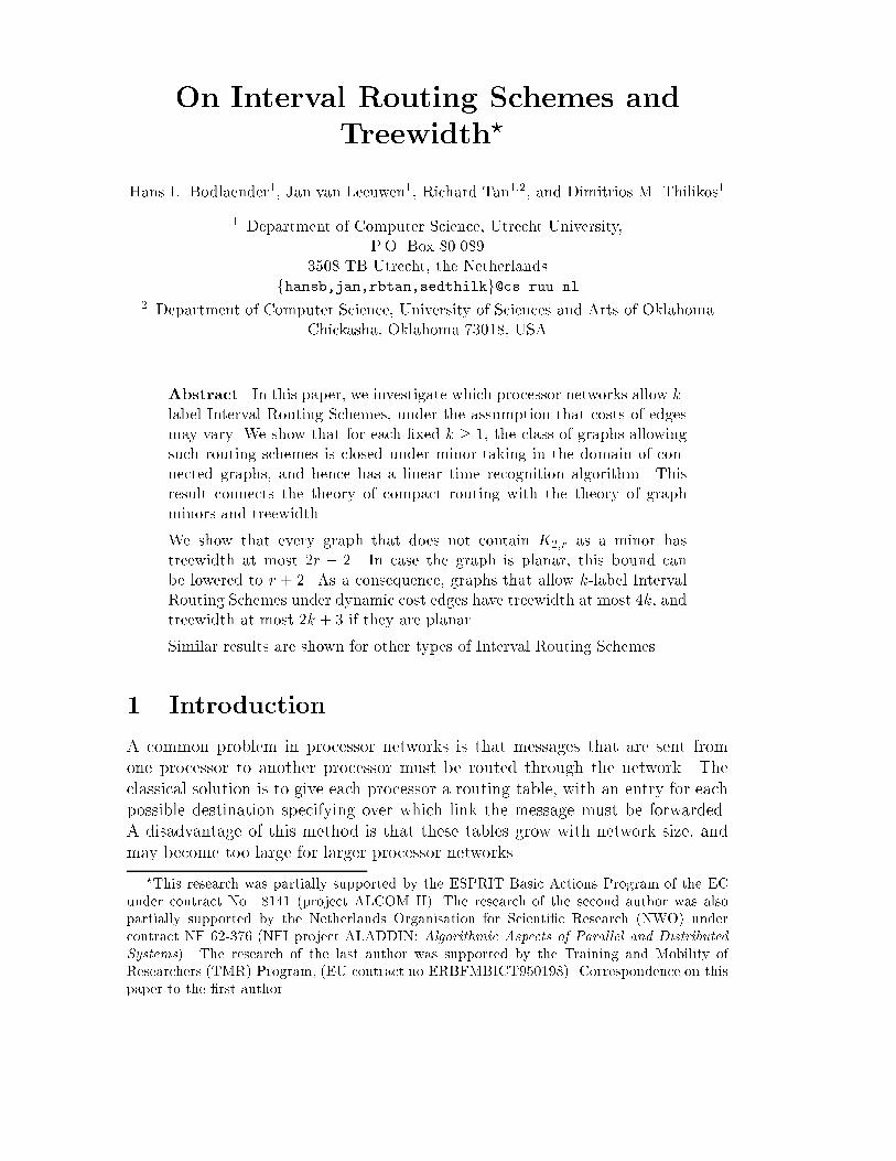
Figure 1: Example of a graph in D6.Lemma 18 (See e.g., [8].) Let (fXi; i 2 Ig; T ) be a tree-decomposition ofgraph G = (V;E). For any clique K of G, there exists an i 2 I with V (K) � Xi.Lemma 19 For any graph G 2 Dr, either K2;r is a minor of G or G has a tree-decomposition of treewidth � 2r� 2 which is also a tree-decomposition of CL(G).Proof: Let Gclique = CL(G), V (K1;r) = fw0; w1; : : : ; wrg and E(K1;r) =ffw0; w1g; : : : ; fw0; wrgg. From Lemma 17, either K1;r is a minor of Gclique[V2] ortreewidth(Gclique[V2]) � r � 1. We consider these cases separately.Case 1. K1;r is a minor of Gclique[V2]: Let i = 0; : : : ; r and Swi be the set ofvertices in Gclique[V2] that were identi�ed to wi when creating K1;r as a minor.Notice that any set Swi induces a connected subgraph in Gclique[V2]. Denote byR the set of vertices in V3 that are adjacent to vertices in Sw0. Finally let wi bea vertex in Swi that is adjacent to a vertex in Sw0. (Note that these vertices wiexist, by the construction of K1;r as a minor.) We observe that Gclique[R [ Sw0]is connected.Claim I: G[R [ Sw0] is connected.Suppose not. As E(G[R [ Sw0]) � E(Gclique[R [ Sw0]), we can add edges inE(Gclique[R [ Sw0]) � E(G[R [ Sw0]) to G[R [ Sw0] until an edge, say fx1; x2g14

makes the graph connected. As fx1; x2g belongs to E(Gclique[R [ Sw0]), but notto E(G[R [ Sw0]), the edge is in one of the added cliques, i.e., there must be avertex x3 2 V3 that is adjacent to both x1 and x2. Now we have a contradiction,as x3 2 R � R [ Sw0.Claim II: For all i, wi is adjacent to a vertex in R [ Sw0 in G.For all i, there exists a vertex xi 2 Sw0 that is adjacent to wi in Gclique. Iffwi; xig 2 E(G), then we are done. If fui; xig 62 E(G), then there is a vertexx3i 2 V3 with fxi; x3i g; fwi; x3i g 2 E(G), and the claim is true, as wi is adjacentto x3i 2 R.We can now show that K2;r is a minor of G. First contract all vertices inR [ Sw0 to a single vertex z0. Next for each i, contract all vertices in Swi to asingle vertex, say zi. Then contract all vertices in V0 [ V1 to a single vertex zr+1.(We can do all of these contractions, as each of these sets induces a connectedsubgraph of G.) By claim II, z0 is adjacent to each vertex in fz1; : : : ; zrg. Alsofor each i, as Swi � V2 and each vertex in V2 is adjacent to at least one vertex inV1, zr+1 is adjacent to each vertex zi, 1 � i � r. We now have a K2;r minor.Case 2. Treewidth(Gclique[V2]) � r�1: We now show that treewidth(Gclique) �2r � 2. Take a tree-decomposition (fXi j i 2 Ig; T = (I; F )) of Gclique[V2] withtreewidth � r � 1. Observe that (fXi [ V1 j i 2 Ig; T ) is a tree-decompositionof Gclique[V1 [ V2] with treewidth at most r � 1 + jV1j � 2r � 2. Using thistree-decomposition, we can build a tree-decomposition of Gclique of treewidth� 2r� 2, as follows. Add nodes j0, j31 ; : : : ; j3m to I, with Xj0 = fv0g [ @fv0g andXj3i = fv3i g [ @fv3i g. By Lemma 18 there exists for each i a node j 0i 2 I, with@fv3i g � Xj0i. We make j3i adjacent to this node j 0i. Finally, make j0 adjacent toan arbitrary node j 00 2 I. We now have a tree-decomposition of G of treewidthat most 2r � 2. utDe�nition. A terminal graph is a triple G = (V;E; S) where (V;E) is a graphand S � V is an ordered subset of its vertices. We call S the terminal set of G.De�nition. Consider two terminal graphs Gi = (Vi; Ei; Si); i = 1; 2 such thatjS1j = jS2j. De�ne G1 � G2 as the graph obtained by taking the disjoint unionof G1 and G2 and then identifying the corresponding terminal vertices in S1 andS2.Lemma 20 Consider two terminal graphs Gi = (Vi; Ei; Si); i = 1; 2 such thatjS1j = jS2j. Suppose that for i = 1; 2, Gi[Si] is a clique. If treewidth(Gi) �ki; i = 1; 2, then there is a tree-decomposition with G1�G2 of treewidth at mostmaxfk1; k2g.Proof: Take tree-decompositions (fX ij j j 2 I ig; T i = (I i; F i)) ofGi of treewidthat most ki, i = 1; 2. By Lemma 18, there are ji0 2 I i with Si � X iji0, i = 1; 2.15

Taking the disjoint union of the two tree-decompositions and connecting nodes j10and j20 yields the desired tree-decomposition: one easily veri�es that (fX1j j j 2I1g [ fX2j j j 2 I2g; T = (I1 [ I2; F 1 [ F 2 [ ffj10 ; j20gg)) is a tree-decompositionwith G1 �G2 with treewidth at most maxfk1; k2g. utWe are now ready to prove Theorem 14. In fact, we prove the following,slightly stronger result.Theorem 21 Let G = (V;E) be a graph that is not a clique. Then, for any r � 1,either K2;r is a minor of G or for any minimal separator S where jSj < r, G hasa tree-decomposition with treewidth � 2r � 2 that is also a tree-decomposition ofCL(G; fSg).Proof: We use induction on jV j. The theorem clearly holds for jV j = 3. Assumethat the theorem holds for any graph with less than n vertices. Let G = (V;E)be a graph with n vertices and let S be a minimal separator with jSj < r (inthe case where jSj � r, we have by Lemma 16 that K2;r is a minor of G). LetGi = (Vi; Ei); i = 1; : : : ; m, be the connected components of G[V � S] and�Gi = EX(G[Vi [ @Vi]; f@Vig). We denote the corresponding \new" nodes as vinew.Notice that each graph �Gi has @fvinewg as a minimal separator and j@fvinewgj < r.We consider two cases.Case 1. jV ( �Gi)j < n for all i � i � m. From the induction hypothesis it followsthat either K2;r is a minor of �Gi for some i or for all i, �Gi has a tree-decompositionof treewidth � 2r� 2 that is also a tree-decomposition of CL( �Gi; f@fvinewgg). Inthe �rst case, as �Gi is a minor of G, K2;r is also a minor of G.So suppose that for all i, �Gi has a tree-decomposition of treewidth � 2r � 2which is also a tree-decomposition of CL( �Gi; f@fvinewgg). We now construct atree-decomposition of CL(G; fSg) of treewidth � 2r � 2. Let Hi be the graphobtained from CL( �Gi; f@fvinewgg) by removing the \new" vertex vinew. Clearlyany graph Hi; i = 1; : : : ; m has a tree-decomposition of treewidth � 2r � 2 andis a subgraph of CL(G; fSg). Consider now the graphs H1 and H2. We have thatS1;2 = V (H1)\V (H2) � S and thus S1;2 induces a clique in H1 and H2. Make H1and H2 into terminal graphs with terminal set S1;2. From Lemma 20 the graphH1;2 = H1 � H2 has also a tree-decomposition of treewidth � 2r � 2. Noticethat H1;2 is a subgraph of CL(G; fSg) and S1;2;3 = V (H1;2) \ V (H3) � S, thusS1;2;3 induces a clique in H1;2 and H3. Now make H1;2 and H3 terminals withterminal set S1;2;3 and apply again Lemma 20 to obtain a tree-decompositionof H1;2;3 = H1;2 � H3 with treewidth � 2r � 2. In this manner, by repeatedlyapplying Lemma 20, we can merge all the tree decompositions of the graphsHi; i = 1; : : : ; m and thus construct a tree-decomposition of CL(G; fSg) thathas treewidth � 2r � 2.16

Case 2. We now examine the remaining case where there are only two connectedcomponents inG[V �S] and at least one of them contains only one vertex v0. Con-sider the set D = @S�fv0g, and assume that it does not contain a minimal sepa-rator of cardinality � r (if it does, then by Lemma 16, K2;r is a minor of G). LetGi be the connected components of G[V �D�S�fv0g] and Ni = @V (Gj) � D,i = 1; : : : ; m. Notice that, asD does not contain minimal separators of cardinality� r; jNij < r. Let �Gi = EX(Gi; fNig); i = 1; : : : ; m, and denote the correspond-ing \new" vertices as vinew. As each �Gi has less than n vertices, by the inductionhypothesis, either K2;r is a minor of �Gi for some i or �Gi has a tree-decompositionof treewidth � 2r�2 which is also tree-decomposition of CL( �Gi; fNig) for each i.In the �rst case, as before, �Gi is a minor of G and thus K2;r is a minor of G. In thesecond case, observe that F = EX(G[D[S]; fS;N1; : : : ; Nmg) is a member of Dr.From Lemma 19, either K2;r is a minor of F (which implies that K2;r is a minorof G, as F is a minor of G) or F has a tree-decomposition of treewidth � 2r� 2which is also a tree-decomposition of CL(F; fS;N1; : : : ; Nmg). We now constructa tree-decomposition of CL(G; fS;N1; : : : ; Nmg) with treewidth� 2r � 2. Foreach i let Hi be the graph obtained from CL( �Gi; fNig) if we eliminate the \new"vertex vinew. Also let F0 be the graph obtained from F by eliminating the \new"vertices vnew;i corresponding to the sets N1; : : : ; Nm. Clearly each Hi and F0have tree decompositions of treewidth� 2r � 2. We observe that for F0 and H1,V (F0)\V (Hi) = N1 induces a clique in F0 and H1. Make F0 and H1 into terminalgraphs with terminal set N1. By Lemma 20 the graph F1 = F0 � H1 has alsoa tree-decomposition of treewidth� 2r � 2. Now N2 induces a clique on F1 andH2, so we can make them terminals with terminal set N2, and apply Lemma 20again to obtain a tree decomposition of F2 = F1�H2 of treewidth� 2r�2. Con-tinuing in this fashion we can merge all the tree decompositions of the graphsHi; i = 1; : : : ; r to the tree-decomposition of F0, and thus construct a tree-decomposition of CL(G; fS;N1; : : : ; Nmg) of treewidth� 2r � 2. As CL(G; fSg)is a subgraph of CL(G; fS;N1; : : : ; Nmg), this completes the proof of the theo-rem. utCorollary 22 (i) Every graph in k-IRS has treewidth at most 4k.(ii) Every graph in k-SIRS has treewidth at most 4k.Proof: If G 2 k-SIRS or G 2 k-IRS, then K2;2k+1 is not a minor of G hence Ghas treewidth at most 2(2k + 1)� 2 = 4k. utA direct consequence is that graphs in the classes k-LIRS and k-SLIRS alsohave treewidth at most 4k. These results can be seen as partial characterisationsof graphs which allow k-label interval routing schemes (with dynamic edge costs).The result also indicates a limitation of the interval routing method: as `mostgraphs have large treewidth' (see e.g. [17], chapter 5), the set of graphs in k-IRSonly covers a small part of all graphs (or even of all sparse graphs, see [17]).17

Interestingly, the proof of Theorem 14 can be made constructive, and can beused to build an algorithm, that either outputs that input graph G has K2;r asa minor, or that outputs a tree-decomposition of G of treewidth at most 2r � 2,and that uses O(rn) time. Combined with the results of Lemma 12 this canlead to a practical algorithm that checks whether for a given node labelling, ank-IRS (or k-SIRS, k-LIRS, k-SLIRS) exists for this labelling and all possible costassignments, especially when additional optimisations are used, and k is small(e.g., k = 2, or k = 3.)In the case when k = 1, more precise bounds are known. As 1-SIRS equals theclass of connected outerplanar graphs [15], and outerplanar graphs have treewidthat most 2, every graph in 1-SIRS has treewidth at most 2. Similarly, the charac-terisations of 1-LIRS in [3] and of 1-SIRS in [2] show that every graph in 1-LIRShas treewidth (and even pathwidth) at most 2, and every graph in 1-IRS hastreewidth at most 3, and has treewidth at most 2 if it is not equal to K4.The results also have consequences for random graphs. We mention someresults, obtained by Kloks [17]. Let Gn;m denote a random graph with n verticesand m edges. For a precise meaning of the term `almost every' we refer to [17]or [9].Theorem 23 (Kloks[17]) (i) Let � > 1:18. Then almost every graph Gn;m withm � �n has treewidth �(n).(ii) For all � > 1 and 0 < � < (� � 1)=(� + 1), almost every graph Gn;m withm � �n has treewidth at least n�.Corollary 24 (i) Let � > 1:18. Then for almost every graph Gn;m with m � �n,the smallest k for which Gn;m 2 k�IRS is of size �(n).(ii) Let � > 1 and 0 < � < (� � 1)=(� + 1). Then for almost every graph Gn;mwith m � �n, the smallest k for which Gn;m 2 k-IRS ful�ls k � n�.5 The treewidth of planar graphs with k-labelinterval routing schemesIn this section we prove results, similar to those of the previous section, for thecase that the graph G is planar.We �rst need some de�nitions and lemmas. The following lemma is easy.Lemma 25 Let G be a graph with treewidth(G) � k, k � 2 and w 62 V (G).Suppose G0 = (V (G) [ fwg; E(G) [ ffv; wg; fu; wgg) where fu; vg 2 E(G) orG0 = (V (G) [ fwg; E(G) [ ffv; wgg where v 2 V (G). Then treewidth(G0) � k.Lemma 26 Let G be a graph and C = fC1; : : : ; Crg be a collection of vertex setsin G where G[Ci] is a clique for each i. If treewidth (G) � k and jCij � k foreach i then treewidth (EX(G; C)) � k. 18

2V

1V Figure 2: A 7-fence.Proof: Let treewidth (G) � k. There is a tree-decomposition of G of treewidth� k. By Lemma 18, for any Ci 2 C there exists a node Xi in the decompo-sition such that Ci � Xi. Now construct a tree-decomposition of EX(G; C) byintroducing r new nodes X 0i; i = 1; : : : ; r, where X 0i = Ci [ fvnew;ig and makeX 0i adjacent to Xi in the new decomposition tree. It is easy to check that thetree-decomposition thus obtained has treewidth � k. utDe�nition. A graph G = (V1 [ V2; E) is called an r-fence, if it can be writtenin the following form: V = V1 [ V2, with Vi = fvi1; : : : ; virg; i = 1; 2 and E =f(vij; vi0j0) j vij 6= vi0j0; jj � j 0j � 1; i; i0 2 f1; 2gg.An example of a 7-fence is given in Figure 2.Lemma 27 If G = (V1[V2; E) is an r-fence then treewidth(CL(G; fV1[V2g)) �r + 1.Proof: Take the tree-decomposition (fXi : i 2 Ig; T ) where T is a path with rnodes and X1 = fv11; : : : ; v1r ; v21; v22g; Xi = Xi�1 [ fv2i+1g� fv1i�1g; i = 2; : : : ; r� 1.It is easy to see that this is a tree-decomposition of G with treewidth� r+1. utDe�nition. Let Zr be the collection of graphs G = (V1 [ V2; E) that can beconstructed as follows:� Take two disjoint sets of vertices V1 = fv11; : : : ; v1k1g; V2 = fv21; : : : ; v2k2g withk1; k2 < r. We call Vi; i = 1; 2, the parts of the graph under construction.� Add edges fvi1; vi2g; : : : ; fviki�1; vikig; i = 1; 2 and edges fv11; v21g; fv1k1; v2k2g.� Add a maximal set of edges such that1. the graph stays planar,2. any vertex in V1 (resp. V2) is adjacent to at least one vertex in V2(resp. V1), 19

12VV Figure 3: The construction of a graph in Z14.3. the resulting planar graph can be embedded such that the outer faceis formed by the cycle (v11; : : : ; v1k1; v2k2 ; v2k2�1; : : : ; v21; v11).Notice that the graph R constructed so far is outerplanar.� The construction is completed by setting Ej = E(G[Vj]); j = 1; 2 andapplying the following operation for an arbitrary number of times:For some edge fv2i ; v2i+1g 2 E2 and a set of vertices V 1l;r = fv1l ; : : : ; v1l+rg �V1; l; r � 1 such that E(G[V 1l;r]) � E1 and fv2i ; v1l g; fv2i+1; v1l+rg 2 E(G) weset(i) E1 E1 � E(G[V 1l;r])(ii) E2 E2 � ffv2i ; v2i+1gg(iii) E(G) E(G) [ ffv2i ; v1l g; : : : ; fv2i ; v1l+rgg[ffv2i+1; v1l g; : : : ; fv2i+1; v1l+rgg.We call the edges in E(G[V2])� E2 unmarked edges of G.For an example of the construction of a graph in Z14 see Figure 3.From now on, given a graph G = (V0 [ : : : [ V�; E), we will use the notationVi(G) = Vi; i = 0; : : : ; � (we call V0; : : : ; V� parts of G).20

De�nition. If R 2 Zr, then de�ne CL(R) = CL(R; fV1(R); V2(R)g). We callVi(R); i = 1; 2, the parts of CL(R). Also we de�ne CL(Zr) = fCL(R) : R 2 Zrg.De�nition. Let G 2 Zr with parts V1; V2. D(vji ; G); i = 1; : : : ; kj; j = 1; 2 isde�ned as the number of vertices that are adjacent to vji and belong to part V3�j.Lemma 28 Let G 2 Zr with parts Vi = fvi1; : : : ; vik1g; i = 1; 2; and k1; k2 < r.Then, either D(v11; G) � 2 or D(v21; G) � 2.Proof: Let R be the outerplanar graph from which G has been created accordingto the de�nition ofZr. Let also E1; E2 be the edge sets de�ned by the constructionofG according to this de�nition. Notice that R 2 Zr and that eitherD(v11; R) = 1or D(v21; R) = 1. Assume �rst that D(v11; R) = 1. If fv11; v12g 62 E1, then clearlyD(v11; G) = 1. If fv11; v12g 2 E1, then it is easy to see that edge fv11; v22g is theonly edge in E(G)�E(R) that is incident to v11 and thus D(v11; G) = 2. Assumenow that D(v21; R) = 1. If fv21; v22g 62 E2, then D(v21; G) = 1. If fv21; v22g 2 E2,then it is easy to see that D(v11; R) = 2 and no edge in E(G)� E(R) is incidentto v11. Thus, D(v11; G) = 2. utLemma 29 If G 2 CL(Zr), then treewidth(G) � r.Proof: Suppose that R = (V1 [ V2; E) 2 Zr. We will show that G =CL(R; fV1; V2g) has treewidth� r.We will use induction on r. If r � 3, then the proposition is trivial. We assumethat lemma holds for any r � k. We will prove that if R = (V1 [ V2; E) 2 Zk+1,then treewidth(CL(R)) � k + 1.Let R 2 Zk+1 with parts V1 and V2. Recall that ki = jVij; i = 1; 2. Ifk1 < k and k2 < k then R 2 Zk and the induction step is obtained easily. Weclaim that it su�ces to prove the induction step for k1 = k2 = k. This is sobecause in case k = kj > k3�j for some j = 1; 2, then we set i = 3 � j andconstruct a graph R�, containing R as a subgraph, as follows: add kj�ki verticesviki+1; : : : ; vikj in part Vi and then add the edge sets ffviki; viki+1g; : : : ; fvikj�1; vikjggand ffvjkj ; viki+1g; : : : ; fvjkj ; vikjgg. Clearly, R� 2 Zk+1 and treewidth(CL(R)) �treewidth(CL(R�)) (see Figures 4.i, 4.ii). Thus, it is su�cient to examine thecase where k1 = k2 = k.If R is a k-fence then the result follows from Lemma 27. Suppose that R isnot an k-fence.If D(v11; R) 6= 2 or D(v21; R) 6= 2 then set q = 1, otherwise setq = maxf i : R[fv11; : : : ; v1i ; v21; : : : ; v2i g] is an i-fenceand the vertex set fv1i ; v2i g is a separator of R g:Notice that q < k. Let R0 = R[fv1q ; : : : ; v1k; v2q ; : : : ; v2kg] and observe that R0 2Zk�q+2 (see Figure 4.ii). 21

G

G

A

B

S

(i)

(ii)

(iv)

(iii)

Figure 4: An example of the proof of Lemma 29.Using Lemma 28 we de�ne m according to the following cases:Case (i) D(v1q ; R0) = 1. In this case we set m = q.Case (ii) D(v2q ; R0) = 1. In this case we also set m = q.Case (iii) D(v1q ; R0) > 1 and D(v2q ; R0) > 1. By a case analysis similar toLemma 28 we can see that D(v1q ; R0) = 2 and D(v2q ; R0) > 2 and we set m = q+1.Observe that in Cases (i) and (iii) the set S = fv21; : : : ; v2m; v1m+1; : : : ; v1kg isa separator of G = CL(R) (see Figure 4.ii). Also, in Case (ii) the set T =fv11; : : : ; v1m; v2m+1; : : : ; v2kg is a separator of G = CL(R).We will present the proof for the Cases (i) and (iii). We set GA =G[fv1m+1; : : : ; v1k; v2m+1; : : : ; v2kg]. Notice that GA is a subgraph of a graph inCL(Zk�m+1) and, as k � m + 1 � k, by the induction hypothesis, GA has atree-decomposition DA = (fXi : i 2 Ig; T ) of treewidth � k � m + 1. No-tice that from Lemma 18 it follows that DA contains a node XA such thatXA � fv1m+1; : : : ; v1kg. Clearly, D0A = (fXi [ fv21; : : : ; v2mg : i 2 Ig; T ) is a tree-decomposition ofG0A = G[V2[S] with treewidth � k+1. Notice also thatD0A con-tains node X 0A = XA[fv21; : : : ; v2mg � S and thus treewidth(Cl(G0A; fSg)) � k+1(see Figure 4.iii).Let now GB = G[fv11; : : : ; v1m; v21; : : : ; v2mg].We de�ne a tree-decomposition DB of GB as follows: DB = (fXi : i 2Ig; T ) where T is a path consisting of m� 1 nodes and X1 = fv11; : : : ; v1m; v21; v22g,22

Xi = X 0i�1 � fv1i�1g [ fv2i+1g; i = 2; m � 1. It is easy to see that DB is a tree-decomposition of GB with treewidth � m + 1. Notice that DB contains nodeXB = Xm�1 � fv21; : : : ; v2mg. Clearly, D0B = (fXi[fv1m+1; : : : ; v1kg : i 2 Ig; T ) is atree-decomposition ofG0B = G[V1[S] with treewidth � k+1. Notice also thatD0Bcontains nodeX 0B = XB[fv1m+1; : : : ; v1kg � S and thus treewidth(Cl(G0B; fSg)) �k + 1 (see Figure 28.iv).Now, if we consider the terminal graphs, obtained by taking CL(G0A; fSg)and CL(G0B; fSg) with S as set of terminals, and then apply Lemma 20, weobtain that treewidth(G) � treewidth(CL(G; fSg)) = treewidth(CL(G0A; fSg)�CL(G0B; fSg)) � k + 1.Case (ii) is similar to Case (i). (We use separator T instead of S). utDe�nition. Let Qr be the collection of graphs G = (V1 [ V2; E) that can beconstructed as follows:Let R be a graph in Zr+1 containing an unmarked edge fv2i ; v2i+1g; 1 � i < jV2j.We apply the following two operations:(i) Let R0 = (V (R); E 0) where E 0 = E(R) [ ffv2i ; v11g; : : : ; fv2i ; v1jV1jgg [ffv2i+1; v11g; : : : ; fv2i+1; v1jV1jgg.(ii) Identify vertices vi1 and vijVij; i = 1; 2 in R0.If R 2 Qr with parts V1; V2, we de�ne CL(R) = CL(R; fV1; V2g) Also, wede�ne CL(Qr) = fCL(R) : R 2 Qrg.For an example of the construction of a graph in Q13 see Figure 5.Lemma 30 If G 2 CL(Qr) then treewidth(G) � r + 2.Proof: We prove that if R 2 Qr, then G = CL(R) has treewidth � r +2. According to the de�nition of Qr, R is constructed by a graph R0 2 Zr+1containing an unmarked edge fv2i ; v2i+1g. Let a be a vertex in V1(R0) connectedwith both v2i and v2i+1 and let b be a neighbour of a in R[V1]. Let also R1 =R[V (R) � fv2i ; v2i+1; a; bg]. It is easy to see that R1 is a subgraph of a graphR2 2 Zr�1 (we use the fact that fv2i ; v2i+1g is an unmarked edge in R0). FromLemma 29 we have that treewidth(Cl(R2)) � r � 2 and CL(R2) has a tree-decomposition of treewidth � r� 2. We can now obtain a tree-decomposition ofG = CL(R) by adding vertex set fa; b; c; dg in each node of the tree-decompositionof R2. Clearly, this tree-decomposition has treewidth � r+2; this completes theproof of the lemma. utNote that if G = (V0 [ V1 [ V2 [ V3; E) is a planar graph in Dr, then G[V2] isouterplanar, because otherwise there would exist a vertex in G[V2] not adjacentwith some vertex in V1 contradicting the de�nition of Dr. Using this fact we caneasily see that if G is a planar graph in D2, then CL(G) has treewidth� 3. Also itis not hard to see that if G is a planar graph in D3, then CL(G) has treewidth� 4.23

(ii)(i)

Figure 5: The construction of a graph in Q13In what follows, we will prove that if G is a planar graph in Dr; r � 4, then CL(G)has treewidth� r + 2.In the remainder of this section, we letDr be as de�ned in the previous section,but we remove from the class all graphs that contain at least one vertex of degreeat most two. Lemma 25 shows that we can actually remove these graphs (thepurpose of the proof below is to show that planar graphs in Dr have treewidthat most r + 2.)De�nition. We de�ne Pr; r � 4 as the set of planar graphs that can be con-structed from a planar graph G 2 Dr; r � 4, by applying the following foursteps:(a) Consider a planar embedding of G. W.l.o.g. we assume that the ver-tices in V1 are arranged around v0 in the cyclic order v11; : : : ; v1jV1j; v11.Let G0 = (V (G0); E(G0)) be de�ned by V (G0) V (G) and E(G0) E(G) � E(G[V1]) [ ffv11; v12g; : : : ; fv1jV1j�1; v1jV1jg; fv1jV1j; v11gg. Notice thatwe have basically the same planar embedding of G0 as of G, and thatCL(G0) = CL(G). The resulting graph is now further denoted as G.(b) If there exist an edge fa; bg 62 E(G) such that at least one of a; b belongsto V2, a; b 62 V3, and G0 = (V (G); E(G) [ ffa; bgg) is a planar graph, thenadd this edge to G. We repeat this step until no such edge can be addedin G. 24

Notice that: (i) all faces in the planar embedding of the resulting graph Gare triangles. (ii) G[V2] is outerplanar and connected.(c) If there is a biconnected component in G[V2] that consists of a singleedge fa; bg then it is easy to see that there is a vertex d 2 V1 such thatfa; dg; fb; dg 2 E(G). In this case, add a new vertex c to V2, and add edgesffa; cg; fb; cg; fc; dgg. Repeat this step until there exist no biconnectedcomponent in G[V2] that is an edge. The resulting graph is now furtherdenoted as G.Notice that G[V2] is outerplanar and G has an embedding such that allvertices of V3(G) are at the inside of the cycle(s) formed by V2(G). We callthis planar embedding the outerplanar embedding.In the outerplanar embedding, we identify the regions of G[V2] as the areasof the plane that constitute an interior face in the embedding of V2(G),obtained by restricting the embedding of G to G[V2].Notice that each region of V2 has at most one vertex of V3 inside and thateach region of V2 that does not contain a vertex of V3 inside is a triangle.(d) If there is a triangle in G[V2] with vertices a; b; c, whose region does notcontain a vertex of V3 inside, then add a new vertex d to V3, and add edgesfa; dg; fb; dg; fc; dg. Repeat this step until all the regions in G[V2] contain avertex of V3 inside in the outerplanar embedding of G. The resulting graphG becomes a member of Pr.After step (d) any region F of G[V2] contains a vertex of V3. We denotethis vertex by vF .Finally, if R 2 Pr, we de�ne CL(R) = CL(R; f@fvg : v 2 V0(R) [ V3(R)g).Also, we de�ne CL(Pr) = fCL(R) : R 2 Pg.For an example of the construction of a graph in Pr see Figure 6.From the de�nition of Pr we can see that if any graph in CL(Pr) hastreewidth� r + 2, then for any planar graph R 2 Dr, with r � 4, it holdsthat the treewidth CL(R) is at most r + 2. In what follows, we prove that ifG 2 CL(Pr), then treewidth(G) � r + 2.De�nition. Let G = (V0[V1[V2[V3; E) be a graph in Pr, r � 4. Consider theouterplanar embedding of G. We call the edges that are incident to the exteriorface of G[V2] exterior edges. If e is an exterior edge of G, then we denote as F (e)the set of vertices in V2 that belong to the unique interior face adjacent to e, inthe embedding of G[V2], obtained by restricting the embedding of G.25

(a) (b)

(d)(c)

Figure 6: The construction of a graph in P726

De�nition. Let G be a graph in Pr; r � 4. Consider the outerplanar embeddingof G. For each region F in G2 we let SF the collection of sets Se, over all edgese = fv; v0g 2 E(G[F ]) that belong to another region of G[V2], where Se is theset fv; a; : : : ; b; v0g, a; : : : ; b 2 V1 such that the cycle (v; a; : : : ; b; v0; v) does notseparate v0 and vF . (Vertices a; : : : ; b are consecutive vertices in the cyclic orderv11; : : : ; v1jV1j; v11). We denote the region of (v; a; : : : ; b; v0; v) that does not containv0 and vF the induced region of Se.Notice that SF is a collection of separators of G (see Figure 7). We �rst provethe following result:Lemma 31 If G = (V0 [ V1 [ V2 [ V3; E) 2 CL(Pr), r � 4 such that G[V2] hasonly one biconnected component, then for any exterior edge e = fv; v0g 2 G[V2],treewidth(CL(G;SF (e) [ ffv; v0g [ V1g)) � r + 2.Proof: Let G be a graph in CL(Pr). Let also R 2 Pr be a planar graph suchthat CL(R) = G. Recall that G[V2] is an outerplanar graph. We use inductionon the number of faces in G[V2].Suppose that the planar embedding of G[V2] contains only one region. No-tice that in this case F (e) = V2, SF (e) = ; and thus G0 = CL(G[V1 [V2];SF (e) [ ffv; v0g [ V1g) 2 CL(Qr). From Lemma 26 we have the requiredas G = EX(G0; f@fug : u 2 V0 [ V3g).Suppose now that lemma holds for any graph G 2 CL(Pr) where G[V2] con-tains less than l faces. Let now G be a graph in CL(Pr) where G[V2] contains lfaces. We now prove that lemma also holds for G.Let SF (e) = fS1; : : : ; Stg. For each Si 2 SF (e) we de�ne the vertex set Ui �V2 [ V3 to be the set of all the vertices contained in the induced region of Si.Let Goi = G[@Ui [ Ui]; i = 1; : : : ; t and Go = G[V (G) � Si=1;:::;t Ui]. Notice thatV (Go) \ V (Goi ) = Si; i = 1; : : : ; t. Observe that, as jF (e)j < r and jV1j < r,we have that CL(G[V (Go)� (fvF (e)g [ V0)];SF (e) [ ffv; v0g [ V1g) 2 Qr and, byLemmas 30 and 26, treewidth(CL(Go;SF (e) [ ffv; v0g [ V1g)) � r + 2.Let Si = fui; ai; : : : ; bi; u0ig; i = 1; : : : ; t where fui; u0ig = F (e) \ V (Goi ) andfai; : : : ; big = V1(G) \ V (Goi ) for i = 1; : : : ; t (see the de�nition of SF above).Observe that Goi is a subgraph of a graph G0oi in CL(Pr) and the number of regionsin the planar embedding of V2(G0oi ) is less than l for i = 1; : : : ; t (w.l.o.g. weassume that V (G0oi ) = V (Goi )). Notice also that fui; u0ig = Si � V1(G0oi ) and thatthe edge ei = fui; u0ig is an exterior edge in the planar embedding of V2[G0oi ] for i =1; : : : ; t. From the induction hypothesis we obtain that treewidth(CL(G0oi ;SF (ei)[ffui; u0ig [ V1(G0oi )g)) � r + 2; i = 1; : : : ; t. Finally, using that Si = fui; u0ig [V1(G0oi ), we conclude that treewidth(CL(Goi ; fSig)) � treewidth(CL(G0oi ; fSig)) �treewidth(CL(G0oi ;SF (ei) [ fSig)) � r + 2; i = 1; : : : ; t.We now set Hi = CL(Goi ; fSig); i = 1; : : : ; t, andH 0 = CL(Go;SF (e)[ffv; v0g[V1g)). We make terminal graphs of Hi by taking as set of terminals Si, for i =27

2ua

u’

v’

v

b

u’

V V V

a

u

2

b

v

G

v’

v u

u’

v

u’

u

v

v

G G

v

u

v

u’

u

u’

V

2

2

F(e)

0

2

0

1

1

1

1

0

2

1 F(e)

1

3

1

0 1 2

2

o

2

o

1

0

1

2

o

Figure 7: An example of the proof of Lemma 31.28

1; : : : ; t. If now we successively take Si, i = 1; : : : ; t as terminals in H and applyrepeatedly Lemma 20 we conclude that the graph (: : : ((H 0�H1)�H2) � � ��Ht) =CL(G;SF (e) [ ffv; v0g [ V1g)), (where during each � operation, a di�erent set ofterminals is used), has also treewidth � r + 2 (this construction is the same asthe one used in the proof of Theorem 21). For an example of the construction ofthe proof see Figure 7. utDe�nition. Let G be a graph in Pr; r � 4. Given a vertex v 2 V2, we de�neCv as the collection of the biconnected components in G[V2] that contain v. IfjCvj > 1, we call v rich, otherwise we call it poor.De�nition. Let G be a graph in Pr. Consider the outerplanar embedding of G.For each vertex v 2 G[V2] we de�ne a collection Sv of sets of vertices, as follows:(i) Set Sv ;. Also, if v is a rich vertex, then set A = ;.(ii) We examine two cases:Case (a) If v is a rich vertex, then for each biconnected component Ci 2Cv � A; i = 1; : : : ; t we set Sv Sv [ fSig where G[Si] de�nes a cycle(v; a; : : : ; b; v); a; : : : ; b 2 V1 that separates the vertices in fv0gSj=1;:::;t;j 6=i V (Cj)�fvg from the vertices in V (Ci)�fvg (vertices a; : : : ; b are consecutive vertices inthe cyclic order v11; : : : ; v1jV1j; v11). We call the area of the plane inside or outsidethe cycle, that contains the vertices in V (Ci)� fvg the induced region of Si.Case (b) If v is a poor vertex, then there is a unique biconnected componentCv 2 Cv that contains it. Let Wv be the set of the rich vertices in Cv. For eachreach vertex vi 2 Wv we set Sv Sv [Svi where Svi is de�ned by setting A = Cvand applying Case (a) for vi, i = 1; : : : ; jWvj.Notice that Sv is a collection of separators of G (see Figure 8 for Case (a) andFigure 9 for Case (b)). We now prove the following:Lemma 32 Let G = (V0 [ V1 [ V2 [ V3; E) be a graph in CL(Pr); r � 4. Thenfor any vertex v 2 G[V2], treewidth(CL(G;Sv [ ffvg [ V1g)) � r + 2.Proof: Let G be a graph in CL(Pr). Let also R be a planar graph such thatG = CL(R). We use induction on the number of biconnected components inG[V2].Suppose thatG[V2] contains only one biconnected component. Clearly, for anyvertex v 2 G[V2] we have that there exists an exterior edge e = fv; v0g; v0 2 G[V2]that is incident to v. From Lemma 31 we have that treewidth(CL(G;SF (e) [ffv; v0g [ V1g)) � k + 2. As CL(G; ffvg [ V1g) is a subgraph of CL(G;SF (e) [ffv; v0g[V1g) and Sv = ;, we have that treewidth(CL(G;Sv[ffvg[V1g)) � r+2.Suppose now that the lemma holds for any graph G 2 CL(Pr) where G[V2]contains less than l biconnected components. Let now G be a graph in CL(Pr)29

V V32

G’

v

V V

a

ba

v

b=a

v

b

G’

v

G

v v v

vvv

0 1

1

2 3

21

0

3

o

1

o

0

0

0

0

2

o o

3G’

Figure 8: Case (i) of the proof of Lemma 32.30

where G[V2] contains l biconnected components. We prove that the lemma alsoholds for G.Let Sv = fS1; : : : ; Stg. For each Si 2 Sv; i = 1; : : : ; t we de�ne the vertex setUi � V2 [ V3 to be the set of all the vertices contained in the induced region ofSi. Let Goi = G[@Ui [ Ui]; i = 1; : : : ; t and Go = G[V (G) � Si=1;:::;t Ui]. Noticethat V (Go) \ V (Goi ) = Si; i = 1; : : : ; t. We examine two cases:(i) v is a rich vertex. Notice that jV (Go)j � r + 1 and, clearlytreewidth(CL(Go;Sv [ ffvg [ V1g)) � r + 2 (see Figure 8).(ii) v is a poor vertex. Let Cv be the unique biconnected component of G[V2]that contains v. Let also V v3 be the set of vertices in V3 that are adjacent withat least two vertices in V (Cv). We de�ne Go = G[fv0g [ V1 [ V (Cv) [ V v3 ]. Itis easy to see that G0 = CL(Go;Sv) 2 CL(Pr) and that G0[V2] = Cv has onlyone biconnected component. Let also e0 = fv; v0g 2 E(Cv) be an exterior edge ofCv containing vertex v. From Lemma 31 we have that treewidth(CL(G0;SF (e0) [ffv; v0g[V1g)) � r+2. It is now easy to see that, as CL(Go;Sv [ffvg[V1g) is asubgraph of CL(G0);SF (e0) [ ffv; v0g [ V1g), we have that treewidth(CL(Go;Sv [ffvg [ V1g)) � r + 2. (See Figure 9).Observe now that Goi is an induced subgraph of a graph G0oi 2 CL(Pr) suchthat V (Goi ) = V (G0oi ) � fv0g. Notice also that the number of biconnected com-ponents in the planar embedding of V2(G0oi ) is < l for i = 1; : : : ; t. Set fuig =Si � V1(G0oi ) (notice that if v is a rich vertex then ui = v; i = 1; : : : ; t). From theinduction hypothesis, we have that treewidth(CL(G0oi ;Sui [ ffuig [ V1(G0oi )g)) �r + 2 and, as Si = fuig [ V1(G0oi ), we obtain that treewidth(CL(G0oi ; fSig)) �r + 2; i = 1; : : : ; t. Finally, since Goi is a subgraph of G0oi we conclude thattreewidth(CL(Goi ; fSig)) � r + 2.We set Hi = CL(Goi ; fSig); i = 1; : : : ; t, and H 0 = CL(Go;Sv [ ffvg [ V1g).For i = 1; : : : ; t, we make Hi a terminal graph by taking Si as set of terminals.If now we successively take Si; i = 1; : : : ; t as set of terminals in H and applyrepeatedly Lemma 20 as in the end of the proof of Lemma 31, we conclude thatthe graph CL(G;Sv [ ffvg [ V1g) has also treewidth � r + 2. utLemma 33 If G 2 Dr and G is planar, then treewidth(CL(G) � r + 2.Proof: We have already examined the cases where r = 2; 3. For the case wherer � 4, the theorem holds because of Lemma 32 as, for any planar graph G 2 Drthere is a graph G0 2 Cl(Pr) such that CL(G) is a subgraph of G0. utNow, we can use the proof of Theorem 21, but with the result of Lemma 33instead of the one of Lemma 19, and obtain the following result.Theorem 34 If G is planar, then either G contains K2;r as a minor or thetreewidth of G is at most r + 2.Corollary 35 (i) Every planar graph in k-IRS has treewidth at most 2r + 3.(ii) Every planar graph in k-SIRS has treewidth at most 2r + 3.31

1

v

b

a

b

u

v’

v

V

u

VVV V

G G’

v

u

u

vV

v’

v

v u

G’

20

0

1o o

2

3

v1

2

0

o

0 1 2 3

1

0

1

1

2

2

3

v1

a

u

Figure 9: Case (ii) of the proof of Lemma 32.32

6 ConclusionsIn this paper, we made a perhaps somewhat surprising and interesting connectionbetween the theory of compact routing schemes, and the theory of graph minorsand treewidth of graphs. Several angles of this connection are still left unexplored.As main open problems, we like to mention several issues that deal withconstructivity. Is it possible to construct linear time algorithms that test whethera given graph belongs to k-IRS or one of its variants, for a �xed k? In severalother cases, a non-constructive proof of a linear or small degree polynomial timebound was only the �rst step towards a fully constructive solution (e.g., [5]).Will our Corollary 10 also be such a �rst step? But even if we know that agraph belongs to k-IRS (or a related class), we do not have a corresponding nodelabelling. How much time does it cost to construct such a node labelling? And,given a node labelling, how much time does it cost to verify that it has a k-labelIRS (or variant) for every edge cost assignment? More related open problems arementioned e.g. in [19].References[1] S. Arnborg, J. Lagergren, and D. Seese. Easy problems for tree-decomposablegraphs. J. Algorithms, 12:308{340, 1991.[2] E. M. Bakker, J. van Leeuwen, and R. B. Tan. Work in progress.[3] E. M. Bakker, J. van Leeuwen, and R. B. Tan. Linear interval routingschemes. Algorithms Review, 2:45{61, 1991.[4] D. Bienstock, N. Robertson, P. D. Seymour, and R. Thomas. Quickly ex-cluding a forest. J. Comb. Theory Series B, 52:274{283, 1991.[5] H. L. Bodlaender. A linear time algorithm for �nding tree-decompositionsof small treewidth. In Proceedings of the 25th Annual Symposium on Theoryof Computing, pages 226{234, New York, 1993. ACM Press. To appear in:SIAM J. Comput., 1996.[6] H. L. Bodlaender. On linear time minor tests with depth �rst search. J.Algorithms, 14:1{23, 1993.[7] H. L. Bodlaender. On disjoint cycles. Int. J. Found. Computer Science,5(1):59{68, 1994.[8] H. L. Bodlaender and R. H. M�ohring. The pathwidth and treewidth ofcographs. SIAM J. Disc. Meth., 6:181{188, 1993.[9] B. Bollobas. Random Graphs. Academic Press, London, 1985.33

[10] R. B. Borie, R. G. Parker, and C. A. Tovey. Automatic generation of linear-time algorithms from predicate calculus descriptions of problems on recur-sively constructed graph families. Algorithmica, 7:555{581, 1992.[11] T. H. Cormen, C. E. Leiserson, and R. L. Rivest. Introduction to Algorithms.MIT Press, Cambridge, Mass., USA, 1989.[12] B. Courcelle. The monadic second-order logic of graphs I: Recognizable setsof �nite graphs. Information and Computation, 85:12{75, 1990.[13] M. R. Fellows and M. A. Langston. Nonconstructive tools for provingpolynomial-time decidability. J. ACM, 35:727{739, 1988.[14] M. R. Fellows and M. A. Langston. On search, decision and the e�ciencyof polynomial-time algorithms. J. Comp. Syst. Sc., 49:769{779, 1994.[15] G. N. Frederickson and R. Janardan. Designing networks with compactrouting tables. Algorithmica, 3:171{190, 1988.[16] Inmos. The T9000 Transputer Products Overview Manual, 1991.[17] T. Kloks. Treewidth. Computations and Approximations. Lecture Notes inComputer Science. Springer Verlag, 1994.[18] J. van Leeuwen and R. B. Tan. Computer networks with compact routingtables. In G. Rozenberg and A. Salomaa, editors, The Book of L, pages298{307. Springer-Verlag, Berlin, 1986.[19] J. van Leeuwen and R. B. Tan. Compact routing methods: A survey. Techni-cal Report UU-CS-1995-05, Department of Computer Science, Utrecht Uni-versity, Utrecht, 1995.[20] N. Robertson and P. D. Seymour. Graph minors | a survey. In I. Anderson,editor, Surveys in Combinatorics, pages 153{171. Cambridge Univ. Press,1985.[21] N. Robertson and P. D. Seymour. Graph minors. II. Algorithmic aspects oftree-width. J. Algorithms, 7:309{322, 1986.[22] N. Robertson and P. D. Seymour. Graph minors. XIII. The disjoint pathsproblem. J. Comb. Theory Series B, 63:65{110, 1995.[23] N. Robertson, P. D. Seymour, and R. Thomas. Quickly excluding a planargraph. J. Comb. Theory Series B, 62:323{348, 1994.[24] N. Santoro and R. Khatib. Labelling and implicit routing in networks. Com-puter Journal, 28:5{8, 1985. 34