Annals of Mathematics and Artificial Intelligence 35: 295–321, 2002. 2002 Kluwer Academic Publishers. Printed in the Netherlands.

Strong conditional independence for credal sets

Serafín Moral ∗ and Andrés CanoDepartamento de Ciencias de la Computatión e I.A., Universidad de Granada, 18071 Granada, Spain

E-mail: {smc,acu}@decsai.ugr.es

This paper investigates the concept of strong conditional independence for sets of proba-bility measures. Couso, Moral and Walley [7] have studied different possible definitions forunconditional independence in imprecise probabilities. Two of them were considered as morerelevant: epistemic independence and strong independence. In this paper, we show that strongindependence can have several extensions to the case in which a conditioning to the valueof additional variables is considered. We will introduce simple examples in order to makeclear their differences. We also give a characterization of strong independence and study theverification of semigraphoid axioms.

Keywords: imprecise probabilities, credal sets, coherence, conditioning, conditional indepen-dence, semigraphoid axioms

AMS subject classification: 60A05, 60A99, 68T37

1. Introduction

The notion of conditional independence is essential in probability theory. In arti-ficial intelligence, it is playing a crucial role in the development of Bayesian networks[5,23]. The basic idea is to study the independence relationships of a given problem, sothat it is possible to build a global model from local pieces of information. This schemehas been extended to the case in which the probabilities are imprecise giving rise to theso-called credal networks [1,2,4,8,11,17]. In the early papers on this topic, no specialattention was paid to the concept of independence, considering that there was a uniquedefinition applicable to imprecise probabilities. However, as it was later shown [2,11], inthis field, there are several possible definitions of conditional independence giving riseto different interpretations of credal networks and different inference problems associ-ated to them. So a clear understanding of the concept of independence and its propertiesis essential too in the theory of imprecise probability. Surveys of different definitionsof independence are given in [7,15,29]. The main conclusion of these works is that allthe definitions are needed and that each one of them is applicable in a different situa-tion. Identifying which are the conditions under which a given concept can be applied isessential for a correct use of it.

∗ Corresponding author.

296 S. Moral, A. Cano / Strong conditional independence for credal sets

In [7] only the case of unconditional independence was considered. Several defin-itions were studied and two of them emerged as the most natural ones as candidate to beapplied in real situations: epistemic independence and strong independence.

Intuitively, we say that two variables are epistemic independent if no observationabout one of them can change our state of knowledge about the other.1 This is a very nat-ural definition with a clear behavioral interpretation. Its properties are studied in [10,13].However, in general, this concept gives rise to very complex inference problems [11].The most usual concept in credal networks [1,4,8,17,27] is strong independence. This in-dependence assumes that all the extreme underlying probabilities verify the probabilisticconcept of independence. It is a concept applicable to the case in which we have randomexperiments that verify the classical notion of independence, but in which the probabili-ties of the experiments are only partially known. Though, this is the most used concept,the foundations of credal networks with strong independence are not clearly established:in most of the cases [2], it is assumed a decomposition of the global information whichis not directly implied by a set of conditional independence relationships. Our opinionis that this is due to the lack of understanding of this concept of independence. Someattempts of studying strong independence have been done in [15] and in [12] but fol-lowing completely different directions. The former is based in a decomposition propertyand the last in the strong Markov condition (epistemic independence is always verifiedeven if we change the marginal information about one variable).

This paper will continue with the study of conditional strong independence, show-ing that again the confusion comes from the fact that in reality there are several alter-natives: four possible mathematical extensions of the concept of unconditional strongindependence will be proposed. We will give simple examples in order to make clear theassumptions associated to the different possibilities. For all of them the semigraphoidaxioms will be checked [23]. One of the definitions will verify all the axioms, but theother three ones will fail in the symmetry or contraction property. The paper will alsodiscuss the implications in the design of propagation algorithms of the different def-initions studying the verification of Shafer and Shenoy axioms for local computation[24,25].

The formal framework adopted in this paper will be sets of probability measures, asthis is the most appropriate for strong independence concepts. The credal set model hassome limitations. The most important one is the appropriate consideration of condition-ing to events of extreme probabilities (0 or 1). Our approach is based in decompositionproperties of the global credal set and not in properties of the conditional information.So the problem of conditioning to extreme probabilities is avoided. This does not meanthat this is not an important issue. But, we have not found a simple way of handling itin the credal set model. There are two main approaches for independence with a propertreatment of extreme probabilities: one is based on coherent sets of gambles [30] and theother is based on more complex classes of probability measures [6]. However, both ofthem consider the case of epistemic irrelevance [21] or epistemic independence and not

1 This definition will be made precise in section 5.

S. Moral, A. Cano / Strong conditional independence for credal sets 297

the case of strong independence [6] and we do not know how this concept can be repre-sented in these models. In any case, to make clear this limitation of the credal set model,we present the basics of imprecise probabilities and unconditional independence usingcredal sets and coherent sets of gambles at the same time, studying the relationshipsbetween both representations.

Some people could argue that only epistemic irrelevance concept makes sense forimprecise probabilities. But most of the papers in the literature in which Bayesian net-works are generalized to the case of imprecise probabilities [1,4,8,17–19,27] are basedon some implicit concept of strong independence. To make clear what are the differentpossibilities and the underlying assumptions of each one of them are the basic aims ofthis paper.

The paper is organized as follows: the second section is devoted to the founda-tions of credal sets with special attention to the concept of conditional and ‘a posteriori’information. Section 3 will introduce the graphoid axioms whereas section 4 is a brief re-minder of Shafer and Shenoy [24,25] axioms for local computation. Section 5 containsdefinitions of unconditional strong and epistemic independence with a new character-ization of strong independence in terms of invariance when adding new information.Section 6 is devoted to the different definitions of strong conditional independence andto study their properties. Finally, section 7 is devoted to the conclusions.

2. Credal sets

This section introduces the notation and the fundamental concepts of credal sets.We shall consider variables X,Y,Z,W, . . . taking values on finite sets UX,UY ,UZ,

UW, . . . , respectively. If X, Y are variables, (X, Y ) will be the joint variable taking val-ues on UX × UY .

A credal set about variable X is a set of probability measures about the valuesof this variable, M(X). Sometimes, and to express the operations with credal sets in asimpler way, we shall consider that a credal set is the set of probability distributions asso-ciated to the probability measures in it. If P is a probability measure, then its probabilitydistribution will be denoted as p.

Credal sets will be our basic model in which all the concepts will be expressed. Inthe following, we give some relationships of this model with other theories of impreciseprobabilities as lower and upper previsions and sets of desirable gambles. We also willtry to express some of the basic concepts for credal sets in the setting of sets of desirablegambles.

Two credal sets are said to be equivalent if their convex hulls are equal. In mostof the cases, we can substitute a credal set by an equivalent one, as they have the sameassociated behavior [29,30]. However, as it was shown in [7], there are situations inwhich if a credal set is going to be combined under a certain type of independence, thenequivalent credal sets can give rise to non-equivalent results. So, in general, we do notassume that two equivalent credal sets are completely indistinguishable.

298 S. Moral, A. Cano / Strong conditional independence for credal sets

A credal set, M(X), assigns a lower and an upper prevision for each real functionf : UX → R defined by,

E[f ] = inf{EP [f ]: P ∈ M(X)

}, E[f ] = sup

{EP [f ]: P ∈ M(X)

}(1)

where EP [f ] denotes the expectation of f with respect to probability P . It is easy toprove that two equivalent credal sets give rise to the same lower and upper previsions forevery function f .

If B ⊆ UX, then the lower (upper) probability of B, P(B) (P (B)), is the lower(upper) prevision of the indicator function IB of B.

Another general and natural approach to imprecise probabilities is to start with setsof desirable gambles. A gamble about X is a real function, f , defined on UX. Each valuef (x) represents the gain associated to the result X = x. A piece of information about Xis a set of desirable gambles, D(X), satisfying the following properties (a coherent setof gambles) [30]:

D1. 0 /∈ D(X).

D2. If f � 0, f = 0 then f ∈ D(X).

D3. If f ∈ D(X) and λ > 0 then λ.f ∈ D.

D4. If f, g ∈ D(X) then f + g ∈ D(X).

D(X) represents the set of strictly desirable gambles, and it is different to the de-sirable gambles considered in [22,31] where the 0 gamble was considered as desirable.Considering only strict desirability has some advantages as allowing to express how tocalculate conditional information to events of upper or lower probability zero [30].

If R(X) is a set of gambles, then the set of gambles generated by application ofproperties D2, D3, and D4, will be denoted as R(X).

Sets of desirable gambles are a more general approach to represent uncertaintythan convex credal sets in the following sense. A set of desirable gambles D(X) definesa convex credal set by

M(X) = {P : EP [f ] � 0, ∀f ∈ D(X)

}. (2)

However, the same convex set can be defined by different sets of desirable gam-bles [30], as shown by the following example.

Example 1. Assume UX = {x1, x2, x3, x4} and a credal set given by a convex setwith two probability distributions as extreme points: p1 = (0, 0, 0.25, 0.75), p2 =(0, 0, 0.5, 0.5). This credal set can be defined by two sets of desirable gambles,Di (X) = Ri(X), i = 1, 2, where

R1(X) = {f : f (x3) + 3f (x4) > 0, f (x3) + f (x4) > 0

},

R2(X) = R1(X) ∪ {f : f (x3) = f (x4) = 0, f (x1) + f (x2) > 0

}.

It is immediate to show that R1(X) impose some restrictions on the probabili-ties, which imply p(x1) = p(x2) = 0, as any gamble with f (x1) = f (x2) = −δ,

S. Moral, A. Cano / Strong conditional independence for credal sets 299

f (x3) = f (x4) = 1 is accepted for every δ > 0, and a positive value for p(x1) or p(x2)

would produce a negative expectation of f for some value of δ. So, the restrictions onthe probabilities imposed by gambles in R2(X) are also trivially verified. Where is thedifference between both sets of desirable gambles? As, we will see later they expressdifferent ways of calculating conditional information in the case of events of a lowerprevision equal to 0. Desirable gambles contain information about how to calculateconditional information even for events of upper prevision equal to zero.

2.1. Combining information

If M1(X) and M2(X) are two credal sets about X, its combination is M1(X) ∩M2(X). In terms of desirable gambles, the combination is given by D1(X) ∪ D2(X).It is immediate to show that if Mi (X) is the convex set associated to Di (X), i = 1, 2,through equation (2) then M1(X) ∩ M2(X) is associated to D1(X) ∪ D2(X).

This type of combination is applied when we have two sources of informationabout the same variable. Both sources of information give generic information abouthow this variable takes its values.

2.2. Marginal information

If (X, Y ) is a bivariate variable and M(X, Y ) is a credal set about this variable,then the marginal information of M(X, Y ) to one of its variables, X, is the credal setM(X, Y )↓X obtained by taking every probability in M(X, Y ) and calculating the mar-ginal probability on UX. If P is a probability measure about (X, Y ), then P ↓X willdenote the marginal probability about X.

In general, the marginal of joint credal set M(X, Y ) to a variable X, M(X, Y )↓X,will be denoted as M(X), as it is a credal set about this variable. If there can be possi-bility of misunderstanding with another existing credal sets about this variable, then wewill keep the notation M(X, Y )↓X.

For sets of desirable gambles, the marginalization is even easier. If a gamble f inUX is identified with the gamble f ′ in UX ×UY with f ′(x, y) = f (x), then the marginalof a set of desirable gambles D(X, Y ) on X are the gambles D(X, Y )↓X on UX belongingto D(X, Y ) (which can be identified with a gamble of this set), i.e., the real functions f

defined on UX such that the function f ′ defined on UX × UY by f ′(x, y) = f (x) is inD(X, Y ).

It is immediate to show that if M(X, Y ) is a convex credal set defined fromD(X, Y ), then M(X, Y )↓X is associated to D(X, Y )↓X.

2.3. Conditioning

Here we introduce conditioning in the sense of focusing [16]. We have a pieceof information about the values of a variable X given by a credal set M(X) and weobserve B ⊆ UX. We want to make a restriction of the ‘a priori’ information to the cases

300 S. Moral, A. Cano / Strong conditional independence for credal sets

in which B is given. There are several approaches depending in how to consider the caseof probabilities equal to zero.

The first definition, due to Walley [29], is the set of probabilities

M1(X|B) ={ {

P(.|B): P ∈ M(X)}

if P(B) > 0,undetermined otherwise

(3)

where P(.|B) stands for classical conditional probability of P to event B withP(B) > 0.

When the lower probability of B is zero, then M1(X|B) cannot be determinedfrom M(X). In this case, we can consider the least informative one: the set of all theprobabilities for which P(B) = 1.

The second definition is used by other authors [1,2,15] and it also appears in [29]under the name of regular extension:

M2(X|B) ={{

P(.|B): P ∈ M(X), P (B) = 0}

if P(B) > 0,undetermined otherwise.

(4)

Now, the conditional set is determined when P(B) = 0 and P(B) > 0.In terms of sets of desirable gambles, conditioning is much simpler. The set of

desirable conditional gambles D(X|B) is the set of gambles f in UX such that f.IB ∈D(X), where IB is the indicator function of B. Here we have a unique definition whichcan reproduce both M1(X|B) and M2(X|B). This is due to the richer expressivenesspossibilities of sets of gambles with respect to credal sets of probabilities:

• If M(X) is defined by the set of gambles D1(X) generated by{f : E(f ) > 0

}(5)

then if we calculate the conditional information D1(X|B), the associated credal set isM1(X|B).

• If M(X) is defined by the set of gambles D2(X) generated by{f : E(f ) � 0, E(f ) > 0

}(6)

then if we calculate the conditional information D2(X|B), the associated credal set isM2(X|B).

Second definition is more general than the first one, as the condition to be applied(P (B) > 0) is weaker. The only question is: is it justified to apply it when P(B) = 0?We think that in our particular case it makes sense to apply the more general condition-ing. The situation is characterized by the following fact: we are doing a focusing of theinformation (restriction to the value of a real observation [16]), under a credal set M(X)

which represents a set of objective probabilities indicating different possibilities asso-ciated to a random stochastic mechanism. In this case, if we observe an event B suchthat for some P,P ′ ∈ M(X), we have that P(B) = 0 and P ′(B) > 0, then we simplyrule out P as impossible and compute with all the probabilities for which the probabilityof B is greater than zero as the case of P ′.

S. Moral, A. Cano / Strong conditional independence for credal sets 301

Example 2. Consider a situation verifying above two conditions. We have two urnseach one of them containing 10 balls. In the first one, all the 10 balls are red and in thesecond one there are 4 red, 3 blue and 3 white. One ball is randomly drawn from one ofthe urns. Imagine that we observe that the ball is not red, i.e., we have the observationB = {blue, white}. The conditional using M1(X|B) is the vacuous information. Butthis seems very uninformative. It looks more natural that, under this observation, thefirst urn is ruled out and that the conditional information is computed only with thesecond one, giving equal probability of 0.5 for blue and white. That is the result of thesecond conditioning. This implies to consider as ‘a priori’ desirable more gambles. Inconcrete, those showing some preferences about blue and white balls, such as f withf (blue) = 2, f (white) = −1, f (red) = 0. This is reasonable, because in the case ofthe first urn we do not experiment any loss or gain, but with the second urn we obtain anexpected benefit.

2.4. Conditionally specified credal sets

If we have two variables, X and Y , a credal set on Y conditioned to the values of X

is a credal set about Y , for each value of X. The credal set on Y for a value X = x

is denoted as Mv(Y |X = x) and the family of all the conditional credal sets for thedifferent values of X is denoted as Mv(Y |X).

Example 3. Assume that we have three urns with 10 balls of red and blue colours. A ballis drawn from the first urn. If the ball is red then a second ball is drawn from the secondurn. If the first ball is blue, then the second ball is drawn from the third urn. Assumethat the second urn has 8 red balls, 1 blue, and 1 of unknown colour and that the thirdurn has 6 red, 3 blue, and 1 of unknown colour. Let X and Y be the colours of the firstand second balls, respectively.

Even, if we have not specified the colour of the balls in the first urn, the conditionalcredal sets for the colour of the second ball are given by:

• For X = red, the probability distributions for the colour of the second ball are

p1(red|red) = 0.8, p1(blue|red) = 0.2,p2(red|red) = 0.9, p2(blue|red) = 0.1.

• For X = blue, the probability distributions for the colour of the second ball are

p3(red|blue) = 0.7, p3(blue|blue) = 0.3,p4(red|blue) = 0.6, p4(blue|blue) = 0.4.

We have a credal set about Y for each one of the values of X.

A global credal set M(X, Y ) and a credal set conditioned to the elements of X,Mv(Y |X), are compatible if and only if for every x ∈ UX, such that P(x) > 0, wehave that M(X, Y |X = x)↓Y = Mv(Y |X = x), where M(X, Y |X = x)↓Y stands forconditioning the joint credal set M(X, Y ) to X = x, and marginalizing the result to Y

302 S. Moral, A. Cano / Strong conditional independence for credal sets

afterwards. This rule says that the result of conditioning (when it can be applied) shouldcoincide with the conditionally specified conditional information. This resembles theupdating principle by Walley [29] according to which updated and contingent beliefsshould coincide, but here in a different context (the model is credal sets and we useregular conditioning).

In terms of probability measures the consistency can be expressed as follows:a probability measure on UY , PY , is in Mv(Y |X = x) with P(x) > 0 if and onlyif there is a probability measure P ∈ M(X, Y ) such that P(X = x) > 0 andP(Y = y|X = x) = PY (Y = y), ∀y ∈ UY .

A conditional credal set is easily interpreted in terms of desirable gambles. A setof desirable gambles conditioned to the elements of X, Dv(Y |X), is a coherent set ofgambles Dv(Y |X = x), for each possible value, x, of X. It represents our current attitudeto accept gambles assuming that the value of X is equal to x. A global set D(X, Y ) anda conditional set Dv(Y |X) are compatible if and only if for all x, Dv(Y |X = x) is theconditioning of D(X, Y ) given X = x and marginalized to Y afterwards. In this model,due to the possibility of expressing beliefs conditioned to events of upper prevision zero,the coincidence must be verified even when P(x) = 0.

If D(X, Y ) is associated to M(X, Y ) through equation (6) and for every x ∈ UX,Dv(Y |X = x) is associated to Mv(Y |X = x) through the same equation, then ifM(X, Y ) and Mv(Y |X) are compatible, to be compatible D(X, Y ) and Dv(Y |X) weneed that if P(x) = 0, then Dv(Y |X = x) is the vacuous set (set of gambles f such thatf = 0, f � 0). In this point we want to make clear that most of the definitions in thispaper will be given in terms of credal sets and not in terms of desirable gambles. Thecorrespondence of concepts in credal sets with similar concepts in sets of desirable gam-bles can put in clear some of the limitations of credal set model. With a global credal setM(X, Y ) we cannot specify how to calculate conditional events when the upper previ-sion of an event is zero. As a consequence, for example, in the definition of compatibilityof a global credal set and a conditional credal set, the equality of computed conditionalbeliefs and specified beliefs is required only when upper prevision is greater than zero.

In general, given a marginal credal set M(X) and a conditional credal setMv(Y |X), there are several compatible global sets M(X, Y ). The least informativeglobal set compatible with them (its natural extension [29]) is the set of probabilitymeasures with probability distribution p(x, y), which can be expressed as p(x, y) =p(x).px(y), where p is a probability distribution of an element of M(X) and for everyx ∈ UX, px is the probability distribution of an element of Mv(Y |X = x).

The following example introduces a new and more general type of conditionallyspecified credal sets.

Example 4. Assume that we have the three urns of example 3. Two balls are drawnwith the same procedure. The only difference is that now we have the information thatthe balls of unknown colours in the second and third urns are both of the same colour.

We continue having the same conditional probabilities for the colour of the secondball than in example 3 given that (X = red) or (X = blue). However, there is a differ-

S. Moral, A. Cano / Strong conditional independence for credal sets 303

ence in how the colour of the second ball depends of the colour of the first one. Let usconsider the set of possible conditional probability distributions of Y given X, i.e., theset of functions q defined on UY × UX given by q(y|x) = P(Y = y|X = x), whereP ∈ M(X, Y ). In example 3 we had the following possible conditional probabilitydistributions:

q1(red|red) = 0.8, q1(blue|red) = 0.2, q1(red|blue) = 0.7, q1(blue|blue) = 0.3,q2(red|red) = 0.8, q2(blue|red) = 0.2, q2(red|blue) = 0.6, q2(blue|blue) = 0.4,q3(red|red) = 0.9, q3(blue|red) = 0.1, q3(red|blue) = 0.7, q3(blue|blue) = 0.3,q4(red|red) = 0.9, q4(blue|red) = 0.1, q4(red|blue) = 0.6, q4(blue|blue) = 0.4.

However, in this example only q1 and q3 are possible, as the unknown colours inurns 2 and 3 are both blue or red at the same time.

It is clear that in both examples, with the same conditional credal sets for Y giventhe different values of X, we have that the way in which Y depends from X is different.

To formalize the situation of example above we are going to define the set of con-ditional probability measures. Given a bivariate variable (X, Y ), the conditional credalset of Y given X, M(Y |X), is a set of conditional probability measures of Y given X.One element of M(Y |X) is a conditional probability P(Y |X), i.e., a probability aboutY for the different possible values x ∈ UX.

A conditional set of probability distributions M(Y |X) and a global set, M(X, Y )

are compatible if and only if the following conditions are verified:

• For each x ∈ UX with P(x) > 0, we have that the conditional set M(X, Y |X = x)↓Y

is equal to the set {p(.|X = x): p ∈ M(Y |X)}.• For each conditional probability distribution, p(y|x), of an element of M(Y |X),

there is a bivariate probability distribution p(x, y) of an element of M(X, Y ), suchthat p(x, y) = p(y|x).p(x), where p(x) is the marginal distribution of p(x, y).

• For all bivariate probability distribution p(x, y), we must have a conditional proba-bility p(y|x) and a marginal p(x) such that p(x, y) = p(y|x).p(x).

It is immediate to check that both sets of conditional probability distributions inexample 4 are compatible with any joint credal set with conditional sets to the values ofX given in example 3.

In general, given M(X) and M(Y |X), there is a least informative global set com-patible with them (its natural extension [29]). It is the set obtained by multiplying eachelement of M(X) with every element of M(Y |X). This operation will be denoted byM(X) ⊗ M(Y |X). Formally,

M(X) ⊗ M(Y |X) = {q: q(x, y) = p(x).p′(y|x), p ∈ M(X), p′ ∈ M(Y |X)

}.

We have not found a simple interpretation of this type of conditional information interms of desirable gambles. In some way, it seems impossible not to go through preciseprobability judgments, at least, about variable X.

304 S. Moral, A. Cano / Strong conditional independence for credal sets

We have called M(Y |X) a conditional information, though it does not correspondto the conditioning of M(X, Y ) to some particular event or partition. It is a conditionalinformation in the sense that it is about how Y depends of X. We have found someconnection of M(Y |X) with the Jeffrey’s conditioning to an uniform distribution [20].However, to our knowledge, this rule has not been studied for imprecise probabilities.2

Then, an exposition of how M(Y |X) could be interpreted as a result of applying Jeffrey’srule is out of the scope of this paper.

3. Semigraphoid axioms

A relation of independence I (X, Y |Z) between variables verifies the semigraphoidaxioms if and only if it fulfills the following properties [14,23,26]:

• Symmetry. I (X, Y |Z) ⇒ I (Y,X|Z).

• Redundancy. I (X, Y |X).

• Decomposition. I (X, (W, Y )|Z) ⇒ I (X, Y |Z).

• Weak union. I (X, (W, Y )|Z) ⇒ I (X, Y |Z,W).

• Contraction. I (X, Y |Z) and I (X,W |(Y, Z)) ⇒ I (X, (W, Y )|Z).

The relation I (X, Y |Z) is to be read as X is independent (or irrelevant) to Y

given Z. As some of the definitions of independence are non symmetrical, we haveto introduce the reverse versions of these axioms, following Cozman and Walley [13].The axioms as they are written will be called the direct versions. If the variables are inreverse order, we call them the reverse versions. Then, the reverse contraction is

• Reverse contraction. I (Y,X|Z) and I (W,X|(Y, Z)) ⇒ I ((W, Y ),X|Z).

4. Valuation based systems

Valuation based systems were introduced by Shafer and Shenoy [24,25], as a basisfor local computations in graphical structures. The idea was to study the properties underwhich the probabilistic propagation algorithms could be extended to another formalismsof representing information.

It is assumed a set of indexed variables (Xi)i∈I . For each J ⊆ I , it is considereda set VJ of valuations about (Xj)j∈J . Each valuation in VJ is the representation of apiece of information about variables (Xj )j∈J . In our framework, valuations are set ofprobability distributions representing all the measures in a credal set (unconditional orconditional). If it is clear from the context, we shall not distinguish between a set ofprobability measures and its associated set of probability distributions. So, we shallconsider a credal set M(X1, X2) as a valuation about these variables. The credal set

2 Only we have found some small discussion about it in Walley’s book [29], but without proposing anyconcrete formulation for imprecise probabilities.

S. Moral, A. Cano / Strong conditional independence for credal sets 305

M(X2|X1) will be identified with the valuation containing all the associated conditionalprobability distributions. And a credal set Mv(X2|X1) will be the set of probabilitydistributions p(.|.) such that for all x1, p(.|x1) ∈ Mv(X2|X1 = x1), i.e., formally,is the same as conditional sets M(X2|X1), but here instead of a global definition of thepossible conditional distributions, they have been defined by giving the set of conditionaldistributions for each one of the possible values of X1. The associated set Mv(X2|X1)

is the set of conditional probability distributions which can be composed by taking aprobability distribution for each of the different values of X1.

Two basic operations are necessary:

• Marginalization. If J ⊆ K and V1 ∈ VK then the marginalization of V1 to J is a va-luation V

↓J

1 in VJ .

• Combination. If V1 ∈ VK and V2 ∈ VJ then their combination is a valuation V1⊗V2

in VK∪J .

In our case, marginalization is simple (see section 2.2): it consists in carrying outa probabilistic marginalization for all the probability distributions in the valuation andthis is done by adding out over variables in K − J .

Combination can be different depending of which is the basic underlying definitionof independence. In most of the cases, combination will be the pointwise multiplication(the probabilistic combination) of the probability distributions in each of the valuations.

The following axioms are assumed to be verified by these operations:

Axiom 1. V1 ⊗ V2 = V2 ⊗ V1, (V1 ⊗ V2) ⊗ V3 = V1 ⊗ (V2 ⊗ V3).

Axiom 2. If J1 ⊆ J2 ⊆ J3 and V ∈ VJ3 then (V ↓J2)↓J1 = V ↓J1 .

Axiom 3. If V1 ∈ VK , V2 ∈ VJ then (V1 ⊗ V2)↓K = V1 ⊗ V

↓(J∩K)

2 .

Then, local computation algorithms are developed and expressed in terms of theseoperations with valuations and, as a consequence, they can be particularized to everyformalism in which the properties are verified. In this paper, we shall check whether thecombination operation associated to a given independence verifies these axioms.

5. Unconditional epistemic and strong independence

Epistemic independence was introduced by Walley [29] and studied in [9,11,13,28].We say that X is irrelevant to Y (denoted by Ir(X, Y )) under M(X, Y ) if and only if foreach x with P(x) > 0, the conditioning of M(X, Y ) to X = x is equivalent3 to the mar-

3 Remember that two credal sets are equivalent when they have the same convex hull.

306 S. Moral, A. Cano / Strong conditional independence for credal sets

ginal information of Y . We shall consider the regular conditioning (second definition insection 2.3). So, the definition can be expressed as:

∀x ∈ UX, with P(x) > 0,CH

(M(Y )

) = CH({

P(Y |X = x): P ∈ M(X, Y ), P (x) = 0})

where CH stands for the convex hull operator.This definition is asymmetrical as the following example shows.

Example 5. Assume that we have 3 urns. All have 10 balls. The first has 3 red and7 blue. The second and the third have 4 red, 4 blue, and 2 of unknown colour. Though,we have the same information about the second and the third urns, this does not implythat they have the same composition as the unknown balls can be different in them.

Assume the following experiment: a ball is drawn from the first urn (X is the colourof the first ball) and then, if the colour is red, a second ball is drawn from the second urn;if the colour of the first ball is blue, the second ball is drawn from the third urn (Y is thecolour of the second ball).

It is clear that the colour of the first ball does not provide any information aboutthe colour of the second. In both cases the set of probability distributions for the colourof the second ball is the set M′(Y ) = {(0.4, 0.6), (0.5, 0.5), (0.6, 0.4)}, where each pair(x, y) represents the pair of probabilities for red and blue colours in the second ball. Themarginal set for Y , M(Y ), contains all elements of M′(Y ) and distributions which canbe obtained by taking the convex combination 0.3p + 0.7q, where p, q ∈ M′(Y ). It isclear that both sets M′(Y ) and M(Y ) have the same convex hull.

On the other hand, the colour of the second ball does change our information aboutthe colour of the first ball. We have a precise ‘a priori’ probability of (0.3, 0.7) for (red,blue). Observing that the second ball is red, this probability will become more imprecise,as this information will induce several possible likelihood functions on the values of X:(0.4, 0.4), (0.4, 0.5), (0.4, 0.6), . . . , with which the set of ‘a posteriori’ probabilities willcontain several different probability measures and cannot be equivalent to a set with asingle probability distribution.

In terms of desirable sets of gambles, this definition can be expressed in the fol-lowing way. We say that X is irrelevant to Y (denoted by Ir(X, Y )) under D(X, Y ) if andonly if for each x ∈ UX, the conditioning of D(Y |X = x) = D(Y ), where D(Y |X = x)

is the conditional set about Y given X = x and D(Y ) is the marginal information aboutvariable Y . We have to be careful as the definitions we have considered are not com-pletely equivalent. If M(X, Y ) and D(X, Y ) are related through equation (2), then if wehave epistemic irrelevance under D(X, Y ), we will also have it under M(X, Y ), but itcan be the case that we can have under M(X, Y ) and not under D(X, Y ). This is dueto the fact that for credal sets the equality of marginal and conditional information mustbe verified only when P(x) > 0 and in sets of desirable gambles the equality has tobe verified for every value of X. If M(X, Y ) and D(X, Y ) are related through equa-

S. Moral, A. Cano / Strong conditional independence for credal sets 307

tion (6), then if we have epistemic irrelevance under D(X, Y ) we will also have it underM(X, Y ).

Given variables X and Y with marginals M(X) and M(Y ) there are several globalsets verifying that X is epistemic irrelevant to Y . Under no additional information wecan consider the irrelevant natural extension: the greatest credal set with these marginalsand verifying the condition of epistemic irrelevance. When M(X) and M(Y ) are notconvex then it is not simple to compute this extension. When they are convex, the naturalextension is not complex [7]: it is the set of probability distributions p such that thereexists a marginal probability p1 ∈ M(X) and for each x ∈ UX we have a probabilitypx

2 ∈ M(Y ), such that p(x, y) = p1(x).px2 (y).

The symmetrical version of epistemic irrelevance is called epistemic independence:we say that X and Y are epistemic independent (Ie(X, Y )) if and only if X is irrelevantto Y and Y irrelevant to X. Again, if we have marginal sets M(X) and M(Y ) and weknow that epistemic independence is verified we can have several joint credal sets withthis property. Again, under no additional information the epistemic natural extensionshould be considered: the least informative credal set verifying epistemic independence.This set can be computed by taking the intersection of the natural extension under X

irrelevant to Y and the natural extension under Y irrelevant to X.Strong independence was studied in [7,11,15,29]. We say that under global con-

vex set M(X, Y ) there is strong independence (Is(X, Y )) if and only if (in terms ofprobability distributions):

M(X, Y ) = {p1.p2: p1 ∈ M(X), p2 ∈ M(Y )

}. (7)

The set {p1.p2: p1 ∈ M(X), p2 ∈ M(Y )} will be denoted as M(X) ⊗ M(Y ). It isclear that this definition is symmetrical.

Usually when this definition is given [7], it is considered that M(X, Y ) is a convexset. However, we can have that being M(X) and M(Y ) convex, the joint set given byequation (7) is not convex. For this reason, our definition is slightly different. In otherversions of it, equation (7) was modified by considering that M(X, Y ) was the convexhull of {p1.p2: p1 ∈ M(X), p2 ∈ M(Y )}. We have preferred the definition withouttaking the convex hull because it allows a characterization in terms of no change in theinformation about one variable if the information about the other changes. Previouslywe show that this definition of strong independence implies epistemic independence.

Theorem 1. If X and Y are strongly independent under credal set M(X, Y ), then X isirrelevant to Y under the same credal set.

Proof. Assume that M(X, Y ) = M(X) ⊗ M(Y ) and consider an arbitrary elementx ∈ UX for which P(x) > 0. There is a probability distribution p ∈ M(X) such thatp(x) > 0. For every q ∈ M(Y ), p.q ∈ M(X, Y ) and p.q(y|x) = q(y), thereforeM(Y ) ⊆ M(Y |X = x).

On the other hand, if p ∈ M(Y |X = x), then p(y) = q(y|x), where q ∈ M(X, Y )

and q(x) = 0. As M(X, Y ) = M(X) ⊗ M(Y ), then q = r.s, with r ∈ M(X),

308 S. Moral, A. Cano / Strong conditional independence for credal sets

s ∈ M(Y ) and r(x) = 0. We have p(y) = q(y|x) = (r.s)(y|x) = s(y). Therefore,p ∈ M(Y ) and M(Y |X = x) ⊆ M(Y ).

As a consequence, M(Y ) = M(Y |X = x) and we have epistemic irrelevance. �

Theorem 2. There is strong independence of X and Y under M(X, Y ) with marginalsM(X) and M(Y ) if and only if M(X, Y ) is the least informative (greatest) credalset having M(X) and M(Y ) as marginals and such that for every new global infor-mation about X, M′(X), if M(X) ∩ M′(X) = ∅, then Y is irrelevant to X underthe combination of M(X, Y ) and M′(X), i.e., under credal set M(X, Y ) ∩ M′(X) ={P ∈ M(X, Y ): P ↓X ∈ M′(X)}.

Proof. Let p1 be an arbitrary probability distribution in M(X) and M′(X) the setcontaining this probability distribution. It is immediate that M(X) ∩ M′(X) = ∅ andthat M′(X) ∩ M(X, Y ) will contain all the joint probability distributions, p, having p1

as marginal. Let us denote M′(X) ∩ M(X, Y ) as M′(X, Y ). Y should be epistemicirrelevant to X under M′(X, Y ). The marginal of M′(X, Y ) on X contains only theprobability on UX with distribution p1. If in this set, we have a joint probability whichis not the product of two probability measures, then we can determine an observationabout Y defining a non-constant likelihood on X. This information will determine an‘a posteriori’ probability distribution in UX which is different from p1, whit which thecondition of epistemic irrelevance is not verified, because the marginal of M′(X, Y ) onX contains only the probability p1.

As above condition is verified for every p1 ∈ M(X), we have that all the proba-bility measures in M(X, Y ) are the product of two marginal probabilities. The biggestset verifying this condition and with given marginals is M(X) ⊗ M(Y ), i.e., we havestrong independence under M(X, Y ).

On the other hand, it is immediate to verify that the condition in the theorem isverified for set M(X, Y ) = M(X)⊗M(Y ), as (M(X)⊗M(Y ))∩M′(X) = (M(X)∩M′(X)) ⊗ M(Y ) and we always have epistemic irrelevance for the product of twomarginal credal sets as proved in previous theorem. �

Theorem 2 gives a characterization of strong independence without making a directreference to a property to be verified by probability distributions in the credal set.

The following example clarifies the difference of epistemic irrelevance and strongindependence.

Example 6. Here, we modify the situation in example 5 so that strong independenceis verified. Now, we will have only 2 urns with 10 balls each. The first has 3 red and7 blue, and the second 4 red, 4 blue, and 2 of unknown colour. One ball is randomlydrawn for each urn in an independent way: no relationship between the procedures. Thesituation is not only that knowing the colour of one of the balls does not change theinformation about the colour of the other, but that we have two random devices withnothing in common. Even if in a future we have information about the colour of the

S. Moral, A. Cano / Strong conditional independence for credal sets 309

unknown balls, if anything else is unchanged, then we will continue having epistemicindependence. This is not the case with the epistemic irrelevance of example 5: if wefinally know the colour of balls in urns 2 and 3, then it is possible that they have differentcomposition and epistemic irrelevance disappears.

6. Strong conditional independence

All the definitions of conditional independence of this section are generalizationsof unconditional strong independence. We shall introduce them from the weakest oneto the strongest one. All of them are stated only for credal sets, as we have not found asimple way of stating them in terms of desirable gambles.

Given three variables, X, Y , and Z, we say that X and Y are independent on thedistribution given Z under global set M(X, Y,Z), if and only if

M(X, Y,Z) = {(p1.p2)/p

↓Z

1 : p1 ∈ M(X,Z), p2 ∈ M(Y, Z), p↓Z

1 = p↓Z

2

}.

In above expression, when computing (p1.p2)/p↓Z

1 , if p↓Z

1 (z) = 0 then wehave p1(x, z) = 0, ∀x ∈ UX and p2(y, z) = 0, ∀y ∈ UY , and the result of(p1(x, z).p2(y, z))/p

↓Z

1 (z) is considered to be 0. It is immediate that if Z does notappear, then this definition collapses to unconditional strong independence.

Given the marginal sets M(X,Z) = M(X, Y,Z)↓X,Z and M(Y, Z) = M(X, Y,

Z)↓X,Z, knowing that there is conditional independence on the distribution we can com-pute the joint credal set M(X, Y,Z) by means of

M(X, Y,Z) = {(p1.p2)/p

↓Z

1 : p1 ∈ M(X,Z), p2 ∈ M(Y, Z), p↓Z

1 = p↓Z

2

}. (8)

This set, {(p1.p2)/p↓Z

1 : p1 ∈ M(X,Z), p2 ∈ M(Y, Z), p↓Z

1 = p↓Z

2 } will bedenoted as M(X,Z) � M(Y, Z).

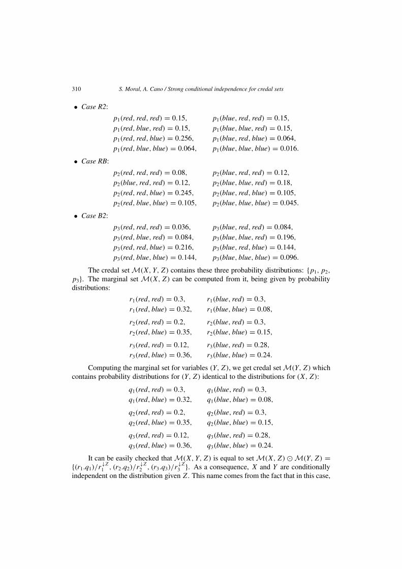
Example 7. Assume that we have three urns with 10 balls each. The first one, U1, has4 red, 4 blue, and 2 of unknown colour, the second, U2, has 3 red, 5 blue, and 2 unknown,and the third, U3, 6 red, 2 blue, and 2 of unknown colour. We also have that the ballswith unknown colour are blue or red and that they have the same composition of coloursin the three urns: either both are red (denoted by R2), or blue (denoted by B2) or one redand the other blue (denoted by RB).

We consider the following experiment: a ball is chosen at random from the firsturn, U1, (its colour is variable Z). Then an urn (U2 or U3) is chosen and two balls aredrawn at random and with replacement from it (variables X and Y represent the coloursof these two balls). If Z is red then both balls are from U2 and if Z is blue then the ballsare from U3.

Taking into account the different possibilities for the composition of the urns andconsidering that if this composition were known then X and Y are stochastically inde-pendent given Z, we have the following three probability distributions for (X, Y,Z):

310 S. Moral, A. Cano / Strong conditional independence for credal sets

• Case R2:

p1(red, red, red) = 0.15, p1(blue, red, red) = 0.15,p1(red, blue, red) = 0.15, p1(blue, blue, red) = 0.15,p1(red, red, blue) = 0.256, p1(blue, red, blue) = 0.064,p1(red, blue, blue) = 0.064, p1(blue, blue, blue) = 0.016.

• Case RB:

p2(red, red, red) = 0.08, p2(blue, red, red) = 0.12,p2(blue, red, red) = 0.12, p2(blue, blue, red) = 0.18,p2(red, red, blue) = 0.245, p2(blue, red, blue) = 0.105,p2(red, blue, blue) = 0.105, p2(blue, blue, blue) = 0.045.

• Case B2:

p3(red, red, red) = 0.036, p3(blue, red, red) = 0.084,p3(red, blue, red) = 0.084, p3(blue, blue, red) = 0.196,p3(red, red, blue) = 0.216, p3(blue, red, blue) = 0.144,p3(red, blue, blue) = 0.144, p3(blue, blue, blue) = 0.096.

The credal set M(X, Y,Z) contains these three probability distributions: {p1, p2,

p3}. The marginal set M(X,Z) can be computed from it, being given by probabilitydistributions:

r1(red, red) = 0.3, r1(blue, red) = 0.3,r1(red, blue) = 0.32, r1(blue, blue) = 0.08,

r2(red, red) = 0.2, r2(blue, red) = 0.3,r2(red, blue) = 0.35, r2(blue, blue) = 0.15,

r3(red, red) = 0.12, r3(blue, red) = 0.28,r3(red, blue) = 0.36, r3(blue, blue) = 0.24.

Computing the marginal set for variables (Y, Z), we get credal set M(Y, Z) whichcontains probability distributions for (Y, Z) identical to the distributions for (X,Z):

q1(red, red) = 0.3, q1(blue, red) = 0.3,q1(red, blue) = 0.32, q1(blue, blue) = 0.08,

q2(red, red) = 0.2, q2(blue, red) = 0.3,q2(red, blue) = 0.35, q2(blue, blue) = 0.15,

q3(red, red) = 0.12, q3(blue, red) = 0.28,q3(red, blue) = 0.36, q3(blue, blue) = 0.24.

It can be easily checked that M(X, Y,Z) is equal to set M(X,Z) � M(Y, Z) ={(r1.q1)/r

↓Z

1 , (r2.q2)/r↓Z

2 , (r3.q3)/r↓Z

3 }. As a consequence, X and Y are conditionallyindependent on the distribution given Z. This name comes from the fact that in this case,

S. Moral, A. Cano / Strong conditional independence for credal sets 311

given each one of the possible probability distributions we have classical probabilisticconditional independence. However, this definition is somewhat weak in the sense thatconditional independence for each one of the probabilities in a credal set not alwaysimplies the intuitive notion of conditional independence under the global credal set, inthe sense that new information about one variable does not change the information aboutother one, given that the exact value of a third variable is known.

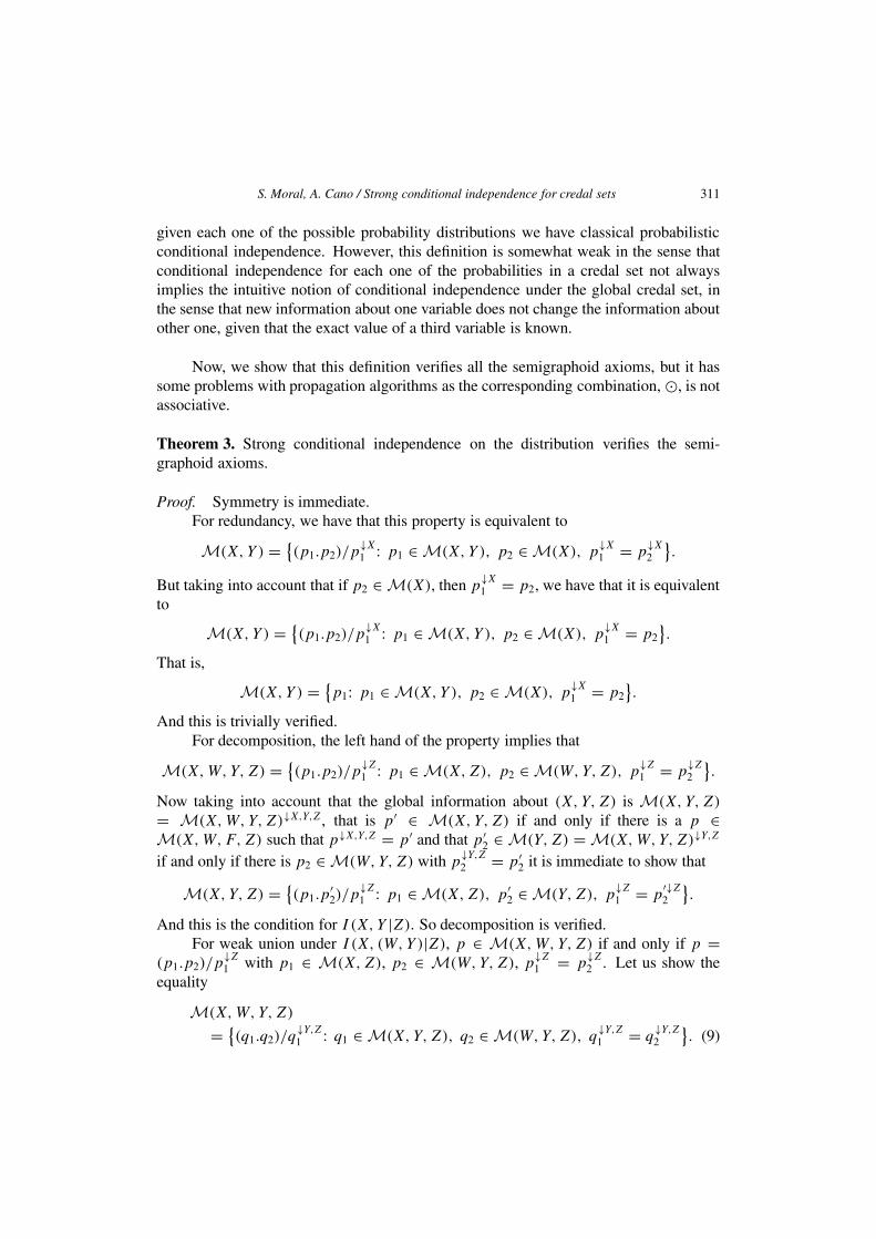
Now, we show that this definition verifies all the semigraphoid axioms, but it hassome problems with propagation algorithms as the corresponding combination, �, is notassociative.

Theorem 3. Strong conditional independence on the distribution verifies the semi-graphoid axioms.

Proof. Symmetry is immediate.For redundancy, we have that this property is equivalent to

M(X, Y ) = {(p1.p2)/p

↓X

1 : p1 ∈ M(X, Y ), p2 ∈ M(X), p↓X

1 = p↓X

2

}.

But taking into account that if p2 ∈ M(X), then p↓X

1 = p2, we have that it is equivalentto

M(X, Y ) = {(p1.p2)/p

↓X

1 : p1 ∈ M(X, Y ), p2 ∈ M(X), p↓X

1 = p2}.

That is,

M(X, Y ) = {p1: p1 ∈ M(X, Y ), p2 ∈ M(X), p

↓X

1 = p2}.

And this is trivially verified.For decomposition, the left hand of the property implies that

M(X,W, Y,Z) = {(p1.p2)/p

↓Z

1 : p1 ∈ M(X,Z), p2 ∈ M(W, Y,Z), p↓Z

1 = p↓Z

2

}.

Now taking into account that the global information about (X, Y,Z) is M(X, Y,Z)

= M(X,W, Y,Z)↓X,Y,Z, that is p′ ∈ M(X, Y,Z) if and only if there is a p ∈M(X,W,F,Z) such that p↓X,Y,Z = p′ and that p′

2 ∈ M(Y, Z) = M(X,W, Y,Z)↓Y,Z

if and only if there is p2 ∈ M(W, Y,Z) with p↓Y,Z

2 = p′2 it is immediate to show that

M(X, Y,Z) = {(p1.p

′2)/p

↓Z

1 : p1 ∈ M(X,Z), p′2 ∈ M(Y, Z), p

↓Z

1 = p′↓Z

2

}.

And this is the condition for I (X, Y |Z). So decomposition is verified.For weak union under I (X, (W, Y )|Z), p ∈ M(X,W, Y,Z) if and only if p =

(p1.p2)/p↓Z

1 with p1 ∈ M(X,Z), p2 ∈ M(W, Y,Z), p↓Z

1 = p↓Z

2 . Let us show theequality

M(X,W, Y,Z)

= {(q1.q2)/q

↓Y,Z

1 : q1 ∈ M(X, Y,Z), q2 ∈ M(W, Y,Z), q↓Y,Z

1 = q↓Y,Z

2

}. (9)

312 S. Moral, A. Cano / Strong conditional independence for credal sets

If p ∈ M(X,W, Y,Z), then p = (p1.p2)/p↓Z

1 with p1 ∈ M(X,Z), p2 ∈M(W, Y,Z), p

↓Z

1 = p↓Z

2 . Let us consider q1 = p↓X,Y,Z = ((p1.p2)/p↓Z

1 ) =(p1.p

↓Y,Z

2 )/p↓Z

1 ∈ M(X,W, Y,Z)↓X,Y,Z = M(X, Y,Z), q2 = p↓W,Y,Z = p2 ∈M(X,W, Y,Z)↓W,Y,Z = M(W, Y,Z). We can prove q

↓Y,Z

1 = q↓Y,Z

2 and (q1.q2)/q↓Y,Z

1

= (((p1.p↓Y,Z

2 )/p↓Z

1 ).p2)/p↓Y,Z

2 = (p1.p2)/p↓Z

1 = p. So p is in the right hand ofequation (9).

Reciprocally, if p can be decomposed as p = (q1.q2)/q↓Y,Z

1 with q1 ∈ M(X,

Y,Z), q2 ∈ M(W, Y,Z), q↓Y,Z

1 = q↓Y,Z

2 , then taking p1 = q↓X,Z

1 , p2 = q2 we canprove that p ∈ M(X,W, Y,Z). So the equality in (9) is verified and as a consequencethe weak union property.

For contraction, assume that

M(X, Y,Z)=M(X,Z) � M(Y, Z)

= {(p1.p2)/p

↓Z

1 : p1 ∈ M(X,Z), p2 ∈ M(Y, Z), p↓Z

1 = p↓Z

2

},

M(X,W, Y,Z) =M(X, Y,Z) � M(W, Y,Z)

= {(q1.q2)/q

↓Y,Z

1 : q1 ∈ M(X, Y,Z),

q2 ∈ M(W, Y,Z), q↓Y,Z

1 = q↓Y,Z

2

}.

We have to prove

M(X,W, Y,Z) =M(X,Z) � M(W, Y,Z)

= {(r1.r2)/r

↓Z

1 : r1 ∈ M(X,Z), r2 ∈ M(W, Y,Z), r↓Z

1 = r↓Z

2

}.

If p ∈ M(X,W, Y,Z) then p = (q1.q2)/q↓Y,Z

1 with q1 ∈ M(X, Y,Z), q2 ∈M(W, Y,Z), q↓Y,Z

1 = q↓Y,Z

2 .As q1 ∈ M(X, Y,Z) then q1 = (p1.p2)/p

↓Z

1 , with p1 ∈ M(X,Z), p2 ∈M(Y, Z), p↓Z

1 = p↓Z

2 .Making the substitution of q1 in the expression for p, and taking into account that

q↓Y,Z

1 = p2, we get p = (p1.p2.q2)/(p2.p↓Z

1 ) = (p1.q2)/p↓Z

1 . As q↓Y,Z

1 = q↓Y,Z

2 wehave that p

↓Z

1 = p↓Z

2 = q↓Z

1 = q↓Z

2 . As a consequence, p ∈ M(X,Z) � M(W,F,Z).Reciprocally, if p ∈ M(X,Z) � M(W, Y,Z) then p = (r1.r2)/r

↓Z

1 with r1 ∈M(X,Z), r2 ∈ M(W, Y,Z), r↓Z

1 = r↓Z

2 .For r1, we have that there is a distribution s1 ∈ M(X, Y,Z) such that s

↓X,Z

1 = r1.This s1 can be decomposed as (p1.p2)/p

↓Z

1 with p1 ∈ M(X,Z), p2 ∈ M(Y, Z), p↓Z

1 =p

↓Z

2 . We have,

r1 = s↓X,Z

1 = p1.

Let us consider s′1 = (p1.r

↓Y,Z

2 )/p↓Z

1 . We have that p↓Z

1 = r↓Z

2 , and, as a conse-quence, s′

1 ∈ M(X, Y,Z). Now, s′↓Y,Z

1 = r↓Y,Z

2 , and p = (s′1.r2)/s

′↓Y,Z

1 , and thereforep ∈ M(X, Y,Z) � M(W, Y,Z), which proves contraction. �

S. Moral, A. Cano / Strong conditional independence for credal sets 313

The main problem with this definition of conditional independence is that the cor-responding decomposition of the global credal set:

M(X, Y,Z) = M(X,Z) � M(Y, Z)

gives rise to a combination operator that is not associative and therefore does not sat-isfy the Shafer and Shenoy axioms. See Cano and Moral [3] for a counterexample ofthe associative property and how in some cases it continues making sense to apply thepropagation algorithms.

The second definition of strong conditional independence is based on the decom-position properties of the joint credal set and was considered in [3,4,15].

Under global set M(X, Y,Z), we say that X and Y are independent on decompo-sition given Z if and only if there are two valuations M1(X,Z) and M2(Y, Z) such thatM(X, Y,Z) = M1(X,Z) ⊗ M2(Y, Z).

Valuations M1(X,Z) and M2(Y, Z) are not always the marginal credal sets ofM(X, Y,Z) on the respective sets of variables. It is possible that M1 is a marginal setand M2 is a conditional credal set, or any other combination.

Again, this property coincides with strong independence when Z is null.

Theorem 4. If X and Y are conditional independent on decomposition given Z then

M(X, Y,Z) ⊆ M(X,Z) � M(Y, Z).

Proof. Assume M(X, Y,Z) = M1(X,Z) ⊗ M2(Y, Z).If p ∈ M(X, Y,Z), then we have that p = r1.r2 with r1 ∈ M1(X,Z) and r2 ∈

M(Y, Z). Let us consider p1 = p↓X,Z = r1.r↓Z

2 and p2 = p↓Y,Z = r↓Z

1 .r2. We havethat p↓Z

1 = p↓Z

2 = r↓Z

1 .r↓Z

2 , and p = (p1.p2)/p↓Z

1 , so p ∈ M(X,Z) � M(Y, Z). �

However, in previous theorem the equality is not always verified. Assume thatM(X, Y,Z) = M1(X,Z) ⊗ M2(Y, Z), then if r1, s1 ∈ M1(X, Y ) and r2, s2 ∈M2(Y, Z), with r

↓Z

1 .r↓Z

2 = s↓Z

1 .s↓Z

2 , then by taking p1 = r1.r↓Z

2 and p2 = s↓Z

1 .s2

we can prove that (p1.p2)/p↓Z

1 = (r1.r2.r↓Z

2 )/s↓Z

2 ∈ M(X,Z) � M(Y, Z), and this isnot always a point of M1(X,Z) ⊗ M2(Y, Z).

Example 8. Examples characterizing this situation and not verifying other more restric-tive definitions are not simple, as we have to describe a case in which none of the setsM1 and M2 contains all marginal information about Z.

We will consider that we have 6 urns with 10 balls each and the following compo-sition (Ui is the urn number i):

U1 U2 U3 U4 U5 U6

red 2 8 1 2 7 8blue 7 1 8 7 2 1unknown 1 1 1 1 1 1

314 S. Moral, A. Cano / Strong conditional independence for credal sets

Assume that we have the information that the colour of the unknown ball in urnsU1, U3, and U4 is the same, and the colour of the unknown ball in urns U2, U5, and U6 isalso the same.

We consider the following experiment: we randomly draw two balls from urns U1

and U2. Let Z1 and Z2 the colours of these balls. If Z1 is red, then we draw a ballfrom U3. If Z1 is blue, then a ball is drawn from urn U4. Let X the colour of this ball.Now, a forth ball, Y , is drawn with the following procedure: if Z1 and Z2 have the samecolour then the ball is chosen from urn U5 and if they have different colour then the ballis drawn from U6.

In these conditions, we have that X and Y are independent on decomposition given(Z1, Z2). In fact, the global convex set can be decomposed as a credal set involving X

and Z1 describing the relationships between the first and second ball, and a credal setinvolving Z1, Z2, and Y , describing the relationships between the probabilities of Z2 andthe conditional probabilities of Y given Z1 and Z2. The marginal credal set relating X

and Z1(M(X,Z1)) contains the following probability distributions:

p1(red, red) = 0.06, p1(blue, red) = 0.24,p1(red, blue) = 0.21, p1(blue, blue) = 0.49,

p2(red, red) = 0.02, p2(blue, red) = 0.18,p2(red, blue) = 0.16, p2(blue, blue) = 0.64.

We can also determine the conditional set M(Y, Z2|Z1) which is given by thefollowing conditional probabilities:

q1(red, red|red) = 0.72, q1(red, blue|red) = 0.09,q1(blue, red|red) = 0.18, q1(blue, blue|red) = 0.01,q1(red, red|blue) = 0.81, q1(red, blue|blue) = 0.08,q1(blue, red|blue) = 0.09, q1(blue, blue|blue) = 0.02,

q2(red, red|red) = 0.56, q2(red, blue|red) = 0.16,q2(blue, red|red) = 0.24, q2(blue, blue|red) = 0.04,q2(red, red|blue) = 0.64, q2(red, blue|blue) = 0.14,q2(blue, red|blue) = 0.16, q2(blue, blue|blue) = 0.06.

The global convex set about (X, Y,Z1, Z2) can be obtained by multiplyingM(X,Z1)⊗M(Y, Z2|Z1). So we have obtained a decomposition in which M1(X,Z1,

Z2) = M(X,Z1), M2(Y, Z1, Z2) = M(Y, Z2|Z1).Observe as a part of the marginal information about the possible probabilities of Z

(Z1) is directly related with X and other part (Z2) with Y . So, it is impossible to decom-pose the global set in the product of a marginal set involving X or Y and the conditioningvariable Z and other set containing the conditional information of the other variable, Y

or X, given Z, but no marginal information about this last variable.

S. Moral, A. Cano / Strong conditional independence for credal sets 315

The combination associated to this conditional independence, ⊗, does verify theShafer and Shenoy axioms [3,4] and so it is enough for propagation algorithms. Howeverthis definition does not verify all the semigraphoid axioms. It fails with contraction.

Theorem 5. Conditional independence on decomposition verifies the symmetry, redun-dancy, decomposition and weak union properties.

Proof. Symmetry is immediate by definition.For redundancy, consider the decomposition M(X, Y ) = M0(X) ⊗ M(X, Y ),

where M0(X) is the neutral valuation about X, i.e., the set containing the unit functionon UX (taking the value 1.0 for every x ∈ UX).

Decomposition is a consequence of the fact that if I (X, (W, Y )|Z) then

M(X,W, Y,Z) = M1(X,Z) ⊗ M2(W, Y,Z).

Then marginalizing over (X, Y,Z) and taking into account axiom 3 of Shafer andShenoy, we have

M(X,W, Y,Z)↓X,Y,Z = M1(X,Z) ⊗ M2(W, Y,Z)↓Y,Z

which implies that I (X, Y |Z).For weak union, we have the equality

M(X,W, Y,Z) = M1(X,Z) ⊗ M2(W, Y,Z).

Then, let M′1(X, Y,Z) = M1(X,Z) ⊗ M0(X, Y,Z) where again M0(X, Y,Z)

only contains the unit function on UX × UY × UZ. It is immediate that,

M(X,W, Y,Z) = M′1(X, Y,Z) ⊗ M2(W, Y,Z)

and, therefore, I (X,W |(Y, Z)). �

The problem with contraction is the following. If we have I (X, Y |Z) andI (X,W |(Y, Z)) then

M(X,W, Y,Z)↓X,Y,Z = M1(X,Z) ⊗ M2(Y, Z),

M(X,W, Y,Z) = M3(X, Y,Z) ⊗ M4(W, Y,Z).

If M3(X, Y,Z) were equal to M(X,W, Y,Z)↓X,Y,Z then we would obtain the de-sired independence I (X, (W, Y )|Z), but, in general, we have M(X,W, Y,Z)↓X,Y,Z =M3(X, Y,Z) ⊗ M4(W, Y,Z)↓Y,Z, and so there is no way of integrating both factoriza-tions.

Next definition is a stronger version of the previous definition. It requires that allthe marginal information about the conditioning variable Z is with one variable of theindependent variables. More precisely, we say that X is causally irrelevant to Y givenZ if and only if

M(X, Y,Z) = M(X,Z) ⊗ M(Y |Z) = {p.q: p ∈ M(X,Z), q ∈ M(Y |Z)

}(10)

where p.q(x, y, z) = p(x, z).q(y|z).

316 S. Moral, A. Cano / Strong conditional independence for credal sets

This is an asymmetric definition. It does not verify the redundancy property either.Redundancy is equivalent to

M(X, Y ) = M(X) ⊗ M(Y |X).

In section 2.4, it was said that, in general, there are several joint credal sets com-patible with a given marginal M(X) and a conditional credal set M(Y |X). The productM(X) ⊗ M(Y |X) is the least informative of all of them. So, it is not always the casethat we have this factorization. In [3] the presence of this factorization was related withthe presence of a causal relationship from X to Y , and this is the reason for the name wehave given to this conditional independence relationship.

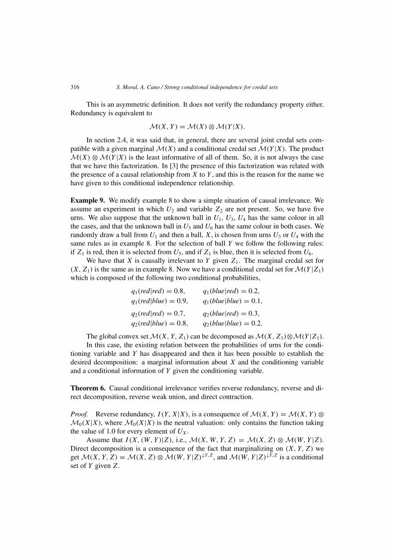
Example 9. We modify example 8 to show a simple situation of causal irrelevance. Weassume an experiment in which U2 and variable Z2 are not present. So, we have fiveurns. We also suppose that the unknown ball in U1, U3, U4 has the same colour in allthe cases, and that the unknown ball in U5 and U6 has the same colour in both cases. Werandomly draw a ball from U1 and then a ball, X, is chosen from urns U3 or U4 with thesame rules as in example 8. For the selection of ball Y we follow the following rules:if Z1 is red, then it is selected from U5, and if Z1 is blue, then it is selected from U6.

We have that X is causally irrelevant to Y given Z1. The marginal credal set for(X,Z1) is the same as in example 8. Now we have a conditional credal set for M(Y |Z1)

which is composed of the following two conditional probabilities,

q1(red|red) = 0.8, q1(blue|red) = 0.2,q1(red|blue) = 0.9, q1(blue|blue) = 0.1,

q2(red|red) = 0.7, q2(blue|red) = 0.3,q2(red|blue) = 0.8, q2(blue|blue) = 0.2.

The global convex set M(X, Y,Z1) can be decomposed as M(X,Z1)⊗M(Y |Z1).In this case, the existing relation between the probabilities of urns for the condi-

tioning variable and Y has disappeared and then it has been possible to establish thedesired decomposition: a marginal information about X and the conditioning variableand a conditional information of Y given the conditioning variable.

Theorem 6. Causal conditional irrelevance verifies reverse redundancy, reverse and di-rect decomposition, reverse weak union, and direct contraction.

Proof. Reverse redundancy, I (Y,X|X), is a consequence of M(X, Y ) = M(X, Y ) ⊗M0(X|X), where M0(X|X) is the neutral valuation: only contains the function takingthe value of 1.0 for every element of UX.

Assume that I (X, (W, Y )|Z), i.e., M(X,W, Y,Z) = M(X,Z) ⊗ M(W, Y |Z).Direct decomposition is a consequence of the fact that marginalizing on (X, Y,Z) weget M(X, Y,Z) = M(X,Z) ⊗ M(W, Y |Z)↓Y,Z, and M(W, Y |Z)↓Y,Z is a conditionalset of Y given Z.

S. Moral, A. Cano / Strong conditional independence for credal sets 317

Now, assume I ((W, Y ),X|Z), i.e., M(X,W, Y,Z) = M(W, Y,Z) ⊗ M(X|Z).Marginalizing on (X, Y,Z) we get M(X, Y,Z) = M(W, Y,Z)↓Y,Z ⊗ M(X|Z). Theindependence I (Y,X|Z) and therefore the reverse decomposition property is obtainedby taking into account that M(W, Y,Z)↓Y,Z is the marginal information about variables(Y, Z), M(Y, Z).

Reverse weak union can be obtained by defining M′(X|Y,Z) = M(X|Z) ⊗M0(X, Y,Z), where M0(X, Y,Z) only contains the unit function. This is a conditionalset and we get the decomposition: M(X,W, Y,Z) = M(W, Y,Z)⊗M′(X|Y,Z), withwhich I (W,X|Y,Z).

For contraction property, assume I (X, Y |Z) and I (X,W |Y,Z). Then, we have

M(X,W, Y,Z) = M(X, Y,Z) ⊗ M(W |Y,Z),

M(X, Y,Z) = M(X,Z) ⊗ M(Y |Z).

Making the substitution of M(X, Y,Z) in the first equality, we get

M(X,W, Y,Z) = M(X,Z) ⊗ (M(Y |Z) ⊗ M(W |Y,Z)

).

The independence I (X, (W, Y )|Z) is a consequence of the fact that (M(Y |Z) ⊗M(W |Y,Z)) is a conditional information of (W, Y ) given Z. �

Next definition of conditional strong independence is a slight modification of lastone. It only demands that the conditional information is conditional to the values: thatis we do not have any restriction for the possible probability distributions associated toeach value of the conditional variable. More formally, we say that X is elementwisecausally irrelevant to Y given Z if and only if

M(X, Y,Z) = M(X,Z) ⊗ Mv(Y |Z). (11)

Now, the only difference is that the conditional set has to be specified by giving acredal set associated with Y for each one of the possible values of variable Z. Mv(Y |Z)

is the set of all the conditional probability distributions which can be built by taking aconditional probability in each of the sets Mv(Y |Z = z).

As the associated combination is the same, we have that with this definition theShafer and Shenoy axioms are verified.

Example 10. A small modification of example 9 can produce a situation of element-wise causal conditional irrelevance. What we have to avoid is the existing restrictionbetween the colour of the unknown ball in urns U5 and U6. Now we assume that thecolour of this ball can be different or equal in both urns.

The conditional probabilities for Y given the value of Z1 are as follows:

• For Z1 = red:

p′1(red|red) = 0.8, p′

1(blue|red) = 0.2,p′

2(red|red) = 0.7, p′2(blue|red) = 0.3.

318 S. Moral, A. Cano / Strong conditional independence for credal sets

• For Z1 = blue:

q ′1(red|red) = 0.9, q ′

1(blue|red) = 0.1,q ′

2(red|blue) = 0.8, q ′2(blue|blue) = 0.2.

An element of Mv(Y |Z1) is any joint conditional distribution obtained by combin-ing an element of the conditional set for Z1 = red and other element from the conditionalset for Z1 = blue. In the previous example, only the combinations of p′

i with q ′j when

i = j were allowed, as the unknown ball had to have the same colour in both urns.Now, we have that M(X, Y,Z1) can be expressed as M(X,Z1) ⊗ Mv(Y |Z1),

where Mv(Y |Z1) is a set of conditional probability distributions which are determinedby giving the set of conditional probability distributions about Y for each one of thevalues of Z1.

This definition verifies the same properties as causal conditional irrelevance.

Theorem 7. Elementwise causal conditional irrelevance verifies reverse redundancy, re-verse and direct decomposition, reverse weak union, and direct contraction.

Proof. The proof is basically the same as in theorem 6. We only have to make someadditional specifications.

In the case of reverse redundancy, M0(X|X) is a credal set conditional to the valuesof X.

For direct decomposition, we have to point out that if Mv(W, Y |Z) is a conditionalcredal set to the values of Z, then Mv(W, Y |Z)↓Y,Z is a credal set of Y given the valuesof Z: Mv(Y |Z).

The proof for reverse decomposition is exactly the same.Reverse weak union is a consequence of the fact that if Mv(X|Z) is a credal set

about X conditional to the values of Z, then M′v(X|Y,Z) = Mv(X|Z)⊗M0(X, Y,Z),

is a conditional credal set conditional to the elements of Z.For contraction property we have to consider that if Mv(Y |Z) and Mv(W |Y,Z)

are conditional sets to the elements of Z and Y , Z, respectively, then (Mv(Y |Z) ⊗Mv(W |Y,Z)) is a conditional information of (W, Y ) conditional to the values of Z. �

7. Conclusions

In this paper we have shown four possible generalizations of the concept of strongunconditional independence to the case of conditional independence. Simple examplesare given for each one of the different extensions showing their different meanings. Ingeneral, the differences are based on the restrictions about the different probabilities inthe marginal or conditional credal sets. In all of them, the probabilities in the joint credalset verify the probabilistic conditional independence property.

The main question is: which is the most appropriate definition? In general, it willdepend of the concrete problem we are trying to represent. We can say that all of them are

S. Moral, A. Cano / Strong conditional independence for credal sets 319

associated to cases in which we have random experiments for which the probabilities areunknown and their applicability to situations of pure subjective assessments is doubtful.

The weak independence in the distribution looks more appropriate for the marginalproblem: in its simplest form, we are given the marginal information M(X,Z) andM(Y, Z) and we want to recover the joint set M(X, Y,Z). The application of the otherdefinitions is in some occasions unsuitable because the marginal problem under condi-tional independence on decomposition does not have always solution [15] and when ithas solution we can have several ones. As shown in theorem 4, the solution provided byconditional independence in the distribution is the least informative (natural extension)of them: so, finally, we always collapse to this definition of conditional independence.

As a basis to generalize Bayesian networks to the case of imprecise probabilities,we think that the most appropriate concept is the elementwise causal conditional irrel-evance. The conditional independence on decomposition is enough to develop localcomputation algorithms as the Shafer and Shenoy axioms are verified, but we think thatthe associated decompositions are difficult to find if other definitions are not applica-ble. Furthermore, in most of the cases the non-verification of the elementwise causalconditional irrelevance is due to the presence of restrictions between the probabilities indifferent credal sets, as in example 9 with the colour of the unknown balls in the two urnsfor the second drawn. In general, it is convenient to make explicit these restrictions byintroducing new variables in the problem explaining that restrictions (as the transparentvariables in [4]). Then, we obtain an elementwise causal conditional independence afterintroducing these variables in the conditional set. So, finally, there is not an importantloss of generality by using this more restrictive definition.

Finally, there is a last question relative to the independence represented by a di-rected acyclic graph with imprecise probabilities and the elementwise causal conditionalirrelevance. The d-separation criterion cannot be applied, because it represents a sym-metrical definition and elementwise causal irrelevance in non-symmetrical. We thinkthat this is not an important difficulty, as essentially directed acyclic graphs are non-symmetrical, and simply we have to change the criterion to a new one, appropriate to theproperties verified by this definition. In fact, this could increase the expressiveness ofdirected acyclic graphs, as we could discriminate between the direction of a link X → Y

or Y → X, depending on which redundancy relation I (X, Y |X) or I (Y,X|Y ) is verified.

Acknowledgements

We want to thank Peter Walley for discussions on this topic which have inspiredthis work. We are very grateful to Fabio G. Cozman, Romano Scozzafava, and twoanonymous reviewers for their insightful comments which have helped to improve thepaper. Anyway, all the expressed opinions here are to be considered as exclusive of theauthors. Most of the examples are based on examples in a paper by F. Cozman andP. Walley [13] for epistemic conditional irrelevance and independence.

320 S. Moral, A. Cano / Strong conditional independence for credal sets

References

[1] A. Cano, J.E. Cano and S. Moral, Convex sets of probabilities propagation by simulated annealing,in: Proceedings of the Fifth International Conference IPMU’94, Paris (1994) pp. 4–8.

[2] A. Cano and S. Moral, A review of propagation algorithms for imprecise probabilities, in: Proceedingsof the First International Symposium on Imprecise Probabilities and their Applications (ISIPTA’99),Ghent (1999) pp. 51–60.

[3] A. Cano and S. Moral, Algorithms for imprecise probabilities, in: Handbook of Defeasible and Un-certainty Management Systems, Vol. 5, Algorithms for Uncertainty and Defeasible Reasoning, eds.J. Kohlas and S. Moral (Kluwer, Dordrecht, 2000) pp. 369–420.

[4] J.E. Cano, S. Moral and J.F. Verdegay-López, Propagation of convex sets of probabilities in directedacyclic networks, in: Uncertainty in Intelligent Systems, eds. B. Bouchon-Meunier et al. (Elsevier,Amsterdam/New York, 1993) pp. 15–26.

[5] E. Castillo, J.M. Gutiérrez and A.S. Hadi, Expert Systems and Probabilistic Network Models(Springer, New York, 1997).

[6] G. Coletti and R. Scozzafava, Stochastic independence for upper and lower probabilities in a coherentsetting, in: Proceedings of Information Processing and Management of Uncertainty in Knowledge-Based Systems Conference (IPMU-2000), Vol. I (2000) pp. 341–348.

[7] I. Couso, S. Moral and P. Walley, A survey of concepts of independence for imprecise probabilities,Risk, Decision and Policy 5 (2000) 165–181.

[8] F.G. Cozman, Robustness analysis of Bayesian networks with local convex sets of distributions, in:Proceedings of the 13th Conference on Uncertainty in Artificial Intelligence, eds. D. Geiger andP.P. Shenoy (Morgan Kaufmann, San Mateo, CA, 1997) pp. 108–115.

[9] F.G. Cozman, Irrelevance and independence relations in quasi-Bayesian networks, in: Proceedings ofthe 14th Conference on Uncertainty in Artificial Intelligence, eds. G.F. Cooper and S. Moral (MorganKaufmann, San Mateo, CA, 1998) pp. 89–96.

[10] F.G. Cozman, Irrelevance and independence axioms in quasi-Bayesian theory, in: Proceedings of theFifth European Conference on Symbolic and Quantitative Approaches to Reasoning and Uncertainty(Ecsqaru’99), eds. A. Hunter and S. Parsons (Springer, Berlin, 1999) pp. 128–136.

[11] F.G. Cozman, Credal networks, Artificial Intelligence 120 (2000) 199–233.[12] F.G. Cozman, Separation properties of sets of probability measures, in: Proceedings of the 16th Con-

ference on Uncertainty in Artificial Intelligence, eds. C. Boutilier and M. Goldsmith (Morgan Kauf-mann, San Mateo, CA, 2000) pp. 107–115.

[13] F.G. Cozman and P. Walley, Graphoid properties of epistemic irrelevance and independence, in: Pro-ceedings of the Second International Symposium on Imprecise Probabilities and Their Applications(ISIPTA’01), eds. G. de Cooman, T.L. Fine and T. Seidenfeld (2001) pp. 112–121.

[14] A.P. Dawid, Conditional independence, in: Encyclopedia of Statistical Sciences, Update Vol. 2, eds.S. Kotz, C.B. Read and D.L. Banks (Wiley, New York, 1999) pp. 146–153.

[15] L.M. de Campos and S. Moral, Independence concepts for convex sets of probabilities, in: Proceed-ings of the 11th Conference on Uncertainty in Artificial Intelligence, eds. Ph. Besnard and S. Hanks(Morgan Kaufmann, San Mateo, CA, 1995) pp. 108–115.

[16] D. Dubois, S. Moral and H. Prade, Belief change rules in ordinal and numerical uncertainty theories,in: Handbook of Defeasible Reasoning and Uncertainty Management Systems, Vol. 3, Belief Change,eds. D. Dubois and H. Prade (Kluwer, Dordrecht, 1999) pp. 311–392.

[17] E. Fagiuoli and M. Zaffalon, 2u: an exact interval propagation algorithm for polytrees with binaryvariables, Artificial Intelligence 106 (1998) 77–107.

[18] K.W. Fertig and J.S. Breese, Interval influence diagrams, in: Uncertainty in Artificial Intelligence 5,eds. M. Henrion, R.D. Shacter, L.N. Kanal and J.F. Lemmer (North-Holland, Amsterdam, 1990)pp. 149–161.

[19] K.W. Fertig and J.S. Breese, Probability intervals over influence diagrams, IEEE Transactions onPattern Analysis and Machine Intelligence 15 (1993) 280–286.

S. Moral, A. Cano / Strong conditional independence for credal sets 321

[20] R.C. Jeffrey, The Logic of Decision, 2nd edn. (Univ. of Chicago Press, Chicago, 1983).[21] S. Moral, Epistemic irrelevance on sets of desirable gambles, in: Proceedings of the Second Interna-

tional Symposium on Imprecise Probabilities and their Applications (ISIPTA’01), eds. G. de Cooman,T.L. Fine and T. Seidenfeld (2001) pp. 247–254.

[22] S. Moral and N. Wilson, Revision rules for convex sets of probabilities, in: Mathematical Models forHandling Partial Knowledge in Artificial Intelligence, eds. G. Coletti, D. Dubois and R. Scozzafava(Plenum Press, 1995) pp. 113–128.

[23] J. Pearl, Probabilistic Reasoning with Intelligent Systems (Morgan Kaufman, San Mateo, CA, 1988).[24] G. Shafer and P.P. Shenoy, Local computation in hypertrees, Working Paper No. 201, School of Busi-

ness, University of Kansas, Lawrence (1988).[25] P.P. Shenoy and G. Shafer, Axioms for probability and belief-function propagation, in: Uncertainty in

Artificial Intelligence 4, eds. Shachter et al. (Elsevier, Amsterdam, 1990) pp. 169–198.[26] M. Studeny, Semigraphoids and structures of probabilistic conditional independence, Annals of Math-

ematics and Artificial Intelligence 21 (1997) 71–98.[27] B. Tessem, Interval probability propagation, International Journal of Approximate Reasoning 7 (1992)

95–120.[28] P. Vicig, Epistemic independence for imprecise probabilities, International Journal of Approximate

Reasoning 24 (2000) 235–250.[29] P. Walley, Statistical Reasoning with Imprecise Probabilities (Chapman and Hall, London, 1991).[30] P. Walley, Towards a unified theory of imprecise probability, International Journal of Approximate

Reasoning 24 (2000) 125–148.[31] N. Wilson and S. Moral, A logical view of probability, in: Proceedings of the Eleventh European

Conference on Artificial Intelligence (ECAI’94), ed. A. Cohn (Wiley, London, 1994) pp. 386–390.