Environmental Report Prepared in Support of 2015 Variance ...
700
Environmental Report Prepared in Support of 2015 Variance Request
-
Upload
khangminh22 -
Category
Documents
-
view
2 -
download
0
Transcript of Environmental Report Prepared in Support of 2015 Variance ...

Environmental Report Prepared in Support of 2015 Variance Request

Temporary Variance from Article 401 (Rule Curve)
Environmental Report
Pensacola Project
FERC Project No. 1494
July 30, 2015

This page intentionally left blank.

Rule Curve Temporary Variance Environmental Report
McMillen Jacobs Associates i July 2015
Table of Contents 1.0 Introduction........................................................................................................................................ 1
2.0 Project Description and Proposed Action ...................................................................................... 2
2.1 Project Description ................................................................................................................... 2
2.2 Proposed Action ....................................................................................................................... 4
2.3 No Action Alternative ............................................................................................................... 5 2.4 Consultation ............................................................................................................................. 5
2.5 Scope of Analysis .................................................................................................................... 5
2.5.1 Geographic Scope .............................................................................................................. 5
2.5.2 Temporal Scope .................................................................................................................. 6
2.6 General Setting ........................................................................................................................ 6
3.0 Flood Potential .................................................................................................................................. 8
3.1 Existing Conditions .................................................................................................................. 8
3.2 Potential Impacts ..................................................................................................................... 8
3.3 Proposed Mitigation ............................................................................................................... 11
4.0 Soils – Erosion and Turbidity......................................................................................................... 11
4.1 Existing Conditions ................................................................................................................ 11
4.2 Potential Impacts ................................................................................................................... 11 4.3 Proposed Mitigation ............................................................................................................... 11
5.0 Water Resources ............................................................................................................................. 12
5.1 Existing Conditions ................................................................................................................ 12
5.2 Potential Impacts ................................................................................................................... 12
5.3 Proposed Mitigation ............................................................................................................... 13
6.0 Water Quality ................................................................................................................................... 13
6.1 Existing Conditions ................................................................................................................ 13
6.2 Potential Impacts ................................................................................................................... 15
6.3 Proposed Mitigation ............................................................................................................... 16
7.0 Fish and Aquatic Resources .......................................................................................................... 16
7.1 Existing Conditions ................................................................................................................ 16 7.2 Potential Impacts ................................................................................................................... 18
7.3 Proposed Mitigation ............................................................................................................... 19

Rule Curve Temporary Variance Environmental Report
McMillen Jacobs Associates ii July 2015
8.0 Terrestrial Resources ..................................................................................................................... 19
8.1 Wildlife.................................................................................................................................... 19
8.1.1 Bald Eagle ......................................................................................................................... 19 8.1.2 Waterfowl .......................................................................................................................... 20
8.1.3 Terrestrial Game Species ................................................................................................. 20
8.2 Vegetation .............................................................................................................................. 20
8.2.1 Existing Conditions............................................................................................................ 20
8.2.2 Potential Impacts ............................................................................................................... 21
8.2.3 Proposed Mitigation .......................................................................................................... 21 8.3 Wetlands ................................................................................................................................ 21
8.3.1 Existing Conditions............................................................................................................ 21
8.3.2 Potential Impacts ............................................................................................................... 22
8.3.3 Proposed Mitigation .......................................................................................................... 23
9.0 Rare, Threatened, and Endangered Species ................................................................................ 23
9.1 Gray Bat ................................................................................................................................. 23 9.1.1 Existing Conditions............................................................................................................ 23
9.1.2 Potential Impacts ............................................................................................................... 23
9.1.3 Proposed Mitigation .......................................................................................................... 24
9.2 Ozark Cavefish ...................................................................................................................... 24
9.2.1 Existing Conditions............................................................................................................ 24
9.2.2 Potential Impacts ............................................................................................................... 24 9.2.3 Proposed Mitigation .......................................................................................................... 24
9.3 Neosho Madtom ..................................................................................................................... 24
9.3.1 Existing Conditions............................................................................................................ 24
9.3.2 Potential Impacts ............................................................................................................... 24
9.3.3 Proposed Mitigation .......................................................................................................... 25 9.4 Neosho Mucket ...................................................................................................................... 25
9.4.1 Existing Conditions............................................................................................................ 25
9.4.2 Potential Impacts ............................................................................................................... 25
9.4.3 Proposed Mitigation .......................................................................................................... 25
10.0 Recreation and Land Use ............................................................................................................... 26
10.1 Existing Conditions ................................................................................................................ 26 10.2 Potential Impacts ................................................................................................................... 27
10.3 Proposed Mitigation ............................................................................................................... 27
11.0 Cultural and Tribal Resources ....................................................................................................... 27
11.1 Existing Conditions ................................................................................................................ 27

Rule Curve Temporary Variance Environmental Report
McMillen Jacobs Associates iii July 2015
11.2 Potential Impacts ................................................................................................................... 28
11.3 Proposed Mitigation ............................................................................................................... 28
12.0 Socioeconomics .............................................................................................................................. 28
12.1 Existing Conditions ................................................................................................................ 28
12.2 Potential Impacts ................................................................................................................... 29
12.3 Proposed Mitigation ............................................................................................................... 30
13.0 Conclusions ..................................................................................................................................... 30
14.0 References ....................................................................................................................................... 31
List of Figures Figure 1. Existing Article 401 Rule Curve Target Elevations for FERC Project No. 1494, Grand Lake,
Oklahoma .............................................................................................................................................. 1
Figure 2. Pensacola Hydroelectric Project boundary and location .............................................................. 3
Figure 3. Proposed Modified Rule Curve ..................................................................................................... 4
Figure 4. Pensacola Hydroelectric Project land cover classes .................................................................... 7
Figure 5. Spring/Summer Inflows in 2015 along the Neosho River near Commerce, Oklahoma north of the City of Miami, and subsequent lake levels ...................................................................................... 8
Figure 6. a) Annual number of artificial habitat structures deployed on GRDA lakes; b) example of completed artificial habitat (“spider blocks”) to enhance the fishery and limit unauthorized shoreline brush and tree removal ........................................................................................................ 18
Figure 7. Summary of millet seeding program at Pensacola Dam Project (GRDA 2015) ......................... 22

Rule Curve Temporary Variance Environmental Report
McMillen Jacobs Associates 1 July 2015
1.0 Introduction The Grand River Dam Authority (GRDA) is the licensee of the Pensacola Hydroelectric Project (Project), Federal Energy Regulatory Commission (FERC) No. 1494. Article 401 of the Pensacola FERC license provides a target elevation for Grand Lake o’ the Cherokees (Grand Lake), the reservoir managed by GRDA pursuant to its license. In 1996, FERC issued an Order amending Article 401 to its present form, hereafter referred to as the existing rule curve (Figure 1).
Period Reservoir Elevation, feet (Pensacola Datum)
May 01 – May 31 Raise elevation from 742 to 744 feet
Jun 01 – Jul 31 Maintain elevation at 744 feet
Aug 01 – Aug 15 Lower elevation from 744 to 743 feet
Aug 16 – Aug 31 Lower elevation from 743 to 741 feet
Sep 01 – Oct 15 Maintain elevation at 741 feet
Oct 16 – Oct 31 Raise elevation from 741 to 742 feet
Nov 01 – Apr 30 Maintain elevation at 742 feet
Figure 1. Existing Article 401 Rule Curve Target Elevations for FERC Project No. 1494, Grand Lake, Oklahoma
GRDA is requesting a temporary variance for 2015 to the existing rule curve, as described more fully below, to (i) assist GRDA in managing the dissolved oxygen levels at the Project and at its other downstream projects, and (ii) increase public safety at Grand Lake.
The current rule curve is closely associated with the practice of seeding millet during the low elevation period pursuant to a mudflat seeding plan required by Article 404 of the Project license. However, the practice has achieved a poor success rate. Over the past 21 years, of the years in which millet seeding was documented, the success rate has only been 50%. Additionally, there were several occasions when millet was not seeded due to poor site conditions associated with lake levels. Millet was last seeded in 2011, and since that time the Technical Committee consisting of GRDA, the U.S. Fish and Wildlife Service (USFWS), the Oklahoma Department of Wildlife Conservation (ODWC), the Oklahoma Water Resources Board (OWRB), and the U.S. Army Corps of Engineers (USACE) has recommended terminating the seeding program and banking funds for use in more promising mitigation efforts, namely wetland development within the Neosho Management Area.
As currently provided for in the Fish and Wildlife Habitat Management Plan, as required by Article 411 of the Project license, GRDA has proposed to escalate the annual funding of the Technical Committee fund to include the amount previously utilized for millet seeding each year. Escalation of the $2.7 million fund will be utilized by GRDA’s water quality and wildlife management experts in conjunction with ODWC to develop a comprehensive hydrology management plan for the 1,538-acre Coal Creek unit. This will occur as soon as reasonably possible after completion of the hydrology restoration portion of the Coal Creek units owned and operated by GRDA in accordance with the Ducks Unlimited plan developed in 2012 (ODWC 2012b). GRDA, in cooperation with ODWC, will finalize a restoration plan for the Coal

Rule Curve Temporary Variance Environmental Report
McMillen Jacobs Associates 2 July 2015
Creek wetland development units and provide final construction drawings and related documents for the purpose of construction bidding and restoration work. Additionally, GRDA will work closely with ODWC biologists and personnel in the continued maintenance of the Coal Creek project and to establish permanent hunting blinds.
2.0 Project Description and Proposed Action 2.1 Project Description FERC issued a license for the 89.6-megawatt (MW) Project (FERC No. 1494) to GRDA on April 24, 1992.1 The Project is located on the Grand River in Craig, Delaware, Mayes, and Ottawa counties, Oklahoma (Figure 2). The Project consists of (a) a reinforced-concrete dam consisting of a 4,284-foot-long multiple arch section, an 861-foot-long spillway containing 21 Taintor gates, a 451-foot-long non-overflow gravity section, and two non-overflow abutments, comprising an overall length of 5,950 feet and maximum height of 147 feet; (b) an 886-foot-long reinforced-concrete gravity-type spillway section containing 21 Taintor gates and located about 1 mile east of the main dam; (c) a reservoir, known as Grand Lake, with a surface area of 46,500 acres and a storage capacity of 1,680,000 acre-feet at a normal maximum water surface elevation of 744 feet National Geodetic Vertical Datum (NGVD);2 (d) six 15-foot-diameter and one 3-foot-diameter steel penstocks supplying flow to six turbine-generators of 14.4-MW capacity each and one turbine-generator of 500-kilowatt (kW) capacity, located in a powerhouse immediately below the dam; (e) a tailrace about 300 feet wide and a spillway channel about 850 feet wide, both about 1.5 miles long; and (f) appurtenant facilities.
The 46,500-acre Grand Lake has 522 miles3 of shoreline and extends 66 miles upstream of the Pensacola Hydroelectric Project dam. The Project boundary is at the 750-foot Pensacola Datum (PD) contour line; thus, FERC regulates only a strip of land (of varying horizontal distance, depending on the steepness of the terrain) around the reservoir’s perimeter (Figure 2).4 GRDA estimates that the general horizontal distance between the reservoir shoreline and the Project boundary is 6 feet; however, this width varies around the reservoir. Most of the land surrounding Grand Lake is privately owned, and many areas along the shoreline have been developed with private homes, docks, condominiums, municipal and state parks, and commercial resorts and marinas.
1 The Pensacola Project was originally licensed in 1939 and relicensed in 1992. 59 FERC ¶ 62,073 (1992), Order Issuing New License (Major Project), April 24, 1992. 2 The reservoir’s normal maximum water surface elevation is locally recognized as 745 feet Pensacola Datum (PD). PD is 1.07 feet higher than NGVD, which is a national standard for measuring elevations above sea level. Reservoir levels discussed in this Environmental Report are in PD values unless otherwise stated. 3 The project license states there are 1,300 miles of shoreline around the Pensacola Project and, traditionally, GRDA has referenced 1,300 miles of shoreline for Grand Lake. However, for consistency in management and tracking of matters related to the SMP, GRDA has turned to a new GIS system, which has produced more accurate data indicating that the amount of shoreline within the project boundary is 522 miles. 4 The U.S. Army Corps of Engineers (Corps) manages flowage easement lands around Grand Lake from 750 feet PD up to the elevation of 760 feet PD in the upper reaches of the reservoir. See the Corps’ USACE comment letter, filed September 17, 2008.

Rule Curve Temporary Variance Environmental Report
McMillen Jacobs Associates 3 July 2015
Figure 2. Pensacola Hydroelectric Project boundary and location
Source: GIS data; GRDA 2015

Rule Curve Temporary Variance Environmental Report
McMillen Jacobs Associates 4 July 2015
2.2 Proposed Action As mentioned above, GRDA is requesting a temporary variance for this year to the existing rule curve to (i) assist GRDA in managing the dissolved oxygen levels at the Project and at its other downstream projects, and (ii) increase public safety at Grand Lake.
GRDA is requesting a variance consistent with a modified rule curve (Figure 3). The proposed modified rule curve would remain identical to the existing rule curve between November 1 and August 15. The only deviation would occur between August 16 and October 31, when the lake elevation under the proposed modified rule curve would be maintained at 743 feet between August 16 and September 15, lowered from 743 feet to 742 feet between September 16 and September 30, and maintained at 742 feet through the remainder of the modified period.
Figure 3. Proposed Modified Rule Curve
The requested temporary variance to the existing rule curve, which would allow a more gradual decrease in water surface elevation under the proposed modified rule curve, would allow GRDA to balance the many competing stakeholder interests at Grand Lake during the modified period from August 16 through October 31. The delayed drawdown of the lake from August 16 through September 30 and maintenance of 742 feet from October 1 through October 31 would allow GRDA to better manage dissolved oxygen levels during this time period and reduce the risk of vessel groundings.

Rule Curve Temporary Variance Environmental Report
McMillen Jacobs Associates 5 July 2015
Additionally, GRDA requests that it be allowed, in the event of drought, to deviate from the target elevations laid out in the proposed modified rule curve, and to release between 0.03 and 0.06 feet per day below the target elevation in order to comply with its Article 403 dissolved oxygen (DO) requirements. GRDA proposes an adaptive management plan designed to meet downstream DO requirements in the event local drought conditions occur in late summer and early fall of 2015, and requests this flexibility be included as part of the temporary variance. This adaptive management plan is designed to meet downstream DO requirements at the Pensacola and Markham-Ferry projects while maintaining lake elevations necessary for the reliable operation of the Salina Pumped Storage facility.
GRDA proposes releasing approximately 0.03 to 0.06 feet per day from Grand Lake, consistent with the plan implemented in 2012 (GRDA 2012). These daily release rates are designed to allow short-duration pulsed releases to simultaneously conserve water in the reservoir while improving downstream DO conditions below the Pensacola and Markham Ferry projects. These releases from Pensacola are expected to provide enough flow to maintain gate releases downstream at Markham-Ferry while maintaining an elevation of 619 feet mean sea level at Lake Hudson, which is necessary to meet general daily operations and North American Electric Reliability Corporation (NERC) reliability standards associated with the Salina Pumped Storage Project. Releases between 0.03 feet and 0.06 feet per day will primarily depend on local site conditions and will be implemented at such times that releases are deemed necessary to comply with Article 403.
While this request is not being made on the basis of drought, prudence would suggest implementing a buffer, such as the proposed modified rule curve, against such a late summer drought scenario.
GRDA will be requesting an amendment to its Pensacola license in order to achieve a permanent modification to the rule curve. For that reason, this temporary variance request is a 1-year measure aimed at bridging the gap between the current license and the license amendment.
2.3 No Action Alternative Under the No Action Alternative, GRDA’s request for temporary variance would not be approved and the Project reservoir would continue to be operated according to the existing rule curve.
2.4 Consultation GRDA initiated a 30-day consultation period with its resource agencies, the City of Miami, and state and federal officials and legislative representatives on April 28, 2015. GRDA has prepared a comment/response table, which is included as Attachment E to its temporary rule curve variance request.
2.5 Scope of Analysis
2.5.1 Geographic Scope
The geographic scope of this environmental analysis is focused on Project lands, waters, and resources in the immediate area of the reservoir’s shorelines that could be affected by the proposed temporary variance to the existing rule curve.

Rule Curve Temporary Variance Environmental Report
McMillen Jacobs Associates 6 July 2015
2.5.2 Temporal Scope
The temporal scope of this environmental analysis focuses on the period from August 15 through October 31, 2015.
2.6 General Setting The Project is located about 78 miles northeast of Tulsa on the Grand (Neosho) River in Craig, Delaware, Mayes, and Ottawa counties, Oklahoma. In addition to hydropower generation, Project lands and waters are used for flood control, water supply, recreation, and environmental resource protection (FERC, 1992).
Most land surrounding Grand Lake is privately owned and many areas along its shorelines have become highly developed with commercial resorts, private homes and condominiums, municipal and state parks, marinas, and private docks. Figure 4 shows developed and undeveloped land cover classes for lands adjoining the Project reservoir. As previously discussed, reservoir water levels fluctuate according to a rule curve established by Article 401, as amended, of the Project’s license, which requires that water levels be maintained between elevations 741 and 744 feet PD, in accordance with seasonal target levels.

Rule Curve Temporary Variance Environmental Report
McMillen Jacobs Associates 7 July 2015
Figure 4. Pensacola Hydroelectric Project land cover classes
(Source: GIS data; GRDA, 2015)

Rule Curve Temporary Variance Environmental Report
McMillen Jacobs Associates 8 July 2015
3.0 Flood Potential 3.1 Existing Conditions A literature review conducted as part of the Master’s thesis research published in 2014 by Alan Dennis, a graduate student at the University of Oklahoma, identified several sources of information regarding historical flooding on the Neosho River. The Chronicles of Oklahoma gives the historical account of the flood studies that were conducted on the river prior to construction of the Pensacola Dam (Holway, 1948). USACE published a report in 1998 investigating easement elevations in the Grand Lake area (USACE 1998). A judicial report filed in 1999 by Holly contains an investigation into the 1992–1995 floods in Miami (Holly Jr. 1999). Holly also published an article investigating the effects of a previously proposed power-pool change in 2004 (Holly Jr. 2004). Manders (2009) investigated the effects and mapped locations of the 2007 major flood on the Neosho River at Miami.
Currently, in the event of extreme rainfall scenarios, both GRDA and USACE control lake levels and discharge at Pensacola Dam. GRDA controls outflow from the dam until the lake stage reaches the top of the “power pool” at 745.0 feet PD (PD elevations are equal to North American Vertical Datum 1988 [NAVD88] elevations minus 1.40 feet [USGS 2014]). When the lake stage reaches 745.1 feet PD, USACE takes control of outflow in order to manage floodwater upstream and downstream throughout the region (GRDA 2013).
GRDA continuously monitors weather conditions for the Grand Lake region in preparation for the annual drawdown and low DO season. During the month of May, the Grand Lake watershed has experienced extraordinary amounts of rain. However, that situation could change quickly. Early summer rainfall, as in 2015, can quickly be replaced by mid and late summer dry conditions followed by gradually lowering reservoir levels (Figure 5). While this request is not being made on the basis of drought, prudence would suggest implementing a buffer, such as the proposed temporary variance to the rule curve, against such a scenario.
3.2 Potential Impacts In the past, debate over the rule curve has centered on the impact that Grand Lake, and its associated water surface elevation (WSE), has on upstream flooding, particularly in the area in and around the city of Miami, Oklahoma.
740.00
742.00
744.00
746.00
748.00
750.00
752.00
754.00
05000
100001500020000250003000035000400004500050000
4/1/15 5/1/15 6/1/15 7/1/15
Lake
Lev
el (P
D)
Disc
harg
e (c
fs)
Axis Title
Commerce Gage
Commerce Gage Lake Level
Figure 5. Spring/Summer Inflows in 2015 along the Neosho River near Commerce, Oklahoma north of the City of Miami,
and subsequent lake levels

Rule Curve Temporary Variance Environmental Report
McMillen Jacobs Associates 9 July 2015
The proposed temporary variance was the subject of a 2014 University of Oklahoma study, which measured the upstream flooding impact of such a modification of Article 401. In a study published in 2014, Alan Dennis (mentioned above), determined that the WSE on Grand Lake has a minimal impact on upstream flooding. The study was conducted as a thesis in partial fulfillment of Mr. Dennis’ Master’s degree requirements, and was overseen by Dr. Randall L. Kolar, Chair of the Hydrology Department and Director of the School of Civil Engineering and Environmental Science at the University of Oklahoma. The study looked specifically at the proposed modified rule curve as noted above, and its implication on flooding in areas upstream from Grand Lake. The study report was filed as part of the original 2015 temporary variance request dated May 28, 2015.
The study determined that the proposed rule curve adjustment would have a negligible impact on upstream flooding, and that stream flow is the major flood driver in Miami. It concluded that “the effect of the proposed rule curve adjustment has been shown to have less than a 0.20 ft effect on WSEs [Water Surface Elevations] in priority locations near Miami, OK.”5 It is important to note that this figure, the highest WSE effect—0.20 feet—occurs below flood stage, meaning that in such a circumstance the WSE never rises beyond the flowage easements owned by USACE. During conditions in which WSEs in Miami would exceed the flowage easements, the study finds that “the results of the proposed rule curve adjustment would not raise WSEs above flood stage more than 0.07 ft.”6 Per a request from United States Senator James Inhofe, the Hydrology and Hydraulics Branch of the Engineering and Construction Division of USACE, Tulsa District, performed a peer review of Mr. Dennis’ work. In a February 20, 2015 letter, Tulsa District Commander, Colonel Richard Pratt, stated that the University of Oklahoma study was of high quality and consistent with previous studies that were completed by the Tulsa District and Dr. Forrest Holly, and concurred with its findings.
As noted in the study report, the flood event used for calibration of the hydraulic model was the August 1 to October 7, 2009 (68-day) hydraulic event. The peak event of this storm occurred between September 9-16, 2009. For model validation, a historic streamflow event was considered relevant if it occurred within the months of August or September and the flood waters approached the USACE easement of 760.33 ft NAVD88. Three streamflow events from 2008 to present were used for model validation because time series datasets were available for this period in 15-minute increments [USGS, 2012]. Based on the excellent agreement of model to observations for these three validation events, it was determined that no further model calibration was necessary.
The table and figures included in section 4.3.3 of the study report represent the HEC-RAS model’s predicted effect of the proposed rule curve adjustment (i.e., a change in downstream boundary conditions) on upstream flooding in three priority locations described in the report:
Priority 1: The section of the Neosho River upstream of the confluence of the Neosho with Tar Creek that is adjacent to the city of Miami.
5 Dennis, Alan C. Floodplain Analysis of the Neosho River Associated with Proposed Rule Curve Modifications for Grand Lake O’ the Cherokees, 2014 at 122. 6 Dennis, Alan C. Floodplain Analysis of the Neosho River Associated with Proposed Rule Curve Modifications for Grand Lake O’ the Cherokees, 2014 at 133.

Rule Curve Temporary Variance Environmental Report
McMillen Jacobs Associates 10 July 2015
Priority 2: The section of Tar Creek upstream of its confluence with the Neosho River that is adjacent to the city of Miami.
Priority 3: The section of the Neosho River downstream of the confluence of the Neosho with Tar Creek to the confluence of the Neosho with Spring River (location of Twin Bridges).
Table 4.11 in the study report shows the maximum WSE calculated for each priority location under the proposed rule curve conditions. Table 4.12 is a summary of the effects of the proposed rule curve adjustment on WSEs in the priority sections for the streamflow scenarios shown.
An analysis of the results shown in Table 4.11 reveals that WSEs exceed flood stage near Riverview Park at a flow between the 10- and 25-year return period flows. Table 4.12 show that the proposed rule curve adjustment would cause between 0.04 and 0.20 ft of increased WSEs at the park under a flow between the 10- and 25-yr return interval. The difference of 0.20 is the maximum predicted increase in WSEs by the HEC-RAS model under the proposed rule curve adjustment for WSEs that exceed flood stage in the priority locations.
The Table 4.11 results also reveal that the WSEs in all the priority locations are affected much more by the streamflow magnitude than the downstream dam WSE. This is evidenced by the fact that as the return period increases, the WSE elevation profiles representing each rule curve scenario move closer together.
The WSE profiles, which represent the existing and proposed rule curve conditions, moving closer together represents a decreased effect of the proposed rule curve adjustment, as represented in Table 4.12. However, as the return period streamflow increases, the WSE profiles simultaneously rise to account for the increased streamflow volume, as shown in Table 4.11. This means that the downstream boundary condition at the dam has much less of an effect on WSEs in the priority locations than the streamflow magnitude.
It should be noted that while the USACE letter states that a “rise in stage during a 25-year flood event is limited to one quarter of a foot,” this only occurs in a hypothetical high-dam situation in which the WSE at Pensacola Dam is at 750 feet PD, which is a full 7 feet above what is being contemplated under the proposed modified rule curve. This is an extremely unlikely scenario—a WSE that historically occurs, on average, 7 days a year. Dennis’ conclusions point to the fact that when the WSE at Pensacola Dam is 743 feet PD—the elevation contemplated by the proposed modified rule curve—as opposed to 741 feet under the current rule curve, the impact on water surface elevation in the Miami area would be 0.05 feet.7
GRDA evaluated whether it could identify the potential incremental flooding effect on structures from the maximum modeled effect from the proposed rule curve adjustment above flood stage of 0.07 ft. GRDA has recent Light Detection and Ranging (LiDAR) coverage encompassing 348 square miles including Grand Lake and its tributaries. The accuracy of the LiDAR data as determined by the USGS Quality
7 Dennis, Alan C. Floodplain Analysis of the Neosho River Associated with Proposed Rule Curve Modifications for Grand Lake O’ the Cherokees, 2014 at 121, Table 4.17. Sensitivity analysis of changes in Manning’s n in Neosho River channel. Maximum change in WSE (ft) in Priority 1 section due to changing dam WSE from 741 to 743 ft PD shown. And at 123, Table 4.20 Sensitivity analysis of changes in Manning’s n in Neosho River floodplain. Maximum change in WSE (ft) in Priority 1 section due to changing dam WSE from 741 to 743 ft PD shown.

Rule Curve Temporary Variance Environmental Report
McMillen Jacobs Associates 11 July 2015
Assessment Report is shown as the Fundamental Vertical Accuracy (FVA) for this dataset is 0.5 US feet. Performing any analysis of change/effects in increments smaller than 0.5 US feet is not possible with this dataset, thus an analysis of incremental flooding of structures based on an increase in flood stage in the range of 0.07 ft is not possible given the available LiDAR data (USGS 2011).
One additional resource which can be used to observe the influence of streamflow and reservoir water surface elevation on flood levels in the Miami vicinity is the USGS interactive website http://ok.water.usgs.gov/projects/webmap/miami/. On this site it is possible to manipulate stage elevations at the Commerce gage near Miami as well as the elevations of Grand Lake as measured by the USGS gage at Pensacola dam. This allows the user to observe relative contributions of streamflow and reservoir elevations to flooding in the Miami area. These data are noted as provisional, subject to revision, on the website. Nonetheless it provides a graphical means of depicting contributing factors to flooding. The site also can depict the FEMA 100-year flood zone in the vicinity of Miami (USGS 2015).
3.3 Proposed Mitigation No mitigation actions with respect to flooding effects are recommended because the temporary change to the rule curve would not, based on the recent modeling, raise WSEs above flood stage more than 0.07 feet during conditions in which WSEs in Miami would exceed the USACE flowage easements.
4.0 Soils – Erosion and Turbidity 4.1 Existing Conditions The southern and eastern portions of the reservoir are generally lined by limestone bluffs and steep rocky beaches. The northern and western areas are typically more gradual slopes with mud substrates, silt deposits, and wetlands at the inlets and coves associated with numerous small tributaries (FERC 1996). The 1996 Environmental Assessment (EA) states that approximately 1,000 acres of mudflats subject to Article 411 are exposed between elevations 741 and 742 PD and are located in the northern portion of the reservoir from Twin Bridges located south of Miami to Sailboat bridge in Grove, Oklahoma. In the past, these mudflats were the target of a millet seeding program, but a lack of successful establishment of the millet has resulted in the cessation of seeding efforts since 2011 (GRDA 2015a).
4.2 Potential Impacts The proposed rule curve temporary variance would likely not affect soil erosion and turbidity in the southern and eastern portions of the reservoir due to the steep, rocky topography in that area. Additionally, the proposed rule curve temporary variance would most likely have a beneficial effect on the unvegetated mudflats because exposure during the drawdown period under the current rule curve leaves them subject to wind-induced soil erosion. Furthermore, the reduction in reservoir fluctuation from 3 feet under the current rule curve to 2 feet under the proposed rule curve temporary variance would reduce both soil erosion and erosion-induced turbidity.
4.3 Proposed Mitigation No mitigation actions for this resource are recommended because the temporary change to the rule curve would positively impact soil erosion and turbidity.

Rule Curve Temporary Variance Environmental Report
McMillen Jacobs Associates 12 July 2015
5.0 Water Resources 5.1 Existing Conditions The Grand Lake watershed comprises more than 10,000 square miles across Oklahoma, Missouri, Kansas, and Arkansas. The Project reservoir, Grand Lake, is the third largest lake in Oklahoma with a surface area of approximately 42,000 acres and a storage capacity of 1,500,000 acre-feet at the normal maximum water surface elevation of 745 feet PD (FERC 2009). Principal tributaries of Grand River are the Neosho, Spring, Cottonwood, and Elk rivers and Labette, Big Cabin, Spavinaw, and Lightning creeks (GRDA 2008).
The supply of raw water to local towns and cities dates back through years of GRDA history. Grand Lake’s raw water is processed by GRDA’s customers and then provided to residents for drinking purposes. At the present time, GRDA has approximately 25 wholesale customers using the waters of Grand Lake as their water supply. Grand Lake’s water is used by approximately 21,000 residential households and 500 commercial customers. In addition, GRDA issues yearly permits for domestic water use (GRDA 2015b).
GRDA’s commercial water customers hold 30- to 50-year contracts with GRDA for the raw water; these contracts allow customers to take a set amount of water each year. In March 2011, the Oklahoma Water Resources Board conducted a yield analysis study of Grand Lake and Lake Hudson (OWRB 2012). Under the current rule curve, when drought conditions occur, GRDA does not have a dependable yield of water to provide to its current customers without deviating from the rule curve (GRDA 2015b). Complicating the matter, in the past 5 years there has been an increase in requests for longer-term contracts from GRDA’s raw water customers, typically rural water districts, in order to borrow money to update their outdated or dilapidated water treatment plants. Lenders of these customers require a supply of water equal to the capacity of the upgraded or new plant. This requirement necessitates the customer contracting for additional water. Based upon the dependable yield study described above (OWRB 2012), strict adherence to the current rule curve puts these customers and GRDA at an impasse because GRDA cannot allocate the additional water requested while still maintaining the current rule curve. The customers thus cannot obtain financing to upgrade their plants (GRDA 2015b).
5.2 Potential Impacts Implementation of the proposed rule curve would have positive impacts on entities utilizing Grand Lake for water supply purposes. Customers of GRDA are constrained in financing options to upgrade their water systems under the current rule curve. Implementation of the proposed rule curve temporary variance would allow more water to be stored in the reservoir in late summer and the first part of autumn. This increased storage would make it easier for customers to demonstrate their ability to contract increased water supplies.
The proposed rule curve temporary variance would allow more water to be held in the reservoir during the hottest time of the summer months and early fall. It is during this time when water users’ consumption increases because the population around the lake increases. Additional residential use of the water for personal consumption increases for such uses as drinking water, household use (showers, toilets, kids running through sprinklers, etc.), and maintenance of landscaping. These increased uses put an

Rule Curve Temporary Variance Environmental Report
McMillen Jacobs Associates 13 July 2015
additional strain on the reservoir, which under the current rule curve is being drawn down to meet the license conditions (GRDA 2015b).
The additional water in the reservoir would allow more water for these uses described above, including those uses that occur due to increased seasonal population (see information on dissolved oxygen in Section 6.2). In extreme drought conditions, the proposed rule curve temporary variance would lessen the likelihood that a decision would be required regarding whether the DO standards are met or water consumption is rationed. Although water contracts contain provisions related to rationing in times of drought, rationing drinking water in times of drought is difficult for an entity to initiate (GRDA 2015b).
5.3 Proposed Mitigation Under the proposed rule curve temporary variance, more water would be available in the reservoir in late summer and early fall to meet competing beneficial uses. Thus, the effect on water resources of the proposed rule curve temporary variance would be positive, and no mitigation would be needed.
6.0 Water Quality 6.1 Existing Conditions The designated beneficial uses for Grand Lake include public and private water supply, fish and wildlife propagation as a warm water aquatic community, Class I irrigation, and primary body contact recreation (GRDA 2008, FERC 2009).
Certain portions of the Grand Lake watershed are listed as impaired on the state 303(d) lists for Oklahoma, Missouri, Kansas, and Arkansas for a number of distinct water quality criteria, including metals, fecal coliform bacteria (FC), pH, and low dissolved oxygen levels (DO). Grand Lake has also been recently listed on Oklahoma’s 303(d) list for organic enrichment/low DO and color (GRDA 2008).
GRDA has a Shoreline Management Plan (GRDA 2008) and lake-wide sanitation rules that protect public health and water quality. These rules:
1. Prohibit dumping of trash or cans and release of bilge water containing oil or grease;
2. Limit materials used in the process of cleaning the outer surfaces of vessels, disposal of sewage in the waters or on shore; and
3. Require vessels to have marine toilets that use a total retention system.
GRDA’s lake patrol is responsible for monitoring user compliance with these requirements and any violations are subject to GRDA enforcement (FERC 2009).Heavy metal contamination of lead, zinc, and cadmium exists in the lake and its sediments from acid mine drainage originating in the Neosho and Spring River watersheds (GRDA 2015b). Tar Creek is a 40 square mile superfund site that lies entirely within the watershed of Grand Lake (OWRB 2012). It had an 80 year history of mining for lead and zinc, ending in 1970. In 1979 acid mine drainage began discharging into Tar Creek, a tributary of the Grand River that flows into Grand Lake. While it is the main source of heavy metal contamination into Grand Lake, possible trace metal contamination may come from current, local surface mining (GRDA 2008).

Rule Curve Temporary Variance Environmental Report
McMillen Jacobs Associates 14 July 2015
Dredging can resuspend heavy metals from sediment into the water column, and thus dredging activities require a dredging permit and testing of metal levels in the sediment, before proposed dredging is allowed (FERC 2009).
In accordance with its license Article 403, GRDA has implemented a Dissolved Oxygen Monitoring and Enhancement Plan intended to achieve compliance with applicable water quality standards for the Project (GRDA 2015c). This license article calls for the licensee to file a plan to mitigate low DO conditions downstream of Pensacola Dam. The licensee has worked continuously since 1995 to provide the DO enhancements required in Article 401 (FERC 2015). DO levels are not to drop below level criterion defined by the Oklahoma Water Quality Standards as follows:
5 milligrams per liter (mg/L) DO water quality criterion for warm water aquatic communities during August;
4 mg/L allowable 1 mg/L excursion from DO currently allowed for fish and wildlife propagation; and
2 mg/L acute DO level.
The criterion listed above were used by the licensee to establish action limits for DO levels during 2012, 2013, and 2014.
As part of the DO mitigation plan, an adaptive management approach is recommended to address water quality concerns during the critical/low DO season. From 2007 to 2009, the Tennessee Valley Authority (TVA) under contract with GRDA made modifications to power generation structures to allow for increased infusion of DO while generating power. After extensive evaluation from 2012 through 2014, GRDA, in conjunction with the resource agencies, developed an adaptive mitigation plan that was analyzed for effectiveness, and the following conclusions were made:
Water releases for mitigation of low DO were determined to be effective at 6-hour intervals.
Three-hour mitigation releases are effective for times of extreme drought to alleviate DO problems in the tailrace of Pensacola Dam, but they are not as efficient or effective for the entire system as 6- to 8-hour releases.
After implementation of the plan in 2014, the area downstream from the tailrace is considered supporting for DO for the Fish and Wildlife Propagation support tests of the Oklahoma Water Quality Standards (OWQS), with less than 1% (0.72%) of the samples below DO criterion for any period, as well as zero samples below the 1 mg/L excursion limit or nuisance criterion levels of 2.0 mg/L.
On April 1, 2015, GRDA submitted to FERC a final Dissolved Oxygen Mitigation Plan for the Pensacola Hydroelectric Project. The implementation of interim measures over a number of years of adaptive management allowed for testing the proposed adaptive mitigation measures. Due to the success of these interim measures and high compliance with DO water quality requirements, the licensee has not significantly modified its approach to DO mitigation since 2011. The Dissolved Oxygen Monitoring and Enhancement Plan was approved by FERC on May 12, 2015 (FERC 2015).

Rule Curve Temporary Variance Environmental Report
McMillen Jacobs Associates 15 July 2015
Pensacola Dissolved Oxygen Monitoring and Enhancement Plan (DO Plan)
The DO Mitigation Plan recently accepted by FERC (FERC 2015) calls for three multi-parameter instruments with DO probes to be installed approximately 1,000 meters downstream from the tailrace of Pensacola Dam on the county road bridge (i.e., Langley Bridge). (These probes have already been installed during implementation of interim DO mitigation measures.) The probes are located near the right and left edges of water as well as midstream. These probes are used and will be used in the future to manage the Pensacola DO Mitigation Plan, with any individual probe on the bridge capable of activating a mitigation response. In an effort to facilitate the response process, an e-mail alert system is set up to notify both operators and other interested parties. When any individual probe indicates a DO mg/L reading below any of the action limits listed below, the software housed at the OWRB offices sends out an alarm e-mail to all necessary personnel at GRDA, FERC, ODWC, USFWS, and OWRB. This e-mail states the most recently measured DO concentration and states the appropriate response according to the Pensacola DO Plan. Once measurements rise above the action limit, the system sends out an alert notification indicating that target values have been achieved.
The action limits are set at the OWQS criterion of:
6 mg/L from October 16 through June 15
5 mg/L from June 16 through October 15
Once DO levels reach the action limit criteria according to any one of the Langley Bridge DO probes, one turbine begins running at 20% wicket gate (~320 cubic feet per second [cfs]) with full aeration. Once this turbine release has been initiated, it continues until the average DO value exceeds the criterion, but, depending on lake level conditions in Grand Lake and Lake Hudson, the release continues for at least 3 to 8 hours. A second action limit for turbine release is set at 4.0 mg/L. If the second action limit is reached, the first turbine will be upped to 25% wicket gate (~ 430 cfs) and this release at 430 cfs continues for a minimum of 2 hours. This operational plan for DO mitigation runs year-round.
6.2 Potential Impacts The proposed rule curve would not have any negative effects on water quality including heavy metal and bacteria contamination, and DO. Keeping water in later summer and early fall at a higher level would make erosion of mud banks and resuspension of heavy metals into the water less likely. Also, maintaining the water at a higher level may have a positive effect on achieving DO levels, especially during times of low inflow.
Holding waters higher from the middle of August until the beginning of November would provide the licensee with more stored water that would aid in DO mitigation efforts by ensuring sufficient water during the months of August and September for mitigation outflows (increased turbine releases as described above), as well as allow GRDA to balance competing interests associated with reservoir maintenance. While these increased turbine releases are effective for DO mitigation for normal years, the proposed rule curve temporary variance would allow GRDA to effectively manage mitigation efforts (through turbine releases) in drought conditions, as well as supply adequate water for downstream uses (GRDA 2015b).

Rule Curve Temporary Variance Environmental Report
McMillen Jacobs Associates 16 July 2015
6.3 Proposed Mitigation The proposed rule curve change would not deleteriously affect water quality, and therefore no additional mitigation, beyond that already implemented and approved, would be necessary.
7.0 Fish and Aquatic Resources 7.1 Existing Conditions Grand Lake lies at the eastern edge of the Prairie Plains and the western edge of the Ozark Plateau. It has a warm water fishery, and both Grand Lake and its tailrace are considered excellent for fishing (FERC 2009). Grand Lake is the top bass fishing lake in Oklahoma and one of the top bass fishing lakes in the nation, consistently attracting top national fishing tournaments such as the Bassmaster Classic (Bledsoe 2014). Recent electrofishing data from ODWC documented a robust largemouth bass fishery, despite no millet seeding in the last four years (GRDA 2015b).
In addition to largemouth bass, the lake is also a popular paddlefish fishery, and the most recent, readily available fish stocking records show that in 2013 Grand Lake was stocked with 2,052 paddlefish (ODWC 2014). Previous stocking efforts by ODWC included paddlefish and hybrid striped bass in 2012, paddlefish in 2011, hybrid striped bass in 2009 (ODWC 2013, ODWC 2012, ODWC 2010), and striped bass and hybrid striped bass in earlier years (FERC 2009).
The lake also has popular fisheries for smallmouth bass, white bass, black and white crappie, warmouth, longear sunfish, bluegill, and green sunfish. Many other fishes are found in the lake including threadfin and gizzard shad, flathead catfish, blue catfish, channel catfish, longnose gar, carp, carpsucker, smallmouth buffalo, logperch, emerald shiner, river shiner, red shiner, ghost shine, silverband shiner, bullhead minnow, blue sucker river redhorse, and river darter (GRDA 2004, FERC 1992).
Many fish become stressed under low dissolved oxygen (DO) levels. Low DO issues in Grand Lake typically occur from late June to the end of October, and the current quick draw-down from 744 PD to 741 PD in August, maintenance of 741 PD through September and rise to 742 PD by October stresses GRDA’s ability to protect fish and address downstream DO issues while maintaining the rule curve after September. Furthermore, because the design of the Pensacola Project necessitates release of hypolimnetic water (below the thermocline; which in summer has elevated nutrient concentrations), the current fast draw-down effectively loads downstream Lake Hudson with high nutrients in August that may lead to increased algal blooms and reduced water quality (GRDA 2015b). Algal blooms pose a significant risk to fisheries as they are often linked with further reduced DO due to demands of algal respiration.
In the original license, protection and management measures focused on protection of largemouth bass populations and bass habitat. The seasonal lowering of the water level under license Article 401 was intended to expose mudflats, promoting young of the year bass recruitment if millet seeded on those mudflats grew or if the mudflats naturally revegetated (GRDA 2015b).
Effects of lake level and vegetative habitat are complex, and thus, have complex effects on fisheries and surrounding wildlife. Years of experience in managing Grand Lake, and more recent fisheries research, have made it clear that the relationship of dense, shallow, aquatic vegetation (thought to provide safe

Rule Curve Temporary Variance Environmental Report
McMillen Jacobs Associates 17 July 2015
habitat for young fish) to juvenile bass recruitment, and recruitment of other species, is complicated. Removal of vegetation in large reservoirs has beneficial effects for channel catfish, white bass, and black crappie (all valuable fisheries) while maintaining the largemouth bass and striped bass fishery (Betolli et al. 1993). Betolli et al. (1993) also showed that bass can readily shift their prey base from bluegill and other centrarchids to threadfin shad when vegetation is removed. Although some vegetation can favor young of the year largemouth bass, dense vegetation can also be a hindrance for adults to detect and capture prey (GRDA 2015b).
GRDA’s annual Rush-4-Brush program is designed to rehabilitate aging reservoirs associated with its two hydropower projects in northeastern Oklahoma. This program encourages local individuals to volunteer as partners in conservation by helping GRDA staff construct and deploy artificial structures to enhance the fishery and protect shoreline habitat. The program is designed to promote habitat conservation by discouraging the common practice of removing trees and shrubs (i.e., shoreline habitat) to construct brush piles that are submerged as attractants for popular game species. This practice is a common strategy employed by fishermen to create habitat structure in the reservoir. However, this practice of removing shoreline trees and shrubs can have a detrimental effect on shoreline habitat, leading to increased erosion and negatively impacting water quality.
Deployment of the Rush-4-Brush artificial structures (see Figure 6) simulates natural brush piles and may provide critical rearing habitat for fry and fingerlings. Biofilm accumulation associated with these artificial structures attracts young of the year fish. The complex structure formed by multiple cinderblock deployments strategically grouped together provides critical habitat in the form of protective cover from predators. Because these structures act as effective attractants for crappie, bluegill, sunfish, and other game species, they are similarly attractive to local fishermen who are the foundation for the successful implementation of this voluntary Rush-4-Brush program. Because volunteers are allowed to place these structures in their favorite fishing spots, they generally receive less fishing pressure than publicly marked brush piles. They are thus likely to receive less fishing pressure and provide refuge for various fish species. Furthermore, this program simultaneously provides GRDA an opportunity to educate outdoor enthusiasts and conservationists alike by demonstrating sound management practices associated with shoreline conservation and habitat restoration of aging reservoirs. Over the last 9 years GRDA has deployed more than 13,500 “spider blocks,” no doubt reducing the number of trees and shrubs removed from the shoreline (Figure 6).
a)

Rule Curve Temporary Variance Environmental Report
McMillen Jacobs Associates 18 July 2015
b)
Figure 6. a) Annual number of artificial habitat structures deployed on GRDA lakes; b) example of
completed artificial habitat (“spider blocks”) to enhance the fishery and limit unauthorized shoreline brush and tree removal
7.2 Potential Impacts The proposed rule curve temporary variance to keep the water level higher in late summer and early fall would have a beneficial impact by giving GRDA more flexibility to protect fish from reduced DO in the Project tailrace, and in the downstream Lake Hudson at the Markham Ferry projects. GRDA’s ability to address low DO in the tailrace is dependent on having water to run through the turbines because it uses vacuum breaker bypass valves to inject air while running water through the turbines (GRDA 2015b). Thus, sufficient water needs to remain in the reservoir in late summer and early fall to allow water releases to raise DO levels, while maintaining enough water in the reservoir for other beneficial uses.
Some studies have suggested that the sediments in the riverine zone of the reservoir (i.e., in the Spring River) are highly contaminated with heavy metals. Although GRDA, ODWC, and USFWS have no evidence that these metals are toxic to aquatic invertebrates, and there is no strong evidence of
-
500
1,000
1,500
2,000
2,500
3,000
2007 2008 2009 2010 2011 2012 2013 2014 2015
Num
ber o
f Str
uctu
res
Number of Rush-4-Brush Structures Deployed Since 2007

Rule Curve Temporary Variance Environmental Report
McMillen Jacobs Associates 19 July 2015
bioaccumulation, drawing down the reservoir under the current rule curve further exposes fish and wildlife to potential contamination from heavy metals concentrated in a smaller volume of water, or from exposed sediments at the lower level (GRDA 2015b).
7.3 Proposed Mitigation GRDA has in place several plans that mitigate impacts to fish populations, including its Shoreline Management Plan that manages vegetative cover along the shoreline, positively affecting shallow water fish habitat (GRDA 2008). GRDA’s Rush 4 Brush program, which has been implemented since 2007 (described in Section 7.1), provides enhancement of fish habitat in the reservoir while helping to reduce removal of shoreline vegetation.
Millet seeding on exposed mudflats has not occurred since 2011, and the agencies participating in the Technical Committee have recommended alternative mitigation measures in lieu of millet seeding to mitigate habitat impacts.
In general, holding the level of the lake higher in late summer and early fall would benefit fish and aquatic life by making water releases to increase DO levels more feasible. Thus, effects of the proposed temporary rule curve change combined with current mitigation such as the Rush 4 Brush program would generally be positive for fish and aquatic life. No further mitigation would be needed.
8.0 Terrestrial Resources 8.1 Wildlife
8.1.1 Bald Eagle
8.1.1.1 Existing Conditions
Bald eagles are known to nest in the Grand Lake vicinity and hunt for fish in the reservoir. The 1985 license application reported a maximum count of 73 eagles in 1984, although the species was included on the federal list of threatened and endangered species at that time (GRDA 1985). Bald eagles were de-listed in 2007 (USFWS 2007).
8.1.1.2 Potential Impacts
Maintaining the reservoir pool level at a higher level during the period of the temporary rule curve variance is not expected to negatively affect the bald eagle. The lower turbidity expected during this time may improve the eagles’ hunting ability. Furthermore, there has been some indication that the nearshore sediments of Grand Lake may contain high concentrations of heavy metals (GRDA 2015b). Maintaining higher water levels between August 16 and October 31 may protect fish and wildlife and thus predatory species such as bald eagles from potential contamination with heavy metals.
8.1.1.3 Proposed Mitigation
No mitigation actions for this resource are recommended because the temporary change to the rule curve is not expected to negatively impact bald eagles.

Rule Curve Temporary Variance Environmental Report
McMillen Jacobs Associates 20 July 2015
8.1.2 Waterfowl
8.1.2.1 Existing Conditions
Waterfowl are present in the Grand Lake reservoir and are known to overwinter there. Previously, a millet seeding program required a drawdown of the reservoir by mid-August in order to provide 60 days of inundation-free growth required to produce mature seeds (FERC 1996). Mature millet was intended to provide nursery habitat for fish species as well as a food source for waterfowl. However, the millet seeding program was largely unsuccessful, and millet seeding has not been performed since 2011 in favor of banking program funds for wetland restoration efforts in the Neosho Management Area (GRDA 2015a).
8.1.2.2 Potential Impacts
The proposed temporary rule curve variance would prevent millet seeding in the Grand Lake reservoir in 2015. However, because the seeding program has been discontinued in recent years, the higher pool levels are not expected to have an impact on millet seeding efforts or waterfowl that may utilize the millet as a food source.
8.1.2.3 Proposed Mitigation
Proposed mitigation for waterfowl includes the continued banking of millet seeding funds for continued wetland habitat restoration in the Neosho Management Area.
8.1.3 Terrestrial Game Species
8.1.3.1 Existing Conditions
Recreational hunting is a common activity in the area surrounding Grand Lake. Game animals include rabbit, squirrel, quail, mourning dove, whitetail deer, ducks, and geese. Many of these species use the shoreline and wetland areas adjacent to Grand Lake for habitat and feeding (GRDA 1985).
8.1.3.2 Potential Impacts
Reducing the fluctuation of the Grand Lake pool level between August 16 and October 31 is expected to result in more stable vegetation and wetlands adjacent to the reservoir. The improved conditions of the vegetation and wetlands would benefit the terrestrial game species relying on these areas for habitat and food.
8.1.3.3 Proposed Mitigation
No mitigation is proposed for this resource because the proposed temporary rule curve variance is expected to positively impact terrestrial game species.
8.2 Vegetation
8.2.1 Existing Conditions
The 1996 EA reports that a number of types of terrestrial habitats occur in the Grand Lake vicinity. These include coniferous and deciduous upland forests, cropland, pasture, and grassland/savannah. Most of
Rule Curve Temporary Variance Environmental Report
McMillen Jacobs Associates 21 July 2015
these habitats (61,462 acres) occur above 755 feet PD, although a relatively small amount (7,902 acres) occurs below 755 feet PD (FERC 1996).
8.2.2 Potential Impacts
The Proposed Action would likely not impact upland vegetation because the vast majority of these habitats occur well above the pool level between 741 and 743 feet PD. Vegetation that does occur near 743 feet PD would likely benefit from less fluctuation of water levels and a more consistent pool level that would result from the temporary rule curve variance between August 16 and October 31.
8.2.3 Proposed Mitigation
No mitigation is proposed for this resource because the proposed action is not expected to negatively impact terrestrial vegetation.
8.3 Wetlands
8.3.1 Existing Conditions
The 1996 EA states that the elevation zones 735-742 and 742-745 contain a total of 7,274.6 acres of bottomland forests and 6,438 acres of wetlands, including emergent wetlands, scrub/shrub wetlands, mudflats, and ponded water (FERC 1996). Most of this vegetation occurs above 742 feet PD because current rule curve mandates pool levels at or above 742 feet PD during the majority of the year. The wetlands primarily exist in the northern and western areas of the reservoir, where silty soils and gently sloping banks provide favorable conditions for wetland vegetation (Figure 2). The emergent wetlands are primarily composed of herbaceous species such as smartweeds, sedges, and reed canary grass. Black willow, eastern cottonwood, and silver maple are also present. These wetlands support a wide variety of wildlife, including large and small mammals, birds, amphibians, and migratory birds (FERC 1996).
The 1992 FERC license order stipulated that GRDA perform millet seeding on a maximum of 1,000 acres in the mudflat portion of the reservoir annually for a minimum of 5 years (FERC 1992). The millet seeding program was a primary reason for the establishment of the current rule curve, particularly the reservoir drawdown to 741 feet PD, because millet seed requires a minimum of 60 days for germination prior to submergence (FERC 1996). However, monitoring of the millet seeding program has shown that the effort is largely unsuccessful and did not result in the establishment of substantial aquatic vegetation for fish nursery habitat and waterfowl food supply (Figure 7).

Rule Curve Temporary Variance Environmental Report
McMillen Jacobs Associates 22 July 2015
Figure 7. Summary of millet seeding program at Pensacola Dam Project (GRDA 2015)
As a result, millet seeding was last performed in 2011 (GRDA 2015a). In order to provide alternative mitigation for the Project, GRDA has banked millet seeding funds and formed a Technical Committee (comprised of GRDA, USFWS, ODWC, OWRB, and USACE). The Technical Committee has acquired more than 3,600 acres, known as the Neosho Management Area, at a cost of more than $7.1 million. This area is comprised mostly of grass, pasture, forests, wetlands, and pecan groves, and provides both wildlife habitat and public hunting opportunities (GRDA 2015b).
8.3.2 Potential Impacts
Wetland vegetation is generally dependent on water table stability (e.g., Ridolfi et al. 2006, Kingsford 2000). The Proposed Action of maintaining Grand Lake at a higher pool level between August 16 and October 31 would presumably have beneficial impacts on established wetland vegetation in the Project area by providing higher water levels in or near wetland vegetation areas. Additionally, the proposed temporary rule curve variance would result in less fluctuation of pool levels during the August 16 – October 31 timeframe, which would provide wetland vegetation with more consistent water and thus stabilize wetland vegetation.
The proposed temporary rule curve variance would not affect millet seeding in the Project area because this effort was previously discontinued and not planned to occur in 2015.
0
5
10
15
20
25
30
Success Failure No Seeding NoDocumentation
Perc
enta
ge o
ver l
ast 2
1 ye
ars
Rule Curve Temporary Variance Environmental Report
McMillen Jacobs Associates 23 July 2015
8.3.3 Proposed Mitigation
GRDA plans to continue the mitigation efforts of the Technical Committee and utilize an additional $2.7 million to purchase acreage to maximize wetland development in the Coal Creek area adjacent to the Project area. Furthermore, GRDA plans to hire a biologist who will develop a management plan for an additional 1,630 acres of property already owned by GRDA as required under Article 406. GRDA is developing a Memorandum of Agreement among GRDA, ODWC, and USFWS detailing agreed to mitigation actions that will be finalized in August 2015 (ODWC 2015b).
9.0 Rare, Threatened, and Endangered Species Several federally listed species occur at the Pensacola Project. The gray bat (Myotis grisescens), the Ozark cavefish (Amblyopsis rosae), the Neosho madtom (Noturus placidus), and the Neosho mucket (Lampsilis rafinesqueana) are all listed as endangered.
9.1 Gray Bat
9.1.1 Existing Conditions
The gray bat (Myotis grisescens) is an endangered species that is found in limestone karst areas of the southeast United States. The bats rely on flying aquatic and terrestrial insects along rivers or lakes for food, and females give birth to a single young in late May or early June. Gray bats are endangered primarily due to their reliance on a small number of caves to support their population. Over time, they have suffered habitat loss due to the flooding and submersion of many important caves. Gray bats live in caves year-round, although they migrate from caves along rivers in the summer to deep vertical caves in the winter (USFWS 1997).
Gray bats rely on two caves in the Grand Lake reservoir: Beaver Dam Cave and Twin Cave. Of these, Beaver Dam Cave is the only cave affected by pool levels. Beaver Dam Cave is a maternity colony for gray bats from March 15 through October 1. Inundation of the cave begins when the pool level reaches 746 feet PD and the cave entrance is completely blocked when the pool level reaches 751 feet PD (FERC 1996).
In 2008 and 2013, GRDA and The Nature Conservancy increased the size of two high passage areas near the entrance of Beaver Dam Cave. These high passages allow the bats to access the cave entrance during periods of high water (GRDA 2015b). GRDA conducts annual monitoring of gray bats and cave conditions, and the most recent report indicates that gray bat populations have been relatively constant for the past 25 years (Martin 2015).
9.1.2 Potential Impacts
No impacts to gray bats are expected as a result of the proposed rule curve temporary variance because the highest pool level during the period of the rule curve variance (743 feet PD) is well below the high water levels that impede the bats’ access to Beaver Dam Cave.

Rule Curve Temporary Variance Environmental Report
McMillen Jacobs Associates 24 July 2015
9.1.3 Proposed Mitigation
No mitigation for gray bats is recommended as a result of the Proposed Action because the alteration of the pool level from 741 to 743 feet PD is not expected to have an impact on gray bats.
9.2 Ozark Cavefish
9.2.1 Existing Conditions
The Ozark cavefish (Amblyopsis rosae), a federally threatened species, is a small fish (up to 2-½ inches long) with no eyes or pigmentation; it lives strictly in subterranean waters (Page and Brooks 1996). It feeds primarily on plankton and bat guano (FERC 2009), and lives in the shallow aquifer of the Springfield Plateau in the Ozark Highlands (USFWS 2015a, ODWC 2015a). This species is only seen in streams and ponds inside caves. They are known to occupy 41 caves, but 2 caves represent approximately 80% of the countable Ozark cavefish (USFWS 2011).
The Ozark cavefish is associated with Jailhouse Cave and Twin Cave found near Grand Lake (GRDA 2015b).
9.2.2 Potential Impacts
Jailhouse Cave is located downstream of the dam on Summerfield Creek and lies outside the area influenced by the rule curve; thus, any proposed changes to the rule curve would not have any adverse effect on Ozark cavefish occupying Jailhouse Cave. Twin Cave is located approximately 1 mile south of Grand Lake at an elevation (770 feet PD) well above the flood control pool of 757 feet PD. Thus, any proposed changes to the rule curve would have no adverse effect on the Ozark cavefish occupying Twin Cave (GRDA 2015b).
9.2.3 Proposed Mitigation
No mitigation for Ozark cavefish is recommended as a result of the Proposed Action because the alteration of the pool level from 741 to 743 feet PD is not expected to have an impact on Ozark cavefish.
9.3 Neosho Madtom
9.3.1 Existing Conditions
The Neosho madtom (Noturus placidus) is a small catfish (up to 3-¼ inch length) with four known populations (USFWS 2015b). It is federally listed as threatened. The Neosho madtom feeds at night on the bottom of rivers and streams. Its habitat is primarily swift-flowing riffles over gravel and runs in small to medium sized rivers (Page and Burr 1991). The Neosho madtom occurs in the Neosho River upstream of Grand Lake at a site periodically inundated by the USACE flood pool (GRDA 2004, FERC 2009). They do not inhabit waters of lakes or reservoirs with any regularity.
9.3.2 Potential Impacts
Analysis of stream flow data from the Neosho River, Spring River, Elk River, and Tar Creek suggests that the magnitude of stream flow along the Neosho River is the main driver of increased water surface

Rule Curve Temporary Variance Environmental Report
McMillen Jacobs Associates 25 July 2015
elevations upstream within the vicinity of the city of Miami (FERC 2009, Dennis 2014). Thus, the proposed change to the rule curve would not affect flooding of Neosho madtom habitat (GRDA 2015b).
USFWS has stated that it has concerns that changes in Grand Lake management that increase sedimentation in occupied areas could have an adverse impact on the Neosho madtom (FERC 2009). However, the change to the rule curve would tend to decrease sedimentation, and the Neosho madtom would only very rarely be found in water inundated by Grand Lake; thus, no impacts to the Neosho madtom are expected.
9.3.3 Proposed Mitigation
No mitigation for the Neosho madtom is recommended as a result of the Proposed Action because the alteration of the pool level from 741 to 743 feet PD is not expected to have an impact on the Neosho madtom.
9.4 Neosho Mucket
9.4.1 Existing Conditions
The Neosho mucket (Lampsilis rafinesqueana) is a freshwater mussel native to streams and rivers in four states including Oklahoma (USFWS 2015d). It was listed as endangered by USFWS in 2013, and Critical Habitat for the Neosho mucket was designated on April 29, 2015 (USFWS 2015c, 2015d).
They live in gravel and sand in shoals and near shore in rivers (USFWS 2015d). It is native to the Neosho, Spring, and Elk River systems in Kansas, northeast Oklahoma, northwest Arkansas, and southwest Missouri. The Neosho mucket spawns in May and broods eggs and larvae for a short time from May to July (Shiver 2002). At a microscopic larval stage (the glochidia stage) they are obligate parasites on fish gills.
9.4.2 Potential Impacts
The Neosho mucket does not occur in inundated areas. Because the proposed rule curve change would not inundate any new areas, rather simply maintains a level of inundation later in the year, it would not affect the Neosho mucket. Although Critical Habitat area NM2 in the Elk River (downstream in the Elk River to its confluence with Buffalo Creek in Delaware County, Oklahoma) is in the vicinity of Grand Lake, areas designated as Critical Habitat occur only in stream channels, not in areas inundated by lakes or reservoirs (USFWS 2015d). Thus, no impacts to the Neosho mucket from the proposed rule curve change are expected.
9.4.3 Proposed Mitigation
No mitigation for the Neosho mucket is recommended as a result of the Proposed Action because the alteration of the pool level from 741 to 743 feet PD is not expected to have an impact on the Neosho mucket.

Rule Curve Temporary Variance Environmental Report
McMillen Jacobs Associates 26 July 2015
10.0 Recreation and Land Use 10.1 Existing Conditions Grand Lake has both year-round and seasonal or vacation residents. Although recreationalists use Grand Lake year-round, the recreational boating season occurs from March until early November. The population increases on the three major holidays occurring during the peak boating season: Memorial Day weekend, 4th of July weekend, and Labor Day weekend (GRDA 2015b).
Grand Lake supports a high quality fishery for largemouth bass, striped bass, white bass, crappie, catfish, and paddlefish. For a comprehensive list of fish species in Grand Lake, see Section 7. Organizations and businesses sponsor an annual average of 117 major fishing tournaments at the lake each summer. Other popular recreation activities include recreational fishing, hunting (primarily for waterfowl), rafting, sailing, swimming, skiing, and pleasure boating (GRDA 2015d).
The State of Oklahoma and several municipalities provide public facilities around the lake and GRDA maintains a number of formal and informal access points. The lake currently supports 5 state parks and approximately 14 municipal parks. Collectively, these provide 22 public boat ramps while GRDA provides 5 boat ramps that allow access to Grand Lake. In comparison, an estimated 350 commercial and residential boat ramps are located on the lower half of the lake alone. Additional commercial outfits, such as marinas, support approximately 390 boat docks with more than 4,000 slips (GRDA 2015d). Extensive private development surrounds the Project. There are an estimated 4,400 private residences constructed within 500 feet of the Grand Lake shoreline (FERC 1996).
The FERC-approved Project boundary follows the 750-foot contour. Within the Project boundary there are three common land use/ownership types: commercial uses, residential uses, and municipal/public uses (GRDA 2008). As required by Standard License Article 5, GRDA believes it possesses “title in fee or the right to use in perpetuity all lands” within the approved Project boundary. Further, GRDA has acquired more than 3,600 acres at a cost of $7.1 million for fish and wildlife purposes where active management of this area will provide for quality hunting opportunities for the general public (ODWC 2015b).
Under the existing rule curve, lower lake levels during the drawdown period cause the areas around docks and boat launches to be shallower and less accessible. This increases the risk not only of boat groundings but also injury to swimmers jumping off docks and swim platforms (GRDA 2015b). In 2013–2014, nearly 80% of all recreation season groundings occurred while the lake was being drawn down or maintained at 741 feet (GRDA 2015a). Water hazards such as shallow bars, stumps, and rock outcrops also become a problem if water levels fluctuate during the recreation season. Muddy waters also detract from aesthetic and recreational values. Boaters, swimmers, skiers, and fishermen prefer clear, unpolluted water (GRDA 2004).
Low lake levels from August 16 through October 31 have contributed to a public safety hazard due to the high number of vessel groundings during this period. Before the drawdown, GRDA issues press releases and notices warning boaters of the dangers of changes in shoreline topography due to low water conditions. GRDA also works to include hazard areas in Grand Lake chart books. However, it is impossible to make the public aware of all areas of the lake that may be hazardous due to the drawdown.

Rule Curve Temporary Variance Environmental Report
McMillen Jacobs Associates 27 July 2015
Since 2013, GRDA Police have compiled a log of reports of vessels that have run aground on Grand Lake. The majority of incidents occurred when the lake was either being drawn down, being maintained at, or being raised from 741 feet. Of the 32 incidents of vessels going aground in 2013–2014, 24 occurred between August 16 and October 31. Of the 29 incidents that occurred during the high recreation season (May 1 – September 30), 23 occurred while the lake was being drawn down or maintained at 741 feet. Nearly 80% of all recreation season groundings occurred during this time, despite the fact that the 46 days making up the August 16 to September 30 timeframe are a full 61 days shorter than the May 1 to August 15 timeframe (when only 20% of the summer season groundings occurred).
When a vessel runs aground, its occupants become stranded until their vessel can be moved from the grounding. GRDA Police have responded to calls where this has occurred in unpopulated and less frequented areas, leaving the occupants stranded in the middle of the water, subject to the elements. Many times GRDA officers respond to assist boaters and are unable to reach them without running aground themselves, or must get in the water in order to move the occupants to safety. This becomes particularly dangerous in times of inclement weather, which typically brings with it very rough water, increasing the chances for injuries to both the officers and the public.
GRDA has received no reports of serious injuries or deaths as a result of vessel groundings related to the annual drawdown. However, groundings unrelated to the drawdown have resulted in injuries to boaters. The drawdown only exacerbates this problem, making conditions during which injuries might occur more likely. In its May 28, 2015 temporary variance filing, GRDA provided a list of the reported vessels running aground in 2013 and 2014.
10.2 Potential Impacts Maintaining a higher water level at or above 742 feet during the height of the recreation season would improve boating on the lake by making shallow areas along the shoreline more accessible. It would reduce the risk of groundings and striking submerged objects such as rocks, logs, or sandbars (FERC 1996). This is especially true for the more riverine section of the lake. The proposed rule curve temporary variance would maintain lake levels 2 feet higher at 743 feet between August 16 and September 15, which runs through Labor Day, a critical period for recreation and public safety at the lake.
10.3 Proposed Mitigation Before any drawdown, in accordance with current practice, GRDA would continue to issue press releases and notices warning boaters of the dangers of changes in shoreline topography and accessibility due to low water conditions. GRDA also works to include hazard areas in Grand Lake chart books. No additional mitigation actions for this resource are recommended because the temporary change to the rule curve would positively impact recreation.
11.0 Cultural and Tribal Resources 11.1 Existing Conditions Prehistoric peoples, Native Americans in the historic period, and Euro-American settlers in the modern period leading up to Oklahoma’s statehood have made extensive use of the Grand River Valley area as a place of both settlement and transportation. This pattern of use creates a high probability within the

Rule Curve Temporary Variance Environmental Report
McMillen Jacobs Associates 28 July 2015
project area for intact cultural resources dating from prehistoric eras, as well as the periods of early European contact, the nineteenth century, and the Civil War (GRDA, 2008).
In addition to the historical evidence for the likelihood of intact archaeological deposits, the topography of the region lends itself to the preservation of archaeological resources. While much of the land in the downstream portion of the project near the dam rises in steep bluffs from the shoreline, the upriver portions of Grand Lake features a shallow, more riverine topography that has the potential to contain intact archaeological resources. In addition, there are a number of tributaries that feed into Grand Lake that have a high potential for intact resources (GRDA, 2008).
Currently, there is risk of exposure of archeological or historical properties during drawdown and drought. Article 409 addresses GRDA’s responsibilities related to land-clearing or land-disturbing activities within the Project boundary and includes a provision for the protection of any unidentified archeological or historical properties exposed or discovered during Project operations. GRDA maintains data supplied by the State Historic Preservation Office (SHPO) and the Oklahoma Historical Society that identified potential and significant cultural resources sites. Approximately 50 cultural sites are known to exist within the Project area (GRDA 2008). Because of the sensitive nature of cultural or historic resources, their locations and significance are not public information.
11.2 Potential Impacts The proposed variance would create less disturbance of the land around the reservoir because more land would be inundated for a longer period of time throughout the year. The risk of greater exposure occurs during the drawdown period of the current rule curve. The proposed variance would prevent the areas below 742 feet from being exposed to natural and human disturbance (GRDA 2015b).
11.3 Proposed Mitigation License Article 409 provides for the protection of previously unidentified archeological or historical properties that are discovered during Project operations, maintenance, or permitted construction. No additional mitigation actions for this resource are recommended because the temporary change to the rule curve would positively impact cultural and tribal resources.
12.0 Socioeconomics 12.1 Existing Conditions Grand Lake is an economic engine for the State of Oklahoma and is expected to provide future economic potential to the state and region (Fallin 2015). The operations, construction, and positive externalities from GRDA result in significant economic impact for Oklahoma. Focusing only on operational impact, GRDA’s economic impact is projected in 2016 to be $541 million in economic activity; 2,870 jobs; and $150 million in real disposable income. In addition to employment and payroll at GRDA, tourism, quality of life, and relatively low cost power are important factors. Quality of life impacts on a region may be demonstrated by population growth. In the period (1940–2010) since completion of Pensacola Dam, the region around Grand Lake and Lake Hudson posted a 33% population growth rate, while Oklahoma’s non-metro counties experienced virtually no population growth (ODC 2015).

Rule Curve Temporary Variance Environmental Report
McMillen Jacobs Associates 29 July 2015
GRDA’s environmental stewardship includes flood mitigation activities as well as management of approximately 70,000 surface acres of lakes. USACE estimates that for every $1 spent on flood mitigation projects, the benefit to the economy is greater than $6 in avoided economic costs and damages. Additionally, the management of lakes in northeastern Oklahoma attracts tourism and generates higher property values. Without the proper management of resources, people from outside the state would not be as willing to spend their time and money in water recreation activities on the lakes (ODC 2015).
Construction of Grand Lake resulted in the development of a significant recreational resource in the region. Grand Lake supports numerous marinas and state recreation sites, all providing water-based access and attracting tourist dollars to the local economy. Local communities capitalize on this by promoting their individual businesses and attractions (GRDA 2008).
The popularity of water-based recreation for swimming, fishing, boating, skiing, and sailing has resulted in significant development around Grand Lake. Along with this specific water-based recreation industry has come a general leisure and retirement community development. All of this has resulted in general economic growth in real estate, goods, and services. The total development has been a product of both the recreation and aesthetic contribution from Grand Lake (GRDA 2004).
Under the current rule curve, lower lake levels during the drawdown period harm property owners and have a negative impact on the local economy. Marinas, waterfront restaurants, local businesses, and real estate values are severely disadvantaged by the mandated drawdown (GTAR 2015). Low water levels hamper these local businesses and prevent future growth (Fallin 2015).
For a detailed description of development and recreation around Grand Lake, see 10.
The city of Miami, Oklahoma lies in the Grand Lake watershed, on the banks of the Neosho River. Miami is located 15 river miles upstream of Twin Bridges State Park which is considered to be the northern boundary of the Grand Lake reservoir (OWRB 2009). Significant flooding has occurred at least 14 times in Miami since 1986 and many of these floods have produced serious economic hardships for Miami residents (Manders 2009). A July 2007 flood event forced 1,500-2,000 to evacuate and affected about 500 homes and 30 businesses (Dennis 2014). It has been suggested that the flooding threat upstream of Twin Bridges may be affected by Grand Lake reservoir levels and that maintenance of the current rule curve can protect the city of Miami from flooding during the drawdown period.
12.2 Potential Impacts The primary and direct socioeconomic impacts relate to recreation and tourist activities during the drawdown period. The alteration of the reservoir level from 741 to 743 feet would positively impact water-based recreation activities during the high recreation season including Labor Day weekend. As a result the associated seasonal businesses that are established to capitalize on the tourism industry are positively impacted by maintaining higher reservoir levels and attracting recreationalists through October. Longer term impacts might produce greater investment, improved real estate values, and economic growth.
As discussed in Section 3, a University of Oklahoma study indicates that under flood conditions on the Neosho River at Miami during the August 15 to September 15 time period, the two foot increase in water

Rule Curve Temporary Variance Environmental Report
McMillen Jacobs Associates 30 July 2015
surface elevation from 741 to 743 feet would have a negligible impact on upstream flooding, and that, instead, stream flow is the major flood driver in Miami (Dennis 2014). Thus, the economic impacts of the temporary rule curve variance are also considered negligible.
12.3 Proposed Mitigation No mitigation actions for this resource are recommended, since the temporary change to the rule curve would likely benefit the local economy. Furthermore, no mitigation actions with respect to flooding are recommended since there is no incremental flooding impact on socioeconomics due to this temporary change.
13.0 Conclusions GRDA is requesting a temporary variance to the existing reservoir rule curve for the period of August 15 through October 31, 2015. The purpose of the temporary variance request is to allow GRDA to effectively address low DO conditions and public safety concerns at the Project in the late summer and early fall timeframe.
The major impetus of the current rule curve implemented in 1996 was to provide a period of low water to allow for seeding of millet as a waterfowl and fisheries mitigation measure. After a significant multi-year effort, the Technical Committee comprised of key agencies concluded that the millet seeding program was not successful and recommended that funding for that program be banked and made available for alternative mitigation measures.
In response to feedback from the Commission, this Environmental Report was prepared to address potential resource effects of the requested temporary variance. As detailed in this report, the requested temporary variance would have either be neutral or have positive effects on potentially affected resources associated with the Project reservoir. A higher reservoir level from mid-August through the end of October would provide additional stored water for making releases to mitigate low DO conditions in the Project tailrace and would provide higher water surface elevations which would reduce the number of hazards to recreational boating that emerge during the required fall drawdown. In addition, higher water levels would be beneficial for adjoining wetland and upland vegetation, would reduce shoreline erosion, would reduce conditions for windblown dust, and would keep potential cultural resources from being exposed. No adverse effects on terrestrial resources or rare, threatened or endangered species have been identified.
GRDA has proposed to escalate the annual funding of the Technical Committee fund to include the amount previously utilized for millet seeding each year. The fund will be utilized by GRDA’s water quality and wildlife management experts in conjunction with ODWC to develop and implement a comprehensive hydrology management plan for the 1,538-acre Coal Creek unit. This will occur as soon as reasonably possible after completion of the hydrology restoration portion of the Coal Creek units owned and operated by GRDA in accordance with the Ducks Unlimited plan developed in 2012.
The potential for incrementally higher risk of flooding in the uppermost portions of the Project reservoir is the only negative concern that has been raised during consultation with stakeholders. The increase in

Rule Curve Temporary Variance Environmental Report
McMillen Jacobs Associates 31 July 2015
water surface elevations in the vicinity of the City of Miami has been calculated to be 0.2 ft with water levels remaining within the Corps of Engineers flood pool. During conditions in which WSEs in Miami would exceed the flowage easements, the study found that the results of the proposed rule curve adjustment would not raise WSEs above flood stage more than 0.07 ft. In addition, modeling shows that stream flow is the major flood driver in Miami and the flooding during high water events is related more directly to backwater effects from constrictions in the river, such as bridge abutments, than from water surface elevations at the dam. A significant risk of increased flooding due to the requested temporary variance is not supported based on the available modeling.
This temporary variance request would provide an interim measure of flexibility in 2015, while GRDA pursues activity to acquire a permanent license amendment to modify the Project’s rule curve for the balance of the current license.
14.0 References
Bettoli, P.W., M.J. Maceina, R.L. Noble, and R.K. Betsill. 1993. Response of a reservoir fish community to aquatic vegetation removal. North American Journal of Fisheries Management 13: 110-124.
Bledsoe, B. 2014. Top Places for Bass Fishing in Oklahoma. Game and Fish. April 4th
http://www.gameandfishmag.com/southwest/oklahoma/top-places-for-bass-fishing-in-oklahoma.
Dennis, A. 2014. Floodplain analysis of the Neosho River Associated with Proposed Rule Curve Modification for Grand Lake O’ the Cherokees. University of Oklahoma, Thesis, 161 pp.
FERC (Federal Energy Regulatory Commission). 1992. Order issuing new license and environmental assessment, Pensacola Project, FERC No. 1494-002 (59 FERC ¶ 63,231 at p. 63,231). Federal Energy Regulatory Commission, Washington, D.C. April 29, 1992 (Order); November 19, 1991 (EA).
FERC. 1996. Environmental Assessment. Application for Amendment of License to Modify Rule Curve. December 3, 1996.
FERC. 2009. Environmental Assessment. Application for Amendment of License. Shoreline Management Plan. August, 2009.
FERC. 2015. Order modifying and approving dissolved oxygen mitigation plan pursuant to article 403. FERC No. 1494-425 (151 FERC ¶ 62,098). Federal Energy Regulatory Commission, Washington, D.C. May 12, 2015 (Order).
Governor Fallin, Mary (Fallin). 2015. Letter: Support for Temporary Variance Request for Pensacola Project (No. 1494). From: Governor Mary Fallin, State of Oklahoma. To: Kimberly D. Bose, Secretary, Federal Energy Regulatory Commission. June 10, 2015.
GRDA (Grand River Dam Authority). 1985. Pensacola Dam Hydropower Project, Project No. 1494-002, New License Application. Vinita, Oklahoma. December 23, 1985.
GRDA. 2004. Pensacola Dam Hydropower Project, Project No. 1494-268. Application to Amend License. Filed January 29, 2004.

Rule Curve Temporary Variance Environmental Report
McMillen Jacobs Associates 32 July 2015
GRDA. 2008. Application for approval of the Pensacola Project, Shoreline Management Plan (FERC No. 1494-348). Filed on July 21, 2008.
GRDA. 2012. Letter: Emergency Drought Response. From: Daniel S. Sullivan, General Manager/CEO and Director of Investments, GRDA. To: Kimberly D. Bose, Secretary, Federal Energy Regulatory Commission. July 23, 2012.
GRDA. Lake Management: Flood Control. URL http://www.grda.com/ lake-management/flood-control/, 2013.
GRDA. 2015a. Pensacola Dam Hydropower Project, Project No. 1494-002. Request for Temporary Variance from Article 401 (Rule Curve). Vinita, Oklahoma. May 28, 2015.
GRDA. 2015b. Draft Initial Consultation Document. Pensacola Project No. 1494. Non-Capacity License Amendment. July 2, 2015.
GRDA. 2015c. Letter: Order Modifying and Approving 2014 Dissolved Oxygen Mitigation Plan (1494-336). From: Darrell E. Townsend II, Ph.D. Assistant General Manager, Ecosystems and Lake Management. To: Kimberly D. Bose, Secretary, Federal Energy Regulatory Commission.
GRDA. 2015d. Pensacola Hydroelectric Project, FERC No. 1494. Public Recreation Management Plan Monitoring Report. April 1, 2015.
GTAR (Greater Tulsa Association of Realtors). 2015. Letter: Support for Temporary Variance from Article 401 (Rule Curve). From: Mike Craddock, President, Greater Tulsa Association of Realtors. To: Kimberly D. Bose, Secretary, Federal Energy Regulatory Commission. Filed June 1, 2015.
Holly Jr., F. M., editor. Referee Report: Dalrymple, et al v. GRDA, number Case CJ 94-444, February 1999. District Court of Ottawa County, Oklahoma.
Holly Jr., F. Analysis of Effect of Grand Lake Power-Pool Elevations on Neosho River Levels During a Major flood. Prepared for: Robert Sullivan, AGM of Risk Management and Regulatory Compliance, GRDA, 2004. Holway, W. Dams on the Grand River. URLhttp://digital.library.okstate.edu/Chronicles/v026/v026p329.pdf, 1948.
Kingsford, Richard Tennant. 2000. Ecological impacts of dams, water diversions and river management on floodplain wetlands in Australia. Austral Ecology 25(2): 109-127.
Manders, G. Mapping of the July 2007 Miami, Oklahoma Flood. Research project, Emporia State University, May 2009.
Martin, Keith W. 2015. Monitoring Patterns and Use by Gray Bat Populations in Caves DL-2 and DL-91 in Delaware County, Oklahoma. Annual Report for Article 405: Gray Bat Compliance Plan of the Pensacola Project (1494-374).
ODC (Oklahoma Department of Commerce). Research and Economic Analysis. Chiappe, Samokhvalova & Sappleton. Economic Impact of the Grand River Dam Authority. March 2015.
ODWC (Oklahoma Department of Wildlife Conservation). 2010. Angler’s Guide. Outdoor Oklahoma 2010. Available at: http://wildlifedepartment.com/facts_maps/archives/2010anglersguide.pdf. Accessed on July 17, 2015.

Rule Curve Temporary Variance Environmental Report
McMillen Jacobs Associates 33 July 2015
ODWC. 2012a. Public Stocking Report. Fisheries Division. 2011. Available at: http://www.wildlifedepartment.com/fishing/survey/2011_stocking_report.pdf. Accessed on July 17, 2015.
ODWC. 2012b. Neosho Bottoms Restoration Plan Volumes 1 and 2. Ducks Unlimited, Inc. Southern Regional Office. August 23, 2012.
ODWC. 2013. Public Stocking Report. Fisheries Division. 2012. Available at: http://www.wildlifedepartment.com/fishing/survey/2012_stocking_report.pdf. Accessed on July 17, 2015.
ODWC. 2014. Public Stocking Report. Fisheries Division. 2013. Available at: http://www.wildlifedepartment.com/fishing/survey/2013_stocking_report.pdf. Accessed on July 12, 2015.
ODWC. 2015a. http://www.wildlifedepartment.com/wildlifemgmt/endangered/cavefish.htm. Accessed on July 9, 2015.
ODWC 2015b. Letter: Support for Temporary Rule Curve Variance. From: Richard Hatcher, Director, ODWC. To: Kimberly D. Bose, Secretary, Federal Energy Regulatory Commission.
OWRB (Oklahoma Water Resources Board). 2009. Hydrographic Survey of Grand Lake. OWRB, Oklahoma City. Accessed July 12, 2015 at: https://www.owrb.ok.gov/studies/reports/reports.php.
OWRB. 2012. Grand Watershed Planning Report. Versions 1.1. OWRB, Oklahoma City. Accessed July 12, 2015 at: https://www.owrb.ok.gov/supply/ocwp/pdf_ocwp/WaterPlanUpdate/regionalreports/OCWP_Grand_Region_Report.pdf.
Page, L.M., and B.M. Burr. 1991. A Field Guide to Freshwater Fishes. Houghton Mifflin Company: New York. Peterson Field Guides.
Ridolfi, Luca, Paolo D’Odorico, and Francesco Laio. 2006. Effect of vegetation-water table feedbacks on the sability and resilience of plant ecosystems. Water Resources Research, 42(1).
Shiver, M.A. 2002. Reproduction and propagation of the Neosho mucket, Lampsilis rafinesqueana. Thesis, Southwest Missouri State University.
USACE. Hydraulic Analysis: Grand Lake Real Estate Adequacy Study. Technical report, USACE, 1998.
USFWS. 1997. Fact sheet Gray bat. Accessed at: http://www.fws.gov/midwest/endangered/mammals/grbat_fc.html on July 27, 2015.
USFWS (U.S. Fish and Wildlife Service). 2007. Bald Eagle Fact Sheet: Natural History, Ecology, and History of Recovery. http://www.fws.gov/midwest/eagle/recovery/biologue.html.
USFWS. 2011. Ozark cavefish (Amblyopsis rosae Eigenmann 1898). 5-year review: summary and evaluation. USFWS, Arkansas Ecological Services Field Office, Conway, Arkansas.
USFWS. 2015a. Fact sheet Ozark cavefish. Accessed at: http://www.fws.gov/midwest/endangered/fishes/ozkcf_fc.html on July 9, 2015.

Rule Curve Temporary Variance Environmental Report
McMillen Jacobs Associates 34 July 2015
USFWS. 2015b. Endangered Species page Neosho madtom. Accessed at: http://www.fws.gov/endangered/map/ESA_success_stories/ks/ks_story2/index.html on July 9, 2015.
USFWS. 2015c. Fish and Wildlife Service Designates Critical Habitat for Two Freshwater Mussels in 12 States. http://www.fws.gov/midwest/news/780.html. Accessed July 9, 2015.
USFWS. 2015d. Neosho mucket. http://www.fws.gov/southeast/species/invertebrate/neosho_mucket.html. United States Geological Survey (USGS). About Vertical Datums. URL http://ok.water.usgs.gov/projects/
webmap/miami/datum.htm, 2014.
United States Geological Survey (USGS). 2015. Neosho River, Ottawa County, Okla.: Provisional Inundation Areas (Subject to Revision). Web Mapping Application available online at: http://ok.water.usgs.gov/projects/webmap/miami/. Accessed July 30, 2015.

Generation Analysis Prepared in Support of 2015 Variance Request

Memorandum DATE: July 24, 2015 TO: Darrell Townsend SUBJECT: Pensacola Dam- FERC Project 1494-OK GRDA Request for Rule Curve Temporary Variance
Generation Analysis Requested in FERC June 26, 2015 Letter Background The Federal Energy Regulatory Commission (FERC) reviewed Grand River Dam Authority’s (GRDA) May 28, 2015 application for a temporary variance from the fall drawdown requirements of the License’s Article 401 reservoir elevation rule curve at Pensacola Dam. That review requested a number of additional items including an analysis on the effects on generation that would result from the requested Grand Lake Reservoir level changes. This memorandum provides such analyses. Assumptions The fall season drawdown from the summer recreation pool level, Elevation 744 Pensacola Local Datum (PD), of Grand Lake begins on August 1. The seasonal drawdown begins August 1, however the requested change to the rule curve affects only the period from August 15 through October 31as the period between August 1 and August 15 is the same for both the Article 401 Rule Curve and the proposed variance. The change proposed eliminates the reduction of the pool level to Elevation 741PD by stopping the lowering of the pool at Elevation 743 PD on August 15 instead of continuing down Elevation 741 PD. On September 15 the lake level proposed would lower the pool to Elevation 742 PD on October 1, a month in advance of the Article 401 curve. Based on the revisions the differences in effect to average annual generation would be from the period of August 15 to November 1.
A change in the lake elevations will not have an effect on precipitation based inflow and minimal effect on evaporative losses. Holding the reservoir at the recreational pool elevation proposed will affect the timing of the generation from changes in the reservoir storage retained instead of generated and refilled. As a comparison of this effect, the study considers historic generation over a period inclusive of drought and higher flows to develop an average daily generation and compares that to changes that would result from the storage capacity to not lowering the reservoir to Elevation 741PD, as shown on Figure 1.
The source data for the study utilizes historic generation flow for the study period of August 15 to October 31 over the available daily generation record from 2006 to 2014. The 2006 to 2014 record includes 9 years of data with 4 being years of significant draught and two moderately significant draught years.

July 24, 2015 Dr. Darrell Townsend Pensacola Rule Curve Variance Request Generation Analysis Page 2 The Rule Curve revisions proposed as shown on Figure 1 are subdivided to staged flow changes and for convenience of the study into Phases 1 through 6, as follows:
Phase 1 August 1 through August 15 Phase 2 August 16 through August 31 Phase 3 September 1 through September 14 Phase 4 September 15 through September 30 Phase 5 October 1 through October 16 Phase 6 October 17 through October 31
Changes in lake level and associated flow for the phases were calculated utilizing an internally developed web based application prepared by the GRDA Operations Group. The App is utilized during our operations to predict daily generation and releases given expected and observed inflows. The application utilizes reservoir stage-storage values as depicted in in Figures 3a through 3c and the generator rating curves to predict generation based on flow, elevation and duration. Screen shots of the input and output screens for both the Pensacola and Kerr Dams are shown in Figures 2A through 2D. The change in elevation over the duration of each Phase was initially calculated on a daily basis and then compared to the overall phase duration. Based on that review it was determined the overall Phase change predicated the same change in generation as the daily. Given that finding, the values utilized in comparison to the historical daily average values were the full Phase value distributed equally over the period.
Also considered with the Generation Predictor App, were the differences in the generation rating curve in regard to the differences in net operating head between Elevation 741PD and 743PD. The added head contributes to the energy produced, however the App indicated no change based on the curve data included in the App’s modeling information. Hence, the calculated energy lost included in Phases 3 and 5 where there is only a different level pool, was assumed as zero.
Energy pricing utilized in the evaluation was obtained from the South HUB futures. The August futures pricing was adjusted to be based on current real SPP Day Ahead rates which in the SPP peak market are nearly double the average South HUB futures.
The comparative findings for historic and projected generation difference based on the adjusted South Hub pricing are depicted on Figures 4A and 4B. Assumptions utilized in constructing the evaluation are listed on Figure 4C. As would be expected the resulting difference in generation and revenue is reduced as the reduced generation flow for the drawdown to Elevation 741PD has been eliminated. The reduction is partially offset with the

July 24, 2015 Dr. Darrell Townsend Pensacola Rule Curve Variance Request Generation Analysis Page 3 savings of refilling the reservoir back to Elevation 742PD that would occur in Phase 6 of the existing rule curve.
As a result of not drawing Pensacola down to 741 the differences in generation are essentially the same. Pensacola due to drawdown and refill nets out to zero difference and Kerr dam loses 126 megawatt-hours of generation. The key issue for revenue is the timing of the generation. The drawdown to 741 and the flow into Kerr at that same time occurs at the late summer peak energy prices. So while the energy produced is nearly the same, the revenue is reduced from $40 prices as compared to $30 prices.
Cost differentials based on expected 2015 late summer and fall pricing at the two GRDA facilities based on elimination of the drawdown to Elevation 741PD and holding at Elevation 742PD are as follows:
Lost Generation ($) Total Generation ($) Pensacola Dam $132,000 $2,035,000 Kerr Dam 58,000 1,095,000 Total $190,000 $3,130,000
Generation revenue lost by extending the recreation curve and holding the rule curve at Elevation 743PD and not dropping to Elevation 741PD results in a loss to revenue of approximately six percent.
Steven R. Jacoby, P.E. AGM-Hydropower Generation/ Chief Dam Safety Engineer
SRJ:al:H240

January
February
March
April
May
June
July
August
September
October
November
December
Target Water Surface Elevation (feet above Pensacola Datum)
740 741 742 743 744 745 746
~: ~ ~:~ ~~:: ~ ::: :~: :::::: ~: :: ~r ~~: ::::~:::I::::::::::::~.:::::::::::::_::::::::::~:~ . . .. .................. . . ........ . ................ -:-· ......... : .
. ,. ·········~············ I ·············!······ ······1············~-·-··········i· . . • •
............... ...... , ........... : ...... ~""'"j ....... - ... : ...... ..... ;. . . ' ' ' '
O,Oo00-000000 ... 00o00H00 00 000000000000t00000 0000:0000 000000 ~-- 00'0 0000:00
0 ,,,,.,,,.A,.,.,.,,.,., ["""""""~"" ,,.,,.,. o,.,., ...... ~. ,.,.,.,,. '' . . ' ................. ou • --·· .................. •••••• ......... ·- •••• '·
,. , ..
o • · " ' ..,. o o 1 oo •¥•• a , ... . .. ':16 • • ~ . ...
······-··-~-- .. ··· ··---~ ........ ···:··· .. ...... ·'·· ........ -~ .. . . . . I . ' •· •. ••. o-: •. -·· •• ·' •••• ··-~-- • . •• • ·· ••. •• - •• .... . • . ••. ••• ~-
• ' . • , ......................... , .......................... ....... _ . ................. c . .
••••••••a-oo - aoo oooooo •••••••••• . . .. .. , ....... : ........ , ",;;·-·r:· . .. >. .. ., ........... -. ~...... ...._ ' c: ' -·······~-.......... . . . ~· tg
~.- ·· ··:·· .......... t ............ G .......... \ .............. t;; ....... ~ .. ........... l ..... (/) 'I •· , , ., • .._. ,, . . . 0 , · :• · oo~r·• • · '" "'·•
...... .......... :. ·· ~· .... _ .. ~ .. •.• '" . • c::r'
•oooO>OoOoo'-
• .................. ..... ~ . . .......... !' •• .
CD ' .... ~
()'1 • ..... ol •
1''""'' 1'"
0"''"''"'""""
0 '"'1"··--······.:.--... ", .... ......... . . . ..•... . .......................................................... ., ... . .
I ~ 1lm -. X 0 - · '0~ 0 -· f/) :::J co <a c.;u ::u£ c co io oc c < <co co
"C 0 '8 (/) ID Q. , CD :::l (/)
AI n 0 Qi c AI 3 ::1:1 c iD (') c < ID )> Q. ..... c g ID :::l ...
sjacoby
Typewritten Text
sjacoby
Typewritten Text
sjacoby
Typewritten Text
FIGURE 1
sjacoby
Typewritten Text
sjacoby
Typewritten Text
sjacoby
Typewritten Text

Lake Level Prediction
Lake Level Prediction (GEN) Grand Lake I Lake Hudson
Please enter data:
Current Elevation: 1743.00 ft
Duration: 1384 hours
Inflow: lo ft3/sec
Evaporation: lo ft3 /sec
Flood Gate Spill: lo ft3/sec
Desired Target: 1742 ft
Calculate
http:/ I oper .grda.net/ apps/lake-level/ genindex. php
Page 1 of 1
7/24/2015
sjacoby
Typewritten Text
Figure 2A
sjacoby
Typewritten Text
sjacoby
Typewritten Text
sjacoby
Typewritten Text
sjacoby
Typewritten Text
sjacoby
Typewritten Text
sjacoby
Typewritten Text
sjacoby
Typewritten Text

Lake Generation Requirements
Lake Generation Requirements Grand Lake
Calcuation Results:
Current Elevation: 743 ft Desired Elevation: 742.00 ft
Interval: 384 hours
Inflow During Interval: 0 ft3/sec
Evaporation During Interval: 0 ft3/sec
Flood Spill During Interval: 0 ft3/sec
Generation Flow Required: 1386.4 f~ 1 sec Generation Output Required: 12.5 MW
-OR- 4796.3 MWh For GRDA Internal Use ONLY.
http:/ I oper. grda.net/ apps/lake-level/ gencalc. php
Page 1 of 1
7/24/2015
sjacoby
Typewritten Text
Figure 2B

Lake Level Prediction
Lake Level Prediction (GEN) Grand Lake I Lake Hudson
Please enter data:
Current Elevation: 1619 ft
Duration: 1384 hours
Inflow: 11386.4 ft3/sec
Evaporation: lo ft3/sec
Flood Gate Spill: lo ft3/sec
Desired Target: 1619 ft
Calculate
http:/ I oper .grda.net/apps/lake-level/ genindex. php
Page 1 of 1
7/24/2015
sjacoby
Typewritten Text
Figure 2C

Lake Generation Requirements
Lake Generation Requirements Lake Hudson
Calcuation Results:
Current Elevation: 619 ft Desired Elevation: 619.00 ft
Interval: 384 hours
Inflow During Interval: 1386.4 ft3jsec
Evaporation During Interval: 0 ft3jsec
Flood Spill During Interval: 0 ft3jsec
Generation Flow Required: 1386.4 tt3f sec
Generation Output Required: 5.1 MW - OR - 1971.8 MWh
For GRDA Internal Use ONLY.
http://oper.grda.net/apps/lake-levellgencalc.php
Page 1 of 1
7/24/2015
sjacoby
Typewritten Text
Figure 2D
sjacoby
Typewritten Text

TABLE 7-4 ELEVATION VERSUS STORAGE CAPACITY DATA
'PENSACOLA RESERVOIR CAPACITY,. IN 1, 000 ACRE-FEET
MARCH 12, 1949 POOL ELEVATION -FT. ---------------------------------------------------------------------------------------(MSL) .00 .01. .02 .• 03 .04 .05 .06 .07 .08 .09
---------------------------------------------------------------------------------------------------714.0 655.6 655.8 656.0 656.3 656.5 656.7 656.9 657.2 657.4 657.6 714.1 657. 8' 658.0 658.3 658.-5 658.7 658.9 659.2 659.4 659.6 659.8 714.2 660.0 660.3 660.5 660.7 660.9 661.2 661.4 661.6 661.8 662.0 714.3 662.3 662.5 662.7 . 662.9 663.2 663.4 663.6 663.8 664.0 664.3 714.4 664.5 664.7 664.9 ' 665.2 665.4 665.6 665.8 666.0 666.3 666.5 714.5 666.7 666.9 667.1 667.4 667.6 667.8 668.0 668.3 668.5 668.7 714.6 668.9 669.1 669.4 669.6 669.8 670.0 670.3 670.5 670.7 670.9 714.7 671.1 671.4 671.6 671.8 672.0 672.3 672.5 672.7 672.9 673.1 714.8 673.4 673.6 673.8 674.0 674.3 674.5 674.7 674.9 675.1 675.4 714.9 675.6 675 .. 8 676.0 676.3 676.5 676.7 676.9 677.1 677.4 677.6 --------·-------------------------------------------------------------------------------------------715.0 677.8 678.0 678.3 678.5 678.7 678.9 679.2 679.4 679.6 679.9 715.1 680.1 680.3 680.5 680.8 681.0 681.2 681.5 681.7 681.9 682.1 715.2 682.4 682.6 682.8 683.0 683.3 683.5 683.7 684.0 684.2 684 .·4 715.3 684.6 684.9 685.1 685.3 685.6 685.8 686.0 686.2 686."5 686.7 715.4 686.9 687.2 687.4 687.6 687.8 688 •. 1 688.3 688.5 688.7 689.0 715.5 689.2 689.4 686.7 689.9 690.1 690.3 690.6 690.8 691.0 691.3 715.6 691.5 691.7 691.9 692.2 692.4 692.6 692.9 693.1. 693.3 693.5 715.7 693.8 694.0 696.2 694.4. 694.7 694.9 695.1 695.4 695.6 695.8 715.8 696.0 696.3 696.5 696.7 697.0 697.2 697.4 697.6 697.9 698.'1. 715.9 698.3 698.6 698.8 699.0 699.2 699.5 699.7 699.9 700.1 700.4
---------------------------------------------------------------------------------------------------716.0 700.6 700.8 701.1 701.3 701.5 701.8 702.0 702.2 702.5 702.7 716.1 702.9 703.2 703.4 703.6 703.9 704.1 704.3 704.6 704.8 705 .1· 716.2 705.3 705.·5 705.8 706.0 706.2 706.5 706.7 706.9 707.2 707.4 716.3 707.6 707.9 708.1 708.3 708.6 708.8 709.0 709.3 709.5 709.7 716.4 710.0 710.2 710.4 710.7 710.9 711.1 711.4 711.6 711.8 712.1
7-9
sjacoby
Typewritten Text
Figure 3A

741.0 1,494.0 1,494.4 1,494.9 1,4~5.3 1,495.7 1,496.2 1,496.6 1,497.0 1,497.4 1,497.9 741.1 1,498.3 l,498.7 1,499.2 1,499.6 1,500.0 1,500.4 1,500.9 1,501.3 1,501.7 1,502.2 741.2 1,502.6 1, 503·. 0 1,503~5 1,503.9 1,504.3 1,504.8 1,505.2 1,505.6 1',506. 0 1,506.5 741.3 1,506.9 1,507.3 1,507.8 1,508.2 1,508.6 1,509.0 1,509.5 1,509.9 1,510.3 1,510.8. 741.4 1,511.2 1,511.6 1,512.1 1,5_12.5 1,512.9 1,513.4 1,513.8 1,514.2 1,514.6 1,515.1 741.5 1,515.5 1,515.9 .1,5'16.4 1,5.16.8 1,517.2 1,517.6 1,518.1 1,518.5 1,518.9 1,519.4 7 4·1. 6 1,519.8 1.,520.2 1,529.7 1,521.~ 1,5~1.5 1,522.0 1,522.4 1,5-22.8 i,523.2 1,523.7 741.7 1,524.1 1,524.5 1,525.0 i,525.4 1,525.8 1,526.2 1,526.7 1,527.1 1,527.5 1,528.0 741.8 1,528.4 1,528.8 1,529.3 1,529.7 1,530.1 1,530.6 1,53._1.0 1,531.4 1,531.8 1,532.3 741.9 1,532.7 1,533.1 1,533.6 1,534.0 1,53"4.4 1,534.8 1,535.3 1,535.7 1,536.1 1,536.6 ---------------------------------------------------------------------------------------------------742.0 1,537. ·a 1,537.4 1,537.9 1,538.3 1,538.8 1,539.2 1,539.6 1,540.1 1,540.5 1,541 •. 0 742.1 1,541.4 1,541.8 1,542.3 1,542.7 1,543.2 1,543.6 1,544.0 1,544.5 1,544.9 1,545.4 742.2 1,545.8 1,546.2 1,546.7 1,547.1 1,547.6 1,548.0 1,548.4 1,548.9 1,549.3 1,549.8 742.3 1,550.2 1,550.6 1,5.51.q 1,551.5 1,552.0 1,552.4 1,552.8 1,553.3 1,553.7 1,554.2 742.4 1,554.6 1, 5-55 ~ 0 1,555.5 1,555.9 1,556.4 1,·556. 8 1,557.2 1,557.7 1,558.1 1,558.6 742.5 1,559.0 1,559.4 1,559.9 1,560.3 1,560.8 1,561.2 1,561.6 1,562.1 1,562.p 1,563.0 742.6 1,563.4 1,563.8 1,564.3 1,564.7 l-,565.2 l,565.6 1,566.0 1,566.5 1,566.9 1,567.4 742.7 ,1,567.8 1,568.2 1,568.7 1,569.1 1,569.6 1,570.0 1,570.4 1,570.9 1,571.3 1,571.8 742.8 1,572.2 1,572.6 1,573.1 1,573.5 1,5-74.0 1,574.4 1,574.8 1,575.3 1,575.7 1,576.2 742.9 1,'576.6 1,577.0 1,577.5 1,577.9 1,578.4 1,578.8 1.:,579.2 1,579.7 1,580.1 1,580.6
' . . \ ---------------------------------------------------------------------------------------------------1
743.0 1,581.0 1,581.4 1,581.9 1,582.4 1,582.8 1,583.2 1,583.7 1,584.2 1,584.6 1,585.0 743.1 '1,585.5 1,586.0 1,586.4 1,586.8 1,587.3 1,587.8 1,588.2 1,588.6 1,589.1 1,589.6 743.2 1,590.0 1,590.4 1,590.9 1,591.4 1,591.8 1,592.2 1,592.7 1,593.2 1,593.6 1,594.0 743.3 1,594.5 1,595.0 1,595.4 1,595.8' 1,596.3 1,596.8 1,597.2 i,597.6 1,598.1 1,598.6 743.4 1,599.0 1,599.4 1,599.9 1,600.4 1,600.8 1,601.2 1,601.7 1,602.2 11602.6 1,603.0 743.5 1,603.5 1,604.0 1,604.4 1,604.8 1,605.3 1,605.8 1,606.2 1,606.6 1,607.1 1,607.6 743.6 1,608.0 1,608.4 1,608.9 1,60~.4 1,609.8 1,610.2 1,610.7 1,611.2 1,611.6 1,612.0 743.7 1,612.5 1,613.0 1,613.4 1,613.8 1,614.3 1,614.8 1,615.2 1,615.6 1,616.1 1,616.6 743.8 1,617.0 1,617.4 1,617.9 1,618.4 1,618.8 1,619.2 1, 619·. 7 1,620.2 1,620.6 1,621.0 743.9 1,621.5 1,622.0 1,622.4 +,622.8 1,623.3 1,623.8 1,624.2 1,624.6 1,625.1 1,625.6 ---------------------------------------------------------------------------------------------------744.0 1,626.0 1, 62.6. 5 1,626.9 1,627.4 1,627.8 1,628.3 1,628.8 1,629.2 1,629.7 1,630.·1 744.1 1,630.6 1,631.1 1,631.5 1,632.9 1,632.4 1,632.9 1,633.4 .1,633.8 1,634.3 1,634.7 744.2 1 ,·635. ~ 1,635.7 1,636.1 1,636.6 1,637.0 1,637.5 1,638.0 1,638.4 1,638.9 1, 639.3 744.3 1,639.8 1,640.3 1,640.7 1,641.2 1,641.6 1;642.1 1;642.6 1,6~3.0 1,643.5 1, 64.·3. 9 744.4 1,644.4 1,644.9 -1,645.3 1,645."8 i,6_4~.2 1, 6.46. 7 1, 6.47. 2 1,647.6 1,648.1 1, 648 .. 5 744.5 1,649.0 1,649.5 1,64~.9 1,650.4 1,650.8 1,651.3 1,651.8 1,652.2 1,652.7 1,653.1
7-17
sjacoby
Typewritten Text
Figure 3B

··~
741.0 11494.0 11494.4 11494.9 114~5.3 11495.7 11496.2 1,496.6 11497.0 1,497.4 1,497.9 741.1 11498.3 1,498.7 1,499.2 1,499.6 1,500.0 11500.4 1~500.9 1,501.3 11501.7 1,502.2 741.2 1,502.6 1,503·. 0 1,503.5 1,503.9 11504.3 1,504.8 1,505.2 1,505.6 1·, 506. 0 1,506.5 741.3 1,506.9 1,507.3 1,507.8 1,508.2 1,508.6 1,509.0 1,509.5 1,509.9 1,510.3 1_, 510.8. 741.4 1,511.2 1,511.6 11512.1 1,5~2.5 1,512.9 1,513.4 1,513.8 .11514.2 1,514.6 1,515.1 741.5 1,515.5 1,515.9 115"1?.4 11516.8 11517.2 11517.6 11518.1 11518.5 1,518.9 1,519.4 7 4·1. 6 1,519.8 1,520.2 1,529.7 1,521.+ 1,521.5 1,522.0 1,522.4 1, 522. 8_ 1,52_3.2 1,523.7' 741.7 1,524.1 11524.5 1,525.0 1,525.4 1,525.8 11526.2 11526.7 1,527.1 1,527.5 1,528.0 741.8 1,528.4 1,528.8 11529.3 11529.7 1,530.1 1,530.6 1,531.0 1,531.4 1,531.8 1,532.3 741.9 1,532.7 11533.1 1,533.6 11534.0 11534.4 1,534.8 1,535.3 1,535.7 1,536.1 1,536.6
----------------------------------------------------------------------------------------------------742.0 1,537.·0 1,537.4 1,537.9 11538.3 1,538.8 11539.2 11539._6 11540.1 11540.5 1,541.0 742.1 1,541.4 11541.8 1,542.3 11542.7 11543.2 11543.6 11544.0 1,544.5 1,544.9 1,545.4 742.2 1,545.8 1,546.2 1,546.7 1,547.1 1,547.6 1,548.0 1,548.4 1,548.9 1,549.3 1,549.8 742.3 1,550.2 1,550.6 1, 5.51 ~ 9 '1, 55.1. 5- 1,552.0 1,552.4 1,552.8 1,553.3 1,553.7 1,554.2 742.4 1,554.6 115-55.0 1,555.5 1,555.9 1,556.4 1 ,·556. 8 1,557.2 1,557.7 1,558.1 11558.6 742.5 1,559.0 1,559.4 1,559.9 11560.3 1,560.8 11561.2 1,561.6 1,562.1 1,562.~ 11563.0 742.6 1,563.4 1,563.8 1,564.3 1,564.7 l-,565.2 1,565.6 1,566.0 1,566.5 1,566.9 11567.4 742.7 1,567.8 11568.2 1,568.7 1,569.1 1,569.6 1,570.0 1,570.4 1,570.9 1,571.3 1,571.8 742.8 11572.2 1,572.6 1,573.1 1,573.5 1 1S74.0 1,574.4 1,574.8 1,575.3 1,575.7 1,576.2 742.9 ~,576.6 1,577.0 1,577.5 1,577.9 11578.4 11578.8 1,579.2 1,579.7 11580.1 1,580.6
---------------------------------------------------------------------------------------------------743.0 1,581.0 1,581.4 1,581.9 1,582.4 1,582.8 1,583.2 1,583.7 11584.2 1,584.6 1,585.0 743.1 1,585.5 1,586.0 1,586.4 1,586.8 1,587.3 1,587.8 1,588.2 1,588.6 1,589.1 1,589.6 743.2 1,590.0 1,590.4 11590.9 11591.4 11591.8 1,592.2 1,592.7 1,593.2 1,593.6 11594.0 743.3 11594.5 11595.0 11595.4 11595.8' 11596.3 11596.8 11597.2 1,597.6 11598.1 1,598.6 743.4 1,599.0 1,599.4 1,599.9 1,600.4 1,600.8 1,601.2 1,601.7 1,602.2 1!602.6 1,603.0 743.5 11603.5 11604.0 1,604.4 11604.8 11605.3 11605.8 11606.2 11606·.6 1,607.1 1,607.6 743.6 1,608.0 1,608.4 1,608.9 1,60~.4 1,609.8 1,610.2 1,610.7 1,611.2 1,611.6 1,612.0 743.7 1,612.5 1,613.0 1,613.4 11613.8 1,614.3 11614.8 11615.2 11615.6 1,616.1 1,616.6 743.8 11617.0 11617.4 1,617.9 1,618.4 1,618.8 11619.2 1, 619·. 7 11620.2 11620.6 1,621.0 743.9 11621.5 1,622.0 1,622.4 11622.8 11623.3 11623.8 1,624.2 1,624.6 11625.1 1,625.6
-------~--------------------------------~--~------------------------------------------------------~ 744.0 11626.0 1,626~5 1,626.9 1,627.4 1,627.8 11628.3 1, 62·8. 8 1,629.2 1,629.7 1,630.1 744.1 1,630.6 1,,631.1 1,631.5 1,632.9 i,632.4 1,632.9 1,633.4 .1,633.8 1,634.3 1,634.7 744.2 1"1•635. ~ 11635.7 11636.1 1,636.6 1,637.0 11637.5 1,638.0 11638.4 1,638.9 1,639.3 744.3 1,639.8 1,640.3 1,640.7 1,641.2 11641.6 1,642.1 1;642.6 1,6~3.0 1,643.5 1, 64-3. 9 744.4 11644.4 11644.9 -11645.3 11645."8 i,6_46.2 1_ 1 6.46 • 7 11 6.4 7 • 2 11647.6 11648.1 11648 .. 5 744.5 11649.0 11649.5 1,64~.9 11650.4 11~50~8 11651.3 11651.8 11652.2 1,652.7 1,653.1
7-17
sjacoby
Typewritten Text
Figure 3C

FIGURE 4A ‐ GENERATION ANALYSIS
COMPARISON OF GENERATION EFFECTS for TEMPORARY VARIANCE REQUESTPensacola Dam Historical Generation 2006‐2014 vs. Projected Changes
Megawatt‐Hours of Gross Generation
PROPOSED VARIANCE
Date Elevation 2006 2007 2008 2009 2010 2011 2012 2013 2014Average Daily Generation
Projected Peak Pricing($/MWH)
Value of Avg Daily
Generation(2006‐2014)
ElevationMWH Lost without
Drawdown
Value of Lost (Recovered) Drawdown Generation
Value of Generation with Drawdown Loss
PHASE 1 ‐ August 1 to August 15 does not change ‐ not included in the comparison
Phase 216‐Aug 743.00 ‐4 2223 1413 99 111 889 74 2730 55 843.3 43.19 $36,424 743.00 592.7 25,600 $10,82417‐Aug 742.87 ‐4 2155 1222 757 103 962 80 2687 742 967.1 43.19 41,770 743.00 592.7 25,600 16,17018‐Aug 742.73 128 1810 1340 822 102 869 82 2731 645 947.7 43.19 40,930 743.00 592.7 25,600 15,33019‐Aug 742.60 ‐4 1797 2099 757 53 908 83 2730 451 986.0 43.19 42,585 743.00 592.7 25,600 16,98620‐Aug 742.47 166 1795 2173 1792 42 652 36 2731 517 1100.4 43.19 47,528 743.00 592.7 25,600 21,92821‐Aug 742.33 393 1795 2170 2686 46 612 47 2729 427 1211.7 43.19 52,332 743.00 592.7 25,600 26,73222‐Aug 742.20 ‐4 1815 2215 2747 44 658 40 2731 554 1200.0 43.19 51,828 743.00 592.7 25,600 26,22823‐Aug 742.07 ‐4 1795 2624 2742 28 644 31 2731 567 1239.8 43.19 53,546 743.00 592.7 25,600 27,94624‐Aug 741.94 ‐4 1794 2610 2686 20 643 49 2729 538 1229.4 43.19 53,100 743.00 592.7 25,600 27,50025‐Aug 741.80 26 1795 2399 2638 1 657 36 2711 505 1196.4 43.19 51,674 743.00 592.7 25,600 26,07526‐Aug 741.67 44 1800 2498 2617 36 648 43 2707 497 1210.0 43.19 52,260 743.00 592.7 25,600 26,66027‐Aug 741.54 54 1795 1693 2602 44 644 46 2705 490 1119.2 43.19 48,339 743.00 592.7 25,600 22,73928‐Aug 741.40 9 1464 514 2512 39 635 42 2407 608 914.4 43.19 39,495 743.00 592.7 25,600 13,89529‐Aug 741.27 455 1091 633 2538 54 385 13 2583 479 914.6 43.19 39,500 743.00 592.7 25,600 13,90030‐Aug 741.14 5 725 1063 2486 46 488 80 2609 497 888.8 43.19 38,386 743.00 592.7 25,600 12,78731‐Aug 741.00 71 204 1428 1102 47 ‐5 80 2610 46 620.3 43.19 26,792 743.00 592.7 25,600 1,192
Phase 31‐Sep 741.00 ‐4 190 1050 283 19 ‐4 192 2610 43 486.6 29.85 14,524 743.00 0.0 0 14,5242‐Sep 741.00 18 199 375 560 25 ‐6 217 2607 1296 587.9 29.85 17,548 743.00 0.0 0 17,5483‐Sep 741.00 98 189 388 582 31 ‐4 180 2608 1888 662.2 29.85 19,767 743.00 0.0 0 19,7674‐Sep 741.00 ‐4 366 1113 1919 54 ‐5 131 2610 374 728.7 29.85 21,751 743.00 0.0 0 21,7515‐Sep 741.00 ‐4 572 2012 2011 98 ‐5 102 2611 33 825.6 29.85 24,643 743.00 0.0 0 24,6436‐Sep 741.00 ‐4 1096 1711 1457 123 ‐4 131 1693 447 738.9 29.85 22,056 743.00 0.0 0 22,0567‐Sep 741.00 ‐4 2334 1887 1357 47 ‐4 157 457 340 730.1 29.85 21,794 743.00 0.0 0 21,7948‐Sep 741.00 ‐4 2361 2637 965 16 ‐4 270 2586 71 988.7 29.85 29,512 743.00 0.0 0 29,5129‐Sep 741.00 ‐4 2530 1083 1938 62 ‐3 173 2586 50 935.0 29.85 27,910 743.00 0.0 0 27,91010‐Sep 741.00 ‐4 2570 429 2555 92 ‐4 130 2586 62 935.1 29.85 27,913 743.00 0.0 0 27,91311‐Sep 741.00 152 2585 587 2562 1581 ‐4 139 2585 126 1145.9 29.85 34,205 743.00 0.0 0 34,20512‐Sep 741.00 88 2611 675 2562 1793 ‐4 170 2495 118 1167.6 29.85 34,852 743.00 0.0 0 34,85213‐Sep 741.00 ‐4 2585 245 2561 1501 ‐4 602 2467 160 1123.7 29.85 33,541 743.00 0.0 0 33,54114‐Sep 741.00 ‐4 2538 1497 2562 612 ‐4 723 2473 105 1166.9 29.85 34,832 743.00 0.0 0 34,832
Phase 415‐Sep 741.00 8 518 2660 2562 640 ‐3 1609 2469 9 1163.6 29.85 34,732 742.94 (299.8) (8,948) 43,68016‐Sep 741.00 57 809 2693 2562 1893 ‐4 967 2383 20 1264.4 29.85 37,744 742.88 (299.8) (8,948) 46,69217‐Sep 741.00 46 1355 2732 2561 2558 ‐4 424 1107 14 1199.2 29.85 35,797 742.81 (299.8) (8,948) 44,74518‐Sep 741.00 ‐4 ‐5 2732 2562 2565 28 231 1108 652 1096.6 29.85 32,732 742.75 (299.8) (8,948) 41,68019‐Sep 741.00 ‐4 ‐5 2714 2561 2555 633 254 952 706 1151.8 29.85 34,381 742.69 (299.8) (8,948) 43,32920‐Sep 741.00 ‐4 410 2732 2560 2543 655 248 652 563 1151.0 29.85 34,357 742.63 (299.8) (8,948) 43,30521‐Sep 741.00 ‐4 694 2732 2561 2104 242 176 386 1 988.0 29.85 29,492 742.56 (299.8) (8,948) 38,44022‐Sep 741.00 ‐4 ‐5 2732 2561 508 460 201 342 298 788.1 29.85 23,525 742.50 (299.8) (8,948) 32,47323‐Sep 741.00 19 ‐5 2720 2562 589 322 153 383 84 758.6 29.85 22,643 742.44 (299.8) (8,948) 31,59124‐Sep 741.00 ‐4 780 2708 2562 807 102 148 250 18 819.0 29.85 24,447 742.38 (299.8) (8,948) 33,39525‐Sep 741.00 ‐4 ‐5 2708 2562 1075 84 179 273 16 765.3 29.85 22,845 742.31 (299.8) (8,948) 31,79326‐Sep 741.00 66 ‐5 2707 2562 797 276 163 286 179 781.2 29.85 23,319 742.25 (299.8) (8,948) 32,26827‐Sep 741.00 237 445 2694 2558 103 92 347 269 69 757.1 29.85 22,600 742.19 (299.8) (8,948) 31,54828‐Sep 741.00 ‐4 1869 2684 2538 304 59 285 340 68 904.8 29.85 27,008 742.13 (299.8) (8,948) 35,95629‐Sep 741.00 ‐4 1583 2702 2524 268 68 139 625 17 880.2 29.85 26,275 742.06 (299.8) (8,948) 35,22330‐Sep 741.00 19 ‐5 2673 2562 282 48 328 ‐5 655.8 29.85 19,575 742.00 (299.8) (8,948) 28,523
HISTORICAL GENERATION
DRAWDOWN ‐ MWH during drawdown
I:\Hydro Documents\Pensacola‐Kerr Generation 8‐16 through 10‐31 Varaince Study.xlsx Pensacola

FIGURE 4A ‐ GENERATION ANALYSIS
COMPARISON OF GENERATION EFFECTS for TEMPORARY VARIANCE REQUESTPensacola Dam Historical Generation 2006‐2014 vs. Projected Changes
Megawatt‐Hours of Gross Generation
PROPOSED VARIANCE
Date Elevation 2006 2007 2008 2009 2010 2011 2012 2013 2014Average Daily Generation
Projected Peak Pricing($/MWH)
Value of Avg Daily
Generation(2006‐2014)
ElevationMWH Lost without
Drawdown
Value of Lost (Recovered) Drawdown Generation
Value of Generation with Drawdown Loss
HISTORICAL GENERATION
PHASE 51‐Oct 741.00 22 379 2653 2284 143 78 158 295 81 677.0 28.65 19,396 742.00 0.0 0 19,3962‐Oct 741.00 272 198 2656 2568 631 259 155 213 369 813.4 28.65 23,305 742.00 0.0 0 23,3053‐Oct 741.00 ‐4 250 2636 2564 407 ‐1 161 180 1130 813.7 28.65 23,312 742.00 0.0 0 23,3124‐Oct 741.00 ‐3 603 2637 2565 385 ‐3 173 325 593 808.3 28.65 23,159 742.00 0.0 0 23,1595‐Oct 741.00 ‐3 1351 2302 2541 165 28 156 416 16 774.7 28.65 22,194 742.00 0.0 0 22,1946‐Oct 741.00 ‐4 1112 2636 2546 171 ‐3 155 378 ‐4 776.3 28.65 22,242 742.00 0.0 0 22,2427‐Oct 741.00 ‐4 204 2636 2508 63 30 149 384 148 679.8 28.65 19,476 742.00 0.0 0 19,4768‐Oct 741.00 ‐4 685 2636 1457 165 46 166 305 157 623.7 28.65 17,868 742.00 0.0 0 17,8689‐Oct 741.00 ‐4 821 2629 2676 137 40 140 312 16 751.9 28.65 21,542 742.00 0.0 0 21,54210‐Oct 741.00 ‐4 913 2610 2726 125 ‐2 139 214 1608 925.4 28.65 26,514 742.00 0.0 0 26,51411‐Oct 741.00 ‐4 728 2566 2656 152 229 144 59 2146 964.0 28.65 27,619 742.00 0.0 0 27,61912‐Oct 741.00 197 201 2549 2638 123 102 326 224 2052 934.7 28.65 26,778 742.00 0.0 0 26,77813‐Oct 741.00 140 ‐3 188 2701 161 29 511 772 2184 742.6 28.65 21,274 742.00 0.0 0 21,27414‐Oct 741.00 168 ‐4 239 2758 116 26 1484 102 2305 799.3 28.65 22,901 742.00 0.0 0 22,90115‐Oct 741.00 126 701 446 2780 128 86 1960 318 2325 985.6 28.65 28,236 742.00 0.0 0 28,23616‐Oct 741.00 139 665 652 2868 92 ‐3 1802 192 2335 971.3 28.65 27,829 742.00 0.0 0 27,829
3,089 65,811 119,777 137,213 29,625 14,229 17,482 92,677 32,901 56,978.2 $1,906,450 4,687.3 $266,427 1,640,023
REFILL ‐ MWH during refillPhase 6
17‐Oct 741.07 149 573 1229 2924 ‐5 ‐2 381 12 2361 846.9 28.65 $24,263 742.00 (312.5) (8,953) 33,21618‐Oct 741.13 131 315 1912 2926 ‐6 ‐3 261 4 2352 876.9 28.65 25,123 742.00 (312.5) (8,953) 34,07619‐Oct 741.20 125 120 497 2926 ‐6 ‐3 141 9 2348 684.1 28.65 19,600 742.00 (312.5) (8,953) 28,55320‐Oct 741.27 76 ‐4 137 2902 ‐7 ‐3 ‐5 ‐4 2347 604.3 28.65 17,314 742.00 (312.5) (8,953) 26,26721‐Oct 741.33 ‐4 ‐3 325 2901 ‐6 ‐3 32 17 2344 622.6 28.65 17,836 742.00 (312.5) (8,953) 26,78922‐Oct 741.40 6 103 151 2885 ‐6 ‐3 1 16 2308 606.8 28.65 17,384 742.00 (312.5) (8,953) 26,33723‐Oct 741.47 96 257 1317 2906 ‐5 ‐2 10 8 2299 765.1 28.65 21,920 742.00 (312.5) (8,953) 30,87324‐Oct 741.53 146 419 2252 2924 ‐6 ‐3 ‐3 ‐3 2241 885.2 28.65 25,362 742.00 (312.5) (8,953) 34,31425‐Oct 741.60 116 404 2589 2925 ‐6 ‐3 ‐4 ‐3 1714 859.1 28.65 24,614 742.00 (312.5) (8,953) 33,56626‐Oct 741.67 115 246 2613 2877 ‐7 ‐3 ‐3 16 27 653.4 28.65 18,721 742.00 (312.5) (8,953) 27,67427‐Oct 741.73 83 89 907 2554 ‐6 ‐3 ‐4 ‐1 20 404.3 28.65 11,584 742.00 (312.5) (8,953) 20,53728‐Oct 741.80 11 54 519 2430 ‐5 ‐3 ‐3 7 27 337.4 28.65 9,668 742.00 (312.5) (8,953) 18,62129‐Oct 741.87 ‐5 ‐3 567 2433 ‐6 ‐3 ‐3 4 31 335.0 28.65 9,598 742.00 (312.5) (8,953) 18,55030‐Oct 741.93 8 ‐2 303 2428 ‐6 ‐2 ‐4 ‐4 23 304.9 28.65 8,735 742.00 (312.5) (8,953) 17,68831‐Oct 742.00 0 ‐2 427 2401 ‐6 ‐3 ‐3 ‐3 6 313.0 28.65 8,967 742.00 (312.5) (8,953) 17,920
1,053 2,566 15,745 41,342 (89) (42) 794 75 20,448 9,099.1 $260,690 (4,687.3) ($134,291) $394,981
TOTAL 4,142 68,377 135,522 178,555 29,536 14,187 18,276 92,752 53,349 66,077.3 $2,167,140 0.0 $132,136 $2,035,004
SUBTOTAL
SUBTOTAL
DRAWDOWN ‐ MWH during drawdown (continued)
I:\Hydro Documents\Pensacola‐Kerr Generation 8‐16 through 10‐31 Varaince Study.xlsx Pensacola

Figure 4B ‐ GENERATION ANALYSIS
COMPARISON OF GENERATION EFFECTS for TEMPORARY VARIANCE REQUEST
Kerr Dam Historical Generation 2006 ‐ 2014 vs. Projected ChangesMegawatt‐Hours of Gross Generation
PROPOSED VARIANCE
Date Elevation 2006 2007 2008 2009 2010 2011 2012 2013 2014Average Daily Generation
Projected Peak Pricing($/MWH)
Value of Avg Daily
Generation(2006‐2014)
ElevationMWH Lost without
Drawdown
Value of Lost (Recovered) Drawdown Generation
Value of Generation with Drawdown Loss
Phase 1 ‐ August 1 to August 15 does not change ‐ not included in the comparison
Phase 216‐Aug 619.00 ‐7 1326 1070 309 ‐8 427 ‐8 1408 ‐10 500.8 43.19 $21,629 619.00 243.7 10,525 $11,10417‐Aug 619.00 ‐8 1322 1019 153 ‐9 504 ‐8 1395 289 517.4 43.19 22,348 619.00 243.7 10,525 11,82418‐Aug 619.00 ‐8 1020 1043 467 ‐7 427 ‐7 1411 340 520.7 43.19 22,488 619.00 243.7 10,525 11,96319‐Aug 619.00 ‐7 988 885 428 1109 427 ‐9 1504 226 616.8 43.19 26,639 619.00 243.7 10,525 16,11420‐Aug 619.00 ‐7 1014 886 444 ‐8 427 ‐8 1818 133 522.1 43.19 22,550 619.00 243.7 10,525 12,02521‐Aug 619.00 ‐5 901 887 1110 ‐8 273 ‐7 1869 185 578.3 43.19 24,978 619.00 243.7 10,525 14,45422‐Aug 619.00 ‐8 842 890 1160 ‐8 353 ‐9 1548 292 562.2 43.19 24,282 619.00 243.7 10,525 13,75823‐Aug 619.00 ‐8 816 1101 1103 845 295 ‐8 1365 253 640.2 43.19 27,651 619.00 243.7 10,525 17,12724‐Aug 619.00 ‐7 843 1109 1180 ‐8 292 ‐8 1216 315 548.0 43.19 23,668 619.00 243.7 10,525 13,14425‐Aug 619.00 ‐7 773 936 1337 ‐9 388 ‐7 1334 214 551.0 43.19 23,798 619.00 243.7 10,525 13,27326‐Aug 619.00 ‐7 760 1314 1322 ‐8 101 ‐8 1006 217 521.9 43.19 22,540 619.00 243.7 10,525 12,01627‐Aug 619.00 ‐7 832 1301 1314 987 ‐5 ‐8 1378 222 668.2 43.19 28,861 619.00 243.7 10,525 18,33628‐Aug 619.00 ‐7 658 214 1300 ‐8 ‐5 ‐9 1333 242 413.1 43.19 17,842 619.00 243.7 10,525 7,31829‐Aug 619.00 ‐7 664 344 1338 ‐8 176 ‐9 1057 189 416.0 43.19 17,967 619.00 243.7 10,525 7,44230‐Aug 619.00 ‐7 418 586 1335 ‐7 244 ‐9 1209 236 445.0 43.19 19,220 619.00 243.7 10,525 8,69531‐Aug 619.00 ‐6 430 808 1285 384 ‐5 ‐8 1059 ‐8 437.7 43.19 18,903 619.00 243.7 10,525 8,378
Phase 31‐Sep 619.00 ‐7 137 524 407 537 ‐5 ‐9 1277 ‐10 316.8 29.85 9,456 619.00 0.0 0 9,4562‐Sep 619.00 ‐7 133 118 255 278 ‐5 ‐9 1318 593 297.1 29.85 8,869 619.00 0.0 0 8,8693‐Sep 619.00 ‐6 122 141 234 198 ‐5 ‐8 1242 967 320.6 29.85 9,569 619.00 0.0 0 9,5694‐Sep 619.00 ‐7 153 482 916 226 ‐5 ‐9 1272 112 348.9 29.85 10,414 619.00 0.0 0 10,4145‐Sep 619.00 ‐6 258 509 1060 190 ‐4 ‐8 1171 ‐9 351.2 29.85 10,484 619.00 0.0 0 10,4846‐Sep 619.00 ‐7 462 676 734 244 ‐5 ‐10 1135 299 392.0 29.85 11,701 619.00 0.0 0 11,7017‐Sep 619.00 ‐7 954 814 640 583 ‐5 ‐8 11 188 352.2 29.85 10,514 619.00 0.0 0 10,5148‐Sep 619.00 ‐6 1017 1331 507 700 ‐5 49 1071 59 524.8 29.85 15,665 619.00 0.0 0 15,6659‐Sep 619.00 ‐7 1165 795 1068 231 ‐5 77 1131 ‐9 494.0 29.85 14,746 619.00 0.0 0 14,746
10‐Sep 619.00 ‐6 1269 737 1701 364 ‐4 52 1211 ‐10 590.4 29.85 17,625 619.00 0.0 0 17,62511‐Sep 619.00 ‐7 1217 263 2004 549 ‐5 46 1261 57 598.3 29.85 17,860 619.00 0.0 0 17,86012‐Sep 619.00 ‐6 1254 423 1990 483 ‐5 64 1280 53 615.1 29.85 18,361 619.00 0.0 0 18,36113‐Sep 619.00 ‐7 1335 123 1918 707 ‐5 31 1204 ‐9 588.6 29.85 17,568 619.00 0.0 0 17,56814‐Sep 619.00 ‐6 1203 705 1982 460 ‐4 456 1126 ‐9 657.0 29.85 19,611 619.00 0.0 0 19,611
Phase 415‐Sep 619.00 ‐7 232 1294 1999 611 ‐5 427 1199 ‐9 637.9 29.85 19,041 619.00 0.0 0 19,04116‐Sep 619.00 ‐6 325 1541 2045 960 ‐5 696 1070 ‐9 735.2 29.85 21,946 619.00 (123.2) (3,679) 25,62517‐Sep 619.00 ‐6 578 1942 2040 1145 ‐4 411 416 ‐9 723.7 29.85 21,601 619.00 (123.2) (3,679) 25,28018‐Sep 619.00 ‐7 ‐7 1974 1699 1053 ‐4 144 463 376 632.3 29.85 18,875 619.00 (123.2) (3,679) 22,55419‐Sep 619.00 ‐6 ‐8 1979 1568 1094 218 83 481 87 610.7 29.85 18,228 619.00 (123.2) (3,679) 21,90720‐Sep 619.00 0 166 1958 1052 1132 196 70 305 250 569.9 29.85 17,011 619.00 (123.2) (3,679) 20,69021‐Sep 619.00 ‐5 295 1953 1570 1098 108 67 263 87 604.0 29.85 18,029 619.00 (123.2) (3,679) 21,70822‐Sep 619.00 ‐7 ‐7 1568 2000 601 281 23 377 119 550.6 29.85 16,434 619.00 (123.2) (3,679) 20,11323‐Sep 619.00 ‐6 ‐7 1330 2002 569 231 138 156 19 492.4 29.85 14,699 619.00 (123.2) (3,679) 18,37824‐Sep 619.00 ‐7 317 1336 1918 327 50 127 136 ‐8 466.2 29.85 13,917 619.00 (123.2) (3,679) 17,59525‐Sep 619.00 ‐5 ‐8 1336 1823 552 30 51 192 ‐10 440.1 29.85 13,137 619.00 (123.2) (3,679) 16,81626‐Sep 619.00 ‐6 ‐7 1336 1369 665 109 56 157 ‐7 408.0 29.85 12,179 619.00 (123.2) (3,679) 15,85727‐Sep 619.00 ‐7 133 1337 1341 44 43 30 93 ‐9 333.9 29.85 9,967 619.00 (123.2) (3,679) 13,64528‐Sep 619.00 ‐6 817 1105 1396 155 ‐4 132 241 ‐8 425.3 29.85 12,696 619.00 (123.2) (3,679) 16,37529‐Sep 619.00 ‐6 547 1106 1510 249 20 133 203 ‐9 417.0 29.85 12,447 619.00 (123.2) (3,679) 16,12630‐Sep 619.00 ‐6 ‐8 1185 1580 138 ‐5 74 172 ‐7 347.0 29.85 10,358 619.00 (123.2) (3,679) 14,037
HISTORICAL GENERATION
DRAWDOWN ‐ MWH during drawdown
I:\Hydro Documents\Pensacola‐Kerr Generation 8‐16 through 10‐31 Varaince Study.xlsx Kerr

Figure 4B ‐ GENERATION ANALYSIS
COMPARISON OF GENERATION EFFECTS for TEMPORARY VARIANCE REQUEST
Kerr Dam Historical Generation 2006 ‐ 2014 vs. Projected ChangesMegawatt‐Hours of Gross Generation
PROPOSED VARIANCE
Date Elevation 2006 2007 2008 2009 2010 2011 2012 2013 2014Average Daily Generation
Projected Peak Pricing($/MWH)
Value of Avg Daily
Generation(2006‐2014)
ElevationMWH Lost without
Drawdown
Value of Lost (Recovered) Drawdown Generation
Value of Generation with Drawdown Loss
HISTORICAL GENERATION
Phase 51‐Oct 619.00 ‐7 146 1334 1181 ‐6 ‐4 43 239 23 327.7 28.65 9,388 619.00 0.0 0 9,3882‐Oct 619.00 ‐6 84 1294 1403 210 ‐5 53 ‐9 152 352.9 28.65 10,110 619.00 0.0 0 10,1103‐Oct 619.00 ‐7 181 1313 1114 174 ‐4 52 91 306 357.8 28.65 10,250 619.00 0.0 0 10,2504‐Oct 619.00 ‐6 355 1305 1339 190 ‐5 26 276 124 400.4 28.65 11,473 619.00 0.0 0 11,4735‐Oct 619.00 ‐7 801 1316 1138 87 ‐4 47 139 355 430.2 28.65 12,326 619.00 0.0 0 12,3266‐Oct 619.00 ‐5 471 1290 1330 11 ‐5 27 164 ‐9 363.8 28.65 10,422 619.00 0.0 0 10,4227‐Oct 619.00 ‐6 76 1303 1004 27 ‐4 23 141 124 298.7 28.65 8,557 619.00 0.0 0 8,5578‐Oct 619.00 ‐6 355 1126 803 47 ‐4 37 116 284 306.4 28.65 8,780 619.00 0.0 0 8,7809‐Oct 619.00 ‐6 511 1162 1887 51 ‐5 27 186 216 447.7 28.65 12,826 619.00 0.0 0 12,826
10‐Oct 619.00 ‐6 430 1092 1904 31 ‐4 9 117 1439 556.9 28.65 15,955 619.00 0.0 0 15,95511‐Oct 619.00 ‐5 354 1123 1905 ‐6 ‐5 36 ‐10 1887 586.6 28.65 16,805 619.00 0.0 0 16,80512‐Oct 619.00 ‐6 86 1188 1921 ‐6 ‐4 230 116 1363 543.1 28.65 15,560 619.00 0.0 0 15,56013‐Oct 619.00 ‐7 ‐7 228 2036 ‐7 ‐5 232 219 1091 420.0 28.65 12,033 619.00 0.0 0 12,03314‐Oct 619.00 ‐7 ‐7 92 2151 ‐7 ‐5 722 132 1619 521.1 28.65 14,930 619.00 0.0 0 14,93015‐Oct 619.00 ‐8 274 169 2078 ‐6 20 1016 134 2141 646.4 28.65 18,521 619.00 0.0 0 18,52116‐Oct 619.00 ‐6 244 348 2158 ‐6 ‐5 912 171 2185 666.8 28.65 19,103 619.00 0.0 0 19,103
(399) 31,998 61,997 83,265 20,156 5,463 6,738 45,766 19,760 30,527.1 $1,015,412 2,050.3 $113,214 902,198
REFILL ‐ MWH during refillPhase 6
17‐Oct 619.00 ‐7 239 495 2067 ‐7 ‐4 295 42 2230 594.4 28.65 $17,031 619.00 (128.5) (3,681) 20,71218‐Oct 619.00 ‐7 114 733 2018 ‐6 ‐5 215 ‐8 1305 484.3 28.65 13,876 619.00 (128.5) (3,681) 17,55719‐Oct 619.00 ‐8 38 225 2039 ‐6 ‐5 ‐9 ‐9 1025 365.6 28.65 10,473 619.00 (128.5) (3,681) 14,15420‐Oct 619.00 ‐8 ‐8 157 1554 ‐5 ‐6 ‐9 ‐9 1085 305.7 28.65 8,757 619.00 (128.5) (3,681) 12,43821‐Oct 619.00 ‐7 ‐7 171 1460 118 ‐5 ‐8 ‐8 1176 321.1 28.65 9,200 619.00 (128.5) (3,681) 12,88122‐Oct 619.00 ‐6 71 80 1281 ‐6 ‐5 ‐9 ‐9 977 263.8 28.65 7,557 619.00 (128.5) (3,681) 11,23823‐Oct 619.00 ‐8 88 659 1477 ‐5 ‐6 ‐9 ‐9 1053 360.0 28.65 10,314 619.00 (128.5) (3,681) 13,99524‐Oct 619.00 ‐8 220 1041 1683 ‐4 ‐5 ‐9 ‐8 903 423.7 28.65 12,138 619.00 (128.5) (3,681) 15,81925‐Oct 619.00 ‐7 206 1221 1556 ‐6 ‐5 ‐9 ‐9 652 399.9 28.65 11,457 619.00 (128.5) (3,681) 15,13826‐Oct 619.00 ‐9 78 1198 1558 ‐5 ‐6 ‐9 ‐8 ‐7 310.0 28.65 8,882 619.00 (128.5) (3,681) 12,56227‐Oct 619.00 ‐7 28 389 1264 ‐6 ‐7 ‐8 ‐8 146 199.0 28.65 5,701 619.00 (128.5) (3,681) 9,38228‐Oct 619.00 ‐8 20 269 1283 ‐4 ‐6 ‐9 ‐9 228 196.0 28.65 5,615 619.00 (128.5) (3,681) 9,29629‐Oct 619.00 ‐7 ‐8 217 1148 ‐6 ‐6 ‐9 ‐8 ‐8 145.9 28.65 4,180 619.00 (128.5) (3,681) 7,86030‐Oct 619.00 ‐8 ‐8 167 1503 ‐7 ‐6 ‐8 ‐9 ‐8 179.6 28.65 5,144 619.00 (128.5) (3,681) 8,82531‐Oct 619.00 ‐9 ‐8 137 2008 ‐7 ‐7 ‐8 204 23 259.2 28.65 7,427 619.00 (128.5) (3,681) 11,107
(114) 1,063 7,159 23,899 38 (84) 397 135 10,780 4,808.1 $137,752 (1,927.1) ($55,211) $192,964
TOTAL (513) 33,061 69,156 107,164 20,194 5,379 7,135 45,901 30,540 35,335.2 $1,153,164 123.2 $58,002 $1,095,161
SUBTOTAL
SUBTOTAL
DRAWDOWN ‐ MWH during drawdown (continued)
I:\Hydro Documents\Pensacola‐Kerr Generation 8‐16 through 10‐31 Varaince Study.xlsx Kerr

Figure 5A Pensacola Generation Analysis Calculation of Generation Values Historic production (energy) will be utilized in conjunction with current market pricing for comparisons. Differences in energy will be based on operational applications utilized to predict and manage operations. Associated results in output are noted below. Phasing of differences in rate curve and proposed variance from August 1 to November 1:
Phase Date Rule Curve Variance 1 8/1-8/15 Elev. 744 to 743 Elev. 744 to 733 2 8/16-9/1 Elev. 743 to 741 Elev. 743 3 9/1-9/15 Elev. 741 Elev. 743 4 9/16-10/1 Elev. 741 Elev. 743-742 5 10/1-10/15 Elev. 741 Elev. 742 6 10/16-11/1 Elev. 741 to 742 Elev. 742
The effects of the phases from Rule Curve to Variance: Phase 1 No change not included Phase 2 & 4 Loss of Drawdown Energy from 743 to 741 until 9/16 when 743 to 742 is
recovered. 742 to 741 lost. Phase 3 & 5 Nominal Energy Differential due to head-calculation shows none Phase 6 Gain Energy that would be lost due to refill Energy Values from GRDA App for Elevation (Head) and flow to energy as developed for operational calculations using reservoir capacity. Energy Lost (Gained) Without Drawdown Phase 1, 3 & 5 No difference not considered further Phase 2 Rule Curve Variance Elev. 743 to 741 Elev. 743 Drawdown Flow 2,741.4 cfs - Pensacola 24.7 MW - 9,483.6 MWH - Kerr Elev. 619 Elev. 619 10.2 MW - 3,898.9 MWH -

Pensacola Generation Analysis Calculation of Generation Values Energy Values (cont’d) Phase 4 Rule Curve Variance
Elev. 741 Elev. 743 to 742 Drawdown Flow - 1,386.4 cfs Pensacola - 12.5 MW - (4,796.3 MWH) Kerr - 5.1 MW
- (1,971.8 MWH) Phase 6 Rule Curve Variance Elev. 741 to 742 Elev. 742 Refill flow (1,445.3 cfs) - Pensacola (13.0 MW) - (4,687.3 MWH) - Kerr (5.4 MW) - (1,927.1 MWH) -

Environmental Report Supplement on Recreational Use and Conditions
Prepared in Support of 2015 Variance Request

Temporary Variance from Article 401 (Rule Curve)
Environmental Report Supplement
Pensacola Project
FERC Project No. 1494
August 10, 2015

This page intentionally left blank.

Rule Curve Temporary Variance Environmental Report Supplement
Table of Contents 1.0 Introduction........................................................................................................................................ 1
2.0 Recreation Use .................................................................................................................................. 1
2.1 Existing Conditions .................................................................................................................. 1
2.1.1 Vessel Groundings .............................................................................................................. 1
2.1.2 Boating Use ......................................................................................................................... 2 2.1.3 Comprehensive Recreational Use ...................................................................................... 3
2.1.4 Private Access Facilities ..................................................................................................... 5
2.2 Potential Impacts ..................................................................................................................... 5
2.3 Proposed Mitigation ................................................................................................................. 5
3.0 References ......................................................................................................................................... 7
List of Figures Figure 1. Daily Vessels Aground 2014 ......................................................................................................... 2
Figure 2. Monthly Reservoir Boating Usage, March–November 2014 ........................................................ 3
Figure 3. Monthly Reservoir (People), March–November 2014 .................................................................. 4
Figure 4. Grand Lake Docks above Elevation 741 Feet .............................................................................. 6
McMillen Jacobs Associates i August 2015

Rule Curve Temporary Variance Environmental Report Supplement
1.0 Introduction On July 30, 2015 Grand River Dam Authority (GRDA) filed a request for a temporary variance from the existing reservoir rule curve for Grand Lake, the reservoir for the Pensacola Project, FERC No. 1494. Included in the request for temporary variance was an environmental report containing information and analysis of the potential benefits and impacts of modifying the rule curve for the period of August 16 through October 30 of 2015. The purpose of this supplement to the environmental report is to provide the Federal Energy Regulatory Commission (FERC or Commission) with additional information related to recreational use and conditions during the requested variance period.
2.0 Recreation Use 2.1 Existing Conditions
2.1.1 Vessel Groundings
As noted in the environmental report, the recreational boating season at Grand Lake occurs from March until early November. The population in close proximity to the lake increases on the three major holidays occurring during the peak boating season: Memorial Day weekend, 4th of July weekend, and Labor Day weekend (GRDA 2015a). An annual average of 117 major fishing tournaments occur at the lake each summer. Other popular recreation activities include recreational fishing, hunting (primarily for waterfowl), rafting, sailing, swimming, skiing, and pleasure boating (GRDA 2015b).
The lake currently supports 5 state parks and approximately 14 municipal parks. Collectively, these provide 22 public boat ramps while GRDA provides 5 boat ramps that allow access to Grand Lake. In addition, an estimated 350 commercial and residential boat ramps are located on the lower half of the lake alone. Additional commercial outfits, such as marinas, support approximately 390 boat docks with more than 4,000 slips (GRDA 2015b). Extensive private development surrounds the Project. There are an estimated 4,400 private residences located within 500 feet of the Grand Lake shoreline (FERC 1996).
In its May 28, 2015 temporary variance filing, GRDA provided a list of the reported vessels running aground in 2013 and 2014. The majority of incidents occurred when the lake was either being drawn down, being maintained at, or being raised from 741 feet. Of the 32 incidents of vessels going aground in 2013–2014, 24 occurred between August 16 and October 31. Of the 29 incidents that occurred during the high recreation season (May 1 – September 30), 23 occurred while the lake was being drawn down or maintained at 741 feet. Nearly 80% of all recreation season groundings occurred during this time, despite the fact that the 46 days making up the August 16 to September 30 timeframe are a full 61 days shorter than the May 1 to August 15 timeframe (when only 20% of the summer season groundings occurred).
Figure 1 provides a graphical representation of the vessel grounding data for 2014 plotted against reservoir water levels. The figure clearly shows that in 2014 vessel grounding events are concentrated during the period when water levels are being reduced from their summer levels down to elevation 741 feet required by the existing rule curve and throughout the period when reservoir levels are maintained at elevation 741 feet.
McMillen Jacobs Associates 1 August 2015

Rule Curve Temporary Variance Environmental Report Supplement
Figure 1. Daily Vessels Aground 2014
2.1.2 Boating Use
Of relevance to the temporary variance request is the level of boating activity that occurs on Grand Lake during the August 16 through October 31 period and in particular the period after the Labor Day holiday weekend. FERC Form 80 survey data recently submitted to the Commission was used to estimate boating use on Grand Lake during the months of March through November, 2014. The counts of boat trailers at public launch sites and vehicles at marinas were extracted from the Form 80 data and calculation factors were applied to arrive at a total boating use estimate for each month. All survey days were included in the calculations, including weekdays, weekends, and holidays.
Three calculation factors were applied to the raw data to account for the fact that 1) turnover is assumed to occur during any given survey day, 2) only approximately 25% of all reservoir access sites were surveyed on any survey day, and 3) surveys were only done two to four times per month, depending on the month. March, April, October, and November surveys included only one weekend day and one weekday per month, while May through September surveys included two weekend days and two weekdays per month. These calculation factors are identical to those used in the analysis of collected data for the Form 80 report. The general formula used to generate total boating use is as follows:
((Daily count of boat trailers) * (2 [turnover factor]) * (4 [25% of sites surveyed])) +
((Daily count of vehicles at marina) * (2 [turnover factor]) * (4 [25% of sites surveyed])) = Total boat use for survey day
The above total boat use for a survey day was summed with totals for other weekdays or weekends in the same month (for May – September, when two weekend days and two weekdays were surveyed each month). This provided a total boat use estimate for the type of day (weekend/weekday). These totals were then multiplied by the number of weekend days or weekdays in each month, divided by two if two days’
McMillen Jacobs Associates 2 August 2015

Rule Curve Temporary Variance Environmental Report Supplement
worth of counts were summed. The formula is as follows, with weekdays in a month with two weekday surveys as an example:
(((Total boat use on survey day 1) + (Total boat use on survey day 2)) * (number of weekdays in the month)) / 2 = Total boat use on all weekdays in the survey month
Finally, the total boat use on all weekdays and all weekend days in the survey month was summed to provide a total boat use for each month. The resulting values were plotted on the 15th of each month in the boating use analysis graph, Figure 2. As shown in the figure, boating use in August and September in 2014 was actually higher that June and July and boating use continues at a substantial level into October. Taken together with the vessel grounding data shown in Figure 1, it is not surprising that the number of vessel groundings increases substantially once the required drawdown begins because boating use remains high during this period.
Figure 2. Monthly Reservoir Boating Usage, March–November 2014
2.1.3 Comprehensive Recreational Use
Many recreational activities occur on Grand Lake in addition to boating activity. In addition to boating activity, FERC Form 80 survey data were collected for other activities including camping, bank fishing, swimming, hiking, and picnicking. These more comprehensive data were used to generate a total number of people using Grand Lake for recreational purposes each month between March and November, 2014. The total number of people across all sites and activities for each survey day was summed and treated similarly to the boating use analysis methodology. All survey days were included in our calculations, including weekdays, weekends, and holidays. Three calculation factors were applied to the raw data to account for the fact that 1) turnover may occur during any given survey day, depending on the type of use/activity, 2) only approximately 25% of all reservoir access sites were surveyed on any survey day, and 3) surveys were only done two to four times per month, depending on the month. March, April,
McMillen Jacobs Associates 3 August 2015

Rule Curve Temporary Variance Environmental Report Supplement
October, and November surveys included only one weekend day and one weekday per month, while May through September surveys included two weekend days and two weekdays per month. These calculation factors are identical to those used to analyze FERC Form 80 data reports. The general formula used to generate total people use is as follows:
((Daily count of people per site/activity) * (x [turnover factor for use/activity]) * (4 [25% of sites surveyed])) = Total people use for survey day
The above total people for a survey day was summed with totals for other weekdays or weekends in the same month (for May – September, when two weekend days and two weekdays were surveyed each month). This provided a total people estimate for the type of day (weekend/weekday). These totals were then multiplied by the number of weekend days or weekdays in each month, divided by two if two days’ worth of counts were summed. The formula is as follows, with weekdays in a month with two weekday surveys as an example:
(((Total people on survey day 1) + (Total people on survey day 2)) * (number of weekdays in the month)) / 2 = Total people on all weekdays in the survey month
Finally, the total people on all weekdays and all weekend days in the survey month was summed to provide a total people result for each month. These values were plotted on the 15th of each month in the comprehensive recreational use graph based on number of people recreating as shown in Figure 3. As can be seen, recreational use both on and adjacent to Grand Lake occurs at a significant level in August and September and continues to remain at substantial levels well into October and November.
Figure 3. Monthly Reservoir (People), March–November 2014
McMillen Jacobs Associates 4 August 2015

Rule Curve Temporary Variance Environmental Report Supplement
2.1.4 Private Access Facilities
As noted above, in addition to the boating activity that occurs at publicly available access facilities, there is substantial use that occurs from private access facilities on Grand Lake. Under the existing rule curve, lower lake levels during the drawdown period cause the areas around docks and boat launches to be shallower, which can adversely affect the ability to launch boats. This increases the risk not only of boat groundings but also injury to swimmers jumping off docks and swim platforms (GRDA 2015a). GRDA collected survey information on water depths at private docks. Water depths were recorded at the “lake side” of each dock. These data were then plotted against the 741 foot elevation. Figure 4 presents graphically the locations of private boat docks where the lake side end of the structure was above elevation 741 feet, or essentially out of the water. In all, 170 private docks are entirely on dry land at elevation 741 feet. It should be expected that additional private docks are also adversely affected at elevation 741 feet, as even if there is some water depth at the lake side of a structure, there would not be adequate water depth to safely operate a boat.
2.2 Potential Impacts Substantial recreational use occurs on Grand Lake starting in May and continuing well into early November. This use includes many types of activities, including substantial boating use. The drawdown from elevation 743 feet to 741 feet starting on August 16 required by the existing rule curve for Grand Lake results in more hazardous boating conditions as evidenced by the concentration of vessel grounds during this drawdown period and in the number of private docks that experience water depths that render use of the structures either more hazardous, or in many cases impossible. Other types of recreational activity include swimming and bank fishing can also be adversely affected by lower water levels. As well, the exposed mud flats created during the required drawdown can adversely affect aesthetic conditions experienced by people camping or hiking adjacent to the lake. Maintaining a higher water level consistent with the temporary variance request would improve boating on the lake by making shallow areas along the shoreline more accessible. It would also reduce the risk of groundings and striking submerged objects such as rocks, logs, or sandbars (FERC 1996).
2.3 Proposed Mitigation Low lake levels from August 16 through October 31 under the existing rule curve have contributed to a public safety hazard as evidenced by the disproportionately high number of vessel groundings during this period. As noted in the environmental report, before the drawdown, GRDA issues press releases and notices warning boaters of the dangers of changes in shoreline topography due to low water conditions. GRDA also works to include hazard areas in Grand Lake chart books. However, it is impossible to make the public aware of all areas of the lake that may be hazardous due to the drawdown.
Maintaining higher reservoir water levels between August 16 and October 31, 2015 would in itself provide a mitigation measure for the adverse effects on recreational use created by the required drawdown under the existing rule curve.
McMillen Jacobs Associates 5 August 2015

Rule Curve Temporary Variance Environmental Report Supplement
Figure 4. Grand Lake Docks above Elevation 741 Feet
McMillen Jacobs Associates 6 August 2015

Rule Curve Temporary Variance Environmental Report Supplement
3.0 References FERC (Federal Energy Regulatory Commission). 1996. Environmental Assessment. Application for
Amendment of License to Modify Rule Curve. December 3, 1996.
GRDA (Grand River Dam Authority). 2015a. Draft Initial Consultation Document. Pensacola Project No. 1494. Non-Capacity License Amendment. July 2, 2015.
GRDA. 2015b. Pensacola Hydroelectric Project, FERC No. 1494. Public Recreation Management Plan Monitoring Report. April 1, 2015.
McMillen Jacobs Associates 7 August 2015

Dennis Report

UNIVERSITY OF OKLAHOMA
GRADUATE COLLEGE
FLOODPLAIN ANALYSIS OF THE NEOSHO RIVER
ASSOCIATED WITH PROPOSED RULE CURVE MODIFICATIONS
FOR GRAND LAKE O’ THE CHEROKEES
A THESIS
SUBMITTED TO THE GRADUATE FACULTY
in partial fulfillment of the requirements for the
Degree of
MASTER OF SCIENCE
By
ALAN C. DENNISNorman, Oklahoma
2014

FLOODPLAIN ANALYSIS OF THE NEOSHO RIVERASSOCIATED WITH PROPOSED RULE CURVE MODIFICATIONS
FOR GRAND LAKE O’ THE CHEROKEES
A THESIS APPROVED FOR THESCHOOL OF CIVIL ENGINEERING AND ENVIRONMENTAL SCIENCE
BY
Dr. Randall L. Kolar, Chair
Dr. Kendra Dresback
Dr. Robert Nairn
Dr. Robert Knox

© Copyright by ALAN C. DENNIS 2014All Rights Reserved.

For Melinda, my love

Acknowledgements
The research summarized in the pages that follow was only possible as a result of the
contributions and support of many people. I would like to take this opportunity to
express my heartfelt gratitude to as many of those people as possible.
First, I must thank my advisor, Dr. Randall Kolar, for allowing me the oppor-
tunity to join his excellent group of researchers, and for his patience as I made the
transition back into the academic world here at the University of Oklahoma. Dr.
Kolar’s approach to teaching has taught me engineering concepts that cannot be
quantified on a test or in a paper, even one as long as this. His focus on teaching
his students information that will be more beneficial to real world problems than any
idealized test case helped me to keep my head above water in this very real-world
research application, and will benefit me for years to come.
I thank Dr. Kendra Dresback for the time she devoted to answering my endless,
and often times ridiculous, questions. Dr. Dresback helped maintain my sanity nu-
merous times by answering all my trivial questions from how to get HEC-RAS to run,
to how to get the computer to boot up using Windows. This often required much of
her time on short notice, and her door was always open.
I am grateful to Dr. Robert Nairn for his willingness to share all of the information
he knows about the Grand Lake and Miami area with me. Dr. Nairn was always
encouraging when he noticed that this research was starting to seem like more than
what I signed up for. I am also grateful to Dr. Robert Knox for his thoughtful input
on the subject of the Miami area, as well as his expertise in technical formatting.
Among all those who contributed to this thesis on an academic level, I am espe-
cially grateful to my friends Kevin Geoghegan, Dr. Evan Tromble, Amanda Oehlert,
iv

Sam Bush, and Russ Dutnell. The weekly research meetings with Kevin, Amanda,
Sam, and I were crucial in reminding me that I was not in this alone, and that we
were all struggling together. While serving as a teaching assistant to Dr. Tromble
and a student in his class, he was always able to provide a perspective on what all of
this research was leading toward: work outside of academia. Russ and I spent many
days struggling through data collection on Little River in Norman. This experience
hanging out with Russ and tugging extremely heavy “torpedoes” up and down the
bridge taught me much about what research is all about once you step away from the
computer screen. Most of all, I am grateful to Kevin for teaching me essentially ev-
erything he learned throughout the one year head start he had on me in grad school.
I most certainly would not be typing this thesis in LATEX right now if it weren’t for
Kevin, and that is one of many skills that he shared to make my life easier throughout
this process.
I gratefully acknowledge the following institutions that provided funding and other
resources that made this research possible: The United States Army Corps of Engi-
neers (USACE), The Grand River Dam Authority (GRDA), The Oklahoma Water
Resources Board (OWRB). I am specifically grateful for the patient attentiveness of
David Adams and Jerrod Smith at the United States Geological Survey (USGS) of-
fice in Oklahoma City. Mr. Adams and Mr. Smith were extremely eager to help and
answer all of the questions I had about the hydrologic data provided by the USGS.
Particularly during the brief government shutdown of 2013, I came to truly appreciate
living in a country where agencies such as these generously contribute to advancing
our knowledge of the world so that we can continue to enjoy the resources with which
we have been blessed.
The most wonderful blessing in my life is unquestionably my tirelessly supportive
and loving wife Melinda. I owe her all of my deepest thanks for helping to accomplish
this task. Even while being exhausted by her own graduate studies, she selflessly
v

served me and kept me feeling loved throughout the time and work involved with this
thesis. Her confidence in my ability to endure and keep my focus on a higher purpose
was my sustenance throughout this process. She is the most wonderful wife for which
a man could ask. I am grateful to Al and Lynette Gore for their loving upbringing of
Melinda, and for loving me as their own son over the past few years.
My family is the reason I am in this position of being a Master’s candidate at the
University of Oklahoma. My mother and father’s years of love and kind upbringing
was too often thankless work, but it truly is the foundation of the man I am today.
My mother taught me endless faith, and my father taught me that no one can have
too much patience. I have never once felt the burden that so many feel, that of having
to live up to my parents expectations. They supported me through every moment
of my life, and had faith in the Lord that the wrong ways I took would turn out for
good. Their patient, loving upbringing molded me into a man with a patience of my
own, and a faith that all will be made well. That faith and patience was especially
crucial in the process of editing this thesis. My little brother Kevin is an example
of strength and discipline of which I will always look up to. My father’s mother and
father have both left a memory of loving patience and endurance for me to follow.
My mother’s father and mother continue to share their beautiful stories of faith that
are a wonderful foretaste of heaven.
The Lord always will be that which he always has been. That knowledge sustains
my every breath.
“Come to earth to taste our sadness,
he whose glories knew no end;
by his life he brings us gladness,
our Redeemer, Shepherd, Friend.”
vi

Contents
Acknowledgements iv
List of Tables x
List of Figures xii
Abstract xiii
1 Introduction and Problem Statement 11.1 Introduction . . . . . . . . . . . . . . . . . . . . . . . . . . . . . . . . 11.2 Problem Statement . . . . . . . . . . . . . . . . . . . . . . . . . . . . 4
2 Literature Review 72.1 Studies Investigating Neosho River . . . . . . . . . . . . . . . . . . . 7
2.1.1 Chronicles of Oklahoma . . . . . . . . . . . . . . . . . . . . . 82.1.2 USACE Hydraulic Analysis of Grand Lake . . . . . . . . . . . 82.1.3 Holly Reports . . . . . . . . . . . . . . . . . . . . . . . . . . . 92.1.4 Manders Research Project . . . . . . . . . . . . . . . . . . . . 12
2.2 Related Streamflow Analysis Literature . . . . . . . . . . . . . . . . . 132.2.1 Available Stream Gauge Data . . . . . . . . . . . . . . . . . . 132.2.2 Bulletin 17B . . . . . . . . . . . . . . . . . . . . . . . . . . . . 152.2.3 Partial Duration Data Sampling Literature . . . . . . . . . . . 162.2.4 Extreme Value Distributions Literature . . . . . . . . . . . . . 17
2.3 Hydraulic Modeling Background . . . . . . . . . . . . . . . . . . . . . 212.3.1 One Dimensional (1D) Modeling Literature . . . . . . . . . . . 222.3.2 2D/3D Modeling Literature . . . . . . . . . . . . . . . . . . . 262.3.3 Geographic Information Systems Literature . . . . . . . . . . 26
3 Methods 283.1 Statistical Streamflow Prediction Methods . . . . . . . . . . . . . . . 28
3.1.1 Approach . . . . . . . . . . . . . . . . . . . . . . . . . . . . . 283.1.2 Data Collection . . . . . . . . . . . . . . . . . . . . . . . . . . 303.1.3 POT Statistical Analysis Using PEAKFQ . . . . . . . . . . . 323.1.4 POT Statistical Analysis Using L-moments . . . . . . . . . . . 323.1.5 Choosing a “Best-fit” Distribution . . . . . . . . . . . . . . . . 343.1.6 Calculation of Streamflows Using Fitted Distributions . . . . . 353.1.7 Choosing a Distribution for Use in Streamflow Estimation . . 36
3.2 Hydraulic Model Development . . . . . . . . . . . . . . . . . . . . . . 363.2.1 Data Collection . . . . . . . . . . . . . . . . . . . . . . . . . . 363.2.2 Data Normalization and TIN Creation . . . . . . . . . . . . . 40
vii

3.2.3 Data Extraction Using HEC-GeoRAS . . . . . . . . . . . . . . 423.3 HEC-RAS Modeling Procedure . . . . . . . . . . . . . . . . . . . . . 46
3.3.1 Correlation of GIS Extractions to Previously Existing Datasets 463.3.2 Model Forcing and Boundary Conditions . . . . . . . . . . . . 473.3.3 Hydraulic Model Calibration . . . . . . . . . . . . . . . . . . . 483.3.4 Hydraulic Model Validation . . . . . . . . . . . . . . . . . . . 513.3.5 Hydraulic Model Application . . . . . . . . . . . . . . . . . . 51
3.4 Model Verifications and Sensitivity Analyses Methods . . . . . . . . . 523.4.1 Hydraulic Model Verifications . . . . . . . . . . . . . . . . . . 523.4.2 Global Sensitivity Analysis . . . . . . . . . . . . . . . . . . . . 553.4.3 Specific Sensitivity Analyses . . . . . . . . . . . . . . . . . . . 57
4 Results and Analysis 604.1 Statistical Streamflow Analysis . . . . . . . . . . . . . . . . . . . . . 61
4.1.1 Data Collection . . . . . . . . . . . . . . . . . . . . . . . . . . 614.1.2 POT Analysis of Neosho River . . . . . . . . . . . . . . . . . . 624.1.3 AM Analysis of Neosho River . . . . . . . . . . . . . . . . . . 674.1.4 Comparison of Degree of Fit of Each Method . . . . . . . . . 694.1.5 Comparison of POT vs. AM Methods of Streamflow Analyses 714.1.6 Final Results of Streamflow Analysis . . . . . . . . . . . . . . 72
4.2 Model Geometry Setup . . . . . . . . . . . . . . . . . . . . . . . . . . 764.3 Model Hydraulics Setup . . . . . . . . . . . . . . . . . . . . . . . . . 83
4.3.1 Calibration Phase . . . . . . . . . . . . . . . . . . . . . . . . . 834.3.2 Validation Phase . . . . . . . . . . . . . . . . . . . . . . . . . 874.3.3 Model Application . . . . . . . . . . . . . . . . . . . . . . . . 92
4.4 Model Verifications and Sensitivity Analyses Results . . . . . . . . . 1104.4.1 Hydraulic Model Verifications . . . . . . . . . . . . . . . . . . 1104.4.2 Global Sensitivity Analysis . . . . . . . . . . . . . . . . . . . . 1174.4.3 Specific Sensitivity Analyses . . . . . . . . . . . . . . . . . . . 120
5 Conclusions and Future Research 1315.1 Conclusions . . . . . . . . . . . . . . . . . . . . . . . . . . . . . . . . 1315.2 Future Work . . . . . . . . . . . . . . . . . . . . . . . . . . . . . . . . 133
References 136
Appendices 142
viii

List of Tables
2.1 USGS stream gauge information. . . . . . . . . . . . . . . . . . . . . 14
3.1 USGS stream gauges used for statistical streamflow prediction. . . . . 303.2 Manning’s n for each land-use . . . . . . . . . . . . . . . . . . . . . . 453.3 Manning’s n for each stream channel. . . . . . . . . . . . . . . . . . . 473.4 Manning’s n ranges used for sensitivity analysis of results. . . . . . . 57
4.1 Peaking factors calculated for each USGS gauge station. . . . . . . . 624.2 Parameters estimated using L-moments for each probability distribution. 624.3 Return-period streamflow predictions for Neosho River, Commerce gauge,
from POT analysis. . . . . . . . . . . . . . . . . . . . . . . . . . . . . 664.4 LP3 parameters calculated for AM dataset . . . . . . . . . . . . . . . 674.5 Extreme streamflow estimation from various AM analyses . . . . . . . 684.6 Bootstrapped RMSE CIs of final PDFs . . . . . . . . . . . . . . . . . 704.7 Comparison of extreme streamflow predictions . . . . . . . . . . . . . 724.8 Estimated LP3 distribution parameters . . . . . . . . . . . . . . . . . 724.9 AM analysis final streamflow predictions . . . . . . . . . . . . . . . . 734.10 NSC values for validation process . . . . . . . . . . . . . . . . . . . . 874.11 Model application process summary table . . . . . . . . . . . . . . . . 934.12 Model application results summary table . . . . . . . . . . . . . . . . 934.13 Table representing simplified backwater trends . . . . . . . . . . . . . 1124.14 Boundary conditions used for steady-state assumption verification . . 1144.15 Global sensitivity analysis results table . . . . . . . . . . . . . . . . . 1194.16 Manning’s n in Neosho River channel sensitivity analysis - average
difference . . . . . . . . . . . . . . . . . . . . . . . . . . . . . . . . . 1214.17 Manning’s n in Neosho River channel sensitivity analysis - maximum
difference . . . . . . . . . . . . . . . . . . . . . . . . . . . . . . . . . 1214.18 Manning’s n in Neosho River channel sensitivity analysis - maximum
calculated WSE . . . . . . . . . . . . . . . . . . . . . . . . . . . . . . 1224.19 Manning’s n in Neosho River floodplain sensitivity analysis - average
difference . . . . . . . . . . . . . . . . . . . . . . . . . . . . . . . . . 1224.20 Manning’s n in Neosho River floodplain sensitivity analysis - maximum
difference . . . . . . . . . . . . . . . . . . . . . . . . . . . . . . . . . 1234.21 Manning’s n in Neosho River floodplain sensitivity analysis - maximum
calculated WSE . . . . . . . . . . . . . . . . . . . . . . . . . . . . . . 1234.22 Results of USACE Riverware analysis . . . . . . . . . . . . . . . . . . 1244.23 Continued results of the USACE Riverware analysis. . . . . . . . . . 1254.24 High dam WSE sensitivity analysis results - maximum calculated WSE 1264.25 High dam WSE sensitivity analysis results - maximum difference . . . 126
ix

4.26 High dam WSE sensitivity analysis results - average difference . . . . 1274.27 Analysis of effect of bridges on upstream WSEs in the priority 1 section.130
x

List of Figures
1.1 Watersheds that feed into Grand Lake . . . . . . . . . . . . . . . . . 21.2 July 2007 flooding extent in Miami, OK . . . . . . . . . . . . . . . . 31.3 Proposed target water surface elevations at Pensacola Dam . . . . . . 5
2.1 USGS gauge locations relative to Grand Lake . . . . . . . . . . . . . 14
3.1 Vertical datum complexity . . . . . . . . . . . . . . . . . . . . . . . . 37
4.1 Priority locations map . . . . . . . . . . . . . . . . . . . . . . . . . . 614.2 Probability distributions fit to POT dataset at Neosho River gauge. . 634.3 RMSE values for all POT distributions . . . . . . . . . . . . . . . . . 644.4 RMSE CIs for all POT distributions . . . . . . . . . . . . . . . . . . 654.5 CIs for 3 best-fit POT distributions . . . . . . . . . . . . . . . . . . . 654.6 PE3 distribution fit to Neosho River POT dataset . . . . . . . . . . . 664.7 LP3 distribution fit using PEAKFQ software . . . . . . . . . . . . . . 684.8 Comparison of LP3 distribution fit to data using various AM methods 694.9 Final RMSE comparison of PDFs . . . . . . . . . . . . . . . . . . . . 704.10 Comparison of flood frequency streamflows . . . . . . . . . . . . . . . 714.11 PEAKFQ output of frequency analysis using August 15- September 15
AM datasets for each stream. . . . . . . . . . . . . . . . . . . . . . . 744.12 TIN at Miami . . . . . . . . . . . . . . . . . . . . . . . . . . . . . . . 764.13 TIN at Pensacola Dam . . . . . . . . . . . . . . . . . . . . . . . . . . 774.14 Full extent of TIN . . . . . . . . . . . . . . . . . . . . . . . . . . . . 784.15 3D TIN at Pensacola Dam . . . . . . . . . . . . . . . . . . . . . . . . 794.16 3D TIN at Miami . . . . . . . . . . . . . . . . . . . . . . . . . . . . . 794.17 HEC-RAS cross sections with aerial imagery . . . . . . . . . . . . . . 804.18 Final HEC-RAS geometry . . . . . . . . . . . . . . . . . . . . . . . . 814.19 Original USACE HEC-RAS geometry . . . . . . . . . . . . . . . . . . 824.20 Full extent of calibration comparison . . . . . . . . . . . . . . . . . . 854.21 Peak WSE comparison of calibration event . . . . . . . . . . . . . . . 864.22 Full extent of 2008 validation . . . . . . . . . . . . . . . . . . . . . . 894.23 Full extent of 2010 validation . . . . . . . . . . . . . . . . . . . . . . 904.24 Full extent of 2013 validation . . . . . . . . . . . . . . . . . . . . . . 914.25 Priority 1 section model application results . . . . . . . . . . . . . . . 944.26 2005 Riverview Park flooding . . . . . . . . . . . . . . . . . . . . . . 984.27 2009 Riverview Park flooding . . . . . . . . . . . . . . . . . . . . . . 994.28 2013 Riverview Park flooding . . . . . . . . . . . . . . . . . . . . . . 994.29 Priority 2 section model application results . . . . . . . . . . . . . . . 1014.30 Priority 3 section model application results . . . . . . . . . . . . . . . 1054.31 Geometry used for backwater trend verification . . . . . . . . . . . . 111
xi

4.32 Simplified model backwater trends . . . . . . . . . . . . . . . . . . . . 1134.33 Results of steady-state assumption verification . . . . . . . . . . . . . 1154.34 Results from verification comparison to Holly’s results with 742 ft PD
downstream boundary condition . . . . . . . . . . . . . . . . . . . . . 1164.35 Results from verification comparison to Holly’s results with 745 ft PD
downstream boundary condition . . . . . . . . . . . . . . . . . . . . . 1164.36 Structures over the Neosho River in close proximity to Miami, OK. . 129
xii

Abstract
A hydraulic model of the Grand Lake O’ The Cherokees hydrologic system was de-
veloped for the purpose of analyzing the backwater effect of a proposed rule curve
adjustment at Pensacola Dam in Langley, OK. The HEC-RAS and HEC-GeoRAS
software developed by the U.S. Army Corps of Engineers were used to develop the
hydraulic model.
Statistical analyses of four streams (Neosho, Spring, and Elk Rivers and Tar
Creek) were conducted in order to estimate extreme flood events. Two methods
of data extraction for statistical analysis were compared, namely annual maxima and
partial duration, or peaks-over-threshold. The partial duration method was found to
be a better fit of the data based on root mean squared error comparison, and the
annual maxima method was found to be more conservative. The more conservative
annual maxima method was chosen for the final flood-frequency analysis. The flood
frequency estimation guidelines included in Bulletin 17B were employed to calculate
the final flood frequency streamflows for the hydraulic model.
Model calibration and validation were conducted using the unsteady flow rout-
ing capability of HEC-RAS, and sensitivity analyses and model application were
conducted using the steady-state capability of the program. The flood frequency
streamflows were applied to the hydraulic model with two downstream conditions
representing the existing and proposed rule curves. The upstream effect of the change
in downstream conditions was recorded and analyzed to understand the effect of the
proposed rule curve adjustment. According to the model, upstream water surface
elevations are influenced much more by streamflow magnitude than downstream dam
conditions.
The conclusions of the study found that the proposed rule curve adjustment would
cause a minimal increase in water surface elevations for upstream locations near Mi-
xiii

ami, OK. Several sensitivity analyses were performed, testing various phenomena in
the model to ensure that the conclusions are not sensitive to changes in the different
parameters. These sensitivity analyses provide insight into the physics governing the
behavior of the hydraulic system, which in turn provides more confidence that the
model results faithfully represent that system.
xiv
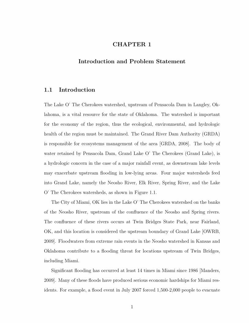
CHAPTER 1
Introduction and Problem Statement
1.1 Introduction
The Lake O’ The Cherokees watershed, upstream of Pensacola Dam in Langley, Ok-
lahoma, is a vital resource for the state of Oklahoma. The watershed is important
for the economy of the region, thus the ecological, environmental, and hydrologic
health of the region must be maintained. The Grand River Dam Authority (GRDA)
is responsible for ecosystems management of the area [GRDA, 2008]. The body of
water retained by Pensacola Dam, Grand Lake O’ The Cherokees (Grand Lake), is
a hydrologic concern in the case of a major rainfall event, as downstream lake levels
may exacerbate upstream flooding in low-lying areas. Four major watersheds feed
into Grand Lake, namely the Neosho River, Elk River, Spring River, and the Lake
O’ The Cherokees watersheds, as shown in Figure 1.1.
The City of Miami, OK lies in the Lake O’ The Cherokees watershed on the banks
of the Neosho River, upstream of the confluence of the Neosho and Spring rivers.
The confluence of these rivers occurs at Twin Bridges State Park, near Fairland,
OK, and this location is considered the upstream boundary of Grand Lake [OWRB,
2009]. Floodwaters from extreme rain events in the Neosho watershed in Kansas and
Oklahoma contribute to a flooding threat for locations upstream of Twin Bridges,
including Miami.
Significant flooding has occurred at least 14 times in Miami since 1986 [Manders,
2009]. Many of these floods have produced serious economic hardships for Miami res-
idents. For example, a flood event in July 2007 forced 1,500-2,000 people to evacuate
1

and affected about 500 homes and 30 businesses. The photo in Figure 1.2 shows the
extent of flooding in Miami during the 2007 flood.
Figure 1.1. Watersheds that feed into Grand Lake [GLWAF, 2008].
2

Figure 1.2. Photo from Manders (2009), indicating buildings damaged (blue squares), and de-stroyed (red squares) in the 2007 Miami flood. The Neosho River runs from the left to the bottomof the picture, and Tar Creek runs from top to bottom in the center of the picture.
3

1.2 Problem Statement
This research will examine whether the flooding threat upstream of Twin Bridges is
significantly affected by water surface levels maintained on the Grand Lake reservoir
at Pensacola Dam during the time period from August 15 to September 15 in any
given year. This time period was chosen in order to compare the effect of the lake
levels under the existing rule curve to proposed changes in the lake levels for the period
under a proposed rule curve adjustment (Figure 1.3). The 2007 flood illustrated in
Figure 1.2 is a well-documented example of why flooding is a major concern for the
City of Miami. This event is used to illustrate the major flooding concern for Miami,
but the event itself is not directly applicable to this research because it occurred in
July, a time frame that is not affected by the proposed rule curve adjustments.
The rule curve is used by GRDA to regulate lake levels at Pensacola Dam during a
normal water year. The Federal Energy Regulatory Commission (FERC) authorizes
this rule curve and any adjustments made to it. GRDA has proposed an adjustment
to the rule curve that would involve maintaining the lake level at 743 ft Pensacola
Datum (PD) from August 15 to September 15, as shown in Figure 1.3 [GRDA, 2013].
Currently, in the event of extreme rainfall scenarios, both GRDA and the United
States Army Corps of Engineers (USACE) control lake levels and discharge at Pen-
sacola Dam. GRDA controls outflow from the Dam until the lake stage reaches the
top of the “power pool” at 745.0 ft Pensacola Datum (PD elevations are equal to
North American Vertical Datum 1988 (NAVD88) elevations minus 1.40 ft [USGS,
2014]). When the lake stage reaches 745.1 ft PD, the USACE takes control of out-
flow in order to manage floodwater upstream and downstream throughout the region
[GRDA, 2013].
The research contained in this thesis addresses the question: "Do the changes in
water surface elevations due to the proposed rule curve adjustment for the August
4

740
741
742
743
744
745
746
Targ
et W
ater
Sur
face
Ele
vatio
n (fe
et a
bove
Pen
saco
la D
atum
)
Janu
ary
Febr
uary
Mar
ch
Apr
il M
ay
June
Ju
ly A
ugus
t S
epte
mbe
r O
ctob
er N
ovem
ber
Dec
embe
r
Proposed Pensacola Dam Rule Curve Adjustment
Existing Rule CurveProposed Rule Curve
August 15
September 15
Figure 1.3. Proposed target water surface elevations at Pensacola Dam [GRDA, 2013].
15-September 15 time period have an effect on major flooding levels upstream of Twin
Bridges and, primarily, the City of Miami, OK?” Three components of this problem
are specifically addressed:
I. The first problem is to determine a reasonable and conservative statistical esti-
mation for an extreme streamflow event for the major streams in the area. The
four streams addressed in detail are the Neosho River, Tar Creek, Spring River,
and Elk River. Historical streamflow data from the August 15 to September 15
time period are used for the streamflow analysis.
II. The second problem is to create a detailed hydraulic model that represents the
study area with the best available datasets. These datasets include topograph-
5

ical data representing the landscape surrounding the water bodies as well as
bathymetric data representing the ground elevations underneath the surface of
the water. The hydraulic model also takes into account hydraulic roughness con-
ditions of the floodplain areas for the August 15 to September 15 time period.
III. The final problem is to apply the hydraulic model to the research question in
order to determine the effect of a difference in water surface elevations (WSEs)
from 741 ft PD to 743 ft PD at the location of Pensacola Dam for the August
15 to September 15 time period.
This thesis is divided into five chapters: an introduction, a literature review, a
methods chapter, a results/analysis chapter, and conclusions. Each chapter is divided
into sections that discuss the individual problems mentioned above.
6

CHAPTER 2
Literature Review
A review of previously-published literature is helpful in order to both learn from
others’ research, and to compare the results of this research to previously-published
studies in this context. The literature review is divided into four sections:
1. Previous studies investigating the specific research context of Grand Lake and
the Neosho River near Miami, OK;
2. Studies involving statistical streamflow analysis;
3. Studies involving building a hydraulic model with modern technology; and,
4. Studies related to executing a hydraulic computer model.
2.1 Studies Investigating Grand Lake and the Neosho River
Near Miami, OK
Previous studies have investigated Neosho River flooding, but the available literature
is not adequate to answer the questions that will be addressed in this thesis. The
Chronicles of Oklahoma gives the historical account of the flood studies that were
conducted on the river prior to Pensacola Dam being built [Holway, 1948]. The US-
ACE published a report in 1998 investigating easement elevations in the Grand Lake
area [USACE, 1998]. A judicial report filed in 1999 by Holly contains an investiga-
tion into the 1992-1995 floods in Miami [Holly Jr., 1999]. Holly also published an
article investigating the effects of a previously proposed power-pool change in 2004
7

[Holly Jr., 2004]. Manders (2009) investigated the effects and mapped locations of
the 2007 major flood on the Neosho River at Miami. The existing literature does not
specifically investigate the effect of the current proposed rule curve adjustment, and
it does not incorporate the most recent geometric and hydrologic data for the river
system.
2.1.1 Chronicles of Oklahoma
A periodical titled Chronicles of Oklahoma contains a historical account of the build-
ing of Pensacola Dam [Holway, 1948]. Holway (1948) states that the “U.S. Army
Engineers,” prior to the construction of the dam, completed a flood study of the
Grand River. This article does not mention the reach of the Neosho River upstream
of the confluence of the Neosho and Spring Rivers. There is no documentation avail-
able for reference from this flood study, but it is noted that there was a flood study
performed prior to construction of the dam.
2.1.2 USACE Hydraulic Analysis of Grand Lake
In 1998, the USACE published a report of their findings from a hydraulic Real Estate
Adequacy Study conducted on Grand Lake of the Cherokees [USACE, 1998]. This
study investigated the adequacy of the elevations of the flood easements the USACE
owns, extending upstream into the tributaries. This report contains useful infor-
mation about the locations and hydraulic descriptions of the areas included in this
thesis. The report includes river mile descriptions, channel and overbank hydraulic
roughness conditions for the rivers, and information about the USGS gauge stations
located in the study area. This report also includes information about the easement
elevations owned by the USACE in the Miami area, which is helpful in determining
what levels constitute the designation of a “flood” in this area [USACE, 1998].
8

The conclusions of this report state that the upstream effect from Grand Lake
does not affect flood elevations on the Neosho upstream of USGS gauge 07185000,
near Commerce, OK. The conclusions also state that the full-lake elevation of 755
ft PD has less than a 6-inch effect on backwater WSEs upstream of the abandoned
bridge in Miami for the 50- and 100-year floods [USACE, 1998]. While this study
is extremely helpful as a guide for the model geometry setup portion of this thesis,
it does not adequately answer the question of what effect the current proposed rule
curve has on backwater flooding.
2.1.3 Holly Reports
Dr. Forrest Holly, Professor Emeritus at the University of Iowa and Adjunct Professor
at the University of Arizona, served as a referee for a legal report published in 1999
concerning flooding on the Neosho River in relation to Pensacola Dam. Holly also
published an academic research report on the same subject in 2004.
1999 Referee Report, including Amendment
In 1999, Holly was appointed as a professional referee on a legal case in the District
Court of Ottawa County [Holly Jr., 1999]. Holly was given the task of determining
the difference in floodwater elevations and durations for with- and without-dam con-
ditions for fourteen specified floods that occurred on the Neosho River between 1992
and 1995. Holly was also asked to develop a backwater envelope curve to represent
the effect of Pensacola Dam for each of the 14 floods.
The hydraulic model used in this study was a one-dimensional model called
CARIMA [Holly Jr. and Benoit-Guyod, 1977]. This model was used because it was
capable of modeling unsteady flow. Although HEC-RAS1 was developed in 1995, the
unsteady-flow modeling capabilities of HEC-RAS were not added until version 3.1.1,1See Section 2.3.1 for more information about HEC-RAS
9

which was publicly released in May 2003 [Brunner, 2010]. It should be noted that the
CARIMA model is fundamentally based on the same unsteady-flow equations (see
Section 2.3.1) as the unsteady HEC-RAS model [Holly Jr. and Benoit-Guyod, 1977;
Brunner, 2010].
Based on the research conducted, Holly (1999) concluded that, when comparing
the with-dam conditions to without-dam conditions, Pensacola Dam had a maximum
3 ft flood-exceedance impact on locations along the Neosho River near Miami, OK.
These conclusions are based on comparing results from running the CARIMA model
with the a) hypothetical scenario of no dam influence, and b) the actual recorded
dam stage elevations for the 14 floods.
Because Holly was investigating the effects of Pensacola Dam based on actual his-
torical datasets for the 14 floods included in the report, this research is only partially
relevant to the research included in this thesis. The model setup and model geometry
are relevant because Holly was modeling the same reach of the Neosho River. How-
ever, the results of the report are limited to specific floods for actual Pensacola Dam
datasets, and, therefore, not adequate to answer the question this thesis addresses
concerning the proposed rule curve change.
2004 Investigation of Proposed Power Pool Change
In 2004, Holly conducted a study investigating the effect of a change in the power
pool elevation of Grand Lake from 741 ft PD to 745 ft PD [Holly Jr., 2004]. For
this research, Holly used the historical streamflow dataset from one of the 14 floods
mentioned in Holly (1999), namely Flood 13 (2 - 22 June 1995), to investigate the
differences in WSEs along the Neosho River based on the hypothetical situation of
holding the dam WSE at 741 ft PD versus 745 ft PD. A hydraulic model called C1/C2
was used for the hydraulic analysis portion of this report [Holly Jr., 1999].
10

The C1/C2 model was developed by Holly in the late 1970s and it is a one-
dimensional/two-dimensional combination hydraulic model. The model has the ca-
pability to treat the flood plain of a stream as a individual cells, while maintaining
1D representation of the river channel. This cell-type rendering of the flood plain was
used upstream of Miami for Holly (2004). This location was chosen for the cell-type
floodplain rendering because the river channel is very sinuous in this portion of the
stream.
The hydraulic transfer between the cell-type floodplain and 1D channel was achieved
by assigning a weir-type or fluvial-type designation for each cell along the combina-
tion portion of the stream [Holly Jr., 2004]. According to Holly (2004), “The overall
purpose of this expanded modeling approach is to capture, as faithfully as possible
in a one-dimensional modeling context, the dynamic storage effects of flood plain ar-
eas where the highly sinuous channel meanders within the flood plain, in particular
upstream of Miami” [Holly Jr., 2004]. Thus, Holly’s approach can be considered a
pseudo-2D model in that it allows floodplain storage and routing to behave indepen-
dently of the river channel, but it does not apply the full two-dimensional St. Venant
equations to the combined channel/ floodplain system. Holly (2004) maintained a
purely 1D representation of the river (similar to the HEC-RAS model used in this
thesis) in the section of the Neosho River downstream of Miami where the channel is
not as sinuous.
Holly (2004) concluded that the effect of the hypothetical dam WSE change from
741 to 745 ft PD for the historical streamflows recorded for Flood 13 had an effect
of about 0.20 ft at “river mile 142.0,” which represents the location of Miami, OK.
This conclusion is very relevant for the research included in this thesis. The research
contained in this thesis is very similar to Holly (2004) with a few exceptions:
• Instead of modeling observed streamflow hydrographs with hypothetical dam
WSEs, this research will be using flood-frequency streamflows, which were de-
11

termined from the historical streamflow information, as the upstream boundary
conditions for the model, with hypothetical dam WSEs for the downstream
boundary conditions.
• This research uses more recent data, which has been collected with more ad-
vanced technology, than the data used in Holly (2004).
• This research uses the industry-standard hydraulic modeling program, HEC-
RAS 4.1.
• This research investigates the effects of the rule curve adjustment of dam WSEs
from 741 ft PD to 743 ft PD, unlike Holly (2004), which investigated the effect
of changing the power pool elevation from 741 ft PD to 745 ft PD.
• This research specifically focuses on the August 15 to September 15 time period
relevant to the proposed rule curve adjustment, while the flood investigated in
Holly (2004) occurred in June.
Therefore, while the conclusions in Holly (2004) are important and relevant, this
thesis will be answering a related question, yet with more recent and more advanced
data, as well as a more widely-accepted modeling program than the C1/C2 model
used in Holly (2004).
2.1.4 Manders Research Project
A 2009 research project by Manders investigated a major flooding event that occurred
in this watershed in July 2007. This study contributed elevation datasets from flood
locations that will be useful in calibrating a hydraulic model of the Neosho River.
The study concluded that backwater effects are a likely contributor to the flooding
at Miami, yet this conclusion is based on eyewitness observation and testimony, as
well as the Holly (1999) report mentioned in Section 2.1.3 [Manders, 2009]. Because
12

Holly (2009) specifically studied floods from 1992-1995, additional hydraulic modeling
research is necessary to adequately understand the primary cause of the high water
marks in the 2007 Miami flood.
2.2 Related Streamflow Analysis Literature
The streamflow analysis portion of this research involved both the collection of a large
number of streamflow datasets, as well as a statistical analysis of those datasets. In
the sections that follow, a literature review is provided concerning both the data
collection methods and the statistical analysis methods used for this research.
2.2.1 Available Stream Gauge Data
Some of the tributaries that contribute to water levels at Miami, OK have been
equipped with USGS stream gauges [USGS, 2012]. These gauges were used to cali-
brate and validate the hydraulic model used in this research. Figure 2.1 represents
the locations of each stream gauge. Two relevant time-varied datasets are available
from most stream gauges: discharge and stage. Table 2.1 summarizes the available
datasets from each USGS gauge used in this research. In Figure 2.1, note that two
of the gauge markers have dots in the middle of the marker. These gauges are used
for calibration purposes, as the stage elevation is available for historic rainfall events.
Calibration of the hydraulic model to these historic gauge stages is a necessary com-
ponent of hydraulic modeling in order to capture the unique and complex physical
characteristics of the region, as represented by parameters in the model.
13

Table 2.1. USGS stream gauge information.Stream Location USGS No. Stage Discharge
Neosho River Commerce, OK 07185000 X XNeosho River Miami, OK 07185080 XSpring River Quapaw, OK 07188000 X XElk River Tiff City, MO 07189000 X XTar Creek Miami, OK 07185095 X X
Pensacola Dam Langley, OK 07190000 X
^
!.
X
$
^
#
X$
!"#$%#&'()"*+&,#--"*."
/0*&,*""1+&2(0-(
34*(56&'()"*+&780409
:;1&'()"*+&/(<<&,(=>
!"#$%#&'()"*+&2(0-(
!"#"$#%&'($)*+%,-*./
#
&3
?"5$0.#;0&@0-+&A056;">&3
!.
Near Grand Lake
Legend
Figure 2.1. USGS Gauge Locations Relative to Grand Lake [USGS, 2012].
14

2.2.2 Bulletin 17B
In 1981, Bulletin 17B (B-17B) was published by the Water Resources Council, within
the U.S. Department of the Interior. This document provides guidelines for deter-
mining flood flow frequency in the United States [USGS, 1982]. It also contains a
glossary that is used to provide consistency of terms throughout this thesis. The
B-17B recommends using the log-Pearson Type-III (LP3) probability distribution for
estimating extreme flows when using annual maxima datasets. The LP3 distribu-
tion uses the Pearson Type-III (PE3) equation, but the parameters are calculated
using the log-transform of the data. The probability density function (PDF) for the
PE3/LP3 distribution is represented in equation 2.1.
f(x) =
(x−ζβ
)α−1exp
(−x−ζβ
)|βΓ(α)| , x > ζ for β > 0, or x < ζ for β < 0 (2.1)
The three parameters in the LP3 distribution are α, (the shape parameter), β,
(the scale parameter,) and ζ, (a shift parameter that makes the LP3 distribution
unique from the Gamma probability distribution) [Wilks, 2011, pp. 95-103]. Γ(α)
represents the gamma function2 evaluated at α [Wilks, 2011, pp. 96]. The use of
the log-transform of the data is the only difference between the LP3 and the PE3,
mentioned in Section 2.2.4. More information about the methodologies involved with
using the B-17B guidelines are found in Section 3.1.
The B-17B guidelines have been analyzed by many hydrologists in the more than
30 years since they were published, and many have found ways that the guidelines
could be improved [Lim and Voeller, 2009; England Jr and Cohn, 2007]. Specifically
for the context of this research, there are no guidelines included in the B-17B for2The gamma function is a mathematical representation of the factorial function for numbers more
complex than a positive integer [Wilks, 2011, pp. 78].
15

performing a flood-frequency analysis for a single month of the year, such as the
August 15 - September 15 time period investigated in this research. For this reason,
in this thesis, the B-17B standard annual maxima method is performed and compared
to another data sampling method called “partial duration” data sampling. B-17B
confirms that partial duration, or “peaks-over-threshold” datasets may be used in flow
estimation, but that more care is required in determining the best fit distribution for
the dataset [USGS, 1982]. Section 3.1.2 discusses the procedure used to ultimately
choose between the two data sampling methods.
2.2.3 Partial Duration Data Sampling Literature
As described in B-17B, data sampling can be accomplished by two methods: either 1)
using the annual maxima streamflows from the recorded datasets (“AM” method), or
2) using all of the streamflow measurements that are peaks over a certain threshold
(“POT”3 method) [Wilks, 2011]. The POT method is able to utilize a larger set of the
historical data because multiple peaks-over-threshold may occur in any given year.
This is specifically useful for streams which do not have a long history of recorded
data. This condition is evident for Tar Creek in this research, which has less than 20
years of data on record.
Several authors have tested and confirmed the applicability of the POT method in
streamflow analysis [Adamowski, 2000; Cunnane, 1973; Ekanayake and Cruise, 1993;
Pham et al., 2013]. According to these studies, the POT method is more accurate
than the AM method only if the number of peaks used is ≥ 1.65 times the number
of years on record. This means that the peaks must be identified, and then at least
the top 1.65 × N (with N being the number of years on record) peaks are used for
the statistical analysis [Cunnane, 1973]. For this thesis, M refers to the number of3Although the POT method is more commonly referred to as the partial duration method, for
the purpose of this thesis, the abbreviation “POT” will be used so as to not confuse the abbreviation“PD” with Pensacola Dam or Pensacola Datum.
16

peaks used and the ratioM/N is referred to as k. Therefore, k represents the average
number of peaks extracted per year from the historical dataset.
When using the AM method, meteorologic independence of events is not a concern
because only one event is extracted per year. However, independence of meteorological
events must be taken into consideration with POT datasets [Wilks, 2011]. With
multiple peak events per year being used by the POT dataset, some care must be
taken to ensure that the peaks are indeed independent [Wilks, 2011]. The method
used to ensure independence in this research is described in Section 3.1.2.
Fitting distributions to the POT datasets is completed in a similar manner to
fitting distributions to AM datasets, but the probability quantiles are different for
a particular return period because the number of data points is greater than the
number of years on record (M > N). The process outlined in Section 3.1.6 must
be followed to calculate the probability quantile associated with a particular return
period derived from a probability distribution fitted to a POT dataset [Wilks, 2011].
2.2.4 Extreme Value Distributions Literature
Determining what streamflow to use for the hydraulic model involves calculating a
probable “extreme value” of the distribution of historical floods. The probability
theory of this process is outlined in Statistical Methods in the Atmospheric Sciences,
by Wilks (2011). Although streamflow itself is not an atmospheric phenomenon, the
primary cause of flooding is rainfall runoff, which is an atmospheric phenomenon and
follows atmospheric statistical patterns. Section 3.1 explains the process of parameter
fitting that was used to fit various probability distribution functions to the observed
POT streamflow data. Eight probability distributions were chosen for POT analysis
based on the literature cited in the following paragraphs.
17

Gamma and Log Pearson Type-III Distributions
The two-parameter Gamma-distribution is commonly used for precipitation modeling
in the United States. The gamma distribution’s probability density function (PDF)
is represented by equation 2.2. The two parameters in the Gamma distribution are
α, the shape parameter, and β, the scale parameter.
f(x) = (x/β)α−1 exp(−x/β)βΓ(α) , x, α, β > 0 (2.2)
The Pearson Type-III distribution is a form of the gamma distribution that uses
an additional shift parameter, ζ [Wilks, 2011, pp. 95-103]. The PDF for the Pearson
Type-III distribution is the same as equation 2.1 in the B-17B explanation above.
The Pearson Type-III differs from the LP3 in that it does not use the log-transform
of the parameters.
The Gamma distribution, the non-transformed Pearson distribution (PE3), and
the LP3 distribution were all included in this POT analysis to investigate whether
any may apply to this specific research context.
Generalized Extreme Value (GEV), Gumbel, Weibull, and
Generalized Pareto Distributions
The three-parameter GEV distribution is used to derive the two-parameter Gumbel
and Weibull distributions. The GEV distribution is also the foundation for the gen-
eralized Pareto distribution, which is used specifically for POT datasets. In Wilks
(2011), the GEV distribution is linked to the study of extremely large precipitation
18

events that may cause flooding. The GEV PDF is represented in equation 2.3, where
κ, ζ, and β are the shape, location, and scale parameters, respectively.
f(x) = 1β
[1 + κ(x− ζ)
β
]1− 1κ
exp
−[1 + κ(x− ζ)
β
]−1κ
, 1 + κ(x− ζ)/β > 0
(2.3)
The GEV distribution can be integrated analytically, yielding the cumulative dis-
tribution function (CDF) in equation 2.4.
F (x) = exp
−[1 + κ(x− ζ)
β
]−1κ
(2.4)
The Gumbel distribution is a form of the GEV distribution in which the shape
parameter (κ) approaches zero. This distribution is also known as the Fisher-Tippett
Type 1 distribution, but will be referred to as the Gumbel distribution for this re-
search. The Gumbel distribution PDF, represented in equation 2.5, may be integrated
analytically yielding the CDF represented in equation 2.6 [Wilks, 2011, p. 106]. The
parameters of the Gumbel distribution are identical to the GEV, but κ is not included.
f(x) = 1β
exp{− exp
[−(x− ζ)
β
]− (x− ζ)
β
}(2.5)
F (x) = exp{− exp
[−(x− ζ)
β
]}(2.6)
The Gumbel distribution has been used to model extreme streamflow in Mujere
(2011), which applied the traditional method of moments to fit the Gumbel distribu-
tion to extreme streamflow on the Nyannyadzi River in Zimbabwe [Mujere, 2011].
The Weibull distribution (also known as the Fisher-Tippett Type III distribution)
is the form of the GEV distribution in which the shape parameter is less than zero
and the shift parameter equal to zero. The PDF for the Weibull distribution is shown
19

in equation 2.7 [Wilks, 2011, p. 107]. The parameters for the Weibull distribution are
the shape (α) and scale (β), similar to the Gamma distribution.
f(x) =(α
β
)(x
β
)α−1exp
[−(x
β
)α], x, α, β > 0 (2.7)
Singh (1987) investigates the applicability of the Weibull distribution to various
hydrologic applications. This research concluded that the Weibull distribution is
inaccurate for the hydrologic applications of rainfall depths and durations [Singh,
1987]. However, Ekanayake and Cruise (1993) compared the Weibull and exponential
distributions in application to flood modeling and found the Weibull distribution to
be superior.
The generalized Pareto distribution is a form of the GEV function that is specifi-
cally designed to work with POT datasets [Wilks, 2011, pp. 109]. Hosking and Wallis
(1987) affirm that the generalized Pareto is useful specifically for POT datasets [Hosk-
ing and Wallis, 1987]. Ashkar and Ouarda (1996) demonstrate the use of the gener-
alized Pareto distribution in modeling extreme flooding events [Ashkar and Ouarda,
1996]. The PDF of the generalized Pareto is represented in equation 2.8 and the CDF
for this distribution is represented in equation 2.9.
f(x) = 1σ∗
[1 + κ(x− u)
σ∗
]− 1κ−1
(2.8)
F (x) = 1−[1 + κ(x− u)
σ∗
]−1/κ(2.9)
In equations 2.8 and 2.9, the value u represents the threshold used for sampling
the POT dataset, κ is the shape parameter for the distribution, and σ∗ is the scale
parameter [Wilks, 2011].
20

3-parameter Lognormal Distribution
The 3-parameter lognormal distribution (LN3) is a logarithmic power-transformation
of the Gaussian distribution [Wilks, 2011, p. 92]. The PDF for the LN3 distribution
is shown in equation 2.10.
f(x) = 1(x− γ)σy
√2π
exp
−[ln(x− γ)− µy
]22σ2y
, x > 0 (2.10)
where σy and µy are the standard deviation and mean, respectively, of the log-
transformed variable, y = ln x [Wilks, 2011]. In the LN3 distribution used in this
thesis, γ represents the lower bound of the data. Vogel and Wilson (1996) compare
the lognormal distribution to the GEV and LN3 distributions at various streamflow
sites across the U.S. and conclude that the LN3 distribution is a viable model for
predicting streamflow with POT datasets.
Usage of Probability Distributions
Each of the aforementioned probability distributions has been shown to be relevant to
streamflow analysis; therefore, they were all included in the POT streamflow analysis
for this research. Each distribution was fit to the historical observed POT dataset,
and then analyzed to find the “best-fit” distribution for the extreme rainfall events.
This process is described in detail in section 3.1 of the Methods chapter of this thesis.
2.3 Hydraulic Modeling Background
Hydraulic models can be evaluated in either one-dimensional (1D) or two-dimensional/
three-dimensional (2D/3D) computational procedures. Although 2D/3D models pro-
vide many advantages over 1D models, they are more complicated to use for large
stream reaches, as well as more computationally expensive. Furthermore, for many
21

river flood studies, 2D/3D models may not provide a significant increase in accuracy
[Merwade et al., 2008]. Therefore in this research, the hydraulic model utilized will
be HEC-RAS (Hydraulic Engineering Center’s River Analysis System), which is a 1D
hydraulic model developed by the USACE. For both 1D and 2D/3D models, Geo-
graphic Information Systems (GIS) may be used to assist in managing the input data
as well as spatially rendering the results.
2.3.1 One Dimensional (1D) Modeling Literature
HEC-RAS is a 1D, physics-based hydraulic modeling program created by the USACE
to model open channel flow [Brunner, 2010]. There are various case studies available
for review that use HEC-RAS to model flooding (e.g., Knebl et al. [2005]; Haghizadeh
et al. [2012]). HEC-RAS is the recommended by the Federal Emergency Management
Agency (FEMA) for floodplain modeling and hydraulic analysis [FEMA, 2012]. The
HEC-RAS model iteratively solves a system of equations and outputs WSEs along a
stream channel at user-defined cross section locations.
The HEC-RAS modeling program is capable of modeling two types of flow sce-
narios: steady-state and unsteady flow routing. The main difference is that unsteady
flow routing is time-dependent, while steady-state flow has no time component in the
water surface calculations.
Steady-state flow computations in HEC-RAS
The basic computational procedure used by HEC-RAS for the steady-state flow cal-
culation is based on the solution of the 1D energy equation [Brunner, 2010], which is
shown in equation 2.11.
Z2 + Y2 + α2V 22
2g = Z1 + Y1 + α1V 21
2g + he (2.11)
22

where,
Z = Channel bottom elevation above datum,
Y = WSE above datum,
V = Average velocity,
α = Kinetic energy correction factor,
g = Gravitational constant, and
he = Head loss term, defined in equation 2.12
he = LSf + C
∣∣∣∣∣α2V 22
2g − α1V 21
2g
∣∣∣∣∣ (2.12)
where,
L = discharge weighted reach length (based on geometry of both channel and flood-
plain),
Sf = friction slope (based on Manning’s-n),
C = expansion or contraction loss coefficient (user input)
The HEC-RAS procedure for steady-state flow WSE computation is as follows:
1. For subcritical flow (known WSE at downstream control point), assume a WSE
at the immediate upstream cross section from the control point;
2. Based on that value, calculate the total conveyance and velocity head;
3. Calculate Sf based on values from step 2, and solve for he using equation 2.12;
4. Solve the energy equation (Eq. 2.11) for Y at the upstream cross section (WSE);
5. Compare calculated WSE with assumed WSE, and iterate until error is less
than the tolerance level, which is either 0.01 ft by default, or else user defined.
The momentum equation is used for certain situations in the steady flow procedure
where the flow may be temporarily rapidly-varied. These situations include bridge
23

contractions and expansions, abrupt changes in slope, and river confluences [Brunner,
2010].
Steady-flow results represent the dynamic equilibrium stage of the system, subject
to a constant forcing. For this reason, for any flow magnitude, Q0, a steady flow
simulation will produce higher water surfaces, in general, than an unsteady flow with a
peak of Q0. Moreover, the steady flow simulation is convenient for determining WSEs
for floods and statistically extreme flows because these are often single discharge
values (the peak) and not flow vs. time hydrographs.
Unsteady flow routing in HEC-RAS
Two laws govern unsteady fluid flow in HEC-RAS calculations [Brunner, 2010]:
• Conservation of Mass, i.e., accumulation in a reach is equal to mass in minus
mass out, and
• Conservation of Momentum, i.e., the time rate of change of momentum in a
control volume is equal to the sum of the forces acting on the water in the
control volume.
The 1D equation for conservation of mass for this context is:
∂AT∂t
+ ∂Q
∂x+ ql = 0 (2.13)
where,∂AT∂t = rate of change in fluid storage in a control volume,∂Q∂x = net rate of fluid flow into the control volume, and
ql = the lateral fluid flow entering the control volume, per unit length.
The 1D conservation of momentum equation is shown in equation 2.14. The left
side of the equation represents the sum of all forces acting on a control volume in the
24

direction of flow, and the right side of the equation represents the momentum flux,
or time rate of change of momentum in the control volume.
∑Fx = dM
dt(2.14)
The discrete equation for the sum of all forces in the direction of flow, for this
context is represented in equation 2.15:
∑Fx = −ρ∂QV
∂x∆x− ρgA∂h
∂x∆x− ρgA∂z0
∂x∆x− ρgASf∆x (2.15)
where,∑Fx = sum of all forces in the x-direction on a control volume
ρ∂QV∂x ∆x = momentum flux through the control volume
ρgA∂h∂x∆x = pressure forces on the control volume
ρgA∂z0∂x ∆x = gravitational forces on the control volume, and
ρgASf∆x = boundary drag associated with the control volume
The discrete equation for the momentum flux acting on the control volume is
represented in equation 2.16.
dM
dt= ρ∆x∂Q
∂t(2.16)
In the limit, equations 2.14, 2.15, and 2.16 become the differential balance of
momentum, represented by equation 2.17.
∂Q
∂t+ ∂QV
∂x+ gA
(∂z
∂x+ Sf
)= 0 (2.17)
Equations 2.13 and 2.17 are solved simultaneously in the HEC-RAS unsteady flow
routing solver based on a four-way iterative process involving two spatial (x) nodes
25

and two temporal (t) nodes, which is outlined in detail in Brunner (2010). The process
yields a WSE for each cross section at each time step during the flow simulation.
Unsteady flow routing is especially useful for conditions where historical observed
datasets have been recorded and can be input into the system as a flow vs. time or
stage vs. time hydrograph.
2.3.2 2D/3D Modeling Literature
The most relevant literature available using the 2D approach is Merwade et al. (2008).
This article outlines the use of a 2D hydraulic modeling technique using GIS on
three rivers in the United States. The article addresses issues that the 2D approach
encounters with geometric data. The traditional 1D approach, according to Merwade
et al. (2008), does not accurately model the water behavior in the case of large-scale
extreme events, such as over-500-year return period flooding or glacial outbursts. The
purpose of the Merwade paper was to provide guidelines for incorporating surveyed
channel data with surrounding Digital Elevation Models (DEMs). While it is helpful
to know that this 2D/3D approach is an option, the traditional 1D approach will be
used in this thesis research for three reasons:
1. The intended application does not include over-500-year return period flooding
or dam breaks;
2. 1D modeling is the approach utilized and accepted by the USACE and the Fed-
eral Emergency Management Agency (FEMA) [Brunner, 2010; Buckley, 2001];
and
2.3.3 Geographic Information Systems Literature
Hydraulic modeling programs may be used in conjunction with GIS to develop maps
that delineate the floodplain of a channel during a flood event [Yang et al., 2006]. This
26

enables the user to visually represent the flood and, also, to store information about
the flood in a format that is useful for many different applications. A tool native to
the GIS program ArcMap 10, called HEC-GeoRAS, is designed to aid the user in using
GIS in conjunction with HEC-RAS [ESRI, 2011; Ackerman, 2009]. The flood maps
created with HEC-GeoRAS may be compared with the existing (FEMA) floodplain
maps in order to note differences and investigate the reason for the differences.
27

CHAPTER 3
Methods
There are three major segments involved in the methodology of this research: 1) a
statistical streamflow analysis; 2) the building of the hydraulic model; and 3) HEC-
RAS modeling.
3.1 Statistical Streamflow Prediction Methods
In order to conduct a hydraulic analysis of the Grand Lake region, extreme stream-
flow conditions are required for use as upstream boundary conditions for the model.
A statistical analysis of the data is necessary for extrapolation of a probability distri-
bution beyond the limits of the 74 years of recorded streamflows in order to estimate
flood-frequency streamflows of lower probability events, such as the 100-year flood.
3.1.1 Approach
There are two acceptable and widely-used approaches to the flood-frequency predic-
tion problem [Bedient et al., 2013]. The approaches differ in their method of defining
the streamflow dataset at the boundary of the hydraulic model. The first approach is
to set up a hydrologic model of the watershed for the all of the parameters that con-
tribute to runoff (the “physics-based” approach). These parameters include historic
rainfall patterns, land use, infiltration capacity, watershed storage, and evaporation.
After calibration of these parameters, the hydrologic model is then used to simulate
the expected runoff that would occur at the boundary of the hydraulic model. The
process is repeated for many rainfall scenarios, and the resulting flow dataset is used
28

to estimate flood-frequencies. The second approach is to use the stream gauges that
are located on the streams in the immediate vicinity of the study area to perform the
flood-frequency analysis (the “stream gauge” approach) [Bedient et al., 2013]. Stream
gauges act as an integration of all the upstream hydrologic parameters; therefore, the
gauges output the cumulative result of all that is happening upstream. The historical
datasets from these gauges are analyzed to produce statistical probabilities of the
streamflow magnitudes.
There are advantages and disadvantages associated with each approach. One ad-
vantage of the physics-based approach is that representation of the actual contributors
to runoff may be isolated and calibrated. For example, a model can take into account
particular releases from upstream dams, seasonal infiltration capacities of the soil on
the contributing watershed, recent changes in upstream land use, as well as histori-
cal rainfall events. The disadvantage of this approach is that it requires a very large
amount of spatial and temporal data, especially for a watershed as large as the Grand
Lake watershed.
An advantage of the stream gauge approach is that the data processing is simpler.
For example, stream gauges have been collecting datasets on the Neosho, Elk, and
Spring rivers since 1939. These datasets have essentially integrated the upstream
hydrologic behavior for 70+ years. One disadvantage of this approach is that specific
contributors to streamflow cannot be isolated (e.g., dam release upstream, infiltration
capacities of the soil, etc.). Another disadvantage is that it depends on having a long
enough period of record (e.g., this approach would not be viable with only 5 years of
recorded data).
Given the relatively long period of record, the acceptance of the second approach
in the floodplain modeling community, and the well-defined objectives of this research
project, the second approach is used in this research. Time-series streamflow datasets
29

from the Neosho, Spring, and Elk Rivers and Tar Creek have been statistically ana-
lyzed in order to predict flood-frequency streamflow values [Bedient et al., 2013].
3.1.2 Data Collection
The datasets used for the statistical streamflow prediction of the Neosho, Spring, and
Elk Rivers and Tar Creek were the observed August 15 to September 15 daily-mean
streamflows at the streams’ USGS gauges nearest Grand Lake, as shown in Table 3.1.1
Table 3.1. USGS stream gauges used for statistical streamflow prediction.USGS Begin Date of
Stream Location Gauge No. Discharge DataNeosho River Commerce, OK 07185000 10/01/1939Spring River Quapaw, OK 07188000 07/12/1939Elk River Tiff City, MO 07189000 10/01/1939Tar Creek Miami, OK 07185095 01/01/1984
Bulletin 17B mentions two methods of data sampling techniques [USGS, 1982].
The two methods are each very prevalent in the hydrologic literature, and can be
summarized as the following:
1. using the maximum annual streamflow from the recorded data (known as the
annual maxima (AM) method), or
2. using all of the streamflow measurements that are peaks over a certain threshold
(POT method) [Wilks, 2011].
B-17B does not recommend a particular method of data sampling for the purpose of
predicting the extreme streamflow for a certain month of the year, as is the case for
this research. Because no specific guidelines are given for this case, both methods1The Tar Creek Miami gauge historical dataset has a gap of 9 years from 10/1/1993 to 5/27/2004,
so there are only N = 20 years of data available for this location.
30

are employed for analysis of the Neosho River, Commerce gauge data, and the most
conservative method is chosen for calculating flood frequencies of each stream for use
in the model application phase of the research.
Averaging streamflow values over a 24-hr window will suppress the peak discharge
values, particularly if the peak flow only occurred for a period of time less than 24-
hrs. This suppression of peak discharge values is referred to as streamflow dampening.
Accounting for streamflow dampening is necessary in order to accurately predict the
extreme flood events, particularly on the smaller streams such as Tar Creek, which
produce peaks that are completely contained within a 24-hr time period. In order to
account for streamflow dampening in the daily-average datasets available from the
USGS, the following procedure is used to convert the daily-average peaks to synthetic
instantaneous-peak streamflow values.
1. First, the annual instantaneous-peak streamflow values for each gauge station
are retrieved from USGS (2012).
2. The daily-average peak values associated with each annual instantaneous-peak
are retrieved from the daily-data section of the same website.
3. A “peaking factor” is calculated for each peak value by dividing the instantaneous-
peak by the daily-average peak.
4. An average peaking factor is calculated for each gauge station using the entire
period of record.2
5. The daily-average peaks for the August 15 - September 15 time period are
multiplied by the respective gauge peaking factor and those modified values
used for input in the statistical analysis.2These values are shown in Table 4.1 in Section 4.1.
31

3.1.3 Statistical analysis of the AM datasets using PEAKFQ
A program developed by USGS, PEAKFQ, is utilized to determine the statistically
extreme streamflows for the streams included in this study [Flynn et al., 2014]. The
users’ manual outlines the computing codes used to follow the B-17B procedures
exactly. PEAKFQ uses a specific input file of a form that is available from the USGS
National Water Information System [USGS, 2012]. The file is available for download
for the annual peak streamflow events on a gauge station webpage, provided that
gauge station records historic streamflow data. This file is accessed for each of the
four streamflow gauges used in this thesis, and the file is modified to include the
maximum streamflow for each August 15 - September 15 on record, with the peaking
factors applied.
The PEAKFQ program uses the historical datasets in the input file to calculate
the parameters for the LP3 distribution in the precise method outlined in B-17B. The
program provides an output file including the details of the statistical analysis as well
as probable extreme value estimates calculated from the fitted LP3 distribution. The
program also provides a graphical output representing the observed gauge data (or
“systematic data”) and the fitted LP3 distribution with its 95% confidence interval
[Flynn et al., 2014]. This program is used to determine the statistically extreme
streamflows used for each of the four upstream streamflow input locations in the
hydraulic model.
3.1.4 Statistical analysis of the POT datasets using
L-moment parameter estimation
The following method is used to compile the POT dataset from the historical datasets
for each stream:
1. First, all of the historical datasets were entered into a spreadsheet.
32

2. The datasets from each year’s August 15 to September 15 period were isolated.
3. Individual peaks were identified for each year, with an independence criteria of
7 days between peaks3
4. The highest M = N × k peaks4 were ranked from highest to lowest.
5. Those M peaks were used for fitting the probability distributions in the statis-
tical analysis portion of the research.
Probability distributions of type Gamma, GEV, Generalized Pareto, Gumbel,
Lognormal, PE3, LP3, and Weibull were fit to the observed POT datasets using
parameter fitting methods. A discussion of each distribution can be found in Sec-
tion 2.2.4.
The method of L-moments is used to estimate parameters for each distribution.
Hosking (1990) presents a concise summary of L-moments and their applicability
to parameter estimation [Hosking, 1990]. L-moments are analogous to traditional
statistical moments, but they are linear combinations of order statistics. L-moments
have been used to estimate probability distribution parameters in additional research
since Hosking’s (1990) paper [Adamowski, 2000; Vogel and Wilson, 1996; Ilorme and
Griffis, 2013]. A detailed explanation of L-moment theory is not included in this
thesis, but may be found in Hosking (1990). Hosking created and maintains an R
package entitled “L-moments,” which is used in this research to calculate the L-
moments and fitted parameters for each probability distribution [Hosking, 2014; R
Core Team, 2013].
After fitting the probability distributions to the observed POT datasets, probabil-
ity plotting-positions are calculated for the observed datasets. The plotting positions3The independence criteria of 7-days between peaks is based on methods outlined in Ashkar and
Ouarda (1996).4See Section 2.2.3 for definitions of M,N, and k
33

are used to compare the fitted distributions’ probability quantiles to the probability
quantiles of the observed datasets [Makkonen et al.; Hirsch, 1987; Weibull, 1939].
3.1.5 Choosing a “Best-fit” Distribution
In order to determine which distribution is the “best fit” to the POT dataset, a
root-mean-square-error (RMSE) analysis is applied comparing each fitted distribution
to the observed dataset [Ritter and Muñoz-Carpena, 2013]. The RMSE equation is
represented by equation 3.1. RMSE is a valuable statistic for this application because
it naturally weights errors in the highest flow values more than in the lower flow values.
RMSE =√∑ (yi − yi)2
n, (3.1)
where,
yi = the observed value at a probability plotting-position,
yi = the distribution value at the matching probability quantile, and
n = the number of observed data points.
The RMSE values are compared for each distribution using a bootstrapping con-
fidence interval (CI) of the RMSE. Bootstrapping is a method of data analysis known
as “resampling with replacement” [Efron and Tibshirani, 1986]. Bootstrapping is
advantageous in streamflow analysis because the true underlying probability distri-
bution is unknown, and bootstrapping is a simple method for deriving the CI for a
statistical property of the data. For this research, the RMSE was bootstrapped 5,000
times for each {simulation vs. observation} dataset. The RMSE CI’s may be used
to determine, with confidence, which probability distribution is the “best fit” of the
observed data.
34

3.1.6 Calculation of Extreme Streamflow Values Using Fitted Distribu-
tions
In order to calculate extreme streamflow values, the probability distributions are
extrapolated beyond the extent of the highest streamflow values recorded in the ob-
served dataset. The calculation of probability is simple for the AM method, and
slightly more complicated for the POT method. For example, with N=74 prior years
of data using the AM method, the most extreme value (rank = r = 1) would have
an r/(N + 1) = 1/75 ≈ 0.0133 probability of occurring in any given year [Makko-
nen et al.; Weibull, 1939]. Using the AM method, to calculate a 100-year storm the
probability distribution was extrapolated to a 0.01, or 1/100 probability value. A
200-year storm would have a 1/200, or 0.005 probability of occurrence in a given
year, a 500-year storm would have a 1/500, or 0.002 probability of occurrence, and
so on [Wilks, 2011]. This process is included in the computations completed by the
PEAKFQ program for calculating flood-frequency values for the AM dataset.
When using the POT method, however, an alteration must be made in order to
calculate quantiles for extrapolating the probability distributions. Equation 3.2 is
used to calculate the CDF quantile “F (x)” associated with a particular return period
for a POT dataset. For example, for the most extreme value in the recorded POT
dataset for the Neosho River, Commerce gauge (where M = 124), the return period
T ′ would be equal to the number of years on record (N = 74), and the probability
quantile would be F (x) ≈ 0.9919355.
F (x) = 1− 1T ′k
(3.2)
where,
F (x) = CDF probability quantile
35

T ′ = Return period for POT dataset
k = Ratio of number of POT data points to number of years on record (M/N)
3.1.7 Choosing a Distribution to Use for Estimating Flood Frequency
Values for This Thesis
The probability quantiles for the 2-, 10-, 20-, 50-, 100-, 200-, and 500-yr return inter-
vals were calculated for the Neosho using the method described above. The method
that produces the most conservative flood frequency estimates (i.e. highest stream-
flow values) is used to calculate extreme streamflow estimates on all other streams.
These extreme streamflow values are used to “force” the model in the sensitivity
analysis and model application portion of the research, as described in section 3.3.2.
3.2 Hydraulic Model Development
3.2.1 Data Collection
In order to build an accurate hydraulic model using the best-available data, informa-
tion had to be compiled from many sources. These datasets then had to be “normal-
ized” for use in a consistent model. Herein, normalization means combining datasets
that may be in different forms into a single form which can be used in a consistent
model. These different data sources all use a different data organization method, and
normalization allows the model to be able to read all of the datasets consistently.
The “topography,” as defined in this paper, are the areas of bare-earth elevations
that were not underwater at the time of the data collection. The underwater areas
are referred to as “bathymetry.”
A major issue encountered in the normalization of the datasets is that there are
many vertical datums used to record elevation data. A diagram developed by USGS
for understanding datums in this region is shown in Figure 3.1(a). The graphical
36

portion of the figure represents the data transformation process for converting between
datums. The physical representation of the datums would be reversed, with PD as the
highest datum and NAVD88 as the lowest datum. For example, suppose a particular
water surface has an elevation of 741 ft above PD. To convert to NAVD88, according
to the text in Figure 3.1(a), 1.4 ft is added to the elevation. Therefore, the same
water surface is 742.4 ft above NAVD88. Visually, the physical representation of the
datums is shown in Figure 3.1(b).
(a) USGS Figure (b) Physical Representation
Figure 3.1. Graphical representation of the complexity of converting between various verticaldatums. USGS Figure taken from USGS (2012).
Topographic Data
The topographic datasets provide information about the floodplain for a hydraulic
model. Detailed topographic datasets are currently publicly available from the Na-
tional Elevation Dataset (NED), which is provided by the USGS. The most recent
detailed dataset for the Grand Lake region was collected in 2008. Details about this
dataset may be accessed from the dataset’s metadata, available from the NED website
[Gesch, 2007]. The relevant details for this thesis are as follows:
• The dataset is downloaded as raster files in .img format.
37

• The dataset is downloaded in sections of 0.25° longitude × 0.25° latitude.
• The resolution of the raster is about 3 meters.
• The elevation data points are stored in SI units and relative to the NAVD88
vertical datum.
• The data points were collected using Light Detection and Ranging (LiDAR)
technology.
– LiDAR is extremely accurate for vertical elevations (~10 cm accuracy5).
– LiDAR does not collect bathymetric data points because the light emitting
device reflects off the surface of the water.
Bathymetric Data
The bathymetric datasets for the Grand Lake region originate from many sources.
Four different sources were collected and combined for use in the hydraulic model,
spanning various collection methods and ages of the datasets.
1. The OklahomaWater Resources Board (OWRB) collected a bathymetric dataset
for the entire Grand Lake reservoir in 2009 [OWRB, 2009].
• The bathymetric data points were collected using an acoustic doppler de-
vice, which is not as accurate as the aforementioned LiDAR, but is still
very accurate, with a published accuracy to within ~16 cm in the vertical
direction for the entire dataset6.5This accuracy of 10 cm vertically is the maximum expected difference between the measured
topography and the actual topographic conditions. This discrepancy is likely found at locationswhere the topography changes drastically over a short distance (e.g., cliffs). Although this datasetis not perfectly accurate, a certain amount of error is present in any dataset, and this is the bestcurrently available dataset. An identical geometry file is used in each hydraulic model run for thisthesis. Therefore, the accuracy of the dataset does not affect the calculation of the WSE differencesrepresenting the proposed rule curve adjustment.
6See footnote 5. This concept applies to the bathyemtric dataset as well.
38

• The bathymetric elevation data points are stored in U.S. customary units
and relative to the Pensacola Datum.
• The OWRB bathymetric study does not extend into the river channels of
the Neosho or Spring Rivers upstream of Twin Bridges or to the USGS
gauge location at Tiff City on the Elk River. Additional bathymetric
datasets are required for these sections of the river channel.
2. USGS updates cross sectional datasets for the river channels at USGS gauge
station locations periodically, and these channel cross section datasets were used
to interpolate between the end of the OWRB bathymetry availability and the
gauge station locations on the Spring and Elk Rivers. The Quapaw gauge is
used for the Spring River and the Tiff City gauge for the Elk River. These
cross section elevations are collected using acoustic doppler technology similar
to that used by OWRB in the reservoir bathymetry study [Strong, 2014].
3. A channel bathymetry dataset for the Neosho River between Twin Bridges and
the USGS Commerce gauge was collected as surveyed cross sections along the
floodplain in 1997 by the USACE. This dataset was received in the form of
a HEC-RAS geometry file from the USACE [Wyckoff, 2014]. This channel
bathymetry dataset is sufficiently accurate for this research (i.e., determining
the effect of Pensacola Dam on upstream flooding), but not nearly as accurate as
the aforementioned acoustic doppler technique used by OWRB for the reservoir
[OWRB, 2009]. The vertical datum for this dataset is not cited, but it was
determined to be relative to the NAVD88 datum7. The data points are stored
in U.S. customary units.7This assumption is made based on the USACE datasets in relation to another dataset received
from USGS for the same cross section locations [Smith, 2013]. The USGS dataset was received asan excel spreadsheet with cross section station/elevation datasets. The topography portion of thesecross sections is apparently extracted from the LiDAR data in the NED dataset (Gesch (2007)), butthe bathymetry is generalized as a single point in the middle of the river channel. This single pointmatches up precisely (i.e., to the hundredths digit) with the USACE dataset in its original form.The USGS dataset is clearly cited as relative to the NAVD88 vertical datum. For this reason, it
39

4. Bathymetry data points were required for the section of Tar Creek south of the
Highway 10 bridge in Miami, where the water is several feet deep even on days
with little flow. GRDA provided spot-depth data points for this section of Tar
Creek in May 2014 using a sonar depth reader. These data points were provided
as coordinates and depths from the water surface in U.S. customary units.
Bridge Data
Physical datasets about the relevant bridges in the study area were provided by the
USACE in the HEC-RAS geometry file previously mentioned as the source of channel
bathymetry data for the Neosho River [Wyckoff, 2014]. These datasets include bridge
deck elevations, pier locations and geometry, as well as all necessary bridge modeling
information, such as weir coefficients and pier-loss coefficients. These datasets are
manually input into the HEC-RAS model created for this research.
3.2.2 Data Normalization and TIN Creation
The raw datasets collected for this research are referenced to different datums and
units as per the needs of the specific agency that collected the datasets. Because the
NED topography is the largest dataset, its units and datum provide the base for nor-
malizing the topographical and bathymetric datasets. The normalized datasets are
then combined in order to create a type of terrain model, called a Triangulated Irreg-
ular Network (TIN), that is used by HEC-GeoRAS for the extraction of a hydraulic
model.can be reasonably assumed that the original USACE dataset is in reference to the NAVD88 verticaldatum.
40

Normalization Procedures
The normalization of the datasets requires a series of step-by-step procedures in the
ArcMap GIS program. The details of these procedures are included in Appendix B.
The main structure of the procedure is outlined in the following list.
1. Normalizing the NED dataset
a. The original raster form of the dataset has a resolution of ~3 meters in the
horizontal direction. The vertical accuracy, however, is about 10 cm. The
dataset is compressed so that data points within 10 cm vertically of one
another are excluded, creating a much smaller file size that still maintains
the vertical accuracy of the original dataset.
b. The original dataset also includes false data points at locations that were
covered by water at the time of the data collection. In order for these data
points to not interfere with the OWRB dataset, the points within the bound-
ary of the OWRB study are removed from the NED dataset.
2. Normalizing the OWRB dataset
a. The OWRB data points are received in U.S. customary units referenced to
the Pensacola Datum. These data points are converted to SI units referenced
to the NAVD88 datum in order to match the larger NED dataset.
b. The OWRB bathymetry dataset is then merged with the normalized NED
dataset to create a dataset including both topography and bathymetry.
3. The NED floodplain topography and OWRB reservoir bathymetry are then
compiled into a triangulated irregular network (TIN), which is the type of DEM
from which HEC-GeoRAS (see section 2.3.3) is able to extract elevation data
points for the hydraulic model. This TIN will henceforth be referred to as
“Grand TIN.”
41

4. In order to include the bathymetry dataset for the Neosho River channel up-
stream of Twin Bridges, the cross sections acquired from the USACE are in-
troduced to Grand TIN. These cross section data points are already in U.S.
customary units and referenced to the NAVD88 vertical datum, so no conver-
sion is necessary in that regard.
5. A tool created by Dr. Venkatesh Merwade of Purdue University is used to
interpolate the channel bathymetry between the coarsely-spaced USACE cross
sections [Merwade et al., 2008]. The interpolated bathymetry is then input into
Grand TIN.
6. The Tar Creek channel bottom depths from GRDA are converted to channel
bottom elevations using recorded WSEs at a nearby USGS gauge station. These
channel bottom elevations are added to Grand TIN as individual points.
7. The channel bottom elevations for the Spring and Elk Rivers require interpo-
lation between the furthest extent of the OWRB (2009) study and the USGS
gauge station cross sections, but that process is completed in the HEC-RAS
program instead of ArcMap, and it is explained in section 3.2.3.
8. After compiling all the available datasets using ArcMap, Grand TIN requires
clean up to remove residual false data points from the NED representation of
water surfaces.
3.2.3 Data Extraction Using HEC-GeoRAS
With the Grand TIN complete and all of the bathymetry and topography datasets
normalized and merged, the process of exporting the data from ArcGIS to HEC-
RAS begins. The tool created by the USACE for communication between ArcMap
10.1 and HEC-RAS is called HEC-GeoRAS 10.1. HEC-GeoRAS is a toolbar that
may be downloaded from the internet and installed into ArcMap [Ackerman, 2009].
42

The documentation in the HEC-GeoRAS users manual is helpful for a step-by-step
guide to using the tool. Merwade’s personal website also contains a helpful step-
by-step walkthrough of generating a HEC-GeoRAS output from a TIN [Merwade,
2014]. HEC-GeoRAS has several capabilities that are particularly useful for this
research. These capabilities are explained below according to the feature classes that
HEC-GeoRAS requires.
• River and River 3D: These feature classes contain the stream centerline datasets
for the river reaches that will be modeled in HEC-RAS. The features are “mea-
surable,” and the measures along the routes are the source of HEC-RAS’ station
assignments for each cross section.
• Banks: The banks feature class is used by HEC-GeoRAS to identify the bank
location for each cross section. This information distinguishes the left overbank
(LOB) and right overbank (ROB) floodplain section from the channel section,
allowing for different Manning’s n values in each section.
• Flowpaths: The flowpath feature class is made up of three lines for each reach:
left, right, and center path lines. The feature measures are used to calculate
the downstream reach lengths for the LOB and ROB (as they can differ for
meandering streams).
• XSCutlines and XSCutlines3D: The cross-section cutline feature class is ar-
guably the most important and valuable feature exported by HEC-GeoRAS.
Cross sections can be drawn at any location the user desires, and the HEC-
GeoRAS program exports all of the information about the cross section (reach
lengths, elevations, bank stations, Manning’s n, ineffective flow areas, blocked
obstructions, etc.) to HEC-RAS. This process could consume a large amount
of time resources to complete manually, especially with a large area like the
Grand Lake project, and, more importantly, manual extraction is more prone
43

to human error. Nearly 1000 cross sections were exported for this research using
HEC-GeoRAS.
• Bridges and Bridges3D: The ability to draw bridge locations in ArcMap and
then export them to HEC-RAS is limited in its usefulness because topographic
datasets do not typically have bridge deck elevations included. However, ex-
porting the bridge locations with HEC-GeoRAS makes the upstream and down-
stream cross sections pre-marked for the user to go in and manually add surveyed
bridge data using HEC-RAS.
• IneffAreas: Ineffective flow areas are areas in which water enters during a flood
scenario, but would not be considered part of the flow path due to nearby
upstream or downstream obstructions. Small stream inlets or areas upstream
and downstream of bridge embankments are the most commonly used ineffective
flow areas in this research. The ineffective flow areas are represented as 2D
polygons in the GIS, but exported as locations intersecting the cross sections
in HEC-RAS.
• BlockedObs: Blocked obstructions are locations that do not allow water to flow
through a part of a cross section. These could be buildings, or, in this con-
text, the water treatment facility near Riverview Park in Miami. The blocked
obstructions are represented in HEC-RAS similarly to the ineffective areas.
• Manning’s n table: Manning’s n is the one parameter in HEC-RAS that is not
based purely on geometry of the area. Land use typically determines Manning’s
n values, but vegetation and other seasonal changes in the landscape can change
Manning’s n values as well. In a basic HEC-RAS model, Manning’s n values
are assigned to the LOB, channel, and ROB as a generalized value. With HEC-
GeoRAS, a land use map may be included that assigns Manning’s n values to
44

different sections along a cross section, based on that section’s intersection with
a land use polygon.
A land use map is available for this region as a downloadable shapefile from the
USGS website [Price et al., 2007]. This shapefile includes land use descriptions
for the different land use polygons in Oklahoma, and the Manning’s n values
shown in Table 3.2 are assigned to the land use descriptions based on recommen-
dations given in Chow (2009). Manning’s n values for the channels of each river
are assigned based on channel description and values used in the Holly reports
[Holly Jr., 2004]. This method of assigning Manning’s n values is much more
refined than the typical LOB-channel-ROB method, but also adds complexity
when calibrating the model to different flows and seasonal conditions.
Table 3.2. Manning’s n For Each Land-Use [Arcement Jr. and Schneider, 1984].
Land Use Manning’s nTransportation 0.013Strip mines 0.02Water Bodies 0.035
Wetland 0.04Urban 0.05Farming 0.06Forestland 0.08
• After assigning datasets from the model to all of the HEC-GeoRAS GIS layers
and telling the program what TIN to use for extracting elevations, the program
runs a code to convert all the information into a format that is able to be read
by HEC-RAS. This file is then imported into HEC-RAS in preparation for the
hydraulic modeling portion of the research.
45

3.3 HEC-RAS Modeling Procedure
The process of producing meaningful results with the hydraulic model is a multi-
step, iterative process. Before using the model, the data extracted from GIS using
HEC-GeoRAS requires clean-up and validation to the existing datasets. The model
is then calibrated to make sure that it accurately represents a historical August 15 to
September 15 flood. After calibration, the model is validated using various historical
streamflows other than the one used for calibration. In the case that the model does
not behave sufficiently in the validation stage, the parameters are slightly adjusted
based on the information gathered in each step, and the process is repeated until
sufficient results are achieved. After the final validation step, the model is ready for
addressing the main question of this research project: “Do the changes in water surface
elevations due to the proposed rule curve adjustment for the August 15-September
15 time period have an effect on major flooding levels upstream of Twin Bridges
and, primarily, the city of Miami, OK?” The model is then verified by comparing the
application results to the results of existing research. Finally, a sensitivity analysis
is conducted in order to determine what phenomena to which the model is most
sensitive (e.g., Spring River flow, Dam WSE, Neosho River roughness values, etc.).
The results of the sensitivity analysis help to qualify the confidence one may have in
the application results.
3.3.1 Correlation of GIS Extractions to Previously Existing Datasets
Several aspects of the model require slight corrections after the export of data from
the GIS to HEC-RAS. One of the issues encountered is that the land-use map did not
distinguish channel locations from LOB and ROB locations along the cross sections.
The channel Manning’s n values, therefore, are input manually. The Manning’s n
values used for each channel are shown in Table 3.3. Note that these are the a priori
46

values used to set up the model. These values were calibrated during the calibration
phase (see Section 3.3.3). These Manning’s n values were chosen based on both a)
Table 3.3. Manning’s n for each stream channel.
Stream Manning’s nNeosho River 0.03Spring River 0.025Elk River 0.03Tar Creek 0.035
investigation of prior models of this area [Holly Jr., 2004; Wyckoff, 2014], and b)
expected values for the channel conditions that typically exist during the relevant
season [Chow, 2009].
Another task that is required before running the model is representing the bridges
in HEC-RAS, as mentioned in section 3.2.1. All of the necessary bridge modeling
datasets were included in the USACE geometry file, but the stationing along the
cross sections required correction in the updated model [Wyckoff, 2014].
For the Spring and Elk Rivers, the channel depth requires interpolation between
the USGS gauge station locations and the furthest upstream extent of the OWRB
(2009) study. This is accomplished using a HEC-RAS tool that creates cross sections
with user-defined side slopes and channel bottom widths along a linear slope. This
process channelizes the horizontal plane created by the LiDAR technology reflecting
off of the water surface along the stream channel, and removes the sharp drop-off in
channel bottom elevation caused by the transition from the NED topography dataset
to the OWRB bathymetry dataset.
3.3.2 Model Forcing and Boundary Conditions
Detailed historical hydrologic datasets are available at USGS stream gauge locations
from the USGS National Water Information System [USGS, 2012]. Therefore, these
47

gauge locations are used in the model as the upstream boundary conditions for stream-
flow on each river reach. Figure 2.1 in Section 2.2.1 contains a map of the locations
used as upstream forcing points for this research.
The symbols without black dots in the middle are those used as upstream forcing
points, (i.e., the furthest upstream point of the model for each river reach). The
octagon shaped symbol marked with a black dot is the location of the downstream
model forcing boundary condition. This location represents the dam location, and
the historical information provided by GRDA for dam operations is the source of the
datasets used as downstream boundary conditions for historical streamflow modeling.
The square and circle symbols with dots are gauge locations at which USGS keeps
historical records of water stage elevations. These locations are used for calibration
of the model to historical flood stage elevations.
3.3.3 Calibration of Model for August 15 to September 15 time period
Using Historical Streamflow Data
In order to calibrate the model to represent what is actually occurring in the real
world, the historical dataset from the September 2009 flood is compared to the model
output. The September 2009 flood is used as the calibration flood for several reasons:
1. 15-minute increment time-varied data points are available from USGS for this
flood event [USGS, 2012];
2. The flood peak occurred within the August 15 to September 15 time frame,
which is ideal for calibrating the model to seasonal physical characteristics;
3. The event hydrograph is fairly uniform and independent of the effect of other
flood events;
48

4. The event caused WSEs at the Neosho River Commerce gauge to exceed the
“flood stage” of 15 ft above zero gauge, which is equal to 764.30 ft NAVD88
(762.90 ft PD) [NOAA, 2013; USACE, 1998];
5. The event caused the WSE in Miami, OK to approach the USACE easement
elevation of 760.33 ft NAVD88 (758.93 ft PD) [Holly Jr., 2004];
USGS stream gauges are located in various locations around Grand Lake, as shown
in Figure 2.1. These gauges are used to gather time-varied information about the
streamflow in each river reach, as well as gauge heights for certain locations. In order
to model the time-varied conditions available from USGS, the unsteady flow HEC-
RAS procedure is used to calculate stage vs. time and flow vs. time hydrographs for
each cross section location in the model. The default HEC-RAS tolerance level of
0.01 ft is used in the computational procedure (see Section 2.3.1).
The USGS gauge station no. 07185080 is located at Miami, and it is the only
gauge station available for calibration purposes on the Neosho River. This gauge
station provides data points in 15 minute increments, and the HEC-RAS output is
calculated in 15 minute increments for comparison.
The HEC-RAS output consists of a flow vs. time and stage vs. time hydrograph for
any location the user specifies. In this case, the model cross section 343647, located
just downstream of the Highway 125 bridge, is closest to the location of the actual
gauge station. The stage vs. time hydrograph from the observed dataset is compared
to the stage vs. time hydrograph output by HEC-RAS at this location in order to
calibrate the model to the September 2009 flood.
Due to the fact that HEC-RAS only has one parameter that is not determined
by the geometry of the physical area (Manning’s n), the calibration phase consists
of adjusting the Manning’s n of the area until the computed hydrograph matches
the observed hydrograph. Manning’s n is a type of lumped parameter for all the
phenomena that affect hydraulic roughness. The calibration of this parameter involves
49

a certain degree of uncertainty, but the value of the parameter is not allowed to fall
out of the expected range for major streams such as the Neosho River (0.025 to 0.20)
[Chow, 2009].
The model is calibrated until the stage vs. time hydrograph from the HEC-RAS
output matches up as close as reasonably possible with the observed stage vs. time
hydrograph at that location. A certain degree of difference is expected because the
model is a simplified portrayal of a very complex system. Therefore, exact agreement
of the model to reality should never be expected. The Nash-Sutcliffe model efficiency
coefficient (NSC) is used for comparison of the model output to the observed hy-
drograph at the calibration location [Nash and Sutcliffe, 1970]. This coefficient was
developed in order to test the efficiency of hydrologic models, and has been used to
test the efficiency of models for streamflow and water quality in various applications
since its publication in 1970 [Moriasi et al., 2007; Farmer and Vogel, 2013; Santhi
et al., 2001; Awawdeh, 2004]. The equation for the NSC efficiency, E is represented
in Equation 3.3.
E = 1−
T∑t=1
(Qto −Qtm)2
T∑t=1
(Qto −Qo)2(3.3)
where,
Qo represents observed streamflows,
Qm represents the model output streamflows, and
Qo represents the mean of the observed streamflows.
This efficiency, E, is compared for different calibrations of the model, and the
calibration which yields the best efficiency is then tested for validation. NSC values
of 0.75, or 75% efficiency, have been cited as a very high level of model efficiency in
various literature [Farmer and Vogel, 2013; Santhi et al., 2001; Awawdeh, 2004]
50

3.3.4 Validation of Hydraulic Model with Historical Streamflows
Validation of the hydraulic model is an iterative process of comparing the calibrated
model to historical observed datasets other than the dataset used in the actual cal-
ibration stage. Ideally, other floods that occurred during the period of August 15 -
September 15 are used in this step in order for the model to remain consistent with
seasonal phenomena such as channel roughness and flood magnitude. Flood datasets
from 2008 to present are used because USGS makes that time period’s streamflow
datasets available in 15 minute increments. Datasets prior to 10/2007 are available in
coarser time increments that dampen the peak streamflow values, making it difficult
to calibrate the system to the real-world behavior.
The unsteady flow routing capability of HEC-RAS is utilized in this process as de-
scribed in the calibration phase explanation in Section 3.3.3. The iterative process of
calibration and validation is repeated until a model is developed that provides an ad-
equate representation of reality. There is a degree of difference expected between the
best possible computer model and the actual observed datasets because the simplified
computer model cannot account for coarse data resolution or unrecorded phenomena.
The efficiency of the model to represent historical events was tested by the same
coefficient, NSC, as was used in the calibration step [Nash and Sutcliffe, 1970]. The
equation for the NCS is shown in equation 3.3. The validation process allows the
researcher to be confident in the fact that the model is consistently and efficiently
representing real-life phenomena under differing scenarios.
3.3.5 Application of the Model with Statistically Extreme August 15 -
September 15 Streamflows
Using the statistically extreme streamflow values described in Section 3.1, the val-
idated model is run in order to quantify the answer to the main research question
of this project. The process of executing the HEC-RAS model is outlined in detail
51

in Brunner (2010). In order to determine the effect of the proposed rule curve ad-
justment, the steady state HEC-RAS model is run with the downstream boundary
condition set at the existing rule curve WSE, and then the same flow is run using
a downstream boundary set as the proposed rule curve WSE. The two scenarios are
compared using the calculated WSEs of the flow at the priority locations described
in Chapter 4.
The proposed rule curve change suggests lowering the WSE at Pensacola Dam
from 744 ft PD to 743 ft PD from 8/1 to 8/15, and then holding a constant WSE
from 8/15 to 9/15 (see Figure 1.3). The existing rule curve calls for the WSE lowering
from 744 ft PD to 743 ft PD from 8/1 to 8/15, and then lowering from 743 ft to 741 ft
PD from 8/15 to 8/31. The existing and proposed rule curves are identical up to 8/15,
therefore the difference from 8/15 to 9/15 is used to test the rule curve changes. A
downstream WSE of 744.4 ft NAVD88 (743 ft PD) is used to represent the proposed
rule curve, and 742.4 ft NAVD88 (741 ft PD) is used to represent the existing rule
curve. Although 741 ft PD is the minimum value of the drawdown of the existing
rule curve, using this minimum value provides the most stark contrast between the
effect of the proposed rule curve and existing rule curve.
3.4 Model Verifications and Sensitivity Analyses Methods
3.4.1 Hydraulic Model Verifications
The results of the application of the hydraulic model are verified by three processes:
1. Creating a simplified model to verify the qualitative pattern of the results;
2. Comparing steady-state results to similar unsteady-state model results for ver-
ification that steady-state model produces more conservative WSEs; and,
52

3. Qualitatively comparing the results from Holly (2004) to results calculated using
the updated model and Holly’s published roughness characteristics
Use of a simplified model to verify backwater pattern
In order to verify the qualitative pattern found in the application of the hydraulic
model, a simplified model of the Grand Lake region is developed. This model follows
the general channel-bottom slope pattern of the real model, but the sinuosity and
acute fluctuations in channel bottom slope are removed. Four representative cross
sections are used for the model: at river stations 0+00, 1870+00, 2760+00, and
3980+00. Cross-sections are interpolated between the user-defined cross sections at
1000 ft spacings. Downstream reach lengths are equal for channel, LOB, and ROB in
order to create a simplified, non-sinuous hydraulic model. The hydraulic roughness
values used in the simplified model coincide with the values published in Holly (2004).
For each of the flood-frequency values determined in the statistical analysis, the
model is executed as if there were no dam (i.e., normal depth at the downstream
boundary model boundary), vs. as if the dam were held at a constant 743 ft PD (i.e.,
a knownWSE at the downstream model boundary), in order to represent the proposed
rule curve adjustment. The streamflow values from the Neosho River alone are used
in order to remove the impact of other streams acting as intermediate boundary
conditions, affecting the WSE upstream.
The upstream backwater effect of the dam is investigated to determine at what
location upstream of the dam the backwater effect is less than 0.10 ft. The backwater
effect is defined as the difference in WSE between the no-dam conditions and with-
dam condition for each streamflow. For this thesis, a 0.10 ft difference in WSEs is
defined as the beginning of a backwater effect. Other research, such as USACE (1998),
has defined “minimal backwater effect” as 0.20 ft. Therefore, 0.10 ft is a reasonable
definition of the beginning of a backwater effect.
53

Comparison of steady-state model to similar unsteady-state model to ver-
ify conservativeness of steady-state procedure
As described in Section 2.3.1, the steady-state HEC-RAS calculations theoretically
output a higher WSE for a given flow scenario than the unsteady flow calculations.
This is verified by running the instantaneous-peak flow scenario from the September
2009 flood through HEC-RAS using the steady state model, and comparing the WSEs
at the priority locations to the WSEs at the same locations using the peak scenario
of the unsteady-flow model. The September 2009 flood is the flow used for this
verification because it is the flow used for the model calibration in Section 3.3.3.
The representative steady-state flow used is the peak flow for the event at the
Neosho River, Commerce gauge location, which occurred at 6:00 AM on 9/12/2009.
The streamflow conditions at this time for each upstream boundary condition are used
to run a steady-state model, and the WSEs at the priority locations are compared to
the WSEs at the same location at the peak of the unsteady flow calculation for the
September 2009 flood.
Comparison of qualitative results from this research to Holly’s 2004 results
In order to verify that the results of this research are consistent with previous pub-
lished research, the results of Holly (2004) are extracted from the published report and
compared to the results found using the hydraulic model used in this research. The
hydraulic model used in this research is modified to emulate Holly’s model because
Holly’s model did not include Tar Creek, and it was calibrated to early-summer Man-
ning’s n conditions. The WSEs calculated using this modified model are compared,
qualitatively, to Holly’s results for the Priority 1 section of the research. In order
to complete this task, the WSEs for the 742 to 745 PD comparison in the table in
Appendix I of Holly (2004) are extracted from the report and compared to the same
scenario in the current HEC-RAS model. The WSEs at the location of Riverview
54

Park in Miami are compared based on results from Holly’s model and the hydraulic
model used for this thesis.
3.4.2 Global Sensitivity Analysis
The objective of the global sensitivity analysis is to isolate different phenomena that
contribute to the results of the experiment, and to rank those phenomena in terms of
the degree of impact. A base scenario representing the final calibrated geometry and
100-yr flow conditions is used for comparing the various scenarios that are used in the
sensitivity analyses. The steady-state computation procedure of HEC-RAS is used
for the sensitivity analysis in order to model peak-flow scenarios. After developing a
ranking of the model’s sensitivity to the various phenomena with the global sensitivity
analysis, a secondary sensitivity analysis is conducted. The secondary sensitivity
analysis consists of systematically adjusting the phenomenon to which the model is
most sensitive to determine whether the research conclusions are highly sensitive to
changes in this phenomenon.
For this research, the following phenomena are studied for model sensitivity:
• Streamflow on the Neosho, Elk, and Spring Rivers, and Tar Creek
• WSEs at Pensacola Dam
• Roughness values summarized with Manning’s n
The following scenario is used as a base for the sensitivity analysis:
• 100-year August 15 - September 15 streamflow on the Neosho, Spring, and Elk
Rivers and Tar Creek
• A WSE of 743.9 ft NAVD88 (742.5 ft PD)8 at Pensacola Dam8This WSE is the average of the target WSEs of the existing and proposed rule curves for the
August 15-September 15 time period.
55

• Bridges modeled as described in the USACE dataset
• Manning’s n values as determined by the initial calibration iteration
The following alternative phenomena are used for building various scenarios during
the sensitivity analysis:
• 2-, 10-, 20-, 50-, 100-, 200-, and 500-year statistical streamflows on the Neosho,
Spring, and Elk Rivers and Tar Creek
• Water surface at the Dam from “normal depth” (as if there were no dam) to
758.4 ft NAVD88 (757 ft PD, the top of the dam)
• Manning’s n values (based on acceptable ranges in Chow (2009)):
– 0.01 to 0.10 in all channels
– 0.02 to 0.20 in all floodplains
The sensitivity analysis process involves keeping all alternatives equal except one,
and changing that one alternative through its entire physically plausible range, in
order to create different scenarios. For example, for testing the sensitivity of the
model to the streamflow on the Spring River, the boundary scenarios represented in
Table 1, in Appendix A, are modeled in HEC-RAS. The table shows the process of
changing the Spring River streamflow values to reflect alternative flow scenarios.
The output from these alternative scenarios is compared to the base scenario to
determine howWSEs near Miami are affected by significant changes to the streamflow
on the Elk River. The statistical value used for comparison is RMSE. The WSE for
each alternative scenario is compared directly to the WSE of the base scenario at
each cross section location, and all of the scenarios for one phenomenon are included
in the representative sensitivity RMSE value. These results are separated based on
priority locations and then ranked in order of degree of sensitivity to the research
56

question. These rankings allow the researcher to determine the level of sensitivity of
the model to each phenomenon.
3.4.3 Specific Sensitivity Analyses
Determining the sensitivity of results to changes in Manning’s n
Section 4.3 reveals that the highest ranked phenomenon for all priority sections is
the roughness coefficient for the Neosho River channel. Although streamflow on the
Neosho River is the second highest ranked phenomenon, it depends on the meteoro-
logic conditions in the watershed, and is not user-defined. The roughness coefficient,
or Manning’s n value, for the Neosho River channel and floodplain is the user-defined
phenomenon to which the model is most sensitive. Therefore, the Manning’s n value
for this section is varied across its possible range of values (as recommended by Chow
(2009)) to determine the sensitivity of the results on this phenomenon. Table 3.4
shows the range of values used for this part of the sensitivity analysis. The ranges of
possible values given in Chow (2009) are used and divided into quartiles to determine
the range of sensitivity of results to Manning’s n.
Table 3.4. Manning’s n ranges used for sensitivity analysis of results.Manning’s n low 25% 50% 75% highNeosho Channel 0.025 0.04375 0.0625 0.08125 0.10
Neosho Floodplain 0.025 0.06875 0.1125 0.15625 0.20
Determining the sensitivity of results to WSEs at the dam
exceeding 743 ft PD
A further concern involved with estimating the effect of the proposed rule curve
adjustment is the impact that the adjustment would have on WSEs at the dam
rising above the target elevation. A study into this question was performed by the
57

USACE in May 2012, investigating the annual exceedance percentages for various
WSEs at the dam [Daylor, 2012]. A reservoir routing program called RiverWare was
employed to compare the existing rule curve to the proposed rule curve based on how
much more percentage time, per year, the lake WSE would exceed specific WSEs.
In order to test the sensitivity of the model application to the higher dam WSEs,
the hypothetical higher dam WSEs are investigated compared to WSEs representing
hypothetical existing rule curve conditions.
An unsteady flow model is conducted using high-dam conditions in order to verify
that the steady-state and unsteady results are consistent. This was accomplished
using the September 2009 flow scenario from the calibration phase, and adding two
feet to the observed downstream WSEs representing Pensacola Dam. Although it is
unlikely that a full two feet of difference in WSEs would be encountered under the
proposed rule curve conditions, this represents a conservative estimate of the effects
of the propose rule curve adjustment. The WSEs in the priority 1 location from the
model using the observed downstream conditions are compared to the WSEs in the
priority 1 location from the model using the hypothetical 2-ft higher dam WSEs. The
differences (i.e., the effect of the proposed rule curve adjustment) is then compared
to the results found in the steady-state analysis above to verify consistency between
the steady and unsteady models.
In addition, a polynomial is fit to the daily-mean dam WSE data in order to deter-
mine whether an inline structure representation of the downstream model boundary
is required rather than the known-downstream-WSE approach taken in Section 3.3.5.
This polynomial interpolation procedure is completed using the “Interpolation” func-
tion in the Mathematica program [Wolfram Research, 2010]. The results from running
the HEC-RAS model with the interpolated dam WSEs (3 hr time-increment) are then
compared to the original results calculated using the daily-mean dam WSEs. This
58

comparison is conducted using the NSC efficiency value (c.f. Section 3.3.3 for an
explanation of NSC).
Determining the sensitivity of results to the effect of structures constrict-
ing streamflow along the Neosho River
In the USACE (1998) Real-Estate Adequacy Study, the structures (bridges and low-
water dam) along the Neosho River were cited as a possible contributor to increased
upstream WSEs in the Miami area. Thus, the final sensitivity analysis in this thesis
takes a preliminary look at the bridges’ contributions to flooding. Although this
thesis does not investigate the structures in-depth, the model is used to investigate
whether they are a likely contributor to increased WSEs upstream. Ten structures
were removed from the model in order to test the effect of the structures on upstream
WSEs in the priority locations.
59

CHAPTER 4
Results and Analysis
This chapter contains both results and analysis of each of the research topics men-
tioned in the methods chapter. After completion of the initial model application,
it was determined that further sensitivity analyses were required to adequately an-
swer the research questions. Methodology, results and analysis from this additional
sensitivity analyses are included at the end of this chapter.
In order to organize and highlight the results that are relevant to this thesis, the
research area is divided into three “priority locations”: These locations are described
below and shown on a map in Figure 4.1.
1. Priority 1: The section of the Neosho River upstream of the confluence of the
Neosho with Tar Creek that is adjacent to the city of Miami. This section spans
from Neosho River XS 354400 to 337106.
2. Priority 2: The section of Tar Creek upstream of its confluence with the Neosho
River that is adjacent to the city of Miami. this section spans from Tar Creek
XS 21647 to 327.
3. Priority 3: The section of the Neosho River downstream of the confluence of
the Neosho with Tar Creek to the confluence of the Neosho with Spring River
(location of Twin Bridges). This section spans from Neosho River XS 335674
to 275762.
60

Priority 1
Priority 2
Priority 1
Priority 1
Priority 3
Figure 4.1. Map of priority locations used to separate relevant results in this section. Note:Priority 2 extends upstream a short distance and Priority 3 extends all the way to Twin Bridges.
4.1 Statistical Streamflow Analysis
4.1.1 Data Collection
The data available from the USGS National Water Information System for the August
15 - September 15 time period are daily-average data. In order to convert the daily-
average peak dataset to an instantaneous-peak dataset, a peaking factor is necessary
for each stream gauge [USGS, 2012]. The daily-mean peaks from both the AM and
POT datasets were multiplied by the peaking factor for each stream in order to create
synthetic instantaneous peaks datasets. This process ensures that the statistical
streamflow analysis takes into account the peak streamflow conditions instead of the
damped daily-mean values. Table 4.1 represents the peaking factors calculated for
each stream gauge used in this research.
61

Table 4.1. Peaking factors calculated for each USGS gauge station.Average Average Average
USGS Instantaneous Daily-Mean PeakingGauge No. River Annual Peak Annual Peak Factor07185000 Neosho 46061 44268 1.04807185095 Tar Creek 3670 2395 1.70107188000 Spring 46170 41674 1.15307189000 Elk 27268 18274 1.458
4.1.2 Analysis of Neosho River, Commerce gauge POT dataset
The lines in Figure 4.2 represent the eight probability distributions discussed in Sec-
tion 2.2.4, fit to the POT dataset for the Neosho River, Commerce gauge. Note that
PE3 and LP3 both use the Pearson Type-III distribution equation, but PE3 uses the
non-log-transformed data and LP3 uses the log-transformed data (see Section 2.2.4
for a discussion of the differences between these two distributions). The LP3 distri-
bution yields quantiles that require a re-transformation in order to be compared to
the original data. This re-transformation is the inverse of the log-transformation, i.e.,
10quantile.
The various probability distributions in Figure 4.2 were fit to the data using
the L-moment parameter estimation method. The parameters calculated for each
distribution are shown in Table 4.2.
Table 4.2. Parameters estimated using L-moments for each probability distribution.Parameter
Distribution Shape Scale LocationGamma 0.642 12382 -GEV -0.410 3849 3135Pareto -0.264 5959 -154Gumbel - 6734 4061
Lognormal 0.999 8.603 -1025PE3 2.816 10351 7948LP3 0.211 0.539 3.602
Weibull 0.730 6247 336
62

1.000 0.500 0.100 0.050 0.010 0.005 0.001
5e+0
22e
+03
1e+0
45e
+04
2e+0
5
Probability Distributions fit toNeosho, Commerce gauge POT Data
(Parameters Calculated Using L-moments in R)
POT-Adjusted Probability of Exceedance
Stre
amflo
w (c
fs)
DataGammaGEVParetoGumbel
LognormalPE3LP3Weibull
Figure 4.2. Probability distributions fit to POT dataset at Neosho River gauge.
After fitting the distributions to the data, it is apparent that some distributions
fit the data better than others. An RMSE analysis was conducted to determine which
distribution is the best fit of the data. Figure 4.3 is a simple bar chart of the actual
RMSE values for the fitted distributions. Figure 4.4 shows the confidence intervals
(CIs) for the RMSE values of each probability distribution compared to the observed
data, calculated using a bootstrap analysis. Figure 4.5 isolates the CIs for the top 3
best-fitting distributions for the Neosho River, Commerce gauge POT dataset.
63

Gamma GEV Pareto Gumbel Lognormal PE3 LP3 Weibull
RMSE For Each Distribution Fit to POT Data
Roo
t Mea
n S
quar
ed E
rror
010
0020
0030
0040
0050
00
1136
2180
1541
3429
1643
861
5013
1029
Figure 4.3. RMSE values for probability distributions fit to Neosho-Commerce POT observeddataset. RMSE value printed on each bar.
64

Gamma GEV Pareto Gumbel Lognormal PE3 LP3 Weibull
020
0040
0060
0080
0010
000
Bootstrapped RMSE Intervals forProbability Distributions
Fit to Commerce POT DataR
oot M
ean
Squ
ared
Err
or (R
MS
E)
Figure 4.4. CIs for each probability distribution fit to Neosho-Commerce POT observed dataset.Black line represents median, box represents 90% CI, and whiskers represent 95% CI.
Gamma PE3 Weibull
050
010
0015
0020
00
Bootstrapped RMSE Intervals forTop-3 Best-Fit Probability Distributions
Fit to Commerce POT Data
Roo
t Mea
n S
quar
ed E
rror
(RM
SE
)
Figure 4.5. CIs for three best-fit probability distributions fit to Neosho-Commerce POT observeddataset.
65

The best-fit probability distribution for the Neosho River, Commerce gauge POT
dataset according to Figure 4.5 is the non-log-transformed Pearson Type-III (PE3)
distribution. The PE3 distribution, graphically fit to the observed data and extrap-
olated out to the 100-, 200-, and 500-year return intervals, is shown in Figure 4.6.
1.000 0.500 0.100 0.050 0.010 0.005 0.001
PE3 Probability Distribution Fit to POT Dataset
POT-Adjusted Probability of Exceedance
Stre
amflo
w (c
fs)
100
101
102
103
104
105
100-
Yea
r Flo
w
200-
Yea
r Flo
w
500-
Yea
r Flo
w
DataPearsonType-III
Figure 4.6. PE3 distribution fitted to the observed Neosho River, Commerce gauge POT dataset.
In order to quantitatively compare the results of this POT analysis to the AM
analysis results, the return-period streamflows for the Neosho River, Commerce gauge
were calculated from the fitted PE3 curve. The results are shown in Table 4.3. The
quantitative comparison is included in Section 4.1.5.
Table 4.3. Return-period streamflow predictions for Neosho River, Commerce gauge, from POTanalysis.
Return-Period Streamflow (cfs)Gauge Location 2-yr 10-yr 20-yr 50-yr 100-yr 200-yr 500-yrNeosho - Comm. 8488 26496 35052 46740 55782 64952 77226
66

4.1.3 Analyses of Neosho River, Commerce gauge AM dataset using B-
17B method and PEAKFQ, with comparison to LP3 parameters
estimated using L-moments
The B-17B method has been criticized for its use of manually-calculated moments
using the method-of-moments (Section 2.2.2). The method of L-moment parameter
estimation is compared to the B-17B method for the Neosho River Commerce gauge
in order to qualitatively and quantitatively compare the two methods. The AM
dataset for the Neosho Commerce gauge is created by multiplying the annual peak
streamflow for each year on record by the peaking factors shown in Table 4.1. Using
this AM dataset, the parameters of the LP3 distribution are calculated using both the
B-17B guidelines and the L-moment method. Table 4.4 shows the LP3 parameters
calculated by PEAKFQ for the B-17B method, and the LP3 parameters estimated
using the L-moment method.
Table 4.4. Log-Pearson Type-III probability distribution parameters for Neosho River, Commercegauge AM dataset.
Parameter Mean St. Dev.Estimation Method of Logs of Logs Skewness
B-17B 3.4485 0.7760 -0.3630L-Moments 3.4781 0.7838 -0.5937
An LP3 curve is fit to the AM data using the PEAKFQ program to precisely follow
the B-17B guidelines for flood-frequency estimation. The PEAKFQ graphical output
of this curve-fitting is shown in Figure 4.7. The red line in the graph represents the
LP3 probability distribution fitted to the observed datasets. The blue lines in the
graph represent the upper and lower limits of the 95% confidence interval (CI) for
the fitted LP3 distribution.
The LP3 distribution fit to the AM dataset using parameters estimated by L-
moments is compared to the B-17B output in Figure 4.8. The probability quantiles
67

Figure 4.7. LP3 distribution fitted to observed Neosho River, Commerce gauge AM dataset usingPEAKFQ.
represented by the 100-, 200, and 500-year statistical floods are shown on this figure
as well.
The return-period streamflows for AM dataset of the Neosho River, Commerce
gauge are shown in Table 4.5. This table may be used to compare the B-17B and
L-moment methods of parameter estimation for fitting the LP3 distribution to the
data.
Table 4.5. Return-Period Streamflow Predictions for Neosho River, Commerce gauge, from AMAnalysis of August 15 - September 15 Time Period.
Return-Period Streamflow (cfs)Est. Method 2-yr 10-yr 20-yr 50-yr 100-yr 200-yr 500-yr
B-17B 3128 25580 50750 77180 110800 152500 220900L-Moments 8641 37404 55431 83921 108626 135702 174585
68

1.000 0.100 0.010 0.001
PE3 Probability Distribution Fit to AM Dataset
Annual Probability of Exceedance
Stre
amflo
w (c
fs)
100
101
102
103
104
105
106
100-
Yea
r Flo
w
200-
Yea
r Flo
w
500-
Yea
r Flo
w
DataLP3 L-Moment FitLP3 B-17B Fit
Figure 4.8. LP3 distribution fitted to the observed Neosho River, Commerce gauge AM dataset.The red line represents the LP3 distribution fit to the data using L-moment parameter estimation.The blue line represents the B-17B method of fitting the LP3 distribution to the data.
4.1.4 Comparison of degree of fit of PDF for POT vs. AM Methods of
Streamflow Analyses
In order to compare the fitted probability distributions, an RMSE analysis is used to
compare the PE3 fit of the POT dataset, the LP3 fit of the AM dataset using B-17B
methods, and the LP3 fit of the AM dataset using L-moment parameter fitting. The
RMSE values are shown in Figure 4.9, and the bootstrapped CIs of the RMSE values
are shown in Table 4.6.
69

AM Method:L-moments
AM Method:B-17B
POT Method:Best Fit
RMSE Comparing Distributions Fit toBoth AM and POT Datasets
Roo
t Mea
n S
quar
ed E
rror
010
0030
0050
00
4081
6088
861
4081
Figure 4.9. RMSE comparison of 3 final distributions chosen for comparison of AM and POT dataextraction methods.
Table 4.6. Bootstrapped CIs of RMSE of 3 final distributions chosen for comparison of AM andPOT data extraction methods.
Distribution 95% ConfidenceFitting Method Interval for RMSEAM Method: (1280 - 6590)L-MomentsAM Method: (1878 - 9863)B-17BPOT Method: (612 - 1100)Best Fit
These figures show that the best fit probability distribution from the POT dataset
is a far better fit to the actual observed data than either method used with the AM
dataset. Analyzing the AM dataset alone, the L-moment parameter fitting method
provides a better fit to the data than the B-17B method. This is an initial assess-
ment of the data extraction and probability distribution-fitting methods. Further
comparison is necessary in order to determine which method is most conservative.
70

4.1.5 Comparison of POT vs. AM Methods of Streamflow Analyses
A comparison of the conservativeness of the extreme return-period streamflows calcu-
lated using the POT vs. AM methods involves extrapolating the fitted distributions
out to the extreme statistics and analyzing the magnitudes of the extreme values.
Figure 4.10 is a graphical representation of the extreme streamflows calculated using
each method.
Comparison of Streamflows Associated With Return IntervalsCalculated using AM Dataset vs. POT Dataset
Return Interval (years)
Stre
amflo
w (c
fs)
103
104
105
106
2 10 25 50 100 200 500
AM dataset: L-momentsAM dataset: B-17BPOT method: PE3 distribution
Figure 4.10. Comparison of flood frequency streamflows calculated using various estimation meth-ods.
The 100-, 200-, and 500-year flow estimates for each of the 3 chosen distributions
representing the AM and POT datasets are shown in Table 4.7.
71

Table 4.7. Comparison of Extreme Return-Period Streamflow Predictions between POT and AMdatasets.
Return Period Streamflow (cfs)Fitting Method 100-yr 200-yr 500-yrAM: L-moments 108626 135702 174585
AM: B-17B 110800 152500 220900POT: Best Fit 55782 64952 77226
According to this assessment of the conservativeness of the return-period stream-
flows calculated using the AM and POT methods, the AM data extraction method
and B-17B parameter-fitting methodologies are the most conservative. This method
estimates streamflows 2-3 times greater than the values calculated using the POT
method, depending on the degree of extreme flow. Due to the conservativeness
of streamflows calculated by the B-17B methods, and the recommended approach
given by USGS (1982) for flood frequency prediction in the United States, the B-17B
methodologies are chosen for flood-frequency prediction in this research.
4.1.6 Final Results of Streamflow Analysis
As described in Section 2.2.2, the B-17B guidelines provide a strict procedure for
fitting the Log-Pearson Type-III distribution to the AM dataset for a given stream.
The values shown in Table 4.8 are the parameters calculated by the PEAKFQ program
for each stream, according to the B-17B guidelines.
Table 4.8. Log-Pearson Type-III probability distribution parameters calculated using B-17Bmethodologies.
USGS Mean St. Dev. WeightedGauge No. River of Logs of Logs Skewness07185000 Neosho 3.4485 0.7760 -0.363007185095 Tar Creek 1.8938 0.9476 0.051007188000 Spring 3.4012 0.6065 0.157007189000 Elk 2.7356 0.5541 0.3910
72

The output shown in Figure 4.11 is a graphical representation of the fitted proba-
bility distributions—completed by PEAKFQ according to the B-17B guidelines—for
each gauge station. The red lines in the graphs represent the LP3 probability dis-
tribution fitted to the observed datasets. The blue lines in the graphs represent the
upper and lower limits of the 95% confidence interval (CI) for the fitted LP3 distribu-
tion. The Tar Creek gauge station had only 19 years of observed data, therefore the
CI is broader for that station than any of the other stations. There is an especially
stark contrast between the width of the Spring River gauge CI and the Tar Creek
gauge CI because the Spring River gauge contains 74 years of observed data with no
outliers, allowing for a higher degree of confidence in the computed LP3 distribution.
The statistically extreme streamflows calculated by PEAKFQ are shown in Ta-
ble 4.9. These values are calculated according to the methods outlined in B-17B, the
industry standard for calculating conservative streamflow estimates. These values are
the streamflows used for the flood-frequency flows henceforth in this thesis.
Table 4.9. Statistical Streamflow Predictions from AM Analyses using B-17B guidelines andPEAKFQ.
Return Period Streamflow (cfs)Gauge Location 2-yr 10-yr 25-yr 50-yr 100-yr 200-yr 500-yrNeosho - Comm. 3128 25580 50750 77180 110800 152500 220900Tar Crk. - Miami 77 1298 3710 7345 13610 24010 47900Spring - Quapaw 2428 15420 31270 49830 76210 113000 183300Elk - Tiff City 501 2916 5969 9682 18980 31070 58000
73

(a) Neosho River, Commerce Gauge
(b) Tar Creek, 22nd St Bridge Gauge
Figure 4.11. PEAKFQ output of frequency analysis using August 15- September 15 AM datasetsfor each stream.
74

(c) Spring River, Quapaw Gauge
(d) Elk River, Tiff City Gauge
Figure 4.11. PEAKFQ output of frequency analysis using August 15- September 15 AM datasetsfor each stream. (cont.)
75

4.2 Model Geometry Setup
The merged TIN, referred to as Grand TIN in Section 3.2, is a 3D representation of
the best-available data for the Grand Lake region. Figure 4.12 is a picture of Grand
TIN in the location of Miami, OK before the bathymetry of the Neosho River channel
was added. The Neosho channel appears very shallow in this location because the
LiDAR technology returns an elevation data point when a water surface is scanned
[Gesch, 2007]. Figure 4.13 is a picture of Grand TIN in the location of Pensacola
Dam. The dam is located at the bottom left part of the picture. This figure provides a
perspective on the detail the Grand TIN contains after the merging of the topographic
and bathymetric datasets. Figure 4.14 is a picture of the entire extent of Grand TIN
after the merging of the NED dataset and the OWRB bathymetric study [Gesch,
2007; OWRB, 2009].
Figure 4.12. Picture of TIN at confluence of Neosho River and Tar Creek showing lower elevationsin green and higher elevations in red.
76

Figure 4.13. Picture of merged TIN at location of Pensacola Dam; lower elevations in blue andhigher elevations in white.
A 3D picture of Pensacola Dam and historic Neosho River channel near the loca-
tion of the modern dam is shown in Figure 4.15. Figure 4.16 is a 3D representation
of the TIN in the Miami area. Note that these are representations of the topography
as if there were no water present in Grand Lake and Neosho.
The final model exported to HEC-RAS is represented in Figures 4.17 and 4.18.
Figure 4.17 shows the HEC-GeoRAS cross sections drawn on a satellite image of
the area, and Figure 4.18 is the HEC-RAS representation of the same cross sections.
Comparing this updated HEC-RAS with the HEC-RAS geometry of the region re-
ceived from Wyckoff (2014), shown in Figure 4.19, the degree of complexity added by
the model building technique outlined in this thesis is obvious.
77

Figure 4.14. Picture of TIN for full study area with merged topography and bathymetry; lowestelevations in blue and highest elevations in red.
78

Figure 4.15. 3D representation of merged TIN near location of Pensacola Dam. Looking southwestfrom the lake side of the dam, with the dam on the left of the picture.
Figure 4.16. 3D representation of merged TIN near location of Miami. Looking downstream fromHwy 125 Bridge.
79

Figure 4.17. Picture taken in ArcMap of HEC-GeoRAS cross sections drawn on a satellite imageof the Grand Lake region.
80

Figure 4.18. Final Geometry model in HEC-RAS depicting Grand Lake model cross sections.
81

Figure 4.19. Original HEC-RAS Geometry model supplied by the USACE, depicting Grand Lakemodel cross sections. Compare this model to Figure 4.18. The richness of modern datasets allowsfor a more realistic description of this complex system.
82

4.3 Model Hydraulics Setup
4.3.1 Calibration Phase
The flood event used for calibration of the hydraulic model was the August 1 to
October 7, 2009 (68-day) hydraulic event. The peak event of this storm occurred
between September 9-16, 2009. The details of this event are listed below:
• Peak streamflow occurred on September 12, 2009
• Peak streamflow at Neosho River, Commerce gauge: 44,600 cfs
• Peak stage at Neosho River, Miami gauge: 758.47 ft NAVD88
• NSC for calibrated model, full modeled time period: 0.9790
• NSC for calibrated model, peak event: 0.9774
• Peak stage at Neosho River, Miami gauge for model: 758.55 ft NAVD88 (0.08
ft higher than observed peak)
• At time of peak of observed data, model stage: 758.52 ft NAVD88 (0.05 ft
higher than observed peak)
• Model peak occurs 2 hours after observed peak, during a 68 day simulation
The graphical representation of the observed dataset vs. the model output for the full
68 day simulation is shown in Figure 4.20. The model output of the peak September
9-16 event compared to the observed dataset is shown in Figure 4.21.
The NSC values (both greater than 0.97) are particularly excellent levels of model
fidelity, according to research cited in Section 3.3.3. In order to achieve the very
accurate NSC values for the model, the Manning’s n values along the Neosho River
floodplain were slightly adjusted from the land-use map used to set the initial pa-
rameters (see Section 3.2.3). In particular, the Manning’s n values in the Neosho
83

River floodplain upstream of Twin Bridges to the model boundary were reduced by
30% from the values imported using the land-use map in order to achieve the results
shown. The reduced values are still well within the bounds of reasonable Manning’s
n values outlined in Chow (2009): 0.025 to 0.1 for natural floodplains with top-width
at flood stage >100 ft.
While Holly’s model used higher Manning’s n values, that model used a much
coarser discretization, it did not include Tar Creek in the model geometry, and it was
calibrated to Manning’s n values for early-summer. The Manning’s n values used
in this model require additional calibration based on the application for which the
model will be used in future research.
84

Fig
ure
4.20
.Fu
llmod
eled
extent
ofSeptem
ber20
09event;
Observedda
tasetcompa
redto
mod
elou
tput.
85

Fig
ure
4.21
.Pe
akflo
odof
Septem
ber20
09event;Observedda
tasetcompa
redto
mod
elou
tput.
86

4.3.2 Validation Phase
As discussed in Section 3.3.4, the NSC efficiency coefficient is applied to the model
output for several other relevant historic streamflow events in order to validate the
hydraulic model. A historic streamflow event is considered relevant if it occurred
within the months of August or September and the flood waters approached the
USACE easement of 760.33 ft NAVD88. Streamflow events from 2008 to present are
used because time series datasets are available for this period in 15-minute increments
[USGS, 2012]. The following events are included in the validation:
1. September 12-15, 2008; Peak streamflow at Neosho River, Commerce gauge:
34,700 cfs; Peak stage at Neosho River, Miami Gauge: 757.96 ft above NAVD88
2. September 15-20, 2010; Peak Streamflow at Neosho River, Commerce gauge:
19,800 cfs; Peak stage at Neosho River, Miami Gauge: 750.84 ft above NAVD88
3. August 4-14, 2013; Peak Streamflow at Neosho River, Commerce gauge: 34,700
cfs; Peak stage at Neosho River, Miami Gauge: 757.47 ft above NAVD88
The NSC efficiency values calculated for each of these events, without any further
adjustments of Manning’s n, are shown in Table 4.10. The NSC for the full time
period modeled is included as well as the NSC isolated to the main peak of the flood
event. Note that these NSC values of >0.90 are sufficiently accurate for streamflow
modeling, according to literature cited in Section 3.3.3.
Table 4.10. Nash-Sutcliffe efficiency coefficient values for validation events.Validation Dates NSC Efficiency
2008 Full: 8/28 - 10/15 0.9888Peak: 9/12-9/19 0.9871
2010 Full: 8/14 - 10/9 0.9494Peak: 9/15 - 9/20 0.9183
2013 Full: 7/15 - 8/19 0.9785Peak: 8/4 - 8/14 0.9590
87

The figures included on the following pages (Figures 4.22, 4.23, and 4.24) show the
observed hydrographs for the validation flood events compared to the model output
for these events. The observed hydrographs are depicted with a red line and the
model output with a blue line, as shown in the legend on each figure. Based on the
excellent agreement of model to observations for these three validation events, it was
determined that no further model calibrations was necessary.
88

Fig
ure
4.22
.Fu
llmod
eled
extent
ofSe
ptem
ber20
08flo
odevent,ob
served
datasetcompa
redto
mod
elou
tput.
89

Fig
ure
4.23
.Fu
llmod
eled
extent
ofSe
ptem
ber20
10flo
odevent,ob
served
datasetcompa
redto
mod
elou
tput.
90

Fig
ure
4.24
.Fu
llmod
eled
extent
ofAug
ust20
13flo
odevent,
observed
datasetcompa
redto
mod
elou
tput.
91

4.3.3 Model Application
The table and figures included in this section represent the HEC-RAS model’s pre-
dicted effect of the proposed rule curve adjustment (i.e., a change in downstream
boundary conditions) on upstream flooding in the priority locations described in the
beginning of this chapter. Table 4.11 shows the maximum WSE calculated for each
priority location under the proposed rule curve conditions. This table should be used
to determine what flow conditions cause the WSEs to exceed the USACE easement of
760.33 ft NAVD88 in the priority locations. Table 4.12 is a summary of the effects of
the proposed rule curve adjustment on WSEs in the priority sections for the stream-
flow scenarios shown. Graphics representing the spatial distribution of the percent
changes in depth and top-width can be found in Appendix C.
Figures 4.25, 4.29, and 4.30 represent the physical changes in WSE due to the
proposed rule curve adjustment at each priority location for each flood-frequency
streamflow determined in Section 4.1.6. The figures are grouped by priority location,
and there are seven sets of figures for each flood-frequency. The figure on the left is a
representation of the entire priority section, including the channel bottom elevations.
The figure on the right is a zoomed-in version of the same figure, accentuating the
difference between the WSE levels for the different dam conditions. Note that the
zoomed-in figures each use very different scales on the y-axis.
92

Table 4.11. Table summarizing model application phase. Maximum WSEs calculated in eachpriority section under the proposed rule curve conditions are shown.
Return Period Flow Priority 1 Priority 2 Priority 3on All Streams Max WSE (ft) Max WSE (ft) Max WSE (ft)
2-yr 746.24 769.09 745.8010-yr 757.26 773.77 754.6725-yr 763.27 776.36 760.7250-yr 767.79 778.07 765.25100-yr 772.30 779.88 769.31200-yr 776.00 781.52 773.75500-yr 781.18 784.07 779.71
Table 4.12. Table summarizing model application phase. The difference in WSE caused by theproposed rule curve adjustment (PRCA) is the PRCA effect. Positive values indicate a higher WSEunder the proposed rule curve conditions. The left-hand column refers to the return period flow oneach stream in the model. The average PRCA effect in the priority location is shown in the “Avg”row, and the maximum PRCA effect in the priority location is shown in the “Max” row.
Priority 1 Priority 2 Priority 3PRCA effect (ft) PRCA effect (ft) PRCA effect (ft)
All 2 Avg 1.76 0.34 1.91Max 1.83 1.84 1.96
All 10 Avg 0.15 0.07 0.47Max 0.20 0.19 0.68
All 25 Avg 0.04 0.02 0.14Max 0.05 0.06 0.24
All 50 Avg 0.03 0.02 0.08Max 0.03 0.04 0.14
All 100 Avg 0.02 0.01 0.05Max 0.03 0.03 0.09
All 200 Avg 0.00 0.01 0.02Max 0.01 0.01 0.05
All 500 Avg 0.01 0.01 0.02Max 0.02 0.02 0.05
93

340
000
345
000
350
000
725
730
735
740
745
XS
stat
ionHftL;
Flow
dire
ctio
nrig
htto
left
WSEinftaboveNAVD88
2-Y
earF
low
onA
llS
tream
s
Chan
nelB
otto
mD
amat
743'
PDD
amat
741'
PD
AbandonedBridge
Low-WaterDam
Highway125Bridge
B&NRailBridge
Highway10ê69Bridge(a)
340
000
345
000
350
000
355
000
740
742
744
746
748
750
XS
stat
ionHftL;
Flow
dire
ctio
nrig
htto
left
WSEinftaboveNAVD88
2-Y
earF
low
onA
llS
tream
s,Zo
om
Chan
nelB
otto
m
Dam
at74
3'PD
Dam
at74
1'PD
AbandonedBridge
Low-WaterDam
Highway125Bridge
B&NRailBridge
Highway10ê69Bridge
(b)
340
000
345
000
350
000
725
730
735
740
745
750
755
XS
stat
ionHftL;
Flow
dire
ctio
nrig
htto
left
WSEinftaboveNAVD88
10-
Yea
rFlo
won
All
Stre
ams
Chan
nelB
otto
mD
amat
743'
PDD
amat
741'
PD
AbandonedBridge
Low-WaterDam
Highway125Bridge
B&NRailBridge
Highway10ê69Bridge
(c)
340
000
345
000
350
000
355
000
754
755
756
757
758
XS
stat
ionHftL;
Flow
dire
ctio
nrig
htto
left
WSEinftaboveNAVD88
10-
Yea
rFlo
won
All
Stre
ams,
Zoom
Chan
nelB
otto
m
Dam
at74
3'PD
Dam
at74
1'PD
AbandonedBridge
Low-WaterDam
Highway125Bridge
B&NRailBridge
Highway10ê69Bridge
(d)
Fig
ure
4.25
.Ph
ysical
chan
gesin
WSE
sforpriorit
y1locatio
nsdu
eto
chan
ging
boun
dary
cond
ition
atda
mfrom
741to
743ft
PDfor2-
and10
-yr
return
perio
ds.Figu
reson
left
arefullvertical
scaleinclud
ingchan
nelb
ottom
elevations,a
ndfig
ures
ontherig
htarezoom
edin
figures.
94

340
000
345
000
350
000
725
730
735
740
745
750
755
760
XS
stat
ionHftL;
Flow
dire
ctio
nrig
htto
left
WSEinftaboveNAVD88
25-
Yea
rFlo
won
All
Stre
ams
Chan
nelB
otto
mD
amat
743'
PDD
amat
741'
PD
AbandonedBridge
Low-WaterDam
Highway125Bridge
B&NRailBridge
Highway10ê69Bridge(e)
340
000
345
000
350
000
355
000
760
761
762
763
764
XS
stat
ionHftL;
Flow
dire
ctio
nrig
htto
left
WSEinftaboveNAVD88
25-
Yea
rFlo
won
All
Stre
ams,
Zoom
Chan
nelB
otto
m
Dam
at74
3'PD
Dam
at74
1'PD
AbandonedBridge
Low-WaterDam
Highway125Bridge
B&NRailBridge
Highway10ê69Bridge
(f)
340
000
345
000
350
000
730
740
750
760
XS
stat
ionHftL;
Flow
dire
ctio
nrig
htto
left
WSEinftaboveNAVD88
50-
Yea
rFlo
won
All
Stre
ams
Chan
nelB
otto
mD
amat
743'
PDD
amat
741'
PD
AbandonedBridge
Low-WaterDam
Highway125Bridge
B&NRailBridge
Highway10ê69Bridge
(g)
340
000
345
000
350
000
355
000
765.
0
765.
5
766.
0
766.
5
767.
0
767.
5
768.
0
XS
stat
ionHftL;
Flow
dire
ctio
nrig
htto
left
WSEinftaboveNAVD88
50-
Yea
rFlo
won
All
Stre
ams,
Zoom
Chan
nelB
otto
mD
amat
743'
PDD
amat
741'
PD
AbandonedBridge
Low-WaterDam
Highway125Bridge
B&NRailBridge
Highway10ê69Bridge
(h)
Fig
ure
4.25
.Ph
ysical
chan
gesin
WSE
sforpriorit
y1locatio
nsdu
eto
chan
ging
boun
dary
cond
ition
atda
mfrom
741to
743ft
PDfor25
-and
50-yr
return
perio
ds.Figu
reson
left
arefullvertical
scaleinclud
ingchan
nelb
ottom
elevations,a
ndfig
ures
ontherig
htarezoom
edin
figures.
95

340
000
345
000
350
000
730
740
750
760
770
XS
stat
ionHftL;
Flow
dire
ctio
nrig
htto
left
WSEinftaboveNAVD88
100-
Yea
rFlo
won
All
Stre
ams
Chan
nelB
otto
mD
amat
743'
PDD
amat
741'
PD
AbandonedBridge
Low-WaterDam
Highway125Bridge
B&NRailBridge
Highway10ê69Bridge
(i)
340
000
345
000
350
000
355
000
769.
0
769.
5
770.
0
770.
5
771.
0
771.
5
772.
0
XS
stat
ionHftL;
Flow
dire
ctio
nrig
htto
left
WSEinftaboveNAVD88
100-
Yea
rFlo
won
All
Stre
ams,
Zoom
Chan
nelB
otto
mD
amat
743'
PDD
amat
741'
PD
AbandonedBridge
Low-WaterDam
Highway125Bridge
B&NRailBridge
Highway10ê69Bridge
(j)
340
000
345
000
350
000
730
740
750
760
770
XS
stat
ionHftL;
Flow
dire
ctio
nrig
htto
left
WSEinftaboveNAVD88
200-
Yea
rFlo
won
All
Stre
ams
Chan
nelB
otto
mD
amat
743'
PDD
amat
741'
PD
AbandonedBridge
Low-WaterDam
Highway125Bridge
B&NRailBridge
Highway10ê69Bridge
(k)
340
000
345
000
350
000
355
000
773.
6
773.
8
774.
0
774.
2
774.
4
774.
6
774.
8
775.
0
XS
stat
ionHftL;
Flow
dire
ctio
nrig
htto
left
WSEinftaboveNAVD88
200-
Yea
rFlo
won
All
Stre
ams,
Zoom
Chan
nelB
otto
mD
amat
743'
PDD
amat
741'
PD
AbandonedBridge
Low-WaterDam
Highway125Bridge
B&NRailBridge
Highway10ê69Bridge
(l)
Fig
ure
4.25
.Ph
ysical
chan
gesin
WSE
sforpriorit
y1locatio
nsdu
eto
chan
ging
boun
dary
cond
ition
atda
mfrom
741to
743ft
PDfor10
0-an
d200-yr
return
perio
ds.Figu
reson
left
arefullvertical
scaleinclud
ingchan
nelb
ottom
elevations,a
ndfig
ures
ontherig
htarezoom
edin
figures.
96

340
000
345
000
350
000
730
740
750
760
770
780
XS
stat
ionHftL;
Flow
dire
ctio
nrig
htto
left
WSEinftaboveNAVD88
500-
Yea
rFlo
won
All
Stre
ams
Chan
nelB
otto
mD
amat
743'
PDD
amat
741'
PD
AbandonedBridge
Low-WaterDam
Highway125Bridge
B&NRailBridge
Highway10ê69Bridge
(m)
340
000
345
000
350
000
355
000
779.
8
779.
9
780.
0
780.
1
780.
2
XS
stat
ionHftL;
Flow
dire
ctio
nrig
htto
left
WSEinftaboveNAVD88
500-
Yea
rFlo
won
All
Stre
ams,
Zoom
Chan
nelB
otto
m
Dam
at74
3'PD
Dam
at74
1'PD
AbandonedBridge
Low-WaterDam
Highway125Bridge
B&NRailBridge
Highway10ê69Bridge
(n)
Fig
ure
4.25
.Ph
ysical
chan
gesin
WSE
sforpriorit
y1locatio
nsdu
eto
chan
ging
boun
dary
cond
ition
atda
mfrom
741to
743ft
PDfor50
0-year
return
perio
d.Figu
reon
left
isfullvertical
scaleinclud
ingchan
nelb
ottom
elevations,a
ndfig
ureon
therig
htis
zoom
edin
figure.
97

The location of Riverview Park (RP) is the first location to flood in the priority
locations during a flood event, according to the National Weather Service’s (NWS)
description of flooding in this area [NOAA, 2013]. The model station of RP along the
Neosho River is near 3436+47, just downstream of the Highway 125 bridge in Miami.
The USACE easements at this location extend to an elevation of 760.33 ft NAVD88
[USACE, 1998]. Flooding in RP occurs when WSEs exceed the USACE easements,
therefore the 760.33 ft NAVD88 elevation is considered “flood-stage.” The location of
RP is shown during various flood events in Figures 4.26, 4.27, and 4.28.
Riverview Park
Figure 4.26. Location of Riverview Park in reference to Miami. Flood event from July 2005.Picture used from Google Earth.
98

Figure 4.27. Picture of Riverview Park during the June 2009 flood event.
Figure 4.28. Picture of Riverview Park during the August 2013 flood event.
99

An analysis of the results shown in Table 4.11 and Figure 4.25 reveals that WSEs
exceed flood stage near RP at a flow between the 10- and 25-year return period flows.
Table 4.12 show that the proposed rule curve adjustment would cause between 0.04
and 0.20 ft of increased WSEs at RP under a flow between the 10- and 25-yr return
interval. The difference of 0.20 is the maximum predicted increase in WSEs by the
HEC-RAS model under the proposed rule curve adjustment for WSEs that exceed
flood stage in the priority locations.
100

050
0010
000
1500
020
000
735
740
745
750
755
760
765
XS
stat
ionHftL;
Flow
dire
ctio
nrig
htto
left
WSEinftaboveNAVD88
2-Y
earF
low
onA
llS
tream
s
Chan
nelB
otto
mD
amat
743'
PDD
amat
741'
PD
Highway10Bridge
B&NRailBridge
22ndStBridge
(a)
050
0010
000
1500
020
000
740
742
744
746
748
750
XS
stat
ionHftL;
Flow
dire
ctio
nrig
htto
left
WSEinftaboveNAVD88
2-Y
earF
low
onA
llS
tream
s,Zo
om
Chan
nelB
otto
mD
amat
743'
PDD
amat
741'
PD
Highway10Bridge
B&NRailBridge
22ndStBridge
(b)
050
0010
000
1500
020
000
740
750
760
770
XS
stat
ionHftL;
Flow
dire
ctio
nrig
htto
left
WSEinftaboveNAVD88
10-
Yea
rFlo
won
All
Stre
ams
Chan
nelB
otto
mD
amat
743'
PDD
amat
741'
PD
Highway10Bridge
B&NRailBridge
22ndStBridge
(c)
050
0010
000
1500
020
000
752
753
754
755
756
757
758
XS
stat
ionHftL;
Flow
dire
ctio
nrig
htto
left
WSEinftaboveNAVD88
10-
Yea
rFlo
won
All
Stre
ams,
Zoom Ch
anne
lBot
tom
Dam
at74
3'PD
Dam
at74
1'PD
Highway10Bridge
B&NRailBridge
22ndStBridge
(d)
Fig
ure
4.29
.Ph
ysical
chan
gesin
WSE
sforpriorit
y2locatio
nsdu
eto
chan
ging
boun
dary
cond
ition
atda
mfrom
741to
743ft
PDfor2-
and10
-yr
return
perio
ds.Figu
reson
left
arefullvertical
scaleinclud
ingchan
nelb
ottom
elevations,a
ndfig
ures
ontherig
htarezoom
edin
figures.
101

050
0010
000
1500
020
000
740
750
760
770
XS
stat
ionHftL;
Flow
dire
ctio
nrig
htto
left
WSEinftaboveNAVD88
25-
Yea
rFlo
won
All
Stre
ams
Chan
nelB
otto
mD
amat
743'
PDD
amat
741'
PD
Highway10Bridge
B&NRailBridge
22ndStBridge
(e)
050
0010
000
1500
020
000
760.
0
760.
5
761.
0
761.
5
762.
0
762.
5
763.
0
XS
stat
ionHftL;
Flow
dire
ctio
nrig
htto
left
WSEinftaboveNAVD88
25-
Yea
rFlo
won
All
Stre
ams,
Zoom
Chan
nelB
otto
mD
amat
743'
PDD
amat
741'
PD
Highway10Bridge
B&NRailBridge
22ndStBridge
(f)
050
0010
000
1500
020
000
740
750
760
770
XS
stat
ionHftL;
Flow
dire
ctio
nrig
htto
left
WSEinftaboveNAVD88
50-
Yea
rFlo
won
All
Stre
ams
Chan
nelB
otto
mD
amat
743'
PDD
amat
741'
PD
Highway10Bridge
B&NRailBridge
22ndStBridge
(g)
050
0010
000
1500
020
000
765.
0
765.
5
766.
0
766.
5
767.
0
XS
stat
ionHftL;
Flow
dire
ctio
nrig
htto
left
WSEinftaboveNAVD88
50-
Yea
rFlo
won
All
Stre
ams,
Zoom
Chan
nelB
otto
mD
amat
743'
PDD
amat
741'
PD
Highway10Bridge
B&NRailBridge
22ndStBridge
(h)
Fig
ure
4.29
.Ph
ysical
chan
gesin
WSE
sforpriorit
y2locatio
nsdu
eto
chan
ging
boun
dary
cond
ition
atda
mfrom
741to
743ft
PDfor25
-and
50-yr
return
perio
ds.Figu
reson
left
arefullvertical
scaleinclud
ingchan
nelb
ottom
elevations,a
ndfig
ures
ontherig
htarezoom
edin
figures.
102

050
0010
000
1500
020
000
740
750
760
770
780
XS
stat
ionHftL;
Flow
dire
ctio
nrig
htto
left
WSEinftaboveNAVD88
100-
Yea
rFlo
won
All
Stre
ams
Chan
nelB
otto
mD
amat
743'
PDD
amat
741'
PDHighway10Bridge
B&NRailBridge
22ndStBridge
(i)
050
0010
000
1500
020
000
769.
0
769.
5
770.
0
770.
5
771.
0
XS
stat
ionHftL;
Flow
dire
ctio
nrig
htto
left
WSEinftaboveNAVD88
100-
Yea
rFlo
won
All
Stre
ams,
Zoom Ch
anne
lBot
tom
Dam
at74
3'PD
Dam
at74
1'PD
Highway10Bridge
B&NRailBridge
22ndStBridge
(j)
050
0010
000
1500
020
000
740
750
760
770
780
XS
stat
ionHftL;
Flow
dire
ctio
nrig
htto
left
WSEinftaboveNAVD88
200-
Yea
rFlo
won
All
Stre
ams
Chan
nelB
otto
mD
amat
743'
PDD
amat
741'
PD
Highway10Bridge
B&NRailBridge
22ndStBridge
(k)
050
0010
000
1500
020
000
773.
6
773.
8
774.
0
774.
2
774.
4
XS
stat
ionHftL;
Flow
dire
ctio
nrig
htto
left
WSEinftaboveNAVD88
200-
Yea
rFlo
won
All
Stre
ams,
Zoom Ch
anne
lBot
tom
Dam
at74
3'PD
Dam
at74
1'PD
Highway10Bridge
B&NRailBridge
22ndStBridge
(l)
Fig
ure
4.29
.Ph
ysical
chan
gesin
WSE
sforpriorit
y2locatio
nsdu
eto
chan
ging
boun
dary
cond
ition
atda
mfrom
741to
743ft
PDfor10
0-an
d200-yr
return
perio
ds.Figu
reson
left
arefullvertical
scaleinclud
ingchan
nelb
ottom
elevations,a
ndfig
ures
ontherig
htarezoom
edin
figures.
103

050
0010
000
1500
020
000
740
750
760
770
780
XS
stat
ionHftL;
Flow
dire
ctio
nrig
htto
left
WSEinftaboveNAVD88
500-
Yea
rFlo
won
All
Stre
ams
Chan
nelB
otto
mD
amat
743'
PDD
amat
741'
PD
Highway10Bridge
B&NRailBridge
22ndStBridge
(m)
050
0010
000
1500
020
000
779.
6
779.
8
780.
0
780.
2
780.
4
XS
stat
ionHftL;
Flow
dire
ctio
nrig
htto
left
WSEinftaboveNAVD88
500-
Yea
rFlo
won
All
Stre
ams,
Zoom Ch
anne
lBot
tom
Dam
at74
3'PD
Dam
at74
1'PD
Highway10Bridge
B&NRailBridge
22ndStBridge
(n)
Fig
ure
4.29
.Ph
ysical
chan
gesin
WSE
sforpriorit
y2locatio
nsdu
eto
chan
ging
boun
dary
cond
ition
atda
mfrom
741to
743ft
PDfor50
0-yr
return
perio
d.Figu
reon
left
isfullvertical
scaleinclud
ingchan
nelb
ottom
elevations,a
ndfig
ureon
therig
htis
zoom
edin
figure.
104

280
000
290
000
300
000
310
000
320
000
330
000
710
720
730
740
XS
stat
ionHftL;
Flow
dire
ctio
nrig
htto
left
WSEinftaboveNAVD88
2-Y
earF
low
onA
llS
tream
s
Chan
nelB
otto
mD
amat
743'
PDD
amat
741'
PD
TwinBridges
FairlandBridge
I-44Bridges
(a)
280
000
290
000
300
000
310
000
320
000
330
000
740
742
744
746
748
750
XS
stat
ionHftL;
Flow
dire
ctio
nrig
htto
left
WSEinftaboveNAVD88
2-Y
earF
low
onA
llS
tream
s,Zo
om
Chan
nelB
otto
m
Dam
at74
3'PD
Dam
at74
1'PD
TwinBridges
FairlandBridge
I-44Bridges
(b)
280
000
290
000
300
000
310
000
320
000
330
000
710
720
730
740
750
XS
stat
ionHftL;
Flow
dire
ctio
nrig
htto
left
WSEinftaboveNAVD88
10-
Yea
rFlo
won
All
Stre
ams
Chan
nelB
otto
m
Dam
at74
3'PD
Dam
at74
1'PD
TwinBridges
FairlandBridge
I-44Bridges
(c)
280
000
290
000
300
000
310
000
320
000
330
000
746
748
750
752
754
XS
stat
ionHftL;
Flow
dire
ctio
nrig
htto
left
WSEinftaboveNAVD88
10-
Yea
rFlo
won
All
Stre
ams,
Zoom Ch
anne
lBot
tom
Dam
at74
3'PD
Dam
at74
1'PD
TwinBridges
FairlandBridge
I-44Bridges
(d)
Fig
ure
4.30
.Ph
ysical
chan
gesin
WSE
sforpriorit
y3locatio
nsdu
eto
chan
ging
boun
dary
cond
ition
atda
mfrom
741to
743ft
PDfor2-
and10
-yr
return
perio
ds.Figu
reson
left
arefullvertical
scaleinclud
ingchan
nelb
ottom
elevations,a
ndfig
ures
ontherig
htarezoom
edin
figures.
105

280
000
290
000
300
000
310
000
320
000
330
000
710
720
730
740
750
760
XS
stat
ionHftL;
Flow
dire
ctio
nrig
htto
left
WSEinftaboveNAVD88
25-
Yea
rFlo
won
All
Stre
ams
Chan
nelB
otto
m
Dam
at74
3'PD
Dam
at74
1'PD
TwinBridges
FairlandBridge
I-44Bridges
(e)
280
000
290
000
300
000
310
000
320
000
330
000
752
754
756
758
760
XS
stat
ionHftL;
Flow
dire
ctio
nrig
htto
left
WSEinftaboveNAVD88
25-
Yea
rFlo
won
All
Stre
ams,
Zoom Ch
anne
lBot
tom
Dam
at74
3'PD
Dam
at74
1'PD
TwinBridges
FairlandBridge
I-44Bridges
(f)
280
000
290
000
300
000
310
000
320
000
330
000
710
720
730
740
750
760
XS
stat
ionHftL;
Flow
dire
ctio
nrig
htto
left
WSEinftaboveNAVD88
50-
Yea
rFlo
won
All
Stre
ams
Chan
nelB
otto
m
Dam
at74
3'PD
Dam
at74
1'PD
TwinBridges
FairlandBridge
I-44Bridges
(g)
280
000
290
000
300
000
310
000
320
000
330
000
755
756
757
758
759
760
XS
stat
ionHftL;
Flow
dire
ctio
nrig
htto
left
WSEinftaboveNAVD88
50-
Yea
rFlo
won
All
Stre
ams,
Zoom Ch
anne
lBot
tom
Dam
at74
3'PD
Dam
at74
1'PD
TwinBridges
FairlandBridge
I-44Bridges
(h)
Fig
ure
4.30
.Ph
ysical
chan
gesin
WSE
sforpriorit
y3locatio
nsdu
eto
chan
ging
boun
dary
cond
ition
atda
mfrom
741to
743ft
PDfor25
-and
50-yr
return
perio
ds.Figu
reson
left
arefullvertical
scaleinclud
ingchan
nelb
ottom
elevations,a
ndfig
ures
ontherig
htarezoom
edin
figures.
106

280
000
290
000
300
000
310
000
320
000
330
000
710
720
730
740
750
760
770
XS
stat
ionHftL;
Flow
dire
ctio
nrig
htto
left
WSEinftaboveNAVD88
100-
Yea
rFlo
won
All
Stre
ams
Chan
nelB
otto
m
Dam
at74
3'PD
Dam
at74
1'PD
TwinBridges
FairlandBridge
I-44Bridges
(i)
280
000
290
000
300
000
310
000
320
000
330
000
760
761
762
763
764
765
XS
stat
ionHftL;
Flow
dire
ctio
nrig
htto
left
WSEinftaboveNAVD88
100-
Yea
rFlo
won
All
Stre
ams,
Zoom Ch
anne
lBot
tom
Dam
at74
3'PD
Dam
at74
1'PD
TwinBridges
FairlandBridge
I-44Bridges
(j)
280
000
290
000
300
000
310
000
320
000
330
000
710
720
730
740
750
760
770
XS
stat
ionHftL;
Flow
dire
ctio
nrig
htto
left
WSEinftaboveNAVD88
200-
Yea
rFlo
won
All
Stre
ams
Chan
nelB
otto
m
Dam
at74
3'PD
Dam
at74
1'PD
TwinBridges
FairlandBridge
I-44Bridges
(k)
280
000
290
000
300
000
310
000
320
000
330
000
765.
0
765.
5
766.
0
766.
5
767.
0
767.
5
768.
0
XS
stat
ionHftL;
Flow
dire
ctio
nrig
htto
left
WSEinftaboveNAVD88
200-
Yea
rFlo
won
All
Stre
ams,
Zoom Ch
anne
lBot
tom
Dam
at74
3'PD
Dam
at74
1'PD
TwinBridges
FairlandBridge
I-44Bridges
(l)
Fig
ure
4.30
.Ph
ysical
chan
gesin
WSE
sforpriorit
y3locatio
nsdu
eto
chan
ging
boun
dary
cond
ition
atda
mfrom
741to
743ft
PDfor10
0-an
d200-yr
return
perio
ds.Figu
reson
left
arefullvertical
scaleinclud
ingchan
nelb
ottom
elevations,a
ndfig
ures
ontherig
htarezoom
edin
figures.
107

280
000
290
000
300
000
310
000
320
000
330
000
710
720
730
740
750
760
770
780
XS
stat
ionHftL;
Flow
dire
ctio
nrig
htto
left
WSEinftaboveNAVD88
500-
Yea
rFlo
won
All
Stre
ams
Chan
nelB
otto
mD
amat
743'
PDD
amat
741'
PD
TwinBridges
FairlandBridge
I-44Bridges
(m)
280
000
290
000
300
000
310
000
320
000
330
000
771.
0
771.
5
772.
0
772.
5
773.
0
XS
stat
ionHftL;
Flow
dire
ctio
nrig
htto
left
WSEinftaboveNAVD88
500-
Yea
rFlo
won
All
Stre
ams,
Zoom Ch
anne
lBot
tom
Dam
at74
3'PD
Dam
at74
1'PD
TwinBridges
FairlandBridge
I-44Bridges
(n)
Fig
ure
4.30
.Ph
ysical
chan
gesin
WSE
sforpriorit
y3locatio
nsdu
eto
chan
ging
boun
dary
cond
ition
atda
mfrom
741to
743ft
PDfor50
0-yr
return
perio
d.Figu
reon
left
isfullvertical
scaleinclud
ingchan
nelb
ottom
elevations,a
ndfig
ureon
therig
htis
zoom
edin
figure.
108

The results shown in Figures 4.25, 4.29, and 4.30 reveal that the WSEs in all the
priority locations are affected much more by the streamflow magnitude than the down-
stream dam WSE. This is evidenced by the fact that as the return period increases,
the WSE elevation profiles representing each rule curve scenario move closer together.
The WSE profiles, which represent the existing and proposed rule curve conditions,
moving closer together represents a decreased effect of the proposed rule curve ad-
justment, as represented in Table 4.12. However, as the return period streamflow
increases, the WSE profiles simultaneously rise to account for the increased stream-
flow volume, as shown in Table 4.11. This means that the downstream boundary
condition at the dam has much less of an effect on WSEs in the priority locations
than the streamflow magnitude.
There are several notable patterns in the figures shown in this section. For ex-
ample, for several return period flows (c.f. Figures 4.25(l), 4.29(b), and 4.30(h)) the
zoomed in figure cuts off the WSE profiles. This is due to the degree to which the
figure is zoomed in, and the inability to capture the minuscule difference between the
WSE profiles without cutting off some of the profile extent.
The effect of the bridges along the Neosho River constricting streamflow is par-
ticularly noticeable in Figure 4.25(j). This figure represents the 100-yr return period
in the priority 1 section. At the locations of the bridges, there is a sharp dip in both
WSE profiles. This phenomenon is due to a constriction of flow through the bridge
embankments. This constriction is not noticeable on the 2- and 10-year flows because
the flow remains in the river channel. Under the higher streamflow conditions of the
more extreme return periods, the flow runs over the bank and backs up behind the
bridge embankments. This causes a rise in WSEs upstream of the bridge, and as the
flow accelerates through the bridge opening, the WSE dips to accommodate the in-
creased velocity. This is the behavior expected from subcritical flow conditions, which
109

are the case for all the scenarios tested in this research, according to the hydraulic
model results [Chow, 2009].
4.4 Model Verifications and Sensitivity Analyses Results
4.4.1 Hydraulic Model Verifications
Model Verification Part 1: Simplified model used to verify qualitative
trend in backwater extent
Section 3.4.1 describes the reasoning behind defining the start of the backwater effect
as 0.10 ft difference between the WSE under with-dam conditions and WSE under
without-dam conditions. As an example of determining the backwater extent for
the 100-year flow, the WSE for without-dam conditions at river station 2760+00
(approximate location of Twin Bridges in the simplified model) is 748.92 ft NAVD88,
and the WSE for with-dam conditions is 750.89 ft NAVD88. The difference caused by
backwater, therefore, is 750.89 - 748.92 = 1.97 ft. Moving upstream, at river station
3290+00 the WSE for no-dam conditions is 764.38 ft, and for with-dam conditions
it is 764.48 ft, yielding a backwater effect of 0.10 ft. Therefore, because 0.10 ft is
defined above as the upstream extent of the backwater effect for a given streamflow,
river station 3290+00 is considered the approximate upstream extent of the backwater
effect for the 100-year streamflow.
The simplified model of the Grand Lake region is represented by Figure 4.31.
There are four user-defined cross sections at river stations 0+00, 1870+00, 2760+00,
and 3980+00, as shown in Figure 4.31(a). Interpolated cross sections are created at
1000 ft spacing, as shown in Figure 4.31(b).
The results of this simplified approach to modeling the backwater effect are shown
in Figure 4.32. For these models, the dam WSE was 743 ft, which is the high point
of the proposed rule curve adjustment. The backwater effect from the dam extends
110

(a) (b)
Figure 4.31. HEC-RAS representation of simplified geometry used to verify qualitative results ofbackwater effect.
further upstream for the lower flow conditions (e.g., 2-year flow) than for the higher
flow conditions (e.g., 500-year flow). This phenomenon seems counter-intuitive, but
makes sense within an open-channel hydraulic system [Bedient et al., 2013]. As the
streamflow magnitude increases, the WSE must rise to carry the flow. This rise in
WSE intersects the lake, which is held at a consistent level-pool elevation of 743
ft PD. The water surface profile from upstream intersects with the level pool in an
asymptotic transition phase. This transition phase moves downstream as the WSE
levels upstream rise with the higher streamflow magnitudes. Therefore, at a location
upstream of the level-pool, the WSE rises due to the increased streamflow and is
affected less by the level-pool elevation during the higher streamflow condition.
The figures in Figure 4.32 show the backwater effect exceeding river station
2760+00 as the flow increases from the 2- to 100-year flows. With streamflows higher
than 100-year, the extent of the backwater does not appear to move further upstream.
When defining the backwater extent as the point upstream of the dam where the dif-
ference in WSEs is ≤0.1 ft, as defined in Section 4.4.3, the backwater extent for each
flow frequency is shown in Table 4.13.
111
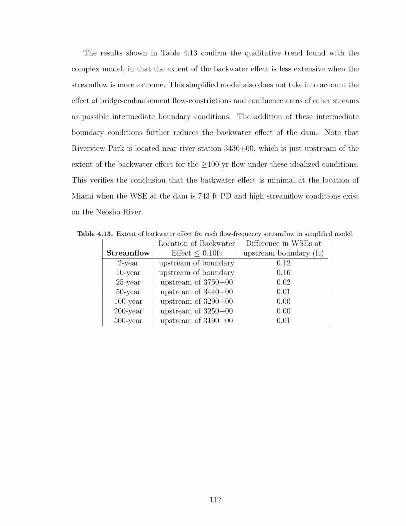
The results shown in Table 4.13 confirm the qualitative trend found with the
complex model, in that the extent of the backwater effect is less extensive when the
streamflow is more extreme. This simplified model also does not take into account the
effect of bridge-embankement flow-constrictions and confluence areas of other streams
as possible intermediate boundary conditions. The addition of these intermediate
boundary conditions further reduces the backwater effect of the dam. Note that
Riverview Park is located near river station 3436+00, which is just upstream of the
extent of the backwater effect for the ≥100-yr flow under these idealized conditions.
This verifies the conclusion that the backwater effect is minimal at the location of
Miami when the WSE at the dam is 743 ft PD and high streamflow conditions exist
on the Neosho River.
Table 4.13. Extent of backwater effect for each flow-frequency streamflow in simplified model.Location of Backwater Difference in WSEs at
Streamflow Effect ≤ 0.10ft upstream boundary (ft)2-year upstream of boundary 0.1210-year upstream of boundary 0.1625-year upstream of 3750+00 0.0250-year upstream of 3440+00 0.01100-year upstream of 3290+00 0.00200-year upstream of 3250+00 0.00500-year upstream of 3190+00 0.01
112

(a) 2-year Flow (b) 10-year Flow
(c) 25-year Flow (d) 50-year Flow
(e) 100-Year Flow (f) 200-year Flow
(g) 500-year Flow
Figure 4.32. Backwater Extents for flood-frequency streamflows for a simplified model of theGrand Lake region.
113

Model Verification Part 2: Steady vs. Unsteady model comparison to ver-
ify conservativeness of steady-state model
As discussed in Section 4.4.3, the assumption that the steady-state computation
method is more conservative for a given streamflow condition than the unsteady
method was tested by comparing the two methods with the September 2009 flow
scenario. The peak streamflow condition on the Neosho River occurred at 6:00AM
on 9/12/2009, and the system boundary conditions at this time are represented in
Table 4.14. These boundary conditions were used in a steady-state model in HEC-
RAS in order to compare the WSEs from the steady state run to the WSEs at the
6:00AM time step of the unsteady run.
Table 4.14. Boundary conditions for use in steady-state comparison of September 2009 peak flowconditions: 9/12/2009 at 6:00 AM.
Boundary Name Boundary ConditionNeosho River, Commerce gauge 44,600 cfs
Tar Creek, Miami gauge 63 cfsSpring River, Quapaw gauge 2,250 cfsElk River, Tiff City gauge 431 cfs
Pensacola Dam 746.72 ft NAVD88
The results of this comparison are shown in Figure 4.33. These results represent
the steady-state WSE minus the unsteady WSE. Therefore, a positive value represents
a higher WSE in the steady-state model, and a negative value represents a higher WSE
in the unsteady model.
The steady-state WSEs in the priority 1 section are generally 0.90 to 1.00 ft
higher than those in the unsteady-flow simulation. This priority 1 section is most
relevant because it is immediately downstream of the boundary condition at which
the streamflow conditions are being introduced to the system. Because there are no
negative values, this process confirms the assumption that for a given peak streamflow,
114

the steady-state WSE computation method of HEC-RAS is more conservative than
the unsteady-state computation method.
Figure 4.33. Comparison of steady vs. unsteady flow WSE computation techniques for peakSeptember 2009 flow.
Model Verification Part 3: Comparison to Holly model to verify consis-
tency with previous studies
This model verification compares the results included in Holly’s (2004) report to re-
sults from the current hydraulic model for similar streamflow and downstream bound-
ary conditions. These values are representative of the June 1995 storm WSEs, which
were used by Holly in the 2004 report to compare the effect of two WSEs at Pen-
sacola Dam. The difference in WSEs at the location of Miami, OK is included in
the following figures. The location of Riverview Park (c.f. Section 4.3.3) in Miami is
represented in Figures 4.34, and 4.35.
As discussed in Section 2.1.3, Holly used a pseudo-2D model called C1/C2 in order
to calculate the WSEs for his report [Holly Jr., 2004]. Although this thesis research
was conducted using a true 1D model, the results are very similar to Holly’s results
using the pseudo-2D model. This information helps to verify the validity of the 1D
model, as opposed to a more complex model system, for this research context.
115

Figure 4.34. Comparison of Holly model WSE to Current model at location of RP in prioritysection 1. The WSE shown represents the max WSE calculated during the June 1995 flood with thedam WSE held at 742 ft PD.
Location of Riverview ParkModel Station 3436+47Dam WSE 745 ft PD
Max WSE from Holly model: 766.93 ft NAVD88Max WSE from Current model: 766.67 ft NAVD88
Figure 4.35. Comparison of Holly model WSE to Current model at location of RP in prioritysection 1. The WSE shown represents the max WSE calculated during the June 1995 flood with thedam WSE held at 745 ft PD.
116

4.4.2 Global Sensitivity Analysis
The RMSE values in Table 4.15 indicate the amount of influence each particular
phenomenon has over the WSEs in each priority section. A few notable results from
the global sensitivity analysis are discussed in the bulleted list below:
• Results in all three priority sections are most sensitive to the roughness coef-
ficient (Manning’s n) along the Neosho River channel, followed closely by the
streamflow in the Neosho. These sensitivity rankings are somewhat subjective
when comparing two completely different phenomena due to the fact that there
are various degrees of extremes that may be used for each phenomenon. For
example, the roughness coefficient is bound by the values explained in Sec-
tion 3.4.2, while streamflow values are bound by upper and lower limits that
are indicated by the probability of exceedance. These differences in extremes
cause variation in what is represented by the RMSE value shown in the table,
which is the sum of the effect of the analyzed range of each phenomenon.
• For the Priority 1 section, the WSEs are 5.5 times more sensitive to the stream-
flow on the Neosho River than the dam WSE. The WSEs in the Priority 2
section are about 2.4 times more sensitive to the Neosho River streamflow than
the Tar Creek streamflow, although the section is along Tar Creek. This reveals
that WSEs along Tar Creek near Miami are much more sensitive to high flows
along the Neosho River (the downstream boundary condition of Tar Creek)
than high flows along Tar Creek. The WSEs at each of the priority sections are
also sensitive to the dam WSE, though not nearly so much as to the magnitude
of the Neosho River streamflow. Note that the most conservative streamflow
estimations were used for the model application portion of the research (c.f. Ta-
ble 4.7 in Section 4.1.5). The B-17B procedure estimates a 100-yr streamflow
117

of 152,500 cfs while the best-fit, less-conservative procedure estimates a 100-yr
streamflow of 65,000 cfs.
• Among the non-Manning’s n phenomena, the streamflow magnitude, WSEs at
the dam, and the bridges are the phenomena that create the largest effect on
water levels near Miami.
• There are several phenomena included in the global sensitivity analysis that
have no effect on WSEs in the priority sections. The phenomena that have a
value of 0.000 in Table 4.15 in a specific priority section have no effect on the
WSE in that priority section. The roughness coefficients on the Spring and Elk
Rivers do not have an effect in any of the three priority sections.
118

Tab
le4.
15.Globa
lSen
sitivity
Ana
lysis
:Se
nsitivity
ofpriorit
ylocatio
nW
SEsto
vario
usmod
elph
enom
ena.
Phenom
enon
Degreeof
Sensitivity
forLo
catio
nPr
iorit
y1
Priorit
y2
Priorit
y3
Ran
kRMSE
Ran
kRMSE
Ran
kRMSE
Stream
flow
Neosho
25.36
22
2.95
02
3.49
2Sp
ring
50.45
17
0.39
95
1.51
5Ta
rCreek
70.09
25
1.21
67
0.08
8Elk
80.00
310
0.00
38
0.00
6
Rou
ghne
ssCoefficient
Neosho
Cha
nnel
15.78
51
3.19
41
6.55
4Floo
dplain
32.29
84
1.28
13
2.83
6Ta
rCreek
Cha
nnel
-0.00
03
1.57
6-
0.00
0Floo
dplain
-0.00
08
0.26
7-
0.00
0Sp
ring
Cha
nnel
-0.00
0-
0.00
0-
0.00
0Floo
dplain
-0.00
0-
0.00
0-
0.00
0Elk
Cha
nnel
-0.00
0-
0.00
0-
0.00
0Floo
dplain
-0.00
0-
0.00
0-
0.00
0Dam
WSE
40.96
56
0.82
84
2.08
7
119

4.4.3 Specific Sensitivity Analyses
Determining the sensitivity of results to changes in Manning’s n
The Manning’s n, being a lumped parameter for various physical phenomena in the
system, is a user-defined parameter. The global sensitivity analysis determined that
the model is significantly sensitive to this user-defined parameter along the Neosho
River channel and floodplain. For this reason, a secondary sensitivity analysis is
necessary to determine how sensitive the conclusions of the research are to changes
in Manning’s n.
This second phase of the sensitivity analysis involves varying the Manning’s n
in only the Priority 1 section, and then applying the research question to the mod-
ified scenarios in order to determine the sensitivity of the research conclusions to
the changing parameters. The following tables represent the results of changing the
Neosho River channel and floodplain Manning’s n values across the typical ranges
outlined in Chow (2009). Due to the fact that HEC-RAS outputs WSEs accurate to
the hundredths decimal place, the values in the following tables have been rounded to
the hundredths decimal place as well, in order to maintain consistency. The “Base”
scenario in each table represents the final calibrated Manning’s n values from Sec-
tion 4.3.1.
Tables 4.16, 4.17, and 4.18 represent the research conclusions’ sensitivity to the
roughness value in the Neosho River channel. The Manning’s n along the channel is
varied (in quartiles) between 0.025 and 0.10, while the rest of the model remains the
same as the base geometry. Table 4.16 represents the average difference between the
WSEs calculated in the Priority 1 section when changing the boundary condition at
the dam from a WSE of 741 to 743 ft PD. The values in Table 4.17 represent the
maximum difference along the Priority 1 section for the same scenarios. Table 4.18
shows the maximum WSE calculated in the Priority 1 section when the boundary
120

condition at the dam is a WSE of 743 ft PD. This table is included to understand
at what flow and roughness scenario the WSE begins to exceed flood stage (760.33
ft NAVD88) in the Miami area [NOAA, 2013]. In each table, the grey-colored cell
values represent conditions at which the max WSE exceeds flood stage (i.e., the
USACE easements).
Table 4.16. Sensitivity analysis of changes in Manning’s n in Neosho River channel. Averagechange in WSE (ft) in Priority 1 section due to changing dam WSE from 741 to 743 ft PD shown.Shaded cells represent conditions for which the flooding easements are exceeded in Miami.
Roughness Channel Flood-Frequency (yrs)Scenario Mannings n 2 10 25 50 100 200 500Base 0.03 1.76 0.15 0.04 0.03 0.02 0.00 0.01Holly 0.035 1.65 0.14 0.06 0.04 0.02 0.03 0.03lowest 0.025 1.76 0.15 0.04 0.03 0.02 0.00 0.0125% 0.04375 1.82 0.22 0.05 0.03 0.02 0.01 0.0150% 0.0625 1.56 0.03 0.02 0.02 0.01 0.00 0.0175% 0.08125 1.31 0.03 0.02 0.01 0.01 0.00 0.01
highest 0.10 0.90 0.02 0.01 0.01 0.01 0.00 0.01
Table 4.17. Sensitivity analysis of changes in Manning’s n in Neosho River channel. Maximumchange in WSE (ft) in Priority 1 section due to changing dam WSE from 741 to 743 ft PD shown.Shaded cells represent conditions for which the flooding easements are exceeded in Miami.
Roughness Channel Flood-Frequency (yrs)Scenario Mannings n 2 10 25 50 100 200 500Base 0.03 1.83 0.20 0.05 0.03 0.03 0.01 0.02Holly 0.035 1.76 0.19 0.07 0.05 0.04 0.04 0.04lowest 0.025 1.83 0.20 0.05 0.03 0.03 0.01 0.0225% 0.04375 1.88 0.28 0.10 0.04 0.03 0.01 0.0250% 0.0625 1.70 0.05 0.04 0.03 0.02 0.01 0.0275% 0.08125 1.50 0.06 0.02 0.02 0.02 0.01 0.01
highest 0.10 1.10 0.03 0.02 0.01 0.01 0.01 0.01
121

Table 4.18. Sensitivity analysis of changes in Manning’s n in Neosho River channel. Highestcalculated WSE (ft NAVD88) in Priority 1 section due to dam WSE of 743 ft PD shown. Shadedcells represent conditions for which the flooding easements are exceeded in Miami.
Roughness Flood-Frequency (yrs)Scenario 2 10 25 50 100 200 500Base 746.24 757.26 763.27 767.79 772.30 776.00 781.18Holly 746.55 758.84 765.94 771.23 776.40 781.50 788.62lowest 746.24 757.26 763.27 767.79 772.30 776.00 781.1825% 746.07 756.18 762.54 767.26 772.04 776.04 781.2750% 746.80 759.16 764.70 768.85 773.01 776.24 781.3375% 747.70 760.69 765.91 769.80 773.56 776.79 781.70
highest 749.57 762.28 767.18 770.83 774.30 777.67 782.54
Tables 4.19, 4.20, and 4.21 represent the research question’s sensitivity to the
roughness value in the Neosho River floodplain. The Manning’s n along the floodplain
is varied (in quartiles) between 0.025 and 0.20 while the rest of the model remains the
same as the calibrated Manning’s n values from Section 4.3.1. The tables are similar
to, and follow the same order as, those listed above.
Table 4.19. Sensitivity analysis of changes in Manning’s n in Neosho River floodplain. Averagechange in WSE (ft) in Priority 1 section due to changing dam WSE from 741 to 743 ft PD shown.Shaded cells represent conditions for which the flooding easements are exceeded in Miami.
Roughness Floodplain Flood-Frequency (yrs)Scenario Mannings n 2 10 25 50 100 200 500Base 0.013-0.08 1.76 0.15 0.04 0.03 0.02 0.00 0.01Holly 0.10 1.65 0.14 0.06 0.04 0.02 0.03 0.03lowest 0.025 1.76 0.12 0.04 0.03 0.01 0.01 0.0125% 0.06875 1.76 0.16 0.04 0.03 0.01 0.02 0.0150% 0.1125 1.76 0.18 0.04 0.00 0.01 0.01 0.0175% 0.15625 1.76 0.18 0.05 0.06 0.00 0.01 0.01
highest 0.20 1.76 0.18 0.05 0.03 0.01 0.01 0.01
This sensitivity analysis provides confidence in the results of the model application
by demonstrating that within the entire range of plausible Manning’s n values, the
results of the proposed rule curve adjustment would not raise WSEs above flood stage
more than 0.07 ft, as shown in the shaded cells in the tables. In model applications
122

Table 4.20. Sensitivity analysis of changes in Manning’s n in Neosho River floodplain. Maximumchange in WSE (ft) in Priority 1 section due to changing dam WSE from 741 to 743 ft PD shown.Shaded cells represent conditions for which the flooding easements are exceeded in Miami.
Roughness Floodplain Flood-Frequency (yrs)Scenario Mannings n 2 10 25 50 100 200 500Base 0.013-0.08 1.83 0.20 0.05 0.03 0.03 0.01 0.02Holly 0.10 1.76 0.19 0.07 0.05 0.04 0.04 0.04lowest 0.025 1.83 0.17 0.05 0.04 0.01 0.02 0.0225% 0.06875 1.83 0.21 0.06 0.03 0.02 0.03 0.0250% 0.1125 1.83 0.23 0.06 0.01 0.02 0.01 0.0175% 0.15625 1.83 0.23 0.06 0.07 0.00 0.01 0.01
highest 0.20 1.83 0.24 0.06 0.04 0.02 0.01 0.01
Table 4.21. Sensitivity analysis of changes in Manning’s n in Neosho River floodplain. Highestcalculated WSE (ft NAVD88) in Priority 1 section due to dam WSE of 743 ft PD shown. Shadedcells represent conditions for which the flooding easements are exceeded in Miami.
Roughness Flood-Frequency (yrs)Scenario 2 10 25 50 100 200 500Base 746.24 757.26 763.27 767.79 772.30 776.00 781.18Holly 746.55 758.84 765.94 771.23 776.40 781.50 788.62lowest 746.24 756.79 761.63 765.44 769.32 773.33 777.7425% 746.24 757.37 763.92 768.97 774.10 778.18 784.2950% 746.24 757.55 764.86 770.60 776.17 781.07 788.1675% 746.24 757.64 765.36 771.53 777.31 783.00 790.45
highest 746.24 757.68 765.68 772.12 778.15 784.22 792.22
using lumped parameters such as Manning’s n, there can be considerable debate over
the “correct” value of Manning’s n to use for a certain application, but this sensitivity
study preempts such debate, because the flood elevations are relatively insulated from
ranges of Manning’s n found in practice.
Determining the sensitivity of results to WSEs at the dam exceeding 743
ft PD
Table 4.22 shows the results of the Riverware study completed by the USACE men-
tioned in Section 3.4.3 [Daylor, 2012]. The percentage of time in one year that a
specific dam WSE is exceeded under each rule curve is shown in the table, along with
123

a conversion of that percentage into number of days. Note that the WSEs both above
and below the target elevations are included, accounting for both flood and drought
scenarios.
Table 4.22. Results of the USACE Riverware analysis [Daylor, 2012].Percent of Time Lake Elevation is Equalled or Exceeded
Elevation Existing Rule Typical Year Proposed Typical Year(ft PD) Curve No. of Days Rule Curve No. of Days755.00 0.000% <1 0.000% <1754.86 0.004% <1 0.004% <1750.00 2.03% 7 2.05% 7748.00 3.9% 14 3.9% 14746.00 7.8% 29 7.9% 29745.00 12.7% 46 13.0% 47744.50 15.9% 58 16.3% 60744.00 20.4% 75 20.8% 76743.00 39.4% 144 41.3% 151742.77 41.6% 152 50.0% 182.5742.50 44.1% 161 53.0% 193742.18 50.0% 182.5 60.1% 219742.00 78.2% 285 96.3% 352741.71 81.6% 298 100% 365741.50 83.4% 304741.00 96.6% 353740.25 100% 365
Table 4.23 shows the value of the difference (proposed minus existing) of the
percent time the lake elevation is equaled or exceeded, along with the difference in
the typical number of days per year the particular lake elevations is exceeded. This
table helps to prioritize the dam WSE situations requiring further investigation for
determining the effect of the proposed rule curve adjustment.
Steady-state high-dam analysis
In Table 4.23, it is apparent that dam WSEs 744, 744.5, and 745 require further
investigation, because the proposed rule curve causes the dam WSE to be exceeded
for at least one additional day per year. DamWSEs of 746 and 750 are exceeded under
124

Table 4.23. Continued results of the USACE Riverware analysis.Differences Between Existing and Proposed Rule CurvesElevation Difference Difference(ft PD) % Time Exceeded Typ. No. of Days755.00 0.00% 0754.86 0.00% 0750.00 0.02% 0748.00 0.00% 0746.00 0.10% 0745.00 0.30% 1744.50 0.40% 2744.00 0.40% 1743.00 1.90% 7742.77 8.40% 31742.50 8.90% 32742.18 10.10% 37742.00 18.10% 67741.71 18.40% 67741.50 16.60% 61741.00 3.40% 12740.25 0.00% 0
the proposed rule curve 0.10% and 0.02% more often, respectively. These dam WSEs
will be investigated using the 0.01%, 0.05%, and 0.02% probability streamflows (100-,
200-, and 500-yr flood-frequencies, respectively) in order to investigate the behavior
of the system under extreme streamflows, which would feasibly cause the dam to rise
to the 746 and 750 ft PD levels.
For each of these scenarios, the existing rule curve will be represented by a dam
WSE 2 ft lower than the high-dam WSEs tested, because the existing rule curve is
initially 2 ft below the proposed rule curve for the August 15 - September 15 time
period. It would be impossible to predict the exact behavior of the stage vs. time
hydrograph at the dam under the respective rule curves because the dam WSE is
not controlled solely by meteorologic phenomenon, but by human intervention in the
form of dam releases. The dam WSEs of 741 to 745 ft PD are controlled by GRDA,
and WSEs of 745 to 755 ft PD are controlled by the USACE [GRDA, 2013]. However,
125

because of the geometry of Grand Lake, the stage vs. storage curve is of a shape that
confirms a peak difference of 2 ft is conservative for maximizing the perceived effect
of a raised rule curve. A proof that this assumption is physically reasonable may be
found in Appendix D.
Table 4.24. Maximum WSE calculated in Priority 1 location for various high-dam conditions underthe proposed rule curve conditions.
Dam WSE Flood-Frequency (yrs)(ft PD) 2 10 25 50 100 200 500744 747.13 757.34 763.29 767.81 772.31 776.01 781.19744.5 747.58 757.38 763.30 767.82 772.32 776.01 781.19745 748.03 757.43 763.32 767.83 772.32 776.01 781.20746 748.97 757.54 763.36 767.86 772.34 776.02 781.21750 752.86 758.26 763.66 768.03 772.47 776.07 781.26
Table 4.25. Maximum WSE difference between proposed and existing scenarios in Priority 1location for various high-dam conditions. Note that existing rule curve WSEs are assumed to beexactly 2 ft lower in elevation at the dam.
Proposed Rule Curve Flood-Frequency (yrs)Dam WSE (ft PD) 2 10 25 50 100 200 500
744 1.88 0.24 0.07 0.05 0.03 0.02 0.02744.5 1.89 0.27 0.08 0.07 0.04 0.02 0.02745 1.91 0.29 0.09 0.05 0.04 0.03 0.02746 1.93 0.36 0.11 0.07 0.05 0.03 0.03750 1.98 0.66 0.29 0.12 0.15 0.06 0.05
The results of the high-dam-WSE analysis, shown in Table 4.24, reveal that there
is very little difference in upstream WSEs for the various dam conditions, particularly
between dam WSEs 744 and 746 ft PD. In the event that the WSE at the dam rises
a full 6 feet from the target WSE, the proposed rule curve adjustment causes a
maximum of 0.15 ft difference for the 100-year flood in the Priority 1 section. An
analysis of the 100-year flood reveals that the Abandoned Bridge in Miami is at over-
topping stage for this streamflow condition, which likely contributes to the larger
increase in backwater effect.
126

Table 4.26. Average WSE difference between proposed and existing scenarios in Priority 1 locationfor various high-dam conditions. Note that existing rule curve WSEs are assumed to be exactly 2 ftlower in elevation at the dam.
Proposed Rule Curve Flood-Frequency (yrs)Dam WSE (ft PD) 2 10 25 50 100 200 500
744 1.82 0.18 0.05 0.04 0.02 0.01 0.01744.5 1.84 0.20 0.06 0.05 0.03 0.01 0.02745 1.86 0.23 0.07 0.04 0.03 0.02 0.02746 1.89 0.27 0.09 0.06 0.03 0.01 0.02750 1.98 0.53 0.24 0.10 0.10 0.04 0.04
Unsteady-flow high-dam analysis
A hypothetical unsteady-flow scenario was created in order to compare the results of
the September 2009 flood used in the calibration process to the results of the same
flood with WSEs at the dam 2 ft higher than the observed data. It is important to
note that this hypothetical scenario is not meant to be a realistic representation of
the expected conditions during the 2009 flood had the proposed rule curve been in
effect at that time. However, this hypothetical scenario is used for the purpose of
demonstrating that a two foot increase in WSE at the dam causes a similar effect in
both unsteady and steady-state analyses.
According to the statistical analysis results, the September 2009 flood peak flow
falls between the 10- and 25-year August 15 - September 15 flow magnitude. The peak
observed WSE at the dam during this event was 746.84 ft PD, or 748.24 ft NAVD88.
Therefore, under the hypothetical scenario, the peak WSE at the dam was 748.84
ft PD, or 750.24 ft NAVD88. The peak modeled WSE at the location of Riverview
Park in Miami under the hypothetical scenario is 758.79 ft NAVD88, compared to
the peak WSE in the calibrated model scenario of 758.55 ft NAVD88. This difference
of 0.24 ft is consistent with the results found in the steady-state analysis shown in
Table 4.26.
127

Fitting a polynomial to the daily-average data from Pensacola Dam
As mentioned in Section 3.4.3, a polynomial was fit to the daily-average dam WSE
data for the September 2009 flood in order to determine whether the results of the
model application are significantly different when using a finer time-increment at the
dam location. The NSC efficiency value comparing the results from the model using
the daily-average dam data to the 3 hr time-increment dam data is 0.99995 for the
full 68-day time period, and 0.99998 for the peak event occurring between 9/8 - 9/16.
These results show that using the finer time-increment dataset at the location of
Pensacola dam has virtually no effect on the behavior of the WSE profile upstream,
compared to the daily-average dataset. These conclusions suggest that using a stage
vs. time hydrograph at a cross-section as the downstream boundary condition for the
hydraulic model is a viable alternative to using an inline-structure approach to model
time-varied effects at the dam.
Determining the sensitivity of results to the effect of structures constrict-
ing streamflow along the Neosho River
As discussed in Section 3.4.3, investigation of the structures constricting flow along
the Neosho River is warranted by the Daylor (2012) study that hypothesized the
structures cause an increase in WSEs near Miami. Furthermore, as discussed in
Section 4.3.3, the simulations of this thesis show that the bridges constrict the flow
at higher return periods.
Table 4.27 contains the results of the analysis of the effect of structures on WSEs in
the priority 1 section. The maximum WSE and average WSE for each model scenario
in the priority section are shown. The max WSE represents the highest calculated
WSE in the priority section for the model scenario. The average WSE represents the
mean of the WSEs calculated at each cross section.
128
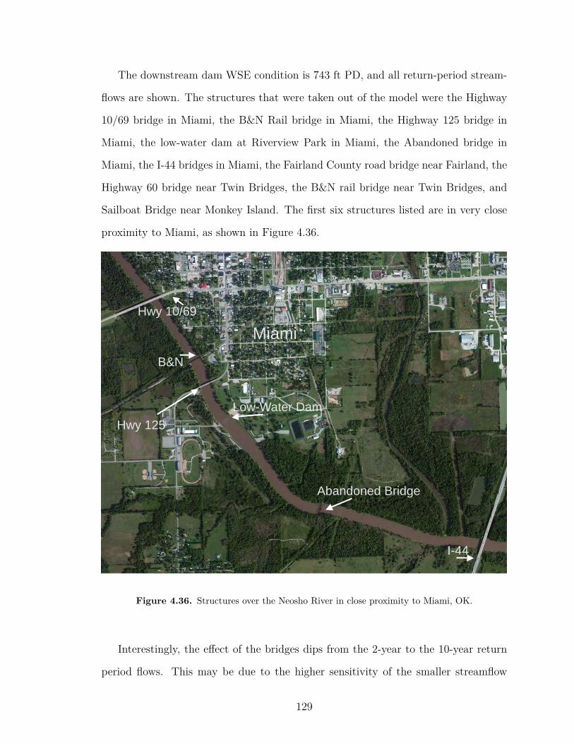
The downstream dam WSE condition is 743 ft PD, and all return-period stream-
flows are shown. The structures that were taken out of the model were the Highway
10/69 bridge in Miami, the B&N Rail bridge in Miami, the Highway 125 bridge in
Miami, the low-water dam at Riverview Park in Miami, the Abandoned bridge in
Miami, the I-44 bridges in Miami, the Fairland County road bridge near Fairland, the
Highway 60 bridge near Twin Bridges, the B&N rail bridge near Twin Bridges, and
Sailboat Bridge near Monkey Island. The first six structures listed are in very close
proximity to Miami, as shown in Figure 4.36.
MiamiHwy 10/69
B&N
Hwy 125Low-Water Dam
Abandoned Bridge
I-44
Figure 4.36. Structures over the Neosho River in close proximity to Miami, OK.
Interestingly, the effect of the bridges dips from the 2-year to the 10-year return
period flows. This may be due to the higher sensitivity of the smaller streamflow
129

Table 4.27. Analysis of effect of bridges on upstream WSEs in the priority 1 section.Flood-Frequency (yrs)
Scenario 2 10 25 50 100 200 500
With Bridges Avg 746.03 756.07 762.08 766.69 771.22 775.12 780.59Max 746.24 757.26 763.27 767.79 772.30 776.00 781.18
No Bridges Avg 745.03 755.67 761.59 765.77 769.80 773.70 779.14Max 745.26 756.85 762.72 766.76 770.59 774.33 779.56
Difference Avg 1.00 0.40 0.49 0.92 1.42 1.42 1.45Max 0.98 0.41 0.55 1.03 1.71 1.67 1.62
magnitude to the bridge piers constricting flow in the channel. The 10-year flow,
being more intense, but not overflowing the river banks, is affected by the bridge
piers, is not as sensitive to the obstruction in the river channel. As the flow magnitude
increases beyond the 10-year flow, however, the bridge embankments in the floodplain
begin to influence the WSEs as well as the bridge piers in the river channel.
The results shown in Table 4.27 reveal that the bridges have a significantly greater
effect on the WSEs in the priority 1 section than the proposed rule curve adjustment.
These results would corroborate the findings that the proposed rule curve has a min-
imal effect on backwater WSEs. Because the structures create increased backwater
effects at a location between the dam and the priority location, they are acting as
an intermediate boundary condition, reducing the effect of the boundary condition
at the dam [Bedient et al., 2013]. The results of this sensitivity analysis provide an
explanation of the decreased effect of the proposed rule curve adjustment on WSEs
near Miami.
The results confirm the bridges constrict the flow and create a greater difference
in WSE than raising the water level at the dam 2 feet. For future research, a study
should systematically remove one bridge at a time (while all the others remain) and
rate the relative impact of the different bridges. Also for future research, a study
should look at what flow each bridge constricts the flow enough that the upstream
WSE is significantly changed.
130

CHAPTER 5
Conclusions and Future Research
5.1 Conclusions
A hydraulic model of the Grand Lake hydrologic system was developed for the purpose
of analyzing the impact on upstream WSEs of a proposed rule curve adjustment at
Pensacola Dam in Langley, Oklahoma. The model was developed with the HEC-RAS
hydraulic model, and it was calibrated and validated using the unsteady flow routing
capabilities of that program [Brunner, 2010]. The model geometry was developed in
ArcGIS using the most advanced datasets for the region [ESRI, 2011; Gesch, 2007;
OWRB, 2009]. The GIS model geometry was exported to HEC-RAS using the HEC-
GeoRAS tool.
A statistical analysis was conducted of the historic August 15 to September 15
streamflow records for each of the four major tributaries. Annual maxima and partial
duration data collection methods were compared. The annual maxima method was
determined to be the most conservative method. The final statistical analysis was
performed with annual maxima data according to the guidelines in Bulletin 17B of
the U.S. Water Resources Council [USGS, 1982]. Return-period streamflows were
calculated for each of the following streams: the Neosho River, Spring River, Elk
River, and Tar Creek. These extreme streamflows were used as upstream boundary
conditions for the hydraulic model. The USGS gauge locations at which the stream-
flow records were recorded were used as the upstream boundary locations on each
tributary.
131

The downstream boundary condition for the steady-state hydraulic model was a
known WSE representing the lake level at Pensacola Dam. In order to determine the
upstream effect of the proposed rule curve adjustment, the downstream WSE was
alternated between 742.4 ft NAVD88 (741 ft PD, the existing rule curve target WSE
for the relevant time period) and 744.4 ft NAVD88 (743 ft PD, the proposed rule
curve target WSE for the relevant time period).
According to the tests performed in this research, an increase in streamflow mag-
nitude causes an increase in upstream WSEs, but the impact of the proposed rule
curve adjustment on upstream WSEs decreases. The location of Riverview Park in
Miami, OK is considered the first to flood by the National Weather Service [NOAA,
2013]. The impact of the proposed rule curve adjustment on this location is less than
0.20 ft for all of the scenarios investigated in this thesis research.
An investigation into effects of dam WSEs exceeding the target WSE due to the
proposed rule curve was also conducted. The dam WSEs that are more likely to be
exceeded due to the proposed rule curve were provided in a study from the USACE
[Daylor, 2012]. These higher dam WSEs were investigated based on a difference
in WSE at the dam of 2.0 ft between the proposed and existing rule curves. The
proposed rule curve causes a maximum of 0.15 ft increase in WSEs in the Priority
1 location for the full range of flow scenarios and dam WSE scenarios tested. Thus,
even with rarely seen WSEs at the dam, the two foot WSE difference at the dam
causes much smaller changes at upstream priority locations.
A sensitivity analysis was performed to test the model sensitivity to changes in
the hydraulic roughness parameter, Manning’s n. The maximum increase in WSEs
over flood-stage due to the proposed rule curve adjustment in the Priority 1 section,
for all flow scenarios and Manning’s n scenarios, was 0.07 ft. This sensitivity analysis
provides confidence in the conclusion that the two foot WSE increase at the dam has
minimal effect on the upstream WSEs in priority locations.
132

These results are consistent with conclusions of previous research by Holly (2004)
that found that the raising the power pool from 741 to 745 ft PD causes less than a
0.20 ft increase on WSEs near Miami, OK. USACE (1998) also determined that the
highest possible dam elevation of 755 ft PD has less than a 0.50 ft effect on depth in
the locations named “Priority 1” in this research.
In conclusion, the effect of the proposed rule curve adjustment has been shown to
have less than a 0.20 ft effect on WSEs in priority locations near Miami, OK.
5.2 Future Work
1. The hydraulic model developed for this thesis was created with the best available
software and best available datasets at the time it was completed in 2014. More
advanced data collection techniques will inevitably allow for improvement of
the model geometry, and advances in computer modeling will inevitably lead
to more accurate modeling capabilities in the future. Despite these advances,
it is likely that the improved technology will serve to confirm the conclusions
reached in this research as well as the prior research conducted by Holly (2004)
and the USACE (1998).
2. Channel bathymetry datasets have significant room for improvement on the
Neosho, Spring, and Elk Rivers. The most recent datasets were collected over
15 years ago using manual survey techniques. The level of sophistication of
bathymetric surveying has improved dramatically since that time, as evidenced
by the OWRB (2009) study included in this report. An updated bathymetric
survey of these locations should be considered.
3. A two-dimensional unsteady hydraulic model may be more feasible with the
release of HEC-RAS 5.0, a USACE software currently in “beta” form (i.e.,
not released for public use). This 2D capability may allow for more accurate
133

portrayals of the reservoir storage capacity for Grand Lake and upstream flood-
plains. An unsteady flow model depicting the reservoir and floodplains with a
stage/storage relationship would be possible if this were the case. This type
of model would allow for investigation of the lag time required to change the
reservoir stage due to dam outflows and flood water inflows from upstream
tributaries, and the effect that this lag time has on upstream water levels. A
pseudo-2D unsteady flow model was used in the Holly (2004) research to por-
tray the floodplain upstream of Miami, but this method has not been used
to represent the Grand Lake reservoir. Future research could potentially use
HEC-RAS 5.0 to include this approach to modeling the Grand Lake reservoir
and floodplains along the tributaries.
4. There is a wide variety of data sources covering the Grand Lake region. These
data should be organized, normalized, and confirmed. One example is the stage-
storage relationship of the reservoir. The OWRB (2009) report concludes that
the storage capacity of Grand Lake is 1,515,415 acre-ft when the dam WSE is
745 ft PD. The National Water Information System website for the Pensacola
Dam gauge reports that the storage is 1,672,000 acre-ft at a dam WSE of 745
ft PD [USGS, 2012]. The true value of the stage-storage relationship should be
determined so that stream inflow and dam outflow may be managed accurately.
This report provides a large amount of organization and normalization of the
Grand Lake data, and the TIN created for this research may be used with the
HYPACK program that OWRB used to create the stage vs. storage curve in
the 2009 report [OWRB, 2009]. The merged-TIN may be used in HYPACK to
develop an updated stage vs. storage curve that extends all the way to the top
of the flood pool (755 ft PD) at Pensacola Dam.
134

5. Future investigation of the effect of bridges in the Miami area is warranted by
the results of this thesis, as mentioned in Section 4.4.3. The nine structures in
the vicinity of Miami have been shown to have a significant effect on WSEs in
the priority locations. Detailed investigations of the effect of particular bridges
is a possibility for future research into the cause of higher WSEs in the priority
locations.
6. An investigation into the effect of the reduced hydraulic roughness upstream
of Miami due to agricultural development is another topic requiring future re-
search. The wide floodplain of previously forested area upstream of Miami has
been developed into agricultural land, likely reducing the ability of that area
to detain floodwaters during an extreme-streamflow event. The global sen-
sitivity analysis conducted for this research (Section 4.4.2) suggests that the
floodplain hydraulic roughness value has an effect on WSEs in the priority loca-
tions. Research should be conducted investigating the effect of the agricultural
development upstream of Miami on WSEs in Miami during extreme streamflow
events occurring on the Neosho River.
7. The results contained in this thesis represent the effect of the current pro-
posed rule curve modification, which affects the time period from August 15-
September 15 in any given year. Therefore, the statistical return period stream-
flows contained herein represent the August 15-September 15 time frame. In
the event that future rule curve modifications are proposed for other months
of the year, more research will be required in order to determine return period
streamflows for those portions of the year, and the model will require further
calibration in order to represent roughness conditions for the new scenario.
135

References
Ackerman, C. T. HEC-GeoRAS User’s Manual. U.S. Army Corps of Engineers, Davis,CA, September 2009.
Adamowski, K. Regional Analysis of Annual Maximum and Partial Duration FloodData by Nonparametric and L-moment Methods. Journal of Hydrology, 229(3–4):219 – 231, 2000. ISSN 0022-1694. URL http://www.sciencedirect.com/science/article/pii/S0022169400001566.
Arcement Jr., G. and Schneider, V. Guide for Selecting Manning’s Roughness Coeffi-cient For Natural Channels and Flood Plains. Hydraulics Engineering Publications,1984.
Ashkar, F. and Ouarda, T. On some methods of fitting the generalized Pareto dis-tribution. Journal of Hydrology, 177(1):117–141, 03 1996.
Awawdeh, M. M. GIS-Based Evaluation of the Conservation Reserve Program inTexas County, Oklahoma. Master’s thesis, Oklahoma State University, 05 2004.
Bedient, P. B., Huber, W. C., and Vieux, B. E. Hydrology and Floodplain Analysis.Pearson Education, Inc., 5 edition, 2013.
Brunner, G. HEC-RAS River Analysis Systems User’s Manual: Version 4.1. USACE,January 2010.
Buckley, M. K. Memo on Policy for Use of HEC-RAS in the NFIP. Technical report,Federal Emergency Management Agency, Washington DC, April 2001.
Chow, T. Open-Channel Hydraulics. McGraw-Hill civil engineering series. BlackburnPress, 2009. ISBN 9781932846188. URL http://books.google.com.et/books?id=JG9_PwAACAAJ.
Cunnane, C. A Particular Comparison of Annual Maxima and Partial DurationSeries Methods of Flood Frequency Prediction. Journal of Hydrology, 18(3–4):257– 271, 1973. ISSN 0022-1694. URL http://www.sciencedirect.com/science/article/pii/0022169473900516.
Daylor, J. RiverWare Simulations for Proposed Change with Seasonal Pool GuideCurve. Technical report, USACE, 2012.
Efron, B. and Tibshirani, R. Bootstrap Methods for Standard Errors, ConfidenceIntervals, and Other Measures of Statistical Accuracy. Statistical Science, 1(1):pp.54–75, 1986. ISSN 08834237. URL http://www.jstor.org/stable/2245500.
136

Ekanayake, S. and Cruise, J. Comparisons of Weibull- and exponential-based partialduration stochastic flood models. Stochastic Hydrology and Hydraulics, 7(4):283–297, 1993. ISSN 0931-1955. URL http://dx.doi.org/10.1007/BF01581616.
England Jr, J. F. and Cohn, T. A. Scientific and Practical Considerations Related toRevising Bulletin 17B: The case for improved treatment of historical informationand low outliers. 2007.
ESRI. ArcGIS Desktop: Release 10, 2011.
Farmer, W. and Vogel, R. Performance-Weighted Methods for Estimating MonthlyStreamflow at Ungauged Sites. Journal of Hydrology, 477(0):240 – 250, 2013.ISSN 0022-1694. URL http://www.sciencedirect.com/science/article/pii/S0022169412010116.
FEMA. Flood Zones: NFIP Policy Index. URL http://www.fema.gov/national-flood-insurance-program-2/flood-zones, 2012.
Flynn, K. M., Kirby, W. H., and Hummel, P. R. User’s Manual for Program PeakFQ,Annual Flood-Frequency Analysis Using Bulletin 17B Guidelines. U.S. GeologicalSurvey, 03 2014.
Gesch, D. The National Elevation Dataset: Digital Elevation Model Technologiesand Applications: The DEM Users Manual, 2nd Edition. American Society forPhotogrammetry and Remote Sensing, pages 99–118, 2007.
GLWAF. Grand Lake Watershed Plan: For improving water quality throughoutthe Grand Lake watershed. URL http://www.ok.gov/conservation/documents/Grand_Lake_%20WBP_DRAFT.pdf, November 2008.
GRDA. Pensacola Project: Shoreline Management Plan. URL http://www.grda.com/wpcontent/uploads/2010/09/SMP-FINAL-FERC-w-Maps.pdf, June 2008.
GRDA. Lake Management: Flood Control. URL http://www.grda.com/lake-management/flood-control/, 2013.
Haghizadeh, A., Shui, L. T., Mirzaei, M., and Memarian, H. Incorporation of GISBased Program into Hydraulic Model for Water Level Modeling on River Basin.Journal of Water Resource & Protection, 4(1), 2012.
Hirsch, R. M. Probability plotting position formulas for flood records withhistorical information. Journal of Hydrology, 96(1–4):185 – 199, 1987.ISSN 0022-1694. URL http://www.sciencedirect.com/science/article/pii/0022169487901521. Analysis of Extraordinary Flood Events.
Holly Jr., F. M., editor. Referee Report: Dalrymple, et al v. GRDA, number Case CJ94-444, February 1999. District Court of Ottawa County, Oklahoma.
137

Holly Jr., F. Analysis of Effect of Grand Lake Power-Pool Elevations on NeoshoRiver Levels During a Major flood. Prepared for: Robert Sullivan, AGM of RiskManagement and Regulatory Compliance, GRDA, 2004.
Holly Jr., F. and Benoit-Guyod, C. Programme CARIMA - Users Manual. Technicalreport, SOGREAH, Grenoble, France, 1977.
Holway, W. Dams on the Grand River. URL http://digital.library.okstate.edu/Chronicles/v026/v026p329.pdf, 1948.
Hosking, J. L-Moments: Analysis and Estimation of Distributions Using LinearCombinations of Order Statistics. Journal of the Royal Statistical Society. SeriesB (Methodological), 52(1):pp. 105–124, 1990. ISSN 00359246. URL http://www.jstor.org/stable/2345653.
Hosking, J. L-moments, 2014. URL http://CRAN.R-project.org/package=lmom.R package, version 2.4.
Hosking, J. and Wallis, J. Parameter and Quantile Estimation for the GeneralizedPareto Distribution. Technometrics, 29(3):pp. 339–349, 1987. ISSN 00401706. URLhttp://www.jstor.org/stable/1269343.
Ilorme, F. and Griffis, V. W. A novel procedure for delineation of hydrologicallyhomogeneous regions and the classification of sites for design flood estimation.Journal of Hydrology, 492(0):151 – 162, 2013. ISSN 0022-1694. URL http://www.sciencedirect.com/science/article/pii/S0022169413002692.
Knebl, M., Yang, Z.-L., Hutchison, K., and Maidment, D. Regional scale flood mod-eling using NEXRAD rainfall, GIS, and HEC-HMS/RAS: a case study for the SanAntonio River Basin Summer 2002 storm event. Journal of environmental man-agement, 75(4):325–336, 2005.
Lim, Y. and Voeller, D. Regional Flood Estimations in Red River Using L -Moment-Based Index-Flood and Bulletin 17B Procedures. Journal of Hydrologic Engi-neering, 14(9):1002–1016, 2009. URL http://dx.doi.org/10.1061/(ASCE)HE.1943-5584.0000102.
Makkonen, L., Pajari, M., and Tikanmäki, M. Closure to “Problems in the extremevalue analysis”. Structural Safety, (0):65 – 67. ISSN 0167-4730.
Manders, G. Mapping of the July 2007 Miami, Oklahoma Flood. Research project,Emporia State University, May 2009.
Merwade, V. Dr. Merwade’s Website, 2014 2014. URL https://web.ics.purdue.edu/~vmerwade/research.html.
Merwade, V., Cook, A., and Coonrod, J. GIS techniques for creating river terrainmodels for hydrodynamic modeling and flood inundation mapping. EnvironmentalModelling & Software, 23(10):1300–1311, 2008.
138

Moriasi, D. N., Arnold, J. G., Van Liew, M. W., Bingner, R. L., Harmel, R. D.,and Veith, T. L. Model Evaluation Guidelines for Systematic Quantification ofAccuracy in Watershed Simulations. Transactions of the ASABE, 50(3):885–900,2007.
Mujere, N. Flood Frequency Analysis Using the Gumbel Distribution. InternationalJournal on Computer Science & Engineering, 3(7), 2011.
Nash, J. and Sutcliffe, J. River Flow Forecasting through Conceptual Models PartI — A Discussion of Principles. Journal of Hydrology, 10(3):282 – 290, 1970.ISSN 0022-1694. URL http://www.sciencedirect.com/science/article/pii/0022169470902556.
NOAA. Hydrologic Information on the Web: A Manual for Users. National Oceanicand Atmospheric Administration, National Weather Service, U.S. Department ofCommerce, 1.2 edition, 04 2013.
OWRB. Hydrographic Survey of Grand Lake. OWRB, Oklahoma City, OK, August2009.
Pham, H., Shamseldin, A., and Melville, B. Statistical Properties of Partial DurationSeries and its Implication on Regional Frequency Analysis. Journal of HydrologicEngineering, 2013. URL http://dx.doi.org/10.1061/(ASCE)HE.1943-5584.0000916.
Price, C. V., Nakagaki, N., Hitt, K. J., and Clawges, R. M. Enhanced Historical Land-Use and Land-Cover Data Sets of the U.S. Geological Survey: polygon format files.Digital Data Set, 04 2007.
R Core Team. R: A Language and Environment for Statistical Computing. RFoundation for Statistical Computing, Vienna, Austria, 2013. URL http://www.R-project.org/.
Ritter, A. and Muñoz-Carpena, R. Performance evaluation of hydrological mod-els: Statistical significance for reducing subjectivity in goodness-of-fit assess-ments. Journal of Hydrology, 480(0):33 – 45, 2013. ISSN 0022-1694. URLhttp://www.sciencedirect.com/science/article/pii/S0022169412010608.
Santhi, C., Arnold, J. G., Williams, J. R., Dugas, W. A., Srinivasan, R., and Hauck,L. M. Validation of the Swat Model on a Large River Basin with Point andNonpoint Sources. JAWRA Journal of the American Water Resources Association,(37):1169–1188, 2001.
Singh, V. P. On Application of the Weibull Distribution in Hydrology. Wa-ter Resources Management, 1(1):33–43, 1987. ISSN 0920-4741. URL http://dx.doi.org/10.1007/BF00421796.
Smith, J. S. Email correspondence including cross sections for Neosho River flood-plain. USGS, 08 2013.
139

Strong, S. Email correspondence including USGS gauge station cross-section elevationdata. USGS Hydrologic Technician, 02 2014.
USACE. Hydraulic Analysis: Grand Lake Real Estate Adequacy Study. Technicalreport, USACE, 1998.
USGS. Guidelines for determining flood flow frequency, Bulletin 17-B of the Hydrol-ogy Subcommittee. U.S. Interagency Advisory Committee on Water Data: U.S.Geological Survey, Office of Water Data Coordination, Reston, Virginia, 1982.
USGS. National Water Information System. URL http://waterdata.usgs.gov/nwis/, 2012.
USGS. About Vertical Datums. URL http://ok.water.usgs.gov/projects/webmap/miami/datum.htm, 2014.
Vogel, R. and Wilson, I. Probability Distribution of Annual Maximum, Mean, andMinimum Streamflows in the United States. Journal of Hydrologic Engineering,1(2):69–76, 1996. URL http://ascelibrary.org/doi/abs/10.1061/%28ASCE%291084-0699%281996%291%3A2%2869%29.
Weibull, W. A Statistical Theory of the Strength of Materials. Ingeniörsvetenskap-sakademiens handlingar. Generalstabens litografiska anstalts förlag, 1939. URLhttp://books.google.com/books?id=otVRAQAAIAAJ.
Wilks, D. Statistical Methods in the Atmospheric Sciences. Academic Press, 3 edition,2011.
Wolfram Research, I. Mathematica. Wolfram Research, Inc., Champaign, Illinois,version 8.0 edition, 2010.
Wyckoff, R. Email correspondence including channel bathymetry data for NeoshoRiver. USACE, 01 2014.
Yang, J., Townsend, R. D., and Daneshfar, B. Applying the HEC-RAS model andGIS techniques in river network floodplain delineation. Canadian Journal of CivilEngineering, 33(1):19–28, 2006.
140

Appendices
141

App
endixA:Exa
mpleSe
nsitivityAna
lysis
Tab
le1.
ForcingSc
enariosUsedforSe
nsitivity
Ana
lysis
ofSp
ringRiver
Stream
flow
(Streamflo
wun
its:cfs)
River
Reac h
Ben
c h2-yr
10-yr
20-yr
50-yr
200-yr
500-yr
Sprin
gTr
ibutary
7621
024
2815
420
3127
049
830
1130
0018
3300
Neosho
Boun
dto
Tar
1108
0011
0800
1108
0011
0800
1108
0011
0800
1108
00Neosho
Tarto
Sprin
g12
4410
1244
1012
4410
1244
1012
4410
1244
1012
4410
Neosho
Sprin
gto
Elk
2006
2012
6838
1398
3015
5680
1742
4023
7410
3077
10Neosho
Elkto
Dam
2196
0014
5818
1588
1017
4660
1932
2025
6390
3266
90Elk
Tributary
1898
018
980
1898
018
980
1898
018
980
1898
0Ta
rCreek
Tributary
1361
013
610
1361
013
610
1361
013
610
1361
0Dam
Elev.
NAV
D88
(ft)
743.9
743.9
743.9
743.9
743.9
743.9
743.9
142

Appendix B: Normalization Procedures
General Normalization Procedures
Before downloading any data to a blank map in ArcMap 10.1, the Data Frame Projec-
tion was set using: “View→ Data Frame Properties→ Coordinate System.” For this
research, “NAD 1983 StatePlane Oklahoma North FIPS 3501 (Meters)” was used.
Chapter 5.2.
NED Topography Dataset
1. The NED dataset was downloaded in multiple sections. A specific procedure
was used for converting the very large raster datasets into data that was a
manageable size and useful for the creation of a TIN for the entire Grand Lake
area.
• First, the raster .img files were projected into the appropriate map pro-
jection using the “Project Raster” tool in ArcMap 10.1. The raster was
projected to the data frame projection.
• The projected raster files were then converted to point data using the
“Raster To Points” tool in ArcMap. This resulted in many millions of
elevation data points at equal 3 m spacing ( 3m is the horizontal resolution
of the LiDAR data).
• A TIN was created from these data points using the “Create TIN” tool in
ArcMap.
• The “Decimate TIN” tool was used to remove TIN nodes which were within
the declared vertical accuracy of the original data (10 cm).
143

• The “TIN Node” tool was used to extract the nodes out of the TIN. This
results in much smaller point datasets than the datasets that were created
in the first step.
• Because the NED data had “false” data points in the location of the Grand
Lake reservoir, these data points were deleted using a “Select By Location”
query in ArcMap. The OWRB study area boundary was used as the target
location for selecting points to delete using the “Delete Features” tool.
2. Once the NED dataset was normalized and ready for use, the OWRB lake
bathymetry data was addressed.
• The lake bathymetry was downloaded in the form of 5 ft contour lines and
a point dataset collected from the acoustic doppler technology. These point
data, however, had elevations in Imperial units relative to the Pensacola
Datum (PD).
• The elevation attribute (“POINT_Z”) of each point and contour line was
added to the Attribute Table of its respective feature class using the “Add
XY Coordinates” tool in ArcMap.
• Using “Add Field” and “Field Calculator,” the elevations were converted
to SI units relative to the NAVD88 vertical datum.
• Using the converted elevations in the point dataset as “mass points” and
contour lines as “soft lines,” a TIN was created for the lake bathymetry.
• This TIN was decimated to remove redundant nodes which were outside of
the 16 cm accuracy of the original dataset and the nodes were extracted
from that TIN using the “TIN Node” tool.
144

3. With the topographic point datasets and the bathymetry point dataset normal-
ized to SI units and the NAVD88 datum, they were able to be merged into a
single dataset using the “Merge” tool in ArcMap.
4. The merged point data file along with the contour lines from the OWRB study
were input into the “Create TIN” tool to create a TIN which represents the
entire Grand Lake region, which will be referred to as the “Grand TIN”.
5. The Grand TIN was decimated again in order to remove redundant points along
the intersection of the raster data sections and the lake dataset.
6. The point elevation data was then converted to Imperial Units relative to the
NAVD88 datum using the “Add XY Coordinates,” “Add Field,” and “Field
Calculator” tools.
7. The converted point data and corresponding converted contour lines for the lake
were then used as inputs to create a new Grand TIN with Imperial units.
Neosho River Bathymetry Cross Sections
The channel data from USACE were added to the map in the form of 3D polylines.
The cross section locations were delivered as a shapefile from USACE, but this shape-
file did not contain 3D polylines, only 2D locations. A complicated procedure was
followed to draw 3D polylines with the correct elevations:
1. Using the “Create Feature Class” tool, a polyline feature class (henceforth re-
ferred to as XSProfiles) was created with “Z” and “M” enabled. Z being enable
allows for the polyline to be 3D. M being enabled allows for the creation of
“measures” along the length of the polyline.
2. Editing was enabled using the “Editor” toolbar and choosing “Start Editing →
XSProfiles”
145

3. With the 2D cross section locations polyline visible on the map, “Create Fea-
tures” was chosen on the editor toolbar and “XSProfiles” selected as the feature
class within which to create features.
4. To create features within the XSProfiles feature class in the exact location of the
existing 2D polyline locations, each line is right-clicked and “Replace Sketch”
selected while creating features. One more right-click and “Finish Sketch” forms
a 3D polyline within the XSProfiles feature class in the same location as the 2D
lines downloaded from USACE.
5. With editing still enabled, but the normal “Editor” cursor engaged instead of
the “Create Features” cursor, each polyline within the XSProfiles feature class
was right-clicked, and “Edit Vertices” selected.
6. While editing vertices, the line was right-clicked again, and “Route Measure
Editing→Set As Distance→Starting M: 0.00” chosen. This adds measures along
the line starting at the LOB at zero, and continuing over the channel to the
ROB.
7. In order to extract elevations for the XSProfiles from the Grand TIN, the “Inter-
polate Shape” tool was used with Grand TIN as the input surface and XSPro-
files and the input feature class. Linear interpolation was used to extract the
elevations.
8. Now that the XSProfiles contained measures and elevations, they could be
matched with the corresponding cross section station/elevation coordinates for
each cross section received in the form of a HEC-RAS geometry file from US-
ACE.
9. After extracting the HEC-RAS cross section data to a spreadsheet, the sta-
tion/elevation data for the XSProfiles was extracted to the same spreadsheet
146

using the “3D Analyst” toolbar in ArcMap. Using the “Select” tool, each
XSProfile line was selected, then the “Profile Graph” button used to display
a station/elevation graph. Right-clicking this graph and choosing “Export →
Data → Save. . . ” allowed for saving the station/elevation data to a .txt file,
which was then extracted to the spreadsheet. The surveyed station/elevation
data for the USACE cross sections was much more coarse than the LiDAR data
extracted from the XSProfiles, but the general shape matched well for each cross
section. The XSProfiles did not have bathymetry data for the channel, rather a
horizontal plane representing the water surface at the time of the LiDAR data
collection. The points within the channel needed to be added to the XSProfiles
manually in ArcMap via the following procedure:
(a) First, the channel station/elevation coordinates were isolated using the
spreadsheet.
(b) Each cross section was then selected in edit-mode, and edit vertices was
initialized.
(c) Using the “Edit Sketch Properties” window, the (X,Y,Z,M) coordinates
of each vertex was visualized, and the existing vertices within the river
channel were deleted by right-clicking and selecting “Delete Vertex”.
(d) Then, after right clicking on the line, “Route Measure Editing → Insert
Vertex at M” was used to enter the station coordinates for the channel
points from the USACE data.
(e) After entering each channel vertex, the Z-value of each vertex was updated
based on the USACE data. This produced a 3D polyline with LiDAR
topography and USACE bathymetry in place of the original 2D locations
of the USACE cross section lines.
147

10. With the 3D XSProfiles polyline feature class, a GIS tool was used to interpolate
between the cross sections along the channel, as explained in the next subsection.
Bathymetry Interpolation Tool For Neosho River
A Civil Engineering professor at Purdue University, Dr. Venkatesh Merwade, devel-
oped a tool for use in ArcGIS that allows for the interpolation of bathymetry between
cross sections along a streamline. This tool was very useful for this research because
it allowed for the drawing of more cross sections at finer resolution than the cross
sections provided by USACE. In support of a finer resolution of cross sections, a pre-
liminary run of HEC-RAS with only the cross sections provided by USACE raised
many error notifications stating that there was a need for more cross sections because
the flow was changing too much in between the existing cross sections during high
flow scenarios. The process of using this tool is explained in detail in a tutorial at
Dr. Merwade’s webpage [Merwade, 2014].
Tar Creek Bathymetric Data Input
The data provided by GRDA containing channel bottom elevations for Tar Creek
from its confluence with the Neosho to the Hwy 10 bridge location were sent as
depths from the water surface. The following procedure was followed to convert the
depths to elevations relative to the NAVD88 vertical datum.
1. The exact time of collection for each data point was included in the raw data file,
and the water surface elevations recorded on the USGS gauge station in Miami,
OK (07185080) for those times were downloaded from the USGS website.1
1The WSEs near Miami on the Neosho and lower Tar Creek for low flow conditions is primarilycontrolled by the WSE on Grand Lake. During the time period these depth measurements weretaken, the gauge WSE varied between 742.56 and 742.60 ft PD, during which time the dam WSEvaried between 742.29 and 742.32 ft PD. Therefore, the WSEs in this lower reach of Tar Creek canbe reasonably assumed to be relatively equal to the WSE at the USGS gauge station.
148

2. The WSEs were converted from the gauge datum to NAVD88–Imperial units–
and the depths were subtracted from the WSEs to yield channel bottom eleva-
tions.
3. The attribute table provided by GRDA containing the data point locations was
then edited to include an elevation field, and the data was exported to a new
shapefile as 3D points.
4. These point data were added to the Grand TIN using the “Edit TIN” tool.
Bathymetry Interpolation for Spring and Elk Rivers
The channel bottom elevations for the Spring and Elk Rivers were interpolated be-
tween the gauge station locations at Quapaw (Spring) and Tiff City (Elk) and the
furthest extent of the OWRB bathymetry study. The channels were assumed to be
trapezoidal and linearly interpolated along the length of the channel. 5.7 river miles
of bathymetry were interpolated on the Elk River and 10.3 river miles were interpo-
lated on the Spring River. This interpolation was completed manually in HEC-RAS
after the cross-sections were extracted using HEC-GeoRAS.
TIN Cleanup for Use with HEC-GeoRAS
After using the bathymetry interpolation tool for the Neosho River and adding the
Tar Creek channel bathymetry points the Grand TIN was messy, with the leftover
“false” data points from the water surface causing small peaks all over the channels.
These imperfections were corrected using the “TIN Editing” toolbar in ArcMap. The
“Delete TIN Node,” “Delete TIN Breakline,” and “Connect TIN Nodes” tools were
especially helpful during this process.
149

Appendix C: Bonus Model Application Graphs
The graphs included in this appendix represent the percent changes in flow depth and
flow top-width due to the flood-frequency flows under the existing rule curve vs. the
proposed rule curve.
150

Aba
ndon
edB
ridg
e
Low
-W
ater
Dam
Hig
hway
125
Bri
dge
B&
NR
ailB
ridg
e
Hig
hway
10�6
9B
ridg
e
340000 345000 350000
0.00
0.05
0.10
0.15
XS station HftL; Flow direction right to left
Pe
rce
ntC
ha
ng
ea
tX
SL
oca
tio
n
2-Year Flow on All Streams
(a)
Aba
ndon
edB
ridg
e
Low
-W
ater
Dam
Hig
hway
125
Bri
dge
B&
NR
ailB
ridg
e
Hig
hway
10�6
9B
ridg
e
340000 345000 350000
0.000
0.002
0.004
0.006
XS station HftL; Flow direction right to left
Pe
rce
ntC
ha
ng
ea
tX
SL
oca
tio
n
10-Year Flow on All Streams
(b)
Aba
ndon
edB
ridg
e
Low
-W
ater
Dam
Hig
hway
125
Bri
dge
B&
NR
ailB
ridg
e
Hig
hway
10�6
9B
ridg
e
340000 345000 350000
0.0000
0.0005
0.0010
0.0015
XS station HftL; Flow direction right to left
Pe
rce
ntC
ha
ng
ea
tX
SL
oca
tio
n
25-Year Flow on All Streams
(c)
Aba
ndon
edB
ridg
e
Low
-W
ater
Dam
Hig
hway
125
Bri
dge
B&
NR
ailB
ridg
e
Hig
hway
10�6
9B
ridg
e
340000 345000 350000
0.000
0.002
0.004
0.006
0.008
0.010
0.012
0.014
XS station HftL; Flow direction right to left
Pe
rce
ntC
ha
ng
ea
tX
SL
oca
tio
n
50-Year Flow on All Streams
(d)
Aba
ndon
edB
ridg
e
Low
-W
ater
Dam
Hig
hway
125
Bri
dge
B&
NR
ailB
ridg
e
Highway 10�69 Bridge
340000 345000 350000
0.0000
0.0002
0.0004
0.0006
XS station HftL; Flow direction right to left
Pe
rce
ntC
ha
ng
ea
tX
SL
oca
tio
n
100-Year Flow on All Streams
(e)
Aba
ndon
edB
ridg
e
Low
-W
ater
Dam
Hig
hway
125
Bri
dge
B&
NR
ailB
ridg
e
Hig
hway
10�6
9B
ridg
e
340000 345000 350000
0.00000
0.00005
0.00010
0.00015
0.00020
0.00025
XS station HftL; Flow direction right to left
Pe
rce
ntC
ha
ng
ea
tX
SL
oca
tio
n
200-Year Flow on All Streams
(f)
Aba
ndon
edB
ridg
e
Low
-W
ater
Dam
Hig
hway
125
Bri
dge
B&
NR
ailB
ridg
e
Hig
hway
10�6
9B
ridg
e
340000 345000 350000
0.0000
0.0001
0.0002
0.0003
0.0004
XS station HftL; Flow direction right to left
Pe
rce
ntC
ha
ng
ea
tX
SL
oca
tio
n
500-Year Flow on All Streams
(g)
Figure 1. Percent changes in flow-depth for priority 1 location due to changing boundary conditionat dam from 741 to 743 ft PD for various extreme flow scenarios. Note differences in scale on y-axis.
151

Aba
ndon
edB
ridg
e
Low
-W
ater
Dam
Hig
hway
125
Bri
dge
B&
NR
ailB
ridg
e
Hig
hway
10�6
9B
ridg
e
340000 345000 350000
0.0
0.1
0.2
0.3
0.4
0.5
XS station HftL; Flow direction right to left
Pe
rce
ntC
ha
ng
ea
tX
SL
oca
tio
n
2-Year Flow on All Streams
(a)
Aba
ndon
edB
ridg
e
Low
-W
ater
Dam
Hig
hway
125
Bri
dge
B&
NR
ailB
ridg
e
Hig
hway
10�6
9B
ridg
e
340000 345000 350000
0.00
0.02
0.04
0.06
0.08
0.10
XS station HftL; Flow direction right to left
Pe
rce
ntC
ha
ng
ea
tX
SL
oca
tio
n
10-Year Flow on All Streams
(b)
Aba
ndon
edB
ridg
e
Low
-W
ater
Dam
Hig
hway
125
Bri
dge
B&
NR
ailB
ridg
e
Hig
hway
10�6
9B
ridg
e
340000 345000 350000
0.000
0.005
0.010
0.015
0.020
0.025
XS station HftL; Flow direction right to left
Pe
rce
ntC
ha
ng
ea
tX
SL
oca
tio
n
25-Year Flow on All Streams
(c)A
band
oned
Bri
dge
Low
-W
ater
Dam
Hig
hway
125
Bri
dge
B&
NR
ailB
ridg
e
Hig
hway
10�6
9B
ridg
e
340000 345000 350000
0.000
0.005
0.010
0.015
0.020
XS station HftL; Flow direction right to left
Pe
rce
ntC
ha
ng
ea
tX
SL
oca
tio
n
50-Year Flow on All Streams
(d)
Aba
ndon
edB
ridg
e
Low
-W
ater
Dam
Hig
hway
125
Bri
dge
B&
NR
ailB
ridg
e
Hig
hway
10�6
9B
ridg
e
340000 345000 350000
0.000
0.002
0.004
0.006
0.008
0.010
0.012
XS station HftL; Flow direction right to left
Pe
rce
ntC
ha
ng
ea
tX
SL
oca
tio
n
100-Year Flow on All Streams
(e)
Aba
ndon
edB
ridg
e
Low
-W
ater
Dam
Hig
hway
125
Bri
dge
B&
NR
ailB
ridg
e
Hig
hway
10�6
9B
ridg
e
340000 345000 350000
0.0000
0.0002
0.0004
0.0006
0.0008
0.0010
0.0012
0.0014
XS station HftL; Flow direction right to left
Pe
rce
ntC
ha
ng
ea
tX
SL
oca
tio
n
200-Year Flow on All Streams
(f)
Aba
ndon
edB
ridg
e
Low
-W
ater
Dam
Hig
hway
125
Bri
dge
B&
NR
ailB
ridg
e
Hig
hway
10�6
9B
ridg
e
340000 345000 350000
0.0000
0.0002
0.0004
0.0006
0.0008
0.0010
XS station HftL; Flow direction right to left
Pe
rce
ntC
ha
ng
ea
tX
SL
oca
tio
n
500-Year Flow on All Streams
(g)
Figure 2. Percent changes in flow top-width for priority 1 location due to changing boundarycondition at dam from 741 to 743 ft PD for various extreme flow scenarios. Note differences in scaleon y-axis.
152

Hig
hway
10B
ridg
e
B&
NR
ailB
ridg
e
22nd
StB
ridg
e
0 5000 10000 15000 20000
0.0
0.2
0.4
0.6
0.8
XS station HftL; Flow direction right to left
Pe
rce
ntC
ha
ng
ea
tX
SL
oca
tio
n
2-Year Flow on All Streams
(a)
Hig
hway
10B
ridg
e
B&
NR
ailB
ridg
e
22nd
StB
ridg
e
0 5000 10000 15000 20000
0.000
0.005
0.010
0.015
0.020
0.025
0.030
XS station HftL; Flow direction right to left
Pe
rce
ntC
ha
ng
ea
tX
SL
oca
tio
n
10-Year Flow on All Streams
(b)H
ighw
ay10
Bri
dge
B&
NR
ailB
ridg
e
22nd
StB
ridg
e
0 5000 10000 15000 20000
0.000
0.001
0.002
0.003
0.004
0.005
XS station HftL; Flow direction right to left
Pe
rce
ntC
ha
ng
ea
tX
SL
oca
tio
n
25-Year Flow on All Streams
(c)
Hig
hway
10B
ridg
e
B&
NR
ailB
ridg
e
22nd
StB
ridg
e
0 5000 10000 15000 20000
0.0000
0.0005
0.0010
0.0015
0.0020
0.0025
0.0030
XS station HftL; Flow direction right to left
Pe
rce
ntC
ha
ng
ea
tX
SL
oca
tio
n
50-Year Flow on All Streams
(d)
Hig
hway
10B
ridg
e
B&
NR
ailB
ridg
e
22nd
StB
ridg
e
0 5000 10000 15000 20000
0.0000
0.0005
0.0010
0.0015
XS station HftL; Flow direction right to left
Pe
rce
ntC
ha
ng
ea
tX
SL
oca
tio
n
100-Year Flow on All Streams
(e)
Hig
hway
10B
ridg
e
B&
NR
ailB
ridg
e
22nd
StB
ridg
e
0 5000 10000 15000 20000
0.0000
0.0001
0.0002
0.0003
0.0004
0.0005
0.0006
0.0007
XS station HftL; Flow direction right to left
Pe
rce
ntC
ha
ng
ea
tX
SL
oca
tio
n
200-Year Flow on All Streams
(f)
Hig
hway
10B
ridg
e
B&
NR
ailB
ridg
e
22nd
StB
ridg
e
0 5000 10000 15000 20000
0.0000
0.0001
0.0002
0.0003
0.0004
0.0005
0.0006
0.0007
XS station HftL; Flow direction right to left
Pe
rce
ntC
ha
ng
ea
tX
SL
oca
tio
n
500-Year Flow on All Streams
(g)
Figure 3. Percent changes in flow-depth for priority 2 location due to changing boundary conditionat dam from 741 to 743 ft PD for various extreme flow scenarios. Note differences in scale on y-axis.
153

Hig
hway
10B
ridg
e
B&
NR
ailB
ridg
e
22nd
StB
ridg
e
0 5000 10000 15000 20000
0.0
0.1
0.2
0.3
0.4
0.5
0.6
0.7
XS station HftL; Flow direction right to left
Pe
rce
ntC
ha
ng
ea
tX
SL
oca
tio
n
2-Year Flow on All Streams
(a)
Hig
hway
10B
ridg
e
B&
NR
ailB
ridg
e
22nd
StB
ridg
e
0 5000 10000 15000 20000
0.00
0.02
0.04
0.06
0.08
0.10
0.12
0.14
XS station HftL; Flow direction right to left
Pe
rce
ntC
ha
ng
ea
tX
SL
oca
tio
n
10-Year Flow on All Streams
(b)
Hig
hway
10B
ridg
e
B&
NR
ailB
ridg
e
22nd
StB
ridg
e
0 5000 10000 15000 20000
0.00
0.01
0.02
0.03
0.04
0.05
0.06
0.07
XS station HftL; Flow direction right to left
Pe
rce
ntC
ha
ng
ea
tX
SL
oca
tio
n
25-Year Flow on All Streams
(c)
Hig
hway
10B
ridg
e
B&
NR
ailB
ridg
e
22nd
StB
ridg
e
0 5000 10000 15000 20000
0.000
0.002
0.004
0.006
0.008
0.010
0.012
XS station HftL; Flow direction right to left
Pe
rce
ntC
ha
ng
ea
tX
SL
oca
tio
n
50-Year Flow on All Streams
(d)
Hig
hway
10B
ridg
e
B&
NR
ailB
ridg
e
22nd
StB
ridg
e
0 5000 10000 15000 20000
0.000
0.002
0.004
0.006
0.008
0.010
0.012
XS station HftL; Flow direction right to left
Pe
rce
ntC
ha
ng
ea
tX
SL
oca
tio
n
100-Year Flow on All Streams
(e)
Hig
hway
10B
ridg
e
B&
NR
ailB
ridg
e
22nd
StB
ridg
e0 5000 10000 15000 20000
0.0000
0.0005
0.0010
0.0015
XS station HftL; Flow direction right to left
Pe
rce
ntC
ha
ng
ea
tX
SL
oca
tio
n
200-Year Flow on All Streams
(f)
Hig
hway
10B
ridg
e
B&
NR
ailB
ridg
e
22nd
StB
ridg
e
0 5000 10000 15000 20000
0.000
0.001
0.002
0.003
0.004
0.005
XS station HftL; Flow direction right to left
Pe
rce
ntC
ha
ng
ea
tX
SL
oca
tio
n
500-Year Flow on All Streams
(g)
Figure 4. Percent changes in flow top-width for priority 2 location due to changing boundarycondition at dam from 741 to 743 ft PD for various extreme flow scenarios. Note differences in scaleon y-axis.
154

Tw
inB
ridg
es
Fair
land
Bri
ge
I-44
Bri
dges
280000 290000 300000 310000 320000 330000
0.00
0.02
0.04
0.06
0.08
0.10
0.12
XS station HftL; Flow direction right to left
Pe
rce
ntC
ha
ng
ea
tX
SL
oca
tio
n
2-Year Flow on All Streams
(a)
Tw
inB
ridg
es
Fair
land
Bri
ge
I-44
Bri
dges
280000 290000 300000 310000 320000 330000
0.000
0.005
0.010
0.015
0.020
XS station HftL; Flow direction right to left
Pe
rce
ntC
ha
ng
ea
tX
SL
oca
tio
n
10-Year Flow on All Streams
(b)
Tw
inB
ridg
es
Fair
land
Bri
ge
I-44
Bri
dges
280000 290000 300000 310000 320000 330000
0.000
0.001
0.002
0.003
0.004
0.005
0.006
XS station HftL; Flow direction right to left
Pe
rce
ntC
ha
ng
ea
tX
SL
oca
tio
n
20-Year Flow on All Streams
(c)T
win
Bri
dges
Fair
land
Bri
ge
I-44
Bri
dges
280000 290000 300000 310000 320000 330000
0.0000
0.0005
0.0010
0.0015
0.0020
0.0025
0.0030
XS station HftL; Flow direction right to left
Pe
rce
ntC
ha
ng
ea
tX
SL
oca
tio
n
50-Year Flow on All Streams
(d)
Tw
inB
ridg
es
Fair
land
Bri
ge
I-44
Bri
dges
280000 290000 300000 310000 320000 330000
0.0000
0.0005
0.0010
0.0015
XS station HftL; Flow direction right to left
Pe
rce
ntC
ha
ng
ea
tX
SL
oca
tio
n
100-Year Flow on All Streams
(e)
Tw
inB
ridg
es
Fair
land
Bri
ge
I-44
Bri
dges
280000 290000 300000 310000 320000 330000
0.0000
0.0002
0.0004
0.0006
0.0008
0.0010
XS station HftL; Flow direction right to left
Pe
rce
ntC
ha
ng
ea
tX
SL
oca
tio
n
200-Year Flow on All Streams
(f)
Tw
inB
ridg
es
Fair
land
Bri
ge
I-44
Bri
dges
280000 290000 300000 310000 320000 330000
0.0000
0.0002
0.0004
0.0006
0.0008
XS station HftL; Flow direction right to left
Pe
rce
ntC
ha
ng
ea
tX
SL
oca
tio
n
500-Year Flow on All Streams
(g)
Figure 5. Percent changes in flow-depth for priority 3 location due to changing boundary conditionat dam from 741 to 743 ft PD for various extreme flow scenarios. Note differences in scale on y-axis.
155

Tw
inB
ridg
es
Fair
land
Bri
ge
I-44
Bri
dges
280000 290000 300000 310000 320000 330000
0.0
0.5
1.0
1.5
XS station HftL; Flow direction right to left
Pe
rce
ntC
ha
ng
ea
tX
SL
oca
tio
n
2-Year Flow on All Streams
(a)
Tw
inB
ridg
es
Fair
land
Bri
ge
I-44
Bri
dges
280000 290000 300000 310000 320000 330000
0.00
0.05
0.10
0.15
0.20
0.25
0.30
0.35
XS station HftL; Flow direction right to left
Pe
rce
ntC
ha
ng
ea
tX
SL
oca
tio
n
10-Year Flow on All Streams
(b)
Tw
inB
ridg
es
Fair
land
Bri
ge
I-44
Bri
dges
280000 290000 300000 310000 320000 330000
0.00
0.02
0.04
0.06
0.08
XS station HftL; Flow direction right to left
Pe
rce
ntC
ha
ng
ea
tX
SL
oca
tio
n
20-Year Flow on All Streams
(c)T
win
Bri
dges
Fair
land
Bri
ge
I-44
Bri
dges
280000 290000 300000 310000 320000 330000
0.000
0.005
0.010
0.015
0.020
0.025
0.030
XS station HftL; Flow direction right to left
Pe
rce
ntC
ha
ng
ea
tX
SL
oca
tio
n
50-Year Flow on All Streams
(d)
Tw
inB
ridg
es
Fair
land
Bri
ge
I-44
Bri
dges
280000 290000 300000 310000 320000 330000
0.000
0.002
0.004
0.006
0.008
0.010
0.012
XS station HftL; Flow direction right to left
Pe
rce
ntC
ha
ng
ea
tX
SL
oca
tio
n
100-Year Flow on All Streams
(e)
Tw
inB
ridg
es
Fair
land
Bri
ge
I-44
Bri
dges
280000 290000 300000 310000 320000 330000
0.000
0.002
0.004
0.006
0.008
XS station HftL; Flow direction right to left
Pe
rce
ntC
ha
ng
ea
tX
SL
oca
tio
n
200-Year Flow on All Streams
(f)
Tw
inB
ridg
es
Fair
land
Bri
dge
I-44
Bri
dges
280000 290000 300000 310000 320000 330000
0.0000
0.0002
0.0004
0.0006
0.0008
0.0010
0.0012
0.0014
XS station HftL; Flow direction right to left
Pe
rce
ntC
ha
ng
ea
tX
SL
oca
tio
n
500-Year Flow on All Streams
(g)
Figure 6. Percent changes in flow top-width for priority 3 location due to changing boundarycondition at dam from 741 to 743 ft PD for various extreme flow scenarios. Note differences in scaleon y-axis.
156

Appendix D: Proof of conservativeness of assumption that a
rise in WSEs from the proposed rule curve target elevation
would produce an equal rise in WSEs from the existing rule
curve target elevation.
Problem Statement
The problem from which this question arises has to do with the question of how the
dam stage elevation behaves apart from an intervention by human-controlled dam
releases. Consider the following scenario: the Pensacola Dam WSE is maintained at
741 ft PD, as per the existing rule curve conditions. At this point, a high-volume
streamflow event enters the system through all four boundary conditions, increasing
the amount of water stored in the Grand Lake reservoir. The question investigated
here is: “How would the reservoir behave under the existing rule curve, compared to
how it would behave under the proposed rule curve, when a high-volume streamflow
enters the system?” The OWRB [2009] study provides a stage vs. capacity curve for
the Grand Lake reservoir. This curve suggests that as more water flows into Grand
Lake, assuming no human interference by dam releases, the lake elevation (“stage”)
will rise based on the increased storage (“capacity”) used by the lake to capture the
high streamflows.
Solution
The stage vs. storage curve data provided in table form in OWRB [2009] is converted
to graphical form in Figure 7. The OWRB [2009] data is extracted from the published
157

table for use in this research, and the same represented in Figure 7 is recreated in
Figure 8. For this example, the curve is zoomed in to the 740 ft PD to 746 ft PD
range in Figure 9. This zoomed-in portion of the stage vs. capacity curve will be
used for illustrative purposes.
The y-axis values of 740.96, 742.96, and 744.96 ft PD are each marked with a
horizontal line in Figure 9 in order to represent the closest data points to 741, 743,
and 745 ft PD. These points correspond to capacities of 1,351,547, 1,431,403, and
1,513,746 acre-feet, respectively. Now, the question in Section 4.4.3 is, essentially,
“To what level would the WSE at the dam rise had the WSE started at the existing
rule curve target elevation, given that the WSE at the dam rises to a particular level
when starting at the proposed rule curve target elevation instead?” In order to answer
this question, the difference between the reservoir capacity at a high WSE (say, 745
ft PD) and the proposed rule curve target elevation (743 ft PD) may be considered
the total volume caused by the high-volume streamflow event. This volume is added
to the capacity of the reservoir at the existing rule curve target elevation, and the
resulting capacity is compared to the data in the OWRB [2009] table to determine
to what stage elevation the capacity corresponds.
158

Figure 7. Stage vs. Capacity and Area curve taken directly from OWRB [2009] report.
0 200000 400000 600000 8000001.0´10
61.2´10
61.4´10
6
620
640
660
680
700
720
740
Lake Capacity, acre-feet
La
ke
Sta
ge,f
ta
bo
ve
PD
Stage vs. Capacity Curve for Grand Lake
Figure 8. Full extent of recreated Stage vs. Capacity curve with data from OWRB [2009].
159

1.30´106
1.35´106
1.40´106
1.45´106
1.50´106
1.55´106
1.60´106
740
741
742
743
744
745
746
Lake Capacity, acre-feet
La
ke
Sta
ge,f
ta
bo
ve
PD
Zoomed-in Stage vs. Capacity Curve for Grand Lake
Figure 9. Stage vs. Capacity curve zoomed in to relevant stage elevations. Horizontal lines drawnthrough relevant data points, and vertical lines drawn from data to x-axis.
160

Results
The difference between the 745 and 743 ft PD corresponding capacities is 82,343 acre-
feet. This volume is added to the 741 ft PD capacity, resulting in 1,433,890 acre-feet
of capacity. This value is greater than the 743 ft capacity (1,431,403 ac-ft), meaning
that the WSE rises to >743 when starting at 741 ft PD, for the same added volume
as for the WSE rising to 745 from 743 ft PD. Therefore, an increase of 2 ft from
the proposed rule curve target elevation will cause a >2 ft increase in WSE from the
existing rule curve target elevation, and the resulting difference peak WSEs would
be less than the original 2 ft difference in target WSEs. Therefore, using a WSE
of 2 ft less than the final anticipated WSE from the proposed rule curve conditions
to represent the final anticipated WSE from the existing rule curve conditions is
conservative when desiring to maximize the difference between the two conditions.
Illustrative Example
An illustrative example of this phenomenon is a kitchen measuring cup. The bottom
circumference is smaller than the brim circumference, similar to a lake. The distance
between the 2-ounce measuring line and the 4-ounce measuring line will be greater
than the distance between the 4-ounce measuring line and the 6-ounce measuring
line, even though the volume required to move the water level between the lines is
identical. In the same way, an identical increase of volume in a lake will create a
greater increase in WSE if the WSE begins at a lower elevation, than if the WSE
begins at a higher elevation.
161

Vessel Aground Log

Vessel Aground Log
Dispatch Call Number Case Number Date Officer Assigned
2015-0308 1/4/2013 139No Report 6/13/2013 1410613101-009 6/15/2013 1012015-0334 9/10/2013 1382015-0345 9/11/2013 109/1052015-0318 9/19/2013 1052015-0342 9/21/2013 109/1222015-0343 9/21/2013 109/1222015-0319 9/21/2013 105/1062015-0320 9/28/2013 105/1222015-0307 10/11/2013 139
0414112-010 4/19/2014 109/1122014-0010 2015-0340 5/11/2014 1112014-0163 2014-0011 5/18/2014 115/1062014-1581 2014-0104 7/6/2014 106/1112014-1775 2014-0113 8/3/2014 1052014-2023 2015-0299 8/19/2014 106/1392014-2155 2014-0129 8/29/2014 1152014-2205 2015-0321 8/30/2014 1052014-2209 2015-0338 8/30/2014 1112014-2369 2014-0136 8/31/2014 1242014-2279 2014-0138 8/31/2014 1382014-2272 2015-0333 8/31/2014 1382014-2267 2015-0322 8/31/2014 1052014-2337 No Report 8/31/2014 1122014-2338 2015-0298 8/31/2014 1392014-2367 2014-0134 9/1/2014 1242014-2368 2014-0135 9/1/2014 1242014-2459 2015-0337 9/11/2014 110/1382014-2641 2014-0155 9/27/2014 1382014-2659 2015-0339 9/29/2014 1112014-2660 2014-0157 9/29/2014 107
Hudson / Horshoe
Echo BayGovernor's Island
2013 - 11 Incidents ; 5 Reports
2014 - 21 Incidents; 16 Reports
Patricia Island
Hudson / Horshoe
Sailboat BridgeGovernor's IslandGovernor's IslandTwo Tree Island
Governor's IslandSnake Island
Two Tree IslandGovernor's Island
Rabbit IslandLakemont Shores
Osage HollowThree Fingers Cove
Governor's IslandWhite Chapel
Location
Sweetwater Hollow
Catfish PointBlue Bluff
Sailboat BridgeGovernor's Island
Two Tree Island/ Governor's IslandSycamore Creek
Bird Island
Twin Bridges
Twin Bridges
CowskinKetchum Cove
Two Tree Island

U.S. Army Corps of Engineers’ Peer Review
of Dennis Report

DEPARTMENT OF ARMY U.S. ARMY CORPS OF ENGINEERS, TULSA DISTRICT
1645 SOUTH 101st EAST AVENUE TULSA, OKLAHOMA 74128-4609
FEB 2 0 2015 Engineering and Construction Division Hydrology and Hydraulics Branch
Mr. Dan Sullivan Chief Executive Officer Grand River Dam Authority Post Office Box 409 226 West Dwain Willis Avenue Vinita, OK 74301
Dear Mr. Sullivan:
At the request of Senator James M. Inhofe, the U.S. Army Corps of Engineers, Tulsa District, performed a peer review of a 2014 study titled "Floodplain Analysis of the Neosho River Associated with Proposed Rule Curve Modifications for Grand Lake 0' The Cherokees" by Alan C. Dennis. This study was completed as part of a long-term cooperative partnership between the Grand River Dam Authority (GRDA) and the University of Oklahoma, whereby GRDA supports graduate students working on watershed issues. The GRDA did not participate in the study or sit on the review board.
We find that this study is of high quality and consistent with previous studies that were completed by the Tulsa District (1998) and Dr. Forrest Holly (2004). Specific findings from the study include:
• The rule curve adjustment for the August-September time frame has a minimal impact on flooding at higher flood stages.
• The occurrence of minor/intermediate floods may become slightly more frequent.
• Rise in stage above flowage easement is limited to two tenths of a foot.
• Rise in stage during a 25-year flood event is limited to one quarter of a foot.

-2-
• The largest change in stage (as much as two feet) occurs below flowage easement.
• Stream flow is the major flood driver, not a backwater effect as the result of starting pool elevation.
• Impacts are correlated with the constricted flood waters at bridge abutments (Highway 10 and railroad bridges in the Miami vicinity).
• A limited evaluation of unsteady flow for the September 2009 storm when compared with steady flow analysis shows lower water surface elevations.
The modeling used in this study relied upon a limited set of calibration storms from 2008 through present that occurred during the same time of year as the proposed rule curve change. Therefore, a significant recent flood that occurred in July 2007 was not included. Even though this flood occurred outside of the season associated with the proposed rule curve change, it was larger than any of the calibration storms, and its addition to the study should be considered.
Although a more diverse set of calibration storms would have been preferable, the results of this study are consistent with previous efforts, and we concur with the findings that were presented.
Sincerely,
~ Richard A. Pratt Colonel, U.S. Army District Commander

Letter from University of Oklahoma
in Support of Dennis Report
Prepared in Support of 2015 Variance Request

The UniversitY of Oklahoma® SCHOOL OF CIVIL ENGINEERING AND ENVIRONMENTAL SCIENCE
Daniel S. Sullivan Chief Executive Officer Grand River Dam Authority PO BOX409 226 West Dwain Willis Avenue Vinita OK 74301-0409
Dear Mr. Sullivan:
July 23, 201s
We have been asked to provide comments on the Federal Energy Regulatory Commission (FERC) letter, dated June 26, 20IS, denying the Grand River Dam Authority (GRDA) request for a temporary variance in the reservoir elevation rule curve requirements of the Pensacola Project. Several of the comments refer to work conducted by a M.S. student from the University of Oklahoma, Mr. Alan Dennis. For his thesis on hydraulic modeling, Mr. Dennis used the Hydraulic Engineering Center - River Analysis System (HEC-RAS) model, developed by the U.S. Army Corps of Engineers, to study the effect of proposed rule curve changes at Pensacola Dam on water surface elevations upstream of the dam. In particular, he focused on the time period from August IS through September IS, when the proposed rule curve change would raise the water level at the dam from 74I ft. to 743 ft. (Pensacola datum). As members of Mr. Dennis' thesis committee, we will only discuss those comments that are directly related to his M.S. work.
Comment on the time frame ofthe analysis. It was decided to focus on the August IS to September IS time period for two reasons: I) that time frame is when the largest variance in the rule curve occurs; 2) that is also the time frame when the proposed rule curve change would result in the highest water level at the dam (for the period under consideration by the variance request). The proposed changes to the rule curve from September IS to October 3I are less in magnitude and deviation from the original. It should be noted on July 24, 20I3, approximately half way through Mr. Dennis' thesis work, we held an open meeting at the OU Schusterman Center in Tulsa, which was attended by the various stakeholders, e.g., GRDA, the City of Miami, the U.S. Army Corps of Engineers, the U.S. Fish and Wildlife Service, etc. The purpose of the meeting was to present the methodology (no results) for Mr. Dennis' study and solicit input on the process. At that time, no one objected to the focus on the August IS -September IS time frame.
Comment on the calibration/validation process. Regarding discharge data used in the study, we would like to emphasize that Mr. Dennis used the entire period of record at the various USGS gage stations to develop flood
202 W. Boyd St., Room 334 Norman, Oklahoma 73019-1024 PHONE: (405) 325-5911 FAX: (405) 325-4217 EMAIL: [email protected] WEB SITE: www.cees.ou.edu

frequency data, but he did filter the data for the August 15- September 15 window for his model applications. For calibration, which involves adjusting the channel roughness parameter, referred to as Manning's n, we used a 2009 event that involved three peaks over a 68-day period, the largest of which occurred on Sept. 12 (i.e., within the time frame chosen). We used three events to validate the model: 2oo8 (8/28 - 10/15); 2010 (8/14 -10/9); and 2013 (7/15 - 8/19), not one as the City of Miami stated in their June 26, 2015 letter.
The use of Manning's n to represent frictional resistance is well-established in the hydraulic literature, as it dates back to a paper published by Robert Manning in 1889 (Open Channel Hydraulics, Sturm, McGraw-Hill, 2001). Because of its longevity, there is large database of acceptable ranges of Manning's n to draw on, based on results from numerous studies, i.e., calibration does not need to start from scratch. Moreover, for this particular river reach, Mr. Dennis could also draw on values determined in previous studies completed by the U.S. Army Corps of Engineers and Dr. Holly. Regardless, no matter how much data are used to calibrate the model, Manning's n is lumped parameter that accounts for many physical processes, so there is always some uncertainty associated with its use. To quantify this uncertainty, Mr. Dennis performed a sensitivity analysis, which looked at the change in predicted responses due to changes in Manning's n; this is detailed in Section 4+3 of the thesis. Results, and hence conclusions, are relatively insensitive to Manning's n for flows that encroach on floodway easements.
Finally, steady flow data sets for model calibration and validation do not exist, so calibration and validation to unsteady events (which contains periods of time that approximate steady flow, as seen in Figure 4.24 in the thesis) is an accepted engineering practice (Open Channel Hydraulics, Sturm, McGraw-Hill, 2001).
Comment on the modeling protocol. Mr. Dennis' modeling protocol was called into question. However, we note that he followed Federal Emergency Management Agency (FEMA) guidelines to the letter, as outlined in their document: Guidelines and Specifications for Flood Hazard Mapping Partners. Appendix C: Guidance for Riverine Flooding Analyses and Mapping (FEMA, November 2009). In particular, he used Bulletin 17B to determine flood frequency, and he used the HEC-RAS model to compute water surface elevations associated with peak flows of various return periods. HEC-RAS was run in one-dimensional, "steady-state" (also called "steady") mode, which is one of the options provided for in the guidelines, and which has served as the de-facto standard for the majority of riverine floodplain studies in this country for many years. Furthermore, Mr. Dennis showed in his thesis (Section 4-4-3) that unsteady and steady analyses produce consistent results with regard to the relative impact of raising the pool elevation at the dam.
Comment on the downstream boundary condition. In steady mode, the downstream boundary condition, whether set by a specified elevation at Pensacola Dam or determined through a rating curve, will, by definition, remain fixed in time. Thus in order to account for possible changes in the downstream pool elevation due to an event, Mr. Dennis performed a parametric study (thesis, Section 4-4-3) that looked at sensitivity of the results to the downstream boundary when varied from 743 feet

up to 750 ft. Results, and hence conclusions, are relatively insensitive to the elevation of the downstream boundary for flows that encroach on floodway easements.
Comment on a statement made during the thesis defense. Dr. Kolar is quoted at his defense as saying, "This is purely an academic exercise." This has been taken out of context. It does not mean that as a university, we do not deal with real world problems and real data. Rather, it was referring to the fact that one of our primary responsibilities at OU is educating the next generation of engineers, so the focus is on learning, not results. Nevertheless, as is frequently the case in engineering, the learning is cast in the context of real world applications; in this case, flooding along the Neosho River. Moreover, two of the members of Mr. Dennis' thesis committee are licensed professional engineers in the State of Oklahoma, and all of the committee members have worked on, and will continue to work on, "real world" problems.
Comment on the data sets used to build the hydraulic model. Mr. Dennis used the most current bathymetric and topographic information that was available; the sources and dates of the data sets are well-documented in Section 3.2.1 of the thesis. In particular, the lake bathymetry, which was called into question by the City of Miami in their June 26, 2015 letter, is based on data collected by the Oklahoma Water Resources Board in 2009, so it would certainly represent sedimentation that occurred between construction of the dam and 2009.
Sincerely,
~L~ Randall L. Kolar, Ph.D., P.E. David Ross Boyd Professor Director, School of Civil Engineering
& Environmental Science
sor Associate Director, Water Technologies
for Emerging Regions Center
cc. Dr. Darrell Townsend
~;b.f~(~) Robert W. Nairn, Ph.D. Sam K. Viersen Presidential Professor Director, Center for Restoration of
Ecosystems and Watersheds
;fk£~ Kendra M. Dresback, Ph.D. Research Assistant Professor

Letter from U.S. Army Corps of Engineers Prepared in Support of 2015 Variance Request

DEPARTMENT OF ARMY U.S. Army CORPS OF ENGINEERS, TULSA DISTRICT
1645 SOUTH 101 sr EAST AVENUE TULSA, OKLAHOMA 741 28-4609
Engineering and Construction Division Hydrology and Hydraulics Branch
Mr. Dan Sullivan Chief Executive Officer Grand River Dam Authority Post Office Box 409 226 West Dwain Willis Avenue Vinita, OK 74301
Dear Mr. Sullivan:
JUL 2 4 2015
In response to your July 10, 2015 letter, the U.S. Army Corps of Engineers, Tulsa District, performed an analysis of the downstream impacts of the Grand River Dam Authority 's modified rule curve. The modified rule curve that you propose would have minimal impact on the Corps' flood control responsibilities and a negligible impact on flooding downstream.
Flood control projects that are owned or otherwise operated by the U.S. Army Corps of Engineers, including Pensacola Dam under Section 7 of the Flood Control Act (1944), minimize downstream damages by keeping releases within channel if possible. These operations occur when the reservoir pool is at or above elevation 745.0, the bottom of flood control storage.
Since the elevations proposed by the Grand River Dam Authority in the temporary variance request remain below elevation 745.0, they have no direct impact on flood control releases. System modeling performed by the Tulsa District shows that the proposed variance will only slightly increase the likelihood of discharges in the 100,000 to 115,000 cfs. Furthermore, the modeling shows no change in discharge probability above 115,000 cfs. Adverse impacts downstream from the dam begin at 130,000 cfs with the Highway 82 bridge south of Langley, Oklahoma. Properties outside of existing flowage easements are not affected until the discharge exceeds 230,000 cfs.
Based on our knowledge of the project, we find negligible impact on potential downstream flooding as a result of the proposed modified rule curve.
Sincerely,
~~ ~~~~~t Colonel , U.S. Army District Commander

. ;.r:,~
An a,gcncy o( the Sidtt' of Okltlht nw, fully supported by cuswmcr reUt' llllt.'S i~ts:ead of ll!Xes .
Colonel Richard Pratt Commander, Tulsa District United States Army Corps of Engineers 1645 S. 101 East Avenue Tulsa, OK 74128-4609
GRDA Grand River Dam Authority
July 10, 2015
Re: Downstream Impact of GRDA's Proposed Modified Rule Curve
Dear Colonel Pratt:
On February 20, 2015 you wrote me concurring in the findings of a floodplain analysis performed by Alan C. Dennis on the effects of a proposed modification to Grand River Dam Authority's (GRDA) rule curve. I would like to thank you and your staff for the time that was spent performing the peer review of that analysis.
As I'm sure you recall , GRDA operates Pensacola Dam (Grand Lake) in accordance with a license issued by the Federal Energy Regulatory Commission (FERC). This license requires that GRDA comply with a rule curve, which means it must meet certain daily target elevation levels throughout the year. In an effort to increase public safety at the lake, meet downstream dissolved oxygen requirements, and enhance recreation at the lake in late summer, GRDA requested a temporary variance to the rule curve during the period of August 1 through October 31, 2015. Unfortunately, FERC denied this request on June 26, 2015.
In its denial letter, FERC cited the need for an analysis of potential downstream flood effects of the proposed rule curve change. Any potential impact downstream during flood conditions would necessitate a response by the Corps, as you have the responsibility for directing the release of water from Pensacola during a flood event.
Your staff, having performed the peer review of Mr. Dennis' floodplain analysis, is familiar with GRDA's proposed modified rule curve . I am respectfully requesting an analysis of the downstream impacts of the modified rule curve, in accordance with FERC's letter denying GRDA's variance request, which is attached .
I ADMINISTRATION PO Box 409. Vnlla OK 74Xl1-04()9 918-256-5545, 918·256-5289 Fax
:l COAL·FIRED COMPLEX PO Box 609. Chouteau OK 74337 918-824-t 074, 918·825-7791 Fax
Sincerely
\'' PD ~/oo~-Daniel S. Sullivan General Manager/CEO
r ECOSYSTEMS & EDUCATION CENTER n ENERGY CONTROL CENTER PO Box 70.1.aJ191ey OK 74350-0070 ROBERTS. KERR DAM 918-782-4726. 9t8-762-4723 Fax PO Box 772, Locust Grove OK 74352
r ENGINEERING & TECHNOLOGY CE!HER 9t8-479-5249. 9t8-825-1935 Fax 9933 E 16th Street, Tu lsa OK 74126 U GRDA POLICE. PO Box70. Langl€'fOK 916-622·2226 74350,918-782-4726, 9t6-782-4723 Fax ~
OKLAHOMA CI TY n SALINA PUMPED STORAGE PROJECT 201 NW 63rd St. Strile 305 PO Box 609, Salina OK 74365 Oklahoma City OK 73116 918- 434-5920 Also Fax 405-297-9963.405-290-7631 Fax n TRANSMISSION HEADQUARTERS PENSACOLA DAM, PO Box70.Langley PO Box 11 28. Pryor OK 74362 OK 74350, 916-782-3382 Also Fax 918·825·0280, 918-825-9416 Fax

FERC Staff Modeling Analysis

FEDERAL ENERGY REGULATORY COMMISSION OFFICE OF ENERGY PROJECTS
DATE: August 31, 2015 MEMORANDUM TO: Public File of Pensacola Project, P-1494-432 SUBJECT: Supporting information for Commission staff’s independent analysis of GRDA’s request for expedited approval of a temporary variance from Article 401
This memo transmits the following materials:
• August 26, 2015 Memorandum, Pensacola Project No. 1494, Review of Supporting Information for Temporary Variance Request
• GRDA Gate Operation Data • USGS Streamflow Data • HEC-RAS files
20150831-4012 FERC PDF (Unofficial) 08/31/2015

- Public -
FEDERAL ENERGY REGULATORY COMMISSION Office of Energy Projects
Division of Dam Safety and Inspections Atlanta Regional Office
MEMORANDUM TO: Director, Division of Dam Safety and Inspections (D2SI) FROM: D2SI – Atlanta Regional Office SUBJECT: Pensacola Project No. 1494
Review of Supporting Information for Temporary Variance Request
DATE: August 26, 2015 I. Introduction
On May 28, 2015, Grand River Dam Authority (GRDA) proposed a temporary
variance from the Article 401 rule curve for the period of August 16 to October 31 for the Pensacola Project No. 1494 (Figure 1). FERC rejected the proposal in a June 26, 2015, letter citing needs for additional information to fully review the proposal. On July 30, 2015, GRDA filed a second temporary variance request for the same reservoir levels over the same time period. GRDA incorporated by reference all information contained in its May 28 application. In addition, the new application included: a letter from four University of Oklahoma Professors responding to questions raised by Commission staff regarding calibration points of the floodplain modeling study and responding to the technical comments of the City of Miami; a July 24, 2015, letter from the Corps commenting on the downstream effects of the proposed temporary variance; and a comment/response matrix identifying and responding to the comments filed in response to GRDA’s May 28 request.
An overview of Pensacola Dam, Grand Lake, and the surrounding area is shown
on Figure 2. Figures 3-4 show the upstream areas of interest and the Federal Emergency Management Agency (FEMA) flood maps for the City of Miami. Figures 5-6 provide flooding and topography details of Miami. Figures 7-9 show the downstream areas of interest and the FEMA flood maps for the area around Highway 82.
20150831-4012 FERC PDF (Unofficial) 08/31/2015

2
- Public -
II. Current GRDA Submittal In support of its request, GRDA submitted Mr. Alan Dennis’ 2014 Master’s Thesis
from the University of Oklahoma entitled Floodplain Analysis of the Neosho River Associated with Proposed Rule Curve Modifications for Grand Lake O’ The Cherokees. The major elements of the newest submittal are the following:
• Flow frequency analysis of all major tributaries to Grand Lake • Steady flow HEC-RAS runs for all flow frequencies comparing flood levels
in Miami with the downstream boundary condition held at 741 and 743 ft Pensacola Datum (PD; PD + 1.47ft = NAVD88)
• Sensitivity analyses for varying flow, channel roughness, and downstream boundary levels
• Unsteady flow routing of the 2009 storm that was used to justify the steady flow routing and calibrate the model.
The Dennis Study concludes that the proposed rule curve causes a maximum increase of 0.2 foot in the water surface elevation in the vicinity of Miami. The maximum rise occurs during the 100-year-flood event when the Neosho River rises above the bottom chord of the US 69 Bridge, causing the river to go from open channel to orifice flow.
The results of the Dennis Study analysis are in general agreement with previous flood studies (see Section III below), but should be assessed further because it does not account for storm composition, there are questions with the input data of the model, and the model assumed constant downstream boundary conditions (see Section IV below and the attached August 25, 2015 Calculations Package). The study recognizes the possible benefit of further evaluation with dynamic reservoir routing, i.e., the reservoir elevation varying due to dam outflows and upstream tributary inflows.
III. Previous Flood Analyses Staff began the review by examining past studies that analyzed the upstream flood impacts of Pensacola Dam, including the U. S. Army Corps of Engineers (USACE) 1998 and Dr. Holly 2004 studies. These studies were reviewed to compare their results to the Dennis study results. A. USACE 1998
In 1996, Congress authorized the USACE to conduct a Real Estate Adequacy Study for the area around Grand Lake. The resulting USACE report Grand Lake, Oklahoma Real Estate Adequacy Study from September 1998 discussed not only the USACE flood impact study, but also the history of the project, flood easements, and
20150831-4012 FERC PDF (Unofficial) 08/31/2015

3
- Public -
flood impacts due to the existence of the dam. The USACE 1998 study focused on the effects of the presence of the dam versus no dam, while the other studies evaluate the incremental impacts of varying reservoir levels.
This USACE 1998 flood study evaluated a range of six storms between 1951 and
1995 and found that backwater effects from the dam do extend upstream to the City of Miami. This study used steady flow and the downstream boundary condition was normal depth or pool elevation based on inflow frequency. The incremental rise in backwater flooding in the City of Miami due to Pensacola Dam varied from 0 feet (negligible) during the 1951 storm to approximately 2 feet during the 1993 storm.
B. Holly 2004 In January 2004 GRDA proposed modifying the Pensacola Dam rule curve to a
year-round target elevation of 744 feet. To support its position, GRDA submitted a January 2004 report by Dr. Forrest M. Holly Jr, Ph.D. entitled Analysis of Effect of Grand Lake Power-Pool Elevations on Neosho River Levels during a Major Flood. The report’s stated purpose was “to demonstrate that raising the power-pool elevation from 742 ft PD to levels as high as 745 ft PD will have negligible to minimal effects on maximum flood elevations in the vicinity of Miami, Oklahoma.” GRDA withdrew the application on June 17, 2004.
The hydraulic model used in the Holly 2004 study to determine the flood
elevations in the vicinity of Miami was an unsteady flow model with constant reservoir elevations as the downstream boundary condition. The results are available in eLibrary. The study modeled the flood of June 2-22, 1995, to quantify increased flooding at the City of Miami due to changes in starting pool elevation. The June 1995 flood was the most severe flood of the 14 floods discussed in the litigation. According to the 2004 Holly Study, raising the reservoir elevation from 742 to 745 feet would cause an increase in water surface elevations of approximately 0.2 foot at the downstream limit of developed areas in the vicinity of Miami. In the vicinity of the upstream limit of Miami, the 3-foot rise in reservoir elevation would cause an increase in water surface elevations of less than 0.1 foot. The 2004 Holly Study did not evaluate water surface elevations downstream of Pensacola Dam.
C. Summary The USACE 1998 study concluded that incremental upstream flooding due to
existence of the Pensacola Dam ranged from 0 to 2 feet. The Holly 2004 study concluded that incremental upstream flooding due to raising the starting pool elevation from 742 ft to 745 ft ranged from 0.1-0.2 foot. The Dennis Study showed incremental upstream flooding of 0.2 foot due to the increase of reservoir elevation 741 to 743, which is consistent with these past studies.
20150831-4012 FERC PDF (Unofficial) 08/31/2015

4
- Public -
IV. Staff Independent Analysis and Results The model of record for this temporary variance request is the submitted Dennis 2014 model. However, the use of steady flow routing, fixed downstream boundary conditions, and HEC-RAS input discrepancies call into question the reliability of the study results. Because of this concern, staff completed independent analyses to confirm the conclusions in the report (for detailed step-by-step description of analyses see the attached calculations). For the analysis, staff modified the model and ensured that it met standard engineering practice as described in the HEC-RAS User’s Manual. Staff used unsteady flow routing to account for the varying water surface elevation throughout the flood events. Staff also used downstream cross sections and structure information from a recent USACE HEC-RAS model, which was used to develop the Emergency Action Plan inundation maps, to analyze downstream impacts. Staff gathered all available stream flow, reservoir elevation, spillway gate operation, and other pertinent data from historic storms to build input files for the model. Staff considered many large historic storms for use in the model. Table 1 shows the streamflow at the Commerce, OK (upstream of Miami) gage, frequency, and peak reservoir elevations for these storms. The frequency and return period were determined using the FEMA Flood Frequency Curve for the Commerce gage (Figure 10).
Staff selected the storms from October 1986, September 1993, and October 2009
for routing because they were large historic storms from the time period of the proposed change. Other large storms were ruled out either because they occurred outside the time frame of the proposed change (April-July storms) or because they lacked hourly streamflow data (October 1998). Rainfall in the drainage area has seasonal variance with the largest storms usually occurring in the spring and summer. The incremental rise, as well as the maximum flood extent, is influenced by various factors such as storm event composition (e.g., path, intensity, and duration), storm location, pre-existing watershed conditions, and the topography of the floodplain. In addition, reservoir elevations at the start of the storm event and gate operations during the event also influence the degree of flooding.
Staff began modeling by creating a mass-balance calculation of the reservoir to determine total reservoir inflows, surface elevation, and outflows. Normally HEC-RAS can be used to route flows through the model to determine the elevation and outflow, but it requires the modeler know all inflows. About 10% of the basin flow comes from ungaged streams and creeks and is not captured in measured inflows. Without this information the HEC-RAS model cannot give accurate results. The mass-balance calculation allowed us to calibrate the model by adjusting the inflows to match historical reservoir elevation and flow release data. By changing one of these three input variables -- flood inflow, starting reservoir elevation, and gate operation -- it is possible to solve for the peak reservoir elevation and downstream flow to determine the effects of the
20150831-4012 FERC PDF (Unofficial) 08/31/2015

5
- Public -
proposed change. Staff matched GRDA’s gate operation records from previous events and assumed that the gate operations would be the same for all routings. While this assumption may be flawed for some scenarios, it is necessary to establish a basis for comparison between routings.
For the selected storms (Oct 1986, Sept 1993, and Oct 2009) staff used the mass
balance equation and varied the starting water surface elevation from 741 to 742 and 743 feet while maintaining the recorded flood inflows and gate operations. This resulted in new reservoir surface elevations and outflow calculations for each different starting reservoir elevation. Simply stated, staff performed a sensitivity analysis on the reservoir elevation. The water surface profiles along the Neosho River, Spring River, and Tar Creek near the City of Miami were modeled in HEC-RAS 4.1.0 for each of the selected storms and starting reservoir water surface elevations using an unsteady flow analysis. The resulting reservoir stage data from the mass-balance calculation was used as the downstream boundary condition to the unsteady HEC-RAS model of the upstream tributaries.
The results of these runs are in Table 2. Staff analysis assumed that the normal
starting reservoir elevation is 741 feet during the months of August to October. Staff calculated that the incremental rise at the City of Miami for a starting reservoir elevation of 743 feet is approximately 0.2 foot and the incremental rise for a starting reservoir elevation of 742 feet is approximately 0.1 foot. These results are similar to the Holly study, and validate the Dennis study.
Staff mapped the results of both the Dennis Study and our independent analyses to
visually represent the horizontal spread due to the increase in flood depth, and to estimate the additional number of structures that could be impacted by the incremental flooding due to the proposed rule curve change. An overview and typical section of the City of Miami are shown in Figures 11-12. The maps show the inundation limits for the October 2009 flood from the FERC model with the reservoir elevation starting at 741 and 743 feet. They also show the inundation limits due to the 100-year flood from the Dennis study with the reservoir elevation starting at 741 and 743 feet. In both cases the change in the downstream boundary conditions yields approximately 0.2 foot incremental flooding. There are eleven structures within the inundation zone; these may be additionally impacted by the modeled incremental rise. There are twenty-two additional structures within a 30-foot horizontal buffer of inundation zone; these may be impacted due to variations between past and future flooding.
Staff recognizes that there is always some systemic uncertainty (built in) with any
computer modeling because it cannot perfectly match the natural world, and in this case there is also considerable epistemic uncertainty (lack of perfect data) due to the coarse elevation model available to staff. The digital elevation model (DEM) available was the
20150831-4012 FERC PDF (Unofficial) 08/31/2015

6
- Public -
National Elevation Dataset (NED) 1/9 arc-second DEM, which has a spatial resolution of 3-meter (10-foot) x 3-meter (10-foot).
Staff also evaluated the potential impact to downstream structures due to gate
releases during floods and found that the maximum incremental flooding at the USGS Langley gage is approximately 0.3 foot if the lake begins at 742 feet and approximately 0.7 foot if the lake begins at 743 feet (Table 2). Similar to the upstream results, the largest incremental rise, for the three storms modeled, had the lowest maximum inundation.
Staff found that the downstream impacts are sensitive to the initial reservoir
elevation. With increased reservoir levels, the flow through the open gates increased. As discussed above, staff matched GRDA’s gate operation records from previous events for each of our flood routings.
Using the USACE HEC-RAS 4.1.0 model staff routed the gate releases
downstream and mapped the results to visually determine the horizontal spread due to the increase in flood depth. Staff then used GIS to estimate the additional number of structures that could be impacted by the incremental flooding due to the proposed rule curve change. The area around the Hwy 82 bridge is shown in Figures 13-15. The map shows the inundation limits for the October 2009 flood from the FERC model with the reservoir elevation starting at 741 and 743 feet. The change in initial condition yields similar results, as described by the 0.7 foot incremental flooding. There are twelve structures within the inundation zone; these may be additionally impacted by the modeled incremental rise. There are seven additional structures within a 30-foot horizontal buffer of inundation zone; these may be additionally impacted due to variations between past and future flooding. As with the upstream modeling, these results are affected by systemic and epistemic uncertainty. For downstream areas, the DEM available was the National Elevation Dataset (NED) 1/3 arc-second DEM, which has a spatial resolution of 10-meter (30-foot) x 10-meter (30-foot), and is coarser than the DEM used for the upstream area.
To quantify the increased danger to residents due to the incremental inundation,
staff used procedures from the U.S. Department of the Interior, Bureau of Reclamation, Assistant Commissioner, Engineering and Research (ACER) Technical Memorandum No. 11, Downstream Hazard Classification Guidelines (December 1988). The ACER 11 procedure describes the danger posed to inundated structures based on flood depth and velocity. Staff first analyzed the structures in the City of Miami, and found no increase in danger (Figure 16). This is primarily due to the small incremental impacts and because many inundated structures are on the edge of the inundation zone where flood depths are very small. Staff then analyzed the structures downstream of the dam and found there are some increases in danger for various structures (Figure 17). The increases remain within the same ACER danger zone and are mitigated by in-place Emergency Action Plan (EAP) procedures. GRDA uses Blackboard Connect, a reverse 911 system, to notify
20150831-4012 FERC PDF (Unofficial) 08/31/2015

7
- Public -
downstream residents of high flood flows and non-failure emergencies. Because of the coarse DEM layers used, structures built on the steep bank adjacent to the river show average flood depths that are higher than expected. The sharp elevation change at the bank is smoothed over a large horizontal distance, which causes unrealistically high average flows across the property. Staff do not have confidence in the absolute depth values above 6-7 feet, but believe the relative change between the scenarios is reasonably accurate. ACER 11 is based on historic flood impacts to structures and provides a reasonable assessment of the danger posed by the proposed rule curve change.
V. Conclusion
Staff independent analyses supported the results in the Dennis study of record. Specifically, the maximum upstream incremental rise at Miami due to the rule curve change is approximately 0.2 foot for the analyzed storms. While this increase may cause additional property damage, since many structures are located at the edge of the inundated area where flood depths are minor and the incremental flooding impacts are minimal, the increase in the probability for risk to human life is negligible at Miami. The downstream maximum incremental increases due to the proposed rule curve change are approximately 0.7 foot for the analyzed storms. If GRDA is proactive in its adaptive management process, via the use of technical experts to continually assess the potential for any storm event, and uses the established EAP procedures there would be little increase in the probability of human risk.
20150831-4012 FERC PDF (Unofficial) 08/31/2015

8
- Public -
Figure 1: GRDA’s Proposed Rule Curve Variance
20150831-4012 FERC PDF (Unofficial) 08/31/2015

9
- Public -
Figure 2: Overview Aerial Image
Pensacola Dam
Miami
Grand Lake
20150831-4012 FERC PDF (Unofficial) 08/31/2015

10
- Public -
Figure 3: Upstream Aerial Image Miami elevations range from 760-780 feet.
Approximate Grand Lake Boundary
USGS Stream Gage – Commerce, OK
20150831-4012 FERC PDF (Unofficial) 08/31/2015

11
- Public -
Figure 4: FEMA 100-year (blue) and 500-year (gold) Flood Map of Miami, OK
20150831-4012 FERC PDF (Unofficial) 08/31/2015

12
- Public -
Figure 5: Residential Areas at Risk Area of Interest is shown in Figure 6.
Area of Interest
20150831-4012 FERC PDF (Unofficial) 08/31/2015

13
- Public -
Figure 6: Typical Residential Street from Figure 5 Facing Away from Neosho River
20150831-4012 FERC PDF (Unofficial) 08/31/2015

14
- Public -
Figure 7: Downstream Area Overview USGS 07190500 Neosho River near Langley, OK
Pensacola Dam
USGS Stream Gage – Langley, OK
20150831-4012 FERC PDF (Unofficial) 08/31/2015

15
- Public -
Figure 8: FEMA 100-year (blue) and 500-year (gold) Flood Map of Highway 82 Bridge Area
OK Hwy 82 Bridge
Langley Gage
20150831-4012 FERC PDF (Unofficial) 08/31/2015

16
- Public -
Figure 9: Homes near Highway 82 Bridge
20150831-4012 FERC PDF (Unofficial) 08/31/2015

17
- Public -
Table 1: Flood Flows at Commerce Stream Gage Date Commerce Peakflow Frequency Return Period Initial Pool Elev Peak Pool Elev
(cfs) (1/yr) (yr) (ft-PD) (ft-PD)
Jul-51 267,000 0.002 500 Oct-86 103,000 0.060 17 742.00 754.97 Jul-92 39,600 0.350 3 Sep-93 75,600 0.120 8 742.10 754.50 Apr-94 106,000 0.050 20 Jun-95 75,000 0.130 8 747.00 754.99 Oct-98 53,700 0.250 4 743.27 750.73 Jul-07 141,000 0.020 50 745.60 754.50 Oct-09 46,100 0.300 3 741.00 749.60
Figure 10: Flood Frequency Curve and Historic Flood Events at Commerce Stream Gage
0
50000
100000
150000
200000
250000
300000
0.0010.010.11
Stre
amflo
w (c
fs)
Frequency (1/yr)
Flood Frequency Curve for Commerce, OK Gage FEMA Flood FrequencyCurveEstimated
Jul-51
Oct-86
Jul-92
Sep-93
Apr-94
Jun-95
Oct-98
Jul-07
Oct-09
20150831-4012 FERC PDF (Unofficial) 08/31/2015

18
- Public -
Table 2: Summary of FERC Modeling Runs for Three Storms
Historic Record
Starting Reservoir Elevation (PD)
741 742 743
Oct
-86
Max Rsvr (ft-msl) 756.36 756.21 756.34 756.48 Rsvr Difference (ft) 0.13 0.26 Max Outflow (cfs) 129800 126800 129400 132200
Max Gage Height (Miami) 769.91 769.89 769.91 769.93 Difference at Miami (ft) 0.02 0.02
Max Gage Height (Downstream) 644.52 644.17 644.47 644.77 Difference Downstream(ft) 0.3 0.6
Sep
-93
Max Rsvr (ft-msl) 755.71 755.18 755.36 755.55 Rsvr Difference (ft) 0.18 0.37 Max Outflow (cfs) 144300 137200 139700 142100
Max Gage Height (Miami) 767.34 767.23 767.27 767.31 Difference at Miami (ft) 0.04 0.04
Max Gage Height (Downstream) 645.74 645.24 645.42 645.59 Difference Downstream (ft) 0.18 0.35
Oct
-09
Max Rsvr (ft-msl) 752.04 752.21 752.55 752.89 Rsvr Difference (ft) 0.34 0.68 Max Outflow (cfs) 92300 93300 96200 99300
Max Gage Height (Miami) 761.06 761.09 761.16 761.25 Difference at Miami (ft) 0.07 0.16
Max Gage Height (Downstream) 639.4 639.59 639.92 640.33 Difference Downstream (ft) 0.33 0.74
Max Impacts @ Miami (ft) 0.1 0.2
Max Impacts @ Downstream (ft) 0.3 0.7
20150831-4012 FERC PDF (Unofficial) 08/31/2015

19
- Public -
Figure 11: Overview of Inundation Zone in Miami, OK
This map shows typical inundation around the railway bridge in the City of Miami. The map shows the inundation limits for the October
2009 flood from the FERC model with reservoir elevation starting at 741 (blue) and 743 (red) feet. It also shows the inundation limits due to the 100-year flood from Mr. Dennis’ thesis with reservoir elevation starting at 741 (yellow) and 743 (green) feet.
20150831-4012 FERC PDF (Unofficial) 08/31/2015

20
- Public -
Figure 12: Typical Inundation Zone in Miami, OK
This map shows typical inundation around the railway bridge in the City of Miami. The map shows the inundation limits for the October
2009 flood from the FERC model with reservoir elevation starting at 741 (blue) and 743 (red) feet. It also shows the inundation limits due to the 100-year flood from Mr. Dennis’ thesis with reservoir elevation starting at 741 (yellow) and 743 (green) feet.
20150831-4012 FERC PDF (Unofficial) 08/31/2015

21
- Public -
Figure 13: Overview 1 of Downstream Inundation Zone
This map shows typical inundation around the Hwy 82 bridge. The map shows the inundation limits for the October 2009 flood from the
FERC model with reservoir elevation starting at 741 (blue) and 743 (red) feet.
20150831-4012 FERC PDF (Unofficial) 08/31/2015

22
- Public -
Figure 14: Overview 2 of Downstream Inundation Zone
This map shows typical inundation around the Hwy 82 bridge. The map shows the inundation limits for the October 2009 flood from the
FERC model with reservoir elevation starting at 741 (blue) and 743 (red) feet.
20150831-4012 FERC PDF (Unofficial) 08/31/2015

23
- Public -
Figure 15: Typical Inundation Zone around Hwy 82 Bridge
This map shows typical inundation around the Hwy 82 bridge. The map shows the inundation limits for the October 2009 flood from the
FERC model with reservoir elevation starting at 741 (blue) and 743 (red) feet.
20150831-4012 FERC PDF (Unofficial) 08/31/2015
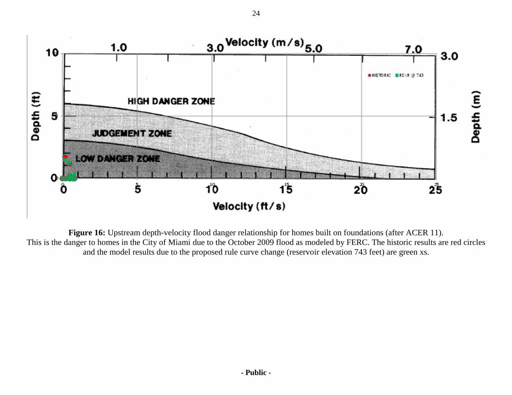
24
- Public -
Figure 16: Upstream depth-velocity flood danger relationship for homes built on foundations (after ACER 11). This is the danger to homes in the City of Miami due to the October 2009 flood as modeled by FERC. The historic results are red circles
and the model results due to the proposed rule curve change (reservoir elevation 743 feet) are green xs.
20150831-4012 FERC PDF (Unofficial) 08/31/2015

25
- Public -
Figure 17: Depth-velocity flood danger relationship for homes built on foundations (after ACER 11). This is the danger to homes downstream of Pensacola Dam due to the October 2009 flood as modeled by FERC. The historic results are
red circles and the model results due to the proposed rule curve change (reservoir elevation 743 feet) are green xs.
Because of the coarse DEM layers used, structures built on the steep bank adjacent to the river show average flood depths against them higher than expected. Staff does not have confidence in the absolute depth values above 6-7 feet, but believe the relative change between the cases is reasonably accurate. There is an increase in danger, but the increases remain within the same danger zone and are mitigated
by in-place EAP procedures.
20150831-4012 FERC PDF (Unofficial) 08/31/2015

Date:Project:
Title:Prepared By:
1.0 OBJECTIVE
2.0 METHODS
3.0 CALCULATIONS3.1 Streamflow Data
Figure 1. USGS Stream Gage Location Map
DIVISION OF DAM SAFETY & INSPECTION, ATLANTA REGIONAL OFFICE
8/25/2015P-1494 PensacolaCalculations Package for Temporary Variance RequestD2SI - Atlanta Regional Office
This calculation package supports the August 26, 2015 memorandum for the review of the proposed rule curve change supporting information. The objective of this calculation package is to evaluate the upstream and downstream effects of the temporary rule curve variance requested for the Pensacola Project, which proposes to raise the target elevation of the reservoir from 741 feet (Pensacola Datum; PD) to between 742 feet and 743 feet from August 15 to October 15, 2015.
In their May 28, 2015 submittal, GRDA submitted the thesis work of Mr. Alan Dennis to support their request for a temporary rule curve variance. The thesis included the development of a steady flow HEC-RAS model for all flow frequencies from 2-year to 500-year comparing flood levels in Miami with the downstream boundary condition held at 741 and 743 ft PD. Additionally, an unsteady model was developed for the 2009 storm to calibrate the model. The limits of the 2014 Dennis study extended from the upstream USGS stream gage at Commerce OK to the Pensacola Reservoir, but did not include an analysis of the downstream impacts. The results of Dennis' study indicates a maximum incremental increase of less than 0.2 foot at the City of Miami during the 100-year storm event.
In order to verify the results of the 2014 Dennis model and estimate the upstream and downstream impacts of the temporary rule curve variance, Staff completed an independent analysis including the following methods:
1. Collection of Streamflow Data for storm events occuring between August and November;2. Reservoir Mass-Balance Computations to establish inflow, outflow, and reservoir elevations for selected storm events and different starting water surface elevations;3. Upstream Unsteady HEC-RAS Hydraulic Modeling for selected storm events;4. Downstream Unsteady HEC-RAS Hydraulic Modeling for selected storm events; and5. ACER 11 hazard analysis of structures identified within inundation zones upstream and downstream of the project.
The following sections detail the assumptions, methods, calculations, and results of staff's independent analysis.
Based on the Flood Frequency Curve published by FEMA for the USGS Stream Gage at Commerce, OK near the City of Miami, staff identified 4 signicant storm events with recorded streamflow data between the months of August and October: October 1986, September 1993, October 1998, and October 2009. Staff identified 5 USGS stream gages within the Project vicinity with a period of record containing each of the four identified storm events. The limits of the 2014 Dennis study are given in Figure 1 below, along with the available USGS stream gage locations within the vicinity of the Project. The available data and chosen USGS stream gages are summarized in Table 1 below.
USGS GAUGE 07185080 NEOSHO @ MIAMI
20150831-4012 FERC PDF (Unofficial) 08/31/2015

Date:Project:
Title:Prepared By:
DIVISION OF DAM SAFETY & INSPECTION, ATLANTA REGIONAL OFFICE
8/25/2015P-1494 PensacolaCalculations Package for Temporary Variance RequestD2SI - Atlanta Regional Office
Table 1. Summary of Available USGS Stream GagesDrainageSq. Mil.
07185000 5,926 36.9286 -94.957207185080 6,011 36.8647 -94.878607188000 2,516 36.9344 -94.746907189000 851 36.6314 -94.586707185095 44.7 36.9000 -94.8681
07190500 Neosho River near Langley, OK 10385 36.4389 -95.0483
3.2 Reservoir Mass-Balance Calculations
3.2.1 Establish Rating Curves for Gates and Reservoir Storage
Table 2. Rating Curves for Pensacola Project
WSE (ft-PD)
WSE (ft-msl)
Q (cfs)
WSE (ft-PD)
WSE (ft-msl)
Q (cfs)
WSE (ft-PD)
WSE (ft-msl)
S (ac-ft)
740.00 741.47 0 730 731.47 0 713.63 715.1 655600741.00 742.47 234 734 735.47 1000 723.63 725.1 904500742.00 743.47 546 736.2 737.67 2000 733.63 735.1 1221000743.00 744.47 865 738.1 739.57 3000 739.63 741.1 1452000744.00 745.47 1198 740 741.47 4000 744.63 746.1 1672000746.10 747.57 1980 741 742.47 5000 749.63 751.1 1917000748.00 749.47 2832 743 744.47 6000 754.63 756.1 2197000750.00 751.47 3936 744 745.47 7000 759.63 761.1 2516000751.53 753 4963 745.6 747.07 8000753.00 754.47 6126 746.5 747.97 9000754.10 755.57 7125 748 749.47 10000755.00 756.47 8031 749 750.47 11000756.20 757.67 9376 750 751.47 12000
751 752.47 13000752 753.47 14000753 754.47 15000754 755.47 16000754.8 756.27 17000755.7 757.17 18000756.4 757.87 19000
Elk River near Tiff, MOTar Creek at Miami, OK
UPSTREAM OF PENSACOLA DAM
DOWNSTREAM OF PENSACOLA DAM
USGS Station ID Latitude LongitudeRiver
Neosho River at Commerce, OK
Spring River near Quapaw, OK
Normally HEC-RAS can be used to route flows through the model to determine the elevation and outflow, but it requires the modeler know all inflows. About 10% of the Pensacola Dam watershed comes from ungaged stream and creeks and is not captured in measured inflows. Without this information the HEC-RAS model gave inaccurate results and would not calibrate to past floods. Staff modeled the Pensacola reservoir water surface elevation, outflow, and inflow by completing a mass-balance calculation which included the following 4 steps:
1. Establish rating curves for discharge from Main and Auxiliary Spillway gates, and for storage within the reservoir;2. Estimate reservoir inflows using a mass-balance of known historic outflows and reservoir elevations for the three identified storm events; 3. Calibrate mass-balance calculations for the three identified storm events; and 4. Calculate reservoir water surface elevations for starting elevations 741, 742, and 743 ft-PD for the three identified storm events.
Staff identified the rating curve for the a single main spillway gate, single auxiliary spillway gate, and the reservoir storage curve based on information presented in the Part 12D Supporting Technical Information document. Table 2 below depicts the values for each of the rating curves. Staff fit 2nd or 3rd-order-polynomial trend line to each of the three rating curves to establish an equation that could be used in the mass-balance calculations for a more precise lookup for each reservoir elevation.
Auxiliary Spillway (Sill at 740 ft-PD)
Main Spillway (Sill at 730 ft-PD)
Storage
Neosho River at Miami, OK
20150831-4012 FERC PDF (Unofficial) 08/31/2015

Date:Project:
Title:Prepared By:
DIVISION OF DAM SAFETY & INSPECTION, ATLANTA REGIONAL OFFICE
8/25/2015P-1494 PensacolaCalculations Package for Temporary Variance RequestD2SI - Atlanta Regional Office
Figure 2. Rating Curves for Pensacola Project
Y = A x3 + Bx2 + Cx + D
A B C DStorage 0 576.2733 -813777 2.88E+08
Auxiliary 1.181133 -2628.65 1950336 -4.8E+08Main -0.04716 123.4181 -104625.4 28953952
3.2.2 Calculate the Historic Inflows to the Reservoir
Eqn 1. where: S(t+1): Storage in reservoir at timestep t+1, ac-ftS(t): Storage in reservoir at timestep t, ac-ftI(t): Inflow rate at timestep t (cfs)
O(t): Outflow rate at timestep t (cfs)t : time (s)
There is no stream gage located directly upstream of the reservoir, and the reservoir is fed by several tributaries along its length. Thus, a measurement of total inflows to the reservoir were not available. Staff estimated the total inflow to the reservoir using a mass-balance calculation summarized by Equation 1. Any change in storage over a time step is equal to the inflow volume minus the outflow volume.
Satff reviewed historic hourly reservoir elevation data and total outflow data for each of the three storm events analyzed. The reservoir elevation data was translated to a storage value based on the rating curve established in Section 3.2.1. Inflows were then calculated for each time step using Equation 1. In order to smooth the results of the inflow hydrograph, a 12-hour running average was calculated and normalized to the peak value of the 12-hour averaged inflow. The normalized inflows were then calculated by a peak inflow that was adjusted until the outflows predicted by the mass-balance calibrated with the outflows measured at the project. Results are given in Tables 3, 4, and 5. Results are shown hourly for the first 6 hours and then reported in 12-hour increments. Calculations were computed using one hour time steps.
Staff fit a 2nd and 3rd order polynomial trendline to each of the rating curves with the coefficients given below:
( ) tOISS tttt ×−+=+ )()()()1(
0
500000
1000000
1500000
2000000
2500000
3000000
-5000
0
5000
10000
15000
20000
710.00 720.00 730.00 740.00 750.00 760.00 770.00
Stor
age
(ac-
ft)
Disc
harg
e (c
fs)
Reservoir Elevation (ft-MSL)
Auxiliary Spillway Gate Auxiliary Gate Trendline Main Spillway Gate
Main Gate Trendline Storage Storage Trendline
20150831-4012 FERC PDF (Unofficial) 08/31/2015

Date:Project:
Title:Prepared By:
DIVISION OF DAM SAFETY & INSPECTION, ATLANTA REGIONAL OFFICE
8/25/2015P-1494 PensacolaCalculations Package for Temporary Variance RequestD2SI - Atlanta Regional Office
Figure 3. October 1986 Estimated Reservoir Inflow
Table 3. Oct 1986 Inflow Hydrograph Results
Outflow (cfs)
Rsvr Elev
(ft-msl)Storage (ac-ft)
Outflow Volume
(O)(ac-ft)
S(t+1)-S(t)
(ac-ft)
Volume Inflow (I)
(ac-ft)Inflow (cfs)
12-hr Averaged
Inflow (cfs)
Normalized 12-hr Avg
Inflow (cfs)
Inflow (Norm. x Peak)
(cfs)
9/28/1986 1:00 11500 744.00 1560353 -950 -874 76 923 5963 0.034 59639/28/1986 2:00 11500 743.98 1559479 -950 0 950 11500 5963 0.034 59639/28/1986 3:00 11500 743.98 1559479 -950 0 950 11500 5963 0.034 59639/28/1986 4:00 11500 743.98 1559479 -950 0 950 11500 5963 0.034 59639/28/1986 5:00 11500 743.98 1559479 -950 -874 77 929 5963 0.034 59639/28/1986 6:00 11500 743.96 1558605 -950 -1310 -359 0 5963 0.034 5963
9/28/1986 12:00 11500 743.86 1554243 -950 0 950 11500 6425 0.037 64259/29/1986 0:00 11500 743.69 1546856 -950 0 950 11500 7231 0.041 7231
9/29/1986 12:00 11500 743.49 1538207 -950 1294 2245 27162 8442 0.048 84429/29/1986 13:00 11500 743.52 1539501 -950 -1294 -344 0 7484 0.043 74839/29/1986 14:00 11500 743.49 1538207 -950 1294 2245 27162 9747 0.055 97479/29/1986 15:00 11500 743.52 1539501 -950 0 950 11500 9747 0.055 97479/29/1986 16:00 11500 743.52 1539501 -950 864 1814 21949 11491 0.065 114919/29/1986 17:00 11500 743.54 1540364 -950 0 950 11500 12450 0.071 124499/29/1986 18:00 11500 743.54 1540364 -950 864 1814 21954 14279 0.081 142799/29/1986 19:00 11500 743.56 1541228 -950 5627 6578 79588 20824 0.118 208249/29/1986 20:00 11500 743.69 1546856 -950 2169 3120 37750 23970 0.136 239709/29/1986 21:00 11500 743.74 1549025 -950 0 950 11500 24929 0.142 249289/29/1986 22:00 11500 743.74 1549025 -950 3042 3992 48309 26693 0.152 266929/29/1986 23:00 11500 743.81 1552067 -950 2176 3127 37834 28017 0.159 28017
9/30/1986 0:00 11500 743.86 1554243 -950 3052 4002 48426 29789 0.169 297899/30/1986 1:00 11500 743.93 1557295 -950 1310 2260 27347 32068 0.182 320689/30/1986 2:00 11500 743.96 1558605 -950 6125 7076 85616 36939 0.210 369399/30/1986 3:00 11500 744.10 1564730 -950 8349 9299 112524 45358 0.258 453579/30/1986 4:00 11500 744.29 1573079 -950 11049 11999 145193 55628 0.316 556289/30/1986 5:00 11500 744.54 1584128 -950 5329 6280 75982 61002 0.347 610019/30/1986 6:00 11500 744.66 1589457 -950 16536 17486 211584 76805 0.437 768039/30/1986 7:00 11500 745.03 1605993 -950 5397 6347 76802 76572 0.435 765719/30/1986 8:00 11500 745.15 1611390 -950 0 950 11500 74385 0.423 743849/30/1986 9:00 11500 745.15 1611390 -950 0 950 11500 74385 0.423 74384
9/30/1986 10:00 11500 745.15 1611390 -950 38243 39193 474238 109879 0.625 1098779/30/1986 11:00 11500 745.99 1649633 -950 12002 12952 156723 119786 0.681 1197849/30/1986 12:00 11500 746.25 1661635 -950 13479 14429 174591 130300 0.741 1302989/30/1986 13:00 26818 746.54 1675113 -2216 10290 12506 151325 140632 0.800 1406299/30/1986 14:00 27169 746.76 1685403 -2245 0 2245 27169 135761 0.772 1357599/30/1986 15:00 42838 746.76 1685403 -3540 7048 10588 128116 137060 0.779 1370589/30/1986 16:00 52983 746.91 1692451 -4379 10384 14762 178625 139846 0.795 139844
Date
OBSERVED CALCULATION FOR INFLOWS
020000400006000080000
100000120000140000160000180000200000
Adju
sted
Inflo
w (c
fs)
20150831-4012 FERC PDF (Unofficial) 08/31/2015

Date:Project:
Title:Prepared By:
DIVISION OF DAM SAFETY & INSPECTION, ATLANTA REGIONAL OFFICE
8/25/2015P-1494 PensacolaCalculations Package for Temporary Variance RequestD2SI - Atlanta Regional Office
9/30/1986 17:00 53958 747.13 1702835 -4459 13773 18232 220609 151899 0.864 1518969/30/1986 18:00 62893 747.42 1716607 -5198 4772 9970 120631 144319 0.820 1443179/30/1986 19:00 63508 747.52 1721379 -5249 7179 12428 150376 150450 0.855 1504489/30/1986 20:00 64436 747.67 1728558 -5325 10576 15902 192410 165526 0.941 1655239/30/1986 21:00 65814 747.89 1739135 -5439 5792 11232 135902 175893 1.000 1758909/30/1986 22:00 66573 748.01 1744927 -5502 8234 13736 166209 150224 0.854 1502219/30/1986 23:00 67658 748.18 1753161 -5592 7293 12885 155907 150156 0.854 150153
10/1/1986 0:00 68626 748.33 1760455 -5672 8297 13969 169020 149691 0.851 14968910/1/1986 12:00 70436 750.16 1851521 -5821 7636 13457 162827 165458 0.941 165455
10/2/1986 0:00 55214 751.48 1919604 -4563 18389 22952 277723 139555 0.793 13955310/2/1986 12:00 64443 753.19 2010788 -5326 4348 9674 117059 138415 0.787 138412
10/3/1986 0:00 73402 754.65 2091308 -6066 7289 13355 161596 153180 0.871 15317710/3/1986 12:00 115332 755.92 2163348 -9532 0 9532 115332 146500 0.833 146497
10/4/1986 0:00 132804 756.14 2176016 -10976 0 10976 132804 144243 0.820 14424110/4/1986 12:00 133152 756.17 2177748 -11004 0 11004 133152 134869 0.767 134867
10/5/1986 0:00 131419 756.02 2169099 -10861 0 10861 131419 123630 0.703 12362810/5/1986 11:59 115144 755.90 2162199 -9516 1149 10665 129045 122908 0.699 12290610/5/1986 23:59 102036 756.14 2176016 -8433 1732 10164 122990 121311 0.690 12130910/6/1986 11:59 120316 756.44 2193381 -9944 -1741 8202 99249 119547 0.680 11954510/6/1986 23:59 126706 756.29 2184686 -10472 -2893 7579 91705 113178 0.643 11317610/7/1986 11:59 116277 756.02 2169099 -9610 0 9610 116277 110347 0.627 11034510/7/1986 23:59 106436 755.75 2153597 -8796 -1145 7651 92581 94408 0.537 9440710/8/1986 11:59 111065 755.46 2137040 -9179 -2845 6334 76642 88649 0.504 8864810/8/1986 23:59 100886 755.07 2114927 -8338 -1694 6644 80392 83962 0.477 8396010/9/1986 11:59 83018 754.75 2096913 -6861 -1122 5739 69443 79267 0.451 7926610/9/1986 23:59 61448 754.78 2098597 -5078 0 5078 61448 73207 0.416 73206
10/10/1986 11:59 61688 754.83 2101406 -5098 -1685 3413 41294 62765 0.357 6276410/10/1986 23:59 72819 754.56 2086274 -6018 -1676 4342 52538 58399 0.332 5839810/11/1986 11:59 70465 754.19 2065674 -5824 -2772 3052 36928 49680 0.282 4968010/11/1986 23:59 67634 753.73 2040283 -5590 -2745 2844 34418 43347 0.246 4334610/12/1986 11:59 63467 753.02 2001572 -5245 -1623 3622 43830 27589 0.157 2758910/12/1986 23:59 59264 752.26 1960779 -4898 -3724 1174 14206 18360 0.104 1835910/13/1986 11:59 35754 751.63 1927467 -2955 -2624 331 4002 23586 0.134 2358510/13/1986 23:59 23104 751.36 1913331 -1909 -1565 344 4161 19025 0.108 1902510/14/1986 11:59 23012 751.31 1910723 -1902 0 1902 23012 21942 0.125 2194210/14/1986 23:59 22831 751.21 1905514 -1887 0 1887 22831 17665 0.100 1766410/15/1986 11:59 22651 751.11 1900317 -1872 -1038 834 10091 16458 0.094 1645810/15/1986 23:59 22438 750.99 1894096 -1854 -1894096 -1892242 0 15457 0.088 15457
1758901 Vailable outflow data was not in hourly format. Therefore, hourly data was obtained from the USGS Langley Gage station downstream of the project.
PEAK INFLOW (CFS)
20150831-4012 FERC PDF (Unofficial) 08/31/2015

Date:Project:
Title:Prepared By:
DIVISION OF DAM SAFETY & INSPECTION, ATLANTA REGIONAL OFFICE
8/25/2015P-1494 PensacolaCalculations Package for Temporary Variance RequestD2SI - Atlanta Regional Office
Figure 4. September 1993 Estimated Reservoir Inflow
Table 4. September 1993 Inflow Hydrograph Results
Outflow (cfs)
Rsvr Elev
(ft-msl)Storage (ac-ft)
Outflow Volume
(O)(ac-ft)
S(t+1)-S(t)
(ac-ft)
Volume Inflow (I)
(ac-ft)Inflow (cfs)
12-hr Averaged
Inflow (cfs)
Normalized 12-hr Avg
Inflow (cfs)
Adj. Inflow (Norm. x Peak)
(cfs)
9/24/1993 0:00 11100 745.32 1619064 -917 -1357 0 0 9754 0.03 87909/24/1993 1:00 11100 745.29 1617707 -917 0 917 11100 9754 0.03 87909/24/1993 2:00 11100 745.29 1617707 -917 -1356 0 0 9754 0.03 87909/24/1993 3:00 11100 745.26 1616352 -917 0 917 11100 9754 0.03 87909/24/1993 3:59 11100 745.26 1616352 -917 0 917 11100 9754 0.03 87909/24/1993 4:59 11100 745.26 1616352 -917 -1355 0 0 9754 0.03 87909/24/1993 5:59 11100 745.23 1614997 -917 0 917 11100 9754 0.03 8790
9/24/1993 11:59 11100 745.23 1614997 -917 -1354 0 0 9754 0.03 87909/24/1993 23:59 52644 745.51 1627680 -4351 2730 7080 85671 47872 0.16 431449/25/1993 11:59 93635 746.69 1682123 -7738 7506 15244 184453 130647 0.44 1177439/25/1993 23:59 99461 748.45 1766308 -8220 -4879 3341 40427 169676 0.58 1529169/26/1993 11:59 134211 751.28 1909159 -11092 4694 15786 191013 253374 0.86 2283479/26/1993 23:59 157307 753.61 2033700 -13001 12082 25083 303505 273940 0.93 2468829/27/1993 11:59 169168 755.28 2126812 -13981 5109 19090 230991 255484 0.87 2302489/27/1993 23:59 166671 755.84 2158755 -13774 0 13774 166671 198771 0.68 1791389/28/1993 11:59 148776 755.92 2163348 -12296 0 12296 148776 162863 0.55 1467769/28/1993 23:59 126512 755.68 2149592 -10456 -3429 7027 85024 121577 0.41 1095689/29/1993 11:59 105288 755.27 2126245 -8701 -1701 7001 84709 92186 0.31 830809/29/1993 23:59 88641 754.74 2096352 -7326 -3364 3962 47941 65626 0.22 591449/30/1993 11:59 75324 754.12 2061794 -6225 -1107 5118 61925 49027 0.17 441849/30/1993 23:59 51187 753.63 2034796 37142 0.13 33473
265000
Date
CALCULATION FOR INFLOWSOBSERVED
PEAK INFLOW (CFS)
0
50000
100000
150000
200000
250000
300000
Adju
sted
Inflo
w (c
fs)
20150831-4012 FERC PDF (Unofficial) 08/31/2015

Date:Project:
Title:Prepared By:
DIVISION OF DAM SAFETY & INSPECTION, ATLANTA REGIONAL OFFICE
8/25/2015P-1494 PensacolaCalculations Package for Temporary Variance RequestD2SI - Atlanta Regional Office
Figure 5. October 2009 Estimated Reservoir Inflow
Table 5. Oct 2009 Inflow Hydrograph Results
Outflow (cfs)
Rsvr Elev
(ft-msl)Storage (ac-ft)
Outflow Volume
(O)(ac-ft)
S(t+1)-S(t)
(ac-ft)
Volume Inflow (I)
(ac-ft)Inflow (cfs)
12-hr Averaged
Inflow (cfs)
Normalized 12-hr Avg
Inflow (cfs)
Adj. Inflow (Norm. x Peak)
(cfs)
10/8/2009 0:00 11948 742.34 1489369 -987 -1254 0 0 1262 0.01 127510/8/2009 1:00 3430 742.31 1488116 -284 0 284 3430 1384 0.01 139810/8/2009 2:00 1981 742.31 1488116 -164 -835 0 0 1384 0.01 139810/8/2009 3:00 1980 742.29 1487280 -164 -417 0 0 1249 0.01 126110/8/2009 4:00 1980 742.28 1486863 -164 0 164 1980 1256 0.01 126910/8/2009 5:00 1980 742.28 1486863 -164 -417 0 0 1112 0.01 112210/8/2009 6:00 1982 742.27 1486446 -164 -417 0 0 1112 0.01 112210/8/2009 7:00 1975 742.26 1486029 -163 0 163 1975 1126 0.01 113710/8/2009 8:00 3522 742.26 1486029 -291 -417 0 0 988 0.01 99710/8/2009 9:00 3856 742.25 1485612 -319 0 319 3856 1284 0.01 1297
10/8/2009 10:00 3525 742.25 1485612 -291 -417 0 0 1145 0.01 115610/8/2009 11:00 5410 742.24 1485195 -447 0 447 5410 1421 0.01 143510/8/2009 12:00 5861 742.24 1485195 -484 -417 68 817 1344 0.01 1357
10/9/2009 0:00 11895 742.20 1483528 -983 1667 2650 32062 10697 0.06 1080110/9/2009 12:00 34112 743.26 1528317 -2819 6012 8832 106862 63375 0.37 6399610/10/2009 0:00 43949 745.56 1629955 -3632 10957 14589 176528 144092 0.85 145502
10/10/2009 12:00 62992 748.08 1748314 -5206 5819 11025 133399 165344 0.97 16696210/11/2009 0:00 78207 749.52 1819234 -6463 5516 11979 144948 146216 0.86 147648
10/11/2009 12:00 82015 750.71 1879645 -6778 4635 11413 138102 140907 0.83 14228610/12/2009 0:00 84546 751.56 1923794 -6987 2623 9610 116284 126932 0.75 128174
10/12/2009 12:00 85314 751.94 1943801 -7051 529 7579 91712 104240 0.61 10526010/13/2009 0:00 83706 751.88 1940631 -6918 -1056 5862 70931 80714 0.47 81504
10/13/2009 12:00 70089 751.51 1921174 -5792 -1047 4745 57417 60286 0.35 6087610/14/2009 0:00 50956 751.36 1913331 -4211 -1565 2646 32013 45701 0.27 46149
10/14/2009 12:00 47731 750.80 1884280 -3945 -3606 339 4099 18923 0.11 1910910/15/2009 0:00 45425 749.98 1842392 -3754 -3540 214 2593 4696 0.03 4742
10/15/2009 12:00 29098 749.23 1804759 -2405 -2486 0 0 5219 0.03 527010/16/2009 0:00 18800 748.84 1785446 -1554 -1478 75 912 2713 0.02 2740
172000
Date
OBSERVED CALCULATION FOR INFLOWS
PEAK INFLOW (CFS)
0
20000
40000
60000
80000
100000
120000
140000
160000
180000
200000
Adju
sted
Inflo
w (c
fs)
20150831-4012 FERC PDF (Unofficial) 08/31/2015

Date:Project:
Title:Prepared By:
DIVISION OF DAM SAFETY & INSPECTION, ATLANTA REGIONAL OFFICE
8/25/2015P-1494 PensacolaCalculations Package for Temporary Variance RequestD2SI - Atlanta Regional Office
3.2.3 Calibrate to Reservoir Elevations and Dynamic Routing
Figure 6. Reservoir Elevation Results for October 1986
Table 6. Oct 1986 Calibration of Reservoir Stage using Mass-Balance
OBSERVED
WSE WSE Storage Inflow
Gate Open
Aux Gate Open
Gate Spill
Aux Gate Spill
Power Gate Spill Total Outflow
ft-MSL ft-MSL ac-ft cfs no. no. cfs cfs cfs cfs
9/29/1986 18:00 743.54 743.54 1540364 12450 0 0 0 0 11500 115009/29/1986 19:00 743.54 743.55 1540443 14279 0 0 0 0 11500 115009/29/1986 20:00 743.56 743.55 1540673 20824 0 0 0 0 11500 115009/29/1986 21:00 743.69 743.57 1541443 23970 0 0 0 0 11500 115009/29/1986 22:00 743.74 743.59 1542474 24929 0 0 0 0 11500 115009/29/1986 23:00 743.74 743.62 1543584 26693 0 0 0 0 11500 11500
9/30/1986 0:00 743.81 743.65 1544839 28017 0 0 0 0 11500 115009/30/1986 6:00 744.54 743.95 1557963 61002 0 0 0 0 11500 11500
9/30/1986 12:00 745.99 744.70 1591354 119786 0 0 0 0 11500 115009/30/1986 18:00 747.13 745.81 1641780 151899 5 5 35464 6550 11500 53514
10/1/1986 0:00 748.18 746.89 1691551 150156 5 5 39692 8505 11500 5969610/1/1986 6:00 749.08 747.88 1738139 158547 5 5 43744 10476 11500 65720
10/1/1986 12:00 749.94 748.82 1783726 165974 4 5 38229 12558 11500 6228710/1/1986 18:00 750.79 749.85 1834404 158884 2 5 20942 15071 11500 47513
10/2/1986 0:00 751.48 750.85 1885484 129981 2 5 22811 17834 11500 5214410/2/1986 6:00 752.30 751.65 1926668 134312 2 5 24332 20238 11500 56070
10/2/1986 12:00 753.12 752.41 1966879 151803 2 5 25828 22743 11500 6007110/2/1986 18:00 753.73 753.14 2006365 143284 2 5 27304 25357 11500 64161
10/3/1986 0:00 754.53 753.86 2046156 149468 2 5 28796 28146 11500 6844210/3/1986 6:00 755.22 754.60 2087643 155896 2 5 30354 31220 11500 73074
10/3/1986 12:00 755.90 755.30 2127730 150355 4 5 63718 34349 11500 10956810/3/1986 18:00 756.07 755.53 2141495 145905 4 7 64751 49643 11500 125894
10/4/1986 0:00 756.14 755.67 2149450 142787 4 7 65348 50553 11500 12740010/4/1986 6:00 756.17 755.77 2155873 138592 4 7 65829 51293 11500 128622
Date
CALCULATED
Using the same mass-balance Equation 1 given in Section 3.2.2 above, staff utilized the inflow hydrographs calculated in Section 3.2.2 to solve for the storage value and cooresponding reservoir elevation for each time step. Gate opening sequences were obtained from GRDA, and corresponding spillway outflows were calculated using the rating curves given in Section 3.2.1. Results are shown in Tables 6, 7, and 8 below for the historic storm events. Starting elevations were obtained from historic measurements. Calculations were completed in 15-minute increments. The first hour is shown in the tables below, and then reported in 6 hour increments.
742.00
744.00
746.00
748.00
750.00
752.00
754.00
756.00
758.00
Elev
atio
n (ft
-MSL
)
Observed Calculated
20150831-4012 FERC PDF (Unofficial) 08/31/2015

Date:Project:
Title:Prepared By:
DIVISION OF DAM SAFETY & INSPECTION, ATLANTA REGIONAL OFFICE
8/25/2015P-1494 PensacolaCalculations Package for Temporary Variance RequestD2SI - Atlanta Regional Office
10/4/1986 12:00 756.17 755.83 2159444 134840 4 7 66096 51707 11500 12930310/4/1986 18:00 756.12 755.86 2160867 130107 4 7 66203 51872 11500 129575
10/5/1986 0:00 756.02 755.84 2159907 123775 4 7 66131 51761 11500 12939210/5/1986 6:00 755.97 755.79 2157057 121759 4 7 65917 51430 11500 128847
10/5/1986 12:00 755.90 755.75 2154230 123105 4 5 65706 36502 11500 11370810/5/1986 18:00 756.00 755.86 2161231 122681 4 4 66230 29666 11500 107396
10/6/1986 0:00 756.12 756.02 2170629 121816 4 3 66934 22720 11500 10115410/6/1986 6:00 756.34 756.19 2180936 123764 4 3 67705 23243 11500 102448
10/6/1986 12:00 756.44 756.35 2190144 121526 4 5 68393 39524 11500 11941710/6/1986 18:00 756.44 756.34 2189838 116817 4 5 68370 39498 11500 119368
10/7/1986 0:00 756.32 756.27 2185602 113807 4 6 68053 46963 11500 12651610/7/1986 6:00 756.17 756.16 2178726 109743 4 6 67539 46261 11500 125300
10/7/1986 12:00 756.02 756.05 2172102 108299 4 5 67044 37991 11500 11653510/7/1986 18:00 755.85 755.97 2167346 103789 4 5 66688 37592 11500 115780
10/8/1986 0:00 755.78 755.90 2163038 96383 4 4 66366 29786 11500 10765110/8/1986 6:00 755.66 755.79 2156907 94460 4 4 65906 29379 11500 106785
10/8/1986 12:00 755.48 755.65 2148448 89977 4 5 65272 36027 11500 11279910/8/1986 18:00 755.26 755.44 2136356 84608 4 4 64366 28034 11500 103900
10/9/1986 0:00 755.12 755.29 2127534 83649 4 4 63704 27467 11500 10267110/9/1986 6:00 754.90 755.13 2118067 81654 4 4 62993 26865 11500 101358
10/9/1986 12:00 754.78 754.98 2109314 80179 3 4 46752 26314 11500 8456610/9/1986 18:00 754.75 754.94 2107303 81187 2 3 31093 19641 11500 6223410/10/1986 0:00 754.80 755.08 2115170 73873 2 3 31388 20011 11500 6289910/10/1986 6:00 754.83 755.15 2119107 65998 2 3 31536 20198 11500 63233
10/10/1986 12:00 754.83 755.16 2119932 64444 2 3 31567 20237 11500 6330410/10/1986 18:00 754.73 755.06 2113955 59534 2 5 31342 33257 11500 76099
10/11/1986 0:00 754.58 754.91 2105530 57462 2 5 31026 32597 11500 7512310/11/1986 6:00 754.41 754.76 2096638 55383 2 5 30692 31909 11500 74101
10/11/1986 12:00 754.21 754.58 2086500 50981 2 5 30311 31133 11500 7294410/11/1986 18:00 753.99 754.38 2075037 47032 2 5 29881 30268 11500 71649
10/12/1986 0:00 753.80 754.15 2062405 43556 2 5 29406 29330 11500 7023610/12/1986 6:00 753.48 753.90 2048299 35013 2 5 28877 28301 11500 68677
10/12/1986 12:00 753.09 753.59 2031112 26805 2 5 28232 27073 11500 6680510/12/1986 18:00 752.72 753.23 2010983 23911 2 5 27477 25672 11500 64650
10/13/1986 0:00 752.33 752.84 1990237 20828 2 5 26701 24271 11500 6247110/13/1986 6:00 751.97 752.46 1969427 21124 2 5 25923 22907 11500 60330
10/13/1986 12:00 751.65 752.09 1949775 24436 1 3 12595 12995 11500 3709010/13/1986 18:00 751.38 752.00 1945023 21414 0 3 0 12817 11500 24317
10/14/1986 0:00 751.36 751.98 1944224 19012 0 3 0 12787 11500 2428710/14/1986 6:00 751.28 751.94 1941718 17830 0 3 0 12694 11500 24194
10/14/1986 12:00 751.28 751.88 1938654 20371 0 3 0 12581 11500 2408110/14/1986 18:00 751.26 751.85 1937037 21913 0 3 0 12521 11500 24021
10/15/1986 0:00 751.23 751.82 1935605 17680 0 3 0 12469 11500 2396910/15/1986 6:00 751.19 751.77 1932839 17607 0 3 0 12367 11500 23867
10/15/1986 12:00 751.11 751.71 1929654 17520 0 3 0 12251 11500 2375110/15/1986 18:00 751.09 751.64 1926396 17430 0 3 0 12133 11500 23633
10/16/1986 0:00 751.01 751.58 1923196 16298 0 3 0 12018 11500 23518PEAK 756.44 756.3513 175893
*Calculations were completed in one-hour increments for October 1986 because the available outflow data was available in one-hour increments.
20150831-4012 FERC PDF (Unofficial) 08/31/2015

Date:Project:
Title:Prepared By:
DIVISION OF DAM SAFETY & INSPECTION, ATLANTA REGIONAL OFFICE
8/25/2015P-1494 PensacolaCalculations Package for Temporary Variance RequestD2SI - Atlanta Regional Office
Figure 7. Reservoir Elevation Results for September 1993
Table 7. Sept 1993 Calibration of Reservoir Stage using Mass-Balance
OBSERVED
WSE WSE Storage Inflow
Gate Open
Aux Gate Open
Gate Spill
Aux Gate Spill
Power Gate Spill Total Outflow
ft-MSL ft-MSL ac-ft cfs no. no. cfs cfs cfs cfs
9/24/1993 0:00 745.32 745.32 1619064 8790 0 0 0 0 11500 115009/24/1993 0:15 745.32 745.31 1619008 8790 0 0 0 0 11500 115009/24/1993 0:30 745.32 745.31 1618952 8790 0 0 0 0 11500 115009/24/1993 0:45 745.32 745.31 1618896 8790 0 0 0 0 11500 115009/24/1993 1:00 745.29 745.31 1618840 8790 0 0 0 0 11500 115009/24/1993 6:00 745.23 745.28 1617720 8790 0 0 0 0 11500 11500
9/24/1993 12:00 745.23 745.24 1615914 8790 0 4 0 4468 11500 159689/24/1993 18:00 745.13 745.14 1611076 14593 0 8 0 8653 11500 20153
9/25/1993 0:00 745.51 745.12 1610165 43144 3 8 19704 8600 11500 398049/25/1993 6:00 746.17 745.36 1621138 88338 3 8 20247 9244 11500 40991
9/25/1993 12:00 746.69 745.97 1648983 117743 5 8 36069 10919 11500 584889/25/1993 18:00 747.32 746.69 1682018 126274 5 8 38873 12990 11500 63364
9/26/1993 0:00 748.45 747.55 1722548 152916 5 8 42379 15679 11500 695579/26/1993 6:00 749.86 748.57 1771550 203416 5 8 46700 19177 11500 77377
9/26/1993 12:00 751.28 749.92 1838060 228347 6 8 63225 24418 11500 991439/26/1993 18:00 752.53 751.30 1908494 239055 6 8 70978 30652 11500 113130
9/27/1993 0:00 753.61 752.51 1972129 246882 6 8 78073 36931 11500 1265039/27/1993 6:00 754.64 753.64 2033798 244778 5 8 70832 43621 11500 125952
9/27/1993 12:00 755.28 754.60 2087562 230248 5 8 75878 49942 11500 1373209/27/1993 18:00 755.63 755.25 2125164 200152 5 7 79407 47802 11500 138709
9/28/1993 0:00 755.84 755.66 2149082 179138 5 7 81650 50510 11500 1436609/28/1993 6:00 755.87 755.88 2162086 160884 5 7 82868 52014 11500 146382
9/28/1993 12:00 755.92 755.96 2166795 146776 5 7 83308 52564 11500 1473739/28/1993 18:00 755.80 755.97 2167384 129141 4 7 66691 52633 11500 130824
9/29/1993 0:00 755.68 755.89 2162495 109568 4 7 66325 52062 11500 1298879/29/1993 6:00 755.42 755.68 2150224 94297 4 7 65405 50641 11500 127547
9/29/1993 12:00 755.27 755.45 2136905 83080 3 7 48305 49122 11500 1089279/29/1993 18:00 755.04 755.21 2122589 74103 3 7 47499 47515 11500 106515
9/30/1993 0:00 754.74 754.89 2104364 59144 3 7 46473 45509 11500 1034829/30/1993 6:00 754.42 754.49 2081467 48218 3 7 45183 43052 11500 99736
Date
Calculated
744.00
746.00
748.00
750.00
752.00
754.00
756.00
758.00
Elev
atio
n (ft
-MSL
)
Observed Calculated
20150831-4012 FERC PDF (Unofficial) 08/31/2015

Date:Project:
Title:Prepared By:
DIVISION OF DAM SAFETY & INSPECTION, ATLANTA REGIONAL OFFICE
8/25/2015P-1494 PensacolaCalculations Package for Temporary Variance RequestD2SI - Atlanta Regional Office
9/30/1993 12:00 754.12 754.08 2058403 44184 2 7 29256 40650 11500 814069/30/1993 18:00 753.89 753.74 2039546 42422 2 7 28548 38741 11500 78789
PEAK 755.97 755.9681 265000
Figure 8. Reservoir Elevation Results for October 2009
Table 8. Oct 2009 Calibration of Reservoir Stage using Mass-Balance
OBSERVED
WSE WSE Storage Inflow
Main Gate Open
Aux Gate Open
Main Gate Spill
Aux Gate Spill
Power Gate Spill Total Outflow
ft-MSL ft-MSL ac-ft cfs no. no. cfs cfs cfs cfs
10/8/2009 20:00 742.14 742.09 1479079 3923 0 0 0 0 12000 1200010/8/2009 20:15 742.14 742.12 1478912 3923 0 0 0 0 12000 1200010/8/2009 20:30 742.14 742.12 1478745 3923 0 0 0 0 12000 1200010/8/2009 20:45 742.14 742.12 1478578 3923 0 0 0 0 12000 1200010/8/2009 21:00 742.14 742.11 1478411 5233 0 0 0 0 12000 12000
10/9/2009 0:00 742.20 742.08 1477138 10801 0 0 0 0 12000 1200010/9/2009 6:00 742.57 742.16 1480450 32481 0 0 0 0 12000 12000
10/9/2009 12:00 743.26 742.49 1494711 63996 2 7 9494 1893 12000 2338710/9/2009 18:00 744.22 743.13 1522187 103131 2 7 10331 3204 12000 2553510/10/2009 0:00 745.56 744.20 1568929 145502 2 7 11799 5464 12000 2926210/10/2009 6:00 746.93 745.59 1631435 169965 2 7 13840 8624 12000 34464
10/10/2009 12:00 748.08 747.01 1697150 166962 4 7 32139 12227 12000 5636710/10/2009 18:00 748.84 748.08 1748123 155157 4 7 35699 15285 12000 62984
10/11/2009 0:00 749.52 748.96 1790633 147648 4 7 38724 18043 12000 6876610/11/2009 6:00 750.15 749.72 1828125 145442 4 7 41428 20647 12000 74075
10/11/2009 12:00 750.71 750.39 1861756 142286 4 7 43880 23129 12000 7900910/11/2009 18:00 751.19 750.96 1890872 136503 4 7 46018 25395 12000 83413
10/12/2009 0:00 751.56 751.42 1914609 128174 4 7 47771 27324 12000 8709610/12/2009 6:00 751.81 751.75 1932120 117308 4 7 49069 28796 12000 89865
10/12/2009 12:00 751.94 751.96 1942900 105260 4 7 49870 29722 12000 9159310/12/2009 18:00 751.97 752.04 1947112 93461 4 7 50184 30089 12000 92273
10/13/2009 0:00 751.88 752.00 1945223 81504 4 7 50043 29924 12000 9196710/13/2009 6:00 751.71 751.86 1937793 69566 4 7 49491 29282 12000 90772
10/13/2009 12:00 751.51 751.70 1929258 60876 3 7 36643 28553 12000 7719510/13/2009 18:00 751.47 751.66 1926995 54699 2 5 24345 20258 12000 56602
Date
Calculated
740.00
742.00
744.00
746.00
748.00
750.00
752.00
754.00
Elev
atio
n (ft
-MSL
)
Observed Calculated
20150831-4012 FERC PDF (Unofficial) 08/31/2015

Date:Project:
Title:Prepared By:
DIVISION OF DAM SAFETY & INSPECTION, ATLANTA REGIONAL OFFICE
8/25/2015P-1494 PensacolaCalculations Package for Temporary Variance RequestD2SI - Atlanta Regional Office
10/14/2009 0:00 751.36 751.61 1924448 46149 2 5 24250 20104 12000 5635410/14/2009 6:00 751.14 751.46 1916718 32642 2 5 23964 19642 12000 55606
10/14/2009 12:00 750.80 751.19 1902776 19109 2 5 23448 18824 12000 5427210/14/2009 18:00 750.39 750.81 1883449 8948 2 5 22736 17719 12000 52455
10/15/2009 0:00 749.98 750.38 1861271 4742 2 5 21922 16495 12000 5041710/15/2009 6:00 749.57 749.93 1838824 3648 2 5 21103 15301 12000 48404
10/15/2009 12:00 749.23 749.53 1818820 5270 1 3 10189 8565 12000 3075410/15/2009 18:00 749.03 749.33 1808728 6156 0.4 3 4003 8262 12000 24265
10/16/2009 6:00 748.84 748.92 1788560 850 0 3 3858 7673 12000 23530PEAK 751.97 752.04 172000
3.2.4 Estimate Reservoir Profile for Reservoir starting Elevations 741, 742, 743 ft-PD
Figure 9. Reservoir Elevation Results for Starting Water Surface Elevations of 741, 742, and 743 ft-PD for October 1986
Table 9. Oct 1986 Calculation of Reservoir Stages for Starting Water Surface Elevations of 741, 742, and 743 ft-PD
WSE Storage Total Outflow WSE Storage
Total Outflow WSE Storage
Total Outflow
no. no. ft-MSL ac-ft cfs ft-MSL ac-ft cfs ft-MSL ac-ft cfs
9/29/1986 18:00 0 0 742.47 1494814 11500 743.47 1537344 11500 744.47 1581027 115009/29/1986 19:00 0 0 742.50 1494892 11500 743.48 1537423 11500 744.47 1581106 115009/29/1986 20:00 0 0 742.50 1495122 11500 743.48 1537652 11500 744.47 1581335 115009/29/1986 21:00 0 0 742.52 1495892 11500 743.50 1538423 11500 744.49 1582106 115009/29/1986 22:00 0 0 742.54 1496923 11500 743.53 1539453 11500 744.51 1583137 115009/29/1986 23:00 0 0 742.57 1498033 11500 743.55 1540563 11500 744.54 1584246 11500
9/30/1986 0:00 0 0 742.60 1499288 11500 743.58 1541819 11500 744.57 1585502 115009/30/1986 6:00 0 0 742.90 1512412 11500 743.88 1554942 11500 744.86 1598626 11500
9/30/1986 12:00 0 0 743.67 1545802 11500 744.63 1588333 11500 745.60 1632016 115009/30/1986 18:00 5 5 744.83 1597377 48205 745.75 1638835 53156 746.67 1681386 58413
10/1/1986 0:00 5 5 745.99 1649758 54488 746.83 1688781 59346 747.68 1728750 6448710/1/1986 6:00 5 5 747.05 1698901 60631 747.82 1735539 65377 748.60 1772988 70381
10/1/1986 12:00 4 5 748.06 1746983 57985 748.77 1781293 61998 749.48 1816291 66219
Following the same procedures as described in Section 3.2.3, the starting reservoir elevations for the mass-balance calculations for each storm event were varied from 741 to 743 ft-PD. The gate openings and inflows were maintained the same as used for the calibration calculations. Results are given in Tables 9, 10, and 11 and Figures 9, 10 and 11. Calculations were completed in 15-minute increments. The first hour is shown in the tables below, and then reported in 6 hour increments.
Main Gate Open
Aux Gate Open
Date
RSVR @ 741 ft-PD RSVR @ 742 ft-PD RSVR @ 743 ft-PD
740.00
742.00
744.00
746.00
748.00
750.00
752.00
754.00
756.00
758.00
Elev
atio
n (ft
-MSL
)
Rsvr @ 741 ft-PD Rsvr @ 742 ft-PD Rsvr @ 743 ft-PD Historic
20150831-4012 FERC PDF (Unofficial) 08/31/2015

Date:Project:
Title:Prepared By:
DIVISION OF DAM SAFETY & INSPECTION, ATLANTA REGIONAL OFFICE
8/25/2015P-1494 PensacolaCalculations Package for Temporary Variance RequestD2SI - Atlanta Regional Office
10/1/1986 18:00 2 5 749.14 1799677 44512 749.80 1832105 47311 750.45 1865125 5026710/2/1986 0:00 2 5 750.20 1852254 49102 750.81 1883285 51940 751.42 1914831 5492410/2/1986 6:00 2 5 751.04 1894945 53031 751.61 1924569 55866 752.18 1954638 58836
10/2/1986 12:00 2 5 751.84 1936659 57049 752.37 1964880 59869 752.90 1993483 6280910/2/1986 18:00 2 5 752.61 1977637 61170 753.11 2004465 63961 753.60 2031617 66859
10/3/1986 0:00 2 5 753.37 2018902 65493 753.83 2044354 68245 754.29 2070078 7109310/3/1986 6:00 2 5 754.14 2061841 70174 754.57 2085937 72880 754.99 2110261 75670
10/3/1986 12:00 4 5 754.87 2103352 105816 755.27 2126117 109318 755.66 2149072 11289710/3/1986 18:00 4 7 755.15 2119195 121716 755.51 2140020 125616 755.86 2160990 129599
10/4/1986 0:00 4 7 755.32 2129148 123573 755.64 2148107 127145 755.96 2167174 13078410/4/1986 6:00 4 7 755.46 2137399 125122 755.75 2154651 128389 756.05 2171980 131708
10/4/1986 12:00 4 7 755.55 2142640 126110 755.82 2158332 129091 756.08 2174078 13211310/4/1986 18:00 4 7 755.60 2145585 126667 755.84 2159854 129382 756.08 2174160 132128
10/5/1986 0:00 4 7 755.61 2146011 126748 755.83 2158986 129216 756.05 2171983 13170910/5/1986 6:00 4 7 755.58 2144419 126447 755.78 2156219 128688 755.98 2168028 130948
10/5/1986 12:00 4 5 755.55 2142720 111902 755.73 2153466 113588 755.91 2164214 11528410/5/1986 18:00 4 4 755.68 2150529 105886 755.85 2160520 107295 756.02 2170508 108710
10/6/1986 0:00 4 3 755.85 2160612 99902 756.01 2169962 101071 756.17 2179307 10224310/6/1986 6:00 4 3 756.04 2171525 101266 756.18 2180309 102369 756.33 2189087 103474
10/6/1986 12:00 4 5 756.20 2181316 118004 756.34 2189555 119323 756.47 2197786 12064610/6/1986 18:00 4 5 756.21 2181687 118063 756.33 2189293 119281 756.46 2196889 120502
10/7/1986 0:00 4 6 756.15 2178119 125193 756.26 2185101 126427 756.38 2192071 12766510/7/1986 6:00 4 6 756.04 2171874 124093 756.15 2178267 125219 756.26 2184647 126347
10/7/1986 12:00 4 5 755.94 2165807 115536 756.04 2171679 116468 756.14 2177538 11740110/7/1986 18:00 4 5 755.87 2161530 114859 755.96 2166955 115718 756.05 2172366 116577
10/8/1986 0:00 4 4 755.80 2157625 106886 755.89 2162674 107600 755.97 2167708 10831310/8/1986 6:00 4 4 755.71 2151861 106074 755.79 2156566 106737 755.87 2161258 107399
10/8/1986 12:00 4 5 755.57 2143756 112064 755.64 2148130 112749 755.72 2152491 11343410/8/1986 18:00 4 4 755.37 2132016 103294 755.44 2136062 103859 755.51 2140095 104422
10/9/1986 0:00 4 4 755.22 2123484 102108 755.29 2127259 102632 755.35 2131020 10315610/9/1986 6:00 4 4 755.06 2114287 100836 755.12 2117809 101322 755.19 2121320 101808
10/9/1986 12:00 3 4 754.92 2105779 84146 754.97 2109073 84537 755.03 2112354 8492810/9/1986 18:00 2 3 754.88 2103971 61953 754.94 2107075 62215 754.99 2110168 6247610/10/1986 0:00 2 3 755.02 2111973 62628 755.08 2114950 62881 755.13 2117915 6313210/10/1986 6:00 2 3 755.09 2116042 62973 755.14 2118896 63216 755.19 2121738 63457
10/10/1986 12:00 2 3 755.11 2116993 63054 755.16 2119729 63286 755.20 2122453 6351810/10/1986 18:00 2 5 755.01 2111175 75776 755.05 2113763 76076 755.10 2116340 76376
10/11/1986 0:00 2 5 754.87 2102905 74820 754.91 2105348 75102 754.95 2107780 7538310/11/1986 6:00 2 5 754.71 2094159 73817 754.75 2096466 74081 754.79 2098763 74344
10/11/1986 12:00 2 5 754.54 2084157 72679 754.58 2086337 72926 754.61 2088507 7317210/11/1986 18:00 2 5 754.34 2072822 71400 754.37 2074883 71632 754.41 2076934 71862
10/12/1986 0:00 2 5 754.12 2060310 70003 754.15 2062258 70220 754.19 2064198 7043610/12/1986 6:00 2 5 753.87 2046316 68460 753.90 2048160 68662 753.93 2049996 68864
10/12/1986 12:00 2 5 753.56 2029233 66602 753.59 2030980 66791 753.62 2032719 6697910/12/1986 18:00 2 5 753.19 2009202 64461 753.22 2010858 64636 753.25 2012506 64811
10/13/1986 0:00 2 5 752.81 1988546 62296 752.84 1990117 62459 752.87 1991681 6262210/13/1986 6:00 2 5 752.43 1967820 60167 752.46 1969313 60319 752.48 1970799 60470
10/13/1986 12:00 1 3 752.06 1948247 37005 752.09 1949667 37084 752.11 1951080 3716410/13/1986 18:00 0 3 751.97 1943533 24262 752.00 1944918 24313 752.02 1946296 24365
10/14/1986 0:00 0 3 751.96 1942761 24233 751.98 1944121 24284 752.01 1945473 2433410/14/1986 6:00 0 3 751.91 1940280 24141 751.93 1941616 24191 751.96 1942944 24240
10/14/1986 12:00 0 3 751.85 1937243 24029 751.88 1938554 24077 751.90 1939857 2412510/14/1986 18:00 0 3 751.82 1935651 23970 751.84 1936938 24018 751.87 1938218 24065
10/15/1986 0:00 0 3 751.79 1934244 23919 751.82 1935508 23965 751.84 1936765 2401110/15/1986 6:00 0 3 751.74 1931503 23819 751.77 1932744 23864 751.79 1933978 23909
10/15/1986 12:00 0 3 751.68 1928341 23704 751.70 1929560 23748 751.73 1930772 2379210/15/1986 18:00 0 3 751.62 1925107 23586 751.64 1926304 23630 751.66 1927494 23673
20150831-4012 FERC PDF (Unofficial) 08/31/2015

Date:Project:
Title:Prepared By:
DIVISION OF DAM SAFETY & INSPECTION, ATLANTA REGIONAL OFFICE
8/25/2015P-1494 PensacolaCalculations Package for Temporary Variance RequestD2SI - Atlanta Regional Office
10/16/1986 0:00 0 3 751.56 1921930 23472 751.58 1923106 23514 751.60 1924275 23556PEAK 756.21 756.34 756.47
Figure 10. Reservoir Elevation Results for Starting Water Surface Elevations of 741, 742, and 743 ft-PD for September 1993
Table 10. Sept 1993 Calculation of Reservoir Stages for Starting Water Surface Elevations of 741, 742, and 743 ft-PD
WSE Storage Total Outflow WSE Storage
Total Outflow WSE Storage
Total Outflow
no. no. ft-MSL ac-ft cfs ft-MSL ac-ft cfs ft-MSL ac-ft cfs
9/24/1993 0:00 0 0 742.47 1494814 11500 743.47 1537344 12000 744.47 1581027 120009/24/1993 0:15 0 0 742.49 1494758 12000 743.48 1537278 12000 744.47 1580961 120009/24/1993 0:30 0 0 742.49 1494691 12000 743.47 1537212 12000 744.46 1580895 120009/24/1993 0:45 0 0 742.49 1494625 12000 743.47 1537145 12000 744.46 1580828 120009/24/1993 1:00 0 0 742.49 1494559 12000 743.47 1537079 12000 744.46 1580762 120009/24/1993 6:00 0 0 742.46 1493232 12000 743.44 1535752 12000 744.43 1579436 12000
9/24/1993 12:00 0 4 742.42 1491537 12995 743.40 1533937 14153 744.39 1577495 153639/24/1993 18:00 0 8 742.37 1489360 13872 743.33 1530791 16133 744.29 1573336 18492
9/25/1993 0:00 3 8 742.45 1492677 28202 743.37 1532621 32214 744.30 1573608 364309/25/1993 6:00 3 8 742.83 1509282 29860 743.70 1547278 33708 744.58 1586218 37753
9/25/1993 12:00 5 8 743.60 1542859 44229 744.42 1578880 49099 745.24 1615742 542259/25/1993 18:00 5 8 744.51 1582832 49642 745.26 1616483 54330 746.01 1650852 59259
9/26/1993 0:00 5 8 745.56 1630057 56259 746.24 1661419 60806 746.93 1693384 655779/26/1993 6:00 5 8 746.76 1685570 64397 747.38 1714705 68840 748.00 1744336 73488
9/26/1993 12:00 6 8 748.30 1758544 84874 748.85 1785466 89755 749.41 1812786 948339/26/1993 18:00 6 8 749.88 1835963 99240 750.36 1860492 104005 750.85 1885329 108935
9/27/1993 0:00 6 8 751.26 1906355 113192 751.69 1928563 117772 752.11 1951004 1224879/27/1993 6:00 5 8 752.54 1974027 114365 752.92 1994163 118371 753.29 2014475 122480
9/27/1993 12:00 5 8 753.63 2033393 126369 753.96 2051591 130163 754.29 2069918 1340399/27/1993 18:00 5 7 754.40 2076209 129310 754.69 2092597 132588 754.97 2109080 135922
9/28/1993 0:00 5 7 754.90 2104611 135014 755.15 2119434 138034 755.41 2134327 1410979/28/1993 6:00 5 7 755.19 2121720 138503 755.42 2135108 141259 755.65 2148548 144049
9/28/1993 12:00 5 7 755.34 2130157 140237 755.54 2142241 142737 755.75 2154360 1452629/28/1993 18:00 4 7 755.40 2133936 124971 755.59 2144897 127037 755.77 2155883 129124
9/29/1993 0:00 4 7 755.37 2131820 124573 755.54 2141802 126452 755.71 2151799 1283469/29/1993 6:00 4 7 755.20 2122060 122749 755.35 2131154 124448 755.51 2140256 126160
9/29/1993 12:00 3 7 755.00 2110865 105059 755.15 2119201 106447 755.29 2127540 1078469/29/1993 18:00 3 7 754.79 2098383 102997 754.92 2106060 104263 755.05 2113735 105536
Main Gate Open
Aux Gate Open
Date
RSVR @ 741 ft-PD RSVR @ 742 ft-PD RSVR @ 743 ft-PD
740.00
742.00
744.00
746.00
748.00
750.00
752.00
754.00
756.00
758.00
Elev
atio
n (ft
-MSL
)
Rsvr @ 741 ft-PD Rsvr @ 742 ft-PD Rsvr @ 743 ft-PD Historic
20150831-4012 FERC PDF (Unofficial) 08/31/2015

Date:Project:
Title:Prepared By:
DIVISION OF DAM SAFETY & INSPECTION, ATLANTA REGIONAL OFFICE
8/25/2015P-1494 PensacolaCalculations Package for Temporary Variance RequestD2SI - Atlanta Regional Office
9/30/1993 0:00 3 7 754.50 2081823 100294 754.62 2088900 101444 754.75 2095972 1026019/30/1993 6:00 3 7 754.12 2060433 96857 754.23 2066965 97900 754.35 2073490 98947
9/30/1993 12:00 2 7 753.73 2038652 79166 753.84 2044714 80001 753.95 2050767 808419/30/1993 18:00 2 7 753.41 2020858 76744 753.51 2026523 77510 753.61 2032177 78279
PEAK 755.41 755.59 755.77
Figure 11. Reservoir Elevation Results for Starting Water Surface Elevations of 741, 742, and 743 ft-PD for October 2009
Table 11. Oct 2009 Calculation of Reservoir Stages for Starting Water Surface Elevations of 741, 742, and 743 ft-PD
WSE Storage Total Outflow WSE Storage
Total Outflow WSE Storage
Total Outflow
no. no. ft-MSL ac-ft cfs ft-MSL ac-ft cfs ft-MSL ac-ft cfs
10/8/2009 20:00 0 0 742.47 1494814 12000 743.47 1537344 12000 744.47 1581027 1200010/8/2009 20:15 0 0 742.49 1494647 12000 743.47 1537177 12000 744.46 1580860 1200010/8/2009 20:30 0 0 742.49 1494480 12000 743.47 1537010 12000 744.46 1580694 1200010/8/2009 20:45 0 0 742.48 1494313 12000 743.47 1536844 12000 744.46 1580527 1200010/8/2009 21:00 0 0 742.48 1494146 12000 743.46 1536677 12000 744.45 1580360 12000
10/9/2009 0:00 0 0 742.45 1492873 12000 743.43 1535404 12000 744.42 1579087 1200010/9/2009 6:00 0 0 742.53 1496185 12000 743.51 1538716 12000 744.50 1582399 12000
10/9/2009 12:00 2 7 742.84 1509750 24560 743.80 1551593 27867 744.77 1594549 3136010/9/2009 18:00 2 7 743.46 1536652 26677 744.37 1576875 29908 745.29 1618118 3333110/10/2009 0:00 2 7 744.51 1582831 30395 745.37 1621458 33614 746.23 1661007 3703710/10/2009 6:00 2 7 745.88 1644773 35615 746.68 1681791 38896 747.49 1719628 42394
10/10/2009 12:00 4 7 747.16 1704294 57274 747.90 1739165 61797 748.63 1774728 6657410/10/2009 18:00 4 7 748.22 1754820 63879 748.90 1787464 68327 749.57 1820679 73005
10/11/2009 0:00 4 7 749.09 1796891 69639 749.70 1827357 73965 750.32 1858286 7849210/11/2009 6:00 4 7 749.84 1833956 74919 750.40 1862313 79092 750.96 1891039 83439
10/11/2009 12:00 4 7 750.50 1867177 79819 751.01 1893505 83817 751.52 1920122 8796310/11/2009 18:00 4 7 751.06 1895900 84186 751.53 1920290 87989 752.00 1944904 91916
10/12/2009 0:00 4 7 751.51 1919263 87827 751.94 1941818 91419 752.37 1964539 9511210/12/2009 6:00 4 7 751.84 1936422 90553 752.23 1957249 93919 752.62 1978196 97369
10/12/2009 12:00 4 7 752.03 1946872 92234 752.39 1966085 95366 752.75 1985381 9856610/12/2009 18:00 4 7 752.11 1950778 92866 752.44 1968494 95763 752.77 1986262 98714
10/13/2009 0:00 4 7 752.07 1948606 92514 752.37 1964941 95178 752.68 1981304 9788610/13/2009 6:00 3 7 751.96 1942954 79133 752.24 1958069 81303 752.53 1973192 83507
10/13/2009 12:00 2 5 751.92 1940734 57951 752.19 1954938 59366 752.45 1969137 6080110/13/2009 18:00 2 5 751.92 1941154 57993 752.18 1954672 59339 752.43 1968177 60703
RSVR @ 742 ft-PD RSVR @ 743 ft-PDMain Gate
OpenAux Gate
Open
Date
RSVR @ 741 ft-PD
740.00
742.00
744.00
746.00
748.00
750.00
752.00
754.00
Elev
atio
n (ft
-MSL
)
Rsvr @ 741 ft-PD Rsvr @ 742 ft-PD Rsvr @ 743 ft-PD Historic
20150831-4012 FERC PDF (Unofficial) 08/31/2015

Date:Project:
Title:Prepared By:
DIVISION OF DAM SAFETY & INSPECTION, ATLANTA REGIONAL OFFICE
8/25/2015P-1494 PensacolaCalculations Package for Temporary Variance RequestD2SI - Atlanta Regional Office
10/14/2009 0:00 2 5 751.86 1937933 57675 752.11 1950801 58952 752.35 1963646 6024310/14/2009 6:00 2 5 751.70 1929566 56853 751.94 1941817 58058 752.17 1954040 59276
10/14/2009 12:00 2 5 751.43 1915023 55443 751.65 1926695 56573 751.87 1938331 5771410/14/2009 18:00 2 5 751.04 1895134 53549 751.26 1906263 54604 751.47 1917352 55667
10/15/2009 0:00 2 5 750.60 1872431 51436 750.81 1883054 52418 751.01 1893634 5340810/15/2009 6:00 2 5 750.15 1849496 49355 750.35 1859648 50269 750.55 1869754 51190
10/15/2009 12:00 1 3 749.74 1829068 31252 749.93 1838813 31731 750.13 1848508 3221410/15/2009 18:00 0.4 3 749.53 1818769 24638 749.72 1828314 24999 749.91 1837809 25362
10/16/2009 0:00 0.4 3 749.34 1809244 24284 749.53 1818614 24633 749.72 1827931 24984
10/16/2009 6:00 0.4 3 749.1156 1798242 23880 749.3024 1807441 24217 749.487269 1816587 24557PEAK 752.11 752.44 752.78
3.3 Development of Upstream Unsteady HEC-RAS 4.1.0 Model 3.3.1 Geometric Inputs
Figure 12. Ineffective flow areas from Dennis model. Left figure shows ineffective flow area where it should not be and right figure shows area where ineffective flow should be specified.
The overbank mannings numbers resulting from calibration of the upstream HEC-RAS model are 0.1 and the channel mannings numbers are 0.035 for cross-sections in all reaches.
Staff obtained the HEC-RAS model from the 2014 Dennis study and modified the model to ensure that it meets current standards of the HEC-RAS User's Manual. The following changes were made to the Dennis model:
1. Several cross-sections were removed from the upstream reaches to improve the unsteady flow model stability.2. Ineffective flow stations were adjusted per the HEC-RAS User's Manual to reflect the area of the cross sections where water is not actively conveyed downstream (See Figure 12 below);3. Bridge decks and piers were adjusted to reflect the real-life geometry of the structures to properly analyze the impact of the structures on flow (See Figure 13); and4. Channel and overbank manning's numbers were iteratively adjusted to calibrate the water surface elevation at cross-section 344,432 on the Neosho Tar reach to the observed gage heights measured at the USGS Gage 07185000 Neosho River at Commerce, OK. These mannings numbers were maintained within the values suggested using the HEC-RAS User's Manual.
20150831-4012 FERC PDF (Unofficial) 08/31/2015

Date:Project:
Title:Prepared By:
DIVISION OF DAM SAFETY & INSPECTION, ATLANTA REGIONAL OFFICE
8/25/2015P-1494 PensacolaCalculations Package for Temporary Variance RequestD2SI - Atlanta Regional Office
3.3.2 Boundary Conditions
Table 13. Boundary Conditions for Upstream Unsteady-Flow HEC-RAS Model
Neosho Tar 397309Neosho Spring 275762Tar Creek Tributary 20364
3.3.3 Calibration
Observed Peak Elevation1
Modeled Peak Elevation1 Datum of the USGS Gage is 1.1 feet above NGVD29. Conversion from NGVD29 to NGVD 88 is 0.102 meters.
3.3.4 Results
Figure 13. Bridge deck data input. Top figure shows that bridge does not properly intersect the ground data on the right and bottom figure shows the Commission staff adjusted cross section.
761.06
Staff routed the inflow hydrographs for the three identified storm events through the unsteady-flow model of the upstream tributaries and calibrated the model's water surface elevation at cross-section 333,432 on the Neosho Tar reach to gage heights measured at the USGS Gage 07185080 on the Neosho River at Miami, OK. Hourly gage heights were available for the October 2009 storm only.
761.45Oct-09
Flow Hydrograph (USGS Gage 07185000)Stage Hydrograph (From Mass-Balance Calculations)Flow Hydrograph (USGS Gage 07188000)
River ReachRiver
Station Boundary Condition
The reservoir mass-balance results were utilized in determination of the downstream boundary condition for the Neosho Spring tributary, and the upstream flow hydrographs for Neosho Tar and Tar Creek were obtained from the hourly USGS Gage data.
Staff used the calibrated unsteady-flow HEC-RAS model and performed 12 runs for three different storm events and four different starting water surface elevations. The peak water surface elevations occuring at the cross-section cooresponding to the USGS Gage 07185080 Neosho River at Miami are given for all 12 runs in Table 14.
20150831-4012 FERC PDF (Unofficial) 08/31/2015

Date:Project:
Title:Prepared By:
DIVISION OF DAM SAFETY & INSPECTION, ATLANTA REGIONAL OFFICE
8/25/2015P-1494 PensacolaCalculations Package for Temporary Variance RequestD2SI - Atlanta Regional Office
Table 14. Peak Water Surface Elevations at the USGS Gage 07185000 on the Neosho River near Miami, OK.
Historic 741 742 743 742 743
768.09 768.07 768.09 768.10 0.02 0.03765.87 765.76 765.80 765.84 0.04 0.08761.06 761.09 761.16 761.25 0.07 0.16
3.4 Development of Downstream Unsteady HEC-RAS 4.1.0 Model 3.4.1 Geometric Inputs
Figure 14. Cross-Section Geometry for Downstream Unsteady-Flow HEC-RAS Model
Starting Reservoir Elevation
Storm EventOct-86Sep-93Oct-09
Staff obtained the US Army Corps of Engineers (USACE) HEC-RAS model for area downstream of the Pensacola Dam. A summary of the summary of the cross-sections and geometric parameters are given in Table 15.
As can be noted in Table 14, the maximum incremental difference occurs during the October 2009 storm events. Staff mapped the inundation extents for the October 2009 storm event for reservoir elevations starting at 741 and 743 ft-MSL to visualize and identify any structures that could be incrementally impacted. ArcGIS and HEC-GeoRAS were used to translate the results of the model into the inundation area. Staff relied on the National Elevation Dataset (NED) 1/9 Arc-Second Digital Elevation Model (DEM) for the determination of the ground elevation at each cross-section. Resulting figures can be found within the staff memo.
Staff identified, using aerial imagery obtained from the ArcGIS basemaps layer, 11 structures located within the inundation zone for both starting reservoir elevations. Staff did not identify any additional structures impacted due to the higher starting reservoir elevation for the 743 run. Additional information on the structures is given in Section 3.5.
Incremental
Difference1
1 Incremental rise is the peak water surface elevation resulting from a starting reservoir of 742 or 743 minus the peak water surface elevation resulting from a starting reservoir elevation of 741.
20150831-4012 FERC PDF (Unofficial) 08/31/2015

Date:Project:
Title:Prepared By:
DIVISION OF DAM SAFETY & INSPECTION, ATLANTA REGIONAL OFFICE
8/25/2015P-1494 PensacolaCalculations Package for Temporary Variance RequestD2SI - Atlanta Regional Office
Table 15. Summary of Cross-Section Input Parameters for Downstream Unsteady-Flow HEC-RAS Model
Left Overbank Channel
Right Overbank
Left Overbank Channel
Right Overbank
Neosho Dam1 52497.81 3863.46 2956.02 2713.74 0.12 0.05 0.12Neosho Dam1 49541.79 1476.16 1557.4 1452.48 0.12 0.05 0.12Neosho Dam1 47984.4 1708.56 1647.08 1549.56 0.12 0.05 0.12Neosho Dam1 46337.31 3157.14 2592.18 2112.72 0.12 0.05 0.12Neosho Dam1 43745.11 5860.24 3798.8 2260.4 0.12 0.05 0.12Neosho Dam1 39946.32 6475.08 6092.04 4182.84 0.12 0.05 0.12Neosho Dam1 33854.32 3490.68 3089.52 3071.44 0.12 0.05 0.12Neosho Dam1 30764.78 2727.14 2117.8 1221.52 0.12 0.05 0.12Neosho Dam1 28646.98 4143 5646.96 5426.28 0.12 0.05 0.12Neosho Dam1 23000.03 4266.78 5266.38 5878.08 0.12 0.05 0.12Neosho Dam1 17733.68 3799.41 4948.41 5467.11 0.12 0.05 0.12Neosho Dam1 12785.26 6459.68 6165.76 4726.81 0.12 0.05 0.12Neosho Dam1 6619.436 3241.5 2691.66 3159.54 0.12 0.05 0.12Neosho Dam1 3927.746 2979.2 3209.52 2726 0.12 0.05 0.12Neosho Dam1 718.2236 494.6 718.22 701.63 0.12 0.05 0.12
3.4.2 Boundary Conditions
Table 16. Summary of Boundary Conditions for Downstream Reach HEC-RAS Model
Neosho Dam1 52497.81
Neosho Dam1 718.22
3.4.3 Calibration
Observed Streamflow
Observed Peak Elevation1
Modeled Peak Elevation1 Datum of the USGS Gage is 607.65 feet above NGVD29. Conversion from NGVD29 to NGVD 88 is 0.102 meters.
3.4.4 Results
Table 17. Peak Water Surface Elevations at the USGS Gage 07190500 on the Neosho River near Langley, OK.
Historic 741 742 743
644.52 644.17 644.47 644.77645.74 645.24 645.42 645.59639.4 639.59 639.92 640.33
River ReachRiver
Station
Reach Lengths
Oct-09
633.37640.97
Storm Event
Starting Reservoir Elevation
Oct-86Sep-93
Staff used the calibrated unsteady-flow HEC-RAS model and performed 12 runs for three different storm events and four different starting water surface elevations. The peak water surface elevations occuring at the cross-section cooresponding to the USGS Gage 07190500 Neosho River at Langley are given for all 12 runs in Table 17.
The reservoir mass-balance results were utilized in determination of the upstream boundary condition for the Neosho River, and the downstream boundary condition was set to normal depth.
Mannings
1040006/3/2013
60400632.48
Normal Depth (Friction Slope: 0.0005)
Staff routed the inflow hydrographs for the three identified storm events through the unsteady-flow model of the downstream reach and calibrated the model to gage heights measured at the USGS Gage 07190500 on the Neosho River at Langley, OK. Hourly gage heights were not available for any of the three storm events; however, several field measurements were available for streamflows ranging from 500 cfs to 150,000 cfs. Staff calibrated the downstream model to two measured gage heights and streamflows as shown below.
5/30/2015
640.97
River ReachRiver
Station Boundary ConditionFlow Hydrograph (Total Outflow from Mass-Balance Calculations)
20150831-4012 FERC PDF (Unofficial) 08/31/2015

Date:Project:
Title:Prepared By:
DIVISION OF DAM SAFETY & INSPECTION, ATLANTA REGIONAL OFFICE
8/25/2015P-1494 PensacolaCalculations Package for Temporary Variance RequestD2SI - Atlanta Regional Office
3.5 ACER 11 Hazard Analysis
Table 18. Upstream Structure Hazard Analysis
HIST (ft) 743 (ft) HIST (ft/s) 743 (ft/s)
1 36.86106 -94.8822 0 0 0.48 0.47 344110 Neosho Tar2 36.860996 -94.8812 1.2 1.2 0.48 0.47 344110 Neosho Tar3 36.862286 -94.8834 0.2 0.3 0.50 0.50 344432 Neosho Tar4 36.875739 -94.8884 0.0 0.0 0.70 0.70 349382 Neosho Tar5 36.872058 -94.8846 0.0 0.0 0.48 0.49 347390 Neosho Tar6 36.871966 -94.8845 0.0 0.0 0.48 0.49 347390 Neosho Tar7 36.869652 -94.8824 0.0 0.0 0.22 0.22 346502 Neosho Tar8 36.871886 -94.8643 0.0 0.0 0.00 0.00 7682 Tar Creek Tributary9 36.846328 -94.8243 0.0 0.0 0.80 0.80 325496 Neosho Spring
10 36.845952 -94.8247 0.1 0.4 0.80 0.80 325496 Neosho Spring11 36.868068 -94.8811 1.7 1.5 0.19 0.18 345667 Neosho Spring
Table 19. Downstream Structure Hazard Analysis
HIST (ft) 743 (ft) HIST (ft/s) 743 (ft/s)
1 36.443566 -95.0576 12.29 13.19 2.76 2.85 30764.782 36.442983 -95.0574 1.94 1.23 2.76 2.85 30764.783 36.442062 -95.0555 16.29 17.19 2.76 2.85 30764.784 36.440228 -95.0532 7.21 8.11 2.76 2.85 30764.785 36.438316 -95.0477 4.97 5.89 1.47 1.49 33854.326 36.44036 -95.0579 0.00 0.00 2.76 2.85 30764.787 36.437985 -95.0483 0.00 0.00 1.47 1.49 33854.328 36.43565 -95.0485 0.00 0.00 1.47 1.49 33854.329 36.464352 -95.0849 0.00 0.00 1.46 1.49 17733.68
10 36.462347 -95.066 0.00 0.00 1.57 1.58 2300011 36.460777 -95.0929 0.00 0.00 1.46 1.49 17733.6812 36.454473 -95.0921 13.14 14.19 1.46 1.49 17733.68
As can be noted in Table 17, the maximum incremental difference occurs during the October 2009 storm events. Staff mapped the inundation extents for the October 2009 storm event for reservoir elevations starting at 741 and 743 ft-MSL to visualize and identify any structures that could be incrementally impacted. ArcGIS and HEC-GeoRAS were used to translate the results of the model into the inundation area. Staff relied on the National Elevation Dataset (NED) 1/3 Arc-Second Digital Elevation Model (DEM) for the determination of the ground elevation at each cross-section. Resulting figures can be found within the staff memo.
Staff identified, using aerial imagery obtained from the ArcGIS basemaps layer, 12 structures located within the inundation zone for both starting reservoir elevations. Staff did not identify any additional structures impacted due to the higher starting reservoir elevation for the 743 run. Additional information on the structures is given in Section 3.5.
Building
AVG Depth (2009)AVG Overbank Velocity (2009)
Lat Long
Once the structures were identified within the inundation zone limits, staff assessed the potential for increased hazard to each of these structures based on the incremental rise due to the increased starting reservoir elevation both upstream and downstream from the Pensacola Dam. The average flow depth and velocity at each of the structure's locations was determined during the October 2009 event based on the mapped results of the unsteady flow runs. Staff visually estimated the footprint of each of the structures and utilized the Zonal Statistics tool within ArcGIS to estimate the average depth within each of the structure footprints. Structures that were located just outside the inundation zone but touching its boundaries were assumed to have a depth of 0. Velocities were taken from the closest cross-sections to each of the structures. Tables 18 and 19 below summarizes the resulting depths and velocities for each structure identified within the inundation zone both upstream and downstream of Pensacola Reservoir.
Building
AVG Depth (2009)AVG Overbank Velocity (2009)
Closest Cross-Section River Reach
Closest Cross-Section
Lat Long
20150831-4012 FERC PDF (Unofficial) 08/31/2015

Date:Project:
Title:Prepared By:
DIVISION OF DAM SAFETY & INSPECTION, ATLANTA REGIONAL OFFICE
8/25/2015P-1494 PensacolaCalculations Package for Temporary Variance RequestD2SI - Atlanta Regional Office
Figure 15. Depth-Velocity Relationship for Upstream Structures
Figure 16. Depth-Velocity Relationship for Downstream Structures
Staff plotted the depth and velocity of each structure on Figures 15 and 16 published in the ACER 11 manual, which depicts the hazard danger zones based on depth and velocity for houses built on foundations. While some of the structure within the inundation zone could be mobile homes or other types of structures, this figure is just a visual aid to determine whether or not the hazard danger zone is increased due to the proposed temporary rule curve variance.
0.00
5.00
10.00
0 5 10 15 20 25
HISTORIC
RSVR @ 743
0
5
10
0.00 5.00 10.00 15.00 20.00 25.00
HISTORICRSVR @ 743
20150831-4012 FERC PDF (Unofficial) 08/31/2015

HWM Date Time Easting Northing Elev501 10/12/2009 13:32 2,858,583.71 716,102.98 770.1502 10/12/2009 10:58 2,870,801.97 707,806.83 764.3503 10/12/2009 10:51 2,872,505.91 707,252.99 764.1504 10/12/2009 11:14 2,875,491.40 700,697.01 763.5507 10/12/2009 12:40 2,880,020.83 695,687.04 761.7508 10/12/2009 12:38 2,880,142.83 695,495.84 761.5509 10/12/2009 12:48 2,880,771.43 694,768.61 761.2510 10/12/2009 12:49 2,881,091.25 694,784.71 761.3512 10/12/2009 13:06 2,882,802.55 692,705.99 760.7513 10/12/2009 13:11 2,883,384.19 692,597.51 760.6514 10/12/2009 13:32 2,885,134.44 692,081.62 759515 10/12/2009 13:45 2,869,750.92 691,090.16 764.2516 10/12/2009 13:54 2,880,462.46 692,217.48 760.9518 10/12/2009 14:49 2,881,167.76 694,056.79 761.1519 10/12/2009 14:54 2,881,591.07 693,581.44 761520 10/12/2009 14:55 2,881,809.92 693,536.71 760.8521 10/12/2009 15:30 2,884,484.19 691,269.49 760522 10/12/2009 15:31 2,884,536.84 691,253.29 759.8523 10/12/2009 15:53 2,886,877.55 695,862.35 758.8524 10/12/2009 15:55 2,886,733.94 696,056.24 759525 10/12/2009 16:01 2,886,903.93 694,306.82 758.9526 10/12/2009 16:18 2,897,632.81 687,228.66 756.5533 10/12/2009 16:14 2,896,337.17 688,690.31 756.7527 10/12/2009 16:43 2,899,568.98 670,684.71 754.7528 10/12/2009 16:45 2,899,667.71 670,505.30 754.5529 10/12/2009 17:05 2,918,410.43 670,703.35 752.6530 10/12/2009 17:06 2,918,255.49 670,879.88 752.7531 10/12/2009 17:42 2,888,910.95 690,636.47 758.2532 10/12/2009 17:55 2,888,687.75 690,683.96 758.3
20150831-4012 FERC PDF (Unofficial) 08/31/2015

20150831-4012 FERC PDF (Unofficial) 08/31/2015

20150831-4012 FERC PDF (Unofficial) 08/31/2015

20150831-4012 FERC PDF (Unofficial) 08/31/2015

20150831-4012 FERC PDF (Unofficial) 08/31/2015

20150831-4012 FERC PDF (Unofficial) 08/31/2015

20150831-4012 FERC PDF (Unofficial) 08/31/2015

20150831-4012 FERC PDF (Unofficial) 08/31/2015

20150831-4012 FERC PDF (Unofficial) 08/31/2015

20150831-4012 FERC PDF (Unofficial) 08/31/2015

20150831-4012 FERC PDF (Unofficial) 08/31/2015

20150831-4012 FERC PDF (Unofficial) 08/31/2015

20150831-4012 FERC PDF (Unofficial) 08/31/2015

20150831-4012 FERC PDF (Unofficial) 08/31/2015

20150831-4012 FERC PDF (Unofficial) 08/31/2015

20150831-4012 FERC PDF (Unofficial) 08/31/2015

20150831-4012 FERC PDF (Unofficial) 08/31/2015

20150831-4012 FERC PDF (Unofficial) 08/31/2015

20150831-4012 FERC PDF (Unofficial) 08/31/2015

20150831-4012 FERC PDF (Unofficial) 08/31/2015

JAN
PENSACOLA HOURLY ELEVATIONS FOR JANUARY 2009DATE
HOUR 1 2 3 4 5 6 7 8 9 10 11 12 13 14 15 16 17 18 19 20 21 22 23 24 25 26 27 28 29 30 31
0100 742.87 742.43 742.12 742.05 742.08 741.99 742.03 742.04 742.06 742.12 742.02 742.01 742.01 741.97 742.11 742.04 741.99 742.03 742.04 742.07 741.99 742.02 742.00 742.08 742.01 742.00 742.08 742.02 741.98 742.04 742.04
0200 742.86 742.43 742.09 742.07 742.06 741.99 742.01 742.07 742.06 742.09 742.02 742.00 742.02 741.95 742.09 742.04 742.01 742.03 742.07 742.09 742.02 741.99 742.00 742.08 742.01 742.02 742.11 742.02 741.98 742.03 742.07
0300 742.83 742.43 742.07 742.07 742.07 741.99 742.01 742.07 742.06 742.10 742.02 742.03 742.02 741.90 742.07 742.02 741.98 742.03 742.07 742.10 741.99 741.99 741.99 742.08 742.01 742.02 742.08 742.00 741.98 742.06 742.07
0400 742.83 742.40 742.06 742.07 742.06 742.02 742.01 742.04 742.05 742.07 742.02 742.02 742.02 741.93 742.08 742.02 741.97 742.03 742.07 742.06 741.96 741.99 742.02 742.07 742.01 742.00 742.05 742.03 742.01 742.06 742.07
0500 742.80 742.38 742.06 742.07 742.06 741.99 742.02 742.07 742.03 742.07 742.02 741.99 742.02 741.96 742.08 742.02 741.98 742.03 742.04 742.04 742.00 741.99 742.01 742.07 742.01 741.99 742.08 742.02 742.01 742.06 742.05
0600 742.77 742.38 742.05 742.11 742.06 741.99 742.03 742.08 742.05 742.06 741.99 742.02 741.99 741.99 742.08 742.02 741.97 742.03 742.04 742.05 741.99 741.99 742.00 742.09 741.98 742.02 742.07 742.02 742.01 742.06 742.08
0700 742.73 742.32 742.07 742.12 742.08 742.02 742.02 742.05 742.01 742.04 741.99 741.99 742.02 741.96 742.06 742.02 741.99 742.03 742.07 742.08 742.02 741.99 742.00 742.04 742.01 742.02 742.09 741.99 742.01 742.06 742.05
0800 742.76 742.32 742.04 742.10 742.08 742.01 742.00 742.05 742.02 742.05 741.99 741.99 742.00 741.99 742.07 742.02 741.96 742.03 742.07 742.03 741.98 741.98 742.00 742.02 742.01 742.02 742.06 741.99 742.01 742.07 742.05
0900 742.73 742.32 742.04 742.10 742.08 742.01 742.03 742.08 742.02 742.04 741.99 741.96 742.00 741.99 742.06 742.00 741.96 742.03 742.04 742.02 741.98 742.00 742.02 742.05 741.98 742.02 742.07 741.99 742.01 742.06 742.07
1000 742.69 742.32 742.01 742.10 742.05 742.02 742.05 742.05 742.05 742.03 741.99 741.96 741.97 741.99 742.06 742.00 741.96 742.03 742.03 742.10 741.97 742.01 741.99 742.02 741.98 742.02 742.08 741.96 742.01 742.05 742.07
1100 742.64 742.26 742.01 742.10 742.03 742.02 742.02 742.07 742.02 742.03 742.02 741.93 742.00 741.99 742.06 741.99 741.96 742.03 742.03 742.07 741.99 742.01 742.02 742.02 741.98 742.01 742.08 741.99 742.01 742.04 742.04
1200 742.63 742.26 741.98 742.08 742.05 742.02 742.02 742.06 742.01 742.03 742.01 741.93 742.01 742.02 742.03 742.00 741.99 742.03 742.07 742.05 741.93 742.01 742.05 742.00 741.99 742.01 742.04 741.99 742.01 742.06 742.02
1300 742.64 742.24 742.00 742.09 742.02 742.02 742.05 742.05 742.07 742.03 742.01 741.93 741.98 742.05 742.03 741.96 741.99 742.03 742.03 742.04 741.99 742.00 742.02 742.03 741.99 742.01 742.04 741.99 742.01 742.03 742.02
1400 742.60 742.21 741.98 742.10 742.02 742.01 742.02 742.06 742.06 742.06 742.01 741.96 741.97 742.03 742.06 741.97 742.00 742.03 742.04 742.07 741.97 741.98 742.05 742.03 741.99 742.01 742.10 741.96 742.04 742.03 742.02
1500 742.58 742.22 742.03 742.07 742.01 742.02 742.01 742.03 742.06 742.04 742.03 741.99 742.02 742.11 742.04 741.97 742.01 742.03 742.04 742.05 741.98 741.98 742.03 742.02 741.99 742.04 742.09 741.96 742.04 742.06 742.02
1600 742.57 742.22 741.99 742.10 742.02 742.03 742.03 742.07 742.06 742.04 742.03 741.97 742.00 742.11 742.04 741.97 742.01 742.01 742.04 742.04 742.00 742.01 742.06 742.01 741.99 742.04 742.06 741.97 742.04 742.06 742.02
1700 742.59 742.19 742.02 742.07 742.02 742.03 742.04 742.06 742.09 742.04 742.03 741.97 742.03 742.06 742.04 742.00 742.04 742.01 742.03 742.04 741.98 741.99 742.07 742.01 741.99 742.04 742.06 741.97 742.04 742.06 742.02
1800 742.57 742.20 742.08 742.05 742.00 742.03 742.01 742.06 742.08 742.01 742.03 742.00 742.01 742.08 742.04 742.02 742.04 742.03 742.03 742.05 741.99 742.01 742.05 741.99 741.99 742.04 742.06 741.97 742.04 742.07 742.02
1900 742.57 742.16 742.07 742.05 742.00 742.03 742.03 742.03 742.05 742.04 742.03 742.02 741.98 742.09 742.07 742.01 742.02 741.99 742.03 742.04 741.99 742.00 742.05 742.02 741.99 742.04 742.06 741.97 742.04 742.07 742.02
2000 742.54 742.16 742.07 742.05 742.00 741.99 742.00 742.07 742.08 742.01 742.03 742.01 741.98 742.09 742.04 742.03 742.01 742.02 742.03 742.01 741.99 742.01 742.07 742.02 742.02 742.04 742.03 742.00 742.04 742.06 742.03
2100 742.54 742.16 742.04 742.05 742.00 742.01 742.06 742.05 742.08 742.02 742.00 742.01 741.98 742.09 742.04 742.00 742.03 742.02 742.05 742.01 741.99 741.99 742.07 742.02 741.99 742.05 742.04 741.99 742.07 742.04 742.03
2200 742.50 742.13 742.04 742.07 741.98 742.01 742.04 742.05 742.08 742.02 742.00 742.00 741.98 742.08 742.04 742.00 742.02 741.99 742.04 742.00 741.99 742.01 742.08 742.02 741.99 742.00 742.04 741.98 742.04 742.04 742.01
2300 742.47 742.13 742.09 742.04 741.97 742.02 742.01 742.05 742.14 742.02 742.02 742.03 741.98 742.08 742.04 742.00 742.01 742.03 742.06 742.02 742.02 741.99 742.03 742.02 742.02 742.05 742.04 741.98 742.06 742.03 742.04
2400 742.46 742.10 742.06 742.07 741.99 742.03 742.01 742.05 742.12 742.02 742.01 742.04 741.95 742.11 742.01 741.97 742.04 742.02 742.04 742.03 742.02 742.00 742.04 742.00 742.00 742.08 742.02 741.98 742.04 742.07 742.01
AVG 742.66 742.27 742.04 742.08 742.03 742.01 742.02 742.06 742.06 742.05 742.01 741.99 742.00 742.03 742.06 742.00 742.00 742.02 742.05 742.05 741.99 742.00 742.03 742.03 742.00 742.02 742.06 741.99 742.02 742.05 742.04
Min = 741.90
Max = 742.87
Page 1
20150831-4012 FERC PDF (Unofficial) 08/31/2015

FEB
PENSACOLA HOURLY ELEVATIONS FOR FEBRUARY 2009DATE
HOUR 1 2 3 4 5 6 7 8 9 10 11 12 13 14 15 16 17 18 19 20 21 22 23 24 25 26 27 28
0100 742.01 742.03 742.01 742.04 742.05 742.01 742.00 742.06 742.07 742.20 742.79 742.79 743.83 744.24 744.32 744.24 744.03 743.74 743.51 743.13 742.69 742.22 742.02 742.05 742.05 742.06 742.04 741.99
0200 742.01 742.03 742.04 742.04 742.05 742.01 742.02 742.06 742.09 742.29 742.82 742.82 743.86 744.27 744.32 744.24 744.03 743.77 743.49 743.10 742.68 742.23 742.04 742.02 742.05 742.04 742.06 741.98
0300 742.01 742.03 742.03 742.03 742.05 742.01 742.01 742.06 742.09 742.23 742.88 742.88 743.88 744.24 744.32 744.24 744.00 743.74 743.48 743.07 742.76 742.19 742.02 742.03 742.07 742.08 742.08 742.01
0400 741.99 742.03 742.01 742.06 742.05 742.01 742.01 742.06 742.09 742.23 742.91 742.91 743.91 744.27 744.32 744.21 744.00 743.77 743.47 743.07 742.79 742.19 742.02 742.05 742.08 742.04 742.06 742.05
0500 742.01 742.03 742.02 742.05 742.05 742.01 741.99 742.08 742.12 742.20 742.94 742.94 743.94 744.27 744.34 744.21 744.00 743.77 743.46 743.04 742.68 742.15 742.03 742.04 742.07 742.06 742.04 742.00
0600 741.99 742.03 742.07 742.03 742.02 742.01 742.01 742.06 742.08 742.23 743.00 743.00 743.97 744.27 744.32 744.21 743.97 743.77 743.42 743.04 742.64 742.16 742.03 742.05 742.10 742.06 742.06 742.00
0700 741.99 742.03 742.08 742.02 742.02 742.01 742.03 742.07 742.10 742.23 743.02 743.02 743.97 744.27 744.33 744.21 743.97 743.77 743.41 743.01 742.64 742.16 742.02 742.03 742.08 742.05 742.08 742.00
0800 742.01 742.06 742.06 742.02 742.02 742.01 742.03 742.09 742.07 742.29 743.05 743.05 744.00 744.27 744.30 744.18 743.94 743.75 743.41 742.99 742.59 742.12 742.02 742.01 742.08 742.05 742.08 742.00
0900 741.98 742.05 742.03 742.02 742.02 742.01 742.03 742.06 742.03 742.31 743.08 743.08 744.03 744.31 744.29 744.18 743.94 743.73 743.38 742.96 742.53 742.12 742.02 742.01 742.07 742.05 742.03 741.98
1000 742.01 742.01 742.10 742.02 742.02 741.97 742.01 742.09 742.03 742.31 743.14 743.14 744.03 744.30 744.32 744.18 743.95 743.75 743.40 742.93 742.52 742.14 742.02 742.01 742.06 742.03 742.06 741.97
1100 742.00 742.02 742.06 742.02 742.02 741.97 742.02 742.09 742.11 742.30 743.17 743.17 744.03 744.28 744.29 744.15 743.92 743.69 743.36 742.93 742.54 742.11 741.98 742.01 742.09 742.01 742.03 742.00
1200 741.98 742.02 742.02 742.02 742.02 741.97 742.04 742.07 742.06 742.35 743.23 743.23 744.03 744.29 744.29 744.15 743.92 743.71 743.34 742.93 742.49 742.10 741.98 742.03 742.07 742.00 742.05 742.00
1300 741.99 742.02 742.02 742.02 742.02 741.96 742.03 742.10 742.07 742.38 743.26 743.26 744.03 744.30 744.27 744.15 743.89 743.71 743.31 742.90 742.47 742.11 742.02 742.00 742.08 742.01 742.07 741.99
1400 742.01 742.03 742.07 742.02 742.02 741.98 742.05 742.09 742.10 742.38 743.32 743.32 744.03 744.28 744.27 744.12 743.86 743.71 743.31 742.87 742.43 742.11 742.00 742.01 742.06 742.00 742.05 741.98
1500 742.04 742.03 742.04 742.02 742.01 742.01 742.05 742.07 742.07 742.38 743.38 743.38 744.06 744.30 744.27 744.12 743.86 743.67 743.28 742.88 742.38 742.07 742.01 742.03 742.06 742.00 742.07 741.97
1600 742.10 742.01 742.04 742.02 742.01 742.01 742.05 742.07 742.07 742.44 743.40 743.40 744.09 744.32 744.27 744.12 743.84 743.68 743.25 742.82 742.35 742.08 741.99 742.00 742.06 742.03 742.05 742.00
1700 742.07 742.03 742.07 742.02 742.01 741.99 742.05 742.09 742.07 742.50 743.47 743.47 744.09 744.32 744.27 744.09 743.84 743.66 743.25 742.77 742.35 742.10 742.02 742.01 742.08 742.04 742.10 742.01
1800 742.03 742.01 742.06 742.02 742.04 741.98 742.06 742.10 742.07 742.50 743.53 743.53 744.12 744.34 744.24 744.09 743.84 743.63 743.22 742.82 742.33 742.08 742.01 742.03 742.06 742.00 742.06 742.03
1900 742.03 742.02 742.06 742.02 742.01 742.03 742.06 742.07 742.07 742.50 743.56 743.56 744.12 744.33 744.27 744.09 743.86 743.61 743.22 742.81 742.30 742.04 742.02 742.02 742.05 742.06 742.07 742.01
2000 742.03 742.04 742.03 742.02 742.01 742.01 742.07 742.07 742.07 742.58 742.62 743.62 744.18 744.31 744.24 744.09 743.85 743.63 743.19 742.79 742.30 742.04 742.01 742.02 742.06 742.05 742.04 742.02
2100 742.03 742.03 742.02 742.02 742.01 741.99 742.07 742.09 742.07 742.61 743.68 743.68 744.18 744.33 744.24 744.09 743.82 743.61 743.19 742.80 742.25 742.04 742.02 742.03 742.05 742.05 742.06 742.02
2200 742.00 742.05 742.05 742.05 742.04 742.03 742.07 742.10 742.07 742.64 743.74 743.74 744.21 744.32 744.24 744.06 743.79 743.55 743.16 742.75 742.23 742.04 742.04 742.04 742.07 742.05 742.02 742.03
2300 742.00 742.05 742.06 742.05 742.01 742.04 742.06 742.10 742.06 742.67 743.74 743.74 744.21 744.35 744.24 744.06 743.79 743.51 743.16 742.74 742.25 742.02 742.03 742.03 742.02 742.07 742.01 742.00
2400 742.03 742.02 742.05 742.05 742.01 742.01 742.06 742.10 742.07 742.73 743.80 743.80 744.24 744.32 744.24 744.06 743.73 743.54 743.13 742.72 742.23 742.05 742.05 742.04 742.05 742.08 741.99 742.00
AVG 742.01 742.03 742.05 742.03 742.02 742.00 742.04 742.08 742.08 742.40 743.23 743.27 744.04 744.30 744.28 744.15 743.90 743.69 743.33 742.91 742.48 742.11 742.02 742.03 742.07 742.04 742.05 742.00
Min = 741.96
Max = 744.35
Page 2
20150831-4012 FERC PDF (Unofficial) 08/31/2015

MAR
PENSACOLA HOURLY ELEVATIONS FOR MARCH 2009DATE
HOUR 1 2 3 4 5 6 7 8 9 10 11 12 13 14 15 16 17 18 19 20 21 22 23 24 25 26 27 28 29 30 31
0100 742.03 742.06 742.04 742.02 742.03 742.04 742.09 742.02 742.09 742.01 742.11 742.06 742.00 741.99 741.99 742.00 742.04 742.03 742.07 742.02 742.09 742.08 742.04 742.05 742.13 742.52 742.44 742.19 742.04 742.64 743.70
0200 742.03 742.08 742.05 742.06 742.00 742.00 742.09 742.09 742.00 742.10 742.10 742.03 741.99 741.99 742.00 742.02 742.02 742.07 742.02 742.08 742.08 742.05 742.04 742.13 742.52 742.43 742.14 742.06 742.68 743.83
0300 742.04 742.06 742.04 742.05 741.99 742.01 742.08 742.01 742.10 742.01 742.11 742.08 742.08 742.05 742.02 742.00 742.03 742.04 742.08 742.04 742.13 742.08 742.04 742.05 742.16 742.54 742.41 742.10 742.06 742.72 743.81
0400 742.04 742.08 742.02 742.05 741.99 742.01 742.06 742.00 742.10 741.99 742.12 742.07 742.07 742.01 741.99 742.02 742.03 742.05 742.10 742.03 742.12 742.10 742.02 742.05 742.15 742.55 742.39 742.12 742.09 742.77 743.86
0500 742.05 742.09 742.02 742.04 741.99 742.03 742.06 742.03 742.10 742.01 742.06 742.08 742.06 742.01 742.01 742.04 742.05 742.05 742.09 742.05 742.09 742.10 742.02 742.03 742.18 742.53 742.39 742.04 742.09 742.80 743.93
0600 742.04 742.06 742.04 742.06 742.01 742.04 742.04 741.98 742.10 741.99 742.09 742.07 742.09 742.01 742.01 742.01 742.05 742.05 742.11 742.03 742.09 742.07 742.05 741.95 742.22 742.56 742.39 742.06 742.09 742.87 743.92
0700 742.00 742.02 742.03 742.04 741.99 742.05 742.04 741.94 742.11 742.04 742.09 742.05 742.07 742.02 742.01 742.01 742.04 742.05 742.09 742.03 742.16 742.10 742.03 741.97 742.23 742.52 742.32 742.05 742.12 742.90 743.95
0800 742.04 742.05 742.03 742.08 741.97 742.04 742.05 741.94 742.08 741.99 742.09 742.03 742.09 742.00 741.99 742.02 742.07 742.04 742.08 742.05 742.13 742.07 742.03 741.98 742.24 742.55 742.34 742.01 742.12 742.91 743.98
0900 742.04 742.03 742.04 742.05 742.00 742.05 742.05 742.01 742.08 742.02 742.11 742.05 742.07 742.02 742.00 741.99 742.04 742.05 742.09 742.03 742.12 742.09 742.04 742.00 742.26 742.55 742.34 742.02 742.15 742.96 744.06
1000 742.02 742.01 742.04 742.06 741.99 742.01 742.03 742.06 742.09 742.00 742.08 742.05 742.09 742.01 741.99 742.01 742.05 742.04 742.09 742.04 742.09 742.07 741.99 741.97 742.33 742.53 742.32 742.04 742.15 742.97 744.06
1100 742.05 742.02 742.02 742.03 741.97 742.03 741.98 742.10 742.08 742.00 742.09 742.03 742.08 742.00 741.99 741.99 742.06 742.04 742.09 742.03 742.14 742.04 741.96 742.00 742.33 742.52 742.31 742.04 742.16 742.98 744.06
1200 742.03 742.00 742.01 742.04 741.98 742.05 742.03 742.08 742.03 742.03 742.07 742.00 742.07 742.00 741.98 741.97 742.02 742.04 742.07 742.01 742.14 742.06 741.98 742.13 742.33 742.55 742.31 742.06 742.16 743.02 744.15
1300 742.05 742.04 742.01 742.02 741.96 742.06 742.06 742.09 742.04 742.06 742.07 742.01 742.06 741.99 742.01 741.97 742.04 742.04 742.05 742.00 742.10 742.04 741.99 742.17 742.34 742.53 742.36 742.04 742.20 743.06 744.15
1400 742.02 742.04 742.04 742.03 742.00 742.05 742.03 742.06 742.04 742.05 742.09 742.04 742.07 742.02 741.97 741.97 742.03 742.04 742.04 742.01 742.11 742.03 741.99 742.09 742.40 742.51 742.31 742.05 742.23 743.06 744.23
1500 742.04 742.04 742.03 742.03 741.97 742.07 742.04 742.10 742.06 742.05 742.09 742.00 742.03 742.01 741.97 741.99 742.03 742.02 742.03 742.02 742.11 741.98 742.00 742.08 742.39 742.56 742.24 742.05 742.26 743.11 744.33
1600 742.04 742.03 742.02 742.01 741.96 742.07 742.05 742.09 742.05 742.09 742.08 742.00 742.03 742.02 741.98 741.98 742.03 742.05 742.00 742.02 742.11 742.03 741.99 742.09 742.42 742.54 742.33 742.01 742.26 743.14 744.34
1700 742.05 742.04 742.01 742.04 742.02 742.08 742.05 742.06 742.02 742.09 742.08 741.99 742.05 741.99 742.00 741.98 742.03 742.04 741.99 742.04 742.09 742.04 742.05 742.07 742.39 742.58 742.33 741.99 742.31 743.16 744.39
1800 742.04 742.04 742.02 742.04 742.05 742.07 742.06 742.08 742.06 742.10 742.09 742.02 742.04 741.99 741.97 741.97 742.02 742.04 742.02 742.03 742.10 742.04 742.01 742.05 742.45 742.44 742.19 742.03 742.36 743.23 744.43
1900 742.04 742.03 742.01 742.05 742.07 742.07 742.06 742.09 742.04 742.10 742.11 742.00 742.02 741.99 741.97 741.99 742.02 742.04 742.02 742.03 742.12 741.99 742.01 742.02 742.49 742.51 742.23 742.03 742.35 743.30 744.54
2000 742.05 742.03 742.03 742.05 742.05 742.07 742.03 742.08 742.04 742.10 742.07 742.01 742.03 742.01 742.00 741.99 742.04 742.03 742.02 742.03 742.12 742.04 742.05 742.09 742.50 742.52 742.21 742.00 742.41 743.36 744.60
2100 742.06 742.03 742.04 742.03 742.05 742.06 742.07 742.08 742.02 742.11 742.07 741.98 742.01 741.97 742.00 742.02 742.04 742.08 742.01 742.02 742.09 742.01 742.03 742.07 742.47 742.48 742.19 742.04 742.45 743.43 744.67
2200 742.08 742.04 742.04 742.03 742.04 742.05 742.03 742.08 742.01 742.10 742.07 741.99 742.01 742.02 742.00 742.01 742.04 742.10 742.01 742.07 742.07 742.05 742.01 742.07 742.50 742.42 742.26 742.05 742.49 743.45 744.71
2300 742.07 742.02 742.04 742.04 742.02 742.05 742.02 742.08 741.99 742.11 742.03 742.00 742.01 741.99 741.98 742.05 742.04 742.05 742.01 742.04 742.10 742.03 742.07 742.09 742.52 742.46 742.23 742.03 742.56 743.50 744.74
2400 742.07 742.04 742.04 742.02 742.03 742.10 742.04 742.09 741.99 742.10 742.08 742.02 742.00 741.98 741.98 742.03 742.05 742.02 742.02 742.07 742.10 742.04 742.06 742.13 742.52 742.46 742.23 742.03 742.58 743.61 744.78
AVG 742.04 742.04 742.03 742.04 742.01 742.05 742.05 742.05 742.06 742.05 742.09 742.03 742.05 742.00 741.99 742.00 742.04 742.04 742.05 742.03 742.11 742.05 742.02 742.05 742.34 742.52 742.31 742.05 742.24 743.07 744.22
Min = 741.94
Max = 744.78
Page 3
20150831-4012 FERC PDF (Unofficial) 08/31/2015

APR
PENSACOLA HOURLY ELEVATIONS FOR APRIL 2009DATE
HOUR 1 2 3 4 5 6 7 8 9 10 11 12 13 14 15 16 17 18 19 20 21 22 23 24 25 26 27 28 29 30
0100 744.84 745.16 745.06 745.02 744.98 745.02 744.93 744.82 744.80 744.46 744.32 744.10 744.12 744.58 745.23 745.62 745.50 745.29 745.35 745.63 746.01 746.11 746.15 745.37 745.13 745.08 744.94 744.87 745.12 745.52
0200 744.87 745.21 745.06 745.01 744.98 745.04 744.95 744.84 744.75 744.43 744.31 744.14 744.14 744.60 745.23 745.64 745.50 745.32 745.38 745.70 746.01 746.11 746.08 745.34 745.13 745.05 744.92 744.89 745.13 745.52
0300 744.91 745.21 745.02 745.01 744.98 745.01 744.95 744.90 744.82 744.41 744.31 744.16 744.12 744.64 745.28 745.65 745.51 745.32 745.35 745.71 746.04 746.11 746.05 745.27 745.13 745.07 744.95 744.89 745.15 745.52
0400 744.96 745.18 745.01 745.00 744.98 744.95 744.93 744.87 744.80 744.53 744.31 744.10 744.12 744.64 745.27 745.60 745.51 745.31 745.32 745.73 746.04 746.11 746.05 745.23 745.11 745.07 744.97 744.89 745.20 745.52
0500 744.97 745.19 745.03 745.01 744.95 744.96 744.88 744.81 744.80 744.47 744.30 744.07 744.13 744.71 745.28 745.65 745.50 745.29 745.35 745.75 746.04 746.11 746.04 745.25 745.13 745.07 744.97 744.89 745.24 745.55
0600 745.01 745.17 745.00 745.01 744.95 744.97 744.88 744.81 744.74 744.34 744.29 744.13 744.13 744.75 745.31 745.64 745.52 745.30 745.38 745.81 746.04 746.13 746.00 745.23 745.12 745.06 744.91 744.86 745.27 745.55
0700 745.05 745.17 745.01 744.99 744.95 744.94 744.91 744.81 744.73 744.48 744.27 744.19 744.13 744.75 745.32 745.65 745.46 745.30 745.34 745.83 746.03 746.13 745.98 745.20 745.12 745.06 744.94 744.88 745.27 745.61
0800 745.05 745.18 744.98 744.97 744.95 744.94 744.88 744.80 744.72 744.45 744.28 744.21 744.15 744.81 745.34 745.65 745.43 745.28 745.34 745.83 746.07 746.12 745.94 745.17 745.13 745.05 744.91 744.88 745.31 745.64
0900 745.05 745.16 744.98 745.00 744.92 744.94 744.87 744.76 744.76 744.45 744.26 744.14 744.17 744.82 745.37 745.67 745.44 745.28 745.10 745.88 746.04 746.14 745.87 745.14 745.12 745.05 744.88 744.88 745.30 745.64
1000 745.09 745.16 744.98 744.97 744.90 744.96 744.88 744.76 744.74 744.39 744.23 744.18 744.16 744.85 745.39 745.64 745.40 745.28 745.37 745.91 746.08 746.13 745.83 745.15 745.09 745.03 744.88 744.91 745.34 745.57
1100 745.08 745.17 744.97 744.94 744.91 744.94 744.88 744.77 744.69 744.42 744.25 744.18 744.17 744.90 745.38 745.63 745.40 745.28 745.40 745.94 746.07 746.13 745.81 745.09 745.08 745.00 744.90 744.91 745.32 745.60
1200 745.08 745.17 744.99 744.94 744.88 744.94 744.85 744.80 744.60 744.42 744.24 744.16 744.19 744.92 745.38 745.62 745.40 745.26 745.41 745.93 746.07 746.13 745.79 745.11 745.11 745.00 744.90 744.92 745.34 745.60
1300 745.09 745.16 744.97 744.92 744.93 744.94 744.85 744.81 744.63 744.42 744.24 744.15 744.20 744.95 745.42 745.63 745.40 745.28 745.41 745.96 746.09 746.14 745.77 745.13 745.11 744.97 744.87 744.90 745.34 745.63
1400 745.09 745.14 745.02 744.91 744.94 744.99 744.86 744.83 744.63 744.40 744.24 744.17 744.22 744.98 745.41 745.57 745.37 745.26 745.43 745.97 746.06 746.13 745.77 745.13 745.08 744.97 744.84 744.93 745.40 745.62
1500 745.11 745.16 745.02 744.94 744.99 744.97 744.84 744.78 744.66 744.44 744.23 744.15 744.24 745.00 745.47 745.58 745.37 745.26 745.46 745.98 746.06 746.13 745.75 745.13 745.09 744.97 744.84 744.95 745.43 745.63
1600 745.12 745.16 744.99 744.94 744.98 744.97 744.87 744.80 744.63 744.41 744.23 744.12 744.27 745.03 745.46 745.64 745.34 745.23 745.46 745.99 746.08 746.14 745.69 745.13 745.10 744.97 744.84 745.00 745.46 745.64
1700 745.13 745.13 745.00 744.95 744.99 744.93 744.87 744.83 744.58 744.40 744.22 744.14 744.31 745.07 745.49 745.66 745.34 745.26 745.46 745.99 746.09 746.14 745.63 745.13 745.09 744.98 744.84 744.99 745.46 745.65
1800 745.13 745.13 745.03 744.97 745.04 744.97 744.80 744.79 744.60 744.43 744.21 744.15 744.34 745.07 745.49 745.57 745.34 745.32 745.47 746.00 746.07 746.14 745.62 745.13 745.07 744.95 744.87 745.00 745.43 745.63
1900 745.19 745.11 745.04 744.96 744.99 744.95 744.82 744.80 744.65 744.40 744.20 744.13 744.37 745.10 745.57 745.60 745.37 745.34 745.49 746.00 746.07 746.14 745.57 745.13 745.06 744.95 744.87 745.04 745.46 745.63
2000 745.17 745.13 745.01 745.00 745.02 744.95 744.85 744.77 744.51 744.37 744.20 744.12 744.39 745.13 745.51 745.60 745.34 745.35 745.53 746.00 746.07 746.13 745.56 745.13 745.07 744.96 744.87 745.03 745.49 745.68
2100 745.17 745.11 745.02 745.01 745.05 744.97 744.89 744.83 744.60 744.34 744.19 744.15 744.41 745.15 745.58 745.59 745.31 745.29 745.52 746.00 746.10 746.13 745.51 745.13 745.10 744.95 744.88 745.03 745.49 745.66
2200 745.18 745.09 745.03 745.01 745.01 744.94 744.88 744.75 744.54 744.34 744.19 744.13 744.45 745.14 745.59 745.56 745.26 745.38 745.56 746.01 746.10 746.13 745.51 745.13 745.07 744.94 744.88 745.05 745.50 745.68
2300 745.16 745.08 745.03 744.99 745.02 744.96 744.81 744.78 744.59 744.34 744.19 744.12 744.48 745.18 745.60 745.57 745.34 745.26 745.58 746.01 746.11 746.11 745.45 745.11 745.06 744.93 744.88 745.10 745.50 745.68
2400 745.16 745.06 745.02 745.01 744.99 744.96 744.82 744.79 744.58 744.31 744.17 744.10 744.50 745.22 745.61 745.52 745.32 745.29 745.62 746.01 746.11 746.10 745.42 745.12 745.10 744.93 744.88 745.10 745.50 745.68
AVG 745.07 745.15 745.01 744.98 744.97 744.96 744.87 744.80 744.67 744.41 744.25 744.14 744.25 744.92 745.42 745.61 745.40 745.29 745.42 745.90 746.06 746.13 745.79 745.17 745.10 745.00 744.89 744.95 745.35 745.61
Min = 744.07
Max = 746.15
Page 4
20150831-4012 FERC PDF (Unofficial) 08/31/2015

MAY
PENSACOLA HOURLY ELEVATIONS FOR MAY 2009DATE
HOUR 1 2 3 4 5 6 7 8 9 10 11 12 13 14 15 16 17 18 19 20 21 22 23 24 25 26 27 28 29 30 31
0100 745.68 746.76 748.19 749.18 750.14 750.63 750.54 750.43 750.22 750.13 750.05 749.92 749.91 749.83 749.59 749.44 749.29 749.06 748.63 748.12 747.79 747.66 747.51 747.37 747.26 747.10 746.91 746.65 746.37 746.16 745.96
0200 745.69 746.79 748.22 749.22 750.17 750.60 750.53 750.43 750.21 750.11 750.06 749.89 749.91 749.82 749.58 749.44 749.28 749.05 748.58 748.10 747.81 747.66 747.51 747.36 747.23 747.09 746.88 746.62 746.36 746.13 745.97
0300 745.69 746.84 748.31 749.23 750.20 750.60 750.51 750.43 750.21 750.11 750.03 749.89 749.93 749.75 749.58 749.35 749.25 749.04 748.56 748.08 747.78 747.64 747.51 747.35 747.24 747.10 746.88 746.61 746.36 746.13 745.93
0400 745.72 746.95 748.34 749.26 750.21 750.57 750.51 750.40 750.18 750.13 750.03 749.89 749.92 749.80 749.56 749.38 749.26 749.01 748.54 748.04 747.78 747.65 747.48 747.33 747.23 747.09 746.86 746.61 746.34 746.12 745.92
0500 745.95 746.98 748.45 749.29 750.23 750.55 750.53 750.40 750.17 750.13 750.03 749.89 749.87 749.75 749.55 749.38 749.26 749.00 748.52 748.03 747.77 747.62 747.48 747.35 747.21 747.09 746.86 746.60 746.34 746.10 745.92
0600 745.90 747.01 748.52 749.32 750.26 750.52 750.52 750.37 750.17 750.11 750.03 749.89 749.89 749.75 749.52 749.40 749.23 748.97 748.50 748.04 747.77 747.63 747.48 747.34 747.20 747.08 746.86 746.57 746.31 746.11 745.94
0700 745.96 747.15 748.59 749.34 750.26 750.53 750.52 750.31 750.17 750.11 750.03 749.86 749.92 749.78 749.47 749.39 749.23 748.98 748.48 748.02 747.77 747.61 747.47 747.33 747.22 747.08 746.84 746.54 746.32 746.09 745.93
0800 746.01 747.15 748.64 749.38 750.26 750.50 750.52 750.41 750.17 750.13 749.99 749.86 749.92 749.74 749.45 749.39 749.19 748.95 748.47 747.98 747.73 747.60 747.47 747.33 747.17 747.05 746.82 746.54 746.30 746.09 745.92
0900 746.28 747.21 748.71 749.43 750.29 750.51 750.52 750.42 750.13 750.09 749.97 749.83 749.92 749.75 749.44 749.38 749.20 748.92 748.41 747.98 747.73 747.61 747.44 747.31 747.16 747.06 746.79 746.54 746.28 746.09 745.92
1000 746.07 747.24 748.74 749.45 750.40 750.49 750.52 750.45 750.10 750.13 749.98 749.82 749.89 749.70 749.43 749.41 749.21 748.91 748.40 747.94 747.72 747.59 747.44 747.32 747.19 747.06 746.79 746.51 746.24 746.06 745.89
1100 746.18 747.36 748.80 749.48 750.36 750.47 750.53 750.45 750.09 750.13 749.98 749.82 749.86 749.71 749.39 749.42 749.20 748.88 748.40 747.95 747.72 747.60 747.44 747.29 747.15 747.03 746.79 746.50 746.24 746.05 745.88
1200 746.23 747.39 748.83 749.54 750.43 750.50 750.51 750.48 750.10 750.11 749.98 749.82 749.86 749.71 749.39 749.41 749.18 748.88 748.37 747.90 747.72 747.59 747.44 747.29 747.16 747.03 746.77 746.51 746.25 746.06 745.89
1300 746.23 747.50 748.86 749.59 750.44 750.50 750.47 750.45 750.12 750.10 749.97 749.82 749.85 749.70 749.34 749.35 749.17 748.88 748.34 747.91 747.70 747.60 747.44 747.30 747.16 747.03 746.74 746.50 746.24 746.05 745.83
1400 746.26 747.55 748.90 749.68 750.48 750.50 750.48 750.46 750.10 750.10 749.98 749.80 749.85 749.69 749.36 749.38 749.16 748.85 748.31 747.91 747.70 747.58 747.44 747.30 747.16 747.00 746.74 746.47 746.23 746.03 745.86
1500 746.28 747.65 748.93 749.71 750.50 750.51 750.49 750.43 750.13 750.10 749.97 749.81 749.85 749.68 749.36 749.38 749.14 748.82 748.31 747.91 747.70 747.59 747.44 747.30 747.13 747.00 746.75 746.48 746.23 746.03 745.85
1600 746.33 747.68 748.96 749.78 750.55 750.48 750.44 750.43 750.10 750.10 749.94 749.83 749.85 749.67 749.34 749.36 749.14 748.81 748.28 747.91 747.70 747.58 747.50 747.29 747.16 747.00 746.75 746.46 746.21 746.03 745.84
1700 746.36 747.76 749.01 749.80 750.57 750.50 750.46 750.40 750.13 750.10 749.94 749.88 749.85 749.66 749.34 749.34 749.14 748.81 748.27 747.88 747.68 747.56 747.43 747.28 747.15 747.00 746.73 746.46 746.19 746.03 745.81
1800 746.41 747.82 749.04 749.86 750.60 750.48 750.45 750.34 750.10 750.10 749.94 749.92 749.85 749.67 749.34 749.34 749.12 748.78 748.22 747.88 747.67 747.57 747.40 747.27 747.12 747.00 746.73 746.43 746.21 745.99 745.80
1900 746.41 747.88 749.04 749.92 750.57 750.51 750.45 750.34 750.11 750.10 749.94 749.83 749.88 749.67 749.38 749.34 749.13 748.76 748.23 747.85 747.67 747.56 747.40 747.26 747.11 746.97 746.73 746.43 746.21 745.99 745.80
2000 746.47 747.94 749.07 749.98 750.56 750.48 750.48 750.31 750.10 750.10 749.92 749.86 749.88 749.67 749.38 749.31 749.12 748.75 748.20 747.86 747.67 747.54 747.40 747.35 747.15 746.98 746.69 746.43 746.20 745.99 745.79
2100 746.50 748.00 749.10 750.01 750.64 750.51 750.47 750.28 750.13 750.10 749.92 749.97 749.84 749.63 749.40 749.31 749.10 748.72 748.19 747.87 747.67 747.53 747.37 747.26 747.13 746.97 746.71 746.41 746.19 745.99 745.80
2200 746.60 748.03 749.12 750.02 750.63 750.51 750.40 750.27 750.11 750.07 749.92 749.91 749.84 749.62 749.39 749.31 749.10 748.71 748.16 747.84 747.68 747.54 747.35 747.23 747.10 746.94 746.68 746.41 746.17 745.99 745.80
2300 746.61 748.10 749.13 750.05 750.56 750.51 750.43 750.25 750.13 750.05 749.92 749.90 749.79 749.62 749.46 749.30 749.07 748.68 748.15 747.84 747.66 747.54 747.38 747.25 747.11 746.94 746.68 746.38 746.18 745.99 745.78
2400 746.68 748.14 749.17 750.09 750.60 750.51 750.43 750.22 750.12 750.05 749.92 749.94 749.84 749.60 749.44 749.29 749.07 748.67 748.13 747.82 747.68 747.54 747.35 747.26 747.11 746.94 746.65 746.38 746.15 745.96 745.78
AVG 746.19 747.45 748.78 749.61 750.41 750.52 750.49 750.38 750.14 750.10 749.98 749.87 749.87 749.71 749.44 749.37 749.18 748.87 748.36 747.94 747.72 747.59 747.44 747.31 747.17 747.03 746.78 746.50 746.26 746.05 745.87
Min = 745.68
Max = 750.64
Page 5
20150831-4012 FERC PDF (Unofficial) 08/31/2015

JUN
PENSACOLA HOURLY ELEVATIONS FOR JUNE 2009DATE
HOUR 1 2 3 4 5 6 7 8 9 10 11 12 13 14 15 16 17 18 19 20 21 22 23 24 25 26 27 28 29 30
0100 745.76 745.49 745.31 745.14 744.95 744.74 744.40 744.18 744.02 744.06 744.35 745.00 745.56 745.44 745.26 745.32 745.48 745.96 746.40 746.91 746.97 746.37 746.03 745.84 745.54 745.35 745.17 744.96 744.57 744.24
0200 745.73 745.46 745.27 745.13 744.95 744.73 744.40 744.18 744.06 744.10 744.37 745.02 745.60 745.44 745.26 745.34 745.48 745.96 746.44 746.90 746.94 746.34 746.03 745.81 745.59 745.35 745.17 744.96 744.56 744.24
0300 745.72 745.41 745.25 745.11 744.93 744.72 744.37 744.17 744.02 744.18 744.37 745.03 745.61 745.41 745.27 745.32 745.52 745.98 746.42 746.90 746.91 746.31 746.03 745.81 745.54 745.32 745.13 744.96 744.52 744.24
0400 745.72 745.45 745.27 745.09 744.94 744.69 744.38 744.13 744.04 744.14 744.41 745.07 745.60 745.43 745.27 745.34 745.52 745.98 746.43 746.93 746.90 746.28 746.03 745.84 745.51 745.32 745.14 744.93 744.52 744.21
0500 745.71 745.42 745.25 745.09 744.91 744.71 744.35 744.16 744.04 744.15 744.41 745.06 745.62 745.43 745.26 745.33 745.52 746.01 746.46 746.93 746.86 746.25 746.00 745.78 745.51 745.32 745.14 744.91 744.49 744.21
0600 745.70 745.38 745.25 745.10 744.91 744.70 744.34 744.15 744.04 744.19 744.44 745.10 745.58 745.41 745.25 745.30 745.52 746.01 746.47 746.95 746.83 746.25 746.01 745.80 745.52 745.30 745.14 744.88 744.49 744.20
0700 745.66 745.41 745.22 745.07 744.91 744.62 744.34 744.18 744.06 744.22 744.49 745.12 745.59 745.43 745.29 745.29 745.51 746.01 746.47 746.98 746.82 746.22 745.97 745.77 745.51 745.28 745.12 744.88 744.46 744.19
0800 745.65 745.36 745.23 745.08 744.88 744.64 744.31 744.07 744.02 744.16 744.50 745.16 745.61 745.34 745.28 745.48 745.56 746.05 746.50 746.98 746.77 746.19 745.99 745.73 745.49 745.28 745.12 744.85 744.46 744.16
0900 745.65 745.34 745.23 745.08 744.87 744.62 744.31 744.06 744.03 744.18 744.50 745.14 745.61 745.37 745.28 745.60 745.55 746.02 746.51 747.01 746.76 746.16 745.97 745.76 745.45 745.25 745.13 744.85 744.42 744.15
1000 745.60 745.35 745.24 745.06 744.87 744.55 744.31 744.09 744.03 744.17 744.55 745.20 745.60 745.37 745.28 745.40 745.56 746.07 746.52 747.02 746.73 746.16 745.98 745.70 745.45 745.26 745.09 744.87 744.42 744.15
1100 745.60 745.34 745.24 745.06 744.87 744.56 744.30 744.08 744.01 744.17 744.58 745.26 745.57 745.34 745.31 745.36 745.58 746.10 746.57 747.01 746.70 746.13 745.94 745.73 745.45 745.26 745.10 744.84 744.41 744.15
1200 745.58 745.32 745.24 745.04 744.87 744.57 744.27 744.07 743.96 744.16 744.62 745.40 745.57 745.32 745.29 745.45 745.64 746.12 746.58 747.01 746.70 746.12 745.94 745.68 745.42 745.26 745.06 744.84 744.38 744.13
1300 745.56 745.32 745.22 745.04 744.87 744.53 744.26 744.06 743.98 744.18 744.67 745.38 745.59 745.35 745.31 745.36 745.63 746.14 746.62 747.01 746.68 746.12 745.92 745.68 745.42 745.23 745.06 744.81 744.38 744.13
1400 745.57 745.30 745.21 745.02 744.87 744.53 744.26 744.06 743.99 744.19 744.68 745.36 745.57 745.30 745.33 745.38 745.67 746.15 746.67 747.04 746.64 746.12 745.92 745.68 745.42 745.23 745.06 744.78 744.36 744.10
1500 745.57 745.32 745.18 745.02 744.84 744.50 744.28 744.09 743.99 744.19 744.71 745.37 745.56 745.32 745.32 745.41 745.74 746.19 746.69 747.07 746.61 746.12 745.92 745.68 745.42 745.23 745.06 744.78 744.33 744.09
1600 745.55 745.32 745.19 745.04 744.84 744.45 744.27 744.06 743.98 744.18 744.74 745.42 745.55 745.29 745.30 745.44 745.71 746.19 746.71 747.07 746.58 746.12 745.92 745.71 745.42 745.23 745.05 744.75 744.33 744.10
1700 745.52 745.29 745.19 745.01 744.84 744.47 744.23 744.08 743.97 744.21 744.78 745.42 745.54 745.28 745.30 745.49 745.76 746.22 746.72 747.07 746.55 746.10 745.92 745.59 745.42 745.23 745.05 744.75 744.34 744.12
1800 745.51 745.30 745.18 745.02 744.81 744.46 744.22 744.07 743.97 744.19 744.78 745.49 745.51 745.28 745.30 745.43 745.76 746.22 746.73 747.04 746.52 746.10 745.92 745.66 745.39 745.23 745.05 744.72 744.30 744.09
1900 745.51 745.31 745.18 745.01 744.81 744.46 744.22 744.02 743.99 744.20 744.83 745.49 745.52 745.28 745.30 745.45 745.81 746.25 746.76 747.07 746.46 746.08 745.89 745.65 745.39 745.23 745.02 744.72 744.29 744.09
2000 745.51 745.31 745.18 744.98 744.81 744.46 744.24 744.03 744.01 744.27 744.87 745.51 745.52 745.28 745.30 745.45 745.83 746.28 746.77 747.04 746.46 746.07 745.90 745.62 745.37 745.19 745.01 744.69 744.30 744.09
2100 745.51 745.27 745.18 744.98 744.78 744.47 744.21 744.02 743.98 744.28 744.87 745.56 745.51 745.28 745.32 745.48 745.86 746.31 746.79 747.02 746.43 746.07 745.87 745.62 745.37 745.19 745.01 744.63 744.28 744.07
2200 745.50 745.29 745.16 744.98 744.76 744.45 744.22 744.02 743.97 744.28 744.90 745.56 745.52 745.29 745.30 745.50 745.89 746.31 746.83 747.03 746.42 746.04 745.90 745.61 745.38 745.19 744.99 744.63 744.29 744.07
2300 745.51 745.30 745.13 744.98 744.76 744.44 744.21 744.06 744.21 744.31 744.93 745.59 745.48 745.29 745.33 745.46 745.89 746.33 746.82 747.00 746.40 746.07 745.84 745.58 745.37 745.19 744.96 744.61 744.27 744.06
2400 745.48 745.29 745.13 744.95 744.73 744.42 744.20 744.06 744.17 744.31 744.97 745.56 745.47 745.29 745.32 745.51 745.93 746.37 746.88 746.98 746.37 746.06 745.81 745.54 745.35 745.17 744.96 744.61 744.27 744.07
AVG 745.60 745.35 745.21 745.05 744.86 744.56 744.29 744.09 744.02 744.19 744.64 745.30 745.56 745.34 745.29 745.41 745.66 746.13 746.62 747.00 746.67 746.16 745.94 745.70 745.45 745.25 745.07 744.80 744.39 744.14
Min = 743.96
Max = 747.07
Page 6
20150831-4012 FERC PDF (Unofficial) 08/31/2015

JUL
PENSACOLA HOURLY ELEVATIONS FOR JULY 2009DATE
HOUR 1 2 3 4 5 6 7 8 9 10 11 12 13 14 15 16 17 18 19 20 21 22 23 24 25 26 27 28 29 30 31
0100 744.08 744.00 744.00 744.00 744.06 744.05 744.02 744.00 744.03 743.97 743.98 744.00 744.00 744.01 743.93 744.04 744.01 744.01 744.03 744.00 744.02 744.01 744.78 744.93 744.78 744.51 744.22 744.05 744.05 744.00 744.07
0200 744.05 744.00 743.99 744.00 744.06 744.05 744.00 744.03 744.03 743.99 743.98 744.00 744.00 744.01 743.96 744.05 744.01 744.01 744.00 744.00 744.02 744.03 744.81 744.93 744.78 744.49 744.20 744.07 744.05 744.00 744.09
0300 744.05 744.02 743.99 744.03 744.08 744.05 744.03 744.03 744.01 744.02 744.00 744.04 744.00 744.01 743.97 744.05 743.99 743.98 744.00 744.00 744.04 744.07 744.84 744.93 744.77 744.52 744.19 744.07 744.02 744.01 744.06
0400 744.05 744.02 744.00 744.00 744.08 744.05 744.03 744.03 744.01 744.02 744.00 744.04 744.06 744.01 743.94 744.02 744.02 744.01 744.00 744.03 744.03 744.10 744.84 744.93 744.74 744.48 744.20 744.08 744.05 744.00 744.09
0500 744.05 744.02 744.08 744.04 744.08 744.05 744.03 744.03 744.02 744.02 744.03 744.03 744.08 744.07 743.96 744.04 744.04 744.01 744.03 744.03 744.06 744.13 744.87 744.93 744.74 744.48 744.17 744.08 744.06 744.02 744.06
0600 744.01 744.05 744.04 744.01 744.08 744.05 744.04 744.05 744.11 744.02 744.03 744.04 744.04 744.07 743.96 744.05 744.03 744.00 744.02 744.00 744.03 744.13 744.87 744.90 744.71 744.46 744.20 744.09 744.06 744.01 744.08
0700 744.05 744.02 744.00 744.06 744.08 744.07 744.04 744.04 744.01 744.02 744.02 744.04 744.02 744.04 743.99 744.02 744.02 744.01 744.02 744.00 744.03 744.17 744.88 744.91 744.71 744.44 744.21 744.07 744.04 743.99 744.06
0800 744.07 744.02 744.04 744.04 744.06 744.07 744.01 744.03 744.01 743.98 744.02 744.05 744.03 744.06 743.97 744.06 744.01 743.97 744.02 744.00 744.06 744.20 744.92 744.90 744.72 744.41 744.18 744.07 744.03 744.04 744.08
0900 744.04 744.05 744.07 744.05 744.08 744.07 744.03 744.04 744.07 744.03 744.01 744.06 744.02 744.06 743.97 744.05 744.04 744.00 744.00 744.00 744.10 744.25 744.89 744.91 744.73 744.39 744.15 744.09 744.06 744.03 744.08
1000 744.04 744.03 744.07 744.05 744.08 744.07 744.00 744.04 743.95 744.04 743.98 744.06 744.02 744.03 743.99 744.07 744.01 743.99 744.00 744.00 744.06 744.25 744.91 744.89 744.76 744.39 744.17 744.09 744.05 744.08 744.07
1100 744.05 744.03 744.04 744.05 744.08 744.04 744.02 744.04 744.04 743.99 743.99 744.02 744.02 744.03 743.97 744.04 744.01 743.99 744.01 744.00 744.10 744.29 744.93 744.86 744.68 744.37 744.13 744.08 744.05 744.08 744.06
1200 744.05 744.03 744.08 744.05 744.08 744.04 744.00 744.04 744.06 744.01 744.00 744.06 744.03 744.03 743.97 744.06 744.01 744.00 744.00 744.00 744.12 744.30 744.93 744.85 744.70 744.35 744.13 744.08 744.03 744.07 744.08
1300 744.04 744.03 744.06 744.05 744.08 744.04 744.01 744.00 744.04 744.03 744.02 744.04 744.05 744.03 743.97 744.04 744.01 744.03 744.00 744.00 744.11 744.36 744.93 744.86 744.62 744.34 744.13 744.08 744.04 744.07 744.09
1400 744.02 744.05 744.09 744.02 744.08 744.03 744.01 744.01 744.00 744.04 744.01 744.01 744.01 744.02 743.99 744.02 744.01 744.00 744.00 744.00 744.07 744.39 744.92 744.83 744.67 744.33 744.13 744.08 744.03 744.08 744.05
1500 744.03 744.04 744.06 744.03 744.08 744.03 743.98 744.01 743.99 743.99 744.01 744.01 744.06 744.02 744.00 744.01 744.02 744.01 744.00 744.02 744.08 744.42 744.91 744.86 744.63 744.34 744.10 744.06 744.04 744.08 744.06
1600 744.02 744.02 744.09 744.03 744.08 744.03 744.01 744.02 744.02 743.99 744.01 744.01 744.04 743.99 744.02 744.01 744.02 744.01 744.00 744.02 744.08 744.48 744.91 744.86 744.61 744.33 744.09 744.04 744.02 744.08 744.06
1700 744.01 744.02 744.06 744.03 744.08 744.03 744.01 744.03 743.99 744.01 744.01 744.01 744.01 743.99 744.02 744.01 744.03 744.01 744.00 744.02 744.05 744.54 744.95 744.84 744.64 744.30 744.07 744.04 744.02 744.09 744.06
1800 743.97 744.02 744.07 744.06 744.08 744.03 743.98 744.02 743.99 744.00 744.01 744.01 744.03 743.99 744.03 744.05 744.01 744.01 744.01 744.02 744.05 744.55 744.95 744.84 744.62 744.30 744.07 744.04 744.02 744.09 744.05
1900 744.00 744.02 744.06 744.03 744.05 744.03 743.99 743.99 743.99 744.00 744.01 744.01 744.03 743.96 744.01 744.02 744.01 744.01 744.01 744.02 744.05 744.61 744.95 744.85 744.57 744.28 744.04 744.04 744.01 744.07 744.05
2000 743.99 744.02 744.02 744.03 744.08 744.03 743.97 743.99 743.99 743.97 744.01 744.01 744.04 743.96 744.04 743.99 744.01 744.02 744.02 744.02 744.05 744.63 744.95 744.84 744.60 744.28 744.04 744.04 744.01 744.09 744.07
2100 743.96 744.02 744.06 744.03 744.05 744.00 744.00 743.99 743.99 744.00 743.99 744.01 744.03 743.96 744.02 743.96 743.99 743.99 744.03 743.98 744.01 744.66 744.95 744.84 744.57 744.28 744.07 744.05 744.00 744.06 744.07
2200 743.99 743.99 744.02 744.03 744.05 744.00 744.00 744.00 743.99 743.98 743.99 744.01 744.03 743.99 744.04 744.01 744.00 744.02 744.02 743.95 743.99 744.69 744.92 744.84 744.54 744.25 744.07 744.06 744.02 744.07 744.04
2300 743.98 743.99 744.03 744.06 744.07 744.00 743.98 743.99 743.99 743.97 744.03 744.00 744.00 743.95 744.04 743.98 743.98 744.02 744.02 743.97 744.03 744.72 744.94 744.84 744.56 744.25 744.03 744.03 744.04 744.10 744.04
2400 744.00 743.99 744.00 744.03 744.05 744.00 743.99 744.00 743.99 743.98 744.00 744.03 744.03 743.95 744.04 743.98 744.01 744.00 744.00 744.08 744.05 744.75 744.92 744.81 744.50 744.23 744.06 744.05 744.00 744.07 744.04
AVG 744.03 744.02 744.04 744.03 744.07 744.04 744.01 744.02 744.01 744.00 744.01 744.03 744.03 744.01 743.99 744.03 744.01 744.00 744.01 744.01 744.05 744.36 744.90 744.87 744.66 744.37 744.13 744.06 744.03 744.05 744.07
Min = 743.93
Max = 744.95
Page 7
20150831-4012 FERC PDF (Unofficial) 08/31/2015

AUG
PENSACOLA HOURLY ELEVATIONS FOR AUGUST 2009DATE
HOUR 1 2 3 4 5 6 7 8 9 10 11 12 13 14 15 16 17 18 19 20 21 22 23 24 25 26 27 28 29 30 31
0100 744.05 744.08 744.03 743.86 743.86 743.78 743.66 743.52 743.49 743.49 743.37 743.34 743.22 743.13 743.08 743.03 743.01 742.94 742.79 742.74 743.40 744.66 745.11 744.90 744.41 743.95 743.35 742.93 742.34 741.82 741.18
0200 744.05 744.08 744.02 743.86 743.85 743.75 743.66 743.52 743.49 743.46 743.44 743.34 743.22 743.12 743.09 743.01 743.02 742.93 742.82 742.74 743.48 744.69 745.14 744.89 744.38 743.92 743.35 742.92 742.30 741.79 741.18
0300 744.03 744.08 744.01 743.84 743.84 743.78 743.69 743.52 743.54 743.44 743.43 743.35 743.21 743.12 743.09 743.03 743.01 742.90 742.79 742.74 743.54 744.71 745.12 744.87 744.35 743.89 743.32 742.90 742.27 741.74 741.15
0400 744.05 744.09 744.01 743.83 743.85 743.78 743.67 743.52 743.49 743.43 743.43 743.35 743.24 743.12 743.06 743.02 743.01 742.92 742.81 742.71 743.63 744.74 745.12 744.87 744.35 743.86 743.29 742.86 742.24 741.73 741.11
0500 744.04 744.05 744.01 743.85 743.85 743.78 743.66 743.49 743.50 743.43 743.43 743.35 743.25 743.12 743.06 743.01 743.00 742.94 742.75 742.75 743.70 744.77 745.13 744.85 744.32 743.86 743.29 742.84 742.24 741.73 741.13
0600 744.00 744.08 744.01 743.84 743.86 743.76 743.64 743.51 743.50 743.43 743.43 743.34 743.19 743.12 743.06 743.01 742.97 742.94 742.72 742.82 743.73 744.80 745.12 744.83 744.32 743.84 743.26 742.78 742.21 741.69 741.13
0700 744.08 744.05 744.01 743.84 743.82 743.76 743.64 743.49 743.50 743.43 743.38 743.33 743.22 743.12 743.06 743.00 742.96 742.91 742.75 742.79 743.79 744.83 745.13 744.83 744.29 743.84 743.26 742.80 742.18 741.66 741.11
0800 744.05 744.07 744.00 743.83 743.83 743.76 743.62 743.50 743.50 743.42 743.36 743.36 743.24 743.14 743.09 743.00 742.99 742.88 742.75 742.80 743.88 744.86 745.12 744.78 744.27 743.81 743.23 742.76 742.15 741.62 741.11
0900 744.08 744.08 744.00 743.86 743.84 743.75 743.64 743.50 743.45 743.42 743.39 743.36 743.21 743.14 743.05 743.00 742.97 742.94 742.72 742.79 743.91 744.87 745.12 744.75 744.24 743.80 743.18 742.73 742.15 741.61 741.11
1000 744.04 744.07 744.00 743.82 743.84 743.73 743.63 743.47 743.47 743.41 743.39 743.33 743.21 743.11 743.05 743.02 742.97 742.91 742.71 742.75 743.94 744.89 745.09 744.72 744.24 743.73 743.15 742.70 742.12 741.56 741.09
1100 744.06 744.05 744.00 743.84 743.84 743.74 743.60 743.46 743.47 743.39 743.41 743.34 743.21 743.11 743.03 743.00 742.97 742.86 742.71 742.80 744.03 744.95 745.07 744.72 744.21 743.74 743.15 742.67 742.12 741.50 741.07
1200 744.08 744.04 744.01 743.85 743.84 743.73 743.61 743.46 743.47 743.42 743.38 743.33 743.21 743.11 743.03 742.98 742.97 742.91 742.70 742.85 744.05 744.97 745.08 744.72 744.18 743.72 743.15 742.64 742.09 741.49 741.06
1300 744.07 744.04 744.01 743.82 743.84 743.73 743.60 743.46 743.47 743.40 743.41 743.30 743.21 743.11 743.03 742.97 742.96 742.90 742.72 742.85 744.09 744.98 745.06 744.67 744.18 743.67 743.12 742.61 742.06 741.45 741.09
1400 744.07 744.03 743.97 743.82 743.84 743.76 743.57 743.46 743.44 743.43 743.38 743.28 743.18 743.11 743.03 743.00 743.01 742.89 742.79 742.86 744.15 745.04 745.04 744.65 744.15 743.68 743.11 742.59 742.03 741.42 741.06
1500 744.07 744.06 743.96 743.82 743.85 743.76 743.58 743.49 743.47 743.40 743.38 743.28 743.18 743.11 743.04 743.00 743.03 742.86 742.80 742.90 744.18 745.04 745.05 744.62 744.14 743.66 743.08 742.60 742.03 741.41 741.04
1600 744.08 744.05 743.93 743.85 743.85 743.76 743.58 743.49 743.47 743.47 743.38 743.28 743.18 743.11 743.03 743.00 742.96 742.87 742.77 742.95 744.24 745.06 745.02 744.62 744.11 743.62 743.08 742.58 741.99 741.36 741.02
1700 744.08 744.05 743.93 743.85 743.80 743.71 743.58 743.49 743.49 743.54 743.38 743.27 743.16 743.11 743.06 743.00 742.94 742.89 742.74 742.99 744.27 745.09 745.02 744.59 744.11 743.57 743.05 742.54 741.96 741.37 741.02
1800 744.08 744.02 743.92 743.84 743.81 743.72 743.57 743.49 743.49 743.56 743.39 743.27 743.16 743.11 743.06 743.00 742.94 742.83 742.72 743.04 744.29 745.11 745.02 744.56 744.08 743.55 743.00 742.53 741.94 741.34 741.02
1900 744.08 744.03 743.87 743.83 743.81 743.70 743.55 743.49 743.49 743.48 743.38 743.27 743.16 743.11 743.02 743.01 742.94 742.82 742.69 743.11 744.35 745.10 745.02 744.53 744.05 743.49 743.00 742.47 741.92 741.31 741.02
2000 744.08 744.01 743.89 743.83 743.78 743.70 743.54 743.49 743.46 743.38 743.38 743.27 743.14 743.09 743.02 743.01 742.86 742.91 742.69 743.14 744.41 745.09 745.00 744.50 744.05 743.49 742.97 742.44 741.93 741.27 741.01
2100 744.05 744.00 743.89 743.86 743.78 743.65 743.54 743.49 743.46 743.42 743.35 743.27 743.14 743.09 743.02 743.01 742.89 742.85 742.70 743.20 744.44 745.10 744.96 744.50 744.02 743.46 743.00 742.41 741.89 741.28 740.98
2200 744.05 744.00 743.89 743.83 743.76 743.70 743.54 743.49 743.46 743.43 743.36 743.25 743.16 743.07 743.00 743.01 742.95 742.82 742.66 743.22 744.47 745.13 744.93 744.47 744.01 743.43 742.97 742.38 741.92 741.26 740.99
2300 744.05 744.02 743.88 743.83 743.73 743.68 743.54 743.51 743.44 743.35 743.38 743.25 743.13 743.08 743.01 743.01 742.92 742.82 742.61 743.28 744.53 745.11 744.94 744.44 743.98 743.43 742.94 742.35 741.84 741.25 740.98
2400 744.08 744.00 743.86 743.86 743.76 743.70 743.52 743.40 743.46 743.37 743.38 743.22 743.13 743.10 743.01 743.01 742.86 742.82 742.68 743.37 744.58 745.13 744.91 744.41 743.95 743.38 742.93 742.32 741.82 741.22 741.01
AVG 744.06 744.05 743.96 743.84 743.82 743.74 743.60 743.49 743.48 743.43 743.39 743.31 743.19 743.11 743.05 743.01 742.96 742.89 742.73 742.92 744.05 744.95 745.06 744.68 744.18 743.68 743.13 742.64 742.07 741.50 741.07
Min = 740.98
Max = 745.14
Page 8
20150831-4012 FERC PDF (Unofficial) 08/31/2015

SEP
PENSACOLA HOURLY ELEVATIONS FOR SEPTEMBER 2009DATE
HOUR 1 2 3 4 5 6 7 8 9 10 11 12 13 14 15 16 17 18 19 20 21 22 23 24 25 26 27 28 29 30
0100 740.98 741.01 741.06 741.15 741.01 741.01 741.03 741.04 741.04 741.98 743.59 744.59 745.35 746.03 746.67 746.82 745.98 745.44 745.21 745.00 744.77 744.78 745.56 746.29 746.29 745.94 745.61 745.24 744.93 744.61
0200 741.00 741.00 741.06 741.16 741.02 740.99 741.06 741.05 741.07 742.11 743.65 744.65 745.38 746.04 746.67 746.82 745.96 745.41 745.17 744.99 744.77 744.87 745.62 746.36 746.26 745.95 745.60 745.21 744.90 744.61
0300 740.98 741.02 741.06 741.19 741.06 741.01 741.08 741.04 741.11 742.21 743.71 744.68 745.44 746.07 746.67 746.79 745.93 745.41 745.17 744.95 744.77 744.83 745.65 746.35 746.23 745.91 745.57 745.21 744.92 744.58
0400 740.98 741.00 741.07 741.18 741.06 741.05 741.09 741.04 741.13 742.30 743.73 744.72 745.47 746.10 746.69 746.76 745.90 745.41 745.17 744.95 744.74 744.83 745.68 746.40 746.20 745.91 745.56 745.18 744.89 744.58
0500 740.98 741.01 741.06 741.21 741.07 741.05 741.11 741.04 741.07 742.33 743.79 744.73 745.50 746.10 746.72 746.73 745.87 745.39 745.17 744.97 744.71 744.92 745.74 746.40 746.17 745.91 745.52 745.19 744.89 744.52
0600 740.98 741.04 741.07 741.18 741.07 741.05 741.08 741.08 741.07 742.42 743.85 744.78 745.55 746.16 746.72 746.70 745.82 745.37 745.17 744.93 744.71 744.98 745.77 746.42 746.17 745.90 745.50 745.16 744.86 744.52
0700 740.97 741.05 741.07 741.15 741.07 741.06 741.10 741.08 741.12 742.52 743.87 744.81 745.58 746.19 746.75 746.67 745.82 745.34 745.14 744.94 744.71 744.98 745.80 746.45 746.11 745.86 745.48 745.13 744.86 744.49
0800 741.00 741.06 741.10 741.16 741.07 741.06 741.10 741.08 741.12 742.60 743.93 744.83 745.63 746.22 746.75 746.61 745.79 745.34 745.12 744.94 744.69 745.04 745.83 746.45 746.10 745.83 745.47 745.11 744.83 744.46
0900 740.98 741.05 741.06 741.15 741.04 741.06 741.12 741.05 741.14 742.70 743.96 744.85 745.64 746.25 746.75 746.58 745.73 745.35 745.12 744.93 744.66 745.04 745.86 746.45 746.08 745.83 745.45 745.13 744.85 744.46
1000 740.98 741.09 741.10 741.16 741.06 741.05 741.09 741.04 741.18 742.73 744.02 744.88 745.66 746.31 746.78 746.55 745.70 745.31 745.12 744.88 744.66 745.10 745.89 746.48 746.08 745.83 745.42 745.10 744.81 744.43
1100 740.98 741.08 741.10 741.13 741.00 741.03 741.10 741.05 741.20 742.80 744.05 744.94 745.71 746.37 746.79 746.51 745.70 745.33 745.12 744.89 744.63 745.10 745.91 746.47 746.05 745.80 745.39 745.08 744.82 744.42
1200 740.96 741.11 741.10 741.14 741.02 741.04 741.07 741.07 741.20 742.86 744.08 744.96 745.74 746.37 746.79 746.44 745.64 745.31 745.09 744.89 744.60 745.13 745.96 746.50 746.06 745.80 745.36 745.09 744.79 744.39
1300 740.99 741.03 741.07 741.17 741.01 741.04 741.10 741.05 741.18 742.93 744.14 744.97 745.77 746.37 746.83 746.42 745.61 745.30 745.09 744.86 744.60 745.17 745.98 746.48 746.06 745.80 745.36 745.09 744.79 744.36
1400 741.01 741.08 741.09 741.15 741.04 741.04 741.06 741.05 741.21 742.96 744.20 745.02 745.79 746.41 746.83 746.37 745.58 745.29 745.09 744.86 744.60 745.20 746.01 746.50 746.06 745.77 745.33 745.06 744.75 744.36
1500 740.98 741.08 741.09 741.13 741.02 741.04 741.06 741.07 741.31 743.02 744.23 745.05 745.82 746.43 746.86 746.34 745.56 745.27 745.09 744.86 744.60 745.23 746.03 746.49 746.03 745.74 745.30 745.06 744.77 744.33
1600 740.98 741.12 741.10 741.13 741.04 741.04 741.06 741.04 741.31 743.08 744.26 745.05 745.85 746.47 746.83 746.28 745.55 745.30 745.09 744.86 744.57 745.23 746.04 746.48 746.03 745.74 745.29 745.03 744.75 744.33
1700 740.98 741.07 741.10 741.10 741.01 741.01 741.06 741.06 741.33 743.13 744.28 745.08 745.85 746.47 746.83 746.22 745.52 745.26 745.09 744.86 744.65 745.30 746.08 746.45 746.03 745.74 745.28 745.03 744.72 744.30
1800 741.00 741.06 741.11 741.09 741.04 741.03 741.08 741.03 741.39 743.18 744.35 745.13 745.89 746.50 746.83 746.18 745.49 745.26 745.09 744.86 744.71 745.31 746.14 746.47 746.00 745.71 745.24 745.00 744.72 744.30
1900 740.98 741.06 741.13 741.06 741.01 741.04 741.05 741.03 741.53 743.23 744.36 745.16 745.92 746.50 746.86 746.13 745.46 745.26 745.06 744.86 744.77 745.34 746.17 746.44 746.00 745.71 745.26 745.00 744.70 744.28
2000 740.98 741.06 741.12 741.09 741.01 741.00 741.02 741.03 741.59 743.28 744.38 745.19 745.95 746.56 746.83 746.11 745.46 745.22 745.06 744.83 744.81 745.38 746.19 746.41 746.00 745.68 745.25 745.00 744.70 744.28
2100 741.00 741.05 741.12 741.03 741.01 741.03 741.02 741.03 741.65 743.36 744.46 745.19 745.94 746.56 746.84 746.08 745.46 745.21 745.03 744.80 744.75 745.45 746.21 746.39 745.98 745.68 745.27 744.97 744.67 744.25
2200 740.98 741.05 741.14 741.04 741.01 741.03 741.00 741.04 741.75 743.41 744.49 745.25 745.97 746.58 746.84 746.04 745.46 745.20 745.03 744.80 744.79 745.46 746.23 746.36 745.98 745.67 745.27 744.97 744.67 744.22
2300 741.01 741.04 741.14 741.04 741.01 741.07 741.01 741.03 741.88 743.43 744.53 745.30 745.97 746.61 746.84 746.01 745.46 745.20 745.00 744.80 744.72 745.48 746.26 746.36 745.97 745.65 745.24 744.95 744.64 744.22
2400 741.01 741.07 741.12 741.02 741.01 741.06 741.03 741.03 741.92 743.52 744.56 745.32 746.01 746.64 746.84 746.01 745.46 745.18 745.00 744.80 744.72 745.54 746.28 746.32 745.97 745.64 745.24 744.96 744.64 744.22
AVG 740.99 741.05 741.09 741.13 741.03 741.04 741.07 741.05 741.31 742.84 744.10 744.96 745.72 746.35 746.78 746.42 745.66 745.31 745.10 744.89 744.70 745.15 745.95 746.42 746.08 745.79 745.39 745.08 744.79 744.40
Min = 740.96
Max = 746.86
Page 9
20150831-4012 FERC PDF (Unofficial) 08/31/2015

OCT
PENSACOLA HOURLY ELEVATIONS FOR OCTOBER 2009DATE
HOUR 1 2 3 4 5 6 7 8 9 10 11 12 13 14 15 16 17 18 19 20 21 22 23 24 25 26 27 28 29 30 31
0100 744.19 743.87 743.37 743.00 742.48 741.97 741.49 741.02 742.06 746.48 748.68 749.47 749.32 748.64 747.22 746.38 746.07 745.87 745.62 745.32 745.05 744.76 744.80 745.04 745.09 744.99 744.78 744.59 744.60 744.73 744.96
0200 744.16 743.85 743.37 742.97 742.45 741.98 741.46 740.99 742.27 746.69 748.71 749.48 749.26 748.58 747.16 746.35 746.04 745.86 745.59 745.29 745.05 744.78 744.81 745.07 745.09 744.97 744.78 744.59 744.61 744.70 744.99
0300 744.16 743.86 743.37 742.97 742.45 741.96 741.46 740.96 742.63 746.82 748.77 749.56 749.25 748.52 747.10 746.32 746.04 745.87 745.59 745.30 745.05 744.78 744.81 745.07 745.09 744.97 744.75 744.59 744.57 744.71 744.99
0400 744.15 743.83 743.34 742.94 742.42 741.91 741.43 740.99 742.69 746.97 748.80 749.56 749.19 748.42 747.06 746.29 746.04 745.85 745.57 745.28 745.02 744.82 744.85 745.06 745.10 744.97 744.75 744.59 744.57 744.69 745.02
0500 744.05 743.80 743.31 742.94 742.39 741.89 741.40 740.98 742.95 747.12 748.86 749.56 749.18 748.39 747.00 746.26 746.04 745.84 745.55 745.25 745.02 744.84 744.81 745.09 745.09 744.95 744.75 744.59 744.60 744.71 745.05
0600 744.03 743.77 743.31 742.91 742.39 741.87 741.40 740.94 743.16 747.22 748.89 749.57 749.13 748.33 746.95 746.23 746.01 745.84 745.52 745.23 745.02 744.84 744.87 745.09 745.09 744.96 744.75 744.59 744.58 744.74 745.05
0700 744.06 743.77 743.28 742.88 742.35 741.86 741.37 740.96 743.34 747.35 748.95 749.57 749.10 748.26 746.91 746.20 746.01 745.84 745.53 745.23 745.02 744.81 744.86 745.09 745.06 744.96 744.71 744.59 744.60 744.76 745.08
0800 744.06 743.68 743.25 742.88 742.32 741.89 741.34 740.94 743.58 747.47 748.96 749.60 749.09 748.21 746.85 746.19 746.03 745.81 745.51 745.22 744.99 744.83 744.89 745.10 745.06 744.94 744.72 744.59 744.60 744.76 745.11
0900 744.06 743.69 743.24 742.85 742.29 741.89 741.29 741.00 743.83 747.63 749.02 749.57 749.09 748.16 746.80 746.16 746.00 745.81 745.50 745.19 744.96 744.81 744.86 745.10 745.08 744.95 744.71 744.60 744.60 744.78 745.11
1000 744.06 743.71 743.22 742.88 742.26 741.83 741.29 741.03 743.97 747.72 749.05 749.57 749.02 748.10 746.81 746.16 746.00 745.78 745.47 745.19 744.96 744.78 744.88 745.13 745.07 744.95 744.71 744.62 744.56 744.78 745.13
1100 743.98 743.65 743.20 742.82 742.24 741.86 741.26 741.01 744.13 747.84 749.08 749.57 748.98 748.05 746.72 746.16 746.01 745.75 745.44 745.16 744.96 744.74 744.88 745.13 745.07 744.92 744.71 744.60 744.58 744.78 745.16
1200 743.99 743.62 743.20 742.78 742.21 741.83 741.23 740.95 744.28 747.86 749.11 749.57 748.96 747.99 746.72 746.15 746.00 745.72 745.41 745.16 744.92 744.78 744.91 745.11 745.04 744.92 744.68 744.59 744.62 744.75 745.16
1300 743.99 743.57 743.17 742.81 742.18 741.74 741.21 741.00 744.46 747.98 749.15 749.57 748.98 747.94 746.67 746.14 746.00 745.72 745.41 745.13 744.92 744.79 744.91 745.13 745.01 744.92 744.68 744.59 744.62 744.78 745.23
1400 743.98 743.57 743.17 742.79 742.19 741.74 741.20 741.07 744.66 748.02 749.18 749.53 748.96 747.90 746.65 746.17 745.98 745.72 745.38 745.13 744.92 744.79 744.91 745.13 745.04 744.89 744.68 744.56 744.59 744.78 745.23
1500 743.98 743.51 743.14 742.73 742.17 741.74 741.17 741.03 744.83 748.05 749.21 749.53 748.94 747.84 746.60 746.14 745.98 745.72 745.38 745.13 744.92 744.81 744.94 745.11 745.04 744.89 744.65 744.55 744.61 744.78 745.22
1600 743.96 743.48 743.12 742.73 742.13 741.72 741.18 741.10 744.98 748.10 749.24 749.53 748.94 747.81 746.57 746.11 745.95 745.72 745.38 745.13 744.89 744.79 744.94 745.11 745.03 744.88 744.65 744.58 744.68 744.79 745.24
1700 743.99 743.45 743.11 742.70 742.14 741.69 741.15 741.15 745.12 748.19 749.31 749.50 748.91 747.71 746.55 746.14 745.95 745.69 745.38 745.13 744.89 744.80 744.94 745.11 745.03 744.88 744.62 744.59 744.67 744.85 745.28
1800 743.99 743.45 743.12 742.66 742.13 741.66 741.13 741.25 745.29 748.25 749.31 749.49 748.88 747.66 746.52 746.11 745.95 745.69 745.38 745.13 744.89 744.82 744.97 745.10 745.03 744.84 744.63 744.57 744.73 744.85 745.27
1900 743.96 743.45 743.09 742.63 742.12 741.66 741.09 741.34 745.50 748.27 749.33 749.47 748.85 747.60 746.49 746.11 745.95 745.69 745.38 745.11 744.86 744.79 744.98 745.13 745.03 744.84 744.63 744.60 744.71 744.87 745.29
2000 743.96 743.45 743.05 742.60 742.09 741.60 741.06 741.38 745.67 748.36 749.37 749.43 748.85 747.50 746.49 746.08 745.92 745.66 745.39 745.11 744.86 744.80 745.01 745.13 745.02 744.84 744.63 744.57 744.63 744.90 745.35
2100 743.93 743.45 743.07 742.60 742.06 741.56 741.07 741.53 745.87 748.43 749.40 749.43 748.82 747.44 746.46 746.08 745.92 745.66 745.36 745.11 744.83 744.78 745.04 745.10 745.02 744.84 744.63 744.58 744.69 744.90 745.35
2200 743.93 743.43 743.01 742.58 742.06 741.57 741.04 741.72 746.02 748.48 749.41 749.38 748.79 747.38 746.43 746.10 745.92 745.65 745.35 745.08 744.82 744.80 745.01 745.10 744.99 744.81 744.62 744.62 744.68 744.93 745.38
2300 743.90 743.40 743.04 742.54 742.03 741.55 741.05 741.91 746.18 748.53 749.47 749.38 748.73 747.29 746.41 746.07 745.89 745.64 745.32 745.08 744.81 744.82 745.04 745.09 744.99 744.81 744.62 744.60 744.71 744.96 745.41
2400 743.87 743.40 743.01 742.51 742.00 741.49 741.02 742.00 746.30 748.58 749.47 749.34 748.70 747.26 746.38 746.07 745.89 745.60 745.32 745.08 744.79 744.84 745.04 745.09 744.99 744.78 744.59 744.59 744.72 744.96 745.41
AVG 744.02 743.61 743.19 742.78 742.23 741.77 741.24 741.18 744.32 747.77 749.11 749.51 749.00 747.96 746.73 746.17 745.98 745.75 745.45 745.17 744.93 744.80 744.92 745.10 745.05 744.90 744.68 744.59 744.63 744.80 745.19
Min = 740.94
Max = 749.60
Page 10
20150831-4012 FERC PDF (Unofficial) 08/31/2015

NOV
PENSACOLA HOURLY ELEVATIONS FOR NOVEMBER 2009DATE
HOUR 1 2 3 4 5 6 7 8 9 10 11 12 13 14 15 16 17 18 19 20 21 22 23 24 25 26 27 28 29 30
0100 745.47 745.81 745.55 745.13 745.07 745.03 744.94 744.93 744.87 744.75 744.58 744.45 744.38 744.25 744.07 743.86 744.28 744.86 745.14 745.17 745.11 744.95 744.71 744.36 744.15 743.89 743.60 743.28 743.04 742.81
0200 745.47 745.81 745.52 745.14 745.06 745.03 744.94 744.92 744.87 744.75 744.58 744.42 744.35 744.22 744.07 743.86 744.29 744.89 745.14 745.17 745.10 744.91 744.70 744.34 744.13 743.89 743.60 743.27 743.02 742.81
0300 745.50 745.81 745.49 745.11 745.06 745.03 744.95 744.95 744.87 744.75 744.58 744.42 744.36 744.22 744.04 743.84 744.33 744.92 745.14 745.17 745.07 744.91 744.71 744.34 744.15 743.90 743.57 743.25 743.02 742.78
0400 745.53 745.81 745.46 745.13 745.06 745.03 744.97 744.91 744.87 744.75 744.58 744.42 744.36 744.22 744.04 743.84 744.36 744.92 745.17 745.17 745.07 744.92 744.71 744.34 744.11 743.86 743.57 743.27 743.00 742.77
0500 745.53 745.81 745.43 745.11 745.06 745.03 744.96 744.96 744.87 744.75 744.55 744.42 744.33 744.19 744.01 743.84 744.38 744.94 745.17 745.17 745.08 744.90 744.68 744.35 744.11 743.84 743.54 743.25 743.00 742.77
0600 745.56 745.81 745.40 745.13 745.06 745.03 744.96 744.92 744.87 744.70 744.55 744.42 744.37 744.19 744.01 743.86 744.39 744.97 745.17 745.17 745.08 744.91 744.67 744.32 744.11 743.87 743.51 743.22 742.97 742.73
0700 745.58 745.81 745.37 745.11 745.06 745.03 744.95 744.93 744.84 744.70 744.55 744.42 744.33 744.19 743.98 743.88 744.42 744.97 745.17 745.17 745.04 744.91 744.68 744.32 744.10 743.86 743.50 743.21 742.97 742.75
0800 745.58 745.78 745.37 745.11 745.06 745.00 744.95 744.95 744.84 744.72 744.55 744.42 744.31 744.19 743.98 743.88 744.45 744.97 745.17 745.17 745.07 744.91 744.67 744.32 744.07 743.82 743.50 743.21 742.97 742.71
0900 745.61 745.78 745.34 745.09 745.06 745.00 744.95 744.94 744.84 744.70 744.55 744.40 744.28 744.19 743.98 743.90 744.51 745.00 745.17 745.17 745.03 744.88 744.66 744.29 744.07 743.84 743.49 743.22 742.94 742.68
1000 745.61 745.75 745.31 745.09 745.06 745.00 744.93 744.93 744.84 744.70 744.52 744.42 744.29 744.16 743.95 743.91 744.54 745.03 745.17 745.14 745.02 744.88 744.61 744.29 744.05 743.79 743.47 743.20 742.94 742.71
1100 745.64 745.75 745.28 745.09 745.03 744.97 744.92 744.93 744.84 744.70 744.52 744.42 744.28 744.13 743.95 743.92 744.54 745.03 745.17 745.15 745.05 744.85 744.60 744.29 744.07 743.81 743.44 743.17 742.94 742.65
1200 745.63 745.75 745.28 745.09 745.03 744.95 744.92 744.90 744.84 744.70 744.52 744.39 744.28 744.13 743.95 743.94 744.60 745.03 745.17 745.15 745.02 744.85 744.59 744.29 744.04 743.82 743.42 743.17 742.97 742.68
1300 745.69 745.75 745.28 745.09 745.03 744.95 744.95 744.88 744.84 744.67 744.49 744.39 744.25 744.13 743.92 743.96 744.64 745.06 745.17 745.14 745.01 744.82 744.58 744.27 744.06 743.77 743.43 743.17 742.94 742.61
1400 745.67 745.75 745.22 745.09 745.03 744.91 744.95 744.89 744.84 744.67 744.49 744.39 744.25 744.13 743.92 743.97 744.67 745.06 745.17 745.14 745.03 744.82 744.58 744.24 744.05 743.77 743.43 743.17 742.97 742.64
1500 745.69 745.72 745.19 745.08 745.03 744.94 744.95 744.88 744.81 744.67 744.49 744.39 744.28 744.13 743.95 744.01 744.68 745.09 745.17 745.14 744.99 744.82 744.59 744.24 744.06 743.73 743.40 743.12 742.94 742.61
1600 745.67 745.72 745.18 745.10 745.03 744.95 744.92 744.90 744.81 744.67 744.46 744.39 744.28 744.13 743.95 744.04 744.68 745.09 745.17 745.12 744.98 744.82 744.55 744.21 744.03 743.76 743.40 743.12 742.91 742.59
1700 745.71 745.69 745.19 745.09 745.03 744.94 744.95 744.90 744.81 744.64 744.46 744.39 744.28 744.13 743.92 744.04 744.73 745.09 745.17 745.12 745.02 744.82 744.55 744.21 743.98 743.75 743.37 743.12 742.88 742.58
1800 745.73 745.70 745.15 745.08 745.03 745.00 744.95 744.91 744.81 744.64 744.46 744.39 744.28 744.13 743.89 744.08 744.74 745.09 745.17 745.12 745.02 744.79 744.58 744.24 743.97 743.73 743.37 743.10 742.89 742.58
1900 745.72 745.64 745.15 745.06 745.03 745.00 744.98 744.88 744.81 744.64 744.43 744.39 744.28 744.10 743.92 744.11 744.74 745.12 745.17 745.12 744.96 744.79 744.52 744.24 743.97 743.70 743.37 743.12 742.86 742.58
2000 745.76 745.64 745.15 745.09 745.03 744.94 744.97 744.91 744.78 744.64 744.43 744.39 744.25 744.10 743.89 744.13 744.80 745.12 745.17 745.12 745.00 744.77 744.49 744.21 743.98 743.70 743.33 743.09 742.85 742.52
2100 745.77 745.64 745.15 745.06 745.03 744.97 744.95 744.89 744.78 744.64 744.46 744.39 744.25 744.10 743.86 744.14 744.80 745.12 745.17 745.12 744.96 744.77 744.48 744.21 743.97 743.67 743.33 743.07 742.85 742.51
2200 745.75 745.60 745.15 745.06 745.03 744.98 744.94 744.91 744.78 744.64 744.42 744.39 744.25 744.07 743.86 744.17 744.80 745.12 745.17 745.13 744.99 744.77 744.47 744.18 743.94 743.66 743.31 743.05 742.88 742.50
2300 745.78 745.60 745.15 745.06 745.03 744.96 744.91 744.88 744.78 744.64 744.42 744.38 744.25 744.07 743.89 744.21 744.83 745.12 745.17 745.08 744.96 744.76 744.48 744.18 743.94 743.66 743.29 743.05 742.85 742.50
2400 745.78 745.57 745.13 745.04 745.03 744.96 744.91 744.89 744.75 744.58 744.45 744.38 744.22 744.07 743.89 744.27 744.86 745.12 745.17 745.09 744.96 744.75 744.43 744.15 743.92 743.60 743.30 743.07 742.83 742.50
2500 745.78
AVG 745.65 745.73 745.29 745.09 745.04 744.98 744.94 744.91 744.83 744.68 744.50 744.40 744.29 744.15 743.95 743.99 744.59 745.03 745.17 745.14 745.03 744.85 744.60 744.27 744.04 743.78 743.44 743.17 742.93 742.65 ##### #####
Min = 742.50
Max = 745.81
Page 11
20150831-4012 FERC PDF (Unofficial) 08/31/2015

DEC
PENSACOLA HOURLY ELEVATIONS FOR DECEMBER 2009DATE
HOUR 1 2 3 4 5 6 7 8 9 10 11 12 13 14 15 16 17 18 19 20 21 22 23 24 25 26 27 28 29 30 31
0100 742.47 742.16 741.99 742.00 742.01 742.03 742.01 742.03 741.93 742.02 742.03 742.02 742.00 742.00 742.05 742.02 742.02 742.04 742.01 742.02 742.03 741.99 742.06 742.09 742.17 742.57 742.81 742.80 742.65 742.43 742.23
0200 742.44 742.16 742.01 742.00 742.00 742.03 741.99 742.06 741.96 742.04 742.01 742.01 742.02 742.00 742.05 742.02 742.00 742.04 742.03 742.02 742.03 742.00 742.04 742.07 742.14 742.58 742.83 742.75 742.63 742.40 742.23
0300 742.44 742.16 742.01 742.03 742.01 742.03 742.00 742.06 741.93 742.02 742.04 742.02 742.03 742.03 742.05 742.02 742.03 742.04 742.06 742.04 742.03 741.99 742.07 742.08 742.16 742.62 742.83 742.75 742.63 742.40 742.23
0400 742.44 742.14 742.01 742.03 742.03 742.02 742.03 742.07 741.96 742.02 742.03 742.02 742.01 742.02 742.02 741.99 742.03 742.06 742.03 742.04 742.04 741.98 742.06 742.08 742.19 742.58 742.81 742.75 742.65 742.41 742.23
0500 742.41 742.14 742.01 742.03 742.01 742.03 742.04 742.04 741.95 742.02 742.03 742.03 742.00 741.98 742.04 741.98 742.03 742.05 742.03 742.04 742.06 741.98 742.06 742.10 742.18 742.64 742.81 742.72 742.61 742.39 742.23
0600 742.38 742.11 742.01 742.03 742.03 742.03 742.05 742.05 742.01 742.02 742.03 742.03 742.03 742.00 742.03 742.01 742.01 742.05 742.06 742.04 742.06 742.02 742.06 742.10 742.18 742.63 742.82 742.72 742.58 742.39 742.21
0700 742.40 742.11 742.01 742.05 742.06 742.05 742.03 742.05 742.02 742.02 742.01 742.02 742.03 742.03 742.02 741.98 742.01 742.06 742.03 742.04 742.05 742.02 742.05 742.12 742.22 742.68 742.82 742.72 742.60 742.37 742.21
0800 742.37 742.11 742.01 742.03 742.05 742.03 742.04 742.05 742.01 742.00 742.01 742.01 742.02 742.01 742.03 741.98 742.02 742.06 742.03 742.07 742.05 741.99 742.09 742.13 742.25 742.68 742.82 742.72 742.60 742.34 742.21
0900 742.37 742.14 742.03 742.03 742.04 742.05 742.01 742.06 741.98 742.02 742.00 742.01 742.01 742.06 742.03 741.98 742.00 742.06 742.03 742.05 742.07 742.00 742.04 742.13 742.27 742.70 742.82 742.74 742.58 742.34 742.21
1000 742.34 742.09 742.00 742.03 742.01 742.03 742.04 742.01 742.01 742.02 742.03 741.99 742.03 742.04 742.03 742.00 742.00 742.07 742.03 742.05 742.07 742.00 742.06 742.14 742.23 742.70 742.82 742.73 742.56 742.34 742.21
1100 742.34 742.09 742.00 742.02 742.01 742.02 742.04 742.03 742.01 742.04 742.02 742.02 742.05 742.05 742.03 741.97 742.00 742.07 742.01 742.05 742.06 742.02 742.11 742.14 742.24 742.72 742.82 742.73 742.56 742.32 742.21
1200 742.31 742.06 742.02 742.02 742.01 742.03 742.06 742.09 742.01 742.00 742.00 742.01 742.01 742.06 742.03 741.97 742.02 742.04 742.04 742.03 742.04 741.99 742.07 742.17 742.28 742.75 742.81 742.73 742.53 742.35 742.18
1300 742.28 742.05 742.00 742.02 741.99 742.04 742.04 742.04 742.02 742.02 742.00 742.02 742.03 742.03 742.02 742.00 742.02 742.04 742.04 742.01 742.06 742.02 742.06 742.17 742.27 742.72 742.84 742.70 742.55 742.32 742.20
1400 742.28 742.07 742.02 742.05 742.01 742.03 742.04 742.05 741.99 742.00 742.00 742.00 742.04 742.07 742.01 741.99 742.00 742.07 742.04 742.00 742.02 742.02 742.08 742.15 742.27 742.75 742.82 742.68 742.52 742.32 742.20
1500 742.28 742.04 742.02 742.02 742.03 742.00 742.03 742.06 741.98 742.00 742.00 742.00 742.04 742.07 742.01 741.99 742.03 742.04 742.03 742.00 742.04 742.02 742.06 742.16 742.31 742.73 742.82 742.68 742.50 742.30 742.19
1600 742.28 742.04 742.00 742.03 742.02 741.99 742.03 742.05 742.00 742.00 742.02 741.99 742.04 742.08 742.01 741.99 742.03 742.09 742.03 742.03 742.02 742.02 742.08 742.15 742.37 742.77 742.82 742.65 742.51 742.29 742.20
1700 742.25 742.00 742.02 742.01 742.03 741.99 742.03 742.02 742.02 742.00 742.02 741.99 742.04 742.06 742.01 741.99 742.02 742.03 742.03 742.06 742.01 742.02 742.06 742.14 742.44 742.77 742.82 742.66 742.48 742.28 742.20
1800 742.25 742.01 742.02 742.02 742.04 741.99 742.03 742.00 742.04 742.03 742.01 741.99 742.04 742.06 742.02 742.01 742.02 742.04 742.03 742.05 742.01 742.02 742.07 742.15 742.44 742.79 742.82 742.66 742.47 742.28 742.18
1900 742.25 742.01 742.01 742.03 742.02 741.98 742.04 741.97 742.04 742.03 742.03 742.00 742.06 742.05 742.02 741.99 742.02 742.04 742.03 742.03 742.01 742.02 742.07 742.15 742.44 742.79 742.79 742.69 742.49 742.25 742.18
2000 742.22 742.01 742.00 742.03 742.01 742.01 742.02 741.96 742.04 742.01 742.01 741.99 742.03 742.05 742.00 742.00 742.03 742.01 742.04 742.04 742.00 742.06 742.07 742.12 742.47 742.79 742.81 742.67 742.46 742.25 742.17
2100 742.22 742.00 742.03 742.02 742.03 741.99 742.06 741.98 742.04 742.01 742.01 741.98 742.03 742.05 742.03 742.00 742.02 742.02 742.01 742.05 742.00 742.05 742.07 742.11 742.50 742.85 742.81 742.65 742.46 742.25 742.16
2200 742.19 742.01 742.02 742.01 742.04 742.00 742.03 741.98 742.04 742.01 742.01 742.01 742.03 742.05 742.00 742.01 742.02 742.04 742.04 742.02 742.00 742.04 742.07 742.14 742.53 742.80 742.80 742.68 742.43 742.23 742.15
2300 742.19 742.00 742.00 742.01 742.01 742.00 742.03 741.92 742.04 742.03 742.00 742.01 742.05 742.05 742.03 742.04 742.04 742.01 742.01 742.01 742.01 742.06 742.08 742.15 742.53 742.80 742.79 742.68 742.46 742.25 742.16
2400 742.16 742.02 742.03 742.01 742.03 742.00 742.05 741.93 742.05 742.03 742.02 742.01 742.02 742.05 742.01 742.03 742.04 742.04 742.02 742.03 742.00 742.04 742.08 742.13 742.56 742.80 742.76 742.65 742.46 742.22 742.15
AVG 742.32 742.07 742.01 742.02 742.02 742.02 742.03 742.02 742.00 742.02 742.02 742.01 742.03 742.04 742.02 742.00 742.02 742.05 742.03 742.03 742.03 742.02 742.07 742.13 742.32 742.72 742.81 742.70 742.54 742.32 742.20
Min = 741.92
Max = 742.85
Page 12
20150831-4012 FERC PDF (Unofficial) 08/31/2015

JAN
PENSACOLA HOURLY ELEVATIONS FOR JANUARY 1993DATE
HOUR 1 2 3 4 5 6 7 8 9 10 11 12
0100 748.89 748.42 747.95 747.66 747.48 747.39 747.19 746.69 746.37 746.57 746.84 746.80
0200 748.86 748.42 747.93 747.66 747.45 747.36 747.16 746.66 746.37 746.60 746.84 746.83
0300 748.86 748.42 747.91 747.60 747.45 747.39 747.13 746.63 746.37 746.63 746.84 746.84
0400 748.83 748.39 747.86 747.60 747.45 747.37 747.13 746.60 746.37 746.66 746.84 746.85
0500 748.83 748.39 747.84 747.59 747.45 747.37 747.07 746.57 746.37 746.66 746.84 746.83
0600 748.80 748.36 747.86 747.59 747.45 747.37 747.07 746.54 746.37 746.69 746.84 746.83
0700 748.80 748.33 747.86 747.62 747.45 747.34 747.07 746.51 746.37 746.69 746.87 746.83
0800 748.77 748.30 747.83 747.53 747.45 747.35 747.04 746.48 746.40 746.69 746.87 746.80
0900 748.77 748.30 747.80 747.58 747.45 747.33 747.04 746.48 746.40 746.69 746.85 746.80
1000 748.74 748.27 747.80 747.54 747.45 747.33 747.01 746.48 746.40 746.72 746.88 746.80
1100 748.71 748.24 747.80 747.54 747.45 747.33 747.01 746.45 746.40 746.72 746.88 746.77
1200 748.68 748.21 747.78 747.54 747.48 747.30 746.98 746.42 746.37 746.72 746.88 746.77
1300 748.68 748.18 747.78 747.54 747.45 747.30 746.95 746.42 746.40 746.72 746.88 746.77
1400 748.65 748.18 747.75 747.51 747.45 747.30 746.92 746.42 746.40 746.72 746.88 746.77
1500 748.62 748.15 747.71 747.51 747.45 747.27 746.92 746.40 746.42 746.75 746.88 746.77
1600 748.59 748.12 747.71 747.51 747.45 747.27 746.89 746.40 746.45 746.75 746.88 746.77
1700 748.59 748.10 747.70 747.51 747.42 747.27 746.86 746.40 746.45 746.75 746.88 746.77
1800 748.59 748.08 747.70 747.51 747.42 747.25 746.83 746.37 746.45 746.78 746.88 746.77
1900 748.56 748.07 747.65 747.51 747.42 747.25 746.81 746.37 746.48 746.78 746.85 746.77
2000 748.53 748.07 747.66 747.48 747.42 747.22 746.78 746.40 746.51 746.81 746.88 746.77
2100 748.51 748.04 747.66 747.48 747.39 747.22 746.78 746.37 746.51 746.81 746.85 746.77
2200 748.51 748.01 747.66 747.48 747.39 747.22 746.75 746.37 746.54 746.81 746.83 746.74
2300 748.45 748.01 747.66 747.48 747.39 747.19 746.75 746.37 746.57 746.81 746.83 746.74
2400 748.45 747.98 747.66 747.48 747.39 747.19 746.72 746.37 746.57 746.82 746.83 746.74
AVG 748.68 748.21 747.77 747.54 747.44 747.30 746.95 746.47 746.43 746.72 746.86 746.79
Page 1
20150831-4012 FERC PDF (Unofficial) 08/31/2015

JAN
13 14 15 16 17 18 19 20 21 22 23 24 25
746.77 746.97 746.94 746.71 746.55 746.36 746.21 746.03 746.37 747.25 747.26 747.05 746.70
746.77 746.97 746.91 746.71 746.52 746.39 746.21 746.04 746.37 747.25 747.31 747.05 746.70
746.78 747.00 746.88 746.71 746.49 746.39 746.21 746.04 746.48 747.25 747.30 747.05 746.70
746.80 747.00 746.88 746.71 746.52 746.36 746.21 746.04 746.54 747.27 747.25 747.02 746.67
746.80 747.00 746.88 746.71 746.49 746.36 746.21 746.07 746.57 747.27 747.30 747.02 746.64
746.80 747.00 746.85 746.71 746.49 746.33 746.18 746.07 746.60 747.30 747.30 746.99 746.64
746.83 747.00 746.85 746.71 746.49 746.33 746.18 746.04 746.66 747.30 747.33 746.99 746.61
746.83 747.00 746.85 746.68 746.49 746.33 746.18 746.07 746.69 747.30 747.27 746.96 746.61
746.83 747.00 746.83 746.68 746.49 746.33 746.15 746.07 746.75 747.30 747.27 746.96 746.58
746.85 747.00 746.83 746.65 746.49 746.33 746.15 746.10 746.81 747.35 747.30 746.93 746.58
746.85 747.00 746.83 746.65 746.46 746.30 746.15 746.10 746.81 747.35 747.25 746.93 746.58
746.85 747.00 746.80 746.65 746.46 746.30 746.15 746.10 746.89 747.35 747.25 746.93 746.52
746.89 747.00 746.77 746.62 746.46 746.30 746.12 746.13 746.99 747.38 747.25 746.90 746.49
746.88 747.00 746.77 746.59 746.43 746.27 746.12 746.13 746.95 747.38 747.25 746.87 746.49
746.88 747.00 746.77 746.59 746.43 746.27 746.12 746.16 746.98 747.38 747.28 746.87 746.49
746.91 747.00 746.77 746.59 746.40 746.24 746.12 746.16 746.98 747.35 747.22 746.87 746.46
746.91 747.00 746.77 746.59 746.40 746.24 746.09 746.19 747.01 747.35 747.22 746.84 746.46
746.91 747.00 746.77 746.59 746.38 746.24 746.09 746.19 747.04 747.35 747.22 746.82 746.43
746.94 746.97 746.74 746.59 746.38 746.24 746.03 746.22 747.04 747.35 747.20 746.79 746.40
746.94 746.97 746.74 746.59 746.40 746.24 746.06 746.25 747.07 747.32 747.20 746.79 746.40
746.97 746.97 746.74 746.59 746.38 746.24 746.09 746.25 747.10 747.32 747.20 746.76 746.40
746.97 746.97 746.74 746.56 746.38 746.23 746.06 746.28 747.13 747.32 747.13 746.76 746.38
746.97 746.94 746.74 746.56 746.39 746.24 746.00 746.34 747.16 747.29 747.11 746.73 746.35
746.97 746.94 746.74 746.55 746.41 746.21 746.03 746.37 747.19 747.28 747.11 746.73 746.32
746.87 746.99 746.81 746.64 746.45 746.29 746.13 746.14 746.84 747.32 747.24 746.90 746.53
Page 2
20150831-4012 FERC PDF (Unofficial) 08/31/2015

JAN
26 27 28 29 30 31
746.32 746.14 746.02 746.06 745.97 745.90
746.32 746.14 746.02 746.03 745.97 745.88
746.29 746.11 746.02 746.05 745.97 745.85
746.26 746.11 746.02 746.06 745.97 745.85
746.23 746.11 746.02 746.06 745.97 745.85
746.23 746.11 746.02 746.06 745.97 745.85
746.20 746.11 746.02 746.03 745.97 745.85
746.20 746.11 746.02 746.05 745.97 745.85
746.17 746.11 746.02 746.02 745.97 745.85
746.17 746.08 746.02 746.02 745.94 745.85
746.14 746.08 746.02 746.02 745.94 745.85
746.11 746.05 746.02 746.02 745.91 745.85
746.11 746.05 746.02 745.99 745.91 745.82
746.14 746.05 746.02 745.99 745.91 745.82
746.11 746.02 746.02 745.99 745.91 745.82
746.14 746.02 746.02 745.99 745.91 745.82
746.14 746.02 746.02 745.99 745.91 745.82
746.14 746.02 746.02 745.99 745.91 745.82
746.14 746.02 746.02 745.99 745.91 745.82
746.14 746.02 746.06 745.99 745.91 745.82
746.14 746.02 746.10 745.99 745.91 745.82
746.14 746.02 746.06 745.99 745.91 745.82
746.14 746.02 746.06 745.99 745.91 745.82
746.14 746.02 746.07 745.99 745.91 745.79
746.18 746.07 746.03 746.02 745.94 745.84
Min = 745.79
Max = 748.89
Page 3
20150831-4012 FERC PDF (Unofficial) 08/31/2015

FEB
PENSACOLA HOURLY ELEVATIONS FOR FEBRUARY 1993DATE
HOUR 1 2 3 4 5 6 7 8 9 10 11 12
0100 745.79 745.7 745.55 745.41 745.26 745.1 745.01 744.86 744.71 744.62 744.53 744.47
0200 745.79 745.7 745.55 745.41 745.26 745.1 745.01 744.86 744.71 744.62 744.53 744.47
0300 745.79 745.68 745.55 745.41 745.26 745.1 745.01 744.86 744.71 744.62 744.5 744.47
0400 745.79 745.67 745.53 745.38 745.26 745.1 744.98 744.83 744.71 744.62 744.5 744.47
0500 745.79 745.67 745.53 745.38 745.23 745.1 744.98 744.83 744.71 744.62 744.5 744.5
0600 745.79 745.67 745.53 745.38 745.23 745.07 744.98 744.83 744.71 744.62 744.5 744.5
0700 745.79 745.67 745.5 745.38 745.23 745.07 744.98 744.83 744.71 744.62 744.5 744.47
0800 745.76 745.64 745.5 745.35 745.2 745.07 744.95 744.83 744.7 744.62 744.5 744.47
0900 745.76 745.64 745.5 745.35 745.2 745.07 744.95 744.8 744.7 744.59 744.5 744.47
1000 745.76 745.64 745.5 745.35 745.2 745.07 744.95 744.8 744.68 744.59 744.47 744.5
1100 745.76 745.64 745.5 745.35 745.2 745.04 744.92 744.8 744.68 744.59 744.5 744.5
1200 745.76 745.61 745.5 745.35 745.2 745.04 744.92 744.8 744.65 744.56 744.47 744.5
1300 745.76 745.61 745.5 745.32 745.2 745.01 744.89 744.8 744.65 744.56 744.47 744.5
1400 745.76 745.61 745.47 745.32 745.2 745.01 744.89 744.77 744.62 744.56 744.47 744.5
1500 745.76 745.61 745.47 745.32 745.18 745.01 744.89 744.77 744.65 744.56 744.47 744.53
1600 745.73 745.61 745.47 745.32 745.15 745.04 744.89 744.77 744.65 744.56 744.47 744.5
1700 745.73 745.58 745.47 745.32 745.15 745.01 744.89 744.77 744.65 744.56 744.47 744.53
1800 745.73 745.58 745.44 745.32 745.15 745.01 744.89 744.74 744.65 744.56 744.44 744.53
1900 745.73 745.58 745.44 745.29 745.15 745.01 744.89 744.74 744.65 744.56 744.44 744.53
2000 745.73 745.58 745.44 745.29 745.13 745.01 744.86 744.74 744.65 744.56 744.44 744.53
2100 745.73 745.58 745.44 745.29 745.13 745.01 744.86 744.74 744.65 744.53 744.44 744.56
2200 745.7 745.58 745.41 745.26 745.13 745.01 744.86 744.74 744.65 744.53 744.47 744.56
2300 745.7 745.55 745.41 745.26 745.1 745.01 744.86 744.74 744.62 744.53 744.47 744.56
2400 745.7 745.55 745.41 745.26 745.1 745.01 744.86 744.71 744.62 744.53 744.47 744.59
AVG 745.75 745.62 745.48 745.34 745.19 745.05 744.92 744.79 744.67 744.58 744.48 744.51
Page 4
20150831-4012 FERC PDF (Unofficial) 08/31/2015

FEB
13 14 15 16 17 18 19 20 21 22 23 24 25
744.59 744.7 744.75 744.83 744.7 744.57 744.43 744.33 744.24 745.16 745.98 746.19 746.18
744.59 744.7 744.78 744.82 744.7 744.57 744.43 744.33 744.24 745.22 746.04 746.19 746.21
744.59 744.72 744.78 744.82 744.7 744.57 744.42 744.33 744.29 745.28 746.04 746.19 746.21
744.59 744.72 744.81 744.79 744.69 744.57 744.42 744.3 744.34 745.31 746.13 746.19 746.21
744.6 744.72 744.81 744.79 744.69 744.54 744.42 744.3 744.38 745.37 746.13 746.18 746.24
744.62 744.72 744.81 744.76 744.69 744.55 744.42 744.3 744.43 745.4 746.13 746.18 746.24
744.62 744.72 744..81 744.78 744.69 744.55 744.39 744.3 744.43 745.43 746.1 746.18 746.24
744.62 744.72 744.85 744.75 744.69 744.52 744.39 744.28 744.4 745.46 746.13 746.18 746.24
744.62 744.72 744.88 744.75 744.66 744.52 744.39 744.28 744.46 745.52 746.19 746.15 746.21
744.65 744.75 744.85 744.75 744.66 744.52 744.39 744.28 744.55 745.55 746.19 746.15 746.21
744.65 744.75 744.75 744.75 744.66 744.52 744.33 744.28 744.58 745.57 746.16 746.15 746.24
744.65 744.75 744.85 744.75 744.66 744.52 744.33 744.25 744.64 745.6 746.16 746.15 746.24
744.65 744.88 744.88 744.72 744.63 744.52 744.36 744.24 744.64 745.69 746.19 746.15 746.24
744.65 744.75 744.91 744.72 744.63 744.49 744.36 744.24 744.69 745.69 746.19 746.15 746.24
744.65 744.75 744.85 744.72 744.63 744.49 744.36 744.25 744.72 745.72 746.19 746.15 746.24
744.65 744.75 744.87 744.7 744.63 744.49 744.36 744.25 744.75 745.75 746.19 746.15 746.24
744.65 744.75 744.84 744.7 744.6 744.49 744.36 744.22 744.81 745.78 746.19 746.15 746.3
744.68 744.75 744.84 744.7 744.6 744.49 744.36 744.25 744.84 745.84 746.19 746.12 746.27
744.7 744.75 744.84 744.7 744.6 744.46 744.33 744.22 744.9 745.84 746.22 746.15 746.3
744.7 744.75 744.84 744.7 744.6 744.46 744.36 744.22 744.93 745.87 746.22 746.15 746.3
744.7 744.75 744.81 744.7 744.6 744.46 744.33 744.24 744.96 745.9 746.22 746.15 746.3
744.7 744.75 744.81 744.7 744.57 744.43 744.33 744.23 745.02 745.93 746.22 746.15 746.3
744.7 744.75 744.81 744.7 744.57 744.43 744.33 744.15 745.05 745.96 746.22 746.18 746.31
744.7 744.75 744.81 744.7 744.57 744.43 744.33 744.24 745.11 745.98 746.22 746.15 746.33
744.65 744.74 744.83 744.74 744.64 744.51 744.37 744.26 744.64 745.62 746.16 746.16 746.25
Page 5
20150831-4012 FERC PDF (Unofficial) 08/31/2015

FEB
26 27 28
746.36 746.45 746.49
746.33 746.45 746.49
746.36 746.45 746.46
746.36 746.45 746.46
746.36 746.46 746.46
746..37 746.46 746.46
746.37 746.46 746.46
746.37 746.46 746.46
746.37 746.46 746.46
746.4 746.46 746.46
746.4 746.46 746.46
746.4 746.46 746.46
746.4 746.46 746.46
746.4 746.46 746.46
746.4 746.49 746.46
746.4 746.49 746.46
746.42 746.49 746.49
746.42 746.49 746.49
746.45 746.49 746.49
746.45 746.49 746.49
746.45 746.48 746.49
746.45 746.49 746.49
746..45 746.49 746.49
746.45 746.49 746.49
746.40 746.47 746.47 #DIV/0! ###### ######
Min = 744.15
Max = 746.49
Page 6
20150831-4012 FERC PDF (Unofficial) 08/31/2015

MAR
PENSACOLA HOURLY ELEVATIONS FOR MARCH 1993DATE
HOUR 1 2 3 4 5 6 7 8 9 10 11 12
0100 746.52 746.41 746.3 746.3 746.36 746.3 745.98 745.73 745.67 745.67 745.67 745.61
0200 746.52 746.44 746.3 746.3 746.36 746.27 745.98 745.73 745.67 745.67 745.67 745.61
0300 746.52 746.44 746.3 746.3 746.36 746.27 745..98 745.73 745.67 745.67 745.67 745.61
0400 746.52 746.41 746.3 746.3 746.36 746.27 745.98 745.73 745.1 745.67 745.67 745.61
0500 746.52 746.41 746.3 746.33 746.36 746.24 745.93 745.67 745.67 745.67 745.67 745.61
0600 746.52 746.41 746.3 746.33 746.36 746.24 745.93 745.67 745.67 745.67 745.67 745.58
0700 746.53 746.41 746.3 746.33 746.36 746.24 745.93 745.67 745.7 745.64 745.64 745.58
0800 746.53 746.39 746.3 746.33 746.36 746.21 745.9 745.67 745.67 745.64 745.64 745.64
0900 746.53 746.39 746.3 746.36 746.36 746.18 745.9 745.64 745.67 745.67 745.64 745.61
1000 746.53 746.39 746.3 746.36 746.36 746.18 745.87 745.63 745.67 745.68 745.64 745.61
1100 746.53 746.36 746.3 746.36 746.36 746.15 745.87 745.65 745..64 745.68 745.67 745.58
1200 746.53 746.36 746.3 746.36 746.36 746.15 745.87 745.65 745.64 745.68 745.64 745.58
1300 746.5 746.36 746.3 746.36 746.36 746.15 745.84 745.65 745.64 745.65 745.61 745.58
1400 746.53 746.36 746.3 746.36 746.36 746.15 745.82 745.65 745.64 745.65 745.61 745.58
1500 746.53 746.36 746.3 746.39 746.36 746.12 745.79 745.65 745.67 745.65 745.61 745.58
1600 746.5 746.33 746.27 746.36 746.36 746.12 745.79 745.67 745.64 745.65 745.61 745.58
1700 746.5 746.33 746.3 746.36 746.33 746.07 745.79 745.67 745.64 745.65 745.61 745.58
1800 746.5 746.33 746.3 746.36 746.33 746.04 745.79 745.67 745.64 745.65 745.61 745.58
1900 746.47 746.33 746.3 746.36 746.33 746.04 745.79 745.67 745.64 745.65 745.61 745.58
2000 746.47 746.33 746.3 746.36 746.33 746.1 745.79 745.67 745.64 745.65 745.58 745.6
2100 746.44 746.33 746.3 746.36 746.3 746.04 745.76 745.67 745.64 745.65 745.58 745.57
2200 746.44 746.33 746.3 746.36 746.3 746.01 745.76 745.67 745.67 745.68 745.61 745.55
2300 746.44 746.3 746.3 746.36 746.3 746.04 745.76 745.67 745.67 745.65 745.64 745.55
2400 746.44 746.3 746.3 746.36 746.3 746.01 745.76 745.67 745.67 745.67 745.61 745.55
AVG 746.50 746.37 746.30 746.35 746.35 746.15 745.85 745.67 745.63 745.66 745.63 745.59
Page 7
20150831-4012 FERC PDF (Unofficial) 08/31/2015

MAR
13 14 15 16 17 18 19 20 21 22 23 24 25
745.55 745.4 745.19 745.02 744.9 744.57 744.44 744.66 744.99 745.13 745.75 746.6 746.6
745.55 745.4 745.19 745.02 744.85 744.57 744.45 744.69 744.99 745.13 745.78 746.6 746.6
745.55 745.37 745.16 745.02 744.82 744.54 744.45 744.69 744.99 745.16 745.84 746.63 746.57
745.52 745.37 745.18 744.99 744.83 744.54 744.45 744.69 744.99 745.16 745.87 746.63 746.57
745.55 745.37 745.16 744.99 744.82 744.51 744.45 744.71 745.02 745.16 745.96 746.63 746.54
745.52 745.34 745.16 744.99 744.79 744.51 744.48 744.71 745.02 745.16 745.98 746.66 746.51
745.52 745.34 745.16 744.99 744.76 744.48 744.45 744.74 745.02 745.16 746.01 746.66 746.51
745.49 745.34 745.13 744.96 744.79 744.48 744.48 744.77 745.05 745.19 746.1 746.66 746.48
745.49 745.34 745.08 744.96 744.74 744.48 744.48 744.77 745.05 745.19 746.13 746.66 746.48
745.46 745.34 745.07 744.92 744.71 744.48 744.48 744.8 745.08 745.25 746.16 746.66 746.45
745.46 745.31 745.09 744.9 744.71 744.48 744.51 744.8 745.08 745.25 746.22 746.69 746.42
745.46 745.31 745.07 744.9 744.69 744.48 744.51 744.8 745.08 745.28 746.25 746.69 746.42
745.43 745.28 745.09 744.88 744.71 744.47 744.54 744.83 745.08 745.31 746.28 746.69 746.4
745.43 745.28 745.11 744.88 744.69 744.47 744.54 744.83 745.08 745.31 746.34 746.66 746.4
745.43 745.28 745.09 744.88 744.63 744.47 744.54 744.88 745.11 745.37 746.37 746.66 746.4
745.43 745.28 745.06 744.9 744.63 744.47 744.54 744.88 745.11 745.4 746.37 746.66 746.37
745.43 745.28 745.06 744.9 744.66 744.47 744.54 744.88 745.11 745.43 746.4 746.66 746.37
745.43 745.28 745.06 744.93 744.66 744.47 744.57 744.91 745.11 745.46 746.42 746.69 746.37
745.43 745.28 745.08 744.9 744.63 744.44 744.57 744.91 745.11 745.49 746.48 746.66 746.37
745.4 745.28 745.08 744.87 744.63 744.44 744.57 744.91 745.11 745.52 746.48 746.63 746.37
745.4 745.25 745.05 744.87 744.63 744.44 744.6 744.94 745.13 745.57 746.5 746.63 746.36
745.4 745.25 745.05 744.87 744.6 744.44 744.6 744.94 745.11 745.63 746.54 746.63 746.36
745.4 745.22 745.05 744.87 744.6 744.47 744.63 744.94 745.13 745.66 746.57 746.63 746.33
745.4 745.2 745.05 744.89 744.6 744.47 744.66 744.96 745.13 745.69 746.57 746.63 746.33
745.46 745.31 745.10 744.93 744.71 744.49 744.52 744.82 745.07 745.34 746.22 746.65 746.44
Page 8
20150831-4012 FERC PDF (Unofficial) 08/31/2015

MAR
26 27 28 29 30 31
746.3 746.15 746.03 745.94 745.85 745.77
746.3 746.15 746.03 745.94 745.85 745.77
746.3 746.15 746.03 745.97 745.82 745.77
746.3 746.15 746.03 745.97 745.82 745.77
746.3 746.15 746.02 745.97 745.99 745.77
746.27 746.15 746.02 745.97 745.88 745.77
746.27 746.12 746.02 745.94 745.89 745.77
746.27 746.12 746.02 745.94 745.89 745.77
746.24 746.12 745.99 745.94 745.89 745.77
746.24 746.09 745.99 745.91 745.84 745.77
746.24 746.09 745.97 745.91 745.81 745.76
746.21 746.09 745.97 745.91 745.83 745.75
746.21 746.09 745.96 745.91 745.86 745.75
746.21 746.06 745.98 745.91 745.8 745.75
746.21 746.07 745.98 745.91 745.77 745.78
746.21 746.07 746 745.91 745.77 745.75
746.21 746.06 745.99 745.88 745.77 745.75
746.21 746.06 745.97 745.88 745.8 745.75
746.21 746.03 745.97 745.88 745.77 745.75
746.18 746.03 745.97 745.88 745.8 745.75
746.18 746.03 745.97 745.88 745.77 745.72
746.18 746.03 745.97 745.88 745.77 745.69
746.18 746.03 745.94 745.88 745.77 745.76
746.18 746.03 745.94 745.85 745.77 745.73
746.23 746.09 745.99 745.92 745.82 745.76
Min = 744.44
Max = 746.69
Page 9
20150831-4012 FERC PDF (Unofficial) 08/31/2015

APR
PENSACOLA HOURLY ELEVATIONS FOR APRIL 1993DATE
HOUR 1 2 3 4 5 6 7 8 9 10 11 12
0100 745.71 745.59 745.55 745.47 745.35 745.53 745.7 745.58 745.53 745.58 745.58 745.58
0200 745.71 745.59 745.58 745.47 745.35 745.53 745.7 745.58 745.53 745.58 745.58 745.58
0300 745.71 745.59 745.55 745.35 745.55 745.7 745.58 745.55 745.58 745.61 745.61
0400 745.71 745.56 745.55 745.47 745.35 745.55 745.7 745.61 745.55 745.61 745.58 745.61
0500 745.71 745.56 745.55 745.47 745.35 745.55 745.7 745.55 745.55 745.61 745.58 745.61
0600 745.74 745.56 745.55 745.47 745.35 745.58 745.7 745.58 745.55 745.61 745.58 745.61
0700 745.71 745.56 745.55 745.44 745.35 745.58 745.7 745.55 745.55 745.61 745.58 745.61
0800 745.68 745.56 745.55 745.44 745.35 745.58 745.68 745.55 745.55 745.61 745.58 745.65
0900 745.71 745.56 745.55 745.44 745.35 745.61 745.68 745.55 745.53 745.61 745.58 745.61
1000 745.68 745.56 745.53 745.41 745.38 745.61 745.68 745.55 745.53 745.61 745.58 745.64
1100 745..65 745.56 745.53 745.41 745.38 745.64 745.67 745.55 745.55 745.57 745.58 745.64
1200 745.68 745.56 745.53 745.44 745.38 745.64 745.64 745.55 745.55 745.59 745.58 745.64
1300 745.65 745.56 745.53 745.44 745.38 745.64 745.67 745.53 745.55 745.59 745.58 745.64
1400 745.65 745.56 745.53 745.44 745.41 745.67 745.67 745.53 745.55 745.58 745.58 745.64
1500 745.65 745.56 745.5 745.41 745.41 745.67 745.67 745.53 745.55 745.58 745.55 745.64
1600 745.65 745.56 745.5 745.41 745.41 745.7 745.67 745.53 745.55 745.55 745.55 745.64
1700 745.65 745.56 745.5 745.4 745.44 745.7 745.67 745.53 745.58 745.55 745.58 745.64
1800 745.65 745.56 745.5 745.38 745.44 745.7 745.64 745.53 745.58 745.58 745.58 745.64
1900 745.62 745.56 745.5 745.38 745.44 745.67 745.64 745.55 745.58 745.58 745.58 745.64
2000 745.62 745.56 745.5 745.38 745.47 745.67 745.67 745.55 745.58 745.58 745.58 745.64
2100 745.62 745.58 745.47 745.38 745.47 745.67 745.64 745.55 745.58 745.58 745.58 745.67
2200 745.62 745.58 745.47 745.38 745.47 745.7 745.64 745.53 745.58 745.58 745.58 745.67
2300 745.62 745.55 745.47 745.38 745.5 745.7 745.61 745.55 745.58 745.61 745.58 745.67
2400 741.59 745.55 745.47 745.38 745.5 745.7 745.58 745.55 745.58 745.58 745.58 745.67
AVG 745.49 745.56 745.52 745.42 745.40 745.63 745.67 745.55 745.56 745.59 745.58 745.63
Page 10
20150831-4012 FERC PDF (Unofficial) 08/31/2015

APR
13 14 15 16 17 18 19 20 21 22 23 24 25
745.67 745.7 745.69 745.87 745.98 746.15 746.31 746.39 746.33 746.01 745.68 745.48 745.32
745.67 745.67 745.66 745.87 745.98 746.18 746.31 746.39 746.33 745.98 745.65 745.48 745.38
745.67 745.67 745.65 745.89 745.98 746.18 746.25 746.36 746.3 745.96 745.65 745.51 745.38
745.67 745.67 745.68 745.9 745.98 746.21 746.28 746.39 746.3 745.96 745.65 745.48 745.35
745.67 745.67 745.65 745.9 745.98 746.21 746.26 746.39 746.29 745.96 745.65 745.48 745.35
745.67 745.67 745.65 745.9 745.98 746.21 746.34 746.39 746.26 745.92 745.65 745.45 745.38
745.67 745.67 745.65 745.9 745.96 746.21 746.32 746.39 746.26 745.89 745.61 745.45 745.35
745.67 745.7 745.65 745.9 745.96 746.24 746.28 746.38 746.23 745.86 745.61 745.45 745.35
745.67 745.7 745.68 745.92 745.98 746.24 746.32 746.42 746.23 745.83 745.58 745.42 745.38
745.67 745.76 745.66 745.93 745.98 746.24 746.28 746.43 746.2 745.8 745.58 745.42 745.38
745.64 745.76 745.69 745.95 745.98 746.24 746.32 746.42 746.2 745.77 745.53 745.42 745.38
745.61 745.76 745.69 745.96 746.01 746.27 746.33 746.45 746.2 745.77 745.53 745.42 745.38
745.61 745.76 745.69 745.96 746.07 746.27 746.38 746.45 746.2 745.74 745.53 745.42 745.41
745.64 745.79 745.7 745.96 746.04 746.27 746.38 746.42 746.17 745.74 745.51 745.42 745.41
745.64 745.71 745.72 745.96 746.07 746.27 746.32 746.45 746.16 745.74 745.48 745.42 745.42
745.64 745.69 745.75 745.96 746.07 746.3 746.34 746.4 746.16 745.74 745.45 745.42 745.43
745.64 745.76 745.75 745.96 746.06 746.29 746.34 746.39 746.16 745.73 745.46 745.42 745.46
745.67 745.73 745.75 745.96 746.07 746.32 746.39 746.41 746.13 745.71 745.42 745.42 745.46
745.67 745.71 745.78 745.96 746.1 746.32 746.35 746.38 746.11 745.71 745.45 745.4 745.49
745.67 745.74 745.81 745.96 746.1 746.32 746.35 746.39 746.07 745.71 745.41 745.39 745.49
745.67 745.68 745.81 745.98 746.13 746.35 746.34 746.39 746.07 745.71 745.49 745.38 745.49
745.67 745.74 745.84 745.98 746.13 746.35 746.36 746.36 746.04 745.71 745.48 745.38 745.52
745.67 745.69 745.81 745.98 746.15 746.32 746.33 746.36 746.04 745.71 745.48 745.41 745.52
745.67 745.66 745.84 745.98 746.15 746.33 746.39 746.33 746.01 745.71 745.51 745.41 745.55
745.66 745.71 745.72 745.94 746.04 746.26 746.33 746.40 746.19 745.81 745.54 745.43 745.42
Page 11
20150831-4012 FERC PDF (Unofficial) 08/31/2015

APR
26 27 28 29 30
745.55 745.75 745.65 745.48 745.29
745.57 745.75 745.65 745.48 745.29
745.6 745.75 745.65 745.48 745.26
745.6 745.75 745.65 745.48 745.26
745.8 745.72 745.62 745.45 745.26
745.63 745.72 745.62 745.45 745.26
745.63 745.72 745.62 745.45 745.23
745.63 745.72 745.61 745.45 745.23
745.66 745.68 745.59 745.42 745.23
745.66 745.68 745.59 745.42 745.2
745.66 745.68 745.54 745.42 745.2
745.69 745.65 745.54 745.42 745.2
745.69 745.65 745.54 745.41 745.2
745.69 745.65 745.54 745.41 745.17
745.69 745.65 745.54 745.41 745.14
745.72 745.65 745.51 745.41 745.14
745.72 745.65 745.48 745.38 745.14
745.72 745.65 745.48 745.38 745.14
745.72 745.68 745.48 745.35 745.14
745.72 745.68 745.54 745.35 745.14
745.75 745.65 745.51 745.32 745.12
745.75 745.65 745.48 745.32 745.12
745.75 745.65 745.51 745.32 745.12
745.75 745.65 745.51 745.32 745.12
745.68 745.68 745.56 745.41 745.19 ######
Min = 741.59
Max = 746.45
Page 12
20150831-4012 FERC PDF (Unofficial) 08/31/2015

MAY
PENSACOLA HOURLY ELEVATIONS FOR MAY 1993DATE
HOUR 1 2 3 4 5 6 7 8 9 10 11 12
0100 745.12 745.01 744.97 745.19 745.58 745.75 745.74 746.00 746.42 747.95 749.02 749.62
0200 745.12 744.98 744.94 745.19 745.60 745.75 745.74 746.00 746.50 748.02 749.05 749.64
0300 745.12 745.01 744.97 745.22 745.61 745.75 745.74 746.00 746.61 748.04 749.08 749.67
0400 745.09 745.01 744.94 745.24 745.63 745.75 745.74 746.00 746.69 748.10 749.14 749.67
0500 745.09 744.98 744.94 745.28 745.63 745.74 745.77 746.00 746.62 748.15 749.17 749.70
0600 745.09 744.98 744.97 745.28 745.63 745.74 745.77 746.00 746.68 748.18 749.20 749.70
0700 745.09 744.98 744.97 745.31 745.66 745.71 745.80 746.00 746.80 748.24 749.23 749.73
0800 745.09 744.98 744.97 745.31 745.66 745.77 745.82 745.98 746.92 748.30 749.26 749.73
0900 745.09 744.98 745.00 745.31 745.66 745.74 745.80 745.98 746.94 748.33 749.29 749.76
1000 745.09 744.95 745.00 745.34 745.69 745.74 745.80 745.98 747.01 748.36 749.32 749.76
1100 745.09 744.95 745.00 745.37 745.69 745.74 745.80 745.98 747.06 748.43 749.35 749.79
1200 745.07 744.94 745.00 745.40 745.69 745.71 745.83 745.98 747.13 748.45 749.38 749.79
1300 745.07 744.91 745.05 745.40 745.69 745.68 745.83 745.95 747.38 748.51 749.38 749.81
1400 745.07 744.91 745.05 745.43 745.69 745.68 745.83 745.99 747.38 748.55 749.40 749.84
1500 745.07 744.91 745.05 745.46 745.72 745.68 745.86 745.98 747.38 748.58 749.43 749.87
1600 745.07 744.91 745.08 745.46 745.72 745.65 745.89 745.97 747.43 748.64 749.46 749.93
1700 745.04 744.91 745.08 745.49 745.69 745.68 745.89 745.99 747.51 748.70 749.49 749.93
1800 745.04 744.88 745.11 745.49 745.69 745.68 745.92 745.99 747.66 748.73 749.52 749.99
1900 745.04 744.85 745.11 745.49 745.69 745.68 745.92 746.02 747.58 748.79 749.55 750.05
2000 745.07 744.91 745.13 745.52 745.72 745.68 745.95 746.18 747.64 748.79 749.55 750.07
2100 745.07 744.94 745.16 745.55 745.75 745.68 745.95 746.16 747.74 748.85 749.55 750.10
2200 745.04 744.91 745.16 745.55 745.75 745.68 745.95 746.22 747.77 748.91 749.58 750.13
2300 745.04 745.03 745.16 745.57 745.75 745.71 745.98 746.26 747.80 748.94 749.61 750.16
2400 745.04 744.97 745.19 745.57 745.75 745.71 745.98 746.28 747.86 748.96 749.61 750.19
AVG 745.08 744.95 745.04 745.39 745.68 745.71 745.85 746.04 747.19 748.48 749.36 749.86
Page 13
20150831-4012 FERC PDF (Unofficial) 08/31/2015

MAY
13 14 15 16 17 18 19 20 21 22 23 24 25
750.22 751.06 751.91 752.69 752.88 753.09 753.66 753.88 754.05 753.94 753.53 753.35 753.30
750.24 751.08 751.93 752.72 752.88 753.11 753.69 754.01 754.07 753.94 753.50 753.36 753.30
750.30 751.11 751.46 752.75 752.88 753.12 753.72 754.01 754.07 753.91 753.50 753.36 753.30
750.33 751.14 752.02 752.75 752.88 753.11 753.75 754.03 754.10 753.88 753.47 753.38 753.27
750.36 751.17 752.05 752.77 752.88 753.14 753.75 754.03 754.10 753.85 753.47 753.38 753.27
750.37 751.20 752.08 752.83 752.88 753.14 753.78 754.05 754.13 753.83 753.47 753.38 753.27
750.42 751.23 752.14 752.83 752.88 753.17 753.81 754.05 754.13 753.79 753.47 753.41 753.24
750.48 751.26 752.20 752.86 752.94 753.17 753.84 754.07 754.16 753.75 753.41 753.41 753.21
750.51 751.29 752.23 752.86 752.97 753.22 753.78 754.07 754.16 753.69 753.41 753.41 753.21
751.54 751.32 752.23 752.86 752.97 753.25 753.81 754.07 754.17 753.68 753.41 753.41 753.21
750.56 751.35 752.29 752.86 752.97 753.28 753.81 754.07 754.17 753.68 753.38 753.41 753.19
750.60 751.38 752.32 752.89 753.00 753.31 753.81 754.05 754.17 753.65 753.35 753.41 753.19
750.63 751.41 752.37 752.92 753.00 753.84 753.75 754.05 754.17 753.62 753.38 753.39 753.16
750.65 751.44 752.40 752.88 753.03 753.37 753.75 754.05 754.14 753.63 753.35 753.39 753.16
750.70 751.50 752.43 752.91 753.06 753.40 753.78 754.05 754.14 753.63 753.35 753.39 753.11
750.76 751.52 752.46 752.91 753.09 753.40 753.81 754.05 754.11 753.61 753.35 753.39 753.08
750.76 751.55 752.51 752.91 753.09 753.43 753.78 754.05 754.11 753.66 753.35 753.39 753.08
750.82 751.58 752.54 752.91 753.06 753.49 753.81 754.02 754.08 753.66 753.35 753.39 753.05
750.85 751.65 752.57 752.91 753.09 753.52 753.92 754.02 754.08 753.63 753.35 753.39 753.05
750.88 751.70 752.60 752.88 753.09 753.52 753.89 754.02 754.05 753.61 753.35 753.36 753.02
750.91 751.76 752.60 752.88 753.09 753.52 753.92 754.02 754.00 753.61 753.35 753.36 752.99
750.94 751.79 752.63 752.88 753.06 753.55 753.95 754.02 754.00 753.58 753.35 753.36 752.96
750.97 751.82 752.66 752.88 753.04 753.58 753.98 754.02 754.00 753.58 753.35 753.33 752.96
751.00 751.85 752.69 752.88 752.99 753.61 753.98 754.02 753.97 753.55 753.35 753.33 752.90
750.66 751.42 752.31 752.85 752.99 753.35 753.81 754.03 754.10 753.71 753.40 753.38 753.15
Page 14
20150831-4012 FERC PDF (Unofficial) 08/31/2015

MAY
26 27 28 29 30 31
752.90 752.30 751.56 751.06 750.80 751.01
752.87 752.30 751.56 751.03 750.80 751.00
752.84 752.27 751.53 751.03 750.80 750.98
752.81 752.25 751.50 751.00 750.80 750.98
752.78 752.21 751.45 751.00 750.80 750.95
752.78 752.18 751.42 751.00 750.80 750.95
752.76 752.18 751.39 750.97 750.77 750.95
752.71 752.15 751.36 750.97 750.80 750.95
752.71 752.09 751.33 750.94 750.86 750.98
752.65 751.97 751.30 750.91 750.86 750.98
752.62 751.94 751.26 750.91 750.86 750.98
752.59 751.92 751.23 750.88 750.80 750.98
752.56 751.89 751.20 750.85 750.85 750.98
752.53 751.86 751.20 750.85 750.91 750.98
752.53 751.83 751.17 750.87 750.88 751.01
752.50 751.80 750.85 750.85 751.01
752.50 751.80 750.88 750.87 751.00
752.47 751.75 751.11 750.85 750.90 751.00
752.44 751.74 750.85 750.89 751.00
752.44 751.71 750.84 750.89 751.00
752.41 751.71 751.09 750.84 750.92 751.01
752.41 751.65 750.84 750.95 751.01
752.35 751.62 751.07 750.84 750.98 751.01
752.35 751.62 751.07 750.84 750.98 751.01
752.60 751.95 751.31 750.91 750.86 750.99
Min = 744.85
Max = 754.17
Page 15
20150831-4012 FERC PDF (Unofficial) 08/31/2015

JUN
PENSACOLA HOURLY ELEVATIONS FOR JUNE 1993DATE
HOUR 1 2 3 4 5 6 7 8 9 10 11 12
0100 751.01 751.02 750.97 750.56 750.49 750.29 750.13 749.79 749.56 749.70 749.93 749.81
0200 751.01 751.02 750.97 750.56 750.46 750.29 750.10 749.79 749.56 749.73 749.93 749.79
0300 751.01 751.02 750.95 750.53 750.46 750.29 750.10 749.75 749.56 749.73 749.93 749.76
0400 751.01 751.02 750.92 750.50 750.43 750.29 750.07 749.74 749.56 749.79 749.93 749.76
0500 751.01 751.05 750.89 750.47 750.43 750.26 750.07 749.82 749.53 749.79 749.93 749.73
0600 751.01 751.13 750.86 750.49 750.43 750.26 750.07 749.80 749.53 749.81 749.93 749.73
0700 751.01 751.10 750.82 750.46 750.40 750.26 750.04 749.78 749.53 749.84 749.93 749.70
0800 751.01 751.10 750.85 750.46 750.40 750.23 750.04 749.76 749.53 749.87 749.93 749.70
0900 750.99 751.10 750.90 750.46 750.40 750.23 750.01 749.73 749.50 749.87 749.93 749.67
1000 751.02 751.05 750.97 750.49 750.37 750.21 749.97 749.67 749.50 749.89 749.93 749.67
1100 750.99 751.02 750.73 750.49 750.34 750.21 749.95 749.62 749.47 749.89 749.90 749.64
1200 750.99 751.02 750.73 750.49 750.34 750.21 749.94 749.59 749.50 749.89 749.90 749.64
1300 751.02 751.02 750.76 750.49 750.34 750.21 749.94 749.59 749.47 749.89 749.90 749.62
1400 751.02 751.02 750.76 750.49 750.34 750.21 749.93 749.66 749.47 749.92 749.87 749.59
1500 751.02 751.03 750.73 750.49 750.34 750.21 749.90 749.63 749.47 749.91 749.87 749.55
1600 750.99 751.03 750.73 750.49 750.33 750.19 749.90 749.60 749.50 749.91 749.84 749.54
1700 750.99 751.03 750.70 750.49 750.33 750.19 749.90 749.59 749.47 749.91 749.87 749.52
1800 750.99 751.03 750.67 750.49 750.33 750.19 749.87 749.57 749.48 749.93 749.87 749.51
1900 750.99 751.03 750.65 750.49 750.33 750.16 749.90 749.55 749.61 749.93 749.84 749.49
2000 751.02 751.00 750.65 750.49 750.33 750.16 749.87 749.59 749.61 749.93 749.84 749.49
2100 751.02 751.00 750.62 750.49 750.32 750.16 749.87 749.60 749.64 749.93 749.84 749.47
2200 751.02 751.00 750.62 750.49 750.32 750.16 749.78 749.62 749.67 749.93 749.84 749.47
2300 751.02 751.00 750.59 750.49 750.32 750.16 749.82 749.62 749.67 749.93 749.81 749.44
2400 751.02 750.97 750.59 750.49 750.29 750.13 749.80 749.59 749.67 749.93 749.81 749.44
AVG 751.01 751.03 750.78 750.49 750.37 750.22 749.96 749.67 749.54 749.87 749.89 749.61
Page 16
20150831-4012 FERC PDF (Unofficial) 08/31/2015

JUN
13 14 15 16 17 18 19 20 21 22 23 24 25
749.42 749.05 748.58 748.10 747.64 747.32 747.06 747.28 747.50 747.57 747.42 747.04 746.85
749.41 749.02 748.58 748.10 747.64 747.27 747.06 747.29 747.51 747.57 747.39 747.04 746.85
749.38 749.02 748.55 748.08 747.61 747.24 747.03 747.28 747.52 747.57 747.39 747.04 746.83
749.38 748.99 748.53 748.05 747.58 747.30 747.07 747.31 747.53 747.57 747.39 747.01 746.85
749.36 748.99 748.50 747.02 747.55 747.32 747.04 747.32 747.56 747.57 747.36 746.98 746.94
749.36 748.96 748.47 747.99 747.55 747.27 747.05 747.45 747.56 747.54 747.36 746.98 746.97
749.36 748.96 748.47 747.96 747.52 747.30 747.05 747.32 747.60 747.54 747.33 746.95 749.97
749.33 748.94 748.44 747.96 747.52 747.24 747.08 747.32 747.57 747.54 747.30 746.92 746.94
749.30 748.94 748.41 747.93 747.49 747.20 747.08 747.34 747.59 747.54 747.27 746.92 746.94
749.27 748.91 748.41 747.93 747.49 746.98 747.12 747.34 747.59 747.51 747.25 746.92 746.97
749.27 748.88 748.36 747.90 747.46 746.58 747.08 747.38 747.58 747.51 747.19 746.89 746.99
749.27 748.85 748.36 747.87 747.46 747.13 747.13 747.37 747.59 747.48 747.16 746.88 747.00
749.24 748.85 748.33 747.84 747.44 747.15 747.10 747.38 747.59 747.48 747.13 746.86 747.03
749.24 748.82 748.30 747.84 747.41 747.13 747.16 747.38 747.59 747.48 747.10 746.83 747.06
749.20 748.82 748.25 747.84 747.41 747.13 747.26 747.43 747.59 747.48 747.11 746.83 747.09
749.20 748.79 748.25 747.81 747.38 747.13 747.31 747.43 747.60 747.48 747.12 746.83 747.12
749.17 748.79 748.25 747.78 747.20 747.13 747.24 747.44 747.60 747.48 747.12 746.82 747.09
749.17 748.76 748.22 747.78 747.26 747.13 747.19 747.47 747.60 747.48 747.12 746.82 747.12
749.14 748.73 748.20 747.75 747.31 747.10 747.23 747.47 747.59 747.48 747.08 746.83 747.12
749.14 748.70 748.19 747.72 747.27 747.13 747.27 747.50 747.59 747.45 747.11 746.83 747.12
749.11 748.69 748.18 747.70 747.25 747.07 747.24 747.50 747.59 747.45 747.07 746.83 747.12
749.11 748.67 748.16 747.69 747.25 747.07 747.24 747.50 747.59 747.45 747.07 746.85 747.12
749.08 748.61 748.13 747.67 747.28 747.07 747.27 747.50 747.59 747.45 747.07 746.85 747.12
749.08 748.61 748.13 747.64 747.28 747.07 747.27 747.50 747.57 747.45 747.07 746.85 747.12
749.25 748.85 748.34 747.83 747.43 747.14 747.15 747.40 747.57 747.51 747.21 746.90 747.14
Page 17
20150831-4012 FERC PDF (Unofficial) 08/31/2015

JUN
26 27 28 29 30
747.09 747.55 747.24 746.76 747.04
747.09 747.55 747.10 746.76 747.13
747.03 747.55 747.08 746.73 747.10
747.00 747.58 747.11 746.70 747.13
746.97 747.58 747.11 746.67 747.10
747.00 747.58 747.08 746.70 747.07
747.07 747.58 747.08 746.79 747.07
747.13 747.58 746.99 746.75 747.16
747.27 747.58 746.99 746.69 747.22
747.30 747.61 746.93 746.69 747.25
747.30 747.58 746.88 746.72 747.27
747.33 747.53 746.88 746.69 747.30
747.35 747.53 746.88 746.75 747.31
747.35 747.57 746.85 746.75 747.33
747.38 747.48 746.83 746.78 747.36
747.43 747.47 746.79 746.78 747.39
747.44 747.44 746.82 746.80 749.39
747.45 747.44 746.79 746.83 749.39
747.45 747.41 746.79 746.86 747.36
747.48 747.38 746.79 746.86 747.39
747.51 747.35 746.79 746.80 747.69
747.51 747.35 746.79 746.95 747.42
747.54 747.32 746.76 746.98 747.42
747.55 747.32 746.76 746.98 747.42
747.29 747.50 746.92 746.78 747.45 ######
Min = 746.58
Max = 751.13
Page 18
20150831-4012 FERC PDF (Unofficial) 08/31/2015

JUL
PENSACOLA HOURLY ELEVATIONS FOR JULY 1993DATE
HOUR 1 2 3 4 5 6 7 8 9 10 11 12
0100 747.36 747.07 746.84 746.69 746.51 746.38 747.22 747.68 747.74 747.61 747.05 746.59
0200 747.36 747.07 746.82 746.69 746.50 746.38 747.30 747.68 747.74 747.61 747.05 746.56
0300 747.36 747.07 746.82 746.69 746.46 746.46 747.30 747.70 747.74 747.60 747.02 746.56
0400 747.36 747.01 746.82 746.67 746.47 746.49 747.36 747.70 747.74 747.57 746.99 746.53
0500 747.36 747.01 746.82 746.67 746.44 746.52 747.36 747.70 747.74 747.54 746.96 746.53
0600 747.36 747.01 746.82 746.67 746.41 746.55 747.39 747.70 747.74 747.51 746.93 746.50
0700 747.36 746.95 746.82 746.67 746.39 746.58 747.42 747.73 747.74 747.48 746.87 746.50
0800 747.42 746.94 746.82 746.63 746.36 746.64 747.41 747.73 747.74 747.48 746.86 746.53
0900 747.39 746.88 746.82 746.63 746.34 746.70 747.41 747.73 747.70 747.48 746.82 746.53
1000 747.39 746.88 746.79 746.63 746.32 746.73 747.44 747.71 747.70 747.45 746.80 746.50
1100 747.39 746.85 746.76 746.63 746.31 746.77 747.48 747.71 747.68 747.39 746.76 746.50
1200 747.36 746.83 746.76 746.65 746.31 746.83 747.50 747.71 747.68 747.39 746.76 746.50
1300 747.36 746.83 746.78 746.66 746.32 746.88 747.60 747.74 747.66 747.36 746.73 746.47
1400 747.33 746.80 746.75 746.63 746.32 746.91 747.57 747.74 747.66 747.33 746.70 746.47
1500 747.33 746.79 746.75 746.60 746.34 746.98 747.59 747.74 747.66 747.30 746.66 746.47
1600 747.30 746.77 746.74 746.57 746.33 747.02 747.59 747.74 747.66 747.29 746.69 746.47
1700 747.25 746.80 746.77 746.58 746.31 747.02 747.59 747.74 747.63 747.26 746.69 746.47
1800 747.25 746.77 746.73 746.58 746.27 747.05 747.62 747.74 747.63 747.24 746.66 746.47
1900 747.13 746.78 746.73 746.58 746.29 747.08 747.62 747.74 747.66 747.12 746.62 746.47
2000 747.11 746.81 746.75 746.58 746.29 747.11 747.62 747.74 747.66 747.05 746.62 746.48
2100 747.07 746.75 746.58 746.32 747.11 747.62 747.74 747.66 747.04 746.59 746.45
2200 747.04 746.75 746.58 746.35 747.01 747.65 747.74 747.66 747.03 746.59 746.45
2300 747.04 746.83 746.72 746.54 746.35 747.01 747.65 747.74 747.64 747.11 746.59 746.45
2400 747.04 746.84 746.72 746.51 746.35 747.01 747.65 747.74 747.64 747.08 746.59 746.45
Avg. 747.28 746.89 746.78 746.62 746.36 746.80 747.50 747.72 747.69 747.35 746.78 746.50
Page 19
20150831-4012 FERC PDF (Unofficial) 08/31/2015

JUL
13 14 15 16 17 18 19 20 21 22 23 24 25
746.45 746.34 746.18 746.54 746.64 746.54 746.29 746.10 746.07 746.07 745.96 745.63 745.48
746.45 746.31 746.18 746.57 746.64 746.51 746.29 746.10 746.04 746.07 745.95 745.60 745.48
746.42 746.31 746.21 746.57 746.64 746.51 746.29 746.10 746.04 746.04 745.94 745.60 745.48
746.42 746.30 746.24 746.57 746.64 746.48 746.29 746.10 746.04 746.04 745.94 745.60 745.45
746.42 746.30 746.27 746.57 746.63 746.48 746.26 746.10 746.04 746.04 745.91 745.57 745.45
746.42 746.30 746.27 746.57 746.63 746.45 746.23 746.10 746.04 746.04 745.91 745.57 745.45
746.42 746.30 746.30 746.57 746.63 746.42 746.23 746.10 746.07 746.04 745.88 745.57 745.45
746.42 746.24 746.34 746.57 746.63 746.42 746.20 746.10 746.13 746.04 745.88 745.57 745.42
746.41 746.21 746.34 746.57 746.59 746.40 746.14 746.08 746.04 746.04 745.85 745.55 745.45
746.39 746.23 746.34 746.57 746.59 746.40 746.14 746.11 746.13 746.04 745.82 745.52 745.45
746.38 746.21 746.37 746.58 746.59 746.40 746.11 746.11 746.11 746.01 745.82 745.52 745.42
746.38 746.21 746.37 746.58 746.59 746.40 746.19 746.11 746.05 746.01 745.79 745.52 745.42
746.38 746.18 746.41 746.61 746.60 746.35 746.26 746.11 746.08 746.01 745.79 745.53 745.42
746.38 746.18 746.41 746.61 746.60 746.35 746.15 746.11 746.11 746.01 745.76 745.54 745.44
746.38 746.18 746.47 746.61 746.60 746.35 746.11 746.11 746.08 746.01 745.75 745.55 745.44
746.38 746.16 746.48 746.61 746.58 746.38 746.10 746.13 746.11 746.01 745.75 745.52 745.45
746.38 746.19 746.48 746.61 746.59 746.35 746.10 746.13 746.11 746.01 745.72 745.50 745.45
746.37 746.22 746.48 746.64 746.58 746.34 746.13 746.13 746.08 746.01 745.75 745.50 745.45
746.38 746.22 746.51 746.64 746.55 746.34 746.10 746.10 746.10 746.01 745.72 745.49 745.45
746.35 746.25 746.51 746.64 746.55 746.35 746.10 746.10 746.07 745.98 745.72 745.49 745.45
746.35 746.15 746.54 746.64 746.55 746.32 746.10 746.10 746.07 745.99 745.69 745.46 745.45
746.35 746.21 746.54 746.64 746.55 746.32 746.10 746.13 746.07 745.99 745.66 745.45 745.45
746.35 746.18 746.54 746.64 746.54 746.32 746.07 746.13 746.10 745.97 745.66 745.45 745.42
746.35 746.18 746.54 746.64 746.54 746.32 746.07 746.07 746.10 745.97 745.63 745.48 745.42
746.39 746.23 746.39 746.60 746.59 746.40 746.17 746.11 746.08 746.02 745.80 745.53 745.45
Page 20
20150831-4012 FERC PDF (Unofficial) 08/31/2015

JUL
26 27 28 29 30 31
745.42 745.36 745.30 745.26 745.20 745.17
745.42 745.36 745.29 745.26 745.20 745.17
745.43 745.34 745.26 745.26 745.20 745.17
745.43 745.34 745.26 745.26 745.20 745.14
745.43 745.34 745.26 745.26 745.17 745.14
745.43 745.34 745.26 745.26 745.17 745.14
745.43 745.31 745.27 745.26 745.20 745.14
745.43 745.31 745.27 745.26 745.20 745.14
745.43 745.31 745.27 745.29 745.20 745.17
745.40 745.28 745.27 745.26 745.20 745.17
745.40 745.28 745.27 745.29 745.20 745.17
745.40 745.28 745.28 745.26 745.21 745.17
745.38 745.28 745.26 745.21 745.20 745.17
745.38 745.28 745.26 745.21 745.22 745.19
745.38 745.28 745.29 745.29 745.22 745.16
745.38 745.28 745.29 745.24 745.24 745.20
745.38 745.28 745.29 745.24 745.21 745.18
745.38 745.28 745.29 745.24 745.21 745.18
745.38 745.30 745.29 745.21 745.21 745.18
745.38 745.30 745.29 745.22 745.21 745.19
745.37 745.29 745.29 745.25 745.20 745.16
745.37 745.29 745.29 745.22 745.20 745.17
745.37 745.29 745.29 745.22 745.17 745.17
745.37 745.29 745.29 745.22 745.17 745.14
745.40 745.30 745.28 745.25 745.20 745.17
Min = 745.14
Max = 747.74
Page 21
20150831-4012 FERC PDF (Unofficial) 08/31/2015

AUG
PENSACOLA HOURLY ELEVATIONS FOR AUGUST 1993DATE
HOUR 1 2 3 4 5 6 7 8 9 10 11 12
0100 745.14 745.14 745.13 745.12 745.13 745.46 745.82 745.91 745.85 745.75 745.66 745.53
0200 745.14 745.17 745.13 745.12 745.13 745.52 745.82 745.91 745.85 745.75 745.66 745.53
0300 745.27 745.17 745.13 745.12 745.13 745.52 745.85 745.91 745.85 745.75 745.65 745.53
0400 745.15 745.14 745.13 745.12 745.13 745.55 745.85 745.91 745.85 745.75 745.64 745.53
0500 745.13 745.14 745.13 745.12 745.13 745.56 745.85 745.91 745.85 745.75 745.64 745.50
0600 745.13 745.14 745.13 745.12 745.13 745.59 745.85 745.91 745.82 745.75 745.64 745.53
0700 745.13 745.14 745.13 745.14 745.13 745.59 745.87 745.91 745.82 745.75 745.61 745.50
0800 745.15 745.17 745.15 745.14 745.13 745.63 745.90 745.91 745.82 745.72 745.61 745.50
0900 745.08 745.16 745.15 745.14 745.13 745.66 745.87 745.88 745.82 745.72 745.61 745.50
1000 745.16 745.16 745.15 745.15 745.13 745.66 745.90 745.88 745.82 745.69 745.61 745.53
1100 745.16 745.16 745.14 745.15 745.13 745.66 745.90 745.88 745.79 745.69 745.58 745.50
1200 745.16 745.16 745.14 745.15 745.14 745.69 745.92 745.85 745.80 745.69 745.58 745.50
1300 745.13 745.16 745.14 745.15 745.33 745.69 745.87 745.87 745.80 745.69 745.55 745.53
1400 745.17 745.16 745.15 745.15 745.19 745.69 745.93 745.87 745.80 745.69 745.55 745.53
1500 745.20 745.16 745.15 745.15 745.22 745.72 745.91 745.87 745.80 745.69 745.55 745.53
1600 745.17 745.17 745.18 745.15 745.29 745.72 745.91 745.86 745.77 745.69 745.58 745.50
1700 745.16 745.17 745.16 745.15 745.28 745.75 745.91 745.88 745.79 745.69 745.55 745.53
1800 745.19 745.17 745.16 745.13 745.28 745.75 745.91 745.87 745.79 745.69 745.58 745.53
1900 745.21 747.17 745.17 745.13 745.34 745.75 745.91 745.91 745.80 745.69 745.58 745.53
2000 745.18 745.16 745.17 745.15 745.34 745.75 745.91 745.91 745.80 745.66 745.55 745.53
2100 745.18 745.16 745.14 745.13 745.40 745.79 745.91 745.88 745.75 745.66 745.55 745.50
2200 745.17 745.13 745.14 745.13 745.40 745.79 745.88 745.85 745.78 745.66 745.55 745.50
2300 745.14 745.13 745.14 745.13 745.43 745.79 745.91 745.85 745.75 745.66 745.55 745.50
2400 745.14 745.13 745.14 745.13 745.46 745.79 745.91 745.85 745.78 745.66 745.55 745.50
AVG 745.16 745.24 745.15 745.14 745.23 745.67 745.89 745.89 745.81 745.70 745.59 745.52
Page 22
20150831-4012 FERC PDF (Unofficial) 08/31/2015
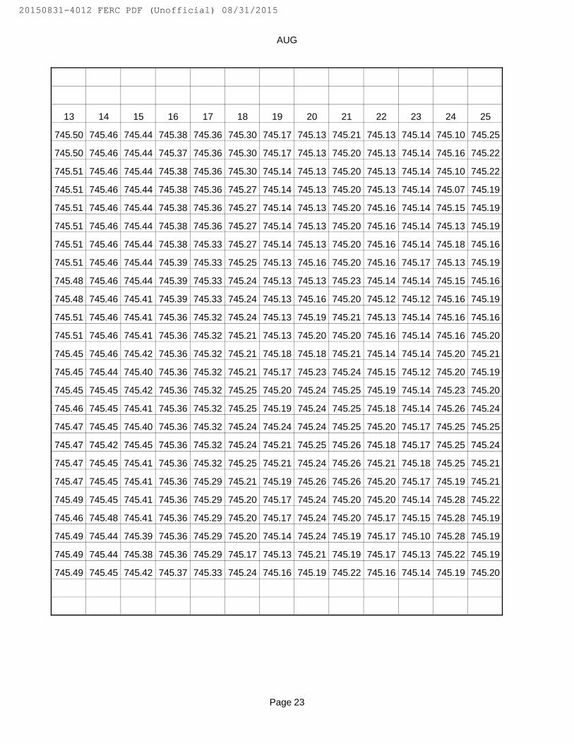
AUG
13 14 15 16 17 18 19 20 21 22 23 24 25
745.50 745.46 745.44 745.38 745.36 745.30 745.17 745.13 745.21 745.13 745.14 745.10 745.25
745.50 745.46 745.44 745.37 745.36 745.30 745.17 745.13 745.20 745.13 745.14 745.16 745.22
745.51 745.46 745.44 745.38 745.36 745.30 745.14 745.13 745.20 745.13 745.14 745.10 745.22
745.51 745.46 745.44 745.38 745.36 745.27 745.14 745.13 745.20 745.13 745.14 745.07 745.19
745.51 745.46 745.44 745.38 745.36 745.27 745.14 745.13 745.20 745.16 745.14 745.15 745.19
745.51 745.46 745.44 745.38 745.36 745.27 745.14 745.13 745.20 745.16 745.14 745.13 745.19
745.51 745.46 745.44 745.38 745.33 745.27 745.14 745.13 745.20 745.16 745.14 745.18 745.16
745.51 745.46 745.44 745.39 745.33 745.25 745.13 745.16 745.20 745.16 745.17 745.13 745.19
745.48 745.46 745.44 745.39 745.33 745.24 745.13 745.13 745.23 745.14 745.14 745.15 745.16
745.48 745.46 745.41 745.39 745.33 745.24 745.13 745.16 745.20 745.12 745.12 745.16 745.19
745.51 745.46 745.41 745.36 745.32 745.24 745.13 745.19 745.21 745.13 745.14 745.16 745.16
745.51 745.46 745.41 745.36 745.32 745.21 745.13 745.20 745.20 745.16 745.14 745.16 745.20
745.45 745.46 745.42 745.36 745.32 745.21 745.18 745.18 745.21 745.14 745.14 745.20 745.21
745.45 745.44 745.40 745.36 745.32 745.21 745.17 745.23 745.24 745.15 745.12 745.20 745.19
745.45 745.45 745.42 745.36 745.32 745.25 745.20 745.24 745.25 745.19 745.14 745.23 745.20
745.46 745.45 745.41 745.36 745.32 745.25 745.19 745.24 745.25 745.18 745.14 745.26 745.24
745.47 745.45 745.40 745.36 745.32 745.24 745.24 745.24 745.25 745.20 745.17 745.25 745.25
745.47 745.42 745.45 745.36 745.32 745.24 745.21 745.25 745.26 745.18 745.17 745.25 745.24
745.47 745.45 745.41 745.36 745.32 745.25 745.21 745.24 745.26 745.21 745.18 745.25 745.21
745.47 745.45 745.41 745.36 745.29 745.21 745.19 745.26 745.26 745.20 745.17 745.19 745.21
745.49 745.45 745.41 745.36 745.29 745.20 745.17 745.24 745.20 745.20 745.14 745.28 745.22
745.46 745.48 745.41 745.36 745.29 745.20 745.17 745.24 745.20 745.17 745.15 745.28 745.19
745.49 745.44 745.39 745.36 745.29 745.20 745.14 745.24 745.19 745.17 745.10 745.28 745.19
745.49 745.44 745.38 745.36 745.29 745.17 745.13 745.21 745.19 745.17 745.13 745.22 745.19
745.49 745.45 745.42 745.37 745.33 745.24 745.16 745.19 745.22 745.16 745.14 745.19 745.20
Page 23
20150831-4012 FERC PDF (Unofficial) 08/31/2015

AUG
26 27 28 29 30 31
745.16 745.13 745.11 744.70 744.27 743.87
745.13 745.10 745.11 744.68 744.27 743.90
745.16 745.10 745.08 744.65 744.24 746.87
745.13 745.10 745.08 744.65 744.24 743.85
745.13 745.10 745.05 744.62 744.21 743.85
745.13 745.10 745.05 744.62 744.21 743.85
745.16 745.10 745.02 744.59 744.18 743.82
745.16 745.13 744.99 744.56 744.15 743.79
745.16 745.15 744.96 744.56 744.12 743.76
745.16 745.15 744.96 744.56 744.12 743.76
745.19 745.15 744.93 744.53 744.06 743.73
745.19 745.18 744.93 744.51 744.06 743.71
745.20 745.18 744.90 744.47 744.00 743.71
745.20 745.18 744.88 744.49 744.00 743.71
745.22 745.19 744.88 744.45 744.00 743.66
745.22 745.16 744.85 744.43 744.00 743.66
745.22 745.16 744.86 744.41 743.97 743.64
745.22 745.19 744.82 744.34 743.94 743.63
745.21 745.16 744.83 744.42 743.93 743.58
745.19 745.13 744.80 744.35 743.96 743.58
745.20 745.13 744.77 744.35 743.93 743.56
745.14 745.12 744.76 744.32 743.93 743.56
745.14 745.13 744.73 744.29 743.93 743.53
745.12 745.11 744.73 744.32 743.87 743.53
745.17 745.14 744.92 744.49 744.07 743.84
Min = 743.53
Max = 747.17
Page 24
20150831-4012 FERC PDF (Unofficial) 08/31/2015

SEP
PENSACOLA HOURLY ELEVATIONS FOR SEPTEMBER 1993DATE
HOUR 1 2 3 4 5 6 7 8 9 10 11 12
0100 743.50 743.08 742.66 742.62 742.63 742.57 742.46 742.26 742.13 742.16 742.17 742.13
0200 743.47 743.08 742.72 742.65 742.63 742.58 742.43 742.26 742.13 742.16 742.17 742.11
0300 743.47 743.05 742.66 742.65 742.61 742.58 742.40 742.26 742.16 742.16 742.20 742.12
0400 743.44 743.05 742.66 742.65 742.61 742.56 742.40 742.26 742.16 742.15 742.17 742.12
0500 743.44 743.02 742.66 742.66 742.61 742.56 742.40 742.31 742.16 742.15 742.20 742.12
0600 743.42 743.00 742.66 742.66 742.61 742.56 742.37 742.28 742.16 742.15 742.20 742.13
0700 743.39 742.97 742.63 742.68 742.60 742.56 742.37 742.25 742.16 742.15 742.19 742.13
0800 743.39 742.97 742.60 742.65 742.60 742.56 742.36 742.27 742.16 742.14 742.19 742.09
0900 743.35 742.94 742.61 742.68 742.60 742.56 742.33 742.25 742.16 742.14 742.19 742.09
1000 743.35 742.92 742.60 742.66 742.60 742.56 742.32 742.22 742.15 742.14 742.19 742.09
1100 743.32 742.82 742.58 742.65 742.58 742.54 742.33 742.22 742.15 742.16 742.19 742.09
1200 743.32 742.79 742.59 742.64 742.60 742.58 742.33 742.26 742.15 742.17 742.18 742.09
1300 743.29 742.79 742.59 742.67 742.57 742.55 742.35 742.20 742.12 742.16 742.17 742.07
1400 743.26 742.74 742.61 742.72 742.57 742.57 742.35 742.19 742.12 742.17 742.14 742.07
1500 743.26 742.72 742.62 742.62 742.58 742.56 742.35 742.18 742.12 742.19 742.14 742.10
1600 743.23 742.74 742.66 742.66 742.59 742.53 742.32 742.16 742.10 742.17 742.14 742.08
1700 743.21 742.71 742.61 742.64 742.58 742.53 742.32 746.16 742.13 742.16 742.14 742.07
1800 743.19 742.71 742.61 742.68 742.60 742.55 742.32 742.16 742.13 742.14 742.14 742.10
1900 743.18 742.71 742.63 742.64 742.60 742.53 742.32 742.16 742.13 742.14 742.13 742.10
2000 743.18 742.71 742.61 742.61 742.67 742.50 742.33 742.16 742.13 742.17 742.13 742.10
2100 743.15 742.79 742.62 742.62 742.58 742.50 742.32 742.13 742.13 742.15 742.13 742.10
2200 743.15 742.78 742.62 742.60 742.58 742.51 742.29 742.13 742.13 742.15 742.13 742.10
2300 743.11 742.81 742.62 742.64 742.58 742.48 742.29 742.13 742.14 742.15 742.13 742.10
2400 743.11 742.71 742.62 742.63 742.58 742.43 742.26 742.13 742.14 742.17 742.13 742.10
AVG 743.30 742.86 742.63 742.65 742.60 742.54 742.35 742.37 742.14 742.16 742.16 742.10
Page 25
20150831-4012 FERC PDF (Unofficial) 08/31/2015

SEP
13 14 15 16 17 18 19 20 21 22 23 24 25
742.07 742.12 743.54 744.78 745.03 744.92 744.67 744.50 744.40 744.34 744.06 743.85 744.04
742.07 742.12 743.60 744.81 745.03 744.89 744.67 744.41 744.40 744.31 744.06 743.82 744.10
742.07 742.16 743.69 744.84 745.03 744.89 744.64 744.38 744.40 744.31 744.06 743.82 744.16
742.10 742.20 743.48 744.87 745.03 744.89 744.64 744.44 744.40 744.31 744.06 743.79 744.28
742.06 742.17 743.83 744.87 745.03 744.89 744.64 744.41 744.40 744.28 744.06 743.79 744.37
742.09 742.30 743.93 744.90 745.03 744.89 744.64 744.41 744.40 744.28 744.03 743.79 744.49
742.10 742.29 743.99 744.90 745.03 744.89 744.61 744.41 744.40 744.28 744.03 743.76 744.70
742.08 742.35 744.05 744.92 745.03 744.86 744.58 744.41 744.40 744.28 744.03 743.76 744.70
742.02 742.41 744.08 744.92 745.02 744.83 744.56 744.41 744.40 744.25 744.03 743.73 744.79
742.04 742.47 744.11 744.94 745.02 744.83 744.53 744.38 744.40 744.21 744.03 743.67 744.98
742.09 742.50 744.26 744.97 745.02 744.82 744.53 744.38 744.40 744.18 744.03 743.67 744.98
742.07 742.54 744.28 744.97 744.99 744.79 744.51 744.38 744.40 744.13 744.03 743.67 745.02
742.06 742.59 744.32 744.97 744.99 744.77 744.49 744.38 744.37 744.11 744.00 743.76 745.22
742.06 742.64 744.36 745.00 744.99 744.78 744.48 744.39 744.37 744.11 743.97 743.73 745.38
742.05 742.70 744.45 745.00 744.99 744.77 744.47 744.39 744.37 744.11 743.97 743.67 745.47
742.08 742.79 744.52 745.01 744.99 744.76 744.49 744.39 744.37 744.11 743.94 743.66 745.59
742.01 742.88 744.55 745.01 744.98 744.75 744.48 744.39 744.37 744.11 743.94 743.66 745.74
742.01 742.94 744.58 745.01 744.98 744.76 744.49 744.39 744.37 744.08 743.94 743.66 745.83
742.07 743.01 744.61 745.01 744.97 744.76 744.46 744.41 744.37 744.08 743.93 743.66 745.85
742.05 743.10 744.64 745.07 744.95 744.72 744.52 744.41 744.37 744.08 743.96 743.70 745.86
742.05 743.10 744.67 745.03 744.95 744.72 744.49 744.40 744.34 744.08 743.90 743.70 746.28
742.07 743.28 744.70 745.03 744.95 744.70 744.52 744.43 744.34 744.08 743.90 743.76 746.40
742.12 743.34 744.75 745.03 744.92 744.70 744.42 744.43 744.34 744.06 743.87 743.84 746.57
742.12 743.43 744.75 745.03 744.92 744.70 744.44 744.43 744.34 744.06 743.85 743.97 746.78
742.07 742.64 744.24 744.95 744.99 744.80 744.54 744.41 744.38 744.18 743.99 743.75 745.23
Page 26
20150831-4012 FERC PDF (Unofficial) 08/31/2015

SEP
26 27 28 29 30
746.98 752.14 754.37 754.21 753.27
746.88 752.36 754.37 754.15 753.21
747.28 752.55 754.37 754.12 753.19
747.60 752.70 754.37 754.09 753.13
747.80 752.84 754.40 754.06 753.07
747.65 753.02 754.40 754.01 753.01
748.39 753.17 754.40 753.95 752.95
748.56 753.31 754.40 753.92 752.89
748.83 753.49 754.40 753.92 752.80
749.00 753.55 754.50 753.89 752.77
749.37 753.66 754.50 753.83 752.72
749.58 753.86 754.47 753.80 752.69
749.81 753.81 754.45 753.80 752.65
749.90 753.90 754.45 753.77 752.63
750.20 753.96 754.39 753.71 752.57
750.51 753.99 754.36 753.67 752.54
750.68 754.05 754.36 753.63 752.48
750.95 754.10 754.33 753.61 752.48
751.06 754.16 754.33 753.57 752.42
751.12 754.19 754.30 753.51 752.42
751.52 754.28 754.30 753.45 752.39
751.70 754.28 754.27 753.42 752.33
751.88 754.31 754.24 753.39 752.27
752.00 754.31 754.21 753.33 752.23
749.55 753.58 754.37 753.78 752.71 ######
Min = 742.01
Max = 754.50
Page 27
20150831-4012 FERC PDF (Unofficial) 08/31/2015

OCT
PENSACOLA HOURLY ELEVATIONS FOR OCTOBER 1993DATE
HOUR 1 2 3 4 5 6 7 8 9 10 11 12
0100 752.20 751.21 749.62 748.29 747.32 746.77 746.38 746.11 745.97 745.85 745.63 745.37
0200 752.13 751.18 749.56 748.26 747.29 746.74 746.35 746.11 745.95 745.85 745.62 745.35
0300 752.06 751.11 749.50 748.20 747.26 746.74 746.35 746.11 745.92 745.82 745.60 745.34
0400 752.05 751.05 749.44 748.14 747.26 746.71 746.35 746.11 745.95 745.82 745.60 745.34
0500 751.99 750.96 749.38 748.09 747.24 746.71 746.32 746.11 745.95 745.79 745.59 745.32
0600 751.94 750.87 749.32 748.06 747.21 746.71 746.32 746.08 745.95 745.79 745.57 745.31
0700 751.90 750.82 749.28 748.03 747.18 746.68 746.32 746.08 745.95 745.79 745.57 745.31
0800 751.85 750.72 749.20 747.92 747.15 746.68 746.29 746.07 745.95 745.79 745.57 745.28
0900 751.82 750.68 749.13 747.91 747.12 746.65 746.26 746.07 745.95 745.79 745.55 745.28
1000 751.80 750.61 749.07 747.88 747.09 746.61 746.26 746.07 745.95 745.76 745.55 745.25
1100 751.74 750.56 749.01 747.79 747.06 746.58 746.23 746.06 745.95 745.76 745.55 745.22
1200 751.65 750.52 748.95 747.73 747.03 746.58 746.23 746.01 745.95 745.73 745.52 745.22
1300 751.68 750.45 748.90 747.70 747.00 746.55 746.20 746.01 745.92 745.72 745.52 745.22
1400 751.65 750.34 748.84 747.68 746.96 746.55 746.20 746.03 745.92 745.73 745.49 745.22
1500 751.65 750.28 748.81 747.62 746.93 746.52 746.20 746.00 745.92 745.70 745.49 745.22
1600 751.62 750.22 748.73 747.62 746.93 746.52 746.17 746.00 745.92 745.70 745.46 745.18
1700 751.59 750.12 748.68 747.56 746.90 746.49 746.17 746.00 745.91 745.72 745.46 745.18
1800 751.53 750.10 748.64 747.53 746.87 746.49 746.17 746.03 745.91 745.69 745.43 745.18
1900 751.50 750.01 748.58 747.50 746.87 746.49 746.17 746.03 745.91 745.69 745.43 745.18
2000 751.45 749.94 748.54 747.50 746.83 746.46 746.17 746.03 745.91 745.66 745.43 745.18
2100 751.42 749.91 748.50 747.44 746.83 746.46 746.17 746.00 745.88 745.69 745.43 745.15
2200 751.39 749.82 748.29 747.41 746.80 746.43 746.17 745.97 745.88 745.69 745.43 745.15
2300 751.30 749.77 748.41 747.38 746.80 746.40 746.17 746.00 745.88 745.66 745.40 745.15
2400 751.27 749.71 748.38 747.35 746.80 746.38 746.14 745.98 745.85 745.63 745.40 745.15
AVG 751.72 750.46 748.95 747.77 747.03 746.58 746.24 746.04 745.93 745.74 745.51 745.24
Page 28
20150831-4012 FERC PDF (Unofficial) 08/31/2015

OCT
13 14 15 16 17 18 19 20 21 22 23 24 25
745.13 744.91 744.70 744.49 744.19 744.02 743.88 743.86 743.72 743.50 743.43 743.30 743.13
745.13 744.88 744.70 744.49 744.19 743.99 743.88 743.86 743.72 743.50 743.43 743.30 743.10
745.13 744.88 744.70 744.49 744.19 744.02 743.91 743.86 743.69 743.50 743.43 743.30 743.10
745.13 744.88 744.70 744.49 744.19 744.02 743.89 743.86 743.69 743.50 743.43 743.30 743.10
745.10 744.87 744.67 744.46 744.19 743.99 743.89 743.86 743.69 743.50 743.41 743.27 743.07
745.10 744.85 744.67 744.45 744.19 743.99 743.89 743.86 743.69 743.50 743.41 743.27 743.07
745.07 744.82 744.67 744.45 744.16 743.99 743.89 743.86 743.69 743.47 743.41 743.27 743.07
745.04 744.82 744.64 744.39 744.16 743.96 743.89 743.83 743.69 743.47 743.41 743.27 743.07
745.01 744.82 744.64 744.42 744.16 743.96 743.88 743.80 743.66 743.45 743.38 743.24 743.04
745.01 744.79 744.61 744.42 744.16 743.96 743.91 743.83 743.63 743.45 743.38 743.24 743.01
745.04 744.78 744.58 744.13 743.93 743.88 743.81 743.63 743.45 743.37 743.25 743.01
745.04 744.78 744.58 744.35 744.11 743.93 743.88 743.81 743.63 743.43 743.33 743.21 743.01
745.01 744.78 744.55 744.13 743.94 743.91 743.81 743.63 743.43 743.36 743.21 742.99
744.98 744.75 744.57 744.32 744.13 743.91 743.88 743.81 743.59 743.43 743.35 743.21 742.99
744.97 744.75 744.53 744.32 744.10 743.91 743.88 743.82 743.59 743.43 743.35 743.20 742.97
744.97 744.75 744.53 744.32 744.07 743.91 743.88 743.79 743.59 743.43 743.35 743.15 742.97
744.97 744.72 744.53 744.32 744.10 743.91 743.91 743.79 743.56 743.43 743.35 743.21 742.97
744.94 744.72 744.53 744.32 744.07 743.91 743.88 743.79 743.56 743.44 743.32 743.18 742.97
744.94 744.72 744.53 744.32 744.04 743.88 743.88 743.79 743.53 743.43 743.32 743.13 742.94
744.94 744.70 744.53 744.32 744.07 743.88 743.88 743.79 743.53 743.43 743.32 743.16 742.94
744.91 744.70 744.53 744.32 744.04 743.88 743.88 743.76 743.53 743.42 743.32 743.16 742.94
744.91 744.70 744.52 744.32 744.04 743.88 743.88 743.81 743.53 743.44 743.33 743.13 742.94
744.91 744.67 744.52 744.32 744.01 743.88 743.88 743.76 743.53 743.44 743.30 743.13 742.94
744.91 744.70 744.52 744.22 744.01 743.88 743.88 743.75 743.53 743.44 743.33 743.13 742.91
745.01 744.78 744.59 744.38 744.12 743.94 743.89 743.82 743.62 743.45 743.37 743.22 743.01
Page 29
20150831-4012 FERC PDF (Unofficial) 08/31/2015

OCT
26 27 28 29 30 31
742.94 742.74 742.65 742.59 742.43 742.23
742.91 742.77 742.65 742.68 742.39 742.20
742.91 742.77 742.65 742.64 742.40 742.20
742.91 742.74 742.66 742.65 742.41 742.20
742.91 742.73 742.62 742.70 742.36 742.17
742.91 742.73 742.62 742.68 742.35 742.20
742.90 742.70 742.60 742.63 742.36 742.17
742.89 742.70 742.59 742.68 742.33 742.17
742.86 742.70 742.60 742.55 742.29 742.17
742.89 742.70 742.60 742.61 742.28 742.18
742.86 742.67 742.56 742.69 742.33 742.14
742.87 742.67 742.56 742.67 742.33 742.16
742.86 742.67 742.54 742.64 742.40 742.16
742.85 742.67 742.57 742.62 742.29 742.16
742.83 742.68 742.57 742.54 742.33 742.16
742.83 742.65 742.58 742.51 742.31 742.13
742.82 742.68 742.58 742.57 742.30 742.13
742.82 742.68 742.64 742.53 742.27 742.13
742.83 742.65 742.60 742.49 742.30 742.10
742.80 742.65 742.60 742.51 742.26 742.10
742.77 742.65 742.61 742.47 742.26 742.10
742.77 742.65 742.45 742.26 742.10
742.77 742.65 742.59 742.45 742.26 742.10
742.74 742.65 742.59 742.46 742.23 742.10
742.85 742.69 742.60 742.58 742.32 742.15
Min = 742.10
Max = 752.20
Page 30
20150831-4012 FERC PDF (Unofficial) 08/31/2015

NOV
PENSACOLA HOURLY ELEVATIONS FOR NOVEMBER 1993DATE
HOUR 1 2 3 4 5 6 7 8 9 10 11 12
0100 742.10 742.08 742.06 742.06 742.16 742.10 742.07 742.09 742.12 742.10 742.07 742.11
0200 742.10 742.08 742.06 742.07 742.16 742.10 742.07 742.09 742.09 742.10 742.10 742.11
0300 742.10 742.08 742.06 742.06 742.10 742.11 742.07 742.09 742.12 742.10 742.10 742.11
0400 742.10 742.08 742.06 742.06 742.12 742.08 742.07 742.09 742.12 742.10 742.10 742.05
0500 742.08 742.11 742.06 742.06 742.14 742.09 742.07 742.09 742.12 742.10 742.07 742.10
0600 742.08 742.11 742.06 742.07 742.15 742.11 742.10 742.09 742.15 742.10 742.10 742.09
0700 742.05 742.08 742.06 742.06 742.07 742.10 742.05 742.09 742.13 742.10 742.10 742.09
0800 742.05 742.08 742.06 742.08 742.10 742.07 742.07 742.09 742.13 742.09 742.10 742.08
0900 742.05 742.08 742.09 742.12 742.16 742.10 742.06 742.09 742.13 742.08 742.10 742.06
1000 742.02 742.07 742.06 742.12 742.16 742.10 742.06 742.09 742.10 742.11 742.07 742.08
1100 742.05 742.10 742.06 742.05 742.18 742.08 742.00 742.06 742.09 742.08 742.04 742.07
1200 742.02 742.10 742.06 742.06 742.15 742.08 742.00 742.09 742.13 742.10 742.04 742.05
1300 742.00 742.10 742.06 742.09 742.14 742.08 742.00 742.09 742.10 742.10 742.05 742.06
1400 742.00 742.07 742.06 742.09 742.12 742.08 742.04 742.09 742.10 742.10 742.06 742.05
1500 742.03 742.07 742.06 742.11 742.08 742.08 742.07 742.10 742.10 742.10 742.06 742.01
1600 742.03 742.07 742.04 742.11 742.10 742.09 742.04 742.10 742.10 742.10 742.09 741.99
1700 742.05 742.09 742.07 742.12 742.13 742.09 742.06 742.13 742.07 742.10 742.09 742.00
1800 742.05 742.06 742.07 742.12 742.12 742.07 742.06 742.09 742.07 742.08 742.10 741.99
1900 742.05 742.06 742.06 742.11 742.12 742.07 742.06 742.09 742.10 742.08 742.07 742.00
2000 742.05 742.06 742.06 742.11 742.13 742.07 742.06 742.12 742.10 742.08 742.04 742.00
2100 742.05 742.06 742.06 742.09 742.10 742.07 742.06 742.09 742.07 742.08 742.04 741.96
2200 742.05 742.06 742.06 742.09 742.09 742.07 742.06 742.09 742.10 742.07 742.04 741.98
2300 742.05 742.06 742.06 742.10 742.10 742.07 742.06 742.12 742.10 742.10 742.04 742.01
2400 742.05 742.06 742.06 742.10 742.10 742.07 742.06 742.09 742.10 742.07 742.08 742.02
AVG 742.05 742.08 742.06 742.09 742.12 742.08 742.06 742.09 742.11 742.09 742.07 742.04
Page 31
20150831-4012 FERC PDF (Unofficial) 08/31/2015

NOV
13 14 15 16 17 18 19 20 21 22 23 24 25
742.01 742.14 742.52 743.20 743.63 744.11 744.98 745.20 745.24 745.15 744.97 744.80 744.57
742.01 742.14 742.55 743.20 743.63 744.17 745.01 745.20 745.24 745.15 744.95 744.77 744.57
742.06 742.12 742.58 743.20 743.63 744.20 745.04 745.20 745.24 745.15 744.95 744.77 744.54
742.03 742.16 742.60 743.26 743.66 744.23 745.07 745.20 745.21 745.15 744.91 744.77 744.54
742.03 742.13 742.66 743.26 743.69 744.31 745.10 745.20 745.21 745.13 744.91 744.77 744.51
742.03 742.10 742.77 743.29 743.69 744.31 745.13 745.23 745.21 745.13 744.89 744.77 744.51
742.06 742.10 742.75 743.35 743.73 744.34 745.13 745.23 745.21 745.13 744.93 744.74 744.51
742.06 742.15 742.75 743.35 743.73 744.37 745.18 745.23 745.21 745.13 744.89 744.74 744.48
742.06 742.17 742.81 743.35 743.75 744.40 745.18 745.23 745.21 745.13 744.88 744.74 744.48
742.06 742.17 742.82 743.35 743.76 744.46 745.26 745.23 745.18 745.10 744.85 744.71 744.47
742.09 742.06 742.88 743.43 743.76 744.49 745.21 745.23 745.18 745.08 744.89 744.71 744.47
742.09 742.13 742.88 743.43 743.79 744.49 745.11 745.23 745.15 745.08 744.85 744.71 744.46
742.10 742.11 742.91 743.46 743.79 744.55 745.16 745.23 745.18 745.08 744.85 744.69 744.44
742.07 742.16 742.94 743.45 743.82 744.58 745.07 745.23 745.18 745.05 744.86 744.69 744.43
742.05 742.16 742.97 743.51 743.85 744.64 745.13 745.21 745.15 745.05 744.86 744.69 744.43
742.10 742.14 743.00 743.48 743.85 744.64 745.14 745.23 745.23 745.06 744.86 744.66 744.41
742.12 742.22 743.02 743.51 743.87 744.69 745.17 745.23 745.18 745.06 744.86 744.66 744.41
742.08 742.25 743.02 743.51 743.90 744.74 745.16 745.26 745.18 745.03 744.86 744.63 744.38
742.08 742.25 743.05 743.54 743.93 744.77 745.17 745.24 745.18 745.03 744.86 744.63 744.38
742.10 742.28 743.07 743.54 743.96 744.83 745.17 745.24 745.18 745.00 744.83 744.60 744.35
742.08 742.31 743.10 743.60 743.99 744.86 745.20 745.24 745.18 745.00 744.83 744.60 744.35
742.13 742.31 743.11 743.57 744.02 744.89 745.20 745.24 745.18 745.00 744.80 744.60 744.37
742.12 742.40 743.14 743.60 744.08 744.92 745.20 745.24 745.18 744.97 744.80 744.57 744.33
742.13 742.43 743.17 743.60 744.08 744.92 745.20 745.24 745.15 745.00 744.80 744.57 744.33
742.07 742.19 742.88 743.42 743.82 744.54 745.14 745.23 745.19 745.08 744.87 744.69 744.45
Page 32
20150831-4012 FERC PDF (Unofficial) 08/31/2015

NOV
26 27 28 29 30
744.33 743.95 743.69 743.45 743.35
744.30 743.92 743.66 743.45 743..5
744.28 743.89 743.66 743.45 743.35
744.28 743.86 743.66 743.45 743.35
744.28 743.89 743.66 743.43 743.35
744.28 743.89 743.63 743.43 743.35
744.22 743.89 743.63 743.43 743.32
744.22 743.89 743.60 743.40 743.34
744.22 743.89 743.60 743.40 743.34
744.22 743.89 743.57 743.40 743.31
744.19 743.84 743.57 743.38 743.31
744.19 743.81 743.54 743.37 743.28
744.16 743.80 743.51 743.37 743.31
744.13 743.78 743.54 743.37 743.30
744.10 743.72 743.48 743.37 743.28
744.10 743.72 743.48 743.37 743.28
744.07 743.72 743.51 743.36 743.28
744.07 743.72 743.51 743.35 743.25
744.07 743.75 743.48 743.35 743.25
744.04 743.78 743.48 743.35 743.28
744.04 743.75 743.48 743.35 743.22
744.01 743.75 743.48 743.35 743.22
744.01 743.72 743.45 743.35 743.19
743.98 743.72 743.45 743.35 743.22
744.16 743.81 743.56 743.39 743.29 ######
Min = 741.96
Max = 745.26
Page 33
20150831-4012 FERC PDF (Unofficial) 08/31/2015

PENSACOLA HOURLY ELEVATIONS FOR DECEMBER 1993DATE
HOUR 1 2 3 4 5 6 7 8 9 10 11 12 13 14 15 16 17 18 19 20 21 22 23 24 25 26 27 28 29 30 31
0100 743.22 743.08 742.94 743.00 742.93 742.77 742.66 742.53 742.54 742.46 742.28 742.09 742.04 742.01 742.08 742.15 742.04 742.03 742.06 742.07 742.04 742.04 741.99 742.06 742.13 742.15 742.32 742.23 742.02 742.03 742.03
0200 743.22 743.09 742.94 742.99 742.93 742.74 742.66 742.56 742.54 742.46 742.25 742.06 742.06 741.98 742.10 742.15 742.05 742.03 742.06 742.07 742.04 742.04 741.99 742.09 742.13 742.17 742.32 742.22 742.05 742.03 742.06
0300 743.22 743.09 742.94 743.01 742.93 742.74 742.66 742.53 742.54 742.44 742.28 742.06 742.03 741.98 742.10 742.15 742.05 742.06 742.06 742.07 742.04 742.04 742.02 742.09 742.17 742.16 742.35 742.28 742.05 742.04 742.09
0400 743.22 743.06 742.93 743.06 742.93 742.74 742.63 742.53 742.52 742.44 742.25 742.06 742.05 741.98 742.13 742.15 742.02 742.06 742.06 742.10 742.04 742.04 742.02 742.09 742.16 742.13 742.35 742.23 742.05 742.04 742.09
0500 743.22 743.06 742.90 743.01 742.93 742.74 742.60 742.52 742.54 742.41 742.26 742.06 742.10 742.00 742.13 742.15 742.02 742.06 742.06 742.06 742.04 742.01 742.02 742.09 742.16 742.12 742.35 742.18 742.05 742.01 742.09
0600 743.17 743.06 742.87 742.98 742.93 742.74 742.60 742.55 742.53 742.41 742.27 742.03 742.08 742.00 742.13 742.15 742.02 742.06 742.06 742.10 742.04 742.04 742.05 742.10 742.19 742.12 742.35 742.19 742.05 742.04 742.09
0700 743.17 743.03 742.93 742.99 742.93 742.74 742.60 742.53 742.55 742.41 742.22 742.06 742.05 742.03 742.14 742.15 742.02 742.06 742.06 742.07 742.04 742.01 742.02 742.10 742.16 742.16 742.35 742.19 742.05 742.04 742.09
0800 743.17 743.03 742.91 743.01 742.90 742.75 742.58 742.54 742.57 742.41 742.24 742.03 742.06 742.03 742.14 742.13 742.02 742.06 742.06 742.06 742.04 742.03 742.02 742.09 742.20 742.16 742.35 742.24 742.05 742.04 742.09
0900 743.13 743.03 743.10 742.95 742.84 742.75 742.58 742.54 742.54 742.38 742.24 742.03 742.05 742.03 742.14 742.13 741.99 742.06 742.06 742.03 742.04 742.04 742.02 742.06 742.20 742.17 742.35 742.16 742.04 742.01 742.09
1000 743.13 743.02 743.11 742.98 742.82 742.75 742.55 742.51 742.54 742.36 742.24 742.03 742.02 742.03 742.15 742.10 741.99 742.06 742.06 742.03 742.04 742.04 742.02 742.12 742.21 742.16 742.35 742.14 742.01 742.02 742.09
1100 743.11 743.02 743.07 742.95 742.78 742.76 742.50 742.54 742.54 742.37 742.17 742.00 741.98 742.05 742.15 742.11 741.99 742.09 742.03 742.04 742.01 742.02 742.02 742.09 742.17 742.19 742.32 742.14 742.04 742.00 742.09
1200 743.08 743.02 743.08 742.98 742.74 742.73 742.47 742.51 742.52 742.37 742.17 742.02 741.98 742.04 742.17 742.11 741.96 742.09 742.06 742.09 742.01 742.04 742.02 742.06 742.23 742.18 742.34 742.13 742.04 741.97 742.06
1300 743.08 743.00 743.08 742.94 742.79 742.70 742.51 742.51 742.51 742.33 742.20 742.06 741.99 742.05 742.15 742.11 741.99 742.09 742.06 742.03 742.01 742.06 742.02 742.06 742.15 742.20 742.31 742.16 742.09 742.00 742.06
1400 743.10 743.00 743.08 742.94 742.85 742.72 742.53 742.47 742.51 742.32 742.17 742.08 741.99 742.05 742.17 742.12 742.01 742.09 742.06 742.04 742.01 742.02 742.02 742.06 742.18 742.17 742.33 742.09 742.13 742.00 742.04
1500 743.07 743.00 743.05 742.94 742.82 742.72 742.56 742.53 742.48 742.34 742.16 742.04 742.02 742.05 742.19 742.12 742.00 742.09 742.06 742.08 741.98 742.04 742.02 742.03 742.20 742.20 742.34 742.09 742.11 741.97 742.07
1600 743.08 742.99 743.05 742.97 742.79 742.72 742.56 742.53 742.47 742.32 742.17 742.05 741.99 742.05 742.19 742.10 742.04 742.09 742.06 742.11 742.02 742.00 742.02 742.03 742.17 742.22 742.30 742.09 742.14 742.00 742.07
1700 743.08 742.91 743.05 742.97 742.82 742.69 742.56 742.50 742.47 742.33 742.15 742.05 742.01 742.08 742.17 742.10 742.01 742.09 742.06 742.06 742.02 742.02 742.05 742.05 742.17 742.23 742.28 742.08 742.13 742.00 742.06
1800 743.05 742.94 743.02 742.94 742.85 742.72 742.58 742.50 742.47 742.30 742.15 742.08 742.01 742.05 742.17 742.10 742.03 742.06 742.07 742.03 741.99 742.02 742.03 742.08 742.18 742.26 742.32 742.07 742.10 742.03 742.10
1900 743.05 742.94 743.02 742.95 742.82 742.70 742.56 742.53 742.47 742.30 742.12 742.04 741.99 742.05 742.17 742.07 742.03 742.09 742.07 742.03 742.02 741.99 742.06 742.08 742.18 742.26 742.26 742.05 742.05 742.03 742.08
2000 743.05 742.94 743.02 742.98 742.79 742.69 742.56 742.51 742.47 742.30 742.12 742.01 742.00 742.05 742.17 742.07 742.03 742.09 742.07 742.06 742.02 741.99 742.06 742.08 742.17 742.26 742.33 742.02 742.05 742.03 742.09
2100 743.05 742.94 743.02 742.95 742.79 742.69 742.56 742.47 742.47 742.30 742.12 742.03 741.97 742.05 742.17 742.07 742.03 742.06 742.07 742.03 742.02 741.99 742.06 742.08 742.17 742.29 742.30 742.02 742.03 742.06 742.06
2200 743.02 742.94 743.02 742.92 742.79 742.69 742.56 742.50 742.46 742.31 742.12 742.05 741.97 742.08 742.17 742.07 742.03 742.06 742.04 742.03 742.06 741.99 742.06 742.11 742.17 742.29 742.27 742.02 742.01 742.03 742.05
2300 743.02 742.94 743.02 742.92 742.80 742.66 742.56 742.51 742.46 742.33 742.09 742.07 741.99 742.08 742.17 742.04 742.06 742.06 742.07 742.03 742.02 741.99 742.06 742.11 742.17 742.29 742.29 742.02 742.04 742.06 742.03
2400 743.05 742.94 743.02 742.92 742.77 742.66 742.56 742.51 742.46 742.31 742.09 742.11 741.98 742.08 742.17 742.04 742.06 742.06 742.07 742.03 742.02 741.99 742.06 742.11 742.17 742.29 742.26 742.02 742.04 742.06 742.04
AVG 743.12 743.00 743.01 742.97 742.84 742.72 742.57 742.52 742.51 742.36 742.19 742.05 742.02 742.04 742.15 742.11 742.02 742.07 742.06 742.06 742.03 742.02 742.03 742.08 742.17 742.20 742.32 742.13 742.06 742.02 742.07
Min = 741.96
Max = 743.22
@[email protected] DEC 8/31/2015
20150831-4012 FERC PDF (Unofficial) 08/31/2015

DATE OCTOBER 1 2009
TOTAL
ITEM TIME TIME TURBINE SPILL DISCHARGE
Pool Elevation 1200 743.99 0100 11,976 0 11,976
Pool Elevation 1600 743.96 0200 11,979 0 11,979
Pool Elevation 2400 743.87 0300 11,981 0 11,981
Pool Elevation 0800 743.74 0400 11,982 0 11,982
Tailwater Elevation 0800 621.51 0500 11,992 0 11,992
0600 11,994 0 11,994
24 Hr Avg Power Discharge 2400 10,499 0700 11,991 0 11,991
24 Hr Avg Spill 2400 0 0800 11,568 0 11,568
24 Hr Total Discharge 2400 10,499 0900 107 0 107
1000 0 0 0
Instantaneous Power Discharge 0800 11,704 1100 860 0 860
Instantaneous Spill 0800 1200 11,713 0 11,713
Instantaneous Total Discharge 0800 11,704 1300 11,960 0 11,960
1400 11,976 0 11,976
Total Precipitation 0.00 1500 11,982 0 11,982
1600 11,984 0 11,984
GATE OPERATIONS 1700 11,987 0 11,987
Time 1800 11,987 0 11,987
Pool Elevation 1900 11,990 0 11,990
From Gate Setting 2000 11,990 0 11,990
To Gate Setting 2100 11,993 0 11,993
GATE OPERATIONS 2200 11,993 0 11,993
Time 2300 11,996 0 11,996
Pool Elevation 2400 11,998 0 11,998
From Gate Setting 10,499 0 10,499
To Gate Setting
PENSACOLA LAKE DATA
20150831-4012 FERC PDF (Unofficial) 08/31/2015

DATE OCTOBER 2 2009
TOTAL
ITEM TIME TIME TURBINE SPILL DISCHARGE
Pool Elevation 1200 743.62 0100 11,998 0 11,998
Pool Elevation 1600 743.48 0200 11,346 0 11,346
Pool Elevation 2400 743.40 0300 11,784 0 11,784
Pool Elevation 0800 743.25 0400 11,799 0 11,799
Tailwater Elevation 0800 622.46 0500 11,801 0 11,801
0600 11,695 0 11,695
24 Hr Avg Power Discharge 2400 11,783 0700 11,701 0 11,701
24 Hr Avg Spill 2400 0 0800 11,714 0 11,714
24 Hr Total Discharge 2400 11,783 0900 11,747 0 11,747
1000 11,761 0 11,761
Instantaneous Power Discharge 0800 11,843 1100 11,784 0 11,784
Instantaneous Spill 0800 1200 11,803 0 11,803
Instantaneous Total Discharge 0800 11,843 1300 11,812 0 11,812
1400 11,812 0 11,812
Total Precipitation 0.00 1500 11,818 0 11,818
1600 11,821 0 11,821
GATE OPERATIONS 1700 11,824 0 11,824
Time 1800 11,824 0 11,824
Pool Elevation 1900 11,824 0 11,824
From Gate Setting 2000 11,824 0 11,824
To Gate Setting 2100 11,824 0 11,824
GATE OPERATIONS 2200 11,826 0 11,826
Time 2300 11,829 0 11,829
Pool Elevation 2400 11,829 0 11,829
From Gate Setting 11,783 0 11,783
To Gate Setting
PENSACOLA LAKE DATA
20150831-4012 FERC PDF (Unofficial) 08/31/2015

DATE OCTOBER 3 2009
TOTAL
ITEM TIME TIME TURBINE SPILL DISCHARGE
Pool Elevation 1200 743.20 0100 11,831 0 11,831
Pool Elevation 1600 743.12 0200 11,831 0 11,831
Pool Elevation 2400 743.01 0300 11,831 0 11,831
Pool Elevation 0800 742.88 0400 11,834 0 11,834
Tailwater Elevation 0800 623.13 0500 11,837 0 11,837
0600 11,837 0 11,837
24 Hr Avg Power Discharge 2400 11,882 0700 11,840 0 11,840
24 Hr Avg Spill 2400 0 0800 11,843 0 11,843
24 Hr Total Discharge 2400 11,882 0900 11,863 0 11,863
1000 11,879 0 11,879
Instantaneous Power Discharge 0800 11,946 1100 11,889 0 11,889
Instantaneous Spill 0800 1200 11,893 0 11,893
Instantaneous Total Discharge 0800 11,946 1300 11,896 0 11,896
1400 11,896 0 11,896
Total Precipitation 0.00 1500 11,905 0 11,905
1600 11,907 0 11,907
GATE OPERATIONS 1700 11,916 0 11,916
Time 1800 11,911 0 11,911
Pool Elevation 1900 11,914 0 11,914
From Gate Setting 2000 11,924 0 11,924
To Gate Setting 2100 11,914 0 11,914
GATE OPERATIONS 2200 11,928 0 11,928
Time 2300 11,919 0 11,919
Pool Elevation 2400 11,922 0 11,922
From Gate Setting 11,882 0 11,882
To Gate Setting
PENSACOLA LAKE DATA
20150831-4012 FERC PDF (Unofficial) 08/31/2015

DATE OCTOBER 4 2009
TOTAL
ITEM TIME TIME TURBINE SPILL DISCHARGE
Pool Elevation 1200 742.78 0100 11,925 0 11,925
Pool Elevation 1600 742.73 0200 11,933 0 11,933
Pool Elevation 2400 742.51 0300 11,932 0 11,932
Pool Elevation 0800 742.32 0400 11,935 0 11,935
Tailwater Elevation 0800 623.61 0500 11,935 0 11,935
0600 11,938 0 11,938
24 Hr Avg Power Discharge 2400 11,978 0700 11,941 0 11,941
24 Hr Avg Spill 2400 0 0800 11,946 0 11,946
24 Hr Total Discharge 2400 11,978 0900 11,955 0 11,955
1000 11,952 0 11,952
Instantaneous Power Discharge 0800 11,938 1100 11,962 0 11,962
Instantaneous Spill 0800 1200 11,972 0 11,972
Instantaneous Total Discharge 0800 11,938 1300 11,978 0 11,978
1400 11,996 0 11,996
Total Precipitation 0.00 1500 12,002 0 12,002
1600 12,007 0 12,007
GATE OPERATIONS 1700 12,010 0 12,010
Time 1800 12,014 0 12,014
Pool Elevation 1900 12,017 0 12,017
From Gate Setting 2000 12,020 0 12,020
To Gate Setting 2100 12,020 0 12,020
GATE OPERATIONS 2200 12,022 0 12,022
Time 2300 12,026 0 12,026
Pool Elevation 2400 12,029 0 12,029
From Gate Setting 11,978 0 11,978
To Gate Setting
PENSACOLA LAKE DATA
20150831-4012 FERC PDF (Unofficial) 08/31/2015

DATE OCTOBER 5 2009
TOTAL
ITEM TIME TIME TURBINE SPILL DISCHARGE
Pool Elevation 1200 742.21 0100 12,035 0 12,035
Pool Elevation 1600 742.13 0200 12,038 0 12,038
Pool Elevation 2400 742.00 0300 12,038 0 12,038
Pool Elevation 0800 741.87 0400 12,041 0 12,041
Tailwater Elevation 0800 624.45 0500 12,044 0 12,044
0600 12,044 0 12,044
24 Hr Avg Power Discharge 2400 11,970 0700 12,048 0 12,048
24 Hr Avg Spill 2400 0 0800 12,051 0 12,051
24 Hr Total Discharge 2400 11,970 0900 12,054 0 12,054
1000 12,057 0 12,057
Instantaneous Power Discharge 0800 11,955 1100 12,071 0 12,071
Instantaneous Spill 0800 1200 12,074 0 12,074
Instantaneous Total Discharge 0800 11,955 1300 12,084 0 12,084
1400 12,094 0 12,094
Total Precipitation 0.01 1500 12,107 0 12,107
1600 12,119 0 12,119
GATE OPERATIONS 1700 12,110 0 12,110
Time 1800 12,113 0 12,113
Pool Elevation 1900 12,122 0 12,122
From Gate Setting 2000 12,125 0 12,125
To Gate Setting 2100 12,128 0 12,128
GATE OPERATIONS 2200 10,774 0 10,774
Time 2300 10,776 0 10,776
Pool Elevation 2400 12,141 0 12,141
From Gate Setting 11,970 0 11,970
To Gate Setting
PENSACOLA LAKE DATA
20150831-4012 FERC PDF (Unofficial) 08/31/2015

DATE OCTOBER 6 2009
TOTAL
ITEM TIME TIME TURBINE SPILL DISCHARGE
Pool Elevation 1200 741.83 0100 12,144 0 12,144
Pool Elevation 1600 741.72 0200 12,148 0 12,148
Pool Elevation 2400 741.49 0300 12,150 0 12,150
Pool Elevation 0800 741.34 0400 12,172 0 12,172
Tailwater Elevation 0800 624.15 0500 12,179 0 12,179
0600 12,181 0 12,181
24 Hr Avg Power Discharge 2400 12,096 0700 12,186 0 12,186
24 Hr Avg Spill 2400 0 0800 12,064 0 12,064
24 Hr Total Discharge 2400 12,096 0900 12,178 0 12,178
1000 12,178 0 12,178
Instantaneous Power Discharge 0800 11,865 1100 12,061 0 12,061
Instantaneous Spill 0800 1200 12,178 0 12,178
Instantaneous Total Discharge 0800 11,865 1300 12,187 0 12,187
1400 12,073 0 12,073
Total Precipitation 0.13 1500 12,073 0 12,073
1600 12,075 0 12,075
GATE OPERATIONS 1700 11,965 0 11,965
Time 1800 12,082 0 12,082
Pool Elevation 1900 12,082 0 12,082
From Gate Setting 2000 11,968 0 11,968
To Gate Setting 2100 11,966 0 11,966
GATE OPERATIONS 2200 11,962 0 11,962
Time 2300 11,964 0 11,964
Pool Elevation 2400 12,084 0 12,084
From Gate Setting 12,096 0 12,096
To Gate Setting
PENSACOLA LAKE DATA
20150831-4012 FERC PDF (Unofficial) 08/31/2015

DATE OCTOBER 7 2009
TOTAL
ITEM TIME TIME TURBINE SPILL DISCHARGE
Pool Elevation 1200 741.23 0100 11,970 0 11,970
Pool Elevation 1600 741.18 0200 11,973 0 11,973
Pool Elevation 2400 741.02 0300 11,973 0 11,973
Pool Elevation 0800 740.98 0400 11,976 0 11,976
Tailwater Elevation 0800 619.29 0500 11,973 0 11,973
0600 11,973 0 11,973
24 Hr Avg Power Discharge 2400 11,978 0700 11,976 0 11,976
24 Hr Avg Spill 2400 0 0800 11,979 0 11,979
24 Hr Total Discharge 2400 11,978 0900 11,990 0 11,990
1000 12,003 0 12,003
Instantaneous Power Discharge 0800 3,516 1100 12,020 0 12,020
Instantaneous Spill 0800 1200 12,035 0 12,035
Instantaneous Total Discharge 0800 3,516 1300 12,047 0 12,047
1400 11,935 0 11,935
Total Precipitation 0.01 1500 12,053 0 12,053
1600 12,047 0 12,047
GATE OPERATIONS 1700 11,933 0 11,933
Time 1800 11,935 0 11,935
Pool Elevation 1900 11,944 0 11,944
From Gate Setting 2000 11,949 0 11,949
To Gate Setting 2100 11,943 0 11,943
GATE OPERATIONS 2200 11,944 0 11,944
Time 2300 11,943 0 11,943
Pool Elevation 2400 11,948 0 11,948
From Gate Setting 11,978 0 11,978
To Gate Setting
PENSACOLA LAKE DATA
20150831-4012 FERC PDF (Unofficial) 08/31/2015

DATE OCTOBER 8 2009
TOTAL
ITEM TIME TIME TURBINE SPILL DISCHARGE
Pool Elevation 1200 740.95 0100 3,430 0 3,430
Pool Elevation 1600 741.10 0200 1,981 0 1,981
Pool Elevation 2400 742.00 0300 1,980 0 1,980
Pool Elevation 0800 743.51 0400 1,980 0 1,980
Tailwater Elevation 0800 621.45 0500 1,980 0 1,980
0600 1,982 0 1,982
24 Hr Avg Power Discharge 2400 6,763 0700 1,975 0 1,975
24 Hr Avg Spill 2400 0 0800 3,522 0 3,522
24 Hr Total Discharge 2400 6,763 0900 3,856 0 3,856
1000 3,525 0 3,525
Instantaneous Power Discharge 0800 11,830 1100 5,410 0 5,410
Instantaneous Spill 0800 1200 5,861 0 5,861
Instantaneous Total Discharge 0800 11,830 1300 5,311 0 5,311
1400 6,760 0 6,760
Total Precipitation 9.41 1500 7,331 0 7,331
1600 10,597 0 10,597
GATE OPERATIONS 1700 11,843 0 11,843
Time 1800 11,846 0 11,846
Pool Elevation 1900 11,849 0 11,849
From Gate Setting 2000 11,854 0 11,854
To Gate Setting 2100 11,833 0 11,833
GATE OPERATIONS 2200 11,812 0 11,812
Time 2300 11,905 0 11,905
Pool Elevation 2400 11,895 0 11,895
From Gate Setting 6,763 0 6,763
To Gate Setting
PENSACOLA LAKE DATA
20150831-4012 FERC PDF (Unofficial) 08/31/2015

DATE OCTOBER 9 2009
TOTAL
ITEM TIME TIME TURBINE SPILL DISCHARGE
Pool Elevation 1200 744.28 0100 11,888 0 11,888
Pool Elevation 1600 744.98 0200 11,867 0 11,867
Pool Elevation 2400 746.30 0300 11,831 0 11,831
Pool Elevation 0800 747.45 0400 12,041 0 12,041
Tailwater Elevation 0800 620.19 0500 12,009 0 12,009
0600 11,984 0 11,984
24 Hr Avg Power Discharge 2400 12,150 0700 11,956 0 11,956
24 Hr Avg Spill 2400 15,932 0800 11,919 0 11,919
24 Hr Total Discharge 2400 28,082 0900 11,894 0 11,894
1000 11,881 10,446 22,327
Instantaneous Power Discharge 0800 12,082 1100 11,877 21,580 33,457
Instantaneous Spill 0800 38,275 1200 11,862 22,250 34,112
Instantaneous Total Discharge 0800 50,357 1300 12,429 23,054 35,483
1400 12,408 23,948 36,356
Total Precipitation 0.43 1500 12,500 24,708 37,208
1600 12,376 25,378 37,754
GATE OPERATIONS 1700 12,462 26,002 38,464
Time 0930 1800 12,444 26,762 39,206
Pool Elevation 743.90 1900 12,407 27,700 40,107
From Gate Setting 0 2000 12,379 28,460 40,839
To Gate Setting 2 Main & 7 East 2100 12,335 29,352 41,687
GATE OPERATIONS 2200 12,312 30,050 42,362
Time 2300 12,279 30,990 43,269
Pool Elevation 2400 12,255 31,694 43,949
From Gate Setting 12,150 15,932 28,082
To Gate Setting
PENSACOLA LAKE DATA
20150831-4012 FERC PDF (Unofficial) 08/31/2015

DATE OCTOBER 10 2009
TOTAL
ITEM TIME TIME TURBINE SPILL DISCHARGE
Pool Elevation 1200 747.86 0100 12,226 32,750 44,976
Pool Elevation 1600 748.10 0200 12,199 33,982 46,181
Pool Elevation 2400 748.58 0300 12,178 34,744 46,922
Pool Elevation 0800 748.96 0400 12,154 35,624 47,778
Tailwater Elevation 0800 622.29 0500 12,123 36,460 48,583
0600 12,209 37,010 49,219
24 Hr Avg Power Discharge 2400 11,999 0700 12,091 37,725 49,816
24 Hr Avg Spill 2400 51,164 0800 12,186 38,385 50,571
24 Hr Total Discharge 2400 63,164 0900 12,164 39,265 51,429
1000 12,161 39,760 51,921
Instantaneous Power Discharge 0800 11,716 1100 12,166 40,420 52,586
Instantaneous Spill 0800 69,212 1200 12,102 50,890 62,992
Instantaneous Total Discharge 0800 80,928 1300 12,026 62,150 74,176
1400 11,940 62,444 74,384
Total Precipitation 0.00 1500 11,842 62,658 74,500
1600 11,848 63,020 74,868
GATE OPERATIONS 1700 11,850 63,670 75,520
Time 1130 1800 11,862 64,102 75,964
Pool Elevation 747.83 1900 11,864 64,246 76,110
From Gate Setting 2 Main & 7 East 2000 11,746 64,892 76,638
To Gate Setting 4 Main & 7 East 2100 11,846 65,394 77,240
GATE OPERATIONS 2200 11,739 65,756 77,495
Time 2300 11,730 66,118 77,848
Pool Elevation 2400 11,731 66,476 78,207
From Gate Setting 11,999 51,164 63,164
To Gate Setting
PENSACOLA LAKE DATA
20150831-4012 FERC PDF (Unofficial) 08/31/2015

DATE OCTOBER 11 2009
TOTAL
ITEM TIME TIME TURBINE SPILL DISCHARGE
Pool Elevation 1200 749.11 0100 11,720 67,196 78,916
Pool Elevation 1600 749.24 0200 11,718 67,414 79,132
Pool Elevation 2400 749.47 0300 11,718 67,846 79,564
Pool Elevation 0800 749.60 0400 11,720 68,060 79,780
Tailwater Elevation 0800 623.75 0500 11,715 68,492 80,207
0600 11,712 68,710 80,422
24 Hr Avg Power Discharge 2400 11,709 0700 11,706 69,142 80,848
24 Hr Avg Spill 2400 70,319 0800 11,716 69,212 80,928
24 Hr Total Discharge 2400 82,028 0900 11,710 69,644 81,354
1000 11,707 69,858 81,565
Instantaneous Power Discharge 0800 11,686 1100 11,718 70,076 81,794
Instantaneous Spill 0800 73,820 1200 11,725 70,290 82,015
Instantaneous Total Discharge 0800 85,506 1300 11,733 70,582 82,315
1400 11,734 70,796 82,530
Total Precipitation 0.01 1500 11,749 71,014 82,763
1600 11,752 71,228 82,980
GATE OPERATIONS 1700 11,645 71,730 83,375
Time 1800 11,756 71,730 83,486
Pool Elevation 1900 11,653 71,878 83,531
From Gate Setting 2000 11,767 72,162 83,929
To Gate Setting 2100 11,658 72,380 84,038
GATE OPERATIONS 2200 11,664 72,450 84,114
Time 2300 11,658 72,882 84,540
Pool Elevation 2400 11,664 72,882 84,546
From Gate Setting 11,709 70,319 82,028
To Gate Setting
PENSACOLA LAKE DATA
20150831-4012 FERC PDF (Unofficial) 08/31/2015

DATE OCTOBER 12 2009
TOTAL
ITEM TIME TIME TURBINE SPILL DISCHARGE
Pool Elevation 1200 749.57 0100 11,664 72,882 84,546
Pool Elevation 1600 749.53 0200 11,677 72,956 84,633
Pool Elevation 2400 749.34 0300 11,670 73,532 85,202
Pool Elevation 0800 749.09 0400 11,675 73,532 85,207
Tailwater Elevation 0800 624.28 0500 11,675 73,532 85,207
0600 11,679 73,606 85,285
24 Hr Avg Power Discharge 2400 11,713 0700 11,683 73,606 85,289
24 Hr Avg Spill 2400 73,169 0800 11,686 73,820 85,506
24 Hr Total Discharge 2400 84,883 0900 11,689 73,606 85,295
1000 11,693 73,606 85,299
Instantaneous Power Discharge 0800 11,783 1100 11,702 73,606 85,308
Instantaneous Spill 0800 70,150 1200 11,708 73,606 85,314
Instantaneous Total Discharge 0800 81,933 1300 11,713 73,606 85,319
1400 11,728 73,318 85,046
Total Precipitation 0.01 1500 11,730 73,318 85,048
1600 11,735 73,318 85,053
GATE OPERATIONS 1700 11,738 73,100 84,838
Time 1800 11,747 73,026 84,773
Pool Elevation 1900 11,745 72,882 84,627
From Gate Setting 2000 11,755 72,594 84,349
To Gate Setting 2100 11,755 72,594 84,349
GATE OPERATIONS 2200 11,760 72,236 83,996
Time 2300 11,758 72,236 83,994
Pool Elevation 2400 11,758 71,948 83,706
From Gate Setting 11,713 73,169 84,883
To Gate Setting
PENSACOLA LAKE DATA
20150831-4012 FERC PDF (Unofficial) 08/31/2015

DATE OCTOBER 13 2009
TOTAL
ITEM TIME TIME TURBINE SPILL DISCHARGE
Pool Elevation 1200 748.96 0100 11,760 71,804 83,564
Pool Elevation 1600 748.94 0200 11,769 71,372 83,141
Pool Elevation 2400 748.70 0300 11,766 71,302 83,068
Pool Elevation 0800 748.21 0400 11,776 70,870 82,646
Tailwater Elevation 0800 623.40 0500 11,777 70,796 82,573
0600 11,785 70,438 82,223
24 Hr Avg Power Discharge 2400 12,053 0700 11,788 70,220 82,008
24 Hr Avg Spill 2400 54,030 0800 11,783 70,150 81,933
24 Hr Total Discharge 2400 66,082 0900 11,781 64,491 76,272
1000 11,992 58,379 70,371
Instantaneous Power Discharge 0800 12,319 1100 12,101 58,121 70,222
Instantaneous Spill 0800 36,446 1200 12,097 57,992 70,089
Instantaneous Total Discharge 0800 48,765 1300 12,097 58,121 70,218
1400 12,073 39,820 51,893
Total Precipitation 0.10 1500 12,282 39,730 52,012
1600 12,282 39,730 52,012
GATE OPERATIONS 1700 12,285 39,594 51,879
Time 0830 1800 12,288 39,460 51,748
Pool Elevation 749.09 1900 12,291 39,324 51,615
From Gate Setting 4 Main & 7 East 2000 12,291 39,324 51,615
To Gate Setting 3 Main & 7 East 2100 12,294 39,190 51,484
GATE OPERATIONS 2200 12,297 39,054 51,351
Time 1300 2300 12,303 38,784 51,087
Pool Elevation 748.98 2400 12,306 38,650 50,956
From Gate Setting 3 Main & 7 East 12,053 54,030 66,082
To Gate Setting 2 Main & 5 East
PENSACOLA LAKE DATA
20150831-4012 FERC PDF (Unofficial) 08/31/2015

DATE OCTOBER 14 2009
TOTAL
ITEM TIME TIME TURBINE SPILL DISCHARGE
Pool Elevation 1200 747.99 0100 12,318 38,380 50,698
Pool Elevation 1600 747.81 0200 12,328 38,110 50,438
Pool Elevation 2400 747.26 0300 12,332 37,840 50,172
Pool Elevation 0800 746.85 0400 12,347 37,390 49,737
Tailwater Elevation 0800 630.73 0500 12,344 37,256 49,600
0600 12,341 36,986 49,327
24 Hr Avg Power Discharge 2400 12,741 0700 12,322 36,670 48,992
24 Hr Avg Spill 2400 35,309 0800 12,313 36,446 48,759
24 Hr Total Discharge 2400 48,050 0900 12,299 36,220 48,519
1000 12,282 35,950 48,232
Instantaneous Power Discharge 0800 13,241 1100 12,276 35,724 48,000
Instantaneous Spill 0800 30,300 1200 12,276 35,455 47,731
Instantaneous Total Discharge 0800 43,541 1300 12,269 35,230 47,499
1400 13,239 35,050 48,289
Total Precipitation 0.07 1500 13,246 34,780 48,026
1600 13,243 34,645 47,888
GATE OPERATIONS 1700 13,247 34,195 47,442
Time 1800 13,246 33,970 47,216
Pool Elevation 1900 13,243 33,700 46,943
From Gate Setting 2000 13,247 33,250 46,497
To Gate Setting 2100 13,254 32,980 46,234
GATE OPERATIONS 2200 13,252 32,710 45,962
Time 2300 13,257 32,305 45,562
Pool Elevation 2400 13,255 32,170 45,425
From Gate Setting 12,741 35,309 48,050
To Gate Setting
PENSACOLA LAKE DATA
20150831-4012 FERC PDF (Unofficial) 08/31/2015

DATE OCTOBER 15 2009
TOTAL
ITEM TIME TIME TURBINE SPILL DISCHARGE
Pool Elevation 1200 746.72 0100 13,253 31,990 45,243
Pool Elevation 1600 746.57 0200 13,252 31,720 44,972
Pool Elevation 2400 746.38 0300 13,257 31,450 44,707
Pool Elevation 0800 746.19 0400 13,247 31,270 44,517
Tailwater Elevation 0800 627.42 0500 13,254 31,000 44,254
0600 13,250 30,766 44,016
24 Hr Avg Power Discharge 2400 13,185 0700 13,243 30,580 43,823
24 Hr Avg Spill 2400 17,918 0800 13,241 30,300 43,541
24 Hr Total Discharge 2400 31,103 0900 13,241 30,066 43,307
1000 13,152 30,114 43,266
Instantaneous Power Discharge 0800 13,170 1100 13,055 15,963 29,018
Instantaneous Spill 0800 5,444 1200 13,135 15,963 29,098
Instantaneous Total Discharge 0800 18,614 1300 13,132 15,831 28,963
1400 13,132 15,778 28,910
Total Precipitation 0.00 1500 13,068 5,827 18,895
1600 13,165 5,799 18,964
GATE OPERATIONS 1700 13,160 5,780 18,940
Time 1000 1800 13,164 5,752 18,916
Pool Elevation 746.81 1900 13,167 5,724 18,891
From Gate Setting 2 Main & 5 East 2000 13,167 5,724 18,891
To Gate Setting 1 Main & 3 East 2100 13,170 5,696 18,866
GATE OPERATIONS 2200 13,174 5,668 18,842
Time 1400 2300 13,176 5,649 18,825
Pool Elevation 746.65 2400 13,179 5,621 18,800
From Gate Setting 1 Main & 3 East 13,185 17,918 31,103
To Gate Setting 1 Main @ 10' & 1E.
PENSACOLA LAKE DATA
20150831-4012 FERC PDF (Unofficial) 08/31/2015

DATE OCTOBER 16 2009
TOTAL
ITEM TIME TIME TURBINE SPILL DISCHARGE
Pool Elevation 1200 746.15 0100 13,179 5,621 18,800
Pool Elevation 1600 746.11 0200 13,183 5,593 18,776
Pool Elevation 2400 746.07 0300 13,186 5,565 18,751
Pool Elevation 0800 746.03 0400 13,180 5,537 18,717
Tailwater Elevation 0800 626.14 0500 13,184 5,509 18,693
0600 13,187 5,481 18,668
24 Hr Avg Power Discharge 2400 13,412 0700 13,186 5,453 18,639
24 Hr Avg Spill 2400 2,548 0800 13,170 5,444 18,614
24 Hr Total Discharge 2400 15,960 0900 13,286 5,416 18,702
1000 13,399 5,416 18,815
Instantaneous Power Discharge 0800 13,605 1100 13,511 2,884 16,395
Instantaneous Spill 0800 242 1200 13,472 252 13,724
Instantaneous Total Discharge 0800 13,847 1300 13,533 252 13,785
1400 13,624 254 13,878
Total Precipitation 0.00 1500 13,628 252 13,880
1600 13,631 248 13,879
GATE OPERATIONS 1700 13,516 252 13,768
Time 1030 1800 13,519 248 13,767
Pool Elevation 746.16 1900 13,631 248 13,879
From Gate Setting 1 Main @ 10' & 1 E 2000 13,523 246 13,769
To Gate Setting 1 East @ 2' 2100 13,621 246 13,867
GATE OPERATIONS 2200 13,618 248 13,866
Time 2300 13,622 246 13,868
Pool Elevation 2400 13,294 246 13,540
From Gate Setting 13,412 2,548 15,960
To Gate Setting
PENSACOLA LAKE DATA
20150831-4012 FERC PDF (Unofficial) 08/31/2015

DATE OCTOBER 17 2009
TOTAL
ITEM TIME TIME TURBINE SPILL DISCHARGE
Pool Elevation 1200 746.00 0100 13,503 246 13,749
Pool Elevation 1600 745.95 0200 13,618 244 13,862
Pool Elevation 2400 745.89 0300 13,618 244 13,862
Pool Elevation 0800 745.81 0400 13,613 244 13,857
Tailwater Elevation 0800 625.79 0500 13,613 244 13,857
0600 13,616 240 13,856
24 Hr Avg Power Discharge 2400 13,602 0700 13,614 240 13,854
24 Hr Avg Spill 2400 239 0800 13,605 242 13,847
24 Hr Total Discharge 2400 13,842 0900 13,608 240 13,848
1000 13,608 240 13,848
Instantaneous Power Discharge 0800 13,590 1100 13,605 240 13,845
Instantaneous Spill 0800 230 1200 13,604 240 13,844
Instantaneous Total Discharge 0800 13,820 1300 13,597 240 13,837
1400 13,599 239 13,838
Total Precipitation 0.07 1500 13,599 239 13,838
1600 13,603 237 13,840
GATE OPERATIONS 1700 13,603 237 13,840
Time 1800 13,603 237 13,840
Pool Elevation 1900 13,603 237 13,840
From Gate Setting 2000 13,606 236 13,842
To Gate Setting 2100 13,606 236 13,842
GATE OPERATIONS 2200 13,606 236 13,842
Time 2300 13,604 234 13,838
Pool Elevation 2400 13,604 234 13,838
From Gate Setting 13,602 239 13,842
To Gate Setting
PENSACOLA LAKE DATA
20150831-4012 FERC PDF (Unofficial) 08/31/2015

DATE OCTOBER 18 2009
TOTAL
ITEM TIME TIME TURBINE SPILL DISCHARGE
Pool Elevation 1200 745.72 0100 13,606 233 13,839
Pool Elevation 1600 745.72 0200 13,607 233 13,840
Pool Elevation 2400 745.60 0300 13,604 233 13,837
Pool Elevation 0800 745.51 0400 13,599 232 13,831
Tailwater Elevation 0800 625.64 0500 13,594 231 13,825
0600 13,594 231 13,825
24 Hr Avg Power Discharge 2400 13,600 0700 13,594 231 13,825
24 Hr Avg Spill 2400 227 0800 13,590 230 13,820
24 Hr Total Discharge 2400 13,827 0900 13,590 230 13,820
1000 13,594 228 13,822
Instantaneous Power Discharge 0800 13,607 1100 13,597 227 13,824
Instantaneous Spill 0800 214 1200 13,600 225 13,825
Instantaneous Total Discharge 0800 13,821 1300 13,600 225 13,825
1400 13,600 225 13,825
Total Precipitation 0.00 1500 13,600 225 13,825
1600 13,600 225 13,825
GATE OPERATIONS 1700 13,604 223 13,827
Time 1800 13,604 223 13,827
Pool Elevation 1900 13,604 223 13,827
From Gate Setting 2000 13,607 222 13,829
To Gate Setting 2100 13,607 222 13,829
GATE OPERATIONS 2200 13,600 221 13,821
Time 2300 13,601 221 13,822
Pool Elevation 2400 13,606 219 13,825
From Gate Setting 13,600 227 13,827
To Gate Setting
PENSACOLA LAKE DATA
20150831-4012 FERC PDF (Unofficial) 08/31/2015

DATE OCTOBER 19 2009
TOTAL
ITEM TIME TIME TURBINE SPILL DISCHARGE
Pool Elevation 1200 745.41 0100 13,604 220 13,824
Pool Elevation 1600 745.38 0200 13,605 218 13,823
Pool Elevation 2400 745.32 0300 13,605 218 13,823
Pool Elevation 0800 745.23 0400 13,607 217 13,824
Tailwater Elevation 0800 625.43 0500 13,609 216 13,825
0600 13,613 214 13,827
24 Hr Avg Power Discharge 2400 13,610 0700 13,605 215 13,820
24 Hr Avg Spill 2400 164 0800 13,607 214 13,821
24 Hr Total Discharge 2400 13,775 0900 13,601 213 13,814
1000 13,605 212 13,817
Instantaneous Power Discharge 0800 13,392 1100 13,608 210 13,818
Instantaneous Spill 0800 99 1200 13,614 209 13,823
Instantaneous Total Discharge 0800 13,491 1300 13,614 209 13,823
1400 13,617 128 13,745
Total Precipitation 1500 13,617 103 13,720
1600 13,617 103 13,720
GATE OPERATIONS 1700 13,617 103 13,720
Time 1310 1800 13,613 103 13,716
Pool Elevation 745.39 1900 13,613 103 13,716
From Gate Setting 1 East @ 2' 2000 13,606 104 13,710
To Gate Setting 1 East @ 1' 2100 13,609 103 13,712
GATE OPERATIONS 2200 13,611 103 13,714
Time 2300 13,614 102 13,716
Pool Elevation 2400 13,620 102 13,722
From Gate Setting 13,610 164 13,775
To Gate Setting
PENSACOLA LAKE DATA
20150831-4012 FERC PDF (Unofficial) 08/31/2015

DATE OCTOBER 20 2009
TOTAL
ITEM TIME TIME TURBINE SPILL DISCHARGE
Pool Elevation 1200 745.16 0100 13,620 102 13,722
Pool Elevation 1600 745.13 0200 13,594 101 13,695
Pool Elevation 2400 745.08 0300 13,607 101 13,708
Pool Elevation 0800 744.99 0400 13,609 101 13,710
Tailwater Elevation 0800 625.37 0500 13,501 100 13,601
0600 13,503 99 13,602
24 Hr Avg Power Discharge 2400 13,510 0700 13,503 99 13,602
24 Hr Avg Spill 2400 98 0800 13,498 99 13,597
24 Hr Total Discharge 2400 13,608 0900 13,503 98 13,601
1000 13,503 98 13,601
Instantaneous Power Discharge 0800 13,300 1100 13,507 98 13,605
Instantaneous Spill 0800 93 1200 13,507 98 13,605
Instantaneous Total Discharge 0800 13,393 1300 13,510 97 13,607
1400 13,510 97 13,607
Total Precipitation 0.00 1500 13,510 97 13,607
1600 13,510 97 13,607
GATE OPERATIONS 1700 13,508 97 13,605
Time 1800 13,508 97 13,605
Pool Elevation 1900 13,510 96 13,606
From Gate Setting 2000 13,510 96 13,606
To Gate Setting 2100 13,510 96 13,606
GATE OPERATIONS 2200 13,290 95 13,385
Time 2300 13,402 95 13,497
Pool Elevation 2400 13,514 95 13,609
From Gate Setting 13,510 98 13,608
To Gate Setting
PENSACOLA LAKE DATA
20150831-4012 FERC PDF (Unofficial) 08/31/2015

DATE OCTOBER 21 2009
TOTAL
ITEM TIME TIME TURBINE SPILL DISCHARGE
Pool Elevation 1200 744.92 0100 13,517 95 13,612
Pool Elevation 1600 744.89 0200 13,517 95 13,612
Pool Elevation 2400 744.79 0300 13,517 95 13,612
Pool Elevation 0800 744.83 0400 13,520 94 13,614
Tailwater Elevation 0800 625.28 0500 13,520 94 13,614
0600 13,520 94 13,614
24 Hr Avg Power Discharge 2400 13,523 0700 13,520 94 13,614
24 Hr Avg Spill 2400 33 0800 13,524 93 13,617
24 Hr Total Discharge 2400 13,556 0900 13,527 46 13,573
1000 13,527 0 13,527
Instantaneous Power Discharge 0800 13,308 1100 13,527 0 13,527
Instantaneous Spill 0800 1200 13,527 0 13,527
Instantaneous Total Discharge 0800 13,308 1300 13,527 0 13,527
1400 13,527 0 13,527
Total Precipitation 0.00 1500 13,527 0 13,527
1600 13,531 0 13,531
GATE OPERATIONS 1700 13,531 0 13,531
Time 0830 1800 13,531 0 13,531
Pool Elevation 744.98 1900 13,534 0 13,534
From Gate Setting 1 @ 1foot 2000 13,534 0 13,534
To Gate Setting 0 2100 13,537 0 13,537
GATE OPERATIONS 2200 13,539 0 13,539
Time 2300 13,540 0 13,540
Pool Elevation 2400 13,422 0 13,422
From Gate Setting 13,523 33 13,556
To Gate Setting
PENSACOLA LAKE DATA
20150831-4012 FERC PDF (Unofficial) 08/31/2015

DATE OCTOBER 22 2009
TOTAL
ITEM TIME TIME TURBINE SPILL DISCHARGE
Pool Elevation 1200 744.78 0100 13,421 0 13,421
Pool Elevation 1600 744.79 0200 13,537 0 13,537
Pool Elevation 2400 744.84 0300 13,537 0 13,537
Pool Elevation 0800 744.86 0400 13,533 0 13,533
Tailwater Elevation 0800 625.33 0500 13,536 0 13,536
0600 13,539 0 13,539
24 Hr Avg Power Discharge 2400 13,456 0700 13,540 0 13,540
24 Hr Avg Spill 2400 0 0800 13,525 0 13,525
24 Hr Total Discharge 2400 13,456 0900 13,428 0 13,428
1000 13,431 0 13,431
Instantaneous Power Discharge 0800 13,310 1100 13,430 0 13,430
Instantaneous Spill 0800 1200 13,426 0 13,426
Instantaneous Total Discharge 0800 13,310 1300 13,424 0 13,424
1400 13,422 0 13,422
Total Precipitation 1.43 1500 13,420 0 13,420
1600 13,422 0 13,422
GATE OPERATIONS 1700 13,421 0 13,421
Time 1800 13,419 0 13,419
Pool Elevation 1900 13,422 0 13,422
From Gate Setting 2000 13,421 0 13,421
To Gate Setting 2100 13,428 0 13,428
GATE OPERATIONS 2200 13,426 0 13,426
Time 2300 13,423 0 13,423
Pool Elevation 2400 13,421 0 13,421
From Gate Setting 13,456 0 13,456
To Gate Setting
PENSACOLA LAKE DATA
20150831-4012 FERC PDF (Unofficial) 08/31/2015

DATE OCTOBER 23 2009
TOTAL
ITEM TIME TIME TURBINE SPILL DISCHARGE
Pool Elevation 1200 744.91 0100 13,426 0 13,426
Pool Elevation 1600 744.94 0200 13,424 0 13,424
Pool Elevation 2400 745.04 0300 13,424 0 13,424
Pool Elevation 0800 745.10 0400 13,420 0 13,420
Tailwater Elevation 0800 625.49 0500 13,424 0 13,424
0600 13,418 0 13,418
24 Hr Avg Power Discharge 2400 13,556 0700 13,419 0 13,419
24 Hr Avg Spill 2400 0 0800 13,413 0 13,413
24 Hr Total Discharge 2400 13,556 0900 13,422 0 13,422
1000 13,536 0 13,536
Instantaneous Power Discharge 0800 13,637 1100 13,648 0 13,648
Instantaneous Spill 0800 1200 13,645 0 13,645
Instantaneous Total Discharge 0800 13,637 1300 13,652 0 13,652
1400 13,652 0 13,652
Total Precipitation 0.00 1500 13,648 0 13,648
1600 13,648 0 13,648
GATE OPERATIONS 1700 13,648 0 13,648
Time 1800 13,645 0 13,645
Pool Elevation 1900 13,644 0 13,644
From Gate Setting 2000 13,640 0 13,640
To Gate Setting 2100 13,637 0 13,637
GATE OPERATIONS 2200 13,647 0 13,647
Time 2300 13,637 0 13,637
Pool Elevation 2400 13,637 0 13,637
From Gate Setting 13,556 0 13,556
To Gate Setting
PENSACOLA LAKE DATA
20150831-4012 FERC PDF (Unofficial) 08/31/2015

DATE OCTOBER 24 2009
TOTAL
ITEM TIME TIME TURBINE SPILL DISCHARGE
Pool Elevation 1200 745.11 0100 13,644 0 13,644
Pool Elevation 1600 745.11 0200 13,633 0 13,633
Pool Elevation 2400 745.09 0300 13,640 0 13,640
Pool Elevation 0800 745.06 0400 13,637 0 13,637
Tailwater Elevation 0800 625.43 0500 13,633 0 13,633
0600 13,638 0 13,638
24 Hr Avg Power Discharge 2400 13,624 0700 13,638 0 13,638
24 Hr Avg Spill 2400 0 0800 13,637 0 13,637
24 Hr Total Discharge 2400 13,624 0900 13,630 0 13,630
1000 13,633 0 13,633
Instantaneous Power Discharge 0800 13,634 1100 13,626 0 13,626
Instantaneous Spill 0800 1200 13,638 0 13,638
Instantaneous Total Discharge 0800 13,634 1300 13,633 0 13,633
1400 13,633 0 13,633
Total Precipitation 0.00 1500 13,636 0 13,636
1600 13,636 0 13,636
GATE OPERATIONS 1700 13,631 0 13,631
Time 1800 13,637 0 13,637
Pool Elevation 1900 13,626 0 13,626
From Gate Setting 2000 13,522 0 13,522
To Gate Setting 2100 13,632 0 13,632
GATE OPERATIONS 2200 13,632 0 13,632
Time 2300 13,513 0 13,513
Pool Elevation 2400 13,624 0 13,624
From Gate Setting 13,624 0 13,624
To Gate Setting
PENSACOLA LAKE DATA
20150831-4012 FERC PDF (Unofficial) 08/31/2015

DATE OCTOBER 25 2009
TOTAL
ITEM TIME TIME TURBINE SPILL DISCHARGE
Pool Elevation 1200 745.04 0100 13,736 0 13,736
Pool Elevation 1600 745.03 0200 13,519 0 13,519
Pool Elevation 2400 744.99 0300 13,743 0 13,743
Pool Elevation 0800 744.95 0400 13,630 0 13,630
Tailwater Elevation 0800 625.26 0500 13,631 0 13,631
0600 13,743 0 13,743
24 Hr Avg Power Discharge 2400 13,618 0700 13,634 0 13,634
24 Hr Avg Spill 2400 0 0800 13,746 0 13,746
24 Hr Total Discharge 2400 13,618 0900 13,744 0 13,744
1000 13,607 0 13,607
Instantaneous Power Discharge 0800 13,404 1100 13,626 0 13,626
Instantaneous Spill 0800 1200 13,630 0 13,630
Instantaneous Total Discharge 0800 13,404 1300 13,631 0 13,631
1400 13,628 0 13,628
Total Precipitation 0.00 1500 13,518 0 13,518
1600 13,507 0 13,507
GATE OPERATIONS 1700 13,517 0 13,517
Time 1800 13,500 0 13,500
Pool Elevation 1900 13,509 0 13,509
From Gate Setting 2000 13,624 0 13,624
To Gate Setting 2100 13,622 0 13,622
GATE OPERATIONS 2200 13,633 0 13,633
Time 2300 13,633 0 13,633
Pool Elevation 2400 13,511 0 13,511
From Gate Setting 13,618 0 13,618
To Gate Setting
PENSACOLA LAKE DATA
20150831-4012 FERC PDF (Unofficial) 08/31/2015

DATE OCTOBER 26 2009
TOTAL
ITEM TIME TIME TURBINE SPILL DISCHARGE
Pool Elevation 1200 744.92 0100 13,511 0 13,511
Pool Elevation 1600 744.88 0200 13,514 0 13,514
Pool Elevation 2400 744.78 0300 13,514 0 13,514
Pool Elevation 0800 744.71 0400 13,514 0 13,514
Tailwater Elevation 0800 625.18 0500 13,516 0 13,516
0600 13,515 0 13,515
24 Hr Avg Power Discharge 2400 13,405 0700 13,515 0 13,515
24 Hr Avg Spill 2400 0 0800 13,517 0 13,517
24 Hr Total Discharge 2400 13,405 0900 12,949 0 12,949
1000 13,284 0 13,284
Instantaneous Power Discharge 0800 13,310 1100 13,510 0 13,510
Instantaneous Spill 0800 1200 13,405 0 13,405
Instantaneous Total Discharge 0800 13,310 1300 13,405 0 13,405
1400 13,409 0 13,409
Total Precipitation 0.16 1500 13,409 0 13,409
1600 13,410 0 13,410
GATE OPERATIONS 1700 13,410 0 13,410
Time 1800 13,189 0 13,189
Pool Elevation 1900 13,182 0 13,182
From Gate Setting 2000 13,405 0 13,405
To Gate Setting 2100 13,405 0 13,405
GATE OPERATIONS 2200 13,409 0 13,409
Time 2300 13,409 0 13,409
Pool Elevation 2400 13,412 0 13,412
From Gate Setting 13,405 0 13,405
To Gate Setting
PENSACOLA LAKE DATA
20150831-4012 FERC PDF (Unofficial) 08/31/2015

DATE OCTOBER 27 2009
TOTAL
ITEM TIME TIME TURBINE SPILL DISCHARGE
Pool Elevation 1200 744.68 0100 13,412 0 13,412
Pool Elevation 1600 744.65 0200 13,412 0 13,412
Pool Elevation 2400 744.59 0300 13,415 0 13,415
Pool Elevation 0800 744.59 0400 13,415 0 13,415
Tailwater Elevation 0800 624.26 0500 13,415 0 13,415
0600 13,401 0 13,401
24 Hr Avg Power Discharge 2400 11,859 0700 13,080 0 13,080
24 Hr Avg Spill 2400 0 0800 13,281 0 13,281
24 Hr Total Discharge 2400 11,859 0900 11,228 0 11,228
1000 11,222 0 11,222
Instantaneous Power Discharge 0800 11,111 1100 11,216 0 11,216
Instantaneous Spill 0800 1200 11,219 0 11,219
Instantaneous Total Discharge 0800 11,111 1300 11,219 0 11,219
1400 10,219 0 10,219
Total Precipitation 0.08 1500 10,222 0 10,222
1600 11,222 0 11,222
GATE OPERATIONS 1700 11,225 0 11,225
Time 1800 11,224 0 11,224
Pool Elevation 1900 11,224 0 11,224
From Gate Setting 2000 11,224 0 11,224
To Gate Setting 2100 11,224 0 11,224
GATE OPERATIONS 2200 11,225 0 11,225
Time 2300 11,336 0 11,336
Pool Elevation 2400 11,339 0 11,339
From Gate Setting 11,859 0 11,859
To Gate Setting
PENSACOLA LAKE DATA
20150831-4012 FERC PDF (Unofficial) 08/31/2015

DATE OCTOBER 28 2009
TOTAL
ITEM TIME TIME TURBINE SPILL DISCHARGE
Pool Elevation 1200 744.59 0100 11,339 0 11,339
Pool Elevation 1600 744.58 0200 11,339 0 11,339
Pool Elevation 2400 744.59 0300 11,339 0 11,339
Pool Elevation 0800 744.55 0400 11,339 0 11,339
Tailwater Elevation 0800 624.30 0500 11,227 0 11,227
0600 11,227 0 11,227
24 Hr Avg Power Discharge 2400 11,261 0700 11,222 0 11,222
24 Hr Avg Spill 2400 0 0800 11,222 0 11,222
24 Hr Total Discharge 2400 11,261 0900 11,219 0 11,219
1000 11,215 0 11,215
Instantaneous Power Discharge 0800 11,118 1100 11,225 0 11,225
Instantaneous Spill 0800 1200 11,218 0 11,218
Instantaneous Total Discharge 0800 11,118 1300 11,218 0 11,218
1400 11,221 0 11,221
Total Precipitation 0.00 1500 11,229 0 11,229
1600 11,227 0 11,227
GATE OPERATIONS 1700 11,218 0 11,218
Time 1800 11,226 0 11,226
Pool Elevation 1900 11,332 0 11,332
From Gate Setting 2000 11,227 0 11,227
To Gate Setting 2100 11,228 0 11,228
GATE OPERATIONS 2200 11,334 0 11,334
Time 2300 11,336 0 11,336
Pool Elevation 2400 11,333 0 11,333
From Gate Setting 11,261 0 11,261
To Gate Setting
PENSACOLA LAKE DATA
20150831-4012 FERC PDF (Unofficial) 08/31/2015
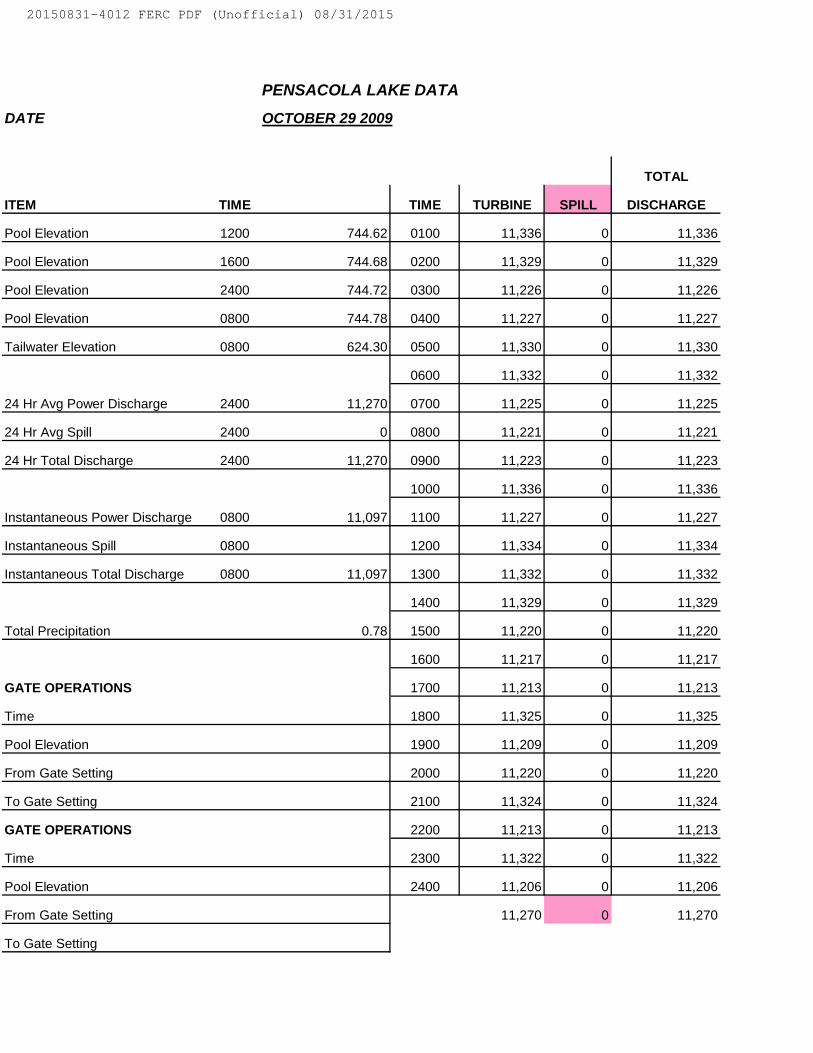
DATE OCTOBER 29 2009
TOTAL
ITEM TIME TIME TURBINE SPILL DISCHARGE
Pool Elevation 1200 744.62 0100 11,336 0 11,336
Pool Elevation 1600 744.68 0200 11,329 0 11,329
Pool Elevation 2400 744.72 0300 11,226 0 11,226
Pool Elevation 0800 744.78 0400 11,227 0 11,227
Tailwater Elevation 0800 624.30 0500 11,330 0 11,330
0600 11,332 0 11,332
24 Hr Avg Power Discharge 2400 11,270 0700 11,225 0 11,225
24 Hr Avg Spill 2400 0 0800 11,221 0 11,221
24 Hr Total Discharge 2400 11,270 0900 11,223 0 11,223
1000 11,336 0 11,336
Instantaneous Power Discharge 0800 11,097 1100 11,227 0 11,227
Instantaneous Spill 0800 1200 11,334 0 11,334
Instantaneous Total Discharge 0800 11,097 1300 11,332 0 11,332
1400 11,329 0 11,329
Total Precipitation 0.78 1500 11,220 0 11,220
1600 11,217 0 11,217
GATE OPERATIONS 1700 11,213 0 11,213
Time 1800 11,325 0 11,325
Pool Elevation 1900 11,209 0 11,209
From Gate Setting 2000 11,220 0 11,220
To Gate Setting 2100 11,324 0 11,324
GATE OPERATIONS 2200 11,213 0 11,213
Time 2300 11,322 0 11,322
Pool Elevation 2400 11,206 0 11,206
From Gate Setting 11,270 0 11,270
To Gate Setting
PENSACOLA LAKE DATA
20150831-4012 FERC PDF (Unofficial) 08/31/2015

DATE OCTOBER 30 2009
TOTAL
ITEM TIME TIME TURBINE SPILL DISCHARGE
Pool Elevation 1200 744.75 0100 11,316 0 11,316
Pool Elevation 1600 744.79 0200 11,326 0 11,326
Pool Elevation 2400 744.96 0300 11,327 0 11,327
Pool Elevation 0800 745.11 0400 11,327 0 11,327
Tailwater Elevation 0800 625.83 0500 11,325 0 11,325
0600 11,323 0 11,323
24 Hr Avg Power Discharge 2400 11,281 0700 11,321 0 11,321
24 Hr Avg Spill 2400 3,706 0800 11,321 0 11,321
24 Hr Total Discharge 2400 14,987 0900 11,319 0 11,319
1000 11,319 0 11,319
Instantaneous Power Discharge 0800 11,209 1100 11,319 0 11,319
Instantaneous Spill 0800 10,813 1200 11,322 0 11,322
Instantaneous Total Discharge 0800 22,022 1300 11,319 0 11,319
1400 11,319 0 11,319
Total Precipitation 0.00 1500 11,319 0 11,319
1600 11,324 5,145 16,469
GATE OPERATIONS 1700 11,293 10,388 21,681
Time 1530 1800 11,213 10,388 21,601
Pool Elevation 744.79 1900 11,109 10,421 21,530
From Gate Setting 0 2000 11,224 10,470 21,694
To Gate Setting 1 Main & 3 East 2100 11,224 10,470 21,694
GATE OPERATIONS 2200 11,109 10,519 21,628
Time 2300 11,218 10,568 21,786
Pool Elevation 2400 11,218 10,568 21,786
From Gate Setting 11,281 3,706 14,987
To Gate Setting
PENSACOLA LAKE DATA
20150831-4012 FERC PDF (Unofficial) 08/31/2015

DATE OCTOBER 31 2009
TOTAL
ITEM TIME TIME TURBINE SPILL DISCHARGE
Pool Elevation 1200 745.16 0100 11,218 10,568 21,786
Pool Elevation 1600 745.24 0200 11,215 10,617 21,832
Pool Elevation 2400 745.41 0300 11,215 10,617 21,832
Pool Elevation 0800 745.61 0400 11,212 10,666 21,878
Tailwater Elevation 0800 626.00 0500 11,209 10,715 21,924
0600 11,214 10,715 21,929
24 Hr Avg Power Discharge 2400 11,220 0700 11,211 10,764 21,975
24 Hr Avg Spill 2400 10,938 0800 11,209 10,813 22,022
24 Hr Total Discharge 2400 22,158 0900 11,209 10,813 22,022
1000 11,207 10,846 22,053
Instantaneous Power Discharge 0800 11,289 1100 11,209 10,895 22,104
Instantaneous Spill 0800 11,630 1200 11,209 10,895 22,104
Instantaneous Total Discharge 0800 22,919 1300 11,203 11,009 22,212
1400 11,203 11,009 22,212
Total Precipitation 0.00 1500 11,209 10,993 22,202
1600 11,202 11,025 22,227
GATE OPERATIONS 1700 11,094 11,091 22,185
Time 1800 11,207 11,074 22,281
Pool Elevation 1900 11,203 11,107 22,310
From Gate Setting 2000 11,309 11,205 22,514
To Gate Setting 2100 11,309 11,205 22,514
GATE OPERATIONS 2200 11,306 11,254 22,560
Time 2300 11,304 11,303 22,607
Pool Elevation 2400 11,192 11,303 22,495
From Gate Setting 11,220 10,938 22,158
To Gate Setting
PENSACOLA LAKE DATA
20150831-4012 FERC PDF (Unofficial) 08/31/2015

JAN
PENSACOLA HOURLY ELEVATIONS FOR JANUARY 1986DATE
HOUR 1 2 3 4 5 6 7 8 9 10 11 12
0100 744.00 743.80 743.61 743.39 743.12 742.85 742.88 742.80 742.68 742.63 742.53 742.46
0200 744.00 743.78 743.61 743.39 743.10 742.85 742.90 742.80 742.71 742.63 742.53 742.46
0300 744.00 743.78 743.61 743.36 743.10 742.85 742.88 742.80 742.68 742.63 742.53 742.44
0400 744.00 743.78 743.58 743.36 743.10 742.85 742.90 742.78 742.71 742.63 742.51 742.44
0500 744.00 743.76 743.56 743.34 743.07 742.85 742.93 742.80 742.68 742.63 742.53 742.44
0600 743.98 743.73 743.56 743.34 743.07 742.83 742.93 742.75 742.68 742.63 742.53 742.44
0700 743.98 743.71 743.56 743.32 743.07 742.83 742.88 742.78 742.71 742.63 742.53 742.44
0800 743.95 743.71 743.56 743.32 743.05 742.83 742.93 742.78 742.71 742.66 742.51 742.41
0900 743.95 743.71 743.54 743.32 743.02 742.85 742.93 742.78 742.71 742.63 742.51 742.39
1000 743.93 743.71 743.54 743.32 743.02 742.85 742.90 742.78 742.71 742.63 742.51 742.41
1100 743.90 743.61 743.51 743.29 743.02 742.85 742.93 742.78 742.68 742.63 742.51 742.39
1200 743.90 743.63 743.51 743.29 743.00 742.85 742.90 742.78 742.68 742.63 742.49 742.39
1300 743.88 743.66 743.51 743.29 742.97 742.85 742.90 742.75 742.68 742.61 742.49 742.41
1400 743.88 743.68 743.49 743.27 742.95 742.85 742.90 742.73 742.68 742.63 742.46 742.40
1500 743.88 743.66 743.49 743.24 742.97 742.83 742.83 742.71 742.68 742.63 742.46 742.39
1600 743.88 743.66 743.49 743.24 742.95 742.83 742.85 742.71 742.68 742.63 742.46 742.39
1700 743.85 743.66 743.46 743.22 742.95 742.83 742.83 742.71 742.63 742.58 742.46 742.39
1800 743.85 743.63 743.44 743.22 742.93 742.80 742.83 742.68 742.63 742.58 742.44 742.39
1900 743.85 743.63 743.44 743.19 742.93 742.80 742.80 742.68 742.66 742.58 742.44 742.36
2000 743.85 743.61 743.44 743.17 742.93 742.80 742.80 742.66 742.63 742.53 742.44 742.36
2100 743.83 743.61 743.44 743.17 742.90 742.80 742.80 742.66 742.61 742.56 742.44 742.34
2200 743.83 743.61 743.41 743.15 742.90 742.80 742.80 742.66 742.61 742.53 742.44 742.34
2300 743.83 743.61 743.39 743.15 742.90 742.80 742.78 742.66 742.61 742.53 742.46 742.34
2400 743.80 743.61 743.39 743.12 742.88 742.85 742.78 742.71 742.63 742.53 742.44 742.36
AVG 743.91 743.68 743.51 743.27 743.00 742.83 742.87 742.74 742.67 742.60 742.49 742.40
Page 1
20150831-4012 FERC PDF (Unofficial) 08/31/2015

JAN
13 14 15 16 17 18 19 20 21 22 23 24 25
742.34 742.22 742.19 742.07 742.02 741.92 741.87 741.80 741.83 741.83 741.73 741.68 741.68
742.36 742.22 742.17 742.09 742.02 741.92 741.85 741.78 741.83 741.85 741.71 741.65 741.68
742.36 742.22 742.17 742.07 742.02 741.92 741.85 741.80 741.85 741.83 741.73 741.63 741.68
742.36 742.22 742.17 742.07 742.05 741.92 741.85 741.80 741.80 741.83 741.78 741.66 741.68
742.36 742.24 742.19 742.07 742.03 741.92 741.85 741.80 741.80 741.80 741.80 741.68 741.66
742.36 742.22 742.17 742.05 742.05 741.92 741.85 741.83 741.83 741.80 741.78 741.63 741.66
742.34 742.22 742.15 742.05 742.05 741.90 741.80 741.78 741.80 741.83 741.80 741.61 741.66
742.34 742.24 742.12 742.02 742.07 741.90 741.83 741.80 741.80 741.80 741.70 741.61 741.66
742.34 742.22 742.12 742.00 742.05 741.87 741.83 741.83 741.80 741.80 741.73 741.61 741.66
742.34 742.22 742.12 742.00 742.05 741.87 741.83 741.83 741.83 741.80 741.73 741.58 741.66
742.34 742.22 742.12 742.20 742.02 741.87 741.85 741.78 741.87 741.80 741.70 741.61 741.66
742.34 742.24 742.14 741.97 742.00 741.87 741.83 741.80 741.85 741.80 741.73 741.61 741.66
742.34 742.24 742.12 741.97 741.97 741.87 741.83 741.80 741.90 741.75 741.73 741.61 741.66
742.36 742.22 742.14 741.97 741.95 741.85 741.85 741.80 741.87 741.78 741.68 741.61 741.66
742.34 742.24 742.12 741.99 741.95 741.85 741.83 741.78 741.87 741.83 741.68 741.63 741.63
742.36 742.22 742.07 742.02 741.95 741.85 741.83 741.78 741.87 741.85 741.68 741.63 741.66
742.34 742.22 742.09 742.02 741.95 741.85 741.80 741.78 741.80 741.83 741.68 741.66 741.66
742.29 742.19 742.09 742.00 741.95 741.85 741.78 741.75 741.80 741.78 741.68 741.66 741.66
742.29 742.19 742.09 742.05 741.95 741.85 741.80 741.78 741.85 741.78 741.70 741.66 741.66
742.27 742.17 742.05 742.00 741.95 741.83 741.80 741.85 741.83 741.75 741.70 741.63 741.63
742.27 742.17 742.05 742.05 741.95 741.85 741.80 741.85 741.85 741.75 741.70 741.66 741.63
742.22 742.14 742.07 742.00 741.92 741.83 741.78 741.85 741.80 741.75 741.70 741.66 741.66
742.22 742.17 742.07 742.02 741.90 741.83 741.80 741.83 741.85 741.73 741.66 741.66 741.66
742.22 742.17 742.05 742.05 741.92 741.85 741.80 741.85 741.85 741.70 741.68 741.66 741.66
742.32 742.21 742.12 742.03 741.99 741.87 741.82 741.81 741.83 741.79 741.72 741.64 741.66
Page 2
20150831-4012 FERC PDF (Unofficial) 08/31/2015

JAN
26 27 28 29 30 31
741.61 741.56 741.66 741.46 741.39 741.34
741.63 741.51 741.44 741.46 741.41 741.34
741.66 741.53 741.46 741.44 741.41 741.34
741.63 741.56 741.46 741.46 741.41 741.36
741.63 741.53 741.46 741.46 741.41 741.36
741.63 741.56 741.46 741.46 741.44 741.34
741.61 741.53 741.48 741.41 741.39 741.34
741.60 741.51 741.46 741.44 741.39 741.36
741.58 741.48 741.46 741.46 741.41 741.29
741.63 741.46 741.48 741.47 741.36 741.29
741.66 741.51 741.46 741.45 741.36 741.29
741.66 741.48 741.48 741.44 741.34 741.29
741.66 741.48 741.51 741.44 741.31 741.24
741.66 741.46 741.51 741.44 741.31 741.29
741.63 741.46 741.51 741.44 741.31 741.24
741.66 741.51 741.53 741.44 741.31 741.29
741.63 741.48 741.51 741.44 741.31 741.24
741.56 741.46 741.51 741.44 741.31 741.24
741.61 741.44 741.48 741.39 741.34 741.24
741.56 741.44 741.51 741.41 741.34 741.24
741.56 741.44 741.46 741.41 741.34 741.24
741.56 741.44 741.44 741.39 741.34 741.22
741.58 741.48 741.44 741.41 741.34 741.24
741.58 741.46 741.44 741.41 741.34 741.24
741.62 741.49 741.48 741.44 741.36 741.29
Min = 741.22
Max = 744.00
Page 3
20150831-4012 FERC PDF (Unofficial) 08/31/2015

FEB
PENSACOLA HOURLY ELEVATIONS FOR FEBRUARY 1986DATE
HOUR 1 2 3 4 5 6 7 8 9 10 11 12
0100 741.24 741.12 741.04 740.92 741.41 742.07 742.22 742.41 742.58 742.88 742.97 742.97
0200 741.23 741.12 741.04 740.90 741.41 742.08 742.22 742.44 742.61 742.88 742.97 743.00
0300 741.22 741.12 741.02 740.90 741.46 742.09 742.24 742.44 742.66 742.90 742.97 743.00
0400 741.22 741.12 741.04 740.90 741.48 742.12 742.24 742.44 742.63 742.88 742.97 743.00
0500 741.22 741.12 741.04 740.90 741.51 742.12 742.24 742.44 742.66 742.88 743.00 743.00
0600 741.22 741.14 741.02 740.90 741.56 742.12 742.24 742.46 742.66 742.90 743.00 743.00
0700 741.22 741.14 741.00 740.90 741.61 742.17 742.24 742.46 742.68 742.90 743.00 743.00
0800 741.24 741.12 741.00 740.90 741.61 742.19 742.27 742.46 742.71 742.88 743.00 743.02
0900 741.24 741.12 741.00 740.90 741.66 742.19 742.27 742.49 742.71 742.88 742.97 743.00
1000 741.24 741.12 741.02 741.02 741.68 742.19 742.29 742.49 742.73 742.90 742.93 743.02
1100 741.19 741.09 741.02 741.02 741.70 742.19 742.31 742.49 742.71 742.93 742.93 743.02
1200 741.19 741.07 740.97 741.02 741.73 742.19 742.31 742.51 742.73 742.93 742.93 743.02
1300 741.17 741.09 740.97 741.07 741.75 742.19 742.31 742.49 742.75 742.93 742.93 743.00
1400 741.17 741.07 740.95 741.07 741.78 742.19 742.31 742.51 742.73 742.93 742.93 743.00
1500 741.17 741.07 740.95 741.09 741.80 742.19 742.31 742.51 742.73 742.93 742.93 743.00
1600 741.17 741.07 740.95 741.12 741.85 742.19 742.34 742.53 742.75 742.93 742.95 743.02
1700 741.14 741.07 740.95 741.17 741.87 742.19 742.36 742.53 742.75 742.93 742.95 743.00
1800 741.14 741.04 740.95 741.19 741.90 742.19 742.34 742.53 742.78 742.95 742.95 743.00
1900 741.14 741.04 740.95 741.22 741.90 742.19 742.36 742.56 742.80 742.93 742.95 743.00
2000 741.17 741.07 740.95 741.24 741.95 742.19 742.36 742.56 742.80 742.93 742.95 743.00
2100 741.14 741.04 740.92 741.29 741.97 742.22 742.39 742.56 742.80 742.93 742.95 743.02
2200 741.14 741.02 740.92 741.31 742.00 742.22 742.39 742.58 742.83 742.95 742.95 743.02
2300 741.14 741.02 740.92 741.34 742.02 742.22 742.39 742.58 742.85 742.95 742.97 743.02
2400 741.14 741.02 740.92 741.36 742.05 742.22 742.41 742.58 742.83 742.95 742.97 743.02
AVG 741.19 741.08 740.98 741.07 741.74 742.17 742.31 742.50 742.73 742.92 742.96 743.01
Page 4
20150831-4012 FERC PDF (Unofficial) 08/31/2015

FEB
13 14 15 16 17 18 19 20 21 22 23 24 25
743.02 742.97 742.80 742.63 742.63 742.75 742.97 743.00 743.00 742.88 742.78 742.63 742.46
743.02 742.97 742.80 742.61 742.63 742.78 742.97 742.97 742.97 742.88 742.78 742.63 742.49
743.02 742.95 742.80 742.63 742.66 742.80 742.97 742.97 742.97 742.88 742.78 742.61 742.46
743.02 742.93 742.83 742.68 742.66 742.80 742.97 742.97 742.95 742.85 742.78 742.61 742.44
743.02 742.97 742.80 742.63 742.63 742.83 742.97 742.97 742.97 742.85 742.75 742.61 742.44
743.02 743.00 742.83 742.61 742.66 742.80 742.97 743.00 742.97 742.83 742.75 742.58 742.44
743.02 743.00 742.80 742.61 742.63 742.85 742.97 743.02 742.97 742.83 742.73 742.58 742.44
743.02 742.95 742.83 742.56 742.66 742.85 742.97 743.02 742.97 742.83 742.71 742.58 742.41
743.02 742.97 742.78 742.61 742.66 742.90 742.97 743.10 742.97 742.80 742.73 742.58 742.41
742.97 743.00 742.78 742.61 742.63 742.88 742.97 743.10 742.97 742.80 742.71 742.58 742.39
742.97 742.93 742.75 742.55 742.66 742.88 743.00 743.05 742.95 742.80 742.70 742.53 742.39
742.97 742.90 742.73 742.58 742.68 742.90 742.97 743.02 742.93 742.83 742.64 742.53 742.39
742.95 742.88 742.73 742.56 742.63 742.90 742.97 743.02 742.93 742.80 742.63 742.51 742.36
742.97 742.90 742.73 742.63 742.66 742.90 742.97 743.02 742.93 742.78 742.63 742.53 742.36
742.97 742.90 742.73 742.61 742.66 742.90 743.02 743.00 742.93 742.80 742.66 742.53 742.36
742.97 742.90 742.68 742.58 742.68 742.80 743.00 743.00 742.93 742.80 742.63 742.53 742.34
742.97 742.88 742.71 742.63 742.68 742.90 743.00 743.00 742.93 742.83 742.66 742.53 742.34
742.97 742.88 742.68 742.61 742.68 742.90 743.00 742.97 742.90 742.83 742.66 742.51 742.34
742.97 742.88 742.68 742.61 742.71 742.90 743.00 742.97 742.90 742.78 742.71 742.51 742.31
742.97 742.88 742.71 742.63 742.71 742.93 742.97 743.00 742.90 742.80 742.66 742.51 742.31
742.97 742.88 742.73 742.61 742.71 742.90 743.00 743.00 742.88 742.78 742.66 742.46 742.31
742.97 742.85 742.68 742.63 742.73 742.93 743.00 742.97 742.88 742.80 742.63 742.46 742.31
743.00 742.88 742.66 742.63 742.43 742.93 743.00 743.05 742.88 742.78 742.66 742.53 742.29
742.97 742.85 742.63 742.63 742.75 742.97 743.02 743.00 742.88 742.78 742.61 742.49 742.31
742.99 742.92 742.75 742.61 742.66 742.87 742.98 743.01 742.94 742.82 742.69 742.55 742.38
Page 5
20150831-4012 FERC PDF (Unofficial) 08/31/2015

FEB
26 27 28 29 30
742.27 742.49 742.34
742.27 742.51 742.36
742.29 742.51 742.34
742.27 742.49 742.34
742.24 742.44 742.29
742.24 742.44 742.34
742.22 742.49 742.31
742.24 742.49 742.27
742.24 742.44 742.24
742.22 742.46 742.27
742.24 742.44 742.27
742.24 742.44 742.24
742.22 742.41 742.22
742.22 742.41 742.22
742.22 742.44 742.22
742.24 742.41 741.79
742.66 742.44 741.45
742.56 742.44 741.75
742.63 742.44 741.75
742.56 742.39 741.73
742.49 742.36 741.70
742.46 742.36 741.70
742.53 742.36 741.70
742.53 742.34 741.68
742.35 742.44 742.06 ###### ###### ######
Min = 740.90
Max = 743.10
Page 6
20150831-4012 FERC PDF (Unofficial) 08/31/2015

MAR
PENSACOLA HOURLY ELEVATIONS FOR MARCH 1986DATE
HOUR 1 2 3 4 5 6 7 8 9 10 11 12
0100 741.68 741.51 741.41 741.14 741.02 741.02 741.04 741.07 740.97 740.82 741.04 741.04
0200 741.68 741.48 741.41 741.14 741.02 741.02 741.07 741.04 740.97 740.87 741.04 741.02
0300 741.68 741.48 741.39 741.12 741.00 741.00 741.07 741.04 740.97 741.04 741.04 741.17
0400 741.68 741.48 741.41 741.12 741.00 741.02 741.12 741.07 741.00 740.97 741.02 741.12
0500 741.66 741.48 741.41 741.14 741.02 741.00 741.12 741.07 740.97 740.95 741.02 741.12
0600 741.65 741.48 741.39 741.12 741.00 741.00 741.14 741.04 740.92 740.87 741.04 741.12
0700 741.66 741.48 741.41 741.12 741.00 741.02 741.14 741.04 740.92 740.90 741.04 741.17
0800 741.63 741.46 741.41 741.12 741.00 741.02 741.17 741.02 740.92 740.95 741.02 741.12
0900 741.63 741.46 741.39 741.12 740.97 741.00 741.17 741.02 740.94 740.95 740.97 741.12
1000 741.61 741.46 741.39 741.12 740.95 741.04 741.17 741.02 740.87 740.97 741.02 741.12
1100 741.61 741.44 741.39 741.12 740.92 741.04 741.09 741.02 740.87 740.97 741.00 741.14
1200 741.61 741.44 741.39 741.12 741.00 741.02 741.12 741.02 740.87 740.95 740.97 741.17
1300 741.58 741.46 741.41 741.14 741.02 741.02 741.14 741.02 740.87 740.97 741.00 741.02
1400 741.58 741.46 741.24 741.09 741.04 741.02 741.12 741.02 740.87 741.02 741.02 741.20
1500 741.58 741.44 741.22 741.09 741.07 741.04 741.09 741.02 740.90 741.00 741.02 741.20
1600 741.58 741.44 741.24 741.09 741.04 741.02 741.12 741.02 740.87 741.00 741.00 741.20
1700 741.53 741.44 741.22 741.09 741.02 741.02 741.09 741.02 740.87 741.02 741.07 741.26
1800 741.53 741.41 741.22 741.07 741.04 741.02 741.09 741.02 740.92 741.00 741.14 741.31
1900 741.53 741.41 741.19 741.02 741.04 741.01 741.07 741.00 740.95 741.00 741.02 741.29
2000 741.53 741.41 741.17 741.07 741.02 741.04 741.09 741.02 740.95 741.02 741.00 741.29
2100 741.53 741.41 741.17 741.07 741.00 741.04 741.07 741.00 740.90 741.02 741.00 741.31
2200 741.51 741.41 741.17 741.04 741.02 741.04 741.07 741.00 740.97 741.02 741.02 741.31
2300 741.51 741.41 741.14 741.04 741.02 741.04 741.07 741.00 740.95 741.02 741.20 741.31
2400 741.51 741.39 741.14 741.04 741.00 741.04 741.04 741.00 740.92 741.00 741.12 741.34
AVG 741.60 741.45 741.31 741.10 741.01 741.02 741.10 741.03 740.92 740.97 741.03 741.19
Page 7
20150831-4012 FERC PDF (Unofficial) 08/31/2015

MAR
13 14 15 16 17 18 19 20 21 22 23 24 25
741.36 741.66 741.70 741.66 741.51 741.36 741.29 741.31 741.31 741.24 741.24 741.22 741.14
741.39 741.66 741.70 741.63 741.53 741.31 741.26 741.31 741.31 741.22 741.24 741.19 741.14
741.39 741.66 741.70 741.63 741.51 741.34 741.26 741.34 741.31 741.22 741.24 741.22 741.17
741.41 741.66 741.70 741.63 741.51 741.31 741.29 741.31 741.31 741.22 741.24 741.22 741.17
741.44 741.66 741.70 741.63 741.51 741.29 741.29 741.34 741.31 741.22 741.24 741.22 741.14
741.41 741.66 741.70 741.63 741.51 741.29 741.26 741.31 741.31 741.19 741.22 741.22 741.14
741.46 741.66 741.70 741.63 741.51 741.36 741.26 741.34 741.29 741.22 741.24 741.19 741.12
741.48 741.66 741.68 741.61 741.51 741.34 741.29 741.34 741.29 741.19 741.22 741.22 741.14
741.48 741.66 741.68 741.61 741.46 741.26 741.31 741.34 741.29 741.17 741.24 741.14 741.04
741.51 741.68 741.70 741.61 741.46 741.26 741.29 741.34 741.31 741.14 741.24 741.12 741.07
741.51 741.68 741.68 741.61 741.41 741.26 741.29 741.29 741.36 741.14 741.22 741.17 741.09
741.53 741.68 741.68 741.58 741.41 741.29 741.31 741.29 741.34 741.14 741.22 741.12 741.12
741.53 741.68 741.68 741.56 741.39 741.24 741.31 741.29 741.34 741.19 741.22 741.09 741.07
741.56 741.70 741.68 741.56 741.36 741.24 741.31 741.29 741.31 741.17 741.20 741.14 741.12
741.58 741.70 741.68 741.56 741.41 741.26 741.31 741.29 741.29 741.14 741.22 741.09 741.07
741.58 741.70 741.66 741.56 741.39 741.24 741.34 741.29 741.26 741.17 741.19 741.09 741.09
741.61 741.70 741.66 741.56 741.39 741.24 741.34 741.31 741.26 741.17 741.19 741.09 741.07
741.61 741.73 741.66 741.56 741.36 741.22 741.33 741.31 741.26 741.17 741.19 741.09 741.09
741.63 741.73 741.66 741.53 741.34 741.22 741.29 741.26 741.24 741.19 741.19 741.12 741.09
741.66 741.70 741.66 741.53 741.36 741.22 741.26 741.27 741.24 741.19 741.17 741.12 741.09
741.63 741.70 741.66 741.53 741.34 741.24 741.26 741.29 741.22 741.22 741.17 741.14 741.07
741.63 741.73 741.66 741.53 741.34 741.24 741.31 741.31 741.22 741.22 741.17 741.14 741.14
741.66 741.70 741.66 741.51 741.39 741.22 741.31 741.31 741.26 741.22 741.19 741.14 741.12
741.66 741.70 741.63 741.51 741.36 741.24 741.29 741.29 741.22 741.24 741.19 741.14 741.09
741.53 741.69 741.68 741.58 741.43 741.27 741.29 741.31 741.29 741.19 741.21 741.15 741.11
Page 8
20150831-4012 FERC PDF (Unofficial) 08/31/2015

MAR
26 27 28 29 30 31
741.12 741.09 741.12 741.07 741.02 741.02
741.12 741.12 741.12 741.07 741.02 741.02
741.12 741.12 741.12 741.07 741.02 741.02
741.14 741.12 741.12 741.07 741.04 741.02
741.12 741.12 741.09 741.07 741.04 741.02
741.12 741.10 741.09 741.07 741.02 741.02
741.12 741.09 741.07 741.09 741.02 741.04
741.09 741.09 741.07 741.07 741.02 741.04
741.09 741.09 741.07 741.07 741.02 741.02
741.07 741.09 741.07 741.07 741.00 741.02
741.07 741.09 741.07 741.07 741.00 741.00
741.07 741.09 741.04 741.04 740.97 740.97
741.09 741.09 741.04 741.04 741.00 741.00
741.09 741.09 741.04 741.04 741.02 741.04
741.09 741.07 741.04 741.02 741.02 741.07
741.12 741.09 741.04 741.04 741.02 741.07
741.09 741.09 741.04 741.04 741.02 741.07
741.09 741.09 741.07 741.04 741.02 741.07
741.07 741.09 741.07 741.04 741.02 741.09
741.09 741.09 741.07 741.04 741.02 741.09
741.09 741.09 741.07 741.04 741.02 741.12
741.12 741.09 741.07 741.02 741.02 741.09
741.10 741.09 741.07 741.00 741.02 741.12
741.12 741.09 741.07 741.02 741.02 741.12
741.10 741.09 741.07 741.05 741.02 741.05
Min = 740.82
Max = 741.73
Page 9
20150831-4012 FERC PDF (Unofficial) 08/31/2015

APR
PENSACOLA HOURLY ELEVATIONS FOR APRIL 1986DATE
HOUR 1 2 3 4 5 6 7 8 9 10 11 12
0100 741.12 741.19 741.16 741.38 742.31 743.71 744.51 745.00 747.59 748.03 747.81 747.42
0200 741.12 741.17 741.17 741.36 742.36 743.71 744.49 745.05 747.66 748.08 747.79 747.42
0300 741.14 741.19 741.12 741.41 742.44 743.73 744.49 745.17 747.63 748.10 747.79 747.42
0400 741.12 741.17 741.14 741.34 742.51 743.73 744.51 745.20 747.74 748.05 747.76 747.42
0500 741.22 741.22 741.10 741.40 742.56 743.73 744.51 745.32 747.79 748.05 747.74 747.40
0600 741.17 741.19 741.12 741.40 742.63 743.73 744.49 745.44 747.81 748.05 747.71 747.38
0700 741.17 741.17 741.10 741.51 742.68 743.73 744.51 745.64 747.83 748.05 747.69 747.37
0800 741.17 741.19 741.12 741.44 742.78 743.73 744.49 745.76 747.86 748.03 747.64 747.35
0900 741.17 741.17 741.09 741.51 742.83 743.71 744.64 745.86 747.88 748.03 747.64 747.35
1000 741.22 741.22 741.12 741.48 742.88 743.73 744.61 745.95 747.91 748.03 747.59 747.35
1100 741.24 741.22 741.09 741.53 742.94 744.12 744.59 746.15 747.96 748.01 747.59 747.32
1200 741.24 741.22 741.09 741.56 743.02 744.22 744.59 746.27 747.96 748.01 747.57 747.32
1300 741.24 741.24 741.12 741.61 743.07 744.24 744.61 746.42 747.98 748.01 747.57 747.32
1400 741.24 741.24 741.09 741.66 743.12 744.29 744.66 746.54 747.98 748.01 747.57 747.32
1500 741.22 741.22 741.12 741.73 743.17 744.32 744.66 746.64 748.01 747.98 747.54 747.27
1600 741.19 741.22 741.09 741.75 743.22 744.34 744.66 746.76 748.03 747.98 747.52 747.30
1700 741.22 741.22 741.12 741.83 743.29 744.37 744.66 746.91 748.03 747.98 747.52 747.30
1800 741.19 741.22 741.14 741.85 743.36 744.39 744.68 747.00 748.05 747.96 747.52 747.30
1900 741.19 741.17 741.12 741.95 743.39 744.42 744.66 747.08 748.05 747.93 747.47 747.27
2000 741.19 741.22 741.12 741.97 743.44 744.42 744.68 747.20 748.05 747.91 747.47 747.27
2100 741.19 741.17 741.12 742.05 743.51 744.44 744.71 747.32 748.08 747.91 747.47 747.27
2200 741.22 741.19 741.24 742.09 743.56 744.44 744.76 747.40 748.05 747.88 747.44 747.25
2300 741.19 741.19 741.17 742.15 743.59 744.44 744.73 747.44 748.10 747.88 747.44 747.25
2400 741.19 741.19 741.26 742.25 743.68 744.51 744.76 747.52 748.05 747.83 747.44 747.22
AVG 741.19 741.20 741.13 741.68 743.01 744.09 744.61 746.29 747.92 747.99 747.60 747.33
Page 10
20150831-4012 FERC PDF (Unofficial) 08/31/2015

APR
13 14 15 16 17 18 19 20 21 22 23 24 25
747.20 746.98 746.81 746.74 746.61 746.34 746.00 745.76 745.49 745.22 744.88 744.63 744.42
747.20 746.98 746.81 746.74 746.61 746.32 746.00 745.71 745.49 745.22 744.88 744.61 744.39
747.20 747.00 746.81 746.74 746.61 746.30 745.98 745.71 745.44 745.17 744.85 744.59 744.39
747.20 746.98 746.81 746.71 746.61 746.32 745.98 745.71 745.42 745.17 744.83 744.59 744.39
747.18 746.96 746.81 746.69 746.61 746.34 745.95 745.64 745.44 745.17 744.83 744.56 744.39
747.18 746.98 746.78 746.66 746.61 746.28 745.93 745.69 745.44 745.12 744.81 744.54 744.39
747.15 746.93 746.78 746.64 746.61 746.22 745.91 745.66 745.41 745.12 744.78 744.54 744.42
747.15 746.93 746.76 746.64 746.45 746.22 745.91 745.64 745.39 745.12 744.78 744.51 744.39
747.13 746.93 746.74 746.64 746.47 746.15 745.88 745.61 745.39 745.12 744.78 744.51 744.39
747.13 746.93 746.74 746.64 746.47 746.25 745.91 745.64 745.37 745.10 744.76 744.49 744.34
747.10 746.88 746.74 746.64 746.54 746.10 745.86 745.61 745.37 745.07 744.76 744.49 744.34
747.08 746.83 746.76 746.64 746.47 746.15 745.86 745.59 745.37 745.07 744.76 744.49 744.34
747.03 746.83 746.71 746.64 746.39 746.15 745.83 745.56 745.37 745.07 744.71 744.49 744.32
747.05 746.83 746.74 746.64 746.39 746.10 745.81 745.56 745.32 745.05 744.74 744.49 744.34
747.05 746.83 746.74 746.61 746.49 746.08 745.81 745.56 745.32 745.03 744.71 744.46 744.32
747.05 746.81 746.74 746.61 746.47 746.12 745.81 745.56 745.32 745.03 744.71 744.46 744.32
747.03 746.83 746.74 746.61 746.42 746.08 745.78 745.56 745.32 745.03 744.68 744.46 744.29
746.98 746.83 746.74 746.61 746.42 746.05 745.78 745.56 745.29 745.00 744.68 744.46 744.29
746.98 746.83 746.74 746.61 746.47 746.05 745.81 745.54 745.29 744.98 744.68 744.44 744.29
747.00 746.83 746.74 746.61 746.39 746.05 745.81 745.56 745.27 744.95 744.68 744.44 744.29
746.96 746.83 746.74 746.61 746.39 746.05 745.78 745.54 745.27 744.93 744.68 744.44 744.29
746.93 746.83 746.74 746.61 746.37 746.03 745.71 745.54 745.25 744.93 744.68 744.44 744.24
746.88 746.83 746.74 746.61 746.37 746.03 745.76 745.51 745.25 744.93 744.63 744.44 744.27
746.96 746.81 746.74 746.61 746.34 746.00 745.76 745.51 745.22 744.90 744.63 744.44 744.24
747.08 746.88 746.76 746.65 746.48 746.16 745.86 745.61 745.35 745.06 744.75 744.50 744.34
Page 11
20150831-4012 FERC PDF (Unofficial) 08/31/2015

APR
26 27 28 29 30
744.24 744.10 743.93 743.80 743.58
744.24 744.10 743.95 743.80 743.56
744.27 743.95 743.80 743.58
744.24 744.07 743.95 743.80 743.58
744.27 744.10 743.95 743.80 743.58
744.22 744.10 743.95 743.76 743.54
744.20 744.10 743.93 743.76 743.56
744.20 744.07 743.95 743.80 743.54
744.20 744.05 743.93 743.76 743.49
744.15 744.05 743.90 743.73 743.46
744.17 744.05 743.90 743.68 743.44
744.17 744.02 743.88 743.66 743.44
744.15 744.07 743.85 743.63 743.41
744.15 744.05 743.85 743.61 743.41
744.15 744.05 743.83 743.61 743.41
744.15 744.02 743.83 743.61 743.41
744.15 744.02 743.83 743.61 743.41
744.15 744.00 743.83 743.61 743.41
744.15 743.98 743.83 743.61 743.39
744.15 743.95 743.83 743.56 743.39
744.15 743.93 743.80 743.56 743.39
744.15 743.93 743.80 743.56 743.36
744.12 743.95 743.80 743.56 743.34
744.10 743.95 743.80 743.54 743.34
744.18 744.03 743.88 743.68 743.46 ######
Min = 741.09
Max = 748.10
Page 12
20150831-4012 FERC PDF (Unofficial) 08/31/2015

MAY
PENSACOLA HOURLY ELEVATIONS FOR MAY 1986DATE
HOUR 1 2 3 4 5 6 7 8 9 10 11 12
0100 743.34 743.24 743.10 742.85 742.56 742.24 741.90 741.75 741.56 741.34 741.44 741.44
0200 743.36 743.24 743.10 742.85 742.53 742.19 741.90 741.78 741.56 741.39 741.44 741.46
0300 743.34 743.23 743.07 742.83 742.49 742.19 741.92 741.75 741.58 741.31 741.41 741.46
0400 743.36 743.22 743.10 742.83 742.49 742.19 741.90 741.75 741.58 741.24 741.46 741.46
0500 743.41 743.22 743.07 742.80 742.46 742.17 741.92 741.75 741.56 741.31 741.41 741.46
0600 743.39 743.22 743.05 742.78 742.41 742.19 741.87 741.75 741.51 741.34 741.39 741.48
0700 743.36 743.22 743.05 742.78 742.41 742.14 741.92 741.76 741.51 741.44 741.40 741.48
0800 743.36 743.19 743.05 742.75 742.39 742.12 741.90 741.75 741.46 741.36 741.44 741.44
0900 743.36 743.22 743.02 742.75 742.36 742.09 741.87 741.73 741.46 741.34 741.44 741.44
1000 743.36 743.19 743.02 742.73 742.34 742.05 741.85 741.68 741.41 741.41 741.39 741.44
1100 743.34 743.19 743.02 742.68 742.39 742.02 741.83 741.68 741.41 741.40 741.46 741.39
1200 743.36 743.19 743.00 742.68 742.39 742.02 741.83 741.66 741.46 741.46 741.46 741.39
1300 743.36 743.17 742.97 742.68 742.36 742.05 741.80 741.66 741.44 741.36 741.44 741.39
1400 743.36 743.15 742.97 742.66 742.29 742.05 741.83 741.63 741.41 741.41 741.41 741.36
1500 743.34 743.15 742.97 742.66 742.27 742.00 741.80 741.61 741.46 741.41 741.44 741.34
1600 743.34 743.15 742.95 742.66 742.27 742.00 741.80 741.61 741.39 741.39 741.44 741.34
1700 743.32 743.15 742.93 742.63 742.27 742.00 741.78 741.61 741.39 741.41 741.44 741.34
1800 743.32 743.15 742.93 742.63 742.24 741.97 741.78 741.58 741.34 741.44 741.46 741.36
1900 743.32 743.12 742.93 742.58 742.24 741.95 741.78 741.56 741.36 741.44 741.46 741.36
2000 743.29 743.15 742.90 742.58 742.24 741.95 741.78 741.56 741.39 741.41 741.44 741.36
2100 743.27 743.12 742.90 742.58 742.24 741.95 741.73 741.56 741.39 741.39 741.46 741.36
2200 743.24 743.12 742.90 742.58 742.24 741.92 741.75 741.53 741.36 741.41 741.44 741.27
2300 743.24 743.10 742.88 742.56 742.22 741.92 741.75 741.53 741.36 741.44 741.46 741.34
2400 743.24 743.10 742.88 742.56 742.24 741.92 741.73 741.53 741.36 741.44 741.46 741.36
AVG 743.33 743.18 742.99 742.69 742.35 742.05 741.83 741.66 741.45 741.39 741.44 741.40
Page 13
20150831-4012 FERC PDF (Unofficial) 08/31/2015

MAY
13 14 15 16 17 18 19 20 21 22 23 24 25
741.36 741.41 741.56 741.39 741.29 741.58 742.29 743.12 743.58 743.44 743.09 743.10 743.10
741.36 741.41 741.58 741.39 741.29 741.58 742.34 743.17 743.61 743.44 743.19 743.12 743.10
741.36 741.41 741.58 741.39 741.26 741.61 742.36 743.17 743.61 743.41 743.19 743.12 743.10
741.36 741.41 741.56 741.39 741.29 741.61 742.39 743.22 743.61 743.41 743.19 743.12 743.10
741.36 741.41 741.48 741.36 741.24 741.63 742.41 743.22 743.61 743.39 743.17 743.12 743.12
741.36 741.44 741.53 741.34 741.29 741.66 742.44 743.24 743.61 743.39 743.17 743.10 743.10
741.36 741.46 741.56 741.34 741.31 741.70 742.46 743.27 743.61 743.36 743.15 743.10 743.10
741.39 741.46 741.51 741.34 741.31 741.75 742.51 743.27 743.58 743.34 743.12 743.10 743.10
741.39 741.46 741.46 741.34 741.31 741.75 742.53 743.32 743.58 743.34 743.12 743.10 743.10
741.36 741.46 741.46 741.29 741.31 741.80 742.56 743.36 743.58 743.32 743.12 743.10 743.10
741.36 741.46 741.46 741.29 741.31 741.83 742.69 743.39 743.58 743.32 743.12 743.10 743.10
741.36 741.44 741.46 741.29 741.34 741.87 742.75 743.41 743.58 743.29 743.12 743.10 743.12
741.39 741.46 741.46 741.29 741.34 741.92 742.80 743.41 743.58 743.29 743.12 743.10 743.12
741.39 741.46 741.46 741.26 741.34 741.95 742.80 743.44 743.56 743.27 743.12 743.10 743.12
741.41 741.46 741.46 741.26 741.34 741.97 742.83 743.46 743.54 743.27 743.12 743.10 743.12
741.41 741.46 741.44 741.29 741.36 742.00 742.88 743.49 743.51 743.24 743.12 743.12 743.10
741.39 741.46 741.44 741.29 741.36 742.02 742.90 743.49 743.51 743.24 743.12 743.12 743.15
741.39 741.51 741.44 741.29 741.40 742.07 742.93 743.51 743.51 743.22 743.12 743.10 743.12
741.39 741.51 741.44 741.26 741.44 742.09 742.97 743.54 743.49 743.24 743.12 743.10 743.12
741.39 741.51 741.44 741.26 741.48 742.12 742.97 743.56 743.49 743.22 743.12 743.10 743.12
741.41 741.48 741.44 741.26 741.49 742.14 743.00 743.56 743.49 743.22 743.12 743.10 743.12
741.41 741.53 741.41 741.26 741.48 742.19 743.02 743.56 743.46 743.22 743.12 743.10 743.15
741.41 741.58 741.41 741.29 741.52 742.22 743.07 743.58 743.46 743.22 743.12 743.10 743.15
741.41 741.53 741.41 741.26 741.53 742.27 743.10 743.58 743.46 743.19 743.12 743.10 743.15
741.38 741.47 741.48 741.31 741.36 741.89 742.71 743.39 743.55 743.30 743.13 743.11 743.12
Page 14
20150831-4012 FERC PDF (Unofficial) 08/31/2015

MAY
26 27 28 29 30 31
743.15 743.02 742.78 742.58 742.46 742.39
743.15 743.02 742.78 742.58 742.46 742.39
743.15 743.02 742.78 742.58 742.46 742.39
743.15 743.02 742.78 742.63 742.46 742.39
743.15 743.02 742.73 742.61 742.49 742.39
743.15 743.02 742.73 742.61 742.46 742.41
743.12 743.02 742.73 742.58 742.49 742.39
743.12 743.02 742.71 742.58 742.49 742.36
743.12 742.95 742.71 742.58 742.49 742.41
743.12 742.90 742.71 742.58 742.49 742.40
743.10 742.90 742.68 742.56 742.51 742.36
743.12 742.90 742.66 742.56 742.44 742.34
743.10 742.90 742.66 742.53 742.44 742.34
743.10 742.90 742.63 742.53 742.44 742.34
743.10 742.88 742.63 742.53 742.44 742.34
743.10 742.88 742.63 742.53 742.44 742.31
743.10 742.88 742.63 742.51 742.41 742.31
743.10 742.85 742.61 742.49 742.41 742.31
743.07 742.83 742.61 742.49 742.41 742.31
743.07 742.83 742.58 742.49 742.41 742.31
743.05 742.83 742.58 742.49 742.39 742.29
743.05 742.80 742.56 742.46 742.39 742.29
743.05 742.80 742.58 742.46 742.39 742.29
743.02 742.78 742.58 742.46 742.39 742.29
743.10 742.92 742.67 742.54 742.44 742.35
Min = 741.24
Max = 743.61
Page 15
20150831-4012 FERC PDF (Unofficial) 08/31/2015

JUN
PENSACOLA HOURLY ELEVATIONS FOR JUNE 1986DATE
HOUR 1 2 3 4 5 6 7 8 9 10 11 12
0100 742.29 742.19 742.19 742.19 742.14 742.24 742.39 742.53 742.44 742.24 742.09 742.31
0200 742.29 742.19 742.17 742.19 742.16 742.24 742.41 742.53 742.44 742.24 742.19 742.31
0300 742.31 742.19 742.19 742.19 742.19 742.27 742.41 742.53 742.44 742.24 742.14 742.31
0400 742.31 742.22 742.19 742.19 742.17 742.27 742.44 742.53 742.41 742.24 742.09 742.31
0500 742.31 742.22 742.19 742.19 742.17 742.29 742.44 742.53 742.41 742.24 742.12 742.31
0600 742.31 742.22 742.19 742.22 742.17 742.29 742.46 742.53 742.39 742.24 742.12 742.31
0700 742.31 742.19 742.19 742.17 742.14 742.29 742.46 742.53 742.39 742.24 742.14 742.31
0800 742.29 742.19 742.19 742.17 742.19 742.29 742.49 742.53 742.41 742.24 742.09 742.34
0900 742.29 742.19 742.19 742.17 742.19 742.29 742.46 742.49 742.39 742.24 742.09 742.34
1000 742.24 742.22 742.14 742.17 742.14 742.31 742.46 742.49 742.36 742.19 742.14 742.31
1100 742.24 742.22 742.19 742.12 742.14 742.29 742.46 742.49 742.34 742.17 742.14 742.31
1200 742.24 742.22 742.19 742.12 742.14 742.29 742.46 742.49 742.36 742.17 742.17 742.31
1300 742.22 742.22 742.14 742.12 742.24 742.29 742.49 742.49 742.34 742.17 742.19 742.31
1400 742.19 742.24 742.17 742.12 742.19 742.29 742.49 742.49 742.31 742.14 742.19 742.31
1500 742.19 742.19 742.17 742.09 742.22 742.29 742.49 742.49 742.31 742.14 742.22 742.31
1600 742.19 742.17 742.13 742.12 742.27 742.27 742.49 742.46 742.31 742.14 742.24 742.31
1700 742.22 742.17 742.14 742.12 742.19 742.29 742.53 742.46 742.31 742.14 742.24 742.31
1800 742.19 742.17 742.17 742.12 742.19 742.31 742.63 742.49 742.31 742.14 742.27 742.31
1900 742.19 742.19 742.17 742.12 742.24 742.36 742.53 742.44 742.29 742.14 742.29 742.29
2000 742.19 742.19 742.14 742.12 742.24 742.36 742.49 742.44 742.29 742.09 742.29 742.31
2100 742.22 742.14 742.19 742.14 742.24 742.34 742.51 742.44 742.29 742.14 742.29 742.29
2200 742.22 742.19 742.17 742.14 742.22 742.36 742.51 742.44 742.27 742.14 742.29 742.29
2300 742.22 742.19 742.17 742.14 742.24 742.36 742.53 742.44 742.27 742.24 742.29 742.29
2400 742.22 742.17 742.19 742.14 742.24 742.39 742.53 742.44 742.27 742.14 742.31 742.29
AVG 742.25 742.20 742.17 742.15 742.19 742.30 742.48 742.49 742.35 742.19 742.19 742.31
Page 16
20150831-4012 FERC PDF (Unofficial) 08/31/2015

JUN
13 14 15 16 17 18 19 20 21 22 23 24 25
742.29 742.24 742.24 742.24 742.27 742.19 742.02 741.95 741.88 741.70 741.70 741.34 741.29
742.29 742.24 742.22 742.24 742.24 742.19 742.05 741.95 741.80 741.70 741.70 741.34 741.31
742.29 742.24 742.24 742.27 742.27 742.19 742.02 741.95 741.80 741.70 741.70 741.34 741.34
742.29 742.24 742.19 742.24 742.24 742.19 742.02 741.95 741.80 741.70 741.70 741.34 741.34
742.29 742.24 742.22 742.24 742.24 742.19 742.02 741.95 741.80 741.70 741.70 741.34 741.34
742.31 742.24 742.24 742.24 742.24 742.19 742.02 741.95 741.80 741.70 741.70 741.34 741.34
742.29 742.24 742.24 742.24 742.27 742.19 742.02 741.95 741.83 741.70 741.70 741.36 741.34
742.29 742.24 742.24 742.24 742.24 742.17 742.05 741.95 741.80 741.70 741.70 741.36 741.34
742.29 742.24 742.24 742.24 742.24 742.17 742.05 741.95 741.80 741.70 741.41 741.36 741.34
742.27 742.24 742.24 742.24 742.26 742.17 742.02 741.95 741.80 741.70 741.41 741.36 741.34
742.24 742.22 742.24 742.24 742.27 742.17 742.02 741.92 741.75 741.70 741.41 741.34 741.36
742.24 742.24 742.24 742.27 742.31 742.12 742.02 741.90 741.73 741.70 741.36 741.34 741.34
742.24 742.24 742.24 742.27 742.27 742.12 742.00 741.90 741.73 741.70 741.36 741.34 741.31
742.24 742.22 742.24 742.27 742.27 742.09 742.00 741.90 741.73 741.70 741.36 741.31 741.31
742.24 742.22 742.22 742.24 742.24 742.09 742.00 741.90 741.73 741.70 741.36 741.31 741.31
742.24 742.24 742.22 742.24 742.22 742.07 742.00 741.90 741.73 741.70 741.36 741.29 741.31
742.22 742.24 742.24 742.24 742.22 742.07 741.97 741.87 741.73 741.70 741.36 741.31 741.29
742.22 742.22 742.24 742.24 742.22 742.05 741.97 741.85 741.70 741.70 741.36 741.29 741.29
742.22 742.24 742.24 742.24 742.24 742.05 741.97 741.85 741.73 741.70 741.36 741.31 741.29
742.24 742.24 742.24 742.27 742.24 742.05 741.97 741.83 741.70 741.70 741.34 741.31 741.29
742.24 742.24 742.24 742.27 742.22 742.05 741.95 741.80 741.70 741.70 741.34 741.29 741.29
742.24 742.22 742.24 742.27 742.22 742.02 741.95 741.83 741.70 741.70 741.34 741.31 741.29
742.24 742.24 742.24 742.27 742.22 742.05 741.95 741.83 741.70 741.70 741.34 741.29 741.29
742.24 742.19 742.24 742.27 742.22 742.05 741.95 741.83 741.70 741.70 741.34 741.29 741.29
742.26 742.23 742.23 742.25 742.25 742.12 742.00 741.90 741.76 741.70 741.48 741.33 741.32
Page 17
20150831-4012 FERC PDF (Unofficial) 08/31/2015

JUN
26 27 28 29 30
741.29 741.24 741.36 741.46 741.46
741.29 741.24 741.34 741.46 741.46
741.29 741.24 741.29 741.46 741.46
741.29 741.24 741.31 741.46 741.46
741.29 741.24 741.34 741.48 741.46
741.31 741.24 741.34 741.48 741.46
741.31 741.24 741.34 741.48 741.46
741.29 741.24 741.34 741.53 741.46
741.29 741.24 741.34 741.53 741.46
741.29 741.24 741.34 741.53 741.46
741.29 741.24 741.36 741.46 741.46
741.29 741.24 741.39 741.48 741.46
741.29 741.22 741.44 741.48 741.46
741.29 741.22 741.44 741.48 741.46
741.29 741.22 741.44 741.46 741.42
741.29 741.22 741.46 741.46 741.39
741.26 741.19 741.46 741.46 741.36
741.26 741.19 741.46 741.46 741.34
741.26 741.24 741.46 741.46 741.34
741.24 741.22 741.46 741.46 741.34
741.24 741.53 741.46 741.48 741.34
741.24 741.46 741.46 741.46 741.31
741.24 741.39 741.46 741.46 741.34
741.24 741.26 741.46 741.46 741.31
741.28 741.26 741.40 741.47 741.41 ######
Min = 741.19
Max = 742.63
Page 18
20150831-4012 FERC PDF (Unofficial) 08/31/2015

JUL
PENSACOLA HOURLY ELEVATIONS FOR JULY 1986DATE
HOUR 1 2 3 4 5 6 7 8 9 10 11 12
0100 741.34 741.29 741.14 741.12 741.20 741.40 741.41 741.39 741.39 741.24 741.41 741.73
0200 741.31 741.29 741.14 741.12 741.20 741.40 741.41 741.41 741.39 741.24 741.44 741.73
0300 741.34 741.29 741.14 741.14 741.20 741.40 741.44 741.41 741.39 741.24 741.44 741.73
0400 741.34 741.29 741.14 741.14 741.25 741.40 741.44 741.44 741.41 741.24 741.46 741.75
0500 741.31 741.29 741.14 741.14 741.25 741.45 741.44 741.44 741.41 741.24 741.46 741.78
0600 741.31 741.29 741.14 741.17 741.25 741.45 741.44 741.44 741.41 741.26 741.48 741.80
0700 741.31 741.29 741.14 741.17 741.25 741.45 741.46 741.46 741.41 741.26 741.48 741.80
0800 741.31 741.31 741.17 741.19 741.26 741.46 741.46 741.46 741.36 741.26 741.51 741.83
0900 741.34 741.31 741.17 741.22 741.31 741.44 741.61 741.46 741.36 741.26 741.56 741.83
1000 741.29 741.26 741.14 741.22 741.31 741.41 741.39 741.48 741.34 741.26 741.48 741.85
1100 741.26 741.26 741.12 741.22 741.24 741.39 741.41 741.46 741.34 741.29 741.48 741.85
1200 741.26 741.29 741.12 741.19 741.26 741.44 741.39 741.46 741.34 741.29 741.48 741.85
1300 741.29 741.24 741.12 741.14 741.31 741.46 741.39 741.46 741.31 741.31 741.48 741.92
1400 741.26 741.24 741.12 741.14 741.31 741.41 741.39 741.46 741.31 741.29 741.53 741.92
1500 741.26 741.24 741.09 741.14 741.31 741.41 741.39 741.44 741.29 741.31 741.53 741.95
1600 741.24 741.22 741.09 741.14 741.31 741.41 741.39 741.44 741.29 741.34 741.56 741.95
1700 741.29 741.22 741.09 741.14 741.31 741.41 741.36 741.41 741.26 741.31 741.61 741.97
1800 741.24 741.17 741.07 741.14 741.31 741.60 741.36 741.41 741.26 741.34 741.61 742.02
1900 741.24 741.17 741.07 741.12 741.31 741.41 741.36 741.41 741.24 741.36 741.61 742.05
2000 741.26 741.17 741.07 741.15 741.34 741.41 741.39 741.36 741.24 741.39 741.66 742.07
2100 741.26 741.17 741.07 741.17 741.36 741.41 741.39 741.36 741.22 741.39 741.68 742.09
2200 741.29 741.12 741.07 741.19 741.36 741.41 741.39 741.41 741.22 741.39 741.70 742.09
2300 741.29 741.17 741.07 741.17 741.39 741.41 741.39 741.41 741.26 741.41 741.70 742.29
2400 741.29 741.14 741.12 741.20 741.40 741.41 741.39 741.39 741.24 741.41 741.70 742.00
AVG 741.29 741.24 741.11 741.16 741.29 741.43 741.41 741.43 741.32 741.31 741.54 741.91
Page 19
20150831-4012 FERC PDF (Unofficial) 08/31/2015

JUL
13 14 15 16 17 18 19 20 21 22 23 24 25
742.24 742.44 742.53 742.63 742.88 743.10 743.22 743.34 743.44 743.44 743.41 743.36 743.22
742.27 742.44 742.53 742.66 742.90 743.10 743.22 743.36 743.44 743.44 743.41 743.36 743.22
742.51 742.44 742.53 742.68 742.93 743.12 743.22 743.36 743.44 743.44 743.41 743.36 743.19
742.24 742.44 742.56 742.71 742.93 743.12 743.22 743.36 743.44 743.44 743.41 743.36 743.22
742.24 742.44 742.58 742.71 742.93 743.12 743.22 743.36 743.44 743.44 743.41 743.36 743.22
742.29 742.44 742.58 742.73 742.93 743.12 743.22 743.36 743.44 743.44 743.41 743.36 743.22
742.34 742.46 742.58 742.73 742.95 743.17 743.22 743.36 743.44 743.41 743.41 743.36 743.22
742.27 742.46 742.61 742.75 742.95 743.17 743.24 743.36 743.44 743.41 743.41 743.36 743.22
742.39 742.51 742.58 742.78 742.97 743.17 743.27 743.41 743.44 743.41 743.41 743.36 743.22
742.41 742.46 742.61 742.80 742.97 743.19 743.27 743.41 743.44 743.41 743.41 743.36 743.22
742.36 742.46 742.61 742.80 743.00 743.19 743.27 743.41 743.44 743.41 743.41 743.36 743.19
742.29 742.46 742.58 742.83 743.02 743.24 743.29 743.41 743.44 743.39 743.39 743.29 743.15
742.36 742.46 742.58 742.80 743.00 743.22 743.29 743.41 743.44 743.39 743.36 743.29 743.17
742.39 742.49 742.58 742.83 743.02 743.24 743.29 743.41 743.44 743.41 743.36 743.29 743.17
742.34 742.46 742.58 742.80 743.00 743.24 743.32 743.41 743.44 743.41 743.36 743.29 743.17
742.46 742.46 742.63 742.83 743.02 743.24 743.32 743.44 743.44 743.41 743.36 743.27 743.15
742.44 742.49 742.56 742.80 743.02 743.22 743.32 743.44 743.44 743.41 743.36 743.27 743.17
742.44 742.49 742.56 742.80 743.02 743.22 743.32 743.44 743.44 743.41 743.34 743.27 743.15
742.41 742.49 742.63 742.80 743.05 743.22 743.34 743.46 743.44 743.41 743.36 743.24 743.17
742.44 742.51 742.66 742.88 743.05 743.22 743.34 743.46 743.44 743.39 743.36 743.24 743.17
742.44 742.49 742.66 742.85 743.05 743.19 743.32 743.46 743.44 743.41 743.36 743.24 743.17
742.44 742.51 742.66 742.88 743.05 743.19 743.34 743.46 743.44 743.39 743.36 743.22 743.15
742.44 742.51 742.66 742.88 743.10 743.19 743.34 743.44 743.44 743.41 743.36 743.22 743.15
742.44 742.53 742.63 742.88 743.10 743.24 743.36 743.44 743.44 743.41 743.36 743.22 743.17
742.37 742.47 742.59 742.79 742.99 743.19 743.28 743.41 743.44 743.41 743.38 743.30 743.19
Page 20
20150831-4012 FERC PDF (Unofficial) 08/31/2015

JUL
26 27 28 29 30 31
743.17 743.19 743.17 743.00 742.90 742.88
743.15 743.19 743.17 743.00 742.90 742.85
743.17 743.19 743.17 743.02 742.90 742.85
743.17 743.22 743.19 743.02 742.90 742.85
743.15 743.19 743.19 743.02 742.90 742.85
743.15 743.22 743.19 743.00 742.90 742.85
743.15 743.17 743.19 743.00 742.90 742.85
743.17 743.22 743.19 743.00 742.90 742.85
743.17 743.22 743.19 743.00 742.90 742.85
743.20 743.22 743.19 742.97 742.90 742.85
743.22 743.19 743.22 742.97 742.90 742.85
743.17 743.19 743.22 742.97 742.90 742.90
743.17 743.19 743.19 742.97 742.93 742.93
743.17 743.19 743.22 742.97 742.93 742.90
743.17 743.19 743.17 742.95 742.88 742.90
743.19 743.19 743.15 742.90 742.85 742.93
743.19 743.19 743.15 742.90 742.88 742.93
743.22 743.19 743.12 742.90 742.88 742.90
743.19 743.19 743.10 742.95 742.88 742.90
743.22 743.19 743.10 742.93 742.85 742.88
743.22 743.19 743.07 742.93 742.88 742.88
743.19 743.19 743.07 742.93 742.88 742.88
743.19 743.19 743.05 742.93 742.85 742.85
743.19 743.19 743.05 742.90 742.88 742.85
743.18 743.20 743.16 742.96 742.89 742.88
Min = 741.07
Max = 743.46
Page 21
20150831-4012 FERC PDF (Unofficial) 08/31/2015

AUG
PENSACOLA HOURLY ELEVATIONS FOR AUGUST 1986DATE
HOUR 1 2 3 4 5 6 7 8 9 10 11 12
0100 742.85 742.90 742.95 742.97 742.93 742.90 743.00 742.97 743.00 743.10 743.10 743.00
0200 742.88 742.96 742.97 742.97 742.93 742.93 743.00 742.97 743.00 743.10 743.10 743.00
0300 742.88 743.00 742.97 742.97 742.93 743.02 743.00 742.97 743.00 743.10 743.10 743.00
0400 742.88 743.07 742.97 742.97 742.93 742.88 743.00 742.97 743.02 743.12 743.10 743.00
0500 742.88 742.95 742.97 742.97 742.90 742.93 743.00 742.97 743.02 743.10 743.10 743.00
0600 742.90 742.88 742.97 742.97 742.93 742.95 743.00 742.97 743.02 743.10 743.10 743.00
0700 742.88 742.90 742.97 742.97 742.93 743.00 743.00 742.97 743.02 743.10 743.10 743.02
0800 742.88 742.93 742.95 742.97 742.90 742.95 743.02 742.93 743.02 743.10 743.10 743.02
0900 742.88 742.93 742.97 742.97 742.93 742.95 743.10 742.95 743.02 743.12 743.05 743.05
1000 742.88 742.93 742.97 742.97 742.85 742.95 743.10 743.00 743.00 743.11 743.05 743.02
1100 742.90 742.95 742.97 742.97 742.90 742.97 743.02 743.02 743.00 743.15 743.02 743.05
1200 742.88 742.95 742.97 742.97 742.82 742.93 742.97 743.00 743.02 743.16 743.02 743.05
1300 742.88 742.97 742.97 742.97 742.90 742.97 743.02 743.00 743.05 743.14 743.00 743.00
1400 742.88 742.95 742.97 742.93 742.90 742.97 743.00 743.00 743.03 743.12 743.00 743.02
1500 742.90 742.95 742.97 743.00 742.93 742.97 742.97 743.00 743.05 743.12 743.00 743.02
1600 742.90 742.95 743.00 742.97 742.93 742.97 742.93 743.00 743.07 743.12 742.97 743.00
1700 742.88 742.97 743.00 742.90 742.90 742.97 742.95 743.00 743.10 743.12 742.97 743.02
1800 742.88 742.97 743.02 742.90 742.90 742.97 742.95 743.02 743.10 743.12 742.95 743.00
1900 742.90 742.97 743.02 742.95 742.90 743.00 742.97 743.02 743.10 743.12 742.97 742.97
2000 742.90 742.97 743.02 742.95 742.90 743.00 742.97 743.02 743.10 743.12 743.00 743.00
2100 743.02 742.95 742.97 742.93 742.90 743.00 742.95 743.02 743.10 743.12 743.00 743.00
2200 742.95 742.95 742.97 742.93 742.93 743.00 742.97 743.02 743.10 743.10 743.00 743.00
2300 742.88 742.95 742.97 742.93 742.95 743.00 742.97 743.00 743.10 743.10 743.00 743.00
2400 742.88 742.95 742.97 742.93 742.97 743.00 742.95 743.00 743.07 743.10 743.00 743.02
AVG 742.89 742.95 742.98 742.96 742.91 742.97 742.99 742.99 743.05 743.12 743.03 743.01
Page 22
20150831-4012 FERC PDF (Unofficial) 08/31/2015

AUG
13 14 15 16 17 18 19 20 21 22 23 24 25
743.00 742.95 742.90 742.83 742.71 742.56 742.34 742.17 742.05 741.97 741.90 741.90 741.90
743.00 742.95 742.88 742.83 742.68 742.53 742.36 742.17 742.05 741.97 741.90 741.90 741.90
743.02 742.95 742.88 742.85 742.71 742.53 742.34 742.17 742.05 741.97 741.90 741.87 741.87
743.02 742.95 742.88 742.85 742.71 742.53 742.36 742.17 742.02 741.95 741.90 741.87 741.90
743.02 742.95 742.88 742.85 742.71 742.53 742.36 742.17 742.02 741.97 741.90 741.87 741.90
743.02 742.95 742.88 742.85 742.71 742.53 742.36 742.14 742.05 742.00 741.90 741.90 741.87
743.02 742.97 742.88 742.83 742.68 742.53 742.34 742.14 742.05 741.97 741.87 741.87 741.90
743.02 742.95 742.88 742.83 742.68 742.53 742.31 742.14 742.00 741.97 741.87 741.87 741.87
743.02 742.95 742.90 742.83 742.68 742.49 742.31 742.14 742.00 741.95 741.85 741.87 741.87
743.02 742.93 742.88 742.83 742.68 742.49 742.31 742.14 742.00 741.97 741.85 741.85 741.85
743.02 742.93 742.90 742.83 742.66 742.46 742.31 742.17 742.02 741.95 741.85 741.85 741.85
743.02 742.95 742.90 742.83 742.65 742.46 742.31 742.14 742.02 741.95 741.85 741.85 741.87
743.02 742.90 742.85 742.80 742.63 742.44 742.29 742.14 742.00 741.95 741.87 741.87 741.87
743.02 742.90 742.90 742.80 742.63 742.44 742.27 742.14 742.00 741.95 741.85 741.87 741.87
743.02 742.90 742.88 742.80 742.61 742.41 742.27 742.12 742.02 741.95 741.85 741.87 741.87
743.00 742.90 742.88 742.75 742.58 742.41 742.24 742.09 742.02 741.95 741.87 741.87 741.87
742.03 742.90 742.88 742.75 742.56 742.39 742.24 742.07 742.02 741.92 741.87 741.87 741.90
743.00 742.90 742.83 742.71 742.58 742.39 742.22 742.07 742.00 741.92 741.87 741.87 741.90
743.00 742.90 742.85 742.71 742.56 742.36 742.19 742.05 742.00 741.92 741.87 741.87 741.87
743.00 742.88 742.88 742.73 742.56 742.39 742.19 742.05 742.00 741.90 741.87 741.87 741.92
743.00 742.88 742.88 742.68 742.51 742.36 742.14 742.02 741.97 741.90 741.87 741.90 741.92
742.95 742.90 742.88 742.71 742.53 742.27 742.14 742.05 742.00 741.90 741.87 741.90 741.90
742.97 742.88 742.83 742.71 742.53 742.34 742.19 742.05 742.00 741.90 741.87 741.87 741.92
742.95 742.90 742.83 742.71 742.56 742.36 742.17 742.05 742.00 741.90 741.90 741.90 741.90
742.97 742.92 742.88 742.79 742.63 742.45 742.27 742.12 742.02 741.94 741.87 741.88 741.89
Page 23
20150831-4012 FERC PDF (Unofficial) 08/31/2015

AUG
26 27 28 29 30 31
741.90 741.97 742.00 741.92 741.90 741.90
741.90 741.97 741.95 741.92 741.90 741.90
741.87 741.95 742.02 741.92 741.90 741.90
741.87 741.87 742.00 741.92 741.90 741.90
741.87 741.87 742.02 741.92 741.90 741.90
741.87 741.90 742.02 741.90 741.90 741.90
741.87 741.92 742.00 741.90 741.90 741.90
741.87 741.92 741.97 741.87 741.90 741.87
741.90 741.95 741.97 741.90 741.90 741.87
741.90 741.95 741.95 741.90 741.87 741.90
741.90 741.95 741.95 741.90 741.90 741.87
741.87 741.97 741.97 741.90 741.90 741.87
741.90 742.02 741.95 741.90 741.90 741.87
741.87 742.00 741.95 741.90 741.90 741.87
741.87 741.97 741.95 741.90 741.90 741.87
741.87 741.97 741.95 741.92 741.90 741.87
741.90 741.97 741.95 741.90 741.90 741.87
741.90 741.97 741.95 741.92 741.90 741.87
741.90 741.97 741.95 741.92 741.90 741.90
741.90 741.92 741.95 741.92 741.90 741.87
741.92 741.95 741.95 741.90 741.90 741.87
741.91 741.97 741.95 741.90 741.90 741.90
741.90 742.00 741.92 741.90 741.90 741.90
741.95 742.00 741.92 741.90 741.90 741.90
741.89 741.95 741.97 741.91 741.90 741.89
Min = 741.85
Max = 743.16
Page 24
20150831-4012 FERC PDF (Unofficial) 08/31/2015

SEP
PENSACOLA HOURLY ELEVATIONS FOR SEPTEMBER 1986DATE
HOUR 1 2 3 4 5 6 7 8 9 10 11 12
0100 741.90 741.90 741.90 741.90 741.95 741.92 742.00 741.95 741.92 741.87 741.75 741.75
0200 741.87 741.90 741.90 741.90 741.95 741.92 742.00 741.95 741.90 741.85 741.75 741.75
0300 741.90 741.90 741.90 741.90 741.95 741.95 742.00 741.95 741.90 741.87 741.70 741.75
0400 741.90 741.90 741.90 741.92 741.95 741.97 742.00 741.95 741.90 741.87 741.73 741.75
0500 741.90 741.90 741.90 741.92 741.95 741.95 742.00 741.95 741.90 741.87 741.73 741.75
0600 741.90 741.90 741.90 741.92 741.95 741.95 742.00 741.95 741.90 741.87 741.80 741.75
0700 741.90 741.87 741.90 741.92 741.95 741.95 742.00 741.95 741.90 741.85 741.70 741.75
0800 741.90 741.87 741.90 741.92 741.95 741.95 742.00 741.95 741.90 741.83 741.70 741.78
0900 741.90 741.87 741.90 741.92 741.95 741.95 742.00 741.95 741.90 741.85 741.70 741.78
1000 741.90 741.87 741.90 741.92 741.95 741.95 742.00 741.95 741.90 741.83 741.70 741.80
1100 741.85 741.87 741.90 741.92 741.95 741.95 742.00 741.92 741.87 741.80 741.78 741.80
1200 741.87 741.87 741.90 741.92 741.95 741.95 741.97 741.95 741.87 741.78 741.80 741.80
1300 741.90 741.90 741.90 741.95 741.95 741.95 741.95 741.92 741.85 741.75 741.78 741.80
1400 741.90 741.90 741.90 741.95 741.95 741.95 741.95 741.92 741.87 741.75 741.83 741.80
1500 741.90 741.90 741.90 741.95 741.95 741.95 741.97 741.92 741.85 741.75 741.80 741.80
1600 741.90 741.90 741.90 741.95 741.95 741.95 741.97 741.92 741.85 741.75 741.81 741.83
1700 741.90 741.90 741.92 741.95 741.95 741.95 741.97 741.95 741.85 741.75 741.78 741.83
1800 741.90 741.90 741.90 741.95 741.92 741.97 741.97 741.95 741.85 741.75 741.78 741.85
1900 741.90 741.90 741.90 741.95 741.92 741.95 741.97 741.95 741.90 741.75 741.78 741.85
2000 741.87 741.90 741.90 741.95 741.92 741.95 741.97 741.95 741.91 741.75 741.78 741.85
2100 741.87 741.90 741.90 741.92 741.92 741.95 741.97 741.95 741.90 741.75 741.78 741.85
2200 741.87 741.90 741.90 741.92 741.92 741.97 741.97 741.92 741.90 741.75 741.78 741.85
2300 741.87 741.90 741.90 741.93 741.92 742.00 741.97 741.92 741.90 741.80 741.78 741.85
2400 741.87 741.90 741.90 741.95 741.92 742.02 741.95 741.92 741.90 741.75 741.78 741.87
AVG 741.89 741.89 741.90 741.93 741.94 741.96 741.98 741.94 741.89 741.80 741.76 741.80
Page 25
20150831-4012 FERC PDF (Unofficial) 08/31/2015

SEP
13 14 15 16 17 18 19 20 21 22 23 24 25
741.90 742.00 742.05 742.12 742.56 742.83 743.41 743.76 743.83 743.68 743.36 742.97 742.63
741.90 742.00 742.05 742.12 742.56 742.85 743.41 743.76 743.83 743.68 743.36 742.95 742.63
741.90 742.00 742.05 742.12 742.56 742.85 743.46 743.76 743.83 743.68 743.36 742.93 742.61
741.90 742.00 742.05 742.12 742.56 742.90 743.46 743.78 743.80 743.68 743.34 742.93 742.58
741.90 742.00 742.05 742.12 742.56 742.90 743.49 743.80 743.83 743.68 743.34 742.90 742.61
741.90 742.00 742.05 742.09 742.56 742.93 743.51 743.80 743.80 743.68 743.32 742.88 742.58
741.92 742.05 742.10 742.19 742.56 742.95 743.54 743.78 743.80 743.66 743.29 742.88 742.61
741.92 742.02 742.17 742.27 742.56 742.95 743.54 743.78 743.83 743.66 743.27 742.85 742.56
741.92 742.05 742.09 742.27 742.58 742.97 743.56 743.80 743.80 743.63 743.22 742.83 742.56
741.92 742.05 742.17 742.39 742.63 742.97 743.56 743.80 743.80 743.63 743.22 742.80 742.56
741.95 742.05 742.24 742.29 742.66 743.00 743.58 743.80 743.78 743.61 743.19 742.80 742.53
741.97 742.05 742.19 742.39 742.66 743.02 743.61 743.80 743.78 743.58 743.19 742.80 742.53
741.97 742.02 742.14 742.44 742.66 743.05 743.61 743.80 743.78 743.61 743.15 742.80 742.53
741.97 742.02 742.14 742.44 742.68 743.12 743.66 743.80 743.78 743.58 743.15 742.75 742.51
741.97 742.02 742.17 742.49 742.68 743.12 743.66 743.80 743.78 743.56 743.12 742.75 742.51
742.00 742.02 742.17 742.53 742.68 743.15 743.66 743.83 743.76 743.51 743.12 742.75 742.49
742.00 742.05 742.12 742.49 742.71 743.17 743.68 743.83 743.78 743.51 743.12 742.73 742.49
742.00 742.05 742.12 742.51 742.75 743.22 743.71 743.85 743.78 743.51 743.12 742.71 742.49
742.00 742.05 742.12 742.49 742.75 743.24 743.73 743.83 743.76 743.49 743.10 742.68 742.46
742.00 742.05 742.12 742.51 742.78 743.24 743.76 743.83 743.76 743.46 743.10 742.71 742.46
742.00 742.05 742.09 742.49 742.78 743.29 743.73 743.83 743.76 743.46 743.05 742.68 742.44
742.00 742.05 742.09 742.53 742.78 743.29 743.73 743.83 743.73 743.44 743.05 742.68 742.44
742.00 742.05 742.09 742.58 742.83 743.32 743.76 743.83 743.71 743.44 743.02 742.63 742.46
742.02 742.05 742.12 742.53 742.83 743.36 743.73 743.83 743.71 743.41 743.00 742.75 742.44
741.96 742.03 742.11 742.36 742.66 743.07 743.61 743.80 743.78 743.58 743.19 742.80 742.53
Page 26
20150831-4012 FERC PDF (Unofficial) 08/31/2015

SEP
26 27 28 29 30
742.44 742.46 742.53 742.22 742.46
742.44 742.49 742.51 742.22 742.49
742.44 742.49 742.51 742.19 742.63
742.44 742.51 742.51 742.19 742.82
742.44 742.56 742.51 742.17 743.07
742.44 742.58 742.49 742.14 743.19
742.39 742.56 742.46 742.09 743.56
742.36 742.53 742.49 742.07 743.68
742.36 742.56 742.46 742.02 743.68
742.36 742.53 742.44 741.97 743.68
742.36 742.53 742.41 742.00 744.52
742.36 742.53 742.39 742.02 744.78
742.39 742.53 742.39 742.05 745.07
742.36 742.53 742.39 742.02 745.29
742.39 742.53 742.34 742.05 745.29
742.46 742.53 742.37 742.05 745.44
742.44 742.53 742.34 742.07 745.66
742.44 742.53 742.34 742.07 745.95
742.44 742.53 742.34 742.09 746.05
742.51 742.53 742.31 742.22 746.20
742.44 742.53 742.31 742.27 746.42
742.44 742.53 742.29 742.27 746.54
742.46 742.53 742.27 742.34 746.71
742.51 742.53 742.22 742.39 746.86
742.42 742.53 742.40 742.13 744.67 ######
Min = 741.70
Max = 746.86
Page 27
20150831-4012 FERC PDF (Unofficial) 08/31/2015

OCT
PENSACOLA HOURLY ELEVATIONS FOR OCTOBER 1986DATE
HOUR 1 2 3 4 5 6 7 8 9 10 11 12
0100 747.03 750.36 753.31 754.67 754.55 754.70 754.77 754.26 753.57 753.31 753.06 752.21
0200 747.18 750.50 753.43 754.70 754.53 754.75 754.77 754.23 753.55 753.33 753.04 752.16
0300 747.32 750.60 753.53 754.70 754.53 754.75 754.75 754.23 753.50 753.33 753.01 752.11
0400 747.47 750.72 753.65 754.70 754.50 754.85 754.72 754.21 753.48 753.33 752.96 752.04
0500 747.61 750.83 753.75 754.70 754.50 754.87 754.70 754.19 753.43 753.36 752.94 752.01
0600 747.79 750.95 753.87 754.70 754.48 754.87 754.67 754.19 753.43 753.36 752.92 751.91
0700 747.91 751.05 753.99 754.70 754.45 754.89 754.65 754.16 753.38 753.36 752.87 751.89
0800 748.05 751.18 754.11 754.70 754.45 754.92 754.63 754.14 753.38 753.36 752.84 751.82
0900 748.20 751.38 754.28 754.70 754.43 754.94 754.60 754.06 753.33 753.36 752.82 751.77
1000 748.30 751.47 754.31 754.70 754.43 754.94 754.60 754.04 753.33 753.36 752.79 751.69
1100 748.47 751.65 754.43 754.70 754.43 754.97 754.55 754.01 753.31 753.36 752.74 751.62
1200 748.69 751.72 754.45 754.70 754.43 754.97 754.55 753.99 753.28 753.36 752.72 751.55
1300 748.84 751.80 754.45 754.70 754.45 754.94 754.55 753.94 753.26 753.33 752.67 751.52
1400 748.93 751.89 754.55 754.67 754.48 754.97 754.50 753.89 753.26 753.33 752.65 751.45
1500 749.08 752.01 754.58 754.67 754.48 754.94 754.50 753.87 753.26 753.31 752.62 751.38
1600 749.18 752.18 754.58 754.67 754.50 754.94 754.48 753.84 753.28 753.26 752.57 751.30
1700 749.32 752.26 754.60 754.65 754.53 754.97 754.38 753.79 753.28 753.26 752.52 751.25
1800 749.47 752.40 754.60 754.65 754.53 754.94 754.41 753.77 753.28 753.23 752.50 751.18
1900 749.57 752.55 754.63 754.63 754.52 754.94 754.38 753.75 753.28 753.21 752.40 751.13
2000 749.69 752.70 754.65 754.63 754.58 754.92 754.36 753.72 753.28 753.18 752.40 751.08
2100 749.84 752.79 754.65 754.60 754.60 754.92 754.33 753.70 753.30 753.16 752.38 751.01
2200 749.96 752.94 754.67 754.60 754.63 754.87 754.33 753.67 753.33 753.14 752.35 750.91
2300 750.01 753.06 754.67 754.55 754.65 754.85 754.31 753.65 753.33 753.11 752.33 750.86
2400 750.01 753.18 754.67 754.55 754.67 754.82 754.28 753.60 753.31 753.09 752.26 750.79
AVG 748.66 751.76 754.27 754.66 754.51 754.89 754.53 753.95 753.35 753.28 752.68 751.53
Page 28
20150831-4012 FERC PDF (Unofficial) 08/31/2015

OCT
13 14 15 16 17 18 19 20 21 22 23 24 25
750.72 749.86 749.74 749.52 749.23 748.96 748.64 748.37 747.98 747.69 747.54 747.61 747.57
750.67 749.89 749.74 749.52 749.23 748.93 748.64 748.37 747.98 747.69 747.54 747.64 747.54
750.62 749.86 749.72 749.50 749.23 748.91 748.62 748.32 747.96 747.69 747.54 747.61 747.54
750.52 749.84 749.72 749.47 749.23 748.91 748.62 748.32 747.96 747.66 747.54 747.64 747.54
750.50 749.81 749.72 749.47 749.20 748.89 748.59 748.30 747.96 747.66 747.54 747.61 747.52
750.45 749.81 749.69 749.47 749.18 748.89 748.59 748.30 747.93 747.66 747.54 747.64 747.52
750.38 749.81 749.69 749.45 749.15 748.96 748.57 748.27 747.91 747.64 747.54 747.64 747.54
750.30 749.81 749.67 749.45 749.15 748.86 748.57 748.27 747.91 747.64 747.54 747.61 747.54
750.25 749.81 749.67 749.42 749.13 748.84 748.57 748.25 747.88 747.64 747.57 747.61 747.54
750.18 749.81 749.67 749.42 749.15 748.81 748.54 748.25 747.88 747.61 747.57 747.64 747.54
750.18 749.81 749.64 749.40 749.13 748.81 748.52 748.23 747.86 747.61 747.57 747.61 747.54
750.16 749.84 749.64 749.37 749.10 748.81 748.49 748.23 747.88 747.59 747.57 747.61 747.54
750.11 749.84 749.62 749.37 749.10 748.81 748.49 748.20 747.86 747.59 747.57 747.59 747.59
750.06 749.81 749.62 749.37 749.10 748.79 748.49 748.20 747.83 747.57 747.59 747.59 747.61
750.06 749.81 749.62 749.35 749.08 748.76 748.47 748.20 747.81 747.57 747.57 747.59 747.61
750.06 749.81 749.62 749.35 749.08 748.76 748.49 748.20 747.81 747.54 747.59 747.59 747.66
749.91 749.79 749.62 749.32 749.06 748.76 748.45 748.13 747.79 747.54 747.59 747.57 747.69
749.91 749.79 749.59 749.32 749.03 748.74 748.45 748.10 747.79 747.54 747.59 747.59 747.71
749.91 749.79 749.59 749.32 749.03 748.71 748.45 748.08 747.76 747.54 747.61 747.59 747.71
749.91 749.79 749.57 749.30 749.01 748.71 748.42 748.05 747.76 747.54 747.61 747.57 747.71
749.91 749.76 749.57 749.30 749.01 748.69 748.40 748.05 747.76 747.54 747.59 747.57 747.74
749.91 749.76 749.54 749.28 748.98 748.69 748.40 748.01 747.71 747.54 747.61 747.54 747.76
749.89 749.76 749.54 749.25 748.96 748.67 748.40 748.01 747.71 747.54 747.61 747.54 747.76
749.89 749.74 749.52 749.25 748.98 748.67 748.37 748.01 747.71 747.54 747.61 747.54 747.79
750.19 749.81 749.64 749.39 749.11 748.81 748.51 748.20 747.85 747.60 747.57 747.60 747.62
Page 29
20150831-4012 FERC PDF (Unofficial) 08/31/2015

OCT
26 27 28 29 30 31
747.83 748.20 748.37 748.42 748.23 747.83
747.83 748.23 748.35 748.42 748.23 747.81
747.83 748.23 748.37 748.40 748.18 747.81
747.86 748.23 748.37 748.42 748.15 747.79
747.91 748.25 748.37 748.40 748.15 747.76
747.91 748.27 748.37 748.45 748.13 747.76
747.93 748.27 748.37 748.43 748.10 747.74
747.96 748.30 748.37 748.45 748.10 747.74
747.96 748.32 748.37 748.42 748.08 747.71
747.98 748.35 748.40 748.42 748.02 747.69
748.01 748.35 748.40 748.42 748.03 747.66
748.03 748.35 748.40 748.42 748.03 747.64
748.03 748.35 748.40 748.42 748.01 747.61
748.05 748.35 748.40 748.42 748.01 747.61
748.10 748.35 748.40 748.40 748.01 747.64
748.10 748.35 748.40 748.40 747.98 747.61
748.10 748.37 748.40 748.37 747.96 747.61
748.10 748.37 748.42 748.35 747.93 747.61
748.15 748.35 748.40 748.35 747.91 747.61
748.15 748.37 748.42 748.32 747.91 747.61
748.15 748.37 748.40 748.30 747.91 747.59
748.15 748.35 748.40 748.27 747.88 747.59
748.15 748.37 748.42 748.27 747.88 747.59
748.18 748.35 748.42 748.25 747.86 747.57
748.02 748.32 748.39 748.38 748.03 747.67
Min = 747.03
Max = 754.97
Page 30
20150831-4012 FERC PDF (Unofficial) 08/31/2015

NOV
PENSACOLA HOURLY ELEVATIONS FOR NOVEMBER 1986DATE
HOUR 1 2 3 4 5 6 7 8 9 10 11 12
0100 741.24 741.12 741.04 740.92 746.93 747.13 747.37 742.41 742.58 742.88 742.97 742.97
0200 741.23 741.12 741.04 740.90 746.93 747.15 747.40 742.44 742.61 742.88 742.97 743.00
0300 741.22 741.12 741.02 740.90 746.93 747.18 747.40 742.44 742.66 742.90 742.97 743.00
0400 741.22 741.12 741.04 740.90 746.98 747.18 747.40 742.44 742.63 742.88 742.97 743.00
0500 741.22 741.12 741.04 740.90 746.98 747.20 747.40 742.44 742.66 742.88 743.00 743.00
0600 741.22 741.14 741.02 740.90 746.98 747.20 747.40 742.46 742.66 742.90 743.00 743.00
0700 741.22 741.14 741.00 740.90 746.98 747.20 747.40 742.46 742.68 742.90 743.00 743.00
0800 741.24 741.12 741.00 740.90 746.98 747.22 747.37 742.46 742.71 742.88 743.00 743.02
0900 741.24 741.12 741.00 740.90 746.98 747.25 747.37 742.49 742.71 742.88 742.97 743.00
1000 741.24 741.12 741.02 741.02 746.97 747.25 747.35 742.49 742.73 742.90 742.93 743.02
1100 741.19 741.09 741.02 741.02 747.00 747.25 747.32 742.49 742.71 742.93 742.93 743.02
1200 741.19 741.07 740.97 741.02 747.03 747.27 747.35 742.51 742.73 742.93 742.93 743.02
1300 741.17 741.09 740.97 741.07 747.03 747.27 747.32 742.49 742.75 742.93 742.93 743.00
1400 741.17 741.07 740.95 741.07 747.05 747.27 747.32 742.51 742.73 742.93 742.93 743.00
1500 741.17 741.07 740.95 741.09 747.05 747.32 747.32 742.51 742.73 742.93 742.93 743.00
1600 741.17 741.07 740.95 741.12 747.05 747.32 747.32 742.53 742.75 742.93 742.95 743.02
1700 741.14 741.07 740.95 741.17 747.08 747.32 747.32 742.53 742.75 742.93 742.95 743.00
1800 741.14 741.04 740.95 741.19 747.08 747.32 747.32 742.53 742.78 742.95 742.95 743.00
1900 741.14 741.04 740.95 741.22 747.08 747.35 747.32 742.56 742.80 742.93 742.95 743.00
2000 741.17 741.07 740.95 741.24 747.08 747.35 747.32 742.56 742.80 742.93 742.95 743.00
2100 741.14 741.04 740.92 741.29 747.10 747.35 747.27 742.56 742.80 742.93 742.95 743.02
2200 741.14 741.02 740.92 741.31 747.13 747.37 747.27 742.58 742.83 742.95 742.95 743.02
2300 741.14 741.02 740.92 741.34 747.13 747.37 747.27 742.58 742.85 742.95 742.97 743.02
2400 741.14 741.02 740.92 741.36 747.43 747.37 747.27 742.58 742.83 742.95 742.97 743.02
AVG 741.19 741.08 740.98 741.07 747.04 747.27 747.34 742.50 742.73 742.92 742.96 743.01
Page 31
20150831-4012 FERC PDF (Unofficial) 08/31/2015

NOV
13 14 15 16 17 18 19 20 21 22 23 24 25
743.02 742.97 742.80 742.63 742.63 742.75 742.97 743.00 743.00 742.88 742.78 742.63 742.46
743.02 742.97 742.80 742.61 742.63 742.78 742.97 742.97 742.97 742.88 742.78 742.63 742.49
743.02 742.95 742.80 742.63 742.66 742.80 742.97 742.97 742.97 742.88 742.78 742.61 742.46
743.02 742.93 742.83 742.68 742.66 742.80 742.97 742.97 742.95 742.85 742.78 742.61 742.44
743.02 742.97 742.80 742.63 742.63 742.83 742.97 742.97 742.97 742.85 742.75 742.61 742.44
743.02 743.00 742.83 742.61 742.66 742.80 742.97 743.00 742.97 742.83 742.75 742.58 742.44
743.02 743.00 742.80 742.61 742.63 742.85 742.97 743.02 742.97 742.83 742.73 742.58 742.44
743.02 742.95 742.83 742.56 742.66 742.85 742.97 743.02 742.97 742.83 742.71 742.58 742.41
743.02 742.97 742.78 742.61 742.66 742.90 742.97 743.10 742.97 742.80 742.73 742.58 742.41
742.97 743.00 742.78 742.61 742.63 742.88 742.97 743.10 742.97 742.80 742.71 742.58 742.39
742.97 742.93 742.75 742.55 742.66 742.88 743.00 743.05 742.95 742.80 742.70 742.53 742.39
742.97 742.90 742.73 742.58 742.68 742.90 742.97 743.02 742.93 742.83 742.64 742.53 742.39
742.95 742.88 742.73 742.56 742.63 742.90 742.97 743.02 742.93 742.80 742.63 742.51 742.36
742.97 742.90 742.73 742.63 742.66 742.90 742.97 743.02 742.93 742.78 742.63 742.53 742.36
742.97 742.90 742.73 742.61 742.66 742.90 743.02 743.00 742.93 742.80 742.66 742.53 742.36
742.97 742.90 742.68 742.58 742.68 742.80 743.00 743.00 742.93 742.80 742.63 742.53 742.34
742.97 742.88 742.71 742.63 742.68 742.90 743.00 743.00 742.93 742.83 742.66 742.53 742.34
742.97 742.88 742.68 742.61 742.68 742.90 743.00 742.97 742.90 742.83 742.66 742.51 742.34
742.97 742.88 742.68 742.61 742.71 742.90 743.00 742.97 742.90 742.78 742.71 742.51 742.31
742.97 742.88 742.71 742.63 742.71 742.93 742.97 743.00 742.90 742.80 742.66 742.51 742.31
742.97 742.88 742.73 742.61 742.71 742.90 743.00 743.00 742.88 742.78 742.66 742.46 742.31
742.97 742.85 742.68 742.63 742.73 742.93 743.00 742.97 742.88 742.80 742.63 742.46 742.31
743.00 742.88 742.66 742.63 742.43 742.93 743.00 743.05 742.88 742.78 742.66 742.53 742.29
742.97 742.85 742.63 742.63 742.75 742.97 743.02 743.00 742.88 742.78 742.61 742.49 742.31
742.99 742.92 742.75 742.61 742.66 742.87 742.98 743.01 742.94 742.82 742.69 742.55 742.38
Page 32
20150831-4012 FERC PDF (Unofficial) 08/31/2015

NOV
26 742.49 28 29 30
742.27 742.51 742.34 745.95 745.88
742.27 742.51 742.36 745.95 745.86
742.29 742.49 742.34 745.95 745.83
742.27 742.44 742.34 745.95 745.83
742.24 742.44 742.29 745.95 745.81
742.24 742.49 742.34 745.98 745.83
742.22 742.49 742.31 745.98 745.81
742.24 742.44 742.27 745.98 745.81
742.24 742.46 742.24 745.98 745.78
742.22 742.44 742.27 745.95 745.78
742.24 742.44 742.27 745.98 745.78
742.24 742.41 742.24 745.98 745.76
742.22 742.41 742.22 745.95 745.76
742.22 742.44 742.22 745.98 745.73
742.22 742.41 742.22 745.95 745.71
742.24 742.44 741.78 745.93 745.71
742.66 742.44 741.45 745.93 745.66
742.56 742.44 741.75 745.93 745.66
742.63 742.39 741.75 745.91 745.66
742.56 742.36 741.73 745.91 745.64
742.49 742.36 741.70 745.91 745.64
742.46 742.36 741.70 745.91 745.61
742.53 742.36 741.70 745.88 745.64
742.53 742.34 741.68 745.86 745.61
742.35 742.43 742.06 745.94 745.74 ######
Min = 740.90
Max = 747.43
Page 33
20150831-4012 FERC PDF (Unofficial) 08/31/2015
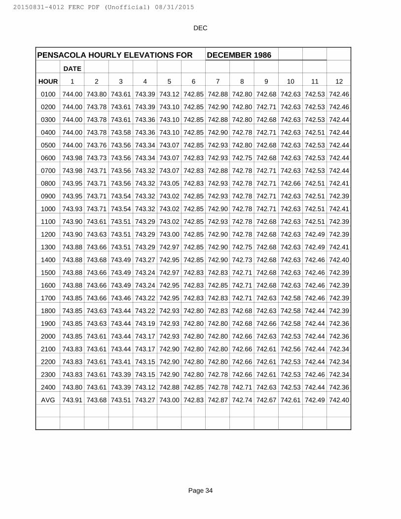
DEC
PENSACOLA HOURLY ELEVATIONS FOR DECEMBER 1986DATE
HOUR 1 2 3 4 5 6 7 8 9 10 11 12
0100 744.00 743.80 743.61 743.39 743.12 742.85 742.88 742.80 742.68 742.63 742.53 742.46
0200 744.00 743.78 743.61 743.39 743.10 742.85 742.90 742.80 742.71 742.63 742.53 742.46
0300 744.00 743.78 743.61 743.36 743.10 742.85 742.88 742.80 742.68 742.63 742.53 742.44
0400 744.00 743.78 743.58 743.36 743.10 742.85 742.90 742.78 742.71 742.63 742.51 742.44
0500 744.00 743.76 743.56 743.34 743.07 742.85 742.93 742.80 742.68 742.63 742.53 742.44
0600 743.98 743.73 743.56 743.34 743.07 742.83 742.93 742.75 742.68 742.63 742.53 742.44
0700 743.98 743.71 743.56 743.32 743.07 742.83 742.88 742.78 742.71 742.63 742.53 742.44
0800 743.95 743.71 743.56 743.32 743.05 742.83 742.93 742.78 742.71 742.66 742.51 742.41
0900 743.95 743.71 743.54 743.32 743.02 742.85 742.93 742.78 742.71 742.63 742.51 742.39
1000 743.93 743.71 743.54 743.32 743.02 742.85 742.90 742.78 742.71 742.63 742.51 742.41
1100 743.90 743.61 743.51 743.29 743.02 742.85 742.93 742.78 742.68 742.63 742.51 742.39
1200 743.90 743.63 743.51 743.29 743.00 742.85 742.90 742.78 742.68 742.63 742.49 742.39
1300 743.88 743.66 743.51 743.29 742.97 742.85 742.90 742.75 742.68 742.63 742.49 742.41
1400 743.88 743.68 743.49 743.27 742.95 742.85 742.90 742.73 742.68 742.63 742.46 742.40
1500 743.88 743.66 743.49 743.24 742.97 742.83 742.83 742.71 742.68 742.63 742.46 742.39
1600 743.88 743.66 743.49 743.24 742.95 742.83 742.85 742.71 742.68 742.63 742.46 742.39
1700 743.85 743.66 743.46 743.22 742.95 742.83 742.83 742.71 742.63 742.58 742.46 742.39
1800 743.85 743.63 743.44 743.22 742.93 742.80 742.83 742.68 742.63 742.58 742.44 742.39
1900 743.85 743.63 743.44 743.19 742.93 742.80 742.80 742.68 742.66 742.58 742.44 742.36
2000 743.85 743.61 743.44 743.17 742.93 742.80 742.80 742.66 742.63 742.53 742.44 742.36
2100 743.83 743.61 743.44 743.17 742.90 742.80 742.80 742.66 742.61 742.56 742.44 742.34
2200 743.83 743.61 743.41 743.15 742.90 742.80 742.80 742.66 742.61 742.53 742.44 742.34
2300 743.83 743.61 743.39 743.15 742.90 742.80 742.78 742.66 742.61 742.53 742.46 742.34
2400 743.80 743.61 743.39 743.12 742.88 742.85 742.78 742.71 742.63 742.53 742.44 742.36
AVG 743.91 743.68 743.51 743.27 743.00 742.83 742.87 742.74 742.67 742.61 742.49 742.40
Page 34
20150831-4012 FERC PDF (Unofficial) 08/31/2015

DEC
13 14 15 16 17 18 19 20 21 22 23 24 25
742.34 742.22 742.19 744.02 743.80 743.61 741.87 741.80 741.83 741.83 741.73 741.68 741.68
742.36 742.22 742.17 744.05 743.80 743.61 741.85 741.78 741.83 741.85 741.71 741.65 741.68
742.36 742.22 742.17 744.00 743.80 743.58 741.85 741.80 741.85 741.83 741.73 741.63 741.68
742.36 742.22 742.17 744.02 743.80 743.58 741.85 741.80 741.80 741.83 741.78 741.66 741.68
742.36 742.24 742.19 744.00 743.80 743.58 741.85 741.80 741.80 741.80 741.80 741.68 741.66
742.36 742.22 742.17 744.00 743.78 743.56 741.85 741.83 741.83 741.80 741.78 741.63 741.66
742.34 742.22 742.15 743.98 743.76 743.54 741.80 741.78 741.80 741.83 741.80 741.61 741.66
742.34 742.24 742.12 743.98 743.76 743.54 741.83 741.80 741.80 741.80 741.70 741.61 741.63
742.34 742.22 742.12 743.95 743.76 743.51 741.83 741.83 741.80 741.80 741.73 741.61 741.63
742.36 742.22 742.12 743.95 743.73 743.51 741.83 741.83 741.83 741.80 741.73 741.58 741.66
742.34 742.22 742.12 743.95 743.73 743.49 741.85 741.78 741.87 741.80 741.70 741.61 741.66
742.34 742.24 742.14 743.93 743.73 743.49 741.83 741.80 741.85 741.80 741.73 741.61 741.66
742.34 742.24 742.12 743.93 743.71 743.44 741.83 741.80 741.90 741.75 741.73 741.61 741.66
742.36 742.22 742.14 743.90 743.71 743.44 741.85 741.80 741.87 741.78 741.68 741.61 741.66
742.34 742.24 742.12 743.90 743.71 743.44 741.83 741.78 741.87 741.83 741.68 741.63 741.63
742.36 742.22 742.07 743.90 743.68 743.44 741.83 741.78 741.87 741.85 741.68 741.63 741.66
742.34 742.22 742.09 743.88 743.68 743.41 741.80 741.78 741.80 741.83 741.68 741.66 741.66
742.29 742.19 742.09 743.88 743.66 743.39 741.78 741.75 741.80 741.78 741.68 741.66 741.66
742.29 742.19 742.09 743.85 743.63 743.41 741.80 741.78 741.85 741.78 741.70 741.66 741.66
742.27 742.17 742.05 743.85 743.63 743.36 741.80 741.85 741.83 741.75 741.70 741.63 741.63
742.27 742.17 742.05 743.85 743.61 743.36 741.80 741.85 741.85 741.75 741.70 741.66 741.63
742.22 742.14 742.07 743.83 743.61 743.34 741.78 741.85 741.80 741.75 741.70 741.66 741.66
742.22 742.17 742.07 743.83 743.61 743.34 741.80 741.83 741.85 741.73 741.66 741.66 741.66
742.22 742.17 742.05 743.80 743.61 743.32 741.80 741.85 741.85 741.70 741.68 741.66 741.66
742.32 742.21 742.12 743.93 743.71 743.47 741.82 741.81 741.83 741.79 741.72 741.64 741.66
Page 35
20150831-4012 FERC PDF (Unofficial) 08/31/2015

DEC
26 27 28 29 30 31
741.61 741.56 741.66 741.46 741.39 741.34
741.63 741.51 741.44 741.46 741.41 741.34
741.66 741.53 741.46 741.46 741.41 741.34
741.63 741.56 741.46 741.46 741.41 741.36
741.63 741.53 741.46 741.46 741.41 741.36
741.63 741.56 741.46 741.46 741.44 741.34
741.61 741.53 741.48 741.41 741.39 741.34
741.60 741.51 741.46 741.44 741.39 741.36
741.58 741.48 741.46 741.46 741.41 741.29
741.63 741.46 741.48 741.47 741.36 741.29
741.66 741.51 741.46 741.45 741.36 741.29
741.66 741.48 741.48 741.44 741.34 741.29
741.66 741.48 741.51 741.44 741.31 741.24
741.66 741.46 741.51 741.44 741.31 741.29
741.63 741.46 741.51 741.44 741.31 741.24
741.66 741.51 741.53 741.44 741.31 741.29
741.63 741.48 741.51 741.44 741.31 741.24
741.56 741.46 741.51 741.44 741.31 741.24
741.61 741.44 741.48 741.39 741.34 741.24
741.56 741.44 741.51 741.41 741.34 741.24
741.56 741.44 741.46 741.41 741.34 741.24
741.56 741.44 741.44 741.39 741.34 741.24
741.58 741.48 741.44 741.41 741.34 741.24
741.58 741.46 741.44 741.41 741.34 741.24
741.62 741.49 741.48 741.44 741.36 741.29
Min = 741.24
Max = 744.05
Page 36
20150831-4012 FERC PDF (Unofficial) 08/31/2015

USGS 07185095TAR CREEK (US)
USGS 07185000NEOSHO - TAR (US) OUTFLOW (cfs)
Reservoir (NAVD88)
9/24/1993 0:00 17 1560 11100 745.329/24/1993 1:00 17 1540 11100 745.299/24/1993 2:00 16.25 1540 11100 745.299/24/1993 3:00 16 1540 11100 745.269/24/1993 3:59 16 1540 11100 745.269/24/1993 4:59 16 1540 11100 745.269/24/1993 5:59 15.75 1540 11100 745.239/24/1993 6:59 15 1540 11100 745.239/24/1993 7:59 15 1540 11100 745.209/24/1993 8:59 15 1540 11100 745.149/24/1993 9:59 15 777 11100 745.14
9/24/1993 10:59 15.75 832 11100 745.149/24/1993 11:59 22.25 950 11100 745.239/24/1993 12:59 101.25 1340 11100 745.209/24/1993 13:59 180.5 2620 11100 745.149/24/1993 14:59 161.75 5270 11100 745.139/24/1993 15:59 155 8500 17686.65851 745.139/24/1993 16:59 151.5 12700 26425.94859 745.139/24/1993 17:59 155 16500 34332.92534 745.139/24/1993 18:59 155.25 19600 40783.35373 745.179/24/1993 19:59 155 21600 44944.92044 745.179/24/1993 20:59 155.5 22800 47441.86047 745.239/24/1993 21:59 156.5 23700 49314.56548 745.319/24/1993 22:59 157 24500 50,979 745.449/24/1993 23:59 157.25 25300 52643.81885 745.51
9/25/1993 0:59 156 26200 54516.52387 745.579/25/1993 1:59 156 27800 57845.77723 745.639/25/1993 2:59 159 29000 60342.71726 745.759/25/1993 3:59 160 31000 64504.28397 745.849/25/1993 4:59 154.5 33300 69290.08568 745.969/25/1993 5:59 156.5 35200 73243.57405 746.179/25/1993 6:59 158.5 37300 77613.21909 746.179/25/1993 7:59 156.5 39000 81150.5508 746.269/25/1993 8:59 156.5 40800 84895.96083 746.459/25/1993 9:59 159.5 42300 88017.13586 746.45
9/25/1993 10:59 162 43800 91138.31089 746.499/25/1993 11:59 157.75 45000 93635.25092 746.699/25/1993 12:59 150.25 45500 94675.64259 746.859/25/1993 13:59 147.25 46000 95716.03427 746.949/25/1993 14:59 148.75 46000 95716.03427 747.069/25/1993 15:59 148.5 46200 96132.19094 747.219/25/1993 16:59 148.25 46000 95716.03427 747.30
USGS OBSERVED FLOWS (cfs) GRDA DATA
20150831-4012 FERC PDF (Unofficial) 08/31/2015

9/25/1993 17:59 148 46000 95716.03427 747.329/25/1993 18:59 148.25 45700 95091.79927 747.339/25/1993 19:59 148 45900 95507.95594 747.759/25/1993 20:59 154.5 45800 95299.8776 747.879/25/1993 21:59 160 46200 96132.19094 748.049/25/1993 22:59 164.75 46800 97,381 748.259/25/1993 23:59 166.5 47800 99461.44431 748.45
9/26/1993 0:59 167 48800 101542.2277 748.359/26/1993 1:59 166.5 50000 104039.1677 748.759/26/1993 2:59 164.75 51200 106536.1077 749.079/26/1993 3:59 166 52500 109241.1261 749.279/26/1993 4:59 167.5 54000 112362.3011 749.129/26/1993 5:59 171 55600 115691.5545 749.869/26/1993 6:59 174 56900 118396.5728 750.039/26/1993 7:59 174.5 58600 121933.9045 750.309/26/1993 8:59 175 60300 125471.2362 750.479/26/1993 9:59 164.25 61600 128176.2546 750.84
9/26/1993 10:59 137 63200 131505.508 751.059/26/1993 11:59 117.75 64500 134210.5263 751.289/26/1993 12:59 124.25 65800 136915.5447 751.379/26/1993 13:59 134.5 66900 139204.4064 751.679/26/1993 14:59 126.25 68000 141493.2681 751.989/26/1993 15:59 126.75 69000 143574.0514 752.159/26/1993 16:59 126.75 69800 145238.6781 752.429/26/1993 17:59 126.75 70800 147319.4614 752.539/26/1993 18:59 122 71800 149400.2448 752.599/26/1993 19:59 132 72600 151064.8715 752.999/26/1993 20:59 151 73300 152521.4198 753.179/26/1993 21:59 161.5 74000 153977.9682 753.359/26/1993 22:59 167 74900 155,851 753.479/26/1993 23:59 172 75600 157307.2215 753.61
9/27/1993 0:59 178 76200 158555.6916 753.839/27/1993 1:59 179.75 76900 160012.2399 754.029/27/1993 2:59 183 77400 161052.6316 754.179/27/1993 3:59 184.5 78200 162717.2583 754.319/27/1993 4:59 187.5 78600 163549.5716 754.499/27/1993 5:59 188 79000 164381.8849 754.649/27/1993 6:59 188.5 79700 165838.4333 754.789/27/1993 7:59 191.5 80100 166670.7466 754.969/27/1993 8:59 190.5 80500 167503.06 755.029/27/1993 9:59 166 80600 167711.1383 755.13
9/27/1993 10:59 142 80900 168335.3733 755.339/27/1993 11:59 123 81300 169167.6867 755.289/27/1993 12:59 156.25 81600 169791.9217 755.379/27/1993 13:59 127.75 81600 169791.9217 755.439/27/1993 14:59 123.5 81600 169791.9217 755.469/27/1993 15:59 117.25 81700 170000 755.52
20150831-4012 FERC PDF (Unofficial) 08/31/2015

9/27/1993 16:59 111.5 81700 170000 755.579/27/1993 17:59 112 81700 170000 755.639/27/1993 18:59 113.5 81500 169583.8433 755.669/27/1993 19:59 129.25 81300 169167.6867 755.759/27/1993 20:59 149 81000 168543.4517 755.759/27/1993 21:59 159.5 80600 167711.1383 755.789/27/1993 22:59 165.5 80400 167,295 755.789/27/1993 23:59 168.5 80100 166670.7466 755.84
9/28/1993 0:59 171 79600 165630.355 755.849/28/1993 1:59 172.5 79000 164381.8849 755.849/28/1993 2:59 175 78500 163341.4933 755.849/28/1993 3:59 177 77900 162093.0233 755.879/28/1993 4:59 177 77300 160844.5532 755.879/28/1993 5:59 176.5 76500 159179.9266 755.879/28/1993 6:59 171 75700 157515.2999 755.879/28/1993 7:59 163.75 75100 156266.8299 755.879/28/1993 8:59 157.75 74000 153977.9682 755.979/28/1993 9:59 153.5 73100 152105.2632 755.97
9/28/1993 10:59 148.5 72500 150856.7931 755.949/28/1993 11:59 140.5 71500 148776.0098 755.929/28/1993 12:59 132.25 70600 146903.3048 755.929/28/1993 13:59 126.25 69600 144822.5214 755.869/28/1993 14:59 119.25 68900 143365.9731 755.839/28/1993 15:59 111.5 67800 141077.1114 755.839/28/1993 16:59 105.75 67100 139620.563 755.809/28/1993 17:59 100.75 66200 137747.858 755.809/28/1993 18:59 94.5 65100 135458.9963 755.779/28/1993 19:59 90 64300 133794.3696 755.779/28/1993 20:59 86.5 63500 132129.743 755.749/28/1993 21:59 83 62500 130048.9596 755.719/28/1993 22:59 80.5 61600 128,176 755.689/28/1993 23:59 78.5 60800 126511.6279 755.68
9/29/1993 0:59 76.5 59800 124430.8446 755.629/29/1993 1:59 75.25 58800 122350.0612 755.599/29/1993 2:59 74.25 58100 120893.5129 755.569/29/1993 3:59 71.5 57300 119228.8862 755.539/29/1993 4:59 70.5 56300 117148.1028 755.489/29/1993 5:59 68 55500 115483.4761 755.429/29/1993 6:59 67 54400 113194.6144 755.399/29/1993 7:59 65 53800 111946.1444 755.399/29/1993 8:59 64 52800 109865.3611 755.369/29/1993 9:59 64 52200 108616.8911 755.30
9/29/1993 10:59 63 51200 106536.1077 755.279/29/1993 11:59 61.75 50600 105287.6377 755.279/29/1993 12:59 61 49700 103414.9327 755.249/29/1993 13:59 60.25 49100 102166.4627 755.189/29/1993 14:59 59.75 48400 100709.9143 755.14
20150831-4012 FERC PDF (Unofficial) 08/31/2015

9/29/1993 15:59 55.25 47700 99253.36597 755.109/29/1993 16:59 55 46900 97588.73929 755.089/29/1993 17:59 54.25 46300 96340.26928 755.049/29/1993 18:59 53 45800 95299.8776 754.989/29/1993 19:59 52 44900 93427.17258 754.929/29/1993 20:59 50.75 44400 92386.78091 754.899/29/1993 21:59 50 43800 91138.31089 754.869/29/1993 22:59 49.5 43200 89,890 754.809/29/1993 23:59 48.75 42600 88641.37087 754.74
9/30/1993 0:59 48 42100 87600.97919 754.689/30/1993 1:59 47 41500 86352.50918 754.669/30/1993 2:59 46.25 41200 85728.27417 754.609/30/1993 3:59 44 40400 84063.64749 754.549/30/1993 4:59 42 40000 83231.33415 754.489/30/1993 5:59 42 39700 82607.09914 754.429/30/1993 6:59 42 39100 81358.62913 754.369/30/1993 7:59 42 38400 79902.08078 754.279/30/1993 8:59 42 38000 79069.76744 754.249/30/1993 9:59 42 37500 78029.37576 754.19
9/30/1993 10:59 42 37000 76988.98409 754.169/30/1993 11:59 41.25 36200 75324.35741 754.129/30/1993 12:59 40.5 35400 73659.73072 754.109/30/1993 13:59 39.75 34600 71995.10404 754.049/30/1993 14:59 39 33800 70330.47736 754.019/30/1993 15:59 39 32800 68249.694 753.959/30/1993 16:59 38 31800 66168.91065 753.959/30/1993 17:59 37.5 30600 63671.97062 753.899/30/1993 18:59 36.25 29300 60966.95226 753.899/30/1993 19:59 35.75 28300 58886.16891 753.869/30/1993 20:59 34.25 27200 56597.30722 753.809/30/1993 21:59 34 26000 54100.3672 753.749/30/1993 22:59 33 25200 52,436 753.709/30/1993 23:59 33 24600 51187.2705 753.63
10/1/1993 0:59 33 23900 49730.7221510/1/1993 1:59 33 23200 48274.1738110/1/1993 2:59 33 22500 46817.6254610/1/1993 3:59 33 21700 45152.9987810/1/1993 4:59 33 21000 43696.4504310/1/1993 5:59 33 20200 42031.8237510/1/1993 6:59 33 19300 40159.1187310/1/1993 7:59 33 18500 38494.4920410/1/1993 8:59 33 17600 36621.7870310/1/1993 9:59 33 16800 34957.16034
10/1/1993 10:59 33 16000 33292.5336610/1/1993 11:59 33 15100 31419.8286410/1/1993 12:59 33 14300 29755.2019610/1/1993 13:59 33 13400 27882.49694
20150831-4012 FERC PDF (Unofficial) 08/31/2015

10/1/1993 14:59 33 12500 26009.7919210/1/1993 15:59 33 11600 24137.086910/1/1993 16:59 33 10800 22472.4602210/1/1993 17:59 33 10000 20807.8335410/1/1993 18:59 33 9220 19184.8225210/1/1993 19:59 33 8490 17665.8506710/1/1993 20:59 33 7800 16230.1101610/1/1993 21:59 33 7230 15044.0636510/1/1993 22:59 33 6710 13,962
# missing data supplemented by D2SI
20150831-4012 FERC PDF (Unofficial) 08/31/2015

20150831-4012 FERC PDF (Unofficial) 08/31/2015

20150831-4012 FERC PDF (Unofficial) 08/31/2015

20150831-4012 FERC PDF (Unofficial) 08/31/2015

20150831-4012 FERC PDF (Unofficial) 08/31/2015

20150831-4012 FERC PDF (Unofficial) 08/31/2015

20150831-4012 FERC PDF (Unofficial) 08/31/2015

20150831-4012 FERC PDF (Unofficial) 08/31/2015

20150831-4012 FERC PDF (Unofficial) 08/31/2015

20150831-4012 FERC PDF (Unofficial) 08/31/2015

1900076000
20150831-4012 FERC PDF (Unofficial) 08/31/2015

USGS 07185095TAR CREEK (US)
USGS 07185000NEOSHO - TAR
(US)
USGS 07185080 Stage at Miami
(ft-MSL NGVD88)OUTFLOW
(cfs)
10/8/2009 20:00 2250 12500 749.1 1420010/8/2009 21:00 2417.5 16000 750.44 1410010/8/2009 22:00 2545 19200 751.47 1405010/8/2009 23:00 2675 21900 752.24 1400010/9/2009 0:00 2845 23600 752.8 1420010/9/2009 1:00 2972.5 25600 753.26 1362510/9/2009 2:00 3090 27100 753.6110/9/2009 3:00 3270 28300 753.8810/9/2009 4:00 3485 29800 754.1210/9/2009 5:00 3867.5 31500 754.3510/9/2009 6:00 4217.5 33500 754.6210/9/2009 7:00 4490 35200 754.8510/9/2009 8:00 4605 34800 755.110/9/2009 9:00 4522.5 35800 755.31
10/9/2009 10:00 4450 36600 755.510/9/2009 11:00 4320 36600 755.7110/9/2009 12:00 4140 36300 755.8710/9/2009 13:00 3980 37600 756.0710/9/2009 14:00 3830 36800 756.210/9/2009 15:00 3655 38500 756.3810/9/2009 16:00 3515 37200 756.510/9/2009 17:00 3340 37600 756.6210/9/2009 18:00 3155 37200 756.7210/9/2009 19:00 2972.5 37300 756.8410/9/2009 20:00 2780 38200 756.9110/9/2009 21:00 2572.5 38300 757.0310/9/2009 22:00 2275 38500 757.0710/9/2009 23:00 2007.5 38100 757.1410/10/2009 0:00 1735 38300 757.210/10/2009 1:00 1457.5 37600 757.2310/10/2009 2:00 1195 38400 757.2610/10/2009 3:00 985.5 37200 757.2810/10/2009 4:00 824.25 38300 757.3410/10/2009 5:00 706 37700 757.3510/10/2009 6:00 608.75 38400 757.3610/10/2009 7:00 531.5 38800 757.4210/10/2009 8:00 471 39000 757.4510/10/2009 9:00 423.5 38900 757.49
10/10/2009 10:00 386 39800 757.4910/10/2009 11:00 355 39900 757.5910/10/2009 12:00 325.75 39400 757.64
USGS OBSERVED DATA GRDA DATA
20150831-4012 FERC PDF (Unofficial) 08/31/2015

10/10/2009 13:00 305 40100 757.6910/10/2009 14:00 286 40200 757.7310/10/2009 15:00 269.25 39800 757.8210/10/2009 16:00 253.5 41200 757.8810/10/2009 17:00 242 41400 757.9610/10/2009 18:00 229 41800 758.0710/10/2009 19:00 216 41900 758.1210/10/2009 20:00 206 40800 758.1910/10/2009 21:00 197 41800 758.2710/10/2009 22:00 188 41300 758.3610/10/2009 23:00 179.75 42400 758.4410/11/2009 0:00 171.75 42100 758.4910/11/2009 1:00 165.25 43400 758.610/11/2009 2:00 158.5 42100 758.6310/11/2009 3:00 153 42000 758.7210/11/2009 4:00 147 43000 758.8210/11/2009 5:00 142 44300 758.8710/11/2009 6:00 137.25 44100 758.9510/11/2009 7:00 130.75 44600 758.9710/11/2009 8:00 124.25 42600 759.0710/11/2009 9:00 120 43900 759.1
10/11/2009 10:00 116.25 43700 759.1210/11/2009 11:00 112.5 44800 759.2310/11/2009 12:00 109.25 44300 759.3110/11/2009 13:00 105.25 46100 759.3910/11/2009 14:00 102.25 44300 759.4410/11/2009 15:00 98.75 44100 759.4410/11/2009 16:00 96.25 44300 759.5410/11/2009 17:00 94.25 45700 759.5610/11/2009 18:00 91 46000 759.6510/11/2009 19:00 87.75 44900 759.6810/11/2009 20:00 86 45300 759.7510/11/2009 21:00 83.75 45700 759.7810/11/2009 22:00 81.75 45500 759.8210/11/2009 23:00 80.5 44900 759.8910/12/2009 0:00 78.5 45500 759.8910/12/2009 1:00 76 45800 759.9110/12/2009 2:00 73.75 44600 759.9510/12/2009 3:00 71.75 45400 759.9910/12/2009 4:00 70.75 44700 759.9910/12/2009 5:00 69.75 43900 759.9810/12/2009 6:00 68.75 44600 759.9710/12/2009 7:00 67.25 43400 759.9810/12/2009 8:00 66 42700 759.9810/12/2009 9:00 65 42900 759.88
10/12/2009 10:00 64 43600 759.9510/12/2009 11:00 62.5 42400 759.93
20150831-4012 FERC PDF (Unofficial) 08/31/2015

10/12/2009 12:00 60.75 41700 759.9110/12/2009 13:00 59.75 42300 759.9110/12/2009 14:00 58.25 40800 759.8710/12/2009 15:00 58 39800 759.7910/12/2009 16:00 57.25 40000 759.7610/12/2009 17:00 56.5 38700 759.6910/12/2009 18:00 55.25 37000 759.5710/12/2009 19:00 55 37000 759.5410/12/2009 20:00 55 35200 759.410/12/2009 21:00 54.5 34300 759.3310/12/2009 22:00 54.25 32800 759.210/12/2009 23:00 54 31300 759.0710/13/2009 0:00 53.75 29700 758.8910/13/2009 1:00 53 28700 758.7410/13/2009 2:00 52.75 27200 758.4910/13/2009 3:00 52.5 26200 758.3110/13/2009 4:00 52 25000 758.0610/13/2009 5:00 51.25 24200 757.8810/13/2009 6:00 51.5 23600 757.5710/13/2009 7:00 51 22800 757.2810/13/2009 8:00 50.75 22200 756.9910/13/2009 9:00 50.25 21400 756.66
10/13/2009 10:00 49.25 20800 756.3410/13/2009 11:00 49 19900 756.0110/13/2009 12:00 49 19100 755.6110/13/2009 13:00 48.25 18300 755.2410/13/2009 14:00 47.5 17300 754.8410/13/2009 15:00 47 16400 754.4210/13/2009 16:00 47.5 15400 753.9410/13/2009 17:00 46.25 14300 753.4310/13/2009 18:00 46.25 13100 752.8810/13/2009 19:00 46.5 11900 752.3210/13/2009 20:00 46.75 10800 751.7610/13/2009 21:00 46.5 9640 751.2310/13/2009 22:00 47 8670 750.7610/13/2009 23:00 47.25 7780 750.3310/14/2009 0:00 46.75 6960 75010/14/2009 1:00 47 6310 749.7410/14/2009 2:00 46.25 5810 749.5210/14/2009 3:00 46.5 5350 749.3510/14/2009 4:00 46.25 5010 749.210/14/2009 5:00 45.75 4760 749.0810/14/2009 6:00 45 4520 748.9710/14/2009 7:00 45 4310 748.8710/14/2009 8:00 44.75 4140 748.7910/14/2009 9:00 44.25 4060 748.71
10/14/2009 10:00 43.25 3900 748.62
20150831-4012 FERC PDF (Unofficial) 08/31/2015

10/14/2009 11:00 42 3850 748.5310/14/2009 12:00 41.5 3730 748.47 5040010/14/2009 13:00 40.25 3650 748.410/14/2009 14:00 39.75 3590 748.3310/14/2009 15:00 38.5 3540 748.2710/14/2009 16:00 38 3470 748.210/14/2009 17:00 38 3410 748.1210/14/2009 18:00 38 3390 748.0610/14/2009 19:00 38 3300 74810/14/2009 20:00 38.5 3290 747.9210/14/2009 21:00 39.25 3220 747.8610/14/2009 22:00 39.5 3180 747.810/14/2009 23:00 40 3150 747.7410/15/2009 0:00 40 3120 747.6710/15/2009 1:00 40.5 3070 747.610/15/2009 2:00 40.5 3050 747.5410/15/2009 3:00 40.5 3020 747.4810/15/2009 4:00 40 2980 747.4510/15/2009 5:00 40 2960 747.3810/15/2009 6:00 40 2930 747.3110/15/2009 7:00 39.5 2900 747.2610/15/2009 8:00 38.25 2900 747.2110/15/2009 9:00 35.75 2860 747.13
10/15/2009 10:00 33.5 2860 747.0710/15/2009 11:00 33.75 2830 747.0110/15/2009 12:00 33.75 2810 746.9410/15/2009 13:00 33.75 2800 746.8910/15/2009 14:00 33.5 2780 746.8910/15/2009 15:00 33.5 2760 746.8910/15/2009 16:00 33 2730 746.8510/15/2009 17:00 33.25 2730 746.8210/15/2009 18:00 33.5 2710 746.8110/15/2009 19:00 34 2700 746.8110/15/2009 20:00 34 2680 746.7810/15/2009 21:00 34 2680 746.7510/15/2009 22:00 34.25 2660 746.7310/15/2009 23:00 35 2660 746.710/16/2009 0:00 35.25 2680 746.6710/16/2009 1:00 36 2700 746.6710/16/2009 2:00 36 2700 746.6510/16/2009 3:00 35.75 2710 746.6310/16/2009 4:00 34.75 2750 746.6210/16/2009 5:00 34 2760 746.6210/16/2009 6:00 33 2810 746.6110/16/2009 7:00 32 2850 746.5910/16/2009 8:00 31.75 2880 746.5610/16/2009 9:00 30.5 2910 746.53
20150831-4012 FERC PDF (Unofficial) 08/31/2015

10/16/2009 10:00 30 2950 746.5110/16/2009 11:00 29.75 2960 746.4910/16/2009 12:00 29 3030 746.4510/16/2009 13:00 28 3030 746.4210/16/2009 14:00 28 3050 746.4110/16/2009 15:00 27 3080 746.4210/16/2009 16:00 26.5 3100 746.4210/16/2009 17:00 26.25 3070 746.4310/16/2009 18:00 26 3100 746.4810/16/2009 19:00 26 3120 746.4810/16/2009 20:00 26.25 3080 746.4410/16/2009 21:00 26.25 3100 746.4410/16/2009 22:00 26 3080 746.4810/16/2009 23:00 26 3080 746.4510/17/2009 0:00 26 3070 746.4110/17/2009 1:00 26 3050 746.42 1287510/17/2009 2:00 26 3050 746.42 1297510/17/2009 3:00 26 3030 746.4 1287510/17/2009 4:00 26 3020 746.39 1305010/17/2009 5:00 25.75 3020 746.38 1302510/17/2009 6:00 26 3000 746.36 1317510/17/2009 7:00 25.25 2980 746.35 1307510/17/2009 8:00 25.25 2950 746.36 1300010/17/2009 9:00 25.25 2960 746.35 13225
10/17/2009 10:00 25 2930 746.32 1317510/17/2009 11:00 25 2930 746.3 1317510/17/2009 12:00 25 2900 746.29 1330010/17/2009 13:00 24.25 2880 746.24 1325010/17/2009 14:00 24 2860 746.21 1322510/17/2009 15:00 23.75 2850 746.23 1325010/17/2009 16:00 23.5 2830 746.25 1327510/17/2009 17:00 23 2810 746.23 1325010/17/2009 18:00 22.75 2830 746.21 1322510/17/2009 19:00 22 2800 746.22 1325010/17/2009 20:00 21.5 2800 746.22 1320010/17/2009 21:00 21 2800 746.2 1332510/17/2009 22:00 20.75 2810 746.21 1322510/17/2009 23:00 20.25 2810 746.21 1322510/18/2009 0:00 20 2850 746.19 1310010/18/2009 1:00 20 2850 746.18 1332510/18/2009 2:00 20 2880 746.18 1340010/18/2009 3:00 20 2930 746.17 1352510/18/2009 4:00 20 2960 746.17 1357510/18/2009 5:00 20 3000 746.17 1342510/18/2009 6:00 20 3030 746.17 1350010/18/2009 7:00 19.75 3050 746.16 1355010/18/2009 8:00 19.5 3080 746.17 13725
20150831-4012 FERC PDF (Unofficial) 08/31/2015

10/18/2009 9:00 19 3120 746.16 1357510/18/2009 10:00 19 3150 746.16 1355010/18/2009 11:00 19 3200 746.17 1367510/18/2009 12:00 18.75 3200 746.17 1370010/18/2009 13:00 17.75 3220 746.18 1367510/18/2009 14:00 17.75 3230 746.21 1372510/18/2009 15:00 18 3220 746.19 1375010/18/2009 16:00 17.25 3250 746.15 1367510/18/2009 17:00 17 3250 746.13 1365010/18/2009 18:00 17 3230 746.13 1372510/18/2009 19:00 17 3250 746.13 1367510/18/2009 20:00 17 3230 746.13 1377510/18/2009 21:00 17 3230 746.12 1390010/18/2009 22:00 17 3250 746.09 1375010/18/2009 23:00 17 3230 746.07 1382510/19/2009 0:00 16.75 3230 746.06 1385010/19/2009 1:00 17 3230 746.07 1410010/19/2009 2:00 16.75 3220 746.06 1412510/19/2009 3:00 16.5 3180 746.05 1400010/19/2009 4:00 16 3180 746.06 1410010/19/2009 5:00 16 3180 746.06 1410010/19/2009 6:00 16 3170 746.04 1420010/19/2009 7:00 16 3170 746 1437510/19/2009 8:00 16 3170 746 1432510/19/2009 9:00 16 3170 745.99 14400
10/19/2009 10:00 15.5 3120 745.96 1432510/19/2009 11:00 16 3080 745.99 1435010/19/2009 12:00 15.5 3120 745.98 1442510/19/2009 13:00 15.75 3100 745.97 1450010/19/2009 14:00 15.25 3030 745.94 1450010/19/2009 15:00 15 3080 745.97 1445010/19/2009 16:00 15.25 3050 745.97 1450010/19/2009 17:00 15 3050 745.92 1462510/19/2009 18:00 14.5 3030 745.87 1455010/19/2009 19:00 15 3030 745.84 1457510/19/2009 20:00 15 3020 745.83 1455010/19/2009 21:00 15 3020 745.8 1452510/19/2009 22:00 15 3000 745.77 1460010/19/2009 23:00 15 3000 745.77 1457510/20/2009 0:00 15 3000 745.79 1457510/20/2009 1:00 15 2980 745.78 1457510/20/2009 2:00 15.25 2950 745.77 1475010/20/2009 3:00 15 2960 745.76 1452510/20/2009 4:00 15 2950 745.74 1452510/20/2009 5:00 15 2950 745.72 1457510/20/2009 6:00 15 2950 745.73 1452510/20/2009 7:00 15 2910 745.69 14450
20150831-4012 FERC PDF (Unofficial) 08/31/2015

10/20/2009 8:00 15 2930 745.72 1452510/20/2009 9:00 14.75 2910 745.73 14525
10/20/2009 10:00 15 2910 745.72 1455010/20/2009 11:00 14.75 2910 745.68 1450010/20/2009 12:00 14.5 2880 745.68 1452510/20/2009 13:00 14.25 2860 745.65 1460010/20/2009 14:00 14 2880 745.65 1457510/20/2009 15:00 14.25 2860 745.67 1455010/20/2009 16:00 14 2880 745.65 1457510/20/2009 17:00 14 2850 745.59 1450010/20/2009 18:00 14 2830 745.56 1455010/20/2009 19:00 13.5 2850 745.55 1452510/20/2009 20:00 13 2830 745.54 1447510/20/2009 21:00 13 2830 745.5 1460010/20/2009 22:00 13 2810 745.47 1445010/20/2009 23:00 13 2810 745.45 14500
20150831-4012 FERC PDF (Unofficial) 08/31/2015

Reservoir (PD)
Reservoir (NGVD88)
741.38 742.85741.53 743.00741.72 743.19741.91 743.38742.00 743.47742.06 743.53742.27 743.74742.63 744.10742.69 744.16742.95 744.42743.16 744.63743.34 744.81743.58 745.05743.83 745.30743.97 745.44744.13 745.60744.28 745.75744.46 745.93744.66 746.13744.83 746.30744.98 746.45745.12 746.59745.29 746.76745.50 746.97745.67 747.14745.87 747.34746.02 747.49746.18 747.65746.30 747.77746.48 747.95746.69 748.16746.82 748.29746.97 748.44747.12 748.59747.22 748.69747.35 748.82747.47 748.94747.63 749.10747.72 749.19747.84 749.31747.86 749.33
GRDA DATA
20150831-4012 FERC PDF (Unofficial) 08/31/2015

747.98 749.45748.02 749.49748.05 749.52748.10 749.57748.19 749.66748.25 749.72748.27 749.74748.36 749.83748.43 749.90748.48 749.95748.53 750.00748.58 750.05748.68 750.15748.71 750.18748.77 750.24748.80 750.27748.86 750.33748.89 750.36748.95 750.42748.96 750.43749.02 750.49749.05 750.52749.08 750.55749.11 750.58749.15 750.62749.18 750.65749.21 750.68749.24 750.71749.31 750.78749.31 750.78749.33 750.80749.37 750.84749.40 750.87749.41 750.88749.47 750.94749.47 750.94749.47 750.94749.48 750.95749.56 751.03749.56 751.03749.56 751.03749.57 751.04749.57 751.04749.60 751.07749.57 751.04749.57 751.04749.57 751.04
20150831-4012 FERC PDF (Unofficial) 08/31/2015

749.57 751.04749.57 751.04749.53 751.00749.53 751.00749.53 751.00749.50 750.97749.49 750.96749.47 750.94749.43 750.90749.43 750.90749.38 750.85749.38 750.85749.34 750.81749.32 750.79749.26 750.73749.25 750.72749.19 750.66749.18 750.65749.13 750.60749.10 750.57749.09 750.56749.09 750.56749.02 750.49748.98 750.45748.96 750.43748.98 750.45748.96 750.43748.94 750.41748.94 750.41748.91 750.38748.88 750.35748.85 750.32748.85 750.32748.82 750.29748.79 750.26748.73 750.20748.70 750.17748.64 750.11748.58 750.05748.52 749.99748.42 749.89748.39 749.86748.33 749.80748.26 749.73748.21 749.68748.16 749.63748.10 749.57
20150831-4012 FERC PDF (Unofficial) 08/31/2015

748.05 749.52747.99 749.46747.94 749.41747.90 749.37747.84 749.31747.81 749.28747.71 749.18747.66 749.13747.60 749.07747.50 748.97747.44 748.91747.38 748.85747.29 748.76747.26 748.73747.22 748.69747.16 748.63747.10 748.57747.06 748.53747.00 748.47746.95 748.42746.91 748.38746.85 748.32746.80 748.27746.81 748.28746.72 748.19746.72 748.19746.67 748.14746.65 748.12746.60 748.07746.57 748.04746.55 748.02746.52 747.99746.49 747.96746.49 747.96746.46 747.93746.43 747.90746.41 747.88746.38 747.85746.38 747.85746.35 747.82746.32 747.79746.29 747.76746.26 747.73746.23 747.70746.20 747.67746.19 747.66746.16 747.63
20150831-4012 FERC PDF (Unofficial) 08/31/2015

746.16 747.63746.16 747.63746.15 747.62746.14 747.61746.17 747.64746.14 747.61746.11 747.58746.14 747.61746.11 747.58746.11 747.58746.08 747.55746.08 747.55746.10 747.57746.07 747.54746.07 747.54746.07 747.54746.04 747.51746.04 747.51746.04 747.51746.04 747.51746.01 747.48746.01 747.48746.03 747.50746.00 747.47746.00 747.47746.01 747.48746.00 747.47746.00 747.47745.98 747.45745.98 747.45745.95 747.42745.95 747.42745.95 747.42745.95 747.42745.92 747.39745.92 747.39745.92 747.39745.89 747.36745.89 747.36745.87 747.34745.86 747.33745.87 747.34745.85 747.32745.84 747.31745.84 747.31745.84 747.31745.81 747.28
20150831-4012 FERC PDF (Unofficial) 08/31/2015

745.81 747.28745.78 747.25745.75 747.22745.72 747.19745.72 747.19745.72 747.19745.72 747.19745.72 747.19745.69 747.16745.69 747.16745.69 747.16745.66 747.13745.66 747.13745.65 747.12745.64 747.11745.60 747.07745.62 747.09745.59 747.06745.59 747.06745.57 747.04745.55 747.02745.52 746.99745.53 747.00745.51 746.98745.50 746.97745.47 746.94745.44 746.91745.41 746.88745.41 746.88745.38 746.85745.38 746.85745.38 746.85745.38 746.85745.38 746.85745.38 746.85745.39 746.86745.36 746.83745.35 746.82745.32 746.79745.32 746.79745.32 746.79745.29 746.76745.30 746.77745.28 746.75745.25 746.72745.23 746.70745.23 746.70
20150831-4012 FERC PDF (Unofficial) 08/31/2015

745.22 746.69745.19 746.66745.19 746.66745.16 746.63745.16 746.63745.13 746.60745.13 746.60745.13 746.60745.13 746.60745.13 746.60745.13 746.60745.11 746.58745.11 746.58745.11 746.58745.08 746.55745.08 746.55
20150831-4012 FERC PDF (Unofficial) 08/31/2015

USGS 07185000NEOSHO - TAR
(US)
USGS 07185095TAR CREEK
(US)Reservoir (NGVD88)
Main Gate Open
9/29/1986 4940 343 9/28/1986 1:00 744.00 09/30/1986 34400 3340 9/28/1986 2:00 743.98 010/1/1986 47900 2710 9/28/1986 3:00 743.98 010/2/1986 58900 453 9/28/1986 4:00 743.98 010/3/1986 67900 313 9/28/1986 5:00 743.98 010/4/1986 72100 524 9/28/1986 6:00 743.96 010/5/1986 84100 332 9/28/1986 7:00 743.93 010/6/1986 101000 738 9/28/1986 8:00 743.96 010/7/1986 92400 638 9/28/1986 9:00 743.93 010/8/1986 72200 114 9/28/1986 10:00 743.91 010/9/1986 53400 24 9/28/1986 11:00 743.88 0
10/10/1986 39100 28 9/28/1986 12:00 743.86 010/11/1986 24700 30 9/28/1986 13:00 743.86 010/12/1986 17400 33 9/28/1986 14:00 743.86 010/13/1986 16600 31 9/28/1986 15:00 743.81 010/14/1986 16500 35 9/28/1986 16:00 743.84 010/15/1986 15300 24 9/28/1986 17:00 743.81 0
9/28/1986 18:00 743.81 09/28/1986 19:00 743.81 09/28/1986 20:00 743.78 09/28/1986 21:00 743.78 09/28/1986 22:00 743.76 09/28/1986 23:00 743.74 0
9/29/1986 0:00 743.69 09/29/1986 1:00 743.69 09/29/1986 2:00 743.69 09/29/1986 3:00 743.66 09/29/1986 4:00 743.66 09/29/1986 5:00 743.64 09/29/1986 6:00 743.61 09/29/1986 7:00 743.56 09/29/1986 8:00 743.54 09/29/1986 9:00 743.49 0
9/29/1986 10:00 743.44 09/29/1986 11:00 743.47 09/29/1986 12:00 743.49 09/29/1986 13:00 743.52 09/29/1986 14:00 743.49 09/29/1986 15:00 743.52 09/29/1986 16:00 743.52 09/29/1986 17:00 743.54 0
USGS OBSERVED FLOWS (cfs)
20150831-4012 FERC PDF (Unofficial) 08/31/2015

9/29/1986 18:00 743.54 09/29/1986 19:00 743.56 09/29/1986 20:00 743.69 09/29/1986 21:00 743.74 09/29/1986 22:00 743.74 09/29/1986 23:00 743.81 0
9/30/1986 0:00 743.86 09/30/1986 1:00 743.93 09/30/1986 2:00 743.96 09/30/1986 3:00 744.10 09/30/1986 4:00 744.29 09/30/1986 5:00 744.54 09/30/1986 6:00 744.66 09/30/1986 7:00 745.03 09/30/1986 8:00 745.15 09/30/1986 9:00 745.15 0
9/30/1986 10:00 745.15 09/30/1986 11:00 745.99 09/30/1986 12:00 746.25 09/30/1986 13:00 746.54 29/30/1986 14:00 746.76 29/30/1986 15:00 746.76 49/30/1986 16:00 746.91 59/30/1986 17:00 747.13 59/30/1986 18:00 747.42 59/30/1986 19:00 747.52 59/30/1986 20:00 747.67 59/30/1986 21:00 747.89 59/30/1986 22:00 748.01 59/30/1986 23:00 748.18 5
10/1/1986 0:00 748.33 510/1/1986 1:00 748.50 510/1/1986 2:00 748.65 510/1/1986 3:00 748.79 510/1/1986 4:00 748.94 510/1/1986 5:00 749.08 510/1/1986 6:00 749.26 510/1/1986 7:00 749.38 510/1/1986 8:00 749.52 510/1/1986 9:00 749.67 5
10/1/1986 10:00 749.77 510/1/1986 11:00 749.94 510/1/1986 12:00 750.16 410/1/1986 13:00 750.31 410/1/1986 14:00 750.40 410/1/1986 15:00 750.55 410/1/1986 16:00 750.65 4
20150831-4012 FERC PDF (Unofficial) 08/31/2015

10/1/1986 17:00 750.79 210/1/1986 18:00 750.94 210/1/1986 19:00 751.04 210/1/1986 20:00 751.16 210/1/1986 21:00 751.31 210/1/1986 22:00 751.43 210/1/1986 23:00 751.48 2
10/2/1986 0:00 751.48 210/2/1986 1:00 751.83 210/2/1986 2:00 751.97 210/2/1986 3:00 752.07 210/2/1986 4:00 752.19 210/2/1986 5:00 752.30 210/2/1986 6:00 752.42 210/2/1986 7:00 752.52 210/2/1986 8:00 752.65 210/2/1986 9:00 752.85 2
10/2/1986 10:00 752.94 210/2/1986 11:00 753.12 210/2/1986 12:00 753.19 210/2/1986 13:00 753.27 210/2/1986 14:00 753.36 210/2/1986 15:00 753.48 210/2/1986 16:00 753.65 210/2/1986 17:00 753.73 210/2/1986 18:00 753.87 210/2/1986 19:00 754.02 210/2/1986 20:00 754.17 210/2/1986 21:00 754.26 210/2/1986 22:00 754.41 210/2/1986 23:00 754.53 2
10/3/1986 0:00 754.65 210/3/1986 1:00 754.78 210/3/1986 2:00 754.90 210/3/1986 3:00 755.00 210/3/1986 4:00 755.12 210/3/1986 5:00 755.22 210/3/1986 6:00 755.34 210/3/1986 7:00 755.46 210/3/1986 8:00 755.58 210/3/1986 9:00 755.75 2
10/3/1986 10:00 755.78 210/3/1986 11:00 755.90 210/3/1986 12:00 755.92 410/3/1986 13:00 755.92 410/3/1986 14:00 756.02 410/3/1986 15:00 756.05 4
20150831-4012 FERC PDF (Unofficial) 08/31/2015

10/3/1986 16:00 756.05 410/3/1986 17:00 756.07 410/3/1986 18:00 756.07 410/3/1986 19:00 756.10 410/3/1986 20:00 756.12 410/3/1986 21:00 756.12 410/3/1986 22:00 756.14 410/3/1986 23:00 756.14 4
10/4/1986 0:00 756.14 410/4/1986 1:00 756.14 410/4/1986 2:00 756.17 410/4/1986 3:00 756.17 410/4/1986 4:00 756.17 410/4/1986 5:00 756.17 410/4/1986 6:00 756.17 410/4/1986 7:00 756.17 410/4/1986 8:00 756.17 410/4/1986 9:00 756.17 4
10/4/1986 10:00 756.17 410/4/1986 11:00 756.17 410/4/1986 12:00 756.17 410/4/1986 13:00 756.17 410/4/1986 14:00 756.14 410/4/1986 15:00 756.14 410/4/1986 16:00 756.14 410/4/1986 17:00 756.12 410/4/1986 18:00 756.12 410/4/1986 19:00 756.10 410/4/1986 20:00 756.10 410/4/1986 21:00 756.07 410/4/1986 22:00 756.07 410/4/1986 23:00 756.02 4
10/5/1986 0:00 756.02 410/5/1986 1:00 756.02 410/5/1986 2:00 756.00 410/5/1986 3:00 756.00 410/5/1986 4:00 755.97 410/5/1986 5:00 755.97 410/5/1986 5:59 755.95 410/5/1986 6:59 755.92 410/5/1986 7:59 755.92 410/5/1986 8:59 755.90 410/5/1986 9:59 755.90 4
10/5/1986 10:59 755.90 410/5/1986 11:59 755.90 410/5/1986 12:59 755.92 410/5/1986 13:59 755.95 4
20150831-4012 FERC PDF (Unofficial) 08/31/2015

10/5/1986 14:59 755.95 410/5/1986 15:59 755.97 410/5/1986 16:59 756.00 410/5/1986 17:59 756.00 410/5/1986 18:59 755.99 410/5/1986 19:59 756.05 410/5/1986 20:59 756.07 410/5/1986 21:59 756.10 410/5/1986 22:59 756.12 410/5/1986 23:59 756.14 4
10/6/1986 0:59 756.17 410/6/1986 1:59 756.22 410/6/1986 2:59 756.22 410/6/1986 3:59 756.32 410/6/1986 4:59 756.34 410/6/1986 5:59 756.34 410/6/1986 6:59 756.36 410/6/1986 7:59 756.39 410/6/1986 8:59 756.41 410/6/1986 9:59 756.41 4
10/6/1986 10:59 756.44 410/6/1986 11:59 756.44 410/6/1986 12:59 756.41 410/6/1986 13:59 756.44 410/6/1986 14:59 756.41 410/6/1986 15:59 756.41 410/6/1986 16:59 756.44 410/6/1986 17:59 756.41 410/6/1986 18:59 756.41 410/6/1986 19:59 756.39 410/6/1986 20:59 756.39 410/6/1986 21:59 756.34 410/6/1986 22:59 756.32 410/6/1986 23:59 756.29 4
10/7/1986 0:59 756.24 410/7/1986 1:59 756.24 410/7/1986 2:59 756.22 410/7/1986 3:59 756.19 410/7/1986 4:59 756.17 410/7/1986 5:59 756.14 410/7/1986 6:59 756.12 410/7/1986 7:59 756.10 410/7/1986 8:59 756.07 410/7/1986 9:59 756.07 4
10/7/1986 10:59 756.02 410/7/1986 11:59 756.02 410/7/1986 12:59 756.02 4
20150831-4012 FERC PDF (Unofficial) 08/31/2015

10/7/1986 13:59 755.97 410/7/1986 14:59 755.97 410/7/1986 15:59 755.95 410/7/1986 16:59 755.85 410/7/1986 17:59 755.88 410/7/1986 18:59 755.85 410/7/1986 19:59 755.83 410/7/1986 20:59 755.80 410/7/1986 21:59 755.80 410/7/1986 22:59 755.78 410/7/1986 23:59 755.75 4
10/8/1986 0:59 755.73 410/8/1986 1:59 755.70 410/8/1986 2:59 755.70 410/8/1986 3:59 755.68 410/8/1986 4:59 755.66 410/8/1986 5:59 755.66 410/8/1986 6:59 755.63 410/8/1986 7:59 755.61 410/8/1986 8:59 755.53 410/8/1986 9:59 755.51 4
10/8/1986 10:59 755.48 410/8/1986 11:59 755.46 410/8/1986 12:59 755.41 410/8/1986 13:59 755.36 410/8/1986 14:59 755.34 410/8/1986 15:59 755.31 410/8/1986 16:59 755.26 410/8/1986 17:59 755.24 410/8/1986 18:59 755.22 410/8/1986 19:59 755.19 410/8/1986 20:59 755.17 410/8/1986 21:59 755.14 410/8/1986 22:59 755.12 410/8/1986 23:59 755.07 4
10/9/1986 0:59 755.04 410/9/1986 1:59 755.02 410/9/1986 2:59 754.97 410/9/1986 3:59 754.95 410/9/1986 4:59 754.90 410/9/1986 5:59 754.90 410/9/1986 6:59 754.85 410/9/1986 7:59 754.85 410/9/1986 8:59 754.80 410/9/1986 9:59 754.80 4
10/9/1986 10:59 754.78 310/9/1986 11:59 754.75 3
20150831-4012 FERC PDF (Unofficial) 08/31/2015

10/9/1986 12:59 754.73 310/9/1986 13:59 754.73 310/9/1986 14:59 754.73 310/9/1986 15:59 754.75 310/9/1986 16:59 754.75 310/9/1986 17:59 754.75 210/9/1986 18:59 754.75 210/9/1986 19:59 754.75 210/9/1986 20:59 754.77 210/9/1986 21:59 754.80 210/9/1986 22:59 754.80 210/9/1986 23:59 754.78 210/10/1986 0:59 754.78 210/10/1986 1:59 754.80 210/10/1986 2:59 754.80 210/10/1986 3:59 754.80 210/10/1986 4:59 754.83 210/10/1986 5:59 754.83 210/10/1986 6:59 754.83 210/10/1986 7:59 754.83 210/10/1986 8:59 754.83 210/10/1986 9:59 754.83 2
10/10/1986 10:59 754.83 210/10/1986 11:59 754.83 210/10/1986 12:59 754.80 210/10/1986 13:59 754.80 210/10/1986 14:59 754.78 210/10/1986 15:59 754.73 210/10/1986 16:59 754.73 210/10/1986 17:59 754.70 210/10/1986 18:59 754.68 210/10/1986 19:59 754.65 210/10/1986 20:59 754.63 210/10/1986 21:59 754.61 210/10/1986 22:59 754.58 210/10/1986 23:59 754.56 2
10/11/1986 0:59 754.53 210/11/1986 1:59 754.51 210/11/1986 2:59 754.48 210/11/1986 3:59 754.43 210/11/1986 4:59 754.41 210/11/1986 5:59 754.39 210/11/1986 6:59 754.34 210/11/1986 7:59 754.31 210/11/1986 8:59 754.29 210/11/1986 9:59 754.26 2
10/11/1986 10:59 754.21 2
20150831-4012 FERC PDF (Unofficial) 08/31/2015

10/11/1986 11:59 754.19 210/11/1986 12:59 754.14 210/11/1986 13:59 754.12 210/11/1986 14:59 754.09 210/11/1986 15:59 754.04 210/11/1986 16:59 753.99 210/11/1986 17:59 753.97 210/11/1986 18:59 753.87 210/11/1986 19:59 753.87 210/11/1986 20:59 753.85 210/11/1986 21:59 753.82 210/11/1986 22:59 753.80 210/11/1986 23:59 753.73 2
10/12/1986 0:59 753.68 210/12/1986 1:59 753.63 210/12/1986 2:59 753.58 210/12/1986 3:59 753.51 210/12/1986 4:59 753.48 210/12/1986 5:59 753.38 210/12/1986 6:59 753.36 210/12/1986 7:59 753.29 210/12/1986 8:59 753.24 210/12/1986 9:59 753.16 2
10/12/1986 10:59 753.09 210/12/1986 11:59 753.02 210/12/1986 12:59 752.99 210/12/1986 13:59 752.92 210/12/1986 14:59 752.85 210/12/1986 15:59 752.77 210/12/1986 16:59 752.72 210/12/1986 17:59 752.65 210/12/1986 18:59 752.60 210/12/1986 19:59 752.55 210/12/1986 20:59 752.48 210/12/1986 21:59 752.38 210/12/1986 22:59 752.33 210/12/1986 23:59 752.26 2
10/13/1986 0:59 752.19 210/13/1986 1:59 752.14 210/13/1986 2:59 752.09 210/13/1986 3:59 751.99 210/13/1986 4:59 751.97 210/13/1986 5:59 751.92 210/13/1986 6:59 751.85 210/13/1986 7:59 751.77 210/13/1986 8:59 751.72 210/13/1986 9:59 751.65 2
20150831-4012 FERC PDF (Unofficial) 08/31/2015

10/13/1986 10:59 751.65 210/13/1986 11:59 751.63 110/13/1986 12:59 751.58 110/13/1986 13:59 751.53 110/13/1986 14:59 751.53 110/13/1986 15:59 751.53 010/13/1986 16:59 751.38 010/13/1986 17:59 751.38 010/13/1986 18:59 751.38 010/13/1986 19:59 751.38 010/13/1986 20:59 751.38 010/13/1986 21:59 751.38 010/13/1986 22:59 751.36 010/13/1986 23:59 751.36 0
10/14/1986 0:59 751.33 010/14/1986 1:59 751.36 010/14/1986 2:59 751.33 010/14/1986 3:59 751.31 010/14/1986 4:59 751.28 010/14/1986 5:59 751.28 010/14/1986 6:59 751.28 010/14/1986 7:59 751.28 010/14/1986 8:59 751.28 010/14/1986 9:59 751.28 0
10/14/1986 10:59 751.28 010/14/1986 11:59 751.31 010/14/1986 12:59 751.31 010/14/1986 13:59 751.28 010/14/1986 14:59 751.28 010/14/1986 15:59 751.28 010/14/1986 16:59 751.26 010/14/1986 17:59 751.26 010/14/1986 18:59 751.26 010/14/1986 19:59 751.26 010/14/1986 20:59 751.23 010/14/1986 21:59 751.23 010/14/1986 22:59 751.23 010/14/1986 23:59 751.21 0
10/15/1986 0:59 751.21 010/15/1986 1:59 751.21 010/15/1986 2:59 751.19 010/15/1986 3:59 751.19 010/15/1986 4:59 751.19 010/15/1986 5:59 751.16 010/15/1986 6:59 751.16 010/15/1986 7:59 751.14 010/15/1986 8:59 751.14 0
20150831-4012 FERC PDF (Unofficial) 08/31/2015

10/15/1986 9:59 751.14 010/15/1986 10:59 751.11 010/15/1986 11:59 751.11 010/15/1986 12:59 751.09 010/15/1986 13:59 751.09 010/15/1986 14:59 751.09 010/15/1986 15:59 751.09 010/15/1986 16:59 751.09 010/15/1986 17:59 751.06 010/15/1986 18:59 751.06 010/15/1986 19:59 751.04 010/15/1986 20:59 751.04 010/15/1986 21:59 751.01 010/15/1986 22:59 751.01 010/15/1986 23:59 750.99 0
20150831-4012 FERC PDF (Unofficial) 08/31/2015

Aux Gate Open
Main Gate Spill
Aux Gate Spill
OUTFLOW (cfs)
0 0 0 115000 0 0 115000 0 0 115000 0 0 115000 0 0 115000 0 0 115000 0 0 115000 0 0 115000 0 0 115000 0 0 115000 0 0 115000 0 0 115000 0 0 115000 0 0 115000 0 0 115000 0 0 115000 0 0 115000 0 0 115000 0 0 115000 0 0 115000 0 0 115000 0 0 115000 0 0 115000 0 0 115000 0 0 115000 0 0 115000 0 0 115000 0 0 115000 0 0 115000 0 0 115000 0 0 115000 0 0 115000 0 0 115000 0 0 115000 0 0 115000 0 0 115000 0 0 115000 0 0 115000 0 0 115000 0 0 115000 0 0 11500
GRDA DATA1 1. GRDA provided hourly reservoir elevation data, but only intermittent outflow data. USGS stream gages only provided daily measurements. D2SI back-calculated the outflows based on the hourly reservoir elevations and known gate openings. D2SI utilized the rating curves for each of the spillways and known water surface elevations to determine hourly outflow from the project.
20150831-4012 FERC PDF (Unofficial) 08/31/2015

0 0 0 115000 0 0 115000 0 0 115000 0 0 115000 0 0 115000 0 0 115000 0 0 115000 0 0 115000 0 0 115000 0 0 115000 0 0 115000 0 0 115000 0 0 115000 0 0 115000 0 0 115000 0 0 115000 0 0 115000 0 0 115000 0 0 115000 15318 0 268180 15669 0 271690 31338 0 428381 39774 1709 529831 40665 1794 539585 41852 9542 628935 42264 9743 635085 42887 10049 644365 43807 10507 658145 44312 10761 665735 45033 11126 676585 45672 11453 686265 46402 11831 697335 47051 12169 707205 47659 12490 716495 48315 12839 726545 48931 13171 736015 49727 13604 748315 50261 13897 756585 50888 14244 766325 51563 14622 776855 52015 14878 783925 52787 15318 796055 43036 15901 704365 43589 16306 713955 43922 16553 719755 44480 16969 729495 44854 17250 73604
20150831-4012 FERC PDF (Unofficial) 08/31/2015

5 22690 17649 518395 22973 18084 525575 23163 18377 530405 23391 18734 536255 23678 19187 543655 23909 19554 549635 24005 19709 552145 24005 19709 552145 24685 20815 570005 24959 21270 577285 25155 21599 582545 25392 21998 588905 25610 22369 594795 25849 22779 601285 26049 23124 606735 26309 23579 613885 26713 24292 625045 26895 24617 630125 27261 25278 640395 27404 25539 644435 27568 25839 649075 27753 26180 654325 28000 26639 661395 28352 27300 671535 28519 27616 676345 28811 28174 684855 29125 28781 694065 29441 29398 703405 29631 29773 709055 29950 30406 718565 30206 30920 726255 30462 31440 734025 30742 32010 742525 31000 32544 750445 31217 32994 757115 31477 33540 765175 31695 34000 771955 31957 34558 780165 32220 35124 788445 32485 35696 796805 32860 36519 808795 32927 36665 810925 33194 37256 819505 66476 37356 1153326 66476 44827 1228037 66922 52996 1314197 67056 53207 131764
20150831-4012 FERC PDF (Unofficial) 08/31/2015

7 67056 53207 1317647 67146 53348 1319947 67146 53348 1319947 67280 53560 1323417 67370 53702 1325727 67370 53702 1325727 67460 53844 1328047 67460 53844 1328047 67460 53844 1328047 67460 53844 1328047 67594 54058 1331527 67594 54058 1331527 67594 54058 1331527 67594 54058 1331527 67594 54058 1331527 67594 54058 1331527 67594 54058 1331527 67594 54058 1331527 67594 54058 1331527 67594 54058 1331527 67594 54058 1331527 67594 54058 1331527 67460 53844 1328047 67460 53844 1328047 67460 53844 1328047 67370 53702 1325727 67370 53702 1325727 67280 53560 1323417 67280 53560 1323417 67146 53348 1319947 67146 53348 1319947 66922 52996 1314197 66922 52996 1314197 66922 52996 1314197 66833 52856 1311897 66833 52856 1311897 66699 52646 1308457 66699 52646 1308457 66610 52507 1306177 66476 52298 1302747 66476 52298 1302747 66387 52159 1300467 66387 52159 1300466 66387 44708 1225955 66387 37256 1151445 66476 37356 1153324 66610 30004 108114
20150831-4012 FERC PDF (Unofficial) 08/31/2015

4 66610 30004 1081144 66699 30084 1082834 66833 30204 1085374 66833 30204 1085374 66788 30164 1084524 67056 30404 1089613 67146 22864 1015103 67280 22954 1017353 67370 23015 1018853 67460 23076 1020363 67594 23168 1022623 67819 23321 1026393 67819 23321 1026393 68269 23629 1033983 68359 23691 1035503 68359 23691 1035503 68449 23753 1037033 68585 23847 1039323 68675 23910 1040853 68675 23910 1040854 68811 32005 1123155 68811 40006 1203165 68675 39849 1200245 68811 40006 1203165 68675 39849 1200245 68675 39849 1200245 68811 40006 1203165 68675 39849 1200245 68675 39849 1200246 68585 47694 1277796 68585 47694 1277796 68359 47383 1272426 68269 47258 1270276 68134 47073 1267066 67909 46764 1261736 67909 46764 1261736 67819 46641 1259606 67684 46457 1256416 67594 46335 1254296 67460 46152 1251126 67370 46030 1249006 67280 45909 1246896 67146 45727 1243735 67146 38106 1167525 66922 37855 1162775 66922 37855 1162775 66922 37855 116277
20150831-4012 FERC PDF (Unofficial) 08/31/2015

5 66699 37604 1158045 66699 37604 1158045 66610 37505 1156155 66165 37009 1146745 66298 37157 1149554 66165 29607 1072724 66076 29529 1071044 65943 29411 1068534 65943 29411 1068534 65854 29332 1066864 65721 29215 1064364 65632 29137 1062694 65499 29020 1060194 65499 29020 1060194 65411 28943 1058534 65322 28865 1056874 65322 28865 1056874 65190 28749 1054394 65101 28672 1052744 64749 28365 1046145 64661 35361 1115225 64529 35219 1112475 64441 35124 1110655 64221 34887 1106095 64002 34652 1101545 63914 34558 1099735 63783 34418 1097015 63565 34185 1092504 63477 27274 1022514 63390 27200 1020904 63259 27089 1018484 63172 27015 1016874 63041 26905 1014474 62954 26832 1012864 62737 26649 1008864 62607 26540 1006474 62520 26468 1004884 62303 26287 1000904 62217 26215 999324 62001 26035 995364 62001 26035 995364 61785 25857 991424 61785 25857 991424 61569 25679 987484 61569 25679 987484 46112 25608 832214 46016 25502 83018
20150831-4012 FERC PDF (Unofficial) 08/31/2015

4 45951 25432 828834 45951 25432 828834 45951 25432 828834 46016 25502 830184 46016 25502 830183 30677 19127 613043 30677 19127 613043 30677 19127 613043 30720 19180 614003 30785 19259 615443 30785 19259 615443 30742 19206 614483 30742 19206 614483 30785 19259 615443 30785 19259 615443 30785 19259 615443 30849 19339 616883 30849 19339 616883 30849 19339 616883 30849 19339 616883 30849 19339 616883 30849 19339 616883 30849 19339 616883 30849 19339 616885 30785 32099 743845 30785 32099 743845 30742 32010 742525 30634 31790 739245 30634 31790 739245 30570 31658 737285 30527 31571 735975 30462 31440 734025 30420 31353 732725 30377 31266 731425 30313 31136 729485 30270 31049 728195 30206 30920 726255 30163 30834 724975 30099 30705 723045 29992 30491 719845 29950 30406 718565 29907 30321 717295 29801 30110 714115 29737 29983 712215 29695 29899 710945 29631 29773 709055 29526 29565 70590
20150831-4012 FERC PDF (Unofficial) 08/31/2015

5 29483 29481 704655 29378 29274 701525 29336 29192 700275 29272 29068 698405 29167 28863 695305 29062 28659 692215 29020 28578 690985 28811 28174 684855 28811 28174 684855 28769 28094 683625 28706 27973 681805 28665 27894 680585 28519 27616 676345 28415 27418 673335 28311 27222 670335 28207 27027 667345 28062 26755 663175 28000 26639 661395 27794 26256 655505 27753 26180 654325 27609 25914 650235 27507 25726 647325 27343 25427 642705 27200 25167 638675 27057 24909 634675 26996 24800 632965 26854 24545 628995 26713 24292 625045 26551 24005 620565 26450 23827 617775 26309 23579 613885 26209 23403 611125 26109 23229 608375 25969 22986 604545 25769 22641 599115 25670 22471 596415 25531 22234 592645 25392 21998 588905 25293 21831 586245 25195 21665 583605 24998 21335 578335 24959 21270 577285 24861 21106 574675 24724 20880 571035 24568 20622 566905 24470 20463 564335 24334 20241 56075
20150831-4012 FERC PDF (Unofficial) 08/31/2015

5 24334 20241 560753 12148 12107 357543 12099 12012 356123 12051 11919 354693 12051 11919 354693 0 11919 234193 0 11640 231403 0 11640 231403 0 11640 231403 0 11640 231403 0 11640 231403 0 11640 231403 0 11604 231043 0 11604 231043 0 11549 230493 0 11604 231043 0 11549 230493 0 11512 230123 0 11457 229573 0 11457 229573 0 11457 229573 0 11457 229573 0 11457 229573 0 11457 229573 0 11457 229573 0 11512 230123 0 11512 230123 0 11457 229573 0 11457 229573 0 11457 229573 0 11421 229213 0 11421 229213 0 11421 229213 0 11421 229213 0 11367 228673 0 11367 228673 0 11367 228673 0 11331 228313 0 11331 228313 0 11331 228313 0 11294 227943 0 11294 227943 0 11294 227943 0 11240 227403 0 11240 227403 0 11205 227053 0 11205 22705
20150831-4012 FERC PDF (Unofficial) 08/31/2015

3 0 11205 227053 0 11151 226513 0 11151 226513 0 11115 226153 0 11115 226153 0 11115 226153 0 11115 226153 0 11115 226153 0 11062 225623 0 11062 225623 0 11026 225263 0 11026 225263 0 10973 224733 0 10973 224733 0 10938 22438
20150831-4012 FERC PDF (Unofficial) 08/31/2015

1. GRDA provided hourly reservoir elevation data, but only intermittent outflow data. USGS stream gages only provided daily measurements. D2SI back-calculated the outflows based on the hourly reservoir elevations and known gate openings. D2SI utilized the rating curves for each of the spillways and known water surface elevations to determine hourly outflow from the project.
20150831-4012 FERC PDF (Unofficial) 08/31/2015

Date:Project:
Title:Prepared By:
1.0 OBJECTIVE
2.0 METHODS
3.0 CALCULATIONS3.1 Streamflow Data
Figure 1. USGS Stream Gage Location Map
DIVISION OF DAM SAFETY & INSPECTION, ATLANTA REGIONAL OFFICE
8/25/2015P-1494 PensacolaCalculations Package for Temporary Variance RequestD2SI - Atlanta Regional Office
This calculation package supports the August 26, 2015 memorandum for the review of the proposed rule curve change supporting information. The objective of this calculation package is to evaluate the upstream and downstream effects of the temporary rule curve variance requested for the Pensacola Project, which proposes to raise the target elevation of the reservoir from 741 feet (Pensacola Datum; PD) to between 742 feet and 743 feet from August 15 to October 15, 2015.
In their May 28, 2015 submittal, GRDA submitted the thesis work of Mr. Alan Dennis to support their request for a temporary rule curve variance. The thesis included the development of a steady flow HEC-RAS model for all flow frequencies from 2-year to 500-year comparing flood levels in Miami with the downstream boundary condition held at 741 and 743 ft PD. Additionally, an unsteady model was developed for the 2009 storm to calibrate the model. The limits of the 2014 Dennis study extended from the upstream USGS stream gage at Commerce OK to the Pensacola Reservoir, but did not include an analysis of the downstream impacts. The results of Dennis' study indicates a maximum incremental increase of less than 0.2 foot at the City of Miami during the 100-year storm event.
In order to verify the results of the 2014 Dennis model and estimate the upstream and downstream impacts of the temporary rule curve variance, Staff completed an independent analysis including the following methods:
1. Collection of Streamflow Data for storm events occuring between August and November;2. Reservoir Mass-Balance Computations to establish inflow, outflow, and reservoir elevations for selected storm events and different starting water surface elevations;3. Upstream Unsteady HEC-RAS Hydraulic Modeling for selected storm events;4. Downstream Unsteady HEC-RAS Hydraulic Modeling for selected storm events; and5. ACER 11 hazard analysis of structures identified within inundation zones upstream and downstream of the project.
The following sections detail the assumptions, methods, calculations, and results of staff's independent analysis.
Based on the Flood Frequency Curve published by FEMA for the USGS Stream Gage at Commerce, OK near the City of Miami, staff identified 4 signicant storm events with recorded streamflow data between the months of August and October: October 1986, September 1993, October 1998, and October 2009. Staff identified 5 USGS stream gages within the Project vicinity with a period of record containing each of the four identified storm events. The limits of the 2014 Dennis study are given in Figure 1 below, along with the available USGS stream gage locations within the vicinity of the Project. The available data and chosen USGS stream gages are summarized in Table 1 below.
USGS GAUGE 07185080NEOSHO @ MIAMI
20150831-4012 FERC PDF (Unofficial) 08/31/2015

Date:Project:
Title:Prepared By:
DIVISION OF DAM SAFETY & INSPECTION, ATLANTA REGIONAL OFFICE
8/25/2015P-1494 PensacolaCalculations Package for Temporary Variance RequestD2SI - Atlanta Regional Office
Table 1. Summary of Available USGS Stream GagesDrainageSq. Mil.
07185000 5,926 36.9286 -94.957207185080 6,011 36.8647 -94.878607188000 2,516 36.9344 -94.746907189000 851 36.6314 -94.586707185095 44.7 36.9000 -94.8681
07190500 Neosho River near Langley, OK 10385 36.4389 -95.0483
3.2 Reservoir Mass-Balance Calculations
3.2.1 Establish Rating Curves for Gates and Reservoir Storage
Table 2. Rating Curves for Pensacola Project
WSE (ft-PD)
WSE (ft-msl)
Q (cfs)
WSE (ft-PD)
WSE (ft-msl)
Q (cfs)
WSE (ft-PD)
WSE (ft-msl)
S (ac-ft)
740.00 741.47 0 730 731.47 0 713.63 715.1 655600741.00 742.47 234 734 735.47 1000 723.63 725.1 904500742.00 743.47 546 736.2 737.67 2000 733.63 735.1 1221000743.00 744.47 865 738.1 739.57 3000 739.63 741.1 1452000744.00 745.47 1198 740 741.47 4000 744.63 746.1 1672000746.10 747.57 1980 741 742.47 5000 749.63 751.1 1917000748.00 749.47 2832 743 744.47 6000 754.63 756.1 2197000750.00 751.47 3936 744 745.47 7000 759.63 761.1 2516000751.53 753 4963 745.6 747.07 8000753.00 754.47 6126 746.5 747.97 9000754.10 755.57 7125 748 749.47 10000755.00 756.47 8031 749 750.47 11000756.20 757.67 9376 750 751.47 12000
751 752.47 13000752 753.47 14000753 754.47 15000754 755.47 16000754.8 756.27 17000755.7 757.17 18000756.4 757.87 19000
Neosho River at Miami, OK
Auxiliary Spillway (Sill at 740 ft-PD)
Main Spillway (Sill at 730 ft-PD)
Storage
UPSTREAM OF PENSACOLA DAM
DOWNSTREAM OF PENSACOLA DAM
USGS Station ID Latitude LongitudeRiver
Neosho River at Commerce, OK
Spring River near Quapaw, OKElk River near Tiff, MOTar Creek at Miami, OK
Normally HEC-RAS can be used to route flows through the model to determine the elevation and outflow, but it requires the modeler know all inflows. About 10% of the Pensacola Dam watershed comes from ungaged stream and creeks and is not captured in measured inflows. Without this information the HEC-RAS model gave inaccurate results and would not calibrate to past floods. Staff modeled the Pensacola reservoir water surface elevation, outflow, and inflow by completing a mass-balance calculation which included the following 4 steps:
1. Establish rating curves for discharge from Main and Auxiliary Spillway gates, and for storage within the reservoir;2. Estimate reservoir inflows using a mass-balance of known historic outflows and reservoir elevations for the three identified storm events; 3. Calibrate mass-balance calculations for the three identified storm events; and 4. Calculate reservoir water surface elevations for starting elevations 741, 742, and 743 ft-PD for the three identified storm events.
Staff identified the rating curve for the a single main spillway gate, single auxiliary spillway gate, and the reservoir storage curve based on information presented in the Part 12D Supporting Technical Information document. Table 2 below depicts the values for each of the rating curves. Staff fit 2nd or 3rd-order-polynomial trend line to each of the three rating curves to establish an equation that could be used in the mass-balance calculations for a more precise lookup for each reservoir elevation.
20150831-4012 FERC PDF (Unofficial) 08/31/2015

Date:Project:
Title:Prepared By:
DIVISION OF DAM SAFETY & INSPECTION, ATLANTA REGIONAL OFFICE
8/25/2015P-1494 PensacolaCalculations Package for Temporary Variance RequestD2SI - Atlanta Regional Office
Figure 2. Rating Curves for Pensacola Project
Y = A x3 + Bx2 + Cx + D
A B C DStorage 0 576.2733 -813777 2.88E+08
Auxiliary 1.181133 -2628.65 1950336 -4.8E+08Main -0.04716 123.4181 -104625.4 28953952
3.2.2 Calculate the Historic Inflows to the Reservoir
Eqn 1. where: S(t+1): Storage in reservoir at timestep t+1, ac-ftS(t): Storage in reservoir at timestep t, ac-ftI(t): Inflow rate at timestep t (cfs)
O(t): Outflow rate at timestep t (cfs)t : time (s)
Staff fit a 2nd and 3rd order polynomial trendline to each of the rating curves with the coefficients given below:
There is no stream gage located directly upstream of the reservoir, and the reservoir is fed by several tributaries along its length. Thus, a measurement of total inflows to the reservoir were not available. Staff estimated the total inflow to the reservoir using a mass-balance calculation summarized by Equation 1. Any change in storage over a time step is equal to the inflow volume minus the outflow volume.
Satff reviewed historic hourly reservoir elevation data and total outflow data for each of the three storm events analyzed. The reservoir elevation data was translated to a storage value based on the rating curve established in Section 3.2.1. Inflows were then calculated for each time step using Equation 1. In order to smooth the results of the inflow hydrograph, a 12-hour running average was calculated and normalized to the peak value of the 12-hour averaged inflow. The normalized inflows were then calculated by a peak inflow that was adjusted until the outflows predicted by the mass-balance calibrated with the outflows measured at the project. Results are given in Tables 3, 4, and 5. Results are shown hourly for the first 6 hours and then reported in 12-hour increments. Calculations were computed using one hour time steps.
tOISS tttt )()()()1(
0
500000
1000000
1500000
2000000
2500000
3000000
-5000
0
5000
10000
15000
20000
710.00 720.00 730.00 740.00 750.00 760.00 770.00
Stor
age
(ac-
ft)
Dis
char
ge (c
fs)
Reservoir Elevation (ft-MSL)
Auxiliary Spillway Gate Auxiliary Gate Trendline Main Spillway Gate
Main Gate Trendline Storage Storage Trendline
20150831-4012 FERC PDF (Unofficial) 08/31/2015

Date:Project:
Title:Prepared By:
DIVISION OF DAM SAFETY & INSPECTION, ATLANTA REGIONAL OFFICE
8/25/2015P-1494 PensacolaCalculations Package for Temporary Variance RequestD2SI - Atlanta Regional Office
Figure 3. October 1986 Estimated Reservoir Inflow
Table 3. Oct 1986 Inflow Hydrograph Results
Outflow (cfs)
Rsvr Elev
(ft-msl)Storage (ac-ft)
Outflow Volume
(O)(ac-ft)
S(t+1)-S(t)
(ac-ft)
Volume Inflow (I)
(ac-ft)Inflow (cfs)
12-hr Averaged
Inflow (cfs)
Normalized 12-hr Avg
Inflow (cfs)
Inflow (Norm. x Peak)
(cfs)
9/28/1986 1:00 11500 744.00 1560353 -950 -874 76 923 5963 0.034 59639/28/1986 2:00 11500 743.98 1559479 -950 0 950 11500 5963 0.034 59639/28/1986 3:00 11500 743.98 1559479 -950 0 950 11500 5963 0.034 59639/28/1986 4:00 11500 743.98 1559479 -950 0 950 11500 5963 0.034 59639/28/1986 5:00 11500 743.98 1559479 -950 -874 77 929 5963 0.034 59639/28/1986 6:00 11500 743.96 1558605 -950 -1310 -359 0 5963 0.034 5963
9/28/1986 12:00 11500 743.86 1554243 -950 0 950 11500 6425 0.037 64259/29/1986 0:00 11500 743.69 1546856 -950 0 950 11500 7231 0.041 7231
9/29/1986 12:00 11500 743.49 1538207 -950 1294 2245 27162 8442 0.048 84429/29/1986 13:00 11500 743.52 1539501 -950 -1294 -344 0 7484 0.043 74839/29/1986 14:00 11500 743.49 1538207 -950 1294 2245 27162 9747 0.055 97479/29/1986 15:00 11500 743.52 1539501 -950 0 950 11500 9747 0.055 97479/29/1986 16:00 11500 743.52 1539501 -950 864 1814 21949 11491 0.065 114919/29/1986 17:00 11500 743.54 1540364 -950 0 950 11500 12450 0.071 124499/29/1986 18:00 11500 743.54 1540364 -950 864 1814 21954 14279 0.081 142799/29/1986 19:00 11500 743.56 1541228 -950 5627 6578 79588 20824 0.118 208249/29/1986 20:00 11500 743.69 1546856 -950 2169 3120 37750 23970 0.136 239709/29/1986 21:00 11500 743.74 1549025 -950 0 950 11500 24929 0.142 249289/29/1986 22:00 11500 743.74 1549025 -950 3042 3992 48309 26693 0.152 266929/29/1986 23:00 11500 743.81 1552067 -950 2176 3127 37834 28017 0.159 280179/30/1986 0:00 11500 743.86 1554243 -950 3052 4002 48426 29789 0.169 297899/30/1986 1:00 11500 743.93 1557295 -950 1310 2260 27347 32068 0.182 320689/30/1986 2:00 11500 743.96 1558605 -950 6125 7076 85616 36939 0.210 369399/30/1986 3:00 11500 744.10 1564730 -950 8349 9299 112524 45358 0.258 453579/30/1986 4:00 11500 744.29 1573079 -950 11049 11999 145193 55628 0.316 556289/30/1986 5:00 11500 744.54 1584128 -950 5329 6280 75982 61002 0.347 610019/30/1986 6:00 11500 744.66 1589457 -950 16536 17486 211584 76805 0.437 768039/30/1986 7:00 11500 745.03 1605993 -950 5397 6347 76802 76572 0.435 765719/30/1986 8:00 11500 745.15 1611390 -950 0 950 11500 74385 0.423 743849/30/1986 9:00 11500 745.15 1611390 -950 0 950 11500 74385 0.423 74384
9/30/1986 10:00 11500 745.15 1611390 -950 38243 39193 474238 109879 0.625 1098779/30/1986 11:00 11500 745.99 1649633 -950 12002 12952 156723 119786 0.681 1197849/30/1986 12:00 11500 746.25 1661635 -950 13479 14429 174591 130300 0.741 1302989/30/1986 13:00 26818 746.54 1675113 -2216 10290 12506 151325 140632 0.800 1406299/30/1986 14:00 27169 746.76 1685403 -2245 0 2245 27169 135761 0.772 1357599/30/1986 15:00 42838 746.76 1685403 -3540 7048 10588 128116 137060 0.779 1370589/30/1986 16:00 52983 746.91 1692451 -4379 10384 14762 178625 139846 0.795 139844
Date
OBSERVED CALCULATION FOR INFLOWS
020000400006000080000
100000120000140000160000180000200000
Adju
sted
Inflo
w (c
fs)
20150831-4012 FERC PDF (Unofficial) 08/31/2015

Date:Project:
Title:Prepared By:
DIVISION OF DAM SAFETY & INSPECTION, ATLANTA REGIONAL OFFICE
8/25/2015P-1494 PensacolaCalculations Package for Temporary Variance RequestD2SI - Atlanta Regional Office
9/30/1986 17:00 53958 747.13 1702835 -4459 13773 18232 220609 151899 0.864 1518969/30/1986 18:00 62893 747.42 1716607 -5198 4772 9970 120631 144319 0.820 1443179/30/1986 19:00 63508 747.52 1721379 -5249 7179 12428 150376 150450 0.855 1504489/30/1986 20:00 64436 747.67 1728558 -5325 10576 15902 192410 165526 0.941 1655239/30/1986 21:00 65814 747.89 1739135 -5439 5792 11232 135902 175893 1.000 1758909/30/1986 22:00 66573 748.01 1744927 -5502 8234 13736 166209 150224 0.854 1502219/30/1986 23:00 67658 748.18 1753161 -5592 7293 12885 155907 150156 0.854 15015310/1/1986 0:00 68626 748.33 1760455 -5672 8297 13969 169020 149691 0.851 149689
10/1/1986 12:00 70436 750.16 1851521 -5821 7636 13457 162827 165458 0.941 16545510/2/1986 0:00 55214 751.48 1919604 -4563 18389 22952 277723 139555 0.793 139553
10/2/1986 12:00 64443 753.19 2010788 -5326 4348 9674 117059 138415 0.787 13841210/3/1986 0:00 73402 754.65 2091308 -6066 7289 13355 161596 153180 0.871 153177
10/3/1986 12:00 115332 755.92 2163348 -9532 0 9532 115332 146500 0.833 14649710/4/1986 0:00 132804 756.14 2176016 -10976 0 10976 132804 144243 0.820 144241
10/4/1986 12:00 133152 756.17 2177748 -11004 0 11004 133152 134869 0.767 13486710/5/1986 0:00 131419 756.02 2169099 -10861 0 10861 131419 123630 0.703 123628
10/5/1986 11:59 115144 755.90 2162199 -9516 1149 10665 129045 122908 0.699 12290610/5/1986 23:59 102036 756.14 2176016 -8433 1732 10164 122990 121311 0.690 12130910/6/1986 11:59 120316 756.44 2193381 -9944 -1741 8202 99249 119547 0.680 11954510/6/1986 23:59 126706 756.29 2184686 -10472 -2893 7579 91705 113178 0.643 11317610/7/1986 11:59 116277 756.02 2169099 -9610 0 9610 116277 110347 0.627 11034510/7/1986 23:59 106436 755.75 2153597 -8796 -1145 7651 92581 94408 0.537 9440710/8/1986 11:59 111065 755.46 2137040 -9179 -2845 6334 76642 88649 0.504 8864810/8/1986 23:59 100886 755.07 2114927 -8338 -1694 6644 80392 83962 0.477 8396010/9/1986 11:59 83018 754.75 2096913 -6861 -1122 5739 69443 79267 0.451 7926610/9/1986 23:59 61448 754.78 2098597 -5078 0 5078 61448 73207 0.416 73206
10/10/1986 11:59 61688 754.83 2101406 -5098 -1685 3413 41294 62765 0.357 6276410/10/1986 23:59 72819 754.56 2086274 -6018 -1676 4342 52538 58399 0.332 5839810/11/1986 11:59 70465 754.19 2065674 -5824 -2772 3052 36928 49680 0.282 4968010/11/1986 23:59 67634 753.73 2040283 -5590 -2745 2844 34418 43347 0.246 4334610/12/1986 11:59 63467 753.02 2001572 -5245 -1623 3622 43830 27589 0.157 2758910/12/1986 23:59 59264 752.26 1960779 -4898 -3724 1174 14206 18360 0.104 1835910/13/1986 11:59 35754 751.63 1927467 -2955 -2624 331 4002 23586 0.134 2358510/13/1986 23:59 23104 751.36 1913331 -1909 -1565 344 4161 19025 0.108 1902510/14/1986 11:59 23012 751.31 1910723 -1902 0 1902 23012 21942 0.125 2194210/14/1986 23:59 22831 751.21 1905514 -1887 0 1887 22831 17665 0.100 1766410/15/1986 11:59 22651 751.11 1900317 -1872 -1038 834 10091 16458 0.094 1645810/15/1986 23:59 22438 750.99 1894096 -1854 -1894096 -1892242 0 15457 0.088 15457
1758901 Vailable outflow data was not in hourly format. Therefore, hourly data was obtained from the USGS Langley Gage station downstream of the project.
PEAK INFLOW (CFS)
20150831-4012 FERC PDF (Unofficial) 08/31/2015

Date:Project:
Title:Prepared By:
DIVISION OF DAM SAFETY & INSPECTION, ATLANTA REGIONAL OFFICE
8/25/2015P-1494 PensacolaCalculations Package for Temporary Variance RequestD2SI - Atlanta Regional Office
Figure 4. September 1993 Estimated Reservoir Inflow
Table 4. September 1993 Inflow Hydrograph Results
Outflow (cfs)
Rsvr Elev
(ft-msl)Storage (ac-ft)
Outflow Volume
(O)(ac-ft)
S(t+1)-S(t)
(ac-ft)
Volume Inflow (I)
(ac-ft)Inflow (cfs)
12-hr Averaged
Inflow (cfs)
Normalized 12-hr Avg
Inflow (cfs)
Adj. Inflow (Norm. x Peak)
(cfs)
9/24/1993 0:00 11100 745.32 1619064 -917 -1357 0 0 9754 0.03 87909/24/1993 1:00 11100 745.29 1617707 -917 0 917 11100 9754 0.03 87909/24/1993 2:00 11100 745.29 1617707 -917 -1356 0 0 9754 0.03 87909/24/1993 3:00 11100 745.26 1616352 -917 0 917 11100 9754 0.03 87909/24/1993 3:59 11100 745.26 1616352 -917 0 917 11100 9754 0.03 87909/24/1993 4:59 11100 745.26 1616352 -917 -1355 0 0 9754 0.03 87909/24/1993 5:59 11100 745.23 1614997 -917 0 917 11100 9754 0.03 8790
9/24/1993 11:59 11100 745.23 1614997 -917 -1354 0 0 9754 0.03 87909/24/1993 23:59 52644 745.51 1627680 -4351 2730 7080 85671 47872 0.16 431449/25/1993 11:59 93635 746.69 1682123 -7738 7506 15244 184453 130647 0.44 1177439/25/1993 23:59 99461 748.45 1766308 -8220 -4879 3341 40427 169676 0.58 1529169/26/1993 11:59 134211 751.28 1909159 -11092 4694 15786 191013 253374 0.86 2283479/26/1993 23:59 157307 753.61 2033700 -13001 12082 25083 303505 273940 0.93 2468829/27/1993 11:59 169168 755.28 2126812 -13981 5109 19090 230991 255484 0.87 2302489/27/1993 23:59 166671 755.84 2158755 -13774 0 13774 166671 198771 0.68 1791389/28/1993 11:59 148776 755.92 2163348 -12296 0 12296 148776 162863 0.55 1467769/28/1993 23:59 126512 755.68 2149592 -10456 -3429 7027 85024 121577 0.41 1095689/29/1993 11:59 105288 755.27 2126245 -8701 -1701 7001 84709 92186 0.31 830809/29/1993 23:59 88641 754.74 2096352 -7326 -3364 3962 47941 65626 0.22 591449/30/1993 11:59 75324 754.12 2061794 -6225 -1107 5118 61925 49027 0.17 441849/30/1993 23:59 51187 753.63 2034796 37142 0.13 33473
265000PEAK INFLOW (CFS)
Date
CALCULATION FOR INFLOWSOBSERVED
0
50000
100000
150000
200000
250000
300000
Adju
sted
Inflo
w (c
fs)
20150831-4012 FERC PDF (Unofficial) 08/31/2015

Date:Project:
Title:Prepared By:
DIVISION OF DAM SAFETY & INSPECTION, ATLANTA REGIONAL OFFICE
8/25/2015P-1494 PensacolaCalculations Package for Temporary Variance RequestD2SI - Atlanta Regional Office
Figure 5. October 2009 Estimated Reservoir Inflow
Table 5. Oct 2009 Inflow Hydrograph Results
Outflow (cfs)
Rsvr Elev
(ft-msl)Storage (ac-ft)
Outflow Volume
(O)(ac-ft)
S(t+1)-S(t)
(ac-ft)
Volume Inflow (I)
(ac-ft)Inflow (cfs)
12-hr Averaged
Inflow (cfs)
Normalized 12-hr Avg
Inflow (cfs)
Adj. Inflow (Norm. x Peak)
(cfs)
10/8/2009 0:00 11948 742.34 1489369 -987 -1254 0 0 1262 0.01 127510/8/2009 1:00 3430 742.31 1488116 -284 0 284 3430 1384 0.01 139810/8/2009 2:00 1981 742.31 1488116 -164 -835 0 0 1384 0.01 139810/8/2009 3:00 1980 742.29 1487280 -164 -417 0 0 1249 0.01 126110/8/2009 4:00 1980 742.28 1486863 -164 0 164 1980 1256 0.01 126910/8/2009 5:00 1980 742.28 1486863 -164 -417 0 0 1112 0.01 112210/8/2009 6:00 1982 742.27 1486446 -164 -417 0 0 1112 0.01 112210/8/2009 7:00 1975 742.26 1486029 -163 0 163 1975 1126 0.01 113710/8/2009 8:00 3522 742.26 1486029 -291 -417 0 0 988 0.01 99710/8/2009 9:00 3856 742.25 1485612 -319 0 319 3856 1284 0.01 1297
10/8/2009 10:00 3525 742.25 1485612 -291 -417 0 0 1145 0.01 115610/8/2009 11:00 5410 742.24 1485195 -447 0 447 5410 1421 0.01 143510/8/2009 12:00 5861 742.24 1485195 -484 -417 68 817 1344 0.01 1357
10/9/2009 0:00 11895 742.20 1483528 -983 1667 2650 32062 10697 0.06 1080110/9/2009 12:00 34112 743.26 1528317 -2819 6012 8832 106862 63375 0.37 6399610/10/2009 0:00 43949 745.56 1629955 -3632 10957 14589 176528 144092 0.85 145502
10/10/2009 12:00 62992 748.08 1748314 -5206 5819 11025 133399 165344 0.97 16696210/11/2009 0:00 78207 749.52 1819234 -6463 5516 11979 144948 146216 0.86 147648
10/11/2009 12:00 82015 750.71 1879645 -6778 4635 11413 138102 140907 0.83 14228610/12/2009 0:00 84546 751.56 1923794 -6987 2623 9610 116284 126932 0.75 128174
10/12/2009 12:00 85314 751.94 1943801 -7051 529 7579 91712 104240 0.61 10526010/13/2009 0:00 83706 751.88 1940631 -6918 -1056 5862 70931 80714 0.47 81504
10/13/2009 12:00 70089 751.51 1921174 -5792 -1047 4745 57417 60286 0.35 6087610/14/2009 0:00 50956 751.36 1913331 -4211 -1565 2646 32013 45701 0.27 46149
10/14/2009 12:00 47731 750.80 1884280 -3945 -3606 339 4099 18923 0.11 1910910/15/2009 0:00 45425 749.98 1842392 -3754 -3540 214 2593 4696 0.03 4742
10/15/2009 12:00 29098 749.23 1804759 -2405 -2486 0 0 5219 0.03 527010/16/2009 0:00 18800 748.84 1785446 -1554 -1478 75 912 2713 0.02 2740
172000
Date
OBSERVED CALCULATION FOR INFLOWS
PEAK INFLOW (CFS)
0
20000
40000
60000
80000
100000
120000
140000
160000
180000
200000
Adju
sted
Inflo
w (c
fs)
20150831-4012 FERC PDF (Unofficial) 08/31/2015

Date:Project:
Title:Prepared By:
DIVISION OF DAM SAFETY & INSPECTION, ATLANTA REGIONAL OFFICE
8/25/2015P-1494 PensacolaCalculations Package for Temporary Variance RequestD2SI - Atlanta Regional Office
3.2.3 Calibrate to Reservoir Elevations and Dynamic Routing
Figure 6. Reservoir Elevation Results for October 1986
Table 6. Oct 1986 Calibration of Reservoir Stage using Mass-Balance
OBSERVED
WSE WSE Storage InflowGate Open
Aux Gate Open
Gate Spill
Aux Gate Spill
Power Gate Spill Total Outflow
ft-MSL ft-MSL ac-ft cfs no. no. cfs cfs cfs cfs
9/29/1986 18:00 743.54 743.54 1540364 12450 0 0 0 0 11500 115009/29/1986 19:00 743.54 743.55 1540443 14279 0 0 0 0 11500 115009/29/1986 20:00 743.56 743.55 1540673 20824 0 0 0 0 11500 115009/29/1986 21:00 743.69 743.57 1541443 23970 0 0 0 0 11500 115009/29/1986 22:00 743.74 743.59 1542474 24929 0 0 0 0 11500 115009/29/1986 23:00 743.74 743.62 1543584 26693 0 0 0 0 11500 11500
9/30/1986 0:00 743.81 743.65 1544839 28017 0 0 0 0 11500 115009/30/1986 6:00 744.54 743.95 1557963 61002 0 0 0 0 11500 11500
9/30/1986 12:00 745.99 744.70 1591354 119786 0 0 0 0 11500 115009/30/1986 18:00 747.13 745.81 1641780 151899 5 5 35464 6550 11500 53514
10/1/1986 0:00 748.18 746.89 1691551 150156 5 5 39692 8505 11500 5969610/1/1986 6:00 749.08 747.88 1738139 158547 5 5 43744 10476 11500 65720
10/1/1986 12:00 749.94 748.82 1783726 165974 4 5 38229 12558 11500 6228710/1/1986 18:00 750.79 749.85 1834404 158884 2 5 20942 15071 11500 47513
10/2/1986 0:00 751.48 750.85 1885484 129981 2 5 22811 17834 11500 5214410/2/1986 6:00 752.30 751.65 1926668 134312 2 5 24332 20238 11500 56070
10/2/1986 12:00 753.12 752.41 1966879 151803 2 5 25828 22743 11500 6007110/2/1986 18:00 753.73 753.14 2006365 143284 2 5 27304 25357 11500 64161
10/3/1986 0:00 754.53 753.86 2046156 149468 2 5 28796 28146 11500 6844210/3/1986 6:00 755.22 754.60 2087643 155896 2 5 30354 31220 11500 73074
10/3/1986 12:00 755.90 755.30 2127730 150355 4 5 63718 34349 11500 10956810/3/1986 18:00 756.07 755.53 2141495 145905 4 7 64751 49643 11500 125894
10/4/1986 0:00 756.14 755.67 2149450 142787 4 7 65348 50553 11500 12740010/4/1986 6:00 756.17 755.77 2155873 138592 4 7 65829 51293 11500 128622
Using the same mass-balance Equation 1 given in Section 3.2.2 above, staff utilized the inflow hydrographs calculated in Section 3.2.2 to solve for the storage value and cooresponding reservoir elevation for each time step. Gate opening sequences were obtained from GRDA, and corresponding spillway outflows were calculated using the rating curves given in Section 3.2.1. Results are shown in Tables 6, 7, and 8 below for the historic storm events. Starting elevations were obtained from historic measurements. Calculations were completed in 15-minute increments. The first hour is shown in the tables below, and then reported in 6 hour increments.
Date
CALCULATED
742.00
744.00
746.00
748.00
750.00
752.00
754.00
756.00
758.00
Elev
atio
n (f
t-M
SL)
Observed Calculated
20150831-4012 FERC PDF (Unofficial) 08/31/2015

Date:Project:
Title:Prepared By:
DIVISION OF DAM SAFETY & INSPECTION, ATLANTA REGIONAL OFFICE
8/25/2015P-1494 PensacolaCalculations Package for Temporary Variance RequestD2SI - Atlanta Regional Office
10/4/1986 12:00 756.17 755.83 2159444 134840 4 7 66096 51707 11500 12930310/4/1986 18:00 756.12 755.86 2160867 130107 4 7 66203 51872 11500 129575
10/5/1986 0:00 756.02 755.84 2159907 123775 4 7 66131 51761 11500 12939210/5/1986 6:00 755.97 755.79 2157057 121759 4 7 65917 51430 11500 128847
10/5/1986 12:00 755.90 755.75 2154230 123105 4 5 65706 36502 11500 11370810/5/1986 18:00 756.00 755.86 2161231 122681 4 4 66230 29666 11500 107396
10/6/1986 0:00 756.12 756.02 2170629 121816 4 3 66934 22720 11500 10115410/6/1986 6:00 756.34 756.19 2180936 123764 4 3 67705 23243 11500 102448
10/6/1986 12:00 756.44 756.35 2190144 121526 4 5 68393 39524 11500 11941710/6/1986 18:00 756.44 756.34 2189838 116817 4 5 68370 39498 11500 119368
10/7/1986 0:00 756.32 756.27 2185602 113807 4 6 68053 46963 11500 12651610/7/1986 6:00 756.17 756.16 2178726 109743 4 6 67539 46261 11500 125300
10/7/1986 12:00 756.02 756.05 2172102 108299 4 5 67044 37991 11500 11653510/7/1986 18:00 755.85 755.97 2167346 103789 4 5 66688 37592 11500 115780
10/8/1986 0:00 755.78 755.90 2163038 96383 4 4 66366 29786 11500 10765110/8/1986 6:00 755.66 755.79 2156907 94460 4 4 65906 29379 11500 106785
10/8/1986 12:00 755.48 755.65 2148448 89977 4 5 65272 36027 11500 11279910/8/1986 18:00 755.26 755.44 2136356 84608 4 4 64366 28034 11500 103900
10/9/1986 0:00 755.12 755.29 2127534 83649 4 4 63704 27467 11500 10267110/9/1986 6:00 754.90 755.13 2118067 81654 4 4 62993 26865 11500 101358
10/9/1986 12:00 754.78 754.98 2109314 80179 3 4 46752 26314 11500 8456610/9/1986 18:00 754.75 754.94 2107303 81187 2 3 31093 19641 11500 6223410/10/1986 0:00 754.80 755.08 2115170 73873 2 3 31388 20011 11500 6289910/10/1986 6:00 754.83 755.15 2119107 65998 2 3 31536 20198 11500 63233
10/10/1986 12:00 754.83 755.16 2119932 64444 2 3 31567 20237 11500 6330410/10/1986 18:00 754.73 755.06 2113955 59534 2 5 31342 33257 11500 76099
10/11/1986 0:00 754.58 754.91 2105530 57462 2 5 31026 32597 11500 7512310/11/1986 6:00 754.41 754.76 2096638 55383 2 5 30692 31909 11500 74101
10/11/1986 12:00 754.21 754.58 2086500 50981 2 5 30311 31133 11500 7294410/11/1986 18:00 753.99 754.38 2075037 47032 2 5 29881 30268 11500 71649
10/12/1986 0:00 753.80 754.15 2062405 43556 2 5 29406 29330 11500 7023610/12/1986 6:00 753.48 753.90 2048299 35013 2 5 28877 28301 11500 68677
10/12/1986 12:00 753.09 753.59 2031112 26805 2 5 28232 27073 11500 6680510/12/1986 18:00 752.72 753.23 2010983 23911 2 5 27477 25672 11500 64650
10/13/1986 0:00 752.33 752.84 1990237 20828 2 5 26701 24271 11500 6247110/13/1986 6:00 751.97 752.46 1969427 21124 2 5 25923 22907 11500 60330
10/13/1986 12:00 751.65 752.09 1949775 24436 1 3 12595 12995 11500 3709010/13/1986 18:00 751.38 752.00 1945023 21414 0 3 0 12817 11500 24317
10/14/1986 0:00 751.36 751.98 1944224 19012 0 3 0 12787 11500 2428710/14/1986 6:00 751.28 751.94 1941718 17830 0 3 0 12694 11500 24194
10/14/1986 12:00 751.28 751.88 1938654 20371 0 3 0 12581 11500 2408110/14/1986 18:00 751.26 751.85 1937037 21913 0 3 0 12521 11500 24021
10/15/1986 0:00 751.23 751.82 1935605 17680 0 3 0 12469 11500 2396910/15/1986 6:00 751.19 751.77 1932839 17607 0 3 0 12367 11500 23867
10/15/1986 12:00 751.11 751.71 1929654 17520 0 3 0 12251 11500 2375110/15/1986 18:00 751.09 751.64 1926396 17430 0 3 0 12133 11500 23633
10/16/1986 0:00 751.01 751.58 1923196 16298 0 3 0 12018 11500 23518PEAK 756.44 756.3513 175893
*Calculations were completed in one-hour increments for October 1986 because the available outflow data was available in one-hour increments.
20150831-4012 FERC PDF (Unofficial) 08/31/2015

Date:Project:
Title:Prepared By:
DIVISION OF DAM SAFETY & INSPECTION, ATLANTA REGIONAL OFFICE
8/25/2015P-1494 PensacolaCalculations Package for Temporary Variance RequestD2SI - Atlanta Regional Office
Figure 7. Reservoir Elevation Results for September 1993
Table 7. Sept 1993 Calibration of Reservoir Stage using Mass-Balance
OBSERVED
WSE WSE Storage InflowGate Open
Aux Gate Open
Gate Spill
Aux Gate Spill
Power Gate Spill Total Outflow
ft-MSL ft-MSL ac-ft cfs no. no. cfs cfs cfs cfs
9/24/1993 0:00 745.32 745.32 1619064 8790 0 0 0 0 11500 115009/24/1993 0:15 745.32 745.31 1619008 8790 0 0 0 0 11500 115009/24/1993 0:30 745.32 745.31 1618952 8790 0 0 0 0 11500 115009/24/1993 0:45 745.32 745.31 1618896 8790 0 0 0 0 11500 115009/24/1993 1:00 745.29 745.31 1618840 8790 0 0 0 0 11500 115009/24/1993 6:00 745.23 745.28 1617720 8790 0 0 0 0 11500 11500
9/24/1993 12:00 745.23 745.24 1615914 8790 0 4 0 4468 11500 159689/24/1993 18:00 745.13 745.14 1611076 14593 0 8 0 8653 11500 20153
9/25/1993 0:00 745.51 745.12 1610165 43144 3 8 19704 8600 11500 398049/25/1993 6:00 746.17 745.36 1621138 88338 3 8 20247 9244 11500 40991
9/25/1993 12:00 746.69 745.97 1648983 117743 5 8 36069 10919 11500 584889/25/1993 18:00 747.32 746.69 1682018 126274 5 8 38873 12990 11500 63364
9/26/1993 0:00 748.45 747.55 1722548 152916 5 8 42379 15679 11500 695579/26/1993 6:00 749.86 748.57 1771550 203416 5 8 46700 19177 11500 77377
9/26/1993 12:00 751.28 749.92 1838060 228347 6 8 63225 24418 11500 991439/26/1993 18:00 752.53 751.30 1908494 239055 6 8 70978 30652 11500 113130
9/27/1993 0:00 753.61 752.51 1972129 246882 6 8 78073 36931 11500 1265039/27/1993 6:00 754.64 753.64 2033798 244778 5 8 70832 43621 11500 125952
9/27/1993 12:00 755.28 754.60 2087562 230248 5 8 75878 49942 11500 1373209/27/1993 18:00 755.63 755.25 2125164 200152 5 7 79407 47802 11500 138709
9/28/1993 0:00 755.84 755.66 2149082 179138 5 7 81650 50510 11500 1436609/28/1993 6:00 755.87 755.88 2162086 160884 5 7 82868 52014 11500 146382
9/28/1993 12:00 755.92 755.96 2166795 146776 5 7 83308 52564 11500 1473739/28/1993 18:00 755.80 755.97 2167384 129141 4 7 66691 52633 11500 130824
9/29/1993 0:00 755.68 755.89 2162495 109568 4 7 66325 52062 11500 1298879/29/1993 6:00 755.42 755.68 2150224 94297 4 7 65405 50641 11500 127547
9/29/1993 12:00 755.27 755.45 2136905 83080 3 7 48305 49122 11500 1089279/29/1993 18:00 755.04 755.21 2122589 74103 3 7 47499 47515 11500 106515
9/30/1993 0:00 754.74 754.89 2104364 59144 3 7 46473 45509 11500 1034829/30/1993 6:00 754.42 754.49 2081467 48218 3 7 45183 43052 11500 99736
Date
Calculated
744.00
746.00
748.00
750.00
752.00
754.00
756.00
758.00
Elev
atio
n (f
t-M
SL)
Observed Calculated
20150831-4012 FERC PDF (Unofficial) 08/31/2015

Date:Project:
Title:Prepared By:
DIVISION OF DAM SAFETY & INSPECTION, ATLANTA REGIONAL OFFICE
8/25/2015P-1494 PensacolaCalculations Package for Temporary Variance RequestD2SI - Atlanta Regional Office
9/30/1993 12:00 754.12 754.08 2058403 44184 2 7 29256 40650 11500 814069/30/1993 18:00 753.89 753.74 2039546 42422 2 7 28548 38741 11500 78789
PEAK 755.97 755.9681 265000
Figure 8. Reservoir Elevation Results for October 2009
Table 8. Oct 2009 Calibration of Reservoir Stage using Mass-Balance
OBSERVED
WSE WSE Storage Inflow
Main Gate Open
Aux Gate Open
Main Gate Spill
Aux Gate Spill
Power Gate Spill Total Outflow
ft-MSL ft-MSL ac-ft cfs no. no. cfs cfs cfs cfs
10/8/2009 20:00 742.14 742.09 1479079 3923 0 0 0 0 12000 1200010/8/2009 20:15 742.14 742.12 1478912 3923 0 0 0 0 12000 1200010/8/2009 20:30 742.14 742.12 1478745 3923 0 0 0 0 12000 1200010/8/2009 20:45 742.14 742.12 1478578 3923 0 0 0 0 12000 1200010/8/2009 21:00 742.14 742.11 1478411 5233 0 0 0 0 12000 12000
10/9/2009 0:00 742.20 742.08 1477138 10801 0 0 0 0 12000 1200010/9/2009 6:00 742.57 742.16 1480450 32481 0 0 0 0 12000 12000
10/9/2009 12:00 743.26 742.49 1494711 63996 2 7 9494 1893 12000 2338710/9/2009 18:00 744.22 743.13 1522187 103131 2 7 10331 3204 12000 2553510/10/2009 0:00 745.56 744.20 1568929 145502 2 7 11799 5464 12000 2926210/10/2009 6:00 746.93 745.59 1631435 169965 2 7 13840 8624 12000 34464
10/10/2009 12:00 748.08 747.01 1697150 166962 4 7 32139 12227 12000 5636710/10/2009 18:00 748.84 748.08 1748123 155157 4 7 35699 15285 12000 62984
10/11/2009 0:00 749.52 748.96 1790633 147648 4 7 38724 18043 12000 6876610/11/2009 6:00 750.15 749.72 1828125 145442 4 7 41428 20647 12000 74075
10/11/2009 12:00 750.71 750.39 1861756 142286 4 7 43880 23129 12000 7900910/11/2009 18:00 751.19 750.96 1890872 136503 4 7 46018 25395 12000 83413
10/12/2009 0:00 751.56 751.42 1914609 128174 4 7 47771 27324 12000 8709610/12/2009 6:00 751.81 751.75 1932120 117308 4 7 49069 28796 12000 89865
10/12/2009 12:00 751.94 751.96 1942900 105260 4 7 49870 29722 12000 9159310/12/2009 18:00 751.97 752.04 1947112 93461 4 7 50184 30089 12000 92273
10/13/2009 0:00 751.88 752.00 1945223 81504 4 7 50043 29924 12000 9196710/13/2009 6:00 751.71 751.86 1937793 69566 4 7 49491 29282 12000 90772
10/13/2009 12:00 751.51 751.70 1929258 60876 3 7 36643 28553 12000 7719510/13/2009 18:00 751.47 751.66 1926995 54699 2 5 24345 20258 12000 56602
Date
Calculated
740.00
742.00
744.00
746.00
748.00
750.00
752.00
754.00
Elev
atio
n (f
t-M
SL)
Observed Calculated
20150831-4012 FERC PDF (Unofficial) 08/31/2015

Date:Project:
Title:Prepared By:
DIVISION OF DAM SAFETY & INSPECTION, ATLANTA REGIONAL OFFICE
8/25/2015P-1494 PensacolaCalculations Package for Temporary Variance RequestD2SI - Atlanta Regional Office
10/14/2009 0:00 751.36 751.61 1924448 46149 2 5 24250 20104 12000 5635410/14/2009 6:00 751.14 751.46 1916718 32642 2 5 23964 19642 12000 55606
10/14/2009 12:00 750.80 751.19 1902776 19109 2 5 23448 18824 12000 5427210/14/2009 18:00 750.39 750.81 1883449 8948 2 5 22736 17719 12000 52455
10/15/2009 0:00 749.98 750.38 1861271 4742 2 5 21922 16495 12000 5041710/15/2009 6:00 749.57 749.93 1838824 3648 2 5 21103 15301 12000 48404
10/15/2009 12:00 749.23 749.53 1818820 5270 1 3 10189 8565 12000 3075410/15/2009 18:00 749.03 749.33 1808728 6156 0.4 3 4003 8262 12000 24265
10/16/2009 6:00 748.84 748.92 1788560 850 0 3 3858 7673 12000 23530PEAK 751.97 752.04 172000
3.2.4 Estimate Reservoir Profile for Reservoir starting Elevations 741, 742, 743 ft-PD
Figure 9. Reservoir Elevation Results for Starting Water Surface Elevations of 741, 742, and 743 ft-PD for October 1986
Table 9. Oct 1986 Calculation of Reservoir Stages for Starting Water Surface Elevations of 741, 742, and 743 ft-PD
WSE Storage Total Outflow WSE Storage
Total Outflow WSE Storage
Total Outflow
no. no. ft-MSL ac-ft cfs ft-MSL ac-ft cfs ft-MSL ac-ft cfs
9/29/1986 18:00 0 0 742.47 1494814 11500 743.47 1537344 11500 744.47 1581027 115009/29/1986 19:00 0 0 742.50 1494892 11500 743.48 1537423 11500 744.47 1581106 115009/29/1986 20:00 0 0 742.50 1495122 11500 743.48 1537652 11500 744.47 1581335 115009/29/1986 21:00 0 0 742.52 1495892 11500 743.50 1538423 11500 744.49 1582106 115009/29/1986 22:00 0 0 742.54 1496923 11500 743.53 1539453 11500 744.51 1583137 115009/29/1986 23:00 0 0 742.57 1498033 11500 743.55 1540563 11500 744.54 1584246 11500
9/30/1986 0:00 0 0 742.60 1499288 11500 743.58 1541819 11500 744.57 1585502 115009/30/1986 6:00 0 0 742.90 1512412 11500 743.88 1554942 11500 744.86 1598626 11500
9/30/1986 12:00 0 0 743.67 1545802 11500 744.63 1588333 11500 745.60 1632016 115009/30/1986 18:00 5 5 744.83 1597377 48205 745.75 1638835 53156 746.67 1681386 58413
10/1/1986 0:00 5 5 745.99 1649758 54488 746.83 1688781 59346 747.68 1728750 6448710/1/1986 6:00 5 5 747.05 1698901 60631 747.82 1735539 65377 748.60 1772988 70381
10/1/1986 12:00 4 5 748.06 1746983 57985 748.77 1781293 61998 749.48 1816291 66219
RSVR @ 742 ft-PD RSVR @ 743 ft-PDMain Gate
OpenAux Gate
Open
Following the same procedures as described in Section 3.2.3, the starting reservoir elevations for the mass-balance calculations for each storm event were varied from 741 to 743 ft-PD. The gate openings and inflows were maintained the same as used for the calibration calculations. Results are given in Tables 9, 10, and 11 and Figures 9, 10 and 11. Calculations were completed in 15-minute increments. The first hour is shown in the tables below, and then reported in 6 hour increments.
Date
RSVR @ 741 ft-PD
740.00
742.00
744.00
746.00
748.00
750.00
752.00
754.00
756.00
758.00
Elev
atio
n (f
t-M
SL)
Rsvr @ 741 ft-PD Rsvr @ 742 ft-PD Rsvr @ 743 ft-PD Historic
20150831-4012 FERC PDF (Unofficial) 08/31/2015

Date:Project:
Title:Prepared By:
DIVISION OF DAM SAFETY & INSPECTION, ATLANTA REGIONAL OFFICE
8/25/2015P-1494 PensacolaCalculations Package for Temporary Variance RequestD2SI - Atlanta Regional Office
10/1/1986 18:00 2 5 749.14 1799677 44512 749.80 1832105 47311 750.45 1865125 5026710/2/1986 0:00 2 5 750.20 1852254 49102 750.81 1883285 51940 751.42 1914831 5492410/2/1986 6:00 2 5 751.04 1894945 53031 751.61 1924569 55866 752.18 1954638 58836
10/2/1986 12:00 2 5 751.84 1936659 57049 752.37 1964880 59869 752.90 1993483 6280910/2/1986 18:00 2 5 752.61 1977637 61170 753.11 2004465 63961 753.60 2031617 66859
10/3/1986 0:00 2 5 753.37 2018902 65493 753.83 2044354 68245 754.29 2070078 7109310/3/1986 6:00 2 5 754.14 2061841 70174 754.57 2085937 72880 754.99 2110261 75670
10/3/1986 12:00 4 5 754.87 2103352 105816 755.27 2126117 109318 755.66 2149072 11289710/3/1986 18:00 4 7 755.15 2119195 121716 755.51 2140020 125616 755.86 2160990 129599
10/4/1986 0:00 4 7 755.32 2129148 123573 755.64 2148107 127145 755.96 2167174 13078410/4/1986 6:00 4 7 755.46 2137399 125122 755.75 2154651 128389 756.05 2171980 131708
10/4/1986 12:00 4 7 755.55 2142640 126110 755.82 2158332 129091 756.08 2174078 13211310/4/1986 18:00 4 7 755.60 2145585 126667 755.84 2159854 129382 756.08 2174160 132128
10/5/1986 0:00 4 7 755.61 2146011 126748 755.83 2158986 129216 756.05 2171983 13170910/5/1986 6:00 4 7 755.58 2144419 126447 755.78 2156219 128688 755.98 2168028 130948
10/5/1986 12:00 4 5 755.55 2142720 111902 755.73 2153466 113588 755.91 2164214 11528410/5/1986 18:00 4 4 755.68 2150529 105886 755.85 2160520 107295 756.02 2170508 108710
10/6/1986 0:00 4 3 755.85 2160612 99902 756.01 2169962 101071 756.17 2179307 10224310/6/1986 6:00 4 3 756.04 2171525 101266 756.18 2180309 102369 756.33 2189087 103474
10/6/1986 12:00 4 5 756.20 2181316 118004 756.34 2189555 119323 756.47 2197786 12064610/6/1986 18:00 4 5 756.21 2181687 118063 756.33 2189293 119281 756.46 2196889 120502
10/7/1986 0:00 4 6 756.15 2178119 125193 756.26 2185101 126427 756.38 2192071 12766510/7/1986 6:00 4 6 756.04 2171874 124093 756.15 2178267 125219 756.26 2184647 126347
10/7/1986 12:00 4 5 755.94 2165807 115536 756.04 2171679 116468 756.14 2177538 11740110/7/1986 18:00 4 5 755.87 2161530 114859 755.96 2166955 115718 756.05 2172366 116577
10/8/1986 0:00 4 4 755.80 2157625 106886 755.89 2162674 107600 755.97 2167708 10831310/8/1986 6:00 4 4 755.71 2151861 106074 755.79 2156566 106737 755.87 2161258 107399
10/8/1986 12:00 4 5 755.57 2143756 112064 755.64 2148130 112749 755.72 2152491 11343410/8/1986 18:00 4 4 755.37 2132016 103294 755.44 2136062 103859 755.51 2140095 104422
10/9/1986 0:00 4 4 755.22 2123484 102108 755.29 2127259 102632 755.35 2131020 10315610/9/1986 6:00 4 4 755.06 2114287 100836 755.12 2117809 101322 755.19 2121320 101808
10/9/1986 12:00 3 4 754.92 2105779 84146 754.97 2109073 84537 755.03 2112354 8492810/9/1986 18:00 2 3 754.88 2103971 61953 754.94 2107075 62215 754.99 2110168 6247610/10/1986 0:00 2 3 755.02 2111973 62628 755.08 2114950 62881 755.13 2117915 6313210/10/1986 6:00 2 3 755.09 2116042 62973 755.14 2118896 63216 755.19 2121738 63457
10/10/1986 12:00 2 3 755.11 2116993 63054 755.16 2119729 63286 755.20 2122453 6351810/10/1986 18:00 2 5 755.01 2111175 75776 755.05 2113763 76076 755.10 2116340 76376
10/11/1986 0:00 2 5 754.87 2102905 74820 754.91 2105348 75102 754.95 2107780 7538310/11/1986 6:00 2 5 754.71 2094159 73817 754.75 2096466 74081 754.79 2098763 74344
10/11/1986 12:00 2 5 754.54 2084157 72679 754.58 2086337 72926 754.61 2088507 7317210/11/1986 18:00 2 5 754.34 2072822 71400 754.37 2074883 71632 754.41 2076934 71862
10/12/1986 0:00 2 5 754.12 2060310 70003 754.15 2062258 70220 754.19 2064198 7043610/12/1986 6:00 2 5 753.87 2046316 68460 753.90 2048160 68662 753.93 2049996 68864
10/12/1986 12:00 2 5 753.56 2029233 66602 753.59 2030980 66791 753.62 2032719 6697910/12/1986 18:00 2 5 753.19 2009202 64461 753.22 2010858 64636 753.25 2012506 64811
10/13/1986 0:00 2 5 752.81 1988546 62296 752.84 1990117 62459 752.87 1991681 6262210/13/1986 6:00 2 5 752.43 1967820 60167 752.46 1969313 60319 752.48 1970799 60470
10/13/1986 12:00 1 3 752.06 1948247 37005 752.09 1949667 37084 752.11 1951080 3716410/13/1986 18:00 0 3 751.97 1943533 24262 752.00 1944918 24313 752.02 1946296 24365
10/14/1986 0:00 0 3 751.96 1942761 24233 751.98 1944121 24284 752.01 1945473 2433410/14/1986 6:00 0 3 751.91 1940280 24141 751.93 1941616 24191 751.96 1942944 24240
10/14/1986 12:00 0 3 751.85 1937243 24029 751.88 1938554 24077 751.90 1939857 2412510/14/1986 18:00 0 3 751.82 1935651 23970 751.84 1936938 24018 751.87 1938218 24065
10/15/1986 0:00 0 3 751.79 1934244 23919 751.82 1935508 23965 751.84 1936765 2401110/15/1986 6:00 0 3 751.74 1931503 23819 751.77 1932744 23864 751.79 1933978 23909
10/15/1986 12:00 0 3 751.68 1928341 23704 751.70 1929560 23748 751.73 1930772 2379210/15/1986 18:00 0 3 751.62 1925107 23586 751.64 1926304 23630 751.66 1927494 23673
20150831-4012 FERC PDF (Unofficial) 08/31/2015

Date:Project:
Title:Prepared By:
DIVISION OF DAM SAFETY & INSPECTION, ATLANTA REGIONAL OFFICE
8/25/2015P-1494 PensacolaCalculations Package for Temporary Variance RequestD2SI - Atlanta Regional Office
10/16/1986 0:00 0 3 751.56 1921930 23472 751.58 1923106 23514 751.60 1924275 23556PEAK 756.21 756.34 756.47
Figure 10. Reservoir Elevation Results for Starting Water Surface Elevations of 741, 742, and 743 ft-PD for September 1993
Table 10. Sept 1993 Calculation of Reservoir Stages for Starting Water Surface Elevations of 741, 742, and 743 ft-PD
WSE Storage Total Outflow WSE Storage
Total Outflow WSE Storage
Total Outflow
no. no. ft-MSL ac-ft cfs ft-MSL ac-ft cfs ft-MSL ac-ft cfs
9/24/1993 0:00 0 0 742.47 1494814 11500 743.47 1537344 12000 744.47 1581027 120009/24/1993 0:15 0 0 742.49 1494758 12000 743.48 1537278 12000 744.47 1580961 120009/24/1993 0:30 0 0 742.49 1494691 12000 743.47 1537212 12000 744.46 1580895 120009/24/1993 0:45 0 0 742.49 1494625 12000 743.47 1537145 12000 744.46 1580828 120009/24/1993 1:00 0 0 742.49 1494559 12000 743.47 1537079 12000 744.46 1580762 120009/24/1993 6:00 0 0 742.46 1493232 12000 743.44 1535752 12000 744.43 1579436 12000
9/24/1993 12:00 0 4 742.42 1491537 12995 743.40 1533937 14153 744.39 1577495 153639/24/1993 18:00 0 8 742.37 1489360 13872 743.33 1530791 16133 744.29 1573336 18492
9/25/1993 0:00 3 8 742.45 1492677 28202 743.37 1532621 32214 744.30 1573608 364309/25/1993 6:00 3 8 742.83 1509282 29860 743.70 1547278 33708 744.58 1586218 37753
9/25/1993 12:00 5 8 743.60 1542859 44229 744.42 1578880 49099 745.24 1615742 542259/25/1993 18:00 5 8 744.51 1582832 49642 745.26 1616483 54330 746.01 1650852 59259
9/26/1993 0:00 5 8 745.56 1630057 56259 746.24 1661419 60806 746.93 1693384 655779/26/1993 6:00 5 8 746.76 1685570 64397 747.38 1714705 68840 748.00 1744336 73488
9/26/1993 12:00 6 8 748.30 1758544 84874 748.85 1785466 89755 749.41 1812786 948339/26/1993 18:00 6 8 749.88 1835963 99240 750.36 1860492 104005 750.85 1885329 108935
9/27/1993 0:00 6 8 751.26 1906355 113192 751.69 1928563 117772 752.11 1951004 1224879/27/1993 6:00 5 8 752.54 1974027 114365 752.92 1994163 118371 753.29 2014475 122480
9/27/1993 12:00 5 8 753.63 2033393 126369 753.96 2051591 130163 754.29 2069918 1340399/27/1993 18:00 5 7 754.40 2076209 129310 754.69 2092597 132588 754.97 2109080 135922
9/28/1993 0:00 5 7 754.90 2104611 135014 755.15 2119434 138034 755.41 2134327 1410979/28/1993 6:00 5 7 755.19 2121720 138503 755.42 2135108 141259 755.65 2148548 144049
9/28/1993 12:00 5 7 755.34 2130157 140237 755.54 2142241 142737 755.75 2154360 1452629/28/1993 18:00 4 7 755.40 2133936 124971 755.59 2144897 127037 755.77 2155883 129124
9/29/1993 0:00 4 7 755.37 2131820 124573 755.54 2141802 126452 755.71 2151799 1283469/29/1993 6:00 4 7 755.20 2122060 122749 755.35 2131154 124448 755.51 2140256 126160
9/29/1993 12:00 3 7 755.00 2110865 105059 755.15 2119201 106447 755.29 2127540 1078469/29/1993 18:00 3 7 754.79 2098383 102997 754.92 2106060 104263 755.05 2113735 105536
Date
RSVR @ 741 ft-PD RSVR @ 742 ft-PD RSVR @ 743 ft-PDMain Gate
OpenAux Gate
Open
740.00
742.00
744.00
746.00
748.00
750.00
752.00
754.00
756.00
758.00
Elev
atio
n (f
t-M
SL)
Rsvr @ 741 ft-PD Rsvr @ 742 ft-PD Rsvr @ 743 ft-PD Historic
20150831-4012 FERC PDF (Unofficial) 08/31/2015

Date:Project:
Title:Prepared By:
DIVISION OF DAM SAFETY & INSPECTION, ATLANTA REGIONAL OFFICE
8/25/2015P-1494 PensacolaCalculations Package for Temporary Variance RequestD2SI - Atlanta Regional Office
9/30/1993 0:00 3 7 754.50 2081823 100294 754.62 2088900 101444 754.75 2095972 1026019/30/1993 6:00 3 7 754.12 2060433 96857 754.23 2066965 97900 754.35 2073490 98947
9/30/1993 12:00 2 7 753.73 2038652 79166 753.84 2044714 80001 753.95 2050767 808419/30/1993 18:00 2 7 753.41 2020858 76744 753.51 2026523 77510 753.61 2032177 78279
PEAK 755.41 755.59 755.77
Figure 11. Reservoir Elevation Results for Starting Water Surface Elevations of 741, 742, and 743 ft-PD for October 2009
Table 11. Oct 2009 Calculation of Reservoir Stages for Starting Water Surface Elevations of 741, 742, and 743 ft-PD
WSE Storage Total Outflow WSE Storage
Total Outflow WSE Storage
Total Outflow
no. no. ft-MSL ac-ft cfs ft-MSL ac-ft cfs ft-MSL ac-ft cfs
10/8/2009 20:00 0 0 742.47 1494814 12000 743.47 1537344 12000 744.47 1581027 1200010/8/2009 20:15 0 0 742.49 1494647 12000 743.47 1537177 12000 744.46 1580860 1200010/8/2009 20:30 0 0 742.49 1494480 12000 743.47 1537010 12000 744.46 1580694 1200010/8/2009 20:45 0 0 742.48 1494313 12000 743.47 1536844 12000 744.46 1580527 1200010/8/2009 21:00 0 0 742.48 1494146 12000 743.46 1536677 12000 744.45 1580360 12000
10/9/2009 0:00 0 0 742.45 1492873 12000 743.43 1535404 12000 744.42 1579087 1200010/9/2009 6:00 0 0 742.53 1496185 12000 743.51 1538716 12000 744.50 1582399 12000
10/9/2009 12:00 2 7 742.84 1509750 24560 743.80 1551593 27867 744.77 1594549 3136010/9/2009 18:00 2 7 743.46 1536652 26677 744.37 1576875 29908 745.29 1618118 3333110/10/2009 0:00 2 7 744.51 1582831 30395 745.37 1621458 33614 746.23 1661007 3703710/10/2009 6:00 2 7 745.88 1644773 35615 746.68 1681791 38896 747.49 1719628 42394
10/10/2009 12:00 4 7 747.16 1704294 57274 747.90 1739165 61797 748.63 1774728 6657410/10/2009 18:00 4 7 748.22 1754820 63879 748.90 1787464 68327 749.57 1820679 73005
10/11/2009 0:00 4 7 749.09 1796891 69639 749.70 1827357 73965 750.32 1858286 7849210/11/2009 6:00 4 7 749.84 1833956 74919 750.40 1862313 79092 750.96 1891039 83439
10/11/2009 12:00 4 7 750.50 1867177 79819 751.01 1893505 83817 751.52 1920122 8796310/11/2009 18:00 4 7 751.06 1895900 84186 751.53 1920290 87989 752.00 1944904 91916
10/12/2009 0:00 4 7 751.51 1919263 87827 751.94 1941818 91419 752.37 1964539 9511210/12/2009 6:00 4 7 751.84 1936422 90553 752.23 1957249 93919 752.62 1978196 97369
10/12/2009 12:00 4 7 752.03 1946872 92234 752.39 1966085 95366 752.75 1985381 9856610/12/2009 18:00 4 7 752.11 1950778 92866 752.44 1968494 95763 752.77 1986262 98714
10/13/2009 0:00 4 7 752.07 1948606 92514 752.37 1964941 95178 752.68 1981304 9788610/13/2009 6:00 3 7 751.96 1942954 79133 752.24 1958069 81303 752.53 1973192 83507
10/13/2009 12:00 2 5 751.92 1940734 57951 752.19 1954938 59366 752.45 1969137 6080110/13/2009 18:00 2 5 751.92 1941154 57993 752.18 1954672 59339 752.43 1968177 60703
Main Gate Open
Aux Gate Open
RSVR @ 742 ft-PD RSVR @ 743 ft-PD
Date
RSVR @ 741 ft-PD
740.00
742.00
744.00
746.00
748.00
750.00
752.00
754.00
Elev
atio
n (f
t-M
SL)
Rsvr @ 741 ft-PD Rsvr @ 742 ft-PD Rsvr @ 743 ft-PD Historic
20150831-4012 FERC PDF (Unofficial) 08/31/2015

Date:Project:
Title:Prepared By:
DIVISION OF DAM SAFETY & INSPECTION, ATLANTA REGIONAL OFFICE
8/25/2015P-1494 PensacolaCalculations Package for Temporary Variance RequestD2SI - Atlanta Regional Office
10/14/2009 0:00 2 5 751.86 1937933 57675 752.11 1950801 58952 752.35 1963646 6024310/14/2009 6:00 2 5 751.70 1929566 56853 751.94 1941817 58058 752.17 1954040 59276
10/14/2009 12:00 2 5 751.43 1915023 55443 751.65 1926695 56573 751.87 1938331 5771410/14/2009 18:00 2 5 751.04 1895134 53549 751.26 1906263 54604 751.47 1917352 55667
10/15/2009 0:00 2 5 750.60 1872431 51436 750.81 1883054 52418 751.01 1893634 5340810/15/2009 6:00 2 5 750.15 1849496 49355 750.35 1859648 50269 750.55 1869754 51190
10/15/2009 12:00 1 3 749.74 1829068 31252 749.93 1838813 31731 750.13 1848508 3221410/15/2009 18:00 0.4 3 749.53 1818769 24638 749.72 1828314 24999 749.91 1837809 25362
10/16/2009 0:00 0.4 3 749.34 1809244 24284 749.53 1818614 24633 749.72 1827931 24984
10/16/2009 6:00 0.4 3 749.1156 1798242 23880 749.3024 1807441 24217 749.4872686 1816587 24557PEAK 752.11 752.44 752.78
3.3 Development of Upstream Unsteady HEC-RAS 4.1.0 Model 3.3.1 Geometric Inputs Staff obtained the HEC-RAS model from the 2014 Dennis study and modified the model to ensure that it meets current standards of the HEC-RAS User's Manual. The following changes were made to the Dennis model:
1. Several cross-sections were removed from the upstream reaches to improve the unsteady flow model stability.2. Ineffective flow stations were adjusted per the HEC-RAS User's Manual to reflect the area of the cross sections where water is not actively conveyed downstream (See Figure 12 below);3. Bridge decks and piers were adjusted to reflect the real-life geometry of the structures to properly analyze the impact of the structures on flow (See Figure 13); and4. Channel and overbank manning's numbers were iteratively adjusted to calibrate the water surface elevation at cross-section 344,432 on the Neosho Tar reach to the observed gage heights measured at the USGS Gage 07185000 Neosho River at Commerce, OK. These mannings numbers were maintained within the values suggested using the HEC-RAS User's Manual.
Figure 12. Ineffective flow areas from Dennis model. Left figure shows ineffective flow area where it should not be and right figure shows area where ineffective flow should be specified.
The overbank mannings numbers resulting from calibration of the upstream HEC-RAS model are 0.1 and the channel mannings numbers are 0.035 for cross-sections in all reaches.
20150831-4012 FERC PDF (Unofficial) 08/31/2015

Date:Project:
Title:Prepared By:
DIVISION OF DAM SAFETY & INSPECTION, ATLANTA REGIONAL OFFICE
8/25/2015P-1494 PensacolaCalculations Package for Temporary Variance RequestD2SI - Atlanta Regional Office
3.3.2 Boundary Conditions
Table 13. Boundary Conditions for Upstream Unsteady-Flow HEC-RAS Model
Neosho Tar 397309Neosho Spring 275762Tar Creek Tributary 20364
3.3.3 Calibration
Observed Peak Elevation1
Modeled Peak Elevation1 Datum of the USGS Gage is 1.1 feet above NGVD29. Conversion from NGVD29 to NGVD 88 is 0.102 meters.
3.3.4 ResultsStaff used the calibrated unsteady-flow HEC-RAS model and performed 12 runs for three different storm events and four different starting water surface elevations. The peak water surface elevations occuring at the cross-section cooresponding to the USGS Gage 07185080 Neosho River at Miami are given for all 12 runs in Table 14.
761.06
Staff routed the inflow hydrographs for the three identified storm events through the unsteady-flow model of the upstream tributaries and calibrated the model's water surface elevation at cross-section 333,432 on the Neosho Tar reach to gage heights measured at the USGS Gage 07185080 on the Neosho River at Miami, OK. Hourly gage heights were available for the October 2009 storm only.
761.45Oct-09
Flow Hydrograph (USGS Gage 07185000)Stage Hydrograph (From Mass-Balance Calculations)Flow Hydrograph (USGS Gage 07188000)
River ReachRiver
Station Boundary Condition
The reservoir mass-balance results were utilized in determination of the downstream boundary condition for the Neosho Spring tributary, and the upstream flow hydrographs for Neosho Tar and Tar Creek were obtained from the hourly USGS Gage data.
Figure 13. Bridge deck data input. Top figure shows that bridge does not properly intersect the ground data on the right and bottom figure shows the Commission staff adjusted cross section.
20150831-4012 FERC PDF (Unofficial) 08/31/2015

Date:Project:
Title:Prepared By:
DIVISION OF DAM SAFETY & INSPECTION, ATLANTA REGIONAL OFFICE
8/25/2015P-1494 PensacolaCalculations Package for Temporary Variance RequestD2SI - Atlanta Regional Office
Table 14. Peak Water Surface Elevations at the USGS Gage 07185000 on the Neosho River near Miami, OK.
Historic 741 742 743 742 743
768.09 768.07 768.09 768.10 0.02 0.03765.87 765.76 765.80 765.84 0.04 0.08761.06 761.09 761.16 761.25 0.07 0.16
3.4 Development of Downstream Unsteady HEC-RAS 4.1.0 Model 3.4.1 Geometric Inputs
Figure 14. Cross-Section Geometry for Downstream Unsteady-Flow HEC-RAS Model
As can be noted in Table 14, the maximum incremental difference occurs during the October 2009 storm events. Staff mapped the inundation extents for the October 2009 storm event for reservoir elevations starting at 741 and 743 ft-MSL to visualize and identify any structures that could be incrementally impacted. ArcGIS and HEC-GeoRAS were used to translate the results of the model into the inundation area. Staff relied on the National Elevation Dataset (NED) 1/9 Arc-Second Digital Elevation Model (DEM) for the determination of the ground elevation at each cross-section. Resulting figures can be found within the staff memo.
Staff identified, using aerial imagery obtained from the ArcGIS basemaps layer, 11 structures located within the inundation zone for both starting reservoir elevations. Staff did not identify any additional structures impacted due to the higher starting reservoir elevation for the 743 run. Additional information on the structures is given in Section 3.5.
Incremental
Difference1
1 Incremental rise is the peak water surface elevation resulting from a starting reservoir of 742 or 743 minus the peak water surface elevation resulting from a starting reservoir elevation of 741.
Oct-86Sep-93Oct-09
Staff obtained the US Army Corps of Engineers (USACE) HEC-RAS model for area downstream of the Pensacola Dam. A summary of the summary of the cross-sections and geometric parameters are given in Table 15.
Starting Reservoir Elevation Storm Event
20150831-4012 FERC PDF (Unofficial) 08/31/2015

Date:Project:
Title:Prepared By:
DIVISION OF DAM SAFETY & INSPECTION, ATLANTA REGIONAL OFFICE
8/25/2015P-1494 PensacolaCalculations Package for Temporary Variance RequestD2SI - Atlanta Regional Office
Table 15. Summary of Cross-Section Input Parameters for Downstream Unsteady-Flow HEC-RAS Model
Left Overbank Channel
Right Overbank
Left Overbank Channel
Right Overbank
Neosho Dam1 52497.81 3863.46 2956.02 2713.74 0.12 0.05 0.12Neosho Dam1 49541.79 1476.16 1557.4 1452.48 0.12 0.05 0.12Neosho Dam1 47984.4 1708.56 1647.08 1549.56 0.12 0.05 0.12Neosho Dam1 46337.31 3157.14 2592.18 2112.72 0.12 0.05 0.12Neosho Dam1 43745.11 5860.24 3798.8 2260.4 0.12 0.05 0.12Neosho Dam1 39946.32 6475.08 6092.04 4182.84 0.12 0.05 0.12Neosho Dam1 33854.32 3490.68 3089.52 3071.44 0.12 0.05 0.12Neosho Dam1 30764.78 2727.14 2117.8 1221.52 0.12 0.05 0.12Neosho Dam1 28646.98 4143 5646.96 5426.28 0.12 0.05 0.12Neosho Dam1 23000.03 4266.78 5266.38 5878.08 0.12 0.05 0.12Neosho Dam1 17733.68 3799.41 4948.41 5467.11 0.12 0.05 0.12Neosho Dam1 12785.26 6459.68 6165.76 4726.81 0.12 0.05 0.12Neosho Dam1 6619.436 3241.5 2691.66 3159.54 0.12 0.05 0.12Neosho Dam1 3927.746 2979.2 3209.52 2726 0.12 0.05 0.12Neosho Dam1 718.2236 494.6 718.22 701.63 0.12 0.05 0.12
3.4.2 Boundary Conditions
Table 16. Summary of Boundary Conditions for Downstream Reach HEC-RAS Model
Neosho Dam1 52497.81
Neosho Dam1 718.22
3.4.3 Calibration
Observed Streamflow
Observed Peak Elevation1
Modeled Peak Elevation1 Datum of the USGS Gage is 607.65 feet above NGVD29. Conversion from NGVD29 to NGVD 88 is 0.102 meters.
3.4.4 Results
Table 17. Peak Water Surface Elevations at the USGS Gage 07190500 on the Neosho River near Langley, OK.
Historic 741 742 743
644.52 644.17 644.47 644.77645.74 645.24 645.42 645.59639.4 639.53 639.92 640.33
Mannings
1040006/3/2013
60400632.48
Normal Depth (Friction Slope: 0.0005)
Staff routed the inflow hydrographs for the three identified storm events through the unsteady-flow model of the downstream reach and calibrated the model to gage heights measured at the USGS Gage 07190500 on the Neosho River at Langley, OK. Hourly gage heights were not available for any of the three storm events; however, several field measurements were available for streamflows ranging from 500 cfs to 150,000 cfs. Staff calibrated the downstream model to two measured gage heights and streamflows as shown below.
5/30/2015
640.97
River ReachRiver
Station Boundary ConditionFlow Hydrograph (Total Outflow from Mass-Balance Calculations)
The reservoir mass-balance results were utilized in determination of the upstream boundary condition for the Neosho River, and the downstream boundary condition was set to normal depth.
River ReachRiver
Station
Reach Lengths
Oct-09
633.01640.97
Storm EventStarting Reservoir Elevation
Oct-86Sep-93
Staff used the calibrated unsteady-flow HEC-RAS model and performed 12 runs for three different storm events and four different starting water surface elevations. The peak water surface elevations occuring at the cross-section cooresponding to the USGS Gage 07190500 Neosho River at Langley are given for all 12 runs in Table 17.
20150831-4012 FERC PDF (Unofficial) 08/31/2015

Date:Project:
Title:Prepared By:
DIVISION OF DAM SAFETY & INSPECTION, ATLANTA REGIONAL OFFICE
8/25/2015P-1494 PensacolaCalculations Package for Temporary Variance RequestD2SI - Atlanta Regional Office
3.5 ACER 11 Hazard Analysis
Table 18. Upstream Structure Hazard Analysis
HIST (ft) 743 (ft) HIST (ft/s) 743 (ft/s)
1 36.86106 -94.8822 0 0 0.48 0.47 344110 Neosho Tar2 36.860996 -94.8812 1.2 1.2 0.48 0.47 344110 Neosho Tar3 36.862286 -94.8834 0.2 0.3 0.50 0.50 344432 Neosho Tar4 36.875739 -94.8884 0.0 0.0 0.70 0.70 349382 Neosho Tar5 36.872058 -94.8846 0.0 0.0 0.48 0.49 347390 Neosho Tar6 36.871966 -94.8845 0.0 0.0 0.48 0.49 347390 Neosho Tar7 36.869652 -94.8824 0.0 0.0 0.22 0.22 346502 Neosho Tar8 36.871886 -94.8643 0.0 0.0 0.00 0.00 7682 Tar Creek Tributary9 36.846328 -94.8243 0.0 0.0 0.80 0.80 325496 Neosho Spring
10 36.845952 -94.8247 0.1 0.4 0.80 0.80 325496 Neosho Spring11 36.868068 -94.8811 1.7 1.5 0.19 0.18 345667 Neosho Spring
Table 19. Downstream Structure Hazard Analysis
HIST (ft) 743 (ft) HIST (ft/s) 743 (ft/s)
1 36.443566 -95.0576 12.29 13.19 2.76 2.85 30764.782 36.442983 -95.0574 1.94 1.23 2.76 2.85 30764.783 36.442062 -95.0555 16.29 17.19 2.76 2.85 30764.784 36.440228 -95.0532 7.21 8.11 2.76 2.85 30764.785 36.438316 -95.0477 4.97 5.89 1.47 1.49 33854.326 36.44036 -95.0579 0.00 0.00 2.76 2.85 30764.787 36.437985 -95.0483 0.00 0.00 1.47 1.49 33854.328 36.43565 -95.0485 0.00 0.00 1.47 1.49 33854.329 36.464352 -95.0849 0.00 0.00 1.46 1.49 17733.68
10 36.462347 -95.066 0.00 0.00 1.57 1.58 2300011 36.460777 -95.0929 0.00 0.00 1.46 1.49 17733.6812 36.454473 -95.0921 13.14 14.19 1.46 1.49 17733.68
BuildingAVG Depth (2009)
AVG Overbank Velocity (2009)
Closest Cross-Section River Reach
Closest Cross-Section
Lat Long
As can be noted in Table 17, the maximum incremental difference occurs during the October 2009 storm events. Staff mapped the inundation extents for the October 2009 storm event for reservoir elevations starting at 741 and 743 ft-MSL to visualize and identify any structures that could be incrementally impacted. ArcGIS and HEC-GeoRAS were used to translate the results of the model into the inundation area. Staff relied on the National Elevation Dataset (NED) 1/3 Arc-Second Digital Elevation Model (DEM) for the determination of the ground elevation at each cross-section. Resulting figures can be found within the staff memo.
Staff identified, using aerial imagery obtained from the ArcGIS basemaps layer, 12 structures located within the inundation zone for both starting reservoir elevations. Staff did not identify any additional structures impacted due to the higher starting reservoir elevation for the 743 run. Additional information on the structures is given in Section 3.5.
BuildingAVG Depth (2009)
AVG Overbank Velocity (2009)
Lat Long
Once the structures were identified within the inundation zone limits, staff assessed the potential for increased hazard to each of these structures based on the incremental rise due to the increased starting reservoir elevation both upstream and downstream from the Pensacola Dam. The average flow depth and velocity at each of the structure's locations was determined during the October 2009 event based on the mapped results of the unsteady flow runs. Staff visually estimated the footprint of each of the structures and utilized the Zonal Statistics tool within ArcGIS to estimate the average depth within each of the structure footprints. Structures that were located just outside the inundation zone but touching its boundaries were assumed to have a depth of 0. Velocities were taken from the closest cross-sections to each of the structures. Tables 18 and 19 below summarizes the resulting depths and velocities for each structure identified within the inundation zone both upstream and downstream of Pensacola Reservoir.
20150831-4012 FERC PDF (Unofficial) 08/31/2015

Date:Project:
Title:Prepared By:
DIVISION OF DAM SAFETY & INSPECTION, ATLANTA REGIONAL OFFICE
8/25/2015P-1494 PensacolaCalculations Package for Temporary Variance RequestD2SI - Atlanta Regional Office
Figure 15. Depth-Velocity Relationship for Upstream Structures
Figure 16. Depth-Velocity Relationship for Downstream Structures
Staff plotted the depth and velocity of each structure on Figures 15 and 16 published in the ACER 11 manual, which depicts the hazard danger zones based on depth and velocity for houses built on foundations. While some of the structure within the inundation zone could be mobile homes or other types of structures, this figure is just a visual aid to determine whether or not the hazard danger zone is increased due to the proposed temporary rule curve variance.
0.00
5.00
10.00
0 5 10 15 20 25
HISTORIC
RSVR @ 743
0
5
10
0.00 5.00 10.00 15.00 20.00 25.00
HISTORICRSVR @ 743
20150831-4012 FERC PDF (Unofficial) 08/31/2015

HWM Date Time Easting Northing Elev501 10/12/2009 13:32 2,858,583.71 716,102.98 770.1502 10/12/2009 10:58 2,870,801.97 707,806.83 764.3503 10/12/2009 10:51 2,872,505.91 707,252.99 764.1504 10/12/2009 11:14 2,875,491.40 700,697.01 763.5507 10/12/2009 12:40 2,880,020.83 695,687.04 761.7508 10/12/2009 12:38 2,880,142.83 695,495.84 761.5509 10/12/2009 12:48 2,880,771.43 694,768.61 761.2510 10/12/2009 12:49 2,881,091.25 694,784.71 761.3512 10/12/2009 13:06 2,882,802.55 692,705.99 760.7513 10/12/2009 13:11 2,883,384.19 692,597.51 760.6514 10/12/2009 13:32 2,885,134.44 692,081.62 759515 10/12/2009 13:45 2,869,750.92 691,090.16 764.2516 10/12/2009 13:54 2,880,462.46 692,217.48 760.9518 10/12/2009 14:49 2,881,167.76 694,056.79 761.1519 10/12/2009 14:54 2,881,591.07 693,581.44 761520 10/12/2009 14:55 2,881,809.92 693,536.71 760.8521 10/12/2009 15:30 2,884,484.19 691,269.49 760522 10/12/2009 15:31 2,884,536.84 691,253.29 759.8523 10/12/2009 15:53 2,886,877.55 695,862.35 758.8524 10/12/2009 15:55 2,886,733.94 696,056.24 759525 10/12/2009 16:01 2,886,903.93 694,306.82 758.9526 10/12/2009 16:18 2,897,632.81 687,228.66 756.5533 10/12/2009 16:14 2,896,337.17 688,690.31 756.7527 10/12/2009 16:43 2,899,568.98 670,684.71 754.7528 10/12/2009 16:45 2,899,667.71 670,505.30 754.5529 10/12/2009 17:05 2,918,410.43 670,703.35 752.6530 10/12/2009 17:06 2,918,255.49 670,879.88 752.7531 10/12/2009 17:42 2,888,910.95 690,636.47 758.2532 10/12/2009 17:55 2,888,687.75 690,683.96 758.3
20150831-4012 FERC PDF (Unofficial) 08/31/2015

FERC Order Granting 2015 Temporary Variance

152 FERC ¶ 61,129UNITED STATES OF AMERICA
FEDERAL ENERGY REGULATORY COMMISSION
Before Commissioners: Norman C. Bay, Chairman; Philip D. Moeller, Cheryl A. LaFleur, Tony Clark, and Colette D. Honorable.
Grand River Dam Authority Project No. 1494-432
ORDER APPROVING REQUEST FOR TEMPORARY VARIANCE
(Issued August 14, 2015)
1. On July 30, 2015, as supplemented August 10, 2015, Grand River Dam Authority (GRDA or licensee) filed a request for a temporary variance from the Article 401 reservoir elevation rule curve requirements at the Pensacola Project. As discussed below, we grant GRDA’s request.
I. Background
2. On April 24, 1992, the Commission issued a new license to GRDA for the continued operation of the 105.18-megawatt Pensacola Project, located on Grand Neosho River in Craig, Delaware, Mayes, and Ottawa Counties, Oklahoma.1 The project, which operates in a peaking mode, includes: a 5,920-foot-long, 147-foot-high dam; a reservoir (Grand Lake); a powerhouse at the base of the dam; and a 1.5-mile-long tailrace and spillway channel in the riverbed below the dam.
3. Grand Lake has a surface area of about 46,500 acres at a pool elevation of 745 feet Pensacola Datum (PD),2 with approximately 522 miles of shoreline that extends about 66 miles upstream from the dam. Grand Lake is used for multiple purposes including power generation, recreation, wildlife enhancement, and flood control. Dedicated flood storage (the flood pool) is provided between elevations 745 and 755 feet. When reservoir elevations are within the limits of the flood pool, the Tulsa District of U.S. Army Corps
1 Grand River Dam Authority, 59 FERC ¶ 62,073 (1992).
2 Pensacola Datum (PD) is 1.07 feet higher than National Vertical Geodetic Datum(NVGD), which is a national standard for measuring elevations above sea level. Reservoir levels discussed in this order are in PD values unless otherwise specified.
20150814-3032 FERC PDF (Unofficial) 08/14/2015

Project No. 1494-432 - 2 -
of Engineers (Corps) directs the water releases from the dam under the terms of a 1992 Letter of Understanding and Water Control Agreement between the Corps and GRDAthat addresses flooding both upstream and downstream of Grand Lake.3
4. When reservoir elevations are below the limits of the flood pool, GRDA operates the project pursuant to the terms of its license. In order to balance the multiple uses of the reservoir, Article 401 of the license, as amended in a December 3, 1996 order,4
requires GRDA to operate the Pensacola Project to maintain, to the extent practicable, the following target reservoir surface elevations (the set of elevations being known as a rule curve), except as necessary for the Corps to provide flood protection: 5
Reservoir Elevation,Period in Feet (Pensacola Datum)
May 1 through May 31 Raise elevation from 742 to 744June 1 through July 31 Maintain elevation at 744August 1 through August 15 Lower elevation from 744 to 743August 16 through August 31 Lower elevation from 743 to 741September 1 through October 15 Maintain elevation at 741October 16 through October 31 Raise elevation from 741 to 742November 1 through April 30 Maintain elevation at 742.
5. Since the December 3, 1996 Order, and prior to this proceeding, GRDA has applied to the Commission seven times for either temporary variances from, or permanent changes to, the reservoir elevations specified in the rule curve. These applications were either withdrawn by GRDA, denied, or dismissed by the Commission,
3 Section 7 of the Flood Control Act of 1944, Pub. L. No. 78-534, 58 Stat. 890, 33 U.S.C. § 709 (2012), directs the Secretary of the Army to prescribe regulations for the use of storage allocation for flood control or navigation at all reservoirs constructed wholly or in part with federal funds. A federal grant provided a substantial part of the funding for the construction of the Pensacola Project.
4 Grand River Dam Authority, 77 FERC ¶ 61,251 (1996).
5 The elevations in the rule curve were based on recommendations from the Grand/Neosho River Committee, a group formed in 1993 by the offices of U.S. Congressional delegations from Kansas and Oklahoma and consisting of representatives of towns, chambers of commerce, counties, and state resource agencies from Kansas and Oklahoma, the Kansas-Oklahoma Flood Control Alliance, the Neosho Basin Advisory Committee, and lakeshore landowners associations.
20150814-3032 FERC PDF (Unofficial) 08/14/2015

Project No. 1494-432 - 3 -
with the exception of an application for temporary variance which was approved in 2012 to alleviate drought.6
II. GRDA’s May 28, 2015 Proposal
6. On May 28, 2015, GRDA filed an application for a temporary variance from the rule curve. GRDA stated that the requested variance would reduce the risk of vessel groundings at Grand Lake in late summer, improve recreation, would generally help to balance competing stakeholder interests, and would provide a cushion against the possibility of late-summer drought. GRDA also asserted that the variance would assist it in managing dissolved oxygen (DO) levels in the river below the project, and at its other projects located downstream7 in the event of a drought in 2015. GRDA’s May 28 application differed from its previous requests primarily by including a 2014 rule curve analysis (2014 Dennis Study). GRDA’s May 28 application also included a February 20, 2015 letter from the Corps stating that the 2014 Dennis Study is of high quality and consistent with the previous 1998 Corps flood study and a report dated January 27, 2004,by Dr. Forrest M. Holly Jr. (2004 Holly Study).8
6 See June 26, 2015, Commission staff letter dismissing, for lack of adequate
information, May 28, 2015 request for temporary variance to enhance recreational boating and tailwater dissolved oxygen management; July 3, 2013 Commission order denying March 20, 2013 request for temporary variance based on drought forecasts, Grand River Dam Authority, 144 FERC ¶ 61,007 (2013), and August 2, 2013 letter denying request for reconsideration; July 25, 2011 Commission staff letter dismissing, for lack of adequate information, April 6, 2011 request for a temporary (two-year) variance to enhance recreational boating; April 4, 2006 Commission staff letter denying March 13, 2006 request for temporary variance to respond to drought conditions, on basis that variance not warranted based on forecasted conditions; June 17, 2004 letter from GRDA withdrawing January 26, 2004 request to permanently amend Article 401 rule curve to enhance recreation, water quality, and wildlife habitat; and August 16, 1999 letter from GRDA withdrawing June 2, 1999 request for temporary variance (for calendar year 1999) to allow for alternative plan for millet seeding.
7 GRDA also holds licenses for the Markham Ferry Project No. 2183 and Salina Pumped Storage Project No. 2524, which are located immediately downstream of the Pensacola Project.
8 Analysis of Effect of Grand Lake Power-Pool Elevations on Neosho River Levels During a Major Flood, Docket No. P-1494-000 (filed Jan. 29, 2004).
20150814-3032 FERC PDF (Unofficial) 08/14/2015

Project No. 1494-432 - 4 -
7. Under GRDA’s proposal, the temporary variance would only affect the project’s rule curve between the dates of August 16 and October 31. Between August 16 and September 15, the reservoir would be maintained at an elevation of 743 feet. Between September 16 and September 30, the elevation would be lowered from 743 to 742 feet. Between October 1 and October 31, the reservoir would be maintained at elevation 742. GRDA’s proposed rule curve variance is illustrated in Figure 1 below.
Figure 1: Proposed temporary variance from the Article 401 reservoir elevation rule curve requirements for the Pensacola Project.9
8. GRDA also proposed an adaptive management plan to maintain downstream water quality during any drought during the variance period (Drought Adaptive Management Plan) by providing specified releases from the dam to ensure maintenance of DO concentrations in the tailwater area downstream in the event that a drought causes reservoir elevations to fall below the rule curve during the period of the variance.Currently no drought is predicted for the project area.10 Under its plan, in the event of drought GRDA would make releases equivalent to 0.03 to 0.06 feet of reservoir elevation
9 GRDA July 30, 2015 Application, Appendix C.
10 http://www.cpc.ncep.noaa.gov/products/expert_assessment/sdo_summary.html.
20150814-3032 FERC PDF (Unofficial) 08/14/2015

Project No. 1494-432 - 5 -
per day during the temporary variance period. GRDA stated that these releases would both conserve water in the reservoir and improve downstream DO conditions.
9. Finally, GRDA proposed to implement an adaptive management approach toaddress major precipitation events that might occur during the temporary variance period(storm adaptive management process). GRDA would: (1) review on a daily basis weather forecasts in the watershed, Grand Lake surface elevation data, U.S. Geological Survey (USGS) gauges upstream of the project, surface elevations at the Corps’ John Redmond Reservoir,11 and other relevant information affecting surface elevations at Grand Lake; (2) provide this information to federal and state resource agencies, local governmental officials, and other interested stakeholders; (3) hold weekly conference calls to discuss current and forecasted Grand Lake surface elevations; and (4) adjust releases at Pensacola Dam as necessary to meet the downstream requirements, while balancing the public interests set forth in Article 401.
10. GRDA provided a draft of its application to federal, state, and local resource agencies, Native American Tribes, elected officials, and municipalities for a 30-day comment period prior to filing it with the Commission. The May 28 application included copies of comments received on the draft.
11. The Commission received comments on GRDA’s May 28 application from local stakeholders, municipalities, elected officials, and Native American Tribes. The majority of the comments expressed support for the variance, citing enhanced recreational opportunities and safety for boaters on Grand Lake. However, upstream constituents, the City of Miami, Oklahoma, the Modoc Tribe of Oklahoma, and Larry Bork (on behalf of citizens and businesses located in Ottawa County, Oklahoma) filed comments opposing the application. These comments primarily expressed concern about the increased risk of upstream flooding caused by backwater effects from Grand Lake, and about the inadequacy of the analysis in the application. In particular, the City of Miami assertedthat the application failed to provide the studies that the Commission has found to be necessary with respect to prior requests for either temporary variances from, or permanent changes to, the rule curve (including a flood routing study, environmental report, generation analysis, and plan to address stakeholder concerns).12 In addition, the City of Miami and Mr. Bork alleged that GRDA does not have adequate flowage
11 This reservoir is used for flood control and is located upstream of the Pensacola
Project.
12 The City of Miami cites Commission staff’s July 25, 2011 letter dismissing, for lack of adequate information, GRDA’s April 6, 2011 request for a temporary (two-year)variance to enhance recreational boating.
20150814-3032 FERC PDF (Unofficial) 08/14/2015

Project No. 1494-432 - 6 -
easements for properties that could be affected by upstream flooding caused by backwater effects from Grand Lake during the proposed temporary variance period.
12. On June 26, 2015, Commission staff issued a letter denying GRDA’s May 28 application.13 While staff acknowledged that the temporary variance would provide somebenefits, staff concluded that the application was deficient in the following respects:
Flood Routing Study. The proposed temporary variance would increase target reservoir elevations by up to two feet from August 16 through October 31. As noted by staff with respect to GRDA’s prior applications,during the time period of the proposed variance, high inflows could cause reservoir elevations to rise into the flood pool more frequently, reach higher maximum levels, and remain in the flood pool longer than under the current rule curve. Staff stated that the following comments would have to beaddressed in order for staff to evaluate GRDA’s proposal:
• The analysis in the 2014 Dennis Study only contained a limited set of calibration storms from 2008 to the present. Staff noted that a preliminary review of USGS data shows that there have been multiple storms during the proposed temporary variance period (August 16 through October 31) since 1986 that should be considered for inclusion in a flood routing analysis, and explained that a more robust analysis would be needed before modifying the project’s rule curve on either a temporary or permanent basis.
• There was no analysis of potential downstream flood effects. A preliminary review of Federal Emergency Management Agency (FEMA)100-year flood maps indicates that there are homes downstream of the Pensacola Dam within the 100-year floodplain. An analysis was needed to determine effects to property and structures located downstream of the project. In addition, although an upstream analysis was performed, details regarding effects to upstream properties and structures were lacking.
• GRDA should specifically address the technical comments from the City of Miami regarding the analysis in the 2014 Dennis Study. Any supporting data and models used in responding to the City’s comments, as well as the supporting data and models used to prepare the submitted rule curve study, would have to be provided.
13 While staff’s letter stated that it was denying GRDA’s request, staff in fact
effectively dismissed the request for lack of sufficient supporting information.
20150814-3032 FERC PDF (Unofficial) 08/14/2015

Project No. 1494-432 - 7 -
Environmental Report. The application did not include an environmental report. An environmental report was needed so staff could determine if there were any likely concerns or effects to wetlands, upland vegetation adjacent to the shoreline, fish and waterfowl that use shallow-water areas, or whether the proposed temporary variance was likely to affect shoreline erosion and/or shoreline stability. In addition, the environmental report needed to describe whether there would be any expected effects to federally-listed threatened and endangered species in the project area.
Generation Analysis. The application did not include information on average annual generation and the estimated dollar value for that generation for the current operating rule curve and for the proposed temporary variance.
Comments on the Draft Application. A draft application was provided to resource agencies, tribes, and other stakeholders for comment. GRDA provided copies of the comments it received with its final application. However, GRDA did not incorporate, respond to, or otherwise address stakeholder comments.
III. GRDA’s July 30, 2015 Proposal
13. On July 30, 2015, GRDA filed a new request for a temporary variance from the rule curve. GRDA incorporates by reference all information contained in its May 28application. In addition, the new application includes: (1) a letter from four University of Oklahoma Professors responding to questions raised by Commission staff regarding calibration points of the floodplain modeling study and responding to the technical comments of the City of Miami; (2) a July 24, 2015, letter from the Corps commenting on the downstream effects of the proposed temporary variance; (3) an environmental report addressing the effects of the proposed temporary variance, including flooding potential and the anticipated effects to properties and structures; (4) a generation analysis assessing the project’s average annual generation and providing an estimated dollar value of the generation resulting from the proposed temporary variance; and (5) a comment/response matrix identifying and responding to the comments filed in response to GRDA’s draft and May 28 applications.
IV. Public Notice, Interventions, Comments
14. The Commission issued public notice of GRDA’s application on July 31, 2015,and published the notice in the Federal Register on August 6, 2015.14 The notice, which
14 80 Fed. Reg. 46,977 (Aug. 6, 2015).
20150814-3032 FERC PDF (Unofficial) 08/14/2015

Project No. 1494-432 - 8 -
established August 10, 2015 as the deadline for submitting comments, motions to intervene, and protests, was also published in five newspapers in the project area. On August 6 and 7, 2015, the City of Miami filed a motion to intervene and comments opposing GRDA’s application.15 Miami’s comments are addressed below.16 The Commission also received several comments expressing support for the variance, citing enhanced recreational opportunities and safety for boaters on Grand Lake, and additional reserve drinking water supply. On August 12, 2015, GRDA filed an answer to Miami’smotion to intervene and comments opposing its July 30 application; and on August 13, 2015, Miami filed an answer to GRDA’s August 12 answer.17
V. Flood Analysis
A. GRDA’s Proposal
15. As noted above, GRDA reiterates its May 28 request, with additional supporting evidence. In support of its request, GRDA relies primarily on the 2014 Dennis Study, which analyzed the upstream flooding impacts, particularly in the area of Miami, that would occur as a result of the proposed rule curve modification. The study determined that the proposed rule curve modification would have a minimal impact on upstream flooding, concluding that the incremental18 increase in water surface elevations would be less than 0.2 foot19 at Miami. In its current application, GRDA responds to the matters raised by Commission staff in the June 26 letter and provides additional information
15 Timely, unopposed motions to intervene are granted by operation of Rule 214(b)
of the Commission’s Rules of Practice and Procedure. 18 C.F.R. § 385.214(b) (2015).
16 The City of Miami complains that the 10-day notice period was not sufficient to respond to GRDA’s July 30 application. We disagree. GRDA’s July 30 application seeks the same approval requested by its May 28 application, and incorporates all information contained in its May 28 filing. Further, while GRDA’s July 30 application does provide some new information, this information is intended to supplement the deficiencies of GRDA’s May 28 application. Between the May 28 application and the current application, Miami and other stakeholders have had sufficient notice and opportunity for comment.
17 Our rules do not permit answers to answers and protests, thus we reject GRDA’s August 12 answer and Miami’s August 13 answer. See 18 C.F.R. § 385.213(a)(2) (2015).
18 In this order, incremental refers to the change in water surface elevation due to the proposed temporary variance.
19 0.2 foot is equivalent to 2.4 inches.
20150814-3032 FERC PDF (Unofficial) 08/14/2015

Project No. 1494-432 - 9 -
regarding the 2014 Dennis Study that evaluates upstream flooding and a July 24, 2015 letter from the Corps, which states that the proposed temporary variance would have negligible impacts on downstream flooding. In addition, GRDA proposes a storm adaptive management process to address potential effects of major precipitation events during the proposed variance period.
B. 2014 Dennis Study
16. GRDA provided data supporting the 2014 Dennis Study, including: (a) a flow frequency analysis of all major tributaries to Grand Lake; (b) a steady flow HEC-RAS20
hydraulic model comparing flood levels at Miami; (c) sensitivity analyses for variousflow, channel roughness, and downstream boundary conditions (reservoir elevations); and (d) unsteady flow routing of the October 2009 storm for comparison with steady-flow modeling.21 The study concludes that the proposed rule curve modification would cause a maximum incremental increase of less than 0.2 foot in water surface elevations in the vicinity of Miami during the 100-year storm event. The study did not evaluate flooding impacts downstream of Pensacola Dam.
17. In the HEC-RAS model for the 2014 Dennis Study, the downstream boundary condition (reservoir elevation) was set at a static elevation of either 741 or 743 feet for all model runs. The study recognizes the possible benefit of further evaluation with dynamic reservoir routing, i.e., the reservoir elevation varying due to dam outflows and upstream tributary inflows.
18. Staff’s review indicates that the HEC-RAS model for the 2014 Dennis Studycontained a number of input data errors (concerning, e.g., bridge deck data,22 cross section data,23 and improper ineffective flow areas24). While these errors were carried
20 HEC-RAS refers to the Corps’ Hydrologic Engineering Center’s River Analysis System, a software package that allows the performance of one-dimensional steady and unsteady flow, sediment transport, and water quality analysis.
21 In steady flow conditions, the flow at a location remains constant over time. In unsteady flow conditions, the flow at a location varies over time.
22 Bridge deck data is the geometric representation of the structure to properly analyze the impact of the structure on flow and water surface elevations.
23 Cross section data is the geometric representation of the river channel and overbanks at a given location.
24 Ineffective flow area is the area of a cross section where water is stored, but not actively conveyed downstream.
20150814-3032 FERC PDF (Unofficial) 08/14/2015

Project No. 1494-432 - 10 -
through for all model runs, thereby possibly negating some impact of the input errors, the errors to some extent call into question the reliability of the modeling results.
C. Other Studies
19. In January 2004, to support a request to modify the reservoir rule curve to a year-round target elevation of 744 feet, GRDA submitted the 2004 Holly Study. The stated purpose of the 2004 Holly Study was to demonstrate that raising the reservoir elevation from 741 feet to levels as high as 745 feet would have negligible to minimal effects on maximum flood elevations in the vicinity of Miami.
20. The hydraulic model used in the 2004 Holly Study to determine the flood elevations in the vicinity of Miami was an unsteady flow model with constant reservoir elevations as the downstream boundary condition. Commission staff did not obtain a copy of the model used in the study; however, the results were available for Commission review. The study quantified the increase in flooding at Miami due to changes in starting reservoir elevation by modeling a severe June 1995 storm event. According to the 2004 Holly Study, raising the reservoir elevation from 742 to 745 feet would cause an increase in water surface elevations of approximately 0.2 foot at the downstream limit of developed areas in the vicinity of Miami. In the vicinity of the upstream limit of Miami, the 3-foot rise in reservoir elevation would cause an increase in water surface elevations of less than 0.1 foot.25 The 2004 Holly Study did not evaluate water surface elevations downstream of Pensacola Dam.
D. Review
21. In order to review the 2014 Dennis Study and attempt to validate the results, Commission staff performed an independent analysis. Using an unsteady HEC-RASmodel and reservoir mass-balance computations, staff simulated fluctuations in the reservoir during the modeled events to take into account actual gate releases and inflows to Grand Lake. For this analysis, Commission staff corrected the model from the 2014 Dennis Study to ensure that it met current hydraulic modeling standards.26 Because reservoir elevation does not remain constant during flood events, Commission staff also rectified the static reservoir elevations that were used in the 2014 Dennis Study. Commission staff gathered available pertinent data, including, but not limited to, stream flows, reservoir elevations, spillway gate operations, and other data from historic storms to build the input files for the independent verification model. Commission staff also
25 0.1 foot is equivalent to 1.2 inches.
26 HEC-RAS Hydraulic Reference Manual version 4.1, January 2010, and HEC-RAS User’s Manual version 4.1, January 2010.
20150814-3032 FERC PDF (Unofficial) 08/14/2015

Project No. 1494-432 - 11 -
extended the model to assess the downstream impacts from Pensacola Dam to the USGS Gage No. 07190500, Neosho River near Langley, Oklahoma (Langley gage).
22. While the 2014 Dennis Study only considered storm events from August 15 to September 15, Commission staff reviewed historic storms during the August 16 to October 31 time period for its independent analysis. Staff selected the October 1986, September 1993, and October 2009 storms for use in the hydraulic verification model since they are large historic storms from the time of year corresponding to the temporary variance. Other storms from the August 16 to October 31 time period were eliminated from consideration due to a lack of data. Staff concluded that historic large spring orearly summer storms were not appropriate for this analysis since they occur outside of the proposed temporary variance period.27 Using flow data from USGS Gage No. 07185000,Neosho River near Commerce, Oklahoma (Commerce gage), along with the FEMA flood frequency curve prepared for that gage,28 Commission staff determined that the flow recurrence intervals for the Neosho River for the October 1986, September 1993, and October 2009 storm are 17-year, 8-year, and 3-year events, respectively.
23. The 2004 Holly Study and the 2014 Dennis Study did not analyze potential downstream flooding impacts due to the proposed rule curve change. Since flooding is known to occur downstream of the dam, Commission staff determined that an evaluation of the potential impacts from Pensacola Dam downstream to the location of the Langley gage was warranted. Commission staff employed the use of a Corps HEC-RAS model and historic releases from the October 1986, September 1993, and October 2009 stormevents to determine downstream effects.
24. The results of the Commission staff independent analysis of the October 1986, September 1993, and October 2009 storm events show the maximum incremental increase in water surface elevation upstream at Miami occurs during the October 2009 storm. The incremental rise, as well as the maximum flood extent, are influenced by various factors such as storm event composition (e.g., path, intensity, duration), storm location, pre-existing watershed conditions, and the topography of the floodplain. In addition, reservoir elevation at the start of the storm event, as well as gate operations during the event, would affect the degree of flooding. The maximum incremental increase is approximately 0.1 foot if the reservoir starting elevation is raised from 741 to 742 feet and approximately 0.2 foot if the reservoir starting elevation is raised from 741 to 743 feet. The maximum incremental increase in water surface elevation downstream
27 Generally, storm intensity and duration vary seasonally throughout the year with larger events occurring in the spring and early summer for this river basin.
28 FEMA, Task Order HSFE06-11-J-0001 for Grand Lake O’ the Cherokees Watershed (Nov. 15, 2013).
20150814-3032 FERC PDF (Unofficial) 08/14/2015

Project No. 1494-432 - 12 -
of Pensacola Dam, at the Langley gage, also occurs during the October 2009 storm event and is approximately 0.3 foot if the reservoir starting elevation is raised from 741 to 742 feet and approximately 0.7 foot if the reservoir starting elevation is raised from 741 to 743 feet.29
25. To visually represent the horizontal spread due to the incremental increase in flooding depth due to the October 2009 storm event, Commission staff mapped the results of its independent analysis at Miami and downstream of Pensacola Dam. There are many structures located near or within the inundated areas, but due to the limitations in topographic data, Commission staff could not quantify with specificity the number of structures that could be impacted by the proposed rule curve change.
26. However, review of aerial photography in the vicinity of Miami indicates that there would be increased flooding of 11 structures already flooded. Under October 2009 storm conditions, these 11 structures may be inundated even with a reservoir starting elevation of 741 feet (i.e., the structures are impacted before the incremental impacts of raising the rule curve are realized). An additional 22 structures that are located within a 30-foot horizontal buffer of the inundation zone may be impacted due to the proposed variance.
27. Also, review of aerial photography downstream of Pensacola Dam indicates that there are some structures located near the Langley gage and near the Highway 82 bridge,which is about 0.5 mile downstream of the gage, that could be impacted due to high releases from Pensacola Dam. Results from the modeling for the October 2009 storm event indicate that residences near Highway 82 are impacted by flooding even with areservoir starting elevation of 741 feet (i.e., the structures are impacted before the incremental impacts of raising the rule curve are realized). Under October 2009 storm conditions, approximately 12 already flooded structures may experience increased flooding due to the proposed variance. An additional 7 structures that are located within a 30-foot horizontal buffer of the inundation zone may also be impacted.
E. Conclusions Regarding Studies
28. The results of the Commission staff’s independent analysis for the three historic storms studied indicate that the maximum incremental flooding increase at the City of Miami is approximately 0.1 foot for a reservoir starting elevation of 742 feet and approximately 0.2 foot for a reservoir starting elevation of 743 feet. These results are similar to those in the 2004 Holly Study (approximately 0.2 to 0.1 foot) and the 2014 Dennis Study (less than 0.2 foot). As discussed above, a precise number of additional structures impacted by the maximum incremental increase of 0.2 foot at Miami could not
29 0.3 and 0.7 foot are equivalent to 3.6 and 8.4 inches, respectively.
20150814-3032 FERC PDF (Unofficial) 08/14/2015

Project No. 1494-432 - 13 -
be determined in the vicinity of Miami due to the lack of surveyed structure data (e.g. first floor elevation or lowest adjacent grade to the structure) and the coarseness of the available topographic data. Review of aerial photographic data in the vicinity of Miami indicates that there would be increased flooding of 11 structures already inundated with a reservoir starting elevation of 741 feet. An additional 22 structures that are located within a 30-foot horizontal buffer of the inundation zone could also be impacted.
29. The results of the Commission staff’s independent analysis demonstrate that the maximum incremental flooding increase downstream of Pensacola Dam at the Langley gage is approximately 0.3 foot for a reservoir starting elevation of 742 feet and approximately 0.7 foot for a reservoir starting elevation of 743 feet. With the same topographic limitations found in the vicinity of Miami, a specific number of additional structures impacted by the maximum incremental increase of 0.7 foot could not be determined. Review of aerial photographic data indicates that there would be increased flooding of 12 structures already inundated with a reservoir starting elevation of 741 feet. An additional 7 structures that are located within a 30-foot horizontal buffer of the inundation zone could also be impacted.
30. In its February 20 letter, the Corps states that it had performed a peer review of the 2014 Dennis Study and found that it is of high quality and consistent with the previous 1998 Corps flood study and the 2004 Holly Study. Although the Corps acknowledges that a more diverse set of calibration storms would have been preferable, the Corps notes that the results of the 2014 Dennis Study are consistent with previous efforts, and states that it concurred with the findings of that study. In its July 24 letter, the Corps states that it had performed an analysis of the temporary variance and determined that the variance would have negligible impacts on downstream flooding. Furthermore, the Corps states that its model results showed a discharge of around 100,000 cubic feet per second (cfs) while adverse impacts (i.e., flooding) did not begin until 130,000 cfs at the Highway 82 bridge. The Corps also notes that properties outside of existing flowage easements are not affected until the discharge exceeds 230,000 cfs.
31. In its independent analysis, Commission staff quantified the increased physical danger to residents due to the incremental increase in inundation that would occur under the temporary variance. Using procedures from the U.S. Department of the Interior, Bureau of Reclamation, Assistant Commissioner, Engineering and Research Technical Memorandum No. 11 (ACER 11), Downstream Hazard Classification Guidelines (December 1988), Commission staff analyzed the structures upstream at Miami, and found no increase in danger.30 Since many inundated structures are located at the edge of
30 The ACER 11 procedure describes the danger posed to inundated structures
based on flood depth and velocity.
20150814-3032 FERC PDF (Unofficial) 08/14/2015

Project No. 1494-432 - 14 -
the inundated area where flood depths are minor and the incremental flooding impacts are minimal, the increase in the probability for risk to human life is negligible at Miami.
32. Commission staff also analyzed the structures downstream of Pensacola Dam and found some increased danger for various structures. However, for each structure, the downstream danger increase remains within the same ACER danger zone and would be mitigated by the existing Emergency Action Plan (EAP) procedures. Pursuant to its EAP, GRDA uses Blackboard Connect, a reverse 911 system, to notify downstream residents of high flow conditions and non-dam-failure emergencies. Due to the heightened awareness of storm impacts during the proposed temporary variance, if GRDA is extremely proactive in its adaptive management procedures, via the use of technical experts to continually assess the potential for any storm event, and reacts quickly by notifying downstream residents using the established EAP procedures – as we expect it to be – there would be little increase in the probability of human risk.
33. The City of Miami’s August 6 comments argue that GRDA has not conducted a flood routing study that sufficiently evaluates the effects of raising the reservoir on upstream and downstream flooding. Specifically, the City expresses concerns with the study time period and the constant reservoir elevations used in the 2014 Dennis Study. The City also contends that a 1998 Corps flood study and the 2004 Holly Study have been provided to the Commission previously, but have never been deemed satisfactory to support a rule curve change. As discussed above, since the 2014 Dennis Study only considered storm events from August 15 to September 15, Commission staff used historic storms that occurred during the entire proposed temporary variance time period for its independent analysis. Commission staff also rectified the static reservoir elevations that were used in the 2014 Dennis Study by using varying reservoir elevations in the modeled historic storm events. Even with these enhancements, the resulting incremental increase in flooding at Miami was similar to that found in the 2014 Dennis Study. Further, Commission staff did not rely on the 1998 Corps flood study or the 2004 Holly Study. Rather, these two studies were reviewed by Commission staff and their results were compared to the 2014 Dennis Study and Commission staff’s independent analysis. All study results were found consistent and did not show a significant risk of substantial increased flooding.
F. Storm Adaptive Management
34. GRDA proposes to supplement its operation management throughout the temporary rule curve variance period by using the storm adaptive management process in anticipation of and during potential major precipitation events. While adaptive management is potentially beneficial for project operations, without established rules and protocols, these measures could possibly exacerbate flooding conditions. Alternatively, releasing flows from the reservoir in anticipation of a storm event that does not occur could possibly result in an undesirable lower reservoir elevation for an extended period, depending upon natural inflows.
20150814-3032 FERC PDF (Unofficial) 08/14/2015

Project No. 1494-432 - 15 -
35. In order to implement an effective adaptive management or pre-release process for the short time period of the temporary variance, the storm adaptive management process should include the following: (1) within seven (7) days of the issuance date of this order, GRDA should file with the Commission a list including contact name, phone numberand email address, of all entities participating in the adaptive management process; (2) GRDA should retain technical experts, with extensive knowledge of the meteorology of the area and the hydrology and hydraulics of the basin and dam, to participate in this process in order to answer questions and provide technical assessments of the current conditions and the impacts on the river basin and dam; (3) GRDA should review, at minimum, on a daily basis weather forecasts in the watershed, Grand Lake surface elevation data, U.S. Geological Survey gages upstream and downstream of the project, surface elevations at the upstream and downstream reservoirs, and other relevant information affecting surface elevations at Grand Lake; (4) GRDA should hold conference calls weekly, or more frequently as needed, to discuss the information in number (3) above and any other relevant information; (5) GRDA should provide theinformation to federal and state resource agencies, local government officials, Commission staff, and interested stakeholders including the Corps, City of Miami, U.S. Fish and Wildlife Service, Oklahoma Water Resources Board, and Oklahoma Department of Wildlife Conservation one day prior to the weekly call or as is practicable before any predicted storm event; (6) GRDA should determine, in consultation with the Corps, whether to initiate pre-releases; (7) GRDA should notify all participants to the storm adaptive management process of any decision to initiate pre-releases; (8) if GRDA initiates pre-releases, it should use the existing operating guide,31 adjusted for the temporary variance, to lower the reservoir via generation and/or spillway gate releases taking into account upstream and downstream impacts; (9) GRDA should continue its in-place Emergency Action Plan protocol32 for notification of downstream residents during high flow events; and (10) within five (5) days of any conference call, GRDA should distribute, via email, reports containing meeting minutes from the conference call to all participants, and should file copies of the reports with the Commission, including any comments.
31 GRDA maintains operating guides to direct staff as to operation of the project’s
powerhouse and spillway gates.
32 An Emergency Action Plan is a formal document that identifies potential emergency conditions at a dam and specifies preplanned actions to be followed to minimize property damage and risk to human life. The Emergency Action Plan describes actions the dam owner will take to moderate or alleviate a problem at the dam, as well as actions the dam owner, in coordination with emergency management authorities, will take to respond to incidents or emergencies related to the dam.
20150814-3032 FERC PDF (Unofficial) 08/14/2015

Project No. 1494-432 - 16 -
36. The storm adaptive management process should be robust enough to consider unpredictable circumstances such as the failure or malfunction of stream gages, spillway gates, or turbine-generator units. Other factors that can impact the adaptive management operating decisions include pre-existing watershed conditions such as soil moisture content and storm event composition (e.g., path, intensity, duration). The storm adaptive management process should be implemented in consultation with federal, state, and local agencies and other stakeholders, and must involve the stakeholders in decision making.
VI. Environmental Analysis
37. Commission staff reviewed the environmental effects of GRDA’s proposed temporary variance. In general, staff found that the proposed variance would result in little or no environmental effects and would have some benefits, particularly increase of water levels for recreation and boater safety and maintenance of adequate DO downstream of the project should drought conditions occur. The proposed temporary variance would not cause Grand Lake to exceed its normal fluctuation range (741 to 744 feet), and would reduce the overall fluctuations within that range. Further, given the short term nature of the variance, Commission staff did not find significant effects to geology and soils or cultural/historic resources; these resources are not discussed further. Other staff resource findings are summarized below.33
A. Water Quantity
38. Grand Lake has a surface area of 46,500 acres at an elevation of 745 feet, with approximately 522 miles of shoreline. The Pensacola Project releases water from Grand Lake through generation to target elevations along the Article 401 rule curve, except during flood events, when gates on the Pensacola dam are operated at the direction of the Corps. During the summer and fall, specific release rates are used to maintain downstream DO in order to meet Oklahoma water quality criteria in the tailrace areawhile also targeting the elevations on the rule curve. GRDA also manages releases from the dam to provide water to operate its downstream Markham Ferry Project and mitigate low DO concentrations below that project, and to support operation of its Salina Pumped Storage Project. The Salina Pumped Storage Project is used to maintain regional energy
33 The information on existing environmental resources in this section comes from the Environmental Report contained in GRDA’s application and from published environmental assessments that staff has produced in support of previous proceedings: (1) for relicensing the Salina Pumped Storage Project located just downstream of the Pensacola Project issued November 4, 2014; (2) for approving the Shoreline Management Plan for the Markham Ferry Project also located just downstream of Pensacola issued April 30, 2014; and (3) for approving the Shoreline Management Plan for the Pensacola Project issued August 14, 2009.
20150814-3032 FERC PDF (Unofficial) 08/14/2015

Project No. 1494-432 - 17 -
reliability. Local municipalities withdraw water from both Grand Lake and Markham Ferry’s Lake Hudson.
39. The licensee’s proposal would allow it to store more water in the reservoir during the late summer and early fall period. This would provide GRDA with more water for making releases to maintain downstream DO during this period, as described in Water Quality, below, while maintaining reservoir elevations targeting the rule curve and protecting recreation, water supply and other beneficial uses. As noted above, the Mayor of the City of Tulsa filed comments in response to the Commission’s public notice ofGRDA’s July 30 application, indicating his support for the temporary variance because the variance would allow GRDA to retain additional drinking water in reserve for the City of Tulsa. The city uses the Markham Ferry Project’s Lake Hudson as its sole back-up water supply in the event of an emergency.
B. Water Quality
40. Existing water quality at the project is affected primarily by heavy recreational use and shoreline development on Grand Lake. Grand Lake has been recently listed on Oklahoma’s 303(d) list34 for organic enrichment/low dissolved oxygen levels, and color. The beneficial uses for Grand Lake waters, as designated by the state of Oklahoma, include public and private water supply, protection of fish and wildlife, irrigation, and recreation. GRDA currently works to mitigate water quality issues through lake-wide sanitation regulations, shoreline use classifications and management of shoreline development, water quality monitoring, and other measures included in its approved Shoreline Management Plan.35
41. The licensee’s proposal would not have any significant effects on water quality in Grand Lake, and may provide minor benefits to lake water quality through reducing shoreline erosion that may be associated with the normal elevation changes and exposure of shallow areas. Any reduction in such erosion would reduce turbidity in near-shore areas, and could reduce exposure and suspension of pollutants in sediment, such as heavy metals.
42. During normal project operation, water quality downstream of the project is dependent on releases from Pensacola dam, especially in late summer and fall. During that period, downstream releases are managed to maintain Oklahoma water quality
34 The 303(d) list waters are those identified by the state pursuant to the Clean
Water Act as having impaired or threatened water quality.
35 Grand River Dam Authority, 145 FERC ¶ 62,041 (2013).
20150814-3032 FERC PDF (Unofficial) 08/14/2015

Project No. 1494-432 - 18 -
criteria for DO in the tailrace area pursuant to plans approved under license Article 403.36 In the past, before institution of the program now used to manage releases to maintain downstream DO, low DO concentrations in the tailrace area have resulted in fish kills.
43. The additional water that would be stored in Grand Lake under the licensee’s proposal would help ensure water is available for making releases to maintain downstream DO concentrations during normal operation. Additionally, the licensee’s proposed Drought Adaptive Management Plan would help to maintain downstream DO concentrations in the event that drought conditions cause reservoir elevations to fall below the rule curve during the variance. Under the Drought Adaptive Management Plan, the licensee would make releases equivalent to between 0.03 and 0.06 foot of reservoir elevation per day. These releases would be equivalent to approximately 175 to 837 cfs per hour over a 24-hour period.37 The licensee indicates that these releases should also help it to have sufficient water to maintain flow releases to maintain DO below its downstream Markham Ferry Project while maintaining lake elevations necessary for the reliable operation of its Salina Pumped Storage facility. While approval of the licensee’s Drought Adaptive Management Plan would help to ensure maintenance of downstream DO concentrations in the event of a drought during the variance period, the plan lacks certain elements necessary for its success. For example, the plan does not specify the drought conditions that would trigger the use of the plan, or that would trigger its conclusion. The missing elements can be taken from the drought management plan that was approved as part of the drought-based variance approved in the Commission’s August 15, 2012 order.38 We identify these elements in the Discussion section below and modify the licensee’s Drought Adaptive Management Plan so that it would be effective for use during the 2015 temporary variance.
44. Downstream water quality could be affected by the temporary variance in the event that flood flows need to be released by the Pensacola Project during the variance period. Flood flow releases could cause downstream river bank erosion, resulting in increases in water turbidity. However, it is unlikely these effects would be significant.
45. We find that downstream water quality should not be negatively affected by the licensee’s proposed variance, and that it could help to ensure water is available for releases normally made in late summer and fall to maintain downstream DO. If a severe
36 Grand River Dam Authority, 151 FERC ¶ 62,098 (2015).
37 This approximation of flow rates for the proposed releases was provided by GRDA in its July 24, 2012 variance request, which was approved in the August 15, 2012 order.
38 Grand River Dam Authority, 140 FERC ¶ 62,123 (2012).
20150814-3032 FERC PDF (Unofficial) 08/14/2015

Project No. 1494-432 - 19 -
to exceptional drought occurs during the variance period, approval of the licensee’s proposal for maintaining downstream DO, with additional elements as included in the approved 2012 drought management plan, could provide significant environmental benefits.
C. Fisheries and Aquatic Resources
1. Grand Lake
46. Grand Lake supports a robust warm water fishery, with populations of largemouth and smallmouth bass, white bass, striped bass and hybrid striped bass, crappie, sunfish, catfish, paddlefish, and a number of species of suckers, minnows, and darters. Grand Lake is one of the top bass fishing destinations in the nation, consistently attracting national fishing tournaments. Largemouth bass, and many of the other sport fishes present, spawn in springtime in relatively shallow waters, and their young use shallow water areas with aquatic and emergent vegetation or other structure as primary habitat through the summer and fall. Clearly, the current water elevation regime under the rule curve adequately supports these seasonally-important fish habitats at Grand Lake.
47. Under the licensee’s proposal, late summer and fall water elevations in Grand Lake would fluctuate less. The normal elevation for late fall, winter, and spring would be reached two weeks earlier and therefore would be maintained slightly longer before it is raised again in spring 2016. This change could have minor positive effects on shallow-water fish and waterfowl habitat, in part by protecting emergent and aquatic plants that become established in such areas. It is not possible to predict effects to fish or other aquatic resources that could occur from any increases in flooding under the licensee’s proposal, or effects of the licensee’s proposed storm adaptive management process.
2. Downstream
48. The tailrace area below the Pensacola Project supports a popular fishery that includes many of the species found in Grand Lake, and this fishery depends on water releases from Pensacola Dam. As described above under Water Quantity and Quality, the licensee’s proposal would allow it to store more water during the late summer and early fall period for releases to maintain downstream DO, which would benefit the fishery below the dam. Approval of the licensee’s proposal, including its proposed Drought Adaptive Management Plan for maintaining downstream DO in the event of a severe to exceptional drought that causes the reservoir to fall below the proposed rule curve, would further provide protection of downstream fisheries. It is not possible to predict effects to downstream aquatic resources that could occur from any increases in flooding under the licensee’s proposal, or effects of the licensee’s proposed stormadaptive management process.
20150814-3032 FERC PDF (Unofficial) 08/14/2015

Project No. 1494-432 - 20 -
D. Terrestrial, Wetland, and Wildlife Resources
49. Terrestrial habitats around Grand Lake generally include coniferous and deciduous upland forests, cropland, pasture, and grassland/savannah. Most of this habitat, approximately 61,462 acres, occurs above 755 feet. At elevations of 735 to 745 feet around the perimeter of Grand Lake, there are approximately 7,274 acres of bottomland forests and 6,438 acres of wetlands, including emergent wetlands, scrub/shrub wetlands, mudflats, and ponded water.39
50. Wetland areas primarily occur along the northern and western shores of the reservoir. Emergent wetland vegetation in these areas is primarily composed of herbaceous plants, with black willow, eastern cottonwood, and silver maple also present. Game animals that inhabit the lake shoreline, wetlands and adjacent areas include rabbit, squirrel, quail, mourning dove, whitetail deer, geese, and several species of ducks. Several waterfowl species overwinter at Grand Lake, using the lake, shoreline, and wetland areas for habitat and feeding.
51. In some years, the licensee seeds millet on up to 1,000 acres of mud flat areas in Grand Lake between September 1 and mid-October, to benefit shallow-water waterfowl and fish habitat in accordance with its Fish and Waterfowl Habitat Management Plan,which was approved in 2003.40 Millet seeding has been a contentious issue in the Grand Lake area for a number of years, because the period of low water elevations, which coincides with millet seeding, also coincides with the late summer boating and recreation season. Under the Fish and Waterfowl Habitat Management Plan, millet may or may not be seeded in a given year based on water levels and other factors, as determined each year by a Fish and Wildlife Technical Committee that was created as part of the plan.41 Since 2003, the committee has only attempted millet seeding in several years, and the seeding that has occurred has resulted in only limited seed germination and plant growth adequate to benefit waterfowl and fish. Millet seeding was last attempted in 2011, and cannot currently be considered a significant factor in the natural resources of Grand Lake.
39 This information is approximate because it reflects conditions prior to the
current Article 401 rule curve that was established in 1996.
40 Grand River Dam Authority, 103 FERC ¶ 62,102 (2003).
41 Annual millet seeding was mandatory under requirements of the 1992 project license. Under the Fish and Waterfowl Habitat Management Plan, it became optional, and as noted, is now performed at the discretion of the Fish and Wildlife Technical Committee.
20150814-3032 FERC PDF (Unofficial) 08/14/2015

Project No. 1494-432 - 21 -
52. Implementation of the temporary variance in 2015 would not affect any terrestrial or wildlife resources located above normal reservoir rule curve elevations. The variance would not likely cause any negative impacts to wetland or wildlife resources located at and below normal reservoir rule curve elevations, because water levels would remain within the range of the current rule curve and may provide minor, short-term benefits by reducing the water level fluctuations that occur under the current rule curve, allowing some degree of increased growth and establishment of riparian and shallow-water vegetation, which could benefit both fish and wildlife that utilize these areas. The variance would eliminate the exposure of any mud flats for millet seeding in 2015, but, as noted, millet seeding has not been conducted in several years.
E. Threatened and Endangered Species
53. Several federally listed species occur at the Pensacola Project. The gray bat(Myotis grisescens) and the Neosho mucket (Lampsilis rafinesqueana) are listed asendangered, while the Ozark cavefish (Amblyopsis rosae) and the Neosho madtom(Noturus placidus) are listed as threatened.
54. Gray bats use two caves that are located in the Grand Lake project area: BeaverDam Cave and Twin Cave. The Beaver Dam Cave is located adjacent to Drowning Creek, a tributary of Grand Lake and the Twin Cave is located more than a mile from Grand Lake. Of these, only the Beaver Dam Cave has been historically affected by lake levels in Grand Lake (Twin Cave is located at elevation 840 feet, well above the elevation affected by Grand Lake).
55. Inundation of the Beaver Dam cave begins when Grand Lake reaches 746 feet and the primary cave entrance becomes totally obstructed when Grand Lake reaches 751 feet. Between elevations 756 and 757 feet the cave will completely fill with water, drowning any bats inside. Bats in the cave can only survive one or two days without food due to the high energy demands of raising young from May through August. In addition, if adults are trapped outside of the cave, the young can also die. Further, the stress of being trapped can also result in aberrant behavior, causing bats to fall into the water. However, according to information filed with the Commission,42 the Nature Conservancy and GRDA slightly enlarged (0.45 meter wide by 0.6 meter high) a high passage area near the entrance of Beaver Dam Cave in 2008 and 2013. This work improves the bats’ ability to access Beaver Dam Cave during periods of high water. Nevertheless, annual surveys of gray bats have been conducted at caves within the project area including Beaver Dam Cave since 2007. Based on these surveys, most bats vacate the cave by mid-August.
42 Annual Report for Article 405: Gray Bat Compliance Plan of the Pensacola
Project, filed June 6, 2013.
20150814-3032 FERC PDF (Unofficial) 08/14/2015

Project No. 1494-432 - 22 -
Only in one 2007 survey were bats found to remain in the cave through August and into September.
56. No effects on gray bats are expected as a result of the proposed temporary variancebecause during non-flood conditions Grand Lake would only reach 743 feet, which is well below the elevation at which access to Beaver Dam Cave would be impeded. During flood conditions, the temporary variance is expected to incrementally increase water levels upstream of Pensacola Dam and therefore at Beaver Dam Cave. However,because gray bats generally leave the cave by mid-August and because higher passage exits have been created in the cave, it is likely any bats remaining in the cave during a flood event would be able to escape. Therefore, the proposed temporary variance is not likely to adversely affect gray bats.
57. The Neosho mucket is a freshwater mussel native to streams and rivers, lives in nearshore habitat, and does not occur in inundated areas (i.e., lakes and ponds). Criticalhabitat for this species has been designated in the Elk River and in the vicinity of Grand Lake; however, areas designated as critical habitat occur only in stream channels and not in areas inundated by lakes or reservoirs. Because the proposed temporary variance would not inundate any new areas during non-flood conditions and would only result in minor incremental inundation during flood events, the temporary variance is not expected to affect the Neosho mucket.
58. The Ozark cavefish is a small fish with no eyes or pigmentation and lives strictlyin subterranean waters. The Ozark cavefish is found in Jailhouse Cave and Twin Cavefound near Grand Lake. As mentioned before, Twin Cave is located well above the elevation of Grand Lake and would not be affected by the temporary variance. Likewise, Jailhouse Cave, which is located downstream of the dam on Summerfield Creek, is also outside the area influenced by Grand Lake. Therefore, the proposed temporary variance would not affect the Ozark cavefish.
59. The Neosho madtom is a small catfish that feeds at night on the bottom of riversand streams. The madtom only occurs within a 14-mile reach of the Neosho River well upstream of Grand Lake near the Oklahoma/Kansas state line. Neosho madtom habitat is periodically affected by the operation of several Corps flood control structures on the Neosho River. As is the case with the other species discussed above, the Neosho madtom would not be affected by the temporary variance during non-flood conditions. During flood conditions, an incremental increase in water surface elevations upstream of Pensacola Dam would not affect this species.
60. In its comments on GRDA’s application for a temporary variance, the U.S. Fish and Wildlife Service (FWS) says, “[t]he proposed temporary variance is not likely to adversely affect federally-listed species, because the listed bats do not typically use
20150814-3032 FERC PDF (Unofficial) 08/14/2015

Project No. 1494-432 - 23 -
Beaver Dam Cave in late August and should not be affected by any added flood risk.”43 FWS does not raise any issues regarding threatened or endangered species. Therefore, no further consultation is needed pursuant to the Endangered Species Act.
F. Recreation Resources
61. Grand Lake is a major recreation resource in northeastern Oklahoma, providing over a million recreation user days during 2014. Boating, fishing, and waterfowl hunting are popular recreation activities conducted on the lake. Recreational access to Grand Lake is provided through public, commercial, and private facilities such as boat ramps, marinas, and boat docks. Grand Lake has 22 public boat ramps, 439 private boat ramps, and 53 commercial boat ramps, and has a total of 11,782 boat slips (4,021 are available at commercial marinas whereas 7,761 are located at private residential boat docks).
62. Boating on Grand Lake occurs year-round, although the primary recreation season extends from April 1 until October 1. Fishing is a year-round activity on Grand Lake and an average of 117 fishing tournaments were held at the lake each year over the past fiveyears. Waterfowl hunting occurs from September through January primarily in the riverine (i.e., uppermost) sections of the lake. Under its approved recreation plan, GRDA’s Lake Patrol is responsible for law enforcement, dock inspections, response to pollution complaints, and marking obstructions and shallow areas in the reservoir. Hazards that lead to boats running aground exist more often at lower lake levels. According to information GRDA included in its May 28 application, in 2013-2014, nearly 80 percent of all boat groundings during the high recreation season (May 1 until September 30) occurred while the lake was being drawn down or maintained at elevation 741 feet.44
63. Granting a temporary variance to the project’s rule curve would allow the licensee to maintain reservoir elevations 2 feet higher from August 15 to September 15, and up to 1 foot higher from September 15 to October 31. These higher reservoir elevations would increase the amount of area available for boating in the reservoir,45 and would
43 Letter from Jonna Polk, FWS, to Daniel Sullivan, GRDA, dated June 29, 2015, filed with the July 30, 2015, application for variance.
44 In 2013, 73 percent (i.e., 8 of 11 reported incidents) of all reported boat groundings occurred after Labor Day, whereas 19 percent (i.e., 4 of 21 reported incidents) of the boat groundings in 2014 occurred after Labor Day.
45 In its December 23, 1985 license application, GRDA estimates that each additional foot of water surface elevation (e.g., an increase from 741 to 742 or 742 to 743 feet) results in an additional 1,000 acres of surface area at the lake.
20150814-3032 FERC PDF (Unofficial) 08/14/2015

Project No. 1494-432 - 24 -
likely allow for easier public and private access at the numerous boat ramps and boat docks located at the project.46 Because the increase in area available for boating and improved recreational access would occur during the recreational boating season, the proposed rule curve amendment would result in benefits to recreation at the project.
64. In addition to the above-stated benefits to the recreational boating experiences, the higher reservoir elevation would also likely decrease boating hazards in the reservoir. Based on the licensee’s provided data, the vast majority of boat groundings during thehigh recreation season occur during the tail end of the season when recreational boating use is still high but the reservoir level is being lowered to or is at 741. Thus, we expect the proposed rule curve to contribute to a decrease in boat groundings at the project.
65. With regard to waterfowl hunting opportunities at the project, as discussed above, GRDA’s millet seeding program to improve habitat for wildlife, including waterfowl, has not been effective. While the proposed rule curve variance would preclude millet seeding efforts in 2015, the proposed variance could result in some positive effects to waterfowl and waterfowl hunting by providing more stable water levels in the fall.
VII. Generation Analysis
66. Using data from 2006 through 2014, GRDA evaluated the effects of the proposed temporary variance on generation at the Pensacola Project and its downstream Markham Ferry Project.47 Under the existing rule curve, historic generation at the Pensacola Project between August 16 and October 31 averaged 66,077 megawatt-hours (MWh) with a value of $2,167,000. Generation at the Markham Ferry Project averaged 35,355 MWh with a value of $1,153,000.
67. The proposed temporary variance would not result in a substantial change to generation at Pensacola. The energy generated by lowering Grand Lake from elevation 743 to 742 would be shifted in time from late August to late September. The energy generated by lowering the lake from elevation 742 to 741 would be off-set by the energy “lost” or not generated during Grand Lake’s refill (back up to 742) toward the end of October. However, because energy generated in late August is more valuable than
46 In its August 10, 2015 supplemental filing, GRDA reported that at 741 feet, 170
private docks are unusable (i.e., the lake-side of the dock is entirely on dry land). GRDA notes that an additional unquantified number of docks would be adversely affected at 741 feet surface elevation (i.e., although not necessarily on dry land, many docks may experience low water and may not be available for boat launching or retrieving).
47 Markham Ferry’s generation is dependent upon the timing and volume of releases from the Pensacola Project.
20150814-3032 FERC PDF (Unofficial) 08/14/2015

Project No. 1494-432 - 25 -
energy generated in late September, there would be a net loss of $132,000 in the value of the generation at Pensacola during the temporary variance period.48
68. At the downstream Markham Ferry Project, the proposed temporary variance would result in an estimated loss of about 123 MWh in generation, which has a value of about $58,000.
69. In summary, GRDA estimates that the temporary variance would result in a total loss of approximately 123 MWh of generation and would have a total cost of about $190,000.
VIII. Discussion
70. As discussed above, we agree that the proposed temporary variance would have some benefits, including increased water levels, greater access for boaters and other recreationists on Grand Lake, improved boating conditions with fewer groundings during the late summer, an extended recreation season resulting in more economic activity in local communities, and improved DO conditions downstream of the project should there be a drought. Further, as discussed above, there would be no significant environmental impacts associated with the proposed variance and relatively little generation lost due to the variance. However, notwithstanding these benefits, the proposal could potentially exacerbate flooding both upstream and downstream of the project during any flood events. As explained above, based upon Commission staff’s independent analysis of three historic storm events (October 1986; September 1993; and October 2009), the proposed temporary variance would increase flood elevations by up to 0.2 foot in the City of Miami and up to 0.7 foot downstream of Pensacola Dam at the Langley gage. Given the presence of certain low lying structures at the City of Miami and near the Langley gage, a flood event could potentially impact additional homes and businessesthat would have been unaffected absent the proposed temporary variance. Commission staff also concluded that using ACER 11 provides a reasonable assessment of the incremental increase in danger due to the proposed temporary variance and shows that additional flooding would not pose a risk to human life.49 In addition, the proposed temporary variance would result in a total loss of approximately 123 MWh of generation at the project.
48 According to GRDA’s analysis, the head differential of up to two feet during the
period of the proposed temporary variance would have a negligible effect on generation relative to the overall head available at Pensacola Dam and no effect on the value of that generation.
49 FEMA, Federal Guidelines for Dam Safety (1998): Selecting and Accommodating Inflow Design Floods for Dams (FEMA 94).
20150814-3032 FERC PDF (Unofficial) 08/14/2015

Project No. 1494-432 - 26 -
71. GRDA proposes to ameliorate the risk of upstream and downstream floodingduring the proposed temporary variance period through use of its storm adaptive management process.
72. GRDA generally describes its plan as being to “adjust releases at Pensacola Dam”in anticipation of a major precipitation event. We interpret this plan to be a “pre-release process,” whereby GRDA would monitor storm forecasting and could release water stored in Grand Lake to lower the reservoir prior to the arrival of an oncoming storm. Staff’s flooding analysis determined that a storm adaptive management process could be beneficial, if GRDA is able to forecast and implement pre-releases effectively. However, inaccurate forecasting or ineffective management by GRDA could result in Grand Lake being lowered unnecessarily or could cause an increase in upstream and downstream flooding due to failure to timely implement pre-releases. It is also possible that downstream water levels would not permit pre-releases from Grand Lake prior to arrival of an oncoming storm.
73. Notwithstanding the above concerns, if managed correctly, GRDA’s proposed storm adaptive management process could ameliorate the risks posed by the temporary variance, and therefore, under Ordering Paragraph (B) we require GRDA to implementits storm adaptive management process while the proposed temporary variance is in effect.50 The storm adaptive management process should include the following: (1) within seven (7) days of the issuance date of this order, GRDA should file with the Commission a list including contact name, phone number and email address, of all entities participating in the adaptive management process; (2) GRDA should retain technical experts, with extensive knowledge of the meteorology of the area and the hydrology and hydraulics of the basin and dam, to participate in this process in order to answer questions and provide technical assessments of the current conditions and the impacts on the river basin and dam; (3) GRDA should review, at minimum, on a daily basis weather forecasts in the watershed, Grand Lake surface elevation data, U.S. Geological Survey gages upstream and downstream of the project, surface elevations at the upstream and downstream reservoirs, and other relevant information affecting surface elevations at Grand Lake; (4) GRDA should hold conference calls weekly, or more frequently as needed, to discuss the information in number (3) above and any other relevant information; (5) GRDA should provide the information to federal and state resource agencies, local government officials, Commission staff, and interested
50 In its August 6 comments, the City of Miami contends that adaptive
management will not ameliorate the risks posed by the temporary variance, because GRDA has refused to release water stored in Grand Lake prior to the arrival of past storms (for example, prior to the arrival of a crest from the Neosho River on May 17 and 18, 2015). The conditions herein should address Miami’s concerns.
20150814-3032 FERC PDF (Unofficial) 08/14/2015

Project No. 1494-432 - 27 -
stakeholders including the Corps, City of Miami, U.S. Fish and Wildlife Service, Oklahoma Water Resources Board, and Oklahoma Department of Wildlife Conservation one day prior to the weekly call or as is practicable before any predicted storm event; (6) GRDA should determine, in consultation with the Corps, whether to initiate pre-releases; (7) GRDA should notify all participants to the storm adaptive management process of any decision to initiate pre-releases; (8) if GRDA initiates pre-releases, it should use the existing operating guide, adjusted for the temporary variance, to lower the reservoir via generation and/or spillway gate releases taking into account upstream and downstream impacts; (9) GRDA should continue its in-place Emergency Action Plan protocol for notification of downstream residents during high flow events; and (10) within five (5) days of any conference call, GRDA should distribute, via email, reports containing meeting minutes from the conference call to all participants, and should file copies of the reports with the Commission, including any comments.
74. As we have noted, the licensee’s proposed Drought Adaptive Management Plan for making downstream releases in the event of drought during the variance period is similar to the plan that was approved as part of the variance that was approved in 2012, under which the GRDA successfully operated the project during drought conditions. After reviewing the plan that was approved in 2012 and the licensee’s current Drought Adaptive Management Plan, we believe GRDA’s current plan lacks certain elements and that addition of the following elements is appropriate. First, the Drought Adaptive Management Plan should only be instituted if the water levels in Grand Lake fall below the elevations on the temporary rule curve as the result of a severe to exceptional regional drought. Drought conditions should be identified using the National Drought Mitigation Center’s (NDMC) U.S. Drought Monitor.51 The NDMC U.S. Drought Monitor provides short-term drought forecasts that are updated weekly, and it is the tool that was utilized in 2012 for monitoring current and expected short-term changes in drought conditions. When it is clear that such conditions are about to occur, the licensee should makedecisions on hourly and daily release rates during the duration of the temporary varianceutilizing input from relevant state and federal agencies and other appropriate entities. This input should be obtained, in part, by hosting weekly teleconferences with the Corps, U.S. Fish and Wildlife Service, Oklahoma Water Resources Board, Oklahoma Department of Wildlife Conservation, and the City of Miami, and Commission staff, throughout the period of the temporary variance. The licensee should ensure that during
51 See http://droughtmonitor.unl.edu/. The NDMC is based in the School of
Natural Resources at the University of Nebraska-Lincoln. The NDMC works in cooperation with the U.S. Department of Agriculture, National Weather Service, National Oceanic and Atmospheric Administration, U.S. Geological Survey, and other federal and state agencies.
20150814-3032 FERC PDF (Unofficial) 08/14/2015

Project No. 1494-432 - 28 -
implementation of the Drought Adaptive Management Plant, at each weekly teleconference the following issues are discussed: (1) current and forecasted drought conditions and planned project operation; (2) maintenance of water levels and flows sufficient to maintain downstream DO concentrations for water quality and the prevention of fish kills; (3) maintenance of reservoir elevations at Markham Ferry sufficient to operate the Salina Pumped Storage Project for system reliability; and (4) based on available information, when the temporary variance should expire and the licensee should begin targeting the rule curve again. Based on the success of this course of action during the 2012 drought, we conclude that approving the licensee’s Drought Adaptive Management Plan, to include these elements, would provide a successful mechanism for responding to significant drought conditions if they occur during the temporary variance period, and it would help to protect fish and wildlife resources in the project area and also regional energy reliability.
75. In the event that the Drought Adaptive Management Plan is used, the licensee should record meeting minutes for each weekly teleconference and distribute a report containing copies of the minutes to all teleconference participants via email within five (5) days of each teleconference. The licensee should also file copies of the reports with the Commission. Copies of any written comments regarding the temporary variance received by the licensee should be included in the reports filed with the Commission. Termination of the use of the Drought Adaptive Management Plan should be determined by Commission order, based on the weekly teleconferences discussed above, and information that may be gathered from other sources.
76. Having considered GRDA’s application for temporary variance, the comments submitted on GRDA’s May 28 and July 30 applications, Commission staff’s flood analysis, environmental analysis, and generation analysis, and GRDA’s proposed stormadaptive management process, we find that the proposed variance would have multiple benefits and is not likely to significantly exacerbate flooding upstream or downstream of the project. Further, incremental increases to upstream and downstream flooding caused by the proposed variance could potentially be ameliorated through effective project operation, particularly pre-releases. Therefore, we approve GRDA’s temporary variance subject to the conditions described in this order.
77. In addition, we note that our approval of GRDA’s request for temporary variance in no way requires GRDA to deviate from the Article 401 reservoir elevation rule curve requirements for the project. Rather, we simply approve GRDA’s request to deviate from the Article 401 reservoir elevation rule curve, which it does at its own risk. Regardless of
20150814-3032 FERC PDF (Unofficial) 08/14/2015

Project No. 1494-432 - 29 -
this temporary variance, section 10(c) of the Federal Power Act (FPA) provides that GRDA is liable for damages caused by its operation of the Pensacola Project.52 Accordingly, should GRDA flood lands on which it has no flowage rights, it may be liable for any damages that result.53
78. We note that, since 1996, GRDA has repeatedly applied for either temporary variances from, or permanent changes to, the late summer/early fall reservoir elevations specified in the rule curve for the project. These prior applications were either withdrawn by GRDA, dismissed, or denied by the Commission, with the exception of this application and an application for a temporary variance that was approved in 2012 to alleviate drought. These applications have, on at least some occasions, been filed so close to the beginning of the proposed action that the Commission lacked sufficient time to examine the application and to provide for public notice and opportunity for comment before the requested action date. While we have obtained enough information in this instance to act on GRDA’s application, in instances where there is a recurring issue at a project, the Commission generally disfavors piecemeal, temporary changes to license conditions, particularly on such an expedited basis. Accordingly, if GRDA believes that the current rule curve is not consistent with the public interest, it should apply for a permanent amendment of its license, after following the public consultation requirements of our regulations. Moreover, it should consult with Commission staff regarding the timing of any such application, so that it can be processed without undue time pressure on GRDA, the public, or the Commission.
52 See 16 U.S.C. § 803(c) (2012) (“Each licensee hereunder shall be liable for all
damages occasioned to the property of others by the construction, maintenance, or operation of the project works or of the works appurtenant or accessory thereto, constructed under the license, and in no event shall the United States be liable therefore.”); also, e.g., Pacific Gas & Electric Company, 115 FERC ¶ 61,320, at P 21 (2006) (observing that while Congress intended for the Commission to ensure that hydroelectric projects were operated and maintained in a safe manner, Congress intended for section 10(c) of the FPA to preserve existing state laws governing the damage liability of licensees) (citing South Carolina Public Service Authority v. FERC, 850 F.2d 788, 795 (D.C. Cir. 1988)).
53 For this reason, the City of Miami’s assertions that we should deny the proposed variation because of its belief that GRDA lacks flowage easements for certain lands is misplaced. GRDA’s right to flood property is constrained by the extent of its legal rights to do so. If GRDA exceeds its rights, it is subject to damages.
20150814-3032 FERC PDF (Unofficial) 08/14/2015

Project No. 1494-432 - 30 -
The Commission orders:
(A) Grand River Dam Authority’s July 30, 2015 request for a temporary variance from the rule curve requirements under license Article 401 at the Pensacola Hydroelectric Project is approved, as modified by Ordering Paragraphs (B) through (D), below. The temporary variance expires October 31, 2015.
(B) Storm Adaptive Management Process: The licensee is required to use its storm adaptive management process during the temporary variance period. The licensee must work with the entities specified below to address concerns related to high water conditions upstream or downstream of Grand Lake O’ the Cherokees (Grand Lake) prior to and during any precipitation event that occurs within the temporary variance period. The storm adaptive management process shall include the following: (1) within seven (7)days of the issuance date of this order, the licensee shall file with the Commission a list including contact name, phone number and email address, of all entities participating in the adaptive management process; (2) the licensee shall retain technical experts, with extensive knowledge of the meteorology of the area and the hydrology and hydraulics of the basin and dam, to participate in this process in order to answer questions and provide technical assessments of the current conditions and the impacts on the river basin and dam; (3) the licensee shall review, at minimum, on a daily basis weather forecasts in the watershed, Grand Lake surface elevation data, U.S. Geological Survey gages upstream and downstream of the project, surface elevations at the upstream and downstream reservoirs, and other relevant information affecting surface elevations at Grand Lake; (4)the licensee shall hold conference calls weekly, or more frequently as needed, to discuss the information in number (3) above and any other relevant information; (5) the licensee shall provide the information to federal and state resource agencies, local government officials, Commission staff, and interested stakeholders including the Corps, City of Miami, U.S. Fish and Wildlife Service, Oklahoma Water Resources Board, and Oklahoma Department of Wildlife Conservation one day prior to the weekly call or as is practicable before any predicted storm event; (6) the licensee shall determine, in consultation with the Corps, whether to initiate pre-releases; (7) the licensee shall notify all participants to the storm adaptive management process of any decision to initiate pre-releases; (8) if the licensee initiates pre-releases, it shall use the existing operating guide, adjusted for the temporary variance, to lower the reservoir via generation and/or spillway gate releases taking into account upstream and downstream impacts; (9) the licensee shallcontinue its in-place Emergency Action Plan protocol for notification of downstream residents during high flow events; and (10) within five (5) days of any conference call, the licensee shall distribute, via email, reports containing meeting minutes from the conference call to all participants, and shall file copies of the reports with the Commission, including any comments.
20150814-3032 FERC PDF (Unofficial) 08/14/2015

Project No. 1494-432 - 31 -
(C) Drought Adaptive Management Plan: The licensee shall institute its Drought Adaptive Management Plan if water levels in Grand Lake fall below the elevations on the temporary rule curve approved in this order as the result of a severe to exceptionalregional drought as identified using information from the National Drought Mitigation Center’s U.S. Drought Monitor. Once the Drought Adaptive Management Plan is instituted, the licensee shall make decisions on hourly and daily release rates during the duration of the temporary variance period utilizing input from the U.S. Army Corps of Engineers, U.S. Fish and Wildlife Service, Oklahoma Water Resources Board, Oklahoma Department of Wildlife Conservation, and the City of Miami, and Commission staff. This input shall be obtained, in part, by the licensee hosting weekly teleconferences with these entities throughout the period of the temporary variance. The licensee shall ensure that, during each weekly teleconference, the following issues are discussed: (1) current and forecasted drought conditions and planned project operation; (2) maintenance of water levels and flows sufficient to maintain downstream dissolved oxygen concentrations for water quality and the prevention of fish kills; (3) maintenance of reservoir elevations at the Markham Ferry Project sufficient to operate the Salina Pumped Storage Project; and (4) based on available information, when the Drought Adaptive Management Plan should expire and the licensee should begin targeting the rule curve again.
Within five (5) days of the weekly teleconferences, the licensee shall distribute, via email, reports containing meeting minutes from the teleconferences to all teleconference participants. The licensee shall also file copies of the reports with the Commission. Copies of any written comments regarding the Drought Adaptive Management Plan shall be included in the reports filed with the Commission. Cancellation of the Drought Adaptive Management Plan shall be determined by Commission order, based on the weekly teleconferences, and information that may be gathered from other sources.
(D) The Commission reserves the right to modify or cancel the Drought Adaptive Management Plan based upon information provided by the licensee, any state or federal agency, other entity, or upon its own determination.
(E) This order constitutes final agency action. Any party may file a request for rehearing of this order within 30 days from the date of its issuance, as provided in
20150814-3032 FERC PDF (Unofficial) 08/14/2015

Project No. 1494-432 - 32 -
§ 313(a) of the FPA, 16 U.S.C. § 825l (2012), and the Commission’s regulations at 18 C.F.R. § 385.713 (2015). By the Commission.
( S E A L )
Kimberly D. Bose,Secretary.
20150814-3032 FERC PDF (Unofficial) 08/14/2015

Technical Conference Report

Daniel S. Sullivan General Manager/Chief Executive Officer
February 16, 2016
Ms. Kimberly D. Bose, Secretary
Federal Energy Regulatory Commission
888 First Street, N.E.
Washington, D.C. 20426
Re: Pensacola Project No. 1494
Report of December 16, 2015 Technical Conference
Dear Secretary Bose:
On December 16, 2015 the Grand River Dam Authority (GRDA), working in consultation with
staff from the Federal Energy Regulatory Commission’s (Commission or FERC) Division of
Hydropower Administration and Compliance (DHAC), held a technical conference for the
Pensacola Project, FERC Project No. 1494 (Project). The purpose of this technical conference was
to discuss hydrologic modeling needs to evaluate potential effects of GRDA’s expected near-term
request to amend the Article 401 rule curve of the Project license to permanently adopt, through the
balance of the existing license term and during any annual license, certain changes that the
Commission approved on a temporary basis by order dated August 14, 2015.1 The purpose of this
letter is to report on this technical conference.
The conference was held in Tulsa, Oklahoma at the University of Oklahoma’s Schusterman Center.
Attendees included representatives from GRDA and its consultants, FERC DHAC and Division of
Dam Safety and Inspections (D2SI-Atlanta), the City of Miami, U.S. Army Corps of Engineers
(USACE), the Modoc Tribe of Oklahoma, and the University of Oklahoma. The sign-in sheet from
the technical conference appears in Attachment A.
The goals of the conference were for the participants to identify existing modeling or other
hydrological information that would inform the Commission’s decision on the amendment
application, and to discuss information that may be needed to evaluate Project-related influences on
water levels upstream and downstream of Grand Lake associated with the proposed amendment.
The agenda for the technical conference appears in Attachment B.
GRDA staff began the technical conference by discussing the scope of the proposed amendment,
including the public interests that would benefit from a modification to the rule curve, such as
drought management, dissolved oxygen, recreation and public safety. Representatives from USACE
discussed its management of flood control at Grand Lake within the broader Arkansas
1 Grand River Dam Auth., 152 FERC ¶ 61,129 (2015).

River Basin,2 which added important context to the discussion. GRDA’s technical conference presentation with USACE material appears in Attachment C. Most of the discussion during the technical conference centered on existing hydrological information of the Grand/Neosho Basin immediately upstream of Grand Lake. Conference attendees reviewed existing flood modeling information, including Alan Dennis’ Flood Plain Analysis of the Neosho River Associated with Proposed Rule Curve Modification for Grand Lake O’ the Cherokees, which GRDA submitted to the Commission in support of its 2015 variance request; D2SI-Atlanta’s independent analysis of the Dennis report, which was prepared in support of the Commission’s order approving the 2015 variance; and the City of Miami’s Hydraulic Analysis of the Effect of Pensacola Dam on Neosho River in the Vicinity of Miami, Oklahoma, which analyzes existing environmental conditions in the basin in and around the City of Miami as compared to pre-Project conditions. The City of Miami’s technical report appears in Attachment D.3 While participants in the technical conference did not reach consensus on the results and conclusions of these various modeling analyses,4 there was a general acknowledgment that in light of the limited scope of GRDA’s amendment proposal, existing information in the Dennis report, supplemented by D2SI-Atlanta, would sufficiently inform the Commission’s decision making on an amendment that seeks only to adopt the 2015 variance through the remainder of the existing license term. Other potential hydrological issues—such as changes to channel geomorphology, sedimentation, the effects of bridges, agriculture, and other anthropological and natural changes to the river basin over time—are best addressed in the upcoming Project relicensing, which GRDA expects to commence no later than March 2017. Thus, technical conference participants focused the balance of the meeting on potential improvements to the coordination and adaptive management aspects of GRDA’s amendment proposal, building on the successful experience of implementing the variance in 2015. GRDA appreciates participants’ feedback on how the Storm Adaptive Management Plan and Drought Adaptive Management Plan might be improved once they are a permanent feature of the Project’s rule curve implementation during the balance of the license, and looks forward to refining these plans during the development of GRDA’s amendment application. Based on the results of the technical conference, GRDA has started developing a draft license amendment application that will seek to implement the changes to the rule curve that the Commission approved as a variance in 2015 for each year during the balance of the license term and during any annual license. GRDA expects to distribute a draft amendment application for comment later this month.
2 Under section 7 of the Flood Control Act of 1944, USACE has jurisdiction to regulate Grand Lake for flood control. 33 U.S.C. § 709. 3 The Dennis study and other information reviewed during the technical conference already appear in the Commission’s record for the 2015 variance and are not submitted again in this report. 4 For its part, GRDA takes no position, at this time, with the methods, findings and conclusions of the City of Miami’s modeling analysis. GRDA’s filing of this analysis herein is intended only to ensure a complete record before the Commission, and cannot be construed as an endorsement of the City’s analysis or any part thereof.

GRDA would like to thank the Commission staff, USACE, the City of Miami, the Modoc Tribe
of Oklahoma, and the University of Oklahoma for their participation in the technical conference,
which has important implications for the safety, recreation, and seasonal economy of Grand Lake
and the surrounding area. The professionalism, technical expertise, and comity of all participants
has been an immense help as GRDA seeks to balance complex resource issues in undertaking its
statutory mandate to operate the Project in the public interest. We look forward to working with
this group in the development and implementation of the proposed license amendment.
Sincerely,
Daniel S. Sullivan
CEO and General Manager
cc: Jennifer Hill, Director, Division of Hydropower Licensing and Compliance
Attached Distribution List
Attachments

Grand River Dam Authority Technical Conference Report Distribution List
Steve Hocking FERC
Peter Yarrington FERC
Linda Stewart FERC
Elise Dombeck FERC
Will Brown FERC
Jeremy Varner FERC
David Williams U. S. Army Corps of Engineers
William Chatron U. S. Army Corps of Engineers
Greg Estep U. S. Army Corps of Engineers
Michael Teague Oklahoma Secretary of Energy and Environment
Josh Johnston Oklahoma Department of Wildlife Conservation
Richard Hatcher Oklahoma Department of Wildlife Conservation
Brad Johnston Oklahoma Department of Wildlife Conservation
Bill Cauthron Oklahoma Water Resources Board
Derek Smithee Oklahoma Water Resources Board
Lance Phillips Oklahoma Water Resources Board
Charles Kerns Oklahoma Office of Emergency Management
Jonna Polk U. S. Fish and Wildlife
Kevin Stubbs U. S. Fish and Wildlife
Bob Mussetter Tetra Tech
Dai Thomas Tetra Tech
Dean Kruithof City of Miami
Rudy Schultz City of Miami

Judy Francisco City of Miami
Glenda Longan City of Miami
Ronnie Cline City of Miami
Brian Forrester Miami City Council
Doug Weston Miami City Council
Neal Johnson Miami City Council
Joe Sharbutt Miami City Council
John Clarke Ottawa County Commissioner
Gary Wyrick Ottawa County Commissioner
Russell Earls Ottawa County Commissioner
Joe Dan Morgan Ottawa County Emergency Management
Bill Follis Modoc Tribe
Jack Dalrymple Modoc Tribe
Jennie Wright Office of U.S. Senator James Inhofe
Jeff Underwood Office of U.S. Senator James Lankford
Debbie Dooley Office of U.S. Congressman Markwayne Mullin
Sen. Charles Wyrick Oklahoma Senate
Rep. Ben Loring Oklahoma House of Representatives

Attachment A
Sign-In Sheet

_ _ _____ ,,--J?ll!t_H__ox.- PbJ-V< '1> t.<.. f6oJ ;:;.t____(-"3_p___j,~d_~--- -·
----··- _ J(£tJtf)A-_ D~ (Jt) ____ ___ dr:[email protected] _$1- eve.. :JA t-c) f._1- 6 ?DA- __ _sj ~~<>.P_,_ e.0,.J41. . <.,_~~-
- ______ :f e. ~ _ c-C' ••• )- £,_ ::j-e'."'~ l)c.. r: ~$.L~~~ ________ ;: E L-ISE _ D:in&e-K f:_f::8C... e.~ f __,_ dQrt-tlx_ot:@l-fGrc _~~-"-- _ _ t w,_L/ __ 5~1\1 f- e_&(., ;//,'4_A •. ~i.J.t! 2 Q &_cc.__._dpl/_
-- - _,J.-irk.&?-_tl~ f£eic, 11.h~±&A.~..t_QL_ __ _____ 5-'1€1-C:;docl?l/lfh -~~ .s-re«L>gf!k'4&- d1LfJ2Y-
- -f.vJ~5~~r2= hi111- 111'E _ _ f<,sc).., urz~-1!Y tJ 111 __ 'iM:_._llt__f_L_ ___ _ , 75~,lYL&c-ieu2rE_e M tAJ'.ILI.~!- Rf;; rrlj'J_e_ir-@-MJAM._·~(jJd_;L Af _e.T __
-.l0o..c.-1.-_a~7 '"'"'~ IL_ rvlos\_o~rl)~ -,b..~\:._dcc..n.~.c~--}'\_Jl_~_n1-~------... -::0£4-M_J{Rt,_cl rr.HaF L111A 1\1 I ______ J)lfAll)_J;}__/!j /JJ.M LOKI-it.JI/ e T -
~fl dJ.tJ~Cl'~'V'__ ~-~- _ &.iufl\11 s~~'fed,,_:_(()~ _ n~ ·_1hll1J1(JJ 1eh _M£f1 da_i~ r__/7fJttJAJ_@te;_lr-al~tA:_ftlH1 __ ·
--~~tpAA~~jf,f_ -- /J?~-Utt4-----·- -- ·- -M,/}ef2.__ /,(Jj.l(l(L__g_£Jp __ ~ tflfvf: ____ /11~1_ ¥-u,__Lf!d-~/-tfi'_l{_j)tf!fA.(/:;_ c;-tJ~- .... N tr.)-<... -l~~"-\A.l<\ 'J t\e.c...J... \. Hvt\ T- I) i'c'i-Gt.c..s. h.-..:·\-"-.•""''"'-Y@-~ lw'\-t . Co...,
G~e;-~&t~ ~~~==Cf)_E~-------. G-"-eaorx~ Esf6f1-@/A.so..ce.-~71'()y_i, vn~/ J3_!_u_ G14 fun co ~ -----~ lha ~,._A--~_etA..~~a11ttr ~T 1 . 1)A\/J~ __ lJILklAmS. C1l15-_ _d&tLu__,_} ._'Nl llitWdC ~-d.lfl .aJI~ ·~

Attachment B
Technical Conference Agenda

Grand River Dam Authority Rule Curve License Amendment for Pensacola Project No. 1494
Technical Conference
Wednesday, December 16, 2015 9:00 a.m. – 5:00 p.m.
University of Oklahoma-Tulsa Building 3, Room 3106
4502 E. 41st Street Tulsa, OK 74135
Purpose of Technical Conference
The Grand River Dam Authority (GRDA) intends to file a request with the Federal Energy Regulatory Commission (FERC) for an amendment to Article 401 of the Pensacola Project license. The amendment will seek the same changes to the Article 401 rule curve as GRDA’s 2015 temporary variance request, but would apply that rule curve change through the remaining term of the license, which ends in 2022, and any annual licenses as necessary. This technical conference is being convened for the purpose of discussing potential modeling or other information needs in order to evaluate flooding impacts that will inform FERC’s decision on the amendment request.
Agenda
Welcome and Introductions
Statement of Purpose and Goals of the Technical Conference
Scope of GRDA’s Proposed Amendment to Rule Curve
Information Needs for FERC to Analyze Upstream and Downstream Effects
Review existing information
Identify possible information gaps and potential areas of new study/modeling
Methods for Developing Any New Information (if Needed)
Timeline for Developing Any New Studies/Modeling (if Needed)
Other Issues
Review Action Items
Adjourn

Attachment C
GRDA Technical Conference Presentation

TECHNICAL CONFERENCE ARTICLE 401 (RULE CURVE) LICENSE AMENDMENT PENSACOLA PROJECT NO. 1494
December 16, 2015 University of Oklahoma - Tulsa

Agenda

Statement of Purpose • The purpose of this technical conference is to:
• Discuss potential modeling or other information that may be needed to
evaluate project-related influences on water levels upstream and downstream of Grand Lake that will inform FERC’s decision on the amendment request.

• The goals of this technical conference are to: • Review existing models and other
information on project-related influences on upstream and downstream water surface elevations.
• Understand the parties’ viewpoints on any additional technical information needed to better understand these influences.
• Develop a consensus, if possible, on the methods for studying project-related influences on water levels to support FERC’s decision making.
• Receive feedback from previous practices and potentially refine adaptive management processes.
Statement of Goals
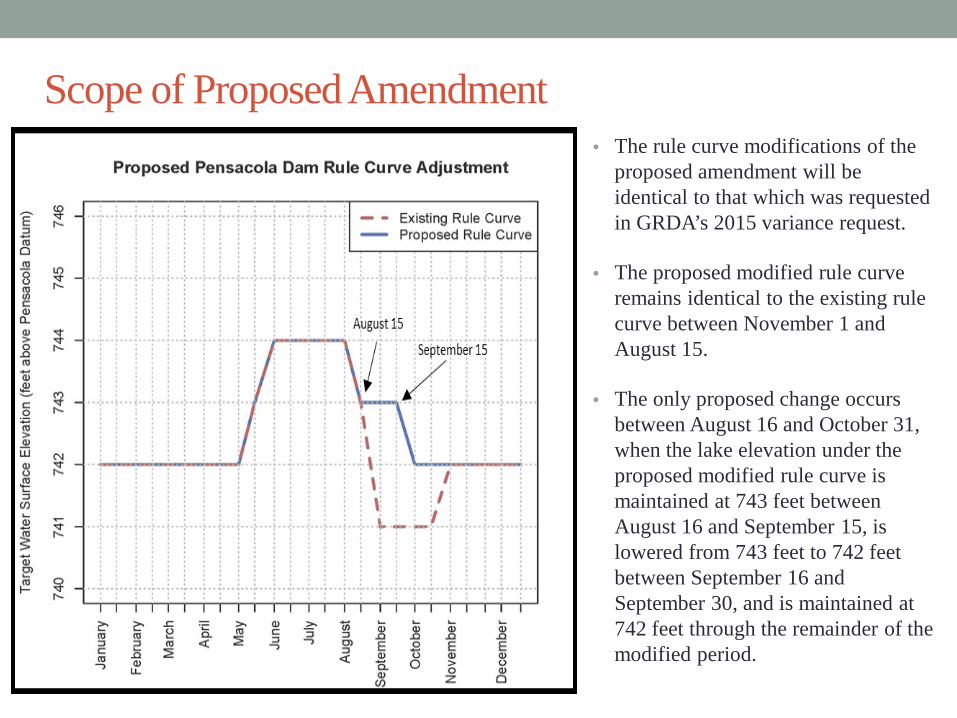
• The rule curve modifications of the proposed amendment will be identical to that which was requested in GRDA’s 2015 variance request.
• The proposed modified rule curve remains identical to the existing rule curve between November 1 and August 15.
• The only proposed change occurs between August 16 and October 31, when the lake elevation under the proposed modified rule curve is maintained at 743 feet between August 16 and September 15, is lowered from 743 feet to 742 feet between September 16 and September 30, and is maintained at 742 feet through the remainder of the modified period.
Scope of Proposed Amendment

• The proposed amendment would benefit the following public interests:
• Drought Management • Dissolved Oxygen • Recreation • Public Safety (Risk of Vessel Groundings)
Scope of Proposed Amendment

• GRDA will also be proposing:
• Storm Adaptive Management Process • GRDA seeks comment on its 2015 S-AMP with the possibility of
refinement for implementation over the balance of the license.
• Drought Adaptive Management Plan, including: • Flexibility to comply with downstream dissolved oxygen requirements. • Maintenance of reservoir elevations at the Markham Ferry Project
sufficient to operate the Salina Pumped Storage Project.
Scope of Proposed Amendment

• This license amendment application is not:
• A request to operate the project beyond an elevation not already allowed during the summer under the currently existing rule curve.
• An amendment or modification of the operations of the project under the provisions of the United States Army Corps of Engineers Water Control Manual or the Letter of Understanding and Water Control Agreement between the Corps of Engineers and GRDA.
Scope of Proposed Amendment

Arkansas River Basin
Information Needs – Arkansas River System Operations

U.S. Army Corps of Engineers Tulsa District
®
Greg Estep, P.E. Chief, Hydrology and Hydraulics Branch December 2015
US Army Corps of Engineers BUILDING STRONG®

BUILDING STRONG®
• 50 Projects 15 in the Red River Basin 35 in the Arkansas River Basin
• 12 Section-7 lakes (owned by others)
• 23 lakes with gated spillways • 8 COE Hydropower • 5 Navigation Locks • 1 Chloride Control Project
Tulsa District Water Management

BUILDING STRONG®
Kaw Hulah Copan
Oologah
Eufaula
Tenkiller
Wister
Ft. Gibson
Hudson
Grand Lake
Keystone
The Eleven Principle Reservoirs Average Travel Time
Van Buren Gage
2 hours
2 hours

BUILDING STRONG®
Arkansas River System Water Control Plan
The system water control plan attempts to balance the percent of storage contained in individual project flood pools.
Only projects above Van Buren, Arkansas are balanced.
All projects above Van Buren share the control point at Van Buren.
Flows at Van Buren are restricted to 150,000 cfs or less.
4

BUILDING STRONG®
The system water control plan focuses on eleven principle reservoirs.
o Kaw o Keystone o Hulah o Copan o Oologah o Eufaula
o Grand o Hudson o Ft. Gibson o Tenkiller o Wister
Upstream projects in subsystems are balanced with these eleven projects.
5
Arkansas River System Water Control Plan

BUILDING STRONG®
Operation Since March 2001 Using the Flexibility of the Current Water Control Plan. Release Conditions:
Forecasts indicate that Pensacola Lake will rise above elevation 745.0
The NWS forecasts the Neosho River at the Commerce, Oklahoma gage to rise above flood stage (15 feet).
Releases, not to exceed channel capacity, can be made from Pensacola Lake.
Releases may cause Grand Lake to be out of balance with the other two projects in the Lower Grand subsystem during the early portion of a flood event.
However, the subsystem will be balanced later in the flood event, if possible, after the Neosho River at Commerce gage drops below flood stage.

BUILDING STRONG®
Hulah263,332Copan186,857
Oologah1,007,060
Hudson244,210
Fort Gibson919,200
Eufaula1,510,793
Wister366,056Tenkiller
576,700
Kaw920,615
Keystone1,167,232
Pensacola525,000
Arkansas River System Flood Storage
11 Principle Reservoirs
Total Flood Storage = 7,687,055 ac-ft

BUILDING STRONG® Van Buren Guide Curve
0%
10%
20%
30%
40%
50%
60%
1-Jan 1-Feb 1-Mar 1-Apr 1-May 1-Jun 1-Jul 1-Aug 1-Sep 1-Oct 1-Nov 1-Dec
Month
Equi
vale
nt P
erce
nt o
f Bas
in S
tora
ge U
tiliz
ed
40,000 to 20,000 cfs
60,000 cfs
135,000 cfs (22 Feet Stage) to 150,000 cfs
150,000 cfs
60,000 to 40,000 cfs
Van Buren Regulating Flows

BUILDING STRONG®
Van Buren Guide Curve The yellow and white zones apply
mostly to a system flood operation. The blue, green, and red zones apply
mostly to the transition back to more normal operations after a flood event.
Van Buren Guide Curve
0%
10%
20%
30%
40%
50%
60%
1-Jan 1-Feb 1-Mar 1-Apr 1-May 1-Jun 1-Jul 1-Aug 1-Sep 1-Oct 1-Nov 1-Dec
Month
Equi
vale
nt P
erce
nt o
f Bas
in S
tora
ge U
tiliz
ed
40,000 to 20,000 cfs
60,000 cfs
135,000 cfs (22 Feet Stage) to 150,000 cfs
150,000 cfs
60,000 to 40,000 cfs

Information Needs – Scope of FERC Review • In evaluating the impacts and alternatives of a proposed action, FERC
uses existing environmental conditions, and not pre-project conditions, as the environmental baseline.
“[I]t is highly doubtful that attempts to ascertain the status of various resources prior to the time a 50-year-old project was constructed would result in the development of any useful information.” FERC is not required “to pretend that current projects do not exist, or to require applicants to gather information to recreate a 50-year-old environmental base upon which to make present day development decisions.”
--FERC Statutes and Regulations (Preambles) ¶ 30,854, at p. 31,401 (1989).
• For this amendment, FERC’s review will focus on whether GRDA’s proposal impacts upstream or downstream flooding, as compared to current, existing conditions.

Review Existing Information
• Dennis/OU Model • FERC Analysis • Tetra Tech Report • Anything Else?

Possible Information Gaps and Study Needs • More critical evaluation of adaptive management process
• More timely release? • Continued communications • What is trigger for mobilization and call? • Paragraph B, procedures, as a starting place?
• GRDA plan is to file in April
• Draft circulated to stakeholders, 30 days to comment • New info? New objections?
• Report of Technical Conference
• Detail Miami’s stance on reports, modeling, broader issue
• GRDA crafted language to Miami, 2nd week of January
• Relicensing workgroup with Miami, tribes, GRDA

Methods for Developing New Information

Timeline for Developing New Information

Remaining Agenda Items
• Other Issues • Review Action Items • Adjourn

Attachment D
City of Miami Technical Report

Hydraulic Analysis of the Effects of Pensacola Dam on
Neosho River Flooding In the Vicinity of Miami, Oklahoma
Bob Mussetter and Dai Thomas December 16, 2015

2
Study Objectives
Develop flood inundation boundaries for a range of historic floods • Assist the City in negotiating a more reasonable flood
easement
• Provide basis/tool for future evaluation of potential flood mitigation alternatives
Improve understanding and ability to quantify impacts of presence and operation of Pensacola Dam on flooding in Miami.

3
Methods/Approach
Update Neosho River bathymetry between Twin Bridges and Commerce (existing conditions)
Develop pre-dam bathymetry and overbank topography
Develop and calibrate with-dam (existing conditions)
Develop pre-dam hydraulic models
Apply models to range of historic floods
Compare results to quantify differences in flood water-surface elevations and inundation boundaries from pre-dam to with-dam conditions
Modeling with HEC-RAS 5.0 1D/2D

4
Modeled Floods
121,000 cfs at Commerce
Flood Peak
Discharge (cfs)
Days >Bankfull1
May 1995 35,900 4.1 June 1995 70,500 15.4 June-July 2007 141,000 9.8 April-May 2009 64,500 10.0 October 2009 46,300 4.3 May-June 2013 57,800 9.6

5
OTTAWA COUNTY, OKLAHOMA Al<O lHOORl'OAATIO AREAS
F looclin2 Source nn<I Loc:·:uion
NEOSHO RIVER
Enlire rt>xh within City of J\1lhmi
Approxirn~udy 50.000 fc~t above i1s 1.:onflucnc:~
with Spdng Rlvcr
QUAIL CREEK
Enrire re~~h wi1hi11 City of l\.liami
TAR CREE K
At itsconnui.:ntc with the Neosho Ri11er
Upstream of '.!'.!nd Avenue Northe.ast
l1p~11·e;un of p1ivntt> road
Bdow D Stl'l!t' I bridge
Dclow U.S. Rourc 69 bridge
Tahle 2: Summary of Discha~es (Cont•d)
Drainage Arca Peak Disd 1argcs (Cullie fc·cl per Sl-COnd)
( Sgunre miles)
6 .057
6.071
2.79
50.5
. ..n.23
'U.29
37.6$
J.i.:n
I 0-prrcenr
86.300
69,600
1.35 1
8,-t70
8,200
7.930
7.220
6,91 0
2-percenr
1-17.lXlO
139,lOO
2,161
12.200
11.860
11 560
10.6 10
10.190
I · J'let'Cenr 0.2-rierct>nt
177 .CX.IU 260.000
175.00U 279.500
'.!,576 .\547
l ·D OO 19,440
13.9:!0 18,950
1 :u~o 18500
12.-1~0 17.020
1 l.990 16,370
[-n;] TETRATECH

6
Bathymetric Survey (April 2015)
• Boat-mounted SonarMite transducer connected to Leica Viva RTK GPS

7
Bathymetric Survey (April 2015)
0
2,000
4,000
6,000
8,000
10,000
12,000
14,000
16,000
16-Apr-15 18-Apr-15 20-Apr-15 22-Apr-15 24-Apr-15 26-Apr-15 28-Apr-15 30-Apr-15
Disc
harg
e (c
fs)
Commerce - Discharge
Hydrographic Survey Period

8
Bathymetric Survey (April 2015)
• Survey control from USACE benchmarks
• Assistance/guidance from Survey Solutions (Bill Thomas, PLS)

9
Bathymetric Survey (April 2015)
• Transect-based survey pattern • 110 total transects Twin
Bridges to Commerce

10
Thalweg Profile from 2015 Bathymetric Survey
250000 270000
cD a:: a:: "'O C>
"'O c 0
"'O c RI
:l
290000 Station (ft)
Cl> C)
RI <!>
E RI
~
Cl> C) RI
<!> Cl> (.) ... Cl>
E E 0 (.)
SettJe Survey (1995,1998)
- Bed Elevation - With-Dam
- Interpolated Section
310000 330000 350000
["ft; I TETRA TECH

11
2015 and 1998 USACE Thalweg Profiles 790
780
770
760
e-750 -s::: ;: 740
"' > Q)
w 730
720
710
700
690
II) m
D 0)
"O
"O 0: c: >-m c c ::II
"i 0 0 t'-
.... Cl) G> m 0) 0)
0: IV IV (!) (!)
0: .E G> "O u Cl) IV G> "O ~ E c 0 E "O c 0 co 0
~
•
- Bed Eevation - With-Dam
- 1998 HEC-RAS Model
Settle 1995, 1998
160000 180000 200000 220000 240000 260000 280000 300000 320000 340000 360000
Station {ft) ~===---------~--------~----------...t......-.-J
["ft; I TETRA TECH

12
2015 and Dennis/FERC Model Thalweg Profiles 790
780
770
760
e-750 -c:: ~ 740 «I > Q,)
w 730
720
710
700
690 160000
m .... «> CD «>
en Ol Ol «> a:: m m O'> "O (.!) (.!)
"O a:: a:: c ,... .E «>
CD "O u c C> m Qj c ::I "O ~ E ~
0 c u 0 E "O
c 0 m u ~
- Bed Elevation -With-Dam
Settle Survey 1995, 1998
- Bed 8evation - Dennis/FERC Model
180000 200000 220000 240000 260000 280000 300000 320000 340000 360000
Station {ft)
["ft; I TETRA TECH

13
Typical Cross Sections
710
720
730
740
750
760
770
780
790
800
810
1300 1400 1500 1600 1700 1800 1900 2000
Elev
atio
n (ft
)
Station (ft)
XS 267690 (River Mile 137.8)
2015
Dennis/FERC
735
740
745
750
755
760
765
770
0 50 100 150 200 250 300 350 400 450 500
Elev
atio
n (ft
)
Station (ft)
XS 334773 (River Mile 150.2)

14
1940s Cross-Section GN-R-1 at Twin Bridges
("It;) TETRA TECH

15
1940s Cross-Section GN-R-15 Old Highway 125 Bridge
. . I ' ' I - I --I
I -I ~
- t t-I I I I r I I I I I -- T' I I I I I
-: f -+. -- - - +- + -L I t I I I I I I -
--- I L_ -- - - ---+ 1. I I -""" I I I ~ I I
•. - --,. I ~ 4 + I ' - - ---· -- --
- - - -- -~ - -- -- ·- --- - - -'-- T ' -- ~--.,.~ - -1- --= ·.. ~' 1.r== l - - - --~ ~ ........ "- - -- - - ----.,... _. __
- , -;;::::F-~ ~-1" :1 --'-
-lJ "T~
, --- -- .L t ~---- , .. ~ ': ;:I;, -~ ...... 1· -- -- - - --· ..... _ ---- I ', -... ,; ·-- .. ~ --
~ -"-
[_ - - - -=-· - ~ ~ 'L I -J :£ •. - -- - ,.;., ~ '
. .,, -./ -1-1-
-·--- - _,_ 1..:: 1- "' } I ., . ~ . L - ,_,_
1- ·- - _ ,_ 1-.II ~ I I 11 n,
~I- I- ' '- ~ l I-
_ ,__ .._ __ - - -... 1-1- '- ~ - -- 1-t-. ,. .
I i _.._ , __
.J. L~ . .. - - ·-, ___ ,_ - - '- - ..__
- . -I- I~ I 1- "· \ - --- .._ ._...,. ·-,,. '-'- -~
' - -·- ,_
t I- -._._ -..,,. ... ,_
~ '-1- - '- '- -:. -
i~
r --_L..,, ->-
_, .. ,..llf_
"11.~~llillhlll.P•QM
~ .,
'-h:
!
' --,.. '-..:~ f ,,, ,_
-·,'
:.:_ ~r - .. ! • - . - ~ I - -- • ·
;.-. . ':: I _: -..J. ' . '~
'L :-~+ -- -. ,_ . I -
I
--........ I= :-=-f;;: --- ,_
- ,_ -- --- --1- '-I-
,,_ 'u V ,.,:_
I ... 8~ -:-1--f.- -- __ ,_
I ~ - ' " · r .. .I~
.. ~ ..1 i --1- '-- ---- -:->- f-1= --~ I
- T - r I I - - '" . --= I "' --- ze> $.. - " - ---,- - -1-
l"'L::. ~ ~ - :: I ~
--1- . -c.. ,-, . ·~· 1.i =
04018:J
["ft; I TETRA TECH

16
1938 Topographic Mapping in the Vicinity of Miami
[ °11;) TETRA TECH 1938 5' Interval Contour Mapping 0 1 ,250
Feet
2,500
[-n;] TETRATECH

17
Pre-Dam and Existing Cross Sections near Twin Bridges (Sta 231,000, RM 130.8)
700
720
740
760
780
800
820
0 200 400 600 800 1000 1200 1400 1600 1800 2000
Ele
vatio
n (ft
, NG
VD
29)
Station (ft)
GNR-1
2015 Geometry
5-foot interval contour mapping

18
Pre-Dam and Existing Cross Sections Sta 273,155 (RM 139.0)
710
720
730
740
750
760
770
780
790
2500 2700 2900 3100 3300 3500 3700 3900
Ele
vatio
n (ft
)
Station (ft)
2015 Geometry (With-Dam)
Pre-Dam Geometry
5-foot Interval Contour Mapping
GNR-7

19
Pre-Dam and Existing Cross Sections Sta 198,960 (RM 125.2)
650
700
750
800
850
900
950
0 500 1000 1500 2000 2500 3000 3500 4000 4500
Ele
vatio
n (ft
)
Station (ft)
Pre-Dam Cross-Section
5-foot Interval Contour Mapping
2008 Bathymetry

20
1940 and 2015 Thalweg and Top-of-Bank Profiles
690
700
710
720
730
740
750
760
770
780
790
160000 180000 200000 220000 240000 260000 280000 300000 320000 340000 360000
Elev
atio
n (ft
)
Station (ft)
Bank Profile 2015-DS of HWY69
Bank Profile 2015 - u/s of HWY69
Bed Eevation - With-Dam
Bank Profile (GNR 1941)
1941 Profile
Linear (Bank Profile 2015 - u/s of HWY69)
Twin
Brid
ges
Mia
mi G
age
Com
mer
ce G
age
Cou
nty
Rd.
Br.
Aban
dond
ed R
R B
r.

21
Limits of the HEC-RAS Model
Type Downstream Limit
Upstream Limit
Reach Length
(mi) 1-D 0 275,605 52.2
2-D 275,605 294,420 3.6
1-D 294,420 301,645 1.4
2-D 301,645 407,300 20.0

22
Limits of the HEC-RAS Model
("ft:) TETRA TECH

23
2-D model grid in vicinity of Tar Creek
'<., Gwmdit 0dld - Otl2009_WD
f ile Edi~ Qptiors Yiew Jables Jools QIS T::iols .t:!.elp '....l:OL°b
Ec<~f" ~~~~~~-
("ft:) TETRA TECH

24
Bridges
Station River Mile Bridge Constructed Replaced 231,200 130.8 Highway 60 Bridge 1940 252,890 135.0 S 590 County Road (Connors) Bridge c1930 2009 290,300 142.1 Will Rodgers Bridge pre1995 294,500 142.9 Abandoned Railroad Bridge @ Tar Creek pre 1940 298,990 143.8 Highway 125 Bridge pre 1940 1966 299,660 143.9 Burlington Northern Railroad Bridge pre 1940 301,570 144.3 Highway 69 Bridge 1935 1997 351,900 153.4 Stepps Ford Bridge c1910 2015

25
Overbank Roughness 2015
Feet [ °'11:) TETRA TECH 2015 Aerial Photography
[-n;] TETRATECH

26
With-Dam Roughness Zones
Light Woody Vegetation
[ "11:;) TETRA TECH 2015 Aerial Photography 0 2,500
Feet
[-n;] TETRATECH

27
Overbank Roughness 1939
Feet ( "'J1;) T ETRA TEC H 1939 Aerial Photography
[-n;] TETRATECH

28
Pre-Dam Roughness Zones Type
- Channel
Water
- Urban
- Pasture
Light Woody Vegetation
["'A: I TETRA TECH Overebank Roughness 1939 0 1,250 2,500
Feet
[-n;] TETRATECH

29
Overbank Manning’s n-values (Arcement and Schneider, 1989)
Parameter Dense Vegetation
Light Vegetation Farmland Urban
Bare Sand-Gravel
Ponded Water
nb 0.04 0.04 0.04 0.03 0.04 0.04 Base value for the floodplains with bare surface
n1 0.01 0.01 0.01 0.02 0 0 Correction for the effect of surface irregularities
n2 0 0 0 0 0 0
Correction for shape and size of the floodplain cross section (assumed 0.0 for this analysis)
n3 0.02 0.02 0.01 0.01 0 0 Correction for obstructions
n4 0.08 0.03 0.02 0.01 0 0 Correction for floodplain vegetation
m 1 1 1 1 1 1 Multiplication factor for floodplain sinuosity (assumed equal to 1.0 for this analysis)
n 0.15 0.1 0.08 0.07 0.04 0.04 Composite overbank n-value n = (nb+n1+ n 2+ n 3+ n 4)*m

30
Overbank Roughness 2015
Feet ( °11:) TETRA TECH 2015 Aerial Photography
0 1 ,300
[-n;] TETRATECH

31
Overbank Roughness 1939
0 1,300 2,600 [ "11:::) TETRA TECH 1939 Aeria l Photography Feet
[-n;] TETRATECH

32
Overbank Roughness 2015
Feet [ °11:) TETRA TECH 2015 Aerial Photography
0
[-n;] TETRATECH

33
Overbank Roughness 1939
Feet [ "11;) TETRA TECH 1939 Aerial Photography
0
[-n;] TETRATECH

34
With-Dam Roughness Zones
Zoom in on Miami-TwinBridges

35
Change color scheme to match with-dam
Pre-Dam Roughness Zones

36
With-Dam Roughness Zones Type
- Channel
Water
Light Woody Vegetation
[-n;] TETRATECH

37
Change color scheme to match with-dam
Pre-Dam Roughness Zones

38
Stream Gages
"""'""
., ., .. . 11
..
Elk River near Tiff City; MO
-fr ...
["ft; I TETRA TECH

39
June-July 2007
0
20,000
40,000
60,000
80,000
100,000
120,000
140,000
160,000
745
750
755
760
765
770
775
780
28-Jun-07 30-Jun-07 2-Jul-07 4-Jul-07 6-Jul-07 8-Jul-07 10-Jul-07
Disc
harg
e (c
fs)
Wat
er-s
urfa
ce E
leva
tion
(feet
NG
VD29
)
WSE - Commerce Gage
WSE - Miami
WSE - Pensacola Dam
Discharge - Commerce
Elk River (MDF)
Spring River

40
Recorded Starting and Maximum Lake Levels
Flood Starting WSE (ft)
Maximum WSE (ft)
May 1995 747.5 751.9
June 1995 748.7 756.0
June-July 2007 746.8 755.6 April-May 2009 746.0 751.7 October 2009 742.1 750.7 May-June 2013 745.0 748.7

41
Main Channel Manning’s-n Values (With-Dam)
Description Station (ft
upstream from Pens. Dam)
May 1995
Oct 2009
May 2013
April-May 2009
Jun 1995
Flood 2007
(June-July)
Reservoir to approximately Twin Bridges 0 - 231,262 0.02 0.02 0.02 0.02 0.02 0.02
Twin Bridges to bend downstream of Tar Creek 231,262-282,500 0.027 0.027 0.027 0.027 0.027 0.037
Bend downstream of Tar Creek to Abandoned RR bridge
282,500-297,360 0.032 0.035 0.037 0.045 0.049 0.083
Abandoned RR bridge to HWY69 297,360-301,645 0.03 0.03 0.03 0.03 0.03 0.035
HWY69 to upstream end of model 301,645-387,500 0.043 0.043 0.043 0.043 0.043 0.043

42
May 1995 High-water Marks
["ft; I TETRA TECH

43
May 1995 Flood Peak Calibration Profile
690
700
710
720
730
740
750
760
770
780
790
200000 220000 240000 260000 280000 300000 320000 340000 360000 380000 400000
Elev
atio
n (ft
)
Station (ft)
WSE -With-Dam
Bed Eevation - With-Dam
HWM
Twin
Brid
ges
Mia
mi G
age
Com
mer
ce G
age
Coun
ty Rd
. Br.
Aban
dond
ed R
R. B
r.

44
May 1995 Predicted and Measured Stage Hydrographs
0
5,000
10,000
15,000
20,000
25,000
30,000
35,000
40,000
745
750
755
760
765
770
5-May-95 6-May-95 7-May-95 8-May-95 9-May-95 10-May-95 11-May-95 12-May-95 13-May-95 14-May-95 15-May-95
Dis
char
ge (c
fs)
Wat
er-s
urfa
ce E
leva
tion
(feet
NG
VD29
)
Commerce - Measured
Commerce - Predicted
Miami -Measured
Miami - Predicted
Commerce - Discharge

45
June 1995 High-water Marks
["ft; I TETRA TECH

46
June 1995 Peak Calibration Profile
690
700
710
720
730
740
750
760
770
780
790
200000 220000 240000 260000 280000 300000 320000 340000 360000 380000 400000
Elev
atio
n (ft
)
Station (ft)
WSE - With-Dam
Bed Eevation- With-Dam
HWM
Twin
Brid
ges
Mia
mi G
age
Com
mer
ce G
age
Cou
nty
Rd.
Br.
Aban
dond
ed R
R. B
r.
Twin
Brid
ges
Mia
mi G
age
Com
mer
ce G
age
Cou
nty
Rd.
Br.
Aban
dond
ed R
R. B
r.

47
June 1995 Predicted and Measured Stage Hydrographs
0
10,000
20,000
30,000
40,000
50,000
60,000
70,000
80,000
750
755
760
765
770
775
31-May-95 2-Jun-95 4-Jun-95 6-Jun-95 8-Jun-95 10-Jun-95 12-Jun-95 14-Jun-95 16-Jun-95 18-Jun-95
Disc
harg
e (c
fs)
Wat
er-s
urfa
ce E
leva
tion
(feet
NG
VD29
)
Commerce - Measured
Commerce - Predicted
Miami -Measured
Miami - Predicted
Commerce - Discharge

48
June-July 2007 High-water Marks
["ft; I TETRA TECH

49
June-July 2007 Peak Calibration Profile
690
700
710
720
730
740
750
760
770
780
790
200000 220000 240000 260000 280000 300000 320000 340000 360000 380000 400000
Elev
atio
n (ft
)
Station (ft)
WSE - With-Dam
Bed Eevation - With-Dam
HWM
Twin
Brid
ges
Mia
mi G
age
Com
mer
ce G
age
Cou
nty
Rd.
Br.
Twin
Brid
ges
Mia
mi G
age
Com
mer
ce G
ageC
ount
y R
d. B
r.
Aban
dond
ed R
R. B
r.

50
June-July 2007 Predicted and Measured Stage Hydrographs
0
20,000
40,000
60,000
80,000
100,000
120,000
140,000
160,000
745
750
755
760
765
770
775
780
28-Jun-07 30-Jun-07 2-Jul-07 4-Jul-07 6-Jul-07 8-Jul-07 10-Jul-07
Disc
harg
e (c
fs)
Wat
er-s
urfa
ce E
leva
tion
(feet
NG
VD29
)
Commerce - Measured
Miami - Measured
Miami - Predicted
Commerce - Predicted
Commerce - Discharge

51
May 2009 High-water Marks
["ft; I TETRA TECH

52
May 2009 Flood Peak Calibration Profile
690
700
710
720
730
740
750
760
770
780
790
200000 220000 240000 260000 280000 300000 320000 340000 360000 380000 400000
Elev
atio
n (ft
)
Station (ft)
WSE -With-Dam
Bed Eevation - With-Dam
HWM
Twin
Brid
ges
Mia
mi G
age
Com
mer
ce G
age
Cou
nty
Rd.
Br.
Aban
dond
ed R
R. B
r.
Twin
Brid
ges
Mia
mi G
age
Com
mer
ce G
age
Cou
nty
Rd.
Br.
Aban
dond
ed R
R. B
r.

53
October 2009 High-water Marks
["ft; I TETRA TECH

54
October 2009 Flood Peak Calibration Profile
690
700
710
720
730
740
750
760
770
780
790
200000 220000 240000 260000 280000 300000 320000 340000 360000 380000 400000
Elev
atio
n (ft
)
Station (ft)
WSE - With-Dam
Bed Eevation (With-Dam)
HWM
Twin
Brid
ges
Mia
mi G
age
Cou
nty
Rd.
Br.
Twin
Brid
ges
Com
mer
ce G
age
Cou
nty
Rd.
Br.
Aban
dond
ed R
R. B
r.

55
October 2009 Predicted and Measured Stage Hydrographs
0
5,000
10,000
15,000
20,000
25,000
30,000
35,000
40,000
45,000
50,000
740
745
750
755
760
765
770
775
7-Oct-09 8-Oct-09 9-Oct-09 10-Oct-09 11-Oct-09 12-Oct-09 13-Oct-09 14-Oct-09 15-Oct-09 16-Oct-09
Disc
harg
e (c
fs)
Wat
er-s
urfa
ce E
leva
tion
(feet
NGV
D29)
Commerce - Measured
Commerce - Predicted
Miami -Measured
Miami - Predicted
Commerce - Discharge

56
May-June 2013 High-water Marks
["ft; I TETRA TECH

57
May 2013 Flood Peak Calibration Profile
690
700
710
720
730
740
750
760
770
780
790
200000 220000 240000 260000 280000 300000 320000 340000 360000 380000 400000
Elev
atio
n (ft
)
Station (ft)
WSE - With-Dam
Bed Elevation - With-Dam
HWM
Twin
Brid
ges
Mia
mi G
age
Cou
nty
Rd.
Br.
Aban
dond
ed R
R. B
r.
Twin
Brid
ges
Mia
mi G
age
Com
mer
ce G
age
Cou
nty
Rd.
Br.
Aban
dond
ed R
R. B
r.
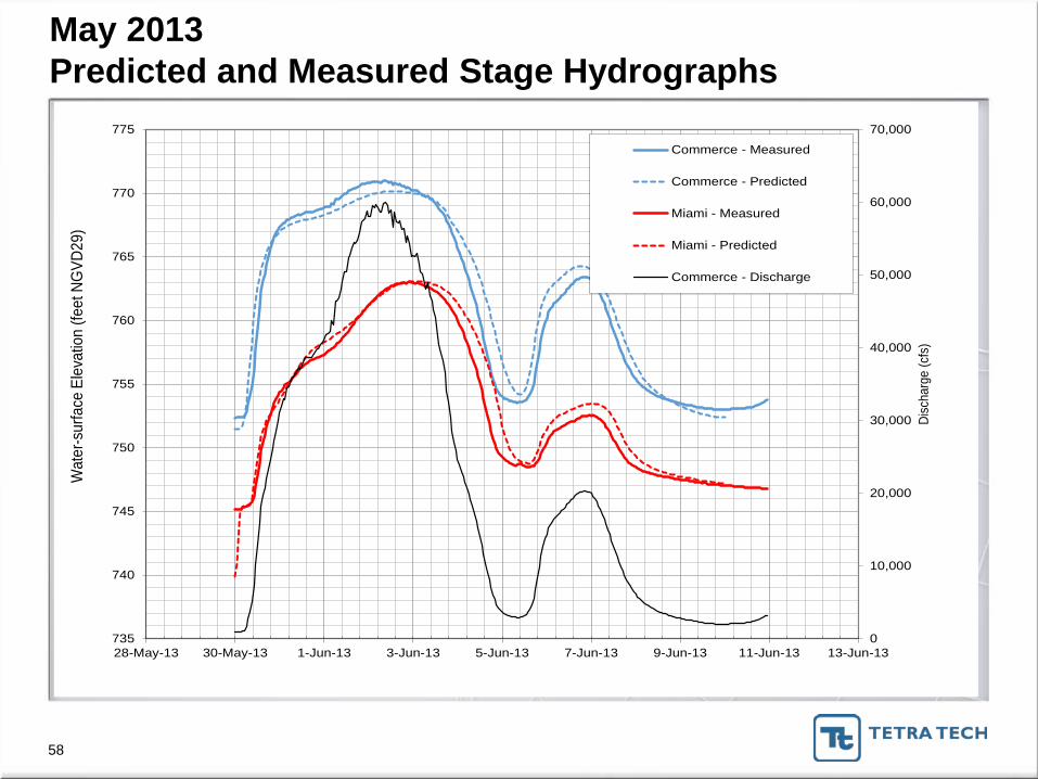
58
May 2013 Predicted and Measured Stage Hydrographs
0
10,000
20,000
30,000
40,000
50,000
60,000
70,000
735
740
745
750
755
760
765
770
775
28-May-13 30-May-13 1-Jun-13 3-Jun-13 5-Jun-13 7-Jun-13 9-Jun-13 11-Jun-13 13-Jun-13
Disc
harg
e (c
fs)
Wat
er-s
urfa
ce E
leva
tion
(feet
NG
VD29
)
Commerce - Measured
Commerce - Predicted
Miami - Measured
Miami - Predicted
Commerce - Discharge

59
May 1995 Maximum Water-Surface Profiles
-5
0
5
10
15
20
25
30
35
690
700
710
720
730
740
750
760
770
780
200000 220000 240000 260000 280000 300000 320000 340000 360000 380000 400000
Diff
eren
ce in
Pre
dict
ed w
ater
-sur
face
ele
vatio
n (ft
)
Elev
atio
n (ft
)
Station (ft)
WSE -With-Dam
WSE - Pre-Dam
Bed Eevation - With-Dam
Bed Elevation- Pre-Dam
HWM
Difference
Twin
Brid
ges
Mia
mi G
age
Com
mer
ce G
age
Cou
nty
Rd.
Br.
Aban
dond
ed R
R. B
r.

60
May 1995 With-dam and Pre-dam Stage Hydrographs
740
745
750
755
760
765
770
775
5-May-95 7-May-95 9-May-95 11-May-95 13-May-95
Wat
er-s
urfa
ce E
leva
tion
(feet
NG
VD29
)
Commerce - Pre-Dam
Commerce - With-Dam
Miami - Pre-Dam
Miami - With-Dam
Flood Easement Elevation (760 feet)

61
June 1995 Maximum Water-Surface Profiles
-5
0
5
10
15
20
25
30
690
700
710
720
730
740
750
760
770
780
790
200000 220000 240000 260000 280000 300000 320000 340000 360000 380000 400000
Diff
eren
ce in
Pre
dict
ed W
ater
-Sur
face
Ele
vatio
n (ft
)
Elev
atio
n (ft
)
Station (ft)
WSE - With-Dam
WSE - Pre-Dam
Bed Eevation- With-Dam
Bed Elevation - Pre-Dam
HWM
Difference
Twin
Brid
ges
Mia
mi G
age
Com
mer
ce G
age
Cou
nty
Rd.
Br.
Aban
dond
ed R
R. B
r.

62
745
750
755
760
765
770
775
31-May-95 3-Jun-95 6-Jun-95 9-Jun-95 12-Jun-95 15-Jun-95 18-Jun-95
Wat
er-s
urfa
ce E
levat
ion (f
eet N
GVD2
9)
Commerce - Pre-Dam
Commerce - With-Dam
Miami - Pre-Dam
Miami - With-Dam
Flood Easement Elevation (760 feet)
June 1995 With-dam and Pre-dam Stage Hydrographs

63
June-July 2007 Maximum Water-surface Profiles
-5
0
5
10
15
20
25
30
690
700
710
720
730
740
750
760
770
780
790
200000 220000 240000 260000 280000 300000 320000 340000 360000 380000 400000
Diff
eren
ce in
Pre
dict
ed W
ater
-sur
face
Ele
vatio
n (ft
)
Elev
atio
n (ft
)
Station (ft)
WSE - With-Dam
WSE - Pre-Dam
Bed Eevation - With-Dam
Bed Elevation - Pre-Dam
HWM
Difference
Twin
Brid
ges
Mia
mi G
age
Cou
nty
Rd.
Br.
Twin
Brid
ges
Com
mer
ce G
ageC
ount
y R
d. B
r.
Aban
dond
ed R
R. B
r.

64
June-July 2007 With-dam and Pre-dam Stage Hydrographs
740
745
750
755
760
765
770
775
780
28-Jun-07 30-Jun-07 2-Jul-07 4-Jul-07 6-Jul-07 8-Jul-07 10-Jul-07
Wat
er-s
urfa
ce E
levat
ion (f
eet N
GVD2
9)
Commerce - With Dam
Commerce - Pre-Dam
Miami - With-Dam
Miami - Pre-Dam
Flood Easement Elevation (760 feet)

65
Flood 2007 Pre-Dam Model (with-dam Channel n-values)
690
700
710
720
730
740
750
760
770
780
790
200000 220000 240000 260000 280000 300000 320000 340000 360000 380000 40000
Elev
atio
n (ft
)
Station (ft)
WSE - With-Dam
WSE - Pre-Dam
Bed Eevation - With-Dam
Bed Elevation - Pre-Dam
Guide Take Line
WSE - Pre-Dam (with Dam n-values)
GTL (with Dam n-values)
Twin
Brid
ges
Mia
mi G
age
Cou
nty
Rd.
Br.
Twin
Brid
ges
Com
mer
ce G
ageC
ount
y R
d. B
r.
Aban
dond
ed R
R. B
r.
1.8' difference

66
April-May 2009 Maximum Water-surface Profiles
-5
0
5
10
15
20
25
690
700
710
720
730
740
750
760
770
780
790
200000 220000 240000 260000 280000 300000 320000 340000 360000 380000 400000
Elev
atio
n (ft
)
Station (ft)
WSE - Pre-Dam
WSE - With-Dam
Bed Elevation - With-Dam
Bed Elevation - Pre-Dam
HWM
Difference
Twin
Brid
ges
Mia
mi G
age
Cou
nty
Rd.
Br.
Aban
dond
ed R
R. B
r.
Twin
Brid
ges
Mia
mi G
age
Com
mer
ce G
age
Cou
nty
Rd.
Br.
Aban
dond
ed R
R. B
r.

67
April-May 2009 With-dam and Pre-dam Stage Hydrographs
740
745
750
755
760
765
770
775
26-Apr-09 28-Apr-09 30-Apr-09 2-May-09 4-May-09 6-May-09
Wat
er-s
urfa
ce E
levat
ion (f
eet N
GVD2
9)
Commerce - With-Dam
Commerce - Pre-Dam
Miami - Pre-Dam
Miami - With-Dam
Flood Easement Elevation (760 feet)

68
October 2009 Maximum Water-surface Profiles
-5
0
5
10
15
20
25
690
700
710
720
730
740
750
760
770
780
790
200000 220000 240000 260000 280000 300000 320000 340000 360000 380000 400000
Diff
eren
ce in
Pre
dict
ed W
ater
-sur
face
Ele
vatio
n (ft
)
Elev
atio
n (ft
)
Station (ft)
WSE - With-Dam
WSE - Pre-Dam
Bed Eevation (With-Dam)
Bed Elevation (Pre-Dam)
HWM
Difference
Twin
Brid
ges
Mia
mi G
age
Cou
nty
Rd.
Br.
Twin
Brid
ges
Com
mer
ce G
age
Cou
nty
Rd.
Br.
Aban
dond
ed R
R. B
r.

69
October 2009 With-dam and Pre-dam Stage Hydrographs
735
740
745
750
755
760
765
770
775
7-Oct-09 8-Oct-09 9-Oct-09 10-Oct-09 11-Oct-09 12-Oct-09 13-Oct-09 14-Oct-09 15-Oct-09 16-Oct-09
Wat
er-s
urfa
ce E
levat
ion (f
eet N
GVD2
9)
Commerce - Pre-Dam
Commerce - With-Dam
Miami - Pre-Dam
Miami - With-Dam
Flood Easement Elevation (760 feet)

70
May 2013 Maximum Water-surface Profiles
-5
0
5
10
15
20
25
690
700
710
720
730
740
750
760
770
780
790
200000 220000 240000 260000 280000 300000 320000 340000 360000 380000 400000
Elev
atio
n (ft
)
Station (ft)
WSE - Pre-Dam
WSE - With-Dam
Bed Elevation - With-Dam
Bed Elevation - Pre-Dam
HWM
Difference
Twin
Brid
ges
Mia
mi G
age
Cou
nty
Rd.
Br.
Aban
dond
ed R
R. B
r.
Twin
Brid
ges
Mia
mi G
age
Com
mer
ce G
age
Cou
nty
Rd.
Br.
Aban
dond
ed R
R. B
r.

71
May 2013 With-dam and Pre-dam Stage Hydrographs
735
740
745
750
755
760
765
770
775
29-May-13 31-May-13 2-Jun-13 4-Jun-13 6-Jun-13 8-Jun-13 10-Jun-13
Wat
er-s
urfa
ce E
levat
ion (f
eet N
GVD2
9)
Commerce - Pre-Dam
Commerce - With-Dam
Miami - Pre-Dam
Miami - With-Dam
Flood EasementElevation (760 feet)

72
Maximum Predicted Water-surface Elevation Difference 760-foot NGVD29 Flood Easement
Flood Event Location Station (ft)
With-Dam Conditions Pre-Dam Conditions Predicted
Water-surface
Elevation (feet
NGVD29)
Height above flood easement (760 feet NGVD29)
Predicted Water-surface
Elevation (feet
NGVD29)
Height above flood easement (760 feet NGVD29)
May-95 Will Rodgers Bridge 290,300 757.3 -2.7 752.0 -8.0 Qpeak= Miami Gage 299,320 759.1 -0.9 754.2 -5.8
35,900cfs Commerce Gage 351,900 768.1 8.1 769.4 9.4
Jun-95 Will Rodgers Bridge 290,300 764.7 4.7 759.7 -0.3 Qpeak= Miami Gage 299,320 767.5 7.5 761.7 1.7
70,500cfs Commerce Gage 351,900 771.7 11.7 771.9 11.9
June-July 2007 Will Rodgers Bridge 290,300 772.7 12.7 767.1 7.1 Qpeak= Miami Gage 299,320 775.0 15.0 769.8 9.8
141,000cfs Commerce Gage 351,900 777.4 17.4 775.5 15.5
April-May 2009 Will Rodgers Bridge 290,300 762.6 2.6 758.5 -1.5 Qpeak= Miami Gage 299,320 764.9 4.9 760.5 0.5
64,500 cfs Commerce Gage 351,900 770.8 10.8 771.5 11.5
October 2009 Will Rodgers Bridge 290,300 759.5 -0.5 754.9 -5.1 Qpeak= Miami Gage 299,320 761.0 1.0 756.9 -3.1
46,300 cfs Commerce Gage 351,900 769.2 9.2 770.2 10.2
May-June 2013 Will Rodgers Bridge 290,300 760.9 0.9 757.5 -2.5 Qpeak= Miami Gage 299,320 763.0 3.0 759.6 -0.4
57,800cfs Commerce Gage 351,900 770.4 10.4 771.2 11.2

73
Peak Water-surface Elevations Duration above Elevation 760 feet at Miami Gage
Flood Qp (cfs)
With-Dam conditions Pre-Dam conditions
Recorded Peak.
WSE (ft)
Recorded Duration above
760 feet (days)
Predicted Duration above
760 feet (days)
Predicted Peak
WSE (ft)
Predicted Duration above
760 feet (days)
May 1995 35,900 758.9 0.0 0.0 754.2 0.0 June 1995 70,500 767.8 6.8 7.8 761.7 2.0 June-July
2007 141,000 775.1 7.2 9.5 769.8 4.5
April-May 2009 64,500 765.0 3.6 4.2 760.5 1.5
October 2009 46,300 761.1 1.8 2.0 756.9 0.0 May-June
2013 57,800 763.0 2.3 2.5 759.6 0.0

74
June-July 2007 With-Dam Inundation Area and 760-foot Contour Line
("11:] TETRA TECH Flood lnnudation Mapping Flood 2007
0 2 4
Miles
[-n;] TETRATECH

75
June-July 2007 Inundation Depth With-dam Conditions
(°11:) TETRA TECH With-Dam Depth Mapping
Flood 2007
0
Legend
Depth (ft)
c:::::J 0-1
c:::::::J 1-2
c::::=J 2-5
c::::=J 5- 1 0
- > 10
0.5 1
Miles
[-n;] TETRATECH

76
June-July 2007 Inundation Depth With-dam Conditions
("ft:] TETRA TECH Pre-Dam Depth Mapping
Flood 2007
0
Legend
Depth (ft) CJ 0-1 ~ 1-2
c=J 2 -5
L::::J 5-10
- >10
0.5 1
Miles
[-n;] TETRATECH

77
June-July 2007 Flood Flood Inundation: With-dam vs Pre-dam
Legend
C::::J 760' Contour
- Reaches
Pre-Dam
CJ
[ "'J1;) TETRA TECH Flood lnnudation Mapping Flood 2007
0 2 4
Miles
[-n;] TETRATECH

78
June-July 2007 Flood Inundation: With-dam vs Pre-dam
1~1 TETRA TECH Flood lnnudation Mapping Flood 2007
0
Legend
-- 760' Contour
Pre-Dam -
0.5 1
Miles
[-n;] TETRATECH

79
Subreaches for Inundated Area Calculations
Subreachc Station Lower Reach - from Twin Bridges to Will Rodgers (I-44) 231,200 – 290,300 Miami Reach - Will Rodgers to HWY 69 Bridge 290,300 - 301,570 Commerce Reach 0 HWY 69 to Commerce gage 301,570 - 351,900 Upper Reach - Commerce gage to u/s end of model. 351,900 - 387,500

80
Inundation Area (acres) With-dam Conditions
Ground Surface Subreach
Lower Miami Commerce Upper Total Area <= 760 feet 2,646 1,493 3,291 226 7,655
May 1995 (Flood 11) Total Wetted Area 1,836 1,242 7,915 2,784 13,777
Area Outside 760-foot Contour 0 0 4,624 2,558 6,122
June 1995 (Flood 13) Total Wetted Area 2,508 2,209 11,511 5,556 21,783
Area Outside 760-foot Contour 0 716 8,220 5,330 14,128
Flood 2007 Total Wetted Area 3,075 3,690 13,556 6,178 26,499
Area Outside 760-foot Contour 430 2,198 10,265 5,952 18,844
April-May 2009 Total Wetted Area 2,037 2,009 10,972 5,461 20,478
Area Outside 760-foot Contour 0 516 7,681 5,235 12,823
October 2009 Total Wetted Area 2,004 1,706 9,370 4,638 17,718
Area Outside 760-foot Contour 0 213 6,079 4,413 10,063
May 2013 Total Wetted Area 1,978 1,853 10,556 5,393 19,780
Area Outside 760-foot Contour 0 361 7,265 5,167 12,125

81
June-July 2007 Flood Inundation: With-dam and Pre-dam
Area innudated within City Limits (at)
Pre-Dam With-Dam
203 337 457 750
937 1,390
556 717 526 610
547 663
[-n;] TETRATECH

82
Guide Take Line Based on the June-July 2007 Flood
-5
0
5
10
15
20
25
30
690
700
710
720
730
740
750
760
770
780
790
200000 220000 240000 260000 280000 300000 320000 340000 360000 380000 400000
Diff
eren
ce in
Pre
dict
ed W
ater
-sur
face
Ele
vatio
n (ft
)
Elev
atio
n (ft
)
Station (ft)
WSE - With-Dam
WSE - Pre-Dam
Bed Eevation - With-Dam
Bed Elevation - Pre-Dam
HWM
Guide Take Line
Difference
Twin
Brid
ges
Mia
mi G
age
Cou
nty
Rd.
Br.
Twin
Brid
ges
Com
mer
ce G
ageC
ount
y R
d. B
r.
Aban
dond
ed R
R. B
r.
778.3 ft NGVD29

83
Flood 2007 Pre-Dam Model (with-dam Channel n-values)
690
700
710
720
730
740
750
760
770
780
790
200000 220000 240000 260000 280000 300000 320000 340000 360000 380000 40000
Elev
atio
n (ft
)
Station (ft)
WSE - With-Dam
WSE - Pre-Dam
Bed Eevation - With-Dam
Bed Elevation - Pre-Dam
Guide Take Line
WSE - Pre-Dam (with Dam n-values)
GTL (with Dam n-values)
Twin
Brid
ges
Mia
mi G
age
Cou
nty
Rd.
Br.
Twin
Brid
ges
Com
mer
ce G
ageC
ount
y R
d. B
r.
Aban
dond
ed R
R. B
r.
1.8' difference
776.9 ft NGVD29

Hydraulic Analysis of the Effects of Pensacola Dam on
Neosho River Flooding In the Vicinity of Miami, Oklahoma
Bob Mussetter and Dai Thomas December 16, 2015

85
May 2013 Truncated Model
-4.0
-3.5
-3.0
-2.5
-2.0
-1.5
-1.0
-0.5
0.0
710
720
730
740
750
760
770
780
790
200000 220000 240000 260000 280000 300000 320000 340000 360000 380000 400000
Diff
eren
ce in
Pre
dict
ed W
ater
-sur
face
Ele
vatio
n (ft
)
Ele
vatio
n (ft
)
Station (ft)
WSE - With-Dam
Bed Elevation - With-Dam
WSE - truncated model
Difference
Twin
Brid
ges
Cou
nty
Rd.
Br.
Aban
dond
ed R
R. B
r.
Twin
Brid
ges
Mia
mi G
age
Com
mer
ce G
age
Cou
nty
Rd.
Br.
3.2'
0.5'

86
October 2009 Flood. Boundary limited to 743PD
690
700
710
720
730
740
750
760
770
780
790
200000 220000 240000 260000 280000 300000 320000 340000 360000 380000 400000
Ele
vatio
n (ft
)
Station (ft)
WSE - With-Dam
Bed Eevation (With-Dam)
WSE - With-Dam (743PD)
Twin
Brid
ges
Mia
mi G
age
Cou
nty
Rd.
Br.
Twin
Brid
ges
Com
mer
ce G
age
Cou
nty
Rd.
Br.
Aban
dond
ed R
R. B
r.
0.5''

87
May 2013 Pre-Dam Model (with-dam Channel n-values)
690
700
710
720
730
740
750
760
770
780
790
200000 220000 240000 260000 280000 300000 320000 340000 360000 380000 400000
Ele
vatio
n (ft
)
Station (ft)
WSE - Pre-Dam
WSE - With-Dam
WSE - Pre-Dam (with Dam n-values)
Bed Elevation - With-Dam
Bed Elevation - Pre-Dam
Twin
Brid
ges
Mia
mi G
age
Cou
nty
Rd.
Br.
Aban
dond
ed R
R. B
r.
Twin
Brid
ges
Mia
mi G
age
Com
mer
ce G
age
Cou
nty
Rd.
Br.
Aban
dond
ed R
R. B
r.

88
Normal Flood Control Regulation Schedule Pensacola Reservoir (modified from Table 7-1, Pensacola Reservoir Water Control Manual).1
Lake Stage Pool Conditions Regulations
Below 745.0 Rising
Hydropower released will be made by G.R.D.A to meets its power requirements. If the pool is forecasted to exceed elevation 745, the Corps may direct that flood control releases be made, provided that there is a sufficient volume of water indicated by stages at the upstream gages to fill the power pool.
745.0 - 755.0 & forecasted not to
exceed 755.0 Rising
Release will not exceed 100,000 cfs below the dam and will be made in such a manner as to balance, as much as practical and within a reasonable time, the percentage of the flood control storage utilized in Pensacola Reservoir, Markham Ferry Reservoir, and Fort Gibson Lake.
745.0 - 755.0 & forecasted to exceed 755.0
Rising Releases will be made to reduce as much as practical the flood damage below the dam and to limit the pool elevation to 755.0. Plate 7-1, Spillway Gate Regulations Schedule Inflow Parameter, may be used as a guide to determine releases.
755.0 or above Rising Spillway gates will be opened to maintain the pool at elevation 755.0 or until all the gates are fully open.
755.0 or above Falling The maximum discharge attained shall be held until the pool recedes to elevation 755.0.
745.0-755.0 Falling
Releases will not exceed 100,000 cfs and will be made in such a manner as to balance the percent of the flood control storage utilized in the 3-reservoir system. Evacuation of the flood control storage ion this system will be governed by the provisions of the Chapter 7 of the Arkansas River Basin Master Manual.
1All elevations in this table are referenced to the Pensacola Datum.

89
Summary of High-water Marks and Modeled Maximum Water-surface Elevations for the May and June 1995 Floods
Flood Obs. Model Station
(ft)
Reported HWM Elev.
(ft)
Model Peak WSEL (ft)
Model Under (-) or
Over (+) Prediction
Remarks
May-95 Commerce Gage 351,850 768.7 768.1 -0.6
May-95 9 301,415 760.6 762.3 1.7 High-water mark seems unusually low1
May-95 10 301,267 759.4 759.1 -0.3 May-95 11 298,684 758.7 758.8 0.1
May-95 Miami Gage 298,928 758.9 759.1 0.2
May-95 12 280,165 755.9 755.8 -0.1 May-95 13 253,013 753.4 753.8 0.4 May-95 14 230,916 752.83 752.9 0.1
Jun-95 Commerce Gage 351,850 772.2 771.7 -0.5
Jun-95 16 318,333 770 769.3 -0.7 Jun-95 17 298,684 767.6 767.6 0.0
Jun-95 Miami Gage 298,928 767.7 767.6 -0.1
Jun-95 18 280,165 763.8 762.4 -1.4 High-water mark seems unusually high1
Jun-95 19 253,013 760.5 759.5 -1.0 High-water mark seems unusually high1
1Adapter from Holly (2001)

90
Summary of High-water Marks and Modeled Maximum Water-surface Elevations for 2007 Flood
Obs. Easting (ft)
Northing (ft)
Reported HWM
Elev. (ft)
Approx. Model Peak WSEL
(ft)
Model under (-) or over
(+) prediction
(ft)
Remark
2 2,859,731 718,764 778.4 777.5 -0.9 40 2,893,266 696,272 771.3 771.5 0.2 42 2,892,354 695,892 771.3 771.5 0.2 44 2,884,670 691,741 773.3 773.6 0.3 Shown on profile 45 2,884,193 694,691 773.3 774.5 1.2 46 2,884,816 696,110 773.3 773.5 0.2 47 2,884,815 696,151 773.2 773.5 0.3 49 2,885,115 696,497 773.2 773.5 0.3 50 2,885,359 697,250 773.2 773.5 0.3 51 2,885,498 697,337 773.2 773.5 0.3 52 2,885,425 699,732 773.2 773.5 0.3 54 2,887,155 699,460 773.2 773.5 0.3 56 2,872,654 691,248 777.2 776.2 -1.0 60 2,880,243 692,291 775.2 775.0 -0.2 Shown on profile 62 2,881,748 694,205 775.5 775.2 -0.3 Shown on profile 63 2,882,417 693,655 775.3 775.0 -0.3 Shown on profile 64 2,881,761 694,628 775.6 775.3 -0.3 Shown on profile 66 2,876,683 699,997 776.8 776.1 -0.7 Shown on profile 72 2,876,475 700,084 776.8 776.1 -0.7 Shown on profile 73 2,879,010 697,008 776.3 775.7 -0.6 Shown on profile 74 2,879,063 697,089 776.3 775.7 -0.6 Shown on profile 76 2,897,530 687,294 769.1 769.1 0.0 77 2,897,368 687,591 769.2 769.2 0.0 Shown on profile 80 2,893,488 693,006 771.3 771.5 0.2
Miami 2,881,386 693,292 775 775.0 0.0 Shown on profile Commerce 2,857,838 716,040 778.22 777.4 -0.8 Shown on profile

91
Summary of High-water Marks and Modeled Maximum Water-surface Elevations for the May 2009 Flood
Obs. Easting (ft)
Northing (ft)
Reported
HWM Elev. (ft)
Approx. Model Peak WSEL
(ft)
Model under (-) or over
(+) prediction
(ft)
Remark
300 2,872,193 708,429 768 767.5 -0.5 301 2,876,232 703,143 768 767.3 -0.7 302 2,875,516 700,748 767.54 767.0 -0.5 Shown on profile 303 2,877,834 698,440 766.56 766.2 -0.3 Shown on profile 304 2,878,757 697,347 766.43 765.9 -0.5 Shown on profile 305 2,880,327 691,396 764.8 764.9 0.1 306 2,872,119 691,146 768.23 767.3 -0.9 307 2,880,057 695,665 765.78 765.5 -0.3 308 2,880,302 695,536 765.69 765.3 -0.4 Shown on profile 309 2,880,795 694,837 765.2 765.2 0.0 Shown on profile 310 2,881,300 694,814 765.24 765.1 -0.1 Shown on profile 311 2,881,601 694,015 764.85 765.1 0.3 Shown on profile 313 2,881,837 693,581 764.77 764.9 0.2 Shown on profile 314 2,883,485 692,669 764.69 764.7 0.0 316 2,885,567 697,200 762.72 762.9 0.2 317 2,885,625 699,126 762.8 762.9 0.1 318 2,886,059 699,972 763.03 762.9 -0.1 319 2,886,865 699,490 762.99 762.9 -0.1 320 2,886,767 696,044 762.7 762.9 0.2 321 2,886,906 695,845 762.76 762.9 0.1 322 2,886,933 694,636 762.78 762.9 0.1 Shown on profile 323 2,893,353 690,945 761.4 761.0 -0.4 Shown on profile 324 2,892,694 694,102 761.39 761.4 0.0 325 2,892,223 695,277 761.35 761.4 0.0 336 2,886,037 700,033 763.27 763.1 -0.2
Miami 2,881,386 693,292 765 764.9 -0.1 Shown on profile
Commerce 2,857,838 716,040 771.18 770.8 -0.4 Shown on profile

92
Comparison of Measured High-water Marks for the October 2009 Flood
Obs. Easting (ft) Northing (ft) Reported
HWM Elev. (ft)
Approx. Model Peak
WSEL (ft)
Model under (-) or over (+) prediction (ft)
Remark
501 716,103 2,858,584 770.1 769.2 -0.9 Shown on profile 502 707,807 2,870,802 764.3 764.5 0.1 503 707,253 2,872,506 764.1 764.3 0.2 504 700,697 2,875,491 763.5 763.5 0.0 Shown on profile 507 695,687 2,880,021 761.7 761.6 -0.1 Shown on profile 508 695,496 2,880,143 761.5 761.4 -0.1 Shown on profile 509 694,769 2,880,771 761.2 761.3 0.1 Shown on profile 510 694,785 2,881,091 761.3 761.3 0.0 Shown on profile 512 692,706 2,882,803 760.7 760.9 0.2 Shown on profile 513 692,598 2,883,384 760.6 760.8 0.1 Shown on profile 514 692,082 2,885,134 759.0 759.7 0.7 515 691,090 2,869,751 764.2 764.0 -0.2 516 692,217 2,880,462 760.9 761.1 0.1 518 694,057 2,881,168 761.0 761.3 0.2 519 693,581 2,881,591 761.0 761.1 0.1 Shown on profile 520 693,537 2,881,810 760.8 761.0 0.3 Shown on profile 521 691,269 2,884,484 760.0 760.3 0.2 Shown on profile 522 691,253 2,884,537 759.8 760.3 0.4 Shown on profile 523 695,862 2,886,878 758.8 758.5 -0.4 524 696,056 2,886,734 759.0 759.7 0.7 525 694,307 2,886,904 758.9 759.7 0.8 526 687,229 2,897,633 756.5 757.6 1.2 Shown on profile 533 688,690 2,896,337 756.7 758.0 1.3 Shown on profile 527 670,685 2,899,569 754.7 755.1 0.4 Shown on profile 528 670,505 2,899,668 754.5 755.1 0.6 Shown on profile 529 670,703 2,918,410 752.6 753.9 1.3 Shown on profile 530 670,880 2,918,255 752.7 753.9 1.3 Shown on profile 531 690,636 2,888,911 758.2 759.3 1.0 Shown on profile 532 690,684 2,888,688 758.3 759.6 1.3 Shown on profile
Miami 2,881,386 693,292 761.1 761.0 0.0 Shown on profile
Commerce 2,857,838 716,040 769.5 769.2 -0.3 Shown on profile

93
Comparison of Measured High-water Marks for the May 2013 Flood
Obs. Easting (ft) Northing (ft)
Reported HWM Elev.
(ft)
Approx. Model Peak
WSEL (ft)
Model under (-) or over
(+) prediction
(ft)
Remark
901 2,858,647 716,110 771.5 770.4 -1.1 903 2,870,785 708,601 766.4 766.5 0.1 906 2,872,474 707,516 766.1 766.2 0.1 910 2,876,136 705,131 766.1 766.0 -0.1 911 2,876,146 704,905 765.9 766.0 0.1 912 2,876,150 704,880 765.8 766.0 0.2
913 2,875,522 700,678 765.7 765.5 -0.1 Shown on profile
914 2,877,345 698,584 764.8 764.9 0.1 Shown on profile
915 2,876,579 694,208 764.6 764.0 -0.6 916 2,871,879 691,140 766.3 766.0 -0.4
917 2,880,321 692,037 762.8 763.0 0.2 Shown on profile
919 2,881,950 693,429 762.7 763.0 0.3 Shown on profile
921 2,882,414 693,007 762.7 763.0 0.2 Shown on profile
922 2,887,167 695,905 760.6 761.4 0.7 923 2,892,202 695,165 759.5 760.2 0.7
924 2,893,920 690,941 759.1 759.6 0.5 Shown on profile
926 2,885,688 697,201 760.5 761.4 0.8 927 2,885,605 697,308 760.6 761.4 0.8 928 2,885,905 699,899 760.6 763.0 2.4 929 2,886,838 698,966 760.6 761.4 0.8
Miami 2,881,386 693,292 763.0 763.0 0.0 Shown on profile
Commerce 2,857,838 716,040 771.0 770.4 -0.6 Shown on profile

94
Proposed Temporary Variance from the Article 401 Reservoir Elevation Rule Curve Requirements for the Pensacola Project
(copied from FERC, 2015)
~· r-
~ .--..
~ r-.
..... ~
* r-
I::" ftJ
~ ~
Proposed PensacoJa Dam Rule Curve Adjustment
~
i;' £ :;::, ?:..... ru ~ m c · IL.:.:. ~ '.:::52 ii "° ~ -, ~
if
~ ._
$ CJ~
~ :::JI < a
~
EMl~ing Rule Curit~ Pm !'-O!!i:~e:I R Lil~ Cu l'V~
._ ,_ ._
~ ~ ~ ~ ; ~ ~ z c
[-n;] TETRATECH

95
Stationing of Key Features Along the Project Reach
Station (ft) Feature
0 Pensacola Dam 124,305 Sailboat Bridge 143,000 Elk River 228,360 Railroad Bridge 199,000 Downstream limit of pre-dam model 229,560 Spring River 231,200 Highway 60 Bridge 252,890 S 590 County Road (Connors) Bridge 290,300 Will Rodgers Bridge 291,200 Tar Creek Confluence 294,500 Abandoned Railroad Bridge 297,950 Low-water dam 298,990 Highway 125 Bridge 299,320 Miami Gage 299,660 Burlington Northern Railroad Bridge 301,570 Highway 69 Bridge 351,900 Commerce Gage 387,500 Upstream end of model

96
USACE Survey Control Points
Point ID Easting (ft) Northing (ft) USACE Elevation (ft, NGVD 29)
OPUS Elevation (ft, NGVD29)
Fairview School 2865246.01 716373.34 805.97 805.74 MON 27 Dotyville 2872685.49 691133.84 773.48 773.11 MON 28 Airport S 2878795.03 706341.42 797.90 797.72 MON 32 Gravel Pt 2908604.89 675506.51 849.25 848.95

97
Temporary Survey Control Set by Tetra Tech
Point ID Easting (ft) Northing (ft) Elevation (ft, NGVD29)
R1 1037 2858087.56 715865.56 785.71 R1 1037 2858087.57 715865.60 785.77 R1 1042 2860285.99 705585.16 763.86 R1 1048 2876604.12 699452.49 775.65 R1 1052 2871094.15 700739.61 757.83 R1 1062 2880765.07 693071.12 770.09 R1 1071 2887806.04 688064.72 795.23 R1 1181 2918129.61 671344.39 829.64 R1 1199 2899522.93 672538.37 765.56 R1 1213 2888344.71 686359.32 813.67

98
Grand Lake Storage-Elevation Curves
710
715
720
725
730
735
740
745
750
755
760
0.6 0.8 1 1.2 1.4 1.6 1.8 2 2.2 2.4
Pens
acol
a Da
m W
ater
Surfa
ce (f
eet,
NGVD
29)
Grand Lake Storage (ac-ft) Millions
1992 Water Control Manual
OWRB (2009)
USACE >Jan 28, 2012
Extrapolated from USACE Data

99
Comparison of the 1940 Channel Profile Used in the Pre-dam HEC-RAS Model, the 2015 Channel Profile and the 1940 and 2015 Top of Bank Profiles
690
700
710
720
730
740
750
760
770
780
790
160000 180000 200000 220000 240000 260000 280000 300000 320000 340000 360000
Elev
atio
n (ft
)
Station (ft)
2015 Top of Bank
Bed Eevation - With-Dam
2015 Top of Bank
1941 Top of Bank
5-foot Contour Eleavtions
1941 Bed Profile
Linear (2015 Top of Bank)
Twin
Brid
ges
Mia
mi G
age
Com
mer
ce G
age
Cou
nty
Rd.
Br.
Aban
dond
ed R
R B
r.

100
Named Flood Events and Associated Peak Discharge
Flood Date Peak Flow at Commerce Gage (cfs)1
1986 9 September - 11 October, 1986 101,000 1 18-19 November, 1992 33700 2 9-21 December, 1992 45,600 3 18-30 March, 1993 14,700 4 6-23 April, 1993 19,500 5 8-26 May, 1993 40,000 6 29 June – 14 July, 1993 21,700 7 21 September - 5 October, 1993 81,700 8 7-20 April, 1994 106,000 9 26 April - 11 May, 1994 43,800
10 17-28 November, 1994 34,3700 11 5-16 May, 1995 35,900 12 17 May - 2 June, 1995 33,700 13 7-20 June, 1995 70,500 14 23 June - 7 July, 1995 22,200
2007 28 June - 8 July, 2007 141,000 2009-1 27 April - 5 May, 2009 64,500 2009-2 7-14 October, 2009 46,300 2013 30 May – 5 June, 2013 57,800 2015 23 May – 4 June, 2015 46,100
1All values are published USGS peak hourly flows, except for the 1986, which are the mean daily values.

101
May 1995
745
750
755
760
765
770
0
5,000
10,000
15,000
20,000
25,000
30,000
35,000
40,000
45,000
50,000
5/6/1995 5/7/1995 5/8/1995 5/9/1995 5/10/1995 5/11/1995 5/12/1995 5/13/1995 5/14/1995 5/15/1995 5/16/1995
Pool
Ele
vatio
n (ft
, NG
VD29
)
Dis
char
ge (c
fs)
Elk River - DischargeSpring River - DischargeCommerce Gage - DischargePensacola Dam - WSECommerce Gage - WSEMiami Gage - WSE

102
April-May 2009
740
745
750
755
760
765
770
775
780
0
10,000
20,000
30,000
40,000
50,000
60,000
70,000
4/27/2009 4/29/2009 5/1/2009 5/3/2009 5/5/2009 5/7/2009
Pool
Ele
vatio
n (ft
, NG
VD29
)
Disc
harg
e (c
fs)
Spring River - Discharge
Elk River - Discharge
Commerce Gage - Discharge
Pensacola Dam - WSE
Commerce - WSE
Miami Gage - WSE

103
October 2009
740
745
750
755
760
765
770
775
780
0
10,000
20,000
30,000
40,000
50,000
60,000
70,000
10/8/2009 10/9/2009 10/10/2009 10/11/2009 10/12/2009 10/13/2009 10/14/2009 10/15/2009
Pool
Ele
vatio
n (ft
, NG
VD29
)
Disc
harg
e (c
fs)
Spring River - Discharge
Elk River - Discharge
Commerce Gage - Discharge
Pensacola Dam - WSE
Commerce - WSE
Miami Gage - WSE

104
June-July 2007
0
20,000
40,000
60,000
80,000
100,000
120,000
140,000
160,000
746
748
750
752
754
756
758
28-Jun-07 30-Jun-07 2-Jul-07 4-Jul-07 6-Jul-07 8-Jul-07 10-Jul-07
Dis
char
ge (c
fs)
Wat
er-s
urfa
ce E
leva
tion
(feet
NG
VD
29)
WSE - Pensacola Dam
WSE - Twin Bridges
Discharge - Commerce

105
June-July 2007
7/1/
2007 7/2/
2007
7/3/
2007
7/4/
2007
7/5/
2007
7/6/
2007
7/7/
2007
7/8/
2007
7/9/
2007
0
5
10
15
20
25
30
35
0 25,000 50,000 75,000 100,000 125,000 150,000
Gag
e H
eigh
t (ft)
Discharge (cfs)
USGS Reported Hourly Q
Reported Discharge at noon on indicated day
USGS Gage Measurements
USGS Rating #12

106
With-Dam Roughness Zones
Light Woody Vegetation
[ °11:; l TETRA TECH 2015 Aerial Photography 0 1,250 2,500
Feet
[-n;] TETRATECH

107
June 1995
745
750
755
760
765
770
775
780
0
10,000
20,000
30,000
40,000
50,000
60,000
70,000
80,000
90,000
6/1/1995 6/3/1995 6/5/1995 6/7/1995 6/9/1995 6/11/1995 6/13/1995 6/15/1995 6/17/1995 6/19/1995 6/21/1995
Poo
l Ele
vatio
n (ft
, NG
VD
29)
Dis
char
ge (c
fs)
Spring River - Discharge
Elk River - Discharge
Commerce Gage - Discharge
Pensacola Dam - WSE
Commerce Gage - WSE
Miami Gage - WSE

108
June 2013
740
745
750
755
760
765
770
775
780
0
10,000
20,000
30,000
40,000
50,000
60,000
70,000
5/28/2013 5/30/2013 6/1/2013 6/3/2013 6/5/2013 6/7/2013 6/9/2013 6/11/2013 6/13/2013
Pool
Ele
vatio
n (ft
, NG
VD29
)
Disc
harg
e (c
fs)
Spring River - Discharge
Elk River - Discharge
Commerce Gage - Discharge
Pensacola Dam - WSE
Commerce Gage - WSE
Miami Gage - WSE

Articles on Benefits of Implementing
2015 Temporary Variance


August 20, 2015 Grandlakenewsonline.com Page 3
... continued on page 14
Has 23 Years of Falling Lake Level Frustration Ended?
How many times over the past 23 years, in August, have I occupied my perch overlooking Grays Hollow and muttered, mostly to myself, “I can’t believe we are taking the lake down to an elevation of 741’ again prior to the Labor Day holiday.” Cor-rection…make that 22 years because last Friday the filed GRDA requested variance to forgo the lowering of lake in 2015 was granted. The result will be an elevation maintained at 743’ until mid-September when it will be lowered another foot to 742’ for the winter and early spring months.
Has common sense finally prevailed after all these years? We certainly hope so and while the variance is just that for one year, it is the first step in correcting something which originally was to be a five year trial to test the results of seeding millet in the exposed mud flats to benefit the ducks and geese. It never was about flooding, but in the end flooding was a dominant factor in proving our case, as the original intent had been long forgotten.
The next step will be a filed amendment to the current oper-ating license, which runs through 2022, to incorporate the newly
approved variance into that license. There’s still work to be done, but this is a huge step in the right direction.
In the end, even though countless studies, including one pro-vided earlier by a graduate student from the University of Okla-homa’s Civil Engineering Department, supported the GRDA position, the feds still had to work the supporting engineering model used before approving the variance. But regardless of the circumstances and the hoops jumped through, it was a breath of fresh air for Grand Lake and now it’s time to move forward.
In a classic case of the historic quote, attributed to historic UCLA basketball coach John Wooden which proclaims, “There is no limit to what we can achieve if we don’t care who gets the credit,” Grand Lake finally came to together as one force on this issue. Without mentioning all involved by name, it certainly took a formula made up of politicians, business operators, lake stake-holders and virtually every lake organization and even some who were located far, far away. The grass root support for the measure had to get even the Federal Energy Regulatory Com-mission’s attention, but make no mistake about it when passing out the accolades; we wouldn’t even be talking about it, much less having a celebration, if it weren’t for Dan Sullivan and the Grand River Dam Authority. Well done Grand Lake!
While the order granting the variance was straight forward enough, it did have one portion which needs some clarification. It reads like this:
Storm Adaptive Management Process: The licensee is re-quired to use its storm adaptive management process during the temporary variance period. The licensee must work with the entities specified below to address concerns related to high water conditions upstream or downstream of Grand Lake O’ the Cherokees (Grand Lake) prior to and during any precipita-tion event that occurs within the temporary variance period. The storm adaptive management process shall include the fol-lowing: (1) within seven (7) days of the issuance date of this or-der, the licensee shall file with the Commission a list including
Eat.Sleep.Golf.Gamble.
4980 Clubhouse Road • Grove, OK 743441-800-495-5253
patriciaisland.com

Page 14 Grandlakenewsonline.com August 20, 2015
The federal government is considering mint-ing a coin with a woman on the face. I can think of no more de-serving person to be on a coin than Oklahoma’s own Kate Barnard.
Before women even had the right to vote, Kate became the first woman in America to be elected to a state-wide office when in 1907 she was elected to the po-
sition of Oklahoma Commissioner of Charities and Corrections. She was later re-elected and served for two four-year terms.
Kate came to Newalla, Indian Territory at the age of 16
Oklahoma Woman On A Coin?
contact name, phone number and email address, of all enti-ties participating in the adaptive management process; (2) the licensee shall retain technical experts, with extensive knowl-edge of the meteorology of the area and the hydrology and hy-draulics of the basin and dam, to participate in this process in order to answer questions and provide technical assessments of the current conditions and the impacts on the river basin and dam; (3) the licensee shall review, at minimum, on a daily basis weather forecasts in the watershed, Grand Lake surface elevation data, U.S. Geological Survey gages upstream and downstream of the project, surface elevations at the upstream and downstream reservoirs, and other relevant information af-fecting surface elevations at Grand Lake; (4) the licensee shall hold conference calls weekly, or more frequently as needed, to discuss the information in number (3) above and any other relevant information; (5) the licensee shall provide the infor-mation to federal and state resource agencies, local govern-ment officials, Commission staff, and interested stakeholders including the Corps, City of Miami, U.S. Fish and Wildlife Service, Oklahoma Water Resources Board, and Oklahoma Department of Wildlife Conservation one day prior to the
... 23 Years of Falling Lake Level continued from page 3
where she lived alone on a land claim while her father worked in Oklahoma City. Her mother had died when Kate was two years old. At the age of 18, she moved to Oklahoma City and obtained her teaching degree. She taught school until 1902. In 1904, she was selected to be one of the hostesses to represent Indian Terri-tory at the World’s Fair in St Louis.
Prior to Oklahoma statehood, Kate was involved in aid and charity work in Oklahoma City. She participated in the Farm-La-bor meetings in 1906 and helped draft the “Shawnee Demands,” which later became the basis for the Oklahoma state Constitu-tion.
Following her election, she was a key player in the enact-ment of our compulsory education law. She also helped get state support for poor widows who were dependent on their children’s earnings, and she was prominent in getting statutes implement-ing the constitutional ban on child labor. Kate was one of the few elected officials who dared cry out against the abuse of Native American children.
One of her most important actions may have been discover-ing the abusive treatment of Oklahoma prisoners, who were be-ing held in Kansas prisons under contract, and were being forced into labor in coal mines and being tortured. Her work and the pressure she put on Oklahoma’s first governor, Charles Haskell, resulted in the prisoners being returned to Oklahoma and the construction of the Oklahoma state penitentiary in McAlester.
It was Kate’s compassion that resulted in her political un-doing. She began to advocate for Indian wards who were being cheated out of their land. Her work on behalf of Indian children raised the ire of William Murray and other prominent business-men and officials, who convinced the Legislature to defund her office.
Kate may have run for governor but her office was the only one the Oklahoma constitution allowed a woman to hold at that time!
First woman ever elected to a statewide office in America; champion for education, children, the eldery and minorities; pas-sionate about fairness and equality for all – I can think of no woman in America more deserving to be on a coin than Okla-homa’s own Kate Barnard!
Thank you for allowing me to serve as your state representa-tive. I can be reached at [email protected] or 405-557-7415
weekly call or as is practicable before any predicted storm event; (6) the licensee shall determine, in consultation with the Corps, whether to initiate pre-releases; (7) the licensee shall notify all participants to the storm adaptive management pro-cess of any decision to initiate pre-releases; (8) if the licensee initiates pre-releases, it shall use the existing operating guide, adjusted for the temporary variance, to lower the reservoir via generation and/or spillway gate releases taking into account upstream and downstream impacts; (9) the licensee shall con-tinue its in-place Emergency Action Plan protocol for notifica-tion of downstream residents during high flow events; and (10) within five (5) days of any conference call, the licensee shall distribute, via email, reports containing meeting minutes from the conference call to all participants, and shall file copies of the reports with the Commission, including any comments.
Let’s move on in a positive way Grand Lake and work with all entities in making sure this waiver becomes an amendment to the license. As this issue and the mandated Shoreline Manage-ment Plan will testify to, there is never a good time to fall asleep at the wheel.
See Ya’ Around the Pond…one with more water than usual!