Electronic copy available at: http://ssrn.com/abstract=1249243

Submission Cover 21st Australasian Finance and Banking Conference

1. Title Noise and Efficient Variance in The Indonesia Stock Exchange 2. Primary Author Zaäfri A. Husodo 3. Co-Authors (separate with comma) Thomas Henker 4. Prizes Select the prizes for which you would like to be considered (you may pick more than one). (For more information about prizes please see the conference web site: www.banking.unsw.edu.au/afbc) Prize Yes/No Barclay's Global Investors Australia Prize No BankScope Prize No Sirca Research Prize Yes Australian Securities Exchange Prize No 5. Journals Select the journals for which you would like to be considered (you may pick more than one). Journal Yes/No Journal of Banking and Finance Yes Journal of Financial Stability No 6. Conference Proceedings Yes/No Would you like your paper (if accepted) to be published by World Scientific Publishing Co Ltd as a review volume compiling selected papers?

No

Electronic copy available at: http://ssrn.com/abstract=1249243

Noise and Efficient Variance in the Indonesia Stock Exchange

Zaäfri A. Husodo Australian School of Business

Banking and Finance

Thomas Henker Australian School of Business

Banking and Finance

Paper date: 22 August 2008

Abstract In this study we applied the realized variance based estimator to extract the information from noise and efficient variance from the Indonesia Stock Exchange (IDX). The stocks in the sample are stratified by trading frequency every six months from 2000 to 2007. The standard deviation of noise variance has changed to a lower level after the first half of 2004 implying an improvement of market quality in the Indonesia Stock Exchange. Using Bandi and Russell’s (2006) method, it is found that the average optimal sampling frequency to estimate the efficient realized variance is 9-minute. The relation between the standard deviation of the noise variance and the square root of the efficient realized variance is positive and significant. From the information asymmetry hypothesis, the positive and significant relationship implies that the higher uncertainty about the fundamental value of asset increases the risk of transacting with traders with superior information. Furthermore, the variance ratio of the average daily efficient realized variance to the daily open-to-close variance reveals that the private information is a significant trading component in the Indonesia Stock Exchange.

Key words : Realized variance, Optimal sampling, Noise, Efficient variance JEL Classification Codes : G14

Electronic copy available at: http://ssrn.com/abstract=1249243

Noise and Efficient Variance in the Indonesia Stock Exchange

Abstract In this study we applied the realized variance based estimator to extract the information from noise and efficient variance from the Indonesia Stock Exchange (IDX). The stocks in the sample are stratified by trading frequency every six months from 2000 to 2007. The standard deviation of noise variance has changed to a lower level after the first half of 2004 implying an improvement of market quality in the Indonesia Stock Exchange. Using Bandi and Russell’s (2006) method, it is found that the average optimal sampling frequency to estimate the efficient realized variance is 9-minute. The relation between the standard deviation of the noise variance and the square root of the efficient realized variance is positive and significant. From the information asymmetry hypothesis, the positive and significant relationship implies that the higher uncertainty about the fundamental value of asset increases the risk of transacting with traders with superior information. Furthermore, the variance ratio of the average daily efficient realized variance to the daily open-to-close variance reveals that the private information is a significant trading component in the Indonesia Stock Exchange. Key words : Realized variance, Optimal sampling, Noise, Efficient variance JEL Classification Codes : G14

1

1. Introduction

The availability of high frequency data provides researchers with an

opportunity to learn about financial return volatility through robust identification

methods that are simple to implement in that they are based on straightforward

descriptive statistics (Andersen, et al. (2002)). Realized variance, as one of the

most important development taking the advantage of more widely available

quality high frequency data, is becoming more appealing as measure of stock

price variability at a very short term interval. Essentially, the realized variance is

estimated by simply summing intra-period high-frequency squared returns, period

by period. For example, for a one-day market with total of 300 minutes of trading

time, daily realized volatility based on five-minute underlying returns is defined

as the sum the 60 intraday squared five-minute returns, taken day by day.

The appeal of realized volatility calculated from high-frequency data

relies at least partially on the assumption that log asset prices evolve as diffusions.

This assumption becomes progressively less tolerable as transaction time is

approached and market microstructure effects emerge. Hence, a tension arises: the

optimal sampling frequency will probably not be the highest available, but rather

some intermediate value. Ideally the frequency is adequately high to produce a

volatility estimate with negligible sampling variation, yet the frequency is

adequately low to avoid microstructure bias. Andersen, et al. (2000) construct

volatility signature plot as a tool to identify an interval which optimally balances

the bias caused by microstructure effects and the variance of the realized variance

estimator. A key insight in their signature plots is that microstructure biases, if

existing, will probably manifest themselves as the sampling frequency increases

2

by distorting the average realized volatility. In their study, they demonstrated

volatility signature plots from highly liquid asset. The volatility signature plot

stabilizes at roughly 20-minute return sampling interval. Increasing realized

variance as the sample frequency increases has been found in the highly liquid

assets. Andersen, et al. (2000) argue that microstructural factors play an important

role in determining the differences in the volatility signature plots for the highly

liquid and less liquid assets. In the following work, Andersen, et al. (2001) rely on

artificially constructed five-minute returns. They argue that the five-minute

horizon is short enough that the accuracy of the continuous record asymptotic

underlying realized volatility measures work well, and long enough that the

confounding influences from market microstructure frictions are not

overwhelming.

The variance (volatility) signature plot may be used to identify the

interval at which the volatility starts to stabilize. However, the exact point is

mostly unclear. Therefore, a technique to estimate a more precise point is needed.

Fortunately, the rapid development of econometric methods focusing on realized

variance estimator in conjunction with the more widely available high-frequency

data provides a way to separate noise from volatility as in the work of Bandi and

Russell (2006), and Hansen and Lunde (2006) works.

One of the most significant works in advancing the classical realized

variance is the work of Bandi and Russell (2006). They develop a formal method

to optimally sample high frequency return data for the purpose of exploiting the

information potential of the classical realized variance estimator. They identify the

optimal sampling interval by exploiting the information from high and low

3

frequency intraday returns. They develop a straightforward method to identify the

noise variance and the efficient return variance from the observed return using

high-frequency data. The method provides three main outcomes: (1) the noise

variance, (2) the optimal sampling interval to minimize the market microstructure

bias in realized variance estimator, and (3) the efficient variance; this is the daily

realized variance sampled at the optimal frequency.

A separate line of research explores the link between information and

stock return variance by way of the time needed for new information to be

incorporated into stock prices. French and Roll (1986) relate variance-ratios to the

amount of information incorporated into prices. They show that (per hour) open-

close return variances are greater than (per hour) close-open variances and offer

three potential explanations for this finding: (i) incorporation of private

information during trading hours, (ii) mispricing caused by investor misreaction

or market frictions and microstructure noise induced by bid-ask bounce, and (iii)

greater incorporation of public information into prices during trading hours. They

reject (iii) because the variance ratios are not significantly different on business

days when the stock market is closed. They conclude that the other two

components help explain the higher ratio during market trading hours, with (i)

being the dominant factor. Relying on their conclusions, the variance ratio

measures either mispricing or the incorporation of private information into prices

during trading hours. Thus, the variance ratio is possibly linked to the degree of

private information content or efficiency of the pricing system in the sense of

Kyle (1985). In sum, French and Roll (1986) use volatility as an indirect measure

of information content.

4

Wood, et al. (1985) found U-shaped pattern in the stock return variability

in the U.S. market suggesting that information incorporation occurs during trading

hours. This finding is consistent with what has also been modelled by Madhavan

(1992); the information is primarily incorporated into prices during trading hours.

We find that there are research opportunities in the realized variance

domain. In particular, we contribute to the realized variance literature by first,

implementing the developed market realized variance based estimators to the less

developed market, i.e. in the Indonesia Stock Exchange to have more

understanding of the market mechanism through second moment analysis.

Secondly, the availability of intraday data that is more accessible through SIRCA

enables us to analyse the efficient and noise variance dynamics. Additionally, the

analysis of noise variance dynamics enables us to infer the deviation of observed

prices from their ‘true’ value. Therefore, we are able to asses the market quality in

the Indonesia Stock Exchange. Thirdly, we analyse the variance ratio to shed

more light on the information incorporation during trading hours using more

reliable measure, i.e. the efficient variance.

In this study we apply Bandi and Russell’s (2006) method to the intraday

data of the most frequently traded stocks from the Indonesia Stock Exchange.

Furthermore, we use the variance ratio analysis to analyse the information content

in the daily realized variance estimate sampled at the optimal interval. The period

of this study covers the year from 2000 to 2007 divided into 16 half-yearly

periods. Result from variance signature plots show that noise is correlated with

the efficient price, particularly at high frequency. Next, the noise has decreased

over the sample period. The decreasing level of noise indicates an improvement of

5

market quality in the Indonesia Stock Exchange from 2000 to 2007. Analysing the

noise variance when the sample was stratified by the price of stocks reveals that

stocks with price between 500 rupiah and 2000 rupiah experienced the most

significant decrease in noise variance. The average optimal sampling frequency is

9 minutes. The optimal sampling frequency is a moderate frequency by developed

market’s standard. We also find that the realized volatility is relatively stable

during our sample period.

2. Methodology

We employ the methodology developed by Bandi and Russell (2006) on

the 50 most frequently traded stocks on the Indonesia Stock Exchange. They offer

two methods to estimate the ideal sampling interval to measure the realized

variance. The first is the true optimal sampling method. This is done by

minimizing mean squared error (MSE) of the realized variance estimator as a

function of the sampling frequency. The second is called the approximate optimal

sampling method which is a more straightforward version of the true optimal

sampling method. The comparison between these two methods resulted in

insignificant difference in the loss of MSE (Bandi and Russell (2006)). Moreover,

from an applied perspective, the approximate optimal interval represents a valid

and immediate methodology for choosing the optimal frequency for a variety of

stocks with different liquidity properties. Therefore, we opt to estimate the

optimal interval using the approximate optimal sampling method for its simplicity

and accuracy. Bandi and Russell (2006) clarify that the approximate optimal

sampling method will only apply for sufficiently large observations, i.e. stocks

6

with high liquidity. Therefore, the use of this method will rule out illiquid stocks

on the Indonesia Stock Exchange.

The procedure builds directly on the work of French, et al. (1987),

Schwert (1989, 1990a, 1990b), Schwert and Seguin (1991), and more recently,

Andersen, et al. (2001), Andersen, et al. (2003), and Barndorff-Nielsen and

Shephard (2002, 2004). In the early literature, as represented by French, et al.

(1987), the variance is measured by using sample averages of squared return data.

In agreement with the recent work of Andersen, et al. (2001), Andersen, et al.

(2003), and Barndorff-Nielsen and Shephard (2002, 2004), the method provides

robust theoretical justifications for variance estimates in the context of a

continuous-time specification for the evolution of the underlying logarithmic price

and the availability of high frequency return data. In contrast to both the early

approaches to nonparametric variance identification and the current work on

realized variance estimation, the procedure does not simply focus on the variance

dynamics of recorded stock returns; rather, the procedure aims to identify both the

variance of the efficient return component and the variance of the microstructure

contaminations by exploiting the considerable information potential of high

frequency return data.

The first stage of the method makes use of data sampled at the highest

possible frequency. In recent work, Bandi and Russell (2008) show that sample

second moments constructed using observed high frequency return data provide

consistent estimates of the second moment of the unobserved microstructure

frictions in a canonical model of price determination with MA(1) microstructure

noise. This result is then used to identify the variance of the noise component in

7

the recorded return data. This procedure represents the substantive core of the

identification of the variance of the zero-mean microstructure noise.

The second stage is the identification of the genuine variance features of

the efficient return process. Should the efficient price process be observable, then

high sampling frequencies would yield consistent estimation through the

conventional realized variance estimator (Andersen, et al. (2003); Barndorff-

Nielsen and Shephard (2002)). If the true price process is not observable, as is the

case in practice due to microstructure frictions, then the realized variance

estimator is an inconsistent estimate of the integrated variance of the efficient

logarithmic price process (Bandi and Russell (2008), and the independent work of

Zhang, et al. (2005)). In effect, frequency increases provide information about the

underlying integrated variance but entail noise accumulation that impacts both the

bias and the variance of the realized variance estimator (Bandi and Russell (2008);

Zhang, et al. (2004)). Thus, the optimal sampling frequency can be chosen to

balance a bias/variance trade-off.

2.1. Price process

Assume the availability of M + 1 equispaced price observation over a

fixed time span [0,1] (say, a trading day), so that the distance between

observations is 1/ Mδ = . The logarithmic observed price jp δ as the sum of

logarithmic efficient price *jp δ , i.e., the price that would prevail in the absence of

market microstructure frictions, and logarithmic market microstructure noise ju δ .

*j j jp pδ δ δη= + , j = 0, 2,…,M ( 1 )

8

Both *jp δ and ju δ are unobservable. Similarly, in terms of continuously

compounded returns,

*j j jr rδ δ δε= + , j = 1,…,M ( 2 )

where

( )1j j jr p pδ δ δ−= − , ( 3 )

( )* * *

1j j jr p pδ δ δ−= − ( 4 )

and

( )1j j jδ δ δε η η −= − , j=1,2,…,M ( 5 )

have obvious interpretations in terms of efficient return and microstructure noise

in the return process.

The efficient price dynamics are modelled as being driven by a

continuous process. Time is needed for market participants to acquire, digest, and

react to new information. The efficient price is expected to adjust slowly with the

exception of discrete responses to important, infrequent public news

announcements. The characteristics of the noise process are different from the

efficient price characteristics since observed price inherently reflect additional

information. First, the observed price cannot vary continuously; rather, they fall

on a fixed grid of prices or ticks. The changes in the prices and midquotes are

therefore discrete in nature. For the Indonesia Stock Market with limit order

market structure, the adjustments that new limit orders induce are necessarily

discrete in nature. Hence, non-negligible adjustments can occur to the noise

process regardless of how short the time interval is between price updates. It is

9

therefore natural to consider the departure of the observed returns from the true

returns as being discontinuous process.

It is shown by Bandi and Russell (2006) that the volatility of the

unobserved microstructure noise can be estimated from the observed squared

return. The following assumptions from Bandi and Russell (2006) are applied:

Assumption 1 (Efficient price process):

(1) The efficient logarithmic price process pt is a continuous stochastic

volatility local martingale. Specifically, pt = mt, where 0

t

t sm dWσ= ∫ and

{ : 0}tW t ≥ is a standard Brownian motion.

(2) The spot volatility process tσ is right-continuous with left limit (càdlàg)

and bounded away from zero.

(3) The spot volatility process tσ is independent of Wt for all t.

(4) The quarticity process 4

0

t

t sQ dsσ= ∫ is bounded almost surely for all t.

Assumption 2 (Microstructure noise):

(1) The true return process rjδ is independent of ujδ for all δ and for all j.

(2) The random shocks u are i.i.d. mean zero with a bounded eight moment.

Assumption 1(1), 1(2) implies that the equilibrium return in

unpredictable because the drift component is known to be negligible at the

sampling frequencies in the realized variance literature. Coherently, classical

10

market microstructure theory predicts that the unobservable equilibrium price

should evolve as a martingale at high frequencies (O’Hara (1995)).

Assumption 2(3) implies absence of leverage effects.

Assumption 2(1) implies independence between the equilibrium returns

and the noise components at all frequencies. At low frequencies, this assumption

provides a reasonable approximation. As advocated by Hansen and Lunde (2006),

one way of assessing the empirical plausibility of the assumption at high

frequencies is by using signature plots developed by Andersen, et al. (2000).

Assumption 2(2) implies that the observed returns display an MA(1)

structure with a negative first order correlation. The MA(1) market microstructure

model in returns (or the i.i.d. market microstructure mode in prices) is typically

justified by bid-ask bounce effect (Roll (1984)).

2.2. Identification at high frequencies: volatility of the

unobserved microstructure noise

Under the set-up in Eq.(2), we can rewrite the realized variance estimator

as the sum of three components, namely

2 2 2

1 1 1 12

M M M M

j j j j jj j j j

r r rδ δ δ δ δε ε= = = =

= + +∑ ∑ ∑ ∑ ( 6 )

that is, the sum of the squared efficient (true) return plus the sum of the

squared noise returns and a cross-product term.

From the specification in Eq.(6) we derive the estimation of price

contamination η from the unobserved noise return ε which is estimated from the

sample moments of the observed return data.

11

2

1 2( )

M

j pj

M

rE

M

δ

ε=

→∞→

∑ ( 7 )

Following Assumption 2 (2),

2

1 2 21

2 21 1

2

( ) ( )

( ) ( ) 2 ( )

2 ( )

M

j pj

j jM

j j j j

rE E

ME E E u u

E

δ

δ δ

δ δ δ δ

ε η η

η η

η

=−→∞

− −

→ = −

= + −

=

∑

so that,

2

1 2( )2

M

j pj

M

rE

M

δ

η=

→∞→

∑ ( 8 )

In the remainder of this work we refer to η as the noise component. In words,

when averaging the observed squared returns, the average of the squared noise

returns constitutes the dominating term in the total average. Intuitively, the price

mechanism that is discussed in the price process makes the squared efficient

return wash out due the asymptotic order of the efficient returns. The other

component, the average noise return variance converges to the second moment of

the noise returns.

We use the following proposition from Bandi and Russell (2006) to

estimate the second moment of the noise return.

Proposition 1a. The arithmetic average of the second powers of the

observed return data within the day, 2,1

Mj ij

r M=∑ , consistently estimates the

second moment of the noise returns, E(ε2). The sampling frequency δ = 1/M is

chosen as the highest frequency at which new information arrives.

12

If the price contaminations are i.i.d. across periods, then the

following extension can be readily justified. In the following proposition, n

denotes the number of days in our sample.

Proposition 1b. The arithmetic average of the second powers of the

observed return data within and across day, 2,1 1

n Mj ii j

r nM= =∑ ∑ , consistently

estimates the second moment of the noise returns, E(ε2). The sampling frequency δ

= 1/M is chosen as the highest frequency at which new information arrives.

2.3. Identification at low frequencies: volatility of the

unobserved efficient return

The other necessary ingredient to estimate the optimal sampling interval

technique is quarticity. The quarticity is the result of asymptotic derivation of the

realized volatility error, that is the difference between the realized (observed) and

actual (latent) volatility. The resulting quarticity is estimated by using fourth

moment of the observed returns of asset under consideration. However, the

traditional quarticity estimator as introduced by Barndorff-Nielsen and Shephard

(2002), i.e., 4,1

3 Mj ij

M r=∑ , cannot be a consistent estimator (as M→ ∞) in the

presence of microstructure noise. In fact, as is the case for realized variance,

frequency increases cause infinite noise accumulation. Consequently, the

construction of quarticity estimates requires low frequencies sampling. Bandi and

Russel (2006) show that plausible alternative sampling intervals for the quarticity

estimate have a relatively small effect on the estimation. In their study, Bandi and

Russel use 15-minute interval to estimate quarticity. However, due to the

13

illiquidity issue in the Indonesia Stock Exchange, we expect that the volatility

signature plot stabilizes at a slower rate. Consequently, we construct the quarticity

at 30 minutes interval (Henker and Husodo (2008)).

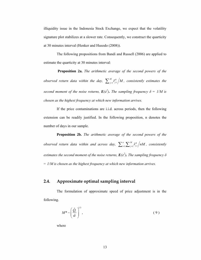
The following propositions from Bandi and Russell (2006) are applied to

estimate the quarticity at 30 minutes interval:

Proposition 2a. The arithmetic average of the second powers of the

observed return data within the day, 4,1

Mj ij

r M=∑ , consistently estimates the

second moment of the noise returns, E(ε2). The sampling frequency δ = 1/M is

chosen as the highest frequency at which new information arrives.

If the price contaminations are i.i.d. across periods, then the following

extension can be readily justified. In the following proposition, n denotes the

number of days in our sample.

Proposition 2b. The arithmetic average of the second powers of the

observed return data within and across day, 4,1 1

n Mj ii j

r nM= =∑ ∑ , consistently

estimates the second moment of the noise returns, E(ε2). The sampling frequency δ

= 1/M is chosen as the highest frequency at which new information arrives.

2.4. Approximate optimal sampling interval

The formulation of approximate speed of price adjustment is in the

following.

1/3ˆ* ,

ˆiQM

α⎛ ⎞⎜ ⎟⎜ ⎟⎝ ⎠∼ ( 9 )

where

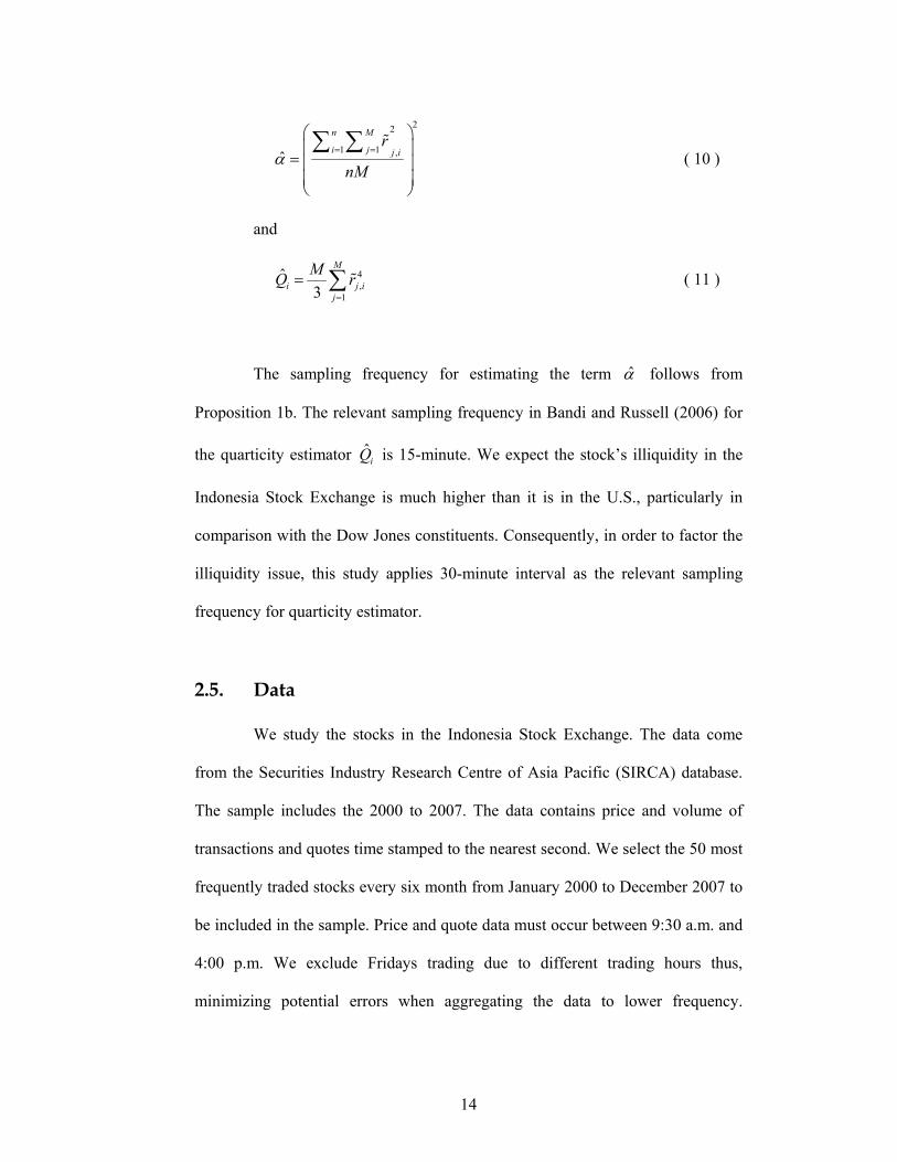
14

22

1 1 ,ˆ

n M

i j j ir

nMα

= =⎛ ⎞⎜ ⎟= ⎜ ⎟⎜ ⎟⎝ ⎠

∑ ∑ ( 10 )

and

4,

1

ˆ3

M

i j ij

MQ r=

= ∑ ( 11 )

The sampling frequency for estimating the term α̂ follows from

Proposition 1b. The relevant sampling frequency in Bandi and Russell (2006) for

the quarticity estimator ˆiQ is 15-minute. We expect the stock’s illiquidity in the

Indonesia Stock Exchange is much higher than it is in the U.S., particularly in

comparison with the Dow Jones constituents. Consequently, in order to factor the

illiquidity issue, this study applies 30-minute interval as the relevant sampling

frequency for quarticity estimator.

2.5. Data

We study the stocks in the Indonesia Stock Exchange. The data come

from the Securities Industry Research Centre of Asia Pacific (SIRCA) database.

The sample includes the 2000 to 2007. The data contains price and volume of

transactions and quotes time stamped to the nearest second. We select the 50 most

frequently traded stocks every six month from January 2000 to December 2007 to

be included in the sample. Price and quote data must occur between 9:30 a.m. and

4:00 p.m. We exclude Fridays trading due to different trading hours thus,

minimizing potential errors when aggregating the data to lower frequency.

15

Following Dacorogna, et al. (2001), analysis of high frequency data necessitates

bid-ask pairs, where the ask price is higher than the bid price. Therefore, the data

is filtered to exclude observations where bid prices exceed concurrently valid ask

prices.

It is common practice in the realized variance literature to use midpoints

of bid-ask quotes as measures of the true prices. While these measures are

affected by residual noise in that there is no theoretical guarantee that the

midpoints coincide with the underlying efficient prices, they are generally less

noisy measures of the efficient prices than are transaction prices since they do not

suffer from bid-ask bounce effects. Thus, in agreement with the realized variance

literature, in this study we use midpoints of bid-ask quotes to measure prices.

Accordingly, the specification in Eq.(1) should be interpreted as a model of

midquote determination based on efficient price and residual microstructure noise.

Considering the less liquid nature of the developing market than the

developed market, we analyse the data on half-yearly basis. This is to provide

sufficient observations to generate reliable results.

2.6. Sampling Schemes

Intraday returns can be constructed using different types of sampling

schemes. The special case where j = 1,…,M, are equidistant in calendar time, i.e.

1/ Mδ = , is referred to as calendar time sampling (CTS). The sampling scheme

requires the construction of artificial prices from the raw transaction or midquote

prices data that are irregularly spaced. Given observed prices at the times

j0<…<jM, a price at time [ , 1)j jτ ∈ + , can be artificially constructed using

16

jp pτ ≡ ( 12 )

or

1( )( 1)j j j

jp p p pj jττ

+−

≡ + −+ −

( 13 )

The former is known as the previous tick method, i.e. taking the most

recent values (Wasserfallen and Zimmermann, 1985), and the latter is the linear

interpolation method (Andersen and Bollerslev, 1997).

The case where jδ denotes the time of a transaction/quotation is referred

to as transaction time sampling (TTS). For example, jδ, j = 1,…,M, are chosen to

be the time of every fifth transaction.

The case where the sampling times, 0, ,..., ,M M Mj j , are such that

2 /j IV Mδσ = for all j = 1,…,M is known as business time sampling (BTS).

Whereas j = 0,…,M, are observable under CTS and TTS, they are latent under

BTS, because the sampling times are defined from the unobserved volatility path.

Empirical result of Andersen and Bollerslev (1997) and Curci and Corsi (2004)

suggest that BTS can be approximated by TTS.

Griffin and Oomen (2008) advocated that the microstructure noise may

appear close to i.i.d in event time which is consistent with the microstructure

noise assumption applied in this study. For this reason, we use event time to

estimate the realized variance based estimator.

2.7. Volatility Signature Plot

The realized variance (RV) is derived from intraday returns that require

the value of the price process to be known at particular points in time. In practice,

17

the price process is latent and prices must be interpolated from transaction and

quotation data. These interpolated prices need not equal the true prices for a

number of reasons that relate to market microstructure effects and aspects of the

interpolation method. First, lack of liquidity could cause the observed price to

differ from the true price, for example during short periods of time where large

trades are being executed. Second, structural aspects of the market, such as the

bid-ask spread and the discrete nature of price data that implies rounding errors. A

third source of pricing errors can arise from the econometric method that is used

to construct the artificial price data. The method is not unique and involves

several choices such as: should prices be inferred from transaction data or

midquotes; how to construct prices at points in time where no transaction or

quotation occurred (at the exact same point in time). A fourth source of pricing

errors relates to the quality of the data. For example, tick-by-tick data sets contain

misrecorded prices, such as transaction prices that are recorded to be zero. While

zero-prices are easy to identify and remove from the data set, other misrecorded

prices need not be.

The realized variance (RV) of p* is defined by

( ) *2*

1

MM

ji

RV r δ=

≡ ∑ ( 14 )

and ( )*

MRV is consistent for the integrated variance (IV) as M →∞ (Protter

(2005)). A feasible asymptotic distribution theory of RV (in relation to IV) was

established by Barndorff-Nielsen and Shephard (2002). Whereas ( )*

MRV is and

ideal estimator, it is not feasible estimator because p* is latent. The realized

variance of p, given by

18

( ) 2

1

MM

jj

RV r δ=

≡∑ ( 15 )

is observable but suffers from a well-known bias problem and is generally

inconsistent for the IV (Bandi and Russell (2006)).

A volatility signature plot provides an easy way to visually inspect the

potential bias problems of RV-type estimators. Such plots appeared is proposed by

Andersen et al. (2000). Let ( )MtRV denote the RV based on M intraday returns on

day t. A volatility signature plot displays the sample average

( ) 1 ( )

1

nM Mt

tRV n RV−

=

≡ ∑ ( 16 )

as a function of the sampling frequencies m, where the average is taken over

multiple periods (typically trading days). A signature plot yields valuable

information about the RV's bias and can uncover important properties of the noise

process.

2.8. CTS and TTS: Why are they different?

Sampling returns in calendar time induces properties of the noise that are

different from the properties of the noise obtained by sampling returns in trade

time. At very high frequencies, calendar time sampling will inevitably result in

sampling between quote updates, thereby artificially inducing persistency in the

observed price, p . The persistency again leads to an artificially negative

correlation between noise returns and efficient returns. Here, we compare the

variance signature plots obtained from tick time sampling to those obtained

previously from calendar time sampling to illustrate the difference. We choose

19

TLKM simply because it is one of the most frequently traded stocks in the

Indonesia Stock Exchange during our sampling period. The illustration presented

in Figure 1 uses the second half of 2007 to construct realized volatility based on

the calendar time and transaction time sampling.

Figure 1 contains tick time and calendar time of mid-quote realized

variance plots at the second half of 2007 for Telekomunikasi Indonesia (TLKM).

As shown in the figure, the variance signature plot of calendar time drops, rather

than increases as the sampling frequency increases while, the variance signature

plots obtained from event time shows otherwise.

3. Results 3.1. The Noise Variance

First, we present the descriptive statistics of daily average standard

deviation of noise variance and daily average relative spread in Table 2. The

median standard deviation of noise variance estimated by transaction data is a

quarter of the median of the average spread. On the other hand, the median

standard deviations of noise variance estimated by midquotes are one seventh and

one sixth for paired and prevailing quotes respectively. The noise estimated by

transaction data is a proxy for total noise in the price process, while one estimated

by midquotes represent residual noise.

The standard deviation of noise variance constructed using transactions

and mid-prices, generated from either quotes at event-time or prevailing quotes

data are presented in the Table 3. On average, the noise variance constructed from

either quote at event-time or quote at transaction time has lower noise variance

20

than the one constructed from transaction data. Scaled to annual rates, the average

standard deviation of noise variance constructed from transaction data is almost

9% while they are 5% and 6% for series constructed from quotes and prevailing

quotes, respectively. The findings are not unexpected since most of the studies in

the realized variance based estimator agree that return series generated from

midprices are less noisy than the one generated from transaction prices.

From Table 3 it is apparent that average noise variance has changed toward a

lower level from 2000 to 2007. The significant decreasing period starts from the

first half of 2004 to the second half of 2006. In this period, the noise variance

estimated by transaction data decreases from 10% to 6%, by quotes midprices

falls from 6% to 3% and by prevailing quotes declines from 7% to 4%. Although

there is increasing noise variance after the second half of 2006, the level is

considerably lower than the initial periods. As noise indicates the deviation

between the observed and actual price of an asset (Black (1986)), the lower level

of noise implies an improving market quality in the Indonesian Stock Exchange

between 2000 and 2007.

The annual standard deviation of noise variance is presented in Table 3.

The method employed in this study requires stocks with high liquidity to produce

consistent results as presented in Eq.(9). Any possible inconsistencies with the

method due to illiquidity issue will manifest themselves in the optimal sampling

frequency estimates that are higher than the interval used to identify signal

(quarticity). Therefore, we select companies with approximate optimal frequency

that is less than the frequency used to estimate the signal (quarticity), i.e. 30-

21

minute interval. As a result, the number of valid companies is less than our

original sample of 50 companies.

As shown in Table 3, there is substantial variability in the sample. We

minimize the variability by analysing the noise variance based on price change

factions groups. Following the Addendum to The Rule Number II-A about

Securities Trading (Firmansyah and Sembiring (2004)), The Indonesia Stock

Exchange classifies price change faction into four groups:

(1) Less than 500 rupiah. The permitted minimum (maximum) price change is

5 (50) rupiah.

(2) From 500 rupiah up to 2000 rupiah. The permitted minimum (maximum)

price change is 10 (100) rupiah.

(3) From 2000 up to 5000 rupiah. The permitted minimum (maximum) price

change is 25 (250) rupiah.

(4) More than 5000 rupiah. The permitted minimum (maximum) price change

is 50 (500) rupiah.

The results are presented in Table 4, Table 5 and Table 6. Noise variance

estimates reported are higher than the estimates of Hansen and Lunde (2006).

They estimate the noise variance of 30 equities of the DJIA from 2000 to 2004

using transaction data. Hansen and Lunde (2006) find that, using their method, the

highest noise variance is 2.4 per cent in 2000. After that, they find decreasing

noise variance from 2000 to 2004. We find that, even for the most frequently

traded stocks in the Indonesia Stock Exchange, the minimum noise variance is

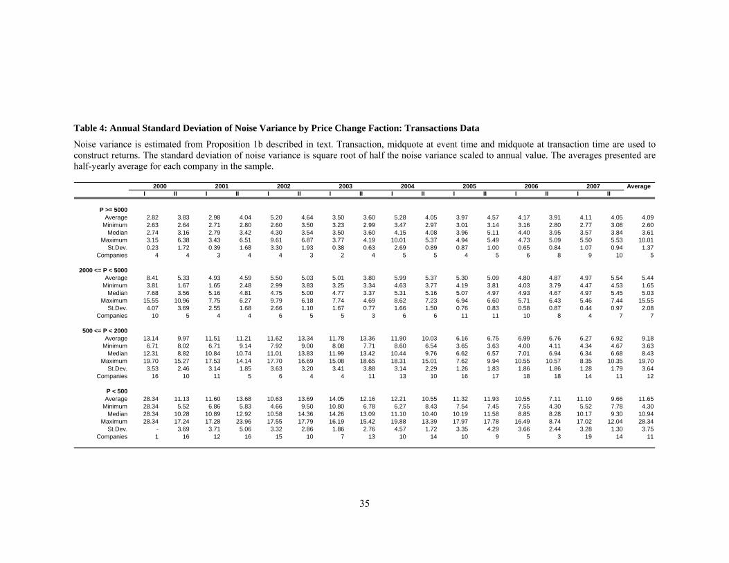
still higher than the estimation of Hansen and Lunde (2006). As shown in Table 4,

22

the minimum noise variance for stock prices of more than 5,000 rupiahs is 3 per

cent in 2007.

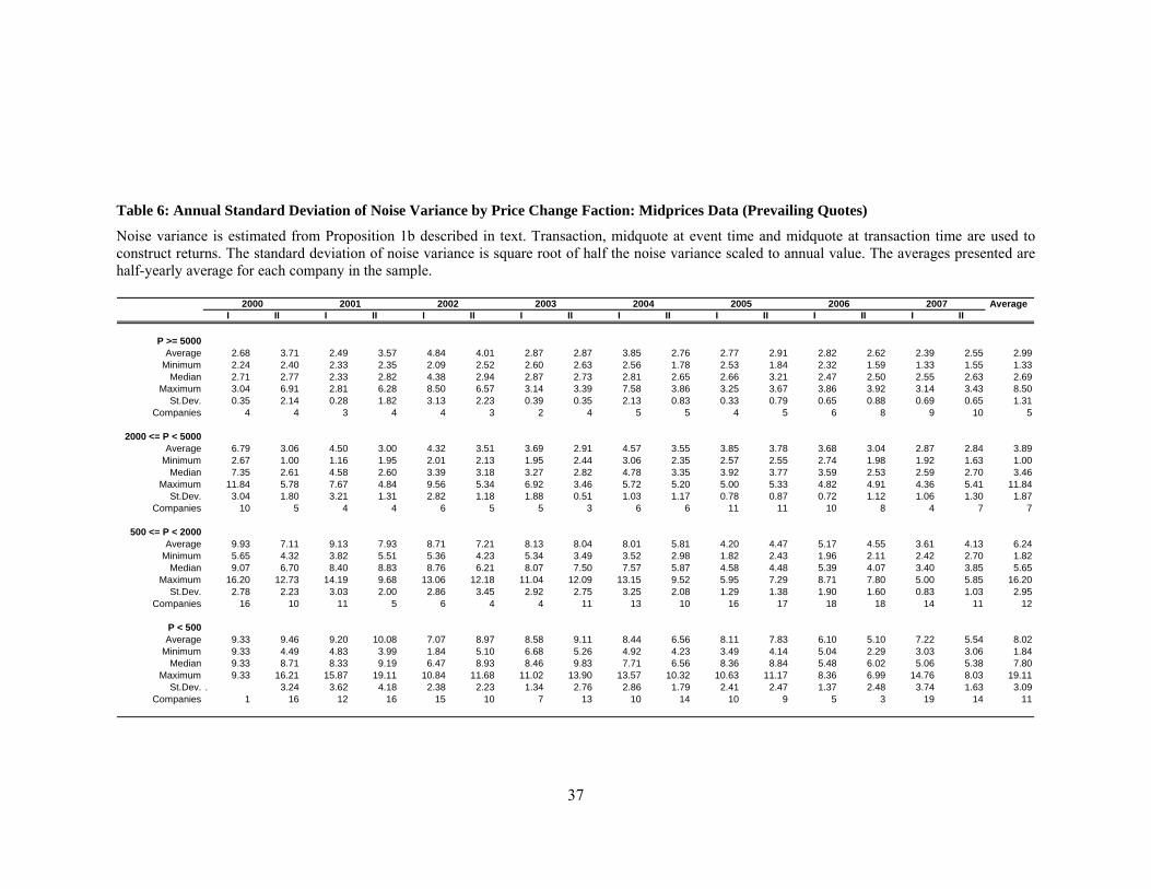
From Table 4, Table 5 and Table 6, we find that the noise variance for

the third and fourth price faction category is fairly stable. At those categories, it

has also found that the noise variance has lower variability from the second half of

2004 to the end of the sample period. The second category, either using

transactions or quotes data, show an obvious periods of high and low noise

variance. The cut-off point between the two periods is the first half of 2004. From

the price change faction based analysis, it is clear that stocks within the price

range of 500 to 2000 rupiah have the most dramatic noise variance change. The

first category shows a gradual decreasing level of noise variance.

Stoll (2000) argues that stock price proxies for stability, greater

disclosure, and a lower probability of informed trading. Table 4, Table 5 and

Table 6 show that stocks with price of more than 5000 rupiah (the fourth

category) have the smallest noise variance. As the noise reflects the deviation

between the observed price and its efficient price, it is clear that the high price

stocks show a greater disclosure than the remaining categories. The disclosure is

even greater from the second half of 2004 because the noise variance is more

stable from that point. As for the lowest priced stocks, the high variability of noise

variance during the sample period indicates that the microstructure effect

dominates the noise. The substantial variability of noise variance is persistent

even after controlling for the bid-ask bounce effect by estimating the noise

variance using quoted midprices. As we have found in our previous study,

(Henker and Husodo (2006)) we conjecture that the infrequent trading due to

23

significant asymmetric information drives the considerable variability of the noise

variance in the lowest priced stocks. The analysis of the asymmetric information

is presented in the next section.

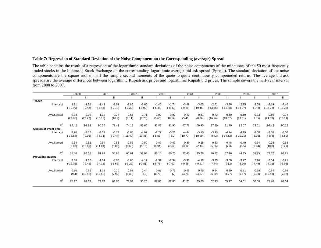
We estimate the constant elasticity model as in Woolridge (2003) to

analyse the relation between the standard deviation of the noise terms to the

average relative spread, namely, the average differences between the quoted

logarithmic ask prices and the corresponding logarithmic bid prices. As shown in

Table 7 , on average, 1% increase in the spread translates into 0.7% increase in the

standard deviation of noise component. The fact that all of the spread coefficients

are positive and significant is not surprising since the wider spreads are associated

with larger market microstructure contaminations in the observed return process.

The result presented in Bandi and Russell (2006) shows a more sensitive

coefficients. One per cent increase in the spread translated into one per cent

increase in the noise variance.

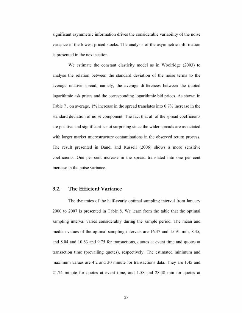
3.2. The Efficient Variance

The dynamics of the half-yearly optimal sampling interval from January

2000 to 2007 is presented in Table 8. We learn from the table that the optimal

sampling interval varies considerably during the sample period. The mean and

median values of the optimal sampling intervals are 16.37 and 15.91 min, 8.45,

and 8.04 and 10.63 and 9.75 for transactions, quotes at event time and quotes at

transaction time (prevailing quotes), respectively. The estimated minimum and

maximum values are 4.2 and 30 minute for transactions data. They are 1.45 and

21.74 minute for quotes at event time, and 1.58 and 28.48 min for quotes at

24

transaction time. For comparisons with developed market (Bandi and Russell

(2006)), the minimum value of approximate optimal sampling interval using mid-

quote returns is about 0.40 minute. The maximum value is 12.6 minute. In

addition, using transaction price returns, Hansen and Lunde (2006) find that the

minimum and maximum value of optimal sampling interval are 0.67 and 21.76

minute, respectively. It is clear that the dispersion of optimal sampling interval

estimates in the Indonesia Stock Exchange is higher than the U.S. equity market.

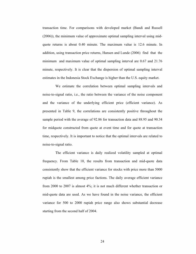
We estimate the correlation between optimal sampling intervals and

noise-to-signal ratio, i.e., the ratio between the variance of the noise component

and the variance of the underlying efficient price (efficient variance). As

presented in Table 9, the correlations are consistently positive throughout the

sample period with the average of 92.86 for transaction data and 88.95 and 90.34

for midquote constructed from quote at event time and for quote at transaction

time, respectively. It is important to notice that the optimal intervals are related to

noise-to-signal ratio.

The efficient variance is daily realized volatility sampled at optimal

frequency. From Table 10, the results from transaction and mid-quote data

consistently show that the efficient variance for stocks with price more than 5000

rupiah is the smallest among price factions. The daily average efficient variance

from 2000 to 2007 is almost 4%; it is not much different whether transaction or

mid-quote data are used. As we have found in the noise variance, the efficient

variance for 500 to 2000 rupiah price range also shows substantial decrease

starting from the second half of 2004.

25

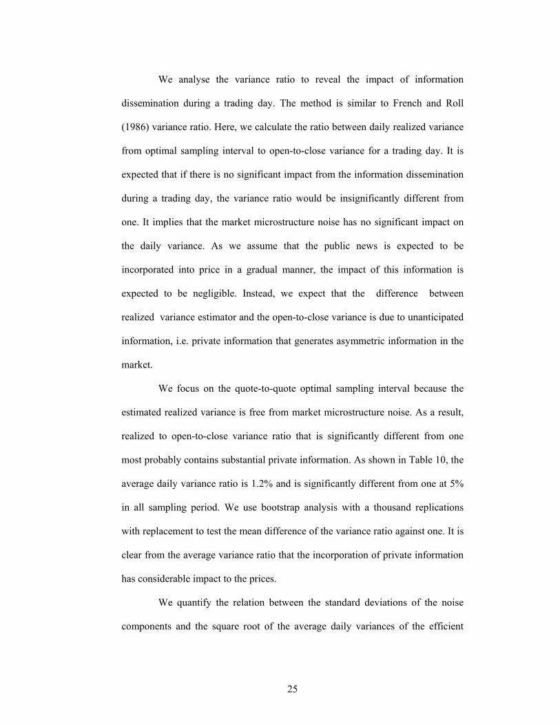
We analyse the variance ratio to reveal the impact of information

dissemination during a trading day. The method is similar to French and Roll

(1986) variance ratio. Here, we calculate the ratio between daily realized variance

from optimal sampling interval to open-to-close variance for a trading day. It is

expected that if there is no significant impact from the information dissemination

during a trading day, the variance ratio would be insignificantly different from

one. It implies that the market microstructure noise has no significant impact on

the daily variance. As we assume that the public news is expected to be

incorporated into price in a gradual manner, the impact of this information is

expected to be negligible. Instead, we expect that the difference between

realized variance estimator and the open-to-close variance is due to unanticipated

information, i.e. private information that generates asymmetric information in the

market.

We focus on the quote-to-quote optimal sampling interval because the

estimated realized variance is free from market microstructure noise. As a result,

realized to open-to-close variance ratio that is significantly different from one

most probably contains substantial private information. As shown in Table 10, the

average daily variance ratio is 1.2% and is significantly different from one at 5%

in all sampling period. We use bootstrap analysis with a thousand replications

with replacement to test the mean difference of the variance ratio against one. It is

clear from the average variance ratio that the incorporation of private information

has considerable impact to the prices.

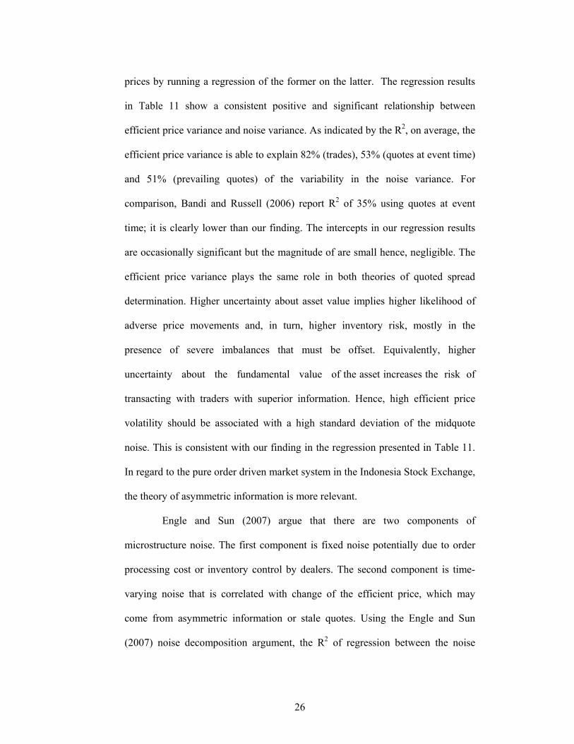
We quantify the relation between the standard deviations of the noise

components and the square root of the average daily variances of the efficient

26

prices by running a regression of the former on the latter. The regression results

in Table 11 show a consistent positive and significant relationship between

efficient price variance and noise variance. As indicated by the R2, on average, the

efficient price variance is able to explain 82% (trades), 53% (quotes at event time)

and 51% (prevailing quotes) of the variability in the noise variance. For

comparison, Bandi and Russell (2006) report R2 of 35% using quotes at event

time; it is clearly lower than our finding. The intercepts in our regression results

are occasionally significant but the magnitude of are small hence, negligible. The

efficient price variance plays the same role in both theories of quoted spread

determination. Higher uncertainty about asset value implies higher likelihood of

adverse price movements and, in turn, higher inventory risk, mostly in the

presence of severe imbalances that must be offset. Equivalently, higher

uncertainty about the fundamental value of the asset increases the risk of

transacting with traders with superior information. Hence, high efficient price

volatility should be associated with a high standard deviation of the midquote

noise. This is consistent with our finding in the regression presented in Table 11.

In regard to the pure order driven market system in the Indonesia Stock Exchange,

the theory of asymmetric information is more relevant.

Engle and Sun (2007) argue that there are two components of

microstructure noise. The first component is fixed noise potentially due to order

processing cost or inventory control by dealers. The second component is time-

varying noise that is correlated with change of the efficient price, which may

come from asymmetric information or stale quotes. Using the Engle and Sun

(2007) noise decomposition argument, the R2 of regression between the noise

27

variance and its corresponding efficient price variance indicates the variability of

noise due to asset uncertainty, or, change of the efficient price.

Back to Table 11 in the quote-to-quote continuously compounded returns

row, the average R2 shows that 53% of the variability in the noise standard

deviation is explained by the efficient price variance. It is imperative that the

midquote return is free from bid and bounce effect hence, it is clear that the

remaining unexplained component of noise variance comes from factor other than

bid and ask fluctuations. Referring to the result from variance ratio between the

efficient variance and open-to-close variance, private information is most

probably the important ingredient in the noise variance in the Indonesia Stock

Exchange.

4. Conclusions

Our results, which are based on samples of the 50 most frequently traded

stocks every six month from 2000 to 2007, can be summarized in the following.

The noise variance estimation from 2000 to 2007 using intraday data shows that

the noise has decreased implying smaller deviation between the observed prices

and their equilibrium values hence, the better market quality in the Indonesia

Stock Exchange.

We analyse the relation between the average relative spread to the noise

variance. The result shows that the standard deviations of the unobserved

midquote components (noise) are positively related to the quoted spreads. This

means higher quoted spread leads to higher noise.

28

The optimal sampling frequency is an interval that balances the bias from

market microstructure noise and the number of observations required to generate

reliable volatility estimate. Therefore, realized variance sampled at the optimal

frequency (efficient variance) is the variance that contains minimum impact from

market microstructure noise. We find that the average optimal sampling interval is

9 minutes. Using variance ratio between efficient variance to open-to-close

variance reveals that the ratio is consistently significantly more than one. It is

concluded that the difference between the variance sampled at optimal sampling

interval and the open-to-close variance at daily level is most likely generated by

private information.

The standard deviation of the unobserved midquote noise components

and the standard deviation of the efficient variance have consistent positive and

significant relationship indicating that the higher uncertainty of the asset value, as

reflected in the standard deviation of efficient variance, is translated into higher

standard deviation of noise. Moreover, standard deviation of efficient variance is

able to explain 53% variability in the standard deviation of noise component. As

the efficient variance is estimated from the midquote prices, it is clear that the bid-

ask bounce effect has been ruled out. Moreover, the variance ratio of daily

efficient variance to daily open-to-close variance is significantly more than one

implying significant private information content in prices. Therefore, we conclude

that the asymmetric information (or private information) makes up 47% of the

noise in the Indonesia Stock Exchange.

29

Bibliography

Andersen, Toben G., and Tim Bollerslev, 1997, Intraday Periodicity and Volatility Persistence in Financial Markets, Journal of Empirical Finance 4, 115-158.

Andersen, Toben G., Tim Bollerslev, and Francis X. Diebold, 2002, Parametric and Nonparametric Volatility Measurement, in Yacine Ait-Sahalia, and Lars Peter Hansen, eds.: Handbook of Financial Econometrics (North Holland, Amsterdam).

Andersen, Toben G., Tim Bollerslev, Francis X. Diebold, and Heiko Ebens, 2001, The Distribution of Realized Stock Return Volatility, Journal of Financial Economics 61, 43-76.

Andersen, Tobin G., Tim Bollerslev, F.X. Diebold, and P. Labys, 2003, Modeling and Forecasting Realized Volatility, Econometrica 71, 579-625.

Andersen, Torben G., Tim Bollerslev, Francis Diebold, and Paul Labys, 2000, Great Realizations, Risk Magazine 105-108.

Bandi, F.M., and J.R. Russell, 2008, Microstructure Noise, Realized Variance, and Optimal Sampling, Review of Economic Studies 75, 339-369.

Bandi, Frederico M., and Jeffrey R. Russell, 2006, Separating Microstructure Noise from Volatility, Journal of Financial Economics 79, 655-692.

Barndorff-Nielsen, O.E., and N. Shephard, 2002, Econometric Analysis of Realized Volatility and Its Use in Estimating Stochastic Volatility Models, Journal of The Royal Statistical Society Series B, 253-280.

Barndorff-Nielsen, Ole E., and Neil Shephard, 2002, Econometric Analysis of Realized Volatility and Its Use in Estimating Stochastic Volatility Models, Journal of Royal Statistical Society B, 253-280.

Barndorff-Nielsen, Ole E., and Neil Shephard, 2004, Econometric Analysis of Realized Covariation: High Frequency Based Covariance, Regression and Correlation in Financial Economics, Econometrica 72, 885-925.

Black, Fischer, 1986, Noise, Journal of Finance 41, 529-543. Curci, Giuseppe, and Fulvio Corsi, 2004, A Discrete Sine Transform Approach

for Realized Volatility Measurement, (Institute of Finance, University of Southern Switzerland, Lugano).

Dacorogna, Michel M., Ramazan Gencay, Ulrich A. Muller, Richard B. Olsen, and Olivier V. Pictet, 2001. An Introduction to High Frequency Finance (Academic Press, London).

Engle, Robert, and Zheng Sun, 2007, When Is Noise Not Noise - A Microstructure Estimate of Realized Volatility, (Stern NYU).

Firmansyah, Erry, and M.S. Sembiring, 2004, Amendment/Addendum to The Rule Number II-A Concerning Securities Trading, in Jakarta Stock Exchange, ed.

French, Kenneth R., and Richard Roll, 1986, Stock Return Variances: The Arrival of Information and the Reaction of Traders, Journal of Financial Economics 17, 5-26.

French, Kenneth R., G.W. Schwert, and R.F. Stambaugh, 1987, Expected Stock Returns and Volatility, Journal of Financial Economics 19, 3-29.

30

Griffin, Jim E., and Roel C. A. Oomen, 2008, Sampling Returns for Realized Variance Calculations: Tick Time or Transaction Time?, Econometric Reviews 27, 230-253.

Hansen, Peter R., and Asger Lunde, 2006, Realized Variance and Market Microstructure Noise, Journal of Business and Economic Statistics 24, 127-161.

Henker, Thomas, and Zaafri Husodo, 2008, Intraday Speed of Adjustment and the Realized Variance in the Indonesia Stock Exchange, (School of Banking and Finance, University of New South Wales, Australia).

Henker, Thomas, and Zaafri A. Husodo, 2006, Short Run Behaviour of Stock Returns: Speed of Adjustment and Its Contributing Factors in The Jakarta Stock Exchange, Working Paper.

Kyle, Albert S., 1985, Continuous Auction and Insider Trading, Econometrica 53, 1315-1335.

Madhavan, Ananth, 1992, Trading Mechanisms in Securities Markets, Journal of Finance 47, 607-641.

Schwert, G.W., 1989, Why Does Stock Market Volatility Change Over Time?, Journal of Finance 44, 1115-1153.

Schwert, G.W., 1990a, Stock Market Volatility, Financial Analyst Journal 46, 23-24.

Schwert, G.W., 1990b, Stock Volatility and the Crash of '87, Review of Financial Studies 3, 77-102.

Schwert, G.W., and P.J. Seguin, 1991, Heteroskedasticity in Stock Returns, Journal of Finance 45, 1129-1155.

Stoll, Hans R., 2000, Friction, Journal of Finance 55, 1479-1514. Wood, Robert A., Thomas H. McInish, and J. Keith Ord, 1985, An Investigation

of Transactions Data for NYSE Stocks, Journal of Finance 40, 723-739. Woolridge, Jeffrey M., 2003. Introductory Econometrics: A Modern Approach

(South-Western). Zhang, L., P. Mykland, and Y Ait-Sahalia, 2005, A Tale of Two Time Scales:

Determining Integrated Voaltility with Noisy High-Frequency Data, Journal of American Statistical Association 100, 1394-1411.

31

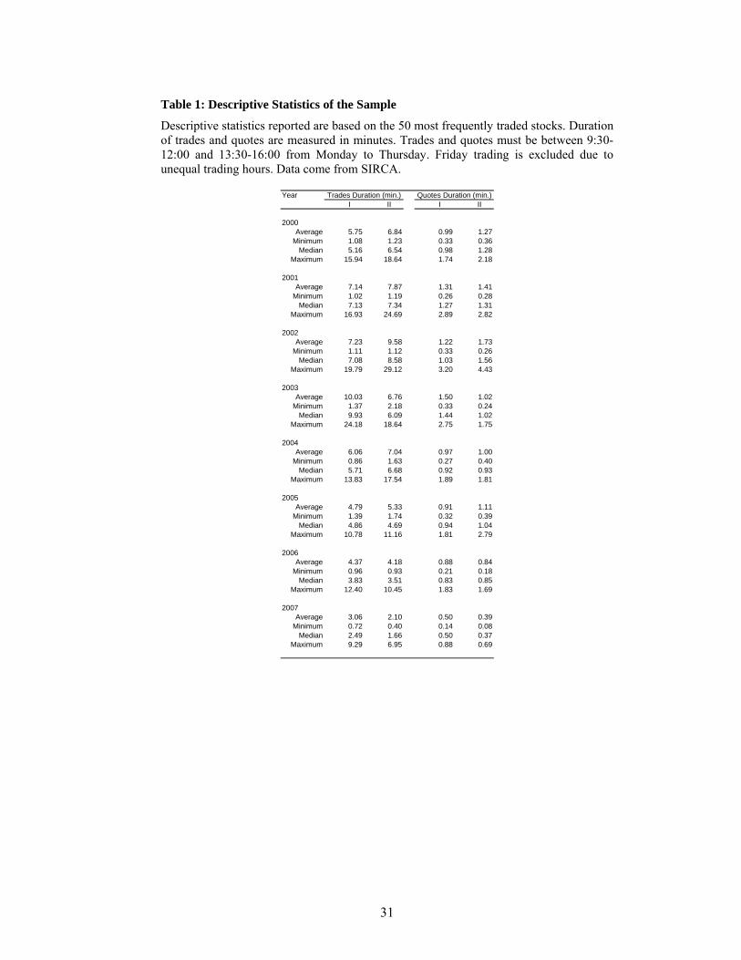
Table 1: Descriptive Statistics of the Sample

Descriptive statistics reported are based on the 50 most frequently traded stocks. Duration of trades and quotes are measured in minutes. Trades and quotes must be between 9:30-12:00 and 13:30-16:00 from Monday to Thursday. Friday trading is excluded due to unequal trading hours. Data come from SIRCA.

Year I II I II

2000Average 5.75 6.84 0.99 1.27

Minimum 1.08 1.23 0.33 0.36Median 5.16 6.54 0.98 1.28

Maximum 15.94 18.64 1.74 2.18

2001Average 7.14 7.87 1.31 1.41

Minimum 1.02 1.19 0.26 0.28Median 7.13 7.34 1.27 1.31

Maximum 16.93 24.69 2.89 2.82

2002Average 7.23 9.58 1.22 1.73

Minimum 1.11 1.12 0.33 0.26Median 7.08 8.58 1.03 1.56

Maximum 19.79 29.12 3.20 4.43

2003Average 10.03 6.76 1.50 1.02

Minimum 1.37 2.18 0.33 0.24Median 9.93 6.09 1.44 1.02

Maximum 24.18 18.64 2.75 1.75

2004Average 6.06 7.04 0.97 1.00

Minimum 0.86 1.63 0.27 0.40Median 5.71 6.68 0.92 0.93

Maximum 13.83 17.54 1.89 1.81

2005Average 4.79 5.33 0.91 1.11

Minimum 1.39 1.74 0.32 0.39Median 4.86 4.69 0.94 1.04

Maximum 10.78 11.16 1.81 2.79

2006Average 4.37 4.18 0.88 0.84

Minimum 0.96 0.93 0.21 0.18Median 3.83 3.51 0.83 0.85

Maximum 12.40 10.45 1.83 1.69

2007Average 3.06 2.10 0.50 0.39

Minimum 0.72 0.40 0.14 0.08Median 2.49 1.66 0.50 0.37

Maximum 9.29 6.95 0.88 0.69

Quotes Duration (min.)Trades Duration (min.)

32

Figure 1: Variance Signature Plot of TLKM (second half of 2007)

Average daily realized variance is constructed from mid-quotes using Calendar Time Sampling and Event Time Sampling Method. The data come from SIRCA.

0.0000

0.0001

0.0002

0.0003

0.0004

0.0005

0.0006

0.0007

0.0008

0.0009

0.0010

0 100 200 300 400 500 600 700 800 900

Interval (second)

Rea

lized

Var

ianc

e (d

aily

)

RvmidctsRvmidtts

33

Table 2: Descriptive Statistics of Daily Noise Standard Deviation and Daily Average Relative Spread

The standard deviation of the noise components are the square root of half the sample second moments of the continuously compounded returns constructed at the highest frequency either from transactions or quotes data. The average bid-ask spreads (Spread) are the average differences between logarithmic Rupiah ask prices and logarithmic Rupiah bid prices at event time. The sample covers the half-year interval from 2000 to 2007.

AverageI II I II I II I II I II I II I II I II

SpreadAverage 0.0232 0.0161 0.0195 0.0277 0.0225 0.0252 0.0192 0.0205 0.0219 0.0182 0.0133 0.0148 0.0115 0.0102 0.0134 0.0109 0.0180

Minimum 0.0033 0.0035 0.0044 0.0053 0.0048 0.0063 0.0065 0.0052 0.0043 0.0040 0.0046 0.0050 0.0047 0.0035 0.0027 0.0027 0.0044Median 0.0227 0.0148 0.0195 0.0220 0.0173 0.0195 0.0221 0.0206 0.0176 0.0160 0.0115 0.0109 0.0099 0.0097 0.0119 0.0104 0.0160

Maximum 0.0947 0.0347 0.0343 0.1576 0.1438 0.0880 0.0311 0.0388 0.1254 0.1239 0.0731 0.1079 0.0411 0.0192 0.0345 0.0197 0.0730St.Dev. 0.0174 0.0080 0.0084 0.0288 0.0241 0.0214 0.0091 0.0097 0.0210 0.0193 0.0108 0.0164 0.0069 0.0038 0.0076 0.0047 0.0136

S.D. NoiseTrade

Average 0.0050 0.0042 0.0045 0.0050 0.0042 0.0048 0.0045 0.0049 0.0046 0.0040 0.0032 0.0033 0.0029 0.0026 0.0035 0.0032 0.0040Minimum 0.0012 0.0008 0.0007 0.0011 0.0012 0.0016 0.0015 0.0014 0.0016 0.0014 0.0014 0.0014 0.0014 0.0013 0.0012 0.0014 0.0013

Median 0.0050 0.0040 0.0045 0.0048 0.0044 0.0049 0.0047 0.0055 0.0044 0.0041 0.0029 0.0028 0.0026 0.0023 0.0031 0.0029 0.0039Maximum 0.0130 0.0078 0.0080 0.0112 0.0081 0.0082 0.0074 0.0085 0.0098 0.0072 0.0083 0.0082 0.0075 0.0050 0.0078 0.0055 0.0082

St.Dev. 0.0028 0.0019 0.0020 0.0027 0.0019 0.0023 0.0022 0.0022 0.0021 0.0015 0.0015 0.0016 0.0012 0.0009 0.0017 0.0012 0.0019

QuotesAverage 0.0032 0.0027 0.0030 0.0030 0.0025 0.0026 0.0024 0.0028 0.0027 0.0020 0.0020 0.0019 0.0017 0.0016 0.0020 0.0017 0.0024

Minimum 0.0010 0.0005 0.0005 0.0009 0.0009 0.0009 0.0008 0.0010 0.0011 0.0008 0.0008 0.0008 0.0008 0.0007 0.0006 0.0007 0.0008Median 0.0033 0.0026 0.0030 0.0025 0.0025 0.0027 0.0026 0.0029 0.0024 0.0020 0.0018 0.0017 0.0016 0.0016 0.0017 0.0015 0.0023

Maximum 0.0055 0.0052 0.0059 0.0077 0.0050 0.0044 0.0040 0.0053 0.0049 0.0040 0.0040 0.0037 0.0033 0.0029 0.0053 0.0035 0.0047St.Dev. 0.0013 0.0012 0.0014 0.0018 0.0010 0.0011 0.0011 0.0012 0.0012 0.0008 0.0008 0.0007 0.0006 0.0006 0.0012 0.0007 0.0011

Prev. QuotesAverage 0.0037 0.0033 0.0036 0.0036 0.0030 0.0031 0.0030 0.0034 0.0032 0.0024 0.0022 0.0022 0.0021 0.0018 0.0022 0.0018 0.0028

Minimum 0.0010 0.0005 0.0005 0.0009 0.0009 0.0010 0.0009 0.0011 0.0012 0.0008 0.0008 0.0008 0.0009 0.0007 0.0006 0.0007 0.0008Median 0.0038 0.0032 0.0035 0.0033 0.0028 0.0030 0.0031 0.0031 0.0028 0.0023 0.0020 0.0019 0.0020 0.0017 0.0018 0.0016 0.0026

Maximum 0.0075 0.0078 0.0072 0.0089 0.0060 0.0056 0.0051 0.0064 0.0067 0.0049 0.0049 0.0053 0.0039 0.0037 0.0067 0.0039 0.0059St.Dev. 0.0017 0.0017 0.0018 0.0021 0.0014 0.0015 0.0014 0.0016 0.0015 0.0010 0.0011 0.0010 0.0008 0.0008 0.0015 0.0008 0.0013

2004 2005 2006 20072000 2001 2002 2003

34

Table 3: Annual Standard Deviation of Noise Variance

Noise variance is estimated from Proposition 1b described in text. Transaction, midquote at event time and midquote at transaction time are used to construct returns. The standard deviation of noise variance is square root of half the noise variance scaled to annual value. The averages presented are cross-sectional average. The data come from SIRCA database.

AverageI II I II I II I II I II I II I II I II

Observations (day) 110 116 114 107 111 107 108 112 111 116 120 121 121 115 122 117 114

Companies 31 35 30 29 31 22 18 31 34 35 41 42 39 37 46 42 34

Duration (minute)Quote 0.99 1.27 1.31 1.41 1.22 1.73 1.50 1.02 0.97 1.00 0.91 1.11 0.88 0.84 0.50 0.39 1Trade 5.75 6.84 7.14 7.87 7.23 9.58 10.03 6.76 6.06 7.04 4.79 5.33 4.37 4.18 3.06 2.10 6

ηtrade (% p.a.)Average 10.77 9.13 9.81 10.67 9.13 10.42 9.86 10.67 9.97 8.58 6.97 7.17 6.45 5.76 7.73 6.92 8.50

Minimum 2.63 1.67 1.65 2.48 2.60 3.50 3.23 2.99 3.47 2.97 3.01 3.14 3.16 2.80 2.77 3.08 1.65Median 10.87 8.75 9.96 10.51 9.61 10.71 10.26 12.02 9.62 9.04 6.44 6.07 5.71 5.09 6.80 6.43 7.78

Maximum 28.34 17.24 17.53 23.96 17.70 17.79 16.19 18.65 19.88 15.01 17.97 17.78 16.49 10.57 17.02 12.04 28.34St.Dev. 5.90 4.12 4.45 5.62 4.08 4.89 4.87 4.81 4.45 3.16 3.16 3.49 2.64 1.96 3.70 2.56 4.26

ηquote (% p.a.)Average 6.84 5.91 6.61 6.45 5.55 5.64 5.28 6.12 5.76 4.37 4.29 4.11 3.76 3.48 4.33 3.72 5.00

Minimum 2.25 1.00 1.18 2.05 1.91 2.03 1.77 2.26 2.34 1.64 1.78 1.76 1.80 1.55 1.28 1.51 1.00Median 7.15 5.65 6.59 5.38 5.53 5.80 5.71 6.32 5.30 4.35 4.03 3.74 3.58 3.55 3.67 3.24 4.48

Maximum 11.94 11.01 12.96 16.53 10.76 9.60 8.82 11.53 10.52 8.46 8.85 8.15 7.35 6.38 11.59 7.31 16.53St.Dev. 2.83 2.65 3.03 3.74 2.28 2.35 2.28 2.69 2.57 1.77 1.77 1.60 1.33 1.33 2.56 1.56 2.52

ηprevquote (% p.a.)Average 7.96 7.22 7.88 7.83 6.57 6.73 6.49 7.32 6.92 5.29 4.92 4.82 4.55 3.85 4.79 4.01 5.88

Minimum 2.24 1.00 1.16 1.95 1.84 2.13 1.95 2.44 2.56 1.78 1.82 1.84 1.96 1.59 1.33 1.55 1.00Median 8.16 6.91 7.77 7.29 6.04 6.41 6.80 6.80 6.14 5.06 4.38 4.25 4.31 3.74 4.00 3.53 5.15

Maximum 16.20 16.21 15.87 19.11 13.06 12.18 11.04 13.90 13.57 10.32 10.63 11.17 8.71 7.80 14.76 8.03 19.11St.Dev. 3.60 3.62 3.89 4.39 2.96 3.25 3.04 3.43 3.22 2.21 2.37 2.23 1.78 1.68 3.22 1.73 3.23

2000 2001 2002 2003 2004 2005 2006 2007

35

Table 4: Annual Standard Deviation of Noise Variance by Price Change Faction: Transactions Data

Noise variance is estimated from Proposition 1b described in text. Transaction, midquote at event time and midquote at transaction time are used to construct returns. The standard deviation of noise variance is square root of half the noise variance scaled to annual value. The averages presented are half-yearly average for each company in the sample.

AverageI II I II I II I II I II I II I II I II

P >= 5000Average 2.82 3.83 2.98 4.04 5.20 4.64 3.50 3.60 5.28 4.05 3.97 4.57 4.17 3.91 4.11 4.05 4.09

Minimum 2.63 2.64 2.71 2.80 2.60 3.50 3.23 2.99 3.47 2.97 3.01 3.14 3.16 2.80 2.77 3.08 2.60Median 2.74 3.16 2.79 3.42 4.30 3.54 3.50 3.60 4.15 4.08 3.96 5.11 4.40 3.95 3.57 3.84 3.61

Maximum 3.15 6.38 3.43 6.51 9.61 6.87 3.77 4.19 10.01 5.37 4.94 5.49 4.73 5.09 5.50 5.53 10.01St.Dev. 0.23 1.72 0.39 1.68 3.30 1.93 0.38 0.63 2.69 0.89 0.87 1.00 0.65 0.84 1.07 0.94 1.37

Companies 4 4 3 4 4 3 2 4 5 5 4 5 6 8 9 10 5

2000 <= P < 5000Average 8.41 5.33 4.93 4.59 5.50 5.03 5.01 3.80 5.99 5.37 5.30 5.09 4.80 4.87 4.97 5.54 5.44

Minimum 3.81 1.67 1.65 2.48 2.99 3.83 3.25 3.34 4.63 3.77 4.19 3.81 4.03 3.79 4.47 4.53 1.65Median 7.68 3.56 5.16 4.81 4.75 5.00 4.77 3.37 5.31 5.16 5.07 4.97 4.93 4.67 4.97 5.45 5.03

Maximum 15.55 10.96 7.75 6.27 9.79 6.18 7.74 4.69 8.62 7.23 6.94 6.60 5.71 6.43 5.46 7.44 15.55St.Dev. 4.07 3.69 2.55 1.68 2.66 1.10 1.67 0.77 1.66 1.50 0.76 0.83 0.58 0.87 0.44 0.97 2.08

Companies 10 5 4 4 6 5 5 3 6 6 11 11 10 8 4 7 7

500 <= P < 2000Average 13.14 9.97 11.51 11.21 11.62 13.34 11.78 13.36 11.90 10.03 6.16 6.75 6.99 6.76 6.27 6.92 9.18

Minimum 6.71 8.02 6.71 9.14 7.92 9.00 8.08 7.71 8.60 6.54 3.65 3.63 4.00 4.11 4.34 4.67 3.63Median 12.31 8.82 10.84 10.74 11.01 13.83 11.99 13.42 10.44 9.76 6.62 6.57 7.01 6.94 6.34 6.68 8.43

Maximum 19.70 15.27 17.53 14.14 17.70 16.69 15.08 18.65 18.31 15.01 7.62 9.94 10.55 10.57 8.35 10.35 19.70St.Dev. 3.53 2.46 3.14 1.85 3.63 3.20 3.41 3.88 3.14 2.29 1.26 1.83 1.86 1.86 1.28 1.79 3.64

Companies 16 10 11 5 6 4 4 11 13 10 16 17 18 18 14 11 12

P < 500Average 28.34 11.13 11.60 13.68 10.63 13.69 14.05 12.16 12.21 10.55 11.32 11.93 10.55 7.11 11.10 9.66 11.65

Minimum 28.34 5.52 6.86 5.83 4.66 9.50 10.80 6.78 6.27 8.43 7.54 7.45 7.55 4.30 5.52 7.78 4.30Median 28.34 10.28 10.89 12.92 10.58 14.36 14.26 13.09 11.10 10.40 10.19 11.58 8.85 8.28 10.17 9.30 10.94

Maximum 28.34 17.24 17.28 23.96 17.55 17.79 16.19 15.42 19.88 13.39 17.97 17.78 16.49 8.74 17.02 12.04 28.34St.Dev. - 3.69 3.71 5.06 3.32 2.86 1.86 2.76 4.57 1.72 3.35 4.29 3.66 2.44 3.28 1.30 3.75

Companies 1 16 12 16 15 10 7 13 10 14 10 9 5 3 19 14 11

2004 2005 2006 20072000 2001 2002 2003

36

Table 5: Annual Standard Deviation of Noise Variance by Price Change Faction: Midprices Data (Quotes at event time)

Noise variance is estimated from Proposition 1b described in text. Transaction, midquote at event time and midquote at transaction time are used to construct returns. The standard deviation of noise variance is square root of half the noise variance scaled to annual value. The averages presented are half-yearly average for each company in the sample.

AverageI II I II I II I II I II I II I II I II

P >= 5000Average 2.58 3.15 2.34 3.14 3.72 3.16 2.43 2.52 3.18 2.49 2.52 2.57 2.47 2.45 2.27 2.38 2.65

Minimum 2.25 2.27 2.12 2.21 2.01 2.29 2.36 2.34 2.34 1.64 2.35 1.76 2.12 1.55 1.28 1.51 1.28Median 2.59 2.61 2.22 2.62 3.56 2.74 2.43 2.43 2.43 2.43 2.45 2.95 2.20 2.19 2.18 2.37 2.44

Maximum 2.87 5.12 2.67 5.09 5.74 4.45 2.51 2.87 5.32 3.38 2.82 2.99 3.19 3.70 2.95 3.19 5.74St.Dev. 0.26 1.32 0.29 1.31 1.81 1.14 0.10 0.24 1.28 0.67 0.21 0.56 0.47 0.82 0.65 0.59 0.85

Companies 4 4 3 4 4 3 2 4 5 5 4 5 6 8 9 10 5

2000 <= P < 5000Average 5.78 2.64 3.58 2.75 3.65 3.09 3.13 2.68 3.92 3.09 3.52 3.39 3.14 2.82 2.74 2.61 3.41

Minimum 2.62 1.00 1.18 2.05 2.06 2.03 1.77 2.26 2.82 2.16 2.53 2.40 2.43 1.93 1.89 1.55 1.00Median 6.25 2.35 3.71 2.50 3.06 2.93 2.86 2.68 3.95 2.88 3.51 3.38 3.06 2.37 2.54 2.58 3.04

Maximum 10.06 4.73 5.72 3.97 6.98 4.39 5.29 3.11 5.01 4.41 4.67 4.79 4.06 4.31 3.97 4.72 10.06St.Dev. 2.32 1.37 2.21 0.88 1.83 0.85 1.30 0.43 0.88 0.90 0.64 0.71 0.55 0.91 0.89 1.09 1.42

Companies 10 5 4 4 6 5 5 3 6 6 11 11 10 8 4 7 7

500 <= P < 2000Average 8.54 5.75 7.53 6.28 7.30 6.56 6.75 6.80 6.73 4.77 3.86 3.95 4.30 4.00 3.46 3.86 5.35

Minimum 5.16 3.67 3.40 4.29 4.86 5.22 4.48 2.83 3.01 2.48 1.78 2.33 1.80 1.95 2.38 2.44 1.78Median 7.78 5.62 7.40 6.63 6.81 6.75 7.03 6.49 6.09 4.78 4.20 3.96 4.46 3.92 3.54 3.60 4.97

Maximum 11.94 9.34 10.69 8.62 10.76 7.52 8.45 9.93 10.52 7.58 5.46 5.90 7.35 6.15 4.65 5.17 11.94St.Dev. 2.03 1.55 2.19 1.66 2.42 1.14 1.84 2.09 2.54 1.57 1.12 1.13 1.41 1.13 0.75 0.96 2.27

Companies 16 10 11 5 6 4 4 11 13 10 16 17 18 18 14 11 12

P < 500Average 7.40 7.71 7.86 8.25 6.10 7.30 6.79 7.45 6.91 5.30 6.54 6.16 4.64 4.87 6.28 5.12 6.66

Minimum 7.40 4.17 4.59 3.72 1.91 4.30 5.37 4.48 2.89 2.21 3.30 3.74 3.01 2.56 2.99 2.88 1.91Median 7.40 7.58 6.94 7.78 6.15 7.40 6.68 7.93 6.32 5.46 6.86 5.67 4.37 5.68 4.89 5.10 6.37

Maximum 7.40 11.01 12.96 16.53 8.92 9.60 8.82 11.53 10.31 8.46 8.85 8.15 6.32 6.38 11.59 7.31 16.53St.Dev. - 2.13 2.76 3.84 1.72 1.66 1.12 2.20 2.40 1.69 1.81 1.70 1.22 2.04 2.90 1.41 2.43

Companies 1 16 12 16 15 10 7 13 10 14 10 9 5 3 19 14 11

2004 2005 2006 20072000 2001 2002 2003

37

Table 6: Annual Standard Deviation of Noise Variance by Price Change Faction: Midprices Data (Prevailing Quotes)

Noise variance is estimated from Proposition 1b described in text. Transaction, midquote at event time and midquote at transaction time are used to construct returns. The standard deviation of noise variance is square root of half the noise variance scaled to annual value. The averages presented are half-yearly average for each company in the sample.

AverageI II I II I II I II I II I II I II I II

P >= 5000Average 2.68 3.71 2.49 3.57 4.84 4.01 2.87 2.87 3.85 2.76 2.77 2.91 2.82 2.62 2.39 2.55 2.99

Minimum 2.24 2.40 2.33 2.35 2.09 2.52 2.60 2.63 2.56 1.78 2.53 1.84 2.32 1.59 1.33 1.55 1.33Median 2.71 2.77 2.33 2.82 4.38 2.94 2.87 2.73 2.81 2.65 2.66 3.21 2.47 2.50 2.55 2.63 2.69

Maximum 3.04 6.91 2.81 6.28 8.50 6.57 3.14 3.39 7.58 3.86 3.25 3.67 3.86 3.92 3.14 3.43 8.50St.Dev. 0.35 2.14 0.28 1.82 3.13 2.23 0.39 0.35 2.13 0.83 0.33 0.79 0.65 0.88 0.69 0.65 1.31

Companies 4 4 3 4 4 3 2 4 5 5 4 5 6 8 9 10 5

2000 <= P < 5000Average 6.79 3.06 4.50 3.00 4.32 3.51 3.69 2.91 4.57 3.55 3.85 3.78 3.68 3.04 2.87 2.84 3.89

Minimum 2.67 1.00 1.16 1.95 2.01 2.13 1.95 2.44 3.06 2.35 2.57 2.55 2.74 1.98 1.92 1.63 1.00Median 7.35 2.61 4.58 2.60 3.39 3.18 3.27 2.82 4.78 3.35 3.92 3.77 3.59 2.53 2.59 2.70 3.46

Maximum 11.84 5.78 7.67 4.84 9.56 5.34 6.92 3.46 5.72 5.20 5.00 5.33 4.82 4.91 4.36 5.41 11.84St.Dev. 3.04 1.80 3.21 1.31 2.82 1.18 1.88 0.51 1.03 1.17 0.78 0.87 0.72 1.12 1.06 1.30 1.87

Companies 10 5 4 4 6 5 5 3 6 6 11 11 10 8 4 7 7

500 <= P < 2000Average 9.93 7.11 9.13 7.93 8.71 7.21 8.13 8.04 8.01 5.81 4.20 4.47 5.17 4.55 3.61 4.13 6.24

Minimum 5.65 4.32 3.82 5.51 5.36 4.23 5.34 3.49 3.52 2.98 1.82 2.43 1.96 2.11 2.42 2.70 1.82Median 9.07 6.70 8.40 8.83 8.76 6.21 8.07 7.50 7.57 5.87 4.58 4.48 5.39 4.07 3.40 3.85 5.65

Maximum 16.20 12.73 14.19 9.68 13.06 12.18 11.04 12.09 13.15 9.52 5.95 7.29 8.71 7.80 5.00 5.85 16.20St.Dev. 2.78 2.23 3.03 2.00 2.86 3.45 2.92 2.75 3.25 2.08 1.29 1.38 1.90 1.60 0.83 1.03 2.95

Companies 16 10 11 5 6 4 4 11 13 10 16 17 18 18 14 11 12

P < 500Average 9.33 9.46 9.20 10.08 7.07 8.97 8.58 9.11 8.44 6.56 8.11 7.83 6.10 5.10 7.22 5.54 8.02

Minimum 9.33 4.49 4.83 3.99 1.84 5.10 6.68 5.26 4.92 4.23 3.49 4.14 5.04 2.29 3.03 3.06 1.84Median 9.33 8.71 8.33 9.19 6.47 8.93 8.46 9.83 7.71 6.56 8.36 8.84 5.48 6.02 5.06 5.38 7.80

Maximum 9.33 16.21 15.87 19.11 10.84 11.68 11.02 13.90 13.57 10.32 10.63 11.17 8.36 6.99 14.76 8.03 19.11St.Dev. . 3.24 3.62 4.18 2.38 2.23 1.34 2.76 2.86 1.79 2.41 2.47 1.37 2.48 3.74 1.63 3.09

Companies 1 16 12 16 15 10 7 13 10 14 10 9 5 3 19 14 11

2004 2005 2006 20072000 2001 2002 2003

38

Table 7: Regression of Standard Deviation of the Noise Component on the Corresponding (average) Spread

The table contains the result of a regression of the logarithmic standard deviations of the noise components of the midquotes of the 50 most frequently traded stocks in the Indonesia Stock Exchange on the corresponding logarithmic average bid-ask spread (Spread). The standard deviation of the noise components are the square root of half the sample second moments of the quote-to-quote continuously compounded returns. The average bid-ask spreads are the average differences between logarithmic Rupiah ask prices and logarithmic Rupiah bid prices. The sample covers the half-year interval from 2000 to 2007.

I II I II I II I II I II I II I II I IITrades

Intercept -2.31 -1.76 -1.41 -2.61 -2.85 -2.65 -1.45 -1.74 -3.49 -3.03 -2.61 -3.16 -2.75 -2.58 -2.19 -2.40(-19.99) (-9.43) (-5.45) (-9.12) (-9.32) (-9.02) (-5.48) (-8.43) (-9.29) (-10.16) (-13.45) (-11.88) (-11.27) (-7.4) (-15.24) (-13.28)

Avg.Spread 0.78 0.90 1.02 0.74 0.68 0.71 1.00 0.92 0.49 0.61 0.72 0.60 0.69 0.73 0.80 0.74(27.96) (20.77) (16.19) (10.2) (9.11) (9.76) (15.65) (18.14) (5.41) (8.76) (16.76) (10.07) (13.01) (9.85) (24.99) (19.11)

R2 96.42 92.89 90.35 79.41 74.12 82.66 93.87 91.90 47.78 69.95 87.80 71.70 82.07 73.51 93.42 90.12Quotes at event time

Intercept -3.70 -2.52 -2.13 -3.72 -3.85 -4.07 -2.77 -3.21 -4.44 -5.10 -3.95 -4.24 -4.19 -3.08 -2.88 -3.30(-15.82) (-9.02) (-6.11) (-9.44) (-11.42) (-10.46) (-8.93) (-8.7) (-10.77) (-10.39) (-9.72) (-14.52) (-10.21) (-5.95) (-8.8) (-8.59)

Avg.Spread 0.54 0.82 0.94 0.58 0.55 0.50 0.82 0.69 0.39 0.28 0.53 0.48 0.49 0.74 0.78 0.68(9.43) (12.69) (11.01) (5.82) (6.68) (5.15) (10.91) (7.62) (3.92) (2.44) (5.86) (7.3) (5.5) (6.64) (10.8) (8.29)

R2 75.40 83.00 81.24 55.65 60.61 57.04 88.16 66.70 32.40 15.26 46.82 57.16 44.95 55.75 72.62 63.21Prevailing quotes

Intercept -3.33 -1.92 -1.64 -3.05 -3.60 -4.17 -2.37 -2.94 -3.98 -4.19 -3.35 -3.60 -3.47 -2.76 -2.54 -3.21(-12.75) (-6.48) (-4.11) (-8.68) (-8.22) (-7.81) (-5.76) (-7.07) (-9.88) (-9.21) (-7.74) (-12) (-8.26) (-4.49) (-7.01) (-7.98)

Avg.Spread 0.60 0.92 1.02 0.70 0.57 0.44 0.87 0.71 0.46 0.45 0.64 0.59 0.61 0.79 0.84 0.69(9.4) (13.48) (10.53) (7.93) (5.38) (3.3) (8.79) (7) (4.74) (4.27) (6.62) (8.77) (6.67) (5.99) (10.48) (7.97)

R2 75.27 84.63 79.83 69.95 79.92 35.20 82.83 62.85 41.21 35.60 52.93 65.77 54.61 50.60 71.40 61.34

2004 2005 2006 20072000 2001 2002 2003

39

Table 8: Optimal Sampling Interval

The optimal sampling intervals are estimated using Eq. (11) from transactions, quotes at event time and quotes at transaction time. Dt, Dq, and Dpq are optimal sampling intervals for returns series constructed using transactions, quotes at event time and quotes at transaction time, respectively. Stocks are classified by the following price faction : 1) more than 5,000 rupiah (P>= 5,000), 2) between 2000 to 5000 rupiah (2000 <= P < 5000), 3) between 500 to 2000 rupiah (500 <= P < 2000) and 4) less than 500 rupiah (P < 500).

AverageI II I II I II I II I II I II I II I II

Dt (minutes)P >= 5000 5.09 6.55 5.97 7.98 11.13 9.36 11.30 8.18 11.53 12.61 10.09 12.30 10.15 10.98 11.97 7.35 9.53

2000 <= P < 5000 12.78 12.73 14.28 14.35 11.23 8.57 11.99 12.41 15.13 17.52 13.07 11.94 9.98 15.79 9.88 9.80 12.59500 <= P < 2000 19.72 18.56 19.26 21.37 22.52 20.09 23.24 23.39 21.99 23.61 13.00 16.50 15.70 17.50 13.53 12.46 18.90

P < 500 29.38 19.06 18.78 22.06 19.25 22.99 24.41 20.57 23.08 21.12 20.92 19.67 19.39 17.10 17.95 14.55 20.64Average 15.91 16.58 17.08 18.94 17.29 17.33 19.24 19.18 19.56 20.00 14.67 15.48 13.85 15.69 14.73 11.50 16.69

Dq (minutes)P >= 5000 4.38 4.88 4.08 5.58 6.66 6.13 7.60 5.24 5.97 6.67 5.68 5.44 5.03 5.86 5.55 3.55 5.52

2000 <= P < 5000 8.18 5.83 10.02 8.40 6.28 4.23 7.07 7.76 8.68 8.36 7.56 6.82 5.77 7.78 4.37 3.89 6.94500 <= P < 2000 11.78 9.01 11.44 9.78 12.18 10.11 10.94 10.31 10.58 9.71 7.12 8.17 8.59 9.43 6.15 5.72 9.44

P < 500 6.23 11.54 11.61 12.09 9.89 11.77 10.60 11.10 10.96 9.64 10.84 8.81 7.71 9.79 8.22 6.08 9.80Average 9.48 9.24 10.58 10.28 9.22 8.98 9.36 9.74 9.68 9.02 8.01 7.63 7.21 8.33 6.73 5.02 8.66

Dpq (minutes)P >= 5000 4.69 5.99 4.53 6.58 9.53 7.71 9.27 6.68 7.58 7.59 6.45 6.76 5.90 6.35 5.86 3.86 6.58

2000 <= P < 5000 10.12 7.10 13.94 9.60 7.95 4.98 8.81 8.61 10.57 10.20 8.37 7.72 7.16 8.86 4.54 4.32 8.30500 <= P < 2000 14.79 12.43 15.48 14.01 16.61 12.13 15.37 13.66 14.18 12.39 7.95 9.41 11.32 10.73 6.45 6.35 12.08

P < 500 8.59 15.72 14.71 16.79 12.38 15.80 15.55 14.91 14.45 12.90 14.05 12.26 10.74 10.09 9.84 6.72 12.84Average 11.78 12.44 13.87 13.91 11.97 11.57 12.94 12.79 12.65 11.53 9.40 9.27 9.34 9.33 7.57 5.54 10.99

2004 2005 2006 20072000 2001 2002 2003

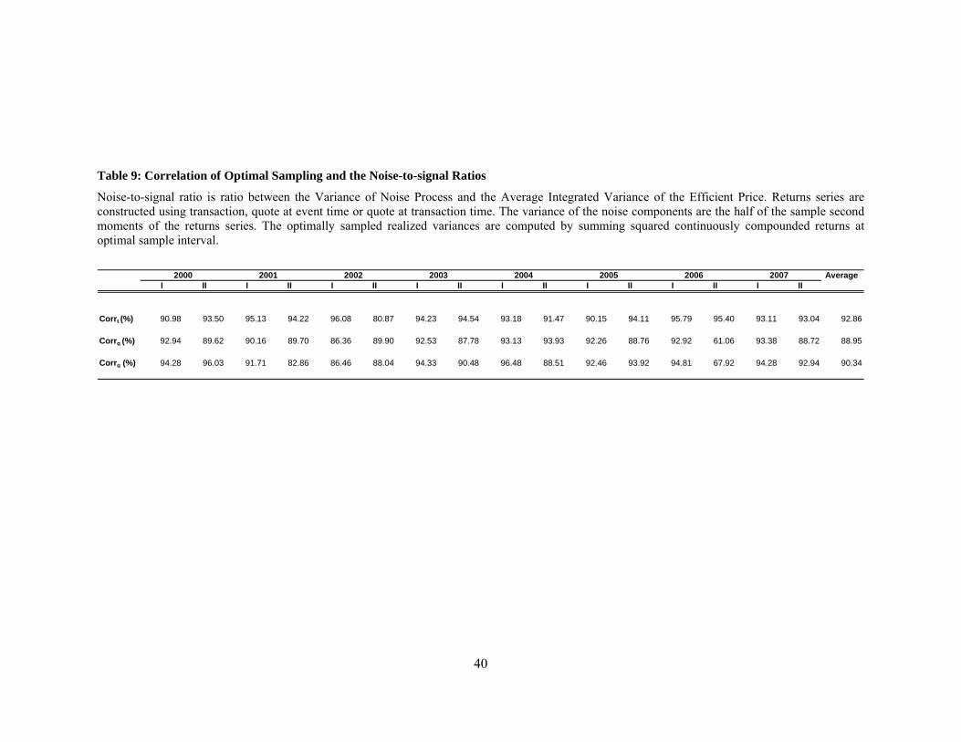
40

Table 9: Correlation of Optimal Sampling and the Noise-to-signal Ratios

Noise-to-signal ratio is ratio between the Variance of Noise Process and the Average Integrated Variance of the Efficient Price. Returns series are constructed using transaction, quote at event time or quote at transaction time. The variance of the noise components are the half of the sample second moments of the returns series. The optimally sampled realized variances are computed by summing squared continuously compounded returns at optimal sample interval.

AverageI II I II I II I II I II I II I II I II

Corrt (%) 90.98 93.50 95.13 94.22 96.08 80.87 94.23 94.54 93.18 91.47 90.15 94.11 95.79 95.40 93.11 93.04 92.86

Corrq (%) 92.94 89.62 90.16 89.70 86.36 89.90 92.53 87.78 93.13 93.93 92.26 88.76 92.92 61.06 93.38 88.72 88.95

Corrq (%) 94.28 96.03 91.71 82.86 86.46 88.04 94.33 90.48 96.48 88.51 92.46 93.92 94.81 67.92 94.28 92.94 90.34

2004 2005 2006 20072000 2001 2002 2003

41

Table 10: Average Efficient Variance

The efficient variance is estimated from optimally sampled daily realized variances based on continuously compounded returns constructed using transactions (t), quote at event time (q) and quote at transaction time (pq). Stocks are classified by the following price faction : 1) more than 5,000 rupiah (P>= 5,000), 2) between 2000 to 5000 rupiah (2000 <= P < 5000), 3) between 500 to 2000 rupiah (500 <= P < 2000) and 4) less than 500 rupiah (P < 500). Open-to-close variance is presented with oc subscript. Variance ratio is ratio between efficient to open-to-close variance.

AverageI II I II I II I II I II I II I II I II

V*t(% p.a.)P >= 5000 68.55 58.61 60.15 65.50 59.34 59.73 44.01 48.33 62.08 48.40 47.30 53.00 61.80 52.79 56.65 70.38 57.29

2000 <= P < 5000 96.32 57.41 49.47 53.52 67.15 76.57 61.11 46.72 58.45 47.35 57.18 62.22 64.02 51.30 71.62 81.55 62.62500 <= P < 2000 119.01 79.48 90.47 85.24 82.15 106.66 88.34 96.67 89.66 70.84 72.28 62.31 70.62 63.52 75.50 82.13 83.43

P < 500 168.29 89.99 95.52 93.07 85.40 100.05 94.78 99.60 85.12 76.51 89.09 95.58 96.01 60.78 106.52 113.36 96.86Average 106.77 78.75 83.99 82.46 77.88 90.42 78.36 86.83 78.76 65.87 69.89 68.31 70.83 58.33 84.29 89.64 79.46

V*q(% p.a.)P >= 5000 71.10 62.36 60.22 65.44 58.38 58.65 44.48 46.96 62.29 49.04 47.10 52.63 61.46 50.78 53.98 68.33 57.08

2000 <= P < 5000 97.66 58.50 52.13 54.73 66.94 76.07 59.44 46.15 58.80 48.12 55.42 61.48 63.11 49.93 70.36 79.35 62.39500 <= P < 2000 128.00 81.42 94.50 90.80 86.22 98.67 82.97 91.34 88.08 67.16 69.65 61.71 69.11 59.83 71.94 79.86 82.58

P < 500 195.49 93.25 99.05 91.88 82.98 100.98 92.30 99.39 91.43 75.47 88.36 87.49 77.13 59.33 100.70 110.27 96.59Average 113.05 81.37 87.24 82.92 77.33 89.13 75.79 84.62 80.11 64.63 68.20 66.09 67.43 55.69 80.17 87.17 78.81

V*pq (% p.a.)P >= 5000 70.39 60.09 60.24 66.37 59.63 59.31 42.88 47.11 61.41 47.05 47.45 51.46 61.67 50.97 55.59 67.51 56.82

2000 <= P < 5000 94.26 55.56 51.74 52.66 68.57 74.73 57.57 46.15 59.02 47.78 56.52 61.48 63.64 49.42 69.40 79.03 61.72500 <= P < 2000 120.61 78.03 91.69 88.50 82.13 95.08 76.10 88.47 84.28 65.77 68.45 61.66 68.03 59.35 71.58 79.90 79.98

P < 500 177.06 90.36 94.39 89.38 82.49 94.95 87.47 97.90 90.05 70.90 86.73 86.55 77.86 61.68 102.70 108.17 93.66Average 107.45 78.41 84.30 80.99 76.78 85.52 71.68 82.99 78.16 62.06 67.66 65.73 67.19 55.58 81.12 86.23 76.99

V*oc (% p.a.)P >= 5000 44.21 37.79 35.68 36.13 39.68 34.90 24.70 31.71 39.53 26.24 27.70 30.81 35.30 29.57 32.19 39.38 34.10

2000 <= P < 5000 58.50 32.71 28.98 31.16 43.60 46.25 34.88 27.42 35.43 25.39 33.51 39.51 38.82 29.19 43.04 45.20 37.10500 <= P < 2000 73.09 44.70 59.20 55.49 49.13 74.23 49.22 54.92 48.52 39.28 41.12 42.32 41.59 36.17 45.44 47.18 50.10

P < 500 142.87 63.14 59.50 60.60 54.18 61.86 54.14 59.71 66.54 51.33 56.16 60.42 48.20 33.61 71.28 68.61 63.26Average 66.91 50.63 52.94 52.28 49.28 56.89 44.42 51.27 50.19 39.86 41.44 44.09 40.76 33.03 53.31 52.13 48.71

Average Daily VRV*t/Voc 1.168 1.147 1.161 1.203 1.187 1.190 1.269 1.221 1.200 1.256 1.231 1.143 1.232 1.279 1.220 1.260 1.210

(4.35) (3.58) (4.63) (2.11) (3.38) (2.88) (4.33) (6.9) (2.36) (2.92) (6.6) (3.15) (2.94) (5.11) (4.98) (7.53) (4.23)V*q/Voc 1.238 1.185 1.233 1.216 1.176 1.170 1.235 1.178 1.198 1.230 1.195 1.125 1.175 1.220 1.157 1.222 1.197

(6.25) (3.89) (4.44) (2.81) (3.05) (2.41) (2.86) (2.93) (2.78) (2.57) (5.87) (2.38) (3.78) (4.89) (3.93) (7.47) (3.89)V*pq/Voc 1.182 1.144 1.200 1.190 1.165 1.131 1.165 1.158 1.173 1.182 1.188 1.114 1.171 1.218 1.165 1.209 1.172

(4.24) (3.53) (4.36) (2.04) (2.8) (2.09) (2.68) (3.33) (2.83) (2.33) (5.04) (2.47) (5.58) (4.88) (4.27) (7.42) (3.74)

2004 2005 2006 20072000 2001 2002 2003

42

Table 11: Regression of the Noise Standard Deviation on the Standard Deviation of Efficient Price Variance

The table presents outcome from regression of noise standard deviation against the standard deviation of efficient price variance ( *V ) The standard deviation of the noise components are the square root of half the sample second moments of the quote-to-quote continuously compounded returns. The standard deviation of efficient price variance is square root of the average daily realized variance sampled at optimal frequency.

I II I II I II I II I II I II I II I IITrades

Intercept -0.0028 -0.0017 -0.0003 -0.0011 -0.0030 -0.0001 -0.0017 -0.0007 -0.0013 -0.0012 -0.0015 -0.0008 -0.0004 -0.0003 -0.0009 -0.0009(-3.00) (-1.85) (-0.34) (-1.25) (-3.22) (-0.06) (-1.42) (-1.12) (-1.91) (-2.15) (-3.18) (-1.45) (-0.61) (-0.76) (-2.07) (-1.85)

0.1566 0.1636 0.1257 0.1598 0.2024 0.1170 0.1745 0.1396 0.1635 0.1701 0.1479 0.1298 0.1028 0.1106 0.1152 0.0986(8.82) (6.56) (5.12) (7.03) (7.82) (4.14) (5.29) (9.92) (8.86) (9.45) (10.09) (7.93) (5.57) (7.34) (10.75) (8.79)

R2 96.42 92.89 90.35 79.41 74.12 82.66 93.87 91.90 47.78 69.95 87.80 71.70 82.07 73.51 93.42 90.12Quotes at event time

Intercept 0.0001 -0.0010 -0.0004 -0.0020 -0.0011 0.0015 -0.0009 -0.0001 -0.0004 -0.0007 -0.0002 -0.0003 0.0006 0.0000 -0.0010 -0.0004(0.19) (-1.52) (-0.63) (-2.8) (-2.19) (1.96) (-1.45) (-0.25) (-0.87) (-1.61) (-0.68) (-0.94) (1.5) (0.13) (-3.57) (-1.04)

0.0584 0.0989 0.0864 0.1303 0.1027 0.0275 0.0951 0.0744 0.0840 0.0906 0.0699 0.0707 0.0356 0.0607 0.0820 0.0517(5.43) (5.9) (5.37) (7.24) (7.47) (1.58) (5.6) (9.77) (6.37) (6.5) (7.01) (8.2) (2.7) (4.43) (11.12) (6.17)

R2 50.42 51.34 50.74 66.03 65.79 11.09 66.23 76.71 55.90 56.12 55.74 62.72 16.45 35.97 73.75 48.80Prevailing quotes

Intercept -0.0001 -0.0019 -0.0009 -0.0010 -0.0013 0.0016 -0.0010 -0.0004 -0.0012 -0.0014 -0.0010 -0.0008 0.0005 -0.0006 -0.0013 -0.0006(-0.08) (-2.02) (-0.9) (-1.11) (-1.58) (1.45) (-1.01) (-0.82) (-2.06) (-2.95) (-2.31) (-1.79) (0.9) (-1.39) (-3.19) (-1.58)

0.0754 0.1441 0.1158 0.1242 0.1230 0.0379 0.1199 0.0977 0.1230 0.1330 0.1038 0.0986 0.0505 0.0914 0.0943 0.0612(4.61) (5.77) (4.83) (5.28) (5.32) (1.41) (4.26) (9) (7.63) (8.42) (7.98) (7.27) (2.71) (5.9) (9.11) (6.8)

R2 42.31 50.21 45.47 50.84 49.43 9.08 53.09 73.62 64.56 68.26 62.03 56.95 16.53 49.89 65.35 53.62

2004 2005 2006 20072000 2001 2002 2003

*V

*V

*V