AIP ADVANCES 1, 022127 (2011)

Hidden temporal order unveiled in stock market volatilityvariance

Y. Shapira, D. Y. Kenett, Ohad Raviv, and E. Ben-Jacoba

School of Physics and Astronomy, Tel-Aviv University, Tel-Aviv 69978, Israel

(Received 16 March 2011; accepted 2 May 2011; published online 27 May 2011)

When analyzed by standard statistical methods, the time series of the daily return offinancial indices appear to behave as Markov random series with no apparent temporalorder or memory. This empirical result seems to be counter intuitive since investor areinfluenced by both short and long term past market behaviors. Consequently mucheffort has been devoted to unveil hidden temporal order in the market dynamics.Here we show that temporal order is hidden in the series of the variance of thestocks volatility. First we show that the correlation between the variances of the dailyreturns and means of segments of these time series is very large and thus cannotbe the output of random series, unless it has some temporal order in it. Next weshow that while the temporal order does not show in the series of the daily return,rather in the variation of the corresponding volatility series. More specifically, wefound that the behavior of the shuffled time series is equivalent to that of a randomtime series, while that of the original time series have large deviations from theexpected random behavior, which is the result of temporal structure. We found thesame generic behavior in 10 different stock markets from 7 different countries. Wealso present analysis of specially constructed sequences in order to better understandthe origin of the observed temporal order in the market sequences. Each sequencewas constructed from segments with equal number of elements taken from algebraicdistributions of three different slopes. C© 2011 Author(s). This article is distributedunder a Creative Commons Attribution Non-Commercial Share Alike 3.0 UnportedLicense. [doi:10.1063/1.3598412]

I. INTRODUCTION

In many models of financial markets, the statistical properties of the price change are the mostimportant factors.1–7 For example, these statistical properties are widely used in the pricing ofderivatives, where the stochastic behavior of the price of the asset is the key factor for determiningthe price of the derivative product. Many stochastic models of stock market price dynamics useBrownian motion like process,8, 9 where increments of the log of the price are randomly generatedfrom a distribution that is derived from empirical data. Usually, the distribution is Gaussian ora truncated Levy flight (to express the leptokurtic nature of the empirical data) or other similardistributions.2, 10–18 According to these models, the price is the result of a random walk, where theincrements are randomly chosen.

This approach is supported in part, by the observation that price changes in financial marketshave practically no memory, and the autocorrelation function of time changes of the price has acharacteristic time scale of a few trading minutes.19

However, many traders use technical analysis to support their trading decisions. According tothis approach, one can predict the future course of a financial assets price, by analyzing the timeevolution of the price and the volume of the asset, and that the past provides clues about futurechanges. This approach seems to contradict the above description of random increments. A possible

aAuthor to whom correspondence should be addressed. Electronic mail: eshelbj@gmail.com

2158-3226/2011/1(2)/022127/14 C© Author(s) 20111, 022127-1

Downloaded 14 Jun 2011 to 96.255.211.14. Content is licensed under a Creative Commons Attribution Non-Commercial Share Alike 3.0 Unported licenseSee: http://creativecommons.org/licenses/by-nc-sa/3.0/

022127-2 Shapira et al. AIP Advances 1, 022127 (2011)

TABLE I. Summary of data. The data used in this work is for 10 different index’s, from 7 countries, for different number oftrading days N, and for long periods.

Country Index N Period

USA S&P500 15035 1950 - 2010DJIA 20343 1930 - 2010NASDAQ 9772 1975 – 2010

U.K. FTSE100 6444 1985 – 2010Japan NIKKEI225 6351 1985 – 2010Hong-Kong Hang-Seng 5664 1990 – 2010Germany Dax 4779 1990 – 2010France CAC40 4996 1990 – 2010Israel TA25 2250 2001 – 2010

TA100 2555 1998 - 2010

explanation that can combine both points of view is the existence of local temporal order in timeseries of financial markets.

One way to identify this temporal order is by comparing the original time series with the sametime series after shuffling. Shuffling preserves the statistical properties of the time series, whileerasing any temporal order. Analyzing the statistical properties of the time series is insensitive toshuffling and to any temporal order.

Here we show that while the existence of temporal order is not transparent in the change of theprice in financial time series, looking at the volatility, the temporal order becomes very prominent.It is easily observed that there are periods of calm activity and other periods of very turbulentactivity.10, 18, 20–25 This is also observed by looking at the standard deviations used for derivativepricing, or by looking at the VIX Index (“fear index”).26

It was previously shown that non linear functions of the price change, like the local variance orthe local average of the absolute value, have large autocorrelation values of few days, and as such amuch longer memory, than the price change itself.23, 25

II. THE DATA SETS

We analyzed long time data sets of 10 different stock markets from 7 different countries(U.S.A, U.K., Japan, Hong-Kong, Germany, France and Israel) downloaded from Yahoo Finance(www.yahoo.com/finance). The summary of index’s and length of time series is presented inTable I.

For each market J, we analyzed the log of the daily return of the market Index RJ (n), givenby:8, 27

RJ (n) ≡ ln [PJ (n)] − ln [PJ (n − 1)] (1)

where [PJ (n)] is the daily adjusted closing price of the Index of market (J) at day (n). Since similarresults were revealed for each of the markets, we present in details the analyses and the results forthe UK FTSE-100 Index. The reasons for selecting this market are that the data set is for 25 years,which is the typical time length of all the data sets and this market also represents a mature marketwith typical size.

In Figure 1(a) we show the time evolvement of the closing prices of the FTSE Index - PFT SE (n),for 6725 trading days (about 25 years) and in Figures 1(b) we show the corresponding log of thedaily return - RFT SE (n). Visual inspection of Figure 1(b) reveal time intervals of large magnitudevariability in RFT SE (n). Comparison between Figure 1(b) and Figure 1(a) further reveals thatthese time intervals correspond to events of sharp minima in PFT SE (n). First indication about theexistence of hidden temporal order are revealed by visual comparison between the original dailyreturn sequence RFT SE (n) and its shuffled version - RSFT SE (n), shown in Figure 1(c). As was

Downloaded 14 Jun 2011 to 96.255.211.14. Content is licensed under a Creative Commons Attribution Non-Commercial Share Alike 3.0 Unported licenseSee: http://creativecommons.org/licenses/by-nc-sa/3.0/

022127-3 Shapira et al. AIP Advances 1, 022127 (2011)

FIG. 1. Time evolvement of the UK FTSE100 Index. (A) The closing price of FTSE Index, PFT SE (n), for 6725 tradingdays (about 25 years). (B) The corresponding daily return - RFT SE (n) for the same period. (C) A typical realization of thetime evolvement of a shuffled version - RFT SE (n), of the original daily return sequence RFT SE (n).

Downloaded 14 Jun 2011 to 96.255.211.14. Content is licensed under a Creative Commons Attribution Non-Commercial Share Alike 3.0 Unported licenseSee: http://creativecommons.org/licenses/by-nc-sa/3.0/

022127-4 Shapira et al. AIP Advances 1, 022127 (2011)

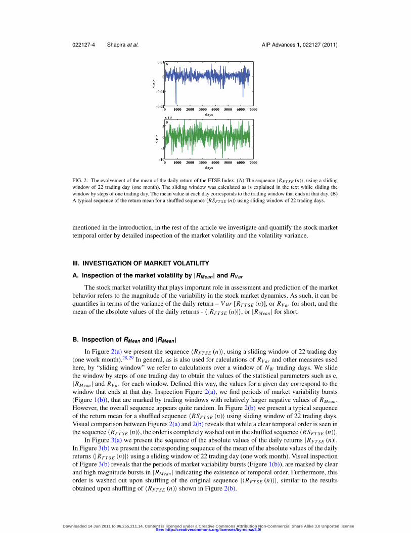
FIG. 2. The evolvement of the mean of the daily return of the FTSE Index. (A) The sequence 〈RFT SE (n)〉, using a slidingwindow of 22 trading day (one month). The sliding window was calculated as is explained in the text while sliding thewindow by steps of one trading day. The mean value at each day corresponds to the trading window that ends at that day. (B)A typical sequence of the return mean for a shuffled sequence 〈RSFT SE (n)〉 using sliding window of 22 trading days.

mentioned in the introduction, in the rest of the article we investigate and quantify the stock markettemporal order by detailed inspection of the market volatility and the volatility variance.

III. INVESTIGATION OF MARKET VOLATILITY

A. Inspection of the market volatility by |RMean| and RVar

The stock market volatility that plays important role in assessment and prediction of the marketbehavior refers to the magnitude of the variability in the stock market dynamics. As such, it can bequantifies in terms of the variance of the daily return – V ar [RFT SE (n)], or RV ar for short, and themean of the absolute values of the daily returns - 〈|RFT SE (n)|〉, or |RMean| for short.

B. Inspection of RMean and |RMean|In Figure 2(a) we present the sequence 〈RFT SE (n)〉, using a sliding window of 22 trading day

(one work month).28, 29 In general, as is also used for calculations of RV ar and other measures usedhere, by “sliding window” we refer to calculations over a window of NW trading days. We slidethe window by steps of one trading day to obtain the values of the statistical parameters such as c,|RMean| and RV ar for each window. Defined this way, the values for a given day correspond to thewindow that ends at that day. Inspection Figure 2(a), we find periods of market variability bursts(Figure 1(b)), that are marked by trading windows with relatively larger negative values of RMean .However, the overall sequence appears quite random. In Figure 2(b) we present a typical sequenceof the return mean for a shuffled sequence 〈RSFT SE (n)〉 using sliding window of 22 trading days.Visual comparison between Figures 2(a) and 2(b) reveals that while a clear temporal order is seen inthe sequence 〈RFT SE (n)〉, the order is completely washed out in the shuffled sequence 〈RSFT SE (n)〉.

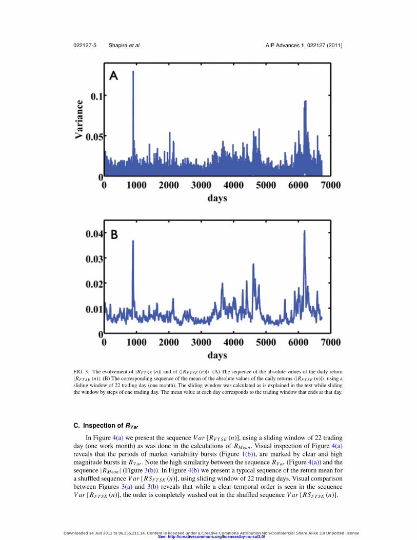
In Figure 3(a) we present the sequence of the absolute values of the daily returns |RFT SE (n)|.In Figure 3(b) we present the corresponding sequence of the mean of the absolute values of the dailyreturns 〈|RFT SE (n)|〉 using a sliding window of 22 trading day (one work month). Visual inspectionof Figure 3(b) reveals that the periods of market variability bursts (Figure 1(b)), are marked by clearand high magnitude bursts in |RMean| indicating the existence of temporal order. Furthermore, thisorder is washed out upon shuffling of the original sequence |〈RFT SE (n)〉|, similar to the resultsobtained upon shuffling of 〈RFT SE (n)〉 shown in Figure 2(b).

Downloaded 14 Jun 2011 to 96.255.211.14. Content is licensed under a Creative Commons Attribution Non-Commercial Share Alike 3.0 Unported licenseSee: http://creativecommons.org/licenses/by-nc-sa/3.0/

022127-5 Shapira et al. AIP Advances 1, 022127 (2011)

FIG. 3. The evolvement of |RFT SE (n)| and of 〈|RFT SE (n)|〉. (A) The sequence of the absolute values of the daily return|RFT SE (n)|. (B) The corresponding sequence of the mean of the absolute values of the daily returns 〈|RFT SE (n)|〉, using asliding window of 22 trading day (one month). The sliding window was calculated as is explained in the text while slidingthe window by steps of one trading day. The mean value at each day corresponds to the trading window that ends at that day.

C. Inspection of RVar

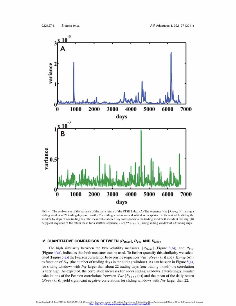
In Figure 4(a) we present the sequence V ar [RFT SE (n)], using a sliding window of 22 tradingday (one work month) as was done in the calculations of RMean . Visual inspection of Figure 4(a)reveals that the periods of market variability bursts (Figure 1(b)), are marked by clear and highmagnitude bursts in RV ar . Note the high similarity between the sequence RV ar (Figure 4(a)) and thesequence |RMean| (Figure 3(b)). In Figure 4(b) we present a typical sequence of the return mean fora shuffled sequence V ar [RSFT SE (n)], using sliding window of 22 trading days. Visual comparisonbetween Figures 3(a) and 3(b) reveals that while a clear temporal order is seen in the sequenceV ar [RFT SE (n)], the order is completely washed out in the shuffled sequence V ar [RSFT SE (n)].

Downloaded 14 Jun 2011 to 96.255.211.14. Content is licensed under a Creative Commons Attribution Non-Commercial Share Alike 3.0 Unported licenseSee: http://creativecommons.org/licenses/by-nc-sa/3.0/

022127-6 Shapira et al. AIP Advances 1, 022127 (2011)

FIG. 4. The evolvement of the variance of the daily return of the FTSE Index. (A) The sequence V ar [RFT SE (n)], using asliding window of 22 trading day (one month). The sliding window was calculated as is explained in the text while sliding thewindow by steps of one trading day. The mean value at each day corresponds to the trading window that ends at that day. (B)A typical sequence of the return mean for a shuffled sequence V ar [RSFT SE (n)] using sliding window of 22 trading days.

IV. QUANTITATIVE COMPARISON BETWEEN |RMean|, RVar AND RMean

The high similarity between the two volatility measures, |RMean| (Figure 3(b)), and RV ar

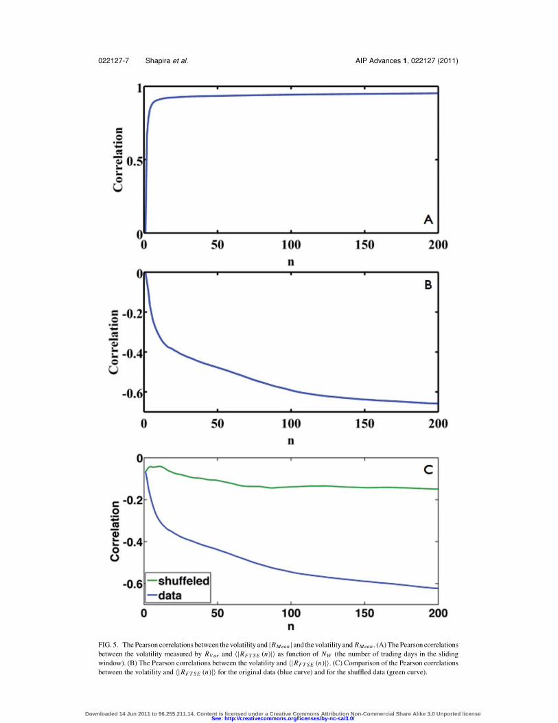
(Figure 4(a)), indicates that both measures can be used. To further quantify this similarity we calcu-lated (Figure 5(a)) the Pearson correlation between the sequences V ar [RFT SE (n)] and 〈|RFT SE (n)|〉as function of NW (the number of trading days in the sliding window). As can be seen in Figure 5(a),for sliding windows with NW larger than about 22 trading days (one trading month) the correlationis very high. As expected, the correlation increases for wider sliding windows. Interestingly, similarcalculations of the Pearson correlations between V ar [RFT SE (n)] and the mean of the daily return〈RFT SE (n)〉, yield significant negative correlations for sliding windows with NW larger than 22.

Downloaded 14 Jun 2011 to 96.255.211.14. Content is licensed under a Creative Commons Attribution Non-Commercial Share Alike 3.0 Unported licenseSee: http://creativecommons.org/licenses/by-nc-sa/3.0/

022127-7 Shapira et al. AIP Advances 1, 022127 (2011)

FIG. 5. The Pearson correlations between the volatility and |RMean | and the volatility and RMean . (A) The Pearson correlationsbetween the volatility measured by RV ar and 〈|RFT SE (n)|〉 as function of NW (the number of trading days in the slidingwindow). (B) The Pearson correlations between the volatility and 〈|RFT SE (n)|〉. (C) Comparison of the Pearson correlationsbetween the volatility and 〈|RFT SE (n)|〉 for the original data (blue curve) and for the shuffled data (green curve).

Downloaded 14 Jun 2011 to 96.255.211.14. Content is licensed under a Creative Commons Attribution Non-Commercial Share Alike 3.0 Unported licenseSee: http://creativecommons.org/licenses/by-nc-sa/3.0/

022127-8 Shapira et al. AIP Advances 1, 022127 (2011)

One of the fundamental assumptions in the core of most market theories is that the daily returnsbehave like random Markov sequences. However, the results shown in Figure 5 indicate the existenceof hidden temporal order and that the daily returns might not behave like random Markov sequences.To further assess this possibility and quantify the putative temporal order we investigated the varianceof the market volatility as is described in the next section.

V. THE VOLATILITY VARIANCE

In this section we present a detailed analysis of the variance of the volatility of the dailyreturn sequence RFT SE (n). More specifically, we present analyses of the “Variance of Variance”–the variance of the volatility as measured by V ar [RFT SE (n)]. We note that similar results areobtained by analyzing the variance of the volatility when it is measured by 〈|RFT SE (n)|〉. We foundsignificant deviation between the volatility variance of the original sequence V ar [RFT SE (n)], andthe corresponding shuffled version V ar [RSFT SE (n)]. As control, we show that the variance of themean of the original sequence 〈RFT SE (n)〉, and the variance of the mean of the shuffled sequence〈RSFT SE (n)〉, are similar. We found that the variance of the mean 〈RFT SE (n)〉 (or V ar [RMean] forshort), of the shuffled mean 〈RSFT SE (n)〉 (or V ar [RSMean] for short), and of the shuffled volatilityV ar [RSFT SE (n)] (or V ar [RSV ar ] for short), scale as 1/NW which is the expected result in theabsence of temporal order (a random Markov sequence). In contrast, the dependence of the varianceof the volatility of the original sequence V ar [RFT SE (n)] (or V ar [RV ar ] for short), on NW issignificantly different.

A. The variance of the mean and volatility of a random Markov sequence

Let have an infinite random Markov sequence whose element (n) is denoted by RM (n) andRMMean (NW ) denotes the mean of a segment of NW elements, while V ar [RM (NW )] denotes thevariance of a segment of NW elements. It is known that30–32 the variance scaling of the mean ofrandomly selected such segments is give by,

V ar [RMmean (Nw)] = V ar [RM]

NW(2)

and

V ar {V ar [RMmean (Nw)]} = V ar [RM]2 ·[

2

NW − 1+ K urt [RM]

NW

](3)

Where, K urt [RM] is the Kurtosis of the sequence. For segments of NW elements taken out of afinite population - N. The variance scaling is given by,

V ar [RMmean (Nw)] = V ar [RM] · (N − NW )

N · NW(4)

Note that this result convergences to the result for infinite sequence (Eq. (2)), for N >> NW . Thevariance of the variance for segments of NW elements taken out of a finite population, N, for N >> 1is given by,

V ar {V ar [RMmean (Nw)]} = V ar [RM]2 · (N − NW )

N·[

2

NW − 1+ K urt [RM]

NW

](5)

Note that this result also converges for the results for infinite sequence (Eq. (3)), for N >> NW .

B. The NW dependence of Var [RMean] and Var [RSMean]

Visual inspections of RSMean (Figure 2(b)) revealed that it looks like a random sequence.Some features of relatively large negative values are observed in the original RMean at the periodsof large market variability, yet the overall pattern of the sequence also appears (to the eye) to berandom. To test and quantify these visual inspections we plotted V ar [RMean] and V ar [RSMean] as

Downloaded 14 Jun 2011 to 96.255.211.14. Content is licensed under a Creative Commons Attribution Non-Commercial Share Alike 3.0 Unported licenseSee: http://creativecommons.org/licenses/by-nc-sa/3.0/

022127-9 Shapira et al. AIP Advances 1, 022127 (2011)

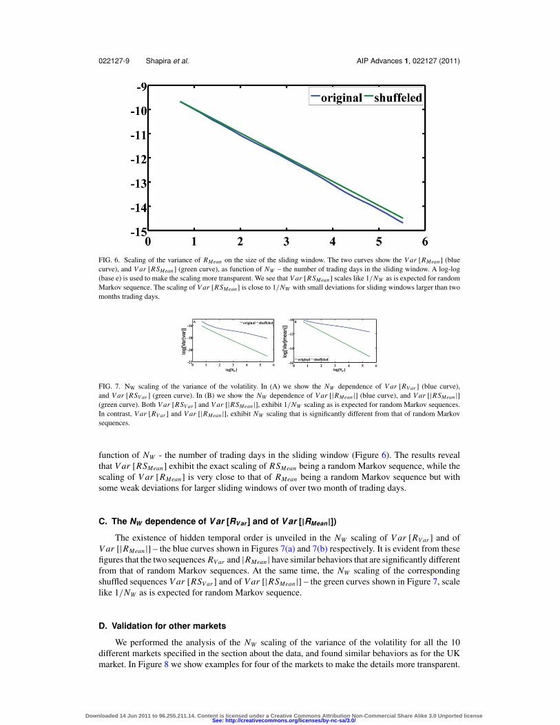
FIG. 6. Scaling of the variance of RMean on the size of the sliding window. The two curves show the V ar [RMean] (bluecurve), and V ar [RSMean] (green curve), as function of NW – the number of trading days in the sliding window. A log-log(base e) is used to make the scaling more transparent. We see that V ar [RSMean] scales like 1/NW as is expected for randomMarkov sequence. The scaling of V ar [RSMean] is close to 1/NW with small deviations for sliding windows larger than twomonths trading days.

FIG. 7. NW scaling of the variance of the volatility. In (A) we show the NW dependence of V ar [RV ar ] (blue curve),and V ar [RSV ar ] (green curve). In (B) we show the NW dependence of V ar [|RMean |] (blue curve), and V ar [|RSMean |](green curve). Both V ar [RSV ar ] and V ar [|RSMean |], exhibit 1/NW scaling as is expected for random Markov sequences.In contrast, V ar [RV ar ] and V ar [|RMean |], exhibit NW scaling that is significantly different from that of random Markovsequences.

function of NW - the number of trading days in the sliding window (Figure 6). The results revealthat V ar [RSMean] exhibit the exact scaling of RSMean being a random Markov sequence, while thescaling of V ar [RMean] is very close to that of RMean being a random Markov sequence but withsome weak deviations for larger sliding windows of over two month of trading days.

C. The NW dependence of Var [RVar ] and of Var [|RMean|])The existence of hidden temporal order is unveiled in the NW scaling of V ar [RV ar ] and of

V ar [|RMean|] – the blue curves shown in Figures 7(a) and 7(b) respectively. It is evident from thesefigures that the two sequences RV ar and |RMean| have similar behaviors that are significantly differentfrom that of random Markov sequences. At the same time, the NW scaling of the correspondingshuffled sequences V ar [RSV ar ] and of V ar [|RSMean|] – the green curves shown in Figure 7, scalelike 1/NW as is expected for random Markov sequence.

D. Validation for other markets

We performed the analysis of the NW scaling of the variance of the volatility for all the 10different markets specified in the section about the data, and found similar behaviors as for the UKmarket. In Figure 8 we show examples for four of the markets to make the details more transparent.

Downloaded 14 Jun 2011 to 96.255.211.14. Content is licensed under a Creative Commons Attribution Non-Commercial Share Alike 3.0 Unported licenseSee: http://creativecommons.org/licenses/by-nc-sa/3.0/

022127-10 Shapira et al. AIP Advances 1, 022127 (2011)

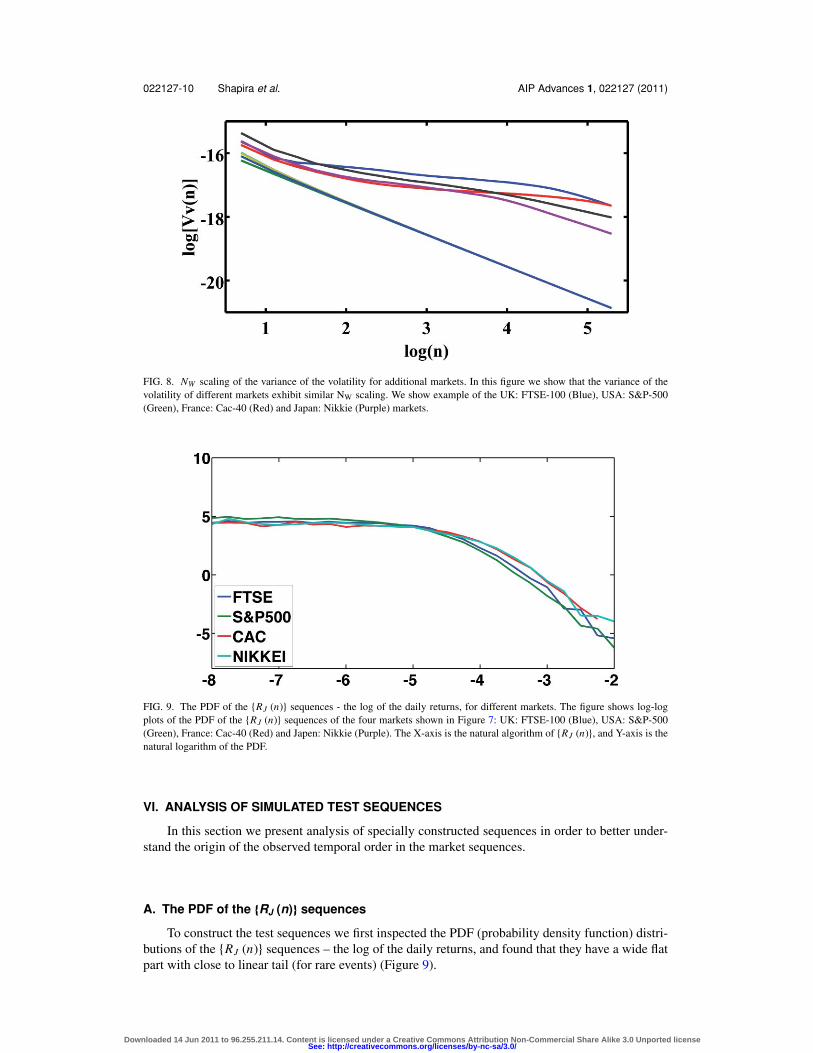
FIG. 8. NW scaling of the variance of the volatility for additional markets. In this figure we show that the variance of thevolatility of different markets exhibit similar NW scaling. We show example of the UK: FTSE-100 (Blue), USA: S&P-500(Green), France: Cac-40 (Red) and Japan: Nikkie (Purple) markets.

FIG. 9. The PDF of the {RJ (n)} sequences - the log of the daily returns, for different markets. The figure shows log-logplots of the PDF of the {RJ (n)} sequences of the four markets shown in Figure 7: UK: FTSE-100 (Blue), USA: S&P-500(Green), France: Cac-40 (Red) and Japen: Nikkie (Purple). The X-axis is the natural algorithm of {RJ (n)}, and Y-axis is thenatural logarithm of the PDF.

VI. ANALYSIS OF SIMULATED TEST SEQUENCES

In this section we present analysis of specially constructed sequences in order to better under-stand the origin of the observed temporal order in the market sequences.

A. The PDF of the {RJ (n)} sequences

To construct the test sequences we first inspected the PDF (probability density function) distri-butions of the {RJ (n)} sequences – the log of the daily returns, and found that they have a wide flatpart with close to linear tail (for rare events) (Figure 9).

Downloaded 14 Jun 2011 to 96.255.211.14. Content is licensed under a Creative Commons Attribution Non-Commercial Share Alike 3.0 Unported licenseSee: http://creativecommons.org/licenses/by-nc-sa/3.0/

022127-11 Shapira et al. AIP Advances 1, 022127 (2011)

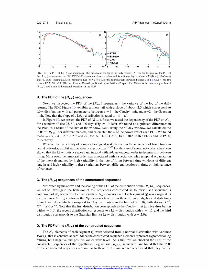
FIG. 10. The PDF of the {RV ar } sequences – the variance of the log of the daily returns. (A) The log-log plots of the PDF ofthe {RV ar } sequence for the UK: FTSE-100 when the variance is calculated for different NW windows – 25 (Blue), 50 (Green)and 100 (Red) trading days. (B) Similar to (A) for NW = 50, for the four markets shown in Figures 7 and 8: UK: FTSE-100(Blue), USA: S&P-500 (Green), France: Cac-40 (Red) and Japen: Nikkie (Purple). The X-axis is the natural algorithm of{RV ar }, and Y-axis is the natural logarithm of the PDF.

B. The PDF of the {RVar } sequences

Next, we inspected the PDF of the {RV ar } sequences – the variance of the log of the dailyreturns. The PDF, Figure 10, exhibits a linear tail with a slope of about -2.5 which correspond toLevy distributions with tail parameter α between α = 1 - the Cauchy limit, and α=2 - the Gaussianlimit. Note that the slope of a Levy distribution is equal to –(1+ α).

In Figure 10, we present the PDF of {RV ar }. First, we tested the dependency of the PDF on NW ,

for a window of size 25, 50, and 100 days (Figure 10, left). We found no significant differences inthe PDF, as a result of the size of the window. Next, using the 50 day window, we calculated thePDF of {RV ar }, for different markets, and calculated the α of the power law of each PDF. We foundthat α = 2.5, 2.4, 2.2, 2.2, 2.9, and 2.6, for the FTSE, CAC, DAX, DJIA, NIKKEI225 and S&P500,respectively.

We note that the activity of complex biological systems such as the sequences of firing times inneural networks, exhibit similar statistical properties.32–37 For the case of neural networks, it has beenshown that the Levy statistics goes hand in hand with hidden temporal order in the intervals betweenfiring. More over, the temporal order was associated with a special complex temporal organizationof the intervals marked by high variability in the rate of firing between time windows of differentlengths and high variability in these variations between different locations in time, or high varianceof variance.

C. The {RVar } sequences of the constructed sequences

Motivated by the above and the scaling of the PDF of the distribution of the {RJ (n)} sequences,we set to investigate the behavior of test sequences constructed as follows: Each sequence iscomposed of NS segments of equal length of NE elements each. Each segment (j) was assigned itsown variance V ar ( j) between the NE elements taken from three different algebraic distributions(pure linear slope which correspond to Levy distribution in the limit of γ = 0), with slopes: X−2,X−2.5 and X−3. Note that the first distribution corresponds to the Cauchy limit (a Levy distributionwith α = 1.0), the second distribution corresponds to a Levy distribution with α = 1.5, and the thirddistribution corresponds to the Gaussian limit (a Levy distribution with α = 2.0).

D. The PDF of the {RVar } of the constructed sequences

The NE elements of each segment (j) were selected from a normal distribution with varianceV ar ( j) that is centered at zero. Since the constructed sequence elements represent hypothetical logreturns, both negative and positive values were taken. As a first test we checked the PDF of theconstructed sequences of the hypothetical log returns {RJ (n)}sequences. We found that the PDFof the constructed sequences are similar to those of the market sequences and that they can be

Downloaded 14 Jun 2011 to 96.255.211.14. Content is licensed under a Creative Commons Attribution Non-Commercial Share Alike 3.0 Unported licenseSee: http://creativecommons.org/licenses/by-nc-sa/3.0/

022127-12 Shapira et al. AIP Advances 1, 022127 (2011)

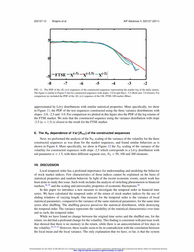
FIG. 11. The PDF of the {RJ (n)} sequences of the constructed sequences representing the market log of the daily returns.The figure is similar to Figure 9, but for constructed sequences with slopes -2.0 (Light blue), -2.5 (Red) and -3.0 (Green). Forcomparison we included the PDF of the {RJ (n)} sequence of the UK: FTSE-100 market (Blue).

approximated by Levy distributions with similar statistical properties. More specifically, we showin Figure 11, the PDF of the test sequences constructed using the three variance distributions withslopes -2.0, -2.5 and -3.0. For comparison we plotted in this figure also the PDF of the log returns ofthe FTSE market. We note that the constructed sequence using the variance distribution with slope-2.5 (α = 1.5) is closest to the result for the FTSE market.

E. The NW dependence of Var [RVar ] of the constructed sequences

Next, we performed the analysis of the NW scaling of the variance of the volatility for the threeconstructed sequences as was done for the market sequences, and found similar behaviors as isshown in Figure 8. More specifically, we show in Figure 12 the NW scaling of the variance of thevolatility for constructed sequences with slope -2.5 which corresponds to a Levy distribution withtail parameter α = 1.5, with three different segment size, NE = 50, 100 and 200 elements.

VII. DISCUSSION

Local temporal order has a profound importance for understanding and modeling the behaviorof stock market indices. Few characteristics of those indices cannot be explained on the basis ofstatistical properties and random behavior. In light of the recent economic events, much work hasbeen done to study this issue. Such work includes the analysis of switching phenomenon in financialmarkets,38, 39 and the scaling and universality properties of economic fluctuations.40

In this paper we introduce a new measure to investigate the temporal order in financial timeseries. We have calculated the temporal order of the return of stock market indices by the use ofsliding windows of varying length. Our measure for the temporal order is the variance of localstatistical parameters, compared to the variance of the same statistical parameters, for the same timeseries after shuffling. The shuffling process preserves the statistical distribution, while destroyingthe temporal order. The variance represents the variability of the statistical characteristics over timeand as such, the temporal order.

While we have found no change between the original time series and the shuffled one, for thereturn, we did find a profound change for the volatility. This finding is consistent with previous workthat showed that there is no memory in the return, while there is an autocorrelation of few days inthe volatility.20, 23, 25 However, these results seem to be in contradiction with the correlation betweenthe local mean and the local variance. The only explanation that we have, so far, is that the system

Downloaded 14 Jun 2011 to 96.255.211.14. Content is licensed under a Creative Commons Attribution Non-Commercial Share Alike 3.0 Unported licenseSee: http://creativecommons.org/licenses/by-nc-sa/3.0/

022127-13 Shapira et al. AIP Advances 1, 022127 (2011)

FIG. 12. NW scaling of the variance of the volatility for constructed sequences. This figure is similar to Figure 7 in which weshow the NW scaling of the variance of the volatility for different markets, but here we show the results for three constructedsequences with slope -2.5 and NE = 50 (Purple), 100 (Pink) and 200 (Red) elements. For comparison we also show the resultsfor the UK: FTSE-100 market (Blue). The linear curves are the results of the NW scaling of the variance of the volatility ofthe corresponding shuffled sequences.

is very “noisy” and the standard deviation is, at least, an order of magnitude greater than the meanof the return.

We have constructed a simple model that combines random changes in the volatility, over definedsegments, with random changes of the return subject to the volatility in that segment. This modelgave very nice results for the variance of the volatility and for the probability distribution function ofthe return. The success of the model emphasis the importance of the volatility and the local temporalorder for understanding and modeling stock market indices, in addition to the importance of thevolatility for assessing risk in financial markets.

The stock market is a complex system, with the time series of the change in the daily closingprice the output of such system. We can characterize these time series by their probability distributionfunction, which expresses its random character, and by the temporal order of its elements in differenttime periods. The complexity of the system can be characterized by the amount of temporal orderin it, while the PDF characterize its amount of order.

In summary, our methodology can be used as a quantitative measure for the amount of localtemporal order. For any specific sample length n, the comparison between the variance of the samplesvolatility for the original series and that of the shuffled one can be used as a measure for the temporalorder for that specific n. Repeating that procedure for each value of n, we get an integral measure forthe temporal order. Furthermore, it seems that the volatility is very important for technical analysis.Our results suggest that traders who use technical analysis should use local temporal behavior of thevolatility, besides local temporal order of the return and the trade volume.

ACKNOWLEDGMENTS

We wish to thank Shelly Zacks for his input, comments and insights on this work presentedin this paper. This research has been supported in part by the Tauber family Foundation and theMaguy-Glass Chair in the Physics of Complex Systems at Tel Aviv University.

1 X. Gabaix, P. Gopikrishnan, V. Plerou and H. Eugene Stanley, Journal of Economic Dynamics and Control 32 (1), 303–319(2008).

2 D. Horvath, M. Gmitra and Z. Kuscsik, Physica A: Statistical Mechanics and its Applications 361 (2), 589–605 (2006).3 T. Kaizoji, S. Bornholdt and Y. Fujiwara, Physica A: Statistical Mechanics and its Applications 316 (1-4), 441–452 (2002).4 F. Lillo and R. N. Mantegna, European Physical Journal B 20 (4), 503–509 (2001).5 F. Michael and M. D. Johnson, Physica A: Statistical Mechanics and its Applications 320, 525–534 (2003).

Downloaded 14 Jun 2011 to 96.255.211.14. Content is licensed under a Creative Commons Attribution Non-Commercial Share Alike 3.0 Unported licenseSee: http://creativecommons.org/licenses/by-nc-sa/3.0/

022127-14 Shapira et al. AIP Advances 1, 022127 (2011)

6 J. D. Noh, Physical Review E 61 (5), 5981–5982 (2000).7 J.-S. Yang, S. Chae, W.-S. Jung and H.-T. Moon, Physica A: Statistical Mechanics and its Applications 363 (2), 377–382

(2006).8 R. N. Mantegna and H. E. Stanley, An Introduction to Econophysics: Correlation and Complexity in Finance. (Cambridge

University Press, Cambridge, UK, 2000).9 M. F. M. Osborne, Operations Research 7, 145–173 (1959).

10 P. Gopikrishnan, V. Plerou, Y. Liu, L. A. N. Amaral, X. Gabaix and H. E. Stanley, Physica A: Statistical Mechanics and itsApplications 287 (3-4), 362–373 (2000).

11 S. Jaroszewicz, M. C. Mariani and M. Ferraro, Physica A: Statistical Mechanics and its Applications 355 (2-4), 461–474(2005).

12 M. Levy and S. Solomon, Physica A 242 (1-2), 90–94 (1997).13 R. N. Mantegna, Physica A 179 (2), 232–242 (1991).14 R. N. Mantegna and H. E. Stanley, Journal of Statistical Physics 89 (1-2), 469–479 (1997).15 M. C. Mariani, J. D. Libbin, V. Kumar Mani, M. P. Beccar Varela, C. A. Erickson and D. J. Valles-Rosales, Physica A:

Statistical Mechanics and its Applications 387 (5-6), 1273–1282 (2008).16 Z. Palagyi and R. N. Mantegna, Physica A 269 (1), 132–139 (1999).17 V. Plerou, P. Gopikrishnan, B. Rosenow, L. A. N. Amaral and H. E. Stanley, Physica A: Statistical Mechanics and its

Applications 279 (1-4), 443–456 (2000).18 H. E. Stanley, L. A. Nunes Amaral, X. Gabaix, P. Gopikrishnan and V. Plerou, Physica A: Statistical Mechanics and its

Applications 302 (1-4), 126–137 (2001).19 W. K. Bertram, Physica A: Statistical Mechanics and its Applications 341, 533–546 (2004).20 D. Canning, L. A. N. Amaral, Y. Lee, M. Meyer, and H. E. Stanley, Economics Letters 60, 335–341 (1998).21 Y. Fujiwara and H. Fujisaka, Physica A: Statistical Mechanics and its Applications 294 (3-4), 439–446 (2001).22 P. Gopikrishnan, V. Plerou, X. Gabaix, L. A. N. Amaral and H. E. Stanley, Physica A: Statistical Mechanics and its

Applications 299 (1-2), 137–143 (2001).23 Y. H. Liu, P. Gopikrishnan, P. Cizeau, M. Meyer, C. K. Peng and H. E. Stanley, Physical Review E 60 (2), 1390–1400

(1999).24 R. Allez and J. P. Bouchaud, (1009.4785) (2010).25 K. Yamasaki, L. Muchnik, S. Havlin, A. Sunde and H. E. Stanley, PNAS 102 (26), 9424–9428 (2005).26 C. Exchange, White Paper (available at www.cboe.com/VIX). Chicago (2009).27 Y. Shapira, D. Y. Kenett and E. Ben-Jacob, The European Physical Journal B 72 (4), 657–669 (2009).28 D. Y. Kenett, Y. Shapira, A. Madi, S. Bransburg-Zabary, G. Gur-Gershgoren and E. Ben Jacob, PLoS ONE 6 (4), e19378

(2011).29 D. Y. Kenett, Y. Shapira, A. Madi, S. Bransburg-Zabary, G. Gur-Gershgoren and E. Ben-Jacob, AUCO Czech Economic

Review 4 (1) (2010).30 W. Cochran, Sampling techniques. (Wiley-India, 2009).31 E. Cho, M. Cho and J. Eltinge, International Journal of Pure and Applied Mathematics 21 (3), 389 (2005).32 E. Hulata, I. Baruchi, S. R, Y. Shapira and B.-J. E, Physical Review Letters 92 (19) (2004).33 R. Segev, M. Benveniste, E. Hulata, N. Cohen, A. Palevski, E. Kapon, Y. Shapira and E. Ben-Jacob, Physical Review

Letters 88 (11), 118102 (2002).34 V. Volman, I. Baruchi, E. Persi and E. Ben-Jacob, Physica A: Statistical Mechanics and its Applications 335 (1-2), 249–278

(2004).35 E. Persi, D. Horn, V. Volman, R. Segev and E. Ben-Jacob, Neural computation 16 (12), 2577–2595 (2004).36 V. Volman, I. Baruchi and E. Ben-Jacob, Experimental Chaos 742, 197–209 (2004).37 E. Persi, D. Horn, R. Segev, E. Ben-Jacob and V. Volman, Neurocomputing 58, 179–184 (2004).38 T. Preis and H. E. Stanley, Journal of Statistical Physics 138 (1), 431–446 (2010).39 T. Preis, J. J. Schneider and H. E. Stanley, Proceedings of the National Academy of Sciences (2011).40 H. E. Stanley, L. A. N. Amaral, P. Gopikrishnan and V. Plerou, Physica A: Statistical Mechanics and its Applications 283

(1-2), 31–41 (2000).

Downloaded 14 Jun 2011 to 96.255.211.14. Content is licensed under a Creative Commons Attribution Non-Commercial Share Alike 3.0 Unported licenseSee: http://creativecommons.org/licenses/by-nc-sa/3.0/