arX

iv:c

hao-

dyn/

9904

049v

1 2

9 A

pr 1

999

Non Asymptotic Properties of Transport and Mixing

G. Boffetta1, A. Celani1, M. Cencini2, G. Lacorata3 and A. Vulpiani21 Dipartimento di Fisica Generale and Istituto Nazionale Fisica della Materia,

Universita di Torino, Via Pietro Giuria 1, 10125 Torino, Italy2Dipartimento di Fisica and Istituto Nazionale Fisica della Materia

Universita di Roma “la Sapienza”, Piazzale Aldo Moro 5, 00185 Roma, Italy3Dipartimento di Fisica, Universita dell’ Aquila,

Via Vetoio 1, 67010 Coppito, L’Aquila, Italy

(February 5, 2008)

Abstract

We study relative dispersion of passive scalar in non-ideal cases, i.e. in situ-

ations in which asymptotic techniques cannot be applied; typically when the

characteristic length scale of the Eulerian velocity field is not much smaller

than the domain size. Of course, in such a situation usual asymptotic quan-

tities (the diffusion coefficients) do not give any relevant information about

the transport mechanisms. On the other hand, we shall show that the Finite

Size Lyapunov Exponent, originally introduced for the predictability problem,

appears to be rather powerful in approaching the non-asymptotic transport

properties. This technique is applied in a series of numerical experiments in

simple flows with chaotic behaviors, in experimental data analysis of drifter

and to study relative dispersion in fully developed turbulence.

1

It is now well known that the Lagrangian motion of test particles in a fluidcan be highly non trivial even for simple Eulerian field. Up to now there existpowerful methods to study in a rigorous way the asymptotic transport propertiesof passive scalar. On the other hand very often (especially in real world) it isnot possible to characterize dispersion in terms of asymptotic quantities suchas average velocity and diffusion coefficients. This happens, typically, in finitedomain systems with no large scale-separation between the domain size andthe largest characteristic Eulerian length; more generally when there is not asharp separation among the characteristic length scales of the system. In thisperspective, we briefly review a recently introduced method to approach thenon-asymptotic properties of transport and mixing. We discuss the relevanceof the Finite Size Lyapunov Exponent for the characterization of diffusion. Inparticular we stress its advantages compared with the usual way of looking atthe relative dispersion at fixed delay time.

I. INTRODUCTION

Transport processes play a crucial role in many natural phenomena. Among the manyexamples, we just mention the particle transport in geophysical flows which is of obviousinterest for atmospheric and oceanic issues. The most natural framework for investigatingsuch phenomena is to adopt a Lagrangian viewpoint in which the particles are advected bya given Eulerian velocity field u(x, t) according to the differential equation

dx

dt= u(x, t) = v(t) , (1)

where, by definition, v(t) is the Lagrangian particle velocity.Despite the apparent simplicity of (1), the problem of connecting the Eulerian properties

of u to the Lagrangian properties of the trajectories x(t) is a very difficult task. In the last20−30 years the scenario has become even more complex by the recognition of the ubiquityof Lagrangian chaos (chaotic advection). Even very simple Eulerian fields can generate verycomplex Lagrangian trajectories which are practically indistinguishable from those obtainedin a complex, turbulent, flow [1–6].

Despite these difficulties, the study of the relative dispersion of two particles can givesome insight on the link between Eulerian and Lagrangian properties at different length-scales. Indeed, the evolution of the separation R(t) = x

(2)(t) − x(1)(t) between two tracers

is given by

dR

dt= v

(2)(t) − v(1)(t) = u(x(1)(t) + R(t), t) − u(x(1)(t), t) (2)

and thus depends on the velocity difference on scale R. It is obvious from (2) that Eulerianvelocity components of typical scale much larger than R will not contribute to the evolutionof R. Since, in incompressible flows, separation R typically grows in time [7,8] we have thenice situation in which from the evolution of the relative separation we can, in principle,extract the contributions of all the components of the velocity field. For these reasons,in this paper we prefer to study relative dispersion instead of absolute dispersion. For

2

spatially infinite cases, without mean drift there is no difference; for closed basins the relativedispersion is, for many aspects, more interesting than the absolute one, which is dominatedby the sweeping induced by large scale flow.

There are very few general results on the link between Eulerian and Lagrangian prop-erties and only for asymptotic behaviors. Let us suppose that the Eulerian velocity field ischaracterized by two typical length-scales: the (small) scale lu below which the velocity issmooth, and a (large) scale L0 representing the size of the largest structures present in theflow. Of course, in most non turbulent flows it will turn out that lu ∼ L0.

At very small separations R ≪ lu we have that the velocity difference in (2) can bereasonably approximated by a linear expansion in R, which in most time-dependent flowsleads to an exponential growth of the separation of initially close particles, a phenomenonknown as Lagrangian chaos

〈lnR(t)〉 ≃ lnR(0) + λt (3)

(the average is taken over many couples with initial separation R(0)). The coefficient λ is theLagrangian Lyapunov exponent of the system [2]. The rigorous definition of the Lyapunovexponent imposes to take the two limits R(0) → 0 and then t→ ∞: in physical terms theselimits amount to the requirement that the separation has not to exceed the scale lu but forvery large times. This is a very strict condition, rarely accomplished in real flows, renderingoften infeasible the experimental observation of the behavior (3).

On the opposite limit, for very long times and for separations R≫ L0, the two trajecto-ries x

(1)(t) and x(2)(t) feel two velocities which can practically be considered as uncorrelated.

We thus expect normal diffusion, i.e.

〈R2(t)〉 ≃ 2D t . (4)

Also in this case it is necessary to remark that the asymptotic behavior (4) cannot be attainedin many realistic situations, the most common of which is the presence of boundaries at ascale comparable with L0. In absence of boundaries it is possible to formulate sufficientconditions on the nature of the Eulerian flow, under which normal diffusion (4) always takesplace asymptotically [9].

Between the two asymptotic regimes (3) and (4) the behavior of R(t) depends on theparticular flow. The study of the evolution of the relative dispersion in this crossover regimeis very interesting and can give an insight on the Eulerian structure of the velocity field.

To summarize, in all systems in which the characteristic length-scales are not sharplyseparated, it is not possible to describe dispersion in terms of asymptotic quantities. Insuch cases, different approaches are required. Let us mention some examples: the symbolicdynamics approach to the sub-diffusive behavior in a stochastic layer [10] and to mixingin meandering jets [11]; the study of tracer dynamics in open flows in terms of chaoticscattering [12] and the exit time description for transport in semi-enclosed basins [13] andopen flows [14].

The aim of the present paper is to discuss the use of an indicator – the Finite SizeLyapunov Exponents (FSLE), originally introduced in the context of predictability problems[15] – to study and characterize non-asymptotic transport in non-ideal systems, e.g. closedbasins and systems in which the characteristic length-scales are not sharply separated.

3

In section II we introduce the basic tools for the finite-scale analysis and we discuss theirgeneral properties. Section III is devoted to the evaluation of our method on some numericalexamples. We shall see that even in apparently simple situations the use of finite scaleanalysis avoids possible misinterpretation of the results. In section IV the method is appliedto two physical problems: the analysis of experimental drifter data and the numerical studyof relative dispersion in fully developed turbulence. Conclusions are presented in section V.The appendices report, for sake of self-consistency, some technical aspects.

II. FINITE SIZE DIFFUSION COEFFICIENT

In order to introduce the finite size analysis for the dispersion problem let us startwith a simple example. We consider a set of N particle pairs advected by a smooth (e.g.spatially periodic) velocity field with characteristic length lu. Denoting with R2

i (t) the squareseparation of the i-th couple, we define

〈R2(t)〉 =1

N

N∑

i=0

R2i . (5)

We assume that the Lagrangian motion is chaotic, thus we expect the following regimes tohold

〈R2(t)〉 ≃{

R20 exp(L(2)t) if 〈R2(t)〉1/2 ≪ lu

2Dt if 〈R2(t)〉1/2 ≫ lu, (6)

where L(2) ≥ 2λ is the generalized Lyapunov exponent [17,18], D is the diffusion coefficientand we assume that Ri(0) = R0.

An alternative method to characterize the dispersion properties is by introducing the“doubling time” τ(δ) at scale δ as follows [16]: given a series of thresholds δ(n) = rnδ(0),one can measure the time Ti(δ

(0)) it takes for the separation Ri(t) to grow from δ(0) toδ(1) = rδ(0), and so on for Ti(δ

(1)) , Ti(δ(2)) , . . . up to the largest considered scale. The r

factor may be any value > 1, properly chosen in order to have a good separation betweenthe scales of motion, i.e. r should be not too large. Strictly speaking, τ(δ) is exactly thedoubling time if r = 2.

Performing the doubling time experiments over the N particle pairs, one defines theaverage doubling time τ(δ) at scale δ as

τ(δ) =< T (δ) >e=1

N

N∑

i=1

Ti(δ) . (7)

It is worth to note that the average (7) is different from the usual time average (see AppendixA).

Now we can define the Finite Size Lagrangian Lyapunov Exponent (see [15] for a detaileddiscussion) in terms of the average doubling time as

λ(δ) =ln r

τ(δ), (8)

4

which quantifies the average rate of separation between two particles at a distance δ. Letus remark that λ(δ) is independent of r, for r close to 1. For very small separations (i.e.δ ≪ lu) one recovers the Lagrangian Lyapunov exponent λ,

λ = limδ→0

1

τ(δ)ln r . (9)

In this framework the finite size diffusion coefficient [16], D(δ), dimensionally turns out tobe

D(δ) = δ2λ(δ) . (10)

Note the absence of the factor 2, as one may expect from (6), in the denominator of D(δ);this is because τ(δ) is a difference of times. For a standard diffusion process D(δ) approachesthe diffusion coefficient D (see eq. (6)) in the limit of very large separations (δ ≫ lu). Thisresult stems from the scaling of the doubling times τ(δ) ∼ δ2 for normal diffusion.

Thus the finite size Lagrangian Lyapunov exponent λ(δ) behaves as follows:

λ(δ) ∼{

λ if δ ≪ luD/δ2 if δ ≫ lu

, (11)

One could naively conclude, matching the behaviors at δ ∼ lu, that D ∼ λl2u. This is notalways true, since one can have a rather large range for the crossover due to nontrivialcorrelations which can be present in the Lagrangian dynamics [4].

One might wonder that the introduction of τ(δ) is just another way to look at 〈R2(t)〉.This is true only in limiting cases, when the different characteristic lengths are well separatedand intermittency is weak. A similar idea of using times for the computation of the factordiffusion coefficient in nontrivial cases was developed in Ref. [19–21].

If one wants to identify the physical mechanisms acting on a given spatial scale, the useof scale dependent quantities is more appropriate than time dependent ones.

For instance, in presence of strong intermittency (which is indeed a rather usual situation)R2(t) as a function of t can be very different in each realization. Typically one has (seefigure 1a), different exponential growth rates for different realizations, producing a ratherodd behavior of the average 〈R2(t)〉 not due to any physical mechanisms. For instance infigure 1b we show the average 〈R2(t)〉 versus time t; at large times one recovers the diffusivebehavior but at intermediate times appears an “anomalous” diffusive regime which is onlydue to the superposition of exponential and diffusive contributions by different samples atthe same time. On the other hand, by exploiting the tool of doubling times one has anunambiguous result (see figure 1c) [16].

An important physical problem where the behavior of τ(δ) is essentially well understoodis the relative dispersion in 3D fully developed turbulence. Here the smallest Eulerian scale luis the Kolmogorov scale at which the flow becomes smooth. In the inertial range lu < R < L0

we expect the Richardson law to hold 〈R2(t)〉 ∼ t3; for separations larger than the integralscale L0 we have normal diffusion. In terms of the finite size Lyapunov exponent we thusexpect three different regimes:

1. λ(δ) = λ for δ ≪ lu

5

2. λ(δ) ∼ δ−2/3 for lu ≪ δ ≪ L0

3. λ(δ) ∼ δ−2 for δ ≫ L0

We will see in section IV than even for large Reynolds numbers, the characteristic lengthslu and L0 are not sufficiently separated and the different scaling regimes for 〈R2(t)〉 cannotbe well detected. The fixed scale analysis in terms of λ(δ) for fully developed turbulencepresents clear advantages with respect to the fixed time approach.

III. NUMERICAL RESULTS ON SIMPLE FLOWS

In this section we shall discuss some examples of applications of the above introducedindicator λ(δ) (or equivalently D(δ)) for simple flows. The technical and numerical detailsof the finite size Lyapunov exponent computation are settled out in Appendix A.

In a generic case in addition to the two asymptotic regimes (11) discussed in section II,we expect another universal regime due to the presence of the boundary of given size LB.For separations close to the saturation value δmax ≃ LB we expect the following behavior tohold for a broad class of systems [16]:

λ(δ) =D(δ)

δ2∝ (δmax − δ)

δ. (12)

The proportionality constant is given by the second eigenvalue of the Perron-Frobeniusoperator which is related to the typical time of exponential relaxation of tracers’ density touniform distribution (see Appendix B).

A. A model for transport in Rayleigh-Benard convection

The advection in two dimensional incompressible flows in absence of molecular diffusionis given by Hamiltonian equation of motion where the stream function, ψ, plays the role ofthe Hamiltonian:

dx

dt=∂ψ

∂y,

dy

dt= −∂ψ

∂x. (13)

If ψ is time-dependent one typically has chaotic advection. As an example let us considerthe time-periodic Rayleigh-Benard convection, which can be described by the followingstream function [22]:

ψ(x, y, t) =A

ksin {k [x+B sin(ωt)]}W (y) , (14)

where W (y) satisfies rigid boundary conditions on the surfaces y = 0 and y = a (we useW (y) = sin(πy/a)). The two surfaces y = a and y = 0 are the top and bottom surfaces ofthe convection cell. The time dependent term B sin(ωt) represents lateral oscillations of theroll pattern which mimic the even oscillatory instability [22].

Concerning the analysis in terms of the finite size Lyapunov exponent one has that, ifδ is much smaller than the domain size, λ(δ) = λ. At larger values of δ we find standard

6

diffusion λ(δ) = D/δ2 with good quantitative agreement with the value of the diffusioncoefficient evaluated by the standard technique, i.e. using 〈R2(t)〉 as a function of time t.

In order to study the effects of finite boundaries on the diffusion properties we confine thetracers’ motion in a closed domain. This can be achieved by slightly modifying the streamfunction (14). We have modulated the oscillating term in such a way that for |x| = LB theamplitude of the oscillation is zero, i.e. B → B sin(πx/LB) with LB = 2 πn/k (n is thenumber of convective cells). In this way the motion is confined in x ∈ [−LB , LB].

In figure 2 we show λ(δ) for two values of LB. If LB is large enough one can distinguishthe three regimes: exponential, diffusive and the saturation regime eq. (12). Decreasing thesize of the boundary LB, the range of the diffusive regime decreases, while for small valuesof LB, it disappears.

B. Point vortices in a Disk

We now consider a two-dimensional time-dependent flow generated by M point vortices,with circulations Γ1, . . . ,ΓM , in a disk of unit radius [23]. The passive tracers are advectedby the time dependent velocity field generated by the vortices and behave chaotically forany M > 2. Let us note that in this case the scale separation is not imposed by hand, butdepends on M and on the energy of the vortex system [24]. Figure 3a shows the relativediffusion as a function of time in a system with M = 4 vortices. Apparently there is anintermediate regime of anomalous diffusion. However from figure 3b one can clearly seethat, with the fixed scale analysis, only two regimes survive: exponential and saturation.Comparing figure 3a and figure 3b one understands that the appearance of the spuriousanomalous diffusion regime in the fixed time analysis is due to the mechanism described insection II.

The absence of the diffusive regime λ(δ) ∼ δ−2 is due to the fact that the characteristiclength of the velocity field, which is comparable with the typical distance between two closevortices, is not much smaller than the size of the basin.

C. Random walk on a fractal object: an anomalous diffusive case

In this section we discuss the case of particles performing a continuous random walk ona fractal object of fractal dimension DF , where one has sub-diffusion. We show that alsoin situation of anomalous diffusion (e.g. sub-diffusion) the FSLE is able to recognize thecorrect behavior. In the following section we consider the case of fully developed turbulencewhich displays super-diffusion.

In a fractal object due to the presence of voids, i.e. forbidden regions for the particles,one expects a decreasing of the spreading, and because of the self-similar structure of thedomain (i.e. voids on all scales) a sub-diffusive behavior is expected. It is worth to notethat the particles do not diffuse with the same law from any points of the domain (due tothe presence of voids), hence in order to define a diffusive-like behavior one has to averageover all possible particles’ position. For discrete random walk on a fractal lattice it is knownthat the diffusion follows the law < R2(t) >∼ t2/DW with DW > 2, i.e. sub-diffusion

7

[25]. The quantity DW is related to the spectral or fracton dimension DS, by the relationDW = 2DF/DS, and it depends on the detailed structure of the fractal object [25].

We study the relative dispersion of 2-D continuous random walk in a Sierpinsky Carpetwith fractal dimension DF = log 8/ log 3. In our computation we use a resolution 3−5,i.e. the fractal is approximated by five steps of the recursive building rule, in practice weperform a continuous random walk in a basin obtained with the above approximation of theSierpinsky Carpet. We initialize the particles inside one of the smallest resolved structures,then we follow the growth of the relative dispersion with the FSLE method, and redeploy theparticles in a small cell randomly chosen at the beginning of each doubling time experiment.From fig. 4 one can see that λ(δ) ∼ δ−1/.45 which is an indication of sub-diffusion theexponent is in good agreement with the usual relative dispersion analysis (see the inset offig. 4).

IV. APPLICATION OF THE FSLE

A. Drifter in the Adriatic Sea: data analysis and modelization

Lagrangian data recorded within oceanographic programs in the Mediterranean Sea [26]offer the opportunity to apply the fixed scale analysis to a geophysical problem, for whichthe standard characterization of the dispersion properties gives poor information.

The Adriatic Sea is a semi-enclosed basin, about 800 by 200 km wide, connected to thewhole Mediterranean Sea through the Otranto Strait [26,27]. We adopt the reference framein which the x, y−axes are aligned, respectively, with the short side (transverse direction),orthogonal to the coasts, and the long side (longitudinal direction), along the coasts.

We have computed relative dispersion along the two axes, 〈R2x(t)〉, 〈R2

y(t)〉 and FSLEλ(δ). The number of selected drifters for the analysis is 37, distributed in 5 different deploy-ments in the Strait of Otranto, happened during the period December 1994 - March 1997,containing respectively 4, 9, 7, 7 and 10 drifters. To get as high statistics as possible, evento the cost of losing information on the seasonal variability, we shift the time tracks of all ofthe 37 drifters to t− t0, where t0 is the time of the deployment, so that the drifters can betreated as a whole cluster. Moreover, to restrict the analysis only to the Adriatic basin, wediscarded a drifter as soon as its latitude goes south of 39.5 N or its longitude goes beyond19.5 E.

Before presenting the results of the data analysis, let us introduce a simplified model forthe Lagrangian tracers motion in the Adriatic Sea. We assume as main features of the surfacecirculation the following elements [28]: the drifter motion is basically two-dimensional; thedomain is a quasi-closed basin; an anti-clockwise coastal current; two large cyclonic gyres;some natural irregularities in the Lagrangian motion induced by small scale structures. Onthe basis of these considerations, we introduce a deterministic chaotic model with mixingproperties for the Lagrangian drifters. The stream function is given by the sum of threeterms:

Ψ(x, y, t) = Ψ0(x, y) + Ψ1(x, y, t) + Ψ2(x, y, t) (15)

defined as follows:

8

Ψ0(x, y) =C0

k0

· [− sin(k0(y + π)) + cos(k0(x+ 2π))] (16)

Ψi(x, y, t) =Ci

ki· sin(ki(x+ ǫi sin(ωit))) sin(ki(y + ǫi sin(ωit+ φi))) , (i = 1, 2) , (17)

where ki = 2π/λi, for i = 0, 1, 2, λi’s are the wavelengths of the spatial structures of theflow; analogously ωj = 2π/Tj, for j = 1, 2, and Tj ’s are the periods of the perturbations.In the non-dimensional expression of the equations, the length and time units have been setto 200 km and 7.5 days, respectively.

The stationary term Ψ0 defines the boundary large scale circulation with positive vortic-ity. The contribution of Ψ1 contains the two cyclonic gyres and it is explicitly time-dependentthrough a periodic perturbation. The term Ψ2 gives the motion over scales smaller than thesize of the large gyres and it is time-dependent as well. The zero-value isoline is defined asthe boundary of the basin.

According to observation, we have chosen the parameters so that the velocity range isaround ∼ 0.3 ms−1; the length scales of the Eulerian structures are LB ∼ 1000 km (coastalcurrent), L0 ∼ 200 km (gyres) and lu ∼ 50 km (vortices); the typical recirculation times,for gyres and vortices, are ∼ 1 month and ∼ 1 week, respectively; the oscillation periods are≃ 10 days (gyres) and ≃ 2 days (vortices).

Let us discuss now the comparison between data and model results. The relative dis-persion along the two directions of the basin, for data and model trajectories, are shown infigures 5a,b. The results for the model are obtained from the spreading of a cluster of 104

initial conditions. When a particle reaches the boundary (Ψ = 0) it is eliminated.For the diffusion properties, one cannot expect a scaling for 〈R2

x,y(t)〉 before the saturationregime, since the Eulerian characteristic lengths are not too small compared with the basinsize. Indeed, we do not observe a power law behavior neither for the experimental data norfor the numerical model.

Let us stress that by opportunely fitting the parameters, we could obtain the modelcurves even closer to the experimental ones, but this would not be very meaningful sincethere is no clear theoretical expectation in a transient regime.

Let us now discuss the finite size Lyapunov exponent. The analysis of the experimentaldata has been averaged over the total number of couples out of 37 trajectories, under thecondition that the evolution of the distance between two drifters is no longer followed whenany of the two exits the Adriatic basin.

In fig. 6 we show the FSLE for data and model. In our case, as discussed above, we arefar from asymptotical conditions, therefore we do not observe the scaling λ(δ) ∼ δ−2.

The λM(δ) obtained from the minimal chaotic model (15-17) shows the typical step-likeshape of a system with two characteristic time scales, and offers a scenario about how theFSLE of real trajectories may come out.

The relevant fact is that the large-scale Lagrangian features are well reproduced, at leastat a qualitative level, by a relatively simple model. We believe that this agreement is notdue to a particular choice of the model parameters, but rather to the fact that transport ismainly dominated by large scales whereas small scale details play a marginal role.

It is evident the major advantages of FSLE with respect to the usual fixed time statisticsof relative dispersion: from the relative dispersion analysis of fig. 5 we are unable to recog-

9

nize the underlying Eulerian structures, while the FSLE of fig. 6 suggests the presence ofstructures on different scales and with different characteristic times. In conclusion, the fixedscale analysis gives information for discriminating among different models for the AdriaticSea.

B. Relative dispersion in fully developed turbulence

We consider now the relative dispersion of particles pairs advected by an incompressible,homogeneous, isotropic, fully developed turbulent field. The Eulerian statistics of velocitydifferences is characterized by the Kolmogorov scaling δv(r) ∼ r1/3, in an interval of scaleslu ≪ r ≪ L0, called the inertial range, lu is now the Kolmogorov scale. Due to theincompressibility of the velocity field particles will typically diffuse away from each other[7,8]. For pair separations less than lu we have exponential growth of the separation oftrajectories, typical of smooth flows, whereas at separations larger than L0 normal diffusiontakes place. In the inertial range the average pair separation is not affected neither by largescale components of the flow, which simply sweep the pair, nor by small scale ones, whoseintensity is low and which act incoherently. Accordingly, the separation R(t) feels mainlythe action of velocity differences δv(R(t)) at scale R. As a consequence of the Kolmogorovscaling the separation grows with the Richardson law [29,30]

〈R2(t)〉 ∼ t3 . (18)

Non-asymptotic behavior takes place in such systems whenever lu is not much smallerthan L0, that is when the Reynolds number is not high enough. As a matter of facts even atvery high Reynolds numbers, the inertial range is still insufficient to observe the scaling (18)without any ambiguity. On the other hand, we shall show that FSLE statistics is effectivealready a relatively small Reynolds numbers.

In order to investigate the problem of relative dispersion at various scale separationsa practical tool is the use of synthetic turbulent fields. In fact, by means of stochasticprocesses it is possible to build a velocity field which reproduces the statistical propertiesof velocity differences observed in fully developed turbulence [31]. In order to avoid thedifficulties related to the presence of sweeping in the velocity field, we limit ourselves toa correct representation of two-point velocity differences. In this case, if one adopts thereference frame in which one of the two tracers is at rest at the origin (the so called aQuasi-Lagrangian frame of reference), the motion of the second particle is ruled by thevelocity difference in this frame of reference, which has the the same single time statistics ofthe Eulerian velocity differences [32,33]. The detailed construction of the synthetic Quasi-Lagrangian velocity field is presented in Appendix C.

In figure 7 we show the results of simulations of pair dispersion by the synthetic turbulentfield with Kolmogorov scaling of velocity differences at Reynolds number Re ≃ 106 [33]. Theexpected super-diffusive regime (18) can be well observed only for huge Reynolds numbers(see also Ref. [34]. To explain the depletion of scaling range for the relative dispersion letus consider a series of pair dispersion experiments, in which a couple of particles is releasedat a separation R0 at time t = 0. At a fixed time t, as customarily is done, we perform anaverage over all different experiments to compute 〈R2(t)〉. But, unless t is large enough that

10

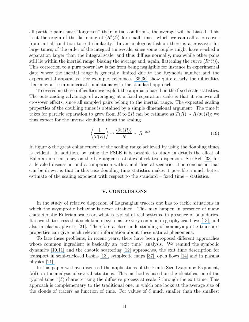
all particle pairs have “forgotten” their initial conditions, the average will be biased. Thisis at the origin of the flattening of 〈R2(t)〉 for small times, which we can call a crossoverfrom initial condition to self similarity. In an analogous fashion there is a crossover forlarge times, of the order of the integral time-scale, since some couples might have reached aseparation larger than the integral scale, and thus diffuse normally, meanwhile other pairsstill lie within the inertial range, biasing the average and, again, flattening the curve 〈R2(t)〉.This correction to a pure power law is far from being negligible for instance in experimentaldata where the inertial range is generally limited due to the Reynolds number and theexperimental apparatus. For example, references [35,36] show quite clearly the difficultiesthat may arise in numerical simulations with the standard approach.

To overcome these difficulties we exploit the approach based on the fixed scale statistics.The outstanding advantage of averaging at a fixed separation scale is that it removes allcrossover effects, since all sampled pairs belong to the inertial range. The expected scalingproperties of the doubling times is obtained by a simple dimensional argument. The time ittakes for particle separation to grow from R to 2R can be estimate as T (R) ∼ R/δv(R); wethus expect for the inverse doubling times the scaling

⟨

1

T (R)

⟩

∼ 〈δv(R)〉R

∼ R−2/3 (19)

In figure 8 the great enhancement of the scaling range achieved by using the doubling timesis evident. In addition, by using the FSLE it is possible to study in details the effect ofEulerian intermittency on the Lagrangian statistics of relative dispersion. See Ref. [33] fora detailed discussion and a comparison with a multifractal scenario. The conclusion thatcan be drawn is that in this case doubling time statistics makes it possible a much betterestimate of the scaling exponent with respect to the standard – fixed time – statistics.

V. CONCLUSIONS

In the study of relative dispersion of Lagrangian tracers one has to tackle situations inwhich the asymptotic behavior is never attained. This may happen in presence of manycharacteristic Eulerian scales or, what is typical of real systems, in presence of boundaries.It is worth to stress that such kind of systems are very common in geophysical flows [13], andalso in plasma physics [21]. Therefore a close understanding of non-asymptotic transportproperties can give much relevant information about these natural phenomena.

To face these problems, in recent years, there have been proposed different approacheswhose common ingredient is basically an “exit time” analysis. We remind the symbolicdynamics [10,11] and the chaotic scattering [12] approaches, the exit time description fortransport in semi-enclosed basins [13], symplectic maps [37], open flows [14] and in plasmaphysics [21].

In this paper we have discussed the applications of the Finite Size Lyapunov Exponent,λ(δ), in the analysis of several situations. This method is based on the identification of thetypical time τ(δ) characterizing the diffusive process at scale δ through the exit time. Thisapproach is complementary to the traditional one, in which one looks at the average size ofthe clouds of tracers as function of time. For values of δ much smaller than the smallest

11

characteristic length of the Eulerian velocity field, one has that λ(δ) coincides with themaximum Lagrangian Lyapunov Exponent. For larger δ the shape of λ(δ) depends on thedetailed mechanisms of spreading, i.e. the structure of the advecting velocity field and/orthe presence of boundaries. The diffusive regime corresponds to the behavior λ(δ) ≃ D/δ2.If δ gets close to its saturation value, i.e. the characteristic size of the basin, the universalshape of λ(δ) can be obtained on the basis of dynamical system theory. In addition, we haveshown that the fixed scale method is able to recognize the presence of a genuine anomalousdiffusion.

A remarkable advantage of working at fixed scale (instead of at fixed time as in the tra-ditional approach) is its ability to avoid misleading results, for instance apparent anomalousscaling over a certain time interval. Moreover, with the FSLE one obtains the proper scalinglaws also for a relatively small inertial range for which the standard technique gives rathercontroversial answers.

The proposed method can be also applied in the analysis of drifter experimental data orin numerical model for Lagrangian transport.

VI. ACKNOWLEDGMENTS

We thank V. Artale, E. Aurell, L. Biferale, P. Castiglione, A. Crisanti, M. Falcioni, R.Pasmanter, P.M. Poulain, M. Vergassola and E. Zambianchi for collaborations and discus-sions in last years. A particular acknowledgment to B. Marani for the continuous and warmencouragement. We are grateful to the ESF-TAO (Transport Processes in the Atmosphereand the Oceans) Scientific Program for providing meeting opportunities. This paper hasbeen partly supported by INFM (Progetto di Ricerca Avanzato PRA-TURBO), MURST(no. 9702265437), and the European Network Intermittency in Turbulent Systems (contractnumber FMRX-CT98-0175).

APPENDIX A: COMPUTATION OF THE FINITE SIZE LYAPUNOV

EXPONENT

In this appendix we discuss in detail the method for computing the Finite Size Lya-punov Exponent for both continuous dynamics (differential equations) and discrete dynamics(maps).

The practical method for computing the FSLE goes as follows. Defined a given norm forthe distance δ(t) between the reference and perturbed trajectories, one has to define a seriesof thresholds δn = rnδ0 (n = 1, . . . , P ), and to measure the “doubling times” Tr(δn) that aperturbation of size δn takes to grow up to δn+1. The threshold rate r should not be takentoo large, because otherwise the error has to grow through different scales before reachingthe next threshold. On the other hand, r cannot be too close to one, because otherwise thedoubling time would be of the order of the time step in the integration. In our examples wetypically use r = 2 or r =

√2. For simplicity Tr is called “doubling time” even if r 6= 2.

The doubling times Tr(δn) are obtained by following the evolution of the separation fromits initial size δmin ≪ δ0 up to the largest threshold δP . This is done by integrating the twotrajectories of the system starting at an initial distance δmin. In general, one must choose

12

δmin ≪ δ0, in order to allow the direction of the initial perturbation to align with the mostunstable direction in the phase-space. Moreover, one must pay attention to keep δP < δmax,so that all the thresholds can be attained (δmax is the typical distance of two uncorrelatedtrajectory).

The evolution of the error from the initial value δmin to the largest threshold δP carriesout a single error-doubling experiment. At this point one rescales the model trajectory atthe initial distance δmin with respect to the true trajectory and starts another experiment.After N error-doubling experiments, we can estimate the expectation value of some quantityA as:

〈A〉e =1

N

N∑

i=1

Ai . (A1)

This is not the same as taking the time average because different error doubling experimentsmay takes different times. Indeed we have

〈A〉t =1

T

∫ T

0A(t)dt =

∑

iAiτi∑

i τi=

〈Aτ〉e〈τ〉e

. (A2)

In the particular case in which A is the doubling time itself we have from (A2)

λ(δn) =1

〈Tr(δn)〉eln r . (A3)

The method above described assumes that the distance between the two trajectories iscontinuous in time. This is not true for maps or for discrete sampling in time, thus themethod has to be slightly modified. In this case Tr(δn) is defined as the minimum time atwhich δ(Tr) ≥ rδn. Because now δ(Tr) is a fluctuating quantity, from (A2) we have

λ(δn) =1

〈Tr(δn)〉e

⟨

ln

(

δ(Tr)

δn

)⟩

e

. (A4)

We conclude by observing that the computation of the FSLE is not more expensivethan the computation of the Lyapunov exponent by standard algorithm. One has simply tointegrate two copies of the system and this can be done also for very complex simulations.

APPENDIX B: UNIVERSAL SATURATION BEHAVIOR OF λ(δ)

In this appendix we present the derivation of the asymptotic behavior (12) of λ(δ) forδ close to the saturation. The computation is explicitly done for the simple case of a onedimensional Brownian motion in the domain [−LB , LB], with reflecting boundary conditions:the numerical simulations indicate that the result is of general applicability.

The evolution of the probability density p is ruled by the Fokker-Planck equation

∂p

∂t=

1

2D∂2p

∂x2(B1)

with the Neumann boundary conditions ∂p∂x

(±LB) = 0 .

13

The general solution of (B1) is

p(x, t) =∞∑

k=−∞

p(k, 0)eikxe−t/τk + c.c (B2)

where

τk =

(

D

2

π2

L2B

k2

)−1

, k = 0,±1,±2, ... (B3)

At large times p approaches the uniform solution p0 = 1/2LB. Writing p as p(x, t) =p0 + δp(x, t) we have, for t≫ τ1 ,

δp ∼ exp(−t/τ1). (B4)

The asymptotic behavior for the relative dispersion 〈R2(t)〉 is

〈R2(t)〉 =1

2

∫

(x− x′)2p(x, t)p(x′, t) dx dx′ (B5)

For t ≫ τ1 using (B4) we obtain 〈R2(t)〉 ∼(

L2

B

3− Ae−t/τ1

)

. Therefore for δ2(t) = 〈R2(t)〉one has δ(t) ∼

(

LB√3−

√3A

2LBe−t/τ1

)

The saturation value of δ is δmax = LB/√

3, so for t≫ τ1,

or equivalently for (δmax − δ)/δ ≪ 1, we expect

d

dtln δ = λ(δ) =

1

τ1

δmax − δ

δ(B6)

which is (12).Let us remark that in the previous argument for λ(δ) for δ ≃ δmax the crucial point is the

exponential relaxation to the asymptotic uniform distribution. In a generic deterministicchaotic system it is not possible to prove this property in a rigorous way. Neverthelessone can expect that this request is fulfilled at least in non-pathological cases. In chaoticsystems the exponential relaxation to asymptotic distribution corresponds to have the secondeigenvalue α of the Perron-Frobenius operator inside the unitary circle; the relaxation timeis τ1 = − ln |α| [38].

APPENDIX C: SYNTHETIC TURBULENT VELOCITY FIELDS

The generation of a synthetic turbulent field which reproduces the relevant statisticalfeatures of fully developed turbulence is not an easy task. Indeed to obtain a physicallysensible evolution for the velocity field one has to take into account the fact that each eddyis subject to the action of all other eddies. Actually the overall effect amounts only to twomain contributions, namely the sweeping exerted by larger eddies and the shearing due toeddies of comparable size. This is indeed a substantial simplification, but nevertheless theproblem of properly mimicking the effect of sweeping is still unsolved.

To get rid of these difficulties we shall limit ourselves to the generation of a syntheticvelocity field in Quasi-Lagrangian (QL) coordinates [32], thus moving to a frame of reference

14

attached to a particle of fluid r1(t). This choice bypasses the problem of sweeping, sinceit allows to work only with relative velocities, unaffected by advection. As a matter offact there is a price to pay for the considerable advantage gained by discarding advection,and it is that only the problem of two-particle dispersion can be well managed within thisframework. The properties of single-particle Lagrangian statistics cannot, on the contrary,be consistently treated.

The QL velocity differences are defined as

v(r, t) = u (r1(t) + r, t) − u (r1(t), t) , (C1)

where the reference particle moves according to

dr1(t)

dt= u(r1(t), t) . (C2)

These velocity differences have the useful property that their single-time statistics are thesame as the Eulerian ones whenever considering statistically stationary flows [32]. For fullydeveloped turbulent flows, in the inertial interval of length scales where both viscosity andforcing are negligible, the QL longitudinal velocity differences show the scaling behavior

〈∣

∣

∣

∣

v(r) · r

r

∣

∣

∣

∣

p

〉 ∼ rζp (C3)

where the exponent ζp is a convex function of p, and ζ3 = 1. This scaling behavior is adistinctive statistical property of fully developed turbulent flows that we shall reproduce bymeans of a synthetic velocity field. In the QL reference frame the first particle is at rest inthe origin and the second particle is at r2 = r1 + R, advected with respect to the referenceparticle by the relative velocity

v(R, t) = u (r1(t) + R, t) − u (r1(t), t) (C4)

By this change of coordinates the problem of pair dispersion in an Eulerian velocity fieldhas been reduced to the problem of single particle dispersion in the velocity difference fieldv(r, t). This yields a substantial simplification: it is indeed sufficient to build a velocitydifference field with proper scaling features in the radial direction only, that is along theline that joins the reference particle r1(t) – at rest in the origin of the QL coordinates –to the second particle r2(t) = r1(t) + R(t). To appreciate this simplification, it must benoted that actually all moments of velocity differences u (r1(t) + r

′, t) − u (r1(t) + r, t) =v(r′, t)−v(r, t) should display power law scaling in |r′−r|. Actually these latter differencesnever appear in the dynamics of pair separation, and so we can limit ourselves to fulfill theweaker request (C3). Needless to say, already for three particle dispersion one needs a fieldwith proper scaling in all directions.

We limit ourselves to the two-dimensional case, where we can introduce a stream functionfor the QL velocity differences

v(r, t) = ∇× ψ(r, t) . (C5)

The extension to a three dimensional velocity field is not difficult but more expensive interms of numerical resources.

15

Under isotropic conditions, the stream function can be decomposed in radial octaves as

ψ(r, θ, t) =N∑

i=1

n∑

j=1

φi,j(t)

kiF (kir)Gi,j(θ) . (C6)

where ki = 2i. Following a heuristic argument, one expects that at a given r the streamfunction is essentially dominated by the contribution from the i term such that r ∼ 2−i.This locality of contributions suggests a simple choice for the functional dependencies of the“basis functions”:

F (x) = x2(1 − x) for 0 ≤ x ≤ 1 (C7)

and zero otherwise,

Gi,1(θ) = 1, Gi,2(θ) = cos(2θ + ϕi) (C8)

and Gi,j = 0 for j > 2 (ϕi is a quenched random phase). It is worth remarking that thischoice is rather general because it can be derived from the lowest order expansion for smallr of a generic streamfunction in Quasi-Lagrangian coordinates.

It is easy to show that, under the usual locality conditions for infra red convergence, ζp <p [39], the leading contribution to the p-th order longitudinal structure function 〈|vr(r)|p〉stems from M-th term in the sum (C6), 〈|vr(r)|p〉 ∼ 〈|φM,2|p〉 with r ≃ 2−M . If the φi,j(t) are

stochastic processes with characteristic times τi = 2−2i/3 τ0, zero mean and 〈|φi,j|p〉 ∼ k−ζp

i ,the scaling (C3) will be accomplished. An efficient way of to generate φi,j is [31]:

φi,j(t) = gi,j(t) z1,j(t) z2,j(t) · · · zi,j(t) (C9)

where the zk,j are independent, positive definite, identically distributed random processeswith characteristic time τk, while the gi,j are independent stochastic processes with zero

mean, 〈g2i,j〉 ∼ k

−2/3i and characteristic time τi. The scaling exponents ζp are determined by

the probability distribution of zi,j via

ζp =p

3− log2〈zp〉 . (C10)

As a last remark we note that by simply fixing the zi,j = 1 we recover the Kolmogorovscaling, which has been used in the simulations presented in section IVB

16

REFERENCES

[1] M. Henon, “Sur la Topologie des Lignes de courant dans in cas particulier”, C. R. Acad.Sci. Paris A 262, 312 (1966).

[2] A.J. Lichtenberg and M.A. Lieberman, Regular and Stochastic Motion (Springer-Verlag,1982).

[3] J.M. Ottino, The kinematics of mixing: stretching, chaos and transport (CambridgeUniversity Press, 1989).

[4] A. Crisanti, M. Falcioni, G. Paladin and A. Vulpiani, “Lagrangian Chaos: Transport,Mixing and Diffusion in Fluids”, La Rivista del Nuovo Cimento 14, 1 (1991).

[5] G.M. Zaslavsky, D. Stevens and H. Weitzner, “Self-similar transport in incompletechaos”, Phys. Rev. E, 48, 1683 (1993).

[6] D. del Castillo Negrete and P.J. Morrison, “Chaotic transport by Rossby waves in shearflow”, Phys. Fluids A5, 948 (1993).

[7] W.J. Cocke, “Turbulent hydrodynamic line stretching: consequences of isotropy”, Phys.Fluids 12, 2488 (1969).

[8] S.A. Orszag, “Comment on: Turbulent hydrodynamic line stretching: consequences ofisotropy”, Phys. Fluids 13, 2203 (1970).

[9] M. Avellaneda and A. Majda, “Stieltjes integral representation and effective diffusivitybounds for turbulent transport”, Phys. Rev. Lett. 62, 753 (1989);M. Avellaneda and M. Vergassola, “Stieltjes integral representation of effective diffusiv-ities in time-dependent flows”, Phys. Rev. E 52, 3249 (1995).

[10] J.H. Misguich, J.D. Reuss, Y. Elskens and R. Balescu, “Motion in a stochastic layerdescribed by symbolic dynamics”. Chaos 8, 248 (1998).

[11] M. Cencini, G. Lacorata, A. Vulpiani and E. Zambianchi, “Mixing in a meandering jet:a Markovian approximation”. J. Phys. Oceanogr. in press (1999) chao-dyn/9801027.

[12] G. Karolyi and T. Tel, “Chaotic tracer scattering and fractal basin boundaries in ablinking vortex-sink system”. Phys. Rep. 290, 125 (1997).

[13] G. Buffoni, P. Falco, A. Griffa and E. Zambianchi, “Dispersion processes and residencetimes in a semi-enclosed basin with recirculating gyres: an application to the Tyrrheniansea.” J. Geophys. Res. 102, 18699 (1997).

[14] P. Castiglione, M. Cencini, A. Vulpiani and E. Zambianchi“Transport in finite size systems: an exit time approach”,chao-dyn/9903014 (submitted to Chaos)

[15] E. Aurell, G. Boffetta, A. Crisanti, G. Paladin and A. Vulpiani, “Growth of nonifinites-imal perturbations in turbulence,” Phys. Rev. Lett. 77, 1262 (1996);“Predictability in the large: an extension of the concept of Lyapunov exponent,” J.Phys. A 30, 1 (1997).

[16] V. Artale, G. Boffetta, A. Celani , M. Cencini and A. Vulpiani, “Dispersion of passivetracers in closed basins: beyond the diffusion coefficient”. Phys. Fluids. 9, 3162 (1997).

[17] R. Benzi, G. Paladin, G. Parisi and A. Vulpiani, “On the multifractal nature of fullydeveloped turbulence and chaotic systems”, J. Phys. A 17, 3521 (1984).

[18] G. Paladin and A. Vulpiani, “Anomalous scaling laws in multifractal objects”, Phys.Rep. 156, 147 (1987).

[19] S. Benkadda, Y. Elskens, B. Ragot and J.T. Mendoca, “Exit times and Chaotic Trans-port in Hamiltonian Systems”, Phys. Rev. Lett. 72, 2859 (1994).

17

[20] A.N. Yannacopoulos and G. Rowlands, “Calculation of diffusion coefficients for chaoticmaps”, Physica D 65, 71 (1993).

[21] R. Sabot and M.A. Dubois, “Diffusion coefficient in a finite domain from exit times andapplication to the tokamak magnetic structure”, Phys. Lett. A 212, 201 (1996).

[22] T.H. Solomon and J.P. Gollub, “Chaotic particle transport in time-dependent Rayleigh-Benard convection”, Phys. Rev. A 38, 6280 (1988);“Passive transport in steady Raleigh-Benard convection”, Phys. Fluids 31, 1372 (1988).

[23] H. Aref, “Integrable, chaotic, and turbulent vortex motions in two dimensional flows”,Ann. Rev. Fluid Mech. 15, 345 (1983).

[24] G. Boffetta, A. Celani e P. Franzese, “Trapping of Passive Tracers in a Point VortexSystem”, J. Phys. A 29, 3749 (1996).

[25] R. Rammal and G. Tolouse, “Random Walks on fractal structures and prcolation clus-ters”, J. Physique (Paris) Lett. 44, L13 (1983);F. D A Aaarao Reis, “Finite-Size scaling for random walks on fractals”, J. Phys., A28,6277 (1995).

[26] P.M. Poulain, “Drifter observations of surface circulation in the Adriatic sea betweenDecember 1994 and March 1996”. J. Mar. Sys., in press 1998.

[27] A. Artegiani, D. Bregant, E. Paschini, N. Pinardi, F. Raicich and A. Russo, “TheAdriatic Sea general circulation, parts I and II”, J. Phys. Oceanogr.,27, 1492 (1997).

[28] G. Lacorata, E. Aurell and A. Vulpiani, “Data analysis and modelling of Lagrangiandrifters in the Adriatic Sea”, submitted to J. of Mar. Res. (1999), chao-dyn/9902014.

[29] L.F. Richardson, “Atmospheric diffusion shown on a distance-neighbor graph”, Proc.Roy. Soc. A 110, 709 (1926).

[30] A. Monin and A. Yaglom, Statistical Fluid Mechanics (MIT Press, Cambridge, Mass.,1975), Vol. 2.

[31] L. Biferale, G. Boffetta, A. Celani, A. Crisanti and A. Vulpiani, “Mimicking a turbulentsignal: Sequential multiaffine processes”, Phys. Rev. E 57, R6261 (1998).

[32] V.S. L’vov, E. Podivilov and I. Procaccia, “Temporal multiscaling in hydrodynamicturbulence”, Phys. Rev. E 55, 7030 (1997).

[33] G. Boffetta, A. Celani, A. Crisanti and A. Vulpiani, “Relative dispersion in fully de-veloped turbulence: Lagrangian statistics in synthetic flows”, Europhy. Lett., 46, 177(1999).

[34] F.W. Elliott, Jr. and A.J. Majda, “Pair dispersion over an inertial range spanning manydecades”, Phys. Fluids 8, 1052 (1996).

[35] J.C.H. Fung and J.C. Vassilicos, “Two-particle dispersion in turbulent-like flows”, Phys.Rev. E 57, 1677 (1998).

[36] J.C.H. Fung, J.C.R Hunt, N.A. Malik and R.J. Perkins, “Kinematic simulation of ho-mogeneous turbulence by unsteady random Fourier modes” J. Fluid Mech. 236, 281(1992).

[37] R.W. Easton, J.D. Meiss and S. Carver, “Exit times and transport for Symplectic TwistMaps”, Chaos 3, 153 (1993).

[38] C. Beck and F. Schlogl, Thermodynamics of chaotic systems (Cambridge UniversityPress, 1993).

[39] H.A. Rose and P.L. Sulem, “Fully developed turbulence and statistical mechanics”, J.Physique 39, 441 (1978).

18

FIGURE CAPTIONS

Figure 1: a) Three realizations of R2(t) as a function of t built as follows: R2(t) =δ20 exp(2γt) if R2(t) < 1 and R2(t) = 2D(t − t∗) with γ = 0.08, 0.05, 0.3 andδ0 = 10−7, D = 1.5. b) 〈R2(t)〉 as function of t averaged on the three realizationsshown in figure 1a. The apparent anomalous regime and the diffusive one are shown.c) λ(δ) vs δ, with Lyapunov and diffusive regimes.

Figure 2: Lagrangian motion given by the Rayleigh-Benard convection model with: A =0.2, B = 0.4, ω = 0.4, k = 1.0, a = π, the number of realizations is N = 2000and the series of thresholds is δn = δ0r

n with δ0 = 10−4 and r = 1.05. λ(δ) vs δ, ina closed domain with 6 (crosses) and 12 (diamonds) convective cells. The lines arerespectively: (a) Lyapunov regime with λ = 0.017; (b) diffusive regime withD = 0.021;(c) saturation regime with δmax = 19.7; (d) saturation regime with δmax = 5.7.

Figure 3: (a)〈R2(t)〉 for the four vortex system with Γ1 = Γ2 = −Γ3 = −Γ4 = 1. Thethreshold parameter is r = 1.03 and δ0 = 10−4, the dashed line is the power law〈R2(t)〉 ∼ t1.8. The number of realizations is N = 2000. (b)λ(δ) vs δ for the samemodel and parameters. The horizontal line indicates the Lyapunov exponent (λ =0.14), the dashed curve is the saturation regime with δmax = 0.76

Figure 4: FSLE computed for particle diffusion in a Sierpinsky Carpet of fractal dimensionDf = log(8)/ log(3) obtained by iteration of the unit structure up to a resolution 3−5,one has: λ(δ) ∼ δ−1/.45, which is in agreement with the value obtained for < R(t) >versus t shown in the inset (i.e. < R(t) >∼ t.45).

Figure 5: Relative dispersion of Lagrangian trajectories, < R2x,y(t) > versus t, in the Adri-

atic Sea, for data (continuous line) and model (dashed line), along the natural axes ofthe basin: (a) transverse direction (x−axis) and (b) longitudinal direction (y−axis).The time is measured in days and the mean square radius of the cluster is in km2.

Figure 6: FSLE of Lagrangian trajectories in the Adriatic Sea, for data (continuous line)and model (dashed line). The scale δ is in km, λ(δ) is in days−1.

Figure 7: Relative dispersion 〈R(t)〉 for N = 20 octaves synthetic turbulent simulationaveraged over 104 realizations. The line is the theoretical Richardson scaling t3/2.

Figure 8: Average inverse doubling time 〈1/T (R)〉 for the same simulation of the previousfigure. Observe the enhanced scaling region. The line is the theoretical Richardsonscaling R−2/3.

19

FIGURES

1e-10

1

0.001 0.01 0.1 1 10 100 1000 10000

R2 (

t)

t

(a)

0.1

1

10

100

1000

10000

100 1000

<R

2 (t)

>

t

2Dt

Ct2ν

(b)

1e-06

1e-05

0.0001

0.001

0.01

0.1

1

0.001 0.01 0.1 1 10 100 1000

λ(δ)

δ

(c)FIG. 1.

20

1e-05

0.0001

0.001

0.01

0.1 1 10

λ(δ)

δ

(a)

(b)(c)

(d)

FIG. 2.

21

1e-07

1e-06

1e-05

0.0001

0.001

0.01

0.1

1

10

0.1 1 10 100 1000

<R

2 (t)>

t

(a)

0.001

0.01

0.1

0.1 1

λ(δ)

δ

(b)FIG. 3.

22

0.001

0.01

0.1

1

10

0.01 0.1

λ(δ)

δ

0.01

0.1

1

0.1 1 10 100 1000

<R(t)>

t

FIG. 4.

23

10

100

1000

10000

100000

0.1 1 10 100

<R

x2 >

t

(a)

10

100

1000

10000

100000

0.1 1 10 100

<R

y2 >

t

(b)FIG. 5.

24

0.01

0.1

1

10 100 1000

λ(δ)

δ

FIG. 6.

25

10-5

10-4

10-3

10-2

0.1

10-4 10-3 10-2 0.1 1

<R

(t)>

t

FIG. 7.

26

10

100

1000

10000

10-6 10-5 10-4 10-3 10-2 0.1

<1/

T(R

)>

R

FIG. 8.

27