Estimation of TAMDAR Observational Error and Assimilation Experiments

Estimation of TAMDAR Observational Error and Assimilation Experiments

FENG GAO

National Center for Atmospheric Research, Boulder, Colorado, and Nanjing University of Information Science

and Technology, Nanjing, Jiangsu, China

XIAOYAN ZHANG

National Center for Atmospheric Research, Boulder, Colorado

NEIL A. JACOBS

AirDat LLC, Morrisville, North Carolina

XIANG-YU HUANG AND XIN ZHANG

National Center for Atmospheric Research, Boulder, Colorado

PETER P. CHILDS

AirDat LLC, Morrisville, North Carolina

(Manuscript received 8 October 2011, in final form 16 March 2012)

ABSTRACT

Tropospheric Airborne Meteorological Data Reporting (TAMDAR) observations are becoming a major

data source for numerical weather prediction (NWP) because of the advantages of their high spatiotemporal

resolution and humidity measurements. In this study, the estimation of TAMDAR observational errors, and

the impacts of TAMDAR observations with new error statistics on short-term forecasts are presented. The

observational errors are estimated by a three-way collocated statistical comparison. This method employs

collocated meteorological reports from three data sources: TAMDAR, radiosondes, and the 6-h forecast from

a Weather Research and Forecasting Model (WRF). The performance of TAMDAR observations with the

new error statistics was then evaluated based on this model, and the WRF Data Assimilation (WRFDA)

three-dimensional variational data assimilation (3DVAR) system. The analysis was conducted for both

January and June of 2010. The experiments assimilate TAMDAR, as well as other conventional data with the

exception of non-TAMDAR aircraft observations, every 6 h, and a 24-h forecast is produced. The standard

deviation of the observational error of TAMDAR, which has relatively stable values regardless of season, is

comparable to radiosondes for temperature, and slightly smaller than that of a radiosonde for relative hu-

midity. The observational errors in wind direction significantly depend on wind speeds. In general, at low wind

speeds, the error in TAMDAR is greater than that of radiosondes; however, the opposite is true for higher

wind speeds. The impact of TAMDAR observations on both the 6- and 24-h WRF forecasts during the studied

period is positive when using the default observational aircraft weather report (AIREP) error statistics. The

new TAMDAR error statistics presented here bring additional improvement over the default error.

1. Introduction

Aircraft observations, which have been significantly

increasing in volume over the past few years due to the

expansion of aircraft-based observing systems, as well as

the increase in commercial air travel, are becoming an

important part in the global observing system (Benjamin

et al. 1999, 2010). Operational numerical prediction cen-

ters have begun to ingest automated aircraft reports from

the Aircraft Communications Addressing and Reporting

System (ACARS), which is a digital datalink system for

transmission of small messages between aircraft and

Corresponding author address: Xiang-Yu Huang, National

Center for Atmospheric Research, 3450 Mitchell Ln., Boulder, CO

80301.

E-mail: [email protected]

856 W E A T H E R A N D F O R E C A S T I N G VOLUME 27

DOI: 10.1175/WAF-D-11-00120.1

� 2012 American Meteorological Society

ground stations via VHF radio. This is the primary system

employed by the Aircraft Meteorological Data Relay

(AMDAR) program of the World Meteorological Or-

ganization (WMO) into regional and global data as-

similation systems (Schwartz and Benjamin 1995; Drue

et al. 2008).

DiMego et al. (1992) reported forecast improvements

from using aircraft data at the National Centers for En-

vironmental Prediction (NCEP). Smith and Benjamin

(1994) showed that ACARS reports improved short-range

forecasts of upper-level winds and temperatures when

added to wind profiler data over the central United States.

However, the absence of humidity observations, as well as

the high cruise heights, are two shortfalls of the current

aircraft observation sets (Moninger et al. 2010). Other than

scattered radiosonde soundings (RAOBs), there is a sig-

nificant lack of routinely collected in situ observations,

particularly humidity, from within the region below the

tropopause, where the majority of moisture resides and

where convective activity originates (Daniels et al. 2006).

To supplement existing technologies, a low-cost sen-

sor called Tropospheric Airborne Meteorological Data

Reporting (TAMDAR) was deployed by AirDat, under

the sponsorship of a joint National Aeronautics and Space

Administration (NASA) and Federal Aviation Admin-

istration (FAA) project as part of Aviation Safety and

Security Program, according to requirements defined by

the FAA, the Global Systems Division (GSD) of the Na-

tional Oceanic and Atmospheric Administration (NOAA),

and WMO. The TAMDAR sensor network has been

providing a continuous stream of real-time observations on

regional airlines since December 2004. Aircraft equipped

with TAMDAR provide coverage over North America,

including Alaska, Hawaii, and Mexico, and generate data

from locations and times not available from any other

observing system. TAMDAR produces thousands of high-

frequency daily observations of humidity, icing, and tur-

bulence, as well as conventional temperature, pressure,

and winds aloft along with GPS-based coordinates in near–

real time. Although TAMDAR will work on any airframe

from a transoceanic 777 to a small unmanned aerial vehicle

(UAV), commercial regional airlines have been the pri-

mary focus because those planes make more daily flights

into a greater number of smaller airports, while still serving

the major hubs. As a result, a larger number of soundings

from a more geographically diverse set of airports are

obtained. TAMDAR observations are rapidly becoming

a major source of critical data utilized by various assimi-

lation systems for the improvement of mesoscale NWP and

the overall safety of aviation in the future (Fischer 2006).

A crucial step in the process of extracting maximal value

from this new observation source is to correctly estimate

the observational error of TAMDAR measurements. This

will provide weighting information among different types

of observations and background fields in the data as-

similation system in order to obtain a statistically opti-

mal estimated value of the true variables (Lorenc 1986;

Benjamin et al. 1999; Barker et al. 2004).

Several previous investigations have addressed var-

ious methods for estimating observational error (e.g.,

Hollingsworth and Lonnberg 1986; Desroziers and

Ivanov 2001; Desroziers et al. 2005). Typically, obser-

vational error includes instrument error, reporting er-

ror (i.e., measurement error), and representativeness

error (Daley 1991; Schwartz and Benjamin 1995). Richner

and Phillips (1981) used three ascents with two sondes

on the same balloon to take simultaneous measurements

of the same air mass. The results showed that the de-

viations between two sondes fell within the accuracies

specified by the manufacturer with respect to the instru-

ment error. As previously stated, this is not the only source

of error in an observing system; therefore, when a com-

parison is made between two observations, or a single

observation and forecast or model analysis, representa-

tiveness error must be taken into account.

Sullivan et al. (1993) updated temperature error statis-

tics for NOAA-10 when the retrieval system in National

Meteorological Center (NMC, since renamed the Na-

tional Centers for Environmental Prediction, or NCEP)

changed from a statistical to a physical algorithm. In their

study, radiosonde soundings were considered the refer-

ence value, and the space–time proximity (i.e., 4 h and

330 km) between those soundings and satellite reports was

the constraint. Their research provided an initial meth-

odology regarding the estimation of observational error;

however, by the inherent nature of the comparison, it

was subject to greater representativeness error because

of the large space–time collocation threshold.

In light of an ever-growing wealth of aircraft obser-

vations to be included as input for generating initial con-

ditions in NWP, the quality of the data has been subject

to several studies. Schwartz and Benjamin (1995) gave

statistical characteristics of the difference between ra-

diosonde observations (RAOBs) and ACARS data sur-

rounding the Denver, Colorado, airport as a function of

time and distance separation. A standard deviation of

0.97 K in temperature was reduced to 0.59 K through

using a more strict collocation match constraint from

150 km and 90 min to 25 km and 15 min, which primarily

arose based on the representativeness error decreasing.

As a result, this study provided an upper bound on the

combined error of ACARS and RAOB data with small

representativeness error. Additionally, the authors spec-

ulated that the large direction difference was related to

mesoscale variability, especially from turbulence in the

boundary layer.

AUGUST 2012 G A O E T A L . 857

In a subsequent study to obtain the independent ob-

servation error of ACARS, Benjamin et al. (1999) re-

ported on a collocation study of ACARS reports with

different tail numbers to estimate observational error, as-

suming an equivalent expected error from each aircraft,

and the minimization of the representativeness error by

a strict match condition of 1.25 km and 2 min and no

vertical separation. They reported a temperature root-

mean-square error (RMSE) of 0.69–1.09 K and wind

vector error of 1.6–2.5 m s21 in a vertical distribution,

which were comparable to RAOB data. The methodology

and assumptions employed by Benjamin et al. (1999) are

reasonable; however, since TAMDAR-equipped planes

frequently fly into airports that do not have operational

radiosonde launches, it is difficult to get enough data for

a robust statistical comparison, while retaining similar

strict collocation constraints.

More recently, Moninger et al. (2010) provide error

characteristics of TAMDAR by comparing the data to

the Rapid Update Cycle (RUC) 1- and 3-h forecasts with

a model grid spacing of 20 km. In this study, the RUC 1-h

forecast is not considered to be ‘‘truth’’ but is treated as

a common denominator by which various aircraft fleets

are compared. The results show the RMS difference of

1 K, 8%–20%, and RMS vector difference 4–6 m s21 in

temperature, RH, and wind observations, respectively.

Since the Moninger et al. (2010) study, a procedure was

implemented to correct for magnetic deviation errors

that were degrading the wind observations (Jacobs et al.

2010), and the results reduced the RMS vector difference

by 1.3 m s21 for planes using this type of heading instru-

mentation. As with previous studies, the RMS difference

reported by Moninger et al. (2010) includes the TAMDAR

observation error, representativeness error, as well as the

RUC 1-h forecast error.

When examining previous studies for the purpose of

constructing a methodology for estimating observational

error of TAMDAR, two issues become apparent.

a. Collocated observational error sources aretypically combined in error statistics

Prior collocation studies consider radiosonde data as

truth, and while the uncertainty can be addressed to

a limited degree by dual-sensor sonde launches in field

experiments (e.g., Schwartz and Benjamin 1995), or by

systematic bias adjustments (e.g., Ballish and Kumar

2008; Miloshevich et al. 2009), automated evaluation of

TAMDAR observations, as well as TAMDAR-related

forecast impacts, for the purposes of deriving error sta-

tistics, inherently include radiosonde observational error

(Moninger et al. 2010). Ballish and Kumar (2008) high-

lighted differences between radiosonde temperature

and traditional AMDAR data, and suggested correcting

temperature biases based on statistics derived against the

model background. While this approach may mitigate

systematic temperature biases, it is still subject to indi-

vidual observing system uncertainty and does not address

similar issues with wind and moisture observations.

b. The wind error is based on vector notation

There are two areas of interest with respect to the error

associated with the assimilation of aircraft wind observa-

tions. First, in the Weather Research and Forecasting

Model (WRF) data assimilation system (WRFDA; Huang

2009), both the instrumentation error file, as well as the

error calculation, use a constant instrumentation error

value of 3.6 m s21 at all levels for aircraft weather reports

(AIREPs), which includes TAMDAR. This is not the

case for RAOBs, which vary the instrumentation error

with height above 800 hPa for vector wind. Second, pre-

vious collocation studies that analyze wind error com-

pare the vector wind (e.g., Benjamin et al. 1999;

Schwartz et al. 2000; Moninger et al. 2010), which in-

herently includes both the observed speed error, as well

as the directional error embedded in the vector compo-

nent value. It should be noted that WRFDA and the

gridpoint statistical interpolation (GSI) handle wind

observations in a slightly different way. In this study, we

only address WRFDA, where the observational error of

wind speed is assigned as a single error value for both u

and v, and can only be defined by level.

The observed wind vector, VWTAM

, is computed by

taking the difference between the ground track vector

(i.e., aircraft motion with respect to Earth), VG, and the

aircraft track vector, VA:

VWTAM

5 VG 2 VA. (1)

The TAMDAR ground track vector is determined by

a very accurate Garmin GPS system, and the associated

error is at least two orders of magnitude less than the error

in VA. The aircraft track vector is calculated from the true

airspeed (TAS) and the heading angle. The TAS is derived

from the difference between the dynamic pressure of the

pitot tube and the static pressure. The heading angle is

determined by either a laser gyro, or magnetic flux valve,

heading system.

This means that there are two primary sources for po-

tential instrumentation error in the wind observation: the

TAS and the heading angle. The pitot tube system, which

determines TAS, and the heading system, which de-

termines the angle, are essentially two unrelated observ-

ing systems. They both provide information to calculate

the wind observation, which is then broken down into its

u and y components. Once this step has occurred, it is not

possible to determine if the error in u or y originated from


the TAS (i.e., speed) or the heading (i.e., direction). The

uncertainty largely depends on the precision of the

heading instrumentation, and older magnetic flux gate

systems are subject to large deviations that can impact the

observed wind accuracy (Moninger et al. 2010). Mulally

and Anderson (2011) introduced a magnetic deviation

bias filter that corrects this error, and results in wind

observations that are comparable to those reported by

aircraft with more sophisticated heading instrumentation.

Small errors in the TAS can result in larger observed

wind errors due to the sensitivity of the equation to minor

fluctuations in dynamic pressure as seen by the pitot tube.

Additionally, the assumption is made that the aircraft is in

perfect inertial alignment (i.e., no roll, pitch, or yaw), and

since this is almost never the case, there is a small angle-

based error introduced in addition to the TAS-based

speed error (Painting 2003). The latter can be flagged and

filtered based on acceptable thresholds as described in

Moninger et al. (2003). Schwartz et al. (2000) explained

that the RMS differences depend upon the observed wind

speeds, and as wind speed increases, so does the RMS

vector difference. They state that one of the reasons for

this increase is that small directional differences can have

a significant impact on vector components when the

magnitude of the wind vector is large. Schwartz et al.

(2000) showed this by stratifying the mean RMS vector

differences by increments in the observed wind speed.

O’Carroll et al. (2008) developed a statistical method for

calculating the standard deviation of the observational

error for each of three different observation types under

the assumption that the observational error of different

systems is uncorrelated, which is typically a reasonable

assumption in error theory. We revisit this problem with

TAMDAR data, but for this study, we characterize the

observational error in its original speed and direction no-

tation. We hypothesize that it may be beneficial to define

the error in terms of both direction and speed, as opposed

to the magnitude of a single vector component, because of

the inverse nature of the relationship between the angle

and magnitude. In this study, we employ the O’Carroll

et al. (2008) method of estimating the TAMDAR obser-

vational error in temperature, RH, wind speed, and wind

direction. We further analyze the error in both wind speed,

as well as direction, as a function of the speed itself. Ad-

ditionally, we follow strict collocation match conditions as

described in Benjamin et al. (1999) for the purpose of

minimizing the representativeness error; however, even

with this protocol, any time a numerical model represen-

tation of the atmosphere is constructed based on obser-

vations, an associated space–time representativeness error

of that observation will be introduced.

The rest of this paper is laid out as follows. In section

2, the error statistics methodology and the data sources

are introduced. Section 3 presents the error statistics

results, which include the difference and vertical distri-

bution of observational error. A brief description of the

WRFDA system and WRF model configuration is pre-

sented in section 4. In section 5, we discuss assimilation

sensitivity experiments that compare the default error to

the new error statistics. Conclusions and plans for future

work are described in section 6.

2. Methodology

a. Error analysis

Following the simultaneous equations for three-way

collocation statistics given by O’Carroll et al. (2008),

where the observation x is expressed as the sum of the

true value of the variable, xT, the bias, or mean error, b,

and the random error «, which has a mean of zero by

definition, we begin with

x 5 b 1 « 1 xT . (2)

For a set of three collocated observation types i, j, and k,

the following set of equations are obtained:

xi 5 bi 1 «i 1 xT

xj 5 bj 1 «j 1 xT

xk 5 bk 1 «k 1 xT . (3)

The variance of the difference, V, between two obser-

vation types can be expressed as

Vij 5 s2i 1 s2

j 2 2rijsisj

Vjk 5 s2j 1 s2

k 2 2rjksjsk

Vki 5 s2k 1 s2

i 2 2rkisksi, (4)

where s is the standard deviation, s2 is the variance, and

rij is the correlation coefficient. Solving this set of

equations allows the error variance of each observation

type to be estimated from the statistics of the differences

between the three types, which can be expressed as

s2i 5

1

2(Vij 2 Vjk 1 Vki)

s2j 5

1

2(Vjk 2 Vki 1 Vij)

s2k 5

1

2(Vki 2 Vij 1 Vjk). (5)

A complete derivation of Eq. (5) is presented in the

appendix.

If the representativeness error is taken into consid-

eration, s2i from Eq. (5) can be expressed as


s2i 5

1

2(Vij 2 Vjk 1 Vki 2 s2

repij

1 s2rep

jk2 s2

repki

),

(6)

where s2rep is the variance of the representativeness error,

which is inherent when comparing any two observation

types in different space–time locations. If the collocation

match conditions between any type (e.g., k 5 fg; WRF 6-h

forecast) and two other types (e.g., i 5 TAMDAR and j 5

RAOB) are met, we can assume s2repRAOB2fg

’ s2repfg2TAMDAR

,

where fg has a constant resolution based on the model grid

spacing. Thus, in terms of the representativeness error

of TAMDAR and RAOB data, Eq. (5) will give an upper

bound of error calculated in Eq. (6). The assumption dis-

cussed above eliminates two terms in Eq. (6); however,

the contribution from the fourth term, in this case

s2repTAMDAR-RAOB

, may still be apparent, and is discussed

below. Additionally, for this study, it is assumed that

the short-term forecast error of a nonlinear numerical

model is uncorrelated to the error of subsequent ob-

servations of any observing system.

b. Data

Based on the methodology discussed in the previous

section, TAMDAR, RAOB, and WRF 6-h forecasts are

selected as the three sources of data employed to esti-

mate the TAMDAR observational error.

1) TAMDAR

The high-frequency TAMDAR observations, which

number in the tens of thousands daily, are collected with

multifunction in situ atmospheric sensors on aircraft

(Daniels et al. 2004; Moninger et al. 2010). In addition to

the conventional measurements of temperature and winds

aloft, the observations contain measurements of humidity,

pressure, icing, and turbulence, along with GPS-derived

coordinates.

For humidity, the fundamental physical parameter that

the TAMDAR capacitive sensor technology responds to

is the density of H2O molecules. The sensor uses a poly-

mer material that either absorbs or desorbs water mole-

cules based on the RH with respect to water. This in turn

affects the capacitance; the relationship is monotonic, so

in principle, a given capacitance, which can be measured

and turned into a voltage, represents a certain RH.

The observations are relayed via satellite in real time

to a ground-based network operations center where they

are received, processed, quality controlled, and avail-

able for distribution or model assimilation in less than

a minute from the sampling time. These observations

are reported at 10-hPa pressure intervals up to 200 hPa,

with the largest time-based interval during cruise being

no more than 3 min.

From 2005 through 2011, NOAA/GSD played a central

role in the distribution, evaluation, and initial quality con-

trol (i.e., reports formatting or units error) of TAMDAR

data. In this study, TAMDAR observations are collected

via the Meteorological Assimilation Data Ingest System

(MADIS) dataset from NOAA/GSD. The TAMDAR

observations used in this study came from fleets that

covered most of the airports in the east-central and

northwest continental United States (CONUS; Fig. 1).

The dataset in this study uses a winter month (January)

and a summer month (1–25 June) in 2010. The time series

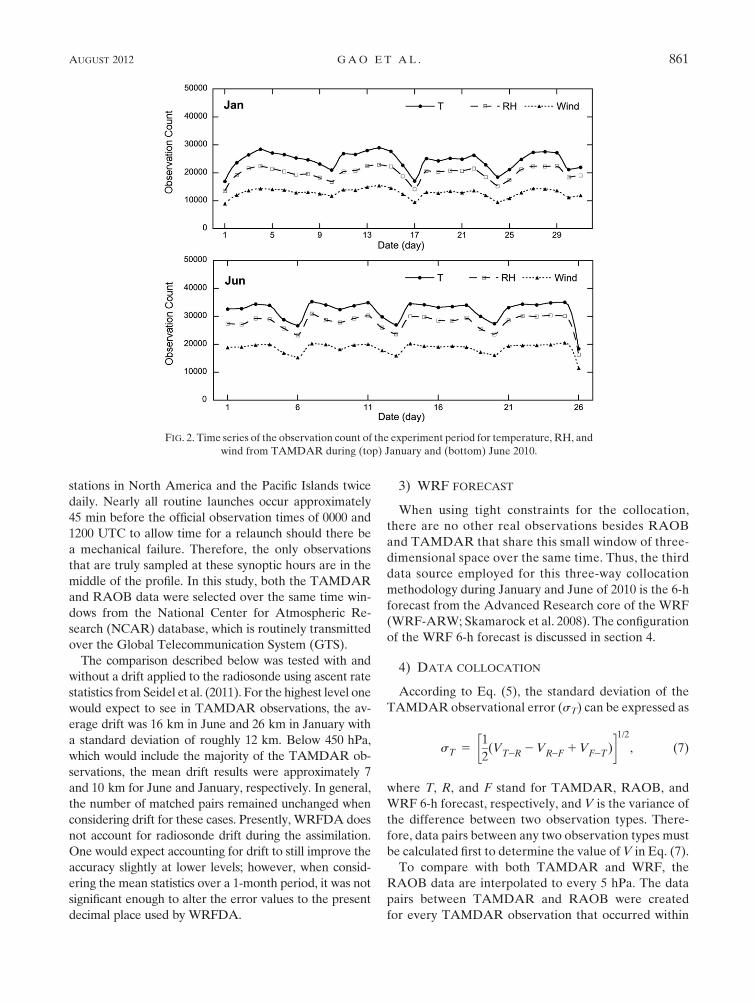
of TAMDAR observation counts are displayed in Fig. 2.

The wind observations are fewer than those for RH, which

is less than for the temperature. This is because the wind

observation requires an accurate aircraft heading reading,

so whenever the plane is banking or rolling in a turn over

a frame-specific threshold, the wind data are flagged. On

occasion, RH data will also be flagged, which typically

happens during brief icing events; these data were with-

held based on the current quality control flagging system.

2) RADIOSONDE

The radiosonde observations are transmitted to a

receiving station where the height of the package is

sequentially computed in incremental layers at each

reporting level using the hypsometric equation. The drift

speed and direction at various levels are determined from

the ground-based radio antenna that tracks the instrument

package as it is carried by the wind during the ascent. These

observations are processed, tabulated, and encoded for

transmission over various communication networks. The

National Weather Service launches radiosondes from 92

FIG. 1. The distribution of TAMDAR observations on 1 Jun

2010; colors represent thousands of feet. The lower-left corner is

the observation number. The distribution and number do not in-

clude TAMDAR observations in the AK area.


stations in North America and the Pacific Islands twice

daily. Nearly all routine launches occur approximately

45 min before the official observation times of 0000 and

1200 UTC to allow time for a relaunch should there be

a mechanical failure. Therefore, the only observations

that are truly sampled at these synoptic hours are in the

middle of the profile. In this study, both the TAMDAR

and RAOB data were selected over the same time win-

dows from the National Center for Atmospheric Re-

search (NCAR) database, which is routinely transmitted

over the Global Telecommunication System (GTS).

The comparison described below was tested with and

without a drift applied to the radiosonde using ascent rate

statistics from Seidel et al. (2011). For the highest level one

would expect to see in TAMDAR observations, the av-

erage drift was 16 km in June and 26 km in January with

a standard deviation of roughly 12 km. Below 450 hPa,

which would include the majority of the TAMDAR ob-

servations, the mean drift results were approximately 7

and 10 km for June and January, respectively. In general,

the number of matched pairs remained unchanged when

considering drift for these cases. Presently, WRFDA does

not account for radiosonde drift during the assimilation.

One would expect accounting for drift to still improve the

accuracy slightly at lower levels; however, when consid-

ering the mean statistics over a 1-month period, it was not

significant enough to alter the error values to the present

decimal place used by WRFDA.

3) WRF FORECAST

When using tight constraints for the collocation,

there are no other real observations besides RAOB

and TAMDAR that share this small window of three-

dimensional space over the same time. Thus, the third

data source employed for this three-way collocation

methodology during January and June of 2010 is the 6-h

forecast from the Advanced Research core of the WRF

(WRF-ARW; Skamarock et al. 2008). The configuration

of the WRF 6-h forecast is discussed in section 4.

4) DATA COLLOCATION

According to Eq. (5), the standard deviation of the

TAMDAR observational error (sT) can be expressed as

sT 5

�1

2(VT2R 2 VR2F 1 VF2T)

�1/2

, (7)

where T, R, and F stand for TAMDAR, RAOB, and

WRF 6-h forecast, respectively, and V is the variance of

the difference between two observation types. There-

fore, data pairs between any two observation types must

be calculated first to determine the value of V in Eq. (7).

To compare with both TAMDAR and WRF, the

RAOB data are interpolated to every 5 hPa. The data

pairs between TAMDAR and RAOB were created

for every TAMDAR observation that occurred within

FIG. 2. Time series of the observation count of the experiment period for temperature, RH, and

wind from TAMDAR during (top) January and (bottom) June 2010.


a certain space–time interval of a RAOB report. This

means that both data types are assumed to represent the

mean value of a small volume of air within a certain

spatial and temporal range. To assure confidence in the

quality of data pairs, as well as to decrease the effect of

representativeness error, different collocation match con-

ditions are applied on different levels for the purpose of

maintaining statistically significant matched-pair volume

counts. A maximum temporal (vertical spatial) separation

difference of 1 h (25 m) was applied in conjunction with

three horizontal spatial separation limits of 10 km below

775 hPa, 20 km between 775 and 450 hPa, and 30 km

above 450 hPa. The main reason why the collocation

matches become fewer with height is that the number of

TAMDAR measurements decreases with height because

not all flights achieve maximum cruise altitude.

When applying these constraints over the study window,

23 551 matched data pairs were obtained. Despite having

less strict horizontal collocation criteria for upper levels

(i.e., 30 km), most of the data pairs still fell into the

,10-km bin, similar to the lower levels. Figure 3 depicts

the distribution of these pairs by distance and time sepa-

ration. Approximately 70%, 71%, and 61% of TAMDAR–

RAOB matched pairs for temperature, RH, and wind,

respectively, have a spatial separation of less than 10 km.

As discussed for Fig. 2, more wind data (RH data) were

withheld because of aircraft maneuvering (icing). This is

also evident in Fig. 3a, where for a collocation threshold

below 10 km, despite more net matched pairs, there are

fewer matched wind observations. This is because most

RAOB sites are located at airports, and during the final

approach, aircraft tend to make more banking maneuvers,

which result in flagged wind data on descents near airports

(i.e., near RAOB launch sites). There is also a notable

increase in matched pairs in Fig. 3b in the 60 min prior to

0000 and 1200 UTC, and fewer after, which is a function of

RAOB launch time and ascent rate, and the flight sched-

ules, which are routed to avoid passing too close to the

ascending balloon during the cruise phase of flight. The

data pairs between the WRF 6-h forecast and both RAOB

and TAMDAR are easily obtained by gridpoint in-

terpolation to the observation location.

Figure 4 presents the RMSE difference of the data pairs

based on the spatial and temporal separation. Generally,

the data-pair difference for temperature (Fig. 4a) and RH

(Fig. 4b) steadily increases, as the space–time separation

grows, which is expected according to the representative-

ness error. The RH values above 400 hPa do not appear

to follow this trend. This is likely a result of the nu-

merically small mixing ratio values; however, based on

the low correlation, any meaningful trend would be hard

to identify. The order of the lines based on RMSE dif-

ference is consistent with temperature becoming more

homogeneous with height, and larger RH RMSE re-

sulting from very dry air at higher levels.

Conversely, the wind vectors can be significantly af-

fected by synoptic flow patterns. The wind speed (Fig.

4c) follows the same trend as the previously mentioned

scalars with the exception of the lowest level, which still

increases, but not at the same rate. This may be a result

of the more chaotic flow observed closer to the surface

combined with smaller speed magnitudes.

In Fig. 4d, there is greater directional error closer to the

surface, and the magnitude of the directional error de-

creases with height. As we will discuss below, higher speeds

typically have less directional error associated with them

despite having larger speed error. Thus, it is somewhat

expected to see the direction error from the three layers

stratified in opposite order of the speed error in Fig. 4c.

The small decrease in error for the middle layer may be

related to the amount of RAOB drift. The top of this layer

is high enough to be slightly affected by drift, but still low

enough that it lacks the homogeneity of the upper-most

layer, which can offset this variability. Since we are using

the launch position of the radiosonde site for the spatial

coordinate, rapidly drifting sondes should have a lower wind

direction error. Another possible cause may occur when

large spatial collocation match conditions are employed. In

FIG. 3. The distribution of matched pairs by (a) horizontal dis-

tance and (b) time separation between TAMDAR and RAOB

observations according to the match conditions.


this case, similar wind directions may be obtained; however,

the actual observations are a full wavelength apart. Either

situation can greatly increase the variance of the represen-

tativeness error term s2rep-TAMDAR-RAOB discussed above,

and as a result, we employed strict collocation match con-

ditions, described in the beginning of this section, to mini-

mize the impact of this term.

3. Error estimation analysis

a. Difference distribution

Figures 5 and 6 present the collocated matched-pair

Gaussian-like distribution patterns between TAMDAR

and RAOBs, and TAMDAR and WRF 6-h forecasts,

respectively. The dotted line is the Gaussian distribution

according to the mean value and standard deviation of

the difference. Observation pairs with a difference more

than 7 K, 40%, 10 m s21, and 608 in the temperature,

RH, speed, and direction variables, respectively, are re-

jected, since abnormal differences are often a result of

representativeness error or mesoscale perturbations. In

both Figs. 5 and 6, the matched-pair counts approach zero

well before the error threshold limits are encountered;

therefore, only clear outliers would fall beyond this limit

and, as such, would be caught by the upstream in-line

quality control procedure. The statistics of the differences

are shown in Table 1, which includes bias (B), standard

deviation (s), and confidence intervals of 68%, 90%, and

99% (i.e., 1, 1.64, and 2.58s) of the normal Gaussian

distribution.

In general, TAMDAR data quality is comparable to

RAOBs data based on the biases (;0.1s) with the ex-

ception of direction (Table 1). One standard deviation

away from the mean, the differences between all the

metrics are more than 68.3%, which means that the col-

located matched pairs exceeded the normal distribution

threshold while maintaining comparable quality. Both

difference distributions also follow a similar trend at the

1.64s confidence interval, and have a percent area of

around 90%, which shows that the three observation types

have a reasonable error range.

It is expected that mesoscale perturbations will lead to

some observation pairs with abnormal differences, which

lie outside 2.58s; however, the collocated data pairs with

large differences resulting from either coarse match con-

ditions, or the occasional bad observation that slipped

FIG. 4. The RMSE difference of the data pairs based on the spatial and temporal separation for (a) temperature,

(b) RH, (c) wind speed, and (d) wind direction.


through the quality control filter, are rare enough so as not

to significantly affect the error estimation of the observa-

tions. In this respect, variables such as RH, wind speed,

and direction should be closely monitored by quality

control and gross error check procedures during opera-

tional preprocessing. The total s of observed RH is typi-

cally smaller in the critical lower levels because the error in

the upper levels increases remarkably based on the very

low water vapor values. An inherent characteristic of the

wind observations is that the direction error feeds back

into the wind vector observations. As a result, mesoscale

variability and fluctuations in accurate heading information

can cause larger directional error at lower wind speeds,

which can increase the frequency of bad observations.

FIG. 5. The difference in (a) temperature, (b) RH, (c) wind speed,

and (d) wind direction between TAMDAR observations and RAOB.

The dotted line is the Gaussian distribution according to the RAOB-

TAM mean value and standard deviation of the difference.

FIG. 6. The difference in (a) temperature, (b) RH, (c) wind

speed, and (d) wind direction between TAMDAR and RAOB

observations and WRF 6-h forecasts. The dotted line is the

Gaussian distribution according to the TAM-WRF mean value and

standard deviation of the difference.


b. Vertical distribution of observational error

1) TEMPERATURE

The standard deviation of the temperature errors

of TAMDAR and RAOB data in January and June are

shown in Fig. 7. The temperature error for TAMDAR

is 0.6–0.9 K depending on the level. It is comparable

to RAOB data below 700 hPa for the June period and

slightly smaller than RAOB data for the January pe-

riod. The maximum difference of about 0.15 K occurs

around 500 hPa in June, and around 700 hPa in January.

Based on the vertical distribution described in the fol-

lowing section, higher impacts between 850 and

700 hPa are expected. The difference seen at 500 hPa in

June may be related to the increased frequency of

small-scale perturbations from the convective mixed

layer during this time of year.

The instrument error, as specified by the manufacturers

of both TAMDAR and the radiosondes, is 0.5 K, and

anything above this is likely representativeness error,

which must always be taken into account when compar-

ing two data sources within an assimilation system.

2) WIND

Wind error can be affected by multiple factors such as

mesoscale perturbations, aircraft heading information, and

even as a function of the wind speed itself. According to

the wind speed observation statistics in Fig. 8, the RAOB

error is about 0.5–1.0 m s21 less than for TAMDAR;

however, the average error of 2.0–2.5 m s21 is still quite

small. It is also interesting to note that the results shown in

Fig. 8 for RAOBs appear to validate the default RAOB

error in WRFDA. The wind direction error can be seen in

Fig. 9. Both RAOB and TAMDAR have a significant

decrease in error with height, and the magnitude of the

error in the lower levels is quite large. Three possible

reasons for these large error statistics are presented:

d The TAMDAR wind observations are dependent on

the accuracy of the heading information supplied

by the aircraft instrumentation, and even the most

accurate avionics will still introduce an additional

source of error. This error source would have more

impact on lower wind speeds.d The error of the wind speed and direction changing as

a function of wind speed is a typical characteristic of

wind observations.d The frequency of TAMDAR is weighted toward the

1800 and 0000 UTC cycles, whereas the RAOB data

have equal numbers for both 0000 and 1200 UTC. An

increase in diurnal instability tends to be more prev-

alent in the 0000 UTC cycle, compared to 1200 UTC,

especially during the summer months because of the

heating and length of day.

Figure 10 further illustrates this error dependence on

wind speed. Both the wind direction error and the wind

speed error for the TAMDAR and RAOB data are plotted

based on bins of wind speed magnitude. In general, wind

speed (direction) error increases (decreases) with wind

speed. RAOBs have less error than TAMDAR for speeds

below 15 m s21, while the opposite is true for speeds above

15 m s21, but the differences typically remain less than

0.5 m s21.

Recent improvements in correcting the heading bias

seen on some aircraft are discussed in Jacobs et al.

(2010) and Mulally and Anderson (2011). The error is

reduced by approximately 2 kt, or 1 m s21, which is

roughly a 45% decrease in error for this subset of mag-

netic-heading-equipped planes, and brings the quality of

the data in line with the remainder of the fleet. It should

also be mentioned that this subset of planes makes up

a small fraction (i.e., 15 out of more than 250) of the

expanding TAMDAR fleet, which typically rely on more

sophisticated avionics.

3) RELATIVE HUMIDITY

The abundant RH observations of TAMDAR should

provide a substantial supplement to present observation

types. The quality of TAMDAR RH observations can

be seen in Fig. 11, where during the month of January

the error of 7%–9% was similar to the RAOB result. In

June, the TAMDAR error ranged from 6% near the

TABLE 1. The statistics of the differences between TAMDAR and RAOB, and TAMDAR and WRF 6-h forecasts.

RAOB–TAMDAR TAMDAR–Forecast

RH T Speed Direction RH T Speed Direction

N 9994 12 549 5384 4810 284 586 374 198 149 044 143 572

B 21.57 (%) 0.04 (K) 20.004 (m s21) 21.22 (8) 20.37 (%) 20.16 (K) 0.15 (m s21) 21.39 (8)

s 12.18 (%) 1.06 (K) 2.83 (m s21) 20.13 (8) 13.81 (%) 1.16 (K) 2.88 (m s21) 16.83 (8)

1s 72.10% 74.90% 71.50% 73.60% 69.80% 70.10% 70.10% 74.30%

1.64s 89.30% 90.70% 89.80% 87.70% 88.80% 89.10% 89.60% 89.50%

2.58s 97.80% 97.50% 97.50% 97.80% 98.30% 98.30% 98.50% 97.10%


FIG. 7. The standard deviation of temperature error for TAMDAR

and RAOB in (a) January and (b) June. FIG. 8. As in Fig. 7, but for wind speed error.


surface to 8% above 400 hPa, and had a maximum re-

duction in error of 3% RH compared to RAOB at

500 hPa. The estimated error range is consistent with

the findings of 5%–10% from Daniels et al. (2006).

4. Model configuration and experiment design

To evaluate the performance of TAMDAR with the

observational error estimated above, three parallel ex-

periments are conducted. These experiments were per-

formed during June 2010, and are based on WRFDA

three-dimensional variational data assimilation (3DVAR)

and the WRF ARW (version 3.2).

In the present WRFDA system, the AIREP error is

the default table for any type of observation collected

by an aircraft regardless of airframe, phase of flight,

or instrumentation type. Since TAMDAR is based on

different operating principles compared to traditional

AIREPs, it is not realistic to assume it possesses similar

error characteristics. The TAMDAR error statistics

derived above will be used in the following assimilation

experiment as a substitute for the default AIREP error.

Both the original default AIREP error, and the newFIG. 9. As in Fig. 7, but for wind direction error.

FIG. 10. The standard deviation of the wind speed (bars) and

wind direction (lines) error as a function of wind speed magnitude

thresholds for TAMDAR and RAOB in (a) January and (b) June.


TAMDAR-specific error, are presented in Table 2. The

WRFDA error file contains values that correspond to

levels up to 10 hPa. Since TAMDAR data would never

appear above 200 hPa, any value entered in the table

above this height would merely serve as a placeholder.

In section 3, both the wind speed error and the wind

direction error were characterized. However, in this part,

only the wind speed error (Fig. 8) was employed to modify

the WRFDA observational error statistics in Table 2. The

results from Figs. 9 and 10 help shed light on some of the

error-related trends, but those results were not applied to

the error table for the NEWerr_T run, as this would re-

quire a modification to the observation operator discussed

in the following section.

a. WRF ARW and WRFDA 3DVAR

The WRF-ARW is a fully compressible and Euler

nonhydrostatic model with a vertical coordinate of terrain-

following hydrostatic pressure, and features time-split in-

tegration using a third-order Runge–Kutta scheme with

a smaller time step for acoustic and gravity wave modes

and multiple dynamical cores with high-order numerics to

improve accuracy. A detailed description of the model can

found in Skamarock et al. (2008).

The WRFDA 3DVAR system originates from the

3DVAR system in the fifth-generation Pennsylvania State

University–NCAR Mesoscale Model (MM5) developed by

Barker et al. (2004), and based on an incremental formu-

lation (Courtier et al. 1994). Following Lorenc et al. (2000),

the control variables are the streamfunction, unbalanced

velocity potential, unbalanced temperature, unbalanced

surface pressure, and pseudo RH, which are used in the

minimization process of the first term of Eq. (8) below.

The basic goal of 3DVAR is to obtain statistically

optimal estimated values of the true atmospheric state at

a desired analysis time through an iterative minimiza-

tion of the prescribed cost function (Ide et al. 1997):

J(x) 51

2(x 2 xb)TB21(x 2 xb)

11

2[y0 2 H(x)]TR21[y0 2 H(x)], (8)

where B is the background error covariance matrix, xb is

the background state, H is the nonlinear observation

operator, y is the data vector, R is the observation error

covariance matrix, and the state vector is defined as

x 5 [uT, vT, TT, qT, pTs ]

T. (9)

If an iterative solution can be found from Eq. (9) that

minimizes Eq. (8), the result represents a minimumFIG. 11. The standard deviation of RH error for TAMDAR and

RAOB in (a) January and (b) June.


variance estimate of the true atmospheric state given the

background xb and observations y0, as well as B and R

(Lorenc 1986). The conjugate gradient method is used to

minimize the incremental cost function. A detailed de-

scription of this system can be found in Barker et al.

(2004), as well as at the WRFDA web site (http://www.

mmm.ucar.edu/wrf/users/wrfda/pub-doc.html). Additional

background on TAMDAR assimilation by WRFDA can

also be found in Wang et al. (2009).

b. Model configuration

The data assimilation experiments and WRF forecasts

were performed on a single 400 3 250 grid with 20-km

spacing that covered the United States and surrounding

oceanic regions. There were 35 vertical levels with a top

of 50 hPa. The model produced a 24-h forecast. While

this configuration is not necessarily optimal for assimilation

of high-resolution asynoptic data like TAMDAR, it was

sufficient to reach conclusions and illustrate the necessity

to consider other methods of determining wind observa-

tion error statistics.

In this study, the Kain–Fritsch cumulus parameteriza-

tion was employed (Kain 2004), along with the Goddard

cloud microphysics scheme, and the Yonsei University

(YSU) planetary boundary layer parameterization (Hong

et al. 2006).

c. Experiment design

Three parallel WRF runs were performed during 1–20

June 2010:

d ‘DEFerr_noT’ is used as a control run, conventionally

assimilating GTS data with default error statistics

in WRFDA, including surface synoptic observations

(SYNOP), aviation routine weather reports (METARs),

PROFILER, RAOB, ground-based GPS precipi-

table water, SHIP, and BUOY, but excluding all

non-TAMDAR automated aircraft data (e.g., the

Meteorological Data Collection and Reporting Sys-

tem, MDCRS);d ‘DEFerr_T’ is identical to ‘DEFerr_noT’ in every way

except that it also assimilates TAMDAR wind, temper-

ature, and RH observations; in this run, the default

AIREP error is applied to the TAMDAR observations;

andd ‘NEWerr_T’ is identical to ‘DEFerr_T’ in every way

except it uses the TAMDAR error statistics intro-

duced in section 3 and Table 2 instead of the default

AIREP error.

The cycling process employed here begins with a 6-h

WRF forecast based on the GFS at the four analysis times

(i.e., 0000, 0600, 1200, and 1800 UTC) for initial back-

ground and lateral boundary conditions (LBCs), after

which, the 6-h WRF forecasts are used as the background

or first guess for all three runs in the experiment. The

LBCs are updated on every run by the latest GFS. All

three assimilation versions produce eighty 24-h forecasts

over the 20-day period during June 2010. The window of

time for the 3D-Var data assimilation process is 2 h on

either side of the analysis time; thus, TAMDAR data

from 0300, 0900, 1500, and 2100 UTC were not included.

Ideally, a more rapid cycling 3DVAR (or 4DVAR) as-

similation process would be able to extract greater value

from the asynoptic observations, but the objective of this

study was only to derive and test the error statistics.

Before assimilation, a basic quality control procedure,

which includes a vertical consistency check (superadiabatic

TABLE 2. The new (TAMDAR) and default (AIREP) errors from the WRFDA error file.

New New Default Default New Default

Level (RH,T) RH (%) T (K) RH (%) T (K) Level (wind) wind (m s21) wind (m s21)

200 8.00 0.8 10.00 1.0 200 2.7 3.6

250 8.00 0.8 10.00 1.0 250 2.7 3.6

300 8.00 0.8 10.00 1.0 300 2.7 3.6

400 7.50 0.8 10.00 1.0 350 2.6 3.6

500 7.00 0.9 10.00 1.0 400 2.5 3.6

700 7.00 0.9 10.00 1.0 450 2.5 3.6

850 6.50 0.7 10.00 1.0 500 2.5 3.6

1000 5.50 0.7 15.00 1.0 550 2.5 3.6

600 2.5 3.6

650 2.5 3.6

700 2.5 3.6

750 2.5 3.6

800 2.5 3.6

850 2.5 3.6

900 2.3 3.6

950 2.1 3.6

1000 2.0 3.6


check and wind shear check), and dry convective ad-

justment, is performed on all observations including

TAMDAR. This is following the initial quality assurance

protocol performed by AirDat on the TAMDAR data

when it is sampled (Anderson 2006). Additionally, ob-

servations that differ from the background by more than

5 times the observational error are also rejected.

The NMC method (Parrish and Derber 1992) was ap-

plied over a period of 1 month prior to each study win-

dow to generate the background error covariances using

monthly statistics of differences between WRF 24- and

12-h daily forecasts. The verifications presented here are

from both the 6- and 24-h forecasts, and are based on the

average results of the 80 forecast cycles.

5. New TAMDAR error statistics in WRFDA

a. Previous studies

Several studies have been conducted on the TAMDAR

dataset, which underwent a lengthy operational evaluation

during the Great Lakes Fleet Experiment (GLFE; e.g.,

Mamrosh et al. 2006; Jacobs et al. 2008; Moninger et al.

2010). Mamrosh et al. (2006) found that TAMDAR, with

high spatial and temporal resolution, was valuable when

used in marine (lake breeze) forecasting, convective fore-

casting, and aviation forecasting. Moninger et al. (2010)

conducted a detailed analysis of the additional forecast

skill provided by TAMDAR to the Rapid Update Cycle

(RUC) model over a period of more than three years. The

estimated temperature, wind, and RH 3-h forecast errors

in RUC were reduced by up to 0.4 K, 0.25 m s21, and 3%,

respectively, by assimilating TAMDAR, which corre-

sponds to an estimated maximum potential improvement

in RUC of 35%, 15%, and 50% for temperature, winds,

and RH, respectively. These experiments were conducted

during the initial phase of installation of the sensors, so the

improvements seen as time progresses are a function of

additional sensors being deployed in the field.

b. Observations assimilated

Figure 12 presents the time series and vertical profile

of RAOB and TAMDAR temperature observation

counts used in assimilation experiments. RAOBs are

routinely launched twice daily at 0000 and 1200 UTC in

FIG. 12. The (a) time series and (b) vertical profile distribution per mandatory level of the

temperature observation numbers for RAOB and TAMDAR.


the CONUS, which leaves a void of upper-air observa-

tional data to initialize the 0600 and 1800 UTC forecast

cycles. Supplementing both the spatial gaps, as well as the

temporal gaps, is critical for improving forecast skill. It is

evident in Fig. 12a that TAMDAR not only is coincident

with the 0000 and 1200 UTC cycles, but also peaks in data

volume during the 1800 UTC cycle. The daily mean ob-

servation count for TAMDAR over the study period for

the 0600 and 1800 UTC cycles, respectively, is 798 and

7402 for temperature, 756 and 6409 for RH, and 230 and

2145 for wind. Figure 12b presents the observation count

per mandatory level for the duration of the study period.

It is hypothesized that these extra observations will make

a statistically significant contribution to forecast skill.

c. Results analysis

The TAMDAR error in the DEFerr_T run is based on

the default AIREP error statistics (i.e., generic aircraft

data) in the obsproc program within WRFDA. The default

errors, especially the wind observational error, which is

a constant 3.6 m s21, are larger than the new error statis-

tics. In this situation, TAMDAR will receive unreasonably

small weight among the other observation types and

background. The new error statistics derived here will

correct this issue.

Because we wanted to highlight the difference in

TAMDAR impact using the default (DEFerr_T) versus

new errors (NEWerr_T), we withheld MDCRS data,

which would be assimilated as a default AIREP in

WRFDA. If the MDCRS data were included as a de-

fault AIREP, we would expect the relative impact of

TAMDAR, especially for wind and temperature, to be

noticeably reduced.

To evaluate the impact of the new error statistics, the

root-mean-square errors (RMSEs) of the 6- and 24-h

forecast are calculated using mainly radiosondes, as well

as various near-surface observation types (e.g., SYNOP

and METAR) available between the surface and 200 hPa

as verification over the entire CONUS domain. Since the

verification package referenced all of the conventional

observations distributed by NCEP over the GTS, a small

fraction of the TAMDAR feed (;2.7%) was also present

in this database. The percentage of improvement is cal-

culated by %IMP 52(a 2 b)/b 3 100, where simulation

a is compared to simulation b, and appears contextually

below as an improvement of a over b (Brooks and

Doswell 1996).

1) TEMPERATURE

The average impact of the TAMDAR temperature ob-

servations on the 6- and 24-h WRF forecasts are presented

in Fig. 13. In general, temperature error decreases with

elevation through the troposphere, and the inaccuracy of

forecasted temperatures associated with errors within the

planetary boundary layer are greatest between 1000 and

900 hPa for a 24-h forecast. In Fig. 13b, the vertical profile

of 24-h forecast error has a maximum around 925 hPa,

which is consistent with the results from Moninger et al.

(2010) discussed in section 1.

Both the DEFerr_T and NEWerr_T results have no-

ticeably less error when compared to DEFerr_noT, par-

ticularly below 500 hPa, which is not surprising given

the vertical distribution of the TAMDAR observations

(cf. Figs. 12b and 13). The maximum difference in the 6-h

forecast RMSE between DEFerr_noT and DEFerr_T is

0.15 K at 925 hPa, and 0.09 K at the same level for the

24-h forecast. The NEWerr_T simulation further reduces

the error, and this reduction is attributed to the new er-

ror statistics. The profile pattern is similar, but for the

6-h forecast RMSE the maximum difference between

NEWerr_T and DEFerr_noT is 0.27 K, which is a 44%

FIG. 13. The RMSEs of WRF (a) 6- and (b) 24-h temperature

forecasts for DEFerr_noT (dotted), DEFerr_T (dashed), and

NEWerr_T (solid).


improvement over the DEFerr_T run. For the 24-h fore-

cast (Fig. 13b), the maximum difference between the

NEWerr_T and DEFerr_noT is 0.2 K, which is roughly

a 55% improvement over the DEFerr_T run at the same

level.

2) WIND

Despite having a wind observation error larger than

a radiosonde, the TAMDAR wind data still produce

a notable improvement in forecast skill. In Fig. 14, there

are two interesting comparisons that are observed. First,

both the DEFerr_T and NEWerr_T simulations pro-

duce a similar decrease in RMSE around 400 hPa. This

is more easily seen in Fig. 14a for the 6-h forecast, and is

a combination of a larger volume of data compared to

300 and 200 hPa and similar error statistics.

However, below 900 hPa, the U and V wind RMSEs of

the DEFerr_T run do not improve much, if any, over the

DEFerr_noT run. This is largely a result of the error sta-

tistics in the default error file, which employ a constant

value of 3.6 m s21 for every level. While this is acceptable

for levels around 400 hPa and higher, it is likely too large

for levels below 800 hPa, especially when dealing with

observations of lower wind speed or aircraft maneuvering

on the final approach of the descent. As a result, fewer

observations are rejected at lower levels. Adjustments

made to the error statistics in the NEWerr_T run mitigate

this problem, and as a result, the U and V wind forecast

RMSEs are reduced. This serves as an alternative to

withholding all of the descent wind observations. A maxi-

mum reduction in error of roughly 0.25 m s21 is observed

around 850 hPa.

3) HUMIDITY

The positive impacts of the TAMDAR RH observa-

tions can be seen in Fig. 15. For the 6-h forecast, the

magnitude of the impact below 500 hPa is approximately

0.1 g kg21; however, above 500 hPa, there is the im-

provement is much less clear, which converges to un-

detectable above 200 hPa. This is partly because the

volume of TAMDAR decreases with height, but it is

primarily a function of the water vapor magnitudes ap-

proaching very small numerical values, as height in-

creases above 500 hPa. A similar trend is seen for the 24-h

FIG. 14. The RMSEs of WRF 6-h (a) U and (b) V forecasts and 24-h (c) U and (d) V forecasts for DEFerr_noT

(dotted), DEFerr_T (dashed), and NEWerr_T (solid).


forecast. The impacts of the new error statistics are positive

but small with the exception of those at the 850-hPa level.

Although the TAMDAR RH error in the NEWerr_T run

was changed, the observations impacted by the change

based on RAOB data and the model background re-

mained similar, so that in the window examined here, the

positive impact from the new error statistics is relatively

small. This is likely a function of atmospheric variability, as

well as dynamic events and seasonal fluctuations, which

may produce larger differences.

6. Summary and outlook

The TAMDAR sensor network provides abundant

meteorological data with high spatial and temporal reso-

lution over most of North America. The large diversity of

regional airport coverage, real-time reporting, adjustable

vertical resolution, as well as humidity measurements are

some of the advantages that this dataset provides

above traditional aircraft observations (e.g., the Aircraft

Communication, Addressing, and Reporting System,

ACARS), which have ascents and descents only at larger

airport hubs. We have estimated the TAMDAR obser-

vational error and evaluated the subsequent impacts

when employing the new error statistics in WRF through

three assimilation experiments. The error estimation re-

sults are summarized as follows:

d The observational error of the TAMDAR RH is

approximately 5.5%–9.0%, which is comparable to

RAOB in winter months, and smaller than RAOB

during summer months.d The TAMDAR temperature error of 0.6–1.0 K is compa-

rable to RAOB. The largest difference between RAOB

and TAMDAR error at any time or level was 0.15 K.d With respect to wind observations, the RAOB data have

less error for speeds below 15 m s21, while the opposite is

true for speeds above this threshold. The differences

typically remained less than 0.5 m s21, with June pro-

ducing slightly larger variance. The average magnitude of

the TAMDAR wind error was approximately 2 m s21.

In general, for both RAOB and TAMDAR, a slight

increase in speed error was seen as a function of in-

creasing wind speed; however, with this same increase in

wind speed came a notable decrease in direction error

from more than 408 for winds ,3 m s21 to roughly 108 for

winds .15 m s21.

Improvements in forecast skill are seen in both the 6-

and 24-h forecasts throughout the altitude range where the

TAMDAR data are collected. Additionally, greater gains,

sometimes exceeding 50%, are achieved when the new

error statistics are applied. As mentioned previously, be-

cause we wanted to highlight the difference in TAMDAR

impact using the new error statistics, we withheld MDCRS

data, which would be assimilated as a default AIREP in

WRFDA. If the MDCRS data were included as a default

AIREP, we would expect the relative impact of TAMDAR

and the improvements discussed below, especially for wind

and temperature, to be noticeably reduced.

d The 6-h (24-h) temperature forecast errors are reduced

by up to 0.27 K (0.2 K), and the new error statistics are

responsible for as much as 0.1 K of that difference

(;37%).d The impact of the TAMDAR wind observations was

largest at 850 hPa, where it reduced the RMSE by

0.25 m s21. Nearly all of this reduction was a result of

the new error statistics at this level. Across the entire

profile, average reductions between 0.1 and 0.2 m s21

were noted, and approximately 50%–75% of that was

attributable to the revised error.

FIG. 15. The RMSEs of WRF (a) 6- and (b) 24-h specific hu-

midity forecasts for DEFerr_noT (dotted), DEFerr_T (dashed),

and NEWerr_T (solid).


d Based on the evidence that the new error statistics play

a leading role in the improvement in wind forecast skill

below 500 hPa, it is concluded that the default AIREP

wind error is large enough to inhibit the contribution of

the TAMDAR wind observations. Thus, unique level-

specific error statistics are warranted.d The impact of TAMDAR RH is generally close to

0.1 g kg21 from 925 to 700 hPa for the 6-h forecast. The

maximum difference of either with-TAMDAR run over

DEFerr_noT was 0.1 g kg21 at 850 hPa. In the case of

water vapor, the revised error statistics produced only

a slight positive impact, which is not unexpected. In

terms of RH, this change was approximately 2% for the

6-h forecast, which is consistent with the findings

presented in Moninger et al. (2010), where the RH

error reduction in the 3-h RUC forecast that was

attributed to TAMDAR varied between 1% and 3%

RH. With an analysis RMSE of roughly 5%–6% RH,

the improvement of 2% RH, according to the estimated

maximum potential improvement (EMPI; Moninger

et al. 2010), would be approximately 35%–40%.

Due to the high temporal and spatial resolution of the

TAMDAR data, real-time changes in the boundary

layer and midtroposphere with respect to temperature

and humidity, several stability parameters can be mon-

itored (Szoke et al. 2006; Fischer 2006), and positive

impacts on quantitative precipitation forecast (QPF) are

achieved (Liu et al. 2010).

Future work will focus on refining the ability of the

data assimilation methodology to extract the maximum

benefit of the RH observations for the purpose of im-

proving QPF skill. Additionally, significant work will be

performed on characterizing the wind errors based on

the phase of flight, space–time position in the atmo-

sphere, and the observed wind direction and magnitude.

Acknowledgments. The authors thank Yong-Run Guo

(NCAR), Daniel Mulally (AirDat), and three anonymous

reviewers for their valuable comments and suggestions.

We are grateful for the code support of TAMDAR as-

similation provided by Hongli Wang (NCAR). The Na-

tional Center for Atmospheric Research is sponsored by

the National Science Foundation. Any opinions, findings,

and conclusions or recommendations expressed in this

publication are those of the author(s) and do not neces-

sarily reflect the views of the National Science Foundation.

APPENDIX

Error Analysis for Three-Way Collocation Statistics

Following the methodology presented by O’Carroll

et al. (2008), below is the complete derivation of the set

of equations used for obtaining the three-way collo-

cation statistics. For a set of three collocated obser-

vation types i, j, and k, the following set of equations is

obtained:

xi 5 bi 1 «i 1 xT

xj 5 bj 1 «j 1 xT

xk 5 bk 1 «k 1 xT , (A1)

where the observation x is expressed as the sum of the

true value of the variable, xT; the bias, or mean error, b;

and the random error «, which, over a reasonable sample

size, has a mean of zero by definition. The mean dif-

ference between two observation types (e.g., i and j) is

xi 2 xj 5 bi 2 bj 1 «i 2 «j 1 brepij

1 «repij, (A2)

where the representativeness error, which is always

present when comparing two observation types, is bro-

ken into its mean (brep) and random («rep) components.

Because it is assumed that « has a mean of zero, and the

mean of b is just b, Eq. (A2) can be written as

xi 2 xj 5 bi 2 bj 1 brepij

5 bi 2 bj 1 brepij

. (A3)

Using Eqs. (A2) and (A3), we can express the difference

between these two observation types as

xi 2 xj 5 xi 2 xj 1 «i 2 «j 1 «repij. (A4)

After rearranging (A4), squaring both sides, and ex-

panding the terms, we obtain

(xi 2 xi)2

1 (xj 2 xj)2

2 2(xj 2 xj)(xi 2 xi)

5 («i 2 «j 1 «repij)2. (A5)

If we apply Eq. (A5) to a sample size of N collocated

observations, we can express the equation as

1

N�N

k51

(xik2 xi)

21

1

N�N

k51

(xjk2 xj)

2

22

N�N

k51

(xjk2 xj)(xi

k2 xi)

51

N�N

k51

(«ik2 «j

k1«rep

ijk

)2, (A6)

where the first two terms in (A6) are the variances of i

and j,


s2i 5

1

N�N

k51

(xik2 xi)

2, s2j 5

1

N�N

k51

(xjk2 xj)

2, (A7)

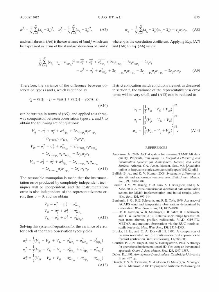
and term three in (A6) is the covariance of i and j, which can

be expressed in terms of the standard deviation of i and j:

sij 51

N�N

k51

(xjk2 xj)(xi

k2 xi) 5 rijsisj, (A8)

where rij is the correlation coefficient. Applying Eqs. (A7)

and (A8) to Eq. (A6) yields

1

N�N

k51

(«ik2«j

k1«rep

ijk

)25 «2

i 1 «2j 1 «2

repij

1 2«i«repij

2 2«j«repij

2 2«i«j

5 s2i 1 s2

j 1 s2rep

ij1 2ri2rep

ijsisrep

ij2 2rj2rep

ijsjsrep

ij2 2rijsisj. (A9)

Therefore, the variance of the difference between ob-

servation types i and j, which is defined as

Vij 5 var(i 2 j) 5 var(i) 1 var( j) 2 2cov(i, j),

(A10)

can be written in terms of (A9), and applied to a three-

way comparison between observation types i, j, and k to

obtain the following set of equations:

Vij 5 s2i 1 s2

j 1 s2rep

ij1 2ri2rep

ij

sisrepij

2 2rj2repij

sjsrepij

2 2rijsisj

Vjk 5 s2j 1 s2

k 1 s2rep

jk1 2rj2rep

jksjsrep

jk

2 2rk2repjk

sksrepjk

2 2rjksjsk

Vki 5 s2k 1 s2

i 1 s2rep

ki1 2rk2rep

kisksrep

ki

2 2ri2repki

sisrepki

2 2rkisksi. (A11)

The reasonable assumption is made that the instrumen-

tation error produced by completely independent tech-

niques will be independent, and the instrumentation

error is also independent of the representativeness er-

ror; thus, r 5 0, and we obtain

Vij 5 s2i 1 s2

j 1 s2rep

ij

Vjk 5 s2j 1 s2

k 1 s2rep

jk

Vki 5 s2k 1 s2

i 1 s2rep

ki. (A12)

Solving this system of equations for the variance of error

for each of the three observation types yields

s2i 5

1

2(Vij 2 Vjk 1 Vki 2 s2

repij

1 s2rep

jk2 s2

repki

)

s2j 5

1

2(Vjk 2 Vki 1 Vij 2 s2

repjk

1 s2rep

ki2 s2

repij)

s2k 5

1

2(Vki 2 Vij 1 Vjk 2 s2

repki

1 s2rep

ij2 s2

repjk

).

(A13)

If strict collocation match conditions are met, as discussed

in section 2, the variance of the representativeness error

terms will be very small, and (A13) can be reduced to

si 5

�1

2(Vij 2 Vjk 1 Vki)

�1/2

sj 5

�1

2(Vjk 2 Vki 1 Vij)

�1/2

sk 5

�1

2(Vki 2 Vij 1 Vjk)

�1/2

. (A14)

REFERENCES

Anderson, A., 2006: AirDat system for ensuring TAMDAR data

quality. Preprints, 10th Symp. on Integrated Observing and

Assimilation Systems for Atmosphere, Oceans, and Land

Surface, Atlanta, GA, Amer. Meteor. Soc., 9.3. [Available

online at http://ams.confex.com/ams/pdfpapers/101342.pdf.]

Ballish, B. A., and K. V. Kumar, 2008: Systematic differences in

aircraft and radiosonde temperatures. Bull. Amer. Meteor.

Soc., 89, 1689–1707.

Barker, D. M., W. Huang, Y.-R. Guo, A. J. Bourgeois, and Q. N.

Xiao, 2004: A three-dimensional variational data assimilation

system for MM5: Implementation and initial results. Mon.

Wea. Rev., 132, 897–914.

Benjamin, S. G., B. E. Schwartz, and R. E. Cole, 1999: Accuracy of

ACARS wind and temperature observations determined by

collocation. Wea. Forecasting, 14, 1032–1038.

——, B. D. Jamison, W. R. Moninger, S. R. Sahm, B. E. Schwartz,

and T. W. Schlatter, 2010: Relative short-range forecast im-

pact from aircraft, profiler, radiosonde, VAD, GPS-PW,

METAR, and mesonet observations via the RUC hourly as-

similation cycle. Mon. Wea. Rev., 138, 1319–1343.

Brooks, H. E., and C. A. Doswell III, 1996: A comparison of

measures-oriented and distributions-oriented approaches to

forecast verification. Wea. Forecasting, 11, 288–303.

Courtier, P., J.-N. Thepaut, and A. Hollingsworth, 1994: A strategy

for operational implementation of 4D-Var, using an incremental

approach. Quart. J. Roy. Meteor. Soc., 120, 1367–1387.

Daley, R., 1991: Atmospheric Data Analysis. Cambridge University

Press, 457 pp.

Daniels, T. S., G. Tsoucalas, M. Anderson, D. Mulally, W. Moninger,

and R. Mamrosh, 2004: Tropospheric Airborne Meteorological


Data Reporting (TAMDAR) sensor development. Preprints,

11th Conf. on Aviation, Range, and Aerospace Meteorology,

Hyannis, MA, Amer. Meteor. Soc., 7.6. [Available online at

http://ams.confex.com/ams/pdfpapers/81841.pdf.]

——, W. R. Moninger, and R. D. Mamrosh, 2006: Tropospheric

Airborne Meteorological Data Reporting (TAMDAR) over-

view. Preprints, 10th Symp. on Integrated Observing and As-

similation Systems for Atmosphere, Oceans, and Land Surface,

Atlanta, GA, Amer. Meteor. Soc., 9.1. [Available online at


Desroziers, G., and S. Ivanov, 2001: Diagnosis and adaptive tuning

of information error parameters in a variational assimilation.

Quart. J. Roy. Meteor. Soc., 127, 1433–1452.

——, L. Berre, B. Chapnik, and P. Poli, 2005: Diagnosis of obser-

vation, background and analysis error statistics. Quart. J. Roy.

Meteor. Soc., 131, 3385–3396.

DiMego, G. J., K. E. Mitchell, R. A. Petersen, J. E. Hoke, J. P.

Gerrity, J. J. Tuccillo, R. L. Wobus, and H.-M. Juang, 1992:

Changes to NMC’s Regional Analysis and Forecast System.

Wea. Forecasting, 7, 185–198.

Drue, C., W. Frey, A. Hoff, and T. Hauf, 2008: Aircraft type-

specific errors in AMDAR weather reports from commercial

aircraft. Quart. J. Roy. Meteor. Soc., 134, 229–239.

Fischer, A., 2006: The use of TAMDAR (Tropospheric Airborne

Meteorological Data Reporting) as a convective forecasting

supplement in the northern plains and upper Midwest. Pre-

prints, 10th Symp. on Integrated Observing and Assimilation

Systems for Atmosphere, Oceans, and Land Surface, Atlanta,

GA, Amer. Meteor. Soc., 9.6. [Available online at http://

ams.confex.com/ams/pdfpapers/104888.pdf.]

Hollingsworth, A., and P. Lonnberg, 1986: The statistical structure

of short-range forecast errors as determined from radiosonde

data. Part I: The wind field. Tellus, 38A, 111–136.

Hong, S.-Y., Y. Noh, and J. Dudhia, 2006: A new vertical diffusion

package with an explicit treatment of entrainment processes.

Mon. Wea. Rev., 134, 2318–2341.

Huang, X.-Y., 2009: The 2009 WRFDA overview. Extended Ab-

stracts, WMO Data Assimilation Symp., Melbourne, WMO.

[Available online at http://www.cawcr.gov.au/staff/pxs/wmoda5/

ExtendedAbstracts/Huang.pdf.]

Ide, K., P. Courtier, M. Ghil, and A. C. Lorenc, 1997: Unified no-

tation for data assimilation: Operational, sequential and var-

iational. J. Meteor. Soc. Japan, 75, 181–189.

Jacobs, N., P. Childs, M. Croke, and Y. Liu, 2008: The effects of

horizontal grid spacing and vertical resolution on TAMDAR

data assimilation in short-range mesoscale forecasts. Pre-

prints, 12th Symp. on Integrated Observing and Assimilation

Systems for the Atmosphere, Oceans, and Land Surface, New

Orleans, LA, Amer. Meteor. Soc., 15B.6. [Available online at


——, ——, ——, ——, and X. Y. Huang, 2010: An update on the

TAMDAR sensor network deployment. Preprints, 14th Symp.

on Integrated Observing and Assimilation Systems for the At-

mosphere, Oceans, and Land Surface, Atlanta, GA, Amer.

Meteor. Soc., 8.3. [Available online at http://ams.confex.com/

ams/pdfpapers/164835.pdf.]

Kain, J. S., 2004: The Kain–Fritsch convective parameterization:

An update. J. Appl. Meteor., 43, 170–181.

Liu, Y., and Coauthors, 2010: Evaluation of TAMDAR data

impact on predicting warm-season convection using the

NCAR-AirDat WRF-based RTFDDA system. Preprints, 14th

Symp. on Integrated Observing and Assimilation Systems for

the Atmosphere, Oceans, and Land Surface, Atlanta, GA,

Amer. Meteor. Soc., 8.6. [Available online at http://ams.confex.

com/ams/pdfpapers/165099.pdf.]

Lorenc, A. C., 1986: Analysis methods for numerical weather

prediction. Quart. J. Roy. Meteor. Soc., 112, 1177–1194.

——, and Coauthors, 2000: The Met. Office global three-dimensional

variational data assimilation scheme. Quart. J. Roy. Meteor. Soc.,

126, 2991–3012.

Mamrosh, R. D., E. S. Brusky, J. K. Last, E. J. Szoke, W. R.

Moninger, and T. S. Daniels, 2006: Applications of TAMDAR

aircraft data reports in NWS forecast offices. Preprints, 14th

Symp. on Integrated Observing and Assimilation Systems

for the Atmosphere, Oceans, and Land Surface, Atlanta, GA,

Amer. Meteor. Soc., 9.4. [Available online at http://ams.confex.

com/ams/pdfpapers/104842.pdf.]

Miloshevich, L. M., H. Vomel, D. N. Whiteman, and T. Leblanc,

2009: Accuracy assessment and correction of Vaisala RS92

radiosonde water vapor measurements. J. Geophys. Res., 114,

D11305, doi:10.1029/2008JD011565.

Moninger, W. R., R. D. Mamrosh, and P. M. Pauley, 2003: Auto-

mated meteorological reports from commercial aircraft. Bull.

Amer. Meteor. Soc., 84, 203–216.

——, S. G. Benjamin, B. D. Jamison, T. W. Schlatter, T. L.

Smith, and E. J. Szoke, 2010: Evaluation of regional air-

craft observations using TAMDAR. Wea. Forecasting, 25,

627–645.

Mulally, D., and A. Anderson, 2011: Correction of aircraft flux

valve based heading for two-dimensional winds aloft calcula-

tions using weather model comparisons. Preprints, 15th Symp.

on Integrated Observing and Assimilation Systems for Atmo-

sphere, Oceans, and Land Surface, Seattle, WA, Amer. Me-

teor. Soc., 5.6. [Available online at http://ams.confex.com/ams/

91Annual/webprogram/Paper184928.html.]

O’Carroll, A. G., J. R. Eyre, and R. W. Saunders, 2008: Three-way

error analysis between AATSR, AMSR-E, and in situ sea

surface temperature observations. J. Atmos. Oceanic Tech-

nol., 25, 1197–1207.

Painting, D. J., 2003: AMDAR reference manual. WMO, 84 pp.

[Available online at http://amdar.wmo.int/Publications/

AMDAR_Reference_Manual_2003.pdf.]

Parrish, D. F., and J. C. Derber, 1992: The National Meteorological

Center’s spectral statistical-interpolation analysis system. Mon.

Wea. Rev., 120, 1747–1763.

Richner, H., and P. D. Phillips, 1981: Reproducibility of VIZ ra-

diosonde data and some sources of error. J. Appl. Meteor., 20,

954–962.

Schwartz, B. E., and S. G. Benjamin, 1995: A comparison

of temperature and wind measurements from ACARS-

equipped aircraft and rawinsondes. Wea. Forecasting, 10,

528–544.

——, ——, S. M. Green, and M. R. Jardin, 2000: Accuracy of

RUC-1 and RUC-2 wind and aircraft trajectory forecasts by

comparison with ACARS observations. Wea. Forecasting, 15,

313–326.

Seidel, D. J., B. Sun, M. Pettey, and A. Reale, 2011: Global radio-

sonde balloon drift statistics. J. Geophys. Res., 116, D07102,

doi:10.1029/2010JD014891.

Skamarock, W. C., and Coauthors, 2008: A description of the

Advanced Research WRF version 3. NCAR Tech. Note

NCAR/TN-4751STR, 113 pp.

Smith, T. L., and S. G. Benjamin, 1994: Relative impact of data

sources on a data assimilation system. Preprints, 10th Conf. on

Numerical Weather Prediction, Portland, OR, Amer. Meteor.

Soc., 491–493.


Sullivan, J., L. Gandin, A. Gruber, and W. Baker, 1993: Observa-

tion error statistics for NOAA-10 temperature and height re-

trievals. Mon. Wea. Rev., 121, 2578–2587.

Szoke, E., B. D. Jamison, W. R. Moninger, S. Benjamin,

B. Schwartz, and T. L. Smith, 2006: Impact of TAMDAR on

RUC forecasts: Case studies. Preprints, 10th Symp. on In-

tegrated Observing and Assimilation Systems for Atmosphere,

Oceans, and Land Surface, Atlanta, GA, Amer. Meteor. Soc.,

9.9. [Available online at http://ams.confex.com/ams/pdfpapers/

104059.pdf.]

Wang, H., X.-Y. Huang, Y. Chen, X. Zhang, D. Stark, and P. Childs,

2009: The impact of TAMDAR observations on Hurricane Ike

(2008) forecast using WRFDA system. 10th WRF Users’

Workshop, Boulder, CO, NCAR, P2A.6. [Available online

at http://www.mmm.ucar.edu/wrf/users/workshops/WS2009/

abstracts/P2A-06.pdf.]


Estimation of TAMDAR Observational Error and Assimilation Experiments

Documents

Transcript of Estimation of TAMDAR Observational Error and Assimilation Experiments