CHAPTER 7

BOUNDARY LAYER MESHING - ELEMENT

CREATION

The Generalized Advancing Layers method attempts to grow anisotropic elements on

all requested model faces while maintaining good element quality and shielding the

isotropic mesh generator from the highly stretched faces of the boundary layer mesh.

The primary construct in the creation of the boundary layer mesh is the triangular

prism formed by connecting the nodes of three growth curves from the vertices of

a single mesh face. Other constructs are boundary layer transition elements and

boundary layer blends.

As explained in Chapter 5, multiple sets of nodes are allowed to emanate from

a single mesh vertex. The presence of multiple growth curves allows adjacent prisms

to be separated from each other. This reduces the distortion of the prisms, a neces-

sary condition for good quality of the tetrahedra formed by subdividing the prism.

The separation of adjacent boundary layer prisms leads to the formation of gaps

in between the prisms. The walls of these gaps consist of highly stretched faces

of the anisotropic mesh and must be shielded from the isotropic mesh generator;

otherwise the isotropic mesher tends form poorly shaped elements in their neigh-

borhood and also su�ers in reliability. It is proposed that these gaps will be �lled

by constructs referred to as boundary layer blends similar to the blends used in

geometric modeling to round o� sharp corners (See Figure 7.1 which is reproduced

here from Chapter 5 for easy reference). Boundary layer blends may occur at mesh

edges or at mesh vertices. In principle, boundary layer blends may or may not have

�xed number of elements along the model edge. Variable blend constructs typically

occur at model edges where the dihedral angle between the connected mesh faces is

changing along the edge. While boundary layer blends at mesh edges are easy to

mesh using templates since only two prisms contribute to their boundary, boundary

layer blends at mesh vertices are harder since an arbitrarily large number of prisms

and blends incident on the mesh vertex may contribute to the polyhedral cavity

67

68

to be meshed. Therefore, such cavities must be meshed by more general meshing

procedures tailored for this purpose (Figure 7.1d).

G20

G21

G22

G23

Boundary layerblend triangle

Boundary layer variableblend polyhedron

Boundary layer fixedblend polyhedron

Boundary layer vertexblend cavity

(a)(b)

(c) (d)

Figure 7.1: Boundary layer blend elements.

When the growth curves of a mesh face forming a prism have di�erent number

of nodes, a step is formed in the boundary layer mesh. This too exposes stretched

faces to the isotropic mesh generator. The di�erence in the number of nodes in the

growth direction comes from user requested mesh attributes, deletion of nodes due to

invalidity of elements or deletion of elements to avoid intersection of boundary layers

(Chapter 8). The step in the boundary layer mesh is formed since boundary layer

quads and prisms can be formed only by connecting nodes of growth curves at equal

levels. To avoid leaving highly stretched faces of the step exposed to the volume

mesher, tetrahedra are created to bridge the the growth curves with more nodes to

those with less nodes (See Figure 7.2). Since the process of recursively adjusting the

number of nodes on growth curves after pruning them tries to enforce a one layer

69

di�erence between adjacent growth curves, transition tetrahedra generally span only

one layer. However, as will be described in Chapter 8, multiple level di�erence may

be created between adjacent growth curves during pruning of growth curves to

�x self-intersections. Therefore, the capability to create multiple level transition

elements also exists to be used when necessary. The idea of a one level transition

element is similar to the procedure used in the work of Connell and Braaten [11] to

phase out the boundary layer at some edges.

All of the boundary layer constructs described above are allowed to abut

a model face and therefore modify the model face triangulation. The equivalent

boundary layer constructs for the boundary layer prisms are boundary layer quads,

boundary layer blend triangles and boundary layer transition triangles.

(c) One level transition tetrahedra

(d) Multi-level transition tetrahedra

(a) One level transition triangles

(b) Multi-level transition triangles

Figure 7.2: Boundary layer transition elements.

Element creation in the generalized advancing layers procedure is done in the

following steps:

1. Growth curves are �rst determined at mesh vertices classi�ed on model ver-

tices. If any of these growth curves lie partly or fully on a model edge, the

boundary layer entities classi�ed on the model edges are created.

70

2. Boundary layer mesh entities classi�ed on model edges are incorporated into

the model edge discretization.

3. Growth curves are determined at mesh vertices classi�ed on model edges.

Boundary layer entities from these growth curves, and growth curves at model

vertices that are classi�ed on model faces are created.

4. Growth curves on the model boundary are combined to form boundary layer

quads, boundary layer transitions and boundary layer blends. First, corre-

sponding nodes of adjacent boundary growth curves from neighboring vertices

are combined to form quads lying partially or fully on model faces. If a level

di�erence exists between the growth curves, transition triangles are formed

on top of the quads. Finally, blends are formed between appropriate multiple

boundary growth curves at mesh vertices.

5. Boundary layer quads, transitions and blends lying on model faces are incor-

porated into the triangulations of model faces.

6. Growth curves are determined at mesh vertices classi�ed on model faces. The

entities of these growth curves and growth curves from model vertices and

model edges that are classi�ed in the interior are created.

7. The interior growth curves are connected up to form prisms, transitions and

blends. First, adjacent growth curves from neighboring vertices are connected

up to form prisms. If a level di�erence exists between growth curves forming

a prism, then transition tetrahedra are formed atop the prisms to bridge the

step. Finally, blends are created between the multiple growth curves at mesh

vertices.

7.1 Conversion of Growth Curves into Boundary Layer Mesh

Entities

The creation of boundary layer mesh entities from growth curves is done in

one step if all the nodes of the growth curve are classi�ed on only one entity. If

the growth curves that are partly boundary and partly interior are permitted, then

71

the parts of the growth curve classi�ed on a model edge, model face and model

region can be converted into mesh entities during model edge retriangulation, face

retriangulation and region triangulation respectively.

Nodes of growth curves are directly converted into mesh vertices with their

classi�cation being derived from the growth curve node classi�cation. On the other

hand, classi�cation of the growth curve segment is not explicitly stored. Therefore,

when converting growth curve segments to mesh edges, their classi�cation has to

be derived from the classi�cation of the mesh vertices. Given two mesh vertices of

a boundary layer mesh edge representing a growth curve segment, the classi�cation

of the mesh edge is determined by �nding the lowest order model entity common

to the two entities that the mesh vertices are classi�ed on. In case there is more

than one common entity that the edge can be classi�ed on, an additional check is

performed. In this additional step, the midpoint of the straight line approximation

of the mesh edge in parametric space is checked if it maps to a point in the interior

of one the candidate model entities. The edge is then classi�ed on the entity that

satis�es this condition.

7.2 Model Edge Retriangulation

The insertion of boundary layer mesh edges and vertices classi�ed on model

edges is carried out through local mesh modi�cation operators [35] (Also see Ap-

pendix A). Given an edge to be inserted into the discretization of a model edge,

existing mesh edges overlapping the edge to be inserted are identi�ed by examining

the one-dimensional parametric space of the model edge. The end vertices of the

edge to be inserted are introduced into the model edge discretization by an edge split

if coincident vertices do not already exist in the mesh. Then all edges overlapping

the edge to be inserted are collapsed out into a single edge. Finally the edge to be

inserted is merged with the duplicate edge in the mesh.

7.3 Triangulation of Boundary Layer Quads

Boundary layer quads are formed by connecting nodes of adjacent growth

curves not originating from the same mesh vertex. Given two adjacent growth

72

curves, Ci1j1having n1 nodes and Ci2

j2having n2 nodes, n � 1 boundary layer quads

are formed (n = min(n1; n2)). For each layer l, a boundary layer quad is formed by

connecting the nodes pi1j1;l, pi1j1;(l+1), p

i2j2;l

and pi2j2;(l+1). In converting these boundary

layer quads to triangles the choice of the diagonal is dictated by the future validity

of the connected prisms. For reasons explained in the section describing prism

tetrahedronization (Section 7.7 below), the diagonal is made so that it connects

node l of the growth curve at the mesh vertex with a lower identifying number

(vertex ID) to node l + 1 of the growth curve at the other vertex. If one of the

growth curves has more nodes than the other, the transition triangles are formed

on top of the quads as explained below.

M0

i1;j1;0=M

0

i1 M0

i2;j2;0=M

0

i2

M0

i2;j2;l

M1

s2=M

1

i2;j2;l

M0

i2;j2;l+1

M1

s1=M

1

i1;j1;l

M0

i1;j1;l

M0

i1;j1;l+1

M2

t

M2

b

Ci2j2

Ci1j1

M1

t

M1

d

M1

b

M1

e

Figure 7.3: Boundary layer quad triangulation template.

The algorithm for constructing a boundary layer quad between the n nodes

of the growth curves Ci1j1and Ci2

j2is given below (See Figure 7.3). In the algorithm,

it is assumed that mesh entities have been created from the two growth curves and

that ID(M0i1) < ID(M0

i2) (where ID(M0

i ) is the identi�cation number assigned to

each mesh vertex) which implies that for a layer l, the diagonal of the quad goes

from pi1j1;l to pi2j2;(l+1). The steps of the algorithm are:

1. The bottommost edge of the boundary layer quad isM1e , whereM

0i1;M0

i2� @M1

e .

Make this the bottom edge of the bottommost quad.

2. For each layer l; l = 1; n � 1, do the following (Refer entities of layer l in

Figure 7.3):

73

(a) Get the bottom mesh edge of the quad,M1b , between mesh verticesM0

i1;j1;l

and M0i2;j2;l

.

(b) Get the side mesh edges, M1s1

= M1i1;j1;l

and M1s2

= M1i2;j2;l

of the quad

from the two growth curves Ci1j1and Ci2

j2respectively.

(c) Create the diagonal edge, M1d between vertices M0

i1;j1;land M0

i2;j2;(l+1) for

this layer. The classi�cation of the edge is derived from its end nodes.

(d) Figure out the classi�cation of the lower triangular face M2b (where

M1b ;M

1s2;M1

d � @M2b ) of the quad from its 3 edges.

(e) If M2b < G3

r, then the orientation of the face is not important as long it

is taken into account by the regions that use it. On the other hand, if

M2b < G2

f , then the face must be oriented in the same direction as the

model face5. In this case, the orientation of the mesh face is determined

by examining M1b .

The natural de�nition of the face is such that its edges are ordered

as M1b , M

1s2, M1

d used in directions de�ned by the fact that the ver-

tices around the face starting from M0i1;j1;l

are the ordered cyclic set

[M0i1;j1;l

;M0i2;j2;l

;M0i2;j2;(l+1)].

� IfM1b < G2

f , then the other mesh face,M2p connected to the edge and

classi�ed on G2f is found, if it exists. If such a face exists, then M2

b

usesM1b in a direction opposite to the direction in whichM2

p usesM1b

(See Figure 7.4a). If the direction of use con icts with the selected

direction of use ofM1b then the orientation of the face is reversed and

the ordered set of edges and vertices around the natural direction

of the face becomes [M1b ;M

1d ;M

1s2] and [M0

i1;j1;l;M0

i2;j2;(l+1);M0i2;j2;l

]

(Figure 7.4b).

� If M1b < G2

e � @G2f , then it is assumed that the mesh edge has

the same direction as the model edge (i. e. the �rst vertex of the

5This is an assumption that is enforced throughout all the mesh generation tools described or

referenced here. While this is not a necessary condition for successful mesh generation, it make the

procedures much simpler without adversely a�ecting the reliability of the mesher or the quality of

the generated meshes

74

edge has a lower parameter with respect to the model edge than the

second except when it spans a periodic boundary). In this case the

direction of use of G1e by G2

f is found and M2b must use M1

b in the

same direction (Figure 7.4c,d).

In the special case when G2f uses G

1e both ways, �rst a check is made

for a mesh faceM2p < G2

f already connected to the edge. If such a face

exists, then the orientation of the current face is checked in the same

way that it was done for mesh edges classi�ed on the model faces. If

not, a geometric check is performed to see if the direction of the face

is right. To do this a mesh face use using the two growth curves of the

boundary layer quad is found and a virtual region constructed using

the vertices of the M2b and the node of the mesh face use opposite

the base edge M1e ; M

0i1;M0

i2� @M1

e of the boundary layer quad. If

the volume of this region is positive, the orientation ofM2b is correct;

if not, it must reversed (See Figure 7.4e).

(f) Create the top edge of the boundary layer quad for this layer, M1t ,

M0i1;j1;(l+1);M

0i2;j2;(l+1) � @M1

t , deriving its from the classi�cation from

its end nodes.

(g) Figure out the classi�cation of the upper face M2u ; M

1t ;M

1s1;M1

d � @M2u

of the quad from its 3 edges. Reverse its orientation, if necessary, as was

done for the lower face using the diagonal edge as a reference edge. Thus

in its natural orientation, the ordered set of edges and vertices of M2u

are [M1t ;M

1s1;M1

d ] and [M0i2;j2;(l+1);M

0i1;j1;(l+1);M

0i1;j1;l

] respectively. In the

reversed orientation, these sets become [M1t ;M

1d ;M

1s1] and

[M0i2;j2;(l+1);M

0i1;j1;l

;M0i1;j1;(l+1)] respectively.

(h) Label M1t as M1

b .

An important point to note here is that although the current implementation

has precluded the existence of partially boundary and partially interior growth curves,

a special type of quad with some faces classi�ed on the boundary and others in

the interior may still exist in the boundary layer mesh. This happens under the

75

(a) (b)

M0

i2;j2;l

M0

i2;j2;l+1

M0

i1;j1;l

M2

b

M2

p

M0

i2;j2;l�1

M1

b

M1

d M1

s2

M0

i2;j2;l

M0

i2;j2;l+1

M0

i1;j1;l

M2

b

M2

p

M0

i2;j2;l�1

M1

b

M1

d M1

s2

M0

i2;j2;l

M0

i2;j2;l+1

M0

i1;j1;l

M2

b

M1

b

M1

d M1

s2

G1

e

G2

f

(c) (d)

M0

i2;j2;l

M0

i2;j2;l+1

M0

i1;j1;l

M2

b

M1

b

M1

d M1

s2

G1

e

G2

f

(e)

M0

i2;j2;l

M0

i2;j2;l+1

M0

i1;j1;l

M2

b

M1

b

M1

d M1

s2

G1

e

G2

f

M0

r

M2

r

G2

h

Assumed direction

Correct direction

Figure 7.4: Determining face directions for boundary layer quad triangles. (a) Bot-tom edge classi�ed on model face and assumed face direction is correct. (b) Bottomedge classi�ed on model face and face direction must be reversed. (c) Bottom edgeclassi�ed on model edge and assumed face direction is correct. (d) Bottom edgeclassi�ed on model edge and face direction must be reversed. (e) Geometric checkwhen bottom edge classi�ed on model edge used twice by the model face.

76

(a) (b)

(c)

Interior triangle

Boundary triangle

G2

f

M1

b< G

1

e

M0

j< G

1

e

M0

i< G

1

e

M

1d<

G2f

M2

b < G2

f

M2

u< G

3

r

M

1 i;0

<

G3 r

M

1 j;0

<

G2 f

M0

j;1 < G2

f

Ci

0 < G3

r

Cj0 < G

2

f

M1

t< G

3

r

M0

i;1 < G3

r

G2

f

M1

b< G

1

e

M0

j< G

1

e

M0

i< G

1

e

M1

t< G

3

r

M2

b < G3

r

M2

u< G

3

r

M0

i;1 < G3

r

M0

j;1 < G2

f

Ci

0 < G3

r

Cj0 < G

2

f

M1

d<G 3r M

1 j;0

<

G2 f

M

1 i;0

<

G3 r

G2

f

M1

b< G

1

e

M0

j< G

1

e

M0

i< G

1

e

M1

t< G

2

f

M2

b < G2

f

M2

u < G2

f

M0

i;1 < G2

f

M0

j;1 < G2

f

Ci0 < G

2

f

Cj0 < G

2

f

M1

d<G 2f

M

1 i;0

<

G2 f M

1 j;0

<

G2 f

Figure 7.5: Types of quads at model edges. (a) Quad with partly boundary andpartly interior classi�cations. (b) Quad with all interior classi�cation. (c) Quadwith all boundary classi�cation.

77

particular circumstance in which the one growth curve is fully interior and the other

is fully boundary and the diagonals of the quad have their lower vertices on the

interior growth curve. This is illustrated in Figure 7.5. In the �gure, M0i ;M

0j < G1

e

and Ci0 < G3

r, Cj0 < G2

f . In the Figure 7.5a, ID(M0i ) < ID(M0

j ). Therefore, by the

methods described above, in the �rst layer M1d < G2

f and M1t < G3

r. As a result of

the classi�cations of their component edges, the bottom face of the lower triangle in

the �rst layer is classi�ed on model face G2f and the top triangle on model region G2

r.

Note that only the �rst layer triangles of such boundary layer quads have di�erent

classi�cations and the rest of the triangles are classi�ed interior. In Figure 7.5b,

ID(M0j ) < ID(M0

i ) and therefore, all the triangles are classi�ed as being interior.

In Figure 7.5c, both growth curves are classi�ed on the same model face and therefore

it is immaterial what the IDs of the vertices are - all triangles are classi�ed on the

model face.

When quads are partly boundary and partly interior, the boundary triangles

are created �rst and inserted into the surface mesh and the interior triangles are

completed later when other fully interior quads are being created. Although it is true

that the procedure can avoid dealing with the quads with multiple classi�cations in

most cases by simply exchanging the ID numbers of vertices, it is not guaranteed that

this type of quad will never be needed since neighboring quads get a�ected by the

change in IDs. In addition, the availability of such mechanisms in the mesh generator

provides the basis for handling more general types of quadrilateral abstractions in

future implementations.

7.4 Creation of Boundary Layer Transition Triangles

Transition triangles are formed atop boundary layer quads with a level di�er-

ence between the two growth curves. This is done by simply connecting the top

node of the growth curve with fewer nodes with nodes of the other growth curve

which are at a higher level. It is important to note that the mesh vertex with the

lower ID may have the growth curve with more nodes and therefore, diagonal edge

of the transition triangle may go in an opposite direction to the diagonals of the

boundary layer quad (Figure 7.2a,b).

78

7.5 Creation of Boundary Layer Blend Triangles

Creation of boundary layer blend triangles is similar to the creation of bound-

ary layer quads. The di�erence is that boundary layer blend triangles establish

connections between nodes of two growth curves originating from the same mesh

vertex. The �rst layer of a blend triangle is made up of a single triangular mesh face

and the rest of the layers contain triangulated quads as in the case of the boundary

layer quad. The direction of the diagonal for the quads in a boundary layer triangle

is arbitrary and may be based solely on the quality of the triangles (Figure 7.1a).

7.6 Model Face Retriangulation

The choice of the method used for the incorporation of mesh entities classi�ed

on model boundaries is very important to the reliability of the boundary layer mesh

generator. While the use of an advancing front type method to retriangulate the

model faces is attractive, it requires the use of the parametric space of the model

faces to check for intersections. This is an error prone procedure if the parametric

space is highly distorted since the underlying assumption is that straight line ap-

proximations of the parametric curves representing mesh edges can be used to check

for intersections. In fact, examples exist of commercial modelers using highly dis-

torted parametric spaces for model faces constructed from a existing set of facets.

An alternative is to create the boundary layer mesh entities on model edges and

then complete the triangulation of the model edges, create entities classi�ed on the

model faces and then complete the triangulation of the faces and �nally create the

interior boundary layer mesh entities before handing the mesh over to a volume

mesher. This may be convenient or di�cult to do depending on the approach of the

isotropic mesher and may require tight integration with the sub-components of the

surface mesh generator. To avoid the use of the parametric space for intersection

checks and to keep the surface meshing, boundary layer meshing and volume mesh-

ing independent and modular, a third alternative is adopted here. This method

uses local mesh modi�cation operators combined with checks for the smoothness

of the surface discretization to incorporate boundaries of the boundary layer mesh

79

(a) (b)

(c) (d)

(e) (f)

Figure 7.6: Model face retriangulation by local mesh modi�cations. (a) Initial sur-face mesh. (b) Surface mesh with boundary layer elements overlayed. (c) Insertionof outermost boundary layer vertices into surface mesh. (d) Recovery of outermostboundary layer edges by edge swapping and edge collapsing. (e) Deletion of surfacemesh triangles overlapping the boundary layer mesh. (f) Incorporation of boundarylayer mesh into surface mesh.

into the existing surface triangulation. It then replaces overlapping triangles of the

underlying mesh with the boundary layer triangles [35].

The model face retriangulation procedure is done for each model face that the

growth curves of each model edge a�ect. Given a model edge and a model face on

which growth curves from mesh vertices of the model edge lie, the following steps

are carried out to create and incorporate the boundary layer mesh into the surface

mesh triangulation:

1. Boundary layer quads and triangles classi�ed on the the model face are created

as described above (Figure 7.6b).

80

2. The boundary layer quads and triangles are temporarily disconnected from

the mesh entities of the original face triangulation. This is done to prevent

the procedures recovering the boundary layer edges from being misled by the

presence of the boundary layer mesh entities in the discretization of the model

face.

3. Each boundary layer mesh entity that forms the outer boundary of the set

of boundary layer mesh faces classi�ed on the model face is incorporated into

the surface mesh by the edge recovery procedure. The recovery procedure

is brie y described below and discussed in full detail in [35]. Once all the

necessary edges have been recovered, the outer boundary of the set of faces to

be inserted into the mesh exactly matches the outer boundary of a set of faces

in the underlying surface mesh (Figure 7.6c,d).

4. Mesh faces of the existing surface triangulation overlapping the boundary layer

mesh faces are deleted (Figure 7.6e). The set of faces overlapping the boundary

layer mesh faces are found using only topological checks and searches.

5. The boundary layer faces are incorporated into the surface mesh in place of

the deleted elements (Figure 7.6f).

The edge recovery procedure �rst identi�es where to insert the vertices of the

edge to be recovered into the existing mesh. The insertion point may be an existing

vertex (in which case no explicit insertion of the vertex is required), a mesh edge or

and mesh face. The mesh entity to be modi�ed for insertion of the vertex or in other

words, the mesh entity \containing" the vertex to be inserted is �rst localized using

the parametric space. However, the �nal decision is made with real space checks

since the results of containment checks in the parametric space can be misleading

for highly distorted spaces. The criterion for �nding the mesh entity to split for

insertion is based on the observation that a good choice for an insertion entity is

one that will preserve or improve the approximation of the true geometry by the

surface mesh since it is guaranteed that the point to be inserted will lie on the true

geometry. Therefore, the methodology used projects the insertion point onto a local

set of mesh faces along their respective normals and among the mesh faces containing

81

the projected point, the one that maintains or improves the approximation of the

true geometry is chosen. The dihedral angles between mesh faces before and after

insertion of the new point is a good measure for assessing the choice of the mesh

entity to be split, the alternative being to use one of many forms of comparison

between the discrete normals (normals of mesh faces) before and after the split.

The point is inserted into the mesh either by merging with an existing vertex, by

an edge split or by a face split operation (See Appendix A).

Once the vertices to be recovered are inserted into the mesh, a path of edge

connected mesh faces is found from one vertex to another. Once again this is done

by projection of the edge to be recovered onto planes of the mesh faces in the

neighborhood. If any mesh vertices lie in the path of the edge to be recovered, they

are either collapsed along a connected edge or perturbed. If the collapses have not

already recovered the edge, it is recovered by successive swaps of mesh edges of the

faces in its path.

The edge split and face split operations used to insert the vertices of the edge

to be recovered often cause poorly shaped elements to be formed. The nearly at

elements then cause numerical imprecision in the remaining steps of the recovery

algorithm thereby reducing its reliability. Two strategies may be used to eliminate

the creation of such poorly shaped elements. The �rst is to use an increased point

tolerance for checking if point lies on a vertex or an edge. This prevents points from

being inserted too close to an existing vertex or an edge. Care has to be taken in

this approach to ensure that use of the increased tolerance does not cause a single

mesh vertex to capture both endpoints of the edge. Also, if the point is declared

to be coincident with a mesh vertex then the vertex must be repositioned within

the real point tolerance of the insertion point. The second approach is to insert the

point using the real point tolerance of the modeler and then perform edge swaps

and edge collapse in the immediate neighborhood to eliminate the poorly shaped

mesh faces. This method has the disadvantage that it is harder to estimate how well

the mesh will approximate the true geometry after the insertion and modi�cation

operations.

82

Once the edge is recovered successfully, a local mesh optimization is performed

to eliminate any other poorly shaped faces created during the edge recovery process.

The optimization procedures are constrained to not modify any existing boundary

layer edges already recovered or any edges classi�ed on model edges. If the edge

cannot be recovered then the procedures split edges of the mesh in its path and

return a list of edges forming a path of edges from one vertex of the original edge to

be recovered to the other. In such a case, the boundary growth curve is deleted and

replaced with an interior growth curve, in e�ect peeling the boundary layer away

from the adjacent wall in the neighborhood. This requires deletion of some existing

boundary layer quads, recalculating one or two growth curves, insertion of newly

exposed edges and updating of data structures. Alternately, it is possible to go back

to the triangulation of the face on which the boundary layer is grown, split the edge

from which the boundary layer quad originates and regrow the boundary layer from

the new vertices. This way the exposed edges of the new quads will match the mesh

edges that the edge recovery algorithm actually created in place of what was earlier

requested.

Finally, after the model face retriangulation procedure is completed, the re-

sulting mesh is subjected to a series of checks to ensure that it is not self intersecting

[13]. If an intersection is found it is �xed by edge splits of unconstrained entities (i. e.

entities that do not belong to the boundary layer mesh and are not constrained in

any other way). This step is necessary to ensure that the �nal mesh that is handed

over to the volume mesher is not self-intersecting.

7.7 Creation of Boundary Layer Prisms

The bulk of the elements in the boundary layer mesh are comprised of tetrahe-

dronized layers of boundary layer prisms. Boundary layer prisms are grown on mesh

face uses by connecting the three growth curves at the face vertices which share each

mesh face use. The tetrahedronization of each boundary layer prism in a layer gives

rise to three tetrahedra. The number of layers of such elements grown atop any

mesh face use is determined by the growth curve forming the smallest number of

nodes.

83

Boundary layer prisms can be thought of as being formed by three quadri-

laterals that are grown from the edges of the mesh face. There are eight possible

combinations of diagonals for the quads of a prism. Of these only six are con�gura-

tions which can be tetrahedronized without the insertion of any new points inside

the prism (Figure 7.7a). Therefore, in assigning directions for the diagonals of the

quads in the boundary layer mesh, care must be taken not to assign directions such

that some prisms cannot be tetrahedronized. This is done by a simple algorithm

based on numbering of the surface mesh vertices. Given a surface mesh with any

arbitrary assignment of unique numbers (IDs) for the mesh vertices, the IDs of ver-

tices of a face in either clockwise or counterclockwise direction cannot be strictly

increasing or strictly decreasing. In other words, the ID of one vertex in each mesh

face has to be lesser than the IDs of the other two vertices. Using this notion, the

diagonals of boundary layer quads are constrained to go from the lower node of the

growth curves of vertices with a lower ID to the upper node of growth curves of

vertices with a higher ID. This is shown in Figure 7.7b.

The tetrahedronization of boundary layer prisms is done using templates. The

six con�gurations for the boundary layer templates are reduced to just two by always

tetrahedronizing the prism using the face vertex with the lowest ID as a reference

vertex. The face vertex with the lowest ID is also the face vertex which has two

prism diagonals connected to it. The two templates are shown in Figure 7.8. Wher-

ever necessary, boundary layer prisms utilize the boundary layer quads previously

incorporated into the model face triangulation.

The process of creating boundary layers prisms in the interior is comprised of

three steps. First all growth curves classi�ed as interior are converted into mesh

entities (edges and vertices). Also, the interior portions of growth curves classi�ed

partly on the boundary and partly interior must converted into mesh entities. Next,

boundary layer quads are grown from all mesh edges classi�ed on model faces as

done for mesh edges classi�ed on model edges. In this step partially created bound-

ary layer quads are also fully converted into mesh entities. Finally, the boundary

layer quads from mesh faces are suitably combined according to the two templates

described above into boundary layer prisms and their component tetrahedra.

84

12

0

3

45

12

0

3

45

12

0

3

45

12

0

3

45

12

0

3

45

12

0

3

45

(i) (ii) (iii) (iv)

(v) (vi) (vii) (viii)

(a)

ID0 < ID2 < ID1

ID1ID2

ID0

ID1

ID2

ID0

(b)

12

0

3

45

12

0

3

45

Figure 7.7: (a) (i)-(vi) Valid prism triangulations. (vii)-(viii) Invalid prism con�gu-rations. (b) Choice of prism diagonals based on Base Vertex IDs to assure validityof prism con�gurations.

7.8 Creation of Transition Tetrahedra

Atop a prism with one level di�erence between its component growth curves,

there may be one or two transition tetrahedra depending on whether one or two

growth curves have fewer nodes than the others. Similar to the transition triangles

for the boundary layer quads, the diagonal faces of the transition tetrahedra may

run counter to the pattern that is used for the diagonal faces of the underlying

prisms. If the level di�erence between the growth curves is more than one, then

85

0

1

2

3

4

5

1

2

0

3

45

(a) (b)

(c) (d)

0

3

45

2

0

45

1

2

0

40

3

45

0

1

4

5

0

1

2

5

Figure 7.8: Boundary Layer Prism Templates.

several layers of transition elements are created on top of the prism. Consider the

case when one of the growth curves has one more node than the other two which

have n nodes. Then the topmost nodes of the two shorter growth curves (nodes

n), the topmost node (node n+1 ) of the tall growth curve and its previous node

(node n) form one transition tetrahedron (Type I transitions, Figure 7.9a). On the

other hand, if two growth curves have one more node (n+1 ) than the third growth

86

curve, then two transition tetrahedra are formed on top of the base prism (Type

II transitions, Figure 7.9b). These two transition tetrahedra together use the nth

node of the short growth curve, and the nth and (n+1 )th nodes of the taller growth

curves. The diagonal connection between the two tall growth curves is chosen to be

in the same direction as the rest of the quad below it, i. e., it is based on the IDs of

the base nodes. Multiple transition layers may be completely Type I (Figure 7.9c),

completely Type II (Figure 7.9d) or may start o� as Type II transitions and then

switch to Type I transitions (Figure 7.9e). It is not possible to switch from Type I

transition to Type II.

It is worthwhile to mention here that the checks for the validity of elements to

be formed in the boundary layer mesh that are performed in the smoothing, shrink-

ing and pruning operations take into account the presence of transition triangles

and tetrahedra.

(b) One level Type II transition layer

(a) One level Type I transition layer

(c) Multi-level Type I transition layers

(d) Multi-level Type II transition layers

(e) Multi-level Type II/I transition layers

Pn

Pn

Pn

Pn+1 Pn+1

Pn

Pn+1

Pn Pn

Figure 7.9: Transition Elements.

7.9 Creation of Boundary Layer Blend Polyhedra

As mentioned before, the introduction of multiple growth curves at mesh ver-

tices due to surface mesh geometry introduces gaps between prisms. These gaps

87

are made up of highly stretched faces present on the sides of prisms. If left as they

are, the highly anisotropic faces of the gaps cause problems for the isotropic volume

mesher. Therefore, the concept of blend meshes is introduced in the generalized

advancing layers procedure. The blend meshes are designed to �ll the gaps between

prisms while maintaining a good mesh gradation in the boundary layer mesh.

Consider a situation in two dimensions where there are two growth curves

at a model vertex representing a convex corner (Figure 7.10a,b). The gap in the

two dimensional boundary layer mesh formed at this vertex must be �lled by blend

triangles (Figure 7.10c). If the angle between the two growth curves is too large,

bridging the gap with a single set of blend elements results in disparate mesh sizes

on the outer surface of the boundary layer mesh exposed to the isotropic mesh.

Therefore, to maintain a good mesh gradation on this outer surface, additional

growth curves may have to be introduced at a mesh vertex in between the growth

curves used by the standard boundary layer elements (quads in 2D and prisms in

3D) as shown in Figure 7.10d.

The number of additional growth curves required at a mesh vertex can be

calculated quite simply by using the model shown in Figure 7.11. Consider a mesh

vertex M0i at which there are two original growth curves separated by an angle �.

Let the average mesh size at the vertex be have. Assuming that all the growth curves

forming quads are nearly perpendicular to their respective base edges, the average

mesh size on the outer boundary of the boundary layer mesh is also taken as have.

Therefore, n additional growth curves must be introduced between the two original

growth curves such that the outer entities of the blend mesh also have a mesh size

of have. It is assumed that the n growth curves will be equispaced in the gap. Also,

the average boundary layer thickness in the neighborhood is taken to be H. The arc

length between the outermost nodes of the two original growth curves is L = H�

Therefore the arc length between the outermost nodes of any two consecutive

growth curves in the blend is:

l =L

n=H�

n(7.1)

88

(a) (b)

(c) (d)

Figure 7.10: Two dimensional illustration of the need for blends and multiple growthcurves within blends. (a) Boundary layer mesh on two surfaces with convex corner.(b) Gap between the corners shown in greater detail. (c) Blend mesh directly bridg-ing the two existing growth curves. (d) Blend mesh with introduction of additionalgrowth curve.

Since the aim is to make l � have, it can be deduced that

have =H�

n; or

n =H�

have

(7.2)

rounded o� to the nearest integer.

In three dimensions, gaps may occur at mesh edges or mesh vertices. For

simplicity of discussion, it is assumed for now that the need for blend meshes occurs

only at mesh edges (and vertices) classi�ed on model edges and at mesh vertices

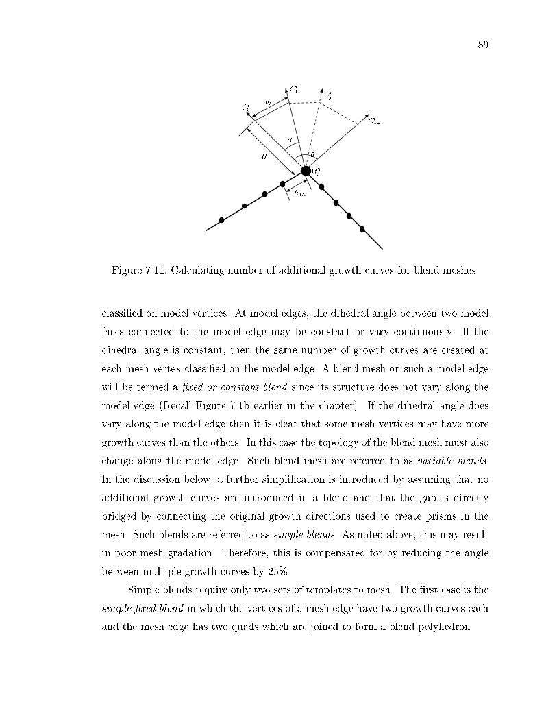
89

Ci

0

Ci

1

Ci

j

Ci

n+1

M0

i

�

�H

have

ht

Figure 7.11: Calculating number of additional growth curves for blend meshes.

classi�ed on model vertices. At model edges, the dihedral angle between two model

faces connected to the model edge may be constant or vary continuously. If the

dihedral angle is constant, then the same number of growth curves are created at

each mesh vertex classi�ed on the model edge. A blend mesh on such a model edge

will be termed a �xed or constant blend since its structure does not vary along the

model edge (Recall Figure 7.1b earlier in the chapter). If the dihedral angle does

vary along the model edge then it is clear that some mesh vertices may have more

growth curves than the others. In this case the topology of the blend mesh must also

change along the model edge. Such blend mesh are referred to as variable blends.

In the discussion below, a further simpli�cation is introduced by assuming that no

additional growth curves are introduced in a blend and that the gap is directly

bridged by connecting the original growth directions used to create prisms in the

mesh. Such blends are referred to as simple blends. As noted above, this may result

in poor mesh gradation. Therefore, this is compensated for by reducing the angle

between multiple growth curves by 25%.

Simple blends require only two sets of templates to mesh. The �rst case is the

simple �xed blend in which the vertices of a mesh edge have two growth curves each

and the mesh edge has two quads which are joined to form a blend polyhedron.

90

A simple �xed blend between two quads at a mesh edge M1i with vertices M0

j

and M0k is shown in Figure 7.12a. As seen in the �gure, the �rst layer of simple

�xed blend consists of a prism while subsequent layers are hexahedra stacked on

top of each other (in the �gure, only one hexahedron is shown since the mesh has

only two layers). A triangulation of the simple �xed blend is shown in Figure 7.12b

and an individual view of the triangulated prism and hexahedron are shown in

Figure 7.12c,d. The salient points of the triangulation are:

1. The sides of prisms and hexahedra formed by the quads always have matching

diagonals since the quads contributing to them arise from the same mesh edge.

2. It is impossible to obtain an invalid triangulation of the bottom prism since

the two matching diagonals from the quads will always meet at a vertex. The

third diagonal (forming the base of the hexahedron can be chosen arbitrarily

and is selected to provide the best element shapes.

3. Since the shape of the tetrahedra resulting from a regular hexahedron is op-

timal when all its opposite diagonals are matching, the free diagonals on the

blend hexahedron are chosen to match each other if possible. The diagonals

that are �xed are the ones from the quads (which have already been shown

to be matching) and the bottom face of the hexahedron (which is inherited

from the bottom prism). The diagonal of the top face of the hexahedron is

unconstrained and is chosen to match the bottom diagonal unless this causes

a geometrically invalid triangulation. The diagonals on the side faces of the

hexahedron are also unconstrained unless one or both of their faces lie on the

model boundary and their diagonals have already been �xed. Even if both

the side diagonals are �xed and are not matching, the hexahedron can still

be triangulated if the top and bottom diagonals match. No tetrahedroniza-

tion is possible without introducing an interior vertex if two sets of diagonals

do not match for a hexahedron. Naturally, if two blend polyhedra share a

common interface originating from a vertex their diagonals are expected to be

conforming.

91

The two prism templates used before can be used as is for meshing the bottom

prism. Accounting for the possibility of a mismatch between the top and bottom

diagonals, and side diagonals, the blend hexahedron can be triangulated by three

distinct templates. The number of di�erent possible templates is reduced to only

three by assuming that the hexahedron will always be considered with a quad di-

agonal and the \bottom" face diagonal meeting in the front lower left corner. Note

that to satisfy this condition and apply one of the templates, the hexahedron may

have to viewed upside down.

The second case is when one vertex of a mesh edge has one growth curve and

the other has two (the edge still has two quads joined at one end and separated at

the other). This is called the simple variable blend and is shown Figure 7.13a. The

simple variable blend is comprised of a 5-vertex wedge and a number of 6-vertex

wedges stacked on top of each other. The 5-vertex and 6-vertex wedges are shown

in Figure 7.13b(i) and Figure 7.13b(ii) respectively. As with the simple �xed blend,

the diagonals of the side faces of the blend polyhedra are constrained to match

each other. The 5-vertex wedge may yield two or one tetrahedra depending on the

direction of the diagonal of the quads as shown in Figure 7.13c(i) and Figure 7.13c(ii)

respectively. In the latter case the triangulation of each quad from the base mesh

edge results in an edge between vertices M0j and M0

k;0;1. Therefore, there are two

coincident edges between the two vertices M0j and M0

k;0;1, and two coincident faces

between the vertices M0j , M

0k and M0

k;0;1, one from each quad. These coincident

entities are merged to prevent the mesh from becoming topologically invalid. This

leaves only one tetrahedron fM0j ;M

0j;1;1;M

0j;0;1;M

0k;0;1g to be created from the 5-

vertex edge. The two tetrahedra that result from the other 5-vertex wedge are easy

to see. The 6-vertex wedge can be triangulated by two templates accounting for the

various symmetries in the polyhedron.

Using the above concepts for simple blends, the gap between prisms at edges

can be closed o� from the isotropic mesh generator. These templates may also be

used to build up general �xed and variable blend meshes.

As mentioned in earlier discussions, gaps between the various boundary layer

constructs at model vertices are much more general since an arbitrary number of

92

(a)

(c)

(b)

(d)

M0

k;0;1

M0

k;1;1

M0

j;0;1

M0

j;1;1

M0

j;1;2

M0

j;0;2

M0

k;0;2

M0

k;1;2M

0

k

M0

j

M0

j;0;1

M0

j;1;1

M0

k;0;1

M0

k;1;1

M0

j

M0

k

M0

k;1;1

M0

k;1;2

M0

k;0;2

M0

j;0;2

M0

j;0;1

M0

j;1;1

M0

j;1;2

M0

k;0;1

M1

i

M0

k;0;1

M0

k;0;2

M0

j;0;2

M0

j;1;1M

0

j;1;2

Ck

0

Cj0

Cj1

Ck

1

M0

j = M0

j;0;0

= M0

j;1;0

M0

j;0;1

M0

k;1;1

M0

k;1;2

M0

k = M0

k;0;0

= M0

k;1;0

Figure 7.12: Simple �xed blend.

prisms and blends may can contribute to them. However, their anisotropy is also

much lesser than that of edge blends making them easier to handle using less spe-

cialized procedures. It is proposed that the vertex blends be created using general

mesh generation techniques tailored for the purpose of �lling these gaps.

The above discussion has focused on �lling gaps between boundary layers at

model edges and model vertices. In fact, multiple growth curves and therefore,

93

(a) (b)

(c) (d)

M1

i

M0

k =M0

k;0;0

M0

k;0;1

M0

k;0;2

M0

j;0;1

M0

j;0;2

M0

j;1;1M

0

j;1;2

Ck

0

Cj0

Cj1

M0

j = M0

j;0;0

= M0

j;1;0

M0

j

M0

k

M0

j;0;1

M0

j;1;1

M0

k;0;1

M0

j

M0

k

M0

j;0;1

M0

j;1;1

M0

k;0;1

M1

d

M0

k;0;1

M0

k;0;2

M0

j;0;1

M0

j;1;1

M0

j;1;2

M0

j;0;2

M0

j

M0

k

M0

j;0;1

M0

j;1;1

M0

k;0;1

M0

k;0;1

M0

k;0;2

M0

j;0;1

M0

j;1;1

M0

j;1;2

M0

j;0;2

M0

k;0;1

M0

k;0;2

M0

j;0;1

M0

j;1;1

M0

j;1;2

M0

j;0;2

(i)

(ii)

(i)

(ii)

Figure 7.13: Simple variable blend.

94

gaps between prisms may occur at any mesh edge or mesh vertex classi�ed on the

boundary. Therefore, a complex blend structure may be constructed on a model

face with sharp corners as shown in Figure 7.14. The procedures and templates to

build blend meshes simply proceed on a mesh entity by entity basis and can be used

throughout the mesh. It must be noted here, that blend meshes are not present in

the current implementation but are expected to be incorporated into the procedures

as described above.

(a)

(b) (c)

Figure 7.14: Blend meshes on model faces. (a) Model face discretization. (b) \Pris-matic" boundary layer mesh on model face with gaps between \prisms". (c) Bound-ary layer mesh with gaps �lled in by edge and vertex blends.

The combination of prism, transition and blend constructs presented in this

chapter may be used e�ectively to construct a good anisotropic mesh for capturing

boundary layers while shielding the isotropic mesh generator from most stretched

faces. However, there may still be some situations where the boundary layer mesh

ends abruptly at a sharp corner. To absolutely prevent the isotropic volume mesher

95

(a) (b)

Figure 7.15: Transitioning of boundary layers at model edge. (a) Boundary layerwithout elimination of exposed faces. (b) Boundary layer with elimination of ex-posed faces by transitioning.

from seeing the stretched faces of the boundary layer mesh, the number of nodes

along the sharp corner edge are reduced to zero and the boundary layer transitioned

out from the edge (as described in [11]). This is shown in Figure 7.15.