Boundary Representation Model Rectification

Graphical Models63,177–195 (2001)

doi:10.1006/gmod.2001.0543, available online at http://www.idealibrary.com on

Boundary Representation Model Rectification

G. Shen, T. Sakkalis, and N. M. Patrikalakis

Massachusetts Institute of Technology, Cambridge, Massachusetts 02139-4307E-mail: [email protected]

Received December 6, 1999; revised June 15, 2001; accepted August 13, 2001

Defects in boundary representation models often lead to system errors in modelingsoftware and associated applications. This paper analyzes the model rectificationproblem of manifold boundary models, and argues that a rectify-by-reconstructionapproach is needed in order to reach the global optimal solution. The restricted faceboundary reconstruction problem is shown to be NP-hard. Based on this, the solidboundary reconstruction problem is also shown to be NP-hard.c© 2001 Academic Press

Key Words:boundary reconstruction; NP-hardness; CAD model defects; robust-ness; data exchange.

1. INTRODUCTION

Model representations of products enable man–machine and machine–machine com-munication. With rules set by representation schemes, models can be realized as physicalartifacts. However, such realization often fails whenever models contradict rules and am-biguities arise. This is especially true for manifold boundary representation (B-rep) asits validity is not self-guaranteed [1–4]. In an earlier paper, we have identified sufficientconditions for validity of manifold B-rep models [5]. Defects in B-rep models are thoserepresentational features that do not conform to constraints set by modeling schemes. Suchdefects are topological and geometric errors, and visually appear as gaps, dangling faces,internal walls, and inconsistent orientations. Defects may cause failures of modeling sys-tems and applications because operations are typically designed with the assumption ofmodel validity. Model rectification, a process that repairs defects, is essential to the successof design and manufacturing defect-free products in an integrated CAD/CAM environment.

Research on model rectification has been done mainly on triangulated models, specifi-cally, STL models for rapid prototyping. STL models represent solids using oriented tri-angles [6]. Defects in STL models are gaps due to missing triangles, inconsistently ori-ented triangles, and inappropriate intersections in the interiors of triangles. Most algorithms[7, 8] identify erroneous triangle edges, string such edges to form hole boundaries, and then

177

1524-0703/01 $35.00Copyright c© 2001 by Academic Press

All rights of reproduction in any form reserved.

178 SHEN, SAKKALIS, AND PATRIKALAKIS

fill holes with triangles. As pointed out in [7], topological ambiguities are resolved byintuitive heuristics. These algorithms [7, 8] use local topology (incidence and adjacency)to rectify defects and are successful in the majority of candidate models, but may createundesirable global topological and geometric changes. See also [9] for a critique of thesemethods.

Barequet and Sharir [9] developed a global gap-closing algorithm for polyhedral models,using a partial curve-matching technique. In their method, gap boundaries are discretized.Each match between any two parts of gap boundaries is given a score based on the closenessof their discrete points. They have shown that finding a consistent set of partial curve matcheswith maximum score, a subproblem of their repairing process, is NP-hard. Barequet andKumar [10] developed a model repairing system using the algorithm in [9], but with amodified score that is the normalized gap area between two matched parts of gap boundaries.Visualization tools were also provided to enable the user to override unwanted modifications.The system was improved by Barequetet al. [11] in terms of efficiency, and extended tomodels with regular arrangement of entire NURBS surface patches. However, this extensiondoes not handle trimmed patches with intersection curve boundaries and general B-repmodels involving nonregular arrangement of surface patches.

A different type of global algorithm is based on spatial subdivision. Murali andFunkhouser [12] developed an algorithm that handles defects such as intersecting andoverlapping polygons and misoriented polygons. The algorithm follows three steps: spatialsubdivision, solid region identification, and model output. It first subdividesR3 into con-vex cells using planes on which polygons sit. A cell adjacency graph is then constructed.Each node is a convex cell, and each arc is a link between two cells sharing a polygon.Whether a cell is a part of the intended solid is determined by its solidity value, rangingfrom−1 to 1. The solidity value of a cell is computed based on how much area of the cellboundary is covered by original polygons as well as solidity values of neighboring cells.Boundary polygons of cells with positive solidity values are then output as the resultingsolid boundary. A major advantage of this algorithm is that it always outputs a valid solid.One limitation is that it may mishandle missing polygons and add cells that do not belongto the model.

Hamann and Jean [13] proposed a user-assisted gap-closing method for curved boundariesusing bivariate scattered data approximation techniques to approximate missing data in gapareas.

Another approach currently investigated by many researchers is the development of newgeometric representations that are free of defects caused by the precision limitation ofthe computer [3, 14]. Two typical examples are precise representation and error-boundedrepresentation (see [15–17]). The common characteristic of these two representations is thatboth use new arithmetic systems for computer representation of numbers, and the algebraicoperations necessary for modeling are closed.

B-rep models contain topological and geometric specification of boundaries. Althoughrarely, topological errors could happen. Often a model has a geometric specification incon-sistent with its topological specification. In such cases, it is unclear which one gives correctinformation about the boundary. The task of model rectification is to create a valid boundarymodel that is also intended by the designer. Sakkaliset al. [5] derived sufficient conditionsfor representational validity of ideal models. Such conditions are useful in developingdefect identification and rectification methods. Krauseet al. [18] proposed a methodology,which views representational validity as an application-dependent concept, for processing

B-REP MODEL RECTIFICATION 179

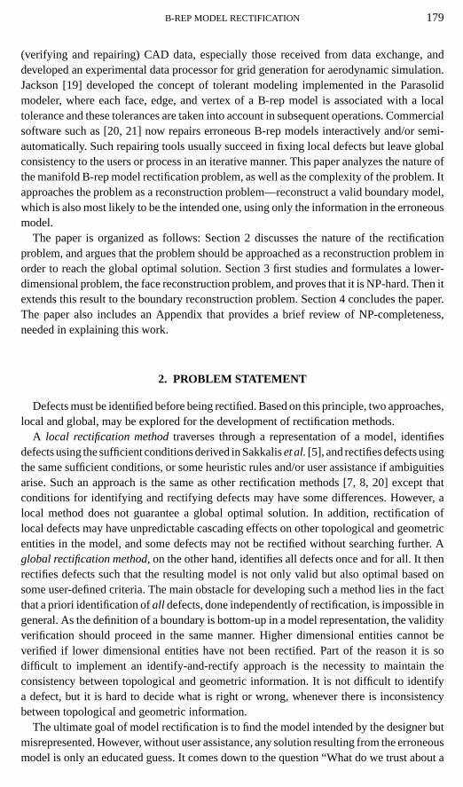
(verifying and repairing) CAD data, especially those received from data exchange, anddeveloped an experimental data processor for grid generation for aerodynamic simulation.Jackson [19] developed the concept of tolerant modeling implemented in the Parasolidmodeler, where each face, edge, and vertex of a B-rep model is associated with a localtolerance and these tolerances are taken into account in subsequent operations. Commercialsoftware such as [20, 21] now repairs erroneous B-rep models interactively and/or semi-automatically. Such repairing tools usually succeed in fixing local defects but leave globalconsistency to the users or process in an iterative manner. This paper analyzes the nature ofthe manifold B-rep model rectification problem, as well as the complexity of the problem. Itapproaches the problem as a reconstruction problem—reconstruct a valid boundary model,which is also most likely to be the intended one, using only the information in the erroneousmodel.

The paper is organized as follows: Section 2 discusses the nature of the rectificationproblem, and argues that the problem should be approached as a reconstruction problem inorder to reach the global optimal solution. Section 3 first studies and formulates a lower-dimensional problem, the face reconstruction problem, and proves that it is NP-hard. Then itextends this result to the boundary reconstruction problem. Section 4 concludes the paper.The paper also includes an Appendix that provides a brief review of NP-completeness,needed in explaining this work.

2. PROBLEM STATEMENT

Defects must be identified before being rectified. Based on this principle, two approaches,local and global, may be explored for the development of rectification methods.

A local rectification methodtraverses through a representation of a model, identifiesdefects using the sufficient conditions derived in Sakkaliset al.[5], and rectifies defects usingthe same sufficient conditions, or some heuristic rules and/or user assistance if ambiguitiesarise. Such an approach is the same as other rectification methods [7, 8, 20] except thatconditions for identifying and rectifying defects may have some differences. However, alocal method does not guarantee a global optimal solution. In addition, rectification oflocal defects may have unpredictable cascading effects on other topological and geometricentities in the model, and some defects may not be rectified without searching further. Aglobal rectification method, on the other hand, identifies all defects once and for all. It thenrectifies defects such that the resulting model is not only valid but also optimal based onsome user-defined criteria. The main obstacle for developing such a method lies in the factthat a priori identification ofall defects, done independently of rectification, is impossible ingeneral. As the definition of a boundary is bottom-up in a model representation, the validityverification should proceed in the same manner. Higher dimensional entities cannot beverified if lower dimensional entities have not been rectified. Part of the reason it is sodifficult to implement an identify-and-rectify approach is the necessity to maintain theconsistency between topological and geometric information. It is not difficult to identifya defect, but it is hard to decide what is right or wrong, whenever there is inconsistencybetween topological and geometric information.

The ultimate goal of model rectification is to find the model intended by the designer butmisrepresented. However, without user assistance, any solution resulting from the erroneousmodel is only an educated guess. It comes down to the question “What do we trust about a


model that contains defects?” This is the most fundamental question we must answer beforewe can move any further. For example, if a B-rep model has correct topological information,while there is no appropriate geometry embedded in the underlying surfaces, what is theintended boundary? Should the topological information be modified to accommodate thegeometry, or should the geometry (surfaces) be perturbed to have a boundary consistentwith the topological information?

To answer such questions, we need to classify the information in a boundary representa-tion: those initialized or selected by the designer and those induced by the system. In a solidmodeling system, the only entities the designer can directly manipulate are the underlyingsurfaces. All others, topological information and individual topological and geometric en-tities, are computed by the system. For this reason, we opt to believe that surfaces are thebasic information to be used in a rectification method. Another reason for such a hypoth-esis is that surfaces are specifically designed to fulfill certain performance requirementsand functionalities, and therefore, should not be subjected to any modification without thedesigner’s permission. In addition to the above, another piece of information that can beused in the rectification process is the genus of the intended solid boundary. Genus cap-tures the designer’s intent and can be computed using the well-known Euler’s formula[22].

In this context, model rectification becomes a model reconstruction problem. An algo-rithm for model rectification searches for the intended boundary in the union of all thesurfaces, and rebuilds all necessary topological and geometric entities. However, there mayexist many potential solid boundaries, or none at all, resulting from the surfaces. Withoutadditional information, it would be difficult to make a choice. Since an erroneous modelin a neutral format (e.g., STEP [23]) is computed with reasonable precision in its nativesystem, the information in the model could help clarify such ambiguities, although it shouldbe used with caution. Roughly speaking, a desirable solution is a model that describes aboundary somewhere “near” the object described by the original model, both topologicallyand geometrically.

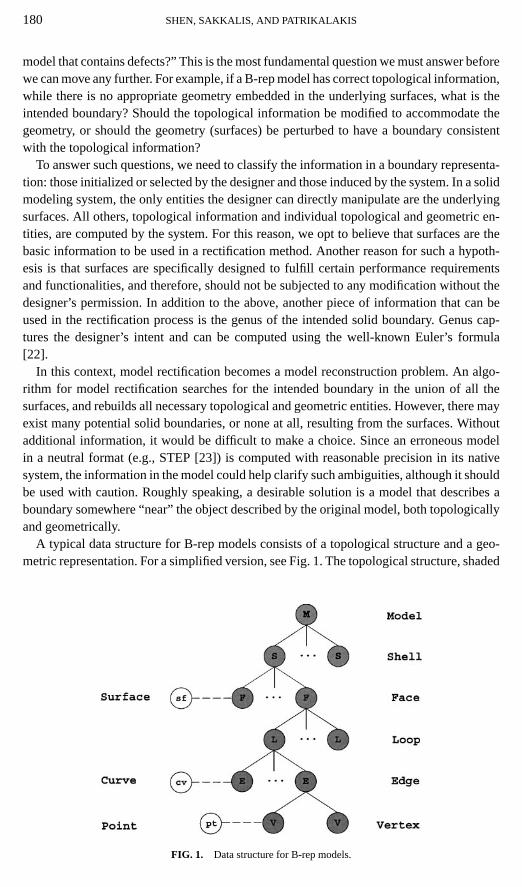
A typical data structure for B-rep models consists of a topological structure and a geo-metric representation. For a simplified version, see Fig. 1. The topological structure, shaded

FIG. 1. Data structure for B-rep models.


in Fig. 1, is a graph that describes adjacency and incidence relations1 (represented by arcs)between topological entities (represented by nodes). In typical implementations topologicalrelations more detailed than those implied in Fig. 1 (e.g., adjacency relations between a faceand all its neighboring faces) are explicitly stored. The geometric representation includespoints, curve, and surface equations, which are associated with appropriate topological en-tities. A model, thus, is aninstanceof the data structure, and isvalid if it describes a solidboundary. In addition, a face is valid if it describes a set homeomorphic to a closed diskminusk mutually disjoint open disks, and has no handles. Also, see [5] for validity of othertopological nodes.

Let mo be a model with topological structureG(mo).2 G(mo) is valid if it is possibleto assign each topological entity (face, edge, vertex) a set of the corresponding dimension(surface, curve, point) whose interior is a manifold, such that the union of these manifoldsbounds a solid. That is, ifG(mo) is valid, there exists a nonempty set

M = {m |m is a valid model and has topological structureG(mo)}. (1)

For simplicity, in the following analysis, we assume thatmodels have only one shell. It will beclear at the end of this paper that the same result applies to models with multiple shells. Withthis assumption, for anym1, m2 ∈M, M1 is homeomorphic toM2. Therefore, in case thatthe geometric representation ofmo is inconsistent withG(mo), if a reconstructed modelmn

has topological structureG(mo), mn is topologically equivalent to the model incorporatingthe design intent. IfG(mn) is different fromG(mo), the topological equivalence betweenmn andmo can be imposed by requiring that the genus of∂Mn is equal to that of∂M , wheremodelm ∈M. We simply denote this byg(mn) = g(mo), because both genuses can becomputed by applying Euler’s formula toG(mn) andG(mo), respectively.

Geometrically, two objects are close to each other if each one is in a neighborhood of theother. Some form of distance function could be used as a measure for this purpose, eitherthe maximum distance or a well-defined average distance. An alternative, arguably moresuitable for boundary rectification, is the boundary area change before and after rectification,because both the rectified and the original models use the same set of underlying surfaces. Acorrespondence can be established between a rectified face and an old face if they both havethe same underlying surface, and the area difference between them measures the geometricchange. No matter what measure is used, it should approach zero as the erroneous modelbecomes the exact model.

SinceMo and∂Mo are not defined for a nonvalid model, we first define another set, called∂M ′o as follows. We project the loops of edgesei of mo onto each of the correspondingsurfaces to obtain new loops of edgese′i that bound new facesF ′i , and let∂M ′o = ∪I F ′i . Notethat∂M ′0 may not bound a solid. The details of this construction are in Sections 3.1.1, 3.1.2,and 3.2. In these sections we define a functionφ that evaluates the geometric differencebetween∂M ′o and∂Mn. We will denote this byφ(∂M ′o, ∂Mn). Let ε be a user-specifiedtolerance for the geometric change and letmo, G(mo) be as above. An ideal boundaryreconstruction algorithm should follow the following procedure (see Fig. 2):

1 Two topological entities of different dimensionalities have an incidence relation if one is a proper subset of theother. Two topological entities of same dimensionality have an adjacency relation if their intersection is a lowerdimensional entity that has an incidence relation with each of them.

2 We denote models and face nodes by lowercase letters, and the point sets they represent by uppercase letters.For example, modelmo represents solidMo. The topological structure of a node is denoted byG(node).


FIG. 2. Flow chart of an ideal global reconstruction algorithm.

1. Find a new modelmn, such thatmn has topological structureG(mo), i.e.,G(Mn) ∼G(mo)3 andφ(∂M ′o, ∂Mn) ≤ ε.

2. If there exists a number of such new models, select the one with the minimalφ value.3. Otherwise, find a new modelmn, such thatG(mn) is different fromG(mo) but

g(mn) = g(mo), andφ(∂M ′o, ∂Mn) ≤ ε.4. If there exists a number of such new models, select the one with the minimal

topological structure change; e.g., the difference of the total numbers of arcs and nodes inG(mn) andG(mo) is minimal.

5. Otherwise, find a new modelmn with φ(∂M ′o, ∂Mn) ≤ ε. If there exist more thanone such new boundaries, select the one with the minimal topological change (i.e., minimalgenus change); otherwise, no new model is reconstructed.

3 Two graphs are homeomorphic if both can be obtained from the same graph by a sequence of subdivisions ofarcs.


In the next section, we study the following subproblem, which is essential to this recon-struction process:

Boundary reconstruction (BR) problem.Given a B-rep modelmo, whose geometricrepresentation is inconsistent with its topological structure, reconstruct a new modelmn

using only the information inmo, such that: (1)g(mn) = g(mo) and (2)φ(∂M ′o, ∂Mn) isminimal.

3. PROBLEM COMPLEXITY

3.1. Face Reconstruction Problem

Before moving onto the BR problem, we first study a lower-dimensional problem thatnot only gives us insight on the nature of such reconstruction problems, but also plays acrucial role in understanding the complexity of the BR problem.

A face node in a B-rep model represented in a certain format such as STEP [23] is likelyto have inconsistent geometric features such as edges whose underlying curves are not onthe underlying surface of the face. Topological errors such as open loops make a cleardefinition of the face geometry even more elusive. Similar to boundary reconstruction, facereconstruction builds a new face nodefn from an erroneous face nodefo, using only theinformation in the given model, such thatfn is not only valid but also close to the objectdescribed byfo in both topology and geometry. We formulate the face reconstructionproblem as an analogue to the BR problem.

A valid face is homeomorphic to a closed disk minusk mutually disjoint open disks, andhas no handles [5]. Iffo is valid,G( fo) is a planar graph that consists of simple cycles. Anytwo of these cycles may share at most one common node. Two graphs are homeomorphicif both can be obtained from the same graph by a sequence of subdivisions of arcs [24].However, two homeomorphic graphs may have different geometric embeddings, and thusdefine two faces that are not homeomorphic. See Fig. 3. In order to capture the designintent topologically, the component containing the outer loop inG( fn) also needs to behomeomorphic to that inG( fo), in addition to thatG( fn) is homeomorphic toG( fo), sothat the above situation is prevented. In this case we say thatG( fn) is homeomorphic toG( fo) in thestrong sense. In the following problem statement,φ f is a function evaluatingthe geometric change before and after rectification, and will be elaborated in Section 3.1.2.

Face reconstruction (FR) problem.Given a face nodefo, whose geometric representa-tion is inconsistent with its topological structure, in a B-rep modelmo, reconstruct a validface nodefn, using only the information inmo, such thatG( fn) is homeomorphic toG( fo)in the strong sense andφ f (Fn, Fo) is minimal.

In the following, we first study how an invalid face node could be rectified, and thenformulate the face reconstruction problem mathematically and prove its NP-hardness.

FIG. 3. Two homeomorphic graphs with different geometric embeddings.


FIG. 4. Curve segments from surface intersections.

3.1.1. Face Boundary Reconstruction

Let R be the underlying surface of face nodefo, and{Ri }1≤i≤N be surfaces inmo suchthatCi = R∩ Ri 6= ∅. Surface intersections could be very complex. Here, for simplicity,we assume that surfaces do not overlap. In addition, we also exclude isolated intersectionpoints, since such a point does not bound a finite region onR, and therefore, is not usedto form the face boundary. However, if an intersection point between two surfaces is on anintersection curve, it may be used as a vertex in the face boundary. See Fig. 4a, where theintersection point ofR andR4 is onC1.

Furthermore,Ci ’s may intersect each other. EachCi is subdivided by intersection pointsinto curve segments, each of which is either an open curve bounded by two intersectionpoints or a simple closed curve. Those intersection points, indeed, are intersections ofthree or more surfaces. Denote the collection of curve segments on allCi ’s by {Si j }. SeeFig. 4b, where broken lines are curve segments and solid dots are intersection points. In thefigure, because the underlying surface is finite, its boundary curves are also used in creatingcurve segments. Note that{Si j } subdivideR into patches whose interiors are disjoint andintersection-free. The face geometry must be either one of these patches or the union ofsome patches. Therefore, the face boundary consists of curve segments from{Si j }.

In the following description, for simplicity, we use a lowercase symbol to denote an edgeor a vertex as a point set. Whenever the corresponding representational node is referred, theword nodeis used before the notation. For example, nodee represents edgee. For modelsand faces, the same notation scheme as in the previous section is used, i.e., lowercasesymbols for nodes and uppercase symbols for point-sets.

Let nodeeik be an edge node info, also shared by face nodefi havingRi as its underlyingsurface. Then, to maintain geometric consistency of the adjacency relation between thesetwo faces,eik must be a subset ofCi . This is rarely true as the underlying curve given innodeeik is often an approximation of the exact intersection curveCi . As a matter of fact,as illustrated in Fig. 5,eik may be pathologically defined by a space curve (the brokenline) and two points (the two circles) that may not be on the curve as they are supposedto be. Because the adjacency relation is symbolic and thus exact, the initial rectificationof nodeeik can be done by usingCi as the underlying curve and discarding the one givenin the original model. Consequently, the vertices must be onCi . They also need to be


FIG. 5. Initial rectification of an edge on a face.

close to their original erroneous positions in order to reflect the design intent. Reasonablereplacements of the original verticesvi 1, vi 2, for instance, could be the projectionsv′i 1, v′i 2of vi 1, vi 2 onto Ci . See Fig. 5, where the new vertices are solid dots. Therefore, such arectified edge, denoted bye′i k , is a subset ofCi , bounded byv′i 1, v′i 2 and oriented in thesame way aseik provided that the given underlying curve in nodeeik andCi are not farapart.

However, as a face should be bounded by curve segments from{Si j }, a rectified edgeshould consist of such curve segments. Edgee′i k is not guaranteed to be so. See Fig. 6a.Further rectification ofeik selects some curve segments onCi such that their union is asimple open or closed curve and an optimal approximation ofe′i k . The union defines a newedgee′′i k , whose corresponding node has the same symbolic information as nodeeik , i.e.,the same embedding surfaces, the same parent faces, and the same orientation, but has aconsistent geometric representation while nodeeik does not. Edgee′′i k can be obtained byperturbing verticesv′i 1, v

′i 2 of e′i k to the closest intersection points onCi . This vertex per-

turbation is also necessary in order to achieve geometric consistency at a vertex. A vertexis involved in various incidence and adjacency relations between its incident faces andedges, and therefore, needs to be positioned at the intersection point of those underlyingsurfaces.

FIG. 6. Creation ofe′′ik by vertex perturbation.


FIG. 7. Trimming of dangling curve segments (a) and gap filling (b).

The collection of such rectified edges, however, may not form a valid face boundary, asthere may exist open loops and/or dangling curve segments. For example, in Fig. 7a (wherethe rectified edges are thick lines), a dangling curve segmentS12 and a gap betweene′′5ande′′9 exist. The final act of face reconstruction is to trim away dangling curve segmentsand fill gaps with curve segments from{Si j }, so that the selected curve segments form avalid face boundary. See Fig. 7b. This trimming and gap-filling process should create a faceboundary that satisfies the topological and geometric requirements stated in the problemstatement.

Assume that, in the final reconstructed face boundary, the selected curve segments fromCi areSi = {Si j l }1≤l≤Li . A new edgeen

ik is created by stringing curve segments inSi . Theprocess starts with an arbitrary curve segmentSi j1 ∈ Si , and searches for its adjacent curvesegments inSi . If, at one endpoint, exactly one adjacent curve segmentSi j2 is found, thenSi j2 is selected and the search marches on at the other endpoint ofSi j2; otherwise, the processterminates and resumes at the other endpoint ofSi j1. Note that there may be more than one


new edge created fromSi . For example, in Fig. 7, curve segmentsS72, S74 onC7 are selectedin the final face boundary, creating two new edgesen

7 anden11.

In summary, an edgeeik in the original model, shared by facesfo and fi , is first rectifiedby projecting its vertices ontoCi = R∩ Ri , which is the exact underlying curve of nodeeik .This producese′i k , and achieves a consistent adjacency relation betweenfo and fi but maynot do so at the vertices. Edgee′i k is then rectified by perturbing its vertices to their closestintersection points onCi , such that the resulting edgee′′i k consists of curve segments in{Si j }. Note that nodee′′i k has the same symbolic information as nodeeik and could begeometrically consistent with all adjacency and incidence relations in which it is involved,if other topological entities are appropriately constructed. Typically, the geometric changebetweene′′i k and eik is minimal. Since such edges may not form a valid face boundary,additional curve segments from{Si j } are added to fill gaps and dangling curve segmentsare trimmed away. In the rectified face boundary, a new edgeen

ik consists of curve segmentsfrom Ci .

3.1.2. Problem Formulation and Proof of NP-Hardness

To mathematically formulate the FR problem, especially to quantify face geometricchange, we classify new edges into two categories:

1. A new edgeenik belongs to the first category if it has a corresponding edgeeik in the

original model; i.e.,enik is considered to be the rectifiedeik . Such a new edge node has the

same symbolic information as nodeeik and a geometry that is an optimal approximation ofthat of nodeeik . Becauseeik is not well defined, the geometric change betweenen

ik andeik

is measured by comparingenik ande′i k , which is not only well defined but also symbolically

the same as and geometrically close toeik . We defineφe: (Ci × Ci )→ R, where

φe(en

ik , e′i k

) = length((

enik ∪ e′i k

)− (enik ∩ e′i k

)), en

ik , e′i k ⊆ Ci . (2)

For example, in Fig. 6, ifenik = e′′i k , meaning that during the trimming-and-filling stage the

edge is unchanged, then

φe(en

ik , e′i k

) = |v′i 1v′′i 1| + |v′i 2v′′i 2|, (3)

where| | denotes the length of a curve segment. If there exist more than one new edges onCi that could belong to the first category, the one with the minimalφe value is designatedas the new edge in the first category; i.e., there is at most one corresponding new edge inthe new boundary for each edge in the original model. In addition,en

ik ∩ e′i k 6= ∅, so that anew edge whose geometry is far away frome′i k will not be taken as the corresponding newedge ofeik . This could happen, for example, when two new edgesen

ik,1, enik,2 have the same

symbolic information aseik but

enik,1 ∩ e′i k 6= ∅,

enik,2 ∩ e′i k = ∅,

φe(en

ik,1, e′i k

)> φe

(en

ik,2, e′i k

).

In Fig. 7b, all the new edges, excepten11, belong to the first category.


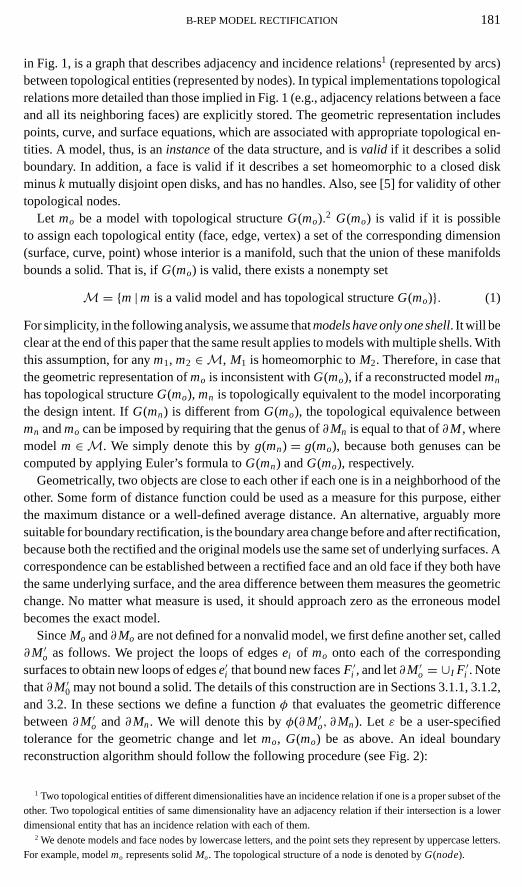
2. All other new edges belong to the second category. These edges are generally addedto close gaps. Let a new edge be on curveCj = R∩ Rj . It is possible that the face onRj

is not adjacent tofo in the original model, and therefore, the new edge onCj does not havea corresponding old edge.

Because the edges in the original face node carry the design intent, geometric changesto them should be minimized, i.e.,

∑φe for the new edges of the first category should be

minimal. If there exist more than one choices of new face boundary having the minimum,that with the shortest total length of the edges of the second category should be chosen,because any drastic change is not trustworthy. Figure 8a shows the curve segments andinitially rectified edges. Note that the original face node has an inconsistent geometricrepresentation. It can be seen in Fig. 8b that if all four edges represented by thick lines are

FIG. 8. Minimization of edge geometric change.


selected in the final boundary,∑φe is the minimum. There exist five such loops. Figure 8c

shows the final face boundary that has the shortest gap-closing edgeen5, and Fig. 8d shows

the other four.We now formulate the face reconstruction problem as a search problem:

Face reconstruction (FR) problem.Let fo be a face node, whose geometric represen-tation is inconsistent with its topological structure, in a B-rep model, and{Si j } be as above.Search for a subcollection {

Si j l

}1≤i≤N,1≤l≤Li

(4)

of {Si j }, whereLi is the number of curve segments selected onCi , such that

1. {Si j l } bounds a faceFn.2. G( fn) is homeomorphic toG( fo) in the strong sense.3.∑φe(e′i k , e

nik ) is minimal for the new edges of the first category.

4. If condition (3) is satisfied, then the total length of the edges of the second categoryis also minimal.

Intuitively, this problem can be converted to a graph problem as{Si j } forms a geometricembedding onR of a graph. This graph,G f = (Vf , E f ), has curve segments in{Si j } asarcs inE f and intersection points as nodes inVf . The solution to the FR problem is thena subgraph satisfying the properties in the problem statement. The face reconstructionprocess is a process of searching for such a subgraph. A straightforward implementationof this process is to search all possible subgraphs and find the one satisfying conditions1 to 4 above. Such an exhaustive search, however, may need exponential time in terms ofthe number of arcs inE f . In the following, we prove that the FR problem is NP-hard byproving a restricted problem is NP-hard. See also the Appendix for some further commentson NP-hard problems, but first, we introduce a known NP-hard problem [25]:

Rural postman problem4: Let graphG = (V, E). Eache∈ E has lengthl (e) ∈ Z+0 . LetE′ ⊆ E. Find the circuit inG that includes each arc inE′ and that has the shortest total length.

THEOREM3.1. FR problem is NP-hard.

Proof. The basic idea of the proof is to consider the following instance of the restrictedFR problem: The topological structure offo represents a closed disk, and there is onlyone curve segment on eachCi (see Fig. 9). The boundary ofFo is then a simple closedcurve. The solution to the problem must be a circuit in graphG f if condition (2) is to besatisfied. For each edgeeik of Fo, we constructe′i k , e

′′i k as above. Because there is only one

curve segmentSi 1 on eachCi , e′′i k = Si 1 provided thate′i k is not far different fromSi 1. IfSi 1 is in the reconstructed face boundary, thenen

ik = e′′i k = Si 1, and therefore,φe(enik , e′i k ) is

minimal, due to the waye′′i k is constructed. If it is not in the face boundary, thenφe(enik , e′i k )

is maximal, becauseenik = ∅. Let

S1 = {Si 1| there existse′′i k = Si 1, 0≤ i ≤ N}. (5)

4 Here we give the rural postman search problem because the FR problem is also a search problem. In [25], therural postman decision problem is given.


FIG. 9. An instance of the restricted FR problem.

Then, if all the curve segments inS1 are selected,∑φe for the edges of the first category

reaches its minimum. This means that a valid face boundary that includes all the curvesegments inS1 will be selected over any choice that does not.

The corresponding instance of the rural postman problem is as follows: GraphGf withl (e) = length(Si 1) for eachi , andE′ = S1. We prove that it can be reduced to the restrictedFR problem at least in the abstract setting of graph theory.5

It can be observed that the solution to the restricted FR problem answers the rural post-man problem; if the solution exists for the restricted FR problem and contains all the curvesegments inS1, it is the circuit with the shortest length and includes all the arcs inE′, andtherefore, is the solution to the rural postman problem; if the solution does not exist orit exists but does not contain all the edges inS1, no solution exists for the rural postmanproblem. j

3.2. Boundary Reconstruction Problem

Now we formulate the BR problem and prove that it is also NP-hard.Let mo be the given B-rep model. The underlying surfaces,{Ri }1≤i≤N , are subdivided by

surface intersections into a collection of patches

{Pi j }1≤i≤N,1≤ j≤Ni , (6)

whereNi is the number of patches on surfaceRi . For a face nodefi , Fi may not be well de-fined. Because the embedding information is symbolic and thus exact, the initial rectificationof Fi can be done by trimming the underlying surfaceRi of fi using projections of the loopsin fi ontoRi . Denote such a face byF ′i . As in face reconstruction,F ′i is further rectified byselecting patches from{Pi j }1≤ j≤Ni to form a new geometry that is an optimal approximationof F ′i . Denote this new face byF ′′i . The difference betweenF ′i and F ′′i can be measuredby functionφ f : (Ri × Ri )→R, where

5 Theoretically, it is possible to develop a linear algorithm to draw a planar graph on the plane. See [26, 27]. Thisestablishes the argument that an abstract graph search problem could be converted to an instance of the geometricproblem (FR problem).


φ f (F′i , F ′′i ) = area((F ′i ∪ F ′′i )− (F ′i ∩ F ′′i )), F ′i , F ′′i ⊆ Ri . (7)

Such rectified faces may not form a valid solid boundary due to the possible existence ofdangling patches and holes. Therefore, a trimming-and-filling process follows. Similar toface reconstruction, in the new solid boundary, a new faceFn

i belongs to the first categoryif it has a corresponding old face, and to the second category if it does not. For the facesof the first category,

∑φ f (Fn

i , F ′i ) should be minimized. If there exist more than one validboundaries having the minimum

∑φ f , that with the minimal total area of the faces of the

second category should be chosen.The boundary reconstruction problem can also be formulated as a search problem:

Boundary reconstruction (BR) problem.Let mo be a B-rep model whose geometricrepresentation is inconsistent with its topological structure, and{Pi j } be as above. Searchfor a subcollection {

Pi jk

}1≤i≤N,1≤k≤Ki

(8)

of {Pi j }, whereKi is the number of patches selected on surfaceRi , such that

1. {Pi jk} bounds a solidMn.2. g(mn) = g(mo), wheremn is the new model representingMn.3.∑φ f (Fn

i , F ′i ) is minimal for the faces of the first category.4. If condition (3) is satisfied, then the total area of the faces of the second category

is also minimal.

We now prove that the BR problem is NP-hard:

THEOREM3.2. BR problem is NP-hard.

Proof. We prove the theorem by converting the restricted FR problem to the BR problem.Assume that in an instance of the restricted FR problem, the face nodefo has a plane asits underlying surface. Sweep the face along the normal direction to a parallel plane. Thesweeping solid ofFo should be homeomorphic to a closed ball. The instance of the BRproblem is a patch collection

{Pi j } = {patches generated from curve segments}∪ {patches from the two planes}, (9)

and a modelmo with its topological structure representing a sphere and{F ′i } generatedfrom {e′i k}. See Fig. 10 for an example. This conversion can be executed in polynomial time.If a subcollection of{Si j } is the solution to the restricted FR problem, then the patchesgenerated from the curve segments in the subcollection, with additional patches from thetwo planes, is the solution to the BR problem. Conversely, if a subcollection of the patchesis the solution to the BR problem, it must be bounded by two patches from the two planesand patches whose generating curve segments indeed form the solution to the restricted FRproblem. j

For models with multiple shells, the same result holds, because the boundary reconstruc-tion problem of models with one shell is a special case of that of models with multipleshells.


FIG. 10. Illustration of the proof of Theorem 3.2.

4. CONCLUSIONS

The BR problem is, in certain ways, similar to the gap boundary matching problem studiedby Barequet and Sharir [9], which is also shown to be an NP-hard (global search) problem.However, they are quite different in nature as the former reconstructs a boundary from aset of surfaces and involves complex topological constraints, whereas the latter matchesboundaries of a set of surface patches. Theoretically, of course, all NP-complete problemsare equivalent, but their specifics can vary significantly.

The understanding of the NP-hardness of a problem helps design algorithms to efficientlyand properly solve the problem. In a recent paper [29], we propose model rectificationalgorithms that approximate the process of finding the optimal solutions described here. Toachieve numerical robustness in a floating point environment, interval model representationproves to be a powerful tool [16, 17]. We further study some key topological issues ofinterval solid models in [28], and develop interval geometric and numerical methods usefulin model rectification in [30]. All these are summarized in a review paper [31].

APPENDIX: SHORT REVIEW OF NP-COMPLETENESS

This Appendix provides a brief introduction to the theory of NP-completeness. For de-tails, see [25]. A decision problem is a problem whose answer isyesor no. A problemis said to belong to the class P if it can be solved by a polynomial time DTM program.DTM is the abbreviation fordeterministic one-tape Turing machine, a simplified comput-ing model. If the problem can be solved by a polynomial time NDTM program, it belongsto the class NP. NDTM,nondeterministic one-tape Turing machine, has the exact samestructure as that of DTM, except that it has aguessing module. A NDTM program hastwo distinct stages: guessing and checking. For example, the traveling salesman problem isgiven as:


Traveling salesman problem.Given a finite set of cities, a distance between each pairof cities, and a boundB, is there a tour of all the cities such that the total distance of thetour is no larger thanB?

A NDTM program first guesses a tour of all the cities, and then verifies in polynomialtime if the length of this guessed tour is less than the given threshold. If at least one guessedtour is accepted, the answer to the problem isyes. Therefore, the traveling salesman problemis in class NP.

It is observed that class(P)⊆ class(NP). It is also an unproven conjecture that P6=NP.For a problem in NP, there exists a polynomialp such that the problem can be solved by adeterministic algorithm having time complexityO(2p(n)), wheren is the length of the inputstring. A decision problem5 is NP-complete if5∈NP and, for all other decision problems5′ ∈NP, there is a polynomial transformation from5′ to5. A polynomial transformationis a mappingf such that

1. There exists a polynomial DTM program that computesf .2. For any instancex of the problem,x is accepted if and only iff (x) is accepted.

Therefore, NP-complete problems are the “hardest” problems in NP. The NP-completenessproof of a decision problem consists of the following four steps:

1. Show that5∈NP, i.e.,5 can be solved by a NDTM program.2. Select a known NP-complete problem5′.3. Construct a transformationf from5′ to5.4. Prove thatf is a polynomial transformation.

The NP-completeness can also be proven by restriction; that is, a problem is NP-completeif it contains a known NP-complete problem as a special case.

The concept of NP-hardness applies to problems outside class NP, e.g., search problems.Informally, a search problem is NP-hard if it is at least as hard as some NP-completeproblem. For example, the search for the shortest tour of all the cites is as hard as thetraveling salesman decision problem, because the solution to the search problem certainlyanswers the decision problem.

ACKNOWLEDGMENTS

Funding for this work was obtained in part from NSF Grant DMI-9215411, ONR Grant N00014-96-1-0857,and the Kawasaki chair endowment at MIT. The authors thank W. Cho and G. Yu for their assistance in the earlyphases of the CAD model rectification project. We also thank T. J. Peters and A. C. Russell, the referees and thearea editor of the Graphical Models journal for their comments on this work.

Note.This paper was also presented at the 6th ACM Symposium on Solid Modeling and Applications, AnnArbor, MI, June 2001.

REFERENCES

1. A. A. G. Requicha, Representations for rigid solids: Theory, methods, and systems,ACM Comput. Surveys12, 1980, 437–464.

2. D. E. LaCourse,Handbook of Solid Modeling, McGraw-Hill, NewYork, 1995.

3. C. M. Hoffmann,Geometric and Solid Modeling—An Introduction, Morgan Kaufmann, San Mateo, CA, 1989.

4. M. Mantyla,An Introduction to Solid Modeling, Computer Science Press, Rockville, MD, 1988.


5. T. Sakkalis, G. Shen, and N. M. Patrikalakis, Representational validity of boundary representation models,Computer Aided Design32, 2000, 719–726.

6. 3D Systems, Inc.,Stereolithography Interface Specification, June 1988.

7. J. H. Bohn and M. J. Wozny, A topology-based approach for shell-closure, inGeometric Modeling for ProductRealization(P. R. Wilson, M. J. Wozny, and M. J. Pratt, Eds.), pp. 297–318, Elsevier, Amsterdam, 1993.

8. I. Makela and A. Dolenc, Some efficient procedures for correcting triangulated models, inProceedings ofSolid Freeform Fabrication Symposium, University of Texas at Austin, 1993, pp. 126–134.

9. G. Barequet and M. Sharir, Filling gaps in the boundary of a polyhedron,Computer Aided Geom. Design, 12,1995, 207–229.

10. G. Barequet and S. Kumar, Repairing CAD Models, inProc. IEEE Visualization, Phoenix, AZ, 1997,pp. 363–370.

11. G. Barequet, C. A. Duncan, and S.Kumar, RSVP: A Geometric Toolkit for Controlled Repair of Solid Models,IEEE Trans. Visualiz. Comput. Graphics, 4, 1998, 162–177.

12. T. M. Murali and T. A. Funkhouser, Consistent solid and boundary representations from arbitrary polygonaldata, inProceedings of 1997 Symposium on Interactive 3D Graphics, Providence, Rhode Island(A. Van Dam,Ed.), pp. 155–162, Assoc. Comput. Mach. Press, New York, 1997.

13. B. Hamann and B. A. Jean, Interactive surface correction based on a local approximation scheme,Comput.Aided Geom. Design13, 1996, 351–368.

14. C. M. Hoffmann, The problems of accuracy and robustness in geometric computation,Computer22, 1989,31–41.

15. S. Fortune, Polyhedral modeling with multiprecision integer arithmetic,Comput. Aided Design29, 1997,123–133.

16. C.-Y. Hu, N. M. Patrikalakis, and X. Ye, Robust interval solid modeling: Part I, representations,Comput.Aided Design28, 1996, 807–817.

17. C.-Y. Hu, N. M. Patrikalakis, and X. Ye, Robust interval solid modeling: Part II, boundary evaluation,Comput.Aided Design28, 1996, 819–830.

18. F.-L. Krause, C. Stiel, and J. Lüddemann, Processing of CAD-data—Conversion, verification and repair, inProceedings of 4th Symposium on Solid Modeling and Applications, Atlanta, GA, May 1997(C. Hoffmannand W. Bronsvoort, Eds.), pp. 248–254, Assoc. Comput. Mach., New York, 1997.

19. D. J. Jackson, Boundary representation modelling with local tolerances, inProceedings of the 3rd Symposiumon Solid Modeling and Applications, Salt Lake City, UT, May 1995(C. Hoffmann and J. Rossignac, Eds.),pp. 247–253, Assoc. Comput. Mach., NewYork, 1995.

20. International TechneGroup Incorporated,Introduction—CAD fix Makes Geometry Data Exchange Work.Available at http://www.iti-oh.com/.

21. Theorem Solutions Inc,Product Information. Available at http://www.theorem.co.uk/productmain.htm.

22. I. C. Braid,Notes on a Geometric Modeller, C.A.D. Group Document 101, University of Cambridge,Cambridge, UK, 1979.

23. U. S. Product Data Association, ANS US PRO/IPO-200-042-1994: Part 42–Integrated Geometric Resources:Geometric and Topological Representation, 1994.

24. F. Harary,Graph Theory, Addison-Wesley, Reading, MA, 1969.

25. M. R. Garey and D. S. Johnson,Computer and Intractability: A Guide to the Theory of NP-completeness, W.H. Freeman, San Francisco, 1979.

26. N. L. Biggs and A. T. White,Permutation Groups and Combinatorial Structures, Cambridge Univ. Press,Cambridge, UK, 1979.

27. N. Chiba, T. Yamanouchi, and T. Nishizeki, Linear algorithms for convex drawings of planar graphs, inProgress in Graph Theory(J. A. Bondy and U. S. R. Murty, Eds.), pp. 153–173, Academic Press, NewYork,1984.

28. T. Sakkalis, G. Shen, and N. M. Patrikalakis, Topological and geometric properties of interval solid models,Graphical Models63, 2001, 163–175.

29. G. Shen, T. Sakkalis, and N. M. Patrikalakis, Manifold boundary representation model rectification (“Larectification des modèles des varietés B-rep”), inProceedings of the 3rd International Conference on Integrated


Design and Manufacturing in Mechanical Engineering(C. Mascle, C. Fortin, and J. Pegna, Eds.), p. 199 andCDROM, Presses internationales Polytechnique, Montreal, Canada, 2000.

30. G. Shen, T. Sakkalis, and N. M. Patrikalakis, Interval methods for B-rep model verification and rectification,in Proceedings of the ASME 26th Design Automation Conference, Baltimore, MD, September 2000, p. 140and CDROM. ASME, NY, 2000.

31. N. M. Patrikalakis, T. Sakkalis, and G. Shen, Boundary representation models: Validity and rectification,Invited paper inProceedings of the 9th IMA Conference on the Mathematics of Surfaces, University ofCambridge, Cambridge, UK, September 2000(R. Cipolla and R. Martin, Eds.), pp. 389–409, Springer-Verlag,London, 2000.

Boundary Representation Model Rectification

Documents

Transcript of Boundary Representation Model Rectification